measure and integration - peoplepeople.math.ethz.ch/~salamon/preprints/measure.pdf · we learn...
TRANSCRIPT

MEASURE AND INTEGRATION
Dietmar A. SalamonETH Zurich
9 September 2016

ii
Preface
This book is based on notes for the lecture course “Measure and Integration”held at ETH Zurich in the spring semester 2014. Prerequisites are the firstyear courses on Analysis and Linear Algebra, including the Riemann inte-gral [9, 18, 19, 21], as well as some basic knowledge of metric and topologicalspaces. The course material is based in large parts on Chapters 1-8 of thetextbook “Real and Complex Analysis” by Walter Rudin [17]. In additionto Rudin’s book the lecture notes by Urs Lang [10, 11], the five volumes onmeasure theory by David H. Fremlin [4], the paper by Heinz Konig [8] onthe generalized Radon–Nikodym theorem, the lecture notes by C.E. Heil [7]on absolutely continuous functions, Dan Ma’s Topology Blog [12] on exoticexamples of topological spaces, and the paper by Gert K. Pedersen [16] onthe Haar measure were very helpful in preparing this manuscript.
This manuscript also contains some material that was not covered in thelecture course, namely some of the results in Sections 4.5 and 5.2 (concerningthe dual space of Lp(µ) in the non σ-finite case), Section 5.4 on the Gen-eralized Radon–Nikodym Theorem, Sections 7.6 and 7.7 on Marcinkiewiczinterpolation and the Calderon–Zygmund inequality, and Chapter 8 on theHaar measure.
I am grateful to many people who helped to improve this manuscript.Thanks to the students at ETH who pointed out typos or errors in earlierdrafts. Thanks to Andreas Leiser for his careful proofreading. Thanks toTheo Buehler for many enlightening discussions and for pointing out thebook by Fremlin, Dan Ma’s Topology Blog, and the paper by Pedersen.Thanks to Urs Lang for his insightful comments on the construction of theHaar measure.
1 August 2015 Dietmar A. Salamon
iii

iv

Contents
Introduction 1
1 Abstract Measure Theory 31.1 σ-Algebras . . . . . . . . . . . . . . . . . . . . . . . . . . . . . 51.2 Measurable Functions . . . . . . . . . . . . . . . . . . . . . . . 111.3 Integration of Nonnegative Functions . . . . . . . . . . . . . . 171.4 Integration of Real Valued Functions . . . . . . . . . . . . . . 291.5 Sets of Measure Zero . . . . . . . . . . . . . . . . . . . . . . . 331.6 Completion of a Measure Space . . . . . . . . . . . . . . . . . 391.7 Exercises . . . . . . . . . . . . . . . . . . . . . . . . . . . . . . 43
2 The Lebesgue Measure 492.1 Outer Measures . . . . . . . . . . . . . . . . . . . . . . . . . . 502.2 The Lebesgue Outer Measure . . . . . . . . . . . . . . . . . . 562.3 The Transformation Formula . . . . . . . . . . . . . . . . . . . 672.4 Lebesgue Equals Riemann . . . . . . . . . . . . . . . . . . . . 752.5 Exercises . . . . . . . . . . . . . . . . . . . . . . . . . . . . . . 78
3 Borel Measures 813.1 Regular Borel Measures . . . . . . . . . . . . . . . . . . . . . 813.2 Borel Outer Measures . . . . . . . . . . . . . . . . . . . . . . . 923.3 The Riesz Representation Theorem . . . . . . . . . . . . . . . 973.4 Exercises . . . . . . . . . . . . . . . . . . . . . . . . . . . . . . 108
4 Lp Spaces 1134.1 Holder and Minkowski . . . . . . . . . . . . . . . . . . . . . . 1134.2 The Banach Space Lp(µ) . . . . . . . . . . . . . . . . . . . . . 1154.3 Separability . . . . . . . . . . . . . . . . . . . . . . . . . . . . 120
v
vi CONTENTS
4.4 Hilbert Spaces . . . . . . . . . . . . . . . . . . . . . . . . . . . 1254.5 The Dual Space of Lp(µ) . . . . . . . . . . . . . . . . . . . . . 1294.6 Exercises . . . . . . . . . . . . . . . . . . . . . . . . . . . . . . 143
5 The Radon–Nikodym Theorem 1515.1 Absolutely Continuous Measures . . . . . . . . . . . . . . . . . 1515.2 The Dual Space of Lp(µ) Revisited . . . . . . . . . . . . . . . 1595.3 Signed Measures . . . . . . . . . . . . . . . . . . . . . . . . . 1665.4 Radon–Nikodym Generalized . . . . . . . . . . . . . . . . . . 1735.5 Exercises . . . . . . . . . . . . . . . . . . . . . . . . . . . . . . 180
6 Differentiation 1856.1 Weakly Integrable Functions . . . . . . . . . . . . . . . . . . . 1856.2 Maximal Functions . . . . . . . . . . . . . . . . . . . . . . . . 1906.3 Lebesgue Points . . . . . . . . . . . . . . . . . . . . . . . . . . 1966.4 Absolutely Continuous Functions . . . . . . . . . . . . . . . . 2016.5 Exercises . . . . . . . . . . . . . . . . . . . . . . . . . . . . . . 205
7 Product Measures 2097.1 The Product σ-Algebra . . . . . . . . . . . . . . . . . . . . . . 2097.2 The Product Measure . . . . . . . . . . . . . . . . . . . . . . . 2147.3 Fubini’s Theorem . . . . . . . . . . . . . . . . . . . . . . . . . 2197.4 Fubini and Lebesgue . . . . . . . . . . . . . . . . . . . . . . . 2287.5 Convolution . . . . . . . . . . . . . . . . . . . . . . . . . . . . 2317.6 Marcinkiewicz Interpolation . . . . . . . . . . . . . . . . . . . 2397.7 The Calderon–Zygmund Inequality . . . . . . . . . . . . . . . 2437.8 Exercises . . . . . . . . . . . . . . . . . . . . . . . . . . . . . . 255
8 The Haar Measure 2598.1 Topological Groups . . . . . . . . . . . . . . . . . . . . . . . . 2598.2 Haar Measures . . . . . . . . . . . . . . . . . . . . . . . . . . 263
A Urysohn’s Lemma 279
B The Product Topology 285
C The Inverse Function Theorem 287
References 289
Introduction
We learn already in high school that integration plays a central role in math-ematics and physics. One encounters integrals in the notions of area orvolume, when solving a differential equation, in the fundamental theorem ofcalculus, in Stokes’ theorem, or in classical and quantum mechanics. Thefirst year analysis course at ETH includes an introduction to the Riemannintegral, which is satisfactory for many applications. However, it has certaindrawbacks, in that some very basic functions are not Riemann integrable,that the pointwise limit of a sequence of Riemann integrable functions neednot be Riemann integrable, and that the space of Riemann integrable func-tions is not complete with respect to the L1-norm. One purpose of this bookis to introduce the Lebesgue integral, which does not suffer from these draw-backs and agrees with the Riemann integral whenever the latter is defined.Chapter 1 introduces abstract integration theory for functions on measurespaces. It includes proofs of the Lebesgue Monotone Convergence Theorem,the Lemma of Fatou, and the Lebesgue Dominated Convergence Theorem.In Chapter 2 we move on to outer measures and introduce the Lebesguemeasure on Euclidean space. Borel measures on locally compact Hausdorffspaces are the subject of Chapter 3. Here the central result is the RieszRepresentation Theorem. In Chapter 4 we encounter Lp spaces and showthat the compactly supported continuous functions form a dense subspace ofLp for a regular Borel measure on a locally compact Hausdorff space whenp < ∞. Chapter 5 is devoted to the proof of the Radon–Nikodym theoremabout absolutely continuous measures and to the proof that Lq is naturallyisomorphic to the dual space of Lp when 1/p + 1/q = 1 and 1 < p < ∞.Chapter 6 deals with differentiation. Chapter 7 introduces product measuresand contains a proof of Fubini’s Theorem, an introduction to the convolu-tion product on L1(Rn), and a proof of the Calderon–Zygmund inequality.Chapter 8 constructs Haar measures on locally compact Hausdorff groups.
1
2 CONTENTS
Despite the overlap with the book of Rudin [17] there are some differ-ences in exposition and content. A small expository difference is that inChapter 1 measurable functions are defined in terms of pre-images of (Borel)measurable sets rather than pre-images of open sets. The Lebesgue measurein Chapter 2 is introduced in terms of the Lebesgue outer measure instead ofas a corollary of the Riesz Representation Theorem. The notion of a Radonmeasure on a locally compact Hausdorff space in Chapter 3 is defined interms of inner regularity, rather than outer regularity together with innerregularity on open sets. This leads to a somewhat different formulation ofthe Riesz Representation Theorem (which includes the result as formulatedby Rudin). In Chapters 4 and 5 it is shown that Lq(µ) is isomorphic tothe dual space of Lp(µ) for all measure spaces (not just the σ-finite ones)whenever 1 < p <∞ and 1/p+ 1/q = 1. It is also shown that L∞(µ) isisomorphic to the dual space of L1(µ) if and only if the measure space islocalizable. Chapter 5 includes a generalized version of the Radon–Nikodymtheorem for signed measures, due to Fremlin [4], which does not require thatthe underying measure µ is σ-finite. In the formulation of Konig [8] it assertsthat a signed measure admits a µ-density if and only if it is both absolutelycontinuous and inner regular with respect to µ. In addition the presentbook includes a self-contained proof of the Calderon–Zygmund inequality inChapter 7 and an existence and uniqueness proof for (left and right) Haarmeasures on locally compact Hausdorff groups in Chapter 8.
The book is intended as a companion for a foundational one semesterlecture course on measure and integration and there are many topics that itdoes not cover. For example the subject of probability theory is only touchedupon briefly at the end of Chapter 1 and the interested reader is referred tothe book of Malliavin [13] which covers many additional topics includingFourier analysis, limit theorems in probability theory, Sobolev spaces, andthe stochastic calculus of variations. Many other fields of mathematics re-quire the basic notions of measure and integration. They include functionalanalysis and partial differential equations (see e.g. Gilbarg–Trudinger [5]),geometric measure theory, geometric group theory, ergodic theory and dy-namical systems, and differential topology and geometry.
There are many other textbooks on measure theory that cover most orall of the material in the present book, as well as much more, perhaps fromsomewhat different view points. They include the book of Bogachev [2]which also contains many historical references, the book of Halmos [6], andthe aforementioned books of Fremlin [4], Malliavin [13], and Rudin [17].
Chapter 1
Abstract Measure Theory
The purpose of this first chapter is to introduce integration on abstract mea-sure spaces. The basic idea is to assign to a real valued function on a givendomain a number that gives a reasonable meaning to the notion of area un-der the graph. For example, to the characteristic function of a subset of thedomain one would want to assign the length or area or volume of that subset.To carry this out one needs a sensible notion of measuring the size of the sub-sets of a given domain. Formally this can take the form of a function whichassigns a nonnegative real number, possibly also infinity, to each subset ofour domain. This function should have the property that the measure of adisjoint union of subsets is the sum of the measures of the individual subsets.However, as is the case with many beautiful ideas, this naive approach doesnot work. Consider for example the notion of the length of an interval of realnumbers. In this situation each single point has measure zero. With the ad-ditivity requirement it would then follow that every subset of the reals, whenexpressed as the disjoint union of all its elements, must also have measurezero, thus defeating the original purpose of defining the length of an arbitrarysubset of the reals. This reasoning carries over to any dimension and makesit impossible to define the familiar notions of area or volume in the manneroutlined above. To find a way around this, it helps to recall the basic obser-vation that any uncountable sum of positive real numbers must be infinity.Namely, if we are given a collection of positive real numbers whose sum isfinite, then only finitely many of these numbers can be bigger than 1/n foreach natural number n, and so it can only be a countable collection. Thus itmakes sense to demand additivity only for countable collections of disjointsets.
3

4 CHAPTER 1. ABSTRACT MEASURE THEORY
Even with the restricted concept of countable additivity it will not bepossible to assign a measure to every subset of the reals and recover thenotion of the length of an interval. For example, call two real numbersequivalent if their difference is rational, and let E be a subset of the halfunit interval that contains precisely one element of each equivalence class.Since each equivalence class has a nonempty intersection with the half unitinterval, such a set exists by the Axiom of Choice. Assume that all translatesof E have the same measure. Then countable additivity would imply thatthe unit interval has measure zero or infinity.
One way out of this dilemma is to give up on the idea of countable ad-ditivity and replace it by the weaker requirement of countable subadditivity.This leads to the notion of an outer measure which will be discussed in Chap-ter 2. Another way out is to retain the requirement of countable additivitybut give up on the idea of assigning a measure to every subset of a givendomain. Instead one assigns a measure only to some subsets which are thencalled measurable. This idea will be pursued in the present chapter. A sub-tlety of this approach is that in some important cases it is not possible to givean explicit description of those subsets of a given domain that one wants tomeasure, and instead one can only impose certain axioms that the collectionof all measurable sets must satisfy. By contrast, in topology the open setscan often be described explicitly. For example the open subsets of the realline are countable unions of open intervals, while there is no such explicitdescription for the Borel measurable subsets of the real line.
The precise formulation of this approach leads to the notion of a σ-algebrawhich is discussed in Section 1.1. Section 1.2 introduces measurable functionsand examines their basic properties. Measures and the integrals of positivemeasurable functions are the subject of Section 1.3. Here the nontrivial partis to establish additivity of the integral and the proof is based on the LebesgueMonotone Convergence Theorem. An important inequality is the Lemma ofFatou. It is needed to prove the Lebesgue Dominated Convergence Theoremin Section 1.4 for real valued integrable functions. Section 1.5 deals with setsof measure zero which are negligible for many purposes. For example, it isoften convenient to identify two measurable functions if they agree almosteverywhere, i.e. on the complement of a set of measure zero. This definesan equivalence relation. The quotient of the space of integrable functions bythis equivalence relation is a Banach space and is denoted by L1. Section 1.6discusses the completion of a measure space. Here the idea is to declare everysubset of a set of measure zero to be measurable as well.
1.1. σ-ALGEBRAS 5
1.1 σ-Algebras
For any fixed set X denote by 2X the set of all subsets of X and, for anysubset A ⊂ X, denote by Ac := X \ A its complement.
Definition 1.1 (Measurable Space). Let X be a set. A collection A ⊂ 2X
of subsets of X is called a σ-algebra if it satisfies the following axioms.
(a) X ∈ A.
(b) If A ∈ A then Ac ∈ A.
(c) Every countable union of elements of A is again an element of A, i.e. ifAi ∈ A for i = 1, 2, 3, . . . then
⋃∞i=1Ai ∈ A.
A measurable space is a pair (X,A) consisting of a set X and a σ-algebraA ⊂ 2X . The elements of a σ-algebra A are called measurable sets.
Lemma 1.2. Every σ-algebra A ⊂ 2X satisfies the following.
(d) ∅ ∈ A.
(e) If n ∈ N and A1, . . . , An ∈ A then⋃ni=1 Ai ∈ A.
(f) Every finite or countable intersection of elements of A is an elementof A.
(g) If A,B ∈ A then A \B ∈ A.
Proof. Condition (d) follows from (a), (b) because Xc = ∅, and (e) followsfrom (c), (d) by taking Ai := ∅ for i > n. Condition (f) follows from (b),(c), (e) because (
⋂iAi)
c =⋃iA
ci , and (g) follows from (b), (f) because
A \B = A ∩Bc. This proves Lemma 1.2.
Example 1.3. The sets A := ∅, X and A := 2X are σ-algebras.
Example 1.4. Let X be an uncountable set. Then the collection A ⊂ 2X
of all subsets A ⊂ X such that either A or Ac is countable is a σ-algebra.(Here countable means finite or countably infinite.)
Example 1.5. Let X be a set and let Aii∈I be a partition of X, i.e.Ai is a nonempty subset of X for each i ∈ I, Ai ∩ Aj = ∅ for i 6= j, andX =
⋃i∈I Ai. Then A := AJ :=
⋃j∈J Aj | J ⊂ I is a σ-algebra.
Exercise 1.6. (i) Let X be a set and let A,B ⊂ X be subsets such thatthe four sets A \ B,B \ A,A ∩ B,X \ (A ∪ B) are nonempty. What is thecardinality of the smallest σ-algebra A ⊂ X containing A and B?
(ii) How many σ-algebras on X are there when #X = k for k = 0, 1, 2, 3, 4?
(iii) Is there an infinite σ-algebra with countable cardinality?
6 CHAPTER 1. ABSTRACT MEASURE THEORY
Exercise 1.7. Let X be any set and let I be any nonempty index set.Suppose that for every i ∈ I a σ-algebra Ai ⊂ 2X is given. Prove that theintersection A :=
⋂i∈I Ai = A ⊂ X |A ∈ Ai for all i ∈ I is a σ-algebra.
Lemma 1.8. Let X be a set and E ⊂ 2X be any set of subsets of X. Thenthere is a unique smallest σ-algebra A ⊂ 2X containing E (i.e. A is a σ-algebra, E ⊂ A, and if B is any other σ-algebra with E ⊂ B then A ⊂ B).
Proof. Uniqueness follows directly from the definition. Namely, if A and Bare two smallest σ-algebras containing E , we have both B ⊂ A and A ⊂ Band hence A = B. To prove existence, denote by S ⊂ 22X the collection ofall σ-algebras B ⊂ 2X that contain E and define
A :=⋂B∈S
B =
A ⊂ X
∣∣∣∣ if B ⊂ 2X is a σ-algebrasuch that E ⊂ B then A ∈ B
.
Thus A is a σ-algebra by Exercise 1.7. Moreover, it follows directly from thedefinition of A that E ⊂ A and that every σ-algebra B that contains E alsocontains A. This proves Lemma 1.8.
Lemma 1.8 is a useful tool to construct nontrivial σ-algebras. Before doingthat let us first take a closer look at Definition 1.1. The letter “σ” stands for“countable” and the crucial observation is that axiom (c) allows for countableunions. On the one hand this is a lot more general than only allowing forfinite unions, which would be the subject of Boolean algebra. On the otherhand it is a lot more restrictive than allowing for arbitrary unions, which oneencounters in the subject of topology. Topological spaces will play a centralrole in this book and we recall here the formal definition.
Definition 1.9 (Topological Space). Let X be a set. A collection U ⊂ 2X
of subsets of X is called a topology on X if it satisfies the following axioms.
(a) ∅, X ∈ U .
(b) If n ∈ N and U1, . . . , Un ∈ U then⋂ni=1 Ui ∈ U .
(c) If I is any index set and Ui ∈ U for i ∈ I then⋃i∈I Ui ∈ U .
A topological space is a pair (X,U) consisting of a set X and a topologyU ⊂ 2X . If (X,U) is a topological space, the elements of U are called opensets, and a subset F ⊂ X is called closed if its complement is open, i.e.F c ∈ U . Thus finite intersections of open sets are open and arbitrary unionsof open sets are open. Likewise, finite unions of closed sets are closed andarbitrary intersections of closed sets are closed.
1.1. σ-ALGEBRAS 7
Conditions (a) and (b) in Definition 1.9 are also properties of every σ-algebra. However, condition (c) in Definition 1.9 is not shared by σ-algebrasbecause it permits arbitrary unions. On the other hand, complements ofopen sets are typically not open. Many of the topologies used in this bookarise from metric spaces and are familiar from first year analysis. Here is arecollection of the definition.
Definition 1.10 (Metric Space). A metric space is a pair (X, d) con-sisting of a set X and a function d : X × X → R satisfying the followingaxioms.
(a) d(x, y) ≥ 0 for all x, y ∈ X, with equality if and only if x = y.
(b) d(x, y) = d(y, x) for all x, y ∈ X.
(c) d(x, z) ≤ d(x, y) + d(y, z) for all x, y, z ∈ X.
A function d : X ×X → R that satisfies these axioms is called a distancefunction and the inequality in (c) is called the triangle inequality. Asubset U ⊂ X of a metric space (X, d) is called open (or d-open) if, forevery x ∈ U , there exists a constant ε > 0 such that the open ball
Bε(x) := Bε(x, d) := y ∈ X | d(x, y) < ε
(centered at x with radius ε) is contained in U . The collection of d-opensubsets of X will be denoted by U(X, d) := U ⊂ X |U is d-open .
It follows directly from the definitions that the collection U(X, d) ⊂ 2X
of d-open sets in a metric space (X, d) satisfies the axioms of a topology inDefinition 1.9. A subset F of a metric space (X, d) is closed if and only ifthe limit point of every convergent sequence in F is itself contained in F .
Example 1.11. A normed vector space is a pair (X, ‖·‖) consisting of areal vector space X and a function X → R : x 7→ ‖x‖ satisfying the following.
(a) ‖x‖ ≥ 0 for all x ∈ X, with equality if and only if x = 0.
(b) ‖λx‖ = |λ| ‖x‖ for all x ∈ X and λ ∈ R.
(c) ‖x+ y‖ ≤ ‖x‖+ ‖y‖ for all x, y ∈ X.
Let (X, ‖·‖) be a normed vector space. Then the formula
d(x, y) := ‖x− y‖
defines a distance function on X. X is called a Banach space if the metricspace (X, d) is complete, i.e. if every Cauchy sequence in X converges.
8 CHAPTER 1. ABSTRACT MEASURE THEORY
Example 1.12. The set X = R of real numbers is a metric space with thestandard distance function
d(x, y) := |x− y|.
The topology on R induced by this distance function is called the standardtopology on R. The open sets in the standard topology are unions of openintervals. Exercise: Every union of open intervals is a countable union ofopen intervals.
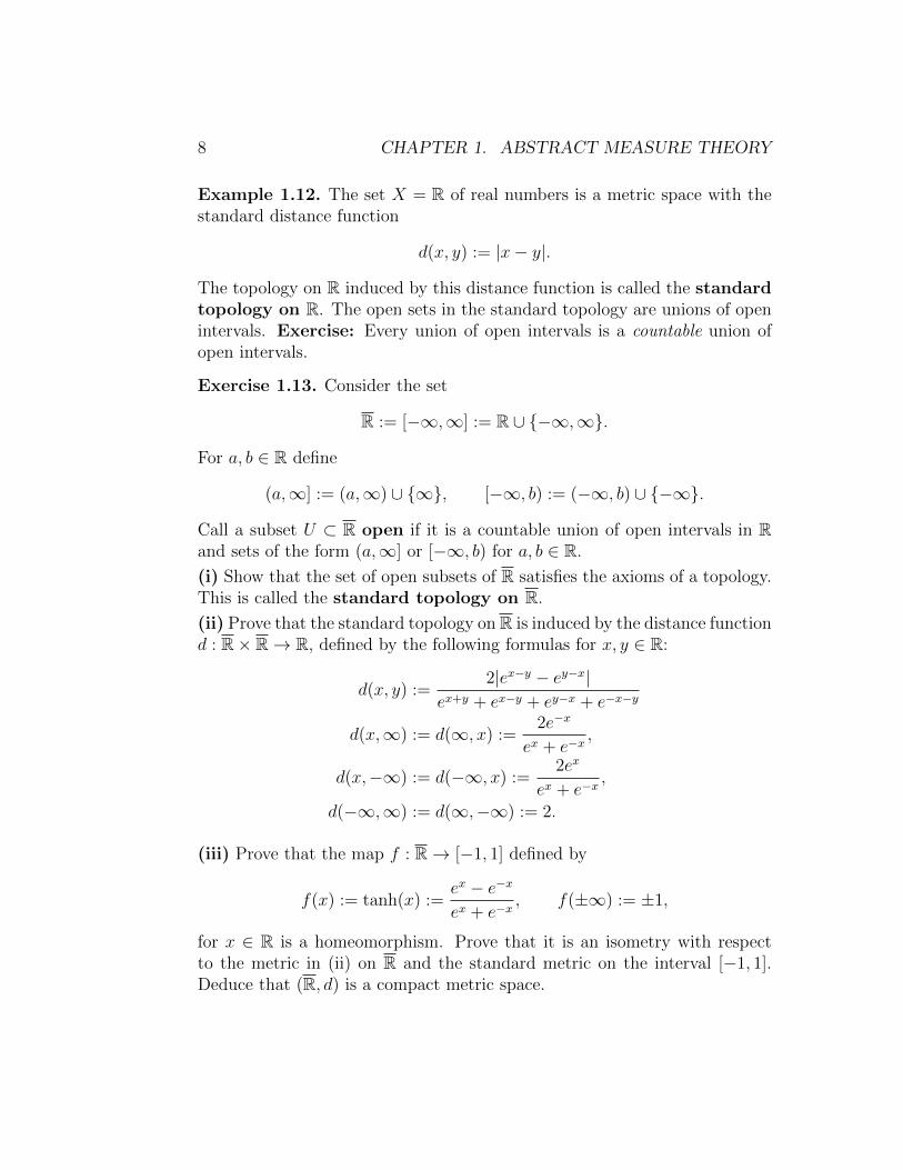
Exercise 1.13. Consider the set
R := [−∞,∞] := R ∪ −∞,∞.
For a, b ∈ R define
(a,∞] := (a,∞) ∪ ∞, [−∞, b) := (−∞, b) ∪ −∞.
Call a subset U ⊂ R open if it is a countable union of open intervals in Rand sets of the form (a,∞] or [−∞, b) for a, b ∈ R.
(i) Show that the set of open subsets of R satisfies the axioms of a topology.This is called the standard topology on R.
(ii) Prove that the standard topology on R is induced by the distance functiond : R× R→ R, defined by the following formulas for x, y ∈ R:
d(x, y) :=2|ex−y − ey−x|
ex+y + ex−y + ey−x + e−x−y
d(x,∞) := d(∞, x) :=2e−x
ex + e−x,
d(x,−∞) := d(−∞, x) :=2ex
ex + e−x,
d(−∞,∞) := d(∞,−∞) := 2.
(iii) Prove that the map f : R→ [−1, 1] defined by
f(x) := tanh(x) :=ex − e−x
ex + e−x, f(±∞) := ±1,
for x ∈ R is a homeomorphism. Prove that it is an isometry with respectto the metric in (ii) on R and the standard metric on the interval [−1, 1].Deduce that (R, d) is a compact metric space.
1.1. σ-ALGEBRAS 9
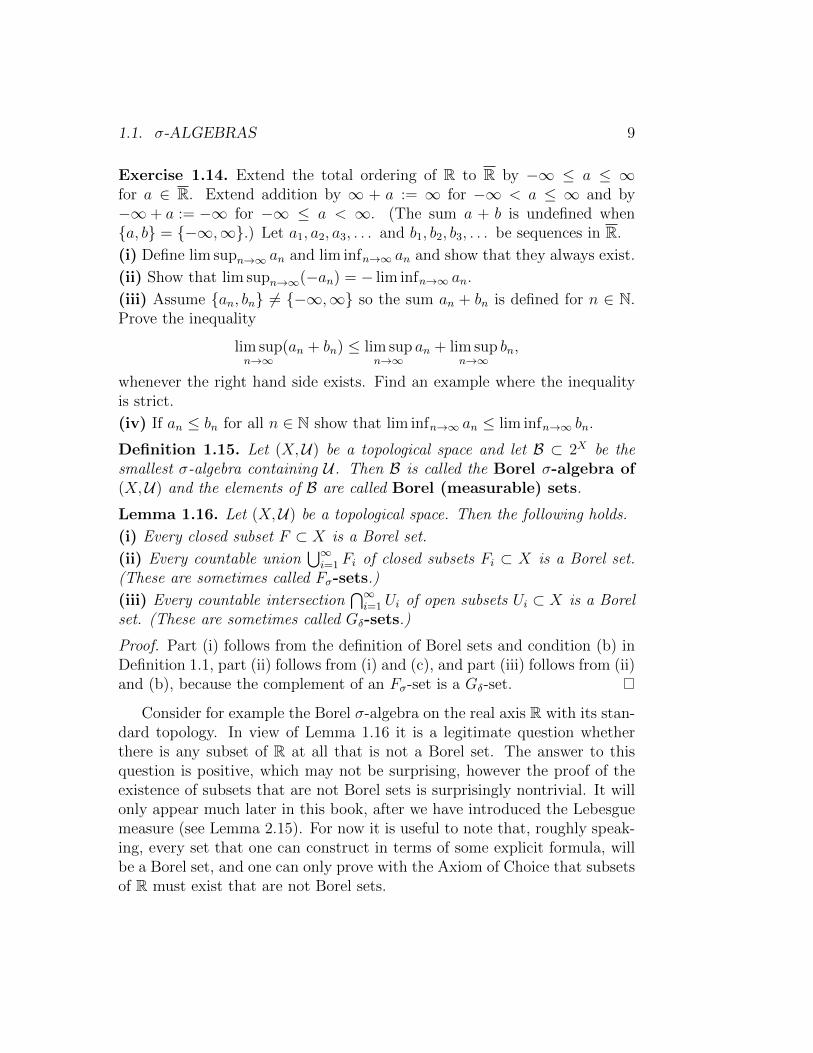
Exercise 1.14. Extend the total ordering of R to R by −∞ ≤ a ≤ ∞for a ∈ R. Extend addition by ∞ + a := ∞ for −∞ < a ≤ ∞ and by−∞+ a := −∞ for −∞ ≤ a < ∞. (The sum a + b is undefined whena, b = −∞,∞.) Let a1, a2, a3, . . . and b1, b2, b3, . . . be sequences in R.
(i) Define lim supn→∞ an and lim infn→∞ an and show that they always exist.
(ii) Show that lim supn→∞(−an) = − lim infn→∞ an.
(iii) Assume an, bn 6= −∞,∞ so the sum an + bn is defined for n ∈ N.Prove the inequality
lim supn→∞
(an + bn) ≤ lim supn→∞
an + lim supn→∞
bn,
whenever the right hand side exists. Find an example where the inequalityis strict.
(iv) If an ≤ bn for all n ∈ N show that lim infn→∞ an ≤ lim infn→∞ bn.
Definition 1.15. Let (X,U) be a topological space and let B ⊂ 2X be thesmallest σ-algebra containing U . Then B is called the Borel σ-algebra of(X,U) and the elements of B are called Borel (measurable) sets.
Lemma 1.16. Let (X,U) be a topological space. Then the following holds.
(i) Every closed subset F ⊂ X is a Borel set.
(ii) Every countable union⋃∞i=1 Fi of closed subsets Fi ⊂ X is a Borel set.
(These are sometimes called Fσ-sets.)
(iii) Every countable intersection⋂∞i=1 Ui of open subsets Ui ⊂ X is a Borel
set. (These are sometimes called Gδ-sets.)
Proof. Part (i) follows from the definition of Borel sets and condition (b) inDefinition 1.1, part (ii) follows from (i) and (c), and part (iii) follows from (ii)and (b), because the complement of an Fσ-set is a Gδ-set.
Consider for example the Borel σ-algebra on the real axis R with its stan-dard topology. In view of Lemma 1.16 it is a legitimate question whetherthere is any subset of R at all that is not a Borel set. The answer to thisquestion is positive, which may not be surprising, however the proof of theexistence of subsets that are not Borel sets is surprisingly nontrivial. It willonly appear much later in this book, after we have introduced the Lebesguemeasure (see Lemma 2.15). For now it is useful to note that, roughly speak-ing, every set that one can construct in terms of some explicit formula, willbe a Borel set, and one can only prove with the Axiom of Choice that subsetsof R must exist that are not Borel sets.

10 CHAPTER 1. ABSTRACT MEASURE THEORY
Recollections About Point Set Topology
We close this section with a digression into some basic notions in topologythat, at least for metric spaces, are familiar from first year analysis and will beused throughout this book. The two concepts we recall here are compactnessand continuity. A subset K ⊂ X of a metric space (X, d) is called compactif every sequence in K has a subsequence that converges to some elementof K. Thus, in particular, every compact subset is closed. The notion ofcompactness carries over to general topological spaces as follows.
Let (X,U) be a topological space and let K ⊂ X. An open coverof K is a collection of open sets Uii∈I , indexed by a set I, such thatK ⊂
⋃i∈I Ui. The set K is called compact if every open cover of K has a
finite subcover, i.e. if for every open cover Uii∈I of K there exist finitelymany indices i1, . . . , in ∈ I such that K ⊂ Ui1 ∪ · · · ∪ Uin . When (X, d) isa metric space and U = U(X, d) is the topology induced by the distancefunction (Definition 1.10), the two notions of compactness agree. Thus, forevery subset K ⊂ X, every sequence in K has a subsequence converging to anelement of K if and only if every open cover of K has a finite subcover. For aproof see for example Munkres [14] or [20, Appendix C.1]. We emphasize thatwhen K is a compact subset of a general topological space (X,U) it does notfollow that K is closed. For example a finite subset of X is always compactbut need not be closed or, if U = ∅, X then every subset of X is compactbut only the empty set and X itself are closed subsets of X. If, however,(X,U) is a Hausdorff space (i.e. for any two distinct points x, y ∈ X thereexist open sets U, V ∈ U such that x ∈ U , y ∈ V , and U ∩V = ∅) then everycompact subset of X is closed (Lemma A.2).
Next recall that a map f : X → Y between two metric spaces (X, dX)and (Y, dY ) is continuous (i.e. for every x ∈ X and every ε > 0 there is aδ > 0 such that f(Bδ(x, dX)) ⊂ Bε(f(x), dY )) if and only if the pre-imagef−1(V ) := x ∈ X | f(x) ∈ V of every open subset of Y is an open subsetof X. This second notion carries over to general topological spaces, i.e. amap f : X → Y between topological spaces (X,UX) and (Y,UY ) is calledcontinuous if V ∈ UY =⇒ f−1(V ) ∈ UX . It follows directly from thedefinition that topological spaces form a category, in that the compositiong f : X → Z of two continuous maps f : X → Y and g : Y → Z betweentopological spaces is again continuous. Another basic observation is thatif f : X → Y is a continuous map between topological spaces and K is acompact subset of X then its image f(K) is a compact subset of Y .
1.2. MEASURABLE FUNCTIONS 11
1.2 Measurable Functions
In analogy to continuous maps between topological spaces one can definemeasurable maps between measurable spaces as those maps under which pre-images of measurable sets are again measurable. A slightly different approachis taken by Rudin [17] who defines a measurable map from a measurablespace to a topological space as one under which pre-images of open sets aremeasurable. Both definitions agree whenever the target space is equippedwith its Borel σ-algebra.
As a warmup we begin with some recollections about pre-images of setsthat are also relevant for the discussion on page 10. For any map f : X → Ybetween two sets X and Y and any subset B ⊂ Y , the pre-image
f−1(B) := x ∈ X | f(x) ∈ B
of B under f is a well defined subset of X, whether or not the map f isbijective, i.e. even if there does not exist any map f−1 : Y → X. Thepre-image defines a map from 2Y to 2X . It satisfies
f−1(Y ) = X, f−1(∅) = ∅, (1.1)
and preserves union, intersection, and complement. Thus
f−1(Y \B) = X \ f−1(B) (1.2)
for every subset B ⊂ Y and
f−1
(⋃i∈I
Bi
)=⋃i∈I
f−1(Bi), f−1
(⋂i∈I
Bi
)=⋂i∈I
f−1(Bi) (1.3)
for every collection of subsets Bi ⊂ Y , indexed by a set I.
Definition 1.17 (Measurable Function). (i) Let (X,AX) and (Y,AY ) bemeasurable spaces. A map f : X → Y is called measurable if the pre-imageof every measurable subset of Y under f is a measurable subset of X, i.e.
B ∈ AY =⇒ f−1(B) ∈ AX .
(ii) Let (X,AX) be a measurable space. A function f : X → R is calledmeasurable if it is measurable with respect to the Borel σ-algebra on Rassociated to the standard topology in Exercise 1.13 (see Definition 1.15).
12 CHAPTER 1. ABSTRACT MEASURE THEORY
(iii) Let (X,UX) and (Y,UY ) be topological spaces. A map f : X → Y iscalled Borel measurable if the pre-image of every Borel measurable subsetof Y under f is a Borel measurable subset of X.
Example 1.18. Let X be a set. The characteristic function of a subsetA ⊂ X is the function χA : X → R defined by
χA(x) :=
1, if x ∈ A,0, if x /∈ A. (1.4)
Now assume (X,A) is a measurable space, consider the Borel σ-algebra on R,and let A ⊂ X be any subset. Then χA is a measurable function if and onlyif A is a measurable set.
Part (iii) in Definition 1.17 is the special case of part (i), where AX ⊂ 2X
and AY ⊂ 2Y are the σ-algebras of Borel sets (see Definition 1.15). The-orem 1.20 below shows that every continuous function between topologicalspaces is Borel measurable. It also shows that a function from a measur-able space to a topological space is measurable with respect to the Borelσ-algebra on the target space if and only if the pre-image of every open set ismeasurable. Since the collection of Borel sets is in general much larger thanthe collection of open sets, the collection of measurable functions is then alsomuch larger than the collection of continuous functions.
Theorem 1.19 (Measurable Maps).Let (X,AX), (Y,AY ), and (Z,AZ) be measurable spaces.
(i) The identity map idX : X → X is measurable.
(ii) If f : X → Y and g : Y → Z are measurable maps then so is thecomposition g f : X → Z.
(iii) Let f : X → Y be any map. Then the set
f∗AX :=B ⊂ Y | f−1(B) ∈ AX
(1.5)
is a σ-algebra on Y , called the pushforward of AX under f .
(iv) A map f : X → Y is measurable if and only if AY ⊂ f∗AX .
Proof. Parts (i) and (ii) follow directly from the definitions. That the setf∗AX ⊂ 2Y defined by (1.5) is a σ-algebra follows from equation (1.1) (foraxiom (a)), equation (1.2) (for axiom (b)), and equation (1.3) (for axiom (c)).This proves part (iii). Moreover, by Definition 1.17 f is measurable if andonly if f−1(B) ∈ AX for every B ∈ AY and this means that AY ⊂ f∗AX .This proves part (iv) and Theorem 1.19.

1.2. MEASURABLE FUNCTIONS 13
Theorem 1.20 (Measurable and Continuous Maps). Let (X,AX) and(Y,AY ) be measurable spaces. Assume UY ⊂ 2Y is a topology on Y suchthat AY is the Borel σ-algebra of (Y,UY ).
(i) A map f : X → Y is measurable if an only if the pre-image of every opensubset V ⊂ Y under f is measurable, i.e.
V ∈ UY =⇒ f−1(V ) ∈ AX .
(ii) Assume UX ⊂ 2X is a topology on X such that AX is the Borel σ-algebraof (X,UX). Then every continuous map f : X → Y is (Borel) measurable.
Proof. By part (iv) of Theorem 1.19 a map f : X → Y is measurable ifand only if AY ⊂ f∗AX . Since f∗AX is a σ-algebra on Y by part (iii) ofTheorem 1.19, and the Borel σ-algebra AY is the smallest σ-algebra on Ycontaining the collection of open sets UY by Definition 1.15, it follows thatAY ⊂ f∗AX if and only if UY ⊂ f∗AX . By the definition of f∗AX in (1.5),this translates into the condition V ∈ UY =⇒ f−1(V ) ∈ AX . This provespart (i). If in addition AX is the Borel σ-algebra of a topology UX on X andf : (X,UX)→ (Y,UY ) is a continuous map then the pre-image of every opensubset V ⊂ Y under f is an open subset of X and hence is a Borel subsetof X; thus it follows from part (i) that f is Borel measurable. This provespart (ii) and Theorem 1.20.
Theorem 1.21 (Characterization of Measurable Functions).Let (X,A) be a measurable space and let f : X → R be any function. Thenthe following are equivalent.
(i) f is measurable.
(ii) f−1((a,∞]) is a measurable subset of X for every a ∈ R.
(iii) f−1([a,∞]) is a measurable subset of X for every a ∈ R.
(iv) f−1([−∞, b)) is a measurable subset of X for every b ∈ R.
(v) f−1([−∞, b]) is a measurable subset of X for every b ∈ R.
Proof. That (i) implies (ii), (iii), (iv), and (v) follows directly from the def-initions. We prove that (ii) implies (i). Thus let f : X → R be a functionsuch that f−1((a,∞]) ∈ AX for every a ∈ R and define
B := f∗AX =B ⊂ R | f−1(B) ∈ AX
⊂ 2R.
14 CHAPTER 1. ABSTRACT MEASURE THEORY
Then B is a σ-algebra on R by part (iii) of Theorem 1.19 and (a,∞] ∈ B forevery a ∈ R by assumption. Hence [−∞, b] = R \ (b,∞] ∈ B for every b ∈ Rby axiom (b) and hence
[−∞, b) =⋃n∈N
[−∞, b− 1n] ∈ B
by axiom (c) in Definition 1.1. Hence it follows from (f) in Lemma 1.2 that
(a, b) = [−∞, b) ∩ (a,∞] ∈ B
for every pair of real numbers a < b. Since every open subset of R is acountable union of sets of the form (a, b), (a,∞], [−∞, b), it follows fromaxiom (c) in Definition 1.1 that every open subset of R is an element of B.Hence it follows from Theorem 1.20 that f is measurable. This shows that (ii)implies (i). That either of the conditions (iii), (iv), and (v) also implies (i) isshown by a similar argument which is left as an exercise for the reader. Thisproves Theorem 1.21.
Our next goal is to show that sums, products, and limits of measurablefunctions are again measurable. The next two results are useful for the proofsof these fundamental facts.
Theorem 1.22 (Vector Valued Measurable Functions). Let (X,A) bea measurable space and let f = (f1, . . . , fn) : X → Rn be a function. Then fis measurable if and only if fi : X → R is measurable for each i.
Proof. For i = 1, . . . , n define the projection πi : Rn → R by πi(x) := xi forx = (x1, . . . , xn) ∈ R. Since πi is continuous it follows from Theorems 1.19and 1.20 that if f is measurable so is fi = πi f for all i. Conversely, supposethat fi is measurable for i = 1, . . . , n. Let ai < bi for i = 1, . . . , n and define
Q(a, b) := x ∈ Rn | ai < xi < bi ∀i = (a1, b1)× · · · × (an, bn).
Then
f−1(Q(a, b)) =n⋂i=1
f−1i ((ai, bi)) ∈ A
by property (f) in Lemma 1.2. Now every open subset of Rn can be expressedas a countable union of sets of the form Q(a, b). (Prove this!) Hence it followsfrom axiom (c) in Definition 1.1 that f−1(U) ∈ A for every open set U ⊂ Rn
and hence f is measurable. This proves Theorem 1.22.

1.2. MEASURABLE FUNCTIONS 15
Lemma 1.23. Let (X,A) be a measurable space and let u, v : X → Rbe measurable functions. If φ : R2 → R is continuous then the functionh : X → R, defined by h(x) := φ(u(x), v(x)) for x ∈ X, is measurable.
Proof. The map f := (u, v) : X → R2 is measurable (with respect to theBorel σ-algebra on R2) by Theorem 1.22 and the map φ : R2 → R is Borelmeasurable by Theorem 1.20. Hence the composition h = φ f : X → R ismeasurable by Theorem 1.19. This proves Lemma 1.23.
Theorem 1.24 (Properties of Measurable Functions).Let (X,A) be a measurable space.
(i) If f, g : X → R are measurable functions then so are the functions
f + g, fg, maxf, g, minf, g, |f |.
(ii) Let fk : X → R, k = 1, 2, 3, . . . , be a sequence of measurable functions.Then the following functions from X to R are measurable:
infkfk, sup
kfk, lim sup
k→∞fk, lim inf
k→∞fk.
Proof. We prove (i). The functions φ : R2 → R defined by φ(s, t) := s + t,φ(s, t) := st, φ(s, t) := maxs, t, φ(s, t) := mins, t, or φ(s, t) := |s| are allcontinuous. Hence assertion (i) follows from Lemma 1.23.
We prove (ii). Define g := supk fk : X → R and let a ∈ R. Then the set
g−1((a,∞]) =
x ∈ X
∣∣∣∣ supkfk(x) > a
= x ∈ X | ∃k ∈ N such that fk(x) > a
=⋃k∈N
x ∈ X | fk(x) > a =⋃k∈N
f−1k ((a,∞])
is measurable. Hence it follows from Theorem 1.21 that g is measurable.It also follows from part (i) (already proved) that −fk is measurable, henceso is supk(−fk) by what we have just proved, and hence so is the functioninfk fk = − supk(−fk). With this understood, it follows that the functions
lim supk→∞
fk = inf`∈N
supk≥`
fk, lim infk→∞
fk = sup`∈N
infk≥`
fk
are also measurable. This proves Theorem 1.24.
It follows from Theorem 1.24 that the pointwise limit of a sequence ofmeasurable functions, if it exists, is again measurable. This is in sharp con-trast to Riemann integrable functions.
16 CHAPTER 1. ABSTRACT MEASURE THEORY
Step Functions
We close this section with a brief discussion of measurable step functions.Such functions will play a central role throughout this book. In particular,they are used in the definition of the Lebesgue integral.
Definition 1.25 (Step Function). Let X be a set. A function s : X → Ris called a step function (or simple function) if it takes on only finitelymany values, i.e. the image s(X) is a finite subset of R.
Let s : X → R be a step function, write s(X) = α1, . . . , α` with αi 6= αjfor i 6= j, and define Ai := s−1(αi) = x ∈ X | s(x) = αi for i = 1, . . . , `.Then the sets A1, . . . , A` form a partition of X, i.e.
X =⋃i=1
Ai, Ai ∩ Aj = ∅ for i 6= j. (1.6)
(See Example 1.5.) Moreover,
s =∑i=1
αiχAi , (1.7)
where χAi : X → R is the characteristic function of the set Ai for i = 1, . . . , `(see equation (1.4)). In this situation s is measurable if and only if the setAi ⊂ X is measurable for each i. For later reference we prove the following.
Theorem 1.26 (Approximation). Let (X,A) be a measurable space andlet f : X → [0,∞] be a function. Then f is measurable if and only if thereexists a sequence of measurable step functions sn : X → [0,∞) such that
0 ≤ s1(x) ≤ s2(x) ≤ · · · ≤ f(x), f(x) = limn→∞
sn(x) for all x ∈ X.
Proof. If f can be approximated by a sequence of measurable step func-tions then f is measurable by Theorem 1.24. Conversely, suppose that f ismeasurable. For n ∈ N define φn : [0,∞]→ R by
φn(t) :=
k2−n, if k2−n ≤ t < (k + 1)2−n, k = 0, 1, . . . , n2n − 1,n, if t ≥ n.
(1.8)
These functions are Borel measurable and satisfy φn(0) = 0 and φn(∞) = nfor all n as well as t− 2−n ≤ φn(t) ≤ φn+1(t) ≤ t whenever n ≥ t > 0. Thus
limn→∞
φn(t) = t for all t ∈ [0,∞].
Hence the functions sn := φn f satisfy the requirements of the theorem.
1.3. INTEGRATION OF NONNEGATIVE FUNCTIONS 17
1.3 Integration of Nonnegative Functions
Our next goal is to define the integral of a measurable step function andthen the integral of a general nonnegative measurable function via approxi-mation. This requires the notion of volume or measure of a measurable set.The definitions of measure and integral will require some arithmetic on thespace [0,∞]. Addition to ∞ and multiplication by ∞ are defined by
a+∞ :=∞+ a :=∞, a · ∞ :=∞ · a :=
∞, if a 6= 0,0, if a = 0.
With this convention addition and multiplication are commutative, associa-tive, and distributive. Moreover, if ai and bi are nondecreasing sequencesin [0,∞] then the limits a := limi→∞ ai and b := limi→∞ bi exists in [0,∞]and satisfy the familiar rules a+ b = limi→∞(ai + bi) and ab = limi→∞(aibi).These rules must be treated with caution. The product rule does not holdwhen the sequences are not nondecreasing. For example ai := i convergesto a = ∞, bi := 1/i converges to b = 0, but aibi = 1 does not converge toab = 0. (Exercise: Show that the sum of two convergent sequences in [0,∞]always converges to the sum of the limits.) Also, for all a, b, c ∈ [0,∞],
a+ b = a+ c, a <∞ =⇒ b = c,
ab = ac, 0 < a <∞ =⇒ b = c.
Neither of these assertions extend to the case a =∞.
Definition 1.27 (Measure). Let (X,A) be a measurable space. A measureon (X,A) is a function
µ : A → [0,∞]
satisfying the following axioms.
(a) µ is σ-additive, i.e. if Ai ∈ A, i = 1, 2, 3, . . . , is a sequence of pairwisedisjoint measurable sets then
µ
(∞⋃i=1
Ai
)=∞∑i=1
µ(Ai).
(b) There exists a measurable set A ∈ A such that µ(A) <∞.
A measure space is a triple (X,A, µ) consisting of a set X, a σ-algebraA ⊂ 2X , and a measure µ : A → [0,∞].
18 CHAPTER 1. ABSTRACT MEASURE THEORY
The basic properties of measures are summarized in the next theorem.
Theorem 1.28 (Properties of Measures).Let (X,A, µ) be a measure space. Then the following holds.
(i) µ(∅) = 0.
(ii) If n ∈ N and A1, . . . , An ∈ A such that Ai ∩ Aj = ∅ for i 6= j then
µ(A1 ∪ · · · ∪ An) = µ(A1) + · · ·+ µ(An).
(iii) If A,B ∈ A such that A ⊂ B then µ(A) ≤ µ(B).
(iv) Let Ai ∈ A be a sequence such that Ai ⊂ Ai+1 for all i. Then
µ
(∞⋃i=1
Ai
)= lim
i→∞µ(Ai).
(v) Let Ai ∈ A be a sequence such that Ai ⊃ Ai+1 for all i. Then
µ(A1) <∞ =⇒ µ
(∞⋂i=1
Ai
)= lim
i→∞µ(Ai).
Proof. We prove (i). Choose A1 ∈ A such that µ(A1) <∞ and define Ai := ∅for i > 1. Then it follows from σ-additivity that
µ(A1) = µ(A1) +∑i>1
µ(∅)
and hence µ(∅) = 0. This proves part (i).Part (ii) follows from (i) and σ-additivity by choosing Ai := ∅ for i > n.We prove (iii). If A,B ∈ A such that A ⊂ B then B \ A ∈ A by
property (g) in Lemma 1.2 and hence µ(B) = µ(A) + µ(B \ A) ≥ µ(A) bypart (ii). This proves part (iii).
We prove (iv). Assume Ai ⊂ Ai+1 for all i and define B1 := A1 andBi := Ai \ Ai−1 for i > 1. Then Bi is measurable for all i and, for n ∈ N,
An =n⋃i=1
Bi, A :=∞⋃i=1
Ai =∞⋃i=1
Bi.
Since Bi ∩Bj = ∅ for i 6= j it follows from σ-additivity that
µ(A) =∞∑i=1
µ(Bi) = limn→∞
n∑i=1
µ(Bi) = limn→∞
µ(An).
Here the last equation follows from part (ii). This proves part (iv).
1.3. INTEGRATION OF NONNEGATIVE FUNCTIONS 19
We prove (v). Assume Ai ⊃ Ai+1 for all i and define Ci := Ai \ Ai+1.Then Ci is measurable for all i and, for n ∈ N,
An = A ∪∞⋃i=n
Ci, A :=∞⋂i=1
Ai.
Since Ci ∩ Cj = ∅ for i 6= j it follows from σ-additivity that
µ(An) = µ(A) +∞∑i=n
µ(Ci)
for all n ∈ N. Since µ(A1) <∞ it follows that∑∞
i=1 µ(Ci) <∞ and hence
limn→∞
µ(An) = µ(A) + limn→∞
∞∑i=n
µ(Ci) = µ(A).
This proves part (v) and Theorem 1.28.
Exercise 1.29. Let (X,A, µ) be a measure space and let Ai ∈ A be asequence of measurable sets. Prove that µ(
⋃iAi) ≤
∑i µ(Ai).
Example 1.30. Let (X,A) be a measurable space. The counting measureµ : A → [0,∞] is defined by µ(A) := #A for A ∈ A. As an example, considerthe counting measure µ : 2N → [0,∞] on the natural numbers. Then the setsAn := n, n + 1, · · · all have infinite measure and their intersection is theempty set and hence has measure zero. Thus the hypothesis µ(A1) < ∞cannot be removed in part (v) of Theorem 1.28.
Example 1.31. Let (X,A) be a measurable space and fix an element x0 ∈ X.The Dirac measure at x0 is the measure δx0 : A → [0,∞] defined by
δx0(A) :=
1, if x0 ∈ A,0, if x0 /∈ A,
for A ∈ A.
Example 1.32. Let X be an uncountable set and let A be the σ-algebraof all subsets of X that are either countable or have countable complements(Example 1.4). Then the function µ : A → [0, 1] defined by µ(A) := 0 whenA is countable and by µ(A) := 1 when Ac is countable is a measure.
Example 1.33. Let X =⋃i∈I Ai be a partition and let A ⊂ 2X be the σ-
algebra in Example 1.5. Then any function I → [0,∞] : i 7→ αi determines ameasure µ : A → [0,∞] via µ(AJ) :=
∑j∈J αj for J ⊂ I and AJ =
⋃j∈J Aj.
20 CHAPTER 1. ABSTRACT MEASURE THEORY
With these preparations in place we are now ready to introduce theLebesgue integral of a nonnegative measurable function
Definition 1.34 (Lebesgue Integral). Let (X,A, µ) be a measure spaceand let E ∈ A be a measurable set.
(i) Let s : X → [0,∞) be a measurable step function of the form
s =n∑i=1
αiχAi (1.9)
with αi ∈ [0,∞) and Ai ∈ A for i = 1, . . . , n. The (Lebesgue) integral ofs over E is the number
∫Es dµ ∈ [0,∞] defined by∫
E
s dµ :=n∑i=1
αiµ(E ∩ Ai). (1.10)
(ii) Let f : X → [0,∞] be a measurable function. The (Lebesgue) integralof f over E is the number
∫Ef dµ ∈ [0,∞] defined by∫
E
f dµ := sups≤f
∫E
s dµ,
where the supremum is taken over all measurable step function s : X → [0,∞)that satisfy s(x) ≤ f(x) for all x ∈ X.
The reader may verify that the right hand side of (1.10) depends only on sand not on the choice of αi and Ai. The same definition can be used if f isonly defined on the measurable set E ⊂ X. Then AE := A ∈ A |A ⊂ E isa σ-algebra on E and µE := µ|AE is a measure. So (E,AE, µE) is a measurespace and the integral
∫Ef dµE is well defined. It agrees with the integral of
the extended function on X, defined by f(x) := 0 for x ∈ X \ E.
Theorem 1.35 (Basic Properties of the Lebesgue Integral).Let (X,A, µ) be a measure space and let f, g : X → [0,∞] be measurablefunctions and let E ∈ A. Then the following holds.
(i) If f ≤ g on E then∫Ef dµ ≤
∫Eg dµ.
(ii)∫Ef dµ =
∫XfχE dµ.
(iii) If f(x) = 0 for all x ∈ E then∫Ef dµ = 0.
(iv) If µ(E) = 0 then∫Ef dµ = 0.
(v) If A ∈ A and E ⊂ A then∫Ef dµ ≤
∫Af dµ.
(vi) If c ∈ [0,∞) then∫Ecf dµ = c
∫Ef dµ.

1.3. INTEGRATION OF NONNEGATIVE FUNCTIONS 21
Proof. To prove (i), assume f ≤ g on E. If s : X → [0,∞) is a measurablestep function such that s ≤ f then sχE ≤ g, so
∫Es dµ =
∫EsχE dµ ≤
∫Eg dµ
by definition of the integral of g. Now take the supremum over all measurablestep functions s ≤ f to obtain
∫Ef dµ ≤
∫Eg dµ. This proves (i).
We prove (ii). It follows from the definitions that∫E
f dµ = sups≤f
∫E
s dµ = sups≤f
∫X
sχE dµ = supt≤fχE
∫X
t dµ =
∫X
fχE dµ.
Here the supremum is over all measurable step functions s : X → [0,∞),respectively t : X → [0,∞), that satisfy s ≤ f , respectively t ≤ fχE. Thesecond equation follows from the fact that every measurable step functions : X → [0,∞) satisfies
∫Es dµ =
∫XsχE dµ by definition of the integral.
The third equation follows from the fact that a measurable step functiont : X → [0,∞) satisfies t ≤ fχE if and only if it has the form t = sχE forsome measurable step function s : X → [0,∞) such that s ≤ f .
Part (iii) follows from part (i) with g = 0 and the fact that∫Ef dµ ≥ 0 by
definition. Part (iv) follows from the fact that∫Es dµ = 0 for every measur-
able step function s when µ(E) = 0. Part (v) follows from parts (i) and (ii)and the fact that fχE ≤ fχA whenever E ⊂ A. Part (vi) follows from thefact that
∫Ecs dµ = c
∫Es dµ for every c ∈ [0,∞) and every measurable step
function s, by the commutative, associative, and distributive rules for calcu-lations with numbers in [0,∞]. This proves Theorem 1.35.
Notably absent from the statements of Theorem 1.35 is the assertionthat the integral of a sum is the sum of the integrals. This is a fundamentalproperty that any integral should have. The proof that the integral in Defi-nition 1.34 indeed satisfies this crucial condition requires some preparation.The first step is to verify this property for integrals of step functions and thesecond step is the Lebesgue Monotone Convergence Theorem 1.37.
Lemma 1.36 (Additivity for Step Functions). Let (X,A, µ) be a mea-sure space and let s, t : X → [0,∞) be measurable step functions.
(i) For every measurable set E ∈ A∫E
(s+ t) dµ =
∫E
s dµ+
∫E
t dµ.
(ii) If E1, E2, E3, . . . is a sequence of pairwise disjoint measurable sets then∫E
s dµ =∞∑k=1
∫Ek
s dµ, E :=⋃k∈N
Ek.
22 CHAPTER 1. ABSTRACT MEASURE THEORY
Proof. Write the functions s and t in the form
s =m∑i=1
αiχAi , t =n∑j=1
βjχBj
where αi, βj ∈ [0,∞) and Ai, Bj ∈ A such that Ai ∩ Ai′ = ∅ for i 6= i′,Bj ∩Bj′ = ∅ for j 6= j′, and X =
⋃mi=1 Ai =
⋃nj=1 Bj. Then
s+ t =m∑i=1
n∑j=1
(αi + βj)χAi∩Bj
and hence∫E
(s+ t) dµ =m∑i=1
n∑j=1
(αi + βj)µ(Ai ∩Bj ∩ E)
=m∑i=1
αi
n∑j=1
µ(Ai ∩Bj ∩ E) +n∑j=1
βj
m∑i=1
µ(Ai ∩Bj ∩ E)
=m∑i=1
αiµ(Ai ∩ E) +n∑j=1
βjµ(Bj ∩ E) =
∫E
s dµ+
∫E
t dµ.
To prove (ii), let E1, E2, E3, . . . be a sequence of pairwise disjoint measurablesets and define E :=
⋃∞k=1Ek. Then∫
E
s dµ =m∑i=1
αiµ(E ∩ Ai) =m∑i=1
αi
∞∑k=1
µ(Ek ∩ Ai)
=m∑i=1
αi limn→∞
n∑k=1
µ(Ek ∩ Ai)
= limn→∞
m∑i=1
αi
n∑k=1
µ(Ek ∩ Ai)
= limn→∞
n∑k=1
m∑i=1
αiµ(Ek ∩ Ai)
= limn→∞
n∑k=1
∫Ek
s dµ =∞∑k=1
∫Ek
s dµ.
This proves Lemma 1.36.
1.3. INTEGRATION OF NONNEGATIVE FUNCTIONS 23
Theorem 1.37 (Lebesgue Monotone Convergence Theorem).Let (X,A, µ) be a measure space and let fn : X → [0,∞] be a sequence ofmeasurable functions such that
fn(x) ≤ fn+1(x) for all x ∈ X and all n ∈ N.
Define f : X → [0,∞] by
f(x) := limn→∞
fn(x) for x ∈ X.
Then f is measurable and
limn→∞
∫X
fn dµ =
∫X
f dµ.
Proof. By part (i) of Theorem 1.35 we have∫X
fn dµ ≤∫X
fn+1 dµ
for all n ∈ N and hence the limit
α := limn→∞
∫X
fn dµ (1.11)
exists in [0,∞]. Moreover, f = supn fn is a measurable function on X, bypart (ii) of Theorem 1.24, and satisfies fn ≤ f for all n ∈ N. Thus it followsfrom part (i) of Theorem 1.35 that∫
X
fn dµ ≤∫X
f dµ for all n ∈ N
and hence
α ≤∫X
f dµ. (1.12)
Now fix a measurable step function s : X → [0,∞) such that s ≤ f . Defineµs : A → [0,∞] by
µs(E) :=
∫E
s dµ for E ∈ A. (1.13)

24 CHAPTER 1. ABSTRACT MEASURE THEORY
This function is a measure by part (ii) of Lemma 1.36 (which asserts that µs isσ-additive) and by part (iv) of Theorem 1.35 (which asserts that µs(∅) = 0).Now fix a constant 0 < c < 1 and define
En := x ∈ X | cs(x) ≤ fn(x) for n ∈ N.
Then En ∈ A is a measurable set and En ⊂ En+1 for all n ∈ N. Moreover,
∞⋃n=1
En = X. (1.14)
(To spell it out, choose an element x ∈ X. If f(x) = ∞, then fn(x) → ∞and hence cs(x) ≤ s(x) ≤ fn(x) for some n ∈ N, which means that x belongsto one of the sets En. If f(x) < ∞, then fn(x) converges to f(x) > cf(x),hence fn(x) > cf(x) ≥ cs(x) for some n ∈ N, and for this n we have x ∈ En.)Since cs ≤ fn on En, it follows from parts (i) and (vi) of Theorem 1.35 that
cµs(En) = c
∫En
s dµ =
∫En
cs dµ ≤∫En
fn dµ ≤∫X
fn dµ ≤ α.
Here the last inequality follows from the definition of α in (1.11). Hence
µs(En) ≤ α
cfor all n ∈ N. (1.15)
Since µs : A → [0,∞] is a measure, by part (i) of Theorem 1.35, it followsfrom equation (1.14) and part (iv) of Theorem 1.28 that∫
X
s dµ = µs(X) = limn→∞
µs(En) ≤ α
c. (1.16)
Here the last inequality follows from (1.15). Since (1.16) holds for everyconstant 0 < c < 1, we have
∫Xs dµ ≤ α for every measurable step function
s : X → [0,∞) such that s ≤ f . Take the supremum over all such s to obtain∫X
f dµ = sups≤f
∫X
s dµ ≤ α.
Combining this with (1.12) we obtain∫Xf dµ = α and hence the assertion
of Theorem 1.37 follows from the definition of α in (1.11).
1.3. INTEGRATION OF NONNEGATIVE FUNCTIONS 25
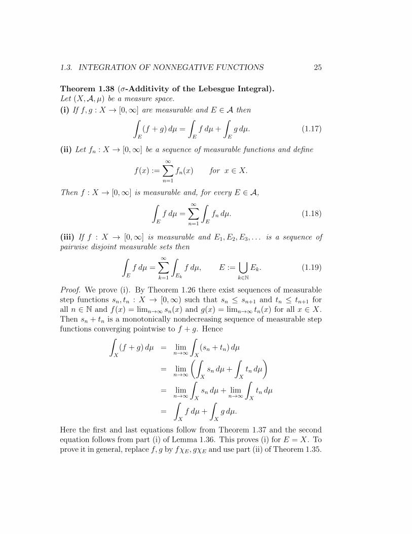
Theorem 1.38 (σ-Additivity of the Lebesgue Integral).Let (X,A, µ) be a measure space.
(i) If f, g : X → [0,∞] are measurable and E ∈ A then∫E
(f + g) dµ =
∫E
f dµ+
∫E
g dµ. (1.17)
(ii) Let fn : X → [0,∞] be a sequence of measurable functions and define
f(x) :=∞∑n=1
fn(x) for x ∈ X.
Then f : X → [0,∞] is measurable and, for every E ∈ A,∫E
f dµ =∞∑n=1
∫E
fn dµ. (1.18)
(iii) If f : X → [0,∞] is measurable and E1, E2, E3, . . . is a sequence ofpairwise disjoint measurable sets then∫
E
f dµ =∞∑k=1
∫Ek
f dµ, E :=⋃k∈N
Ek. (1.19)
Proof. We prove (i). By Theorem 1.26 there exist sequences of measurablestep functions sn, tn : X → [0,∞) such that sn ≤ sn+1 and tn ≤ tn+1 forall n ∈ N and f(x) = limn→∞ sn(x) and g(x) = limn→∞ tn(x) for all x ∈ X.Then sn + tn is a monotonically nondecreasing sequence of measurable stepfunctions converging pointwise to f + g. Hence∫
X
(f + g) dµ = limn→∞
∫X
(sn + tn) dµ
= limn→∞
(∫X
sn dµ+
∫X
tn dµ
)= lim
n→∞
∫X
sn dµ+ limn→∞
∫X
tn dµ
=
∫X
f dµ+
∫X
g dµ.
Here the first and last equations follow from Theorem 1.37 and the secondequation follows from part (i) of Lemma 1.36. This proves (i) for E = X. Toprove it in general, replace f, g by fχE, gχE and use part (ii) of Theorem 1.35.

26 CHAPTER 1. ABSTRACT MEASURE THEORY
We prove (ii). Define gn : X → [0,∞] by gn :=∑n
k=1 fk. This is a nonde-creasing sequence of measurable functions, by part (i) of Theorem 1.24, and itconverges pointwise to f by definition. Hence it follows from part (ii) of The-orem 1.24 that f is measurable and it follows from the Lebesgue MonotoneConvergence Theorem 1.37 that∫
X
f dµ = limn→∞
∫X
gn dµ
= limn→∞
∫X
n∑k=1
fk dµ
= limn→∞
n∑k=1
∫X
fk dµ
=∞∑n=1
∫X
fn dµ.
Here the second equation follows from the definition of gn and the thirdequation follows from part (i) of the present theorem (already proved). Thisproves (ii) for E = X. To prove it in general replace f, fn by fχE, fnχE anduse part (ii) of Theorem 1.35.
We prove (iii). Let f : X → [0,∞] be a measurable function and letEk ∈ A be a sequence of pairwise disjoint measurable sets. Define
E :=∞⋃k=1
Ek, fn :=n∑k=1
fχEk .
Then it follows from part (i) of the present theorem (already proved) andpart (ii) of Theorem 1.35 that∫
X
fn dµ =
∫X
n∑k=1
fχEk dµ =n∑k=1
∫X
fχEk dµ =n∑k=1
∫Ek
f dµ.
Now fn : X → [0,∞] is a nondecreasing sequence of measurable functionsconverging pointwise to fχE. Hence it follows from the Lebesgue MonotoneConvergence Theorem 1.37 that∫
E
f dµ =
∫X
fχE dµ = limn→∞
∫X
fn dµ = limn→∞
n∑k=1
∫Ek
f dµ =∞∑k=1
∫Ek
f dµ.
This proves Theorem 1.38.
1.3. INTEGRATION OF NONNEGATIVE FUNCTIONS 27
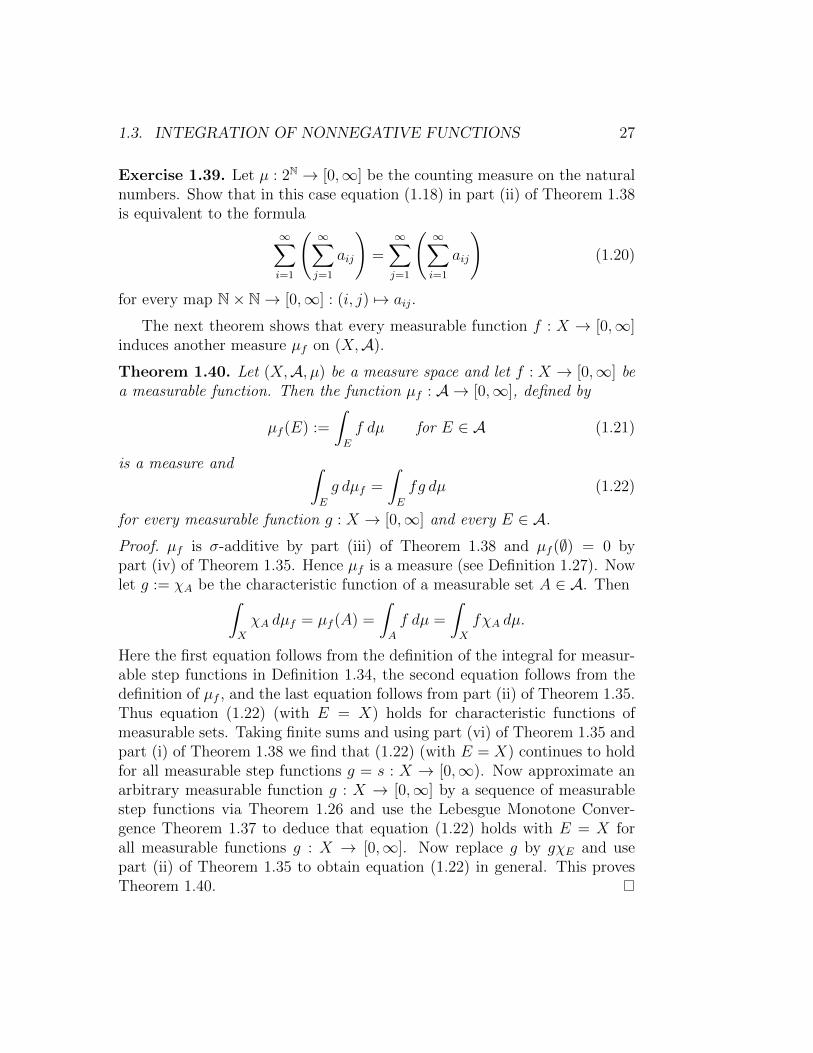
Exercise 1.39. Let µ : 2N → [0,∞] be the counting measure on the naturalnumbers. Show that in this case equation (1.18) in part (ii) of Theorem 1.38is equivalent to the formula
∞∑i=1
(∞∑j=1
aij
)=∞∑j=1
(∞∑i=1
aij
)(1.20)
for every map N× N→ [0,∞] : (i, j) 7→ aij.
The next theorem shows that every measurable function f : X → [0,∞]induces another measure µf on (X,A).
Theorem 1.40. Let (X,A, µ) be a measure space and let f : X → [0,∞] bea measurable function. Then the function µf : A → [0,∞], defined by
µf (E) :=
∫E
f dµ for E ∈ A (1.21)
is a measure and ∫E
g dµf =
∫E
fg dµ (1.22)
for every measurable function g : X → [0,∞] and every E ∈ A.
Proof. µf is σ-additive by part (iii) of Theorem 1.38 and µf (∅) = 0 bypart (iv) of Theorem 1.35. Hence µf is a measure (see Definition 1.27). Nowlet g := χA be the characteristic function of a measurable set A ∈ A. Then∫
X
χA dµf = µf (A) =
∫A
f dµ =
∫X
fχA dµ.
Here the first equation follows from the definition of the integral for measur-able step functions in Definition 1.34, the second equation follows from thedefinition of µf , and the last equation follows from part (ii) of Theorem 1.35.Thus equation (1.22) (with E = X) holds for characteristic functions ofmeasurable sets. Taking finite sums and using part (vi) of Theorem 1.35 andpart (i) of Theorem 1.38 we find that (1.22) (with E = X) continues to holdfor all measurable step functions g = s : X → [0,∞). Now approximate anarbitrary measurable function g : X → [0,∞] by a sequence of measurablestep functions via Theorem 1.26 and use the Lebesgue Monotone Conver-gence Theorem 1.37 to deduce that equation (1.22) holds with E = X forall measurable functions g : X → [0,∞]. Now replace g by gχE and usepart (ii) of Theorem 1.35 to obtain equation (1.22) in general. This provesTheorem 1.40.

28 CHAPTER 1. ABSTRACT MEASURE THEORY
It is one of the central questions in measure theory under which conditionsa measure λ : A → [0,∞] can be expressed in the form µf for some mea-surable function f : X → [0,∞]. We return to this question in Chapter 5.The final result in this section is an inequality which will be used in the proofof the Lebesgue Dominated Convergence Theorem 1.45.
Theorem 1.41 (Lemma of Fatou). Let (X,A, µ) be a measure space andlet fn : X → [0,∞] be a sequence of measurable functions. Then∫
X
lim infn→∞
fn dµ ≤ lim infn→∞
∫X
fn dµ.
Proof. For n ∈ N define gn : X → [0,∞] by
gn(x) := infi≥n
fi(x)
for x ∈ X. Then gn is measurable, by Theorem 1.24, and
g1(x) ≤ g2(x) ≤ g3(x) ≤ · · · , limn→∞
gn(x) = lim infn→∞
fn(x) =: f(x)
for all x ∈ X. Moreover, gn ≤ fi for all i ≥ n. By part (i) of Theorem 1.35this implies ∫
X
gn dµ ≤∫X
fi dµ
for all i ≥ n, and hence ∫X
gn dµ ≤ infi≥n
∫X
fi dµ
for all n ∈ N. Thus, by the Lebesgue Monotone Convergence Theorem 1.37,∫X
f dµ = limn→∞
∫X
gn dµ ≤ limn→∞
infi≥n
∫X
fi dµ = lim infn→∞
∫X
fn dµ.
This proves Theorem 1.41.
Example 1.42. Let (X,A, µ) be a measure space and E ∈ A be a measur-able set such that 0 < µ(E) < µ(X). Define fn := χE when n is even andfn := 1− χE when n is odd. Then lim infn→∞ fn = 0 and so∫
X
lim infn→∞
fndµ = 0 < minµ(E), µ(X \ E) = lim infn→∞
∫X
fn dµ.
Thus the inequality in Theorem 1.41 can be strict.
1.4. INTEGRATION OF REAL VALUED FUNCTIONS 29
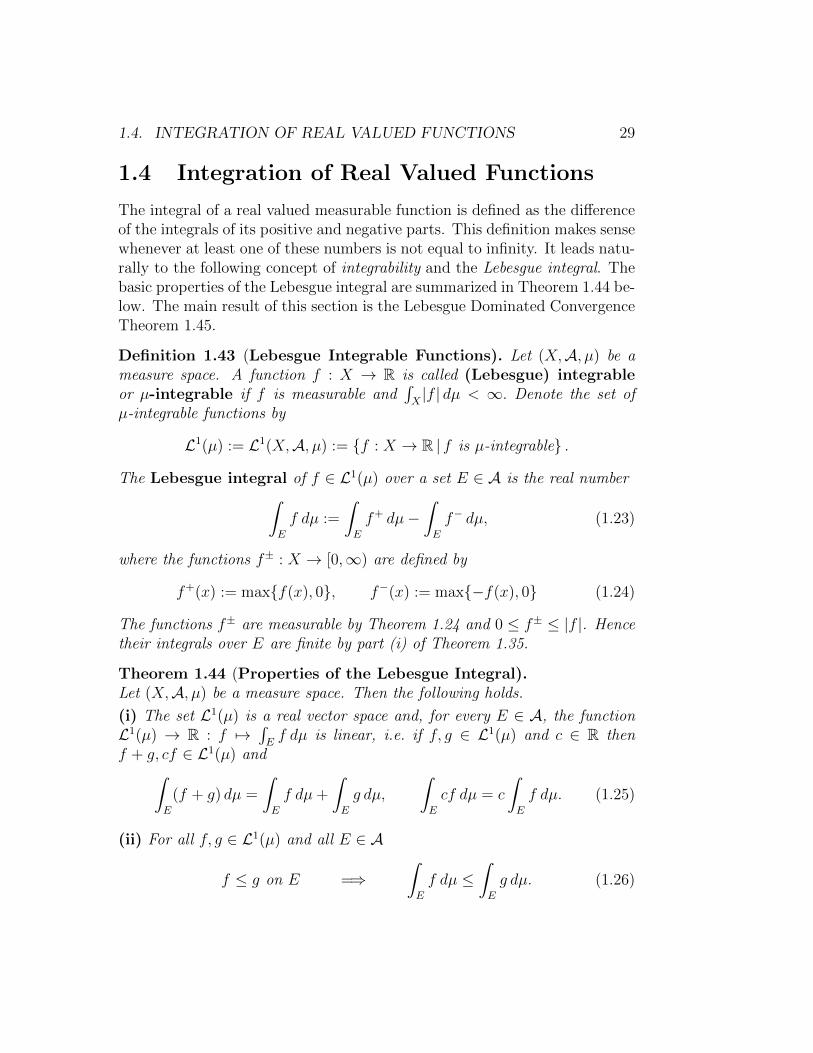
1.4 Integration of Real Valued Functions
The integral of a real valued measurable function is defined as the differenceof the integrals of its positive and negative parts. This definition makes sensewhenever at least one of these numbers is not equal to infinity. It leads natu-rally to the following concept of integrability and the Lebesgue integral. Thebasic properties of the Lebesgue integral are summarized in Theorem 1.44 be-low. The main result of this section is the Lebesgue Dominated ConvergenceTheorem 1.45.
Definition 1.43 (Lebesgue Integrable Functions). Let (X,A, µ) be ameasure space. A function f : X → R is called (Lebesgue) integrableor µ-integrable if f is measurable and
∫X|f | dµ < ∞. Denote the set of
µ-integrable functions by
L1(µ) := L1(X,A, µ) := f : X → R | f is µ-integrable .
The Lebesgue integral of f ∈ L1(µ) over a set E ∈ A is the real number∫E
f dµ :=
∫E
f+ dµ−∫E
f− dµ, (1.23)
where the functions f± : X → [0,∞) are defined by
f+(x) := maxf(x), 0, f−(x) := max−f(x), 0 (1.24)
The functions f± are measurable by Theorem 1.24 and 0 ≤ f± ≤ |f |. Hencetheir integrals over E are finite by part (i) of Theorem 1.35.
Theorem 1.44 (Properties of the Lebesgue Integral).Let (X,A, µ) be a measure space. Then the following holds.
(i) The set L1(µ) is a real vector space and, for every E ∈ A, the functionL1(µ) → R : f 7→
∫Ef dµ is linear, i.e. if f, g ∈ L1(µ) and c ∈ R then
f + g, cf ∈ L1(µ) and∫E
(f + g) dµ =
∫E
f dµ+
∫E
g dµ,
∫E
cf dµ = c
∫E
f dµ. (1.25)
(ii) For all f, g ∈ L1(µ) and all E ∈ A
f ≤ g on E =⇒∫E
f dµ ≤∫E
g dµ. (1.26)
30 CHAPTER 1. ABSTRACT MEASURE THEORY
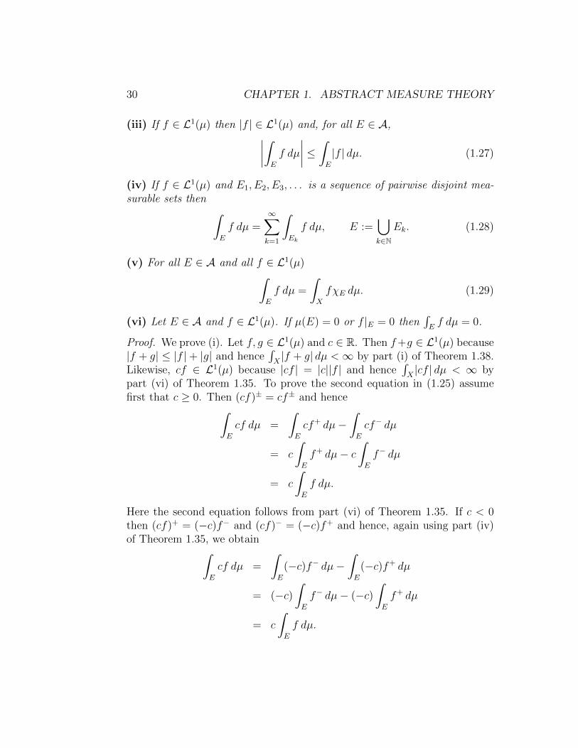
(iii) If f ∈ L1(µ) then |f | ∈ L1(µ) and, for all E ∈ A,∣∣∣∣∫E
f dµ
∣∣∣∣ ≤ ∫E
|f | dµ. (1.27)
(iv) If f ∈ L1(µ) and E1, E2, E3, . . . is a sequence of pairwise disjoint mea-surable sets then ∫
E
f dµ =∞∑k=1
∫Ek
f dµ, E :=⋃k∈N
Ek. (1.28)
(v) For all E ∈ A and all f ∈ L1(µ)∫E
f dµ =
∫X
fχE dµ. (1.29)
(vi) Let E ∈ A and f ∈ L1(µ). If µ(E) = 0 or f |E = 0 then∫Ef dµ = 0.
Proof. We prove (i). Let f, g ∈ L1(µ) and c ∈ R. Then f+g ∈ L1(µ) because|f + g| ≤ |f |+ |g| and hence
∫X|f + g| dµ <∞ by part (i) of Theorem 1.38.
Likewise, cf ∈ L1(µ) because |cf | = |c||f | and hence∫X|cf | dµ < ∞ by
part (vi) of Theorem 1.35. To prove the second equation in (1.25) assumefirst that c ≥ 0. Then (cf)± = cf± and hence∫
E
cf dµ =
∫E
cf+ dµ−∫E
cf− dµ
= c
∫E
f+ dµ− c∫E
f− dµ
= c
∫E
f dµ.
Here the second equation follows from part (vi) of Theorem 1.35. If c < 0then (cf)+ = (−c)f− and (cf)− = (−c)f+ and hence, again using part (iv)of Theorem 1.35, we obtain∫
E
cf dµ =
∫E
(−c)f− dµ−∫E
(−c)f+ dµ
= (−c)∫E
f− dµ− (−c)∫E
f+ dµ
= c
∫E
f dµ.

1.4. INTEGRATION OF REAL VALUED FUNCTIONS 31
Now let h := f + g. Then h+ − h− = f+ − f− + g+ − g− and hence
h+ + f− + g− = h− + f+ + g+.
Hence it follows from part (i) of Theorem 1.38 that∫E
h+ dµ+
∫E
f− dµ+
∫E
g− dµ =
∫E
h− dµ+
∫E
f+ dµ+
∫E
g+ dµ.
Hence ∫E
h dµ =
∫E
h+ dµ−∫E
h− dµ
=
∫E
f+ dµ+
∫E
g+ dµ−∫E
f− dµ−∫E
g− dµ
=
∫E
f dµ+
∫E
g dµ
and this proves (i).We prove (ii). Thus assume f = f+ − f− ≤ g = g+ − g− on E. Then
f+ + g− ≤ g+ + f− on E and hence∫E
(f+ + g−) dµ ≤∫E
(g+ + f−) dµ bypart (i) of Theorem 1.35. Now use the additivity of the integral in part (i)of Theorem 1.38 to obtain∫
E
f+ dµ+
∫E
g− dµ ≤∫E
g+ dµ+
∫E
f− dµ.
This implies (1.26).We prove (iii). Since −|f | ≤ f ≤ |f | it follows from (1.25) and (1.26)
that
−∫E
|f | dµ =
∫E
(−|f |) dµ ≤∫E
f dµ ≤∫E
|f | dµ
and this implies (1.27).We prove (iv). Equation (1.28) holds for f± by part (iii) of Theorem 1.38
and hence holds for f by definition of the integral in Definition 1.43.We prove (v). The formula
∫Ef dµ =
∫XfχE dµ in (1.29) follows from
part (ii) of Theorem 1.35 since f±χE = (fχE)±.We prove (vi). If f vanishes on E then f± also vanish on E and hence∫
Ef± dµ = 0 by part (iii) of Theorem 1.35. If µ(E) = 0 then
∫Ef± dµ = 0 by
part (iv) of Theorem 1.35. In either case it follows from the definition of theintegral in Definition 1.43 that
∫Ef dµ = 0. This proves Theorem 1.44.
32 CHAPTER 1. ABSTRACT MEASURE THEORY
Theorem 1.45 (Lebesgue Dominated Convergence Theorem).Let (X,A, µ) be a measure space, let g : X → [0,∞) be an integrable function,and let fn : X → R be a sequence of integrable functions satisfying
|fn(x)| ≤ g(x) for all x ∈ X and n ∈ N, (1.30)
and converging pointwise to f : X → R, i.e.
f(x) = limn→∞
fn(x) for all x ∈ X. (1.31)
Then f is integrable and, for every E ∈ A,∫E
f dµ = limn→∞
∫E
fn dµ. (1.32)
Proof. f is measurable by part (ii) of Theorem 1.24 and |f(x)| ≤ g(x) for allx ∈ X by (1.30) and (1.31). Hence it follows from part (i) of Theorem 1.35that ∫
X
|f | dµ ≤∫X
g dµ <∞
and so f is integrable. Moreover
|fn − f | ≤ |fn|+ |f | ≤ 2g.
Hence it follows from the Lemma of Fatou (Theorem 1.41) that∫X
2g dµ =
∫X
lim infn→∞
(2g − |fn − f |
)dµ
≤ lim infn→∞
∫X
(2g − |fn − f |
)dµ
= lim infn→∞
(∫X
2g dµ−∫X
|fn − f | dµ)
=
∫X
2g dµ− lim supn→∞
∫X
|fn − f | dµ.
Here penultimate step follows from part (i) of Theorem 1.44. This implies
lim supn→∞
∫X
|fn − f | dµ ≤ 0.
1.5. SETS OF MEASURE ZERO 33
Hence
limn→∞
∫X
|fn − f | dµ = 0.
Since ∣∣∣∣∫E
fn dµ−∫E
f dµ
∣∣∣∣ ≤ ∫E
|fn − f | dµ ≤∫X
|fn − f | dµ
by part (iii) of Theorem 1.44 it follows that
limn→∞
∣∣∣∣∫E
fn dµ−∫E
f dµ
∣∣∣∣ = 0,
which is equivalent to (1.32). This proves Theorem 1.45.
1.5 Sets of Measure Zero
Assume throughout this section that (X,A, µ) is a measure space. A set ofmeasure zero (or null set) is a measurable set N ∈ A such that µ(N) = 0.Let P be a name for some property that a point x ∈ X may have, or nothave, depending on x. For example, if f : X → [0,∞] is a measurablefunction on X, then P could stand for the condition f(x) > 0 or for thecondition f(x) = 0 or for the condition f(x) = ∞. Or if fn : X → Ris a sequence of measurable functions the property P could stand for thestatement “the sequence fn(x) converges”. In such a situation we say thatP holds almost everywhere if there exists a set N ⊂ X of measure zerosuch that every element x ∈ X \ N has the property P. It is not requiredthat the set of all elements x ∈ X that have the property P is measurable,although that may often be the case.
Example 1.46. Let fn : X → R be any sequence of measurable functions.Then the set
E := x ∈ X | (fn(x))∞n=1 is a Cauchy sequence
=⋂k∈N
⋃n0∈N
⋂n,m≥n0
x ∈ X | |fn(x)− fm(x)| < 2−k
is measurable. If N := X \ E is a set of measure zero then fn convergesalmost everywhere to a function f : X → R. This function can be chosenmeasurable by defining f(x) := limn→∞ fn(x) for x ∈ E and f(x) := 0 forx ∈ N . This is the pointwise limit of the sequence of measurable functionsgn := fnχE and hence is measurable by part (ii) of Theorem 1.24.
34 CHAPTER 1. ABSTRACT MEASURE THEORY
The first observation is that every nonnegative function with finite inte-gral is almost everywhere finite.
Lemma 1.47. Let f : X → [0,∞] be a measurable function. If∫Xf dµ <∞
then f <∞ almost everywhere.
Proof. Define N := x ∈ X | f(x) =∞ and h :=∞χN . Then h ≤ f and so∞µ(N) =
∫Xh dµ ≤
∫Xf dµ <∞ by Theorem 1.35. Hence µ(N) = 0.
The second observation is that if two integrable, or nonnegative measur-able, functions agree almost everywhere, then their integrals agree over everymeasurable set.
Lemma 1.48. Assume either that f, g : X → [0,∞] are measurable functionsthat agree almost everywhere or that f, g : X → R are µ-integrable functionsthat agree almost everywhere. Then∫
A
f dµ =
∫A
g dµ for all A ∈ A. (1.33)
Proof. Fix a measurable set A ∈ A and define N := x ∈ X | f(x) 6= g(x).Then N is measurable and µ(N) = 0 by assumption. Hence µ(A ∩ N) = 0by part (iii) of Theorem 1.28. This implies∫
A
f dµ =
∫A\N
f dµ+
∫A∩N
f dµ =
∫A\N
f dµ =
∫X
fχA\N dµ.
Here the first equation follows from part (iii) of Theorem 1.38 in the non-negative case and from part (iv) of Theorem 1.44 in the integrable case.The second equation follows from part (iv) of Theorem 1.35 in the non-negative case and from part (vi) of Theorem 1.44 in the integrable case.The third equation follows from part (ii) of Theorem 1.35 in the nonnega-tive case and from part (v) of Theorem 1.44 in the integrable case. SincefχA\N = gχA\N it follows that the integrals of f and g over A agree. Thisproves Lemma 1.48.
The converse of Lemma 1.48 fails for nonnegative measurable functions.For example, if X is a singleton and µ(X) =∞ then the integrals of any twopositive functions agree over every measurable set. However, the converse ofLemma 1.48 does hold for integrable functions. Since the difference of twointegrable functions is again integrable, it suffices to assume g = 0, and inthis case the converse also holds for nonnegative measurable functions. Thisis the content of the next lemma.
1.5. SETS OF MEASURE ZERO 35
Lemma 1.49. Assume either that f : X → [0,∞] is measurable or thatf : X → R is µ-integrable. Then the following are equivalent.
(i) f = 0 almost everywhere.
(ii)∫Af dµ = 0 for all A ∈ A.
(iii)∫X|f | dµ = 0.
Proof. That (i) implies (ii) is the content of Lemma 1.48. That (ii) im-plies (iii) is obvious in the nonnegative case. In the integrable case define
A+ := x ∈ X | f(x) ≥ 0 , A− := x ∈ X | f(x) < 0 .
Then f+ = fχA+ and f− = −fχA− by (1.24). Hence∫X
|f | dµ =
∫X
f+ dµ+
∫X
f− dµ =
∫A+
f dµ−∫A−f dµ = 0
by Theorem 1.44 and (ii).It remains to prove that (iii) implies (i). Let f : X → [0,∞] be a
measurable function such that∫Xf = 0 and define the measurable sets
An :=x ∈ X | f(x) > 2−n
for n ∈ N.
Then
2−nµ(An) =
∫X
2−nχAn dµ ≤∫X
f dµ = 0
for all n ∈ N by Theorem 1.35. Hence µ(An) = 0 for all n ∈ N and so
N := x ∈ X | f(x) 6= 0 =∞⋃n=1
An
is a set of measure zero. In the integrable case apply this argument to thefunction |f | : X → [0,∞). This proves Lemma 1.49.
Lemma 1.50. Let f ∈ L1(µ). Then∣∣∣∣∫X
f dµ
∣∣∣∣ =
∫X
|f | dµ (1.34)
if and only if f = |f | almost everywhere or f = −|f | almost everywhere.
Proof. Assume (1.34). Then∫Xf dµ =
∫X|f | dµ or
∫Xf dµ = −
∫X|f | dµ. In
the first case∫X
(|f | − f) dµ = 0 and so |f | − f = 0 almost everywhere byLemma 1.49. In the second case
∫X
(|f |+f) dµ = 0 and so |f |+f = 0 almosteverywhere. This proves Lemma 1.50.
36 CHAPTER 1. ABSTRACT MEASURE THEORY
Definition 1.51 (The Banach Space L1(µ)). Define an equivalence rela-tion on the real vector space of all measurable function from X to R by
fµ∼ g
def⇐⇒ the set x ∈ X | f(x) 6= g(x)has measure zero.
(1.35)
Thus two functions are equivalent iff they agree almost everywhere. (Verifythat this is an equivalence relation!) By Lemma 1.48 the subspace L1(µ) isinvariant under this equivalence relation, i.e. if f, g : X → R are measurable,f ∈ L1(µ), and f
µ∼ g then g ∈ L1(µ). Moreover, the set f ∈ L1(µ) | f µ∼ 0is a linear subspace of L1(µ) and hence the quotient space
L1(µ) := L1(µ)/µ∼
is again a real vector space. It is the space of all equivalence classes in L1(µ)under the equivalence relation (1.35). Thus an element of L1(µ) is not afunction on X but a set of functions on X. By Lemma 1.48 the map
L1(µ)→ R : f 7→∫X
|f | dµ =: ‖f‖L1
takes on the same value on all the elements in a given equivalence class andso descends to the quotient space L1(µ). By Lemma 1.49 it defines a normon L1(µ) and Theorem 1.53 below shows that L1(µ) is a Banach space withthis norm (i.e. a complete normed vector space).
Theorem 1.52 (Convergent Series of Integrable Functions).Let (X,A, µ) be a measure space and let fn : X → R be a sequence ofµ-integrable functions such that
∞∑n=1
∫X
|fn| dµ <∞. (1.36)
Then there is a set N of measure zero and a function f ∈ L1(µ) such that
∞∑n=1
|fn(x)| <∞ and f(x) =∞∑n=1
fn(x) for all x ∈ X \N, (1.37)
∫A
f dµ =∞∑n=1
∫A
fn dµ for all A ∈ A, (1.38)
limn→∞
∫X
∣∣∣f − n∑k=1
fk
∣∣∣ dµ = 0. (1.39)

1.5. SETS OF MEASURE ZERO 37
Proof. Define
φ(x) :=∞∑k=1
|fk(x)|
for x ∈ X. This function is measurable by part (ii) of Theorem 1.24. More-over, it follows from the Lebesgue Monotone Convergence Theorem 1.37 andfrom part (i) of Theorem 1.38 that∫
X
φ dµ = limn→∞
∫X
n∑k=1
|fk| dµ = limn→∞
n∑k=1
∫X
|fk| dµ =∞∑k=1
∫X
|fk| dµ <∞.
Hence the set N := x ∈ X |φ(x) =∞ has measure zero by Lemma 1.47and
∑∞k=1|fk(x)| <∞ for all x ∈ X \N . Define the function f : X → R by
f(x) := 0 for x ∈ N and by
f(x) :=∞∑k=1
fk(x) for x ∈ X \N.
Then f satisfies (1.37). Define the functions g : X → R and gn : X → R by
g := φχX\N , gn :=n∑k=1
fkχX\N for n ∈ N.
These functions are measurable by part (i) of Theorem 1.24. Moreover,∫Xg dµ =
∫Xφ dµ < ∞ by Lemma 1.48. Since |gn(x)| ≤ g(x) for all n ∈ N
and gn converges pointwise to f it follows from the Lebesgue DominatedConvergence Theorem 1.45 that f ∈ L1(µ) and, for all A ∈ A,∫
A
f dµ = limn→∞
∫A
gn dµ = limn→∞
∫A
n∑k=1
fk dµ =∞∑n=1
∫A
fn dµ.
Here the second step follows from Lemma 1.48 because gn =∑n
k=1 fk almosteverywhere. The last step follows by interchanging sum and integral, usingpart (i) of Theorem 1.44. This proves (1.38). To prove equation (1.39) notethat f−
∑nk=1 fk = f−gn almost everywhere, that f(x)−gn(x) converges to
zero for all x ∈ X, and that |f−gn| ≤ |f |+g where |f |+g is integrable. Hence,by Lemma 1.48 and the Lebesgue Dominated Convergence Theorem 1.45
limn→∞
∫X
∣∣∣f − n∑k=1
fk
∣∣∣ dµ = limn→∞
∫X
|f − gn| dµ = 0,
This proves (1.39) and Theorem 1.52.
38 CHAPTER 1. ABSTRACT MEASURE THEORY
Theorem 1.53 (Completeness of L1). Let (X,A, µ) be a measure spaceand let fn ∈ L1(µ) be a sequence of integrable functions. Assume fn is aCauchy sequence with respect to the L1-norm, i.e. for every ε > 0 there is ann0 ∈ N such that, for all m,n ∈ N,
n,m ≥ n0 =⇒∫X
|fn − fm| dµ < ε. (1.40)
Then there exists a function f ∈ L1(µ) such that
limn→∞
∫X
|fn − f | dµ = 0. (1.41)
Moreover, there is a subsequence fni that converges almost everywhere to f .
Proof. By assumption there is a sequence ni ∈ N such that∫X
|fni+1− fni | dµ < 2−i, ni < ni+1, for all i ∈ N.
Then the sequence gi := fni+1− fni ∈ L1(µ) satisfies (1.36). Hence, by
Theorem 1.52, there exists a function g ∈ L1(µ) such that
g =∞∑i=1
gi =∞∑i=1
(fni+1
− fni)
almost everywhere and
0 = limk→∞
∫X
∣∣∣k−1∑i=1
gi − g∣∣∣ dµ = lim
k→∞
∫X
|fnk − fn1 − g| dµ. (1.42)
Definef := fn1 + g.
Then fni = fn1 +∑i−1
j=1 gj converges almost everywhere to f . We prove (1.41).
Let ε > 0. By (1.42) there is an ` ∈ N such that∫X|fnk − f | dµ < ε/2 for all
k ≥ `. By (1.40) the integer ` can be chosen such that∫X|fn − fm| dµ < ε/2
for all n,m ≥ n`. Then∫X
|fn − f | dµ ≤∫X
|fn − fn`| dµ+
∫X
|fn` − f | dµ < ε
for all n ≥ n`. This proves (1.41) and Theorem 1.53.
1.6. COMPLETION OF A MEASURE SPACE 39
1.6 Completion of a Measure Space
The discussion in Section 1.5 shows that sets of measure zero are negligiblein the sense that the integral of a measurable function remains the same ifthe function is modified on a set of measure zero. Thus also subsets of setsof measure zero can be considered negligible. However such subsets need notbe elements of our σ-algebra A. It is sometimes convenient to form a newσ-algebra by including all subsets of sets of measure zero. This leads to thenotion of a completion of a measure space (X,A, µ).
Definition 1.54. A measure space (X,A, µ) is called complete if
N ∈ A, µ(N) = 0, E ⊂ N =⇒ E ∈ A.
Theorem 1.55. Let (X,A, µ) be a measure space and define
A∗ :=
E ⊂ X
∣∣∣ there exist measurable sets A,B ∈ A such thatA ⊂ E ⊂ B and µ(B \ A) = 0
.
Then the following holds.
(i) A∗ is a σ-algebra and A ⊂ A∗.(ii) There exists a unique measure µ∗ : A∗ → [0,∞] such that
µ∗|A = µ.
(iii) The triple (X,A∗, µ∗) is a complete measure space. It is called thecompletion of (X,A, µ).
(iv) If f : X → R is µ-integrable then f is µ∗-integrable and, for E ∈ A,∫E
f dµ∗ =
∫E
f dµ (1.43)
This continues to hold for all A-measurable functions f : X → [0,∞].
(v) If f ∗ : X → R is A∗-measurable then there exists an A-measurablefunction f : X → R such that the set
N∗ := x ∈ X | f(x) 6= f ∗(x) ∈ A∗
has measure zero, i.e. µ∗(N∗) = 0.
40 CHAPTER 1. ABSTRACT MEASURE THEORY
Proof. We prove (i). First X ∈ A∗ because A ⊂ A∗. Second, let E ∈ A∗and choose A,B ∈ A such that A ⊂ E ⊂ B and µ(B \ A) = 0. ThenBc ⊂ Ec ⊂ Ac and Ac \ Bc = Ac ∩ B = B \ A. Hence µ(Ac \ Bc) = 0 andso Ec ∈ A∗. Third, let Ei ∈ A∗ for i ∈ N and choose Ai, Bi ∈ A such thatAi ⊂ Ei ⊂ Bi and µ(Bi \ Ai) = 0. Define
A :=⋃i
Ai, E :=⋃i
Ei, B :=⋃i
Bi.
Then A ⊂ E ⊂ B and B \ A =⋃i(Bi \ A) ⊂
⋃i(Bi \ Ai). Hence
µ(B \ A) ≤∑i
µ(Bi \ Ai) = 0
and this implies E ∈ A∗. Thus we have proved (i).We prove (ii). For E ∈ A∗ define
µ∗(E) := µ(A) whereA,B ∈ A,A ⊂ E ⊂ B,µ(B \ A) = 0.
(1.44)
This is the only possibility for defining a measure µ∗ : A∗ → [0,∞] thatagrees with µ on A because µ(A) = µ(B) whenever A,B ∈ A such thatA ⊂ B and µ(B \ A) = 0. To prove that µ∗ is well defined let E ∈ A∗ andA,B ∈ A as in (1.44). If A′, B′ ∈ A is another pair such that A′ ⊂ E ⊂ B′
and µ(B′ \A′) = 0, then A \A′ ⊂ E \A′ ⊂ B′ \A′ and hence µ(A \A′) = 0.This implies µ(A) = µ(A ∩ A′) = µ(A′), where the last equation followsby interchanging the roles of the pairs (A,B) and (A′, B′). Thus the mapµ∗ : A∗ → [0,∞] in (1.44) is well defined.
We prove that µ∗ is a measure. Let Ei ∈ A∗ be a sequence of pairwisedisjoint sets and choose sequences Ai, Bi ∈ A such that Ai ⊂ Ei ⊂ Bi forall i. Then the Ai are pairwise disjoint and µ∗(Ei) = µ(Ai) for all i. MoreoverA :=
⋃iAi ∈ A, B :=
⋃iBi ∈ A, A ⊂ E ⊂ B, and µ(B \A) = 0 as we have
seen in the proof of part (i). Hence µ∗(E) = µ(A) =∑
i µ(Ai) =∑
i µ∗(Ei).
This proves (ii).We prove (iii). Let E ∈ A∗ such that µ∗(E) = 0 and let E ′ ⊂ E. Choose
A,B ∈ A such that A ⊂ E ⊂ B and µ(B \ A) = 0. Then µ(A) = µ∗(E) = 0and hence µ(B) = µ(A)+µ(B \A) = 0. Since E ′ ⊂ E ⊂ B, this implies thatE ′ ∈ A∗ (by choosing B′ := B and A′ := ∅). This shows that (X,A∗, µ∗) isa complete measure space.
1.6. COMPLETION OF A MEASURE SPACE 41
We prove (iv). Assume f : X → [0,∞] is A-measurable. By Theo-rem 1.26 there exists a sequence of A-measurable step functions sn : X → Rsuch that 0 ≤ s1 ≤ s2 ≤ · · · ≤ f and f(x) = limn→∞ sn(x) for all x ∈ X.Since µ∗|A = µ we have
∫Xsn dµ =
∫Xsn dµ
∗ for all n and hence it followsfrom the Lebesgue Monotone Convergence Theorem 1.37 for both µ and µ∗
that ∫X
f dµ = limn→∞
∫X
sn dµ = limn→∞
∫X
sn dµ∗ =
∫X
f dµ∗.
This proves (1.43) for E = X and all A-measurable functions f : X → [0,∞].To prove it for all E replace f by fχE and use part (ii) of Theorem 1.35. Thisproves equation (1.43) for all A-measurable functions f : X → [0,∞]. Thatit continues to hold for all f ∈ L1(µ) follows directly from Definition 1.43.This proves (iv).
We prove (v). If f ∗ = χE for E ∈ A∗, choose A,B ∈ A such that
A ⊂ E ⊂ B, µ(B \ A) = 0,
and define f := χA. Then
N∗ = x ∈ X | f ∗(x) 6= f(x) = E \ A ⊂ B \ A.
Hence µ∗(N∗) ≤ µ∗(B \ A) = µ(B \ A) = 0. This proves (v) for charac-teristic functions of A∗-measurable sets. For A∗-measurable step functionsthe assertion follows by multiplication with real numbers and taking finitesums. Now let f ∗ : X → [0,∞] be an arbitrary A∗-measurable function.By Theorem 1.26 there exists a sequence of A∗-measurable step functionss∗i : X → [0,∞) such that s∗i converges pointwise to f ∗. For each i ∈ Nchoose an A-measurable step function si : X → [0,∞) and a set N∗i ∈ A∗such that si = s∗i on X \N∗i and µ∗(N∗i ) = 0. Then there is a sequence of setsNi ∈ A such that N∗i ⊂ Ni and µ(Ni) = 0 for all i. Define f : X → [0,∞] by
f(x) :=
f ∗(x), if x /∈ N,0, if x ∈ N, N :=
⋃i
Ni.
Then N ∈ A, µ(N) = 0, and the sequence of A-measurable functions siχX\Nconverges pointwise to f as i tends to infinity. Hence f is A-measurableby part (ii) of Theorem 1.24 and agrees with f ∗ on X \ N by definition.Now let f ∗ : X → R be A∗-measurable. Then so are (f ∗)± := max±f ∗, 0.Construct f± : X → [0,∞] as above. Then f−(x) = 0 whenever f+(x) > 0and vice versa. Thus f := f+−f− is well defined, A-measurable, and agreeswith f ∗ on the complement of a µ-null set. This proves Theorem 1.55.

42 CHAPTER 1. ABSTRACT MEASURE THEORY
Corollary 1.56. Let (X,A, µ) be a measure space and let (X,A∗, µ∗) be itscompletion. Denote the equivalence class of a µ-integrable function f ∈ L1(µ)under the equivalence relation (1.35) in Definition 1.51 by
[f ]µ :=g ∈ L1(µ)
∣∣∣µ(x ∈ X | f(x) 6= g(x))
= 0.
Then the mapL1(µ)→ L1(µ∗) : [f ]µ 7→ [f ]µ∗ (1.45)
is a Banach space isometry.
Proof. The map (1.45) is linear and injective by definition. It preservesthe L1-norm by part (iv) of Theorem 1.55 and is surjective by part (v) ofTheorem 1.55.
As noted in Section 1.5, sets of measure zero can be neglected whenintegrating functions. Hence it is sometimes convenient to enlarge the notionof integrability. It is not even necessary that the function be defined on allof X, as long as it is defined on the complement of a set of measure zero.
Thus let (X,A, µ) be a measure space and call a function f : E → R,defined on a measurable subset E ⊂ X, measurable if µ(X \E) = 0 and theset f−1(B) ⊂ E is measurable for every Borel set B ⊂ R. Call it integrableif the function on all of X, obtained by setting f |X\E = 0, is integrable.
If (X,A, µ) is complete our integrable function f : E → R can be ex-tended in any manner whatsoever to all of X, and the extended functionon X is then integrable in the original sense, regardless of the choice of theextension. Moreover, its integral over any measurable set A ∈ A is unaffectedby the choice of the extension (see Lemma 1.48).
With this extended notion of integrability we see that the Lebesgue Dom-inated Convergence Theorem 1.45 continues to hold if (1.31) is replaced bythe weaker assumption that fn only converges to f almost everywhere.
That such an extended terminology might be useful can also be seen inTheorem 1.52, where the series
∑∞n=1 fn only converges on the complement of
a set N of measure zero, and the function f can only be naturally defined onE := X \N . Our choice in the proof of Theorem 1.52 was to define f |N := 0,but this choice does not affect any of the statements of the theorem. More-over, when working with the quotient space L1(µ) = L1(µ)/
µ∼ we are onlyinterested in the equivalence class of f under the equivalence relation (1.35)rather than a specific choice of an element of this equivalence class.
1.7. EXERCISES 43
1.7 Exercises
Exercise 1.57. Let X be an uncountable set and let A ⊂ 2X be the set ofall subsets A ⊂ X such either A or Ac is countable. Define
µ(A) :=
0, if A is countable,1, if Ac is countable,
for A ∈ A. Show that (X,A, µ) is a measure space. Describe the measurablefunctions and their integrals. (See Examples 1.4 and 1.32.)
Exercise 1.58. Let (X,A, µ) be a measure space such that µ(X) <∞ andlet fn : X → [0,∞) be a sequence of bounded measurable functions thatconverges uniformly to f : X → [0,∞). Prove that∫
X
f dµ = limn→∞
∫X
fn dµ. (1.46)
Find an example of a measure space (X,A, µ) with µ(X) =∞ and a sequenceof bounded measurable functions fn : X → [0,∞) converging uniformly to fsuch that (1.46) does not hold.
Exercise 1.59. (i) Let fn : [0, 1] → [−1, 1] be a sequence of continuousfunctions that converges uniformly to zero. Show that
limn→∞
∫ 1
0
fn(x) dx = 0.
(ii) Let fn : [0, 1]→ [−1, 1] be a sequence of continuous functions such that
limn→∞
fn(x) = 0 for all x ∈ [0, 1].
Prove that
limn→∞
∫ 1
0
fn(x) dx = 0,
without using Theorem 1.45. A good reference is Eberlein [3].
(iii) Construct a sequence of continuous functions fn : [0, 1] → [−1, 1] thatconverges pointwise, but not uniformly, to zero.
(iv) Construct a sequence of continuous functions fn : [0, 1] → [−1, 1] such
that∫ 1
0fn(x) dx = 0 for all n and fn(x) does not converge for any x ∈ [0, 1].
44 CHAPTER 1. ABSTRACT MEASURE THEORY
Exercise 1.60. Let (X,A, µ) be a measure space and f : X → [0,∞] be ameasurable function such that 0 < c :=
∫Xf dµ <∞. Prove that
limn→∞
∫X
n log
(1 +
fα
nα
)dµ =
∞, if α < 1,c, if α = 1,0, if α > 1,
for 0 < α <∞.
Hint: The integrand can be estimated by αf when α ≥ 1.
Exercise 1.61. Let X := N and A := 2N and let µ : 2N → [0,∞] be thecounting measure (Example 1.30). Prove that a function f : N → R is µ-integrable if and only if the sequence (f(n))n∈N of real numbers is absolutelysummable and that in this case∫
Nf dµ =
∞∑n=1
f(n).
Exercise 1.62. Let (X,A) be a measurable space and let µn : A → [0,∞]be a sequence of measures. Show that the formula
µ(A) :=∞∑n=1
µn(A)
for A ∈ A defines a measure µ : A → [0,∞]. Let f : X → R be a measurablefunction. Show that f is µ-integrable if and only if
∞∑n=1
∫X
|f | dµn <∞.
If f is µ-integrable prove that∫X
f dµ =∞∑n=1
∫X
f dµn.
Exercise 1.63. Let (X,A, µ) be a measure space such that µ(X) <∞ andlet f : X → R be a measurable function. Show that f is integrable if andonly if
∞∑n=1
|µ(x ∈ X | |f(x)| > n)| <∞.
1.7. EXERCISES 45
Exercise 1.64. Let (X,A, µ) be a measure space and let f : X → R be aµ-integrable function.
(i) Prove that for every ε > 0 there exists a δ > 0 such that, for all A ∈ A,
µ(A) < δ =⇒∣∣∣∣∫A
f dµ
∣∣∣∣ < ε.
Hint: Argue indirectly. See Lemma 5.21.
(ii) Prove that for every ε > 0 there exists a measurable set A ∈ A suchthat, for all B ∈ A,
B ⊃ A =⇒∣∣∣∣∫X
f dµ−∫B
f dµ
∣∣∣∣ < ε.
Exercise 1.65. Let (X,A) be a measurable space and define
µ(A) :=
0, if A = ∅,∞, if A ∈ A and A 6= ∅.
Determine the completion (X,A∗, µ∗) and the space L1(µ).
Exercise 1.66. Let (X,A, µ) be a measure space such that µ = δx0 is theDirac measure at some point x0 ∈ X (Example 1.31). Determine the com-pletion (X,A∗, µ∗) and the space L1(µ).
Exercise 1.67. Let (X,A, µ) be a complete measure space. Prove that(X,A, µ) is equal to its own completion.
Exercise 1.68. Let (X,A, µ) and (X,A′, µ′) be two measure spaces withA ⊂ A′ and µ′|A = µ. Prove that L1(µ) ⊂ L1(µ′) and∫
X
f dµ =
∫X
f dµ′
for every f ∈ L1(µ). Hint: Prove the following.
(i) Let f : X → [0,∞] be A-measurable and define
fδ(x) :=
0, if f(x) ≤ δ,f(x), if δ < f(x) ≤ δ−1,δ−1, if f(x) > δ−1.
Then fδ is A-measurable for every δ > 0 and limδ→0
∫Xfδ dµ =
∫Xf dµ.
(ii) Let 0 < c < ∞, let f : X → [0, c] be A-measurable, and assume thatµ(x ∈ X | f(x) > 0) < ∞. Then
∫Xf dµ =
∫Xf dµ′. (Consider also the
function c− f .)
46 CHAPTER 1. ABSTRACT MEASURE THEORY
Exercise 1.69 (Pushforward of a Measure).Let (X,A, µ) be a measure space, let Y be a set, and let φ : X → Y be amap. The pushforward of A is the σ-algebra
φ∗A :=B ⊂ Y |φ−1(B) ∈ A
⊂ 2Y . (1.47)
The pushforward of µ is the function φ∗µ : φ∗A → [0,∞] defined by
(φ∗µ)(B) := µ(φ−1(B)), for B ∈ φ∗A. (1.48)
(i) Prove that (Y, φ∗A, φ∗µ) is a measure space.
(ii) Let (X,A∗, µ∗) be the completion of (X,A, µ) and let (Y, (φ∗A)∗, (φ∗µ)∗)be the completion of (Y, φ∗A, φ∗µ). Prove that
(φ∗µ)∗(E) = µ∗(φ−1(E)) for all E ∈ (φ∗A)∗ ⊂ φ∗A∗. (1.49)
Deduce that (Y, φ∗A, φ∗µ) is complete whenever (X,A, µ) is complete. Findan example where (φ∗A)∗ ( φ∗A∗.(iii) Fix a function f : Y → [0,∞]. Prove that f is φ∗A-measurable if andonly if f φ is A-measurable. If f is φ∗A-measurable, prove that∫
Y
f d(φ∗µ) =
∫X
(f φ) dµ. (1.50)
(iv) Determine the pushforward of (X,A, µ) under a constant map.
The following extended remark contains a brief introduction to some ofthe basic concepts and terminology in probability theory. It will not be usedelsewhere in this book and can be skipped at first reading.
Remark 1.70 (Probability Theory). A probability space is a measurespace (Ω,F , P ) such that P (Ω) = 1. The underlying set Ω is called the sam-ple space, the σ-algebra F ⊂ 2Ω is called the set of events, and the measureP : F → [0, 1] is called a probability measure. Examples of finite samplespaces are the set Ω = h, t for tossing a coin, the set Ω = 1, 2, 3, 4, 5, 6for rolling a dice, the set Ω = 00, 0, 1, . . . , 36 for spinning a roulette wheel,and the set Ω = 2, . . . , 10, j, q, k, a × ♦,♥,♠,♣ for drawing a card froma deck. Examples of infinite sample spaces are the set Ω = N ∪ ∞ forrepeatedly tossing a coin until the first tail shows up, a compact interval ofreal numbers for random arrival times, and a disc in the plane for throwinga dart.

1.7. EXERCISES 47
A random variable is an integrable function X : Ω→ R. Its expecta-tion E(X) and variance V(X) are defined by
E(X) :=
∫Ω
X dP, V(X) :=
∫Ω
(X − E(X))2 dP = E(X2)− E(X)2.
Given a random variable X : Ω→ R one is interested in the value of the prob-ability measure on the set X−1(B) for a Borel set B ⊂ R. This value is theprobability of the event that the random variable X takes its value in the set Band is denoted by P (X ∈ B) := P (X−1(B)) = (X∗P )(B). Here X∗P denotesthe pushforward of the probability measure P to the Borel σ-algebra B ⊂ 2R
(Exercise 1.69). By (1.50) the expectation and variance of X are given byE(X) =
∫R x d(X∗P )(x) and V(X) =
∫R(x− E(X))2 d(X∗P )(x).
The (cumulative) distribution function of a random variable X isthe function FX : R→ [0, 1] defined by
FX(x) := P (X ≤ x) = P (ω ∈ Ω |X(ω) ≤ x) = (X∗P )((−∞, x]).
It is nondecreasing and right continuous, satisfies
limx→−∞
FX(x) = 0, limx→∞
FX(x) = 1,
and the integral of a continuous function on R with respect to the pushfor-ward measure X∗P agrees with the Riemann–Stieltjes integral (Exercise 6.20)with respect to FX . Moreover,
FX(x)− limt→x−
FX(t) = P (X−1(x))
by Theorem 1.28. Thus FX is continuous at x if and only if P (X−1(x)) = 0.This leads to the following notions of convergence. Let X : Ω → R be arandom variable. A sequence (Xi)i∈N of random variables is said to
converge in probability to X if limi→∞ P (|Xi−X| ≥ ε) = 0 for all ε > 0,
converge in distribution to X if FX(x) = limi→∞ FXi(x) for every x ∈ Rsuch that FX is continuous at x.
We prove that that convergence almost everywhere implies convergencein probability. Let ε > 0 and define Ai := ω ∈ Ω | |Xi(ω)−X(ω)| ≥ ε.Let E ⊂ Ω be the set of all ω ∈ Ω such that the sequence Xi(ω) does notconverge to X(ω). This set is measurable by Example 1.46 and has measurezero by convergence almost everywhere. Moreover,
⋂i∈N⋃j≥iAj ⊂ E and so
limi→∞ P (⋃j≥iAj) = P (E) = 0 by Theorem 1.28. Thus limi→∞ P (Ai) = 0.

48 CHAPTER 1. ABSTRACT MEASURE THEORY
We prove that convergence in probability implies convergence in distri-bution. Let x ∈ R such that FX is continuous at x. Let ε > 0 and chooseδ > 0 such that FX(x) − ε
2< FX(x − δ) ≤ FX(x + δ) < FX(x) + ε
2.
Now choose i0 ∈ N such that P (|Xi − X| ≥ δ) < ε2
for all i ≥ i0. ThenFX(x − δ) − P (|Xi − X| ≥ δ) ≤ FXi(x) ≤ FX(x + δ) + P (|Xi − X| ≥ δ)and hence FX(x) − ε < FXi(x) < FX(x) + ε for all i ≥ i0. This shows thatlimi→∞ FXi(x) = FX(x) as claimed.
A finite collection of random variables X1, . . . , Xn is called independentif, for every collection of Borel sets B1, . . . , Bn ⊂ R, it satisfies
P
( n⋂i=1
X−1i (Bi)
)=
n∏i=1
P(X−1i (Bi)
).
In Chapter 7 we shall see that this condition asserts that the pushforward of Punder the map X := (X1, . . . , Xn) : Ω → Rn agrees with the product of themeasures (Xi)∗P . Two foundational theorems in probability theory are thelaw of large numbers and the central limit theorem. These are results aboutsequences of random variables Xk : Ω→ R that satisfy the following.(a) The random variables X1, . . . , Xn are independent for all n.(b) The Xk have expectation E(Xk) = 0.(c) The Xk are identically distributed, i.e. FXk = FX` for all k and `.For n ∈ N define Sn := X1 + · · · + Xn. Kolmogorov’s strong law of largenumbers asserts that, under these assumptions, the sequence Sn/n con-verges almost everywhere to zero. (This continues to hold when (c) is re-placed by the assumption
∑∞k=1
1k2 V(Xk) <∞.) If, in addition, V(Xk) = σ2
for all k and some positive real number σ then the central limit theoremof Lindeberg–Levy asserts that the sequence Tn := Sn/σ
√n converges in dis-
tribution to a so-called standard normal random variable with expectationzero and variance one, i.e. limn→∞ FTn(x) = 1√
2π
∫ x−∞ e
−t2/2 dt for all x ∈ R.The hypotheses listed above are quite restrictive and in modern probabil-ity theory these theorems are often needed in much greater generality. Forproofs, many examples, and comprehensive expositions of probability theorysee Ash [1], Fremlin [4, Chapter 27], Malliavin [13].
An important class of random variables are those where the distributionfunctions FX : R → [0, 1] are absolutely continuous (Theorem 6.19). Thismeans that the pushforward measures X∗P on the Borel σ-algebra B ⊂ 2R
admit densities as in Theorem 1.40 with respect to the Lebesgue measure.The Lebesgue measure is introduced in Chapter 2 and the existence of adensity is the subject of Chapter 5 on the Radon–Nikodym Theorem.

Chapter 2
The Lebesgue Measure
This chapter introduces the most important example, namely the Lebesguemeasure on Euclidean space. Let n ∈ N and denote by B ⊂ 2Rn the σ-algebraof all Borel sets in Rn, i.e. the smallest σ-algebra on Rn that contains all opensets in the standard topology (Definition 1.15). Then
B + x := y + x | y ∈ B ∈ B for all B ∈ B and all x ∈ Rn,
because the translation Rn → Rn : y 7→ y + x is a homeomorphism. Ameasure µ : B → [0,∞] is called translation invariant if it satisfies
µ(B + x) = µ(B) for all B ∈ B and all x ∈ Rn. (2.1)
Theorem 2.1. There exists a unique measure µ : B → [0,∞] that is trans-lation invariant and satisfies the normalization condition µ([0, 1]n) = 1.
Proof. See page 64.
Definition 2.2. Let (Rn,B, µ) be the measure space in Theorem 2.1 anddenote by (Rn,A,m) its completion as in Theorem 1.55. Thus
A :=
A ⊂ Rn
∣∣∣∣ there exist Borel sets B0, B1 ∈ Bsuch that B0 ⊂ A ⊂ B1 and µ(B1 \B0) = 0
(2.2)
and m(A) := µ(B0) for A ∈ A, where B0, B1 ∈ B are chosen such thatB0 ⊂ A ⊂ B1 and µ(B1 \ B0) = 0. The elements of A are called Lebesguemeasurable subsets of Rn, the function m : A → [0,∞] is called theLebesgue measure, and the triple (Rn,A,m) is called the Lebesgue mea-sure space. A function f : Rn → R is called Lebesgue measurable if itis measurable with respect to the Lebesgue σ-algebra A on Rn (and the Borelσ-algebra on the target space R).
49
50 CHAPTER 2. THE LEBESGUE MEASURE
2.1 Outer Measures
In preparation for the proof of Theorem 2.1 we now take up the idea, an-nounced in the beginning of Chapter 1, of assigning a measure to every subsetof a given set but requiring only subadditivity. Here is the basic definition.
Definition 2.3. Let X be a set. A function ν : 2X → [0,∞] is called anouter measure if it satisfies the following three axioms.
(a) ν(∅) = 0.
(b) If A ⊂ B ⊂ X then ν(A) ≤ ν(B).
(c) If Ai ⊂ X for i ∈ N then ν (⋃∞i=1Ai) ≤
∑∞i=1 ν(Ai).
Let ν : 2X → [0,∞] be an outer measure. A subset A ⊂ X is called ν-measurable if it satisfies
ν(D) = ν(D ∩ A) + ν(D \ A) (2.3)
for every subset D ⊂ X.
The inequality ν(D) ≤ ν(D∩A)+ν(D\A) holds for every outer measureand any two subsets A,D ⊂ X by (a) and (c). However, the outer measureof a disjoint union need not be equal to the sum of the outer measures.Caratheodory’s Theorem 2.4 below asserts that the ν-measurable sets forma σ-algebra A and that the restriction of ν to A is a measure. Theorem 2.5(the Caratheodory Criterion) characterises outer measues ν on metric spacessuch that every Borel set is ν-measurable.
Theorem 2.4 (Caratheodory). Let X be a set, let ν : 2X → [0,∞] be anouter measure, and define
A := A(ν) :=A ⊂ X
∣∣A is ν-measurable
(2.4)
Then A is a σ-algebra, the function
µ := ν|A : A → [0,∞]
is a measure, and the measure space (X,A, µ) is complete.
Proof. The proof has six steps.
Step 1. X ∈ A.
For every subset D ⊂ X, we have
ν(D ∩X) + ν(D \X) = ν(D) + ν(∅) = ν(D)
by condition (a) in Definition 2.3. Hence X ∈ A.

2.1. OUTER MEASURES 51
Step 2. If A ∈ A then Ac ∈ A.
Let A ∈ A. Since
D ∩ Ac = D \ A, D \ Ac = D ∩ A,
it follows from equation (2.3) that ν(D) = ν(D ∩ Ac) + ν(D \ Ac) for everysubset D ⊂ X. Hence Ac ∈ A.
Step 3. If A,B ∈ A then A ∪B ∈ A.
Let A,B ∈ A. Then, for every subset D ⊂ X,
ν(D) = ν(D ∩ A) + ν(D \ A)
= ν(D ∩ A) + ν(D ∩ Ac)= ν(D ∩ A) + ν(D ∩ Ac ∩B) + ν((D ∩ Ac) \B)
≥ ν((D ∩ A) ∪ (D ∩ Ac ∩B)) + ν(D ∩ Ac ∩Bc)
= ν(D ∩ (A ∪B)) + ν(D ∩ (A ∪B)c)
= ν(D ∩ (A ∪B)) + ν(D \ (A ∪B)).
Here the inequality follows from axioms (a) and (c) in Definition 2.3. Usingaxioms (a) and (c) again we obtain ν(D) = ν(D∩ (A∪B)) + ν(D \ (A∪B))for every subset D ⊂ X and hence A ∪B ∈ A.
Step 4. Let Ai ∈ A for i ∈ N such that Ai ∩ Aj = ∅ for i 6= j. Then
A :=∞⋃i=1
Ai ∈ A, ν(A) =∞∑i=1
ν(Ai).
For k ∈ N defineBk := A1 ∪ A2 ∪ · · · ∪ Ak.
Then Bk ∈ A for all k ∈ N by Step 3. Now let D ⊂ X. Then, for all k ≥ 2,
ν(D ∩Bk) = ν(D ∩Bk ∩ Ak) + ν((D ∩Bk) \ Ak)= ν(D ∩ Ak) + ν(D ∩Bk−1)
and so, by induction on k,
ν(D ∩Bk) =k∑i=1
ν(D ∩ Ai).

52 CHAPTER 2. THE LEBESGUE MEASURE
Since Bk ∈ A, this implies
ν(D) = ν(D ∩Bk) + ν(D \Bk)
=k∑i=1
ν(D ∩ Ai) + ν(D \Bk)
≥k∑i=1
ν(D ∩ Ai) + ν(D \ A).
Here the last inequality follows from axiom (b) in Definition 2.3. Since thisholds for all k ∈ N and D ∩ A =
⋃∞i=1(D ∩ Ai), it follows that
ν(D) ≥∞∑i=1
ν(D ∩ Ai) + ν(D \ A) ≥ ν(D ∩ A) + ν(D \ A) ≥ ν(D).
Here the last two inequalities follow from axiom (c). Hence
ν(D) =∞∑i=1
ν(D ∩ Ai) + ν(D \ A) = ν(D ∩ A) + ν(D \ A) (2.5)
for all D ⊂ X. This shows that A ∈ A. Now take D = A to obtain D\A = ∅and D ∩ Ai = Ai. Then it follows from (2.5) that ν(A) =
∑∞i=1 ν(Ai).
Step 5. Let Ai ∈ A for i ∈ N. Then A :=⋃∞i=1 Ai ∈ A.
Define B1 := A1 and Bi := Ai \ (A1∪ · · · ∪Ai−1) for i ≥ 2. Then Bi ∩Bj = ∅for i 6= j and Bi = (A1 ∪ · · · ∪ Ai−1 ∪ Aci)c ∈ A for all i by Steps 2 and 3.Hence A =
⋃∞i=1 Bi ∈ A by Step 4. This proves Step 5.
Step 6. (X,A, µ) is a complete measure space.
It follows from Steps 1, 2, 4, and 5 that (X,A, µ = ν|A) is a measure space.We prove that it is complete. To see this, let A ⊂ X and suppose thatA ⊂ N where N ∈ A satisfies µ(N) = 0. Then it follows from axiom (b) inDefinition 2.3 that ν(A) ≤ ν(N) = µ(N) = 0 and therefore ν(A) = 0. Nowuse axioms (a), (b) and (c) to obtain
ν(D) ≤ ν(D ∩ A) + ν(D \ A) ≤ ν(A) + ν(D) = ν(D)
and so ν(D) = ν(D∩A) + ν(D \A) for all D ⊂ X, which shows that A ∈ A.This proves Step 6 and Theorem 2.4.
2.1. OUTER MEASURES 53
Theorem 2.5 (Caratheodory Criterion). Let (X, d) be a metric spaceand ν : 2X → [0,∞] be an outer measure. Let A(ν) ⊂ 2X be the σ-algebragiven by (2.4) and let B ⊂ 2X the Borel σ-algebra of (X, d). Then thefollowing are equivalent.
(i) B ⊂ A(ν).
(ii) If A,B ⊂ X satisfy d(A,B) := infa∈A, b∈B d(a, b) > 0 then
ν(A ∪B) = ν(A) + ν(B).
Proof. We prove that (i) implies (ii). Thus assume that ν satisfies (i). LetA,B ⊂ X such that ε := d(A,B) > 0. Define
U :=x ∈ X
∣∣ ∃ a ∈ A such that d(a, x) < ε
=⋃a∈A
Bε(a).
Then U is open, A ⊂ U , and U∩B = ∅. Hence U ∈ B ⊂ A(ν) by assumptionand hence ν(A∪B) = ν((A∪B)∩U) + ν((A∪B) \U) = ν(A) + ν(B). Thusthe outer measure ν satisfies (ii).
We prove that (ii) implies (i). Thus assume that ν satisfies (ii). We provethat every closed set A ⊂ X is ν-measurable, i.e. ν(D) = ν(D∩A)+ν(D\A)for all D ⊂ X. Since ν(D) ≤ ν(D ∩A) + ν(D \A), by definition of an outermeasure, it suffices to prove the following.
Claim 1. Fix a closed set A ⊂ X and a set D ⊂ X such that ν(D) < ∞.Then ν(D) ≥ ν(D ∩ A) + ν(D \ A).
To see this, replace the set D \ A by the smaller set D \ Uk, where
Uk :=x ∈ X
∣∣ ∃ a ∈ A such that d(a, x) < 1/k
=⋃a∈A
B1/k(a).
For each k ∈ N the set Uk is open and d(x, y) ≥ 1/k for all x ∈ D ∩ A andall y ∈ D \ Uk. Hence
d(D ∩ A,D \ Uk) ≥1
k.
By (ii) and axiom (b) this implies
ν(D ∩ A) + ν(D \ Uk) = ν((D ∩ A) ∪ (D \ Uk)) ≤ ν(D) (2.6)
for every subset D ⊂ X and every k ∈ N. We will prove the following.
54 CHAPTER 2. THE LEBESGUE MEASURE
Claim 2. limk→∞ ν(D \ Uk) = ν(D \ A).
Claim 1 follows directly from Claim 2 and (2.6). To prove Claim 2 note that
A =∞⋂i=1
Ui
because A is closed. (If x ∈ Ui for all i ∈ N then there exists a sequenceai ∈ A such that d(ai, x) < 1/i and hence x = limi→∞ ai ∈ A.) This implies
Uk \ A =∞⋃i=1
(Uk \ Ui) =∞⋃i=k
(Ui \ Ui+1
)and hence
D \ A = (D \ Uk) ∪ (D ∩ (Uk \ A))
= (D \ Uk) ∪∞⋃i=k
(D ∩ (Ui \ Ui+1)).
Thus
D \ A = (D \ Uk) ∪∞⋃i=k
Ei, Ei := (D ∩ Ui) \ Ui+1. (2.7)
Claim 3. The outer measures of the Ei satisfy∑∞
i=1 ν(Ei) <∞.
Claim 3 implies Claim 2. It follows from Claim 3 that the sequence
εk :=∞∑i=k
ν(Ei)
converges to zero. Moreover, it follows from equation (2.7) and axiom (c) inDefinition 2.3 that
ν(D \ A) ≤ ν(D \ Uk) +∞∑i=k
ν(Ei) = ν(D \ Uk) + εk.
Hence it follows from axiom (b) in Definition 2.3 that
ν(D \ A)− εk ≤ ν(D \ Uk) ≤ ν(D \ A)
for every k ∈ N. Since εk converges to zero, this implies Claim 2. The proofof Claim 3 relies on the next assertion.
2.1. OUTER MEASURES 55
Claim 4. d(Ei, Ej) > 0 for i ≥ j + 2.
Claim 4 implies Claim 3. It follows from Claim 4, axiom (b), and (ii) that
n∑i=1
ν(E2i) = ν
(n⋃i=1
E2i
)≤ ν(D)
andn∑i=1
ν(E2i−1) = ν
(n⋃i=1
E2i−1
)≤ ν(D)
for every n ∈ N. Hence∑∞
i=1 ν(Ei) ≤ 2ν(D) < ∞ and this shows thatClaim 4 implies Claim 3.
Proof of Claim 4. We show that
d(Ei, Ej) ≥1
(i+ 1)(i+ 2)for j ≥ i+ 2.
To see this, fix indices i, j with j ≥ i+ 2. Let x ∈ Ei and y ∈ X such that
d(x, y) <1
(i+ 1)(i+ 2).
Then x /∈ Ui+1 because Ei ∩ Ui+1 = ∅. (See equation (2.7).) Hence
d(a, x) ≥ 1
i+ 1for all a ∈ A.
This implies
d(a, y) ≥ d(a, x)− d(x, y)
>1
i+ 1− 1
(i+ 1)(i+ 2)
=1
i+ 2
≥ 1
j
for all a ∈ A. Hence y /∈ Uj and hence y /∈ Ej because Ej ⊂ Uj. This provesClaim 4 and Theorem 2.5.
56 CHAPTER 2. THE LEBESGUE MEASURE
2.2 The Lebesgue Outer Measure
The purpose of this section is to introduce the Lebesgue outer measure νon Rn, construct the Lebesgue measure as the restriction of ν to the σ-algebraof all ν-measurable subsets of Rn, and prove Theorem 2.1.
Definition 2.6. A closed cuboid in Rn is a set of the form
Q := Q(a, b)
:= [a1, b1]× [a2, b2]× · · · × [an, bn]
=x = (x1, . . . , xn) ∈ Rn
∣∣ aj ≤ xj ≤ bj for j = 1, . . . , n (2.8)
for a1, . . . , an, b1, . . . , bn ∈ R with aj < bj for all j. The (n-dimensional)volume of the cuboid Q(a, b) is defined by
Vol(Q(a, b)) := Voln(Q(a, b)) :=n∏j=1
(bj − aj). (2.9)
The volume of the open cuboid U := int(Q) =∏n
i=1(ai, bi) is defined byVol(U) := Vol(Q). The set of all closed cuboids in Rn will be denoted by
Qn :=
Q(a, b)
∣∣∣∣ a1, . . . , an, b1, . . . , bn ∈ R,aj < bj for j = 1, . . . , n
.
Definition 2.7. A subset A ⊂ Rn is called a Jordan null set if, for everyε > 0, there exist finitely many closed cuboids Q1, . . . , Q` ∈ Qn such that
A ⊂⋃i=1
Qi,∑i=1
Vol(Qi) < ε.
Definition 2.8. A subset A ⊂ Rn is called a Lebesgue null set if, forevery ε > 0, there is a sequence of closed cuboids Qi ∈ Qn, i ∈ N, such that
A ⊂∞⋃i=1
Qi,∞∑i=1
Vol(Qi) < ε.
Definition 2.9. The Lebesgue outer measure on Rn is the functionν = νn : 2Rn → [0,∞] defined by
ν(A) := inf
∞∑i=1
Voln(Qi)
∣∣∣∣∣Qi ∈ Qn, A ⊂∞⋃i=1
Qi
for A ⊂ Rn. (2.10)
2.2. THE LEBESGUE OUTER MEASURE 57
Theorem 2.10 (The Lebesgue Outer Measure). Let ν : 2Rn → [0,∞]be the function defined by (2.10). Then the following holds.
(i) ν is an outer measure.
(ii) ν is translation invariant, i.e. for all A ⊂ Rn and all x ∈ Rn
ν(A+ x) = ν(A).
(iii) If A,B ⊂ Rn such that d(A,B) > 0 then ν(A ∪B) = ν(A) + ν(B).
(iv) ν(int(Q)) = ν(Q) = Vol(Q) for all Q ∈ Qn.
Proof. We prove (i). The empty set is contained in every cuboid Q ∈ Qn.Since there are cuboids with arbitrarily small volume it follows that ν(∅) = 0.If A ⊂ B ⊂ Rn it follows directly from Definition 2.9 that ν(A) ≤ ν(B). Nowlet Ai ⊂ Rn for i ∈ N, define
A :=∞⋃i=1
Ai,
and fix a constant ε > 0. Then it follows from Definition 2.9 that, for i ∈ N,there exists a sequence of cuboids Qij ∈ Qn, j ∈ N, such that
Ai ⊂∞⋃j=1
Qij,∞∑j=1
Vol(Qij) <ε
2i+ ν(Ai).
Hence
A ⊂⋃i,j∈N
Qij,∑i,j∈N
Vol(Qij) <∞∑i=1
( ε2i
+ ν(Ai))
= ε+∞∑i=1
ν(Ai).
This implies
ν(A) < ε+∞∑i=1
ν(Ai)
for every ε > 0 and thus ν(A) ≤∑∞
i=1 ν(Ai). This proves part (i).We prove (ii). If A ⊂
⋃∞i=1Qi with Qi ∈ Qn, then A+ x ⊂
⋃∞i=1(Qi + x)
for every x ∈ Rn and Vol(Qi + x) = Vol(Qi) by definition of the volume.Hence part (ii) follows from Definition 2.9.
58 CHAPTER 2. THE LEBESGUE MEASURE
We prove (iii). Let A,B ⊂ Rn such that d(A,B) > 0. Choose a sequenceof closed cuboids Qi ∈ Qn such that
A ∪B ⊂∞⋃i=1
Qi,
∞∑i=1
Vol(Qi) < ν(A ∪B) + ε.
Subdividing each Qi into finitely many smaller cuboids, if necessary, we mayassume without loss of generality that
diam(Qi) := supx,y∈Qi
|x− y| < d(A,B)
2.
Here |·| denotes the Euclidean norm on Rn. Then, for every i ∈ N, we haveeither Qi ∩ A = ∅ of Qi ∩B = ∅. This implies
I ∩ J = ∅, I := i ∈ N |Qi ∩ A 6= ∅, J := i ∈ N |Qi ∩B 6= ∅.
Hence
ν(A) + ν(B) ≤∑i∈I
Vol(Qi) +∑i∈J
Vol(Qi)
≤∞∑i=1
Vol(Qi)
< ν(A ∪B) + ε.
Thus ν(A) + ν(B) < ν(A∪B) + ε for all ε > 0, so ν(A) + ν(B) ≤ ν(A∪B),and hence ν(A) + ν(B) = ν(A∪B), by axioms (a) and (c) in Definition 2.3.This proves part (iii).
We prove (iv) by an argument due to von Neumann. Fix a closed cuboid
Q = I1 × · · · × In, Ii = [ai, bi].
We claim thatVol(Q) ≤ ν(Q). (2.11)
Equivalently, if Qi ∈ Qn, i ∈ N, is a sequence of closed cuboids then
Q ⊂∞⋃i=1
Qi =⇒ Vol(Q) ≤∞∑i=1
Vol(Qi). (2.12)
2.2. THE LEBESGUE OUTER MEASURE 59
For a closed interval I = [a, b] ⊂ R with a < b define
|I| := b− a.
Then|I| − 1 ≤ #(I ∩ Z) ≤ |I|+ 1.
HenceN |I| − 1 ≤ #(NI ∩ Z) ≤ N |I|+ 1
and thus
|I| − 1
N≤ 1
N#
(I ∩ 1
NZ)≤ |I|+ 1
N
for every integer N ∈ N. Take the limit N →∞ to obtain
|I| = limN→∞
1
N#
(I ∩ 1
NZ).
Thus
Vol(Q) = limN→∞
n∏j=1
1
N#
(Ij ∩
1
NZ)
= limN→∞
1
Nn#
(Q ∩ 1
NZn).
(2.13)
Now suppose Qi ∈ Qn, i ∈ N, is a sequence of closed cuboids such thatQ ⊂
⋃∞i=1Qi. Fix a constant ε > 0 and choose a sequence of open cuboids
Ui ⊂ Rn such that
Qi ⊂ Ui, Vol(Ui) < Vol(Qi) +ε
2i.
Since Q is compact, and the Ui form an open cover of Q, there exists aconstant k ∈ N such that
Q ⊂k⋃i=1
Ui.
This implies
1
Nn#
(Q ∩ 1
NZn)≤
k∑i=1
1
Nn#
(Ui ∩
1
NZn)≤
k∑i=1
1
Nn#
(U i ∩
1
NZn).

60 CHAPTER 2. THE LEBESGUE MEASURE
Take the limit N →∞ and use equation (2.13) to obtain
Vol(Q) ≤k∑i=1
Vol(Ui)
≤∞∑i=1
Vol(Ui)
≤∞∑i=1
( ε2i
+ Vol(Qi))
= ε+∞∑i=1
Vol(Qi).
Since ε > 0 can be chosen arbitrarily small, this proves (2.12) and (2.11).Thus we have proved that ν(Q) ≤ Vol(Q) ≤ ν(Q) and so ν(Q) = Vol(Q).To prove that ν(int(Q)) = Vol(Q), fix a constant ε > 0 and choose a closedcuboid P ∈ Qn such that
P ⊂ int(Q), Vol(Q)− ε < Vol(P ).
ThenVol(Q)− ε < Vol(P ) = ν(P ) ≤ ν(int(Q)).
Thus Vol(Q)− ε < ν(int(Q)) for all ε > 0. Hence, by axiom (b),
Vol(Q) ≤ ν(int(Q)) ≤ ν(Q) = Vol(Q),
and hence ν(int(Q)) = Vol(Q). This proves part (iv) and Theorem 2.10.
Definition 2.11. Let ν : 2Rn → [0,∞] be the Lebesgue outer measure. Asubset A ⊂ Rn is called Lebesgue measurable if A is ν-measurable, i.e.
ν(D) = ν(D ∩ A) + ν(D \ A) for all D ⊂ Rn.
The set of all Lebesgue measurable subsets of Rn will be denoted by
A :=A ⊂ Rn
∣∣A is Lebesgue measurable.
The functionm := ν|A : A → [0,∞]
is called the Lebesgue measure on Rn. A function f : Rn → R is calledLebesgue measurable if it is measurable with respect to the Lebesgue σ-algebra A on Rn (and the Borel σ-algebra on the target space R).
2.2. THE LEBESGUE OUTER MEASURE 61
Corollary 2.12. (i) (Rn,A,m) is a complete measure space.
(ii) m is translation invariant, i.e. if A ∈ A and x ∈ Rn then A + x ∈ Aand m(A+ x) = m(A).
(iii) Every Borel set in Rn is Lebesgue measurable.
(iv) If Q ∈ Qn then Q, int(Q) ∈ A and m(int(Q)) = m(Q) = Vol(Q) .
Proof. Assertion (i) follows from Theorem 2.4 and part (i) of Theorem 2.10.Assertion (ii) follows from the definitions and part (ii) of Theorem 2.10.Assertion (iii) follows from Theorem 2.5 and part (iii) of Theorem 2.10. As-sertion (iv) follows from (iii) and part (iv) of Theorem 2.10.
The restriction of the measure m in Corollary 2.12 to the Borel σ-algebraof Rn satisfies the requirements of Theorem 2.1 (translation invariance andnormalization) and hence settles the existence problem. The uniquenessproof relies on certain regularity properties of the measure m which areestablished in the next theorem along with continuity from below for theLebesgue outer measure ν. Theorem 2.14 shows that m is the completion ofits restriction to the Borel σ-algebra of Rn and, with that at hand, we canthen prove uniqueness in Theorem 2.1.
Theorem 2.13 (Regularity of the Lebesgue Outer Measure).The Lebesgue outer measure ν : 2Rn → [0,∞] satisfies the following.
(i) For every subset A ⊂ Rn
ν(A) = infν(U)
∣∣A ⊂ U ⊂ Rn and U is open.
(ii) If A ⊂ Rn is Lebesgue measurable then
ν(A) = supν(K)
∣∣K ⊂ A and K is compact.
(iii) If Ai is a sequence of subsets of Rn such that Ai ⊂ Ai+1 for all i ∈ N thentheir union A :=
⋃∞i=1Ai has Lebesgue outer measure ν(A) = limi→∞ ν(Ai).
Proof. We prove (i). Fix a subset A ⊂ Rn and a constant ε > 0. Theassertion is obvious when ν(A) =∞. Hence assume ν(A) <∞ and choose asequence of closed cuboids Qi ∈ Qn such that
A ⊂∞⋃i=1
Qi,∞∑i=1
Vol(Qi) < ν(A) +ε
2.

62 CHAPTER 2. THE LEBESGUE MEASURE
Now choose a sequence of open cuboids Ui ⊂ Rn such that
Qi ⊂ Ui, Vol(Ui) < Vol(Qi) +ε
2i+1.
Then U :=⋃∞i=1 Ui is an open subset of Rn containing A and
ν(U) ≤∞∑i=1
ν(Ui) =∞∑i=1
Vol(Ui) <∞∑i=1
(Vol(Qi) +
ε
2i+1
)< ν(A) + ε.
This proves part (i).To prove (ii), assume first that A ⊂ Rn is Lebesgue measurable and
bounded. Choose r > 0 so large that A ⊂ Br := x ∈ Rn | |x| < r . Fix aconstant ε > 0. By (i) there exists an open set U ⊂ Rn such that Br \A ⊂ Uand ν(U) ≤ ν(Br \A) + ε. Hence K := Br \U is a compact subset of A and
ν(K) = ν(Br)− ν(U) ≥ ν(Br)− ν(Br \ A)− ε = ν(A)− ε.
Here the first equation uses the fact that K and U are disjoint Lebesguemeasurable sets with union Br and the last equation uses the fact that A andBr \A are disjoint Lebesgue measurable sets with union Br. This proves (ii)for bounded Lebesgue measurable sets. If A ∈ A is unbounded then
ν(A) = supr>0
ν(A ∩Br)
= supr>0
supν(K)
∣∣K ⊂ (A ∩Br) and K is compact
= supν(K)
∣∣K ⊂ A and K is compact.
This proves part (ii).We prove (iii). If ν(Ai) = ∞ for some i then the assertion is obvious.
Hence assume ν(Ai) <∞ for all i and fix a constant ε > 0. By part (i) thereis a sequence of open sets Ui ⊂ Rn such that ν(Ui) < ν(Ai) + ε2−i for all i.Since Ai ⊂ Ui ∩ Ui+1 this implies
ν(Ui+1 \ Ui) = ν(Ui+1)− ν(Ui ∩ Ui+1) < ν(Ai+1)− ν(Ai) + ε2−i−1
for all i ∈ N. This implies
ν
(k⋃i=1
Ui
)= ν(U1) +
k−1∑i=1
ν(Ui+1 \ Ui) < ν(Ak) + ε.
Take the limit k → ∞ to obtain ν(⋃∞i=1 Ui) ≤ limk→∞ ν(Ak) + ε. Thus
ν(A) ≤ limk→∞ ν(Ak) + ε for all ε > 0 and so ν(A) ≤ limk→∞ ν(Ak). Theconverse inequality is obvious. This proves part (iii) and Theorem 2.13.
2.2. THE LEBESGUE OUTER MEASURE 63
Theorem 2.14 (The Lebesgue Measure as a Completion).Let ν : 2Rn → [0,∞] be the Lebesgue outer measure in Definition 2.9, letm = ν|A : A → [0,∞] be the Lebesgue measure, let B ⊂ A be the Borelσ-algebra of Rn, and define µ := ν|B : B → [0,∞]. Then (Rn,A,m) is thecompletion of (Rn,B, µ).
Proof. Let (Rn,B∗, µ∗) denote the completion of (Rn,B, µ).
Claim. Let A ⊂ Rn. Then the following are equivalent.
(I) A ∈ A, i.e. ν(D) = ν(D ∩ A) + ν(D \ A) for all D ⊂ Rn.
(II) A ∈ B∗, i.e. there exist Borel measurable sets B0, B1 ∈ B such thatB0 ⊂ A ⊂ B1 and ν(B1 \B0) = 0.
If the set A satisfies both (I) and (II) then
ν(A) ≤ ν(B1) = ν(B0) + ν(B1 \B0) = ν(B0) ≤ ν(A)
and hence m(A) = ν(A) = ν(B0) = µ∗(A). This shows that A = B∗ andm = µ∗. Thus it remains to prove the claim. Fix a subset A ⊂ Rn.
We prove that (II) implies (I). Thus assume that A ∈ B∗ and choose Borelmeasurable sets B0, B1 ∈ B such that
B0 ⊂ A ⊂ B1, ν(B1 \B0) = 0.
Then ν(A \ B0) ≤ ν(B1 \ B0) = 0 and hence ν(A \ B0) = 0. Since ν is anouter measure, by part (i) of Theorem 2.10, it follows from Theorem 2.4 thatA \B0 ∈ A and hence A = B0 ∪ (A \B0) ∈ A.
We prove that (I) implies (II). Thus assume that A ∈ A. Suppose firstthat ν(A) < ∞. By Theorem 2.13 there exists a sequence of compact setsKi ⊂ Rn and a sequence of open sets Ui ⊂ Rn such that
Ki ⊂ A ⊂ Ui, ν(A)− 1
i≤ ν(Ki) ≤ ν(Ui) ≤ ν(A) +
1
i.
Define
B0 :=∞⋃i=1
Ki, B1 :=∞⋂i=1
Ui.
These are Borel sets satisfying B0 ⊂ A ⊂ B1 and
ν(A)− 1
i≤ ν(Ki) ≤ ν(B0) ≤ ν(B1) ≤ ν(Ui) ≤ ν(A) +
1
i.
Take the limit i → ∞ to obtain ν(A) ≤ ν(B0) ≤ ν(B1) ≤ ν(A), henceν(B0) = ν(B1) = ν(A) < ∞, and hence ν(B1 \ B0) = ν(B1) − ν(B0) = 0.This shows that A ∈ B∗ for every A ∈ A with ν(A) <∞.
64 CHAPTER 2. THE LEBESGUE MEASURE
Now suppose that our set A ∈ A satisfies ν(A) =∞ and define
Ak := x ∈ A | |xi| ≤ k for i = 1, . . . , n for k ∈ N.
Then Ak ∈ A and ν(Ak) ≤ (2k)n for all k. Hence Ak ∈ B∗ for all k and sothere exist sequences of Borel sets Bk, B
′k ∈ B such that Bk ⊂ Ak ⊂ B′k and
ν(B′k \ Bk) = 0. Define B :=⋃∞k=1 Bk and B′ :=
⋃∞k=1 B
′k. Then B,B′ ∈ B,
B ⊂ A ⊂ B′, and
ν(B′ \B) ≤∞∑k=1
ν(B′k \B) ≤∞∑k=1
ν(B′k \Bk) = 0.
This shows that A ∈ B∗ for every A ∈ A. Thus we have proved that (I)implies (II) and this completes the proof of Theorem 2.14.
Proof of Theorem 2.1. The existence of a translation invariant normalizedBorel measure on Rn follows from Corollary 2.12. We prove uniqueness.Thus assume that µ′ : B → [0,∞] is a translation invariant measure suchthat µ′([0, 1]n) = 1. Define λ := µ′([0, 1)n). Then 0 ≤ λ ≤ 1. We prove infive steps that λ = 1 and µ′ = µ.
Step 1. For x = (x1, . . . , xn) and k ∈ N0 := N ∪ 0 define
R(x, k) := [x1, x1 + 2−k)× · · · × [xn, xn + 2−k).
Then µ′(R(x, k)) = λ2−nk = λµ(R(x, k)).
Fix an integer k ∈ N0. Since R(x, k) = R(0, k)+x for every x ∈ Rn it followsfrom the translation invariance of µ′ that there is a constant ck ≥ 0 such that
µ′(R(x, k)) = ck for all x ∈ Rn.
Since R(x, 0) can be expressed as the disjoint union
R(x, 0) =⋃
`∈Zn, 0≤`j≤2k−1
R(x+ 2−k`, k),
this implies
λ = µ′(R(x, 0)) =∑
`∈Zn, 0≤`j≤2k−1
µ′(R(x+ 2−k`, k)) = 2nkck.
Hence ck = λ2−nk = λµ(R(x, k)). Here the last equation folows from the factthat (0, 2−k)n ⊂ R(0, k) ⊂ [0, 2−k]n and hence µ(R(x, k)) = µ(R(0, k)) = 2−k
by part (iv) of Corollary 2.12. This proves Step 1.
2.2. THE LEBESGUE OUTER MEASURE 65
Step 2. µ′(U) = λµ(U) for every open set U ⊂ Rn.
Let U ⊂ Rn be open. We prove that U can be expressed as a countable unionof sets Ri = R(xi, ki) as in Step 1. To see this, define
R0 :=R(x, 0)
∣∣x ∈ Zn, R(x, 0) ⊂ U,
R1 :=
R(x, 1)
∣∣∣∣ x ∈ 2−1Zn, R(x, 1) ⊂ U,R(x, 1) 6⊂ R ∀R ∈ R0
,
Rk :=
R(x, k)
∣∣∣∣ x ∈ 2−kZn, R(x, k) ⊂ U,R(x, k) 6⊂ R ∀R ∈ R0 ∪R1 ∪ · · · ∪Rk−1
for k ≥ 2 and denote R :=
⋃∞k=0 Rk. Then U can be expressed as the disjoint
union U =⋃R∈R R and µ′(R) = µ(R) for all R ∈ R by Step 1. Hence
µ′(U) =∑R∈R
µ′(R) =∑R∈R
λµ(R) = λµ(U)
and this proves Step 2.
Step 3. µ′(K) = λµ(K) for every compact set K ⊂ Rn.
Let K ⊂ Rn be compact. Choose r > 0 so large that K ⊂ U := (−r, r)n.Then U and U \K are open. Hence, by Step 2,
µ′(K) = µ′(U)− µ′(U \K) = λµ(U)− λµ(U \K) = λµ(K).
This proves Step 3.
Step 4. µ′(B) = λµ(B) for every Borel set B ∈ B.
Let B ∈ B. It follows from Step 2, Step 3, and Theorem 2.13 that
µ′(B) ≤ inf µ′(U) |B ⊂ U ⊂ Rn and U is open= inf λµ(U) |B ⊂ U ⊂ Rn and U is open= λµ(B)
= sup λµ(K) |K ⊂ B and K is compact= sup µ′(K) |K ⊂ B and K is compact≤ µ′(B).
This proves Step 4.
Step 5. λ = 1 and µ′ = µ.
By Step 4 we have λ = λµ([0, 1]n) = µ′([0, 1]n) = 1 and hence µ′ = λµ = µ.This proves Step 5 and Theorem 2.1.
66 CHAPTER 2. THE LEBESGUE MEASURE
We have given two definitions of the Lebesgue measure m : A → [0,∞].The first in Definition 2.2 uses the existence and uniqueness of a normalizedtranslation invariant Borel measure µ : B → [0,∞], established in Theo-rem 2.1 and then defines (Rn,A,m) as the completion of that measure. Thesecond in Definition 2.11 uses the Lebesgue outer measure ν : 2Rn → [0,∞]of Definition 2.9 and Theorem 2.10 and defines the Lebesgue measure as therestriction of ν to the σ-algebra of ν-measurable subsets of Rn (see Theo-rem 2.4). Theorem 2.14 asserts that the two definitions agree. The nextlemma uses the Axiom of Choice to establish the existence of subsets of Rn
that are not Lebesgue measurable.
Lemma 2.15. Let A ⊂ R be a Lebesgue measurable set such that m(A) > 0.Then there exists a set B ⊂ A that is not Lebesgue measurable.
Proof. Consider the equivalence relation on R defined by
x ∼ ydef⇐⇒ x− y ∈ Q
for x, y ∈ R. By the Axiom of Choice there exists a subset E ⊂ R whichcontains precisely one element of each equivalence class. This means that Esatisfies the following two conditions.
(I) For every x ∈ R there exists a rational number q ∈ Q such that x−q ∈ E.
(II) If x, y ∈ E and x 6= y then x− y /∈ Q.
For q ∈ Q define the set
Bq := A ∩ (E + q) = x ∈ A |x− q ∈ E .
Then it follows from (I) that A =⋃q∈QBq.
Fix a rational number q ∈ Q. We prove that if Bq is Lebesgue measurablethen m(Bq) = 0. Assume Bq is Lebesgue measurable, let n ∈ N, and define
Bq,q′,n := (Bq ∩ [−n, n]) + q′ = x+ q′ |x ∈ Bq, |x| ≤ n for q′ ∈ Q.
This set is Lebesgue measurable, its Lebesgue measure is independent of q′,and Bq,q′,n∩Bq,q′′,n = ∅ for all q′, q′′ ∈ Q with q′ 6= q′′ by condition (II). SinceBq,q′,n ⊂ [−n, n+1] for q′ ∈ [0, 1]∩Q, we have
∑q′∈[0,1]∩Qm(Bq,q′,n) ≤ 2n+ 1.
This sum is infinite and all summands agree, so m(Bq ∩ [−n, n]) = 0. Thisholds for all n ∈ N and hence m(Bq) = 0 as claimed.
If Bq is Lebesgue measurable for all q ∈ Q it follows that A =⋃q∈QBq is
a Lebesgue null set, a contradiction. Thus one of the sets Bq is not Lebesguemeasurable and this proves Lemma 2.15.

2.3. THE TRANSFORMATION FORMULA 67
Remark 2.16. (i) Using Lemma 2.15 one can construct a continuous func-tion f : R → R and a Lebesgue measurable function g : R → R such thatthe composition g f is not Lebesgue measurable (see Example 6.24).
(ii) Let E ⊂ R be the set constructed in the proof of Lemma 2.15. Thenthe set E ×R ⊂ R2 is not Lebesgue measurable. This follows from a similarargument as in Lemma 2.15 using the sets ((E∩ [−n, n]) + q)× [0, 1]. On theother hand, the set E × 0 ⊂ R2 is Lebesgue measurable and has Lebesguemeasure zero. However, it is not a Borel set, because its pre-image in Runder the continuous map R → R2 : x 7→ (x, 0) is the original set E andhence is not a Borel set.
2.3 The Transformation Formula
The transformation formula describes how the integral of a Legesgue measur-able function transforms under composition with a C1 diffeomorphism. Fix apositive integer n ∈ N and denote by (Rn,A,m) the Lebesgue measure space.For any Lebesgue measurable set X ⊂ Rn denote by AX := A ∈ A |A ⊂ Xthe restricted Lebesgue σ-algebra and by mX := m|AX : AX → [0,∞] therestriction of the Lebesgue measure to AX .
Theorem 2.17 (Transformation Formula).Suppose φ : U → V is a C1 diffeomorphism between open subsets of Rn.
(i) If f : V → [0,∞] is Lebesgue measurable then f φ : U → [0,∞] isLebesgue measurable and∫
U
(f φ)|det(dφ)| dm =
∫V
f dm. (2.14)
(ii) If E ∈ AU and f ∈ L1(mV ) then φ(E) ∈ AV , (f φ)|det(dφ)| ∈ L1(mU),and ∫
E
(f φ)|det(dφ)| dm =
∫φ(E)
f dm. (2.15)
Proof. See page 72.
The proof of Theorem 2.17 relies on the next two lemmas. The first lemmais the special case where φ is linear and f is the characteristic function of aLebesgue measurable set. The second lemma is a basic estimate that followsfrom the linear case and implies the formula (2.14) for the characteristicfunctions of open sets.
68 CHAPTER 2. THE LEBESGUE MEASURE
Lemma 2.18. Let Φ : Rn → Rn be a linear transformation and let A ⊂ Rn
be a Lebesgue measurable set. Then Φ(A) is a Lebesgue measurable set and
m(Φ(A)) = |det(Φ)|m(A). (2.16)
Proof. If det(Φ) = 0 then Φ(A) is contained in a proper linear subspace ofRn and hence is a Lebesgue null set for every A ∈ A. In this case bothsides of equation (2.16) vanish. Hence it suffices to assume that Φ is a vectorspace isomorphism. For vector space isomorphisms we prove the assertionin six steps. Denote by B ⊂ 2Rn the Borel σ-algebra and by µ := m|Bthe restriction of the Lebesgue measure to the Borel σ-algebra. Thus µis the unique translation invariant Borel measure on Rn that satisfies thenormalization condition µ([0, 1]n) = 1 (Theorem 2.1) and (Rn,A,m) is thecompletion of (Rn,B, µ) (Theorem 2.14).
Step 1. There exists a unique map ρ : GL(n,R)→ (0,∞) such that
µ(Φ(B)) = ρ(Φ)µ(B) (2.17)
for every Φ ∈ GL(n,R) and every Borel set B ∈ B.
Fix a vector space isomorphism Φ : Rn → Rn. Since Φ is a homeomorphismof Rn with its standard topology it follows that Φ(B) ∈ B for every B ∈ B.Define the number ρ(Φ) ∈ [0,∞] by
ρ(Φ) := µ(Φ([0, 1)n)). (2.18)
Since Φ([0, 1)n) has nonempty interior it follows that ρ(Φ) > 0 and sinceΦ([0, 1)n) is contained in the compact set Φ([0, 1]n) it follows that ρ(Φ) <∞.Now define the map µΦ : B → [0,∞] by
µΦ(B) :=µ(Φ(B))
ρ(Φ)for B ∈ B.
Then µΦ is a normalized translation invariant Borel measure. The σ-addi-tivity follows directly from the σ-additivity of µ, the formula µΦ(∅) = 0 isobvious from the definition, that compact sets have finite measure followsfrom the fact that Φ(K) is compact if and only if K ⊂ Rn is compact, thetranslation invariance follows immediately from the translation invarianceof µ and the fact that Φ(B+x) = Φ(B) + Φ(x) for all B ∈ B and all x ∈ Rn,and the normalization condition µΦ([0, 1)n) = 1 follows directly from thedefinition of µΦ. Hence µΦ = µ by Theorem 2.1. This proves Step 1.
2.3. THE TRANSFORMATION FORMULA 69
Step 2. Let ρ be as in Step 1 and let A ∈ A and Φ ∈ GL(n,R). ThenΦ(A) ∈ A and m(Φ(A)) = ρ(Φ)m(A).
By Theorem 2.14 there exist Borel sets B0, B1 ∈ B such that B0 ⊂ A ⊂ B1
and µ(B1 \B0) = 0. Then Φ(B0) ⊂ Φ(A) ⊂ Φ(B1) and, by Step 1,
µ(Φ(B1) \ Φ(B0)) = µ(Φ(B1 \B0)) = ρ(Φ)µ(B1 \B0) = 0.
Hence Φ(A) is a Lebesgue measurable set and
m(Φ(A)) = µ(Φ(B0)) = ρ(Φ)µ(B0) = ρ(Φ)m(A)
by Theorem 2.14 and Step 1. This proves Step 2.
Step 3. Let ρ be as in Step 1 and let Φ = diag(λ1, . . . , λn) be a diagonalmatrix with nonzero diagonal entries λi ∈ R \ 0. Then ρ(Φ) = |λ1| · · · |λn|.Define I := [−1, 1] and Ii := [−|λi|, |λi|] for i = 1, . . . , n. Then Q := In
has Lebesgue measure m(Q) = 2n and the cuboid Φ(Q) = I1 × · · · × In hasLebesgue measure m(Φ(Q)) = 2n|λ1| · · · |λn| by part (iv) of Corollary 2.12.Hence Step 3 follows from Step 2.
Step 4. The map ρ : GL(n,R)→ (0,∞) in Step 1 is a group homomorphismfrom the general linear group of automorphisms of Rn to the multiplicativegroup of positive real numbers.
Let Φ,Ψ ∈ GL(n,R). Then it follows from (2.17) with B := Ψ([0, 1)n) andfrom the definition of ρ(Ψ) in (2.18) that
ρ(ΦΨ) = µ(ΦΨ([0, 1)n)) = ρ(Φ)µ(Ψ([0, 1)n)) = ρ(Φ)ρ(Ψ).
Thus ρ is a group homomorphism as claimed and this proves Step 4.
Step 5. The map ρ : GL(n,R)→ (0,∞) in Step 1 is continuous with respectto the standard topologies on GL(n,R) and (0,∞).
It suffices to prove continuity at the identity. Define the norms
‖x‖∞ := maxi=1,...,n
|xi| , ‖Φ‖∞ := sup06=x∈Rn
‖Φx‖∞‖x‖∞
(2.19)
for x ∈ Rn and a linear map Φ : Rn → Rn. Denote the closed unit ball inRn by Q := x ∈ Rn | ‖x‖∞ ≤ 1 = [−1, 1]n. Fix a constant 0 < δ < 1 and alinear map Φ : Rn → Rn such that ‖Φ− 1l‖∞ < δ. Then Φ ∈ GL(n,R) and
Φ−1 =∞∑k=0
(1l− Φ)k, ‖Φ−1‖∞ <1
1− δ.

70 CHAPTER 2. THE LEBESGUE MEASURE
Thus Φ(Q) ⊂ (1 + δ)Q and (1− δ)Φ−1(Q) ⊂ Q. Hence
(1− δ)Q ⊂ Φ(Q) ⊂ (1 + δ)Q.
Since ρ(Φ) = m(Φ(Q))/m(Q) by Step 2 and m(rQ) = rnm(Q) for r > 0 bySteps 2 and 3, this shows that (1 − δ)n ≤ ρ(Φ) ≤ (1 + δ)n. Given ε > 0choose a constant 0 < δ < 1 such that 1 − ε < (1 − δ)n < (1 + δ)n < 1 + ε.Then
‖Φ− 1l‖∞ < δ =⇒ |ρ(Φ)− 1|∞ < ε
for all Φ ∈ GL(n,R). This proves Step 5.
Step 6. ρ(Φ) = |det(Φ)| for all Φ ∈ GL(n,R).
If Φ ∈ GL(n,R) is diagonalizable with real eigenvalues then ρ(Φ) = |det(Φ)|by Step 3 and Step 4. If Φ ∈ GL(n,R) has only real eigenvalues then itcan be approximated by a sequence of diagonalizable automorphisms withreal eigenvalues and hence it follows from Step 5 that ρ(Φ) = |det(Φ)|. Sinceevery automorphism of Rn is a finite composition of automorphisms with realeigenvalues (elementary matrices) this proves Step 6. Lemma 2.18 followsimmediately from Step 2 and Step 6.
Define the metric d∞ : Rn × Rn → [0,∞) by d∞(x, y) := ‖x− y‖∞ forx, y ∈ Rn, where ‖·‖∞ is as in (2.19). The open ball of radius r > 0 about apoint a = (a1, . . . , an) ∈ Rn with respect to this metric is the open cube
Br(a) := (a1 − r, a1 + r)× · · · × (an − r, an + r)
and its closure is Br(a) = [a1 − r, a1 + r]× · · · × [an − r, an + r].
Lemma 2.19. Let U ⊂ Rn be an open set and let K ⊂ U be a compactsubset. Let φ : U → Rn be a continuously differentiable map such thatdet(dφ(x)) 6= 0 for all x ∈ K. For every ε > 0 there exists a constant δ > 0such that the following holds. If 0 < r < δ, a ∈ Rn, and R ⊂ Rn satisfyBr(a) ⊂ R ⊂ Br(a) ⊂ K then∣∣∣m(φ(R))− |det(dφ(a))|m(R)
∣∣∣ < εm(R). (2.20)
Proof. The maps K → R : x 7→ ‖dφ(x)−1‖∞ and K → R : x 7→ |det(dφ(x))|are continuous by assumption. Since K is compact these maps are bounded.Hence there is a constant c > 0 such that∥∥dφ(x)−1
∥∥∞ ≤ c, |det(dφ(x))| ≤ c for all x ∈ K. (2.21)
2.3. THE TRANSFORMATION FORMULA 71
Let ε > 0 and choose a constant 0 < α < 1 so small that
1− ε
c< (1− α)n < (1 + α)n < 1 +
ε
c. (2.22)
Choose δ > 0 so small that, for all x, y ∈ Rn,
x, y ∈ K, ‖x− y‖∞ < δ =⇒ ‖dφ(x)− dφ(y)‖∞ <α
c. (2.23)
Such a constant exists because the map dφ : U → Rn×n is uniformly contin-uous on the compact set K ⊂ U . We prove that the assertion of Lemma 2.19holds with this constant δ.
Choose a ∈ Rn and 0 < r < δ such that Br(a) ⊂ K. Then ‖a− x‖∞ < δfor all x ∈ Br(a). By (2.23) with Φ := dφ(a) this implies
‖dφ(x)− Φ‖∞ <α
c≤ α
‖Φ−1‖∞for all x ∈ Br(a).
Here the first step follows from (2.23) and the second step follows from (2.21).Define the map ψ : U → Rn by ψ(x) := Φ−1
(φ(x) − φ(a)
). Then ψ(a) = 0
and dψ(x) = Φ−1dφ(x) and hence, by (2.23),
‖dψ(x)− 1l‖∞ =∥∥Φ−1(dφ(x)− Φ)
∥∥∞ ≤
∥∥Φ−1∥∥∞ ‖dφ(x)− Φ‖∞ ≤ α
for all x ∈ Br(a). By Theorem C.1 this implies
B(1−α)s(0) ⊂ ψ(Br(a)) ⊂ ψ(Br(a)) ⊂ B(1+α)s(0) (2.24)
Now fix a subset R ⊂ Rn such that Br(a) ⊂ R ⊂ Br(a). Then by (2.24)
(1− α)Φ(Br(0)) ⊂ φ(R)− φ(a) ⊂ (1 + α)Φ(Br(0)).
Since m(R) = m(Br(0)) = m(Br(0)) by part (iv) of Corollary 2.12, it followsfrom Lemma 2.18 and the inequalities (2.21) and (2.22) that
|det(Φ)|m(R)− εm(R) ≤(
1− ε
c
)|det(Φ)|m(R)
< (1− α)n |det(Φ)|m(R)
= m((1− α)Φ(Br(0)))
≤ m(φ(R))
≤ m((1 + α)Φ(Br(0)))
= (1 + α)n |det(Φ)|m(R)
<(
1 +ε
c
)|det(Φ)|m(R)
≤ |det(Φ)|m(R) + εm(R).
This proves (2.20) and Lemma 2.19.
72 CHAPTER 2. THE LEBESGUE MEASURE
Proof of Theorem 2.17. The proof has seven steps. The first four steps es-tablish equation (2.14) for the characteristic functions of open sets, compactsets, Borel sets, and Lebesgue measurable sets with compact closure in U .
Step 1. If W ⊂ Rn is an open set with compact closure W ⊂ U then
m(φ(W )) =
∫W
|det(dφ)| dm.
Fix a constant ε > 0. Then there exists a constant δ > 0 that satisfies thefollowing two conditions.
(a) If a ∈ Rn, 0 < r < δ, R ⊂ Rn satisfy Br(a) ⊂ R ⊂ Br(a) ⊂ W then∣∣∣m(φ(R))− |det(dφ(a))|m(R)∣∣∣ < εm(R)
2m(W ).
(b) For all x, y ∈ W
‖x− y‖∞ < δ =⇒ |det(dφ(x))− det(dφ(y))| < ε
2m(W ).
That δ > 0 can be chosen so small that (a) holds follows from Lemma 2.19and that it can be chosen so small that (b) holds follows from the factthat the function det(dφ) : U → R is uniformly continuous on the com-pact set W . Now write W as a countable union of pairwise disjoint half-opencubes Ri ⊂ Rn centered at ai ∈ Rn with side lengths 2ri such that 0 < ri < δ.(See page 64.) Then Bri(ai) ⊂ Ri ⊂ Bri(ai) ⊂ W for all i and
m(W ) =∑i
m(Ri), m(φ(W )) =∑i
m(φ(Ri)). (2.25)
It follows from (2.25) and (a) that∣∣∣∣m(φ(W ))−∑i
|det(dφ(ai))|m(Ri)
∣∣∣∣ < ε
2. (2.26)
It follows from (b) that ||det(dφ)| −∑
i |det(dφ(ai))|χRi | < ε2m(W )
on W .Integrate this inequality over W to obtain∣∣∣∣∫
W
|det(dφ)| dm−∑i
|det(dφ(ai))|m(Ri)
∣∣∣∣ < ε
2. (2.27)
By (2.26) and (2.27) we have |m(φ(W )) −∫W|det(dφ)| dm| < ε. Since this
holds for all ε > 0, Step 1 follows.
2.3. THE TRANSFORMATION FORMULA 73
Step 2. If K ⊂ U is compact then
m(φ(K)) =
∫K
|det(dφ)| dm.
Choose an open set W ⊃ K with compact closure W ⊂ U . Then
m(φ(K)) = m(φ(W ))−m(φ(W \K))
=
∫W
|det(dφ)| dm−∫W\K|det(dφ)| dm =
∫K
|det(dφ)| dm.
Here the second equation follows from Step 1. This proves Step 2.
Step 3. If B ∈ B has compact closure B ⊂ U then φ(B) ∈ B and
m(φ(B)) =
∫B
|det(dφ)| dm.
That φ(B) is a Borel set follows from the fact that it is the pre-image ofthe Borel set B under the continuous map φ−1 : V → U (Theorem 1.20).Abbreviate b := m(φ(B)). Assume first that b <∞ and fix a constant ε > 0.Then it follows from Theorem 2.13 that there exists an open set W ′ ⊂ Rn
with compact closure W ′ ⊂ V such that φ(B) ⊂ W ′ and m(W ′) < b+ ε anda compact set K ′ ⊂ B such that µ(K ′) > b − ε. Define K := φ−1(K ′) andW := φ−1(W ′). Then K is compact, W is open, W ⊂ U is compact, and
K ⊂ B ⊂ W, b− ε < m(φ(K)) ≤ m(φ(W )) < b+ ε.
Hence it follows from Step 1 and Step 2 that
b− ε <∫K
|det(dφ)| dm ≤∫B
|det(dφ)| dm ≤∫W
|det(dφ)| dm < b+ ε.
Thus b− ε <∫B|det(dφ)| dm < b+ ε for every ε > 0 and so∫
B
|det(dφ)| dm = b = m(φ(B)).
If b = ∞ then, by Theorem 2.13, there exists a sequence of compact setsK ′i ⊂ φ(B) such that µ(K ′i) > i. Hence Ki := φ−1(K ′i) is compact and∫Ki|det(dφ)| dm = µ(φ(Ki)) > i by Step 2. Since Ki ⊂ B this implies∫
B|det(dφ)| dm > i for all i ∈ N and hence
∫B|det(dφ)| dm =∞ = m(φ(B)).
This proves Step 3.

74 CHAPTER 2. THE LEBESGUE MEASURE
Step 4. If A ∈ A has compact closure A ⊂ U then φ(A) ∈ A and
m(φ(A)) =
∫A
|det(dφ)| dm.
Let A ∈ A. By Theorem 2.14 there exist Borel sets B0, B1 ∈ B, with compactclosure contained in U , such that B0 ⊂ A ⊂ B1 and m(B1 \ B0) = 0. Thenφ(B0) ⊂ φ(A) ⊂ φ(B1) and it follows from Step 3 that φ(B0) and φ(B1) areBorel sets and m(φ(B1) \ φ(B0)) = m(φ(B1 \B0)) =
∫B1\B0
|det(dφ)| dm = 0.
Hence it follows from Theorem 2.14 that φ(A) is a Lebesgue measurable setand m(φ(A)) = m(φ(B0)) =
∫B0|det(dφ)| dm =
∫A|det(dφ)| dm. Here the last
equation follows from the fact that the set A \ B0 is Lebesgue measurableand has Lebesgue measure zero. This proves Step 4.
Step 5. Assertion (i) of Theorem 2.17 holds for every Lebesgue measurablestep function f = s : V → R whose support is a compact subset of V .
Write s =∑`
i=1 αiχAi with αi ∈ R and Ai ∈ A such that Ai is a compactsubset of V for all i. Then φ−1(Ai) is a Lebesgue measurable set with com-pact closure in U by Step 4. Hence s φ =
∑`i=1 αiχφ−1(Ai) is a Lebesgue
measurable step function and∫U
(s φ)|det(dφ)| dm =∑i=1
αi
∫φ−1(Ai)
|det(dφ)| dm
=∑i=1
αim(Ai) =
∫V
s dm.
Here the second equation follows from Step 4. This proves Step 5.
Step 6. We prove (i).
By Theorem 1.26 there is a sequence of Lebesgue measurable step functionssi : V → [0,∞) such that 0 ≤ s1 ≤ s2 ≤ · · · and f(x) = limi→∞ si(x) forevery x ∈ V . Choose an exhausing sequence of compact sets Ki ⊂ V suchthat Ki ⊂ Ki+1 for all i and
⋃iKi = V and replace si by siχKi . Then part (i)
follows from Step 5 and the Lebesgue Monotone Convergence Theorem 1.37.
Step 7. We prove (ii).
For E = U part (ii) follows from part (i) and the fact that (f φ)± = f± φ.If F ∈ AV then f := χF |V is Lebesgue measurable, hence f φ = χφ−1(F )|U
2.4. LEBESGUE EQUALS RIEMANN 75
is Lebesgue measurable by part (i), and so φ−1(F ) ∈ AU . Replace φ by φ−1
to deduce that if E ∈ AU then φ(E) ∈ AV . Then (ii) follows for all E ∈ AUby replacing f with fχφ(E). This proves Step 7 and Theorem 2.17.
2.4 Lebesgue Equals Riemann
The main theorem of this section asserts that the Lebesgue integral of a func-tion on Rn agrees with the Riemann integral whenever the latter is definedand the function in question has compact support. The section begins witha recollection of the definition of the Riemann integral. (For more detailssee [9, 19, 21].)
The Riemann Integral
Recall the notation R(x, k) := x+ [0, 2−k)n for x ∈ Rn and k ∈ N, which wasused in the proof of Theorem 2.1 on page 64. The closure of R(x, k) is theclosed cube R(x, k) = x+ [0, 2−k]n. The sets R(`, k), with ` ranging over thecountable set 2−kZn, form a partition of the Euclidean space Rn.
Definition 2.20. Let f : Rn → R be a bounded function whose support
supp(f) :=x ∈ Rn
∣∣ f(x) 6= 0
is a bounded subset of Rn. For k ∈ N define the lower sum S(f, k) ∈ R andthe upper sum S(f, k) ∈ R by
S(f, k) :=∑
`∈2−kZn
(infR(`,k)
f
)2−nk,
S(f, k) :=∑
`∈2−kZn
(supR(`,k)
f
)2−nk.
(2.28)
These are finite sums and satisfy supk S(f, k) ≤ infk S(f, k). The functionf : Rn → R is called Riemann integrable if supk S(f, k) = infk S(f, k).The Riemann integral of a Riemann integrable function f : Rn → R is thereal number
R(f) :=
∫Rnf(x) dx := sup
k∈NS(f, k) = inf
k∈NS(f, k) = lim
k→∞S(f, k). (2.29)
76 CHAPTER 2. THE LEBESGUE MEASURE
Remark 2.21. The Riemann integral can also be defined by allowing forarbitrary partitions of Rn into cuboids (see [19, Definition 2.3]) or in terms ofconvergence of the so-called Riemann sums (see [21, Definition 7.1.2]). Thatall three definitions agree is proved in [19, Satz 2.8] and [21, Theorem 7.1.8]).
Definition 2.22. A bounded set A ⊂ Rn us called Jordan measurable ifits characteristic function χA : Rn → R is Riemann integrable. The Jordanmeasure of a Jordan measurable set A ⊂ Rn is the real number
µJ(A) := R(χA)
=
∫RnχA(x) dx
= limk→∞
2−nk#` ∈ 2−kZn
∣∣R(`, k) ∩ A 6= ∅.
(2.30)
Exercise 2.23. (i) Prove the last equation in (2.30).(ii) Prove that a bounded set A ⊂ Rn is Jordan measurable if and only if itsboundary ∂A = A \ int(A) is a Jordan null set. (See Definition 2.7.)(iii) Prove that the closure of a Jordan null set is a Jordan null set.
The Lebesgue and Riemann Integrals Agree
Theorem 2.24. (i) If f : Rn → R is Riemann integrable then f ∈ L1(m)and its Lebesgue integral agrees with the Riemann integral, i.e.∫
Rnf dm = R(f).
(ii) If A ⊂ Rn is Jordan measurable then A is Lebesgue measurable and
m(A) = µJ(A).
Proof. Assertion (ii) follows from (i) by taking f = χA. Thus it remains toprove (i). Let f : Rn → R be a Riemann integrable function. Then f isbounded and has bounded support. Define the functions f
k, fk : Rn → R by
fk(x) := inf
R(`,k)f, fk(x) := sup
R(`,k)
f for x ∈ R(`, k), ` ∈ 2−kZn. (2.31)
These are Lebesgue measurable step functions and∫Rnfkdm = S(f, k),
∫Rnfk dm = S(f, k).
2.4. LEBESGUE EQUALS RIEMANN 77
They also satisfyfk≤ f
k+1≤ f ≤ fk+1 ≤ fk
for all k ∈ N. Define the functions f, f : Rn → R by
f(x) := limk→∞
fk(x), f(x) := lim
k→∞fk(x) for x ∈ Rn.
Thenf(x) ≤ f(x) ≤ f(x)
for every x ∈ Rn. Moreover, |fk| and |fk| are bounded above by the Lebesgue
integrable function cχA, where c := supx∈Rn|f(x)| and A := [−N,N ]n withN ∈ N chosen such that supp(f) ⊂ [−N,N ]n. Hence it follows from theLebesgue Dominated Convergence Theorem 1.45 that f and f are Lebesgueintegrable and∫
Rnf dm = lim
k→∞
∫Rnfkdm = lim
k→∞S(f, k) = R(f)
= limk→∞
S(f, k) = limk→∞
∫Rnfk dm =
∫Rnf dm.
By Lemma 1.49, with f replaced by f − f , this implies that f = f = fLebesgue almost everywhere. Hence f ∈ L1(m) and∫
Rnf dm =
∫Rnf dm = R(f).
This proves Theorem 2.24.
The discussion in this section is restricted to Riemann integrable functionsf : Rn → R with compact support and Theorem 2.24 asserts that for suchfunctions the Riemann integral agrees with the Lebesgue integral. When fdoes not have compact support and is locally Riemann integrable, the im-proper Riemann integral is defined by∫
Rnf(x)dx := lim
r→∞
∫Br
f(x) dx, (2.32)
provided that the limit exists. Here Br ⊂ Rn denotes the ball of radius rcentered at the origin. There are many examples where the limit (2.32) existseven though the Lebesgue integral
∫Rn|f | dm is infinite and so the Lebesgue
78 CHAPTER 2. THE LEBESGUE MEASURE
integral of f does not exist. An example is the function f : R→ R given byf(x) := x−1 sin(x) for x ∈ R\0 and f(0) := 1. This function is continuousand is not Lebesgue integrable, but the improper Riemann integral existsand is equal to π (see Example 7.49). Improper integrals play a centralrole in Fourier analysis, probability theory, and partial differential equations.However, this topic will not be pursued any further in this book
2.5 Exercises
Exercise 2.25. Show that the Cantor set in R is a Jordan null set. Showthat Q ∩ [0, 1] is a Lebesgue null set but not a Jordan null set. Show thatA ⊂ Rn is a Lebesgue null set if and only if ν(A) = 0. Find an open setU ⊂ R whose boundary has positive Lebesgue measure.
Exercise 2.26. Prove that every subset of a proper linear subspace of Rn
is Lebesgue measurable and has Lebesgue measure zero. Find a Jordanmeasurable subset of Rn that is not a Borel set. Find a bounded Lebesguemeasurable subset of Rn with positive Lebesgue measure that is neither aBorel set nor Jordan measurable.
Exercise 2.27. Let A,B ⊂ Rn be Lebesgue null sets. Prove that their sumA+B := x+ y |x ∈ A, y ∈ B is a Lebesgue null set.
Exercise 2.28. Let (X,A, µ) be a measure space and define the functionν : 2X → [0,∞] by
ν(B) := infµ(A)
∣∣A ∈ A, B ⊂ A. (2.33)
(i) Prove that ν is an outer measure and that A ⊂ A(ν).
(ii) Assume µ(X) < ∞. Prove that the measure space (X,A(ν), ν|A(ν)) isthe completion of (X,A, µ). Hint: Show that for every subset B ⊂ X thereexists a set A ∈ A such that B ⊂ A and ν(B) = µ(A).
(iii) Let X be a set and A ( X be a nonempty subset. Define
A := ∅, A,Ac, X, µ(∅) := µ(A) := 0, µ(Ac) := µ(X) :=∞.
Prove that (X,A, µ) is a measure space. Given B ⊂ X, prove that ν(B) = 0whenever B ⊂ A and ν(B) = ∞ whenever B 6⊂ A. Prove that A(ν) = 2X
and that the completion of (X,A, µ) is the measure space (X,A∗, µ∗) withA∗ = B ⊂ X |B ⊂ A or Ac ⊂ B and µ∗ = ν|A∗ . (Thus the hypothesisµ(X) <∞ cannot be removed in part (ii).)
2.5. EXERCISES 79
Exercise 2.29. Let f : R→ R be continuously differentiable and define
A := x ∈ R | f ′(x) = 0 .
Prove that f(A) is a Lebesgue null set. Hint: Consider the sets
An,ε :=x ∈ R | |x| < n, |f ′(x)| < 2−nε
.
Exercise 2.30. Find a continuous function f : [0,∞) → R such that f is
not Lebesgue integrable but the limit limT→∞∫ T
0f(t) dt exists.
Exercise 2.31. Determine the limits of the sequences
an :=
∫ n
0
(1− x
n
)nex/2dx, bn :=
∫ n
0
(1 +
x
n
)ne−2x dx, n ∈ N.
Hint: Use the Lebesgue Dominated Convergence Theorem 1.45.
Exercise 2.32. Let (R,A,m) be the Lebesgue measure space. Construct aBorel set E ⊂ R such that
0 <m(E ∩ I)
m(I)< 1
for every nonempty bounded open interval I ⊂ R. (See also Exercise 6.21.)
Exercise 2.33. Find the smallest constant c such that
log(1 + et) ≤ c+ t for all t ≥ 0.
Does the limit
limn→∞
1
n
∫ 1
0
log(1 + enf(x)
)dx
exist for every Lebesgue integrable function f : [0, 1] → R? Determine thelimit when it does exist.
Exercise 2.34. Let (Rn,A,m) be the Lebesgue measure space and let
φ : Rn → Rn
be a C1-diffeomorphism. Prove that φ∗A = A and that
(φ∗m)(A) =
∫A
1
|det(dφ) φ−1|dm for all A ∈ A.
Hint: See Exercise 1.69 and Theorems 1.40 and 2.17.
80 CHAPTER 2. THE LEBESGUE MEASURE
Exercise 2.35 (Hausdorff Measure). Let (X, ρ) be a metric space andfix a real number d ≥ 0. The diameter of a subset A ⊂ X is defined by
diam(A) := supx,y∈A
ρ(x, y). (2.34)
For ε > 0 define the function νd,ε : 2X → [0,∞] by
νd,ε(A) := inf
∑i∈I
diam(Di)d
∣∣∣∣∣I is finite or countably infinite,Di ⊂ X, diam(Di) < ε for i ∈ Iand A ⊂
⋃i∈I Di
. (2.35)
for A ⊂ X. Thus νd,ε(∅) = 0 and νd,ε(A) =∞ whenever A does not admit acountable cover by subsets of diameter less than ε. Moreover, the functionε 7→ νd,ε(A) is nonincreasing for every subset A ⊂ X. The d-dimensionalHausdorff outer measure is the function νd : 2X → [0,∞] defined by
νd(A) := supε>0
νd,ε(A) = limε→0
νd,ε(A) for A ⊂ X. (2.36)
Prove the following.
(i) νd is an outer measure.
(ii) If A,B ⊂ X satisfy ρ(A,B) := inf ρ(x, y) |x ∈ A, y ∈ B > 0 thenνd(A ∪B) = νd(A) + νd(B). Hence, by Theorems 2.4 and 2.5, the set
Ad :=A ⊂ X
∣∣A is νd-measurable
is a σ-algebra containing the Borel sets and
µd := νd|Ad : Ad → [0,∞]
is a measure. It is called the d-dimensional Hausdorff measure on X.Hausdorff measures play a central role in geometric measure theory.
(iii) If d = 0 then A0 = 2X and ν0 = µ0 is the counting measure.
(iv) The n-dimensional Hausdorff measure on Rn agrees with the Lebesguemeasure up to a factor (the Lebesgue measure of the ball of radius 1/2).
(v) Let A ⊂ X be nonempty. The Hausdorff dimension of A is the number
dim(A) := sup r ≥ 0 | νr(A) =∞ = inf s ≥ 0 | νs(A) = 0 . (2.37)
The second equality follows from the fact that νd(A) > 0 implies νr(A) =∞for 0 ≤ r < d, and νd(A) <∞ implies νs(A) = 0 for s > d.
(vi) The Hausdorff dimension of a smooth embedded curve Γ ⊂ Rn is d = 1and its 1-dimensional Hausdorff measure µ1(Γ) is the length of the curve.
(vii) The Hausdorff dimension of the Cantor set is d = log(2)/ log(3).
Chapter 3
Borel Measures
The regularity properties established for the Lebesgue (outer) measure inTheorem 2.13 play an important role in much greater generality. The presentchapter is devoted to the study of Borel measures on locally compact Haus-dorff spaces that satisfy similar regularity properties. The main result is theRiesz Representation Theorem 3.15. We begin with some further recollec-tions about topological spaces.
Let (X,U) be a topological space (see Definition 1.9). A neighborhoodof a point x ∈ X is a subset A ⊂ X that contains x in its interior, i.e.x ∈ U ⊂ A for some open set U . X is called a Hausdorff space if anytwo distinct points in X have disjoint neighborhoods, i.e. for all x, y ∈ Xwith x 6= y there exist open sets U, V ⊂ X such that x ∈ U , y ∈ V , andU ∩ V = ∅. X is called locally compact if every point in X has a compactneighborhood. It is called σ-compact if there exists a sequence of compactsets Ki ⊂ X, i ∈ N, such that Ki ⊂ Ki+1 for all i and X =
⋃∞i=1 Ki.
3.1 Regular Borel Measures
Assume throughout that (X,U) is a locally compact Hausdorff space anddenote by B ⊂ 2X the Borel σ-algebra. Thus B is the smallest σ-algebra on Xthat contains all open sets. In the context of this chapter it is convenient toinclude local finiteness (compact sets have finite measure) in the definitionof a Borel measure. There are other geometric settings, such as the studyof Hausdorff measures (Exercise 2.35), where one allows for compact sets tohave infinite measure, but these are not discussed here.
81

82 CHAPTER 3. BOREL MEASURES
Definition 3.1. A measure µ : B → [0,∞] is called a Borel measure ifµ(K) <∞ for every compact set K ⊂ X. A measure µ : B → [0,∞] is calledouter regular if
µ(B) = infµ(U)
∣∣B ⊂ U ⊂ X and U is open
(3.1)
for every Borel set B ∈ B, is called inner regular if
µ(B) = supµ(K)
∣∣K ⊂ B and K is compact
(3.2)
for every Borel set B ∈ B, and is called regular if it is both outer and innerregular. A Radon measure is an inner regular Borel measure.
Example 3.2. The restriction of the Lebesgue measure on X = Rn to theBorel σ-algebra is a regular Borel measure by Theorem 2.13.
Example 3.3. The counting measure on X = N with the discrete topologyU = B = 2N is a regular Borel measure.
Example 3.4. Let (X,U) be any locally compact Hausdorff space and fixa point x0 ∈ X. Then the Dirac measure µ = δx0 at x0 is a regular Borelmeasure (Example 1.31).
Example 3.5. Let X be an uncountable set equipped with the discretetopology U = B = 2X . Define µ : B → [0,∞] by
µ(B) :=
0, if B is countable,∞, if B is uncountable.
This is a Borel measure. Moreover, a subset K ⊂ X is compact if and onlyif it is finite. Hence µ(X) =∞ and µ(K) = 0 for every compact set K ⊂ X.Thus µ is not a Radon measure.
The next example occupies three pages and illustrates the subtlety ofthe subject (see also Exercise 18 in Rudin [17, page 59]). It constructs acompact Hausdorff space (X,U) and a Borel measure µ on X that is not aRadon measure. More precisely, there is a point κ ∈ X such that the openset U := X \ κ is not σ-compact and satisfies µ(U) = 1 and µ(K) = 0for every compact subset K ⊂ U . This example is a kind of refinement ofExample 3.5. It is due to Dieudonne.
3.1. REGULAR BOREL MEASURES 83
Example 3.6 (Dieudonne’s measure). (i) Let (X,4) be an uncountablewell ordered set with a maximal element κ ∈ X such that every elementx ∈ X \ κ has only countably many predecessors. Here a set is calledcountable iff it is finite or countably infinite. (Think of this as the uncountableMount Everest; no sequence reaches the mountain peak κ.) Thus the relation4 on X satisfies the following axioms.
(a) If x, y, z ∈ X satisfy x 4 y and y 4 z then x 4 z.
(b) If x, y ∈ X satisfy x 4 y and y 4 x then x = y.
(c) If x, y ∈ X then x 4 y or y 4 x.
(d) If ∅ 6= A ⊂ X then there is an a ∈ A such that a 4 x for all x ∈ A.
(e) If x ∈ X \ κ then x 4 κ and the set y ∈ X | y 4 x is countable.
Define the relation ≺ on X by x ≺ y iff x 4 y and x 6= y. For ∅ 6= A ⊂ Xdenote by min(A) ∈ A the unique element of A that satisfies min(A) 4 x forall x ∈ A. (See conditions (b) and (d).) For x ∈ X define
Sx := y ∈ X |x ≺ y , Px := y ∈ X | y ≺ x .Thus Px is the set of predecessors of x and Sx is the set of successors of x.If x ∈ X \ κ then Px is countable and Sx is uncountable. Define the map
s : X \ κ → X \ κ, s(x) := min(Sx).
Then X \ Sx = Ps(x) = Px ∪ x for all x ∈ X. Let U ⊂ 2X be the smallesttopology that contains the sets Px and Sx for all x ∈ X. A set U ⊂ X isopen in this topology if it is a union of sets of the form Pb, Sa and Sa ∩ Pb.(ii) We prove that (X,U) is a Hausdorff space. Let x, y ∈ X such that x 6= yand suppose without loss of generality that x ≺ y. Then Ps(x) and Sx aredisjoint open sets such that x ∈ Ps(x) and y ∈ Sx.(iii) We prove that every nonempty compact set K ⊂ X contains a largestelement max(K) ∈ K such that K ∩ Smax(K) = ∅. This is obvious whenκ ∈ K because Sκ = ∅. Thus assume κ /∈ K and define
V := x ∈ X |K ⊂ Px .Since κ ∈ V this set is nonempty and min(X) ≺ min(V ) =: v because K 6= ∅.Since X \K is open and v ∈ X \K there exist elements a, b ∈ X such thata ≺ v ≺ b and Sa ∩ Pb ∩K = ∅. This implies
K ⊂ Pv \ (Sa ∩ Pb) ⊂ Pb \ (Sa ∩ Pb) ⊂ X \ Sa = Ps(a).
Hence K \ a ⊂ Ps(a) \ a = Pa and K 6⊂ Pa because a ≺ v and so a /∈ V .This implies a ∈ K ⊂ Ps(a) and hence K ∩ Sa = K \ Ps(a) = ∅.

84 CHAPTER 3. BOREL MEASURES
(iv) We prove that (X,U) is compact. Let Uii∈I be an open cover of X.We prove by induction that there exist finite sequences x1, . . . , x` ∈ X andi1, . . . , i` ∈ I such that xk ∈ Uik \Uik−1
and Sxk ⊂ Ui1 ∪ · · · ∪Uik−1for k ≥ 2,
and X =⋃`j=1 Uij . Define x1 := κ and choose i1 ∈ I such that κ ∈ Ui1 .
If Ui1 = X the assertion holds with ` = 1. Now suppose, by induction,that x1, . . . , xk and i1, . . . , ik have been constructed such that xj ∈ Uij forj = 1, . . . , k and Sxk ⊂ Ui1∪· · ·∪Uik−1
. If Ui1∪· · ·∪Uik = X we are done with` = k. Otherwise Ck := X \Ui1 ∪· · ·∪Uik is a nonempty compact set and wedefine xk+1 := max(Ck) by part (iii). Then xk+1 ∈ Ck and Ck ∩ Sxk+1
= ∅.Hence Sxk+1
⊂ Ui1 ∪ · · · ∪ Uik . Choose ik+1 ∈ I such that xk+1 ∈ Uik+1.
This completes the induction argument. The induction must stop becausexk+1 ≺ xk for all k and every strictly decreasing sequence in X is finite bythe well ordering axiom (d). This shows that (X,U) is compact.
(v) Let Ki ⊂ X, i ∈ N, be a sequence of uncountable compact sets. Weprove that the compact set
K :=⋂i∈N
Ki
is uncountable. To see this, we first prove that
K \ κ 6= ∅. (3.3)
Choose a sequence xn ∈ X \ κ such that xn ≺ xn+1 for all n ∈ N andx2k+i ∈ Ki for 1 ≤ i ≤ 2k− 1 and k ∈ N. That such a sequence exists followsby induction from the fact that the set X \Sxn = Ps(xn) is countable for eachn while the sets Ki are uncountable for all i. Now the set P :=
⋃n∈N Pxn is
countable and hence the set
S := X \ P = X \⋃n∈N
Pxn = X \⋃n∈N
Ps(xn) =⋂n∈N
(X \ Ps(xn)
)=⋂n∈N
Sxn
is uncountable. Hence x := min(S) ≺ κ. We prove that x ∈ Ki for all i ∈ N.Assume by contradiction that x /∈ Ki for some i. Then there are elementsa, b ∈ X such that a ≺ x ≺ b and U := Pb ∩ Sa ⊂ X \ Ki. If xn 4 a forall n ∈ N then P ⊂ Pa and so a ∈ X \ P = S, which is impossible becausea ≺ x = min(S). Thus there must be an integer n0 ∈ N such that a ≺ xn0 .This implies a ≺ xn ≺ x ≺ b and hence xn ∈ U ⊂ X \ Ki for all n ≥ n0,contradicting the fact that x2k+i ∈ Ki for all k ∈ N. This contradictionshows that our assumption that x /∈ Ki for some i ∈ N must have beenwrong. Thus x ∈ K and this proves (3.3).

3.1. REGULAR BOREL MEASURES 85
We prove that K is uncountable. Assume by contradiction that K iscountable and choose a sequence xi ∈ K such that K \ κ = xi | i ∈ N.Then s(xi) ≺ κ and K ′i := Ki ∩ Sxi = Ki \ Ps(xi) is an uncountable compactset for every i ∈ N. Moreover, K ′ :=
⋂i∈NK
′i ⊂ K \ xi | i ∈ N = κ,
contradicting the fact that K ′ \ κ 6= ∅ by (3.3). This contradiction showsthat K is uncountable as claimed.
(vi) Define A ⊂ 2X by
A :=
A ⊂ X
∣∣∣∣ A ∪ κ contains an uncountable compact set,or Ac ∪ κ contains an uncountable compact set.
.
We prove that this is a σ-algebra. To see this note first that X ∈ A and thatA ∈ A implies Ac ∈ A by definition. Now choose a sequence Ai ∈ A anddenote A :=
⋃i∈NAi. If one of the sets Ai ∪ κ contains an uncountable
compact set then so does the set A∪κ. If none of the sets Ai∪κ containsan uncountable compact set then the set Aci ∪ κ contains an uncountablecompact set for all i ∈ N and hence so does the set
⋂i∈N(Aci∪κ) = Ac∪κ
by part (v). In both cases it follows that A ∈ A.
(vii) Define the map µ : A → [0,∞] by
µ(A) :=
1, if A ∪ κ contains an uncountable compact set,0, if Ac ∪ κ contains an uncountable compact set.
This map is well defined because the sets A ∪ κ and Ac ∪ κ cannotboth contain uncountable compact sets by part (v). It satisfies µ(∅) = 0.Moreover, if Ai ∈ A is a sequence of pairwise disjoint measurable sets thenat most one of the sets Ai∪κ can contain an uncountable compact set andhence µ(
⋃i∈NAi) =
∑i∈N µ(Ai). Hence µ is a measure.
(viii) The σ-algebra B ⊂ 2X of all Borel sets in X is contained in A. Tosee this, let U ⊂ X be open. If U c is uncountable then U c ∪ κ is anuncountable compact set and hence U ∈ A. If U c is countable choose asequence xi ∈ U c such that U c \ κ = xi | i ∈ N and define S :=
⋂i∈N Sxi .
Then X \ S =⋃i∈N(X \ Sxi) =
⋃i∈N Ps(xi) is a countable set and hence
s := min(S) ≺ κ. Since xi ≺ s for all i ∈ N it follows that U c \ κ ⊂ Ps.Hence X \ Ps is an uncountable compact subset of U ∪ κ and so U ∈ A.
(ix) The set U := X \ κ is uncountable and every compact subset of Uis countable by part (v). Hence µ(K) = 0 for every compact subset K ⊂ Uand µ(U) = 1 because U ∪ κ = X is an uncountable compact set. Thusµ|B : B → [0,∞] is a Borel measure but not a Radon measure.
86 CHAPTER 3. BOREL MEASURES
The next lemma and theorem are included here in preparation for theRiesz Representation Theorem 3.15. They explain the relation between thevarious regularity properties of Borel measures.
Lemma 3.7. Let µ : B → [0,∞] be an outer regular Borel measure that isinner regular on open sets, i.e.
µ(U) = supµ(K)
∣∣K ⊂ U and K is compact
(3.4)
for every open set U ⊂ X. Then the following holds.
(i) Every Borel set B ⊂ X with µ(B) <∞ satisfies (3.2).
(ii) If X is σ-compact then µ is regular.
Proof. We prove (i). Fix a Borel set B ⊂ X with µ(B) <∞ and a constantε > 0. Since µ is outer regular, there exists an open set U ⊂ X such that
B ⊂ U, µ(U) < µ(B) +ε
2.
Thus U \B is a Borel set and µ(U \B) = µ(U)−µ(B) < ε/2. Use the outerregularity of µ again to obtain an open set V ⊂ X such that
U \B ⊂ V, µ(V ) <ε
2.
Now it follows from (3.4) that there exists a compact set K ⊂ X such that
K ⊂ U, µ(K) > µ(U)− ε
2.
Define C := K \ V . Since X is a Hausdorff space, K is closed, hence C is aclosed subset of K, and hence C is compact (see Lemma A.2). Moreover,
C ⊂ U \ V ⊂ B, B \ C ⊂ (B \K) ∪ V ⊂ (U \K) ∪ V,
and hence µ(B \ C) ≤ µ(U \K) + µ(V ) < ε. This proves (i).We prove (ii). Choose a sequence of compact sets Ki ⊂ X such that
Ki ⊂ Ki+1 for all i ∈ N and X =⋃∞i=1Ki. Fix a Borel set B ∈ B. If
µ(B) < ∞ then B satisfies (3.2) by (i). Hence assume µ(B) = ∞. Thenit follows from part (iv) of Theorem 1.28 that limi→∞ µ(B ∩Ki) = ∞. Foreach integer n ∈ N choose in ∈ N such that
µ(B ∩Kin) > n.
Since µ(B ∩Kin) ≤ µ(Kin) < ∞ it follows from (i) that (3.2) holds with Breplaced by B ∩Kin . Hence there exists a compact set Cn ⊂ B ∩Kin suchthat µ(Cn) > n. This proves (ii) and Lemma 3.7.
3.1. REGULAR BOREL MEASURES 87
Theorem 3.8. Let µ1 : B → [0,∞] be an outer regular Borel measure thatis inner regular on open sets. Define µ0 : B → [0,∞] by
µ0(B) := supµ1(K)
∣∣K ⊂ B and K is compact
for B ∈ B. (3.5)
Then the following holds
(i) µ0 is a Radon measure, it agrees with µ1 on all compact sets and all opensets, and µ0(B) ≤ µ1(B) for all B ∈ B.
(ii) If X is σ-compact then µ0 = µ1.
(iii) If f : X → R is a compactly supported continuous function then∫X
f dµ0 =
∫X
f dµ1. (3.6)
(iv) Let µ : B → [0,∞] be a Borel measure that is inner regular on open sets.Then
∫Xf dµ =
∫Xf dµ1 for every compactly supported continuous function
f : X → R if and only if µ0(B) ≤ µ(B) ≤ µ1(B) for all B ∈ B.
Proof. We prove that µ0 is a measure. It follows directly from the definitionthat µ0(∅) = 0. Now assume that Bi ∈ B is a sequence of pairwise disjointBorel sets and define B :=
⋃∞i=1Bi. Choose any compact set K ⊂ B. Then
µ1(Bi ∩K) <∞ and hence it follows from part (i) of Lemma 3.7 that
µ0(Bi ∩K) = µ1(Bi ∩K)
for all i ∈ N. This implies
µ1(K) =∞∑i=1
µ1(Bi ∩K) =∞∑i=1
µ0(Bi ∩K) ≤∞∑i=1
µ0(Bi).
Take the supremum over all compact sets K ⊂ B to obtain
µ0(B) ≤∞∑i=1
µ0(Bi). (3.7)
To prove the converse inequality, it suffices to assume that µ0(B) < ∞.Then µ0(Bi) ≤ µ0(B) <∞ for all i ∈ N. Fix a constant ε > 0 and choose asequence of compact sets Ki ⊂ Bi such that µ1(Ki) > µ0(Bi)− 2−iε for all i.Then, for every n ∈ N, the set K1 ∪ · · · ∪Kn is a compact subset of B and
µ0(B) ≥ µ1(K1 ∪ · · · ∪Kn) =n∑i=1
µ1(Ki) >n∑i=1
µ0(Bi)− ε.

88 CHAPTER 3. BOREL MEASURES
Now take the limit n→∞ to obtain
µ0(B) ≥∞∑i=1
µ0(Bi)− ε.
Since this holds for all ε > 0 it follows that µ0(B) ≥∑∞
i=1 µ0(Bi) and henceµ0(B) =
∑∞i=1 µ0(Bi) by (3.7). This shows that µ0 is a measure. Moreover
it follows directly from the definition of µ0 that µ0(K) = µ1(K) for everycompact set K ⊂ X. Since µ1 is inner regular on open sets it follows thatµ0(U) = µ1(U) for every open set U ⊂ X. Since µ0(K) = µ1(K) for everycompact set K ⊂ X it follows from the definition of µ0 in (3.5) that µ0 isinner regular and hence is a Radon measure. The inequality µ0(B) ≤ µ1(B)for B ∈ B follows directly from the definition of µ0. This proves part (i).Part (ii) follows directly from the definition of µ0 and part (ii) of Lemma 3.7.
We prove part (iii). Assume first that s : X → R is a Borel measurablestep function with compact support. Then
s =∑i=1
αiχBi
where αi ∈ R and Bi ∈ B with µ1(Bi) < ∞. Hence µ0(Bi) = µ1(Bi) bypart (i) of Lemma 3.7 and hence∫
X
s dµ0 =∑i=1
αiµ0(Bi) =
∫X
s dµ1.
Now let f : X → [0,∞] be a Borel measurable function with compactsupport. By Theorem 1.26 there exists a sequence of Borel measurablestep functions sn : X → [0,∞) such that 0 ≤ s1(x) ≤ s2(x) ≤ · · · andf(x) = limn→∞ sn(x) for all x ∈ X. Thus sn has compact support for each n.By the Lebesgue Monotone Convergence Theorem 1.37 this implies∫
X
f dµ0 = limn→∞
∫X
sn dµ0 = limn→∞
∫X
sn dµ1 =
∫X
f dµ1.
If f : X → R is a µ1-integrable function with compact support then, by whatwe have just proved,
∫Xf± dµ0 =
∫Xf± dµ1 < ∞, so f is µ0-integrable and
satisfies (3.6). This proves part (iii).

3.1. REGULAR BOREL MEASURES 89
We prove part (iv) in four steps.
Step 1. Let µ : B → [0,∞] be a Borel measure such that∫X
f dµ =
∫X
f dµ1 (3.8)
for every compactly supported continuous function f : X → R. Then
µ(K) ≤ µ1(K), µ1(U) ≤ µ(U)
for every compact set K ⊂ X and every open set U ⊂ X.
Fix an open set U ⊂ X and a compact set K ⊂ U . Then Urysohn’sLemma A.1 asserts that there exists a compactly supported continuous func-tion f : X → R such that
f |K ≡ 1, supp(f) ⊂ U, 0 ≤ f ≤ 1.
Hence it follows from equation (3.8) that
µ(K) ≤∫X
f dµ =
∫X
f dµ1 ≤ µ1(U)
and likewise
µ1(K) ≤∫X
f dµ1 =
∫X
f dµ ≤ µ(U).
Since µ(K) ≤ µ1(U) for every open set U ⊂ X containing K and µ1 is outerregular we obtain
µ(K) ≤ inf µ1(U) |K ⊂ U ⊂ X and U is open = µ1(K).
Since µ1(K) ≤ µ(U) for every compact set K ⊂ U and µ1 is inner regular onopen sets we obtain
µ1(U) = sup µ1(K) |K ⊂ U and K is compact ≤ µ(U).
This proves Step 1.
Step 2. Let µ be as in Step 1 and assume in addition that µ is innerregular on open sets. Then µ(K) = µ1(K) for every compact set K ⊂ X andµ(U) = µ1(U) for every open set U ⊂ X.
90 CHAPTER 3. BOREL MEASURES
If U ⊂ X is an open set then
µ(U) = sup µ(K) |K ⊂ U and K is compact≤ sup µ1(K) |K ⊂ U and K is compact= µ1(U) ≤ µ(U).
Here the two inequalities follow from Step 1. It follows that µ(U) = µ1(U).Now let K be a compact set. Then µ1(K) < ∞. Since µ1 is outer regular,there exists an open set U ⊂ X such that K ⊂ U and µ1(U) < ∞. Since µand µ1 agree on open sets it follows that
µ(K) = µ(U)− µ(U \K) = µ1(U)− µ1(U \K) = µ1(K).
This proves Step 2.
Step 3. Let µ be as in Step 2. Then
µ0(B) ≤ µ(B) ≤ µ1(B) for all B ∈ B. (3.9)
Fix a Borel set B ∈ B. Then, by Step 2,
µ0(B) = sup µ1(K) |K ⊂ B and K is compact= sup µ(K) |K ⊂ B and K is compact≤ µ(B)
≤ inf µ(U) |B ⊂ U ⊂ X and U is open= inf µ1(U) |B ⊂ U ⊂ X and U is open= µ1(B).
This proves Step 3.
Step 4. Let µ : B → [0,∞] be a Borel measure that satisfies (3.9). Then∫Xf dµ =
∫Xf dµ0 =
∫Xf dµ1 for every continuous function f : X → R with
compact support.
It follows from the definition of the integral and part (iii) that∫X
f dµ0 ≤∫X
f dµ ≤∫X
f dµ1 =
∫X
f dµ0
for every compactly supported continuous function f : X → [0,∞). Hence∫Xf dµ =
∫Xf dµ0 =
∫Xf dµ1 for every compactly supported continuous
function f : X → [0,∞) and hence also for every compactly supportedcontinuous function f : X → R. This proves Step 4 and Theorem 3.8.
3.1. REGULAR BOREL MEASURES 91
Example 3.9. Let (X,U) be the compact Hausdorff space in Example 3.6and let µ : B → [0,∞] be Dieudonne’s measure.
(i) Take µ1 := µ and define the function µ0 : B → [0,∞] by (3.5). Then
µ0(X) = 1, µ0(κ) = 0, µ0(X \ κ) = 0,
and so µ0 is not a measure. Hence the assumptions on µ1 cannot be removedin part (i) of Theorem 3.8.
(ii) Take µ1 := δκ to be the Dirac measure at the point κ ∈ X. This is aregular Borel measure and so the measure µ0 in (3.5) agrees with µ1. It is aneasy exercise to show that the integral of a continuous function f : X → Rwith respect to the Dieudonne measure µ is given by∫
X
f dµ = f(κ) =
∫X
f dµ0 =
∫X
f dµ1.
Moreover, the compact set K = κ satisfies µ(K) = 0 < 1 = µ1(K) andthe open set U := X \ κ satisfies µ1(U) = 0 < 1 = µ(U). This showsthat the inequalities in Step 1 in the proof of Theorem 3.8 can be strict andthat the hypothesis that µ is inner regular on open sets cannot be removedin part (iv) of Theorem 3.8.
Remark 3.10. As Example 3.6 shows, it may sometimes be convenient todefine a Borel measure first on a σ-algebra that contains the σ-algebra ofall Borel measurable sets and then restrict it to B. Thus let A ⊂ 2X bea σ-algebra containing B and let µ : A → [0,∞] be a measure. Call µouter regular if it satisfies (3.1) for all B ∈ A, call it inner regular if itsatisfies (3.2) for all B ∈ A, and call it regular if it is both outer and innerregular. If µ is regular and (X,B∗, µ∗) denotes the completion of (X,B, µ|B),it turns out that the completion is also regular (exercise). If in addition(X,A, µ) is σ-finite (see Definition 4.29 below) then
A ⊂ B∗, µ = µ∗|A. (3.10)
To see this, let A ∈ A such that µ(A) < ∞. Choose a sequence of compactsets Ki ⊂ X and a sequence of open sets Ui ⊂ X such that Ki ⊂ A ⊂ Ui andµ(A)− 2−i ≤ µ(Ki) ≤ µ(Ui) ≤ µ(A) + 2−i for all i ∈ N. Then B0 :=
⋃∞i=1Ki
and B1 :=⋂∞i=1 Ui are Borel sets such that B0 ⊂ A ⊂ B1 and µ(B1 \B0) = 0.
Thus every set A ∈ A with µ(A) < ∞ belongs to B∗ and µ∗(A) = µ(A).This proves (3.10) because every A-measurable set is a countable union ofA-measurable sets with finite measure. Note that if X is σ-compact andµ(K) <∞ for every compact set K ⊂ X then (X,A, µ) is σ-finite.
92 CHAPTER 3. BOREL MEASURES
3.2 Borel Outer Measures
This section is of preparatory nature. It discusses outer measures on a locallycompact Hausdorff space that satisfy suitable regularity properties and showsthat the resulting measures on the Borel σ-algebra are outer/inner regular.The result will play a central role in the proof of the Riesz RepresentationTheorem. As in Section 3.1 we assume that (X,U) is a locally compactHausdorff space and denote by B the Borel σ-algebra of (X,U).
Definition 3.11. A Borel outer measure on X is an outer measureν : 2X → [0,∞] that satisfies the following axioms.
(a) If K ⊂ X is compact then ν(K) <∞.
(b) If K0, K1 ⊂ X are disjoint compact sets then ν(K0∪K1) = ν(K0)+ν(K1).
(c) ν(A) = inf ν(U) |A ⊂ U ⊂ X, U is open for every subset A ⊂ X.
(d) ν(U) = sup ν(K) |K ⊂ U, K is compact for every open set U ⊂ X.
Theorem 3.12. Let ν : 2X → [0,∞] be a Borel outer measure. Then ν|B isan outer regular Borel measure and is inner regular on open sets.
One can deduce Theorem 3.12 from Caratheodory’s Theorem 2.4 and useaxioms (a) and (b) (instead of the Caratheodory Criterion in Theorem 2.5) toshow that the σ-algebra of ν-measurable sets contains the Borel σ-algebra.That the resulting Borel measure has the required regularity properties isthen obvious from axioms (c) and (d). We choose a different route, followingRudin [17], and give a direct proof of Theorem 3.12 which does not relyon Theorem 2.4. The former approach is left to the reader as well as theverification that both proofs give rise to the the same σ-algebra, i.e. the σ-algebra A in (3.11) agrees with the σ-algebra of ν-measurable subsets of X.
Proof of Theorem 3.12. Define
Ae :=E ⊂ X
∣∣∣ ν(E) = sup ν(K) |K ⊂ E, K is compact <∞,
A :=A ⊂ X
∣∣∣A ∩K ∈ Ae for every compact set K ⊂ X.
(3.11)
Here the subscript ”e” stands for ”endlich” and indicates that the elementsof Ae have finite measure. We prove in seven steps that A is a σ-algebracontaining B, that µ := ν|A : A → [0,∞] is a measure, and that (X,A, µ) isa complete measure space. That µ is outer regular and is inner regular onopen sets follows immediately from conditions (c) and (d) in Definition 3.11.

3.2. BOREL OUTER MEASURES 93
Step 1. Let E1, E2, E3, . . . be a sequence of pairwise disjoint sets in Ae anddefine E :=
⋃∞i=1Ei. Then the following holds.
(i) ν(E) =∑∞
i=1 ν(Ei).
(ii) If ν(E) <∞ then E ∈ Ae.The assertions are obvious when ν(E) = ∞ because ν(E) ≤
∑∞i=1 ν(Ei).
Hence assume ν(E) < ∞. We argue as in the proof of Theorem 3.8. Fix aconstant ε > 0. Since Ei ∈ Ae for all i there is a sequence of compact setsKi ⊂ Ei such that ν(Ki) > ν(Ei)− 2−iε for all i. Then for all n ∈ N
ν(E) ≥ ν(K1 ∪ · · · ∪Kn)
= ν(K1) + · · ·+ ν(Kn)
≥ ν(E1) + · · ·+ ν(En)− ε(3.12)
Here the equality follows from condition (b) in Definition 3.11. Take thelimit n→∞ to obtain
∞∑i=1
ν(Ei) ≤ ν(E) + ε.
Since this holds for all ε > 0 it follows that∞∑i=1
ν(Ei) ≤ ν(E) ≤∞∑i=1
ν(Ei)
and hence∞∑i=1
ν(Ei) = ν(E). (3.13)
Now it follows from (3.12) and (3.13) that
ν(E) ≥ ν(K1 ∪ · · · ∪Kn) ≥n∑i=1
ν(Ei)− ε = ν(E)−∞∑
i=n+1
ν(Ei)− ε
for all n ∈ N. By (3.13) there exists an nε ∈ N such that∑∞
i=nε+1 ν(Ei) < ε.Hence the compact set Kε := K1 ∪ · · · ∪Knε ⊂ E satisfies
ν(E) ≥ ν(Kε) ≥ ν(E)− 2ε.
Since this holds for all ε > 0 we obtain
ν(E) = sup ν(K) |K ⊂ E, K is compact
and hence E ∈ Ae. This proves Step 1.

94 CHAPTER 3. BOREL MEASURES
Step 2. If E0, E1 ∈ Ae then E0 ∪E1 ∈ Ae, E0 ∩E1 ∈ Ae, and E0 \E1 ∈ Ae.
We first prove that E0 \ E1 ∈ Ae. Fix a constant ε > 0. Since E0, E1 ∈ Ae,and by condition (c) in Definition 3.11, there exist compact sets K0, K1 ⊂ Xand open sets U0, U1 ⊂ X such that
Ki ⊂ Ei ⊂ Ui, ν(Ei)− ε < ν(Ki) ≤ ν(Ui) < ν(Ei) + ε, i = 0, 1.
Moreover, every compact set with finite outer measure is an element of Ae bydefinition and every open set with finite outer measure is an element of Aeby condition (d) in Definition 3.11. Hence
Ki, Ui, Ui \Ki ∈ Ae
for i = 0, 1 and it follows from Step 1 that
ν(Ei \Ki) ≤ ν(Ui \Ki) = ν(Ui)− ν(Ki) ≤ 2ε,
ν(Ui \ Ei) ≤ ν(Ui \Ki) = ν(Ui)− ν(Ki) ≤ 2ε(3.14)
for i = 0, 1. Define
K := K0 \ U1 ⊂ E0 \ E1. (3.15)
Then K is a compact set and
E0 \ E1 ⊂ (E0 \K0) ∪ (K0 \ U1) ∪ (U1 \ E1).
By definition of an outer measure this implies
ν(E0 \ E1) ≤ ν(E0 \K0) + ν(K0 \ U1) + ν(U1 \ E1) ≤ ν(K) + 4ε.
Here the last inequality follows from the definition of K in (3.15) and theinequalities in (3.14). Since ε > 0 was chosen arbitrarily it follows that
ν(E0 \ E1) = sup ν(K) |K ⊂ E0 \ E1, K is compact
and hence E0 \ E1 ∈ Ae. With this understood it follows from Step 1 that
E0 ∪ E1 = (E0 \ E1) ∪ E1 ∈ Ae, E0 ∩ E1 = E0 \ (E0 \ E1) ∈ Ae.
This proves Step 2.
3.2. BOREL OUTER MEASURES 95
Step 3. A is a σ-algebra.
First, X ∈ A because K ∈ Ae for every compact set K ⊂ X.Second, assume A ∈ A and let K ⊂ X be a compact set. Then by
definition A ∩K ∈ Ae. Moreover K ∈ Ae and hence, by Step 2,
Ac ∩K = K \ (A ∩K) ∈ Ae.
Since this holds for every compact set K ⊂ X we have Ac ∈ Ae.Third, let Ai ∈ A for i ∈ N and denote
A :=∞⋃i=1
Ai.
Fix a compact set K ⊂ X. Then
Ai ∩K ∈ Ae
for all i by definition of A. Hence, by Step 2
Bi := Ai ∩K ∈ Ae
for all i and hence, again by Step 2
Ei := Bi \ (B1 ∪ · · · ∪Bi−1) ∈ Ae
for all i. The sets Ei are pairwise disjoint and
∞⋃i=1
Ei =∞⋃i=1
Bi = A ∩K.
Since ν(A ∩K) ≤ ν(K) < ∞ by condition (a) in Definition 3.11, it followsfrom Step 1 that A∩K ∈ Ae. This holds for every compact set K ⊂ X andhence A ∈ A. This proves Step 3.
Step 4. B ⊂ A.
Let F ⊂ X be closed. If K ⊂ X is compact then F ∩K is a closed subsetof a compact set and hence is compact (see Lemma A.2). Thus F ∩K ∈ Aefor every compact subset K ⊂ X and so F ∈ A. Thus we have proved thatA contains all closed subsets of X. Since A is a σ-algebra by Step 3, it alsocontains all open subsets of X and thus B ⊂ A. This proves Step 4.
96 CHAPTER 3. BOREL MEASURES
Step 5. Let A ⊂ X. Then A ∈ Ae if and only if A ∈ A and ν(A) <∞.
If A ∈ Ae then A ∩ K ∈ Ae for every compact set K ⊂ X by Step 2 andhence A ∈ A. Conversely, let A ∈ A such that ν(A) < ∞. Fix a constantε > 0. By condition (c) in Definition 3.11, there exists an open set U ⊂ Xsuch that A ⊂ U and ν(U) < ∞. By condition (d) in Definition 3.11, thereexists a compact set K ⊂ X such that
K ⊂ U, ν(K) > ν(U)− ε.
Since K,U ∈ Ae and U = (U \K) ∪K it follows from Step 1 that
ν(U \K) = ν(U)− ν(K) < ε.
Moreover, A ∩K ∈ Ae because A ∈ A. Hence it follows from the definitionof Ae that there exists a compact set H ⊂ A ∩K such that
ν(H) ≥ ν(A ∩K)− ε= ν(A \ (A \K))− ε≥ ν(A)− ν(A \K)− ε≥ ν(A)− ν(U \K)− ε≥ ν(A)− 2ε.
Since ε > 0 was chosen arbitrarily it follows that
ν(A) = sup ν(K) |K ⊂ A, K is compact
and hence A ∈ Ae. This proves Step 5.
Step 6. µ := ν|A is an outer regular extended Borel measure and µ is innerregular on open sets.
We prove that µ is a measure. By definition µ(∅) = 0. Now let Ai ∈ A bea sequence of pairwise disjoint measurable sets and define A :=
⋃∞i=1 Ai. If
µ(Ai) < ∞ for all i then Ai ∈ Ae by Step 5 and hence µ(A) =∑∞
i=1 µ(Ai)by Step 1. If ν(Ai) = ∞ for some i then µ(A) ≥ µ(Ai) and so µ(A) =∞.Thus µ is a measure. Moreover, B ⊂ A by Step 4, µ(K) < ∞ for everycompact set K ⊂ X by condition (a) in Definition 3.11, µ is outer regularby condition (c) in Definition 3.11, and µ is inner regular on open sets bycondition (d) in Definition 3.11. This proves Step 6.
Step 7. (X,A, µ) is a complete measure space.
If E ⊂ X satisfies ν(E) = 0 then E ∈ Ae by definition of Ae and henceE ∈ A by Step 5. This proves Step 7 and Theorem 3.12.
3.3. THE RIESZ REPRESENTATION THEOREM 97
3.3 The Riesz Representation Theorem
Let (X,U) be a locally compact Hausdorff space and B be its Borel σ-algebra.A function f : X → R is called compactly supported if its support
supp(f) :=x ∈ X
∣∣ f(x) 6= 0
is a compact subset of X. The set of compactly supported continuous func-tions on X will be denoted by
Cc(X) :=
f : X → R
∣∣∣∣ f is continuous andsupp(f) is a compact subset of X
.
Thus a continuous function f : X → R belongs to Cc(X) if and only if thereexists a compact set K ⊂ X such that f(x) = 0 for all x ∈ X \K. The setCc(X) is a real vector space.
Definition 3.13. A linear functional Λ : Cc(X)→ R is called positive if
f ≥ 0 =⇒ Λ(f) ≥ 0
for all f ∈ Cc(X).
The next lemma shows that every positive linear functional on Cc(X)is continuous with respect to the topology of uniform convergence whenrestricted to the subspace of functions with support contained in a fixedcompact subset of X.
Lemma 3.14. Let Λ : Cc(X) → R be a positive linear functional and letfi ∈ Cc(X) be a sequence of compactly supported continuous functions thatconverges uniformly to f ∈ Cc(X). If there exists a compact set K ⊂ X suchthat supp(fi) ⊂ K for all i ∈ N then Λ(f) = limi→∞ Λ(fi).
Proof. Since fi converges uniformly to f the sequence
εi := supx∈X|fi(x)− f(x)|
converges to zero. By Urysohn’s Lemma A.1 there exists a compactly sup-ported continuous function φ : X → [0, 1] such that φ(x) = 1 for all x ∈ K.This function satisfies −εiφ ≤ fi − f ≤ εiφ for all i. Hence
−εiΛ(φ) ≤ Λ(fi)− Λ(f) ≤ εiΛ(φ),
because Λ is positive, and hence |Λ(fi) − Λ(f)| ≤ εiΛ(φ) for all i. Since εiconverges to zero so does |Λ(fi)− Λ(f)| and this proves Lemma 3.14.
98 CHAPTER 3. BOREL MEASURES
Let µ : B → [0,∞] be a Borel measure. Then every continuous functionf : X → R with compact support is integrable with respect to µ. Define themap Λµ : Cc(X)→ R by
Λµ(f) :=
∫X
f dµ. (3.16)
Then Λµ is a positive linear functional. The Riesz Representation Theoremasserts that every positive linear functional on Cc(X) has this form. It alsoasserts uniqueness under certain regularity hypotheses on the Borel measure.The following theorem includes two versions of the uniqueness statement.
Theorem 3.15 (Riesz Representation Theorem). Let Λ : Cc(X) → Rbe a positive linear functional. Then the following holds.
(i) There exists a unique Radon measure µ0 : B → [0,∞] such that Λµ0 = Λ.
(ii) There exists a unique outer regular Borel measure µ1 : B → [0,∞] suchthat µ1 is inner regular on open sets and Λµ1 = Λ.
(iii) The Borel measures µ0 and µ1 in (i) and (ii) agree on all compact setsand on all open sets. Moreover, µ0(B) ≤ µ1(B) for all B ∈ B.
(iv) Let µ : B → [0,∞] be a Borel measure that is inner regular on opensets. Then Λµ = Λ if and only if µ0(B) ≤ µ(B) ≤ µ1(B) for all B ∈ B.
Proof. The proof has nine steps. Step 1 defines a function ν : 2X → [0,∞],Step 2 shows that it is an outer measure, and Steps 3, 4, and 5 show that itsatisfies the axioms of Definition 3.11. Step 6 defines µ1 and Step 7 showsthat Λµ1 = Λ. Step 8 defines µ0 and Step 9 proves uniqueness.
Step 1. Define the function νU : U → [0,∞] by
νU(U) := sup
Λ(f)∣∣ f ∈ Cc(X), 0 ≤ f ≤ 1, supp(f) ⊂ U
(3.17)
for every open set U ⊂ X and define ν : 2X → [0,∞]
ν(A) := inf νU(U) |A ⊂ U ⊂ X, U is open (3.18)
for every subset A ⊂ X. Then ν(U) = νU(U) for every open set U ⊂ X.
If U, V ⊂ X are open sets such that U ⊂ V then νU(U) ≤ νU(V ) by definition.Hence ν(U) = inf νU(V ) |U ⊂ V ⊂ X, V is open = νU(U) for every openset U ⊂ X and this proves Step 1.

3.3. THE RIESZ REPRESENTATION THEOREM 99
Step 2. The function ν : 2X → [0,∞] in Step 1 is an outer measure.
By definition ν(∅) = νU(∅) = 0. Since νU(U) ≤ νU(V ) for all open setsU, V ⊂ X with U ⊂ V , it follows also from the definition that ν(A) ≤ ν(B)whenever A ⊂ B ⊂ X. Next we prove that for all open sets U, V ⊂ X
νU(U ∪ V ) ≤ νU(U) + νU(V ). (3.19)
To see this, let f ∈ Cc(X) such that 0 ≤ f ≤ 1 and K := supp(f) ⊂ U ∪ V.By Theorem A.4 there exist functions φ, ψ ∈ Cc(X) such that
supp(φ) ⊂ U, supp(ψ) ⊂ V, φ, ψ ≥ 0, φ+ ψ ≤ 1, (φ+ ψ)|K ≡ 1.
Hence f = φf + ψf and hence
Λ(f) = Λ(φf + ψf) = Λ(φf) + Λ(ψf) ≤ νU(U) + νU(V ).
This proves (3.19).Now choose a sequence of subsets Ai ⊂ X and define A :=
⋃∞i=1Ai. We
must prove that
ν(A) ≤∞∑i=1
ν(Ai). (3.20)
If there exists an i ∈ N such that ν(Ai) =∞ then ν(A) =∞ because Ai ⊂ Aand hence
∑∞i=1 ν(Ai) =∞ = ν(A). Hence assume ν(Ai) <∞ for all i. Fix
a constant ε > 0. By definition of ν in (3.18) there exists a sequence of opensets Ui ⊂ X such that
Ai ⊂ Ui, νU(Ui) < ν(Ai) + 2−iε.
Define U :=⋃∞i=1 Ui. Let f ∈ Cc(X) such that 0 ≤ f ≤ 1 and supp(f) ⊂ U .
Since f has compact support, there exists an integer k ∈ N such thatsupp(f) ⊂
⋃ki=1 Ui. By definition of νU and (3.19) this implies
Λ(f) ≤ νU(U1 ∪ · · · ∪ Uk)≤ νU(U1) + · · ·+ νU(Uk)
< ν(A1) + · · ·+ ν(Ak) + ε.
Hence Λ(f) ≤∑∞
i=1 ν(Ai) + ε for every f ∈ Cc(X) such that 0 ≤ f ≤ 1 andsupp(f) ⊂ U . This implies
ν(A) ≤ νU(U) ≤∞∑i=1
ν(Ai) + ε
by definition of νU(U) in (3.17). Thus ν(A) ≤∑∞
i=1 ν(Ai) + ε for every ε > 0and hence ν(A) ≤
∑∞i=1 ν(Ai). This proves (3.20) and Step 2.
100 CHAPTER 3. BOREL MEASURES
Step 3. Let U ⊂ X be an open set. Then
νU(U) = supν(K)
∣∣K ⊂ U, K is compact. (3.21)
Let f ∈ Cc(X) such that
0 ≤ f ≤ 1, K := supp(f) ⊂ U.
Then it follows from the definition of νU in (3.17) that Λ(f) ≤ νU(V ) forevery open set V ⊂ X with K ⊂ V . Hence it follows from the definition ofν in (3.18) that
Λ(f) ≤ ν(K).
Hence
νU(U) = sup
Λ(f)∣∣ f ∈ Cc(X), 0 ≤ f ≤ 1, supp(f) ⊂ U
≤ sup
ν(K)
∣∣K ⊂ U, K is compact
≤ ν(U)
= νU(U).
Hence νU(U) = sup ν(K) |K ⊂ U, K is compact and this proves Step 3.
Step 4. Let K ⊂ X be an compact set. Then
ν(K) = inf
Λ(f)∣∣ f ∈ Cc(X), f ≥ 0, f |K ≡ 1
. (3.22)
In particular, ν(K) <∞.
Definea := inf
Λ(f)
∣∣ f ∈ Cc(X), f ≥ 0, f |K ≡ 1.
We prove that a ≤ ν(K). Let U ⊂ X be any open set containing K. ByUrysohn’s Lemma A.1 there exists a function f ∈ Cc(X) such that
0 ≤ f ≤ 1, supp(f) ⊂ U, f |K ≡ 1.
Hencea ≤ Λ(f) ≤ νU(U).
This shows that a ≤ νU(U) for every open set U ⊂ X containing K. Takethe infimum over all open sets containing K and use the definition of ν inequation (3.18) to obtain a ≤ ν(K).

3.3. THE RIESZ REPRESENTATION THEOREM 101
We prove that ν(K) ≤ a. Choose a function f ∈ Cc(X) such that f ≥ 0and f(x) = 1 for all x ∈ K. Fix a constant 0 < α < 1 and define
Uα := x ∈ X | f(x) > α .
Then Uα is open and K ⊂ Uα. Hence
ν(K) ≤ νU(Uα).
Moreover, every function g ∈ Cc(X) with 0 ≤ g ≤ 1 and supp(g) ⊂ Uαsatisfies αg(x) ≤ α ≤ f(x) for x ∈ Uα, hence αg ≤ f , and so αΛ(g) ≤ Λ(f).Take the supremum over all such g to obtain ανU(Uα) ≤ Λ(f) and hence
ν(K) ≤ νU(Uα) ≤ 1
αΛ(f).
This shows that ν(K) ≤ 1α
Λ(f) for all α ∈ (0, 1) and hence
ν(K) ≤ Λ(f).
Since this holds for every function f ∈ Cc(X) with f ≥ 0 and f |K ≡ 1 itfollows that ν(K) ≤ a. This proves Step 4.
Step 5. Let K0, K1 ⊂ X be compact sets such that K0 ∩K1 = ∅. Then
ν(K0 ∪K1) = ν(K0) + ν(K1).
The inequality ν(K0 ∪ K1) ≤ ν(K0) + ν(K1) holds because ν is an outermeasure by Step 2. To prove the converse inequality choose f ∈ Cc(X) suchthat
0 ≤ f ≤ 1, f |K0 ≡ 0, f |K1 ≡ 1.
That such a function exists follows from Urysohn’s Lemma A.1 with K := K1
and U := X \ K0. Now fix a constant ε > 0. Then it follows from Step 4that there exists a function g ∈ Cc(X) such that
g ≥ 0, g|K0∪K1 ≡ 1, Λ(g) < ν(K0 ∪K1) + ε.
It follows also from Step 4 that
ν(K0) + ν(K1) ≤ Λ((1− f)g) + Λ(fg) = Λ(g) < ν(K0 +K1) + ε.
Hence ν(K0) + ν(K1) < ν(K0 + K1) + ε for every ε > 0 and thereforeν(K0) + ν(K1) ≤ ν(K0 +K1). This proves Step 5.
102 CHAPTER 3. BOREL MEASURES
Step 6. The function µ1 := ν|B : B → [0,∞] is an outer regular Borelmeasure that is inner regular on open sets.
The function ν is an outer measure by Step 2. It satisfies condition (a) inDefinition 3.11 by Step 4, it satisfies condition (b) by Step 5, it satisfiescondition (c) by Step 1, and it satisfies condition (d) by Step 3. Hence ν isa Borel outer measure. Hence Step 6 follows from Theorem 3.12.
Step 7. Let µ1 be as in Step 6. Then Λµ1 = Λ.
We will prove that
Λ(f) ≤∫X
f dµ1 (3.23)
for all f ∈ Cc(X). Once this is understood, it follows that
−Λ(f) = Λ(−f) ≤∫X
(−f) dµ1 = −∫X
f dµ1
and hence∫Xf dµ1 ≤ Λ(f) for all f ∈ Cc(X). Thus Λ(f) =
∫Xf dµ1 for all
f ∈ Cc(X), and this proves Step 7.Thus it remains to prove the inequality (3.23). Fix a continuous function
f : X → R with compact support and denote
K := supp(f), a := infx∈X
f(x), b := supx∈X
f(x).
Fix a constant ε > 0 and choose real numbers
y0 < a < y1 < y2 < · · · < yn−1 < yn = b
such thatyi − yi−1 < ε, i = 1, . . . , n.
For i = 1, . . . , n define
Ei :=x ∈ K
∣∣ yi−1 < f(x) ≤ yi.
Then Ei is the intersection of the open set f−1((yi−1,∞)) with the closed setf−1((−∞, yi]) and hence is a Borel set. Moreover Ei ∩ Ej = ∅ for i 6= j and
K =n⋃i=1
Ei.
3.3. THE RIESZ REPRESENTATION THEOREM 103
Since µ1 is outer regular there exist open sets U1, . . . , Un ⊂ X such that
Ei ⊂ Ui, µ1(Ui) < µ1(Ei) +ε
n, sup
Ui
f < yi + ε (3.24)
for all i. (For each i, choose first an open set that satisfies the first twoconditions in (3.24) and then intersect it with the open set f−1((−∞, yi+ε)).)By Theorem A.4 there exist functions φ1, . . . , φn ∈ Cc(X) such that
φi ≥ 0, supp(φi) ⊂ Ui,
n∑i=1
φi ≤ 1,n∑i=1
φi|K ≡ 1. (3.25)
It follows from (3.24), (3.25), and Step 4 that
f =n∑i=1
φif, φif ≤ (yi + ε)φi,
µ1(K) ≤n∑i=1
Λ(φi), Λ(φi) ≤ µ1(Ui) < µ1(Ei) +ε
n.
Hence
Λ(f) =n∑i=1
Λ(φif)
≤n∑i=1
(yi + ε)Λ(φi)
=n∑i=1
(yi + |a|+ ε
)Λ(φi)− |a|
n∑i=1
Λ(φi)
≤n∑i=1
(yi + |a|+ ε
) (µ1(Ei) +
ε
n
)− |a|µ1(K)
=n∑i=1
(yi + ε
)µ1(Ei) +
ε
n
n∑i=1
(yi + |a|+ ε
)≤
n∑i=1
(yi − ε
)µ1(Ei) + ε
(2µ1(K) + b+ |a|+ ε
)≤
∫X
f dµ1 + ε(2µ1(K) + b+ |a|+ ε
).
Here we have used the inequality yi + |a|+ ε ≥ 0. Since ε > 0 can be chosenarbitrarily small it follows that Λ(f) ≤
∫Xf dµ1. This proves (3.23).

104 CHAPTER 3. BOREL MEASURES
Step 8. Define µ0 : B → [0,∞] by
µ0(B) := supν(K)
∣∣K ⊂ B, K is compact
Then µ0 is a Radon measure, Λµ0 = Λ, and µ0 and µ1 satisfy (iii) and (iv).
It follows from Step 6 and part (i) of Theorem 3.8 that µ0 is a Radon measureand it follows from Step 7 and part (iii) of Theorem 3.8 that Λµ0 = Λµ1 = Λ.That the measures µ0 and µ1 satisfy assertions (iii) and (iv) follows fromparts (i) and (iv) of Theorem 3.8.
Step 9. We prove uniqueness in (i) and (ii).
By definition µ0(K) = ν(K) = µ1(K) for every compact set K ⊂ X. Second,it follows from and Steps 1 and 3 that µ0(U) = νU(U) = ν(U) = µ1(U) forevery open set U ⊂ X. Third, Steps 7 and 8 assert that Λµ0 = Λµ1 = Λ.Hence it follows from part (iv) of Theorem 3.8 that every Borel measureµ : B → [0,∞] that is inner regular on open sets and satisfies Λµ = Λ agreeswith ν on all compact sets and on all open sets. Hence every Radon measureµ : B → [0,∞] that satisfies Λµ = Λ is given by
µ(B) = supν(K)
∣∣K ⊂ B, K is compact
= µ0(B)
for every B ∈ B. Likewise, every outer regular Borel measure µ : B → [0,∞]that is inner regular on open sets and satisfies Λµ = Λ is given by
µ(B) = infν(U)
∣∣B ⊂ U ⊂ X, U is open
= ν(B) = µ1(B)
for every B ∈ B. This proves Step 9 and Theorem 3.15.
The following corollary is the converse of Theorem 3.8.
Corollary 3.16. Let µ0 : B → [0,∞] be a Radon measure and define
µ1(B) := inf µ0(U) |B ⊂ U ⊂ X, U is open for all B ∈ B. (3.26)
Then µ1 is an outer regular Borel measure, is inner regular on open sets, and
µ0(B) = sup µ1(K) |K ⊂ B, K is compact for all B ∈ B. (3.27)
Proof. Let µ1 be the unique outer regular Borel measure on X that is innerregular on open sets and satisfies Λµ1 = Λµ0 . Then Theorem 3.15 assertsthat µ0 and µ1 agree on all compact sets and all open sets. Since µ1 is outerregular, it follows that µ1 is given by (3.26). Since µ0 is inner regular itfollows that µ0 satisfies (3.27). This proves Corollary 3.16.
3.3. THE RIESZ REPRESENTATION THEOREM 105
Corollary 3.17. Every Radon measure is outer regular on compact sets.
Proof. Equation (3.26) with B = K compact and µ0(K) = µ1(K).
The next theorem formulates a condition on a locally compact Hausdorffspace which guarantees that all Borel measures are regular. The condition(every open subset is σ-compact) is shown below to be strictly weaker thansecond countability.
Theorem 3.18. Let X be a locally compact Hausdorff space.
(i) Assume X is σ-compact. Then every Borel measure on X that is innerregular on open sets is regular.
(ii) Assume every open subset of X is σ-compact. Then every Borel measureon X is regular.
Proof. We prove (i). Let µ : B → [0,∞] be a Borel measure that is inner reg-ular on open sets and let µ0, µ1 : B → [0,∞] be the Borel measures associatedto Λ := Λµ in parts (i) and (ii) of the Riesz Representation Theorem 3.15.Since µ is inner regular on open sets, it follows from part (iii) of Theorem 3.15that µ0(B) ≤ µ(B) ≤ µ1(B) for all B ∈ B. Since X is σ-compact, it followsfrom part (ii) of Theorem 3.8 that µ0 = µ = µ1. Hence µ is regular.
We prove (ii). Let µ : B → [0,∞] be a Borel measure. We prove that µis inner regular on open sets. Fix an open set U ⊂ X. Since U is σ-compact,there exists a sequence of compact sets Ki ⊂ U such that Ki ⊂ Ki+1 for alli ∈ N and U =
⋃∞i=1Ki. Hence µ(U) = limi→∞ µ(Ki) by Theorem 1.28, so
µ(U) = sup µ(K) |K ⊂ U and K is compact .
This shows that µ is inner regular on open sets and hence it follows from (i)that µ is regular. This proves Theorem 3.18.
Example 3.9 shows that the assumption that every open set is σ-compactcannot be removed in part (ii) of Theorem 3.18 even if X is compact. Notealso that Theorem 3.18 provides another proof of regularity for the Lebesguemeasure, which was established in Theorem 2.13.
Corollary 3.19. Let X be a locally compact Hausdorff space such that everyopen subset of X is σ-compact. Then for every positive linear functionalΛ : Cc(X)→ R there exists a unique Borel measure µ such that Λµ = Λ.
Proof. This follows from Theorem 3.15 and part (ii) of Theorem 3.18.
106 CHAPTER 3. BOREL MEASURES
Remark 3.20. Let X be a compact Hausdorff space and let C(X) = Cc(X)be the space of continuous real valued functions on X. From a functionalanalytic viewpoint it is interesting to understand the dual space of C(X),i.e. the space of all bounded linear functionals on C(X) (Definition 4.23).Exercise 5.35 below shows that every bounded linear functional on C(X) isthe difference of two positive linear functionals. If every open subset of Xis σ-compact it then follows from Corollary 3.19 that every bounded linearfunctional on C(X) can be represented uniquely by a signed Borel measure.(See Definition 5.10 in Section 5.3 below.)
An important class of locally compact Hausdorff spaces that satisfy thehypotheses of Theorem 3.18 and Corollary 3.19 are the second countableones. Here are the definitions. A basis of a topological space (X,U) is acollection V ⊂ U of open sets such that every open set U ⊂ X is a union ofelements of V . A topological space (X,U) is called second countable if itadmits a countable basis. It is called first countable if, for every x ∈ X,there is a sequence of open sets Wi, i ∈ N, such that x ∈ Wi for all i andevery open set that contains x contains one of the sets Wi.
Lemma 3.21. Let X be a locally compact Hausdorff space.
(i) If X is second countable then every open subset of X is σ-compact.
(ii) If every open subset of X is σ-compact then X is first countable.
Proof. We prove (i). Let V be a countable basis of the topology and letU ⊂ X be an open set. Denote by V(U) the collection of all sets V ∈ V suchthat V ⊂ U and V is compact. Let x ∈ U . By Lemma A.3 there is an openset W ⊂ X with compact closure such that x ∈ W ⊂ W ⊂ U . Since V is abasis of the topology, there is an element V ∈ V such that x ∈ V ⊂ W . HenceV is a closed subset of the compact set W and so is compact by Lemma A.2.Thus V ∈ V(U) and x ∈ V . This shows that
U =⋃
V ∈V(U)
V.
Since V is countable so is V(U). Choose a bijection N→ V(U) : i 7→ Vi anddefine
Ki := V 1 ∪ · · · ∪ V i
for i ∈ N. Then Ki ⊂ Ki+1 for all i and U =⋃∞i=1Ki. Hence U is σ-compact.
3.3. THE RIESZ REPRESENTATION THEOREM 107
We prove (ii). Fix an element x ∈ X. Since X is a Hausdorff space,the set X \ x is open and hence is σ-compact by assumption. Choose asequence of compact sets Ki ⊂ X \x such that Ki ⊂ Ki+1 for all i ∈ N and⋃∞i=1 Ki = X \ x. Then each set Ui := X \Ki is open and contains x. By
Lemma A.3 there exists a sequence of open sets Vi ⊂ X with compact closuresuch that x ∈ Vi ⊂ V i ⊂ Ui = X \Ki for all i ∈ N. Define Wi := V1∩ · · · ∩Vifor i ∈ N. Then W i ⊂
⋂ij=1(X \Kj) = X \Ki and hence
⋂∞i=1W i = x.
This implies that each open set U ⊂ X that contains x also contains one ofthe sets W i. Namely, if x ∈ U and U is open, then W 1 \ U is a compact setcontained in X \ x =
⋃∞i=1(X \W i), hence there exists a j ∈ N such that
W 1 \ U ⊂⋃ji=1(X \W i) = X \W j, and so W j ⊂ U . Thus the sets Wj form
a countable neighborhood basis of x and this proves Lemma 3.21.
Example 3.22. The Alexandrov Double Arrow Space is an exampleof a compact Hausdorff space in which every open subset is σ-compact andwhich is not second countable. It is defined as the ordered space (X,≺),where X := [0, 1]× 0, 1 and ≺ denotes the lexicographic ordering
(s, i) ≺ (t, j) ⇐⇒s < t ors = t and i = 0 and j = 1.
The topology U ⊂ 2X is defined as the smallest topology containing the sets
Sa := x ∈ X | a ≺ x , Pb := x ∈ X |x ≺ b , a, b ∈ X.
It has a basis consisting of the sets Sa, Pb, Sa ∩ Pb for all a, b ∈ X.This topological space (X,U) is a compact Hausdorff space and is per-
fectly normal, i.e. for any two disjoint closed subsets F0, F1 ⊂ X thereexists a continuous function f : X → [0, 1] such that
F0 = f−1(0), F1 = f−1(1).
(For a proof see Dan Ma’s Topology Blog [12].) This implies that every opensubset of X is σ-compact. Moreover, the subsets
Y0 := (0, 1)× 0, Y1 := (0, 1)× 1
are both homeomorphic to the Sorgenfrey line, defined as the real axiswith the (nonstandard) topology in which the open sets are the unions ofhalf open intervals [a, b). Since the Sorgenfrey line is not second countableneither is the double arrow space (X,U). (The Sorgenfrey line is Hausdorffand perfectly normal, but is not locally compact because every compactsubset of it is countable.)
108 CHAPTER 3. BOREL MEASURES
3.4 Exercises
Exercise 3.23. This exercise shows that the measures µ0, µ1 in Theorem 3.15need not agree. Let (X, d) be the metric space given by X := R2 and
d((x1, y1), (x2, y2)) := |y1 − y2|+
0, if x1 = x2,1, if x1 6= x2.
Let B ⊂ 2X be the Borel σ-algebra of (X, d).
(i) Show that (X, d) is locally compact.
(ii) Show that for every compactly supported continuous function f : X → Rthere exists a finite set Sf ⊂ R such that supp(f) ⊂ Sf × R.
(iii) Define the positive linear functional Λ : Cc(X)→ R by
Λ(f) :=∑x∈Sf
∫ ∞−∞
f(x, y) dy.
(Here the integrals on the right are understood as the Riemann integrals or,equivalently by Theorem 2.24, as the Lebesgue integrals.) Let µ : B → [0,∞]be a Borel measure such that∫
X
f dµ = Λ(f) for all f ∈ Cc(X).
Prove that every one-element subset of X has measure zero.
(iv) Let µ be as in (iii) and let E := R×0. This set is closed. If µ is innerregular prove that µ(E) = 0. If µ is outer regular, prove that µ(E) =∞.
Exercise 3.24. This exercise shows that the Borel assumption cannot beremoved in Theorem 3.18. (The measure µ in part (ii) is not a Borel measure.)Let (X,U) be the topological space defined by X := N ∪ ∞ and
U :=U ⊂ X
∣∣U ⊂ N or #U c <∞.
Thus (X,U) is the (Alexandrov) one-point compactification of the set Nof natural numbers with the discrete topology. (If∞ ∈ U then the condition#U c <∞ is equivalent to the assertion that U c is compact.)
(i) Prove that (X,U) is a compact Hausdorff space and that every subsetof X is σ-compact. Prove that the Borel σ-algebra of X is B = 2X .
(ii) Let µ : 2X → [0,∞] be the counting measure. Prove that µ is innerregular, but not outer regular.

3.4. EXERCISES 109
Exercise 3.25. Let (X,UX) and (Y,UY ) be locally compact Hausdorff spacesand denote their Borel σ-algebras by BX ⊂ 2X and BY ⊂ 2Y . Let φ : X → Ybe a continuous map and let µX : BX → [0,∞] be a measure.
(i) Prove that BY ⊂ φ∗BX (See Exercise 1.69).
(ii) If µX is inner regular show that φ∗µX |BY is inner regular.
(iii) Find an example where µX is outer regular and φ∗µX |BY is not outerregular. Hint: Consider the inclusion of N into its one-point compactificationand use Exercise 3.24. (In this example µX is a Borel measure, however, φ∗µXis not a Borel measure.)
Exercise 3.26. Let (X, d) be a metric space. Prove that (X, d) is perfectlynormal, i.e. if F0, F1 ⊂ X are disjoint closed subsets then there is a continuousfunction f : X → [0, 1] such that F0 = f−1(0) and F1 = f−1(1). Comparethis with Urysohn’s Lemma A.1. Hint: An explicit formula for f is given by
f(x) :=d(x, F0)
d(x, F0) + d(x, F1),
whered(x, F ) := inf
y∈Fd(x, y)
for x ∈ X and F ⊂ X.
Exercise 3.27. Recall that the Sorgenfrey line is the topological space(R,U), where U ⊂ 2R is the smallest topology that contains all half openintervals [a, b) with a < b. Prove that the Borel σ-algebra of (R,U) agreeswith the Borel σ-algebra of the standard topology on R.
Exercise 3.28. Recall from Example 3.22 that the Double Arrow Space is
X := [0, 1]× 0, 1
with the topology induced by the lexicographic ordering. Prove that B ⊂ Xis a Borel set for this topology if and only if there is a Borel set E ⊂ [0, 1]and two countable sets F,G ⊂ X such that
B = ((E × 0, 1) ∪ F ) \G. (3.28)
Hint 1: Show that the projection f : X → [0, 1] onto the first factor iscontinuous with respect to the standard topology on the unit interval.
Hint 2: Denote by B ⊂ 2X the set of all sets of the form (3.28) with E ⊂ [0, 1]a Borel set and F,G ⊂ X countable. Prove that B is a σ-algebra.

110 CHAPTER 3. BOREL MEASURES
Exercise 3.29 (The Baire σ-algebra).Let (X,U) be a locally compact Hausdorff space and define
Ka :=
K ⊂ X
∣∣∣ K is compact and there is a sequence of open setsUi such that Ui+1 ⊂ Ui for all i and K =
⋂∞i=1 Ui
.
LetBa ⊂ 2X
be the smallest σ-algebra that contains Ka. It is contained in the Borel σ-algebra B ⊂ 2X and is called the Baire σ-algebra of (X,U). The elements ofBa are called Baire sets. A function f : X → R is called Baire measurableif f−1(U) ∈ Ba for every open set U ⊂ R. A Baire measure is a measureµ : Ba → [0,∞] such that µ(K) <∞ for all K ∈ Ka.(i) Let f : X → R be a continuous function with compact support. Provethat f−1(c) ∈ Ka for every nonzero real number c.
(ii) Prove that Ba is the smallest σ-algebra such that every continuous func-tion f : X → R with compact support is Ba-measurable.
(iii) If every open subset of X is σ-compact prove that Ba = B. Hint:Show first that every compact set belongs to Ka and then that every openset belongs to Ba.
Exercise 3.30. (i) Let X be an uncountable set and let U := 2X be thediscrete topology. Prove that B ⊂ X is a Baire set if and only if B iscountable or has a countable complement. Define µ : Ba → [0, 1] by
µ(B) :=
0, if B is countable,1, if Bc is countable.
Show that∫Xf dµ = 0 for every f ∈ Cc(X). Thus positive linear functionals
Λ : Cc(X)→ R need not be uniquely represented by Baire measures.
(ii) Let X be the compact Hausdorff space of Example 3.6. Prove that theBaire sets in X are the countable subsets of X \ κ and their complements.
(iii) Let X be the Stone–Cech compactification of N in Example 4.60 below.Prove that the Baire sets in X are the subsets of N and their complements.
(iv) Let X = R2 be the locally compact Hausdorff space in Exercise 3.23(with a nonstandard topology). Show that B ⊂ X is a Baire set if and only ifthe set Bx := y ∈ R | (x, y) ∈ B is a Borel set in R for every x ∈ R and oneof the sets S0 := x ∈ R |Bx 6= ∅ and S1 := x ∈ R |Bx 6= R is countable.
3.4. EXERCISES 111
Exercise 3.31. Let (X,U) be a locally compact Hausdorff space and let
Ba ⊂ B ⊂ 2X
be the Baire and Borel σ-algebras. Let F (X) denote the real vector space ofall functions f : X → R. For F ⊂ F (X) consider the following conditions.
(a) Cc(X) ⊂ F .
(b) If fi ∈ F is a sequence converging pointwise to f ∈ F (X) then f ∈ F .
Let Fa ⊂ F (X) be the intersection of all subsets F ⊂ F (X) that satisfyconditions (a) and (b). Prove the following.
(i) Fa satisfies (a) and (b).
(ii) Every element of Fa is Baire measurable. Hint: The set of Baire mea-surable functions on X satisfies (a) and (b).
(iii) If f ∈ Fa and g ∈ Cc(X) then f + g ∈ Fa. Hint: Let g ∈ Cc(X). Thenthe set Fa − g satisfy (a) and (b) and hence contains Fa.(iv) If f, g ∈ Fa then f + g ∈ Fa. Hint: Let g ∈ Fa. Then the set Fa − gsatisfy (a) and (b) and hence contains Fa.(v) If f ∈ Fa and c ∈ R then cf ∈ Fa. Hint: Fix a real number c 6= 0.Then the set c−1Fa satisfy (a) and (b) and hence contains Fa.(vi) If f ∈ Fa and g ∈ Cc(X) then fg ∈ Fa. Hint: Fix a real number c suchthat c+ g(x) > 0 for all x ∈ R. Then the set (c+ g)−1Fa satisfy (a) and (b)and hence contains Fa. Now use (iv) and (v).
(vii) If A ⊂ X such that χA ∈ Fa and f ∈ Fa then fχA ∈ Fa. Hint: Theset (1 + χA)−1Fa satisfy (a) and (b) and hence contains Fa.(viii) The set
A :=A ⊂ X |χA ∈ Fa or χX\A ∈ Fa
is a σ-algebra. Hint: If χA, χB ∈ FA then χA∪B = χA +χB −χAχB ∈ Fa. IfχX\A, χX\B ∈ FA then χX\(A∪B) = χX\AχX\B ∈ Fa. If χA, χX\B ∈ FA thenχX\(A∪B) = χ(X\A)∩(X\B) = χX\B − χAχX\B ∈ Fa. Thus
A,B ∈ A =⇒ A ∪B ∈ A.
(ix) A = Ba. Hint: Let K ∈ Ka. Use Urysohn’s Lemma A.1 to construct asequence gi ∈ Cc(X) that converges pointwise to χK .
(x) For every f ∈ Fa there exists a sequence of compact sets Ki ∈ Ka suchthat Ki ⊂ Ki+1 for all i and supp(f) ⊂
⋃i∈NKi. Hint: The set of functions
f : X → R with this property satisfies conditions (a) and (b).
112 CHAPTER 3. BOREL MEASURES
Exercise 3.32. Show that, for every locally compact Hausdorff space X andany two Borel measures µ0, µ1 as in Theorem 3.8, there is a Baire set N ⊂ Xsuch that µ0(N) = 0 and µ0(B) = µ1(B) for every Baire set B ⊂ X \N .
Hint 1: Show first that
µ0(B) = supµ0(K)
∣∣K ∈ Ka, K ⊂ B, (3.29)
where Ka is as in Exercise 3.29. To see this, prove that the right hand sideof equation (3.29) defines a Borel measure µ on X that is inner regular onopen sets and satisfies µ ≤ µ0 and Λµ = Λµ0 .
Hint 2: Suppose there exists a Baire set N ⊂ X such that µ0(N) < µ1(N).Show that µ1(N) =∞ and that N can be chosen such that µ0(N) = 0. Nextshow that χX\N ∈ Fa, where Fa is as in Exercise 3.31, and deduce that X \Nis contained in a countable union of compact sets.
Example 3.33. Let X be the Stone–Cech compactification of N discussedin Example 4.60 below and denote by Ba ⊂ B ⊂ 2X the Baire and Borel σ-algebras. Thus B ⊂ X is a Baire set if and only if either B ⊂ N or X\B ⊂ N.(See part (iii) of Exercise 3.30.) For a Borel set B ⊂ X define
µ0(B) :=∑n∈B
1
n, µ1(B) := inf
µ0(U)
∣∣∣∣ B ⊂ U ⊂ X,U is open
.
As in Example 4.60 denote by X0 ⊂ X the union of all open sets U ⊂ Xwith µ0(U) < ∞. Then the restriction of µ0 to X0 is a Radon measure, therestriction of µ1 to X0 is outer regular and is inner regular on open sets, andµ0 is given by (3.5) as in Theorem 3.8. Moreover, X0 \N is a Baire set in X0
and µ0(X0 \N) = 0 while µ1(X0 \N) =∞. Thus we can choose N := X0 \Nin Exercise 3.32 and µ0 and µ1 do not agree on the Baire σ-algebra.
Example 3.34. Let X = R2 be the locally compact Hausdorff space inExample 3.23 and let µ0, µ1 be the Borel measures of Theorem 3.15 associatedto the linear functional Λ : Cc(X)→ R in that example. Then it follows frompart (iv) of Exercise 3.30 that µ0(B) = µ1(B) for every Baire set B ⊂ X.Thus we can choose N = ∅ in Exercise 3.32. However, there does not existany Borel set N ⊂ X such that µ0(N) = 0 and µ0 agrees with µ1 on all Borelsubsets of X \N . (A set N ⊂ X is a Borel set with µ0(N) = 0 if and only ifNx := y ∈ R | (x, y) ∈ N is a Borel set and m(Nx) = 0 for all x ∈ R.)
Exercise 3.35. Let Z be the disjoint union of the locally compact Hausdorffspaces X0 in Example 3.33 and X = R2 in Example 3.34. Find Baire setsB0 ⊂ X0 and B ⊂ X whose (disjoint) union is not a Baire set in Z.
Chapter 4
Lp Spaces
This chapter discusses the Banach space Lp(µ) associated to a measure space(X,A, µ) and a number 1 ≤ p ≤ ∞. Section 4.1 introduces the inequalitiesof Holder and Minkowski and Section 4.2 shows that Lp(µ) is complete. InSection 4.3 we prove that, when X is a locally compact Hausdorff space, µ isa Radon measure, and 1 ≤ p <∞, the subspace of continuous functions withcompact support is dense in Lp(µ). If in addition X is second countable itfollows that Lp(µ) is separable. When 1 < p <∞ (or p = 1 and the measurespace (X,A, µ) is localizable) the dual space of Lp(µ) is isomorphic to Lq(µ),where 1/p + 1/q = 1. For p = 2 this follows from elementary Hilbert spacetheory and is proved in Section 4.4. For general p the proof requires theRadon–Nikodym theorem and is deferred to Chapter 5. Some preparatoryresults are proved in Section 4.5.
4.1 Holder and Minkowski
Assume throughout that (X,A, µ) is a measure space and that p, q are realnumbers such that
1
p+
1
q= 1, 1 < p <∞, 1 < q <∞. (4.1)
Then any two nonnegative real numbers a and b satisfy Young’s inequality
ab ≤ 1
pap +
1
qbq (4.2)
and equality holds in (4.2) if and only if ap = bq. (Exercise: Prove this byexamining the critical points of the function (0,∞)→ R : x 7→ 1
pxp − xb.)
113
114 CHAPTER 4. LP SPACES
Theorem 4.1. Let f, g : X → [0,∞] be measurable functions. Then f andg satisfy the Holder inequality∫
X
fg dµ ≤(∫
X
fp dµ
)1/p(∫X
gq dµ
)1/q
(4.3)
and the Minkowski inequality(∫X
(f + g)p dµ
)1/p
≤(∫
X
fp dµ
)1/p
+
(∫X
gp dµ
)1/p
. (4.4)
Proof. Define
A :=
(∫X
fp dµ
)1/p
, B :=
(∫X
gq dµ
)1/q
.
If A = 0 then f = 0 almost everywhere by Lemma 1.49, hence fg = 0 almosteverywhere, and hence
∫Xfg dµ = 0 by Lemma 1.48. This proves the Holder
inequality (4.3) in the case A = 0. If A =∞ and B > 0 then AB =∞ andso (4.3) holds trivially. Interchanging A and B if necessary, we find that (4.3)holds whenever one of the numbers A,B is zero or infinity. Hence assume0 < A <∞ and 0 < B <∞. Then it follows from (4.2) that∫
Xfg dµ
AB=
∫X
f
A
g
Bdµ
≤∫X
(1
p
(f
A
)p+
1
q
( gB
)q)dµ
=1
p
∫Xfp dµ
Ap+
1
q
∫Xgq dµ
Bq
=1
p+
1
q= 1.
This proves the Holder inequality. To prove the Minkowski inequality, define
a :=
(∫X
fp dµ
)1/p
, b :=
(∫X
gp dµ
)1/p
, c :=
(∫X
(f + g)p dµ
)1/p
.
We must prove that c ≤ a + b. This is obvious when a = ∞ or b = ∞.Hence assume a, b < ∞. We first show that c < ∞. This holds because
4.2. THE BANACH SPACE LP (µ) 115
f ≤ (fp + gp)1/p and g ≤ (fp + gp)1/p, hence f + g ≤ 2(fp + gp)1/p, therefore(f+g)p ≤ 2p(fp+gp), and integrating this inequality and raising the integralto the power 1/p we obtain c ≤ 2(ap + bp)1/p <∞. With this understood, itfollows from the Holder inequality that
cp =
∫X
f(f + g)p−1 dµ+
∫X
g(f + g)p−1 dµ
≤(∫
X
fp dµ
)1/p(∫X
(f + g)(p−1)q dµ
)1/q
+
(∫X
gp dµ
)1/p(∫X
(f + g)(p−1)q dµ
)1/q
= (a+ b)
(∫X
(f + g)p dµ
)1−1/p
= (a+ b)cp−1.
Here we have used the identity pq− q = p. It follows that c ≤ a+ b and thisproves Theorem 4.1.
Exercise 4.2. (i) Assume 0 <∫Xfp dµ <∞ and 0 <
∫Xgq dµ <∞. Prove
that equality holds in (4.3) if and only if there exists a constant α > 0such that gq = αf p almost everywhere. Hint: Use the proof of the Holderinequality and the fact that equality holds in (4.2) if and only ap = bq.
(ii) Assume 0 <∫Xfp dµ < ∞ and 0 <
∫Xgp dµ < ∞. Prove that equality
holds in (4.4) if and only if there is a real number λ > 0 such that g = λfalmost everywhere. Hint: Use part (i) and the proof of the Minkowskiinequality.
4.2 The Banach Space Lp(µ)
Definition 4.3. Let (X,A, µ) be a measure space and let 1 ≤ p < ∞. Letf : X → R be a measurable function. The Lp-norm of f is the number
‖f‖p :=
(∫X
|f |p dµ)1/p
. (4.5)
A function f : X → R is called p-integrable or an Lp-function if it ismeasurable and ‖f‖p <∞. The space of Lp-functions is denoted by
Lp(µ) :=f : X → R
∣∣ f is A-measurable and ‖f‖p <∞. (4.6)
116 CHAPTER 4. LP SPACES
It follows from the Minkowski inequality (4.4) that the sum of two Lp-functions is again an Lp-function and hence Lp(µ) is a real vector space.Moreover, the function
Lp(µ)→ [0,∞) : f 7→ ‖f‖psatisfies the triangle inequality
‖f + g‖p ≤ ‖f‖p + ‖g‖pfor all f, g ∈ Lp(µ) by (4.4) and
‖λf‖p = |λ| ‖f‖pfor all λ ∈ R and f ∈ Lp(µ) by definition. However, in general ‖·‖p is nota norm on Lp(µ) because ‖f‖p = 0 if and only if f = 0 almost everywhereby Lemma 1.49. We can turn the space Lp(µ) into a normed vector spaceby identifying two functions f, g ∈ Lp(µ) whenever they agree almost every-where. Thus we introduce the equivalence relation
fµ∼ g ⇐⇒ f = g µ-almost everywhere. (4.7)
Denote the equivalence class of a function f ∈ Lp(µ) under this equivalencerelation by [f ]µ and the quotient space by
Lp(µ) := Lp(µ)/µ∼ . (4.8)
This is again a real vector space. (For p = 1 see Definition 1.51.) TheLp-norm in (4.5) depends only on the equivalence class of f and so the map
Lp(µ)→ [0,∞) : [f ]µ 7→ ‖f‖pis well defined. It is a norm on Lp(µ) by Lemma 1.49. Thus we have definedthe normed vector space Lp(µ) for 1 ≤ p <∞. It is sometimes convenient toabuse notation and write f ∈ Lp(µ) instead of [f ]µ ∈ Lp(µ), always bearingin mind that then f denotes an equivalence class of p-integrable functions. If(X,A∗, µ∗) denotes the completion of (X,A, µ) it follows as in Corollary 1.56that Lp(µ) is naturally isomorphic to Lp(µ∗).
Remark 4.4. Assume 1 < p <∞ and let f, g ∈ Lp(µ) such that
‖f + g‖p = ‖f‖p + ‖g‖p , ‖f‖p 6= 0.
Then it follows from part (ii) of Exercise 4.2 that there exists a real numberλ ≥ 0 such that g = λf almost everywhere.
4.2. THE BANACH SPACE LP (µ) 117
Example 4.5. If (Rn,A,m) is the Lebesgue measure space we write
Lp(Rn) := Lp(m).
(See Definition 2.2 and Definition 2.11.)
Example 4.6. If µ : 2N → [0,∞] is the counting measure we write
`p := Lp(µ).
Thus the elements of `p are sequences (xn)n∈N of real numbers such that
‖(xn)‖p :=
(∞∑p=1
|xn|p)1/p
<∞.
If we define f : N→ R by f(n) := xn for n ∈ N then∫N|f |
p dµ =∑∞
p=1|xn|p.
For p =∞ there is a similar normed vector space L∞(µ) defined next.
Definition 4.7. Let (X,A, µ) be a measure space and let f : X → [0,∞]be a measurable function. The essential supremum of f is the numberess sup f ∈ [0,∞] defined by
ess sup f := infc ∈ [0,∞]
∣∣ f ≤ c almost everywhere
(4.9)
A function f : X → R is called an L∞-function if it is measurable and
‖f‖∞ := ess sup |f | <∞ (4.10)
The set of L∞-functions on X will be denoted by
L∞(µ) :=f : X → R
∣∣ f is measurable and ess sup|f | <∞
and the quotient space by the equivalence relation (4.7) by
L∞(µ) := L∞(µ)/µ∼ . (4.11)
This is a normed vector space with the norm defined by (4.10), which dependsonly on the equivalence class of f .
Lemma 4.8. For every f ∈ L∞(µ) there exists a measurable set E ∈ A suchthat µ(E) = 0 and supX\E|f | = ‖f‖∞.
Proof. The set En := x ∈ X | |f(x)| > ‖f‖∞ + 1/n has measure zero forall n. Hence E :=
⋃n∈NEn is also a set of measure zero and |f(x)| ≤ ‖f‖∞
for all x ∈ X \ E. Hence supX\E|f | = ‖f‖∞. This proves Lemma 4.8.
118 CHAPTER 4. LP SPACES
Theorem 4.9. Lp(µ) is a Banach space for 1 ≤ p ≤ ∞.
Proof. Assume first that 1 ≤ p < ∞. In this case the argument is a refine-ment of the proof of Theorem 1.52 and Theorem 1.53 for the case p = 1. Letfn ∈ Lp(µ) be a Cauchy sequence with respect to the norm (4.5). Choose asequence of positive integers n1 < n2 < n3 < · · · such that∥∥fni − fni+1
∥∥p< 2−i
for all i ∈ N. Define
gk :=k∑i=1
|fni+1− fni |, g :=
∞∑i=1
|fni+1− fni | = lim
k→∞gk.
Then it follows from Minkowski’s inequality (4.4) that
‖gk‖p ≤k∑i=1
∥∥fni − fni+1
∥∥p<
k∑i=1
2−i ≤ 1
for all k ∈ N. Moreover, gpk ≤ gpk+1 for all k ∈ N and the sequence of functionsgpk : X → [0,∞] converges pointwise to the integrable function gp. Hence itfollows from the Lebesgue Monotone Convergence Theorem 1.37 that
‖g‖p = limk→∞‖gk‖p ≤ 1.
Hence, by Lemma 1.47, there is a measurable set E ∈ A such that
µ(E) = 0, g(x) <∞ for all x ∈ X \ E.
Hence the series∑∞
i=1(fni+1(x)− fni(x)) converges absolutely for x ∈ X \ E.
Define the function f : X → R by
f(x) := fn1(x) +∞∑i=1
(fni+1(x)− fni(x))
for x ∈ X \ E and by f(x) := 0 for x ∈ E. Then the sequence
fnkχX\E = fn1χX\E +k−1∑i=1
(fni+1− fni)χX\E
converges pointwise to f . Hence f is A-measurable by Theorem 1.24.
4.2. THE BANACH SPACE LP (µ) 119
We must prove that f ∈ Lp(µ) and that limn→∞ ‖f − fn‖p = 0. To seethis fix a constant ε > 0. Then there exists an integer n0 ∈ N such that‖fn − fm‖p < ε for all n,m ≥ n0. By the Lemma of Fatou 1.41 this implies∫
X
|fn − f |p dµ =
∫X
lim infk→∞
|fn − fnkχX\E|p dµ
≤ lim infk→∞
∫X
|fn − fnkχX\E|p dµ
= lim infk→∞
∫X
|fn − fnk |p dµ
≤ εp
for all n ≥ n0. Hence ‖fn − f‖p ≤ ε for all n ≥ n0 and hence
‖f‖p ≤ ‖fn0‖p + ‖f − fn0‖p ≤ ‖fn0‖p + ε <∞.
Thus f ∈ Lp(µ) and limn→∞ ‖f − fn‖p = 0 as claimed. This shows thatLp(µ) is a Banach space for p <∞.
The proof for p =∞ is simpler. Let fn ∈ L∞(µ) such that the [fn]µ forma Cauchy sequence in L∞(µ). Then there is a set E ∈ A such that
µ(E) = 0, ‖fn‖∞ = supX\E|fn|, ‖fm − fn‖∞ = sup
X\E|fm − fn| (4.12)
for all m,n ∈ N. To see this, use Lemma 4.8 to find null sets En, Em,n ∈ Asuch that supX\En|fn| = ‖fn‖∞ and supX\Em,n|fm − fn| = ‖fm − fn‖∞ forall m,n ∈ N. Then the union E of the sets En and Em,n is measurable andsatisfies (4.12). Since [fn]µ is a Cauchy sequence in L∞(µ) we have
limn→∞
εn = 0, εn := supm≥n‖fm − fn‖∞ .
Since |fm(x) − fn(x)| ≤ εn for all m ≥ n and all x ∈ X \ E it follows that(fn(x))n∈N is Cauchy sequence in R and hence converges for every x ∈ X \E.Define f : X → R by f(x) := limn→∞ fn(x) for x ∈ X \ E and by f(x) := 0for x ∈ E. Then
‖f − fn‖∞ ≤ supx∈X\E
|f(x)− fn(x)| = supx∈X\E
limm→∞
|fm(x)− fn(x)| ≤ εn
for all n ∈ N. Hence ‖f‖∞ ≤ ‖f1‖∞ + ε1 < ∞ and limn→∞‖f − fn‖∞ = 0.This proves Theorem 4.9.
120 CHAPTER 4. LP SPACES
Corollary 4.10. Let (X,A, µ) be a measure space and let 1 ≤ p ≤ ∞. Letf ∈ Lp(µ) and let fn ∈ Lp(µ) be a sequence such that limn→∞ ‖fn − f‖p = 0.If p = ∞ then fn converges almost everywhere to f . If p < ∞ then thereexists a subsequence fni that converges almost everywhere to f .
Proof. For p =∞ this follows directly from the definitions. For p <∞ choosea sequence of integers 0 < n1 < n2 < n3 < · · · such that ‖fni − fni+1
‖p < 2−i
for all i ∈ N. Then the proof of Theorem 4.9 shows that fni converges almosteverywhere to an Lp-function g such that limn→∞ ‖fn − g‖p = 0. Since thelimit is unique in Lp(µ) it follows that g = f almost everywhere.
4.3 Separability
Definition 4.11. Let X be a topological space. A subset S ⊂ X is calleddense (in X) if its closure is equal to X or, equivalently, U∩S 6= ∅ for everynonempty open set U ⊂ X. A subset S ⊂ X of a metric space is dense if andonly if every element of X is the limit of a sequence in S. The topologicalspace X is called separable if it admits a countable dense subset.
Every second countable topological space is separable and first countable(see Lemma 3.21). The Sorgenfrey line is separable and first countable but isnot second countable (see Example 3.22). A metric space is separable if andonly if it is second countable. (If S is a countable dense subset then the ballswith rational radii centered at the points of S form a basis of the topology.)The Euclidean space X = Rn with its standard topology is separable (Qn isa countable dense subset) and hence is second countable. The next lemmagives a criterion for a linear subspace to be dense in Lp(µ).
Lemma 4.12. Let (X,A, µ) be a measure space and let 1 ≤ p <∞. Let Xbe a linear subspace of Lp(µ) such that [χA]µ ∈ X for every measurable setA ∈ A with µ(A) <∞. Then X is dense in Lp(µ).
Proof. Let Y denote the closure of X in Lp(µ). Then Y is a closed linearsubspace of Lp(µ). We prove in three steps that Y = Lp(µ).
Step 1. If s ∈ Lp(µ) is a measurable step function then [s]µ ∈ Y .
Write s =∑`
i=1 αiχAi where αi ∈ R \ 0 and Ai = s−1(αi) ∈ A. Then|αi|pµ(Ai) =
∫X|αiχAi |p dµ ≤
∫X|s|p dµ < ∞ and hence µ(Ai) < ∞ for all i.
This implies [χAi ]µ ∈ Y for all i. Since Y is a linear subspace of Lp(µ) itfollows that [s]µ ∈ Y . This proves Step 1.
4.3. SEPARABILITY 121
Step 2. If f ∈ Lp(µ) and f ≥ 0 then [f ]µ ∈ Y .
By Theorem 1.26 there is a sequence of measurable step functions si : X → Rsuch that 0 ≤ s1 ≤ s2 ≤ · · · and si converges pointwise to f . Then si ∈ Lp(µ)and hence [si]µ ∈ Y for all i by Step 1. Moreover, |f − si|p ≤ fp, fp isintegrable, and |f−si|p converges pointwise to zero. Hence it follows from theLebesgue Dominated Convergence Theorem 1.45 that limi→∞ ‖f − si‖p = 0.Since [si]µ ∈ Y for all i and Y is a closed subspace of Lp(µ), it follows that[f ]µ ∈ Y . This proves Step 2.
Step 3. Y = Lp(µ).
Let f ∈ Lp(µ). Then f± ∈ Lp(µ), hence [f±]µ ∈ Y by Step 2, and hence[f ]µ = [f+]µ − [f−]µ ∈ Y . This proves Step 3 and Lemma 4.12.
Standing Assumption. Assume throughout the remainder of this sectionthat (X,U) is a locally compact Hausdorff space, B ⊂ 2X is its Borel σ-algebra, µ : B → [0,∞] is a Borel measure, and fix a constant 1 ≤ p <∞.
Theorem 4.13. If X is second countable then Lp(µ) is separable.
Proof. See page 122.
Example 4.14. IfX is an uncountable set with the discrete topology U = 2X
and µ : 2X → [0,∞] is the counting measure then X is not second countableand Lp(µ) = Lp(µ) is not separable.
Theorem 4.15. Assume µ is outer regular and is inner regular on open sets.Define
Sc(X) :=
s : X → R
∣∣∣∣ s is a Borel measurable step functionand supp(s) is a compact subset of X
. (4.13)
Then the linear subspaces Sc(X)/µ∼ and Cc(X)/
µ∼ are dense in Lp(µ). Thiscontinues to hold when µ is a Radon measure.
Proof. See page 123.
Example 4.16. Let (X,U) be the compact Hausdorff space constructed inExample 3.6, let µ : A → [0, 1] be the Dieudonne measure constructed inthat example, let δ : 2X → [0, 1] be the Dirac measure at the point κ ∈ X,and define µ′ := µ|B + δ|B : B → [0, 2]. Then Lp(µ′) is a 2-dimensional
vector space and Cc(X)/µ′∼ is a 1-dimensional subspace of Lp(µ′) and hence
is not dense. Thus the regularity assumption on µ cannot be removed inTheorem 4.15.
122 CHAPTER 4. LP SPACES
Lemma 4.17. Assume µ = µ1 is outer regular and is inner regular on opensets. Let µ0 : B → [0,∞] be the unique Radon measure such that Λµ1 = Λµ0.Then Lp(µ1) ⊂ Lp(µ0) and the linear map
Lp(µ1)→ Lp(µ0) : [f ]µ1 7→ [f ]µ0 (4.14)
is a Banach space isometry.
Proof. Since µ0(B) ≤ µ1(B) for all B ∈ B by Theorem 3.15 it follows that∫X|f |p dµ0 ≤
∫X|f |p dµ1 for every Borel measurable function f : X → R.
Hence Lp(µ1) ⊂ Lp(µ0). We prove that∫X
|f |p dµ0 =
∫X
|f |p dµ1 for all f ∈ Lp(µ1). (4.15)
Thus the map (4.14) is injective and has a closed image. To prove (4.15),define Eε := x ∈ X | |f(x)| > ε for ε > 0. Then µ1(Eε) < ∞ and henceµ1 and µ0 agree on all Borel subsets of Eε by Lemma 3.7. This implies∫Eε|f |p dµ0 =
∫Eε|f |p dµ1, and (4.15) follows by taking the limit ε→ 0.
We prove that the map (4.14) is surjective. Denote its image by X . Thisis a closed linear subspace of Lp(µ0), by what we have just proved. Let B ∈ Bsuch that µ0(B) <∞. By (3.5) there is a sequence of compact sets Ki ⊂ Bsuch that Ki ⊂ Ki+1 and µ1(Ki) = µ0(Ki) > µ0(B) − 2−i for all i. DefineA :=
⋃i∈NKi ⊂ B. Then µ1(A) = µ0(A) = limi→∞ µ0(Ki) = µ0(B). This
implies χA ∈ Lp(µ1) and [χB]µ0 = [χA]µ0 ∈ X . By Lemma 4.12, it followsthat X = Lp(µ0) and this proves Lemma 4.17.
Proof of Theorem 4.13. Let V ⊂ U be a countable basis for the topology. As-sume without of generality that V is compact for all V ∈ V . (IfW ⊂ U is anycountable basis for the topology then the set V :=
V ∈ W |V is compact
is also a countable basis for the topology by Lemma A.3.) Choose a bijectionN → V : i 7→ Vi and let I := I ⊂ N |#I <∞ be the set of finite subsetsof N. Then the map I → N : I 7→
∑i∈I 2i−1 is a bijection, so the set I is
countable. For I ∈ I define VI :=⋃i∈I Vi. Define the set V ⊂ Lp(µ) by
V :=
s =
∑j=1
αjχVIj
∣∣∣ ` ∈ N and αj ∈ Q, Ij ∈ I for j = 1, . . . , `
.
This set is contained in Lp(µ) because V is compact for all V ∈ V . Itis countable and its closure X := V in Lp(µ) is a closed linear subspace.
4.3. SEPARABILITY 123
By Lemma 4.12 it suffices to prove that [χB]µ ∈ X for every B ∈ B withµ(B) <∞. To see this, fix a Borel set B ∈ B with µ(B) <∞ and a constantε > 0. Since X is second countable every open subset of X is σ-compact(Lemma 3.21). Hence µ is regular by Theorem 3.18. Hence there exists acompact set K ⊂ X and an open set U ⊂ X such that
K ⊂ B ⊂ U, µ(U \K) < εp.
Define I := i ∈ N |Vi ⊂ U. Since V is a basis of the topology we haveK ⊂ U =
⋃i∈I Vi. Since K is compact there is a finite set I ⊂ I such that
K ⊂ VI ⊂ U.
Since χB − χVI vanishes on X \ (U \K) and |χB − χVI | ≤ 1 it follows that
‖χB − χVI‖p ≤ µ(U \K)1/p < ε.
Since χVI ∈ V and ε > 0 was chosen arbitrary it follows that [χB]µ ∈X = V .This proves Theorem 4.13.
Proof of Theorem 4.15. By Corollary 3.16 and Lemma 4.17 it suffices to con-sider the case where µ is outer regular and is inner regular on open sets.Define
S :=
[f ]µ ∈ Lp(µ) | ∀ ε > 0 ∃ s ∈ Sc(X) such that ‖f − s‖p < ε,
C :=
[f ]µ ∈ Lp(µ1) | ∀ ε > 0 ∃ g ∈ Cc(X) such that ‖f − g‖p < ε.
We must prove that Lp(µ) = S = C . Since S and C are closed linearsubspaces of Lp(µ) it suffices to prove that [χB]µ ∈ S ∩C for every Borel setB ∈ B with µ(B) < ∞ by Lemma 4.12. Let B ∈ B with µ(B) < ∞ and letε > 0. By Lemma 3.7 there is a compact set K ⊂ X and an open set U ⊂ Xsuch that K ⊂ B ⊂ U and µ(U \K) < εp. By Urysohn’s Lemma A.1 thereis a function f ∈ Cc(X) such that 0 ≤ f ≤ 1, f |K ≡ 1, and supp(f) ⊂ U .This implies 0 ≤ f − χK ≤ χU\K and 0 ≤ χB − χK ≤ χU\K . Hence
‖χB − χK‖p ≤∥∥χU\K∥∥p = µ(U \K)1/p < ε
and likewise ‖f − χK‖p < ε. By Minkowski’s inequality (4.4) this implies
‖χB − f‖p ≤ ‖χB − χK‖p + ‖χK − f‖p < 2ε.
This shows that [χB]µ ∈ S ∩ C . This proves Theorem 4.15.
124 CHAPTER 4. LP SPACES
Remark 4.18. The reader may wonder whether Theorem 4.15 continues tohold for all Borel measures µ : B → [0,∞] that are inner regular on open sets.To answer this question one can try to proceed as follows. Let µ0, µ1 be theBorel measures on X in Theorem 3.15 that satisfy Λµ0 = Λµ1 = Λµ. Thenµ0 is a Radon measure, µ1 is outer regular and is inner regular on open sets,and µ0(B) ≤ µ(B) ≤ µ1(B) for all B ∈ B. Thus Lp(µ1) ⊂ Lp(µ) ⊂ Lp(µ0)and one can consider the maps
Lp(µ1)→ Lp(µ)→ Lp(µ0).
Their composition is a Banach space isometry by Lemma 4.17. The questionis now whether or not the first map Lp(µ1) → Lp(µ) is surjective or, equiv-alently, whether the second map Lp(µ) → Lp(µ0) is injective. If this holds
then the subspace Cc(X)/µ∼ is dense in Lp(µ), otherwise it is not. The proof
of Lemma 4.17 shows that the answer is affirmative if and only if every Borelset B ⊂ X with µ0(B) < µ(B) satisfies µ(B) = ∞. Thus the quest for acounterexample can be rephrased as follows.
Question. Does there exist a locally compact Hausdorff space (X,U) andBorel measures µ0, µ1, µ : B → [0,∞] on its Borel σ-algebra B ⊂ 2X suchthat all three measures are inner regular on open sets, µ1 is outer regular,µ0 is given by (3.5), µ0(B) ≤ µ(B) ≤ µ1(B) for all Borel sets B ∈ B, and0 = µ0(B) < µ(B) < µ1(B) =∞ for some Borel set B ∈ B?
This leads to deep problems in set theory. A probability measure on a mea-surable space (X,A) is a measure µ : A → [0, 1] such that µ(X) = 1. A mea-sure µ : A → [0,∞] is called nonatomic if countable sets have measure zero.Now consider the measure on X = R2 in Exercise 3.23 with µ0(R×0) = 0and µ1(R × 0) = ∞, and define ι : R → R2 by ι(x) := (x, 0). If there isa nonatomic probability measure µ : 2R → [0, 1] then the measure µ0 + ι∗µprovides a positive answer to the above question, and thus Theorem 4.15would not extend to all Borel measures that are inner regular on open sets.The question of the existence of a nonatomic probability measure is relatedto the continuum hypothesis. The generalized continuum hypothesisasserts that, if X is any infinite set, then each subset of 2X whose cardinalityis strictly larger than that of X admits a bijection to 2X . It is independentof the other axioms of set theory and implies that nonatomic probabilitymeasures µ : 2X → [0, 1] do not exist on any set X. This is closely relatedto the theory of measure-free cardinals. (See Fremlin [4, Section 4.3.7].)
4.4. HILBERT SPACES 125
4.4 Hilbert Spaces
This section introduces some elementary Hilbert space theory. It serves twopurposes. First, it shows that the Hilbert space L2(µ) is isomorphic to itsown dual space. Second, this result in turn will be used in the proof of theRadon–Nikodym Theorem for σ-finite measure spaces in the next chapter.
Definition 4.19. Let H be a real vector space. A bilinear map
H ×H → R : (x, y) 7→ 〈x, y〉 (4.16)
is called an inner product if it is symmetric, i.e. 〈x, y〉 = 〈y, x〉 for allx, y ∈ H and positive definite, i.e. 〈x, x〉 > 0 for all x ∈ H \ 0. Thenorm associated to an inner product (4.16) is the function
H → R : x 7→ ‖x‖ :=√〈x, x〉. (4.17)
Lemma 4.20. Let H be a real vector space equipped with an inner prod-uct (4.16) and the associated norm (4.17). The inner product and normsatisfy the Cauchy–Schwarz inequality
|〈x, y〉| ≤ ‖x‖ ‖y‖ (4.18)
and the triangle inequality
‖x+ y‖ ≤ ‖x‖+ ‖y‖ (4.19)
for all x, y ∈ H. Thus (4.17) is a norm on H.
Proof. The Cauchy–Schwarz inequality is obvious when x = 0 or y = 0.Hence assume x 6= 0 and y 6= 0 and define ξ := ‖x‖−1 x and η := ‖y‖−1 y.Then ‖ξ‖ = ‖η‖ = 1. Hence
0 ≤ ‖η − 〈ξ, η〉ξ‖2 = 〈η, η − 〈ξ, η〉ξ〉 = 1− 〈ξ, η〉2.
This implies |〈ξ, η〉| ≤ 1 and hence |〈x, y〉| ≤ ‖x‖ ‖y‖. In turn it follows fromthe Cauchy–Schwarz inequality that
‖x+ y‖2 = ‖x‖2 + 2〈x, y〉+ ‖y‖2
≤ ‖x‖2 + 2 ‖x‖ ‖y‖+ ‖y‖2
= (‖x‖+ ‖y‖)2 .
This proves the triangle inequality (4.19) and Lemma 4.20.
126 CHAPTER 4. LP SPACES
Definition 4.21. An inner product space (H, 〈·, ·〉) is called a Hilbert spaceif the norm (4.17) is complete, i.e. every Cauchy sequence in H converges.
Example 4.22. Let (X,A, µ) be a measure space. Then H := L2(µ) is aHilbert space. The inner product is induced by the bilinear map
L2(µ)× L2(µ)→ R : (f, g) 7→ 〈f, g〉 :=
∫X
fg dµ. (4.20)
It is well defined because the product of two L2-functions f, g : X → R isintegrable by (4.3) with p = q = 2. That it is bilinear follows from Theo-rem 1.44 and that it is symmetric is obvious. In general, it is not positivedefinite. However, it descends to a symmetric bilinear form
L2(µ)× L2(µ)→ R : ([f ]µ, [g]µ) 7→ 〈f, g〉 =
∫X
fg dµ. (4.21)
by Lemma 1.48 which is positive definite by Lemma 1.49. Hence (4.21) isan inner product on L2(µ). It is called the L2 inner product. The normassociated to this inner product is
L2(µ)→ R : [f ]µ 7→ ‖f‖2 =
(∫X
f 2 dµ
)1/2
=√〈f, f〉. (4.22)
This is the L2-norm in (4.5) with p = 2. By Theorem 4.9, L2(µ) is completewith the norm (4.22) and hence is a Hilbert space.
Definition 4.23. Let (V, ‖·‖) be a normed vector space. A linear functionalΛ : V → R is called bounded if there exists a constant c ≥ 0 such that
|Λ(x)| ≤ c ‖x‖ for all x ∈ V.
The norm of a bounded linear functional Λ : V → R is the smallestsuch constant c and will be denoted by
‖Λ‖ := sup0 6=x∈V
|Λ(x)|‖x‖
. (4.23)
The set of bounded linear functionals on V is denoted by V ∗ and is called thedual space of V .
Exercise 4.24. Prove that a linear functional on a normed vector space isbounded if and only if it is continuous.
Exercise 4.25. Let (V, ‖·‖) be a normed vector space. Prove that the dualspace V ∗ with the norm (4.23) is a Banach space. (See Example 1.11.)

4.4. HILBERT SPACES 127
Theorem 4.26 (Riesz). Let H be a Hilbert space and let Λ : H → R be abounded linear functional. Then there exists a unique element y ∈ H suchthat
Λ(x) = 〈y, x〉 for all x ∈ H. (4.24)
This element y ∈ H satisfies
‖y‖ = sup06=x∈H
|〈y, x〉|‖x‖
= ‖Λ‖ . (4.25)
Thus the map H → H∗ : y 7→ 〈y, ·〉 is an isometry of normed vector spaces.
Theorem 4.27. Let H be a Hilbert space and let E ⊂ H be a nonemptyclosed convex subset. Then there exists a unique element x0 ∈ E such that‖x0‖ ≤ ‖x‖ for all x ∈ E.
Proof. See page 128.
Theorem 4.27 implies Theorem 4.26. We prove existence. If Λ = 0 theny = 0 satisfies (4.24). Hence assume Λ 6= 0 and define
E := x ∈ H |Λ(x) = 1 .
Then E 6= ∅ because there exists an element ξ ∈ H such that Λ(ξ) 6= 0and hence x := Λ(ξ)−1ξ ∈ E. The set E is a closed because Λ : H → R iscontinuous, and it is convex because Λ is linear. Hence Theorem 4.27 assertsthat there exists an element x0 ∈ E such that
‖x0‖ ≤ ‖x‖ for all x ∈ E.
We prove that
x ∈ H, Λ(x) = 0 =⇒ 〈x0, x〉 = 0. (4.26)
To see this, fix an element x ∈ H such that Λ(x) = 0. Then x0 + tx ∈ E forall t ∈ R. This implies
‖x0‖2 ≤ ‖x0 + tx‖2 = ‖x0‖2 + 2t〈x0, x〉+ t2 ‖x‖2 for all t ∈ R.
Thus the differentiable function t 7→ ‖x0 + tx‖2 attains its minimum at t = 0and so its derivative vanishes at t = 0. Hence
0 =d
dt
∣∣∣∣t=0
‖x0 + tx‖2 = 2〈x0, x〉
and this proves (4.26).

128 CHAPTER 4. LP SPACES
Now definey :=
x0
‖x0‖2.
Fix an element x ∈ H and define λ := Λ(x). Then Λ(x−λx0) = Λ(x)−λ = 0.Hence it follows from (4.26) that
0 = 〈x0, x− λx0〉 = 〈x0, x〉 − λ‖x0‖2.
This implies
〈y, x〉 =〈x0, x〉‖x0‖2
= λ = Λ(x).
Thus y satisfies (4.24).We prove (4.25). Assume y ∈ H satisfies (4.24). If y = 0 then Λ = 0 and
so ‖y‖ = 0 = ‖Λ‖. Hence assume y 6= 0. Then
‖y‖ =‖y‖2
‖y‖=
Λ(y)
‖y‖≤ sup
06=x∈H
|Λ(x)|‖x‖
= ‖Λ‖ .
Conversely, it follows from the Cauchy–Schwarz inequality that
|Λ(x)| = |〈y, x〉| ≤ ‖y‖‖x‖
for all x ∈ H and hence ‖Λ‖ ≤ ‖y‖. This proves (4.25).We prove uniqueness. Assume y, z ∈ H satisfy
〈y, x〉 = 〈z, x〉 = Λ(x)
for all x ∈ H. Then 〈y − z, x〉 = 0 for all x ∈ H. Take x := y − z to obtain
‖y − z‖2 = 〈y − z, y − z〉 = 0
and hence y−z = 0. This proves Theorem 4.26, assuming Theorem 4.27.
Proof of Theorem 4.27. Define
δ := inf‖x‖
∣∣x ∈ E .We prove uniqueness. Let x0, x1 ∈ E such that
‖x0‖ = ‖x1‖ = δ.
Then 12(x0 + x1) ∈ E because E is convex and so ‖x0 + x1‖ ≥ 2δ. Thus
‖x0 − x1‖2 = 2 ‖x0‖2 + 2 ‖x1‖2 − ‖x0 + x1‖2 = 4δ2 − ‖x0 + x1‖2 ≤ 0
and therefore x0 = x1.
4.5. THE DUAL SPACE OF LP (µ) 129
We prove existence. Choose a sequence xi ∈ E such that
limi→∞‖xi‖ = δ.
We prove that xi is a Cauchy sequence. Fix a constant ε > 0. Then thereexists an integer i0 ∈ N such that
i ∈ N, i ≥ i0 =⇒ ‖xi‖2 < δ2 +ε
4.
Let i, j ∈ N such that i ≥ i0 and j ≥ i0. Then 12(xi + xj) ∈ E because E is
convex and hence ‖xi + xj‖ ≥ 2δ. This implies
‖xi − xj‖2 = 2 ‖xi‖2 + 2 ‖xj‖2 − ‖xi + xj‖2
< 4(δ2 +
ε
4
)− 4δ2 = ε.
Thus xi is a Cauchy sequence. Since H is complete the limit x0 := limi→∞ xiexists. Moreover x0 ∈ E because E is closed and ‖x0‖ = δ because the Normfunction (4.17) is continuous. This proves Theorem 4.27.
Corollary 4.28. Let (X,A, µ) be a measure space and let Λ : L2(µ)→ R bea bounded linear functional. Then there exists a function g ∈ L2(µ), uniqueup to equality almost everywhere, such that
Λ([f ]µ) =
∫X
fg dµ for all f ∈ L2(µ).
Moreover ‖Λ‖ = ‖g‖2. Thus L2(µ)∗ is isomorphic to L2(µ).
Proof. This follows immediately from Theorem 4.26 and Example 4.22.
4.5 The Dual Space of Lp(µ)
We wish to extend Corollary 4.28 to the Lp-spaces in Definition 4.3 andequation (4.8) (for 1 ≤ p < ∞) and in Definition 4.7 (for p = ∞). When1 < p < ∞ it turns out that the dual space of Lp(µ) is always isomorphicto Lq(µ) where 1/p + 1/q = 1. For p = ∞ the natural homomorphismL1(µ)→ L∞(µ)∗ is an isometric embedding, however, in most cases the dualspace of L∞(µ) is much larger than L1(µ). For p = 1 the situation is moresubtle. The natural homomorphism L∞(µ)→ L1(µ)∗ need not be injective orsurjective. However, it is bijective for a large class of measure spaces and onecan characterize those measure spaces for which it is injective, respectivelybijective. This requires the following definition.
130 CHAPTER 4. LP SPACES
Definition 4.29. A measure space (X,A, µ) is called σ-finite if there existsa sequence of measurable subsets Xi ∈ A such that
X =∞⋃i=1
Xi, Xi ⊂ Xi+1, µ(Xi) <∞ for all i ∈ N. (4.27)
It is called semi-finite if every measurable set A ∈ A satisfies
µ(A) > 0 =⇒ ∃ E ∈ A such that E ⊂ Aand 0 < µ(E) <∞. (4.28)
It is called localizable if it is semi-finite and, for every collection of measur-able sets E ⊂ A, there is a set H ∈ A satisfying the following two conditions.
(L1) µ(E \H) = 0 for all E ∈ E.
(L2) If G ∈ A satisfies µ(E \G) = 0 for all E ∈ E then µ(H \G) = 0.
A measurable set H satisfying (L1) and (L2) is called an envelope of E.
The geometric intuition behind the definition of localizable is as follows.The collection E ⊂ A will typically be uncountable so one cannot expect itsunion to be measurable. The envelope H is a measurable set that replacesthe union of the sets in E . It covers each set E ∈ E up to a set of measurezero and, if any other measurable set G covers each set E ∈ E up to a set ofmeasure zero, it also covers H up to a set of measure zero. The next lemmaclarifies the notion of semi-finiteness.
Lemma 4.30. Let (X,A, µ) be a measure space.
(i) (X,A, µ) is semi-finite if and only if
µ(A) = sup µ(E) |E ∈ A, E ⊂ A, µ(E) <∞ (4.29)
for every measurable set A ∈ A.
(ii) If (X,A, µ) is σ-finite then it is semi-finite.
Proof. We prove (i). Assume (X,A, µ) is semi-finite, let A ∈ A, and define
a := sup µ(E) |E ∈ A, E ⊂ A, µ(E) <∞ .
Then a ≤ µ(A) and we must prove that a = µ(A). This is obvious whena =∞. Hence assume a <∞. Choose a sequence of measurable sets Ei ⊂ Asuch that µ(Ei) <∞ and µ(Ei) > a− 2−i for all i. Define
Bi := E1 ∪ · · · ∪ Ei, B :=∞⋃i=1
Bi =∞⋃i=1
Ei.
4.5. THE DUAL SPACE OF LP (µ) 131
Then Bi ∈ A, Ei ⊂ Bi ⊂ A, and µ(Bi) < ∞. Hence µ(Ei) ≤ µ(Bi) ≤ a forall i ∈ N and hence
µ(B) = limi→∞
µ(Bi) = a <∞.
If µ(A \B) > 0 then, since (X,A, µ) is semi-finite, there exists a measurableset F ∈ A such that F ⊂ A \B and 0 < µ(F ) <∞, and hence
B ∪ F ⊂ A, a < µ(B ∪ F ) = µ(B) + µ(F ) <∞,
contradicting the definition of a. This shows that µ(A \ B) = 0 and henceµ(A) = µ(B) + µ(A \ B) = a, as claimed. Thus we have proved that everysemi-finite measure space satisfies (4.29). The converse is obvious and thisproves part (i).
We prove (ii). Assume that (X,A, µ) is σ-finite and choose a sequence ofmeasurable sets Xi ∈ A that satisfies (4.27). If A ∈ A then it follows fromTheorem 1.28 that µ(A) = limi→∞ µ(A ∩Xi). Since µ(A ∩Xi) < ∞ for alli this shows that every measurable set A satisfies (4.29) and so (X,A, µ) issemi-finite. This proves Lemma 4.30.
It is also true that every σ-finite measure space is localizable. This can bederived as a consequence of Theorem 4.35 (see Corollary 5.9 below). A moredirect proof is outlined in Exercise 4.58.
Example 4.31. Define (X,A, µ) by
X := a, b, A := 2X , µ(a) := 1, µ(b) :=∞.
This measure space is not semi-finite. Thus the linear map L∞(µ)→ L1(µ)∗
in Theorem 4.33 below is not injective. In fact, L∞(µ) has dimension twoand L1(µ) has dimension one.
Example 4.32. Let X be an uncountable set, let A ⊂ 2X be the σ-algebra ofall subsets A ⊂ X such that A or Ac is countable, and let µ : A → [0,∞] bethe counting measure. Then (X,A, µ) is semi-finite, but it is not localizable.For example, let H ⊂ X be an uncountable set with an uncountable com-plement and let E be the collection of all finite subsets of H. Then the onlypossible envelope of E would be the set H itself, which is not measurable.Thus Theorem 4.33 below shows that the map L∞(µ) → L1(µ)∗ is injectiveand Theorem 4.35 below shows that it is not surjective. An example of abounded linear functional Λ : L1(µ) → R that cannot be represented by anL∞-function is given by Λ(f) :=
∑x∈H f(x) for f ∈ L1(µ) = L1(µ).
132 CHAPTER 4. LP SPACES
The next theorem is the first step towards understanding the dual spaceof Lp(µ) and is a fairly easy consequence of the Holder inequality. It assertsthat for 1/p + 1/q = 1 every element of Lq(µ) determines a bounded lin-ear functional on Lp(µ) and that the resulting map Lq(µ) → Lp(µ)∗ is anisometric embedding (for p = 1 under the semi-finite hypothesis). The keyquestion is then whether every bounded linear functional on Lp(µ) is of thatform. That this is indeed the case for 1 < p < ∞ (and for p = 1 under thelocalizable hypothesis) is the content of Theorem 4.35 below. This is a muchdeeper theorem whose proof for p 6= 2 requires the Radon–Nikodym theoremand will be carried out in Chapter 5.
Theorem 4.33. Let (X,A, µ) be a measure space and fix constants
1 ≤ p ≤ ∞, 1 ≤ q ≤ ∞, 1
p+
1
q= 1. (4.30)
Then the following holds.
(i) Let g ∈ Lq(µ). Then the formula
Λg([f ]µ) :=
∫X
fg dµ for f ∈ Lp(µ) (4.31)
defines a bounded linear functional Λg : Lp(µ)→ R and
‖Λg‖ = supf∈Lp(µ), ‖f‖p 6=0
|∫Xfg dµ|‖f‖p
≤ ‖g‖q . (4.32)
(ii) The map g 7→ Λg in (4.31) descends to a bounded linear operator
Lq(µ)→ Lp(µ)∗ : [g]µ 7→ Λg. (4.33)
(iii) Assume 1 < p ≤ ∞ Then ‖Λg‖ = ‖g‖q for all g ∈ Lq(µ).
(iv) Assume p = 1. Then the map L∞(µ)→ L1(µ)∗ in (4.33) is injective ifand only if it is an isometric embedding if and only if (X,A, µ) is semi-finite.
Proof. See page 134.
The heart of the proof is the next lemma. It is slightly stronger thanwhat is required to prove Theorem 4.33 in that the hypothesis on g to beq-integrable is dropped in part (iii) and replaced by the assumption thatthe measure space is semi-finite. In this form Lemma 4.34 is needed in theproof of Theorem 4.35 and will also be useful for proving the inequalities ofMinkowski and Calderon–Zygmund in Theorems 7.19 and 7.43 below.
4.5. THE DUAL SPACE OF LP (µ) 133
Lemma 4.34. Let (X,A, µ) be a measure space and let p, q be as in (4.30).Let g : X → [0,∞] be a measurable function and suppose that there exists aconstant c ≥ 0 such that
f ∈ Lp(µ), f ≥ 0 =⇒∫X
fg dµ ≤ c ‖f‖p . (4.34)
Then the following holds.
(i) If q = 1 then ‖g‖1 ≤ c.
(ii) If 1 < q <∞ and ‖g‖q <∞ then ‖g‖q ≤ c.
(iii) If 1 < q <∞ and (X,A, µ) is semi-finite then ‖g‖q ≤ c.
(iv) If q =∞ and (X,A, µ) is semi-finite then ‖g‖∞ ≤ c.
Proof. We prove (i). If q = 1 take f ≡ 1 in (4.34) to obtain ‖g‖1 ≤ c.We prove (ii). Assume 1 < q < ∞ and ‖g‖q < ∞. Then it follows from
Lemma 1.47 that the set A := x ∈ X | g(x) =∞ has measure zero. Definethe function h : X → [0,∞) by h(x) := g(x) for x ∈ X \A and by h(x) := 0for x ∈ A. Then h is measurable and
‖h‖q = ‖g‖q <∞,∫X
fh dµ =
∫X
fg dµ ≤ c ‖f‖p
for all f ∈ Lp(µ) with f ≥ 0 by Lemma 1.48. Define f : X → [0,∞) byf(x) := h(x)q−1 for x ∈ X. Then fp = hp(q−1) = hq = fh and hence
‖f‖p =
(∫X
hq dµ
)1−1/q
= ‖h‖q−1q ,
∫X
fh dµ = ‖h‖qq .
Thus f ∈ Lp(µ) and so ‖h‖qq =∫Xfh dµ ≤ c ‖f‖p = c ‖h‖q−1
q . Since‖h‖q <∞ it follows that ‖g‖q = ‖h‖q ≤ c and this proves part (ii).
We prove (iii). Assume (X,A, µ) is semi-finite and 1 < q <∞. Suppose,by contradiction, that ‖g‖q > c. We will prove that there exists a measurablefunction h : X → [0,∞) such that
0 ≤ h ≤ g, c < ‖h‖q <∞. (4.35)
By (4.34) this function h satisfies∫Xfh dµ ≤
∫Xfg dµ ≤ c ‖f‖p for all
f ∈ Lp(µ) with f ≥ 0. Since ‖h‖q <∞ it follows from part (ii) that ‖h‖q ≤ c,which contradicts the inequality ‖h‖q > c in (4.35).
134 CHAPTER 4. LP SPACES
It remains to prove the existence of h. Since ‖g‖q > c it follows fromDefinition 1.34 that there exists a measurable step function s : X → [0,∞)such that 0 ≤ s ≤ g and
∫Xsq dµ > cq. If ‖s‖q < ∞ take h := s. If
‖s‖q = ∞ there exists a measurable set A ⊂ X and a constant δ > 0 suchthat µ(A) =∞ and δχA ≤ s ≤ g. Since (X,A, µ) is semi-finite, Lemma 4.30asserts that there exists a measurable set E ∈ A such that E ⊂ A andcq < δqµ(E) < ∞. Then the function h := δχE : X → [0,∞) satisfies0 ≤ h ≤ g and ‖h‖q = δµ(E)1/q > c as required. This proves part (iii).
We prove (iv). Let q =∞ and assume (X,A, µ) is semi-finite. Suppose,by contradiction, that ‖g‖∞ > c. Then there exists a constant δ > 0 such thatthe set A := x ∈ X | g(x) ≥ c+ δ has positive measure. Since (X,A, µ) issemi-finite there exists a measurable set E ⊂ A such that 0 < µ(E) < ∞.Hence f := χE ∈ L1(µ) and
∫Xfg dµ ≥ (c + δ)µ(E) > cµ(E) = c ‖f‖1, in
contradiction to (4.34). This proves (iv) and Lemma 4.34.
Proof of Theorem 4.33. The proof has four steps.
Step 1. Let f ∈ Lp(µ), g ∈ Lq(µ). Then fg ∈ L1(µ) and ‖fg‖1 ≤ ‖f‖p ‖g‖q.If 1 < p < ∞ then
∫X|fg| dµ ≤ ‖f‖p ‖g‖q by the Holder inequality (4.3). If
p = 1 then |fg| ≤ |f | ‖g‖∞ almost everywhere by Lemma 4.8, so fg ∈ L1(µ)and ‖fg‖1 ≤ ‖f‖1 ‖g‖∞. If p =∞ interchange the pairs (f, p) and (g, q).
Step 2. We prove (i) and (ii).
By Step 1 the right hand side of (4.31) is well defined and by Lemma 1.48 itdepends only on the equivalence class of f under equality almost everywhere.Hence Λg is well defined. It is linear by Theorem 1.44 and ‖Λg‖ ≤ ‖g‖q byStep 1. This proves (i). The bounded linear functional Λg : Lp(µ) → Rdepends only on the equivalence class of g, again by Lemma 1.48. Hencethe map (4.33) is well defined. By Theorem 1.44 and (4.32) it is a boundedlinear operator of norm less than or equal to one. This proves (ii).
Step 3. If 1 < p ≤ ∞ then ‖Λg‖ = ‖g‖q for all g ∈ Lq(µ). This continuesto hold for p = 1 when (X,A, µ) is semi-finite.
Let g ∈ Lq(µ). For t ∈ R define sign(t) ∈ −1, 0, 1 by sign(t) := 1 for t > 0,sign(t) := −1 for t < 0, and by sign(0) = 0. If f ∈ Lp(µ) is nonnegative thenthe function fsign(g) : X → R is p-integrable and∫
X
f |g| dµ = Λg(fsign(g)) ≤ ‖Λg‖ ‖fsign(g)‖p ≤ ‖Λg‖ ‖f‖p .
Hence ‖g‖q ≤ ‖Λg‖ by Lemma 4.34 and so ‖Λg‖ = ‖g‖q by Step 2.
4.5. THE DUAL SPACE OF LP (µ) 135
Step 4. If the map L∞(µ)→ L1(µ)∗ is injective then (X,A, µ) is semi-finite.
Let A ∈ A such that µ(A) > 0 and define g := χA. Then Λg : L1(µ)→ R isnonzero by assumption. Hence there is an f ∈ L1(µ) such that
0 < Λg(f) =
∫X
fg dµ =
∫A
f dµ. (4.36)
For i ∈ N define Ei := x ∈ A | f(x) > 2−i. Then Ei ∈ A, Ei ⊂ A, and
µ(Ei) ≤ 2i∫Ei
f dµ ≤ 2i ‖f‖1 <∞.
Moreover E :=⋃∞i=1Ei = x ∈ A | f(x) > 0 is not a null set by (4.36).
Hence one of the sets Ei has positive measure. Thus (X,A, µ) is semi-finite.This proves Step 4 and Theorem 4.33.
The next theorem asserts that, for 1 < p < ∞, every bounded linearfunctional on Lp(µ) has the form (4.31) for some g ∈ Lq(µ). For p 6= 2this is a much deeper result than Corollary 4.28. The proof requires theRadon–Nikodym Theorem and will be deferred to the next chapter.
Theorem 4.35 (The Dual Space of Lp). Let (X,A, µ) be a measure spaceand fix constants
1 ≤ p <∞, 1 < q ≤ ∞, 1
p+
1
q= 1.
Then the following holds.
(i) Assume 1 < p < ∞. Then the map Lq(µ) → Lp(µ)∗ : [g]µ 7→ Λg definedby (4.31) is bijective and hence is a Banach space isometry.
(ii) Assume p = 1. Then the map L∞(µ) → L1(µ)∗ : [g]µ 7→ Λg definedby (4.31) is bijective if and only if (X,A, µ) is localizable.
Proof. See page 165.
This next example shows that, in general, Theorem 4.35 does not extendto the case p =∞ (regardless of whether or not the measure space (X,A, µ)is σ-finite). By Theorem 4.33 the Banach space L1(µ) is equipped with anisometric inclusion L1(µ) → L∞(µ)∗, however, the dual space of L∞(µ) istypically much larger than L1(µ).
136 CHAPTER 4. LP SPACES
Example 4.36. Let µ : 2N → [0,∞] be the counting measure on the positiveintegers. Then `∞ := L∞(µ) = L∞(µ) is the Banach space of boundedsequences x = (xn)n∈N of real numbers equipped with the supremum norm‖x‖∞ := supn∈N|xn|. An interesting closed subspace of `∞ is
c := x = (xn)n∈N ∈ `∞ |x is a Cauchy sequence .It is equipped with a bounded linear functional Λ0 : c→ R, defined by
Λ0(x) := limn→∞
xn for x = (xn)n∈N ∈ c.
The Hahn–Banach Theorem, one of the fundamental principles of Func-tional Analysis, asserts that every bounded linear functional on a linear sub-space of a Banach space extends to a bounded linear functional on the entireBanach space (whose norm is no larger than the norm of the original boundedlinear functional on the subspace). In the case at hand this means that thereis a bounded linear functional Λ : `∞ → R such that Λ|c = Λ0. This lin-ear functional cannot have the form (4.31) for any g ∈ L1(µ). To see this,note that `1 := L1(µ) = L1(µ) is the space of summable sequences of realnumbers. Let y = (yn)n∈N ∈ `1 be a sequence of real numbers such that∑∞
n=1|yn| <∞ and define the linear functional Λy : `∞ → R by
Λy(x) :=∞∑n=1
xnyn for x = (xn)n∈N ∈ `∞.
Choose N ∈ N such that∑∞
n=N |yn| =: α < 1 and define x = (xn)n∈N ∈ c byxn := 0 for n < N and xn := 1 for n ≥ N . Then Λy(x) ≤ α < 1 = Λ(x)and hence Λy 6= Λ. This shows that Λ does not belong to the image of theisometric inclusion `1 → (`∞)∗.
Exercise 4.37. Let Λ0 : c → R be the functional in Example 4.36 anddenote its kernel by c0 := ker Λ0. Thus c0 is the set of all sequences of realnumbers that converge to zero, i.e.
c0 =
x = (xn)n∈N ∈ `∞
∣∣∣∣ limn→∞
xn = 0
.
Prove that c0 is a closed linear subspace of `∞ and that `1 is naturally iso-morphic to the dual space of c0. Thus
`1 ∼= (c0)∗, c0 ( `∞ ∼= (`1)∗ ∼= (c0)∗∗, `1 ( (`∞)∗ ∼= (`1)∗∗.
In the language of Functional Analysis this means that the Banach spaces c0
and `1 are not reflexive, and neither is `∞.

4.5. THE DUAL SPACE OF LP (µ) 137
We close this section with two results that will be needed in the proofof Theorem 4.35. The first asserts that every bounded linear functional onLp(µ) can be written as the difference of two positive bounded linear function-als (Theorem 4.39). The second asserts that every positive bounded linearfunctional on Lp(µ) is supported on a σ-finite subset of X (Theorem 4.40).When Λ : Lp(µ)→ R is a bounded linear functional it will be convenient toabuse notation and write Λ(f) := Λ([f ]µ) for f ∈ Lp(µ).
Definition 4.38. Let (X,A, µ) be a measure space and let 1 ≤ p < ∞. Abounded linear functional Λ : Lp(µ)→ R is called positive if
f ≥ 0 =⇒ Λ(f) ≥ 0
for all f ∈ Lp(µ).
Theorem 4.39. Let (X,A, µ) be a measure space, let 1 ≤ p < ∞, and letΛ : Lp(µ)→ R be a bounded linear functional. Define λ± : A → [0,∞] by
λ±(A) := sup Λ(±χE) |E ∈ A, E ⊂ A, µ(E) <∞ (4.37)
Then the maps λ± are measures, Lp(µ) ⊂ L1(λ+)∩L1(λ−), and the formulas
Λ±(f) :=
∫X
f dλ± for f ∈ Lp(µ) (4.38)
define positive bounded linear functionals Λ± : Lp(µ)→ R such that
Λ = Λ+ − Λ−, ‖Λ+‖+ ‖Λ−‖ = ‖Λ‖. (4.39)
Proof. The proof has four steps.
Step 1. The maps λ± : A → [0,∞] in (4.37) are measures.
It follows directly from the definition that λ±(∅) = 0. We must prove thatλ+ is σ-additive. That λ− is then also σ-additive follows by reversing thesign of Λ. Thus let Ai ∈ A be a sequence of pairwise disjoint measurable setsand define A :=
⋃∞i=1 Ai. Let E ∈ A such that E ⊂ A and µ(E) <∞. Then
it follows from the definition of λ+ that
Λ(χE∩Ai) ≤ λ+(Ai) for all i ∈ N. (4.40)
Moreover the sequence of measurable functions fn := χE −∑n
i=1 χE∩Ai ≥ 0converges pointwise to zero and satisfies 0 ≤ fpn ≤ χE for all n. Since
138 CHAPTER 4. LP SPACES
µ(E) <∞ the function χE is integrable and so it follows from the LebesgueDominated Convergence Theorem 1.45 that limn→∞
∫Xfpn dµ = 0, i.e.
limn→∞
∥∥∥∥χE − n∑i=1
χE∩Ai
∥∥∥∥p
= 0.
Hence it follows from (4.40) that
Λ(χE) = limn→∞
n∑i=1
Λ(χE∩Ai) =∞∑i=1
Λ(χE∩Ai) ≤∞∑i=1
λ+(Ai).
Take the supremum over all E ∈ A with E ⊂ A and µ(E) <∞ to obtain
λ+(A) ≤∞∑i=1
λ+(Ai).
To prove the converse inequality, assume first that λ+(Ai) = ∞ for some i;since Ai ⊂ A this implies λ+(A) = ∞ =
∑∞i=1 λ
+(Ai). Hence it suffices toassume λ+(Ai) <∞ for all i. Fix a constant ε > 0 and choose a sequence ofmeasurable sets Ei ∈ A such that Ei ⊂ Ai and Λ(χEi) > λ+(Ai) − 2−iε forall i. Since E1 ∪ · · · ∪ En ⊂ A it follows from the definition of λ+ that
λ+(A) ≥ Λ(χE1∪···∪En) =n∑i=1
Λ(χEi) >n∑i=1
λ+(Ai)− ε.
Take the limit n→∞ to obtain λ+(A) ≥∑∞
i=1 λ+(Ai)− ε for all ε > 0, so
λ+(A) ≥∞∑i=1
λ+(Ai)
as claimed. Thus λ+ is σ-additive and this proves Step 1.
Step 2. Let c := ‖Λ‖. Then every measurable function f : X → R satisfies∫X
|f | dλ+ +
∫X
|f | dλ− ≤ c ‖f‖p . (4.41)
In particular, Lp(µ) ⊂ L1(λ+) ∩ L1(λ−).
Assume first that f = s : X → [0,∞) is a measurable step function inLp(µ). Then there exist real numbers αi > 0 and measurable sets Ai ∈ A
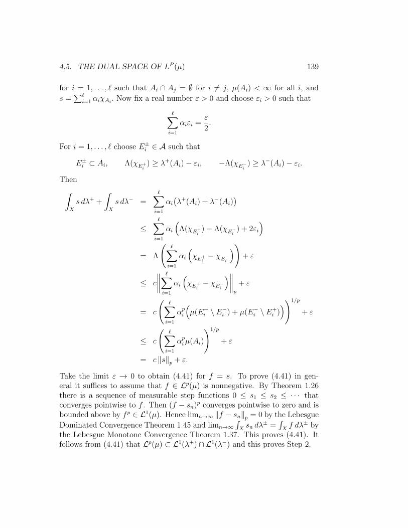
4.5. THE DUAL SPACE OF LP (µ) 139
for i = 1, . . . , ` such that Ai ∩ Aj = ∅ for i 6= j, µ(Ai) < ∞ for all i, and
s =∑`
i=1 αiχAi . Now fix a real number ε > 0 and choose εi > 0 such that
∑i=1
αiεi =ε
2.
For i = 1, . . . , ` choose E±i ∈ A such that
E±i ⊂ Ai, Λ(χE+i
) ≥ λ+(Ai)− εi, −Λ(χE−i ) ≥ λ−(Ai)− εi.
Then∫X
s dλ+ +
∫X
s dλ− =∑i=1
αi(λ+(Ai) + λ−(Ai)
)≤
∑i=1
αi
(Λ(χE+
i)− Λ(χE−i ) + 2εi
)= Λ
(∑i=1
αi
(χE+
i− χE−i
))+ ε
≤ c
∥∥∥∥∑i=1
αi
(χE+
i− χE−i
)∥∥∥∥p
+ ε
= c
(∑i=1
αpi
(µ(E+
i \ E−i ) + µ(E−i \ E+i )))1/p
+ ε
≤ c
(∑i=1
αpiµ(Ai)
)1/p
+ ε
= c ‖s‖p + ε.
Take the limit ε → 0 to obtain (4.41) for f = s. To prove (4.41) in gen-eral it suffices to assume that f ∈ Lp(µ) is nonnegative. By Theorem 1.26there is a sequence of measurable step functions 0 ≤ s1 ≤ s2 ≤ · · · thatconverges pointwise to f . Then (f − sn)p converges pointwise to zero and isbounded above by fp ∈ L1(µ). Hence limn→∞ ‖f − sn‖p = 0 by the Lebesgue
Dominated Convergence Theorem 1.45 and limn→∞∫Xsn dλ
± =∫Xf dλ± by
the Lebesgue Monotone Convergence Theorem 1.37. This proves (4.41). Itfollows from (4.41) that Lp(µ) ⊂ L1(λ+) ∩ L1(λ−) and this proves Step 2.
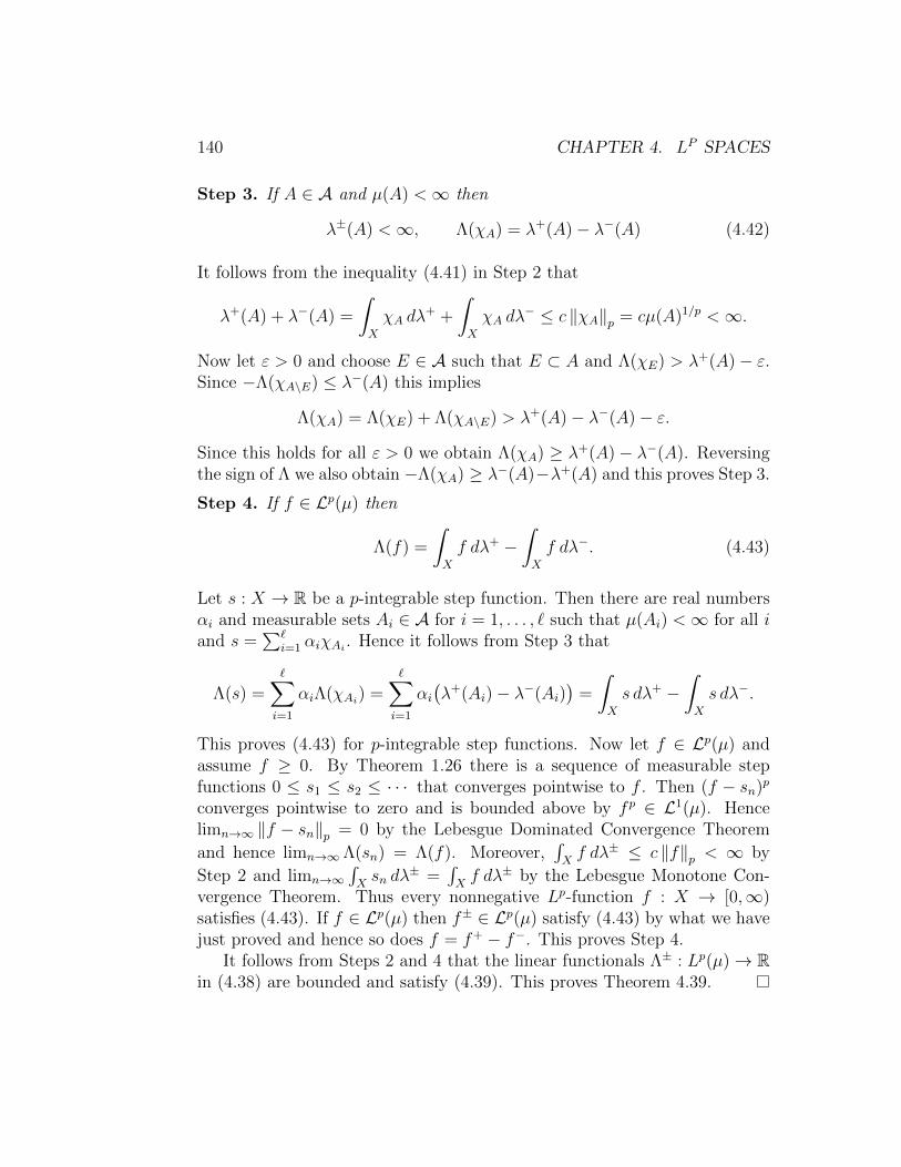
140 CHAPTER 4. LP SPACES
Step 3. If A ∈ A and µ(A) <∞ then
λ±(A) <∞, Λ(χA) = λ+(A)− λ−(A) (4.42)
It follows from the inequality (4.41) in Step 2 that
λ+(A) + λ−(A) =
∫X
χA dλ+ +
∫X
χA dλ− ≤ c ‖χA‖p = cµ(A)1/p <∞.
Now let ε > 0 and choose E ∈ A such that E ⊂ A and Λ(χE) > λ+(A)− ε.Since −Λ(χA\E) ≤ λ−(A) this implies
Λ(χA) = Λ(χE) + Λ(χA\E) > λ+(A)− λ−(A)− ε.
Since this holds for all ε > 0 we obtain Λ(χA) ≥ λ+(A)− λ−(A). Reversingthe sign of Λ we also obtain −Λ(χA) ≥ λ−(A)−λ+(A) and this proves Step 3.
Step 4. If f ∈ Lp(µ) then
Λ(f) =
∫X
f dλ+ −∫X
f dλ−. (4.43)
Let s : X → R be a p-integrable step function. Then there are real numbersαi and measurable sets Ai ∈ A for i = 1, . . . , ` such that µ(Ai) <∞ for all iand s =
∑`i=1 αiχAi . Hence it follows from Step 3 that
Λ(s) =∑i=1
αiΛ(χAi) =∑i=1
αi(λ+(Ai)− λ−(Ai)
)=
∫X
s dλ+ −∫X
s dλ−.
This proves (4.43) for p-integrable step functions. Now let f ∈ Lp(µ) andassume f ≥ 0. By Theorem 1.26 there is a sequence of measurable stepfunctions 0 ≤ s1 ≤ s2 ≤ · · · that converges pointwise to f . Then (f − sn)p
converges pointwise to zero and is bounded above by fp ∈ L1(µ). Hencelimn→∞ ‖f − sn‖p = 0 by the Lebesgue Dominated Convergence Theorem
and hence limn→∞ Λ(sn) = Λ(f). Moreover,∫Xf dλ± ≤ c ‖f‖p < ∞ by
Step 2 and limn→∞∫Xsn dλ
± =∫Xf dλ± by the Lebesgue Monotone Con-
vergence Theorem. Thus every nonnegative Lp-function f : X → [0,∞)satisfies (4.43). If f ∈ Lp(µ) then f± ∈ Lp(µ) satisfy (4.43) by what we havejust proved and hence so does f = f+ − f−. This proves Step 4.
It follows from Steps 2 and 4 that the linear functionals Λ± : Lp(µ)→ Rin (4.38) are bounded and satisfy (4.39). This proves Theorem 4.39.
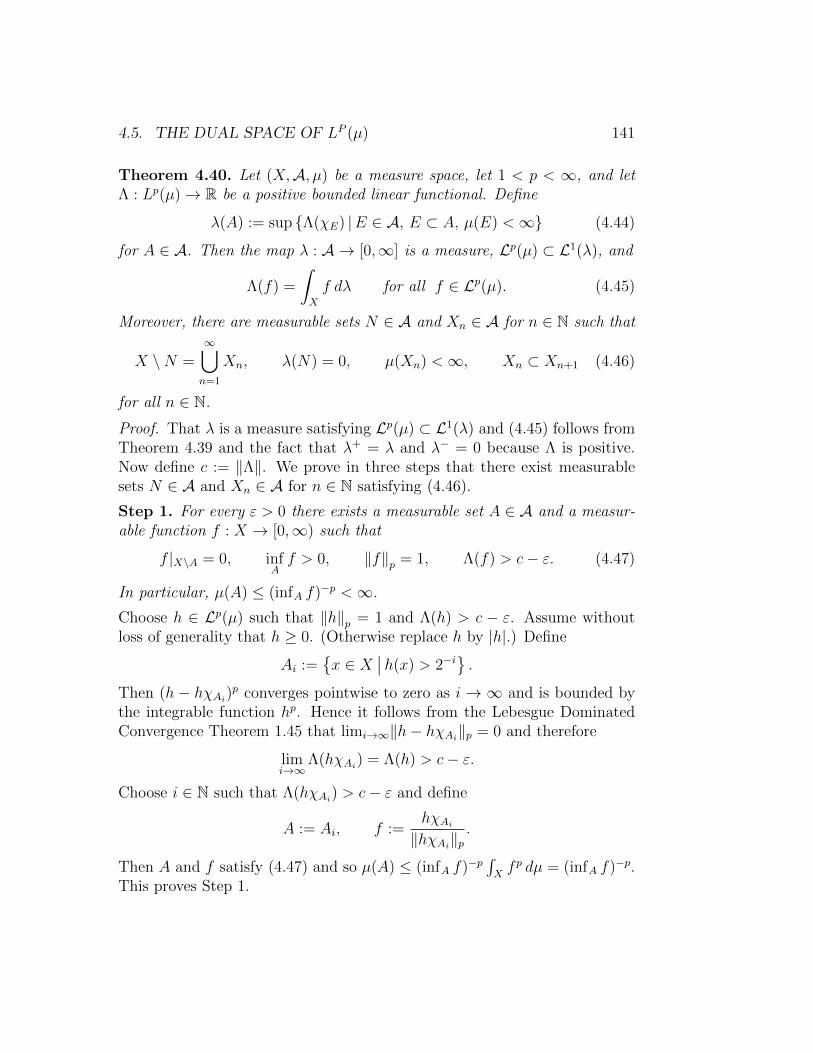
4.5. THE DUAL SPACE OF LP (µ) 141
Theorem 4.40. Let (X,A, µ) be a measure space, let 1 < p < ∞, and letΛ : Lp(µ)→ R be a positive bounded linear functional. Define
λ(A) := sup Λ(χE) |E ∈ A, E ⊂ A, µ(E) <∞ (4.44)
for A ∈ A. Then the map λ : A → [0,∞] is a measure, Lp(µ) ⊂ L1(λ), and
Λ(f) =
∫X
f dλ for all f ∈ Lp(µ). (4.45)
Moreover, there are measurable sets N ∈ A and Xn ∈ A for n ∈ N such that
X \N =∞⋃n=1
Xn, λ(N) = 0, µ(Xn) <∞, Xn ⊂ Xn+1 (4.46)
for all n ∈ N.
Proof. That λ is a measure satisfying Lp(µ) ⊂ L1(λ) and (4.45) follows fromTheorem 4.39 and the fact that λ+ = λ and λ− = 0 because Λ is positive.Now define c := ‖Λ‖. We prove in three steps that there exist measurablesets N ∈ A and Xn ∈ A for n ∈ N satisfying (4.46).
Step 1. For every ε > 0 there exists a measurable set A ∈ A and a measur-able function f : X → [0,∞) such that
f |X\A = 0, infAf > 0, ‖f‖p = 1, Λ(f) > c− ε. (4.47)
In particular, µ(A) ≤ (infA f)−p <∞.
Choose h ∈ Lp(µ) such that ‖h‖p = 1 and Λ(h) > c − ε. Assume withoutloss of generality that h ≥ 0. (Otherwise replace h by |h|.) Define
Ai :=x ∈ X
∣∣h(x) > 2−i.
Then (h − hχAi)p converges pointwise to zero as i → ∞ and is bounded bythe integrable function hp. Hence it follows from the Lebesgue DominatedConvergence Theorem 1.45 that limi→∞‖h− hχAi‖p = 0 and therefore
limi→∞
Λ(hχAi) = Λ(h) > c− ε.
Choose i ∈ N such that Λ(hχAi) > c− ε and define
A := Ai, f :=hχAi‖hχAi‖p
.
Then A and f satisfy (4.47) and so µ(A) ≤ (infA f)−p∫Xfp dµ = (infA f)−p.
This proves Step 1.
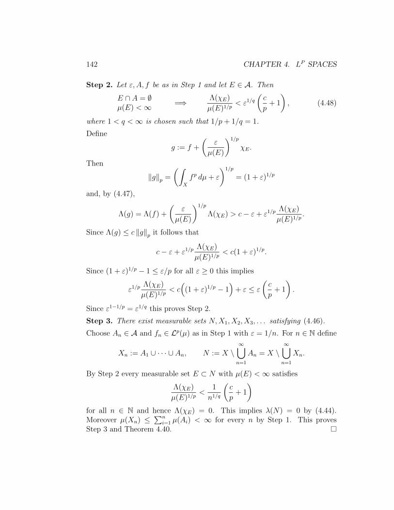
142 CHAPTER 4. LP SPACES
Step 2. Let ε, A, f be as in Step 1 and let E ∈ A. Then
E ∩ A = ∅µ(E) <∞ =⇒ Λ(χE)
µ(E)1/p< ε1/q
(c
p+ 1
), (4.48)
where 1 < q <∞ is chosen such that 1/p+ 1/q = 1.
Define
g := f +
(ε
µ(E)
)1/p
χE.
Then
‖g‖p =
(∫X
fp dµ+ ε
)1/p
= (1 + ε)1/p
and, by (4.47),
Λ(g) = Λ(f) +
(ε
µ(E)
)1/p
Λ(χE) > c− ε+ ε1/p Λ(χE)
µ(E)1/p.
Since Λ(g) ≤ c ‖g‖p it follows that
c− ε+ ε1/p Λ(χE)
µ(E)1/p< c(1 + ε)1/p.
Since (1 + ε)1/p − 1 ≤ ε/p for all ε ≥ 0 this implies
ε1/p Λ(χE)
µ(E)1/p< c(
(1 + ε)1/p − 1)
+ ε ≤ ε
(c
p+ 1
).
Since ε1−1/p = ε1/q this proves Step 2.
Step 3. There exist measurable sets N,X1, X2, X3, . . . satisfying (4.46).
Choose An ∈ A and fn ∈ Lp(µ) as in Step 1 with ε = 1/n. For n ∈ N define
Xn := A1 ∪ · · · ∪ An, N := X \∞⋃n=1
An = X \∞⋃n=1
Xn.
By Step 2 every measurable set E ⊂ N with µ(E) <∞ satisfies
Λ(χE)
µ(E)1/p<
1
n1/q
(c
p+ 1
)for all n ∈ N and hence Λ(χE) = 0. This implies λ(N) = 0 by (4.44).Moreover µ(Xn) ≤
∑ni=1 µ(Ai) < ∞ for every n by Step 1. This proves
Step 3 and Theorem 4.40.

4.6. EXERCISES 143
4.6 Exercises
Many of the exercises in this section are taken from Rudin [17, pages 71–75].
Exercise 4.41. Let (X,A, µ) be a measure space and let
f = (f1, . . . , fn) : X → Rn
be a measurable function such that∫X|fi| dµ <∞ for i = 1, . . . , n. Define∫
X
f dµ :=
(∫X
f1 dµ, . . . ,
∫X
fn dµ
)∈ Rn.
Let Rn → [0,∞) : v 7→ ‖v‖ be any norm on Rn. Prove that the functionX → [0,∞) : x 7→ ‖f(x)‖ is integrable and∥∥∥∥∫
X
f dµ
∥∥∥∥ ≤ ∫X
‖f‖ dµ. (4.49)
Hint: Prove the inequality first for vector valued integrable step functionss : X → Rn. Show that for all ε > 0 there is a vector valued integrable stepfunction s : X → Rn such that ‖
∫X
(f − s) dµ‖ < ε and∫X‖f − s‖ dµ < ε.
Exercise 4.42. Let (X,A, µ) be a measure space such that µ(X) = 1. Letf ∈ L1(µ) and let φ : R→ R be convex. Prove Jensen’s inequality
φ
(∫X
f dµ
)≤∫X
(φ f) dµ. (4.50)
(In particular, show that φ− f is necessarily integrable so the right handside is well defined, even if φ f is not integrable.) Deduce that
exp
(∫X
f dµ
)≤∫X
exp(f) dµ. (4.51)
Deduce also the inequality
n∑i=1
λi = 1 =⇒n∏i=1
aλii ≤n∑i=1
λiai (4.52)
for all positive real numbers λi and ai. In particular, ab ≤ ap/p+ bq/q for allpositive real numbers a, b, p, q such that 1/p+ 1/q = 1.
144 CHAPTER 4. LP SPACES
Exercise 4.43. Let (X,A, µ) be a measure space, choose p, q, r ∈ [1,∞]such that
1
p+
1
q=
1
r,
and let f ∈ Lp(µ) and g ∈ Lq(µ). Prove that fg ∈ Lr(µ) and
‖fg‖r ≤ ‖f‖p ‖g‖q . (4.53)
Exercise 4.44. Let (X,A, µ) be a measure space, choose real numbers
1 ≤ r < p < s <∞,
and let 0 < λ < 1 such that
λ
r+
1− λs
=1
p.
Prove that every measurable function f : X → R satisfies the inequality
‖f‖p ≤ ‖f‖λr ‖f‖
1−λs . (4.54)
Deduce that Lr(µ) ∩ Ls(µ) ⊂ Lp(µ).
Exercise 4.45. Let (X,A, µ) be a measure space and let f : X → R be ameasurable function. Define
If := p ∈ R | 1 < p <∞, f ∈ Lp(µ) .
Prove that If is an interval. Assume f does not vanish almost everywhereand define the function φf : (1,∞)→ R by
φf (p) := p log‖f‖p for p > 1.
Prove that φf is continuous and that the restriction of φf to the interior of Ifis convex. Find examples where If is closed, where If is open, and where Ifis a single point. If If 6= ∅ prove that
limp→∞‖f‖p = ‖f‖∞ .
Exercise 4.46. For each of the following three conditions find an exampleof measure space (X,A, µ) that satisfies it for all p, q ∈ [1,∞].
(a) If p < q then Lp(µ) ( Lq(µ).
(b) If p < q then Lq(µ) ( Lp(µ).
(c) If p 6= q then Lp(µ) 6⊂ Lq(µ) and Lq(µ) 6⊂ Lq(µ).

4.6. EXERCISES 145
Exercise 4.47. Let (X,U) be a locally compact Hausdorff space and define
C0(X) :=
f : X → R∣∣∣∣ f is continuous and∀ ε > 0 ∃K ⊂ X such thatK is compact and supX\K |f | < ε
Prove that X is a Banach space with respect to the sup-norm. Prove thatCc(X) is dense in C0(X).
Exercise 4.48. Let (X,A, µ) be a measure space such that µ(X) = 1 andlet f, g : X → [0,∞] be measurable functions such that fg ≥ 1. Prove that
‖f‖1 ‖g‖1 ≥ 1.
Exercise 4.49. Let (X,A, µ) be a measure space such that µ(X) = 1 andlet f : X → [0,∞] be a measurable function. Prove that√
1 + ‖f‖21 ≤
∫X
√1 + f 2 dµ ≤ 1 + ‖f‖1 . (4.55)
Find a geometric interpretation of this inequality when µ is the restrictionof the Lebesgue measure to the unit interval X = [0, 1] and f = F ′ is thederivative of a continuously differentiable function F : [0, 1] → R. Underwhich conditions does equality hold in either of the two inequalities in (4.55)?
Exercise 4.50. Let (X,A, µ) be a measure space and let f : X → R bea measurable function such that f > 0 and
∫Xf dµ = 1. Let E ⊂ X be a
measurable set such that 0 < µ(E) <∞. Prove that∫E
log(f) dµ ≤ µ(E) log
(1
µ(E)
)(4.56)
and ∫E
fp dµ ≤ µ(E)1−p for 0 < p < 1. (4.57)
Exercise 4.51. Let f : [0, 1]→ (0,∞) be Lebesgue measurable. Prove that∫ 1
0
f(s) ds
∫ 1
0
log(f(t)) dt ≤∫ 1
0
f(x) log(f(x)) dx. (4.58)
146 CHAPTER 4. LP SPACES
Exercise 4.52. Fix two constants 1 < p <∞ and a > 0.(i) Let f : (0,∞)→ R be Lebesgue measurable and suppose that the function(0,∞)→ R : x 7→ xp−1−a|f(x)|p is integrable. Show that the restriction of fto each interval (0, x] is integrable and prove Hardy’s inequality(∫ ∞
0
x−1−a∣∣∣∣∫ x
0
f(t) dt
∣∣∣∣p dx)1/p
≤ p
a
(∫ ∞0
xp−1−a|f(x)|p dx)1/p
. (4.59)
Show that equality holds in (4.59) if and only if f = 0 almost everywhere.Hint: Assume first that f is nonnegative with compact support and de-fine F (x) := 1
x
∫ x0f(t) dt for x > 0. Use integration by parts to obtain∫∞
0xp−1−aF (x)p dx = p
a
∫∞0xp−1−aF (x)p−1f(x) dx. Use Holder’s inequality.
(ii) Show that the constant p/a in Hardy’s inequality is sharp. Hint: Chooseλ < 1− a/p and take f(x) := x−λ for x ≤ 1 and f(x) := 0 for x > 1.(iii) Prove that every sequence (an)n∈N of positive real numbers satisfies
∞∑N=1
(1
N
N∑n=1
an
)p
≤(
p
p− 1
)p ∞∑n=1
apn. (4.60)
Hint: If an is nonincreasing then (4.60) follows from (4.59) with a = p − 1for a suitable function f . Deduce the general case from the special case.(iv) Let f : (0,∞) → R be Lebesgue measurable and suppose that thefunction (0,∞) → R : x 7→ xp−1+a|f(x)|p is integrable. Show that therestriction of f to each interval [x,∞) is integrable and prove the inequality(∫ ∞
0
xa−1
∣∣∣∣∫ ∞x
f(t) dt
∣∣∣∣p dx)1/p
≤ p
a
(∫ ∞0
xp−1+a|f(x)|p dx)1/p
. (4.61)
Hint: Apply the inequality (4.59) to the function g(x) := x−2f(x−1).
Exercise 4.53. Let (X,U) be a locally compact Hausdorff space and letµ : B → [0,∞] be an outer regular Borel measure on X that is inner regularon open sets. Let g ∈ L1(µ). Prove that the following are equivalent.(i) The function g vanishes µ-almost everywhere.(ii)
∫Xfg dµ = 0 for all f ∈ Cc(X).
Hint: Assume (ii). Let K ⊂ X be compact. Use Urysohn’s Lemma A.1to show that there is a sequence fn ∈ Cc(X) such that 0 ≤ fn ≤ 1 and fnconverges almost everywhere to χK . Deduce that
∫Kg dµ = 0. Then prove
that∫Ug dµ = 0 for every open set U ⊂ X and
∫Bg dµ = 0 for all B ∈ B.
Warning: The regularity hypotheses on µ cannot be removed. Find anexample of a Borel measure where (ii) does not imply (i). (See Example 4.16.)

4.6. EXERCISES 147
Exercise 4.54. Prove Egoroff’s Theorem: Let (X,A, µ) be a measurespace such that µ(X) < ∞ and let fn : X → R be a sequence of measurablefunctions that converges pointwise to f : X → R. Fix a constant ε > 0.Then there exists a measurable set E ∈ A such that µ(X \ E) < ε and fn|Econverges uniformly to f |E. Hint: Define
S(k, n) := x ∈ X | |fi(x)− fj(x)| < 1/k ∀ i, j > n for k, n ∈ N.
Prove thatlimn→∞
µ(S(k, n)) = µ(X) for all k ∈ N.
Deduce that there is a sequence nk ∈ N such that E :=⋂k∈N S(k, nk) satisfies
the required conditions. Show that Egoroff’s theorem does not extend to σ-finite measure spaces.
Exercise 4.55. Let (X,A, µ) be a measure space and let 1 < p < ∞. Letf ∈ Lp(µ) and let fn ∈ Lp(µ) be a sequence such that limn→∞ ‖fn‖p = ‖f‖pand fn converges to f almost everywhere. Prove that limn→∞ ‖f − fn‖p = 0.Prove that the hypothesis limn→∞ ‖fn‖p = ‖f‖p cannot be removed.Hint 1: Fix a constant ε > 0. Use Egoroff’s Theorem to construct disjointmeasurable sets A,B ∈ A such that X = A ∪ B,
∫A|f |p dµ < ε, µ(B) < ∞,
and fn converges to f uniformly on B. Use Fatou’s Lemma 1.41 to provethat lim supn→∞
∫A|fn|p dµ < ε.
Hint 2: Let gn := 2p−1 (|fn|p + |f |p)−|f −fn|p and use Fatou’s Lemma 1.41as in the proof of the Lebesgue Dominated Convergence Theorem 1.45.
Exercise 4.56. Let (X,A, µ) be a measure space and let fn : X → R bea sequence of measurable functions and let f : X → R be a measurablefunction. The sequence fn is said to converge in measure to f if
limn→∞
µ(x ∈ X
∣∣ |fn(x)− f(x)| > ε)
= 0
for all ε > 0. (On page 47 this is called convergence in probability.) Assumeµ(X) <∞ and prove the following.
(i) If fn converges to f almost everywhere then fn converges to f in measure.Hint: See page 47.
(ii) If fn converges to f in measure then a subsequence of fn converges to falmost everywhere.
(iii) If 1 ≤ p ≤ ∞ and fn, f ∈ Lp(µ) satisfy limn→∞ ‖fn − f‖p = 0 then fnconverges to f in measure.

148 CHAPTER 4. LP SPACES
Exercise 4.57. Let (X,U) be a compact Hausdorff space and µ : B → [0,∞]be a Borel measure. Let C(X) = Cc(X) be the space of continuous realvalued functions on X. Consider the following conditions.
(a) Every nonempty open subset of X has positive measure.
(b) There exists a Borel set E ⊂ X and an element x0 ∈ X such that everyopen neighborhood U of x0 satisfies µ(U ∩ E) > 0 and µ(U \ E) > 0.
(c) µ is outer regular and is inner regular on open sets.
Prove the following.
(i) Assume (a). Then the map C(X) → L∞(µ) in (b) is an isometric em-bedding and hence its image is a closed linear subspace of L∞(µ).
(ii) Assume (a) and (b). Then there is a nonzero bounded linear functionalΛ : L∞(µ)→ R that vanishes on the image of the inclusion C(µ)→ L∞(µ).Hint: If f = χE almost everywhere then f is discontinuous at x0.
(iii) Assume (a), (b), (c). Then the isometric embedding L1(µ) → L∞(µ)∗
of Theorem 4.33 is not surjective. Hint: Use part (ii) and Exercise 4.53.
(iv) The Lebesgue measure on [0, 1] satisfies (a), (b), and (c).
Exercise 4.58. Prove that every σ-finite measure space (X,A, µ) is localiz-able. Hint: Assume first that µ(X) <∞. Let E ⊂ A and define
c := supµ(E1 ∪ · · · ∪ En)
∣∣n ∈ N, E1, . . . , En ∈ E.
Show that there is a sequence Ei ∈ E such that µ(⋃∞i=1 Ei) = c. Prove that
H :=⋃∞i=1Ei is an envelope of E .
Exercise 4.59. Let (X,A, µ) be a localizable measure space. Prove that itsatisfies the following.
(F) Let F be a collection of measurable functions f : Af → R, each definedon a measurable set Af ∈ A. Suppose that any two functions f1, f2 ∈ F agreealmost everywhere on Af1 ∩ Af2. Then there exists a measurable functiong : X → R such that g|Af = f almost everywhere for all f ∈ F .
We will see in the next chapter that condition (F) is equivalent to localizabil-ity for semi-finite measure spaces. Hint: Let F be a collection of measurablefunctions as in (F). For a ∈ R and f ∈ F define Aaf := x ∈ Af | f(x) < a .For q ∈ Q let Hq ∈ A be an envelope of the collection Eq :=
Aqf | f ∈ F
.
Define the measurable sets
Xa :=⋃q∈Qq<a
Hq, a ∈ R.
4.6. EXERCISES 149
Prove the following.
(i) If a < b then Xa ⊂ Xb.
(ii) For every a ∈ R the measurable set Xa is an envelope of the collection
Ea :=Aaf | f ∈ F
.
Thus µ(Aaf \Xa) = 0 for all f ∈ F and, if G ∈ A, then
µ(Aaf \G) = 0 ∀ f ∈ F =⇒ µ(Xa \G) = 0.
(iii) If a ∈ R and E ∈ A then
µ(Aaf ∩ E) = 0 ∀ f ∈ F =⇒ µ(Xa ∩ E) = 0.
(iv) µ(Xa ∩ Af \ Aaf ) = 0 for all f ∈ F and all a ∈ R.
(v) Define E0 :=(⋂
r∈RXr)∪(X \
⋃s∈RX
s). Then E0 is measurable and
µ(Af ∩ E0) = 0 for all f ∈ F .
(vi) For f ∈ F define the measurable set Ef ⊂ Af by
Ef := (Af ∩ E0) ∪⋃q∈Q
(Aqf \Xq) ∪
⋃q∈Q
(Xq ∩ Af \ Aqf ).
Then µ(Ef ) = 0.
(vii) Define g : X → R by
g(x) :=
0, if x ∈ E0,a, if x ∈ Xs for all s > a and x /∈ Xr for all r < a.
(4.62)
Then g is well defined and measurable and g = f on Af \ Ef for all f ∈ F .
Example 4.60. This example is closely related to Exercise 3.24, however,it requires a considerable knowledge of Functional Analysis and the detailsgo much beyond the scope of the present manuscript. It introduces theStone–Cech compactification X of the natural numbers. This is a com-pact Hausdorff space containing N and satisfying the universality propertythat every continuous map from N to another compact Hausdorff space Yextends uniquely to a continuous map from X to Y . The space C(X) ofcontinuous functions on X can be naturally identified with the space `∞.Hence the space of positive bounded linear functionals on `∞ is isomorphicto the space of Radon measures on X by Theorem 3.15. Thus the Stone–Cech compactification of N can be used to understand the dual space of `∞.Moreover, it gives rise to an interesting example of a Radon measure whichis not outer regular (explained to me by Theo Buehler).
150 CHAPTER 4. LP SPACES
Consider the inclusion N → (`∞)∗ : n 7→ Λn which assigns to each nat-ural number n ∈ N the bounded linear functional Λn : `∞ → R defined byΛn(ξ) := ξn for ξ = (ξi)i∈N ∈ `∞. This functional has norm one. Now thespace of all bounded linear functionals on `∞ of norm at most one, i.e. theunit ball in (`∞)∗, is compact with respect to the weak-∗ topology by theBanach–Alaoglu theorem. Define X to be the closure of the set Λn |n ∈ Nin (`∞)∗ with respect to the weak-∗ topology. Thus
X :=
Λ ∈ (`∞)∗
∣∣∣∣∣For all finite sequences c1, . . . , c` ∈ Rand ξ1 = (ξ1
i )i∈N, . . . , ξ` = (ξ`i )i∈N ∈ `∞
satisfying Λ(ξj) < cj for j = 1, . . . , `there exists an n ∈ N such thatξjn < cj for j = 1, . . . , `
.
The weak-∗ topology U ⊂ 2X is the smallest topology such that the map
fξ : X → R, fξ(Λ) := Λ(ξ),
is continuous for each ξ ∈ `∞. The topological space (X,U) is a separablecompact Hausdorff space, called the Stone–Cech compactification of N.It is not second countable and one can show that the complement of a pointin X that is not equal to one of the Λn is not σ-compact. The only continuousfunctions on X are those of the form fξ, so the map `∞ → C(X) : ξ 7→ fξ isa Banach space isometry. (Verify that ‖fξ‖ := supΛ∈X |fξ(Λ)| = ‖ξ‖∞ for allξ ∈ `∞.) Thus the dual space of `∞ can be understood in terms of the Borelmeasures on X.
By Theorem 3.18 every Radon measure on X is regular. However, theBorel σ-algebra B ⊂ 2X does carry σ-finite measures µ : B → [0,∞] that areinner regular but not outer regular (and must necessarily satisfy µ(X) =∞).Here is an example pointed out to me by Theo Buehler. Define
µ(B) :=∑n∈N
Λn∈B
1
n
for every Borel set B ⊂ X. This measure is σ-finite and inner regular butis not outer regular. (The set U := Λn |n ∈ N is open, its complementK := X \U is compact and has measure zero, and every open set containingK misses only a finite subset of U and hence has infinite measure.) Now letX0 ⊂ X be the union of all open sets in X with finite measure. Then X0
is not σ-compact and the restriction of µ to the Borel σ-algebra of X0 is aRadon measure but is not outer regular.

Chapter 5
The Radon–Nikodym Theorem
Recall from Theorem 1.40 that every measurable function f : X → [0,∞)on a measure space (X,A, µ) determines a measure µf : A → [0,∞] definedby µf (A) :=
∫Af dµ for A ∈ A. By Theorem 1.35 it satisfies µf (A) = 0
whenever µ(A) = 0. A measure with this property is called absolutely con-tinuous with respect to µ. The Radon–Nikodym Theorem asserts that, whenµ is σ-finite, every σ-finite measure that is absolutely continuous with re-spect to µ has the form µf for some measurable function f : X → [0,∞). Itwas proved by Johann Radon in 1913 for the Lebesgue measure space andextended by Otton Nikodym in 1930 to general σ-finite measure spaces. Aproof is given in Section 5.1. Consequences of the Radon–Nikodym Theoreminclude the proof of Theorem 4.35 about the dual space of Lp(µ) (Section 5.2)and the decomposition theorems of Lebesgue, Hahn, and Jordan for signedmeasures (Section 5.3). An extension of the Radon–Nikodym Theorem togeneral measure spaces is proved in Section 5.4.
5.1 Absolutely Continuous Measures
Definition 5.1. Let (X,A, µ) be a measure space. A measure λ : A → [0,∞)is called absolutely continuous with respect to µ if
µ(A) = 0 =⇒ λ(A) = 0
for all A ∈ A. It is called singular with respect to µ if there exists ameasurable set A such that λ(A) = 0 and µ(Ac) = 0. In this case we also saythat λ and µ are mutually singular. We write “λ µ” iff λ is absolutelycontinuous with respect to µ and “λ ⊥ µ” iff λ and µ are mutually singular.
151
152 CHAPTER 5. THE RADON–NIKODYM THEOREM
Lemma 5.2. Let (X,A) be a measurable space and let µ, λ, λ1, λ2 be measureson A. Then the following holds.
(i) If λ1 ⊥ µ and λ2 ⊥ µ then λ1 + λ2 ⊥ µ.
(ii) If λ1 µ and λ2 µ then λ1 + λ2 µ.
(iii) If λ1 µ and λ2 ⊥ µ then λ1 ⊥ λ2.
(iv) If λ µ and λ ⊥ µ then λ = 0.
Proof. We prove (i). Suppose that λ1 ⊥ µ and λ2 ⊥ µ. Then there existmeasurable sets Ai ∈ A such that λi(Ai) = 0 and µ(Aci) = 0 for i = 1, 2.Define A := A1 ∩ A2. Then Ac = Ac1 ∪ Ac2 is a null set for µ and A is a nullset for both λ1 and λ2 and hence also for λ1 +λ2. Thus λ1 +λ2 ⊥ µ and thisproves (i).
We prove (ii). Suppose that λ1 µ and λ2 µ. If A ∈ A satisfiesµ(A) = 0 then λ1(A) = λ2(A) = 0 and so (λ1 +λ2)(A) = λ1(A) +λ2(A) = 0.Thus λ1 + λ2 µ and this proves (ii).
We prove (iii). Suppose that λ1 µ and λ2 ⊥ µ. Since λ2 ⊥ µ thereexists a measurable set A ∈ A such that λ2(A) = 0 and µ(Ac) = 0. Sinceλ1 µ it follows that λ1(Ac) = 0 and hence λ1 ⊥ λ2. This proves (iii).
We prove (iv). Suppose that λ µ and λ ⊥ µ. Since λ ⊥ µ there existsa measurable set A ∈ A such that λ(A) = 0 and µ(Ac) = 0. Since λ µ itfollows that λ(Ac) = 0 and hence λ(X) = λ(A)+λ(Ac) = 0. This proves (iv)and Lemma 5.2.
Theorem 5.3 (Lebesgue Decomposition Theorem). Let (X,A, µ) be aσ-finite measure space and let λ be a σ-finite measure on A. Then there existunique measures λa, λs : A → [0,∞] such that
λ = λa + λs, λa µ, λs ⊥ µ. (5.1)
Proof. See page 157.
Theorem 5.4 (Radon–Nikodym). Let (X,A, µ) be a σ-finite measurespace and let λ : A → [0,∞] be a measure. The following are equivalent.
(i) λ is σ-finite and absolutely continuous with respect to µ.
(ii) There exists a measurable function f : X → [0,∞) such that
λ(A) =
∫A
f dµ for all A ∈ A. (5.2)
If (i) holds then equation (5.2) determines f uniquely up to equality µ-almosteverywhere. Moreover, f ∈ L1(µ) if and only if λ(X) <∞.
5.1. ABSOLUTELY CONTINUOUS MEASURES 153
Proof. The last assertion follows by taking A = X in (5.2).We prove that (ii) implies (i). Thus assume that there exists a measurable
function f : X → [0,∞) such that λ is given by (5.2). Then λ is absolutelycontinuous with respect to µ by Theorem 1.35. Since µ is σ-finite, there existsa sequence of measurable sets X1 ⊂ X2 ⊂ X3 ⊂ · · · such that µ(Xn) < ∞and X =
⋃∞n=1 Xn. Define An := x ∈ Xn | f(x) ≤ n. Then An ⊂ An+1 and
λ(An) ≤ nµ(Xn) < ∞ for all n and X =⋃∞n=1An. Thus λ is σ-finite and
this shows that (ii) implies (i).It remains to prove that (i) implies (ii) and that f is uniquely determined
by (5.2) up to equality µ-almost everywhere. This is proved in three steps.The first step is uniqueness, the second step is existence under the assumptionλ(X) <∞ and µ(X) <∞, and the last step establishes existence in general.
Step 1. Let (X,A, µ) be a measure space, let λ : A → [0,∞] be a σ-finitemeasure, and let f, g : X → [0,∞) be two measurable functions such that
λ(A) =
∫A
f dµ =
∫A
g dµ for all A ∈ A. (5.3)
Then f and g agree µ-almost everywhere.
Since (X,A, λ) is a σ-finite measure space there exists a sequence of mea-surable sets A1 ⊂ A2 ⊂ A3 ⊂ · · · such that λ(An) < ∞ for all n ∈ N andX =
⋃∞n=1An. For n ∈ N define
An := E ∈ A |E ⊂ An , µn := µ|An .
Take A = An in (5.3) to obtain f, g ∈ L1(µn) for all n. Thus
f − g ∈ L1(µn),
∫E
(f − g) dµn = 0 for all E ∈ An.
Hence f − g vanishes µn-almost everywhere by Lemma 1.49. Thus the set
En := x ∈ An | f(x) 6= g(x)
satisfies µ(En) = µn(En) = 0 and hence the set
E := x ∈ X | f(x) 6= g(x) =∞⋃n=1
En
satisfies µ(E) = 0. This proves Step 1.
154 CHAPTER 5. THE RADON–NIKODYM THEOREM
Step 2. Let (X,A) be a measurable space and let λ, µ : A → [0,∞] bemeasures such that λ(X) <∞, µ(X) <∞, and λ µ. Then there exists ameasurable function h : X → [0,∞) such that λ(A) =
∫Ah dµ for all A ∈ A.
By assumption λ+ µ : A → [0,∞] is a finite measure defined by
(λ+ µ)(A) := λ(A) + µ(A) for A ∈ A.
Since (λ+ µ)(X) <∞ it follows from the Cauchy–Schwarz inequality that
H := L2(λ+ µ) ⊂ L1(λ+ µ).
Namely, if f ∈ L2(λ+ µ) then∫X
|f | d(λ+ µ) ≤ c
√∫X
|f |2 d(λ+ µ) <∞, c :=√λ(X) + µ(X).
Define Λ : L2(λ+ µ)→ R by
Λ(f) :=
∫X
f dλ.
for f ∈ L2(λ + µ). (Here we abuse notation and use the same letter f for afunction in L2(λ+ µ) and its equivalence class in L2(λ+ µ).) Then
|Λ(f)| ≤∫X
|f | dλ ≤∫X
|f | d(λ+ µ) ≤ c ‖f‖L2(λ+µ)
for all f ∈ L2(λ+µ). Thus Λ is a bounded linear functional on L2(λ+µ) andit follows from Corollary 4.28 that there exists an L2-function g ∈ L2(λ+ µ)such that ∫
X
f dλ =
∫X
fg d(λ+ µ) (5.4)
for all f ∈ L2(λ+ µ). This implies∫X
f(1− g) d(λ+ µ) =
∫X
f d(λ+ µ)−∫X
fg d(λ+ µ)
=
∫X
f d(λ+ µ)−∫X
f dλ
=
∫X
f dµ
(5.5)
for all f ∈ L2(λ+ µ).

5.1. ABSOLUTELY CONTINUOUS MEASURES 155
We claim that the inequalities 0 ≤ g < 1 hold (λ+µ)-almost everywhere.To see this, consider the measurable sets
E0 :=x ∈ X
∣∣ g(x) < 0, E1 :=
x ∈ X
∣∣ g(x) ≥ 1.
Then it follows from (5.4) with f := χE0 that
0 ≤ λ(E0) =
∫X
χE0 dλ =
∫X
χE0g d(λ+ µ) ≤ 0.
Hence∫XχE0g d(λ+µ) = 0 and it follows from Lemma 1.49 that the function
f := −χE0g vanishes (λ + µ)-almost everywhere. Hence (λ + µ)(E0) = 0.Likewise, it follows from (5.5) with f := χE1 that
µ(E1) =
∫X
χE1 dµ =
∫E1
(1− g) d(λ+ µ) ≤ 0.
Hence µ(E1) = 0. Since λ is absolutely continuous with respect to µ it followsthat λ(E1) = 0 and hence (λ+ µ)(E1) = 0 as claimed. Assume from now onthat 0 ≤ g(x) < 1 for all x ∈ X. (Namely, redefine g(x) := 0 for x ∈ E0 ∪E1
without changing the identities (5.4) and (5.5).)Apply equation (5.5) to the characteristic function f := χA ∈ L2(λ + µ)
of a measurable set A to obtain the identity
µ(A) =
∫A
(1− g) d(λ+ µ) for all A ∈ A.
By Theorem 1.40 this implies that equation (5.5) continues to hold for everymeasurable function f : X → [0,∞), whether or not it belongs to L2(λ+µ).Now define the measurable function h : X → [0,∞) by
h(x) :=g(x)
1− g(x)for x ∈ X.
By equation (5.4) with f = χA and equation (5.5) with f = χAh it satisfies
λ(A) =
∫X
χA dλ =
∫X
χAg d(λ+ µ)
=
∫X
χAh(1− g) d(λ+ µ) =
∫X
χAh dµ
=
∫A
h dµ
for all A ∈ A. This proves Step 2.
156 CHAPTER 5. THE RADON–NIKODYM THEOREM
Step 3. We prove that (i) implies (ii).
Since λ and µ are σ-finite measures, there exist sequences of measurable setsAn, Bn ∈ A such that An ⊂ An+1, λ(An) < ∞, Bn ⊂ Bn+1, µ(Bn) < ∞ forall n and X =
⋃∞n=1 An =
⋃∞n=1 Bn. Define Xn := An ∩Bn. Then
Xn ⊂ Xn+1, λ(Xn) <∞, µ(Xn) <∞for all n and X =
⋃∞n=1Xn. Thus it follows from Step 2 that there exists a
sequence of measurable functions fn : Xn → [0,∞) such that
λ(A) =
∫A
fn dµ for all n ∈ N and all A ∈ A such that A ⊂ Xn. (5.6)
It follows from Step 1 that the restriction of fn+1 to Xn agrees with fnµ-almost everywhere. Thus, modifying fn+1 on a set of measure zero ifnecessary, we may assume without loss of generality that fn+1|Xn = fn forall n ∈ N. With this understood, define f : X → [0,∞) by
f |Xn := fn for n ∈ N.This function is measurable because
f−1([0, c]) =∞⋃n=1
(Xn ∩ f−1([0, c])
)=∞⋃n=1
f−1n ([0, c]) ∈ A
for all c ≥ 0. Now let E ∈ A and define En := E ∩Xn ∈ A for n ∈ N. Then
E1 ⊂ E2 ⊂ E3 ⊂ · · · , E =∞⋃n=1
En.
Hence it follows from part (iv) of Theorem 1.28 that
λ(E) = limn→∞
λ(En)
= limn→∞
∫En
f dµ
= limn→∞
∫X
χEnf dµ
=
∫X
χEf dµ
=
∫E
f dµ.
Here the last but one equation follows from the Lebesgue Monotone Conver-gence Theorem 1.37. This proves Step 3 and Theorem 5.4.
5.1. ABSOLUTELY CONTINUOUS MEASURES 157
Example 5.5. Let X be a one element set and let A := 2X . Define themeasure µ : 2X → [0,∞] by µ(∅) := 0 and µ(X) :=∞.
(i) Choose λ(∅) := 0 and λ(X) := 1. Then λ µ but there does not exist a(measurable) function f : X → [0,∞] such that
∫Xf dµ = λ(X). Thus the
hypothesis that (X,A, µ) is σ-finite cannot be removed in Theorem 5.4.
(ii) Choose λ := µ. Then λ(A) =∫Af dµ for every nonzero function
f : X → [0,∞). Thus the hypothesis that (X,A, λ) is σ-finite cannot beremoved in Step 1 in the proof of Theorem 5.4.
Example 5.6. Let X be an uncountable set and denote by A ⊂ 2X theset of all subsets A ⊂ X such that either A or Ac is countable. Choosean uncountable subset H ⊂ X with an uncountable complement and defineλ, µ, ν : A → [0,∞] by
λ(A) :=
0, if A is countable,1, if Ac is countable,
µ(A) := #(A ∩H), ν(A) := #A.
Then λ µ ν and µ and ν are not σ-finite. There does not exist anymeasurable function f : X → [0,∞] such that λ(X) =
∫Xf dµ. Nor is there
any measurable function h : X → R such that µ(A) =∫Ah dν for all A ∈ A.
(The only possible such function would be h := χH which is not measurable.)
Proof of Theorem 5.3. We prove uniqueness. Let λa, λs, λ′a, λ
′s : A → [0,∞]
be measures such that
λ = λa + λs = λ′a + λ′s, λa µ, λ′a µ, λs ⊥ µ, λ′s ⊥ µ.
Then there exist measurable sets A,A′ ∈ A such that
λs(A) = 0, µ(X \ A) = 0, λ′s(A′) = 0, µ(X \ A′) = 0.
Since X \ (A ∩ A′) = (X \ A) ∪ (X \ A′), this implies µ(X \ (A ∩ A′)) = 0.Let E ∈ A. Then λs(E ∩ A ∩ A′) = 0 = λ′s(E ∩ A ∩ A′) and hence
λa(E ∩ A ∩ A′) = λ(E ∩ A ∩ A′) = λ′a(E ∩ A ∩ A′).
Moreover µ(E \ (A∩A′)) = 0, hence λa(E \ (A∩A′)) = 0 = λ′a(E \ (A∩A′))and hence
λs(E \ (A ∩ A′)) = λ(E \ (A ∩ A′)) = λ′s(E \ (A ∩ A′)).

158 CHAPTER 5. THE RADON–NIKODYM THEOREM
This implies
λa(E) = λa(E ∩ A ∩ A′) = λ′a(E ∩ A ∩ A′) = λ′a(E)
λs(E) = λs(E \ (A ∩ A′)) = λ′s(E \ (A ∩ A′)) = λ′s(E).
This proves uniqueness.We prove existence. The measure
ν := λ+ µ : A → [0,∞]
is σ-finite. Hence it follows from the Radon–Nikodym Theorem 5.4 that thereexist measurable functions f, g : X → [0,∞) such that
λ(E) =
∫E
f dν, µ(E) =
∫E
g dν for all E ∈ A. (5.7)
DefineA :=
x ∈ X
∣∣ g(x) > 0
(5.8)
and
λa(E) := λ(E ∩ A), λs(E) := λ(E ∩ Ac) for E ∈ A. (5.9)
Then it follows directly from (5.9) that the maps λa, λs : A → [0,∞] aremeasures and satisfy λa + λs = λ. Moreover, it follows from (5.9) that
λs(A) = λ(A ∩ Ac) = λ(∅) = 0
and from (5.8) that g|Ac = 0, so by (5.7)
µ(Ac) =
∫Acg dν = 0.
This shows that λs ⊥ µ. It remains to prove that λa is absolutely continuouswith respect to µ. To see this, let E ∈ A such that µ(E) = 0. Then by (5.7)∫
X
χEg dν =
∫E
g dν = µ(E) = 0.
Hence it follows from Lemma 1.49 that χEg vanishes ν-almost everywhere.Thus χE∩Ag = χAχEg vanishes ν-almost everywhere. Since g(x) > 0 for allx ∈ E ∩ A, this implies
ν(E ∩ A) = 0.
Hence
λa(E) = λ(E ∩ A) =
∫E∩A
f dν = 0.
This shows that λa µ and completes the proof of Theorem 5.3.

5.2. THE DUAL SPACE OF LP (µ) REVISITED 159
5.2 The Dual Space of Lp(µ) Revisited
This section is devoted to the proof of Theorem 4.35. Assume throughoutthat (X,A, µ) is a measure space and fix two constants
1 ≤ p <∞, 1 < q ≤ ∞, 1
p+
1
q= 1. (5.10)
As in Section 4.5 we abuse notation and write Λ(f) := Λ([f ]µ) for the valueof a bounded linear functional Λ : Lp(µ) → R on the equivalence classof a function f ∈ Lp(µ). Recall from Theorem 4.33 that every g ∈ Lq(µ)determines a bounded linear functional Λg : Lp(µ)→ R via
Λg(f) :=
∫X
fg dµ for f ∈ Lp(µ).
The next result proves Theorem 4.35 in σ-finite case.
Theorem 5.7. Assume (X,A, µ) is σ-finite and let Λ : Lp(µ) → R be abounded linear functional. Then there exists a function g ∈ Lq(µ) such that
Λg = Λ.
Proof. Assume first that Λ is positive. We prove in six steps that there existsa function g ∈ Lq(µ) such that g ≥ 0 and Λg = Λ.
Step 1. Define
λ(A) := sup
Λ(χE)∣∣E ∈ A, E ⊂ A, µ(E) <∞
(5.11)
for A ∈ A. Then the map λ : A → [0,∞] is a measure, Lp(µ) ⊂ L1(λ), andΛ(f) =
∫Xf dλ for all f ∈ Lp(µ).
This follows directly from Theorem 4.40.
Step 2. Let λ be as in Step 1 and define c := ‖Λ‖. Then λ(A) ≤ cµ(A)1/p
for all A ∈ A.
By assumption Λ(f) ≤ c ‖f‖p for all f ∈ Lp(µ). Take f := χE to obtain
Λ(χE) ≤ cµ(E)1/p ≤ cµ(A)1/p for all E ∈ A with E ⊂ A and µ(E) < ∞.Take the supremum over all such E to obtain λ(A) ≤ cµ(A)1/p by (5.11).
Step 3. Let λ be as in Step 1. Then there exists a measurable functiong : X → [0,∞) such that λ(A) =
∫Ag dµ for all A ∈ A.
By Step 2, λ is σ-finite and λ µ. Hence Step 3 follows from the Radon–Nikodym Theorem 5.4 for σ-finite measure spaces.

160 CHAPTER 5. THE RADON–NIKODYM THEOREM
Step 4. Let λ be as in Step 1 and g be as in Step 3. Then∫Xfg dµ =
∫Xf dλ
for every measurable function f : X → [0,∞).
This follows immediatey from Step 3 and Theorem 1.40.
Step 5. Let c be as in Step 2 and g be as in Step 3. Then ‖g‖q ≤ c.
Let λ be as in Step 1 and let f ∈ Lp(µ) such that f ≥ 0. Then∫X
fg dµStep 4=
∫X
f dλStep 1= Λ(f) ≤ c ‖f‖p . (5.12)
Moreover, the measure space (X,A, µ) is semi-finite by Lemma 4.30. Henceit follows from parts (iii) and (iv) of Lemma 4.34 that ‖g‖q ≤ c.
Step 6. Let g be as in Step 3. Then Λ = Λg.
Since g ∈ Lq(µ) by Step 5, the function g determines a bounded linearfunctional Λg : Lp(µ)→ R via Λg(f) :=
∫Xfg dµ for f ∈ Lp(µ). By (5.12)
it satisfies Λg(f) = Λ(f) for all f ∈ Lp(µ) with f ≥ 0. Apply this identityto the functions f± : X → [0,∞) for all f ∈ Lp(µ) to obtain Λ = Λg.This proves the assertion of Theorem 5.7 for every positive bounded linearfunctional Λ : Lp(µ)→ R.
Let Λ : Lp(µ) → R be any bounded linear functional. By Theorem 4.39there exist positive bounded linear functionals Λ± : Lp(µ) → R such thatΛ = Λ+ − Λ−. Hence, by what we have just proved, there exist functionsg± ∈ Lq(µ) such that g± ≥ 0 and Λ± = Λg± . Define g := g+ − g−. Theng ∈ Lq(µ) and Λg = Λg+−Λg− = Λ+−Λ− = Λ. This proves Theorem 5.7.
The next result proves Theorem 4.35 in the case p = 1.
Theorem 5.8. Assume p = 1. Then the following are equivalent.
(i) The measure space (X,A, µ) is localizable.
(ii) The measure space (X,A, µ) is semi-finite and satisfies condition (F) inExercise 4.59, i.e. if F is a collection of measurable functions f : Af → R,each defined on a measurable set Af ∈ A, such that any two functionsf1, f2 ∈ F agree almost everywhere on Af1 ∩ Af2, then there exists a measur-able function g : X → R such that g|Af = f almost everywhere for all f ∈ F .
(iii) The linear map
L∞(µ)→ L1(µ)∗ : g 7→ Λg (5.13)
is bijective.
5.2. THE DUAL SPACE OF LP (µ) REVISITED 161
Proof. The proof that (i) implies (ii) is outlined in Exercise 4.59.We prove that (ii) implies (iii). Since (X,A, µ) is semi-finite, the linear
map (5.13) is injective by Theorem 4.33. We must prove that it is surjective.Assume first that Λ : L1(µ) → R is a positive bounded linear functional.Define E :=
E ∈ A
∣∣µ(E) <∞
and, for E ∈ E , define
AE := A ∈ A |A ⊂ E , µE := µ|AE . (5.14)
Then there is an extension operator ιE : L1(µE)→ L1(µ) defined by
ιE(f)(x) :=
f(x), for x ∈ E,0, for x ∈ X \ E, (5.15)
It descends to a bounded linear operator from L1(µE) to L1(µ) which willstill be denoted by ιE. Define
ΛE = Λ ιE : L1(µE)→ R.
This is a positive bounded linear functional for every E ∈ E . Hence it followsfrom Theorem 5.7 (and the Axiom of Choice) that there is a collection ofbounded measurable functions gE : E → [0,∞), E ∈ E , such that
ΛE(f) =
∫E
fgE dµE for all E ∈ E and all f ∈ L1(µE).
If E,F ∈ E then E ∩ F ∈ E and the functions gE|E∩F , gF |E∩F , and gE∩Fall represent the same bounded linear functional ΛE∩F : L1(µE∩F ) → R.Hence they agree almost everywhere by Theorem 4.33. This shows that thecollection
F :=gE∣∣E ∈ E
satisfies the hypotheses of condition (F) on page 148. Thus it follows from (ii)that there exists a measurable function g : X → R such that, for all E ∈ E ,the restriction g|E agrees with gE almost everywhere on E.
We prove that g ≥ 0 almost everywhere. Suppose otherwise that theset A− := x ∈ X | g(x) < 0 has positive measure. Since (X,A, µ) is semi-finite there exists a set E ∈ E such that E ⊂ A− and µ(E) > 0. Sinceg(x) < 0 ≤ gE(x) for all x ∈ E it follows that g|E does not agree with gEalmost everywhere, a contradiction. This contradiction shows that g ≥ 0almost everywhere.

162 CHAPTER 5. THE RADON–NIKODYM THEOREM
We prove that g ≤ ‖Λ‖ almost everywhere. Suppose otherwise that theset A+ := x ∈ X | g(x) > ‖Λ‖ has positive measure. Since (X,A, µ) issemi-finite there exists a set E ∈ E such that E ⊂ A+ and µ(E) > 0. Since‖gE‖∞ = ‖ΛE‖ ≤ ‖Λ‖ it follows from Lemma 4.8 that gE(x) ≤ ‖Λ‖ < g(x)for almost every x ∈ E. Hence g|E does not agree with gE almost everywhere,a contradiction. This contradiction shows that g ≤ ‖Λ‖ almost everywhereand we may assume without loss of generality that
0 ≤ g(x) ≤ ‖Λ‖
for all x ∈ X.We prove that Λg = Λ. Fix a function f ∈ L1(µ) such that f ≥ 0. Then
there exists a sequence Ei ∈ E such that E1 ⊂ E2 ⊂ E3 ⊂ · · · and χEifconverges pointwise to f . Namely, by Theorem 1.26 there exists a sequenceof measurable step functions si : X → [0,∞) such that 0 ≤ s1 ≤ s2 ≤ · · ·and si converges pointwise to f . Since
∫Xsi dµ ≤
∫Xf dµ <∞ for all i the
sets Ei := x ∈ X | si(x) > 0 have finite measure and 0 ≤ si ≤ χEif ≤ f forall i. Thus the Ei are as required. Since the sequence |f − χEif | convergespointwise to zero and is bounded above by the integrable function f it followsfrom the Lebesgue Dominated Convergence Theorem 1.45 that
limi→∞‖f − χEif‖1 = 0.
Hence
Λ(f) = limi→∞
Λ(χEif) = limi→∞
ΛEi(f |Ei)
= limi→∞
∫Ei
fgEi dµ = limi→∞
∫Ei
fg dµ =
∫X
fg dµ.
Here the last step follows from the Lebesgue Monotone Convergence Theo-rem 1.37. This shows that Λ(f) = Λg(f) for every nonnegative integrablefunction f : X → [0,∞). It follows that
Λ(f) = Λ(f+)− Λ(f−) = Λg(f+)− Λg(f
−) = Λg(f)
for all f ∈ L1(µ). Thus Λ = Λg as claimed.This shows that every positive bounded linear functional on L1(µ) be-
longs to the image of the map (5.13). Since every bounded linear functionalon L1(µ) is the difference of two positive bounded linear functionals by The-orem 4.39, it follows that the map (5.13) is surjective. Thus we have provedthat (ii) implies (iii).
5.2. THE DUAL SPACE OF LP (µ) REVISITED 163
We prove that (iii) implies (i). Assume that the map (5.13) is bijective.Then (X,A, µ) is semi-finite by part (iv) of Theorem 4.33. Now let E ⊂ Abe any collection of measurable sets. Assume without loss of generality that
E1, . . . , E` ∈ E =⇒ E1 ∪ · · · ∪ E` ∈ E .
(Otherwise, replace E by the collection E ′ of all finite unions of elementsof E ; then every measurable envelope of E ′ is also an envelope of E .) ForE ∈ E define AE and µE by (5.14) and define the bounded linear functionalΛE : L1(µE)→ R by
ΛE(f) :=
∫E
f dµE for f ∈ L1(µE). (5.16)
Then for all E,F ∈ A and f ∈ L1(µ)
E ⊂ F, f ≥ 0 =⇒ ΛE(f) ≤ ΛF (f). (5.17)
Define Λ : L1(µ)→ R by
Λ(f) := supE∈E
ΛE(f+|E)− supE∈E
ΛE(f−|E). (5.18)
We prove that this is a well defined bounded linear functional with ‖Λ‖ ≤ 1.To see this, note that ΛE(f |E) ≤
∫Xf dµ for every nonnegative function
f ∈ L1(µ) and so |Λ(f)| ≤∫Xf+ dµ +
∫Xf− dµ = ‖f‖1 for all f ∈ L1(µ).
Moreover, it follows directly from the definition that Λ(cf) = cΛ(f) forall c ≥ 0 and Λ(−f) = −Λ(f). Now let f, g ∈ L1(µ) be nonnegative inte-grable functions. Then
Λ(f + g) = supE∈E
ΛE(f |E + g|E)
≤ supE∈E
ΛE(f |E) + supE∈E
ΛE(g|E)
= Λ(f) + Λ(g).
To prove the converse inequality, let ε > 0 and choose E,F ∈ E such that
ΛE(f |E) > Λ(f)− ε, ΛF (g|F ) > Λ(g)− ε.
Then E ∪ F ∈ E and it follows from (5.17) that
ΛE∪F ((f + g)|E∪F ) = ΛE∪F (f |E∪F ) + ΛE∪F (g|E∪F )
≥ ΛE(f |E) + ΛF (g|F )
> Λ(f) + Λ(g)− 2ε.

164 CHAPTER 5. THE RADON–NIKODYM THEOREM
Hence Λ(f + g) > Λ(f) + Λ(g)− 2ε for all ε > 0 and so
Λ(f) + Λ(g) ≤ Λ(f + g) ≤ Λ(f) + Λ(g).
This shows that Λ(f+g) = Λ(f)+Λ(g) for all f, g ∈ L1(µ) such that f, g ≥ 0.If f, g ∈ L1(µ) then (f + g)+ + f− + g− = (f + g)− + f+ + g+ and hence
Λ((f + g)+) + Λ(f−) + Λ(g−) = Λ((f + g)−) + Λ(f+) + Λ(g+)
by what we have just proved. Since Λ(f) = Λ(f+) − Λ(f−) by definition itfollows that Λ(f + g) = Λ(f) + Λ(g) for all f, g ∈ L1(µ). This shows thatΛ : L1 → R is a positive bounded linear functional of norm ‖Λ‖ ≤ 1.
With this understood, it follows from (iii) that there exists a functiong ∈ L∞(µ) such that Λ = Λg. Define
H := x ∈ X | g(x) > 0 .
We prove that H is an envelope of E . Fix a set E ∈ E and suppose, bycontradiction, that µ(E \H) > 0. Then, since (X,A, µ) is semi-finite, thereexists a measurable set A ∈ A such that 0 < µ(A) < ∞ and A ⊂ E \ H.Since g(x) ≤ 0 for all x ∈ A it follows that
0 < µ(A) = ΛE(χA|E) =
∫A
g dµ ≤ 0,
a contradiction. This contradiction shows that our assumption µ(E \H) > 0must have been wrong. Hence µ(E \H) = 0 for all E ∈ E as claimed.
Now let G ∈ A be any measurable set such that µ(E \ G) = 0 for allE ∈ E . We must prove that µ(H \ G) = 0. Suppose, by contradiction, thatµ(H \ G) > 0. Since (X,A, µ) is semi-finite there exists a measurable setA ∈ A such that 0 < µ(A) <∞ and A ⊂ H \G. Then∫
A
g dµ = Λ(χA) = supE∈E
ΛE(χA|E) = supE∈E
µ(E ∩ A) = 0.
Here the second equation follows from (5.18), the third follows from (5.16),and the last follows from the fact that E ∩ A ⊂ E \ G for all E ∈ E . Sinceg > 0 on A it follows from Lemma 1.49 that µ(A) = 0, a contradiction. Thiscontradiction shows that our assumption that µ(H \G) > 0 must have beenwrong and so µ(H \ G) = 0 as claimed. Thus we have proved that everycollection of measurable sets E ⊂ A has a measurable envelope, and thiscompletes the proof of Theorem 5.8.
5.2. THE DUAL SPACE OF LP (µ) REVISITED 165
Now we are in a position to prove Theorem 4.35 in general.
Proof of Theorem 4.35. For p = 1 the assertion of Theorem 4.35 follows fromthe equivalence of (i) and (iii) in Theorem 5.8. Hence assume p > 1. Wemust prove that the linear map Lq(µ) → Lp(µ)∗ : g 7→ Λg is surjective. LetΛ : Lp(µ)→ R be a positive bounded linear functional and define
λ(A) := sup Λ(χE) |E ∈ A, E ⊂ A, µ(E) <∞ for A ∈ A.
Then λ : A → [0,∞] is a measure by Theorem 4.40 and
Lp(µ) ⊂ L1(λ), Λ(f) =
∫X
f dλ for all f ∈ Lp(µ).
Theorem 4.40 also asserts that there exists a measurable set N ∈ A suchthat λ(N) = 0 and the restriction of µ to X \N is σ-finite. Define
X0 := X \N, A0 := A ∈ A |A ⊂ X0 , µ0 := µ|A0
as in (5.14), let ι0 : Lp(µ0) → Lp(µ) be the extension operator as in (5.15),and define Λ0 := Λ ι0 : Lp(µ0) → R. Then Λ0 is a positive bounded linearfunctional on Lp(µ0) and
Λ(f) =
∫X
f dλ =
∫X\N
f dλ = Λ0(f |X0) for all f ∈ Lp(µ).
Since (X0,A0, µ0) is σ-finite it follows from Theorem 5.7 that there exists afunction g0 ∈ Lq(µ0) such that g0 ≥ 0 and
Λ0(f0) =
∫X0
f0g0 dµ0 for all f0 ∈ Lp(µ0).
Define g : X → [0,∞) by g(x) := g0(x) for x ∈ X0 = X \ N and g(x) := 0for x ∈ N . Then ‖g‖Lq(µ) = ‖g0‖Lq(µ0) = ‖Λ0‖ = ‖Λ‖ by Theorem 4.33, and
Λ(f) = Λ0(f |X0) =∫X0fg0 dµ0 =
∫Xfg dµ for all f ∈ Lp(µ). This proves
the assertion for positive bounded linear functionals. Since every boundedlinear functional Λ : Lp(µ) → R is the difference of two positive boundedlinear functionals by Theorem 4.39, this proves Theorem 4.35.
Corollary 5.9. Every σ-finite measure space is localizable.
Proof. Let (X,A, µ) be a σ-finite measure space. Then (X,A, µ) is semi-finite by Lemma 4.30. Hence the map L∞(µ)→ L1(µ)∗ : g 7→ Λg in (4.31) isinjective by Theorem 4.33 and is surjective by Theorem 5.7. Hence it followsfrom Theorem 5.8 that (X,A, µ) is localizable.
166 CHAPTER 5. THE RADON–NIKODYM THEOREM
5.3 Signed Measures
Throughout this section (X,A) is a measurable space, i.e. X is a set andA ⊂ 2X is a σ-algebra. The following definition extends the notion of ameasure on (X,A) to a signed measure which can have positive and negativevalues. As an example from physics one can think of electrical charge.
Definition 5.10. A function λ : A → R is called a signed measure if it isσ-additive, i.e. every sequence Ei ∈ A of pairwise disjoint measurable setssatisfies
∞∑i=1
|λ(Ei)| <∞, λ
(∞⋃i=1
Ei
)=∞∑i=1
λ(Ei). (5.19)
Lemma 5.11. Every signed measure λ : A → R satisfies the following.
(i) µ(∅) = 0.
(ii) If E1, . . . , E` ∈ A are pairwise disjoint then λ(⋃`i=1Ei) =
∑`i=1 λ(Ei).
Proof. To prove (i) take Ei := ∅ in equation (5.19). To prove (ii) take Ei := ∅for all i > `.
Given a signed measure λ : A → R it is a natural question to ask whetherit can be written as the difference of two measures λ± : A → [0,∞). Closelyrelated to this is the question whether there exists a measure µ : A → [0,∞)that satisfies
|λ(A)| ≤ µ(A) for all A ∈ A. (5.20)
If such a measure exists it must satisfy
E,F ∈ A, E ∩ F = ∅ =⇒ λ(E)− λ(F ) ≤ µ(E ∪ F )
Thus a lower bound for µ(A) is the supremum of the numbers λ(E)− λ(F )over all decompositions of A into pairwise disjoint measurable sets E and F .The next theorem shows that this supremum defines the smallest measurethat satisfies (5.20).
Theorem 5.12. Let λ : A → R be a signed measure and define
|λ|(A) := sup
λ(E)− λ(F )
∣∣∣∣∣E,F ∈ A,E ∩ F = ∅,E ∪ F = A
for A ∈ A. (5.21)
Then |λ(A)| ≤ |λ|(A) <∞ for all A ∈ A and |λ| : A → [0,∞) is a measure,called the total variation of λ.

5.3. SIGNED MEASURES 167
Proof. We prove that |λ| is a measure. If follows directly from the definitionthat |λ|(∅) = 0 and |λ|(A) ≥ |λ(A)| ≥ 0 for all A ∈ A. We must prove thatthe function |λ| : A → [0,∞] is σ-additive. Let Ai ∈ A be a sequence ofpairwise disjoint measurable sets and define
A :=∞⋃i=1
Ai.
Let E,F ∈ A are measurable sets such that
E ∩ F = ∅, E ∪ F = A. (5.22)
Then
E =∞⋃i=1
(E ∩ Ai), F =∞⋃i=1
(F ∩ Ai).
Hence
λ(E)− λ(F ) =∞∑i=1
λ(E ∩ Ai)−∞∑i=1
λ(F ∩ Ai)
=∞∑i=1
(λ(E ∩ Ai)− λ(F ∩ Ai)
)≤
∞∑i=1
|λ|(Ai).
Take the supremum over all pairs of measurable sets E,F satisfying (5.22)to obtain
|λ|(A) ≤∞∑i=1
|λ|(Ai) (5.23)
To prove the converse inequality, fix a constant ε > 0. Then there aresequences of measurable sets Ei, Fi ∈ A such that
Ei ∩ Fi = ∅, Ei ∪ Fi = Ai, λ(Ei)− λ(Fi) > |λ|(Ai)−ε
2i
for all i ∈ N. The sets E :=⋃∞i=1Ei and F :=
⋃∞i=1 Fi satisfy (5.22) and so
|λ|(A) ≥ λ(E)− λ(F ) =∞∑i=1
(λ(Ei)− λ(Fi)
)>∞∑i=1
|λ|(Ai)− ε.
Hence |λ|(A) >∑∞
i=1|λ|(Ai) − ε for all ε > 0. Thus |λ|(A) ≥∑∞
i=1|λ|(Ai)and so |λ|(A) =
∑∞i=1|λ|(Ai) by (5.23). This shows that |λ| is a measure.
168 CHAPTER 5. THE RADON–NIKODYM THEOREM
It remains to prove that |λ|(X) < ∞. Suppose, by contradiction, that|λ|(X) =∞. We prove the following.
Claim. Let A ∈ A such that |λ|(X \A) =∞. Then there exists a measurableset B ∈ A such that A ⊂ B, |λ(B \ A)| ≥ 1, and |λ|(X \B) =∞.
There exist measurable sets E,F such that E ∩ F = ∅, E ∪ F = X \A, and
λ(E)− λ(F ) ≥ 2 + |λ(X \ A)|,λ(E) + λ(F ) = λ(X \ A).
Take the sum, respectively the difference, of these (in)equalities to obtain
2λ(E) ≥ 2 + |λ(X \ A)|+ λ(X \ A) ≥ 2,
2λ(F ) ≤ λ(X \ A)− 2− |λ(X \ A)| ≤ −2,
and hence |λ(E)| ≥ 1 and |λ(F )| ≥ 1. Since |λ|(E)+|λ|(F ) = |λ|(X\A) =∞it follows that |λ|(E) =∞ or |λ|(F ) =∞. If |λ|(E) =∞ choose B := A∪Fand if |λ|(F ) =∞ choose B := A ∪ E. This proves the claim.
It follows from the claim by induction that there exists a sequence ofmeasurable sets ∅ := A0 ⊂ A1 ⊂ A2 ⊂ · · · such that |λ(An \ An−1)| ≥ 1 forall n ∈ N. Hence En := An\An−1 is a sequence of pairwise disjoint measurablesets such that
∑∞n=1|λ(En)| = ∞, in contradiction to Definition 5.10. This
contradiction shows that the assumption that |λ|(X) = ∞ must have beenwrong. Hence |λ|(X) <∞ and thus |λ|(A) <∞ for all A ∈ A. This provesTheorem 5.12.
Definition 5.13. Let λ : A → R be a signed measure and let |λ| : A → [0,∞)the measure in Theorem 5.12. The Jordan decomposition of λ is therepresentation of λ as the difference of two measures λ± whose sum is equalto |λ|. The measures λ± : A → [0,∞) are defined by
λ±(A) :=|λ|(A)± λ(A)
2= sup ±λ(E) |E ∈ A, E ⊂ A (5.24)
for A ∈ A and they satisfy
λ+ − λ− = λ, λ+ + λ− = |λ|. (5.25)
Exercise 5.14. Let (X,A, µ) be a measure space, let f ∈ L1(µ), and defineλ(A) :=
∫Af dµ for A ∈ A. Prove that λ is a signed measure and
|λ|(A) =
∫A
|f | dµ, λ±(A) =
∫A
f± dµ for all A ∈ A. (5.26)

5.3. SIGNED MEASURES 169
Definition 5.15. Let µ : A → [0,∞] be a measure and let λ, λ1, λ2 : A → Rbe signed measures.
(i) λ is called absolutely continuous with respect to µ (notation “λ µ”)if µ(E) = 0 implies λ(E) = 0 for all E ∈ A.
(iii) λ is called concentrated on A ∈ A if λ(E) = λ(E ∩A) for all E ∈ A.
(iii) λ is called singular with respect to µ (notation “λ ⊥ µ”) if there existsa measurable set A such that µ(A) = 0 and λ is concentrated on A.
(iv) λ1 and λ2 are called mutually singular (notation “λ1 ⊥ λ2”) if thereare measurable sets A1, A2 such that A1 ∩ A2 = ∅, A1 ∪ A2 = X, and λi isconcentrated on Ai for i = 1, 2.
Lemma 5.16. Let µ be a measure on A and let λ, λ1, λ2 be signed measureson A. Then the following holds.
(i) λ µ if and only if |λ| µ.
(ii) λ ⊥ µ if and only if |λ| ⊥ µ.
(iii) λ1 ⊥ λ2 if and only if |λ1| ⊥ |λ2|.
Proof. The proof has four steps.
Step 1. Let A ∈ A. Then |λ|(A) = 0 if and only if λ(E) = 0 for allmeasurable sets E ⊂ A.
If |λ|(A) = 0 then |λ(E)| ≤ |λ|(E) ≤ |λ|(A) = 0 for all measurable setsE ⊂ A. The converse implication follows directly from the definition.
Step 2. λ is concentrated on A ∈ A if and only if |λ|(X \ A) = 0.
The signed measure λ is concentrated on A if and only if λ(E) = λ(E ∩ A)for all E ∈ A, or equivalently λ(E \ A) = 0 for all E ∈ A. By Step 1 thisholds if and only if |λ|(X \ A) = 0.
Step 3. We prove (i).
Assume λ µ. If E ∈ A satisfies µ(E) = 0 then every measurable setF ∈ A with F ⊂ E satisfies µ(F ) = 0 and hence λ(F ) = 0; hence |λ|(E) = 0by Step 1. Thus |λ| µ. The converse follows from the fact that λ |λ|.Step 4. We prove (ii) and (iii).
λ ⊥ µ if and only if there is a measurable sets A ∈ A such that µ(A) = 0 andλ is concentrated on A. By Step 2 the latter holds if and only if |λ|(X\A) = 0or, equivalently, |λ| ⊥ µ. This proves (ii). Assertion (iii) follows from Step 2by the same argument and this proves Lemma 5.16.
170 CHAPTER 5. THE RADON–NIKODYM THEOREM
Theorem 5.17 (Lebesgue Decomposition). Let (X,A, µ) be a σ-finitemeasure space and let λ : A → R be a signed measure. Then there exists aunique pair of signed measures λa, λs : A → R such that
λ = λa + λs, λa µ, λs ⊥ µ. (5.27)
Proof. We prove existence. Let λ± : A → [0,∞) be the measures definedby (5.24). By Theorem 5.3 there exist measures λ±a : A → [0,∞) andλ±s : A → [0,∞) such that λ±a µ, λ±s ⊥ µ, and λ± = λ±a + λ±s . Hence thesigned measures λa := λ+
a − λ−a and λs := λ+s − λ−s satisfy (5.27).
We prove uniqueness. Assume λ = λa + λs = λ′a + λ′s where λa, λs, λ′a, λ
′s
are signed measures on A such that λa, λ′a µ and λs, λ
′s ⊥ µ. Then
|λa|, |λ′a| µ and |λs|, |λ′s| ⊥ µ by Lemma 5.16. This implies |λa|+ |λ′a| µand |λs|+ |λ′s| ⊥ µ by parts (i) and (ii) of Lemma 5.2. Moreover,
|λa − λ′a| |λa|+ |λ′a|, |λ′a − λa| = |λs − λ′s| |λs|+ |λ′s|.
Hence |λa − λ′a| µ and |λa − λ′a| ⊥ µ by part (iii) of Lemma 5.2. Thus|λa − λ′a| = 0 by part (iv) of Lemma 5.2 and therefore λa = λ′a and λs = λ′s.This proves Theorem 5.17.
Theorem 5.18 (Radon–Nikodym). Let (X,A, µ) be a σ-finite measurespace and let λ : A → R be a signed measure. Then λ µ if and only ifthere exists a µ-integrable function f : X → R such that
λ(A) =
∫A
f dµ for all A ∈ A. (5.28)
f is determined uniquely by (5.28) up to equality µ-almost everywhere.
Proof. If λ is given by (5.28) for some f ∈ L1(µ) then λ µ by part (vi) ofTheorem 1.44. Conversely, assume λ µ and let |λ|, λ+, λ− : A → [0,∞)be the measures defined by (5.21) and (5.24). Then |λ| µ by part (i) ofLemma 5.16 and so λ± µ. Hence it follows from Theorem 5.4 that there ex-ist µ-integrable functions f± : A → [0,∞) such that λ±(A) =
∫Af± dµ for all
A ∈ A. Hence the function f := f+−f− ∈ L1(µ) satisfies (5.28). The unique-ness of f , up to equality µ-almost everywhere, follows from Lemma 1.49. Thisproves Theorem 5.18.

5.3. SIGNED MEASURES 171
Theorem 5.19 (Hahn Decomposition). Let λ : A → R be a signedmeasure. Then there exists a measurable set P ∈ A such that
λ(A ∩ P ) ≥ 0, λ(A \ P ) ≤ 0 for all A ∈ A. (5.29)
Moreover, there exists a measurable function h : X → 1,−1 such that
λ(A) =
∫A
h d|λ| for all A ∈ A. (5.30)
Proof. By Theorem 5.12 the function µ := |λ| : A → [0,∞) in (5.21) is afinite measure and satisfies |λ(A)| ≤ µ(A) for all A ∈ A. Hence λ µ andit follows from Theorem 5.18 that there exists a function h ∈ L1(µ) suchthat (5.30) holds. We prove that h(x) ∈ 1,−1 for µ-almost every x ∈ X.To see this, fix a real number 0 < r < 1 and define
Ar :=x ∈ X
∣∣ |h(x)| ≤ r.
If E,F ∈ A such that E ∩ F = ∅ and E ∪ F = Ar then
λ(E)− λ(F ) =
∫E
h dµ−∫F
h dµ ≤∫E
|h| dµ+
∫F
|h| dµ ≤ rµ(Ar)
Take the supremum over all pairs E,F ∈ A such that E ∩ F = ∅ andE∪F = Ar to obtain µ(Ar) ≤ rµ(Ar) and hence µ(Ar) = 0. Since this holdsfor all r < 1 it follows that |h| ≥ 1 µ-almost everywhere. Modifying h on aset of measure zero, if necessary, we may assume without loss of generalitythat |h(x)| ≥ 1 for all x ∈ X. Define
P :=x ∈ X
∣∣h(x) ≥ 1, N :=
x ∈ X
∣∣h(x) ≤ −1.
Then P ∩N = ∅, P ∪N = X, and
µ(P ) ≤∫P
h dµ = λ(P ) ≤ µ(P ), −µ(N) ≤ λ(N) =
∫N
h dµ ≤ −µ(N).
Hence∫P
(h− 1) dµ = λ(P )− µ(P ) = 0,
∫N
(h+ 1) dµ = λ(N) + µ(N) = 0.
By Lemma 1.49 this implies h = 1 µ-almost everywhere on P and h = −1µ-almost everywhere on N . Modify h again on a set of measure zero, ifnecessary, to obtain h(x) = 1 for all x ∈ P and h(x) = −1 for all x ∈ N .This proves Theorem 5.19.
172 CHAPTER 5. THE RADON–NIKODYM THEOREM
Theorem 5.20 (Jordan Decomposition). Let (X,A) be a measurablespace, let λ : A → R be a signed measure, and let λ± : A → [0,∞) be finitemeasures such that λ = λ+ − λ−. Then the following are equivalent.
(i) λ+ + λ− = |λ|.(ii) λ+ ⊥ λ−.
(iii) There exists a measurable set P ∈ A such that λ+(A) = λ(A ∩ P ) andλ−(A) = −λ(A \ P ) for all A ∈ A.
Moreover, for every signed measure λ, there is a unique pair of measures λ±
satisfying λ = λ+ − λ− and these equivalent conditions.
Proof. We prove that (i) implies (ii). By Theorem 5.19 there exists a mea-surable function h : X → ±1 such that λ(A) =
∫Ah d|λ| for all A ∈ A.
Define P := x ∈ X |h(x) = 1. Then it follows from (i) that
λ+(P c) =|λ|(P c) + λ(P c)
2=
∫P c
1 + h
2d|λ| = 0,
λ−(P ) =|λ|(P )− λ(P )
2=
∫P
1− h2
d|λ| = 0.
Hence λ+ ⊥ λ−.We prove that (ii) implies (iii). By (ii) there exists a measurable set
P ∈ A such that λ+(P c) = 0 and λ−(P ) = 0. Hence
λ+(A) = λ+(A ∩ P ) = λ+(A ∩ P )− λ−(A ∩ P ) = λ(A ∩ P ),
λ−(A) = λ−(A \ P ) = λ−(A \ P )− λ+(A \ P ) = −λ(A \ P )
for all A ∈ A.We prove that (iii) implies (i). Assume (iii) and fix a set A ∈ A. Then
λ+(A) + λ−(A) = λ(A ∩ P )− λ(A \ P ) ≤ |λ|(A).
Now choose E,F ∈ A such that E ∩ F = ∅ and E ∪ F = A. Then
λ(E)− λ(F ) = λ(E ∩ P ) + λ(E \ P )− λ(F ∩ P )− λ(F \ P )
≤ λ(E ∩ P )− λ(E \ P ) + λ(F ∩ P )− λ(F \ P )
= λ(A ∩ P )− λ(A \ P ) = λ+(A) + λ−(A).
Take the supremum over all such pairs E,F ∈ A to obtain the inequality|λ|(A) ≤ λ+(A) + λ−(A) for all A ∈ A and hence |λ| = λ+ + λ−.
Thus we have proved that assertions (i), (ii), and (iii) are equivalent.Existence and uniqueness of λ± now follows from (i) with λ± = 1
2(|λ| ± λ).
This proves Theorem 5.20.
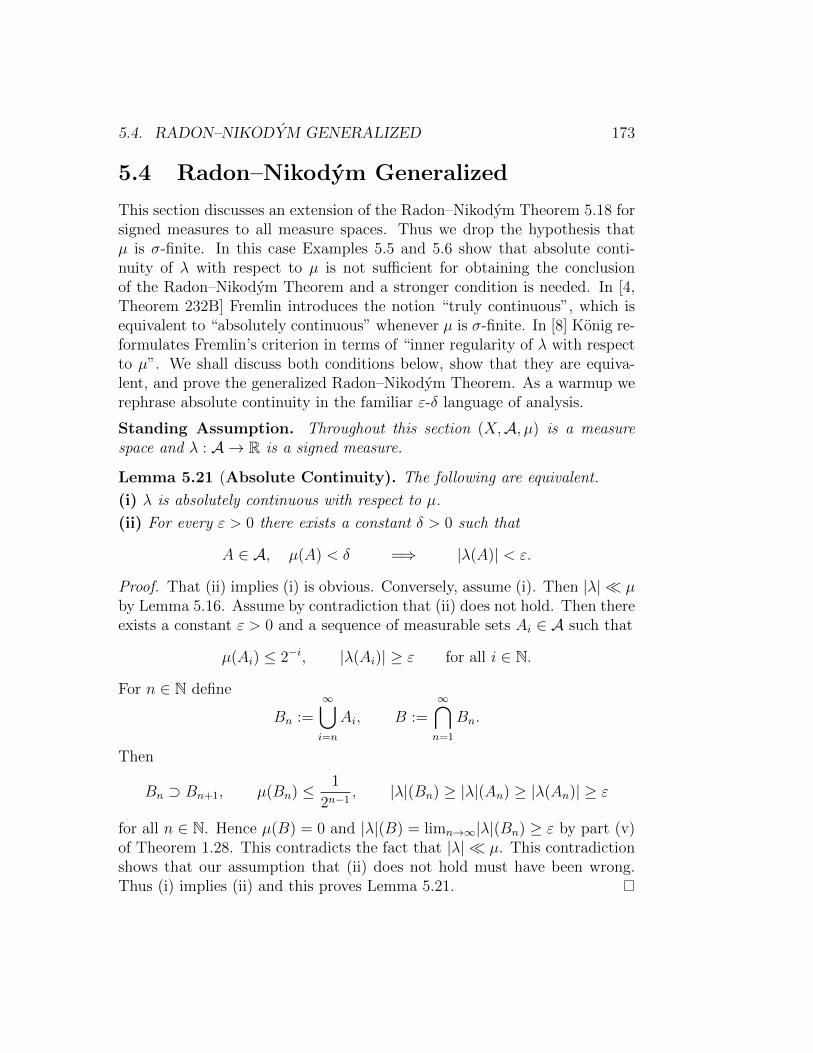
5.4. RADON–NIKODYM GENERALIZED 173
5.4 Radon–Nikodym Generalized
This section discusses an extension of the Radon–Nikodym Theorem 5.18 forsigned measures to all measure spaces. Thus we drop the hypothesis thatµ is σ-finite. In this case Examples 5.5 and 5.6 show that absolute conti-nuity of λ with respect to µ is not sufficient for obtaining the conclusionof the Radon–Nikodym Theorem and a stronger condition is needed. In [4,Theorem 232B] Fremlin introduces the notion “truly continuous”, which isequivalent to “absolutely continuous” whenever µ is σ-finite. In [8] Konig re-formulates Fremlin’s criterion in terms of “inner regularity of λ with respectto µ”. We shall discuss both conditions below, show that they are equiva-lent, and prove the generalized Radon–Nikodym Theorem. As a warmup werephrase absolute continuity in the familiar ε-δ language of analysis.
Standing Assumption. Throughout this section (X,A, µ) is a measurespace and λ : A → R is a signed measure.
Lemma 5.21 (Absolute Continuity). The following are equivalent.
(i) λ is absolutely continuous with respect to µ.
(ii) For every ε > 0 there exists a constant δ > 0 such that
A ∈ A, µ(A) < δ =⇒ |λ(A)| < ε.
Proof. That (ii) implies (i) is obvious. Conversely, assume (i). Then |λ| µby Lemma 5.16. Assume by contradiction that (ii) does not hold. Then thereexists a constant ε > 0 and a sequence of measurable sets Ai ∈ A such that
µ(Ai) ≤ 2−i, |λ(Ai)| ≥ ε for all i ∈ N.
For n ∈ N define
Bn :=∞⋃i=n
Ai, B :=∞⋂n=1
Bn.
Then
Bn ⊃ Bn+1, µ(Bn) ≤ 1
2n−1, |λ|(Bn) ≥ |λ|(An) ≥ |λ(An)| ≥ ε
for all n ∈ N. Hence µ(B) = 0 and |λ|(B) = limn→∞|λ|(Bn) ≥ ε by part (v)of Theorem 1.28. This contradicts the fact that |λ| µ. This contradictionshows that our assumption that (ii) does not hold must have been wrong.Thus (i) implies (ii) and this proves Lemma 5.21.
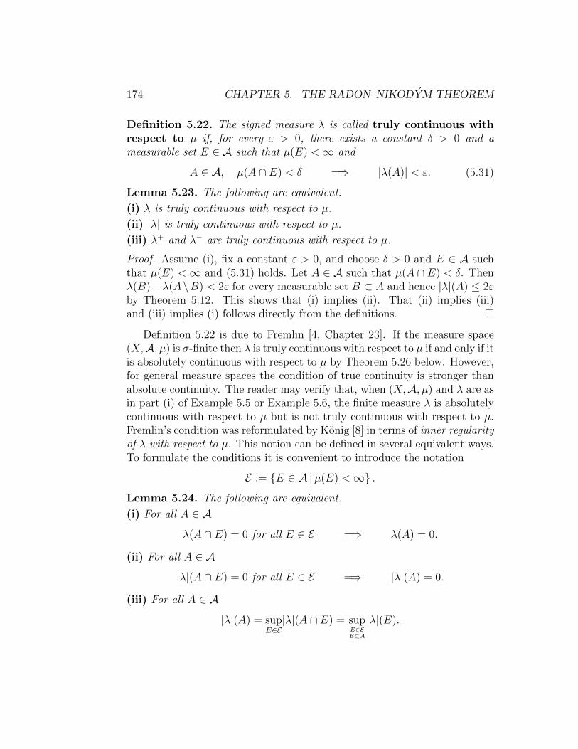
174 CHAPTER 5. THE RADON–NIKODYM THEOREM
Definition 5.22. The signed measure λ is called truly continuous withrespect to µ if, for every ε > 0, there exists a constant δ > 0 and ameasurable set E ∈ A such that µ(E) <∞ and
A ∈ A, µ(A ∩ E) < δ =⇒ |λ(A)| < ε. (5.31)
Lemma 5.23. The following are equivalent.
(i) λ is truly continuous with respect to µ.
(ii) |λ| is truly continuous with respect to µ.
(iii) λ+ and λ− are truly continuous with respect to µ.
Proof. Assume (i), fix a constant ε > 0, and choose δ > 0 and E ∈ A suchthat µ(E) <∞ and (5.31) holds. Let A ∈ A such that µ(A ∩ E) < δ. Thenλ(B)−λ(A\B) < 2ε for every measurable set B ⊂ A and hence |λ|(A) ≤ 2εby Theorem 5.12. This shows that (i) implies (ii). That (ii) implies (iii)and (iii) implies (i) follows directly from the definitions.
Definition 5.22 is due to Fremlin [4, Chapter 23]. If the measure space(X,A, µ) is σ-finite then λ is truly continuous with respect to µ if and only if itis absolutely continuous with respect to µ by Theorem 5.26 below. However,for general measure spaces the condition of true continuity is stronger thanabsolute continuity. The reader may verify that, when (X,A, µ) and λ are asin part (i) of Example 5.5 or Example 5.6, the finite measure λ is absolutelycontinuous with respect to µ but is not truly continuous with respect to µ.Fremlin’s condition was reformulated by Konig [8] in terms of inner regularityof λ with respect to µ. This notion can be defined in several equivalent ways.To formulate the conditions it is convenient to introduce the notation
E := E ∈ A |µ(E) <∞ .
Lemma 5.24. The following are equivalent.
(i) For all A ∈ A
λ(A ∩ E) = 0 for all E ∈ E =⇒ λ(A) = 0.
(ii) For all A ∈ A
|λ|(A ∩ E) = 0 for all E ∈ E =⇒ |λ|(A) = 0.
(iii) For all A ∈ A
|λ|(A) = supE∈E|λ|(A ∩ E) = sup
E∈EE⊂A
|λ|(E).

5.4. RADON–NIKODYM GENERALIZED 175
Proof. By Theorem 5.19 there exists a set P ∈ A such that
λ(A ∩ P ) ≥ 0, λ(A \ P ) ≤ 0, |λ|(P ) = λ(A ∩ P )− λ(A \ P ) (5.32)
for all A ∈ A. Such a measurable set P will be fixed throughout the proof.We prove that (i) implies (ii). Fix a set A ∈ A such that |λ|(A∩E) = 0 for
all E ∈ E . Then it follows from (5.32) that λ(A∩E ∩P ) = λ(A∩E \P ) = 0for all E ∈ E . By (i) this implies λ(A ∩ P ) = λ(A \ P ) = 0 and hence|λ|(A) = 0 by (5.32). This shows that (i) implies (ii).
We prove that (ii) implies (i). Fix a set A ∈ A such that λ(A ∩ E) = 0for all E ∈ E . Since E ∩ P ∈ E and E \ P ∈ E for all E ∈ E this impliesλ(A∩E ∩P ) = λ(A∩E \P ) = 0 for all E ∈ E . Hence it follows from (5.32)that |λ|(A ∩ E) = 0 for all E ∈ E . By (ii) this implies |λ|(A) = 0 and henceλ(A) = 0 because |λ(A)| ≤ |λ|(A). This shows that (ii) implies (i).
We prove that (ii) implies (iii). Fix a set A ∈ A and define
c := supE∈EE⊂A
|λ|(E) ≤ |λ|(A). (5.33)
Choose a sequence Ei ∈ E such that Ei ⊂ A for all i and limi→∞|λ|(Ei) = c.For i ∈ N define Fi := E1 ∪ E2 ∪ · · · ∪ Ei. Then
Fi ∈ E , Fi ⊂ Fi+1 ⊂ A, |λ|(Ei) ≤ |λ|(Fi) ≤ c (5.34)
for all i and hencelimi→∞|λ|(Fi) = c. (5.35)
Define
B := A \ F, F :=∞⋃i=1
Fi. (5.36)
Then |λ|(F ) = limi→∞|λ|(Fi) = c by part (iv) of Theorem 1.28 and hence
|λ|(B) = |λ|(A)− |λ|(F ) = |λ|(A)− c. (5.37)
Let E ∈ E such that E ⊂ B. Then E ∩ Fi = ∅, E ∪ Fi ∈ E , and E ∪ Fi ⊂ Afor all i by (5.36). Hence |λ|(E)+ |λ|(Fi) = |λ|(E∪Fi) ≤ c for all i by (5.33).This implies |λ|(E) ≤ limi→∞
(c − |λ|(Fi)
)= 0 by (5.35). Hence |λ|(E) = 0
for all E ∈ E with E ⊂ B and it follows from (ii) that |λ|(B) = 0. Henceit follows from (5.37) that |λ|(A) = c. This shows that (ii) implies (iii).That (iii) implies (ii) is obvious and this proves Lemma 5.24.
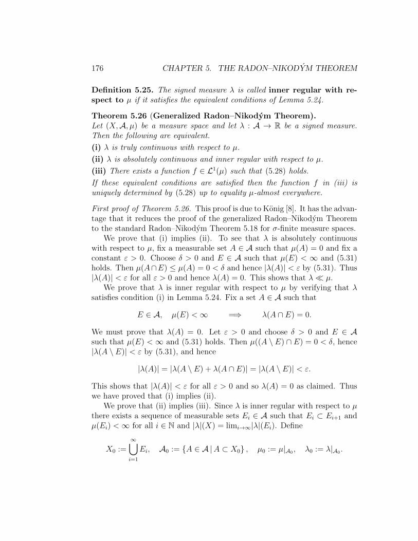
176 CHAPTER 5. THE RADON–NIKODYM THEOREM
Definition 5.25. The signed measure λ is called inner regular with re-spect to µ if it satisfies the equivalent conditions of Lemma 5.24.
Theorem 5.26 (Generalized Radon–Nikodym Theorem).Let (X,A, µ) be a measure space and let λ : A → R be a signed measure.Then the following are equivalent.
(i) λ is truly continuous with respect to µ.
(ii) λ is absolutely continuous and inner regular with respect to µ.
(iii) There exists a function f ∈ L1(µ) such that (5.28) holds.
If these equivalent conditions are satisfied then the function f in (iii) isuniquely determined by (5.28) up to equality µ-almost everywhere.
First proof of Theorem 5.26. This proof is due to Konig [8]. It has the advan-tage that it reduces the proof of the generalized Radon–Nikodym Theoremto the standard Radon–Nikodym Theorem 5.18 for σ-finite measure spaces.
We prove that (i) implies (ii). To see that λ is absolutely continuouswith respect to µ, fix a measurable set A ∈ A such that µ(A) = 0 and fix aconstant ε > 0. Choose δ > 0 and E ∈ A such that µ(E) < ∞ and (5.31)holds. Then µ(A∩E) ≤ µ(A) = 0 < δ and hence |λ(A)| < ε by (5.31). Thus|λ(A)| < ε for all ε > 0 and hence λ(A) = 0. This shows that λ µ.
We prove that λ is inner regular with respect to µ by verifying that λsatisfies condition (i) in Lemma 5.24. Fix a set A ∈ A such that
E ∈ A, µ(E) <∞ =⇒ λ(A ∩ E) = 0.
We must prove that λ(A) = 0. Let ε > 0 and choose δ > 0 and E ∈ Asuch that µ(E) <∞ and (5.31) holds. Then µ((A \ E) ∩ E) = 0 < δ, hence|λ(A \ E)| < ε by (5.31), and hence
|λ(A)| = |λ(A \ E) + λ(A ∩ E)| = |λ(A \ E)| < ε.
This shows that |λ(A)| < ε for all ε > 0 and so λ(A) = 0 as claimed. Thuswe have proved that (i) implies (ii).
We prove that (ii) implies (iii). Since λ is inner regular with respect to µthere exists a sequence of measurable sets Ei ∈ A such that Ei ⊂ Ei+1 andµ(Ei) <∞ for all i ∈ N and |λ|(X) = limi→∞|λ|(Ei). Define
X0 :=∞⋃i=1
Ei, A0 := A ∈ A |A ⊂ X0 , µ0 := µ|A0 , λ0 := λ|A0 .
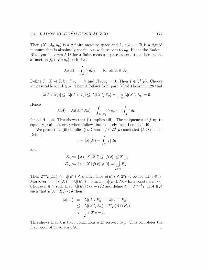
5.4. RADON–NIKODYM GENERALIZED 177
Then (X0,A0, µ0) is a σ-finite measure space and λ0 : A0 → R is a signedmeasure that is absolutely continuous with respect to µ0. Hence the Radon–Nikodym Theorem 5.18 for σ-finite measure spaces asserts that there existsa function f0 ∈ L1(µ0) such that
λ0(A) =
∫A
f0 dµ0 for all A ∈ A0.
Define f : X → R by f |X0 := f0 and f |X\X0 := 0. Then f ∈ L1(µ). Choosea measurable set A ∈ A. Then it follows from part (v) of Theorem 1.28 that
|λ(A \X0)| ≤ |λ|(A \X0) ≤ |λ|(X \X0) = limi→∞|λ|(X \ Ei) = 0.
Hence
λ(A) = λ0(A ∩X0) =
∫A∩X0
f0 dµ0 =
∫A
f dµ
for all A ∈ A. This shows that (i) implies (iii). The uniqueness of f up toequality µ-almost everywhere follows immediately from Lemma 1.49.
We prove that (iii) implies (i). Choose f ∈ L1(µ) such that (5.28) holds.Define
c := |λ|(X) =
∫X
|f | dµ
and
En :=x ∈ X | 2−n ≤ |f(x)| ≤ 2n
,
E∞ := x ∈ X | f(x) 6= 0 =⋃n∈N
En.
Then 2−nµ(En) ≤ |λ|(En) ≤ c and hence µ(En) ≤ 2nc < ∞ for all n ∈ N.Moreover, c = |λ|(X) = |λ|(E∞) = limn→∞|λ|(En). Now fix a constant ε > 0.Choose n ∈ N such that |λ|(En) > c− ε/2 and define δ := 2−n−1ε. If A ∈ Asuch that µ(A ∩ En) < δ then
|λ|(A) = |λ|(A \ En) + |λ|(A ∩ En)
≤ |λ|(X \ En) + 2nµ(A ∩ En)
<ε
2+ 2nδ = ε.
This shows that λ is truly continuous with respect to µ. This completes thefirst proof of Theorem 5.26.
178 CHAPTER 5. THE RADON–NIKODYM THEOREM
Second proof of Theorem 5.26. This proof is due to Fremlin [4, Chapter 23].It shows directly that (i) implies (iii) and has the advantage that it only usesthe Hahn Decomposition Theorem 5.19. It thus also provides an alternativeproof of Theorem 5.18 (assuming the Hahn Decomposition Theorem) whichis of interest on its own. By Lemma 5.23 it suffices to consider the case whereλ : A → [0,∞) is a finite measure that is truly continuous with respect to µ.
Consider the set
F :=
f : X → [0,∞)
∣∣∣∣ f is measurable and∫Af dµ ≤ λ(A) for all A ∈ A
.
This set is nonempty because 0 ∈ F . Moreover,∫Xf dµ ≤ λ(X) < ∞ for
all f ∈ F and
f, g ∈ F =⇒ maxf, g ∈ F . (5.38)
(Let f, g ∈ F and A ∈ A and define the sets Af := x ∈ A | f(x) > g(x) andAg := x ∈ A | g(x) ≥ f(x); then Af , Ag ∈ A, Af∩Ag = ∅, and Af∪Ag = A;hence
∫A
maxf, g dµ =∫Aff dµ+
∫Agg dµ ≤ λ(Af ) + λ(Ag) = λ(A).)
Now define
c := supf∈F
∫X
f dµ ≤ λ(X)
and choose a sequence gi ∈ F such that limi→∞∫Xgi dµ = c. Then it follows
from (5.38) that fi := maxg1, g2, . . . , gi ∈ F and∫Xgi dµ ≤
∫Xfi dµ ≤ c
for all i ∈ N. Hence fi ≤ fi+1 for all i and limi→∞∫Xfi dµ = c. Define the
function f : X → [0,∞] by f(x) := limi→∞ fi(x) for x ∈ X. Then it followsfrom the Lebesgue Monotone Convergence Theorem 1.37 that∫X
f dµ = limi→∞
∫X
fi dµ = c,
∫A
f dµ = limi→∞
∫A
fi dµ ≤ λ(A) for all A ∈ A
Hence f < ∞ µ-almost everywhere by Lemma 1.47 and we may assumewithout loss of generality that f(x) <∞ for all x ∈ X. Thus f ∈ F .
We prove that∫Af dµ = λ(A) for all A ∈ A. Suppose otherwise that
there exists a set A0 ∈ A such that∫A0f dµ < λ(A0). Then the formula
λ′(A) := λ(A)−∫A
f dµ for A ∈ A (5.39)
defines a finite measure by Theorem 1.40.
5.4. RADON–NIKODYM GENERALIZED 179
We prove that there is a measurable function h : X → [0,∞) such that∫X
h dµ > 0,
∫A
h dµ ≤ λ′(A) for all A ∈ A. (5.40)
Define
ε :=λ′(A0)
3> 0. (5.41)
Since λ is truly continuous with respect to µ so is λ′. Hence there is a δ > 0and a set E ∈ A such that µ(E) <∞ and
A ∈ A, µ(A ∩ E) < δ =⇒ λ′(A) < ε. (5.42)
Take A := X \ E to obtain λ′(X \ E) < ε and hence
λ′(E) ≥ λ′(A0 ∩ E) = λ′(A0)− λ′(A0 \ E) = 3ε− λ′(A0 \ E) > 2ε.
Then take A := A0. Since λ′(A0) = 3ε ≥ ε by (5.41) it follows from (5.42)that µ(E) ≥ µ(A0 ∩ E) ≥ δ > 0. Define the signed measure λ′′ : A → R by
λ′′(A) := λ′(A)− εµ(A ∩ E)
µ(E)(5.43)
for A ∈ A. Then λ′′(E) = λ′(E) − ε ≥ ε. By the Hahn DecompositionTheorem 5.19 there exists a measurable set P ∈ A such that
λ′′(A ∩ P ) ≥ 0, λ′′(A \ P ) ≤ 0 for all A ∈ A.Since λ′′(E \ P ) ≤ 0 it follows that ε ≤ λ′′(E) ≤ λ′′(E ∩ P ) ≤ λ′(E ∩ P ).Hence µ(E ∩ P ) ≥ δ by (5.42). Now define
h :=ε
µ(E)χE∩P . (5.44)
Then∫Xh dµ > 0. Moreover, if A ∈ A then λ′′(A∩P ) ≥ 0 and so, by (5.43),
λ′(A ∩ P ) ≥ εµ(A ∩ P ∩ E)
µ(E)=
∫A
h dµ.
Thus∫Ah dµ ≤ λ′(A) for all A ∈ A and so h satisfies (5.40) as claimed.
It follows from (5.40) that∫A
(f + h) dµ ≤∫A
f dµ+ λ′(A) = λ(A)
for all A ∈ A and hence f + h ∈ F . Since∫X
(f + h) dµ = c +∫Xh dµ > c,
this contradicts the definition of c. Thus we have proved that∫Af dµ = λ(A)
for all A ∈ A and hence f satisfies (5.28). This completes the second proofof Theorem 5.26.
180 CHAPTER 5. THE RADON–NIKODYM THEOREM
5.5 Exercises
Exercise 5.27. Let (X,A, µ) be a measure space such that µ(X) < ∞.Define
ρ(A,B) := µ(A \B) + µ(B \ A) for A,B ∈ A. (5.45)
Define an equivalence relation on A by A ∼ B iff ρ(A,B) = 0. Prove thatρ descends to a function ρ : A/∼ × A/∼ → [0,∞) (denoted by the sameletter) and that the pair (A/∼, ρ) is a complete metric space. Prove that thefunction A → R : A 7→
∫Af dµ descends to a continuous function on A/∼
for every f ∈ L1(µ).
Exercise 5.28 (Rudin [17, page 133]). Let (X,A, µ) be a measure space.A subset F ⊂ L1(µ) is called uniformly integrable if, for every ε > 0,there is a constant δ > 0 such that, for all E ∈ A and all f ∈ F ,
µ(E) < δ =⇒∣∣∣∣∫E
f dµ
∣∣∣∣ < ε.
Prove the following.
(i) Every finite subset of L1(µ) is uniformly integrable. Hint: Lemma 5.21.
(ii) Vitali’s Theorem. Assume µ(X) < ∞, let f : X → R be measurable,and let fn ∈ L1(µ) be a uniformly integrable sequence that converges almosteverywhere to f . Then f ∈ L1(µ) and limn→∞
∫X|f − fn| dµ = 0.
Hint: Use Egoroff’s Theorem in Exercise 4.54.
(iii) The hypothesis µ(X) < ∞ cannot be omitted in Vitali’s Theorem.Hint: Consider the Lebesgue measure on R. Find a uniformly integrablesequence fn ∈ L1(R) that converges pointwise to the constant function f ≡ 1.
(iv) Vitali’s Theorem implies the Lebesgue Dominated Convergence Theo-rem 1.45 under the assumption µ(X) <∞.
(v) Find an example where Vitali’s Theorem applies although the hypothesesof the Lebesgue Dominated Convergence Theorem are not satisfied.
(vi) Find an example of a measure space (X,A, µ) with µ(X) < ∞ and asequence fn ∈ L1(µ) that is not uniformly integrable, converges pointwiseto zero, and satisfies limn→∞
∫Xfn dµ = 0. Hint: Consider the Lebesgue
measure on X = [0, 1].
(vii) Converse of Vitali’s Theorem. Assume µ(X) <∞ and let fn be asequence in L1(µ) such that the limit limn→∞
∫Afn dµ exists for all A ∈ A.
Then the sequence fn is uniformly integrable.
5.5. EXERCISES 181
Hint: Let ε > 0. Prove that there is a constant δ > 0, an integer n0 ∈ N,and a measurable set E0 ∈ E such that, for all E ∈ A and all n ∈ N,
ρ(E,E0) < δ, n ≥ n0 =⇒∣∣∣∣∫E
(fn − fn0) dµ
∣∣∣∣ < ε. (5.46)
(Here ρ(E,E0) is defined by (5.45) as in Exercise 5.27.) If A ∈ A satisfiesµ(A) < δ then the sets E := E0\A and E := E0∪A both satisfy ρ(E,E0) < δ.Deduce that, for all A ∈ A and all n ∈ N,
µ(A) < δ, n ≥ n0 =⇒∣∣∣∣∫A
(fn − fn0) dµ
∣∣∣∣ < 2ε. (5.47)
Now use part (i) to find a constant δ′ > 0 such that, for all A ∈ A,
µ(A) < δ′ =⇒ supn∈N
∣∣∣∣∫A
fn dµ
∣∣∣∣ < 3ε. (5.48)
Exercise 5.29 (Rudin [17, page 134]). Let (X,A, µ) be a measure spacesuch that µ(X) < ∞ and fix a real number p > 1. Let f : X → R bea measurable function and let fn ∈ L1(µ) be a sequence that convergespointwise to f and satisfies
supn∈N
∫X
|fn|p dµ <∞.
Prove that
f ∈ L1(µ), limn→∞
∫X
|f − fn| dµ = 0.
Hint: Use Vitali’s Theorem in Exercise 5.28.
Exercise 5.30. Let X := R, denote by B ⊂ 2X the Borel σ-algebra, andlet µ : B → [0,∞] be the restriction of the Lebesgue measure to B. Letλ : B → [0,∞] be a measure. Prove the following.
(i) If B ∈ B and 0 < c < µ(B) then there exists a Borel set A ⊂ B such thatµ(A) = c. Hint: Show that the function f(t) := µ(B∩ [−t, t]) is continuous.
(ii) If there exists a constant 0 < c <∞ such that
µ(B) = c =⇒ λ(B) = c.
for all B ∈ B, then λ µ.
182 CHAPTER 5. THE RADON–NIKODYM THEOREM
Exercise 5.31. Let X := R, denote by B ⊂ 2X the Borel σ-algebra, letµ : B → [0,∞] be the restriction of the Lebesgue measure to B, and letν : B → [0,∞] be the counting measure. Prove the following.
(i) µ ν
(ii) µ is not inner regular with respect to ν.
(iii) There does not exist any measurable function f : X → [0,∞] such thatµ(B) =
∫Bf dν for all B ∈ B.
Exercise 5.32. Let X := [1,∞), denote by B ⊂ 2X the Borel σ-algebra,and let µ : B → [0,∞] be the restriction of the Lebesgue measure to B. Letλ : B → [0,∞] be a Borel measure such that
λ(B) = αλ(αB) for all α ≥ 1 and all B ∈ B. (5.49)
Prove that there exists a real number c ≥ 0 such that
λ(B) :=
∫B
f dµ for all B ∈ B, (5.50)
where f : [1,∞)→ [0,∞) is the function given by
f(x) :=c
x2for x ≥ 1. (5.51)
Hint: Show that λ([1,∞)) <∞ and then that λ µ.
Exercise 5.33. Let X := [0,∞) denote by B ⊂ 2X the Borel σ-algebra, andlet µ : B → [0,∞] be the restriction of the Lebesgue measure to B. Definethe measures λ1, λ2 : B → [0,∞] by
λ1(B) :=∞∑n=1
1
n3
∫B∩[n,n+1]
x dx, λ2(B) :=
∫B∩[1,∞)
1
x2dx
for B ∈ B. (Here we denote by∫Bf(x) dx :=
∫Bf dµ the Lebesgue integral
of a Borel measurable function f : [0,∞)→ [0,∞) over a Borel set B ∈ B.)Prove that λ1 and λ2 are finite measures that satisfy
λ1 µ, λ2 µ, λ1 λ2, λ2 λ1,
andµ 6 λ1, µ 6 λ2.
5.5. EXERCISES 183
Exercise 5.34. Let (X,A, µ) be a measure space. Show that the signedmeasures λ : A → R form a Banach space M =M(X,A) with norm
‖λ‖ := |λ|(X).
Show that the mapL1(µ)→M : [f ]µ 7→ µf
defined by (5.53) is an isometric linear embedding and hence L1(µ) is a closedsubspace of M.
Exercise 5.35. Let (X,U) be a compact Hausdorff space such that everyopen subset of X is σ-compact and denote by B ⊂ 2X its Borel σ-algebra.Denote by C(X) := Cc(X) the space of continuous real valued functionson X. This is a Banach space equipped with the supremum norm
‖f‖ := supx∈X|f(x)|.
Let M(X) denote the space of signed Borel measures as in Exercise 5.34.For λ ∈M(X) define the linear functional Λλ : C(X)→ R by
Λλ(f) :=
∫X
f dλ.
Prove the following.
(i) ‖Λλ‖ = ‖λ‖. Hint: Use the Hahn Decomposition Theorem 5.19 and thefact that every Borel measure on X is regular by Theorem 3.18.
(ii) Every bounded linear functional on C(X) is the difference of two positivelinear functionals. Hint: For f ∈ C(X) with f ≥ 0 prove that
Λ+(f) := sup
Λ(hf)∣∣h ∈ C(X), 0 ≤ h ≤ 1
= sup
Λ(g)
∣∣ g ∈ C(X), 0 ≤ g ≤ f.
(5.52)
Here the second supremum is obviously greater than or equal to the first. Toprove the converse inequality show that, for all g ∈ C(X) with 0 ≤ g ≤ fand all ε > 0 there is an h ∈ C(X) such that 0 ≤ h ≤ 1 and |Λ(g−hf)| < ε.Namely, find φ ∈ C(X) such that 0 ≤ φ ≤ 1, φ(x) = 0 when f(x) ≤ ε/2 ‖Λ‖and φ(x) = 1 when f(x) ≥ ε/ ‖Λ‖; then define h := φg/f . Once (5.52) isestablished show that Λ+ extends to a positive linear functional on C(X).
(iii) The map M(X) → C(X)∗ : λ 7→ Λλ is bijective. Hint: Use the RieszRepresentation Theorem 3.15.
(iv) The hypothesis that every open subset of X is σ-compact cannot beremoved in part (i). Hint: Consider Example 3.6.
184 CHAPTER 5. THE RADON–NIKODYM THEOREM
Exercise 5.36. Let (X,A, µ) be a measure space and let f : X → [0,∞) bea measurable function. Define the measure µf : A → [0,∞] by
µf (A) :=
∫A
f dµ for A ∈ A. (5.53)
(See Theorem 1.40.) Prove the following.
(i) If µ is σ-finite so is µf .
(ii) If µ is semi-finite so is µf .
(iii) If µ is localizable so is µf .
Note: See Theorem 5.4 for (i) and [4, Proposition 234N] for (ii) and (iii).It is essential that f does not take on the value ∞. Find an example ofa measure space (X,A, µ) and a measurable function f : X → [0,∞] thatviolates the assertions (i), (ii), (iii).
Hint 1: To prove (ii), fix a set A ∈ A, define Af := x ∈ A | f(x) > 0,and choose a measurable set E ∈ A such that E ⊂ Af and 0 < µ(E) < ∞.Consider the sets En := x ∈ E | f(x) ≤ n.Hint 2: To prove (iii), let E ⊂ A be any collection of measurable sets andchoose a measurable µ-envelope H ∈ A of E . Prove that the set
Hf :=x ∈ H
∣∣ f(x) > 0
is a measurable µf -envelope of E . In particular, if N ∈ A is a measurableset such that µf (E ∩N) = 0 for all E ∈ E , define Nf := x ∈ N | f(x) > 0,show that µ(H ∩Nf ) = 0, and deduce that µf (Hf ∩N) = µf (H ∩Nf ) = 0.
Chapter 6
Differentiation
This chapter returns to the Lebesgue measure on Euclidean space Rn intro-duced in Chapter 2. The main result is the Lebesgue Differentiation Theorem(Section 6.3). It implies that if f : Rn → R is a Lebesgue integrable func-tion then, for almost every element x ∈ Rn, the mean value of f over a ballcentered at x converges to f(x) as the radius tends to zero. Essential ingre-dients in the proof are the Vitali Covering Lemma and the Hardy–LittlewoodMaximal Inequality (Section 6.2). One of the consequences of the LebesgueDifferentiation Theorem is the Fundamental Theorem of Calculus for abso-lutely continuous functions of one real variable (Section 6.4). The LebesgueDifferentiation Theorem also plays a central role in the proof of the Calderon–Zygmund inequality (Section 7.7). The chapter begins with a discussion ofweakly integrable functions on general measure spaces.
6.1 Weakly Integrable Functions
Assume throughout that (X,A, µ) is a measure space. Let f : X → R be ameasurable function. Define the function κf : [0,∞)→ [0,∞] by
κf (t) := κ(t, f) := µ(A(t, f)), A(t, f) :=x ∈ X
∣∣ |f(x)| > t, (6.1)
for t ≥ 0. The function κf is nonincreasing and hence Borel measurable.Define the function f ∗ : [0,∞)→ [0,∞] by
f ∗(α) := inf t ≥ 0 |κ(t, f) ≤ α for 0 ≤ α <∞. (6.2)
Thus f ∗(0) = ‖f‖∞ and f ∗ is nonincreasing and hence Borel measurable.By definition, the infimum of the empty set is infinity. Thus f ∗(α) = ∞ if
185

186 CHAPTER 6. DIFFERENTIATION
and only if µ(A(t, f)) > α for all t > 0. When f ∗(α) < ∞ it is the smallestnumber t such that the domain A(t, f) (on which |f | > t) has measure atmost α. This is spelled out in the next lemma.
Lemma 6.1. Let 0 ≤ α <∞ and 0 ≤ t <∞. Then the following holds.
(i) f ∗(α) =∞ if and only if κf (s) > α for all s ≥ 0.
(ii) f ∗(α) = t if and only if κf (t) ≤ α and κf (s) > α for 0 ≤ s < t.
(iii) f ∗(α) ≤ t if and only if κf (t) ≤ α.
Proof. It follows directly from the definition of f ∗ in (6.2) that f ∗(α) = ∞if and only if κ(s, f) > α for all s ∈ [0,∞) and this proves (i).
To prove (ii), fix a constant 0 ≤ t < ∞. Assume first that κ(t, f) ≤ αand κ(s, f) > α for 0 ≤ s < t. Since κf is nonincreasing this impliesκ(s, f) ≤ κ(t, f) ≤ α for all s ≥ t and hence f ∗(α) = t by definition.Conversely, suppose that f ∗(α) = t. Then it follows from the definition off ∗ that κ(s, f) ≤ α for s > t and κ(s, t) > α for 0 ≤ s < t. We must provethat κ(t, f) ≤ α. To see this observe that
A(t, f) =∞⋃n=1
A(t+ 1/n, f).
Hence it follows from part (iv) of Theorem 1.28 that
κf (t) = µ(A(t, f)) = limn→∞
µ(A(t+ 1/n, f)) = limn→∞
κ(t+ 1/n, f) ≤ α.
This proves (ii). If f ∗(α) ≤ t then κf (t) ≤ κf (f∗(α)) ≤ α by (ii). If κf (t) ≤ α
then f ∗(α) ≤ t by definition of f ∗. This proves (iii) and Lemma 6.1.
Lemma 6.2. Let f, g : X → R be measurable functions and let c ∈ R. Then
‖f‖1,∞ := supα>0
αf ∗(α) = supt>0
tκf (t) ≤ ‖f‖1 , (6.3)
‖cf‖1,∞ = |c| ‖f‖1,∞ , (6.4)
‖f + g‖1,∞ ≤‖f‖1,∞
λ+‖g‖1,∞
1− λfor 0 < λ < 1, (6.5)√
‖f + g‖1,∞ ≤√‖f‖1,∞ +
√‖g‖1,∞. (6.6)
Moreover ‖f‖1,∞ = 0 if and only if f vanishes almost everywhere. Theinequality (6.6) is called the weak triangle inequality.
6.1. WEAKLY INTEGRABLE FUNCTIONS 187
Proof. For 0 < t, c <∞ it follows from part (iii) of Lemma 6.1 that
tκ(t, f) ≤ c ⇐⇒ κ(t, f) ≤ ct−1 ⇐⇒ f ∗(ct−1) ≤ t ⇐⇒ ct−1f ∗(ct−1) ≤ c.
This shows that supt>0 tκ(t, f) = supα>0 αf∗(α). Moreover,
tκ(t, f) = tµ(A(t, f)) ≤∫A(t,f)
|f | dµ ≤∫X
|f | dµ
for all t > 0. This proves (6.3).For c > 0 equation (6.4) follows from the fact that A(t, cf) = A(t/c, f)
and hence κ(t, cf) = κ(t/c, f) for all t > 0. Since ‖−f‖1,∞ = ‖f‖1,∞ bydefinition, this proves (6.4).
To prove (6.5), observe that A(t, f + g) ⊂ A(λt, f)∪A((1−λ)t, g), hence
κ(t, f + g) ≤ κ(λt, f) + κ((1− λ)t, g), (6.7)
and hence
tκ(t, f + g) ≤ tκ(λt, f) + tκ((1− λ)t, g) ≤‖f‖1,∞
λ+‖g‖1,∞
1− λfor all t > 0. Take the supremum over all t > 0 to obtain (6.5).
The inequality (6.6) follows from (6.5) and the identity
inf0<λ<1
√a
λ+
b
1− λ=√a+√b for a, b ≥ 0. (6.8)
This is obvious when a = 0 or b = 0. Hence assume a and b are positive anddefine the function h : (0, 1)→ (0,∞) by h(λ) := a
λ+ b
1−λ . It satisfies
h′(λ) =b
(1− λ)2− a
λ2
and hence has a unique critical point at
λ0 :=
√a
√a+√b.
Since h(λ0) = (√a+√b)2, this proves (6.8). The inequality (6.6) then follows
by taking a := ‖f‖1,∞ and b := ‖g‖1,∞.The last assertion follows from the fact that ‖f‖1,∞ = 0 if and only if
κf (0) = 0 if and only if the set A(0, f) = x ∈ X | f(x) 6= 0 has measurezero. This proves Lemma 6.2.
188 CHAPTER 6. DIFFERENTIATION
Example 6.3. This example shows that the weak triangle inequality (6.6) issharp. Let (R,A,m) be the Lebesgue measure space and define f, g : R→ Rby
f(x) :=1
x, g(x) :=
1
1− xfor 0 < x < 1
and f(x) := g(x) := 0 for x ≤ 0 and for x ≥ 1. Then
‖f‖1,∞ = ‖g‖1,∞ = 1, ‖f + g‖1,∞ = 4.
Definition 6.4. Let (X,A, µ) be a measure space. A measurable functionf : X → R is called weakly integrable if ‖f‖1,∞ <∞. The space of weaklyintegrable functions will be denoted by
L1,∞(µ) :=f : X → R
∣∣ f is measurable and ‖f‖1,∞ <∞.
The quotient spaceL1,∞(µ) := L1,∞(µ)/
µ∼
under the equivalence relation fµ∼ g iff f = g µ-almost everywhere is called
the weak L1 space. It is not a normed vector space because the functionL1,∞(µ)→ [0,∞) : [f ]µ 7→ ‖f‖1,∞ does not satisfy the triangle inequality, ingeneral, and hence is not a norm. However, it is a topological vector spaceand the topology is determined by the metric
d1,∞([f ]µ, [g]µ) :=√‖f − g‖1,∞ for f, g ∈ L1,∞(µ). (6.9)
For the Lebesgue measure space (Rn,A,m) we write L1,∞(Rn) := L1,∞(m)and L1,∞(Rn) := L1,∞(m).
A subset of L1,∞(µ) is open in the topology determined by the metric (6.9)if and only if it is a union of sets of the form [g]µ ∈ L1,∞(µ) | ‖f − g‖1,∞ < rwith f ∈ L1,∞(µ) and r > 0. A sequence [fi]µ ∈ L1,∞(µ) converges to [f ]µ inthis topology if and only if limi→∞ ‖fi − f‖1,∞ = 0. The inequality (6.3) inLemma 6.2 shows that
L1(µ) ⊂ L1,∞(µ)
for every measure space (X,A, µ). In general, L1,∞(µ) is not equal to L1(µ).For example the function f : R → R defined by f(x) := 1/x for x > 0 andf(x) := 0 for x ≤ 0 is weakly integrable but is not integrable.
6.1. WEAKLY INTEGRABLE FUNCTIONS 189
Theorem 6.5. The metric space (L1,∞(µ), d1,∞) is complete.
Proof. Choose a sequence of weakly integrable functions fi : X → R whoseequivalence classes [fi]µ form a Cauchy sequence in L1,∞(µ) with respect tothe metric (6.9). Then there is a subsequence i1 < i2 < i3 < · · · such that∥∥fik − fik+1
∥∥1,∞ < 2−2k for all k ∈ N. For k, ` ∈ N define
Ak := A(2−k, fik − fik+1), E` :=
∞⋃k=`
Ak, E :=∞⋂`=1
E`.
Then 2−kµ(Ak) ≤∥∥fik − fik+1
∥∥1,∞ < 2−2k for all k ∈ N, hence
µ(E`) ≤∞∑k=`
µ(Ak) ≤∞∑k=`
2−k = 21−`
for all ` ∈ N, and hence µ(E) = 0. If x ∈ X \ E then there exists an ` ∈ Nsuch that x /∈ Ak for all k ≥ ` and so |fik(x)− fik+1
(x)| ≤ 2−k for all k ≥ `.This shows that the limit f(x) := limk→∞ fik(x) exists for all x ∈ X \ E.Extend f to a measurable function on X by setting f(x) := 0 for x ∈ E.
We prove that limi→∞ ‖fi − f‖1,∞ = 0 and hence also f ∈ L1,∞(µ). Tosee this, fix a constant ε > 0 and choose an integer i0 ∈ N such that
i, j ∈ N, i, j ≥ i0 =⇒ 4 ‖fi − fj‖1,∞ < ε.
Now fix a constant t > 0 and choose ` ∈ N such that
i` ≥ i0, 22−`t ≤ ε, 22−` ≤ t.
If x /∈ E` then x /∈ Ak for all k ≥ `, hence |fik(x)− fik+1(x)| ≤ 2−k for k ≥ `,
and hence |fi`(x)−f(x)| ≤∑∞
k=`|fik(x)−fik+1(x)| ≤
∑∞k=` 2−k = 21−` ≤ t/2.
This shows that A(t/2, fi` − f) ⊂ E` and hence
tκfi`−f (t/2) = tµ(A(t/2, fi` − f)) ≤ tµ(E`) ≤ t21−` ≤ ε/2.
With this understood, it follows from (6.7) with λ = 1/2 that
tκfi−f (t) ≤ tκfi−fi` (t/2) + tκfi`−f (t/2) ≤ 2 ‖fi − fi`‖1,∞ + ε/2 < ε
for all i ∈ N with i ≥ i0. Hence
‖fi − f‖1,∞ = supt>0
tκfi−f (t) ≤ ε
for every integer i ≥ i0 and this proves Theorem 6.5.
190 CHAPTER 6. DIFFERENTIATION
6.2 Maximal Functions
Let (R,A,m) be the Lebesgue measure space on R. In particular, the lengthof an interval I ⊂ R is m(I). As a warmup we characterize the differentia-bility of a function that is obtained by integrating a signed measure.
Theorem 6.6. Let λ : A → R be a signed measure and define f : R→ R by
f(x) := λ((−∞, x)) for x ∈ R. (6.10)
Fix two real numbers x,A ∈ R. Then the following are equivalent.
(i) f is differentiable at x and f ′(x) = A.
(ii) For every ε > 0 there is a δ > 0 such that, for every open interval U ⊂ R,
x ∈ U, m(U) < δ =⇒∣∣∣∣ λ(U)
m(U)− A
∣∣∣∣ ≤ ε. (6.11)
Proof. We prove that (i) implies (ii). Fix a constant ε > 0. Since f isdifferentiable at x and f ′(x) = A, there exists a constant δ > 0 such that,for all y ∈ R,
0 < |x− y| < δ =⇒∣∣∣∣f(x)− f(y)
x− y− A
∣∣∣∣ ≤ ε. (6.12)
Let a, b ∈ R such that a < x < b and b− a < δ. Then, by (6.12),∣∣∣∣f(x)− f(a)
x− a− A
∣∣∣∣ ≤ ε,
∣∣∣∣f(b)− f(x)
b− x− A
∣∣∣∣ ≤ ε,
or, equivalently,
−ε(x− a) ≤ f(x)− f(a)− A(x− a) ≤ ε(x− a),
−ε(b− x) ≤ f(b)− f(x)− A(b− x) ≤ ε(b− x).
Add these inequalities to obtain
−ε(b− a) ≤ f(b)− f(a)− A(b− a) ≤ ε(b− a).
Since λ([a, b)) = f(b)− f(a) and m([a, b)) = b− a it follows that∣∣∣∣ λ([a, b))
m([a, b))− A
∣∣∣∣ ≤ ε.
6.2. MAXIMAL FUNCTIONS 191
Replace a by a+ 2−k and take the limit k →∞ to obtain∣∣∣∣ λ((a, b))
m((a, b))− A
∣∣∣∣ ≤ ε.
Thus we have proved that (i) implies (ii).Conversely, assume (ii) and fix a constant ε > 0. Choose δ > 0 such
that (6.11) holds for every open interval U ⊂ R. Choose y ∈ R such thatx < y < x+δ. Choose k ∈ N such that y−x+2−k < δ. Then Uk := (x−2−k, y)is an open interval of length m(Uk) < δ containing x and hence∣∣∣∣ λ(Uk)
m(Uk)− A
∣∣∣∣ ≤ ε
by (6.11). Take the limit k →∞ to obtain∣∣∣∣f(y)− f(x)
y − x− A
∣∣∣∣ =
∣∣∣∣ λ([x, y))
m([x, y))− A
∣∣∣∣ = limk→∞
∣∣∣∣ λ(Uk)
m(Uk)− A
∣∣∣∣ ≤ ε.
Thus (6.12) holds for x < y < x + δ and an analogous argument provesthe inequality for x − δ < y < x. Thus (ii) implies (i) and this provesTheorem 6.6.
The main theorem of this chapter will imply that, when λ is absolutelycontinuous with respect to m, the derivative of the function f in (6.10) existsalmost everywhere, defines a Lebesgue integrable function f ′ : R → R, andthat
λ(A) =
∫A
f ′ dm
for all Lebesgue measurable sets A ∈ A. It will then follow that an absolutelycontinuous function on R can be written as the integral of its derivative. Thisis the fundamental theorem of calculus in measure theory (Theorem 6.19).
The starting point for this program is the assertion of Theorem 6.6. Itsuggests the definition of the derivative of a signed measure
λ : A → R
at a point x ∈ R as the limit of the quotients λ(U)/m(U) over all openintervals U containing x as m(U) tends to zero, provided that the limitexists. This idea carries over to all dimensions and leads to the concept of amaximal function which we explain next.
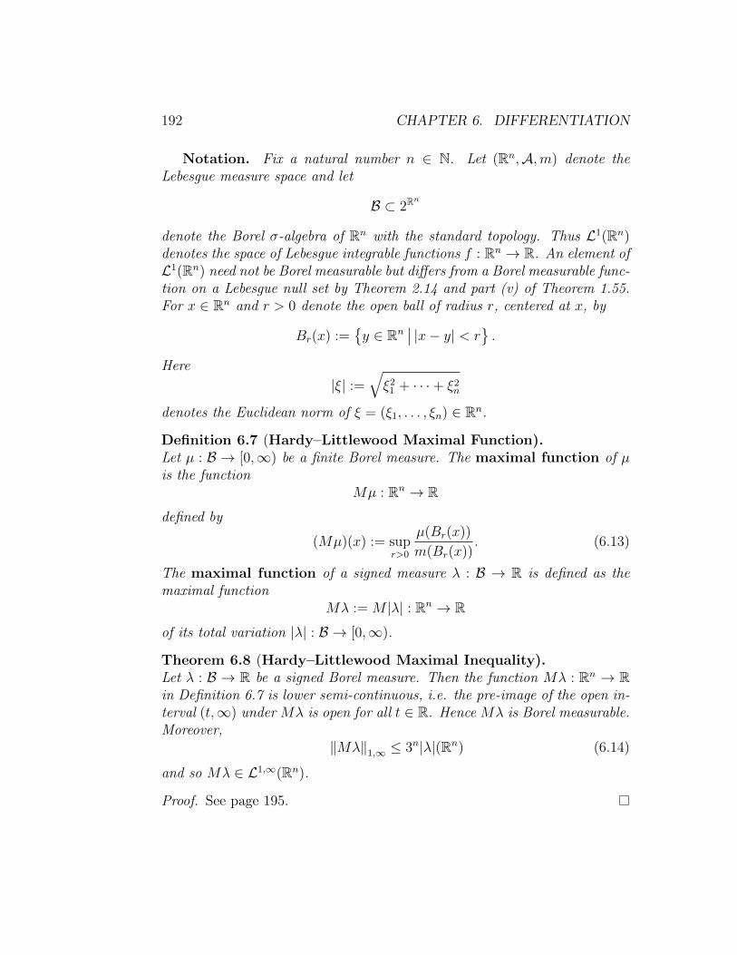
192 CHAPTER 6. DIFFERENTIATION
Notation. Fix a natural number n ∈ N. Let (Rn,A,m) denote theLebesgue measure space and let
B ⊂ 2Rn
denote the Borel σ-algebra of Rn with the standard topology. Thus L1(Rn)denotes the space of Lebesgue integrable functions f : Rn → R. An element ofL1(Rn) need not be Borel measurable but differs from a Borel measurable func-tion on a Lebesgue null set by Theorem 2.14 and part (v) of Theorem 1.55.For x ∈ Rn and r > 0 denote the open ball of radius r, centered at x, by
Br(x) :=y ∈ Rn
∣∣ |x− y| < r.
Here
|ξ| :=√ξ2
1 + · · ·+ ξ2n
denotes the Euclidean norm of ξ = (ξ1, . . . , ξn) ∈ Rn.
Definition 6.7 (Hardy–Littlewood Maximal Function).Let µ : B → [0,∞) be a finite Borel measure. The maximal function of µis the function
Mµ : Rn → R
defined by
(Mµ)(x) := supr>0
µ(Br(x))
m(Br(x)). (6.13)
The maximal function of a signed measure λ : B → R is defined as themaximal function
Mλ := M |λ| : Rn → R
of its total variation |λ| : B → [0,∞).
Theorem 6.8 (Hardy–Littlewood Maximal Inequality).Let λ : B → R be a signed Borel measure. Then the function Mλ : Rn → Rin Definition 6.7 is lower semi-continuous, i.e. the pre-image of the open in-terval (t,∞) under Mλ is open for all t ∈ R. Hence Mλ is Borel measurable.Moreover,
‖Mλ‖1,∞ ≤ 3n|λ|(Rn) (6.14)
and so Mλ ∈ L1,∞(Rn).
Proof. See page 195.
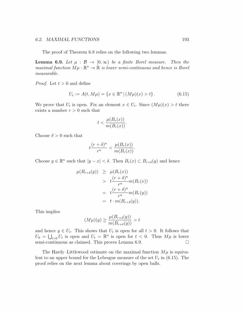
6.2. MAXIMAL FUNCTIONS 193
The proof of Theorem 6.8 relies on the following two lemmas.
Lemma 6.9. Let µ : B → [0,∞) be a finite Borel measure. Then themaximal function Mµ : Rn → R is lower semi-continuous and hence is Borelmeasurable.
Proof. Let t > 0 and define
Ut := A(t,Mµ) = x ∈ Rn | (Mµ)(x) > t . (6.15)
We prove that Ut is open. Fix an element x ∈ Ut. Since (Mµ)(x) > t thereexists a number r > 0 such that
t <µ(Br(x))
m(Br(x)).
Choose δ > 0 such that
t(r + δ)n
rn<µ(Br(x))
m(Br(x)).
Choose y ∈ Rn such that |y − x| < δ. Then Br(x) ⊂ Br+δ(y) and hence
µ(Br+δ(y)) ≥ µ(Br(x))
> t(r + δ)n
rnm(Br(x))
= t(r + δ)n
rnm(Br(y))
= t ·m(Br+δ(y)).
This implies
(Mµ)(y) ≥ µ(Br+δ(y))
m(Br+δ(y))> t
and hence y ∈ Ut. This shows that Ut is open for all t > 0. It follows thatU0 =
⋃t>0 Ut is open and Ut = Rn is open for t < 0. Thus Mµ is lower
semi-continuous as claimed. This proves Lemma 6.9.
The Hardy–Littlewood estimate on the maximal function Mµ is equiva-lent to an upper bound for the Lebesgue measure of the set Ut in (6.15). Theproof relies on the next lemma about coverings by open balls.
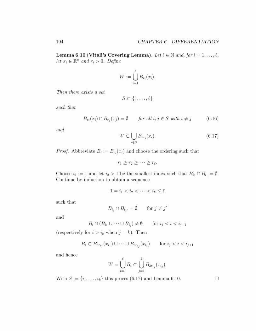
194 CHAPTER 6. DIFFERENTIATION
Lemma 6.10 (Vitali’s Covering Lemma). Let ` ∈ N and, for i = 1, . . . , `,let xi ∈ Rn and ri > 0. Define
W :=⋃i=1
Bri(xi).
Then there exists a setS ⊂ 1, . . . , `
such that
Bri(xi) ∩Brj(xj) = ∅ for all i, j ∈ S with i 6= j (6.16)
andW ⊂
⋃i∈S
B3ri(xi). (6.17)
Proof. Abbreviate Bi := Bri(xi) and choose the ordering such that
r1 ≥ r2 ≥ · · · ≥ r`.
Choose i1 := 1 and let i2 > 1 be the smallest index such that Bi2 ∩ Bi1 = ∅.Continue by induction to obtain a sequence
1 = i1 < i2 < · · · < ik ≤ `
such thatBij ∩Bij′
= ∅ for j 6= j′
andBi ∩ (Bi1 ∪ · · · ∪Bij) 6= ∅ for ij < i < ij+1
(respectively for i > ik when j = k). Then
Bi ⊂ B3ri1(xi1) ∪ · · · ∪B3rij
(xij) for ij < i < ij+1
and hence
W =⋃i=1
Bi ⊂k⋃j=1
B3rij(xij).
With S := i1, . . . , ik this proves (6.17) and Lemma 6.10.

6.2. MAXIMAL FUNCTIONS 195
Proof of Theorem 6.8. Fix a constant t > 0. Then the set Ut := A(t,Mλ) isopen by Lemma 6.9. Choose a compact set K ⊂ Ut. If x ∈ K ⊂ Ut then(Mλ)(x) > t and so there exists a number r(x) > 0 such that
|λ|(Br(x)(x))
m(Br(x)(x))> t. (6.18)
Since K is compact there exist finitely many points x1, . . . , x` ∈ K suchthat K ⊂
⋃`i=1Bri(xi), where ri := r(xi). By Lemma 6.10 there is a subset
S ⊂ 1, . . . , ` such that the balls Bri(xi) for i ∈ S are pairwise disjoint andK ⊂
⋃i∈S B3ri(xi). Since m(B3r) = 3nm(Br) by Theorem 2.17, this gives
m(K) ≤ 3n∑i∈S
m(Bri(xi)) <3n
t
∑i∈S
|λ|(Bri(xi)) ≤3n
t|λ|(Rn).
Here the second step follows from (6.18) with ri = r(xi) and the last stepfollows from the fact that the balls Bri(xi) for i ∈ S are pairwise disjoint.Take the supremum over all compact sets K ⊂ Ut to obtain
m(A(t,Mλ)) = m(Ut) ≤3n
t|λ|(Rn). (6.19)
(See Theorem 2.13.) Multiply the inequality (6.19) by t and take the supre-mum over all real numbers t > 0 to obtain ‖Mλ‖1,∞ ≤ 3n|λ|(Rn). Thisproves Theorem 6.8.
Definition 6.11. Let f ∈ L1(Rn). The maximal function of f is thefunction Mf : Rn → [0,∞) defined by
(Mf)(x) := supr>0
1
m(Br(x))
∫Br(x)
|f | dm for x ∈ Rn. (6.20)
Corollary 6.12. Let f ∈ L1(Rn) and define the signed Borel measure µfon Rn by µf (B) :=
∫Bf dm for every Borel set B ⊂ Rn. Then
Mf = Mµf ∈ L1,∞(Rn), ‖Mf‖1,∞ ≤ 3n ‖f‖1 .
Proof. The formula |µf |(B) =∫B|f | dm for B ∈ B shows that Mf = Mµf .
Hence the assertion follows from Theorem 6.8.
196 CHAPTER 6. DIFFERENTIATION
Corollary 6.12 shows that the map f 7→ Mf descends to an operator(denoted by the same letter) from the Banach space L1(Rn) to the topologicalvector space L1,∞(Rn). Corollary 6.12 also shows that the resulting operator
M : L1(Rn)→ L1,∞(Rn)
is continuous (because |Mf−Mg| ≤M(f−g)). Note that it is not linear. ByTheorem 6.8 it extends naturally to an operator λ 7→ Mλ from the Banachspace of signed Borel measures on Rn to L1,∞(Rn). (See Exercise 5.34.)
6.3 Lebesgue Points
Definition 6.13. Let f ∈ L1(Rn). An element x ∈ Rn is a called aLebesgue point of f if
limr→0
1
m(Br(x))
∫Br(x)
|f − f(x)| dm = 0. (6.21)
In particular, x is a Lebesgue point of f whenever f is continuous at x.
The next theorem is the main result of this chapter.
Theorem 6.14 (Lebesgue Differentiation Theorem).Let f ∈ L1(Rn). Then there exists a Borel set E ⊂ Rn such that m(E) = 0and every element of Rn \ E is a Lebesgue point of f .
Proof. For f ∈ L1(Rn) and r > 0 define the function Trf : Rn → [0,∞) by
(Trf)(x) :=1
m(Br(x))
∫Br(x)
|f − f(x)| dm for x ∈ Rn. (6.22)
One can prove via an approximation argument that Trf is Lebesgue measur-able for every r > 0 and every f ∈ L1(Rn). However, we shall not use thisfact in the proof. For f ∈ L1(Rn) define the function Tf : Rn → [0,∞] by
(Tf)(x) := lim supr→0
(Trf)(x) for x ∈ Rn. (6.23)
We must prove that Tf = 0 almost everywhere for every f ∈ L1(Rn).
6.3. LEBESGUE POINTS 197
To see this, fix a function f ∈ L1(Rn) and assume without loss of gener-ality that f is Borel measurable. (See Theorem 2.14 and part (v) of Theo-rem 1.55.) By Theorem 4.15 there exists a sequence of continuous functionsgi : Rn → R with compact support such that
‖f − gi‖1 <1
2ifor all i ∈ N.
Since gi is continuous we have Tgi = 0. Moreover, the function
hi := f − gi
is Borel measurable and satisfies
(Trhi)(x) =1
m(Br(x))
∫Br(x)
|hi − hi(x)| dm
≤ 1
m(Br(x))
∫Br(x)
|hi| dm+ |hi(x)|
≤ (Mhi)(x) + |hi(x)|
for all x ∈ Rn. ThusTrhi ≤Mhi + |hi|
for all i and all r > 0. Take the limit superior as r tends to zero to obtain
Thi ≤Mhi + |hi|
for all i. Moreover, it follows from the definition of Tr that
Trf = Tr(gi + hi) ≤ Trgi + Trhi
for all i and all r > 0. Take the limit superior as r tends to zero to obtain
Tf ≤ Tgi + Thi = Thi ≤Mhi + |hi|
for all i. This implies
A(ε, Tf) ⊂ A(ε/2,Mhi) ∪ A(ε/2, hi). (6.24)
for all i and all ε > 0. (See equation (6.1) for the notation A(ε, Tf) etc.)Since hi and Mhi are Borel measurable (see Theorem 6.8) the set
Ei(ε) := A(ε/2,Mhi) ∪ A(ε/2, hi) (6.25)
198 CHAPTER 6. DIFFERENTIATION
is a Borel set. Since ‖hi‖1 < 2−i we have
m(A(ε/2, hi)) ≤2
ε‖hi‖1,∞ ≤
2
ε‖hi‖1 ≤
1
2i−1ε
and, by Theorem 6.8,
m(A(ε/2,Mhi)) ≤2
ε‖Mhi‖1,∞ ≤
2 · 3n
ε‖hi‖1 ≤
3n
2i−1ε.
Thus
m(Ei(ε)) ≤3n + 1
2i−1ε.
Since this holds for all i ∈ N it follows that the Borel set
E(ε) :=∞⋂i=1
Ei(ε)
has Lebesgue measure zero for all ε > 0. Hence the Borel set
E :=∞⋃k=1
E(1/k)
has Lebesgue measure zero. By (6.24) and (6.25), we have
A(1/k, Tf) ⊂ E(1/k)
for all k ∈ N and hence
x ∈ Rn
∣∣ (Tf)(x) 6= 0
=∞⋃k=1
x ∈ Rn
∣∣ (Tf)(x) > 1/k
=∞⋃k=1
A(1/k, Tf)
⊂∞⋃k=1
E(1/k)
= E.
This shows that (Tf)(x) = 0 for all x ∈ Rn \ E and hence every element ofRn \ E is a Lebesgue point of f . This proves Theorem 6.14.

6.3. LEBESGUE POINTS 199
The first consequence of Theorem 6.14 discussed here concerns a signedBorel measure λ on Rn that is absolutely continuous with respect to theLebesgue measure. The following theorem provides a formula for the functionf in Theorem 5.18 (also called the Radon–Nikodym derivative of λ).
Theorem 6.15. Let λ : B → R be a signed Borel measure on Rn that isabsolutely continuous with respect to the Lebesgue measure. Choose a Borelmeasurable function f ∈ L1(Rn) such that λ(B) =
∫Bf dm for all B ∈ B.
Then there exists a Borel set E ⊂ Rn such that m(E) = 0 and
f(x) = limr→0
λ(Br(x))
m(Br(x))for all x ∈ Rn \ E. (6.26)
Proof. By Theorem 6.14 there exists a Borel set E ⊂ Rn of Lebesgue measurezero such that every element of X \ E is a Lebesgue point. Since∣∣∣∣ λ(Br(x))
m(Br(x))− f(x)
∣∣∣∣ =1
m(Br(x))
∣∣∣∣∫Br(x)
(f − f(x)
)dm
∣∣∣∣≤ 1
m(Br(x))
∫Br(x)
|f − f(x)| dm
for all r > 0 and all x ∈ Rn, it follows that (6.26) holds for all x ∈ Rn \ E.This proves Theorem 6.15.
Theorem 6.16. Let f ∈ L1(Rn) and let x ∈ Rn be a Lebesgue point of f .Fix two constants 0 < α < 1 and ε > 0. Then there exists a δ > 0 such that,for every Borel set E ∈ B and every r > 0,
r < δ,E ⊂ Br(x),
m(E) > αm(Br(x))=⇒
∣∣∣∣ 1
m(E)
∫E
f dm− f(x)
∣∣∣∣ < ε. (6.27)
Proof. Since x is a Lebesgue point of f , there exists a constant δ > 0 suchthat m(Br(x))−1
∫Br(x)|f − f(x)| dm < αε for 0 < r < δ. Assume 0 < r < δ
and let E ⊂ Br(x) be a Borel set such that m(E) ≥ αm(Br(x)). Then∣∣∣∣ 1
m(E)
∫E
f dm− f(x)
∣∣∣∣ ≤ 1
m(E)
∫E
|f − f(x)| dm
≤ 1
αm(Br(x))
∫Br(x)
|f − f(x)| dm
< ε.
This proves Theorem 6.16.
200 CHAPTER 6. DIFFERENTIATION
The Lebesgue Differentiation Theorem 6.14 can be viewed as a theoremabout signed Borel measures that are absolutely continuous with respect tothe Lebesgue measure. The next theorem is an analogous result for signedBorel measures that are singular with respect to the Lebesgue measure.
Theorem 6.17 (Singular Lebesgue Differentiation).Let λ : B → R be a signed Borel measure on Rn such that λ ⊥ m. Thenthere exists a Borel set E ⊂ Rn such that m(E) = 0 = |λ|(Rn \ E) and
limr→0
|λ|(Br(x))
m(Br(x))= 0 for all x ∈ Rn \ E. (6.28)
Proof. The proof follows an argument in Heil [7, Section 3.4]. By assumptionand Lemma 5.16, there exists a Borel set A ⊂ Rn such that
m(A) = 0, |λ|(Rn \ A) = 0.
For ε > 0, define the set
Aε :=
x ∈ Rn \ A
∣∣∣∣ lim supr→0
|λ|(Br(x))
m(Br(x))> ε
.
We prove that Aε is a Lebesgue null set for every ε > 0. To see this, fixtwo constants ε > 0 and δ > 0. Since the Borel measure |λ| is regular byTheorem 3.18 there exists an open set Uδ ⊂ Rn such that
A ⊂ Uδ, |λ|(Uδ) < δ.
For x ∈ Aε choose a radius r = r(x) > 0 such that
|λ|(Br(x)(x))
m(Br(x)(x))> ε, Br(x)(x) ⊂ Uδ,
and consider the open set Wδ :=⋃x∈Aε Br(x)(x) ⊂ Uδ. Fix a compact subset
K ⊂ Wδ and cover K by finitely many of the balls Br(x)(x) with x ∈ Aε. ByVitali’s Covering Lemma 6.10 there are elements x1, . . . , xN ∈ Aε such thatthe balls Br(xi)(xi) are pairwise disjoint and K ⊂
⋃Ni=1 B3r(xi)(xi). Thus
m(K) ≤N∑i=1
3nm(Br(xi)(xi)) <3n
ε
N∑i=1
|λ|(Br(xi)(xi)) ≤3n
ε
N∑i=1
|λ|(Uδ) ≤3nδ
ε.
This holds for every compact set K ⊂ Wδ and hence m(Wδ) ≤ 3nδ/ε. Sinceδ > 0 was arbitrary, the set Aε is contained in an open set of arbitrarily smallLebesgue measure and so is a Lebesgue null set as claimed. This implies thatthe set E := A∪
⋃∞k=1 A1/k is a Lebesgue null set. It satisfies |λ|(Rn \E) = 0
and (6.28) by definition and this proves Theorem 6.17.

6.4. ABSOLUTELY CONTINUOUS FUNCTIONS 201
6.4 Absolutely Continuous Functions
Definition 6.18. Let I ⊂ R be an interval. A function f : I → R is calledabsolutely continuous if for every ε > 0 there exists a δ > 0 such that,for every finite sequence s1 ≤ t1 ≤ s2 ≤ t2 ≤ · · · ≤ s` ≤ t` in I,∑
i=1
|si − ti| < δ =⇒∑i=1
|f(si)− f(ti)| < ε. (6.29)
Every absolutely continuous function is continuous.
The equivalence of (i) and (iii) in the following result is the FundamentalTheorem of Calculus for Lebesgue integrable functions. The equivalenceof (i) and (ii) is known as the Banach–Zarecki Theorem. For functionsof bounded variation see Exercise 6.20 below.
Theorem 6.19 (Fundamental Theorem of Calculus).Let I = [a, b] ⊂ R be a compact interval, let B ⊂ 2I be the Borel σ algebra,and let m : B → [0,∞] be the restriction of the Lebesgue measure to B. Letf : I → R be a function. Then the following are equivalent.
(i) f is absolutely continuous.
(ii) f is continuous, it has bounded variation, and if E ⊂ I is a Lebesguenull set then so is f(E).
(iii) There is a Borel measurable function g : I → R such that∫I|g| dm <∞
and, for all x, y ∈ I with x < y,
f(y)− f(x) =
∫ y
x
g(t) dt. (6.30)
The right hand side denotes the Lebesgue integral of g over the interval [x, y].
If (iii) holds then there exists a Borel set E ⊂ I such that m(E) = 0 and,for all x ∈ I \ E, f is differentiable at x and f ′(x) = g(x).
Proof. We prove that (iii) implies the last assertion of the theorem. Thusassume that there exists a function g ∈ L1(I) that satisfies (6.30) for allx, y ∈ I with x < y. Then Theorem 6.14 asserts that there exists a Borelset E ⊂ I of Lebesgue measure zero such that every element of I \ E is aLebesgue point of g. By Theorem 6.16 with α = 1/2, every element x ∈ I \Esatisfies condition (ii) in Theorem 6.6 with A := g(x). Hence Theorem 6.6asserts that the function f is differentiable at every point x ∈ I \ E andsatisfies f ′(x) = g(x) for x ∈ I \ E.
202 CHAPTER 6. DIFFERENTIATION
We prove that (iii) implies (i). Thus assume f satisfies (iii) and definethe signed measure λ : B → R by
λ(B) :=
∫B
g dm (6.31)
for every Borel set B ⊂ I. Then λ is absolutely continuous with respect tothe Lebesgue measure and
|λ|(B) =
∫B
|g| dm
for ever Borel set B ⊂ I. Now let ε > 0. Since |λ| m it follows fromLemma 5.21 that there exists a constant δ > 0 such that |λ|(B) < ε for everyBorel set B ⊂ I with m(B) < δ. Choose a sequence s1 ≤ t1 ≤ · · · ≤ s` ≤ t`in I such that
∑`i=1|ti−si| < δ and define Ui := (si, ti) for i = 1, . . . , `. Then
the Borel set B :=⋃`i=1 Ui has Lebesgue measure m(B) =
∑`i=1|ti − si| < δ.
Hence |λ|(B) < ε. Since
|f(ti)− f(si)| =∣∣∣∣∫Ui
g dm
∣∣∣∣ ≤ ∫Ui
|g| dm = |λ|(Ui)
for all i it follows that∑i=1
|f(ti)− f(si)| ≤∑i=1
|λ|(Ui) = |λ|(B) < ε.
Hence f is absolutely continuous.We prove that (i) implies (ii). Assume f is absolutely continuous. It
follows directly from the definition that f is continuous, and that it hasbounded variation is part (v) of Exercise 6.20. Now suppose that E ⊂ Iis a Lebesgue null set and assume without loss of generality that a, b /∈ E.Fix any constant ε > 0 and choose δ > 0 such that (6.29) holds. Since theLebesgue measure is outer regular by Theorem 2.13, there exists an openset U ⊂ int(I) such that E ⊂ U and m(U) < δ. Choose a (possibly finite)sequence of pairwise disjoint open intervals Ui ⊂ I such that U =
⋃i Ui.
Choose si, ti ∈ Ui such that f(si) = infUi f and f(ti) = supUi f . Then itfollows from (6.29) that
∑im(f(Ui)) =
∑i(f(ti)−f(si)) < ε for every finite
sum. Take the limit to obtain m(f(U)) ≤∑
im(f(Ui)) ≤ ε. Since ε > 0 waschosen arbitrary and the Lebesgue measure is complete, it follows that f(E)is a Lebesgue measurable set and m(f(E)) = 0.

6.4. ABSOLUTELY CONTINUOUS FUNCTIONS 203
We prove that (ii) implies (iii). Assume f satisfies (ii). Then f hasbounded variation and under this assumption Exercise 6.20 below outlinesa proof that there exists a signed Borel measure λ : B → R such thatf(y)− f(x) = λ((x, y]) for x, y ∈ I with x < y. Since λ+ and λ− are regularby Theorem 3.18 and f is continuous, we have
f(y)− f(x) = λ([x, y]) = λ((x, y]) = λ([x, y)) = λ((x, y)) (6.32)
for all x, y ∈ I with x < y. By the Lebesgue Decomposition Theorem 5.17there exist two signed Borel measures λa, λs : B → R such that
λ = λa + λs, λa m, λs ⊥ m. (6.33)
Since λa m it follows from Theorem 5.18 that there is an integrablefunction g ∈ L1(I) such that
λa(B) =
∫B
g dm (6.34)
for every Borel set B ⊂ I. Define the functions fa, fs : I → R by
fa(x) := f(a) + λa([a, x]) = f(a) +
∫ x
a
g(t) dt, fs(x) := λs([a, x]).
Then f = fa+fs by (6.32) and (6.33). Since (iii) implies (i) and (i) implies (ii)(already proved) both functions f and fa satisfy (ii) and fa is absolutelycontinuous. Moreover fs = f − fa is continuous.
It remains to prove that fs ≡ 0. The proof given below follows an ar-gument in Heil [7, Section 3.5.4]. By Theorem 6.17, there exists a Lebesguenull set Es ⊂ I such that a, b ∈ Es (without loss of generality) and
|λs|(I \ Es) = 0, limr→0
|λs((x− r, x+ r))|r
= 0 for all x ∈ I \ Es.
This implies that every element x ∈ I \ Es satisfies condition (ii) in Theo-rem 6.6 with A = 0 and f replaced by fs. Hence fs is differentiable at everypoint x ∈ I \ Es and f ′s(x) = 0 for x ∈ I \ Es.
Since Es is a Lebesgue null set so are the sets f(Es) and fa(Es), becausethe functions f and fa satisfy (ii). Since the difference of two Lebesgue nullsets in R is a Lebesgue null set, by Exercise 2.27, it follows that
fs(Es) = f(x)− fa(x) |x ∈ Es ⊂ f(x)− fa(y) |x, y ∈ Es
is a Lebesgue null set.
204 CHAPTER 6. DIFFERENTIATION
We claim that fs(I \ Es) is also a Lebesgue null set. To see this, fix aconstant ε > 0. For n ∈ N define the set
An :=
x ∈ I \ Es
∣∣∣∣ y ∈ I, |x− y| < 1
n=⇒ |fs(x)− fs(y)| ≤ ε|x− y|
.
ThenAn ⊂ An+1 for all n ∈ N and I \ Es =
⋃n∈N
An.
Here the last assertion follows from the fact that fs is differentiable on I \Eswith derivative zero. We prove that the Lebesgue outer measure of the setfs(I \ Es) satisfies the estimate
ν(fs(I \ Es)) ≤ ε(b− a+ ε). (6.35)
To see this, cover the set An by at most countably many open intervals Ui,each of length less than 1/n, such that∑
i
m(Ui) ≤ ν(An) + ε
and each interval Ui contains an element of An. Then f(Ui) is contained inan interval of length at most εm(Ui), by definition of An. Hence
ν(f(An)) ≤ ε∑i
m(Ui) ≤ ε(ν(An) + ε) ≤ ε(b− a+ ε).
Since the Lebesgue outer measure is continuous from below by part (iii) ofTheorem 2.13 and
fs(I \ Es) =⋃n∈N
fs(An),
it follows that
ν(fs(I \ Es)) = limn→∞
ν(f(An)) ≤ ε(b− a+ ε).
This proves (6.35). Since ε > 0 was chosen arbitrary, this implies thatfs(I \ Es) is a Lebesgue null set as claimed. Since fs(Es) is also a Lebesguenull set, as noted above, it follows that fs(I) is a Lebesgue null set. Since fsis continuous and fs(0) = 0 by definition, this implies fs ≡ 0. Hence f = fais absolutely continuous and this proves Theorem 6.19.
6.5. EXERCISES 205
6.5 Exercises
Exercise 6.20. Let I = [a, b] ⊂ R be a compact interval and let B ⊂ 2I
be the Borel σ-algebra. A function f : I → R is said to be of boundedvariation if
V (f) := supa=t0<t1<···<t`=b
∑i=1
|f(ti)− f(ti−1)| <∞. (6.36)
Denote by BV(I) the set of all functions f : I → R of bounded variation.This is a real vector space. Functions of bounded variation have at mostcountably many discontinuities and the left and right limits exist everywhere.Prove the following.
(i) Every monotone function f : I → R has bounded variation.
(ii) Let f ∈ BV(I) be right continuous. Then there exist right continuousmonotone functions f± : I → R such that f = f+ − f−. Hint: Define
F (x) := V (f |[a,x]) = supa=t0<t1<···<t`=x
∑i=1
|f(ti)− f(ti−1)| (6.37)
for a ≤ x ≤ b. Prove that F is right continuous and F ± f are monotone.
(iii) If f is continuous then the function F in (6.37) is continuous.
(iv) Let f : I → R be right continuous. Then f ∈ BV(I) if and only if thereexists a signed Borel measure λ = λf : B → R such that λ(a) = 0 and
f(x)− f(a) = λ([a, x]) for a ≤ x ≤ b. (6.38)
Hint: Assume f is monotone. For h ∈ C(I) define
Λf (h) :=
∫ b
a
h df := supa=t0<t1<···<t`=b
∑i=1
(inf
[ti−1,ti]h
)·(f(ti)− f(ti−1)
). (6.39)
(This is the Riemann–Stieltjes integral. See Korner [9] and compare itwith the Riemann integral [9, 18, 21].) Prove that Λf : C(I)→ R is a positivelinear functional. Use the Riesz Representation Theorem 3.15 to find a Borelmeasure λf : B → [0,∞) such that Λf (h) =
∫Ih dλf for all h ∈ C(I). Use
the fact that f is right continuous to prove that λf satisfies (6.38).
(v) If f ∈ BV(I) is right continuous and λf is as in (iii) then V (f) = |λf |(I).
(vi) Every absolutely continuous function f : I → R has bounded variation.
206 CHAPTER 6. DIFFERENTIATION
Exercise 6.21. Let (R,A,m) be the Lebesgue measure space and fix a con-stant 0 < ε < 1/2. Prove that there does not exist a Lebesgue measurableset E ⊂ R such that
ε <m(E ∩ I)
m(I)< 1− ε
for every nonempty bounded open interval I ⊂ R. Hint: Consider thefunction f := χE∩[−1,1] and define the measure µf : B → R by
µf (B) :=
∫B
f dm = m(B ∩ E ∩ [−1, 1]).
Examine the Lebesgue points of f . (Compare this with Exercise 2.32.)
Exercise 6.22. Prove the Theorem of Vitali–Caratheodory:Let (X,U) be a locally compact Hausdorff space and let B ⊂ 2X be its Borelσ-algebra. Let µ : B → [0,∞] be an outer regular Borel measure that isinner regular on open sets. Let f ∈ L1(µ) and let ε > 0. Then there existsan upper semi-continuous function u : X → R that is bounded above and alower semi-continuous function v : X → R that is bounded below such that
u ≤ f ≤ v,
∫X
(v − u) dµ < ε. (6.40)
Hint: Assume first that f ≥ 0. Use Theorem 1.26 to find a sequence ofmeasurable sets Ei ∈ A, not necessarily disjoint, and a sequence of realnumbers ci > 0 such that µ(Ei) <∞ for all i and
f =∞∑i=1
ciχEi .
Thus∞∑i=1
ciµ(Ei) =
∫X
f dµ <∞.
Choose a sequence of compact sets Ki ⊂ X and a sequence of open setsUi ⊂ X such that Ki ⊂ Ei ⊂ Ui and ciµ(Ui \Ki) < ε2−i−1 for all i. Choosen ∈ N such that
∑∞i=n+1 ciµ(Ei) < ε/2 and define
u :=n∑i=1
ciχKi , v :=∞∑i=1
ciχUi .
Show that∫X
(v − u) dµ < ε, v is lower semi-continuous (i.e. v−1((t,∞))is open for all t ∈ R), and u is upper semi-continuous (i.e. u−1((−∞, t))is open for all t ∈ R).
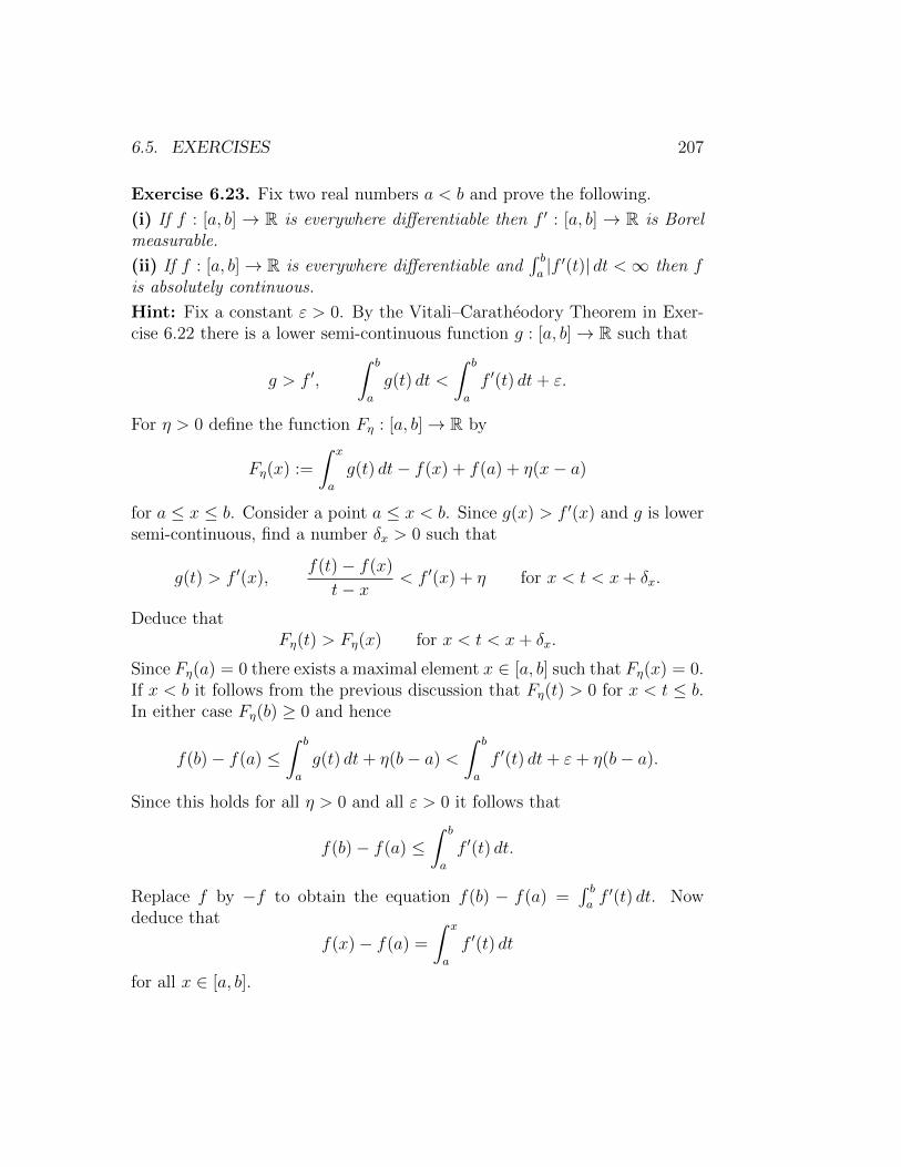
6.5. EXERCISES 207
Exercise 6.23. Fix two real numbers a < b and prove the following.
(i) If f : [a, b] → R is everywhere differentiable then f ′ : [a, b] → R is Borelmeasurable.
(ii) If f : [a, b]→ R is everywhere differentiable and∫ ba|f ′(t)| dt <∞ then f
is absolutely continuous.
Hint: Fix a constant ε > 0. By the Vitali–Caratheodory Theorem in Exer-cise 6.22 there is a lower semi-continuous function g : [a, b]→ R such that
g > f ′,
∫ b
a
g(t) dt <
∫ b
a
f ′(t) dt+ ε.
For η > 0 define the function Fη : [a, b]→ R by
Fη(x) :=
∫ x
a
g(t) dt− f(x) + f(a) + η(x− a)
for a ≤ x ≤ b. Consider a point a ≤ x < b. Since g(x) > f ′(x) and g is lowersemi-continuous, find a number δx > 0 such that
g(t) > f ′(x),f(t)− f(x)
t− x< f ′(x) + η for x < t < x+ δx.
Deduce thatFη(t) > Fη(x) for x < t < x+ δx.
Since Fη(a) = 0 there exists a maximal element x ∈ [a, b] such that Fη(x) = 0.If x < b it follows from the previous discussion that Fη(t) > 0 for x < t ≤ b.In either case Fη(b) ≥ 0 and hence
f(b)− f(a) ≤∫ b
a
g(t) dt+ η(b− a) <
∫ b
a
f ′(t) dt+ ε+ η(b− a).
Since this holds for all η > 0 and all ε > 0 it follows that
f(b)− f(a) ≤∫ b
a
f ′(t) dt.
Replace f by −f to obtain the equation f(b) − f(a) =∫ baf ′(t) dt. Now
deduce that
f(x)− f(a) =
∫ x
a
f ′(t) dt
for all x ∈ [a, b].

208 CHAPTER 6. DIFFERENTIATION
Example 6.24. (i) The Cantor function is the unique monotone functionf : [0, 1]→ [0, 1] that satisfies
f
(2∞∑i=1
ai3i
)=∞∑i=1
ai2i
for all sequences ai ∈ 0, 1. It is continuous and nonconstant and its deriva-tive exists and vanishes on the complement of the standard Cantor set
C :=∞⋂n=1
⋃ai∈0,1
[2
n∑i=1
ai3i, 2
n∑i=1
ai3i
+1
3n
].
This Cantor set has Lebesgue measure zero. Hence f is almost everywheredifferentiable and its derivative is integrable. However, f is not equal to theintegral of its derivative and therefore is not absolutely continuous.
(ii) The following construction was explained to me by Theo Buehler. Definethe homeomorphisms g : [0, 1]→ [0, 2] and h : [0, 2]→ [0, 1] by
g(x) := f(x) + x, h := g−1.
The image g([0, 1] \ C) is a countable union of disjoint open intervals oftotal length one and hence has Lebesgue measure one. Thus its complementK := g(C) ⊂ [0, 2] is a modified Cantor set of Lebesgue measure one. Hence,by Theorem 6.19, g is not absolutely continuous. Moreover, by Lemma 2.15there exists a set E ⊂ K which is not Lebesgue measurable. However, itsimage F := h(E) ⊂ [0, 1] under h is a subset of the Lebesgue null set Cand hence is a Lebesgue null set. Thus F is a Lebesgue measurable setand E = h−1(F ) is not Lebesgue measurable. This shows that the functionh : [0, 2]→ [0, 1] is not measurable with respect to the Lebesgue σ-algebras onboth domain and target (i.e. it is not Lebesgue-Lebesgue measurable).
(iii) Let I, J ⊂ R be intervals. Then it follows from Lemma 2.15 andTheorem 6.19 that every Lebesgue-Lebesgue measurable homeomorphismh : I → J has an absolutely continuous inverse.
(iv) Let h : [0, 2] → [0, 1] and F ⊂ C ⊂ [0, 1] be as in part (ii). Then thecharacteristic function χF : R→ R is Lebesgue measurable and h : [0, 2]→ Ris continuous. However, the composition χF h : [0, 2]→ R is not Lebesguemeasurable because the set (χF h)−1(1) = E is not Lebesgue measurable.
(v) By contrast, if I, J ⊂ R are intervals, f : J → R is Lebesgue measurable,and h : I → J is a C1 diffeomorphism, then f h : I → R is again Lebesguemeasurable by Theorem 2.17.
Chapter 7
Product Measures
The purpose of this chapter is to study products of two measurable spaces(Section 7.1), introduce the product measure (Section 7.2), and prove Fubini’sTheorem (Section 7.3). The archetypal example is the Lebesgue measure onRk+` = Rk × R`; it is the completion of the product measure associated tothe Lebesgue measures on Rk and R` (Section 7.4). Applications include theconvolution (Section 7.5), Marcinkiewicz interpolation (Section 7.6), and theCalderon–Zygmund inequality (Section 7.7).
7.1 The Product σ-Algebra
Assume throughout that (X,A) and (Y,B) are measurable spaces.
Definition 7.1. The product σ-algebra of A and B is defined as the small-est σ-algebra on the product space X×Y := (x, y) |x ∈ X, y ∈ Y that con-tains all subsets of the form A × B, where A ∈ A and B ∈ B. It will bedenoted by A⊗ B ⊂ 2X×Y .
Lemma 7.2. Let E ∈ A⊗B and let f : X×Y → R be an (A⊗B)-measurablefunction. Then the following holds.(i) For every x ∈ X the function fx : Y → R, defined by fx(y) := f(x, y) fory ∈ Y , is B-measurable and
Ex :=y ∈ Y
∣∣ (x, y) ∈ E∈ B. (7.1)
(ii) For every y ∈ Y the function f y : X → R, defined by f y(x) := f(x, y)for x ∈ X, is A-measurable and
Ey :=x ∈ X
∣∣ (x, y) ∈ E∈ A. (7.2)
209

210 CHAPTER 7. PRODUCT MEASURES
Proof. Define Ω ⊂ 2X×Y by
Ω :=E ⊂ X × Y
∣∣Ex ∈ B for all x ∈ X.
We prove that Ω is a σ-algebra. To see this, note first that X × Y ∈ Ω.Second, if E ∈ Ω then Ex ∈ B for all x ∈ X, hence
(Ec)x = y ∈ Y | (x, y) /∈ E = (Ex)c ∈ B
for all x ∈ X, and hence Ec ∈ Ω. Third, if Ei ∈ Ω is a sequence andE :=
⋃∞i=1Ei, then Ex =
⋃∞i=1(Ei)x ∈ B for all x ∈ X, and hence E ∈ Ω.
This shows that Ω is a σ-algebra. Since A × B ∈ Ω for all A ∈ A and allB ∈ B it follows that A⊗ B ⊂ Ω. This proves (7.1) for all x ∈ X.
Now fix an element x ∈ X. If V ⊂ R is open then E := f−1(V ) ∈ A⊗ Band hence (fx)
−1(V ) = Ex ∈ B by (7.1). Thus fx is B-measurable. Thisproves (i). The proof of (ii) is analogous and this proves Lemma 7.2.
Definition 7.3. Let Z be a set. A collection of subsets M ⊂ 2Z is called amonotone class if it satisfies the following two axioms
(a) If Ai ∈M for i ∈ N such that Ai ⊂ Ai+1 for all i then⋃∞i=1Ai ∈M.
(b) If Bi ∈M for i ∈ N such that Bi ⊃ Bi+1 for all i then⋂∞i=1 Bi ∈M.
Definition 7.4. A subset Q ⊂ X×Y is called elementary if it is the unionof finitely many pairwise disjoint subsets of the form A×B with A ∈ A andB ∈ B.
The next lemma is a useful characterization of the product σ-algebra.
Lemma 7.5. The product σ-algebra A ⊗ B is the smallest monotone classin X × Y that contains all elementary subsets.
Proof. Let E ⊂ 2X×Y denote the collection of all elementary subsets anddefine M ⊂ 2X×Y as the smallest monotone class that contains E . This iswell defined because the intersection of any collection of monotone classes isagain a monotone class. Since every σ-algebra is a monotone class and everyelementary set is an element of A⊗ B it follows that
M⊂ A⊗B.
Since E ⊂ M by definition, the converse inclusion follows once we knowthat M is a σ-algebra. We prove this in seven steps.
7.1. THE PRODUCT σ-ALGEBRA 211
Step 1. For every set P ⊂ X × Y the collection
Ω(P ) :=Q ⊂ X × Y
∣∣P \Q, Q \ P, P ∪Q ∈Mis a monotone class.
This follows immediately from the definition of monotone class.
Step 2. Let P,Q ⊂ X × Y . Then Q ∈ Ω(P ) if and only if P ∈ Ω(Q).
This follows immediately from the definition of Ω(P ) in Step 1.
Step 3. If P,Q ∈ E then P ∩Q,P \Q,P ∪Q ∈ E.
For the intersection this follows from the fact that
(A1 ×B1) ∩ (A2 ×B2) = (A1 ∩ A2)× (B1 ∩B2) .
For the complement it follows from the fact that
(A1 ×B1) \ (A2 ×B2) =((A1 \ A2)×B1
)∪((A1 ∩ A2)× (B1 \B2)
).
For the union this follows from the fact that P ∪Q = (P \Q) ∪Q.
Step 4. If P ∈ E then M⊂ Ω(P ).
Let P ∈ E . Then P \ Q,Q \ P, P ∪ Q ∈ E ⊂ M for all Q ∈ E by Step 3.Hence Q ∈ Ω(P ) for all Q ∈ E by definition of Ω(P ) in Step 1. Thus we haveproved that E ⊂ Ω(P ). Since Ω(P ) is a monotone class by Step 1 it followsthat M⊂ Ω(P ). This proves Step 4.
Step 5. If P ∈M then M⊂ Ω(P ).
Fix a set P ∈M. Then P ∈ Ω(Q) for all Q ∈ E by Step 4. Hence Q ∈ Ω(P )for all Q ∈ E by Step 2. Thus E ⊂ Ω(P ) and hence it follows from Step 1that M⊂ Ω(P ). This proves Step 5.
Step 6. If P,Q ∈M then P \Q,P ∪Q ∈M.
If P,Q ∈ M then Q ∈ M ⊂ Ω(P ) by Step 5 and hence P \ Q,P ∪ Q ∈ Mby the definition of Ω(P ) in Step 1.
Step 7. M is a σ-algebra.
By definition X × Y ∈ E ⊂ M. If P ∈ M then P c = (X × Y ) \ P ∈ M byStep 6. If Pi ∈M for i ∈ N then Qn :=
⋃ni=1 Pi ∈M for all n ∈ N by Step 6
and hence⋃∞i=1 Pi =
⋃∞n=1Qn ∈ M because M is a monotone class. This
proves Step 7 and Lemma 7.5.
212 CHAPTER 7. PRODUCT MEASURES
Lemma 7.6. Let (X,UX) and (Y,UY ) be topological spaces, let UX×Y bethe product topology on X ×Y (see Appendix B), and let BX , BY , BX×Y bethe associated Borel σ-algebras. Then
BX ⊗ BY ⊂ BX×Y . (7.3)
If (X,UX) is a second countable locally compact Hausdorff space then
BX ⊗ BY = BX×Y . (7.4)
Proof. The projections πX : X×Y → X and πY : X×Y → Y are continuousand hence Borel measurable by Theorem 1.20. Thus π−1
X (A) = A×Y ∈ BX×Yfor all A ∈ BX and π−1
Y (B) = X × B ∈ BX×Y for all B ∈ BY . HenceA×B ∈ BX×Y for all A ∈ BX and all B ∈ BY , and this implies (7.3).
Now assume (X,UX) is a second countable locally compact Hausdorffspace and choose a countable basis Ui | i ∈ N of UX such that U i is compactfor all i ∈ N. Fix an open set W ∈ UX×Y and, for i ∈ N, define
Vi :=y ∈ Y | (x, y) ∈ W for all x ∈ U i
.
We prove that Vi is open. Let y0 ∈ Vi. Then (x, y0) ∈ W for all x ∈ U i.Hence, for every x ∈ U i, there exist open sets U(x) ∈ UX and V (x) ∈ UYsuch that (x, y0) ∈ U(x)× V (x) ⊂ W . Since U i is compact there are finitelymany elements x1, . . . , x` ∈ U i such that U i ⊂ U(x1) ∪ · · · ∪ U(x`). DefineV := V (x1)∩ · · · ∩ V (x`). Then V is open and U i× V ⊂ W , so y0 ∈ V ⊂ Vi.This shows that Vi is open for all i ∈ N. Next we prove that
W =∞⋃i=1
(Ui × Vi). (7.5)
Let (x0, y0) ∈ W . Then there exist open sets U ∈ UX and V ∈ UY suchthat (x0, y0) ∈ U × V ⊂ W . Since (X,UX) is a locally compact Hausdorffspace, Lemma A.3 asserts that there exists an open set U ′ ⊂ X such thatx0 ∈ U ′ ⊂ U ′ ⊂ U . Since the sets Ui form a basis of the topology, thereexists an integer i ∈ N such that x0 ∈ Ui ⊂ U ′ and hence x0 ∈ U i ⊂ U ′ ⊂ U .Thus U i × y0 ⊂ U × V ⊂ W , hence y0 ∈ Vi, and so (x0, y0) ∈ Ui × Vi ⊂ W .Since the element (x0, y0) ∈ W was chosen arbitrarily, this proves (7.5). Thuswe have proved that UX×Y ⊂ BX ⊗ BY and this implies BX×Y ⊂ BX ⊗ BY .Hence (7.4) follows from (7.3). This proves Lemma 7.6.

7.1. THE PRODUCT σ-ALGEBRA 213
Lemma 7.7. Let (X,A) be a measurable space such that the cardinality ofX is greater than that of 2N. Then the diagonal ∆ := (x, x) |x ∈ X is notan element of A⊗A.
Proof. The proof has three steps.
Step 1. Let Y be a set. For E ⊂ 2Y denote by σ(E) ⊂ 2Y the smallestσ-algebra containing E. If D ∈ σ(E) then there exists a sequence Ei ∈ E fori ∈ N such that D ∈ σ(Ei | i ∈ N).
The union of the sets σ(E ′) over all countable subsets E ′ ⊂ E is a σ-algebrathat contains E and is contained in σ(E). Hence it is equal to σ(E).
Step 2. Let Y be a set, let E ⊂ 2Y , and let D ∈ σ(E). Then there is asequence Ei ∈ E and a set I ⊂ 2N such that D =
⋃I∈I(⋂
i∈I Ei ∩⋂i∈N\I E
ci
).
By Step 1 there exists a sequence Ei ∈ E such that D ∈ σ(Ei | i ∈ N). ForI ⊂ N define EI :=
⋂i∈I Ei ∩
⋂i∈N\I E
ci . These sets form a partition of Y .
Hence the collection F :=⋃
I∈I EI | I ⊂ 2N
is a σ-algebra on Y . SinceEi ∈ F for each i ∈ N it follows that D ∈ F . This proves Step 2.
Step 3. ∆ /∈ A⊗A.
Let E ⊂ 2X×X be the collection of all sets of the form A×B with A,B ∈ A.Let D ∈ A⊗A. By Step 2 there are sequences Ai, Bi ∈ A and a set I ⊂ 2N
such that D =⋃I∈I EI , where EI :=
(⋂i∈I(Ai × Bi) ∩
⋂i∈N\I(Ai × Bi)
c).
Thus EI =⋃J⊂N\I AIJ × BIJ , where AIJ :=
⋂i∈I Ai ∩
⋂j∈J(X \ Aj) and
BIJ :=⋂i∈I Bi ∩
⋂j∈N\(I∪J)(X \ Bj). If D ⊂ ∆ then, for all I and J , we
have AIJ × BIJ ⊂ ∆ and so AIJ × BIJ is either empty or a singleton. Thusthe cardinality of D is at most the cardinality of the set of pairs of disjointsubsets of N, which is equal to the cardinality of 2N. Since the cardinality ofthe diagonal is bigger than that of 2N it follows that ∆ /∈ A⊗A as claimed.This proves Lemma 7.7.
Example 7.8. Let X be an uncountable set, of cardinality greater thanthat of 2N, and equipped with the discrete topology so that BX = UX = 2X .Then ∆ is an open subset of X × X with respect to the product topology(which is also discrete because points are open). Hence ∆ ∈ BX×X = 2X×X .However, ∆ /∈ BX ⊗ BX by Lemma 7.7. Thus the product BX ⊗ BX of theBorel σ-algebras is not the Borel σ-algebra of the product. In other words,the inclusion (7.3) in Lemma 7.6 is strict in this example. Note also thatthe distance function d : X ×X → R defined by d(x, y) := 1 for x 6= y andd(x, x) := 0 is continuous with respect to the product topology but is notmeasurable with respect to the product of the Borel σ-algebras.
214 CHAPTER 7. PRODUCT MEASURES
7.2 The Product Measure
The definition of the product measure on the product σ-algebra is basedon the following theorem. For a measure space (X,A, µ) and a measurablefunction φ : X → [0,∞] we use the notation
∫Xφ(x) dµ(x) :=
∫Xφ dµ.
Theorem 7.9. Let (X,A, µ) and (Y,B, ν) be σ-finite measure spaces and letQ ∈ A⊗ B. Then the functions
X → [0,∞] : x 7→ ν(Qx), Y → [0,∞] : y 7→ µ(Qy) (7.6)
are measurable and ∫X
ν(Qx) dµ(x) =
∫Y
µ(Qy) dν(y). (7.7)
Definition 7.10. Let (X,A, µ) and (Y,B, ν) be σ-finite measure spaces. Theproduct measure of µ and ν is the map µ⊗ ν : A⊗B → [0,∞] defined by
(µ⊗ ν)(Q) :=
∫X
ν(Qx) dµ(x) =
∫Y
µ(Qy) dν(y) (7.8)
for Q ∈ A⊗B. That µ⊗ν is σ-additive, and hence is a measure, follows fromTheorem 1.38 and the fact that ν(Qx) =
∑∞i=1 ν((Qi)x) for every sequence of
pairwise disjoint sets Qi ∈ A⊗ B. The product measure satisfies
(µ⊗ ν)(A×B) = µ(A) · ν(B) (7.9)
for A ∈ A and B ∈ B and hence is σ-finite.
Proof of Theorem 7.9. Define
Ω :=
Q ∈ A⊗ B
∣∣∣∣ the functions (7.6) are measurableand satisfy equation (7.7)
.
We prove in five steps that Ω = A⊗ B.
Step 1. If A ∈ A and B ∈ B then Q := A×B ∈ Ω.
By assumption
Qx =
B, if x ∈ A,∅, if x /∈ A, Qy =
A, if y ∈ B,∅, if y /∈ B.
Define the function φ : X → [0,∞] by φ(x) := ν(Qx) = ν(B)χA(x) for x ∈ Xand the function ψ : Y → [0,∞] by ψ(y) := µ(Qy) = µ(A)χB(y) for y ∈ Y .Then φ, ψ are measurable and
∫Xφ dµ = µ(A)ν(B) =
∫Yψ dν. Thus Q ∈ Ω.
7.2. THE PRODUCT MEASURE 215
Step 2. If Q1, Q1 ∈ Ω and Q1 ∩Q2 = ∅ then Q := Q1 ∪Q2 ∈ Ω.
Define
φi(x) := ν((Qi)x), φ(x) := ν(Qx),
ψi(y) := ν((Qi)y), ψ(y) := ν(Qy)
(7.10)
for x ∈ X, y ∈ Y and i = 1, 2. Then φ = φ1 +φ2 and ψ = ψ1 +ψ2. Moreover,∫X
φi dµ =
∫Y
ψi dν
for i = 1, 2 because Qi ∈ Ω. Hence∫Xφ dµ =
∫Yψ dν and so Q ∈ Ω.
Step 3. If Qi ∈ Ω for i ∈ N and Qi ⊂ Qi+1 for all i then Q :=⋃∞i=1Qi ∈ Ω.
Define φi, φ : X → [0,∞] and ψi, ψ : Y → [0,∞] by (7.10) for i ∈ N. Since
Qx =∞⋃i=1
(Qi)x, Qy =∞⋃i=1
(Qi)y
and (Qi)x ∈ B and (Qi)y ∈ A for all i it follows from Theorem 1.28 (iv) that
φ(x) = ν(Qx) = limi→∞
ν((Qi)x) = limi→∞
φi(x) for all x ∈ X,
ψ(y) = ν(Qy) = limi→∞
ν((Qi)y) = lim
i→∞ψi(y) for all y ∈ Y.
By the Lebesgue Monotone Convergence Theorem 1.37 this implies∫X
φ dµ = limi→∞
∫X
φi dµ = limi→∞
∫Y
ψi dµ =
∫Y
ψ dµ.
Thus Q ∈ Ω and this proves Step 3.
Step 4. Let A ∈ A and B ∈ B such that µ(A) < ∞ and ν(B) < ∞. IfQi ∈ Ω for i ∈ N such that A×B ⊃ Q1 ⊃ Q2 ⊃ · · · then Q :=
⋂∞i=1Qi ∈ Ω.
Let φi, φ, ψi, ψ be as in the proof of Step 3. Since (Qi)x ⊂ B and ν(B) <∞it follows from part (v) of Theorem 1.28 that φi converges pointwise to φ.Moreover, φi ≤ ν(B)χA for all i and the function ν(B)χA : X → [0,∞) isintegrable because µ(A) < ∞ and ν(B) < ∞. Hence it follows from theLebesgue Dominated Convergence Theorem 1.45 that∫
X
φ dµ = limi→∞
∫X
φi dµ.
The same argument shows that∫Yψ dµ = limi→∞
∫Yψi dµ. Since Qi ∈ Ω for
all i, this implies∫Xφ dµ =
∫Yψ dµ and hence Q ∈ Ω. This proves Step 4.
216 CHAPTER 7. PRODUCT MEASURES
Step 5. Ω = A⊗ B.
Since (X,A, µ) and (Y,B, ν) are σ-finite, there exist sequences of measurablesets Xn ∈ A and Yn ∈ B such that
Xn ⊂ Xn+1, Yn ⊂ Yn+1, µ(Xn) <∞, ν(Yn) <∞
for all n ∈ N and X =⋃∞n=1 Xn and Y =
⋃∞n=1 Yn. Define
M :=Q ∈ A⊗ B
∣∣Q ∩ (Xn × Yn) ∈ Ω for all n ∈ N.
ThenM is a monotone class by Steps 3 an 4, E ⊂M by Steps 1 and 2, andM⊂ A⊗B by definition. Hence it follows from Lemma 7.5 thatM = A⊗B.In other words Q ∩ (Xn ∩ Yn) ∈ Ω for all Q ∈ A⊗B. By Step 3 this implies
Q =∞⋃n=1
(Q ∩ (Xn × Yn)
)∈ Ω for all Q ∈ A⊗ B.
Thus A⊗B ⊂ Ω ⊂ A⊗B and so Ω = A⊗B as claimed. This proves Step 5and Theorem 7.9.
Examples and exercises
Example 7.11. Let X = Y = [0, 1], letA ⊂ 2X be the σ-algebra of Lebesguemeasurable sets, let B := 2Y , let µ : A → [0, 1] be the Lebesgue measure,and let ν : B → [0,∞] be the counting measure. Consider the diagonal
∆ :=
(x, x)∣∣ 0 ≤ x ≤ 1
=∞⋂n=1
n⋃i=1
[i− 1
n,i
n
]2
∈ A⊗ B.
Its characteristic function f := χ∆ : X × Y → R is given by
f(x, y) :=
1, if x = y,0, if x 6= y.
Hence
µ(∆y) =
∫X
f(x, y) dµ(x) = 0 for 0 ≤ y ≤ 1,
ν(∆x) =
∫Y
f(x, y) dν(y) = 1 for 0 ≤ x ≤ 1,
and so∫Xµ(∆y) dν = 0 6= 1 =
∫Yµ(∆x) dµ(x). Thus the hypothesis that
(X,A, µ) and (Y,B, ν) are σ-finite cannot be removed in Theorem 7.9.
7.2. THE PRODUCT MEASURE 217
Example 7.12. Let X := Y := [0, 1], let A = B ⊂ 2[0,1] be the σ-algebra ofLebesgue measurable sets, and let µ = ν be the Lebesgue measure.
Claim 1. Assume the continuum hypothesis. Then there is a set Q ⊂ [0, 1]2
such that [0, 1] \Qx is countable for all x and Qy is countable for all y.
Let Q be as in Claim 1 and define f := χQ : [0, 1]2 → R. Then
µ(Qy) =
∫X
f(x, y) dµ(x) = 0 for 0 ≤ y ≤ 1,
ν(Qx) =
∫Y
f(x, y) dν(y) = 1 for 0 ≤ x ≤ 1,
and hence ∫X
µ(Qy) dν = 0 6= 1 =
∫Y
µ(Q) dµ(x).
The sets Qx and Qy are all measurable and the integrals are finite, but theset Q is not A⊗ B-measurable. This shows that the hypothesis Q ∈ A ⊗ Bin Theorem 7.9 cannot be replaced by the weaker hypothesis that sets Qx
and Qy are all measurable, even when the integrals are finite. It also showsthat Lemma 7.2 does not have a converse. Namely, fx and f y are measurablefor all x and y, but f is not A⊗ B-measurable.
Claim 2. Assume the continuum hypothesis. Then there exists a bijectionj : [0, 1] → W with values in a well ordered set (W,≺) such that the setw ∈ W |w ≺ z is countable for all z ∈ W .
Claim 2 implies Claim 1. Let j be as in Claim 2 and define
Q :=
(x, y) ∈ [0, 1]2 | j(x) ≺ j(y).
Then the set Qy = x ∈ [0, 1] | j(x) ≺ j(y) is countable for all y ∈ [0, 1] andthe set [0, 1] \Qx = y ∈ [0, 1] | j(y) 4 j(x) is countable for all x ∈ [0, 1].
Proof of Claim 2. By Zorn’s Lemma every set admits a well ordering.Choose any well ordering ≺ on A := [0, 1] and define
B := b ∈ A | the set a ∈ A | a ≺ b is uncountable .
If B = ∅ choose W := A = [0, 1] and j = id. If B 6= ∅ then, by the wellordering axiom, B contains a smallest element b0. Since b0 ∈ B, the setW := B \ A = w ∈ A |w ≺ b0 is uncountable. Since W ∩ B = ∅ the setw ∈ W |w ≺ z is countable for all z ∈ W . Since W is an uncountablesubset of [0, 1], the continuum hypothesis asserts that there exists a bijectionj : [0, 1]→ W . This proves Claim 2.
218 CHAPTER 7. PRODUCT MEASURES
Example 7.13. Let X and Y be countable sets, let A = 2X and B = 2Y ,and let µ : 2X → [0,∞] and ν : 2Y → [0,∞] be the counting measures. ThenA⊗ B = 2X×Y and µ⊗ ν : 2X×Y → [0,∞] is the counting measure.
Example 7.14. Let (X,A, µ) and (Y,B, ν) be probability measure spacesso that µ(X) = ν(Y ) = 1. Then µ⊗ ν : A⊗ B → [0, 1] is also a probabilitymeasure. A trivial example is A = ∅, X and B = ∅, Y . In this case theproduct σ-algebra is A⊗ B = ∅, X × Y and the product measure is givenby (µ⊗ ν)(∅) = 0 and (µ⊗ ν)(X × Y ) = 1.
Exercise 7.15. Let (X,A, µ), (Y,B, ν) be σ-finite measure spaces and let
φ : X → X, ψ : Y → Y
be bijections. Define the bijection φ× ψ : X × Y → X × Y by
(φ× ψ)(x, y) := (φ(x), ψ(y))
for x ∈ X and y ∈ Y . Prove that
(φ× ψ)∗(A⊗ B) = φ∗A⊗ ψ∗B, (φ× ψ)∗(µ⊗ ν) = φ∗µ⊗ ψ∗ν.
Hint: Use Theorem 1.19 to show that φ∗A ⊗ ψ∗B ⊂ (φ × ψ)∗(A ⊗ B). Seealso Exercise 2.34.
Exercise 7.16. For n ∈ N let Bn ⊂ Rn be the Borel σ-algebra and let
µn : Bn → [0,∞]
be the restriction of the Lebesgue measure to Bn. Let k, ` ∈ N and n := k+`.Identify Rk × R` with Rn in the obvious manner. Then
Bk ⊗ B` = Bn
by Lemma 7.6. Prove that the product measure µk⊗µ` is translation invari-ant and satisfies (µk ⊗ µ`)([0, 1]n) = 1. Deduce that
µk ⊗ µ` = µn.
Hint: Use Exercise 7.15. We return to this example in Section 7.4.

7.3. FUBINI’S THEOREM 219
7.3 Fubini’s Theorem
There are three versions of Fubini’s Theorem. The first concerns nonegativefunctions that are measurable with respect to the product σ-algebra (Theo-rem 7.17), the second concerns real valued functions that are integrable withrespect to the product measure (Theorem 7.20), and the third concerns realvalued functions that are integrable with respect to the completion of theproduct measure (Theorem 7.23).
Theorem 7.17 (Fubini for Positive Functions). Let (X,A, µ), (Y,B, ν)be σ-finite measure spaces and let µ⊗ν : A⊗B → [0,∞] be the product mea-sure in Definition 7.10. Let f : X×Y → [0,∞] be an A⊗B-measurable func-tion. Then the function X → [0,∞] : x 7→
∫Yf(x, y) dν(y) is A-measurable,
the function Y → [0,∞] : y 7→∫Xf(x, y) dµ(x) is B-measurable, and∫
X×Yf d(µ⊗ ν) =
∫X
(∫Y
f(x, y) dν(y)
)dµ(x)
=
∫Y
(∫X
f(x, y) dµ(x)
)dν(y).
(7.11)
Example 7.18. Equation (1.20) is equivalent to equation (7.11) for thecounting measure on X = Y = N.
Proof of Theorem 7.17. Let fx(y) := f y(x) := f(x, y) for (x, y) ∈ X×Y anddefine the functions φ : X → [0,∞] and ψ : Y → [0,∞] by
φ(x) :=
∫Y
fx dν, ψ(y) :=
∫X
f y dµ (7.12)
for x ∈ X and y ∈ Y . We prove in three steps that φ is A-measurable, ψ isB-measurable, and φ and ψ satisfy equation (7.11).
Step 1. The assertion holds when f : X × Y → [0,∞) is the characteristicfunction of an A⊗ B-measurable set.
Let Q ∈ A⊗ B and f = χQ. Then fx = χQx and f y = χQy , and so
φ(x) = ν(Qx), ψ(y) = µ(Qy)
for all x ∈ X and all y ∈ Y . Hence it follows from Theorem 7.9 that∫X
φ dµ =
∫Y
ψ dµ = (µ⊗ ν)(Q) =
∫X
f d(µ⊗ ν).
Here the third equation follows from the definition of the measure µ ⊗ ν.This proves Step 1.
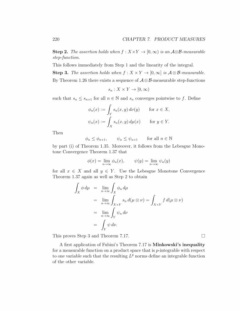
220 CHAPTER 7. PRODUCT MEASURES
Step 2. The assertion holds when f : X×Y → [0,∞) is an A⊗B-measurablestep-function.
This follows immediately from Step 1 and the linearity of the integral.
Step 3. The assertion holds when f : X × Y → [0,∞] is A⊗B-measurable.
By Theorem 1.26 there exists a sequence of A⊗B-measurable step-functions
sn : X × Y → [0,∞)
such that sn ≤ sn+1 for all n ∈ N and sn converges pointwise to f . Define
φn(x) :=
∫Y
sn(x, y) dν(y) for x ∈ X,
ψn(x) :=
∫X
sn(x, y) dµ(x) for y ∈ Y.
Thenφn ≤ φn+1, ψn ≤ ψn+1 for all n ∈ N
by part (i) of Theorem 1.35. Moreover, it follows from the Lebesgue Mono-tone Convergence Theorem 1.37 that
φ(x) = limn→∞
φn(x), ψ(y) = limn→∞
ψn(y)
for all x ∈ X and all y ∈ Y . Use the Lebesgue Monotone ConvergenceTheorem 1.37 again as well as Step 2 to obtain∫
X
φ dµ = limn→∞
∫X
φn dµ
= limn→∞
∫X×Y
sn d(µ⊗ ν) =
∫X×Y
f d(µ⊗ ν)
= limn→∞
∫Y
ψn dν
=
∫Y
ψ dν.
This proves Step 3 and Theorem 7.17.
A first application of Fubini’s Theorem 7.17 is Minkowski’s inequalityfor a measurable function on a product space that is p-integrable with respectto one variable such that the resulting Lp norms define an integrable functionof the other variable.
7.3. FUBINI’S THEOREM 221
Theorem 7.19 (Minkowski). Fix a constant 1 ≤ p < ∞. Let (X,A, µ)and (Y,B, ν) be σ-finite measure spaces and let f : X×Y → [0,∞] be A⊗B-measurable. Then(∫
X
(∫Y
f(x, y) dν(y)
)pdµ(x)
)1/p
≤∫Y
(∫X
f(x, y)p dµ(x)
)1/p
dν(y).
In the notation fx(y) := f y(x) := f(x, y) Minkowski’s inequality has the form(∫X
‖fx‖pL1(ν) dµ(x)
)1/p
≤∫Y
‖f y‖Lp(µ) dν(y). (7.13)
Proof. By Lemma 7.2 fx : Y → [0,∞] is B-measurable for all x ∈ X andfy : X → [0,∞] is A-measurable for all y ∈ Y . Moreover, by Theorem 7.17,the function X → [0,∞] : x 7→ ‖fx‖pL1(ν) is A-measurable and the function
Y → [0,∞] : y 7→ ‖f y‖Lp(µ) is B-measurable. Hence both sides of theinequality (7.13) are well defined. Theorem 7.17 also shows that for p = 1equality holds in (7.13). Hence assume 1 < p <∞ and a choose 1 < q <∞such that 1/p+ 1/q = 1. It suffices to assume
c :=
∫Y
‖f y‖Lp(µ) dν(y) <∞.
Define φ : X → [0,∞] by
φ(x) :=
∫Y
fx dν for x ∈ X
and let g ∈ Lq(µ). Then the function X×Y → [0,∞] : (x, y) 7→ f(x, y)|g(x)|is A⊗ B-measurable. Hence it follows from Theorem 7.17 that∫
X
φ|g| dµ =
∫X
(∫Y
f(x, y)|g(x)| dν(y)
)dµ(x)
=
∫Y
(∫X
f(x, y)|g(x)| dµ(x)
)dν(y)
≤∫Y
‖f y‖Lp(µ) ‖g‖Lq(µ) dν(y)
= c ‖g‖Lq(µ) .
Here the third step follows from Holder’s inequality in Theorem 4.1. Since(X,A, µ) is semi-finite by part (ii) of Lemma 4.30, it follows from Lemma 4.34that ‖φ‖Lp(µ) ≤ c. This proves Theorem 7.19.
222 CHAPTER 7. PRODUCT MEASURES
Theorem 7.20 (Fubini for Integrable Functions). Let (X,A, µ) and(Y,B, ν) be σ-finite measure spaces, let µ⊗ν : A⊗B → [0,∞] be the productmeasure, and let f ∈ L1(µ⊗ ν). Define fx(y) := f y(x) := f(x, y) for x ∈ Xand y ∈ Y . Then the following holds.
(i) fx ∈ L1(ν) for µ-almost every x ∈ X and the map φ : X → R defined by
φ(x) :=
∫Yfx dν, if fx ∈ L1(ν),
0, if fx /∈ L1(ν),(7.14)
is µ-integrable.
(ii) f y ∈ L1(µ) for ν-almost every y ∈ Y and the map ψ : Y → R defined by
ψ(y) :=
∫Xf y dµ, if f y ∈ L1(µ),
0, if f y /∈ L1(µ),(7.15)
is ν-integrable.
(iii) Let φ ∈ L1(µ) and ψ ∈ L1(ν) be as in (i) and (ii). Then∫X
φ dµ =
∫X×Y
f d(µ⊗ ν) =
∫Y
ψ dν. (7.16)
Proof. We prove part (i) and the first equation in (7.16). The functionsf± := max±f, 0 : X×Y → [0,∞) are A×B-measurable by Theorem 1.24.Hence the functions f±x := max±fx, 0 = f±(x, ·) : Y → [0,∞) are B-measurable by Lemma 7.2. Define Φ± : Y → [0,∞] by
Φ±(x) :=
∫Y
f±x dν for x ∈ X.
By Theorem 7.17 the functions Φ± : X → [0,∞] are A-measurable and∫X
Φ± dµ =
∫X×Y
f± d(µ⊗ ν) ≤∫X×Y|f | d(µ⊗ ν) <∞. (7.17)
Now Lemma 1.47 asserts that the A-measurable set
E :=
x ∈ X
∣∣∣∣ ∫Y
|fx| dν =∞
=
x ∈ X
∣∣∣∣Φ+(x) =∞ or Φ−(x) =∞
has measure µ(E) = 0. Moreover, for all x ∈ X,
x ∈ E ⇐⇒ fx /∈ L1(ν).
7.3. FUBINI’S THEOREM 223
Define φ± : X → [0,∞) by
φ±(x) :=
Φ±(x), if x /∈ E,0, if x ∈ E, for x ∈ X.
Then it follows from (7.17) that φ± ∈ L1(µ) and∫X
φ± dµ =
∫X×Y
f± d(µ⊗ ν).
Hence φ = φ+ − φ− ∈ L1(µ) and∫X
φ dµ =
∫X
φ+ dµ−∫X
φ− dµ
=
∫X×Y
f+ d(µ⊗ ν)−∫X×Y
f− d(µ⊗ ν)
=
∫X×Y
f d(µ⊗ ν).
This proves (i) and the first equation in (7.16). An analogous argumentproves (ii) and the second equation in (7.16). This proves Theorem 7.20.
Example 7.21. Let (X,A, µ) = (Y,B, ν) be the Lebesgue measure spacein the unit interval [0, 1] as in Example 7.12. Let gn : [0, 1] → [0,∞) be asequence of smooth functions such that∫ 1
0
gn(x) dx = 1, gn(x) = 0 for x ∈ [0, 1] \ [2−n−1, 2−n]
for all n ∈ N. Define f : [0, 1]2 → R by
f(x, y) :=∞∑n=1
(gn(x)− gn+1(x)
)gn(y).
The sum on the right is finite for every pair (x, y) ∈ [0, 1]2. Then∫X
f(x, y) dx = 0,
∫Y
f(x, y) dy =∞∑n=1
(gn(x)− gn+1(x)
)= g1(x),
and hence∫ 1
0
(∫ 1
0
f(x, y) dx
)dy = 0 6= 1 =
∫ 1
0
(∫ 1
0
f(x, y) dy
)dx.
Thus the hypothesis f ∈ L1(µ⊗ ν) cannot be removed in Theorem 7.20.
224 CHAPTER 7. PRODUCT MEASURES
Example 7.22. This example shows that the product measure is typicallynot complete. Let (X,A, µ) and (Y,B, ν) be two complete σ-finite measurespaces. Suppose (X,A, µ) admits a nonempty null set A ∈ A and B 6= 2Y .Choose B ∈ 2Y \ B. Then A× B /∈ A⊗ B. However, A× B is contained inthe µ⊗ ν-null set A× Y and so belongs to the completion (A⊗ B)∗.
In the first version of Fubini’s Theorem integrability was not an issue. Inthe second version integrability of fx was only guaranteed for almost all x.In the third version the function fx may not even be measurable for all x.
Theorem 7.23 (Fubini for the Completion). Let (X,A, µ) and (Y,B, ν)be complete σ-finite measure spaces, let (X × Y, (A ⊗ B)∗, (µ ⊗ ν)∗) de-note the completion of the product space, and let f ∈ L1((µ ⊗ ν)∗). Definefx(y) := f y(x) := f(x, y) for x ∈ X and y ∈ Y . Then the following holds.
(i) fx ∈ L1(ν) for µ-almost every x ∈ X and the map φ : X → R defined by
φ(x) :=
∫Yfx dν, if fx ∈ L1(ν),
0, if fx /∈ L1(ν),(7.18)
is µ-integrable.
(ii) f y ∈ L1(µ) for ν-almost every y ∈ Y and the map ψ : Y → R defined by
ψ(y) :=
∫Xf y dµ, if f y ∈ L1(µ),
0, if f y /∈ L1(µ),(7.19)
is ν-integrable.
(iii) Let φ ∈ L1(µ) and ψ ∈ L1(ν) be as in (i) and (ii). Then∫X
φ dµ =
∫X×Y
f d(µ⊗ ν)∗ =
∫Y
ψ dν. (7.20)
Proof. By part (v) of Theorem 1.55 there exists a function g ∈ L1(µ ⊗ ν)such that the set N := (x, y) ∈ X × Y | f(x, y) 6= g(x, y) ∈ (A ⊗ B)∗ hasmeasure zero, i.e. (µ ⊗ ν)∗(N) = 0. By definition of the completion thereexists a set Q ∈ A⊗ B such that N ⊂ Q and (µ⊗ ν)(Q) = 0. Thus∫
X
ν(Qx) dµ(x) =
∫Y
µ(Qy) dν(y) = 0.
Hence, by Lemma 1.49,
µ(E) = 0, E :=x ∈ X
∣∣ ν(Qx) 6= 0,
ν(F ) = 0, F :=y ∈ Y
∣∣µ(Qy) 6= 0.
7.3. FUBINI’S THEOREM 225
Since f = g on (X × Y ) \ Q we have fx = gx on Y \ Qx for all x ∈ X andf y = gy on X \ Qy for all y ∈ Y . By Theorem 7.20 for g ∈ L1(µ ⊗ ν) thereare measurable sets E ′ ∈ A and F ′ ∈ B such that µ(E ′) = ν(F ′) = 0 and
gx ∈ L1(ν) for all x ∈ X \ E ′,gy ∈ L1(µ) for all y ∈ Y \ F ′.
If x ∈ X \ (E ∪ E ′) then ν(Qx) = 0 and fx = gx on Y \ Qx. Since (Y,B, ν)is complete and gx ∈ L1(ν), every function that differs from gx on a set ofmeasure zero is also B-measurable and ν-integrable. Hence fx ∈ L1(ν) forall x ∈ X \ (E ∪ E ′). The same argument shows that f y ∈ L1(µ) for ally ∈ Y \ (F ∪ F ′). Define the functions φ : X → R and ψ : Y → R by
φ(x) :=
∫Yfx dν, for x ∈ X \ (E ∪ E ′),
0, for x ∈ E ∪ E ′,
ψ(y) :=
∫Xf y dν, for y ∈ Y \ (F ∪ F ′),
0, for y ∈ F ∪ F ′.
Since φ(x) =∫Ygx dν for all x ∈ X \ (E ∪ E ′) it follows from part (i) of The-
orem 7.20 for g that φ ∈ L1(µ). The same argument, using part (ii) of Theo-rem 7.20 for g, shows that ψ ∈ L1(ν). Moreover, the three integrals in (7.20)for f agree with the corresponding integrals for g because
µ(E ∪ E ′) = ν(F ∪ F ′) = (µ⊗ ν)(Q) = 0.
Hence equation (7.20) for f follows from part (iii) of Theorem 7.20 for g.This proves Theorem 7.23.
Example 7.24. Assume (X,A, µ) is not complete. Then there exists a setE ∈ 2X \ A and a set N ∈ A such that E ⊂ N and µ(N) = 0. In this casethe set E × Y is a null set in the completion (X × Y, (A ⊗ B)∗, (µ ⊗ ν)∗).Hence f := χE×Y ∈ L1((µ ⊗ ν)∗). However, the function f y = χE is notmeasurable for every y ∈ Y . This shows that the hypothesis that (X,A, µ)and (Y,B, ν) are complete cannot be removed in Theorem 7.23.
Exercise 7.25. Continue the notation of Theorem 7.23 and suppose thatf : X × Y → [0,∞] is (A⊗ B)∗-measurable. Prove that fx is B-measurablefor µ-almost all x ∈ X, that f y is A-measurable for ν-almost all y ∈ Y , andthat equation (7.11) continues to hold. Hint: The proof of Theorem 7.23carries over verbatim to nonnegative measurable functions.
226 CHAPTER 7. PRODUCT MEASURES
We close this section with two remarks about the construction of productmeasures in the non σ-finite case, where the story is considerably more subtle.These remarks are not used elsewhere in this book and can safely be ignored.
Remark 7.26. Let (X,A, µ) and (Y,B, ν) be two arbitrary measure spaces.In [4, Chapter 251] Fremlin defines the function θ : 2X×Y → [0,∞] by
θ(W ) := inf
∞∑n=1
µ(An) · µ(Bn)
∣∣∣∣ An ∈ A, Bn ∈ B for n ∈ Nand W ⊂
⋃∞n=1
(An ×Bn
) (7.21)
for W ⊂ X × Y and proves that it is an outer measure. He shows thatthe σ-algebra C ⊂ 2X×Y of θ-measurable sets contains the product σ-algebraA⊗ B and calls the measure
λ1 := θ|C : C → [0,∞]
the primitive product measure. By Caratheodory’s Theorem 2.4 themeasure space (X × Y, C, λ1) is complete. By definition
λ1(A×B) = µ(A) · ν(B)
for all A ∈ A and all B ∈ B. Fremlin then defines the complete locallydetermined (CLD) product measure λ0 : C → [0,∞] by
λ0(W ) := sup
λ1
(W ∩ (E × F )
) ∣∣∣∣ E ∈ A, F ∈ B,µ(E) <∞, ν(F ) <∞
. (7.22)
He shows that (X ×Y, C, λ0) is a complete measure space, that λ0 ≤ λ1, and
λ1(W ) <∞ =⇒ λ0(W ) = λ1(W )
for all W ∈ C. (See [4, Theorem 251I].) One can also prove that a measureλ : C → [0,∞] satisfies λ(E × F ) = µ(E) · ν(F ) for all E ∈ A and F ∈ Bwith µ(E) · ν(F ) < ∞ if and only if λ0 ≤ λ ≤ λ1. With these definitionsFubini’s Theorem holds for λ0 whenever the factor (Y,B, ν) (over which theintegral is performed first) is σ-finite and the factor (X,A, µ) (over whichthe integral is performed second) is either strictly localizable (i.e. thereis a partition X =
⋃i∈I Xi into measurable sets with µ(Xi) < ∞ such that
a set A ⊂ X is A-measurable if and only if A ∩ Xi ∈ A for all i ∈ Iand, moreover, µ(A) =
∑i∈I µ(A ∩ Xi) for all A ∈ A) or is complete and
locally determined (i.e. it is semi-finite and a set A ⊂ X is A-measurableif and only if A ∩ E ∈ A for all E ∈ A with µ(E) < ∞). See Fremlin [4,Theorem 252B] for details.
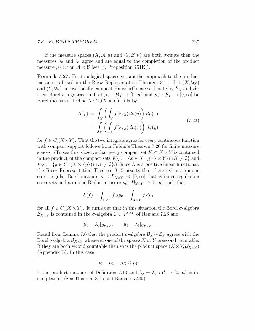
7.3. FUBINI’S THEOREM 227
If the measure spaces (X,A, µ) and (Y,B, ν) are both σ-finite then themeasures λ0 and λ1 agree and are equal to the completion of the productmeasure µ⊗ ν on A⊗ B (see [4, Proposition 251K]).
Remark 7.27. For topological spaces yet another approach to the productmeasure is based on the Riesz Representation Theorem 3.15. Let (X,UX)and (Y,UY ) be two locally compact Hausdorff spaces, denote by BX and BYtheir Borel σ-algebras, and let µX : BX → [0,∞] and µY : BY → [0,∞] beBorel measures. Define Λ : Cc(X × Y )→ R by
Λ(f) :=
∫X
(∫Y
f(x, y) dν(y)
)dµ(x)
=
∫Y
(∫X
f(x, y) dµ(x)
)dν(y)
(7.23)
for f ∈ Cc(X×Y ). That the two integrals agree for every continuous functionwith compact support follows from Fubini’s Theorem 7.20 for finite measurespaces. (To see this, observe that every compact set K ⊂ X×Y is containedin the product of the compact sets KX := x ∈ X | (x × Y ) ∩K 6= ∅ andKY := y ∈ Y | (X × y) ∩K 6= ∅.) Since Λ is a positive linear functional,the Riesz Representation Theorem 3.15 asserts that there exists a uniqueouter regular Borel measure µ1 : BX×Y → [0,∞] that is inner regular onopen sets and a unique Radon measure µ0 : BX×Y → [0,∞] such that
Λ(f) =
∫X×Y
f dµ0 =
∫X×Y
f dµ1
for all f ∈ Cc(X ×Y ). It turns out that in this situation the Borel σ-algebraBX×Y is contained in the σ-algebra C ⊂ 2X×Y of Remark 7.26 and
µ0 = λ0|BX×Y , µ1 = λ1|BX×Y .
Recall from Lemma 7.6 that the product σ-algebra BX ⊗BY agrees with theBorel σ-algebra BX×Y whenever one of the spaces X or Y is second countable.If they are both second countable then so is the product space (X×Y,UX×Y )(Appendix B). In this case
µ0 = µ1 = µX ⊗ µY
is the product measure of Definition 7.10 and λ0 = λ1 : C → [0,∞] is itscompletion. (See Theorem 3.15 and Remark 7.26.)
228 CHAPTER 7. PRODUCT MEASURES
7.4 Fubini and Lebesgue
For n ∈ N denote by (Rn,An,mn) the Lebesgue measure space on Rn and byBn ⊂ An the Borel σ-algebra on Rn with respect to the standard topology.For k, ` ∈ N we identify Rk+` with Rk×R` in the standard manner. Since Rn
is second countable for all n it follows from Lemma 7.6 and Theorem 2.1 that
Bk ⊗ B` = Bk+`, (mk|Bk)⊗ (m`|B`) = mk+`|Bk+`. (7.24)
(See Exercise 7.16.) Thus Theorem 7.17 has the following consequence.
Theorem 7.28 (Fubini and Borel). Let k, ` ∈ N and n := k + `. Letf : Rn → [0,∞] be Borel measurable. Then fx := f(x, ·) : R` → [0,∞] andf y := f(·, y) : Rk → [0,∞] are Borel measurable for all x ∈ Rk and ally ∈ R`. Moreover, the functions Rk → [0,∞] : x 7→
∫R` f(x, y) dm`(y) and
R` → [0,∞] : y 7→∫Rk f(x, y) dmk(x) are Borel measurable and∫
Rnf dmn =
∫Rk
(∫R`f(x, y) dm`(y)
)dmk(x)
=
∫R`
(∫Rkf(x, y) dmk(x)
)dm`(y).
(7.25)
Proof. The assertion follows directly from (7.24) and Theorem 7.17.
For Lebesgue measurable functions f : Rn → [0,∞] the analogous state-ment is considerably more subtle. In that case the function fx, respec-tively f y, need not be Lebesgue measurable for all x, respectively all y.However, they are Lebesgue measurable for almost all x ∈ Rk, respectivelyalmost all y ∈ R`, and the three integrals in (7.25) can still be defined andagree. The key result that one needs to prove this is that the Lebesguemeasure on Rn = Rk × R` is the completion of the product of the Lebesguemeasures on Rk and R`. Then the assertion follows from Exercise 7.25.
Theorem 7.29. Let k, ` ∈ N, define n := k + `, and identify Rn with theproduct space Rk × R` in the canonical way. Denote the completion of theproduct space (Rk×R`,Ak⊗A`,mk⊗m`) by (Rk×R`, (Ak⊗A`)∗, (mk⊗m`)
∗).Then An = (Ak ⊗A`)∗ and mn = (mk ⊗m`)
∗.
Proof. Define
Cn :=
[a1, b1)× · · · × [an, bn)∣∣∣ ai, bi ∈ R and ai < bi for i = 1, . . . , n
so that Cn ⊂ Bn ⊂ An ⊂ 2Rn for all n. We prove the assertion in three steps.
7.4. FUBINI AND LEBESGUE 229
Step 1. Bn ⊂ Ak ⊗A` and mn(B) = (mk ⊗m`)(B) for all B ∈ Bn.
By Lemma 7.6 we have Bn = Bk ⊗ B` ⊂ Ak ⊗ A`. It then follows fromthe uniqueness of a normalized translation invariant Borel measure on Rn inTheorem 2.1 that mn|Bn = (mk ⊗m`)|Bn . Here is a more direct proof.
First, assume B = E = [a1, b1)× · · · × [an, bn) ∈ Cn. Define
E ′ := [a1, b1)× · · · × [ak, bk), E ′′ := [ak+1, bk+1)× · · · × [an, bn).
Thus E ′ ∈ Ck ⊂ Ak, E ′′ ∈ C` ⊂ A`, and so E = E ′×E ′′ ∈ Ak⊗A`. Moreover
mn(E) =n∏i=1
(bi − ai) = mk(E′) ·m`(E
′′) = (mk ⊗m`)(E).
Second, assume B = U ⊂ Rn is open. Then there is a sequence of pairwisedisjoint sets Ei ∈ Cn such that U =
⋃∞i=1Ei. Hence U ∈ Ak ⊗A` and
(mk ⊗m`)(U) =∞∑i=1
(mk ⊗m`)(Ei) =∞∑i=1
mn(Ei) = mn(U).
Thus every open set is an element of Ak ⊗A` and so Bn ⊂ Ak ⊗A`. Third,assume B = K ⊂ Rn is compact. Then there is an open set U ⊂ Rn suchthat K ⊂ U and mn(U) < ∞. Hence the set V := U \ K is open. Thisimplies that K = U \ V ∈ Ak ⊗A` and
(mk ⊗m`)(K) = (mk ⊗m`)(U)− (mk ⊗m`)(V )
= mn(U)−mn(V )
= mn(K).
Now let B ⊂ Rn be any Borel set. Then B ∈ Ak⊗A` as we have seen above.Moreover, it follows from Theorem 2.13 that
mn(B) = infU⊃B
U is open
mn(U) = infU⊃B
U is open
(mk ⊗m`)(U) ≥ (mk ⊗m`)(B)
and
mn(B) = infK⊂B
K is compact
mn(K) = infK⊂B
K is compact
(mk ⊗m`)(K) ≤ (mk ⊗m`)(B).
Hence mn(B) = (mk ⊗m`)(B) and this proves Step 1.
230 CHAPTER 7. PRODUCT MEASURES
Step 2. Ak ⊗A` ⊂ An.
We prove thatE ∈ Ak =⇒ E × R` ∈ An. (7.26)
To see this, fix a set E ∈ Ak. Then there exist Borel sets A,B ∈ Bk such thatA ⊂ E ⊂ B and mk(B \A) = 0. Let π : Rn ×Rk denote the projection ontothe first k coordinates. This map is continuous and hence Borel measurableby Theorem 1.20. Thus the sets A×R` = π−1(A) and B ×R` = π−1(B) areBorel sets in Rn. Moreover, by Step 1
mn((B × R`) \ (A× R`)) = mn((B \ A)× R`)
= (mk ⊗m`)((B \ A)× R`)
= mk(B \ A) ·m`(R`)
= 0.
Since A × R` ⊂ E × R` ⊂ B × R` it follows that E × R` ∈ An. Thisproves (7.26). A similar argument shows that
F ∈ A` =⇒ Rk × F ∈ An.
Hence E × F = (E × R`) ∩ (Rk × F ) ∈ An for all E ∈ Ak and all F ∈ A`.Thus Ak ⊗A` ⊂ An and this proves Step 2.
Step 3. (Ak ⊗A`)∗ = An and (mk ⊗m`)∗ = mn.
Let A ∈ An. Then there are Borel sets B0, B1 ∈ Bn such that B0 ⊂ A ⊂ B1
andmn(B1\B0) = 0. By Step 1, B0, B1 ∈ Ak⊗A` and (mk⊗m`)(B1\B0) = 0.Hence A ∈ (Ak ⊗A`)∗ and
(mk ⊗m`)∗(A) = (mk ⊗m`)(B0) = mn(B0) = mn(A).
Thus we have proved that
An ⊂ (Ak ⊗A`)∗, (mk ⊗m`)∗|An = mn.
Since Ak ⊗A` ⊂ An by Step 2 it follows that
mn|Ak⊗A` = (mk ⊗m`)∗|Ak⊗A` = mk ⊗m`.
Now let A ∈ (Ak ⊗ A`)∗. Then there are sets A0, A1 ∈ Ak ⊗ A` such thatA0 ⊂ A ⊂ A1 and (mk⊗m`)(A1 \A0) = 0. Hence A0, A1 ∈ An by Step 2 andmn(A1 \A0) = 0. Since (Rn,An,mn) is complete it follows that A \A0 ∈ Anand so A = A0 ∪ (A \A0) ∈ An. Hence An = (Ak⊗A`)∗. This proves Step 3and Theorem 7.29.

7.5. CONVOLUTION 231
The next result specializes Theorem 7.23 to the Lebesgue measure.
Theorem 7.30 (Fubini and Lebesgue). Let k, ` ∈ N and n := k + `.Let f : Rn → R be Lebesgue integrable and, for x = (x1, . . . , xk) ∈ Rk andy = (y1, . . . , y`) ∈ R`, define fx(y) := f y(x) := f(x1, . . . , xk, y1, . . . , y`). Thenthere are Lebesgue null sets E ⊂ Rk and F ⊂ R` such that the following holds.
(i) fx ∈ L1(R`) for every x ∈ Rk \ E and the map φ : Rk → R defined by
φ(x) :=
∫R` fx dm`, for x ∈ Rk \ E,
0, for x ∈ E, (7.27)
is Lebesgue integrable.
(ii) f y ∈ L1(Rk) for every y ∈ R` \ F and the map ψ : R` → R defined by
ψ(y) :=
∫Rk f
y dmk, for y ∈ R` \ F,0, for y ∈ F, (7.28)
is Lebesgue integrable.
(iii) Let φ ∈ L1(µ) and ψ ∈ L1(ν) be as in (i) and (ii). Then∫Rkφ dmk =
∫Rnf dmn =
∫R`ψ dm`. (7.29)
Proof. This follows directly from Theorem 7.23 and Theorem 7.29.
7.5 Convolution
An application of Fubini’s Theorem is the convolution product on the spaceof Lebesgue integrable functions on Euclidean space. Fix an integer n ∈ Nand let (Rn,A,m) be the Lebesgue measure space. The convolution of twoLebesgue integrable functions f, g ∈ L1(Rn) is defined by
(f ∗ g)(x) :=
∫Rnf(x− y)g(y) dm(y) for almost all x ∈ Rn.
Here the function Rn → R : y 7→ f(x− y)g(y) is Lebesgue integrable for al-most every x ∈ Rn and the resulting almost everywhere defined function f ∗ gis again Lebesgue integrable. This is the content of Theorem 7.33. The con-volution descends to a bilinear map ∗ : L1(Rn) × L1(Rn) → L1(Rn). Thismap is associative and endows L1(Rn) with the structure of a Banach alge-bra. Throughout we use the notation f ∼ g for two Lebesgue measurablefunctions f, g : Rn → R to mean that they agree almost everywhere withrespect to the Lebesgue measure.
232 CHAPTER 7. PRODUCT MEASURES
Definition 7.31. Let f, g : Rn → R be Lebesgue measurable and define
E(f, g) :=
x ∈ Rn
∣∣∣∣ the function Rn → R : y 7→ f(x− y)g(y)is not Lebesgue integrable
. (7.30)
The convolution of f and g is the function f ∗ g : Rn → R defined by
(f ∗ g)(x) :=
∫Rnf(x− y)g(y) dm(y) for x ∈ Rn \ E(f, g) (7.31)
and by (f ∗ g)(x) := 0 for x ∈ E(f, g).
The next theorem shows that the convolution is very robust in that f ∗ gis always Borel measurable and depends only on the equivalence classes of fand g under equality almost everywhere.
Theorem 7.32. Let f, g, h, f ′, g′ : Rn → R be Lebesgue measurable. Thenthe following holds.
(i) The function y 7→ f(x− y)g(y) is Lebesgue measurable for all x ∈ Rn.
(ii) If f ′ ∼ f and g′ ∼ g then E(f ′, g′) = E(f, g) and f ′ ∗ g′ = f ∗ g.
(iii) E(f, g) is a Borel set and f ∗ g is Borel measurable.
(iv) E(g, f) = E(f, g) and g ∗ f = f ∗ g.
(v) If m(E(f, g)) = m(E(g, h)) = 0 then
E := E(|f |, |g| ∗ |h|) = E(|f | ∗ |g|, |h|)and f ∗ (g ∗ h) = (f ∗ g) ∗ h on Rn \ E.
An example with n = 1, where E(f, g ∗ h) = E(f ∗ g, h) = ∅ and E = Rin part (v) of Theorem 7.32, is discussed in Exercise 7.53 below.
Proof of Theorem 7.32. We prove (i). For x ∈ Rn define fx : Rn → Rand φx : Rn → Rn by fx(y) := f(x − y) and φx(y) := x − y. Then φxis a diffeomorphism and |det(dφx)| ≡ 1. Hence Theorem 2.17 asserts thatfx = f φx is Lebesgue measurable for all x ∈ Rn and this proves (i).
We prove (ii). By assumption the sets
A := y ∈ Rn | f(y) 6= f ′(y) , B := y ∈ Rn | g(y) 6= g′(y) .are Lebesgue null sets. Hence so are the sets
Cx := φx(A) ∪B = y ∈ Rn | f(x− y) 6= f ′(x− y) or g(y) 6= g′(y)for all x ∈ Rn. Hence the functions fxg and f ′xg
′ agree on the complement ofa Lebesgue null set for every x ∈ Rn. Hence they are either both integrable orboth not integrable and when they are their integrals agree. This proves (ii).

7.5. CONVOLUTION 233
We prove (iii). By (ii) and Theorem 1.55 it suffices to assume that f andg are Borel measurable. Now define F,G : R2n → R and φ : R2n → R2n by
F (x, y) := f(x− y)g(y),
G(x, y) := f(x)g(y),
φ(x, y) := (x− y, y)
for x, y ∈ Rn. Then G is Borel measurable and φ is a diffeomorphism. Henceφ preserves the Borel σ-algebra and this implies that
F = G φ
is Borel measurable. Hence the function
Rn → [0,∞] : x 7→∫Rn|F (x, y)| dm(y),
is Borel measurable by Fubini’s Theorem 7.28. Thus the set E(f, g) wherethis function takes on the value ∞ is a Borel set. Moreover, the functions
F± := max±F, 0
are Borel measurable and so are the functions F± : R2n → [0,∞) defined by
F±(x, y) :=
F±(x, y), if x ∈ Rn \ E(f, g),0, if x ∈ E(f, g),
for (x, y) ∈ R2n.
Since
(f ∗ g)(x) =
∫RnF+(x, y) dm(y)−
∫RnF−(x, y) dm(y)
for all x ∈ Rn it follows from Theorem 7.28 that f ∗ g is Borel measurable.This proves (iii).
We prove (iv). Since gxf = (fxg) φx it follows from Theorem 2.17 that
E(g, f) =x ∈ Rn | gxf ∈ L1(Rn)
= E(f, g)
and
(f ∗ g)(x) =
∫Rnfxg dm =
∫Rn
(fxg) φx dm =
∫Rngxf dm = (g ∗ f)(x)
for all x ∈ Rn \ E(f, g). This proves (iv).
234 CHAPTER 7. PRODUCT MEASURES
We prove (v). By (ii) and Theorem 1.55 it suffices to assume that f , g,and h are Borel measurable. Let x ∈ Rn and define Fx : R2n → R by
Fx(y, z) := f(z)g(x− y − z)h(y).
Thus Fx is the composition of the maps R2n → R3n : (y, z) 7→ (z, x−y−z, y)and R3n → R : (ξ, η, ζ) 7→ (f(ξ), g(η), h(ζ)). Since the first map is continuousand the second is Borel measurable it follows that Fx is Borel measurable.We claim that
x ∈ E(|f |, |g| ∗ |h|) ⇐⇒∫R2n
|Fx| =∞ ⇐⇒ x ∈ E(|f | ∗ |g|, |h|). (7.32)
It follows from Theorem 7.28 that∫R2n
|Fx| dm2n =
∫Rn
(∫Rn|Fx(y, z)| dm(y)
)dm(z).
This integral is finite if and only if Fx ∈ L1(R2n). Moreover,∫Rn|Fx(y, z)| dm(y) = |f(z)|
∫Rn|g(x− y − z)||h(y)| dm(y)
= |f(z)|(|g| ∗ |h|)(x− z)
for z ∈ Rn \ (x−E(g, h)). Since E(g, h) is a Lebesgue null set it follows that
‖Fx‖L1(R2n) =
∫Rn|f(z)|(|g| ∗ |h|)(x− z) dm(z).
The integral on the right is infinite if and only if x ∈ E(|f |, |g| ∗ |h|). Thisproves the first equivalence in (7.32). The proof of the second equivalence isanalogous with y and z interchanged.
Now let x ∈ Rn \ E. Then Fx ∈ L1(R2n) and x ∈ Rn \ E(f, g ∗ h).Moreover, for z ∈ Rn, the function Rn → R : y 7→ Fx(y, z) is integrable ifand only x− z /∈ E(g, h) and in that case its integral is equal to∫
RnFx(y, z) dm(y) = f(z)
∫Rng(x− y − z)h(y) dm(y) = f(z)(g ∗ h)(x− z).
Since E(g, h) is a Lebesgue null set, it follows from Theorem 7.30 that∫R2n
Fx dm2n =
∫Rnf(z)(g ∗ h)(x− z) dm(z) = (f ∗ (g ∗ h))(x)
The last equation holds because x /∈ E(f, g ∗ h). A similar argument with yand z interchanged shows that
∫R2n Fx dm2n = ((f∗g)∗h)(x) for all x ∈ Rn\E.
This proves (v) and Theorem 7.32.
7.5. CONVOLUTION 235
Theorem 7.33. Let 1 ≤ p, q, r ≤ ∞ such that 1/p + 1/q = 1 + 1/r and letf ∈ Lp(Rn) and g ∈ Lq(Rn). Then m(E(f, g)) = 0 and
‖f ∗ g‖r ≤ ‖f‖p ‖g‖q . (7.33)
Thus f ∗ g ∈ Lr(Rn). The estimate (7.33) is called Young’s inequality.
Proof. Define the function h : Rn → [0,∞] by
h(x) :=
∫Rn|f(x− y)g(y)| dm(y) for x ∈ Rn.
Then |f ∗ g| ≤ h and E(f, g) = x ∈ Rn |h(x) =∞. Hence it suffices toprove that ‖h‖r ≤ ‖f‖p ‖g‖q. For r =∞ this follows from Holder’s inequality.So assume r <∞. Then 1 ≤ p, q <∞. Define
λ := 1− p
r= p− p
q, q′ :=
p
λ.
Then 0 ≤ λ < 1 and 1/q+ 1/q′ = 1. Also λ = 0 if and only if q = 1. If λ > 0then Holder’s inequality in Theorem 4.1 shows that
h(x) =
∫Rn|fx|λ|fx|1−λ|g| dm ≤
∥∥|fx|λ∥∥q′ ∥∥|fx|1−λ|g|∥∥q ,where fx(y) := f(x− y). Since λq′ = p this implies
h(x)q ≤(∫
Rn|fx|λq
′dm
)q/q′ ∫Rn|fx|(1−λ)q|g|q dm
= ‖f‖λqp∫Rn|f(x− y)|(1−λ)q|g(y)|q dm(y)
(7.34)
for all x ∈ Rn. This continues to hold for λ = 0. Now it follows fromMinkowski’s inequality in Theorem 7.19 with the exponent s := r/q ≥ 1 that
‖h‖qr =
(∫Rnhr dm
)q/r=
(∫Rnhqs dm
)1/s
≤ ‖f‖λqp(∫
Rn
(∫Rn|f(x− y)|(1−λ)q|g(y)|q dm(y)
)sdm(x)
)1/s
≤ ‖f‖λqp∫Rn
(∫Rn|f(x− y)|(1−λ)qs|g(y)|qs dm(x)
)1/s
dm(y)
= ‖f‖λqp ‖f‖(1−λ)qp ‖g‖qq .
Here the last equation follows from the fact that (1 − λ)qs = (1 − λ)r = p.This proves Theorem 7.33.
236 CHAPTER 7. PRODUCT MEASURES
It follows from Theorem 7.33 and part (ii) of Theorem 7.32 that theconvolution descends to a map
L1(Rn)× L1(Rn)→ L1(Rn) : (f, g) 7→ f ∗ g. (7.35)
This map is bilinear by Theorem 1.44, it is associative by part (v) of Theo-rem 7.32, and satisfies ‖f ∗ g‖1 ≤ ‖f‖1 ‖g‖1 by Young’s inequality in Theo-rem 7.33. Hence L1(Rn) is a Banach algebra. By part (iv) of Theorem 7.32the Banach algebra L1(Rn) is commutative and by Theorem 7.33 with q = 1and r = p it acts on Lp(Rn). (A Banach algebra is a Banach space (X , ‖·‖)equipped with an associative bilinear map X × X → X : (x, y) 7→ xy thatsatisfies the inequality ‖xy‖ ≤ ‖x‖ ‖y‖ for all x, y ∈ X .)
Definition 7.34. Fix a constant 1 ≤ p < ∞. A Lebesgue measurable func-tion f : Rn → R is called locally p-integrable if
∫K|f |pdm < ∞ for ev-
ery compact set K ⊂ Rn. It is called locally integrable if it is locallyp-integrable for p = 1.
Theorem 7.33 carries over to locally integrable functions as follows. If1/p + 1/q = 1 + 1/r, f is locally p-integrable, and g ∈ Lq(Rn) has compactsupport, then E(f, g) is a Lebesgue null set and f∗g is locally r-integrable. Tosee this, let K ⊂ Rn be any compact set and choose a compactly supportedsmooth function β such that β|K ≡ 1. Then βf ∈ Lp(Rn) and (βf)∗g agreeswith f ∗ g on the set x ∈ Rn |x− supp(g) ⊂ K. In the following theoremC∞0 (Rn) denotes the space of compactly supported smooth functions on Rn.
Theorem 7.35. Let 1 ≤ p <∞ and 1 < q ≤ ∞ such that 1/p+ 1/q = 1.
(i) If f : Rn → R is locally p-integrable then
limξ→0
∫B
|f(x+ ξ)− f(x)|p dm(x) = 0
for every bounded Lebesgue measurable subset B ⊂ Rn. If f ∈ Lp(Rn) thiscontinues to hold for B = Rn.
(ii) If f ∈ Lp(Rn) and g ∈ Lq(Rn) then f ∗ g is uniformly continuous. If fis locally p-integrable and g ∈ Lq(Rn) has compact support (or if f ∈ Lp(Rn)has compact support and g is locally q-integrable) then f ∗ g is continuous.
(iii) If f : Rn → R is locally integrable and g ∈ C∞0 (Rn) then f ∗ g is smoothand ∂α(f ∗ g) = f ∗ ∂αg for every multi-index α.
(iv) C∞0 (Rn) is dense in Lp(Rn) for 1 ≤ p <∞.
7.5. CONVOLUTION 237
Proof. We prove (i). Assume first that f ∈ Lp(Rn) and fix a constant ε > 0.By Theorem 4.15 there is a function g ∈ Cc(Rn) such that ‖f − g‖p < ε1/p/3.Since g is uniformly continuous there is a δ > 0 such that, for all ξ ∈ Rn,
|ξ| < δ =⇒ supx∈Rn|g(x+ ξ)− g(x)| <
(ε
3pm(supp(g)
)1/p
Take ξ ∈ Rn such that |ξ| < δ. Then(∫Rn|f(x+ ξ)− f(x)|p dm(x)
)1/p
≤ 2 ‖f − g‖p +
(∫Rn|g(x+ ξ)− g(x)|p dm(x)
)1/p
≤ 2ε1/p
3+
(m(supp(g)) sup
x∈Rn|g(x+ ξ)− g(x)|p
)1/p
< ε1/p.
This proves (i) for f ∈ Lp(Rn). To prove the result in general choose acompact set K ⊂ Rn such that B1(x) ⊂ K for all x ∈ B and multiply f by asmooth compactly supported cutoff function to obtain a function f ′ ∈ Lp(Rn)that agrees with f on K. Then (i) holds for f ′ and hence also for f .
We prove (ii). Assume first that f ∈ Lp(Rn) and g ∈ Lq(Rn) and fix aconstant ε > 0. By part (i) there exists a δ > 0 such that, for all ξ ∈ Rn,
|ξ| < δ =⇒∫Rn|f(y + ξ)− f(y)|p dm(y) <
(ε
‖g‖q
)p
Fix two elements x, ξ ∈ Rn such that |ξ| < δ and denote fx(y) := f(x − y).Then, by Holder’s inequality in Theorem 4.1,
|(f ∗ g)(x+ ξ)− (f ∗ g)(x)| =
∣∣∣∣∫Rn
(fx+ξ − fx)g dm∣∣∣∣
≤ ‖fx+ξ − fx‖p ‖g‖q
=
(∫Rn|f(y + ξ)− f(y)|p dm(y)
)1/p
‖g‖q< ε.
This shows that f ∗g is uniformly continuous. If f is locally p-integrable andg ∈ Lq(Rn) has compact support continuity follows by taking the integralover a suitable compact set. In the converse case continuity follows by takingthe Lq-norm of g over a suitable compact set. This proves (ii).

238 CHAPTER 7. PRODUCT MEASURES
We prove (iii). Fix an index i ∈ 1, . . . , n and denote by ei ∈ Rn the ithunit vector. Fix an element x ∈ Rn and choose a compact set K ⊂ Rn suchthat B1(y) ⊂ K whenever x−y ∈ supp(g). Let ε > 0. Since ∂ig is continuous,there is a constant 0 < δ < 1 such that |∂ig(y + hei)− ∂ig(y)| < ε/
∫K|f | dm
for all y ∈ Rn and all h ∈ R with |h| < δ. Hence the fundamental theoremof calculus asserts that
supy∈Rn
∣∣∣∣g(y + hei − y)− g(y)
h− ∂ig(y)
∣∣∣∣ < ε∫K|f | dm
for all h ∈ R with 0 < |h| < δ. Take h ∈ Rn with 0 < |h| < δ. Then∣∣∣∣(f ∗ g)(x+ hei)− (f ∗ g)(x)
h− (f ∗ ∂ig)(x)
∣∣∣∣=
∣∣∣∣∫Rnf(y)
(g(x+ hei − y)− g(x− y)
h− ∂ig(x− y)
)dm(y)
∣∣∣∣≤∫Rn|f(y)|
∣∣∣∣g(x+ hei − y)− g(x− y)
h− ∂ig(x− y) dm(y)
∣∣∣∣ < ε.
By part (ii) the function ∂i(f ∗ g) = f ∗ ∂ig is continuous for i = 1, . . . , n.For higher derivatives the assertion follows by induction. This proves (iii).
We prove (iv). Let f ∈ Lp(Rn) and choose a compactly supported smoothfunction ρ : Rn → [0,∞) such that
supp(ρ) ⊂ B1,
∫Rnρ dm = 1.
Define ρδ : Rn → R by
ρδ(x) :=1
δnρ(xδ
)for δ > 0 and x ∈ Rn. Then
supp(ρδ) ⊂ Bδ,
∫Rnρδ dm = 1
by Theorem 2.17. By part (iii) the function
fδ := ρδ ∗ f : Rn → R
is smooth for all δ > 0. Now fix a constant ε > 0. By part (i) there exists aconstant δ > 0 such that, for all y ∈ Rn,
|y| < δ =⇒∫Rn|f(x− y)− f(x)|p dm(x) < εp.
7.6. MARCINKIEWICZ INTERPOLATION 239
Hence, by Minkowski’s inequality in Theorem 7.19,
‖fδ − f‖p =
(∫Rn
∣∣∣∣∫Rn
(f(x− y)− f(x)
)ρδ(y) dm(y)
∣∣∣∣p dm(x)
)1/p
≤∫Rn
(∫Rn|f(x− y)− f(x)|pρδ(y)p dm(x)
)1/p
dm(y)
≤ sup|y|<δ
(∫Rn|f(x− y)− f(x)|p dm(x)
)1/p
≤ ε.
If f has compact support then so does fδ. If not, choose a function g ∈ Lp(Rn)with compact support such that ‖f − g‖p < ε/2 and then a smooth functionh : Rn → R with compact support such that ‖g − h‖p < ε/2. This proves (iv)and Theorem 7.35.
The method explained in the proof of part (iv) of Theorem 7.35 is calledthe mollifier technique. The functions ρδ can be viewed as approximateDirac delta functions that concentrate near the origin as δ tends to zero.
7.6 Marcinkiewicz Interpolation
Another interesting application of Fubini’s Theorem is Marcinkiewicz inter-polation which provides a criterion for a linear operator on L2(µ) to induce alinear operator on Lp(µ) for 1 < p < 2. Marcinkiewicz interpolation appliesto all measure spaces, although it is used here only for the Lebesgue measurespace on Rn. In particular, Marcinkiewicz interpolation plays a central rolein the proof of the Calderon–Zygmund inequality in Section 7.7.
Let (X,A, µ) be a measure space. For a measurable function f : X → Rdefine the function κf : [0,∞)→ [0,∞] by (6.1), i.e.
κf (t) := µ(A(t, f)), A(t, f) :=x ∈ X
∣∣ |f(x)| > t,
for t ≥ 0. The function κf is nonincreasing and hence Borel measurable.
Lemma 7.36. Let 1 ≤ p <∞ and let f, g : X → R be measurable. Then
κf+g(t) ≤ κf (t/2) + κg(t/2), (7.36)
tpκf (t) ≤∫X
|f |p dµ = p
∫ ∞0
sp−1κf (s) ds (7.37)
for all t ≥ 0.
240 CHAPTER 7. PRODUCT MEASURES
Proof. The inequality (7.36) was established in the proof of Lemma 6.2. Weprove (7.37) in four steps.
Step 1. tpκf (t) ≤∫X|f |p dµ for all t ≥ 0.
Since tpχA(t,f) ≤ |f |p it follows that tpκf (t) =∫Xtpχ(A(t,f) dµ ≤
∫X|f |p dµ for
all t ≥ 0. This proves Step 1.
Step 2. If κf (t) =∞ for some t > 0 then∫X|f |p dµ =∞ =
∫∞0tp−1κf (t) dt.
By Step 1, we have∫X|f |p dµ = ∞. Moreover, tp−1κf (t) = ∞ for t > 0
sufficiently small and hence∫∞
0tp−1κf (t) dt =∞. This proves Step 2.
Step 3. Assume (X,A, µ) is σ-finite and κf (t) < ∞ for all t > 0. Thenequation (7.37) holds.
Let B ⊂ 2[0,∞) be the Borel σ-algebra and denote by m : B → [0,∞] therestriction of the Lebesgue measure to B. Let (X × [0,∞),A⊗B, µ⊗m) bethe product measure space of Definition 7.10. We prove that
Q(f) :=
(x, t) ∈ X × [0,∞)∣∣ 0 ≤ t < |f(x)|
∈ A⊗ B.
To see this, assume first that f is an A-measurable step-function. Thenthere exist finitely many pairwise disjoint measurable sets A1, . . . , A` ∈ Aand positive real numbers α1, . . . , α` such that |f | =
∑`i=1 αiχAi . In this
case Q(f) =⋃`i=1 Ai× [0, αi) ∈ A⊗B. Now consider the general case. Then
Theorem 1.26 asserts that there is a sequence of A-measurable step-functionsfi : X → [0,∞) such that 0 ≤ f1 ≤ f2 ≤ · · · and fi converges pointwiseto |f |. Then Q(fi) ∈ A⊗ B for all i and so Q(f) =
⋃∞i=1 Q(fi) ∈ A⊗ B.
Now define h : X × [0,∞)→ [0,∞) by h(x, t) := ptp−1. This function isA⊗ B-measurable and so is hχQ(f). Hence, by Fubini’s Theorem 7.17,∫
X
|f |p dµ =
∫X
(∫ |f(x)|
0
ptp−1 dt
)dµ(x)
=
∫X
(∫ ∞0
(hχQ(f))(x, t) dm(t)
)dµ(x)
=
∫ ∞0
(∫X
(hχQ(f))(x, t) dµ(x)
)dm(t)
=
∫ ∞0
ptp−1µ(A(t, f)) dt.
This proves Step 3.

7.6. MARCINKIEWICZ INTERPOLATION 241
Step 4. Assume κf (t) <∞ for all t > 0. Then (7.37) holds.
Define X0 := x ∈ X | f(x) 6= 0, A0 :=A ∈ A
∣∣A ⊂ X0
, and µ0 := µ|A0 .
Then the measure space (X0,A0, µ0) is σ-finite because Xn := A(1/n, f) isa sequence of An-measurable sets such that µ0(Xn) = κf (1/n) <∞ for all nand X0 =
⋃∞n=1Xn. Moreover, f0 := f |X0 : X0 → R is A0-measurable and
κf = κf0 . Hence it follows from Step 3 that∫X
|f |p dµ =
∫X0
|f0|p dµ0 =
∫ ∞0
tp−1κf0(t) dt =
∫ ∞0
tp−1κf (t) dt.
This proves Step 4 and Lemma 7.36.
Fix real numbers 1 ≤ p ≤ q. Then the inequality
‖f‖p ≤ ‖f‖q−pp(q−1)
1 ‖f‖q(p−1)p(q−1)q (7.38)
in Exercise 4.44 shows that
L1(µ) ∩ Lq(µ) ⊂ Lp(µ).
Since the intersection L1(µ)∩Lq(µ) contains (the equivalences classes of) allcharacteristic functions of measurable sets with finite measure, it is dense inLp(µ) by Lemma 4.12. The following theorem was proved in 1939 by JozefMarcinkiewicz (a PhD student of Antoni Zygmund). To formulate the resultit will be convenient to slightly abuse notation and use the same letter f todenote an element of Lp(µ) and its equivalence class in Lp(µ).
Theorem 7.37 (Marcinkiewicz). Let q > 1 and let T : Lq(µ)→ Lq(µ) bea linear operator. Suppose that there exist constants c1 > 0 and cq > 0 suchthat
‖Tf‖1,∞ ≤ c1 ‖f‖1 , ‖Tf‖q ≤ cq ‖f‖q (7.39)
for all f ∈ L1(µ) ∩ Lq(µ). Fix a constant 1 < p < q. Then
‖Tf‖p ≤ cp ‖f‖p , cp := 2
(p(q − 1)
(q − p)(p− 1)
)1/p
cq−pp(q−1)
1 cq(p−1)p(q−1)q , (7.40)
for all f ∈ L1(µ)∩Lq(µ). Thus the restriction of T to L1(µ)∩Lq(µ) extends(uniquely) to a bounded linear operator from Lp(µ) to itself for 1 < p < q.
242 CHAPTER 7. PRODUCT MEASURES
Proof. Let c > 0 and let f ∈ L1(µ) ∩ L2(µ). For t ≥ 0 define
ft(x) :=
f(x), if |f(x)| > ct,0, if |f(x)| ≤ ct,
gt(x) :=
0, if |f(x)| > ct,f(x), if |f(x)| ≤ ct.
Then
A(s, ft) =
A(s, f), if s > ct,A(ct, f), if s ≤ ct,
A(s, gt) =
∅, if s ≥ ct,A(s, f) \ A(ct, f), if s < ct,
κft(s) =
κf (s), if s > ct,κf (ct), if s ≤ ct,
κgt(s) =
0, if s ≥ ct,κf (s)− κf (ct), if s < ct.
By Lemma 7.36 and Fubini’s Theorem 7.28 this implies∫ ∞0
tp−2 ‖ft‖1 dt =
∫ ∞0
tp−2
(∫ ∞0
κft(s) ds
)dt
=
∫ ∞0
tp−2
(ctκf (ct) +
∫ ∞ct
κf (s) ds
)dt
= c1−p∫ ∞
0
tp−1κf (t) dt+
∫ ∞0
∫ s/c
0
tp−2 dt κf (s) ds
= c1−p∫ ∞
0
tp−1κf (t) dt+
∫ ∞0
(s/c)p−1
p− 1κf (s) ds
=c1−pp
p− 1
∫ ∞0
tp−1κf (t) dt
=c1−p
p− 1
∫X
|f |p dµ,∫ ∞0
tp−q−1 ‖gt‖qq dt =
∫ ∞0
tp−q−1
(∫ ∞0
qsq−1κgt(s) ds
)dt
=
∫ ∞0
tp−q−1
(∫ ct
0
qsq−1(κf (s)− κf (ct)) ds)dt
= q
∫ ∞0
∫ ∞s/c
tp−q−1 dt sq−1κf (s) ds− cq∫ ∞
0
tp−1κf (ct) dt
= q
∫ ∞0
sp−1cq−p
q − pκf (s) ds− cq−p
∫ ∞0
tp−1κf (t) dt
=cq−pp
q − p
∫ ∞0
tp−1κf (t) dt
=cq−p
q − p
∫X
|f |p dµ.

7.7. THE CALDERON–ZYGMUND INEQUALITY 243
Moreover, f = ft + gt for all t ≥ 0. Hence, by Lemma 7.36 and (7.39),
κTf (t) ≤ κTft(t/2) + κTgt(t/2)
≤ 2
t‖Tft‖1,∞ +
2q
tq‖Tgt‖qq
≤ 2c1
t‖ft‖1 +
(2cq)q
tq‖gt‖qq .
Hence, by Lemma 7.36 and the identities on page 242,∫X
|Tf |p dµ = p
∫ ∞0
tp−1κTf (t) dt
≤ p2c1
∫ ∞0
tp−2 ‖ft‖1 dt+ p(2cq)q
∫ ∞0
tp−q−1 ‖gt‖qq dt
=
(p2c1c
1−p
p− 1+p(2cq)
qcq−p
q − p
)∫X
|f |p dµ
=p(q − 1)2pc
(q−p)/(q−1)1 c
(qp−q)/(q−1)q
(q − p)(p− 1)
∫X
|f |p dµ
Here the last equation follows with the choice of c := (2c1)1/(q−1)/(2cq)q/(q−1).
This proves Theorem 7.37.
7.7 The Calderon–Zygmund Inequality
The convolution product discussed in Section 7.5 has many applications, no-tably in the theory of partial differential equations. One such application isthe Calderon–Zygmund inequality which plays a central role in the regularitytheory for elliptic equations. Its proof requires many results from measuretheory, including Fubini’s Theorem, convolution, Marcinkiewicz interpola-tion, Lebesgues’ differentiation theorem, and the dual space of Lp. Denotethe standard Laplace operator on Rn by
∆ :=n∑i=1
∂2
∂x2i
(7.41)
and, for i = 1, . . . , n, denote the partial derivative with respect to the ithcoordinate by ∂i = ∂/∂xi. Denote the open ball of radius r > 0 centered atthe origin by Br := x ∈ Rn | |x| < r. Call a function u : Rn → R smoothif all its partial derivatives exist and are continuous. Denote by C∞0 (Rn) thespace of compactly supported smooth functions on Rn.
244 CHAPTER 7. PRODUCT MEASURES
Definition 7.38. Fix an integer n ≥ 2. The fundamental solution ofLaplace’s equation is the function K : Rn \ 0 → R defined by
K(x) :=
(2π)−1 log(|x|), if n = 2,(2− n)−1ω−1
n |x|2−n, if n > 2.(7.42)
Here ωn denotes the area of the unit sphere Sn−1 ⊂ Rn or, equivalently,ωn/n := m(B1) denotes the Lebesgue measure of the unit ball in Rn. Thefirst and second partial derivatives Ki := ∂iK and Kij := ∂i∂jK of thefundamental solution are given by
Ki(x) =xi
ωn|x|n, Kij(x) =
−nxixjωn|x|n+2
, Kii(x) =|x|2 − nx2
i
ωn|x|n+2(7.43)
for 1 ≤ i, j ≤ n with i 6= j. Extend the functions K, Ki, Kij to all of Rn bysetting K(0) := Ki(0) := Kij(0) := 0 for all i, j.
Exercise 7.39. Prove that ∆K = 0. Prove that K and Ki are locallyintegrable while Kij is not Lebesgue integrable over any neighborhood of theorigin. Hint: Use Fubini’s Theorem in polar coordinates (Exercise 7.47).
Exercise 7.40. Prove that m(B1) = ωn/n. Prove that
ωn =2πn/2
Γ(n/2)=
2πn/2
(n/2−1)!, if n is even,
2(n+1)/2π(n−1)/2
1·3···(n−2), if n is odd.
(7.44)
Hint: Use Fubini’s Theorem to prove that∫Rn e
−|x|2 dm(x) = πn/2. Use polarcoordinates to express the integral in terms of ωn (Exercise 7.47).
Theorem 7.41. Fix an integer n ≥ 2 and let f ∈ C∞0 (Rn). Then
f = K ∗∆f. (7.45)
Moreover, the function u : Rn → R, defined by
u(x) := (K ∗ f)(x) =
∫RnK(x− y)f(y) dm(y) (7.46)
for x ∈ Rn, is smooth and satisfies
∆u = f, ∂iu = Ki ∗ f for i = 1, . . . , n. (7.47)
The equations (7.45) and (7.47) are called Poisson’s identities.
7.7. THE CALDERON–ZYGMUND INEQUALITY 245
Proof. The proof relies on Green’s formula∫Ω
(u∆v − v∆u) dm =
∫∂Ω
(u∂v
∂ν− v∂u
∂ν
)dσ (7.48)
for a bounded open set Ω ⊂ Rn with smooth boundary ∂Ω and two smoothfunctions u, v : Rn → R. The term
∂u
∂ν(x) :=
n∑i=1
νi(x)∂u
∂xi(x)
for x ∈ ∂Ω denotes the outward normal derivative and ν : ∂Ω→ Sn−1 denotesthe outward pointing unit normal vector field on the boundary. The integralover the boundary is understood with respect to the Borel measure σ inducedby the geometry of the ambient Euclidean space. We do not give a precisedefinition because the boundary integral will only be needed here when theboundary component is a sphere (see Exercise 7.47 below). Equation (7.48)can be viewed as a higher-dimensional analogue of the fundamental theoremof calculus.
Now let f ∈ C∞0 (Rn) and choose r > 0 so large that supp(f) ⊂ Br. Fixan element ξ ∈ supp(f) and a constant ε > 0 such that Bε(ξ) ⊂ Br. Choose
Ω := Br \Bε(ξ), u(x) := Kξ(x) := K(ξ − x), v := f.
Then ∂Ω = ∂Br ∪ ∂Bε(ξ) and the functions v, ∂v/∂ν vanish on ∂Br. More-over, ∆Kξ ≡ 0. Hence Green’s formula (7.48) asserts that∫
Rn\Bε(ξ)Kξ∆f dm =
∫∂Bε(ξ)
(f∂Kξ
∂ν−Kξ
∂f
∂ν
)dσ. (7.49)
Here the reversal of sign arises from the fact that the outward unit nor-mal vector on ∂Bε(ξ) is inward pointing with respect to Ω. Moreover,ν(x) = |x− ξ|−1(x− ξ) for x ∈ ∂Bε(ξ), so ∂Kξ/∂ν(x) = ω−1
n ε1−n by (7.43).Also, by (7.42),
Kξ(x) =
2π−1 log(ε), if n = 2,(2− n)−1ω−1
n ε2−n, if n > 2,=: ψ(ε) for x ∈ ∂Bε(ξ).
Hence it follows from (7.49) that∫Rn\Bε(ξ)
Kξ∆f dm =1
ωnεn−1
∫∂Bε(ξ)
u dσ − ψ(ε)
∫Bε(ξ)
∆f dm. (7.50)
246 CHAPTER 7. PRODUCT MEASURES
The last summand is obtained from (7.48) with u = 1, v = f , Ω = Bε(ξ).Now take the limit ε→ 0. Then the first term on the right in (7.50) convergesto f(ξ) and the second term converges to zero. This proves (7.45). It followsfrom Theorem 7.35 and equation (7.45) that
∆u = ∆(K ∗ f) = K ∗∆f = f.
To prove the second equation in (7.47) fix an index i ∈ 1, . . . , n and a pointξ ∈ Rn. Then the divergence theorem on Ω := Br \Bε(ξ) asserts that∫
Rn\Bε(ξ)
(Ki(ξ − x)f(x)−K(ξ − x)∂if(x)
)dm(x)
= −∫Rn\Bε(ξ)
((∂iKξ)f +Kξ∂if
)dm
= −∫Rn\Bε(ξ)
∂i(Kξf) dm
=
∫∂Bε(ξ)
νiKξf dσ
= ψ(ε)
∫∂Bε(ξ)
xi − ξiε
f(x) dσ(x)
The last term converges to zero as ε tends to zero. Hence
(Ki ∗ f)(ξ) = (K ∗ ∂if)(ξ) = ∂i(K ∗ f)(ξ)
by Theorem 7.35. This proves Theorem 7.41.
Remark 7.42. Theorem 7.41 extends to compactly supported C1-functionsf : Rn → R and asserts that K ∗ f is C2. However, this does not hold forcontinuous functions with compact support. A counterexample is u(x) = |x|3which is not C2 and satisfies f := ∆u = 3(n + 1)|x|. It then follows thatK ∗ βf (for any β ∈ C∞0 (Rn) equal to one near the origin) cannot be C2.
Theorem 7.43 (Calderon–Zygmund). Fix an integer n ≥ 2 and a number1 < p <∞. Then there exists a constant c = c(n, p) > 0 such that
n∑i,j=1
‖∂i∂ju‖p ≤ c ‖∆u‖p (7.51)
for all u ∈ C∞0 (Rn).
Proof. See page 254. The proof is based on the exposition in Gilbarg–Trudinger [5].
7.7. THE CALDERON–ZYGMUND INEQUALITY 247
The Calderon–Zygmund inequality is a beautiful and deep theorem in thetheory of partial differential equations. It extends to all functions u = K ∗ fwith f ∈ C∞0 (Rn) and thus can be viewed as a result about the convolutionoperator f 7→ K ∗ f . Theorem 7.35 shows that a derivative of a convolutionis equal to the convolution with the derivative. This extends to the casewhere the derivative only exists in the weak sense and is locally integrable.For the function K this is spelled out in equation (7.47) in Theorem 7.41.Thus the convolution of an Lp function with a function whose derivativesare integrable has derivatives in Lp. The same holds for second derivatives.(The precise formulation of this observation requires the theory of Sobolevspaces.) The remarkable fact is that the second derivatives of the fundamentalsolution K of Laplace’s equation are not locally integrable and, nevertheless,the Calderon–Zygmund inequality still asserts that the second derivatives ofits convolution u = K ∗ f with a p-integrable function f are p-integrable.Despite this subtlety the proof is elementary in the case p = 2. Denote by
∇u := (∂1u, . . . , ∂nu) : Rn → Rn
the gradient of a smooth function u : Rn → R.
Lemma 7.44. Fix an integer n ≥ 2 and let f ∈ C∞0 (Rn). Then
‖∇(Kj ∗ f)‖2 ≤ ‖f‖2 for j = 1, . . . , n. (7.52)
Proof. Define u := Kj ∗ f . This function is smooth by Theorem 7.35 but itneed not have compact support. By the divergence theorem∫
Br
|∇u|2 dm+
∫Br
u∆u dm =
∫Br
n∑i=1
∂i(u∂iu) dm =
∫∂Br
u∂u
∂νdσ (7.53)
for all r > 0. By Poisson’s identities (7.45) and (7.47), we have
∆u = ∆(Kj ∗ f) = ∆∂j(K ∗ f) = ∂j(K ∗∆f) = ∂jf
Since f has compact support it follows from (7.43) that there is a constantc > 0 such that |u(x)|+ |∂u/∂ν(x)| ≤ c|x|1−n for |x| sufficiently large. Hencethe integral on the right in (7.53) tends to zero as r tends to infinity. Thus
‖∇u‖22 =
∫Rn|∇u|2 dm = −
∫Rnu∂jf dm =
∫Rn
(∂ju)f dm ≤ ‖∇u‖2 ‖f‖2 .
This proves Lemma 7.44.

248 CHAPTER 7. PRODUCT MEASURES
By Theorem 7.35 the space C∞0 (Rn) is dense in L2(Rn). Thus Lemma 7.44shows that the linear operator f 7→ ∂k(Kj ∗f) extends uniquely to a boundedlinear operator from L2(Rn) to L2(Rn). The heart of the proof of theCalderon–Zygmund inequality is the following delicate argument which showsthat this operator also extends to a continuous linear operator from the Ba-nach space L1(Rn) to the topological vector space L1,∞(Rn) of weakly inte-grable functions introduced in Section 6.1. This argument occupies the nextsix pages. Recall the definition
‖f‖1,∞ := supt>0
tκf (t),
where
κf (t) := m(A(t, f)), A(t, f) :=x ∈ Rn
∣∣ |f(x)| > t.
(See equation (6.1).)
Lemma 7.45. Fix an integer n ≥ 2. Then there is a constant c = c(n) > 0such that
‖∂k(Kj ∗ f)‖1,∞ ≤ c ‖f‖1 (7.54)
for all f ∈ C∞0 (Rn) and all indices j, k = 1, . . . , n.
Proof. Fix two integers j, k ∈ 1, . . . , n and let T : L2(Rn) → L2(Rn) bethe unique bounded linear operator that satisfies
Tf = ∂k(Kj ∗ f) (7.55)
for f ∈ C∞0 (Rn). This operator is well defined by Lemma 7.44. We prove inthree steps that there is a constant c = c(n) > 0 such that ‖Tf‖1,∞ ≤ c ‖f‖1
for all f ∈ L1(Rn)∩L2(Rn). Throughout we abuse notation and use the sameletter f to denote a function in L2(Rn) and its equivalence class in L2(Rn).
Step 1. There is a constant c = c(n) ≥ 1 with the following significance. IfB ⊂ Rn is a countable union of closed cubes Qi ⊂ Rn with pairwise disjointinteriors and if h ∈ L2(Rn) ∩ L1(Rn) satisfies
h|Rn\B ≡ 0,
∫Qi
h dm = 0 for all i ∈ N (7.56)
then
κTh(t) ≤ c
(m(B) +
1
t‖h‖1
)(7.57)
for all t > 0.
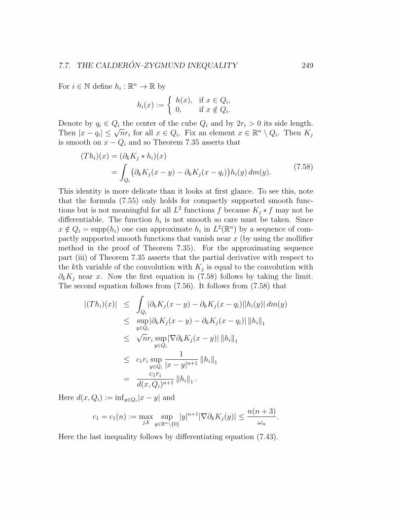
7.7. THE CALDERON–ZYGMUND INEQUALITY 249
For i ∈ N define hi : Rn → R by
hi(x) :=
h(x), if x ∈ Qi,0, if x /∈ Qi.
Denote by qi ∈ Qi the center of the cube Qi and by 2ri > 0 its side length.Then |x − qi| ≤
√nri for all x ∈ Qi. Fix an element x ∈ Rn \ Qi. Then Kj
is smooth on x−Qi and so Theorem 7.35 asserts that
(Thi)(x) = (∂kKj ∗ hi)(x)
=
∫Qi
(∂kKj(x− y)− ∂kKj(x− qi)
)hi(y) dm(y).
(7.58)
This identity is more delicate than it looks at first glance. To see this, notethat the formula (7.55) only holds for compactly supported smooth func-tions but is not meaningful for all L2 functions f because Kj ∗ f may not bedifferentiable. The function hi is not smooth so care must be taken. Sincex /∈ Qi = supp(hi) one can approximate hi in L2(Rn) by a sequence of com-pactly supported smooth functions that vanish near x (by using the mollifiermethod in the proof of Theorem 7.35). For the approximating sequencepart (iii) of Theorem 7.35 asserts that the partial derivative with respect tothe kth variable of the convolution with Kj is equal to the convolution with∂kKj near x. Now the first equation in (7.58) follows by taking the limit.The second equation follows from (7.56). It follows from (7.58) that
|(Thi)(x)| ≤∫Qi
|∂kKj(x− y)− ∂kKj(x− qi)||hi(y)| dm(y)
≤ supy∈Qi|∂kKj(x− y)− ∂kKj(x− qi)| ‖hi‖1
≤√nri sup
y∈Qi|∇∂kKj(x− y)| ‖hi‖1
≤ c1ri supy∈Qi
1
|x− y|n+1‖hi‖1
=c1ri
d(x,Qi)n+1‖hi‖1 .
Here d(x,Qi) := infy∈Qi |x− y| and
c1 = c1(n) := maxj,k
supy∈Rn\0
|y|n+1|∇∂kKj(y)| ≤ n(n+ 3)
ωn.
Here the last inequality follows by differentiating equation (7.43).

250 CHAPTER 7. PRODUCT MEASURES
Now define
Pi :=x ∈ Rn
∣∣ |x− qi| < 2√nri⊃ Qi.
Then d(x,Qi) ≥ |x− qi| −√nri for all x ∈ Rn \ Pi. Hence∫
Rn\Pi|Thi| dm ≤ c1ri
∫Rn\Pi
1
(|x− qi| −√nri)
n+1 dm(x) ‖hi‖1
= c1ri
∫|y|>2
√nri
1
(|y| −√nri)
n+1 dm(y) ‖hi‖1
= c1ri
∫ ∞2√nri
ωnsn−1ds
(s−√nri)
n+1 ‖hi‖1
= c1ωnri
∫ ∞√nri
(s+√nri)
n−1ds
sn+1‖hi‖1
≤ c12n−1ωnri
∫ ∞√nri
ds
s2‖hi‖1
= c2 ‖hi‖1 .
Here c2 = c2(n) := c1(n)2n−1ωn√n ≤ 2n−1n3/2(n + 3). The third step in
the above computation follows from Fubini’s Theorem in polar coordinates(Exercise 7.47). Thus we have proved that∫
Rn\Pi|Thi| dm ≤ c2 ‖hi‖1 for all i ∈ N. (7.59)
Recall that Th and Thi are only equivalence classes in L2(Rn). Choosesquare integrable functions on Rn representing these equivalence classes anddenote them by the same letters Th, Thi ∈ L2(Rn). We prove that there isa Lebesgue null set E ⊂ Rn such that
|Th(x)| ≤∞∑i=1
|Thi(x)| for all x ∈ Rn \ E. (7.60)
To see this, note that the sequence∑`
i=1 hi converges to h in L2(Rn) as `
tends to infinity. So the sequence∑`
i=1 Thi converges to Th in L2(Rn) byLemma 7.44. By Corollary 4.10 a subsequence converges almost everywhere.Hence there exists a Lebesgue null set E ⊂ Rn and a sequence of integers0 < `1 < `2 < `3 < · · · such that the sequence
∑`νi=1 Thi(x) coverges to Th(x)
as ν tends to infinity for all x ∈ Rn \E. Since |∑`ν
i=1 Thi(x)| ≤∑∞
i=1 |Thi(x)|for all x ∈ Rn, this proves (7.60).
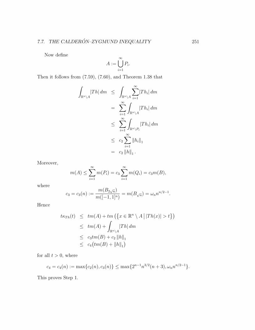
7.7. THE CALDERON–ZYGMUND INEQUALITY 251
Now define
A :=∞⋃i=1
Pi.
Then it follows from (7.59), (7.60), and Theorem 1.38 that∫Rn\A|Th| dm ≤
∫Rn\A
∞∑i=1
|Thi| dm
=∞∑i=1
∫Rn\A|Thi| dm
≤∞∑i=1
∫Rn\Pi
|Thi| dm
≤ c2
∞∑i=1
‖hi‖1
= c2 ‖h‖1 .
Moreover,
m(A) ≤∞∑i=1
m(Pi) = c3
∞∑i=1
m(Qi) = c3m(B),
where
c3 = c3(n) :=m(B2
√n)
m([−1, 1]n)= m(B√n) = ωnn
n/2−1.
Hence
tκTh(t) ≤ tm(A) + tm(x ∈ Rn \ A
∣∣ |Th(x)| > t)
≤ tm(A) +
∫Rn\A|Th| dm
≤ c3tm(B) + c2 ‖h‖1
≤ c4
(tm(B) + ‖h‖1
)for all t > 0, where
c4 = c4(n) := maxc2(n), c3(n) ≤ max2n−1n3/2(n+ 3), ωnnn/2−1.
This proves Step 1.
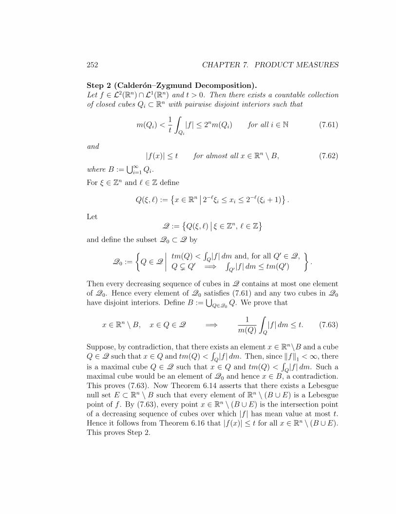
252 CHAPTER 7. PRODUCT MEASURES
Step 2 (Calderon–Zygmund Decomposition).Let f ∈ L2(Rn)∩L1(Rn) and t > 0. Then there exists a countable collectionof closed cubes Qi ⊂ Rn with pairwise disjoint interiors such that
m(Qi) <1
t
∫Qi
|f | ≤ 2nm(Qi) for all i ∈ N (7.61)
and|f(x)| ≤ t for almost all x ∈ Rn \B, (7.62)
where B :=⋃∞i=1Qi.
For ξ ∈ Zn and ` ∈ Z define
Q(ξ, `) :=x ∈ Rn
∣∣ 2−`ξi ≤ xi ≤ 2−`(ξi + 1).
LetQ :=
Q(ξ, `)
∣∣ ξ ∈ Zn, ` ∈ Z
and define the subset Q0 ⊂ Q by
Q0 :=
Q ∈ Q
∣∣∣∣ tm(Q) <∫Q|f | dm and, for all Q′ ∈ Q,
Q ( Q′ =⇒∫Q′|f | dm ≤ tm(Q′)
.
Then every decreasing sequence of cubes in Q contains at most one elementof Q0. Hence every element of Q0 satisfies (7.61) and any two cubes in Q0
have disjoint interiors. Define B :=⋃Q∈Q0
Q. We prove that
x ∈ Rn \B, x ∈ Q ∈ Q =⇒ 1
m(Q)
∫Q
|f | dm ≤ t. (7.63)
Suppose, by contradiction, that there exists an element x ∈ Rn\B and a cubeQ ∈ Q such that x ∈ Q and tm(Q) <
∫Q|f | dm. Then, since ‖f‖1 <∞, there
is a maximal cube Q ∈ Q such that x ∈ Q and tm(Q) <∫Q|f | dm. Such a
maximal cube would be an element of Q0 and hence x ∈ B, a contradiction.This proves (7.63). Now Theorem 6.14 asserts that there exists a Lebesguenull set E ⊂ Rn \ B such that every element of Rn \ (B ∪ E) is a Lebesguepoint of f . By (7.63), every point x ∈ Rn \ (B ∪E) is the intersection pointof a decreasing sequence of cubes over which |f | has mean value at most t.Hence it follows from Theorem 6.16 that |f(x)| ≤ t for all x ∈ Rn \ (B ∪E).This proves Step 2.

7.7. THE CALDERON–ZYGMUND INEQUALITY 253
Step 3. Let c = c(n) ≥ 1 be the constant in Step 1. Then
‖Tf‖1,∞ ≤(2n+1 + 6c
)‖f‖1 (7.64)
for all f ∈ L2(Rn) ∩ L1(Rn).
Fix a function f ∈ L2(Rn) ∩ L1(Rn) and a constant t > 0. Let the Qi be asin Step 2 and define
B :=⋃i
Qi.
Then m(Qi) <1t
∫Qi|f | dm for all i by Step 2 and hence
m(B) =∑i
m(Qi) ≤1
t
∑i
∫Qi
|f | dm ≤ 1
t‖f‖1 .
Define g, h : Rn → R by
g := fχRn\B +∑i
∫Qif dm
m(Qi)χQi , h := f − g.
Then‖g‖1 ≤ ‖f‖1 , ‖h‖1 ≤ 2 ‖f‖1 .
Moreover, h vanishes on Rn \ B and∫Qih dm = 0 for all i. Hence it follows
from Step 1 that
κTh(t) ≤ c
(m(B) +
1
t‖h‖1
)≤ 3c
t‖f‖1 . (7.65)
Moreover, it follows from Step 2 that |g(x)| ≤ t for almost every x ∈ Rn \Band |g(x)| ≤ 2nt for every x ∈ int(Qi). Thus |g| ≤ 2nt almost everywhere.Hence it follows from Lemma 7.36 that
κTg(t) ≤1
t2
∫Rn|g|2 dm ≤ 2n
t
∫Rn|g| dm ≤ 2n
t‖f‖1 . (7.66)
Now combine (7.65) and (7.66) with the inequality (7.36) in Lemma 7.36 toobtain the estimate
κTf (2t) ≤ κTg(t) + κTh(t) ≤2n+1 + 6c
2t‖f‖1 .
Here the splitting f = g + h depends on t but the constant c does not. Mul-tiply the inequality by 2t and take the supremum over all t to obtain (7.64).This proves Step 3 and Lemma 7.45.

254 CHAPTER 7. PRODUCT MEASURES
Theorem 7.46 (Calderon–Zygmund). Fix an integer n ≥ 2 and a number1 < p <∞. Then there exists a constant c = c(n, p) > 0 such that
‖∂i(Kj ∗ f)‖p ≤ c ‖f‖p (7.67)
for all f ∈ C∞0 (Rn) and all i, j = 1, . . . , n.
Proof. For p = 2 this estimate was established in Lemma 7.44 with c = 1.Second, suppose 1 < p < 2 and let c1(n) be the constant of Lemma 7.45.For i, j = 1, . . . , n denote by Tij : L2(Rn) → L2(Rn) the unique boundedlinear operator that satisfies Tijf = ∂i(Kj ∗ f) for f ∈ C∞0 (Rn). Then‖Tijf‖1,∞ ≤ c1(n) ‖f‖1 for all f ∈ C∞0 (Rn) and all i, j by Lemma 7.45.
Since C∞0 (Rn) is dense in L2(Rn) ∩ L1(Rn) by Theorem 7.35 it follows that‖Tijf‖1,∞ ≤ c1(n) ‖f‖1 for all f ∈ L2(Rn) ∩ L1(Rn). Hence Theorem 7.37(with q = 2) asserts that (7.67) holds with
c = c(n, p) := 2
(p
(2− p)(p− 1)
)1/p
c1(n)2/p−1.
Third, suppose 2 < p < ∞ and choose 1 < q < 2 such that 1/p + 1/q = 1.Then it follows from Theorem 7.41, integration by parts, Holder’s inequality,and from what we have just proved that, for all f, g ∈ C∞0 (Rn),∫
Rn(∂i(Kj ∗ f))g dm =
∫Rn
(∂i∂jf)g dm
=
∫Rnf(∂i∂jg) dm
=
∫Rnf(∂i(Kj ∗ g)) dm
≤ ‖f‖p ‖∂i(Kj ∗ g)‖q≤ c(n, q) ‖f‖p ‖g‖q .
Since C∞0 (Rn) is dense in Lq(Rn) by Theorem 7.35, and the Lebesgue measureis semi-finite, it follows from Lemma 4.34 that ‖∂i(Kj ∗ f)‖p ≤ c(n, q) ‖f‖pfor all f ∈ C∞0 (Rn). This proves Theorem 7.46.
Proof of Theorem 7.43. Fix an integer n ≥ 2 and a number 1 < p < ∞.Let c = c(n, p) be the constant of Theorem 7.46 and let u ∈ C∞0 (Rn). Then∂ju = ∂j(K ∗∆u) = Kj ∗∆u by Theorem 7.41. Hence it follow from Theo-rem 7.46 with f = ∆u that ‖∂i∂ju‖p = ‖∂i(Kj ∗∆u)‖p ≤ c(n, p) ‖∆u‖p fori, j = 1, . . . , n. This proves Theorem 7.43.
7.8. EXERCISES 255
7.8 Exercises
Exercise 7.47 (Lebesgue Measure on the Sphere).For n ∈ N let (Rn,An,mn) the Lebesgue measure space, denote the openunit ball by Bn := x ∈ Rn | |n| < 1, and the unit sphere by
Sn−1 := ∂Bn = x ∈ Rn | |x| = 1 .For A ⊂ Sn−1 define A± := x ∈ Bn−1 | (x,±
√1− |x|2) ∈ A. Prove that
the collectionAS :=
A ⊂ Sn−1 |A+, A− ∈ An−1
is a σ-algebra and that the map σ : AS → [0,∞] defined by
σ(A) :=
∫A+
1√1− |x|2
dmn−1(x) +
∫A−
1√1− |x|2
dmn−1(x)
for A ∈ AS is a measure. Prove Fubini’s Theorem in Polar Coordinatesstated below. Use it to prove that ωn := σ(Sn−1) <∞.
Fubini’s Theorem for Polar Coordinates: Let f : Rn → R be Lebesgueintegrable. For r ≥ 0 and x ∈ Sn−1 define f r(x) := fx(r) := f(rx). Thenthere exists a set E ∈ AS such that σ(E) = 0 and fx ∈ L1([0,∞)) for allx ∈ Sn−1 \ E, and there exists a Lebesgue null set F ⊂ [0,∞) such thatf r ∈ L1(σ) for all r ∈ [0,∞) \ F . Define g : Sn−1 → R and h : [0,∞) → Rby g(x) := 0 for x ∈ E, h(r) := 0 for r ∈ F , and
g(x) :=
∫[0,∞)
rn−1fx(r) dm1(r), h(r) := rn−1
∫Sn−1
f r dσ, (7.68)
for x ∈ Sn−1 \ E and r ∈ [0,∞) \ F . Then g ∈ L1(σ), h ∈ L1([0,∞)), and∫Rnf dmn =
∫Sn−1
g dσ =
∫[0,∞)
h dm1. (7.69)
Hint: Define the diffeomorphism φ : Bn−1 × (0,∞)→ x ∈ Rn |xn > 0 byφ(x, r) := (rx, r(1 − |x|2)1/2). Prove that det(dφ(x, r)) = (1 − |x|2)−1/2rn−1
for x ∈ Bn−1 and r > 0. Use Theorem 2.17 and Fubini’s Theorem 7.30.
Exercise 7.48 (Divergence Theorem). Let f : Rn → R be a smoothfunction. Prove that ∫
Bn∂if dmn =
∫Sn−1
xif(x) dσ(x). (7.70)
Hint: Assume first that i = n. Use the fundamental theorem of calculusand Fubini’s Theorem 7.30 for Rn = Rn−1 × R.

256 CHAPTER 7. PRODUCT MEASURES
Exercise 7.49. Prove that∫ ∞0
sin(x)
xdx := lim
ε→0
∫ 1/ε
ε
sin(x)
xdx =
π
2.
Hint: Use the identity∫∞
0e−rt dt = 1/r for r > 0 and Fubini’s Theorem.
Exercise 7.50. Define the function f : R2 → R by
f(x, y) :=sign(xy)
x2 + y2, sign(z) :=
1, if z > 0,0, if z = 0,−1, if z < 0,
for (x, y) 6= 0 and by f(0, 0) := 0. Prove that fx, fy : R → R are Lebesgue
integrable for all x, y ∈ R. Prove that the functions R→ R : x 7→∫R fx dm1
and R→ R : y 7→∫R f
y dm1 are Lebesgue integrable and∫R
(∫Rf(x, y) dm1(x)
)dm1(y) =
∫R
(∫Rf(x, y) dm1(y)
)dm1(x).
Prove that f is not Lebesgue integrable.
Exercise 7.51. Let (X,A, µ) and (Y,B, ν) be two σ-finite measure spacesand let f ∈ L1(µ) and g ∈ L1(ν). Define h : X × Y → R by
h(x, y) := f(x)g(y), for x ∈ X and y ∈ Y.
Prove that h ∈ L1(µ⊗ ν) and∫X×Y h d(µ⊗ ν) =
∫Xf dµ
∫Yg dν.
Exercise 7.52. Let (X,A, µ) and (Y,B, ν) be two σ-finite measure spacesand let λ : A⊗ B → R be any measure such that λ(A× B) = µ(A)ν(B) forall A ∈ A and all B ∈ B. Prove that λ = µ⊗ ν.
Exercise 7.53. Define φ : R→ R by
φ(x) :=
1− cos(x), for 0 ≤ x ≤ 2π,0, otherwise.
Define the functions f, g, h : R→ R by
f(x) := 1, g(x) := φ′(x), h(x) :=
∫ x
−∞φ(t) dt
for x ∈ R. Prove that (f ∗ g) ∗ h = 0 and f ∗ (g ∗ h) > 0. Thus the convolu-tion need not be associative on nonintegrable functions. Compare this withpart (v) of Theorem 7.32. Prove that E(|f | ∗ |g|, |h|) = E(|f |, |g| ∗ |h|) = Rwhile E(f ∗ g, h) = E(f, g ∗ h) = ∅.
7.8. EXERCISES 257
Exercise 7.54. Let (R,A,m) be the Lebesgue measure space, let B ⊂ A bethe Borel σ-algebra, and denote by M the Banach space of all signed Borelmeasures µ : B → [0,∞) with the norm ‖µ‖ := |µ|(R). (See Exercise 5.34.)The convolution of two signed measures µ, ν ∈M is the map
µ ∗ ν : B → R
defined by
(µ ∗ ν)(B) := (µ⊗ ν)(
(x, y) ∈ R2∣∣x+ y ∈ B
)(7.71)
for B ∈ B, where
(µ⊗ ν) := µ+ ⊗ ν+ + µ− ⊗ ν− − µ+ ⊗ ν− − µ− ⊗ ν+.
(See Definition 5.13 and Theorem 5.20.) Prove the following.
(i) If µ, ν ∈M then µ ∗ ν ∈M and
‖µ ∗ ν‖ ≤ ‖µ‖ ‖ν‖ .
(ii) There exists a unique element δ ∈M such that
δ ∗ µ = µ
for all µ ∈M.
(iii) The convolution product on M is commutative, associative, and dis-tributive. Thus M is a commutative Banach algebra with unit.
(iv) If f ∈ L1(R) and µf : B → R is defined by
µf (B) :=
∫B
f dm for B ∈ B
then µf ∈M and ‖µf‖ = ‖f‖1.
(v) If f, g ∈ L1(R) thenµf ∗ µg = µf∗g.
(vi) Let λ, µ, ν ∈M. Then λ = µ ∗ ν if and only if∫Rf dλ =
∫R2
f(x+ y)d(µ⊗ ν)(x, y)
for all bounded Borel measurable functions f : R→ R.
(vii) If µ, ν ∈M and B ∈ B then
(µ ∗ ν)(B) =
∫Rµ(B − t) dν(t).

258 CHAPTER 7. PRODUCT MEASURES
Chapter 8
The Haar Measure
The purpose of this last chapter is to prove the existence and uniqueness of anormalized invariant Radon measure on any compact Hausdorff group. In thecase of a locally compact Hausdorff group the theorem asserts the existenceof a left invariant Radon measure that is unique up to a scaling factor. Anexample is the Lebesgue measure on Rn. A useful exposition is the paper byGert K. Pedersen [16] which also discusses the original references.
8.1 Topological Groups
Let G be a group, in multiplicative notation, with the group operation
G×G→ G : (x, y) 7→ xy, (8.1)
the unit 1l ∈ G, and the inverse map
G→ G : x 7→ x−1. (8.2)
A topological group is a pair (G,U) consisting of a group G and a topology
U ⊂ 2G
such that the group multiplication (8.1) and the inverse map (8.2) are con-tinuous. Here the continuity of the group multiplication (8.1) is understoodwith respect to the product topology on G × G (see Appendix B). A lo-cally compact Hausdorff group is a topological group (G,U) such thatthe topology is locally compact and Hausdorff (see page 81).
259
260 CHAPTER 8. THE HAAR MEASURE
Example 8.1. Let G be any group and define U := ∅,G. Then (G,U) isa compact topological group but is not Hausdorff unless G = 1l.
Example 8.2 (Discrete Groups). Let G be any group. Then the pair(G,U) with the discrete topology U := 2G is a locally compact Hausdorffgroup, called a discrete group. Examples of discrete groups (where thediscrete topology appears naturally) are the additive group Zn, the multi-plicative group SL(n,Z) of integer n× n-matrices with determinant one, themapping class group of isotopy classes of diffeomorphisms of any manifold,and every finite group.
Example 8.3 (Lie Groups). Let G ⊂ GL(n,C) be any subgroup of thegeneral linear group of invertible complex n× n-matrices that is closed as asubset of GL(n,C) with respect to the relative topology, i.e. GL(n,C) \G isan open set in Cn×n. Let U ⊂ 2G be the relative topology on G, i.e. U ⊂ G isopen if and only if there is an open subset V ⊂ Cn×n such that U = G ∩ V .Then (G,U) is a locally compact Hausdorff group. In fact, it is a basicresult in the theory of Lie groups that every closed subgroup of GL(n,C) is asmooth submanifold of Cn×n and hence is a Lie group. Specific examples ofLie groups are the general linear groups GL(n,R) and GL(n,C), the speciallinear groups SL(n,R) and SL(n,C) of real and complex n×n-matrices withdeterminant one, the orthogonal group O(n) of matrices x ∈ Rn×n such thatxTx = 1l, the special orthogonal group SO(n) := O(n)∩SL(n,R), the unitarygroup U(n) of matrices x ∈ Cn×n such that x∗x = 1l, the special unitary groupSU(n) := U(n)∩ SL(n,C), the group Sp(1) of the unit quaternions, the unitcircle S1 = U(1) in the complex plane, the torus Tn := S1 × · · · × S1 (ntimes), or, for any multi-linear form τ : (Cn)k → C, the group of all matricesx ∈ GL(n,C) that preserve τ . The additive groups Rn and Cn are also Liegroups. Lie groups form an important class of locally compact Hausdorffgroups and play a central role in differential geometry.
Example 8.4. If (V, ‖·‖) is a normed vector space (Example 1.11) then theadditive group V is a Hausdorff topological group. It is locally compact ifand only if V is finite-dimensional.
Example 8.5. The rational numbers Q with the additive structure form aHausdorff topological group with the relative topology as a subset of R. It istotally disconnected (every connected component is a single point) but doesnot have the discrete topology. It is not locally compact.

8.1. TOPOLOGICAL GROUPS 261
Example 8.6 (p-adic Integers). Fix a prime number p ∈ N and denote by
N0 := N ∪ 0
the set of nonnegative integers. For x, y ∈ Z define
dp(x, y) := |x− y|p := infp−k
∣∣∣ k ∈ N0, x− y ∈ pkZ. (8.3)
Then the function
dp : Z× Z→ [0, 1]
is a distance function and so (Z, dp) is a metric space. It is not complete.Its completion is denoted by Zp and called the ring of p-adic integers.Here is another description of the p-adic integers. Consider the sequence ofprojections
· · · πk+1−→ Z/pkZ πk−→ Z/pk−1Z πk−1−→ · · · π3−→ Z/p2Z π2−→ Z/pZ π1−→ 1.
The inverse limit of this sequence of maps is the set of sequences
Zp :=x = (xk)k∈N0
∣∣∣xk ∈ Z/pkZ, πk(xk) = xk−1 for all k ∈ N.
This set is a commutative ring with unit. Addition and multiplication aredefined term by term, i.e.
x+ y := (xk + yk)k∈N0 , xy := (xkyk)k∈N0
for x = (xk)k∈N0 ∈ Zp and y = (yk)k∈N0 ∈ Zp. The ring of p-adic integers isa compact metric space with
dp(x, y) := infp−k
∣∣∣ k ∈ N0, xk = yk
. (8.4)
The inclusion of Z into the p-adic integers is given by
ιp : Z→ Zp, ιp(x) := (x mod pk)k∈N.
This is an isometric embedding with respect to the distance functions (8.3)and (8.4). The additive p-adic integers form an uncountable compact Haus-dorff group (with the topology of a Cantor set) that is not a Lie group.
262 CHAPTER 8. THE HAAR MEASURE
Example 8.7 (p-adic Rationals). Fix a prime number p ∈ N. Write anonzero rational number x ∈ Q in the form x = pka/b where k ∈ Z and thenumbers a ∈ Z and b ∈ N are relatively prime to p, and define |x|p := p−k.For x = 0 define |0|p := 0. Define the function dp : Q×Q→ [0,∞) by
dp(x, y) := |x− y|p:= inf
p−k
∣∣ k ∈ Z, x− y = pka
b, a ∈ Z, b ∈ N \ pN
.
(8.5)
Then (Q, dp) is a metric space. The completion of Q with respect to dp isdenoted by Qp and is called the field of p-adic rational numbers. Itcan also be described as the quotient field of the ring of p-adic integers inExample 8.6. The multiplicative group of nonzero p-adic rationals is a locallycompact Hausdorff group that is not a Lie group. One can also considergroups of matrices whose entries are p-adic rationals. Such groups play animportant role in number theory.
Example 8.8 (Infinite Products). Let I be any index set and, for i ∈ I,let Gi be a compact Hausdorff group. Then the product
G :=∏i∈I
Gi
is a compact Hausdorff group. Its elements are maps I → ti∈IGi : i 7→ xisuch that xi ∈ Gi for all i ∈ I. Write such a map as x = (xi)i∈I . Theproduct topology on G is defined as the smallest topology such that theobvious projections πi : G→ Gi are continuous. Thus the (infinite) productsU =
∏i∈I Ui of open sets Ui ⊂ Gi, such that Ui = Gi for all but finitely
many i, form a basis for the topology of G. (See Appendix B for #I = 2.)The product topology is obviously Hausdorff and Tychonoff’s Theoremasserts that it is compact (see Munkres [14]). An uncountable product ofnontrivial groups Gi is not first countable.
Example 8.9. Let (X , ‖·‖) be a Banach algebra with a unit 1l and theproduct X × X → X : (x, y) 7→ xy. (See page 236.) Then the group ofinvertible elements G := x ∈ X | ∃ y ∈ X such that xy = yx = 1l is a Haus-dorff topological group. Examples include the group of nonzero quaternions,the general linear group of a finite-dimensional vector space, the group ofbijective bounded linear operators on a Banach space, and the multiplicativegroup of nowhere vanishing real valued continuous functions on a compacttopological space. In general G is not locally compact.
8.2. HAAR MEASURES 263
8.2 Haar Measures
Throughout let G be a locally compact Hausdorff group, in multiplicativenotation, and denote by B ⊂ 2G its Borel σ-algebra. We begin our discussionwith a technical lemma about continuous functions on G.
Lemma 8.10. Let f ∈ Cc(G) and fix a constant ε > 0. Then there exists anopen neighborhood U of 1l such that, for all x, y ∈ G,
x−1y ∈ U =⇒ |f(x)− f(y)| < ε. (8.6)
Proof. Choose an open neighborhood U0 ⊂ G with compact closure anddefine K :=
ab−1 | a ∈ supp(f), b ∈ U0
. This set is compact because the
maps (8.1) and (8.2) are continuous. Also,
x /∈ K, x−1y ∈ U0 =⇒ f(x) = f(y) = 0 (8.7)
for all x, y ∈ G. (If y ∈ supp(f) and x−1y ∈ U0 then x = y(x−1y)−1 ∈ K.)Since f is continuous there exists, for each x ∈ K, an open neighborhoodV (x) ⊂ G of x such that
y ∈ V (x) =⇒ |f(x)− f(y)| < ε
2. (8.8)
Since the map G→ G : y 7→ x−1y is a homeomorphism, the set x−1V (x) is anopen neighborhood of 1l for every x ∈ K. Since the map (8.1) is continuousit follows from the definition of the product topology in Appendix B that,for every x ∈ K, there exists an open neighborhood U(x) ⊂ G of 1l such thatthe product neighborhood U(x)× U(x) of the pair (1l, 1l) is contained in thepre-image of x−1V (x) under the multiplication map (8.1). In other words,
a, b ∈ U(x) =⇒ xab ∈ V (x). (8.9)
Since the map G → G : y 7→ xy is a homeomorphism the set xU(x) isan open neighborhood of x for every x ∈ K. Since K is compact thereexist finitely many elements x1, . . . , x` ∈ K such that K ⊂
⋃`i=1 xiU(xi).
Define U := U0 ∩⋂`i=1 U(xi) and let x, y ∈ G such that x−1y ∈ U . If x /∈ K
then f(x) = f(y) = 0 by (8.7). Hence assume x ∈ K. Then there existsan index i ∈ 1, . . . , ` such that x ∈ xiU(xi) and therefore x−1
i x ∈ U(xi).Hence x = xi(x
−1i x)1l ∈ V (xi) and y = xi(x
−1i x)(x−1y) ∈ V (xi) by (8.9).
Hence it follows from (8.8) that
|f(x)− f(y)| ≤ |f(x)− f(xi)|+ |f(xi)− f(y)| < ε.
This proves Lemma 8.10.
264 CHAPTER 8. THE HAAR MEASURE
For x ∈ G define the homeomorphisms Lx, Rx : G→ G by
Lx(a) := xa, Rx(a) := ax for x ∈ G. (8.10)
They satisfy
Lx Ly = Lxy, Rx Ry = Ryx, Lx Ry = Ry Lx. (8.11)
For A ⊂ G and x ∈ G define
xA :=xa∣∣ a ∈ A , Ax :=
ax∣∣ a ∈ A , A−1 :=
a−1
∣∣ a ∈ A .Thus xA = Lx(A) and Ax = Rx(A).
Definition 8.11. A measure µ : B → [0,∞] is called left invariant ifµ(xB) = µ(B) for all B ∈ B and all x ∈ G. It is called right invariant ifµ(Bx) = µ(B) for all B ∈ B and all x ∈ G. It is called invariant if it isboth left and right invariant. A left Haar measure on G is a left invariantRadon measure that does not vanish identically. A right Haar measure onG is a right invariant Radon measure that does not vanish identically. Aninvariant Haar measure on G is an invariant Radon measure that doesnot vanish identically.
Theorem 8.12 (Haar). Let G be a locally compact Hausdorff group. Thenthe following holds.
(i) G admits a left Haar measure µ, unique up to a positive factor. Everysuch measure satisfies µ(U) > 0 for every nonempty open set U ⊂ G.
(ii) G admits a right Haar measure µ, unique up to a positive factor. Everysuch measure satisfies µ(U) > 0 for every nonempty open set U ⊂ G.
(iii) Assume G is compact. Then G admits a unique invariant Haar measureµ such that µ(G) = 1. This measure satisfies µ(B−1) = µ(B) for all B ∈ Band µ(U) > 0 for every nonempty open set U ⊂ G.
Proof. See page 276.
Examples of Haar measures are the restriction to the Borel σ-algebra ofthe Lebesgue measure on Rn (where the group structure is additive), therestriction to the Borel σ-algebra of the measure σ on S1 = U(1) or onS3 = Sp(1) in Exercise 7.47, the measure dt/t on the multiplicative group ofthe positive real numbers, and the counting measure on any discrete group.The proof of Theorem 8.12 rests on the Riesz Representation Theorem 3.15and the following result about positive linear functionals.
8.2. HAAR MEASURES 265
Definition 8.13. Let G be a locally compact Hausdorff group. A linearfunctional Λ : Cc(G)→ R is called left invariant if
Λ(f Lx) = Λ(f) (8.12)
for all f ∈ Cc(G) and all x ∈ G. It is called right invariant if
Λ(f Rx) = Λ(f) (8.13)
for all f ∈ Cc(G) and all x ∈ G. It is called invariant if it is both left andright invariant. It is called a left Haar integral if it is left invariant, posi-tive, and nonzero. It is called a right Haar integral if it is right invariant,positive, and nonzero.
Theorem 8.14 (Haar). Every locally compact Hausdorff group G admits aleft Haar integral, unique up to a positive factor. Moreover, if Λ : Cc(G)→ Ris a left Haar integral and f ∈ Cc(G) is a nonnegative function that does notvanish identically then Λ(f) > 0.
Proof. See page 268.
The proof of Theorem 8.14 given below follows the notes of Pedersen [16]which are based on a proof by Weil. Our exposition benefits from elegantsimplifications due to Urs Lang [11]. In preparation for the proof it is con-venient to introduce some notation. Let
C+c (G) :=
f ∈ Cc(G)
∣∣ f ≥ 0, f 6≡ 0
(8.14)
be the space of nonnegative continuous functions with compact support thatdo not vanish identically. A function Λ : C+
c (G)→ [0,∞) is called
• additive iff Λ(f + g) = Λ(f) + Λ(g) for all f, g ∈ C+c (G),
• subadditive iff Λ(f + g) ≤ Λ(f) + Λ(g) for all f, g ∈ C+c (G),
• homogeneous iff Λ(cg) = cΛ(f) for all f ∈ C+c (G) and all c > 0,
• monotone iff f ≤ g implies Λ(f) ≤ Λ(g) for all f, g ∈ C+c (G),
• left invariant iff Λ(f Lx) = Λ(f) for all f ∈ C+c (G) and all x ∈ G.
Every additive functional Λ : C+c (G) → [0,∞) is necessarily homogeneous
and monotone. Moreover, every positive linear functional on Cc(G) restrictsto an additive functional Λ : C+
c (G) → [0,∞) and, conversely, every addi-tive functional Λ : C+
c (G) → [0,∞) extends uniquely to a positive linearfunctional on Cc(G). This is the content of the next lemma.
266 CHAPTER 8. THE HAAR MEASURE
Lemma 8.15. Let Λ : C+c (G)→ [0,∞) be an additive functional. Then there
is a unique positive linear functional on Cc(G) whose restriction to C+c (G)
agrees with Λ. If Λ is left invariant then so is its linear extension to Cc(G).
Proof. We prove that Λ is monotone. Let f, g ∈ C+c (G) such that f ≤ g. If
f 6= g then g − f ∈ C+c (G) and hence
Λ(f) ≤ Λ(f) + Λ(g − f) = Λ(g)
by additivity. If f = g there is nothing to prove.We prove that Λ is homogeneous. Let f ∈ C+
c (G). Then Λ(nf) = nΛ(f)for all n ∈ N by additivity and induction. If c = m/n is a positive ratio-nal number then Λ(f) = nΛ(f/n) and hence Λ(cf) = mΛ(f/n) = cΛ(f).If c > 0 is irrational then it follows from monotonicity that
aΛ(f) = Λ(af) ≤ Λ(cf) ≤ Λ(bf) = bΛ(f)
for all a, b ∈ Q with 0 < a < c < b, and this implies Λ(cf) = cΛ(f).Now define Λ(0) := 0 and, for f ∈ Cc(G), define Λ(f) := Λ(f+)−Λ(f−).
If f, g ∈ Cc(G) then f+ + g+ + (f + g)− = f− + g− + (f + g)+, hence
Λ(f+) + Λ(g+) + Λ((f + g)−) = Λ(f−) + Λ(g−) + Λ((f + g)+)
by additivity, and hence Λ(f) + Λ(g) = Λ(f + g). Moreover, (−f)+ = f−
and (−f)− = f+ and so Λ(−f) = Λ(f−)−Λ(f+) = −Λ(f). Hence it followsfrom homogeneity that Λ(cf) = cΛ(f) for all f ∈ Cc(G) and all c ∈ R. Thisshows that the extended functional is linear.
If the original functional Λ : C+c (G) → [0,∞) is left-invariant then so is
the extended linear functional on Cc(G) because (f Lx)± = f± Lx for allf ∈ Cc(G) and all x ∈ G. This proves Lemma 8.15.
Consider the space
L :=
Λ : C+
c (G)→ (0,∞)
∣∣∣∣ Λ is subadditive, monotone,homogeneous, and left invariant
. (8.15)
The strategy of the proof of Theorem 8.14 is to construct certain functionalsΛg ∈ L associated to functions g ∈ C+
c (G) supported near the identity ele-ment and to construct the required positive linear functional Λ : Cc(G)→ Ras a suitable limit where the functions g converge to a Dirac δ-function at theidentity. The precise definition of the Λg involves the following construction.
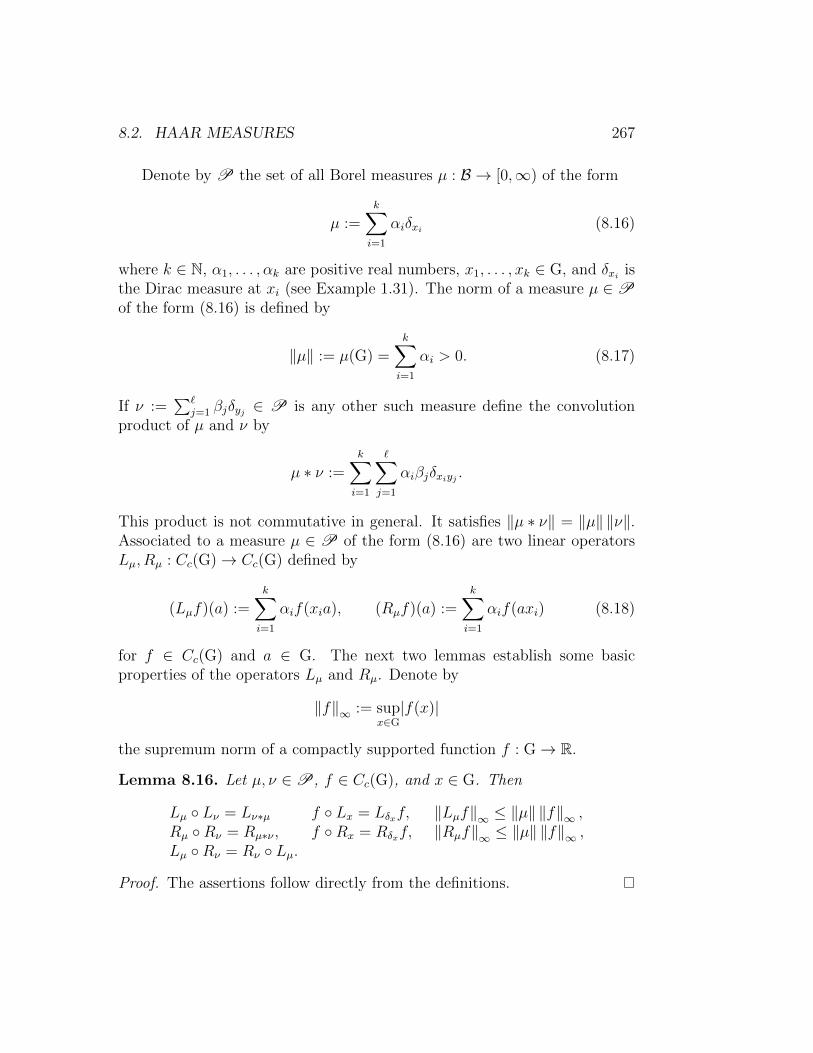
8.2. HAAR MEASURES 267
Denote by P the set of all Borel measures µ : B → [0,∞) of the form
µ :=k∑i=1
αiδxi (8.16)
where k ∈ N, α1, . . . , αk are positive real numbers, x1, . . . , xk ∈ G, and δxi isthe Dirac measure at xi (see Example 1.31). The norm of a measure µ ∈Pof the form (8.16) is defined by
‖µ‖ := µ(G) =k∑i=1
αi > 0. (8.17)
If ν :=∑`
j=1 βjδyj ∈ P is any other such measure define the convolutionproduct of µ and ν by
µ ∗ ν :=k∑i=1
∑j=1
αiβjδxiyj .
This product is not commutative in general. It satisfies ‖µ ∗ ν‖ = ‖µ‖ ‖ν‖.Associated to a measure µ ∈ P of the form (8.16) are two linear operatorsLµ, Rµ : Cc(G)→ Cc(G) defined by
(Lµf)(a) :=k∑i=1
αif(xia), (Rµf)(a) :=k∑i=1
αif(axi) (8.18)
for f ∈ Cc(G) and a ∈ G. The next two lemmas establish some basicproperties of the operators Lµ and Rµ. Denote by
‖f‖∞ := supx∈G|f(x)|
the supremum norm of a compactly supported function f : G→ R.
Lemma 8.16. Let µ, ν ∈P, f ∈ Cc(G), and x ∈ G. Then
Lµ Lν = Lν∗µ f Lx = Lδxf, ‖Lµf‖∞ ≤ ‖µ‖ ‖f‖∞ ,Rµ Rν = Rµ∗ν , f Rx = Rδxf, ‖Rµf‖∞ ≤ ‖µ‖ ‖f‖∞ ,Lµ Rν = Rν Lµ.
Proof. The assertions follow directly from the definitions.

268 CHAPTER 8. THE HAAR MEASURE
Lemma 8.17. Let f, g ∈ C+c (G). Then there exists a µ ∈P such that
f ≤ Lµg.
Proof. Fix an element y ∈ G such that g(y) > 0. For x ∈ G define
Ux :=
a ∈ G
∣∣∣∣ f(a) <f(x) + 1
g(y)g(yx−1a)
This set is an open neighborhood of x. Since f has compact support thereexist finitely many points x1, . . . , xk ∈ G such that supp(f) ⊂ Ux1∪· · ·∪Uxk .Define
µ :=k∑i=1
f(xi) + 1
g(y)δyx−1
i.
Then
f(a) ≤k∑i=1
f(xi) + 1
g(y)g(yx−1
i a) = (Lµg)(a)
for all a ∈ supp(f) and hence f ≤ Lµg. This proves Lemma 8.17.
Proof of Theorem 8.14. The proof has five steps. Step 1 is the main con-struction of a subadditive functional Mg : C+
c (G) → (0,∞) associated to afunction g ∈ C+
c (G). Step 2 shows that Mg is asymptotically linear as gconcentrates near the unit 1l. The heart of the convergence proof is Step 3and is due to Cartan. Step 4 proves uniqueness and Step 5 proves existence.
Step 1. For f ∈ C+c (G) define
Mg(f) := M(f ; g) := inf‖µ‖
∣∣µ ∈P, f ≤ Lµg. (8.19)
Then the following holds.
(i) M(f ; g) > 0 for all f, g ∈ C+c (G).
(ii) For every g ∈ C+c (G) the functional Mg : C+
c (G)→ (0,∞) is subadditive,homogeneous, monotone, and left invariant and hence is an element of L .
(iii) Let Λ ∈ L . Then
Λ(f) ≤M(f ; g)Λ(g) for all f, g ∈ C+c (G). (8.20)
In particular, M(f ;h) ≤M(f ; g)M(g;h) for all f, g, h ∈ C+c (G).
(iv) M(f ; f) = 1 for all f ∈ C+c (G).
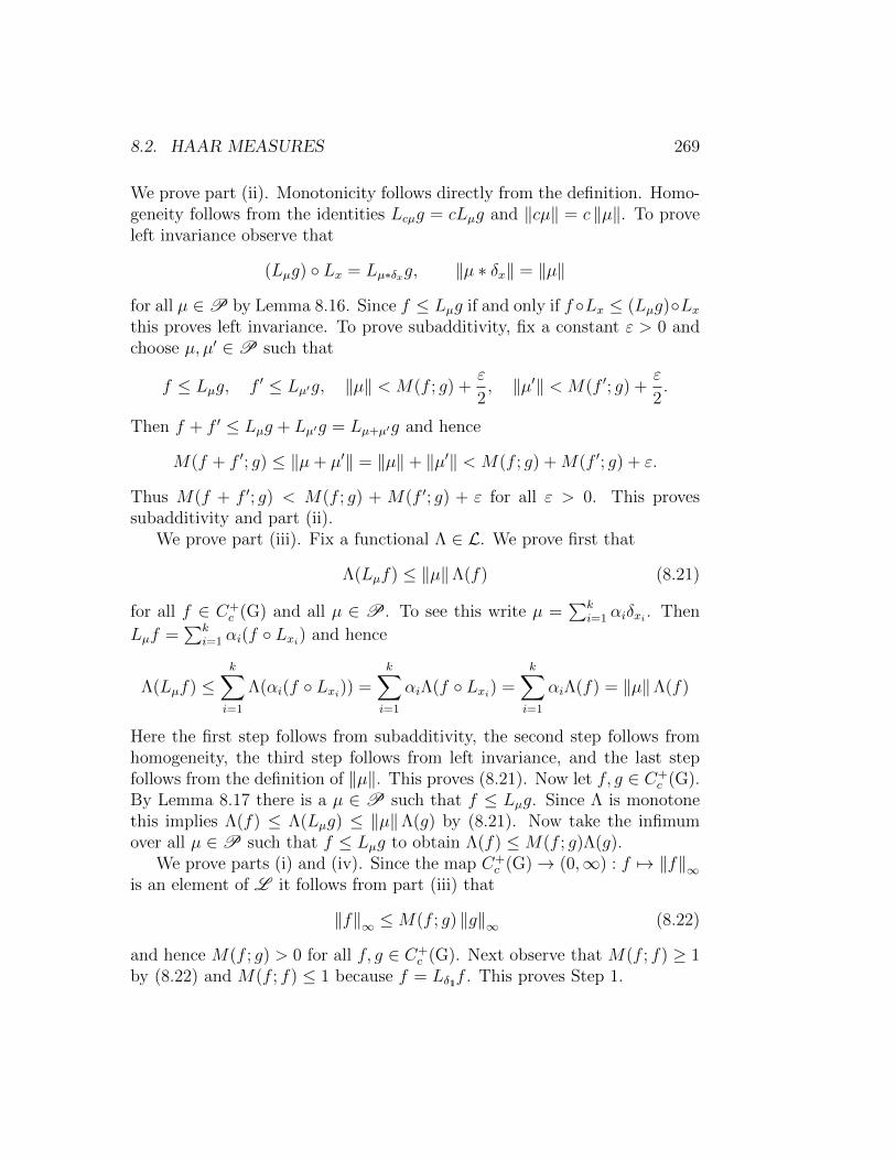
8.2. HAAR MEASURES 269
We prove part (ii). Monotonicity follows directly from the definition. Homo-geneity follows from the identities Lcµg = cLµg and ‖cµ‖ = c ‖µ‖. To proveleft invariance observe that
(Lµg) Lx = Lµ∗δxg, ‖µ ∗ δx‖ = ‖µ‖
for all µ ∈P by Lemma 8.16. Since f ≤ Lµg if and only if f Lx ≤ (Lµg)Lxthis proves left invariance. To prove subadditivity, fix a constant ε > 0 andchoose µ, µ′ ∈P such that
f ≤ Lµg, f ′ ≤ Lµ′g, ‖µ‖ < M(f ; g) +ε
2, ‖µ′‖ < M(f ′; g) +
ε
2.
Then f + f ′ ≤ Lµg + Lµ′g = Lµ+µ′g and hence
M(f + f ′; g) ≤ ‖µ+ µ′‖ = ‖µ‖+ ‖µ′‖ < M(f ; g) +M(f ′; g) + ε.
Thus M(f + f ′; g) < M(f ; g) + M(f ′; g) + ε for all ε > 0. This provessubadditivity and part (ii).
We prove part (iii). Fix a functional Λ ∈ L. We prove first that
Λ(Lµf) ≤ ‖µ‖Λ(f) (8.21)
for all f ∈ C+c (G) and all µ ∈ P. To see this write µ =
∑ki=1 αiδxi . Then
Lµf =∑k
i=1 αi(f Lxi) and hence
Λ(Lµf) ≤k∑i=1
Λ(αi(f Lxi)) =k∑i=1
αiΛ(f Lxi) =k∑i=1
αiΛ(f) = ‖µ‖Λ(f)
Here the first step follows from subadditivity, the second step follows fromhomogeneity, the third step follows from left invariance, and the last stepfollows from the definition of ‖µ‖. This proves (8.21). Now let f, g ∈ C+
c (G).By Lemma 8.17 there is a µ ∈ P such that f ≤ Lµg. Since Λ is monotonethis implies Λ(f) ≤ Λ(Lµg) ≤ ‖µ‖Λ(g) by (8.21). Now take the infimumover all µ ∈P such that f ≤ Lµg to obtain Λ(f) ≤M(f ; g)Λ(g).
We prove parts (i) and (iv). Since the map C+c (G)→ (0,∞) : f 7→ ‖f‖∞
is an element of L it follows from part (iii) that
‖f‖∞ ≤M(f ; g) ‖g‖∞ (8.22)
and hence M(f ; g) > 0 for all f, g ∈ C+c (G). Next observe that M(f ; f) ≥ 1
by (8.22) and M(f ; f) ≤ 1 because f = Lδ1lf . This proves Step 1.
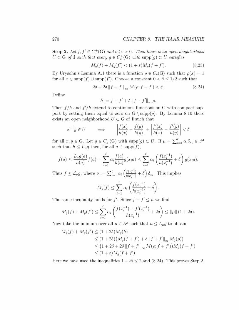
270 CHAPTER 8. THE HAAR MEASURE
Step 2. Let f, f ′ ∈ C+c (G) and let ε > 0. Then there is an open neighborhood
U ⊂ G of 1l such that every g ∈ C+c (G) with supp(g) ⊂ U satisfies
Mg(f) +Mg(f′) < (1 + ε)Mg(f + f ′). (8.23)
By Urysohn’s Lemma A.1 there is a function ρ ∈ Cc(G) such that ρ(x) = 1for all x ∈ supp(f) ∪ supp(f ′). Choose a constant 0 < δ ≤ 1/2 such that
2δ + 2δ ‖f + f ′‖∞M(ρ; f + f ′) < ε. (8.24)
Defineh := f + f ′ + δ ‖f + f ′‖∞ ρ.
Then f/h and f ′/h extend to continuous functions on G with compact sup-port by setting them equal to zero on G \ supp(ρ). By Lemma 8.10 thereexists an open neighborhood U ⊂ G of 1l such that
x−1y ∈ U =⇒∣∣∣∣f(x)
h(x)− f(y)
h(y)
∣∣∣∣+
∣∣∣∣f ′(x)
h(x)− f ′(y)
h(y)
∣∣∣∣ < δ
for all x, y ∈ G. Let g ∈ C+c (G) with supp(g) ⊂ U . If µ =
∑`i=1 αiδxi ∈ P
such that h ≤ Lµg then, for all a ∈ supp(f),
f(a) ≤ Lµg(a)
h(a)f(a) =
∑i=1
αif(a)
h(a)g(xia) ≤
∑i=1
αi
(f(x−1
i )
h(x−1i )
+ δ
)g(xia).
Thus f ≤ Lνg, where ν :=∑`
i=1 αi
(f(x−1
i )
h(x−1i )
+ δ)δxi . This implies
Mg(f) ≤∑i=1
αi
(f(x−1
i )
h(x−1i )
+ δ
).
The same inequality holds for f ′. Since f + f ′ ≤ h we find
Mg(f) +Mg(f′) ≤
∑i=1
αi
(f(x−1
i ) + f ′(x−1i )
h(x−1i )
+ 2δ
)≤ ‖µ‖ (1 + 2δ).
Now take the infimum over all µ ∈P such that h ≤ Lµg to obtain
Mg(f) +Mg(f′) ≤ (1 + 2δ)Mg(h)
≤ (1 + 2δ)(Mg(f + f ′) + δ ‖f + f ′‖∞Mg(ρ)
)≤(1 + 2δ + 2δ ‖f + f ′‖∞M(ρ; f + f ′)
)Mg(f + f ′)
≤ (1 + ε)Mg(f + f ′).
Here we have used the inequalities 1+2δ ≤ 2 and (8.24). This proves Step 2.
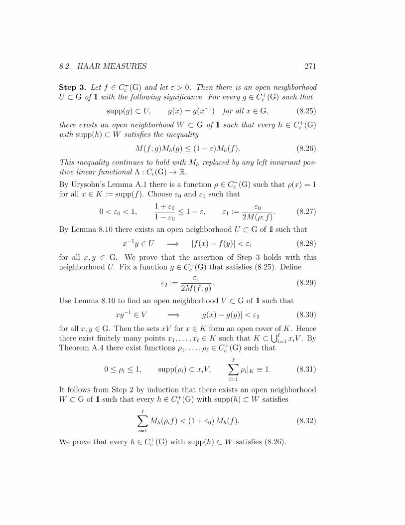
8.2. HAAR MEASURES 271
Step 3. Let f ∈ C+c (G) and let ε > 0. Then there is an open neighborhood
U ⊂ G of 1l with the following significance. For every g ∈ C+c (G) such that
supp(g) ⊂ U, g(x) = g(x−1) for all x ∈ G, (8.25)
there exists an open neighborhood W ⊂ G of 1l such that every h ∈ C+c (G)
with supp(h) ⊂ W satisfies the inequality
M(f ; g)Mh(g) ≤ (1 + ε)Mh(f). (8.26)
This inequality continues to hold with Mh replaced by any left invariant pos-itive linear functional Λ : Cc(G)→ R.
By Urysohn’s Lemma A.1 there is a function ρ ∈ C+c (G) such that ρ(x) = 1
for all x ∈ K := supp(f). Choose ε0 and ε1 such that
0 < ε0 < 1,1 + ε0
1− ε0
≤ 1 + ε, ε1 :=ε0
2M(ρ; f). (8.27)
By Lemma 8.10 there exists an open neighborhood U ⊂ G of 1l such that
x−1y ∈ U =⇒ |f(x)− f(y)| < ε1 (8.28)
for all x, y ∈ G. We prove that the assertion of Step 3 holds with thisneighborhood U . Fix a function g ∈ C+
c (G) that satisfies (8.25). Define
ε2 :=ε1
2M(f ; g). (8.29)
Use Lemma 8.10 to find an open neighborhood V ⊂ G of 1l such that
xy−1 ∈ V =⇒ |g(x)− g(y)| < ε2 (8.30)
for all x, y ∈ G. Then the sets xV for x ∈ K form an open cover of K. Hencethere exist finitely many points x1, . . . , x` ∈ K such that K ⊂
⋃`i=1 xiV . By
Theorem A.4 there exist functions ρ1, . . . , ρ` ∈ C+c (G) such that
0 ≤ ρi ≤ 1, supp(ρi) ⊂ xiV,∑i=1
ρi|K ≡ 1. (8.31)
It follows from Step 2 by induction that there exists an open neighborhoodW ⊂ G of 1l such that every h ∈ C+
c (G) with supp(h) ⊂ W satisfies∑i=1
Mh(ρif) < (1 + ε0)Mh(f). (8.32)
We prove that every h ∈ C+c (G) with supp(h) ⊂ W satisfies (8.26).
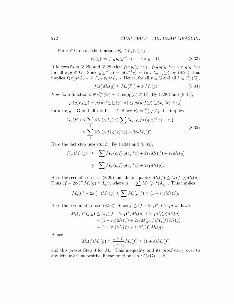
272 CHAPTER 8. THE HAAR MEASURE
For x ∈ G define the function Fx ∈ Cc(G) by
Fx(y) := f(y)g(y−1x) for y ∈ G. (8.33)
It follows from (8.25) and (8.28) that f(x)g(y−1x)−f(y)g(y−1x) ≤ ε1g(y−1x)for all x, y ∈ G. Since g(y−1x) = g(x−1y) = (g Lx−1)(y) by (8.25), thisimplies f(x)gLx−1 ≤ Fx+ε1gLx−1 . Hence, for all x ∈ G and all h ∈ C+
c (G),
f(x)Mh(g) ≤Mh(Fx) + ε1Mh(g) (8.34)
Now fix a function h ∈ C+c (G) with supp(h) ⊂ W . By (8.30) and (8.31),
ρi(y)Fx(y) = ρi(y)f(y)g(y−1x) ≤ ρi(y)f(y)(g(x−1
i x) + ε2
)for all x, y ∈ G and all i = 1, . . . , `. Since Fx =
∑i ρiFx this implies
Mh(Fx) ≤∑i
Mh (ρiFx) ≤∑i
Mh (ρif)(g(x−1
i x) + ε2
)≤∑i
Mh (ρif) g(x−1i x) + 2ε2Mh(f).
(8.35)
Here the last step uses (8.32). By (8.34) and (8.35),
f(x)Mh(g) ≤∑i
Mh (ρif) g(x−1i x) + 2ε2Mh(f) + ε1Mh(g)
≤∑i
Mh (ρif) g(x−1i x) + 2ε1Mh(g).
Here the second step uses (8.29) and the inequality Mh(f) ≤M(f ; g)Mh(g).Thus (f − 2ε1)+ Mh(g) ≤ Lµg, where µ :=
∑iMh (ρif) δx−1
i. This implies
Mg((f − 2ε1)+)Mh(g) ≤∑i
Mh(ρif) ≤ (1 + ε0)Mh(f).
Here the second step uses (8.32). Since f ≤ (f − 2ε1)+ + 2ε1ρ we have
Mg(f)Mh(g) ≤Mg((f − 2ε1)+)Mh(g) + 2ε1Mg(ρ)Mh(g)
≤ (1 + ε0)Mh(f) + 2ε1M(ρ; f)Mg(f)Mh(g)
= (1 + ε0)Mh(f) + ε0Mg(f)Mh(g).
Hence
Mg(f)Mh(g) ≤ 1 + ε0
1− ε0
Mh(f) ≤ (1 + ε)Mh(f)
and this proves Step 3 for Mh. This inequality and its proof carry over toany left invariant positive linear functional Λ : Cc(G)→ R.
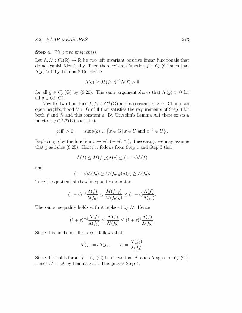
8.2. HAAR MEASURES 273
Step 4. We prove uniqueness.
Let Λ,Λ′ : Cc(R) → R be two left invariant positive linear functionals thatdo not vanish identically. Then there exists a function f ∈ C+
c (G) such thatΛ(f) > 0 by Lemma 8.15. Hence
Λ(g) ≥M(f ; g)−1Λ(f) > 0
for all g ∈ C+c (G) by (8.20). The same argument shows that Λ′(g) > 0 for
all g ∈ C+c (G).
Now fix two functions f, f0 ∈ C+c (G) and a constant ε > 0. Choose an
open neighborhood U ⊂ G of 1l that satisfies the requirements of Step 3 forboth f and f0 and this constant ε. By Urysohn’s Lemma A.1 there exists afunction g ∈ C+
c (G) such that
g(1l) > 0, supp(g) ⊂x ∈ G |x ∈ U and x−1 ∈ U
.
Replacing g by the function x 7→ g(x) + g(x−1), if necessary, we may assumethat g satisfies (8.25). Hence it follows from Step 1 and Step 3 that
Λ(f) ≤M(f ; g)Λ(g) ≤ (1 + ε)Λ(f)
and(1 + ε)Λ(f0) ≥M(f0; g)Λ(g) ≥ Λ(f0).
Take the quotient of these inequalities to obtain
(1 + ε)−1 Λ(f)
Λ(f0)≤ M(f ; g)
M(f0; g)≤ (1 + ε)
Λ(f)
Λ(f0).
The same inequality holds with Λ replaced by Λ′. Hence
(1 + ε)−2 Λ(f)
Λ(f0)≤ Λ′(f)
Λ′(f0)≤ (1 + ε)2 Λ(f)
Λ(f0).
Since this holds for all ε > 0 it follows that
Λ′(f) = cΛ(f), c :=Λ′(f0)
Λ(f0).
Since this holds for all f ∈ C+c (G) it follows that Λ′ and cΛ agree on C+
c (G).Hence Λ′ = cΛ by Lemma 8.15. This proves Step 4.
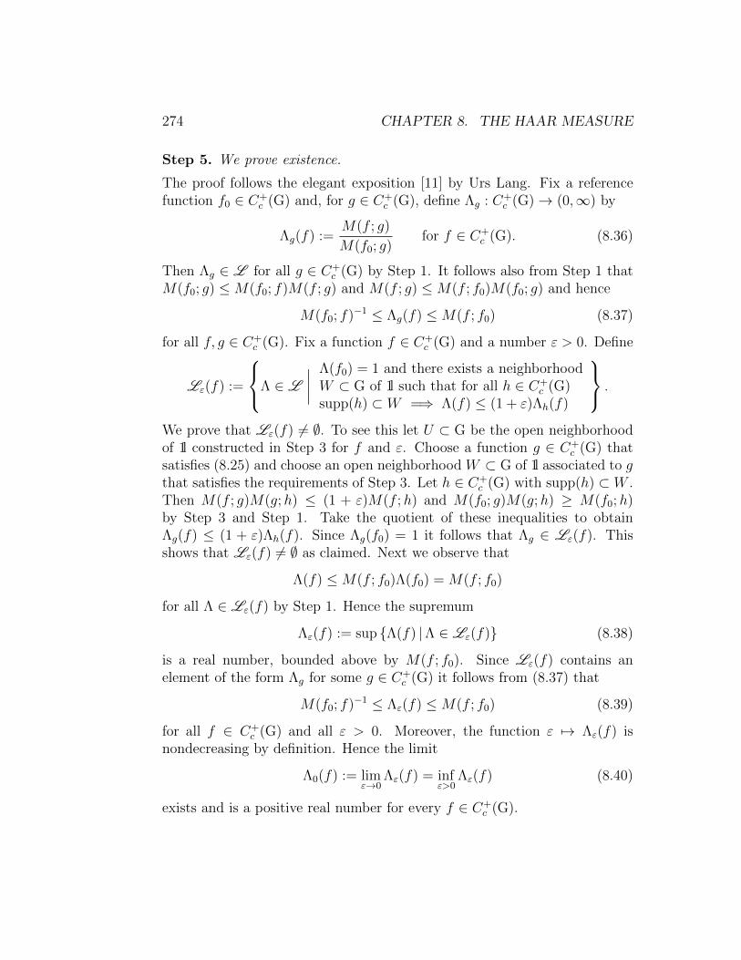
274 CHAPTER 8. THE HAAR MEASURE
Step 5. We prove existence.
The proof follows the elegant exposition [11] by Urs Lang. Fix a referencefunction f0 ∈ C+
c (G) and, for g ∈ C+c (G), define Λg : C+
c (G)→ (0,∞) by
Λg(f) :=M(f ; g)
M(f0; g)for f ∈ C+
c (G). (8.36)
Then Λg ∈ L for all g ∈ C+c (G) by Step 1. It follows also from Step 1 that
M(f0; g) ≤M(f0; f)M(f ; g) and M(f ; g) ≤M(f ; f0)M(f0; g) and hence
M(f0; f)−1 ≤ Λg(f) ≤M(f ; f0) (8.37)
for all f, g ∈ C+c (G). Fix a function f ∈ C+
c (G) and a number ε > 0. Define
Lε(f) :=
Λ ∈ L
∣∣∣∣ Λ(f0) = 1 and there exists a neighborhoodW ⊂ G of 1l such that for all h ∈ C+
c (G)supp(h) ⊂ W =⇒ Λ(f) ≤ (1 + ε)Λh(f)
.
We prove that Lε(f) 6= ∅. To see this let U ⊂ G be the open neighborhoodof 1l constructed in Step 3 for f and ε. Choose a function g ∈ C+
c (G) thatsatisfies (8.25) and choose an open neighborhood W ⊂ G of 1l associated to gthat satisfies the requirements of Step 3. Let h ∈ C+
c (G) with supp(h) ⊂ W .Then M(f ; g)M(g;h) ≤ (1 + ε)M(f ;h) and M(f0; g)M(g;h) ≥ M(f0;h)by Step 3 and Step 1. Take the quotient of these inequalities to obtainΛg(f) ≤ (1 + ε)Λh(f). Since Λg(f0) = 1 it follows that Λg ∈ Lε(f). Thisshows that Lε(f) 6= ∅ as claimed. Next we observe that
Λ(f) ≤M(f ; f0)Λ(f0) = M(f ; f0)
for all Λ ∈ Lε(f) by Step 1. Hence the supremum
Λε(f) := sup Λ(f) |Λ ∈ Lε(f) (8.38)
is a real number, bounded above by M(f ; f0). Since Lε(f) contains anelement of the form Λg for some g ∈ C+
c (G) it follows from (8.37) that
M(f0; f)−1 ≤ Λε(f) ≤M(f ; f0) (8.39)
for all f ∈ C+c (G) and all ε > 0. Moreover, the function ε 7→ Λε(f) is
nondecreasing by definition. Hence the limit
Λ0(f) := limε→0
Λε(f) = infε>0
Λε(f) (8.40)
exists and is a positive real number for every f ∈ C+c (G).

8.2. HAAR MEASURES 275
We prove that the functional Λ0 : C+c (G) → (0,∞) is left invariant. To
see this, fix a function f ∈ C+c (G) and an element x ∈ G. Then
Lε(f) = Lε(f Lx)
for all ε > 0. Namely, if W ⊂ G is an open neighborhood of 1l such thatΛ(f) ≤ (1 + ε)Λh(f) for all h ∈ C+
c (G) with supp(h) ⊂ W , then the sameinequality holds with f replaced by f Lx because both Λ and Λh are leftinvariant. Hence Λε(f) = Λε(f Lx) for all ε > 0 and so Λ0(f) = Λ0(f Lx).
We prove that the functional Λ0 : C+c (G) → (0,∞) is additive. To see
this, fix two functions f, f ′ ∈ C+c (G). We prove that
(1 + ε)−1Λε(f + f ′) ≤ Λε(f) + Λε(f′) ≤ (1 + ε)Λε(f + f ′) (8.41)
for all ε > 0. To prove the first inequality in (8.41) choose any functionalΛ ∈ Lε(f + f ′). Then there exists an open neighborhood W ⊂ G of 1l suchthat Λ(f + f ′) ≤ (1 + ε)Λh(f + f ′) for all h ∈ C+
c (G) with supp(h) ⊂ W .Moreover, we have seen above that h ∈ C+
c (G) can be chosen such thatsupp(h) ⊂ W and also Λh ∈ Lε(f) ∩Lε(f
′). Any such h satisfies
(1 + ε)−1Λ(f + f ′) ≤ Λh(f + f ′) ≤ Λh(f) + λh(f′) ≤ Λε(f) + Λε(f
′).
Take the supremum over all Λ ∈ Lε(f + f ′) to obtain the first inequalityin (8.41). To prove the second inequality in (8.41) fix a constant α > 1and choose two functionals Λ ∈ Lε(f) and Λ′ ∈ Lε(f
′). Then there existsan open neighborhood W ⊂ G of 1l such that Λ(f) ≤ (1 + ε)Λh(f) andΛ′(f ′) ≤ (1 + ε)Λh(f
′) for all h ∈ C+c (G) with supp(h) ⊂ W . By Step 2,
the function h ∈ C+c (G) can be chosen such that supp(h) ⊂ W and also
Λh(f) + Λh(f′) ≤ αΛh(f + f ′) and Λh ∈ Lε(f + f ′). Any such h satisfies
(1 + ε)−1(Λ(f) + Λ′(f ′)
)≤ Λh(f) + Λh(f
′) ≤ αΛh(f + f ′) ≤ αΛε(f + f ′).
Take the supremum over all pairs of functionals Λ ∈ Lε(f) and Λ′ ∈ Lε(f′)
to obtain (1− ε)−1(Λε(f) + Λε(f
′))≤ αΛε(f + f ′) for all α > 1. This proves
the second inequality in (8.41). Take the limit ε → 0 in (8.41) to obtainthat Λ0 is additive. Moreover, it follows directly from the definition thatΛ0(f0) = 1. Hence it follows from Lemma 8.15 that Λ0 extends to a nonzeroleft invariant positive linear functional on Cc(G). This proves Step 5 andTheorem 8.14.

276 CHAPTER 8. THE HAAR MEASURE
If one is prepared to use some abstract concepts from general topologythen the existence proof in Theorem 8.14 is essentially complete after Step 2.This approach is taken in Pedersen [16]. In this language the space
G :=g ∈ C+
c (G)∣∣ 0 ≤ g ≤ 1, g(1l) = 1
is a directed set equipped with a map g 7→ Λg that takes values in the space
L :=
Λ : C+
c (G)→ R∣∣∣∣ M(f0; f)−1 ≤ Λ(f) ≤M(f0; f)
for all f ∈ C+c (G)
.
The map G → L : g 7→ Λg is a net. A net can be thought of as an uncountableanalogue of a sequence and a subnet as an analogue of a subsequence. Theexistence of a universal subnet is guaranteed by the general theory and itsconvergence for each f by the fact that the target space is compact. InsteadStep 3 in the proof of Theorem 8.14 implies that the original net g 7→ Λg
converges and so there is no need to choose a universal subnet. That thiscan be proved with a refinement of the uniqueness argument (Λ in Step 3) ispointed out in Pedersen [16]. That paper also contains two further uniquenessproofs. One is based on Fubini’s Theorem and the other on the Radon–Nikodym Theorem. Another existence proof for compact second countableHausdorff groups is due to Pontryagin. It uses the Arzela–Ascoli theorem toestablish the existence of a sequence µi ∈ P with ‖µi‖ = 1 such that Lµifconverges to a constant function whose value is then taken to be Λ(f).
Proof of Theorem 8.12. Existence and uniqueness in (i) follow directly fromTheorem 8.14 and the Riesz Representation theorem 3.15. That nonemptyopen sets have positive measure follows from Urysohn’s Lemma A.1. Toprove (ii) consider the map φ : G → G defined by φ(x) := x−1 for x ∈ G.Since φ is a homeomorphism it preserves the Borel σ-algebra B. Sinceφ Rx = Lx−1 φ, a measure µ : B → [0,∞] is a left Haar measure if andonly if the measure ν : B → [0,∞] defined by ν(B) := µ(φ(B)) = µ(B−1) isa right Haar measure. Hence assertion (ii) follows from (i).
We prove (iii). Assume G is compact and let µ : B → [0, 1] be the uniqueleft Haar measure such that µ(G) = 1. For x ∈ G define µx : B → [0, 1]by µx(B) := µ(Rx(B)) for B ∈ B. Since Rx commutes with Ly for all yby (8.11), µx is a left Haar measure. Since µx(G) = µ(Rx(G)) = µ(G) = 1it follows that µx = µ for all x ∈ G. Hence µ is right invariant. Thereforethe map B → [0, 1] : B 7→ ν(B) := µ(φ(B)) = µ(B−1) is a left Haar measureand, since ν(G) = 1, it agrees with µ. This proves Theorem 8.12.
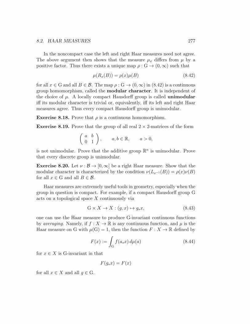
8.2. HAAR MEASURES 277
In the noncompact case the left and right Haar measures need not agree.The above argument then shows that the measure µx differs from µ by apositive factor. Thus there exists a unique map ρ : G→ (0,∞) such that
µ(Rx(B)) = ρ(x)µ(B) (8.42)
for all x ∈ G and all B ∈ B. The map ρ : G→ (0,∞) in (8.42) is a continuousgroup homomorphism, called the modular character. It is independent ofthe choice of µ. A locally compact Hausdorff group is called unimodulariff its modular character is trivial or, equivalently, iff its left and right Haarmeasures agree. Thus every compact Hausdorff group is unimodular.
Exercise 8.18. Prove that ρ is a continuous homomorphism.
Exercise 8.19. Prove that the group of all real 2× 2-matrices of the form(a b0 1
), a, b ∈ R, a > 0,
is not unimodular. Prove that the additive group Rn is unimodular. Provethat every discrete group is unimodular.
Exercise 8.20. Let ν : B → [0,∞] be a right Haar measure. Show that themodular character is characterized by the condition ν(Lx−1(B)) = ρ(x)ν(B)for all x ∈ G and all B ∈ B.
Haar measures are extremely useful tools in geometry, especially when thegroup in question is compact. For example, if a compact Hausdorff group Gacts on a topological space X continuously via
G×X → X : (g, x) 7→ g∗x, (8.43)
one can use the Haar measure to produce G-invariant continuous functionsby averaging. Namely, if f : X → R is any continuous function, and µ is theHaar measure on G with µ(G) = 1, then the function F : X → R defined by
F (x) :=
∫G
f(a∗x) dµ(a) (8.44)
for x ∈ X is G-invariant in that
F (g∗x) = F (x)
for all x ∈ X and all g ∈ G.

278 CHAPTER 8. THE HAAR MEASURE
Exercise 8.21. Give a precise definition of what it means for a topologicalgroup to act continuously on a topological space.
Exercise 8.22. Show that the map F in (8.44) is continuous and G-invariant.
Exercise 8.23. Let ρ : G → GL(V ) be a homomorphism from a com-pact Hausdorff group to the general linear group of automorphisms of afinite-dimensional vector space. (Such a homomorphism is called a repre-sentation of G.) Prove that V admits a G-invariant inner product. Thisobservation does not extend to noncompact groups. Show that the standardrepresentation of SL(2,R) on R2 does not admit an invariant inner product.
Exercise 8.24. Show that the Haar measure on a discrete group is a multipleof the counting measure. Deduce that for a finite group the formula (8.44)defines F (x) as the average (with multiplicities) of the values of f over thegroup orbit of x.
Exercise 8.25. Let G be a locally compact Hausdorff group and let µ bea left Haar measure on G. Define the convolution product on L1(µ). Showthat L1(µ) is a Banach algebra. (See page 236.) Find conditions under whichf ∗g = g∗f . Show that the convolution is not commutative in general. Hint:See Section 7.5 for G = Rn. See also Step 3 in the proof of Theorem 8.14.

Appendix A
Urysohn’s Lemma
Theorem A.1 (Urysohn’s Lemma). Let X be a locally compact Hausdorffspace and let K ⊂ X be a compact set and U ⊂ X be an open set such that
K ⊂ U.
Then there exists a compactly supported continuous function
f : X → [0, 1]
such that
f |K ≡ 1, supp(f) =x ∈ X
∣∣ f(x) 6= 0⊂ U. (A.1)
Proof. See page 281.
Lemma A.2. Let X be a topological space and let K ⊂ X be compact. Thenthe following holds.
(i) Every closed subset of K is compact.
(ii) If X is Hausdorff then, for every y ∈ X \ K, there exist open setsU, V ⊂ X such that K ⊂ U , y ∈ V , and U ∩ V = ∅.(iii) If X is Hausdorff then K is closed.
Proof. We prove (i). Let F ⊂ K be closed and let Uii∈I be an open coverof F . Then the sets Uii∈I together with V := X \ F form an open coverof K. Hence there exist finitely many indices i1, . . . , in such that the setsUi1 , . . . , Uin , V cover K. Hence F ⊂ Ui1 ∪ · · · ∪ Uin . This shows that everyopen cover of F has a finite subcover and so F is compact.
279
280 APPENDIX A. URYSOHN’S LEMMA
We prove (ii). Assume X is Hausdorff and let y ∈ X \K. Define
U :=U ⊂ X |U is open and y /∈ U
.
Since X is Hausdorff the collection U is an open cover of K. Since K iscompact, there exists finitely many set U1, . . . , Un ∈ U such that
K ⊂ U := U1 ∪ · · · ∪ Un.
Since y /∈ U i for all i it follows that y ∈ V := X \ U and U ∩ V = ∅. Hencethe sets U and V satisfy the requirements of (ii).
We prove (iii). Assume X is Hausdorff. Then it follows from part (ii)that, for every y ∈ X \K, there exists an open set V ⊂ X such that y ∈ Vand V ∩ K = ∅. Hence X \ K is the union of all open sets in X thatare disjoint from K. Thus X \ K is open and so K is closed. This provesLemma A.2.
Lemma A.3. Let X be a locally compact Hausdorff space and let K,U besubsets of X such that K is compact, U is open, and K ⊂ U . Then thereexists an open set V ⊂ X such that V is compact and
K ⊂ V ⊂ V ⊂ U. (A.2)
Proof. We first prove the assertion in the case where K = x consist ofa single element. Choose a compact neighborhood B ⊂ X of x. ThenF := B \ U is a closed subset of B and hence is compact by part (i) ofLemma A.2. Since x /∈ F it follows from part (ii) of Lemma A.2 that thereexist open sets W,W ′ ⊂ X such that x ∈ W , F ⊂ W ′ and W ∩W ′ = ∅.Hence V := int(B) ∩W is an open neighborhood of x, its closure is a closedsubset of B and hence compact, and
V ⊂ B ∩W ⊂ B \W ′ ⊂ B \ F ⊂ U.
This proves the lemma in the case #K = 1.Now consider the general case. By the first part of the proof the open
sets whose closures are compact and contained in U form an open cover of K.Since K is compact there exist finitely any open sets V1, . . . , Vn such that V i
is a compact subset of U for all i and K ⊂⋃ni=1 Vi. Hence V :=
⋃ni=1 Vi is
an open set containing K and its closure V =⋃ni=1 V i is a compact subset
of U . This proves Lemma A.3.
281
Proof of Theorem A.1. The proof has three steps. The first step requires theAxiom of Dependent Choice.
Step 1. There exists a family of open sets Vr ⊂ X with compact closure,parametrized by r ∈ Q ∩ [0, 1], such that
K ⊂ V1 ⊂ V 1 ⊂ V0 ⊂ V 0 ⊂ U (A.3)
ands > r =⇒ V s ⊂ Vr (A.4)
for all r, s ∈ Q ∩ [0, 1].
The existence of open sets V0 and V1 with compact closure satisfying (A.3)follows from Lemma A.3. Now choose a bijective map N0 → Q ∩ [0, 1] : i 7→ qisuch that q0 = 0 and q1 = 1. Suppose by induction that the open setsVi = Vqi have been constructed for i = 0, 1, . . . , n such that (A.4) holds forr, s ∈ q0, q1, . . . , qn. Choose k, ` ∈ 0, 1, . . . , n such that
qk := max qi | 0 ≤ i ≤ n, qi < qn+1 ,q` := min qi | 0 ≤ i ≤ n, qi > qn+1 .
Then V ` ⊂ Vk. Hence it follows from Lemma A.3 that there exists an open setVn+1 = Vqn+1 ⊂ X with compact closure such that V ` ⊂ Vn+1 ⊂ V n+1 ⊂ Vk.This completes the induction argument and Step 1 then follows from theAxiom of Dependent Choice. (Denote by V the set of all open sets V ⊂ Xsuch that K ⊂ V ⊂ V ⊂ U . Denote by V the set of all finite sequencesv = (V0, . . . , Vn) in V that satisfy (A.3) and qi < qj =⇒ V j ⊂ Vi for all i, j.Define a relation on V by v = (V1, . . . , Vn) ≺ v′ = (V ′1 , . . . , V
′n′) iff n < n′ and
Vi = V ′i for i = 0, . . . , n. Then V is nonempty and for every v ∈ V there isa v′ ∈ V such that v ≺ v′. Hence, by the Axiom of Dependent Choice, thereexists a sequence vj = (Vj,0, . . . , Vj,nj) ∈ V such that vj ≺ vj+1 for all j ∈ N.Define the map Q∩ [0, 1]→ V : q 7→ Vq by Vqi := Vj,i for i, j ∈ N with nj ≥ i.This map is well and satisfies (A.3) and (A.4) by definition of V and ≺.)
Step 2. Let Vr ⊂ X be as in Step 1 for r ∈ Q ∩ [0, 1]. Then
f(x) := sup r ∈ Q ∩ [0, 1] |x ∈ Vr= inf
s ∈ Q ∩ [0, 1] |x /∈ V s
(A.5)
for all x ∈ X. (Here the supremum of the empty set is zero and the infimumover the empty set is one.)
282 APPENDIX A. URYSOHN’S LEMMA
We prove equality in (A.5). Fix a point x ∈ X and define
a := sup r ∈ Q ∩ [0, 1] |x ∈ Vr ,b := inf
s ∈ Q ∩ [0, 1] |x /∈ V s
.
We prove that a ≤ b. If b = 1 this follows directly from the definitions.Hence assume b < 1 and choose an element s ∈ Q ∩ [0, 1] such that
x /∈ V s.
If r ∈ Q∩ [0, 1] such that x ∈ Vr then Vr \V s 6= ∅, hence V s ⊂ Vr, and hencer ≤ s. Thus we have proved that
x ∈ Vr =⇒ r ≤ s
for all r ∈ Q ∩ [0, 1]. Take the supremum over all r ∈ Q ∩ [0, 1] with x ∈ Vrto obtain a ≤ s. Then take the infimum over all s ∈ Q ∩ [0, 1] with x /∈ V s
to obtain a ≤ b. Now suppose, by contradiction, that a < b. Choose rationalnumbers r, s ∈ Q∩ [0, 1] such that a < r < s < b. Since a < r it follows thatx /∈ Vr, since s < b it follows that x ∈ V s, and since r < s it follows fromStep 1 that V s ⊂ Vr. This is a contradiction and shows that our assumptionthat a < b must have been wrong. Thus a = b and this proves Step 2.
Step 3. The function f : X → [0, 1] in Step 2 is continuous and
f(x) =
0, for x ∈ X \ V0,1, for x ∈ V 1
(A.6)
Thus f satisfies the requirements of Theorem A.1.
That f satisfies (A.6) follows directly from the definition of f in (A.5). Weprove that f is continuous. To see this fix a constant c ∈ R. Then f(x) < cif and only if there exists a rational number s ∈ Q ∩ [0, 1] such that s < cand x /∈ Vs. Likewise, f(x) > c if and only if there exists a rational numberr ∈ Q ∩ [0, 1] such that r > c and x ∈ Vr. Hence
f−1((c,∞)) =⋃
r∈Q∩(c,1]
Vr, f−1((−∞, c)) =⋃
s∈Q∩[0,c)
(X \ V s).
This implies that the pre-image under f of every open interval in R is anopen subset of X. Hence also the pre-image under f of every union ofopen intervals is open in X and so f is continuous. This proves Step 3 andTheorem A.1.
283
Theorem A.4 (Partition of Unity). Let X be a locally compact Hausdorffspace, let U1, . . . , Un ⊂ X be open sets, and let K ⊂ U1∪· · ·∪Un be a compactset. Then there exist continuous functions f1, . . . , fn : X → R with compactsupport such that
fi ≥ 0,n∑i=1
fi ≤ 1, supp(fi) ⊂ Ui
for all i and∑n
i=1 fi(x) = 1 for all x ∈ K.
Proof. Define the set
V :=
V ⊂ X
∣∣∣∣ V is open, V is compact, and there existsan index i ∈ 1, . . . , n such that V ⊂ Ui
.
If x ∈ K then x ∈ Ui for some index i ∈ 1, . . . , n and, by Lemma A.3,there is an open set V ⊂ X such that V is compact and x ∈ V ⊂ V ⊂ Ui.Thus V is an open cover of K. Since K is compact there exist finitely manyopen sets V1, . . . , V` ∈ V such that K ⊂ V1 ∪ · · · ∪ V`. For i = 1, . . . , n define
Ki :=⋃
1≤j≤`, V j⊂Ui
V j.
Then K ⊂ K1∪· · ·∪Kn and Ki is a compact subset of Ui for each i. Hence itfollows from Urysohn’s Lemma A.1 that, for each i, there exists a compactlysupported continuous function gi : X → R such that
0 ≤ gi ≤ 1, supp(gi) ⊂ Ui, gi|Ki ≡ 1.
Define
f1 := g1,
f2 := (1− g1)g2,
f3 := (1− g1)(1− g2)g3,...
fn := (1− g1) · · · (1− gn−1)gn.
Then supp(fi) ⊂ supp(gi) ⊂ Ui for each i and
1−n∑i=1
fi =n∏i=1
(1− gi).
Since K ⊂ K1 ∪ · · · ∪Kn and the factor 1 − gi vanishes on Ki, this implies∑ni=1 fi(x) = 1 for all x ∈ K. This proves Theorem A.4.

284 APPENDIX A. URYSOHN’S LEMMA
Appendix B
The Product Topology
Let (X,UX) and (Y,UY ) be topological spaces, denote the product space by
X × Y :=
(x, y)∣∣x ∈ X, y ∈ Y ,
and let πX : X × Y → X and πY : X × Y → Y be the projections ontothe first and second factor. Consider the following universality property fora topology U ⊂ 2X×Y on the product space.
(P) Let (Z,UZ) be any topological space and let h : Z → X × Y be any map.Then h : (Z,UZ)→ (X × Y,U) is continuous if and only if the maps
f := πX h : (Z,UZ)→ (X,UX),
g := πY h : (Z,UZ)→ (Y,UY )(B.1)
are continuous.
Theorem B.1. (i) There is a unique topology U on X×Y that satisfies (P).
(ii) Let U ⊂ 2X×Y be as in (i). Then W ∈ U if and only if there are open setsUi ∈ UX and Vi ∈ UY , indexed by any set I, such that W =
⋃i∈I(Ui × Vi).
(iii) Let U ⊂ 2X×Y be as in (i). Then U is the smallest topology on X × Ywith respect to which the projections πX and πY are continuous.
(iv) Let U ⊂ 2X×Y be as in (i). Then the inclusion
ιx : (Y,UY )→ (X × Y,U), ιx(y) := (x, y) for y ∈ Y,
is continuous for every x ∈ X and the inclusion
ιy : (X,UX)→ (X × Y,U), ιy(x) := (x, y) for x ∈ X,
is continuous for every y ∈ Y .
285
286 APPENDIX B. THE PRODUCT TOPOLOGY
Definition B.2. The product topology on X×Y is defined as the uniquetopology that satisfies (P) or, equivalently, as the smallest topology on X×Ysuch that the projections πX and πY are continuous. It is denoted by
UX×Y ⊂ 2X×Y .
Proof of Theorem B.1. The proof has five steps.
Step 1. If U ⊂ 2X×Y is a topology satisfying (P) then the projections πXand πY are continuous.
Take h := id : X×Y → X×Y so that f = πX h = πX and g = πY h = πY .
Step 2. We prove uniqueness in (i).
Let U ,U ′ ⊂ 2X×Y be two topologies satisfying (P) and consider the maph := id : (X × Y,U) → (X × Y,U ′). Since f = πX : (X × Y,U) → (X,UX)and g = πY : (X × Y,U) → (Y,UY ) are continuous by Step 1, and U ′satisfies (P), it follows that h is continuous and hence U ′ ⊂ U . Interchangethe roles of U and U ′ to obtain U ′ = U .
Step 3. We prove (ii) and existence in (i).
Define U ⊂ 2X×Y as the collection of all sets of the form W =⋃i∈I(Ui× Vi),
where I is any index set and Ui ∈ UX , Vi ∈ UY for i ∈ I. Then U is a topologyand the projections πX : (X×Y,U)→ (X,UX) and πY : (X×Y,U)→ (Y,UY )are continuous. We prove that U satisfies (P). To see this, let (Z,UZ) be anytopological space, let h : Z → X×Y be any map, and define f := πX h andg := πY h as in (B.1). If h is continuous then so are f and g. Conversely,if f and g are continuous, then h−1(U × V ) = f−1(U) ∩ g−1(V ) is open in Zfor all U ∈ UX and all V ∈ UY , and hence it follows from the definition of Uthat h−1(W ) is open for all W ∈ U . Thus h is continuous.
Step 4. We prove (iii).
Let U be the topology in (i) and let U ′ be any topology on X × Y withrespect to which πX and πY are continuous. If U ∈ UX and V ∈ UY thenU × V = π−1
X (U) ∩ π−1Y (V ) ∈ U ′. Hence U ⊂ U ′ by (ii). Since πX and πY
are continuous with respect to U it follows that U is the smallest topologyon X × Y with respect to which πX and πY are continuous.
Step 5. We prove (iv).
Fix an element x ∈ X and consider the map h := ιx : Y → X × Y . Thenthe map f := πX h : Y → X is constant and g := πY h : Y → Y isthe identity. Hence f and g are continuous and so is h by condition (P). Ananalogous argument shows that ιy is continuous for all y ∈ Y .
Appendix C
The Inverse Function Theorem
This appendix contains a proof of the inverse function theorem. The resultis formulated in the setting of continuously differentiable maps between opensets in a Banach space. Readers who are unfamiliar with bounded linearoperators on Banach spaces may simply think of continuously differentiablemaps between open sets in finite-dimensional normed vector spaces. The in-verse function theorem is used on page 71 in the proof of Lemma 2.19, whichis a key step in the proof of the transformation formula for the Lebesgue mea-sure (Theorem 2.17). Assume throughout that (X, ‖·‖) is a Banach space.When Φ : X → X is a bounded linear operator denote its operator norm by
‖Φ‖ := ‖Φ‖L(X) := supx∈X\0
‖Φx‖‖x‖
.
For x ∈ X and r > 0 denote by Br(x) := y ∈ X | ‖x− y‖ < r the openball of radius r about x. For x = 0 abbreviate Br := Br(0).
Theorem C.1 (Inverse Function Theorem). Fix an element x0 ∈ Xand two real numbers r > 0 and 0 < α < 1. Let ψ : Br(x0) → X be acontinuously differentiable map such that
‖dψ(x)− 1l‖L(X) ≤ α for all x ∈ Br(x0). (C.1)
ThenB(1−α)r(ψ(x0)) ⊂ ψ(Br(x0)) ⊂ B(1+α)r(ψ(x0)). (C.2)
Moreover, the map ψ is injective, its image is open, the map ψ−1 is contin-uously differentiable, and dψ−1(y) = dψ(ψ−1(y))−1 for all y ∈ ψ(Br(x0)).
287
288 APPENDIX C. THE INVERSE FUNCTION THEOREM
Proof. Assume without loss of generality that x0 = ψ(x0) = 0.
Step 1. ψ is a homeomorphism onto its image and ψ(Br) ⊂ B(1+α)r.
Define φ := id− ψ : Br → X. Then ‖dφ(x)‖ ≤ α for all x ∈ Br. Hence
‖φ(x)− φ(y)‖ ≤ α‖x− y‖. (C.3)
for all x, y ∈ Br and so
(1− α) ‖x− y‖ ≤ ‖ψ(x)− ψ(y)‖ ≤ (1 + α) ‖x− y‖ . (C.4)
The second inequality in (C.4) shows that ψ(Br) ⊂ B(1+α)r and the firstinequality in (C.4) shows that ψ is injective and ψ−1 is Lipschitz continuous.
Step 2. B(1−α)r ⊂ ψ(Br).
Let ξ ∈ B(1−α)r and define ε > 0 by ‖ξ‖ =: (1 − α)(r − ε). Then, by (C.3)with y = 0, we have ‖φ(x)‖ ≤ α‖x‖ for all x ∈ Br. If ‖x‖ ≤ r−ε this implies‖φ(x)+ ξ‖ ≤ r−ε. Thus the map x 7→ φ(x)+ ξ is a contraction of the closedball Br−ε. By the contraction mapping principle it has a unique fixed pointx and the fixed point satisfies ψ(x) = x− φ(x) = ξ. Hence ξ ∈ ψ(Br).
Step 3. ψ(Br) is open.
Let x ∈ Br and define y := ψ(x). Choose ε > 0 such that Bε(x) ⊂ Br. Then,by Step 2, B(1−α)ε(ψ(x)) ⊂ ψ(Bε(x)) ⊂ ψ(Br).
Step 4. ψ−1 is continuously differentiable.
Let x0 ∈ Br and define y0 := ψ(x0) and Ψ := dψ(x0). Then ‖1l−Ψ‖ ≤ α, so Ψis invertible, Ψ−1 =
∑∞k=0(1l−Ψ)k, and ‖Ψ−1‖ ≤ (1−α)−1. We prove that ψ−1
is differentiable at y0 and dψ−1(y0) = Ψ−1. Let ε > 0. Since ψ is differentiableat x0 and dψ(x0) = Ψ, there is a constant δ > 0 such that, for all x ∈ Br with‖x−x0‖ < δ(1−α)−1, we have ‖ψ(x)−ψ(x0)−Ψ(x−x0)‖ ≤ ε(1−α)2‖x−x0‖.Shrinking δ, if necessary, we may assume, by Step 3, that Bδ(y0) ⊂ ψ(Br).Now suppose ‖y − y0‖ < δ and denote x := ψ−1(y) ∈ Br. Then, by (C.4),‖x− x0‖ ≤ (1− α)−1 ‖y − y0‖ < δ(1− α)−1 and hence∥∥ψ−1(y)− ψ−1(y0)−Ψ−1(y − y0)
∥∥ =∥∥Ψ−1
(y − y0 −Ψ(x− x0)
)∥∥≤ 1
1− α‖ψ(x)− ψ(x0)−Ψ(x− x0)‖
≤ ε(1− α) ‖x− x0‖≤ ε ‖y − y0‖ .
Hence ψ−1 is differentiable at y0 and dψ−1(y0) = Ψ−1 = dψ(ψ−1(y0))−1. Thusdψ−1 is continuous by Step 1. This proves Theorem C.1.
Bibliography
[1] R.B. Ash, Basic Probability Theory, John Wiley & Sons 1970, Dover Publications, 2008.http://www.math.uiuc.edu/~r-ash/BPT/BPT.pdf
[2] V.I. Bogachev, Measure Theory, Volumes 1 & 2, Springer Verlag, 2006.
[3] W.F. Eberlein, Notes on integration I: The underlying convergence theorem. Comm. Pure Appl.Math. 10 (1957), 357–360.
[4] D.H. Fremlin, Measure Theory, Volumes 1–5, 2000.https://www.essex.ac.uk/maths/people/fremlin/mt.htm
[5] D. Gilbarg and N.S. Trudinger, Elliptic Partial Differential Equations of the Second Order, SpringerVerlag, 1983.
[6] P.R. Halmos, Measure Theory, Springer-Verlag, 1974.
[7] C.E. Heil, Lecture Notes on Real Analysis, Georgia Institute of Technology, Fall 2007.http://people.math.gatech.edu/~heil/6337/fall07/section3.4.pdf
http://people.math.gatech.edu/~heil/6337/fall07/section3.5b.pdf
[8] H. Konig, New versions of the Radon–Nikodym theorem. Arch. Math. 86 (2006), 251–260.http://www.math.uni-sb.de/service/preprints/preprint132.pdf
[9] T.W. Korner, A Companion to Analysis. Graduate Studies in Mathematics 62, AMS 2004. https://www.dpmms.cam.ac.uk/~twk/
[10] U. Lang, Mass & Integral, Vorlesungsmanuskript, ETH Zurich, September 2006.http://www.math.ethz.ch/~lang/mi.pdf
[11] U. Lang, Existence and uniqueness of Haar integrals. ETH Zurich, January 2015.http://www.math.ethz.ch/~lang/HaarIntegral.pdf
[12] Dan Ma, The Lexicographic Order and The Double Arrow Space. 7 Oct. 2009.http://dantopology.wordpress.com/2009/10/07/
[13] P. Malliavin, Integration and Probability (in cooperation with Helene Airault, Leslie Kay, GerardLetac), Springer-Verlag, 1995.
[14] J.R. Munkres, Topology, Second Edition. Prentice Hall, 2000.
[15] G. Nagy, Real Analysis IV.6, Duals of Lp spaces.http://www.math.ksu.edu/~nagy/real-an/4-06-dual-lp.pdf
[16] G.K. Pedersen, The existence and uniqueness of the Haar integral on a locally compact topologicalgroup. Preprint, University of Copenhagen, November 2000.http://www.math.ku.dk/kurser/2004-2/mat3re/haarintegral.pdf
[17] W. Rudin, Real and Complex Analysis, 3rd Ed. McGraw–Hill, 1987.
[18] D.A. Salamon, Das Riemannsche Integral. Lecture Notes, ETHZ, 2014.http://www.math.ethz.ch/~salamon/PREPRINTS/ana1-int.pdf
[19] D.A. Salamon, Mehrfache Integrale. Lecture notes, ETHZ, 2014.http://www.math.ethz.ch/~salamon/PREPRINTS/ana2-int.pdf
[20] D.A. Salamon, Funktionentheorie. Birkhauser, 2012.http://www.math.ethz.ch/~salamon/PREPRINTS/cxana.pdf
[21] W.F. Trench, Introduction to Real Analysis, Prentice Hall, 2003.http://ramanujan.math.trinity.edu/wtrench/misc/index.shtml
289
Index
absolutely continuousfunction, 201, 207measure, 151signed measure, 169, 173
almost everywhere, 33
Baire measurablefunction, 110set, 110
Baire measure, 110Baire σ-algebra, 110Banach algebra, 236Banach space, 7Banach–Zarecki Theorem, 201basis of a topological space, 106bilinear form
positive definite, 125symmetric, 125
Boolean algebra, 6Borel measurable
function, 12set, 9
Borel measure, 82extended, 91left invariant, 264right invariant, 264
Borel outer measure, 92Borel set, 9Borel σ-algebra, 9bounded linear functional, 126bounded variation, 205
Calderon–Zygmund inequality, 246Caratheodory Criterion, 53Cauchy–Schwarz inequality, 125characteristic function, 12closed set, 6compact set, 10compactly supported function, 97complete measure space, 39complete metric space, 7completion of a measure space, 39continuous map, 10continuum hypothesis, 124convergence in measure, 147convolution, 232
of signed measures, 257counting measure, 19cuboid, 56
dense subset, 120Dieudonne’s measure, 83Dirac measure, 19Divergence Theorem, 255double arrow space, 107dual space
of a Hilbert space, 127of a normed vector space, 126of C(X), 106, 183of L2(µ), 129of Lp(µ), 135of `∞, 136, 149
290
INDEX 291
Egoroff’s Thorem, 147elementary set, 210envelope, 130essential supremum, 117
first countable, 106Fubini’s Theorem
for integrable functions, 222for positive functions, 219for the completion, 224for the Lebesgue measure, 231in polar coordinates, 255
fundamental solutionof Laplace’s equation, 244
Fundamental Theoremof Calculus, 201
Green’s formula, 245group
discrete, 260Lie, 260topological, 259unimodular, 277
Haar integral, 265Haar measure, 264Hahn decomposition, 171Hahn–Banach Theorem, 136Hardy’s inequality, 146Hardy–Littlewood
maximal inequality, 192Hausdorff dimension, 80Hausdorff measure, 80Hausdorff space, 10, 81Hilbert space, 126Holder inequality, 114
inner product, 125on L2(µ), 126
inner regular, 82, 176on open sets, 86
integrable functionLebesgue, 29locally, 236partially defined, 42Riemann, 75weakly, 188
integralHaar, 265Lebesgue, 20, 29Riemann, 75Riemann–Stieltjes, 205
invariantlinear functional, 265measure, 264
inverse limit, 261
Jensen’s inequality, 143Jordan decomposition, 168, 172Jordan measurable set, 76Jordan measure, 76Jordan null set, 56
Laplace operator, 243Lebesgue
Differentiation Theorem, 196, 200Lebesgue decomposition, 152
for signed measures, 170Lebesgue Dominated
Convergence Theorem, 32Lebesgue integrable, 29Lebesgue integral, 20, 29Lebesgue measurable
function, 49, 60set, 49, 60
Lebesgue measure, 49, 60on the sphere, 255
292 INDEX
Lebesgue MonotoneConvergence Theorem, 23
Lebesgue null set, 56Lebesgue outer measure, 56
continuous from below, 61regularity, 61
Lebesgue point, 196left invariant
linear functional, 265measure, 264
lexicographic ordering, 107Lie group, 260linear functional
left/right invariant, 265localizable, 130, 148
strictly, 226locally compact, 81
Hausdorff group, 259locally determined, 226locally integrable, 236lower semi-continuous, 206lower sum, 75Lp(µ), 115Lp(Rn), 117L∞(µ), 117`p, 117`∞, 136
Marcinkiewicz interpolation, 241maximal function, 192, 195measurable function, 11
Baire, 110Borel, 12Lebesgue, 49, 60partially defined, 42
measurable set, 5Baire, 110Borel, 9
Jordan, 76Lebesgue, 49, 60w.r.t. an outer measure, 50
measurable space, 5measure, 17
absolutely continuous, 151Baire, 110Borel, 82Borel outer, 92counting, 19Dirac, 19Haar, 264Hausdorff, 80inner regular, 82, 86Jordan, 76Lebesgue, 49, 60Lebesgue outer, 56left invariant, 264localizable, 130, 148locally determined, 226nonatomic, 124outer, 50outer regular, 82probability, 124product, 214Radon, 82regular, 82right invariant, 264semi-finite, 130σ-finite, 130signed, 166singular, 151strictly localizable, 226translation invariant, 49truly continuous, 174
measure space, 17complete, 39Lebesgue, 49, 60
INDEX 293
localizable, 130, 148locally determined, 226semi-finite, 130σ-finite, 130strictly localizable, 226
metric space, 7Minkowski inequality, 114, 220modular character, 277mollifier, 239monotone class, 210mutually singular, 151
signed measures, 169
neighborhood, 81nonatomic measure, 124norm of a bounded
linear functional, 126normed vector space, 7null set, 33
Jordan, 56Lebesgue, 56
one-point compactification, 108open ball, 7open set, 6
in a metric space, 7outer measure, 50
Borel, 92Lebesgue, 56translation invariant, 57
outer regular, 82
p-adic integers, 261p-adic rationals, 262partition of a set, 5partition of unity, 283perfectly normal, 107
metric spaces are, 109Poisson identity, 244
positive linear functionalon Cc(X), 97on Lp(µ), 137
pre-image, 11probability theory, 46–48, 124product measure, 214
complete locally determined, 226primitive, 226
product σ-algebra, 209product topology, 262, 286pushforward
of a measure, 46of a σ-algebra, 12, 46
Radon measure, 82Radon–Nikodym derivative, 199Radon–Nikodym Theorem, 152
for signed measures, 170generalized, 176
regular measure, 82Riemann integrable, 75Riemann integral, 75Riemann–Stieltjes integral, 205Riesz Representation Theorem, 98right invariant
linear functional, 265measure, 264
second countable, 106semi-finite, 130separability of Lp(µ), 121separable, 120set of measure zero, 33σ-additive
measure, 17signed measure, 166
σ-algebra, 5Baire, 110
294 INDEX
Borel, 9Lebesgue, 49, 60product, 209
σ-compact, 81σ-finite, 130signed measure, 166
absolutely continuous, 169, 173concentrated, 169Hahn decomposition, 171inner regular
w.r.t. a measure, 176Jordan decomposition, 168, 172Lebesgue decomposition, 170mutually singular, 169Radon–Nikodym Theorem, 170total variation, 166truly continuous, 174
simple function, 16singular measure, 151smooth function, 243Sorgenfrey line, 107, 109step function, 16Stone–Cech compactification
of N, 150
topological group, 259invariant measure, 264left invariant measure, 264locally compact Hausdorff, 259right invariant measure, 264
topology, 6basis, 106first countable, 106group, 259Hausdorff, 10, 81locally compact, 81perfectly normal, 107product, 262, 286
second countable, 106separable, 120σ-compact, 81standard on R, 8standard on R, 8
total variationof a signed measure, 166
transformation formula, 67translation invariant
measure, 49outer measure, 57
triangle inequality, 7, 125weak, 186
truly continuous, 174Tychonoff’s Theorem, 262
uniformly integrable, 180upper semi-continuous, 206upper sum, 75Urysohn’s Lemma, 279
Vitali’s Covering Lemma, 194Vitali’s Theorem, 180Vitali–Caratheodory Theorem, 206
weak triangle inequality, 186weakly integrable, 188
Young’s inequality, 113, 235