mean reversion in stock prices : evidence and implications
TRANSCRIPT


Digitized by the Internet Archive
in 2011 with funding from
Boston Library Consortium Member Libraries
http://www.archive.org/details/meanreversioninsOOpote

\AP
working paper
department
of economics
MEAN REVERSION IN STOCK PRICES:
EVIDENCE AND IMPLICATIONS
James M. PoterbaLawrence H. Summers
No. 457 August 1987
massachusetts
institute of
technology
50 memorial drive
Cambridge, mass. 02139


MEAN REVERSION IN STOCK PRICES:EVIDENCE AND IMPLICATIONS
James M. PoterbaLawrence H. Summers
No. 457 August 1987

OevjeV

MEAN REVERSION IN STOCK PRICES:EVIDENCE AND IMPLICATIONS
James M. PoterbaMIT and NBER
and
Lawrence H. SummersHarvard and NBER
December 1986Revised August 1987
We are grateful to Barry Perlstein, Changyong Rhee, Jeff Zweibel and especiallyDavid Cutler for excellent research assistance, to Ben Bernanke, John Campbell,Robert Engle, Eugene Fama, Pete Kyle, Greg Mankiw, Julio Rotemberg, WilliamSchwert, Kenneth Singleton, and Mark Watson for helpful comments, and to JamesDarcel , Matthew Shapiro, and Ian Tonks for data assistance. This research wassupported by the National Science Foundation and was conducted while the firstauthor was a Batterymarch Fellow. It is part of the NBER Programs in EconomicFluctuations and Financial Markets.
*-*>oose

j:t. l

August 1987
Mean Reversion in Stock Prices: Evidence and Implications
ABSTRACT
This paper analyzes the statistical evidence bearing on whether transitory
components account for a large fraction of the variance in common stock returns.
The first part treats methodological issues involved in testing for transitory
return components. It demonstrates that variance ratios are among the most
powerful tests for detecting mean reversion in stock prices, but that they have
little power against the principal interesting alternatives to the random walk
hypothesis. The second part applies variance ratio tests to market returns for
the United States over the 1871-1986 period and for seventeen other countries over
the 1957-1985 period, as well as to returns on individual firms over the 1926-
1985 period. We find consistent evidence that stock returns are positively
serially correlated over short horizons, and negatively autocorrelated over long
horizons. The point estimates suggest that the transitory components in stock
prices have a standard deviation of between 15 and 25 percent and account for
more than half of the variance in monthly returns. The last part of the paper
discusses two possible explanations for mean reversion: time varying required
returns, and slowly-decaying "price fads" that cause stock prices to deviate
from fundamental values for periods of several years. We conclude that
explaining observed transitory components in stock prices on the basis of move-
ments in required returns due to risk factors is likely to be difficult.
James M. PoterbaDepartment of EconomicsMassachusetts Institute of TechnologyCambridge, MA 02139(617) 253-6673
Lawrence H. SummersDepartment of EconomicsHarvard UniversityCambridge, MA 02138
(617) 495-2447


This paper examines the evidence on the extent to which stock prices
exhibit mean-reverting behavior. The question of whether stock prices contain
transitory components is important for financial practice and theory. For
example, consider the question of investment strategy. If stock price movements
contain large transitory components then for long-horizon investors the stock
market may be much less risky than it appears when the variance of single-period
returns is extrapolated using the random walk model. Market folklore has long
suggested that those who "take the long view" should invest more in equity than
those with a short horizon. Although harshly rejected by most economists, this
view is correct if prices exhibit mean-reverting behavior.! Furthermore, the
presence of transitory price components suggests the desirability of investment
strategies involving the purchase of securities that have recently declined in
value.
Important transitory components in stock prices could also impart some
logic to economic agents' reluctance to tie decisions to current market values.
Corporate managers often assert that their common stock is misvalued and claim
that it would be unwise to base investment decisions on its current market
price. A common procedure among universities and other institutions that rely
on endowment income is to spend on the basis of a weighted average of past
endowment values. Harvard University spends out of endowment according to a
preset trend line regardless of the market's value. Such rules are hard to
understand if stock prices follow a random walk, but make sense if prices con-
tain important transitory components.
As a matter of theory, evaluating the extent of mean-reversion in stock
prices is crucial for assessing claims such as Keynes' (1936) assertion that

-2-
"all sorts of considerations enter into market valuation which are in no way
relevant to the prospective yield (p. 152)." If divergences between market and
fundamental values exist, but beyond some limit are eliminated by speculative
forces, then stock prices will exhibit mean reversion. Returns must be negati-
vely serially correlated at some frequency if "erroneous" market moves are even-
tually corrected. 2 As Merton (1987) notes, reasoning of this type has been used
to draw conclusions about market valuations from failures to reject the absence
of negative serial correlation in returns. Conversely, the presence of negative
autocorrelation may signal departures from fundamental values, though it could
also arise from risk factors that vary through time.
The paper is organized as follows. Section 1 begins by evaluating alter-
native statistical procedures for testing for transitory components in stock
prices. We find that variance ratio tests of the type used by Fama and French
(1986a) and Lo and MacKinlay (1987) come close to being the most powerful tests
of the null hypothesis of market efficiency cum constant required returns
against plausible alternative hypotheses such as the "fads" model suggested by
Shi Tier (1984) and Summers (1986). Nevertheless, these tests have little power,
even with data spanning a sixty year period. They have less than a one in four
chance of rejecting the random walk model in favor of alternative hypotheses
that attribute most of the variance in stock returns to transitory factors. We
conclude that a sensible balancing of Type I and Type II errors suggests use of
critical values above the conventional .05 level.
Section 2 examines the evidence on the presence of mean reversion in stock
prices. For the United States, we analyze monthly data on real and excess New
York Stock Exchange returns since 1926, as well as annual returns data for the

-3-
1871-1986 period. We also analyze evidence from seventeen other equity markets
around the world, and study the mean-reverting behavior of individual corporate
securities in the United States. The results are fairly consistent in suggest-
ing the presence of transitory components in stock prices, with returns exhibit-
ing positive autocorrelation over short periods but negative autocorrelation
over longer periods.
Section 3 uses our variance ratio estimates to gauge the substantive signi-
ficance of transitory components in stock prices. For the United States we find
that the standard deviation of the transitory price component varies between 15
and 25 percent of value, depending on what assumption we make about its per-
sistence. The point estimates imply that transitory components account for more
than half of the variance in monthly returns, a finding that is confirmed by the
evidence from other countries.
Section 4 addresses the question of whether observed patterns of mean
reversion and the associated movements in ex ante returns are better explained
by fundamentals such as changes in interest rates or market volatility, or as
byproducts of noise trading. We review several types of evidence indicating the
difficulty of accounting for observed transitory components on the basis of
changes in real interest rates or risk premia. Noise trading appears to be a
plausible alternative explanation for transitory price components.
Section 5 concludes by discussing some implications of our results and
directions for future research.

1. Methodological Issues Involved in Testing for Transitory Components
A vast literature dating at least back to Kendall (1933) has tested the
efficient markets/constant required returns model by examining individual auto-
correlations in security returns. This literature, surveyed in Fama (1970),
generally found little evidence of patterns in security returns and is frequent-
ly adduced in support of the efficient markets hypothesis. Recent work by
Shi Her and Perron (1985) and Summers (1986) has shown that such tests have
relatively little power against interesting alternatives to the null hypothesis
of market efficiency with constant required returns.
Several recent studies using new tests for serial dependence, notably Fama
and French (1986a), have nonetheless rejected the random walk model. This sec-
tion begins by describing several possible tests for the presence of stationary
stock price components, including those used in recent studies. We then present
Monte Carlo evidence on the power of each test against plausible alternatives to
the null hyothesis of serially independent returns. We find that even the best
possible tests have little power against plausible alternatives to the random
walk model when we specify the (conventional) size of .05. We conclude with a
discussion of general issues involved in test design when the data can only
weakly differentiate alternative hypotheses, addressing in particular the degree
of presumption that should be accorded to our null hypothesis of serially inde-
pendent returns.
1.1. Test Methods
Recent studies employ different but related tests for mean reversion. Fama
and French (1986a) and Lo and MacKinlay (1987) compare the relative variability

of returns over different horizons using variance ratio tests. Fama and French
(1987) use regression tests which also involve studying the serial correlation
in many-period returns. Campbell and Mankiw (1987), studying transitory com-
ponents in real output, use parametric ARMA models to gauge the importance of
mean reversion. As we shall see, each of these approaches involves using a par-
ticular function of the sample autocorrelations to test the hypothesis that all
autocorrelations equal zero.
The variance ratio test exploits the fact that if the logarithm of the
stock price, including cumulated dividends, follows a random walk then the
return variance should be proportional to the return horizon. 3 We study the
variability of returns at different horizons, relative to the variation over a
one-year period. When we analyze monthly returns, the variance ratio statistic
is therefore:
(1) VR(k) = [Var(R^)/k]/[Var(Rj2)/12]
kkr1
where R =J. R
t _''Rtdenoting the total return in month t. 4 This statistic
i=01
converges to unity if returns are uncorrelated through time. If some of the
price variation is due to transitory factors, this will generate negative auto-
correlations at some lags and yield a variance ratio below one.
The variance ratio is closely related to earlier tests based on estimated
autocorrelations. Cochrane (1986) shows that the ratio of the k-month return
variance to k times the one-month return variance is approximately equal to a
linear combination of sample autocorrelations. Using his results, it is
straightforward to show that (1) can be approximated by:

k-1k
. 11
(2) VR(k) = 1 + 2 I (-fJ)p. - 2 I (
iJr
L)P-
j=lK J j=l
12 J
11 . . k-1 .1 + 21 J(\M )pi
+ 2 I (k
)pi
•
j=l12k J j=i2
K J
The variance ratio statistic places increasing positive weight on autocorrel-
ations up to and including lag 11, with declining positive weight thereafter.
The small sample distribution of the variance ratio can be inferred from
its relationship to the sample autocorrelations. Kendall and Stuart (1976) show
that under the null hypothesis of serial independence, the jth sample autocorre-
lation has (i) an expected value of -l/(T-j), where T denotes sample size, (ii)
an asymptotic variance of 1/T, and (iii) zero covariance with estimated auto-
correlations at other lags. The expected value of VR(k) is therefore:
(3) e(VR<io>.iH* fVf^ - l.rf^f •
j=i J j=i J
The variance ratio statistics reported below are bias-corrected by dividing the
measured variance ratio by E(VR(k)). 5
A second test for mean reversion, used by Fama and French (1987), involves
regressing multi-period returns on lagged values of multiperiod returns. This
test is also designed to exploit information on the high-order autocorrelations
in returns. The test is based on whether
(4) K = i { *kA k
)7 1 {K k)2
kt=2k
t t kt-2k
k
~kis significantly different from zero, where R. denotes the de-meaned k-period
return. The probability limit of this statistic may be approximated as a linear
combination of autocorrelations:

-7-
- Pi+ 2 P
2+ ••• + kP k + (k-^Pk + l
+ ••• + 2p 2k-2+ p 2k-l
['
P ^k"
k + (2k-2)p1
+ (2k-4)p2
+ ... + 2 P|< _ 1
== £ (i+(3-2k)p1
+ ... + (3(k-l)-2k)p|<_ 1
+ k P|< + (k-l)Pk+1
+ ... P 2k _ 1)-
j3, applies negative weight to autocorrelations up to order 2k/3, followed by
increasing positive weight up to lag k, followed by decaying positive weights.
The difficulties that affect the variance ratio also induce small sample bias in
/3. ; Fama and French (1987) use Monte Carlo simulations to correct this problem.
A third method of detecting mean reversion involves computing a likelihood
ratio test of the null hypothesis of serial independence against a particular
alternative. A wide range of likelihood ratio tests could be developed for dif-
ferent alternative hypotheses. We present results for two such tests below.
1.2 Power Calculations
To analyze the power of alternative tests for mean reversion, we consider
the class of alternative hypotheses to the random walk model that Summers (1986)
suggests, where the logarithm of stock prices (p.) embodies both a permanent
(p*) and a transitory (u ) component. The transitory component might be due to
variation in required returns, or to some type of pricing fads. We assume that
(6) pt
= p* + ut
.
If the stationary component is a first-order autoregression
(7) ut
= p1ut _ 1
+ vt
then
(8) Apt
= et
+ (l-L)(l-p1L)"
1ut

-8-
where e denotes the innovation in the nonstationary component, p* -p* .
If v and e are independent, it is straightforward to show that Ap follows
an ARMA(1,1) process since
(9) (l- Pl L)Ap t= (l-p
1L)e
t+ (1-L)u
t.
This description of returns allows us to capture in a simple way the possibility
that stock prices contain transitory, but persistent, components. 6 The parameter
p. determines the persistence of the transitory component, while its importance
2 2in return movements is determined by the relative magnitudes of a and a .
We perform Monte Carlo experiments by generating 25,000 sequences of 720
returns; the length of each series corresponds to the number of monthly obser-
vations in the Center for Research in Security Prices' data base. Each return
sequence is generated by drawing 720 pairs of standard normal variates. We
2 2set a = 1, so that the variance of returns (Ap.) equals 1 + 2a /(1+p-). The
share of the return variance accounted for by the stationary component is:
2a2
(10) 5 = —(1 +
Pl ) + 2a2
v
We parameterize the return generating process by choosing p and 6; these
2choices determine a . We consider cases where 6 equals .25 and .75. We set
p.. = .98 for both cases, implying that innovations in the transitory price com-
ponent have a half-life of 2.9 years.
In evaluating power, we use the empirical distribution of the test statist-
ic generated with 6=0 (no transitory component) to determine the critical
region for a one-sided .05 test of the random walk null against the alternative

hypothesis of mean-reversion. The panels of Table 1 report the probability that
each test rejects the null hypothesis when the data are generated by the process
indicated at the column head. The mean value of the test statistic under the
alternative hypothesis is also reported.
The first row in Table 1 analyzes a size .05 test based on the first-order
autocorrelation coefficient. This test has minimal power against the alter-
native hypotheses we consider-. .059 when one quarter of the variation in returns
is from the stationary factor, and .076 when three quarters of return movements
are due to transitory pricing factors. These results confirm the findings of
Shiller and Perron (1985) and Summers (1985).
The next panel in Table 1 considers variance ratio tests with values of k
ranging from 24 to 96 months. The results suggest that the variance ratio tests
are much more powerful than tests based on the first-order autocorrelation coef-
ficient, but still have relatively little power to detect mean reversion for
models with fairly persistent transitory components. When one quarter of the
variation in returns is due to transitory factors, the power of the variance
ratio tests range between .06 and .075. Even when three quarters of the
variance in returns is due to the stationary component, the power of the test
never rises above .190. The variance ratio tests over long horizons have
somewhat more power than the tests over short horizons. It appears however that
the power gains from lengthening the horizon are largely exhausted after 48
months. It will be useful in considering the empirical results below to recall
that in the price fads framework, even when the transitory component in prices
has a half-life of less than three years and accounts for three-quarters of the
variation in returns, the variance ratio at 96 months is .67.


Table 1: Power of Alternative Tests for Transitory Components
Parameters of Return Generating Process
Test p = .98 p = .98
Statistic 5 = .25 5 = .75
Mean Value Mean ValuePower of Statistic Power of Statistic
,076 -.007First-OrderAutoccorrelation .059 -.002
Variance Ratio
24 months .067 .973
36 months .069 .952
48 months .071 .935
60 months .073 .920
72 months .075 .906
84 months .073 .894
96 months .071 .884
Return Regression
12 months .067 -.044
24 months .071 -.080
36 months .071 -.112
48 months .066 -.141
60 months .066 -.167
72 months .059 -.194
84 months .059 -.221
96 months .057 -.250
LR Test .076 1.244
137 .927
156 .867
161 .815
180 .771
186 .733
186 .700
187 .670
137 -.089
158 -.158
159 -.210
144 -.250
132 -.282
113 -.308
097 -.332
086 -.354
240 4.497
Notes: Tabulations are based on 25000 Monte Carlo experiments using monthlyreturns generated by the indicated process, where 5 indicates the
share of return variation due to transitory components, while p
describes the monthly serial correlation in the transitory component,


-10-
The second panel in Table 1 shows power calculations for the long-horizon
regression tests. The results are similar to those for variance ratios.
Regression tests appear to be less powerful than variance ratios against our
alternative hypotheses, however, since the maximum power as the length of the
regression horizon varies is below the maximum power for the variance ratio
test. For example, the best variance ratio test against the 6 = .25 case has a
power of .075, while the best regression test's power is .071. Similarly, in
the 6 = .75 case, the best variance ratio test has a power of .187; the best
regression test has a power of .159. It is interesting to note that the power
of the regression tests is maximized with windows of about forty-eight months.
The final panel of Table 1 presents results on likelihood ratio tests. 7
When the data are generated by an ARMA(1,1) model, the Neyman-Pearson lemma dic-
tates that the likelihood ratio test is the most powerful test of the null of
serial independence against this particular alternative. The power values asso-
ciated with these tests are therefore upper bounds on the possible power that
any other tests could achieve for a given size. In practice, even likelihood
ratio tests will have lower power since we are unlikely to construct the test
for the precise alternative hypothesis that generated the data.
Although the likelihood ratio tests have somewhat more power than the
variance ratio tests, .078 in the 6 = .25 case and .240 in the 5 = .75 case, the
absolute power levels are still low. This provides perhaps the most telling
demonstration of the difficulty of distinguishing the random walk model of stock
prices from alternatives that imply highly persistent, yet transitory, price
components. Even the best possible tests have very low power.

-11-
1.3 Evaluating Statistical Significance
The preceding discussion highlights the low power of available tests for
the presence of transitory components in stock prices. One dramatic way of
making this point is to note that using the conventional 5% significance level
in choosing between the random walk hypothesis and our two alternatives involves
in the best case a 76% probability of Type II error. For most tests, the Type
II error rate would be between .85 and .95. Learner (1978) echoes a point made
in most statistics courses, but rarely heeded in practice, when he writes that
"the [popular] rule of thumb, setting the significance level arbitrarily at .05,
is ... deficient in the sense that from every reasonable viewpoint the signifi-
cance level should be a decreasing function of sample size (p. 92)."
How should a significance level be set? This is obviously a matter of
judgment. Figure 1 depicts the attainable tradeoff between Type I and Type II
errors for the most powerful variance ratio and regression tests, as well as for
the likelihood ratio test against the alternative hypothesis that the data are
generated by an ARMA(1,1) process with three quarters of the monthly return
variation due to transitory price components. As our previous discussion
suggests, the power curve for the variance ratio test lies everywhere between
the frontiers attainable using regression and likelihood ratio tests. For the
variance ratio test, a .40 significance level is appropriate if the goal is to
minimize the sum of Type I and Type II errors. In order to justify using the
conventional .05 test, one would have to assign three times as great a cost to
Type I as to Type II errors.
Unless one is strongly attached to the random walk hypothesis, significance
levels in excess of .05 seem appropriate in evaluating the importance of tran-

Type II vs. Type I ErrorAlternative Tests of Mean Reversion
u
u
u
H
HH
ft
b
i i i i i i i i i i i i i i i ii i i i i i i i i i i i i i i i i i
0.25 0.45 0.65 0.85
Vir. Ratio
Type I Error
Like. Ratio o Re{. Beta
Figure 1


-12-
sitory components in stock prices. We see little basis for strong attachment to
the null hypothesis. Many plausible alternative models of asset pricing,
involving rational and irrational behavior, suggest the presence of transitory
components. Furthermore, since the same problems of statistical power which
plague our search for transitory components also complicate the lives of specu-
lators, it may be difficult for speculative behavior to eliminate these tran-
sitory components. The only real solution to the problem of "low power" is the
collection of more data. In the next section, we try to bring to bear as much
data as possible in evaluating the importance of transitory stock price com-
ponents.

-13-
2. Statistical Evidence on Mean Reversion
This section uses variance ratio tests to analyze the importance of sta-
tionary components in stock prices. We focus primarily on excess and real
returns rather than nominal returns. Fama and French (1986a) and Lo and
MacKinlay (1987) work with nominal returns, so they are implicitly testing the
hypothesis that nominal ex-ante returns are constant. 8 It seems more natural to
postulate that the required risk premium is constant, or that the required real
return is constant.
We analyze four major data sets. The first consists of monthly returns on
the New York Stock Exchange for the period since 1926. These data have been
used in other studies of mean reversion and are presented in part to demonstrate
our comparability with previous work. Our second data set includes annual
returns on the Standard and Poor's stock price indices for the period since
1871. Although these data are less reliable than the monthly CRSP data, they
are available for a much longer period. Third, we analyze post-war monthly
stock returns for seventeen stock markets outside the United States. Finally,
we consider data on individual firms in the United States for the post-1926
period to explore both mean reversion in individual share prices, and to study
whether share prices tend to revert to a market average.
2.1 Monthly NYSE Returns, 1926-1985
We begin by analyzing monthly returns on both the value-weighted and equal-
weighted NYSE indices from the Center for Research in Security Prices data base
for the 1926-1985 period. We consider nominal returns on these indices, excess
returns with the risk-free rate measured as the Treasury bill yield, as well as
real returns measured using the CPI inflation rate.

-14-
The variance ratio statistics for these series are shown in Table 2. We
confirm Fama and French's (1986a) finding that returns at long horizons exhibit
negative serial correlation, as reflected in values of the variance ratio far
below unity. The same findings obtain for both real and excess returns.
Typically, the results indicate that the variance of eight year returns is about
four rather than eight times the variance of one year returns. The point esti-
mates thus suggest more mean reversion in stock prices than the examples of the
previous section where transitory components accounted for three quarters of the
variance in returns. Despite the low power of our tests, the null hypothesis of
serial independence is rejected at the .08 level for value-weighted excess
returns, and the .005 level for equal-weighted excess returns. 9 Mean reversion
is more pronounced for the equal-weighted than for the value-weighted index, but
the variance ratios at long horizons are well below unity for both indices.
The variance ratios also suggest that at horizons shorter than one year,
there is some positive autocorrelation in returns. The variance of the one
month return on the equal weighted index is only .79 times as large as it would
be predicted to be given the variability of twelve-month returns. A similar
conclusion applies to the value-weighted index. This finding of first positive
then negative serial correlation accounts for Lo and MacKinlay's (1987a) result
that variance ratios exceed unity in their weekly data, while variance ratios
fall below one in other studies concerned with longer horizons. 1"
An issue that arises in analzying results for the CRSP sample is the sen-
sitivity of the findings to inclusion or exclusion of the Depression years. A
number of previous studies, such as Officer (1973), have documented the unusual
behavior of stock prices during the early 1930s, and one could make a serious

inCOenrH
I
IDCMCD
CD
Q>
co
to
3L.
O
o
to
or
o;
ocCOr-s_
CO
>
CM
a;
CO
co
CDCD
to
x:+j
co
co
tox:
co
co
oCD
00
Co
co"3-
coI™
C +J£- CO3 -r-
4-> >0) (1)
or q— -aCO I_
3 COC T3C C< CO
co
to
a;•r—
!_
CD
CO
CO
CO
Q
CM «* CD «* t- «tf in ** o ** in «*** CD O CD t— CD ro CD CD CD CM CDID CO in ro ID CO ro ro CM ro ** ro
COD
O O o O O O O O O o O O CO r—
o•r-
T5cCO+Jl/l
ro
E01
-—
*
*—
»
^-^ ^-^ ^—
.
^-^ o t-
ID CO CD CO CD CO CO CO CO CO C~ CO 4- CD oco in in in 00 in T-H in t- in co m +- x: H-in co in ro ID ro >=f ro ro ro >* ro
o+->
T3o o o o O O o o o o o o CL <4- <D
LUCO
z
o
01CD+->
-MoCD
[_
!_*—
»
-—
*
.—
-
*—*
-
^^ -—
*
CO ot- o ID o i—
l
o CO o ro o CD O T3 E o •
O CM CO CM co CM CD CM CD CM «* CM CD •r- c:
r- ro CD ro t- ro in ro in ro id ro -M01
oi or- *r-
o o o o o o o o o o o o O) (D +J•r-
CD
21
o£_
CO
O COr- i
—
+-> CD
CO L.
^-^ -—
-
*-*. .—
*
>—
»
.—
*
CO CJ OCM CO ID 00 in CO o CO r-t CO ID CO 3 CD OO C- 00 t~ in t- in t~ CM t- co r- cr cd oCO CM r- CM CO CM r- CM r- CM r- cm cd
cc —CO CO
O O o O o O o o o O o o D o r- *r—
cCO
-aCD
z:
CO
CO
£_ J_
CO CD
> l/>
x: o*—~. ^^ ^—
«
,*-» *^ »—
*
+j u cro CM ** CM t~ CM I-H CM t-H CM CO CM ^: 01 roco ro t- CO I"H ro in ro ro ro t- ro en ai LU M-CO CM 00 CM CD CM CO CM CO CM CO CM •r-
0)
01
CDO
o o o O O o o o o o O O X .c • 01
1
CD3CO
cCD
c(0
10 T-C 01
O CD•r- SZ4-> -M
^^ ~—
-
,—
*
*~^ ^^» ^-^ > CL CO O>=r c- T-< t- CD t— CM r- CM f- in t~ O Clr- r- t— t- CO e- <—
i
f- o t— CM C— 0) c •r- >»CD rH O) r-l CD I-H CD i-i CD T-* CD t-H sz 1
—
i— _CQ.o o O o O o o o O o O O 01 CD —
oM-
<D3
CO
>
1_ r—3
O CoO CD
^-« *-~. .—
^
-—
~
^^ ^-% c in x:en co O CO ID CO CM CO CO CO O CO L. CM -rJ
CM o ro o ro o o o CD O rH O 3 •
O rH O t-H O I-H o r-H CD r-H O rH MCD
CD
O <Di-i o i—" o T~t o t-H O O o rH O u •r— X>
>x:
*4-
01
c
D CCD 301
CO >**-~. > s *—
.
*-^ ^* ^^ w s_ XI +->
ro o ID o «* o o o CO o in o c 3 •T—
co m t— m CD m o in CD in co in o +J - cC- i-l r- rH t— I-H CD rH r- t-t r- i-h £ (D
1_O 3•r-
o o O o O o o o o o o o CD -M M-
+-'
co
oCD
CO
CO
>
coE0-
CO Ol_
cCD (0
O CD
C Eco•r- ro
cCO 01
etf> <*> <*> <*> <*? <•* X! or > roi-H ID r- o CD ID
CD
u x:CDo O o CD CD CD s_ CD SZ XI
CM CM CM CM CM CM co
CO
co•T—
+->
JZ
cr-
on
of
t
bias
an
to m CO <D •r-
"O c "O 00 o "O c D {/I "D r— -M +J CD
CD i. CD c CD CD i_ <V c CD 3 !_ CO r-+> 3 +J L. 4-> oi ±> 3 -M 1_ *-> l/l o o •r- ClX! +J sz 3 x: c SZ -M JZ 3 sz c r— CL > £a> <u CD +J a> L- O) CD a> -p a> c CO CD CD COi- or *r- cu •r- 3 T" cc •r— CD •f- 3 CJ I_ u coCD CD or CD -H CD CD cr (D +J2 r- 2 2 <D 2 I
—
2 2 <D1 CO i t/i I or I CO i U) i or • •
CD C CD (/) CD i
—
c r— in i
—
CO3 -r- 3 0) 3 i
—
CO -1— CO 0) CO i— CDr- £ r— o i
—
CO 3 E 3 o 3 CO •f-1
CO O CO X CO CD V o IT X cr o> 2 > LU > or LU z LU LU lu or z.

-15-
argument for excluding these years from analyses designed to shed light on
current conditions. The counter-argument, suggesting this period should be
included, is that the 1930s by virtue of the large movements in prices contain a
great deal of information about the persistence of price shocks. We explored
the robustness of our findings by truncating the sample period at both the
beginning and the end. Excluding the first ten years of the sample slightly
weakens the evidence for mean-reversion at long horizons. The negative serial
correlation in nominal returns is virtually unaffected by this sample change,
and the results for both equal-weighted real and excess returns are also quite
robust. The long-horizon variance ratios for real and excess returns on the
value-weighted index rise substantially, however. The 96-month variance ratios
are .94 and 1.07 for these two return series, compared with .71 and .54 for the
real and excess returns on the equal-weighted index. Truncating the sample to
exclude the last ten years of data has an opposite effect on the estimated
variance ratios; the evidence for mean reversion is even more pronounced than
for the full sample period. The postwar period, another subsample we analyzed,
displays less mean reversion than the full sample or the post-1936 period.
2.2 Historical Data for the United States
The CRSP data are the best available for analyzing recent U.S. experience,
but the low power of the available statistical tests suggests the value of exa-
mining other data as well. This also reduces the data-mining risks stressed by
Merton (1987). We therefore consider returns based on the combined Standard and
Poors'/Cowles Commission stock price indices that are available beginning in
1871. These data have recently been checked and corrected for errors by Jones

-16-
and Wilson (1986); we use the series they report for the pre-1926 period. We
analyze annual return series for the period 1871-1925, as well as the longer
1871-1985 period. The S&P data have the advantage of being used relatively
infrequently in studies of the serial correlation properties of stock returns.
H
We again consider nominal, excess, and real returns.
The results are presented in Table 3. For the pre-1925 period, the nominal
and excess returns display pronounced negative serial correlation at long hori-
zons. For the real returns, however, this pattern is much weaker. Although the
explanation of this phenomenon is unclear, it appears to result from the jagged
character of the Consumer Price Index series in the years before 1900. The ex
post inflation rate may prove a particularly unreliable measure of expected
inflation during this period. The three lower rows in Table 3 present results
for the full 1871-1985 sample period. All three return series show negative
serial correlation at long lags, but real and excess returns provide less evi-
dence of mean-reversion than the monthly post-1925 CRSP data.
2.3 Equity Markets Outside the United States
Additional evidence on mean reversion can be obtained by analyzing the
behavior of equity markets outside the United States. We analyze returns in
Canada for the period since 1919, in Britain since 1939, and in fifteen other
nations for shorter post-war periods. The Canadian data set consists of monthly
capital gains on the Toronto Stock Exchange. The British data are monthly
returns, inclusive of dividends, on the Financial Times -Actuaries Share Price
Index.
Results for these two equity markets are shown in the first two rows of
Table 4. Both markets display substantively important mean reversion at long

ro Co o
s:
w o• ID
ZD
r— wro jru +->
r- cL oo 2:4-1
(/) CO*r— «*XL. in
o .c4- -M
c1/1
o zr"+J IDro roCC
<u in
o -Cc Mro C-r— O!_ sro
> **(NJ
mCD
.Qro
h- c-r—
C +JS- (03 •!-
*> >CD CDa:
r- "O03 I_
3 (0C T3c c< ffl
L0
i—1 ID«tf CO
O O
to
-C *—
>
w O COc en
"tf co2: • •
-Cf —
-
CO
CD CO^t in»* CO
o o
r-i ror- i-h
in ro
o o
cm inCO IDin cm
o o
c- OO i-H
ID CM
O O
ro oen i-h
o o
ID
cL.
3+->
<Ua in
CM1— cn(0 1—
1
c 1
•r- 1—
(
E t-O CO
i—I ID"3 CO
O O
O COi-h en** CO
o o
•** 00id in«* CO
o o
CM COCO i-H
in co
o o
r-H inen idin cm
o o
CM OID CM
O O
in oI-H «3-
en <-i
o o
CM
(/)
cI_3+->
a; mor CM
cnw t—
1
(A 1
CD r-t
t—X COLU 1-1
C- IDO COCO *»
O O
O CO1-1 ent- CO
o o
t- COco int- co
o o
o coCM i-H
CO CO
o o
id inO IDCO CM
o o
<Dor-l
C- CM
o o
ID Ocn «a-
cn i-h
s?CM
(/)
ct_
3 in4-> CMm cntx H
1
co
I-H
ir-
<D COor I-H
cn oco cnID CM
O O
CO IDCO (DID CM
O O
ID Ot- CM
O O
ID ,-H
CM ,-H
CO CM
O O
in cnco c-co i-h
o o
m cocn «*CO rH
o o
in inro cno o
CM
inc£_
3+Jd'
rr Ifl
COr— cnco t-H
c 1
'I— pHE t~O CO
CO Oco cnCO CM
o o
r- IDO IDCO CM
o o
ID Oin ^CO CM
o o
O I-H
O i-H
en cm
cn cncm r-cn i-h
O o
cm cocm «*Cn r-H
o o
t- in«tf cno o
cn
co
wc!_
3*->
<v inor co
c-1/1 pH10 1
CD (He-
X coLLI I-H
-H Oco cn£- CM
o o
ID IDin idt- CM
O O
t- ocn «*t- CM
o o
CM i-H
"=f l-H
CO CM
id cnr- r-CO i-H
o o
o roco «*CO i-h
o o
in inro cno o
o
10cI_
3 in4-> COa> cnor i—
1
r— i—
<
ro r-0} coK I-H
ro-mro
1 cn -0c caj -1— ws_ >> CD
ro 1
—
F
Q. 1_ X(U O
C ~o (J)1— c
3 CD
(0 .C<D CD +J
3 -C1
—
h- Olro c>
.
"1—
in10 3c
1/1 I-H
r— r— c-in -W CO0) ro I-H
si O+j •r- O
1
—
-HQ. a.> 0) X5-C L. CD
1
—
O ro1
—
O "O3 O ^C m
CM ro
0) 12-C c+J
XL. TJ CD
0J a.' TJX! V) cc ro •r~
3 .Q^
> ^ O4-> O Or- r- -UC +-> in3 rc
L. CD^ -hO a) •r-
(/)
C c Oro (0 Q.03
1— c£ I_ O
ro UCO >
(/)
-C ai -4-> -C s_•r- +j
sM- CLO
r- O+J (/) Cro C ro!_ O
1— O •
CJ 4-> £_ -—
*
CO CO t-c 1— TT COco > C cnr- CD co i-H
L.— 4-1 *—
'
co to> O c
£_ CDa CO ^ in
CD O +J r—+-> c •1—
w CO c 23 +J>-> in TOT> in CCO c co
1p
—
£_
if) L. 3 in
ro co +J CD*r~ CD cc L. O
a>•->
CO +j r—c (0 c
w 3 •r~
-r- ^ CC TJ> 0) CO CD
L. l_ 4->
-M CO CD S_
C L. OCD in (0 a
CD CD
-C in ro t_
0) 4J
co JZ co in
UJ +J TC co
in
CD-Mo

XIo
c
coo
cocI-
M0)
EC
co2:
(0
o>0:
co
ro
Q
cO
(0c£_CD
O
o
(T3
cr
0)
ocro'T—
£_
>
CD
.0(0
cr-
c +JI_ rc3 t—*J >0) 0)cr Qr— "Orc £_3 IT.
C TJC C< ro
+J
CO
O)w i
—
CD a•r- F1_ ro
(1) intfl •v
>c !_
1_ M=> C-t-' "I
01 Oa: CJ
-3 t-CO IDC— in
1-1 "3CO IDCD CM
O O
C- r-co toOD in
H C-in ID1—1 in
co cdt- oro id
cf> r—rsi idid in
r\j c—CO toro id
o t-O ID00 in
CD «3«* LOt— cm
o o
ro <ID IDo rM
"3- roCO t-m rsi
cm «a-
CM IDCO CM
o o
ID «3en mro rM
ro >a-
un mID CSJ
*3 •>*
m rot- t-H
OIDO
ro t—in roID t-H
O rH O CM O O O O
«3co
COt—
1
in
COCDCO
CO
inro<—
1
COr-l
in
r->?
ro
10inin
(Dr-
COI—
1
in
CDCO
COr-l
in
roOCO
CO!-H
mCMCO
roCMt—
1
COCMt—
inCMr-H
O t-H rM O O O
inCMco
(DCDroCO
»3ID"3/
OCDO
«3ID«3
ID
cm
COCD
IDr-l
CD
"3-
*3
CD
r-
"3ID*3-
*3OCO
«3ID»3
inCDCO
Oi-l
rH
T-H
t-H
CO
CMr-l
t—l
O r-l O rM O O O O O O
CO
roO>3
roOr—
roO*3
OCOen
roO"3-
CO roro«3
inCOCO
roO«3/
"3roO
roO«3
IDCDID
ro
«3
ro
CD
inCD
r-r-co
COCD
O O CM O H O O O O
IDCMCD
«3roro
t—Ot-
*3roro
roIDCD
«3-
roro
T-H
roCO
CDinro
r-
1
OCD
"3-
roro
OOro
•3roro
IDinID
roro
inro
CDt-O
inCOCD
t-H
CO
O O O O O O T-H O O 1—
1
O
CD CMro ido o
roroOmint-H
CO
CD
mmt-H
rHint-H
inint-H
CDCOCM
IDIDt-H
COCDCO
inin
ro»3ro
inmt-H
•>3
t—1
CO
mmrH
CDCO
r-ro
r-r-O
coro
rH O t-H f-H t-H t-H O t-H
t-H
OID
"3-
i—t
rM
Ot-H
CD
"3-
t-H
CM
r-IDr-
t-H
rM
roOID
rorM
COCMf-
«3-
t-H
CM
CDCOr-
"3-
1—
1
rM
ro
CO
"3-
CMinr-
rHmO
IDIDt-
in
O O O O O O O O O D O O O
d? d? <# c* dP <W d?CM r- CM r- rH in ID
1 CD ro r- t-H rH CDCM CM
ID
cm
IDCO
CM rM rM
CO
T-t
c.^^ CO ^^ CD *—
s
^—
*
*—^ CO *^-» *-^ -1—
> CD > t-H > > > CD >. >> rc
r- t-H T— 1 r— r— 1
—
t-H r— r— r,
C 1 C t— C C a 11— C in
ID O r- O m O O ID r- O O -—
.
CC in CD CD CO m • a.
CD CO CD CO t-H CO CO CO CD 10 CD CO CD CO CO (0r^ r; rH c ^- c CD c t-H c t-H c CO c OJ CD •
1 r- V, *f— ro -T- t-H •r- 1 •r- ~^ •r— CD -r— 3 :o 3 ->r- ro in ro ro 1 ro t~ K T3 ro t-H rc 1
—
1—
lf) CO CO CO •»— CO t-H CO in CO C to 1 CO ro TO ro cnCD c c ID CD ro t— > C > crH r— •r- r— M- r— CD r— rH r— r— 1
—
m r— -r— •r-
*\ ro Q. ro <. ro t-H ro ^^ rc !_ ro CD ro CD -O CD TJ>- +j -r- *j 4H >X +- a -M (D 4H rH +j a> 3 Dl Drc •r- r— •1- -C •1— c -r" ai -r- N -r— \ r- ro r— ro 1
—
£ Cl r— Q. 4J Q. •r— Q. TO Q. 4-J a • n c O c OI_ ro -r- (0 3 ro ro ro ro •r- ro CO ro 0) X (D XO u r- CJ O CJ a. cj X CJ s CJ . CJ > OJ > UJZ ^—
'
0- s— CJ — CO '
—
CO *
—
CO —* r> -—
-
< —
-
<L -—
-
CO r—m ro
CDn c!_ t-H
rc
E
r— co1
—
ro •1-
+->
(_ CO
O •r—
u- -Mro
ro -wM COro
TO r—rc
CD -r-
-C O(— C
ro• c
CO -r-
o u.
CO
ro
CD r-C nro
cro
•M r-ro 4-1
TO ro
CT>•
^ i_- CT>
3 raro
CD
-C ID
-M ,
—
10 ror- cUro r-
u +jco ro
c!_
t— CD-m -IH
ro c!_ t-H
CD -
O TOc cro 3
crc
>
CD
sz
10 ro
c co o
ro ro•r- C> CCD CDTO -M
cTO rHCro CDTO SI
ro+-' ECO o
I_
O M-
C- Cro 2cj ro
!_
(D TO4H
c ai
o c^ ro
cd roc- toro ro
cco ro
CD CJCO
CD TO-C c+- ro
I_ -r-
rc ro
Q. 4H
C -m
cCQ
10
CD
ro
>
to
CD
to 01CD -CD 4-"
1
—
ro L.
> O
><
—
T)^ <])
<D -mCD O£. CD
CL. LO O
>1
—
Ol•r- t_
ro ro
TOCO
M- •
O -1— JZ+J 4->
to ro ca> !_a> Hro 0)i_ CJ j:CD r~
> rc ro
ro
i-
0)
>^ rc c
—
> •I—
JZ j:4-1 01 -uc c •r-
r- Xb
XCD • 01'_ £_ TOro ro C
a; •r—
ro >*4-> 0)ro .c JZTO to
rc
4-<
01 a> <J-
JZ. O4-> •4-
O 1/1
f- 0)
TO z>
ro C
—
01 rcr- >4-J a)•r- JZ en2 -M c
r—TO -w to
CD ro O-ii r
J_ >. CJro 1
—
E c a>c
0) •r-
to 4J CTD ro
-£ O i_-M CD
TJ >4J 0.) ro
a.CD a >
F <Zl
X ro
CD
1
TOCD
W 4^ OCD c z>
to -r- TOro O C(J D. •r-

-18-
fifteen countries have variance ratios at 96 months that exceed unity, and many
are substantially below. Evidence of positive serial correlation at short hori-
zons is also pervasive. In only one country, Colombia, is the variance ratio at
one month greater than unity. The short data samples make it extremely dif-
ficult to reject the null hypothesis of serial independence for any individual
country. Nonetheless, the similarity of the results for the majority of nations
supports our earlier conclusion of potentially important transitory price com-
ponents.
The average variance ratios at each horizon are shown in the last two rows
of the table. The mean 96-month variance ratio is .754 when all countries are
aggregated, and .653 when we exclude Spain (which is clearly an outlier, pro-
bably because of the unusual pattern of hyperinflation followed by deflation
that it experienced during our sample). By averaging across many countries, we
also obtain a more precise estimate of the long-horizon variance ratios. The
standard error of the Spain-exclusive average for the 96-month variance ratio is
.142 assuming that the variance ratios for different countries are independent.
If we assume that these statistics have a correlation of .25, however, the stan-
dard error rises to .326, again implying that the null hypothesis of serial
independence would not be rejected at standard levels.
^
3 The qualitative results
on positive autocorrelation at short horizons and negative autocorrelation at
long lags are, however, supportive of our qualitative findings using CRSP data.
2.4. Individual Firm Data
We also consider evidence on mean reversion for individual firms. It is
much less plausible on a priori grounds to expect transitory components in the

-19-
relative prices of -individual stocks than in the market as a whole. Arbitrag-
eurs should find the task of trading in individual securities to correct mis-
pricing far easier than taking positions in the entire market to offset persist-
ent misvaluations. In spite of this, some previous work has suggested that
individual stock returns may exhibit negative serial correlation. Miller and
Scholes (1982), for example, show that regressing ex post returns on the
reciprocal of the stock price yields a significant negative coefficient. Since
the reciprocal price is close to the cumulative value of past returns, this
indicates higher returns after periods of poor performance.
We examine the 82 firms in the CRSP monthly master file that have no
missing return information between 1926 and 1985. There are a number of obvious
biases in a sample of this type. It is weighted toward large firms that have
been traded actively over the entire period. Firms that went bankrupt or began
trading during the sample period are necessarily excluded. Since the value
weighted NYSE index shows less mean reversion than the equal weighted index,
our sample of 82 large firms might display less mean reversion than a sample of
smaller stocks traded over shorter periods. For these 82 firms, however, we
compute variance ratios using both nominal and real returns. Because the
returns on different firms are not independent, we also examine the returns on
portfolios formed by buying one dollar of each firm, and short-selling $82 of
the aggregate market. That is, we examine properties of the time series R-t
-
Rmt
wnere Rmt ^ s tne va ^ ue ~we "i9hted NYSE return.
^
4
The mean values of the individual firm variance ratios are shown in Table
5. They suggest some long-horizon mean reversion for individual stock prices
relative to the overall market or relative to a risk-free return. Although the

IDCOCT)
rHI
IDCM
coci-
3MCUcr
co
>c(0
aEO
CO
3T3
o
o
to
o
ro
cr
CD
ocro•r-
!_
ro
>CU
aro
!_
><
CU
ro
co
IDCD
Co
•*00
lo
co
CMr-
lo
x:uco2:
oCD
LO
co
CO
CO
x:
co
IDro
-C
co
-a-
CM
co
CO "* CD *3- ID **t- >* ro "tf CO ^CD O c- o CO oo o
CD OO »*C- O
* "
o o
o o
o o
o o
o o
r-l O
o o
Qcu
ocoocI-
3*->
CU
rr
o o
Lf) Oin *Jt- oo o
o o
o o
o o
<-< o
o o
o o
CO oCD «*CO oo o
CM LO o w co coCO 00 cm ro cm rot- o CO o O) o
o o
I-l l-< CO i-l CO rHCD CO co ro CD roCO O CO O en O
o o
CM CD O CD CM CDro cm CD CM O CMO) o CD O o o
t-H O
CM O o o en oen cm O CM rH CMai o o o o o
r-l CM m cm «* CMro i-< ro t-t ro «-i
o o o o o o
<• r- CM t- CO c~CO i-H >* t-H co «-<
en o ai o o orH O
OJ cu
> > LU*I— r- CO4-1 +< >ro ro zt— ^—CU CU CU T5cr J-J cr cu
LO ro 4->
C CO cr co x:£_ c C D)3 !_ cu s_ T-+-1 3 cu 3 CU
CU +-> i_ -H 2ce 0) U- cu >
cr 1 rr cui
—
_y 3ro L0 CO LO r-c LO •1
—
10 ro•r- cu rr CU >E u OO X o X oz OJ +J UJ -M
10co
10 T- cuC +J l_
i- ro ro
3 -r-+J > L0
cu cu EC -D £_
-i—
a. -d M-CO s_
cr ro *->
o u cc cu^ ro £_— -m cu
-C L0 M-+J 4-c o •T—
O i— T3E C
ro £_
CU O o-C 4-w cu
+* LO
c c Oo o •f—
s 4->
L0 ro
E CU :_
i- !_•r- (0 cu4- u
LO cCM QJ ro
CO LO •r-
CU L.
<D X: ro
x: -M >M ccu cu
c I_ -CO ro +J4- a. MT3 c ro
CU -r- x+j +J
(0 CO-— cu c3 3 oCJ r- •r-
<— ro 4-<
ro > a.O E
3CO . L0
O CM L0r- i—i ro+J ..
ro in cut- CO JZ
en +J
CU i-i
u !_
C -D curo c T3r- ro c!_ 3ro i—i
> •• T3CO CU
CU CM M-C en 3+J l-H a.
EH- C Oo cu o
0)CU 2 ^
O) -M ons CU •1—
C JD +'
CU (0
> ro l.
ro -hro CU
cu -o o.c c•t-' L0 ro
3 •r—
L0 O l_
-M 3 ro
!_ C >O !-O. +J CU
CU C a>t- o 03 •
o L. +J
> CU cc- x: > cu-t-" +j ro -oC !- ccu s CU CU
x: o.x: cu 4J CUU i— •oro -r- <4- CUJ M- O -i-
in
CU

-20-
point estimates suggest that only twelve percent of the 8-year variance in firm
excess returns is due to stationary factors, the increased precision gained by
studying returns on many independent firms enables us to reject the null
hypothesis that all of the return variation arises from non-stationary factors.
However, there is also much less evidence than for the market aggregate of posi-
tive short-run serial correlation in excess returns, since the one-month
variance ratios are close to unity.
2.5. Summary
The power calculations of the last section demonstrate the difficulty of
detecting mean reversion in stock prices. Given the low power of available
tests, our results are quite striking. The point estimates generally suggest
that over long horizons return variance rises less than proportionally with
time, and in many cases imply more mean reversion than our examples in the last
section where transitory factors accounted for three-fourths of the variation in
returns. Many of the results imply rejections of the null hypothesis of serial
independence at the .15 level, a level that may not be inappropriate given our
previous discussion of size vs. power tradeoffs. Furthermore, each of the dif-
ferent types of data we analyze provides evidence of some deviation from serial
independence in stock returns. Taken together, the results are stronger than
any individual finding.
It is interesting to note that there is a clear tendency for more mean
reversion in less broad-based and sophisticated equity markets. The U.S. data
before 1925 show greater evidence of mean-reversion than the post-1926 data,
especially when we recognize that the appropriate comparison series for the

-21-
Standard and Poor's index is the value-weighted NYSE. The equal-weighted port-
folio of NYSE stocks exhibits more mean reversion than the value-weighted port-
folio. In recent years, mean reversion is more pronounced in foreign countries
with less sophisticated equity markets than the United States.

-22-
3. The Substantive Importance of Transitory Components in Stock Prices
Our discussion so far has focused on the strength of the statistical evi-
dence regarding transitory price components. This section uses our point esti-
mates of the degree of mean reversion in stock prices to assess their substant-
ive importance. One possible approach would involve calibrating models of the
class considered in the first section. We do not follow this strategy because
our finding of positive autocorrelation over short intervals implies that the
AR(1) specification of the transitory component is inappropriate. Instead, we
use an approach that does not require us to specify a process for the transitory
component, but allows us to focus on its standard deviation and the fraction of
the variance in one period returns that can be attributed to it.
We treat stock prices p, as the sum of a permanent component and a trans-
itory component. The permanent component evolves as a random walk and the tran-
sitory component follows a stationary process, A(L)u. = v.. This decomposition
may be given two (not necessarily mutually exclusive) interpretations. First,
u. may reflect "fads", speculation-induced deviations of prices from fundamental
values. Second, u. may be a consequence of changes in required returns. In
either case, describing the stochastic properties of u. is a way of characteriz-
ing the part of stock price movements that cannot be explained on the basis of
changing expectations about future cash flows.
Given our assumptions, the variance of T period returns is:
(11) o* = Ta2
e+ 2(l-p
T)cA
2 2where a is the variance of innovations to the permanent price component, a
is the variance of the stationary component, and p is the T-period autocorrel-
ation of the stationary component. Given data on the variance of returns over
-23-
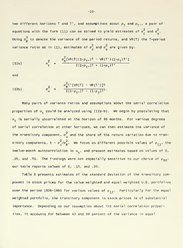
two different horizons T and T', and assumptions about p Tand p Jt , a pair of
2 2equations with the form (11) can be solved to yield estimates of a and a .-1
e u
2Using a to denote the variance of one period returns, and VR(T) the T-period
R
2 2variance ratio as in (1), estimates of a and a are given by:
e ua '
(12a) a2
Gp[VR(T)(l-pT,)T - VR(T')(1-P
T)T']
e=
2(l-pT,)T - (1-PT
)T'
and
(12b) a2
a*T'[VR(T) - VR(T')]T
U=
2(l-pT,)T - (1-P
T)T"
Many pairs of variance ratios and assumptions about the serial correlation
properties of u. could be analyzed using (12a-b). We begin by postulating that
u is serially uncorrelated at the horizon of 96 months. For various degrees
of serial correlation at other horizons, we can then estimate the variance of
2the transitory component, a and the share of the return variation due to tran-
2 2sitory components, 1 - a /a . We focus on different possible values of p.~, theEH 1 2.
twelve-month autocorrelation in u , and present estimates based on values of 0,
.35, and .70. The findings were not especially sensitive to our choice of Pgc;
our table reports values of 0, .15, and .30.
Table 6 presents estimates of the standard deviation of the transitory com-
ponent in stock prices for the value weighted and equal weighted U.S. portfolios
over the period 1926-1985 for various values of P 12 - Particularly for the equal
weighted portfolio, the transitory component in stock prices is of substantial
importance. Depending on our assumption about its serial correlation proper-
ties, it accounts for between 43 and 99 percent of the variance in equal
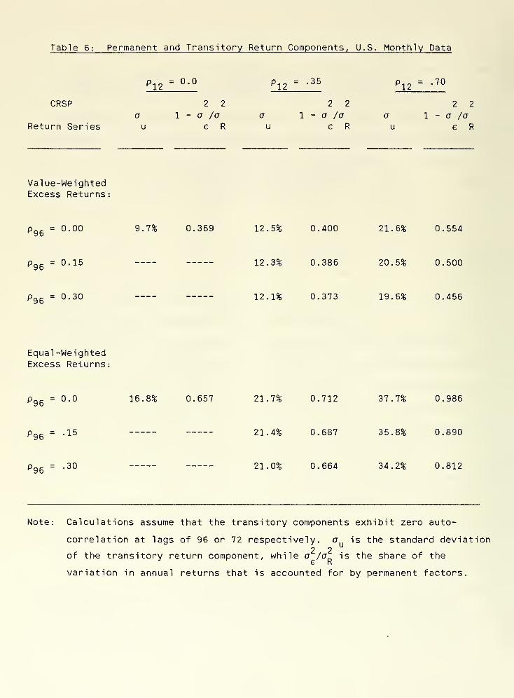
Table 6: Permanent and Transitory Return Components, U.S. Monthly Data
P 12= 0.0 P 12
= .35 P 12= .70
CRSP 2 2 2 2 2 2
o I - a /a a I - a /a a I - a /aReturn Series u e R u e R u e R
Value-WeightedExcess Returns:
Pg5 = 0.00 9.7% 0.369 12.5% 0.400 21.6% 0.554
P 96 = 0-15 12.3% 0.386 20.5% 0.500
P 95= 0.30 12.1% 0.373 19.6% 0.456
Equal-WeightedExcess Returns:
p g6= 0.0 16.8% 0.657 21.7% 0.712 37.7% 0.986
pg6= .15 21.4% 0.687 35.8% 0.890
p g6= .30 21.0% 0.664 34.2% 0.812
Note: Calculations assume that the transitory components exhibit zero auto-
correlation at lags of 96 or 72 respectively, a is the standard deviation2 2
of the transitory return component, while a /a is the share of the£ R
variation in annual returns that is accounted for by permanent factors.

-24-
weighted monthly returns, and has a standard deviation of between 14 percent and
37 percent. Results for the value weighted portfolio similarly suggest that the
transitory component accounts for a large, though smaller, portion of the
variance in returns. Some estimates are as high as 56 percent.
As one would expect, Table 6 indicates that increasing the assumed
persistence of the transitory component raises both its standard deviation and
its contribution to the return variance. More persistent transitory components
are less able to account for declining variance ratios at long horizons.
Therefore, to rationalize any given long horizon variance ratio, increasing the
persistence of the transitory component will require increasing the weight on
the transitory component relative to the permanent component. Sufficiently per-
sistent transitory components will be unable to account for low long horizon
variance ratios, even if they account for all of the variation in returns. For
example, a transitory component that is almost as persistent as a random walk
will be unable to explain very much long-horizon mean reversion.
Which cases in Table 6 are most relevant? As an a priori matter, it is
difficult to see a compelling argument for assuming that transitory components
should die out extremely quickly. Previous suggestions that there are "fads" in
stock prices have typically suggested half lives of several years, implying that
the elements in the table corresponding to p 1?= .70 are most relevant. If the
decay is geometric, this suggests a half life of two years for the transitory
component. Even greater values of p,~ might be even more plausible. One other
2 2consideration supports this conclusion. For given values of a and a , equation
(11) permits us to calculate p Tover any horizon. A reasonable restriction,
that pTnot be very negative over periods of up to 96 months, is only satisfied

-25-
for cases where p..- "> s Targe. For example, with p gg= 0, when we impose p.„ =
.35 the value of the stationary component's implied autocorrelation is -.744 at
36 months, -1.27 at 60 months, and -.274 at 84 months. Even more negative
values obtain assuming p.- = °# ar| d the results are also less satisfactory when
p g6is positive. In contrast, when p 12
= - 70 ar,d P g6= 0, the implied values of
P 36 and p R0are .168 and -.173, respectively. Similar results obtain for other
large values of p.,. This is because variance ratios continue to decline
substantially between long and longer horizons, and as equation (11) demonstra-
tes, rationalizing this requires declining values of p T. If p T starts small, it
therefore must become negative to account for the observed variance ratio pat-
tern. Imposing larger autocorrelations at short horizons does not necessitate
such autocorrelation patterns.
Since other countries and historical periods exhibit patterns of variance
ratio decline that are similar to those in the American data, we do not present
calculations similar to those in Table 6 for them. As one would expect,
countries with 96-month variance ratios lower than those for the United States
have larger transitory components than the U.S., and vice versa.
Insofar as the evidence in the first section and in Fama and French (1987)
is persuasive in suggesting that transitory components in stock prices are pre-
sent and statistically significant, this section's results confirm Shiller's
(1981) conclusion that models assuming constant ex-ante returns cannot account
for a large fraction of the variance in stock market returns. Stock market vol-
atility is excessive relative to the predictions of these models.
*
5 Since our
analysis uses only returns data and does not exploit the present value relation-
ship between stock prices and expected future dividends, it does not suffer from
some of the problems that have been highlighted in the volatility test debate.

-26-
4. The Source of the Transitory Component in Stock Prices
If stock prices have a transitory component, ex-ante returns must vary. 16
Any stochastic process for the transitory component can be mapped into a stoch-
astic process for ex-ante returns, and any pattern for ex-ante returns can
alternatively be represented by describing the associated transitory component
of prices. The economically interesting issue is whether variations in ex-ante
returns are better explained by "fundamentals" such as changes in interest rates
or volatility 17, or instead as byproducts of price deviations caused by noise
traders.
I
8 This section notes a number of considerations that incline us toward
the latter view.
4.1 How Variable Must Risk Premia Be?
It is instructive to calibrate the amount of variation in expected returns
that risk factors would have to generate in order for them to account for the
observed transitory components in stock prices. To do this we assume for
simplicity that the transitory component follows an AR(1) process as postulated
in the "fads" example of Summers (1986). This has the virtue of tractabi 1 i ty
,
although it is inconsistent with the observation that actual returns exhibit
positive, then negative, serial correlation.
Changes over time in the required return on common stocks can generate
mean-reverting stock price behavior. If required returns exhibit positive auto-
correlation, then an innovation that raises required returns will reduce share
prices. This will generate a holding period loss, followed by higher returns in
subsequent periods. We show in the appendix that when required returns follow
an AR(1) process 19 , then

-27-
(13) R - R - —la (r- F) -(1+F)
"1(1+ g
)2(r - -r) + r
1+r-Pjtl+g) 1 +r-p^l+g)
where f , a serially uncorrelated innovation that is orthogonal to innovations
about the future path of required returns (£ t), reflects revisions in expected
future dividends. The constants in this expression depend upon d and g, the
average dividend yield and dividend growth rate respectively. In steady state
r = d + g.
If changes in required returns and profits are positively correlated, as is
plausible given the importance of shocks to the perceived productivity of
capital, then the assumption that £. and f. are orthogonal will understate the
variance in ex-ante returns needed to rationalize mean reversion in stock pri-
ces. Although it is possible to construct theoretical examples where profits
and interest rates are negatively related, as in Campbell (1986), the empirical
finding that bond and stock returns are weakly correlated suggests positive
correlation between shocks to cash flows and required returns. ^0 Negative correl-
ation between f. and £. would cause bond and stock returns to move together.
Our assumption that required returns are given by (r - r) = (1 - P.L) £
- -1 - ?enables us to rewrite (13), defining ?.=-?. .(1+r) (1+g) /[1+r-p (1+g) ] , as
(14) (l-P1L)(R
t- R) s ?
t+ C
t" ( 1+3)V a
" PlCt-l°
The first order autocovariance of the expression on the right-hand side of (14)
is nonzero, but all higher-order autocovariances equal zero. Ansley, Spivey,
and Wrobleski (1977) show that this implies that the right hand side of (14) is
2an MA(1) process that can be represented as (l+9L)w. . Provided o^ > 0, this
2implies that returns follow an ARMA(1,1) process; if a = 0, then returns are
white noise.

-28-
The simple model of stationary and nonstationary price components summar-
ized in equation (9) also yields an ARMA(1,1) representation for returns. This
allows us to calculate the amount of variation in required returns that would be
needed to generate the same time series process for observed returns as would be
generated by "fads" of various sizes in equation (6). We measure the size of
fads, or transitory factors more generally, by a , the standard deviation of the
transitory component. In the appendix we show that the required return variance
corresponding to a given fad variance is:
2[l+F-p (i+g)]
2(i-p )
2(i+F)
2
(15) CTr
= 17 I~5 I"? V
{d+dm+pp-p^i+d+dnjd+gr
This expression indicates the variation in required returns needed to generate
transitory components of a given size.
Table 7 reports the standard deviation of required excess returns, measured
on an annual basis, implied by a variety of different fad models. We calibrate
the calculations using the average excess return (8.9% per year) on the NYSE
equal -weighted share price index over the 1926-1985 period. The dividend yield
on these shares averages 4.5%, implying an average dividend growth rate of 4.4%.
We use our estimates of the variance ratio at 96 months (from Table 2) to
calibrate the degree of mean reversion.
The findings suggest that a great deal of variability in required returns
is needed to explain the degree of mean reversion in prices. For example, if we
postulate that the standard deviation of the transitory price component is 20%,
then even when required return shocks have a half life of 2.9 years, the stand-
ard deviation of ex ante returns (at an annual frequency) must be 5.8%. Even

Table 7: Time-Varying Return Models Needed to Account for Mean Reversion
Standard Deviation of Transitory Component
Half Life 15.0% 20.0% 25.0% 30.0%
1.4 Years 7.9% 10.6% 13.2% 15.8%
1.9 Years 6.1% 8.2% 10.2% 12.3%
2.9 Years 4.4% 5.8% 7.3% 8.7%
Notes: Each entry indicates the standard deviation of required returns,assuming that required returns follow an AR(1) process with the halflife indicated in the left margin. The calculations are calibratedusing data on excess returns for the equal-weighted NYSE index overthe 1926-1985 period. The average excess return for this period is 8.9%per year, with a dividend yield of 4.5%.

-29-
larger amounts of required return variation are needed to explain the same size
price fads when the persistence of required return shocks is lower. These esti-
mates of the standard deviation of required returns are large relative to the
mean of ex post excess returns. If ex ante returns are never negative, they
imply that ex ante returns must exceed 20% fairly frequently.
It is difficult to think of risk factors that could account for such large
variations in required returns. Campbell and Shiller's (1986) conclusion that
stock price movements have no predictive power for changes in discount rates is
especially relevant in this context. They reason that if stock price movements
are caused by changes in future discount rates, then realized values of future
discount rates should be Granger caused by stock prices. They find no evidence
that this is the case using data on real interest rates and market volatilities,
While they find evidence that stock prices Granger cause consumption, the sign
is counter to the theory's prediction.
4.2 Negative Ex-Ante Returns
The principle restriction implied by homogeneous expectations models of
financial markets is that ex-ante returns conditional on public information
can never be negative. This is not a property of some models with noise tra-
ders. Sufficiently optimistic noise traders may drive prices high enough to
make ex-ante returns negative, so risk averse speculators may not be willing or
able to short the market to the point where ex-ante returns are driven to zero.
There is an obvious problem with evaluating whether or not ex-ante returns
are ever negative. In estimating any model, there is a possibility of over-
fitting that may cause the spurious appearance of negative ex-ante returns.

-30-
This is especially likely when many parameters are present. Table 8 therefore
presents the fraction of ex-ante returns that were negative when various auto-
regressive models were estimated using the CRSP returns data for 1926-1985 along
with Monte-Carlo calculations of the share of negative ex-ante returns that
resulted when similar models were estimated using serially independent returns.
The results indicate that negative ex-ante returns show up reasonably
frequently, and to a greater extent than can be explained by statistical over-
fitting. For example, in a regression of monthly excess returns on 24 lags,
using the equal weighted data, 31.2 percent of the fitted values are negative
compared with 25 percent in the corresponding Monte-Carlo calculation. The
corresponding values for the value-weighted index are 33.3% and 28.1%, respect-
ively. Our Monte Carlo results show that the p-value associated with the
outcome for the equal-weighted case is .172, and for the value-weighted case,
.240. These results provide weak evidence against the risk factors hypothesis,
since they suggest negative ex-ante returns in some periods. 2 ^ Since it is not
possible to know in which periods ex ante returns are actually negative, they do
not have strong implications for investment strategy.
4.3 The Difficulty of Accounting for the Observed Autocorreloqram
In section 2 we demonstrated that stock returns exhibited positive serial
correlation over short periods and negative serial correlation over longer
stretches. The AR(1) transitory components model treated in the previous sub-
section can rationalize the second but not the first of these observations. It
is instructive to consider what type of behavior for expected returns is
necessary to account for both observations.
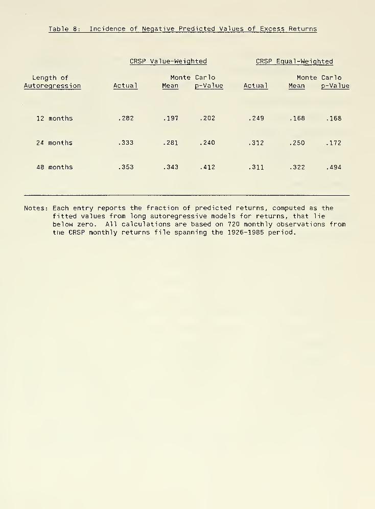
Table 8: Incidence of Negative Predicted Values of Excess Returns
CR5P Value-Weighted CRSP Equal-Weighted
Length of Monte Carlo Monte CarloAutoreqression Actual Mean p-Value Actual Mean p-Value
12 months .282 .197 .202 .249 .168 .168
24 months .333 .281 .240 .312 .250 .172
48 months .353 .343 .412 .311 .322 .494
Notes: Each entry reports the fraction of predicted returns, computed as the
fitted values from long autoregressive models for returns, that lie
below zero. All calculations are based on 720 monthly observations fromthe CRSP monthly returns file spanning the 1926-1985 period.

-31-
Positive serial correlation in ex-post returns over short periods requires
that increases in prospective required returns that reduce stock prices are
followed by reduced returns. Shocks that have a large effect on the expected
discounted present value of required returns must not have a large impact on
required returns in the immediately succeeding periods. The impulse response
function for required returns must cross the zero-axis; a positive current shock
must lead to a reduction in required returns for a period in the immediate
future, followed by higher required returns at a later date. The analysis in
Poterba and Summers (1986) of the time series properties of volatility, as well
as Litterman and Weiss' (1986) work on the time series properties of real
interest rates, does not suggest that these series have the impulse response
functions needed to account for the behavior of market returns.

-32-
5. Conclusions
The empirical results in this paper suggest that stock returns exhibit
positive serial correlation over short periods and negative correlation over
longer intervals. This conclusion emerges from the standard CRSP data on equal
and value weighted returns over the 1926-1985 period. It is corroborated by
data from the pre-1925 period, data for individual firms, and data on stock
returns in seventeen foreign countries. While individual data sets do not con-
sistently permit rejection of the random walk hypothesis at a high confidence
level, the various data sets taken together establish a fairly strong case
against its validity. Furthermore our point estimates generally suggest that
the transitory component in stock prices is quantitatively important, accounting
for the bulk of the variance in returns.
While the temptation to apply more sophisticated statistical techniques
to stock return data in an effort to extract more information about the magni-
tude and structure of transitory components is ever present, we doubt that a
great deal can be learned in this way. Even the relatively gross features of
the data examined in this paper cannot be estimated precisely. As the debate
over volatility tests has illustrated, sophisticated statistical results are
often very sensitive to maintained assumptions that are difficult to evaluate.
We have checked all the statistical procedures used in this paper by applying
them to pseudo data conforming exactly to the random walk model. Our suspicion,
supported by the dramatic illustrations in Kleidon (1986), is that a great deal
of more elaborate work on stock price volatility could not meet this test.
We suggest in the paper's final section that noise trading provides a
plausible account for the transitory components that are present in stock

-33-
pn'ces. Pursuing this -issue will involve constructing and testing theories of
either noise trading or changing risk factors that can account for the
characteristic stock return autocorrel logram documented here. Evaluating such
theories is likely to require that information other than stock returns be
studied. Such information might include information on fundamental values,
proxies for noise trading such as odd-lot sales, and indicators of risk factors
such as ex-ante volatilities implied from stock market options. Only by
comparing the persuasiveness of models based on the presence of noise traders
and models based on changing risk factors, can we come to a judgment about
whether or not financial markets are efficient in the sense of rationally
valuing assets, as well as in the sense of precluding the generation of easy
excess profits.

-34-
Endnotes
1. This point is independent of Fischer's (1984) conclusion in analyzing the
appropriate portfolio strategy for an investor concerned about terminalconsumption but restricted in the frequency with which he can rebalance his
portfolio. Our conclusion applies to investors who can rebalance continuously,as most investors probably can.
2. Stochastic speculative bubbles, considered by Blanchard and Watson(1982), could generate deviations between market prices and fundamental values
without negative serial correlation in returns. In the presence of any limits
on valuation errors set by speculators or real investment opportunities,however, such bubbles could not exist.
3. Testing the relationship between the variability of returns at differenthorizons has a long tradition: Osborne (1959) and Alexander (1961) apply testssimilar to the variance ratio to much shorter data samples.
4. When in subsequent sections we examine annual returns data, the denomina-
tor of the variance ratio is simply Var(R.).
5. When the horizon of the variance ratio is large relative to the samplesize, this bias can be substantial. For example, with T=720 and k=60, the biasis -.069. It rises to -.160 if k=120. Detailed Monte Carlo analysis of the
variance ratio statistic may be found in Lo and MacKinlay (1987b).
6. The ARMA(1,1) parameters associated with this model, for the general ARMA
(l-(J>L)Apt
= (l+8L)w., are:
(J>= p
1
e -{-(1+pJ)
- 2o2
v+ (l-p
1)[4aj + (1+P
1)
2]'£
}/(2ctJ + 2Pl )
a2= -(p, + a
2)/6.
w vrl v
7. We compute the likelihood value under each hypothesis using the exactmaximum likelihood method described in Harvey (1981). Because of the biastoward negative autocorrelations induced by estimating the mean return in eachdata sample, the mean likelihood ratios are actually above one for each of thehypotheses we consider.
8. Real returns are analyzed in Fama and French (1987), a revision of Famaand French (1986a)
.
9. These p-values are calculated from the empirical distribution of our teststatistic, based on Monte Carlo results. They permit rejection at lower levelsthan would be possible using the normal approximation to the distribution of the
variance ratio, along with the Monte Carlo estimates of the standard deviationof the variance ratio.

-35-
10. French and Roll (1986) apply variance ratio tests to daily returns for a
sample of NYSE and AMEX stocks for the period 1963-1982. They find evidence of
negative serial correlation especially among smaller securities. The divergencebetween their findings and those of Lo and MacKinlay (1987a) is presumably dueto differences in the two data sets.
11. These data have been used in some studies of stock market volatility,such as Shiller (1981)
.
12. The monthly stock index data from the IFS also suffer from a secondlimitation. In many cases they are time averages of daily or weekly index
values. Working (1960) showed that the first difference of a time-averaged ran-dom walk would exhibit positive serial correlation, with a first order auto-correlation coefficient of .25 as the number of observations in the averagebecomes large. This will bias our estimated variance ratios. For the countrieswith time aggregated data we therefore modify our small-sample bias correction.Instead of taking the expected value of the first-order autocorrelation to be
-1/(T-1) when evaluating E(VR(k)) we use .25-l/(T-l). The reported varianceratios have been bias-adjusted by dividing by the resulting expected value.
13. The cross-country correlation of own-currency returns is typically below.25 in our data sample. Only five of the 171 pairwise correlations for the
eighteen countries we consider (including the U.S.) exceed .50.
14. We also applied variance ratio tests to the residuals from the marketmodel estimated for each firm, imposing a constant /3 for the entire 1926-1985period. These residuals showed less correlation than the excess returns rela-tive to the market, computed as R-. - R„^.
' r it mt
15. Shiller's conclusion that market returns are too volatile to be
reconciled with valuation models assuming constant required returns has beendisputed by Kleidon (1986) and Marsh and Merton (1986). Mankiw, Romer, and
Shapiro (1985) provide evidence in support of Shiller's conclusion.
16. Several recent studies have considered the extent to which equity returnscan be predicted using various information sets. Keim and Stambaugh (1986) findthat between eight and thirteen percent of the variation in returns for a port-folio of stocks in the bottom quintile of the NYSE can be predicted using laggedinformation. A much smaller share of the variation in returns to larger com-panies can be accounted for in this way. Campbell (1987) finds that approxima-tely eleven percent of the variation in excess returns can be explained on thebasis of lagged information derived from the term structure.
17. Market efficiency does not require constant ex ante returns, and the
models of Lucas (1978) and Cox, Ingersoll, and Ross (1985) study the pricing of
assets with time-varying required returns. Fama and French (1986b) show thatthe negative serial correlation in different stocks may be attributable to a
common factor, and interpret this finding as supporting the view thattime-varying returns account for mean-reversion in prices.
18. Several recent papers, including Black (1986), Campbell and Kyle (1986),DeLong et al . (1987), and Shiller (1984), have discussed the role of noisetraders in security pricing.

-36-
19. The possibility of negative expected excess returns is an unattractivefeature of the simple model we have analyzed. In principle the analysis couldbe repeated using Merton's (1980) model, which constrains the expected excessreturn to be positive. The exact parallel between the time-varying returnsmodel and the fads model would not hold in this case, however.
20. Campbell (1987) estimates that the correlation between excess returns on
long-term bonds and corporate equities was .22 for the 1959-1979 period, and .36
for the more recent 1979-83 period.
21. We perform Monte Carlo calculations holding the expected return on themarket constant at its sample mean value. If required returns varied throughtime, but were always positive, it is possible that the fraction of negativepredicted returns would be greater than our Monte Carlo results suggest.

-37-
References
Alexander, Sidney S. "Price Movements in Speculative Markets: Trends or RandomWalks?" Industrial Management Review 2 (1961), 7-26.
Ansley, Craig, W. Allen Spivey and William Wrobleski, "On the Structure of
Moving Average Processes," Journal of Econometrics 6 (1977), 121-134.
Black, Fischer. "Noise." Journal of Finance 41 (1986), 529-543.
Blanchard, Olivier J. and Mark Watson. "Bubbles, Crashes, and Rational Expect-ations," in P. Wachtel , ed., Crises in the Economic and Financial Struct-ure (Lexington: Lexington Books, 1982).
Campbell, John Y. "Bond and Stock Returns in a Simple Exchange Model,"Quarterly Journal of Economics 102 (1986), 785-803.
Campbell, John Y. "Stock Returns and the Term Structure." Journal of FinancialEconomics 18 (1987), 373-400.
Campbell, John Y. and Albert S. Kyle. "Smart Money, Noise Trading, and StockPrice Behavior." Manuscript, Princeton University, September 1986.
Campbell, John Y. and N. Gregory Mankiw, "Are Output Fluctuations Transitory?,"Quarterly Journal of Economics 103 (1987), forthcoming.
Cochrane, John H., "How Big is the Random Walk in GNP?" Mimeo, University of
Chicago, 1987.
Cox, John C, Jonathan Ingersoll, and Stephen Ross. "An Intertemporal GeneralEquilibrium Model of Asset Prices," Econometrica 53 (1985), 363-384.
DeLong, J. Bradford, Andrei Shleifer, Lawrence Summers, and Robert Waldman, "TheEconomic Consequences of Noise Traders," mimeo, Harvard University, 1987.
Fama, Eugene F., "Efficient Capital Markets: A Review of Theory and EmpiricalWork," Journal of Finance 25 (1970), 383-417.
Fama, Eugene F., and Kenneth R. French, "Permanent and Temporary Components of
Stock Prices." Center for Research in Security Prices Working Paper 178.
Chicago, July 1986a.
Fama, Eugene F., and Kenneth R. French, "Common Factors in the SerialCorrelation of Stock Returns." Center for Research in Security PricesWorking Paper 200, October 1986b.
Fama, Eugene F., and Kenneth R. French, "Permanent and Temporary Components of
Stock Prices." Center for Research in Security Prices Working Paper 178.
Chicago, July 1987.
Fischer, Stanley, "Investing for the Short and the Long Term," in Zvi Bodie and

-38-
John B. Shoven, eds., Financial Aspects of the U.S. Pension System(Chicago: University of Chicago Press, 1984), 153-176.
French, Kenneth R., and Richard Roll. "Stock Return Variances: The Arrival of
Information and the Reaction of Traders," Journal of Financial Economics17 (1986), 5-26.
Harvey, Andrew. Time Series Models (Oxford: Philip Allan Publishers, 1981).
Kendall, Maurice G., "The Analysis of Economic Time Series--Part I: Prices,"Journal of the Royal Statistical Society (Series A), 96 (1933), 11-25.
Kendall, Maurice G. and Alan Stuart. The Advanced Theory of Statistics , 3rdEdition, Volume 3. London: Griffin, 1976.
Keim, Donald B. and Robert F. Stambaugh, "Predicting Returns in the Stock and
Bond Markets," Journal of Financial Economics 17 (1986) ,357-390.
Keynes, John M., The General Theory of Employment, Interest, and Money . (New
York: Harcourt, Brace and Company, 1936).
Kleidon, Allan, "Variance Bounds Tests and Stock Price Valuation Models,"Journal of Political Economy 94 (October 1986), 953-1001.
Learner, Edward. Specification Searches: Ad Hoc Inferences with NonexperimentalData (New York: John Wiley & Sons, 1978).
Litterman, Robert and Laurence Weiss, "Money, Real Interest Rates, and Output:A Reinterpretation of Postwar U.S. Data," Econometrica 53 (1985), 129-156.
Lo, Andrew W. and A. Craig MacKinlay, "Stock Market Prices Do Not FollowRandom Walks: Evidence from a Simple Specification Test." NBER WorkingPaper 2168, February 1987a.
Lo, Andrew W. and A. Craig MacKinlay, "A Simple Specification Test of the RandomWalk Hypothesis," Rodney L. White Center for Financial Research DiscussionPaper 13-87, Wharton School, University of Pennsylvania, 1987b.
Lucas, Robert. "Asset Prices in an Exchange Economy," Econometrica 66 (1978),1429-1445.
Mankiw, N. Gregory, David Romer, and Matthew Shapiro, "An Unbiased Test of
Stock Market Volatility," Journal of Finance 40 (July 1985), 677-687.
Marsh, Terry A. and Robert C. Merton, "Dividend Variability and VarianceBounds Tests for the Rationality of Stock Market Prices," AmericanEconomic Review 76 (June 1986), 483-496.
Merton, Robert C, "On Estimating the Expected Return on the Market," Journalof Financial Economics 8 (December 1980), 323-361.

-39-
Merton, Robert C, "On the State of the Efficient Market Hypothesis in FinancialEconomics," in R. Dornbusch, S. Fischer, and J. Bossons, Macroeconomics and
Finance: Essays in Honor of Franco Modigliani (Cambridge: MIT Press, 1987),93-124.
Miller, Merton and Myron S. Scholes. "Dividends and Taxes: Some EmpiricalEvidence," Journal of Political Economy 90 (1982), 1118-1141.
Officer, Robert R., "The Variability of the Market Factor of the New York StockExchange," Journal of Business 46 (1973), 434-453.
Osborne, M.F.M., "Brownian Motion in the Stock Market," Operations Research7 (1959), 145-173.
Poterba, James M. and Lawrence H. Summers, "The Persistence of Volatility andStock Market Returns," American Economic Review 76 (December 1986),1142-51.
Shiller, Robert J., "Do Stock Prices Move Too Much to be Justified by Subse-quent Changes in Dividends?" American Economic Review 71 (June 1981),421-436.
Shiller, Robert J., "Stock Prices and Social Dynamics," Brookings Papers onEconomic Activity , 2:1984, 457-498.
Shiller, Robert J., and P. Perron. "Testing the Random Walk Hypothesis: Powerversus Frequency of Observation," Economics Letters 18 (1985), 381-386.
Summers, Lawrence H., "Does the Stock Market Rationally Reflect FundamentalValues?" Journal of Finance 41 (July 1986), 591-601.
Wilson, Jack W. and Charles Jones. "A Comparison of Annual Common StockReturns: 1871-1925 with 1926-1985." Journal of Business 60 (April 1987),239-258.
Working, Holbrook, "Note on the Correlation of First Differences of Averages in
a Random Chain," Econometrica 28 (1960), 916-918.

-40-
Appendix: Derivation of Ex Post Return Process when Required Returns are AR(1)
The price of a common stock, P., equals
™ J -1 _i(A.i) p = e { I [ n (i+r
t+.) d+g
t+i)]D
t}
j=0 1=0
where r.+
. denotes the required real return in period t+i, D. is the dividend
paid in period t, g. +. is the real dividend growth rate between periods t+i and
t+i+1, and E.{«) designates expectations formed using information available as
of period t. We linearize inside the expectation operator in r. and g.
:
00 - . 00 3P 00 9P(A.2) P
t. E
t ( I(f?)
J-\ * ij-t- [r - ?] * l^- [g - i)|j=l 1+r j=0 t+j J j=0 u t+j J
D (1+F) D (1+g) « . D . « .
= ~Z 1" ^T^ Et(I iS
J [rt
- F]) + ^ Et{Z /3
J[g
t- g]}
r - 9 (l+r)(r-g) j=0 J r-g j=0 J
where /3 = (l+g)/(l+r). We denote D (l+F)/(F-g) as P . In the special case of
(A. 3) (rt-F) = P
1(r
t _ 1-F) + ?
t
we can simplify the second term in (A. 2) to obtain:
(A. 4) p - p a -i°tHlsJ_i
pJpJ [r _ F] + A e (I PJ[gt+r g])
(1 + r) (r-g) j=0 ' r-g j=0 J
(r-g)(l+r-p (1+g)) r-g j=0 J
Now recall that the holding period return, R , is given by
(A . 5) Rt. !«p _,.
t
It can be linearized around P. and P . . as follows:
P - P (P +D )
Pt
?t

-41-
where P = (l+g)P. and R = r (l+g)/(l+r) . Substituting (A. 4) into (A. 6) yields
- Dt + i
(1+ g }
Pt(r-g)[l+r - p^l+g)]
(a. 7) Rt
- r = = :~ (r
t+i" r)
Dt+1 '
Dt(l+r)(l+g)
+ -——— —Pt(F-g)[i + F - p^i+g)]
(rt-r)
D.(l+r) oo
Pt(r-g) j=o
This can be rewritten,2
WVj " «:
D (1+g)(A. 8) R - R = [(r - r) - /3
_1(r - r)] + C
Pt(r-g)(l+r-Pl (l+g))
= - m+~
9) [(1-P.LfV. - Ml-P^D'V] + Ct
where f reflects changes in expected future dividend growth rates between t
and t+1, and the last expression exploits the fact that (1-p L)(r -r) = E, . Now
defining {/S( 1+g)/ [1 + r-p .(1+g) ] } ?. = £., we can multiply through by (1-p L) so-.
(A. 9) (1-p L)(R - R) = | - (~) L_ + C t- P,Ct ,.
This yields an ARMA(1,1) representation of returns. Since (l+r)/(l+g) ~ (1+d),
this is equation (14) in the text.
We now explore the parallel between the time-varying returns model and the
fad model, which postulates that returns evolve according to:
(a. io) (i-p1D(R
t- S) a e
t- P
1ft . 1
+ wt
- »>
t_i•

-42-
This is also an ARMA(1,1) model. For this process to be the same as (A. 9),
two restrictions must be satisfied. We find them by equating the variance and
first autocovariance of the right hand sides of (A. 9) and (A. 10):
(A. 11) [l+(l+d)2]CT^ + {l+p*)o
2= 2o
2
v+ d+p
2)a
2
and
(A. 12) d+d)a2
+ p^2
= cr2
+ p^2
.
2Using (A. 12) to eliminate a from (A. 11) we find
(A.i3, Jt . .<\->£—— °i-
K (i+cDd+pp-p^i+d+d)^]
2 2 2Recall that the variance of the fad, a , equals a /(1-p ). Using this and the
definition of ? , we find from (A. 13) that the variance of required returns
corresponding to a given fad variance is:
, [i+F-P.d+g)]2(i-P
1)
2d+i:
)
2,
(A " 14)°r = : S - 2 ; - 2 V
{(l+d)(l+pp-p1[l+(l+d)^]}(l+g)^
This leads immediately to (15) in the text.

-a
oj•i—
>-
-acCD
"Or->r—a
oJZm•i—
2T3cf0
CO
Ci_
Z>
Ma:
o
to
ol—
ro
cr
ucro
-r-
ro
>
<CD
nf0
.3511 086
co•r—
c +JL to3 r—
w >(U id
cc ar- D(0 s_
Z> ro
^ TJc C< (0
+J
in
CSJ CO LD o t- in in in •«* t- en cm«* o ro CTI t- o CM ID en cn ID COID LT) ro cm CO ID «* ro i— t- ID ID
0)
O O O o O o o o o o O O i
—
JZ2
b ^^ _ s , % t s in
ID CO CO CO cn <-i CO ID ID t— t— ID cCO LO I-H t- CO ro CO ro O o c— CO i_
m in 1 ro ID ID «* ** CO CO ID ID o
o o
t- inO COt- ID
CM IDO COCO t—
O O
ro **co c-co co
o o
M- rHc- e'-
en cn
o o
en enCM CMo o
ro idco r-t- c-
o o
CM CM
o oCM CM
co roen idm in
o o
O rHin rM
o o
in roco co
o o
rM CMrH ocn en
o o
cm eno eno en
o coo enco t-
o o
O CM
cn enCSI CM
o o
cm t-co roc- t-
m cmin cmco co
o o
t- IDr-i encn co
o o
cn coCO r-cn cn
o o
id roro roO O
«=t oCD ID[- t~
O O
ID t—
O OCM CM
o o
cn in«? OID ID
O O
ID rHco m
o o
CD CMr— inCO CO
o o
in cmCM rHcn cn
o o
cn ino oo o
in roco co
o o
ID 00
cn cnrvj CM
TJ tj o TJCD CD a< CD
LL +J 0_ +- 4J 4J
CO r- CO jz 0. i—
Q. -Ccc U) cc a> CO CT> 10 O)o •r- in o •i- in CC *r- in cc r- in
CD CO CD CO c_> <D CO u CD CO1
—
2 cn I
—
2 cn .£ cn 2 cnro 1
rH ro 1 rH to 1 rH L0 1 rHc CD 1
r- i— | to 0) i L0 r— |
-r— Z3 CD •r— ro id 0) D CD CD TO CDcr r— CM E 3 CM o i
—
CM o 3 CMo as cn o cr cn X ro cn X cr cni; > rH z UJ rH UJ > rH UJ UJ rH
o o
E- t—O OCO CO
cm -a-
in m
o o
O CD•a- -a-
o o
CO COCD t—CO CO
o o
C~ CDco cncn cn
o o
cm cnrO rHco co
o o
Cn rH
O rHCM CM
o
O CD-J CO— cn
o o
CD CMr- COCD ID
O O
O CDCM CMCD CD
O O
ro orH CMCD CD
o o
m mCD t-
o o
CO IDcm roen cn
o o
cn cnrH ocn cn
o o
rH CO
O OCM CM
o~o
O CD-J CO~^ cn
to 1
1
—
Q) cnro fc roa) •r- cnrr 1— rH
to
to
CD
OXUJ
a> to
H- ro
o +-•
CD4-J TJ!_
CU L.C (1)
o JZa. +->
t t-
o Z)
o 4-
c s_r- o(0 H-Dl
rj;
i
—
ro "D-m c•r" roQ_m CMu
toCD 0)JZ 1
—
*j aro
>h-i
—
c a>
o CD
toOlcr—V) (/)
D c£_
"O Z3
CD -M•u CDD £_
Q.E i
—
O ro
O +->
Oto +jor- O)4-< cro -r-
t_ to
Z)
0)
CJ toc nro r-•r- 4^£_ ro
ro s_
>OJ
0) oL. c(0 re
r"cn £_
CU ro
to >CD
JZ CD-w L.c ro
CD
S_ toro <\>
Q. i
—
s_c +J
•r- cOJ
WCD £_D a.'
i
—
JZro -m
> o
rnnm- r iWTiWTTJiMiannwnnnni


Date Due
^1393
1
Lib-26-67

MIT LIBRARIES
3 ioao oos 1 30 lb3
