mean level signal crossing rate for an arbitrary...

General rights Copyright and moral rights for the publications made accessible in the public portal are retained by the authors and/or other copyright owners and it is a condition of accessing publications that users recognise and abide by the legal requirements associated with these rights.

• Users may download and print one copy of any publication from the public portal for the purpose of private study or research. • You may not further distribute the material or use it for any profit-making activity or commercial gain • You may freely distribute the URL identifying the publication in the public portal

If you believe that this document breaches copyright please contact us providing details, and we will remove access to the work immediately and investigate your claim.

Downloaded from orbit.dtu.dk on: Sep 06, 2018

Mean level signal crossing rate for an arbitrary stochastic process

Yura, Harold T.; Hanson, Steen Grüner

Published in:Optical Society of America. Journal A: Optics, Image Science, and Vision

Link to article, DOI:10.1364/JOSAA.27.000797

Publication date:2010

Document VersionPublisher's PDF, also known as Version of record

Link back to DTU Orbit

Citation (APA):Yura, H. T., & Hanson, S. G. (2010). Mean level signal crossing rate for an arbitrary stochastic process. OpticalSociety of America. Journal A: Optics, Image Science, and Vision, 27(4), 797-807. DOI:10.1364/JOSAA.27.000797

http://dx.doi.org/10.1364/JOSAA.27.000797

http://orbit.dtu.dk/en/publications/mean-level-signal-crossing-rate-for-an-arbitrary-stochastic-process(7f639875-9d24-49bb-8cb7-2bcdfb94fd8c).html

Mean level signal crossing rate for an arbitrarystochastic process

Harold T. Yura1 and Steen G. Hanson2,*1Electronics and Photonics Laboratory, The Aerospace Corporation, Los Angeles, California 90009, USA

2DTU Fotonik, Department of Photonics Engineering, Danish Technical University,4000 Roskilde, Denmark

*Corresponding author: [email protected]

Received November 4, 2009; accepted January 6, 2010;posted January 20, 2010 (Doc. ID 119557); published March 24, 2010

The issue of the mean signal level crossing rate for various probability density functions with primary rel-evance for optics is discussed based on a new analytical method. This method relies on a unique transformationthat transforms the probability distribution under investigation into a normal probability distribution, forwhich the distribution of mean level crossings is known. In general, the analytical results for the mean levelcrossing rate are supported and confirmed by numerical simulations. In particular, we illustrate the presentmethod by presenting analytic expressions for the mean level crossing rate for various probability distribu-tions, including ones that previously were unavailable, such as the uniform, the so-called gamma-gamma, andthe Rice–Nakagami distribution. However, in a limited number of cases the present results differ somewhatfrom the result reported in the literature. At present, this discrepancy remains unexplained and is laid open forfuture discussion. © 2010 Optical Society of America

OCIS codes: 030.1630, 030.1670, 030.6140, 030.6600.

1. INTRODUCTIONThe investigation of fade and surge statistics and the as-sociated mean level crossing rate of a stationary differen-tiable random process has been of considerable interestsince the pioneering work of Rice [1]. Physically, the de-rivative of each realization of such a random process isthe derivative in the usual sense of the corresponding re-alization. For example, in optical communication systems,and especially for propagation through the atmosphere ofinformation-carrying laser beams, the received light willbe aberrated both by optical turbulence between thetransmitter and the receiver and by line-of-sight platformjitter. This will inevitably result in intensity modulationof the received signal, the extent of which will be deter-mined by the intermediate atmosphere and the opticalsetup. Thus, knowledge of fading and level crossings ofthe received, perturbed signal becomes of uttermost im-portance. In case of sensor systems, tracking of specklepatterns, shearing of dynamic speckle patterns, and deri-vation of the structure of a fringe pattern are commonlyappearing issues of importance for the sensor systems. Inthese cases, the random nature of the underlying specklestructure will inevitably cause signal drop-out, the extentof which will constitute a major factor in the reliability ofthe sensor system. Thus, knowledge about the level cross-ings is of crucial importance in cases where the intensityvariations possess statistical properties governed by ran-dom polarization and where coherent and incoherent ad-dition random electromagnetic fields are interfered.

According to Rice, the mean level crossing rate (for bothpositive and negative crossings), ��x0�, for an arbitrarystationary differentiable random process is given by

��x0� =�−�

�

�x�pX,X�x0, x�dx, �1�

where x is the first derivative of x with respect to time(i.e., dx /dt) and p�x0 , x� is the joint probability densityfunction (PDF) of x�t� and x�t� at time t. The subscripts inEq. (1) refer to the arbitrary random process, while lower-case variables refer to the random variable. For a normalrandom process, where the joint PDF of x�t� and x�t� areknown to be independent [i.e., p�x0 , x�=p�x0�p�x�], Eq. (1)yields [2]

��x0� =��x

2

�exp�−

�x0 − ��2

2�2 � =�− R�0�

�exp�−

�x0 − ��2

2�2 � ,

�2�

where �x2 is the variance of the time derivative of the nor-

mal process, � and � are the mean and standard devia-tion of the normal process, and R�t� is the correspondingtemporal autocorrelation coefficient.

Although analytic expressions for the mean level cross-ing rate ��x0� at an arbitrary level x0 have been obtainedfor a limited number of other random processes, the cor-responding analytic expressions for the mean level cross-ing rate for an arbitrary random process has remainedelusive [3–6]. This is because the joint PDF of the leveland its time derivative for an arbitrary stochastic processhas not been obtained, and thus the integral in Eq. (1)cannot be determined.

H. T. Yura and S. G. Hanson Vol. 27, No. 4 /April 2010 /J. Opt. Soc. Am. A 797

1084-7529/10/040797-11/$15.00 © 2010 Optical Society of America

Khimenko [3] was the first to obtain analytic solutionsof Eq. (1) for processes with statistically independent de-rivatives and corresponding processes that are functionaltransformations of these processes. For example, his re-sults include processes with an exponential, Rayleigh,gamma, Maxwell, and Laplace distribution. Subse-quently, several other authors have independently de-rived several of Khimenko’s results including the expo-nential distribution, as the level-crossing rate of theintensity of speckle patterns have been the subject of boththeoretical [7–10] and experimental [11,12] interest overthe past several years. Barakat [4], based on the gammadistribution, obtained analytic results for the mean levelcrossing rate of aperture-integrated speckles. By astraightforward extension of the derivation of the levelcrossing rate for a normal distribution, Yura and McKin-ley derived the corresponding rate for the log-normal dis-tribution [13], and while making a simplifying assump-tion, an integral expression for the level crossing rate forthe gamma-gamma distribution has been obtained by Vet-elino et al. [14].

In general, however, the level crossing rate for an arbi-trary random process has not been found. Thus, for ex-ample, closed-form analytic results for the mean levelcrossing rate for a uniform distribution, a power law dis-tribution, and the gamma-gamma distribution are un-available. This paper will introduce a novel method forderiving closed-form analytical expressions for the meanlevel crossings for signals obeying an arbitrary probabil-ity density function (PDF) and in particular for variousPDFs for signals of interest to the optical community. Ingeneral, the analytical results for the mean level crossingrate are supported and confirmed by numerical simula-tions. In particular, we illustrate the present method bypresenting analytic expressions for ��x0� that previouslywere unavailable (including those mentioned above), andthese results are confirmed by numerical simulations.However, as discussed below, in a limited number of casesthe present results differ somewhat from the result ob-tained originally by Khimenko (and subsequently by oth-ers). This discrepancy remains unexplained and is laidopen for future discussion.

The essence of the present method is the introductionof a unique bijective mathematical transformation thatconverts a signal obeying an arbitrary PDF into a signalthat obeys a normal distribution. This allows one, as dis-cussed below, to use the mean level crossing rate for thenormal distribution to obtain the corresponding result foran arbitrary PDF. In Section 2 this transformation is in-troduced and discussed, and a general expression for themean level crossing rate for and arbitrary PDF is derived.In Section 3 new results for several PDFs of interest arepresented, compared with numerical simulations, anddiscussed. Additionally, as alluded to above, the devia-tions of the present analysis with some previously pub-lished results, which are not presently understood, arepresented and laid open for discussion. However, despitethese discrepancies we feel that the present work repre-sents a step forward in our understanding of the levelcrossing rate for arbitrary random processes and shouldbe made available in the literature. Finally, in Section 4we present our concluding remarks.

2. GENERAL CONSIDERATIONSHere we consider only differentiable stationary randomprocesses (i.e., random processes that are continuous inthe mean square sense) designated by “X” and “Y.” The Xprocess is assumed known in that all the various prob-ability functions are implicitly given to us, and we wouldlike to find out the corresponding functions of the Y pro-cess. In particular, we would like to obtain the joint prob-ability density function of y and its time derivative, giventhe corresponding joint probability function of the X pro-cess. In the following we denote by x�t� and y�t� the valuesof the random process X and Y at time t, respectively.

Let pX�x� and pY�y� be two arbitrary PDFs. Consider atransformation of variables given by

x = f�y�, �3�

where the arbitrary (real) function f is bijective (i.e., asingle value of y corresponds to a single value of x andvice versa). By the standard laws of transformation ofPDFs we have

pY�y� = �f��y��pX�x�y� �where f��y� df�y�

dy � . �4�

Next consider the joint PDF of the random variable y andits first derivative with respect to time y, pYY�y , y�.

Note that from Eq. (3) it follows directly from the chainrule of differentiation that

x =df�y�

dy

dy

dt= f��y�y. �5�

Here we assume that x is not a function of y and thus thejoint PDF, pYY�y , y�, is related to the corresponding jointPDF of x and x by the Jacobian [15,16]:

pYY�y, y� = pXX�x�y, x�y, y��x

�y

�x

�y

�x

�y

�x

�y� = pXX�x�y, x�y, y�

��f��y� 0

f�y f��y�� = �f��y�2pXX�x�y, x�y, y�. �6�

This is true for any bijective transformation of Eq. (3) thatis not a function of the time derivative. Equation (6) re-lates the joint PDF of the random process of interest “Y”to that of the corresponding PDF of the assumed knownprocess “X.”

Now consider the special case where X is a zero-mean,unit-variance, normally distributed random process. It iswell known that for a normally distributed random vari-able the joint PDF pXX�x , x� is given by (i.e., a normal sta-tionary random process and its derivative are indepen-dent [17])

pXX�x, x� = pX�x�pX�x�, �7�

where pX�x�=exp�−x2 /2 /�2�, pX�x� is also of Gaussianform given by [17]

798 J. Opt. Soc. Am. A/Vol. 27, No. 4 /April 2010 H. T. Yura and S. G. Hanson

pX�x� =1

�2��x2

exp −x2

2�x2� , �8�

and �x2 is the variance of the time derivative of x. For the

zero-mean, unit-variance normal PDF, we obtain fromEqs. (7) and (8)

pYY�y, y� = f��y�1

�2�exp −

f2�y�

2 � � f��y�1

�2��x2

�exp −f�2�y�y2

2�x2 � = pY�y�

f��y�

�2��x2

�exp −f�2�y�y2

2�x2 � . �9�

Next, we express �x2 in terms of parameters related to the

random process of interest. To do this we note that themean value of the time derivative of any stationary ran-dom process is zero [18], from which it follows that theunconditional variance of the time derivative of the Y pro-cess is given by

�y2 =�� dydyy2�y�pYY�y, y�. �10�

Substituting Eq. (9) into Eq. (10) and performing the in-tegration over y, simplifying, and rearranging termsyields

�x2 = �y

2/�, �11�

where the constant � (which is independent of the level) isgiven by

� =� dypY�y�

f�2�y�. �12�

Equation (11) gives the relationship between the varianceof the derivative of the zero-mean, unit-variance normaldistribution and the variance of the derivative of the ran-dom process of interest. Thus, Eq. (9), with �x

2 given byEq. (11), depends only on parameters related to the ran-dom process of interest. We note for any stationary ran-dom process that

�y2 = � − RY��=0 =

�0

�

d2SY��

�0

�

dSY��

, �13�

where RY�� is the temporal autocorrelation coefficient ofthe random process of interest and SY�� is the corre-sponding temporal power spectrum.

In general, for an arbitrary transformation functionf�y�, one does not obtain a normal process x. We will showthat the transformation of variables given by

x = �2 erf−1�2FY�y� − 1, �14�

where FY�y� is the cumulative distribution function (CDF)of the arbitrary stationary random process characterized

by the PDF pY�y�, yields a zero-mean, unit-variance nor-mally distributed random variable x. The transformationgiven by Eq. (14) is bijective (i.e., one-to-one) and thus thetransformed PDF, pX�x�, is given by (see [15], Sec. 5-2, pp.125–126)

pX�x� =pY�y�x�

�dx

dy�. �15�

From Eq. (14) we obtain

dx

dy= �2� exp��erf−1�2FY�y� − 1�2

dFY�y�x�

dy

= �2� exp��erf−1�2FY�y� − 1�2pY�y�x�, �16�

where pY�y� is the corresponding PDF of the arbitrary dis-tribution. Substituting Eq. (16) into Eq. (15) and simpli-fying yields

pX�x� =pY�y�x�

�2� exp��erf−1�2FY�y�x� − 1�2pY�y�x�

=1

�2� exp��erf−1�2FY�y�x� − 1�2. �17�

Now from Eq. (14) we obtain that 2FY�y�x�−1=erf�x /�2,from which it follows that

pX�x� =exp�− x2/2

�2�, QED. �18�

Thus, the transformation given by Eq. (14) transforms thearbitrary random process of interest into a zero-mean,unit-variance normal process, and hence Eq. (9) is thejoint PDF of an arbitrary random process and its time de-rivative. Each level “y” is uniquely mapped onto a singlenormally distributed level “x.” Hence the mean levelcrossing rate for the Y process can be obtained from Rice’sresults for the zero-mean, unit-variance normal process.The mean level crossings at level x0 (i.e., for the sum ofboth positive and negative crossings) for a zero-mean,unit-variance normal process, as obtained from Eq. (2), isgiven by

��x0� =��x

2

�exp�−

x02

2 � . �19�

Substituting Eq. (14) into Eq. (19) [or, equivalently,substituting Eq. (14) into Eq. (1) and performing the inte-gration over y] yields that the mean level crossing rate foran arbitrary random differentiable process is given by

��y0� =�x

�exp�− f2�y0�/2 =

�y

��exp�− f2�y0�/2, �20�

where � and �y are obtained from Eqs. (12) and (13), re-spectively, and


x0 = f�y0� = �2 erf_1�2FY�y0� − 1. �21�

This is the main result of this paper. For a given analyti-cal representation of the CDF, the corresponding meanlevel crossing rate is given by Eq. (20). If, however, theCDF is not available in analytic form, numerical resultscan be obtained readily from the corresponding integralform of the CDF. Examination of Eq. (20) reveals that, ingeneral, the maximum value of the mean level crossingrate occurs at the level ymax that satisfies FY�ymax�=1/2.

Note that �y=��0�d2SY�� /�0

�dSY�� is indepen-dent of the level; rather, it depends on the specific physi-cal circumstance of the problem at hand and represents arelative measure of the absolute magnitude of the meanlevel crossing rate. For example, the clear-air turbulence-induced scintillation power spectrum for slant rangepropagation through the atmosphere is a function of boththe zenith angle and the direction and magnitude of thenormal component of the “effective” wind speed with re-spect to the line of sight. As a result, in the following, wefocus our attention on the profile shape function of themean level crossing rate, given by the exponential on theright-hand side of Eq. (20), and, in the following figures,we normalize the maximum value of ��y0� to unity.

In general, the mean frequency of negative crossings,�−, must equal the mean frequency of positive crossing,�+, so that �=�++�−=2�+=2�−. Thus, for example, themean duration of a fade at level y0, T−�y0� is

T−�y0� =FY�y0�

�−�y0�, �22�

while the corresponding duration of a surge, T+�y0�, is

T+�y0� =1 − FY�y0�

�+�y0�. �23�

The crossing level for which the mean duration of a fadeequals the mean duration of a surge occurs for FY�y0�=1/2.

3. ILLUSTRATIVE EXAMPLES ANDCOMPARISON TO PREVIOUS WORKIn what follows, as appropriate, we normalized the leveleither to its mean or otherwise, as noted.

A. Log-Normal DistributionThe log-normal PDF and CDF are given by

pY�y� = �exp −�log y − ��2

2�2 ��2��y

,for y 0

0 otherwise� , �24�

where “log” denotes the natural logarithm, � and � arethe mean and standard deviation of log y, respectively,and

FY�y� =1

2�1 + erf log y − �

�2�� . �25�

Substituting Eq. (25) into Eq. (20) and simplifying yieldsthat the profile shape for the log-normal distribution isgiven by

��y0� = constant � exp −�log y0 − ��2

2�2 � , �26�

in agreement with the results of [13].Next, we illustrate the usefulness of Eq. (18) by pre-

senting the mean level crossing rate for a number of PDFsthat have not been previously obtained and comparedthese results with numerical simulations. The CDF of anarbitrary random process is a bijective monotonically in-creasing function of its argument. Consider two randomprocesses specified by CDFs FX�x� and FY�y�. Now for anygiven value of x, the transformation y=FY

−1�FX�x� yields asingle unique value of y that satisfies FY�y�=FX�x�. In par-ticular, a discrete random sample set xj is mapped onto acorresponding set yj whose underlying statistics are givenby pY�y�. In particular, the analytic results are comparedwith corresponding numerical simulations of discrete cor-related signal samples, as such samples are generally ob-tained in practice. The method used here to obtain corre-lated signal samples for an arbitrary random process Y isas follows. Let x be a zero-mean, unit-variance normallydistributed random variable. Then, because a normal pro-cess plays such a central role in obtaining correlatedsimulation samples, we show explicitly in Appendix Athat FY

−1�FX�x� has the PDF of interest pY. Correlatednormal signal samples for a zero-mean, unit-variance nor-mal process are readily obtained using the Uhlenbeck–Ornstein method of producing a normally distributed sig-nal x with an arbitrary degree of correlation [19]. Thisinverse method can be used when the inverse function FY

−1

can be obtained explicitly or can be accurately approxi-mated. For each of the comparison cases shown below,more than 105 samples have been employed.

Fig. 1. (Color online) Relative level crossing rate for the powerlaw PDF for various values of m. The analytic and simulation re-sults are given by the solid and dotted curves, respectively.


B. Power Law DistributionThe PDF is given by

pY�y� = �mym−1, for 0 � y � 1

0, otherwise � , �27�

where m is an arbitrary real number greater than zero.For example, such a PDF describes the irradiance statis-tics for a Gaussian-shaped laser beam in the presence ofline-of-sight mechanical platform jitter, where m is givenby the square of the ratio of the 1/�e angular beam radius

to the 1−�, single-axis standard deviation of jitter [20].For this PDF we have

FY�y� = ym. �28�

Figure 1 is a plot of the relative level crossing rate as afunction of normalized level for various values of m. Ex-amination of Fig. 1 reveals that excellent agreement is ob-tained between the analytic and the simulation results.Note that the special case m=1 corresponds to a uniformPDF between zero and unity, and hence the m=1 curve

Fig. 2. (Color online) Mean level crossing rate for the gamma-gamma distribution as a function of the level for various values of � and . The solid curve is the analytic result, the dashed curve is the “new integral expression” obtained in [14], and the points are our simu-lation results, which are obtained from a very accurate inversion approximation to Eq. (30).


represents the mean level crossing rate for the uniformdistribution.

C. Gamma-Gamma DistributionThe PDF of the gamma-gamma distribution is given by[21,14]

pY�y� =2�� + �/2

�� y��+ �/2−1K�− �2�� y�, for y 0,

�29�

where Kn� · � is the modified Bessel function of the secondkind of order n, and � and are free parameters. The cor-responding CDF is

FY�y� =� csc�� − ��

��

� �� y��1F2��;1 + �,1 + � − ;� y�

− �� y� 1F2� ;1 + ,1 − � + ;� y�� ,

�30�

where �� · � is the gamma function and 1F2 denotes a gen-eralized hypergeometric function [22]. It can be readilyverified that the mean of this distribution is unity and thevariance is given by

�gg2 =

1

�+

1

+

1

� . �31�

The gamma-gamma distribution has been used to modelthe irradiance distribution for moderate-to-strong clear-air turbulence-induced scintillation in the atmosphere,where �gg

2 �1 [23]. The resulting mean level crossing rate,obtained from Eqs. (30) and (20), is plotted in Figs.2(a)–2(e) as a function of the level for various values of �and consistent with a variance 1. The solid curve isthe analytic result, the dashed curve is the “new integralexpression” obtained in [14], and the points are our simu-lation results, which are obtained from a very accurate in-version approximation to Eq. (30).

Examination of Figs. 2(a)–2(e) reveals very good agree-ment between the analytic theory and the numericalsimulations. In contrast, the “new integral expression” forthe mean level crossing rate, which is based on an unjus-tified simplification [see the paragraph below Eq. (21) of[14]] is less accurate, and this inaccuracy increases withincreasing values of the variance.

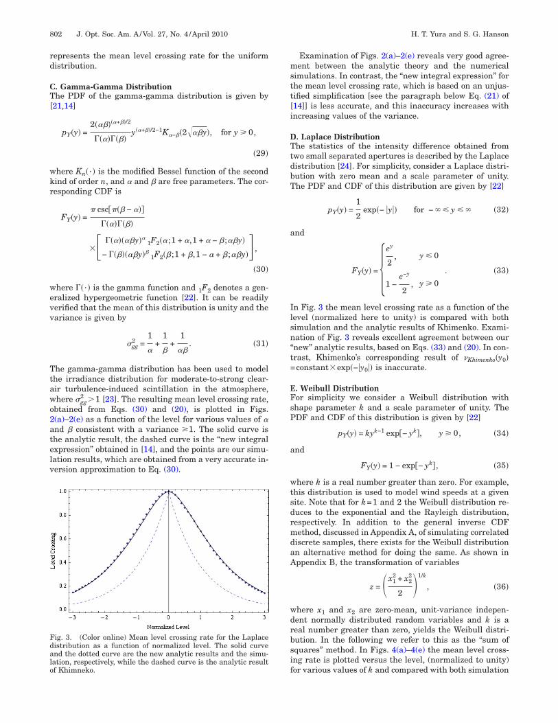
D. Laplace DistributionThe statistics of the intensity difference obtained fromtwo small separated apertures is described by the Laplacedistribution [24]. For simplicity, consider a Laplace distri-bution with zero mean and a scale parameter of unity.The PDF and CDF of this distribution are given by [22]

pY�y� =1

2exp�− �y�� for − � � y � � �32�

and

FY�y� = �ey

2, y � 0

1 −e−y

2, y 0� . �33�

In Fig. 3 the mean level crossing rate as a function of thelevel (normalized here to unity) is compared with bothsimulation and the analytic results of Khimenko. Exami-nation of Fig. 3 reveals excellent agreement between our“new” analytic results, based on Eqs. (33) and (20). In con-trast, Khimenko’s corresponding result of �Khimenko�y0�=constant�exp�−�y0�� is inaccurate.

E. Weibull DistributionFor simplicity we consider a Weibull distribution withshape parameter k and a scale parameter of unity. ThePDF and CDF of this distribution is given by [22]

pY�y� = kyk−1 exp�− yk, y 0, �34�

and

FY�y� = 1 − exp�− yk, �35�

where k is a real number greater than zero. For example,this distribution is used to model wind speeds at a givensite. Note that for k=1 and 2 the Weibull distribution re-duces to the exponential and the Rayleigh distribution,respectively. In addition to the general inverse CDFmethod, discussed in Appendix A, of simulating correlateddiscrete samples, there exists for the Weibull distributionan alternative method for doing the same. As shown inAppendix B, the transformation of variables

z = �x12 + x2

2

2 �1/k

, �36�

where x1 and x2 are zero-mean, unit-variance indepen-dent normally distributed random variables and k is areal number greater than zero, yields the Weibull distri-bution. In the following we refer to this as the “sum ofsquares” method. In Figs. 4(a)–4(e) the mean level cross-ing rate is plotted versus the level, (normalized to unity)for various values of k and compared with both simulation

Fig. 3. (Color online) Mean level crossing rate for the Laplacedistribution as a function of normalized level. The solid curveand the dotted curve are the new analytic results and the simu-lation, respectively, while the dashed curve is the analytic resultof Khimneko.


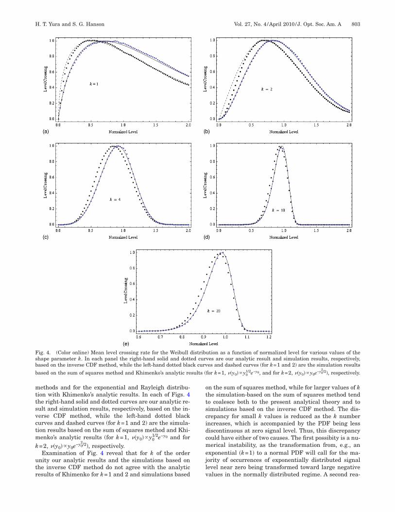
methods and for the exponential and Rayleigh distribu-tion with Khimenko’s analytic results. In each of Figs. 4the right-hand solid and dotted curves are our analytic re-sult and simulation results, respectively, based on the in-verse CDF method, while the left-hand dotted blackcurves and dashed curves (for k=1 and 2) are the simula-tion results based on the sum of squares method and Khi-menko’s analytic results (for k=1, ��y0��y0

1/2e−y0 and fork=2, ��y0��y0e−y0

2/2), respectively.Examination of Fig. 4 reveal that for k of the order

unity our analytic results and the simulations based onthe inverse CDF method do not agree with the analyticresults of Khimenko for k=1 and 2 and simulations based

on the sum of squares method, while for larger values of kthe simulation-based on the sum of squares method tendto coalesce both to the present analytical theory and tosimulations based on the inverse CDF method. The dis-crepancy for small k values is reduced as the k numberincreases, which is accompanied by the PDF being lessdiscontinuous at zero signal level. Thus, this discrepancycould have either of two causes. The first possibity is a nu-merical instability, as the transformation from, e.g., anexponential �k=1� to a normal PDF will call for the ma-jority of occurrences of exponentially distributed signallevel near zero being transformed toward large negativevalues in the normally distributed regime. A second rea-

Fig. 4. (Color online) Mean level crossing rate for the Weibull distribution as a function of normalized level for various values of theshape parameter k. In each panel the right-hand solid and dotted curves are our analytic result and simulation results, respectively,based on the inverse CDF method, while the left-hand dotted black curves and dashed curves (for k=1 and 2) are the simulation results

based on the sum of squares method and Khimenko’s analytic results (for k=1, ��y0��y01/2e−y0, and for k=2, ��y0��y0e−y0

2/2), respectively.


son for the discrepancy could be that simulations haveshown that the level crossing rate depends on the corre-lation time versus the sampling time interval. Simula-tions with signals derived by different numerical methodshave even yielded different results for the level crossings,yet their statistics yield virtually identical moments,which are in accordance with textbook values. The reasonfor this discrepancy, however, is currently not understood.

F. Gamma DistributionNext, we consider the gamma distribution, which hasbeen used extensively in the literature to model the PDFof aperture-integrated speckle [4,10]. This PDF and cor-responding CDF are given by

pY�y� =1

��y�−1 exp�− �y, for y 0 �37�

and

FY�y� = 1 −��,�y�

��, �38�

where for simplicity in notation we have normalized thelevel, y, to its mean and �� ,�y� is the incomplete gammafunction. The parameter � can be physically interpretedas the mean number of speckles contained within a col-lecting aperture [10]. Figures 5(a)–5(d) compare thepresent analytic results (solid curves) for the mean levelcrossing rate with the corresponding results obtained byBarakat [Eq. (4.2)] [4] (dashed curves) for various values

of �. Because for �=1 the PDF of the gamma distributionbecomes the exponential PDF, we omit this case from Fig.5, as it has been considered previously.

We remark that simulations of the mean level crossingrate for the gamma distribution based on the inverse CDFmethod are in excellent agreement with our analytical re-sults, and therefore, for presentation purposes they arenot shown in Fig. 5. Examination of Fig. 5 reveals that for� less than about 4 our analytic results are somewhat dif-ferent from the corresponding results of Barakat [4],while for larger values of � the two results are in verygood agreement. Again, the reason for this discrepancy forsmall values of � is currently not understood.

G. Rice–Nakagami DistributionAs a final example we illustrate the utility of obtainingthe mean level crossing rate for a PDF whose correspond-ing CDF cannot be obtained analytically [25]. The PDFand CDF of the Rice–Nakagami is given by

pY�y� = 2y exp�− �y2 + C2�I0�2yC�, for y 0 �39�

and

FY�y� =�0

y

2x exp�− �x2 + C2�I0�2xC�dx, �40�

where I0� · � is the modified Bessel function of the firstkind the order zero, C is a real constant, and both y and Care normalized to twice the variance of the underlyingnormal distribution [26]. In a variety of applications, the

Fig. 5. Mean level crossing rate for the gamma distribution as a function of level normalized to the mean. In each panel the solid anddashed curves are our analytic results and the corresponding results of Barakat, given by Eq. (4.2) of [4], respectively.


Rice–Nakagami distribution is used to model the inten-sity distribution in a speckle pattern that consists of aspecular component and a diffuse scattered component[27]. Rice has shown that the mean level crossing rate isdirectly proportional to the PDF and is given by [28]

��y0� =�− R�0�

2�pY�y0�. �41�

In addition to the inverse CDF method of obtaining corre-lated sample simulations, one also can obtain suchsamples for the Rice–Nakagami distribution from an ex-tension of the sum of squares method discussed in Appen-dix B given by

y =��x1 − C�2 + x22

2, �42�

where x1,2 are independent, zero-mean, unit-variance nor-mal distributions and C is a real constant.

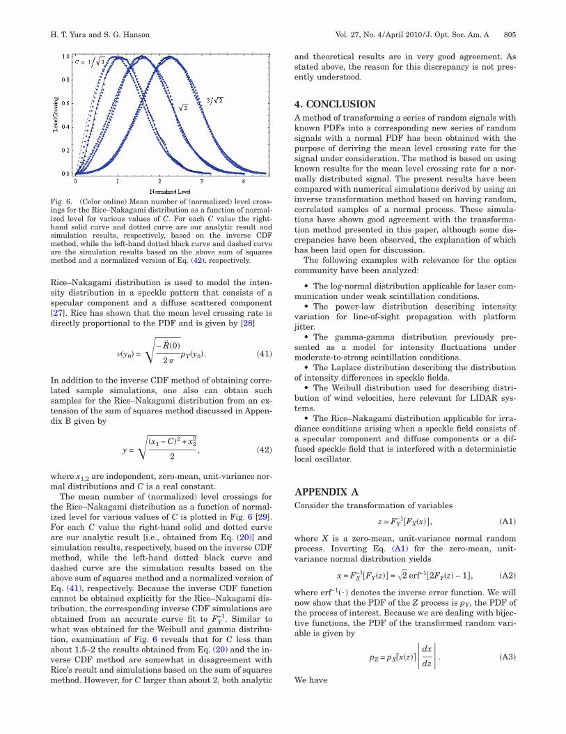
The mean number of (normalized) level crossings forthe Rice–Nakagami distribution as a function of normal-ized level for various values of C is plotted in Fig. 6 [29].For each C value the right-hand solid and dotted curveare our analytic result [i.e., obtained from Eq. (20)] andsimulation results, respectively, based on the inverse CDFmethod, while the left-hand dotted black curve anddashed curve are the simulation results based on theabove sum of squares method and a normalized version ofEq. (41), respectively. Because the inverse CDF functioncannot be obtained explicitly for the Rice–Nakagami dis-tribution, the corresponding inverse CDF simulations areobtained from an accurate curve fit to FY

−1. Similar towhat was obtained for the Weibull and gamma distribu-tion, examination of Fig. 6 reveals that for C less thanabout 1.5–2 the results obtained from Eq. (20) and the in-verse CDF method are somewhat in disagreement withRice’s result and simulations based on the sum of squaresmethod. However, for C larger than about 2, both analytic

and theoretical results are in very good agreement. Asstated above, the reason for this discrepancy is not pres-ently understood.

4. CONCLUSIONA method of transforming a series of random signals withknown PDFs into a corresponding new series of randomsignals with a normal PDF has been obtained with thepurpose of deriving the mean level crossing rate for thesignal under consideration. The method is based on usingknown results for the mean level crossing rate for a nor-mally distributed signal. The present results have beencompared with numerical simulations derived by using aninverse transformation method based on having random,correlated samples of a normal process. These simula-tions have shown good agreement with the transforma-tion method presented in this paper, although some dis-crepancies have been observed, the explanation of whichhas been laid open for discussion.

The following examples with relevance for the opticscommunity have been analyzed:

• The log-normal distribution applicable for laser com-munication under weak scintillation conditions.

• The power-law distribution describing intensityvariation for line-of-sight propagation with platformjitter.

• The gamma-gamma distribution previously pre-sented as a model for intensity fluctuations undermoderate-to-strong scintillation conditions.

• The Laplace distribution describing the distributionof intensity differences in speckle fields.

• The Weibull distribution used for describing distri-bution of wind velocities, here relevant for LIDAR sys-tems.

• The Rice–Nakagami distribution applicable for irra-diance conditions arising when a speckle field consists ofa specular component and diffuse components or a dif-fused speckle field that is interfered with a deterministiclocal oscillator.

APPENDIX AConsider the transformation of variables

z = FY−1�FX�x�, �A1�

where X is a zero-mean, unit-variance normal randomprocess. Inverting Eq. (A1) for the zero-mean, unit-variance normal distribution yields

x = FX−1�FY�z� = �2 erf−1�2FY�z� − 1, �A2�

where erf−1� · � denotes the inverse error function. We willnow show that the PDF of the Z process is pY, the PDF ofthe process of interest. Because we are dealing with bijec-tive functions, the PDF of the transformed random vari-able is given by

pZ = pX�x�z��dx

dz� . �A3�

We have

Fig. 6. (Color online) Mean number of (normalized) level cross-ings for the Rice–Nakagami distribution as a function of normal-ized level for various values of C. For each C value the right-hand solid curve and dotted curve are our analytic result andsimulation results, respectively, based on the inverse CDFmethod, while the left-hand dotted black curve and dashed curveare the simulation results based on the above sum of squaresmethod and a normalized version of Eq. (42), respectively.


pX�x�z� = exp�− �erf−1�2FY�z� − 1�2, �A4�

and from Eq. (A2)

dx

dz= �2� exp��erf−1�2FY�z� − 1�2FY��z�

= �2� exp��erf−1�2FY�z� − 1�2pY�z�. �A5�

Substituting Eqs. (A4) and (A5) into Eq. (A3) yields pZ=pY. QED.

Our simulation of correlated samples for an arbitraryPDF pY is based on Eq. (A1) where a correlated zero-mean, unit-variance normal sample distribution xj is ob-tained from [19]

xj = e−t0xj−1 + �1 − e−2t0xnew, j = 1,2, ... NS, �A6�

where xjx�tj�, NS is the number of samples, and for eachj the numerical value of xnew is obtained from an indepen-dent zero-mean, unit-variance normal distribution (i.e.,xj−1 and xnew are independent). Physically, t0 can be inter-preted as the ratio of the sampling time interval to thecorrelation time of the process. For t0�1 and t0�1 Eq.(A6) yields correlated and uncorrelated samples, respec-tively. Here we consider only correlated samples, obtainedfrom Eq. (A6) with t0�0.1, and NS105. Then the simu-lated level crossing rate, �sim�y0�, is obtained from

�sim�y0� = �j=1

NS−1

cj, �A7�

where the count for the j sample is

cj = �1 if either yj � y0 and yj+1 � y0

or yj � y0 and yj+1 � y0

0 otherwise� . �A8�

APPENDIX BConsider the transformation of variables

z = �x12 + x2

2

2 �1/k

, �B1�

where x1 and x2 are zero-mean, unit-variance indepen-dent normally distributed random variables and k is areal number greater than zero. We now show that thePDF of the Z process is the Weibull distribution consid-ered in the text. Because x1 and x2 are independent, wehave that the PDF of Eq. (B1) is given by

pZ�z� =�−�

�

dx1�−�

�

dx2pX�x1,x2��z − x12 + x2

2

2 �1/k�=�

−�

�

dx1�−�

�

dx2pX�x1�pX�x2��z − x12 + x2

2

2 �1/k� ,

�B2�

where pX�x�=exp�−x2 /2 /�2� and �� · � is the one-dimensional Dirac delta function.

Substituting pX�x1� and pX�x2� into Eq. (B2), performingthe integrations, and simplifying yields

pZ�z� = kzk−1 exp�− zk1

��

−�2zk

�2zk dx1

�2zk − x12

= kzk−1 exp�− zk,

�B3�

which is the Weibull distribution.

ACKNOWLEDGMENTSWe acknowledge financial support from the Danish Coun-cil for Technology and Innovation under the InnovationConsortium CINO (Centre for Industrial Nano Optics).The research of H. T. Yura was performed while he was aguest scientist at DTU Fotonik, Denmark, September–November 2009.

REFERENCES1. S. O. Rice, “Mathematical analysis of random noise,” in Se-

lected Papers on Noise and Stochastic Processes (Dover, Inc.New York, 1954).

2. P. Beckmann, Probability in Communication Engineering(Hartcourt Brace & World, 1967), Sec. 6.7.

3. V. I. Khimenko, “The average number of trajectory over-shoots of a non-Gaussian random process above a givenlevel,” Izv. Vyssh. Uchebn. Zaved., Radiofiz. 21, 1170–1176(1977).

4. R. Barakat, “Level-crossing statistics of aperture averaged-integrated isotropic speckle,” J. Opt. Soc. Am. A 5, 1244–1247 (1988).

5. J. Bendat, Principles and Applications of Random NoiseTheory (Wiley, 1958).

6. J. Abrahams, “A survey of recent progress on level crossingproblems for random processes,” in Communications andNetworks, A Survey of Recent Advances, I. F. Blake and H.V. Poor, eds. (Springer-Verlag, 1986).

7. K. Ebeling, “Statistical properties of spatial derivatives ofthe amplitude and intensity of monochromatic speckle pat-terns,” Opt. Acta 26, 1505–1521 (1979).

8. R. Barakat, “The level-crossing rate and above-level dura-tion time of the intensity of a Gaussian random process,”Inf. Sci. (N.Y.) 20, 83–87 (1980).

9. R. D. Bahuguna, K. K. Gupta, and K. Singh, “Expectednumber of intensity level crossings in a normal speckle pat-tern,” J. Opt. Soc. Am. 70, 874–876 (1980).

10. J. W. Goodman, Speckle Phenomena in Optics: Theory andApplications (Roberts, 2006).

11. K. Eebeling, “Experimental investigation of some statisticalproperties of monochromatic speckle patterns,” Opt. Acta26, 1345–1349 (1979).

12. N. Takai, T. Iwai, and T. Asakura, “Real-time velocity mea-surements for a diffuse object using zero-crossings of laserspeckle,” J. Opt. Soc. Am. 70, 450–455 (1980).

13. H. T. Yura and W. G. McKinley, “Optical scintillation statis-tics for IR ground-to-space laser communication systems,”Appl. Opt. 22, 3353–3358 (1983).

14. F. S. Vetelino, C. Young, and L. Andrews, “Fade statisticsand aperture averaging for Gaussian waves in moderate-to-strong turbulence,” Appl. Opt. 46, 3780–3789 (2007).

15. P. Beckmann, Probability in Communication Engineering(Hartcourt Brace & World, 1967), Sec. 2.4, p. 73, Eq. 2.4-4.

16. A. Papoulis, Probability, Random Variables, and StochasticProcesses (McGraw-Hill, 1965), Sec. 7-2, pp. 201–202.

17. P. Beckmann, Probability in Communication Engineering(Hartcourt Brace & World, 1967), Sec. 6.6, pp. 223 and 230.

18. P. Beckmann, Probability in Communication Engineering(Hartcourt Brace & World, 1967), Sec. 6.6, Eq. 6.6-21, p.222.

19. G. E. Uhlenbeck and L. S. Ornstein, “On the theory ofBrownian motion,” Phys. Rev. 36, 823–841 (1930).

20. H. T. Yura, “LADAR detection statistics in the presence ofpointing errors,” Appl. Opt. 33, 6482–6498 (1994).


21. L. C. Andrews, R. L. Phillips, and C. Y. Hopen, Laser BeamScintillation with Applications (SPIE Press, 2001), Sec. 2.5.

22. S. Wolfram, Mathematica, Version 7 (Cambridge Univ.Press, 2008).

23. See Ref. [14] and references therein.24. S. G. Hanson and H. T. Yura, “Statistics of spatially inte-

grated speckle intensity difference,” J. Opt. Soc. Am. A 26,371–375 (2009).

25. The CDF of the Rice-Nakagami distribution can be ex-pressed in terms of the Marcum Q functions, which aretabulated, but not supported, to the best of our knowledge,by any commercial commuter programs such as Math-

ematica and Matlab. Consequently, numerical integrationof Eq. (3.17) is used to obtain the results indicated in Fig. 6.

26. P. Beckmann, Probability in Communication Engineering(Hartcourt Brace & World, 1967), Sec. 4.4.

27. J. W. Goodman, Speckle Phenomena in Optics: Theory andApplications (Roberts, 2006), Sec. 3.2.2.

28. S. O. Rice, “Statistical properties of a sine wave plus ran-dom noise,” Bell Syst. Tech. J. 27, 109–157 (1948).

29. Because for C=0 the Rice–Nakagami distribution becomesthe Rayleigh distribution, which has already been consid-ered in Subsection 3.E, we omit this case in Fig. 6.


mean level signal crossing rate for an arbitrary...

Documents