mean annual runoff estimation in north-western …claps/papers/prin03_viglione.pdf · part 2 -...

Editors

Goffredo La Loggia Giuseppe T. Aronica Giuseppe Ciraolo

MEAN ANNUAL RUNOFF ESTIMATION IN NORTH-WESTERN ITALY

Alberto VIGLIONE, Pierluigi CLAPS, Francesco LAIO

Part 2 - Water scarcity risk assessment

71

MEAN ANNUAL RUNOFF ESTIMATION IN NORTH-WESTERN ITALY

Alberto VIGLIONE∗, Pierluigi CLAPS∗, Francesco LAIO∗

ABSTRACT

Assessment of water resources in a region starts with the application of statistical models for estimation of annual flow with a given return period, that evaluate the spatial variability of the studied variable. The most popular model in regional frequency analysis is the “index-flow”, based on the hypothesis that the distributions of the variable are identical in different sites of a statistically homogeneous region, with the exception of a scale parameter.

In this work we discuss an objective method of choice of the best statistical model for estimation of the index-flow, selected as the mean annual runoff, in ungauged basins. Special attention is dedicated to the selection of meaningful morphological and climatic characteristics of the river basins, which behave as prediction variables in the regression model.

The proposed procedure has been applied to 47 basins in Piemonte and Valle d'Aosta (North-Western Italy), whose physiographic characteristics vary substantially moving from the alpine regions to the more temperate southern basins.

1. INTRODUCTION

Many practical hydrological problems require reliable models for estimation of mean annual runoff in a region. Runoff cannot be interpolated like purely distributed variables, as precipitation or temperature, because runoff in a cross section is representative of the whole contributing basin. Therefore, usual spatial interpolation methods cannot be used for estimation in ungauged basins.

As regards the statistical approach, one of the firsts and more popular methods in regional frequency analysis is the “index-flood” technique (Dalrymple, 1960). Many Regional Flood estimation projects (see e.g. Rossi & Villani, 1995 or Robson & Reed, 1999) are based on Dalrymple's methodology, but also flow duration curves can be referred to the index flow method (Claps & Fiorentino, 1997; Castellarin et al., 2004). In this work we are interested in the annual

∗ Dipartimento di Idraulica, Trasporti ed Infrastrutture Civili, Politecnico di Torino, Corso Duca degli Abruzzi 24, 10129,

Torino

A. Viglione, P. Claps, F. Laio

72

flow, that is the amount of water crossing a river section in one year. If compared with hydrological extremes, applications of regional analysis to average variables, like the annual flow, are much less frequent in literature. Vogel & Wilson (1996) present some applications related to the US, while in Italy some previous works can be traced back to Ferraresi et al. (1988), Claps & Mancino (2002) and Brath et al. (2004).

The purpose of the Regional frequency analysis of the annual flow is the estimation of its probability distribution in basins with few or no data. The fundamental hypothesis of Dalrymple's method is that the distribution of a variable in different sites belonging to a “homogeneous region” is identical, with the exception of a scale parameter. This latter varies in the region according to climatic, morphometric and geologic characteristics of every considered basin.

In this work we are interested in the regional estimation of the “index-flow” parameter, that can be either the sample mean (e.g. Hosking & Wallis, 1997) or the sample median (e.g. Robson & Reed, 1999). Viglione et al. (2006) show that, for variables characterized by low skewness coefficients, the estimation of the mean is less biased than that of the median. For this reason in this work the sample mean is used as the index-flow.

Many methodological approaches are available for the index-flow estimation, and their differences can be related to the amount of information available (see e.g. Bocchiola et al., 2003). Excluding direct methods, that use information provided by flow data available at the station of interest, regional estimation methods require ancillary hydrological and physical information. Those methods can be divided in two classes: the multiregressive approach and the hydrological simulation approach. For both of them, the “best” estimator is the one that optimizes some criterion, such as the minimum error, the minimum variance or the maximum efficiency.

Due to its simplicity, the most frequently used method is the multiregressive approach (see e.g. Kottegoda & Rosso, 1998), that relates the index-flow to catchment characteristics, such as climatic indices, geologic and morphologic parameters, land cover type, etc., through linear or non-linear equations.

In this work, several morphologic and climatic attributes of catchments are selected and computed for 47 basins in North Western Italy. Using these descriptors, a comprehensive multiregressive approach is established to select the most influential descriptors for this geographic context.

2. SELECTION OF MORPHOCLIMATIC BASIN DESCRIPTORS

Meaningful morphoclimatic descriptors of river basins should have direct connection to the hydrological processes taking place in drainage basins. These indices give synthetic information on the shape of basin surfaces, the nature of soil and vegetation and its climatic features. Ideally, these indices should play a role in the average water balance within the basin, with the


73

morphologic ones related to the hydrologic response, and the climatic ones related to the water losses.

2.1 SELECTION OF MORPHOLOGIC PARAMETERS

In this subsection, some morphometric parameters of drainage basins and river networks are described. All of them can be computed automatically using GIS tools, using a procedure that has been developed within the “Linux” operating system, using the “bash” language of scripting, to exploit together the “GRASS” GIS and the “Fluidturtle” libraries (http://www.ing.unitn.it/~rigon/indexo.html). The “R” statistical computing software has been also used for the computation of statistical indices. The choice of open source software, under the GNU General Public License, has been determined by the fact that all these packages are constantly updated and improved by experts of the international scientific community. Following this philosophy our script is open, easily customizable, and available at the address www.idrologia.polito.it/~alviglio/software/GRASSindex.htm.

Two different types of morphologic parameters are considered: drainage basin and river network parameters.

2.1.1 Drainage basin parameters

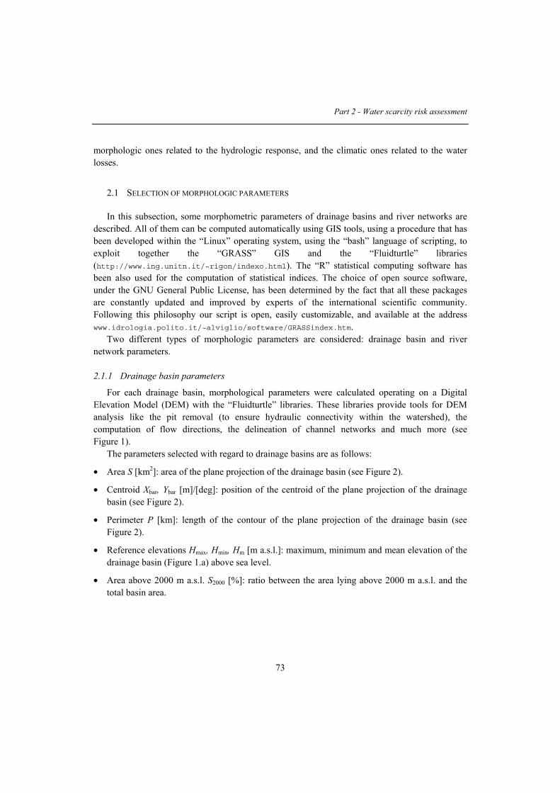
For each drainage basin, morphological parameters were calculated operating on a Digital Elevation Model (DEM) with the “Fluidturtle” libraries. These libraries provide tools for DEM analysis like the pit removal (to ensure hydraulic connectivity within the watershed), the computation of flow directions, the delineation of channel networks and much more (see Figure 1).

The parameters selected with regard to drainage basins are as follows:

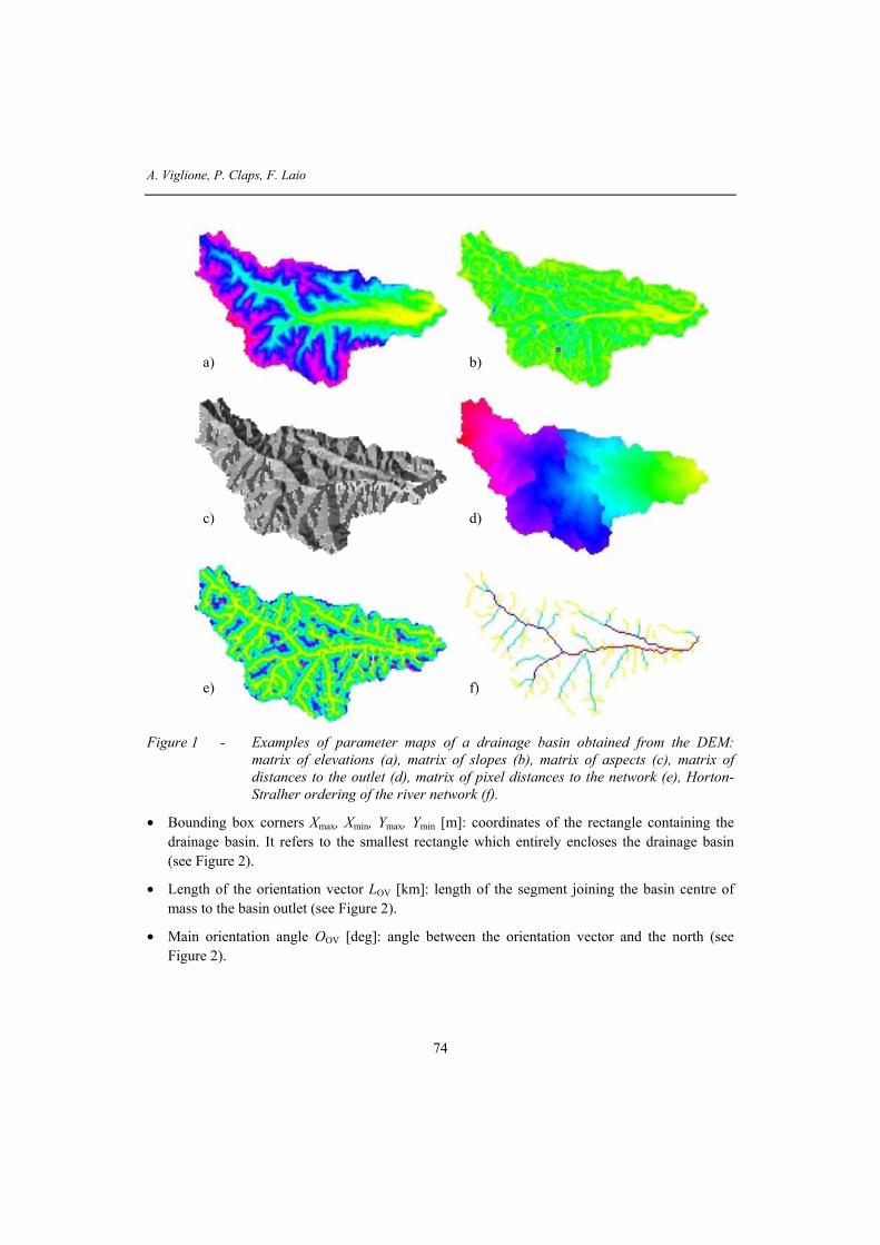
• Area S [km2]: area of the plane projection of the drainage basin (see Figure 2).

• Centroid Xbar, Ybar [m]/[deg]: position of the centroid of the plane projection of the drainage basin (see Figure 2).

• Perimeter P [km]: length of the contour of the plane projection of the drainage basin (see Figure 2).

• Reference elevations Hmax, Hmin, Hm [m a.s.l.]: maximum, minimum and mean elevation of the drainage basin (Figure 1.a) above sea level.

• Area above 2000 m a.s.l. S2000 [%]: ratio between the area lying above 2000 m a.s.l. and the total basin area.


74

Figure 1 - Examples of parameter maps of a drainage basin obtained from the DEM:

matrix of elevations (a), matrix of slopes (b), matrix of aspects (c), matrix of distances to the outlet (d), matrix of pixel distances to the network (e), Horton-Stralher ordering of the river network (f).

• Bounding box corners Xmax, Xmin, Ymax, Ymin [m]: coordinates of the rectangle containing the drainage basin. It refers to the smallest rectangle which entirely encloses the drainage basin (see Figure 2).

• Length of the orientation vector LOV [km]: length of the segment joining the basin centre of mass to the basin outlet (see Figure 2).

• Main orientation angle OOV [deg]: angle between the orientation vector and the north (see Figure 2).

a) b)

c) d)

e) f)


75

Figure 2 - Geographic parameters of the catchment.

• Northing NORD and Easting EST: cosine and sine of OOV . NORD is 1 if the basin is oriented northward, -1 if it is oriented southward. EST is 1 if the basin is oriented eastward, -1 if it is oriented westward.

• Mean small-scale slope pm [%]: average of the slope values associated to each pixel in the DEM of the drainage basin (Figure 1.b).

• Mean large-scale slope Pm [%]:

⎟⎟⎠

⎞⎜⎜⎝

⎛ −=

SHH

arctgP medm

)(2 min (1)

where S is the basin area, Hmed the median elevation and Hmin the elevation of the closing section. The Pm is a slope measure of a square equivalent basin, and does not account for basin shape; its definition is objective, i.e. not affected by the DEM resolution.

• Mean aspect MA [deg]: geometric (vector) average of the aspect of each cell (Figure 1.c). The aspect is the direction towards which a slope faces and is important in hilly or mountainous terrain. Here it is defined as the angle of exposure of the cell (computed from the north).


76

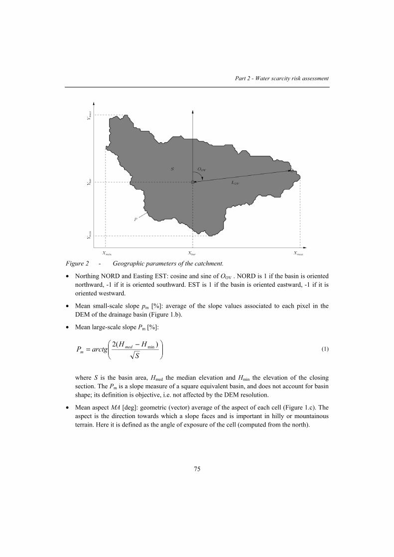
• Area-elevation curve (hypsometric curve) h% [m a.s.l.]: the curve represents the portion of the basin area located above a given elevation (Figure 3). The curve is represented recording elevations corresponding to the 2.5%, 5%, 10%, 25%, 50%, 75%, 90%, 95% and 97.5% of the area.

Figure 3 - Area-elevation curve.

• Circularity ratio Rc: ratio between the basin area and the area of a circle having the same perimeter:

2cP

S4=R π (2)

where P is the watershed perimeter.

• Compactness (Gravelius) coefficient Cc: ratio between the perimeter of the basin and the diameter of the equivalent circle:

π/S2P=Cc (3)


77

2.1.2 River network parameters

Selected analyses can be performed on the river network, that is automatically extracted from the DEM, using the above-described drainage directions and the following constraints:

• a pixel belongs to the network if its contributing area exceeds 1 km2;

• a stream belongs to the network if it is composed of more than one pixel.

Parameters computed on the river networks are as follows:

• Length of the main stream LMS [km]: length of the longest series of streams that connects the basin outlet to the foremost source point (i.e. the upper stream end).

• Main stream mean slope MSMS [%]: the mean slope of the main stream is defined as the ratio between its total elevation drop ΔH and its length:

MSMS L

HMS Δ= (4)

• Length of the longest drainage path LLDP [km]: the longest drainage path is the longest path between the basin outlet and the most distant point on the basin border, following drainage directions. Actually the longest drainage path corresponds to the main stream plus the path on the hillslope that connects the stream source to the basin border.

• Slope of the longest drainage path PLDP [%]: average of the slope values associated to each pixel in the longest drainage path.

• Elongation ratio Ral: ratio between the diameter of a circle with area equivalent to the basin area and the length of the longest drainage path:

LDPal L

π/S2=R (5)

• Shape factor Ff: ratio between the basin area and the square of the longest drainage path length:

2LDP

f LS=F (6)


78

• Width function FA [m]: moments (mean, variance, skewness and kurtosis) and percentiles (5%, 15%, 30%, 40%, 50%, 60%, 70%, 85%, 95%) of the width function, which is defined as the cumulated frequency of the pixel metric distance from the basin outlet (Figure 1.d).

• Mean hillslope length MHL [m]: average distance (throughout all the basin) between pixels and channel (Figure 1.e).

• Magnitude M: number of source points of the network.

• Topological diameter dT: number of links that constitute the main stream, or number of confluences to the main stream.

• Horton-Strahler ordering: number of links, average length, average contributing area and mean slope corresponding to every Horton class. These classes form an ordering classification system in which channel segments are ordered numerically from a stream's headwaters to the basin outlet (Figure 1.f). Numerical ordering begins with the tributaries at the stream's headwaters being assigned the value 1. A stream segment that results from the joining of two 1st order segments is given an order 2. Two 2nd order streams form a 3rd order stream, and so on.

• Horton ratios Rhb, Rhl, Rha, Rhs: slope of the interpolation straight line (computed with the Ordinary Least Squares method) between the points given by the order and the variable (number of links, average length, average contributing area and mean slope) on a semi-logarithmic diagram. R.E. Horton applied morphometric analysis to a variety of stream attributes and from these studies he proposed a number of laws of drainage composition. For instance, Horton's law of stream lengths suggests that a geometric progression exists between the number of stream segments in successive stream orders (Rhb).

• Total network length TNL [km]: sum of the lengths of all stream within the basin.

• Drainage density Dd [km/km2]: measure of the length of stream channel per unit area of drainage basin. Mathematically it is expressed as the total network length divided by the area of the drainage basin. The measurement of drainage density provides a hydrologist or geomorphologist with a useful numerical measure of landscape dissection and runoff potential. On a highly permeable landscape, with small potential for runoff, drainage densities are sometimes less than 1 kilometer per square kilometer. On highly dissected surfaces densities of over 500 kilometers per square kilometer are often reported. Closer investigations of the processes responsible for drainage density variation have discovered that a number of factors collectively influence stream density. These factors include climate, topography, soil infiltration capacity, vegetation, and geology.


79

2.2 ESTIMATION OF CLIMATIC PARAMETERS

For a river basin, average climatic features can be considered attributes or “descriptors”, similarly to its morphologic parameters. Some scalar indices were considered, that account for climatic features related to the average water balance:

• Mean annual rainfall Am [mm] areally averaged over the catchment;

• Thornthwaite index IT: a global moisture index that can be estimated, in its simplest form, as the ratio

0

0mT ET

ETAI

−= (7)

where ET0 the mean annual potential evapotranspiration on the basin;

• Budyko index IB: a radiational aridity index expressed as

m

nB A

RI

λ= , (8)

where Rn is the mean annual net radiation and λ is the latent vaporization heat. Values assumed by IB are lower than 1 for humid regions and greater than 1 in arid regions.

The computation of the climatic indices proposed by Thornthwaite and Budyko requires the estimate of average annual precipitation, temperature, evapotranspiration and net radiation in the study area.

Evapotranspiration and solar radiation are estimated here using the procedures suggested by FAO (Allen et al., 1998). In place of the potential evapotranspiration, the reference crop evapotranspiration ET0 is computed as a climatic parameter expressing the evaporation potential of the atmosphere from a unit surface, under well-watered conditions, cultivated with a reference crop with specific characteristics. The only factors affecting ET0 are of climatic nature. ET0 has been estimated through the Hargreaves formulation (Hargreaves-Samani, 1982):

( ) ( ) a0.5

minmaxmeanH0 RTT17.8+T0.0023=ET ⋅−⋅⋅ (9)

where Ra is the extraterrestrial radiation, expressed in mm and computed on a daily basis. The Hargreaves formula is applied on a monthly basis, using the mean monthly temperature Tmean and the monthly averages of daily maximum and minimum temperatures Tmax and Tmin [°C]. Ra [MJ m-2 day-1] can be easily calculated as a function of latitude and Julian day as:


80

)senωδ+senδsen(ωdRπ

=R ssroa ⋅⋅⋅⋅⋅⋅⋅× coscos6024 ϕϕ (10)

with:

⎟⎠⎞

⎜⎝⎛ ⋅⋅ J

3652πcos0,033+1=dr (11)

⎟⎠⎞

⎜⎝⎛ −⋅⋅ 1,39J

3652πsen0,409=δ (12)

( )δar=ωs tantancos ⋅− ϕ (13)

where R0 is the solar constant, that is the radiation reaching a surface perpendicular to the sun's rays at the top of the earth's atmosphere (0.082 MJ m-2 min-1), dr is the relative distance between the Earth and the Sun, δ [rad] is the solar declination, φ [rad] is the latitude, ωs [rad] is the hour angle at sunset and J is the Julian day. To give a monthly balance, J can be determined by the relation:

)15.23M30.42(int=J − (14)

where M is the sequential number of the month. As regards net radiation Rn, a much more complex procedure is requested for its estimation. As

the radiation enters the atmosphere, it is partly scattered, reflected or absorbed by the atmospheric gases, clouds, aerosols and dust. The amount of radiation reaching a horizontal plane is named the solar radiation, Rs. For a cloudless day, Rs is roughly 75% of extraterrestrial radiation. A well-known method of estimation of Rs [MJ m-2 day-1] is the Angstrom relation (1924):

as RNnb+a=R ⋅⎟⎠⎞

⎜⎝⎛ ⋅ (15)

where n is the actual duration of sunshine [hour], N is the maximum possible duration of sunshine for any given day [hour] and a and b are regression constants. The daylight hours, N, are given by:

sωπ24=N (16)


81

where ωs is the sunset hour angle in radians given by Equation (13). Depending on atmospheric conditions (humidity and dust) and solar declination (latitude and month), the Angstrom parameters a and b vary. Where observed solar radiation data are not available and no specific calibration has been carried out, the values a=0.25 and b=0.50 are recommended. In Italy we suggest the coefficients a=0.33 and b=40, determined by Canova (2003) using a database published by ENEA (Petrarca et al., 1999).

When n is unknown, the ratio n/N can be estimated using the cloudiness fraction mc with:

cm1=Nn − (17)

A considerable amount of solar radiation reaching the earth's surface is reflected. The fraction, αs, of the solar radiation reflected by the surface is known as the albedo. For the green grass reference crop, αs is assumed to have a value of 0.23. The net shortwave radiation Rns [MJ m-2 day-

1] is the fraction of the solar radiation Rs that is not reflected from the surface:

)α1(R=R ssns − (18)

The solar radiation absorbed by the earth is converted to heat energy. The earth’s surface both emits and receives longwave radiation. The difference between outgoing and incoming longwave radiation is called the net longwave radiation, Rnl [MJ m-2 day-1] that can be estimated as (see e.g. Allen et al., 1998):

( ) ⎟⎟⎠

⎞⎜⎜⎝

⎛−⋅−⋅

⎥⎥⎦

⎤

⎢⎢⎣

⎡⋅ 0.35

RR

1.35e0.140.342

T+Tk=R

s0

sa

4Kmin

4Kmax

nl (19)

where k is the Stefan-Boltzmann constant [4.903 10-9 MJ K-4 m-2 day-1], TmaxK and TminK are the maximum and minimum absolute temperatures during the 24-hour period [K = °C + 273.16], ea is the actual vapour pressure [kPa] and Rs/Rs0 is the relative shortwave radiation [MJ m-2 day-1] (Rs is the measured or calculated (Equation (15)) solar radiation and Rs0 is the computed clear-sky radiation). The actual vapour pressure ea has been estimated assuming the minimum daily temperature as a good estimation of the dew-point temperature (see e.g. Allen et al., 1998) using the expression ea = 0.611 exp[17.27 Tmin/(Tmin+237.3)].

The net radiation Rn [MJ m-2 day-1] is the difference between incoming and outgoing radiation of both short and long wavelengths:

nlnsn RR=R − (20)


82

Rn represents the balance between the energy absorbed, reflected and emitted by the earth's surface. It is normally positive during the daytime and negative during night time. The total daily value for Rn is almost always positive over a period of 24 hours, except in extreme conditions at high latitudes.

3. METHODS FOR THE ESTIMATION OF THE MEAN ANNUAL RUNOFF

Many of the morphometric and climatic parameters described in the previous sections can be used in regional frequency analysis, in particular for the multiregressive estimation of the mean annual runoff. In this section, some methodological aspects concerning mean annual runoff estimation are discussed.

In the following, the population mean for a given gauging station is indicated as Dm, the sample mean as mD~ and the estimated mean as mD̂ . Our aim is to build a model that relates Dm to some morphoclimatic descriptors, starting from the available information in a group of gauged basins. This can be achieved using multilinear regression techniques. Different types of linear models have been investigated:

ε+Mβ++Mβ+Mβ+β=D 1p1p22110m −−… (21)

ε⋅⋅⋅⋅α= −β−

ββ 1p1p

22

11m M...MMD (22)

ε+Mβ++Mβ+Mβ+β=D 1p1p22110m −−λ … (23)

where Mi are morphoclimatic descriptors and βi are regression coefficients. Equation (22) can be linearised and trasformed in the Equation (21) using a logarithmic transformation. For the estimation of the coefficients βi in Equations (21)-(23) the Ordinary Least Squares technique (e.g. Montgomery et al., 2001) has been used.

For all regression models, a combination of all morphoclimatic variables has been attempted, for a total of k·2h model forms (where k is the number of forms, as expressed in Equations (21)-(23), and h is the number of candidate regression parameters). In this work, we consider 4 types of regression (Equation (21), Equation (22) and Equation (23) with exponent λ=1/2 and λ =1/3) along with 14 morphoclimatic variables (see Section 4) and a logarithmic transformation of 4 of them (Am, S, Hm and Pm, see Section 4), for a total of over 1 million of models.

All the models for which at least one of the independent variables resulted to be non-significant according to the Student t test at a 95% significance level (e.g. Montgomery et al.,


83

2001) have been discarded. The descriptive power of each regression has been assessed through the adjusted determination coefficient R2

adj, defined as (e.g. Montgomery et al., 2001):

∑∑

=

=

⟩⟨−−

−−−=

n1i

2mi,m

n1i

2i,mi,m

adj2

)D~D~()pn(

)D̂D~()1n(1R (24)

where n is the number of considered stations, p the number of estimated coefficients, i,mD~ and

i,mD̂ are the measured and estimated mean annual flow at the i-th site, and ⟩⟨ mD~ is the average

of the mean annual flows for all the considered stations. The determination coefficient R2

adj is useful to choose the best model among the ones belonging to a given class (Equation (21) or (22) or (23)) but cannot be used to compare models of different nature. To this purpose a cross-validation method has been carried out, computing the RMSE (Root Mean Square Error) on the residuals i,mi,m D~'D̂ − , where i,m'D̂ is the estimated

value of the i-th dependent variable obtained using a model estimated with all the observations except the i-th one. The RMSEcv is defined as:

∑ −=n

1

2i,mi,mcv )D~'D̂(

n1RMSE (25)

Five multiregressive models for each class (Equation (21), Equation (22) and Equation (23) with exponent λ=1/2 and λ=1/3) have been chosen, based on the best performances in terms of their R2

adj. Among them, two models have been selected: the model with lower RMSEcv (the best model), and the model that uses the most commonly-available parameters (the simplest model).

Those two selected models have then been checked with respect to the assumptions underlying the regression analysis. These assumptions are that the relationship between the dependent variable and the regressors is linear, at least approximately, that there is no linear relationship between the regressors (absence of multicollinearity) and that the residuals satisfy some requirements. In particular, it is required that their mean is zero (that is guarantee by the OLS procedure), their variance is constant (homoscedasticity) and that they are uncorrelated and normally distributed. Gross violations of the assumptions may produce an unstable model, in the sense that a different sample could lead to a totally different model.

Usually, departures from the underlying assumptions cannot be detected by examination of the standard summary statistics as t or R2. Multicollinearity affects the OLS procedure determining large variances and covariances for the least-squares estimators of the regression coefficients. A simple statistic to measure the presence of multicollinearity is the Variance Inflation Factor (e.g. Montgomery et al., 2001):


84

( ) 12jR1VIF

−−= (26)

where R2j is the coefficient of determination obtained when the independent variable Mj is

regressed on the remaining p-1 regressors. Practical experience indicates that if any of the VIFs exceeds 5 or 10, this is an indication that the associated regression coefficients are poorly estimated because of multicollinearity.

Heteroscedasticity (no constancy of variance) of residuals, determines that the OLS procedure is not the Best Linear Unbiased Estimator (BLUE) of the model coefficients. In that case it would be better to use the Weighted (WLS) or Generalized (GLS) Least Squares procedures. To detect heteroscedasticity, we plot the residuals against the fitted values in order to recognize if they display particular patterns, and we perform the Harrison-McCabe (1979) homoscedasticity test. The Harrison-McCabe test statistic is the fraction of the residual sum of squares that relates to the fraction of the data before a chosen breakpoint (e.g. in our case the fraction of the residual sum of squares that relates to the first half of the ordered data). Under the hypothesis H0, the test statistic should be close to the size of this fraction, e.g. in our case close to 0.5. The null hypothesis is rejected if the statistic is too small.

Normality of residuals is required for hypothesis testing (the significance t test) and for confidence/prediction interval estimation. To detect non-normality, residuals are plotted on a normal probability paper and a normality test, the Anderson-Darling (e.g. Laio, 2004) test, is performed. The Anderson-Darling test is an EDF (Empirical Distribution Function) omnibus test for the composite hypothesis of normality. The test statistic is:

( ) ( ) ( )[ ]∑=

+−−+−−−=n

1i)i1n()i( p1lnpln1i2

n1nA (27)

where ( )( )s/xxp )i()i( −Ψ= . Here, Ψ is the cumulative distribution function of the standard

normal distribution, and x and s are mean and standard deviation of the data values.

4. APPLICATION

The methodology described in the previous section has been applied to Piemonte and Valle d’Aosta, two contiguous regions in the North-West of Italy. This territory is characterized by a marked heterogeneity. In this relatively small region, very different orographic and climatic conditions coexist: in few hundreds kilometres the climate changes from the appenninic-mediterranean one in the south-eastern hills to the alpine-continental one in the mountainous Valle d'Aosta, passing from all the intermediate conditions. For this reason, a regional frequency analysis in this territory is both complex and interesting.


85

Figure 4 - Closing sections of the Piemonte and Valle d’Aosta catchments considered in the

study.

Mean annual rainfall Am and runoff Dm have been extracted from the technical report “Pubblicazione n. 17” of the Italian hydrographic service for 47 gauging stations (Table 1 and Figure 4). This publication contains characteristic data for the Italian main rivers until 1970.

The morphometric and climatic descriptors (Table 1) have been derived for all these river basins (Figure 4) that have been used to calibrate the multiregressive model of estimation of the mean annual runoff.


86

4.1 ESTIMATION OF MORPHOLOGIC PARAMETERS

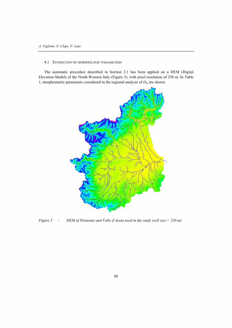
The automatic procedure described in Section 2.1 has been applied on a DEM (Digital Elevation Model) of the North-Western Italy (Figure 5), with pixel resolution of 250 m. In Table 1, morphometric parameters considered in the regional analysis of Dm are shown.

Figure 5 - DEM of Piemonte and Valle d’Aosta used in the study (cell size = 250 m)


87

Table 1 - Catchment characteristics: code used in Figure 4 (cod), measured mean annual runoff mD~ and morphoclimatic parameters for the 47 river basins of Piemonte and Valle d’Aosta used in the multiregressive analysis.

cod nome Dm Am S Hm Pm LLDP PLDP S2000 EAST NORTH Rc Xbar Ybar IT IB

[mm] [mm] [km 2] [m slm] [%] [km] [%] [%] [deg] [deg] 1 Toce a Cadarese 1571 1457 190 2137 22.10 31.6 18.20 66.0 −0.29 −0.96 0.52 8.397 46.375 1.52 0.65

2 Toce a Candoglia 1382 1519 1540 1674 7.70 82.4 10.20 36.4 0.63 −0.78 0.31 8.225 46.149 1.31 0.63

3 Niguglia a Omegna 1353 1901 122 637 4.80 16.0 8.30 0.0 0.33 0.94 0.41 8.384 45.821 1.28 0.51

4 Ticino a Miorina 1395 1695 6692 1286 2.60 168.1 7.80 20.2 0.00 −1.00 0.30 8.652 46.169 1.32 0.56

5 SBernardino a Santino 1730 2113 119 1251 17.90 22.6 26.30 2.4 0.51 −0.86 0.53 8.456 46.035 1.92 0.45

6 Mastallone a PonteFolle 1600 1936 147 1319 12.60 23.8 22.60 6.3 0.53 −0.85 0.49 8.206 45.888 1.69 0.50

7 Cervo a Passobreve 1461 1803 75 1490 20.20 14.4 22.90 13.5 0.70 −0.71 0.62 7.978 45.679 1.49 0.54

8 Sesia a Campertogno 1275 1427 170 2112 19.80 21.8 26.10 57.4 0.90 −0.44 0.49 7.936 45.838 1.10 0.77

9 Sesia a PonteAranco 1428 1735 703 1491 8.30 62.2 16.20 21.9 0.75 −0.66 0.47 8.091 45.833 1.04 0.68

10 DoraBaltea a Tavagnasco 918 949 3311 2090 6.60 110.9 10.80 58.1 0.85 −0.52 0.39 7.395 45.728 0.50 1.04

11 Orco a PonteCanavese 1034 1263 615 1924 12.10 47.9 18.60 46.7 0.93 −0.36 0.43 7.425 45.470 0.98 0.79

12 SturaLanzo a Lanzo 1090 1296 577 1773 10.60 40.3 21.00 37.4 0.99 −0.17 0.54 7.287 45.290 0.90 0.77

13 Chisone a SoucheresBasses 819 966 92 2222 15.40 17.0 17.60 73.3 0.25 0.97 0.49 6.938 44.974 0.48 1.06

14 Chisone a SMartino 694 1058 581 1730 11.20 56.6 13.70 36.9 0.87 −0.49 0.49 7.084 44.963 0.48 0.96

15 Chisone a Fenestrelle 654 910 157 2144 15.90 26.6 15.30 64.5 0.88 0.47 0.41 6.965 45.001 0.37 1.12

16 DoraRiparia a Oulx 663 851 254 2165 13.20 34.9 16.80 63.9 −0.09 1.00 0.46 6.851 44.932 0.24 1.20

17 DoraRiparia a SAntonino 591 841 993 1867 9.90 78.0 11.80 46.3 0.99 0.16 0.24 6.912 45.070 0.16 1.20

18 Po a Crissolo 1254 1271 38 2261 28.80 8.4 29.30 73.7 0.97 0.25 0.74 7.115 44.693 1.03 0.83

19 Po a Moncalieri 507 952 5032 924 0.80 114.0 5.40 14.5 0.61 0.79 0.39 7.398 44.736 0.18 1.10

20 Grana a Monterosso 811 1135 103 1565 15.00 19.0 19.50 20.5 0.99 0.13 0.54 7.240 44.403 0.67 0.93

21 SturaDemonte a Pianche 925 1112 180 2074 17.30 26.8 16.10 61.8 0.83 −0.55 0.47 7.007 44.356 0.76 0.96

22 RioBagni a BagniVinadio 1241 1398 62 2138 19.10 9.7 26.00 66.6 0.72 0.70 0.73 7.053 44.267 1.25 0.77

23 Vermenagna a Limone 1128 1364 57 1677 17.60 10.7 23.10 20.9 0.06 1.00 0.56 7.576 44.178 1.09 0.79

24 RioPiz a Pietraporzio 1272 1273 21 2194 38.70 8.3 24.70 71.5 0.42 0.91 0.55 7.018 44.311 1.06 0.84

25 SturaDemonte a Gaiola 1011 1219 560 1814 10.20 55.3 12.10 43.1 1.00 0.09 0.41 7.137 44.316 0.85 0.88

26 GessoValletta a SLorenzo 1384 1392 110 2105 22.30 17.1 19.50 61.2 0.79 0.61 0.59 7.277 44.212 1.28 0.77

27 GessoEntracque a Entracque 1404 1468 157 1894 17.00 16.9 23.80 44.4 −0.10 0.99 0.61 7.407 44.182 1.31 0.73

28 Tanaro a Montecastello 501 997 8024 651 0.80 209.8 6.40 6.0 0.75 0.66 0.28 8.064 44.548 0.18 1.07

29 Tanaro a PonteNava 1030 1281 148 1576 11.30 19.5 23.80 17.6 1.00 −0.04 0.50 7.771 44.124 0.90 0.84

30 Tanaro a Nucetto 902 1233 376 1222 7.20 55.4 16.10 7.8 0.60 0.80 0.28 7.901 44.179 0.65 0.87

31 Tanaro a Farigliano 776 1120 1516 938 2.70 93.2 12.30 5.2 0.17 0.98 0.54 7.852 44.298 0.47 0.96

32 Corsaglia a Molline 1068 1366 89 1513 17.80 18.8 20.60 17.0 0.17 0.99 0.58 7.828 44.226 1.19 0.79

33 Scrivia a Serravalle 827 1389 616 688 3.50 51.9 8.10 0.0 −0.80 0.60 0.51 9.040 44.628 0.77 0.76

34 BormidaMallare a Ferrania 965 1228 50 602 5.90 18.0 9.60 0.0 0.26 0.97 0.39 8.300 44.297 0.38 0.87

35 Erro a Sassello 882 1200 83 605 5.30 17.6 6.40 0.0 0.00 1.00 0.36 8.458 44.447 0.30 0.88

36 Bormida a Cassine 510 971 1542 481 1.80 131.1 5.80 0.0 0.50 0.87 0.35 8.322 44.500 0.04 1.09

37 Borbera a Baracche 779 1220 202 867 6.40 25.3 13.40 0.0 −0.80 0.61 0.57 9.112 44.668 0.57 0.86

38 Vobbia a Vobbietta 835 1461 57 727 9.70 14.9 14.90 0.0 −0.81 0.58 0.55 9.046 44.605 0.88 0.72

39 DoraRhemes a Pelaud 1453 1041 54 2743 24.00 12.6 19.60 97.8 0.36 0.93 0.57 7.091 45.514 1.09 0.97

40 GrandEyvia a Cretaz 1109 940 179 2593 17.10 15.3 25.80 86.4 −0.60 0.80 0.53 7.377 45.584 0.75 1.06

41 DoraBaltea a Aosta 898 952 1824 2267 8.40 55.7 15.40 67.9 0.99 0.11 0.29 7.177 45.718 0.60 1.04

42 Lys a Gressoney 1357 1191 91 2625 24.90 16.4 22.50 84.2 −0.03 −1.00 0.59 7.830 45.855 1.23 0.83

43 Rutor a Promise 1648 1314 46 2512 31.10 10.8 27.30 89.7 −0.19 0.98 0.53 6.970 45.672 1.26 0.75

44 Artanavaz a StOyen 1023 1283 71 2229 22.30 11.9 22.10 71.8 0.98 −0.19 0.59 7.151 45.828 1.15 0.76

45 Evancon a Champoluc 977 1048 105 2631 20.20 15.1 21.20 88.6 −0.31 −0.95 0.54 7.742 45.872 0.96 0.94

46 Ayasse a Champorcher 1258 1179 41 2352 30.40 12.4 17.90 82.4 0.98 0.19 0.56 7.559 45.613 0.95 0.84

47 Savara a EauRousse 1079 987 84 2723 22.90 11.5 28.30 95.8 0.10 1.00 0.60 7.206 45.523 1.11 1.02


88

4.2 ESTIMATION OF CLIMATIC PARAMETERS

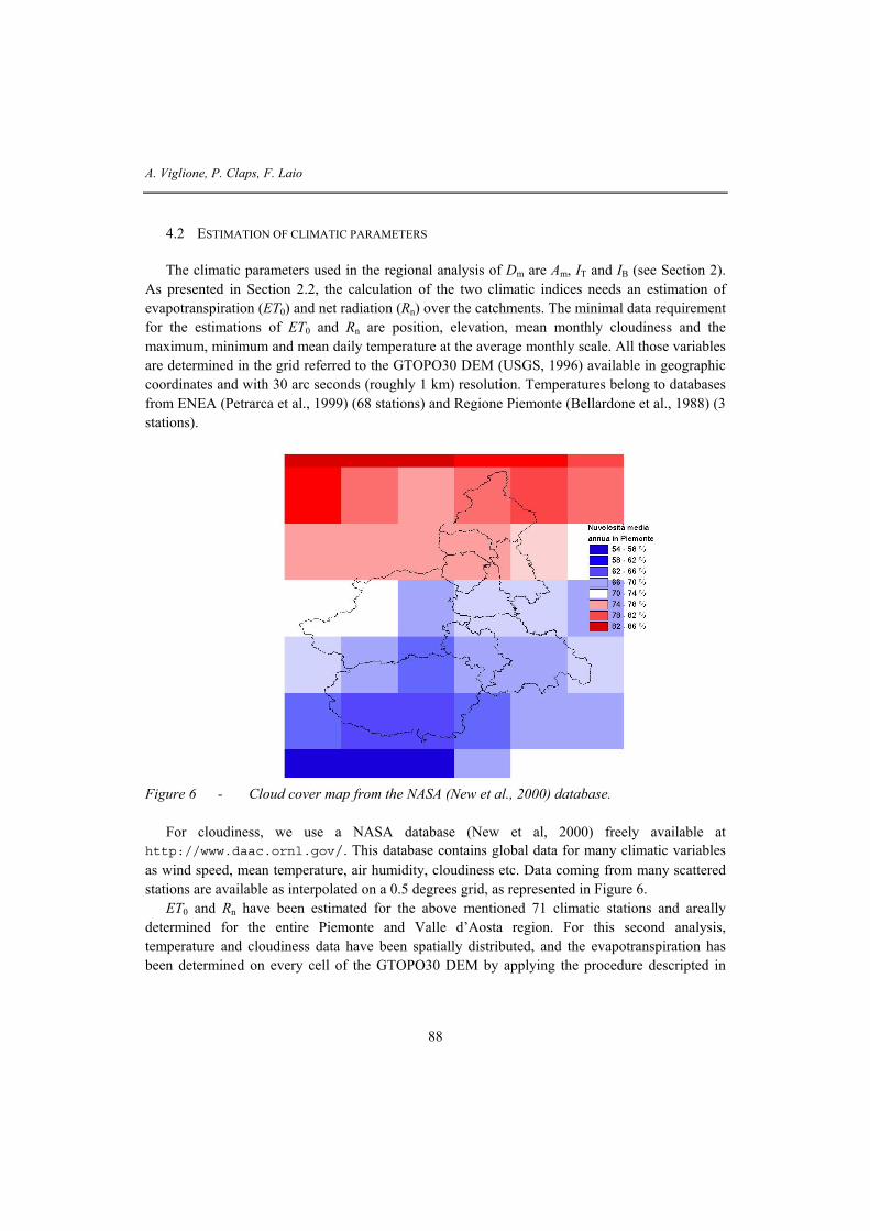
The climatic parameters used in the regional analysis of Dm are Am, IT and IB (see Section 2). As presented in Section 2.2, the calculation of the two climatic indices needs an estimation of evapotranspiration (ET0) and net radiation (Rn) over the catchments. The minimal data requirement for the estimations of ET0 and Rn are position, elevation, mean monthly cloudiness and the maximum, minimum and mean daily temperature at the average monthly scale. All those variables are determined in the grid referred to the GTOPO30 DEM (USGS, 1996) available in geographic coordinates and with 30 arc seconds (roughly 1 km) resolution. Temperatures belong to databases from ENEA (Petrarca et al., 1999) (68 stations) and Regione Piemonte (Bellardone et al., 1988) (3 stations).

Figure 6 - Cloud cover map from the NASA (New et al., 2000) database.

For cloudiness, we use a NASA database (New et al, 2000) freely available at

http://www.daac.ornl.gov/. This database contains global data for many climatic variables as wind speed, mean temperature, air humidity, cloudiness etc. Data coming from many scattered stations are available as interpolated on a 0.5 degrees grid, as represented in Figure 6.

ET0 and Rn have been estimated for the above mentioned 71 climatic stations and areally determined for the entire Piemonte and Valle d’Aosta region. For this second analysis, temperature and cloudiness data have been spatially distributed, and the evapotranspiration has been determined on every cell of the GTOPO30 DEM by applying the procedure descripted in


89

Section 2.2. Temperatures (monthly mean of minimum and maximum daily values) have been estimated by linear regression with elevation, then interpolating the residuals through the inverse distance squared weighting method (e.g. Neteler et al, 2004). Average monthly cloudiness of each pixel of the NASA dataset (Figure 6) has been assigned to its centre, and a spatial interpolation has been again conducted by the inverse distance squared weighting method.

The Thornthwaite and Budyko indices have been computed using Equations (7) and (8). All the results are reported in Table 1.

4.3 ESTIMATION OF THE MEAN ANNUAL RUNOFF

All the possible linear regression models described in Section 3 have been considered between the 47 mean annual flows mD~ and the morphoclimatic variables. Results are reported in Table 2, along with R2

adj, RMSE and RMSEcv statistics. On the basis of the criteria discussed in Section 3, the best regression obtained is:

Bmm INORDHD ⋅−⋅⋅+⋅⋅+= −− 69.11022.71091.286.7)ˆln( 24 (28)

The above model is characterized by a determination coefficient R2adj=0.900 and by a

RMSEcv=110.5 mm (referred to the non-transformed variable Dm). As we have shown in Section 2.2, the Budyko Index IB is difficult to compute, as it depends on the average net radiation Rn over the basin (Equation (8)) which, in turn, requires estimations of spatial distribution of temperatures and cloudiness. For this reason we also consider the most efficient simple model among the ones reported in Table 2. Using only Am and Hm we selected the model:

m3

m3/1

m H10)Aln(37.47.22D̂ ⋅+⋅+−= − (29)

characterized by a determination coefficient R2adj=0.883 and by a RMSEcv=115.8 mm (referred to

the non-transformed variable Dm). An analogous relation has been used in the regionalization of the annual flow in Basilicata region (Claps et al., 1998).

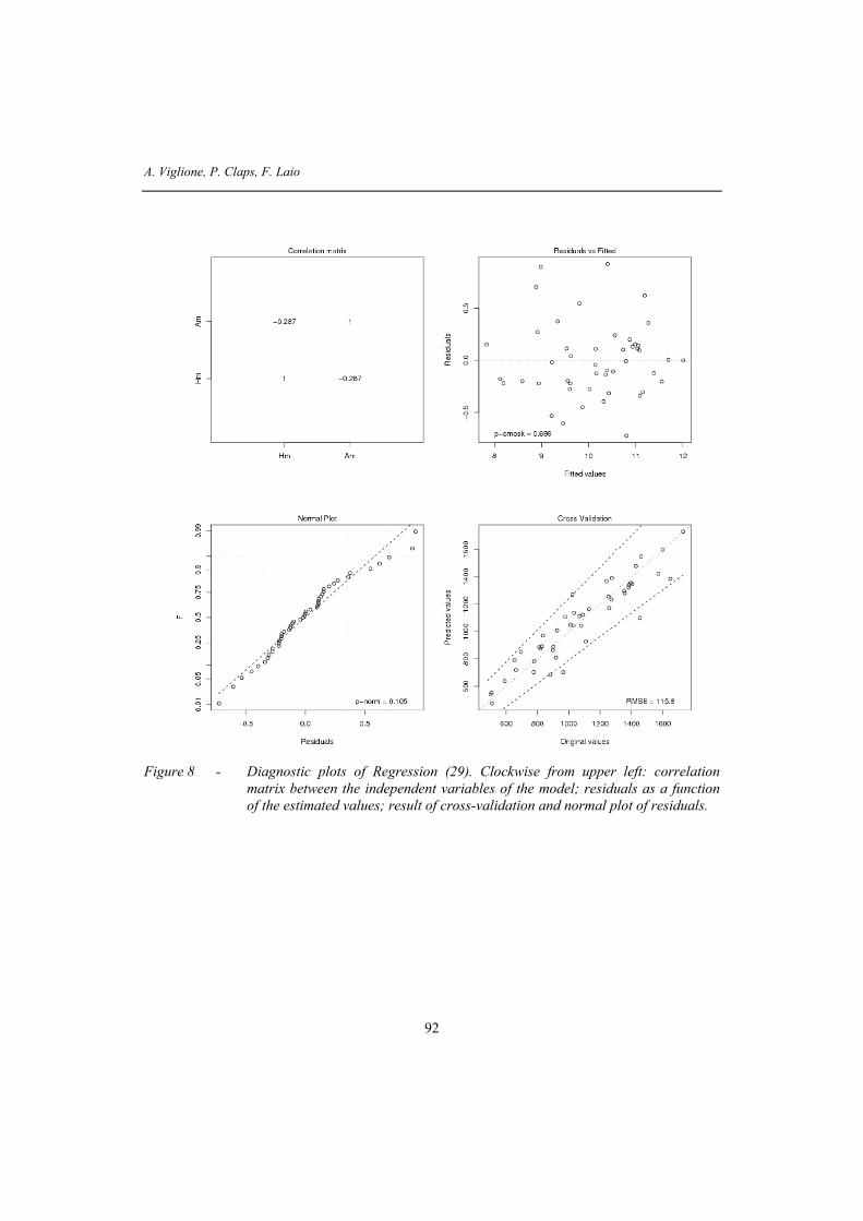
Figures 7 and 8 reproduce some diagnostic graph derived by the regression results. Proceeding by rows, the first graph represents the correlation matrix between the independent variables of the model. In order to check for multicollinearity, the VIF factor (see Section 3) has been computed for all the regressors: for Regression (28) the values of the factor is 1.15 for Hm, 1.33 for NORD and 1.34 for IB; for Regression (29) the values of the factor is 1.09 for both Hm and ln(Am). In all cases VIF is much below 5, value indicating possible multicollinearity.

The second graph represents the residuals plotted versus the respective estimated values. It is useful to investigate if residuals are affected by heteroscedasticity (diversity in variance) using the probability “p-omosk” associated with the Harrison-McCabe (1979) homoscedasticity test (see


90

Section 3). We decided that if p-omosk<0.05 the hypothesis of homoscedasticity should be rejected. The residuals of the two models can be considered homoscedastic, being the values of p-omosk 0.74 and 0.70 for Regression (28) and (29), respectively.

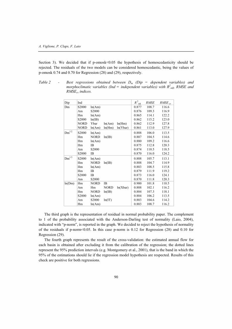
Table 2 - Best regressions obtained between Dm (Dip = dependent variables) and

morphoclimatic variables (Ind = independent variables) with R2adj, RMSE and

RMSEcv indices.

Dip Ind R 2adj RMSE RMSE cv

Dm S2000 ln(Am) 0.877 108.7 116.6Am S2000 0.876 109.3 116.9Hm ln(Am) 0.865 114.1 122.2S2000 ln(IB) 0.862 115.2 123.0NORD Ybar ln(Am) ln(Hm) 0.862 112.9 127.8NORD ln(Am) ln(Hm) ln(Ybar) 0.861 113.0 127.9

Dm1/2 S2000 ln(Am) 0.888 106.0 113.5Hm NORD ln(IB) 0.887 104.5 114.6Hm ln(Am) 0.880 109.2 116.6Hm IB 0.875 112.8 120.3Am S2000 0.874 110.5 118.5S2000 IB 0.870 116.0 124.2

Dm1/3 S2000 ln(Am) 0.888 105.7 113.1Hm NORD ln(IB) 0.888 104.7 114.9Hm ln(Am) 0.883 108.5 115.8Hm IB 0.879 111.9 119.2S2000 IB 0.873 116.0 124.1Am S2000 0.870 111.8 120.3

ln(Dm) Hm NORD IB 0.900 101.8 110.5Am Hm NORD ln(Xbar) 0.888 102.1 116.2Hm NORD ln(IB) 0.884 107.3 118.1S2000 ln(Am) 0.884 106.2 113.5Am S2000 ln(IT) 0.883 104.6 114.2Hm ln(Am) 0.883 108.7 116.2

The third graph is the representation of residual in normal probability paper. The complement

to 1 of the probability associated with the Anderson-Darling test of normality (Laio, 2004), indicated with “p-norm”, is reported in the graph. We decided to reject the hypothesis of normality of the residuals if p-norm<0.05. In this case p-norm is 0.12 for Regression (28) and 0.10 for Regression (29).

The fourth graph represents the result of the cross-validation: the estimated annual flow for each basin is obtained after excluding it from the calibration of the regression; the dotted lines represent the 95% prediction intervals (e.g. Montgomery et al., 2001), that is the band in which the 95% of the estimations should lie if the regression model hypothesis are respected. Results of this check are positive for both regressions.


91

Figure 7 - Diagnostic plots of Regression (28). Clockwise from upper left: correlation

matrix between the independent variables of the model; residuals as a function of the estimated values; result of cross-validation and normal plot of residuals.


92

Figure 8 - Diagnostic plots of Regression (29). Clockwise from upper left: correlation

matrix between the independent variables of the model; residuals as a function of the estimated values; result of cross-validation and normal plot of residuals.


93

5. CONCLUSIONS

In water resources assessment plans, it is of primary importance to transfer hydrological information from gauged to ungauged watersheds. This task is heavily based on a proper selection of climatic and morphological catchment descriptors. These parameters can drive the transfer of information when they demonstrate to connect physical and hydrological similarities among different basins. In this paper, the average annual runoff, considered as the index parameter within an index-flow statistical method, is examined with regard to its estimation in ungauged basins within the Piemonte and Valle d'Aosta region (Northern Italy).

Selection of meaningful parameters is usually performed through multiple regression. In this case, an objective method of choice of the best multiple-regression model for estimation of the index-flow is devised. The method examines in a comprehensive way all possible combinations of sets of a great number of catchment descriptors, using different data transformation, within a multiple regression framework. Thorough testing of the quality of results for each of the over 1 million models examined was performed to select the meaningful morphoclimatic variables.

In the considered region, mean basin elevation, main basin orientation and Budyko aridity index demonstrate to be the most significant variables for the transfer of hydrological information regarding mean annual runoff. A much simpler two-variable model, referring just to mean annual rainfall and mean basin elevation, was also found quite efficient.

Results of this procedure can ensure complete control of the quality of estimates obtained with regression models based on different kinds of descriptors. Procedures related to the estimation of the entire probability distribution of annual runoff in ungauged basins can also benefit from this kind of analysis.

ACKNOWLEDGEMENT

This work has been co-funded by the Regione Piemonte, B.U.R. n° 35 of 28/08/03.

6. REFERENCES

Allen R.G., Pereira L.S., Raes D., Smith M. Crop evapotranspiration. Guidelines for computing crop water requirements. FAO Irrigation And Drainage Paper 56, Roma, 1998.

Angstrom A. Solar and terrestrial radiation. Q.J.Meteorol. Soc., Vol.50, pp. 121-125, 1924.

Bellardone G., Biancotti A., Bovo S., Cagnazzi B., Giacomelli L., Marchisio C. Precipitazioni e temperature. Collana studi climatologici in Piemonte (CD-ROM). Regione Piemonte, Università degli Studi di Torino, 1998.


94

Bocchiola D., De Michele C., Rosso R., Review of recent advances in index flood estimation. Hydrology and Earth System Sciences, 7(3), 283-296, 2003.

Brath A., Camorani G., Castellarin A., Una tecnica di stima regionale della curva di durata delle portate in bacini non strumentati. In: XXIX Convegno di Idraulica e Costruzioni Idrauliche, volume 2, pp. 391–398, Trento. Università di Trento, 2004.

Canova M.E., Valutazione a scala nazionale dell’evapo-traspirazione e della radiazione solare. Tesi di laurea, Politecnico di Torino, 2003.

Castellarin A., Vogel R.M., Brath A., A stochastic index flow model of flow duration curves. Water Resourches Research, 40(3), W03104, 2004.

Claps P., Mancino L., Impiego di classificazioni climatiche quantitative nell’analisi regionale del deflusso annuo. In XXVIII Convegno di Idraulica e Costruzioni Idrauliche, pp. 169–178, Potenza, 2002.

Claps P., Fiorentino M, Probabilistic flow duration curves for use in environmental planning and management, In: Integrated approach to environmental data management systems, edited by Harmancioglu et al., NATO-ASI series 2 (31), 255-266, Kluwer, Dordrecht, The Netherlands, 1997.

Claps P., Fiorentino M., Silvagni G., Studio per la valorizzazione e la salvaguardia delle risorse idriche in Basilicata. valutazione delle risorse idriche e possibilità di regolazione dei deflussi. Regione Basilicata, 1998.

Dalrymple T., Flood frequency analyses, volume 1543-A on Water Supply Paper. U.S. Geological Survey, Reston, Va., 1960.

Ferraresi M., Todini E., Franchini M., Un metodo per la regionalizzazione dei deflussi medi. In XXI Convegno di Idraulica, volume 1, pp. 109-121, L’Aquila, 1988.

Hargreaves G.H., Samani Z.A. Estimating potential evapotranspiration. Tech. Note, J.Irrig. and. Drain Eng. ASCE 18: pp. 980-984, 1982.

Harrison M.J., McCabe B.P.M, A Test for Heteroscedasticity based on Ordinary Least Squares Residuals. Journal of the American Statistical Association 74, 494–499, 1979.

Hosking J., Wallis J., Some statistics useful in regional frequency analysis. Water Resources Research, 29 (2), pp. 271–281, 1993.

Hosking J., Wallis J., Regional Frequency Analysis: An Approach Based on L-Moments. Cambridge University Press, 1997.

Kottegoda N., Rosso R., Statistics, probability, and reliability for civil and environmental engineers. McGraw-Hill, International Edition, 1998.


95

Laio F., Cramer-von Mises and Anderson-Darling goodness of fit tests for extreme value distributions with unknown parameters. Water Resources Research, 40, pp.W09308, doi:10.1029/2004WR003204, 2004.

Montgomery D., Peck E., Vining G., Introduction to linear regression analysis. Wiley, New York, 2001.

Neteler M., Mitasova H. OPEN SOURCE GIS. A GRASS GIS Approach. 464 pp., Kluwer Academic Publishers, Boston, Dordrecht, 2004.

New M., Hulme M., Jones P.D. Global 30-Year Mean Monthly Climatology, 1961-1990 Data set. Available on-line [http://www.daac.ornl.gov] from Oak Ridge National Laboratory Distributed Active Archive Center, Oak Ridge, Tennessee, U.S.A, 2000.

Petrarca S., Spinelli F., Cogliani E., Mancini M. Profilo climatico dell’Italia. ENEA (6 volumes), 1999.

Robson A., Reed D., Statistical procedures for flood frequency estimation. In Flood Estimation Handbook, volume 3. Institute of Hydrology Crowmarsh Gifford,Wallingford, Oxfordshire, 1999.

Rossi F., Villani P., Valutazione delle piene in Campania, CNR-GNDCI and Civil Engineering Departement of Salerno University, 1995.

USGS GTOPO30. U.S. Geological Survey's EROS Data Center, Available on-line [http:// edcdaac.usgs.gov], 1996.

Viglione A., Laio F., Claps P., A comparison of homogeneity tests for regional frequency analysis. Water Resources Research, Under revision, 2006.

Vogel R., Wilson I., Probability distribution of annual maximum, mean, and minimum streamflows in the united states. Journal of Hydrologic Engineering, 1 (2), pp. 69–76, 1996.

7. WEB REFERENCES

Fluidturtles, tools for geomorphology, http://www.ing.unitn.it/~rigon/indexo.html

Geographic Resources Analysis Support System (GRASS), http://www.grass.itc.it/

The R Project for Statistical Computing, http://www.r-project.org/

The GRASS script r.parametri_bacino.pg.sh www.idrologia.polito.it/~alviglio/software/GRASSindex.htm

mean annual runoff estimation in north-western …claps/papers/prin03_viglione.pdf · part 2 -...

Documents