ME 350, Heat Transfer Laboratory, 3rd edition Updates for Fall 2018 LAB 1. POLYTROPIC PROCESS IN A CLOSED SYSTEM Use the updated steps below for your Report section: IV. Report 1. Open the data files created by the DAQ system for each run either in Excel, EES, MATLAB,

or other analysis software. There is one “header” line followed by three columns of volume, pressure, and temperature data. For the “original” data sheet for Attachment (1) make eight tables (one for each case in Table 1-2). NOTE: Each data file will have a different number of rows because only data during the actual compression or expansion process is saved.

2. Set the values from the first row of data to , , and . NOTE: refer to the Modeling

section for details on nomenclature. First, calculate , , and

. Second, calculate dimensionless work, , from the measured volume and pressure data and using the trapazoidal rule to numerically integrate Eqn. (1-2) using

.

For Attachment (2) make eight additional tables with these values.

3. Plot versus . For the experimental data use symbols with no lines. For Figure 1 (a) include all the data for the four compression cases (Runs 1, 2, 5, and 6) and for Figure 1 (b) include all the data for the four expansion cases (Runs 3, 4, 7, and 8). Use a linear curve fit to calculate the slope for each run which corresponds to the negative value of n given by Eqn. (1-12). Add to the plots lines for an isentropic process and an isothermal process using Eqn. (1-12) and values for n as indicated in Table 1-1. For Table 1 list the n values for each case.

4. In your discussion of Figure 1 and Table 1, comment on the meaning of your measured n-values. Does n depend on process type (compression or expansion)? Does n depend on the rate (fast or slow) of the process? How would you modify this experiment to make these values approach the limiting cases?

5. Plot versus . For the experimental data use symbols with no lines. For Figure 2 (a) include all the data for the four compression cases (Runs 1, 2, 5, and 6) and for Figure 2 (b) include all the data for the four expansion cases (Runs 3, 4, 7, and 8). Add to the

V0,1 p0,1 T0,1ln V0 V0,1( ) ln p0 p0,1( )

ln T0 T0,1( ) W p0,1V0,1( )

Wi+1

p0,1V0,1=

12 p0, i + p0, i+1( )

p0,1

V0, i − V0, i+1( )V0,1i=1

N

∑

ln p0 p0,1( ) ln V0 V0,1( )

ln T0 T0,1( ) ln V0 V0,1( )

plots lines for an isentropic process using Eqn. (1-11). NOTE: The isothermal case corresponds to the x-axis.

6. In your discussion of Figure 2, comment on how your data compares to the limiting cases. Does your data depend on process type (compression or expansion)? Does your data depend on the rate (fast or slow) of the process?

7. For Figure 3, plot versus . For the experimental data use symbols with no lines. For Figure 3 (a) include all the data for the four compression cases (Runs 1, 2, 5, and 6) and for Figure 3 (b) include all the data for the four expansion cases (Runs 3, 4, 7, and 8). Add to the plots lines for an isentropic process using Eqn. (1-15) and an isothermal process using Eqn. (1-18). NOTE: Divide each equation by to obtain an equation for dimensionless work.

8. In your discussion of Figure 3, comment on how your data compares to the limiting cases. Does your data depend on process type (compression or expansion)? Does your data depend on the rate (fast or slow) of the process?

W p0,1V0,1( ) ln V0 V0,1( )

p0,1V0,1

ME 350, Heat Transfer Laboratory, 3rd edition Updates for Fall 2018 LAB 4. SATURATION PROPERTIES II. Introduction Experiment For Eqn. (4-1) one of the constants is incorrect and should be: B = -5.775 x 10-7 /(˚C)2 Theory and Modeling For Eqn. (4-10) the temperature is in ˚C and the units for b are ˚C. III. Experiment Experimental Procedure Filling the Apparatus (not necessary if already full) The last group should have left the apparatus with distilled water still in the system. However, if the water level is below ¾ of the way up the sight glass add water as indicated. 2. Change this step to the following: Insure the drain valve tube for the condensate collection

container is fully closed runs to the drain bucket. Preparations for Testing (expelling air from apparatus) 2. Use the supplied flashlight to observe all the boiling stages for approximately 10 minutes.

During this step, confirm that gage pressure in the system remains at approximately 0 bar by monitoring the Bourdon-type pressure gage.

3. Skip this step. 4. Make sure to close the filler valve completely. Verify that it is closed by watching or

listening for steam escaping as you increase the pressure in the vessel. Saturation Properties and Throttling Calorimeter Testing 1. It will take approximately 5 to 10 minutes to reach 1 bar (100 kN/m2) in the system while

heating at maximum power. When you reduce the power to reach a steady state, you will need between ¼ to ½ maximum power for the readings to stabilize.

2. Open the isolating valve completely for the throttling calorimeter when bleeding off the steam sample. The throttling calorimeter is very restrictive and only a small sample of steam will escape even with the valve fully open. Also, it will take about 30 seconds for the reading to change and about 5 minutes to reach steady state due to a high time constant for the temperature probe.

4. Do not take any additional data as indicated by this step. Instead, open the isolating valve

completely for the throttling calorimeter and turn off the power to the heaters. The system will slowly return (about 30-40 minutes) to atmospheric pressure and temperature. Turn off the power to the electric console and leave the system full of water for the next group.

IV. Report 2. Change the first sentence for this step to the following: For Attachment (2) make two

additional reduced data tables that include the absolute pressure in kPa, the corrected resistance calculated using Eqn. (4-2), the absolute temperature in Kelvin ˚C calculated using Eqn. (4-1), and the absolute temperature in ˚C Kelvin for both raw data tables from Step 1. For the raw data from the “Saturation Properties” table add ln(𝑝) and ℎ'((𝑇*). For the raw data from the “Quality Measurement” table add ℎ'(𝑇*), ℎ'((𝑇*), ℎ'((𝑇+, 𝑃./0), and the quality calculated using Eqn. (4-15).

Switch the order for Step 4 and Step 5. Then, include a plot of saturation pressure versus saturation temperature obtained using the new Step 4 in Figure 2. 6. Instead of using the finite difference method to estimate (𝑑𝑝 𝑑𝑇⁄ )3./, you can differentiate

Eqn. (4-9) and which gives

4𝑑𝑝𝑑𝑇53./

=𝑎𝑝9𝑇+ 𝑒

;. <⁄

which can be combined with Eqn. (4-8) to get

ℎ'( = 𝑎𝑅 4𝑝9𝑝 5𝑒

;. <⁄

Use can use either method for your report.

ME 350, Heat Transfer Laboratory, 3rd edition Updates for Fall 2018 LAB 9. AIR/WATER PARALLEL FLOW HEAT EXCHANGER Added instructions for running the chilled water system and using the new DAQ. III. Experiment Procedure 1. Use the cooling water system instead of tap water as follows: a. Turn on the red lighted COOLING WATER SWITCH located to the right of the heat

exchanger near the corner of the room. Let the water circulate for 2 to 3 minutes to flush any air out of the system.

b. Open the COOLING WATER SUPPLY ball valve located to the left of the heat exchanger

by pulling the arm completely down (vertical position). After 1 to 2 minutes close the two PET COCK DRAIN valves (horizontal position) attached to the heat exchanger test section.

c. Open the COOLING WATER RETURN ball valve located to the left of the heat exchanger

by pushing the arm completely up (vertical position). d. Adjust the NIBCO TRIM VALVE located downstream of the COOLING WATER SUPPLY

ball valve until the DWYER RATE-MASTER FLOWMETER reads 5 gpm. 3. The blower will not be able to obtain 3000 ft3/hr. 4. Instead of the thermocouple reader box, use the OMEGA MICROPROCESSOR

THERMOMETER, MODEL HH23, to monitor position 1 of the thermocouple rotary switch box corresponding to the “air temperature downstream of the heater.” Make sure the thermocouple reader SENSOR SELECT MODE is set to type K. All other thermocouple readings are monitored using a computer data acquisition (DAQ) system as follows:

a. Double-click on the Heat_Exch_Air_Water icon on the desktop to start the software. b. Click OK for the popup window that instructs you to “Make sure both hot air and cold

water streams are on and then click OK to continue.” c. Set the flowrate for the hot air (QH, scfh) as indicated by the flowmeter. All of the other

default values for the Input Parameters are correct. Hold down Ctrl-H to open the Context Help window. Hover the mouse over any of fields to see more information in this window.

d. Click START to begin reading the thermocouple data. All of the readings will be displayed numerically under Output Parameters and graphically in the lower left corner.

e. Turn on and adjust the heater switches as needed to maintain an air temperature

between 60 °C (140 °F) and 90 °C (194 °F) at position 1 throughout the experiment (to avoid boiling the water). For the highest flowrate this will correspond to turning on the UNREGULATED HEATER SWITCH NO 1 and setting the HEATER REGULATOR to approximately 140.

f. Monitor the system to check for steady-state which is indicated by green squares next to

the readings for TH,1 and TH,2. These squares turn green when the coefficient of variation (standard deviation divided by mean) for the last 10 readings drops below the percentage in the upper right hand corner. Click the red CALC off button to switch it to a green CALC on button to have the program calculate the performance parameters for the heat exchanger and the temperature of the hot air at the intermediate axial locations.

g. To save the temperature data enter a file name in the Data file path field and then click the

red SAVE off button to switch it to a green SAVE on. Data are appended to the file name indicated until the button is clicked again. Temperatures saved are as follows: hot air inlet and outlet (Ta,in and Ta,out), cold water temperatures (TC1, TC2, TC3, TC4, TC5, TC6, TC7) and wall temperatures (Tw1, Tw2, Tw3, Tw4, Tw5, Tw6, Tw7).

5. In addition to the temperatures recorded in Step 4, record pressures and flowrate as indicated. 6. After all data has been collected exit the DAQ software by clicking the STOP button. 8. Turn off the cooling water system as follows: a. Close the COOLING WATER RETURN ball valve located to the left of the heat exchanger

by pushing the arm completely down (horizontal position). b. Close the COOLING WATER SUPPLY ball valve located to the left of the heat exchanger

by pulling the arm completely up (horizontal position). Open the two PET COCK DRAIN valves (vertical position) attached to the heat exchanger test section.

c. Turn off the red COOLING WATER SWITCH located to the right of the heat exchanger

near the corner of the room.

ME 350, Heat Transfer Laboratory, 3rd edition Updates for Fall 2018 LAB 10. AIR/AIR PARALLEL AND COUNTER FLOW HEAT EXCHANGER Experiment

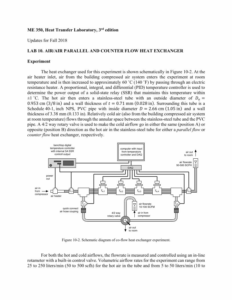
The heat exchanger used for this experiment is shown schematically in Figure 10-2. At the

air heater inlet, air from the building compressed air system enters the experiment at room temperature and is then increased to approximately 60 ˚C (140 ˚F) by passing through an electric resistance heater. A proportional, integral, and differential (PID) temperature controller is used to determine the power output of a solid-state relay (SSR) that maintains this temperature within ±1 ˚C. The hot air then enters a stainless-steel tube with an outside diameter of 𝐷? =0.953cm(3/8in) and a wall thickness of 𝑡 = 0.71mm(0.028in). Surrounding this tube is a Schedule 40-1, inch NPS, PVC pipe with inside diameter 𝐷 = 2.66cm(1.05in) and a wall thickness of 3.38 mm (0.133 in). Relatively cold air (also from the building compressed air system at room temperature) flows through the annular space between the stainless-steel tube and the PVC pipe. A 4/2 way rotary valve is used to make the cold airflow go in either the same (position A) or opposite (position B) direction as the hot air in the stainless-steel tube for either a parallel flow or counter flow heat exchanger, respectively.

Figure 10-2. Schematic diagram of co-flow heat exchanger experiment. For both the hot and cold airflows, the flowrate is measured and controlled using an in-line

rotameter with a built-in control valve. Volumetric airflow rates for the experiment can range from 25 to 250 liters/min (50 to 500 scfh) for the hot air in the tube and from 5 to 50 liters/min (10 to

air heater

air in!from!compressor

benchtop digital !temperature controller!with internal 5A SSR!

controll output

power!out

air in from !compressor

DAQ

air flowrate!10-100 SCFM

air flowrate!50-500 SCFH

air out!to room

air out !to room

quick connect !air hose couping

Tw,1 Tw,2 Tw,3 Tw,4 Th,2Th,1

Tc,1 Tc,2

A

B

4/2 way !rotary valve

computer with input !from temperature!

controller and DAQ

100 scfh) for the cold air in the annulus. Recall that flow through a tube or annulus is turbulent (or characterized by a high degree of mixing) at high values of Reynolds number (defined as the dimensionless ratio of inertial to viscous forces). We will assume turbulent flow for

𝑅𝑒OP =𝜌𝑉S𝐷T𝜇 > 2300,𝐷T = 4𝐴Y 𝑃⁄ (10-1)

where r is density, µ is viscosity, is average velocity, is the hydraulic diameter, Ac is the cross-sectional area, and P is the wetted perimeter (Ref. 1). For the tube, 𝐷T = 𝐷Z = 𝐷? − 2𝑡 =0.801cm(0.319in) which corresponds to approximately 3,250 < 𝑅𝑒OP < 32,500. Thus, for the flow in the tube the flow regime will be assumed turbulent. For the annulus, 𝐷T = 𝐷 − 𝐷? =1.71cm(0.644in) which corresponds approximately to . Thus, for the flow in the annulus the flow regime will be assumed laminar.

The length of the heat exchanger test section is approximately L = 1.5 m (5.0 ft) which corresponds to a length to hydraulic diameter ratio of approximately 160 for both the tube and the annulus. For laminar flow, the hydraulic and thermal development lengths can be approximated by the following correlations:

4𝐿𝐷T5T^_`?

≈ 0.05𝑅𝑒OP ,4𝐿𝐷T5/Tb`0?

≈ 0.05𝑃𝑟𝑅𝑒OP (10-2)

where Pr is the Prandtl number which is approximately 0.7 for air at STP. Thus, for laminar flow near transition the flow will be developing both hydro-dynamically and thermally for most of the test section. For turbulent flow, both the hydraulic and thermal development lengths are approximately the same and equal to about 10 diameters. Thus, for turbulent flow the flow will be both hydro-dynamically and thermally fully-developed for most of the test section.

Once the system is allowed to reach steady state (where properties no longer change with time), thermocouples are used to measure mean hot and cold air temperatures, 𝑇T and 𝑇Y, at the test section inlets and outlets and wall temperature, 𝑇d, at 4 locations along the test section. In addition, the volumetric flowrates of the hot and cold air, �̇�T and �̇�Y , are measured with rotameters that are calibrated for air at standard temperature and pressure. Thus, the actual temperature and pressure in the rotameter are needed to calculate the flowrate for actual conditions.

From these measurements, the heat transfer for each air stream can be calculated by

applying conservation of energy

�̇�Zg − �̇�?h/ + �̇�( = �̇�3/ (10-3)

to two separate control volumes, CVs; one for the hot airflow and one for the cold airflow. Both CVs span the cross-section of the flow and extend the length of the test section. The net rate of energy transfer for the CV, (�̇�Zg − �̇�?h/), includes the energy carried into and out of the CV by the fluid and the convection heat transfer either out of the hot air in the tube or into the cold air in the annulus. Also, for the cold airflow CV there is energy transfer to the room air, but we will assume

V Dh

180 < ReDh <1800

L / Dh ≈

this is negligible. The energy generated in the CV is zero, (�̇�( = 0). Assuming the flow has reached steady state, the rate of change of energy storage in the CV is also zero (�̇�3/ = 0). Finally, assuming only sensible heat transfer (no phase change), incompressible fluid, and constant specific heats, 𝑐k, Eqn. (10-3) reduces to

𝑞T = �̇�T𝑐k,Tn𝑇T,Z − 𝑇T,?o = 𝐶T∆𝑇T (10-4)

𝑞Y = �̇�Y𝑐k,Yn𝑇Y,? − 𝑇Y,Zo = 𝐶Y∆𝑇Y (10-5)

where the subscripts h and c are for hot and cold air, the subscripts i and o are for inlet and outlet flow, �̇� = 𝜌�̇� is the mass flowrate, 𝐶 = �̇�𝑐k is the fluid heat capacity rate (Ref. 2), and ∆𝑇T =n𝑇T,Z − 𝑇T,?o and ∆𝑇Y = n𝑇Y,? − 𝑇Y,Zo are the changes in temperature of the hot and the cold airflows.

The effectiveness of the heat exchanger, a dimensionless performance parameter for a heat exchanger, can then be calculated using

𝜀T =𝑞T𝑞0.s

,𝜀Y =𝑞Y𝑞0.s

,𝑞0.s = 𝐶0Zgn𝑇T,Z − 𝑇Y,Zo (10-6)

where 𝑞0.s is the maximum possible heat transfer between the two air streams, n𝑇T,Z − 𝑇Y,Zo is the maximum temperature difference, and 𝐶0Zg is the minimum value of 𝐶T and 𝐶Y (Ref. 2 and Ref. 3). Because we are comparing the actual heat transfer to the maximum possible we must get 𝜀 < 1. Again, note that for a heat exchanger with an outer surface that is perfectly insulated by conservation of energy 𝑞T = 𝑞Y and 𝜀T = 𝜀Y. For our actual heat exchanger 𝑞T = 𝑞Y + 𝑞t?33 , thus we should expect to get 𝑞T > 𝑞Y and 𝜀T > 𝜀Y.

Modeling For a heat exchanger the log mean temperature difference (LMTD) method can be used to

predict the heat transfer between the streams, 𝑞, the outlet temperatures, and the heat exchanger effectiveness given the size of the heat exchanger and the inlet conditions (Ref. 2). This is a global (or one-dimensional) method of analysis that assumes the following: uniform cross-sectional properties, perfectly insulated exterior, negligible axial conduction in each fluid and changes in potential and kinetic energy, and constant specific heats and convection coefficients. We will consider two different configurations: (1) parallel flow where the cold and hot streams move in the same direction as shown in Figure 10-3 and (2) counter flow where the cold and hot streams move in opposite directions as shown in Figure 10-4.

Figure 10-3. Schematic diagram of concentric tube, parallel flow heat exchanger.

Figure 10-4. Schematic diagram of concentric tube, counter flow heat exchanger.

Cc

Ch Th Th + dTh

Tc Tc + dTcdq

dx

heat transfer !surface area

1

Th,i

Tc,i

∆T1

Th

Tc

2

xdx

∆T2

Th,o

Tc,o∆T

Cc

Ch Th Th + dTh

TcTc + dTc dq

dx

heat transfer !surface area

1

Th,i

Tc,o

∆T1

Th

Tc

2

xdx

∆T2

Th,o

Tc,i

∆T

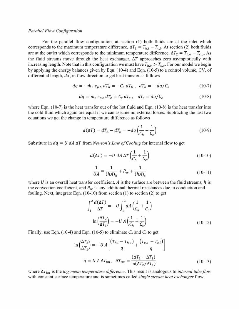
Parallel Flow Configuration For the parallel flow configuration, at section (1) both fluids are at the inlet which

corresponds to the maximum temperature difference, ∆𝑇* = 𝑇T,Z − 𝑇Y,Z. At section (2) both fluids are at the outlet which corresponds to the minimum temperature difference, ∆𝑇+ = 𝑇T,? − 𝑇Y,?. As the fluid streams move through the heat exchanger, ∆𝑇 approaches zero asymptotically with increasing length. Note that in this configuration we must have 𝑇T,? > 𝑇Y,?. For our model we begin by applying the energy balances given by Eqn. (10-4) and Eqn. (10-5) to a control volume, CV, of differential length, 𝑑𝑥, in flow direction to get heat transfer as follows

𝑑𝑞 = −�̇�T𝑐k,T𝑑𝑇T = −𝐶T𝑑𝑇T , 𝑑𝑇T = −𝑑𝑞 𝐶T⁄ (10-7)

𝑑𝑞 = �̇�Y𝑐k,Y𝑑𝑇Y = 𝐶Y𝑑𝑇Y , 𝑑𝑇Y = 𝑑𝑞 𝐶Y⁄ (10-8)

where Eqn. (10-7) is the heat transfer out of the hot fluid and Eqn. (10-8) is the heat transfer into the cold fluid which again are equal if we can assume no external losses. Subtracting the last two equations we get the change in temperature difference as follows

𝑑(∆𝑇) = 𝑑𝑇T − 𝑑𝑇Y = −𝑑𝑞 41𝐶T+1𝐶Y5 (10-9)

Substitute in 𝑑𝑞 = 𝑈𝑑𝐴∆𝑇 from Newton’s Law of Cooling for internal flow to get

𝑑(∆𝑇) = −𝑈𝑑𝐴∆𝑇 41𝐶T+1𝐶Y5 (10-10)

1𝑈𝐴 =

1(ℎ𝐴)T

+ 𝑅d +1

(ℎ𝐴)Y (10-11)

where 𝑈 is an overall heat transfer coefficient, 𝐴 is the surface are between the fluid streams, ℎ is the convection coefficient, and 𝑅d is any additional thermal resistances due to conduction and fouling. Next, integrate Eqn. (10-10) from section (1) to section (2) to get

w𝑑(∆𝑇)∆𝑇 = −𝑈w 𝑑𝐴

+

*41𝐶T+1𝐶Y5

+

*

ln 4∆𝑇+∆𝑇*

5 = −𝑈𝐴 41𝐶T+1𝐶Y5 (10-12)

Finally, use Eqn. (10-4) and Eqn. (10-5) to eliminate Ch and Cc to get

ln 4∆𝑇+∆𝑇*

5 = −𝑈𝐴 xn𝑇T,Z − 𝑇T,?o

𝑞 +n𝑇Y,? − 𝑇Y,Zo

𝑞y

𝑞 = 𝑈𝐴∆𝑇t0,∆𝑇t0 =(∆𝑇+ − ∆𝑇*)ln(∆𝑇+ ∆𝑇*⁄ ) (10-13)

where ∆𝑇t0 is the log-mean temperature difference. This result is analogous to internal tube flow with constant surface temperature and is sometimes called single stream heat exchanger flow.

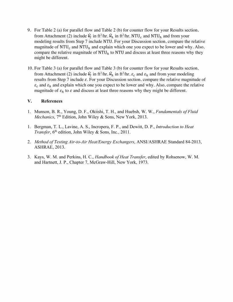
Counter Flow Configuration For the counter flow configuration, at section (1) is the hottest portion of both fluid streams

with temperature difference ∆𝑇* = 𝑇T,Z − 𝑇Y,?. At section (2) is the coldest portion of both fluid streams with temperature difference ∆𝑇+ = 𝑇T,? − 𝑇Y,Z. Note that we can now have 𝑇T,? > 𝑇Y,?. Similar to above the change in temperature difference now becomes (for Tc rising in -x direction)

𝑑(∆𝑇) = 𝑑𝑇T + 𝑑𝑇Y = 𝑑𝑞 41𝐶Y−1𝐶T5 (10-14)

Again, substitute in dq from Newton’s Law of Cooling for internal flow to get

𝑑(∆𝑇) = 𝑈𝑑𝐴∆𝑇 41𝐶T−1𝐶Y5 (10-15)

Again, integrate from section (1) to section (2) to get

w𝑑(∆𝑇)∆𝑇 = 𝑈w 𝑑𝐴

+

*41𝐶Y−1𝐶T5

+

*

ln 4∆𝑇+∆𝑇*

5 = 𝑈𝐴 41𝐶Y−1𝐶T5 (10-16)

Finally, again use Eqn. (10-4) and Eqn. (10-5) to eliminate Ch and Cc:

ln 4∆𝑇+∆𝑇*

5 = 𝑈𝐴 xn𝑇Y,? − 𝑇Y,Zo

𝑞 −n𝑇T,Z − 𝑇T,?o

𝑞y

𝑞 = 𝑈𝐴∆𝑇t0, ∆𝑇t0 =(∆𝑇+ − ∆𝑇*)ln(∆𝑇+ ∆𝑇*⁄ ) (10-17)

Note, this is the same result as for parallel flow, but ∆𝑇* and ∆𝑇+ are now defined differently. For either case, we can now use this with Eqn. (10-6) to estimate the heat exchanger effectiveness.

𝜀-NTU (Number of Transfer Units) Method

The 𝜀-NTU method uses the results of the LMTD method to give heat exchanger

performance in terms of three dimensionless parameters where NTU is defined as

NTU =𝑈𝐴𝐶0Zg

= 𝑓(𝜀, 𝐶`) (10-18)

𝐶` = 𝐶0Zg 𝐶0.s ≤ 1⁄ (10-19)

where 𝐶` is the heat capacity ratio. Note that for all boilers, condensers, and single stream heat exchangers where 𝐶0.s ≫ 𝐶0Zg , 𝐶` = 0 for all flow configurations.

To derive the NTU relationship for parallel flow, begin by rewriting Eqn. (10-12) in terms of NTU, 𝐶0Zg, and 𝐶` as

ln 4∆𝑇+∆𝑇*

5 = −𝑈𝐴 41𝐶T+1𝐶Y5 = −

𝑈𝐴𝐶0Zg

(1 + 𝐶`)

NTU =

−ln(∆𝑇+ ∆𝑇*⁄ )(1 + 𝐶`)

(10-20)

Next, for 𝐶0Zg = 𝐶T and from Eqn. (10-4), Eqn. (10-5), and Eqn. (10-16)

𝜀 =𝑞T𝑞0.s

=𝑇T,Z − 𝑇T,?𝑇T,Z − 𝑇Y,Z

,𝐶` =𝐶0Zg𝐶0.s

=𝑇Y,? − 𝑇Y,Z𝑇T,Z − 𝑇T,?

∆𝑇+∆𝑇*

=𝑇T,? − 𝑇Y,?𝑇T,Z − 𝑇Y,Z

=n𝑇T,? − 𝑇T,Zo + n𝑇T,Z − 𝑇Y,Zo + n𝑇Y,Z − 𝑇Y,?o

𝑇T,Z − 𝑇Y

∆𝑇+∆𝑇*

= 1 − 𝜀(1 + 𝐶`) (10-21)

Substitute into Eqn. (10-20) to get

NTU = −ln[1 − 𝜀(1 + 𝐶`)]

(1 + 𝐶`) or 𝜀 =

1 − exp[−NTU(1 + 𝐶`)]1 + 𝐶`

(10-22)

where the same result is obtained for 𝐶0Zg = 𝐶Y. A similar derivation can be performed to develop the NTU relationship for counter flow in terms of 𝜀 and 𝐶`. The result is given by

NTU = �

1(𝐶` − 1)

ln 4𝜀 − 1𝜀𝐶` − 1

5𝜀

(1 − 𝜀) for𝐶` = 1 or ε =

⎩⎨

⎧1 − exp[−NTU(1 − 𝐶`)]1 − 𝐶`exp[−NTU(1 − 𝐶`)]

NTU(1 + NTU) for𝐶` = 1

(10-23)

Finally, experimental data can be used to estimate NTU by starting with the definition of

NTU given by Eqn. (10-18), substituting in for 𝑈𝐴 from Eqn. (10.13) from the LMTD method, and then substituting in for q from Eqn. (10-4) or Eqn. (10-5) to get

NTU ≈𝐶T∆𝑇T

𝐶0Zg∆𝑇t0≈

𝐶Y∆𝑇Y𝐶0Zg∆𝑇t0

(10-24)

where for the experimental data, due to heat transfer losses for the cold stream to the room air, these two values will typically not be the same. In addition, the analysis assumes constant convection coefficients which is not always valid for developing flow.

Convection Coefficients

To use Eqn. (10-13), we need to calculate 𝑈 using Eqn. (10-11). For our heat exchanger

with a clean, thin stainless-steel tube separating the streams we can assume 𝑅d ≈ 0, thus we just need values for ℎ for inside a tube and annulus. We will estimate values using experimentally

developed correlations for Nusselt number (a dimensionless form of h defined as the ratio of convection to conduction heat transfer through the fluid) given by

𝑁𝑢OP =ℎ𝐷T𝑘'

,𝐷T =4𝐴Y𝑃 (10-25)

where kf is the thermal conductivity of the fluid. Recall that the LMTD model assumes constant 𝑈. This assumption is valid for hydro-dynamically and thermally fully developed flow, thus all of the correlations below will correspond to these conditions. Note that the actual conditions in the heat exchanger can be significantly different and these correlations will underestimate ℎ and 𝑈.

For flow in a tube where 𝐷T = 𝐷, if the flow remans laminar based on the condition in Eqn. (10-2), 𝑁𝑢O = 4.36 for constant heat flux and 𝑁𝑢O = 3.66 for constant surface temperature (Ref. 2). If the flow is turbulent, one commonly used correlation for flow in a smooth tube for a low to moderate temperature difference between the wall and fluid is a modified form of the Dittus-Boetler correlation (Ref. 2) given by

𝑁𝑢O = 0.023𝑅𝑒O� �⁄ 𝑃𝑟g for �

0.6 ≲ 𝑃𝑟 ≲ 160𝑅𝑒O ≳ 10�𝐿 𝐷⁄ ≳ 10

� (10-26)

where Pr is the Prandtl number (dimensionless ratio of thermal to momentum diffusion rates which is a thermodynamic property of the fluid), for heating, and for cooling. All properties for this correlation are calculated at the mean temperature of the fluid. This correlation can be used for either a constant wall temperature or uniform wall heat flux boundary condition.

For flow in an annulus where 𝐷T = 𝐷 − 𝐷? , if the flow remans laminar again based on the

condition in Eqn. (10-2), values for 𝑁𝑢OP are given in Table 10-1 with perfect insulation on the outer surface and for either constant surface temperature or constant heat flux on the inner surface (Ref. 4). For our case 𝐷? 𝐷⁄ = 0.357, thus using linear interpolation 𝑁𝑢OP = 6.67 for constant 𝑇3 and 𝑁𝑢OP = 7.25 for constant 𝑞3. If the flow is turbulent, to a first approximation the Dittus-Boetler correlation can be used with 𝐷T for either boundary condition.

Table 10-1. Nusselt number for laminar hydrodynamically and thermally fully developed flow in an annulus with perfect insulation on outer surface and constant surface temperature on inner surface.

n = 0.4 n = 0.3

DoDihot air !in tube

cold air !in annulus

D

𝑫𝒐 𝑫⁄ 𝑻𝒔 constant 𝒒𝒔 constant 0.05 17.46 17.81 0.10 11.56 11.91 0.25 7.37 8.02 0.50 5.74 6.25 »1.00 4.86 5.39

III. Experiment Equipment

Stainless steel 304 welded tubing (3/8 in OD, 0.319 in ID, 6 ft length) PVC clear pipe (1 in - SCH 40, approximate 1 ft length sections) Flowmeters (air variable area, polycarbonate with stainless steel valve, 50-500 SCFH,

5 in scale), Dwyer Instruments, Model RMB-56-SSV Air process heater (120 V, 200 W, 1-8 CFM, 3/8 in DIA), Omega, Model AHP-3741 Universal benchtop digital controller, Platinum Series, Omega, Model CS8DPT Pipe plug TC probe, Omega, Model TC-T-NPT-G-72 Quick disconnect TC probe (stainless steel, 1/8 in DIA, 6 in length, type T, grounded,

miniature connector), Omega, Model TMQSS-125G-6 DAQ module (8 thermocouple channels, 14-bit, USB interface), Measurement

Computing, Model USB-TC Experiment Setup 1. For the hot airflow inside the tube, ensure that the compressed airflow inlet is connected to

the heat exchanger on the left side upstream of the air process heater using flexible tubing and quick disconnect fittings.

2. For the cold airflow inside the annulus, ensure that the compressed airflow is connected to the flowmeter and the 4/2-way rotary valve using flexible tubing and quick-disconnect fittings. Set the 4/2-way rotary valve to the A position for parallel flow (thus, the compressed airflow inlet is on the left side with the heater).

3. Slowly open the compressed airflow valves (one provides air to the tube and the other provides air to the annulus) until the volumetric flowrate for both flows is 100 scfm. Use the valves on the front of each flow meter to fine tune the adjustments. Note that the two lines are connected, thus they are not independent and some iteration may be required.

4. For the Measurement Computing DAQ module ensure that the USB cable is connected to the computer and that thermocouples for the air inlets, air outlets, and wall temperature readings are connected.

5. For the Platinum Series universal benchtop digital controller ensure that its USB cable is connected to the computer, power output 1 is connected to the air process heater, and a thermocouple cable from the TC plug after the heater is plugged in. Turn on the digital controller using the power switch on the back right-hand side. After the initial startup sequence, the larger LED display labeled PV (for process value) should indicate oPER for operating mode and the smaller LED display labeled SV (for setpoint value) should indicate the current setpoint temperature of 60.00 ˚C. However, if the unit was turned off in a different mode PV may indicate INIt for initializing mode or ProG for programming mode.

Experiment Procedure 1. Start the DAQ software by double clicking on the Heat Exchanger icon on the desktop. This

will open the Heat_Exch_Air_Air.vi window and a window prompting you to Make sure both hot and cold fluid streams are on with a minimum flowrate of 50 scfh and then click OK to continue. For the Experimental Setup section above, flowrates are set to 100 scfh, so this condition is satisfied and you can click OK.

2. In the Heat_Exch_Air_Air.vi window, in the Input Parameters panel on the top-left side the following parameters can be set (but leave them at their default values for now):

𝑇� setpoint temperature for the benchtop controller 𝐷 diameter of inner tube for heat exchanger calculations 𝐿 length of test section for heat exchanger 𝑥 axial location of the wall temperature probes 𝑄Y, 𝑄T volumetric flowrate of cold and hot air flows (�̇�Y and �̇�T in Experiment section) 𝑐k,Y, 𝑐k,T specific heat at constant pressure for cold and hot air flows 𝜌Y, 𝜌T density of cold and hot air flows

3. Click the START button to begin heating the airflow in the tube and measuring temperatures. You should see the PV display on the benchtop controller begin to increase in magnitude for about 3 minutes until it reaches the setpoint temperature value of approximately 60 ˚C. In the Heat_Exch_Air_Air.vi window for the graph on the lower-left side you should see a plot of cold flow temperature, 𝑇Y, hot flow temperature, 𝑇T, and wall temperature, 𝑇d, versus axial location. The values plotted are all displayed in the Output Parameters panel on the right side.

NOTE: If the program cannot open communications with the benchtop controller and/or the DAQ module you will get a warning message. Cancel the execution and quit the program. Open the Settings and ensure that under Devices for Other devices that the benchtop controller listed as USB Serial Device (COM6) and the DAQ module listed as USB-TC are visible. If they are not, check the USB cable connections, ensure they now appear, and then reopen the Heat_Exch_Air_Air.vi.

4. Monitor the system to check for steady-state which is indicated by green squares next to the readings for TC,1, TC,2, TH,1 and TH,2. These squares turn green when the coefficient of variation (standard deviation divided by mean) for the last 10 readings drops below the percentage in the upper right-hand corner. Once the readings approximately reach steady state after about 5 minutes, click the CALC off button so that it now reads CALC on. The program will now use the LMTD method to estimate and display 𝑇Y and 𝑇T at each of the same measurement locations for 𝑇d. In addition, other performance parameters such as 𝜀Y, 𝜀T, 𝑈, and NTU are also displayed.

5. After reaching steady state, record 𝑄Y (or �̇�Y), 𝑄T (or �̇�T), 𝑇Y,*, 𝑇Y,+, 𝑇T,*, 𝑇T,+, and 𝑇d at the 4 axial locations.

NOTE: If you run too many other software programs (such as Excel, a web browser, etc.) while collecting data the Heat_Exch_Air_Air.vi may not be able to sample/buffer data at the specified rate and will stop reading data or give a warning. If possible, press STOP to send the command to the benchtop controller to stop heating and halt the execution of the program. The PV display on the benchtop controller should again start blinking red and start decreasing. Then rerun the DAQ software by clicking on the run arrow ( ) in the upper-left hand corner (or on the task bar click Operate and select Run from the pull-down menu) and click the START button to turn the heater back on. If it is not possible to halt execution this way, then just quit and rerun the program as usual for Windows.

6. Increase the volumetric flowrate for hot airflow in the tube to 200 scfm using the compressed air valves and the flowmeter valves while keeping the cold annulus airflow at 100 scfm. Again, some iteration may be required.

7. In the Input Panel change 𝑄T to 200 scfm and then repeat Steps 4 and 5.

8. Repeat Steps 6 and 7 for hot air volumetric flowrates of 300 and 400 scfm.

9. Set the 4/2-way rotary valve to the B position for counter flow (thus, the compressed airflow inlet is on the right side).

10. Repeat the heat exchanger tests for the 4 volumetric airflow rates from the parallel flow configuration. Note that the first case will take about 10 minutes to reach steady state.

11. Press STOP to stop heating and halt the execution of the program. After the temperature has dropped by at least 10 ˚C, close the compressed air valves to turn off the airflow. Turn off the power to the benchtop digital controller using the power switch on the back right-hand side.

IV. Report 1. For Attachment (1) make a “Parallel Flow” raw data table and a “Counter Flow” raw data

table that includes cold and hot air volumetric flowrates and all the measured temperatures. This corresponds to 8 flowrate test conditions.

2. For Figure 1 for your Results section, make a plot of 𝑇Y, 𝑇T, and 𝑇d versus axial location

using your data from Attachment (1) at the lowest air flowrates for both the counter flow and parallel flow configurations. For your Discussion section, comment on the trends in the data and if they make sense. Also, comment on if either configuration is more effective at changing the temperature of the airflow and possible reasons.

3. For Attachment (2) make a “Parallel Flow” reduced data table and a “Counter Flow” reduced

data table for all 8 flowrate test conditions. Include the following calculations for both the cold and hot air flows (assuming ideal gas behavior and negligible pressure drops in the tube and annulus, 𝑝./0 ≈ 𝑝`?/ ≈ 𝑝0, which are valid assumptions for our conditions): • Rotameter density, 𝜌`?/ = 𝑝./0 (𝑅𝑇 ?/)⁄ , using the temperature at the test section exit • Actual volumetric flowrate in ft3/hr using Eqn. (A-5) • Mass flowrate in kg/s using Eqn. (A-6)

• Fluid heat capacity rate, 𝐶 = �̇�𝑐k, temperature change from inlet to outlet, ∆𝑇, and heat transfer, 𝑞, in W using Eqn. (10-4) and Eqn. (10-5)

4. For Figure 2 for your Results section, make a plot of ∆𝑇Y and ∆𝑇T versus �̇�T in ft3/hr using

the data from Attachment (2) for both the counter flow and parallel flow configurations. For your Discussion section, comment on the trends in the data and if they make sense. Also, comment on if either configuration is a more effective at changing the temperature and possible reasons.

5. For Figure 3 for your Results section, make a plot of 𝑞Y and 𝑞T versus �̇�T in ft3/hr using the

data from Attachment (2) for both the counter flow and parallel flow configurations. For your Discussion section, comment on the trends in the data and if they make sense. Also, comment on if either configuration is a more effective at transferring heat and possible reasons.

6. For Attachment (3) make a “Parallel Flow” performance data table and a “Counter Flow”

performance data table for all 8 test conditions. Include the following calculations for both the cold and hot air flows: • Heat exchanger effectiveness, 𝜀, using Eqn. (10-6) • Overall heat transfer coefficient, 𝑈, using Eqn. (10-13) where for 𝑞 use 𝑞Y and 𝑞T from

the calculations in Attachment (2), the area is the surface area between the hot and cold flows, and ∆𝑇t0 is the same for the hot and cold flows

• Number of transfer units, NTU, using either Eqn. (10-18) or Eqn. (10-23) 7. For your modeling predictions, at the same 8 test conditions for both the hot and cold air

flows calculate the following: • Mean temperature in the test section using 𝑇0 = (𝑇* + 𝑇+) 2⁄ • Mean density in the test section using 𝜌0 = 𝑝./0 (𝑅𝑇0)⁄ • Mean velocity in the test section using 𝑉S = �̇� (𝜌0𝐴Y)⁄ where 𝐴Y is cross-sectional area • Reynolds number, 𝑅𝑒OP, using Eqn. (10-1) • Nusselt number, 𝑁𝑢OP, using a correlation or table from the Convection Coefficient

section and heat transfer coefficient, ℎ, using Eqn. (10-25) • Overall heat transfer coefficient, 𝑈, using Eqn. (10-11) assuming all areas are

approximately equal and 𝑅d ≈ 0 • Number of transfer units, NTU, using Eqn. (10-18) • Heat exchanger effectiveness, 𝜀, using Eqn. (10-23) and Eqn. (10-24)

8. For Table 1 (a) for parallel flow and Table 1 (b) for counter flow for your Results section,

from Attachment (2) include �̇�Y in ft3/hr, �̇�T in ft3/hr, 𝑈Y in W/m2•˚C, and 𝑈T in W/m2•˚C and from your modeling results from Step 7 include 𝑈 in W/m2•˚C. For your Discussion section, compare the relative magnitude of 𝑈Y to 𝑈T and explain which one you expect to be lower and why. Also, compare the relative magnitude of 𝑈T to 𝑈 and discuss at least three reasons why they might be different.

9. For Table 2 (a) for parallel flow and Table 2 (b) for counter flow for your Results section, from Attachment (2) include �̇�Y in ft3/hr, �̇�T in ft3/hr, NTUY and NTUT and from your modeling results from Step 7 include NTU. For your Discussion section, compare the relative magnitude of NTUY and NTUT and explain which one you expect to be lower and why. Also, compare the relative magnitude of NTUT to NTU and discuss at least three reasons why they might be different.

10. For Table 3 (a) for parallel flow and Table 3 (b) for counter flow for your Results section,

from Attachment (2) include �̇�Y in ft3/hr, �̇�T in ft3/hr, 𝜀Y and 𝜀T and from your modeling results from Step 7 include 𝜀. For your Discussion section, compare the relative magnitude of 𝜀Y and 𝜀T and explain which one you expect to be lower and why. Also, compare the relative magnitude of 𝜀T to 𝜀 and discuss at least three reasons why they might be different.

V. References 1. Munson, B. R., Young, D. F., Okiishi, T. H., and Huebsh, W. W., Fundamentals of Fluid

Mechanics, 7th Edition, John Wiley & Sons, New York, 2013.

1. Bergman, T. L., Lavine, A. S., Incropera, F. P., and Dewitt, D. P., Introduction to Heat Transfer, 6th edition, John Wiley & Sons, Inc., 2011.

2. Method of Testing Air-to-Air Heat/Energy Exchangers, ANSI/ASHRAE Standard 84-2013, ASHRAE, 2013.

3. Kays, W. M. and Perkins, H. C., Handbook of Heat Transfer, edited by Rohsenow, W. M. and Hartnett, J. P., Chapter 7, McGraw-Hill, New York, 1973.

APPENDIX A ROTAMETER CALIBRATION

Figure A-1 Picture and schematic for a rotameter used to measure volumetric flowrate. A rotameter, a type of variable area flowmeter, is a device used to measure the volumetric

flowrate, , of a fluid flowing in a tube. It consists of a solid weight, often called a float, located inside a tapered flow tube as shown schematically in Figure A-1. It must be oriented vertically with the tube cross-sectional area increasing in the upwards direction. When fluid moves at a steady rate through the tube, there is a balance between the float drag, 𝐹O, and float buoyancy force, 𝐹�h?^, acting upwards and the float weight, 𝑊, acting downwards given by

𝐹O + 𝐹�h?^ = 𝑊 (A-1)

The dimensionless drag coefficient, 𝐶O, can be used to calculate drag as follows

𝐹O =*+𝜌𝐴3𝑉S+𝐶O (A-2)

where 𝜌 is fluid density, 𝐴3 is maximum cross-sectional area of the solid weight normal to the flow, 𝑉S = �̇� 𝐴'  is average fluid velocity, and 𝐴' is minimum area for the flow between the tube

fluid inlet

fluid outlet

tapered!flow tube

solid weight!or float

calibration!flowrate lines

!V

and the float. The solid weight density, 𝜌3, and volume, 𝑉3, are used to calculate the float weight, 𝑊 =𝜌3𝑉3𝑔, and the float buoyancy force, 𝐹�h?^ = 𝜌𝑉3𝑔. Substituting into Eqn. (A-1) we get

*+𝜌𝐴3𝑉S+𝐶O = (𝜌3 − 𝜌)𝑉3𝑔 (A-3)

Note from Eqn. (A-3) that the right side is constant, thus for approximately constant 𝐶O in order for the left side to also remain constant as �̇� increases, 𝐴' must also increase, which corresponds to upward movement of the float for the tapered flow tube.

Figure A-2 Schematic for how to read a float for a variable area flowmeter.

To calibrate a rotameter, a standard fluid (usually air or water) at calibration pressure, 𝑝Y.t, temperature, 𝑇Y.t, and density, 𝜌Y.t, is allowed to flow through the rotameter over a range of known flowrates. Based on calibration data, a scale is drawn on the flow tube. The standard technique for drawing (and then reading) the scale is to align the highest point of greatest diameter on the float with the corresponding known flowrate marked on the scale as shown for several float geometries in Figure A-2.

For many applications the fluid will not be at the same operating conditions or can be a

fluid different from the one used for calibration. Thus, the fluid will have a different density in the rotameter, 𝜌`?/, and the indicated flowrate will need to be corrected. To derive a correction equation, we divide Eqn. (A-3) for actual rotameter conditions (with subscript rot) from the same equation for calibration conditions (with subscript cal) to get

�̇�Y.t�̇�`?/

  = ¢1 𝜌Y.t⁄ − 1 𝜌3⁄1 𝜌`?/⁄ − 1 𝜌3⁄ (A-4)

where we assume 𝐶O and 𝐴' are approximately constant for the two different operating conditions. In addition, for an ideal gas where the density of the fluid, 𝜌 = 𝑝 (𝑅𝑇)⁄ from the ideal gas law, is much less than that of the solid float this can be further reduced to get

�̇�Y.t�̇̀� ?/

= ¢4𝑝Y.t𝑝`?/

5 4𝑇 ?/

𝑇Y.t5 (A-5)

These assumptions are reasonable for our experiments, but for a more accurate measurement the rotameter should be calibrated with the actual fluid at the actual flow conditions. As a result, detailed calibration sheets for additional fluids and flow conditions can often be provided by the rotameter manufacturer.

reading!level

Finally, by definition the mass flow rate can be calculated by multiplying the volumetric flowrate by the fluid density.

�̇� = 𝜌`?/�̇�Y.t (A-6)

For steady flow, by conservation of mass this will be the same at any location throughout a closed flow system with a single flow passage. Thus, the volumetric flowrate can be calculated at any other location using the local fluid density. If the density at standard conditions, defined by the National Institute of Standards and Technology, NIST, as a temperature of 20 ˚C (68 ˚F) and a pressure of 1 atmosphere, is used to calculate the volumetric flowrate then “standard” is added to the units. For example, for English units it is common to use standard cubic feet per hour (SCFH) or standard cubic feet per minute (SCFM) for air for volumetric flowrate.