me 310 numerical methods introduction - odtÜ web...
TRANSCRIPT

1
ME 310
Numerical Methods
Introduction
These presentations are prepared by
Dr. Cüneyt Sert
Mechanical Engineering Department
Middle East Technical University
Ankara, Turkey
They can not be used and/or modified without the permission of the author

2
Frequently Asked Questions (FAQs)
1. Why are we taking this course ?2. I am in section X but I need to attend the lectures of section Y. Is it possible ?3. Unfortunately I will always be late to your class because I have another class that I need
to attend at the ABC department just before yours. Is this OK ?4. What about other excuses for coming late ?5. Do you have office hours? What is the best time to find you in the office ?6. What should I bring to the classroom ?7. Is it possible to work in groups for the homework assignments ?8. How much programming does this course involve ?9. Will there be any programming type questions in the exams ?10. But I forgot everything I learned in CENG 230. What should I do ?11. For the homework assignments I don’t want to use the compiler/software mentioned at
the course web site, but I want to use another one. Is it OK ?12. My program works OK with THIS compiler, but not with THAT one. Why ?13. Matlab/Mathcad/My calculator already has the built-in capability for many of the methods
that we learn in this course. So why do we learn the details of these methods ?14. What is EasyNumerics? How can I make use of it in this course ?15. Other similar questions . . .
For answers visit www.me.metu.edu.tr/me310/section2/faq.html
3
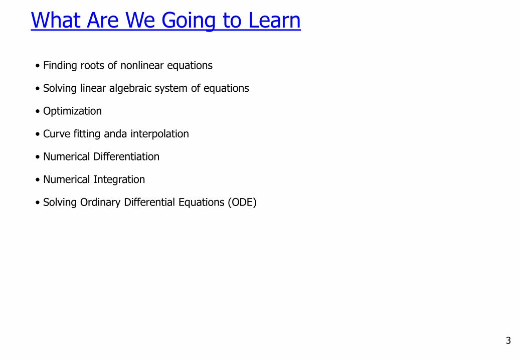
What Are We Going to Learn
• Finding roots of nonlinear equations
• Solving linear algebraic system of equations
• Optimization
• Curve fitting anda interpolation
• Numerical Differentiation
• Numerical Integration
• Solving Ordinary Differential Equations (ODE)

44
Finding Roots of Nonlinear Equations
For a curved beam subjected to bending, such as a crane hook lifting a load, the location of the neutral axis (rn) is given by
where R is the radius of the centroidal axis and d is the diameter of the cross section (assumed to be circular) of the curved beam. Find the value of d for which rn = 4d when R=10 cm.
222
n d)dR4R2(r4

555
Solution of Linear Algebraic Equations
Two sides of a square plate, with uniform heat generation, are insulated as shown. The heat conduction analysis of the plate, using the finite element grid shown by dashed lines, lead to the equations
6666
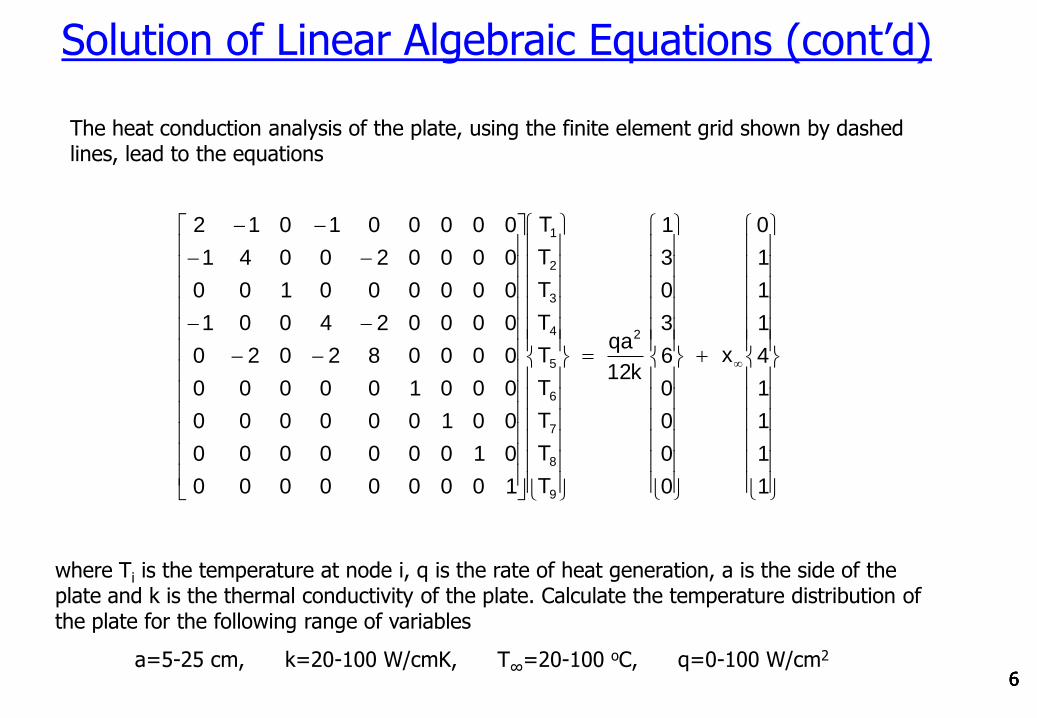
Solution of Linear Algebraic Equations (cont’d)
The heat conduction analysis of the plate, using the finite element grid shown by dashed lines, lead to the equations
where Ti is the temperature at node i, q is the rate of heat generation, a is the side of the plate and k is the thermal conductivity of the plate. Calculate the temperature distribution of the plate for the following range of variables
a=5-25 cm, k=20-100 W/cmK, T∞=20-100 oC, q=0-100 W/cm2
1
1
1
1
4
1
1
1
0
x
0
0
0
0
6
3
0
3
1
k12
qa
T
T
T
T
T
T
T
T
T
100000000
010000000
001000000
000100000
000082020
000024001
000000100
000020041
000001012
2
9
8
7
6
5
4
3
2
1
7777
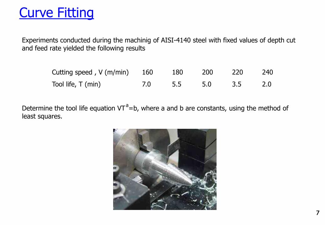
Curve Fitting
Experiments conducted during the machinig of AISI-4140 steel with fixed values of depth cut and feed rate yielded the following results
Cutting speed , V (m/min) 160 180 200 220 240
Tool life, T (min) 7.0 5.5 5.0 3.5 2.0
Determine the tool life equation VTa=b, where a and b are constants, using the method of
least squares.

888888
Numerical Differentiation
The displacement of an instrument subjected to a random vibration test, at different instants of time, is found to be as follows
Time, t (s) Displacement, y (cm)
0.05 0.144
0.10 0.172
0.15 0.213
0.20 0.296
0.25 0.070
0.30 0.085
0.35 0.525
0.40 0.110
Determine the velocity (dy/dt), acceleration (d2y/dt2), and jerk (d3y/dt3) at t = 0.05 and 0.20.
9999999
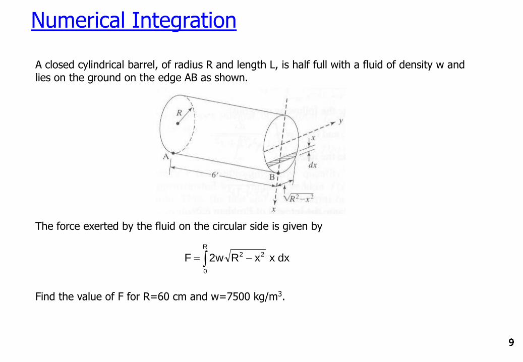
Numerical Integration
A closed cylindrical barrel, of radius R and length L, is half full with a fluid of density w and lies on the ground on the edge AB as shown.
R
0
22 dxxxRw2F
The force exerted by the fluid on the circular side is given by
Find the value of F for R=60 cm and w=7500 kg/m3.

1010101010101010
Solution of ODEs
In the mirror used in a solar heater, all the incident light rays are required to reflect through a single point (focus) as shown. For this, the shape of the mirror is governed by the equation
0xdx
dyy2
dx
dyx
2
Solve for y(x).

11
Programming
Algorithm: Sequence of logical steps required to perform a specific task.
Pseudocode: English description of a program.
Flowchart: Visual / graphical representation of a program.
Numerical Method
Programming Language
Pseudocode or Flowchart
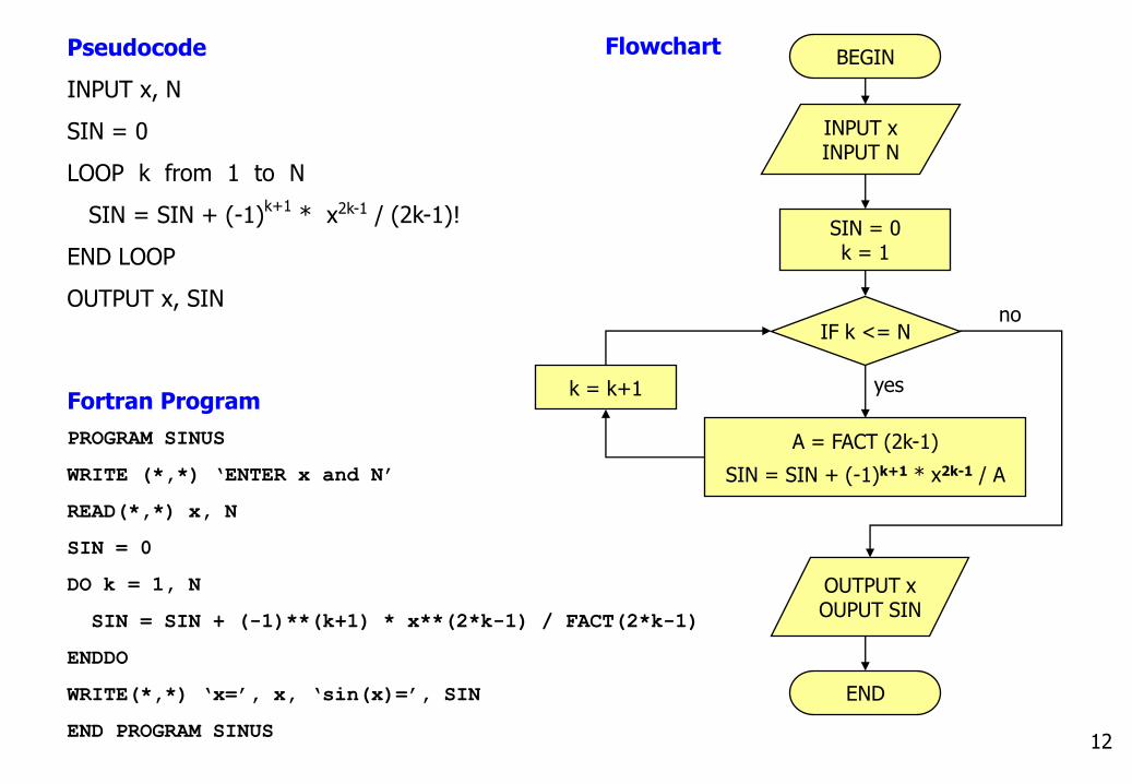
Example 1: Write a computer program to calculate sin(x) using the following series expansion.
......! 7
x
! 5
x
! 3
xx)xsin(
753
Algorithm
Step 1: Enter x and the number of terms to use, N.
Step 2: Calculate sin(x) using the Taylor series.
Step 3: Print the result.
12
Pseudocode
INPUT x, N
SIN = 0
LOOP k from 1 to N
SIN = SIN + (-1)k+1
* x2k-1 / (2k-1)!
END LOOP
OUTPUT x, SIN
FlowchartBEGIN
INPUT xINPUT N
SIN = 0k = 1
IF k <= N
A = FACT (2k-1)
SIN = SIN + (-1)k+1 * x2k-1 / A
k = k+1
OUTPUT xOUPUT SIN
END
yes
no
Fortran Program
PROGRAM SINUS
WRITE (*,*) ‘ENTER x and N’
READ(*,*) x, N
SIN = 0
DO k = 1, N
SIN = SIN + (-1)**(k+1) * x**(2*k-1) / FACT(2*k-1)
ENDDO
WRITE(*,*) ‘x=’, x, ‘sin(x)=’, SIN
END PROGRAM SINUS

13
Programming Errors (Bugs)
• Syntax error Will not compile. Compiler will help you to find it.
e.g. writing primtf instead of printf
• Run-time error Will compile but stop running at some point.
e.g. division by zero or trying to read from a non-existing file.
• Logical error Will compile and run, but the result is wrong.
e.g. in the sin(x) example taking all the terms as positive.
Especially the last two needs careful debugging of the program.
Hints About Programming
• Clarity put header (author, date, version, purpose, variable definitions, etc.)
put comments to explain variables, purpose of code segments, etc.
• Testing run with typical data
run with unusual but valid data
run with invalid data to check error handling
14
What do you need to know about programming?
• Basic programming skills that you studied in CENG 230
• MATLAB syntax
• data types (integers, single vs. double precision, arrays, etc.)
• loops, if statements
• input / output
• etc.
Advice on programming
• Refresh your programming knowledge. Attend the programming tutorial.
• Download the DevCpp4 compiler from the course website and practice at home.
• Approach the problem through the algorithm-pseudocode-computer code link.
• Obtain an introductory level programming book.
• Do not afraid of programming, try to feel the power of it.
15
Errors
Significant Figures
• Designate the reliability of a number.
• Number of sig. figs. to be used in a number depends on the origin of the number.
• Consider the calculation of the area of a circle, A=p D2/4
• Some numbers, like p, are mathematically exact. We can use as many sig. figs. as we want. p = 3.141592653589793236433832795028841971 ……
• Constants in the formulae, like 4 in the above formula, are exact. We can use as many sig. figs. as we want. 4=4.0000000000000000000000000 …….
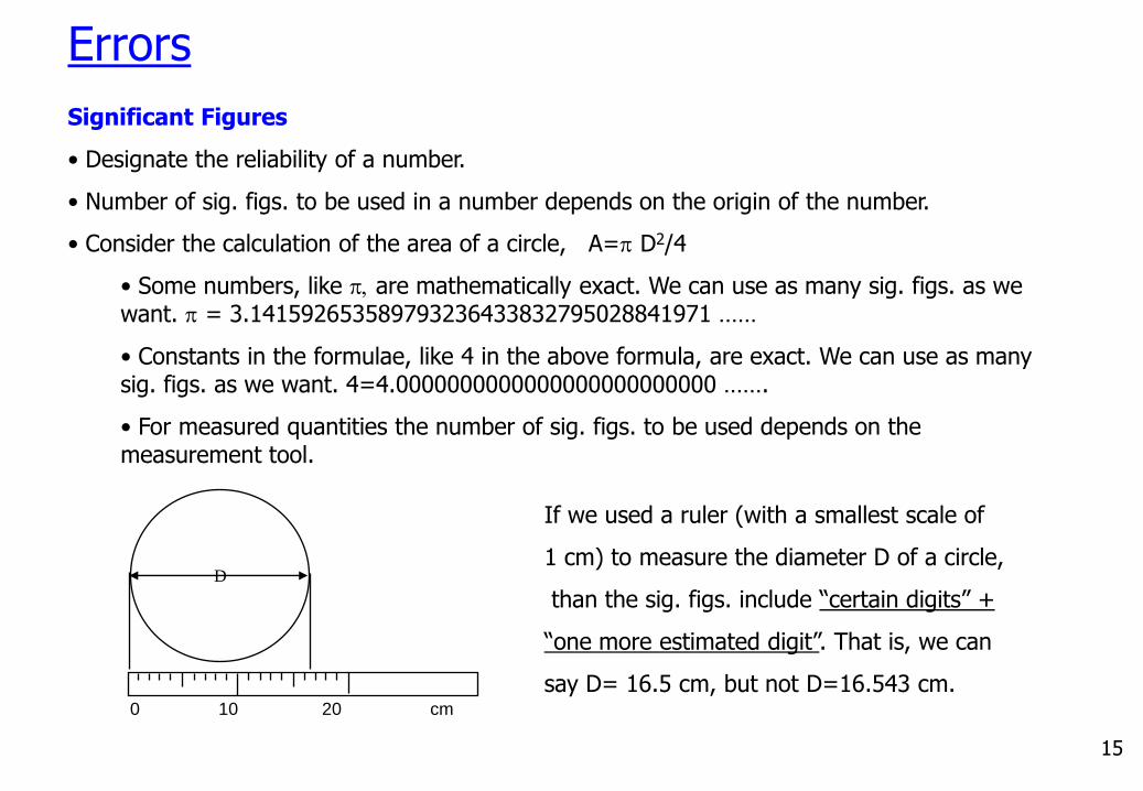
• For measured quantities the number of sig. figs. to be used depends on the measurement tool.
If we used a ruler (with a smallest scale of
1 cm) to measure the diameter D of a circle,
than the sig. figs. include “certain digits” +
“one more estimated digit”. That is, we can
say D= 16.5 cm, but not D=16.543 cm.
D
0 10 20 cm

16
Loss of significance during calculations
Classical example is the subtraction of two very close numbers.
Example 2: Calculate x - sin(x) for x=1/15.
x = 0.6666666667 * 10-1
sin(x) = 0.6661729492 * 10-1
x-sin(x) = 0.0004937175 * 10-1
First 4 zeros are not significant. They are used just to place the decimal point properly.
In other words if we represent this result as 0.4937175000 * 10-4 last 4 digits have error.
The result should be 0.4937174327 * 10-4
Accuracy: How closely a computed or measured value agrees with the true value.
Precision: How closely computed or measured values agree with each other.
Example 3: We measure the centerline velocity of a flow in a pipe as follows.(actual velocity is 10.0 m/s)
• Measurement set 1: 9.9 9.8 10.1 10.0 9.9 10.2 (accurate and precise)
• Measurement set 2: 7.3 7.5 7.1 7.2 7.3 7.1 (precise but inaccurate)
• Measurement set 3: 6.4 11.2 10.4 5.5 11.5 9.5 (inaccurate and imprecise)

17
Error Definitions (very important)
• TRUE
• True Error: E t = True Value – Approximation
• Relative True Error (fractional): e t = E t / TV
Relative True Error (percentage): e t = E t / TV * 100 % (preferred)
• APPROXIMATE
• Approx. Error: E a = Present Approx. – Past Approx.
• Relative Approx. Error (fractional): e a = E a / Present Approx.
Relative Approx. Error (percentage): e a = E a / Present Approx. * 100 % (preferred)
Tolerance: Many numerical methods work in an iterative fashion. There should be a stopping criteria for these methods. We stop when the error level drops below a certain tolerance value
(e s) that we select (|e a| < e s)
Scarborough criteria: If the tolerance is selected to be e s=0.5x10²-n % than the
approximation is guaranteed to be correct to at least n digits (See Problem 3.10).
18
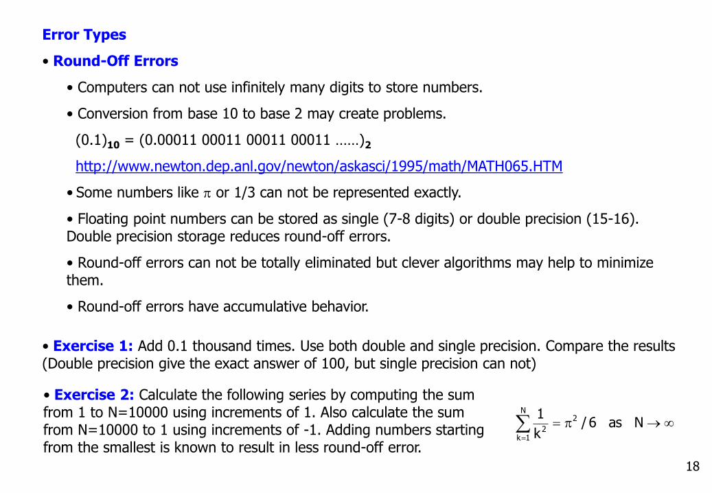
Error Types
• Round-Off Errors
• Computers can not use infinitely many digits to store numbers.
• Conversion from base 10 to base 2 may create problems.
(0.1)10 = (0.00011 00011 00011 00011 ……)2
http://www.newton.dep.anl.gov/newton/askasci/1995/math/MATH065.HTM
• Some numbers like p or 1/3 can not be represented exactly.
• Floating point numbers can be stored as single (7-8 digits) or double precision (15-16). Double precision storage reduces round-off errors.
• Round-off errors can not be totally eliminated but clever algorithms may help to minimize them.
• Round-off errors have accumulative behavior.
• Exercise 1: Add 0.1 thousand times. Use both double and single precision. Compare the results(Double precision give the exact answer of 100, but single precision can not)
p
N as 6/k
1 2N
1k2
• Exercise 2: Calculate the following series by computing the sum from 1 to N=10000 using increments of 1. Also calculate the sum from N=10000 to 1 using increments of -1. Adding numbers starting from the smallest is known to result in less round-off error.
19
Error Types (cont’d)
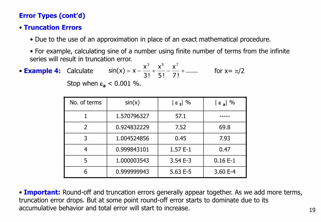
• Truncation Errors
• Due to the use of an approximation in place of an exact mathematical procedure.
• For example, calculating sine of a number using finite number of terms from the infinite series will result in truncation error.
• Example 4: Calculate for x= p/2
Stop when ea < 0.001 %.
......! 7
x
! 5
x
! 3
xx)xsin(
753
No. of terms sin(x) | e t| % | e a| %
1 1.570796327 57.1 -----
2 0.924832229 7.52 69.8
3 1.004524856 0.45 7.93
4 0.999843101 1.57 E-1 0.47
5 1.000003543 3.54 E-3 0.16 E-1
6 0.999999943 5.63 E-5 3.60 E-4
• Important: Round-off and truncation errors generally appear together. As we add more terms,truncation error drops. But at some point round-off error starts to dominate due to its accumulative behavior and total error will start to increase.
20
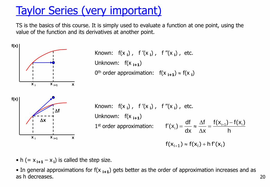
TS is the basics of this course. It is simply used to evaluate a function at one point, using the value of the function and its derivatives at another point.
Known: f(x i) , f ’(x i) , f ’’(x i) , etc.
Unknown: f(x i+1)
0th order approximation: f(x i+1) f(x i)
Known: f(x i) , f ’(x i) , f ’’(x i) , etc.
Unknown: f(x i+1)
1st order approximation: h
)x(f)x(f
x
f
dx
df)x(f i1i
i
)x(f h)x(f)x(f ii1i
• h (= x i+1 – x i) is called the step size.
• In general approximations for f(x i+1) gets better as the order of approximation increases and as as h decreases.
x
f(x)
x i x i+1
x
f(x)
x i x i+1
x
f
Taylor Series (very important)
21
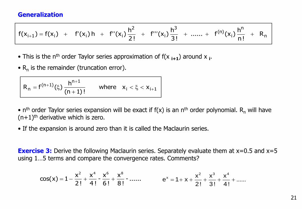
Generalization
n
n
i)n(
3
i
2
iii1i R ! n
h )x(f ......
! 3
h )x(f
! 2
h )x(f h )x(f )x(f)x(f
• This is the nth order Taylor series approximation of f(x i+1) around x i.
• Rn is the remainder (truncation error).
1ii
1n)1n(
n x xwhere ! )1n(
h )(f R
• nth order Taylor series expansion will be exact if f(x) is an nth order polynomial. Rn will have (n+1)th derivative which is zero.
• If the expansion is around zero than it is called the Maclaurin series.
Exercise 3: Derive the following Maclaurin series. Separately evaluate them at x=0.5 and x=5 using 1…5 terms and compare the convergence rates. Comments?
...... ! 4
x
! 3
x
! 2
x x 1e
432x ...... -
! 8
x
! 6
x -
! 4
x
! 2
x 1)xcos(
8642

22
Error Propagation (Reading Assignment)
How do errors propagate in mathematical formulae?
• Functions of a single variable, f(x)
f(x) in error ?|)x~(f)x(f|)x~(f
xin error of estimate |:x~x|x~quantity) measured a be can(x x of approx. :x~
Example 5: f(x) in error the estimate 01.0x~ ,5.2x~ ,x)x(f 3
x~|)x~(f|)x~(f
|)x~x)(x~(f| |)x~(f)x(f|
analysis) order (1 )x~x)(x~(f)x~(f)x(f st
0.187515.625f(2.5) analysis error this After
15.625f(2.5) that Note
1875.0)01.0)(x~3()x~(f 2
23
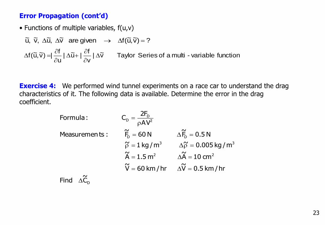
Error Propagation (cont’d)
• Functions of multiple variables, f(u,v)
?)v~,u~(f given are v~ ,u~ ,v~ ,u~
function variable-multi a of Series Taylor v~|v
f|u~|
u
f|)v~,u~(f
Exercise 4: We performed wind tunnel experiments on a race car to understand the drag characteristics of it. The following data is available. Determine the error in the drag coefficient.
D
22
33
DD
2
DD
C~
Find
hr/mk 5.0V~
hr/mk 60V~
cm 10A~
m 5.1A~
m/kg 005.0~ m/kg 1~
N 5.0F~
N 60F~
:tsMeasuremen
AV
F2C :Formula