mce 647: robot dynamics and control term...
TRANSCRIPT

MCE 647: Robot Dynamics and Control
Term Project
Kinematics, Dynamics, Control and Simulation
of RP Planar Arm
Instructor: Dr. Hanz Richter
Mechanical Engineering Department
Submitted by: Dmitry Storozhev
December 12, 2008


Part #1: Kinematics and Dynamics
Figure 1. Coordinate systems of the RP planar arm
Table 1 shows D-H parameters of the RP planar arm corresponding to figure 1.
Link
1 0 0
0 0 0
0 0 0
2 0 0 0
Table 1. D-H parameters for the RP planar manipulator

Matlab software was used to find:
a) T matrices relating each link-attached frame to the world frame,
b) Two velocity Jacobians ( and ) and two angular velocity Jacobians ( and )
relative to each center of mass,
c) and matrices.
M-file syntax:
clear;clc
syms
('a1','d2','theta1','Ixx_1','Ixy_1','Ixz_1','Iyx_1','Iyy_1','Iyz_1','Izx_1','Izy_1','
Izz_1','Ixx_2','Ixy_2','Ixz_2','Iyx_2','Iyy_2','Iyz_2','Izx_2','Izy_2','Izz_2','m1','
m2','g');
%-------------- DH parameters for link 1 ----------------
theta1=input('Enter "theta1" (rotation angle for link 1) = ');
d1=0;
a1=input('Enter "a1" (length of link 1) = ');
ac1=a1/2;
alpha1=0;
%-------------- DH parameters for link 2 -----------------
theta1_1=90;
d1_1=0;
a1_1=0;
alpha1_1=0;
theta1_2=0;
d1_2=0;
a1_2=0;
alpha1_2=90;
theta2=0;
d2=input('Enter "d2" (distance between the centers of mass of link 1 and link 2) = ');
a2=0;
alpha2=0;
%----------------------------------------------------------------
Ac1=[cos(theta1) -sin(theta1)*cos(alpha1*pi/180) sin(theta1)*sin(alpha1*pi/180)
ac1*cos(theta1);
sin(theta1) cos(theta1)*cos(alpha1*pi/180) -cos(theta1)*sin(alpha1*pi/180)
ac1*sin(theta1);
0 sin(alpha1*pi/180) cos(alpha1*pi/180) d1;
0 0 0 1];

A1_1=[cos(theta1_1) -sin(theta1_1)*cos(alpha1_1*pi/180)
sin(theta1_1)*sin(alpha1_1*pi/180) a1_1*cos(theta1_1);
sin(theta1_1) cos(theta1_1)*cos(alpha1_1*pi/180)
-cos(theta1_1)*sin(alpha1_1*pi/180) a1_1*sin(theta1_1);
0 sin(alpha1_1*pi/180) cos(alpha1_1*pi/180)) d1_1;
0 0 0 1];
A1_2=[cos(theta1_2)) -sin(theta1_2)*cos(alpha1_2*pi/180)
sin(theta1_2)*sin(alpha1_2*pi/180) a1_2*cos(theta1_2);
sin(theta1_2) cos(theta1_2)*cos(alpha1_2*pi/180)
-cos(theta1_2)*sin(alpha1_2*pi/180) a1_2*sin(theta1_2);
0 sin(alpha1_2*pi/180) cos(alpha1_2*pi/180) d1_2;
0 0 0 1];
Ac2=[cos(theta2) -sin(theta2)*cos(alpha2*pi/180) sin(theta2)*sin(alpha2*pi/180)
a2*cos(theta2);
sin(theta2) cos(theta2)*cos(alpha2*pi/180)
-cos(theta2)*sin(alpha2*pi/180) a2*sin(theta2);
0 sin(alpha2*pi/180) cos(alpha2*pi/180) d2;
0 0 0 1];
%---------------------------------------------------------------
T_c1_0=Ac1 % Transformation matrices from origin of the world frame to
T_c2_0=Ac1*A1_1*A1_2*Ac2 %the center of the mass for each link
%---------------Velocity Jacobians and Angular Velocity Jacobians------------
z0=[0;0;1]; % the first three elements in the third column of T_i_0
z1=T_c1_0(1:3,3); % where i=0,1,2
o0=[0;0;0]; % the first three elements in the fourth column of T_i_0
oc1=T_c1_0(1:3,4); % where i=0,1,2
oc2=T_c2_0(1:3,4);
Jc1=[cross(z0,(oc1-o0)) [0;0;0]; % The 6x2 Jacobian relative to the
z0 [0;0;0]] % center of mass of link 1
Jc2=[cross(z0,(oc2-o0)) z1; % The 6x2 Jacobian relative to the
z0 [0;0;0]] % center of mass of link 2
Jv1=Jc1(1:3,1:2);
Jw1=Jc1(4:6,1:2);
Jv2=Jc2(1:3,1:2);
Jw2=Jc2(4:6,1:2);
%--------------------------------------------------------------------------
R_1_0=T_c1_0(1:3,1:3); % Rotation matrices
R_2_0=T_c2_0(1:3,1:3);
%--------------------------------------------------------------------------
I_1=[Ixx_1 Ixy_1 Ixz_1; % The inertia tensor
Iyx_1 Iyy_1 Iyz_1;
Izx_1 Izy_1 Izz_1];

I_2=[Ixx_2 Ixy_2 Ixz_2;
Iyx_2 Iyy_2 Iyz_2;
Izx_2 Izy_2 Izz_2];
II_1=(R_1_0)*(I_1)*(R_1_0).' ;
II_2=(R_2_0)*(I_2)*(R_2_0).' ;
D_1=(Jw1.')*(II_1)*(Jw1);
D_2=(Jw2.')*(II_2)*(Jw2);
D=D_1+D_2;
% Translational part of kinetic energy
K=(m1)*(Jv1.')*(Jv1)+(m2)*(Jv2.')*(Jv2);
% Inertia matrix
D_q=K+D;
D_q=simplify(D_q)
q=[theta1;d2];
for i=1:2
for j=1:2
for k=1:2
c(i,j,k)=(1/2)*((diff(D_q(k,j),q(i)))+(diff(D_q(k,i),q(j)))-
(diff(D_q(i,j),q(k))));
end
end
end
syms ('theta1_dot','d2_dot')
for k=1:2
for j=1:2
C(k,j)=(c(1,j,k)*theta1_dot+c(2,j,k)*d2_dot);
end
end
% Potential energy
P_1=m1*g*ac1*sin(theta1);
P_2=m2*g*(ac1+d2)*sin(theta1);
P=P_1+P_2;
g_1=diff(P,theta1);
g_2=diff(P,d2);
g_q=[g_1;g_2]
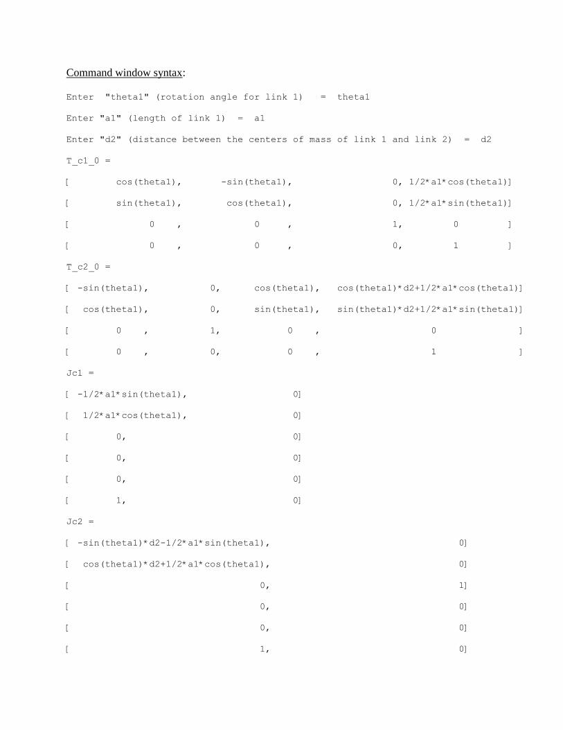
Command window syntax:
Enter "theta1" (rotation angle for link 1) = theta1
Enter "a1" (length of link 1) = a1
Enter "d2" (distance between the centers of mass of link 1 and link 2) = d2
T_c1_0 =
[ cos(theta1), -sin(theta1), 0, 1/2*a1*cos(theta1)]
[ sin(theta1), cos(theta1), 0, 1/2*a1*sin(theta1)]
[ 0 , 0 , 1, 0 ]
[ 0 , 0 , 0, 1 ]
T_c2_0 =
[ -sin(theta1), 0, cos(theta1), cos(theta1)*d2+1/2*a1*cos(theta1)]
[ cos(theta1), 0, sin(theta1), sin(theta1)*d2+1/2*a1*sin(theta1)]
[ 0 , 1, 0 , 0 ]
[ 0 , 0, 0 , 1 ]
Jc1 =
[ -1/2*a1*sin(theta1), 0]
[ 1/2*a1*cos(theta1), 0]
[ 0, 0]
[ 0, 0]
[ 0, 0]
[ 1, 0]
Jc2 =
[ -sin(theta1)*d2-1/2*a1*sin(theta1), 0]
[ cos(theta1)*d2+1/2*a1*cos(theta1), 0]
[ 0, 1]
[ 0, 0]
[ 0, 0]
[ 1, 0]

D_q =
[ 1/4*m1*a1^2+m2*d2^2+m2*d2*a1+1/4*m2*a1^2+Izz_1+Iyy_2, 0]
[ 0 , m2]
C =
[ (m2*d2+1/2*m2*a1)*d2_dot, (m2*d2+1/2*m2*a1)*theta1_dot]
[ (-m2*d2-1/2*m2*a1)*theta1_dot, 0 ]
g_q =
[ 1/2*m1*g*a1*cos(theta1)+m2*g*(1/2*a1+d2)*cos(theta1)]
[ m2*g*sin(theta1) ]
The dynamic equation for the RP planar arm is:
where: – joint variable of link 1 (angle of link 1)
– joint variable of link 2 (distance between centers of mass of link 1 and link 2)
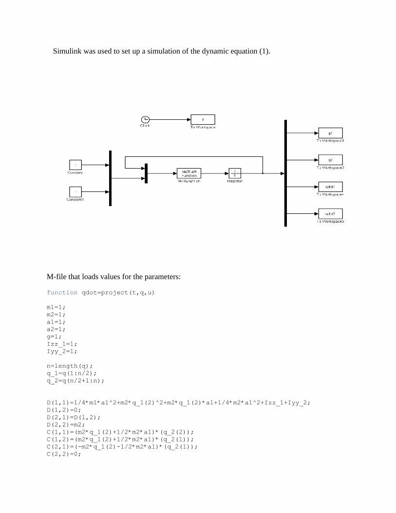
Simulink was used to set up a simulation of the dynamic equation (1).
M-file that loads values for the parameters:
function qdot=project(t,q,u)
m1=1;
m2=1;
a1=1;
a2=1;
g=1;
Izz_1=1;
Iyy_2=1;
n=length(q);
q_1=q(1:n/2);
q_2=q(n/2+1:n);
D(1,1)=1/4*m1*a1^2+m2*q_1(2)^2+m2*q_1(2)*a1+1/4*m2*a1^2+Izz_1+Iyy_2;
D(1,2)=0;
D(2,1)=D(1,2);
D(2,2)=m2;
C(1,1)=(m2*q_1(2)+1/2*m2*a1)*(q_2(2));
C(1,2)=(m2*q_1(2)+1/2*m2*a1)*(q_2(1));
C(2,1)=(-m2*q_1(2)-1/2*m2*a1)*(q_2(1));
C(2,2)=0;

g_q(1,1)=1/2*g*m1*a1*cos(q_1(1))+m2*g*(1/2*a1+q_1(2))*cos(q_1(1));
g_q(2,1)=m2*g*sin(q_1(1));
qdot=[q_2;inv(D)*(u-C*q_2-g_q)];
Simulation was done by settling all parameters to 1 and applying . Figure 2 shows positions and
velocities of joint 1 and joint 2.
Figure 2. Positions and Velocities of Joint 1 and Joint 2

Part #2: Linear Parameterization
(1)
(2)
(3)
From equation (2):
First row of :
+ (4)
Second row of :
(5)

(6)
Comparing equation (2) and equation (6) with and , we can conclude that the regressor
and parameter vector satisfy the dynamic equations i.e.
Procedure for finding the regressor corresponding to the term +
Using given regressor and parameter vector:
+

First row of + :
+
Second row of + :
+
Factoring out from the first row of + :
+
Factoring out from the second row of + :
+
The regressor corresponding to the term + :

M-file was set up to generate the nominal parameter vector and a “true” set of parameters.
m1=10; m2=8; a1=0.6; Izz_1=26; Iyy_2=12; g=9.8;
TH1_0=(1/4)*m1*a1^2+Izz_1+(1/4)*m2*a1^2+Iyy_2; TH2_0=m2; TH3_0=(1/2)*m2*a1; TH4_0=(1/2)*m1*a1;
TH_0=[TH1_0;TH2_0;TH3_0;TH4_0];
level=0.1; % 10% uncertainty level %level=0.25; % 25% uncertainty level %level=0.8; % 80% uncertainty level
m1_max=(1+level)*m1; m2_max=(1+level)*m2; a1_max=(1+level)*a1; Izz_1_max=(1+level)*Izz_1; Iyy_2_max=(1+level)*Iyy_2;
TH1_max=(1/4)*m1_max*a1_max^2+Izz_1_max+(1/4)*m2_max*a1_max^2+Iyy_2_max; TH2_max=m2_max; TH3_max=(1/2)*m2_max*a1_max; TH4_max=(1/2)*m1_max*a1_max;
DTH=[TH1_max-TH1_0;TH2_max-TH2_0;TH3_max-TH3_0;TH4_max-TH4_0];
rho=norm(DTH);
% Perturbations for use in plant m1=m1+m1*(1-2*rand)*level m2=m2+m2*(1-2*rand)*level a1=a1+a1*(1-2*rand)*level Izz_1=Izz_1+Izz_1*(1-2*rand)*level Iyy_2=Iyy_2+Iyy_2*(1-2*rand)*level
The maximum error bound for the parameter vector is:
for is
for is
for is
The nominal parameters vector is TH_0=

Part #3: Control Design
Robust Passivity-Based Control
M-file was generated for use in the plant (10% uncertainty):
function zdot=plant_10_uncert(t,z,u)
m1=10.5721; m2=7.7704; a1=0.6216; g=9.8; Izz_1=23.6075; Iyy_2=11.4561;
n=length(z); z_1=z(1:n/2); z_2=z(n/2+1:n);
D(1,1)=1/4*m1*a1^2+m2*z_1(2)^2+m2*z_1(2)*a1+1/4*m2*a1^2+Izz_1+Iyy_2; D(1,2)=0; D(2,1)=D(1,2); D(2,2)=m2;
C(1,1)=(m2*z_1(2)+1/2*m2*a1)*(z_2(2)); C(1,2)=(m2*z_1(2)+1/2*m2*a1)*(z_2(1)); C(2,1)=(-m2*z_1(2)-1/2*m2*a1)*(z_2(1)); C(2,2)=0;
g_z(1,1)=1/2*g*m1*a1*cos(z_1(1))+m2*g*(1/2*a1+z_1(2))*cos(z_1(1)); g_z(2,1)=m2*g*sin(z_1(1));
zdot=[z_2;inv(D)*(u-C*z_2-g_z)];
M-file was generated for use in the control law:
function u=robust_passivity_10_uncert(t,z,zd)
g=9.8; q1=z(1); q2=z(2); q1dot=z(3); q2dot=z(4);
q1d=zd(1); q2d=zd(2); q1ddot=zd(3); q2ddot=zd(4); q1dddot=zd(5); q2dddot=zd(6);

qtilde=[q1-q1d;q2-q2d]; qtildedot=[q1dot-q1ddot;q2dot-q2ddot];
%Gains L=diag([100 100]); K=diag([100 100]);
v=[q1ddot;q2ddot]-L*qtilde; a=[q1dddot;q2dddot]-L*qtildedot; r=qtildedot+L*qtilde;
%Regressor Y(1,1)=a(1); Y(1,2)=q2^2*a(1)+q2*q2dot*v(1)+q2*q1dot*v(2)+q2*g*cos(q1); Y(1,3)=2*q2*a(1)+q2dot*v(1)+q1dot*v(2)+g*cos(q1); Y(1,4)=g*cos(q1);
Y(2,1)=0; Y(2,2)=a(2)-q2*q1dot*v(1)+g*sin(q1); Y(2,3)=-q1dot*v(1); Y(2,4)=0;
TH_0=[39.62;8;2.4;3]; % Nominal parameters
deadzone=0.1; rho=4.4826; s=Y'*r; if norm(s)>deadzone, dTh=-rho*s/norm(s); else dTh=[0;0;0;0]; end Th_hat=TH_0+dTh;
u=Y*Th_hat-K*r;
Simulink was used to set up a simulation of the robust passivity-based control for use in RP planar arm.
Figure 3 shows the Simulink diagram for a RP planar arm with the robust passivity-based control.
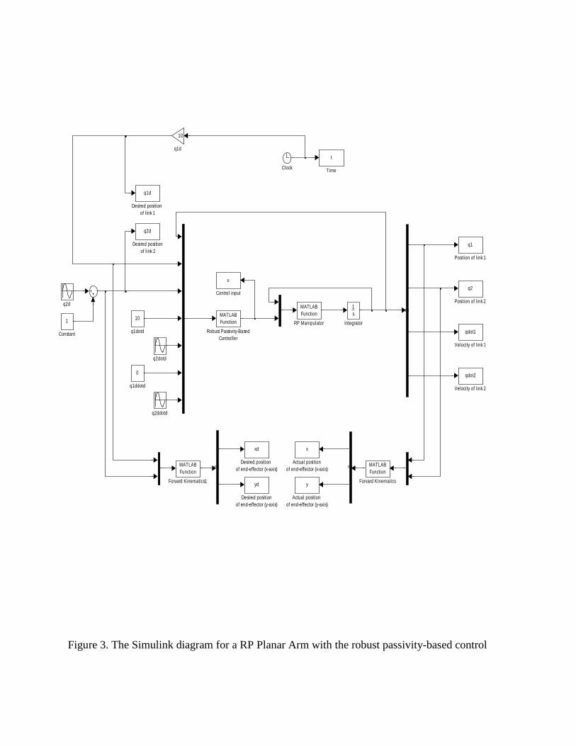
Figure 3. The Simulink diagram for a RP Planar Arm with the robust passivity-based control
q2dotd
q2ddotd
q2d
10
q1dotd
0
q1ddotd
10
q1d
qdot2
Velocity of l ink 2
qdot1
Velocity of l ink 1
t
Time
MATLAB
Function
Robust Passivity-Based
Controller
MATLAB
Function
RP Manipulator
q2
Position of l ink 2
q1
Position of l ink 1
1
s
Integrator
MATLAB
Function
Forvard Kinematics1
MATLAB
Function
Forvard Kinematics
q1d
Desired position
of l ink 1
xd
Desired position
of end-effector (x-axis)
yd
Desired position
of end-effector (y-axis)
q2d
Desired position
of l ink 2
Demux Demux
Demux
u
Control input
1
Constant
Clock
y
Actual position
of end-effector (y-axis)
x
Actual position
of end-effector (x-axis)

Figure 4 shows a position error for link 1 (between actual position and desired)
Figure 4. Position Error of Link 1
Figure 5 shows a position error of link 2.
Figure 5. Position of link 2
Figure 6 shows plots of desired and actual positions of the end-effector of the RP planar arm using robust
0 1 2 3 4 5 6 7 8 9 10-0.08
-0.07
-0.06
-0.05
-0.04
-0.03
-0.02
-0.01
0
0.01
q1tilde(t)
Time,sec
Posi
tion
Erro
r
0 1 2 3 4 5 6 7 8 9 10-2
-1.5
-1
-0.5
0
0.5
q2tilde(t)
Time, sec
Posi
tion
Erro
r

passivity-based control (10 % uncertainty).
Figure 6. Desired and Actual Positions of the End-Effector Using Robust Passivity-Based Control
Figure 7 shows the control input for link 1.
Figure 7. Control Input for Link 1
-1.5 -1 -0.5 0 0.5 1 1.5 2 2.5-2.5
-2
-1.5
-1
-0.5
0
0.5
1
1.5
2
2.5Desired and Actual Positions of the End-Effector
Time, sec
Pos
ition
xd vs. y
d (desired position)
x vs. y (actual position)
0 1 2 3 4 5 6 7 8 9 10-2
-1
0
1
2
3
4
5x 10
4
Time, sec
Cont
rol I
nput
Control Input u1 for Link 1
Control Input for Link 1

Figure 8 shows the control input for link 2.
Figure 8. Control Input for Link 2
M-file was generated for use in the plant (25% uncertainty):
function qdot=plant_25_uncert(t,q,u)
m1=11.4643; m2=7.5712; a1=0.5610; g=9.8; Izz_1=27.6838; Iyy_2=11.5491;
n=length(q); q_1=q(1:n/2); q_2=q(n/2+1:n);
D(1,1)=1/4*m1*a1^2+m2*q_1(2)^2+m2*q_1(2)*a1+1/4*m2*a1^2+Izz_1+Iyy_2; D(1,2)=0; D(2,1)=D(1,2); D(2,2)=m2;
C(1,1)=(m2*q_1(2)+1/2*m2*a1)*(q_2(2)); C(1,2)=(m2*q_1(2)+1/2*m2*a1)*(q_2(1)); C(2,1)=(-m2*q_1(2)-1/2*m2*a1)*(q_2(1)); C(2,2)=0;
0 1 2 3 4 5 6 7 8 9 10-2
-1
0
1
2
3
4
5x 10
4
Time, sec
Con
trol I
nput
Control Input u2 for Link 2
Control Input for Link 2

g_q(1,1)=1/2*g*m1*a1*cos(q_1(1))+m2*g*(1/2*a1+q_1(2))*cos(q_1(1)); g_q(2,1)=m2*g*sin(q_1(1));
qdot=[q_2;inv(D)*(u-C*q_2-g_q)];
M-file was generated for use in the control law:
function u=robust_passivity_25_uncert(t,z,zd)
g=9.8; q1=z(1); q2=z(2); q1dot=z(3); q2dot=z(4);
q1d=zd(1); q2d=zd(2); q1ddot=zd(3); q2ddot=zd(4); q1dddot=zd(5); q2dddot=zd(6);
qtilde=[q1-q1d;q2-q2d]; qtildedot=[q1dot-q1ddot;q2dot-q2ddot];
%Gains L=diag([100 100]); K=diag([100 100]);
v=[q1ddot;q2ddot]-L*qtilde; a=[q1dddot;q2dddot]-L*qtildedot; r=qtildedot+L*qtilde;
%Regressor Y(1,1)=a(1); Y(1,2)=q2^2*a(1)+q2*q2dot*v(1)+q2*q1dot*v(2)+q2*g*cos(q1); Y(1,3)=2*q2*a(1)+q2dot*v(1)+q1dot*v(2)+g*cos(q1); Y(1,4)=g*cos(q1); Y(2,1)=0; Y(2,2)=a(2)-q2*q1dot*v(1)+g*sin(q1); Y(2,3)=-q1dot*v(1); Y(2,4)=0;
TH_0=[39.62;8;2.4;3]; % Nominal parameters
deadzone=0.1; rho=11.4299; s=Y'*r; if norm(s)>deadzone, dTh=-rho*s/norm(s); else dTh=[0;0;0;0]; end

Th_hat=TH_0+dTh; u=Y*Th_hat-K*r;
Figure 9 shows a position error for link 1 (between actual position and desired)
Figure 9. Position Error of Link 1
Figure 10 shows a position error for link 2 (between actual position and desired)
Figure 10. Position Error of Link 2
0 1 2 3 4 5 6 7 8 9 10-0.09
-0.08
-0.07
-0.06
-0.05
-0.04
-0.03
-0.02
-0.01
0
0.01
q1tilde(t)
Time, sec
Posi
tion
Erro
r
0 1 2 3 4 5 6 7 8 9 10-2
-1.5
-1
-0.5
0
0.5
q2tilde(t)
Time, sec
Posi
tion
Erro
r

Figure 11 shows plots of desired and actual positions of the end-effector of the RP planar arm using the
robust passivity-based control (25% uncertainty).
Figure 11. Desired and Actual Positions of the End-Effector Using Robust Passivity-Based Control
Figure 12 shows the control input for link 1.
Figure 12. The Control Input for Link 1
-1.5 -1 -0.5 0 0.5 1 1.5 2 2.5-2.5
-2
-1.5
-1
-0.5
0
0.5
1
1.5
2
2.5Desired and Actual Positions of the End-Effector
xd vs. y
d (desired position)
x vs. y (actual position)
0 1 2 3 4 5 6 7 8 9 10-4
-3
-2
-1
0
1
2
3
4
5
6x 10
4
Time, sec
Cont
rol I
nput
Control Input u1 for Link 1
Control Input u1

Figure 13 shows the control input for link 2.
Figure 13. The Control Input for Link 2
Adaptive Passivity-Based Control
M-file was generated for use in the plant (80% uncertainty):
function qdot=plant_80_uncert(t,q,u)
m1=8.2634; m2=14.1983; a1=1.0643; g=9.8; Izz_1=38.8929; Iyy_2=10.3312;
n=length(q); q_1=q(1:n/2); q_2=q(n/2+1:n);
D(1,1)=1/4*m1*a1^2+m2*q_1(2)^2+m2*q_1(2)*a1+1/4*m2*a1^2+Izz_1+Iyy_2; D(1,2)=0; D(2,1)=D(1,2); D(2,2)=m2;
0 1 2 3 4 5 6 7 8 9 10-4
-3
-2
-1
0
1
2
3
4
5
6x 10
4
Time, sec
Con
trol I
nput
Control Input u2 for Link 2
Control Input u2

C(1,1)=(m2*q_1(2)+1/2*m2*a1)*(q_2(2)); C(1,2)=(m2*q_1(2)+1/2*m2*a1)*(q_2(1)); C(2,1)=(-m2*q_1(2)-1/2*m2*a1)*(q_2(1)); C(2,2)=0;
g_q(1,1)=1/2*g*m1*a1*cos(q_1(1))+m2*g*(1/2*a1+q_1(2))*cos(q_1(1)); g_q(2,1)=m2*g*sin(q_1(1));
qdot=[q_2;inv(D)*(u-C*q_2-g_q)];
M-file was generated for use in the control law:
function u=adaptive_passivity(t,z,zd,Th_hat)
g=9.8; q1=z(1); q2=z(2); q1dot=z(3); q2dot=z(4);
q1d=zd(1); q2d=zd(2); q1ddot=zd(3); q2ddot=zd(4); q1dddot=zd(5); q2dddot=zd(6);
qtilde=[q1-q1d;q2-q2d]; qtildedot=[q1dot-q1ddot;q2dot-q2ddot];
%Gains L=diag([500 500]); K=diag([500 500]);
v=[q1ddot;q2ddot]-L*qtilde; a=[q1dddot;q2dddot]-L*qtildedot; r=qtildedot+L*qtilde;
%Regressor Y(1,1)=a(1); Y(1,2)=q2^2*a(1)+q2*q2dot*v(1)+q2*q1dot*v(2)+q2*g*cos(q1); Y(1,3)=2*q2*a(1)+q2dot*v(1)+q1dot*v(2)+g*cos(q1); Y(1,4)=g*cos(q1); Y(2,1)=0; Y(2,2)=a(2)-q2*q1dot*v(1)+g*sin(q1); Y(2,3)=-q1dot*v(1); Y(2,4)=0;
u=Y*Th_hat-K*r;

function th_hat_dot=parameter_adaptive(t,z,zd)
g=9.8; q1=z(1); q2=z(2); q1dot=z(3); q2dot=z(4);
q1d=zd(1); q2d=zd(2); q1ddot=zd(3); q2ddot=zd(4); q1dddot=zd(5); q2dddot=zd(6);
qtilde=[q1-q1d;q2-q2d]; qtildedot=[q1dot-q1ddot;q2dot-q2ddot];
%Gains L=diag([500 500]); G=eye(4);
v=[q1ddot;q2ddot]-L*qtilde; a=[q1dddot;q2dddot]-L*qtildedot; r=qtildedot+L*qtilde;
% Regressor Y(1,1)=a(1); Y(1,2)=q2^2*a(1)+q2*q2dot*v(1)+q2*q1dot*v(2)+q2*g*cos(q1); Y(1,3)=2*q2*a(1)+q2dot*v(1)+q1dot*v(2)+g*cos(q1); Y(1,4)=g*cos(q1);
Y(2,1)=0; Y(2,2)=a(2)-q2*q1dot*v(1)+g*sin(q1); Y(2,3)=-q1dot*v(1); Y(2,4)=0;
th_hat_dot=-G*Y'*r;
Simulink was used to set up a simulation of the adaptive passivity-based control for use in RP planar arm.
Figure 14 shows the Simulink diagram for a RP Planar Arm with the adaptive passivity-based control.

Figure 14. The Simulink diagram for a RP Planar Arm with the adaptive passivity-based control
q2dotd
q2ddotd
q2d
10
q1dotd
0
q1ddotd
10
q1d
qdot2
Velocity of l ink 2
qdot1
Velocity of l ink 1
theta_hat
To Workspace7
t
Time
MATLAB
Function
RP manipulator
q2
Position of l ink 2
q1
Position of l ink 1
MATLAB
Function
Parameter Estimate
Derivatives
1
s
Integrator1
1
s
Integrator
MATLAB
Function
Forvard Kinematics1
MATLAB
Function
Forvard Kinematics
q1d
Desired position of
end_effector of l ink 1
yd
Desired position of
end-effector (y-axis)
xd
Desired position of
end-effector (x-axis)
q2d
Desired position of
end-effector of l ink 2
Demux Demux
Demux
u
Control Input
1
Constant
Clock
MATLAB
Function
Adaptive Passivity-Based
Controller
y
Actual position of
end-effector (y-axis)
x
Actual position of
end-ffector (x-axis)
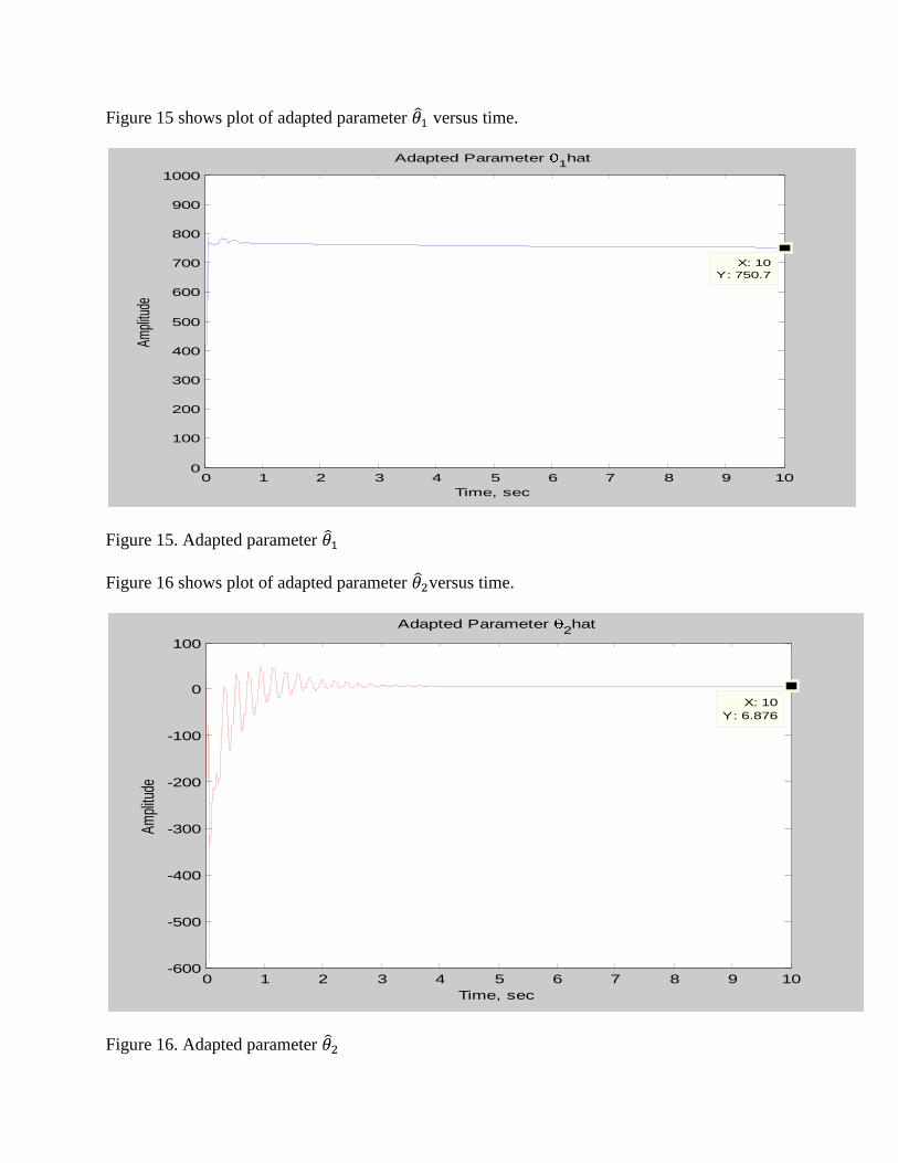
Figure 15 shows plot of adapted parameter versus time.
Figure 15. Adapted parameter
Figure 16 shows plot of adapted parameter versus time.
Figure 16. Adapted parameter
0 1 2 3 4 5 6 7 8 9 100
100
200
300
400
500
600
700
800
900
1000
Time, sec
Ampl
itude
Adapted Parameter 1hat
X: 10
Y: 750.7
0 1 2 3 4 5 6 7 8 9 10-600
-500
-400
-300
-200
-100
0
100
Time, sec
Am
plitu
de
Adapted Parameter 2hat
X: 10
Y: 6.876

Figure 17 shows plot of adapted parameter versus time.
Figure 17. Adapted parameter
Figure 18 shows plot of adapted parameter versus time.
Figure 18. Adapted parameter
0 1 2 3 4 5 6 7 8 9 10-500
-400
-300
-200
-100
0
100
200
300
400
500
Time, sec
Am
plitu
deAdapted Parameter
3hat
X: 10
Y: 13.94
0 1 2 3 4 5 6 7 8 9 10
-10
-5
0
5
10
15
20
25
30
35
Time, sec
Ampl
itude
Adapted Parameter 4hat
X: 10
Y: 16.92
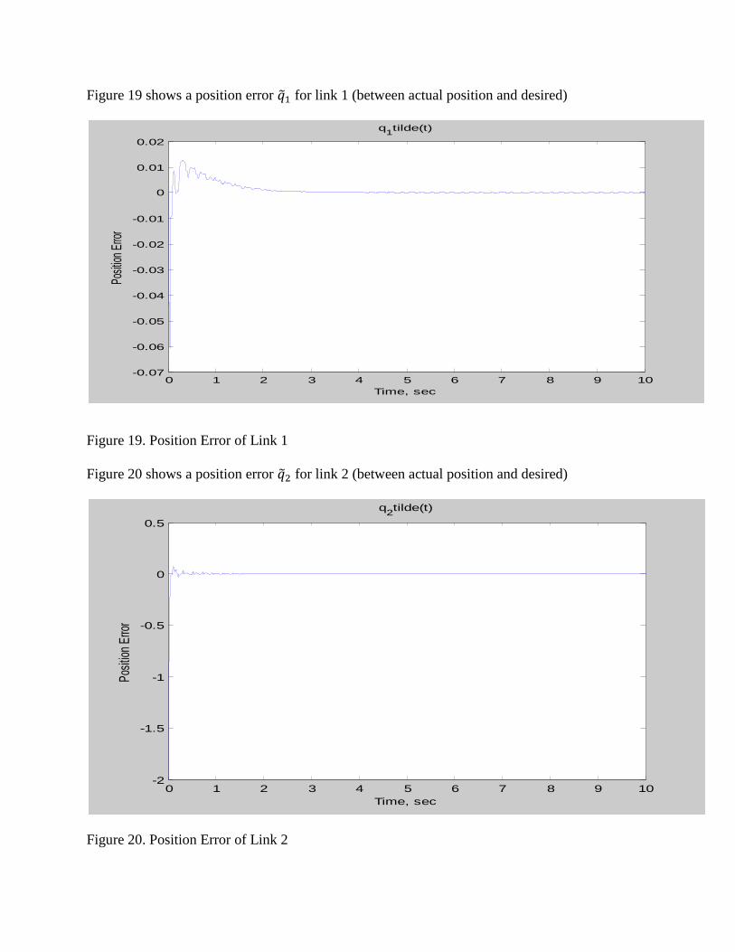
Figure 19 shows a position error for link 1 (between actual position and desired)
Figure 19. Position Error of Link 1
Figure 20 shows a position error for link 2 (between actual position and desired)
Figure 20. Position Error of Link 2
0 1 2 3 4 5 6 7 8 9 10-0.07
-0.06
-0.05
-0.04
-0.03
-0.02
-0.01
0
0.01
0.02
q1tilde(t)
Time, sec
Posi
tion
Erro
r
0 1 2 3 4 5 6 7 8 9 10-2
-1.5
-1
-0.5
0
0.5
q2tilde(t)
Time, sec
Pos
ition
Erro
r
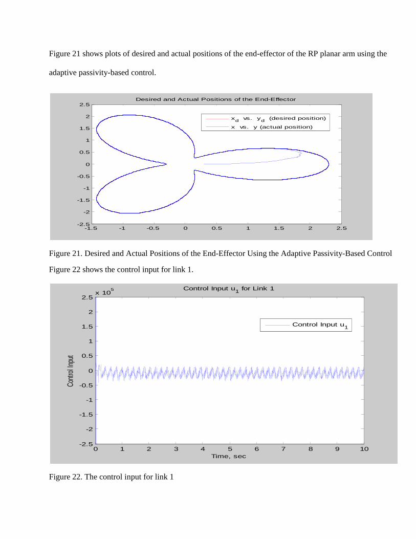
Figure 21 shows plots of desired and actual positions of the end-effector of the RP planar arm using the
adaptive passivity-based control.
Figure 21. Desired and Actual Positions of the End-Effector Using the Adaptive Passivity-Based Control
Figure 22 shows the control input for link 1.
Figure 22. The control input for link 1
-1.5 -1 -0.5 0 0.5 1 1.5 2 2.5-2.5
-2
-1.5
-1
-0.5
0
0.5
1
1.5
2
2.5Desired and Actual Positions of the End-Effector
xd vs. y
d (desired position)
x vs. y (actual position)
0 1 2 3 4 5 6 7 8 9 10-2.5
-2
-1.5
-1
-0.5
0
0.5
1
1.5
2
2.5x 10
5
Time, sec
Con
trol I
nput
Control Input u1 for Link 1
Control Input u1

Figure 23 shows the control input for link 2.
Figure 23. The control input for link 2
The nominal parameters vector is TH_0= . Using figures 15-18 we can conclude that the
parameters did not converge to their true values.
0 1 2 3 4 5 6 7 8 9 10-2.5
-2
-1.5
-1
-0.5
0
0.5
1
1.5
2
2.5x 10
5
Time, sec
Con
trol I
nput
Control Input u2 for Link 2
Control Input u2