Course: MBASubject: Research Methodology

Unit-4.1

DATA ANALYSIS & PRESENTATION

Data Preparation Hypothesis Testing

Introduction to bivariate and multivariate analysis

Data Preparation: Introduction

• Once the data begin to flow, a researcher’s attention turns to data analysis.

• Data preparation includes editing, coding, and data entry;– It is the activity that ensures the accuracy of

the data and their conversion from raw form to reduced and classified forms that are more appropriate for analysis.

Data Preparation: Introduction

• Preparing a descriptive statistical summary is another preliminary step leading to an understanding of the collected data;– It is during this step that data entry errors may

be revealed and corrected.

Data Preparation: Editing

• The customary first step in analysis is to edit the raw data.

• Editing detects errors and omissions, corrects them when possible, and certifies that maximum data quality standards are achieved.

Data Preparation: Editing

• The editor’s purpose is to guarantee that data are:– Accurate;– Consistent with the intent of the question and

their information in the survey;– Uniformly entered;– Complete; and– Arranged to simplify coding and tabulation.

Data Preparation: Editing

• In the following question asked of adults aged 18 or older, one respondent checked two categories, indicating that he was a retired officer and currently serving on active duty.

– Please indicate your current military status:• Active duty• Reserve• Retired• National Guard• Separated• Never served in the army

Data Preparation: Editing

• The editor’s responsibility is to decide which of the responses is both – consistent with the intent of the question or

other information in the survey, and – most accurate for this individual participant.

Data Preparation: EditingTwo types of editing are field editing and central

editing.• Field Editing: In large projects, field editing

review is the responsibility of the field supervisor;– When entry gaps are present from interviews, a

callback should be made rather than guessing what the respondent “probably would have said”.

– Self-interviewing has no place in quality research.– Validating the field research is the control function of

the supervisor. • It means he or she will reinterview some percentage of the

respondents to make sure they have participated. • Many research firms will recontact about 10 percent of the

respondents in this process of data validation.

Data Preparation: Editing• Central Editing: For a small study, the use of a

single editor produces maximum consistency. In large studies, editing tasks should be allocated so that each editor deals with one entire section.

– When replies are inappropriate or missing, the editor can sometimes detect the proper answer by reviewing the other information in the data set.

• It may be better to contact the respondent for correct information, if time and budget allow.

• Another alternative is for the editor to strike out the answer if it is inappropriate. Here an editing entry of “no answer” is called for.

– Another problem that editing can detect concerns faking an interview that never took place.

• This “armchair interviewing” is difficult to spot, but the editor is in the best position to do so.

• One approach is to check responses to open-ended questions. These are most difficult to fake. Distinctive response patterns in other questions will often emerge if data falsification is occurring. To uncover this, the editor must analyze the set of instruments used by each interviewer.

Data Preparation: Coding

• Coding involves assigning numbers or other symbols to answers so that the responses can be grouped into a limited number of categories.

• In coding, categories are the partitions of a data set of a given variable. For example, if the variable is gender, the partitions are male and female.

• Categorization is the process of using rules to partition a body of data.

• Both closed and free-response questions must be coded.

Data Preparation: Coding

• The categorization of data sacrifices some data detail but is necessary for efficient analysis.

• Most software programs work more efficiently in the numeric mode;– Instead of entering the word male or female in

response to a question that asks for the identification of one’s gender, we would use numeric codes, e.g., 0 for male and 1 for female

• Numeric coding simplifies the researcher’s task in converting a nominal variable, like gender, to a “dummy variable”

Data Preparation: Missing Data

• In survey studies, missing data typically occur when participants accidentally skip, refuse to answer, or do not know the answer to an item on the questionnaire.

• In longitudinal studies, missing data may result from participants dropping out of the study, or being absent for one or more data collection periods.

• Missing data also occur due to researcher error, corrupted data files, and changes in the research or instrument design after data were collected from some participants, such as when variables are dropped or added.

Data Preparation: Missing Data

• The strategy for handling missing data consists of two-step process: – the researcher first explores the pattern of missing

data to determine the mechanism for missingness (the probability that a value is missing rather than observed), and

– then selects a missing-data technique. The three basic types of techniques which can be used to salvage data sets with missing values are:

• Listwise deletion• Pairwise deletion • Replacement of missing values with estimated scores

Data Preparation: Data Entry

• Data entry converts information gathered by secondary or primary methods to a medium for reviewing and manipulation.

• Keyboarding remains a mainstay for researchers who need to create a data file immediately and store it in a minimal space on a variety of media.

• However, researchers have profited from more efficient ways of speeding up the research process, especially from bar coding and optical character and mark recognition.

Data Preparation: Data Entry• Keyboarding: A full screen editor, where an

entire data file can be edited or browsed, is a viable means of data entry for statistical packages like SPSS or SAS.– SPSS offers several data entry products, including

Data Entry Builder which enables the development of forms and surveys, and Data Entry Station which gives centralized entry staff, such as telephone interviews or online participants, access to the survey.

– Both SAS and SPSS offer software that effortless accesses data from databases, spreadsheets, data warehouses, or data marts.

Data Preparation: Data Entry

• Bar-code technology is used to simplify the interviewer’s role as a data recorder. When an interviewer passes a bar-code over the appropriate codes, the data are recorded in a small, lightweight unit for translation later

• Researchers studying magazine readership can scan bar codes to denote a magazine cover that is recognized by an interview participant.

Data Preparation: Data Entry• Optical Character Recognition (OCR):

– Users of a PC image scanner are familiar with OCR programs which transfer printed text into computer files in order to edit and use it without retyping.

• Optical scanning of instruments is efficient for researchers.– Optical scanners process the marked-sensed

questionnaires and store the answers in a file.– This method has been adopted by researchers for

data entry and preprocessing due to its faster speed, cost savings on data entry, convenience in charting and reporting data, and improved accuracy.

– It reduces the number of times data are handed, thereby reducing the number of errors that are introduced.

Hypothesis Testing

• Is also called significance testing

• Tests a claim about a parameter using evidence (data in a sample

• The technique is introduced by considering a one-sample z test

• The procedure is broken into four steps

• Each element of the procedure must be understood

Hypothesis Testing Steps

A. Null and alternative hypotheses

B. Test statistic

C. P-value and interpretation

D. Significance level (optional)

§9.1 Null and Alternative Hypotheses

• Convert the research question to null and alternative hypotheses

• The null hypothesis (H0) is a claim of “no difference in the population”

• The alternative hypothesis (Ha) claims “H0 is false”

• Collect data and seek evidence against H0

as a way of bolstering Ha (deduction)

Illustrative Example: “Body Weight”

• The problem: In the 1970s, 20–29 year old men in the U.S. had a mean μ body weight of 170 pounds. Standard deviation σ was 40 pounds. We test whether mean body weight in the population now differs.

• Null hypothesis H0: μ = 170 (“no difference”)

• The alternative hypothesis can be either Ha: μ > 170 (one-sided test) or Ha: μ ≠ 170 (two-sided test)

§9.2 Test Statistic

nSE

H

SE

x

x

x

and

trueis assumingmean population where

z

00

0stat

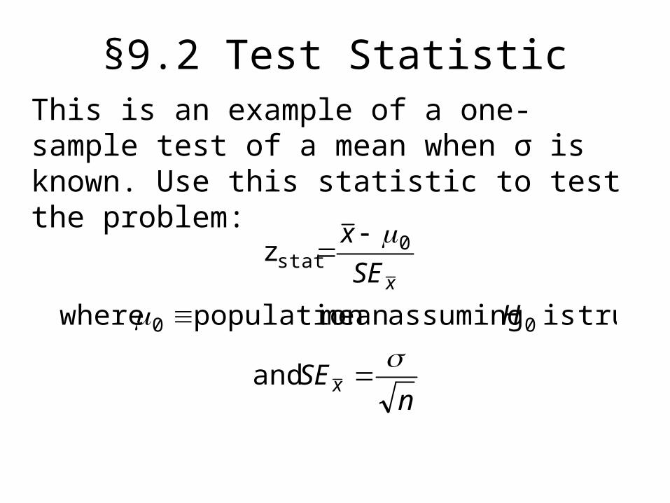
This is an example of a one-sample test of a mean when σ is known. Use this statistic to test the problem:

Illustrative Example: z statistic• For the illustrative example, μ0 = 170

• We know σ = 40• Take an SRS of n = 64. Therefore

• If we found a sample mean of 173, then

564

40

nSEx

60.05

170173 0

stat

xSE

xz

Illustrative Example: z statisticIf we found a sample mean of 185, then

00.35

170185 0

stat

xSE

xz

Reasoning Behinµzstat

5,170~ NxSampling distribution of xbar under H0: µ = 170 for n = 64

§9.3 P-value• The P-value answer the question: What is the

probability of the observed test statistic or one more extreme when H0 is true?

• This corresponds to the AUC in the tail of the Standard Normal distribution beyond the zstat.

• Convert z statistics to P-value : For Ha: μ> μ0 P = Pr(Z > zstat) = right-tail beyond zstat

For Ha: μ< μ0 P = Pr(Z < zstat) = left tail beyond zstat

For Ha: μμ0 P = 2 × one-tailed P-value

• Use Table B or software to find these probabilities (next two slides).

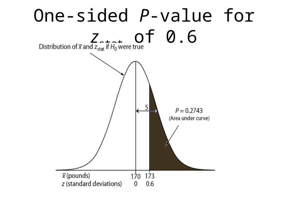
One-sided P-value for zstat of 0.6

One-sided P-value for zstat of 3.0

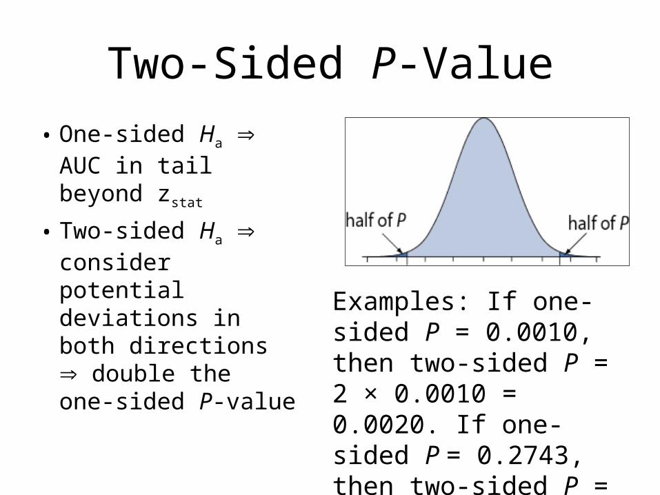
Two-Sided P-Value

• One-sided Ha AUC in tail beyond zstat

• Two-sided Ha consider potential deviations in both directions double the one-sided P-value

Examples: If one-sided P = 0.0010, then two-sided P = 2 × 0.0010 = 0.0020. If one-sided P = 0.2743, then two-sided P = 2 × 0.2743 = 0.5486.

Interpretation • P-value answer the question: What is the

probability of the observed test statistic … when H0 is true?

• Thus, smaller and smaller P-values provide stronger and stronger evidence against H0

• Small P-value strong evidence

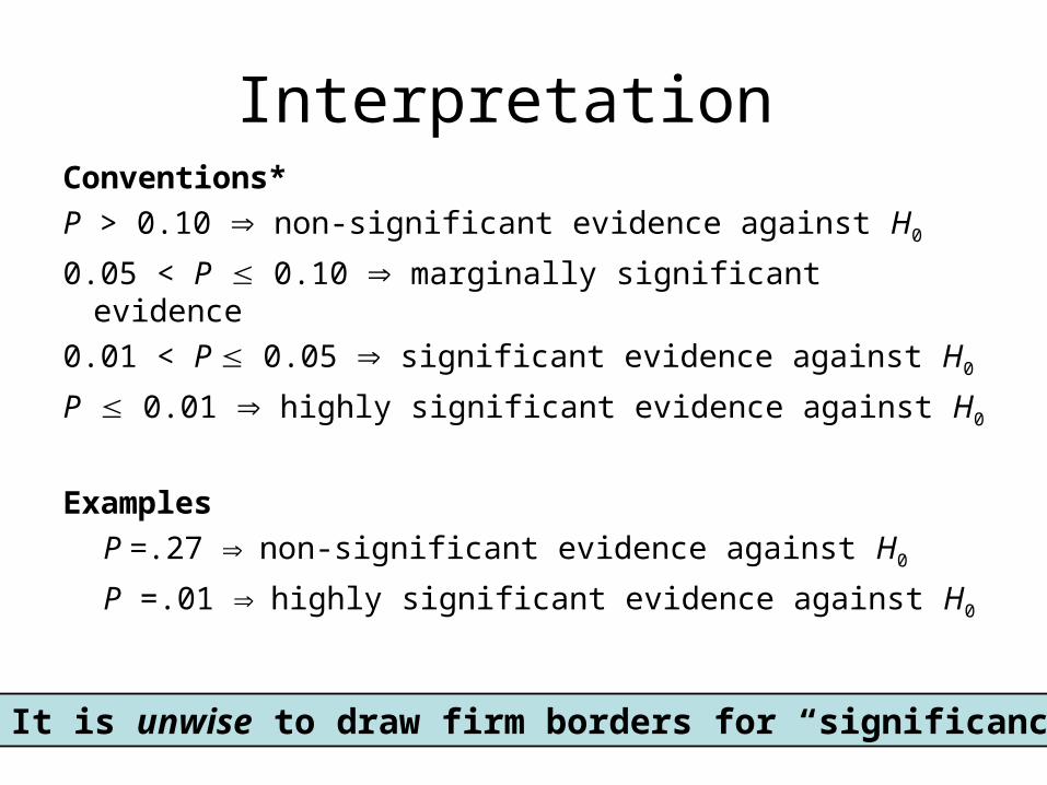
Interpretation Conventions*

P > 0.10 non-significant evidence against H0

0.05 < P 0.10 marginally significant evidence

0.01 < P 0.05 significant evidence against H0

P 0.01 highly significant evidence against H0

Examples

P =.27 non-significant evidence against H0

P =.01 highly significant evidence against H0

* It is unwise to draw firm borders for “significance”

α-Level (Used in some situations)

• Let α ≡ probability of erroneously rejecting H0

• Set α threshold (e.g., let α = .10, .05, or whatever)

• Reject H0 when P ≤ α

• Retain H0 when P > α

• Example: Set α = .10. Find P = 0.27 retain H0

• Example: Set α = .01. Find P = .001 reject H0

(Summary) One-Sample z Test

A. Hypothesis statements H0: µ = µ0 vs. Ha: µ ≠ µ0 (two-sided) or Ha: µ < µ0 (left-sided) orHa: µ > µ0 (right-sided)

B. Test statistic

C. P-value: convert zstat to P value

D. Significance statement (usually not necessary)

nSE

SE

xx

x

where z 0

stat

§9.5 Conditions for z test

• σ known (not from data)

• Population approximately Normal or large sample (central limit theorem)

• SRS (or facsimile)

• Data valid

The Lake Wobegon Example“where all the children are above average”

• Let X represent Weschler Adult Intelligence scores (WAIS)

• Typically, X ~ N(100, 15)• Take SRS of n = 9 from Lake Wobegon

population• Data {116, 128, 125, 119, 89, 99, 105,

116, 118}• Calculate: x-bar = 112.8 • Does sample mean provide strong evidence

that population mean μ > 100?

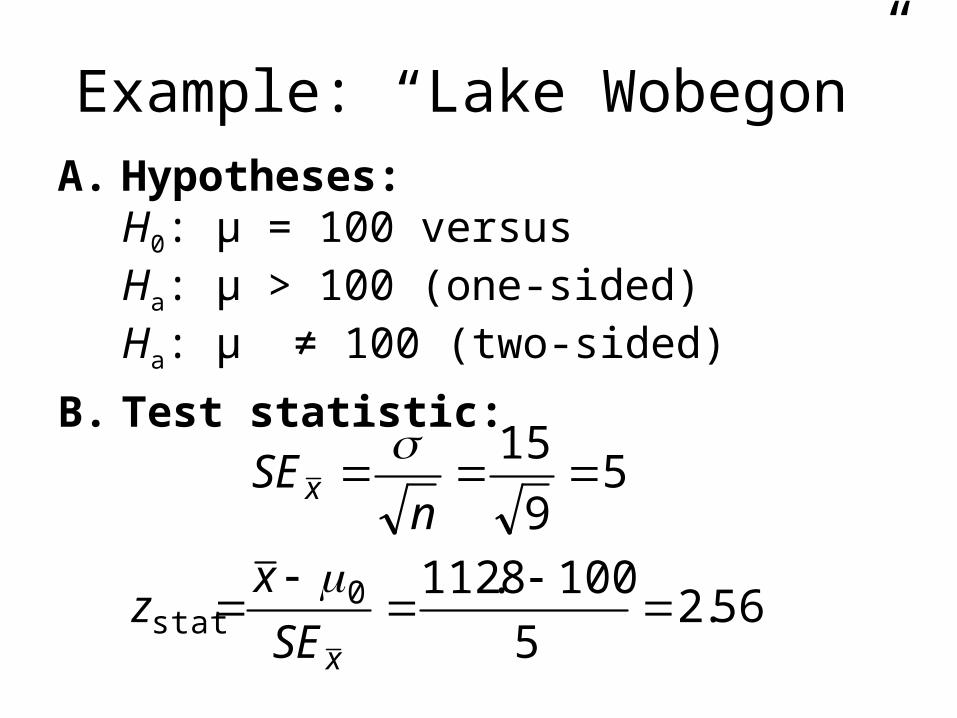
Example: “Lake Wobegon”A. Hypotheses:

H0: µ = 100 versus Ha: µ > 100 (one-sided)Ha: µ ≠ 100 (two-sided)

B. Test statistic:

56.25

1008.112

59

15

0stat

x

x

SE

xz

nSE

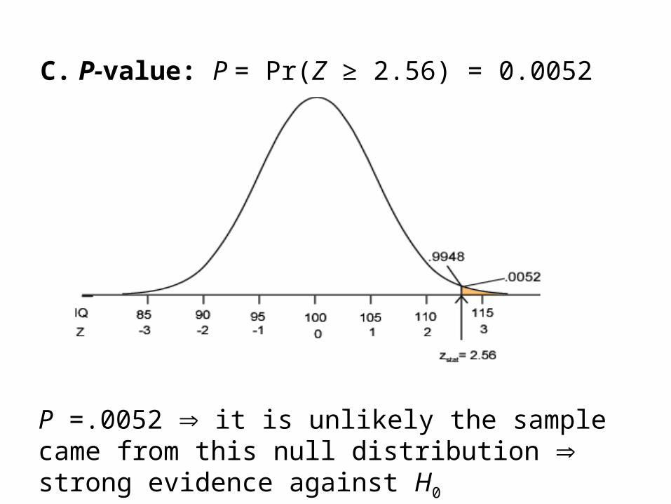
C. P-value: P = Pr(Z ≥ 2.56) = 0.0052

P =.0052 it is unlikely the sample came from this null distribution strong evidence against H0

• Ha: µ ≠100

• Considers random deviations “up” and “down” from μ0 tails above and below ±zstat

• Thus, two-sided P = 2 × 0.0052 = 0.0104

Two-Sided P-value: Lake Wobegon

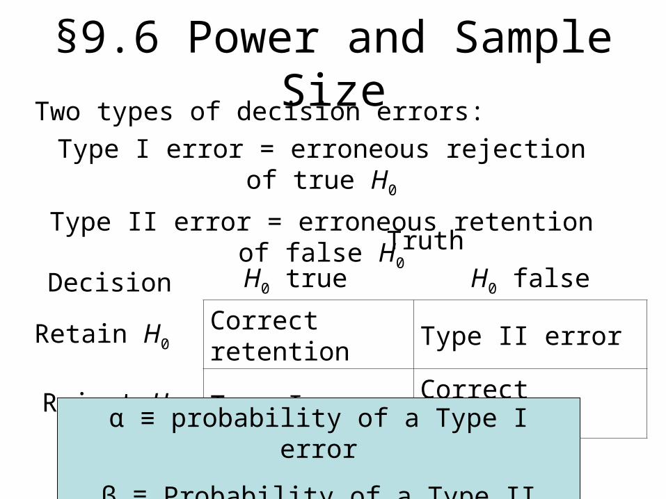
§9.6 Power and Sample Size

Truth

Decision H0 true H0 false

Retain H0 Correct retention

Type II error

Reject H0 Type I error Correct rejectionα ≡ probability of a Type I error

β ≡ Probability of a Type II error

Two types of decision errors:Type I error = erroneous rejection of true H0

Type II error = erroneous retention of false H0

Power• β ≡ probability of a Type II error

β = Pr(retain H0 | H0 false)(the “|” is read as “given”)

• 1 – β “Power” ≡ probability of avoiding a Type II error1– β = Pr(reject H0 | H0 false)

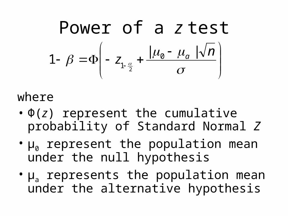
Power of a z test

where • Φ(z) represent the cumulative probability

of Standard Normal Z• μ0 represent the population mean under

the null hypothesis• μa represents the population mean under

the alternative hypothesis

nz a ||

1 01

2

Calculating Power: ExampleA study of n = 16 retains H0: μ = 170 at α = 0.05 (two-sided); σ is 40. What was the power of test’s conditions to identify a population mean of 190?

5160.0

04.0

40

16|190170|96.1

||1 0

1 2

n

z a

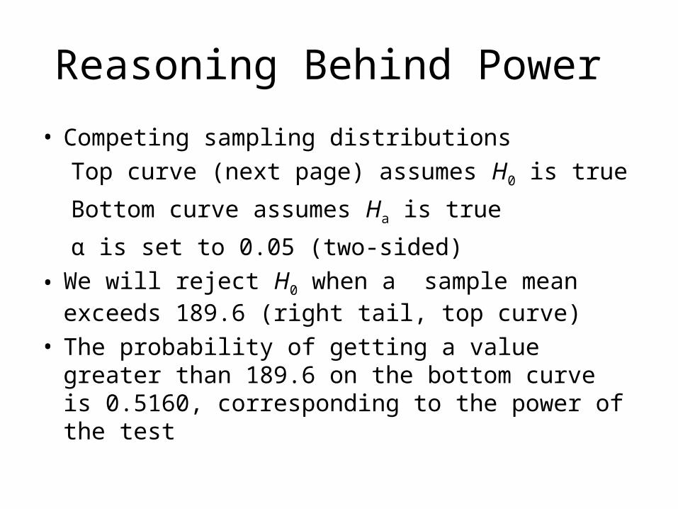
Reasoning Behind Power

• Competing sampling distributions

Top curve (next page) assumes H0 is true

Bottom curve assumes Ha is true

α is set to 0.05 (two-sided)

• We will reject H0 when a sample mean exceeds 189.6 (right tail, top curve)

• The probability of getting a value greater than 189.6 on the bottom curve is 0.5160, corresponding to the power of the test

Sample Size RequirementsSample size for one-sample z test:

where

1 – β ≡ desired power

α ≡ desired significance level (two-sided)

σ ≡ population standard deviation

Δ = μ0 – μa ≡ the difference worth detecting

2

2

112

2

zzn

Example: Sample Size Requirement

How large a sample is needed for a one-sample z test with 90% power and α = 0.05 (two-tailed) when σ = 40? Let H0: μ = 170 and Ha: μ = 190 (thus, Δ = μ0 − μa = 170 – 190 = −20)

Round up to 42 to ensure adequate power.

99.41

20

)96.128.1(402

22

2

211

2

2

zzn

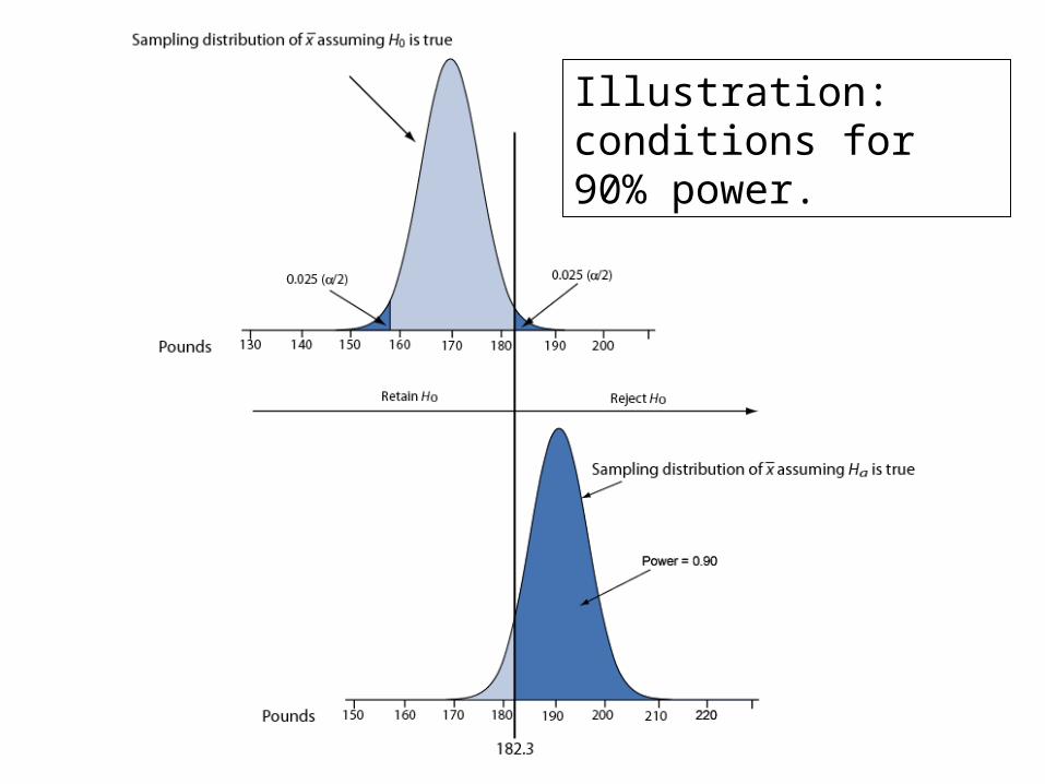
Illustration: conditions for 90% power.

Three types of analysis

• Univariate analysis – the examination of the distribution of cases on only

one variable at a time (e.g., college graduation)• Bivariate analysis

– the examination of two variables simultaneously (e.g., the relation between gender and college graduation)

• Multivariate analysis – the examination of more than two variables

simultaneously (e.g., the relationship between gender, race, and college graduation)

“Purpose”

• Univariate analysis

– Purpose: description

• Bivariate analysis

– Purpose: determining the empirical relationship between the two variables

• Multivariate analysis

– Purpose: determining the empirical relationship among the variables

Types of Statistics• Techniques that summarize and describe

characteristics of a group or make comparisons of characteristics between groups are knows as descriptive statistics.

• Inferential statistics are used to make generalizations or inferences about a population based on findings from a sample.

• The choice of a type of analysis is based on the evaluation questions, the type of data collected, and the audience who will receive the results. 

Univariate Analysis• Involves examination of the distribution of

cases on only ONE variable at a time

• Frequency distributionsFrequency distributions are listings of the number of cases in each attribute of a variable– Ungrouped frequency distribution– Grouped frequency distribution

• ProportionsProportions express number of cases of the criterion variable as part of the total population; frequency of criterion variable divided by N

Cont..• Percentages Percentages are simple 100 X

proportion – Or [100 X (frequency of criterion

variable divided by N)]

• RatesRates make comparisons more meaningful by controlling for population differences

Measures of Central Tendency

• Measures of central tendencyMeasures of central tendency reflect the central tendencies of a distribution

– ModeMode reflects the attribute with the greatest frequency

– Median Median reflects the attribute that cuts the distribution in half

– MeanMean reflects the average; sum of attributes divided by # of cases

Measures of Dispersion

• Measures of dispersionMeasures of dispersion reflect the spread or distribution of the distribution

– RangeRange is the difference between largest & smallest scores; high – low

– VarianceVariance is the average of the squared differences between each observation and the mean

– Standard deviationStandard deviation is the square root of variance

Types of Variables

• Continuous:Continuous: increase steadily in tiny fractions

• Discrete:Discrete: jumps from category to category

Subgroup Comparisons

• Somewhere between univariate & bivariate, are Subgroup Comparisons

• Present descriptive univariate data for each of several subgroups– Ratios: compare the number of cases in

one category with the number in another

Bivariate Analysis

• Bivariate analysisBivariate analysis focus on the relationship between two variables

Contingency Tables• Format: attributes of independent

variable are used as column headings and attributes of the dependent variable are used as row headings

• Guidelines for presenting & interpreting contingency tables – Contents of table described in title – Attributes of each variable clearly described – Base on which percentages are computed

should be shown – Norm is to percentage down & compare across– Table should indicate # of cases omitted from

analysis

Multivariate Analysis

• Multivariate AnalysisMultivariate Analysis allow the separate and combined effects of the independent variable to be examined

Reference

• www.uky.edu

• https://www.stat.auckland.ac

• www.polymtl.ca