contentsmay/vigre/vigre2009/reu... · if you are familiar with the usual mathematical formulation...
TRANSCRIPT
THE C∗-ALGEBRAIC FORMALISM OF QUANTUM MECHANICS
JONATHAN JAMES GLEASON
Abstract. In this paper, by examining the more tangible, more physically
intuitive classical mechanics, we aim to motivate more natural axioms of quan-
tum mechanics than those usually given in terms of Hilbert spaces. Specifically,we plan to replace the assumptions that observable are self-adjoint operators
on a separable Hilbert space and states are normalized vectors in that Hilbert
space with more natural assumptions about the observables and states in termsof C∗-algebras. Then, with these assumptions in place, we plan to derive the
aforementioned assumptions about observables and states in terms of Hilbert
spaces from our new assumptions about observables and states in terms ofC∗-algebras.
Contents
1. Introduction 12. A Brief Look at Classical Mechanics 23. What’s Wrong with Classical Mechanics 44. The Theory of C∗-Algebras 75. The Theory of Hilbert Spaces 76. Quantum Mechanics from the Ground Up 87. Closing Comments 178. Appendix: Definitions 18Acknowledgments 20References 20
1. Introduction
If you are familiar with the usual mathematical formulation of quantum mechan-ics (i.e., the states are elements of a separable Hilbert space and the observablesself-adjoint linear operators on that space), then you have certainly realized thatthis mathematical formulation is starkly different from the mathematical formula-tion used in Classical Mechanics. In classical mechanics, at a very early stage oneis usually introduced to the Newtonian formalism of classical mechanics, and as thestudent progresses through his or her study of physics, in particular mechanics, theyare eventually introduced to the Hamiltonian formalism of classical mechanics andthey are shown that this formalism is in fact equivalent to the Newtonian formalism.I see this development as rather aesthetic in nature, as opposed to what is usuallydone with quantum mechanics: we start with very intuitive physical axioms of atheory (those in the Newtonian formalism), and eventually these laws are shown
Date: August 30, 2009.
1
2 JONATHAN JAMES GLEASON
to be equivalent to the more mathematically convenient Hamiltonian formalism.However, as is usually done with quantum mechanics, we immediately begin byintroducing the typical axioms (i.e., where states are elements of a Hilbert spaceand observables are self-adjoint operators on that space), which, while mathemati-cally convenient, they have absolutely no physical intuitive justification whatsoever.I view this as a significant problem.
In this paper, I aim to introduce equivalent axioms of quantum mechanics, whichare much more natural than the axioms usually taken. To motivate these morenatural axioms, we shall first examine the mathematical formalism of classical me-chanics. In particular, we shall prove results about the observables and states inclassical mechanics. We then examine these results about observables and states todetermine why these results are not in agreement with experimental observation.Once it is determined why this characterization of states and observables is notcompatible with our physical world, we take these results about observables andstates from classical mechanics, and modify them just slightly so as to be compat-ible with the physical laws that govern our world, and then taking the resultingstatements as axioms of quantum theory. Once we have those axioms in place, wewill show that these axioms actually imply that our observables are the self-adjointoperators on some separable Hilbert space and that states are normalized elementsin that Hilbert space.
2. A Brief Look at Classical Mechanics
In order to motivate more natural axioms of a quantum theory (as mentioned inthe abstract), I first wish to examine (superficially) the mathematical formulationof classical mechanics (in the Hamiltonian sense). In any theory of mechanics, wemust come to grips with two ubiquitous concepts: the notion of a state and thenotion of an observable.
In Hamiltonian mechanics, we describe the state of a system by an point (q, p)1
in a two dimensional symplectic manifold M , known as phase space (usually, weidentify the classical system with phase space itself). Now, in all real physicalsystems, a particles position and momentum must remain bounded, and hence, forthe remainder of the paper, we shall assume that M is compact.
It is an experimental fact that we can never measure something with infiniteprecision; however, there are such things that we can, in principle, measure to anarbitrary precise degree. We call such things classical observables.
We would like to come up with a mathematically precise, physically motivatedway to characterize these classical observables. A first natural requirement is thatobservables depend on the state of the system, that is, observables better be func-tions of q and p. Secondly, we better require that these functions be real-valued.Thirdly, we must require that there is some way to make the error, when we mea-sure an observable in the laboratory, arbitrarily small. Let us assume (by virtue ofexperimental fact, in the classical realm of course), that we can always measure qand p arbitrarily precisely.2 Now, say I want to measurable something, namely areal valued function of q and p, call it f , and I want to measure f with error less
1We shall just restrict ourselves to the case where our system consists of one particle. For our
purposes, there is no loss of generality.2Of course, we mean to imply that the measurements of q and p are simultaneous, which, in
classical mechanics, is perfectly acceptable.
THE C∗-ALGEBRAIC FORMALISM OF QUANTUM MECHANICS 3
than some ε > 0. Now, I know that I can make the error in q and p arbitrarilysmall, so, if there is some maximum error in q and p, call it δ, so that when I plugin my measured values of q and p into f , my experimental value of f will be withinε of the true value of f , then f will be observable. But of course, this is just thedefinition of a continuous function! Thus, the natural definition for an observablesin classical mechanics can be stated as follows:
Definition 2.1 (Classical Observables). The classical observables onM are exactlythe continuous real-valued functions on M .
Hereafter, we shall simply denote the set of all observables on M as O =C0 (M,R). Now that we have a concrete way of viewing observables on M , wecan define some obvious structure:
Definition 2.2. Let S = (p, q) ∈M , f, g ∈ O, and a ∈ R. Then, define(1) (f + g)(S) ≡ f(S) + g(S)(2) (af)(S) ≡ af(S)(3) (fg)(S) ≡ f(S)g(S)(4) ‖f‖ = sup {|f(S)| |S = (p, q) ∈M}(5) (f∗)(S) = f(S)
With these simple definitions, we have the following theorem:
Theorem 2.1 (Properties of Classical Observables). The set of observables O ofa classical system are exactly the self-adjoint elements of a separable commutativeunital C∗-algebra A.
Proof. Step 1: Construct A.Define A ≡ C0 (M,C) and equip A with the operations given in Definition 2.2.
Step 2: Relegate the trivial work to the reader.Except for proving that A is separable and complete, everything is just a matter ofchecking and we leave it to the reader.
Step 3: Find the limit of a Cauchy sequence.To prove that A is complete, let fn ∈ A be a Cauchy sequence. It follows that, foreach x ∈ M , fn(x) is Cauchy in C. But C is complete, so define f : M → C suchthat f(x) = lim fn(x). We now show that fn converges to f . Let ε > 0, and chooseN ′ ∈ N, so that if n > m ≥ N ′, it follows that ‖fn(x)− fm(x)‖ < ε
2 for all x ∈M .Then, pick N ≥ N so that whenever n ≥ N , it follows that ‖fM (x0)− f(x0)‖ < ε
2for a fixed x0 ∈M . Then, whenever n ≥ N ,
|f(x0)− fn(x0)| ≤ |fn(x0)− fN (x0)|+ |fN (x0)− f(x0)| < ε.
And so fn converges to f .Step 4: Show the limit of a Cauchy sequence is continuous.
To prove f is continuous, fix x0 ∈M , let ε > 0, and choose N ∈ N so that whenevern ≥ N , it follows that |fn(x)− f(x)| < ε
3 for all x ∈ M . Then, let n ≥ N , andchoose δ > 0 so that whenever d(x, x0) < δ,3 it follows that |fn(x)− fn(x0)| < ε
3 .Then, whenever d(x, x0) < δ, it follows that
|f(x)− f(x0)| ≤ |f(x)− fn(x)|+ |fn(x)− fn(x0)|+ |fn(x0)− f(x0)| < ε.
Thus, f ∈ A, and so A is complete.
3Here, d is the metric on M .
4 JONATHAN JAMES GLEASON
Step 5: Prove that A is separable.By the Stone-Weierstrass Theorem4, the set of all polynomials in q and p withcoefficients with rational real and imaginary part form a countable dense subset ofA, and hence A is separable. �
This theorem will serve as our guide for axiomizing quantum mechanics for theremainder of the paper. Eventually, we will take the above theorem (with a slightmodification) as an axiom of the observables of quantum mechanics.
Now we wish to do something similar with the states of a classical system. Thatis to say, we would like to examine the mathematical description of states in classicalmechanics, and arrive at a result that we can hopefully take as an axiom for ourtheory of quantum mechanics. There is a natural way of viewing states in a classicalsystem as linear functionals on O.
Definition 2.3. Let S = (p, q) ∈ M be a state. Then, we define S : A → C suchthat, for f ∈ A:
S(f) = f(S)
Note that, we will not distinguish between classical states and the correspondinglinear functional, which we also refer to as states; which one we are referring to willbe clear from context.
It is easy to prove some trivial results about these states:
Theorem 2.2 (Properties of Classical States). Let S ∈ M be a state. Then,S : A → C is normalized positive linear functional on A.
Proof. Except normalization, these properties are all trivial to check. We note firstthat
‖S‖ = sup {|S(f)| | ‖f‖ = 1} ≥ |S (1)| = 1.
Secondly, for f ∈ A,
|S(f)| = |f(S)| ≤ sup {|f(S)| |S ∈M} = ‖f‖ ,
and so ‖S‖ ≤ 1, from which it follows that ‖S‖ = 1, and hence S is normalized. �
At this point, we have fully characterized both the observables and states inclassical mechanics. The characterization of the observables is given in Theorem2.1 and the characterization of the states is given in Theorem 2.2. The idea nowis to examine Theorems 1.1 and 1.2 and determine what it is about them thatis incompatible with quantum mechanics, and to figure out in what way we canmodify them so that they are consistent with the way in which our world actuallyworks.
3. What’s Wrong with Classical Mechanics
Before we attempt at “fixing” our notions of states and observables for classicalmechanics, we first want to gain a more enlightening view of states when viewed aslinear functionals. A nice theorem, due to Riesz and Markov5, actually characterizesthese states very nicely:
4See [11], pg. 175.5See [10] pg. 130.
THE C∗-ALGEBRAIC FORMALISM OF QUANTUM MECHANICS 5
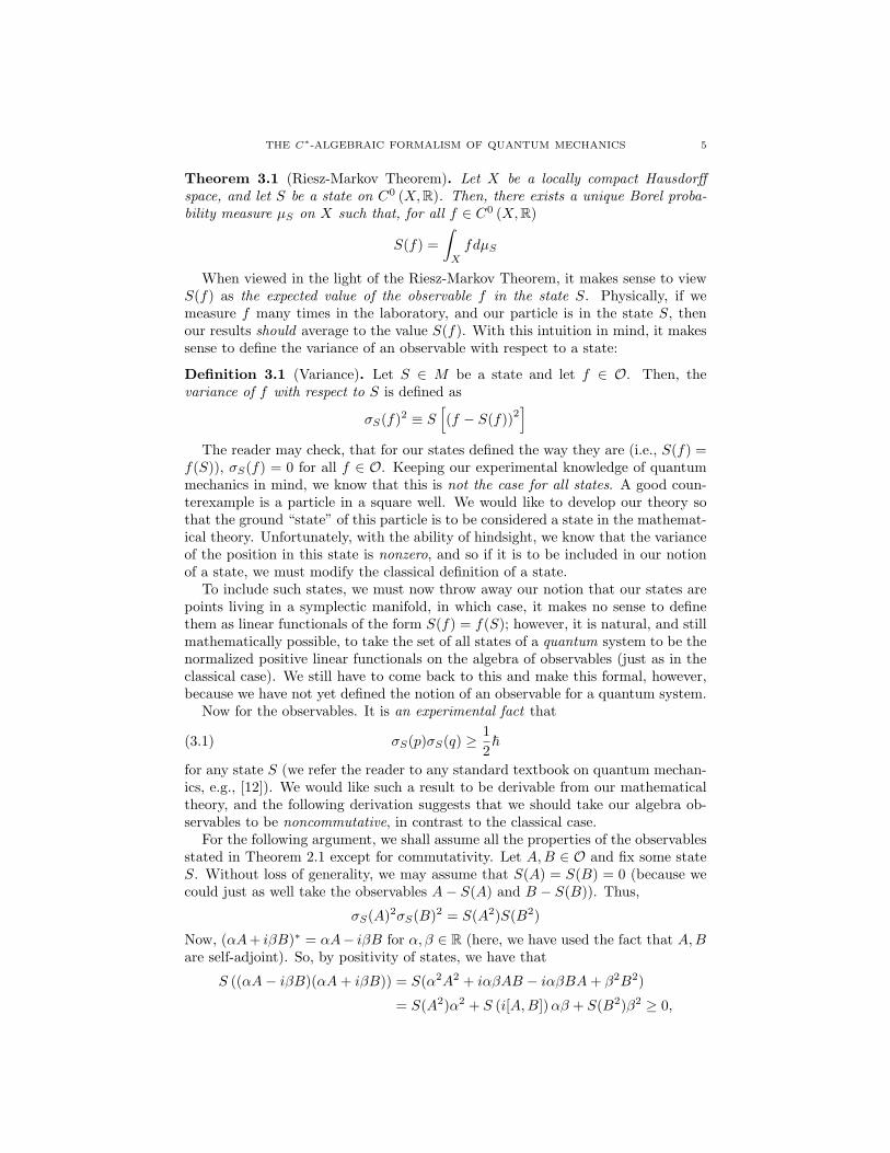
Theorem 3.1 (Riesz-Markov Theorem). Let X be a locally compact Hausdorffspace, and let S be a state on C0 (X,R). Then, there exists a unique Borel proba-bility measure µS on X such that, for all f ∈ C0 (X,R)
S(f) =∫X
fdµS
When viewed in the light of the Riesz-Markov Theorem, it makes sense to viewS(f) as the expected value of the observable f in the state S. Physically, if wemeasure f many times in the laboratory, and our particle is in the state S, thenour results should average to the value S(f). With this intuition in mind, it makessense to define the variance of an observable with respect to a state:
Definition 3.1 (Variance). Let S ∈ M be a state and let f ∈ O. Then, thevariance of f with respect to S is defined as
σS(f)2 ≡ S[(f − S(f))2
]The reader may check, that for our states defined the way they are (i.e., S(f) =
f(S)), σS(f) = 0 for all f ∈ O. Keeping our experimental knowledge of quantummechanics in mind, we know that this is not the case for all states. A good coun-terexample is a particle in a square well. We would like to develop our theory sothat the ground “state” of this particle is to be considered a state in the mathemat-ical theory. Unfortunately, with the ability of hindsight, we know that the varianceof the position in this state is nonzero, and so if it is to be included in our notionof a state, we must modify the classical definition of a state.
To include such states, we must now throw away our notion that our states arepoints living in a symplectic manifold, in which case, it makes no sense to definethem as linear functionals of the form S(f) = f(S); however, it is natural, and stillmathematically possible, to take the set of all states of a quantum system to be thenormalized positive linear functionals on the algebra of observables (just as in theclassical case). We still have to come back to this and make this formal, however,because we have not yet defined the notion of an observable for a quantum system.
Now for the observables. It is an experimental fact that
(3.1) σS(p)σS(q) ≥ 12
~
for any state S (we refer the reader to any standard textbook on quantum mechan-ics, e.g., [12]). We would like such a result to be derivable from our mathematicaltheory, and the following derivation suggests that we should take our algebra ob-servables to be noncommutative, in contrast to the classical case.
For the following argument, we shall assume all the properties of the observablesstated in Theorem 2.1 except for commutativity. Let A,B ∈ O and fix some stateS. Without loss of generality, we may assume that S(A) = S(B) = 0 (because wecould just as well take the observables A− S(A) and B − S(B)). Thus,
σS(A)2σS(B)2 = S(A2)S(B2)
Now, (αA+ iβB)∗ = αA− iβB for α, β ∈ R (here, we have used the fact that A,Bare self-adjoint). So, by positivity of states, we have that
S ((αA− iβB)(αA+ iβB)) = S(α2A2 + iαβAB − iαβBA+ β2B2)
= S(A2)α2 + S (i[A,B])αβ + S(B2)β2 ≥ 0,
6 JONATHAN JAMES GLEASON
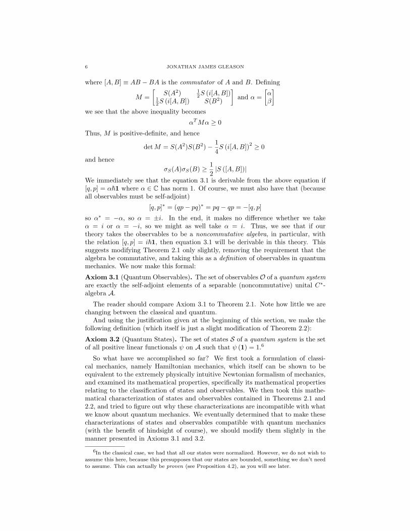
where [A,B] ≡ AB −BA is the commutator of A and B. Defining
M =[
S(A2) 12S (i[A,B])
12S (i[A,B]) S(B2)
]and α =
[αβ
]we see that the above inequality becomes
αTMα ≥ 0
Thus, M is positive-definite, and hence
detM = S(A2)S(B2)− 14S (i[A,B])2 ≥ 0
and henceσS(A)σS(B) ≥ 1
2|S ([A,B])|
We immediately see that the equation 3.1 is derivable from the above equation if[q, p] = α~1 where α ∈ C has norm 1. Of course, we must also have that (becauseall observables must be self-adjoint)
[q, p]∗ = (qp− pq)∗ = pq − qp = −[q, p]
so α∗ = −α, so α = ±i. In the end, it makes no difference whether we takeα = i or α = −i, so we might as well take α = i. Thus, we see that if ourtheory takes the observables to be a noncommutative algebra, in particular, withthe relation [q, p] = i~1, then equation 3.1 will be derivable in this theory. Thissuggests modifying Theorem 2.1 only slightly, removing the requirement that thealgebra be commutative, and taking this as a definition of observables in quantummechanics. We now make this formal:
Axiom 3.1 (Quantum Observables). The set of observables O of a quantum systemare exactly the self-adjoint elements of a separable (noncommutative) unital C∗-algebra A.
The reader should compare Axiom 3.1 to Theorem 2.1. Note how little we arechanging between the classical and quantum.
And using the justification given at the beginning of this section, we make thefollowing definition (which itself is just a slight modification of Theorem 2.2):
Axiom 3.2 (Quantum States). The set of states S of a quantum system is the setof all positive linear functionals ψ on A such that ψ (1) = 1.6
So what have we accomplished so far? We first took a formulation of classi-cal mechanics, namely Hamiltonian mechanics, which itself can be shown to beequivalent to the extremely physically intuitive Newtonian formalism of mechanics,and examined its mathematical properties, specifically its mathematical propertiesrelating to the classification of states and observables. We then took this mathe-matical characterization of states and observables contained in Theorems 2.1 and2.2, and tried to figure out why these characterizations are incompatible with whatwe know about quantum mechanics. We eventually determined that to make thesecharacterizations of states and observables compatible with quantum mechanics(with the benefit of hindsight of course), we should modify them slightly in themanner presented in Axioms 3.1 and 3.2.
6In the classical case, we had that all our states were normalized. However, we do not wish toassume this here, because this presupposes that our states are bounded, something we don’t need
to assume. This can actually be proven (see Proposition 4.2), as you will see later.

THE C∗-ALGEBRAIC FORMALISM OF QUANTUM MECHANICS 7
What has been presented up to this point has mostly been all physical andmathematical justification for taking as assumptions Axioms 3.1 and 3.2. We nowseek to build the theory of Quantum Mechanics from the ground up with thesetwo fundamental assumptions, assumptions that arise naturally from the studyof classical mechanics. Before we attempt to do this, however, a fair amount ofmachinery is needed to be built up from the theories of C∗-algebra and Hilbertspaces. Instead of going into the details of how all this might be built up, wesimply state the results we shall need throughout the rest of the paper. The readerwho is already familiar with the theories of C∗-algebras and Hilbert spaces, mayskip to section 6 and use the following two sections as reference when necessary.The unfamiliar reader should be warned that the following two sections are notintended to teach, but merely provide a library of useful results that will be usedwithin the paper.
4. The Theory of C∗-Algebras
Proposition 4.1. Let A be a unital C∗-algebra and let ψ be a bounded linearfunctional on A. Then, if ‖ψ‖ = ψ (1), then for A ∈ A, ψ (A∗) = ψ (A)∗.
Proposition 4.2. Let A be a unital C∗-algebra and let ψ be a linear functional onA. Then, ψ is positive iff ‖ψ‖ = ψ (1).
Proposition 4.3. The states on a unital C∗-algebra A separate the elements of A.
Proposition 4.4. Let A and B be unital C∗-algebras, and let π : A → B be a∗-homomorphism. Then, ‖π (A)‖ ≤ ‖A‖. Furthermore, if π is a ∗-isomorphism,then, ‖π (A)‖ = ‖A‖.
5. The Theory of Hilbert Spaces
Notation. For the rest of the paper, unless otherwise stated, a sesquilinear form ona vector space will be denoted (·|·), with the sesquilinear form conjugate linear inthe first coordinate.
Notation. We shall denote by BL(V ) the set of all bounded linear operators on anormed vector space V and by L(V ) the set of all linear operators on a vector spaceV .
We would eventually like to prove that our observables are actually operators ona Hilbert space. Before we attempt to do this, however, we better first show thatthe bounded linear operators on a Hilbert space do in fact form a C∗-algebra. Todo this, we must first come up with an involution to put on our space of operators.The notion of “adjointing” is a natural one; however, we must first prove that thisnotion is well-defined and makes sense:
Proposition 5.1. Let H be a Hilbert space. Then, for A ∈ BL(H), there exists aunique A∗ ∈ BL(H) such that (Ay|x) = (y|A∗x) for all x,y ∈ H.
We now show that the set of all bounded operators on a Hilbert spaces, equippedwith pointwise addition and scalar multiplication, “adjointing” as the involution,and the usual operator norm forms a C∗-algebra:
8 JONATHAN JAMES GLEASON
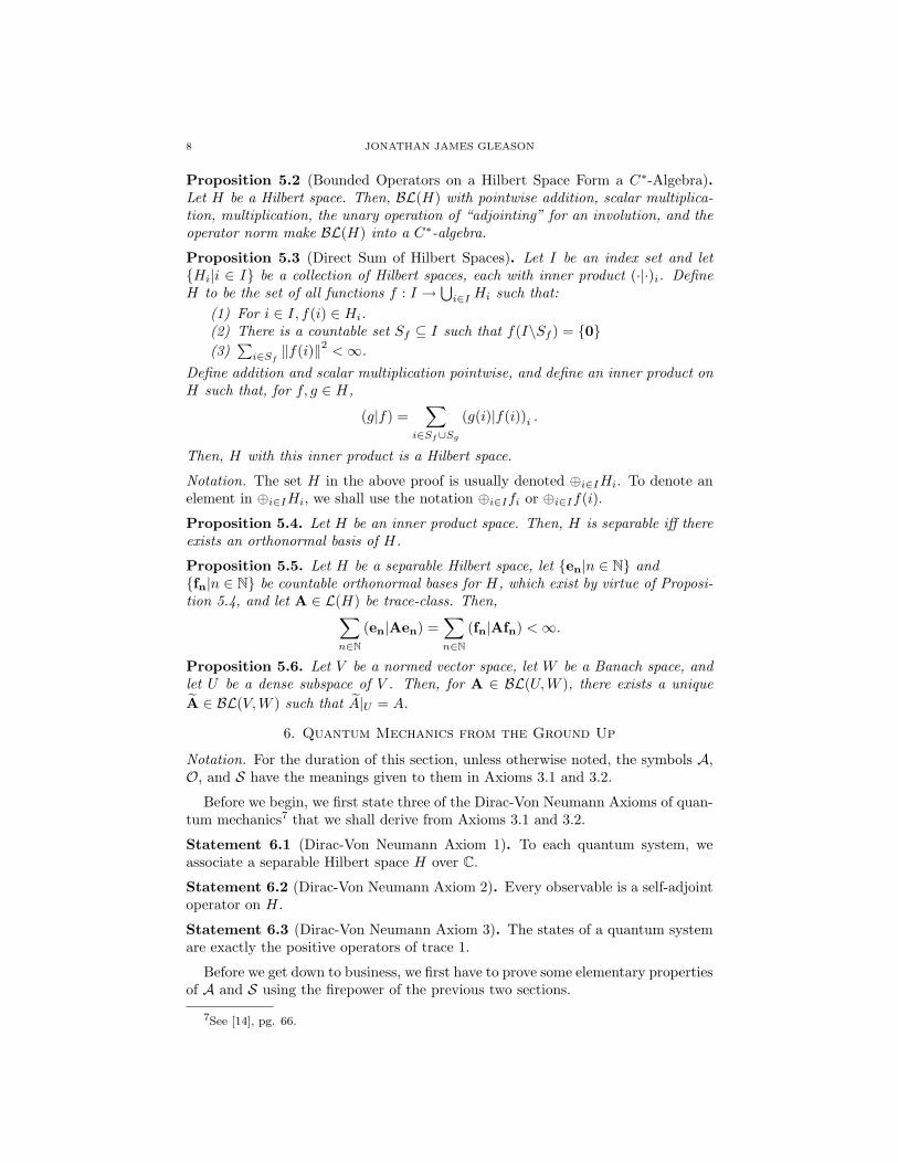
Proposition 5.2 (Bounded Operators on a Hilbert Space Form a C∗-Algebra).Let H be a Hilbert space. Then, BL(H) with pointwise addition, scalar multiplica-tion, multiplication, the unary operation of “adjointing” for an involution, and theoperator norm make BL(H) into a C∗-algebra.
Proposition 5.3 (Direct Sum of Hilbert Spaces). Let I be an index set and let{Hi|i ∈ I} be a collection of Hilbert spaces, each with inner product (·|·)i. DefineH to be the set of all functions f : I →
⋃i∈I Hi such that:
(1) For i ∈ I, f(i) ∈ Hi.(2) There is a countable set Sf ⊆ I such that f(I\Sf ) = {0}(3)
∑i∈Sf
‖f(i)‖2 <∞.Define addition and scalar multiplication pointwise, and define an inner product onH such that, for f, g ∈ H,
(g|f) =∑
i∈Sf∪Sg
(g(i)|f(i))i .
Then, H with this inner product is a Hilbert space.
Notation. The set H in the above proof is usually denoted ⊕i∈IHi. To denote anelement in ⊕i∈IHi, we shall use the notation ⊕i∈Ifi or ⊕i∈If(i).
Proposition 5.4. Let H be an inner product space. Then, H is separable iff thereexists an orthonormal basis of H.
Proposition 5.5. Let H be a separable Hilbert space, let {en|n ∈ N} and{fn|n ∈ N} be countable orthonormal bases for H, which exist by virtue of Proposi-tion 5.4, and let A ∈ L(H) be trace-class. Then,∑
n∈N(en|Aen) =
∑n∈N
(fn|Afn) <∞.
Proposition 5.6. Let V be a normed vector space, let W be a Banach space, andlet U be a dense subspace of V . Then, for A ∈ BL(U,W ), there exists a uniqueA ∈ BL(V,W ) such that A|U = A.
6. Quantum Mechanics from the Ground Up
Notation. For the duration of this section, unless otherwise noted, the symbols A,O, and S have the meanings given to them in Axioms 3.1 and 3.2.
Before we begin, we first state three of the Dirac-Von Neumann Axioms of quan-tum mechanics7 that we shall derive from Axioms 3.1 and 3.2.
Statement 6.1 (Dirac-Von Neumann Axiom 1). To each quantum system, weassociate a separable Hilbert space H over C.
Statement 6.2 (Dirac-Von Neumann Axiom 2). Every observable is a self-adjointoperator on H.
Statement 6.3 (Dirac-Von Neumann Axiom 3). The states of a quantum systemare exactly the positive operators of trace 1.
Before we get down to business, we first have to prove some elementary propertiesof A and S using the firepower of the previous two sections.
7See [14], pg. 66.
THE C∗-ALGEBRAIC FORMALISM OF QUANTUM MECHANICS 9
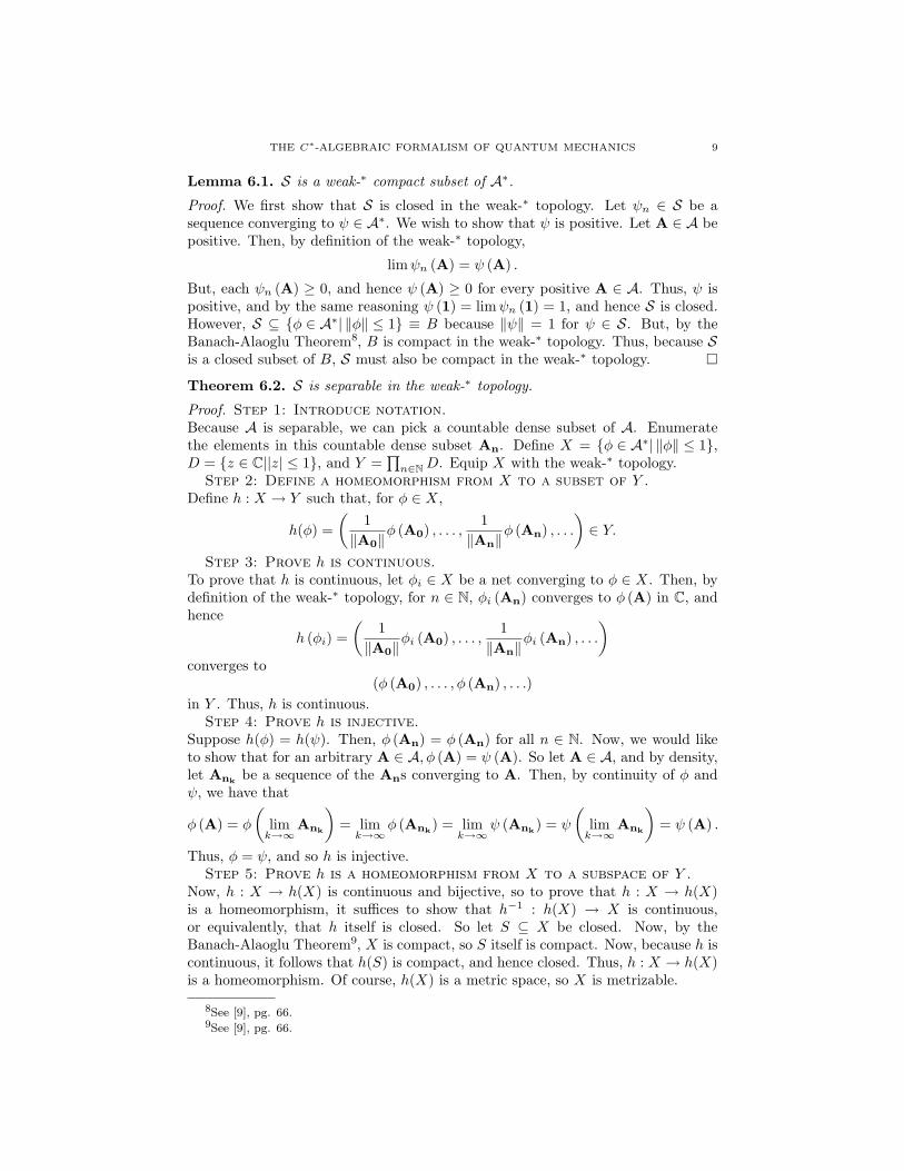
Lemma 6.1. S is a weak-∗ compact subset of A∗.Proof. We first show that S is closed in the weak-∗ topology. Let ψn ∈ S be asequence converging to ψ ∈ A∗. We wish to show that ψ is positive. Let A ∈ A bepositive. Then, by definition of the weak-∗ topology,
limψn (A) = ψ (A) .
But, each ψn (A) ≥ 0, and hence ψ (A) ≥ 0 for every positive A ∈ A. Thus, ψ ispositive, and by the same reasoning ψ (1) = limψn (1) = 1, and hence S is closed.However, S ⊆ {φ ∈ A∗| ‖φ‖ ≤ 1} ≡ B because ‖ψ‖ = 1 for ψ ∈ S. But, by theBanach-Alaoglu Theorem8, B is compact in the weak-∗ topology. Thus, because Sis a closed subset of B, S must also be compact in the weak-∗ topology. �
Theorem 6.2. S is separable in the weak-∗ topology.
Proof. Step 1: Introduce notation.Because A is separable, we can pick a countable dense subset of A. Enumeratethe elements in this countable dense subset An. Define X = {φ ∈ A∗| ‖φ‖ ≤ 1},D = {z ∈ C||z| ≤ 1}, and Y =
∏n∈N D. Equip X with the weak-∗ topology.
Step 2: Define a homeomorphism from X to a subset of Y .Define h : X → Y such that, for φ ∈ X,
h(φ) =(
1‖A0‖
φ (A0) , . . . ,1
‖An‖φ (An) , . . .
)∈ Y.
Step 3: Prove h is continuous.To prove that h is continuous, let φi ∈ X be a net converging to φ ∈ X. Then, bydefinition of the weak-∗ topology, for n ∈ N, φi (An) converges to φ (A) in C, andhence
h (φi) =(
1‖A0‖
φi (A0) , . . . ,1
‖An‖φi (An) , . . .
)converges to
(φ (A0) , . . . , φ (An) , . . .)in Y . Thus, h is continuous.
Step 4: Prove h is injective.Suppose h(φ) = h(ψ). Then, φ (An) = φ (An) for all n ∈ N. Now, we would liketo show that for an arbitrary A ∈ A, φ (A) = ψ (A). So let A ∈ A, and by density,let Ank
be a sequence of the Ans converging to A. Then, by continuity of φ andψ, we have that
φ (A) = φ
(limk→∞
Ank
)= limk→∞
φ (Ank) = lim
k→∞ψ (Ank
) = ψ
(limk→∞
Ank
)= ψ (A) .
Thus, φ = ψ, and so h is injective.Step 5: Prove h is a homeomorphism from X to a subspace of Y .
Now, h : X → h(X) is continuous and bijective, so to prove that h : X → h(X)is a homeomorphism, it suffices to show that h−1 : h(X) → X is continuous,or equivalently, that h itself is closed. So let S ⊆ X be closed. Now, by theBanach-Alaoglu Theorem9, X is compact, so S itself is compact. Now, because h iscontinuous, it follows that h(S) is compact, and hence closed. Thus, h : X → h(X)is a homeomorphism. Of course, h(X) is a metric space, so X is metrizable.
8See [9], pg. 66.9See [9], pg. 66.
10 JONATHAN JAMES GLEASON
Step 6: Conclude S is separable.S ⊆ X, so S is of course also metrizable. Let d be the metric on S that induces theweak-∗ topology on X. Define Sn =
{B 1
n(φ)|φ ∈ X
}. Each Sn is an open cover of
S. Now, by Lemma 6.1, S is compact, so for each Sn, we can pick a finite subcoverTn. For each Tn, let Cn be the set of the centers of the balls in Tn. Note that eachCn is finite. Define C = ∪n∈NCn. Because each Cn is finite, it follows that C isat most countable. To show that C is dense, let φ ∈ S. We wish to construct asequence in C converging to φ. Now, each Tn covers X, so pick center of the openball that φ is contained in: call it φn. It follows that d(φ, φn) < 1
n , and hence φnconverges to φ. Thus, C is dense, and hence X is separable. �
Now, with the appropriate machinery in place, we plan to link our definitions ofquantum observables and states, which were given in terms of C∗-algebras, to theusual definitions of quantum observables and states, which are given in terms ofHilbert spaces.
The following theorem is the key that links everything together, and it, alongwith the Gelfand-Naimark Theorem, is one of the two primary results of this paper.
Theorem 6.3 (Gelfand-Naimark-Segal Theorem). Let ψ ∈ S. Then, there existsa separable Hilbert space Hψ over C and a ∗-representation πψ : A → BL(Hψ) suchthat:
(1) There exists a cyclic vector xψ ∈ H of πψ.(2) There is some positive Ψ ∈ BL(Hψ) with TrΨ = 1 such that, for A ∈ A,
ψ (A) = (xψ|πψ (A)xψ) = Tr [Ψπψ (A)].(3) Every ∗-representation π of A into a Hilbert space H over C with cyclic
vector x such that ψ (A) = (x|π (A)x) for A ∈ A is equivalent to πψ inthe sense that, for every such representation, there exists a unitary trans-formation U : H → Hψ such that Ux = xψ and for A ∈ A, πψ (A) =Uπ (A)U−1.
Proof. Step 1: Define a semidefinite sesquilinear form on A.We first wish to turn A into an inner product space. To do this, we first define asesquilinear form on A. Define, for A,B ∈ A:
(A|B) ≡ ψ (A∗B)
The reader may check that this is linear in the first argument, and conjugate sym-metric (conjugate symmetry follows from Propositions 4.2 and 4.1). We would likethis to be an inner product; however, while it certainly is nonnegative, it isn’t nec-essarily positive definite. To turn it into an inner product product, we plan to showthat the set
I = {B ∈ A|∀A ∈ A, (A|B) = 0}
is a subspace of A. Then, we would like to show that the above defined sesquilinearform is a well-defined inner product on the quotient space A/I.
Step 2: Show that A/I is an inner product space with the innerproduct (·|·) extended naturally to the quotient space.The reader may check for themselves that I is in fact a left-sided ideal. Now, I is asubspace of A, so if we temporarily forget about the extra structure on A, we canconstruct the quotient space A/I by the usual means. We define the sesquilinear
THE C∗-ALGEBRAIC FORMALISM OF QUANTUM MECHANICS 11
form on the quotient space in the obvious way: for A + I,B + I ∈ A/I, we define
(A + I|B + I) ≡ (A|B) .
Once again, this is obviously linear in the first argument and conjugate symmetric,so all that we have to prove is well-definedness and positive-definiteness. To provewell-definedness, let A,B,C,D ∈ A, and suppose A+I = C+I and B+I = D+I.Thus, we may write C = A + I1 and D = B + I2 for I1, I2 ∈ I. Then,
(C|D) = (A + I1|B + I2) = (A|B) + (I1|B) + (A|I2) + (I1|I2) = (A|B)
and so the sesquilinear form is well-defined. To prove positive-definiteness, suppose(A + I|A + I) = 0. It immediately follows that (A|A) = 0. By the Cauchy-Schwarz Inequality (whose proof does not require positive-definiteness), for B ∈ A
|(B|A)|2 ≤ (A|A) (B|B) = 0,
and hence, for B ∈ A, (B|A) = 0, and so A ∈ I. Thus, A + I = 0 + I and hence(·|·) is a well-defined inner product on A/I. In fact, this actually proves that
I = {A ∈ A| (A|A) = 0} ,
a result that we will use later in the proof.Step 3: Complete A/I to a Hilbert space, Hψ.
This inner product induces a norm, and hence a metric on A/I. Complete themetric space A/I in to a Hilbert space Hψ over C. We now proceed to constructour representation.
Step 4: Construct a ∗-homomorphism φ : A → BL (A/I).We first define a ∗-homomorphism φ : A → BL (A/I) defined such that, for A ∈ A,φ sends A to the operator that sends B + I ∈ A/I to AB + I. That is,
φ (A) (B + I) = AB + I.
We first prove well-definedness of the “operator” φ (A). Suppose B + I = C + I.Then, C = B + I for some I ∈ I. Thus,
φ (A) (C + I) = AC + I = A (B + I) + I= AB + AI + I = AB + I = φ (A) (B + I) ,
where we have used the fact that I is a left-ideal so that we know AI ∈ I. Thereader may check that φ (A) is actually linear. To prove that φ (A) is bounded, itsuffices to show that the set
{‖φ (A) (B + I)‖2 | ‖B + I‖ = 1
}is bounded above,
so let B + I ∈ A/I be of norm 1. For convenience, let us first define
ψB (A) ≡ ψ (B∗AB) .
The reader may check that ψB is a positive linear functional on A (this followstrivially from the fact that ψ is a positive linear functional on A). Then,
‖φ (A) (B + I)‖2 = ‖AB + I‖2 = (AB|AB) = ψ (B∗A∗AB) = ψB (A∗A)
≤ ‖ψB‖ ‖A∗A‖A = ψB (1) ‖A‖2A = ‖A‖2A ,
where we have applied Proposition 4.2 and used the subscript A to denote thenorm on A that makes it into a C∗-algebra, to distinguish it from the semi-normon A induced by the semi-definite sesquilinear form. Thus, φ (A) is well-definedand φ (A) ∈ BL (A/I).
12 JONATHAN JAMES GLEASON
Step 5: Show that φ is actually a ∗-homomorphism.To show that φ is a ∗-homomorphism, for A,B,C ∈ A we see that
φ (A + B) (C + I) = (A + B)C + I = AC + BC + I= (AC + I) + (AB + I) = φ (A) (C + I) + φ (B) (C + I)
= (φ (A) + φ (B)) (C + I) ,
and so φ (A + B) = φ (A) + φ (B). Similarly, we obtain φ (AB) = φ (A)φ (B) andφ (1) = 1. To show that φ (A∗) = φ (A)∗, we see that
(C + I|φ (A∗) (B + I)) = (C + I|A∗B + I) = (C|A∗B) = ψ (C∗A∗B)
= ψ((AC)∗B
)= (AC|B) = (AC + I|B + I)
= (φ (A) (C + I) |B + I) .
Thus, by Proposition 5.1, it follows that φ (A∗) = φ (A)∗. Thus, φ is a∗-homomorphism.
Step 6: Extend φ to a ∗-representation πψ of A.Now, by the usual process of completion, A/I is dense in Hψ, thus, by Proposi-tion 5.6, there exists a unique bounded linear operator, call it πψ (A), such thatπψ (A) |A/I = φ (A). This defines a function πψ : A → BL(Hψ). It follows fromthe fact that φ is a ∗-homomorphism that πψ is a ∗-representation.
Step 7: Construct the cyclic vector.Define xψ ≡ 1 + I ∈ Hψ. Then,
π (A)xψ = {A + I|A ∈ A} = A/I.
But, by the completion process, A/I is dense in H, and so xψ is a cyclic vector ofπψ.
Step 8: Prove Hψ is separable.Because A is separable, it follows that πψ (A)xψ is separable. But, πψ (A)xψ isdense in Hψ, and hence Hψ is separable.
Step 9: Prove the first equality of (2).We see that, for A ∈ A,
(xψ|πψ (A)xψ) = (1 + I|πψ (A) (1 + I)) = (1 + I|A + I) = (1|A) = ψ (1∗A)
= ψ (A) .
and so the first equality of (2) is proved.Step 10: Prove the second equality of (2).
Because Hψ is separable, by Proposition 5.4, Hψ has a countable orthonormal basis.Denote the basis by {en|n ∈ N}. Now, write
xψ =∑n∈N
cnen
for cn ∈ C, and define Ψ ∈ BL(Hψ) such that
(en|Ψem) = c∗mcn.
THE C∗-ALGEBRAIC FORMALISM OF QUANTUM MECHANICS 13
It follows that
ψ (A) =
(∑m∈N
cmem|πψ (A)
(∑n∈N
cnen
))=
(∑m∈N
em|∑n∈N
[cnπψ (A) en]
)
=∑n∈N
[(∑m∈N
cmem|cnπψ (A) en
)]=∑n∈N
∑m∈N
[c∗mcn (em|πψ (A) en)]
=∑n∈N
[(em|
∑m∈N
[c∗mcnπψ (A) en]
)]
=∑n∈N
[(em|πψ (A)
(∑m∈N
[c∗mcnen]
))]=∑n∈N
[(em|πψ (A)Ψem)]
= Tr [πψ (A)Ψ] = Tr [Ψπψ (A)] .
Using the fact that ψ (1) = 1, we easily see that TrΨ = 1. To prove that Ψ ispositive, we define B ∈ BL(H) such that
(em|Ben) =
{c∗n if m = 10 otherwise
.
It follows that
(en|B∗Bem) = (Ben|Bem) = (c∗ne1|c∗me1) = c∗mcn,
and hence Ψ = B∗B. Thus, Ψ is positive.Step 11: Define the unitary transformation of property (3) on
π (A)x.Let H be a Hilbert space10 over C and let π : A → BL(H) be a ∗-representation ofA with cyclic vector x such that, for A ∈ A,
ψ (A) = (x|π (A)x) .
We first define U : π (A)x → Hψ and then aim to extend it uniquely to all of Hby Proposition 5.6. First of all, for v ∈ π (A)x write v = π (A)x for some A ∈ A.Then, define
Uv = U (π (A)x) = πψ (A)xψ.Step 12: Prove this transformation is well-defined.
We first show that U is well-defined, i.e., Uv does not depend on our choice ofA ∈ A such that π (A)x = v because such an A might not be unique. So supposeA′ ∈ A is such that π (A′)x = v. It follows that
ψ (A∗A′) = (x|π (A∗A′)x) = (x|π (A∗)π (A′)x) = (x|π (A∗)π (A)x)
= (x|π (A∗A)x) = ψ (A∗A) .
Similarly,ψ (A∗A) = ψ
(A′∗A
)= ψ
(A′∗A′) .
Thus,
(A−A′|A−A′) = ψ((A−A′)∗ (A−A′)
)= ψ (A∗A)− ψ (A∗A′)− ψ
(A′∗A
)+ ψ
(A′∗A′) = 0,
10The inner product on H will also be denoted (·|·). This should cause no confusion.

14 JONATHAN JAMES GLEASON
and so A−A′ ∈ I. But then,
U (π (A′)x) = πψ (A′)xψ = A′ + I = A + I = U (π (A)x) ,
and so U is well-defined.Step 13: Prove this transformation is linear and bounded. It is easy
to check that U is linear. To check that is is bounded, we see that∥∥∥U (π (A)x)∥∥∥2
= ‖πψ (A)xψ‖2 = ‖A + I‖2 = (A + I|A + I) = (A|A)
= ψ (A∗A) = (x|π (A∗A)x) =(x|π (A)∗ π (A)x
)= (π (A)x|π (A)x) = ‖π (A)x‖2 ,
and so U ∈ BL (π (A)x,Hψ).Step 14: Extend this transformation to all of H.
Because π (A)x is dense in H, by Proposition 5.6, there exists a unique U ∈BL(H,Hψ) such that U |π(A)x = U .
Step 15: Prove that U is unitary.To prove U is injective, it suffices to show that Uv = 0 + I implies v = 0 forv ∈ π (A)x by linearity of U , continuity of U , and denseness of π (A)x. So letv ∈ π (A)x and write v = π (A)x for A ∈ A. If Uv = 0, then
πψ (A)xψ = A + I = 0 + I.
Thus, A ∈ I. So
0 = (A|A) = ψ (A∗A) = (x|π (A∗A)x) = (π (A)x|π (A)x) = (v|v) .
Thus, by positive-definiteness, v = 0, and hence U is injective.To prove U is surjective, by linearity of U , continuity of U , denseness of πψ (A)xin Hψ, and denseness of π (A)x in H, it suffices to show that for w ∈ πψ (A)xψ,there exists v ∈ π (A)xψ such that Uv = w. Write w = πψ (A)xψ ∈ πψ (A)xψ forA. Then, pick v = π (A)x ∈ π (A)x. It is easy to show that Uv = w, and henceU is surjective, and hence bijective.To prove that U is unitary, it suffices to show that
(w|v) = (Uw|Uv)
for v,w ∈ π (A)x, by density of π (A)x and continuity of U . Write v = π (A)xand w = π (B)x for A,B ∈ A. Then,
(w|v) = (π (B)x|π (A)x) = (x|π (B∗A)x) = ψ (B∗A) = (B|A)
= (B + I|A + I) = (πψ (B)xψ|πψ (A)xψ)
= (U (π (B)x) |U (π (A)x)) = (Uw|Uv) .
Thus, U is a unitary transformation.Step 16: Prove U satisfies the properties listed in (3)
We see thatUx = U (π (1))x = πψ (1)xψ = xψ.
Let B + I ∈ A/I. Then, for A ∈ A
Uπ (A)U−1 (B + I) = Uπ (A)π (B)x = Uπ (AB)x = πψ (AB)xψ= πψ (A)πψ (B)xψ = πψ (A) (B + I) .
THE C∗-ALGEBRAIC FORMALISM OF QUANTUM MECHANICS 15
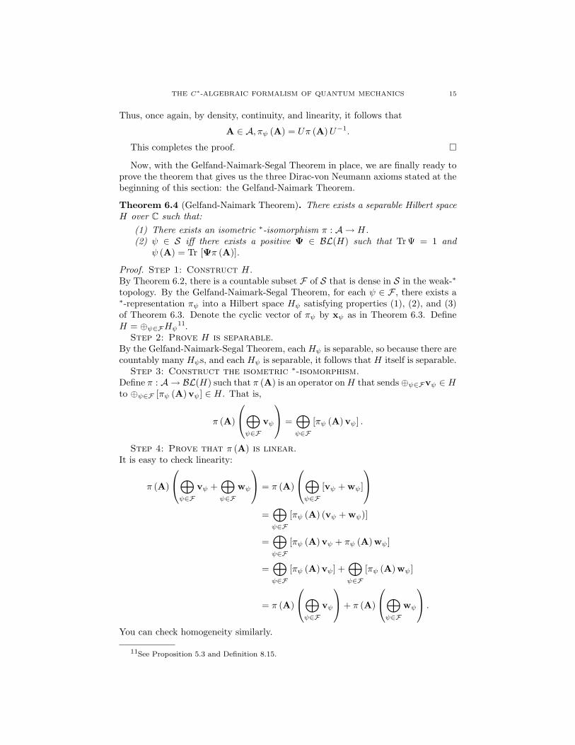
Thus, once again, by density, continuity, and linearity, it follows that
A ∈ A, πψ (A) = Uπ (A)U−1.
This completes the proof. �
Now, with the Gelfand-Naimark-Segal Theorem in place, we are finally ready toprove the theorem that gives us the three Dirac-von Neumann axioms stated at thebeginning of this section: the Gelfand-Naimark Theorem.
Theorem 6.4 (Gelfand-Naimark Theorem). There exists a separable Hilbert spaceH over C such that:
(1) There exists an isometric ∗-isomorphism π : A → H.(2) ψ ∈ S iff there exists a positive Ψ ∈ BL(H) such that TrΨ = 1 and
ψ (A) = Tr [Ψπ (A)].
Proof. Step 1: Construct H.By Theorem 6.2, there is a countable subset F of S that is dense in S in the weak-∗
topology. By the Gelfand-Naimark-Segal Theorem, for each ψ ∈ F , there exists a∗-representation πψ into a Hilbert space Hψ satisfying properties (1), (2), and (3)of Theorem 6.3. Denote the cyclic vector of πψ by xψ as in Theorem 6.3. DefineH = ⊕ψ∈FHψ
11.Step 2: Prove H is separable.
By the Gelfand-Naimark-Segal Theorem, each Hψ is separable, so because there arecountably many Hψs, and each Hψ is separable, it follows that H itself is separable.
Step 3: Construct the isometric ∗-isomorphism.Define π : A → BL(H) such that π (A) is an operator onH that sends⊕ψ∈Fvψ ∈ Hto ⊕ψ∈F [πψ (A)vψ] ∈ H. That is,
π (A)
⊕ψ∈F
vψ
=⊕ψ∈F
[πψ (A)vψ] .
Step 4: Prove that π (A) is linear.It is easy to check linearity:
π (A)
⊕ψ∈F
vψ +⊕ψ∈F
wψ
= π (A)
⊕ψ∈F
[vψ + wψ]
=⊕ψ∈F
[πψ (A) (vψ + wψ)]
=⊕ψ∈F
[πψ (A)vψ + πψ (A)wψ]
=⊕ψ∈F
[πψ (A)vψ] +⊕ψ∈F
[πψ (A)wψ]
= π (A)
⊕ψ∈F
vψ
+ π (A)
⊕ψ∈F
wψ
.
You can check homogeneity similarly.
11See Proposition 5.3 and Definition 8.15.
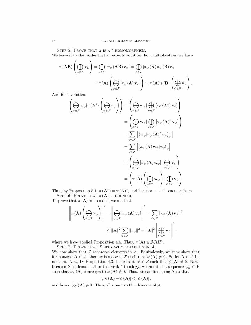
16 JONATHAN JAMES GLEASON
Step 5: Prove that π is a ∗-homomorphism.We leave it to the reader that π respects addition. For multiplication, we have
π (AB)
⊕ψ∈F
vψ
=⊕ψ∈F
[πψ (AB)vψ] =⊕ψ∈F
[πψ (A)πψ (B)vψ]
= π (A)
⊕ψ∈F
[πψ (A)vψ]
= π (A)π (B)
⊕ψ∈F
vψ
.
And for involution:⊕ψ∈F
wψ|π (A∗)
⊕ψ∈F
vψ
=
⊕ψ∈F
wψ|⊕ψ∈F
[πψ (A∗)vψ]
=
⊕ψ∈F
wψ|⊕ψ∈F
[πψ (A)∗ vψ
]=∑ψ∈F
[(wψ|πψ (A)∗ vψ
)ψ
]=∑ψ∈F
[(πψ (A)wψ|vψ)ψ
]
=
⊕ψ∈F
[πψ (A)wψ] |⊕ψ∈F
vψ
=
π (A)
⊕ψ∈F
wψ
|⊕ψ∈F
vψ
Thus, by Proposition 5.1, π (A∗) = π (A)∗, and hence π is a ∗-homomorphism.
Step 6: Prove that π (A) is boundedTo prove that π (A) is bounded, we see that∥∥∥∥∥∥π (A)
⊕ψ∈F
vψ
∥∥∥∥∥∥2
=
∥∥∥∥∥∥⊕ψ∈F
[πψ (A)vψ]
∥∥∥∥∥∥2
=∑ψ∈F
‖πψ (A)vψ‖2
≤ ‖A‖2∑ψ∈F
‖vψ‖2 = ‖A‖2∥∥∥∥∥∥⊕ψ∈F
vψ
∥∥∥∥∥∥2
,
where we have applied Proposition 4.4. Thus, π (A) ∈ BL(H).Step 7: Prove that F separates elements in A.
We now show that F separates elements in A. Equivalently, we may show thatfor nonzero A ∈ A, there exists a ψ ∈ F such that ψ (A) 6= 0. So let A ∈ A benonzero. Now, by Proposition 4.3, there exists ψ ∈ S such that ψ (A) 6= 0. Now,because F is dense in S in the weak-∗ topology, we can find a sequence ψn ∈ Fsuch that ψn (A) converges to ψ (A) 6= 0. Thus, we can find some N so that
|ψN (A)− ψ (A)| < |ψ (A)| ,and hence ψN (A) 6= 0. Thus, F separates the elements of A.

THE C∗-ALGEBRAIC FORMALISM OF QUANTUM MECHANICS 17
Step 8: Prove that π is injective.Because π is linear, to prove π is injective, it suffices to show that π (A) = 0 impliesA = 0. So suppose π (A) = 0. This implies that each πψ (A) = 0. We proceedby contradiction: suppose A 6= 0. Then, because F separates the elements of A,there is some ψ ∈ F such that
0 6= ψ (A) = (xψ|πψ (A)xψ) = (xψ|0) = 0 :
a contradiction. Thus, π is injective, and hence π : A → π (A) is a ∗-isomorphism.Step 8: Prove that φ is an isometry.
Because π is a ∗-isomorphism, by Proposition 4.4, ‖π (A)‖ = ‖A‖. Thus, π (A) is aC∗-subalgebra of BL(H), with H separable, and π : A → π (A) is an ∗-isomorphicisometry.
Step 9: Prove (2).It is easy to verify that if Ψ ∈ BL(H) is positive TrΨ = 1, then Tr [Ψπ (A)] definesa state on A. To prove the other direction, let ψ ∈ S and let ψn be a sequence in Fconverging to ψ in the weak-∗ topology. Now, for each ψn, define Ψn ∈ BL(H) suchthat Ψn maps every vector in Hφ for φ ∈ F not equal to ψn to 0 and agrees withthe positive operator given in (2) of the Gelfand-Naimark-Segal Theorem on Hψn
.It is easy to check that Ψn is positive, TrΨn = 1, and Tr [Ψnπ (A)] = ψn (A).Thus, if we define Ψ to be the limit of Ψn, we have that
ψ (A) = limψn (A) = Tr [Ψnπ (A)] = Tr [Ψπ (A)] .
Similarly, we also have that TrΨ = 1 and that Ψ is positive.This completes the proof. �
Thus, finally, we have proven, from our C∗-algebraic axioms of quantum me-chanics given in Axioms 3.1 and 3.2, that: to every quantum system there is anassociated separable Hilbert space, the observables are the self-adjoint operators onthis space, and that the states are positive operators of trace 1.
7. Closing Comments
A little should be said about this last statement, namely, the identification ofstates with positive operators of trace 1, as this is not the typical formulation ofstates. Although we do not have room to do so here, one can define the notion ofa pure state, and then, prove that every pure state is a projection operator onto aone dimensional subspace. Thus, we can identify the pure states with elements inthe Hilbert space, that is, we identify the pure state with the element in the Hilbertspace of norm 1 contained in the one dimensional subspace the operator projectsonto. This is the usual presentation of states in quantum mechanics; however, as itturns out, the manner of looking at states in the Hilbert space formulation given inStatement 6.3 is more mathematically convenient, and essentially the same as theusual presentation when the state is a pure state.
The reader should take note that this is far from a complete treatment. For onething, there are still three other Dirac-von Neumann axioms (see [14], pgs. 66-73)that need to be proven from equivalent axioms in terms of C∗-algebra. In fact, it isclear from their statement, that we will actually need to assume more than we have ifwe wish to prove them. This, however, should not be seen as a problem. One shouldnot expect to be able to derive all of quantum mechanics from two relatively simpleaxioms. However, I personally know of no natural axioms (although I’m sure they
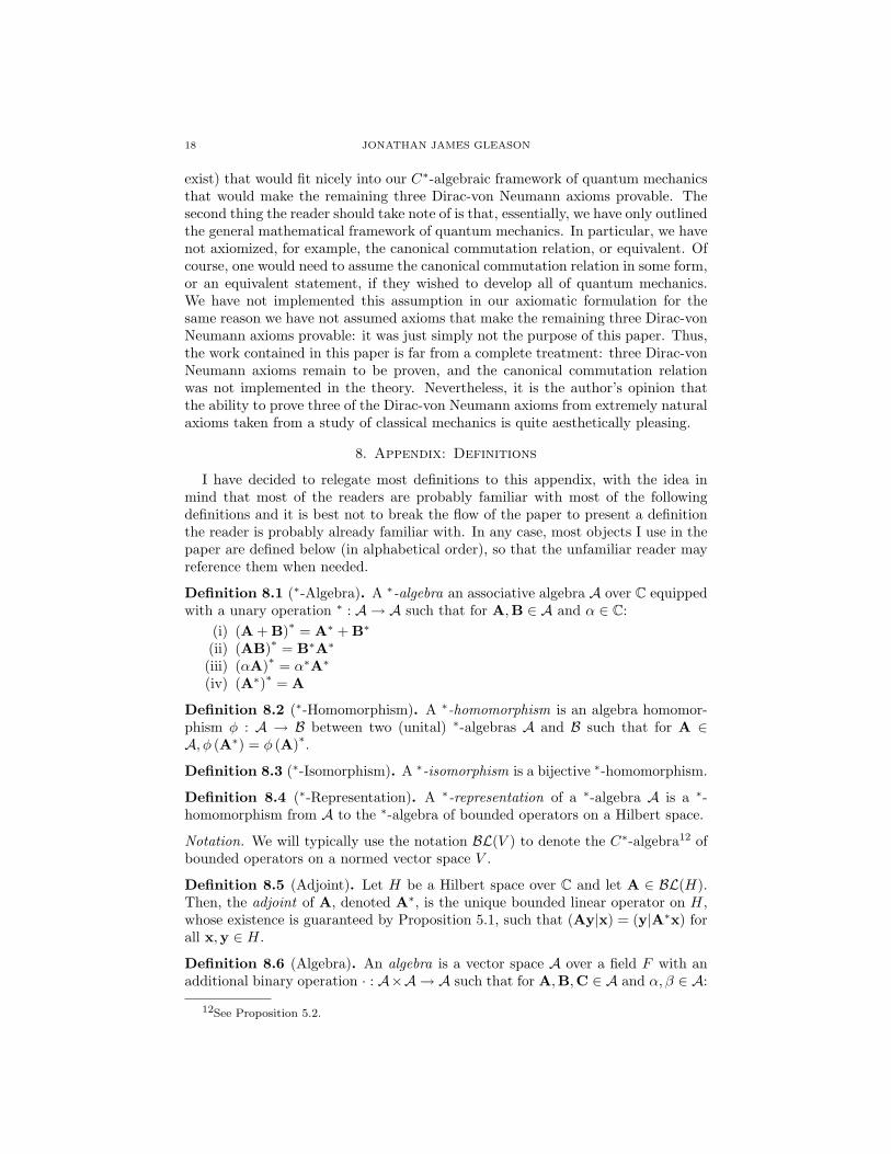
18 JONATHAN JAMES GLEASON
exist) that would fit nicely into our C∗-algebraic framework of quantum mechanicsthat would make the remaining three Dirac-von Neumann axioms provable. Thesecond thing the reader should take note of is that, essentially, we have only outlinedthe general mathematical framework of quantum mechanics. In particular, we havenot axiomized, for example, the canonical commutation relation, or equivalent. Ofcourse, one would need to assume the canonical commutation relation in some form,or an equivalent statement, if they wished to develop all of quantum mechanics.We have not implemented this assumption in our axiomatic formulation for thesame reason we have not assumed axioms that make the remaining three Dirac-vonNeumann axioms provable: it was just simply not the purpose of this paper. Thus,the work contained in this paper is far from a complete treatment: three Dirac-vonNeumann axioms remain to be proven, and the canonical commutation relationwas not implemented in the theory. Nevertheless, it is the author’s opinion thatthe ability to prove three of the Dirac-von Neumann axioms from extremely naturalaxioms taken from a study of classical mechanics is quite aesthetically pleasing.
8. Appendix: Definitions
I have decided to relegate most definitions to this appendix, with the idea inmind that most of the readers are probably familiar with most of the followingdefinitions and it is best not to break the flow of the paper to present a definitionthe reader is probably already familiar with. In any case, most objects I use in thepaper are defined below (in alphabetical order), so that the unfamiliar reader mayreference them when needed.
Definition 8.1 (∗-Algebra). A ∗-algebra an associative algebra A over C equippedwith a unary operation ∗ : A → A such that for A,B ∈ A and α ∈ C:
(i) (A + B)∗ = A∗ + B∗
(ii) (AB)∗ = B∗A∗
(iii) (αA)∗ = α∗A∗
(iv) (A∗)∗ = A
Definition 8.2 (∗-Homomorphism). A ∗-homomorphism is an algebra homomor-phism φ : A → B between two (unital) ∗-algebras A and B such that for A ∈A, φ (A∗) = φ (A)∗.
Definition 8.3 (∗-Isomorphism). A ∗-isomorphism is a bijective ∗-homomorphism.
Definition 8.4 (∗-Representation). A ∗-representation of a ∗-algebra A is a ∗-homomorphism from A to the ∗-algebra of bounded operators on a Hilbert space.
Notation. We will typically use the notation BL(V ) to denote the C∗-algebra12 ofbounded operators on a normed vector space V .
Definition 8.5 (Adjoint). Let H be a Hilbert space over C and let A ∈ BL(H).Then, the adjoint of A, denoted A∗, is the unique bounded linear operator on H,whose existence is guaranteed by Proposition 5.1, such that (Ay|x) = (y|A∗x) forall x,y ∈ H.
Definition 8.6 (Algebra). An algebra is a vector space A over a field F with anadditional binary operation · : A×A → A such that for A,B,C ∈ A and α, β ∈ A:
12See Proposition 5.2.
THE C∗-ALGEBRAIC FORMALISM OF QUANTUM MECHANICS 19
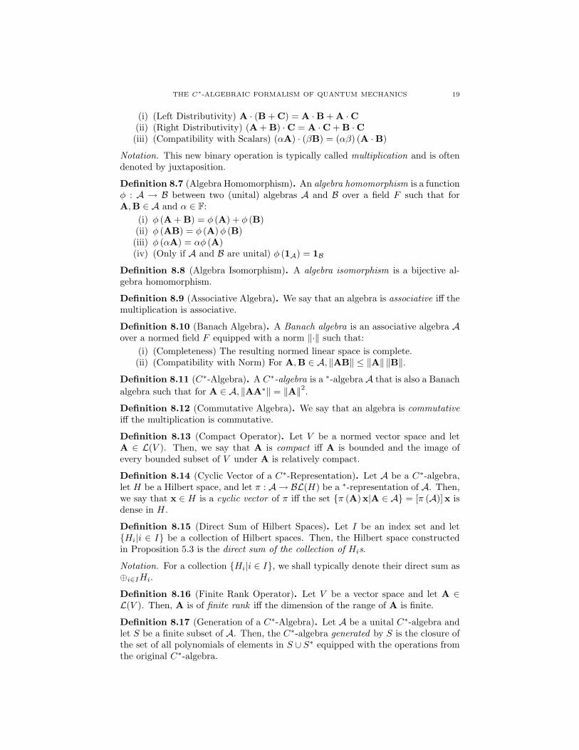
(i) (Left Distributivity) A · (B + C) = A ·B + A ·C(ii) (Right Distributivity) (A + B) ·C = A ·C + B ·C(iii) (Compatibility with Scalars) (αA) · (βB) = (αβ) (A ·B)
Notation. This new binary operation is typically called multiplication and is oftendenoted by juxtaposition.
Definition 8.7 (Algebra Homomorphism). An algebra homomorphism is a functionφ : A → B between two (unital) algebras A and B over a field F such that forA,B ∈ A and α ∈ F:
(i) φ (A + B) = φ (A) + φ (B)(ii) φ (AB) = φ (A)φ (B)(iii) φ (αA) = αφ (A)(iv) (Only if A and B are unital) φ (1A) = 1B
Definition 8.8 (Algebra Isomorphism). A algebra isomorphism is a bijective al-gebra homomorphism.
Definition 8.9 (Associative Algebra). We say that an algebra is associative iff themultiplication is associative.
Definition 8.10 (Banach Algebra). A Banach algebra is an associative algebra Aover a normed field F equipped with a norm ‖·‖ such that:
(i) (Completeness) The resulting normed linear space is complete.(ii) (Compatibility with Norm) For A,B ∈ A, ‖AB‖ ≤ ‖A‖ ‖B‖.
Definition 8.11 (C∗-Algebra). A C∗-algebra is a ∗-algebra A that is also a Banachalgebra such that for A ∈ A, ‖AA∗‖ = ‖A‖2.
Definition 8.12 (Commutative Algebra). We say that an algebra is commutativeiff the multiplication is commutative.
Definition 8.13 (Compact Operator). Let V be a normed vector space and letA ∈ L(V ). Then, we say that A is compact iff A is bounded and the image ofevery bounded subset of V under A is relatively compact.
Definition 8.14 (Cyclic Vector of a C∗-Representation). Let A be a C∗-algebra,let H be a Hilbert space, and let π : A → BL(H) be a ∗-representation of A. Then,we say that x ∈ H is a cyclic vector of π iff the set {π (A)x|A ∈ A} = [π (A)]x isdense in H.
Definition 8.15 (Direct Sum of Hilbert Spaces). Let I be an index set and let{Hi|i ∈ I} be a collection of Hilbert spaces. Then, the Hilbert space constructedin Proposition 5.3 is the direct sum of the collection of His.
Notation. For a collection {Hi|i ∈ I}, we shall typically denote their direct sum as⊕i∈IHi.
Definition 8.16 (Finite Rank Operator). Let V be a vector space and let A ∈L(V ). Then, A is of finite rank iff the dimension of the range of A is finite.
Definition 8.17 (Generation of a C∗-Algebra). Let A be a unital C∗-algebra andlet S be a finite subset of A. Then, the C∗-algebra generated by S is the closure ofthe set of all polynomials of elements in S ∪ S∗ equipped with the operations fromthe original C∗-algebra.

20 JONATHAN JAMES GLEASON
Definition 8.18 (Ideal of an Algebra). Let A be an algebra. We say that a subsetII ⊆ A is a left/right ideal iff I is a subspace of A (when considered just as avector space) and for A ∈ I and B ∈ A, BA ∈ I/AA ∈ I.
Definition 8.19 (Multiplicative Linear Functional). A multiplicative linear func-tional on an algebra A over C is a algebra homomorphism from A to C.
Definition 8.20 (Normal Element). Let A be a ∗-algebra and let A ∈ A. Then,we say that A is normal iff A commutes with A∗.
Definition 8.21 (Normalized). Let V be a normed vector space and let v ∈ V .Then, we say that v is normalized iff ‖v‖ = 1.
Definition 8.22 (Positivity of an Element of a ∗-Algebra). Let A be a ∗-algebra.Then, we say that A ∈ A is positive iff A = B∗B for some B ∈ A.
Definition 8.23 (Positivity of a Linear Functional). Let A be a ∗-algebra an letφ : A → C be a linear functional. Then, we say that φ is positive iff φ (A) ≥ 0 forall positive A ∈ A.
Definition 8.24 (Self-Adjoint). Let A be a ∗-algebra and let A ∈ A. Then, wesay that A is self-adjoint iff A = A∗.
Definition 8.25 (Spectrum). Let A be a unital algebra over C and let A ∈ A.Then, the spectrum of A, denoted σA (A), is the set of complex numbers λ suchthat A− λ1 is not invertible in A.
Notation. When it causes no confusion, we may omit the subscript on σA (A).
Definition 8.26 (State). Let A be a normed ∗-algebra and let ψ be a linearfunctional on A. Then, we say that ψ is a state iff ψ is positive and normalized.
Definition 8.27 (Trace). Let H be a separable inner product space and let A ∈L(H) be trace-class. By Proposition 5.4, H has a countable orthonormal basis{en|n ∈ N}. Then, the trace of A is defined as
∑n∈N (en|Aen), which is finite and
well-defined by Proposition 5.5.
Notation. For A ∈ L(H) trace-class, we denote the trace of A by TrA.
Definition 8.28 (Trace-Class). Let H be a separable inner product space and letA ∈ L(H). Then, we say that A is trace-class iff A = BC for Hilbert-Schmidtoperators B and C.
Definition 8.29 (Unital Algebra). We say that an algebra is unital iff there existsa multiplicative identity.
Acknowledgments. It is a pleasure to thank my mentors, Catalin Carstea,Thomasz Zamojski, and Brent Werness for their contributions to this paper, with-out which, it would not have been possible.
References
[1] Arnold, Douglas. Functional Analysis. 1997. Print.[2] Conway, John. A Course in Functional Analysis. New York: Springer-Verlag, 1990. Print.[3] Dunford, Nelson, and Jacob Schwartz. Linear Operators Part II: Spectral Theory. New York:
Interscience Publishing, 1963. Print.[4] Folland, Gerald. A Course in Abstract Harmonic Analysis. CRC-Press LLC, 1995. Print.
THE C∗-ALGEBRAIC FORMALISM OF QUANTUM MECHANICS 21
[5] Hassani, Sadri. Mathematical Physics: A Modern Introduction to Its Foundations. New York:
Springer Science and Business Media, Inc., 2006. Print.
[6] Lang, Serge. Complex Analysis. 4th. New York: Springer Science and Business Media, Inc.,1999. Print.
[7] Morris, Sidney. Topology Without Tears. 2001. Print.
[8] Munkres, James. Topology. 2nd. Upper Saddle River, New Jersey: Prentice Hall, 2000. Print.[9] Rudin, Walter. Functional Analysis. McGraw-Hill Book Company, 1973. Print.
[10] Rudin, Walter. Real and Complex Analysis. 3rd. McGraw-Hill Book Company, 1986. Print.
[11] Sally, Paul. Tools of the Trade: Introduction to Advanced Mathematics. Providence, RhodeIsland: American Mathematical Society, 2008. Print.
[12] Shankar, R.. Principles of Quantum Mechanics. 2nd. New York: Springer Science and Busi-
ness Media, Inc., 1994. Print.[13] Strocchi, F.. An Introduction to Quantum Mechanics: A Short Course for Mathematicians.
Toh Tuck Link, Singapore: World Scientific Publishing Co., 2005. Print.[14] Takhtajan, Leon. Quantum Mechanics for Mathematicians. American Mathematical Society,
2008. Print.
[15] Wassermann, A.. Functional Analysis. 1999. Print.