may 8, 2007 report 2 - exploratory case study on the...
TRANSCRIPT

May 8, 2007
Report 2 - Exploratory Case Study on the Value of Improving Soil Moisture
Forecast Information for Rangeland Management
Corona Range and Livestock Research Center Corona, NM

i
Report 2 - Exploratory Case Study on the Value of Improving Soil Moisture
Forecast Information for Rangeland Management
L. Allen Torell, Kirk C. McDaniel, and Brian H. Hurd
Executive Summary
Rainfall builds soil moisture that is either immediately available for plant production or is available for later use once temperatures warm and favorable growing conditions exist. When automated soil moisture recording devices became available in the early 1990s this greatly expanded the potential to quantify how range forage production is related to key environmental variables. Soil moisture probes coupled with automated recording devices have the potential to provide a continuous record (hourly and daily observations) of soil moisture conditions realized at various depths within the soil profile. Measuring and explaining annual variability in forage production will improve with time as soil moisture and grass yield data become increasingly available.
In this report we use soil moisture, rainfall, and temperature data to construct a forecast model for forage yield on the New Mexico State University (NMSU) Corona Ranch and then use the model to estimate the economic value of an accurate weather forecast for range livestock producers. Field data collected over a 17 year period illustrates the value of weather information for predicting grass growth over a growing season. Data from soil moisture (TDR) probes while only in the ground for 6 of the 17 years were shown to be significantly related to grass yield. NOAA simulated soil moisture also provided a satisfactory alternative to on-site soil moisture probes for predicting annual variations in grass yields.
Considering the rainfall history on the Corona Ranch and the linkages between rainfall and herbage production, a flexible, profit-maximizing stocking strategy is preferable to a constant stocking strategy when producers have reasonably accurate long-run (e.g., 6 month lead time) weather forecasts . Under the assumption of an accurate long-run weather forecast, we found that livestock producers who adopt a flexible strategy that fully utilizes herbaceous production during favorable years and avoids overstocking during bad years results in an added annual net return of about $2.60/ha ($1.05/acre). This was about $30,000 for the Corona Ranch. Improved weather forecasts have the potential to increase ranch returns by as much as 40% over levels obtained with a constant stocking rate that does not adjust to forage conditions.

ii
Acknowledgements
We acknowledge the financial support of the National Oceanic and Atmospheric
Administration (NOAA), and especially thank Drs. Rodney Weiher and Gary Carter of NOAA for their interest and support of this research. We would also like to thank Dr. Richard Adams of Oregon State University for his guidance and support throughout the project. Expressed thanks also go to Ken Pavelle, Mike Smith, and Victor Koren of NOAA’s Office of Hydrologic Development for their technical assistance and cooperation in preparing data and technical support. We thank Dr. Octavio Ramirez, New Mexico State University, for assistance with the multivariate analysis of rainfall and grass yield data. We acknowledge the New Mexico State University Agricultural Experiment Station for continued support of each of our research programs.

iii
Table of Contents
Introduction and Background .......................................................................................... 1 How Soil Moisture Information May Enhance Rangeland Decision Making .... 1 Factors Influencing Forage Forecasts ................................................................. 2 Measuring Soil Moisture..................................................................................... 3 Other Factors that Influence Forage Growth ...................................................... 3
Corona Ranch Exploratory Case Study ........................................................................... 4 Study Area and Procedures ................................................................................. 4 Setting ................................................................................................................. 4 Climate and Weather Information on the Corona Ranch .................................... 5
Temperature Data Summary ........................................................................... 6 Rainfall Data Summary ................................................................................... 6 Soil Moisture Data Summary.......................................................................... 8
NOAA Predicted Soil Moisture ..................................................................................... 10 Grass and Snakeweed Yield Collection Procedures and Data Summary ...................... 11 Relating Grass Yield to Rainfall and Soil Moisture ...................................................... 13
Rainfall Modeling ............................................................................................. 13 Rainfall and Grass Yield Distributions ............................................................. 14 Soil Moisture Modeling .................................................................................... 15
Model Specification ...................................................................................... 18 Soil Moisture Model Results ........................................................................ 21
The Economic Value of Precipitation and Weather Forecasts ...................................... 21 Economic Value of a Rainfall Event ................................................................ 24 Economic Value of an Accurate Weather Forecast .......................................... 27
Economic Model. .......................................................................................... 28 Corona Ranch Model Application. ............................................................... 30 Potential Value of Weather Forecasting and Speculative Technology Adoption. ...................................................................................................... 36
Conclusions .................................................................................................................... 37 Literature Cited .............................................................................................................. 38 Appendix A: Corona Ranch seasonal and annual rainfall amounts, 1914 – 2006 ......... 43 Appendix B: Recorded and simulated soil moisture measurements (% by Volume) at
the SH and OW research sites, recorded daily rainfall (mm) and end-of-season grass yield (kg/ha). ............................................................................................. 45

iv
List of Tables
Table 1. Gravimetric soil moisture comparison between hand samples taken on August
26, 2006 and on November 27, 2006 and automated recordings made at OW, SH, and Adams sites at these times. ............................................................................. 10
Table 2. Regression equation for estimating grass yield as a function of quarterly rainfall and level of snakeweed infestation. ...................................................................... 14
Table 3. Number of days during the growing season when NOAA simulated soil moisture reached alternative levels at the SH site. .............................................................. 19
Table 4. Number of days during the growing season when NOAA simulated soil moisture reached alternative levels at the OW site. ............................................................. 20
Table 5. Regression parameter estimates for grass yield equations using soil moisture measured at 10 cm. ............................................................................................... 22
Table 6. Regression parameter estimates for grass yield equations using soil moisture measured at 10 – 30 cm. ....................................................................................... 23
Table 7. Altered soil moisture categorizations with an additional 25.4 mm storm. ......... 24
Table 8. Selected equations, parameters, and assumptions used in valuing a perfect weather forecast. ................................................................................................... 31
Table 9. Net returns ($/ha) and grazing intensities with alternative stocking rate prescriptions for alternative price situations. ........................................................ 33
v
List of Figures
Figure 1. Weather stations and rain gauges located on the Corona Ranch. ........................ 5
Figure 2. Daily average minimum and maximum air temperature and average diurnal air temperature recorded at the SH and OW sites (July 17, 1990 - October 12, 2006).................................................................................................................................. 7
Figure 3. Average annual and growing season (April - October) rainfall recorded at the SH, OW and Adams sites (January 1990 - December 2006). ................................. 7
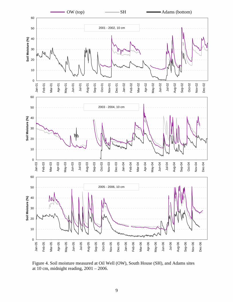
Figure 4. Soil moisture measured at Oil Well (OW), South House (SH), and Adams sites at 10 cm, midnight reading, 2001 - 2006. ............................................................... 9
Figure 5 shows average annual grass and snakeweed yield (kg/ha) measured on herbicide treated (T) and untreated (UT) areas at SH and OW sites, 1990 - 2006. .............. 12
Figure 6. PDF and CDF distributions for seasonal rainfall on the Corona Ranch. ........... 16
Figure 7. PDF and CDF distributions for grass yields on blue grama rangeland on the Corona Ranch........................................................................................................ 17
Figure 8. Estimated soil moisture (10 - 30 cm) in 2003 and 2005 and the result of a 25.4 mm rainfall event on April 1. ................................................................................ 25
Figure 9. Cumulative probability of receiving alternative levels of herbage production and the corresponding probability of receiving different returns per ha when following rigid and flexible stocking strategies. ................................................... 35

1
NMSU Corona Ranch Case-Study Examining the Relationship between Soil Moisture and Grass Yield
Introduction and Background Soil moisture modeling is of importance to rangeland managers because it directly
reflects plant growth potential. The amount of water stored in the soil at different depths through time coupled with soil temperature information is needed to determine when a particular plant species is apt to progress through its phenological stages of root, shoot, leaf and reproductive development. Every plant species possesses unique environmental requirements that are different from other species growing in the same plant community. Thus, while some plant species grow actively under relative cool moist conditions early in a season, others prefer warmer drier conditions later in a season.
How Soil Moisture Information May Enhance Rangeland Decision Making Livestock producers face uncertain weather conditions, and weather variability
causes major variation in the seasonal and annual amounts of forage produced. This variability is one of the most economically important types of risk that livestock producers face1. As noted by Bement (1969, p. 86), “In April, when the stocking rate decision is made, there is no way of knowing what kind of season is to follow. Wide yearly and seasonal fluctuations in forage production as well as annual and seasonal variations in forage quality will occur.”
The economic viability of rangeland-based livestock enterprises is critically affected by management’s ability to cope with climatic variability. Seasonal climate outlooks with lead times of up to 13 months are currently being disseminated (O’Lenic 1994, Mason et al. 1999). The basis for these outlooks is the substantial scientific advancements made in understanding the climate system and technology in the last part of the 20th century (Hill 2000). One area that has received little attention in the literature is how improved climate forecasts may influence rangeland management decisions. Precipitation and ultimately available soil moisture are recognized as the most important environmental factors determining annual forage production on non-irrigated rangelands (Vallentine 1990). Given the strong tie, stocking rate decisions could be greatly improved with better weather forecasts. With improved forecasts, grazers could better match the expected grazing capacity to actual realized forage conditions, and thus maximize current-year beef production and profit while minimizing resource damages that can occur with overgrazing. In a discussion piece, Stone (1994) states “ideally, grazers should be able to match stocking rates to seasonal conditions so that animal production is maximized and damage to a pasture and land production is minimized.” But, according to Ash et al. (2000), decision makers are reluctant to accept and use such forecasts. Stafford-Smith et al. (2000) concluded that current seasonal forecasts have some value but future developments promise to be even more valuable.
1/Other major risks include uncertain livestock prices, expenses and financial variables; possible destruction of forage by pests, disease, and brush and poisonous plant infestation; and potential soil and resource damage from poor stocking decisions and livestock distribution.

2
Factors Influencing Forage Forecasts The major factors that influence the economic value of seasonal climate forecasts
and soil moisture estimates for rangeland grazing purposes include precipitation variability, available soil moisture, soil holding capacity, wetting-front movement, plant growth characteristics, forage production potential, ecological site conditions, and the stocking rate decision making process. The relevance of each of these factors is discussed below. We focus on the potential economic value of soil moisture information for estimating plant growth on southwestern U.S. rangelands, in particular short and mixed grassland types. An in depth analysis of this topic, which is beyond the scope of this study, should be driven by site specific information taken across many different rangeland areas and types.
Precipitation and ultimately available soil moisture are recognized as the most important environmental factors determining annual forage production on non-irrigated rangelands (Vallentine 1990). Recognizing the importance of rainfall and soil moisture, numerous authors have attempted to relate herbaceous production to moisture conditions. Most of these studies have related peak standing herbaceous production to rainfall amounts realized over various months of the year, or the previous year (Nelson 1934, Sneva and Hyder 1962, Pieper et al. 1971, Cable 1975, McDaniel et al. 1993, Khumalo and Holechek 2005).
Storm frequency, seasonal timing of rainfall, and the types of forage species have all been found to be important for estimating plant productivity. This is because plant growth characteristics are genetically linked to physiological requirements that are ultimately driven by environmental conditions. Photosynthetic pathways among grass species, for example, are generally grouped by those species that maintain C4 or C3 modes of carbon assimilation. C3 species are often referred to as cool-season perennial grasses and produce the majority of their growth in the spring, particularly in northern climates. C4 species are referred to as warm-season species and produce the majority of their growth with summer rainfall, and are most common in southern climates. Corresponding to these physiological distinctions, spring precipitation amounts have been a good predictor of forage production in northern climates (Andales et al. 2006), whereas, summer rainfall predicts better in southern climates with predominately C4 grasses (Pieper et al. 1971, McDaniel et al. 1993).
Total rainfall which occurs during a year or growing season is but an indirect measure of soil moisture available for forage growth at key times. It is the periodicity, frequency, and magnitude of rainfall received over time above a minimal threshold that most influences plant productivity. Rainfall received evenly over the course of a growing season results in greater plant production than high rainfall events that occur only a few times. Thus, it is recognized that measured or simulated soil moisture potentially provides a better indicator of moisture conditions for rangeland planning purposes (Andales et al. 2006).
Soil moisture holding capacity relates to the amount of water potentially stored in the soil and is directly influenced by particle size (texture) and depth to an impervious layer. Sandy, coarse textured soils retain or hold water for shorter periods of time compared to finer textured loams and clays. Finer textured soils, which store larger amounts of water over longer periods of time, provide grazers more management flexibility. Wetting-front movement is also linked to soil texture as soil water moves

3
deeper and more rapidly through coarse particles than finer textures. Water movement, which flows principally by gravity, may be impaired whenever the flow region includes boundaries such as the soil surface, seepage faces, planes of symmetry, or actual layers that are effectively impermeable, such as heavy clays or coarse materials below the water-entry pressure (Ross et al. 1995). By considering site-specific soil characteristics (ecological sites) and by carefully monitoring current soil moisture levels and projecting future levels, rangeland managers can potentially project the expected magnitude and duration of plant growth. With this information stocking rate decision making can be made up to 6 to 9 months in advance (Bement 1969).
Measuring Soil Moisture Because of the laborious task of extracting periodic soil moisture samples using a
shovel and soil sampling tool, it is not surprising that few studies have directly evaluated the influence of soil moisture on range forage production. An early study relating forage production to soil moisture, Rogler and Haas (1947) considered the relationship between fall soil moisture and the subsequent year production of forage. Using eighteen years of data collected at the Northern Great Plains Field Station, Mandan, N.D., Rogler and Haas found highly significant correlation coefficients between forage yield and available soil moisture in the surface 3 feet (91 cm) and 6 feet (183 cm) of the soil profile.
Heitschmidt et al. (1999) measured soil moisture using lysimeters at 5 depths and over a four year period (1993 – 1996). They then related soil moisture levels to annual variation in forage production for C3 grasses in Montana and concluded, as others have, that for the Northern Great Plains, grazing is a secondary factor relative to drought in affecting ecosystem processes. They found grazing to have little effect on annual herbage production and were surprised to also measure minimal drought effects. They attributed this to the cool season, early maturing grasses found on the site and with the 1994 drought occurring late in the year after the annual forage production cycle had been completed.
Dahl (1963) found grass yield predictions could be improved by considering the quantity of available soil moisture and the depth of the moisture distribution. Dahl found that if a single factor was used to predict forage yield, soil moisture or depth of moist soil in the spring would be best. Results and management recommendations were similar to those of Cole and Mathews (1940) and Rogler and Haas (1947) that suggested using depth of wet soil as an approximation of water content in the soil, because of its practical measurement. Available soil moisture was considered to be a better predictor of forage yield, however.
How soil water is maintained within the soil profile is best understood with data provided by soil moisture probes placed at various depths below the surface. Simulated soil moisture data where soil characteristics, temperature and hourly rainfall amounts are used to predict hourly and daily changes in soil moisture provide another estimate of soil moisture and these predicted soil moisture levels also have potential for improved management decisions, as explored later in this report.
Other Factors that Influence Forage Growth In addition to available soil moisture, overstory woody canopies have been shown
to highly suppress understory grass production. Tree, brush, and weed overstory cover is

4
an important consideration when trying to predict understory productivity on both range and forest lands. In general, the relationship between herbaceous production and woody cover has been found to be a downward sloping curve that is either convex to the origin or S-shaped over the relevant range (Ffolliot and Clary 1972, Bartlett and Betters 1983). In certain situations when overstory cover is exceptionally high, soil moisture available for understory productivity is equivalent to drought conditions (McDaniel et al. 2000).
Corona Ranch Exploratory Case Study
Study Area and Procedures This case-study research was conducted at the New Mexico State University
Corona Range and Livestock Research Center (CRLRC or Corona Ranch). Two long-term study sites referred to as ‘South House’ and ‘Oil Well’, each within 8 ha enclosures and located about 10 km from one another were established on the Corona Ranch in mid-1990 by Dr. Kirk. C. McDaniel (Department of Animal and Range Science, New Mexico State University). Research to evaluate control alternatives for broom snakeweed (Gutierrezia sarothrae), including herbicide and fire treatments, has been conducted at the sites and has been partly reported previously in McDaniel et al. (1997 and 2000). Data collected from 1990 through 2006 includes automated weather data, and annual grass and snakeweed yield.
Setting The Corona Ranch is a working ranch located in Lincoln and Torrance counties,
New Mexico approximately 306 km northeast of Las Cruces and 13 km east of the village of Corona. The ranch covers approximately 11,381 ha (28,112 acres) in the north central part of Lincoln county and the southeast corner of Torrance county. The ranch is characterized by a semiarid, continental climate with wide ranges in diurnal and seasonal temperatures, variable but relatively low precipitation, and plentiful sunshine.
Hart (1992), Berry (1992), and Ebel (2006) provide detailed descriptions of the vegetation and soils found on the ranch and at the two specific study sites. Elevation is about 1875 m (6150 ft) at the South House (SH) site, and 1860 m (6100 ft) at the Oil Well (OW) site. Soil on both study sites are of the Taipa-Dean loam association, which are shallow and underlain by highly calcareous limestone bedrock. The Taipa loam is a fine-loamy, mixed, mesic, Ustollic Haplagrid, and Dean loam is a fine carbonatic, mesic Ustollic Calcioathid.
The Corona Ranch has two major plant communities or types of vegetation, blue grama (Bouteloua gracilis) grassland and pinyon-juniper woodland. The two research areas are located in the relatively productive blue grama grassland area which is composed mostly of warm season (C4) grasses. Broom snakeweed periodically invades the area and snakeweed was a major problem on the ranch when the study sites were established in 1990. Snakeweed infestations have remained relatively low since 1994 when a natural die-off of this cyclic weed occurred. Other common plants at the study sites that are desired for grazing by livestock include winterfat (Ceratoides lanata [Pursh.] J.T. Howell), wolftail (Lycurus phleoides [H.B.K.], sand dropseed (Sporobofus cryptundrus [Torr.] A. Gray), squirreltail (Elymus longifolius [Smith] Gould), and

5
threeawns (Aristida spp.). Cholla (Opunita imbricata [Haw.] DC.) and various weeds are common on the sites but are not usually selected by grazing animals.
Climate and Weather Information on the Corona Ranch Weather data for the Corona Ranch are available from multiple sources including
4 instrumented stations, and 8 rainfall gauges scattered at various locations across the ranch (Figure 1). Instrumented recording locations are referred to as Oil Well (OW), South House (SH), New Mexico Climate Center (NMCC), and the NRCS-Scan site (Adams site). Data for the last two recording stations are available online (NMCC 2006, NRCS 2006).
The primary weather related data used in this study to examine plant growth was recorded at the SH and OW study sites. Weather data was recorded using Campbell Scientific instruments and included one minute readings averaged to hourly measurements for precipitation; air temperature; soil temperature at 10 cm (~4 inches) and 50 cm (~20 inches); relative humidity; wind speed and direction; and soil moisture at 10 cm (~4 inches) and between 10 cm and 30 cm (~12 inches). Approximately 85% of the elapsed hours over the July 1990 through December 2006 period had climatic data successfully recorded by the automated recorders at both sites. When rainfall or temperature data from one site was missing then data from the other site was substituted into the database. When weather data was missing from both sites then data was substituted into the database from the NMSU Climate Center Network (NMCC) recorder located at the North Camp facility. Data from NOAA Ramon and Corona 10SW sites
Figure 1. Weather stations and rain gauges located on the Corona Ranch.

6
were also used to fill in missing data during the early 1990s. With these substitutions an Access™ database was built with a complete daily record of rainfall amounts over the period July 17, 1990 through 2006. Hourly estimates are provided over most days for both the SH and OW sites. This database was provided to NOAA hydrologists and hourly temperature and rainfall data were used to simulate soil moisture on the ranch.
Soil volumetric water content (volume of water per volume of soil) was recorded at the SH and OW sites using time domain reflectory (TDR) soil moisture probes (CS 615-L, Campbell Scientific Inc., Logan, UT, 1996). Two TDR probes were buried in the same configuration at each site. One probe was placed horizontally into the soil profile at a 10 cm depth whereas the second probe was positioned vertically at a 10-30 cm depth. Instrument readings were taken at one minute intervals and averaged hourly.
Automated Soil Climate Analysis Network (SCAN) sites, like the Adams site maintained by the Natural Resources Conservation Service (NRCS), collect soil moisture, soil temperature, precipitation, wind, and solar radiation data. These stations are located throughout the United States and other global locations and the data is used for the management and prediction of climatic issues affecting natural resources. The Adams site facility records hourly with soil moisture measured at 5 cm (2 inches), 10 cm (4 inches), 20 cm (8 inches), 51 cm (20 inches), and 101 cm (40 inches) (NRCS 2006). A TDR Hydra-Probe II was used for recording soil moisture (Stevens Water Monitoring Systems 2006). Though the Adams site was initiated in 1994, rainfall measurements appear to be complete and accurate only after October 2003. Only partial valid soil moisture measurements were recorded from 1997 to 2003.
Temperature Data Summary. Over the study period, average daily maximum air temperature on the ranch, recorded at the SH and OW sites, was 9°C (48°F) during December-January and 29°C (84°F) in July. Average daily minimum air temperature was -4°C (25°F) during December-January and 14°C (57°F) in July. The frost-free period is about 214 days, from April 1 to late-October or early-November. Perhaps more important for range forage production, an approximate 10°C is considered a critical minimum temperature for growth of blue grama (Stubbendieck and Burzlaff 1970), the predominant forage species found on the Corona Ranch. As shown in Figure 2, average daily diurnal air temperatures begin to consistently exceed 10°C near the first of April and remain above this threshold until early-November. This suggests an average growing season that is favorable for warm-season grass growth to be about 7 months in length, (i.e. April – November), similar to the frost-free period.
Rainfall Data Summary. Rainfall on the Corona Ranch exhibits a seasonal pattern with a wet season during the third quarter. The seasonality of rainfall is apparent in Figure 3 with the 7-month growing season usually providing the majority of annual rainfall. The average 325 mm of annual rainfall realized over the 17-year study period was below the long-term (1914-2006) average for the Corona, NM area (370 mm) (Appendix A). Growing season rainfall totals for the 1990 to 2006 period averaged 261 mm as compared to a 283 mm long-term average.
A 5-year drought occurred on the Corona Ranch from late 1999 through 2003 with growing season rainfall well below average for most of these years. Because of the resulting lack of forage growth, the ranch was largely de-stocked in 2001 with some re-stocking during 2004.

14
24
34
44
54
64
74
84
94
Jan Feb Mar Apr May Jun Jul Aug Sep Oct Nov Dec
Month
Air
Tem
pera
ture
( F)
-10
-5
0
5
10
15
20
25
30
35
Air
Tem
pera
ture
( C
)
Minimum
Maximum
Diurnal
Figure 2. Daily average minimum and maximum air temperature and average diurnal air temperature recorded at the SH and OW sites (July 17, 1990 – October 12, 2006).
0
2
4
6
8
10
12
14
16
18
20
90 91 92 93 94 95 96 97 98 99 00 01 02 03 04 05 06Year
Prec
ipita
tion
(inch
es)
0
50
100
150
200
250
300
350
400
450
500
Prec
ipita
tion
(mm
)
Winter
Growing Season Average
Annual Average
Growing Season
Figure 3. Average annual and growing season (April – October) rainfall recorded at the SH, OW and Adams sites (January 1990 - December 2006).
7

8
Unlike other regions, such as in Australia (Stone 1994), where weather patterns are reportedly cyclic and have wet and dry years that tend to go together. The Corona Ranch exhibits no apparent cyclic weather pattern. Efforts to predict next year’s rainfall using previous year rainfall conditions was unsuccessful. We found over the 1914-2006 period there was an insignificant correlation (P = 0.60) between growing season rainfall from one year to the next.
Soil Moisture Data Summary. Figure 4 shows midnight volumetric soil water content measurements recorded at the SH, OW and Adams sites over the 2001 – 2006 period. Given the close proximity of the study sites (Figure 1) a similar pattern of soil moisture was recorded across sites. Only on rare occasions did a particular storm provide a higher record of soil moisture at one site compared to another.
Each weather station had periodic recording problems with some gaps in the data. Data shown in Figure 4 are only from probes set horizontally into the soil profile at a 10 cm depth. Appendix B provides additional detail about soil moisture measurements recorded at both the 10 cm and the 10 – 30 cm depths at SH and OW. Additional detail and comparisons are also made with NOAA-simulated soil moisture measurements (described below) over the 1991 to 2006 period. Daily rainfall (mm) and end-of-season measurements of grass yield (kg/ha) are also shown in the Appendix B graphs.
When TDR probes were installed at the SH and OW sites they were commonly calibrated at the factory and as such, they provided in-the-field readings that are scaled differently. At the 10 cm depth, the OW probe consistently recorded about 20% higher than the SH probe. At the 10 – 30 cm depth the SH probe consistently recorded about 6% higher than the OW probe. The readings reported for OW site have been adjusted by these levels and are scaled similar to the SH site. With this adjustment, the range in OW and SH readings were similar, from about 10% for very dry soils to about 55% for saturated soils (Figure 4). This is near the same range previously estimated by Berry (1992) using pressure plate tests (7% to 51%) to determine volumetric water content of the soils at SH and OW sites.
Soil moisture recorded at the Adams site has a daily pattern similar to that of SH and OW (Figure 4), but readings are consistently lower and give a narrower range in value. The Adams site used a Hydra Probe II sensor manufactured by Stevens Water Monitoring Systems (2006) whereas Campbell Scientific TDR probes were installed at SH and OW sites. Given the observed inconsistencies between probes among sites, an on-site calibration analysis was conducted to determine in-situ gravimetric soil moisture on August 26, 2006 and again on November 27, 2006. Three soil samples were taken at the two alternative probe depths near the OW and SH weather stations. Using a soil bulk density sampling probe to extract each soil sample, the contents was placed in a separate plastic bag and immediately weighed in the field. Samples were later oven dried at 60°C for 48 hours then reweighed to compute soil moisture for the volume of soil removed. As shown in Table 1, recorded soil moisture levels at the SH and OW weather stations were much higher than the two hand sample estimates. The recordings at the Adams site were very similar to the hand samples. Recordings at all three sites were within the range of soil moisture estimates that would be expected from the pressure tests conducted on Corona soils by Berry (1992). Recorders at all three sites, while scaled differently (Figure 4), give a consistent index of relative soil wetness and dryness.
0
10
20
30
40
50
60
Jan-
01
Feb-
01
Mar
-01
Apr
-01
May
-01
Jun-
01
Jul-0
1
Aug
-01
Sep
-01
Oct
-01
Nov
-01
Dec
-01
Jan-
02
Feb-
02
Mar
-02
Apr
-02
May
-02
Jun-
02
Jul-0
2
Aug
-02
Sep
-02
Oct
-02
Nov
-02
Dec
-02
Soil
Moi
stur
e (%
)2001 - 2002, 10 cm
0
10
20
30
40
50
60
Jan-
03
Feb-
03
Mar
-03
Apr
-03
May
-03
Jun-
03
Jul-0
3
Aug
-03
Sep
-03
Oct
-03
Nov
-03
Dec
-03
Jan-
04
Feb-
04
Mar
-04
Apr
-04
May
-04
Jun-
04
Jul-0
4
Aug
-04
Sep
-04
Oct
-04
Nov
-04
Dec
-04
Soil
Moi
stur
e (%
)
2003 - 2004, 10 cm
0
10
20
30
40
50
60
Jan-
05
Feb-
05
Mar
-05
Apr
-05
May
-05
Jun-
05
Jul-0
5
Aug
-05
Sep
-05
Oct
-05
Nov
-05
Dec
-05
Jan-
06
Feb-
06
Mar
-06
Apr
-06
May
-06
Jun-
06
Jul-0
6
Aug
-06
Sep
-06
Nov
-06
Dec
-06
Soil
Moi
stur
e (%
)
2005 - 2006, 10 cm
Figure 4. Soil moisture measured at Oil Well (OW), South House (SH), and Adams sites at 10 cm, midnight reading, 2001 – 2006.
OW (top) SH Adams (bottom)
9

10
Table 1. Gravimetric soil moisture comparison between hand samples taken on August 26, 2006 and on November 27, 2006 and automated recordings made at OW, SH, and Adams sites at these times.
Site Depth DateOW 10 cm 26-Aug-06 44% 21%SH 10 cm 26-Aug-06 38% 21%Adams 10 cm 26-Aug-06 22% 21%
OW 10 -30 cm 26-Aug-06 45% 21%SH 10 -30 cm 26-Aug-06 48% 21%Adams 10 -30 cm 26-Aug-06 18% 21%OW 10 cm 27-Nov-06 37% 19%SH 10 cm 27-Nov-06 32% 19%Adams 10 cm 27-Nov-06 21% 19%OW 10 -30 cm 27-Nov-06 36% 18%SH 10 -30 cm 27-Nov-06 37% 18%Adams 10 -30 cm 27-Nov-06 17% 18%
Automated Recording Hand Sample
NOAA Predicted Soil Moisture Using the database defining hourly rainfall and temperature data recorded for the
SH and OW sites, NOAA personnel estimated (simulated) soil moisture at the SH and OW study sites using a modified Sacramento soil moisture accounting model (SAC-SMA). The model uses a conceptualization of the rainfall-runoff process and simulates water content at two soil storage levels (a thin upper level and thicker lower level). The estimates are uniquely defined based on soil properties such as porosity, field capacity, wilting point, and hydraulic conductivity. The Sacramento Catchment Model expands on the basic water balance equation: Runoff = Rainfall – Evapotranspiration – Changes in soil Moisture (Burnash 1995). Each soil layer consists of tension and free water storages that interact to generate soil moisture states and runoff components. The SAC-SMA application was calibrated to the soils of the Corona Ranch using soils information described by Berry (1992).
Appendix B includes plots of the NOAA-simulated soil moisture estimates for the OW and SH site at both the 10 cm and 10 – 30 cm depths, as compared to the observed values starting in 2001. NOAA-simulated values for earlier years (1991 – 2000) are also shown in the graphs. NOAA simulated soil moisture at the two depths were nearly identical when low soil moisture levels existed and they were about 2% less at the 10 – 30 cm depth when soil moisture levels were above 25%.
Comparing simulated versus observed soil moisture levels for the study sites indicates a very consistent daily pattern and level of soil moisture. The estimated correlation coefficient between the observed and simulated 10 cm series was 0.88 at the

11
SH site and 0.81 for the OW site. The estimated correlation coefficient for the 10 – 30 cm probes were lower, 0.75 at the SH site and 0.76 at the OW site. The consistency of the NOAA simulated soil moisture levels versus actual recorded values suggests potential for using rainfall and temperature data to simulate soil moisture conditions at rangeland sites.
Grass and Snakeweed Yield Collection Procedures and Data Summary An increased canopy of brush is detrimental to understory grass growth and
broom snakeweed has been a periodic problem on the Corona Ranch. To explore overstory/understory relationships and to investigate efficient control measures, various broom snakeweed control treatments were implemented at the SH and OW sites beginning in 1990. Vegetation response to treatments was measured every year in late fall through 2006 (Hart 1992, Carroll 1994 and Ebell 2006). Standing crop estimates of grass, forbs, and snakeweed yield were made in ten 31.5 cm by 61 cm quadrats placed on permanently marked stakes located along each of two transects in 95 individual 0.1 acre research plots. Sampling was done each year from mid-October to mid-November. Ebel (2006) provides additional detail about the double sampling procedure used. Majumdar (2006, Appendix B) provides a detailed listing of the grass and snakeweed yield estimates by year, site, treatment, and plot, excluding 2006 data which was recorded later2.
Only control plots and those treated by herbicide spraying (treatment numbers 0, 3, 6, and 10 in the Majumdar appendix) were included in this case study. Standing crop (yield) estimates totaled 384 kg/ha across both sites (i.e. averaged over 10 frames per plot per year, and with samples taken every year from 1990 through 2006).
Figure 5 shows the average grass and snakeweed yield (kg/ha) by year. No significant differences were found between study sites. In 1990 snakeweed yield and density was at a level considered detrimental to grass yield. Herbicide treatments resulted in an immediate reduction in snakeweed yield and subsequent increase in grass yield. As the study progressed snakeweed declined from natural mortality resulting in little difference in snakeweed yield on treated and untreated areas after 1994. Average grass yield over the 17 year study on untreated areas was 651 kg/ha (standard deviation, s.d. = 412). Below average rainfall received from 1999 to 2003 is clearly reflected in reduced average grass yield, ranging from less than 200 kg/ha in 2000 and 2001 at the OW site to nearly 1,400 kg/ha in 1998 at the SH site (Figure 5).
It should be noted that standing crop grass estimates represent yield at the end of the growing season. Standing crop yield does not capture total production which is plant growth through time. Peak standing crop for blue grama rangelands is estimated to occur earlier in the year in August or September, and while variable, peak estimates will be 30% to 40% more than the end-of-season estimates presented in Figure 5 (Turner and Klipple 1952, Pieper et al. 1974) This distinction is important because grass growth is actually dynamic throughout a growing season and standing crop yield does not capture total plant productivity. Plants subject to excessive herbivory or disturbance, for example, can bias standing crop estimates. Grazing or plant material lost to trampling etc. is lost productivity that is not accounted for when making standing crop estimates. An
2/An error was also found and corrected in the 1998 data. The soil moisture factor used to adjustment grass yield to a dry-weight basis was improperly recorded at 93% in the dataset reported by Majumdar (2006) for 1998 and this error was corrected to the recorded 80%.

0
200
400
600
800
1,000
1,200
1,400
1,600
TU
T TU
T TU
T TU
T TU
T TU
T TU
T TU
T TU
T TU
T TU
T TU
T TU
T TU
T TU
T TU
T TU
T
1990 1991 1992 1993 1994 1995 1996 1997 1998 1999 2000 2001 2002 2003 2004 2005 2006
Gra
ss a
nd S
nake
wee
d Yi
eld
(Kg/
ha)
Grass Yield Snakeweed Yield
SH Site
0
200
400
600
800
1,000
1,200
1,400
TU
T TU
T TU
T TU
T TU
T TU
T TU
T TU
T TU
T TU
T TU
T TU
T TU
T TU
T TU
T TU
T TU
T
1990 1991 1992 1993 1994 1995 1996 1997 1998 1999 2000 2001 2002 2003 2004 2005 2006
Gra
ss a
nd S
nake
wee
d Yi
eld
(Kg/
ha)
OW Site
Figure 5. Average annual grass and snakeweed yield (kg/ha) measured on herbicide treated (T) and untreated (UT) areas at the SH and OW sites, 1990 – 2006.
12

13
additional bias with standing crop estimates that must be considered is that carryover grass produced in a prior year may be included in current year estimates. This error is most likely to occur when grass yield data is gathered in a drought year that was preceded by a particularly wet or productive year.
Relating Grass Yield to Rainfall and Soil Moisture As noted above, seasonal rainfall amounts have been used to predict herbaceous
yield for both warm and cool season grasses. A relevant question is can soil moisture data be substituted for seasonal rainfall amounts to accomplish and improve upon the prediction objective? To examine this question we first compare grass yield and rainfall data from 1990 to 2006. We then evaluate potential model improvements using soil moisture data. Rainfall Modeling
Various functional forms and combinations of monthly rainfall amounts were initially considered to estimate the relationship between annual grass yield and seasonal rainfall. Grass yield, snakeweed yield, and quarterly rainfall at the OW and SH sites were used in the final analysis. SAS™ software diagnostics did not indicate a problem with multicollinearity, but an unequal variance (heteroscedasticity) across years was problematic. Thus, White’s heteroscedasticity-corrected variances and covariances were used for hypothesis testing.
We considered an increased amount of broom snakeweed to be detrimental to grass growth and included snakeweed yield (kg/ha) in the model in natural log form (LNGUSAt). A minimum of 1 kg/ha of snakeweed was assumed to be present on an experimental plot so as to avoid errors that occur in taking logs when zero amounts occur. With the log specification, broom snakeweed is defined to suppress grass yield at a decreasing rate, similar to the shape observed for numerous brush species including broom snakeweed (McDaniel et al. 1993, Ffolliot and Clary 1972). The -33.96 parameter estimate (Table 2) indicates that a 1% increase in snakeweed yield decreased grass yield by about 0.34 kg/ha.
We initially considered rainfall amounts during Q4 (Oct, Nov, Dec) of the previous year and Q1 to Q3 (Jan through Sep.) rainfall amounts during the current year as separate explanatory variables in the regression model. Parameter estimates of 1.82 and 1.52 for Q4t-1 and Q1t were not statistically different (P = 0.66) and thus combined to a WINTER variable in the final model (Table 2). Rainfall during this winter period can conceptually increase the level of soil moisture available once temperatures warm and herbaceous growth begins.
Added rainfall during the third quarter (Q3) resulted in the largest increase in grass yield, as would be expected with the C4 grasses found at the study sites. During this quarter each mm of rainfall added an estimated 2.22 kg/ha of grass (Table 2). This was statistically more than the 0.86 kg/ha added during Q2t (P = 0.0001) but not the 1.75 kg/ha added with winter precipitation (P=0.05). It was somewhat surprising that β1 exceeded β2 (P=0.001). It was anticipated that the rainfall beta coefficients would increase as the growing season progressed, or that Q2 and Q3 parameter estimates would be the same. Contrary to the results obtained here, others have found winter rainfall to be

14
Table 2. Regression equation for estimating grass yield as a function of quarterly rainfall and level of snakeweed infestation.
Para-meter Variable Mean ± Std Variable Description
Parameter Estimate
Consistent Standard
Error t-valueβ0 Intercept Model intercept 129.88 37.18 3.49β1 WINTER 91.1 ± 68.6 Amount of rainfall (mm)
received during quarter 4 of previous year or quarter 1 of this year
1.75 0.21 8.45
β2 Q2 76.4 ± 49.6 Amount of rainfall (mm) received during quarter 2
0.86 0.33 2.64
β3 Q3 161 ± 77.7 Amount of rainfall (mm) received during quarter 3
2.22 0.17 13.24
β4 LNGUSA 1.8 ± 2.5 Natural log of broom snakeweed weight (kg/ha)
-33.96 5.73 -5.93
R2 0.31n 383Mean ± Std of dependent variable (Grass Yield, kg/ha) 651 ± 355Root mean square error 295
Note: All parameters were statistically significant at the 0.01 level or higher.
statistically insignificant on southwestern rangelands (Pieper et al. 1971, McDaniel et al. 1993).
Measured grass yield was quite variable with an estimated R2 for the model of only 31%. There was not a systematic difference in yield by study site when a dummy variable for site was included in the model (P = 0.46). However, residual plots indicated predicted grass yields tended to be over predicted especially during some years that were preceded by drought conditions (1991, 1994, 2001), and under predicted during other years that were preceded by relatively wet years (1993, 1998, 2006).
Rainfall and Grass Yield Distributions As noted by Sneva and Hyder (1962), precipitation frequency distributions for
semiarid and arid regions are usually not normally distributed but instead show a right skewness. Hart and Ashby (1998) found this to be the case when describing grazing treatments conducted over numerous years at the Central Plains Experimental Range (CPER) near Fort Collins, Colorado. Herbage yield data were collected for 26 of 56 years (1940-1996) for light, moderate, and heavy stocking rate treatments. The yield distribution was not normally distributed (P < 0.01). Rather, it was right skewed with a relatively high number of years with herbage yields below the mean. Hart(1991) used the SPUR rangeland simulation model (Wight and Skiles 1987) to conclude that forage production on the High Plains of Wyoming is near average fewer years and substantially above or below average in more years than expected with a statistically normal distribution (a platykurtic distribution).

15
Ramirez and McDonald (2006) developed a re-parameterization technique that expands the normal probability distribution by two parameters. The maximum likelihood procedure developed can be used to model any conceivable mean and variance combination while allowing skewness and kurtosis to vary. Using long-term rainfall data shown in Appendix A, this procedure was used to evaluate seasonal rainfall frequency distributions for the Corona Ranch. The multivariate analysis indicated Q2 rainfall amounts were slightly correlated with both winter and Q3 rainfall. Higher levels of winter rainfall were generally associated with higher rainfall amounts during Q2 (r = 0.23, P = 0.02). Similarly, increased amounts of Q2 rainfall were associated with higher amounts of summer (Q3) rainfall. The two seasonal correlation coefficients were not statistically different from each other. Summer rainfall was not found to be correlated with winter precipitation (P= 0.76).
As for the shape of the seasonal rainfall distributions, moisture during the winter and Q2 were found to be right skewed (Figure 6), suggesting a relatively high proportion of the probability curve lies under the right tail. Q2 rainfall was above the 76 mm mean level (Table 2) 57% of the time. Based on a likelihood ratio test, Q3 rainfall was not statistically different from a normal curve (P=0.31). By estimating the rainfall model parameters shown in Table 2 using maximum likelihood procedures and then using the model to simulate grass yields, the distribution of expected average annual grass yields was estimated. The simplifying assumption that seasonal rainfall amounts are independent was made to estimate the probability density function and yield distribution. Further, the distribution is estimated assuming no broom snakeweed is present. Even with the estimated right-skewed rainfall amounts during the winter and spring (Figure 6), the distribution of average grass yields were not statistically different from that of a normal distribution with a mean of 786 kg/ha and with a standard deviation of 200 kg/ha (Figure 7). Using this mean and standard deviation, a normal curve or a standardized normal table can be used to estimate the probability that alternative amounts of herbage will be grown on the Corona Ranch during any particular year (Figure 7). The variability in grass yield is driven by annual variation in seasonal rainfall patterns.
Soil Moisture Modeling Estimating how forage yield varied with different soil moisture levels would not
have been possible without using the simulated data provided by NOAA. Soil moisture probes were not installed until fall 2001 and attempts to estimate grass production relationships over only the most recent 5 years was not successful with only two study sites. Eleven of the 17 years with grass yield data had a recorded history of rainfall and temperature but not soil moisture. Valid NOAA simulated soil moisture estimates begin in January 1991 (Appendix B).
As noted earlier, OW soil moisture readings were multiplied by 0.80 for data recorded by the 10 cm probe and by 1.06 for readings taken at the 10 – 30 cm depth. This adjustment similarly scaled the SH and OW soil moisture probe readings. After October 2001, whenever soil moisture data were missing, adjusted data from the other research site were used as the estimated value when it was available. When recoded data from the other site were not available, and for dates prior to October 2001, NOAA simulated soil moisture data at the appropriate depth was substituted as the soil moisture estimate. April

PDF for Seasonal Rainfall
0.0%
0.5%
1.0%
1.5%
2.0%
2.5%
3.0%
3.5%
4.0%
0 37 73 110 146 183 219 256 293 329 366 402 439
Rainfall Amount (mm)
Prob
abili
ty (%
)
Q3
CDF for Seasonal Rainfall
0%10%20%30%40%50%60%70%80%90%
100%
0 37 73 110 146 183 219 256 293 329 366 402 439Rainfall Amount (mm)
Cum
ulat
ive
Prob
abili
ty
Q2
Winter
Q2
Winter Q3
Figure 6. PDF and CDF distributions for seasonal rainfall on the Corona Ranch.
16

PDF for Grass Yield
0.0%0.5%1.0%1.5%2.0%2.5%3.0%3.5%4.0%4.5%
0 161 323 484 645 807 968 1129 1290 1452 1613
Grass Yield (kg/ha)
Prob
abili
ty (%
)
CDF for Grass Yield
0%10%20%30%40%50%60%70%80%90%
100%
0 161 323 484 645 807 968 1129 1290 1452 1613
Grass Yield (kg/ha)
Cum
ulat
ive
Prob
abili
ty
Figure 7. PDF and CDF distributions for grass yields on blue grama rangeland on the Corona Ranch.
17
18
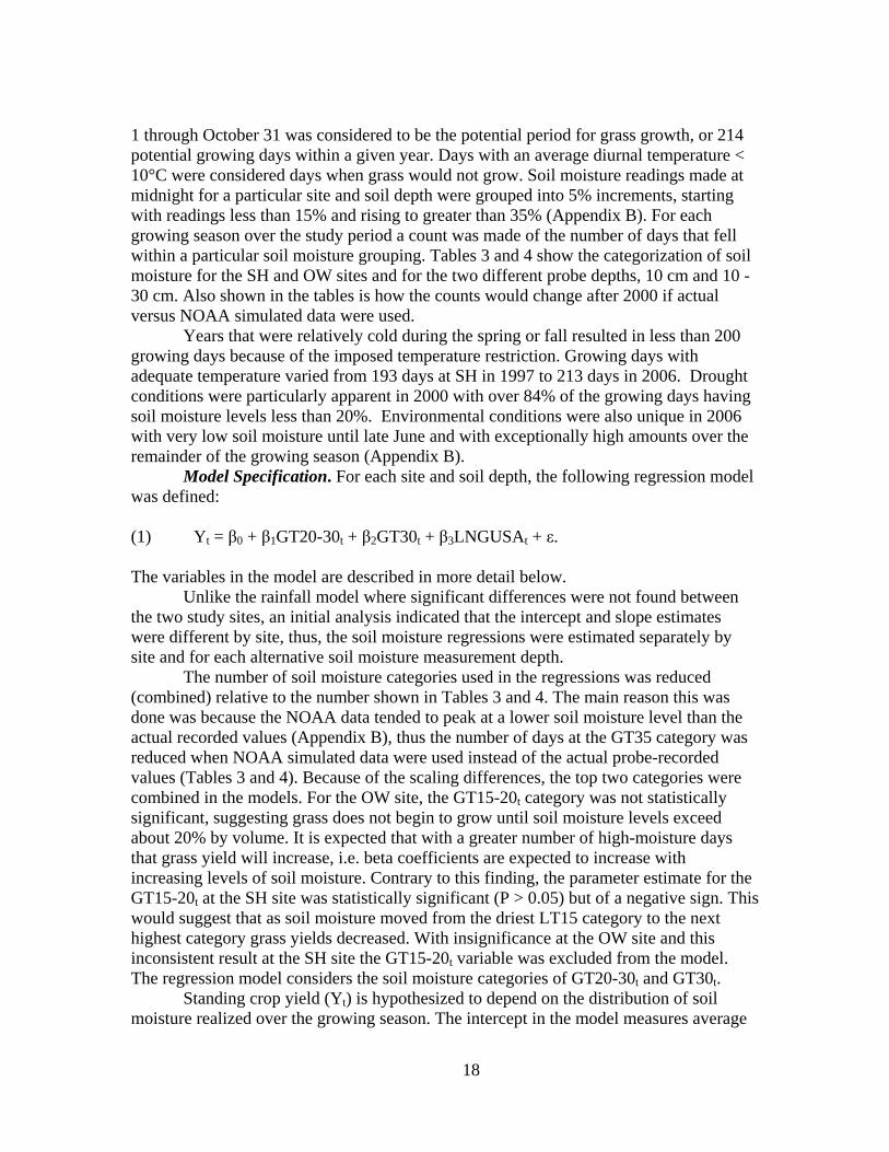
1 through October 31 was considered to be the potential period for grass growth, or 214 potential growing days within a given year. Days with an average diurnal temperature < 10°C were considered days when grass would not grow. Soil moisture readings made at midnight for a particular site and soil depth were grouped into 5% increments, starting with readings less than 15% and rising to greater than 35% (Appendix B). For each growing season over the study period a count was made of the number of days that fell within a particular soil moisture grouping. Tables 3 and 4 show the categorization of soil moisture for the SH and OW sites and for the two different probe depths, 10 cm and 10 - 30 cm. Also shown in the tables is how the counts would change after 2000 if actual versus NOAA simulated data were used.
Years that were relatively cold during the spring or fall resulted in less than 200 growing days because of the imposed temperature restriction. Growing days with adequate temperature varied from 193 days at SH in 1997 to 213 days in 2006. Drought conditions were particularly apparent in 2000 with over 84% of the growing days having soil moisture levels less than 20%. Environmental conditions were also unique in 2006 with very low soil moisture until late June and with exceptionally high amounts over the remainder of the growing season (Appendix B).
Model Specification. For each site and soil depth, the following regression model was defined:
(1) Yt = β0 + β1GT20-30t + β2GT30t + β3LNGUSAt + ε.
The variables in the model are described in more detail below.
Unlike the rainfall model where significant differences were not found between the two study sites, an initial analysis indicated that the intercept and slope estimates were different by site, thus, the soil moisture regressions were estimated separately by site and for each alternative soil moisture measurement depth.
The number of soil moisture categories used in the regressions was reduced (combined) relative to the number shown in Tables 3 and 4. The main reason this was done was because the NOAA data tended to peak at a lower soil moisture level than the actual recorded values (Appendix B), thus the number of days at the GT35 category was reduced when NOAA simulated data were used instead of the actual probe-recorded values (Tables 3 and 4). Because of the scaling differences, the top two categories were combined in the models. For the OW site, the GT15-20t category was not statistically significant, suggesting grass does not begin to grow until soil moisture levels exceed about 20% by volume. It is expected that with a greater number of high-moisture days that grass yield will increase, i.e. beta coefficients are expected to increase with increasing levels of soil moisture. Contrary to this finding, the parameter estimate for the GT15-20t at the SH site was statistically significant (P > 0.05) but of a negative sign. This would suggest that as soil moisture moved from the driest LT15 category to the next highest category grass yields decreased. With insignificance at the OW site and this inconsistent result at the SH site the GT15-20t variable was excluded from the model. The regression model considers the soil moisture categories of GT20-30t and GT30t.
Standing crop yield (Yt) is hypothesized to depend on the distribution of soil moisture realized over the growing season. The intercept in the model measures average

Site Probe Depth Year LT15GT15 -
20GT20 -
25GT25 -
30GT30 -
35 GT35Total Days
NOAA Simulated DataSH 10 cm 1991 24 54 49 28 35 19 209SH 10 cm 1992 55 60 53 25 8 8 209SH 10 cm 1993 23 92 62 19 4 0 200SH 10 cm 1994 0 71 53 41 30 6 201SH 10 cm 1995 10 79 50 33 21 5 198SH 10 cm 1996 53 16 14 46 50 22 201SH 10 cm 1997 8 32 45 53 40 15 193SH 10 cm 1998 45 30 52 38 25 10 200SH 10 cm 1999 6 70 65 37 16 3 197SH 10 cm 2000 134 37 13 7 4 8 203SH 10 cm 2001 26 56 67 40 14 4 207SH 10 cm 2002 46 44 53 27 26 8 204SH 10 cm 2003 25 115 51 16 0 0 207SH 10 cm 2004 21 40 45 39 42 14 201SH 10 cm 2005 2 78 45 48 29 2 204SH 10 cm 2006 52 47 21 26 39 28 213
Actual Recorded DataSH 10 cm 2001 52 58 41 38 14 4 207SH 10 cm 2002 87 33 36 18 9 21 204SH 10 cm 2003 87 61 34 16 6 3 207SH 10 cm 2004 69 45 22 22 20 23 201SH 10 cm 2005 58 45 16 25 31 29 204SH 10 cm 2006 95 6 13 14 13 72 213SH 33 58 46 33 24 10 203
SH 10 - 30 cm 1991 23 60 49 34 37 6 209SH 10 - 30 cm 1992 53 68 51 25 9 3 209SH 10 - 30 cm 1993 25 97 69 6 3 0 200SH 10 - 30 cm 1994 0 79 54 45 22 1 201SH 10 - 30 cm 1995 11 87 52 34 14 0 198SH 10 - 30 cm 1996 55 14 19 58 47 8 201SH 10 - 30 cm 1997 1 39 54 56 39 4 193SH 10 - 30 cm 1998 44 33 59 38 22 4 200SH 10 - 30 cm 1999 4 80 67 35 11 0 197SH 10 - 30 cm 2000 136 37 12 7 10 1 203SH 10 - 30 cm 2001 27 67 65 37 11 0 207SH 10 - 30 cm 2002 49 51 48 30 25 1 204SH 10 - 30 cm 2003 27 116 56 8 0 0 207SH 10 - 30 cm 2004 20 43 56 45 34 3 201SH 10 - 30 cm 2005 0 70 54 54 25 1 204SH 10 - 30 cm 2006 50 51 21 29 48 14 213
Actual Recorded DataSH 10 - 30 cm 2001 27 59 73 37 11 0 207SH 10 - 30 cm 2002 0 29 94 35 17 29 204SH 10 - 30 cm 2003 1 59 91 36 15 5 207SH 10 - 30 cm 2004 0 7 100 40 28 26 201SH 10 - 30 cm 2005 0 30 54 57 29 34 204SH 10 - 30 cm 2006 0 89 14 12 14 84 213SH 33 62 49 34 22 3 203
Table 3. Number of days during the growing season when NOAA simulated soil moisture reached alternative levels at the SH site.
NOAA Average
NOAA Average
File = SMDATA2.xls19

Site Probe Depth Year LT15GT15-
20GT20-
25GT25-
30GT30-
35 GT35Total Days
NOAA Simulated DataOW 10 cm 1991 16 49 54 36 34 20 209OW 10 cm 1992 0 49 62 58 28 12 209OW 10 cm 1993 2 90 63 34 12 1 202OW 10 cm 1994 0 33 72 44 41 15 205OW 10 cm 1995 3 70 57 39 29 3 201OW 10 cm 1996 45 25 5 41 57 29 202OW 10 cm 1997 1 36 33 59 46 19 194OW 10 cm 1998 44 21 51 47 25 11 199OW 10 cm 1999 0 51 80 40 24 3 198OW 10 cm 2000 124 41 13 14 4 6 202OW 10 cm 2001 8 76 63 43 11 5 206OW 10 cm 2002 43 39 56 26 27 12 203OW 10 cm 2003 16 106 59 26 0 0 207OW 10 cm 2004 22 24 45 41 52 17 201OW 10 cm 2005 16 63 38 35 40 12 204OW 10 cm 2006 26 76 22 23 34 31 212
Actual Recorded DataOW 10 cm 2001 33 72 42 43 11 5 206OW 10 cm 2002 89 47 26 12 17 12 203OW 10 cm 2003 88 59 37 10 5 8 207OW 10 cm 2004 37 58 32 21 27 26 201OW 10 cm 2005 20 71 23 33 43 14 204OW 10 cm 2006 99 11 16 12 28 46 212OW 23 53 48 38 29 12 203
NOAA Simulated DataOW 10 - 30 cm 1991 13 57 54 41 40 4 209OW 10 - 30 cm 1992 0 51 72 56 25 5 209OW 10 - 30 cm 1993 2 97 71 23 9 0 202OW 10 - 30 cm 1994 0 38 75 49 38 5 205OW 10 - 30 cm 1995 1 78 59 41 22 0 201OW 10 - 30 cm 1996 46 24 12 46 63 11 202OW 10 - 30 cm 1997 0 35 35 66 47 11 194OW 10 - 30 cm 1998 40 25 58 46 26 4 199OW 10 - 30 cm 1999 0 53 84 42 19 0 198OW 10 - 30 cm 2000 125 41 14 14 7 1 202OW 10 - 30 cm 2001 9 84 64 40 9 0 206OW 10 - 30 cm 2002 45 47 51 32 26 2 203OW 10 - 30 cm 2003 18 112 62 15 0 0 207OW 10 - 30 cm 2004 18 28 50 52 49 4 201OW 10 - 30 cm 2005 7 62 47 40 45 3 204OW 10 - 30 cm 2006 17 85 24 24 46 16 212
Actual Recorded DataOW 10 - 30 cm 2001 9 93 55 40 9 0 206OW 10 - 30 cm 2002 0 53 97 20 13 20 203OW 10 - 30 cm 2003 0 104 60 23 20 0 207OW 10 - 30 cm 2004 0 47 36 30 18 70 201OW 10 - 30 cm 2005 0 59 26 31 29 59 204OW 10 - 30 cm 2006 14 87 12 7 14 78 212OW 21 57 52 39 29 4 203
Table 4. Number of days during the growing season when NOAA simulated soil moisture reached alternative levels at the OW site.
NOAA Average
NOAA Average
file = SMDATA2.xls20

21
herbaceous yield expected on snakeweed free areas with very dry soils, i.e. all recorded soil moisture measurements below 20%. The first 2 variables measure the number of days over the growing season when soil moisture was categorized at that particular level. The variable GT20-30t, for example, measures the number of days in year t when soil moisture was estimated to be greater than or equal to 20% but less than 30%. Similar to the rainfall model (Table 2), parameter β3 measures the amount by which a 1% increase in broom snakeweed reduced grass yield. The variable LNGUSAt is specified in natural log form.
Soil Moisture Model Results. Regression results were consistent between the two soil moisture depths, 10 cm (Table 5) and 10 – 30 cm (Table 6). Results were also similar when actual probe data were used when available versus regressions that only used NOAA simulated data. R2 values were 1% to 4% higher when actual probe-recorded data were used when available. The exception was the SH site at 10 – 30 cm when using the actual data resulted in a reduced R2 and increased prediction error (Table 6).
Consider the regression for the OW site using NOAA simulated data at the 10 cm depth (Table 5). By holding broom snakeweed yield constant, the base grass yield is estimated to be 243 kg/ha (β0). Each day during the growing season with a midnight soil moisture reading between 20% and 30% increased grass yield by 1.69 kg/ha beyond this base amount. Days with soil moisture exceeding 30% grew 8.32 kg/ha of grass which was statistically more than the lower category (P < 0.0001). Movement of soil moisture to relatively high levels (above 30%) nearly doubled the daily production of grass.
Grass yields, as expected, was found to depend largely on the number of days when soil moisture conditions were relatively wet. Soil moisture is conceptually a better measure for predicting grass yield as accumulated rainfall amounts does not consider the recent and past history of rainfall events. Based on root mean square error and R2 comparisons, the rainfall model (Table 2) and soil moisture models (Tables 5 and 6) predicted about the same. A great deal of grass yield variability between years remains unexplained with R2 values in the 30% range.
The Economic Value of Precipitation and Weather Forecasts In this section we use the history of storm events on the Corona Ranch and soil
moisture estimates from the NOAA SAC-SMA model to estimate the economic value of an individual storm event, which provides an estimate of the economic value of water for range forage production. We then use the relationship found earlier between seasonal rainfall amounts and herbage production (Table 2) and the estimated probability distribution for herbage production on the Corona Ranch (Figure 7) to estimate the expected economic value of an accurate weather forecast for livestock producers3. We assume that without an accurate forecast, livestock producers would follow a constant, conservative stocking strategy that would usually provide adequate forage. In productive years some forage will go unused and in dry year’s animal performance, profits and rangeland conditions will deteriorate as overgrazing occurs and possible herd reductions become necessary. Yearling stockers are considered because key production relationships have been estimated for this class of livestock.
3/Soil moisture equations and relationships were not used for this valuation because soil moisture measurements were not available for an extended period of time.

Par
a-m
eter
Var
iabl
eV
aria
ble
Des
crip
tion
Par
amet
er
Est
imat
e
Con
sist
ent
Sta
ndar
d E
rror
t-val
ueP
aram
eter
E
stim
ate
Con
sist
ent
Sta
ndar
d E
rror
t-val
ue
β 0In
terc
ept
Mod
el in
terc
ept
242.
6978
.93
3.07
***
242.
7964
.18
3.78
***
β 1G
T20
- 30
Num
ber o
f day
s w
ith s
oil
moi
stur
e >
20%
and
≤ 3
0%1.
690.
911.
86*
3.40
0.72
4.72
***
β 2G
T30
Num
ber o
f day
s w
ith s
oil
moi
stur
e >
30%
8.32
0.75
11.0
9**
*5.
540.
886.
32**
*
β 3LN
GU
SA
Nat
ural
log
of w
eigh
t of b
room
sn
akew
eed
(kg/
ha)
-36.
138.
69-4
.16
***
-27.
408.
99-3
.05
***
R2
0.33
0.23
n (1
991-
200
6)18
618
6M
ean
of d
epen
dent
var
iabl
e (G
rass
Yie
ld, k
g/ha
)66
1.5
650.
5R
oot m
ean
squa
re e
rror
315
297.
6
β 0In
terc
ept
Mod
el in
terc
ept
196.
7760
.11
3.27
***
217.
2258
.65
3.70
***
β 1G
T20
- 30
Num
ber o
f day
s w
ith s
oil
moi
stur
e >
20%
and
≤ 3
0%2.
180.
802.
73**
*3.
980.
775.
14**
*
β 2G
T30
Num
ber o
f day
s w
ith s
oil
moi
stur
e >
30%
9.07
0.86
10.5
0**
*6.
020.
787.
70**
*
β 3LN
GU
SA
Nat
ural
log
of w
eigh
t of b
room
sn
akew
eed
(kg/
ha)
-38.
048.
97-4
.24
***
-29.
968.
99-3
.33
***
R2
0.37
0.27
n (1
991-
200
6)18
618
6M
ean
of d
epen
dent
var
iabl
e (G
rass
Yie
ld, k
g/ha
)66
1.5
650.
5R
oot m
ean
squa
re e
rror
304.
928
8.8
Sou
th H
ouse
(SH
)O
il W
ell (
OW
)
Not
e: S
ingl
e, d
oubl
e an
d tri
ple
aste
ricks
(*) d
enot
e co
effic
ient
s ar
e st
atis
tical
ly s
igni
fican
t at t
he 1
0%, 5
% a
nd 1
% le
vels
, re
spec
tivel
y.
Tabl
e 5.
Reg
ress
ion
para
met
er e
stim
ates
for g
rass
yie
ld e
quat
ions
usi
ng s
oil m
oist
ure
mea
sure
d at
10
cm.
10 c
m N
OA
A s
imul
ated
soi
l moi
stur
e on
ly
10 c
m a
ctua
l dat
a w
hen
avai
labl
e an
d N
OA
A s
imul
ated
soi
l moi
stur
e ot
herw
ise
22

Par
a-m
eter
Var
iabl
eV
aria
ble
Des
crip
tion
Par
amet
er
Est
imat
e
Con
sist
ent
Sta
ndar
d E
rro r
t-val
ueP
aram
eter
E
stim
ate
Con
sist
ent
Sta
ndar
d E
rror
t-val
ue
β 0In
terc
ept
Mod
el in
terc
ept
154.
6570
.06
2.21
**22
2.57
60.5
33.
68**
*
β 1G
T20
- 30
Num
ber o
f day
s w
ith s
oil
moi
stur
e >
20%
and
≤ 3
0%2.
710.
853.
19**
*3.
720.
645.
82**
*
β 2G
T30
Num
ber o
f day
s w
ith s
oil
moi
stur
e >
30%
9.77
0.84
11.6
2**
*6.
401.
036.
20**
*
β 3LN
GU
SA
Nat
ural
log
of w
eigh
t of b
room
sn
akew
eed
(kg/
ha)
-35.
378.
36-4
.23
***
-25.
308.
83-2
.86
***
R2
0.39
0.26
n (1
991-
200
6)18
618
6M
ean
of d
epen
dent
var
iabl
e (G
rass
Yie
ld, k
g/ha
)66
1.5
650.
5R
oot m
ean
squa
re e
rror
300.
529
1.0
β 0In
terc
ept
Mod
el in
terc
ept
163.
4266
.30
2.46
***
506.
3190
.47
5.60
***
β 1G
T20
- 30
Num
ber o
f day
s w
ith s
oil
moi
stur
e >
20%
and
≤ 3
0%2.
110.
732.
90**
*0.
540.
630.
86
β 2G
T30
Num
ber o
f day
s w
ith s
oil
moi
stur
e >
30%
8.59
0.62
13.8
2**
*3.
970.
814.
90**
*
β 3LN
GU
SA
Nat
ural
log
of w
eigh
t of b
room
sn
akew
eed
(kg/
ha)
-23.
428.
30-2
.82
***
-23.
2710
.14
-2.2
9**
*
R2
0.40
0.15
n (1
991-
200
6)18
618
6M
ean
of d
epen
dent
var
iabl
e (G
rass
Yie
ld, k
g/ha
)66
1.5
650.
5R
oot m
ean
squa
re e
rror
299.
631
1.7
Sou
th H
ouse
(SH
)O
il W
ell (
OW
)
Not
e: S
ingl
e, d
oubl
e an
d tri
ple
aste
ricks
(*) d
enot
e co
effic
ient
s ar
e st
atis
tical
ly s
igni
fican
t at t
he 1
0%, 5
% a
nd 1
% le
vels
, re
spec
tivel
y.
Tabl
e 6.
Reg
ress
ion
para
met
er e
stim
ates
for g
rass
yie
ld e
quat
ions
usi
ng s
oil m
oist
ure
mea
sure
d at
10
- 30
cm.
10 -
30 c
m N
OA
A s
imul
ated
soi
l moi
stur
e on
ly
10 -
30 c
m a
ctua
l dat
a w
hen
avai
labl
e an
d N
OA
A s
imul
ated
soi
l moi
stur
e ot
herw
ise
23

24
Economic Value of a Rainfall Event Appendix B details the history of storm events and end-of-season grass yields
recorded on the Corona Ranch from 1991 through 2006. NOAA simulated soil moisture plotted in the appendix provides a daily estimate of the resulting soil moisture conditions. Using these values as the base, the economic value of an altered weather situation was estimated at two different points in time. NOAA hydrologists re-estimated soil moisture assuming a 1 inch (25.4 mm) rainfall event occurred on April 1, 2003. This was a relatively dry year (Figure 3) and forage production was well below average (Figure 5). In fact, average end-of-season yield estimates this year were below the minimum 336 kg/ha (300 lb/acre) that Bement (1969) suggests as a minimum desired forage residual. There was little if any grazing capacity on the Corona Ranch during 2003.
Similar estimates of forage response were made for a 1 inch storm on April 1, 2005, an average rainfall year. Results would be different depending on the time of year (temperature) and current state of soil moisture. The 10 – 30 cm soil depth is considered in the soil moisture analysis.
As shown in Figure 8, an additional storm would alter estimated soil moisture conditions, pushing the level of soil moisture upwards for a variable length of time in the future. For 2003 at the OW site, this would mean 10 more days with soil moisture above 30% and 3 less days with soil moisture between 20 and 30% (Table 7). Similarly, with an added April 1 storm during 2005 there would be 10 more days with soil moisture greater than 30% and 6 fewer days between 20% and 30%. The change in soil moisture classification is slightly different for the SH site (Table 7).
The economic value of the 1 inch storm can be estimated using either the rainfall model (Table 2) or the soil moisture model.4 As shown in Table 2, each mm of rainfall received during Q2 was estimated to add 0.86 kg/ha to grass production. Thus, the 25.4 mm of added rainfall would add an estimated 0.86×25.4 = 22 kg/ha to forage production.
The estimate of yield increase using the rainfall model would not be different by site, year or existing soil moisture conditions. Using the soil moisture model, however, the estimated change in grass yield will be different depending on soil moisture conditions at the time of the storm. Consider the OW site during 2003. From the regression results (Table 6), every day for which NOAA simulated soil moisture was categorized between 20 and 30% meant grass yields were increased by 2.71 kg/ha, relative to the drier state. The grass yield increase was 9.77 kg/ha if daily soil moisture
4/We consider only the 10 – 30 cm soil moisture model here (Table 6) but the 10 cm soil moisture model fit nearly as well (Table 5) and could also be used.
Site Year
Soil Moisture Category
Change in Soil
Moisture Days
OW 2003 GT20-30 -3OW 2003 GT30 10SH 2003 GT20-30 -6SH 2003 GT30 10OW 2005 GT20-30 0OW 2005 GT30 8SH 2005 GT20-30 -5SH 2005 GT30 7
Table 7. Altered soil moisture categorizations with an additional 25.4 mm storm.

0
5
10
15
20
25
30
35
40
45
Mar-22 Mar-29 Apr-05 Apr-12 Apr-19 Apr-26 May-03 May-10 May-17 May-24 May-31
Date
Soil
Moi
stur
e (%
)
Base Run Added Rain
OW 2003
0
5
10
15
20
25
30
35
40
45
Mar-22 Mar-29 Apr-05 Apr-12 Apr-19 Apr-26 May-03 May-10 May-17 May-24 May-31
Date
Soil
Moi
stur
e (%
)
OW 2005
Figure 8. Estimated soil moisture (10 - 30 cm) in 2003 and 2005 and the result of a 25.4 mm rainfall event on April 1.
25

26
was categorized to be greater than 30%. The estimated amount of grass yield added from the April 1, 2003 storm is then estimated to be 2.71×(-3 days) + 9.77×(10 days) = 90 kg/ha. The similar marginal estimate for 2005, a wetter year, was reduced to 78 kg/ha because soil moisture before the storm starts at a higher level and there is less to be gained from the storm (Figure 8). The marginal forage yield benefit from the storm at the SH site is estimated to be less, 42 kg/ha during 2003 and 26 kg/ha during 2005.
According to Bartlett et al. (2002), a reasonable estimate of net forage value is about 70% of the average USDA reported lease price for rangeland forage. The 30% reduction is because in many cases part of the lease price paid is for services provided by the lessee and not for the grass harvested by grazing animals. Recent lease rates have
been about $14/AUM5 (USDA-NASS 2007). Thus, the economic value of forage is estimated to be about $0.027/kg ($9.80/AUM). At this rate, the 1 inch storm at the OW site on April 1, 2003 that added an estimated 90 kg/ha adds $2.40/ha in annual production value. This is the marginal lease value of the additional forage that would be produced from the storm. The April 2005 storm at the OW site added an estimated 78 kg/ha for an economic value of $2.08/ha. For the SH site the 2003 value would be reduced to 42 kg/ha ($1.12/ha) during 2003 and 26 kg/ha ($0.69/ha) during 2005. The economic value of the storm is thus variable depending on existing soil moisture conditions and the magnitude of the estimated regression parameters.
The magnitude of economic values estimated for the storm appear trivial at only $1 to $2.40/ha, but it is important to remember that this is the economic value of only one relatively large storm. Further, as noted in the next section where the economic value of an improved weather forecast is evaluated, stocking the range at a constant 15 AUY/section would result in an average profit level of $6.31/ha using 2004 – 2006 average beef prices. The one large storm results in from 15% to 42% of the total net annual production value of the Corona ranch. It is also important to remember the relatively large size of many western ranches. The Corona Ranch has about 11,381 ha (28,112 acres) of total rangeland of which 6,175 ha [15,250 acres is designated to be blue grama rangeland (McDaniel et al. 2002)]. Using 60 kg/ha as a mid-point response estimate and assuming minimum residual forage requirements have already been met, the 25.4 mm April 1 rainstorm is estimated to produce about 370,500 kg of added grass on the relatively productive blue grama grassland areas of the Corona Ranch. This is enough forage to carry 85 head for the year (1,020 AUMs) for an estimated economic value of $10,003 when valued at 2.7¢/kg. The less productive pinyon-juniper rangeland areas on the Corona Ranch would also receive an expected boost in forage production such that the estimated $10,000 value reflects a minimum addition to value from the storm.
The $1.62/ha value estimate (60 kg/ha × 2.7¢) is an approximate average forage value obtained from a 1 inch rainstorm on the Corona Ranch, assuming no snakeweed or woody overstory is present on the rangeland area. This value and its calculation demonstrates how soil moisture data can be used to value a particular storm event and would be most relevant for a project like cloud-seeding. As Mjelde et al. (1998) notes, however, there is an important difference between the value of a climate event and the value of improving a climate forecast. This topic is investigated next.
5/An AU is considered to be one mature cow or the equivalent. An AUM (animal unit month) is considered to be the amount of forage required by an AU over a 1 month period. An AUY (animal unit yearlong) is the forage required by an AUY for the year. An 800 pound (363 kg) AUM is considered here.

27
Economic Value of an Accurate Weather Forecast Valuing an improved weather forecast requires an expanded decision model
describing how prior expectations about future forage conditions are improved using a forecast or observation about the current situation or weather pattern (e.g., ENSO). Using an expected value approach, Mjelde et al. (1988) show that the value of an improved forecast can be estimated as the difference in expected net returns with and without updated forecast probabilites. Stafford-Smith et al. (2000) use this approach, as described in Section 5 of the companion report. They consider the value of seasonal forecasting in rangeland livestock production from the whole-farm or enterprise level. In this analysis, the authors link the GRASP model of forage and livestock production (Day et al. 1997) to a herd and property management model, RANGEPACK Herd-Econ (Stafford-Smith and Foran, 1992) in order to assess the overall changes in profitability associated with alternative grazing strategies and seasonal climate forecasts. They found that increasing forecast reliability led to more responsive changes in stocking rates, and that longer forecast lead times generated modest increases in cash flow (or alternatively, could provide equivalent cash flow at much lower risk). In addition, they found that the relative value of seasonal climate forecasts was sensitive to livestock prices, with the forecasting strategies improving in favor over constant stocking rates as sale prices rose – and even more so when the margins between sale and purchase prices increased. They observe that for grazing strategies to successfully employ climate forecasts it is first necessary that they have a management system “that is sensitive to pasture conditions and hence using the appropriate stocking rate strategies over time”.
We follow a similar procedure here. We assume the livestock producer’s prior knowledge of climatic conditions is identical to historical probabilities. Thus, without an accurate weather forecast livestock producers are largely forced to follow a constant stocking rate strategy consistent with the historical production levels used by land agencies to develop stocking rate recommendations, requirements, and guidelines. As an example, the Natural Resource Conservation Service (NRCS) provides stocking rate recommendations (suggested acreage allowances per head) for alternative rangelands in different condition states. A second common rule-of-thumb for southwest rangelands is that a ranch can carry 1 animal unit yearlong (AUY)/section (640 acres) for each inch of average annual rainfall. The Corona Ranch has a long-term 370 mm (14.6 inches) average for annual rainfall (Appendix A) and this would be the average estimated grazing capacity following the “one head per inch of rain” prescriptive rule.
Range management principles and stocking rate recommendations are well defined when annual herbaceous production is known, and flexible stocking strategies are recommended in this case. Guidelines suggest, depending on the type of rangeland considered (e.g., shortgrass prairie, southern desert shrublands, etc.), that the maximum use of peak annual herbage production should not exceed 35% to 60% (Vallentine 1990). The most common flexible stocking rate recommendation is to utilize no more than 50% of peak standing crop of forage, the “take-half-leave-half rule.” Another “rule” developed by Bement (1969) for blue grama rangeland is that a livestock producer should strive to leave at least 300 lb/acre (336 kg/ha) at the end of the grazing season. This maximized animal performance in grazing trials conducted at the Central Great Plains Experimental Range near Fort Collins, Colorado (1940 through 1963). Yet, basic production economic principles dictate that maximizing yield (gain/ha) does not maximize profit.

28
Hart (1991) notes that to take advantage of flexible profit-maximizing stocking rates requires that early and accurate stocking rate decisions must be made. This requires an accurate prediction of how much forage will be available for the year, thus requiring an accurate weather forecast. He notes that in the northern High Plains of Wyoming forage production is primarily determined by precipitation in March, April, and May and with yearlings typically entering the pasture in May, annual forage production is largely known as the stocking decision is made. This is not the situation for many other areas and for cow-calf producers. On the ranges of the southwest where warm season (C4) grasses predominate, grass growth does not typically commence until the summer rains of June, July and August. The amount of herbaceous production that will be available in the upcoming season remains largely unknown. This is especially true for cow-calf producers that must maintain animals yearlong and budget enough forage to maintain the herd throughout the year.
Economic Model. Following Hart et al. (1988), define stocking rate (SR) to be the number of animals grazing an area for a defined length of time (v). SR is often used as a measure of grazing use but poorly considers the potential harmful effects of a constant number of animals on future forage production. A given SR is not the same for two rangeland areas that produce different amounts and kinds of plants. Nor is it the same for a particular grazing area between years, given fluctuating forage production.
As noted by Hart et al. (1988), to account for the differences in grazing use for different rangeland production situations a better measure of grazing intensity is grazing pressure (GP):
1) GP = (SR·v)/H), where H is a measure of forage production on the area, defined to be metric tonne/ha (1,000 kg/ha) measured at peak standing crop. Numerous studies (Bement 1969, Hart et al. 1988, Hart and Ashby 1998) have
found average daily gain (ADG) for yearling animals to decrease as a linear function of GP over the relevant economic range.
2) =ADG β0 + β1GP (with β0 > 0, β1< 0).
The intercept measures the expected ADG at low stocking rates and some studies have found a range of light grazing pressures where ADG is relatively high and constant (Bement 1969, Hart et al. 1988). The slope coefficient measures the deterioration of animal performance once GP reaches a level where animals must compete for the most desirable forage.
With Wp defined to be the average weight of yearling animals purchased, sale weight and gain per ha are determined as:
3) Ws = [Wp + v·ADG] Average Sale weight
4) Gain = f(GP((SR,H)) = SR·v·ADG Livestock gain per ha = SR·v·(β0 + β1GP) = β0v·SR + β1v·SR×(SR·v)/H)
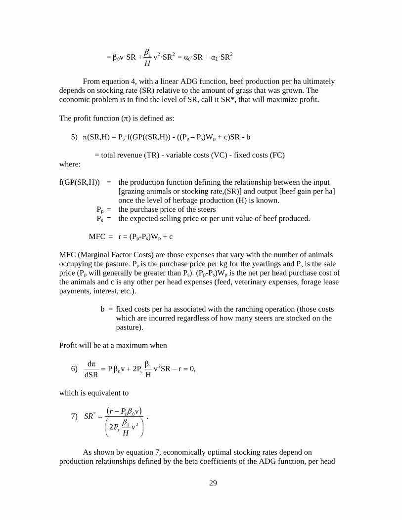
29
= β0v·SR +H
1β v2·SR2 = α0·SR + α1·SR2
From equation 4, with a linear ADG function, beef production per ha ultimately depends on stocking rate (SR) relative to the amount of grass that was grown. The economic problem is to find the level of SR, call it SR*, that will maximize profit.
The profit function (π) is defined as:
5) π(SR,H) = Ps·f(GP((SR,H)) - ((Pp – Ps)Wp + c)SR - b
= total revenue (TR) - variable costs (VC) - fixed costs (FC)
where:
f(GP(SR,H)) = the production function defining the relationship between the input [grazing animals or stocking rate,(SR)] and output [beef gain per ha] once the level of herbage production (H) is known.
Pp = the purchase price of the steers Ps = the expected selling price or per unit value of beef produced. MFC = r = (Pp-Ps)Wp + c MFC (Marginal Factor Costs) are those expenses that vary with the number of animals occupying the pasture. Pp is the purchase price per kg for the yearlings and Ps is the sale price (Pp will generally be greater than Ps). (Pp-Ps)Wp is the net per head purchase cost of the animals and c is any other per head expenses (feed, veterinary expenses, forage lease payments, interest, etc.). b = fixed costs per ha associated with the ranching operation (those costs
which are incurred regardless of how many steers are stocked on the pasture).
Profit will be at a maximum when
6) ,0rSRvHβ2PvβP
dSRdπ 21
s0s =−+=
which is equivalent to
7) ( )
⎟⎠⎞
⎜⎝⎛
−=
21
0*
2 vH
P
vPrSRs
s
ββ .
As shown by equation 7, economically optimal stocking rates depend on
production relationships defined by the beta coefficients of the ADG function, per head

30
costs (r), beef prices (Pp and Ps), the length of the grazing season (v), and the amount of forage grown (H). Note in equation 7 that fixed costs do not affect economically optimal stocking rates in the short-run. Thus, in this application we exclude fixed costs and compute profit as a return over variable costs.
As noted by Hart et al. (1988), the β1 parameter must be corrected for the level of annual forage production. Uncertainty about the level of H creates uncertainty as to what the profit maximizing stocking rate should be. Uncertainty is also associated with prices and costs but the futures and options market could be used to largely remove price risk.
In the stocking rate model, the economically optimal stocking rate is driven by declining animal performance as stocking rates increase; yet, the traditional concern is that livestock grazing deteriorates rangeland conditions and future production potential. Torell et al. (1991) found intertemporal grazing impacts are not as important as declining current period animal performance for rangelands dominated by blue grama (Bouteloua gracilis). Falling animal performance will generally set profit-maximizing stocking rates well below those levels that will severely deteriorate the range. As noted by Klipple and Bement (1961) blue grama rangelands are very resilient and herbage yields lowered by heavy grazing can be restored with subsequent use of light stocking rates.
Table 8 defines the parameters and assumptions used in the Corona Ranch forecast valuation. A spreadsheet program was written to perform the calculations. To define the ADG function we used the regression equation estimated by Hart and Ashby (1998) from long-term grazing trials conducted at the Central Plains Experimental Range (CPER) near Fort Collins, Colorado. This shortgrass rangeland site is dominated by blue grama similar to the Corona Ranch. Average annual herbage production at the site is also similar to the Corona Ranch (35-year mean = 717 kg/ha, S.D. = 226 kg/ha), though as noted earlier the distribution of herbage production at the CPER site was not normally distributed. Other ADG functions estimated for more productive rangelands dominated by western wheatgrass (Agropyron smithii) in Wyoming (Hart 1991, Hart et al. 1988) had an intercept of 0.95 kg/head/day and with a much steeper slope (-0.006), nearly twice the decline of ADG found at the CPER site (Table 8). At a moderate stocking rate, the estimated CPER ADG is consistent with the 0.68 kg daily gain expected of yearlings grazing in Union County, New Mexico (Graham, Unpublished Fact Sheet).
The economics of stocker cattle operations depends largely on the spread between purchase prices of calves versus the price of feeder cattle sold later in the fall. We estimate the economic value of an accurate weather forecast using average 2004-2006 beef prices adjusted for inflation (Table 8). We also calculate and present optimal stocking rates and profit levels for annual 2004 - 2006 price conditions and for the average over all of these years. The price spread in 2004 was very favorable for yearling stocker producers whereas 2005 had a wide price spread and thus unfavorable economic conditions. Expected production costs were estimated from yearling stocker budgets prepared by the Cooperative Extension Service in various western states.
Corona Ranch Model Application. Assume that each year the Corona Ranch follows a rule of stocking the range at a constant rate in head/section. Yearling stockers are assumed to be purchased in the spring and grazed for a 150 day grazing season. Grazing use is expressed as the equivalent number of AUY grazing yearlong. Two constant stocking rate rules plus a flexible optimal stocking rate rule (calculated using equation 7) are considered. First, we consider the rule of stocking at 1 AUY/section

Tabl
e 8.
Sel
ecte
d eq
uatio
ns, p
aram
eter
s, a
nd a
ssum
ptio
ns u
sed
in v
alui
ng a
per
fect
wea
ther
fore
cast
.
Mod
el P
aram
eter
Par
amet
erV
alue
Sou
rce
Ave
rage
dai
ly g
ain
(kg/
head
/day
)H
art a
nd A
shby
(199
8)Le
ngth
of g
razi
ng s
easo
nv
150
days
Yea
rling
pur
chas
e w
eigh
tW
p20
0 kg
AU
equ
ival
ency
of a
yea
rling
0.
7V
alle
ntin
e (1
990)
Freq
uenc
y di
strib
utio
n fo
r lev
els
of fo
rage
pro
duct
ion
Oct
ober
-Nov
embe
r mea
sure
men
tFi
gure
7
Pea
k st
andi
ng c
rop
of fo
rage
pro
duct
ion
H/1
000
Pie
per e
t al.
(197
4), T
urne
r and
K
lippl
e(19
60)
k g o
f for
age
per A
UM
Val
lent
ine
(199
0)
Eco
nom
ic F
acto
rs20
0420
0520
06A
vera
geA
pril
Ste
er P
urch
ase
Pric
e (P
p) ($
/kg)
Pp
$2.9
8$3
.20
$2.9
83.
05C
attle
-Fax
™ a
t http
://w
ww
.cat
tle-fa
x.co
m/
Sep
tem
ber S
ale
Pric
e (P
s) ($
/kg)
Ps
$2.6
2$2
.58
$2.5
12.
57C
attle
-Fax
™ a
t http
://w
ww
.cat
tle-fa
x.co
m/
Pric
e S
prea
d ($
/kg)
Ps - P
p-$
0.36
-$0.
62-$
0.47
-0.4
8O
ther
var
iabl
e ex
pens
es in
clud
ing
inte
rest
, m
iner
als,
vet
erin
ary
and
drug
s, p
astu
re re
nt,
labo
rc
$123
$123
$123
$123
Sto
cker
cat
tle b
udge
ts fr
om K
ansa
s, Id
aho,
an
d N
ew M
exic
o
Mar
gina
l Fac
tor C
osts
(MFC
)r
$193
$247
$215
$218
Sto
cker
cat
tle b
udge
ts fr
om K
ansa
s, Id
aho,
an
d N
ew M
exic
o ( S
mat
hers
and
Rim
bey
2006
, Dum
ler 2
006,
Gra
ham
(U
npub
lishe
d)).
Pea
k st
andi
ng c
rop
(H) o
ccur
s in
Aug
ust o
r S
epte
mbe
r and
is e
stim
ated
to b
e 30
% m
ore
than
the
Oct
ober
/Nov
embe
r mea
sure
men
t. G
Pt
is re
late
d to
pea
k st
andi
ng c
rop
whe
re th
e pe
ak s
tand
ing
crop
est
imat
e is
div
ided
by
1 ,00
0 an
d ex
pres
sed
in m
etric
tonn
e.
Nor
mal
Dis
tribu
tion
with
a m
ean
of 7
68 k
g/ha
an
d st
anda
rd d
evia
tion
of 2
00 k
g/ha
, as
estim
ated
for t
he C
oron
a R
anch
.
AD
Gt =
0.7
87 -
0.00
364
GP
t
363
kg/A
UM
31

32
for each inch of average annual rainfall. This would be about 15 AUY/section for the Corona Ranch (Appendix A). Second, using the spreadsheet it is easy to compute the constant stocking rate that results in the largest expected profit ($/ha) given the specified prices and probabilities for realizing alternative levels of herbage production. This economically optimal constant stocking rate varies widely with the beef price situation considered. It was very near the 15 head/section rule with average prices and with 2006 prices (Table 9), but, the optimal constant stocking rate was as high as 20.7 AUY/section with favorable 2004 prices and only 10.4 AUY/section for the 2005 price situation.
With average prices (Table 9) and with expected profit defined to be net return over variable expenses (the PDF probability times profit calculated for each level of herbage production), average profit was estimated to be $6.31/ha at 15 AUY/section. The range was from $2.32/ha (2005) to $10.62/ha (2004). If the livestock producer had foresight about the annual price situation, or hedged prices, additional profits could be made by purchasing less animals during relatively poor price years and more animals during favorable price years. On average, though, if a constant stocking rate is to be used, the 15 AUY/section rule comes very close to maximizing profits with average prices. Even without an accurate forecast, some economic improvement could likely be made by paying attention to the amount of forage carried over from the previous year, adjusting stocking rates upward or downward depending on the amount of carryover.
For the flexible stocking rate rule, made possible only with an accurate weather forecast that defines the forage situation that will be realized later in the year, the rancher would adjust GP accordingly so as to maximize profits for the annual forage conditions. Thus, as shown in Table 9, optimal GP and forage use rates are constant with the flexible profit-maximizing stocking rate but variable with the constant stocking rate rules.
With a constant 15 AUY/section stocking rate, GP averaged 29.4 steer days/ metric tonne of forage, but varied from 12 steer days/metric tonne with very high herbage production to an unrealistic situation where only 260 kg/ha or less of herbage grows such that 100% of the forage would be harvested by livestock and GP would be an exorbitant 107 steer days/ metric tonne. The corresponding ADG is estimated to be 0.45 kg/head/day (1 lb/head/day). It is likely that the estimated level of profit for a constant stocking rate is overstated at these low levels of herbage production. In reality, this would not be an obtainable scenario and additional expenses would have to be incurred to lease other forage or animals would have to be sold early, as was done on the Corona Ranch during 2000-01 when this situation occurred. Yet, as shown in Figure 7, less than 400 kg/ha of peak standing crop occurs with a negligible probability (<1%) given the historical rainfall patterns found on the Corona Ranch. This overstatement of profit is thus negligible in the computation of average profit.
To determine the profit-maximizing SR* the estimate of H would be plugged into equation 7 along with specific beef prices and costs. Figure 9 shows the detail of the expected profit calculations. Three curves are drawn. First, in Panel A, the CDF for herbage production measured from mid-October to early November is reproduced from Figure 7. Added to the top axis is the estimate of peak standing crop, assumed to be 30% more than the measured fall level of herbaceous production (Pieper et al. 1974, Turner and Klipple 1952). Grazing pressure (GP) was calculated using the peak standing crop

Model Parameter 2004 2005 2006 Average
Economic Situation from Table 8Pp $2.98 $3.20 $2.98 $3.05Ps $2.62 $2.58 $2.51 $2.57
Ps - Pp -$0.36 -$0.62 -$0.47 -$0.48c $123 $123 $123 $123r $193 $247 $215 $218
Net Returns and Grazing UseConstant 15 AUY/Section
Average Net Returns ($/ha) $10.62 $2.32 $5.87 $6.31Average AUY/Section constant 15.0 15.0 15.0 15.0Average SR (head/ha) constant 0.142 0.143 0.143 0.143Average GP (head/metric tonne) variable 29.4 29.4 29.4 29.4Average % of Peak Forage Production variable 27% 27% 27% 27%Average % Fall Forage Measurement variable 35% 35% 35% 35%
Optimal Constant Stocking RateAverage Net Returns ($/ha) $11.50 $2.86 $5.87 $6.32Average AUY/Section constant 20.7 10.4 15.2 15.6Average SR (head/ha) constant 0.198 0.099 0.144 0.148Average GP (head/metric tonne) variable 40.6 20.4 29.7 30.4Average % of Peak Forage Production variable 37% 18% 27% 28%Average % Fall Forage Measurement variable 48% 24% 35% 36%
Optimal Flexible Stocking RateAverage Net Returns ($/ha) $16.20 $4.03 $8.27 $8.91Average AUY/Section variable 19.3 9.7 14.1 14.1Average SR (head/ha) variable 0.181 0.091 0.132 0.132Average GP (head/metric tonne) constant 40.6 20.4 29.7 30.4Average % of Peak Forage Production constant 49% 24% 35% 36%Average % Fall Forage Measurement constant 63% 32% 46% 47%
Marginal Factor Costs (MFC)
Table 9. Net returns ($/ha) and grazing intensities with alternative stocking rate prescriptions for alternative price situations.
April Steer Purchase Price (Pp) ($/kg)September Sale Price (Ps) ($/kg)Price Spread ($/kg)Other variable expenses
33

34
estimate, consistent with the procedure used by Hart and Ashby (1998) when estimating the ADG function.
As an example of how to read the CDF of Panel A, consider an October- November production level of 530 kg/ha. This level or something less can be expected for the fall measurement 10% of the time, assuming range forage is normally distribution with a mean of 786 kg/ha and standard deviation of 200 kg/ha. The corresponding peak standing crop realized in late August to early September (689 kg/ha) occurs with this same 10% frequency, ignoring the observed variation in the annual rate of natural herbage disappearance (Pieper et al. 1974).
As shown in Panel B, there is a 10% probability that profits will be below $4.09/ha with a constant 15 AUY/section SR. For the flexible stocking rate, profits will be below $6/ha 10% of the time. These profit levels correspond to when 689 kg/ha of peak standing crop was produced. For the average prices considered in the economic analysis 465 kg/ha of peak standing crop must be grown for profit to be positive with the 15 AUY/section stocking rate. Notice in Figure 9 that with flexible stocking rates, profit (returns over variable costs) is never negative.6 If very low levels of herbage will grow this year, the manager will know this and will not buy any stocker animals. For the average prices considered in the economic analysis (Table 9), a constant GP of 30 steer days per metric tonne of forage would be economically best. This means the stocking rate would vary from 2.8 AUY/section when only 130 kg/ha of peak standing crop is produced to 33.7 AUY/section when 1,560 kg/ha of herbage is produced. Producers would stock more heavily during favorable production years. At the optimal GP of 30, ADG would remain constant at 0.68 kg/head/day (1.49 lb/head/day) such that yearlings sold would always weigh an average 301 kg/head (665 lb/head). Forage utilization (% of peak standing crop harvested by livestock) would remain constant at 36%, or when expressed as a percentage of the fall measurement it would be very close to the commonly prescribed 50% use rate (Table 9). Average profit would be $8.91/ha, a 41% increase relative to the maximum $6.31/ha obtained with the 15 AUY/section constant SR rule. When profit is compared between the constant 15 AUY/section stocking rule and the flexible profit maximizing rule, the flexible stocking rule results in more profit for every level of forage production and the difference in profit widens as the amount of forage produced increases (Figure 9). This is because with an accurate weather forecast and the flexible stocking adjustments made possible by the accurate forecast, livestock producers could more fully utilize forage resources during favorable production years, and not overgraze during bad years. At the infrequently occurring production level of 1,560 kg/ha and with the 15 AUY/section SR, nearly 1,170 kg/ha of forage would remain unused at the end of the grazing season. By comparison, by setting profit-maximizing stocking rates the residual remaining forage would be reduced to an estimated 683 kg/ha. Further depletion of the forage beyond this level would increase GP above the economically optimal rate of 30 steer days per metric tonne of herbage produced. It is interesting to note that the average optimal constant-rate GP is always the same as the optimal flexible rate (Table 9).
6/ Cost and return studies show that beef producers have failed to cover fixed and opportunity costs (the value of the managers time and monetary investments) in all recent years (Torell et al. 2001).
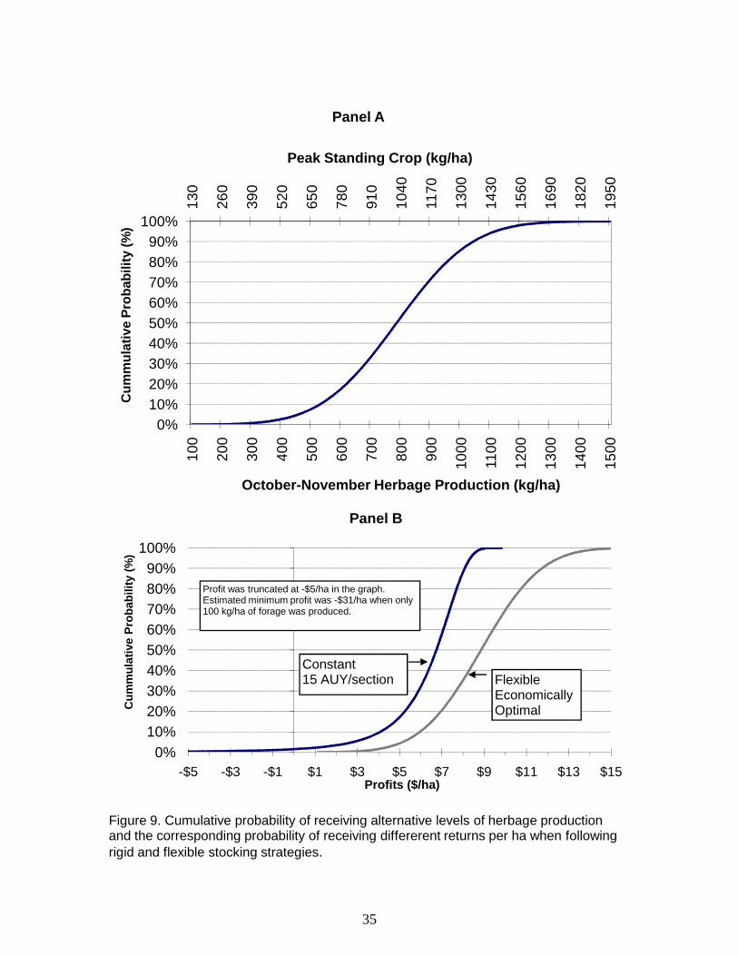
130
260
390
520
650
780
910
1040
1170
1300
1430
1560
1690
1820
1950
0%10%20%30%40%50%60%70%80%90%
100%
00 00 00 00 00 00 00 00 00 00 00 00 00 00 00
Peak Standing Crop (kg/ha)
Cum
mul
ativ
e Pr
obab
ility
(%)
Panel A
0%10%20%30%40%50%60%70%80%90%
100%
-$5 -$3 -$1 $1 $3 $5 $7 $9 $11 $13 $15
Cum
mul
ativ
e Pr
obab
ility
(%)
Profits ($/ha)
Panel B
Constant15 AUY/section Flexible
Economically Optimal
10 20 30 40 50 60 70 80 90 100
110
120
130
140
150
October-November Herbage Production (kg/ha)
Figure 9. Cumulative probability of receiving alternative levels of herbage production and the corresponding probability of receiving differerent returns per ha when following rigid and flexible stocking strategies.
Profit was truncated at -$5/ha in the graph. Estimated minimum profit was -$31/ha when only 100 kg/ha of forage was produced.
35

36
Comparing net returns for a fixed stocking rate of 15 AUY/section with net
returns for the flexible profit maximizing strategy would mean a $2.60/ha ($1.05/acre) increase in net returns at average prices (Table 9), a 41% increase in average profits, as noted earlier. Similar to the findings of Stafford-Smith and Foran (1992) the difference in net returns between the constant and flexible stocking alternatives is sensitive to beef prices, suggesting an increased economic value for an accurate weather forecast during favorable price years.
Potential Value of Weather Forecasting and Speculative Technology Adoption. There are an estimated 398.7 million acres (161.4 million ha) of rangeland in the United States. The Rocky Mountain area has 69% of this area (102.7 ha) (Mitchell 2000). The southern part of this arid area is where the value of improved weather (forage) forecasts might be the highest because as noted by Hart (1991) flexible stocking rates can already be applied with some accuracy in the northern High Plains because in this area most of the forage grows before the stocking rate decision has to be made in April-May. The value of an improved forecast also increases for areas with increased variability in rainfall and forage conditions. Without justification assume that livestock producers on 10% of the rangelands in the Rocky Mountain states adopt a flexible profit-maximizing stocking strategy and increase net returns by the estimated average $2.60/ha with a perfectly accurate 6 month weather (forage) forecast. The total forecast value would then be $26 million. Further, assume that forecast accuracy is linearly valued ( i.e. a 50% accuracy yields one half the benefits), then the economic value of a change in forecast accuracy from, for example, 40% accuracy to 50% accuracy, applied to 10% of the Rocky Mountain rangelands would reflect an increase in net returns to livestock producers of about $2.6 million. While the $/ha estimate of the forecast value is soundly based using production economic models and principles, it is anybody’s guess as to the rate of adoption.
We anticipate, however, that the rate of adoption and adjustment in stocking strategies from an improved forecast would initially be quite low. Livestock producers have not been shown to be highly motivated to adopt new grazing strategies. The rural lifestyle and way of life are often more important then profit in the hierarchy of stated goals (Torell et al. 2001, Blank 2002). Key production relationships are not known so as to reliability adopt profit maximizing stocking rate strategies in many situations. Further, survey respondents in Australia where climate variability is extremely important and has been widely studied, showed a general reluctance to use and adjust stocking rate strategies based on an improved (though relatively inaccurate) weather forecast. Correlations between the Southern Oscillation Index (SOI) and pasture growth were developed as a potential forecast (Ash et al. 2000). While 60% of 41 livestock producers responding to a survey about using seasonal climate forecasts as a management tool were interested in the SOI forecast, only 8% were using seasonal climate forecasting as a management tool and even if more reliable forecasts were available 30% said they still would not adjust stocking decisions base on the improved forecast. Instead they preferred to act on opportunities and hazards as they arose.

37
Conclusions Soil moisture is conceptually a better indicator of growing conditions than
precipitation data alone. This is partially because the periodicity, frequency, magnitude, and past history of rainfall events are incorporated into the current state of soil moisture conditions. Using the distribution of alternative soil moisture levels resulted in slight improvement in R2 values when predicting annual grass yields, versus using quarterly or monthly rainfall totals as others have done.
NOAA simulated soil moisture was very consistent with measurements taken at the two study sites with correlation coefficients exceeding 75%. Estimating the relationship between grass yield and soil moisture was not possible without the NOAA simulated data because long-term measurements of soil moisture matching the 1990-2001 grass yield measurements were not available. Nearly identical regression results were obtained when using NOAA simulated data versus actual probe-recorded data.
Winter and Q2 rainfall amounts on the Corona Ranch were found to be right skewed. Summer rainfall was found to be normally distributed. The variability of grass yield on the ranch was found to be driven by variation in seasonal rainfall amounts, as others have found for many western rangelands. When seasonal rainfall patterns were combined to predict grass yield, the resulting distribution of grass yield was found to be normally distributed with a mean of 786 kg/ha and with a standard deviation of 200 kg/ha. Stocking rate decisions on the Corona Ranch are conceptually made with this level of annual variability.
An accurate forecast and linkage between current weather and soil moisture conditions and future forage conditions could potentially improve stocking rate decisions. Net returns per ha were estimated to increase an average of $2.60/ha (41%) if an accurate forecast allowed livestock producers to adopt a flexible, profit-maximizing stocking strategy. While the rate of adoption for adjusting grazing use based on seasonal forecasts is unknown, the potential for increased returns for livestock producers is substantial and will be highest for the rangeland areas of the southwest where grasses mature late in the year. Those areas with a high level of variation in annual rainfall and production also could benefit substantially from an improved accurate forecast.

38
Literature Cited
Andales, A.A., J.D. Derner, L.R. Ahuja, and R.H. Hart. 2006. Strategic and tactical prediction of forage production in Northern mixed-grass prairie. Rangeland Ecology and Management 59:576-584.
Ash, A., O'reagain, P., McKeon, G., & Stafford-Smith, M. 2000. Managing Climate Variability in Grazing Enterprises: A Case Study of Dalrymple Shire, North-Eastern Australia. In Applications of Seasonal Climate Forecasting in Agricultural and Natural Ecosystems - The Australian Experience (Eds G. L. Hammer, N. Nicholls, & C. and Mitchell), pp. 253-270. The Netherlands: Kluwer Academic.
Bartlett, E.T., and D.R. Betters. 1983. Overstory-understory relationships in western forests. Colorado State Agr. Exp. Sta., Western regional research publication no. 1. Fort Collins.
Bartlett, E.T., Torell, L.A., Rimbey, N.R., Vantassell, AND D.W. MCCollum. 2002. Valuing grazing use on public land. Journal of Range Management 55:426–438.
Bement, R.E. 1969. A stocking-rate guide for beef production on blue-grama range. Journal of Range Management 22:83-86.
Berry, P. N. 1992. Influence of soil moisture on propagation and survival of broom snakeweed, Gutierrezia sarothrae (Pursh) Britt. and Rusby. M.S. Thesis, New Mexico State Univ., Las Cruces, NM.
Blank, S. C. 2002. “Is Agriculture a ‘Way of Life’ or a Business? – Farm Bill Choices 02” Choices Summer:26-30.
Burnash, R.J.C. 1995. The NWS river forecast system – catchment modeling. pp. 311-366. In: V.P. Singh (ed.), Computer Models of Watershed Hydrology, Water Resources Publications, Littleton, Colorado.
Cable, D.R. 1975. Influence of precipitation on perennial grass production in the semidesert southwest. Ecology 54:243-248.
Campbell Scientific Inc. 1996. CS615 water content reflectometer instruction manual. Campbell Scientific Inc., Logan, UT.
Carroll, D.B. 1994. Broom snakeweed [Gutierrezia sarothrae (Pursh) Britt. & Rusby] seedling response to spring and summer burning in central New Mexico. M.S. Thesis, New Mexico State Univ., Las Cruces, New Mexico.
Cole, J.S. and O. R. Mathews. 1940. Relation of the depth to which the soil is wet at seeding time to the yield of spring wheat on the Great Plains. U.S. Dept. Agr. Circ. 563. 20 pp.
Dahl, B.E. 1963. Soil moisture as a predictive index to forage yield for the sandhills range type. Journal of Range Management 16:128-132.

39
Day, K. A., McKeon, G. M., & Carter, J. O. 1997. Evaluating the risks of pasture and land degradation in native pasture in Queensland. Project DAQ124A. Brisbane, Queensland Dept. of Natural Resources. Report to the Rural Industries and Research Development Corporation.
Dumler, T.J. and R. Jones. 2006. Summer grazing of steers in western Kansas, Kansas State University, Agr. Exp. Sta. and Coop. Ext Service Farm Management Guide MF-1007.
Ebel, C.A. 2006. Controlling shrub invasion: Effects on a short-grass plant community. M.S. Thesis, New Mexico State Univ., Las Cruces, New Mexico.
Ffolliot, P.F., and W.P. Clary. 1972. A selected and annotated bibliography of understory-overstory vegetation relationships. Univ.Ariz. Agr. Exp. Sta. Tech. Bull. 198. Tucson, AZ.
Graham, D. Unpublished. Leasing prices and stocking rate rule-of-thumb for Union County. New Mexico State Univ. Coop. Ext. Service, Union County.
Hart, C.R. 1992. Broom snakeweed (Gutierrezia sarothrae (Pursh) Britt. & Rusby) and associated herbage response to seasonal burning in New Mexico. Ph.D. Dissertation, New Mexico State Univ., Las Cruces, New Mexico.
Hart, R.H. 1991. Managing range cattle for risk – The STEERISK spreadsheet. Journal of Range Management 44:227-231.
Hart, R.H. and M.M. Ashby. 1998. Grazing intensities, vegetation, and heifer gains: 55 years on shortgrass. Journal of Range Management 51: 392- 398.
Hart, R.H., M.J. Samuel, P.S. Test, and M.A. Smith. 1988. Cattle, vegetation, and economic responses to grazing systems and grazing pressure. Journal of Range Management 41:282-286.
Heitschmidt, R. K., M. R. Haferkamp, M. G. Karl, and A. L. Hild. 1999. Drought and grazing: I. Effects on quantity of forage produced. Journal of Range Management 52:440-446.
Hill, H. S. 2000. Estimating the effect of decision makers’ responses to improved climate forecasts on international wheat trade Ph.D. dissertation. Texas A&M University, College station, TX, 179pp.
Khumalo, G. and J. Holochek. 2005. Relationships between Chihuahuan desert perennial grass production and precipitation. Rangeland Ecology and Management 58:239-246.
Klipple, G.E. and R.E. Bement. 1961. Light grazing – is it economically feasible as a range improvement practice. Journal of Range Management 14:57-62.
Majumdar, S. 2006. The economic value of water for range forage production. M.S. Thesis, New Mexico State Univ., Las Cruces, New Mexico.

40
Mason, S. J., I. Goddard, N. E. Graham, E. Yulasve, L. Sun, and P. Arkin. 1999. The IRI seasonal climate prediction system and the 1997/98 El Nino event. Bull. Amer. Metero. Soc. 80:1853-1873.
McDaniel, K.C., J. Hartung, S. Cox, R. McNeely, and G. Timmons. 2002. Brush management plan for the NMSU Corona Ranch. Dept. of Animal and Range Science, Las Cruces.
McDaniel, K.C., Torell, L.A., and J.W. Bain. 1993. Overstory-understory relationships for broom snakeweed-blue grama grasslands. Journal of Range Management 46:506-511.
McDaniel, K.C., C. Hart and D. B. Carroll. 1997. Broom snakeweed control with fire on New Mexico blue grama rangeland. J. Range Manage. 50:652-59.
McDaniel, K.C., D. B. Carroll and C. Hart. 2000. Broom snakeweed establishment on blue grama grassland after fire and herbicide treatments. J. Range Manage. 53:239-245.
Mitchell, J.E. 2000. Rangeland resource trends in the United States: A technical document supporting the 2000 USDA Forest Service RPA assessment. Gen. Tech. Rep. RMRS-GTR-68. Fort Collins, CO. USDA, Forest Service, Rocky Mountain Research Station, 84p.
Mjelde, J. W., Sonka, S. T., Dixon, B. L., & Lamb, P. J. (1988). Valuing Forecast Characteristics in a Dynamic Agricultural Production System. American Journal of Agricultural Economics 70(3), 674-684.
Mjelde, J. W., Hill, H. S. J., & Griffiths, J. F. (1998). A review of current evidence on climate forecasts and their economic effects in agriculture. American Journal of Agricultural Economics, 80, 1089-1095.
Natural Resource Conservation Service (NRCS). 2006. SCAN Site Information for Adams Ranch in New Mexico. Available at http://www.wcc.nrcs.usda.gov/ scan/site.pl?sitenum=2015&state=nm. Accessed November 3, 2006.
Nelson, E.W. 1934. The influence of precipitation and grazing upon black grama grass range. U.S. Dep. Agric. Tech. Bull. 409. 32 p.
New Mexico Climate Center (NMCC). 2006. New Mexico Climate Center Retrieval Page. Available at (http://weather.nmsu.edu/cgi-shl/cns/stninfo.pl?stn=43). Accessed November 3, 2006.
O’Lenic, E. A. 1994. Operational long-lead outlooks of seasonal mean temperature and precipitation. NOAA Climate Prediction Center Tech. Procedures Bulletin 418. 30pp.
Pieper, R.D., J.R. Montoya, and V.L. Groce. 1971. Site characteristics on pinyon-juniper and blue grama ranges in south-central New Mexico. New Mexico Agricultural Experimental Station Bulletin 573. Las Cruces.
Pieper, R.D., C.H. Herbel, D.D. Dwyer, and R.E. Banner. 1974. Management implications of herbage weight changes on native rangeland. Journal of Soil and Water Conservation 29:227-229.

41
Ramirez, O.A. and T.U. McDonald. 2006. The expanded Johnson system: a highly flexible crop yield distribution. Selected paper presented at the American Economics Assoc. Annual Meeting, Long Beach, CA, July 23-26, 2006. Available online at http://agecon.lib.umn.edu/.
Rogler, G.A., and H. J. Haas. 1947. Range production as related to soil moisture and precipitation on the Northern Great Plains. Journal of the American Society of Agronomy 39(5):378-389.
Ross, P.J., J.Y. Parlange and R. Haverkamp. 1995. Two-dimensional interaction of a wetting front with an impervious layer: Analytical and numerical solutions. Earth and Environmental Sciences 20: 251-263.
Smathers, R.L. and N.R. Rimbey. 2006. Stocker – 200 head, no wintering, bought in the spring, sold in Fall. Univ. of Idaho, Coop. Ext. Service, 2006 Idaho Livestock Costs and Returns Estimates, EBB-ST3-06.
Sneva, F.A., and D.N. Hyder. 1962. Estimating herbage production on semiarid ranges in the intermountain region. Journal of Range Management 15:88-93.
Stafford-Smith, M., R. Buxton, G. McKeon and A. Ash. 2000. Seasonal climate forecasting and the management of rangelands: do production benefits translate into enterprise profits? Application of Seasonal Climate Forecasting in Agricultural and Natural Ecosystems. Kluwer Academic 271-290.
Stern, P. C. 1994. Making climate forecast matter. National Academy Press. 175 pp.
Stevens Water Monitoring Systems. 2006. Hydra Probe II. Available at http://www.stevenswater.com/ catalog/stevensProduct.aspx?SKU='93640. Accessed Sept. 29, 2006.
Stone, R. C. 1994. Examples of weather-related concerns in agriculture and grazing systems in Northern Australia. Usable Science: the potential use and misuse of El Nino information in North America. National Center for Atmospheric Research, Boulder, CO. 221pp.
Stubbendieck, J. and D.F. Burzlaff. 1970. Effects of temperature and day length on axillary bud and tiller development in blue grama. Journal of Range Management 23(1):63-66.
Torell, L.A., N.R. Rimbey, J.A. Tanaka, and S.A. Bailey. 2001. The Lack of a Profit Motive for Ranching: Implications for Policy Analysis. 2001. In: Torell, L. A., E. T. Bartlett, and R. Larranaga (eds.). Current issues in rangeland resource economics: Proceedings of a symposium sponsored by Western Coordinating Committee 55 (WCC-55), Agricultural Experiment Station Research Report No. 737, New Mexico State University, Las Cruces, Online. Available at http://agecon.lib.umn.edu.
Torell, L.A., K.S. Lyon, and E.B. Godfrey. 1991. Long-run Versus Short-run Planning Horizons and the Rangeland Stocking Rate Decision. Amer. J. Agr. Econ. 73:795-807.

42
Turner, G.T. and G.E. Klipple. 1952. Growth characteristics of blue grama in northeast Colorado. Journal of Range Management 5:22-28.
U.S. Department of Agriculture National Agricultural Statistical Service (USDA-NASS). 2007 Agricultural prices monthly. Available online at http://usda.mannlib. cornell.edu/MannUsda/viewDocumentInfo.do?documentID=1002. January issue.
Vallentine, J.F. 1990. Grazing Management. Academic Press, Inc. New York, NY.
Wight, J.R. and J.W. Skiles (eds.). 1987. SPUR: Simulation of Production and Utilization of Rangelands. Documentation and user guide. USDA-ARS Pub. ARS-63.

43
Appendix A: Corona Ranch seasonal and annual rainfall amounts, 1914 – 2006

05101520253035
1914
1917
1920
1923
1926
1929
1932
1935
1938
1941
1944
1947
1950
1953
1956
1959
1962
1965
1968
1971
1974
1978
1981
1984
1987
1990
1993
1996
1999
2002
2005
Year
precipitation (Inches)
0100
200
300
400
500
600
700
800
900
1000
Precipitation (mm)
Win
ter
Gro
win
g S
easo
n (A
pr -
Oct
)M
ean
Gro
win
g S
easo
nM
ean
Ann
ual
Not
e th
at d
ata
for 1
977
was
inco
mpl
ete
and
not i
nclu
ded.
App
endi
x A
. Cor
ona
Ran
ch s
easo
nal a
nd a
nnua
l rai
nfal
l am
ount
s, 1
914
- 200
6.
44

45
Appendix B: Recorded and simulated soil moisture measurements (% by Volume) at the SH and OW research sites, recorded daily rainfall (mm) and end-of-season grass yield (kg/ha).

286
1009
0102030405060Jan 1991
Feb 1991
Mar 1991
Apr 1991
May 1991
Jun 1991
Jul 1991
Aug 1991
Sep 1991
Oct 1991
Nov 1991
Dec 1991
Jan 1992
Feb 1992
Mar 1992
Apr 1992
May 1992
Jun 1992
Jul 1992
Aug 1992
Sep 1992
Oct 1992
Nov 1992
Dec 1992
Rainfall (mm) and Soil Moisture (%)
0200
400
600
800
1,00
0
1,20
0
1,40
0
Grass Yield (Kg/ha)
SH 1
991
- 199
2, 1
0 cm
805
367
0102030405060
Jan 1993
Feb 1993
Mar 1993
Apr 1993
May 1993
Jun 1993
Jul 1993
Aug 1993
Sep 1993
Oct 1993
Nov 1993
Dec 1993
Jan 1994
Feb 1994
Mar 1994
Apr 1994
May 1994
Jun 1994
Jul 1994
Aug 1994
Sep 1994
Oct 1994
Nov 1994
Dec 1994
Rainfall (mm) and Soil Moisture (%)
0200
400
600
800
1,00
0
1,20
0
1,40
0
Grass Yield (Kg/ha)
SH 1
993
- 199
4, 1
0 cm
App
endi
x B
, Fig
ure
1. S
outh
Hou
se si
te d
aily
rain
fall
(mm
, blu
e ba
rs re
ad fr
om th
e le
ft ax
is),
gras
s yie
ld (k
g/ha
, gre
en b
ar re
ad fr
om th
e rig
ht
axis
), an
d N
OA
A p
redi
cted
(%, g
rey
line
read
from
the
left
axis
) ver
sus a
ctua
l soi
l moi
stur
e (%
, bla
ck li
ne re
ad fr
om le
ft ax
is),
mid
nigh
t re
adin
g m
easu
red
at 1
0 cm
.
46

634
1021
0102030405060Jan 1995
Feb 1995
Mar 1995
Apr 1995
May 1995
Jun 1995
Jul 1995
Aug 1995
Sep 1995
Oct 1995
Nov 1995
Dec 1995
Jan 1996
Feb 1996
Mar 1996
Apr 1996
May 1996
Jun 1996
Jul 1996
Aug 1996
Sep 1996
Oct 1996
Nov 1996
Dec 1996
Rainfall (mm) and Soil Moisture (%)
0200
400
600
800
1,00
0
1,20
0
1,40
0
Grass Yield (Kg/ha)
SH 1
995
- 199
6, 1
0 cm
839
1,37
2
0102030405060
Jan 1997
Feb 1997
Mar 1997
Apr 1997
May 1997
Jun 1997
Jul 1997
Aug 1997
Sep 1997
Oct 1997
Nov 1997
Dec 1997
Jan 1998
Feb 1998
Mar 1998
Apr 1998
May 1998
Jun 1998
Jul 1998
Aug 1998
Sep 1998
Oct 1998
Nov 1998
Dec 1998
Rainfall (mm) and Soil Moisture (%)
0200
400
600
800
1,00
0
1,20
0
1,40
0
Grass Yield (Kg/ha)
SH 1
997
- 199
8, 1
0 cm
App
endi
x B
, Fig
ure
1. S
outh
Hou
se si
te 1
0 cm
con
tinue
d.
47

735
198
0102030405060Jan 1999
Feb 1999
Mar 1999
Apr 1999
May 1999
Jun 1999
Jul 1999
Aug 1999
Sep 1999
Oct 1999
Nov 1999
Dec 1999
Jan 2000
Feb 2000
Mar 2000
Apr 2000
May 2000
Jun 2000
Jul 2000
Aug 2000
Sep 2000
Oct 2000
Nov 2000
Dec 2000
Rainfall (mm) and Soil Moisture (%)
0200
400
600
800
1,00
0
1,20
0
1,40
0
Grass Yield (Kg/ha)
SH 1
999
- 200
0, 1
0 cm
416
672
0102030405060
Jan 2001
Feb 2001
Mar 2001
Apr 2001
May 2001
Jun 2001
Jul 2001
Aug 2001
Sep 2001
Oct 2001
Nov 2001
Dec 2001
Jan 2002
Feb 2002
Mar 2002
Apr 2002
May 2002
Jun 2002
Jul 2002
Aug 2002
Sep 2002
Oct 2002
Nov 2002
Dec 2002
Rainfall (mm) and Soil Moisture (%)
0200
400
600
800
1,00
0
1,20
0
1,40
0
Grass Yield (Kg/ha)
SH 2
001
- 200
2, 1
0 cm
App
endi
x B
, Fig
ure
1. S
outh
Hou
se si
te 1
0 cm
con
tinue
d.
48

367
657
0102030405060Jan 2003
Feb 2003
Mar 2003
Apr 2003
May 2003
Jun 2003
Jul 2003
Aug 2003
Sep 2003
Oct 2003
Nov 2003
Dec 2003
Jan 2004
Feb 2004
Mar 2004
Apr 2004
May 2004
Jun 2004
Jul 2004
Aug 2004
Sep 2004
Oct 2004
Nov 2004
Dec 2004
Rainfall (mm) and Soil Moisture (%)
0200
400
600
800
1,00
0
1,20
0
1,40
0
Grass Yield (Kg/ha)
SH 2
003
- 200
4, 1
0 cm
779
1,03
3
0102030405060
Jan 2005
Feb 2005
Mar 2005
Apr 2005
May 2005
Jun 2005
Jul 2005
Aug 2005
Sep 2005
Oct 2005
Nov 2005
Dec 2005
Jan 2006
Feb 2006
Mar 2006
Apr 2006
May 2006
Jun 2006
Jul 2006
Aug 2006
Sep 2006
Oct 2006
Nov 2006
Dec 2006
Rainfall (mm) and Soil Moisture (%)
0200
400
600
800
1,00
0
1,20
0
1,40
0
Grass Yield (Kg/ha)
SH 2
005
- 200
6, 1
0 cm
App
endi
x B
, Fig
ure
1. S
outh
Hou
se si
te 1
0 cm
con
tinue
d.
49

286
1009
0102030405060Jan 1991
Feb 1991
Mar 1991
Apr 1991
May 1991
Jun 1991
Jul 1991
Aug 1991
Sep 1991
Oct 1991
Nov 1991
Dec 1991
Jan 1992
Feb 1992
Mar 1992
Apr 1992
May 1992
Jun 1992
Jul 1992
Aug 1992
Sep 1992
Oct 1992
Nov 1992
Dec 1992
Rainfall (mm) and Soil Moisture (%)
0200
400
600
800
1,00
0
1,20
0
1,40
0
Grass Yield (Kg/ha)
SH 1
991
- 199
2, 1
0-30
cm
805
367
0102030405060
Jan 1993
Feb 1993
Mar 1993
Apr 1993
May 1993
Jun 1993
Jul 1993
Aug 1993
Sep 1993
Oct 1993
Nov 1993
Dec 1993
Jan 1994
Feb 1994
Mar 1994
Apr 1994
May 1994
Jun 1994
Jul 1994
Aug 1994
Sep 1994
Oct 1994
Nov 1994
Dec 1994
Rainfall (mm) and Soil Moisture (%)
0200
400
600
800
1,00
0
1,20
0
1,40
0
Grass Yield (Kg/ha)
SH 1
993
- 199
4, 1
0-30
cm
App
endi
x B
, Fig
ure
2. S
outh
Hou
se si
te d
aily
rain
fall
(mm
, blu
e ba
rs re
ad fr
om th
e le
ft ax
is),
gras
s yie
ld (k
g/ha
, gre
en b
ar re
ad fr
om th
e rig
ht
axis
), an
d N
OA
A p
redi
cted
(%, g
rey
line
read
from
the
left
axis
) ver
sus a
ctua
l soi
l moi
stur
e (%
, bla
ck li
ne re
ad fr
om le
ft ax
is),
mid
nigh
t re
adin
g m
easu
red
at 1
0 -
30 c
m.
50

634
1021
0102030405060Jan 1995
Feb 1995
Mar 1995
Apr 1995
May 1995
Jun 1995
Jul 1995
Aug 1995
Sep 1995
Oct 1995
Nov 1995
Dec 1995
Jan 1996
Feb 1996
Mar 1996
Apr 1996
May 1996
Jun 1996
Jul 1996
Aug 1996
Sep 1996
Oct 1996
Nov 1996
Dec 1996
Rainfall (mm) and Soil Moisture (%)
0200
400
600
800
1,00
0
1,20
0
1,40
0
Grass Yield (Kg/ha)
SH 1
995
- 199
6, 1
0-30
cm
839
1,37
2
0102030405060
Jan 1997
Feb 1997
Mar 1997
Apr 1997
May 1997
Jun 1997
Jul 1997
Aug 1997
Sep 1997
Oct 1997
Nov 1997
Dec 1997
Jan 1998
Feb 1998
Mar 1998
Apr 1998
May 1998
Jun 1998
Jul 1998
Aug 1998
Sep 1998
Oct 1998
Nov 1998
Dec 1998
Rainfall (mm) and Soil Moisture (%)
0200
400
600
800
1,00
0
1,20
0
1,40
0
Grass Yield (Kg/ha)
SH 1
997
- 199
8, 1
0-30
cm
A
ppen
dix
B, F
igur
e 2.
Sou
th H
ouse
site
10
- 30
cm
con
tinue
d.
51
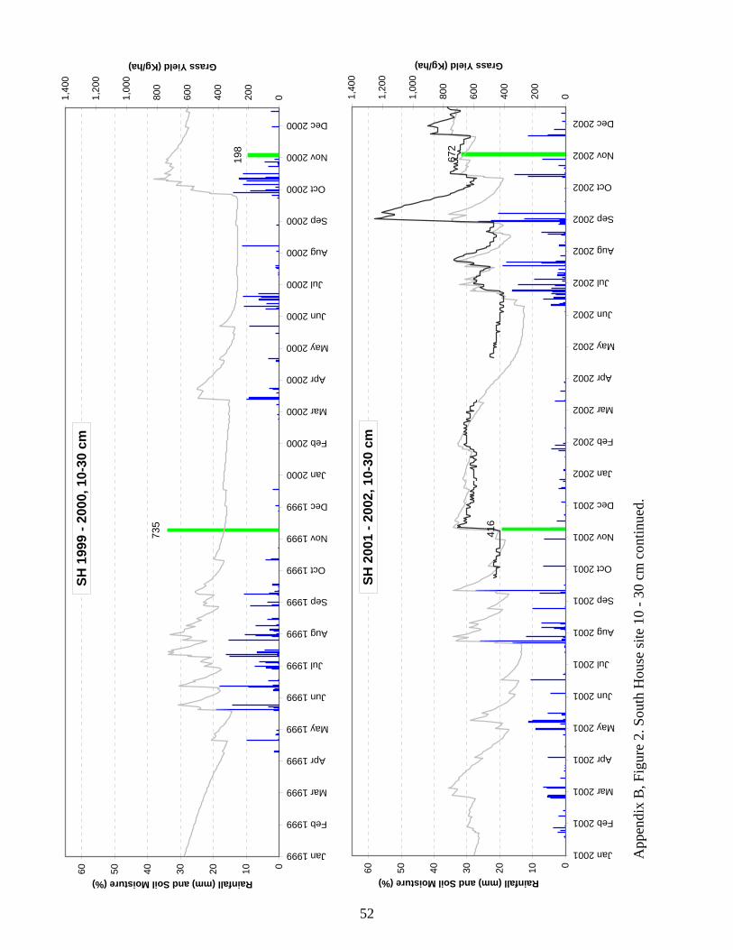
735
198
0102030405060Jan 1999
Feb 1999
Mar 1999
Apr 1999
May 1999
Jun 1999
Jul 1999
Aug 1999
Sep 1999
Oct 1999
Nov 1999
Dec 1999
Jan 2000
Feb 2000
Mar 2000
Apr 2000
May 2000
Jun 2000
Jul 2000
Aug 2000
Sep 2000
Oct 2000
Nov 2000
Dec 2000
Rainfall (mm) and Soil Moisture (%)
0200
400
600
800
1,00
0
1,20
0
1,40
0
Grass Yield (Kg/ha)
SH 1
999
- 200
0, 1
0-30
cm
416
672
0102030405060
Jan 2001
Feb 2001
Mar 2001
Apr 2001
May 2001
Jun 2001
Jul 2001
Aug 2001
Sep 2001
Oct 2001
Nov 2001
Dec 2001
Jan 2002
Feb 2002
Mar 2002
Apr 2002
May 2002
Jun 2002
Jul 2002
Aug 2002
Sep 2002
Oct 2002
Nov 2002
Dec 2002
Rainfall (mm) and Soil Moisture (%)
0200
400
600
800
1,00
0
1,20
0
1,40
0
Grass Yield (Kg/ha)
SH 2
001
- 200
2, 1
0-30
cm
App
endi
x B
, Fig
ure
2. S
outh
Hou
se si
te 1
0 -
30 c
m c
ontin
ued.
52

367
657
0102030405060Jan 2003
Feb 2003
Mar 2003
Apr 2003
May 2003
Jun 2003
Jul 2003
Aug 2003
Sep 2003
Oct 2003
Nov 2003
Dec 2003
Jan 2004
Feb 2004
Mar 2004
Apr 2004
May 2004
Jun 2004
Jul 2004
Aug 2004
Sep 2004
Oct 2004
Nov 2004
Dec 2004
Rainfall (mm) and Soil Moisture (%)
0200
400
600
800
1,00
0
1,20
0
1,40
0
Grass Yield (Kg/ha)
SH 2
003
- 200
4, 1
0-30
cm
779
1,03
3
0102030405060
Jan 2005
Feb 2005
Mar 2005
Apr 2005
May 2005
Jun 2005
Jul 2005
Aug 2005
Sep 2005
Oct 2005
Nov 2005
Dec 2005
Jan 2006
Feb 2006
Mar 2006
Apr 2006
May 2006
Jun 2006
Jul 2006
Aug 2006
Sep 2006
Oct 2006
Nov 2006
Dec 2006
Rainfall (mm) and Soil Moisture (%)
0200
400
600
800
1,00
0
1,20
0
1,40
0
Grass Yield (Kg/ha)
SH 2
005
- 200
6, 1
0-30
cm
App
endi
x B
, Fig
ure
2. S
outh
Hou
se si
te 1
0 -
30 c
m c
ontin
ued.
53

609
1056
0102030405060
Jan 1991
Feb 1991
Mar 1991
Apr 1991
May 1991
Jun 1991
Jul 1991
Aug 1991
Sep 1991
Oct 1991
Nov 1991
Dec 1991
Jan 1992
Feb 1992
Mar 1992
Apr 1992
May 1992
Jun 1992
Jul 1992
Aug 1992
Sep 1992
Oct 1992
Nov 1992
Dec 1992
Rainfall (mm) and Soil Moisture (%)
0200
400
600
800
1,00
0
1,20
0
1,40
0
Grass Yield (Kg/ha)
OW
199
1 - 1
992,
10
cm
676
366
0102030405060
Jan 1993
Feb 1993
Mar 1993
Apr 1993
May 1993
Jun 1993
Jul 1993
Aug 1993
Sep 1993
Oct 1993
Nov 1993
Dec 1993
Jan 1994
Feb 1994
Mar 1994
Apr 1994
May 1994
Jun 1994
Jul 1994
Aug 1994
Sep 1994
Oct 1994
Nov 1994
Dec 1994
Rainfall (mm) and Soil Moisture (%)
0200
400
600
800
1,00
0
1,20
0
1,40
0
Grass Yield (Kg/ha)
OW
199
3 - 1
994,
10
cm
App
endi
x B
, Fig
ure
3. O
il W
ell s
ite d
aily
rain
fall
(mm
, blu
e ba
rs re
ad fr
om th
e le
ft ax
is),
gras
s yie
ld (k
g/ha
, gre
en b
ar re
ad fr
om th
e rig
ht
axis
), an
d N
OA
A p
redi
cted
soil
moi
stur
e (%
, gre
y lin
e re
ad fr
om th
e le
ft ax
is) v
ersu
s act
ual s
oil m
oist
ure
(%, b
lack
line
read
from
left
axis
), m
idni
ght r
eadi
ng m
easu
red
at 1
0 cm
.
54

581
819
0102030405060Jan 1995
Feb 1995
Mar 1995
Apr 1995
May 1995
Jun 1995
Jul 1995
Aug 1995
Sep 1995
Oct 1995
Nov 1995
Dec 1995
Jan 1996
Feb 1996
Mar 1996
Apr 1996
May 1996
Jun 1996
Jul 1996
Aug 1996
Sep 1996
Oct 1996
Nov 1996
Dec 1996
Rainfall (mm) and Soil Moisture (%)
0200
400
600
800
1,00
0
1,20
0
1,40
0
Grass Yield (Kg/ha)
OW
199
5 - 1
996,
10
cm
952
1,00
7
0102030405060
Jan 1997
Feb 1997
Mar 1997
Apr 1997
May 1997
Jun 1997
Jul 1997
Aug 1997
Sep 1997
Oct 1997
Nov 1997
Dec 1997
Jan 1998
Feb 1998
Mar 1998
Apr 1998
May 1998
Jun 1998
Jul 1998
Aug 1998
Sep 1998
Oct 1998
Nov 1998
Dec 1998
Rainfall (mm) and Soil Moisture (%)
0200
400
600
800
1,00
0
1,20
0
1,40
0
Grass Yield (Kg/ha)
OW
199
7 - 1
998,
10
cm
App
endi
x B
, Fig
ure
3. O
il W
ell s
ite 1
0 cm
con
tinue
d.
55

1032
239
0102030405060Jan 1999
Feb 1999
Mar 1999
Apr 1999
May 1999
Jun 1999
Jul 1999
Aug 1999
Sep 1999
Oct 1999
Nov 1999
Dec 1999
Jan 2000
Feb 2000
Mar 2000
Apr 2000
May 2000
Jun 2000
Jul 2000
Aug 2000
Sep 2000
Oct 2000
Nov 2000
Dec 2000
Rainfall (mm) and Soil Moisture (%)
0200
400
600
800
1,00
0
1,20
0
1,40
0
Grass Yield (Kg/ha)
OW
199
9 - 2
000,
10
cm
113
414
0102030405060
Jan 2001
Feb 2001
Mar 2001
Apr 2001
May 2001
Jun 2001
Jul 2001
Aug 2001
Sep 2001
Oct 2001
Nov 2001
Dec 2001
Jan 2002
Feb 2002
Mar 2002
Apr 2002
May 2002
Jun 2002
Jul 2002
Aug 2002
Sep 2002
Oct 2002
Nov 2002
Dec 2002
Rainfall (mm) and Soil Moisture (%)
0200
400
600
800
1,00
0
1,20
0
1,40
0
Grass Yield (Kg/ha)
OW
200
1 - 2
002,
10
cm
App
endi
x B
, Fig
ure
3. O
il W
ell s
ite 1
0 cm
con
tinue
d.
56

408
1043
0102030405060Jan 2003
Feb 2003
Mar 2003
Apr 2003
May 2003
Jun 2003
Jul 2003
Aug 2003
Sep 2003
Oct 2003
Nov 2003
Dec 2003
Jan 2004
Feb 2004
Mar 2004
Apr 2004
May 2004
Jun 2004
Jul 2004
Aug 2004
Sep 2004
Oct 2004
Nov 2004
Dec 2004
Rainfall (mm) and Soil Moisture (%)
0200
400
600
800
1,00
0
1,20
0
1,40
0
Grass Yield (Kg/ha)
OW
200
3 - 2
004,
10
cm
936
1,20
2
0102030405060
Jan 2005
Feb 2005
Mar 2005
Apr 2005
May 2005
Jun 2005
Jul 2005
Aug 2005
Sep 2005
Oct 2005
Nov 2005
Dec 2005
Jan 2006
Feb 2006
Mar 2006
Apr 2006
May 2006
Jun 2006
Jul 2006
Aug 2006
Sep 2006
Oct 2006
Nov 2006
Dec 2006
Rainfall (mm) and Soil Moisture (%)
0200
400
600
800
1,00
0
1,20
0
1,40
0
Grass Yield (Kg/ha)
OW
200
5 - 2
006,
10
cm
App
endi
x B
, Fig
ure
3. O
il W
ell s
ite 1
0 cm
con
tinue
d.
57

609
1056
0102030405060Jan 1991
Feb 1991
Mar 1991
Apr 1991
May 1991
Jun 1991
Jul 1991
Aug 1991
Sep 1991
Oct 1991
Nov 1991
Dec 1991
Jan 1992
Feb 1992
Mar 1992
Apr 1992
May 1992
Jun 1992
Jul 1992
Aug 1992
Sep 1992
Oct 1992
Nov 1992
Dec 1992
Rainfall (mm) and Soil Moisture (%)
0200
400
600
800
1,00
0
1,20
0
1,40
0
Grass Yield (Kg/ha)
OW
199
1 - 1
992,
10-
30 c
m
676
366
0102030405060
Jan 1993
Feb 1993
Mar 1993
Apr 1993
May 1993
Jun 1993
Jul 1993
Aug 1993
Sep 1993
Oct 1993
Nov 1993
Dec 1993
Jan 1994
Feb 1994
Mar 1994
Apr 1994
May 1994
Jun 1994
Jul 1994
Aug 1994
Sep 1994
Oct 1994
Nov 1994
Dec 1994
Rainfall (mm) and Soil Moisture (%)
0200
400
600
800
1,00
0
1,20
0
1,40
0
Grass Yield (Kg/ha)
OW
199
3 - 1
994,
10-
30 c
m
App
endi
x B
, Fig
ure
4. O
il W
ell s
ite d
aily
rain
fall
(mm
, blu
e ba
rs re
ad fr
om th
e le
ft ax
is),
gras
s yie
ld (k
g/ha
, gre
en b
ar re
ad fr
om th
e rig
ht
axis
), an
d N
OA
A p
redi
cted
(%, g
rey
line
read
from
the
left
axis
) ver
sus a
ctua
l soi
l moi
stur
e (%
, bla
ck li
ne re
ad fr
om le
ft ax
is),
mid
nigh
t re
adin
g m
easu
red
at 1
0 -
30 c
m.
58

581
819
0102030405060Jan 1995
Feb 1995
Mar 1995
Apr 1995
May 1995
Jun 1995
Jul 1995
Aug 1995
Sep 1995
Oct 1995
Nov 1995
Dec 1995
Jan 1996
Feb 1996
Mar 1996
Apr 1996
May 1996
Jun 1996
Jul 1996
Aug 1996
Sep 1996
Oct 1996
Nov 1996
Dec 1996
Rainfall (mm) and Soil Moisture (%)
0200
400
600
800
1,00
0
1,20
0
1,40
0
Grass Yield (Kg/ha)
OW
199
5 - 1
996,
10-
30 c
m
952
1,00
7
0102030405060
Jan 1997
Feb 1997
Mar 1997
Apr 1997
May 1997
Jun 1997
Jul 1997
Aug 1997
Sep 1997
Oct 1997
Nov 1997
Dec 1997
Jan 1998
Feb 1998
Mar 1998
Apr 1998
May 1998
Jun 1998
Jul 1998
Aug 1998
Sep 1998
Oct 1998
Nov 1998
Dec 1998
Rainfall (mm) and Soil Moisture (%)
0200
400
600
800
1,00
0
1,20
0
1,40
0
Grass Yield (Kg/ha)
OW
199
7 - 1
998,
10-
30 c
m
App
endi
x B
, Fig
ure
4. O
il W
ell s
ite 1
0 -
30 c
m c
ontin
ued.
59

1032
239
0102030405060Jan 1999
Feb 1999
Mar 1999
Apr 1999
May 1999
Jun 1999
Jul 1999
Aug 1999
Sep 1999
Oct 1999
Nov 1999
Dec 1999
Jan 2000
Feb 2000
Mar 2000
Apr 2000
May 2000
Jun 2000
Jul 2000
Aug 2000
Sep 2000
Oct 2000
Nov 2000
Dec 2000
Rainfall (mm) and Soil Moisture (%)
0200
400
600
800
1,00
0
1,20
0
1,40
0
Grass Yield (Kg/ha)
OW
199
9 - 2
000,
10-
30 c
m
113
414
0102030405060
Jan 2001
Feb 2001
Mar 2001
Apr 2001
May 2001
Jun 2001
Jul 2001
Aug 2001
Sep 2001
Oct 2001
Nov 2001
Dec 2001
Jan 2002
Feb 2002
Mar 2002
Apr 2002
May 2002
Jun 2002
Jul 2002
Aug 2002
Sep 2002
Oct 2002
Nov 2002
Dec 2002
Rainfall (mm) and Soil Moisture (%)
0200
400
600
800
1,00
0
1,20
0
1,40
0
Grass Yield (Kg/ha)
OW
200
1 - 2
002,
10-
30 c
m
App
endi
x B
, Fig
ure
4. O
il W
ell s
ite 1
0 -
30 c
m c
ontin
ued.
60

408
1043
0102030405060Jan 2003
Feb 2003
Mar 2003
Apr 2003
May 2003
Jun 2003
Jul 2003
Aug 2003
Sep 2003
Oct 2003
Nov 2003
Dec 2003
Jan 2004
Feb 2004
Mar 2004
Apr 2004
May 2004
Jun 2004
Jul 2004
Aug 2004
Sep 2004
Oct 2004
Nov 2004
Dec 2004
Rainfall (mm) and Soil Moisture (%)
0200
400
600
800
1,00
0
1,20
0
1,40
0
Grass Yield (Kg/ha)
OW
200
3 - 2
004,
10-
30 c
m
936
1,20
2
0102030405060
Jan 2005
Feb 2005
Mar 2005
Apr 2005
May 2005
Jun 2005
Jul 2005
Aug 2005
Sep 2005
Oct 2005
Nov 2005
Dec 2005
Jan 2006
Feb 2006
Mar 2006
Apr 2006
May 2006
Jun 2006
Jul 2006
Aug 2006
Sep 2006
Oct 2006
Nov 2006
Dec 2006
Rainfall (mm) and Soil Moisture (%)
0200
400
600
800
1,00
0
1,20
0
1,40
0
Grass Yield (Kg/ha)
OW
200
5 - 2
006,
10-
30 c
m
App
endi
x B
, Fig
ure
4. O
il W
ell s
ite 1
0 -
30 c
m c
ontin
ued.
61