The Pennsylvania State University

The Graduate School

Industrial Engineering Department

AN INVESTIGATION ON THE SUPPLY CHAIN IMPLICATIONS OF MODULARIZED

DESIGNS CONSIDERING END-OF-LIFE AND LIFE EXPECTANCY

A Thesis in

Industrial Engineering

by

Nirup Philip

2013 Nirup Philip

Submitted in Partial Fulfillment

of the Requirements

for the Degree of

Master of Science

May 2013

ii

The thesis of Nirup Philip was reviewed and approved* by the following:

Gül E. Okudan Kremer Associate Professor of Engineering Design and Industrial Engineering Thesis Advisor

Vittal Prabhu Professor of Industrial Engineering Harold and Inge Marcus Department of Industrial and Manufacturing Engineering

Paul Griffin Peter and Angela Dal Pezzo Department Head Chair Head of the Department, Industrial and Manufacturing Engineering

*Signatures are on file in the Graduate School

iii

ABSTRACT

Modularity aids in the development of new products quickly and easily. Companies nowadays are

faced with the challenge of providing as much variety as possible; accordingly, mass customization is

adopted. Mass customization frequently employs modularity. However, in order to mass customize

effectively, supply chain factors also have to be taken into account. Along with supply chain and

manufacturing considerations growing environmental concerns have forced companies to look at the end-

of-life options for different components present in their products.

This study presents a framework to incorporate component end-of-life options (i.e., reuse, recycle

and dispose) during early design stages in order to simultaneously account for supply chain factors, such

as cost and carbon footprint. Manufacturers could benefit from a methodology that analyzes modular

product architectures for overall life-cycle efficiency. In order to accomplish this, we extend a software

framework originally developed by (Gupta and Okudan, 2008); this software aimed at creating a

computational design tool that would aid designers in developing new modular products by taking into

account design for assembly (DfA) and design for variety (DfV). This is an extension to that work where

the user will have the ability to generate designs taking into account component end-of-life options, and

to select suppliers for the components present in these modules.

Three types of modularization methodologies are used and their results are analyzed. In the first

methodology the decomposition approach (DA) is used where the main focus for modularization is

component suitability in addition to their interactions. For the second modularization method a new

methodology called green decomposition approach (Green DA) is presented in which the end-of-life

options are used to determine the component suitability; however, the decomposition algorithm is still

employed. In the third approach, a simulated annealing (SA) inspired hierarchical search algorithm is

used. In all three methodologies component suitability, life expectancy and end-of-life are used as criteria

for module selection, this enables us to compare the three which methodologies. Suppliers are then

iv

selected for these components based on their cost, lead time and overall carbon footprint. This enables the

designer to understand the trade-offs between the designs generated by each of these modularization

methodologies and their associated costs, lead times and carbon footprints.

We compare two designs which are selected based on their DFA index and the three main

modularization methodologies. The decomposition approach with a three module assembly generates the

lowest total cost however the hierarchical search algorithm methodology generates the option with a

lower carbon footprint.

v

TABLE OF CONTENTS

LIST OF FIGURES ..................................................................................................... vii

LIST OF TABLES ....................................................................................................... ix

ACKNOWLEDGEMENTS ......................................................................................... x

Chapter 1 Introduction ................................................................................................. 1

1.1 Overview of the Proposed Framework ........................................................... 2 1.2 Thesis Roadmap .............................................................................................. 3

Chapter 2 Literature Review ........................................................................................ 5

2.1 Modular Product Architecture ........................................................................ 5

2.1.1 Advantages of Modularization ............................................................. 6 2.1.2 Constraints Imposed by Modularization .............................................. 6 2.1.3 Taxonomy of Modular Product Architecture ....................................... 7

2.1.4 Industry Examples of Modularization .................................................. 8

2.2 Sustainability .................................................................................................. 9 2.2.1 Need for Sustainability ......................................................................... 10 2.2.2 Carbon Footprint .................................................................................. 11

2.3 Supplier Selection ........................................................................................... 12 2.3.1 Supplier Selection Methods .................................................................. 12

2.3.2 Supplier Selection Models at the Conceptual Stage ............................. 14 2.4 Comparison of Different Modularization Methodologies .............................. 15 2.5 Modularization and Sustainability .................................................................. 17

Chapter 3 Methodology .............................................................................................. 19

3.1 Design Repository .......................................................................................... 20 3.2 Modularization Methodologies ....................................................................... 25

Chapter 4 Bicycle Case Study ..................................................................................... 27

4.2 Components present in the bicycle ................................................................. 27 4.3 EMS model mapping and DFA index ............................................................ 29 4.4 Supply chain costs .......................................................................................... 30

Table 4-3 a): Manufacturing cost and time for Assembly 1 (Chiu, 2010) .... 31

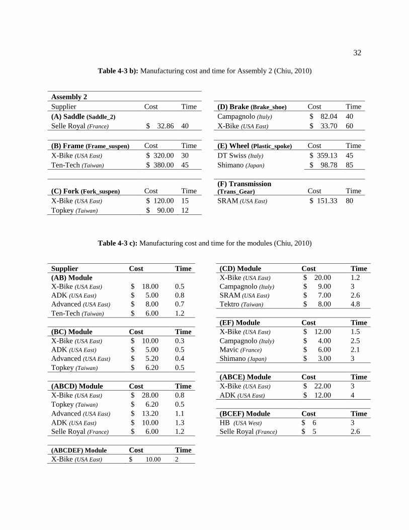
Table 4-3 b): Manufacturing cost and time for Assembly 2 (Chiu, 2010) .... 32

Table 4-3 c): Manufacturing cost and time for the modules (Chiu, 2010) .... 32

4.4.1 Inputting component information and supply chain costs .................... 33 4.4.1 Inputting supply chain information ...................................................... 34

4.5 End-of-life Options ......................................................................................... 36

vi

4.6 Carbon Footprint ............................................................................................. 39 4.6 Suitability Level and Modularization for Decomposition Approach ............. 41

4.7 Suitability Level and Modularization for Green Decomposition Approach .. 43 4.8 Simulated Annealing Inspired Hierarchical Search Algorithm (HSA) .......... 45

4.8.1 Overview of the Hierarchical search algorithm (HSA) ........................ 45 4.8.2 Matrix Generation for the Hierarchical Search Process ....................... 47 4.8.3 Temperature and Module Clustering .................................................... 49

4.8.4 Constraints Imposed ............................................................................. 51 4.8.5 Modules Obtained ................................................................................ 51

4.9 Comparison of Results .................................................................................... 52

Chapter 5 Conclusion ................................................................................................... 61

References .................................................................................................................... 63

Appendix Java code used to develop the software ...................................................... 69

vii

LIST OF FIGURES

Figure 1-1. Prior Research Inspiring the Proposed Framework …...………………….…………...……. 2

Figure 2-2: Different Types of Modularity (Adopted from Ulrich, 1995).….…….…….……...……….. 7

Figure 2-3: Supplier Selection Methodologies (Aamer and Sawhney, 2004)……………………...…… 12

Figure 3-1. Energy Material Signal (EMS) Diagram .……….…………………..…….…….………..… 18

Figure 3-2. GUI for Inputting the EMS Functional Model …………………….……….………………. 19

Figure 3-3. a) ‘dfa’ b) ‘rules’ Table ………………….………………….……………….………..….... 22

Figure 3-4. GUI for the Interaction Matrix ...…………..…………………….……….………...…...…. 22

Figure 3-5. a) ‘supplier_information’ b) ‘locationmat’………………………………...…….…….…… 23

Figure 3-6. Generated Conceptual Designs with different designs ……………….….……...………..... 24

Figure 3-7. Suitability Level …………………….……………………………….……….…………..... 25

Figure 4-1. Simplified Bike Architecture (Chiu and Okudan, 2011) …………………………………... 24

Figure 4-2. Bike Supply Chain Structure Adopted from Chiu and Okudan (2011)……………………. 25

Figure 4-3. GUI for Inputting the Component Level Information ……………………….……….……. 29

Figure 4-4. Energy Material Signal (EMS) Diagram ……………...………………………..…………. 30

Figure 4-5. GUI for Inputting Supplier Information.………………………………...………………… 31

Figure 4-6. GUI for Inputting Component Level Supplier Information ……….……………………….31

Figure 4-7. Suitability Matrix for Decomposition Approach ……………….………………………...... 36

Figure 4-8. Modules Obtained When Modularized Using Decomposition Approach …………………. 36

Figure 4-9. Suitability Matrix based on End-of-life Options ………….……………………………..... 37

Figure 4-10. Modules Obtained When Modularized Using Green Decomposition Approach …….…. 38

Figure 4-11. Overview of simulated annealing (Gu and Sosale, 1999) ………………………...….…. 39

Figure 4-12. Interaction Matrix for the bicycle case study. ……….………..………………………..... 43

viii

Figure 4-13. Suitability Matrix for the SA process ………………………………………………...…. 44

Figure 4-14. Modules Obtained When Modularized Using Simulated Annealing ….…………...….…. 39

Figure 4-15. Suitability Matrix for Case 1. ……………………...………………………………...…. 48

Figure 4-16. Product Architecture for Case 1. ….……………………………………………......….…. 48

Figure 4-17. Interaction Matrix for Case 5 ….……………………….……………………………...…. 49

Figure 4-18. Suitability Matrix for Case 5 …..………………….……………………………......….…. 50

ix

LIST OF TABLES

Table 4-1. Transportation cost of bike components ……………….……...……………………………. 27

Table 4-2. Transportation time of bike components (in days) …………………………………………. 27

Table 4-3. Manufacturing cost and time (Chiu and Okudan, 2011).……….............................................28

Table 4-4. End-of-life options based on material used for Assembly 1. …………………...……..…..... 32

Table 4-5. End-of-life options based on material used for Assembly2 …………………….…………... 33

Table 4-6. Carbon footprint for bicycle Assembly 1without transportation in Kg CO2.……................... 34

Table 4-7. Carbon footprint for bicycle Assembly 2 without transportation in Kg CO2 ……………….. 34

Table 4-8. Carbon footprint of component assemblies ……………………...……………....………….. 36

Table 4-9. Suitability matrix mapping based on end-of-life options ………………..………………….. 39

Table 4-10. Degree of interaction for simulated annealing ………………………...……....………….. 42

Table 4-11. Life expectancy of components for SA ……………….…………………………………… 43

Table 4-12. Range of assigning memberships for SA …………………...…………...……....………… 42

Table 4-13. Supply chain and carbon footprint values for the different cases ……………….……...….. 43

x

ACKNOWLEDGEMENTS

My time at Penn State has been one of the best experiences of my life that I will cherish forever. I

would like to thank my parents for their support and motivation in completing my Masters program.

I would like to express my heartfelt gratitude to my adviser Dr. Gül E Okudan Kremer for her

unending support and assistance in completing this thesis. Her advice and encouragement has enabled me

to work harder in achieving my goals.

In addition I would like to thank Dr. Vittal Prabhu for agreeing to be the reader of my thesis. He

has been a great source of knowledge for me.

I thank my lab mates Jesse Lin, Kijung Park, Omar Ashour and Roger Chung for their support in

the completion of my thesis.

I also thank my professors at Penn State who have given me the knowledge to succeed. Finally I

would like to thank my friends at Penn State for their moral support and wonderful memories.

The work culminating in this thesis was supported in part through funds from a National Science

Foundation award (OCI #1041328); I gratefully acknowledge this support.

1

Chapter 1

Introduction

Due to the growing demand for variety in the products that are being offered to customers and

increasing costs, there is a need to modularize products so that newer products can be released into the

market without much delay. Companies such as Dell and BMW have built entire business models on

being able to customize the product to suit personal requirements (Aigbedo, 2007). Customers also want

to get their products much faster now with shorter lead times.

Modular design aids variety because new products can be designed by the replacement of

modules. Modularity enables design for variety (Martin and Ishii, 1997) and assembly, which are

common DfX methods widely adopted in industry. Originally, assembly issues after the completion of

design led to the incorporation of Design for Manufacturing (DfM) and Design for Assembly (DfA)

techniques at the conceptual design stage (Boothroyd, 1994).

Most companies now are not completely vertically integrated. They specialize in their core

product and source different components from different specialized suppliers. Hence, with the growing

demand in product differentiation and shorter lead times, there is a need to integrate product design with

supply chain management. Design for Supply Chain (DfSC) takes into account the product line structure

and the different costs and times associated with the product design. It enables optimizing the logistics

costs and customer service performance (Chiu and Okudan, 2011).

In the past few decades, the importance of environmental protection has steadily increased and

people have begun evaluating the impacts caused by the manufacturing industry. Green products have

gained popularity and more and more manufacturers have joined in green production (Li et al., 2008). As

part of becoming a green manufacturer, companies also consider the aftermath of their products upon

completion of their useful life. When products retire some components can be reused or recycled; by

exploiting modular design methodologies it is possible to organize the components such that an entire

2

module consists of components of only one type (e.g., reuse or recycle). This way, manufacturers can

maximize the usage percentage of the resources and also minimize the adverse environmental impacts

(Gu and Sosale, 1999).

As a response to above mentioned needs, the growing importance of both green products and the

need to reduce supply chain costs, the research presented in this thesis investigates the implications on

supply chain costs and carbon footprint when modular products are manufactured by taking into account

the end-of-life options and also design for manufacture and assembly.

1.1 Overview of the Proposed Framework

The proposed research framework aims at generating modularized conceptual designs based on

design for assembly and end-of-life options, and then investigating their implications on the overall

supply chain costs and the carbon footprint of the product. This work was inspired from three key

research works in prior literature, which have been further developed and modified to create the current

framework.

Figure 1-1: Prior Research Inspiring the Proposed Framework Modified from Gupta and Okudan (2008).

Conceptual Design Generation

(Gupta and Okudan, 2008)

Modularization and

Sustainability

(Gu and Sosale, 1999)

)

Supplier Selection

Methodology

(Chiu and Okudan, 2010)

Proposed Research

Framework

3

From the prior research framework created by Gupta and Okudan (2008), the software platform is

used as part of this research. Modularity based on end-of-life options and the methodology to calculate

supply chain costs is added to this framework. A design repository is used to store all information with

regard to the product and the functional rules that are associated with that product. The user first needs to

input the different components into the design repository by using the Graphical User Interface (GUI),

which has been created. Then, the graph-grammar rules associated with these components are entered into

the system and their associated interactions. Conceptual designs are generated from the design repository

based on the functional basis and the pre-defined graph grammar rules. These are ranked based on the

design for assembly (DFA) index.

Upon completion of this ranking, the user has the ability to modularize the design based on

decomposition approach (DA), where he enters the values for the suitability matrix; or based on the

simulated annealing (SA) inspired hierarchical search algorithm (HSA), where the suitability matrix is

decided based on pre-defined end-of- life options for the different components in the design repository.

Once the modules have been generated, their associated supply chain costs and total carbon footprint (CF)

can be seen. The design for variety (DFV) index is then calculated by assessing customer needs. Thus, the

two designs and their associated supply chain costs and the total DFV indexes will enable users to decide

which design to select as the final.

1.2 Thesis Roadmap

Modularity, design for assembly and supply chain considerations at the conceptual stage have

been found to benefit firms tremendously; hence, integration of all of these tools into a single software

framework is beneficial. Chapter 2 contains a literature review on the different modularity approaches and

the importance of supply chain at the conceptual stage. A lot of research has focused on trying to develop

Computer Aided Design (CAD) technologies for designers at the conceptual stage. Chapter 2 also

4

discusses the research undertaken to incorporate sustainability considerations at the conceptual stage.

Chapter 3 provides an explanation of the proposed research framework along with figures and examples.

In Chapter 4, the proposed framework is illustrated through a bicycle case study. This case shows the

generation of different conceptual models and their results for both the modularity methodology based on

end-of-life options and also based on assembly considerations.

5

Chapter 2

Literature Review

This chapter presents literature reviews of the three main research topics that are discussed and

used in this thesis. Section 2.1 discusses modular product architecture and the need for and constraints of

modular architecture. Section 2.2 discusses sustainability, component end-of-life options, carbon footprint

and their relationship with product design. Section 2.3 discusses supplier selection methodologies and the

integration of supplier selection at the conceptual stage. Finally Section 2.4 explains the different

modularity methodologies that exist in literature and methods to combine these three ideas so that

modularity can be used to improve sustainability and supplier selection.

2.1 Modular Product Architecture

Complex products are often made up of a series of components that are linked in a particular way.

The link that connects these components together is called the “interface”. Modularity is said to occur

when component interfaces are kept constant over a range of products (Galvin and Morkel, 2001).

With the increasing challenges offered by mass customization, implementation of modular

product architecture is seen as a method by which firms can manage a large variety of products (Mikkola

and Gassmann, 2003; Kusiak, 2002). In modular architecture there is a one–to-one mapping between the

functional elements and the physical components in such a way that each functional element of the

product is implemented in exactly one sub-assembly with little or no interaction between sub-assemblies

(Ulrich and Eppinger, 2011).

6

2.1.1 Advantages of Modularization

There are several advantages to modularity that have been discussed in the literature. Modularity

allows customers to mix and match elements to come up with components that suit their needs (Baldwin

and Clark, 2003). Modular design enhances the variety of a product line because combining old and new

versions of various subsystems results in distinct versions of the product (Schaefer, 1999). Mixing and

matching also aids in the firms’ learning of the different interactions between components (Mikkola et al.,

2000). In addition to the large number of variations that can be produced, the overall manufacturing costs

of the company can also be reduced (Shirley, 1990). One of the biggest advantages of modularity is that it

delays product differentiation until customer orders are received and this reduces inventory costs

substantially (Feitzinger and Lee, 1997). Modularity also increases the ease of reuse, recycle and disposal

as it allows grouping of these components into one module (Gershenson et al., 2003).

Modular design decouples development tasks and facilitates module development concurrently

thereby reducing development time (Ulrich and Tung, 1991); updating products becomes easy as they are

based on functional modules. Decentralized networks based on modularity have their advantage when it

comes to innovation in trying out alternate approaches simultaneously leading to trial-and-error learning

(Mikkola et al., 2000).

2.1.2 Constraints Imposed by Modularization

Modular systems are difficult to design because modularity is achieved by partitioning

information into visible design rules and design parameters and these have to be precise and complete.

The designers of modular systems must know a great deal about the inner workings of the overall product

in order to develop the visible design rules necessary to make the modules function as a whole. Hölttä et

al. (2005) showed that modular design is not the ideal solution when technical constraint driven systems

7

are designed. The authors showed using three different examples that an integral system provides a more

suitable architecture than modular system if the main drivers of design are technical constraints such as

power consumption or weight.

Modular products are designed with less function sharing so that they can be compatible across

other products and thereby potentially increasing variable costs (Ulrich and Tung, 1991). It has also been

argued that the use of standardized components for mass customization has resulted in increased material

costs (Feitzinger and Lee, 1997).

Finally, in modular designs the interconnections between components and their functions are

obvious, this makes reverse engineering of the product by competitors easy (Ulrich and Tung, 1991).

2.1.3 Taxonomy of Modular Product Architecture

A detailed classification of modular methodologies was developed by Ulrich and Tung (1991);

the authors defined five categories based on the kind of pairing between components for generating

variants of the product. These are: 1) component swapping modularity, 2) component-sharing modularity,

3) fabricate-to-fit modularity, 4) bus modularity, and 5) sectional modularity.

In component swapping modularity two or more alternative types of a component are paired with

the same basic product to creating different product variants. In computer manufacturing, the matching of

different hard disc types, monitor types with the same keyboard is an example of component swapping

modularity. Component sharing modularity is when the same modular product is matched with different

basic products to create new products. The use of a common power chord across different product

families is a manifestation of the component sharing modularity. Fabricate to fit modularity is when a

product includes a component with some continually varying feature, examples of this type of modularity

include typewriter frames that can include any width of paper and airframes that can be stretched to create

new models. Bus modularity consists of a bus that can be matched with any number of modules. This

8

type of modularity allows for variation in the number and location of basic module types in a product.

Sectional modularity allows the linking of components from a standard set of component types to be

connected in any way as long as the components are attached to each other at their interfaces. The degree

of standardization of the interface between the components was defined as a classification criterion by

(Ulrich, 1995).

2.1.4 Industry Examples of Modularization

Modularity has been implemented in various industries for over two decades. This section shows

some of the most famous cases where modularity has been implemented.

The Sony Walkman is one of the first examples of a product that made use of modularization; it

was introduced in 1979 and has since dominated the personal and portable stereo market. These Walkman

models were built around key modules and platforms. Modular design methodologies were used to

Figure 2-2: Different Types of Modularity (Adopted from Ulrich, 1995).

9

produce a wide variety of products at low cost (Sanderson and Uzumeri, 1995). 85% of Sony’s models

were produced by making minor rearrangements of existing features and redesigns of the external case

(Sanderson and Uzumeri, 1995).

Mercedes Benz purchases modules only when the car is being assembled; hence, it is more

responsive to orders without any significant inventories. This type of modularization helps in delayed

product differentiation, which in turn reduces inventory and also enables them to supply cars with shorter

lead times (Gershenson et al., 2003).

Nippondenso Co. Ltd. is a manufacturer of automotive components for various car makers around

the world. They redesigned their panel meters so that its mating features to its neighbors are identical

across the part type. This was done by standardizing their design in order to reduce the number of

variants. Overall inventory and manufacturing costs were reduced without sacrificing the product

offerings (Whitney 1993; Gupta and Okudan, 2007).

2.2 Sustainability

A 1987 United Nations conference defined sustainable development as one which “meet[s]

present needs without compromising the ability of future generations to meet their needs" (WECD, 1987).

The objective of sustainable development is the creation of a product, a system or a process that satisfies

the functional requirements for a particular desired level, while at the same time producing a low-impact

or a no-impact on the environment (Bryant et al., 2004). Consideration of sustainability within the

product development domain brings assigning an end-of-life option to designed components, modules and

products. These end-of-life options are referred to as reuse, recycle and dispose.

After the retirement of the product, working components are often refurbished and resold

domestically or abroad. Depending on the type of component that is being used, it can be determined

whether a particular component can be reused or recycled. Some old components are often sold at cheaper

10

prices to developing countries (Lin, 2011). Recyclable components are those that can be remanufactured

normally. Recycling typically entails the recovery of the product by removing hazardous components

followed by a shredding of the evacuated appliances (Lin, 2011). Components that cannot be recycled or

reused are disposed. By grouping all the disposable components into one module one can separate it

completely from the rest of the product.

2.2.1 Need for Sustainability

Depletion among nonrenewable resources and concern for future generation has led to a growing

impetus for research in the field of sustainability (Rose, 2000). With the hope of preserving the natural

environment companies and countries are establishing goals for achieving sustainable development (Rose,

2000). Rose (2000) stated that there are three main drivers for research in the field of sustainability at the

product design stage; these are:

a) Customer Pressure

Surveys have shown that private consumers place a fair amount of importance to the

environment (Ottman, 1998); however, not all consumers are willing to pay extra for environment

friendly products. In combination with other improvements, at least 65% of consumers are

inclined to purchase a more environmentally friendly product (Ottman, 1998). Companies have

also started looking at the environmental aspect as a means of increasing the market position of

their products (Nilsson, 1998). These factors tend to create good publicity for a company.

b) Competitive Forces

Environmental initiatives that reduce operating costs are of tremendous importance to

companies as increasing profitability is a main driving force. Increasing cost of materials which

directly relates to scarcity in the natural ecosystem naturally makes the manufacture of parts more

expensive; thus, reducing part weight and size gives substantial reduction in the overall

11

manufacturing costs (Rose, 2000). Companies also tend to eliminate product steps so that energy

consumed can be reduced.

c) Legislation initiatives

Legislation has increased in recent years to constrain environmental effects. The end-of-

life regulation restricted the types of materials that could be discarded. Other regulations include

the Clean Air Act, Clean Water Act, and the Resource Conservation Recovery Act (Rose, 2000).

Legislation has high monetary penalties for companies who do not follow the practices, and

hence, encourages companies to respond, thereby forcing industries to find environment friendly

ways (Matthews, 1993).

2.2.2 Carbon Footprint

"The carbon footprint (CF) is a measure of the exclusive total amount of carbon dioxide emissions that is

directly and indirectly caused by an activity or is accumulated over the life stages of a product" (Weidema

et al., 2008). The overall carbon footprint of an organization or product serves as an indicator of the total

greenhouse gasses emitted through transportation methods, production and consumption of food, fuels

manufactured goods and services. Throughout their supply chain, firms have started becoming more

sensitive towards reducing carbon emissions (Hoffman, 2007). This involves waste reduction through

process optimization, recycling and use of energy efficient vehicles. Companies such as Walmart, Tesco,

Hewlett Packard, and Patagonia, are very concerned with the environmental burden of supply chain

processes as they have understood the benefits of green supply chain management (Sundarakani et al.,

2010).

12

2.3 Supplier Selection

Traditionally, supply chain decisions were made after the product architecture was fixed.

However, due to complications later on, such as increased cost and lack of suppliers, there is a growing

interest to make supply chain decisions at the product development stage. Supplier selection essentially

deals with the selection of the optimum supplier for a particular component or sub-assembly. Integration

of suppliers into the product development process lets companies gain more access to pertinent

information earlier in the product development process (Petersen et al., 2005). Information exchange on

jointly agreed upon technical specifications can also improve the overall capability of the product.

2.3.1 Supplier Selection Methods

Supplier selection problems can be divided into two main problems. The first is supplier selection

where there are no constraints, i.e., the suppliers can satisfy all the buyers’ requirements of demand,

quality and delivery. The second is when there are limitations on the supplier’s capacity, quality, etc. In

this case, no single supplier will be able to satisfy all the requirements of the buyer, or the original

equipment manufacturer (OEM), and OEM will have to purchase parts from multiple suppliers

(Ghodsypour and O’Brien, 1998).

The widely used method for single sourcing is the linear weighted point method, which is a

scoring method that heavily depends on human judgment (Ghobadian et al., 1993). Another method that

is more complicated is the cost ratio method in which the cost of each criterion is a percentage of the total

purchased value. This is a complex method as it needs a lot of financial information (Timmerman, 1987).

Another method that is more accurate than the other scoring methods is the Analytical Hierarchy Process

(AHP), which uses pairwise comparisons (Narasimhan, 1983).

13

Aamer and Sawhney (2004) evaluated 49 papers on supplier selection methodologies and

classified them into two main categories: (1) appraisal methods, and (2) mathematical methods. Appraisal

methods compare suppliers based on criteria ranking or cost to evaluate their performance whereas in

mathematical methods the trade-offs among selection criteria are evaluated by linear weighting,

optimization, statistical and neural network techniques.

In all these methods, it has to be noted that there are different factors based on which suppliers

are selected, and trade-offs are made between the tangible and intangible factors to select the best supplier

(Ghodsypour and O’Brien, 1998). Cost, quality and delivery performance were consistently identified as

the main determinants of supplier selection; however, recent research has revealed that specific criteria

and their relative importance are highly dependent on the type of purchase being made (Kannan and Tan,

2002). Choi and Hartley (1996) identified eight factors in the US auto industry based on which suppliers

are selected: (a) finances, (b) consistency, (c) relationship, (d) flexibility, (e) technological capability, (f)

customer service, (g) reliability, and (h) price. Verma and Pullman (1998) concluded that quality is

determined to be the most important selection criterion; however, selection decision is most likely to be

made on the basis of cost and delivery performance.

Supplier Selection

Methods

Hybrid

Methods

Appraisal

Methods

Criteria

RankingOptimization Statistical Cost

Mathematical

Methods

Neural

Network

Supplier Performance

Evaluation

Methodology

Linear

Weighting

Supplier Criteria

Tradeoffs

Figure 2-3: Supplier Selection Methodologies (Adopted from Aamer and Sawhney, 2004).

14

2.3.2 Supplier Selection Models at the Conceptual Stage

Supplier involvement early on in the product design stage minimizes post-production problems

and enhances innovation (Cusumano and Takeishi, 1991; Bozdogan et al., 1998). Upstream participation

in the product development process has increased the tendency of buyer-supplier relationships to form

partnerships. Three major steps were deemed necessary in order to combine product development with

supply chain; the first being a detailed assessment of suppliers involved, second being the inputs that they

were willing to share and the third being their input and involvement in the assessment of cost, schedule

and other business factors critical to the new product development project (Petersen et al., 2005).

Chiu and Okudan (2011) proposed a graph theory based optimization method that would include

supply chain factors at the conceptual stage. In this model, the product was first modularized and after

that the supply chain factors were included. Effective development of modular product architectures and

the ability to take into account the supply chain factors at the design stage itself enable designers to

deliver new products to the markets efficiently. With companies decentralizing operations, the overall

carbon footprint of the organization is affected by supplier selection. The growing trend to mass

customize products can be realized fully only if design and supply chain decisions are integrated to a

much higher level. As such, in this thesis, the implications of the appropriate supplier selection to support

the design choices on the overall cost and carbon footprint of the designed product are investigated.

Overall, components with long lead times and high values are desired to be made as common as

possible, and differentiation is sought for the components with short lead times and low value (Ishii,

1998). Thus, late differentiation or postponement has been proven efficient for several industries. A

famous industry implementation of Design for Supply Chain is the postponement strategy adopted at

Hewitt-Packard, which resulted in substantial inventory cost reductions. This idea was illustrated with the

example of Rainbow, the code name of a new product, which is a computer peripheral device (Lee and

Sasser, 1995). Postponement strategies allow product differentiation at the final step and thereby allowing

15

the changes necessary for the target market to be made allowing platform based development of products

and also eliminating the need to develop products specific to the target market. By using postponement

strategies, certain elements of the supply chain can be performed after the customer orders are received

(Lee and Sasser, 1995). This is one of the few examples where supply chain considerations were made at

the product design stage.

Despite the growing importance of incorporating supplier selection methodologies during the

product design stages, it is found that there have been hardly any strategies that have taken into account

the implications of supplier selection on sustainability and carbon footprint. Also with most companies

decentralizing operations, supplier selection affects the overall carbon footprint of the organization; and

with the growing need to minimize carbon footprint, the impact of sustainable design can be investigated

as part of this thesis.

2.4 Comparison of Different Modularization Methodologies

Various researchers have developed different techniques to modularize products based on a

particular criterion. Pimmler and Eppinger (1994) developed a design structure matrix based (DSM) on

four types of interactions: energy, spatial, information and material. These interactions are quantified on a

+2 to -2 scale. The clustering algorithm reorders rows and columns in a matrix such that positive elements

are clustered close to the diagonal. This method works well when the objective is to reduce inter-modular

interactions; however, it ignores similarity (Gershenson et al., 2004).

Stone et al. (2000) developed the Function Heuristic Method (FHM) for the identification of

modules from a function structure with flows of energy, materials and signals. Ericsson and Erixon

(2000) developed the Modular Function Deployment (MFD) methodology to modularize products with

specified interfaces, which are driven by company-specific strategies to assist evaluations and analyses of

the rationalization of product architecture. Gu and Sosale (1999) utilized product life cycle engineering

16

approach to modularize products based on their life cycle objectives through an interaction matrix of

components with simulated annealing.

Huang and Kusiak (1998) developed the decomposition approach, which clusters components

based on two matrices: the interaction matrix and the suitability matrix. This process allows the removal

of components from a module if it is incompatible and results in the formation of a new module if two

components are desirable.

Hölttä and Salonen (2003) compared three popular modular design methods, FHM by Stone et al.

(2000), DSM by Pimmler and Eppinger (1994) and MFD by Ericsson and Erixon (2000); and applied

them to four products (intraoral camera, electronic pipette, MRI injector, and CT injector) to see if there

were any common modules among these methods. Their analysis showed that each method partitioned

product differently showing little consistency from one method to another. The authors found that MFD is

best suited to define design variants and to decide on make-buy decisions; DSM technique is best suited

for modularizing a complex system with many interactions for a person to handle. In order to modularize

a product family, FHM approach was found to be the most reasonable. Guo and Gershenson (2004) argue

that this research did not reach a conclusion due to the absence of a modularity measure.

Four different modularity methods (Zhang and Gershenson, 2003; Stone et al., 2000; Gu et al.

1997; Coulter et al. 1998) were compared by Guo and Gershenson (2004). Their hypothesis was that the

methodology which generated more modular products efficiently was the best design for the same initial

design and same modularity measure. They tested these modularity methodologies on four products: a

Kodak single-use camera, a Conair supermax hairdryer, an Adhesive Tech mini glue gun and a Regent

halogen clamp lamp; and concluded that the best method was the one that showed highest modularity

improvement with the fastest redesign speed. Stone et al.'s method was found to be better from the

retirement viewpoint rather than from the function view point. Gu et al.'s method showed problems with

infeasible designs for products with many components. Coulter et al.’s approach was found to be a stable

redesign method when the main goal of the modularization was product reliability. The authors also

17

concluded that this method could be used as an alternate and efficient method for product structure

decomposition in any modular product design method.

Gupta and Okudan (2008) compared three modularization techniques by Stone et al. (2000),

Zhang et al. (2006), and Huang and Kusiak (1998). The authors tested these methodologies using an Oral-

B Vitality TM electronic toothbrush. Later, these authors added the case of a bicycle to their comparison

of the same three modularization methodologies (Okudan Kremer and Gupta, 2012). They concluded that

the Decomposition Approach (DA) developed by Huang and Kusiak (1998) is the best approach under

the hypothesis that ease of assembly and clustering components to meet customer needs is the best

methodology.

Different modularization methodologies exist in literature and each of them has different criteria

as the basis to modularize. No one methodology exists that will enable optimization according to all

criteria (Hölttä et al., 2005). The best modularization methodology is one that best suits the specific

criterion of the designer. In this thesis, we implement and compare the cost and carbon footprint

implications of decomposition approach and the hierarchical search algorithm.

2.5 Modularization and Sustainability

Modularity provides designers with easily detachable subassemblies and components which

facilitate remanufacture, reuse, material recycling and disposal. The goal of combining modularity and

end-of-life is that modules and components that have different post-life intent characteristics can be easily

separated from one another (Newcomb et al., 2001). Xerox Europe has an extensive Design for the

Environment program in place where each new component is accompanied with instructions for what to

do with them at the end-of-use. Through modular attachment methods and component standardization,

Xerox made their copiers easier to disassemble, modify, and reassemble (Maslennikova and Foley, 2000;

Congress, 1992).

18

Ishii (1998) proposed a set of metrics and design charts that aid in life cycle modularity. These

metrics and charts were illustrated using the example of an inkjet printer. Complexities of sorting and

material recovery rate were determined to be the two main life cycle metrics. A recyclability chart was

constructed for scrap rate against sort complexity, this chart along with the metrics promotes advanced

life cycle planning (Ishii, 1998). Newcomb et al. (2001) presented an algorithm to partition product

architecture into modules from a life cycle viewpoint. They proposed a step-wise redesign methodology

to guide designers in developing modular products by focusing on independence and similarity across the

life-cycle. Two measures of modularity were put forth; the first to measure module correspondence

between different viewpoints, and the second to measure the coupling between them. The Recyclability

Map focuses on two key factors in the recyclability of subassemblies and modules: the disassembly

complexity and the recovery efficiency. These two metrics lead to an evaluation chart for recycle

modularity.

The concept of service model analysis (SMA) as an evaluation method of design for

serviceability was developed by Gershenson and Ishii (1991). SMA focuses on service needs in

estimating life cycle ownership cost. Gu and Sosale (1999) proposed the simulated annealing approach to

the modularization problem by taking into account the interaction, and life cycle compatibility of the

components. This approach is further explained in section 3.2. A number of researchers have proposed

methods in decomposing the product into modules that are not only responsive to technical requirements

but also taking into account the end-of-life options. However these investigations do not cover the supply

chain level implications of the generated design. As supply chain decisions such as locations of

manufacturing plants and the mode of transportation have implications on the end-of life options we are

proposing a new methodology that will include these factors into new product design.

19

Chapter 3

Methodology

This chapter provides a detailed step-by-step explanation of the proposed research framework.

The software framework developed by (Gupta and Okudan 2008; Chiu and Okudan 2011) is used as the

base on which this research framework is constructed. The framework was developed using Java Swing

within the NetBeans IDE 5.5.1 programming environment. A design repository is made use of in this

project to store the component and supplier information. A MySQL database is created to serve as the

design repository. The function of the design repository will be described in Section 3.1. Java Database

Connectivity (JDBC) is used to open the MySQL tables within the Java environment. As explained in the

introduction, this study is to compare the supply chain and carbon footprint implications of modular

designs created by the decomposition approach, green decomposition approach (a modification of DA

where end-of-life options are considered) with an hierarchical search algorithm (HAS).

The first step in generating conceptual designs and modularizing them is extracting them from the

design repository. In order to do this an Energy Material Signal (EMS) diagram is made use of. The EMS

functional model is basically the overall functions decomposed into simpler sub-functions and flows,

described in verb-object form. These sub-functions and flows are obtained from a standard set of

vocabulary referred to as functional basis (Stone, 1997; Little et al., 1997). The advantage of using this

method is that components can be extracted on their functional basis. Figure 3-1 shows the EMS diagram

for a bicycle. We will be using a bicycle case study to explain our research. Supply chain costs for the

case study provided are taken from Chiu and Okudan (2011), and Chiu (2010). For the supply chain cost

calculations, transportation cost and component costs are taken into account with their associated lead

times. All the required information for the product in use is stored in the design repository.

20

3.1 Design Repository

The design repository serves as a product design database from which various design solutions can be

searched and re-used for future needs. In the proposed framework the design repository created by Gupta

and Okudan (2008) is used. Additions were made to the three main original tables and new tables were

created to improve the system. The ‘dfa’ table was initially used to store the DFA index and the image file

of the component along with the component id; now it contains the end-of-life option for every

component present. Each of these components are associated with a rule in the ‘rules’ table. The ‘rules’

table is used to store the input/output flows and sub-functions associated with these EMS diagram. Each

rule has a component associated with it. In order to automatically generate the conceptual designs, each

node of the EMS model needs to be compared with all the nodes of each rule, in order to obtain a direct

match. Once the rule gets triggered, all the components associated with that rule are retrieved, resulting in

the generation of multiple conceptual designs satisfying the same overall function. Figure 3-2 shows the

Graphical User Interface (GUI) created by Gupta and Okudan (2008) which is being used for this study.

Figure 3-3 shows the two tables ‘dfa’ and ‘rules’ present in the design repository. Both these tables are

Import Assemble Position Support

Convert Convert

OrientStabilize

Actuate Convert

Store Supply Transer Actuate

Transport Stop Dis-Assemble Export

Convert

Regulate

Human

M.E.

Human Human Human Human Human

Human Human Human Human

E.E. E.E. E.E. T.E.E.E.E.E.

H.E.

H.E. H.E.H.E.

H.E. H.E. H.E.

Visual Signal

H.E.

H.E.

R.E.

H.E. T.E.

M.E. H.E.

Wheel

Fork

Transmission

Break

Saddle Frame

Human

Battery + Motor (Optional)

On/off Signal

Human Body (Human)

Human Body (Human)

Signal

Figure 3-1: Energy Material Signal (EMS) Diagram.

21

connected by a common base id. So whenever a particular rule is triggered all components with that base

id will be generated. Both these tables are shown in Figure 3-3 a) and b), respectively.

Figure 3-3: a) ‘dfa’

Figure 3-3: a) b) ‘rules’ Table

Figure 3-2: GUI for Inputting the EMS Functional Model.

22

The interactions between the components present in the design repository are stored in a table called

‘interaction’. These interactions can be forces exerted or energy flow between components. Interactions

can be unidirectional or bi-directional and depending on the interaction, they are implemented in the

modularization algorithm. Figure 3-4 shows the GUI which is used to input the interactions between the

different components present in the design repository.

A new table has been created called ‘suitability_eol’ to indicate the suitability matrix based on

end-of-life options. This matrix is a standard matrix and will be used when the

modularization is based on end-of-life options. This table is related to the ‘dfa’ table by the column ’Two

tables ‘supplier_input’ and ‘supplier_information’ are used to store the component cost information and

the locations of the suppliers. The suppliers have to be first input into the system with their location. This

is stored in the table ‘supplier_input’. The table ‘supplier_information’ stores the component cost

information. This is done when the user inputs a new component into the system. A table ‘locationmat’ is

used to store the distances between the locations in the system and this is indicated by the number of days

Figure 3-4: GUI for the Interaction Matrix.

23

taken to reach location. The table supplier_information contains location for every supplier and this way

these two tables are connected. When the modules are generated the tables ‘supplier_information’ and

‘locationmat’ are used to calculate the transportation costs along with the total component costs.

Figure 3-5: a) ‘supplier_information’ b) ‘locationmat’

The first step in this process is to determine the end-of-life options for the different components

present in the design repository. This is done using the Life Cycle Assessment software SimaPro and

subsequent expert decisions. Based on the manufacturing process and the locations of manufacture for the

different components their carbon footprints (CF) can be calculated. The CF information is used to make

the end-of-life designation for each component. For this study, we have consulted with Dr. Karl Haapala

24

of Oregon State University to make the final end-of-life designations. These are then stored in the design

repository along with the different components present.

After the EMS functional model in Figure 3.2 is input several designs are generated and these are

ordered based on their DfA index. Figure 3.6 shows the GUI that displays the different components and

the designs that can be generated using these combinations. Design 1 has the lowest DFA index and

Design 64 has the highest DFA index. For the result analysis both these designs will be used for

comparison.

Figure 3-6: Generated Conceptual Designs with different designs.

25

3.2 Modularization Methodologies

In the proposed research framework, Decomposition Approach (DA) created by (Gupta and

Okudan, 2008) is compared to the Green Decomposition Approach (Green DA) and the hierarchical

search algorithm (HSA). Decomposition Approach is a matrix based modularization approach with the

two matrices being the interaction matrix and the suitability matrix. The suitability matrix for the regular

decomposition approach is based on user input whereas in the second case, the green decomposition

approach, it is based on the end-of-life options.

The direction is not important for the suitability matrix unlike the interaction matrix. The degree

of suitability is indicated in the box as shown in Figure 3-7. In the case of the Green Decomposition

approach the suitability matrix is based on the end-of-life options of the components present in the

repository. If the suitability matrix is left blank then it means that it does not make a difference if the two

components are included within the same module.

Once the two matrices are generated then the decomposition approach developed by (Huang and

Kusiak 1998) is applied to transform the two matrices to explore the potential modules that can be

generated between these components. The triangularization approach presented by Kusiak et al. (1994) is

used by Gupta and Okudan (2008) to transform the interaction and suitability matrices to their

triangularized equivalent such that the sequence of rows in both matrices are the same. Next the two

matrices are combined to form the modularity matrix after which components are removed from these

matrices based on three conditions. The first is if one component ‘i’ and any other component ‘j’ are

Input Letter Corresponding Meaning

a strongly desired

e desired

o strongly undesired

u undesired

Figure 3-7: Suitability Level.

26

undesirable for inclusion in the same module. The second is if component ‘i’ interacts with the remaining

components in the module to a degree less than component ‘j’. The third is that the resulting module

should not be empty. The removed components are placed at the end of the matrix and the same

procedure is repeated until no components can be deleted. This procedure results in the generation of the

modular product architecture. In the green decomposition approach, the same procedure is repeated with

the suitability matrix being replaced with the pre-defined matrix based on end-of-life options. Thus, the

interactions between components remain the same with the exception of their suitability.

The second modularization methodology that we are using in this software framework is the

simulated annealing (SA) inspired hierarchical search algorithm (HSA). SA a generic computational

algorithm developed by Kirkpatrick et al. (1983) for discovering a good approximation to a global

optimum solution. The HAS algorithm and the steps involved in this process are explained further in

Section 4.8.1.

27

Chapter 4

Bicycle Case Study

The working of the proposed framework is demonstrated with the help of a bicycle case study. As

mentioned earlier, our research objective is to compare the supply chain implications of the product

design when the modularization is done based on three modularization methodologies, decomposition

approach, green decomposition approach and the hierarchical search algorithm. The entire product is

decomposed and explained in the sections below.

4.2 Components present in the bicycle

Bicycles have traditionally been divided into five different types: the road bike, the mountain

bike, the city and path bike, the children’s bike and bicycle motocross (BMX) (Chiu and Okudan, 2011).

The city and path bike is chosen in this case study. Figure 4-1 shows the simplified architecture of the

bicycle. The components of the first level are structure, braking system, transmission system, and wheel

system. Two main bicycle assemblies are considered in this study with six components in each assembly.

Thus, the design repository will have a total of 12 components; every component will have two

variations.

The Structure system is composed of three sub-structures: fork, frame and saddle. The braking

system, as reflected in its name, is responsible for decelerating the bike speed. Another important sub-

system is transmission, which serves as one of the key functions that translates human power to rotational

energy in the cycling process. Wheel system enables the bike to move by creating friction with the

ground. These four sub-systems are mutually independent but cooperate as a whole product. Two other

sub-systems are the electric motor with battery set and accessories, which are optional equipment, and

28

thus are not included in this case. The EMS model displayed in Figure 3-1 takes into account six main

components and functions. The motor and accessories are excluded in this study.

Figure 4-2 shows the basic supply chain structure of a bicycle. The supply chain structure of the

bicycle is divided into four layers. The upstream layer provides the raw materials and components

required to manufacture the subsystems, which is the second layer (Industry Overview 2010- National

Bicycle Dealers Association). The final assembly usually happens at the focal company and the focal

company could also manufacture some key components themselves. The last layer consists of distributers

who set up market channels which provide service to customers. Bicycle sales in the United States is

achieved through five primary channels: the specialty bicycle distributer, the mass merchant, full line

sporting goods stores, outdoor specialty stores and the last channel comprises of a mixture of retailers

including internet sales (Industry Overview 2010, National Bicycle Dealers Association). Additionally,

road bikes occupied 23% of the market share in the year 2010 which is the largest segment of the market.

Bike

Structure System

Braking System

Transmission

System

Wheel System

Motor

Accessory

Fork

Frame

Saddle

Figure 4-1: Simplified Bike Architecture(Chiu and Okudan, 2011).

29

4.3 EMS model mapping and DFA index

In order to extract the components from the design repository the EMS model is generated as

shown in Figure 3-1. The first part of the EMS model consists of the human body climbing on the saddle

which consists of ‘import’ and ‘assemble’. The saddle provides ‘position’ and ‘support’ functions while

the frame stabilizes the human body. The transmission system converts human energy onto rotational

energy which is in turn converted to mechanical energy. The braking system converts human energy to

mechanical energy to slow down the bike. Once the designer enters the nodes of the EMS diagram into

the system using the GUI shown in Figure 3-2 designs are generated. These designs are ordered based on

their DFA index and the designer will have the ability to view the component cost and carbon footprint at

Metal (Alloy) Pipe

Mass market

Foam

Independent Bike

Distributor

Bike Assembly

Plastic

Metals

Rubber

Transmission System

Paint

Motor & Accessory

Sports Store

Structure System

Brake System

Wheel System

Co

nsu

mer

s/En

d-C

ust

om

er

Tier I Suppliers DistributorsTier II Suppliers Customers

Figure 4-2: Bike Supply Chain Structure Adopted from Chiu and Okudan (2011).

30

the component level. Figure 4-3 shows the designs generated when the nodes of the EMS diagram have

been input. The designer can choose the component combination of his/her choice.

In this study, 13 criteria such as weight, number of unique components, stiffness, length, presence

of base component, vulnerability, hardness, shape, size, composing movement, composing direction,

symmetry, alignment and joining methods were evaluated for every component as they were input into

the system and their overall DFA index was calculated using the formula given below, where Pi is the

point value of each criterion with Vmin being the minimum value and Vmax being the maximum value with i

varying from 1 to 13.

(Hsu et al., 1998)

4.4 Supply chain costs

Supply chain costs include component costs, transportation costs and assembly costs.

Transportation cost plays a vital role in supplier selection because parts are sourced from all over the

world. Supplier cost information has been determined from several websites. The transportation times

between different locations were determined through logistics websites. Table 4-1 shows the

transportation cost, and Table 4-2 shows the transportation time. Transportation cost depends on the type

of transportation. We are using less than truck load (LTL) rates from various logistic sites to calculate our

transportation costs. The transportation time is the maximum time taken from one location to another.

Possible bike suppliers were surveyed worldwide and 18 suppliers were selected for this case study. Table

4-3 shows the list of component and module suppliers with their cost to manufacture. Assembly cost is

mentioned for the module suppliers. As the total number of components and suppliers are not too

prohibitive, the optimum choices are found through search loops within the software after enumeration of

all combinations.

31

Table 4-3 a): Manufacturing cost and time for Assembly 1 (Chiu, 2010)

Assembly 1 (A) Saddle (Saddle_1)

(D) Brake (brake_reverse) Cost Time

Supplier Cost Time

Shimano (Japan) $ 8.44 40 Velo (Taiwan) $ 7.75 45

SRAM (USA East) $ 56.76 60 Viscount (England) $ 6.15 45

Tektro (Taiwan) $ 23.00 45 X-Bike $ 6.15 45

(B) Frame

(Frame_no_suspen) Cost Time

(E) Wheel (Steel_Spoke) Cost Time

ADK (USA East) $ 290.00 45

Formula Engineering (Taiwan) $ 17.50 45

Topkey (Taiwan) $ 278.60 35

Campagnolo (Italy) $ 38.16 40

(C) Fork (Fork_no_sus) Cost Time

(F) Transmission (Trans_Classic) Cost Time

ADK (USA East) $ 53.00 10

Shimano (Japan) $ 39.65 50 Advanced (USA East) $ 22.66 15

Tien Hsin (Taiwan) $ 34.00 45

Easton Sports (USA East) $ 93.45 8 Velo (Taiwan) $ 90.00 12

Table 4-1: Transportation cost of bike components (Chiu and Okudan, 2011).

Components Freight Class

Sea

shipping

Cost

(USD)

CA ->PA

(USD) IL->PA

(USD) NY dock->PA

(USD)

Saddle 70(fabrics) 0.1 0.293 0.139 0.218 Frame 60(steel pipe) 3.95 0.402 0.187 0.932 Fork 60(steel pipe) 0.13 0.974 0.476 0.457

Brake 70 (tools-non-

electric) 0.06 1.163 0.584 0.546

Wheel 60(steel pipe) 1.34 2.066 1.007 0.934 Transmission 85 (transmission) 0.11 0.689 0.319 0.357

…vvvv Table 4-2: Transportation time of bike components (in days) (Chiu and Okudan, 2011).

Area Taiwan Japan Holland USA East USA West

Taiwan 1 5 35 40 25

Japan 5 1 40 35 25

Holland 35 40 1 30 40

USA East 40 35 30 1 6

USA West 25 25 40 7 3

32

Table 4-3 b): Manufacturing cost and time for Assembly 2 (Chiu, 2010)

Assembly 2 Supplier Cost Time

(D) Brake (Brake_shoe) Cost Time

(A) Saddle (Saddle_2)

Campagnolo (Italy) $ 82.04 40

Selle Royal (France) $ 32.86 40

X-Bike (USA East) $ 33.70 60

(B) Frame (Frame_suspen) Cost Time

(E) Wheel (Plastic_spoke) Cost Time

X-Bike (USA East) $ 320.00 30

DT Swiss (Italy) $ 359.13 45

Ten-Tech (Taiwan) $ 380.00 45

Shimano (Japan) $ 98.78 85

(C) Fork (Fork_suspen) Cost Time

(F) Transmission (Trans_Gear) Cost Time

X-Bike (USA East) $ 120.00 15

SRAM (USA East) $ 151.33 80

Topkey (Taiwan) $ 90.00 12

Table 4-3 c): Manufacturing cost and time for the modules (Chiu, 2010)

Supplier Cost Time

(CD) Module Cost Time

(AB) Module

X-Bike (USA East) $ 20.00 1.2 X-Bike (USA East) $ 18.00 0.5

Campagnolo (Italy) $ 9.00 3

ADK (USA East) $ 5.00 0.8

SRAM (USA East) $ 7.00 2.6 Advanced (USA East) $ 8.00 0.7

Tektro (Taiwan) $ 8.00 4.8

Ten-Tech (Taiwan) $ 6.00 1.2

(EF) Module Cost Time

(BC) Module Cost Time

X-Bike (USA East) $ 12.00 1.5

X-Bike (USA East) $ 10.00 0.3

Campagnolo (Italy) $ 4.00 2.5 ADK (USA East) $ 5.00 0.5

Mavic (France) $ 6.00 2.1

Advanced (USA East) $ 5.20 0.4

Shimano (Japan) $ 3.00 3

Topkey (Taiwan) $ 6.20 0.5

(ABCE) Module Cost Time

(ABCD) Module Cost Time

X-Bike (USA East) $ 22.00 3

X-Bike (USA East) $ 28.00 0.8

ADK (USA East) $ 12.00 4

Topkey (Taiwan) $ 6.20 0.5 Advanced (USA East) $ 13.20 1.1

(BCEF) Module Cost Time

ADK (USA East) $ 10.00 1.3

HB (USA West) $ 6 3 Selle Royal (France) $ 6.00 1.2

Selle Royal (France) $ 5 2.6

(ABCDEF) Module Cost Time X-Bike (USA East) $ 10.00 2

33

4.4.1 Inputting component information and supply chain costs

Transportation costs are different for each component because their individual weights and

dimensions vary. Additions have been made to the framework developed by (Gupta and Okudan 2008) in

order to include the end-of-life and supply chain costs. When the user inputs the component specifications

to calculate the DFA index, he also has the option of inputting end-of-life option as they do not change

based on the supplier. Figure 4-3 shows the GUI for inputting the component with the end-of-life option.

The information from the GUI is directly input into the mysql database when the user chooses to

insert into the design repository. Figure 4-4 shows the mysql table into which additions will be made. The

DFA index will be calculated for every component using the formula illustrated in Section 4.3. The

Figure 4-3: GUI for inputting the component level information.

Drop-down menu

to choose the

component end-

of-life option

34

information is stored into a table called as ‘dfa’. Section 4.5 explains how we determined the end-of-life

options for the bicycle.

A family of components is represented by a ‘baseid’ and individual components are represented by a

component ID which is represented as ‘compid’. In this case study, a set of 12 components is presented

for 6 base ids. Thus, every functional unit will have two components.

4.4.1 Inputting supply chain information

Once the user chooses to enter the component information he has the option of adding supplier

information for the component. Multiple suppliers can be added for each component. The supply chain

information that is being entered is the ‘component cost’, ‘carbon footprint’ and lead time. Carbon

footprint varies based on the location of manufacture hence it is supplier specific. A batch of 1000

components is used; hence, the lead time has to be input in days. However, the component cost is the

individual cost when a batch of 1000 is manufactured. Carbon footprint has been calculated using the life

cycle impact evaluation software SimaPro. The calculation of carbon footprint and the material

mysql> select * from dfa;

Figure 4-4: Energy Material Signal (EMS) diagram.

35

information for the different components in this case study are explained in Section 4.5. Figure 4-5 shows

the GUI for inputting supplier information for components as they are input.

In order to enter the supply chain information for the different components, all suppliers have to

first be entered along with their respective location. For this case study, possible bike suppliers were

surveyed worldwide by Chiu (2010) and Chiu and Okudan (2011) and selected as the best suppliers based

on their technological capability. Figure 4-6 shows the home screen GUI and the GUI for inputting

supplier information along with their locations.

Figure 4-5: GUI for Inputting Component Level Supplier Information.

36

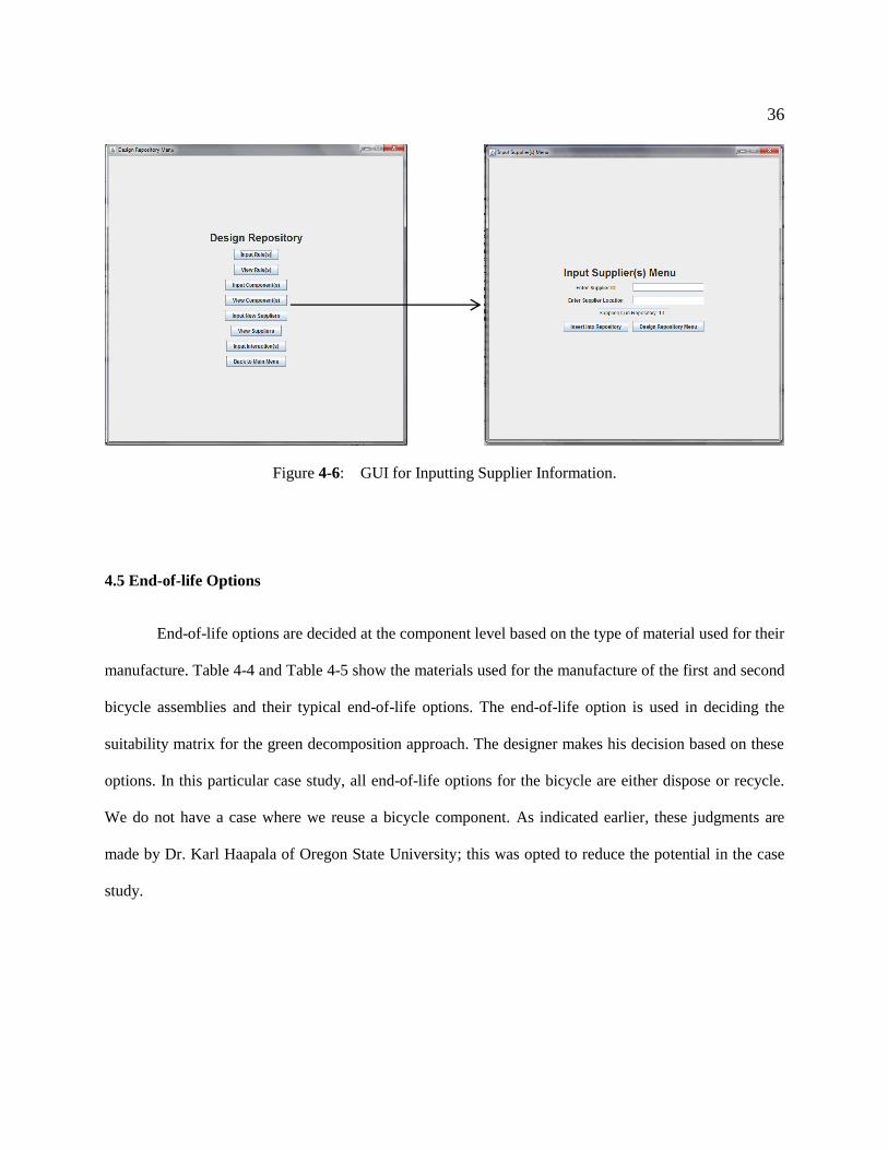
Figure 4-6: GUI for Inputting Supplier Information.

4.5 End-of-life Options

End-of-life options are decided at the component level based on the type of material used for their

manufacture. Table 4-4 and Table 4-5 show the materials used for the manufacture of the first and second

bicycle assemblies and their typical end-of-life options. The end-of-life option is used in deciding the

suitability matrix for the green decomposition approach. The designer makes his decision based on these

options. In this particular case study, all end-of-life options for the bicycle are either dispose or recycle.

We do not have a case where we reuse a bicycle component. As indicated earlier, these judgments are

made by Dr. Karl Haapala of Oregon State University; this was opted to reduce the potential in the case

study.

37

Table 4-4: End-of-life options based on material used for Assembly 1.

Subassembly Material “Typical End-of-Life

Option” Image

(A) Saddle (A1)

Plastic resin Landfill

Foam Landfill

Fabric Landfill

(B) Frame (B1) Steel pipes Steel/iron recycling

Metal slab Steel/iron recycling

(C) Steel fork w/o

suspension (C1)

Steel pipes Steel/iron recycling

Metal slab Steel/iron recycling

(D) Reverse brake rotor

(D1)

High friction material Landfill

Steel pipe Steel/iron recycling

Iron rod Steel/iron recycling

Iron sheet Steel/iron recycling

(E) Wheels w/ steel

spokes (E1)

Iron sheet Steel/iron recycling

Iron rod Steel/iron recycling

Inner tube Landfill

Tire Landfill

(F) Single speed

transmission (F1)

Steel sheet Steel/iron recycling

Steel plate Steel/iron recycling

Chain Steel/iron recycling

Bearing Steel/iron recycling

Pedal Landfill

38

Table 4-5: End-of-life options based on material used for Assembly 2.

Subassembly Material “Typical End-of-Life

Option” Image

(A) Saddle (A2)

Plastic resin Landfill

Foam Landfill

Fabric Landfill

(B) Frame with

suspension (B2)

Steel pipes Steel/iron recycling

Metal slab Steel/iron recycling

Iron rods Steel/iron recycling

(C) Fork with suspension

(C2)

Steel pipes Steel/iron recycling

Metal slab Steel/iron recycling

Iron rods Steel/iron recycling

(D) Brake with brake

shoe (D2)

Brake shoes Landfill

Brake arm Landfill

(E) Wheels w/ plastic

spokes (E2)

Plastic ball Landfill

Metal mold Landfill

Inner tube Landfill

Tire Landfill

(F) Transmission with

freewheels (F2)

Steel sheet Steel/iron recycling

Steel plate Steel/iron recycling

Front and rear

derailleur Landfill

Bearing Steel/iron recycling

Chain Steel/iron recycling

Pedals Landfill

39

4.6 Carbon Footprint

Carbon footprint is calculated for every component and for each assembly based on the

manufacturing processes and their sourcing locations because energy grids vary in different countries, and

therefore overall carbon footprint varies. The carbon footprint was calculated using SimaPro which is a

life-cycle assessment simulation software. Carbon footprint also increases based on the transportation

mode used. In this study, we are taking into account only road and sea transportation. Suppliers for this

study mainly are from the United States, Japan, Netherlands and Taiwan. The energy supply and

distribution has been used to determine the carbon footprint of these suppliers. Table 4-6 and 4-7 show

the carbon footprints for bicycle Assembly 1 and Assembly 2 at the component level in terms Kg of CO2

equivalent.

Table 4-6: Carbon Footprint for Bicycle Assembly 1 without transportation in Kg CO2 equivalent.

Suppliers

Saddle_1 Frame

without

suspension

Fork

without

suspension

Reverse

brake

rotor

Wheels w/

steel

spokes

Single speed

transmission

Velo 0.644 4.118

Tektro

13.57

Shimano

13.206 2.576

X-Bike 0.597

Formula

Engineering

15.54

Tien Hsin

2.6221

Campagnolo

15.154

Easton Sports

4.118

Topkey 15.52

Advanced

4.118

ADK 15.52 4.118

Viscount 0.597

SRAM 13.369

40

The carbon footprint for the assembly of components will depend on their mode of attachment. At

the module level, all attachments are made using screws and a power screw driver is used. Table 4-8

shows the SimaPro results obtained for the attachment of modules, Component A and Component B will

be attached using a power screw driver and we are taking different kilograms of force based on the mode

of attachment. The overall carbon footprint of the product will be the sum of their individual carbon

footprints and their assemblies.

When modules are generated the different components need to be attached to each other, each of

these attachments result in an increase of carbon footprint. The different attachments and their associated

carbon footprints are shown in Table 4-8. If they are attached at the component level then at the final

assembly stage no attachment is required; however, otherwise an attachment is required. All components

are attached to the frame in the bicycle. In the final results shown in Tables 4.13 and Tables 4.14, the final

assembly carbon footprints are added so that the total product carbon footprint can be calculated.

Table 4-7: Carbon Footprint for Bicycle Assembly 2 without transportation in Kg CO2 equivalent.

Assembly 2

Saddle_2 Frame with

suspension Fork with

suspension Brake with

brake shoe Wheels w/

plastic

spokes

Transmission

with

freewheels

Campagnolo 16.866 1.801

DT Swiss

3.225

HB

1.815

Selle Royal 0.597

Spinner

3.107

SRAM

6.701

Ten-Tech 16.866

Topkey

11.349

X-Bike 16.866 11.349 1.815

41

Considering the design shown in Figure 4-16, at the final assembly stage we consider that

within module assemblies are completed and only the necessary final assemblies need to be

done. As per the assembly requirements given in Table 4-8 and the fact that frame and saddle are

within separate modules, these components need to be assembled to assemble the modules; thus,

additional CF will be incurred because of this assembly. In the case of the brake, different brake

designs require different attachments. In the case for the reverse brake rotor (D1), the brake

needs to be attached to the transmission; whereas for the case brake with show (D2), the brake

needs to be attached either to the frame or to fork; for both of these attachment CF values are

also provided in Table 4-8. For the case presented, when brake is modularized separately from

the frame and fork, the assembly between brake (D2) and frame was considered.

4.6 Suitability Level and Modularization for Decomposition Approach

The suitability matrix represents the suitability of inclusion for a component in a particular

module. The suitability matrix in this software is generated after the selection of components because

components could interact with each other, however, they may not be suitable for inclusion. For the

decomposition approach the designer decides the suitability level. Figure 4-7 shows the suitability level of

Table 4-8: Carbon Footprint of Component Assemblies.

Component A

Component B Kg of Force Carbon Footprint (in Kg CO2 eq.)

Saddle + Frame 0.10 0.308 Fork + Brake 0.20 0.675

Transmission + Wheel 0.05 0.754 Frame + Fork 0.15 0.467 Frame + Brake 0.16 0.492 Frame + Transmission 0.17 0.523 Frame + Wheel 0.18 0.554 Brake + Transmission 0.10 0.308

42

components for the decomposition approach. After the suitability level has been declared the user can

modularize and select suppliers. This selection can be for carbon footprint, cost or lead time. The level of

suitability is indicated as per the scale shown in Figure 3-6.

After the suitability matrix is selected the user can choose to modularize based on decomposition

approach and select suppliers. The selection of suppliers can be to minimize cost, lead time or carbon

footprint. Figure 4-8 shows the modules obtained for the decomposition approach. The designer will have

the ability to view the carbon footprint, and lead time as well for the module.

Figure 4-7: Suitability Matrix for Decomposition Approach.

43

4.7 Suitability Level and Modularization for Green Decomposition Approach

In the case of the green decomposition approach, the designer enters the suitability level based on

the end-of-life options for the components present. Table 4-9 shows the suitability matrix mapping based

on end-of-life options. Figure 4-8 shows the suitability matrix based on end-of-life options for the bicycle

case.

Figure 4-8: Modules Obtained When Modularized Using Decomposition Approach.

Table 4-9: Suitability Matrix Mapping based on end-of-life options.

Reuse Recycle Disposal

Reuse Strongly desired Desired Strongly undesired

Recycle Desired Strongly desired Undesired

Disposal Strongly undesired Undesired Strongly desired

44

Once the suitability level is entered based on the end-of-life option then the procedure is the

same. Modules are generated based on the decomposition approach algorithm developed by (Huang and

Kusiak, 1998). Figure 4-10 shows the modules obtained when the green decomposition approach has

been used. Just as the previous case, the user will have the ability to view suppliers and know the total

cost.

Figure 4-9: Suitability Matrix based on End-of-life Options.

Figure 4-10: Modules Obtained When Modularized Using Green Decomposition Approach.

45

4.8 Simulated Annealing Inspired Hierarchical Search Algorithm (HSA)

The second modularization methodology that we have adopted is a hierarchical search algorithm

which has been inspired from the Simulated Annealing process. One of the primary differences between

this process and the decomposition approach which we have adopted before is that in this new approach

the degree of interaction is taken into account whereas in our first two methodologies this was not

factored in. Section 4.8.1 gives an overview of the hierarchical search algorithm which has been inspired

from the Simulated Annealing process.

4.8.1 Overview of the Hierarchical search algorithm (HSA)

The simulated annealing algorithm was developed by Kirkpatrick et al. (1983) originally to

optimize the design of integrated circuit chips. This process simulates the actual metallurgical process of

annealing, which is heating up a solid and then cooling it until it crystallizes. The atoms of the material

have high energies at high temperatures which gives them the ability to restructure themselves. Their

energy of these atoms decreases as their temperature reduces. The only difference between the Simulated

Annealing process and the methodology that we have adopted is that we are not factoring in a probability

for change into the algorithm; in the SA algorithm after the first set of results are generated based on a

pre-defined metric there is a function which decides whether or not to search further. However, in our

case as the feasible solution space is small we are allowing ourselves to generate all possible results.

Figure 4-11 shows an overview of the SA process.

46

The simulated annealing algorithm runs through a certain set of cycles for each temperature and this is

fixed. For each temperature the inputs are randomized so that a different result set is produced. The

randomization process is an important part of the annealing process. The inputs are randomized according

to the temperature. Higher temperatures result in more randomizations, and lower temperatures will have

less randomization. In this study, the number of modules will be set as the temperature and the size of the

modules will be randomized for every step. This means that the randomizations would basically comprise

of generating different combinations for each temperature. With the number of components in this study

being 6 the search space is limited hence an optimum solution can be attained. Two matrices are used for

this process as well, the interaction matrix and the suitability matrix based on the life expectancy.

Randomize according to the

current temperature

Better than current solution ?

Reached max tries for this temperature

Decrease temperature by specified rate

Lower temperature

bound

Replace current solution with new

solution

Start

End

No

No Yes

Yes

Figure 4-11: Overview of simulated annealing (Gu and Sosale, 1999).

47

4.8.2 Matrix Generation for the Hierarchical Search Process

As mentioned previously one of the biggest differences between (HSA) and DA is that the

interaction matrix in (HSA) takes into account the degree of interaction. Also the interaction matrix in

HSA is symmetrical. An interaction value of 2 indicates low interaction whereas an interaction value of 5

would reflect a high interaction. Table 4-10 shows the interaction values based on the mode of

attachment.

As the degree of interaction varies depending on the components selected, within the software framework,

the interaction matrix needs to be input after the components have been selected unlike DA where the

interaction matrix is input at the beginning. Figure 4-13 shows the Interaction Matrix created for the

bicycle case study. This information was taken based on surveys from different bicycle shops.

Table 4-10: Degree of Interaction for Simulated Annealing (Gu and Sosale, 1999).

Attachment Alignment Exchange of force,

energy, signal, etc. Interaction

Value

Permanent

attachment More than two components aligning

with more than one component Material Exchange 5

Not easily

separable (press

fits, snap fits)

More than two components aligning

with one component Torque exchange 4

Spline and key

attachment Two components need alignment with

each other Displacement

exchange 3

Threaded fasteners One components aligning with a fixed

component Force exchange 2

Easily separable Alignment preventing parts from

blocking other parts way Signal exchange 1

Not even contact No alignment required No exchange 0

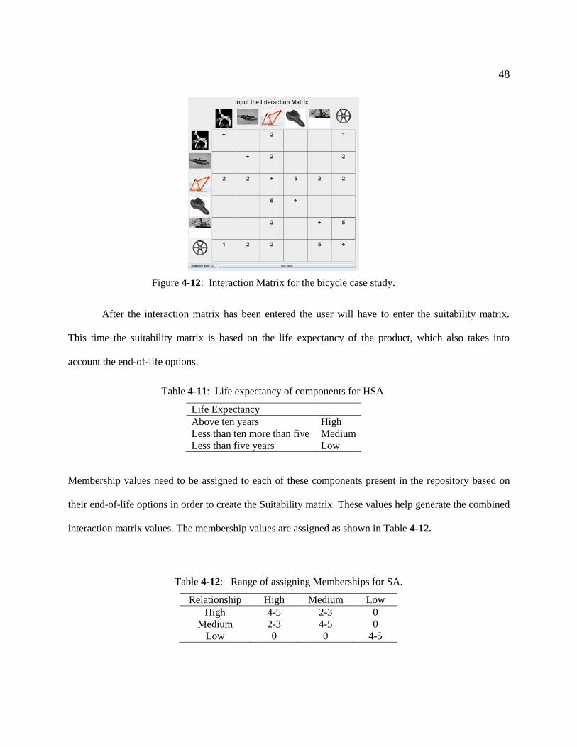
48

After the interaction matrix has been entered the user will have to enter the suitability matrix.

This time the suitability matrix is based on the life expectancy of the product, which also takes into

account the end-of-life options.

Membership values need to be assigned to each of these components present in the repository based on

their end-of-life options in order to create the Suitability matrix. These values help generate the combined

interaction matrix values. The membership values are assigned as shown in Table 4-12.

Figure 4-12: Interaction Matrix for the bicycle case study.

Table 4-11: Life expectancy of components for HSA.

Life Expectancy Above ten years High Less than ten more than five Medium Less than five years Low

Table 4-12: Range of assigning Memberships for SA.

Relationship High Medium Low High 4-5 2-3 0

Medium 2-3 4-5 0 Low 0 0 4-5

49

The suitability matrix like the interaction matrix was decided based on surveys conducted from various

bicycle shops. Figure 4-13 shows the suitability matrix of the components in the bicycle case study. Once

the suitability matrix and the interaction matrix are entered then a new matrix is created by creating a

weighted average between the values of the two matrices. In this study, a weight of 0.5 is assigned for

both matrices and a new matrix is created with a combined objective. The user can simultaneously select

suppliers based on cost, lead time and carbon footprint as in the previous cases. The suitability matrix is

based on the life expectancy of the components.

4.8.3 Temperature and Module Clustering

In this research work, we have varied the temperature from 1 to the total number of components

present in a product. The total number of components present in a product in this case is 6. A combination

algorithm is used to randomize the components in the repository based on the temperature. The

methodology is illustrated below. Let a, b, c, d, e and f be the six components present in the product.

Figure 4-13: Suitability Matrix for the HSA process.

50

All possible combinations are generated for the particular case. Certain cases such as 3+1+1+1 were

eliminated because we felt that ideally a module should have more than one individual component.

However, this can be changed based on the designer’s choice. For each combination the values of

interaction and suitability are summed up to generate a combined value. Weights can be provided based

on user discretion. This is explained in the following example.

If a module generated is (note that within brackets components of a module are given):

[Brake + Frame + Saddle + Fork] [Wheel + Transmission]

Then the interaction and suitability values will be summed up for all components in the module; in the

example below the life expectancy is used to calculate the suitability.

Brake + Frame = 3 (the interaction value is 1 and suitability is 2 from Figures 4.12 & 4.13)

Brake + Saddle = 5 (the interaction value is 0 and suitability is 5 from Figures 4.12 & 4.13)

Brake + Fork = 6 (the interaction value is 5 and suitability is 1 from Figures 4.12 & 4.13)

Frame + Saddle = 7 (the interaction value is 5 and suitability is 2 from Figures 4.12 & 4.13)

Frame + Fork = 7 (the interaction value is 2 and suitability is 5 from Figures 4.12 & 4.13)

Saddle + Fork = 0 (the interaction value is 0 and suitability is 0 from Figures 4.12 & 4.13)

&

Wheel + Transmission = 10 (the interaction value is 5 and suitability is 5 from Figures 4.12 & 4.13)

Table 4-12: Range of assigning Memberships for SA.

Temperature Module Formation Examples

1 1+2+2+1 a + bc + de + f

2 2+2+2 ab + bc + ef

3 3+3 & 3+2+1 abc +def & abc +de + f

4 4+2 abcd + ef

5 5+1 abcde + f

51

4.8.4 Constraints Imposed

The primary constraint imposed on the module formation is that each and every component

present in the modules should have a physical connection with at least one other component. This

prevents isolated components or a group of isolated components in a module. The number of modules that

is formed is specified by the designer. There is also a tendency to form only one module which is when

the temperature is equal to 6, thus, this condition has been removed.

4.8.5 Modules Obtained

As the primary objective of the clustering process is to obtain modules with the highest

interaction and suitability level, the modules are sorted based after all combinations have been generated.

The combination with the highest value is considered as the best design. Figure 4.14 shows the designs

generated after the interaction and suitability matrices are input. The supplier selection process happens

the same way as in the previous cases.

Figure 4-14: Modules Obtained When Modularized Using Simulated Annealing.

52

4.9 Comparison of Results

Results were generated for the decomposition approach, green decomposition approach and HSA.

The HSA algorithm was performed for different cases of the interaction and suitability matrices. These

were done so that a good comparison can be established between the different methods. From the designs

that were generated as shown in Figure 3-6 two designs were selected for the comparison of results. The

design with the lowest DFA index was taken first, Design 1 and the design with the highest DFA index

was taken next, Design 64. The final comparison of results between these two designs is shown in Table

4-13 and in Table 4-14.

The two main types of interaction matrix and the suitability matrices are explained below.

Interaction Matrix

1. 1-0 Interaction: A 1, 0 interaction matrix takes into account interaction at a binary level. The

degree of interaction is not important here.

2. 0-5 Interaction: Here, the degree of interaction factors into the module formation.

Suitability Matrix:

1. a, e, o, u: This is the suitability matrix explained in detail in section 3.2 and the level of suitability

is explained in Figure 3.6. This suitability matrix denotes positive and negative values for the

component suitability.

2. 0-5 based on End-of-Life option: This suitability matrix will depend on the end-of life option of

the different components present in the system. The level of suitability will vary from 0 to 5 and

the mapping will be based on Table 4.9 and the range assignment will be as shown previously in

Table 4.12.

3. 0-5 based on Life Expectancy: This suitability matrix will be based on the life expectancy of the

different components present in the system and the level of suitability will vary from 0 to 5 with

the mapping based on Table 4.12.

When all interaction matrices were combined with the three suitability matrices a total of 6 result

sets were obtained. These are explained below.

Case i: 1, 0 Interaction Matrix with Suitability Matrix based on End-of-Life

53

The HSA algorithm is used with the interaction matrix being at a 1, 0 level so that we can

understand the metrics that we are using. Here the interaction is assumed to be binary and the degree of

interaction does not play an important role. The suitability matrix is entered based on the end-of-life of

the different components present in the repository. The interaction matrix will be the same as the matrix

shown in Figure 3-4. The suitability matrix for case 1 is based on the end-of life options. Figure 4-15

shows the suitability matrix. This matrix is on a scale from 1 to 5. The range of assignment is based on

the membership value provided in Tables 4-9 and 4-12.

Figure 4-15 shows the modules obtained when the components are modularized with parameters

from Case i. The Brake and Saddle are both components suitable for disposal and hence they are coupled

into one module; however, there is no interaction between these components. This is because the

suitability matrix is given more importance than the interaction matrix as the interaction is only on a 1-0

level. The second module in this case is not feasible to be combined, and hence is separated as individual

modules for the calculation of supply chain costs.

Figure 4-16: Product Architecture for Case 1 (1, 0 Interaction matrix and 1-5 Suitability Matrix).

54

Case ii: 1, 0 Interaction Matrix with Suitability Matrix based on Life expectancy

In this case the interaction matrix is the same as the previous case from Figure 3-4 but the

suitability matrix is based on life expectancy which is shown in Figure 4-13. The product architecture for

this case is the same as that of the regular HSA case which is shown in Figure 4-14. This is considered to

be better than the first architecture because interaction exists between all components in the module.

Case iii: Same parameters as the Decomposition Approach.

In this case, the parameters are the same as that of the decomposition approach, i.e., the

interaction matrix will have a 1, 0 interaction as shown in Figure 3-4 and the suitability matrix will be the

matrix used for decomposition approach. The only difference is that the matrix will be a symmetrical

matrix and hence all values need to be entered. The interaction matrix is shown in Figure 4-17. A negative

value (-2) is inserted if no interaction exists between the components so that components without any

interaction will not be combined.

Figure 4-15: Suitability Matrix for Case 1 (‘1, 0’ Interaction matrix and a ‘1-5’ Suitability Matrix).

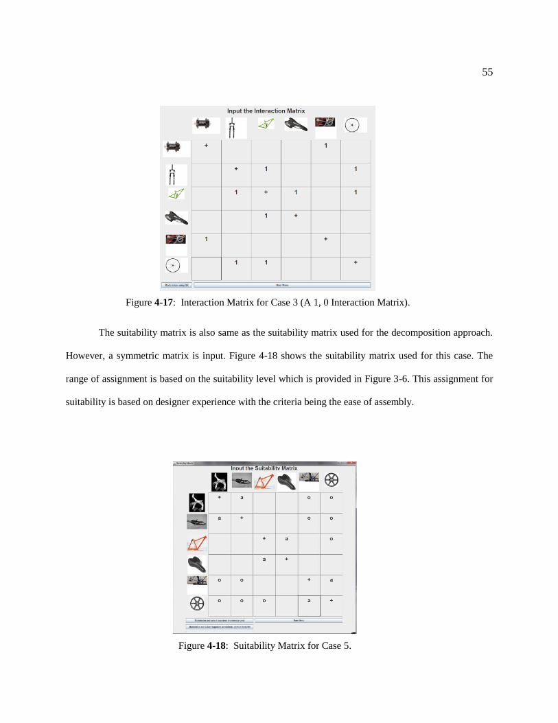
55

The suitability matrix is also same as the suitability matrix used for the decomposition approach.

However, a symmetric matrix is input. Figure 4-18 shows the suitability matrix used for this case. The

range of assignment is based on the suitability level which is provided in Figure 3-6. This assignment for

suitability is based on designer experience with the criteria being the ease of assembly.

Figure 4-17: Interaction Matrix for Case 3 (A 1, 0 Interaction Matrix).

Figure 4-18: Suitability Matrix for Case 5.

56

Case iv: A 0-5 Interaction Matrix with the Suitability Matrix same as the Decomposition Approach

The interaction matrix will be the same as the matrix shown in Figure 4-13 and the suitability

matrix used for this case is shown in Figure 4-7. The product architecture obtained is the same as shown

in Figure 4-15.

Case v: A 0-5 Interaction Matrix with a 0-5 Suitability Matrix based on Life Expectancy

The interaction matrix and the suitability matrix will be on a 0-5 level. The 0-5 scale provides a

degree for interaction and suitability and hence the modules obtained are suitable for assembly and also

serve the purpose of assembly based on life expectancy. The product architecture obtained is the same as

shown in Figure 4-15.

Case vi: A 0-5 Interaction Matrix with a 0-5 Suitability Matrix based on End-of-Life

The interaction matrix and the suitability matrix will be on a 0-5 level. The 0-5 scale provides a degree for

interaction and suitability and hence the modules obtained are suitable for assembly and also serve the

purpose of assembly based on life expectancy. The product architecture obtained is the same as shown in

Figure 4-16. After the modules were generated, their supply chain costs and carbon footprints were also

calculated. The carbon footprints for the components present in the repository are shown in Tables 4.6,

4.7 and Table 4.8. The component cost and lead times for the components is shown in Table 4.3. Tables

4.1 and 4.2 show the transportation costs and transportation lead times, respectively.

The product architecture for HSA with the suitability matrix based on end-of-life options has two

modules. The first module consists of the saddle, fork, wheel and transmission. This module can be

assembled into one product and shipped to the dealer because there is interaction between the

components. The second module consists of the saddle and the brake. This cannot be assembled into a

single product. Hence, we have taken them to be separate components, the supply chain results are

generated such that the brake and saddle are attached onto the rest of the product at the final stage of

assembly. This case produces the best result as far as carbon footprint minimization because the module

57

assembly stage is eliminated and hence carbon footprint due to transportation is eliminated. In all other

cases there is an extra step for module assembly.

Comparison of above cases only on one design would only generate results that are relevant for

that specific design. In order to have a broader comparison, we have used two distinct designs. The

comparison of costs for design 1 and design 64 are shown in Table 4.13 and Table 4.14. As stated earlier

in Section 4.9 Design 1 has the lowest DFA index and Design 64 has the highest DFA index. Design 1

has a lower average carbon footprint and supply chain cost when compared to Design 64. The adverse

implications in manufacturing can be clearly seen with the increase in cost and carbon footprint thereby

showing a direct correlation between carbon footprint and DFA index.

58

Table 4-13: Cost Comparison for the different cases when applied to Design 1.

Design 1

3-module Assembly (Regular

DA) Fig 4.8

2- Module Assembly

(Green DA) Fig 4.10 HSA (Life Cycle) Fig 4.14 HSA (EOL) Fig 4.14

Supply

Chain Cost

Min.

Carbon

Footprint

Min.

Supply

Chain

Cost Min.

Carbon

Footprint

Min.

Supply

Chain Cost

Min.

Carbon

Footprint

Min.

Supply

Chain

Cost Min.

Carbon

Footprint Min.

Carbon

Footprint

(kg CO2

eq.)

31.444 30.999 30.831 30.3708 31.5052 31.492 30.782 30.767

Total

Cost ($) 509.64 649.22 581.235 649.736 525.661 652.431 515.378 627.234

Number

of

Suppliers

6 6 7 6 5 5 6 6

Module and Component Information

ABCDEF X-Bike X-Bike X-Bike X-Bike X-Bike X-Bike X-Bike X-Bike

ABCD

Ten-Tech X-Bike

ABCE

ADK X-Bike

BCEF

HB HB

AB Ten-Tech X-Bike

CD SRAM SRAM

EF Shimano Shimano

Shimano Shimano

DF

SRAM SRAM

A X-bike X-bike X-bike X-Bike X-bike X-bike Viscount X-Bike

B Topkey ADK Topkey ADK ADK ADK ADK ADK

C Advanced Velo Velo Velo Advanced Velo Advanced Velo

D X-Bike Campagnolo X-Bike Campagnolo X-bike Campagnolo HB Campagnolo

E Shimano Shimano Shimano Shimano Shimano Shimano Shimano Shimano

F Shimano Shimano Shimano Shimano Shimano Shimano Shimano Shimano

59

Table 4-14: Cost Comparison for the different cases when applied to Design 64.

Design 2

3-module Assembly

(Regular DA

2- Module Assembly

(Green DA) HSA (Life Cycle) HSA (EOL)

Supply

Chain Cost

Min.

Carbon

Footprint

Min.

Supply

Chain Cost

Min.

Carbon

Footprint

Min.

Supply

Chain Cost

Min.

Carbon

Footprint

Min.

Supply

Chain Cost

Min.

Carbon

Footprint

Min.

Carbon

Footprint

(kg CO2

eq.)

67.518 67.154 66.889 66.525 68.0101 67.6461 66.25 66.244

Total

Cost ($) 674.44698 701.81998 694.279 695.363 671.879 704.501 671.704 675.057

Number

of

Suppliers

8 6 7 5 9 5 6 6

Module and Component Information

ABCDEF X-bike X-bike X-bike X-bike X-bike X-bike X-bike X-bike

ABCD

Ten-Tech X-bike

ABCE

ADK X-bike

BCEF

Selle Royal HB

AB ADK X-Bike

CD Tektro SRAM

EF Shimano Shimano

Shimano Shimano

DF

SRAM SRAM

A Selle Royal Selle Royal Selle Royal Selle Royal Selle Royal Selle Royal Selle Royal Selle Royal

B X-bike X-bike X-Bike X-bike Campagnolo X-bike X-bike X-bike

C Tektro SRAM Topkey X-bike Topkey X-bike Topkey X-bike

D Topkey X-bike Tektro Shimano Tektro Shimano Shimano Shimano

E

Formula

Engineering

Formula

Engineering Campagnolo

Formula

Engineering

Formula

Engineering

Formula

Engineering Campagnolo

Formula

Engineering

F SRAM SRAM SRAM SRAM SRAM SRAM SRAM SRAM

In both results the lowest carbon footprint is for the hierarchical search algorithm with the end-of-

life option; this is because the number of modules is lesser. Assembly for two components is done at the

final assembly stage reducing the manufacturing processes thereby reducing the total carbon footprint.

The three modules assembly generated by the decomposition approach generated the lowest supply chain

cost in first design and in the second design also this cost is on the lower side; this is because in all other

assemblies the number of components in the module is high thereby increasing the manufacturing cost. In

60

this case the modules are assembled at the nearest location and after that they are shipped to the final

location. This reduced the overall cost because transportation distance is optimized first at the module

level and then from the module to the final assembly. If the product has more components then there

could be a case where there are several sub-assemblies and these could be combined in a way that their

end-of-life options are the same. An argument could be made that this assembly would generate the

lowest carbon footprint and total cost.

61

Chapter 5

Conclusion

In this thesis, we presented a software platform that can create product architectures using three

main modularity methods namely, decomposition approach, green decomposition approach and a

simulated annealing inspired hierarchical search algorithm. The methodology used in this thesis and the

data used have been explained. Our results indicate that the HSA process which takes into account the

end-of-life provides the best result for both supply chain minimization as well as carbon footprint

minimization. The other methodologies also provide competitive results. Taking life expectancy into

account plays an important role as well because with every time a part is replaced the carbon footprint for

the product increases.

This software provides a platform to compare the different modularization methodologies and

also serves as a guide to designers so that whenever conceptual product designs are thought of, and when

a design is planned they can get a good idea of the carbon footprint and overall costs. This will provide as

a better judgment for designers.

Two extreme cases were chosen for comparison and we get an understanding of the relationship

between the manufacturability, cost and carbon footprint; Design 1 with the lowest DFA index also has

the lower carbon footprint and a total cost. Design 64 with the higher DFA index in turn has a higher

carbon footprint and higher cost. A correlation could be established between DFA index and carbon

footprint. However, this would require more products in the design repository and also their related costs

and carbon footprints.

The results of this study point to the need for development of modularity methods that take into

account both the component end-of-life options and total supply chain carbon footprint and life

expectancy of the product. In general, the lowest carbon footprint can be obtained if all the components

62

with similar life expectancies and end-of-life options are combined. Ideally a completely vertically

integrated system where everything is manufactured at the same location would be the case with the

lowest cost; however, there are overhead costs in that case which needs to be factored in. The overall risk

in this process is also high. As the number of components in this case study is low, further investigations

with products having more components are necessary; our future studies will account for this.

63

References

Aamer, AM, and R. Sawhney. 2004. “Review of Suppliers Selection from a Production Perspective.” In

IIE Annual Conference and Exhibition, 2135–2140.

Aigbedo, H. 2007. “An Assessment of the Effect of Mass Customization on Suppliers’ Inventory Levels

in a JIT Supply Chain.” European Journal of Operational Research 181 (2): 704–715.

Anon. “Industry Overview 2010 - National Bicycle Dealers Association.”

http://nbda.com/articles/industry-overview-2010-pg34.htm.

Assessment, United States. Congress. Office of Technology. 1992. Green Products by Design: Choices

for a Cleaner Environment. Office of Technology Assessment.

Baldwin, C.Y., and K.B. Clark. 2003. Managing in an Age of Modularity. Blackwell: Malden, MA.

Boothroyd, G. 1994. “Product Design for Manufacture and Assembly.” Computer-Aided Design 26 (7):

505–520.

Bozdogan, K., J. Deyst, D. Hoult, and M. Lucas. 1998. “Architectural Innovation in Product

Development Through Early Supplier Integration.” R&D Management 28 (3): 163–173.

Bryant, C.R., K.L. Sivaramakrishnan, M. Van Wie, R.B. Stone, and D.A. McAdams. 2004. “A Modular

Design Approach to Support Sustainable Design.” In Proceedings of DETC. Vol. 4.

Chiu, M.C. 2010. “A Graph Theory-Based Integration of Product Design and Supply Chain Design”, PhD

Dissertation, Department of Industrial and Manufacturing Engineering, Pennsylvania State

University, December 2010.

Chiu, M.C., and G. Okudan. 2011. “An Integrative Methodology for Product and Supply Chain Design

Decisions at the Product Design Stage.” Journal of Mechanical Design 133: 021008.

Choi, T.Y., and J.L. Hartley. 1996. “An Exploration of Supplier Selection Practices Across the Supply

Chain.” Journal of Operations Management 14 (4): 333–343.

64

Coulter, S.L., M.W. McIntosh, B. Bras, and D.W. Rosen. 1998. “Identification of Limiting Factors for

Improving Design Modularity.” In ASME Design Engineering Technical Conference

Proceedings, DETC1998, Atlanta, GA.

Cusumano, M.A., and A. Takeishi. 1991. “Supplier Relations and Management: A Survey of Japanese,

Japanese-transplant, and US Auto Plants.” Strategic Management Journal 12 (8): 563–588.

Ericsson, A., and G. Erixon. 2000. Controlling Design Variants: Modular Product Platforms. Sme.

Feitzinger, E., and H.L. Lee. 1997. “Mass Customization at Hewlett-Packard: The Power of

Postponement.” Harvard Business Review 75: 116–123.

Galvin, P., and A. Morkel. 2001. “The Effect of Product Modularity on Industry Structure: The Case of

the World Bicycle Industry.” Industry and Innovation 8 (1): 31–48.

Gershenson, J., and K. Ishii. 1991. “Life-cycle Serviceability Design.” In Proceedings of ASME

Conference on Design and Theory and Methodology.

Gershenson, J.K., G.J. Prasad, and Y. Zhang. 2004. “Product Modularity: Measures and Design

Methods.” Journal of Engineering Design 15 (1): 33–51.

Gershenson, JK, GJ Prasad, and Y. Zhang. 2003. “Product Modularity: Definitions and Benefits.” Journal

of Engineering Design 14 (3): 295–313.

Ghobadian, A., A. Stainer, and T. Kiss. 1993. “A Computerized Vendor Rating System.” In Proceedings

of the First International Symposium on Logistics, 321–328.

Ghodsypour, S.H., and C. O’Brien. 1998. “A Decision Support System for Supplier Selection Using an

Integrated Analytic Hierarchy Process and Linear Programming.” International Journal of

Production Economics 56: 199–212.

Gu, P., M. Hashemian, S. Sosale, and E. Rivin. 1997. “An Integrated Modular Design Methodology for

Life-cycle Engineering.” CIRP Annals-Manufacturing Technology 46 (1): 71–74.

Gu, P., and S. Sosale. 1999. “Product Modularization for Life Cycle Engineering.” Robotics and

Computer-Integrated Manufacturing 15 (5): 387–401.

65

Guo, F., and J.K. Gershenson. 2004. “A Comparison of Modular Product Design Methods Based on

Improvement and Iteration.” In .

Gupta, S., and G. E. Okudan. 2007. “Modular Design: A Review of Research and Industrial

Applications.” In Proceedings of IIE Annual Conference and Expo 2007-Industrial Engineering’s

Critical Role in a Flat World, 1563–1568.

Gupta, S., and G.E. Okudan. 2008. “Computer-aided Generation of Modularised Conceptual Designs with

Assembly and Variety Considerations.” Journal of Engineering Design 19 (6): 533–551.

Hau, L., and M.S. Marguerita. 1995. “Product Universality and Design for Supply Chain Management.”

Production Planning & Control 6 (3): 270–277.

Hoffman, W. 2007. “Who’s Carbon-free? Wal-Mart Takes on Supply Chains of Products as Expansive

Carbon Measuring Plan Eyes Distribution.” Traffic World 271 (42): 15.

Hölttä, K., E.S. Suh, and O. de Weck. 2005. “Trade-off Between Modularity and Performance for

Engineered Systems and Products.” In Proceedings of the 15th International Conference on

Engineering Design.

Holtta, K.M.M., and M.P. Salonen. 2003. “Comparing Three Different Modularity Methods.” In .

Hsu, W., Y. H. Jerry Fuh, and Y. Zhang. 1998. “Synthesis of Design Concepts from a Design for

Assembly Perspective.” Computer Integrated Manufacturing Systems 11 (1-2): 1–13.

Huang, C.C., and A. Kusiak. 1998. “Modularity in Design of Products and Systems.” Systems, Man and

Cybernetics, Part A: Systems and Humans, IEEE Transactions On 28 (1): 66–77.

Ishii, K. 1998. “Modularity: a Key Concept in Product Life-cycle Engineering.” Handbook of Life-cycle

Engineering.

Kannan, V.R., and K.C. Tan. 2002. “Supplier Selection and Assessment: Their Impact on Business

Performance.” Journal of Supply Chain Management 38 (4): 11–21.

Kirkpatrick, S., C. D. Gelatt Jr, and M. P. Vecchi. 1983. “Optimization by Simulated Annealing.” Science

220 (4598): 671–680.

66

Kusiak, A. 2002. “Integrated Product and Process Design: a Modularity Perspective.” Journal of

Engineering Design 13 (3): 223–231.

Kusiak, A., T. Nick Larson, and J. R. Wang. 1994. “Reengineering of Design and Manufacturing

Processes.” Computers & Industrial Engineering 26 (3): 521–536.

Maslennikova, I., and D. Foley. 2000. “Xerox’s Approach to Sustainability.” Interfaces: 226–233.

Matthews, V. 1993. “Overview of Plastics Recycling in Europe.” Plastics, Rubber and Composites

Processing and Applications(UK) 19 (4): 197–204.

Mikkola, J.H., Danish Research Unit for Industrial Dynamics, A. Universitet, and H. Syd. 2000.

Modularization Assessment of Product Architecture. Department of Industrial Economics and

Strategy, CopenhagenBusiness School.

Mikkola, J.H., and O. Gassmann. 2003. “Managing Modularity of Product Architectures: Toward an

Integrated Theory.” Engineering Management, IEEE Transactions On 50 (2): 204–218.

Narasimhan, R. 1983. “An Analytical Approach to Supplier Selection.” Journal of Purchasing and

Materials Management 19 (4): 27–32.

Newcomb, P. J, B. Bras, and D. W Rosen. 2001. “Implications of Modularity on Product Design for the

Life Cycle”. School of Mechanical Engineering, Georgia Institute of Technology.

Nilsson, J. 1998. The Recycling Aspect in Product Development: Framework for a Systematic Approach.

Division of Assembly Technology, Department of Mechanical Engineering, Linköping

University.

Okudan, G.E. and Gupta, S. (2012). “Analysis of Modularity Implementation Methods from an Assembly

and Variety Viewpoint”, International Journal of Advanced Manufacturing Technology

(published on line in September, 2012; DOI: 10.1007/s00170-012-4473-9).

Ottman, J., and N.T.C.B. Books. 1998. “Green Marketing: Opportunity for Innovation.” The Journal of

Sustainable Product Design: 60.

67

Petersen, K.J., R.B. Handfield, and G.L. Ragatz. 2005. “Supplier Integration into New Product

Development: Coordinating Product, Process and Supply Chain Design.” Journal of Operations

Management 23 (3): 371–388.

Pimmler, T.U., and S.D. Eppinger. 1994. Integration Analysis of Product Decompositions. Alfred P.

Sloan School of Management, Massachusetts Institute of Technology.

Rose, C.M. 2000. “Design for Environment: a Method for Formulating Product End-of-life Strategies”.

Stanford University.

Sanderson, S., and M. Uzumeri. 1995. “Managing Product Families: The Case of the Sony Walkman.”

Research Policy 24 (5): 761–782.

Shirley, G.V. 1990. “Models for Managing the Redesign and Manufacture of Product Sets.” Journal of

Manufacturing and Operations Management 3 (2): 85–104.

Stone, R.B., K.L. Wood, and R.H. Crawford. 2000. “A Heuristic Method for Identifying Modules for

Product Architectures.” Design Studies 21 (1): 5–31.

R. Stone (1997), Towards a Theory of Modular Design, Doctoral Thesis, The University of Texas at

Austin.

Sundarakani, B., R. De Souza, M. Goh, S.M. Wagner, and S. Manikandan. 2010. “Modeling Carbon

Footprints Across the Supply Chain.” International Journal of Production Economics 128 (1):

43–50.

Timmerman, E. 1987. “An Approach to Vendor Performance Evaluation.” Engineering Management

Review, IEEE 15 (3): 14–20.

Ulrich, K. 1995. “The Role of Product Architecture in the Manufacturing Firm.” Research Policy 24 (3):

419–440.

Ulrich, K.T., and S.D. Eppinger. 2011. Product Design and Development. Vol. 2. McGraw-Hill.

Ulrich, K.T., K. Tung, and Sloan School of Management. 1991. “Fundamentals of Product Modularity.”

68

Verma, R., and M.E. Pullman. 1998. “An Analysis of the Supplier Selection Process.” Omega 26 (6):

739–750.

Weidema, B.P., M. Thrane, P. Christensen, J. Schmidt, and S. Løkke. 2008. “Carbon Footprint.” Journal

of Industrial Ecology 12 (1): 3–6.

Whitney, D.E. 1993. “Nippondenso Co. Ltd: A Case Study of Strategic Product Design.” Research in

Engineering Design 5 (1): 1–20.

Zhang, WY, SY Tor, and GA Britton. 2006. “Managing Modularity in Product Family Design with

Functional Modeling.” The International Journal of Advanced Manufacturing Technology 30 (7):

579–588.

Zhang, Y., and JK Gershenson. 2003. “An Initial Study of Direct Relationships Between Life-cycle

Modularity and Life-cycle Cost.” Concurrent Engineering 11 (2): 121–128.

http://nbda.com/articles/industry-overview-2010-pg34.htm

69

Appendix

Java code used to develop the software

1. Mod.java

// This section is used to generate the conceptual designs and display them

import javax.swing.*;

import java.util.*;

import java.awt.*;

import java.awt.image.BufferedImage;

import java.sql.*;

import java.net.*;

import javax.imageio.*;

import javax.swing.border.*;

import java.io.*;

import java.awt.event.*;

public class mod extends JFrame implements ActionListener

{

JPanel p;

JTextField[] tf = new JTextField[100];

String driver,url;

Connection conn;

int l=0,ddx1,ab1,num1,ddy1,mst=0,mts=0,a1,a2;

Statement stmt,stmt1;

ResultSet rs, rse;

BufferedImage imageo;

ImageIcon image1;

StringTokenizer st;

70

int counter=0;

JButton b1,main1,dfv1;

JButton main2;

JLabel[] img = new JLabel[100];

JPanel[] p1 = new JPanel[100];

Border[] linec = new Border[100];

JLabel[] lbl = new JLabel[100];

JLabel[] lbl1 = new JLabel[100];

JLabel[] lbl2 = new JLabel[100];

JLabel[] lbl3 = new JLabel[100];

JLabel[] lbl4 = new JLabel[100];

JLabel[] lbl5 = new JLabel[100];

JLabel[] lbl6 = new JLabel[100];

JLabel[] lbl7 = new JLabel[100];

JLabel[] lbl8 = new JLabel[100];

JLabel[] lbl9 = new JLabel[100];

JLabel[] lbl20 = new JLabel[100];

JLabel[] lbl21 = new JLabel[100];

JLabel md;

GridBagConstraints[][] gridBagConstraints = new GridBagConstraints[10][100];

GridBagConstraints[] gridBagConstraints1 = new GridBagConstraints[100];

GridBagConstraints[] gridBagConstraints2 = new GridBagConstraints[100];

GridBagConstraints[] gridBagConstraints3 = new GridBagConstraints[100];

GridBagConstraints[] gridBagConstraints4 = new GridBagConstraints[100];

GridBagConstraints[] gridBagConstraints5 = new GridBagConstraints[100];

GridBagConstraints[] gridBagConstraints6 = new GridBagConstraints[100];

71

GridBagConstraints[] gridBagConstraints7 = new GridBagConstraints[100];

GridBagConstraints[] gridBagConstraints8 = new GridBagConstraints[100];

GridBagConstraints[] gridBagConstraints9= new GridBagConstraints[100];

GridBagConstraints[] gridBagConstraints10= new GridBagConstraints[100];

GridBagConstraints[] gridBagConstraints11= new GridBagConstraints[100];

GridBagConstraints[] gridBagConstraints12= new GridBagConstraints[100];

GridBagConstraints[] gridBagConstraints13= new GridBagConstraints[100];

GridBagConstraints[] gridBagConstraints14= new GridBagConstraints[100];

GridBagConstraints[] gridBagConstraints15= new GridBagConstraints[100];

String[] mod = new String[20];

int[][] dd1 = new int[10][100];

float min[];

ArrayList<ArrayList<Float>> minmodi=new ArrayList<ArrayList<Float>>();

// int min1[],min2[],min3[],min4[],min5[],min6[];

String min1,min2,min3,min4,min5,min6;

float i;

char s[];

ArrayList<Float> akg=new ArrayList<Float>();

ArrayList<String> strs=new ArrayList<String>();

static ArrayList<String> aa= new ArrayList<String>(); //suppliers

Float total,LT,CF;

mod( ArrayList<ArrayList<Float>> i, ArrayList<String> arr1)

{

this.minmodi=i;

this.aa=arr1;

// this.s=d;

}

72

public void init1(int num, int[][] dd, int ddx, int ddy, int bb)

{

System.out.println("inside mod.java");

System.out.println("akg "+akg.size());

System.out.println("third row "+minmodi.size());

ab1 = bb; //Keeps a track of whether 1st or 2nd design alternative.

ddx1 = ddx;

num1 = num;

ddy1 = ddy;

dd1=dd;

p = new JPanel(new GridBagLayout());

this.setSize(700,700);

this.setTitle("Modules after Decomposition Algorithm ");

md = new JLabel("Module(s) Obtained after DA (Supplier Selection based on Cost)");

main1 = new JButton("Design Repository Menu");

main1.addActionListener(this);

dfv1 = new JButton("Generate DFV Index");

dfv1.addActionListener (this);

md.setFont(new Font("System",Font.BOLD,25));

main2 = new JButton("Select Suppliers");

main2.addActionListener(this);

try

{

driver = "com.mysql.jdbc.Driver";

url = "jdbc:mysql://localhost:3306/test";

Class.forName(driver);

conn =DriverManager.getConnection(url,"root","pennstate");

73

stmt = conn.createStatement();

stmt1 = conn.createStatement ();

rs = stmt.executeQuery("Select * from final_info where num = " + num + " order by

dfa_index_sum ASC;");

while(rs.next())

{

st = new StringTokenizer(rs.getString ("compon_id"),"$");

while(st.hasMoreTokens ())

{

rse = stmt1.executeQuery("select * from DFA where compid = \'" + st.nextToken () + "\';");

while(rse.next())

{

l++;

imageo = ImageIO.read(new File(rse.getString ("image1")));

int w = (int)(imageo.getWidth()*0.4);

int h = (int)(imageo.getHeight ()*0.4);

Image imagei = imageo.getScaledInstance(w, h, Image.SCALE_AREA_AVERAGING);

BufferedImage image00 = new BufferedImage(w, h, BufferedImage.TYPE_INT_RGB);

Graphics2D g = image00.createGraphics();

g.drawImage(imagei, 0, 0, null);

g.dispose();

image1 = new ImageIcon(image00);

img[l] = new JLabel(image1);

}

}

}

GridBagConstraints gridBagConstraintsx011a = new GridBagConstraints();

74

gridBagConstraintsx011a.gridx = 0;

gridBagConstraintsx011a.gridy = 0;

gridBagConstraintsx011a.insets = new Insets(5,5,5,5);

gridBagConstraintsx011a.gridwidth = 4;

gridBagConstraintsx011a.fill = GridBagConstraints.BOTH;

p.add(md, gridBagConstraintsx011a);

int base=0;

float base1=0;

int d=-1;

for(int u=1; u<=ddx; u++)

{

d++;

for(d=counter;d<minmodi.size();d++)

{

akg =minmodi.get(d);

if(akg.size()==5)

{

total = akg.get(0);

LT = akg.get(1);

CF = akg.get(2);

float j =akg.get(3);

int k = (int) j;

float j2 =akg.get(4);

int k2 = (int) j2;

min1 = aa.get(k);

min3 = aa.get(k2);

++counter;

75

break;

}

if(akg.size()==6)

{

System.out.println(" inside akg.size ");

total = akg.get(0);

LT = akg.get(1);

CF = akg.get(2);

float j =akg.get(3);

int k = (int) j;

float j2 =akg.get(4);

int k2 = (int) j2;

float j3 =akg.get(5);

int k3 = (int) j3;

min1 = aa.get(k);

min2 = aa.get(k2);

min3 = aa.get(k3);

++counter;

break;

}

if(akg.size()==7)

{

total = akg.get(0);

LT = akg.get(1);

CF = akg.get(2);

float j =akg.get(3);

int k = (int) j;

76

float j2 =akg.get(4);

int k2 = (int) j2;

float j3 =akg.get(5);

int k3 = (int) j3;

float j4 =akg.get(6);

int k4 = (int) j4;

min1 = aa.get(k);

min2 = aa.get(k2);

min4 = aa.get(k3);

min3 = aa.get(k4);

++counter;

break;

}

if(akg.size()==8)

{

System.out.println(" here I am ");

total = akg.get(0);

LT = akg.get(1);

CF = akg.get(2);

float j =akg.get(3);

int k = (int) j;

float j2 =akg.get(4);

int k2 = (int) j2;

float j3 =akg.get(5);

int k3 = (int) j3;

float j4 =akg.get(6);

77

int k4 = (int) j4;

float j5 =akg.get(7);

int k5 = (int) j5;

min1 = aa.get(k);

min2 = aa.get(k2);

min4 = aa.get(k3);

min5 = aa.get(k4);

min3 = aa.get(k5);

++counter;

break;

}

if(akg.size()==9)

{

total = akg.get(0);

LT = akg.get(1);

CF = akg.get(2);

float j =akg.get(3);

int k = (int) j;

float j2 =akg.get(4);

int k2 = (int) j2;

float j3 =akg.get(5);

int k3 = (int) j3;

float j4 =akg.get(6);

int k4 = (int) j4;

float j5 =akg.get(7);

int k5 = (int) j5;

float j6 =akg.get(8);

78

int k6 = (int) j6;

min1 = aa.get(k);

min2 = aa.get(k2);

min4 = aa.get(k3);

min5 = aa.get(k4);

min6 = aa.get(k5);

min3 = aa.get(k6);

++counter;

break;

}

}

mts++;

p1[u] = new JPanel(new GridBagLayout());

linec[u] = new LineBorder(Color.BLACK);

p1[u].setBorder(linec[u]);

lbl[u] = new JLabel("Enter Name for Module #" + u + " : ");

lbl1[u] = new JLabel("Total Cost for Module : " + total );

lbl2[u] = new JLabel("Total Carbon Footprint for the module is : " + CF);

lbl3[u] = new JLabel("Total Lead Time for the module is : " + LT);

lbl4[u] = new JLabel("The best supplier for the module is : " + min3);

if(akg.size()==5)

{

lbl7[u] = new JLabel("Supplier for Component1 : " + min1);

}

if(akg.size()==6)

{

lbl7[u] = new JLabel("Supplier for Component1 : " + min1);

79

lbl8[u] = new JLabel("Supplier for Component2 : " + min2);

}

if(akg.size()==7)

{

lbl7[u] = new JLabel("Supplier for Component1 : " + min1);

lbl8[u] = new JLabel("Supplier for Component2 : " + min2);

lbl9[u] = new JLabel("Supplier for Component3 : " + min4);

}

if(akg.size()==8)

{

lbl7[u] = new JLabel("Supplier for Component1 : " + min1);

lbl8[u] = new JLabel("Supplier for Component2 : " + min2);

lbl9[u] = new JLabel("Supplier for Component3 : " + min4);

lbl20[u] = new JLabel("Supplier for Component4 : " + min5);

}

if(akg.size()==9)

{

lbl7[u] = new JLabel("Supplier for Component1 : " + min1);

lbl8[u] = new JLabel("Supplier for Component2 : " + min2);

lbl9[u] = new JLabel("Supplier for Component3 : " + min4);

lbl20[u] = new JLabel("Supplier for Component4 : " + min5);

lbl21[u] = new JLabel("Supplier for Component5 : " + min6);

}

base1=base1+3;

base=base+3;

tf[u] = new JTextField();

mst=0;

80

for(int v=1; v<=ddy; v++)

{

if(dd[u][v]!=0)

{

mst++;

gridBagConstraints[u][v] = new GridBagConstraints();

gridBagConstraints[u][v].gridx = v;

gridBagConstraints[u][v].gridy = 0;

gridBagConstraints[u][v].gridwidth = 1;

gridBagConstraints[u][v].insets = new Insets(5,5,5,5);

p1[u].add(img[dd[u][v]],gridBagConstraints[u][v]);

}

}

gridBagConstraints4[u] = new GridBagConstraints();

gridBagConstraints4[u].gridx = 0;

gridBagConstraints4[u].gridy = -3;

//gridBagConstraints1[u].insets = new Insets(5,5,5,5);

gridBagConstraints4[u].gridwidth = mst+1;

gridBagConstraints4[u].fill = GridBagConstraints.BOTH;

p1[u].add(lbl1[u], gridBagConstraints4[u]);

///////////////////

gridBagConstraints5[u] = new GridBagConstraints();

gridBagConstraints5[u].gridx = 0;

gridBagConstraints5[u].gridy = -4;

//gridBagConstraints1[u].insets = new Insets(5,5,5,5);

gridBagConstraints5[u].gridwidth = mst+1;

gridBagConstraints5[u].fill = GridBagConstraints.BOTH;

81

p1[u].add(lbl2[u], gridBagConstraints5[u]);

//////////

gridBagConstraints6[u] = new GridBagConstraints();

gridBagConstraints6[u].gridx = 0;

gridBagConstraints6[u].gridy = -5;

//gridBagConstraints1[u].insets = new Insets(5,5,5,5);

gridBagConstraints6[u].gridwidth = mst+1;

gridBagConstraints6[u].fill = GridBagConstraints.BOTH;

p1[u].add(lbl3[u], gridBagConstraints5[u]);

////////////

gridBagConstraints7[u] = new GridBagConstraints();

gridBagConstraints7[u].gridx = 0;

gridBagConstraints7[u].gridy = -6;

//gridBagConstraints1[u].insets = new Insets(5,5,5,5);

gridBagConstraints7[u].gridwidth = mst+1;

gridBagConstraints7[u].fill = GridBagConstraints.BOTH;

p1[u].add(lbl4[u], gridBagConstraints7[u]);

////////////

if (akg.size()==5)

{

gridBagConstraints8[u] = new GridBagConstraints();

gridBagConstraints8[u].gridx = 0;

gridBagConstraints8[u].gridy = -7; //// created on 5/3/2012

//gridBagConstraints1[u].insets = new Insets(5,5,5,5);

gridBagConstraints8[u].gridwidth = mst+1;

gridBagConstraints8[u].fill = GridBagConstraints.BOTH;

82

p1[u].add(lbl7[u], gridBagConstraints5[u]);

}

if (akg.size()==6)

{

gridBagConstraints8[u] = new GridBagConstraints();

gridBagConstraints8[u].gridx = 0;

gridBagConstraints8[u].gridy = -7; //// created on 5/3/2012

//gridBagConstraints1[u].insets = new Insets(5,5,5,5);

gridBagConstraints8[u].gridwidth = mst+1;

gridBagConstraints8[u].fill = GridBagConstraints.BOTH;

p1[u].add(lbl7[u], gridBagConstraints5[u]);

////////////////////////////////////////////

gridBagConstraints9[u] = new GridBagConstraints();

gridBagConstraints9[u].gridx = 0;

gridBagConstraints9[u].gridy = -8; //// created on 5/3/2012

//gridBagConstraints1[u].insets = new Insets(5,5,5,5);

gridBagConstraints9[u].gridwidth = mst+1;

gridBagConstraints9[u].fill = GridBagConstraints.BOTH;

p1[u].add(lbl8[u], gridBagConstraints5[u]);

////////////

}

////////////////////////////////////////////

if (akg.size()==7)

{

gridBagConstraints8[u] = new GridBagConstraints();

gridBagConstraints8[u].gridx = 0;

83

gridBagConstraints8[u].gridy = -7; //// created on 5/3/2012

//gridBagConstraints1[u].insets = new Insets(5,5,5,5);

gridBagConstraints8[u].gridwidth = mst+1;

gridBagConstraints8[u].fill = GridBagConstraints.BOTH;

p1[u].add(lbl7[u], gridBagConstraints5[u]);

////////////

gridBagConstraints9[u] = new GridBagConstraints();

gridBagConstraints9[u].gridx = 0;

gridBagConstraints9[u].gridy = -8; //// created on 5/3/2012

//gridBagConstraints1[u].insets = new Insets(5,5,5,5);

gridBagConstraints9[u].gridwidth = mst+1;

gridBagConstraints9[u].fill = GridBagConstraints.BOTH;

p1[u].add(lbl8[u], gridBagConstraints5[u]);

////////////

gridBagConstraints10[u] = new GridBagConstraints();

gridBagConstraints10[u].gridx = 0;

gridBagConstraints10[u].gridy = -9; //// created on 5/3/2012

//gridBagConstraints1[u].insets = new Insets(5,5,5,5);

gridBagConstraints10[u].gridwidth = mst+1;

gridBagConstraints10[u].fill = GridBagConstraints.BOTH;

p1[u].add(lbl9[u], gridBagConstraints5[u]);

}

if (akg.size()==8)

{

gridBagConstraints8[u] = new GridBagConstraints();

gridBagConstraints8[u].gridx = 0;

gridBagConstraints8[u].gridy = -7; //// created on 5/3/2012

84

//gridBagConstraints1[u].insets = new Insets(5,5,5,5);

gridBagConstraints8[u].gridwidth = mst+1;

gridBagConstraints8[u].fill = GridBagConstraints.BOTH;

p1[u].add(lbl7[u], gridBagConstraints5[u]);

////////////

gridBagConstraints9[u] = new GridBagConstraints();

gridBagConstraints9[u].gridx = 0;

gridBagConstraints9[u].gridy = -8; //// created on 5/3/2012

//gridBagConstraints1[u].insets = new Insets(5,5,5,5);

gridBagConstraints9[u].gridwidth = mst+1;

gridBagConstraints9[u].fill = GridBagConstraints.BOTH;

p1[u].add(lbl8[u], gridBagConstraints5[u]);

////////////

gridBagConstraints10[u] = new GridBagConstraints();

gridBagConstraints10[u].gridx = 0;

gridBagConstraints10[u].gridy = -9; //// created on 5/3/2012

//gridBagConstraints1[u].insets = new Insets(5,5,5,5);

gridBagConstraints10[u].gridwidth = mst+1;

gridBagConstraints10[u].fill = GridBagConstraints.BOTH;

p1[u].add(lbl9[u], gridBagConstraints5[u]);

////////////

gridBagConstraints11[u] = new GridBagConstraints();

gridBagConstraints11[u].gridx = 0;

gridBagConstraints11[u].gridy = -10; //// created on 5/3/2012

//gridBagConstraints1[u].insets = new Insets(5,5,5,5);

gridBagConstraints11[u].gridwidth = mst+1;

gridBagConstraints11[u].fill = GridBagConstraints.BOTH;

85

p1[u].add(lbl20[u], gridBagConstraints5[u]);

}

if (akg.size()==9)

{

///////////////////////

gridBagConstraints8[u] = new GridBagConstraints();

gridBagConstraints8[u].gridx = 0;

gridBagConstraints8[u].gridy = -7; //// created on 5/3/2012

//gridBagConstraints1[u].insets = new Insets(5,5,5,5);

gridBagConstraints8[u].gridwidth = mst+1;

gridBagConstraints8[u].fill = GridBagConstraints.BOTH;

p1[u].add(lbl7[u], gridBagConstraints5[u]);

//////////////////////////

gridBagConstraints9[u] = new GridBagConstraints();

gridBagConstraints9[u].gridx = 0;

gridBagConstraints9[u].gridy = -8; //// created on 5/3/2012

//gridBagConstraints1[u].insets = new Insets(5,5,5,5);

gridBagConstraints9[u].gridwidth = mst+1;

gridBagConstraints9[u].fill = GridBagConstraints.BOTH;

p1[u].add(lbl8[u], gridBagConstraints5[u]);

////////////////////////

gridBagConstraints10[u] = new GridBagConstraints();

gridBagConstraints10[u].gridx = 0;

gridBagConstraints10[u].gridy = -9; //// created on 5/3/2012

//gridBagConstraints1[u].insets = new Insets(5,5,5,5);

gridBagConstraints10[u].gridwidth = mst+1;

gridBagConstraints10[u].fill = GridBagConstraints.BOTH;

86

p1[u].add(lbl9[u], gridBagConstraints5[u]);

////////////

gridBagConstraints11[u] = new GridBagConstraints();

gridBagConstraints11[u].gridx = 0;

gridBagConstraints11[u].gridy = -10; //// created on 5/3/2012

//gridBagConstraints1[u].insets = new Insets(5,5,5,5);

gridBagConstraints11[u].gridwidth = mst+1;

gridBagConstraints11[u].fill = GridBagConstraints.BOTH;

p1[u].add(lbl20[u], gridBagConstraints5[u]);

////////////

gridBagConstraints12[u] = new GridBagConstraints();

gridBagConstraints12[u].gridx = 0;

gridBagConstraints12[u].gridy = -11; //// created on 5/3/2012

//gridBagConstraints1[u].insets = new Insets(5,5,5,5);

gridBagConstraints12[u].gridwidth = mst+1;

gridBagConstraints12[u].fill = GridBagConstraints.BOTH;

p1[u].add(lbl21[u], gridBagConstraints5[u]);

}

gridBagConstraints1[u] = new GridBagConstraints();

gridBagConstraints1[u].gridx = 0;

gridBagConstraints1[u].gridy = 1;

//gridBagConstraints1[u].insets = new Insets(5,5,5,5);

gridBagConstraints1[u].gridwidth = mst+1;

gridBagConstraints1[u].fill = GridBagConstraints.BOTH;

p1[u].add(lbl[u], gridBagConstraints1[u]);

////////////

gridBagConstraints2[u] = new GridBagConstraints();

87

gridBagConstraints2[u].gridx = 0;

gridBagConstraints2[u].gridy = 2;

//gridBagConstraints2[u].insets = new Insets(5,5,5,5);

gridBagConstraints2[u].gridwidth = mst+1;

gridBagConstraints2[u].fill = GridBagConstraints.BOTH;

p1[u].add(tf[u], gridBagConstraints2[u]);

gridBagConstraints3[u] = new GridBagConstraints();

gridBagConstraints3[u].gridx = u-1;

gridBagConstraints3[u].gridy = 1;

gridBagConstraints3[u].insets = new Insets(5,5,5,5);

gridBagConstraints3[u].gridwidth = 1;

gridBagConstraints3[u].fill = GridBagConstraints.BOTH;

p.add(p1[u], gridBagConstraints3[u]);

}

}

catch (Exception ex)

{

System.out.println(ex);

}

if(mts%2==0)//number of modules!

{

a1=(int)mts/2;

a2=(int)mts/2;

}

else

{

a1=(int)((mts-1)/2);

88

a2=(int)((mts+1)/2);

}

GridBagConstraints gridBagConstraintsx015 = new GridBagConstraints();

gridBagConstraintsx015.gridx = 0;

gridBagConstraintsx015.gridy = 2;

gridBagConstraintsx015.insets = new Insets(5,5,5,5);

gridBagConstraintsx015.gridwidth = a1;

gridBagConstraintsx015.fill = GridBagConstraints.BOTH;

p.add(dfv1, gridBagConstraintsx015);

GridBagConstraints gridBagConstraintsx016 = new GridBagConstraints();

gridBagConstraintsx016.gridx = a1;

gridBagConstraintsx016.gridy = 2;

gridBagConstraintsx016.insets = new Insets(5,5,5,5);

gridBagConstraintsx016.gridwidth = a2;

gridBagConstraintsx016.fill = GridBagConstraints.BOTH;

p.add(main1, gridBagConstraintsx016);

GridBagConstraints gridBagConstraintsx017 = new GridBagConstraints();

gridBagConstraintsx017.gridx = a2;

gridBagConstraintsx017.gridy = 2;

gridBagConstraintsx017.insets = new Insets(5,5,5,5);

gridBagConstraintsx017.gridwidth = a2;

gridBagConstraintsx017.fill = GridBagConstraints.BOTH;

p.add(main2, gridBagConstraintsx017);

this.getContentPane().add(p);

setVisible(true);

}

public void actionPerformed(ActionEvent ae)

89

{

String str = ae.getActionCommand();

if(str.equals("Design Repository Menu"))

{

this.dispose();

main1 mm = new main1();

mm.Gen1 ();

}

if(str.equals("Select Suppliers"))

{

this.dispose();

// sub.init1 (ddstng,bbx,bby,anb,ab1,step,num1);

}

if(str.equals("Generate DFV Index"))

{

for(int i=1; i<=ddx1; i++)

{

mod[i] = tf[i].getText();

}

this.dispose();

if(ab1==1)

{

QFD1 qf = new QFD1();

qf.init1(mod,ddx1,ab1,dd1,ddy1,num1);

}

if(ab1==2)//for second design combination, no need to go through QFD1

{

90

QFD2 qf = new QFD2();

qf.init1(mod,ddx1,ab1,dd1,ddy1,num1);

}

}

}

}

2. modularization.SA

// This section of the code provides the logic used for the hierarchical search algorithm

public void init1() throws SQLException //removing modules

{

try

{

driver = "com.mysql.jdbc.Driver";

url = "jdbc:mysql://localhost:3306/test";

Class.forName(driver);

conn =DriverManager.getConnection(url,"root","pennstate");

stmt = conn.createStatement ();

stmt1=conn.createStatement();

stmt2=conn.createStatement ();

stmt3=conn.createStatement();

rs = stmt.executeQuery("Select * from final_info where num = " + number + " order by

dfa_index_sum ASC;");

while(rs.next ())

{

st = new StringTokenizer(rs.getString ("compon_id"),"$");

while(st.hasMoreTokens ())

{

list.add(st.nextToken());

}

}

step = list.size();

step=step+1;

rs = stmt.executeQuery("Select * from final_info where num = " + number + " order by

dfa_index_sum ASC;");

while(rs.next())

{

st = new StringTokenizer(rs.getString ("compon_id"),"$");

while(st.hasMoreTokens ())

{

m++;

anb[m] = st.nextToken ();

}

91

}

stmt.executeUpdate("drop table if exists modularizationsa;");

stmt.executeUpdate("create table modularizationsa (comp1 varchar(15),comp2

varchar(15),combined int(2));");

stmt.executeUpdate("INSERT INTO modularizationsa (comp1,comp2) SELECT

comp1,comp2 FROM interactionSA;");

stmt.executeUpdate("UPDATE modularizationsa m INNER JOIN interactionsa i ON

m.comp1 = i.comp1 AND m.comp2 = i.comp2 INNER JOIN suitabilitysa s ON m.comp1 = s.comp1

AND m.comp2 = s.comp2 SET m.combined = i.interaction + s.suitability;");

int gg = list.size();

String[] elements = new String[gg];

for(int aa=0; aa<list.size(); aa++)

{

elements[aa] = list.get(aa);

// System.out.println("inside "+elements[aa]);

// System.out.println(aa);

}

////////////////////////////////////////////////////////////////////////////////////

int eve_flag=0,comb=0;

for(int k=1;k<elements.length-1;k++){

System.out.println("elements.length: "+elements.length);

CombinationGenerator x = new CombinationGenerator (elements.length, k);

StringBuffer combination;

while (x.hasMore ()) {

combination = new StringBuffer ();

indices = x.getNext ();

for (int i = 0; i < indices.length; i++) {

combination.append (elements[indices[i]]+",");

}

counter =0;

combination.append(" ");

for(int j=0; j<elements.length;j++) {

if(!combination.toString().contains(elements[j])) {

counter++;

combination.append(elements[j] +",");

if(counter ==2) {

combination.append(" ");

counter=0;

}

}

}

System.out.println (combination.toString ());

resultgenerator(combination.toString());

if((elements.length %2==0) && (k==elements.length/2)){

while(combination.toString().contains(" ")){

92

combination.deleteCharAt(combination.toString().indexOf(' '));

}

combination.insert(combination.length()/2, ' ');

System.out.println (combination.toString ());

resultgenerator(combination.toString());

}

}

}

int highest =0;

int highvalue = 0;

// Arrays.sort(output);

for(int n=0;n<l;n++){

if(highest<output[n]){

highest = output[n];

highvalue=n;

}

}

System.out.println("this is the output: "+highest);

System.out.println("combination: "+f[highvalue]);

String[] hello = f[highvalue].split(" ");

for(int z=0;z<=hello.length-1;z++)

{

data.add(hello[z]);

}

System.out.println("data : "+data);

System.out.println("data.size : "+data.size());

System.out.println("data.get(0) : "+data.get(0));

System.out.println("data.get(1) : "+data.get(1));

// char c,d,e,f,gg;

int x = data.size();

int mat[][] = new int [10][10];

int inttt=0;

for(int g=0;g<data.size();g++){

for(int d=0;d<list.size();d++){

if(list.get(d).equals(data.get(g))){

mat[0][inttt++] = d+1;

}

}

}

for(int h=0;h<9;h++){

for(int h1=0;h1<0;h1++){

System.out.print(mat [h][h1]+" ");

}

System.out.println( );

}

for(int dd=0;dd<data.size();dd++)

93

{

String two = data.get(dd);

String str[] = two.split(",");

inttt = 1;

for(int g=0;g<str.length;g++){

for(int d=0;d<list.size();d++){

if(list.get(d).equals(str[g])){

mat[var][inttt++] = d+1;

}

}

}

for(int h=0;h<9;h++){

for(int h1=0;h1<9;h1++){

// System.out.println("hey");

System.out.print(mat [h][h1]+" ");

}

System.out.println( );

}

System.out.println("here i am");

var++;

Arrays.sort(str);

// char s[] = str.toCharArray();

if(str.length==1)

{

String c = str[0];

System.out.println("one: "+c);

read11(c);

justmain(c);

}

if(str.length==2)

{

String c = str[0];

String d = str[1];

String one = c+"$"+d;

System.out.println("one: "+one);

System.out.println("c: "+c+" d:"+d);

read(c,d,one);

justmain(c,d,one);

}

if(str.length==3)

{

String c = str[0];

String d = str[1];

String e = str[2];

String one = c+"$"+d+""+e;

System.out.println("hey");

read1(c,d,e,one);

justmain1(c,d,e,one);

94

}

if(str.length==4)

{

String c = str[0];

String d = str[1];

String e = str[2];

String f = str[3];

String one = c+"$"+d+"$"+e+"$"+f;

System.out.println("c: "+c+"d: "+d+"e: "+e+"f: "+f+"one "+one);

read111(c,d,e,f,one);

justmain111(c,d,e,f,one);

}

if(str.length==5)

{

String c = str[0];

String d = str[1];

String e = str[2];

String f = str[3];

String g = str[4];

String one = c+"$"+d+""+e+"$"+f+"$"+g;

System.out.println("c: "+c+" d: "+d+" e:"+e+" f: "+f+" gg: "+g);

read5(c,d,e,f,g,one);

justmain5(c,d,e,f,g,one);

}

}

int y=5;

/////////////////

mod_SA_LT mm = new mod_SA_LT(ist,aa);

mm.init1(number, mat,x,y);

// mm.init1(num1, mod_int,x,y,ab1);

}

public void resultgenerator(String a){

try

{

driver = "com.mysql.jdbc.Driver";

url = "jdbc:mysql://localhost:3306/test";

Class.forName(driver);

conn =DriverManager.getConnection(url,"root","pennstate");

stmt = conn.createStatement ();

String [] column1 = new String[60];

String [] column2 = new String[60];

String [] column3 = new String[60];

ResultSet res = stmt.executeQuery("SELECT * from modularizationsa");

int ii=0;

while (res.next()) {

column1[ii] = res.getString("comp1");

column2[ii] = res.getString("comp2");

column3[ii] = res.getString("combined");

95

System.out.println(" "+column1[ii]+" "+column2[ii]+" "+column3[ii]);

ii=ii+1;

}

String[] arr = a.split(" ");

int sum=0;

for(int i=0;i<arr.length;i++){

String[] att = arr[i].split(",");

if(att.length==2)

{

String h = CombinationResult(att[0], att[1],ii,column1,column2,column3);

if(h!=""){

sum= sum+Integer.parseInt(h);

// System.out.println("sum: "+sum);

}

}

else if(att.length>2)

{

sum=0;

for(int jj=0;jj<att.length-1;jj++){

int k=1;

while(k<att.length){

// if(jj!=k){

String h = CombinationResult(att[jj], att[k],ii,column1,column2,column3);

if(h!=""){

sum= sum+Integer.parseInt(h);

}

// }

k=k+1;

}

}

}

}

if(sum!=0){

f[l] = a;

output[l] = sum;

l++;

}

System.out.println("oooooooooooooooo: "+sum);

////////////////////////////////////////////////////////

}

catch (Exception ex)

{

System.out.println(ex);

}

}

//////////////////

public void CombinationSplit(){

}

96

public String CombinationResult(String a, String b,int ii,String[] column1, String[]

column2,String[] column3){

String value="";

for(int h=0;h<ii;h++)

{

if(column1[h].trim().equals(a.trim()) && column2[h].trim().equals(b.trim()))

{

value = column3[h];

}

}

return value;

}

///////////

public void CombinationGenerator (int n, int r) {

if (r > n) {

throw new IllegalArgumentException ();

}

if (n < 1) {

throw new IllegalArgumentException ();

}

this.n = n;

this.r = r;

a = new int[r];

BigInteger nFact = getFactorial (n);

BigInteger rFact = getFactorial (r);

BigInteger nminusrFact = getFactorial (n - r);

totalC = nFact.divide (rFact.multiply (nminusrFact));

reset ();

}

public void reset () {

for (int i = 0; i < a.length; i++) {

a[i] = i;

}

numLeft = new BigInteger (totalC.toString ());

}

public boolean hasMore () {

return numLeft.compareTo (BigInteger.ZERO) == 1;

}

public BigInteger getTotal () {

return totalC;

}

private static BigInteger getFactorial (int n) {

BigInteger fact = BigInteger.ONE;

for (int i = n; i > 1; i--) {

fact = fact.multiply (new BigInteger (Integer.toString (i)));

}

return fact;

}

public int[] getNext () {

97

if (numLeft.equals (totalC)) {

numLeft = numLeft.subtract (BigInteger.ONE);

return a;

}

int i = r - 1;

while (a[i] == n - r + i) {

i--;

}

a[i] = a[i] + 1;

for (int j = i + 1; j < r; j++) {

a[j] = a[i] + j - i;

}

numLeft = numLeft.subtract (BigInteger.ONE);

return a;

}

3. Suitability.java

//// this section of the code generates the modules for the green DA and the regular DA

for(int z=1;z<=columnNameInDB.length-1;z++)

{

data.add(columnNameInDB[z]);

}

for(int i=0;i<data.size();i++)

{

String one = data.get(i);

char s[] = one.toCharArray();

if(s.length==2)

{

c = s[0];

d = s[1];

read(c,d,one);

System.out.println("inside2");

justmain(c,d,one);

}

if(s.length==3)

{

c = s[0];

d = s[1];

e = s[2];

//three()

read1(c,d,e,one);

justmain1(c,d,e,one);

}

if(s.length==1)

{

c= s[0];

read11(c);

justmain11(c,one);

98

}

if(s.length==4)

{

c = s[0];

d = s[1];

e = s[2];

f = s[3];

read111(c,d,e,f,one);

justmain111(c,d,e,f,one);

//four()

}

if(s.length==5)

{

c = s[0];

d = s[1];

e = s[2];

f = s[3];

g = s[4];

read5(c,d,e,f,g,one);

justmain5(c,d,e,f,g,one);

//five()

}

}

System.out.println("num1: "+num1+" mod_int: "+mod_int+" x: "+x+" y: "+y+" ab1: "+ab1);

mod_LT mm = new mod_LT(ist,aa);

mm.init1(num1, mod_int,x,y,ab1);

void justmain(char c, char d, String one)

{

int i;

calc();

String l1,l2,l3;

float cfsum = 0;

float jus=0,bus=0,tot=0;

min[count]=total11.get(0);

if(total11.size()>1)

{

for(i=1;i<total11.size();i++)

{ if(total11.get(i)<min[count])

{

min[count]=total11.get(i);

min1[count]= indexi.get(i).intValue();

min2[count]= indexj.get(i).intValue();

min3[count]= indexk.get(i).intValue();

}

}

unos = aa.get(min1[count]);

two = aa.get(min2[count]);

three = aa.get(min3[count]);

99

try

{

driver = "com.mysql.jdbc.Driver";

url = "jdbc:mysql://localhost:3306/test";

Class.forName(driver);

conn =DriverManager.getConnection(url,"root","pennstate");

stmt = (Statement) conn.createStatement();

rs = (ResultSet) stmt.executeQuery("Select $"+c+" from carbonfootprint where Suppliers =

'"+unos+"';");

while(rs.next()){

carbon.add(rs.getFloat("$"+c));

}

stmt = (Statement) conn.createStatement();

rs = (ResultSet) stmt.executeQuery("Select $"+d+" from carbonfootprint where Suppliers =

'"+two+"';");

while(rs.next()){

carbon.add(rs.getFloat("$"+d));

}

stmt = (Statement) conn.createStatement();

rs = (ResultSet) stmt.executeQuery("Select $"+one+" from carbonfootprint where Suppliers =

'"+three+"';");

while(rs.next()){

carbon.add(rs.getFloat("$"+one));

}

for (int l=0;l<carbon.size();l++)

{

cfsum= cfsum+carbon.get(l);

}

////////////////////////////////

stmt = (Statement) conn.createStatement();

rs = (ResultSet) stmt.executeQuery("Select $"+c+" from supplier_information where Suppliers

= '"+unos+"';");

while(rs.next()){

cost.add(rs.getFloat("$"+c));

}

stmt = (Statement) conn.createStatement();

rs = (ResultSet) stmt.executeQuery("Select $"+d+" from supplier_information where Suppliers

= '"+two+"';");

while(rs.next()){

cost.add(rs.getFloat("$"+d));

}

stmt = (Statement) conn.createStatement();

rs = (ResultSet) stmt.executeQuery("Select $"+one+" from supplier_information where

Suppliers = '"+three+"';");

while(rs.next()){

cost.add(rs.getFloat("$"+one));

}

///////////////////////////

for (int l=0;l<cost.size();l++)

100

{

jus= jus+cost.get(l);

}

// System.out.println(leadtime+" leadtime and its sum"+jus);

///////////////////////////

stmt = (Statement) conn.createStatement();

rs = (ResultSet) stmt.executeQuery("Select location from supplier_information where Suppliers

= '"+unos+"';");

while(rs.next()){

ltloc.add(rs.getString("location"));

}

stmt = (Statement) conn.createStatement();

rs = (ResultSet) stmt.executeQuery("Select location from supplier_information where Suppliers

= '"+two+"';");

while(rs.next()){

ltloc.add(rs.getString("location"));

}

stmt = (Statement) conn.createStatement();

rs = (ResultSet) stmt.executeQuery("Select location from supplier_information where Suppliers

= '"+three+"';");

while(rs.next()){

ltloc.add(rs.getString("location"));

}

////////////////////////////

l1=ltloc.get(0);

l2=ltloc.get(1);

l3=ltloc.get(2);

///////////////////////////

int flag=1;

for(int j1=0;j1<acc.size();j1++)

{

if(acc.get(j1).equals(l1) && (ac1.get(j1).equals(l3)))

{

bus=ac2.get(j1);

tot=jus+bus;

flag=0;

}

if(flag==0 && bcc.get(j1).equals(l2) && (bc1.get(j1).equals(l3)))

{

bus=(float)bc2.get(j1);

tot=tot+bus;

flag=1;

}

}

// System.out.println(tot+" l1 "+l1+" l2 "+l2+" l3 "+l3+"");

stmt.close();

conn.close();

}

catch (Exception ex)

101

{

System.out.println(ex);

}

ArrayList<Float> ist1= new ArrayList<Float>();

ist1.add((min[count]));

ist1.add((float)(tot));

ist1.add((float)(cfsum));

ist1.add((float)(min1[count]));

ist1.add((float)(min2[count]));

ist1.add((float)(min3[count]));

ist.add(ist1);

}

System.out.println("Total Cost "+ min[count]);

System.out.println("Total LT "+ tot);

System.out.println("Total CF "+ cfsum);

System.out.println("Min 1 is "+ aa.get(min1[count]));

System.out.println("Min 2 is "+ aa.get(min2[count]));

System.out.println("Min 12 is "+ aa.get(min3[count]));

total11.clear();

indexi.clear();

indexj.clear();

indexk.clear();

a1.clear();

a2.clear();

a12.clear();

acc.clear();

ac1.clear();

ac2.clear();

bcc.clear();

bc1.clear();

bc2.clear();

carbon.clear();

ltloc.clear();

cost.clear();

++count;

++count1;

}

static void calc()

{

String l1,l2,l3;

int i,j,j1,j2,k;

float tot,jus;

for(i=0;i<a1.size();i++)

{ tot=0;

float af=a1.get(i);

l1=al.get(i);

102

for(j=0;j<a2.size();j++)

{ l2=al.get(j);

float b1=a2.get(j);

for(k=0;k<a12.size();k++)

{

l3=al.get(k);

float cf=a12.get(k);

tot=0;

int flag=1;

for(j1=0;j1<cc.size();j1++)

{

if(cc.get(j1).equals(l1) && (c1.get(j1).equals(l3)))

{

jus=c2.get(j1);

tot=jus+af+b1+cf;

flag=0;

}

if(flag==0 && cc.get(j1).equals(l2) && (c1.get(j1).equals(l3)))

{

jus=(float)c2.get(j1);

tot=tot+jus;

total11.add(tot);

indexi.add((float)i);

indexj.add((float)j);

indexk.add((float)k);

flag=1;

}

}

}

}

}

}