CTEQ-MCnet SchoolDebrecen 8/8/08

Heavy Quarks

Matteo CacciariLPTHE Paris

1

The word for "eight" (八，捌) in Chinese (Pinyin: bā) sounds similar to the

word which means "prosper" or "wealth" (发 - short for "发财", Pinyin: fā)

8/8/08

Outlinefrom Wikipedia

History: discoveries and interpretation

Masses and their consequences

Perturbative calculations and resummations

Charm and bottom hadronisation

Top mass and experimental studies

Won’t cover charm and bottom decays and oscillations, and many aspects of top physics

2

Previous lectures and reviews

CTEQ 2007: Zack Sullivan

CTEQ 2006: Carlo Oleari

Top role in SM and beyond

Details of pQCD calculations

arXiv:0805.1333 W. Bernreuther Top quark physics at the LHC

arXiv:0712.2733 R. Kehoe et al CDF and D0 results

hep-ph/0003033 M. Beneke et al LHC Workshop: top

hep-ph/0003142 P. Nason et al LHC Workshop: bottom

... and many more of course

3

DefinitionBy definition, “heavy quarks” are the ones whose

mass is larger than the QCD scale Λ:

Charm, m ~ 1.5 GeV

Bottom, m ~ 5 GeV

Top, m ~ 170 GeV

} m >> Λ ~ 300 MeV

4

Discovery: charmThe first heavy quark, charm, was simultaneously discovered in 1974

(the “November revolution”) in ppbar collisions at BNL and e+e- at SLACObservation of HUGE PEAK with

extremely NARROW WIDTH[Phys. Rev. Lett. 33 , 1406 (1974), Phys. Rev. Lett. 33 , 1404 (1974)]

The existence of a FOURTH quark had been predicted a few years earlier:

This was very soon interpreted as due to a charm-anticharm bound state

[Appelquist, Politzer, PRL 34]

[De Rujula, Glashow PRL 34]

5

• It completed the second family, superseding Gell-Mann’s ‘Eightfold way’, SU(3)flavour

• Made SU(2)xU(1) consistent ➨ Standard Model

• It cemented our belief in QCD (asymptotic freedom)

It is indeed worth recalling that in those early years the extremely important role of charm was well recognized:

[Collins, Wilczek, Zee, PRD 18 (1978) 242]

The November revolutionThe charm discovery was a big deal because:

6

Why a ‘Revolution’

to BR(K0L! µ+µ")# 7$10"9BR(K+ ! µ+µ )# .635

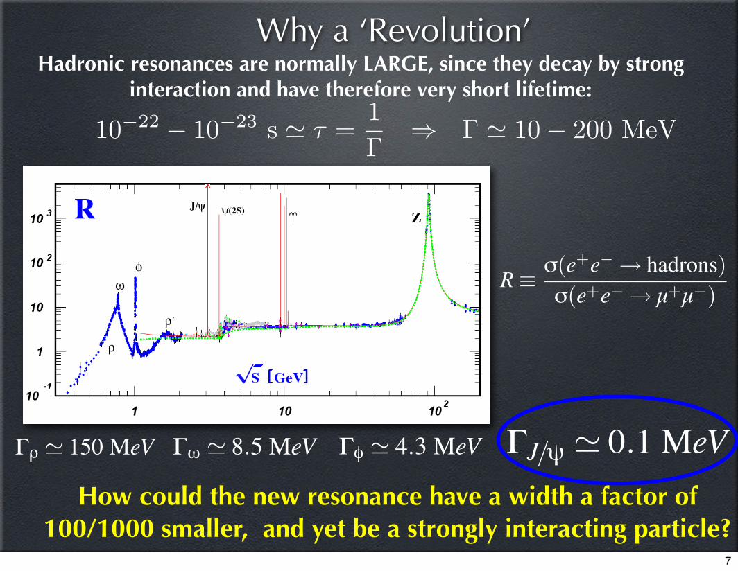
Hadronic resonances are normally LARGE, since they decay by strong interaction and have therefore very short lifetime:

10-1

1

10

10 2

10 3

1 10 102

ρ

ωφ

ρ

J/ψ ψ(2S) ZR

S GeV

Γρ ! 150 MeV Γω ! 8.5 MeV Γφ ! 4.3 MeV

How could the new resonance have a width a factor of 100/1000 smaller, and yet be a strongly interacting particle?

R! σ(e+e" # hadrons)σ(e+e" # µ+µ")

ΓJ/ψ ! 0.1 MeV

10!22 ! 10!23 s " ! =1!# ! " 10! 200 MeV

7

The J/ψ width

Long answer: see extra material at the end of lectures

Short answer: it’s due to the existence of a small strong coupling

at the ‘large’ scale set by the charm quark mass

8

Is the J/ψ really a charm-anticharm bound state?

to BR(K0L! µ+µ")# 7$10"9BR(K+ ! µ+µ )# .635

10-1

1

10

10 2

10 3

1 10 102

ρ

ωφ

ρ

J/ψ ψ(2S) ZR

S GeV

How can a hadronic system not be (much) sensitive to the strong force?

Obvious answer: it’s a small system! NB. Proton radius ~ 1 fm ~ 1/(200 MeV) ~ 1/Λ

Two masses m orbiting each other + Heisenberg uncertainty principle:

r ! 12p! 12

1(m/2)v

=1mv

To estimate v, consider the Virial Theorem

!T " = #12!V "

and first energy level: E1 =!12m2

!43αS

"2

!m2

"v2 = 2!T " = #2E1 =

m2

#43αS

$2==>

==> v! 43αS((1/mv)2) ==> v! 0.5c

QCD potential: Coulomb + linear

2

-4

-2

0

-6

0.2 0.4 0.6 0.8 1

3-loop

1-loop

2-loop

Figure 3: Comparison of VC(r)+C r corresponding to the cases (a),(b),(c) (solid lines) and the latticedata [20]: Takahashi et al. (!), Necco/Sommer (•), and JLQCD (!).

where !(x, ") "! !0 dt tx!1 e!t represents the incomplete gamma function; !1-loop

MSand !2-loop

MS

denote the Lambda parameters in the MS scheme; # = $1/$20 . In the case (c), C can be

expressed in terms of confluent hypergeometric functions except for the coe"cient of a2, whilethe coe"cient of a2 can be expressed in terms of generalized confluent hypergeometic functions.Since, however, the expression is lengthy and not very illuminating, we do not present it here.

The asymptotic behaviors of VC(r) for r # 0 are same as those of VQCD(r) in the respectivecases, as determined by RG equations. The asymptotic behaviors of VC(r) for r # $ are givenby %4%CF /($0r) [the first term of eq. (24)] in all the cases.

As for B(N) and D(r, N), we have not obtained simple expressions in the cases (b),(c),since analytic treatments are more di"cult than in the case (a): we have not separated thedivergent parts as N # $ nor obtained the asymptotic forms for r # 0, r # $. Based onsome analytic examinations, together with numerical examinations for N & 30, we conjecturethat B(N) and D(r, N) in the cases (b),(c) have behaviors similar to those in the case (a).

Let us compare the “Coulomb–plus–linear” potential, VC(r) + C r, for the three cases whenthe number of quark flavors is zero. We also compare them with lattice calculations of theQCD potential in the quenched approximation. See Fig. 3. We take the input parameterfor VC(r) + C r as &S(Q) = 0.2, which corresponds to !1-loop

MS/Q = 0.057, !2-loop

MS/Q = 0.13,

!3-loopMS

/Q = 0.12.‡ Then, the scale for each lattice data set is fixed using the central value of the

relation [18] !3-loopMS

r0 = 0.602(48), where r0 is the Sommer scale. An arbitrary r-independentconstant has been added to each potential and each lattice data set to facilitate the comparison.We see that VC(r) + C r for (a),(b),(c) agree well at small distances, whereas at large distancesthe potential becomes steeper as &S(q) accelerates in the IR region, i.e. C(a) < C(b) < C(c). Thisfeature is in accordance with the qualitative understanding within perturbative QCD [10,2,3].

‡As well-known, when the strong coupling constant at some large scale, e.g. "S(mb), is fixed, the values of

!1-loopMS

, !2-loopMS

, and !3-loopMS

di"er substantially. As a result, if we take a common value of !MS as the input

parameter, VC(r) + C r for (a),(b),(c) di"er significantly at small distances, where the predictions are supposedto be more accurate.

8

V (r)!"43αS(1/r2)

r+Kr

and consequently

r ! 1750 MeV

! 13Λ! 0.3 fm

J/ψNB. Tight bound system below threshold for DDbar decay (on the contrary, phi -> KKbar)=> further explanation for small width

9

“For every complex problem, there is a solution that is simple, neat and wrong’’ -- H.L. Mencken

ΓJ/ψ ! 100 KeV Γηc ! 25 MeVFurther evidence of asymptotic freedom (i.e. small coupling):

J/ψ(3S1) is 1-- ηc(1S0) is 0

-+

decays to three gluons decays to two gluons

Suppressed by a factor of αS,

helped by a small coefficient:

10

In 1977 the Upsilon (bbar bound state) was observed for the first time at Fermilab

[Phys. Rev. Lett. 39 (1977) 252]

The discovery of the bottom quark, the FIFTH, points to a new family, the third.

Hence, we’ll then need to find a SIXTH quark

Less than three years had passed between the discoveries of charm and bottom. But then, the waiting got longer.....

Discovery: bottom

[NB. Upsilon also very narrow. Large width here due to experimental resolution]

11

.....or did it?

UA1 “almost” discovers the top quark with m=40 GeV in 1984

[Phys. Lett. B147 (1984) 493]

.....oooops!

12

The top quark is finally really found at Fermilab by the CDF collaboration in 1994, with a much larger mass, ~ 175 GeV

Excess of events with many jets. Needs very good control of background

Phys. Rev. Lett. 73 (1994) 225

Discovery: top

13

Such a heavy top was a surprise. However, the lower limit had been increasing and there had been hints from analysis of electroweak data, where the top mass enters via loop

corrections

Quigg

You might notice, however, how knowing the top mass helps a lot in predicting it......

SM fits

direct measurements...

14

Heavy Quark Masses

The PDG tells you:

Same symbol ‘m’ but different objets: not their best choice of notation

Only for bottom it’s at least (partially) clear which mass they are quoting Charm and top, anybody’s guess (or knowledge)

15

Heavy Quark MassesLeading order: (pole) mass = m! 1

p/"m

(At least) two possible renormalisation schemes: MSbar and on-shell, leading to to different mass definitions:

The pole mass m (or M)(real part of the pole of the propagator)

The MSbar mass m(μ)(A short-distance mass,

evalutated at the renormalisation scale μ)

_

Higher orders: m0 = bare massNeed for

renormalisation

! 1p/"m0 " !

16

Heavy Quark Masses: pros and consThe pole mass is more physical (pole = propagation of particle, though a quark doesn’t usually really propagate -- hadronisation!) but is affected by long-distance effects: it can never be determined with accuracy better than ΛQCD

The MSbar mass is a fully perturbative object, not sensitive to long-distance dynamics. It can be determined as precisely as the perturbative calculation allows. Of course, it is also fully artificial.

The two masses are related by the perturbative relation:

+ ... + O(ΛQCD)

17

MSbar: m(m) Pole: M

Charm 1.27 +0.7 -0.11 GeV 1.3 -- 1.7 GeV

Bottom 4.20 +0.17 -0.07 GeV 4.5 -- 5 GeV

Top ~ 163 GeV 172.6 ± 1.4 GeV

Heavy Quark Masses: summary

_ _

?

18

Heavy quarks are different: the dead cone

Consider now ‘shaking’ (i.e. accelerating) a quark. The regeneration time of a gluon field of momentum k around it is given by

tregeng (k) =k!k2"

For gluons such that k! " Λ, k# " E we have tregeng (k)! thadrq

A heavy quark will therefore behave like a light one only if

thadrQ > tregeng (k)! Em1Λ

>k"k2#$ 1Θ1Λ!Θ>

mE%Θ0

Gluon transverse momenta leading to longer regeneration times will instead be suppressed (as the heavy quark is not there any more!!)

is called the ‘dead cone’ (no radiation from the heavyquark in a collinear region close to the quark)Θ<Θ0

The time a coloured particle takes to hadronize is that taken by the colour field to travel a distance of the order of the typical hadron size: t’ ~ R ~ 1/Λ

thadrq = t !γ= REΛ

= ER2 =EΛ2

light quarks

thadrQ = t !γ= REm

heavy quarks

Boosting to the lab frame we find

19

The ‘Dead Cone’ in perturbative QCDConsider gluon emission off a heavy quark using perturbation theory:

Dreal(x,k2!,m2) =CFαS2π

!1+ x2

1" x1

k2!+(1" x)2m2" x(1" x) 2m2

(k2!+(1" x)2m2)2

"

The presence of the heavy quark mass suppresses instead the radiation at small

transverse momenta and allows the integration down to zero

In the massless case (m=0) we have a non-integrable collinear singularity:

Z

0D(x,k2!)dk2! =

1+ x2

1" x

Z

0

dk2!k2!

= ∞

=> We can calculate in pQCD heavy quark total cross sections and momentum distributions

[NB. The cone is not really fully dead, just feeling unwell...]

20

A Massive Calculation

heavy quark mass

Obviously, finite ≠ good description of data

Back to this problem later on

21

Heavy Quark hadroproduction

Leading Orderdiagrams:

NB: light quarks and gluons only,

in the initial state

22

Next-to-Leading Order calculation also available:

Virtual corrections

Real corrections

First data: UA1 in 1990

Good agreement with NLOQCD predictions

WITHIN UNCERTAINTIES

[Nason, Dawson, Ellis; Beenakker et al, 1988-1989]

[At the time, quite a massive (no pun intended) calculation NNLO started only very recently and still in progress]

23

How does the NLO calculation look like?

LO NLO

Must be calculated explicitly

Can be derived from LO

velocity of the heavy quark

24

NLO short distance cross sectionsqqbar

gg

gq

25

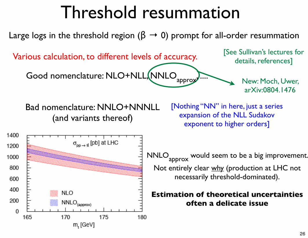
Threshold resummationLarge logs in the threshold region (β → 0) prompt for all-order resummation

Various calculation, to different levels of accuracy.

Bad nomenclature: NNLO+NNNLL (and variants thereof)

[Nothing “NN” in here, just a series expansion of the NLL Sudakov

exponent to higher orders]

[See Sullivan’s lectures for details, references]

New: Moch, Uwer, arXiv:0804.1476

NNLOapprox would seem to be a big improvement.

Not entirely clear why (production at LHC not necessarily threshold-dominated).

Estimation of theoretical uncertainties often a delicate issue

Good nomenclature: NLO+NLL, NNLOapprox, ....

26

Theoretical uncertainties

dd lnµ2

lnσphys = 0Ideally

NB. Such uncertainty is a....known unknown, but still an unknown

The ‘best value’ of a scale cannot be fixed using data, as if it were a physical parameter.

[High energy physics version of ‘There’s no free lunch’]

This only holds for all-order calculations. In real life: residual dependence at one order

higher than the calculation

Vary scales (around a physical one) to ESTIMATE the uncalculated higher order

i.e. independence of cross sections on artificial scales

27

“Typical” behaviour of a cross-section

w.r.t. scale variations NLO

LO

µ/mtop

σ (pb)

“Reasonable” scale variation

}} Uncertainty

}

The rule of thumb on uncertainties

- A LO calculation gives you a rough estimate of the cross section- A NLO calculation gives you a good estimate of the cross sectionand a rough estimate of the uncertainty

- A NNLO calculation gives you a good estimate of the uncertainty

28

Theoretical uncertainty: an example

Example:Higgs boson production

at the LHCAnastasiou, Melnikov. Petriello,

hep-ph/0501130

Scale variations

NB. This example shows that the center of the NLO band has nothing to do with the most accurate theoretical prediction.

Theoretical uncertainty bands are not gaussian errors!

29

Top @ TevatronStandard procedure: vary renormalisation and factorisation scales.

But, better do so independently

σ: 6.82 > 6.70 > 6.23 pb 0.5 < μR,F/m < 2

σ: 6.97 > 6.70 > 6.23 pb 0.5 < μR,F/m < 2 && 0.5 < μR/μF < 2

Order ±5% uncertainty along the diagonal, a little more considering

independent scale variations

“Fiducial” region

BTW, the PDF uncertainty (±10-15%) is probably the dominant one here

μR

μF

(NLO+NLL, m=175 GeV)

30

σ(|y|<1): 28.9 > 23.6 > 20.1 μb 0.5 < μR,F/μ0 < 2

σ(|y|<1): 34.4 > 23.6 > 17.3 μb 0.5 < μR,F/μ0 < 2 && 0.5 < μR/μF < 2

The scales uncertainty increases from ±18% to ±35% when going off-diagonal

μF

μR

Independent scale variationsSometimes, varying scales together can be misleading!

bottom at the Tevatron

31

Independent scale variationsSometimes, varying scales together can be

very misleading!

σ(|y|<1): 122 > 120 > 115 μb 0.5 < μR,F/μ0 < 2

Only a ±4% uncertainty when varying the scales together.......

σ(|y|<1): 178 > 120 > 75 μb 0.5 < μR,F/μ0 < 2 && 0.5 < μR/μF < 2

....which becomes a ±40% one when going off-diagonal!

μR

μF

Case in point: bottom cross section at the LHC:

32

Top @ LHCGoing to independent scale variations matters more at the LHC

(NLO+NLL, m = 171 GeV, scale uncertainties only)

σ: 970 > 908 > 860 pb 0.5 < μR,F/m < 2

σ: 990 > 908 > 823 pb 0.5 < μR,F/m < 2 && 0.5 < μR/μF < 2

This would not have been obvious looking only at NLO

0.5 < μR,F/m < 2

0.5 < μR,F/m < 2 && 0.5 < μR/μF < 2

Lesson to take home here: every process/energy can be different. Uncertainty estimates should always be carried out in detail,

and not ‘carried over’ from a supposedly (or hopefully) similar case

σ: 977 > 875 > 774 pb

33

Top @ LHC: one more lesson?

NLO+NLL, different choice for subleading terms:

σ: 964 > 945 > 939 pb 0.5 < μR,F/m < 2

σ: 1041 > 945 > 861 pb 0.5 < μR,F/m < 2 && 0.5 < μR/μF < 2

σ: 970 > 908 > 860 pb 0.5 < μR,F/m < 2

σ: 990 > 908 > 823 pb 0.5 < μR,F/m < 2 && 0.5 < μR/μF < 2

NLO+NLL, same as before:Compare

with

Lessons:* different central values, but within uncertainties of ‘choice 1’* ‘choice 2’ has very small uncertainty for equal scales, O(2%).* when the scales are kept different, both choices are compatible (as they should)

In NNLOapprox the ‘choice 2’ was made and uncertainties were studied

equal scales. Could this explain its very small uncertainty?

Choice ‘1’

Choice ‘2’

34

Differential cross sectionsDo we actually observe charm

and bottom quarks?Of course not!

Real measurements are done with (decay products of) charmed and bottom

hadrons, i.e. mainly D and B

The ‘old school’ called for ‘reconstructing’ from such measurements the bare quark cross section, present the data in this way

(see plot) and compare the latter to pQCD predictions.

Is this a good idea?UA1

35

Perturbative: gluon radiation

Non-perturbative:hadronization

Not being the b quark a physical particle, the quark-to-meson transition cannot be a physical observable:

its details depend on the perturbative calculation it is interfaced with. Deconvoluting to the quark level is therefore AMBIGUOUS

36

pp pQCD! Q NP f ragm.! HQdecay! e

Observables More modern attitude

(also made more easily feasible by computer power):compare at (or as close as possible to) the observable level

Full process

37

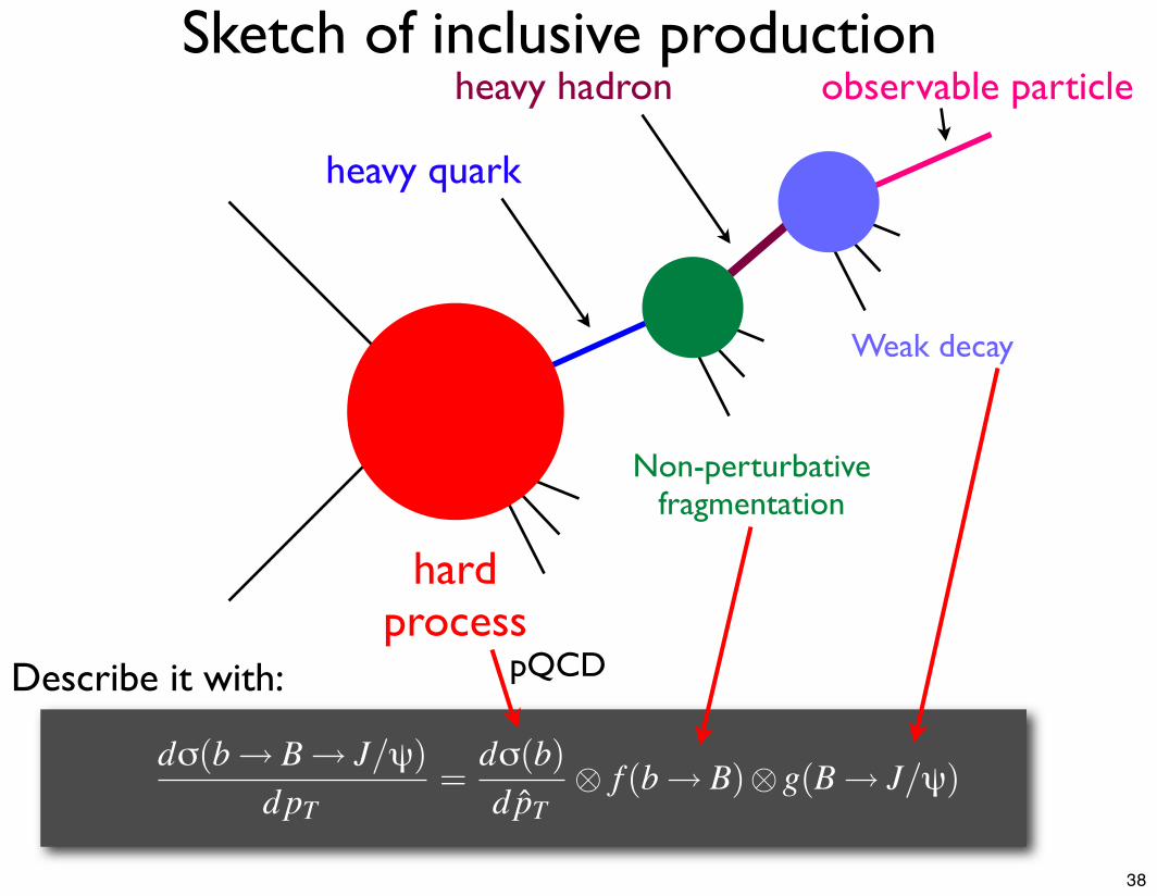
Sketch of inclusive production

hard process

heavy quark

Non-perturbative fragmentation

heavy hadron

Weak decay

observable particle

dσ(b! B! J/ψ)dpT

=dσ(b)d pT

" f (b! B)"g(B! J/ψ)

Describe it with: pQCD

38

Non-perturbative fragmentationWhat do we know about it?

If the quark is light, not much. It’s a process-independent artificial object (factorisation theorem) which we must extract from data

(e.g. pion fragmentation functions)

If the quark is heavy, its fragmentation function is still ambiguous, but we can tell something more about it:

* we know it’s a (parametrically) small effect

* we can relate it to the hadronisation scale and to the heavy quark mass

* we can test this on D and B data

39

Bjorken and Suzuki (circa 1977)

It boils down to: a heavy object is hard to slow downWe can see it in the following way (likely another Mencken’s simple and wrong solution....)

[NB. Bjorken and Suzuky used different, better, derivations]

Final result: a heavy quark only loses on average a fraction Λ/m of its momentum when hadronising.

A heavy quark fragmentation function will be peaked near z=1

pQCD substantiates this by indicating: <zN-1> =

40

Charm Bottom

O(Λ/mcharm) O(Λ/mbottom)e+e! " QX " HQX

pQCD

non-perturbativecontribution

non-perturbative contribution limited in size and compatible with expectations

high-accuracy expt. data allow it to be precisely determined

Test of scaling in D and B fragmentation

41

Test of scaling in D and B fragmentation

LEP B meson data translated to Mellin space:

fN !Z 1

0xN"1 f (x) dx= #xN"1$

In this space convolutions become products

!x"expt = !x"pQCD!x"np

This gap: non-perturbative QCD

42

pQCD (NLL)

data

Dnp = data

pQCD

DnpN = 1! (N!1)Λ

m+ · · ·Compatible withcharm ~ 1 - 0.16

bottom ~ 1 - 0.06and Λ! 0.25 GeV

moments can give a more quantitative picture:!xN"1#

N=2 moments (i.e. 〈x〉)

(very precise!)

Test of scaling in D and B fragmentation

43

B-mesons differential cross sections @ Tevatron

Good agreement, with minimal non-perturbative correction

NLO is sufficient for correct total rate prediction

100

101

102

103

0 5 10 15 20 25 30 35 40

dσ/d

p T(p

pbar

→ B

+ + X

, |y|

< 1

) (n

b/G

eV)

pT (GeV)

fB+ = 0.389All data rescaled to B+ and |y| < 1

FONLL, CTEQ6M, Kart. α = 29.1NLO, same as above

NLO, no fragm.CDF B+ → J/ψ K+

CDF Hb → µ- D0CDF Hb → J/ψ X

44

Lessons in heavy quark fragmentation

Charm and bottom are heavy and have limited non-perturbative contributions, but still hadronise

We can predict to some extent their non-perturbative fragmentation functions

After pQCD has done its job (gluon radiation, possibly resummed) the remaining contribution is small and scales as predicted

the non-perturbative fragmentation function is ambiguous and non-observable, and must be matched properly with the pQCD part

Even a small contribution can be enhanced by steeply falling spectra (i.e. transverse momentum distributions) and lead to large effects. Hence, importance of proper treatment of fragmentation in hadronic collisions

45

The top exceptionYou’ll have noticed that the top was not discovered first as a bound state.

Why ?

The revolution time of a ttbar bound state goes like

For the top quark this yields tR ~ 10-25 s

tR !1

mt!2S

So a heavy (>> MW) top vanishes before a toponium can be formed

[Bigi, Dokshitzer, Khoze, Kuehn, Zerwas, PLB 181 (1986) 157]

tdecay =1

!bW! 1/

!GF m3

t

8!"

2

"# 1

GF m3t

# m2W

m3t

# 10!28 s

On the other hand, as member of a weak isospin doublet, a heavy top can decay weakly:

t! bW+

[NB. The ‘right’ number with all the numerical factors it’s actually a lot closer to 10-25 s]

46

The top exceptionA similar, even more stringent, argument applies to standard

hadronisation, i.e. the formation of t-(light quark) states

Hadronisation takes a certain time, namely the time for gluons to propagate the distance of a typical hadron radius R ~ 1 fm:

thadr ! R/c! 1/Λ! 10"24 s

Recalling the top weak decay:

tdecay =1ΓbW

! 1/!GFm3t8π"2

"# 1/(GFm3t )#

M2Wm3t

=1ΛM2WΛ

m3t

so that NB. Neglected pretty

big numerical factors. Real limit larger.

One more, a heavy top quark with mass larger than the W boson will therefore decay before hadronising

tdecay < thadr if mt > (M2WΛ)1/3 ! 10 GeV

47

all-hadronic

electron+jets

elec

tron

+jet

s

muo

n+je

ts

muon+jets

tau+

jets

tau+jets

eµ e!

e! µ!

µ!

!!

e+ cs ud!+µ+

e–cs

ud

!–µ–

Top Pair Decay Channels

W

deca

y

eµ

ee

µµ

dilep

tons

proton

antiproton

q

q

g t

t

!

e+

W +

b

W –

b

!

µ+

antilepton-neutrinoquark-antiquark

Top decaysClassified according

to the W decay

11% 11% 11% 33% 33%

~44%

~10%~ 23%

~ 23%

dilepton: low yield, low bckgd

lepton+jet: higher yield, moderate bckgd

all hadronic: highest yield, huge bckgd

[NB. the tau is usually considered a ‘hadron’]

lepton-antineutrinoquark-antiquark

48

The top massWhy are we interested in a precise measurement of the top mass?

Indirect handle on the Higgs mass

mt [GeV]

A 2 GeV change in mt changes the limit on mH by ~20 GeV

49

The top mass

D. Glenzinski’s talk at Top 2008

What is this mass? What are we

actually measuring?

50

The top massSince the top does not hadronise,

can we measure its pole mass to any given accuracy?

Not really

The top mass is usually measured through kinematic distributions of the top decay products, the bottom quark

among themhadronisation and decay

The hadronisation (= long-distance) uncertainties enter the top mass determination through its decay products

51

The top massA second source of uncertainty

hadronisation and decay

Presently no higher-order calculation relates a kinematical distribution used for top mass extraction to the mass parameter in the QCD lagrangian

Processes of this kind are only calculated/simulated at

tree level in pQCD

We are therefore measuring a leading order pole mass

52

The top mass: a NLO extractionActually, there is an observable, dependent on the top mass, calculated at

higher order in pQCD: the total ttbar production cross section

Example of extraction by D0:

mt = 170± 7 GeVFairly large uncertainty, but

compatible with kinematic measurements, and

we know exactly what we are measuring.

Might become competitive with NNLO calculation and

better measurement

53

ttbar cross section at the Tevatron

Overall uncertainty ~ 10%

A.Castro’s and V. Sharyy’s talks at Top 200854

Top quark perspectives at the LHCLHC is a top factory:

8 million ttbar pairs at L = 10 fb-1 /year

Unfortunately, it’s also a background factory…. :-(

The expectations for mass and cross section measurements are therefore not significantly better

than already achieved at the Tevatron:

!mt ! 1 GeV!!tt

!tt! 5" 10%

55

t-channel s-channel tW associated production

Essentially electroweak processes: proportional to (and therefore probe of) |Vtb|2

Moreover, source of highly polarized top quarks: investigations of charged weak current interactions possible

Single top

Predicted cross sections (NLO) at the Tevatron:

Cross section not much smaller than ttbar, but measurement more challenging because backgrounds are larger

t-channel s-channel tW associated production

0.9± 0.1 pb2.0± 0.2 pb ! 0.1 pb

[See Z. Sullivan’s lecture at CTEQ ’07]

56

J. Lueck and S.Jabeen talks at Top 2008

Single top

Measurements compatible with predictions (~ 3 pb), but

still large uncertainties

57

ConclusionsHeavy quarks are nice to pQCD: large mass means smaller running coupling and collinear safety

Charm and bottom hadronise, but the effect tends to be small in sufficiently inclusive observables: predictivity is maintained

Top behaves essentially as an electroweak particle

A number of tools which have recently appeared for studying today’s (and tomorrow’s) top physics: ALPGEN, MC@NLO, POWHEG, MADGRAPH, ….. , without forgetting the evergreen PYTHIA and HERWIG

58

Extra material

59

to BR(K0L! µ+µ")# 7$10"9BR(K+ ! µ+µ )# .635

10-1

1

10

10 2

10 3

1 10 102

ρ

ωφ

ρ

J/ψ ψ(2S) ZR

S GeV

The J/ψ widthIf J/ψ is produced in the interaction of an electron and a positron via a photon it

must therefore have the same quantum numbers as the photon: JP = 1-

If we assume that its decay into hadrons goes via gluons, the Landau-Yang theorem (a vector particle cannot decay into two

vector states) implies there must be at least three of them in the final state

J/ψ }hadrons

We write the decay width as:

Probability of finding the two quarks at the same point

annihilation probability at rest

We now need the tools to perform the calculations of the two terms.We shall use a Coulomb approximation for the first term and the QCD

Feynman rules for the second

Γ(3S1! 3 gluons) = |R(0)|2|M(qq! 3 gluons)|2

60

Colour factors

to BR(K0L! µ+µ")# 7$10"9BR(K+ ! µ+µ )# .635

10-1

1

10

10 2

10 3

1 10 102

ρ

ωφ

ρ

J/ψ ψ(2S) ZR

S GeV

The J/ψ widthCoulomb potential:

Solving the Schroedinger equation we find

The QCD probability for annihilation into 3 gluons will also be proportional to the cube of the

strong coupling:

V (r)!"43αSr

|R(0)|2 =4

(Bohr radius)3= 4

!43αS

"3#m2

$3

|M(qq! 3 gluons)|2 =α3Sm2

!518

"4(π2"9)9π

Finally: Γ(3S1! 3 gluons) ∝ α6SThe strong coupling runs with the scale. At what scale should I take it?

Γ(Q,g,µ) = Γ(Q, g(Q),Q)

Γ(3S1! 3 gluons) ∝ [αS(4m2)]6so that

In 1974, however, we had no measurement for the strong coupling at a scale around 3 GeV. We did not even know if such a perturbative

coupling existed!

The renormalization group fixes it:

61

to BR(K0L! µ+µ")# 7$10"9BR(K+ ! µ+µ )# .635

10-1

1

10

10 2

10 3

1 10 102

ρ

ωφ

ρ

J/ψ ψ(2S) ZR

S GeV

The J/ψ widthTwo options for checking the consistency of the picture

1. - Try to rescale a lower energy decay width

Γ(φ! 3π)" 600 keVAsymptotic freedom scales this to

From one can extract αS((1 GeV)2)! 0.53αS((3 GeV)2)! 0.29

Γ(J/ψ! hadrons) =32MJ/ψ

Mφ

!αS(M2

J/ψ)

αS(M2φ)

"6

Γ(φ! 3π)" 73 keV

2. - Use leptonic width to eliminate wavefunction and extract value of strong coupling

From Γ(J/ψ! leptons) = |R(0)|2|M(qq! e+e")|2 =1m2

!23αem

"2|R(0)|2 # 3 keV

and

we get

Γ(J/ψ! leptons)Γ(J/ψ! hadrons)

=18πα2em

5(π2"9)α3S# 0.04

αS((3 GeV)2)! 0.26

Good consistency between strong coupling values. Good estimate of hadronic width.

OK!

OK!

62