matrix valued orthogonal polynomials of jacobi type: the role...
TRANSCRIPT

ANNALE
S D
E
L’INSTITUT FO
URIER
ANNALESDE
L’INSTITUT FOURIER
F. Alberto GRÜNBAUM, Inés PACHARONI & Juan Alfredo TIRAO
Matrix valued orthogonal polynomials of Jacobi type: the role of grouprepresentation theoryTome 55, no 6 (2005), p. 2051-2068.
<http://aif.cedram.org/item?id=AIF_2005__55_6_2051_0>
© Association des Annales de l’institut Fourier, 2005, tous droitsréservés.
L’accès aux articles de la revue « Annales de l’institut Fourier »(http://aif.cedram.org/), implique l’accord avec les conditionsgénérales d’utilisation (http://aif.cedram.org/legal/). Toute re-production en tout ou partie cet article sous quelque forme que cesoit pour tout usage autre que l’utilisation à fin strictement per-sonnelle du copiste est constitutive d’une infraction pénale. Toutecopie ou impression de ce fichier doit contenir la présente mentionde copyright.
cedramArticle mis en ligne dans le cadre du
Centre de diffusion des revues académiques de mathématiqueshttp://www.cedram.org/
Ann. Inst. Fourier, Grenoble55, 6 (2005), 2051–2068
MATRIX VALUED ORTHOGONAL POLYNOMIALS
OF JACOBI TYPE: THE ROLE OF GROUP
REPRESENTATION THEORY
by F. Alberto GRUNBAUM, Ines PACHARONI& Juan TIRAO (*)
1. Introduction.
Starting with the work of M. G. Krein, [K1] and [K2], as well asmore recent contributions, including for instance [D1], [D2], [D3], [D4],[DP], [DvA], [Ge], and [SvA], there is a nice and general theory of matrixvalued orthogonal polynomials. These are bound to play an important partin many areas of mathematics and its applications, just as their scalarcounterparts. This should be particularly true for those matrix valuedorthogonal polynomials that have some extra property, such as the onesingled out for further study in [DG] and generally known under the labelthe bispectral property. The search for concrete instances enjoying thesetwo properties has received a certain amount of recent attention, followingearlier work started in [D1]. The collection of known examples enjoying thisextra property is still very small. For a family of examples (in arbitrarydimension), not reducible to the scalar case, see [GPT1], [GPT2] and theclosing paragraph in [GPT4]. For recent progress in this area, including ageneral method to attack this problem and a relevant hierarchy of examples,
(*) This paper is partially supported by NSF Grant # DMS 0204682, by AFOSR underContract F41 624-02-1-7000, by CONICET grants PIP 655 and PEI 6150, by ANPCyTgrant PICT 03-10646 and by the ICTP Associate Scheme.Keywords: Matrix valued orthogonal polynomials, Jacobi polynomials.Math. classification: 33C45, 22E45.

2052 F. Alberto GRUNBAUM, Ines PACHARONI & Juan TIRAO
see [DG1] and [DG2]. For a different source of examples one can consult[G] and [GPT5].
In this paper we restrict our attention to examples that are of theJacobi type, meaning that the differential operator is given by the Gausshypergeometric one, see [T2].
Even a cursory look at the emerging family of examples revealstwo distinct tools: either one poses and solves a certain set of matrixvalued differential equations (along with certain boundary conditions) asin [DG1] and [GPT5], or one ignores these equations altogether, startswith a symmetric space G/K, as in [GPT1], [GPT2],[ GPT3], [GPT4] andeventually arrives at explicit examples. No one familiar with the historyof these developments in the scalar case should be surprised with theuseful role played by these symmetric spaces. For a good general referencesee [VK]. None of the two routes mentioned above gives an easy path toexamples. For this reason alone we consider it very important, at this earlystage of this search for examples, to exploit all possible avenues. For theexamples obtained in [GPT1] one starts with the theory of matrix valuedspherical functions, see [T1] and [GV]. Specifically one takes G = SU(3) andK = S(U(2)×U(1)) � U(2). The corresponding symmetric space is thenthe complex projective plane. As noticed in [GPT1], see page 355, whentalking about properly packaged matrix valued spherical functions one isnot quite dealing with matrix valued orthogonal polynomials. The stepneeded to make this connection is given in the last section of [GPT4]. Tobetter understand the point of view of this paper it is important to reviewin more detail some of the developments discussed above. The results in[GPT1] give instances of matrix valued classical pairs {W,D} of arbitrary
size, the only restriction is that the value of the parameter β needs to be 1.The classical scalar valued case corresponds to the further specialization� = 0. Since the value of α in [GPT1] is only restricted to be an integer,it is not hard to see how to extend this beyond group values. The issueof extending beyond the case of β = 1 is a completely different game.This was achieved in [G] for square matrices of size 2 by postulating acertain structure for the weight matrix which was consistent with all theexamples known up to that point. Later in [GPT5] three one parameterfamilies of classical pairs of the same size were constructed, one of whichextends the example in [G]. The extension of this search of classical pairsto larger size is not an easy matter. In this paper we use some preliminariesresults from [PT] where the complex projective plane considered in [GPT1]is replaced by the n-dimensional complex projective space. This gives us
ANNALES DE L’INSTITUT FOURIER

MATRIX VALUED ORTHOGONAL POLYNOMIALS 2053
a group theoretical framework which provides enough integers parametersm and n. Extending the resulting classical pairs to arbitrary values of theparameters α and β is then completely straightforward.
2. Matrix valued orthogonal polynomialsand symmetric differential operators.
Here we recall some standard facts. Given a self adjoint positivedefinite matrix valued smooth weight function W (t) with finite momentswe can consider the skew symmetric bilinear form defined for any pair ofmatrix valued polynomial functions P (t) and Q(t) by the numerical matrix
(P,Q) = (P,Q)W =∫R
P (t)W (t)Q∗(t)dt,
where Q∗(t) denotes the conjugate transpose of Q(t). By the usual construc-tion this leads to the existence of a sequence of matrix valued orthogonalpolynomials with non singular leading coefficient. The skew symmetric bi-linear form introduced above is not the only possible such choice, as noticedfor instance in [SvA]. In this section we will also consider the form
〈P,Q〉 = (P ∗, Q∗)∗.
The reason for considering this form can be traced back to [GPT1] aswill be noticed below. Observe that a sequence {Pn}n�0 of matrix valuedpolynomials is orthogonal with respect to (·, ·) if and only if the sequence{P ∗n}n�0 is orthogonal with respect to 〈·, ·〉. Given an orthonormal sequence{Pn(t)}n�0 one gets by the usual argument a three term recursion relation
(1) tPn(t) = An+1Pn+1(t) + BnPn(t) + Cn−1Pn−1(t),
where An+1 is nonsingular, B∗n = Bn and Cn−1 = A∗n. We now turn ourattention to an important class of orthogonal polynomials which we willcall classical matrix valued orthogonal polynomials. As in [GPT5] we saythat the weight function is classical if there exists a second order ordinarydifferential operator D with matrix valued polynomial coefficients Aj(t) ofdegree less or equal to j of the form
(2) D = A2(t)d2
dt2+ A1(t)
d
dt+ A0(t),
such that
(3) 〈DP,Q〉 = 〈P,DQ〉
TOME 55 (2005), FASCICULE 6
2054 F. Alberto GRUNBAUM, Ines PACHARONI & Juan TIRAO
for all matrix valued polynomial functions P and Q. We refer to sucha pair {W,D} as a classical pair. If {W,D} is a classical pair then thereexists an orthonormal sequence {Pn}, with respect to (·, ·), of matrix valuedpolynomials such that
(4) DP ∗n = P ∗nΛn,
where Λn is a real valued diagonal matrix. This form of the eigenvalueequation (4) appears naturally in [GPT1] and corresponds to the fact thatthe rows of Pn are eigenfunctions of D. One could avoid the introductionof the inner product 〈 , 〉 in (3) by introducing right handed differentialoperators as in [D1]. Either choice has its own drawbacks. This is aconsequence of the fact that in the matrix valued case D and the differenceoperator in the right hand side of (1) do not commute. Assume that theweight function W = W (t) is supported in the interval (a, b). We recallthat in [GPT5] and in [DG1] (except for a change due to the fact thatthe differential operator there is acting on the right hand side) we haveproved that the condition of symmetry (3) is equivalent to the followingthree differential equations
A∗2W = WA2,
A∗1W = −WA1 + 2d
dt(WA2),(5)
A∗0W = WA0 −d
dt(WA1) +
d2
dt2(WA2),
with the boundary conditions
limt→x
W (t)A2(t) = 0 = limt→x
(W (t)A1(t)−A∗1(t)W (t)
),
for x = a, b.
The second condition can be replaced by
(6) limt→x
(W (t)A1(t)−
d
dt
(W (t)A2(t)
))= 0.
These equations are quite general and do not depend on the assump-tions that the matrix valued coefficients of D are polynomials nor on thefact that the interval (a, b) is finite. Finding explicit solutions of these equa-tions is a highly non trivial task. As noted before, in [GPT1] we computedexplicitly the matrix valued spherical functions of any K-type associatedto the complex projective plane. These results were connected in [GPT4]with the established theory of matrix valued orthogonal polynomials. Wewill see later that by using just the first few steps of the analysis in [GPT1]
ANNALES DE L’INSTITUT FOURIER

MATRIX VALUED ORTHOGONAL POLYNOMIALS 2055
and [PT] one gets solutions of equations (5) and (6). More explicitly theCasimir of G is symmetric with respect to the L2-inner product betweenmatrix valued functions on G. The method of [GPT1] allows one to replacethis differential operator by a second order differential operator in the vari-able t ∈ (0, 1). By an appropriate conjugation as in [GPT4] one convertsthis operator into a matrix valued differential operator D of the hypergeo-metric type. Similarly the L2-inner product on G leads to a matrix valuedweight function W on (0, 1). The symmetry of the Casimir mentioned abovemakes D symmetric with respect to W , hence we obtain a classical pair{W,D}. This program will be carried out in the next sections.
3. Some background material from representation theory.
In the forthcoming paper [PT] one tackles the problem of determiningthe matrix valued spherical functions associated to the n-dimensional com-plex projective space Pn(C). This space can be realized as the homogeneousspace G/K, where G = SU(n + 1) and K = S(U(n) × U(1)) � U(n). Bygoing from the complex projective plane as in [GPT1] to the n-dimensionalcomplex projective space one gets a plethora of new phenomena. Here werecall a few facts from [PT] obtained in a similar way as those correspondingto the case n = 2 given in [GPT1]. Let (Vπ, π) be any irreducible repre-sentation of K. An irreducible spherical function can be characterized as afunction Φ : G −→ End(Vπ) such that
i) Φ is analytic.
ii) Φ(k1gk2) = π(k1)Φ(g)π(k2), for all k1, k2 ∈ K, g ∈ G, and Φ(e) = I.
iii) [∆Φ](g) = Φ(g)[∆Φ](e), for all g ∈ G and ∆ ∈ D(G)G
where D(G)G denotes the algebra of all left and right invariant differentialoperators on G. We observe that the Casimir operator ∆2 of G belongsto D(G)G. For our purposes it is convenient to consider a larger class offunctions, namely the vector space of all functions Φ that satisfy
i) Φ is analytic.
ii) Φ(k1gk2) = π(k1)Φ(g)π(k2), for all k1, k2 ∈ K, g ∈ G.
iii) [∆2Φ](g) = Φ(g)[∆2Φ](e), for all g ∈ G.
The study of these spaces of functions is carried out in [PT] by using theapproach of [GPT1]. This naturally lead us to a very rich collection ofclassical pairs {W,D}.
TOME 55 (2005), FASCICULE 6

2056 F. Alberto GRUNBAUM, Ines PACHARONI & Juan TIRAO
For any g ∈ SU(n + 1) we denote by A(g) the left upper n× n blockof g, and we consider the open dense subset A = {g ∈ G : det(A(g)) �= 0}.Then A is left and right invariant under K. We introduce the followingfunction defined on A:
Φπ(g) = π(A(g)),
where π above denotes the unique holomorphic representation of GL(n,C)which extends the given representation of U(n). For any function Φ in ourclass we associate to it a function H : A −→ End(Vπ) defined by
H(g) = Φ(g)Φπ(g)−1.
Then H satisfies that H(e) = I and
i) H(gk) = H(g), for all g ∈ A, k ∈ K.
ii) H(kg) = π(k)H(g)π(k−1), for all g ∈ A, k ∈ K.
The canonical projection p : G −→ Pn(C) maps the open dense subsetA onto the affine space Cn of those points in Pn(C) whose last homogeneouscoordinate is not zero. Thus, property i) says that H may be considered as afunction on Cn. The fact that Φ is an eigenfunction of ∆2 makes H into aneigenfunction of a differential operator D on Cn. The explicit computationof D is carried out in [PT]: For H ∈ C∞(Cn)⊗ End(Vπ) we have
D(H)(z1, . . . , zn) =(1 +
∑1�j�n
|zj |2)( ∑
1�i�n
(∂2H∂x2i
+ ∂2H∂y2i
)(1 + |zi|)2
+ 2∑
1�i�n
∑j>i
(∂2H∂xi∂xj
+ ∂2H∂yi∂yj
)Re(zizj)
− 2∑
1�i�n
∑j>i
(∂2H∂xi∂yj
− ∂2H∂xj∂yi
)Im (zizj)
)
− 2∑
1�i�n
(∂H∂xi− ∂H
∂yi
)π(Pi),
where zj = xj + iyj and Pj is the n × n matrix whose (r, s) element is(Pj)rs = zr(δjs+zjzs). Here π denotes the representation of the Lie algebraof K obtained by taking the derivative at the identity of the representationπ. By property ii), H is determined by its restriction H = H(r) to the crosssection {(r, 0, . . . , 0) : r � 0} of the K-orbits in Cn, which are the spheresof radius r � 0. Then H = H(r) becomes an eigenfunction of the followingdifferential operator
ANNALES DE L’INSTITUT FOURIER
MATRIX VALUED ORTHOGONAL POLYNOMIALS 2057
DH(r) = (1 + r2)2d2H
dr2+
(1 + r2)r
dH
dr
(2n−1 + r2 − 2r2π(E11)
)+
4r2
( ∑2�j�n
π(Ej1)H(r)π(E1j)−H(r)∑
2�j�nπ(Ej1)π(E1j)
)(7)
+4(1+r2)
r2
( ∑2�j�n
π(E1j)H(r)π(Ej1)−H(r)∑
2�j�nπ(E1j)π(Ej1)
),
where Eij denotes the n × n matrix with entry (i, j) equal to 1 and 0elsewhere.
The irreducible representations of U(n) are restrictions of irreducibleholomorphic representations of GL(n,C), which are parameterized, up toequivalence, by n-tuples of integers
π = (m1,m2, . . . ,mn) such that m1 � m2 � · · · � mn.
As GL(n−1,C)-module, Vπ decomposes as a direct sum of irreduciblerepresentations, each one with multiplicity one, namely
Vπ =⊕
µ interlace π
Vµ,
where the sum is over all (n−1)-tuples that satisfy
µ = (mµ1 , . . . ,m
µn−1) ∈ Zn−1, with mi � mµ
i � mi+1, i = 1, . . . , n−1.
The above facts are well known and can be found in [VK].
The subgroup M of all matrices in K of the form(a 00 A
), with
A ∈ U(n−1) fixes all points (r, 0, . . . , 0) ∈ Cn. Then since H satisfiesproperty ii) above, it follows that the linear transformation H(r) commuteswith π(M), for all r � 0. Thus H(r) is a scalar hµ(r) on each Vµ. Therefore,after a choice of an ordering of the interlacing µ′s, we can identify thefunction H(r) with the vector valued function (hµ(r))µ ∈ CL, where L isthe number of all (n−1)-tuples µ which interlace π.
We observe that the linear transformations∑2�j�n
π(Ej1)H(r)π(E1j),∑
2�j�nπ(Ej1)π(E1j),
∑2�j�n
π(E1j)H(r)π(Ej1) and∑
2�j�nπ(E1j)π(Ej1),
which appear in (7) commute with π(M). Therefore they are scalarmultiples of the identity on each Vµ. These scalars are computed in [PT] by
TOME 55 (2005), FASCICULE 6

2058 F. Alberto GRUNBAUM, Ines PACHARONI & Juan TIRAO
looking at the fine structure of the representation π going along a Gelfand-Cetlin basis of Vπ. In the next section we will carry out this computationin the particular case L = 3.
The fact that H = H(r) is an eigenfunction of the differential operator(7), and after the change of variable t = (1 + r2)−1, implies that thefunction H(t) = (hµ(t))µ associated to the spherical function Φ satisfiesthe following system of differential equations
t(1− t)h′′µ(t) +(sπ − sµ + 1− t(sπ − sµ + n + 1)
)h′µ(t)
+1
1− t
(n−1∑j=1
tj,µ(hµ+ej (t)− hµ(t)
))(8)
+t
1− t
(n−1∑j=1
sj,µ(hµ−ej (t)− hµ(t)
))= λhµ(t),
where ej denotes the j-th canonical basis vector in Rn−1, sπ =∑ni=1 mi,
sµ =∑n−1i=1 mµ
i ,
tj,µ =
∏ni=1 |mi −mµ
j − i + j|∏1�i�n−1,
i �=j|mµ
i −mµj − i + j|
and
sj,µ =
∏ni=1 |mi −mµ
j − i + j + 1|∏1�i�n−1,
i �=j|mµ
i −mµj − i + j| .
As mentioned in Section 2 the group representation theory recalledabove has given us in (8) a differential operator in the variable t which issymmetric with respect to the inner product given below.
The L2-inner product for matrix valued functions Φ and Ψ in theclass introduced above gives rise to the following inner product of thecorresponding functions H and K on (0, 1),
(9) 〈H,K〉 =∑
µ interlace π
2n dim(Vµ)∫ 1
0
(1− t)n−1tsπ−sµ hµ(t)kµ(t) dt.
Explicitly the dimension of Vµ can be computed by using the Weyl’s formula
dimVµ =∏
1�i<k�n−1
mµi −mµ
k + k − i
k − i.
ANNALES DE L’INSTITUT FOURIER

MATRIX VALUED ORTHOGONAL POLYNOMIALS 2059
4. The new Jacobi type examples.
In this section we continue with the program advertised at the end ofSection 2, i.e. we will give explicit classical pairs {W , D} with
(10) W (t) = tα(1− t)βF (t) α, β > −1
and
(11) D = t(1− t)d2
dt2+ (X − tU)
d
dt+ V,
where F (t) is a polynomial function and X,U, V are constant matrices.
The important step involved in going from (8) to (11) and from theweight implicit in (9) to the one in (10) will be carried out for two specialkinds of representations π in Sections 4.1 and 4.2 below.
4.1. Examples of size 3× 3.
We consider representations π of GL(n,C) that correspond to n-tuplesof the form
π = (m + 2, . . . ,m + 2︸ ︷︷ ︸k
, m, . . . ,m︸ ︷︷ ︸n−k
),
with 1 � k � n−1. We have
dimVπ =k−1∏j=0
(n−j)(n−j + 1)(k − j)(k − j + 1)
.
As GL(n−1,C)-modules one has the decomposition
Vπ = Vµ1 ⊕ Vµ2 ⊕ Vµ3 ,
whereµ1 = (m + 2, . . . ,m + 2︸ ︷︷ ︸
k−1
, m, m, . . . ,m︸ ︷︷ ︸n−k−1
),
µ2 = (m + 2, . . . ,m + 2︸ ︷︷ ︸k−1
, m + 1, m, . . . ,m︸ ︷︷ ︸n−k−1
),
µ3 = (m + 2, . . . ,m + 2︸ ︷︷ ︸k−1
, m + 2, m, . . . ,m︸ ︷︷ ︸n−k−1
).
It is important to note that
TOME 55 (2005), FASCICULE 6
2060 F. Alberto GRUNBAUM, Ines PACHARONI & Juan TIRAO
dimVµ1 =k−2∏j=0
(n−j − 1)(n−j)(k − j − 1)(k − j)
,
dimVµ2 = k(n−k)k−2∏j=0
(n−j − 1)(n−j)(k − j)(k − j + 1)
,
dimVµ3 =k−1∏j=0
(n−j − 1)(n−j)(k − j)(k − j + 1)
.
In this particular case the derivation of (8) from (7) is much simpler than inthe general case. Next we give an idea of what is involved in this process.We recall that we need to compute in each Vµi (i = 1, 2, 3) the lineartransformations∑
2�j�nπ(Ej1)H(r)π(E1j),
∑2�j�n
π(Ej1)π(E1j),
∑2�j�n
π(E1j)H(r)π(Ej1) and∑
2�j�nπ(E1j)π(Ej1).
The highest weight of Vµi is
µi = (m+3−i)x1+(m+2)(x2+· · ·+xk)+(m+i−1)xk+1+m(xk+2+· · ·+xn).
Therefore all weights in Vµi are of the form µ = µi −∑n−1r=2 nrαr with
αr = xr −xr+1, thus µ = (m+3− i)x1 + · · · . Now we observe that for therepresentations π considered here, for all j = 2, . . . , n we have
π(E1j)(Vµi) ⊂ Vµi−1 and π(Ej1)(Vµi) ⊂ Vµi+1 .
In fact, if v ∈ Vµi is a vector of weight µ then π(E1j)v is a vector of weightµ + x1 − xj = (m + 3 − (i − 1))x1 + · · ·. Similarly π(Ej1)v is a vector ofweight µ + xj − x1 = (m + 3− (i + 1))x1 + · · ·. Therefore∑
2�j�nπ(Ej1)H(r)π(E1j)v = hµi−1(r)
∑2�j�n
π(Ej1)π(E1j)v
and ∑2�j�n
π(E1j)H(r)π(Ej1)v = hµi+1(r)∑
2�j�nπ(E1j)π(Ej1)v.
The Casimir element of GL(n,C) is
∆(n)2 =
∑1�i,j�n
EijEji =∑
1�i�nE2ii +
∑1�i<j�n
(Eii − Ejj) + 2∑
1�i<j�nEjiEij .
ANNALES DE L’INSTITUT FOURIER

MATRIX VALUED ORTHOGONAL POLYNOMIALS 2061
Similarly the Casimir operator of GL(n−1,C) ⊂ GL(n,C) is
∆(n−1)2 =
∑2�i�n
E2ii +
∑2�i<j�n
(Eii − Ejj) + 2∑
2�i<j�nEjiEij .
Hence
(12)∑
2�j�nEj1E1j =
12
(∆(n)
2 −∆(n−1)2 − E2
11 −∑
2�j�n(E11 − Ejj)
).
To compute the scalar linear transformation∑
2�j�n π(Ej1)π(E1j) on Vµiit is enough to apply it to a highest weight vector vi of Vµi . The highestweight of Vπ is (m+2)(x1+ · · ·+xk)+m(xk+1+ · · ·+xn), and the weight ofvi is (m+3−i)x1+(m+2)(x2+· · ·+xk)+(m+i−1)xk+1+m(xk+2+· · ·+xn).Then we have that, π(∆(n−1)
2 ) acting on Vµi is the scalar
π(∆(n)2 )vi =
(k(m + 2)2 + (n−k)m2 + 2k(n−k)
)vi,
π(∆(n−1)2 )vi =
((k − 1)(m + 2)2 + (m + i− 1)2
+ (n−k − 1)m2 + (3− i)(k − 1)
+ (i− 1)(n−k − 1) + 2(k − 1)(n−k − 1))vi,
π(E11)vi = (m + 3− i)vi,
π( ∑2�j�n
(E11 − Ejj))vi =
(2(n−k)− n(i− 1)
)vi.
Therefore, by using (12), we obtain for all v ∈ Vµi∑2�j�n
π(Ej1)π(E1j)v = π( ∑
2�j�nEj1E1j
)v = (i− 1)(3 + k − i)v.
Similarly for all v ∈ Vµi we have∑2�j�n
π(E1j)π(Ej1)v = π( ∑
2�j�nE1jEj1
)v = (3− i)(n + i− 1− k)v.
Hence, the differential operator D in (7) becomes, for i = 1, 2, 3
(DH)i(r) =(1 + r2)2h′′i (r) +1 + r2
r
(2n−1 + r2 − 2(m + 3− i)r2
)h′i(r)
+4r2
(i− 1)(3 + k − i)(hi−1(r)− hi(r)
)+
4(1 + r2)r2
(3− i)(n + i− 1− k)(hi+1(r)− hi(r)
).
After the change of variable t = (1+r2)−1, one gets the matrix valueddifferential operator
TOME 55 (2005), FASCICULE 6
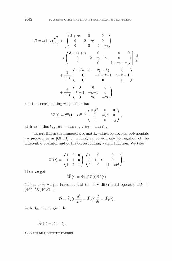
2062 F. Alberto GRUNBAUM, Ines PACHARONI & Juan TIRAO
D = t(1−t) d2
dt2+
3 + m 0 0
0 2 + m 00 0 1 + m
−t
3 + m + n 0 0
0 2 + m + n 00 0 1 + m + n
d
dt
+1
1−t
−2(n−k) 2(n−k) 0
0 −n + k−1 n−k + 10 0 0
+t
1−t
0 0 0
k + 1 −k−1 00 2k −2k
and the corresponding weight function
W (t) = tm(1− t)n−1
w1t
2 0 00 w2t 00 0 w3
,
with w1 = dimVµ1 , w2 = dimVµ2 y w3 = dimVµ3 .
To put this in the framework of matrix valued orthogonal polynomialswe proceed as in [GPT4] by finding an appropriate conjugation of thedifferential operator and of the corresponding weight function. We take
Ψ∗(t) =
1 0 0
1 1 01 2 1
1 0 0
0 1− t 00 0 (1− t)2
.
Then we getW (t) = Ψ(t)W (t)Ψ∗(t)
for the new weight function, and the new differential operator DF =(Ψ∗)−1D(Ψ∗F ) is
D = A2(t)d2
dt2+ A1(t)
d
dt+ A0(t),
with A2, A1, A0 given by
A2(t) = t(1− t),
ANNALES DE L’INSTITUT FOURIER

MATRIX VALUED ORTHOGONAL POLYNOMIALS 2063
A1(t) =
m + 3 0 0−1 m + 2 0
0 −2 m + 1
− t
(n + m + 3) 0 0
0 (n + m + 4) 00 0 (m + n + 5)
,
A0(t) =
0 2(n−k) 0
0 −(n + m + 1− k) n + 1− k
0 0 −2(n + m + 2− k)
.
From the program outlined at the end of Section 2 it follows that forany m ∈ N0 and n = 2, 3, . . . the following equations are satisfied
A∗0W − W A0 + (W A1)′ − (W A2)′′ = 0,
A∗1W + W A1 − 2(W A2)′ = 0,
W A2|t=0 = W A2|t=1 = 0,
(W A1 − A∗1W )|t=0 = (W A1 − A∗1W )|
t=1 = 0.
A look at the dependence of A2, A1, A0 and W on the parameters m andn makes it clear that these equations are satisfied if one replaces m by anyα ∈ R and n−1 by any β ∈ R. In conclusion for any α, β > −1 we haveexhibited a classical pair {W , D}.
4.2. Examples of size 4× 4.
We consider representations of GL(n,C) that correspond to n-tuplesof the form
π = (m + 2, . . . ,m + 2︸ ︷︷ ︸k1
, m + 1, . . . ,m + 1︸ ︷︷ ︸k2−k1
, m, . . . ,m︸ ︷︷ ︸n−k2
)
with 1 � k1 < k2 � n−1. We have
dimVπ =k2 − k1 + 1
k2 + 1
(n
k2
)(n + 1k1
).
As GL(n−1,C)-modules one has the decomposition
Vπ = Vµ1 ⊕ Vµ2 ⊕ Vµ3 ⊕ Vµ4 ,
TOME 55 (2005), FASCICULE 6
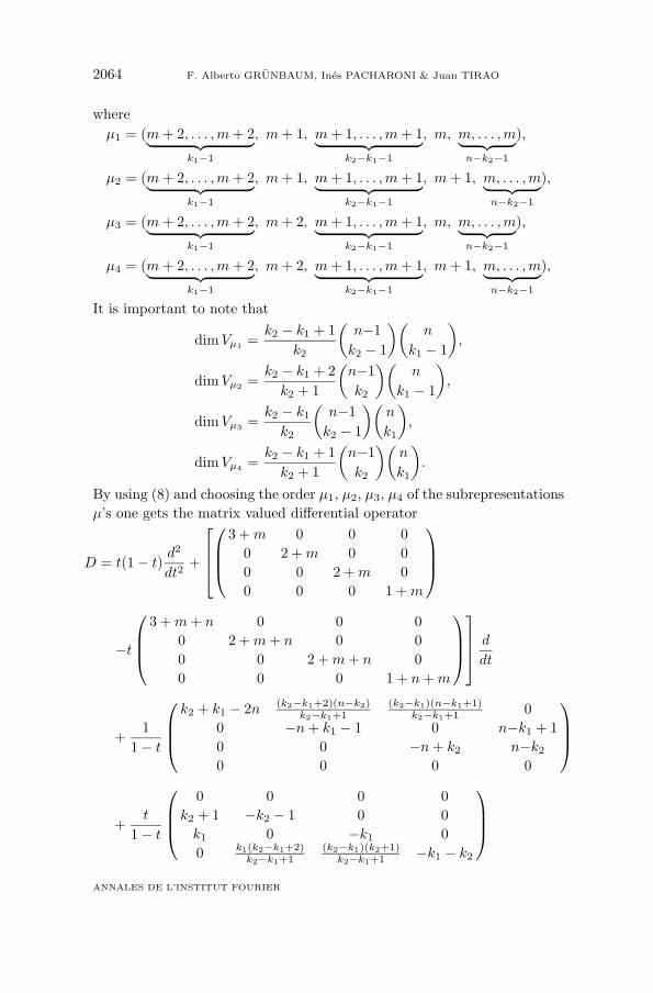
2064 F. Alberto GRUNBAUM, Ines PACHARONI & Juan TIRAO
whereµ1 = (m + 2, . . . ,m + 2︸ ︷︷ ︸
k1−1
, m + 1, m + 1, . . . ,m + 1︸ ︷︷ ︸k2−k1−1
, m, m, . . . ,m︸ ︷︷ ︸n−k2−1
),
µ2 = (m + 2, . . . ,m + 2︸ ︷︷ ︸k1−1
, m + 1, m + 1, . . . ,m + 1︸ ︷︷ ︸k2−k1−1
, m + 1, m, . . . ,m︸ ︷︷ ︸n−k2−1
),
µ3 = (m + 2, . . . ,m + 2︸ ︷︷ ︸k1−1
, m + 2, m + 1, . . . ,m + 1︸ ︷︷ ︸k2−k1−1
, m, m, . . . ,m︸ ︷︷ ︸n−k2−1
),
µ4 = (m + 2, . . . ,m + 2︸ ︷︷ ︸k1−1
, m + 2, m + 1, . . . ,m + 1︸ ︷︷ ︸k2−k1−1
, m + 1, m, . . . ,m︸ ︷︷ ︸n−k2−1
),
It is important to note that
dimVµ1 =k2 − k1 + 1
k2
(n−1k2 − 1
)(n
k1 − 1
),
dimVµ2 =k2 − k1 + 2
k2 + 1
(n−1k2
)(n
k1 − 1
),
dimVµ3 =k2 − k1
k2
(n−1k2 − 1
)(n
k1
),
dimVµ4 =k2 − k1 + 1
k2 + 1
(n−1k2
)(n
k1
).
By using (8) and choosing the order µ1, µ2, µ3, µ4 of the subrepresentationsµ’s one gets the matrix valued differential operator
D = t(1− t)d2
dt2+
3 + m 0 0 00 2 + m 0 00 0 2 + m 00 0 0 1 + m
−t
3 + m + n 0 0 00 2 + m + n 0 00 0 2 + m + n 00 0 0 1 + n + m
d
dt
+1
1− t
k2 + k1 − 2n (k2−k1+2)(n−k2)k2−k1+1
(k2−k1)(n−k1+1)k2−k1+1 0
0 −n + k1 − 1 0 n−k1 + 10 0 −n + k2 n−k2
0 0 0 0
+t
1− t
0 0 0 0k2 + 1 −k2 − 1 0 0k1 0 −k1 00 k1(k2−k1+2)
k2−k1+1(k2−k1)(k2+1)k2−k1+1 −k1 − k2
ANNALES DE L’INSTITUT FOURIER

MATRIX VALUED ORTHOGONAL POLYNOMIALS 2065
and the corresponding weight
W (t) = tm(1− t)n−1
w1t2 0 0 0
0 w2t 0 00 0 w3t 00 0 0 w4
,
with w1 = dimVµ1 , w2 = dimVµ2 , w3 = dimVµ3 and w4 = dimVµ4 . Toobtain out of this a classical pair {W , D} we use the conjugating function
Ψ∗(t) =
1 0 0 01 1 0 01 0 1 01 k2−k1+2
k2−k1+1k2−k1k2−k1+1 1
1 0 0 00 1− t 0 00 0 1− t 00 0 0 (1− t)2
.
Then we getW (t) = Ψ(t)W (t)Ψ∗(t)
for the new weight function, and the new differential operator DF =(Ψ∗)−1D(Ψ∗F ) is
D = A2(t)d2
dt2+ A1(t)
d
dt+ A0(t),
with A2, A1, A0 given by
A2(t) = t(1−t)
A1(t) =
m+ 3 0 0 0−1 m+ 2 0 0−1 0 m+ 2 00 − k2−k1+2
k2−k1+1− k2−k1k2−k1+1
m+ 1
− t
(n+m+ 3) 0 0 0
0 (n+m+ 4) 0 00 0 (n+m+ 4)0 0 0 (n+m+ 5)
A0(t) =
0
(k2−k1+2)(n−k2)k2−k1+1
(k2−k1)(n−k1+1)k2−k1+1
0
0 −(n+m+ 1) + k2 0 n+ 1−k10 0 −(n+m+ 2) + k1 n−k20 0 0 −2(n+m+ 2) + k1 + k2
.
A look at the dependence of A2, A1, A0 and W on the parameters m andn makes it clear that {W , D} remains a classical pair if one replaces m byany α ∈ R and n−1 by any β ∈ R. In conclusion for any α, β > −1 {W , D}is a classical pair.
TOME 55 (2005), FASCICULE 6

2066 F. Alberto GRUNBAUM, Ines PACHARONI & Juan TIRAO
4.3. Closing remarks.
We close with a few remarks pertaining to all examples discussed sofar that arise from a group theoretical situation. For concreteness we limitourselves to Example 4.2. First we note that W (t) has the factorization
W (t) =ρ(t)
ρ(1/2)T (t)W (1/2)T ∗(t)
with T (1/2) = I and ρ(t) = tα(1 − t)β . The matrix T (t), introduced in[DG1], solves the equation
T ′(t) =(A∗
t+
B∗
t− 1
)T (t)
with
A =
1 0 0 0− 1
212 0 0
− 12 0 1
2 00 k1−k2−2
2(k2−k1+1)k1−k2
2(k2−k1+1) 0
,
B =
0 0 0 012 1 0 012 0 1 00 k2−k1+2
2(k2−k1+1)k2−k−1
2(k2−k1+1) 2
.
The matrices A,B do not depend on α nor β and satisfy
[A,B] = I −A−B/2
independently of the others free parameters k1, k2. A deeper understandingof commutation relations of the type given above for all the examples in[GPT1], [GPT2], [GPT3], [GPT4], [GPT5] remains an interesting challenge.Finally we turn to some monodromy type considerations. The operator T (t)in Example 4.2 has a nice expression
T (t) = I +4∑i=1
(√t− 1√
2
)iTi
with very simple upper triangular Ti’s. The appropriate operator χ(t), alsointroduced in [DG1], has in this instance a nice expression
χ(t) = P +Q
t+
R√t− 1
+S√t + 1
with simple constant and symmetric matrices P , Q, R, S. It would be ofinterest to find some group representation interpretation for the matricesTi as well as the matrices P , Q, R, S.
ANNALES DE L’INSTITUT FOURIER
MATRIX VALUED ORTHOGONAL POLYNOMIALS 2067
BIBLIOGRAPHY
[DG] J. J. DUISTERMAAT and F. A. GRUNBAUM, Differential equations in the spectralparameter, Comm. Math. Phys., 103 (1986), 177–240.
[D1] A. DURAN, Matrix inner product having a matrix symmetric second orderdifferential operators, Rocky Mountain Journal of Mathematics, 27-2 (Spring1997), 585–600.
[D2] A. DURAN, On orthogonal polynomials with respect to a positive definite matrixof measures, Canadian J. Math., 47 (1995), 88–112.
[D3] A. DURAN, Markov Theorem for orthogonal matrix polynomials, Canadian J.Math. 4i, 48 (1996), 1180–1195.
[D4] A. DURAN, Ratio Asymptotics for orthogonal matrix polynomials, J. Approx.Th., 100 (1999), 304–344.
[DP] A. DURAN and B. POLO, Gaussian quadrature formulae for matrix weights,Linear Algebra and Appl., 355 (2002), 119–146.
[DG1] A. J. DURAN and F. A. GRUNBAUM, Orthogonal matrix polynomials satisfyingsecond order differential equations, International Math. Research Notices,2004 : 10 (2004), 461–484.
[DG2] A. J. DURAN and F. A. GRUNBAUM, A characterization for a class of weightmatrices with orthogonal matrix polynomials satisfying second order differ-ential equations. To appear in Math. Research Notices.
[DvA] A. DURAN and van W. ASSCHE, Orthogonal matrix polynomials and higherorder recurrence relations, Linear Algebra and Its Applications, 219 (1995),261–280.
[Ge] J. S. GERONIMO, Scattering theory and matrix orthogonal polynomials on thereal line, Circuits Systems Signal Process, 1 (1982), 471–495.
[G] F. A. GRUNBAUM, Matrix valued Jacobi polynomials, Bull. Sciences Math.,127-3 (May 2003), 207–214.
[GPT1] F. A. GRUNBAUM, I. PACHARONI and J. TIRAO, Matrix valued sphericalfunctions associated to the complex projective plane, J. Functional Analysis,188 (2002), 350–441.
[GPT2] F. A. GRUNBAUM, I. PACHARONI and J. TIRAO, A matrix valued solution toBochner’s problem, J. Physics A: Math. Gen., 34 (2001), 10647–10656.
[GPT3] F. A. GRUNBAUM, I. PACHARONI and J. TIRAO, Matrix valued sphericalfunctions associated to the three dimensional hyperbolic space, Internat. J.of Mathematics, 13 (2002), 727–784.
[GPT4] F. A. GRUNBAUM, I. PACHARONI and J. TIRAO, An invitation to matrix valuedspherical functions: Linearization of products in the case of the complexprojective space P2(C), MSRI publication, Modern Signal Processing, D.Healy and D. Rockmore, editors, 46 (2003), 147–160.
[GPT5] F. A. GRUNBAUM, I. PACHARONI and J. TIRAO, Matrix valued orthogonalpolynomials of the Jacobi type, Indag. Mathem., 14-3,4 (2003), 353–366.
[GV] R. GANGOLLI and V. S. VARADARAJAN, Harmonic analysis of spherical func-tions on real reductive groups, Springer-Verlag, Berlin, New York, 1988. Se-ries title: Ergebnisse der Mathematik und ihrer Grenzgebiete, 101.
[K1] M. G. KREIN, Fundamental aspects of the representation theory of Hermitianoperators with deficiency index (m,m), AMS Translations, Series 2, 97,Providence, Rhode Island (1971), 75–143.
TOME 55 (2005), FASCICULE 6
2068 F. Alberto GRUNBAUM, Ines PACHARONI & Juan TIRAO
[K2] M. G. KREIN, Infinite J-matrices and a matrix moment problem, Dokl. Akad.Nauk SSSR, 69-2 (1949), 125–128.
[PT] I. PACHARONI and J. TIRAO, Matrix valued spherical functions associated tothe complex projective space, in preparation.
[SvA] A. SINAP and van W. ASSCHE, Orthogonal matrix polynomials and applications,J. Comput. and Applied Math., 66 (1996), 27–52.
[T1] J. TIRAO, Spherical functions, Rev. de la Union Matem. Argentina, 28 (1977),75–98.
[T2] J. TIRAO, The matrix valued hypergeometric equation, Proc. Nat. Acad. Sci.U.S.A., 100-14 (2003), 8138–8141.
[VK] N. VILENKIN and A. KLIMYK, Representation of Lie Groups and Specialfunctions, vol. 3, Kluwer Academic, Dordrecht, MA, 1992.
F. Alberto GRUNBAUM,University of CaliforniaDepartment of MathematicsBerkeley CA 94705 (USA)
Ines PACHARONI & Juan TIRAO,Universidad Nacional de CordobaCIEM-FaMAFCordoba 5000 (Argentina)
[email protected]@mate.uncor.edu
ANNALES DE L’INSTITUT FOURIER