matrix valued orthogonal polynomials for gelfand pairs …heckman/2012 heckman and van...
TRANSCRIPT

Matrix Valued Orthogonal Polynomials for
Gelfand Pairs of Rank One
Gert Heckman and Maarten van Pruijssen
Radboud University Nijmegen
October 18, 2013
Abstract
In this paper we study matrix valued orthogonal polynomials of one
variable associated with a compact connected Gelfand pair (G,K) of rank
one, as a generalization of earlier work by Koornwinder [29] and sub-
sequently by Koelink, van Pruijssen and Roman [27], [28] for the pair
(SU(2) × SU(2), SU(2)), and by Grunbaum, Pacharoni and Tirao [13] for
the pair (SU(3),U(2)). Our method is based on representation theory
using an explicit determination of the relevant branching rules. Our ma-
trix valued orthogonal polynomials have the Sturm–Liouville property of
being eigenfunctions of a second order matrix valued linear differential op-
erator coming from the Casimir operator, and in fact are eigenfunctions
of a commutative algebra op matrix valued linear differential operators
coming from U(gc)K .
1
Contents
1 Introduction 3
2 The pair (G,K) = (G2,SU(3)) 9
3 Multiplicity free systems 11
4 The pair (G,K) = (Spin(7),G2) 16
5 The pair (G,K) = (USp(2n),USp(2n− 2)×USp(2)) 24
6 The pair (G,K) = (F4,Spin(9)) 27
7 The differential equations 34
8 Conclusions 36
2

1 Introduction
For N = 1, 2, 3, · · · a fixed positive integer let M denote the associative algebra
of square matrices of size N × N with complex entries. Denote by M[x] the
associative algebra of matrix valued polynomials. A matrix valued weight func-
tion W on some open interval (a, b), with −∞ ≤ a < b ≤ ∞, assigns to each
x ∈ (a, b) a selfadjoint matrix W (x) ∈M (so W (x)† = W (x)), which is positive
definite (denoted W (x) > 0) almost everywhere on (a, b), such that the matrix
valued moments ∫ b
a
xnW (x)dx
are finite (and selfadjoint) for all n ∈ N. Such a weight function defines a
sesquilinear matrix valued form
〈P,Q〉 =
∫ b
a
P †(x)W (x)Q(x)dx
on the polynomial algebra M[x]. Sesquilinear in the convention of this paper
amounts to antilinear in the first and linear in the second argument. The addi-
tional properties
〈PA,Q〉 = A†〈P,Q〉 , 〈P,QA〉 = 〈P,Q〉A , 〈P,Q〉† = 〈Q,P 〉
for all A ∈M and P,Q ∈M[x] are trivially checked, while
〈P, P 〉 ≥ 0 , 〈P, P 〉 = 0⇔ P = 0
holds for all P ∈ M[x], since A ∈ M;A† = A,A ≥ 0 is a convex cone, and
for A in this cone A = 0 ⇔ trA = 0. Observe that 〈P, P 〉 > 0 as soon as
detP (x) 6= 0 at some point x ∈ (a, b).
We can apply the Gram–Schmidt orthogonalization process to the (right
module for M) basis xn;n ∈ N of M[x]. By induction on n we can define
monic matrix valued polynomials Mn(x) of degree n by
Mn(x) = xn +
n−1∑m=0
Mm(x)Cn,m , 〈Mm(x), xn〉+ 〈Mm(x),Mm(x)〉Cn,m = 0
for all m < n. Indeed, the matrix Cn,m can be solved, because 〈Mm,Mm〉 > 0
and hence is invertible. Since 〈Mm,Mn〉 = 0 for m 6= n by construction any
matrix valued polynomial P (x) has a unique expansion
P (x) =∑n
Mn(x)Cn , 〈Mn, P 〉 = 〈Mn,Mn〉Cn
3
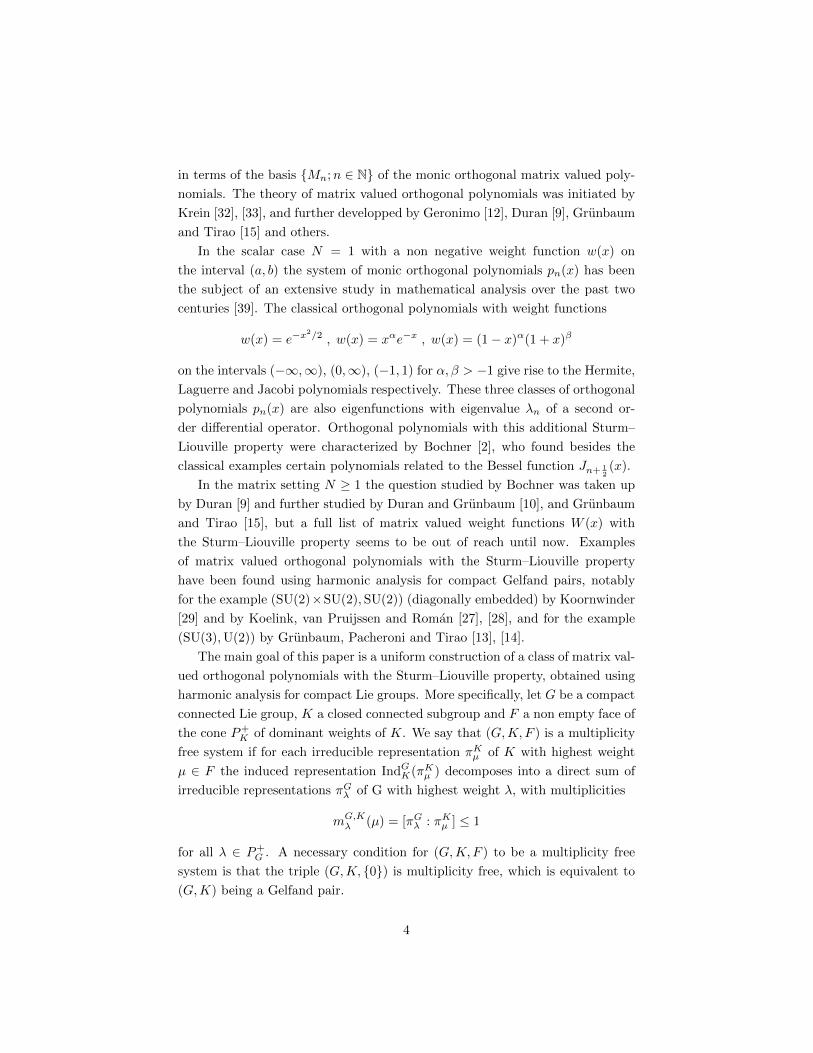
in terms of the basis Mn;n ∈ N of the monic orthogonal matrix valued poly-
nomials. The theory of matrix valued orthogonal polynomials was initiated by
Krein [32], [33], and further developped by Geronimo [12], Duran [9], Grunbaum
and Tirao [15] and others.
In the scalar case N = 1 with a non negative weight function w(x) on
the interval (a, b) the system of monic orthogonal polynomials pn(x) has been
the subject of an extensive study in mathematical analysis over the past two
centuries [39]. The classical orthogonal polynomials with weight functions
w(x) = e−x2/2 , w(x) = xαe−x , w(x) = (1− x)α(1 + x)β
on the intervals (−∞,∞), (0,∞), (−1, 1) for α, β > −1 give rise to the Hermite,
Laguerre and Jacobi polynomials respectively. These three classes of orthogonal
polynomials pn(x) are also eigenfunctions with eigenvalue λn of a second or-
der differential operator. Orthogonal polynomials with this additional Sturm–
Liouville property were characterized by Bochner [2], who found besides the
classical examples certain polynomials related to the Bessel function Jn+ 12(x).
In the matrix setting N ≥ 1 the question studied by Bochner was taken up
by Duran [9] and further studied by Duran and Grunbaum [10], and Grunbaum
and Tirao [15], but a full list of matrix valued weight functions W (x) with
the Sturm–Liouville property seems to be out of reach until now. Examples
of matrix valued orthogonal polynomials with the Sturm–Liouville property
have been found using harmonic analysis for compact Gelfand pairs, notably
for the example (SU(2)×SU(2),SU(2)) (diagonally embedded) by Koornwinder
[29] and by Koelink, van Pruijssen and Roman [27], [28], and for the example
(SU(3),U(2)) by Grunbaum, Pacheroni and Tirao [13], [14].
The main goal of this paper is a uniform construction of a class of matrix val-
ued orthogonal polynomials with the Sturm–Liouville property, obtained using
harmonic analysis for compact Lie groups. More specifically, let G be a compact
connected Lie group, K a closed connected subgroup and F a non empty face of
the cone P+K of dominant weights of K. We say that (G,K,F ) is a multiplicity
free system if for each irreducible representation πKµ of K with highest weight
µ ∈ F the induced representation IndGK(πKµ ) decomposes into a direct sum of
irreducible representations πGλ of G with highest weight λ, with multiplicities
mG,Kλ (µ) = [πGλ : πKµ ] ≤ 1
for all λ ∈ P+G . A necessary condition for (G,K,F ) to be a multiplicity free
system is that the triple (G,K, 0) is multiplicity free, which is equivalent to
(G,K) being a Gelfand pair.
4
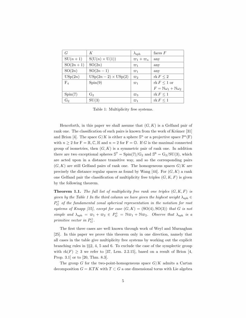
G K λsph faces F
SU(n+ 1) S(U(n)×U(1)) $1 +$n any
SO(2n+ 1) SO(2n) $1 any
SO(2n) SO(2n− 1) $1 any
USp(2n) USp(2n− 2)×USp(2) $2 rkF ≤ 2
F4 Spin(9) $1 rkF ≤ 1 or
F = Nω1 + Nω2
Spin(7) G2 $3 rkF ≤ 1
G2 SU(3) $1 rkF ≤ 1
Table 1: Multiplicity free systems.
Henceforth, in this paper we shall assume that (G,K) is a Gelfand pair of
rank one. The classification of such pairs is known from the work of Kramer [31]
and Brion [4]. The space G/K is either a sphere Sn or a projective space Pn(F)
with n ≥ 2 for F = R,C,H and n = 2 for F = O. If G is the maximal connected
group of isometries, then (G,K) is a symmetric pair of rank one. In addition
there are two exceptional spheres S7 = Spin(7)/G2 and S6 = G2/SU(3), which
are acted upon in a distance transitive way, and so the corresponding pairs
(G,K) are still Gelfand pairs of rank one. The homogeneous spaces G/K are
precisely the distance regular spaces as found by Wang [44]. For (G,K) a rank
one Gelfand pair the classification of multiplicity free triples (G,K,F ) is given
by the following theorem.
Theorem 1.1. The full list of multiplicity free rank one triples (G,K,F ) is
given by the Table 1 In the third column we have given the highest weight λsph ∈P+G of the fundamental zonal spherical representation in the notation for root
systems of Knapp [25], except for case (G,K) = (SO(4),SO(3)) that G is not
simple and λsph = $1 + $2 ∈ P+G = N$1 + N$2. Observe that λsph is a
primitive vector in P+G .
The first three cases are well known through work of Weyl and Murnaghan
[25]. In this paper we prove this theorem only in one direction, namely that
all cases in the table give multiplicity free systems by working out the explicit
branching rules in §§2, 4, 5 and 6. To exclude the case of the symplectic group
with rk(F ) ≥ 3 we refer to [37, Lem. 2.2.15], based on a result of Brion [4,
Prop. 3.1] or to [20, Thm. 8.3].
The group G for the two-point-homogeneous space G/K admits a Cartan
decomposition G = KTK with T ⊂ G a one dimensional torus with Lie algebra
5
t ⊂ k⊥. Denote M = ZK(T ), the centralizer of T in K. A triple (G,K,F ) is
a multiplicity free system if and only if the restriction of πKµ to M decomposes
multiplicity free for all µ ∈ F , which is proved in [37, Prop. 2.2.9] using the
theory of spherical varieties. In the symmetric space examples this result goes
back to Kostant and Camporesi [30, 5].
For each of these triples (G,K,F ) we determine for all µ ∈ F the induced
spectrum
P+G (µ) = λ ∈ P+
G ;mG,Kλ (µ) = 1
explicitly through a case by case analysis. We claim that if λ ∈ P+G (µ) then also
λ + λsph ∈ P+G (µ). This can be derived from the Borel–Weil theorem. Indeed,
if V Gλ = H0(Gc/Bc, Lλ) denotes the Borel–Weil realization of the finite dimen-
sional representation of G with highest weight λ ∈ P+G then the intertwining
projection
V Gλ ⊗ V Gλsph→ V Gλ+λsph
onto the Cartan component of the tensor product is just realized by the point-
wise multiplication of holomorphic sections.
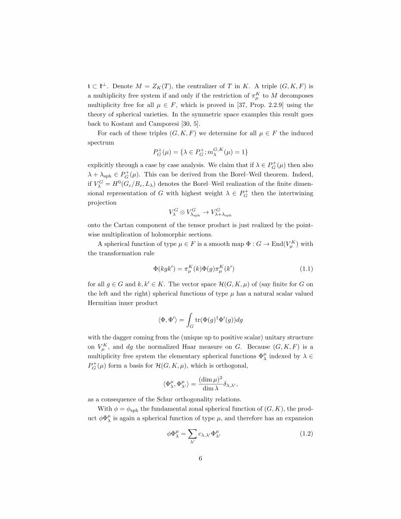
A spherical function of type µ ∈ F is a smooth map Φ : G→ End(V Kµ ) with
the transformation rule
Φ(kgk′) = πKµ (k)Φ(g)πKµ (k′) (1.1)
for all g ∈ G and k, k′ ∈ K. The vector space H(G,K, µ) of (say finite for G on
the left and the right) spherical functions of type µ has a natural scalar valued
Hermitian inner product
〈Φ,Φ′〉 =
∫G
tr(Φ(g)†Φ′(g))dg
with the dagger coming from the (unique up to positive scalar) unitary structure
on V Kµ , and dg the normalized Haar measure on G. Because (G,K,F ) is a
multiplicity free system the elementary spherical functions Φµλ indexed by λ ∈P+G (µ) form a basis for H(G,K, µ), which is orthogonal,
〈Φµλ,Φµλ′〉 =
(dimµ)2
dimλδλ,λ′ ,
as a consequence of the Schur orthogonality relations.
With φ = φsph the fundamental zonal spherical function of (G,K), the prod-
uct φΦµλ is again a spherical function of type µ, and therefore has an expansion
φΦµλ =∑λ′
cλ,λ′Φµλ′ (1.2)
6
with λ′ ∈ P+G (µ). For λ, λ′ ∈ P+
G (µ) the coefficient cλ,λ′ = 0 unless
λ− λsph λ′ λ+ λsph, (1.3)
where is the usual partial ordering on P+G , and the leading coefficient cλ,λ+λsph
is non-zero. This allows one to define a degree d : P+G (µ)→ N by
d(λ+ λsph) = d(λ) + 1 , mind(P+G (µ) ∩ λ+ Zλsph) = 0
for all λ ∈ P+G (µ).
The bottom B(µ) of the induced spectrum P+G (µ) is defined as
B(µ) = λ ∈ P+G (µ); d(λ) = 0
giving P+G (µ) = B(µ) + Nλsph the structure of a well. We have determined
explicitly the structure of the bottom B(µ) with µ ∈ F for all multiplicity
free triples (G,K,F ) in the above table. The first three lines of this table follow
from a straightforward application of branching rules going back to Weyl for the
unitary group and Murnaghan for the orthogonal groups [25]. The case of the
symplectic group follows using the branching rule of Lepowsky [25, 34], which
under the restriction rkF ≤ 2 we are able to make completely explicit in §5.
The remaining last two lines with the exceptional group of type G2 appearing
turn out to be manageable as well and are treated in §§2, 4. The appropriate
branching rules for the symmetric case (F4,Spin(9)) are calculated in §6, using
computer algebra.
Behind all these explicit calculations is a general multiplicity formula for
branching rules going back to Kostant [34, 41] and rediscovered by Heckman
[21]. On the basis of our explicit knowledge of the bottom B(µ) for µ ∈ F we
are able to verify case by case the following degree inequality in §§2, 4, 5 and 6.
Theorem 1.2. The degree d : P+G (µ)→ N satisfies the inequality
d(λ)− 1 ≤ d(λ′) ≤ d(λ) + 1
for all λ′ ∈ P+G (µ) with cλ,λ′ 6= 0.
As stated before, in all cases of our table the restriction of πKµ for µ ∈ F to
the centralizer M of a Cartan circle T in G is multiplicity free. Moreover, the
irreducible constituents are indexed in a natural way by the bottom B(µ), as
we shall explain in §3. The restriction of the elementary spherical function Φµλto the Cartan circle T takes values in EndM (V Kµ ), and so is block diagonal by
Schur’s Lemma: EndM (V Kµ ) ∼= CNµ withNµ the cardinality of the bottomB(µ).
7

Operators on the left become vectors on the right. In view of this isomorphism,
Φµλ(t) for t ∈ T is identified with the function Ψµλ(t) taking values in CNµ . We
define for n ∈ N the matrix valued spherical functions Ψµn(t), whose columns are
the vector valued functions Ψµλ(t) with λ ∈ P+
G (µ) of degree d(λ) = n. Observe
that both rows and columns of the matrix Ψµn(t) are indexed by the bottom
B(µ). Finally we can define our matrix valued polynomials Pµn (x) ∈ M[x] of
size Nµ ×Nµ as functions of a real variable x by
Ψµn(t) = Ψµ
0 (t)Pµn (x)
with t 7→ x a new variable, defined by x = cφ + (1 − c) for some c > 0 (with
φ the fundamental zonal spherical function as before) in order to make the
orthogonality interval x(T ) equal to [−1, 1].
The crucial fact that Pµn (x) is a matrix valued polynomial in x of degree
n with invertible leading coefficient Dµn (inductively given by Dµ
n = Dµn+1A
µn)
follows from a three term recurrence relation
xPµn (x) = Pµn+1(x)Aµn + Pµn (x)Bµn + Pµn−1(x)Cµn
which is obtained using the expansion (1.2). Theorem 1.2 together with the
ordering relation (1.3) and cλ,λ+λsph6= 0 imply that the matrices An are tri-
angular with non-zero diagonal, and hence are invertible. The matrix valued
weight function is given by
Wµ(x) = (Ψµ0 (t))†DµΨµ
0 (t)w(x)
with w(x) = (1 − x)α(1 + x)β the usual scalar weight function for the Car-
tan decomposition G = KTK and suitable α, β ∈ N/2 given in terms of root
multiplicities. The matrix Dµ is diagonal with entries the dimensions of the
irreducible constituents of the restriction of πKµ to M , which as a set was in-
dexed by the bottom B(µ) as should. The diagonal matrix Dµ arises from the
identification EndM (V Kµ ) ∼= CNµ with the trace form of the left operator side
and the standard Hermitian form on the right vector side.
The matrix valued polynomials Pµn (x) are orthogonal with respect to the
weight function Wµ(x) and have diagonal square norms, since
〈Pµn , Pµn′〉ν,ν′ = 〈Φµλ,Φ
µλ′〉
with λ = ν + nλsph, λ′ = ν′ + n′λsph ∈ P+
G (µ) = B(µ) + Nλsph. Finally, the
monic orthogonal polynomialsMµn (x) = xn+· · · and the orthogonal polynomials
Pµn (x) = Mµn (x)Dµ
n are related by eliminating the invertible leading coefficient
Dµn.
8

By Lie algebraic methods the polynomials Pµn (x) are shown to be eigen-
functions of a commutative algebra Dµ ⊂ M[x, ∂x] of matrix valued differential
operators
DPµn = PµnΛµn(D)
with Λµn(D) a diagonal eigenvalue matrix for all D ∈ Dµ. The desired second
order operator for the orthogonal polynomials with the Sturm–Liouville prop-
erty comes from the quadratic Casimir operator. The dimension of the affine
variety underlying the commutative algebra Dµ is equal to the affine rank of the
well P+G (µ).
Our explicit results on branching rules provide examples of the convexity
theorem for Hamiltonian actions of connected compact Lie groups on connected
symplectic manifolds with a proper moment map [21], [17], [18], [19], [23]. The
multiplicities occur at the integral points in the moment polytopes in accordance
with the [Q,R] = 0 principle of geometric quantization [16].
In the next section we first discuss the pair (G,K) = (G2,SU(3)), which
is an instructive example to illustrate the various aspects of the representation
theory and the construction of the matrix valued orthogonal polynomials.
Acknowledgement. We thank Noud Aldenhoven for his help in program-
ming certain branching rules, which gave us a good idea about the multiplicity
freeness in the symplectic case. Furthermore, we thank Erik Koelink and Pablo
Roman for fruitful discussions concerning matrix valued orthogonal polynomi-
als.
2 The pair (G,K) = (G2, SU(3))
In this section we take G of type G2 and K = SU(3) the subgroup of type A2.
Having the same rank the root systems RG of G and RK of K can be drawn
in one picture, and RK consists of the 6 long roots. The simple roots α1, α2in R+
G and β1, β2 in R+K are indicated in Figure 1 and P+
G = N$1 + N$2 is
contained in P+K = Nω1 + Nω2.
The branching rule from G to K is well known, see for example [21]. In
the picture below s1 ∈ WG is the orthogonal reflection in the mirror R$2. For
λ ∈ P+G the multiplicities mλ(µ) for µ ∈ P+
K are supported in the gray region
in the left picture. They have the familiar pattern of the weight multiplicities
for SU(3) as discussed in the various text books [22], [11]. They are one on
the outer hexagon, and increase by one on each inner shell hexagon, untill the
hexagon becomes a triangle, and from that moment on they stabilize. Hence the
restriction to K of any irreducible representation of G with highest weight λ ∈
9

α2 = β2
β1 $2
ω2
$1 = ω1
α1
Figure 1: Roots for G2.
P+G is multiplicity free on the two rank one faces Nω1 and Nω2 of the dominant
cone P+K . In other words, the triples (G2,A2, Fi = Nωi) are multiplicity free for
i = 1, 2, which proves the last line of the table in Theorem 1.1.
The irreducible spherical representations of G containing the trivial repre-
sentation of K have highest weight in N$1, and λsph = $1 is the fundamental
spherical weight. Given µ = nω1 ∈ F1 (and likewise µ = nω2 ∈ F2) the cor-
responding induced spectrum of G is multiplicity free by Frobenius reciprocity,
and by inversion of the branching rule has multiplicity one on the well shaped
region
P+G (µ) = B(µ) + N$1 , B(µ) = k$1 + l$2; k + l = n
with bottom B(µ). The bottom is given by a single linear relation.
If we take M the SU(2) group corresponding to the roots ±α2 and denote
by p : P+G → P+
M = N( 12α2) the natural projection along the spherical direction
$1, then p is a bijection from the bottom B(µ) onto the image p(B(µ)), which
is just the restricted spectrum P+M (µ) for M of the irreducible representation of
K with highest weight µ.
There is warning about the choice of the various Cartan subalgebras. In
order to compute branching rules it is natural and convenient (as we did above)
to choose the Cartan subalgebra of K contained in the Cartan subalgebra of
G. The other choice is that we start with a rank one Gelfand pair (G,K),
and choose the Cartan circle group T in G perpendicular to K. If M is the
centralizer of T in K, then MT is a subgroup in G of full rank. A maximal
10

β2
β1
ω2
ω1
λ
s1λ
α2
$2
$1
α1
µ
P+G2
(µ)
B(µ)
Figure 2: Branching from G2 to SU(3) on the left and the µ-well on the right.
torus in MT is then a maximal torus for G as well. But this maximal torus
need not contain a maximal torus for K, as is clear from the present example.
It will only do so if the rank of K is equal to the rank of M , which is equal to
the rank of G minus 1, and a maximal torus of M is a maximal torus of K as
well.
3 Multiplicity free systems
Connected compact irreducible Gelfand pairs (G,K) have been classified by
Kramer for G a simple Lie group and by Brion for G a semisimple Lie group
[31], [4]. We shall assume that G and K are connected, and that the connected
space G/K is also simply connected. The pair (G,K) is called rank one if the
Hecke algebra H(G,K) of zonal spherical (so bi-G-finite and bi-K-invariant)
functions is a polynomial algebra C[φ] with one generator, the fundamental
elementary zonal spherical function φ = φsph. We shall assume throughout this
paper that (G,K) is a rank one Gelfand pair, with G/K simply connected. The
corresponding spaces G/K are just the distance regular spaces found by Wang
[44].
11

Indeed, for K < G compact connected Lie groups the homogeneous space
G/K equipped with an invariant Riemannian metric is distance transitive for
the action of G on G/K if and only if the action of K on the tangent space
TeKG/K is transitive on the unit sphere. This is equivalent with the algebra
P (TeKG/K)K of polynomial invariants being a polynomial algebra in a single
generator (the quadratic norm), which in turn is equivalent with the Hecke
algebra H(G,K) being a polynomial algebra C[φ] in the single generator φ =
φsph. If H(G,K) = C[φ] has a single generator then it is commutative as
convolution algebra, which is equivalent with (G,K) being a Gelfand pair.
Let k < g be the Lie algebras of K < G. By definition the infinitesimal
Cartan decomposition g = k⊕p is the orthogonal decomposition with respect to
minus the Killing form on g. Since (G,K) has rank one the adjoint homomor-
phism K → SO(p) is a surjection. Fix a (maximal Abelian) one dimensional
subspace t in p. Any two such are clearly conjugated by K, and let T < G
be the corresponding Cartan circle group. Let M < N be the centralizer and
normalizer of T in K with Lie algebra m. The Weyl group W = N/M has order
2 and acts on T by t 7→ t±1.
The subgroup MT has maximal rank in G, and choosing a maximal torus
in MT for G defines a natural restriction map from the weight lattice PG of G
to the weight lattice of the circle T . The next result for symmetric pairs is just
the Cartan–Helgason theorem.
Proposition 3.1. Suppose G is simply connected and K is connected, so that
G/K is simply connected. Then T ∩K has order 2, except for the Gelfand pair
(G,K) = (Spin(7), G2) where it has order 3.
Proof. The crucial remark is that the highest weight λsph ∈ P+G of the funda-
mental zonal spherical representation of (G,K) after restriction to T becomes
a generator for the weight lattice of T/(T ∩K). For a symmetric pair (G,K)
with Cartan involution θ : G → G we have K = Gθ and θ(t) = t−1 for t ∈ T .
Hence T ∩ K has order 2 for (G,K) a symmetric pair. In the remaining two
cases we use the notation of Bourbaki [3].
For (G,K) = (Spin(7), G2) the weight lattice of G is naturally identified with
Z3 with basis εi, and likewise the dual coroot lattice becomes Z3 with basis ei.
The character lattice of T/(T ∩K) has generator $3 = (ε1 + ε2 + ε3)/2, which
takes the value 3 on the generator 2(e1 + e2 + e3) of the coroot lattice of T .
For (G,K) = (G2,SU(3)) the weight lattice of G is naturally identified
with ξ ∈ Z3; ξ1 + ξ2 + ξ3 = 0, and likewise the dual coroot lattice becomes
x ∈ Z3;x1 + x2 + x3 = 0. The character lattice of T/(T ∩K) has generator
12
$1 = 2α1 + α2 = −ε2 + ε3, which takes the value 2 on the generator −e2 + e3
of the coroot lattice of T .
In the next definition we explain the well shape of the induced spectrum
P+G (µ) = B(µ) +Nλsph with bottom B(µ). This idea goes back to Kostant and
Camporesi [30], [5].
Definition 3.2. For µ ∈ P+K the highest weight of an irreducible representation
πKµ of K the induced representation IndGK(πKµ ) decomposes as a direct sum of
irreducible representations πGλ of G with branching multiplicities
mG,Kλ (µ) = [πGλ : πKµ ]
for all λ ∈ P+G by Frobenius reciprocity. We denote
P+G (µ) = λ ∈ P+
G ;mG,Kλ (µ) ≥ 1
for the induced spectrum. In the introduction we have explained using the Borel–
Weil theorem that λ ∈ P+G (µ) implies λ + λsph ∈ P+
G (µ). In turn we see that
P+G (µ) = B(µ) + Nλsph has the shape of a well with
B(µ) = λ ∈ P+G (µ);λ− λsph /∈ P+
G (µ)
the bottom of the induced spectrum P+G (µ).
To arrive at a good theory of matrix valued orthogonal polynomials we
have to restrict ourselves to multiplicity free triples (G,K, µ) and (G,K,F ) for
µ ∈ P+K a suitable dominant weight for K and F a suitable facet of the dominant
cone P+K for K.
Definition 3.3. The triple (G,K, µ) with µ ∈ P+K a highest weight for K is
called multiplicity free if the branching multiplicity mλ(µ) ≤ 1 for all λ ∈ P+G ,
so if the induced representation IndGK(πKµ ) decomposes multiplicity free as a
representation of G. Likewise, (G,K,F ) is called a multiplicity free system with
F a facet of the dominant integral cone P+K if (G,K, µ) is multiplicity free for
all µ ∈ F .
Camporesi calculated the bottoms B(µ) of the well P+G (µ) explicitly in the
first three examples of the table in Theorem 1.1 using the classical branching
laws of Weyl for the unitary group and Murnaghan for the orthogonal groups
[5],[25]. In the fourth example of the symplectic group he obtained partial
results, because of the complexity of the branching law of Lepowsky (from G
to K) [34] and of Baldoni Silva (from K to M) [1] in that case. However, in
this symplectic case the restriction on a multiplicity free system(G,K,F ) is just
strong enough to find a completely explicit description of the bottom.
13

Proposition 3.4. Let F be a facet of the dominant integral cone P+K . Then
the branching multiplicity mG,Kλ (µ) ≤ 1 for all µ ∈ F and all dominant weights
λ ∈ P+G if and only if the branching multiplicity mK,M
µ (ν) ≤ 1 for all µ ∈ F and
all dominant weights ν ∈ P+M .
Proof. Let us complexify all our compact Lie groups G,K,M, T to complex
reductive algebraic groups Gc,Kc,Mc, Tc. The statement of the proposition
translates into the following geometric statement. For Pc the parabolic subgroup
of Kc with Levi component the stabilizer of F the variety Gc/Pc is spherical
for Gc if and only if Kc/Pc is spherical for Mc. Here we say that a variety with
an action of a reductive group is spherical if the Borel subgroup has an open
orbit. Observe that (also for the non symmetric pairs) we have an infinitesimal
Iwasawa decomposition
gc = kc ⊕ tc ⊕ nc
with nc the direct sum of those root spaces gαc for which the restriction of α
to tc is a positive multiple of the restriction of λsph to tc. Taking the Borel
subgroup of Gc of the form BMcTcNc with BMc
a Borel subgroup for Mc the
equivalence of Gc/Pc having an open orbit for BMcTcNc is equivalent to Kc/Pc
having an open orbit for BMcfollows, since the orbit of TcNc through Kc is
open in Gc/Kc.
Let us take the Cartan subalgebra of gc a direct sum of tc and a Cartan
subalgebra of mc, and extend a set of positive roots for mc to a set of positive
roots for gc. Let V Gλ be an irreducible representation of G with highest weight
λ ∈ P+G . Because McTcNc is a standard parabolic subgroup of Gc the vector
space
(V Gλ )nc = v ∈ V Gλ ;Xv = 0 ∀X ∈ nc
is an irreducible representation of Mc with highest weight ν ∈ P+M . Clearly
ν = p(λ) with p : P+G → P+
M the natural projection along the spherical direction
Nλsph. The Iwasawa decomposition gc = kc⊕ tc⊕nc of the above proof gives the
Poincare–Birkhoff-Witt factorization U(gc) = U(kc)U(tc)U(nc) and we conclude
that U(kc)(VGλ )nc = V Gλ .
Proposition 3.5. Let (G,K,F ) be a multiplicity free system and let µ ∈ F .
Then the natural projection p : P+G → P+
M is a surjection from the induced
spectrum P+G (µ) for G onto the restricted spectrum
P+M (µ) = ν ∈ P+
M ;mK,Mµ (ν) ≥ 1
for M , and thefore p : B(µ) → P+M (µ) is a bijection. Note that mK,M
µ (ν) ≤ 1
for all ν ∈ P+M by the previous proposition.
14
Proof. Let 〈·, ·〉 be a unitary structure on V Gλ for G. Suppose V is an irreducible
subrepresentation of K in the restriction of V Gλ to K. If u is a nonzero vector
in (V Gλ )nc then 〈u, v〉 6= 0 for some v ∈ V . Indeed 〈u, v〉 = 0 for all v ∈ V
contradicts U(kc)(VGλ )nc = V Gλ . Hence the restriction of V to M contains a
copy of VMp(λ) by Schur’s Lemma. One of the subspaces V is a copy of V Kµ , and
so mµ(p(λ)) ≥ 1. This proves that the natural projection p maps the induced
spectrum P+G (µ) of G inside the restricted spectrum P+
M (µ) of M .
It remains to show that
p : P+G (µ)→ P+
M (µ)
is onto for all µ ∈ F . This follows from Proposition 3.6.
Proposition 3.6. Let λ ∈ P+G , µ ∈ P+
K and let p : P+G → P+
M be the natural
projection. Then
• mG,Kλ+kλsph
(µ) ≤ mG,Kλ+sλsph
(µ) if k ≤ s and
• limn→∞mG,Kλ+nλsph
(µ) = mK,Mµ (p(λ)).
Proof. Every irreducible K-representation that occurs in the K-module Vλ also
occurs in the K-module Vλ+λsph. Indeed, let vK ∈ Vλsph
be a non-zero K-fixed
vector and consider the composition of Vλ → Vλ ⊗ Vλsph: v 7→ v ⊗ vK and the
projection Vλ ⊗ Vλsph→ Vλ+λsph
. Both maps intertwine the K-action and the
first statement follows.
For (G,K) a symmetric pair (even of arbitrary rank) the second statement
is a result of Kostant [30, Thm. 3.5] and Wallach [42, Cor. 8.5.15]. For spherical
pairs (G,K) a similar stability result is shown by Kitagawa [24, Cor. 4.10].
However, since we have control over the branching rules of the remaining non-
symmetric pairs, we present our own proof.
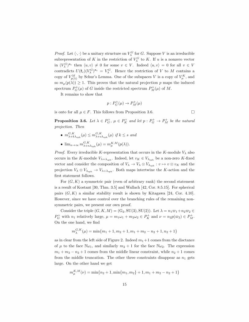
Consider the triple (G,K,M) = (G2,SU(3),SU(2)). Let λ = n1$1+n2$2 ∈P+G with n1 relatively large, µ = m1ω1 + m2ω2 ∈ P+
K and ν = n2p($2) ∈ P+M .
On the one hand, we find
mG,Kλ (µ) = minm1 + 1,m2 + 1,m1 +m2 − n2 + 1, n2 + 1
as in clear from the left side of Figure 2. Indeed m1 +1 comes from the disctance
of µ to the face Nω1, and similarly m2 + 1 for the face Nω2. The expression
m1 +m2 − n2 + 1 comes from the middle linear constraint, while n2 + 1 comes
from the middle truncation. The other three constraints disappear as n1 gets
large. On the other hand we get
mK,Mµ (ν) = minn2 + 1,minm1,m2+ 1,m1 +m2 − n2 + 1
15
as easily checked from the familiar branching from SU(3) to SU(2). It follows
that mG,Kλ (µ) = mK,M
µ (ν) for large n1.
The proof for the case (Spin(7),G2,SU(3)) is postponed to the end of Section
4, where we discuss the branching rules that are needed.
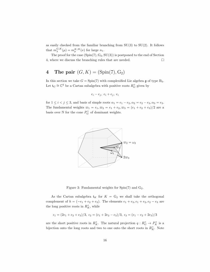
4 The pair (G,K) = (Spin(7),G2)
In this section we take G = Spin(7) with complexified Lie algebra g of type B3.
Let tG ∼= C3 be a Cartan subalgebra with positive roots R+G given by
ei − ej , ei + ej , ei
for 1 ≤ i < j ≤ 3, and basis of simple roots α1 = e1 − e2, α2 = e2 − e3, α3 = e3.
The fundamental weights $1 = e1, $2 = e1 + e2, $3 = (e1 + e2 + e3)/2 are a
basis over N for the cone P+G of dominant weights.
$1
$2 = ω2
ω1
2$3
Figure 3: Fundamental weights for Spin(7) and G2.
As the Cartan subalgebra tK for K = G2 we shall take the orthogonal
complement of h = (−e1 + e2 + e3). The elements e1 + e3, e1 + e2, e2 − e3 are
the long positive roots in R+K , while
ε1 = (2e1 + e2 + e3)/3, ε2 = (e1 + 2e2 − e3)/3, ε3 = (e1 − e2 + 2e3)/3
are the short positive roots in R+K . The natural projection q : R+
G → P+K is a
bijection onto the long roots and two to one onto the short roots in R+K . Note
16

that εi = q(ei) for i = 1, 2, 3. The simple roots in R+K are β1 = ε3, β2 = ε2−ε3
with corresponding fundamental weights ω1 = ε1, ω2 = ε1 + ε2. Observe that
ω1 = q($1) = q($3) and ω2 = q($2), and hence q : P+G → P+
K is a surjection.
Note that the natural projection q : PG → PK is equivariant for the action of
the Weyl group WM∼= S3 of the centralizer M = SU(3) in K of h. The Weyl
group WG is the semidirect product of C2 ×C2 ×C2 acting by sign changes on
the three coordinates and the permutation group S3.
As a set with multiplicities we have
A = q(R+G)−R+
K = ε1, ε2, ε3
whose partition function pA enters in the formula for the branching from B3
to G2. Note that pA(kε1 + lε2) = pA(kε1 + mε3) = k + 1 for k, l,m ∈ N and
pA(µ) = 0 otherwise.
Lemma 4.1. For λ ∈ P+G and µ ∈ P+
K the multiplicity mG,Kλ (µ) ∈ N with which
an irreducible representation of K with highest weight µ occurs in the restriction
to K of an irreducible representation of G with highest weight λ is given by
mG,Kλ (µ) =
∑w∈WG
det(w)pA(q(w(λ+ ρG)− ρG)− µ)
and if we extend mG,Kλ (µ) ∈ Z by this formula for all λ ∈ PG and µ ∈ PK then
mG,Kw(λ+ρG)−ρG(v(µ+ ρK)− ρK) = det(w) det(v)mG,K
λ (µ)
for all w ∈WG and v ∈WK . Here ρG and ρK are the Weyl vectors of R+G and
R+K respectively.
This lemma was obtained in Heckman [21] as a direct application of the
Weyl charcter formula. The above type formula, valid for any pair K < G of
connected compact Lie groups [21], might be cumbersome for practical com-
putations of the multiplicities, because of the (possibly large) alternating sum
over a Weyl group WG and the piecewise polynomial behaviour of the partition
function. However in the present (fairly small) example one can proceed as
follows.
If λ = k$1 + l$2 +m$3 = klm = (x, y, z) with
x = k + l +m/2, y = l +m/2, z = m/2⇔ k = x− y, l = y − z,m = 2z
then λ is dominant if k, l,m ≥ 0 or equivalently x ≥ y ≥ z ≥ 0. We tabulate
the 8 elements w1, · · · , w8 ∈WG such that the projection q(wiλ) ∈ Nε1 +Nε2 is
17

dominant for R+M for all λ which are dominant for R+
G. Clearly the projection
of (x, y, z) is given by
q(x, y, z) = xε1 + yε2 + zε3 = (x+ z)ε1 + (y − z)ε2
and ρG = $1 +$2 +$3 = (2 12 , 1
12 ,
12 ) is the Weyl vector for R+
G.
i det(wi) wiλ q(wiλ) q(wiρG − ρG)
1 + (x, y, z) (x+ z)ε1 + (y − z)ε2 0
2 − (x, y,−z) (x− z)ε1 + (y + z)ε2 −ε33 + (x, z,−y) (x− y)ε1 + (y + z)ε2 −ε1 − ε34 − (x,−z,−y) (x− y)ε1 + (y − z)ε2 −ε1 − ε2 − ε35 − (y, x, z) (y + z)ε1 + (x− z)ε2 −ε3 + 0
6 + (y, x,−z) (y − z)ε1 + (x+ z)ε2 −ε3 − ε37 + (z, x, y) (y + z)ε1 + (x− y)ε2 −ε3 − ε28 − (−z, x, y) (y − z)ε1 + (x− y)ε2 −ε3 − ε1 − ε2
Table 2: Projection of wλ in P+M .
In the picture below the location of the points q(wiλ) ∈ P+M , indicated
by the number i, with the sign of det(wi) attached, is drawn. Observe that
q(w1λ) = (k +m)ω1 + lω2 ∈ P+K for all λ = klm ∈ P+
G .
ε2
ε1ε3
b+4−
3+
2−
1+a−
d+
8−
7+5−
6+
c−
Figure 4: Projection of WGλ onto P+M .
Let us denote a = (k + l + m)ε1 and b = (k + l)ε1, and so these two points
together with the four points q(wiλ) for i = 1, 2, 3, 4 form the vertices of a
18
hexagon with three pairs of parallel sides. In the picture we have drawn all six
vertices in P+K , which happens if and only if q(w3λ) = kε1 + (l + m)ε2 ∈ P+
K ,
or equivalently if k ≥ (l + m). But in general some of the q(wiλ) ∈ P+M for
i = 2, 3, 4 might lie outside P+K . Indeed q(w2λ) = (k + l)ε1 + (l + m)ε2 lies
outside P+K if k < m, and q(w4λ) = kε1 + lε2 lies outside P+
K if k < l.
For fixed λ ∈ P+G the sum mλ(µ) of the following six partition functions as
a function of µ ∈ PK4∑1
det(w)pA(q(wi(λ+ ρG)− ρG)− µ)− pA(a− ε2 − µ) + pA(b− ε1 − ε2 − µ)
is just the familiar multiplicity function for the weight multiplicities of the root
system A2. It vanishes outside the hexagon with vertices a, b and q(wiλ) for
i = 1, 2, 3, 4. On the outer shell hexagon it is equal to 1, and it steadily increases
by 1 for each inner shell hexagon, untill the hexagon becomes a triangle, and
from that moment on it stabilizes on the inner triangle. The two partition
functions we have added corresponding to the points a and b are invariant as
a function of µ for the action µ 7→ s2(µ + ρK) − ρK of the simple reflection
s2 ∈ WK with mirror Rω1, because s2(A) = A. In order to obtain the final
multiplicity function
µ 7→ mG,Kλ (µ) =
∑v∈WK
det(v)mλ(v(µ+ ρK)− ρK)
for the branching from G to K we have to antisymmetrize for the shifted by
ρK action of WK . Note that the two additional partition functions and their
transforms under WK all cancel because of their symmetry and the antisym-
metrization. For µ ∈ P+K the only terms in the sum over v ∈ WK that have a
nonzero contribution are those for v = e the identity element and v = s1 the
reflection with mirror Rω2, and we arrive at the following result.
Theorem 4.2. For λ ∈ P+G and µ ∈ P+
K the branching multiplicity from G =
Spin(7) to K = G2 is given by
mG,Kλ (µ) = mλ(µ)−mλ(s1µ− ε3) (4.1)
with mλ the weight multiplicty function of type A2 as given by the above alter-
nating sum of the six partition functions.
Indeed, we have s1(µ + ρK) − ρK = s1µ − ε3. As before, we denote klm =
k$1 + l$2 +m$3 and kl = kω1 + lω2 with k, l,m ∈ N for the highest weight of
irreducible representations of G and K respectively. For µ ∈ Nω1 the multiplic-
ities mG,Kλ (µ) are only governed by the first term on the right hand side of (4.1)
19
with v = e and so are equal to 1 for µ = n0 with n = (k+ l), · · · , (k+ l+m) and
0 elsewhere. Indeed, µ = n0 has multiplicity one if and only if it is contained in
the segment from b = (k + l)ε1 to a = (k + l + m)ε1. This proves to following
statement.
Corollary 4.3. The fundamental representation of G with highest weight λ =
001 is the spin representation of dimension 8 with K-types µ = 10 and µ = 00.
It is the fundamental spherical representation for the Gelfand pair (G,K). The
irreducible spherical representations of G have highest weights 00m with K-
spectrum the set n0; 0 ≤ n ≤ m.
Corollary 4.4. For any irreducible representation of G with highest weight
λ = klm all K-types with highest weight µ ∈ F1 = Nω1 are multiplicity free,
and the K-type with highest weight µ = n0 has multiplicity one if and only if
(k + l) ≤ n ≤ (k + l +m). The domain of those λ = klm for which the K-type
µ = n0 occurs has a well shape P+G (n0) = B(n0) + N001 with bottom
B(n0) = klm ∈ P+G ; k + l +m = n
given by a single linear relation.
Proof. The multiplicity freeness and the bounds for n follow from Theorem 4.2
and in turn these inequalities n ≤ k + l +m imply the formulae for B(n0) and
P+G (n0).
This ends our discussion that (G,K,F1 = Nω1) is a multiplicity free system.
In order to show that (G,K,F2 = Nω2) is also a multiplicity free triple we shall
carry out a similar analysis.
Corollary 4.5. For an irreducible representation of G with highest weight λ =
klm all K-types with highest weight µ ∈ F2 = Nω2 are multiplicity free, and the
K-type with highest weight µ = 0n has multiplicity one if and only if max(k, l) ≤n ≤ min(k+l, l+m). The domain of those λ = klm for which the K-type µ = 0n
occurs has a well shape P+G (0n) = B(0n) + N001 with bottom
B(0n) = klm ∈ P+G ;m ≤ k ≤ n, l +m = n
given by a single linear relation and inequalities.
Proof. Under the assumption of the first part of this proposition klm ∈ P+G (0n)
implies that kl(m+1) ∈ P+G (0n), and the bottom B(0n) of those klm ∈ P+
G (0n)
for which kl(m− 1) /∈ P+G (0n) contains klm if and only if n = l+m and k ≥ m.
It remains to show the first part of the proposition.
20

ε2
ε1ε3
b+
a−1+
5−
e
f4−
7+
d+
c−
6+
2−
8−
3+
Nω1
Nω2
Figure 5: Support of the multiplicity function µ 7→ mG,Kλ (µ).
In order to determine the K-spectrum associated to the highest weight λ =
klm ∈ N3 for G observe that
q(w3λ) = kε1 + (l +m)ε2
and so the K-spectrum on Nω2 is empty for k > (l +m), while for k = (l +m)
the K-spectrum has a unique point kω2 on Nω2. If k < (l + m) the point
q(w3λ) moves out of the dominant cone P+K into P+
M − P+K , and the support of
the function P+K 3 µ 7→ mG,K
λ (µ) consists of (the integral points of) a heptagon
with an additional side on Nω2 from e to f as in the picture above. On the outer
shell heptagon the multiplicity is one, and the multiplicities increase by one for
each inner shell heptagon, untill the heptagon becomes a triangle or quadrangle,
and it stabilizes. This follows from Theorem 4.2 in a straightforward way.
Depending on whether the vertex
q(w2λ) = (k + l)ε1 + (l +m)ε2
lies in P+K (for k ≥ m) or in P+
M − P+K (for k < m) we get e = (l + m)ω2 or
e = (k + l)ω2 respectively. Hence we find
e = min(k + l, l +m)ω2 , f = max(k, l)ω2
by a similar consideration for
q(w4λ) = kε1 + lε2
21

as before (f = k for k ≥ l and f = l for k < l). This finishes the proof of
Corollary 4.5.
Our choice of positive roots for G = B3 and K = G2 was made in such a
way that the dominant cone P+K for K was contained in the dominant cone P+
G
for G. In turn this implies that the set
A = q(R+G)−R+
K = ε1, ε1, ε3
lies in an open half plane, which was required for the application of the branching
rule of Lemma 4.1.
However, we now switch to a different positive system in RG, or rather we
keep R+G fixed as before, but take the Lie algebra k of G2 to be perpendicular to
the spherical direction $3 = (e1 +e2 +e3)/2 instead. Under this assumption the
positive roots R+M form a parabolic subsystem in R+
G, and so the simple roots
α1 = e1 − e2, α2 = e2 − e3 of R+M are also simple roots in R+
G.
α2
α1
ε2
ε1ε3
nε1
nε1
α2
α1
ε2
ε1ε3
nε1
nε1
n(ε1 + ε2)
Figure 6: Projections of the bottoms Bn0 and B0n.
Let p : PG → PM = PK be the orthogonal projection along the spherical
direction. By abuse of notation we denote (with p($3) = 0)
ε1 = p($1) = (2,−1,−1)/3 , ε2 = p($2) = (1, 1,−2)/3
for the fundamental weights for P+M = p(P+
G ). It is now easy to check that this
22
projection
p : B(n0)→ p(B(n0)) , p : B(0n)→ p(B(0n))
is a bijection from the bottom onto its image in P+M . In the Figure 6 we have
drawn the projections
p(B(n0)) = kε1 + lε2; k + l ≤ n , p(B(0n)) = kε1 + lε2; k, l ≤ n, k + l ≥ n
on the left and the right side respectively.
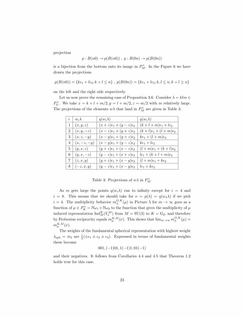
Let us now prove the remaining case of Proposition 3.6. Consider λ = klm ∈P+G . We take x = k + l + m/2, y = l + m/2, z = m/2 with m relatively large.
The projections of the elements wλ that land in P+M are given in Table 3.
i wiλ q(wiλ) q(wiλ)
1 (x, y, z) (x+ z)ε1 + (y − z)ε2 (k + l +m)ε1 + lε2
2 (x, y,−z) (x− z)ε1 + (y + z)ε2 (k + l)ε1 + (l +m)ε2
3 (x, z,−y) (x− y)ε1 + (y + z)ε2 kε1 + (l +m)ε2
4 (x,−z,−y) (x− y)ε1 + (y − z)ε2 kε1 + lε2
5 (y, x, z) (y + z)ε1 + (x− z)ε2 (l +m)ε1 + (k + l)ε2
6 (y, x,−z) (y − z)ε1 + (x+ z)ε2 lε1 + (k + l +m)ε2
7 (z, x, y) (y + z)ε1 + (x− y)ε2 (l +m)ε1 + kε2
8 (−z, x, y) (y − z)ε1 + (x− y)ε2 lε1 + kε2
Table 3: Projections of wλ in P+M .
As m gets large the points q(wiλ) run to infinity except for i = 4 and
i = 8. This means that we should take for ν = p(λ) = q(w4λ) if we pick
i = 4. The multiplicity behavior mG,Kλ (µ) in Picture 5 for m → ∞ goes as a
function of µ ∈ P+K = Nω1 +Nω2 to the function that gives the multiplicity of µ
induced representation IndKM (VMν ) from M = SU(3) to K = G2, and therefore
by Frobenius reciprocity equals mK,Mµ (ν). This shows that limm→∞mG,K
λ (µ) =
mK,Mµ (ν).
The weights of the fundamental spherical representation with highest weight
λsph = $3 are 12 (±ε1 ± ε2 ± ε3). Expressed in terms of fundamental weights
these become
001, (−1)01, 1(−1)1, 01(−1)
and their negatives. It follows from Corollaries 4.4 and 4.5 that Theorem 1.2
holds true for this case.
23

5 The pair (G,K) = (USp(2n),USp(2n−2)×USp(2))LetG = USp(2n) andK = USp(2n−2)×USp(2) with n ≥ 3. The weight lattices
of G and K are equal, P = Zn, and we denote by εi the i-th basis vector. The
set of dominant weights for G is P+G = (a1, . . . , an) ∈ P : a1 ≥ . . . ≥ an ≥ 0.
The set of dominant weights for K is P+K = (b1, . . . , bn) ∈ P : b1 ≥ . . . ≥
bn−1 ≥ 0, bn ≥ 0. The branching rule from G to K is due to Lepowsky [34],
[25, Thm. 9.50].
Theorem 5.1 (Lepowsky). Let λ = (a1, . . . , an) ∈ P+G and µ = (b1, . . . , bn) ∈
P+K . Define A1 = a1 − max(a2, b1), Ak = min(ak, bk−1) − max(ak+1, bk) for
2 ≤ k ≤ n − 1 and An = min(an, bn−1). The multiplicity mG,Kλ (µ) = 0 unless
all Ai ≥ 0 and bn +∑ni=1Ai ∈ 2Z. In this case the multiplicity is given by
mG,Kλ (µ) = pΣ(A1ε1 +A2ε2 + · · ·+ (An − bn)εn)−
pΣ(A1ε1 +A2ε2 + · · ·+ (An + bn + 2)εn) (5.1)
where pΣ is the multiplicity function for the set Σ = εi ± εn : 1 ≤ i ≤ n− 1.
Theorem 5.2. Let µ = xωi + yωj ∈ P+K with i < j and write µ = (b1, . . . , bn).
Let λ = (a1, . . . , an) ∈ P+G . Let A1, . . . , An be defined as in Theorem 5.1. Then
mG,Kλ (µ) ≤ 1 with equality precisely when (1) Ak ≥ 0 for k = 1, . . . , n − 1, (2)
bn +∑nk=1Ak ∈ 2Z and (3) max(Ak, bn) ≤ 1
2 (bn +∑nk=1Ak).
Proof. Suppose that mG,Kλ (µ) ≥ 1. Then (1) and (2) follow from Theorem 5.1.
In fact, Ak = 0 unless k ∈ 1, i+ 1, j + 1 ∩ [1, n], because of the hypothesis on
µ. We evaluate (5.1) below, showing that mG,Kλ (µ) ≤ 1 with equality precisely
when (3) holds.
We distinguish 4 cases: (i) j < n − 1, (ii) j = n − 1, (iii) j = n, i = n − 1,
(iv) j = n, i < n− 1. In all cases we reduce to n = 4 and we find the following
expressions for mG,Kλ (µ):
(i) pΣ(A1ε1 +A2ε2 +A3ε3)− pΣ(A1ε1 +A2ε2 +A3ε3 + 2ε4),
(ii) pΣ(A1ε1 +A2ε2 +A4ε4)− pΣ(A1ε1 +A2ε2 + (A4 + 2)ε4),
(iii) pΣ(A1ε1 + (A4 − b4)ε4)− pΣ(A1ε1 + (A4 + b4 + 2)ε4),
(iv) pΣ(A1ε1 +A2ε2 − b4ε4)− pΣ(A1ε1 +A2ε2 + (b4 + 2)ε4).
The cases (ii) and (iv) reduce to (i) using elementary manipulations of partition
functions, see [25, p. 588]. Case (iii) can also be reduced to (i) but this is not
necessary as we can handle this case directly. We have pΣ(A1ε1+(A4−b4)ε4) ≤ 1
24

with equality if and only if A1 +A4− b4 ∈ 2N and A1−A4 + b4 ∈ 2N. Similarly
pΞ(A1ε1 +(A4 + b4 +2)ε4) ≤ 1 with equality if and only if A1 +A4 + b4 +2 ∈ 2Nand A1 −A4 − b4 − 2 ∈ 2N. This implies the assertion in case (iii).
In case (i) we have
3∑k=1
Akεk =
3∑k=1
Bk(εk + ε4) +
3∑k=1
(Ak −Bk)(εk − ε4)
if and only if∑3i=1Bk = A. It follows that
pΣ(A1ε1 +A2ε2 +A3ε3) = #(B1, B2, B3) ∈ N3 :
3∑k=1
Bk = A and Bk ≤ Ak
and similarly
pΣ(A1ε1 +A2ε2 +A3ε3 + 2ε4) =
#(B1, B2, B3) ∈ N3 :
3∑k=1
Bk = A+ 1 and Bk ≤ Ak. (5.2)
Assume that A1 ≥ A2 ≥ A3. We distinguish two possibilities: (1) A1 ≤ A and
(2) A1 > A. In case (1) we have
pΣ(
3∑i=1
Aiεi) = #lattice points in hexagon indicated in Figure 7
which is given by
pΣ(
3∑i=1
Aiεi) = (A+ 1)(A+ 2)/2−3∑i=1
(A−Ai)(A−Ai + 1)/2.
Similarly
pΣ(
3∑i=1
Aiεi + 2ε4) = (A+ 2)(A+ 3)/2−3∑i=1
(A+ 1−Ai)(A−Ai + 2)/2
and the difference is one, as was to be shown.
In case (2) where A1 > A we have
pΣ(
3∑i=1
Aiεi) = #lattice points in parallelogram in Figure 7
which is given by A2A3. Similarly pΣ(∑3i=1Aiεi + 2ε4) = A2A3 and hence the
difference is zero.
25

A
A
A
A2
A3
A1
A1
A2
A3
A
A
A
Figure 7: Counting integral points.
The bottom B(µ) of the µ-well P+G (µ) is parametrized by P+
M (µ), where
M ∼= USp(2) × USp(2n − 4) × USp(2). In [1] the branching rules for K to M
are described. The dominant integral weights for M are parametrized by P+M =
(c1, c2, . . . , cn−1, c1) : 2c1 ∈ N, c2 ≥ · · · ≥ cn−1 ⊂ P . The map p : P+G → P+
M
from Proposition 3.5 is given as follows. Write λ = (a1, . . . , an) ∈ P+G as
λ = (λ− a1 + a2
2λsph) +
a1 + a2
2λsph, (5.3)
with λsph = $2 = ε1 + ε2. Then p(λ) = ( 12 (a1 + a2), a3, . . . , an−1,
12 (a1 +
a2)) ∈ P+M . The map q : P → P : λ 7→ λ − (a1 + a2)λsph/2 projects onto the
orthocomplement of λsph and the maps p and q differ by a Weyl group element
in WG. To determine the bottom B(µ) we have to find for each λ ∈ P+G (µ) the
minimal d ∈ 12N for which q(λ) + dλsph ∈ P+
G (µ). We distinguish two cases for
the K-type µ = xωi + yωj = (b1, . . . , bn), i < j: (1) i = 1, (2) i > 1. Assume
(1). Then the relevant inequalities are A1 ≥ 0, A2 ≥ 0 and A1 + A2 ≥ B, with
B equal to Aj+1 or y, depending on j < n or j = n respectively. Plugging in
λ = q(λ) + dλsph and minimizing for d yields
d = max(b1 − c1, b2 + c1,1
2(b1 +B + max(a3, b2))),
where c1 = (a1 − a2)/2. The branching rules for K to M specialized to the
specific choice of µ implies that d = 12 (b1 +B + max(a3, b2)) (see [38]). Assume
(2). The relevant inequality is A1 ≥ 0. Since i > 1 we have b1 = b2 so
A1 = a1 − a2, which is invariant for adding multiples of λsph. We plug in
26
q(λ) + dλsph and write c1 = (a1 − a2)/2 . Minimizing d so that Ak ≥ 0 yields
d = c1 + b1.
The weights of the fundamental spherical representation of highest weight
λsph = ε1 + ε2 are ±εi ± εj : i < j ∪ 0. One easily checks that Theorem 1.2
holds true for this case.
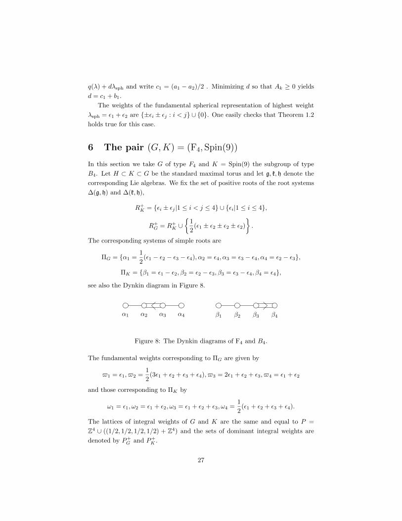
6 The pair (G,K) = (F4, Spin(9))
In this section we take G of type F4 and K = Spin(9) the subgroup of type
B4. Let H ⊂ K ⊂ G be the standard maximal torus and let g, k, h denote the
corresponding Lie algebras. We fix the set of positive roots of the root systems
∆(g, h) and ∆(k, h),
R+K = εi ± εj |1 ≤ i < j ≤ 4 ∪ εi|1 ≤ i ≤ 4,
R+G = R+
K ∪
1
2(ε1 ± ε2 ± ε2 ± ε2)
.
The corresponding systems of simple roots are
ΠG = α1 =1
2(ε1 − ε2 − ε3 − ε4), α2 = ε4, α3 = ε3 − ε4, α4 = ε2 − ε3,
ΠK = β1 = ε1 − ε2, β2 = ε2 − ε3, β3 = ε3 − ε4, β4 = ε4,
see also the Dynkin diagram in Figure 8.
α1 α2 α3 α4 β1 β2 β3 β4
Figure 8: The Dynkin diagrams of F4 and B4.
The fundamental weights corresponding to ΠG are given by
$1 = ε1, $2 =1
2(3ε1 + ε2 + ε3 + ε4), $3 = 2ε1 + ε2 + ε3, $4 = ε1 + ε2
and those corresponding to ΠK by
ω1 = ε1, ω2 = ε1 + ε2, ω3 = ε1 + ε2 + ε3, ω4 =1
2(ε1 + ε2 + ε3 + ε4).
The lattices of integral weights of G and K are the same and equal to P =
Z4 ∪ ((1/2, 1/2, 1/2, 1/2) + Z4) and the sets of dominant integral weights are
denoted by P+G and P+
K .
27
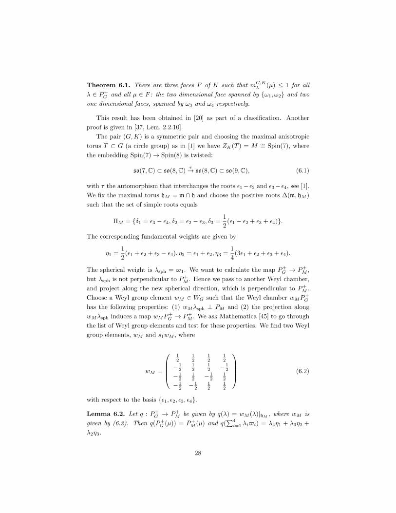
Theorem 6.1. There are three faces F of K such that mG,Kλ (µ) ≤ 1 for all
λ ∈ P+G and all µ ∈ F : the two dimensional face spanned by ω1, ω2 and two
one dimensional faces, spanned by ω3 and ω4 respectively.
This result has been obtained in [20] as part of a classification. Another
proof is given in [37, Lem. 2.2.10].
The pair (G,K) is a symmetric pair and choosing the maximal anisotropic
torus T ⊂ G (a circle group) as in [1] we have ZK(T ) = M ∼= Spin(7), where
the embedding Spin(7)→ Spin(8) is twisted:
so(7,C) ⊂ so(8,C)τ→ so(8,C) ⊂ so(9,C), (6.1)
with τ the automorphism that interchanges the roots ε1− ε2 and ε3− ε4, see [1].
We fix the maximal torus hM = m ∩ h and choose the positive roots ∆(m, hM )
such that the set of simple roots equals
ΠM = δ1 = ε3 − ε4, δ2 = ε2 − ε3, δ3 =1
2(ε1 − ε2 + ε3 + ε4).
The corresponding fundamental weights are given by
η1 =1
2(ε1 + ε2 + ε3 − ε4), η2 = ε1 + ε2, η3 =
1
4(3ε1 + ε2 + ε3 + ε4).
The spherical weight is λsph = $1. We want to calculate the map P+G → P+
M ,
but λsph is not perpendicular to P+M . Hence we pass to another Weyl chamber,
and project along the new spherical direction, which is perpendicular to P+M .
Choose a Weyl group element wM ∈ WG such that the Weyl chamber wMP+G
has the following properties: (1) wMλsph ⊥ PM and (2) the projection along
wMλsph induces a map wMP+G → P+
M . We ask Mathematica [45] to go through
the list of Weyl group elements and test for these properties. We find two Weyl
group elements, wM and s1wM , where
wM =
12
12
12
12
− 12
12
12 − 1
2
− 12
12 − 1
212
− 12 − 1
212
12
(6.2)
with respect to the basis ε1, ε2, ε3, ε4.
Lemma 6.2. Let q : P+G → P+
M be given by q(λ) = wM (λ)|hM , where wM is
given by (6.2). Then q(P+G (µ)) = P+
M (µ) and q(∑4i=1 λi$i) = λ4η1 + λ3η2 +
λ2η3.
28

Proof. The surjectivity is implied by Proposition 3.6. The calculation involves
a base change for wM with basis η1, η2, η3, α1 and follows readily.
It follows that λ = λ1$1 + λ2$2 + λ3$3 + λ4$4 ∈ P+G (µ) implies that
λ4η1 +λ3η2 +λ2η3 ∈ P+M (µ). The branching rule Spin(9)→ Spin(7) is described
in [1, Thm. 6.3] and we recall it for our special choices of µ. It is basically the
same as branching B4 ↓ D4 ↓ B3 via interlacing, see e.g. [25, Thm. 9.16], but
on the D4-level we have to interchange the coefficients of the first and the third
fundamental weight.
Proposition 6.3. The spectrum P+M (µ) is given by the following inequalities.
• Let µ = µ1ω1 + µ2ω2. Then λ4η1 + λ3η2 + λ2η3 ∈ P+M (µ) if and only if
λ2 + λ3 + λ4 ≤ µ1 + µ2,
λ3 + λ4 ≤ µ2 ≤ λ2 + λ3 + λ4.
• Let µ = µ2ω3. Then λ4η1 + λ3η2 + λ2η3 ∈ P+M (µ) if and only if
λ2 + λ3 ≤ µ3,
λ3 + λ4 ≤ µ3 ≤ λ2 + λ3 + λ4.
• Let µ = µ4ω4. Then λ4η1 + λ3η2 + λ2η3 ∈ P+M (µ) if and only if
λ3 = 0,
λ2 + λ4 ≤ µ4.
Given an element µ ∈ P+K we can determine the M -types ν = ν1η1 + ν2η2 +
ν3η3 ∈ P+M (µ) and we know from Proposition 3.6 that for λ1 large enough,
λ = λ1$1 + ν3$2 + ν2$3 + ν1$4 ∈ P+G (µ). (6.3)
We proceed to determine the minimal λ1 such that (6.3) holds, in the case that
µ satisfies the multiplicity free condition of Theorem 6.1.
Theorem 6.4. Let µ ∈ (Nω1⊕Nω2)∪(Nω3)∪(Nω4). Then λ = λ1$1 +λ2$2 +
λ3$3 + λ4$4 ∈ B(µ) if and only if (i) q(λ) ∈ P+M (µ) and (ii)
µ1 + µ2 = λ1 + λ2 + λ3 + λ4 if µ = µ1ω1 + µ2ω2, (6.4)
µ3 = λ1 + λ2 + λ3 if µ = µ3ω3, (6.5)
µ4 = λ1 + λ2 + λ4 if µ = µ4ω4. (6.6)
29

Hence the bottom B(µ) is given by a singular equation and the inequalities
of P+M (µ) in all cases, except for (G,K) = (SU(n+1),S(U(n)×U(1))). We have
found the inequalities of Theorem 6.4 using an implementation of the branching
rule from F4 to Spin(9) in Mathematica and looking at some examples. Before
we prove Theorem 6.4 we settle the proof of the final case of Theorem 1.2.
Corollary 6.5. Let λ ∈ P+G (µ)→ N and let λ′ ∈ P be a weight of the spherical
representation. Then |d(λ + λ′) − d(λ| ≤ 1 with d : P+G (µ) → N the degree
function of Theorem 1.2.
Proof. The weights of the spherical representation are the short roots and zero
(with multiplicity two). After expressing these weights as linear combinations
of fundamental weights, one easily checks the assertion.
Proof of Theorem 6.4. The proof of Theorem 6.4 is devided into two parts, cor-
responding to the dimension of the face. The strategy in both cases is the
same. Fix µ ∈ (Nω1 ⊕ Nω2) ∪ (Nω3) ∪ (Nω4) and choose a suitable system R+G
of positive roots of G. Let A = R+G\R
+K and let pA denote the corresponding
partition function. Let λ ∈ P+G have the property that q(λ) ∈ P+
M (µ). This
gives restrictions on λ2, λ3, λ4, according to Proposition 6.3. Let λ1 satisfy the
appropriate linear equation from the theorem.
For w ∈ WG define Λw(λ, µ) = w(λ + ρ) − (µ + ρ). Explicit knowledge of
the partition function pA allows us, using Mathematica, to determine for which
w ∈WG the quantity pA(Λw(λ, µ)) is zero. We end up with two elements in case
µ ∈ Nω1 ⊕ Nω2 and twelve elements in the other cases, for which pA(Λw(λ, µ))
is possibly not zero. This allows us to calculate mG,Kλ (µ) using Lemma 4.1. One
checks that the multiplicity is one for this choice of λ ∈ P+G (µ).
Moreover, if µ ∈ Nω1 ⊕ Nω2 then p(Λw(λ − λsph)) = 0 for all Weyl group
elements. In the other cases for µ we find the same twelve Weyl group elements
for which pA(Λw(λ − λsph, µ)) possibly does not vanish. One checks that the
multiplicity is zero in this case.
We conclude the proof by indicating the the positive system that we chose
in the various cases, a description of the partition function and lists of the Weyl
group elements that may contribute in the Kostant multiplicity formula.
The case µ = µ1ω1 + µ2ω2. Here we take the standard positive system R+G
and we have A = R+G\R
+K = 1
2 (ε1±ε2±ε3±ε4). Let Λ = (Λ1,Λ2,Λ3,Λ4) ∈ P .
We claim that pA(Λ) > 0 if and only if |Λj | ≤ Λ1 for j = 2, 3, 4.
Let us denote A = a000, . . . , a111 where the binary index indicates where
to put the + or the − sign on positions 2,3,4, e.g. a100 = 12 (ε1 − ε2 + ε3 + ε4).
30

Let
Λ =
111∑i=000
niai. (6.7)
We are going to count the number of tuples (n000, . . . , n111) ∈ N8 for which (6.7)
holds. First of all, it follows from (6.7) that
011∑i=000
ni = Λ1 + Λ2,
111∑i=100
ni = Λ1 − Λ2.
In other words, any linear combination (6.7) uses Λ1 + Λ2 elements from the set
a000, . . . , a011 and Λ1−Λ2 elements from the set a100, . . . , a111. Let us write
(Λ3,Λ4) = (v1, v2)+(Λ3−v1,Λ4−v2). For each such decomposition we need to
count (1) the number of tuples (n000, . . . , n011) ∈ N4 for which∑011i=000 niai =
((Λ1 +Λ2)/2, (Λ1 +Λ2)/2, v1, v2) and (2) the number of tuples (n100, . . . , n111) ∈N4 for which
∑111i=100 niai = ((Λ1 − Λ2)/2,−(Λ1 − Λ2)/2,Λ3 − v1,Λ4 − v2). For
each (v1, v2) we take the product of these quantities, and summing these for the
possible vectors (v1, v2) yields the desired formula for pA.
This reduces the calculation of pA to the following counting problem. Let
L = Z2 ∪ (( 12 ,
12 ) + Z2), let A′ = (± 1
2 ,±12 ) and let p ∈ N. Let us denote
A′ = a′00, . . . , a′11, where the binary number indicates where to put the + and
the − signs, e.g. a′10 = (−1/2, 1/2). Given a vector v = (v1, v2) we want to
calculate the number of tuples (n00, . . . , n11) ∈ N4 such that∑11i=00 nia
′i = v
and∑11i=00 ni = p. It is necessary that |v1|, |v2| ≤ p/2. In this case, the number
of tuples is 1 + p2 −max(|v1|, |v2|).
Returning to our original problem, we have
pA(Λ) =∑v1,v2
(1 +
Λ1 + Λ2
2−max(|v1|, |v2|)
)×(
1 +Λ1 − Λ2
2−max(|Λ3 − v1|, |Λ4 − v2|)
),
where (v1, v2) satisfies the restrictions |v1|, |v2| ≤ (Λ1+Λ2)/2 and simultaneously
|Λ3 − v1|, |Λ4 − v2| ≤ (Λ1 − Λ2)/2. As a result, the ranges for the summations
are
v1 = max
(−Λ1 + Λ2
2,Λ3 −
Λ1 − Λ2
2
), . . . ,min
(Λ1 + Λ2
2,Λ3 +
Λ1 − Λ2
2
),
v2 = max
(−Λ1 + Λ2
2,Λ4 −
Λ1 − Λ2
2
), . . . ,min
(Λ1 + Λ2
2,Λ4 +
Λ1 − Λ2
2
).
31

In particular, pA(Λ) > 0 if and only if the ranges for v1 and v2 are both
non-empty, which is equivalent to
|Λ2| ≤ Λ1, (6.8)
|Λ3| ≤ Λ1, (6.9)
|Λ4| ≤ Λ1. (6.10)
The only two Weyl group elements for which pA(Λw(λ, µ)) contributes to the
multiplicity mG,Kλ (µ), under the assumptions (6.4) and q(λ) ∈ P+
M (µ) are e, s2.
In this case mG,Kλ (µ) = 1. Also, mG,K
λ−λsph(µ) = 0 under the same conditions, as
there are no Weyl group elements for which pA(Λw(λ− λsph, µ)) is non-zero.
The case µ = µ3ω3 and µ = µ4ω4. Let µ = µ3ω3 or µ = µ4ω4 and λ ∈ B(µ)
and consider Λw(λ, µ) = w(λ+ ρ)− (µ+ ρ) for w ∈WG. Using Mathematica to
check the inequalities (6.8,6.9,6.10) under the condition (6.5) or (6.6) we find a
number of 16 Weyl group elements for which Λw(λ, µ) is possibly in the support
of pA. However, the formulas for the elements Λw(λ, µ) that possibly contribute
do not look tempting to perform calculations with.
Instead we pass to another Weyl chamber for F4 while remaining in the same
Weyl chamber for Spin(9). The Weyl chamber that we choose contains ω3 and
ω4. The element w = s2s1 ∈ W translates the standard Weyl chamber to one
that we are looking for. The set of positive roots that corresponds to the system
of simple roots is wΠG = R+K ∪B, where
B =
1
2(−ε1 + ε2 + ε3 ± ε4),
1
2(ε1 − ε2 + ε3 ± ε4),
1
2(ε1 + ε2 − ε3 ± ε4),
1
2(ε1 + ε2 + ε3 ± ε4)
is the new set of positive roots of G that are not roots of K. The Kostant
multiplicity formula reads
mG,Kλ (µ) =
∑w∈WG
det(w)pB(Λw(w(λ+ ρ)− (µ+ ρ)),
where ρ = 12 (9ε1 + 7ε2 + 5ε3 + ε4) is the Weyl vector for the new system of
positive roots.
Our aim is to calculate the partition pB(Λ) for Λ = (Λ1,Λ2,Λ3,Λ4) ∈ P . To
begin with we focus on the first three coordinates. Let π : P → Z3∪ (( 12 ,
12 ,
12 )+
Z3) denote the projection on the first three coordinates. Let C = c1, c2, c3, c4
32
with
c1 =1
2(−ε1 + ε2 + ε3), c2 =
1
2(ε1 − ε2 + ε3),
c3 =1
2(ε1 + ε2 − ε3), c4 =
1
2(ε1 + ε2 + ε3).
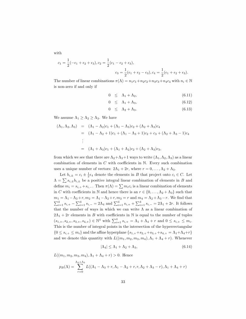
The number of linear combinations π(Λ) = n1c1+n2c2+n3c3+n4c4 with ni ∈ Nis non-zero if and only if
0 ≤ Λ1 + Λ2, (6.11)
0 ≤ Λ1 + Λ3, (6.12)
0 ≤ Λ2 + Λ3. (6.13)
We assume Λ1 ≥ Λ2 ≥ Λ3. We have
(Λ1,Λ2,Λ3) = (Λ1 − Λ2)c1 + (Λ1 − Λ3)c2 + (Λ2 + Λ3)c4
= (Λ1 − Λ2 + 1)c1 + (Λ1 − Λ3 + 1)c2 + c3 + (Λ2 + Λ3 − 1)c4...
= (Λ1 + Λ3)c1 + (Λ1 + Λ2)c2 + (Λ2 + Λ3)c3,
from which we see that there are Λ2+Λ3+1 ways to write (Λ1,Λ2,Λ3) as a linear
combination of elements in C with coefficients in N. Every such combination
uses a unique number of vectors: 2Λ1 + 2r, where r = 0, . . . ,Λ2 + Λ3.
Let bi,± = ci ± 12ε4 denote the elements in B that project onto ci ∈ C. Let
Λ =∑si,±bi,± be a positive integral linear combination of elements in B and
define mi = si,++si,−. Then π(Λ) =∑mici is a linear combination of elements
in C with coefficients in N and hence there is an r ∈ 0, . . . ,Λ2 + Λ3 such that
m1 = Λ1−Λ3 +r,m2 = Λ1−Λ2 +r,m3 = r and m4 = Λ2 +Λ3−r. We find that∑4i=1 si,+ −
∑4i=1 si,− = 2Λ4 and
∑4i=1 si,+ +
∑4i=1 si,− = 2Λ1 + 2r. It follows
that the number of ways in which we can write Λ as a linear combination of
2Λ1 + 2r elements in B with coefficients in N is equal to the number of tuples
(s1,+, s2,+, s3,+, s4,+) ∈ N4 with∑4i=1 si,+ = Λ1 + Λ4 + r and 0 ≤ si,+ ≤ mi.
This is the number of integral points in the intersection of the hyperrectangular
0 ≤ si,+ ≤ mi and the affine hyperplane s1,++s2,++s3,++s4,+ = Λ1+Λ4+rand we denote this quantity with L((m1,m2,m3,m4),Λ1 + Λ4 + r). Whenever
|Λ4| ≤ Λ1 + Λ2 + Λ3, (6.14)
L((m1,m2,m3,m4),Λ1 + Λ4 + r) > 0. Hence
pB(Λ) =
Λ2+Λ3∑r=0
L((Λ1 − Λ3 + r,Λ1 − Λ2 + r, r,Λ2 + Λ3 − r),Λ1 + Λ4 + r)
33

if Λ1 ≥ Λ2 ≥ Λ3. The quantity pB(Λ) is positive if and only if the inequalities
(6.11),(6.12),(6.13) and (6.14) hold. Note that these inequalities are invariant
for permuting the first three coordinates of Λ.
Let µ = µ3ω3 or µ = µ4ω4 and let λ ∈ P+G satisfy q(λ) ∈ P+
M (µ) and (6.5)
or (6.6) respectively. Define Γw(λ, µ) = w(wλ+ ρ)− (µ+ ρ). For the elements
Γw(λ, µ) and Γw(λ − λsph, µ) we check the inequalities (6.11),(6.12),(6.13) and
(6.14). We get 12 Weyl group elements for which pB(Γw(λ, µ)) and pB(Γw(λ−λsph, µ)) are possibly non-zero. Moreover, the twelve elements are the same for
µ = µ3ω3 and µ = µ4ω4 and we have listed them in Table 4.
w1 w2 w3 w4 w5 w6 w7 w8 w9 w10 w11 w12
e s1 s2 s3 s4 s1s2 s1s3 s1s4 s2s1 s2s3 s2s4 s3s2
Table 4: The Weyl group elements w for which Γw(wλ, µ) is possibly in the
support of pB .
Using the explicit description of pB one verifies the equalities mG,Kλ (µ) = 1 and
mG,Kλ−λsph
(µ) = 0.
7 The differential equations
Our goal is to define a non-trivial commutative algebra of differential operators
for the matrix valued orthogonal polynomials defined in Section 1. Let (G,K,F )
be a multiplicity free system from Table 1 and let µ ∈ F . Let gc, kc denote the
complexifications, let U(gc) denote the universal enveloping algebra of gc and
let U(gc)kc denote the commutant of kc in U(gc). Let πKµ be an irreducible
representation of K in Vµ and let πKµ denote the corresponding representation
of U(kc). Let I(µ) ⊂ U(kc) denote the kernel of πKµ and consider the left ideal
U(gc)I(µ) ⊂ U(gc). As in [8, Ch. 9] we define
D(µ) = U(gc)kc/(U(gc)
kc ∩ U(gc)I(µ)),
which is an associative algebra. In fact, D(µ) is commutative because it can be
embedded, using an anti homomorphism, into the commutative algebra U(ac)⊗EndM (Vµ) (see [8, 9.2.10]), which is commutative by Proposition 3.4. The irre-
ducible representations of D(µ) are in a 1–1 correspondence with the irreducible
representations of gc that contain πKµ upon restriction, see [8, Thm. 9.2.12].
Let D ∈ U(gc). The µ-radial part R(µ,D) is a differential operator that
34
satisfies
R(µ,D)(Φ|T ) = D(Φ)|T (7.1)
for all functions Φ : G → End(Vµ) satisfying (1.1). Following Casselman and
Milicic [7, Thm. 3.1] we find a homomorphism
R(µ) : U(gc)kc → C(T )⊗ U(tc)⊗ End(EndM (Vµ))
such that (7.1) holds for all D ∈ U(gc)kc and all Φ ∈ C∞(G,End(Vµ)) sat-
isfying (1.1). For the two non-symmetric multiplicity free triples we have an
Iwasawa-like decomposition gc = kc ⊕ tc ⊕ n+ and a map n+ → kc onto the
orthocomplement of mc in kc. This map replaces I + θ in the symmetric
case and is essential in the construction of Rµ, see [7, Lem. 2.2]. The ho-
momorphism R(µ) factors through the projection U(gc)kc → D(µ) and we ob-
tain an injective algebra homomorphism that we denote by the same symbol,
R(µ) : Dµ → C(T ) ⊗ U(tc) ⊗ End(EndM (Vµ)). We identify EndM (Vµ) = CNµ
by Schur’s Lemma with Nµ the cardinality of the bottom B(µ) and we write
Mµ = End(CNµ). The elementary spherical functions Φµλ are simultaneous
eigenfunctions for the algebra D(µ). The differential operators R(µ,D) become
differential operators for the functions Ψµd : T →Mµ and, according to the con-
struction, the functions Ψµn are simultaneous eigenfunctions for the operators
R(µ,D) with D ∈ D(µ). The eigenvalues are diagonal matrices Λn(D) ∈ Mµ
acting on the right, i.e. we have R(µ,D)Ψµn = Ψµ
nΛn(D).
In the forthcoming paper [38] it is shown that the function Ψµ0 : T →Mµ is
point wise invertible on Treg, the open subset of T on which the restriction of the
minimal spherical function, φ|T , is regular. The proof relies on the bispectral
property that is present for the family of matrix valued functions Ψµn : n ∈ N.
More precisely, the interplay between the differential operators and the three
term recurrence relation imply that the function Ψµ0 satisfies an ODE whose
coefficients are regular on Treg. If we conjugate R(µ,D) with Ψµ0 and perform
the change of variables x = cφ(t) + (1− c), such that x runs in [−1, 1], then we
obtain a differential operator acting on the space of matrix valued orthogonal
polynomials Mµ[x]. The algebra of differential operators that is obtained in
this way is denoted by Dµ. The family of matrix valued orthogonal polynomials
(Pµn (x);n ∈ N) that we obtain from the functions (Ψµn;n ∈ N), is a family
of simultaneous eigenfunctions for the algebra Dµ. The algebra of differential
operators Mµ[x, ∂x] acts on Mµ[x], where the matrices act by left multiplication.
Note that Dµ ⊂Mµ[x, ∂x].
The description of the map R(µ) in [7] allows one to calculate explicitly
the radial part of the (order two) Casimir operator Ω ∈ U(gc)kc . An explicit
35

expression can be found in [43, Prop. 9.1.2.11] for the case where (G,K) is
symmetric. The image of Ω in the algebra Dµ is denoted by Ωµ and is of order
two. Its eigenvalues can be calculated explicitly in terms of highest weights
and they are real, which implies that Ωµ is symmetric with respect to the
matrix valued inner product 〈·, ·〉Wµ . These are examples of matrix valued
hypergeometric differential operators [40].
8 Conclusions
Several questions remain. We have shown the existence of families of matrix val-
ued orthogonal polynomials, together with a commutative algebra of differential
operators for which the polynomials are simultaneous eigenfunctions, mainly by
working out the branching rules. The key result is that the bottom of the µ-
well is well behaved with respect to the weights of the fundamental spherical
representation, so that the degree function has the right properties. It would be
interesting to see whether one can draw the same conclusions by investigating
of the differential equations for the matrix valued orthogonal polynomials. This
would require more precise knowledge of the algebra D(µ).
On the other hand, it would be interesting to investigate whether the good
properties of the degree function follow from convexity arguments that come
about if we formulate matters concerning the representation theory, such as
induction and restriction, in terms of symplectic or algebraic geometry. For
example, in this light, it is interesting to learn more about the (spherical) spaces
Gc/Q and their Gc-equivariant line bundles, where Q ⊂ Kc is the parabolic
subgroup associated to F , for a multiplicity free system (G,K,F ).
The existence of multiplicity free systems (G,K,F ) with (G,K) a Gelfand
pair of rank > 1, raises the question whether the spectra of the induced rep-
resentations have a similar structure as in the rank one case. If the answer is
affirmative we expect that we can associate families of matrix valued orthogo-
nal polynomials in several variables to these spectra, together with commutative
algebras of differential operators that have these polynomials as simultaneous
eigenfunctions. For the examples (Spin(9),Spin(7),Nω1) and (SU(n+1)×SU(n+
1),diag(SU(n+ 1)), F ), where F = ω1N or F = ωnN, this seems to be the case.
In general the branching rules will not be of great help in understanding the
bottom of the µ-well, as they soon become too complicated in the higher rank
situations.
36
References
[1] M.W. Baldoni Silva, Branching theorems for semisimple Lie groups of real
rank one, Rend. Sem. Univ. Padova 61 (1979), 229-250.
[2] S. Bochner, Uber Sturm–Liouvillesche Polynomsysteme, Mathematisch
Zeitschrift 29 (1929), 730-736.
[3] N. Bourbaki, Groupes et Algebres de Lie, Chapitres 4,5 et 6, Masson, Paris,
1981.
[4] M. Brion, Classification des espaces homogenes spheriques, Compositio
Math. 63:2 (1987), 189-208.
[5] R. Camporesi, The Helgason Fourier transform for homogeneous vector
bundles over compact Riemannian symmetric spaces–the local theory, J. of
Funct. Analysis 220 (2005), 97-117.
[6] R. Camporesi, A generalization of the Cartan–Helgason theorem for Rie-
mannian symmetric spaces of rank one, Pacific J. Math. 222:1 (2005), 1-27.
[7] W. Casselman and D. Milicic, Asymptotic behavior of matrix coefficients
of admissable representations, Duke Math. J. 49:4(1982), 869–930.
[8] J. Dixmier, Algebres envelloppantes, Editions Jacques Gabay, Paris, 1996.
[9] A.J. Duran, Matrix inner product having a matrix second order differential
operator, Rocky Mountain J. of Math. 27:2 (1997), 585-600.
[10] A.J. Duran and F.A. Grunbaum, A Survey of orthogonal matrix polynomi-
als satisfying second order differential equations, Journal of Computational
Applied Mathematics 178 (2005), 169-190.
[11] W. Fulton and J. Harris, Representation Theory, Graduate Texts in Math-
ematics 129, Springer, New York, 1991.
[12] J.S. Geronimo, Scattering theory and matrix orthogonal polynomials on
the real line, Circuits Systems Signal Process 1 (1982), 261-180.
[13] F.A. Grunbaum, I. Pacharoni and J.A. Tirao, Matrix valued spherical func-
tions associated to the complex projective plane, J. Funct. Anal. 188 (2002),
350-441.
37

[14] F.A. Grunbaum, I. Pacharoni and J.A. Tirao, Matrix valued orthogonal
polynomials of Jacobi type: the role of group representation theory, Annales
de l’ institut Fourier 55:6 (2005), 2051-2068.
[15] F.A. Grunbaum and J.A. Tirao, The Algebra of Differential Operators
Associated to a Weight Matrix, Integr. Equ. Oper. Theory 58 (2007), 449-
475.
[16] V. Guillemin and S. Sternberg, Geometric Quantization and Multiplicities
of Group Representations, Invent. Math. 67 (1982), 515-538.
[17] V. Guillemin and S. Sternberg, Convexity Properties of the Moment Map
II, Invent. Math. 77 (1984), 533-546.
[18] V. Guillemin and S. Sternberg, The Frobenius Reciprocity Theorem from
a Symplectic Point of View, Lecture Notes Math. 1037 (1983), 242-256.
[19] V. Guillemin and S. Sternberg, Multiplicity Free Spaces, J. Differential
Geometry 19 (1984), 31-56.
[20] X. He, K. Nishiyama, H. Ochiai, Y. Oshima, On orbits in double flag
varieties for symmetric spaces, arXiv1208.2084v1.
[21] G.J. Heckman, Projections of Orbits and Asymptotic Behavior of Multiplic-
ities for Compact Connected Lie groups, Invent. Math 67 (1982), 333-356.
[22] J.E. Humphreys, Introduction to Lie Algebras and Representation Theory,
Graduate Texts in Mathematics 9, Springer, New York, 1972.
[23] F.C. Kirwan, Convexity Properties of the Moment Map III, Invent. Math.
77 (1984), 547-552.
[24] M. Kitagawa, Stability of Branching Laws for Highest Weight Modules,
arXiv:1307.0606.
[25] A.W.Knapp, Lie Groups Beyond an Introduction, Second Edition, Progress
in Mathematics 140, Birkhauser, Boston, 2002.
[26] F. Knop, B. Van Steirteghem, Classification of smooth affine spherical va-
rieties, Transformation Groups, Vol. 11, No. 3, (2006),495–516.
[27] E. Koelink, M. van Pruijssen and P. Roman, Matrix Valued Orthogonal
Polynomials related to (SU(2)×SU(2),diag), Part I, Int Math Res Notices
(2012) 2012 (24): 5673-5730.
38

[28] E. Koelink, M. van Pruijssen and P. Roman, Matrix Valued Orthogonal
Polynomials associated to (SU(2) × SU(2),SU(2)), Part II, Publ. RIMS
Kyoto Univ. 49 (2013), 271–312.
[29] T.H. Koornwinder, Matrix elements of irreducible representations of
SU(2)× SU(2) and vector-valued orthogonal polynomials, SIAM J. Math.
Anal. 16 (1985), 602–613.
[30] B. Kostant, A branching law for subgroups fixed by an involution and
a noncompact analogue of the Borel–Weil theorem, 291-353, Progress in
Math. 220, Birkhauser, Boston, 2004.
[31] M. Kramer, Spharische Untergruppen in kompakten zusammenhangen-den
Liegruppen, Compositio Math. 38 (1979), 129–153.
[32] M.G. Krein, Infinite J-matrices and a matrix moment problem, Dokl. Akad.
Nauk, SSSR 69:2 (1949), 125–128.
[33] M.G. Krein, Fundamental aspects of the representation theory of Hermi-
tian operators with deficiency index (m,m), AMS Translations, Series 2 97
(1971), 75–143.
[34] J. Lepowsky, Multiplicity formulas for certain semisimple Lie groups, Bull.
Amer. Math. Soc. 77 (1971),601–605.
[35] W.G. McKay and J. Patera, Tables of Dimensions, Indices and Branching
Rules for Representations of Simple Lie Algebras, Marcel Dekker, New
York, 1981.
[36] I. Pacharoni and J.A. Tirao, Matrix Valued Orthogonal Polynomials Aris-
ing from the Complex Projective Space, Constr. Approx. 25 (2007), 177–
192.
[37] M. van Pruijssen, Matrix Valued Orthogonal Polynomials related to
Gelfand Pairs of Rank One, PhD Nijmegen, 2012.
[38] M. van Pruijssen, P. Roman, Algorithm paper, work in progress.
[39] G. Szego, Orthogonal Polynomials, American Mathematical Society Collo-
quium Publications 23, New York, 1959.
[40] J. A. Tirao, The matrix-valued hypergeometric equation, PNAS 100:14
(2003), 8138–8141.
39

[41] D.A. Vogan, Lie algebra cohomology and a multiplicity formula of Kostant,
J. Algebra 51 (1978), 69–75.
[42] N. R. Wallach, Harmonic Analysis on Homogeneous Spaces, Marcel
Dekkers, New York, 1973.
[43] G. Warner, Harmonic analysis on semi-simple Lie groups II, Springer–
Verlag, New York– Heidelberg, 1972.
[44] H.-C. Wang, Two-point Homogeneous Spaces, Annals of Math. 55:1 (1952),
177–191.
[45] Wolfram Research, Inc., Mathematica, Version 5.1, Champaign, IL (2005).
40