matrix structural analysis · matrix structural analysis giuliano basile august 5, 2010 abstract...

Matrix Structural Analysis

Giuliano Basile

August 5, 2010

Abstract

This report will cover the obstacles faced by three undergraduate students, advised by Dr. Nima Rahbar fromthe University of Massachusetts Dartmouth Civil Department during the summer of 2010. We were sponsored bythe Computational Science Training for Undergraduates in the Mathematical Sciences (CSUMS), which was fundedby the National Science Foundation (NSF). Our main focus was to study the 2-D Thermal Temperature Distributionthroughout a plate specimen produced in Matlab and revised in Octave. Nodes and elements were created which leadto the use of Matrix Structural Analysis. We want to compare our numerical solutions against our exact analyticalsolutions. I should note that this study is a gateway to more advanced studies to come. We were able to build andmanipulate our specimen to fit our advisors needs.

1 IntroductionPeople are given many opportunities in life. Depending on what that person does with their opportunity, is what makesthat person who they are. Before entering college I was balancing my thoughts based on my previous experience andat the time there was not much experience to balance. Every student before entering college has a choice as to whatthey should major in. Given the opportunity I was given, I choose Mechanical Engineering. I will now enter my Junioryear of college. My first year of college was very interesting. I was granted a special gift without knowledge of thisgift. I was to be advised by the soon to be Chairmen of the Mechanical Engineering Department. It was now time toconstruct my schedule for the following year. I had a chance to let my advisor know that even though my true passionwas for Engineering, I also a a desire for numbers, or in this case, mathematics. At the time my advisor, Dr. PeterFriedman, told me that I should pick up a math minor. It took me only seconds to agree and the next thing you know,I was enrolled at the University pursuing a Bachelor of Science Degree in Mechanical Engineering and a Minor inMathematics.

Shortly after I was introduced to Probability, low and behold, the Chairman of the Math department was theprofessor. After spending some time with Dr. Ron Tannenwald and discussing my true desire, I soon became amath tutor. Not only was I working with a mass majority of the Math majors, I was also teaching a wide variety ofmathematics to a wide variety of students. This was a tremendous feeling. I was able to better my understanding formathematics and also improve my knowledge in ares I was unfamiliar with. Sadly, the semester was coming to anend. During this time period I was in the process of finding summer work. Gaining the respect and friendship of myco-workers, a couple of good friends of mine now had introduced me to CSUMS.

Well a month later, I was given an opportunity to work with some very intelligent members of the MathematicsDepartment, given a MacBook and was left to figure the rest out on my own. Finding new ways to learn, communicate,and present my work all came along with the job description. This is where the other two students I was working withand I differed from the rest of the CSUMS community. All three of us were Engineering Students, Vihn Nguyen(Mechanical), Christine Rohr (Civil), and Giuliano Basile (Mechanical). We were to be Advised by a member formthe Civil Engineering Department, Dr. Nima Rahbar. Our instructions were simple, Learn Matlab and learn the art ofFinite Element Structuring.

1

2 Finite Element AnalysisFinite Element Analysis (FEA) is a computer animated model used to design and run test creatively and cost effectivly.In our case, FEA is used to analyze the specific temperature readings at different nodes created. We are using FEA tomeet specifications provided by Dr. Rahbar. FEA can be used to determine the design modifications required to meetour new condition. In general there are two types of analysis used for FEA; 2-D and 3-D modeling. 2-D modelingtends to be less accurate than 3-D modeling but for our purpose we will used 2-D modeling. Our only concern here isthe study of temperature distribution throughout our plate specimen.

2.1 How does Finite Element Analysis Work?FEA uses a system of points called nodes, these nodes form meshes. Structural and material properties have tobe programmed into our mesh. Nodes are assigned certain density properties, for reason of simplicity, we will beworking with a uniform mesh. Meshes necessarily do not have to be uniform, they can be designed to have higherconcentrations of nodes in one part of the mesh then others. Concentrations are ued to focus ones studies on a certainpart of the specimen they are working with. The mesh acts like a spider web allowing our team to analyze and calculateerrors produced between numerical and analytical results.

3 Given ProblemWe want to build a plate specimen in Matlab to study the temperature distribution throughout. We will build triangularelements as shown in Figure 1 using Finite Element Structuring. As stated earlier we will use a 2-D model. Thisspecimen is 5 units wide by 10 units high. We are dividing this plate into five equally spaced nodes in both the x and ydirections. A heat function is provided and applied to the top of the specimen. The left, right and bottom sides of theplate will be given boundary conditions and will be discussed.

ϑ = 100 ∗ sinπx

10(1)

Figure 1: 5x5 Matrix with Linear Triangular Elements

2

3.1 Boundary Conditions

ϑ(x, 0) = 0 0 < x < 5 (2)ϑ(0, y) = 0 0 < y < 10 (3)

ϑ(x, 10) = 100 sinπx

100 < x < 5 (4)

δϑ

δx(5, y) = 0 0 < y < 10 (5)

3.2 Specimen DetailsAs seen from lines 2 and 3, we are setting the temperature on the bottom and left sides of the the plate equal to zero.We start by taking a look at line 2. With the given parameters of ϑ(x, 0), which sets the bottom of the plate equal tozero. This is done by starting at node 0, moving through each node until we reach node 5. We are setting these nodesto zero to represent no initial temperature. The same is done for the parameters in line 3 (left side), except we startfrom the bottom of the plate and work our way up to the top of the plate.

Moving on to line 4, the Steady State Temperature equation ϑ(x, 10) = 100 sin πx10 is being applied to the top

nodes of the plate from nodes 0 to 5. Later we will see how this numerical temperature solution compares with theexact analytical temperature solution.

Our final boundary condition can be seen in line 4. δϑδx (5, y) = 0 which says that the flux on the right side of the

plate is 0. This means that there is no heat leaving or entering the plate. The only temperature change on the right sideof the plate will be do only to the initial funtion.

4 Application of ResearchOne may ask, what is the purpose for the study of Steady State Temperature Distribution? There are a multitude ofanswers. Sometimes Engineers are given design specifications for a plate of some material that has to cover a portionsof a high performance engine that gives off a tremendous amount of heat. Common knowledge tells us that millionsof dollars are spent to ensure that these engines work properly. Sometimes there are parts in the engine that need tobe placed in specific ares due to design specifications. Well lets say that this pice cannot be placed in an environmentthat exceed a temperature to some degree. Periodically the distance between this pice and lets say the cylinder blockis centimeters or even millimeters. This is where the study of Thermal Distribution comes into play. We build ourplate specimen in some computer language program, Matlab and study the temperature distribution throughout. Aftercareful analysis we conclude if this plate specimen will be suitable for the design specifications. If not, we concludethat the design has to be reconsidered.

4.1 Material ConditionsAlong with design applications comes material specifications. Certain materials have certain conductivities. Conduc-tivity is due to the material’s atomic structure. In order to proceed with our study we consider our materials to be atSteady State.

• Metals – Crystalline

• Ceramics – Amorphous

• Polymers – Chains

Atomic structures lead to different Thermal Conductivity or how heat travels throughout a material. Differentmaterials have different temperature distributions. The atomic structures of each material listed above can be seen inFigures 2, 3 and 4. Preceding the figures is a list of some common material’s conductivities seen in Table 1. Knowledgeof conductivity allows for proper material selection.

3

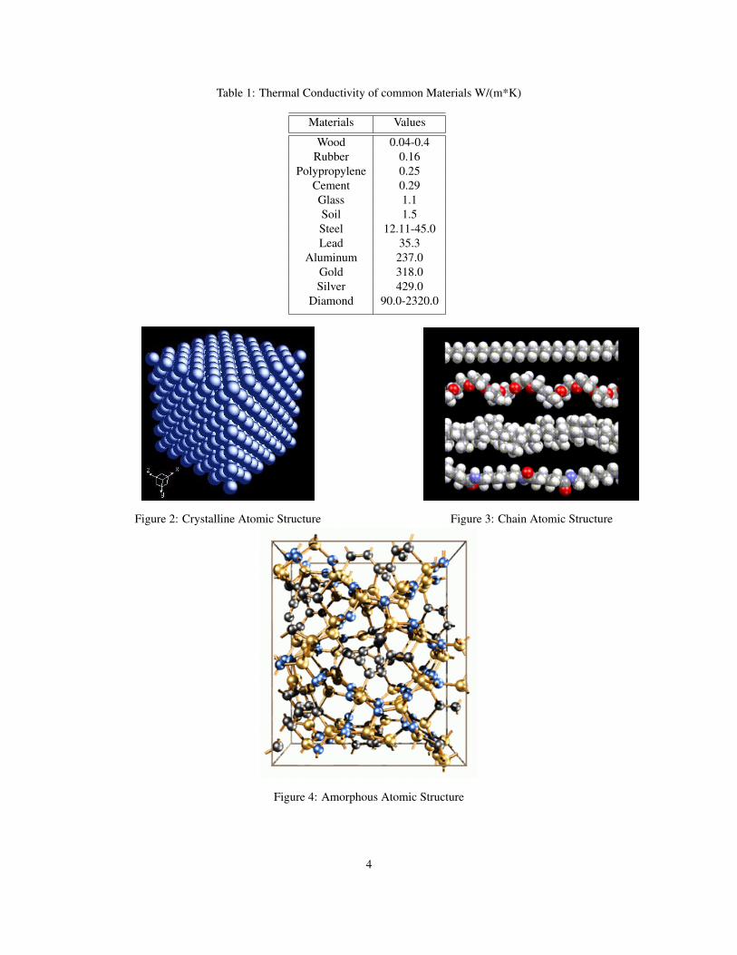
Table 1: Thermal Conductivity of common Materials W/(m*K)

Materials Values

Wood 0.04-0.4Rubber 0.16

Polypropylene 0.25Cement 0.29Glass 1.1Soil 1.5Steel 12.11-45.0Lead 35.3

Aluminum 237.0Gold 318.0Silver 429.0

Diamond 90.0-2320.0

Figure 2: Crystalline Atomic Structure Figure 3: Chain Atomic Structure

Figure 4: Amorphous Atomic Structure

4

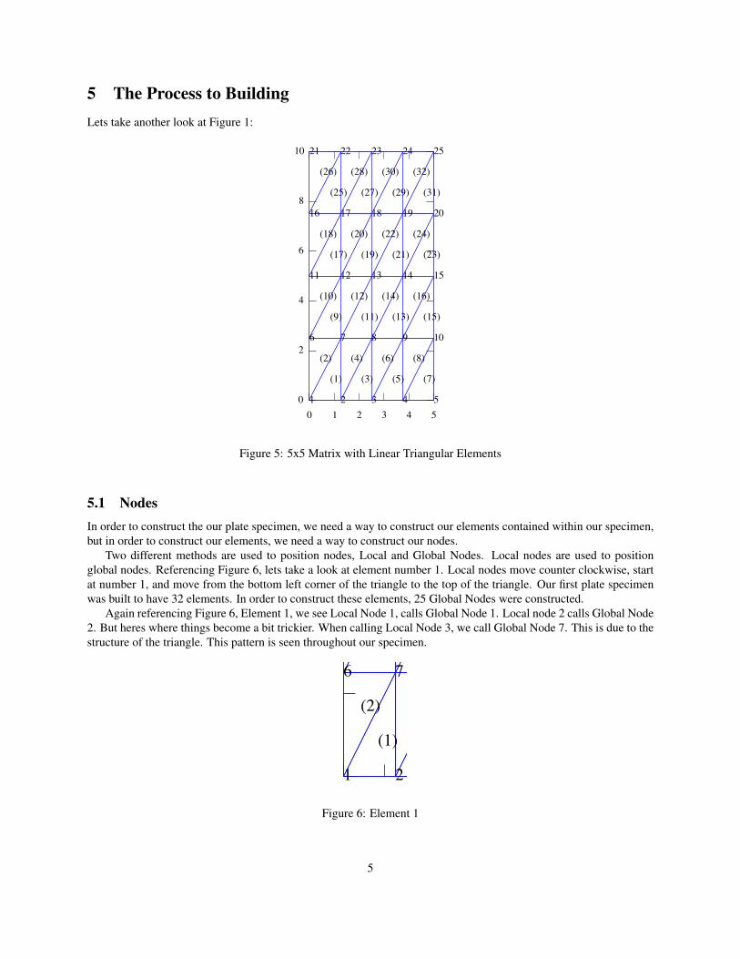
5 The Process to BuildingLets take another look at Figure 1:

Figure 5: 5x5 Matrix with Linear Triangular Elements

5.1 NodesIn order to construct the our plate specimen, we need a way to construct our elements contained within our specimen,but in order to construct our elements, we need a way to construct our nodes.

Two different methods are used to position nodes, Local and Global Nodes. Local nodes are used to positionglobal nodes. Referencing Figure 6, lets take a look at element number 1. Local nodes move counter clockwise, startat number 1, and move from the bottom left corner of the triangle to the top of the triangle. Our first plate specimenwas built to have 32 elements. In order to construct these elements, 25 Global Nodes were constructed.

Again referencing Figure 6, Element 1, we see Local Node 1, calls Global Node 1. Local node 2 calls Global Node2. But heres where things become a bit trickier. When calling Local Node 3, we call Global Node 7. This is due to thestructure of the triangle. This pattern is seen throughout our specimen.

Figure 6: Element 1

5

5.2 ElementsWhy use triangle elements? Triangle elements are used to map most 2-D and 3-D objects. Triangles work well whentrying to bend around curves, fill irregular shapes, or map a simple rectangular plate specimen.

Since we found a way to create local and global nodes, we now need a way to number our elements. Continuingto focus our attention at Figure 5, 5x5 Matrix with Linear Triangular Elements, We see that Element 1 and Element 2are created as one complete rectangle. This pattern is followed throughout the row. After each the row has reach itsmaximum number of elements, the next row is created. This pattern is seen throughout our plate specimen. As a result,we form 32 elements with 25 global nodes. Now that we have an idea of how Nodes and Elements are formulated, letstake a look at how the code relates to our description.

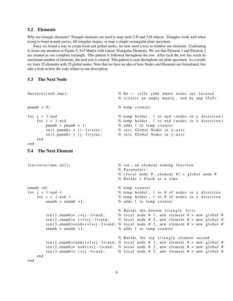
5.3 The Next Node

Xn= z e r o s ( nsd , nnp ) ; % Xn −− t e l l s code where nodes a r e l o c a t e d% c r e a t e s an empty ma t r ix , nsd by nnp (5 x5 )

pnumb = 0 ; % temp c o u n t e r

f o r j = 1 : nyd % temp h o l d e r , 1 t o nyd ( nodes i n y d i r e c t i o n )f o r i = 1 : nxd % temp h o l d e r , 1 t o nxd ( nodes i n x d i r e c t i o n )

pnumb = pnumb + 1 ; % adds 1 t o temp c o u n t e rxn ( 1 , pnumb ) = ( i −1)∗ x i n c ; % s e t s G l ob a l Nodes i n x−a x i sxn ( 2 , pnumb ) = ( j −1)∗ y i n c ; % s e t s G l ob a l Nodes i n y−a x i s

endend

5.4 The Next Element

i e n = z e r o s ( nen , n e l ) ; % ien , an e l e m e n t naming f u n c i t o n% P a r a m e t e r s :% ( l o c a l node # , e l e m e n t # ) = g l o b a l node #% B u i l d s 1 b l o c k a t a t ime

enumb =0; % temp c o u n t e rf o r j = 1 : nyd−1 % temp h o l d e r , 1 t o # of nodes i n y d i r e c t i o n

f o r i = 1 : nxd−1 % temp h o l d e r , 1 t o # of nodes i n x d i r e c t i o nenumb = enumb +1; % adds 1 t o temp c o u n t e r

% B u i l d s t h e bot tom t r i a n g l e f i r s ti e n ( 1 , enumb )= i +( j −1)∗nxd ; % l o c a l node # 1 , new e l e m e n t # = new g l o b a l #i e n ( 2 , enumb )= i +1+( j −1)∗nxd ; % l o c a l node # 2 , new e l e m e n t # = new g l o b a l #i e n ( 3 , enumb )= nxd+ i +1+( j −1)∗nxd ; % l o c a l node # 3 , new e l e m e n t # = new g l o b a l #enumb = enumb +1; % adds 1 t o temp c o u n t e r

% B u i l d s t h e t o p t r i a n g l e e l e m e n t secondi e n ( 1 , enumb )= nxd+ i +1+( j −1)∗nxd ; % l o c a l node # 1 , new e l e m e n t # = new g l o b a l #i e n ( 2 , enumb )= nxd+ i +( j −1)∗nxd ; % l o c a l node # 2 , new e l e m e n t # = new g l o b a l #i e n ( 3 , enumb )= i +( j −1)∗nxd ; % l o c a l node # 3 , new e l e m e n t # = new g l o b a l #

endend

6

6 Numerical vs. AnalyticalNow that we have a way to create nodes and elements, its time to study the temperature distribution. Temperaturedistribution results from the following heat equation.

ϑ = 100 ∗ sinπx

10(6)

6.1 Numerical ResultsAs discussed previously in section 3.1 Boundary Conditions, the sine function is applied to the top of our platespecimen. In the following four Figures 7-10, there are four different refined temperature distributions. My teammate,Vinh was able to increased the number of elements within the specimen. As a result, one can see that with the numberof elements increasing, the temperature distribution becomes clearer. Later in Section 6.2, Analytical data, we will seehow our numerical data compares to our analytical data.

Vinh had decided the new number of element would derive from the the starting number of nodes. As I statedearlier, we created our first plate specimen with a 5x5 Nodal Matrix. In order to produce Figure 8, Vinh added a newnode in-between each old node. As a result, nine nodes were calculated and used both in the x and y-direction to create81 nodes. With the increase number of nodes, we see an increase in the number of elements and as a result we have128 elements, Figure 8. As the number of elements increase, the temperature distribution become clearer.

0 1 2 3 4 50

1

2

3

4

5

6

7

8

9

10Temperature Distribution

Horizontal Side

Vert

ical S

ide

45

50

55

60

65

70

75

80

85

90

Student Version of MATLAB

Figure 7: 32 Elements

0 1 2 3 4 50

1

2

3

4

5

6

7

8

9


Horizontal side

Vert

ical sid

e

70

75

80

85

90



One might notice the difference between each Figure’s temperature bar. For accuracy, Matlab scales the temper-ature distribution. This is due to the fact the majority of the temperature change takes place at the top right portionof the plate. For this reason, Matlab scales appropriately. Continuing to focus our attention to Figures 9 and 10, thetemperature distribution is clearly seen. Later we will see why 512 Elements will be most suitable.

To create 512 elements 324 nodes were created, 18 nodes in the x and y-direction. To create 1682 elements, 900nodes were created, 30 nodes in both the x and y-direction.

7

0 1 2 3 4 50

1

2

3

4

5

6

7

8

9


Horizontal side

Vert

ical sid

e

82

84

86

88

90

92

94

96



0 1 2 3 4 50

1

2

3

4

5

6

7

8

9


Horizontal Side

Vert

ical S

ide

90

91

92

93

94

95

96

97

98



6.2 Analytical ResultsIts time to compare our numerical results produced in Matlab to our Analytical Results produced in Octave. But firstlets take some time to answer a few questions...

• What is Numerical data?

• What is Analytical data?

• How do both Numerical and Analytical data compare?

Numerical data is a result of finite element structuring. The resulting elements created allow for an uneven dis-tribution. The reason for this uneven distribution is to represent natures unpredictable irregularities. Even thoughwe have seen a uniform atomic formation in Figure 2, the Crystalline Atomic Structure, sometimes there are humandefects to the material which leads to imperfections. The same can be said for the ceramic’s and the polymer’s atomicstructure.

Analytical data is the result of a function that represents an ideal situation. As we can see in Figures 11-14, noelements are visible because no elements were produced. Each progressing figure corresponds to each progressingfigure located in subsection 6.1, Numerical Results. I’d like to give special notice to the increasing clarity of eachadvancing figure. This is a result of the increase number of nodes. As the plate specimen increases the number ofnodal points located inside the plate, the temperature distributions fans out in a smoother pattern.

Now that we have both the Numerical and Analytical results we can make comparisons. Lets start by comparingFigure 7, 32 Elements to Figure 11, 25 Nodes. Both figures contain 25 nodes, but heres where the two figures differ.Figure 7 was made up of 32 elements and Figure 11 was produced without elements. Hence, Figure 11 is consideredto be our Analytical result. Both Figures produced data in under ten seconds. Even though the data was really quick,the resolution in Figure 7 and Figure 11 is very low. Later I will introduce errors produced between both figures.

As with Figure 12, 81 Nodes, the data starts to become clearer. But the temperature lines still look as if they arepieced together. This is because the number of nodal points within the specimen are still low. Comparing Figure 12

8

to Figure 13, we see a dramatic increase in clarity. This is due to the fact that 324 nodes were used (18 nodes in the xand y-direction). The same can be said for Figure 14 where 900 nodes were used (30 nodes in the x and y-direction).Again to reenforce what was said in subsection 6.1, Numerical Results, Figure 12 takes too long to produce, just undereight minutes. This ends up coasting time and money in the long run.

Figure 11: 25 Nodes Figure 12: 81 Nodes

Figure 13: 324 Nodes Figure 14: 900 Nodes

Questions may arise as to why the temperature bars are the same for Figures 11-14? This is due to the fact that theAnalytical results were produced in Octave. Unlike Matlab, Octave does not take into consideration the temperatureconcentration. The distribution of temperature still radiants outwards and still can be considered.

9

6.3 Computational TimeIncreasing the number of elements brings concerns for computational time.

• Is it cost effective to produce such a great number of elements?

• Can optimizations be made?

Lets say a student is taking an engineering class which a project has been assigned. This student has the option towork with three other students. This student knows that if he creates task and distributes them throughout the group,not only will data and results be produced quickly, but also will give time to review data and collaborate. If this studenthad decided to do the work all on his own, it would take hours, days even weeks.

We can relate this story to computational time needed to complete tasks on the computer using Matlab. Morefunctions needing to be completed, results in longer computation time. If we are able to spread the functions usinga method of parallel computing, the results will be faster and more accurate. To answer our first question, it is costeffective to produce a great amount of elements. Figure 10 which shows 1682 Elements, takes too long to compute.Therefore we can say that Figure 9, 512 Elements is suitable. This statement reenforces the comparison of Figures, 13and 14. Figure 13 uses 324 nodes but when compared to Figure 14 which used 900 nodes, the difference is very small.This difference will be magnified in section 7, Nodal Errors.

6.4 Analytical CodeI have created this code using Octave. The step sizes can be redefined to fit the corresponding number of nodes needed.In this example a 9x9 Nodal Matrix is created and can be related to Figure 12, 81 Nodes.

%−−−−−−−−−−−−−−−−−−−−−−−−−−−−−−−−−−−−−−−−−−−−−−−−−−−−−−−−−−−−−−−−−−−−−−−−%−−−−−−−−D i s t r a b u t i o n o f Tempera tu r e due t o t h e number o f nodes−−−−−−−−−−%−−−−−−−−−−−−−−−−−−−−−−−−−−−−−−−−−−−−−−−−−−−−−−−−−−−−−−−−−−−−−−−−−−−−−−−−

s t e p s x = 9 ; % Step s i z e i n x−d i r e c t i o ns t e p s y = 9 ; % Step s i z e i n y−d i r e c t i o nx = l i n s p a c e ( 0 , 5 , s t e p s x ) ; % C r e a t e s nodes x−a x i stempy = l i n s p a c e ( 0 , 1 0 , s t e p s y ) ; % C r e a t e s nodes y−a x i sy = tempy ( end : −1 : 1 ) ’ ; % F l i p s a r r a y t o match d iagram l a y o u t

u = meshgr id ( x ) ; % C r e a t e s t h e meshq = meshgr id ( y ) ’ ;

f = @( x , y ) ( 1 0 0 .∗ s i n h ( p i . ∗ y . / 1 0 ) . ∗ s i n ( p i .∗ x . / 1 0 ) ) . / s i n h ( p i ) ; % F u n c t i o n used f o r d a t ak = f ( u , q ) ; % C r e a t e s m a t r i x o f d a t a

f i g u r e ( 1 ) ; % C r e a t e s a f i g u r ec o n t o u r f ( x , y , k ) ; % C r e a t e s a c o n t o u r mapa x i s ( ’ equa l ’ ) % R e l a t e s s t e p s i z e sc o l o r b a r ( ’ west ’ ) % S e t s Tempera tu r e Bar t o t h e l e f t

7 Nodal ErrorsWith both numerical and analytical results produced, we can now compute Nodal Error. For example, if we take Figure7, 32 Elements, which has 25 nodes and compare it to Figure 11, 25 Nodes, we find an error of about 6.2 percent, thegreatest of the errors. In Figure 7, each node in the matrix is taken and compared to each node in Figure 11. This

10

is done by taking the absolute value of the analytical value, subtracted by the numerical value and then dividing thisby the analytical value. The following function is done for values in the x and y-direiction. A matrix of values iscomputed and then graphed.

NV −NumericalV alue

AV −AnalyticalV alue

x = abs(AV −NV )/AV

0 1 2 3 4 50

1

2

3

4

5

6

732 elements

X!axis

Perc

enta

ge E

rror

0 1 2 3 4 50

0.5

1

1.5

2128 elements

X!axis

Perc

enta

ge E

rror

0 1 2 3 4 50

0.05

0.1

0.15

0.2

0.25

0.3

0.35

0.4

0.45512 elements

X!axis

Perc

enta

ge E

rror

0 1 2 3 4 50

0.02

0.04

0.06

0.08

0.1

0.12

0.141682 elements

X!axis

Perc

enta

ge E

rror


0 1 2 3 4 50

1

2

3

4

5

6

732 elements

X!axis

Perc

enta

ge E

rror

0 1 2 3 4 50

0.5

1

1.5

2128 elements

X!axis

Perc

enta

ge E

rror

0 1 2 3 4 50

0.05

0.1

0.15

0.2

0.25

0.3

0.35

0.4

0.45512 elements

X!axis

Perc

enta

ge E

rror

0 1 2 3 4 50

0.02

0.04

0.06

0.08

0.1

0.12

0.141682 elements

X!axis

Perc

enta

ge E

rror


As we pan over the data produced left to right, we see a decrease in the error readings. This is due to the fact we areincreasing the number of elements and nodes. As the number of elements increase the resolution become clearer andthe error between the numerical and analytical data becomes less. As discussed previously, here is where producingdata for elements greater than 512 is not necessary. The error produced for 512 elements is about .43 percent. Theerror produced for 1662 elements is about .13 percent. Thats only a 2.3 percent decrease in error. Even though theerror produced is smaller for 1682, the difference between the two is not significant enough to see a difference in thedata being produced. The time taken to produce the 1683 element figure, is just under 10 minutes, whereas the thetime taken to build the 512 element figure is just under 3 minutes.

11

8 Right Side Temperature MappingReferring to section 3.1 Boundary Conditions, one of the conditions was that there was no flux on the right side of theplate. This means that no heat can enter or leave the plate on this side. My teammates and I have decided to map thistemperature change along the right side.

Lets start with 32 Elements. In Figure 15 we see a temperature line pieced together with secant lines. These secantlines connect to a few points which represent the nodes on the right side. In this case there are only 5 nodes on theright side so one only see 5 points within this graph.

0 1 2 3 4 5 6 7 8 9 100

10

20

30

40

50

60

70

80

90

100

Y!Axis

Temperature

32Elements


Figure 15: Right Side 32 Elements

Here in Figure 16, we see a graph of the right side temperature change for 128 Elements which contains 9 nodeson the right side. This graph is overlaid with Figure 15. The graph begins to smooth out but still nodal points can stillbe seen in the graph.

0 1 2 3 4 5 6 7 8 9 100

10

20

30

40

50

60

70

80

90

100

Y!Axis

Temperature

32elements

128elements



12

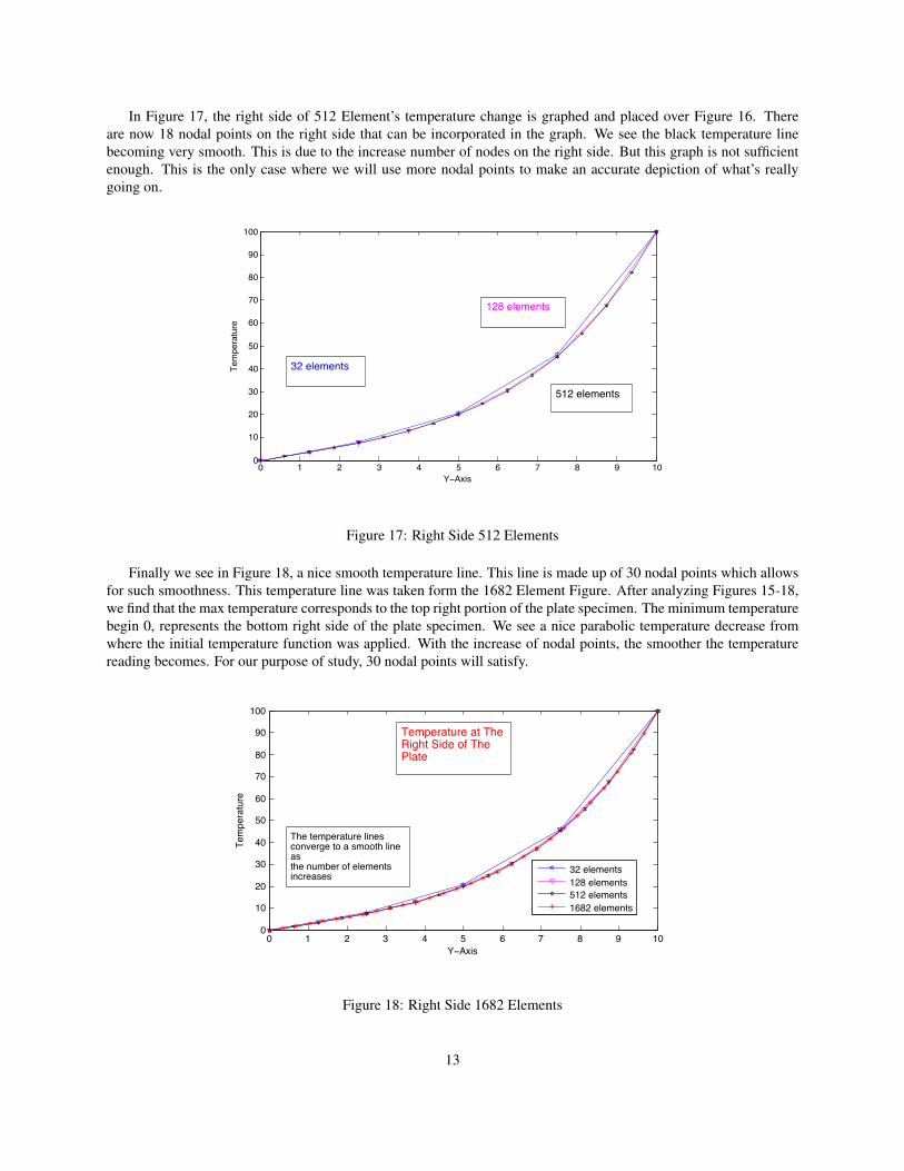
In Figure 17, the right side of 512 Element’s temperature change is graphed and placed over Figure 16. Thereare now 18 nodal points on the right side that can be incorporated in the graph. We see the black temperature linebecoming very smooth. This is due to the increase number of nodes on the right side. But this graph is not sufficientenough. This is the only case where we will use more nodal points to make an accurate depiction of what’s reallygoing on.

0 1 2 3 4 5 6 7 8 9 100

10

20

30

40

50

60

70

80

90

100

Y!Axis

Te

mpera

ture

32 elements

128 elements

512 elements



Finally we see in Figure 18, a nice smooth temperature line. This line is made up of 30 nodal points which allowsfor such smoothness. This temperature line was taken form the 1682 Element Figure. After analyzing Figures 15-18,we find that the max temperature corresponds to the top right portion of the plate specimen. The minimum temperaturebegin 0, represents the bottom right side of the plate specimen. We see a nice parabolic temperature decrease fromwhere the initial temperature function was applied. With the increase of nodal points, the smoother the temperaturereading becomes. For our purpose of study, 30 nodal points will satisfy.

0 1 2 3 4 5 6 7 8 9 100

10

20

30

40

50

60

70

80

90

100

Y!Axis

Tem

pe

ratu

re

32 elements

128 elements

512 elements

1682 elements

Temperature at TheRight Side of ThePlate

The temperature linesconverge to a smooth lineasthe number of elementsincreases



13

9 Future WorkDue to time constraints, our work has been put on hold. There are no limitations with Finite Element Structuring.Most engineering designs if not all designs can be modeled using some computer language. Our work was producedusing Matlab and Octave. But FEA is not limited to these computer programs.

I would like to see our work continued. My research team has decided we should make a hole in our specimenand then study the temperature distribution throughout. This plate specimen was produced in its most simplest form,in order to walk you have to crawl. I would like to see how square elements compare to triangle elements. Throughresearch has shown and also through simple geometry, triangle should prove to be superior.

To reenforce our initial question asked in section 4 Application of Research, ”What is the purpose for the study ofSteady State Temperature Distribution?” With our current study conducted, my teammates and I were able to producevaluable data which can be used for real world applications. Assignments cannot be assigned without following certainparameters. Once parameters have been set, a team of engineers, scientists, mathematicians are able to decipher theproblem.

The data provided was produced using Matlab and Octave. Without these mathematical computer programs, nonof our work could have been produced. We have proven that triangle elements are best for mapping 2-D models.

10 References

10.1

70 ’ s , The E a r l y . ” I n t r o d u c t i o n t o F i n i t e Element A n a l y s i s . ” Va Tech −

Lab f o r S c i e n t i f i c V i s u a l A n a l y s i s . Web . 04 Aug . 2010 .

<h t t p : / / www. sv . v t . edu / c l a s s e s / MSE2094 NoteBook / 9 7 C l a s s P r o j /

num / widas / h i s t o r y . html >.

10.2

” Thermal C o n d u c t i v i t y . ” Wikipedia , t h e F ree E n c y c l o p e d i a .

Web . 04 Aug . 2010 . <h t t p :

en . w i k i p e d i a . o rg / w ik i / T h e r m a l c o n d u c t i v i t y >.

14

matrix structural analysis · matrix structural analysis giuliano basile august 5, 2010 abstract...

Documents