matlab for finance - lmu

Part 4:Christian Groll, August 2011.

Seminar für Finanzökonometrie, Ludwig-Maximilians-Universität München.

All rights reserved.

Contents

Required functionsMonte Carlo simulationApplication to real dataVaRBacktestingSimulation study: empirical quantilesAutoregressive processesFitting AR(2) processesGARCH(1,1)

Although the previous parts of the script shall not be understood as rigorousscientific investigation of the topics treated, they nevertheless demonstrate somefirst indications that simple regression models or curve fitting techniques do notprovide the desired information gains in financial applications. The deterministicand predictable part of stock prices is usually too small, compared with the largeuncertainty that is involved. Hence, stock market prices are commonly perceived asstochastic, so that they are best described in the framework of probability theory.This part of the course shall introduce some of the basic concepts used to capturethe stochasticity in stock prices.

Required functions

garchestimation

Monte Carlo simulation

As part of the standard MATLAB program the function rand() enables simulation ofuniformly distributed pseudo random variables. This is one of the most importanttools for financial econometrics. However, the key to understanding this importanceis to understand that these uniformly distributed simulated values can betransformed to samples of any given distribution function by a simpletransformation.

% init paramsn = 1000; % sample sizenBins = 20; % number of points per bin

% simulate from uniform distributionU = rand(n,1);

% check appropriatenesshist(U,nBins)

% calculate expected number of bins

expNum = n/nBins;

% include horizontal line at expected number of points per binline([0 1],expNum*[1 1],'Color','r')title(['sample size: ' num2str(n) ' / expected points per bin: '... num2str(expNum)])

In order to simulate random numbers of different distributions, one has to makeuse of the fact that the inverse cumulative distribution function F^(-1), applied to auniformly distributed random variable U, generates a random vector withcumulative distribution equal to F. This theorem is called inverse probability integraltransformation (PIT), and can be best understood by looking at a graphicalvisualization. Here, we use the normal distribution as an example.

% init paramsn2 = 10; % sample sizemu = 4; % params distributionsigma = 1;

% show first n2 points of U on y-axisclosescatter(zeros(n2,1),U(1:n2),'r.')hold on;

% plot cumulative distribution functiongrid = 0:0.01:8;vals = normcdf(grid,mu,sigma);plot(grid,vals)

% scatter resulting values after inverse PITX = norminv(U,mu,sigma);scatter(X(1:n2),zeros(n2,1),'r.')

% plot lines between points to indicate relationfor ii=1:n2 % horizontal line, beginning in uniform sample point line([0 X(ii)],[U(ii) U(ii)],'Color','r','LineStyle',':')

% vertical line, beginning in new point, up to function line([X(ii) X(ii)],[0 U(ii)],'Color','r','LineStyle',':')endtitle('Inverse probability integral transformation')

As can be seen, points in the middle of the [0 1] interval encounter a very steepslope of the cumulative distribution function, so that the distances between thosepoints are effectively reduced. Hence, the associated area on the x-axis will exhibitan accumulation of sample points. In contrast to that, points in the outer quantilesof the distribution will encounter a very shallow slope, and hence will be takenfurther apart of each other.

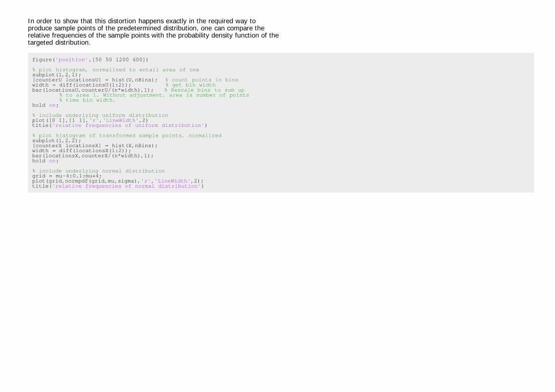
In order to show that this distortion happens exactly in the required way toproduce sample points of the predetermined distribution, one can compare therelative frequencies of the sample points with the probability density function of thetargeted distribution.

figure('position',[50 50 1200 600])

% plot histogram, normalized to entail area of onesubplot(1,2,1);[counterU locationsU] = hist(U,nBins); % count points in binswidth = diff(locationsU(1:2)); % get bin widthbar(locationsU,counterU/(n*width),1); % Rescale bins to sum up % to area 1. Without adjustment, area is number of points % time bin width.hold on;

% include underlying uniform distributionplot([0 1],[1 1],'r','LineWidth',2)title('relative frequencies of uniform distribution')

% plot histogram of transformed sample points, normalizedsubplot(1,2,2);[counterX locationsX] = hist(X,nBins);width = diff(locationsX(1:2));bar(locationsX,counterX/(n*width),1);hold on;

% include underlying normal distributiongrid = mu-4:0.1:mu+4;plot(grid,normpdf(grid,mu,sigma),'r','LineWidth',2);title('relative frequencies of normal distribution')

Hence, given any distribution function, we now are capable of simulating samples ofit. However, in practice we usually encounter a different problem : we observesome data, but do not know the underlying distribution function, which has to beestimated based on the data.

We will now implement code to estimate the parameters of a given distributionfunction based on maximum likelihood. In order to get an impression of how goodthe estimation step performs, we will adapt it to simulated data with knownunderlying distribution first.

The likelihood of a given sample point is defined as the value of the probabilitydensity function. Furthermore, the likelihood of a given sample with more than onepoint is defined as the product of the individual likelihoods.

% init params examplen = 1000; % number sample pointsmu = 2;sigma = 1;points = normrnd(mu,sigma,n,1); % simulate data points

% likelihood first point onlylh1 = (sigma^2*2*pi)^(-0.5)*exp((-0.5)*(points(1)-mu)^2/sigma^2);fprintf(['\nThe likelihood of the first point is given by '... num2str(lh1) '.\n'])fprintf(['It also can be calculated using an '... 'existing MATLAB function:\n'... 'normpdf(points(1),mu,sigma) = ' ... num2str(normpdf(points(1),mu,sigma))... '.\n'])

The likelihood of the first point is given by 0.23541.It also can be calculated using an existing MATLAB function:normpdf(points(1),mu,sigma) = 0.23541.

% calculate lh for all individual pointslhs = normpdf(points,mu,sigma);

% multiply first k points for each k up to 10cumulatedLikelihoods = cumprod(lhs(1:10))'

cumulatedLikelihoods =

Columns 1 through 7

0.2354 0.0043 0.0011 0.0001 0.0000 0.0000 0.0000

Columns 8 through 10

0.0000 0.0000 0.0000

As can be seen, through multiplication the absolute value of the overall likelihoodbecomes vanishingly small very fast. This imposes numerical problems to theprocess of calculation, since MATLAB only uses a finite number of decimal places.Hence, parameter estimation is always done by maximization of the log-likelihoodfunction. Note that multiplication of individual likelihoods becomes summationunder the transformation to log-likelihoods.

% calculate log-likelihood for sample pointsllh = -0.5*log(sigma^2*2*pi)-0.5*(points-mu).^2/sigma^2;

% show cumulate sumcumulatedSum = cumsum(llh(1:10))'

cumulatedSum =

Columns 1 through 7

-1.4464 -5.4394 -6.8403 -9.5368 -10.9840 -11.9535 -16.6205

Columns 8 through 10

-17.5863 -19.1697 -20.1017

As can be seen, using log-likelihood does not cause the same numerical problems.Now, let's create an anonymous function that takes the parameters of the normaldistribution and the sample points as input, and calculates the negative log-likelihood. This function subsequently can be used in the optimization routine.

% anonymous functionnllh = @(params,data)sum(0.5*log(params(2)^2*2*pi)+... 0.5*(data-params(1)).^2/params(2)^2); % note: in order to % fulfill the requirements of the subsequent % optimization, the argument that shall be optimized % has to be given first, with all parameters % contained in one vector!

% check correctness with existing MATLAB functionnegLogLikelihoods = ... [nllh([mu sigma],points) normlike([mu sigma],points)]

negLogLikelihoods =

1.0e+003 *

1.3670 1.3670

Obviously, both values are identical.

Since the parameter sigma of the normal distribution may not take on negativevalues, we are confronted with a constrained optimization problem. Hence, we haveto use the function fmincon.

% simulate random points from normal distributionpoints = normrnd(mu,sigma,1000,1);

% standard normal as first guessparams0 = [0 1];

% specify bounds on parameterslb = [-inf 0.1];ub = [inf inf];

% set options for optimizationopt = optimset('algorithm','interior-point','TolX',1e-14);

% three ways to perform optimization: using anonymous functionparamsHat1 = ... fmincon(@(params)nllh(params,points),params0,... [],[],[],[],lb,ub,[],opt);

% different way, using anonymous functionparamsHat2 =... fmincon(nllh,params0,... [],[],[],[],lb,ub,[],opt,points);

% using existing MATLAB functionparamsHat3 =... fmincon(@(params)normlike(params,points),params0,... [],[],[],[],lb,ub,[],opt);

% showing wrong syntax using existing functiontry paramsHat4 =... fmincon(normlike,params0,...

[],[],[],[],lb,ub,[],opt,points);catch err fprintf(['MATLAB displays the following error:\n"'... err.message '"\n']);end

Local minimum possible. Constraints satisfied.

fmincon stopped because the size of the current step is less thanthe selected value of the step size tolerance and constraints are satisfied to within the default value of the constraint tolerance.





MATLAB displays the following error:"Requires two input arguments"

While the first three optimization calls stop regularly, the fourth syntax produces anerror as predicted. Comparison of the estimated parameters of the successfuloptimizations show equally good results for all three.

% compare results of different optimizations with real valuescompareToRealParams = [mu sigma; paramsHat1; ... paramsHat2; paramsHat3]

compareToRealParams =

2.0000 1.0000 1.9416 1.0029 1.9416 1.0029 1.9416 1.0029

Now that we successfully estimated the underlying normal distribution, we want totry the same estimation procedure for a Student's t-distribution.

% init paramsn = 1000;nu = 4;

% simulate values per inverse PITX = tinv(rand(n,1),nu);

% determine individual likelihoods for vector of observations

lh = @(nu,X)gamma((nu+1)/2)*(nu*pi)^(-0.5)/gamma(nu/2)... *(1+X.^2/nu).^(-(nu+1)/2);

Note: function lh returns a vector itself. See for example:

outputDimension = size(lh(4,X))

outputDimension =

1000 1

Define function nllh_t that calculates the negative overall log-likelihood based onthe output of function lh.

% taking log of each entry and summing upnllh_t = @(nu,X)-sum(log(lh(nu,X)));

Specify optimization settings and conduct optimization.

% init guessparam0 = 10;

% boundary constraintslb = 0.1;ub = inf;

% optimizationparamHat = fmincon(nllh_t,param0,[],[],[],[],... lb,ub,[],[],X);

Warning: Trust-region-reflective algorithm does not solve this type ofproblem, using active-set algorithm. You could also try the interior-pointor sqp algorithms: set the Algorithm option to 'interior-point' or 'sqp'and rerun. For more help, see Choosing the Algorithm in the documentation.


fmincon stopped because the predicted change in the objective functionis less than the default value of the function tolerance and constraints are satisfied to within the default value of the constraint tolerance.

No active inequalities.

Note that MATLAB displays a warning message, indicating that the currently usedsearching algorithm might not be accurate. You can switch to any of the suggestedalgorithms by changing the respective property of the optimization options structrevia optimset(). Nevertheless, the results obtained are not too bad after all.

% compare with real parametercompareToRealParam = [nu paramHat]

compareToRealParam =

4.0000 3.7095

Application to real data

Now we want to examine whether observed returns in the real world approximatelyfollow a normal distribution. As first example we will chose the German stockmarket index for our investigation.

% specify ticker symbol as string variabletickSym = '^GDAXI'; % specify stock data of interest

% specify beginning and ending as string variablesdateBeg = '01011990'; % day, month, year: ddmmyyyydateEnd = datestr(today,'ddmmyyyy'); % today as last date

% load dataDAX_crude = hist_stock_data(dateBeg,dateEnd,tickSym);

% process data[DAX.dates DAX.prices] = processData(DAX_crude);

% calculate percentage log returnsDAX.logRet = 100*(log(DAX.prices(2:end))-log(DAX.prices(1:end-1)));

Fitting parameters of normal distribution to data.

% init boundslb = [-inf 0.001];ub = [inf inf];

% optimization settingsopt = optimset('display','off','algorithm','sqp');

% estimate normal distribution parametersparamsHat = ... fmincon(nllh,params0,... [],[],[],[],lb,ub,[],opt,DAX.logRet);

% compare parameters with estimation from existing function[muHat sigmaHat] = normfit(DAX.logRet);paramComparison = [paramsHat; muHat sigmaHat]

paramComparison =

0.0242 1.4609 0.0242 1.4611

In order to examine the goodness-of-fit of the estimated normal distribution, somevisualizations can be helpful. First, a normalized histogram of the data shall becompared to the probability density function of the fitted distribution. Moreover, asthe largest financial risks are located in the tails of the distribution, the figure alsoshall show a more amplified view on the lower tail.

% show normalized histogram with density of normal distribution[counterX locationsX] = hist(DAX.logRet,50);

width = diff(locationsX(1:2));

% show bar diagram in first subplotfigure('position',[50 50 1200 600])subplot(1,2,1);bar(locationsX,counterX/(numel(DAX.logRet)*width),1);hold on;

% init gridgrid =... paramsHat(1)-5*paramsHat(2):0.01:paramsHat(1)+5*paramsHat(2);

% include underlying normal distributionplot(grid,normpdf(grid,paramsHat(1),paramsHat(2)),... 'r','LineWidth',2);title('relative frequencies with normal distribution')

% show lower tail region amplifiedsubplot(1,2,2);hold on;bar(locationsX,counterX/(numel(DAX.logRet)*width),1);plot(grid,normpdf(grid,paramsHat(1),paramsHat(2)),... 'r','LineWidth',2);axis([paramsHat(1)-7*paramsHat(2) paramsHat(1)-2*paramsHat(2)... 0 0.02])title('lower tail')hold off

As the amplification of the comparison of the lower tails shows, the relativefrequency of extremely negative realizations is much larger than what would besuggested by the normal distribution. This indicates that the shape of the normaldistribution is not able to provide a good fit to the realizations of stock returnsobserved. Another way to visualize the deviations between normal distributionmodeling and reality is the QQ-plot.

In order to compare the quantiles of the empirical returns with the quantiles of agiven distribution function using MATLAB's qq-plot function, we need to specify therespective distribution by handing over simulated sample points with givendistribution.

close % close previous figurefigure('position',[50 50 1200 600])subplot(1,2,1)

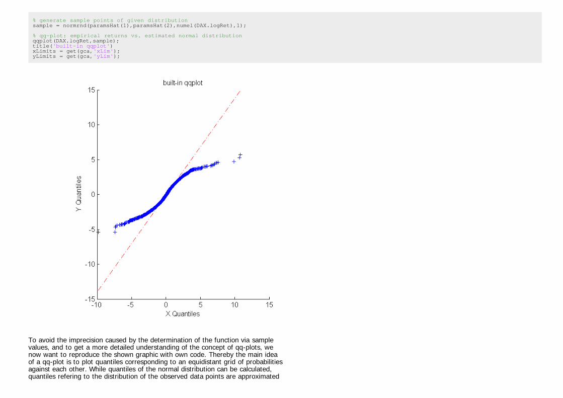
% generate sample points of given distributionsample = normrnd(paramsHat(1),paramsHat(2),numel(DAX.logRet),1);

% qq-plot: empirical returns vs. estimated normal distributionqqplot(DAX.logRet,sample);title('built-in qqplot')xLimits = get(gca,'xLim');yLimits = get(gca,'yLim');

To avoid the imprecision caused by the determination of the function via samplevalues, and to get a more detailed understanding of the concept of qq-plots, wenow want to reproduce the shown graphic with own code. Thereby the main ideaof a qq-plot is to plot quantiles corresponding to an equidistant grid of probabilitiesagainst each other. While quantiles of the normal distribution can be calculated,quantiles refering to the distribution of the observed data points are approximated

with the respective empirically estimated values.

% arrange entries in chronological ordersorted = sort(DAX.logRet);

% init grid of equidistant probabilitiesassociatedCDFvalues = ((1:numel(sorted))/(numel(sorted)+1));

% associated ecdf values increase with fixed step sizeformat ratassociatedCDFvalues(1:4)format short

ans =

1/5261 2/5261 3/5261 4/5261

% get associated normal quantile valuesconvertToNormalQuantiles = ... norminv(associatedCDFvalues,paramsHat(1),paramsHat(2));

% generate qq-plotsubplot(1,2,2)scatter(sorted,convertToNormalQuantiles,'+'); shgxlabel('empirical quantiles')ylabel('quantiles normal distribution')set(gca,'xLim',xLimits,'yLim',yLimits);title('manually programmed qq-plot')

% include straight line to indicate matching quantilesline(xLimits,xLimits,'LineStyle','-.','Color','r')

Again, the qq-plot shows that the empirical quantiles in the lower tail are lowerthan suggested by the normal distribution. This is a commonly observable patternof financial data, and it is refered to as fat tails.

VaR

With these insights in mind, we now want to estimate the value-at-risk for theGerman stock index. The value-at-risk associated with a given asset is nothing elsethan a lower quantile of the distribution of returns. Hence, a value-at-risk ofconfidence level 95% denotes nothing else than a return level that is fallen short ofat maximum 5% of the times. This value will be estimated on three different ways.

% init different value-at-risk confidence levelsquants = [0.005 0.01 0.05];

% estimate VaR based on fitted values of normal distributionVaR_norm = norminv(quants,paramsHat(1),paramsHat(2));

Estimate DoF parameter for Student's t-distribution.

% determine individual likelihoods for a points vectorlh = @(nu,X)gamma((nu+1)/2)*(nu*pi)^(-0.5)/gamma(nu/2)... *(1+X.^2/nu).^(-(nu+1)/2);

% define function taking log of each entry and summing upnllh_t = @(nu,X)-sum(log(lh(nu,X)));

% init guessparam0 = 10;

% boundary constraintslb = 0.1;ub = inf;

% set options for optimizationopt = optimset('algorithm','sqp');

% optimizationparamHat_t = fmincon(nllh_t,param0,[],[],[],[],... lb,ub,[],opt,DAX.logRet);


fmincon stopped because the size of the current step is less thanthe default value of the step size tolerance and constraints are satisfied to within the default value of the constraint tolerance.

Associated value-at-risk estimations are given as the quantiles of the fittedStudent's t-distribution and can be calculated by inversion.

% apply inverse cumulative distribution functionVaR_t = icdf('t',quants,paramHat_t);

As third alternative, the value-at-risk can be estimated directly based on theobserved returns as empirical quantiles.

% estimate VaR based on empirical quantilesVaR_emp = quantile(DAX.logRet,quants);

% compare different VaR estimationscompareVaRs = [quants' VaR_norm' VaR_t' VaR_emp']

% display labels of columns belowfprintf('\nConfLevels Norm Distr T Distr Emp Quants\n')

compareVaRs =

0.0050 -3.7389 -5.1008 -5.2897 0.0100 -3.3744 -4.0705 -4.5215 0.0500 -2.3788 -2.2252 -2.3215

ConfLevels Norm Distr T Distr Emp Quants

As can be seen, the estimated values of VaR are quite different for differentestimators. In contrast to the normal distribution, the Student's t-distributionassigns more probability to tail regions, which results in more extreme quantilevalues. However, this result does not yet automatically imply that a Student's t-distribution is the more appropriate distribution. In order to check both distributionsfor their goodness, we have to compare them in a backtesting procedure.

Backtesting

For reasons of space we want to conduct the visual analysis only for one level ofconfidence. However, figures of the other confidence levels easily can be accessedthrough changing the determining index variable lev.

% init confidence level as index of variable quantslev = 2;

figure('position',[50 50 1200 600]);

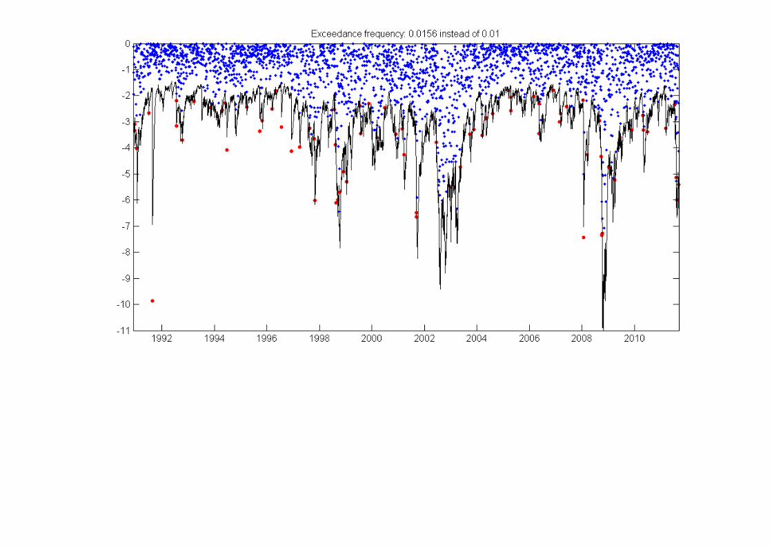
% show exceedances for normal distributionsubplot(1,2,1);

% indicate exceedances with logical vectorexceed = DAX.logRet <= VaR_norm(lev);

% show exceedances in redscatter(DAX.dates([logical(0); exceed]),DAX.logRet(exceed),'.r') % first date entry left out since DAX.dates refers to % longer time series of priceshold on;

% show non-exceedances in bluescatter(DAX.dates([logical(0); ~exceed]),... DAX.logRet(~exceed),'.b')datetick 'x'set(gca,'xLim',[DAX.dates(2) DAX.dates(end)]);

% include VaR estimationline([DAX.dates(2) DAX.dates(end)],VaR_norm(lev)*[1 1],... 'Color','k')title(['Exceedance frequency ' ... num2str(sum(exceed)/numel(DAX.logRet),2) ' instead of '... num2str(quants(lev))])

% same plot with results based on Student's t-distributionsubplot(1,2,2);exceed2 = DAX.logRet <= VaR_t(lev);scatter(DAX.dates([logical(0); exceed2]),... DAX.logRet(exceed2),'.r')hold on;scatter(DAX.dates([logical(0); ~exceed2]),... DAX.logRet(~exceed2),'.b')datetick 'x'set(gca,'xLim',[DAX.dates(2) DAX.dates(end)]);line([DAX.dates(2) DAX.dates(end)],VaR_t(lev)*[1 1],... 'Color','k')title(['Exceedance frequency ' ... num2str(sum(exceed2)/numel(DAX.logRet),2) ' instead of '... num2str(quants(lev))])

For further investigation of the goodness of the respective estimation approaches,all exceedance frequencies are compared to in a table.

% calculate exceedance frequencies for normal distributionnormFrequ = ... [sum((DAX.logRet <= VaR_norm(1))/numel(DAX.logRet));... sum((DAX.logRet <= VaR_norm(2))/numel(DAX.logRet));... sum((DAX.logRet <= VaR_norm(3))/numel(DAX.logRet))];

% calcualte exceedance frequencies for Student's t-distributiontFrequ = ... [sum((DAX.logRet <= VaR_t(1))/numel(DAX.logRet));... sum((DAX.logRet <= VaR_t(2))/numel(DAX.logRet));... sum((DAX.logRet <= VaR_t(3))/numel(DAX.logRet))];

% calculate exceedance frequencies for empirical quantilesempFrequ = ... [sum((DAX.logRet <= VaR_emp(1))/numel(DAX.logRet));... sum((DAX.logRet <= VaR emp(2))/numel(DAX.logRet));...

sum((DAX.logRet <= VaR_emp(3))/numel(DAX.logRet))];

% display tablefprintf('\nExceedance frequencies:\n')fprintf('Norm distr t distr Emp distr\n')for ii=1:numel(quants) fprintf('%1.5f %1.5f %1.5f\n',... normFrequ(ii),tFrequ(ii),empFrequ(ii));end

Exceedance frequencies:Norm distr t distr Emp distr0.01540 0.00646 0.004940.02015 0.01274 0.010080.04753 0.05532 0.05000

This analysis shows two commonly observable characteristics. First, the exceedancefrequencies associated with the empirical estimator are almost exactly the size thatwe want to observe. However, this should not lead you to erroneously concludethat the empirical estimator is unambiguously the best estimator, since the perfectfit is only achieved in-sample, that is it is achieved only on the data that we usedfor estimation. This is a classical overfitting problem, since we adjusted theestimated quantiles to exactly match the observed data points in the first place.Examining the out-of-sample properties of the empirical estimator will show that itis not performing equally well when applied to "unseen" data.

And second, while all three estimators seem to approximately match the demandedexceedance frequencies, the occurrences of the exceedances are clustered throughtime. That is, exceedances are not distributed uniformly over time, but observingan exceedance at one day increases the likelihood of an additional exceedancewithin the next days. This weakness of all estimators arises from the fact that wedropped all information of the sample with respect to the time dimension, since wetreated returns as i.i.d. realizations of a certain random variable. Hence, estimatingrisk more adequately requires modeling the observations as time series in order tobe able to match temporarily evolving high-volatility phases.

Simulation study: empirical quantiles

In order to examine the properties of the empirical quantiles estimator we now willperform a short simulation study. The idea is to sample observations of a givendistribution function, apply the empirical quantiles estimator to the sample data,and check whether we are able to approximately retrieve the quantile values of theoriginal underlying distribution.

% init paramsreps = 10000; % number of repetitionssampSize = 2500; % approximately 10 years of datadist = 't'; % underlying distributionparam = 5; % parameters: dimension depending on distr.nBins = 30; % number of bins in histogram plot

% get real quantile valuesrealQuants = icdf(dist,quants,param);

% preallocate result matrixestQuants = zeros(reps,numel(quants)); % for each repetition we % will get estimated values for each confidence level

% using for-loop, because of limited memoryfor ii=1:reps % simulate data sample U = rand(sampSize,1); sampData = icdf(dist,U,param);

% get empirical quantiles for this repetition estQuants(ii,:) = quantile(sampData,quants);end

% plot resultsfigure('position',[50 50 1200 600])for ii=1:numel(quants) subplot(1,numel(quants),ii); hist(estQuants(:,ii),nBins)

% include line indicating real quantile value yLimits = get(gca,'yLim'); line(realQuants(ii)*[1 1],yLimits,'Color','r')

% calculate mean squared error MSE = sum((estQuants(:,ii)-realQuants(ii)).^2)/reps;

title(['Quantile: ' num2str(quants(ii),2) ', MSE: ' ... num2str(MSE,3)])end

As indicated by the mean squared error as well as by the different scales of the x-axis, the goodness of the empirical quantile estimator decreases with decreasingquantile values. This is no surprise, since a sample of size 2500 on average onlyproduces 12.5 observations below it's 0.005 quantile. Since the number of expectedobservations below the quantile value is the relevant size to the estimationprocedure, the average performance of the estimator is rather poor.

Autoregressive processes

The main idea of time series analysis is to not consider observations as independentover time, but to admit an effect of past returns to the distribution of todays return.The most common way thereby is to render first and second moments conditional.We will start with time-varying first moments. A very helpful device to detect serialdependence is to estimate the autocorrelation function of the process.

% init paramsnLags = 20; % number of lags

% estimate autocorrelation functionautoCorrCoeff = zeros(1,nLags);for ii=1:nLags % get correlation between days of distance ii autoCorrCoeff(ii) = ... corr(DAX.logRet(1:end-ii),DAX.logRet(ii+1:end));end

% plot estimated autocorrelation functionclosefigure('position',[50 50 1200 600])subplot(1,2,1)stem(1:nLags,autoCorrCoeff,'r.','MarkerSize',12)set(gca,'yLim',[-0.2 1]);set(gca,'xGrid','on','yGrid','on')

% plot autocorrelation using existing MATLAB functionsubplot(1,2,2)autocorr(DAX.logRet)

Though there might be evidence for autocorrelation at lags 3 and 4, there is ratherno clear pattern observable. We now will try to replicate the observedautocorrelation function. First, we will investigate the properties of an AR(1)process by simulating a sample path of it.

% init paramsa = 0.4; % autoregression coefficientn = 10000; % path lengthsigma = 0.8; % standard deviation residualY0 = 0; % starting value

% simulate dataepsilons = normrnd(0,sigma,n,1);Y = zeros(n,1);Y(1,1) = Y0;

% because of the recursive nature of autoregressive processes we% have to use for-loop

for ii=2:n Y(ii) = a*Y(ii-1)+epsilons(ii);end

% plot pathclosefigure('position',[50 50 1200 600])subplot(1,2,1);plot(Y(1:150))title('Simulated sample path')

% plot associated empirical autocorrelation functionsubplot(1,2,2);autocorr(Y)

As can be seen, the autoregressive term of lag 1 causes a significant non-zeroautocorrelation function in both first two lags. Since we observed a negative thirdlag and positive fourth lag, we will take a look at a fourth order autoregressive

process.

% init paramsa3 = -0.1;a4 = 0.1;Y0 = 0;Y1 = 0;Y2 = 0;Y3 = 0;

% simulate dataepsilons = normrnd(0,sigma,n,1);Y = zeros(n,1);Y(1:4,1) = [Y0; Y1; Y2; Y3];

for ii=5:n Y(ii) = a3*Y(ii-3)+a4*Y(ii-4)+epsilons(ii);end

% plot sample pathclosefigure('position',[50 50 1200 600])subplot(1,2,1);plot(Y(1:150))title('simulate sample path')

% plot empirical autocorrelation functionsubplot(1,2,2);autocorr(Y)

As both graphics indicate, there lies a great flexibility in AR-processes when itcomes to replicating first-moment features of real data. However, it is very difficultto distinguish between stochastically evolved artificial patterns and real existingautocorrelated structures.

% Although the empirical autocorrelation function seems to% indicate that AR-processes could be able to replicate some% first-moment characteristics of observable financial time% series, there are some considerable differences in% the patterns of the second moments. One way to see this is by% looking at the empirical autocorrelation functions of squared% returns.

% compare autocorrelation functions of squared returnsclosefigure('position',[50 50 1200 600])subplot(1,2,1);autocorr(DAX.logRet.^2)

title('real data')subplot(1,2,2)autocorr(Y.^2)title('simulated AR-data')

As can be seen, squared returns exhibit long-lasting and persistentautocorrelations. This result can be interpreted as follows: correlation betweensquared returns is an indication of correlation between absolute return sizes. Thatis, if we observe high absolute returns at previous days, there is a high likelihood ofa high absolute return for today, too. In other words: if previous returns exhibithigh volatilities (high absolute values), today's absolute return is more likely to behigh itself, while low volatility of previous days is likely to be followed by a returnwith small absolute value itself. This observation matches with the volatility clustersobserved before.

Fitting AR(2) processes

This is part of the homework.

GARCH(1,1)

Since autoregressive processes are not able to replicate the persistent volatilitiesobservable at financial time series, we need to come up with another model, calledGARCH (generalized autoregressive conditional heteroscedasticity). The ideaassociated with GARCH models is to render second moments conditional. That is,the model shall capture the pattern of financial time series that periods of highvolatility are followed more likely by another high absolute return. Hence, themodel treats the volatility prevailing at a certain point in time as conditional on thepast realizations, with positive relationship between past volatility and conditionalcurrent volatility. Today's variance h(t) is modelled as linear function of yesterday'svariance h(t-1) and yesterday's squared observation Y(t-1).^2.

Y(t) = sqrt(h(t))*epsilon(t) h(t) = k + GARCH*h(t-1) + ARCH*Y(t-1)^2

In order to get a first impression about the model, we will first simulate some datawith given parameters.

Since conditional distributions depend on yesterday's observation and standarddeviation, the first simulated value of our path also needs some specification of thevalues of the previous days.

% starting valuesY0 = 0;sigma0 = 1;

% init paramssampSize = 10000; % path length

% GARCH parameters: h(t)=k+GARCH*h(t-1)+ARCH*Y(t-1)^2GARCH = 0.6;ARCH = 0.2;k = 0.2;

% preallocate Y and sigmaY = zeros(sampSize,1);sigmas = zeros(sampSize,1);

% simulate standardized residualsepsilons = randn(sampSize,1);

% take first values as givenY(1) = Y0;sigmas(1) = sigma0;

for ii=2:sampSize % calculate new sigma sigmas(ii) = ... sqrt(k+GARCH*sigmas(ii-1)^2 + ARCH*Y(ii-1)^2);

% multiply standardized residual with current standard dev. Y(ii) = epsilons(ii)*sigmas(ii);end

% visualization of simulated data patternsclosefigure('position',[50 50 1200 800])

% show sample pathsubplot(3,2,1:2);plot(Y(1:600))title('sample path')

% show simulated series of conditional standard deviationssubplot(3,2,3:4);plot(sigmas(1:600))title('conditional standard deviations')

% show autocorrelation functionssubplot(3,2,5);autocorr(Y)title('autocorr returns')set(gca,'yLim',[-0.2 0.6]);subplot(3,2,6);autocorr(Y.^2)set(gca,'yLim',[-0.2 0.6]);title('autocorr squared returns')

When looking at the visualization, some points become evident. First, the timeseries does exhibit volatility clusters of small scale. While there do appear shortperiods with relatively high standard deviations, the high volatility phases seem to

disappear faster than in reality. And second, the model in general seems to beappropriate to generate persistent dependencies in absolute returns, measurablethrough the autocorrelation function applied to squared returns. Nevertheless, thepersistency measured with the autocorrelation also drops faster than forcomparable real data.

To break away from the distortions incorporated by arbitrarily chosing theparameters of the model, we now want to fit a GARCH model to empirical data viamaximum likelihood. However, in order to get a better understanding about theindividual steps of the fitting procedure, we first implement some stand-alone partsfor simulated data.

% determine time seriestSeries = Y;

% treat initial standard deviation and parameters as giveninitSigma = 1;params = [k GARCH ARCH];

The main point here is that once we are given the time series, the parametervalues and the initial standard deviation, we are able to reconstruct the series ofsigmas.

% preallocate reconstructed sigmasretrieveSigmas = zeros(numel(tSeries),1);retrieveSigmas(1) = initSigma;

% reconstructionfor ii=2:numel(tSeries) % current sigmas depend on last sigma and last observation % through parameter values of the model retrieveSigmas(ii) = sqrt(params(1)+... params(2)*retrieveSigmas(ii-1)^2 + ... params(3)*tSeries(ii-1)^2);end

As verification, sigmas of simulated time series can be compared with thosereconstructed.

figure('position',[50 50 1200 600])subplot(2,1,1);plot(sigmas)title('simulated sigmas')subplot(2,1,2);plot(retrieveSigmas)title('retrieved sigmas')

Given the reconstructed series of time-varying sigma values, we now can calculatethe log-likelihood of the observed time series. Thereby observations are assumed tobe conditionally normally distributed with standard deviation given by sigma.

% calculate negative log-likelihoodnllh = sum(0.5*log(retrieveSigmas.^2*2*pi)+... 0.5*(tSeries.^2./retrieveSigmas.^2));

Since the series of retrieved sigmas depends on the selection of parameters andinitial values, the negative log-likelihood also is influenced by these inputs. Hence,we can come up with a two-step estimation procedure, where in a first step theseries of sigmas is retrieved, and in a second step the associated negative log-likelihood is calculated. Bundling both steps in one function, we get an objectivefunction usable for optimization. This function is implemented as garchEstimation().

Now we will perform the estimation of the GARCH parameters.

% init paramsparams0 = [0.1 0.1 0.1];

% linear parameter restrictions: params(2)+params(3)<1A = [0 1 1];b = 1;

% lower and upper boundslb = [0.01 0.01 0.01];ub = [0.99 0.99 0.99];

% init valsdata = Y;initVals = [0 1];

% optimization settingsopt = optimset('algorithm','sqp');

% optimizationparamsHat = fmincon(... @(params)garchEstimation(params,data,initVals),params0,... A,b,[],[],lb,ub,[],opt);

compareToRealParams = [paramsHat; params]



compareToRealParams =

0.2122 0.5617 0.2241 0.2000 0.6000 0.2000

Given our estimated values we are again able to extract a series of sigma values.These extracted sigma values give us an indication of whether there have beenperiods of high volatility in the time series or not. The following cell will perform thesame analysis for real stock data.

% specify datadata = DAX.logRet;

% optimization settingsopt = optimset('algorithm','sqp');

% optimization[paramsHat nllhVal] = fmincon(... @(params)garchEstimation(params,data,initVals),params0,... A,b,[],[],lb,ub,[],opt);

% extract estimated sigma seriesretrieveSigmas = zeros(numel(data),1);retrieveSigmas(1) = initVals(2);

% reconstructionfor ii=2:numel(data) % current sigmas depend on last sigma and last observation

% through parameter values of the model retrieveSigmas(ii) = sqrt(paramsHat(1)+... paramsHat(2)*retrieveSigmas(ii-1)^2 + ... paramsHat(3)*data(ii-1)^2);end

% plot observed values with extracted sigmasclosefigure('position',[50 50 1200 600])

subplot(2,1,1);plot(DAX.dates(2:end),DAX.logRet)datetick 'x'set(gca,'xLim',[DAX.dates(2) DAX.dates(end)]);

subplot(2,1,2);plot(DAX.dates(2:end),retrieveSigmas)datetick 'x'set(gca,'xLim',[DAX.dates(2) DAX.dates(end)]);



Since GARCH is one of the most important models in econometrics, all the standardapplications associated with the model are already implemented in theeconometrics toolbox of MATLAB. The framework is built on specification of GARCHmodels using a structure variable, which is the basic component to pass over modelspecifications between functions. As default model MATLAB has chosen the sameGARCH(1,1) model with constant in the variance equation that we already havechosen above, with the one deviation that it also incorporates a constant term inthe mean equation. However, we fit the default model to data without furtherspecifications and compare it with our results so far.

% maximum likelihood estimation of parameters[Coeff,Errors,LLF,Innovations,Sigmas,Summary] = ... garchfit(DAX.logRet);

____________________________________________________________ Diagnostic Information

Number of variables: 4

Functions Objective: internal.econ.garchllfn Gradient: finite-differencing Hessian: finite-differencing (or Quasi-Newton) Nonlinear constraints: armanlc Gradient of nonlinear constraints: finite-differencing

Constraints Number of nonlinear inequality constraints: 0 Number of nonlinear equality constraints: 0 Number of linear inequality constraints: 1 Number of linear equality constraints: 0 Number of lower bound constraints: 4 Number of upper bound constraints: 4

Algorithm selected medium-scale: SQP, Quasi-Newton, line-search

____________________________________________________________ End diagnostic information

Max Line search Directional First-order Iter F-count f(x) constraint steplength derivative optimality Procedure 0 5 8883.5 -0.05 1 16 8845.19 -0.06484 0.0156 -532 3.65e+003 2 24 8735.86 -0.08613 0.125 -1.51e+003 3.02e+003 3 34 8711.46 -0.1147 0.0313 -744 2.22e+003 4 43 8691.87 -0.1075 0.0625 -462 1.93e+003 5 49 8623.43 -0.07637 0.5 -424 1.65e+003 6 55 8579.06 -0.03819 0.5 -781 1.18e+003 7 66 8576.88 -0.03759 0.0156 -272 2.07e+003 8 72 8561.17 -0.01879 0.5 -368 1.05e+003 9 82 8561.07 -0.01984 0.0313 -49.5 228 10 89 8560.52 -0.01724 0.25 -107 80.7 11 94 8560.51 -0.01648 1 -21.5 74.3 12 99 8560.5 -0.01681 1 -20 1.33 13 104 8560.5 -0.01681 1 -0.425 0.0804


fmincon stopped because the predicted change in the objective functionis less than the selected value of the function tolerance and constraints are satisfied to within the selected value of the constraint tolerance.

No active inequalities.

Displaying the estimated coefficient structure allows comparison with the valuesestimated based on our own functions.

% display coefficient structureCoeff

% own valuesfprintf('\nIn contrast to that, own values are:\n')fprintf(' K: %1.4f\n',paramsHat(1))fprintf(' GARCH: %1.4f\n',paramsHat(2))fprintf(' ARCH: %1.4f\n',paramsHat(3))

% compare log-likelihoodslogLikelihoods = [-nllhVal LLF]

Coeff =

Comment: 'Mean: ARMAX(0,0,0); Variance: GARCH(1,1) ' Distribution: 'Gaussian' C: 0.0629 VarianceModel: 'GARCH' P: 1 Q: 1 K: 0.0331 GARCH: 0.8968 ARCH: 0.0864

In contrast to that, own values are: K: 0.0329 GARCH: 0.8966 ARCH: 0.0870

logLikelihoods =

1.0e+003 *

-8.5706 -8.5605

As the displayed values show, there are no substantial deviations, since theconstant term in the mean equation is rather small. However, the garchfit functionconveniently returns some more outputs, which are useful for furtherinvestigations. For example, previous plots easily can be replicated.

closefigure('position',[50 50 1200 600])subplot(2,1,1)plot(DAX.dates(2:end),DAX.logRet)datetick 'x'set(gca,'xLim',[DAX.dates(2) DAX.dates(end)]);

subplot(2,1,2)plot(DAX.dates(2:end),Sigmas)datetick 'x'set(gca,'xLim',[DAX.dates(2) DAX.dates(end)]);

Furthermore, it is easy to derive the standardized returns, where distortions fromtime-varying conditional first two moments have been extracted. Since thedistribution of these standardized returns is the foundation in our maximumlikelihood estimation procedure, it is reasonable to examine our assumption ofnormally distributed conditional returns.

% init paramsnBins = 30;n = numel(DAX.logRet); % number of observations

% get standardized returnsstdRets = Innovations./Sigmas;

% compare with normal distribution[counterX locationsX] = hist(stdRets,nBins);width = diff(locationsX(1:2));close all

bar(locationsX,counterX/(n*width),1);hold on;

% include best fitting normal distribution[muhat sigmahat] = normfit(stdRets);grid = muhat-4:0.1:muhat+4;plot(grid,normpdf(grid,muhat,sigmahat),'r','LineWidth',2);title('relative frequency normal distribution')

Since the figure does not exhibit substantial deviations, our priorly madeassumption of conditional normally distributed returns seems to be sustainable. Thenext step now is to examine the performance of the GARCH model in a backtestingprocedure.

% preallocate VaR vectorVaRs = zeros(numel(quants),numel(DAX.logRet));

for ii=1:numel(DAX.logRet) % get sigma value curr_sigma = Sigmas(ii); VaRs(:,ii) = norminv(quants',Coeff.C,curr_sigma);end

for ii=1:numel(quants)

% get exceedances exceeds = (DAX.logRet' <= VaRs(ii,:));

% include in figure figure('position',[50 50 1200 600]) plot(DAX.dates([logical(0) ~exceeds]),... DAX.logRet(~exceeds),'.') hold on; plot(DAX.dates([logical(0) exceeds]),... DAX.logRet(exceeds),'.r','MarkerSize',12) datetick 'x' set(gca,'xLim',[DAX.dates(2) DAX.dates(end)],... 'yLim',[floor(min(DAX.logRet))-1 0]);

% include line for VaR estimations hold on; plot(DAX.dates(2:end),VaRs(ii,:),'-k')

% calculate exceedance frequency frequ = sum(exceeds)/numel(DAX.logRet);

title(['Exceedance frequency: ' num2str(frequ,3)... ' instead of ' num2str(quants(ii),3)])end

close all

Published with MATLAB® 7.12

matlab for finance - lmu

Documents