mathematics of granular materials · granular materials are a very trendy subject nowadays, and the...

MATHEMATICS OF GRANULAR MATERIALS

CEDRIC VILLANI

Abstract. This is a short and somewhat informal review on the most mathe-matical parts of the kinetic theory of granular media, intended for physicists andfor mathematicians outside the field.

Contents

Introduction 11. Modelling 22. Maxwellian toolbox 113. Gradient flow structure 194. One-dimensional rigidity 215. True inelastic hard spheres 246. The future of inelastic kinetic theory? 31References 32

Introduction

Granular materials are a very trendy subject nowadays, and the number of pub-lications devoted to it has grown tremendously since the beginning of the nineties.These contributions deal with experiments, modelling, numerical simulations, in-dustrial design as well as theoretical work. Some of the most spectacular effectsappearing in the dynamics of granular gases are reviewed in a short and pedagogicsurvey by Barrat, Trizac and Ernst [3]; they include clustering, spontaneous loss ofhomogeneity, inverse Maxwell Demons, modification of Fourier’s law, violation ofequipartition of energy, and non-Gaussian equilibrium kinetic distributions. Thereis also a recent textbook on the subject by Brilliantov and Poschel [18].

This field constitutes a potential whole new area of applications opening up formathematicians; yet the relevant mathematical literature is still restricted, due tothe extreme theoretical complexity of the subject. The present survey deals withone of the (relatively) most advanced parts of the theory, in which kinetic models areused for granular gases, and interactions are described by inelastic collisions. On thissubject, two short reviews by mathematicians are already available in the publishedliterature: the first one is a concise and very clear introduction by Cercignani [25];the other one was written by the author a few years ago [44, Chapter 5, Section 2].While these references might still be acceptable from the point of view of modellingor the presentation, they are by now obsolete as far as the results are concerned; thisis not surprising since the subject is still very young (the first truly mathematicalpaper about granular collisions is arguably the work by Benedetto, Caglioti and

Date: March 18, 2006.

1

2 CEDRIC VILLANI

Pulvirenti [7], as late as 1997). Here I shall endeavor to fill this gap by presenting atentative up-to-date review of rigorous results in inelastic collisional kinetic theory.The style will be somewhat informal to ensure that the text can be read by a wideaudience; more precise results and statements can be found in the quoted researchpapers, including the two papers by Mischler, Mouhot and Rodriguez Ricard [39, 40]in the present volume.

Although the body of available physics literature is enormous, I decided to keepthe bibliography to the minimum, quoting almost only mathematically oriented pa-pers, most of them in direct relation to the subject, with the main exception of afew review papers like [3]; the interested reader will have no trouble finding physicaldocumentation by starting with the references there. For the classical kinetic theory,the reader will find almost everything that he or she needs in the above-mentionedreview [44]. Also I did not address hydrodynamic limits (see e.g. [34, 43, 10, 18])which are still poorly understood from the mathematical point of view, and some-what controversial from the physical point of view.

Acknowledgements: This set of notes is an expanded version of a course which Igave in February 2005 in Institut Henri Poincare, on the invitation of Alain Barrat,in a thematic semester about granular material. Many thanks are due to Alain andthe other participants for their invitation and their active participation, which con-tributed in the presentation of these notes. Additional thanks are due to ClementMouhot for helpful discussions during the preparation of the courses, and to SashaBobylev, Jose Antonio Carrillo, Irene Gamba and Giuseppe Toscani for their help-ful comments on a preliminary version of this text. These thanks extend to theanonymous referees for their careful reading and comments.

Dedication: This review paper is dedicated to the memory of Frederic Poupaud,one of the most inventive specialists of kinetic theory in recent years, equally at easein theory and modelling. Frederic explored many areas of physics, from quite pureto quite messy, with the eyes of kinetic theory. His untimely death is a heavy lossfor our community and for science in general.

1. Modelling

A typical kinetic model for granular material takes the following form: the un-known is a time-dependent distribution function in phase space f(t, x, v) (t is time,x is position and v is velocity) satisfying an equation like

(1)∂f

∂t+ v · ∇xf + ∇v · (Ff) = C(f) + diffusion and/or friction terms.

Here v · ∇x is the usual transport operator, F is a force, that may depend on t andx, or even on v, and C is an inelastic collision operator describing the effect ofcollisions with energy dissipation built in (this energy dissipation might be due tothe roughness of the surface or just to a non-perfect restitution, and does not affectthe conservation of momentum). It is natural to assume that we are working in a3-dimensional space. I shall not discuss boundary conditions (which are very tricky),but this issue seems to be quite important in the field, since in experiments granularmaterials are rarely left alone, but usually forced in one or another way (shaking,etc.)

MATHEMATICS OF GRANULAR MATERIALS 3

The particles themselves are considered as small balls, just as in the popular modelof hard spheres. The usual rules of kinetic description apply: for instance, one mightdefine a temperature in terms of the variance of the velocity distribution.

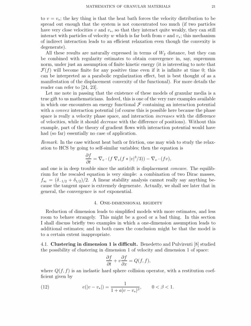
1.1. Collisions. As said above, collisions are supposed to incorporate inelasticity.I shall only consider inelasticity due to an imperfect restitution of energy, and neglectrotational degrees of freedom, although they might be quite important [34, 25]. Theillustration below provides a schematic picture of what goes on. The incomingvelocities are v and v∗; ω is the impact direction. Would the collision be elastic,the outgoing velocities would be given by the dashed arrows below; but because ofinelasticity effect, there is some loss of momentum in the impact direction, resultingin the boldface arrows indicating the outgoing velocities v ′ and v′∗.

ω

v

v∗

v′∗

v′

Let e stand for the restitution coefficient or (in)elasticity parameter:

〈v′ − v′∗, ω〉 = −e 〈v − v∗, ω〉, 0 ≤ e ≤ 1.

Then the collision equations can be solved into

(2)

v′ = v − 1 + e

2〈v − v∗, ω〉ω,

v′∗ = v∗ +1 + e

2〈v − v∗, ω〉ω.

In particular the variation of kinetic energy is

|v′|22

+|v′∗|2

2− |v|2

2− |v∗|2

2= −

(1 − e2

4

)〈v − v∗, ω〉2 ≤ 0.

In general the coefficient e might depend on the norm of the relative velocity, thatis |v− v∗|, on the deviation angle θ; for phenomenological reasons a constitutive de-pendence on the temperature T of the gas is also often assumed. For some authors,this dependence has important consequences (see e.g. [11]), for others it does notmatter so much; many researchers work with a constant restitution coefficient. It isgood to keep in mind that the two limit regimes e = 1 and e = 0 respectively corre-spond to elastic (no loss of energy) and sticky collisions (after collision, particlestravel together).

The velocities v′ have to lie on a certain sphere S with center c′ and radiusr ≤ |v− v∗|/2. It is often convenient to parameterize collisions by the direction σ of

4 CEDRIC VILLANI

the vector v′ − c′; in the terminology of [44], this is the σ-representation. Here arethe corresponding formulas:

(3)

v′ =v + v∗

2+

(1 − e

4

)(v − v∗) +

(1 + e

4

)|v − v∗| σ

v′∗ =v + v∗

2−(

1 − e

4

)(v − v∗) −

(1 + e

4

)|v − v∗| σ.

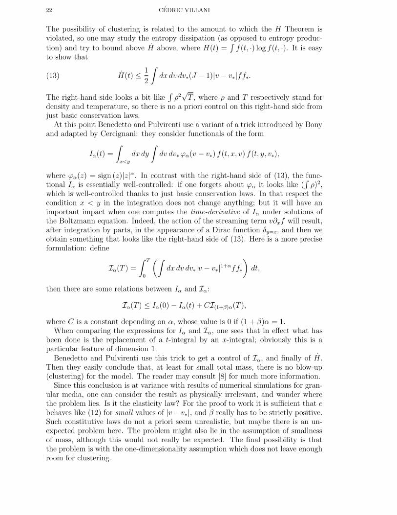
The parameter σ varies in the unit sphere S2. The reader can meditate on thefigure below, which is drawn in velocity space (in dashed lines are the elastic rulesof collision).

c

v′∗

c′∗

c′

v′

vv′∗

To write the Boltzmann equation, one needs to compute the pre-collisional

velocities: Given two velocities v and v∗ after collision, find the velocities ′v and ′v∗before collision. Here are the formulas:

(4)

′v =v + v∗

2−(

1 − e

4e

)(v − v∗) +

(1 + e

4e

)|v − v∗|σ

′v∗ =v + v∗

2+

(1 − e

4e

)(v − v∗) −

(1 + e

4e

)|v − v∗|σ.

Note carefully that ′v and ′v∗ do not coincide with v′ and v′∗; in other words,the collisions are not reversible. This is in agreement with the fact that we areobserving a dissipative process. Accordingly, the Jacobian of the transformation(v, v∗) → (′v,′ v∗) is not 1, but

(5) J =|v − v∗|

e2 |′v −′ v∗|.


Remark. In dimension 1, elastic collisions are “stupid”: since v ′, v′∗ = v, v∗ (ve-locities are either preserved or swapped), these collisions do not change the velocitydistribution. It is not so for inelastic collisions:

v′, v′∗ = v, v∗ or

v + v∗

2± e

2(v − v∗)

,

depending on the value of σ ∈ −1,+1. Similarly,

′v,′ v∗ = v, v∗ or

v + v∗

2± 1

2e(v − v∗)

.

1.2. Collision operator. Two collision operators are classically used for describingthe effect of collisions on the distribution function. The first one is the Boltzmann

collision operator:

(6) QB(f, f) =

∫

R3

dv∗

∫

S2

dσ |v − v∗|(J|′v −′ v∗||v − v∗|

f(′v) f(′v∗) − f(v) f(v∗)).

Here the factor |v−v∗| is characteristic of the “hard sphere model”: the mean numberof collisions between particles of given velocities is proportional to the difference ofvelocities (this is intuitively obvious); the factor J is given by (5). The parameters tand x do not appear explicitly in (6), because this operator only acts on the velocitydependence: in other words, collisions are supposed to be localized in space andtime. The fact that the Boltzmann equation is written in terms of the “local tensorproduct” f(x, ·)⊗f(x, ·) reflects the fundamental statistical assumption of molecularchaos (no correlation between pre-collisional velocities).

Notation. It is customary to write f ′ as a shorthand for f(v′) or f(x, v′); similarrules apply to f , f∗, f

′∗,

′f , ′f∗. Also the Boltzmann operator naturally splits intotwo parts: Q(f, f) = Q+(f, f) − Q−(f, f), which are traditionally called the gain

term and the loss term. The notation which I use is by no means universal: allkinds of symbols are used to denote pre- or post-collisional velocities, e.g. v∗, v∗∗,etc. I recommend the convention with v′ and ′v (due to V. Panferov).

The second popular model is the Enskog collision operator:

(7)

QE(f, f) = r2

∫

R3

dv∗

∫

S2

dσ |v− v∗|(J|′v −′ v∗||v − v∗|

G(x, x− rω) f(x,′ v) f(x− rω,′ v∗)

−G(x, x + rω) f(x, v) f(x+ rω, v∗)).

Here r > 0 is the radius of the particles, ω is the impact direction, and G(x, y)is the correlation function between points x and y. There are obvious similaritiesand obvious differences between the Enskog and the Boltzmann collision operator:in particular, the space variable enters explicitly in equation (7), which means thatcollisions are delocalized in space. Moreover, the assumption of molecular chaoshas been dropped, and now the function G takes care of correlations. Roughlyspeaking, G is defined by the formula

f (2)(x, v; y, w) = G(x, y)f(x, v)f(y, w),

where f (2) is the two-particle distribution density. The need for such a correlationfunction is more or less obvious if one realizes that the assumption of “thick” spheres

6 CEDRIC VILLANI

implies correlations between various positions: as a trivial example, if a particle ispresent at position x, then no particle can be present at y if |x− y| < r. In practise,G might be given by an explicit expression of x and y, or an expression of x, y andρ(x), ρ(y), where ρ(x) stands for the density of the gas at x; it might even depend onthe whole density profile. For more information see the short but intricate enoughdiscussion in Cercignani [25].

The mathematical status of the Boltzmann and the Enskog collision operatorsare not comparable. The localization in the Boltzmann equation leads to formalsimplicity and analytical difficulty; it is also at the source of a rich mathematicalstructure, which has contributed to establish the Boltzmann equation as one of themost renowned and challenging partial differential equations studied by mathemati-cians. The Enskog equation on the other hand leads to a very messy theory andhorrendous calculations; it is often considered with a bit of awe by physicists andmathematicians. It is important to note that, while the “validity” of the Boltzmannequation for hard spheres has been established (even though only under certain re-strictions, see [44, Chapter 1, Section 2.1]) by Lanford, no such result exists forthe Enskog equation. Thus the latter model might be considered as a heuristic orphenomenological model.

In the context of granular material, however, the Enskog equation is supposed tobe much better adapted, since particles are almost “macroscopic” in size. Whetherthis will be sufficient to re-boost the theory of the Enskog equation is still unclear.For the moment, no serious mathematical work on the inelastic Enskog equationhas been performed, so all the rest of these notes will deal with the Boltzmannequation. Note that the distinction between both models is irrelevant when thespace dependence is taken away.

As a final general comment, it is very striking to see the devastating effects of theinelasticity assumption on the classical theory of the Boltzmann equation.

1.3. When to use pre- and post-collisional velocities. The pre-collisional ve-locities ′v and ′v∗ appear in the collision operator and are therefore useful wheneverone wants to study properties of that operator; in particular regularity issues, thatmight be used in a regularity study for the solution of the equation.

However, most of the time, in practical applications, one studies the density dis-tribution f via observables, that are integrals of f against some test function whichdepends only on v, or on x and v. In that case the correct equation is the weakversion of the Boltzmann collision operator:

(8)

∫

R3

Q(f, f)(v)ϕ(v) dv =

∫|v − v∗|f(v)f(v∗) (ϕ(v′) − ϕ(v)) dv dv∗ dσ.

In that sense the formulas for post-collisional velocities are used much more often,in practise, than the formulas for pre-collisional velocities.

1.4. Variants and simplifications. The chief simplification is spatial homo-

geneity, which amounts to look for solutions of the form f(t, v). While this isa huge simplification, it often allows a fine description of purely kinetic effects incomplicated subjects.

Another way to simplify the Boltzmann equation consists in a reduction of the

dimension, either by symmetry or phenomenological arguments. Thus one mayobtain two-dimensional or even one-dimensional models. As I mentioned above, a


one-dimensional elastic Boltzmann equation is meaningless, but a one-dimensionalinelastic one makes sense.

It is possible to replace the collision kernel |v−v∗| by |v−v∗|γ, for some exponent γwhich varies between, say, −1 and 1. In classical (elastic) kinetic theory, γ can rangefrom −3 (Coulomb interaction) to 1 (hard spheres). There is no real microscopicbasis for such a generalization in the context of granular material, but there might bephenomenological reasons. A particularly interesting case for analytical resolutionis γ = 0 (Maxwellian collisions).

Finally, one may take into account only quasi-frontal collisions (θ ' π, or, whatamounts to the same by symmetry, θ ' 0, that is grazing collisions) or quasi-elasticcollisions (e ' 1). In one dimension both asymptotic regimes are about the same.It is sometimes found in physics literature that velocities in a granular gas have atendency to align on each other, which might be a justification for the use of modelswhere grazing collisions play an important role. Some models that can be used inthis respect look like

QL + ∇v ·(f ∇v(f ∗ |v|γ+2v)

),

where QL is a Landau-Fokker-Planck (elastic) collision operator. Here ∗ stands forconvolution with respect to the velocity; since ∗ commutes with ∇v, the operator onthe right-hand side really is proportional to

∇v ·(∫

R3

ff∗|v − v∗|γ(v − v∗) dv∗

).

There is nothing mysterious in the exponent γ + 2: Taking into account the twoderivatives in v, it corresponds to a homogeneity like |v|γ (γ = 1 for hard spheres).See Li and Toscani [37] for a study of how certain qualitative properties of thisequation vary with γ.

Here is a “historically” important example of oversimplified model: at the begin-ning of the nineties, McNamara and Young suggested the following collision-typeoperator in dimension 1:

QMNY(f, f) =∂

∂v

(f(f ∗ |v|v)

),

which remained popular for some time. Most of the first works by mathematiciansin granular media, in particular those by Pulvirenti and co-authors between 1997and 2000, dealt with the McNamara-Young model.

1.5. Other operators. Apart from collisions, one may add to the kinetic modelvarious terms which either model external physical forces, or arise from particularsituations. Here are four such possibilities.

(i) Heat bath: Many experiments about granular material include shaking, asa way to input energy into the system, counterbalancing the freezing due to energyloss. A rather trivial but seemingly not so absurd model consists in a heat bath,or white noise forcing: this amounts to adding to the right-hand side of the kineticequation a term like

Te ∆vf,

where Te is an “external temperature”, normalized to 1 in the sequel. Such modelswere introduced by mathematicians and physicists in various contexts [46, 6, 11].

8 CEDRIC VILLANI

(ii) Friction: Particles may experience extra friction forces if they are goingthrough a viscous fluid or something to that effect. Here again, there is a trivialmodel consisting in adding a drift term to the equation; the most simple case beingthat of a linear drift,

α∇v · (fv) (α > 0).

(iii) Shear flow: The behavior of grains in a flowing fluid is of interest. Cer-cignani [26] proposed the following simplified model. Look for solutions of the freeBoltzmann equation

∂f

∂t+ v · ∇xf = QB(f, f)

between two surfaces x2 = 0 and x2 = L, moving at respective speed 0 and V ,with bounce-back boundary conditions. Make the ansatz f(t, x, v) = f(t, c), wherec = v − u(t, x) is the deviation to the local mean velocity; and assume some self-similarity in the solution, in particular u(t, x) = K(t)x+v0(t). Then it is found thata sufficient condition for f(t, c) to solve the problem is

(9)∂f

∂t−∇cf · (Kc) = Q(f, f),

where K is a matrix that can be written, in a well-chosen coordinate system, withonly one nonzero entry, outside the diagonal. In practise, this means that a sim-ple solution to the shear flow problem can be constructed by solving the spatiallyhomogeneous Boltzmann equation with an additional term like, say,

v1∂f

∂v2

on the right-hand side.

(iv) Homogeneous Cooling State: Solutions of the “free” inelastic Boltzmannequation will typically lose energy until all the particles travel at the same speed (ateach point x). For simplicity, let us consider a spatially homogeneous situation andassume that the mean velocity is 0; then the asymptotic state is δ0 (all particles atrest). To study more precisely the asymptotic behavior, it is natural to “zoom” onthe velocity distribution close to 0, that is to rescale the distribution function. TheBoltzmann collision operator does satisfy some scaling properties: if the collisionkernel is proportional to |v − v∗| in dimension d, then

Q(f(λ·), f(λ·)

)= λ−(d+1)Q(f, f)(λ·).

It is not difficult to find that the new unknown f(t, v) defined by

f(t, v) = (1 + t)d f(log(1 + t), (1 + t)v

)

satisfies a nice equation:

∂f

∂t= Q(f , f) −∇v · (vf).

That equation now may admit a nontrivial steady state, because the energy-dissipativeeffects of the Boltzmann collision operator are balanced by the energy input comingfrom the term in −∇v ·(v·f). Any result about the convergence to such a steady stateleads to some qualitative information about the way the original equation converges


to δ0. Of course, to a steady state in the new variables t = log(1 + t), v = (1 + t)vis associated a self-similar solution in the original variables t, v, traditionally called“homogeneous cooling state”. The moral here is that, to study the relaxation tohomogeneous cooling states, one is led to consider the Boltzmann equation with anadditional anti-drift term

−∇v · (fv).Note that the change of variable from time t to time t is logarithmic, so one has

to be careful in interpreting these results (a fast decay in the t scale does not meanso fast a decay in the original scale).

By the way, similar “logarithmic” rescalings of variables are classical in the liter-ature about the large-time behavior of diffusion equations, and also lead to addeddrift terms. For instance, this rescaling transforms the heat equation ∂tf = ∆vfinto the linear Fokker-Planck equation ∂tf = ∆vf + ∇v · (fv). (Note that here wegain a drift, not an anti-drift!) The literature related to such changes of variables isso vast that I prefer not to provide any reference.

1.6. “Simple” problems. Here is a non-exhaustive list of problems that at leastcan be formulated in a relatively precise mathematical way.

- What is the behavior of temperature in a granular gas? In a spatially homoge-neous gas, a simple dimensional analysis leads to the intuitive formula

dT

dt' −const. T 3/2

(think that |v − v∗| has the same physical dimension as√T ). This suggests that

the temperature decays like O(t−2) with time; this is classically called Haff’s law,since it was proposed by Haff [33] in the beginning eighties. Among other things,Haff’s law implies that the solution at time t lies at distance O(t−1) to the Diracmass δu, where u is the mean velocity. In a spatially inhomogeneous context, thingsmight become more intricate and the temperature may undergo important spatialvariations.

- What is the large-time behavior? In the case of elastic collisions, a lot of workhas been devoted to the approach of Maxwellian equilibrium, in relation with themaximum entropy principle and Boltzmann’s H Theorem. For inelastic collisionsthere is no H Theorem (only an approximate version of it when the restitutionparameter e is close to 1) and no intuitive way to attack the problem.

- What about the large velocity behavior? Is it still Gaussian, as in the elasticcase, or not? We shall see that the answer is negative.

- Inhomogeneities and clustering: In the classical theory, spatial homogeneity isa very strong assumption, but at least it is stable: under appropriate boundaryand size conditions, a weakly inhomogeneous gas remains weakly inhomogeneousfor all times. In the case of inelastic collisions, there is extensive numerical evi-dence to support the possibility of inelastic collapse (temperature falls down to 0at certain places, meaning that the variance of the distribution vanishes), clustering(aggregates of particles with zero temperature form) and ensuing pattern formation.From a theoretical perspective, it would be very exciting if such behavior could bedemonstrated; for that, new tools probably have to be developed.

10 CEDRIC VILLANI

To summarize the state of the art about these questions, I could say that several(very) simplified models are quite well understood; and that as a general rule thespatially homogeneous theory is starting to be in a quite decent situation, althoughstill incomplete. On the other hand there is essentially nothing relevant known aboutinhomogeneities.

1.7. Heuristics about the tail behavior. One of the most famous predictions ofinelastic kinetic theory is the possibility of overpopulated distribution tails, meaningthat the typical large-velocity behavior of the velocity distribution is not Gaussian,but displays much thicker tails (so the inelasticity results in the presence of manyvery fast particles, which is not so intuitive). In addition to the fact that it contra-dicts the universality of the familiar Gaussian distribution, one of the reasons whythis prediction is famous is certainly the fact that it can be obtained by quite simpleheuristics.

Here is one way to argue. For the free Boltzmann equation, the asymptotic state isthe Dirac mass, say at zero velocity. Thus the gain term (which increases the energy)is dominated in some sense by the loss term (which decreases the energy). Hence,when studying the large-velocity behavior, it is natural to neglect the former in frontof the latter. Then the loss term is asymptotically proportional to something likeK|v|γf , where K is some constant, if the collision kernel is proportional to |v− v∗|γ(γ = 1 for hard spheres). Let us look for a radially symmetric distribution function

f(v) = f(r), r = |v|, and make the ansatz f(r) ' e−arβ. Then Q−(f, f) ' Krγe−arβ

;

∆vf = r−2∂r(r2∂rf) ' Cr2β−2e−arβ

; ∇v · (fv) ' rβe−arβ. By balancing dominant

terms in the equation for the steady state one easily obtains

heat bath: β = 1 + γ2;

heat bath + friction: β = 2;

anti-drift: β = γ.

This argument predicts for the hard spheres model tails like e−a|v|3/2for the heat bath,

like e−a|v|2 for heat bath and friction, and like e−a|v| for homogeneous cooling states.Such behaviors were predicted, on the basis of slightly more precise arguments, byErnst and Brito (see the review papers [29, 28, 27]; e.g. [28, Section 4.4]). There isall reason to believe that this is the correct theoretical answer, let apart the specialcase β = γ = 0 which is more subtle (as discussed in [28]).

The shear flow case is more intricate since there is no reason for solutions to beradially symmetric.

1.8. What is the trouble with non-Gaussianity? The reader might legitimatelyask: Elastic collisions lead to Gaussian distributions, but inelastic collisions do not,so what is the big deal? It is no wonder that a change in the assumptions leads toa change in the conclusion...

Yet there is some reason to be struck by the non-Gaussian behavior. In fact, inthe classical kinetic theory there are three different, yet related, ways to arrive atthe Gaussian, or rather the Maxwellian distribution (i.e. a Gaussian with scalar co-variance matrix). The first and probably most well-known is the one by Boltzmann,which can be stated informally as follows:


Let f be a probability distribution such that

f(v)f(v∗) = F(v + v∗, |v|2 + |v∗|2

).

Then f is Maxwellian.

This argument obviously deals with pairs of particles; it is related with the chaosassumption (particles are uncorrelated before collision) and the conservation laws(elasticity means conservation of v + v∗ and |v|2 + |v∗|2 through a collision).

Now comes another argument by Maxwell, which considers the system of all par-ticles as a whole:

Consider N particles with velocities v1, . . . , vN . Assume that these velocities arerandomly uniformly distributed, given the only constraints that (v1+ . . .+vN)/N = uand (|v1 − u|2 + . . .+ |vN − u|2)/N = T are determined. Then, the law of one theseparticles, say v1, is very close (if N is large) to a Maxwellian distribution with meanu and temperature T .

The requirement that the velocities should be uniformly distributed apart fromthe constraints coming from the conservation laws can be seen as a most elementaryexample of microcanonical ensemble in statistical mechanics. Actually Maxwell’stheorem is probably the most basic example of equivalence of ensembles.

The last statement, also due to Maxwell (before Boltzmann’s argument) is theone which is of most direct interest here. It goes as follows:

Let v be a random velocity in R3 such that (i) the distribution of v is radially

symmetric, i.e. it only depends on |v|, (ii) the coordinates of v are independentrandom variables; then the distribution of v is Maxwellian.

In other words, if we have probability distributions fi, i = 1, 2, 3, such thatf1(v1)f2(v2)f3(v3) = g(v2

1 + v22 + v2

3), then each fi has to be Gaussian. (The di-mension 3 has nothing special; any dimension d ≥ 2 would work just the same.)

The converse of the last statement may be more striking. If the velocity distri-bution is not Gaussian, then there are correlations between the components of thevelocity distribution. Roughly speaking, by measuring v1 we can obtain some in-formation about v2. This looks quite strange if we are used to classical gases, butfrom the point of view of mathematics there is no contradiction with the isotropicityassumption: take for instance an extreme case where the probability distribution issupported in |v| ≤ R. If I measure v1 to be greater than

√R2 − 1, then I know

for sure that v22 + v2

3 is less than 1; so the various components are indeed correlated.

2. Maxwellian toolbox

2.1. The model. Maxwell collisions are defined by the assumption that the collisionkernel is a function of just the deviation angle θ: so the weak form of the collisionkernel is ∫

R3

QB(f, f)ϕ =

∫

R3×R3×S2

b(cos θ)ff∗(ϕ′ − ϕ) dv dv∗ dσ,

and similarly the restitution coefficient e only depends on θ. Actually it is commonpractise to choose b and e to be just constants.

This modification makes the model analytically much simpler. To understandwhy, think that, by integrating out successively σ, then v∗ in the loss term one nowobtains Q−(f, f) = Kρf , where K is a constant and ρ is the macroscopic density

12 CEDRIC VILLANI

(which can be taken to be just 1 in the spatially homogeneous case). This shouldbe compared with the loss term for hard spheres, that is Kf(f ∗ |v|).

In classical kinetic theory, Maxwell collisions may be interpreted as describinginteractions between particles that repel each other with a force proportional tothe inverse of the fifth power of the distance. For the description of granular ma-terial, such an interpretation is certainly irrelevant, so one should rather considerthe model as just an analytical simplification. An alternative point of view consistsin forgetting about the “true” collisional mechanism and replace it by random dy-namics: Whenever two particles collide, the parameter σ is chosen randomly on S2

(uniformly if b is a constant). This interpretation is due to Kac (see [44, Chapter 1,Section 2.1] for the elastic case).

With the added structure in the Maxwell model come new specific tools andfeatures which may be useful. The most important are:

- closed moment equations;

- Fourier transform;

- contracting distances;

- information-theoretical tools.

All this is described and explained, in the elastic case, in [44, Chapter 4]. In factthere is a good analogy between the Boltzmann collision operator with Maxwelliankernel on one hand, and the usual convolution operators on the other hand. I shouldinsist that so far, all this extra structure has been exploited only in the spatiallyhomogeneous case, which is the only one considered in this section.

2.2. Temperature dependence. Replacing the collision kernel |v− v∗| by a func-tion of just θ leads to irrelevant temperature behavior. To keep a correct temper-ature law it is better to replace |v − v∗| by something which has the same physicaldimension: an averaged value of the relative velocity. The most common choice issomething like the square root of the temperature T : indeed, if v and v∗ are indepen-dent random variables distributed according to the probability density f(v), thenthe mean value of |v − v∗|2 is

∫ff∗|v − v∗|2 dv dv∗ = 2

(∫f(v)|v|2 dv −

∣∣∣∣∫f(v)v dv

∣∣∣∣2)

= 2T.

So it would be natural to replace |v − v∗| by just√

2T . There is a dimensionalconstant in front of the collision operator, so the

√2 does not really matter, but the

fact that the collision rate is proportional to the square root of the temperature isimportant.

With this modification, from the weak formulation of the Boltzmann equation it iseasy to check that (i) the mean momentum

∫f v dv is preserved, (ii) the temperature

T (t) at time t satisfies the differential equation

dT

dt= −KT 3/2,

which integrates exactly to

T (t) =T (0)

(1 + at)2(a > 0),


where a is proportional to e(1 − e) for a constant coefficient e. Hence Haff’s lawis correct for this model (this is of course not surprising, we kind of enforced it).Thus, in the spatially homogeneous case, the effect of the temperature dependencecomes only through an explicit function of time in front of the collision kernel, andthe analytical simplicity of the model is preserved.

2.3. References. The three-dimensional inelastic Maxwellian model was first intro-duced and studied by Bobylev, Carrillo and Gamba [12]; at almost the same time,simple one-dimensional models were studied independently by Baldassari, Marconiand Puglisi [2]; see also Ben Naım and Krapivski [4, 35]. Since then these equationshave been studied thoroughly by several authors. Good recent review papers havebeen written by Ben Naım and Krapivsky [5], Ernst and Brito [28, 27], who surveythe existing physical literature and physical results. In [28] the emphasis is put onthe Maxwell model as a model arising from stochastic dynamics.

Apart from the above-mentioned works, another important source on the Maxwellmodel is the series of papers by Bobylev and Cercignani, sometimes with other co-authors such as Carrillo, Gamba or Toscani, in various issues of the Journal ofStatistical Physics [13, 14, 15, 17].

2.4. Moments equations. Let P (v) be a polynomial in v, that is, in the variablesv1, v2, v3. To compute the time-evolution of the observable associated with P , oneshould evaluate∫

R3

Q+(f, f)P dv =

∫

R3×R3

ff∗

(∫

S2

P (v′) dσ

)dv dv∗.

The expression inside inner parentheses depends only on the polynomial, and has tosatisfy certain homogeneity conditions. Actually, one can show that it is a polyno-mial in v and v∗; in particular it can be split into a sum of products of polynomials:

∫

S2

P (v′) dσ =∑

i

Pi(v)P∗,i(v∗).

Then one can integrate against ff∗ dv dv∗ and separate variables, obtaining productslike (

∫fPi)(

∫fP∗,i). Of course these polynomials Pi, P∗,i are of lower degree than

P itself. The conclusion is that the equation for the evolution of a polynomialmoment of a certain order can be expressed in terms of polynomial moments oflower order. Since the first moments can be evaluated explicitly, we understand thatin principle, the time-evolution of all polynomial moments can be exactly integrated.For the elastic model, this observation was first made by Truesdell in the fifties, andit remains relevant in the inelastic case. Of course things are not so simple becausethe coefficients in the equations become more and more tricky as the degree of thepolynomial increases, so if one wants precise estimates one has to be clever to keepthese coefficients under control.

It is a classical result in probability theory that a distribution function whichdecays fast enough is uniquely determined by all its polynomial moments. So, aslong as one remains in the class of distribution functions which decay very fast (andin particular have all their moments finite), one can in principle integrate “explicitly”the spatially homogeneous Boltzmann equation with Maxwellian kernel. Informationabout the asymptotic behavior can also be obtained in this way: if one proves thatall polynomial moments of f converge, as time goes to infinity, to the corresponding

14 CEDRIC VILLANI

polynomial moments of some distribution f∞, this means that f does converge tof∞, at least in weak sense (in the sense of convergence of observables).

2.5. Fourier transform. Let the Fourier transform of f (with respect to the ve-locity variable) be defined by

f(ξ) =

∫

R3

f(v)e−iξ·v dv.

To compute the time-evolution of the Fourier transform, one is again led to evaluate∫Q+(f, f)e−iξ·v dv =

∫

R3×R3

ff∗

(∫

S2

e−iξ·v′ dσ

)dv dv∗.

Now, from (3),∫

S2

e−iξ·v′ dσ = e−iξ·(v+v∗2 )e−i( 1−e

4 )ξ·(v−v∗)

∫e−i( 1+e

4 )(ξ·σ)|v−v∗| dσ.

(The reader should not confuse the e standing for exponential, and the one standingfor the restitution coefficient.) The factor in front of the integral is of the formeiv·keiv∗·k∗, which is good; but the expression inside the integral is more ugly. How-ever, in the integration process, the particular direction of ξ should not matter verymuch, since it enters the integral only through ξ · σ, and σ varies over the sphere.As noticed by Bobylev in the seventies, a simple symmetry argument allows one toreplace the expression (ξ ·σ)|v− v∗| inside the σ-integral by |ξ|σ · (v− v∗). Then onecan write ∫

S2

e−iξ·v′ dσ =

∫

S2

e−iv·ke−iv∗·k∗ dσ,

where k and k∗ are certain frequency vectors that depend only on ξ and σ. Thenintegrate against ff∗ dv dv∗, and exchange integrals, to come up with∫Q+(f, f) e−iξ·v dv =

∫

S2

(∫

R3×R3

ff∗e−iv·ke−iv∗·k∗ dv dv∗

)dσ =

∫

S2

f(k)f(k∗) dσ.

(For careful such computations in the elastic case, consider, e.g. [1, Appendix].)To better appreciate what has been achieved, let us rewrite the corresponding

equation for f in the case of a constant collision kernel of unit integral (forgettingthe temperature dependence for simplicity):

∂f

∂t+ f =

1

4π

∫

S2

f(ξ+)f(ξ−) dσ,

where

ξ± =ξ

2±[(

1 − e

4

)ξ +

(1 + e

4

)|ξ|σ

].

This looks like a Boltzmann equation, except that the integral is only over S2,not over R

3 × S2! The R3 integral has been absorbed into the definition of Fourier

transform. As a consequence, this equation is much simpler and reveals convenientfor

- studying moments (polynomial moments are derivatives in Fourier space at fre-quency vector ξ = 0, and it is often more convenient to manipulate Taylor expansionsthan moment expansions);


- study the regularity of the Boltzmann equation (regularity is all about controlof the amplitude of high Fourier modes);

- linearizing and computing eigenfunctions and eigenvalues;

- looking for exact equilibrium or self-similar solutions. (Think that Fourier trans-form is the standard method for the study of the central limit theorem, which is allabout the asymptotic behavior of sequences of densities obtained by successive con-volutions.)

2.6. Some results. In the heat bath problem, moment equations have been estab-lished by Carrillo, Cercignani and Gamba [22], then used to prove the convergenceto equilibrium by Bobylev and Cercignani [14]. This is a neat application of themethods described before.

The problem of self-similar profiles is more subtle. In dimension d = 1, thereis a simple, explicit Homogeneous Cooling State, or “HCS” (see for instance [5,Section 2.1]):

f(t, v) =

(2

π√T (t)

)1

(1 +

v2

T (t)

)2 .

Recall that there is no equivalent for the elastic case, since the elastic collisionoperator is trivial in dimension 1.

In dimension 3, the situation is more complicated. Let us assume for simplicitythat the restitution coefficient e is constant. The rescaled equation for HCS

Q(f, f) −∇v · (fv) = 0,

written in Fourier variables, always admits a unique physically relevant solution1.As conjectured by Ernst and Brito, this solution has a very fat tail, decaying likean inverse power law in the velocity variable (with a complicated exponent). Thissolution is often called the Ernst-Brito solution. Up to changing the origin of time,we may assume that it has temperature 1 at initial time. The relevant mathematicalreference here is the work by Bobylev and Cercignani [14] who completely justifiedthe conjecture of Ernst and Brito.

Once we know there is a unique HCS, the natural question is whether it is at-tractive. Thus we go to self-similar variables and study convergence to equilibrium.Using Fourier techniques again, Bobylev and Cercignani [14] did prove convergencein the rescaled variables, under certain assumptions on the initial datum which werelater removed by Bobylev, Cercignani and Toscani [15]. The final result is as fol-lows [15, Theorem 5.1]. Let f(t, v) be a solution of the spatially homogeneous inelas-tic Maxwellian Boltzmann equation with constant restitution coefficient e ∈ [0, 1).Assume that the initial datum f0 has unit temperature, zero mean momentum, and

1Another family of solutions was described earlier by Bobylev, Carrillo and Gamba [12]; thesesolutions have rapid decay, but they are not nonnegative for (at least) almost all values of e.It was mistakenly stated in [14] that there is a countable set of “exceptional” (resonant) valuesof e for which the two families coincide; but such a statement appeared to be in contradictionwith the positivity of the Ernst-Brito solutions. Thus, the physically relevant self-similar solutionshave power-like tails for all values of e. This issue is clarified in the last section of Bobylev andGamba [16]. (All of this was explained to me by Bobylev.)

16 CEDRIC VILLANI

let F be the associated self-similar Ernst-Brito profile. Further assume that f0 hasa finite moment of order s > 2. Then, for a well-chosen parameter µ > 0,

e−3µtf(t, ve−µt) −→ F (v),

in the sense of weak convergence (convergence of observables).

It is interesting to note that, in contrast with the heat bath problem, the methodof moments is not applicable here, since the asymptotic state has only slow decay –yet Fourier transform continues to be useful.

Let me conclude with some variants:

- I am not aware of a decisive study for variable restitution coefficient. Bobylev,Carillo and Gamba [12, Section 6.2] have considered the case e = e(T ) under thecondition that

limT→0

1 − e(T )

T α∈ (0,∞), 0 < α < 1,

and established an asymptotic Maxwellian self-similar behavior of the form

f(t, v) ' e−|v|2

2T (t)

(2πT (t))3/2, t→ ∞,

where of course T (t) satisfies the Haff law.

- The linear Boltzmann equation (for inelastic Maxwellian collisions) was studiedby Spiga and Toscani [42].

2.7. Contracting distances. Lyapunov functionals often yield precious informa-tion about asymptotic behavior, for instance if one is interested in rates of conver-gence. In kinetic theory, the standard Lyapunov functionals are related to entropyand Boltzmann’s H Theorem; but there is no H Theorem for inelastic Boltzmannequation.

In the seventies, Tanaka discovered a new Lyapunov functional for the spatiallyhomogeneous Boltzmann equation with Maxwellian kernel. He actually found more:a distance in which any two solutions of the Boltzmann equation become closer:

t′ ≥ t =⇒ d(f(t′, ·), g(t′, ·)

)≤ d(f(t, ·), g(t, ·)

).

Tanaka’s distance is a well-known object in probability theory, also called Monge-Kantorovich or Wasserstein distance of order 2: whenever µ, ν are any two proba-bility measures in R

d, define

W2(µ, ν) =√

inf E|X − Y |2,where E stands for expected value, and the infimum is taken over all random variablesX and Y with respective laws µ and ν. This amounts to look for a coupling of µ andν with maximum covariance. It turns out that W2 satisfies the axioms of a distance(triangular inequality, etc.)

In the nineties, Toscani and collaborators found other contracting distances whichare simpler to use, of the form

ds(µ, ν) = supξ∈Rd

∣∣µ(ξ) − ν(ξ)∣∣

|ξ|s .

This is well-defined (finite) as soon as µ, ν have the same polynomial moments upto order dse−1 (this means in particular that µ and ν should have same mean value


if s = 2; the same mean value and covariance matrix if 2 < s ≤ 3). The behavior ofthese distances with respect to the Boltzmann equation has been studied by Toscanitogether with various researchers such as Gabetta, Wennberg or the author. Notethat related distances have proved to be useful for the Navier-Stokes equation, inparticular after the work of Le Jan and Sznitman [36] (related issues are discussedin the recent review paper by Cannone [20]).

These techniques were recently adapted by Bisi, Carrillo and Toscani [9] whoproved that d2 is contracting along solutions of both the spatially homogeneousinelastic Boltzmann equation with Maxwell molecules, either with or without a heatbath ∆v term. In the presence of ∆v, this is even a strict contraction, in the sensethat one has an equation like

d+

dtd2

(f(t), g(t)

)+K d2

(f(t), g(t)

)≤ 0,

with d+/dt standing for the upper right-derivative. Of course this implies that fand g become exponentially closer as t → ∞; by choosing g to be the stationarystate one deduces that the convergence to equilibrium is exponentially fast.

Convergence here is again in the sense of weak convergence, however it is a gen-eral rule that the combination of (i) exponential convergence in the sense of sucha distance, (ii) uniform in time moment bounds, and (iii) uniform in time regular-

ity bounds in Sobolev spaces (say∫|ξ|2k|f(ξ)|2 dξ) imply exponential convergence

in strong sense. For instance, if moments and regularity bounds are as strong aspossible, then all derivatives of f converge uniformly in v, and exponentially fast,towards the corresponding derivatives of the equilibrium. Thus the convergence isas smooth as one can hope for; moreover the rate of convergence is almost as goodas in the weak distance.

In the case without heat bath, one may also wish to use this technique to studythe relaxation to the Ernst-Brito HCS, and then rephrase the convergence resultsof Bobylev, Cercignani and Toscani in the setting of Fourier distances. This is notjust for the sake of formalism: contractive distances give strong information (aboutnonlinear stability, for instance). But now d2 is no longer a strict contraction; thismotivates the use of a stronger distance ds for s > 2. There is a recent work on thistopic by Bisi, Carrillo and Toscani; although computations are quite more tricky,the result is similar, and exponential convergence to equilibrium can be proven inthis way. Exponential convergence in the rescaled variables, when translated backin the original time variables, means that there is an improvement of the power oft−1 in the convergence rate when one replaces the Dirac mass by the Ernst-Britosolution:

d(f(t), δ0

)= O(t−1), d

(f(t), fEB(t)

)= O(t−(1+α)), α > 0.

Two remarks are in order about this result. First, the exponent α which is foundby Bisi, Carrillo and Toscani agrees with the one which appears in previous compu-tations by Bobylev, Cercignani and Toscani [14, 15]; and the result of convergenceto equilibrium is not new either; the main progress here is that this is recast in theform of a true contraction estimate. Secondly, to deduce a decay result “in physicalspace”, one would need to have some a priori bounds on the solutions, which do notseem to be known at present.

18 CEDRIC VILLANI

Here are some further comments. Li and Toscani have applied the tools of Wasser-stein distances to variants of the McNamara-Young equation [37], in dimension 1.But it would also be interesting to check whether the original Tanaka distance isalso nonexpanding in the inelastic case. This might be of interest if one has in mindto do something about it in a spatially inhomogeneous context, since Tanaka’s dis-tance may be easier to use in that context (see for instance Carlen and Gangbo [21]).Further note the neat identity

√T = W2(f, δu) u =

∫

R3

f(v) v dv,

which suggests that W2 is somewhat natural in that context. A result of convergencein Wasserstein sense would be judged by many authors to be physically relevant initself, while Fourier-based metrics can be criticized in that respect.

In practical problems, W2 might be plotted from experimental data, since it canbe computed explicitly for radially symmetric functions:

W2(f1, f2) =

√∫ 1

0

∣∣F−11 (t) − F−1

2 (t)∣∣2 dt,

where F−1 F is the identity, and

Fi(x) = (4π)

∫ x

0

fi(r)r2 dr.

A lot of information about Wasserstein distances can be found in [45, Chapter 7];see also Chapter 2 in the same reference.

2.8. Information theory. The natural tendency of collisions is to kill information:By adding some kind of randomness in the system, collisions make it more and moredifficult to estimate parameters of the distribution, or to reconstruct the initial dis-tribution. One can interpret in this way the trend to Gaussian as a tragic loss ofinformation. For Maxwell collision kernels, this is related to certain information-theoretical inequalities: for instance, H(Q+(f, f)) ≤ H(f), where H(f) =

∫f log f

is the familiar H-functional; a similar inequality holds true with the Fisher informa-tion (for all that see [44, Chapter 4, Section 3]).

Inelastic collisions however create correlations (information) at the same time asthe destroy it. It is not so clear in which sense this statement should be taken, andmaybe one can establish some variants of these information-theoretical inequalities,that would help understanding better the evolution of information in a granular gas.

2.9. Conclusion. To summarize, one can fairly say that during the period 2000-2005 the most important questions about the spatially homogeneous Maxwell modelof granular gas have been solved, and that there is a rather good understanding ofthe evolution of temperature and moments, the asymptotic behavior as t→ ∞, andthe tail behavior. Of course there is room for refinements, but the priority now forthe Maxwell model is certainly to tackle inhomogeneous situations.


3. Gradient flow structure

Among the simplified models of granular media that were mentioned before is

(10)∂f

∂t= ∇v ·

(f(v)

∫f(v∗)|v − v∗|(v − v∗) dv∗

)

+ Te∆vf + α∇v · (fv) (Te, α ≥ 0)

where the first term on the right-hand side is a phenomenological model for inelasticcollisions (with a cooling effect), similar to the McNamara-Young operator; thesecond one describes a heat bath; and the last one is a friction term.

Complicated as it may seem, equation (10) has a particular structure: it can berewritten

(11)∂f

∂t= ∇v ·

(f ∇v

δFδf

),

where the functional F reads

F(f) =1

2

∫

Rd×Rd

f(v)f(v∗)|v − v∗|3

3dv dv∗ + Te

∫

Rd

f log f + α

∫

Rd

f|v|22dv

and (δF)/(δf) is defined by the identity

DF · (δf) =

∫δFδf

δf,

where DF is the differential of F and δf is an infinitesimal variation of f . In otherwords, an infinitesimal variation of F along an infinitesimal change δf of the densityf can be computed by integrating δF/δf against δf .

Equations of the type (11) are a gradient flow in a very precise sense. What is agradient flow? It is an equation of the form

dX

dt= − grad F(X(t)),

where X is an unknown living in a “manifold” M (the phase space of the system),F is an “energy” defined on M, and grad is the “gradient” operator, which isassociated to F by the relation

DF(X) · (δX) =⟨grad F(X), δX

⟩X.

Here the left-hand side is the infinitesimal variation of F at X under an infinitesimalvariation δX, and the right-hand side is the scalar product of grad F(X) and δX.Both grad F(X) and δX should be thought of as vectors in the tangent space to Mat X, and the scalar product 〈·, ·〉X should be specified. To summarize, a gradientflow is given by a manifold M, an energy functional F on M, and a “Riemannianstructure”, which is a family of scalar products defined (smoothly) on each tangentspace to M. It so happens that gradient flows occur everywhere in physics andmathematics.

In the case which is of interest to us, equation (11) can be formally rewritten as

∂f

∂t= − grad F(f),

where M is the space of probability measures, equipped with the following “Rie-mannian” structure: whenever δf is a small variation of density (so δf is a function

20 CEDRIC VILLANI

of v), its square norm, as measured by the scalar product at “point” f , is

‖δf‖2 = inf

∫f(v)|u(v)|2 dv; δf + ∇v · (fu) = 0

.

Here is how one can understand this formula: think of velocities v as being positionsin phase space; particles are distributed according to density f(v) dv, and theyperform certain infinitesimal movements in such a way that the density varies froma certain amount δf . You don’t know the velocities u = v (velocity in phase space)of the particles, but you can try to guess: these velocities should be compatible withthe observed variation δf , so the continuity equation δf + ∇v · (fu) = 0 should besatisfied. Among all admissible vector fields, select one which is most economical,in the sense of having minimum kinetic energy.

This structure has been studied at length by many authors, starting from thepioneering work of Otto around 2000. It is intimately related to the quadraticWasserstein distance W2: in fact W2 is nothing but the associated geodesic distance.A lot of information about that can be found in [45, Chapter 8].

Why are we doing all that? One advantage of identifying a gradient flow structureis that it yields interesting recipes for computing, say derivatives of functionalsalong the flow, in terms of gradients and Hessians; this is what is described in [45,Chapter 8] as Otto’s calculus. Another advantage of such a formalism is that theconvexity properties of the energy functional might help the study of convergenceto equilibrium. For instance, if F is λ-uniformly convex (i.e. the Hessian operator,in an appropriate sense, is greater than λ Id ), then trajectories get closer to eachother like O(e−λt), and there is exponential convergence to the unique infimum f∞of F . This also comes with automatic inequalities such as

λ

2W2(f, f∞)2 ≤ F(f) − F(f∞) ≤ 1

2λ‖ grad F‖2 = − 1

2λ

(dFdt

).

One has to be careful: convexity of a functional is here understood as convexityalong geodesics of the induced structure. For instance

∫f |v|2 dv should be consid-

ered as strictly convex, and −∫f |v|2 dv as strictly concave! (although both are

formally linear functionals of f ...) The technical word is “displacement convex”,which means more or less that the functional is convex along variations of densitieswhich correspond to particles going in straight lines.

In the present case, the convexity of the “interaction potential” |v − v∗|3 guaran-tees that the first term in F is displacement convex; it is known from the work ofMcCann that the second term is also displacement convex; finally the last term isalso displacement convex (uniformly if α > 0).

Using this apparatus and some work, Carrillo, McCann and the author [24, 23]studied in some detail the convergence to equilibrium for (10). The convergenceitself was already established by Benedetto, Caglioti, Carrillo and Pulvirenti [6] (indimension 1 only), so the novelty lied in the derivation of explicit bounds on therate of convergence.

The conclusions can be summarized roughly as follows: For Te > 0 (heat bathcase) there is always a unique equilibrium (up to translation if α = 0). If α > 0then the convergence is at least like O(e−αt). If α = 0 there is still exponentialconvergence, and one can obtain a lower bound on the rate of convergence. Themain problem here is to overcome that lack of convexity of the cubic potential close


to v = v∗; the key thing is that the heat bath forces the velocity distribution to bespread out enough that the system is not concentrated too much (if two particleshave very close velocities v and v∗, so that they interact quite weakly, they can stillinteract with particles of velocity w which is far both from v and v∗; this mechanismof indirect interaction leads to an efficient relaxation even though the convexity isdegenerate).

All these results are naturally expressed in terms of W2 distance, but they canbe combined with regularity estimates to obtain convergence in, say, supremumnorm, under just an assumption of finite kinetic energy (it is interesting to note thatF(f) will become finite for any positive time even if it is infinite at time 0; thiscan be interpreted as a parabolic regularization effect, but is best thought of as amanifestation of the displacement convexity of the functional). For more details thereader can refer to [24, 23].

Let me note in passing that the existence of these models of granular media is atrue gift to us mathematicians. Indeed, this is one of the very rare examples availablein which one encounters an energy functional F containing an interaction potentialwith a convex interaction potential (of course this is possible here because the phasespace is really a velocity phase space, and interaction increases with the differenceof velocities, while it should decrease with the difference of positions). Without thisexample, part of the theory of gradient flows with interaction potential would havehad (so far) essentially no case of application.

Remark. In the case without heat bath or friction, one may wish to study the relax-ation to HCS by going to self-similar variables; then the equation is

∂f

∂t= ∇v · (f ∇v(f ∗ |v|3/3)) −∇v · (fv),

and one is in deep trouble since the antidrift is displacement concave. The equilib-rium for the rescaled equation is very simple: a combination of two Dirac masses,f∞ = (δ−1/2 + δ1/2)/2. A linear stability analysis cannot really say anything be-cause the tangent space is extremely degenerate. Actually, we shall see later that ingeneral, the convergence is not exponential.

4. One-dimensional rigidity

Reduction of dimension leads to simplified models with more estimates, and lessroom to behave strangely. This might be a good or a bad thing. In this sectionI shall discuss briefly two examples in which a one-dimension assumption leads toadditional estimates; and in both cases the conclusion might be that the model isto a certain extent inappropriate.

4.1. Clustering in dimension 1 is difficult. Benedetto and Pulvirenti [8] studiedthe possibility of clustering in dimension 1 of velocity and dimension 1 of space:

∂f

∂t+ v

∂f

∂x= Q(f, f),

where Q(f, f) is an inelastic hard sphere collision operator, with a restitution coef-ficient given by

(12) e(|v − v∗|) =1

1 + a|v − v∗|β, 0 < β < 1.

22 CEDRIC VILLANI

The possibility of clustering is related to the amount to which the H Theorem isviolated, so one may study the entropy dissipation (as opposed to entropy produc-

tion) and try to bound above H above, where H(t) =∫f(t, ·) log f(t, ·). It is easy

to show that

(13) H(t) ≤ 1

2

∫dx dv dv∗(J − 1)|v − v∗|ff∗.

The right-hand side looks a bit like∫ρ2√T , where ρ and T respectively stand for

density and temperature, so there is no a priori control on this right-hand side fromjust basic conservation laws.

At this point Benedetto and Pulvirenti use a variant of a trick introduced by Bonyand adapted by Cercignani: they consider functionals of the form

Iα(t) =

∫

x<y

dx dy

∫dv dv∗ ϕα(v − v∗) f(t, x, v) f(t, y, v∗),

where ϕα(z) = sign (z)|z|α. In contrast with the right-hand side of (13), the func-tional Iα is essentially well-controlled: if one forgets about ϕα it looks like (

∫ρ)2,

which is well-controlled thanks to just basic conservation laws. In that respect thecondition x < y in the integration does not change anything; but it will have animportant impact when one computes the time-derivative of Iα under solutions ofthe Boltzmann equation. Indeed, the action of the streaming term v∂xf will result,after integration by parts, in the appearance of a Dirac function δy=x, and then weobtain something that looks like the right-hand side of (13). Here is a more preciseformulation: define

Iα(T ) =

∫ T

0

(∫dx dv dv∗|v − v∗|1+αff∗

)dt,

then there are some relations between Iα and Iα:

Iα(T ) ≤ Iα(0) − Iα(t) + CI(1+β)α(T ),

where C is a constant depending on α, whose value is 0 if (1 + β)α = 1.When comparing the expressions for Iα and Iα, one sees that in effect what has

been done is the replacement of a t-integral by an x-integral; obviously this is aparticular feature of dimension 1.

Benedetto and Pulvirenti use this trick to get a control of Iα, and finally of H.Then they easily conclude that, at least for small total mass, there is no blow-up(clustering) for the model. The reader may consult [8] for much more information.

Since this conclusion is at variance with results of numerical simulations for gran-ular media, one can consider the result as physically irrelevant, and wonder wherethe problem lies. Is it the elasticity law? For the proof to work it is sufficient that ebehaves like (12) for small values of |v− v∗|, and β really has to be strictly positive.Such constitutive laws do not a priori seem unrealistic, but maybe there is an un-expected problem here. The problem might also lie in the assumption of smallnessof mass, although this would not really be expected. The final possibility is thatthe problem is with the one-dimensionality assumption which does not leave enoughroom for clustering.


4.2. HCS are a bad approximation for the McNamara-Young model. NowI shall consider what may be the most simple phenomenological kinetic model forgranular medium: the spatially homogeneous McNamara-Young equation in dimen-sion 1,

∂f

∂t=

∂

∂v

(∂

∂v

(f ∗ |v|3

3

)).

To fix ideas, assume that the mean velocity is 0. As time goes to infinity, f(t, ·) con-verges to δ0 like O(t−1). The question now is whether f(t, ·) is better approximatedby the HCS, which in that case is just

S(t) =1

2

(δ− 1

2t+ δ 1

2t

).

To study that problem, let us go to rescaled variables, which adds an anti-drift term:

(14)∂f

∂t=

∂

∂v

(f∂

∂v

(f ∗ |v|3

3

))− ∂

∂v(fv),

and then the HCS transforms into the stationary solution S = (δ−1/2 + δ1/2)/2.It was proven by Benedetto, Caglioti and Pulvirenti [7] that there is indeed con-

vergence, in rescaled variables, to the stationary state. This conveys the idea thatthe HCS is indeed a better approximation to the solution. However, it was laterproven by Caglioti and the author [19] that the convergence is actually very poor:essentially, it can be at best like O(t−1) in the rescaled variables, which means a log-arithmic in time improvement at the level of the original variables. This is actuallya good example in which a quantitative result essentially kills a qualitative one.

Here is an idea of the argument. Equation (14) has the form of a continuityequation, so it can be formally solved by the characteristic methods (in velocityspace): f(t) can be interpreted as the velocity distribution for a bunch of particleswhose velocity evolves according to

dv

dt= ξ(v) ≡ v −

∫

R

(v − v∗)|v − v∗|f(t, v∗) dv∗.

Since we are in dimension 1, the associated flow is order-preserving : particles witha higher velocity always keep a higher velocity than particles with a lower velocity.The vector field ξ is a function on R which goes to +∞ for v → −∞, −∞ forv → +∞, and is successively decreasing, increasing, decreasing again. Its derivativeis maximum at the median of f . Since ξ is an integral expression of f and vanishesfor f = S, it is plausible that ξ can be controlled in terms of some weak distance off to S; actually one can show that

∂ξ(t, v)

∂v≤ 2W2

(f(t, ·), S

).

Now what happens as t → ∞? Since the flow is order-preserving, the left-half ofthe particles should go to velocity −1/2, while the right-half should go to velocity+1/2 (Possible trajectories in (t, v) variables are represented on the figure below).

If there are some particles that are around the median of f , it will be necessaryto separate them, resulting in a considerable stretching in velocity space. But themaximum amount of stretching is controlled by an upper bound on the divergence ofthe vector field, which in the present case means an upper bound on the derivativeof ξ, and we have seen that this derivative is controlled by the distance of f toS. So when the solution approaches S, the amount of stretching which is available

24 CEDRIC VILLANI

t

v−1/2 1/2

vanishes, precisely when a strong stretching should take place! Combining all theseelements, it is possible to show that

(15)

∫ T

0

W2

(f(t, ·), S

)dt ≥ K logT

as T → ∞.A similar estimate holds true even if there is no mass close to the median of f : in

that case one can use the property that a very strong negative divergence of the flowis necessary to concentrate mass around the points −1/2 and +1/2. Consult [19]for more details.

The bound (15) prevents any convergence rate like O(t−(1+ε)), no matter howsmall ε is. In this sense the convergence has to be very slow, and, as I said above,in the original variables W2(f(t), St) cannot be much smaller than O(1/(t log t)),while W2(f(t), δ0) is O(1/t). The physical relevance of this conclusion seems to becorroborated by numerical simulations of A. Barrat, indicating that the convergenceto self-similar solutions is indeed poor for large times.

Once again it is not clear where the problem lies. Maybe this is due to theoversimplified form of the HCS, or the fact that it has a singular part, and somevacuum regions (not all velocities lie in the support). Maybe this is also due to theone-dimensional nature of the equation.

5. True inelastic hard spheres

To caricature, mathematical research on the inelastic Boltzmann equation focusedon baby models from 1997 to 2000, then turned to the Maxwell model, and around2004 appeared the first works devoted to the true inelastic hard spheres model, whilestaying spatially homogeneous. Here below is a rather exhaustive list of references:

- Gamba, Panferov and the author [32] set up the framework and devised severaltechniques that would be used again in the sequel;

- Bobylev, Gamba and Panferov [17] proved an important technical result for thestudy of tail behavior in integrated version;

- Mischler, Mouhot and Rodriguez Ricard [39, 40] sharpened and generalizedall the previous results; in these works are considered for the first time generalrestitution constitutive laws with a dependence of e upon T or |v − v∗|;

- In a still unpublished sequel to their first work, Gamba, Panferov and the authorpushed some maximum principle techniques to study pointwise tail estimates.


- Some results about the linear case were obtained by Lods and Toscani [38](they guessed the form of the equilibrium by first replacing the model by its grazingcollision limit).

In this section, I shall informally describe some of the techniques and results thatcan be found in these works. For simplicity, I shall assume the restitution coefficientto be constant, but in most cases this assumption can be relaxed.

5.1. Energy dissipation. Consider the spatially homogeneous inelastic Boltzmannequation; fix the mean momentum to be zero, and as usual assume that the totalmass is normalized to 1. It is easy to show that the energy dissipation due tocollisions is

K

∫ff∗|v − v∗|3 dv dv∗ (K > 0).

Thus the energy does not satisfy a closed equation as in case of Maxwell collisions.Yet something can be done: by Jensen’s inequality, applied with the convex function| · |3 and the probability measure f(v) dv,

∫f(v∗)|v − v∗|3 dv∗ ≥

∣∣∣∣v −∫f∗ v∗ dv∗

∣∣∣∣3

= |v|3.

Then, by Holder’s inequality (or Jensen’s inequality with the convex function x3/2),

∫f(v)|v|3 dv ≥

(∫f(v)|v|2 dv

)3/2

.

Then we can write the temperature equation in the form

dT

dt≤ −KT 3/2 + contributions from noncollisional terms.

This results in two main consequences: First, a priori estimates on the temper-ature: the temperature is always controlled uniformly in time, be it for the “raw”Boltzmann equation or in presence of a heat bath, an anti-drift or a shear flow addi-tional term. Secondly, for the plain Boltzmann equation we recover a half of Haff’slaw (if I may say), namely

T (t) ≤ C

t2.

The other half is true also, as will be seen later.

5.2. Moment estimates. Moment equations can still be written, but now they arenot closed any longer. Yet inequalities can be hoped for. If we are interested in themoment of order s > 2, then the relevant quantity is

(|v′|s + |v′∗|s) − (|v|s + |v∗|s).

Povzner inequalities have been used for many years in kinetic theory to bound thisfrom above; see [44, Chapter 2, Section 2.2]. The search of precise tail estimatesmotivated the development of refined such inequalities, taking into advantage theintegration over the collision parameter σ. The following estimate, due to Bobylev in

26 CEDRIC VILLANI

the elastic case, was obtained by Bobylev, Gamba and Panferov [17] in the inelasticsetting: for any integer p ≥ 1,

(16)1

4π

∫

S2

(|v′|2p + |v′∗|2p − |v|2p − |v∗|2p) dσ ≤ −(|v|2p + |v∗|2p)

+ γp(|v|2 + |v∗|2)p, γp = O

(1

p

).

Although it can be formulated in very elementary terms and does not involve anypartial differential equations, this estimate is very tricky. A nice observation madein [17] to simplify the proof is the following: whenever ϕ1 and ϕ2 are nondecreasingfunctions on [−1, 1], and α1, α2 are given unit vectors, then

∫

S2

ϕ1(α1 · ω)ϕ2(α2 · ω) dω

is maximum when α1 = α2. The rest of the proof, unfortunately, is plenty of heavycomputations and convexity arguments.

Why is (16) interesting? Expand the last term using the binomial formula, thenthe terms of higher degree, |v|2p and |v∗|2p, appear with a positive coefficient γp,which is negligible in front of the negative coefficient −1 at the beginning of theright-hand side of (16). All the terms that remain have the form O(|v|2`|v∗|2p−2`)for some positive integers `. Fix such a term and integrate the whole (16) againstf(v)f(v∗)|v − v∗| dv dv∗ to compute the rate of change of the moment of order 2p:the contribution of that term is bounded above by something like

∫f(v)f(v∗)(|v| + |v∗|)|v|2`|v∗|2p−2` dv dv∗,

which in turn can be bounded in terms of moments of order 2`, 2`+ 1, 2p− 2` and2p− 2`+ 1, all of which are strictly less than 2p. It is not so for the contribution ofthe first term in the right-hand side of (16), which leads to a negative term involvingmoments of order 2p+ 1. To summarize, (16) implies differential inequalities of theform

dM2p

dt≤ −KM2p+1 + C

∑

`

(M2`M2p+2`−1 +M2`+1M2p+2

),

where Ms stands for the moment of order s. From Jensen’s inequality again, thisimplies

dM2p

dt≤ −KM1+(2p)−1

2p + C∑

`

(M2`M2p+2`−1 +M2`+1M2p+2

),

and after a bit of work one actually deduces

dM2p

dt≤ −KM1+(2p)−1

2p + C,

where the constant C and K may depend on the kinetic energy, but not on highermoments.

This has two consequences. First, for each fixed s > 2, the moment of order sbecomes immediately finite even if it is infinite at time 0 (so there is instantaneousdestruction of fat tails; in the elastic case this observation was first made by Desvil-lettes in the beginning nineties). Secondly, by using the precise form of (16), one can


refine the computations to get bounds on (stretched) exponential moments, since∫f(v)ea|v|s dv =

∞∑

k=0

ak

k!

(∫f(v)|v|sk dv

).

(This was actually Bobylev’s initial motivation, in the elastic case.)Using this apparatus, Bobylev, Gamba and Panferov [17] prove that steady state(s)

f∞(v) satisfy

∃a, A > 0;

∫eA|v|s f(v) dv = +∞,

∫ea|v|s f(v) dv < +∞,

where

s =

3/2 for the heat bath case;

2 for heat bath + friction;

1 for the HCS.

These bounds establish the validity of the conjectures about the large-velocity be-havior of the stationary states, in an integrated sense. Estimates such as

∫ea|v|sf∞ <

+∞ may be considered as an integrated upper bound on f∞, while estimates such as∫eA|v|sf∞ = +∞ may be considered as an integrated lower bound. The same authors

also show that for the shear flow problem, steady states satisfy∫ea|v|f∞(v) dv < +∞

for some a > 0, but are unable to get a lower bound.These estimates were proven only for the stationary solution; there is reason to

believe that- the integrated lower bound is always true;- the integrated upper bound is propagated in time, that is, if it holds true for the

initial datum then it holds true for all times;- a weaker version of the integrated upper bound (with other exponents) auto-

matically appears for positive times, whatever the initial datum.

5.3. Regularity estimates. One of the important discoveries by Lions in thenineties was the regularity of the gain operator : the operator Q+ is regularizing,meaning that Q+(f, f) is typically smoother than f itself. In contrast, Q−(f, f)typically has the same regularity as f . Many versions exist under different sets ofassumptions; if the collision kernel was perfectly smooth and compactly supported,avoiding frontal and grazing collisions as well with large or small relative velocitycollisions, then there would be a gain of (d − 1)/2 derivatives (1 derivative in di-mension 3). For realistic operators such as the hard sphere kernel, one cannot ingeneral prove better than just a fractional gain. See [44, Chapter 2, Section 3.4]for references and discussion. It is important to note that properties of improvedsmoothness can be transformed into properties of improved integrability.

This feature was recently used by Mouhot and the author [41] as the basis forthe regularity theory of the spatially homogeneous Boltzmann equation with hardspheres. It is easy to understand why the property of Q+ is useful for regularityestimates: think that Q− resembles a multiplication operator, then solutions of thespatially homogeneous Boltzmann equation should have a regularity comparable tosolutions of

∂f

∂t+Kf = S,

where S is a source term, smoother than f .

28 CEDRIC VILLANI

Here are the consequences that can be drawn for that: First, a priori integrabilitybounds which prevent blow up of the solution, as well as extinction in finite time.Next, there is a lower bound on the temperature in rescaled variables; Mischlerand Mouhot [40] use that to prove the lower bound in the Haff law: for the “raw”Boltzmann equation,

T (t) ≥ c

(1 + t)2.

In the case of the Boltzmann equation with an additional anti-drift, there is prop-agation of regularity, and moreover there is exponential decay of singularities: thesolution f(t) can be decomposed into S(t) +R(t), where S(t) is very smooth (of ar-bitrary smoothness, fixed in advance), and the remainder R(t) decays exponentiallyfast. This is proven by Mischler and Mouhot [40]. One of the technical tools usedthere is an inelastic variant of the Carleman representation (see [44, Chapter 2,Section 4.6] in the elastic case2) which is a way to write the Boltzmann collisionoperator parameterized by the precollisional velocities ′v and ′v∗.

In the case of the heat bath, there is in addition instant regularization [32].

5.4. Maximum principle. Moment methods and Povzner inequalities lead to in-tegrated tail estimates, but what about pointwise estimates? Is it true that in thecase of the heat bath one has

ce−A|v|3/2 ≤ f∞(v) ≤ Ce−A|v|3/2

?

(Ideally one could hope that such an estimate holds true with a = A, but for themoment this looks out of reach.)

Pointwise estimates are often associated with maximum principles. The standardmaximum principle for the Laplace operator is well-known: let f be a solution of∆vf ≥ 0 in a domain Ω, with f ≤ M on the boundary ∂Ω. Then it follows thatf ≤M in the whole of Ω. In other words,

∆vf ≥ 0 =⇒ supΩf = max

∂Ωf.

There is also a time-dependent version of this maximum principle: if f ≤ M attime t = 0, ∂tf − ∆vf ≤ 0 in Ω and f ≤ M on ∂Ω × [0, T ), then again f ≤ M inthe whole of Ω and for all times t ∈ [0, T ).

Gamba, Panferov and the author [32] use this principle to show a lower bound,for the heat bath problem, of the form

f∞(v) ≥ ce−A|v|3/2

.

The idea is in two steps: first, the smoothness and localization implies that f isbounded below on a certain small ball Br(v0), with center v0 and radius r (v0 is notknown with precision, but it is localized inside a larger ball). Then one can use acomparison function ϕ(t, v) which is singular at v0, but very smooth outside Br(v0),

identically zero for t = 0, has the correct velocity decay as e−A|v|3/2, and such that

∂tϕ ≤ ∆vϕ−K|v|ϕ.In fact,

ϕ(t, v) = K exp(−bt − a(1 + |v|2)3/4

)

2Beware: In the published version of [44] there was a typo in the Carleman formula: the collision

kernel should be B and not B; both symbols stand for different expressions.


does the job for well-chosen parameters a, b and K.Since on the other hand (by the trivial bound Q+ ≥ 0 and the easy bound Q− ≥

K|v|f)

∂tf ≥ ∆vf −K|v|f,the maximum principle, applied in the complement of the ball Br(v0), implies that fstays above ϕ for all times. Now we have a control of f inside Br(v0), and a controlof f outside Br(v0), and the desired bound follows. See [32] for more explanations.

When the operator ∆v is replaced by the anti-drift, Mischler and Mouhot [40] havea variant of this argument which implies a lower bound like Ke−A|v| for radially sym-metric stationary states (so a similar bound holds true for radially symmetric HCSin the original variables). It is likely that this argument adapts to time-dependentsolutions, not necessarily radially symmetric, but the job remains to be done.

Upper bounds are more tricky because the Q+ operator needs to be controlled byabove. Here again, Mischler and Mouhot obtain good bounds by above like O(e−a|v|)for stationary radially symmetric solutions with the anti-drift, but then the methodseems not to adapt to the time-dependent case.

To go further in this direction, Gamba, Panferov and the author built on an ideasuggested in [44, Chapter 2, Section 6.2], namely to use a maximum principle for theBoltzmann operator. Here is an informal version of this principle, stated for instancein the heat bath case. Let f(t, v) satisfy

∂f

∂t= Q(f, f) + ∆vf

and let ϕ(t, v) be a “reasonably smooth” comparison function satisfying

f(0, v) ≤ ϕ(0, v) for all v,

∂tϕ−Q(f, ϕ) − ∆vϕ ≥ 0 in [0, T ) × Ω,

f(t, v) ≤ ϕ(t, v) outside Ω, for all t ∈ [0, T ).

Then f ≤ ϕ everywhere in [0, T ) × R3. Here Q(f, ϕ) is defined in weak form by

∫Q(f, ϕ)ψ =

∫|v − v∗|f∗ϕ(ψ′ − ψ).

This principle looks rather similar to the usual maximum principle for the heatequation; there is however an important difference: a control of f by ϕ is assumedeverywhere outside Ω, not just at the boundary ∂Ω. There is a good reason for that,namely the fact that the Boltzmann collision operator is nonlocal.

In practise, to use this principle it is desirable to have nice pointwise upper boundson the gain term Q+(f, ϕ). Such bounds can be deduced from integrated bounds:indeed, the spreading properties of Q+ make it possible to recover pointwise boundson Q+ from integrated bounds on f . A nicer example, worked out by Gamba,Panferov and the author in the case of elastic collisions, is the neat bound

Q+(f, e−β|v|2) ≤ C

(∫f(v)eβ|v|2 dv

)e−β|v|2

(for the elastic collision operator).In the elastic case, this approach was completely worked out and it was proven by

the same authors [31] that if the initial datum is bounded above by a Maxwellian,then this property holds true for all times (this was one of the last irritating open

30 CEDRIC VILLANI

problems in elastic spatially homogeneous kinetic theory). A similar study is on itsway in the inelastic context; although it is not complete due to technical complica-tions, it looks safe to bet that the same method does work in the end, and showsthat if the initial datum is bounded above by Ce−a|v|3/2

, then f(t, v) ≤ C ′e−a′|v|3/2

for all times t ≥ 0.

5.5. Summary. Let me now summarize the main results known to this date for thespatially homogeneous inelastic hard spheres model. I shall focus on two cases: the“heat bath”, or “driven” case,

∂f

∂t= Q(f, f) + ∆vf,

and the free or “undriven” case, distinguishing between the unrescaled version

∂f

∂t= Q(f, f)

and the rescaled version∂f

∂t= Q(f, f) −∇v · (fv).

5.5.1. Temperature. It is proven thatc ≤ T (t) ≤ C (driven)c

t2≤ T (t) ≤ C

t2(undriven, unrescaled)

where c, C are positive constants depending on the initial datum.

5.5.2. Integrated tail behavior. It is proven that equilibrium distributions satisfy

∫

R3

f∞(v)ea|v|3/2

dv < +∞,

∫

R3

f∞(v)eA|v|3/2

dv = +∞ (driven)

∫

R3

f∞(v)ea|v| dv < +∞,

∫

R3

f∞(v)eA|v| dv = +∞ (undriven, rescaled).

The lower bound should also be true for time-dependent solutions.

5.5.3. Pointwise tail behavior. It is very likely that we can provece−A|v|3/2 ≤ f∞(v) ≤ Ce−a|v|3/2

(driven)

ce−A|v| ≤ f∞(v) ≤ Ce−a|v| (undriven, rescaled)

At present, only the lower bound in the driven case was proven, while both boundswere established in the undriven case, but only for radially symmetric solutions.Moreover, the lower bound also holds true for time-dependent solutions in the drivencase, and this should also be the case in the undriven case.

5.5.4. Stationary states. In the driven case, it is known that there exists at leastone smooth (with bounded derivatives up to any order) positive radially symmetricstationary state, with fast decay at infinity. It is not known whether this state isunique. In the undriven (unrescaled) case, it is known that there exists at least onesmooth positive radially symmetric self-similar HCS. It is not known whether it isunique (say, unique for a given value of the initial kinetic energy).


5.5.5. Convergence to equilibrium. In the driven case, it is not known whether thereis convergence to equilibrium. A theorem of uniqueness of the stationary state wouldhelp, but would still not be sufficient to conclude because of the absence of knownLyapunov functional. In the undriven case, it is known that there is convergence toa Dirac mass, but it is not known whether the HCS are attractive.

5.5.6. Conclusion. From the qualitative point of view we have a reasonable deal ofinformation, and predictions of physicists have been confirmed at theoretical level,although by means of a very sophisticated machinery (the original papers quoted inthis text might appear quite hard to read for non-experts of mathematical kinetictheory).

Unlike for the Maxwell model, we are unable to prove uniqueness of equilibrium,and we are in bad need of a new idea to resolve the problem of the asymptoticbehavior in large time. Numerical simulations indicate that the convergence shouldbe excellent, and that the equilibrium should be unique. Apart from the possibilityof finding a miraculous Lyapunov functional (maybe in the form of a variant of thecontracting distances known in the Maxwell case), there is no idea in the air.

Mischler and Mouhot recently tried to tackle the problem of uniqueness of theHCS by considering a family of stationary solutions (with the anti-drift) dependingon a restitution coefficient e going continuously from 1 to 0 (the coefficient in frontof the anti-drift is rescaled with e in such a way as to go to 0 when e → 1, so thatthere is a nontrivial Maxwellian equilibrium for e = 1). There is an H Theoremwith an O(1 − e) error term, which may imply the uniqueness close to e = 1 by aperturbative argument. Then they try to use a continuity argument letting e de-crease continuously to 0, and showing that no bifurcation is possible in the family ofequilibria. At a bifurcation point, there would be appearance of a new conservationlaw for the linearized Boltzmann equation. Such an event cannot really be ruledout a priori (after all we have already seen in the Maxwell case that some valuesof the restitution coefficient lead to “resonance” effects and change of qualitativeproperties of the HCS) but might be dismissed by a theorem of classification of con-servation laws for the linearized equation, proving that only mass and momentumare preserved by collisions. Would that attempt work out in the end, it would beproven that HCS are unique, leaving some hope for a proof of convergence.

6. The future of inelastic kinetic theory?

It seems clear that the next step in the mathematical kinetic theory of granularmedia is the introduction of the space variable and the study of clustering or breakingof space homogeneity. In fact, for engineers there is essentially no interest in spatiallyindependent models, and it has been a long time since the spatial structure ofgranular flows has been studied (The reader can consult the recent textbook byBrilliantov and Poschel [18] for references and pointers to the physical literature.)However, even for engineers, subtle phenomena such as clustering seem to retainsome mystery.

Physicists say that the HCS is very unstable, unless the gas is driven by strongboundary conditions. In a personal communication, J. Brey has suggested that thereshould be an inhomogeneous stable self-similar solution which would describe thelocal behavior of the solution (this would be a fascinating eventuality). In any casethe behavior which is observed in experiments or simulations is often well-described

32 CEDRIC VILLANI

by a separation between a cold, high-density phase and a warm, low-density one,with pattern formation and “inverse Maxwell demon”.

As for the mathematical justification of these observations, we are nowhere. Theonly available inhomogeneous results are the works by Benedetto and Pulvirenti [8]indicating that for certain restitution coefficient laws there is no blow-up in dimen-sion 1. We do not know whether the collapse should be expected in finite or infinitetime (in which case finite-time collapse in numerical simulations should be attributedeither to measurement errors or to a breakdown of the Boltzmann model).

It seems reasonable to start the study in the case of Maxwell collisions, whereconvergence to HCS is proven and there are contracting distances; it also seems agood idea to start with the close-to-equilibrium regime. Discussions with C. Mouhotlet me suggest the following. The linearized Boltzmann collision operator shouldhave a nice spectral theory (even that is not so clear because of the slow decay ofthe HCS) when associated with either the heat bath term or the anti-drift. However,one can think that these two cases behave radically differently when one adds thetransport term −v ·∇x: there should be destabilization by the anti-drift, not by thediffusion. Would that guess be true, this would be the first hope of displaying someinstability of the homogeneous description. The dependence of that effect upon thedimension should be checked.

On the contrary, in the case of the heat bath, the good spectral properties of thelinearized operator should make it possible to prove stability of weak inhomogeneity:indeed, if f0 is an initial datum that lies at distance O(ε) from a spatially homo-geneous datum fh

0 , then one can hope that f(t) lies at distance O(εeCt) from thespatially homogeneous solution fh(t); then for t ≥ T , fh(t) should be be sufficientlyclose to the HCS, that linearization is possible, and then for ε small enough, alsof(t) would be very close to the HCS. From that point on the good linear propertiescan be exploited.

Getting out of the perturbative regime looks completely hopeless for the moment.After all, even in the elastic case, there is still no good nonperturbative theory of thespatially inhomogeneous Boltzmann equation, and inelasticity makes things muchworse. Even the rather soft DiPerna-Lions theory of weak solutions does not extendto the inelastic Boltzmann equation! (In this direction are available only some worksabout the inelastic Enskog model [30].)

Some day one will have to discuss boundary conditions more precisely than is donenow. While the heat bath model might be in first approximation a honest model forshaking, it seems clear that it does not describe accurately the complicated space-dependent phenomena which occur in such a process. This looks extremely delicate.

Some other day one will have to rediscuss the relevance of the kinetic description:Is there molecular chaos or not? What qualitative differences between the Boltzmannand Enskog descriptions? How to choose the correlation function in the Enskogdescription? Does the kinetic description break down in presence of clustering?How to couple it with hydrodynamic equations? For the most part, these questionsare open from the physical point of view, and seem to arise incredible difficulties.

References

[1] Alexandre, R., Desvillettes, L., Villani, C., and Wennberg, B. Entropy dissipationand long-range interactions. Arch. Ration. Mech. Anal. 152, 4 (2000), 327–355.


[2] Baldassari, A., Marini Bettolo Marconi, U., and Puglisi, A. Influence of correlationson the velocity statistics of scalar granular gases. Europhys. Lett. 58, 1 (2002), 14–20.

[3] Barrat, A., Trizac, E., and Ernst, M. Granular gases: Dynamics and collective effects.To appear in Journal of Physics C: Condensed Matter. condmat-0411435.

[4] Ben-Naım, E., and Krapivsky, P. Multiscaling in inelastic collisions. Phys. Rev. E 61(2000), R5–R8.

[5] Ben-Naım, E., and Krapivsky, P. The inelastic Maxwell model. In Granular Gas Dynam-ics, T. Poeschel and N. Brilliantov, Eds., vol. 624 of Lect. Notes Phys. Springer-Verlag, Berlin,2003. cond-mat/0301238.

[6] Benedetto, D., Caglioti, E., Carrillo, J. A., and Pulvirenti, M. A non-Maxwelliansteady distribution for one-dimensional granular media. J. Statist. Phys. 91, 5-6 (1998), 979–990.

[7] Benedetto, D., Caglioti, E., and Pulvirenti, M. A kinetic equation for granular media.RAIRO Model. Math. Anal. Numer. 31, 5 (1997), 615–641. Erratum in M2AN Math. Model.Numer. Anal. 33, 2 (1999), 439–441.

[8] Benedetto, D., and Pulvirenti, M. On the one-dimensional Boltzmann equation forgranular flows. M2AN Math. Model. Numer. Anal. 35, 5 (2001), 899–905.

[9] Bisi, M., Carrillo, J., and Toscani, G. Contractive metrics for a Boltzmann equationfor granular gases: Diffusive equilibria. J. Statist. Phys. 118 (2005), 301–331.

[10] Bisi, M., Spiga, G., and Toscani, G. Grad’s equations and hydrodynamics for weaklyinelastic granular flows. Phys. Fluids 16, 12 (2004), 4235–4247.

[11] Bizon, C., Shattuck, M., Swift, J., and Swinney, H. Transport coefficients for granularmedia from molecular dynamics simulations. Phys. Rev. E 60 (1999), 4340–4351.

[12] Bobylev, A. V., Carrillo, J. A., and Gamba, I. M. On some properties of kinetic andhydrodynamic equations for inelastic interactions. J. Statist. Phys. 98, 3-4 (2000), 743–773.Erratum in: J. Statist. Phys. 103 (2001), no.5–6, 1137–1138.

[13] Bobylev, A. V., and Cercignani, C. Moment equations for a granular material in athermal bath. J. Statist. Phys. 106, 3-4 (2002), 547–567.

[14] Bobylev, A. V., and Cercignani, C. Self-similar asymptotics for the Boltzmann equationwith inelastic and elastic interactions. J. Statist. Phys. 110, 1-2 (2003), 333–375.

[15] Bobylev, A. V., Cercignani, C., and Toscani, G. Proof of an asymptotic property ofself-similar solutions of the Boltzmann equation for granular materials. J. Statist. Phys. 111,1-2 (2003), 403–417.

[16] Bobylev, A. V., and Gamba, I. M. Boltzmann equations for mixtures of Maxwell gases:exact solutions and power like tails. J. Statist. Phys., this issue.

[17] Bobylev, A. V., Gamba, I. M., and Panferov, V. A. Moment inequalities and high-energy tails for Boltzmann equations with inelastic interactions. J. Statist. Phys. 116, 5-6(2004), 1651–1682.

[18] Brilliantov, N., and Poschel, T. Kinetic theory of granular gases. Oxford GraduateTexts. Oxford University Press, 2004.

[19] Caglioti, E., and Villani, C. Homogeneous cooling states are not always good approxi-mations to granular flows. Arch. Ration. Mech. Anal. 163, 4 (2002), 329–343.

[20] Cannone, M. Harmonic analysis tools for solving the incompressible Navier-Stokes equa-tions. In Handbook of mathematical fluid dynamics. Vol. III. North-Holland, Amsterdam, 2004,pp. 161–244.

[21] Carlen, E. A., and Gangbo, W. Solution of a model Boltzmann equation via steepestdescent in the 2-Wasserstein metric. Arch. Ration. Mech. Anal. 172, 1 (2004), 21–64.

[22] Carrillo, J. A., Cercignani, C., and Gamba, I. M. Steady states of a Boltzmannequation for driven granular media. Phys. Rev. E (3) 62, 6, part A (2000), 7700–7707.

[23] Carrillo, J. A., McCann, R. J., and Villani, C. Contraction in the 2-Wassersteinlength space and thermalization of granular media. Arch. Rational Mech. Anal. 179 (2006),217–263.

[24] Carrillo, J. A., McCann, R. J., and Villani, C. Kinetic equilibration rates for granularmedia and related equations: entropy dissipation and mass transportation estimates. Rev.Mat. Iberoamericana 19, 3 (2003), 971–1018.

34 CEDRIC VILLANI

[25] Cercignani, C. Recent developments in the mechanics of granular materials. In Fisicamatematica e ingeneria delle strutture : rapporti e compatibilita, G. Ferrarese, Ed. PitagoraEd., Bologna, 1995, pp. 119–132.

[26] Cercignani, C. Shear flow of a granular material. J. Statist. Phys. 102, 5-6 (2001), 1407–1415.

[27] Ernst, M., and Brito, R. Anomalous velocity distributions in inelastic Maxwell gases.cond-mat/0310406.

[28] Ernst, M., and Brito, R. Asymptotic solutions of the nonlinear Boltzmann equation fordissipative systems. In Granular Gas Dynamics, T. Poeschel and N. Brilliantov, Eds., vol. 624of Lect. Notes Phys. Springer-Verlag, Berlin, 2003. cond-mat/0304608.

[29] Ernst, M. H., and Brito, R. Scaling solutions of inelastic Boltzmann equations with over-populated high energy tails. J. Statist. Phys. 109, 3-4 (2002), 407–432. Special issue dedicatedto J. Robert Dorfman on the occasion of his sixty-fifth birthday.

[30] Esteban, M. J., and Perthame, B. On the modified Enskog equation for elastic andinelastic collisions. Models with spin. Ann. Inst. H. Poincare Anal. Non Lineaire 8, 3-4 (1991),289–308.

[31] Gamba, I. M., Panferov, V., and Villani, C. Upper Maxwellian bounds for the spatiallyhomogeneous Boltzmann equation. Preprint.

[32] Gamba, I. M., Panferov, V., and Villani, C. On the Boltzmann equation for diffusivelyexcited granular media. Comm. Math. Phys. 246, 3 (2004), 503–541.

[33] Haff, P. Grain flow as a fluid-mechanical phenomenon. J. Fluid. Mech. 134 (1983), 401–430.[34] Jenkins, J. T., and Richman, M. W. Grad’s 13-moment system for a dense gas of inelastic

spheres. Arch. Rational Mech. Anal. 87, 4 (1985), 355–377.[35] Krapivsky, P., and Ben-Naım, E. Nontrivial velocity distributions in inelastic gases. J.

Phys. A: Math. Gen. 35 (2002), L147–L152.[36] Le Jan, Y., and Sznitman, A. S. Stochastic cascades and 3-dimensional Navier-Stokes

equations. Probab. Theory Related Fields 109, 3 (1997), 343–366.[37] Li, H., and Toscani, G. Long-time asymptotics of kinetic models of granular flows. Arch.

Ration. Mech. Anal. 172, 3 (2004), 407–428.[38] Lods, B., and Toscani, G. The dissipative linear Boltzmann equation for hard spheres. J.

Statist. Phys. 117, 3-4 (2004), 635–664.[39] Mischler, S., and Mouhot, C. Cooling process for inelastic Boltzmann equations for hard

spheres, Part I: The Cauchy problem. J. Statist. Phys., this issue.[40] Mischler, S., Mouhot, C., and Rodriguez Ricard, M. Cooling process for inelasic

Boltzmann equations for hard spheres, Part II: Self-similar solutions and tail behavior. J.Statist. Phys., this issue.

[41] Mouhot, C., and Villani, C. Regularity theory for the spatially homogeneous Boltzmannequation with cut-off. Arch. Ration. Mech. Anal. 173, 2 (2004), 169–212.

[42] Spiga, G., and Toscani, G. The dissipative linear Boltzmann equation. Appl. Math. Lett.17, 3 (2004), 295–301.

[43] Toscani, G. Kinetic and hydrodynamic models of nearly elastic granular flows. Monatsh.Math. 142, 1-2 (2004), 179–192.

[44] Villani, C. A review of mathematical topics in collisional kinetic theory. In Handbook ofmathematical fluid dynamics, Vol. I. North-Holland, Amsterdam, 2002, pp. 71–305.

[45] Villani, C. Topics in optimal transportation, vol. 58 of Graduate Studies in Mathematics.American Mathematical Society, Providence, RI, 2003.

[46] Williams, D., and MacKintosh, F. Driven granular media in one dimension: Correlationsand equation of state. Phys. Rev. E 54 (1996), R9–R12.

C. Villani

UMPA, ENS Lyon

46 allee d’Italie

69364 Lyon Cedex 07

FRANCE


e-mail: [email protected]

mathematics of granular materials · granular materials are a very trendy subject nowadays, and the...

Documents