mathematics 246a algebraic topology | i detailed table...
TRANSCRIPT

Mathematics 246A
Algebraic Topology — I
Detailed Table of Contents
Fall 2014
Department of Mathematics
University of California, Riverside
i
Brief Table of Contents
Preface . . . . . . . . . . . . . . . . . . . . . . . . . . . . . . . . . . . . . . . . . . . . . . . . . . . . . . . . . . . . . . . . . . . . .1
I. Further properties of simplicial complexes . . . . . . . . . . . . . . . . . . . . . . . . . . . . . 6
0. Review . . . . . . . . . . . . . . . . . . . . . . . . . . . . . . . . . . . . . . . . . . . . . . . . . . . . . . . . . . . . . . . . . 6
1. Ordered simplicial chains . . . . . . . . . . . . . . . . . . . . . . . . . . . . . . . . . . . . . . . . . . . . . . . 9
2. Subdivisions . . . . . . . . . . . . . . . . . . . . . . . . . . . . . . . . . . . . . . . . . . . . . . . . . . . . . . . . . . . .16
3. Abstract cell complexes . . . . . . . . . . . . . . . . . . . . . . . . . . . . . . . . . . . . . . . . . . . . . . . . 23
4. The Homotopy Extension Property . . . . . . . . . . . . . . . . . . . . . . . . . . . . . . . . . . . . . 31
5. Chain homotopies . . . . . . . . . . . . . . . . . . . . . . . . . . . . . . . . . . . . . . . . . . . . . . . . . . . . . 34
6. Cones and suspensions . . . . . . . . . . . . . . . . . . . . . . . . . . . . . . . . . . . . . . . . . . . . . . . . . .36
II. Construction and uniqueness of singular homology . . . . . . . . . . . . . . . . . . . .39
1. Basic definitions and properties . . . . . . . . . . . . . . . . . . . . . . . . . . . . . . . . . . . . . . . . . 40
2. Exactness and homotopy invariance . . . . . . . . . . . . . . . . . . . . . . . . . . . . . . . . . . . . .43
3. Excision and Mayer-Vietoris sequences . . . . . . . . . . . . . . . . . . . . . . . . . . . . . . . . . .46
4. Equivalence of simplicial and singular homology . . . . . . . . . . . . . . . . . . . . . . . . .52
5. Polyhedral generation, direct limits and uniqueness . . . . . . . . . . . . . . . . . . . . . 52
III. Additional geometric applications . . . . . . . . . . . . . . . . . . . . . . . . . . . . . . . . . . . . . . .58
1. Homology and the fundamental group . . . . . . . . . . . . . . . . . . . . . . . . . . . . . . . . . . 58
2. Degree theory . . . . . . . . . . . . . . . . . . . . . . . . . . . . . . . . . . . . . . . . . . . . . . . . . . . . . . . . . . 61
3. Simplicial approximation . . . . . . . . . . . . . . . . . . . . . . . . . . . . . . . . . . . . . . . . . . . . . . . 66
4. The Lefschetz Fixed Point Theorem . . . . . . . . . . . . . . . . . . . . . . . . . . . . . . . . . . . . 67
5. Dimension theory . . . . . . . . . . . . . . . . . . . . . . . . . . . . . . . . . . . . . . . . . . . . . . . . . . . . . . .71
6. Homology and line integrals . . . . . . . . . . . . . . . . . . . . . . . . . . . . . . . . . . . . . . . . . . . . 87
IV. Singular cohomology . . . . . . . . . . . . . . . . . . . . . . . . . . . . . . . . . . . . . . . . . . . . . . . . . . . . . 88
1. The basic definitions . . . . . . . . . . . . . . . . . . . . . . . . . . . . . . . . . . . . . . . . . . . . . . . . . . . .89
2. A weak Universal Coefficient Theorem . . . . . . . . . . . . . . . . . . . . . . . . . . . . . . . . . . 95
3. Kunneth formulas . . . . . . . . . . . . . . . . . . . . . . . . . . . . . . . . . . . . . . . . . . . . . . . . . . . . . . 98
4. Grade-commutativity and examples . . . . . . . . . . . . . . . . . . . . . . . . . . . . . . . . . . . . .107
5. Two applications . . . . . . . . . . . . . . . . . . . . . . . . . . . . . . . . . . . . . . . . . . . . . . . . . . . . . . . 112
6. Open disk coverings of manifolds . . . . . . . . . . . . . . . . . . . . . . . . . . . . . . . . . . . . . . . 116
7. Real and complex projective spaces . . . . . . . . . . . . . . . . . . . . . . . . . . . . . . . . . . . . . 118
V. Cohomology and differential forms . . . . . . . . . . . . . . . . . . . . . . . . . . . . . . . . . . . . . .119
0. Review of differential forms . . . . . . . . . . . . . . . . . . . . . . . . . . . . . . . . . . . . . . . . . . . . . 120
1. Smooth singular chains . . . . . . . . . . . . . . . . . . . . . . . . . . . . . . . . . . . . . . . . . . . . . . . . . 125
2. Generalized Stokes’ Formula . . . . . . . . . . . . . . . . . . . . . . . . . . . . . . . . . . . . . . . . . . . . 131
3. Definition and properties of de Rham cohomology . . . . . . . . . . . . . . . . . . . . . . .133
4. De Rham’s Theorem . . . . . . . . . . . . . . . . . . . . . . . . . . . . . . . . . . . . . . . . . . . . . . . . . . . .137
5. Multiplicative properties of de Rham cohomology . . . . . . . . . . . . . . . . . . . . . . . 141
6. Path independence of line integrals . . . . . . . . . . . . . . . . . . . . . . . . . . . . . . . . . . . . . 144
ii

Preface
This course is a continuation of the entry level graduate courses in algebraic topology givenduring the past two years (Mathematics 205C in Spring 2011 and Mathematics 205B in Winter2012). In these courses we discussed an algebraic construction on spaces known as singular ho-mology theory, which gives algebraic “pictures” of topological spaces in terms of certain abeliangroups. We did not actually construct the theory, but we did the following:
(1) For a certain class of spaces known as polyhedra, we defined simplicial homology groupswhich turn out to be isomorphic to singular homology groups.
(2) We gave a somewhat lengthy list of properties or axioms for singular homology theorywhich turn out to characterize the theory uniquely up to natural isomorphism. Theequivalence of simplicial homology groups with singular homology groups was included inthis list of axioms.
This approach allowed us to use work with simplicial homology and use it to answer some easilystated topological and geometric problems, illustrating that homology theory is an effective toolfor analyzing some fundamental types of questions in these subjects. However, the answers derivedin the earlier course(s) are contingent upon knowing that there actually is a singular homologytheory satisfying the given axioms. Thus the first goal of this course is to construct such a theory.In order to motivate the construction further, we shall also give a few applications beyond thosein the previous entry level course; one possible example is a topological proof of the FundamentalTheorem of Algebra.
The approach described above can be compared to the way that one often studies the realnumber system, which is completely characterized by the algebraic and order-theoretic axioms fora complete ordered field. These axioms suffice to prove everything that one might want to provein the theory of functions of real variables, but at some point it is necessary to show that thereactually is a system which satisfies the axioms. This is generally done either by means of Dedekindcuts or equivalence classes of rational Cauchy sequences. In either case, once the constructionshave yielded a complete ordered field, they have basically served their purpose and one does notneed to remember the details of the construction.
The situation for singular homology theory is somewhat different, for one needs the details ofthe formal construction in order to refine the theory even further, and the next phase of the coursewill involve such refinements. In somewhat oversimplified terms, we can describe the situation asfollows: When we think of algebra, we think of a system which has both addition and multiplication.Homology groups have an obvious additive structure, but in the previous course we did not reallysay anything about a multiplicative structure. It turns out that a very substantial multiplicativestructure exists, and an understanding of the standard construction for singular homology is almostindispensable for motivating and working with this additional structure. We shall try to giveapplications of this extra structure to a few clearly basic mathematical problems whose statementsdo not involve homology.
1

The methods of algebraic topology turn out to be extremely effective for studying many sortsof questions involving topological or smooth manifolds, even in simple cases like open subsets ofRn (i.e., questions in geometric topology), and the final portion of the course will be devoted toestablishing a rew fundamental algebraic tools for studying such manifolds (the specifics dependupon time constraints). For example, one topic might be a unified approach to certain fundamentalresults in multivariable calculus involving the ∇ operator, Green’s Theorem, Stokes’ Theorem andthe Divergence Theorem(s) in 2 and 3 dimensions, and to formulate analogs of these results forhigher dimensions. A related topic could be the relationships among various approaches to definingan orientation for a manifold.
Course references
Mathematics 205A and 205B are prerequisites for this course. Lecture notes for these coursesare available at the sites given below; the directories containing these files also contain exercisesand other related documents (remove the pdf file names to get the links for the directories).
http://math.ucr.edu/∼res/math205A-2014/gentopnotes2014.pdfhttp://math.ucr.edu/∼res/math205A-2014/fundgp-notes.pdfhttp://math.ucr.edu/∼res/math205B-2012/algtop-notes.pdf
Some topics near the end of the second document will be covered at the start of this course.
More formally, throughout the course we shall use the following texts for the basic graduatetopology courses as references for many topics and definitions (the first and third are the currenttexts, and the second might be a helpful bridge between them):
J. R. Munkres. Topology (Second Edition), Prentice-Hall, Saddle River NJ, 2000.ISBN: 0–13–181629–2.
J. M. Lee. Introduction to Topological Manifolds (Second Edition), Springer -Verlag,
New York, 2010. ISBN: 1–441–97939–5.
J. M. Lee. Introduction to Smooth Manifolds, Springer -Verlag, New York, 2002. ISBN:0–387–95448–6.
The official text for this course is the following book:
A. Hatcher. Algebraic Topology (Third Paperback Printing), Cambridge University
Press, New York NY, 2002. ISBN: 0–521–79540–0.
This book can be legally downloaded from the Internet at no cost for personal use, and here is thelink to the online version:
www.math.cornell.edu/∼hatcher/AT/ATpage.htmlThis web page also contains links to numerous updates, including corrections (one might add thatsolutions to many exercises are posted online and fairly easy to find using Google or somethingsimilar).
Comments on Hatcher’s book. This text covers far more material than can be covered in twoquarters, and in fact one could easily spend four quarters or three semesters covering the topicsin that book by inserting a few extra topics. The challenges faced in covering so much groundare formidable. In particular, the gap between abstract formalism and geometrical intuition issignificant, and it is not clear how well any single book can reconcile these complementary factors.
2

More often than not, algebraic topology books stress the former at the expense of the latter, and oneimportant strength of Hatcher’s book is that its emphasis tilts very much in the opposite direction.The book makes a sustained effort to include examples that will provide insight and motivation,using pictures as well as words, and it also attempts to explain how working mathematicians viewthe subject. Because of these objectives, the exposition in Hatcher is significantly more casual thanin most if not all other books on the subject. Online reviews suggest that many readers find thesefeatures very appealing.
Unfortunately, the book’s informality is arguably taken too far in numerous places, leadingto significant problems in several directions; as noted in several online reviews of the book, theseinclude assumptions about prerequisites, clarity, wordiness, thoroughness and some sketchy moti-vations that are difficult for many readers to grasp (these points are raised in some online reviewsof the book, and in my opinion these criticisms are legitimate and constructive; of course, it isalso necessary to give appropriate weight to the many positive comments about the book and toremember that, despite the drawbacks, it was chosen as the text for this course). Regarding theoverall organization, the numbers of sections in both Chapters 2 and 3 are misleadingly small —each section tends to contain three to six significant topics which arguably deserve to be separateunits on their own — and perhaps the supplementary topics could have been integrated into thebasic structure of the text more systematically; other choices may have made the book easier toread and understand, but it not at all certain that any alternatives would not have given rise tonew problems. In any case, one goal of the course and these notes is to deal with some of the issuesmentioned in this paragraph.
Selected additional references. Here are four other references; many others could have been listed,but one has to draw the line somewhere. The first is a book that has been used as a text atUCR and other places in the past, the second is a fairly detailed history of the subject duringits formative years from the early 1890s to the early 1950s, and the last two are classic (but notoutdated) books; the first book also has detailed historical notes.
J. W. Vick. Homology Theory . (Second Edition). Springer -Verlag, New York etc.,1994. ISBN: 3–540–94126–6.
J. Dieudonne. A History of Algebraic and Differential Topology (1900 − 1960).Birkhauser Verlag, Zurich etc., 1989. ISBN: 0–817–63388–X.
S. Eilenberg and N. Steenrod. Foundations of Algebraic Topology . (Second Edition).Princeton University Press, Princeton NJ, 1952. ISBN: 0–691–07965–X.
E. H. Spanier. Algebraic Topology, Springer -Verlag, New York etc., 1994.
The amazon.com sites for Hatcher’s and Spanier’s books also give numerous other texts inalgebraic topology that may be useful.
Finally, there are two other books by Munkres that we shall quote repeatedly throughoutthese notes. The first will be denoted by [MunkresEDT] and the second by [MunkresAT]; if wesimply refer to “Munkres,” it will be understood that we mean the previously cited book, Topology(Second Edition).
J. R. Munkres. Elementary differential topology . (Lectures given at MassachusettsInstitute of Technology, Fall, 1961. Revised edition. Annals of Mathematics Studies, No.54.) Princeton University Press, Princeton, NJ , 1966. ISBN: 0–691–09093–9.
J. R. Munkres. Elements of Algebraic Topology . Addison-Wesley, Reading, MA, 1984.(Reprinted by Westview Press, Boulder, CO, 1993.) ISBN: 0–201–62728–0.
3

Overview of the course
The course directory file outline2012.pdf lists the main topics in the course with referencesto Hatcher when such references exist. As noted above, the course will begin by building uponthe coverage of simplicial complexes and related structures in 205B; this is basically limited todefinitions and results that will be needed later in the course. These properties will then be usedin the construction of singular homology theory and the proof that it satisfies the axioms presentedin 205B; we shall also prove uniqueness results for systems satisfying the axioms and describeadditional applications of the theory beyond those of 205B.
At first glance, the next step in the course may seem like formalism gone crazy. Althoughhomology is initially defined to take values in the category of abelian groups, which can be viewedas modules over the integers Z, one can easily modify the definitions to obtain homology theorieswith coefficients in some field F, which take values in the category of vector spaces over F. Forsuch theories, one can define cohomology groups H q(X,A; F) to be the dual vector spaces to thecorresponding homology groups Hq(X,A; F). Since the dual space construction is a contravari-ant functor, this definition extends to a contravariant functor on pairs of spaces and continuousmappings of pairs.
Why in the world might one want to do this? The following analogies may provide someinsight:
(1) When one studies smooth manifolds, the spaces of tangent vectors to points of a manifoldare of course central to the subject, but there are also many situations in which it ispreferable to work with the dual spaces of cotangent vectors or covectors at points ofthe manifold. One key reason for this is that smooth fields of covectors — usually calleddifferential 1-forms — have many useful formal properties which are at best very awkwardto describe in terms of tangent vector fields. Similarly, if we define homology groups withcoefficients in a field then their dual spaces turn out to have some nice formal propertieswhich the spaces themselves do not.
(2) A loosely related analogy involves spaces of continuous real valued functions. Given twospaces X and Y with a continuous mapping f : X → Y , the spaces of bounded continuousreal valued functions BC(X) and BC(Y ) can be made into a contravariant functor if wedefine f∗ : BC(Y )→ BC(X) so that f ∗(h) = h of , but usually there is no useful way tomake the function spaces into a covariant functor.
It turns out that there is also an extra structure on cohomology groups which has no com-parably simple counterpart in homology; namely, we have a functorial multiplicative structure oncohomology groups which is called the cup product. As noted on page 185 of Hatcher, theseproducts “are considerably more subtle than the additive structure of cohomology.” After definingthese products and giving examples which show that they can be highly nontrivial, we shall alsogive a few applications to homotopy-theoretic questions; we have chosen some applications whoseconclusions can be easily stated using concepts from 205A and 205C without mentioning homologyor cohomology groups (or fundamental groups).
The last two units deal with the homological and cohomological properties of topological andsmooth manifolds. It is unlikely that both can be covered completely in the present course, buteach unit deals with fundamentally important results. Unit V proves de Rham’s Theorem, whichstates that the cohomology of a smooth manifold can be computed using differential forms. Amongother things, this theorem provides a comprehensive setting for answering certain sorts of resultswhich are often stated without proof in multivariable calculus courses like the following:
4

Theorem. Let A ⊂ R3 be finite, let U be the complement of A, and let F be a smooth vector fielddefined on U . Then F = ∇g for some smooth function g if and only if its curl satisfies ∇× F = 0(in other words, F has a potential function if and only if it is irrotational).
Note that the conclusion fails if, say, we take A to be the z-axis and let U = R3 − A. In thiscase the familiar vector field
xj − yi
x2 + y2
is irrotational but is not the gradient of a smooth function defined over all of U (line integrals ofthis vector field over closed paths are dependent upon the choice of path; if the vector field were agradient the line integrals would be independent of the choice of path).
Finally, if time permits there will be a Unit VI, which will cover a class of results known asduality theorems. One example of such a result is the following:
Simply connected Poincare duality theorem. If M n is a compact simply connected n-manifold and 0 ≤ k ≤ n, then the groups Hk(Mn; F) and Hn−k(Mn; F) are isomorphic for everyfield F.
Note. It is not difficult to check that this result holds in many special cases like products ofspheres.
Results like this suggest that homology and cohomology can be applied effectively to studygeometrical and topological questions involving manifolds.
Footnote conventions
At a some points of these notes, certain assertions are made without detailed proofs becausethe details of verifying them are fairly straightforward. In many cases the details are written outin separate files footnotesn.pdf, where n refers to the unit in question, and a supserscript (?)
denotes a reference to the appropriate file for these details.
5

I . Further Properties of Simplicial Complexes
Most homology theories for topological spaces can be described using some method of ap-proximating a space X by maps from compact polyhedra into X or maps from X into compactpolyhedra. In order to develop such theories, it is necessary to know more about polyhedra andsimplicial complexes than we presented in 205B, and accordingly the first unit is devoted to es-tablishing various additional and important facts about simplicial complexes and their (simplicial)homology groups. The first section describes a way of constructing simplicial chains homology thatdoes not require some auxiliary linear ordering of the vertices, and the second shows that everypolyhedron in R
n admits a simplicial decomposition for which the diameters of the simplices arearbitrarily small. In the third section we consider an extremely useful generalization of simplicialcomplexes called a finite cell complex or a finite CW-complex, and in Section 4 we prove afundamentally important result about such complexes known as the homotopy extension property ,which states that if X is a finite cell complex and A ⊂ X is a suitably defined subcomplex, then acontinuous map f from A to some space Y extends to X if and only if there is a mapping g : A→ Ysuch that g is homotopic to f and g extends. Finally, in Section 5 we summarize the basic factsabout chain homotopies of chain complexes; these objects were defined and studied in the exercisesfor 205B, but their role in this course is so important that we are restating the main points here.
I.0 : Review
(Hatcher, various sections)
This is a summary of results from Units IV.2–3 from algtopnotes2012.tex. At the end ofthe first part of that course it was clear that algebraic techniques worked very well for spaces calledgraphs. The effectiveness with which such spaces can be studied can be viewed as an example ofthe following principle:
Although topological spaces exist in great variety and can exhibit strikingly orig-inal properties, the main concern of topology has generally been the study ofspaces which are relatively well-behaved.
RS, Some recent results on topological manifolds, Amer. Math. Monthly 78(1971), 941–952.
One goal of algtopnotes2012.tex was to define higher dimensional analogs of graphs whichcan also be studied effectively using algebraic techniques. It turns out that the appropriate gen-eralization involves spaces which, up to homeomorphism, can be built from a class of buildingblocks called q-dimensional simplices (sing. = simplex), where q runs through all nonnegative inte-gers. Spaces which have geometric decompositions of this form were called polyhedra, the buildingblocks were called a simplicial decomposition, and the pair of space with decomposition was calleda (finite) simplicial complex.
The general versions of several key results from vector analysis — namely, Green’s Theorem,Stokes’ Theorem and the Divergence Theorem — rely heavily on the fact that certain subsets of R2
6

and R3 are nicely homeomorphic to polyhedra; for Green’s Theorem, the subsets are regions in theplane with piecewise smooth boundaries, for Stokes’ Theorem, the subsets are oriented piecewisesmooth surfaces bounded by piecewise smooth curves, and for the Divergence Theorem, the subsetsare regions in space whose boundaries are piecewise smooth surfaces (which have outward pointingorientations). It turns out that many important types of topological spaces are homeomorphicto polyhedra; disks and spheres were particularly important examples in 205B. One large andimportant class of examples is given by the smooth manifolds which are defined and studied in205C. A proof of this result is given in the second half of [MunkresEDT]. Furthermore, althoughit is far beyond the scope of the present course to do so, one can also prove that every closedbounded subsets of some Rn which is real semialgebraic set — namely, definable by finitely manyreal polynomial equations and inequalities — is homeomorphic to a polyhedron. These resultscombine to show that the class of spaces homeomorphic to polyhedra is broad enough to includemany spaces of interest in topology, other branches of mathematics, and even other branches of thesciences. Here is an online reference for the proof of the result on semialgebraic sets and additionalbackground information:
http://perso.univ-rennes1.fr/michel.coste/polyens/SAG.pdf
If a space X is homeomorphic to a polyhedron we often say that a triangulation of the space consistsof a simplicial complex (P,K) and a homeomorphism from P to X.
In Section IV.1 of algtopnotes2012.texwe saw that we could recover the isomorphism type ofa connected graphs’s fundamental group from a purely algebraic construction given by chain groups,which are defined in terms of the edges and vertices of the graph. There are analogous algebraicchain groups for simplicial complexes, and one construction for them was given in 205B. Thereare several motivations for the algebraic definition of boundary homomorphisms which send chainsof a given dimension into their boundaries in lower dimensions. For example, in the previouslymentioned results from vector analysis the algebraic boundary behaves as follows:
In Green’s Theorem, the boundary takes a suitably oriented sum of all the 2-simplicesin the decomposition into a suitably oriented sum of the 1-simplices in the correspondingdecomposition of the boundary.
In Stokes’s Theorem, the boundary takes a suitably oriented sum of all the 2-simplicesin the decomposition into a suitably oriented sum of the 1-simplices in the correspondingdecomposition of the boundary.
In the Divergence Theorem, the boundary takes a suitably oriented sum of all the 3-simplices in the decomposition into a suitably oriented sum of the 2-simplices in thecorresponding decomposition of the boundary.
In each of the preceding types of examples, it turns out that the algebraic boundaries of theboundary chains are always zero. More generally, this is always the case for the algebraic chainsthat were defined in 205B for a simplicial complex with respect to a fixed linear ordering of its(finitely many) vertices. Motivated by the 1-dimensional case, one defines a cycle to be a chainwhose boundary is zero. Since the boundary of a boundary is zero, every boundary chain isautomatically a cycle, and one defines homology groups to be the quotients of the subgroups ofcycles modulo the subgroups of boundaries.
One obvious question with this definition is the reason(s) for wanting to set boundaries equalto zero. Once again vector analysis provides some insight; in some sense the following discussionis not mathematically rigorous because we have not developed all the tools needed to make itcomplete, but if one does so then all the assertions can be justified. Suppose we have a connected
7

open subset U ⊂ R3, and let F be a smooth vector field defined on U such that its divergence∇ · F is zero; this can be viewed as a model for a moving fluid in U which is incompressible —the volume around a point neither increases or decreases with the motion — but we do not needthis interpretation. Suppose now that we are given two closed surfaces Σi in U for i = 0 or 1,oriented with suitably defined outward pointing normals. Then we can form the surface integralsof F · dΣi over the surfaces Σi (we shall call these the flux integrals below). Experience suggeststhat there is a bounded region between these two surfaces if they are disjoint, and in fact one canprove this is always the case. Suppose now that this region is entirely contained in U , so that wecan view Σ0 ∪ Σ1 as the boundary of something in U ; if we do this, then for the inner surface theoutward pointing normal for the region is the opposite of the usual orientation (think about twoconcentric spheres). Under these conditions the Divergence Theorem and ∇ ·F = 0 imply that theflux integrals of F over Σ0 and Σ1 are the same, for their difference bounds some subregion E ofU , and by the divergense theorem the difference of flux integrals is the integral of ∇ · F = 0 overE. So we have the principle that the flux integrals of two surfaces agree if their difference boundsa region in U .
The basic identity d od = 0 in a simplicial chain complex arises in several contexts, and it isuseful to formulate this abstractly as the definition of a chain complex. Homology groups given byHk := Kernel dk/Image dk+1 can be defined in this generality, and one can prove many useful formalproperties. For example, if one defines morphisms of chain complexes in the obvious fashion, then amorphism of chain complexes induces a morphism of homology, and this construction is functorial.
The usefulness of simplicial chain complexes depends upon our ability to compute their ho-mology groups, so the next step is to develop tools for doing so. The boundary homomorphisms ina simplicial chain complex are defined fairly explicitly, and it is not particularly difficult to writea computer program for carrying out the algebraic computations needed to describe simplicial ho-mology groups up to algebraic isomorphism. However, these calculations do not necessarily providemuch geometrical insight into the topological structure of a polyhedron, so one also needs furthermethods which shed more light on such matters.
For example, given a simplicial complex (P,K) and a homology class u ∈ Hr(P,Kω), one often
wants to know if this class is the image of a homology class u′ ∈ Hr(Q,Lω) of some subcomplex
(Q,L) ⊂ (P,K). For example, if P is a polyhedral region in R3 and r = 2, then one might wantto find a 2-dimensional subcomplex with this property; such subcomplexes always exist, but it isoften useful to have more specific information. Questions of this sort can often be answered veryeffectively using exact sequences of homology groups. Two types of such sequences were describedin 205B, one of which is the long exact sequence of a pair consisting of a complex and a subcomplex,and the other of which is the Mayer-Vietoris exact sequence which relates the homology of a unionof two subcomplexes
(P,K) = (P1,K1) ∪ (P2,K2)
to the homology of the subcomplexes (Pi,Ki) and the homology of the intersection subcomplex(P1,K1) ∩ (P2,K2) in much the same way that the Seifert-van Kampen Theorem relates thefundamental group of a union of two open subsets X = U1 ∪ U2 to the fundamental groups of thesubspaces Ui and the intersection U1 ∩ U2 provided that all spaces are arcwise connected.
The material discussed thus far can be used very effectively to analyze homology groups ofsimplicial complexes. However, there is one fundamental point which was not established in 205B:
TOPOLOGICAL INVARIANCE QUESTION. If P and P ′ are homeomorphic poly-hedra with corresponding simplicial decompositions, are the associated simplicialhomology groups isomorphic?
8
This turns out to be true for graphs because the homology groups are determined by the fun-damental groups of the components of the graph, and these fundamental groups of componentsare isomorphic if the underlying spaces are homeomorphic. For complexes of higher dimension, theproblem was avoided by postulating the existence of some construction for homology groups (whichwe called a singular homology theory) which satisfies the topological invariance condition and alsohas many other important and useful properties. We made this choice for two reasons:
(i) The construction requires a substantial amount of time and effort, and the motivation formany of the steps involves properties of simplicial complexes beyond those introduced in205B. Historically, it took about 50 years for mathematicians to perfect the now definitiveapproach to constructing the singular homology groups in Hatcher’s book (Poincare’s firstpapers on the subject appeared in the 1890s, and the Eilenberg-Steenrod approach wascompleted in the 1940s).
(ii) One of the strongest motivations for such a construction is an understanding of its use-fulness, and the last part of 205B was devoted to using homology groups to prove a fewtopological results — for example, the fact that open subsets of Rn and Rm are not home-omorphic if m 6= n, the Jordan Curve Theorem which states that a simple closed curvein S2 separates its complement into two connected components, the Brouwer Fixed PointTheorem, and the fact that certain graphs are not homeomorphic to subsets of R
2. It isoften easier to work slowly through some complicated mathematical constructions if theirultimate benefits are understood.
As noted at the beginning of this unit, the first step in constructing a singular homology theorysatisfying the axioms in 205B is to formulate and prove results about simplicial complexes that areneeded in the construction or are useful in some other respect, and the present unit is devoted tothis process. The construction of singular homology will be given in the next unit.
I.1 : Ordered simplicial chains
(Hatcher, § 2.1)
We have already mentioned the topological invariance question, and in fact there is anotherissue along these lines which is even more basic. The definition of simplicial chains in 205B requiredthe choice of a linear ordering for the vertices, so the first step is to prove that different orderingsyield isomorphic homology groups. In order to show this, we have to go back and give alternatedefinitions of simplicial homology groups which by construction do not involve any choices of vertexorderings. As noted in the 205B notes, this need to redo fundamental definitions frequently is typicalof the subject, and it sometimes makes algebraic topology seem like a real-life parody of the filmGroundhog Day (see http://www.imdb.com/title/t0107048).
Well, it’s Groundhog Day ... again. ... I was in the Virgin Islands once ... Thatwas a pretty good day. Why couldn’t I get that day over and over and over?
Phil Connors, in the film Groundhog Day
9
Definition. Suppose that (P,K) is a simplicial complex The unordered simplicial chain groupCk(P,K) is the free abelian group on all symbols u0 · · · uk, where the uj are all vertices ofsome simplex in K and repetitions of vertices are allowed. A family of differential or boundaryhomomorphisms dk is defined as before, and the k-dimensional simplicial homology Hk(P,K) isdefined to be the k-dimensional homology of this chain complex.
If ω is a linear ordering for the vertices of K, then the unordered simplicial chain complexC∗(P,K) contains the ordered simplicial chain complex C∗(P,K
ω) as a chain subcomplex, and weshall let i denote the resulting inclusion map of chain complexes. If we can show that the associatedhomology maps i∗ are isomorphisms, then it will follow that the homology groups for the orderedsimplicial chain complex agree with the corresponding groups for the unordered simplicial chaincomplex, and therefore the homology groups do not depend upon choosing a linear ordering of thevertices.
One major difference between the unordered and ordered simplicial chain groups is that thelatter are nontrivial in every positive dimension. In particular, if v is a vertex of K, then the freegenerator v · · · v = u0 · · · uk, with uj = v for all j, represents a nonzero element of Ck(P,K).On the other hand, the ordered simplicial chain groups are nonzero for only finitely many valuesof k.
In order to analyze the mappings i∗, we shall introduce yet another definition of homologygroups.
Third Definition. In the setting above, define the subgroup C ′k(P,K) of degenerate simplicialk-chains to be the subgroup generated by
(a) all elements v0 · · · vk such that vi = vi+1 for some (at least one) i,
(b) all sums v0 · · · vivi+1 · · · vk + v0 · · · vi+1vi · · · vk, where 0 ≤ i < k.
We claim these subgroups define a chain subcomplex, and to show this we need to verify thefollowing.
LEMMA 1. The boundary homomorphism dk sends elements of C ′k(P,K) to C ′k−1(P,K).
It suffices to prove that the boundary map sends the previously described generators intodegenerate chains, and checking this is essentially a routine calculation.
We now define the complex of alternating simplicial chains C alt∗ (P,K) to be the quotient
complex C∗(P,K)/C ′∗(P,K) with the associated differential or boundary map.
PROPOSITION 2. The composite ϕ : C∗(P,Kω)→ C∗(P,K)→ Calt
∗ (P,K) is an isomorphismof chain complexes.
COROLLARY 3. The morphism i∗ : H∗(P,Kω) → H∗(P,K) is injection onto a direct sum-
mand.
Proof that Proposition 2 implies Corollary 3. Let q be the projection map from unorderedto alternating chains, so that ϕ∗ = q∗ oi∗. General considerations imply that ϕ∗ is an isomorphism.
Suppose now that i∗(a) = i∗(b). Applying q∗ to each side we obtain
ϕ∗(a) = q∗ oi∗(a) = q∗ oi∗(b) = ϕ∗(b)
and since ϕ∗ is bijective it follows that a = b.
10

Now let B∗ be the kernel of q∗. We shall prove that every element of H∗(P,K) has a uniqueexpression as i∗(a) + c, where c ∈ B∗. Given u ∈ H∗(P,K), direct computation implies that
u − i∗(ϕ∗)−1q∗(u) ∈ B∗
and thus yields existence. Suppose now that u = i∗(a) + c, where c ∈ B∗. It then follows from thedefinitions that
i∗(a) = i∗(ϕ∗)−1q∗(u)
and hence we also have
c = u − i∗(a) = u − i∗(ϕ∗)−1q∗(u)
which proves uniqueness.
Proof of Proposition 2. Analogs of standard arguments for determinants yield the followingobservations:
(1) The generator v0 · · · vk ∈ Ck(P,K) lies in the subgroup of degenerate chains if twovertices are equal.
(2) If σ is a permutation of 0, · · · , k, then v0 · · · vk − (−1)sgn(σ)vσ(0) · · · vσ(k) is adegenerate chain.
Define a map of graded abelian groups Ψ from C∗(P,K) to C∗(P,Kω) which sends v0 · · · vk to
zero if there are repeated vertices and sends v0 · · · vk to (−1)sgn(σ)vσ(0) · · · vσ(k) if the verticesare distinct and σ is the unique permutation which puts the vertices in the proper order:
vσ(0) < · · · < vσ(k)
It follows that Ψ passes to a map ψ of quotients from C alt∗ (P,K) to C∗(P,K
ω) such that ψ oϕ isthe identity. In particular, it follows that ϕ is injective. To prove it is surjective, note that (1) and(2) imply that Calt
k (P,K) is generated by the image of ϕ and hence ϕ is also surjective. It followsthat ϕ determines an isomorphism of chain complexes as required.
Acyclic complexes
Definition. An augmented chain complex over a ring R consists of a chain complex (C∗, d) anda homomorphism ε : C0 → R (the augmentation map) such that ε is onto and ε od1 = 0.
All of the simplicial chain complexes defined above have canonical augmentations given bysending expressions of the form
∑nv v to the corresponding integers
∑nv.
Definition. A simplicial complex is said to be acyclic (“has no nontrivial cycles”) if Hj(P,K) = 0for j 6= 0 and H0
∼= Z, with the generator in homology represented by an arbitrary free generatorof C0(P,K).
There is a simple geometric criterion for a simplicial chain complexe to be acyclic.
Definition. A simplicial complex (P,K) is said to be star shaped with respect to some vertex vin K if for each simplex A in K either v is a vertex of A or else there is a simplex B in K suchthat A is a face of B and v is a vertex of B.
Some examples of star shaped complexes are described in advnotesfigures.pdf (see Figures???). One particularly important example for the time being is the standard simplex ∆n with itsstandard decomposition.
11

PROPOSITION 4. If the simplicial complex (P,K) is star shaped with respect to some vertex,then it is acyclic, and the map i∗ : H∗(P,K
ω)→ H∗(P,K) is an isomorphism.
Proof. Define a map of graded abelian groups η : C∗(P,K)→ C∗(P,K) such that ηq : Cq(P,K)→Cq(P,K) is zero if q 6= 0 and η0 sends a chain y to ε(y)v. Then η is a chain map because ε od1 = 0.
We next define homomorphisms Dq : Cq(P,K)→ Cq+1(P,K) such that
dq+1oDq = identity − dq oDq−1
if q is positive andd1
oD0 = identity − η0
on C0. We do this by setting Dq(x0 · · · xq) = vx0 · · · xq and taking the unique extension whichexists since the classes x0 · · · xq are free generators for Cq. Elementary calculations show that themappings Dq satisfy the conditions given above.
To see that Hq(P,K) = 0 if q > 0, suppose that dq(z) = 0. Then the first formula implies thatz = dq+1
oDq(z). Therefore Hq = 0 if q > 0. On the other hand, if z ∈ C0, then the second formulaimplies that d1
oD0(z) = z − ε(z)v. Furthermore, since ε od1 = 0 and d0 = 0, it follows that
(i) the map ε passes to a homomorphism from H0 to Z,
(ii) since ε(v) = 1 this homomorphism is onto,
(iii) the multiples of the class [v] give all the classes in H0.
Taken together, these imply that H0(P,K) ∼= Z, and it is generated by [v]. This completes thecomputation of H∗(P,K).
By Corollary 3 we know that Hq(P,Kω) is isomorphic to a direct summand of Hq(P,K) and
since the latter is zero if q > 0 it follows that the former is also zero if q > 0. Similarly, we knowthat H0(P,K
ω) is isomorphic to a direct summand of H0(P,K) ∼= Z. By construction we knowthat the generating class [v] for the latter lies in the image of i∗, and therefore it follows that themap from H0(P,K
ω) to H0(P,K) must also be an isomorphism.
COROLLARY 5. If ∆ is a simplex with the standard simplicial decomposition, then
Hq(∆,Kω) ∼= Hq(∆,K)
is trivial if q 6= 0 and infinite cyclic if q = 0.
Clearly we would like to “leverage” this result into a proof for an arbitrary simplicial complex(P,K). This will require some additional algebraic tools.
Extension to pairs
Let(
(P,K), (Q,L))
be a simplicial complex pair consisting of a simplicial complex (P,K)and a subcomplex (Q,L). To simplify notation, we shall often denote such a pair by (K,L).The unordered simplicial chain complex C∗(K,L) is defined to be the quotient chain complexC∗(K)/C∗(L), and the unordered relative simplicial homology groups, denoted by H∗(K,L), arethe homlogy groups of these chain complexes. As in the absolute case, we have canonical homo-morphisms from the relative homology groups for ordered chains to the relative homology groupsfor unordered chains. We should also note that the previously defined absolute chain groups maybe viewed as special cases of this definition where L = ∅.
12

By the preceding discussion and Theorem V.3.2 from algtopnotes2012.tex; (i.e., short exactsequences of chain complexes determine long exact sequences of homology groups), we have thefollowing result:
THEOREM 6. (Long Exact Homology Sequence Theorem — Simplicial Version). Let i : L→ Kdenote a simplicial subcomplex inclusion, and let ω be a linear ordering of the vertices. Then thereare long exact sequences of homology groups, and they fit into the following commutative diagram,in which the rows are exact and the horizontal arrows represent the canonical maps from orderedto unordered chains:
· · · Hk+1(Kω,Lω)
∂−→ Hk(Lω)
i∗−→ Hk(Kω)
j∗−→ Hk(Kω,Lω)
∂−→ Hk−1(Lω) · · ·
yϕ∗yϕ∗
yϕ∗yϕ∗
yϕ∗
· · · Hk+1(K,L)∂−→ Hk(L)
i∗−→ Hk(K)j∗−→ Hk(K,L)
∂−→ Hk−1(L) · · ·
Sketch of proof. The definitions of simplicial chain groups imply that one has a commutativediagram of short exact sequences which goes from the ordered chain complex short exact sequence
0 → C∗(Lω) → C∗(K
ω) → C∗(Kω,Lω) → 0
to the unordered chain complex short exact sequence
0 → C∗(L) → C∗(K) → C∗(K,L) → 0 .
The theorem follows by taking the associated long exact homology sequences and using the natu-rality of these sequences with respect to maps of short exact sequences of chain complexes.
At this point it is also appropriate to recall another result on diagrams with exact sequencesfrom algtopnotes2012.tex; namely, the Five Lemma (Theorem V.3.4).
The isomorphism theorem
Here is the result that has been our main objective:
THEOREM 7. If (K,L) is a simplicial complex pair, then the canonical map
ϕ∗ : H∗(Kω,Lω) → H∗(K,L)
is an isomorphism.
Proof. Consider the following statements:
(Xn) The map ϕ above is an isomorphism for all simplicial complex pairs (K,L) suchthat dimK ≤ n.
(Yn+1) The map ϕ above is an isomorphism for all (K,L) such that dimK ≤ n and alsofor (∆n+1, ∂∆n+1).
(Wn+1,m) The map ϕ above is an isomorphism for all (K,L) such that dimK ≤ n andalso for all (K,L) such that dimK ≤ n+ 1 and K has at most m simplices of dimensionequal to n+ 1.
The theorem is then established by the following double inductive argument:
13

[F] The statement (X0) and the equivalent statement (W1,0) are true.
[G] For all nonnegative integers n, the statement (Xn) implies (Yn+1).
[K] For all nonnegative integers n and m, the statements (Wn+1,m) and (Yn+1) imply(Wn+1,m+1).
Since statement (Xn) is true if and only if (Wn,m) is true for all m, and the latter are all true ifand only if (Wn+1,0) is true, we also have the following:
[L] For all n the statements (Xn)⇐⇒ (Wn+1,0) and (Yn+1) imply (Wn+1,m) for all m, andhence (Xn) implies (Xn+1).
Therefore (Xn) is true for all n, and this is the conclusion of the theorem.
Proof of [F]. By the Five Lemma it suffices to prove the result when L is empty. Since the0-dimensional complex determined by K is merely a finite set of vertices, write these vertices asw1, · · · wm. We then have canonical chain complex isomorphisms
m⊕
j=1
C∗(wjω) −→ C∗(Kω) ,
m⊕
j=1
C∗(wj) −→ C∗(K)
and these pass to homology isomorphisms
m⊕
j=1
H∗(wjω) −→ H∗(Kω) ,
m⊕
j=1
H∗(wj) −→ H∗(K) .
These maps commute with the homomorphisms ϕ∗ sending ordered to unordered chains. and sincethe maps ϕ∗ are isomorphisms for one point complexes (= 0-simplices), it follows that ϕ defines anisomorphism from H∗(K
ω) to H∗(K). The completes the proof of (X0).
Proof of [G]. By (Xn) we know that ϕ∗ is an isomorphism for the complex ∂∆n+1. Since ϕ∗is also an isomorphism for ∆n+1 by Corollary III.3.6. Therefore the Five Lemma implies that ϕ∗is an isomorphism for (∆n+1, ∂∆n+1).
Proof of [K]. This is the crucial step. Let K be an (n + 1)-dimensional complex, and letM be a subcomplex obtained by removing exactly one (n + 1)-simplex from K, so that ϕ∗ is anisomorphism for M by the inductive hypothesis. If we can show that ϕ∗ is an isomorphism for(K,M), then it will follow that ϕ∗ is an isomorphism for K, and the relative case will the followfrom the Five Lemma.
Let S be the extra simplex of K and let ∂S be its boundary. Then there are canonicalisomorphism from the chain groups of ∆n+1, ∂∆n+1 and (∆n, ∂∆n+1) to the chain groups of S, ∂Sand (S, ∂S). We then have the following commutative diagram, in which the morphisms α and βare determined by subcomplex inclusions:
C∗(Sω, ∂Sω)
α−−−−−→ C∗(Kω,Mω)
yϕ(S, ∂S)yϕ(K,M)
C∗(S, ∂S)β−−−−−→ C∗(K,M)
We CLAIM that α and β are isomorphisms of chain complexes. For the mapping α, this followsbecause the relative ordered chain groups of a pair (T,T0) are free abelian groups on the simplices
14

in T − T0, and each of the sets S − ∂S and K −M is given by the same (n + 1)-simplex. Forthe mapping β, this follows because the relative unordered chain groups of a pair (T,T0) are freeabelian groups on the generators v0 · · · vk, where the vj are vertices of a simplex that is in T butnot in T0 (with repetitions allowed as usual), and once again these free generators are identical forte pairs (S, ∂S) and (K,M) because S− ∂S and K−M are the same.
By (Yn+1) we know that ϕ(S, ∂S) defines an isomorphism in homology, and therefore it followsthat the homology map
ϕ(K,M)∗ = β∗ oϕ(S, ∂S)∗ oα−1∗
also defines an isomorphism in homology. We can now use the Five Lemma and (Wn+1,m) toconclude that the map ϕ(K) defines an isomorphism in homology, and finally we can use the FiveLemma once more to see that the statement (Wn+1,m+1) is true. This completes the proof of [K],and as noted above it also yields [L] and the theorem.
The preceding result can be reformulated in an abstract setting that will be needed later. Webegin by defining a category SCPairs whose objects are pairs of simplicial complexes (K,K0) andwhose morphisms are given by subcomplex inclusions (L,L0) ⊂ (K,K0); in other words, L0 isa subcomplex of both L and K0 while L is also a subcomplex of K. A homology theory on thiscategory is a covariant functor h∗ valued in some category of modules together with a naturaltransformation
∂(K,L) : h∗(K,L) −→ h∗−1(L)
such that
(a) one has long exact homology sequences,
(b) if K is a simplex and v is a vertex of K then h∗(v)→ h∗(K) is an isomorphism,
(c) if K is 0-dimensional with vertices vj then the associated map from ⊕j hj(vj) to h∗(K)is an isomorphism,
(d) if K is obtained from M by adding a single simplex S, then h∗(S, ∂S) → h∗(M,K) is anisomorphism,
(d) if K is complex consisting only of a single vertex then h0(K) is the underlying ring R andhj(K) = 0 if j 6= 0.
A natural transformation from one such theory (h∗, ∂) to another (h′∗, ∂′) is a natural transformation
of θ of functors that is compatible with the mappings ∂ and ∂ ′; specifically, we want
θ(L) o∂ = ∂ ′ oθ(K,L) .
These conditions imply the existence of a commutative ladder diagram as in Theorem 6, wherethe rows are the long exact sequences determined by the two abstract homology theories. Thedefinition is set up so that the proof of the next result is formally parallel to the proof of Theorem7:
THEOREM 8. Suppose we are given a natural transformation of homology theories θ asabove such that θ(K) is an isomorphism if K consists of just a single vertex. Then θ(K,L) is anisomorphism for all pairs (K,L).
15

I.2 : Subdivisions
(Hatcher, § 2.1)
For many purposes it is convenient or necessary to replace a simplicial decomposition K of apolyhedron P by another decomposition L with smaller simplices. More precisely, we would likethe smaller simplices in L to determine simplicial decompositions for each of the simplices in K.
The need for working with subdivisions arises in many contexts. For example, as Figure ???in advnotesfigures.pdf suggests, the union of two solid triangular regions in the plane usuallydoes not satify the conditions for a simplicial decomposition, but it is possible to subdivide theunion and obtain a simplicial decomposition such that each of the original regions is a subcomplex.Similar considerations apply to arbitrary polyhedra. We shall not attempt to state this preciselyor prove it because we do not need such results in this course, but here are some references:
J. F. P. Hudson. Piecewise Linear Topology . W. A. Benjamin, New York , 1969.(Online: http://www.maths.ed.ac.uk/∼aar/surgery/hudson.pdf)C. P. Rourke and B. J. Sanderson. Introduction to Piecewise-Linear Topology(Ergeb. Math. Bd. 69). Springer -Verlag, New York–etc., 1972.
A few topics are also discussed in [MunkresEDT]. An extremely detailed study of some topicsin this section also appears in the following online book:
http://www.cis.penn.edu/∼jean/gbooks/convexpoly.html
Explicit simple examples
1. If P is a 1-simplex with vertices x and y, and K is the standard decomposition given byP and the endpoints, then there is a subdivision L given by trisecting P ; specifically, thevertices are given by x, y, z = 2
3x + 13y, and w = 1
3x + 23y, and the 1-simplices are xw,
wz and zy. This is illustrated as Figure ??? in the file advnotesfigures.pdf.
2. Similarly, if [a, b] is a closed interval in the real line and we are given a finite sequencea = t0 < · · · < tm = b, then these points and the intervals [tj−1, tj ], where 1 ≤ j ≤ n,form a subdivision of the standard decomposition of [a, b].
3. If P is the 2-simplex with vertices x, y and z, and K is the standard decomposition givenby P and its faces, then there is an obvious decomposition L which splits P into twosimplices xyz and xyw, where w = 1
2y + 12z is the midpoint of the 1-simplex yz. Similar
eamples exist if we take z = ay + (1 − a)z, where a is an arbitrary number such that0 < a < 1 (see Figure ??? in the file advnotesfigures.pdf).
Formal definition of subdivisions
Each of the preceding examples is consistent with the following general concept.
Definition. Let (P,K) be a simplicial complex, and let L be a simplicial decomposition of P .Then L is called a (linear) subdivision of K if every simplex of L is contained in a simplex of K.
The following observation is very elementary, but we shall need it in the discussion below.
16

PROPOSITION 0. Suppose P is a polyhedron with simplicial decompositions K, L and Msuch that L is a subdivision of K and M is a subdivision of L. Then M is also a subdivision of K.
Figure ??? in advnotesfigures.pdf depicts two subdivisions of a 2-simplex that are differentfrom the one in Example 3 above. As indicated by Figure ??? in the same document, in general ifwe have two simplicial decompositions of a polyhedron then neither is a subdivision of the other.However, it is possible to prove the following:
If K and L are simplicial decompositions of the same polyhedron P , then thereis a third decomposition which is a subdivision of both K and L.
Proving this requires more machinery than we need for other purposes, and since we shall not needthe existence of such subdivisions in this course we shall simply note that one can prove this resultusing methods from the second part of [MunkresEDT]:
SUBDIVISION AND SUBCOMPLEXES. These two concepts are related by the following ele-mentary results.
PROPOSITION 1. Suppose that (P,K) is a simplicial complex and that (P1,K1) is a subcom-plex of (P,K). If L is a subdivision of K and L1 is the set of all simplices in L which are containedin P1, then (P1,L1) is a subcomplex of (P,L).
Recall our Default Hypothesis (at the end of Section I.2) that all simplicial decompositionsshould be closed under taking faces unless specifically stated otherwise.
COROLLARY 2. Let P , K and L be as above, and let A ⊂ P be a simplex of K. Then Ldetermines a simplicial decomposition of A.
Barycentric subdivisions
We are particularly interested in describing a systematic construction for subdivisions thatworks for all simplicial complexes and allows one to form decompositions for which the diametersof all the simplices are very small. This will generalize a standard method for partitioning an interval[a, b] into small intervals by first splitting the interval in half at the midpoint, then splitting thetwo subintervals in half similarly, and so on. If this is done n times, the length of each interval inthe subdivision is equal to (b− a)/2n, and if ε > 0 is arbitrary then for sufficiently large values ofn the lengths of the subintervales will all be less than ε.
The generalization of this to higher dimensions is called the barycentric subdivision.
Definition. Given an n-simplex A ⊂ Rm with vertices v0, · · · ,vn, the barycenter bA of A isgiven by
bA =1
n+ 1
n∑
i=0
vi .
If n ≤ m ≤ 3, this corresponds to the physical center of mass for A, assuming the density in A isuniform.
Definition. If P ⊂ Rm is a polyhedron and (P,K) is a simplicial complex, then the barycentricsubdivision B(K) consists of all simplices having the form b0 · · · bk, where (i) each bj is thebarycenter of a simplex Aj ∈ K, (ii) for each j > 0 the simplex Aj−1 is a face of Aj .
In order to justify this definition, we need to prove the following result:
17
PROPOSITION 3. Let A be an n-simplex, suppose that we are given simplices Aj ⊂ A suchthat Aj−1 is a face of Aj for each j, and let bj be the barycenter of Aj . Then the set of verticesb0, · · · ,bq is affinely independent.
Proof. We can extend the sequence of simplices Aj to obtain a new sequence C0 ⊂ · · · ⊂Cn = A such that each Ck is obtained from the preceding one Ck−1 by adding a single vertex, andit suffices to prove the result for the corresponding sequence of barycenters. Therefore we shallassume henceforth in this proof that each Aj is obtained from its predecessor by adding a singlevertex and that A is the last simplex in the list.
It suffices to show that the vectors bj − b0 are linearly independent. For each j let vji be thevertex in Aj that is not in its predecessor. Then for each j > 0 we have
bj − b0 =
1
j + 1
∑
k≤j
vik
− v0 =
1
j + 1
∑
k≤j
(vik − vi0) .
which is a linear combination of the linearly independent vectors vi1 −vi0 , · · · ,vij −vi0 such thatthe coefficient of the last vector in the set is nonzero.
If we let uk = vik − vi0 , then it follows that for all k > 0 we have bk − b0 = akuk + yk,where yk is a linear combination of u1, · · · ,uk−1 and ak 6= 0. Since the vectors uj are linearlyindependent, it follows that the vectors bk − b0 (where 0 < k ≤ n) are linearly independent andhence the vectors b0, · · · ,bn are affinely independent.
The simplest nontrivial examples of barycentric subdivisions are given by 2-simplices, andFigure ??? in advnotesfigures.pdf gives a typical example. We shall enumerate the simplices insuch a barycentric subdivision using the definition. For the sake of definiteness, we shall call thesimplex P and the vertices v0, v1 and v2.
(i) The 0-simplices are merely the barycenters bA, where A runs through all the nonemptyfaces of P and P itself. There are 7 such simplices and hence 7 vertices in B(K).
(ii) The 1-simplices have the form bAbC , where A is a face of C. There are three possiblechoices for the ordered pair (dimA,dimC); namely, (0, 1), (0, 2) and (1, 2). The numberof pairs A, C for the case (0, 1) is equal to 6, the number for the case (0, 2) is equal to3, and the number for the case (0, 1) is also equal to 3, so there are 12 different 1-simplicesin B(K).
(iii) The 2-simplices have the form bAbCbE , where A is a face of C and C is a face of E.There are 6 possible choices for A, C, E.
Obviously one could carry out a similar analysis for a 3-simplex but the details would be morecomplicated.
Of course, it is absolutely essential to verify the that barycentric subdivision constructionactually defines simplicial decompositions.
THEOREM 4. If (P,K) is a simplicial complex and B(K) is the barycentric subdivision ofK, then (P,B(K) ) is also a simplicial complex (in other words, the collection B(K) determines asimplicial decomposition of P ).
Several steps in the proof of this result are fairly intricate, and the following remark from Davisand Kirk, Lecture Notes in Algebraic Topology , are worth remembering:
18

By their second year of graduate studies students must make the transition fromunderstanding simple proofs line-by-line to understanding the overall structure ofproofs of [long or] difficult theorems. [Of course it is still necessary to understandsimple proofs in detail, but as one progresses it is necessary to begin the studyof more complicated arguments by having some grasp of the main steps and howthey are studied.]
Proof. We shall concentrate on the special case where P is a simplex. The general case can berecovered from the special case and Lemma IV.2.6 in algtop-notes.pdf (see p. 51).
Suppose now that P is a simplex with vertices vertices v0, · · · ,vn. We first show that P isthe union of the simplices in B(K). Given x ∈ P , write x as a convex combination
∑j tj vj, and
rearrange the scalars into a sequence
tk0≥ tk1
· · · ≥ tkn
(this is not necessarily unique, and in particular it is not so if tu = tv for u 6= v). For each i between0 and n, let Ai be the simplex whose vertices are vk0
, · · · ,vki. We CLAIM that x ∈ b0 · · · bn,
where bi is the barycenter of Ai.
Let si = tki− tki+1
for 0 ≤ i ≤ n − 1 and set sn = tkn. Then si ≥ 0 for all i, and it is
elementary to verify that
x =n∑
i=0
(i+ 1) si bi , wheren∑
1=0
(i+ 1) si =n∑
i=0
tki= 1 .
Therefore x ∈ b0 · · · bn, so that every point in A lies on one of the simplices in the barycentricsubdivision.
To conclude the proof, we must show that the intersection of two simplices in B(K) is a commonface. First of all, it suffices to show this for a pair of n-dimensional simplices; this follows from theargument following the Default Hypothesis at the end of Section IV.2 in algtop-notes.pdf.
Suppose now that α and γ are n-simplices in B(K). Then the vertices of α are barycenters ofsimplices A0, · · · , An where Aj has one more vertex than Aj−1 for each j, and the vertices of γ arebarycenters of simplices C0, · · · , Cn where Cj has one more vertex than Cj−1 for each j. Label thevertices of the original simplex as vi0 , · · · ,vin where Aj = vi0 · · · vij and also as vk0
, · · · ,vkn
where Cj = vk0· · · vkj
. The key point is to determine how (i0, · · · , in) and (k0, · · · , kn) arerelated.
If x lies on the original simplex and x is written as a convex combination∑
j tj vj , then wehave shown that x ∈ A if ti0 ≤ · · · ≤ tin . In fact, we can reverse the steps in that argument to showthat if x ∈ A then conversely we have ti0 ≤ · · · ≤ tin . Similarly, if x ∈ C then tk0
≤ · · · ≤ tkn.
Therefore if x ∈ A ∩ C then tij = tkjfor all j. Choose m0, · · · ,mq ∈ 0, · · · , n such that
tmj> tmj+1
, with the convention that tn+1 = 0, and split 0, · · · ,n into equivalence classesM0, · · · ,Mq such that Mj is the set of all u such that tu = tmj
. It follows that x lies on thesimplex z0 · · · zq , where zj is the barycenter of the simplex whose vertices are M0 ∪ · · · ∪Mj .The vertices of this simplex are vertices of both A and C. Since A ∩C is convex, this implies thatit is the simplex whose vertices are those which lie in A ∩ C, and thus A ∩ C is a face of both Aand C.
19

Terminology. Frequently the complex (P,B(K)) is called the derived complex of (P,K). Thebarycentric subdivision construction can be iterated, and thus one obtains a sequence of decom-positions Br(K). The latter is often called the rth barycentric subdivision of K and (P,Br(K)) isoften called the rth derived complex of (P,K).
Diameters of barycentric subdivisions
Given a metric space (X,d), its diameter is the least upper bound of the distances d(y, z),where y, z ∈ X; if the set of distances is unbounded, we shall follow standard usage and say thatthe diameter is infinite or equal to ∞.
PROPOSITION 5. Let A ⊂ Rn be an n-simplex with vertices v0, · · · ,vn. Then the diameterof A is the maximum of the distances |vi − vj |, where 0 ≤ i, j ≤ n.
Proof. Let x,y ∈ A, and write these as convex combinations x =∑
j tj vj and y =∑
j sj vj .Then
x− y =
(∑
i
si
)x −
∑
j
tj
y =
∑
i,j
sitj vj −∑
i,j
sitj vi .
Since 0 ≤ si, tj ≤ 1 for all i and j, we have 0 ≤ sitj ≤ 1 for all i and j, so that
d(x, y) = |x− y| ≤∣∣∑
i,j
sitj (xj − xi)∣∣ ≤
∑
i,j
sitj |vi − vj | ≤∑
i,j
sitj max |vk − v`| = max |vk − v`|
as required.
Definition. If K is a simplicial decomposition of a polyhedron P , then the mesh of K, writtenµ(K), is the maximum diameter of the simplices in K.
PROPOSITION 6. In the preceding notation, the mesh of K is the maximum distance |v−w|,where v and w are vertices of some simplex in K.
The main result in this discussion is a comparison of the mesh of K with the mesh of B(K).
PROPOSITION 7. Suppose that (P,K) be a simplicial complex and that all simplices of Khave dimension ≤ n. Then
µ(B(K) ) ≤ n
n+ 1· µ(K) .
Before proving this result, we shall derive some of its consequences.
COROLLARY 8. In the preceding notation, if r ≥ 1 then
µ(Br(K) ) ≤(
n
n+ 1
)r· µ(K) .
COROLLARY 9. In the preceding notation, if ε > 0 then there exists an r0 such that r ≥ r0implies µ(Br(K) ) < ε.
20

Corollary 9 follows from Corollary 8 and the fact that
limr→∞
(n
n+ 1
)r= 0 .
Proof of Proposition 7. By Proposition 5 and the definition of barycentric subdivision weknow that µ(B(K) ) is the maximum of all distances |bA−bC |, where bA and bC are barycentersof simplices A, C ∈ K such that A ⊂ C. Suppose that A is an a-simplex and C is a c-simplex, sothat 0 ≤ a < c ≤ n. We then have
|bA − bC | =
∣∣∣∣∣1
a+ 1
∑
v∈A
v − 1
c+ 1
∑
w∈C
w
∣∣∣∣∣
and as in the proof of Proposition 5 we have
1
a+ 1
∑
v∈A
v − 1
c+ 1
∑
w∈C
w =1
(a+ 1)(c + 1)
∑
v,w
(v −w) .
There are (a + 1) terms in this summation which vanish (namely, those for which w = v), andtherefore we have
|bA − bC | =
∣∣∣∣∣∣1
(a+ 1)(c + 1)
∑
v 6=w
(v −w)
∣∣∣∣∣∣≤ 1
(a+ 1)(c+ 1)
∑
v 6=w
|v −w| ≤
1
(a+ 1)(c + 1)·(maxv,w
)|v −w| ·
[(a+ 1)(c+ 1)− (a+ 1)
]=
(maxv,w |v −w|
)·(
1 − 1
c+ 1
)≤
(1 − 1
n+ 1
).
At the last step we use c ≤ n and the fact that the function 1− (1/x) is an increasing function ofx if x > 1. The inequality in the corollary follows directly from the precedng chain of inequalities.
One further consequence of Proposition 7 will be important for our purposes.
COROLLARY 10. Let (P,K) be a simplicial complex, and let W be an open covering of P .Then there is a positive integer r0 such that r ≥ r0 implies that every simplex of µ(Br(K) ) iscontained in an element of W.
Proof. By construction, P is a compact subset of a the metric space Rm. Therefore the Lebesgue
Covering Lemma implies the existence of a real number η > 0 such that every subset of diameter< η is contained in an element ofW. If we choose r0 > 0 such that r ≥ r0 implies µ(Br(K) ) < η,then Br(K) will have the required properties.
Homology and barycentric subdivisions
We shall now use the preceding results to show that the homology groups of a barycentricsubdivision B(K) are isomorphic to the homology groups of the original complex K. In this casethe homology theories will beH∗(K
ω,Lω) andH∗(B(K)τ , B(L)τ
), and the natural transformation
will be associated to maps defined on the chain level. It will suffice to define these chain maps for
21

a simplex and to extend to arbitrary complexes and pairs by putting things together in an obviousmanner.
PROPOSITION 11. Given a nonnegative integer n, let ∂j : ∆n−1 → ∆n be the order preservingaffine map sending ∆n−1 to the face of ∆n opposite the j th vertex, and let (δj)# generically denotean associated chain map. Then there are classes βn ∈ Cn(∆ω
n) such that β0 is just the standardgenerator and if n > 0 then
dn(βn) =
n∑
j=0
(−1)j(∂j)#(βn−1) .
Proof. Since ∆n is acyclic, it suffices to show that the right hand side lies in the kernel of dn−1
if n > 1 and in the kernel of ε if n = 1. Both of these are routine (but tedious) calculations.
Using the chains βn one can piece together chain maps
C∗(Kω,Lω) −→ C∗
(B(K)τ , B(L)τ
).
We claim these define a natural transformation of homology theories, but in order to do this wemust first show that H∗
(B(K)τ , B(L)τ
)actually defines a homology theory. Properties (a), (c)
and (e) follow directly from the construction. Property (b) follows because B(∆n) is star shapedwith respect to the vertex b given by the barycenter of ∆n. Thus it only remains to verify property(d); in fact, direct inspection similar to an argument in the proof of Theorem 1.6 shows that themap on the chain level is an isomorphism.
By Theorem 1.7, it suffices to check that the natural transformation of homology theories isan isomorphism for a simplicial complex consisting of a single vertex; in fact, for such complexesthe map is already an isomorphism on the chain level. Therefore the barycentric subdivision chainmaps determine isomorphism of homology groups as asserted in the proposition.
I.3 : Abstract cell complexes
(Hatcher, Ch. 0)
One possible way to view a polyhedron is to think of it as an object that is constructible in afinite number of steps as follows:
(0) Start with the finite set P0 of vertices,
(n) If Pn−1 is the partial polyhedron constructed at Step (n−1), at Step (n) one adds finitelymany simplices Sj , identifying each face of each simplex Sj with a simplex in Pn−1.
In fact, one can do this in order of increasing dimension, attaching all 1-simplices to the verticesat Step 1, then attaching 2-simplices along the boundary faces at Step 2, and so on. It is oftenuseful in topology to consider objects that are generalizations of this procedure that are moreflexible in certain key respects. The objects used these days in algebraic topology are known ascell complexes.
One immediate difference between cell complexes and simplicial complexes is that the formeruse the closed unit disk Dn ⊂ Rn and its boundary Sn−1 in place of an n-simplex ∆ and its
22
boundary ∂∆n. Since the results of pages 84–85 in algtop-notes.pdf (in particular, TheoremVII.1.1) imply that Dn is homeomorphic to ∆n such that Sn−1 corresponds to ∂∆n, it follows thatone can view simplicial complexes as special cases of cell complexes.
Adjoining cells to a space
We shall now give the basic step in the construction of cell complexes. The discussion belowrelies heavily on the material in Unit V of the online Mathematics 205A notes that were previouslycited.
Definition. Let X be a compact Hausdorff space and let A be a closed subset of X. If kis a nonnegative integer, we shall say that the space X is obtained from A by adjoining finitelymany k-cells if there are continuous mappings fi : Sk−1 → A for i = 1, · · · , n such that X ishomeomorphic to the quotient space of the topological disjoint union
A∐ (
1, · · · , N ×Dk)
modulo the equivalence relation generated by identifying (j,x) ∈ j×Sk−1 with fj(x) ∈ A, wherethe homeomorphism maps A ⊂ X to the image of A in the quotient by the canonical mapping.
By construction, there is a 1–1 correspondence of sets between X and
A∐ (
1, · · · , N × open(Dk))
where open(Dk) ⊂ Dk is the complement of the boundary sphere. The set Ej ⊂ X correspondingto the image of j×Dk in the quotient is called a (closed) k-cell, and the subset EO
j corresponding
to the image of j × open(Dk) in the quotient is called an open k-cell. One can then restate theobservation in the first sentence of the paragraph to say that X is a union of A and the open k-cells,and these subsets are pairwise disjoint.
Before discussing some topological properties of a space obtained by adjoining k-cells, we shallconsider some special cases.
Example 1. Let (P,K) be a simplicial complex,let Pk be the union of all k-simplices in K,and let Pk−1 be defined similarly. Then the whole point of stating and proving Theorem 1 was tojustify an assertion that Pk is obtained from Pk−1 by attaching k-cells, one for each k-simplex inK. Specifically, for each k-simplex A the map fA is given by the composite of the homeomorphismSk−1 → ∂A with the inclusion ∂A ⊂ Pk−1. The homeomorphism from the quotient of the disjointunion to Pk is given by starting with the composite
Pk−1
∐ (1, · · · , N ×Dk
)−→ Pk−1 q∂A A −→ Pk
where qA runs over all the k-simplices of K, the first map is a disjoint union of homeomorphismson the pieces where the maps of Theorem 1 are used to define the homeomorphisms j×Dk ∼= A,and the second map is inclusion on each disjoint summand. This composite passes to a map ofthe quotient of the space on the left modulo the equivalence relation described above, and it isstraightforward to show this map is 1–1 onto and hence a homeomorphism (all relevant spaces arecompact Hausdorff).
Example 2. (GRAPHS) As in Section 64 of Munkres, one may define a finite (vertex-edge)graph to be a space obtained from a finite discrete space by adjoining 1-cells. Frequently there is
23

an added condition that the attaching maps for the boundaries should be 1–1 (so that each 1-cellhas two endpoints), and the weaker notion introduced in algtop-notes.pdf (and Hatcher) is thencalled a pseudograph. The graph corresponds to a simplicial decomposition of a simplicial complexif and only if different 1-cells have different endpoints, and the simplest example of a graph structurethat does not come from a simplicial complex is given by taking X = S1 and A = S0 with two1-cells corresponding to the upper and lower semicircles E1
± in the complex plane. The attachingmaps are defined to map the endpoints of D1 = [−1, 1] bijectively to −1, 1. — Another examplethat is historically noteworthy is the Konigsberg Bridge Graph, in which the vertices correspondto four land masses in the city of Konigsberg (now Kaliningrad, Russia) and the 1-cells (or edges)correspond to the bridges which joined pairs of land masses in the 18th century (see Figure ???in advnotesfigures.pdf for a drawing). This is another example of a graph that does not comefrom a simplicial complex but is not a pseudograph; if there are two bridges joining the same pairsof land masses, then the graph has two edges with the same boundary points.
Example 3. Yet another example is given by Sn, which is homeomorphic to the quo-tient Dn/Sn−1 obtained by identifying all points in the boundary to a single point. An explicitattachment map is given by the continuous onto mapping sending x ∈ Dn to
(x
2√|x| − |x|2]
, 2|x| − 1
);
checking that the first coordinate function is continuous at x = 0 and |x| = 1 with limits equal to0 is a straightforward exercise (look at the limits as t→ 0 and t→ 1−, where t replaces |x| and ± treplaces x). In these examples the attaching maps are constant, which is the complete opposite ofbeing 1–1 for spaces containing more than a single point.
We shall encounter further examples of adjoining cells after we define the main concept of thissection. For the time being, we mention a few simple properties of spaces obtained by attachingk-cells for some k
PROPOSITION 2. If X is obtained from A by attaching 0-cells, then X is homeomorphic tothe disjoint union of A with a finite discrete space.
This is true because the 0-disk D0 has an empty unit sphere, so there are no attaching mapsand the equivalence relation on the space A q 1, · , N is the equality relation.
PROPOSITION 3. If X is obtained from A by attaching k-cells, then each open cell EOj is an
open subset of X, and each such open cell is homeomorphic to open(Dk).
Proof. Each closed cell is compact because it is a continuous image of Dk, and hence each suchsubset is closed in X. By the set-theoretic description given above, the open cell EO
j is just thecomplement of the closed set
A ∪⋃
i6=j
Ei
and hence it is open in X. Since the quotient space map from the disjoint union to X defines a1–1 onto continuous mapping from open(Dk) to EO
j , it suffices to show that an open subset of
open(Dk) is sent to an open subset of EOj . Let
ϕ : A∐ (
1, · · · , N ×Dk)−→ X
24

be the continuous onto quotient map corresponding to the cell attachments, and suppose that U isopen in j × open(Dk). By construction we then have
U = ϕ−1[ϕ[U ]
]
and thus ϕ[U ] is open in X by the definition of the quotient topology.
The last result in this subsection implies that the inclusion of A in X is homotopically well-behaved if X is obtained from A by adjoining k-cells.
PROPOSITION 4. If X is obtained from A by attaching k-cells and U is an open subset of Xcontaining A, then there is an open subset V such that
A ⊂ V ⊂ V ⊂ U
and A is a strong deformation retract of both V and V .
The file advnotesfigures.pdf contains an drawing (Figure ???) for the case N = 1.
Proof. As in the preceding argument, take
ϕ : A∐ (
1, · · · , N ×Dk)−→ X
to be the continuous onto map corresponding to the k-cell attachments.
Let F = X −U , and let F0 = ϕ−1[F ], so that F0 corresponds to a disjoint union qj Fj , whereeach Fj is a compact subset of open(Dk); compactness follows because the image of each Fj in Xis a closed subset of the compact k-cell Ej . Therefore we can find constants cj such that 0 < cj < 1and Fj is contained in the open disk of radius cj about the origin in j×Dk; let c be the maximumof the numbers cj , and let V ⊂ X be the image under ϕ of the set
W = A∐
⋃
j
j × x ∈ Dk | c < |x| ≤ 1
.
Then V is open because it is the complement of a compact set, and it follows that V is the imageof
Y = A∐
⋃
j
j × x ∈ Dk | c ≤ |x| ≤ 1
.
Each of the sets W and Y is a strong deformation retract of
B = A∐
⋃
j
j × Sk−1
.
Specifically, the homotopies deforming W and Y into B are the identity on A and map each ofthe sets c < |x| ≤ 1 , c ≤ |x| ≤ 1 to Sk−1 by sending a (necessarily nonzero) vectory to |y|−1y and taking a staight line homotopy to join these two points. A direct check of theequivalence relation defining ϕ shows that the associated maps and homotopies W → B →W andY → B → Y pass to the quotients V → A → V and V → A → V , and these quotient mapsdisplay A as a strong deformation retract of both V and V .
25

Cell complex structures
By the preceding discussion, a simplicial complex (P,K) has a finite, linearly ordered chain ofclosed subspaces
∅ = P−1 ⊂ P0 ⊂ · · · ⊂ Pm = P
such that for each k satisfying 0 ≤ k ≤ m, the subspace Pk is obtained from Pk−1 by attachingfinitely many k-cells. We shall generalize this property into a definition for arbitrary cell complexstructures.
Definition. Let X be a topological space. A finite cell complex structure (or finite CW structure)on X is a chain E of closed subspaces
∅ = X−1 ⊂ X0 ⊂ · · · ⊂ Xm = X
such that for each k satisfying 0 ≤ k ≤ m, the subspace Xk is obtained from Xk−1 by attachingfinitely many k-cells. The subspaceXk is called the k-skeleton ofX, or more correctly the k-skeletonof (X, E)
At this level of abstraction, the notion of cell complex structure is due to J. H. C. Whitehead(1904–1960); his definition extended to infinite cell complex structures and the letters CW weredescribed as abbreviations for two properties of the infinite complexes that are explained in theAppendix of Hatcher’s book, but one should also note that the letters also represent Whitehead’slast two initials.
It follows immediately that simplicial complexes are examples of cell complexes. Numerousfurther examples appear on pages 5–8 of Hatcher. Furthermore, the ∆-complexes discussed onpages 102–104 are also examples of cell complexes. In analogy with (edge-vertex) graphs, the maindifference between ∆-complexes and simplicial complexes is that two k-simplices in a ∆-complexmay have the same faces, but two k-simplices in a simplicial complex have at most a single (k− 1)-face in common.
Because of the following result, one often describes a cell complex structure as a cellulardecomposition of X.
PROPOSITION 5. If X is a space and E is a cell decomposition of X, then every point of Xlies on exactly one open cell of X.
Proof. Since X = ∪k (Xk −Xk−1), it follows that every point y ∈ X lies in a exactly subset ofthe form Xk−Xk−1. Therefore there is at most one value of k such that x can lie on an open k-cell.Furthermore, since Xk −Xk−1 is a union of the open k-cells and the latter are pairwise disjoint, itfollows that x lies on exactly one of these open k-cells.
NOTE. If a cell complex has an n-cell for some n > 0 and 0 < m < n, the cell complex might nothave any m-cells (in contrast to the situation for, say, simplicial complexes); see Example 0.3 onpage 6 of Hatcher.
Finally, we shall give a slightly different definition of subcomplex than the one in Hatcher.
Definition. If (X, E) is a cell complex, we say that a closed subspace A ⊂ X determines a cellsubcomplex if for each k ≥ 0 the set Ak = Xk ∩A is obtained from Ak−1 by attaching k-cells suchthat the every k-cell for A is also a k-cell for X.
There is an simple relationship between this notion of cell subcomplex and the previous defi-nition of subcomplex for a simplicial complex; the proof is straightforward.
26

PROPOSITION 6. If (P,K) is a simplicial complex and (P1,K1) is a simplicial subcomplex,then P1 also determines a cell subcomplex.
Finally, here are two further observations regarding subcomplexes. Again, the proofs arestraightforward.
PROPOSITION 7. If X is a cell complex such that A ⊂ X determines a subcomplex of X andB ⊂ A determines a subcomplex of A, then B also determines a subcomplex of X. Likewise, if Bdetermines a subcomplex of X then B determines a subcomplex of A.
PROPOSITION 8. If X is a cell complex such that A ⊂ X determines a subcomplex of X,then for each k ≥ 0 the set Xk ∪A determines a subcomplex of X.
Cellular homology
If P is a polyhedron of positive dimension, the preceding discussion implies that the singularhomology groups of P are finitely generated abelian groups. In fact, the conclusion holds moregenerally if X has the structure of a finite cell complex by the following result:
THEOREM 9. Let (X, E) be a finite cell complex of dimension n. Then there is a chain complex(C∗(X, E), d
)such that the chain groups are finitely generated free abelian in every dimension with
Cq(X, E) = 0 if q < 0 or q > n, and the q-dimensional homology of this chain complex is isomorphicto the singular homology group Hq(X).
The chain complex will be defined explicitly in terms of singular homology and the cell structurefor (X, E), and it will be called the cellular chain complex. For each k such that −1 ≤ k ≤ n, letXk denote the k-skeleton of X, where X−1 = ∅. Specifically, we set Cq(X, E) = Hq(Xq, Xq−1) anddefine the differential dq to be the following composite:
Hq(Xq , Xq−1)∂[q]−−−−−→ Hq−1(Xq−1)
j[q−1]∗−−−−−→ Hq−1(Xq−1, Xq−2)
These maps define a chain complex since
dq−1odq = j[q − 2]∗ o∂[q − 1] oj[q − 1]∗ o∂[q]
and ∂[q−1] oj[q−1]∗ = 0 because the factors are consecutive morphisms in the long exact homologysequence for (Xq−1, Xq−2). By the results of the preceding section, the q-dimensional cellular chaingroup is isomorphic to a free abelian group on the set of q-cells in E .Proof of Theorem 9. The result is immediate if dimX = 0 or −1, in which cases X is anonempty finite set or the empty set. In this case the cellular chain groups are either concentratedin degree zero (the 0-dimensional case) or are all equal to zero (the (−1)-dimensional case).
We shall prove the result for the explicit cellular chain complex described above by inductionon dimX, and for this purpose we assume that the result is true when dimX ≤ n − 1. Theinductive hypothesis then implies that the theorem is true for the (n− 1)-skeleton Xn−1. Now theonly difference between the cellular chain complex for X and the corresponding complex for Xn−1
is that the n-dimensional chain group for the latter is zero while the n-dimensional chain group forthe latter is nonzero, and likewise the differentials in both complexes are equal except for the onesgoing from n-chains to (n− 1)-chains (in the second case the differential must be zero). It followsthat the homology groups of these cell complexes are isomorphic except perhaps in dimensions nand n− 1.
27

Similarly, since Hq(Xn, Xn−1) = 0 if q 6= n or n−1, it follows that Hq(X) ∼= Hq(Xn−1) exceptperhaps in these dimensions. Therefore, we have shown the inductive step except when q = n orn− 1. It will be necessary to examine these cases more closely.
We shall describe the n-dimensional homology of C∗(X, E) first. By definition the map dn is acomposite j[q − 1]∗ o∂[q]∗, and the factors fit into the following long exact sequences:
0 = Hn(Xn−1) −→ Hn(X) −→ Hn(X,Xn−1) −→ Hn−1(Xn−1) · · ·
0 = Hn−1(Xn−2) −→ Hn−1(Xn−1) −→ Hn−1(Xn−1Xn−2)
It follows that Hn(X) is isomorphic to the kernel of ∂[q]∗ and the map j[q − 1]∗ is injective.Similarly, it also follows that Hn−1(X) is isomorphic to the kernel of ∂[q−1]∗ and the map j[q−2]∗is injective. Since dq = j[q − 1]∗ o∂[q], it follows that Hn(X) is also isomorphic to the kernel of dn,and since Cn+1(X, E) = 0 it follows that the kernel of dn is also isomorphic to the n-dimensionalhomology of C∗(X, E). Thus we now know the theorem is true for all dimensions except possibly(n− 1).
In order to describe the (n − 1)-dimensional homology of C∗(X, E) we shall consider the fol-lowing diagram, in which both the row and the column are exact:
Hn−1(Xn−2) = 0y
· · · Hn(X,Xn−1)∂[n]−−−−−→ Hn−1(Xn−1) −→ Hn−1(X) −→ Hn−1(X,Xn−1) = 0
yj[n− 1]∗
Hn−1(Xn−1, Xn−2)
By the exactness of the row we know that Hn−1(X) is isomorphic to the quotient group
Hn−1(Xn−1) / Image ∂[n]
and since j[n−1]∗ is injective we know from the previous discussion that j[n−1]∗ sendsHn−1(Xn−1)onto the kernel of dn−1 (note this map is the same for both X and Xn−1). Furthermore, byconstruction we also know that j[n− 1]∗ maps the image of ∂[n] onto the image of dn. If we makethese substitutions into the displayed expression above, we see that Hn−1(X) is isomorphic to thekernel of dn−1 modulo the image of dn, which proves that the conclusion of the theorem also holdsin dimension n− 1.
If we let C(q) = Eqα denote the (finite) set of q-cells for E and view the cellular chain groupsCq(X, E) as free abelian groups on the sets C(q) by the preceding construction and result, it followsthat for each Eqα we have
dq (Eqα ) =∑
C(q−1)
[α : β]Eq−1β
for suitable integers [α : β]; classically, these coefficients were called incidence numbers. Unlike thesituation for simplicial chain complexes, there are no general formulas for finding these numbers. Ifwe already know the homology of X from some other result, then it is often possible to recover themby working backwards (i.e., if we know the homology then often there are not many possibilitiesfor the incidence numbers which will yield the correct homology groups).
28

One condition under which the incidence numbers are recursively computable is if the cellcomplex is a regular cell complex; in other words, each closed n-cell is in fact homeomorphic toto Dn via the attaching map and is a subcomplex in the evident sense of the word (the boundaryis a union of cells in the big complex). These will be true for the cell complexes considered in thenext subheading.
Here is a very brief summary of the recursive process: Suppose we have worked out thedifferentials for the chain complex through dimension n−1, and we want to find the differentials indimension n. Let E be an n-cell; by definition, E determines a cell complex which has the homologyof a disk. Let ∂E be the subcomplex given by the boundary, so that we have the incidence numberson ∂E already. It is only necessary to figure out the map from Z = Cn(E) to Cn−1(E). Now thehomology of ∂E is just the homology of Sn−1, and since Cn(∂E) = 0 it follows that there are nonontrivial boundaries in Cn−1(∂E), so that Hn−1(∂E) ∼= Z may be viewed as a subgroup A ofCn−1(∂E) = Cn−1(E). Now the image of this copy of Z in Cn−1(E) represents zero in homologysince Hn−1(E) = 0, and therefore there must be some element in Cn(E) which maps to a generatorof A. Since Cn(E) is infinite cyclic, it follows that some multiple of the generator [E] for Cn(E)must map to the generator of A. Let a ∈ A be the generator such that d(k[E]) = a; then it followsthat a = k d([E]). But since d([E]) is also a cycle, it follows that d([E]) = ma for some integer m.Combining these, we see that a = kma, and since A is torsion free this implies that km = 1, so thatk = m = ± 1. Thus we must have d([E]) = ± a. the generator of Cn(E). In fact, the exact choicefor the sign is unimportant because one obtains the same homology in all cases; we can alwayschoose the generator for Cn(E) so that the incidence number is +1. More detailed information isgiven in the following reference:
G. E. Cooke and R. L. Finney. Homology of cell complexes (Based on lecturesby N. E. Steenrod), Princeton Mathematical Notes No. 4. Princeton University Press,
Princeton, 1967.
Convex linear cells
In elementary geometry, the terms polygon and polyhedron are often used to denote frontiers ofbounded open sets in R2 and R3 that are defined by finitely many linear equations and inequalities.For example, one has the standard isosceles right triangle in the plane which bounds the compactconvex set defined by the inequalities
x ≥ 0 , y ≥ 0 , x + y ≤ 1
while standard squares and cubes in the plane and 3-space are defined by
0 ≤ x, y ≤ 1 , 0 ≤ x, y, z ≤ 1
and the octagon in the plane with vertices
(2, ±1), (−2, ±1), (1, ±2), (−1, ±2)
is defined by the eight inequalities
−2 ≤ x, y ≤ 2 , −3 ≤ x + y ≤ 3 , −3 ≤ x − y ≤ 3 .
Convex sets in Rn defined by finitely many linear equations and inequalities are basic objects ofstudy in the usual theory of linear programming. In particular, it turns out that the sorts of sets we
29

consider are given by all convex combinations of a finite subset of extreme points which correspondto the usual geometric notion of vertices. The reference below is the text for Mathematics 120, whichcovers linear programming and provides some background on the sets considered here, (particularlyin Sections 15.4 – 15.8 on pages 264 – 285).
E. K. P. Chong and S. Zak. An Introduction to Optimization. Wiley, New York, 2001.ISBN: 0-471-39126-3.
We defined convex linear cells in Section I.2; recall that a bounded subset E ⊂ Rn is a convex linearcell (or also as a rectilinear cell) if it is defined by finitely many linear equations and inequalities.It follows immediately that such a set is compact and convex.
The main properties of such cells that we shall need are formulated and proved in Section 7of [MunkresEDT]. Here is a summary of what we need: If we define a k-plane in a real vectorspace V to be a set of the form x+W , where W is a k-dimensional vector subspace of V , then thedimension of a convex linear cell E is equal to the least k such that E lies in a k-plane. If V is ann-dimensional vector space, this dimension is a nonnegative integer which is less than or equal ton. Suppose now that E is k-dimensional in this sense and P = x+W is a k-plane containing E; itfollows fairly directly that P is the unique such k-plane. Less obvious is the fact that the interiorof E with respect to P is nonempty.
[For the sake of completeness, here is a sketch of the proof: The cell E must contain a setof k+ 1 points that are affinely independent, for otherwise it would lie in a (k− 1)-plane.Since a convex linear cell is a closed convex set, it must contain the k-simplex whosevertices are these points, and this set has a nonempty interior in the k-plane P.]
It is convenient to describe a minimal and irredundant set of equations and inequalities whichdefine a convex linear cell E. The unique minimal k-plane containing E can be defined as the setof solutions to a system of n− k independent linear equations, and to describe E it is enough toadd a MINIMAL set of inequalities which define E.
Definition. If E is a k-dimensional convex linear cell and we are given an efficient set of defininglinear equations and inequalities as in the preceding paragraph, then a (k−1)-dimensional face of Eis obtained by taking the subset for which one of the listed inequalities is replaced by an equation.
For example, in the square the four faces are given by adding one of the four conditions
x = 0, x = 1, y = 0, y = 1
to the equations and inequalities defining the square, and for the 2-simplex whose vertices are (0, 0),(1, 0) and (0, 1) one has the three faces defined by strengthening one of the defining inequalities toone of the three equations x = 0, y = 0 or x+ y = 1.
It follows immediately that each (k− 1)-face of E is a convex linear cell, and Lemmas 7.3 and7.5 on pages 72 – 74 of [MunkresEDT] show that each face described in this manner is (k − 1)-dimensional. — One can iterate the process of taking faces and define q-faces of E where −1 ≤q ≤ k; more details appear on page 75 of the book by Munkres (by definition, the empty set is a(−1)-face).
The geometric boundary of E, written Bdy(E), may be described in two equivalent ways: Itis the union of all the lower dimensional faces ofr E, and it is also the point set theoretic frontier ofE in P. We shall need the following theorem, which is discussed on pages 71 – 74 of the Munkresbook:
30

PROPOSITION 10. If E ⊂ Rn is a convex linear cell, then the pair(E,Bdy(E)
)is homeo-
morphic to (Dk, Sk−1).
We have already shown this result when E is a simplex by constructing a radial projectionhomeomorphism, and as noted on page 71 of Munkres’ book a similar construction proves thecorresponding result for an arbitrary convex linear k-cell.
If we combine this proposition with the remaining material on convex linear cells, we obtainthe following basic consequence.
PROPOSITION 11. If E is a convex linear k-cell and Bdy(E) is its boundary, then thesespaces have cell decompositions such that (i) the cells of Bdy(E) are the faces of dimension lessthan k, (ii) the cells of E are the cells of Bdy(E) together with E itself.
If we combine the preceding result with Theorem 3, we obtain the following conclusion relatingthe geometry and algebraic topology of E and its boundary.
COROLLARY 12. If E and Bdy(E) are as above, then there exist chain complexes A∗ and B∗such the groups Aq are free abelian groups on the sets of nonempty faces of dimension less thank, the groups Bq are free abelian groups on the sets of nonempty faces of dimension ≤ k, and thehomology groups of A∗ and B∗ are isomorphic to H∗(S
k−1) and H∗(Dk) respectively.
One can use the preceding discussion to place the proof of Euler’s Formula E + 2 = V + Finto a more general setting (see the exercises).
I.4 : The Homotopy Extension Property
(Hatcher, Ch. 0, § 2.1)
In this section we shall bring together several concepts from the preceding sections. The basisis the following central Extension Question stated at the beginning of this unit, and our first resultdescribes a condition under which this question always has an affirmative answer.
PROPSITION 1. Suppose that X and Y are topological spaces, that A ⊂ X is a retract, andthat g : A→ Y is continuous. Then there is an extension of g to a continuous mapping f : X → Y .
Proof. Let r : X → A be a continuous function such that r|A is the identity, and define f = g or.Then if a ∈ A we have f(a) = g or(a) = g( r(a) ), and the latter is equal to g(a) because r|A is theidentity.
The hypothesis of the proposition is fairly rigid, but the result itself is a key step in proving ageneral result on the Extension Question.
THEOREM 2. (HOMOTOPY EXTENSION PROPERTY) Let (X, E) be a cell complex, andsuppose that A determines a subcomplex. Suppose that Y is a topological space, that g : A → Yis a continuous map, and f : X → Y is a continuous map such that f |A is homotopic to g. Thenthere is a continuous map G : X → Y such that G|A = g.
COROLLARY 3. Suppose that X and A are as above and that g : A → Y is homotopic to aconstant map. Then g extends to a continuous function from X to Y .
COROLLARY 4. Suppose that X and A are as above and that g : A→ X is homotopic to theinclusion map. Then g extends to a continuous function from X to itself.
31

Corollary 3 follows because every constant map from A to Y extends to the analogous constantmap from X to Y , and Corollary 4 follows because the inclusion of A in X extends continuouslyto the identity map from X to itself.
One important step in the proof of the Homotopy Extension Property relies upon the followingresult:
PROPOSITION 5. For all k > 0 the set Dk × 0 ∪ Sk−1 × [0, 1] is a strong deformationretract of Dk × [0, 1].
Proof. This argument is outlined in Proposition 0.16 on page 15 of Hatcher, and there is adrawing to illustrate the proof in the file advnotesfigures.pdf.
The retraction r : Dk × [0, 1] → Dk × 0 ∪ Sk−1 × [0, 1] is defined by a radial projectionwith center (0, 2) ∈ Dk×R. As indicated by the drawing, the formula for r depends upon whether2|x|+ t ≥ 2 or 2|x| + t ≤ 2. Specifically, if 2|x|+ t ≥ 2 then
r(x, t) =1
|x|(x, 2|x|+ t− 2
)
while if 2|x|+ t ≤ 2 then we have
r(x, t) =1
2
((2− t)x, 0
)
and these are consistent when 2|x|+ t = 2 then both formulas yield the value |x|−1(x, 0). Elemen-tary but slightly tedious calculation then implies that r(x, t) always lies in Dk× [0, 1], and likewisethat r is the identity on Dk×0 ∪ Sk−1× [0, 1].(?) The homotopy from inclusion or to the identityis then the straight line homotopy
H(x, t; s) = (1− s) · r(x, t) + s · (x, t)
and this completes the proof of the proposition.
Proof of Theorem 2. In the course of the proof we shall need the following basic fact: If Aand B are compact Hausdorff spaces and ϕ : A → B is a quotient map in the sense of Munkres’book, then for each compact Hausdorff space C the product map ϕ× 1C : A×C → B×C is also aquotient map. — This follows because ϕ × 1C is closed, continuous and surjective; as noted inExercise 11 on page 186 of Munkres, the same conclusion also holds with weaker hypotheses on ϕand C.
Since the homotopy relation on continuous functions is transitive, a standard recursive argu-ment reduces the proof of the theorem to the special cases of subcomplex inclusions
Xk−1 ∪ A ⊂ Xk ∪ A .
In other words, it will suffice to prove the theorem when X is obtained from A by attaching k-cells.
We now assume the condition in the preceding sentence. Let h : A×[0, 1] → Y be the homotopyfrom f (when t = 0) to g (when t = 1). If we can show that the inclusion
A× [0, 1] ∪ X × 0 ⊂ X × [0, 1]
is a retract, then we can use Proposition 1 to find an extension of the map
32
θ = “h ∪ f”: A× [0, 1] ∪X × 0 −→ Y
to X × [0, 1], and the restriction of this extension to X × 1 will be a continuous extension of g.— In fact, we shall show that the space A × [0, 1] ∪ X × 0 is a strong deformation retract ofX × [0, 1].
As in earlier discussions let
ϕ : A q(1, · · · , N ×Dk
)−→ X
be the topological quotient map which exists by the definition of attaching k-cells. By Proposition5 we know that the space
A× [0, 1] q ( 1, · · · , N )×(Sk−1 × [0, 1] ∪Dk × 0
)
is a strong deformation retract of
(A q 1, · · · , N ×Dk
)× [0, 1]
because we can the mappings piecewise using the identity on A × [0, 1] and the functions fromProposition 5 on each of the pieces j ×Dk × [0, 1]. Let
r′ :(A q
(1, · · · , N ×Dk
) )× [0, 1] −→
A× [0, 1] q(1, · · · , N ×
(Sk−1 × [0, 1] ∪Dk × 0
) )
be the retraction obtained in this fashion, and let
H ′ :( (
A q 1, · · · , N ×Dk)× [0, 1]
)× [0, 1] −→
(A q 1, · · · , N ×Dk
)× [0, 1]
be defined similarly. It will suffice to show that these pass to continuous mappings of quotientspaces; in other words, we want to show there are (continuous) mappings r and H such that thefollowing diagrams are commutative, in which ψ is the mapping whose values are given by ϕ:
(A q · · ·)× [0, 1]r′−−−−−→ A× [0, 1] q
(1, ..., N × [· · ·]
)yϕ× 1
yψ
X × [0, 1]r−−−−−→ A× [0, 1] ∪X × 0
((A q · · ·)× [0, 1]
)× [0, 1]
H′
−−−−−→ (Aq · · ·)× [0, 1]yϕ× 1× 1
yφ× 1(X × [0, 1]
)× [0, 1]
H−−−−−→ X × [0, 1]
Standard results on factoring maps through quotient spaces imply that such commutative diagramsexist if and only if (i) if two points map to the same point under ψ or′, then they map to the samepoint under ϕ× 1, (ii) if two points map to the same point under φ× 1 oH ′, then they map to thesame point under ϕ× 1× 1. It is a routine exercise to check both of these statements are true.
COROLLARY 6. Suppose that X and Y are as in the theorem and Y is contractible. Thenevery continuous mapping f : X → Y has a continuous extension to X.
33

Proof. It will suffice to prove that an arbitrary continuous mapping f : A → Y is homotopicto a constant. We know that 1Y is homotopic to a constant map k, and therefore f = 1Y of ishomotopic to the constant map k of .
I.5 : Chain homotopies
(Hatcher, § 2.1)
In this section we shall generalize a key step in the proof of that starshaped complexes haveacyclic homology. The main feature of the proof is that it constructs an algebraic analog of thestraight line contracting homotopy from the identity to the constant map whose value is v.
Definition. Let (A, d) and (B, e) be chain complexes, and let f and g be chain maps from Ato B. A chain homotopy from f to g is a sequence of mappings dk : Ak → Bk+1 satisfying thefollowing condition for all integers k:
dBk+1oDk + Dk−1
odAk = gk − fk
Two chain mappings f, g from A to B are said to be chain homotopic if there is a chain homotopyfrom the first to the second, and this is often written f ' g.
The proof of the following result is an elementary exercise:
PROPOSITION 1. The relation ' is an equivalence relation on chain maps from one chaincomplex (A, d) to another (B, e). Furthermore, if f and g are chain homotopic chain maps from(A, d) to (B, e), and h and k are chain homotopic chain maps from (B, e) to (C, θ), then thecomposites h of and k og are also chain homotopic. Finally, if f, g, h, k are chain maps from A toB and r ∈ R, then f ' g and h ' k imply f + h ' g + k and rf ' rg.Proof. For the first part of the proof let f , g and h be chain maps from (A, d) to (B, e). Thezero homomorphisms define a chain homotopy from f to itself. If D is a chain homotopy from fto g then −D is a chain homotopy from g to f . Finally, if D is a chain homotopy from f to g andE is a chain homotopy from g to h, then D +E is a chain homotopy from f to h.
To prove the assertion in the second sentence, let D be a chain homotopy from f to g and letE be a chain homotopy from g to h. Then one can check directly that
h oD + E og
defines a chain homotopy from h of to k og.(?) The proof of the final assertion is also elementaryand is left to the reader.
Chain homotopies are useful and important because of the following result:
PROPOSITION 2. If f and g are chain homotopic chain maps from one chain complex (A, d)to another complex (B, e), then the associated homology mappings f∗ and g∗ are equal.
Proof. Suppose that u ∈ Hk(A) and x ∈ Ak is a cycle representing u, so that dk(a) = 0. If D isa chain homotopy from f to gh, then by definition we have
dBk+1oDk(x) + Dk−1
odAk (x) = gk(x) − fk(x)
34

and since dAk (x) = 0 it follows that the expression above is a boundary. Therefore g∗(u) − f∗(u)must be the zero element of Hk(B).
An important example
The following basic construction gives an explicit connection between the topological notionof homotopy and the algebraic notion of chain homotopy. Let n ≥ 0, and let Pn+1 denote thestandard (n+ 1)-dimensional prism ∆n × [0, 1] with the simplicial decomposition given in Unit II.As in that unit, label the vertices of this prism decomposition by xj = (ej , 0) and yj = (ej , 1).
PROPOSITION 3. The simplicial chain complexes C∗(Pωn+1) and C∗(Pn+1) are acyclic.
Proof. These follow from the isomorphism theorem and the fact that Pn+1 is star shaped withrespect to yn.
For each integer j satisfying 0 ≤ j ≤ n, let ∂j : ∆n−1 → ∆n be the affine map which sends∆n−1 to the face opposite the vertex ej and is order preserving on the vertices, and let ∂j × Idenote the product of the map ∂j with the identity on [0, 1]. It then follows immediately that wehave associated injections of simplicial chain groups
(∂j)# : Cj(∆n−1) −→ Cj(∆n) , (∂j × I)# : C∗(Pn−1) −→ C∗(Pn)
and these are chain maps. Furthermore, these chain maps send ordered chains to ordered chains.
Similarly, for t = 0, 1 we also have injections of simplicial chain groups
(it)# : C∗(∆n) −→ C∗(Pn)
which send a free generator v0 · · · vq to it(v0) · · · it(vq), where it(v) = (v, t).
We then have the following result:
THEOREM 4. For all n ≥ 0 there are chains Pn+1 ∈ Cn+1(Pωn) such that
dn+1(Pn+1) = y0 · · · yn − x0 · · · xn −∑
j
(−1)j (∂j × I)#(Pn−1) .
Sketch of proof. Not surprisingly, the construction is inductive, with P0 = 0. Suppose we haveconstructed the chains Pj for j ≤ n. There is a chain Pn+1 with the required properties if andonly if the expression on the right hand side of the equation is a cycle, so we need to show thatthe right hand side vanishes if we apply dn. This is a straightforward but messy calculation likeseveral previous ones. Some key details are worked out in the bottom half of page 112 of Hatcher.
The preceding result implies that the inclusion mappings it, which are topologically homotopic,determine algebraic chain maps that are chain homotopic. Specifically, if we are given a freegenerator v0 · · · vq of Cq(∆n) then we may form a chain
Dq(v0 · · · vq) ∈ Cq+1(∆n × I)
by substituting i0(v) for x and i1(v) for y. In fact, one can carry out all of this for an arbitrarysimplicial complex (P,K), and one has the following conclusion.
35

PROPOSITION 5. In the setting above the maps (i0)# and (i1)# from C∗(K) to C∗(K × I)are chain homotopic, and hence the associated homology maps
(i0)∗, (i1)∗ : H∗(K) −→ H∗(K× I)
are equal.
I.6 : Cones and suspensions
(Hatcher, Ch. 0)
These two basic constructions are described on pages 8–9 of Hatcher. We shall say a littlemore about them and apply them to construct a homeomorphism from the standard n-disk and(n− 1)-sphere to the standard n-simplex and its boundary.
The constructions and their properties
Definition. Let X be a topological space. The cone on X, usually written C(X), is the quotientof X × [0, 1] modulo the equivalence relation whose equivalence classes are all one point subsets ofthe form (x, t) , where t 6= 0, and the subset X × 0.
The first result explains the motivation for the name.
PROPOSITION 1. If X is a compact subset of Rn, then C(X) is homeomorphic to a subset ofRn+1 so that the image of X × 1 in C(X) corresponds to X × 0 and every point of the imageis on a closed line setment joining a point of the latter to the last unit vector (0, · · · , 0, 1).Proof. Define a continuous map g from X × [0, 1] to R
n+1 sending (x, t) to (tx, 1 − t). Thispasses to a continuous 1–1 mapping f from C(X) to Rn+1 whose image is the set described in thestatement of the result, and since C(X) is a (continuous image of a) compact space it follows thatf maps the cone homeomorphically onto its image.
Examples. The cone on Sn is canonically homeomorphic to Dn+1; specifically, the mapSn × [0, 1] → Dn+1 which sends (x, t) to (1 − t)x passes to a map of quotients C(Sn) → Dn+1
which is a homeomorphism. Also, the cone on Dn is canonically homeomorphic to Dn+1. Perhapsthe quickest way to see this is the following: The preceding argument shows that the cone onthe upper hemisphere Dn
+ of Sn (where the last coordinate is nonnegative) is the set of points inDn+1 whose last coordinate is nonnegative (its “upper half”), so we have to show that the latteris homeomorphic to Dn+1. If we let |x|2 and |x|∞ denote the appropriate norms on Rn+1 (see the205A notes), then the homeomorphism h of Rn+1 to itself defined by
h(x) =|x|∞|x|2
· x if x 6= 0
and h(0) = 0 (continuity here must be checked, but this is not difficult) will send the upperhalf of Dn+1 to the subspace [−1, 1]n × [0, 1] ⊂ Rn+1. Since this product of closed intervals ishomeomorphic to [−1, 1]n and the latter is homeomorphic to Dn+1 by the inverse of the map h,the assertion about C(Dn) and Dn+1 follows.
36

The cone construction extends to a covariant functor as follows: If f : X → Y is continuous,then the map f × id[0,1] : X × [0, 1]→ Y × [0, 1] is also continuous, and if qW : W × [0, 1]→ C(W )is the quotient projection for W = X or Y , then passage to quotients defines a unique continuousmapping C(f) : C(X)→ C(Y ) such that
C(f) oqX = qY o(f × id[0,1]
).
It is a routine exercise to verify that this construction satisfies the covariant functor identitiesC(id[0,1]) = idC(X) and C(g of) = C(g) oC(f).
Definition. Let X be a topological space. The (unreduced) suspension on X, usually writtenS(X) or Σ(X), is the quotient of X × [−1, 1] modulo the equivalence relation whose equivalenceclasses are all one point subsets of the form (x, t) , where |t| < 1, and the subsets X × ±.
The suspension of a circle is illustrated in the figures file. The name arises because the originalspace, viewed as the image of X × 0, is effectively “suspended” between the north and southpoles (the classes of X × ± 1 in the quotient), being held in place by the “cables” x × [−1, 1].
We have the following analog of Propositions 1 for cones.
PROPOSITION 2. If X is a compact subset of Rn, then S(X) is homeomorphic to a subset
of Rn+1 so that the images of X × ± 1 in S(X) correspond to the point (0, · · · 0,± 1) and thehomeomorphism is the inclusion on X × 0.Proof. This is very similar to the proof for cones. Define a continuous map g from X × [−1, 1] toRn+1 sending (x, t) to
((1−|t|)x, t
). This passes to a continuous 1–1 mapping f from S(X) to Rn+1
whose image is the set described in the statement of the result, and since C(X) is a (continuousimage of a) compact space it follows that f maps the suspension homeomorphically onto its image.
Examples. The suspension on Sn is canonically homeomorphic to Sn+1 by the map sendingthe class of (x, t) ∈ Sn × [0, 1] to
(√1− t2 · x, t) ∈ Rn+1. Similarly, the suspension of Dn is
canonically homeomorphic to Dn+1, and this can be shown by adapting the previous argumentwhich proved that the cone on Dn is homeomorphic to the upper half of Dn+1 (the cone is just theupper half of the suspension; use symmetry considerations to define the homeomorphism on thelower halves of everything).
The suspension construction extends to a covariant functor as follows: If f : X → Y iscontinuous, then the map f × id[−1,1] : X × [0, 1] → Y × [−1, 1] is also continuous, and if qW :W × [−1, 1]→ S(W ) is the quotient projection for W = X or Y , then passage to quotients definesa unique continuous mapping S(f) : S(X)→ S(Y ) such that
S(f) oqX = qY o(f × id[0,1]
).
It is a routine exercise to verify that this construction satisfies the covariant functor identitiesS(id[0,1]) = idS(X) and S(g of) = S(g) oS(f).
Observe that projection onto the second coordinate from X × [−1, 1] to [−1, 1] passes to acontinuous map from S(X), and we shall say that the value of this map on a point is the latter’ssecond coordinate or latitude (the second term is suggested by the drawing in the figures file).
Definition. If X is a topological space, then the upper and lower cones C±(X) are the sub-spaces of S(X) consisting of all classes of all poinst whose second coordinates are nonnegative andnonpositive respectively.
37

By construction, both the upper and lower cones on X are canonically homeomorphic to thecone on X; in fact, these concepts extend to subfunctors C± of the suspension functor (in otherwords, the inclusions of the upper and lower cones are natural transformations).
The exercises for 205B include results showing that the cone or suspension of a polyhedronP ⊂ Rn is homeomorphic to a subspace of Rn+1 with the following properties;
(1) The unit vector en+1 is a vertex of the cone, and the unit vectors ± en+1 are vertices ofthe suspension.
(2) The intersection of the cone and suspension with Rn × 0 is just P .
(3) The upper and lower cones of the suspension are the points whose last coordinates arenonnegative and nonpositive respectively.
Homological and homotopic properties of cones and suspensions
The following result is a standard sequence of exercises:
THEOREM 3. Let X be a topological space (for example, assume X is locally compactHausdorff or metric).
(i) The cone C(X) is contractible to its vertex.
(ii) If X is arcwise connected and locally simply connected, then the suspension S(X) is simplyconnected (in fact, the conclusion still holds under weaker assumptions).
(iii) If X is arcwise connected and q > 0, then there is a natural isomorphism (in X) fromHq+1(S(X) ) to Hq(X).
We shall not prove this, but here are a few hints. First, if p : X× [0, 1]→ C(X) is the quotientprojection, then the product of p with the identity on [0, 1] is a quotient map by Exercise 11 onpage 186 of Munkres (this is needed to prove that the cone is contractible. The same exercisefrom Munkres also shows that if we delete either pole from the suspension, then the complement iscontractible to the other pole; similarly, the upper cone is a deformation retract of the complementof the south pole and the lower cone is a deformation retract of the complement of the north pole.In particular, the last sentence yields a decomposition of the suspension for whose Mayer-Vietorissequence is easy to analyze (recall that the complement of both poles is just X × (−1, 1)). Finally,the simple connectivity statement is a consequence of the Seifert-van Kampen Theorem.
Finally, here are some remarks about cases not covered in the theorem.
COMPLEMENT TO THEOREM 3. The suspension is always arcwise connected, and thereis an isomorphism
H1(S(X) ) ∼= Kernel c∗ : H0(X) → H0(pt.)where c is the constant map.
Arcwise connectedness follows because every point can be joined to the “poles” by a continuouscurve, and the statement about H1 follows from the same Mayer-Vietoris sequence which arises inthe proof of Theorem 3.
38

II . Construction and uniqueness of singular homology
This unit proves the existence of a homology theory which satisfies nearly all the conditionsformulated in Unit VI of algtop-notes.tex. The following summarizing table provides moreprecise references:
Axiom Type Axiom Numbers Pages
Primitive Data (T.1)–(T.5) 74–75Functoriality and naturality (A.1)–(A.6) 75–77
Exactness (B.1)–(B.3) 77–78Homotopy Invariance (C.1) 79
Compact/Polyhedral Generation (C.2)–(C.3) 79–80Normalization (D.1)–(D.5) 80–81
Excision (E.1)–(E.2) 82Mayer-Vietoris Sequences (E.3)–(E.4) 82–83
The basic idea of the existence proof is very simple: We modify the construction of simplicialchain complexes to obtain a new functor from the category of topological spaces to the categoryof chain complexes, and we take the homology groups of these chain complexes. By functoriality,such groups will automatically be topologically invariant. Many steps in verifying the axioms willbe fairly straightforward, but there are two crucial pieces of input from Unit I of these notes thatwill be needed:
(1) In Section I.5 we constructed a chain Pq+1 ∈ Cq+1(∆q× [0, 1]) which was an integral linearcombination of all the simplices in ∆q× [0, 1] with coefficients ± 1. This chain will be usedto show that homotopic maps of spaces define chain homotopic maps of chain complexes,which will imply that the homotopic maps induce the same mappings in homology.
(2) Given an open covering U of a space X, it is sometimes necessary to know that we cansomehow replace an algebraic chain for X by another chain whose pieces are so small thateach one lies inside a set in the open covering. If we are dealing with simplicial chains overa simplicial complex, this can be done using iterated barycentric subdivisions. Historicallyspeaking, one of the most important steps in the development of singular homology theorywas to “leverage” barycentric subdivision into a construction for singular homology.
In the final section of this unit we shall prove uniqueness theorems for constructions satisfyingall the axioms for singular homology described in Unit VI of algtop-notes.tex except for (D.5),which relates the fundamental group of an arcwise connected space to its 1-dimensional homology;the statement of this axiom assumes the existence of certain natural transformations relating fun-damental groups and homology, and the uniqueness results do not require any of this structure. InUnit III we shall construct these natural transformations from the fundamental group functor to thesingular homology theory constructed here, and we shall verify the axiom relating the fundamentalgroup to 1-dimensional homology.
It took about a half century for mathematicians to come up with the formulation that is nowstandard, starting with Poincare’s initial papers on topology (which he called analysis situs) at theend of the 19th century and culminating with the definition of singular homology by S. Eilenbergand N. Steenrod in the nineteen forties (with many important contributions by others along theway).
39

Some books start directly with singular homology and do not bother to develop simplicialhomology. The reason for considering the latter here is that it is in some sense a “toy model” ofsingular homology for which many basic ideas appear in a more simplified framework.
II.1 : Basic definitions and properties
(Hatcher, §§ 2.1, 2.3)
As before, let ∆q be the standard q-simplex in Rq+1 whose vertices are the standard unit
vectors e0, · · · , eq . If (P,K) is a simplicial complex, then for each free generator v0 · · · vqof Cq(P,K) there is a unique affine (hence continuous) map T : ∆q → P which sends a point(t0, · · · , tq) ∈ ∆q+1 to
∑j tj vj ∈ P . One can think of these as linear simplices in P . The idea of
singular homology is to consider more general continuous mappings from ∆q to a space X, viewingthem as simplices with possible singularities or singular simplices in the space.
Definition. Let X be a topological space. A singular q-simplex in X is a continuous mappingT : ∆q → X, and the abelian group of singular q-chains Sq(X) is defined to be the free abeliangroup on the set of singular q-simplices.
If we let ∂j : ∆q−1 → ∆q be the affine map which sends ∆q−1 to the face opposite the vertexej and is order preserving on the vertices, then as in the case of simplicial chains we have boundaryhomomorphisms dq : Sq(X)→ Sq−1(X) given on generators by the standard formula:
dq(T ) =n∑
j=0
(−1)i∂i(T ) =n∑
j=0
(−1)iT o∂i
Likewise, there are augmentation maps ε : S0(X)→ Z which send each free generator T : ∆0 → Xto 1 ∈ Z.
We then have the following results:
PROPOSITION 1. The homomorphisms dq make S∗(X) into a chain complex, and if (P,K)is a simplicial complex, then the affine map construction makes C∗(P,K) into a chain subcomplexof Sq(P ), and the inclusion is augmentation preserving. Furthermore, if A is a subset of X, thenS∗(A) is canonically identified with a subcomplex of S∗(X) by the map taking T : ∆q → X intoi oT : ∆q → X, where i : A→ X is the inclusion mapping.
PROPOSITION 2. Let X and Y be topological spaces, and let f : X → Y be a continuous map.Then there is a chain map f# from S∗(X) to S∗(Y ) such that for each singular q-simplex T thevalue f#(T ) is given by f oT . This construction transforms the singular chain complex constructioninto a covariant functor from topological spaces and continuous maps to chain complexes (and chainmaps). Furthermore, passage to quotients yields a covariant functor from pairs of topological spacesand continuous maps of pairs to chain complexes and chain maps.
This is essentially an elementary verification, and probably the most noteworthy part is theneed to verify that f# is a chain map. Details are left to the reader.(?)
Predictably, the homology groups we want are the homology groups of the singular chaincomplexes.
40

Definition. If X is a topological space, then the singular homology groups H∗(X) are thecorresponding homology groups of the chain complex defined by S∗(X). More generally, if Ais a subset of X, then the relative chain complex S∗(X,A) is defined to be S∗(X)/S∗(A), andthe relative singular homology groups H∗(X,A) are the corresponding homology groups of thatquotient complex. Note that if (K,L) is a pair consisting of a simplicial complex and a subcomplexwith underlying space pair (P,Q), then Proposition 1 generalizes to yield a chain map from θ# :C∗(K,L) to S∗(P,Q). — Note that the relative groups (both singular and simplicial) do not haveaugmentation homomorphisms if A or L is nonempty.
It is not difficult to show that the singular homology groups of homeomorphic spaces areisomorphic, and in fact it is an immediate consequence of the following results:
PROPOSITION 3. The homology groups H∗(X,A) and homomorphisms f∗;H∗(X,A) →H∗(Y,B) define a covariant functor from the category of pairs of topological spaces to the categoryof abelian groups and homomorphisms. Furthermore, if (K,L) is a pair consisting of a simplicialcomplex and a subcomplex with underlying space pair (P,Q), then the chain map θ# induces anatural transformation of functors θ∗ : H∗(K,L)→ H∗(P,Q).
This proposition shows that we have data types (T.3) and (T.5) in our axiomatic descriptionof singular homology, and it also verifies axioms (A.1) and (A.2), which involve functoriality andnaturality with respect to simplicial homology.
Since functors send isomorphisms in source category to isomorphisms in the target, the topo-logical invariance of singular homology groups is a trivial consequence of Proposition 3.
COROLLARY 4. If X and Y are topological spaces and f : X → Y is a homeomorphism, thenthe associated homomorphism of graded homology groups f∗ : H∗(X)→ H∗(Y ) is an isomorphism.
By Corollary 3, the simplicial homology groups of homeomorphic polyhedra will be isomorphicif we can give an affirmative answer to the following question for all simplicial complexes (P,K):
PROBLEM. If (P,K) is a simplicial complex and λ : C∗(K)→ S∗(P ) is the associated chain map,does θ∗ : H∗(K)→ H∗(P ) define an isomorphism of homology groups?
We shall prove this later. For the time being we note that the map λ is a chain level isomorphismif K is given by a single vertex (in this case each of the groups Sq(X) is cyclic, and it is generatedby the constant map from ∆q to X).
The simplest normalization properties of homology groups
It will be convenient to go through the verifications roughly in order of increasing complexityrather than to follow the ordering given in algtop-notes.pdf. From this viewpoint, the nextaxioms to consider are the normalization axioms (D.2)–(D.4); it is mildly ironic that (D.1) will beone of the last axioms to be verified.
The verification of (D.4), which states that negative-dimensional homology groups are zero, isparticularly tirival; the simplicial chain groups Sq(X,A) vanish by construction if q < 0, and sincethe homology groups are subquotients of the chain groups they must also vanish.
If X is a topological space and T : ∆q → X is a singular simplex, then the image of T liesentirely in a single path component of X. Therefore the next result, whose conclusion includes thestatement of (D.2), follows immediately.
PROPOSITION 5. If X is a topological space and its path components are the subspaces Xα,then the maps S∗(Xα) to S∗(X) induced by inclusion define an isomorphism of chain complexes⊕
S∗(Xα)→ S∗(X) and hence also a homology isomorphism from⊕
H∗(Xα) to H∗(X).
41

The preceding results lead directly to a verification of (D.3).
COROLLARY 6. In the setting above, H0(X) is isomorphic to the free abelian group on theset of path components of X.
A proof of this result is given on pages 109 – 110 of Hatcher.
One immediate consequence of the preceding observations is that the map from C∗(K) to S∗(P )is an isomorphism if (P,K) is 0-dimensional, and similarly for the map from H∗(K) to H∗(P ).
Although we are far from ready to verify (D.1) in complete generality, we can do so for thevery simplest examples.
PROPOSITION 7. (The Eilenberg-Steenrod Dimension Axiom) If X = x consists of a singlepoint, then Hq(X) = 0 if q 6= 0, and H0(X) ∼= Z with the isomorphism given by the augmentationmap.
Proof. Suppose first that x ∈ Rn for some n, so that x is naturally a 0-dimensional polyhedron.We have already noted that the simplicial and singular chains on X are isomorphic. Since theconclusion of the proposition holds for (unordered) simplicial chains by the results of the precedingunit, it follows that the same holds for singular chains. To prove the general case, note that if xis an arbitrary space consisting of a single point and 0 ∈ Rn, then 0 is homeomorphic to xand in this case the conclusion follows from the special case because homeomorphic spaces haveisomorphic homology groups.
The compact supports property
Our next result verifies (C.2) and is often summarized with the phrase, singular homologyis compactly supported. This was not one of the original Eilenberg-Steenrod axioms, but itsimportance for using singular homology was already clear when Eilenberg and Steenrod developedsingular homology.
THEOREM 8. Let X be a topological space, and let u ∈ Hq(X). Then there is a compactsubspace A ⊂ X such that u lies in the image of the associated map from Hq(A) to Hq(X).Furthermore, if A is a compact subset of X and u, v ∈ Hq(A) are two classes with the same imagein Hq(X), then there is a compact subset B satisfying A ⊂ B ⊂ X such that the images of u andv are equal in Hq(B).
Proof. If c is a singular q-chain and
c =∑
j
nj Tj
define the support of c, written Supp (c), to be the compact set ∪j Tj(∆q). Note that this subsetis compact.
If u ∈ Hq(X) is represented by the chain z and if A = Supp (z), then since S∗(A)→ S∗(X) is1–1 it follows that z represents a cycle in A and hence u lies in the image of Hq(A)→ Hq(X).
Suppose now that A is a compact subset of X and u, v ∈ Hq(A) are two classes with thesame image in Hq(X). Let z and w be chains in Sq(A) representing u and v respectively, and letb ∈ Sq+1(X) be such that d(b) = i#(z) − i#(w). If we set B = A ∪ Supp (b), then it follows thatthe images of z−w bounds in Sq(B), and therefore it follows that u and v have the same image inHq(B).
42

II.2 : Exactness and homotopy invariance
(Hatcher, §§ 2.1, 2.3)
We have seen that long exact sequences and homotopy invariance yield a great deal of in-formation about homology groups. The next step is to verify some of the properties for singularhomology and their compatibility with the analogous properties for simplicial homology.
The exact sequence of a pair
In 205B the long exact sequence of a pair in simplicial homology turned out to be a directconsequence of the corresponding long exact homology sequence for a short exact sequence of chaincomplexes. In view of our definitions, it is not surprising that the same considerations yield longexact sequences of pairs in singular homology.
THEOREM 1. (Long Exact Homology Sequence Theorem — Singular Homology Version). Let(X,A) be a pair of topological spaces where A is a subspace of X. Then there is a long exactsequence of homology groups as follows:
· · · Hk+1(X,A)∂−→ Hk(A)
i∗−→ Hk(X)j∗−→ Hk(X,A)
∂−→ Hk−1(A) · · ·
This sequence extends indefinitely to the left and right. Furthermore, if we are given another pair ofspaces (Y,B) and a continuous map of pairs f : (X,A)→ (Y,B) such that f : X → Y is continuousand f [A] ⊂ B, then we have the following commutative diagram in which the two rows are exact:
· · · Hk+1(X,A)∂−→ Hk(A)
i∗−→ Hk(X)j∗−→ Hk(X,A)
∂−→ Hk−1(A) · · ·
· · ·yf∗
yf∗yf∗
yf∗yf∗
· · · Hk+1(Y,B)∂′
−→ Hk(B)i′∗−→ Hk(Y )
j′∗−→ Hk(Y,B)
∂′
−→ Hk−1(B) · · ·
This follows immediately from the algebraic theorem on long exact homology sequences and thedefinitions of the various homology groups in terms of a short exact sequence of chain complexes.
There is also a map of long exact sequences relating simplicial and singular homology forsimplicial complexes. This is not one of the Eilenberg-Steenrod properties, but logically it fitsnaturally into the discussion here.
THEOREM 2. Let (X,K) be a simplicial complex, and let (A,L) determine a subcomplex.Then there is a commutative ladder as below in which the horizontal lines represent the long exacthomology sequences of pairs and the vertical maps are the natural transformations from simplicialto singular homology.
· · · Hk+1(K,L)∂−→ Hk(L)
i∗−→ Hk(K)j∗−→ Hk(K,L)
∂−→ Hk−1(L) · · ·
· · ·yλ∗
yλ∗yλ∗
yλ∗yλ∗
· · · Hk+1(X,A)∂−→ Hk(A)
i∗−→ Hk(X)j∗−→ Hk(X,A)
∂−→ Hk−1(A) · · ·
The results follow directly from the Five Lemma and the fact that the previously defined chainmaps λ pass to morphisms of quotient complexes of relative chains from C∗(K,L) to S∗(X,A).
43

Theorems 1 and 2 combine to show that our construction has several of the necessary propertiesfor an abstract singular homology theory; namely, it yields data types (T.2) and (T.5) and axioms(A.2)–(A.3), (A.5) and (B-1)–(B.3). The remainder of this section is devoted to verifying axiom(C.1), and thus the results of this section reduce the verification of singular homology axioms tothe following:
(1) Construction of data type (T.2).
(2) Verification of axioms (A.4), (D.1) and (E.1)–(E.4).
(3) Construction of data type (T.4), and verification of axioms (A.6), (C.3) and (D.5).
We shall take care of the first two points in Sections II.3 and II.4. This will prove that one has atheory with all the properties needed to derive the applications in Unit VII in algtop-notes.pdf.Axiom (C.3) will be needed to prove the uniqueness results for axiomatic singular homology inSection II.5, and a reader who wishes to skip this may do so without loss of continuity. Finally,data type (T.4), and axioms (A.6) and (D.5) are not needed to prove uniqueness, and we arepostponing the discussion of these features until the next unit.
Homotopy invariance
By definition, two maps of topological space pairs f, g : (X,A) → (Y,B) are homotopic asmaps of pairs if there is a homotopy H : (X × [0, 1], A × [0, 1]) → (Y,B) such that the restrictionof H to (X × 0, A × 0) and (X × 1, A × 1) are given by f and g respectively
The discussion of chain homotopies in Section I.5 suggests the following question: If f andg are homotopic maps from (X,A) to (Y,B), will the associated chain maps from Sq(X,A) toSq(Y,B) be chain homotopic?
An affirmative answer to this question implies axiom (C.1), which states that homotopic mapsof pairs induce the same homomorphisms in singular homology. The next result confirms that theanswer to the preceding question is yes.
THEOREM 3. (Homotopy invariance of singular homology) Suppose that f, g : (X,A)→ (Y,B)are homotopic as maps of pairs. Then the associated chain maps f#, g# : S∗(X,A)→ s∗(Y,B) arechain homotopic, and the associated homology homomorphisms f∗, g∗ : H∗(X,A) → H∗(Y,B) areequal.
Before proving this result, we shall state three important consequences.
COROLLARY 4. If f : X → Y is a homotopy equivalence, then the associated homology mapsf∗ : H∗(X)→ H∗(Y ) are isomorphisms.
Proof. Let g : Y → X be a homotopy inverse to f . Since g of is homotopic to the identity on Xand g og is homotopic to the identity on Y , it follows that the composites of the homology mapsg∗ of∗ and f∗ og∗ are equal to the identity maps on H∗(X) and H∗(Y ) respectively, and thereforef∗ and g∗ are isomorphisms.
COROLLARY 5. If X is a contractible space and there is a contracting homotopy from theidentity to the constant map whose value is given by y ∈ X, then the inclusion of y in X definesan isomorphism of singular homology groups.
Proof. Let i : y → X be the inclusion map, and let r : X → y be the constant map, sothat r oi is the identity. The contracting homotopy is in fact a homotopy from the identity to the
44

reverse composite i or, and therefore y is a deformation retract of X. By the preceding corollary,it follows that i∗ defines an isomorphism of singular homology groups.
COROLLARY 6. If f : (X,A) → (Y,B) is a continuous map of pairs such that the associatedmaps X → Y and A→ B are homotopy equivalences, then the homology maps f∗ from H∗(X,A)to H∗(Y,B) all isomorphisms.
Proof. In this case we have a commutative ladder as in Theorem 1, in which the horizontal linesrepresent the exact homology sequences of (X,A) and (Y,B), while the vertical arrows representthe homology maps defined by the mapping f . Since the mappings from X to Y and from A toB are homotopy equivalences, it follows that all the vertical maps except possibly those involvingH∗(X,A) → H∗(Y,B) are isomorphisms; one can now use the Five Lemma to prove that theseremaining vertical maps are also isomorphisms.
The following simple observation will be useful in the proof of Theorem 3:
LEMMA 7. For each t ∈ [0, 1] let it : X → X × [0, 1] denote the slice inclusion it(x) = (x, t),Then i0 and i1 are homotopic.
Proof. The identity map on X × [0, 1] defines a homotopy from i0 to i1.
Proof of Theorem 3. We shall first show that it suffices to prove the theorem for the mappingsi0 and i1 described in Lemma 7. For suppose we have continuous mappings f, g : X → Y and ahomotopy H : X × [0, 1]→ Y such that H oi0 = f and H o i1 = g. Then we also have
f∗ = (H oi0)∗ = H∗ o(i0)∗ = H∗ o(i1)∗ = (H oi1)∗ = g∗
showing that f and g define the same maps in homology.
To prove the result for the mappings in Lemma 7 we shall in fact prove that the chain maps(i0)# and (i1)# from S∗(X) to S∗(X × [0, 1]) are chain homotopic. — The results of Section I.5will then imply that the homology maps (i0)∗ and (i1)∗ are equal.
In Section I.5 we noted the existence of simplicial chains Pq+1 ∈ Cq+1(∆q× [0, 1]) such thatP0 = 0, P1 = y0x0 and more generally
dPq+1 = (i1)#1q − (i0)#1q −∑
j
(−1)j(∂j × 1)#Pq
where 1q = e0 · · · eq ∈ Cq(∆q), the map ∂j = ∂[q]j : ∆q−1 → ∆q is affine linear onto the face
opposite ej , and (−)# generically denotes an associated chain map. Recall that the existence ofthe chains Pq+1 was proved inductively, the key point being that since ∆q × I is acyclic, such achain exists if the boundary of
(i1)#1q − (i0)#1q −∑
j
(−1)j(∂j × 1)#Pq
is equal to zero.
To construct the chain homotopy K : Sq(X) → Sq+1(X × [0, 1], let T : ∆q → X be a freegenerator of Sq(X) and set K(T ) = (T × id[0,1])#Pq+1. We then have
dK(T ) = d o(T × id[0,1])#Pq+1 = (T × id[0,1])# od(Pq+1) =
45

(T × 1)# o(i1)#1q − (T × 1)# o(i0)#1q −∑
j
(−1)jd o(T o∂j × 1)#Pq =
(i1)# oT#(1q) − (i0)# oT#(1q) −∑
j
(−1)j(T o∂j × 1)#d(Pq) =
(i1)#(T ) − (i0)#(T ) − K od(T ) .
Therefore K defines a chain homotopy between (i1)# and (i0)# as required.
II.3 : Excision and Mayer-Vietoris sequences
(Hatcher, §§ 2.1 – 2.3)
The final Eilenberg-Steenrod axiom, called excision, is the most complicated to state and toprove, and the crucial steps in the argument trace back to the proofs of the following two resultsin simplicial homology theory:
(1) If the polyhedron P is obtained from the polyhedron Q by adjoining a single simplexS (whose boundary must lie in Q), then the inclusion from (S, ∂S) to (P,Q) defines anisomorphism in simplicial homology. More generally, if P1 and P2 correspond to subcom-plexes of P in some simplicial decomposition and P = P1 ∪ P2, then the inclusion mapfrom (P1, P1 ∩ P2) to (P = P1 ∪ P2, P2) defines isomorphisms in homology.
(2) For every simplicial complex (P,K), the homology groups of (P,K) and its barycentricsubdivision
(P,B(K)
)are naturally isomorphic (with respect to subcomplex inclusions).
In particular, the excision axioms are essentially abstract, highly generalized versions of statement(1), both in terms of their formulations and their proofs. Usually the following restatement of (E.2)is taken to be the main version of excision.
THEOREM 1. Suppose that (X,A) is a topological space and that U is a subset of X suchthat U ⊂ U ⊂ Interior(A). Then the inclusion map from (X − U,A − U) to (X,A) determinesisomorphisms in homology.
Here is the analogous restatement of (E.1).
THEOREM 2. Suppose that the space X can be written as a union of subsets A∪B such thatthe interiors of A and B form an open covering of X. Then the inclusion of pairs from (B,A ∩B)to (X = A ∪B,A) induces isomorphisms in homology.
In particular, the conclusion of Theorem 2 is valid if both A and B are open subsets of X.
One can derive Theorem 1 as a consequence of Theorem 2 by taking B = X − U (note thatthe open set X − U is contained in X − U).
There is an obvious formal similarity involving the most general statement in (1), the statementof (E.1) in Theorem 2, and the standard module isomorphism
M/M ∩N ∼= M +N/N x (where M and N are submodules of some module L)
and we shall see that the similarities are more than just a coincidence.
46
Barycentric subdivision and small singular chains
Using the acyclicity of C∗(∆q) we may inductively construct chains βq ∈ Cq(B(∆q)
)(simpli-
cial chains on the barycentric subdivision) such that β0 = 10 and
d(βq) =∑
j
(−1)j (∂j)#βq−1
for q ≥ 0. If X is a topological space, then we may define a graded homomorphism β : S∗(X) →S∗(X) such that for each singular simplex T : ∆q → X we have β(T ) = T#(βq).
LEMMA 3. The graded homomorphism β is a map of chain complexes. Furthermore, if A is asubspace of X then β maps S∗(A) into itself.
Proof. We have d oβ(T ) = d oT#(βq) = T#od(βq), and the last term is equal to
T#
∑
j
(−1)j (∂j)#βq−1
=
∑
j
(−1)j (T o∂j)#βq−1
which in turn is equal to β(d(T )
).
The significance of the barycentric subdivision chain map is that it takes a chain in a givenhomology class and replaces it by a chain which is in the same homology class but is composed ofsmaller pieces; in fact, if one applies barycentric subdivision sufficiently many times, it is possibleto find a chain representing the same homology class such that its chain are arbitrarily small.Justifications of these assertions will require several steps.
The first objective is to prove that the barycentric subdivision map is chain homotopic to theidentity. As in previous constructions, this begins with the description of some universal examples.
PROPOSITION 4. There are singular chains Lq+1 ∈ Sq+1(∆n) such that L1 = 0 and d(Lq+1) =βq − 1q −
∑j (−1)j(∂j)#(Lq).
By convention we take L0 = 0.
Sketch of proof. Once again, the idea is to construct the chains recursively. Since ∆q is acyclic,we can find a chain with the desired properties provided the difference
βq − 1q −∑
j
(−1)j(∂j)#(Lq)
is a cycle. One can prove this chain lies in the kernel of dq by using the recursive formulas fordq(βq), dq(1q), and dq(Lq).
(?)
PROPOSITION 5. If X is a topological space and A ⊂ X is a subspace, then the identity andthe barycentric subdivision maps on S∗(X,A) are chain homotopic.
Proof. It will suffice to construct a chain homotopy on S∗(X) that sends the subcomplex S∗(A)to itself, for one can then obtain the relative statement by passage to quotients.
Define homomorphisms W : Sq(X) → Sq+1(X) on the standard free generators T : ∆q → Xby the formula
W (T ) = T#Lq+1 .
47

By construction, if T ∈ Sq(A) then W (T ) ∈ Sq+1(A). The proof that W is a chain homotopy usesthe recursive formula for Lq+1 and is entirely analogous to the proof that the map K in the proofof Theorem ????? is a chain homotopy.
Small singular chains
We have noted that barycentric subdivision takes a cycle and replaces it by a homologous cyclecomposed of smaller pieces and that if one iterates this procedure then one obtains a chain whosepieces are arbitrarily small. Not surprisingly, we need to formulate this more precisely.
Definition. Let X be a topological space, and let F be a family of subsets whose interiors forman open covering of X. A singular chain
∑i ni Ti ∈ Sq(X) is said to be F -small if for each i the
image Ti(∆q) lies in a member of F . Denote the subgroup of F -small singular chains by SF∗ (X).It follows immediately that the latter is a chain subcomplex of SF∗ (X); furthermore, if A ⊂ X andwe define SF∗ (A) to be the intersection of SF∗ (X) and SF∗ (A), then we may define relative F -smallchain groups of the form
SF∗ (X,A) = SF∗ (X)/SF∗ (A) .
Note further that the barycentric subdivision maps send F -small chains into F -small chains.
THEOREM 6. For all (X,A) and F , the inclusion mappings SF∗ (X,A) → S∗(X,A) defineisomorphisms in homology.
Proof. It is a straightforward algebraic exercise to prove that if L is a chain homotopy from thebarycentric subdivision map β to the identity, then for each r ≥ 1 the map (1 + · · · + β r−1) oLdefines a chain homotopy from βr to the identity.
Let U be the open covering of X obtained by taking the interiors of the sets in F .
Suppose first that we have u ∈ H∗(X,A) and u is represented by the cycle z ∈ S∗(X,A).Write z =
∑i niTi and construct open coverings Wi of ∆q by Wi = T−1
i (∆q). Then by theLebesgue Covering Lemma there is a positive integer r such that for each i, every simplex in therth barycentric subdivision of ∆q lies in a member of Wi. It follows immediately that βr(z) isF -small. Since βr is a chain map, it follows that βr(z) is also a cycle in both S∗(X,A) and thesubcomplex SF∗ (X,A), and since β is chain homotopic to the identity it follows that
u = β∗(u) = · · · = (β∗)r(u) = (βr)∗(u)
and hence u lies in the image of the homology of the small singular chain group.
To complete the proof we must show that if two cycles in SF∗ (X,A) are homologous in S∗(X,A)then they are also homologous in SF∗ (X,A). Let z1 and z2 be the cycles, and let dw = z2 − z1 inS∗(X,A). As in the preceding paragraph there is some t such that β t(w) ∈ SF∗ (X,A). Since βt isa chain map and is chain homotopic to the identity, it follows that we have
[z2] = (βt)∗[z2] = [βt(z2)] = [βt(z1)] = (βt)∗[z1] = [z1]
in the F -small homology HF∗ (X,A). Therefore we have shown that the map from HF∗ (X,A) toH∗(X,A) is also injective, and hence it must be an isomorphism.
48

Application to Excision
We recall the hypotheses of the Excision Property: A pair of topological spaces (X,A) is given,and we have an open subset U ⊂ X such that U ⊂ Int(A). Excision then states that the inclusionmap of pairs from (X − U,A− U) to (X,A) defines isomorphisms of singular homology groups.
Predictably, we shall use the previous results on small chains. Let F be the family of subsetsgiven by A and X − U . Then by the hypotheses we know that the interiors of the sets in F forman open covering of X, and by definition the subcomplex SF∗ (X) is equal to S∗(A) + S∗(X − U).Therefore the chain level inclusion map from S∗(X − U,A − U) to S∗(X,A) may be factored asfollows:
S∗(X − U,A− U) = S∗(X − U)/S∗(A− U) = S∗(X − U)/ ( S∗(A) ∩ S∗(X − U) ) −→
(S∗(A) + S∗(X − U) ) /S∗(A) = SF∗ (X,A) ⊂ S∗(X,A)
Standard results in group theory imply that the last morphism on the top line is an isomorphism,and the preceding theorem shows that the last morphism on the second line is an isomorphism.Therefore if we pass to homology we obtain an isomorphism from H∗(X − U,A−U) to H∗(X,A),which is precisely the statement of the Excision Property.
The same methods also yield the following result:
PROPOSITION 7. If U and V are open subsets of a topological space, then the maps insingular homology induced by the inclusions (U,U ∩ V ) ⊂ (U ∪ V, V ) are isomorphisms.
Axioms (E.1) and (E.2) follow immediately from the preceding discussion.
Mayer-Vietoris sequences
One of the most useful results for computing fundamental groups is the Seifert-van KampenTheorem. There is a similar principle that can be applied to find the homology groups of a spaceX presented as the union of two open subsets U and V ; in fact, the result in homology does notrequire any connectedness hypotheses on the intersection.
THEOREM 8. (Mayer-Vietoris Sequence for open sets in singular homology.) Let X be atopological space, and let U and V be open subsets such that X = U ∪ V . Denote the inclusionsof U and V in X by iU and iv respectively, and denote the inclusions of U ∩ V in U and V by gUand gV respectively. Then there is a long exact sequence
· · · → Hq+1(X)→ Hq(U ∩ V )→ Hq(U)⊕Hq(V )→ Hq(X)→ · · ·
in which the map from H∗(U) ⊕ H∗(V ) to H∗(X) is given on the summands by (iU )∗ and (iV )∗respectively, and the map from H∗(U ∩ V ) to H∗(U) ⊕ H∗(V ) is given on the factors by −(gU )∗and (gV )∗ respectively (note the signs!!).
Theorem 8 yields data type (T.2) and axiom (E.3) for singular homology.
Proof. Let U be the open covering of X whose sets are U and V , and let SU∗ (X) be the chaincomplex of all U -small chains in S∗(X). Then we have
SU∗ (X) = S∗(U) + S∗(V ) ⊂ S∗(X)
49

(note that the sum is not direct) and hence we also have the following short exact sequence of chaincomplexes, in which the injection is given by the chain map whose coordinates are −(gU )# and(gV )# and the surjection is given on the respective summands by (iU )# and (iV )#:
0 −→ S∗(U ∩ V ) −→ S∗(U)⊕ S∗(V ) −→ SU∗ (X) −→ 0
The Mayer-Vietoris sequence is the long exact homology sequence associated to this short exactsequence of chain complexes combined with the isomorphism HU∗ (X) ∼= H∗(X).
We have noted that one also has a Mayer-Vietoris sequences in simplicial homology, but formuch different types of subspaces (in particular, the assumption is that a polyhedron is the unionof two subcomplexes, and every subcomplex is closed and usually not open in P ). Specifically, if K1
and K2 are subcomplexes of some K, where (P,K) is a simplicial complex, then the correspondingMayer-Vietoris sequence has the following form:
· · · → Hq+1(K)→ Hq(K1 ∩K2)→ Hq(K1)⊕Hq(K2)→ Hq(K)→ · · ·
It is possible to construct a unified framework that will include both of these exact sequences, butwe shall not do so here because it involves numerous further results about simplicial complexes.However, it is important to note that in general one does NOT have a Mayer-Vietoris sequence insingular homology for presentations of a space X as a union of two closed subsets, and this evenfails for compact subsets of the 2-sphere.
Example. Let P ⊂ R2 be the Polish circle constructed in polishcircle.pdf and polish-
circleA.pdf, which is the union of the graph of sin(1/x) for 0 < |x|1 and the three closed linesegments joining (0, 1) to (0,−2), (0,−2) to (1,−2), and (1,−2) to (1, sin 1); there is a sketch of Pin polishcircleA.pdf. By the discussion in the two references, P is a compact arcwise connectedsubset of the plane, and one can use the same argument as in Proposition 2 and Corollary 3 ofpolishcircle.pdf to prove that if K is compact and locally connected and h : K → P is contin-uous, then h[K] lies in a contractible open subset of P and hence Hq(P ) = 0 if q 6= 0 (by arcwiseconnectedness we have H0(Γ) ∼= Z). Now let B be the set of points (x, y) in R2 satisfying
0 ≤ x ≤ 1 and either
−2 ≤ y ≤ sin(1/x) if x 6= 0 or − 2 ≤ y ≤ 1 if x = 0 .
In the drawing on the first page of polishcircleA.pdf, B corresponds to the “closed boundedregion whose boundary is P ,” and it follows immediately that B = Interior(B) ∪ P , where thetwo subsets on the right hand side are disjoint, and that B is the closure of Interior(B). It isstraightforward to show that the closed line segment [0, 1] × − 3
2 is a strong deformation retract
of B; specifically, the retraction r sends (x, y) to (x,− 32) and the homotopy is given by t · r(x, y) +
(1− t) · (x, y). Therefore we know that the singular homology groups of both P and B are zero inall positive dimensions.
Viewing R2 ⊂ S2 in the usual way, let A = S2 − Interior(B); then the observations in thepreceding paragraph imply that A ∩B = P .
If there was an exact Mayer-Vietoris sequence in singular homology of the form
· · · → Hq(P )→ Hq(A)⊕Hq(B)→ Hq(S2)→ Hq−1(P ) · · ·
then the results of the preceding paragraph would imply that Hq(A) ∼= Hq(S2) for all q ≥ 2, and
in particular that the map H2(A) → H2(S2) is nontrivial. Now A is a proper subset of S2, and it
is elementary to prove the following result:
50

LEMMA 9. If n > 0 and A is a proper subset of Sn, then the inclusion map induces the trivialhomomorphism from Hn(A) to Hn(S
n) ∼= Z.
Proof of Lemma 9. If p is a point of Sn that does not lie in A, then the homology map definedby inclusion factors as a composite
Hn(A)→ Hn(Sn − p)→ Hn(S
n)
and this map is trivial because the complement of p is homeomorphic to Rn and the n-dimensionalhomology of the latter is trivial.
This result and the discussion in the paragraphs preceding the lemma yield a contradiction;the source of this contradiction is our assumption that there is an exact Mayer-Vietoris sequencefor S2 = A ∪B, and therefore no such sequence can exist.
WHAT GOES WRONG IN THE EXAMPLE? In order to obtain an exact Mayer-Vietorissequence for closed subsets, one generally needs an extra condition on the regularity of the inclusionmaps. One standard type of condition on the closed subsets is that one can find arbitrarily smallopen neighborhoods such that the subsets are deformation retracts of these neighborhoods. Thisdefinitely fails for P ⊂ R2. In fact, one can use the methods of polishcircle.pdf and polishcir-
cleA.pdf to show that P has a cofinal system of decreasing open neighborhoods Wm such thatWm+1 ⊂ Wm is a homotopy equivalence for all m and each neighborhood is homotopy equivalentto S1. Since H1(P ) = 0, there cannot be arbitrarily small open neighborhoods V ⊃ P such thatP is a deformation retract of V (if, say, V ⊂ W1 and we choose n such that Wn ⊂ V , then thenontriviality of H1(Wn) → H1(W1) implies the nontriviality of H1(Wn) → H1(V ) and hence Vcannot be contractible).
A more refined analysis yields axiom (E.4).
THEOREM 10. (Naturality of Mayer-Vietoris sequences) In the setting of Theorem 5, assumewe are given a map of triads f from (X1;U1, V1) to (X2;U2, v2). Then there for all integers q there isa commutative ladder as below in which the horizontal lines represent the long exact Mayer-Vietorissequences of Theorem 5 and the vertical maps are all induced by f :
· · · → Hq+1(X1) → Hq(U1 ∩ V1) → Hq(U1)⊕Hq(V1) → Hq(X1) → · · ·↓ ↓ ↓ ↓
· · · → Hq+1(X2) → Hq(U2 ∩ V2) → Hq(U2)⊕Hq(V2) → Hq(X2) → · · ·
Proof. For i = 1, 2 let F(i) denote the open covering of Xi by Ui and Vi. Then we have thefollowing commutative diagram of chain complexes whose rows are short exact sequences:
0 → S∗(U1) ∩ S∗(V1) → S∗(U1)⊕ S∗(V1) → SF(1)∗ (X1) → 0
↓ ↓ ↓0 → S∗(U2) ∩ S∗(V2) → S∗(U2)⊕ S∗(V2) → S
F(2)∗ (X2) → 0
The theorem follows by taking the long exact commutative ladder associated to this diagram.
For the sake of completeness, we note that our work thus far yields the following conclusion,which corresponds to one of the axioms for a simplicial homology theory.
THEOREM 11. Suppose that the pair (X,A) is obtained by regularly attaching a k-cell toA, and let D ⊂ X denote the image f [Dk], and let S ⊂ X denote the image f [Sk−1]. Then the
51

inclusion of (D,S) in (X,A) induces isomorphisms of singular homology groups from H∗(D,S) toH∗(X,A).
Proof. In algtop-notes.tex this statement appeared as Theorem VII.6.1 and was derived as aconsequence of axioms (A.1)–(A.5), (B.1)–(B.3), (C.1), (D.1)–(D.4) and (E.1)–(E.4). Since we haveshown all of these hold for our construction of singular homology, the proof in the cited referenceapplies directly to yield the stated result.
II.4 : Equivalence of simplicial and singular homology
(Hatcher, §§ 2.1 – 2.3)
We now have all the tools we need for verifying axiom (D.1), and as noted before this completesthe justification of the applications in Unit VII of algtop-notes.pdf.
THEOREM 1. Let (X,K) be a simplicial complex, let (A,L) determine a subcomplex, andlet θ∗ : H∗(K,L)→ H∗(X,A) be the natural transformation from simplicial to singular homologythat was described previously. Then θ∗ is an isomorphism.
Proof. The idea is to apply Theorem I.1.8 on natural transformations of homology theories onsimplicial complex pairs. In order to do this, we must check that singular homology for simplicialcomplexes satisfies the five properties (a)−(e) listed shortly before the statement of I.1.8. Property(c), which gives the homology of a finite set, is verified in Proposition IV.1.4, and Properties (a),(b), (d) and (e) — which involve long exact sequences, the homology of a contractible space (moreprecisely, a simplex), excision for adjoining a single simplex, and the homology of a point — arerespectively established in Theorem II.2.2, Corollary II.2.5, Theorem II.3.8, and the discussionfollowing the problem stated after Corollary 1.1.4. Since all these properties hold, Theorem I.1.8implies that the map θ∗ must be an isomorphism for all simplicial complex pairs.
II.5 : Polyhedral generation, direct limits and uniqueness
(Hatcher: 2.1–2.3, 3.F)
None of the material in this section will be used subsequently in these notes, so the readermay proceed directly to the next unit without loss of continuity. Since the material is optional,there will be less motivation, fewer details, and more reliance on references for topics not coveredelsewhere in the course.
Here is one particularly important example to illustrate the preceding sentence: TheoremVI.8.1 in Eilenberg and Steenrod shows that the restrictions of two singular homology theories arenaturally isomorphic on the full subcategory of the underlying space pairs (P, P ′) for simplicialcomplex pairs (P ′,K′) ⊂ (P,K) (i.e., the mappings are arbitrary continuous maps of pairs andnot just subcomplex inclusions of one pair in another), and we shall use this fact without furtherdiscussion.
52

As indicated earlier, the key idea in extending simplicial to singular homology is approximatinga space X by continuous maps of polyhedra into X, and axiom (C.3) is basically a formalizationof this idea.
Polyhedral generation
This property, which is (C.3) on our list, is definitely less elementary than the ones we havediscussed thus far, but for a number of reasons this seems to be the best place to verify it. Onereason is that it only figures in proving the uniqueness of singular homology up to isomorphism(something that was never used in Unit VII of algtop-notes.pdf), and the reader may skip therest of this section without loss of continuity.
In fact, we shall prove a modified version of (C.3); the reasons for making changes are givenbelow.
THEOREM 1. (Polyhderal generation, slightly weakened) If (X,A) is a pair of topologicalspaces, and let u ∈ Hq(X,A), then there is a simplicial complex pair (K,K′) with (P ′,K′) ⊂ (P,K)and a continuous map of pairs
f : (P, P ′) −→ (X,A)
such that u is in the image of the map f∗ from Hq(P, P′) to Hq(X,A). Furthermore, if (K,K′) is
a simplicial complex pair with underlying space pair (P, P ′) and v ∈ Hq(P, P′) maps trivially to
Hq(X,A) under the map f∗, then there is another simplicial complex pair (Q′,L′) ⊂ (Q,L) andcontinuous functions h : (P, P ′)→ (Q,Q′) and g : (Q,Q′)→ (X,A) such that the following hold:
(i) The composite g oh is homotopic to f .
(ii) We have 0 = h∗(v) ∈ Hq(Q,Q′).
This property has been well known to most (and perhaps nearly all) mathematicians who haveworked extensively with algebraic topology (in particular, it is an immediate consequence of resultson geometric realizations of semisimplicial sets; one reference suitable for a course at this level is J.P. May, Simplicial Objects in Algebraic Topology , University of Chicago Press, Chicago IL, 1982).
Note. This version of (C.3) is slightly weaker than the one stated in algtop-notes.pdf,in which the maps (P, P ′)→ (Q,Q′) were required to come from subcomplex inclusions. We havemade this adjustment because the weaker statement is much easier to verify (for the original version,considerably more information involving simplicial complexes is needed) and the weakened versionof (C.3) suffices for proving the uniqueness theorem that we want.
We shall use Hatcher’s concept of ∆-complex explicitly in the course of the proof, and we shallalso need a few properties of such objects.
LEMMA 2. A finite ∆-complex in the sense of Hatcher is (compact and) Hausdorff.
Although this property is dismissed as “obvious” on page 104 of Hatcher, some care seemsappropriate because quotient spaces of compact Hausdorff spaces are not necessarily Hausdorff(of course they must be compact), so we shall outline the argument here. Hatcher’s complex isconstructed by taking a finite disjoint union of simplices and identifying selected subsets of faceswith the same dimension. In abstract terms, this construction starts with a compact Hausdorffspace X (which is the disjoint union of the simplices) and factors out an equivalence relation Rwhose graph in X×X is a closed subset of the latter (verify this explicitly!). One can then use pointset topology to prove that the quotient space is Hausdorff. There is a particularly clear accountof the proof in Theorem A.5.4 on page 252 of the following text (note that there are several texts
53
on algebraic topology by the same author in the same series, so the precise title is particularlyimportant here):
W. S. Massey. Algebraic Topology: An Introduction, Graduate Texts in MathematicsVol. 56, Springer -Verlag, New York NY , 1977.
Another important fact about ∆-complexes is that they are always homeomorphic to simplicialcomplexes. In fact, the second barycentric subdivision of the ∆-complex decomposition is alwaysa simplicial decomposition, so one can actually say slightly more:
If (K,K′) is a ∆-complex pair with underlying space pair (P, P ′), then the second barycen-tric subdivision induces a simplicial complex structure such that P ′ corresponds to asimplicial complex.
This follows from Exercise 2.1.23 on page 133 of Hatcher, and a full proof is given in Theorem 16.41on pages 148–149 of the following text:
B. Gray. Homotopy Theory: An Introduction to Algebraic Topology, Pure and AppliedMathematics Vol. 64. Academic Press, New York , 1975.
It will be useful to introduce some notation for iterated faces of a simplex; specifically, if we aregiven a sequence i = (i1, · · · , ir) such that 0 ≤ it ≤ q − t + 1 for all t, the iterated face map∂i : ∆q−r → ∆q will denote the composite of the ordinary face operators ∂ir
o · · · o∂i1 .
We now have enough machinery to prove the polyhderal generation property.
Proof of Theorem 1. By construction u is represented on the chain level by a singular chainy =
∑j nj Tj such that the coefficients nj are integers and the maps Tj : ∆q → X are continuous
such that dy ∈ Sq−1(A) (which is equivalent to saying that the image of y in Sq(X,A) is a relativecycle). Form a ∆-complex P and a continuous map g : P → X by starting whose q-simplices σj arein 1–1 correspondence with the maps Tj , and identify two (q − r)-dimensional faces ∂iσ ⊂ σk and∂jβ ⊂ σm if Tk|∂i∆q = Tm|∂j∆q. Define g so that its restriction to σj is Tj for all j, and let P ′ ⊂ Pbe the ∆-subcomplex of all (q − 1)-simplices that have nontrivial coefficients in the absolute chaindy, which by our choice automatically lifts back to Sq−1(A). It follows immediately that g passesto a map of pairs, and by the preceding discussion there is a simplicial complex structure on P forwhich P ′ is a subcomplex (namely, the second barycentric subdivision). This completes the proofof the first part of the result.
Suppose now that (K,K′) is a simplicial complex pair with underlying space pair (P, P ′)and v ∈ Hq(P, P
′) maps trivially to Hq(X,A) under the map f∗. If ω is a linear ordering ofthe vertices of K, then Theorems I.1.7 and II.4.1 imply that v is represented by a relative cyclez =
∑j nj Tj in Cq(K
ω), where the sum ranges over certain q-simplices of K that are not in K′
such that dz ∈ Cq((K′)
). If this cycle goes to zero in Hq(X,A), then there is a singular chain
c =∑
j m` V` ∈ Sq+1(X) such that dc = z + b for some b ∈ Sq(A); the latter condition impliesthat b is a linear combination
∑j pnWn for singular simplices Wn : ∆q → A. One can now
construct a ∆-complex structure M as in the preceding discussion, and the condition dc = z + bimplies that K is a subcomplex of M; if Q is the underlying space of M, then P ⊂ Q and thedata defining c yield a continuous extension g of f . Let M′ be the union of K′ and the q-simplicesin M corresponding to the singular simplices Wn, let Q′ ⊂ Q be the underlying space of M′, andlet h : (P, P ′) → (Q,Q′) be the inclusion map. By construction g[Q′] ⊂ A and the map of pairsf : (P, P ′)→ (X,A) determines an extension to g : (Q,Q′)→ (X,A) such that h∗(v) = 0, and thefinal statement in the conclusion of the theorem follows immediately from this.
54

Directed systems and direct limits
We shall merely state what we need and use Chapter VIII of Eilenberg and Steenrod for proofsand other details whenever possible. We shall be working with quasi-ordered sets (D,≤) whichsatisfy the reflexive and transitive conditions for partial orderings (the symmetric condition a ≤ band b ≤ a ⇒ a = b is dropped); as in the partially ordered case, a quasi-ordered set definesa category whose objects are the elements of the set, and if d1, d2 ∈ D there is one morphismd1 → d2 if d1 ≤ d2 and there are no morphisms otherwise. A quasi-ordered sets (D,≤) is said tobe directed if it satisfies the following condition:
(?) If x, y ∈ D then there is some z ∈ P such that x, y ≤ z.Linearly ordered sets and lattices are obvious examples for which this condition holds. We areparticularly interested in the following special case and certain constructions involving it:
Example. Let R∞ be the set of all infinite sequences of real numbers (x1, x2, · · · ) such thatall but finitely many xk are zero, and consider the set of P all simplicial complexes (P,K) in R∞
such that the vertices of each simplex are unit vectors (a single nonzero coordinate, which is equalto 1); by finiteness each subspace P of this type lies in some RN ⊂ R∞ given by all sequences suchthat xk = 0 for k > N . Condition (?) holds because the union of two such complexes contains bothof them. Note that every simplicial complex is isomorphic to a complex in P.
Definition. A directed system Bx : x ∈ D in a category A is a covariant functor B from thecategory defined by (D,≤) to A, and a morphism of directed systems in A, from Bx : x ∈ D toB′x : x ∈ D′, is a natural transformation of functors.
The simplest way to motivate the concept of direct limit is to look a simple class of examples.Suppose that we have an increasing sequence Gn of groups (i.e., Gn is a subgroup of Gn+1 forall positive integers n). Then it is fairly easy to form a limiting object G∞ which is essentiallya monotone union of the groups Gn. More generally, if may view an object L in A as a directedsystem •(L) defined on the category • with a single morphism (and a single object), then wemay define direct limits as follows:
Definition. Given a directed system B : D → A, a natural transformation ϕ : B → •(L)is a direct limit if it has the universal mapping property: If ω : B → •(M) is another naturaltransformation, then there is a unique morphism h : L→M such that •(h) oϕ = ω.
The usual sort of argument yields the following standard uniqueness and functoriality results:
THEOREM 3. (i) If ϕ : B → •(L) and ω : B → •(M) are direct limits, then there is aunique isomorphism h : L→M such that •(h) oϕ = ω.
(ii) If ϕ : B → •(L) and ω : C → •(M) are direct limits with values in the same categoryand F : B → C is a map of directed systems, then there is a unique map of direct limit objectsf∞ : L → M such that •(f∞) oϕ = ω oF . Furthermore, the construction sending F to f∞ is(covariantly) functorial.
The usefulness of the direct limit concept obviously depends upon a reasonable existencestatement for such objects. The following can be found in Eilenberg and Steenrod:
THEOREM 4. If A is a category of groups with operators (for example, modules over a ring orthe category of groups), then every directed system in A has a direct limit ϕ : B → •(L), and ithas the following properties:
(i) Every element of L has the form ϕx(u) for some x ∈ D and some u ∈ Bx.
55

(ii) if v ∈ Bx is such that ϕx(v) is the trivial element, then there is some y ≥ x such that vmaps to the trivial element of Dy.
A (the) direct limit of ϕ is often denoted by dir lim (B) or similar notation, and the universalmap is often denoted by something like dir lim (ω).
There are some clear analogies between the conclusions in Theorems 1 and 4; needless to say,we are going to exploit these similarities.
An isomorphism theorem for singular homology theories
Following Eilenberg and Steenrod, we shall say that a pair of compact Hausdorff spaces (P, P ′)is P−triangulable (it can be triangulated) if it is the underlying space pair for a simplicial complexpair (K,K′) in P. The restriction to P is added to obtain a family of bounded cardinality which islarge enough to include all isomorphism types of simplicial complex pairs.
Let (X,A) be a pair of topological spaces, and define a directed system P(X,A) whose elementsare given by a P−triangulable pair (P, P ′) and a continuous map of pairs f : (P, P ′) → (X,A).The quasi-ordering on such objects
f : (P, P ′)→ (X,A) ≤ g : (Q,Q′)→ (X,A)
(often shortened to f ≤ g) is given by the existence of a continuous mapping of pairs h : (P, P ′)→(Q,Q′) such that f ' g oh. The following result shows that P(X,A) satisfies the required condition(?) for a directed system:
LEMMA 5. The quasi-ordered set P(X,A) is directed.
Proof. We begin with a general observation about P(X,A). Suppose that (P1, P′1) is a pair of
subcomplexes in P which is simplicially isomorphic to (P, P ′), and let J : (P1, P′1) → (P, P ′) be a
simplicial isomorphism. Then we have f ≤ f oJ ≤ f in P(X,A).
Suppose now that we are given f : (P, P ′) → (X,A) and g : (Q,Q′) → (X,A). Clearly wecan construct a subcomplex pair (P1, P
′1) which is isomorphic to (P, P ′) and disjoint from Q (take
the vertices of P1 to be vertices which are not in Q). Let J be a simplicial isomorphism as in thepreceding paragraph, and take the map α of pairs from the disjoint union (P1, P
′1) q (Q,Q′) =
(P1 qQ, P ′1 qQ′) to (X,A) whose restriction to (P1, P′1) is f oJ and whose restriction to (Q,Q′) is
g. By construction we have α ≥ f oJ, g, and since f oJ ≥ f we also have α ≥ f, g, which is exactlywhat we needed to prove.
THEOREM 6. There is a canonical isomorphism Γ from the direct limit of H∗(Pα, P ′α) : α ∈ Pto H∗(X,A), and it is natural with respect to continuous maps of pairs.
Proof. For each nonnegative integer q there is a natural transformation
γq : Hq(Pα, P′α) : α ∈ P −→ •
(Hq(X,A)
)
defined by the homology homomorphisms associated to the continuous mappings gα : (Pα, P′α) →
(X,A), and by the universal mapping property these yield homomorphisms
dir lim (ω) : dir lim Hq(Pα, P′α) : α ∈ P −→ Hq(X,A) .
Theorems 1 and 4 combine to imply that these homomorphisms are isomorphisms.
56

Suppose now that we are given a continuous map of pairs ϕ : (X,A) → (Y,B). Compositionwith ϕ defines a map of directed sets P(ϕ) : P(X,A)→ P(Y,B), and this construction is functorialwith respect to continuous maps of pairs. If we apply the homology functor H∗, we obtain a mapof the corresponding direct systems of abelian groups, and by Theorem 3 we obtain a naturaltransformation from dir lim Hq(Pα, P
′α) : α ∈ PtoHq(X,A); in this setting naturality is with
respect to continuous maps of pairs. By Theorems 1 and 4 this natural mapping is an isomorphism.
We now have the machinery we need to prove the following uniqueness theorem:
THEOREM 7. Suppose that (h∗, ∂) and (h′∗, ∂′) satisfy the following weak versions of the
axioms for a singular homology theory:
(a) All the data types except possibly (T.2) and (T.4), and all the axioms except possibly(A.6), (D.5), (E.3)–(E.4) and (C.3).
(b) The weaker version of (C.3) corresponding to Theorem 1.
Then there is a unique natural isomorphism λ : h∗ → h′∗ such that for each point p the isomorphismλp commutes with the normalization isomorphisms h0(p) ∼= Z and h′0(p) ∼= Z.
Proof. The proof of Theorem 6 is valid for an arbitrary axiomatic singular homology satisfyingthe conditions in the conclusion of Theorem 1, so the conclusion of Theorem 6 remains valid for anabstract singular homology theory satisfying the hypotheses in the present theorem. In other words,if k = h or h′ then k(X,A) is naturally isomorphic to the direct limit of the system k∗(Pα, P ′α),where α ∈ P(X,A).
For each pair of spaces (X,A) the previously cited uniqueness theorem in Eilenberg and Steen-rod yields a natural isomorphism λ of directed systems
h∗(Pα, P′α)α∈P(X,A) −→ h′∗(Pα, P
′α)t∈P(X,A) .
The direct limits of these systems are h∗(X,A) and h′∗(X,A) respectively, and therefore one obtainsa direct limit isomorphism λ∞ from h∗(X,A) to h′∗(X,A).
The naturality of this isomorphism follows from Theorem 3.
57

III . Additional geometric applications
We shall begin this unit by constructing the data and verifying the axioms relating our con-struction of singular homology to the fundamental group. The remaining sections deal with someadditional standard applications of homology to questions involving roots of equations (Section2), fixed points and integer invariants of spaces which can be used to distinguish homotopy typesin certain cases (Section 4), a topological definition for the dimension of a space (Section 5), andquestions about the extent to which certain line integrals over closed curves are path-independent(Section ∞).
These applications are just a few simple examples of what can be done with homology groups,and the following examples show that homology theory can be a very powerful tool in studyingquestions about homotopy classes of maps from one space to another. Both can be found in Hatcher.
HOPF’S THEOREM. Let P be a finite connected n-dimensional polyhedron, where n ≥ 1.Then there is an abelian group structure on the set of homotopy classes [P, Sn] such that thetorsion free part is isomorphic to the set of homomorphisms Hom (Hn(P ), Hn(S
n) ∼= Z) and thetorsion subgroup is isomorphic to the torsion subgroup of Hn−1(P ).
Since the result obviously also holds if P is merely homeomorphic to a polyhedron, it followsthat two continuous maps from Sn to itself are homotopic if and only if they induce the samehomomorphism from Hn(S
n) ∼= Z to itself; such a homomorphism is determined by its value on agenerator and thus determines a number called the degree. We shall look at this concept furtherin Section 2.
SIMPLY CONNECTED CASE OF J. H. C. WHITEHEAD’S THEOREM. Supposethat P and Q are finite simply connected polyhedra and f : P → Q is a continuous map such thatfor each i ≥ 0 the induced map of homology f∗ : Hi(P ) → Hi(Q) is an isomorphism. Then f is ahomotopy equivalence.
The converse is an immediate consequence of the functoriality and homotopy invariance ofhomology groups. There are versions of Whitehead’s Theorem for connected finite polyhedra thatare not simply connected, but once again we do not have the background needed to formulate sucha result here. However, it is important to note that the non-simply connected case requires strongerhypotheses than the condition that f defines isomorphisms of ordinary homology groups (specifi-cally, one needs to know that f induces an isomorphism of fundamental groups and isomorphismson the homology groups of the universal covering spaces for P and Q).
III.1 : Homology and the fundamental group
(Hatcher, §§ 2.A, 3.G)
Axiom (D.5) formulates a simple but important relationship between the fundamental groupπ1(X,x) of a pointed arcwise connected space and the homology group H1(X) ∼= H1(X, x).Definition. Let [S1] ∈ H1(S
1) be the homology class represented by the singular 1-simplex
T (1− s, s) =(cos 2πs, sin 2πs
)
58

so that T corresponds to the standard counterclockwise parametrization of the unit circle underthe identification of [0, 1] with the 1-simplex whose vertices are (1, 0) and (0, 1). The Hurewicz(hoo-RAY-vich) map h : π1(X,x) → H1(X) is given by taking a representative f of α ∈ π1(X,x)and setting h(α) = f∗([S
1]). By homotopy invariance, this class does not depend upon the choiceof a representative, and it is natural with respect to basepoint preserving continuous maps.
PROPOSITION 1. The Hurewicz map h is a group homomorphism.
Proof. The discussion on pages 166–167 of Hatcher provides a good conceptual summary of theproof. For the sake of completeness we shall add a few details.
Let p : ∆2 → [0, 1] be the map sending (t0, t1, t2) ∈ ∆2 to t2 + 12 t1 ∈ [0.1]. Geometrically, p is
the composite of the perpendicular projection from ∆2 onto the edge e0e2 followed by the linearhomeomorphism from the latter to [0, 1] sending e0 to 0 and e2 to 1. Represent u, v ∈ π1(X,x) byf, g : [0, 1]→ X, and let c : [0, 1]→ X be the concatenation f+g. If α is the linear homeomorphismfrom ∆1 to [0, 1] sending vertex et to t (where t = 0, 1), then direct calculation yields the identities
∂2op oh = f oα, ∂0
op oh = g oα, ∂1op oh = c oα
(compare the drawing on page 166 of Hatcher) so that we have
d2(p oh) = f oα+ g oα− c oα ∈ S1(X, x) .
By construction, the images of the three summands on the right hand side of this equation areh(u), h(v) and −h(uv) respectively, and since the left hand side is a boundary it follows thath(u) + h(v) − h(uv) = 0, which is what we wanted to prove.
The preceding discussion and the theorem below show that the standard construction forsingular homology has extra data type (T.2) and satisfies axioms (A.6) and (D.4); by the uniquenessresult in the preceding unit, the same conclusions are true for an arbitrary axiomatic singularhomology theory.
THEOREM 2. If X is arcwise connected, then h is onto and its kernel is the commutatorsubgroup of π1(X,x).
The assertion in the first sentence of the theorem is verified on page 167 of Hatcher; the proofof the assertion in the second sentence will take the remainder of this section.
Suppose that (X,x) is a pointed space such that X is arcwise connected. The Eilenbergsubcomplex S∗ (X) ⊂ S∗(X) is the chain subcomplex generated by all singular simplices T : ∆q →X which send each vertex of ∆q to the chosen basepoint x.
PROPOSITION 3. Under the conditions given above, the inclusion of the Eilenberg subcomplexdefines an isomorphism in singular homology.
Sketch of proof. For each y ∈ X there is a continuous curve joining y to x, and hence foreach singular 0-simplex given by a point y there is a singular 1-simplex P (y) such that P (y) o∂1
is the constant function with value x and P (y) o∂0 is the constant function with value y; clearly itis possible to choose P (x) to be the constant function, and we shall do so. Starting from this, weclaim by induction on q that for each singular q-simplex T : ∆q → X there is a continuous map
P (T ) : ∆q × [0, 1] −→ X
with the following properties:
59

(i) The restriction of P (T ) to ∆q×0 is given by T , and the restriction of P (T ) to ∆q×1is given by a singular simplex in the Eilenberg subcomplex.
(ii) If T lies in the Eilenberg subcomplex, then P (T ) is equal to T × id[0,1].
(iii) For each face map ∂i : ∆q−1 → ∆q we have P (T o∂i) = P (T ) o(∂i × id[0,1]).
To complete the inductive step, one uses (iii) and the first property in (i) to define P (T ) on∆q × 0 ∪ ∂∆q × [0, 1], and then one extends this to all of ∆q × [0, 1] using the HomotopyExtension Property.
Let i denote the inclusion of the Eilenberg subcomplex, and define a map ρ from S∗(X) tothe Eilenberg subcomplex by taking ρ(T ) to be the restriction of P (T ) to ∆q × 1. The property(iii) ensures that ρ is a chain map, and we also know that ρ o i is the identity on the Eilenbergsubcomplex. The proof of the proposition will be complete if we can show that i oρ is chainhomotopic to the identity. The proof of this is very similar to the proof of homotopy invariance.Let Pq+1 ∈ Sq+1(δq × [0, 1]) be the standard chain used in that proof, and define
E(T ) =(P (T )
)#Pq+1 .
Then the properties of Pq+1 and its boundary imply this defines a chain homotopy from the identityto i oρ.
Conclusion of the proof of Theorem 2. We shall use the following commutative diagram:
F2(X,x)abel−−−−−→ S2 (X)
=−−−−−→ S2 (X)yδ
yd2
yd2
F1(X,x)abel−−−−−→ S1 (X)
=−−−−−→ S1 (X)ycan
ycan′yclass
π1(X,x)abel−−−−−→ πab
1 (X,x)h′
−−−−−→ H1(X)
Many items in this diagram need to be explained. On the bottom line, πab1 denotes the abelianiza-
tion of the fundamental group formed by factoring out the (normal) commutator subgroup, and theHurewicz map has a unique factorization as h′ oabel, where abel refers to the canonical surjectionfrom π1 to its quotient modulo the commutator subgroup. The groups Fj(X,x) are the free groupson the free generators for the Eilenberg subcomplexes S∗ (X), and abel generically denotes thepassage from free groups to the corresponding free abelian groups. The maps d2 and class aremerely the relevant maps for the Eilenberg subcomplex, the map can ′” is the abelianization of themap can taking a free generator T : ∆1 → X, which is merely a closed curve in X based at x, toits homotopy class in the fundamental group. Finally, δ is a nonabelian boundary map defined onfree generators by
δ(T ) = [T o∂2] · [T o∂0] · [T o∂1]−1 .
Observe that the composite can oδ is trivial and hence its abelianization can′ od2 is also trivial.
Proof that the Hurewicz map is onto. Suppose we are given a cycle z =∑
i niTi in theEilenberg subcomplex. and we let γ(Ti) ∈ F1(X,x) denote the free generator corresponding to Ti.Then it follows immediately from the commutative diagram that the homology class u representedby z satisfies
u = h(α) , where α =∏
i
[can
(γ(Ti)
)]ni.
60

Proof that the reduced Hurewicz map (i.e., its factorization through the abelianization of thefundamental group) is injective. Suppose that h(α) = 0 and that the free generator y ∈F1(X,x) represents α. Then it follows that abel(y) = d2(w) for some 2-chain w, and if w′ ∈F2(X,x) projects to w then y = δ(w) · v, where v lies in the commutator subgroup of F1(X,x).Since can oδ is trivial, it follows that the image of y in πabel
1 is trivial. Finally, since the image ofy in π1 is α, it also follows that the image of α in πabel
1 is trivial, or equivalently that α lies in thecommutator subgroup.
The results of this section and the normalization axioms for singular homology theories implya strong converse to the Seifert-van Kampen Theorem for describing the fundamental group of aspace X which is the union of arcwise connected open subset U and V . Namely, if the images ofπ1(U) and π1(V ) generate π1(X), then the intersection is arcwise connected.
PROPOSITION 4. Suppose that X is a topological space which is the union of arcwiseconnected open subsets U and V (such that the base point lies in U ∩V ), and assume that U ∩V isnot arcwise connected, and let Γ ⊂ π1(X) be the subgroup generated by the images of π1(U) andπ1(V ). Then Γ has infinite index in π1(X).
Since one of the simplest examples for Theorem 3 is the circle expressed as a union of two openarcs whose intersections are two small closed arcs, the conclusion of Theorem 3 is obvious in thisspecial case and thus the theorem shows that something similar happens in every other example.
Proof. By Theorem 1, it will suffice to show that the image of Γ in H1(X) has infinite indexin the latter group, for if a subgroup K ⊂ G has finite index, then its image in the abelianizationG/[G,G] will also have finite index (verify this; it is an elementary exercise in group theory(?)).
Theorem 1 implies that the image of Γ in H1(X) is equal to the image of the inclusion inducedhomomorphism
H1(U) ⊕ H1(V ) −→ H1(X)
in the Mayer-Vietoris exact sequence associated to the decomposition X = U ∪ V :
H1(U)⊕H1(V )→→ H1(X)→ H0(U ∩ V )→ H0(U)⊕H0(V )→ H0(X) ∼= Z→ 0
Since 0-dimensional homology groups are free abelian on their sets of arc components, this sequenceis given more concretely as follows, in which Π denotes the set of arc components of U ∩ V , themaps from ZΠ to the two Z factors are given up to sign by adding coordinates, and the map fromZ⊕ Z is also addition:
H1(U)⊕H1(V )→ H1(X)→ ZΠ → Z⊕ Z→ H0(X) ∼= Z→ 0
Since we are assuming that Π contains at least two elements, it follows that the map ZΠ → Z⊕ Z
has a nontrivial kernel and hence by exactness the map H1(X) → ZΠ has an infinite image. One
more application of exactness implies that the image of the map H1(U) ⊕H1(V ) → H1(X) musthave infinite index, and by the remarks at the beginning of this paragraph the same is true for theimage of the subgroup Γ ⊂ π1(X). As noted in the first paragraph of the proof, this means that Γmust have infinite index in the fundamental group of X.
61
III.2 : Degree theory
(Hatcher, § 2.2)
Definition. If n > 0 and f : Sn → Sn is a continuous mapping, then the degree of f is the uniqueinteger d such that the map f∗ : Hn(S
n)→ Hn(Sn) is multiplication by d (recall that Hn(S
n) ∼= Zand every homomorphism of the latter to itself is multiplication by some integer).
Several properties of the degree are immediate:
(1) If f is the identity, then the degree of f is 1.
(2) If f is a constant map, then the degree of f is 0.
(3) If f and g are homotopic, then their degrees are equal.
(4) If f and g are continuous maps from Sn to itself, then the degree of f og is equal to thedegree of f times the degree of g.
(5) If h is a homeomorphism of Sn to itself, then the degree of h and h−1 is ± 1, and thedegree of h of oh−1 is equal to the degree of f .
(6) If n = 1 and f(z) = zm (complex arithmetic), then the degree of f is equal to m.
The last property is the only one which is nontrivial. It follows because (a) the map f∗ fromπ1(S
1, 1) ∼= Z is multiplication by m, (b) the Hurewicz map from π1(S1, 1) to H1(S
1) is an isomor-phism, (c) the Hurewicz map defines a natural transformation of functors from the fundamentalgroup to 1-dimensional singular homology.
For all n ≥ 2, there is a standard recursive process for constructing continuous maps from Sn
to itself with arbitrary degree.
PROPOSITION 1. Let f : Sn−1 → Sn−1 be a continuous mapping of degree d, and letΣ(f) : Sn → Sn be defined on (x, t) ∈ Sn ⊂ R
n × R by
Σ(f)(x, t)
=(√
1− t2f(x), t).
Then the degree of Σ(f) is also equal to d.
COROLLARY 2. If n ≥ 1 and d is an arbitrary integer, then there exists a continuous mappingg : Sn → Sn whose degree is equal to d.
The case n = 1 of the corollary is just (6), above, and the proposition supplies the inductivestep to show that if the corollary is true for (n− 1) then it is also true for n.
Proof of Proposition 1. We should check first that the map Σ(f) is continuous. This isimmediate from the formula for all points except the north and south poles, and at the latter onecan check directly that if ε > 0 then we can take δ = ε.
Define Dn+ and Dn
− to be the subsets of Sn on which the last coordinates are nonnegative andnonpositive respectively. It follows immediately that Sn is formed from Sn−1 by attaching two n-cells corresponding to Dn
±. This and the vanishing of the homology of disks in positive dimensionsimply that all the arrows in the diagram below are isomorphisms:
H∗−1(Sn−1)← H∗(D
n+, S
n−1)→ H∗(Sn, Dn
−)← H∗(Sn)
62
Furthermore, the mappings f and Σ(f) determine homomorphisms from each of these homologygroups to themselves such that the following diagram commutes:
Hn−1(Sn−1)
∼=←−−−−− Hn(Dn+, S
n−1)∼=−−−−−→ Hn(S
n, Dn−)
∼=←−−−−− H∗(Sn)
yf∗yΣ(f)∗
yΣ(f)∗
yΣ(f)∗
Hn−1(Sn−1)
∼=←−−−−− Hn(Dn+, S
n−1)∼=−−−−−→ Hn(S
n, Dn−)
∼=←−−−−− H∗(Sn)
It follows immediately that the degrees of f and Σ(f) must be equal.
Here is another basic property:
PROPOSITION 3. If f : Sn → Sn is continuous and the degree of f is nonzero, then f is onto.
Proof. If the image of f does not include some point p, then f∗ has a factorization of the form
Hn(Sn) → Hn(S
n − p) → Hn(Sn)
and this homomorphism is trivial because the middle group is zero.
Linear algebra and degree theory
We shall start with orthogonal transformations.
PROPOSITION 4. Suppose that T is an orthogonal linear transformation of Rn, where n ≥ 2,and let fT : Sn−1 → Sn−1 be the corresponding homeomorphism of Sn−1. Then the degree of fTis equal to the determinant of T .
Sketch of proof. We shall use a basic fact about orthogonal matrices; namely, if A is anorthogonal matrix then there is another orthogonal matrix B such that B · A · B−1 is equal to ablock sum of 2 × 2 rotation matrices plus a block sum of 1 × 1 matrices such that at most one ofthe latter has an entry of −1 (and the rest must have entries of 1).
Every 2× 2 rotation matrix can be joined to the identity by a path consisting entirely of 2× 2rotation matrices. Therefore it follows that fT is homotopic to fS, where S is a diagonal matrixwith at most one entry equal to −1 and all others equal to 1. Clearly the degrees of fS and fT areequal, and likewise the determinants of S and T must be equal (by continuity of the determinantand the fact that its value for an orthogonal matrix is always ±1). Thus the proof reduces toshowing that the degree of fS is equal to −1 if there is a negative diagonal entry and is equal to 1if there are no negative diagonal entries. — In fact, the second statement is obvious since T andfT are identity mappings in this case.
Therefore everything reduces to showing that the degree of fS is equal to −1. We can useProposition 2 to show that the result is true for all n if it is true for n = 2, and the truth ofthe result when n = 2 follows immediately from Property (6) of degrees that was stated at thebeginning of this document.
We shall now consider an arbitrary invertible linear transformation T from Rn to itself. Sucha map is a homeomorphism and thus extends to a map T • of one point compactifications from Sn
to itself.
THEOREM 5. In the setting above, the degree of T • is equal to the sign of the determinant ofT .
63

The proof of this result requires some additional input.
LEMMA 6. Suppose that we are given a continuous curve Tt defined for t ∈ [0, 1] and tak-ing values in the set of all invertible linear transformations on Rn (equivalently, invertible n × nmatrices). Then T •0 is homotopic to T •1 .
Proof of Lemma 6. We would like to define a homotopy by the formula Ht = T •t , and we cando so if and only if the latter is continuous at every point of ∞× [0, 1]. The latter in turn reducesto showing the following: For each t ∈ [0, 1] and M > 0 there are numbers δ > 0 and P > 0such that |s− t| < δ and |v| ≥ P imply |Ts(v)| ≥M .
Let ‖T‖ be the usual norm of a linear transformation given by the maximum value of |T | on theunit sphere. It follows immediately that the norm is a continuous function in (the matrix entriesassociated to) T . It follows that
|Ts(v)| ≥ ‖T−1s ‖ · |v|
and since the inverse operation is also continuous it follows that ‖T −1s ‖ is a continuous function of s.
In particular, if ‖T−1t ‖ = B > 0 then we can find δ > 0 such that |s− t| < δ implies ‖T−1
s ‖ > B/2,and hence if |v| > 2M/B and |t− s| < δ then Ts(v)| ≥M , as required.
Proof of Theorem 5. Both the degree of T • and the sign of the determinant are homomorphismsfrom invertible matrices to ± 1 , and therefore it will suffice to prove the theorem for a set oflinear transformations which generate all the invertible linear transformations. Not surprisingly,we shall take this set to be the linear transformations given by the elementary matrices.
Let Ei,j denote the n× n matrix which has a 1 in the (i, j) entry and zeros elsewhere. Thenthe function sending t ∈ [0, 1] to I + tEi,j defines a curve from the elementary matrix I + Ei,j tothe identity. Therefore the associated linear transformation determines a map which is homotopicto the identity, and consequently the degree and determinant sign agree for elementary lineartransformations given by adding a multiple of one row to another.
Similarly, ifD(k, r) is a diagonal matrix which has ones except in the kth position and a positivereal number r in the latter position, then there is a continuous straight line curve joining the matrixin question to the identity, and this matrix takes values in the group of invertible diagonal matrices.It follows that the degree and determinant sign agree for elementary linear transformations givenby multiplying one row by a positive constant.
We are now left with elementary matrices given by either multiplying one row by −1 orby interchanging two rows. These two types of matrices are similar, so both the degrees anddeterminant signs are equal in each case. Therefore it will suffice to check that the degree anddeterminant sign agree when one considers an elementary matrix given by multiplying a single rowby −1.
By Proposition 2 and the invariance of our numerical invariants under similarity, it will sufficeto consider the case where n = 2 and we are multiplying the second row by −1. Let W ⊂ R
2 be theopen disk of radius 2 about the origin, so that there is a canonical homeomorphism from W − 0to S1 × (0, 2). Now the map T • sends S2 − 0 to itself and likewise for W and S1. Excision andhomotopy invariance now yield the following chain of isomorphic homology groups:
H1(S1) ← H1(W − 0) → H2(W,W − 0) ← H2(S
2, S2 − 0) −→ H2(S2)
As in Proposition 3, one has associated maps of homology groups to form a corresponding com-mutative diagram, and from this diagram one sees that the degree of T • is equal to the degree of
64

the map determined by T • on S1. Since the map on S1 is merely the mapping sending z to z−1, itfollows that the degree is equal to −1, and of course this is the same as the sign of the determinant.
The Fundamental Theorem of Algebra
One can use degree theory to prove the Fundamental Theorem of Algebra. All proofs of thelatter involve some analysis and plane topology, and one advantage of the degree-theoretic proofis that the role of topology is particularly easy to recognize. This proof can also be generalized toobtain a generalization of the Fundamental Theorem of Algebra to polynomials with quaternioniccoefficients (this was done by Eilenberg and Niven in the nineteen forties).
We start with an argument that is similar to the proof in the last part of Theorem 5.
PROPOSITION 7. The map ψm of the complex plane sending z to zm (where m is a positiveinteger) extends continuously to a map of one point compactifications sending the point at infinityto itself, and the degree of the compactified map is equal to m.
Proof. The existence of a continuous extension follows because if M > 0 then |z| > M 1/m implies|zm| > M .
It follows that ψm sends C − 0 to itself. Of course, the map also sends S1 to itself andthis map has degree m, so a diagram chase plus the naturality of the Hurewicz homomorphismimply that ψm∗ is multiplication by m on H1(C− 0) ∼= Z. Diagram chases now show that ψ∗ ismultiplication by m on
H2(C,C− 0) ∼= H2(S2, S2 − 0) ∼= H2(S
2)
and thus the degree of the compactified map is equal to m.
The following result is standard.
PROPOSITION 8. If p is a nonconstant monic polynomial, then p extends continuously to amap of one point compactifications sending the point at infinity to itself.
Sketch of proof. We need to show that if M > 0 then there is some ρ > 0 such that |z| > ρimplies |p(z)| > M . One easy way of doing this is to begin by writing p as follows:
p(z) = zm ·(1 +
an−1
z+ · · · +
a0
zn
)
If we write the expression inside the parentheses as 1+ b(z), then it is clear that if |z| is sufficientlylarge (say |z| > N) then |b(z)| < 1
2 . It follows immediately that if M > 0 and |z| > 2M 1/m + Nthen |p(z)| > M .
The Fundamental Theorem of Algebra will now be a consequence of Proposition 3 and thefollowing generalization of Proposition 8:
PROPOSITION 9. If p is a nonconstant monic polynomial of degree m ≥ 1, then the degreeof the compactified map p• is equal to m.
Proof. It will suffice to show that p• is homotopic to (ψm)•.
Define a homotopy from ψm to p on the set where |z| ≥ N + 1 by ht(z) = zm(1 + t b(z) ). Bythe Tietze Extension Theorem, one can extend this to a homotopy over all of C. As in the previousargument, if M > 0 and |z| > 2M 1/m +N + 1 then |ht(z)| > M for all t. One can then argue asin the first paragraph of the proof of Lemma 6 to show that p• is homotopic to (ψm)•.
65
Local degree theory
In many situations it is necessary or useful to have a version of degree theory which appliesto certain continuous maps from an open subset of Rn into Rn. There is an elegant and definitivetreatment of this subject in Section IV.5 of the following text:
A. Dold. Lectures on Algebraic Topology (Second Edition), Grundlehren der math-ematischen Wissenschaften, Bd. 200. Springer -Verlag, New York etc., 1980. ISBN:3540586601.
INFINITE-DIMENSIONAL LERAY-SCHAUDER DEGREE THEORY. A basic theme in linear func-tional analysis is the partial generalization of finite-dimensional linear algebra to some infinite-dimensional settings, and one reason for doing this is to develop techniques for studying solutionsto linear differential and integral equations. In the 1930s J. Leray and J. Schauder constructed aninfinite-dimensional version of degree theory, with a corresponding motivation to analyze certainnonlinear differential and integral equations. This theory is described in Part II of the book byBrown cited below; the article by Mawhin summarizes the history of the theory along with itsgeneralizations and applications.
R. Akerkar. Nonlinear functional analysis. Narosa Publishing House, New Delhi, 1999.
R. F. Brown. A Topological Introduction to Nonlinear Analysis (2nd Ed.). Birkhauser,Boston, 2004.
J. Mawhin. Leray-Schauder degree: a half century of extensions and applications.Topological Methods in Nonlinear Analysis 14 (1999), 195–228.
http://www.mat.univie.ac.at/∼gerald/ftp/book-nlfa/nlfa.pdf
III.3 : Simplicial approximation
(Hatcher, § 2.C)
The treatment in Hatcher is fairly standard, so we shall only discuss a few issues here(?).
PROPOSITION 1. Let g : K→ L be a simplicial map, let |g| be the associated continuous mapof underlying topological spaces, and let λ∗ denote the standard natural transformation obtainedfrom the chain complex inclusion C∗(K) → S∗(P ), where P is the polyhedron with simplicialdecomposition K. Then λ∗ og∗ = |g|∗ oλ∗.
This follows immediately from the construction of λ, for if v0 · · · vq is one of the free gen-erators for Cq(K), then its image under the associated simplicial chain map associated to g isg(v0) · · · g(vq)i, and under the chain map λ(L)# this goes to |g|# oλ(K)# (v0 · · · vq).
COROLLARY 2. Suppose that (P,K) and (Q,L) are simplicial complexes, and let f : P → Q becontinuous. Suppose that r > 0 and g : Br(K) → L are such that g is a simplicial approximationto f , and let βr : C∗(K) → C∗(B
r(K) ) be the iterated barycentric subdivision map. Thenf∗ oλ∗ = λ∗ og∗ o(βr)∗.
Sketch of proof. We have an analog of βr defined from S∗(P ) to itself, and by the resultsleading to the proof of the Excision Property this map is chain homotopic to the identity. From
66

this it follows that |g|∗ oλ∗ = λ∗ og∗ o(βr)∗. Since g is a simplicial approximation to f we know thatf∗ = |g|∗, and if we make this substitution into the equation in the preceding sentence we obtainthe assertion in the corollary.
Of course, the point of the corollary is that one can compute the map in homology associatedto f using the simplicial approximation g.
Given a continuous function f as above, one natural question about simplicial approximationsis to find the value(s) of r for which there is a simplicial approximation g : B r(K)→ L. The resultbelow shows that in many cases we must take r to be very large.
PROPOSITION 3. Suppose that (P,K) and (Q,L) are simplicial complexes, and let f : P → Qbe continuous. Let r0(f) > 0 be the smallest value of r such that f is homotopic to a simplicialmap g : Br(K)→ L. Then the following hold:
(i) The number r0(f) depends only upon the homotopy class of f .
(ii) If the set of homotopy classes [P,Q] is infinite, then for each positive integer M there areinfinitely many homotopy classes [fn] such that r0(fn) > M .
Proof. The first part follows immediately from the definition, so we turn out attention to thesecond. Recall that a simplicial map is completely determined by its values on the vertices of thedomain.
Suppose now that L has b vertices and Br(K) has ar. There are bar different ways of mappingthe vertices of Br(K) to those of L; although some of these might not arise from a simplicial map,we can still use this to obtain a finite upper bound on the number of simplicial maps from B r(K)to L, and we also have a finite upper bound on the number of simplicial maps from B r(K) to L forall r ≤M if M is any fixed positive integer. It follows that there are only finitely many homotopyclasses for which r0 ≤M .
In particular, by the results of Section V.1 we can apply this proposition to [P,Q] where Pand Q are both homeomorphic to Sn for some n ≥ 1.
III.4 : The Lefschetz Fixed Point Theorem
(Hatcher, § 2.C)
Once again the treatment in Hatcher is fairly standard, so we shall only concentrate on a fewissues.
The Euler characteristic
In algtop-notes.pdf we discussed the Euler characteristic of a regular cell complex; ourpurpose here is prove extensions of the main results on Euler characteristics to finite cell complexesas defined in Section I.3 of these notes, and the crucial result is Theorem I.3.9, which shows thatthe singular homology of a cell complex is isomorphic to the homology of a cellular chain complexwhose q-dimensional group may be viewed as a free abelian group on the set of q-cells.
Notation. Let (C, d) be a chain complex over the rationals such that only finitely many chaingroups Cq are nonzero and the nonzero groups are all finite-dimensional vector spaces over therationals.
67

(i) Set cq equal to the dimension of Cq.
(ii) Set bq equal to the rank of dq.
(iii) Set zq equal to the dimension of the kernel of dq.
(iv) Set hq equal to the dimension of Hq(C).
It follows immediately that these numbers are defined for all q and are equal to zero for all butfinitely many a.
The equation involving the numbers of faces for a convex linear cell depends upon the followingalgebraic result.
PROPOSITION 1. In the setting above we have
∑
q
(−1)qcq =∑
q
(−1)qhq .
Proof. The main idea of the argument is given on pages 146 – 147 of Hatcher. In analogy withthe discussion there, we have cq − zq = bq and zq − bq+1 = hq , so that
∑
q
(−1)qhq =∑
q
(−1)q(zq − bq+1) =∑
q
(−1)qzq −∑
q
(−1)qbq+1 =
∑
r
(−1)rzr +∑
r
(−1)rbr =∑
q
(−1)qcq
proving that the two sums in the proposition are equal.
COROLLARY 2. Suppose that (X, E) is a finite cell complex with cq cells in dimension q ≥ 0,and suppose that Hq(X) is isomorphic to a direct sum of βq infinite cyclic groups plus a finitegroup. Then we have ∑
q≥0
(−1)qcq =∑
q≥0
(−1)qβq .
The statement regarding convex linear cells follows immediately from Corollary 11 and Propo-sition 5. — In general, the topologically invariant number on the right hand side is called the Eulercharacteristic of X and is written χ(X).
Proof. Let A∗ be the chain complex over the rational numbers with Aq = Cq(X, E)(0) and thedifferential given by rationalizing dq . It then follows that dimAq = cq and dimHq(A) = βq. Thecorollary then follows by applying Proposition 1.
The Lefschetz number
From the viewpoint of these notes, the Lefschetz number is obtained using the traces of variousmaps on rational chain groups or cohomology groups. The proof that the alternating sum of tracesis the same for simplicial chains and simplicial homology is a special case of the following result:
PROPOSITION 3. Suppose that C∗ is a chain complex of rational vector spaces such thateach Cq is finite-dimensional and only finitely many are nontrivial, and let T : C∗ → C∗ be a chainmap. Then ∑
q
(−1)q trace Tq =∑
q
(−1)q trace (T∗)q .
68

The proof of this combines the method of Proposition 1 with the following result:
LEMMA 4. Let V be a finite-dimensional vector space over a field, let W be a vector subspace,and suppose that T : V → V is a linear transformation such that T [W ] ⊂ W . Let TW be theassociated linear transformation from W to itself, and let TV/W denote the linear transformationfrom V/W to itself which sends v + W to T (v) + W for all v ∈ V (this is well-defined). Thentrace (T ) = trace (TW ) + trace (TV/W ).
Proof of Lemma 4. Pick a basis w1, · · · ,wk for W and extend it to a basis for V by addingvectors uk+1, · · · ,un. It follows that the vectors uk+1 +W, · · · ,un +W form a basis for V/W .If we now let v denote either v or w and as usual write
T (vj) =∑
i
ai,j vi
then the traces of T , TW and TV/W are given by the sums of the scalars ai,i from 1 to n in the caseof T , from 1 to k in the case of TW , and from k + 1 to n in the case of TV/W .
As noted above, Proposition 3 follows by applying the same method used in Proposition 1 withthe dimensions cq , zq , bq and hq replaced by the traces of the corresponding linear transformations.
Vector fields on S2
We may think of a tangent vector field on the sphere S2 as a continuous map X : S2 → R3
such that X(u) is perpendicular to u for all u ∈ S2 (in other words, the value of X at a point uin S2 is the tangent vector to a curve passing through u). One can use the Lefschetz Fixed PointTheorem to prove the following fundamental result on such vector fields.
THEOREM 5. If X is a tangent vector field on S2, then there is some u ∈ S2 such thatX(u) = 0.
Proof. Suppose that the vector field is everywhere nonzero. If we set
Y(u) = |X(u)|−1 ·X(u)
then Y is a continuous vector field such that |Y| is always equal to 1, so that Y defines a continuousmap from S2 to itself. By the perpendicularity condition we know that Y(u) 6= u for all u, andtherefore by the Lefschetz Fixed Point Theorem we know that the Lefschetz number of Y must bezero.
We now claim that Y defines a continuous map from S2 to itself which is homotopic to theidentity. Specifically, take the homotopy
H(u, t) = cos
(tπ
2
)·Y(u) + sin
(tπ
2
)· u
which which moves u to Y(u) along a 90 great circle arc. Since Y is homotopic to the identity, itfollows that its Lefschetz number equals the Lefschetz number of the identity, which is χ(S 2) = 2.This contradicts the conclusion of the preceding paragraph; the source of this contradiction wasour assumption that X(u) 6= 0 for all u, and therefore it follows that there is some u0 ∈ S2 suchthat X(u0) = 0.
69

In fact, the same argument goes through virtually unchanged for all even-dimensional spheres.On the other hand, every odd-dimensional sphere does admit a tangent vector field which is every-where nonzero. One quick way to construct an example is to take the vector field on S 2n+1 ⊂ R2n+2
given by the formula
X(x1, x2, x3, x4, · · · , x2n+1, x2n+2) = (−x2, x1,−x4, x3, · · · ,−x2n+2, x2n+1) ;
if we view R2n+2 as Cn+1, then the vector field sends a vector z = (z1, · · · , zn+1) to i z.
Geometric interpretation of the Lefschetz number. Suppose that P is a polyhedronwhich is homeomorphic to a compact smooth manifold M (without boundary), and let f : M →Mbe a smooth self-map. Basic results on approximating mappings on smooth manifolds imply thatf is homotopic to a smooth map g : M → M such that g has only finitely many fixed points andfor each fixed point x ∈M the associated linear map of the tangent space T (x) at x
Lf (x) = T(g)x : T (x) −→ T (x)
has the property that Lf (x) − idT (x) is an isomorphism (in such cases the fixed point set is saidto be isolated and nondegenerate). For each fixed point x one can define a local fixed point indexΛ(g)x to be the sign of the determinant of Lf (x) − idT (x). Under these conditions the Lefschetznumber of g turns out to be given by
Λ(g) =∑
g(x)=x
Λ(g)x .
Proving this is beyond the scope of these notes and requires the notion of local fixed point index. Inthe paper cited below, a set of axioms for fixed point indices of smooth maps is given, and Chapter7 of the text by Dold explains how such indices are related to the Lefschetz number as describedhere:
M. Furi, M. P. Pera, and M. Spadini. On the uniqueness of the fixed point indexon differentiable manifolds. Fixed point theory and its applications 2004, 251–259.
Generalizations of the Brouwer Fixed Point Theorem. One can view the BrouwerFixed Point Theorem as a special case of the Lefschetz Fixed Point Theorem in which the polyhe-dron P is homeomorphic to a disk or simplex. More generally, we have the following:
THEOREM 6. Suppose that P is a connected polyhedron such that Hi(P,Q) = 0 for all i > 0,and let f : P → P be a continuous mapping. Then the Lefschetz number of f is equal to 1 andhence f has a fixed point.
Proof. Since P is connected it follows that f induces the identity on H0(P ; Q) ∼= Q, and sinceall higher dimensional rational homology groups vanish it follows that the Lefschetz number mustbe 1. The conclusion regarding fixed points now follows from the Lefschetz Fixed Point Theorem.
A very similar argument yields another generalization in a somewhat different direction.
THEOREM 7. Suppose that P is a connected polyhedron, and let f : P → P be a nullhomotopiccontinuous mapping. Then the Lefschetz number of f is equal to 1 and hence f has a fixed point.
Proof. Since P is connected it follows that f induces the identity on H0(P ; Q) ∼= Q, and since fis nullhomotopic all self maps of higher dimensional (rational) homology groups are trivial, so thatthe Lefschetz number of f must be 1. The conclusion regarding fixed points now follows from theLefschetz Fixed Point Theorem.
70

Finally, we should also mention an infinite-dimensional generalization of the Brouwer FixedPoint Theorem.
THEOREM 8. (Schauder Fixed Point Theorem) Let C be a closed convex subset of theBanach space X, and suppose that f : C → C is a continuous self-map Which is also compact (i.e.,the image of a bounded subset in C has compact closure). Then f has a fixed point in C.
Here is an online reference for a proof of this result:
http://www.math.unl.edu/∼s-bbockel1/933-notes/node5.html
III.5 : Dimension theory
(Munkres, § 50)
In this section, we are interested in the following basic question:
Is there some purely topological way to describe the intuitive notion of n−dimensionality,at least for spaces that are relatively well-behaved?
Of course, in linear algebra there is the standard notion of dimension, and this concept has far-reaching consequences for understanding dimensions in geometry. A topological approach to de-scribing the dimensions of at least some spaces is implicit in our proof for Invariance of Dimension(see Proposition IV.2.16), which can be used to define a notion of dimension for topological spaceswhich locally look like an open subset of Rn for some fixed n ≥ 0. There is an extensive literatureon topological approaches to defining the dimensions of spaces. Our purpose here is to discuss oneparticularly important example known as the Lebesgue covering dimension; for reasonably well-behaved classes of spaces this is equivalent to other frequently used concepts of dimension. Hereare some printed and online references for topological dimension theory:
W. Hurewicz and H. Wallman. Dimension Theory (Revised Edition, PrincetonMathematical Series, Vol. 4). Princeton University Press, Princeton, 1996.
K. Nagami. Dimension Theory (with an appendix by Y. Kodama, Pure and AppliedMathematics Series, Vol. 37). Academic Press, New York , 1970.
J. Nagata. Modern Dimension Theory (Second Edition, revised and extended; SigmaSeries in Pure Mathematics, Vol. 2). Heldermann-Verlag, Berlin, 1983.
http://en.wikipedia.org/wiki/Lebesgue covering dimension
http://en.wikipedia.org/wiki/Dimension
http://en.wikipedia.org/wiki/Inductive dimension
FRACTAL DIMENSIONS. There are several notions of fractal dimension for subsets of Rn
which depend on the way in which an object is embedded in Rn and not just the subset’s underlyingtopological structure; for example, various standard examples of nonrectifiable curves in the planehave fractal dimensions which are numbers strictly between 1 and 2. Such objects are interestingfor a variety of reasons, but they are beyond the scope of this course so we shall only give twoonline references here:
http://en.wikipedia.org/wiki/Fractal dimension
71

http://www.warwick.ac.uk/∼masdbl/dimension-total.pdf
The basic setting
We shall base our discussion upon the material in Section 50 of Munkres. For the sake ofclarity we shall state the main definition and mention some standard conventions.
Definition. Let X be a topological space, let n be a nonnegative integer, and let U be an indexedopen covering of X. Then we shall say that the open covering U has order at most n providedevery intersection of the form
Uα(0) ∩ · · · ∩ Uα(n)
is empty, and we shall say that the space X has Lebesgue covering dimension ≤ n provided everyopen covering U of X has a refinement V of order ≤ n. Frequently we shall write dimX ≤ n if theLebesgue covering dimension is at most n.
We shall say that dimX = n (the Lebesgue covering dimension is equal to n) if dimX ≤ n istrue but dimX ≤ n− 1 is not. By convention, the Lebesgue covering dimension of the empty setis taken to be −1, and we shall write dimX =∞ if dimX ≤ n is false for all n.
Munkres states and proves many fundamental results about the Lebesgue covering dimension,and we shall not try to copy or rework most of his results here. Instead, our emphasis in this sectionwill be on the following key issues:
(1) Describing precise connections between the topological theory of dimension as in Munkresand the algebraic notions of k-dimensional homology groups for various choices of k.
(2) Using the methods of these notes to give an alternate proof of Theorem 50.6 in Munkres;namely, if A ⊂ Rn is compact, then the topological dimension of A satisfies dimA ≤ n.
(3) Using algebraic topology to prove that the topological dimension of an n-dimensionalpolyhedron is in fact equal to n (the results in Munkres show that this dimension is atmost n).
We shall begin by addressing the dimension question in (2); one reason for doing this is thatthe approach taken here will play a crucial role in our treatment of the subject.
MUNKRES, THEOREM 50.6. If A is a compact subset of Rn, then dimA ≤ n.
Alternate proof. We know that there is some very large hypercube K of the form [−M,M ]n
which contains A, and we also know that A is closed in this hypercube. By Theorem 50.1 on pages306–307 of Munkres, it is enough to show that the hypercube has dimension at most n. Since everyhypercube has a simplicial decomposition with simplices of dimension ≤ n, it will suffice to provethe following result:
LEMMA 1. If P ⊂ Rm is a polyhedron with an n-dimensional simplicial decomposition, thenthe topological dimension of P is at most n.
If we know this, then we know that the hypercube, and hence A, must have topologicaldimension ≤ n.
Proof of Lemma 1. Let U be an open covering of the hypercube K, and let ε > 0 be aLebesgue number for U . Using barycentric subdivisions, we can find an n-dimensional simplicialdecomposition of K whose simplices all have diameter less than ε/2. Therefore if v is a vertex ofthis simplicial decomposition, then the open set Openstar(v) is contained in some element of U .Now these sets form an open covering of K (see Section 2.C of Hatcher), and therefore these open
72

stars form a finite open refinement of U . Since an intersection of open stars ∩i Openstar(vi) isnonempty if and only if the vertices vi lie on a simplex from the underlying simplicial decomposition,the n-dimensionality of the decomposition implies that every intersection of (n + 2) distinct openstars must be empty. This is exactly the criterion for the covering by open stars to have order atmost (n+1). Therefore we have shown that U has a finite open refinement with at most this order,which means that the topological dimension of K is at most n.
The discussions of the first and third issues are closely related, and they use the material onpartitions of unity on pags 225–226 of Munkres (see Theorem 36.1 in particular).
Definitions. Let X be a T4 space, and let U be a finite open covering of X. Set Vec(U) equalto the (finite-dimensional) real vector space with basis given by the sets in U , and define the nerveof U , written N(U), to be the simplicial complex whose simplices are given by all vertex sets of theform Uα(0), · · · , Uα(q) such that
Uα(0) ∩ · · · ∩ Uα(q) 6= ∅ .
By construction, the vertices of this simplicial complex are all symbols of the form [Uα], where Uαis nonempty and belongs to U .
If ϕα is a partition of unity which is subordinate to (= dominated by) U , then there is acanonical map kϕ from X to N(U) given by the partition of unity:
kϕ(x) =∑
ϕα(x) · [Uα]
Different partitions of unity yield different maps, but we have the following:
CLAIM: For each finite open covering U , all canonical maps from X to N(U) are homotopic to eachother.
Proof of the claim. For each choice of x and canonical maps ϕ0, ϕ1, we know that the points ϕi(x)lie on the simplex whose vertices are all [Uα] such that x ∈ Uα. Thus the straight line segmentjoining ϕ0(x) to ϕ1(x) also lies on this simplex, and hence also lies in the nerve of U . In otherwords, the image of the straight line homotopy from ϕ0 to ϕ1 is always contained in N(U), andtherefore the two canonical maps into N(U) are homotopic.
In the special case where (P,K) is a simplicial complex and U is the open covering given byopen stars of vertices (see Hatcher for the definitions), the canonical map(s) from P to the nerveof U can be described very simply as follows:
PROPOSITION 2. Let P , K and U be as above, and for each vertex v of K define the extendedbarycentric coordinate function v∗ : P → [0, 1] as follows: If x ∈ A for some simplex A which containsv as a vertex, let v∗(x) denote the barycentric coordinate of x with respect to v, and if x lies ona simplex A which does not contain v as a vertex, set v∗(x) = 0 (it follows immediately that thismap is well-defined and continuous). Define a map κ : P → N(U) by κ(x) =
∑v∗(x) · v. Then
κ defines a homeomorphism from P to N(U), and every canonical map with respect to the opencovering U is homotopic to κ.
Sketch of proof. First of all, the barycentric coordinate functions are well-defined, for if x lieson a simplex A with vertex v and also on a simplex B for which v is not a vertex, then it followsthat the barycentric coordinate of x with respect to v must be zero. The assertion that κ defines ahomeomorphism from P to the nerve of U follows because κ maps the simplices of K bijectively tothe simplices of N(U); more precisely, there is a 1–1 correspondence of simplices and each simplexof K is sent to a simplex of the nerve by a bijective affine map.
73

Finally, the proof that κ is homeomorphic to a canonical map associated to a partition ofunity follows from the same considerations which appear in the proof that two canonical maps arehomotopic (for every x ∈ P , there is a simplex in the nerve containing both κ(x) and the value ofa canonical map at x).
Cech homology groups
The idea behind singular homology groups is that one approximates a space by maps fromsimplicial complexes (in particular, simplices) into a space X. Dually, the idea behind Cech homol-ogy groups is that one approximates a space by maps into simplicial complexes. Constructions ofthis type play an important role in the theory and applications of machinery from algebraic topol-ogy, but we shall only focus on what we need. As is often the case, the first step is to constructsome necessary algebraic machinery.
Inverse systems and inverse limits
The definition of Cech homology requires the notion of inverse limit; special cases of thisconcept appear in Hatcher, but since we need the general case we must begin from scratch.
Definition. A codirected set is a pair (A,≺) consisting of a set A and a binary operation ≺ suchthat the following hold:
(a) (Reflexive Property) For all x ∈ A we have x ≺ x.(b) (Transitive Property) If x, y, z ∈ A are such that x ≺ y and y ≺ z, then x ≺ z.(c) (Lower Bound Property) For all x, y ∈ A there is some w ∈ A such that w ≺ x and w ≺ y.
These are similar to the defining conditions for a partially ordered set, but we do not assume thesymmetric property (so x ≺ y and y ≺ x does not necessarily imply x = y), and the Lower BoundProperty does not necessarily hold for a partially ordered set which is not linearly ordered. Onthe other hand, if a partially ordered set is a lattice (i.e., finite subsets always have least upperbounds and greatest lower bounds), then it is a codirected set.
The basic example of a codirected set in Hatcher is given by the positive integers N+ with thereverse of the usual partial ordering, so that a ≺ b if and only if b ≥ a.
Given a codirected set (A,≺), there is an associated category CAT (A,≺) for which Morph (x, y)is nonempty if and only if x ≺ y, and in this case Morph (x, y) contains exactly one element.
Definition. Let (A,≺) be a codirected set, and let C be a category. An inverse system in Cindexed by (A,≺) is a covariant functor F from CAT (A,≺) to C. If a ≺ b, then the value of F on theunique morphism a→ b is frequently denoted by notation like fa,b; in other words, fa,b = F (a ≺ b).
There is a closely related concept of inverse limit for inverse systems. One can do this inpurely categorical terms, but we are only interested in working with inverse limits over categoriesof modules. For inverse systems F = F (a) of modules, the inverse limit
lim←
= inv limA
F (a) = proj limA
F (a)
is defined to be the set of all x = (xa) in∏A F (a) such that for each a ≺ b we have fa,b(xa) = xb.
For each a ∈ A the map pa denotes projection onto the a-coordinate.
Inverse limits have the following universal mapping property, which in fact characterizes theconstruction.
74

PROPOSITION 3. Suppose that F is an inverse system as above, and suppose that we aregiven a module L with maps qa : L→ F (a) such that fa,b oqa = qb whenever a ≺ b. Then there isa unique homomorphism h : L→ lim
←F (a) such that ga = fa oh for all a.
This is an immediate consequence of the definitions.
There are straightforward analogs of the inverse limit construction for may categories (sets,compact Hausdorff spaces, groups, ...), and we shall leave the details of setting up such objects tothe reader as an exercise.
Frequently it is important to recognize that inverse limits of directed systems can be given byinverse limits over “good” subobjects. We shall say that B ⊂ A is a codirected subobject if B isa subset, the binary relation is the restriction of the binary relation on A, and the Lower BoundProperty still holds on B (however, if w ∈ A is such that w ≺ b, a we do not necessarily assumethat w ∈ B; we only assume that there is some w′ ∈ B with w′ ≺ a, b). We shall say that such aobject is cofinal if for each x ∈ A there is some y ∈ B such that y ≺ x.
Example. Let γ be a cardinal number, and let Cov γ(X) be the family of indexed opencoverings of X such that the cardinality of the indexing set is at most γ. We shall say that anindexed open covering V = Vββ∈B is an indexed refinement of U = Uαα∈A if there is a mapof indexing spaces j : B → A such that Vβ ⊂ Uj(β) for all β; note that if V is a refinement of Uin the usual sense then by the Axiom of Choice we can always find a function j with the requiredproperties. — Suppose now that X is a compact metric space and FinCov (X) is a set of all finiteindexed open coverings whose indexing sets are subsets of the set N of nonnegative integers. If A
is a subset of FinCov (X) such that for each k > 0 there is an open covering Ak ∈ A whose (open)subsets all have diameter less than 1/k, then a Lebesgue number argument implies that A is cofinalin FinCov (X).
Given a cofinal subobject B and an inverse system F on A, then there is an associated inversesystem F |B. The following crucial observation suggests the importance an usefulness of suchrestricted inverse systems.
PROPOSITION 4. Suppose that we are given the setting above, and let B be a cofinalsubobject. Then there is a canonical isomorphism from lim
←F to lim
←F |B.
Proof. By definition, the inverse limit LA over all of A is a submodule of PA =∏a∈A F (a) and
the inverse LB limit over B is a submodule of PB =∏b∈B F (b). Let ϕ0 : PA → PB be given by the
projections onto the factors F (b); since the operations in the product are defined coordinatewise,it follows immediately that ϕ0 is a module homomorphism.
By construction it follows that ϕ0 maps LA to LB . If ϕ : LA → LB be the homomorphismdefined by ϕ0, the objective is to prove that ϕ is an isomorphism. It is straightforward to verifythat ϕ is onto. Suppose now that we are given x = (xa) and y = (ya) such that ϕ(x) = ϕ(y).Then xb = yb for all b ∈ B, and we need to show that this implies xa = ya for all a. Let α ∈ Abe arbitrary, and choose β ∈ B such that β ≺ α. Then we have xα = fβ,α(xβ) and yα = fβ,α(yβ).Since we are assuming that yβ = xβ , it follows that yα = xα.
Definition and properties of Cech homology
Suppose that X is a compact Hausdorff space, let A ⊂ X be a closed subspace, and letFinCov (X,A) denote the codirected set of all pairs (U ,U|A), where U is a finite open covering ofX and U|A denotes its restriction to A with all empty intersections deleted; the binary relation
β = (V,V|A) ≺ (U ,U|A) = α
75

is taken to mean that (V,V|A) is an indexed refinement of (U ,U|A). Since we are working withindexed refinements, it follows that the map of indexing sets will define a simplicial mapping ofnerve pairs
jβ,α : (Nβ , N′β) =
(N(V),N(V|A)
)−→
(N(U),N(U|A)
)= (Nα, N
′α)
and therefore we obtain an inverse system of simplicial complex pairs and simplicial mappings. Ifwe take the simplicial or singular chain complexes associated to such a system we obtain inversesystems of chain complexes, and if we pass to homology we obtain inverse systems of homologygroups; at the chain complex level the inverse systems are different, but their homology groups arethe same.
Definition. If X is a compact Hausdorff space and A ⊂ X is a closed subspace, then the Cechhomology groups Hq(X,A) are the inverse limits of the inverse systems Hq(Nα, N
′α), where α
runs through all pairs (U ,U|A).
Presumably we have introduced these groups because they have implications for dimensiontheory, and one can also ask if these groups can be computed for finite simplicial complexes. Thenext two results confirm these expectations.
THEOREM 5. If X is a compact Hausdorff space whose Lebesgue covering dimension is ≤ nand A is a closed subset of X, then Hq(X,A) = 0 for all q > n.
Proof. The condition on the Lebesgue covering dimension implies that every finite open coveringU of X has a (finite) refinement such that each subcollection of n+ 2 open subsets from U has anempty intersection. This condition means that the nerve of U has no simplices with n+ 2 verticesand hence no simplices of dimension ≥ n + 1; in other words, the (geometric) dimension of thenerve is at most n. By Proposition 4 and the assumption on the Lebesgue covering dimension,we know that the Cech homology of (X,A) can be computed using open coverings for which eachsubcollection of n+2 open subsets from U has an empty intersection, and hence the Cech homologyis an inverse limit of homology groups of simplicial complexes with dimension ≤ n. Since the q-dimensional homology of such complexes vanishes if q > n, it follows that the same is true for theinverse limit groups when q > n, and therefore we must have Hq(X,A) = 0 for all q > n.
The next main result states that the Cech homology for a simplicial complex pair is the sameas the homology we have already defined. a more general result:
THEOREM 6. If X is a compact Hausdorff space and A ⊂ X is a closed subspace, then thereis a canonical mapping ϕ∞ from H∗(X,A) to H∗(X,A) (the singular-Cech comparison map), wherethe groups on the left are singular homology groups. If X is a polyhedron with some simplicial Ksuch that A is a subcomplex with respect to this decomposition, then the singular-Cech comparisonmap is an isomorphism.
Before proving this result, we shall use the conclusion to derive the main implications fordimension theory.
THEOREM 7. (i) For all n ≥ 0, the Lebesgue covering dimension of the disk Dn is equal to n.
(ii) If (P,K) is a simplicial complex whose geometric definition is equal to n, then the Lebesguecovering dimension of P is also equal to n.
(iii) If A ⊂ Rn is a compact subset with a nonempty interior, then the Lebesgue coveringdimension of A is equal to n.
76

(iv) If Q = [0, 1]∞ is the Cartesian product of countably infinitely many copies of the unitinterval (the so-called Hilbert cube), then the Lebesgue covering dimension of Q is equal to ∞.
Proof. We shall take these in order.
Proof of (i). By the discussion at the beginning of this section (or the corresponding discussionin Munkres), we know that the Lebesgue covering dimension of Dn is at most n, so we need toshow that it cannot be ≤ (n− 1). We shall exclude this by deriving a contradiction from it. If theLebesgue covering dimension was strictly less than n, then it would follow that Hn(Dn, A) wouldvanish for all closed subsets A ⊂ Dn. By Theorem 6 we know that Hn(Dn, Sn−1) ∼= Hn(D
n, Sn−1),and since the latter is isomorphic to Z it follows from Theorem 5 that the Lebesgue coveringdimension cannot be ≤ n− 1. Therefore this dimension must be equal to n.
Proof of (ii). This follows immediately from (i) and Theorem 50.2 of Munkres (see page 307for details).
Proof of (iii). By the discussion at the beginning of this section we know that the Lebesguecovering dimension of A is ≤ n. Since A has a nonempty interior, it follows that A contains aclosed subset which is homeomorphic to Dn. This means that the Lebesgue covering dimension ofA must be at least as large as the Lebesgue covering dimension of Dn, which is n. Combining theseobservations, we conclude that the Lebesgue covering dimension of A is equal to n.
Proof of (iv). Let H〈n〉 ⊂ Q be the subset of all points whose coordinates satisfy xk = 0 fork ≥ n+ 1. Then it follows that H〈n〉 is a closed subset of Q which is homeomorphic to Dn, andtherefore we have n = dimH〈n〉 ≤ dimQ for all n.
Remark. The preceding result implies that the Lebesgue covering dimension does not behavewell with respect to quotients, even if the space and its quotient are polyhedra. In particular, iff : X → Y is a continuous and onto mapping of compact Hausdorff spaces, then in general wecannot say anything about the relation between the Lebesgue covering dimensions of X and Y evenif we know that both numbers are finite. The simplest counterexamples are given by the continuoussurjection from [0, 1] to [0, 1]2 given by the Peano curve (described in Section 44 of Munkres) andthe usual first coordinate projection from [0, 1]2 to [0, 1]; in the first case the dimension increaseswhen one passes to the quotient, and in the second case the dimension decreases (which is what onereasonably expects). Of course, if we take f as above to be an identity map, then the dimensiondoes not change.
We shall discuss the behavior of dimensions under taking products after proving Theorem 6.
Proof of Theorem 6. We begin by proving the general statement. If U is an open covering of Xand A is a closed subset of X, then we have seen that a partition of unity subordinate to U definesa canonical map from X into the nerve N(U), and by construction this map sends A into N(U|A).We have also seen that the homotopy class of this map is well defined (at least when A = ∅, butthe same argument implies that the canonical maps of pairs associated to different partitions ofunity will be homotopic as maps of pairs). Therefore we have homomorphisms
(kα)∗ : H∗(X,A) −→ H∗(N(U),N(U|A)
)
and we need to show that these yield a map into the inverse limit of the groups on the right handside, which is true if and only if
(kα)∗ = (jβα)∗o (kβ)∗
for all α and β such that β ≺ α. But if the latter holds, then it follows that the composite jβα o (kβ)defines a canonical map into the nerve pair (Nα, N
′α), and therefore this composite is homotopic to
77

kα; therefore the associated maps in homology are equal, and this implies that we have the desiredhomomorphism ϕ∞ into the inverse limit H∗(X,A).
We must now show that the singular-Cech comparison map ϕ∞ is an isomorphism if X is apolyhedron with simplicial decomposition K and A corresponds to a subcomplex of (X,K). Letr > 0, and let Wr be the open covering by open stars of vertices in the rth barycentric subdivisionBr(K). Then by construction we have Wr+1 ≺ Wr for all r, and a Lebesgue number argumentshows that the set of all open coverings Wr determines a cofinal subset of FinCov (X). If (Nr, N
′r)
denotes the nerve pair associated to Wr, then it follows that H∗(X,A) is isomorphic to the inverselimit of the groups H∗(Nr, N
′r).
If we can show that the canonical maps kr into Nr all define isomorphisms from H∗(X,A) toH∗(Nr, N
′r), then the map into the inverse limit will be an isomorphism for the following reasons:
(1) If ϕ∞(u) = 0, then (kr)∗ (u) = 0 for all r, and since each of these maps is an isomorphismit follows that u = 0.
(2) If v lies in the inverse limit, then v has the form (v1, v2, · · · ) where vr = (jr,r+1)∗ (vr+1)for all r. Since kr defines an isomorphism, it follows that vr = (kr)∗ (ur) for some uniqueur ∈ H(X,A), and if we can show that ur = ur+1 for all r then it will follow thatv = ϕ∞(u). But the previous equations imply that
(kr)∗ (ur+1) = (jr,r+1)∗o (kr+1)∗ (ur+1) = (jr,r+1)∗ (vr+1) vr = (kr)∗ (ur)
and since (kr)∗ is injective it follows that ur+1 = ur.
To conclude the proof, we note that the relative version of Proposition 2 implies that the map ofpairs determined by each kr is homotopic to a homeomorphism of pairs.
As noted before, this concludes the proof that the Lebesgue covering dimension of Dn is equalto n. It is also possible to prove the following result:
THEOREM 8. For every n ≥ 0 the Lebesgue covering dimension of Rn is equal to n.
Sketch of proof. The exercises at the end of Section 50 in Munkres (see pages 315–316) providemachinery for extending results on covering dimensions to “reasonable” noncompact spaces. Inparticular, Exercise 8 shows that the Lebesgue covering dimension of Rn is at most n. Since thedimension of the closed subspace Dn is equal to n, it follows that the Lebesgue covering dimensionof Rn is at least n, and therefore it must be exactly n.
One cap proceed similarly to extend the conclusions for Exercises 9 and 10 on page 316 ofMunkres. Specifically, every (second countable) topological n-manifold has Lebesgue covering di-mension equal to n, and if A ⊂ Rn is a close subset with nonempty interior, then the Lebesguecovering dimension of A is also equal to n.
Note. For topological n-manifolds, second countability is equivalent to the σ-compactnesscondition which appears on page 316 of Munkres (proof?).
Dimensions of products
The standard homeomorphism Rn × Rm ∼= Rm+n strongly suggests the following question:
QUESTION. If we know that the Lebesgue covering dimensions of the nonempty compact Hausdorffspaces X and Y are m and n respectively, does it follow that the Lebesgue covering dimension ofthe product X × Y is equal to m+ n?
78

In the next subheading we shall prove the following result:
PROPOSITION 9. If X and Y are compact Hausdorff spaces whose Lebesgue covering dimen-sions are m and n respectively, then the Lebesgue covering dimension of the product X × Y is lessthan or equal to m+ n.
We shall derive this result as an immediate consequence of Proposition 18 below.
If we assume that our spaces are somewhat reasonable, then we can prove a stronger and moresatisfying result:
PROPOSITION 10. In the setting of Proposition 9, suppose that X = ∪i Ai and Y = ∪j Bjwhere the sets Ai and Bj are all homeomorphic to k-disks for suitable values of k. Then theLebesgue covering dimension of X × Y is equal to m+ n.
Proof of Proposition 10. By Theorem 50.2 of Munkres and finite induction, it follows thatthe dimension of X × Y is equal to the maximum of the dimensions of the closed subsets Ai ×Bj .On the other hand, the same result implies that there are some indices p and q such that Ap ishomeomorphic to Dm and Bq is homeomorphic to Dn (otherwise the dimensions of X and Y wouldbe strictly less than m and n). Since Dm ×Dn is homeomorphic to Dm+n it follows that X × Yhas a closed subset with Lebesgue covering dimension equal to m+ n. On the other hand, we alsoknow that the dimension of each disk Ai is at most m and the dimension of each disk Bj is at mostn, so the dimension of X × Y is at most m + n. If we combine these, we find that the dimensionof X × Y is equal to m+ n.
Counterexamples to the general question
Although Propositions 9 and 10 may suggest that the formula dim(X × Y ) = dimX + dimYholds more generally, it is possible to construct examples where the left hand side is less than theright. The first examples of this sort were discovered by L. S. Pontryagin; here is a reference to theoriginal paper:
L. S. Pontryagin. Sur une hypothese fondementale de la theorie de la dimension.Comptes Rendus Acad. Sci. (Paris) 190 (1930), 1105–1107.
In Pontryagin’s example one has X = Y and dimX = 2 but dim(X ×X) = 3. By the followingresult, these are the lowest dimensions in which one can have dim(X × Y ) < dimX + dimY .
DIMENSION ESTIMATES FOR PRODUCTS. Let X and Y be nonempty compact metricspaces. Then the following hold:
(a) If dimY = 0, then dimX × Y = dimX.
(b) If dimY = 1, then dimX × Y = dimX + 1.
(c) If dimY ≥ 2, then dimX × Y ≥ dimX + 1.
Proofs of these results are beyond the scope of this course, so we shall limit ourselves tomentioning some key points which arise in the proofs.
The proof of the first statement is actually fairly direct, and it only requires a small amountof additional machinery. Proofs of the second and third statements using an alternate approachto defining topological dimensions (the weak inductive or Menger-Urysohn dimension) are due toHurewicz (we should note that the Menger-Urysohn definition is the one which appears in Hurewiczand Wallman). Here is a reference to the original paper.
79

W. Hurewicz. Sur la dimension des produits cartesiens. Annals of Mathematics 36(1935), 194–197.
There is a brief indication of another way to retrieve (b) at the top of page 241 in the book byNagami (however, this requires a substantial amount of input from algebraic topology). One proofof (c) can be obtained by combining (b) with the following existence theorem: If Y is a compactmetric space such that n = dimY is finite and 0 < k < n, then there is a closed subset B ⊂ Ysuch that dimB = k. — This result and the equivalence of the Lebesgue and Menger-Urysohndimensions for compact metric spaces are discussed in an appendix to this section.
Spaces for which dim(X × Y ) < dimX + dimY are generally far removed from the sorts ofobjects studied in most of topology, but it is important to recognize their existence. On the otherhand, even though there is no general product formula for the dimensions of compact metric spaces,the validity of the formula for many well-behaved examples (see Proposition 9) leads one naturallyto look for necessary and sufficient conditions under which one has dim(X × Y ) = dimX + dimY .Here is one reference which answers the question:
Y. Kodama. A necessary and sufficient condition under which dim(X × Y ) = dimX +dimY . Proc. Japan. Acad. 36 (1960), 400–404.
As in several previously cited cases, the proofs of the main results in this paper rely heavily oninput from algebraic topology.
Further results
We shall consider two issues related to the discussion of dimension theory:
1. Giving an example of a compact subset of R2 for which the singular and Cech homologygroups are not isomorphic.
2. Showing that a compact subset of Rn has Lebesgue covering dimension n if and only ifit has a nonempty interior (one can then use the previously cited exercises in Munkresto show that the same conclusion holds for arbitrary closed subsets). The machinerydeveloped for this question will also yield a proof of Proposition 9 on the Lebesgue coveringdimensions of cartesian products.
The example for the first problem will be the Polish circle, and our discussion will be basedupon the following online reference:
http://math.ucr.edu/∼res/math205B/polishcircle.pdfThe key to studying the Cech homology of arbitrary compact subsets in Rn is a fundamentalcontinuity property which does not hold in singular homology.
Continuity in Cech homology
The results in Chapter IX of Eilenberg and Steenrod show that Cech homology is functorialwith respect to continuous maps of compact Hausdorff spaces. Given this, we can the basic resultvery simply.
THEOREM 11. (Continuity Property) Suppose that X is a subspace of some Hausdorfftopological space E, and suppose further that there are compact subsets Xα ⊂ E such that X =∩α Xα for all α and the family Xα is closed under taking finite intersections. Then we have
H∗(X) ∼= lim←
H∗(Xα) .
80
If E = Rn for some n, then it is always possible to find such a family of compact subsets Xn
such that Xn+1 ⊂ Xn for all n and Xn is a finite union of hypercubes of the form
n∏
i=1
(xi, xi +
1
2n
)
where each xi is a rational number expressible in the form pi/2n for some integer pi. For example,
one can take Xn to be the union of all such cubes which have a nonempty intersection with X.
Reference for the proof of Theorem 11. A proof is given on page 261 of Eilenberg andSteenrod (specifically, see theorem X.3.1).
Remark. One can also make the singular-Cech comparison map into a natural transformationof covariant functors, but we shall not do this here because it is not needed for our purposes exceptfor a remark following the proof of Theorem 15 (as before, details may be found in Chapters IXand X of Eilenberg and Steenrod).
Singular and Cech homology of the Polish circle
As in the previously cited document
http://math.ucr.edu/∼res/math205B/polishcircle.pdfthe Polish circle P is defined to be the union of the following curves:
(1) The graph of y = sin(1/x) over the interval 0 ≤ x ≤ 1.
(2) The vertical line segment 1 × [−2, 1].
(3) The horizontal line segment [0, 1] × −2.(4) The vertical line segment 0 × [−2, 1].
One important fact about the Polish circle is that it is arcwise connected but not locally arcwiseconnected. The proof of this is analogous to the discussion on page 66 of the online notes
http://math.ucr.edu/∼res/math205A/gentopnotes2008.pdfwhich shows that the space B, which is given by closure (in R2) of the graph of sin(1/x) for x > 0,is connected but not arcwise connected. For the sake of completeness, we shall indicate how onemodifies the argument to show the properties of P stated above. First of all, since P is the union offour arcwise connected subspaces A∪B∪C∪D such that A∩B, B∩C and C∪D are all nonempty,the arcwise connectedness of P follows immediately. To prove that P is not arcwise connected, weneed the following result, whose proof is similar to the previously cited argument which shows thatB is not arcwise connected:
LEMMA 12. Let Y be a compact, arcwise connected, locally arcwise connected topologicalspace, let f : Y → P be continuous, and suppose that a0 ∈ Y is such that the first coordinate off(a0) is zero and f(a0) 6= (0,−2). Then there is an arcwise connected open neighborhood V of a0
in Y such that f [V ] is contained in the intersection of Y with the y−axis.
This observation has far-reaching consequences for the fundamental group and singular homol-ogy of P , all of which come from the following:
PROPOSITION 13. Let Y and f be as in the preceding lemma. Then there is some ε > 0such that f [Y ] is disjoint from the open rectangular region (0, ε) × (−2, 2).
81

In terms of the presentation of P given above, this means that f [Y ] is contained in the union ofB∪C ∪D with the graph of sin(1/x) over the interval [ε, 1]. This subspace Mε is homeomorphic toa closed interval and as such is contractible. Therefore Proposition 13 has the following applicationto the algebraic-topological invariants of the Polish circle:
THEOREM 14. If P is the Polish circle, then π1(P, p) is trivial for all p ∈ P , and the inclusionof p in P induces an isomorphism of singular homology groups.
Proof of Theorem 14, assuming Proposition 13. We begin with the result on the funda-mental group. Suppose that γ is a closed curve in P based at p. By Proposition 13 we know thatthe image of γ lies in Mε for some ε > 0, so that the class of γ in π1(P, p) lies in the image ofπ1(Mε, p). Since Mε is contractible, it follows that the image of π1(Mε, p) in π1(P, p) is trivial, andtherefore the latter must also be trivial.
The proof for singular homology is similar. If z ∈ Sq(P ) is a cycle, then there is some Mε suchthat p ∈Mε and z lies in the image of Sq(Mε). Of course, this means that the class u represented byz lies in the image of the homomorphism Hq(Mε)→ Hq(P ), and since Mε is contractible it followsthat this image is trivial if q > 0. On the other hand, if q = 0, then the arcwise connectednessof all the spaces implies that the various inclusion maps all induce isomorphisms in 0-dimensionalsingular homology.
Proof of Proposition 13. Let E denote the inverse image of the intersection of P with0 × [− 3
2 , 1]. Then for each c ∈ E there is an arcwise connected open neighborhood Vc of cin Y such that f [Vc] is contained in the intersection of Y with the y−axis. Let Wc be an openneighborhood of c whose closure is contained in Vc. By continuity E is closed in Y and hence Eis a compact subset, so there is a finite subcollection of the sets Wc, say W1, · · · ,Wn, whichcovers E.
Define G ⊂ Y to be the closed subset
Y − ∪ni=1 Wi
so that f [G] is compact and disjoint from P ∩ 0 × [− 32, 1]. If A ⊂ P is the piece of the graph of
sin(1x) described above, then it follows that the second coordinates of all points in f [G] ∩ A arepositive and by compactness must be bounded away from zero; in other words, there is some ε > 0such that f [G] ∩A is disjoint from (0, ε) × R. But this means that
f [Y ] = f [G] ∪(∪ni=1 f [Wi]
)
must be disjoint from (0, ε) × (−2, 2).
In contrast to the preceding, we have the following result:
THEOREM 15. The Cech homology groups of the Polish circle P are given by Hq(P ) = Z ifq = 0, 1 and zero otherwise.
The results on Cech homology groups in Eilenberg and Steenrod show that these groupsare functorial for continuous mappings and that homotopic mappings induce the same algebraichomomorphisms in Cech homology. If we combine this with Theorem 15 and the results on singularhomology, we see that the Polish circle P is a space which is simply connected and has the singularhomology of a point, but P is not a contractible space. A self-contained proof of the precedingstatement is given in polishcircle.pdf.
82

Proof. We shall prove this using the continuity property of Cech homology as stated above, andwe shall use the presentation of P as an intersection of the decreasing closed subsets Bn in thepreviously cited polishcircle.pdf. Since P = ∩n Bn it follows that
H∗ ∼= lim←
H∗(Bn)
and since each Bn is homeomorphic to a finite simplicial complex (describe this explicitly — it isfairly straightforward), we can replace Cech homology with singular homology on the right handside. It will suffice to prove that each Bn is homotopic to a circle and the inclusion mappingsBn+1 ⊂ Bn are all homotopy equivalences. We shall do this using the subspaces Cn from thepolishcircle document.
By construction, Cn is a subset of Bn, and we claim that Cn is a deformation retract of Bn.Let Xn be the closed rectangular box
[2
(4n+ 3)π
]× [−1, 1]
(the piece shaded in blue in the third figure of polishcircleA.pdf), and let Qn denote the bottomedge of Xn defined by the equation y = −1. It follows immediately that Qn is a strong deformationretract of Xn; since the closure of Bn−Xn intersects Xn in the two endpoints of Yn, we can extendthe retract Xn → Yn and homotopy Xn× [0, 1]→ Xn by taking the identity on Bn −Xn to extendthe retraction and the trivial homotopy from the identity to itself on Bn −Xn . This completesthe proof that Cn is a strong deformation retract of Bn.
By construction the space Cn is homeomorphic to the standard unit circle, and furthermore itis straightforward to check that the composite
Cn+1 ⊂ Bn+1 ⊂ Bn −→ Cn
(where the last map is the previously described homotopy inverse) must be a homeomorphismwhich is the identity off the points which lie in the vertical strip
(2
4n+ 7,
2
4n+ 3
)× R
and on this strip it is the flattening map which sends a point (x, y) ∈ Cn+1 to (x,−1) ∈ Cn.Therefore the map in homology from Hq(Cn+1) to Hq(Cn) is an isomorphism of infinite cyclicgroups in dimensions 0 and 1 and of trivial groups otherwise, and it follows that the map fromHq(Bn+1) to Hq(Bn) is also an isomorphism of of infinite cyclic groups in dimensions 0 and 1 andof trivial groups otherwise. As in the proof of the second half of Theorem 6, it follows that Hq(X)must be infinite cyclic if q = 0 or 1 and trivial otherwise.
In fact, as noted before the proof of Theorem 15 one can show that a standard map fromP to S1 induces isomorphisms in Cech homology. This requires the naturality property of thecomparison map from singular to Cech homology.
Dimensions of nowhere dense subsets
We have seen that if A is a compact subset of Rn with a nonempty interior, then the Lebesguecovering dimension of A is equal to n; we shall conclude this section with a converse to this result.
83

In order to prove the converse we shall need some refinements of the ideas which arise in the proofof the embedding theorem stated as Theorem 50.5 in Munkres (see pages 311–313).
Definition. Let (X,d) be a metric space, let f : X → Y be a continuous map of topologicalspaces, and let ε > 0. We shall say that f is an ε−map if for all u, v ∈ X the equation f(u) = f(v)implies that d(u, v) ≤ ε; an equivalent formulation is that for all y ∈ Y the diameter of the levelset f−1[y] is less than or equal to ε.
Clearly a continuous map f is 1–1 if and only if it is an ε−map for all ε > 0 (equivalently, itsuffices to have this condition for all numbers of the form 1/k where k is a positive integer or allnumbers of the form 2−k where k is a positive integer).
We shall need the following result, which is entirely point set-theoretic.
LEMMA 17. Let (X,dX) and (Y,dY ) be compact metric spaces, let ε > ε′ > 0, and letf : X → Y be a continuous ε′−map. Then there is a δ > 0 such that if A ⊂ Y has diameter lessthan or equal to δ, then f−1[A] has diameter less than ε.
Proof. Let η = 12(ε+ ε′) and let Kη ⊂ X ×X be the set of all (x1, x2) such that dX(x1, x2) ≥ η.
Then Kη is a closed (hence compact) subset of X ×X and f × f [Kη] is a compact subset of Y ×Ywhich is disjoint from the diagonal ∆Y because f is an ε′−map. It follows that the restrictionof the distance function dY to f × f [Kη] is bounded away from zero by a positive constant h; inother words, if Uh ⊂ Y × Y is the set of all (y1, y2) ∈ Y × Y such that dY (y1, y2) ≤ h/2, then(y1, y2) 6∈ f × f [Kη].
Suppose now that the diameter of A is less than δ = h/2; then we have A × A ⊂ Uh, and itfollows that if (p, q) ∈ f−1[A], then dY
(f(p), f(q)
)< δ, and this means that (p, q) cannot lie in
Kη because the image of the latter under f × f is disjoint from Uh, which contains A×A. In otherwords, if the diameter of A is less than δ, then the diameter of f−1[A] must be less than or equalto η, which is less than ε.
The next result gives a method for approximating n-dimensional compact metric spaces byn-dimensional simplicial complexes.
PROPOSITION 18. Let X be a compact metric space, and let n be a nonnegative integer.Then the Lebesgue covering dimension of X is ≤ n if and only if for every ε > 0 there is an ε−mapfrom X into some n-dimensional polyhedron P .
Proof. Suppose first that the Lebesgue covering dimension of X is ≤ n. Take the open coveringof X by open disks of radius ε/2 about the points of X, and extract a finite subcovering
U =Nε/2(x1), · · · , Nε/2(xm)
.
Let ϕj be a partition of unity subordinate to this finite covering, and consider the canonical mapk from X to N(U). If k(u) = k(v), then ϕj(u) = ϕj(v) for all j; at least one of these values mustbe positive, and therefore we can find some j such that u, v ∈ Nε/2(xj). Since the latter impliesd(u, v) ≤ diameterNε/2(xj) ≤ ε, it follows that k is an ε−map.
As usual, with respect to this metric there is a Lebesgue number η > 0 for this open covering.Let 0 < ε′ < ε < η, and let f : X → P be an ε′−map from X to some polyhedron P of dimension≤ n. By the preceding lemma there is some δ > 0 such that if A ⊂ Y has diameter less than δ thenf−1[A] has diameter less than ε.
Take a sufficiently large barycentric subdivision of P such that all simplices have diameter atmost δ/2, and let V be the open covering given by the inverse images (under f) of open stars of the
84

vertices in P . Then the intersection of any n+ 2 open subsets in V is empty; if we can show thatV is a refinement of U , then we are done. But the open stars of vertices in P all have diameter atmost δ, and thus by Lemma 17 their inverse images have diameters which are at most ε. Since ε isless than a Lebesgue number for U , it follows that each of the open subsets in V must be containedin some open set from U , and thus V is an open refinement of U such that every subcollection n+2subsets in V has an empty intersection.
Before proceeding, we shall show that Proposition 18 yields the previously stated result aboutthe dimensions of Cartesian products (namely, dim(X × Y ) ≤ dimX + dimY ). In this argumentwe assume that dimX and dimY are both finite; it is straightforward to verify that if X and Y areT1 spaces and either dimX =∞ or dimY =∞, then dim(X×Y ) =∞ (look at the contrapositivestatement).
Proof of Proposition 9. Suppose that dimX ≤ m and dimY ≤ n, and let ε > 0. By Proposition18, it will suffice to construct an ε-map from X × Y to some polyhedron T of dimension at mostm+ n. For the sake of definiteness, in this argument the metrics on products are given by the d2
metrics associated to metrics on the factors (using the notation of the 205A notes).
The construction is fairly straightforward. By the dimension hypotheses and Proposition 18we know there are (ε/
√2)-maps f : X → P and g : Y → Q, where P and Q are polyhedra of
dimension at most m and n respectively. It follows that the product map f × g : X × Y → P ×Qis an ε-map into a polyhedron whose dimension is at most m+ n.
Using Proposition 18, we can prove the result on the dimensions of nowhere dense subsetsmentioned above.
THEOREM 19. Suppose that A ⊂ Rn is compact and nowhere dense. Then the Lebesguecovering dimension of A is at most n− 1.
The estimate in the theorem is the best possible estimate because we know that the Lebesguecovering dimension of the nowhere dense subset Sn−1 is equal to n− 1.
Proof. We shall prove that A satisfies the criterion in Proposition 18. One step in the proofinvolves the following result:
CLAIM. If v is an interior point of the disk Dn where n > 0, then Sn−1 is a retract of Dn−v.The quickest way to prove this is to take the map ρ : Dn×Dn−diagonal→ Sn−1 constructed
in the file brouwer.pdf and restrict it to (Dn − v) × v.The first steps in the proof are to let ε > 0 and to take a large hypercube Q containing A.
We know that Q has a simplicial decomposition, and if we take repeated barycentric subdivisionswe can construct a decomposition whose simplices all have diameter less than ε/2. Let σ be an n-simplex in this decomposition. Since σ has a nonempty interior (in the sense of point set topology)and A is nowhere dense in Rn, it follows that there is some interior point w(σ) in σ such thatw(σ) 6∈ A. By the claim above, we know that the boundary ∂σ is a retract of σ − w(σ), and wecan piece the associated retractions together to obtain a retraction
r : Q −(
⋃
dimσ=n
w(σ))−→ Q[n−1]
where Q[n−1] (the n-skeleton) is the union of all simplices in Q with dimension strictly less than n.By construction the set A is contained in the domain of r, and therefore we also obtain a retractionr : A → Q[n−1]. The inverse image of a point z in the codomain is contained in all simplices
85

which contain z, and since these simplices all have diameter less than ε/2, it follows that eachset r−1[z] has diameter less than ε. Therefore we have shown that r|A is an ε−map into the(n − 1)-dimensional polyhedron Q[n−1]. By Proposition 18, it follows that the Lebesgue coveringdimension of A is at most n− 1.
Using results from Section 50 of Munkres (including the exercises), it is a straightforwardexercise to prove the following generalization of Theorem 19:
COROLLARY 20. Let Mn be a second countable topological n-manifold, and suppose thatA ⊂ M is a closed nowhere dense subset of Mn. Then the Lebesgue covering dimension of A isstrictly less than n.
Appendix : The Flag Property
Default hypothesis. Unless stated otherwise, all spaces discussed in this Appendix are compactmetric spaces with finite Lebesgue covering dimensions.
In our discussion of product formulas for the Lebesgue covering dimension, we noted thatdimX × Y > dimX if dimY > 0, and we gave references for the proof when dimY = 1. We alsoasserted that the general case followed quickly from this special case because dimY > 0 impliesthe existence of a closed subset A ⊂ Y with dimA = 1. In fact, we have the following:
PROPOSITION A1. (Flag Property) Suppose that X satisfies the Default Hypothesis anddimX = n > 0. Then there is a chain of closed subsets
y = A0 ⊂ A1 ⊂ · · · ⊂ An = X
such that dimAk = k for all k.
Note. The name for this result is motivatived by a standard geometrical concept of a flag ofsubspaces in Rn, which is a sequence of vector subspaces
0 = V0 ⊂ V1 ⊂ · · · ⊂ Vn = Rn
such that dimVk = k for all k; of course, there is a similar concept if R is replaced by an arbitraryfield.
The proof of the Flag Property is a fairly direct consequence of equality of the Lebesguecovering dimension and the previously cited Menger-Urysohn or weak inductive dimension forcompact metric spaces. Here is a summary of what we need in order to prove the Flag Property:
THEOREM A2. Let X be a compact metric space such that dimX ≤ n, and let x ∈ X. Thenthere is a countable neighborhood base at x of the form
B = W1 ⊃ W2 · · ·
such that for each k the set Bdyx(Wk) has dimension at most n−1. Conversely, if such neighborhoodbases exist for each point of X, then dimX ≤ n.
As in Munkres, the boundary (or frontier) BdyX(E) of E ⊂ X (in X) is the intersection ofthe limit point sets LX(E) ∩ LX(X −E); since we are working with metric spaces, this is a closedsubset of X.
86

Idea of proof for Theorem A2. The statement in the conclusion is essentially the same asthe condition for the Menger-Urysohn dimension of X to be at most n (this is given on page 24 ofHurewicz and Wallman). Therefore the conclusion will follow if we know that the Lebesgue coveringdimension and the Menger-Urysohn dimension are equal for compact metric spaces. Virtually everybook on dimension theory from the past 50 years contains some abstract version of this equality.More directly, one can use Theorem V.8 on page 67 of Hurewicz and Wallman (in which “dimension”means the Menger-Urysohn dimension) to show that the two definitions are the same for compactmetric spaces.
One reason that the standard references for dimension theory phrase things in more abstractterms is that the Lebesgue covering dimension and Menger-Urysohn dimension are not necessarilyequal for more general topological spaces (usually it is easy to find examples; see also the Wikipediaarticle on inductive dimension mentioned earlier).
Proof of Proposition A1. (Compare Hurewicz and Wallman, Proposition III.1.D, pp. 24–25.) If dimX = 1 then X is nonempty and the conclusion follows immediately. Proceedingby induction on the dimension, we shall assume the result is true for compact metric spaces ofdimension ≤ n− 1. Suppose that X is an n-dimensional compact metric space. Since dimX is notless than or equal to n − 1, Theorem A2 implies the existence of some point z ∈ X such that forall countable neighborhood bases at z of the form
A = V1 ⊃ V2 · · ·
we have dim (BdyX(Vk)) > n − 2 for infinitely many k (why?). In particular, this holds for theneighborhood base B for z described in the statement of Theorem A2 (we know such a neighborhoodbase exists because dimX = n). It follows that dim (BdyX(Wk)) = n − 1 for all such k. Choosea specific m such that dim (BdyX(Wm)) = n− 1. By the induction hypothesis, there is a chain ofclosed subspaces
y = A0 ⊂ A1 ⊂ · · · ⊂ An−1 = BdyX(Wm)
and we may extend this to a chain of subspaces as in the conclusion of the proposition by takingAn = X.
III.6 : Homology and line integrals
(Lee, Introduction to Smooth Manifolds, Chs. 6, 12, 14)
See Section VIII.6 in the course directory file fundgp-notes.pdf, the exercises for this sectionin fundgpexercises2014.pdf, and the file disks-with-holes.pdf. Among other things, thesedocuments discuss some basic questions involving analytic functions of one complex variable. Far-reaching generalizations of the results in these documents are discussed at the end of Unit V.
87

IV. Singular Cohomology
Suppose that F is a field and (X,A) is a pair of topological spaces. One can then define the q-dimensional cohomology Hq(X,A; F) to be the vector space dual HomF
(Hq(X,A; F), F
), and this
construction extends to a contravariant functor on the category of pairs of spaces and continuousmaps. Similarly, by taking adjoint maps of dual spaces we obtain natural coboundary morphismsδ : Hq(A; F)→ Hq+1(X,A; F) and long exact cohomology sequences for pairs.
One natural question is why one would bother to do this, especially since it follows thatHq(X; F) ∼= Hq(X; F) if X has the homotopy type of a finite cell complex (because the homologyis finite dimensional and is isomorphic to its vector space dual). There are two related answers:
(1) Even when mathematical objects and their duals are equivalent, in many cases it is moreconvenient to work with the dual object rather than the original one, and vice versa.— For example, vector fields and differential 1-forms on a smooth manifold are dual toeach other, but they play markedly different roles in the theory of smooth manifolds. Inparticular, vector fields are better for working with differential equations, while differentialforms provide a more convenient way for manipulating expressions like line integrals.
(2) Frequently the dual objects have some extremely useful extra structure which is not easilystudied in the original objects. — To continue with our example of vector fields and differ-ential 1-forms, the latter have better functoriality properties, and the exterior derivativeconstruction on differential forms does not have a functorial counterpart for vector fieldsunless one adds some further structure like a riemannian metric. On the other hand,there can also be some nice structure on the original objects which is not on their duals;for example, the Lie bracket construction on vector fields has no obvious counterpart on1-forms unless one adds some further structure.
In fact, it turns out that cohomology groups have a useful additional structure; namely, thereare natural bilinear cup product mappings
∪ : Hp(X,A; F)×Hq(X,A; F) −→ Hp+q(X,A; F)
which do not have comparably simple counterparts in homology. This illustrates the second pointabout objects and their duals. Later in these notes we shall illustrate how the first point manifestsitself in homology and cohomology.
A useful result
At several points in this unit we shall need the following result on acyclic (no homology) chaincomplexes.
THEOREM 0. Let C∗ be a chain complex such that Ck = 0 for k < M for some integer M andeach Ck is free abelian on some set of generators Gk. Then H∗(C) = 0 in all dimensions if and onlyif there is a contracting chain homotopy Dq : Cq → Cq+1 (for all q) such that Dd+ dD = idC .
Proof. If D exists then clearly the homology is zero by the usual sort of argument. Conversely,suppose that H∗(C) = 0, and let m be the first degree in which C is nonzero. We may constructDm as follows: If T ∈ Gm, then dT = 0 and hence T = du for some u ∈ Cm+1. Define Dm(T ) = uand extend the map using the freeness property. Now suppose by induction that we have definedDk for k ≤ N − 1.
88

Let T be an element of the free generating set GN . Then we need to find an element uT ∈ Cn+1
so that duT = T −DdT . Since the complex has no homology, such a class exists if and only if theright hand side is a boundary. But now we have a familiar sort of inductive calculation:
d(T −DdT ) = dT − dDdT = dT − (1−Dd)dT = dT − dT −DddT = −DddT = D0T = 0
Hence we can define D(T ) = uT and extend by freeness. This completes the inductive step andproves the existence of the contracting chain homotopy.
REMARK ON THE EXPOSITION. Many of the arguments and constructions in the remainingunits of these notes are variations of ideas that were introduced earlier. Partly for this reason, theproofs will often be less detailed than in previous units, with the details left to the reader (alsosee the earlier quotation from Davis and Kirk on pages 18–19 of these notes and the followingquotation from page vii of Spanier: The reader is expected to develop facility for the subject as he[or she] progresses, and accordingly, the further he [or she] is in the book, the more he [or she] is calledupon to fill in details of proofs).
IV.1 : The basic definitions
(Hatcher, §§ 3.1–3.2)
We begin by defining the singular cohomology of a space with coefficients in an arbitrary D-module, where D is a commutative ring with unit (a setting broad enough to contain coefficientsin fields, the integers, and quotients of the latter). However, we shall quickly specialize to the caseof fields in order to minimize the amount of algebraic machinery that is needed.
Definition. Let (X,A) be a pair of topological spaces, and let π be a module over the ring D
as above. The singular cochain complex(S∗(X,A;π), δ
)of (X,A) with coefficients in π is
defined with Sq(X,A) = Hom(Sq(X,A), π
)and the coboundary mapping
δq−1 : Sq−1(X,A;π) −→ Sq(X,A;π)
given by the adjoint map Hom(dq , π).
Many basic properties of singular cochain complexes follow immediately from the definitions,including the following:
PROPOSITION 1. (i) We have δq oδq−1 = 0.
(ii) The singular cochain complex is contravariantly functorial with respect to continuousmappings on pairs of topological spaces.
The first of these follows because dq odq+1 = 0 and the functor Hom(−,−) is additive, whilethe second is basically just a consequence of the definition and the covariant functoriality of thesingular chain complex.
Before going further, we shall define the q-dimensional singular cohomology H q(X,A;π) of(X,A) with coefficients in π to be the kernel of δq modulo the image of δq−1. Elements of the
89

kernel are usually called cocycles, and elements of the image are usually called cobooundaries.As in the case of singular chain complexes, it follows that the map of singular cochains
f# : S∗(Y,B;π) −→ S∗(X,A;π)
associated to a continuous map f : (X,A)→ (Y,B) will pass to a homomorphism
f∗ : H∗(Y,B;π) −→ H∗(X,A;π)
and this makes singular cohomology into a contravariant functor on pairs of spaces and continuousmaps.
If (X,A) is a pair of topological spaces, then for each q we know that Sq(X) ∼= Sq(A)⊕Sq(X,A)as free abelian groups (but this is NOT an isomorphism of chain complexes!), and from this itfollows that for each q we have a split short exact sequence of modules
0 −→ S∗(X,A;π)j#−−−−−→S∗(X;π)
i#−−−−−→S∗(A;π) −→ 0
where j : X → (X,A) and i : A → X are the usual inclusions. As in the case of singular chains,this leads to a natural long exact cohomology sequence; to simplify the notation we shall omitthe coefficient module π in the display below:
· · · Hk−1(A)δ−→ Hk(X,A)
j∗−→ Hk(X)i∗−→ Hk(A)
δ−→ Hk+1(X,A) · · ·
As in the case of homology, this sequence extends indefinitely to the left and right.
Notational convention. The contravariant algebraic maps induced by inclusions are oftencalled restriction maps; one motivation for this terminology is that a map like i# restricts attentionfrom objects defined for X to objects defined only for the subspace A (for example, consider therestriction map from continuous real valued functions on X to those defined on A, which is definedby composing a function f : X → R with the inclusion mapping i).
We can now proceed as in the study of singular homology to prove homotopy invariance,excision, and Mayer-Vietoris theorems for singular cohomology; informally speaking, one need onlyapply the functor Hom(−, π) to everything in sight, including chain homotopies. At some pointsone needs Theorem 0 to conclude that if C∗ is an acyclic, free abelian chain complex, then it hasa contracting chain homotopy and the latter implies that Hom(C∗, π) has no nonzero cohomology(verify this!).
Cup products
We shall now assume that our coefficients π are a commutative ring with unit, which we shallcall D.
Definition. Let X be a space; then the augmentation mapping εX(D) = εX ∈ S0(X; D) is thehomomorphism from S0(X) to D which sends each singular 0-simplex T : ∆0 → X to the unitelement of D.
The following is an immediate consequence of the definitions.
PROPOSITION 2. If f : X → Y is continuous, then f#(εY ) = εX . Furthermore, δ0(εX) = 0.
The augmentation plays a key role in the multiplicative structure mentioned earlier. Beforeproceeding, we need some geometric definitions.
90

Definition. Let p and q be nonnegative integers, and as usual let ∆p+q denote the standard sim-plex. Then the front and back faces Frontp(∆p+q) and Backq(∆p+q) are the p- and q-dimensionalfaces whose vertices are respectively the first (p+1) and last (q+1) vertices of the original simplex.Note that these intersect in the pth vertex of ∆p+q.
Definition. Given two cochains f ∈ Sp(X,A; D) and g ∈ Sq(X,A; D), their cup productf ∪ g ∈ Sp+q(X,A; D) is given as follows: For each standard free generator of Sp+q(X,A) — inother words, each singular simplex of X whose image is not entirely contained in A — we define
f ∪ g(T ) = (f |Frontp) · (g|Backq) .
We then have the following:
PROPOSITION 3. The cup product is functorial for continuous maps of pairs. Furthermore,it is bilinear and associative, and if A = ∅ then εX is a two sided multiplicative identity.(?)
At this point we do not want to address questions about the possible commutativity proper-ties of the cup product. This is a decidedly nonelementary issue, and in several respects it is afundamental difficulty which has an enormous impact across most if not all of algebraic topology.
Clearly one would hope the cup product will pass to cohomology, and the following resultguarantees this:
PROPOSITION 4. In the notation of the cup product definition, we have
δ(f ∪ g) = (δf) ∪ g + (−1)p f ∪ (δg) .
In particular, it follows that f ∪ g is a cocycle if both f and g are, and if we are given equivalentrepresentatives f ′ and g′ for the same cohomology classes, then f ∪ g − f ′ ∪ g′ is a coboundary.
Proof. The identity involving the coboundary of f ∪ g is derived in Lemma 3.6 on page 206 ofHatcher(?). If f and g are both coboundaries, the formula immediately implies that f ∪ g is also acoboundary. Suppose now that we also have f − f ′ = δv and g − g′ = δw. It then follows that
δ(v ∪ g) = (f − f ′) ∪ g , δ(f ′ ∪ w) = ± f ′ ∪ (g − g′) .
The first of these implies that f ∪ g and f ′ ∪ g determine the same cohomology class, while thesecond implies that f ′ ∪ g and f ′ ∪ g′ also determine the same cohomology class.
Relative cup products
In many contexts it is useful to have a slight refinement of the cup product described above.Specifically, if A and B are both subspaces of X which satisfy some regularity condition — forexample, if both are open in X — then we shall define a relative cup product
Hp(X,A; D)×Hq(X,B; D) −→ Hp+q(X,A ∪B; D)
which is a very slight modification of the definition given above.
Suppose first that A and B are open in X, and let F be the open covering of X given byA, B. Let SF∗ (A ∪ B) be the subcomplex of F -small singular chains, let S∗F (A ∪ B) be theassociated cochain complex, and let S∗F (X,A∪B) be the kernel of the restriction map from S∗(X)to S∗F (A ∪B). Equivalently, S∗F (X,A ∪B) is the cochain complex associated to the quotient
S∗(X)/SF∗ (A ∪B) = S∗(X)/ ( S∗(A) + S∗(B) )
91

and since A and B are open in X, it follows that S∗F (X,A∪B) is a quotient of S∗(X,A) such thatthe projection from S∗(X,A ∪B)→ S∗F (X,A ∪B) induces isomorphisms in cohomology.
Suppose now that we are given cochains f ∈ Sp(X,A) and g ∈ Sq(X,B); by constructionSp(X,A) and Sq(X,B) are cochain subcomplexes of S∗(X), and therefore the cup product con-struction defines a cochain f ∪ g : Sp+q(X) → D. We need to show that this cochain actually liesinside S∗F (A ∪ B), or equivalently that the restriction of f ∪ g to SF∗ (A ∪ B) = S∗(A) + S∗(B) istrivial. This will follow if we can show that the restrictions of f ∪ g to both S∗(A) and S∗(B) arezero, and thus it suffices to show that f ∪ g(T ) = 0 if T is a singular simplex in A or B.
Let T be a singular simplex in A or B; symmetry considerations show it suffices to considerthe first case (reverse the roles of the variables to get the other case). Then f∪g(T ) = f(T1) ·g(T2),where Ti is obtained by restricting T to a front or back face of ∆p+q. If the restriction of f to S∗(A)is zero, then it follows from the previous formula that f ∪ g(T ) = 0. Similarly, if the restriction of gto S∗(B) is zero, then one obtains the same conclusion. Therefore f ∪ g actually lies in S ∗F (A∪B);the previous arguments show that f ∪ g is a cocycle if f and g are cocycles and in this case thecohomology class of f ∪ g depends only on the cohomology classes of f and g. This gives us amap from Hp(X,A)×Hq(X,B) to the cohomology of S∗F (X,A∪B), and since the surjection fromS∗(X,A ∪ B) to this group induces cohomology isomorphisms it follows that we obtain a class inHp+q(X,A∪B; D). This refined cup product has analogs of all the properties one might expect togeneralize from the case A = B; for example, it is associative.
Simplicial cohomology
As before, let π be an abelian group.
Given a simplicial complex (P,K) and a subcomplex (Q,L), one can define the (unordered)simplicial cochain complex C∗(K,L;π) to be Hom(C∗(K,L);π). These objects are contravari-antly functorial with respect to subcomplex inclusions, and as before one obtains long exact co-homology sequences for pairs. Furthermore, if we apply Hom(...;π) to the canonical natural mapsλ : C∗(K,L)→ S∗(P,Q), then we obtain canonical natural cochain complex maps
ψ : S∗(P,Q;π) −→ C∗(K,L;π)
and these in turn yield a commutative ladder diagram relating the long exact cohomology sequencesfor (P,Q) and (K,L). Previous experience suggests that the associated cohomology maps ψ∗ shouldbe isomorphisms, and we shall prove this below.
PROPOSITION 5. The maps ψ∗ define isomorphisms relating the long exact cohomologysequences for (P,Q) and (K,L).
Proof. Consider the functorial chain maps λ as above; we known these maps define isomorphismsin homology. By construction λ maps a free generator v0 · · · vq of Cq(K,L) to an affine singularq-simplex T for (P,Q); therefore, if V∗(K,L) is the quotient of S∗(P,Q) by the image of λ, thenit follows that the chain group Vq(K,L) is free abelian on a subset of free generators for Sq(P,Q),and by the long exact homology sequence for the short exact sequence
0 → C∗ → S∗ → V∗ → 0
it follows that all homology groups of V∗(K,L) are zero. We can now use Proposition VI.0 toconclude that V∗(K,L) has a contracting chain homotopy D∗, and we can use the associatedmaps Hom(D∗, π) to conclude that for each π all the cohomology groups of the cochain complex
92

Hom(V∗, π) are also zero. If we now apply this observation to the long exact cohomology sequenceassociated to
0 → Hom(V∗, π) → Hom(S∗, π) → Hom(C∗, π) → 0
we see that the map ψ : Hom(S∗, π)→ Hom(C∗, π) must also induce isomorphisms in cohomology.
Given a simplicial complex (P,K) and an ordering of its vertices, one can similarly define anordered cochain complex C∗(P,Kω) and canonical cochain complex maps
α : C∗(P,K) −→ C∗(P,Kω)
and an analog of the preceding argument then yields the following result:
COROLLARY 6. The associated maps in cohomology α∗ are isomorphisms.
CUP PRODUCTS. If D is a commuative ring with unit, then one can define cup products onthe cochain complexes C∗(K,D) using the same construction as in the singular case, and it is anelementary exercise to check that (a) this cup product has the previously described properties ofthe singular cup product, (b) the cochain map ψ preserves cup products at the cochain level (hencealso in cohomology)(?) .
Examples of cochains
Formally speaking, cochains are fairly arbitrary objects, so we shall describe some “toy models”which reflect typical and important contexts in which concrete examples arise (also see ExerciseVI.2 in advnotesexercises.pdf). As usual, let (P,K) be a polyhedron in Rn, and let f : P → R
be a continuous function. We can then define a (simplicial) line integral cochain Lf ∈ C1(K; R)on free generators v0v1 by the formula
Lf (v0v1) =
∫ 1
0
f(tv1 + (1− t)v0
)|v1 − v0| dt ∈ R .
By construction, this is just the scalar line integral of f along the directed straight line curve fromv0 to v1.
Similarly, if (P,K) is a polyhedron in R3 and f : P → R is continuous, then we can define asurface integral cochain Sf ∈ C2(K; R) by the standard surface integral formula for scalar functions:
Sf (v0v1v2) =
∫ 1
0
∫ 1−t
0
f(sv1 + tv2) · |(v1 − v0)× (v2 − v0)| ds dt
In this formula “×” denotes the usual vector cross product. There are also versions of this con-struction in higher dimensions which yield cochains of higher dimension, but we shall not try todiscuss them here.
Finally, given a field F we shall construct an explicit example of a cocycle in C 1(∂∆ω2 ; F) which
is not a coboundary.
By construction C1(∂∆ω2 ) is free abelian on free generators eiej , where 0 ≤ i < j ≤ 2. Thus
a 1-dimensional cochain f is determined by its three values at e0e1, e0e2, and e1e2, each suchcochain must be a cocycle because C2(∂∆ω
2 ; F) is trivial (hence δ1 = 0). Also, a cochain f is acoboundary if and only if there is some 0-dimensional cochain g such that
f(eiej) = g(ei) − g(ej)
93

for all i and j such taht 0 ≤ i < j ≤ 2.
Now consider the cochain f with f(e0e1) = f(e0e2) = f(e1e2) = 1. We claim that f cannotbe a coboundary. If it were, then as above we could find integers xi = g(vi) such that
x1 − x0 = x2 − x0 = x2 − x1 = 1 .
This is a system of three linear equations in three unknowns, but it has no solutions. The nonex-istence of solutions means that f cannot possibly be a coboundary. Similar considerations showthat if k is an integer which is prime to the characteristic of F (in the characteristic zero case thismeans k 6= 0), then k · f is a cocycle which is not a coboundary.
By the previous results on cohomology isomorphisms, it follows that the singular cohomologyH1(S1; F) and simplicial cohomology H1(∂∆2; F) must also be nonzero.
RELATIVE CUP PRODUCTS. If (P,K) is a simplicial complex and we are given two subcom-plexes (Qi,Li) for i = 1, 2, then one can define relative cup products on the simplicial cochainlevel
Ci(K,L1; D)× Cj(K,L2; D) −→ Ci+j(K,L1 ∪ L2; D)
in much the same way that one defines such products of singular cochains, and once again theseproducts pass to bilinear maps of cohomology groups
Hi(K,L1; D)×Hj(K,L2; D) −→ Hi+j(K,L1 ∪ L2; D) .
Specifically, if L1 and L2 are both subcomplexes of K and we are given cochains
f : Ci(K,L1; D)→ D , g : Cj(K,L2; D)
then the cochain level cup product
Ci(K,L1; D)× Cj(K,L2; D) −→ Ci+j(K,L1 ∪ L2; D)
sends (f, g) to the cochain f ∪ g whose value on a simplex generator T of Ci+j(K) is the productof f evaluated on the front i-face of T and g evaluated on the back j-face of T . Since f and gare cochains which vanish on Ci(L1) and Cj(L2) respectively, it follows that f ∪ g vanishes onCi+j(L1 ∪ L2) and hence defines a relative cochain. One can then reason exactly in the singularcase to show that this cochain level cup product passes to a cup product in simplicial cohomology,and once again this refined cup product has analogs of all the properties one has in the singularcase.
COMPATIBILITY OF THE SINGULAR AND SIMPLICIAL CUP PRODUCTS. Clearly it wouldbe very useful to know that the singular and simplicial cup products correspond under the standardisomorphism from singular to simplicial cohomology. This is slightly less trivial than one mightinitially expect, for the relative cup product in singular cohomology is defined for pairs (X,A) suchthat A is open in X and the corresponding product in simplicial cohomology is defined for pairs(X,A) such that A is a closed subset of X. We shall need the following result in order to provecompatibility:
Suppose that (P,K) is a simplicial complex and (Q,L) is a (Q1,L1) and (Q2,L2) aresubcomplex. Then there is an open neighborhoodW ofQ in P such thatQ is a deformationretract of W .
94
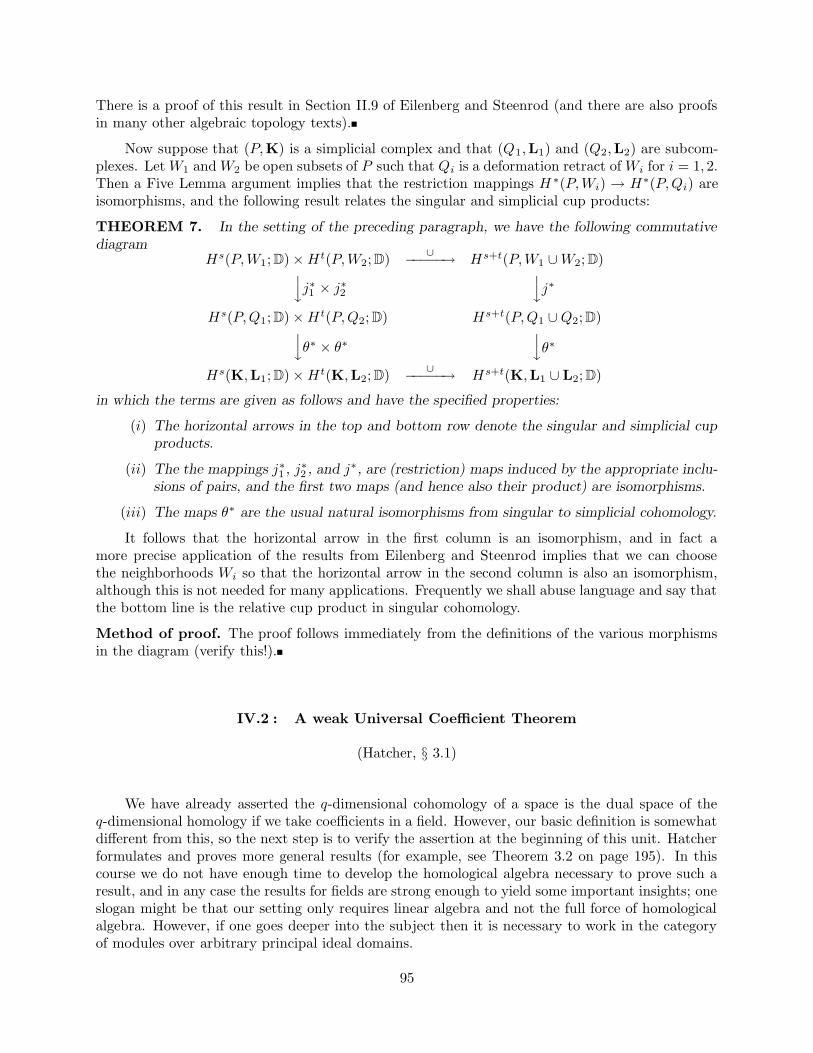
There is a proof of this result in Section II.9 of Eilenberg and Steenrod (and there are also proofsin many other algebraic topology texts).
Now suppose that (P,K) is a simplicial complex and that (Q1,L1) and (Q2,L2) are subcom-plexes. Let W1 and W2 be open subsets of P such that Qi is a deformation retract of Wi for i = 1, 2.Then a Five Lemma argument implies that the restriction mappings H ∗(P,Wi) → H∗(P,Qi) areisomorphisms, and the following result relates the singular and simplicial cup products:
THEOREM 7. In the setting of the preceding paragraph, we have the following commutativediagram
Hs(P,W1; D)×Ht(P,W2; D)∪−−−−−→ Hs+t(P,W1 ∪W2; D)
yj∗1 × j∗2yj∗
Hs(P,Q1; D)×Ht(P,Q2; D) Hs+t(P,Q1 ∪Q2; D)yθ∗ × θ∗
yθ∗
Hs(K,L1; D)×Ht(K,L2; D)∪−−−−−→ Hs+t(K,L1 ∪ L2; D)
in which the terms are given as follows and have the specified properties:
(i) The horizontal arrows in the top and bottom row denote the singular and simplicial cupproducts.
(ii) The the mappings j∗1 , j∗2 , and j∗, are (restriction) maps induced by the appropriate inclu-sions of pairs, and the first two maps (and hence also their product) are isomorphisms.
(iii) The maps θ∗ are the usual natural isomorphisms from singular to simplicial cohomology.
It follows that the horizontal arrow in the first column is an isomorphism, and in fact amore precise application of the results from Eilenberg and Steenrod implies that we can choosethe neighborhoods Wi so that the horizontal arrow in the second column is also an isomorphism,although this is not needed for many applications. Frequently we shall abuse language and say thatthe bottom line is the relative cup product in singular cohomology.
Method of proof. The proof follows immediately from the definitions of the various morphismsin the diagram (verify this!).
IV.2 : A weak Universal Coefficient Theorem
(Hatcher, § 3.1)
We have already asserted the q-dimensional cohomology of a space is the dual space of theq-dimensional homology if we take coefficients in a field. However, our basic definition is somewhatdifferent from this, so the next step is to verify the assertion at the beginning of this unit. Hatcherformulates and proves more general results (for example, see Theorem 3.2 on page 195). In thiscourse we do not have enough time to develop the homological algebra necessary to prove such aresult, and in any case the results for fields are strong enough to yield some important insights; oneslogan might be that our setting only requires linear algebra and not the full force of homologicalalgebra. However, if one goes deeper into the subject then it is necessary to work in the categoryof modules over arbitrary principal ideal domains.
95

The Kronecker Index
As usual let D be a commutative ring with unit, let C∗ be a chain complex of D-modules,and define an associated cochain complex by C q = HomD(Cq ,D), with a coboundary map dq =Hom(dq+1,D) analogous to the construction for singular cochains. Then evaluation defines a bilinearmap Cq ×Cq → D which is called the Kronecker index pairing and its value at f ∈ C q and x ∈ Cqis usually written as 〈f, x〉.LEMMA 1. Suppose that f, f ′ ∈ Cq are cocycles and x, x′ ∈ Cq are cycles such that f − f ′ = δaand x− x′ = db. Then 〈f, x〉 = 〈f ′, x′〉.Proof. For an arbitrary cochain g and chain y it follows immediately that 〈δg, y〉 = 〈g, dy〉.Therefore we have
〈f, x− x′〉 = 〈f, db〉 = 〈δf, b〉 〈0, b〉 = 0
and similarly〈f − f ′, x′〉 = 〈δa, x′〉 = 〈a, dx′〉 〈a, 0〉 = 0
which combine to show that 〈f, x〉 = 〈f ′, x′〉.COROLLARY 2. The chain/cochain level Kronecker index pairing passes to a well-definedbilinear pairing from Hq(C)×Hq(C) to D.
Manipulations with dual vector spaces
We now assume that F is a field. If V is a vector space over F and U is a subspace of V , thenwe have a short exact sequence of vector spaces
0 → U → V → V/U → 0
and applying the dual space functor we obtain the following short exact sequence of dual spaces:
0 → (V/U)∗ → V ∗ → U∗ → 0
The image of the map from (V/U)∗ to V ∗ is the annihilator of U , which consists of all linear
functionals which vanish on U and will be denoted by U †.Suppose now that V1 and V2 are vector spaces over F and T : V1 → V2 is a linear transformation.
Then we can factor T into a composite
V1 → J1∼= J2 ⊂ V2
where J1 is the quotient of V1 by the kernel of T , the map from J1 to J2 is an isomorphism, and J2
is the image of T . There is also a corresponding factorization for the induced map of dual spaces
V ∗2 → J∗2∼= J∗1 ⊂ V ∗1
These factorizations will be useful in proving the following abstract version of a key result in linearalgebra:
PROPOSITION 3. In the notation above, let T ∗ : V2 → V ∗1 be the associated map of dual
spaces. Then we have (Kernel T )† = Image T∗ ⊂ V ∗1 and (Image T )† = Kernel T ∗ ⊂ V ∗2 .
96

Proof. By our previous observations we know that (Kernel T )† corresponds to J∗1 = J∗2 , and
since J2 is the image of T , we have the asserted relationship. Similarly, we know that (ImageT )†corresponds to (V2/J2)
∗, and one can check directly that this corresponds to all linear functionalsf on V2 such that 0 = f oT = T ∗(f).
We now have enough machinery to derive the relationship between homology and cohomologyover a field.
PROPOSITION 4. Let C∗ be a chain complex over a field F, and let C∗ be the dual cochaincomplex. Then for each q there is a natural isomorphism from H q(C) to Hq(C)∗.
Proof. We shall focus on verifying the assertion about the isomorphism first. By definition weknow that
Hq ∼= (Kernel δq)/(Image δq−1) .
Using the relationship δ = d∗ we may rewrite the right hand side in the form
(Image dq+1)†/(Kernel dq)
†
and conclude by noting that the latter subquotient of C ∗q corresponds to
H∗q∼=
((Kernel dq)/(Image dq+1)
)∗.
Under these correspondences and the defining isomorphism
Hq∼=
((Kernel dq)/(Image dq+1)
)
all the standard pairings which evaluate linear functionals at vectors are preserved. In particular,this means that the isomorphism is given by the pairing described in Corollary 2. Now this pairingis natural by construction, and therefore our isomorphism is also natural.
Only a little more work is needed to derive the description of singular cohomology that wewant.
COROLLARY 5. If (X,A) is a topological space and F is a field, then for each q there is anatural isomorphism from Hq(X,A; F) to the dual space Hq(X,A; F)∗.
Proof. At this point all we need to do is describe a natural isomorphism
S∗(X,A; F) ∼= Hom(S∗(X,A),F) −→ HomF (S∗(X,A) ⊗ F,F)
because the latter is the cochain complex to which Proposition 4 applies. However, the isomorphismin question is given directly by the universal properties of the tensor product construction sendingthe chain groups Sq(X,A) to Sq(X,A)⊗ F; in other words, there is a 1–1 correspondence betweenabelian group homomorphisms from Sq(X,A) to F and F-linear maps from Sq(X,A) ⊗ F to F.
If (X,A) is a pair of topological spaces, then similar considerations show that under thisisomorphism the connecting morphism in cohomology
δ∗ : Hp(A; F) −→ Hp+1(X,A; F)
corresponds to the map HomF (∂,F), where ∂ : Hp+1(X, ; F) → Hp(A; F) is the connecting mor-phism in homology. This reflects the fact that chain complex boundaries and cochain complex
97

coboundaries are adjoint to each other with respect to the Kronecker index pairing; details of theverification are left to the reader(?).
IV.3 : Kunneth formulas
(Hatcher, §§ 3.2, 3.B)
One obvious point about the preceding discussion is that we have not yet produced examplesfor which the cup product of two positive-dimensional cohomology classes is nontrivial. Our nextorder of business is to find classes of examples with this property. The first step is to prove purelyalgebraic versions of the results we want.
Algebraic cross products
The proof of the topological result in the preceding paragraph depends on finding a suitablechain complex for computing the homology of a product space X×Y ; more precisely, we want thisto be an algebraic construction on the singular chain complexes of X and Y which is somehow analgebraic product of S∗(X) and S∗(Y ). The correct model is given by a tensor product construction.
Definition. Let (A∗, dA∗ ) and (B∗, d
B∗ ) be chain complexes over a principal ideal domain D such
that the chain groups in negative dimensions are zero. Then the tensor product (A∗, dA∗ )⊗D(B∗, d
B∗ )
has chain groups
(A⊗B)n =
n⊕
p=0
Ap ⊗Bn−p
and the differential is given on Ap ⊗Bq by the formula
dA⊗B(x⊗ y) = dA(x)⊗ y + (−1)px⊗ dB(y) .
The sign is needed to ensure that dA⊗B odA⊗B = 0 so that we actually get a chain complex;proving this algebraic identity is a fairly straightforward (and not too messy) exercise. It is alsofairly straightforward to verify that this construction is covariantly functorial in A and B.(?)
If we are simply given graded modules A∗ and B∗ (which may be viewed as chain complexeswith zero differentials), then the preceding also yields a definition of the tensor product A∗ ⊗B∗.
We shall need the following elementary observation, whose proof is left to the reader(?).
PROPOSITION 1. If B∗ is a graded module which is free in all gradings (each Bk is free) andwe are given a short exact sequence 0 → K∗ → A∗ → C∗ → 0 of graded modules, then the tensorproduct
0 −→ K∗ ⊗D B∗ −→ A∗ ⊗D B∗ −→ C∗ ⊗D B∗ → 0
is also a short exact sequence of graded modules. A similar conclusion holds for all B∗ providedeach of the graded modules K∗, A∗, C∗ is free.
One important consequence of the definition for tensor products of chain complexes is thefollowing method of constructing classes in H∗(A⊗B) from classes in H∗(A) and H∗(B).
98

PROPOSITION 2. In the setting above, there are bilinear mappings
× : Hp(A; D) ⊗ Hq(B; D) −→ Hp+q(A⊗B; D)
with the following property: If x ∈ Ap is a cycle representing u and y ∈ Bq is a cycle representingv, then x⊗ y is a cycle representing u× v.
This construction is called the external homology cross product.
Proof. We shall only sketch the main steps and leave the details to the reader(?). First of all, if xand y are cycles, then the definitions imply that x⊗ y is also a cycle, and if x = dw or y = dz thenx ⊗ y is a boundary. Bilinearity follows from the definition, and this plus the preceding sentenceimply that the bilinear map is well defined.
Our next result states that these products are maximally nontrivial if D is a field.
THEOREM 3. (The algebraic Kunneth Theorem) If F is a field, then the external homologycross product defines an isomorphism
n⊕
p=0
Hp(A; F)⊗Hn−p(B; F) −→ Hn(A⊗B; F)
for all n ≥ 0.
Proof. In the argument below, all tensor products are taken over the field F.
For each integer k let z(Aq) ⊂ Aq be the subspace of cycles; if we define a chain complexstructure on z(A∗) by setting all boundary homomorphisms equal to zero, then z(A∗) is a chainsubcomplex of A∗, and the quotient complex
q(A∗) = A∗/z(A∗)
also has a trivial differential because q(Ak) ∼= d[Ak] ⊂ Ak−1 and d od = 0.
Since we are working over a field F, all modules are free, and hence if we apply Proposition 3to the previous short exact sequence we obtain a short exact sequence of chain complexes
0 −→ z(A∗)⊗F B∗ −→ A∗ ⊗F B∗ −→ q(A∗)⊗F B∗ −→ 0
which of course has an associated long exact homology sequence. Since the differentials in z(A∗)and q(A∗) are trivial, this long exact sequence has the form
· · · [z(A)∗ ⊗H∗(B)]k → Hk((A⊗B) → [q(A)∗ ⊗H∗(B)]k → [z(A)∗ ⊗H∗(B)]k−1 · · ·
and the definitions of the connecting homomorphisms imply that the right hand arrow ∂k is givenby d∗ ⊗ id [H∗(B)], where
dm : q(A)m −→ z(A)m−1
is the compositedm : q(A)m ∼= dm[Am] ⊂ z(A)m−1 .
This implies that the map dm is injective, and since the tensor product functor over a field preservesshort exact sequences it follows that the connecting homomorphisms ∂k are also injective. Thereforethe maps
Hk((A⊗B) → [q(A)∗ ⊗H∗(B)]k
99

are zero, so by exactness it follows that Hk(A⊗B) is isomorphic to the quotient
[z(A)∗ ⊗H∗(B)]k / [q(A)∗ ⊗H∗(B)]k∼= [H∗(A)∗ ⊗H∗(B)]k
and a check of the definitions shows that the isomorphism is induced by the homology cross product.
There is also a dual cross product in cohomology. If g : Ap → F and h : Bq → F arecochains, then we define a cross product cochain g × h : [A ⊗B]p+q → F such that the restrictionto Ar ⊗Bp+q−r is zero if r 6= p and the restriction to Ap ⊗Bq satisfies the identity
g × h(x⊗ y) = g(x) · h(y) , (x ∈ Ap , y ∈ Bq) .
The coboundary of g × h is given by the following identity:
LEMMA 4. In the setting above we have
δ(g × h) = δg × h + (−1)p g × δh .
In particular, if g and h are cocycles then so is g×h, and if in addition one of g and h is a coboundarythen so is g × h, so that the cross product passes to a bilinear mapping from H p(A) ⊗Hq(B) →Hp+q(A⊗B).
Sketch of proof. By definition we have
δ(g × h) = (g × h) od = (g × h) o(dA ⊗ id + (−1)pid⊗ dB
)
and if we apply the right hand expression to a typical generator z ⊗ w ∈ Am ⊗ Bp+q−m−1 we seethat the value equals the value of the right hand side in the displayed expression of the lemma. Thesecond sentence in the lemma follows by adding the conditions δg = δh = 0 for the first assertion,and adding one of the additional conditions g = δg ′ or h = δh′ in the second. The third sentencefollows immediately from these and the fact that the cochain cross product is bilinear.
It is now very easy to show that the cross product of two nontrivial cohomology classes isnonzero.
COROLLARY 5. If α ∈ Hp(A) and β ∈ Hq(B) are nonzero, then so is α× β.
Proof. By the Weak Universal Coefficient Theorem there are homology classes u ∈ Hp(A) andv ∈ Hq(B) such that the Kronecker indices α(u) and β(v) are nonzero elements of F. Since theKronecker index of the cohomology cross product satisfies
〈α× β, u× v〉 = α(u) · β(v)
and the right hand side is nonzero (it is a product of two nonzero elements in F), it follows thatα× β is also nonzero.
Topological cross products
We can define the cross product of two singular cochains by a variant of the cup productdefinition. If D is a commutative ring with unit and we are given two singular cochains f :Sp(X,D)→ D and g : Sq(Y,D)→ D, then their cross product
f × g : Sp+q(X × Y ; D) −→ D
100

is defined on a singular simplex T = (TX , TY ) : ∆p+q → X × Y by the formula
f × g(T ) = f (Frontp(TX) ) · g (Backq(TY ) ) .
The usual bilinearity and associativity properties follow directly from the definition (details areleft to the reader). We also have the following identities showing that each of the cup and crossproducts can be easily described in terms of the other:
PROPOSITION 6. In the setting above we have the following identities, whose verificationsare left to the reader:
(i) If πX : X × Y → X and πY : X × Y → Y are coordinate projections with associated
singular cochain homomorphisms π#X and π#
Y , then f × g = π#X(f) ∪ π#
Y (g).
(ii) If X = Y and ∆X : X → X ×X is the diagonal map, then f ∪ g = ∆#X(f × g).
The singular cohomology cross product also satisfies analogs of the basic properties for coho-mology products in Lemma 4;
LEMMA 7. In the setting above we have
δ(f × g) = δf × g + (−1)p f × δg .In particular, if f and g are cocycles then so is f×g, and if in addition one of f and g is a coboundarythen so is f×g, so that the cross product passes to a bilinear mapping from H p(X; D)⊗Hq(Y ; D)→Hp+q(X × Y ; D).
The Topological Kunneth Theorem
At this point we need a result relating the singular homology relating the singular homologyof X × Y to the singular homology of the factors X and Y ; to shorten the discussion, we restrictourselves to field coefficients in these notes. Some of the earliest general results of this type weredue to H. Kunneth in the early 1920s, and in singular homology this relationship follows from ageneral method of acyclic models due to Eilenberg and J. A. Zilber. We shall not formulate thismethod abstractly, but the reader may be able to see the general pattern emerge.
THEOREM 8. (Eilenberg-Zilber) If D is a principal ideal domain and X and Y are topologicalspaces, then there are functorial chain homotopy equivalences
ψX,Y : S∗(X × Y ; D) → S∗(X; D)⊗D S∗(Y ; D) , ϕX,Y : S∗(X; D)⊗D S∗(Y ; D) → S∗(X × Y ; D)
with the following properties:
(i) The composites ϕ oψ and ψ oϕ are naturally chain homotopic to the identity.
(ii) In degree 0 the map ψ takes a singular 0-simplex T = (TX , TY ) to TX ⊗ TY , and ϕ isinverse to ψ.
We shall describe an explicit choice for ψX,Y known as the Alexander-Whitney map.
Before proving Theorem 8, we shall list some of its consequences:
THEOREM 9. (Classical Kunneth Formula for field coefficients) Let X and Y be topologicalspaces, and let F be a field. Then the composite of the homology cross product and inducedmapping ψ∗ in homology defines isomorphisms of singular homology groups
n⊕
p=0
Hp(X; F)⊗F Hn−p(Y ; F) −→ Hn(X × Y ; F)
101

for all n ≥ 0.
This result follows directly from Theorem 8 and the Algebraic Kunneth Formula (Theorem3).
THEOREM 10. (Cohomological Kunneth Formula) Let X and Y be topological spaces, let F
be a field, and assume that the homology groups Hp(X; F) and Hq(Y ; F) are finite for all p.q ≥ 0.Then the cohomology cross product map defines isomorphisms of singular homology groups
n⊕
p=0
Hp(X; F)⊗F Hn−p(Y ; F) −→ Hn(X × Y ; F)
for all n ≥ 0.
Sketch of the proof that Theorem 9 implies Theorem 10. This is a consequence of thefollowing observations:
(1) The Universal Coefficient isomorphism from Hk(W ; F) to the dual space of Hk(W ; F),where W = X or Y and k ≥ 0.
(2) The natural isomorphism (V1 ⊕V2)∗ ∼= V ∗1 ⊕V ∗2 , where V ∗ denotes the dual space and V1
and V2 are vector spaces over F.
(3) The natural isomorphism (V1 ⊗F V2)∗ ∼= V ∗1 ⊗F V
∗2 , where V ∗ denotes the dual space and
V1 and V2 are finite dimensional vector spaces over F (in fact, the conclusion of thetheorem is generally false if the finite dimensionality conditions do not hold, but therestill is a natural monomorphism from V ∗1 ⊗F V
∗2 to (V1 ⊗F V2)
∗).
Note that under these isomorphisms the homology and cohomology cross products correspond;namely, if fi ∈ V ∗i and xi ∈ Vi then f1 ⊗ f2(x1 ⊗ x2) = f1(x1) · f2(x2).
The first step in proving Theorem 7 is to consider the special case where X = Y = ∆n forsome n.
LEMMA 11. Let D be a commutative ring with unit. If p, q ≥ 0 and an augmentation is definedon S∗(∆n; D)⊗ S∗(∆n; D) using the multiplication and tensor product maps
S0(∆n : D)⊗D S0(∆n : D) → D⊗D → D
then S∗(∆p; D)⊗D S∗(∆q ; D) is acyclic.
Proof of Lemma 11. Let C∗(D) be the ordered simplicial chain complex C∗(eω0 ; D), where e0is a standard vertex of ∆n, let η : C∗(D) → S∗(∆p; D) be the augmentation-preserving inclusiondetermined by viewing the generator of C0(D) as the singular 0-simplex sending the unique pointin ∆0 to the vertex e0 ∈ ∆p, and note that the augmentation map ε on S∗(∆p) can be viewedas a chain map from the latter to C∗(D). Then the proof of homotopy invariance for singularhomology implies that η[C∗(D)] is a chain homotopy deformation retract of S∗(∆p; D). We canthen construct the tensor product of a contracting chain homotopy with the identity on S∗(∆q; D),and it follows immediately that S∗(∆q; D) ∼= C∗(D) ⊗⊗DS∗(∆q; D) is a chain deformation retractof S∗(∆p; D) ⊗D S∗(∆q; D). Since the smaller chain complex is acyclic, it follows that the largerchain complex is also acyclic.
SIMPLICIAL ANALOGS OF LEMMA 11. Similar results hold for the ordered and unorderedsimplicial chain complexes of ∆−n. The proofs are straightforward adaptations of the proof in thesingular case and are left to the reader.
102

Proof of Theorem 8. The Alexander-Whitney map ψX,Y is just a formalization of earlierconstructions, Specifically, if T = (TX , TY ) : ∆n : X × Y is a singular simplex given by thecoordinate projections TX and TY , then
ψX,Y (T ) =
n∑
p=0
Frontp(TX)⊗Backn−p(TY ) .
It is a routine exercise to check that this construction defines a natural chain map(?).
The idea behind constructing ϕ and the chain homotopies is to look at universal examples andextend to the general case by naturality. The chain groups
[S∗(X; D)⊗ S∗(Y ; D)]n
are free modules, and explicit free generators are given by all objects of the form FX ⊗BY , whereFX : ∆p → X and BY : ∆n−p → Y are singular simplices and 0 ≤ p ≤ n. We shall define ϕ onsuch objects recursively with respect to n. The stated conditions define ϕ in degree 0. Once weare given ϕ in degrees ≤ n− 1, we shall define ϕ first on the universal class
id[∆p]⊗ id[∆n−p] ∈ Sp(∆p; D)⊗D Sn−p(∆n−p; D)
and then we shall define ϕ(FX ⊗BY ) by the naturality condition
ϕ(FX ⊗BY ) = FX# (id[∆p])⊗BY# (id[∆n−p]) .
It is a straightforward exercise to verify that this construction defines a chain map in degree n, andthis completes the inductive step(?).
By the preceding discussion, the construction of ϕ reduces to finding a choice W (p, q) forϕ(id[∆p]⊗ id[∆p]) which satisfies the chain map condition
dW (p, q) = ϕ od (id[∆p]⊗ id[∆p]) .
Since S∗(∆p×∆n−p; D) is acyclic, such a class exists if and only if the right hand side is a cycle, soeverything comes down to computing the boundary map on the right hand side. By the inductionhypothesis, we know that ϕ is a chain map in degree n− 1, and therefore the boundary of the righthand side is given by
d (ϕ od (id[∆p]⊗ id[∆p]) ) = (ϕ od) od (id[∆p]⊗ id[∆p])
which vanishes because d od = 0 as required. This completes the inductive step and the constructionof ϕ.
The chain homotopies from ϕ oψ and ψ oϕ to the respective identity maps are also constructedusing universal examples. We shall start by constructing the chain homotopy ϕ oψ ' id. Sinceϕ0
oψ0 is the identity map, we can take D0 = 0. Assume that se have defined Dk for k < n; asbefore, we first define Dn on the diagonal map Diagn : ∆n → ∆n × ∆n and then we extend bynaturality. The classes
θn+1 = Dn (Diagn) ∈ Sn+1(∆n ×∆n)
are required to satisfy the identity
dθn = Diagn − ϕψ (Diagn) − Dn−1odn (Diagn)
103

for all n > 0. Once again, everything reduces to showing that the right hand side is a cycle becauseS∗(∆n ×∆n; D) is acyclic. Much as before, one can use the inductive hypothesis
ϕn−1oψn−1 − identity = Dn−2
odn−1 + dn oDn−1
and d od = 0 to prove that Diagn − ϕψ (Diagn) − Dn−1odn (Diagn) is a cycle. As before, one
extends by naturality, and it is another formal exercise to check that the construction defines anatural chain homotopy from ϕ oψ to the identity.
Similar considerations yield the chain homotopy E : ψ oϕ ' id. In this case we must use thefree generators of S∗(X; D) ⊗ S∗(Y ; D) described above, and we need Lemma 10 for the fact thatS∗(∆p; D)⊗D S∗(∆q; D) is acyclic.
The next result, which yields many examples of nontrivial cross products in singular homologyand cohomology, is an immediate consequence of the results in this section.
COROLLARY 12. Let X and Y be nonempty topological spaces, and let F be a field.
(i) If u ∈ Hp(X; F) and v ∈ Hq(Y ; F) are nonzero, then so is u× v.(ii) If α ∈ Hp(X; F) and β ∈ Hq(Y ; F) are nonzero, then so is α× β.
Products in relative homology groups
We would also like to have a version of Corollary 11 for cross products in relative homologyand cohomology. There are a few complications, but one can develop a reasonably good theoryin this case. The first step is a generalization of the Eilenberg-Zilber Theorem. For the rest ofthis section we shall assume that all coefficients lie in some commutative ring with unit D which issuppressed from the notation.
THEOREM 13. Suppose that (X,A) and (Y,B) are pairs of spaces such that A and B are openin X and Y respectively. Then there is a relative cross product on the cochain level
Sp(X,A) ⊗ Sq(Y,B) −→ Sp+q(X × Y,A× Y ∪X ×B)
which is compatible with the absolute cross product defined in this unit. This product satisfiesanalogs of the coboundary formulas in the absolute case and passes to a cohomology cross productwhich is also compatible with the previous construction when A = B = ∅. Furthermore, if thecoefficients lie in a field F and all the cohomology groups H p(X,A) and Hq(Y,B) are finite dimen-sional vector spaces, then the cross product defines an isomorphism from H ∗(X,A)⊗H∗(Y,B) toH∗(X × Y,A× Y ∪X ×B).
Proof. Let U be the open covering of A × Y ∪X × B given by A × Y,X × B. Then one cancheck directly that the composite of the cochain level cross product from Sp(X,A) ⊗ Sq(Y,B) toSp+q(X × Y ) with the restriction mapping
Sp+q(X × Y ) → Sp+qU (A× Y ∪X ×B) = HomD(Sp+q(A× Y ) + Sp+q(X ×B),D)
is trivial; in other words, if f is a cochain on Sp(X) which vanishes on Sp(A) and g is a cochain onSq(Y ) which vanishes on Sq(B), then f×g vanishes on Sp+q(A×Y )+Sp+q(X×B) = SUp+q(A×Y ∪X ×B). The Leibniz Formula for the coboundary of a cross product is an immediate consequenceof the construction and known results when A = B = ∅ (recall that the relative cochain groups
104

S∗(Z,C) are contained in the absolute groups S∗(Z) as the subgroups of cochains whose restrictionsto S∗(C) are zero). It follows that the cochain level cross product passes to cohomology mappings
Hp(X,A) ⊗Hq(Y,B) → Hp+q (S∗(X × Y )/S∗U (A× Y ∪X ×B) )
and since the inclusion of the latter in Sp+q(A×Y ∪X×B) is a chain homotopy equivalence by theproof of excision we get the desired map from Hp(X,A)⊗Hq(Y,B) to Hp+q(X×Y,A×Y ∪X×B).This completes the derivation of the construction, We must now prove the relative Kunneth Formulain the final sentence of the theorem.
Consider first the case where B = ∅. Since the short exact sequences of singular chain com-plexes for the pair (X,A) is split in each degree (the standard free generators of Sk(A) are a subsetof the standard free generators for Sk(X)), we have the following commutative diagram in whichthe vertical maps are Alexander-Whitney maps and the rows are short exact sequences; all tensorproducts are taken with respect to the field F.
0 → S∗(A× Y ) → S∗(X × Y ) → S∗(X × Y,A× Y ) → 0yψ
yψyψ
0 → S∗(A)⊗ S∗(Y ) → S∗(X)⊗ S∗(Y ) → S∗(X,A) ⊗ S∗(Y ) → 0
Since the vertical maps on the left and center induce isomorphisms in homology, it follows that thevertical map on the right also induces isomorphisms in homology; in fact, this part of the argumentdoes not require A to be an open subset of X.
Now consider the following commutative diagram, in which the second and third rows are shortexact sequences of chain complexes and the maps denoted by ψ are Alexander-Whitney maps:
S∗(X ×B,A×B)
∼=
SU∗ (A× Y ∪X ×B,A× Y )y⊂
S∗(A× Y ∪X ×B,A× Y ) → S∗(X × Y,A× Y ) → S∗(X × Y,A× Y ∪X ×B)y?
yψyψ
S∗(X,A) ⊗ S∗(B) → S∗(X,A) ⊗ S∗(Y ) → S∗(X,A) ⊗ S∗(Y,B)
The question mark represents the following claim: There is a chain map ψ ′ from S∗(A × Y ∪X × B,A × Y ) to S∗(X,A) ⊗ S∗(B) whose restriction to the subcomplex S∗(x × B,A × B) ∼=SU∗ (A×Y ∪X×B,A×Y ) is the usual Alexander-Whitney map. The existence of ψ ′ follows fromthe commutativity of the right hand square, for the latter implies that ψ : S∗(X × Y,A × Y ) →S∗(X,A) ⊗ S∗(Y ) maps the kernel of the surjection from S∗(X × Y,A × Y ) to the kernel of thesurjection from S∗(X,A) ⊗ S∗(Y ). Furthermore, the commutativity of the diagram
S∗(X ×B,A×B) → S∗(X × Y,A× Y )yψ
yψ
S∗(X,A) ⊗ S∗(B) → S∗(X,A) ⊗ S∗(Y )
105

implies that ψ′ extends the Alexander-Whitney map ψ on S∗(X,A) ⊗ S∗(B).
By earlier discussion of special cases, which applies to the pair (X×B,A×B) by interchangingthe roles of the first and second factors, we know that the Alexander-Whitney map on S∗(X,A)⊗S∗(B) induces isomorphisms in singular homology, and by the proof of excision we know that theinclusion of S∗(X ×B,A×B) in S∗(A× Y ∪X ×B) induces isomorphisms in singular homology,and it follows immediately that the mapping ψ ′ also induces isomorphisms in singular homology.We have already shown that the Alexander-Whitney map from S∗(X × Y,A × Y ) induces anisomorphism in homology, and therefore the Five Lemma implies that the Alexander-Whitney mapfrom S∗(X × Y,A× Y ∪X ×B) also induces isomorphisms in homology.
If we now take coefficients in a field and assume all homology and cohomology groups are finitedimensional, then the weak Universal Coefficient Theorem implies that the dual cochain complexmaps
S∗(X,A; F)⊗F S∗(Y,B; F) → S∗(X × Y,A× Y ∪X ×B; F)
induce isomorphisms in cohomology fromH∗(X,A; F)⊗FH∗(Y,B; F) toH∗(X×Y,A×Y ∪X×B; F).
In particular, just as before we know that if the homology groups of (X,A) and (Y,B) arefinite dimensional over F in each dimension, then the cross product of a nontrivial cohomology classα ∈ H∗(X,A; F) and a nontrivial cohomology class β ∈ H∗(Y,B; F) will always be nontrivial.
CORRESPONDING RESULTS FOR CLOSED SUBSETS. Frequently we want versions of thepreceding when A and B are closed subsets rather than open subsets. As in earlier discussions,analogous results hold if we assume that A and B are deformation retracts of open neighborhoodsA ⊂ U ⊂ X and B ⊂ V ⊂ Y (details are left to the reader(?) — the crucial point is that pairslike (X,A) and (X,U) have isomorphic homology), and in many (most?) situations of interest inalgebraic and geometric topology this sort of condition is satisfied. For example, this is the case ifX is a polyhedron and A is a subpolyhedron.
Cap products
Although the homology groups of a space do not have a ring structure, it turns out that thegraded object H∗(X,D) is a graded module over the cohomology ring if one multiply cohomologydegrees by (−1).
Definition. Let X be a space, and let A1 and A2 be open subsets of X. The chain/cochain levelcap product
∩ : Sp(X,A1; D)⊗D Sn(X; D)/[Sn(A1; D) + Sn(A2; D)] −→ Sn−p(X,A2; D)
is defined as follows: Given g : Sp(X,A1) → D and a singular simplex T : ∆n → X, the cochaing ∩ T is given by g
(Frontp(T )
)· Backn−p(T ). Strictly speaking this construction is defined on
Sp(X,A1; D) ⊗ Sn(X; D), but it factors through the displayed quotient because g ∩ T is trival onall singular simplices in Sn(A1; D) + Sn(A2; D) ⊂ Sn(X; D); if the image of T lies in A2, then theimage is trivial by the definition of Sn−p(X,A2; D), and if the image of T lies in A1 then trivialityfollows because f |Sp(X,A1; D) is zero. If c is a p-chain in Sp(X,A1; D), then one has the usual sortof graded Leibniz rule for computing d(g ∩ c), and it follows that (1) g∩ c is a cycle if g is a cocycleand c is a cycle, (2) g ∩ c is a boundary if either g is a coboundary or c is a boundary. Since A1
and A2 are open subsets of X, the proof of excision implies that the chain complex inclusion
S∗(A1; D) + S∗(A2; D) ⊂ S∗(A1 ∪A2; D)
106

induces isomorphisms in homology, it follows that the chain/cochain level cap product induces amap in homology/cohomology
∩ : Hp(X,A1; D)⊗D Hn(X,A1 ∪A2; D) −→ Sn−p(X,A2; D) .
The cap product map is D-bilinear, and it also has the following formal properties:
PROPOSITION 14. Let X be a space. Then the cap product has the following properties:
(i) If εX : S0(X)→ D is the augmentation and [εX ] ∈ H0(X; D) is its cohomology class, thencap product with [εX ] induces the identity on H∗(X; D).
(ii) The cap and cup product satisfy a mixed associative law: If u ∈ H q(X; D), v ∈ Hp(X; D),and z ∈ Hn(X; D), then (u ∪ v) ∩ z = u ∩ (v ∩ z).
(iii) If f : X → Y is continuous with u ∈ Hp(Y ; D) and z ∈ Hn(x; D), then f∗( f∗u ∩ z) =
u ∩ f∗(z).In each case, one can verify that the corresponding identities hold at the chain/cochain level;
details are left to the reader(?).
IV.4 : Grade-commutativity and examples
(Hatcher, §§ 3.2, 3.B)
DEFAULT HYPOTHESES. Unless explicitly stated otherwise, througout this section D willdenote a commutative ring with unit, all chain complexes will be assumed to be modules over D,and tensor products will be assumed to be given over D.
It was fairly easy to prove that the cup product on cohomology is associative, and in fact thisis also true on the cochain level. Furthermore, it was even easier to prove that the augmentationcocycle ε : S∗(X) → D is a two sided identity in the absolute case (pairs where the subspace isempty). We shall now consider commutativity properties of cup products, both at the cohomologylevel and at the cochain level.
One can do direct calculations to show that the cup product is usually not commutative inthe standard sense. For example, one can check this in the simplicial cohomology of complexeshomeomorphic to T 2 = S1 × S1. Our results contain both good news and bad news:
Good news. On the cohomology level the cup product is grade-commutative in thesense that if α ∈ Hp(X,D) and β ∈ Hq(Y,D), then β ∪ α = (−1)pqα ∪ β.
Bad news. On the cochain level the cup product is usually not even grade-commutative,although it is so up to a system of higher chain homotopies (however, we shall only showcommutativity up to an ordinary chain homotopy).
In particular, it turns out that the Steenrod squares and reduced powers in Section 4.L of Hatcherare defined using such higher chain homotopies and in fact imply the impossibility of constructing agrade-commutative cup product on the cochain level for coefficients in a field F of finite character-istic. On a more positive note, relatively recent results of M. Mandell show that if X is reasonablynice — for example, if X is a polyhedron — then the homotopy type of X is determined by the
107

singular chain complex together with the a suitably defined structure of higher chain homotopiesfor cup product commutativity. Here is the reference:
M. A. Mandell. Cochains and homotopy type, Publ. Math. Inst. Hautes Etudes Sci.103 (2006), 213–246.
In contrast, if we work over a field F of characteristic zero, then it is possible to define cohomologygroups using cochain constructions that are grade commutative (on the cochain level). There is amore extensive discussion of commutative cochains on pages 110–111 of the following book:
P. A. Griffiths and J. W. Morgan. Rational homotopy theory and differential forms,Progress in Mathematics Vol. 16. Birkhauser, Boston, MA, 1981.
In the next unit we shall discuss some fundamental constructions which are closely related to thetopics covered in this book.
Coalgebraic structures on simplicial chain complexes
Since homology and cohomology are essentially dual to each other, the existence of a productstructure in the latter but not the former may seem puzzling. However, it turns out that one canresolve this by a more systematic approach to dualization. One can view a multiplicative structureon a (graded) algebraic object as a (grade-preserving0 homomorphism µ : A⊗A→ A; dually, onecan define a COMULTIPLICATIVE structure as a homomorphism ψ : A→ A⊗ A; such a structurecan also be called a coproduct. Every concept that is meaningful for an algebra or product hasa natural dual concept which is meaningful for a coalgebra or coproduct. For example, just as analgebra is associative if and only if the diagram
A⊗A⊗A µ⊗1−→ A⊗Ay1⊗ µ
yµ
A⊗A µ−→ A
commutes, we can say that an algebra is coassociative if the diagram
Aψ−→ A⊗A
yψy1⊗ ψ
A⊗A ψ⊗1−→ A⊗A⊗A
commutes. All of this is intrinsically formal, but the next result shows that such structures actuallyarise in concrete situations.
PROPOSITION 1. If X is a topological space, let ∆X be the diagonal and let ψX,X be theAlexander-Whitney map for X×X. Then the chain map ΨX = ψX,X o∆X# defines a coassociativecomultiplication on S∗(X). Furthermore, if f : X → Y is a continuous mapping, then the inducedmap of singular chain complexes is a morphism of coalgebras.
This follows directly from the definition of the Alexander-Whitney map (details are left to thereader(?)).
COROLLARY 2. If our underlying commutative ring with unit is a field F, then the chain levelcomultiplication induces a comultiplication in homology, and this comultiplication is functorial andcoassociative.
108

The conceptual point of the proposition and corollary is that one can view the multiplicativestructure in cohomology as the dual of the given comultiplicative structure in homology.
We can view a two-sided identity in an algebra as a homomorphism from D → A such thatthe composites
A ∼= D⊗A→ A⊗A→ A , A ∼= A⊗ D→ A⊗A→ A
are the identity mapping (in the graded case, we assume D is contained in degree zero). The dualnotion is basically just an augmentation A → D, and of course it is supposed to satisfy the dualconditions that the composite mappings
A→ A⊗A→ D⊗A ∼= A , A→ A⊗A→ A⊗ D ∼= A
are the identity. It is routine to verify that the standard augmentation maps on singular chaincomplexes have this property, so in fact the singular chain complex may be viewed as a functorfrom spaces to coassociative coalgebra chain complexes with augmentations.
Algebraic and topological twist maps
The preceding discussion indicates that grade-commutativity properties of cup products shouldbe dual to grade-cocommutativity properties of the functorial comultiplication on singular chaincomplexes. At this point we need to introduce some algebra.
Definition. Suppose that A∗ and B∗ are chain complexes over D. The transposition or twistisomorphism
τA,B : A∗ ⊗B∗ −→ B∗ ⊗A∗is determined by the identity τA,B(ap ⊗ bq) = (−1)pq(bq ⊗ ap), where ap ∈ Ap and bq ∈ Bq.
It follows immediately that τ is a functorial chain map and τB,A oτA,B is the identity(?) .
One motivation for this construction is the following result:
THEOREM 3. Let X and Y be topological spaces, and let T : X × Y → Y ×X be the mapT (x, y) = (y, x) which transposes coordinates. Then there is a commutative diagram up to naturalchain homotopy
S∗(X × Y )ψ−→ S∗(X)⊗ S∗(Y )
yT#
yτ
S∗(X × Y )ψ−→ S∗(X) ⊗ S∗(Y )
in which the horizontal maps are Alexander-Whitney maps and τ is the algebraic transpositionmap on S∗(X)⊗ S∗(Y ).
Proof. The first things to observe is that all maps of chain complexes are augmentation preservingand the diagram commutes in degree zero. Assume inductively that the diagram commutes up tonatural chain homotopy through dimension n− 1 ≥ 0. We shall use the method of acyclic modelsto construct the chain homotopy in degree n for the universal example of the diagonal singularsimplex Diagn : ∆n → ∆n ×∆n and extend it to all singular simplices by naturality.
To construct the chain homotopy on the universal example in degree n, we need to find someϕn ∈ [S∗(∆n)⊗ S∗(∆n)]n+1 such that
dϕn = ψ oT# (Diagn) − τ oψ (Diagn) − D od (Diagn) .
109

Since S∗(∆n) ⊗ S∗(∆n) is acyclic, we can find a suitable element ϕn if and only if the right handside is a cycle. As in previous examples, this can be shown using the facts that ψ, T and τ arechain maps, the chain complex identity d od = 0, and the fact that D is a chain homotopy throughdegree n− 1; details are left to the reader.
We are now ready to state the grade-commutativity properties of the cross product and theirimplications for grade-commutativity of the cup product.
THEOREM 4. Let X and Y be topological spaces, let u ∈ Hp(X) and v ∈ Hq(Y ) becohomology classes, and let T : X × Y → Y ×X denote the transposition homeomorphism. Thenthe cohomology cross product satisfies u× v = (−1)pqT ∗(v × u).COROLLARY 5. If X is a space with u ∈ Hp(X) and v ∈ Hq(X), then u ∪ v = (−1)pqv ∪ u.Proof of Corollary 5. If ∆X : X → X × X is the diagonal, then u ∪ v = ∆∗X(u × v), and ifT : X ×X → X ×X transposes coordinates, then T o∆X = ∆X . Therefore by Theorem 5 we have
u∪ v = ∆∗X(u× v) = (T o∆X)∗(u× v) = ∆∗XoT ∗(u× v) = ∆∗X ( (−1)pqv × u) = (−1)pqv ∪ u
which is what we wanted to prove.
Proof of Theorem 4. Choose cocycles f and g representing u and v respectively, and let ψX,Yand ψY,X be the Alexander-Whitney maps for X × Y and Y × X. Then we have the followingdiagram in which the right hand square commutes and the left hand square commutes up to chainhomotopy:
Sp+q(X × Y )proj(p,q)ψ−→ Sp(X)⊗ Sq(Y )
f⊗g−→ D⊗ D ∼= DyT#
yτy=
Sp+q(Y ×X)proj(p,q)ψ−→ Sp(X)⊗ Sq(Y )
(−1)pqg⊗f−→ D⊗ D ∼= D
The map proj(p, q) is projection onto the direct summand Sp(X)⊗ Sq(Y ) in [S∗(X) ⊗ S∗(Y )]p+q ,while the top row is a cochain level representative for u× v and the bottom row is a cochain levelrepresentative for (−1)pqu× v.
Let E be the chain homotopy relating ψY,X oT# and τ oψX,Y . Then we have
f×g = (f⊗g) oψX,Y = (−1)pq(g⊗f) oτ oψX,Y = (−1)pq(g⊗f) o (ψY,X oT# + dE +Ed) =
T# ( (−1)pq(g ⊗ f) oψY,X) + (−1)pqδ(g × f) oE + δU
where δ is the coboundary map and U is some cochain whose precise value is unimportant becauseit disappears when we take cohomology classes. The term δ(g × f) vanishes because f and g arecocycles, and therefore the displayed identities show that the cohomology classes represented byf × g and (−1)pq(g × f) — namely, u× v and (−1)pqT ∗(v × u) — must be equal.
Some examples
The results of this and the previous section yield complete information on the cup productstructure for a product of spheres with coefficients in a field. This can be done inductively usingthe theorem stated below. Before stating this result, we need the following construction:
Definition. Let A∗ and B∗ be graded algebras over D with multiplication maps µA and µBrespectively. Then the tensor product A∗ ⊗B∗ has a multiplication given by
(A∗ ⊗B∗)⊗ (A∗ ⊗B∗)→ A∗ ⊗A∗ ⊗B∗ ⊗B∗ → A∗ ⊗B∗
110

where the first map is the middle four interchange
xp ⊗ yq ⊗ zr ⊗ ws −→ (−1)qr xp ⊗ zr ⊗ yq ⊗ ws
and the second map is µA ⊗ µB .
THEOREM 6. Let n be a positive integer, let F be a field, and let X be a space such thatHk(X; F) is finite dimensional for all k. Then the cohomology algebra H ∗(Sn×X; F) is isomorphicto the tensor product algebra H∗(Sn)⊗F H
∗(X).
This result is an immediate consequence of the cohomological Kunneth Theorem; details areagain left to the reader.
The preceding theorem and induction yield the computation for the cohomology of a product
r∏
k=1
Sn(k)
where each n(k) is positive.
COROLLARY 7. In the setting above we have
H∗(∏r
k=1 Sn(k); F
) ∼=r⊗
k=1
H∗(Sn(k); F
).
The following results are immediate consequences of this corollary:
COROLLARY 8. In the setting above, assume that for each k the cohomology class uk is theimage of a generator for Hn(k)(Sn(k); F) under the map induced by the coordinate projection pkonto the kth factor. Then ∏
k
uk 6= 0 .
This is merely an iteration of the fact that the cross product of two nontrivial cohomologyclasses is always nontrivial.
COROLLARY 9. In the setting above, assume that the dimensions n(k) are all even and equalto some fixed integer n (hence the cup product is commutative in the usual sense), and assumefurther that for each k the cohomology class uk is the image of a generator for H (Sn; F) under themap induced by the coordinate projection pk onto the kth factor. Then
(∑
k
uk
)r6= 0 .
This reduces to a purely algebraic computation, which shows that the class in question is equalto n! ·∏k uk (the details are again left as an exercise(?)).
111

IV.5 : Two applications
(Hatcher, §§ 3.2, 4.2)
Although we have only obtained relatively weak versions of the basic results on products insingular homology and cohomology theory, they suffice to yield two fairly significant results. Oneis a restriction on the maps in homology associated to a homotopy self-equivalence from S 2m×S2m
to itself, and the other is a proof that for all m > 1 there is a continuous mapping from S 4m−1
to S2m which is not homotopic to a constant. The existence of such maps reflects several of thefundamental difficulties one encounters when trying to study homotopy theory.
Coefficient homomorphisms in singular homology and cohomology
We would like to have some way of extracting information about homology and cohomologygroups with integer coefficients from computations of homology and cohomology with coefficientsin various fields (not surprisingly, the usual examples are the rationals Q and the prime fields Zp
where p is prime). There are two or three main ideas.
(1) If ϕ : D → E is a homomorphism of commutative rings with unit, then there are associ-ated natural coefficient homomorphisms ϕ# and ϕ# of singular chain and cochain groups.These are compatible with the cup and cap product structures, and they induce corre-sponding natural transformations in homology and cohomology which commute with theconnecting homomorphisms in the long exact sequences of pairs and Mayer-Vietoris exactsequences.
(2) Let A→ A(0) be the rationalization functor on abelian groups which is defined in SectionVII.5 of algtop-notes.pdf. Then there is a natural isomorphism of ∂-functors fromH∗(X,A; Z)(0) to H∗(X,A; Q) which commutes with the connecting homomorphisms inthe long exact sequences of pairs and Mayer-Vietoris exact sequences.
(3) The Universal Coefficient Theorems in Hatcher provide the “right” way of extractinginformation about homology and cohomology groups with integer coefficients from com-putations involving Zp coefficients. — We are avoiding this to minimize the amount ofalgebraic machinery developed in the course.
The first of these is easy to show; given a pair of spaces (X,A), the natural map S∗(X,A) ⊗ D→S∗(X,A) ⊗ E is just the tensor product of the identity on S∗(X,A) with ϕ, and the map oncochains takes f : S∗(X,A) ⊗ D to f oϕ. All of the assertions about these maps then follow bypurely formal considerations. The second principle follows immediately from Corollary VII.5.3 inalgtop-notes.pdf.
Similar considerations hold for simplicial chain and cochain groups, and this is true for groupsdefined with respect to orderings of vertices and groups defined without such orderings. Further-more, the coefficient homomorphisms commute with the maps defined by passage from ordered tounordered simplicial chains, and from unordered simplicial chains to singular chains.
Cellular homology and cohomology with coefficients. Let (X, E) be a finite cell complex,and let Xk denote the k-skeleton of this complex. Then one can define cellular chain groups withcoefficients in an arbitrary commutative ring with unit D, and the proof given in the integer caseextends directly to show that the groups H∗(X; D) are isomorphic to the homology groups ofthe complex C∗(X, E ; D). One can also define cellular cochain complexes C ∗(X, E ; D) such that
112

Ck(X, E ; D) = Hk(Xk, Xk−1; D) — which will be a free abelian group whose rank is the numberof k-cells — and a dualization of the earlier arguments shows that the cohomology of X withcoefficients in D is isomorphic to the cohomology of the cellular cochain complex (the details areleft to the reader).
It is not difficult to guess how cellular chain and cochain complexes behave under the coefficienthomomorphism associated to a ring homomorphism ϕ : D→ E:
PROPOSITION 0. In the setting above, let F (D) denote the chain or cochain group Ck(X, E ; D)or Ck(X, E ; D), and let ϕ∗ : F (D) → F (E) be the coefficient map induced by ϕ. Use the standardfree generators for the chain or cochain group (corresponding to the k-cells in X) to identify F (D)and F (E) with F (Z) ⊗ D and F (Z) ⊗ E respectively. Then the coefficient homomorphism ϕ∗corresponds to id[F (Z)]⊗ ϕ.
Sketch of proof. By naturality considerations it suffices to prove the analogous result for thehomology of (Dk, Sk−1). This case can be treated explicitly using the ordered simplicial chaincomplex for the pair (∆k, ∂δk).
Cell decompositions for products of spheres
Let n be a positive integer, and let D be a commutative ring with unit.
If we take the simplest cell decomposition for Sn with a 0-cell and an n-cell, then the productconstruction yields a cell decomposition of Sn × Sn with one 0-cell, two n-cells and one 2n-cell. Ifn ≥ 2 then there are no possible nonzero differentials in the cellular chain complex for computingH∗(S
n × Sn; D) and hence one can read off the homology immediately. If σ ∈ Hn(Sn; D) ∼= D is a
generator and i1, i2 are the usual slice inclusions, then the classes i1∗σ and i2∗σ form a free basisfor Hn(S
n×Sn; D). The top cell of this complex is attached to the n-skeleton, which is a wedge oftwo copies of Sn by a continuous map
P : S2n−1 −→ Sn ∨ Sn
that we shall call the universal Whitehead product.
Let n be as in the preceding paragraph, and let PT n ⊂ Tn denote the (n − 1)-skeletonwith respect to the standard cell decomposition of T n described earlier. Then the quotient spaceTn/PTn is homeomorphic to Sn; let κ : T n → Sn denote the associated collapsing map. Itfollows that κ∗ and κ∗ induce isomorphisms in n-dimensional homology and cohomology (say withfield coefficients in the second case). Furthermore, it follows that κ × κ : T n × Tn → Sn × Sn
induces a monomorphism in cohomology; verifying this is a fairly straightforward exercise usingthe corresponding property of κ∗, the known structure of H∗(Sn × Sn), and the known structureof H∗(Tn × Fn).
The preceding discussion reduces the computation of the cohomology cup product for Sn×Snto questions about the corresponding structure for T 2n = Tn × Tn. Here is a formal statement ofthe conclusions:
PROPOSITION 1. Let Ω ∈ Hn(Sn) be such that the Kronecker index 〈Ω, σ〉 = 1, and letπ1, π2 denote the projections of Sn × Sn onto the factors. Then the cohomology classes π∗jΩ aredual to the homology classes ij∗σ with respect to the Kronecker index pairing, and these classessatisfy the following conditions:
(i) Their cup squares are zero.
113

(ii) The class π∗1Ω ∪ π∗2Ω generates H2n(Sn × Sn).
Proof. In the cellular decomposition for Sn × Sn described above, there are no cells in adjacentdimensions, and hence the cellular chain and cochain complexes have trivial differentials. Thusthe cellular decomposition and the discussion of cellular cohomology with coefficients imply thatHk(Sn×Sn; D) is isomorphic to D⊕D if k = n, D if k = 0 or 2n, and zero otherwise. Furthermore,by construction Hn(Sn×Sn; D) is freely generated by the classes π∗1ΩD and π∗2ΩD, where ΩD is theimage of Ω under the coefficient homomorphism ϕ : Z→ D sending 1 to the identity in D.
The first conclusion holds because Ω2 in the cohomology of Sn and the maps π∗t are multi-plicative. To prove the second statment, let p be a prime and take D = Zp. Then the KunnethTheorem for cohomology implies that π∗1ΩD ∪ π∗2ΩD generates H2n(Sn × Sn; Zp) ∼= Zp. Thereforeby Proposition 0 the image of π∗1Ω ∪ π∗2Ω in Zp is a generator for all primes p, and it follows thatπ∗1Ω ∪ π∗2Ω must be a generator for H2n(Sn × Sn) ∼= Z (otherwise, its image in some Zp would betrivial).
Finally, we also note that if n is even then grade-commutativity of cup products implies thatπ∗1Ω ∪ π∗2Ω = π∗2Ω ∪ π∗1Ω.
These computations lead directly to our first application.
THEOREM 2. Suppose that m ≥ 1 and f is a homotopy self-equivalence of S2m×S2m. Let σ1
and σ2 denote the free basis for H2m(S2m × S2m; Z) described earlier. Then either the associatedmap in homology f∗ sends the σj to εjσj , where εj = ± 1, or else f∗ sends σ1 to ε1σ2 and sends σ2
to ε1σ1 where again εj = ±1.
All of the possibilities in the theorem can be realized. For the first alternatives this can be doneby considering various product of the form 1, 1×ρ, ρ×1 and ρ×ρ, where ρ is the reflection involutionon a sphere, and the second alternatives can be realized by composing the first alternatives withthe transposition map τ on S2m × S2m.
Suppose now that n is an arbitrary positive integer. Since Hn(Sn × Sn; Z) ∼= Z2, the only
general algebraic restriction one can get on a map f∗ induced by a homotopy self-equivalence isthat it must correspond to a 2 × 2 matrix over the integers with determinant equal to ± 1. It isfairly simple to construct examples of homotopy self equivalences of T 2 which realize every suchmatrix (the associated linear transformations of R
2 pass to homeomorphisms of T 2). If n is odd,then the possible 2× 2 matrices are also understood, but this is a deeper result; the conclusion isthat one can realize every matrix if n = 1, 3, 7, while for the remaining odd values of n it is possibleto realize every integral 2×2 matrix with determinant ±1 whose reduction mod 2 is a permutationmatrix. For the exceptional odd values of n, one can show this using standard “multiplications”on Sn (given by restricting complex, quaternionic, and Cayley number multiplication to the unitsphere in Rn+1 where n+ 1 = 2, 4, 8). For the remaining odd values of n, this fact is due to J. F.Adams and was proved in the nineteen fifties. Here are (very terse) references for the latter:
http://mathworld.wolfram.com/H-Space.html
http://mathworld.wolfram.com/HopfInvariantOneTheorem.html
Proof of Theorem 2. As noted in the preceding paragraph, if σ1 and σ2 are the given standardfree basis for H2m(S2m×S2m; Z) ∼= Z2, then there are integers a, b, c, d such that ad− bc = ±1 andf∗(σ1) = aσ1 + bσ2, f∗(σ2) = cσ1 + dσ2. By the naturality of homology with respect to coefficienthomomorphisms, it follows that one has a similar description of f∗ with rational coefficients. Ifwe take the dual basis ξ1, ξ2 of H2m(S2m × S2m; Q), then it follows that f ∗ξ1 = aξ1 + cξ2 and
114

f∗ξ2 = bξ1 + dξ2. Since f preserves cup products and ξ2j = 0, the same is true for f ∗(ξj). But
Proposition 1 implies that
f∗(ξ1)2 = 2ac ξ1 ∪ ξ2 , f∗(ξ2)
2 = 2bd ξ1 ∪ ξ2
and since ξ1∪ ξ2 is nonzero it follows that ac = bd = 0, so that either a = 0 or c = 0 and also eitherb = 0 and d = 0. The cases a = b = 0 and c = d = 0 both imply that ad − bc = 0, so neither canhold, and therefore the only possibilities are a = d = 0 or c = b = 0. In the first case the conditionad − bc implies that b, c ∈ ± 1, while in the second case we must have a, d ∈ ± 1. These areprecisely the options listed in the theorem.
Homotopically nontrivial mappings of spheres
If m < n then simplicial approximation implies that every continuous mapping from Sm toSn is homotopically trivial, and if m = n we know that there are infinitely many homotopy classesof maps Sn → Sn which can be distinguished homotopically by their degrees; we have not provedthat two maps of the same degree are homotopic, but it would not be exceedingly difficult for us todo so at this point (for example, see the argument in Maunder, Algebraic Topology , pages 288–291;the statement of this result in Hatcher is Corollary 4.25 on page 361). The important point is thatif m ≤ n, then homotopy classes of maps from Sm to Sn can be distinguished using homologytheory. Given that every map from Sm to S1 is nullhomotopic if m > 1, it was natural to hope thatall maps Sm → Sn would be homotopic to constant maps. However, counterexamples began tosurface during the nineteen thirties, and describing the homotopy classes of mappings from Sn+k
to Sn where k > 0 turns out to be an exceedingly difficult problem, although it is known that theanswer for any specific choice of n and k is finitely computable (although the basic algorithm seemsunlikely to be implemented in the foreseeable future). We shall limit ourselves to a single class ofimportant examples:
THEOREM 3. Suppose that m is a positive integer. Then there is a continuous mappingf : S4m−1 → S2m which is not homotopic to a constant.
In fact, refinements of our methods show that there are infinitely many distinct homotopyclasses of such maps. There is actually a very striking converse to this result discovered by J.-P.Serre in the nineteen fifties:
For all m,n > 0, there are only finitely many homotopy classes of continuous mappingsfrom Sn to Sm unless m = n or m is even and n = 2m− 1.
One reference for this result is Section 9.7 of Spanier. The basic reference for the finitecomputability statement is the following paper;
E. (= Edgar) H. Brown. Finite computability of Postnikov complexes. Annals ofMathematics 65 (1957), 1–20.
Proof. Throughout this discussion the coefficient field will be the rational numbers Q.
The examples will be composites of the form ∇ oP , where P : S4m−1 → S2m ∨ S2m is theuniversal Whitehead product described earlier and ∇ : S2m ∨ S2m → S2m folds the two wedgesummands together (so its restriction to each summand is the identity). This class is generallyknown as the Whitehead product of the identity map on S2m with itself and denoted by [ι2m, ι2m](compare Hatcher, Example 4.52, page 381). The argument wll require the following relativelyelementary observation:
115

LEMMA 4. Suppose that f : Sp−1 → A is a continuous map into a compact metric space andX is the space obtained by attaching a p-cell to A along f . If f is homotopic to a constant map,then the inclusion of A in X is a retract.
Proof of Lemma 4. If f is homotopic to a constant, then f extends to a mapping g : Dp → A.Write X = A ∪ E, where E is the p-cell. Then the retraction from X to A is defined by takingthe identity on A and using g to define the mapping on E. By construction, it follows that thesedefinitions fit together to yield a well-defined continuous retraction from X to A.
Returning to the proof of Theorem 3, let K(f) be the space obtained by adjoining a 4m-cell toS2m along the mapping ∇ oP . We then have the following commutative diagram, in which the twohorizontal arrows on the left are attaching maps, the middle horizontal arrows are inclusions, andthe horizontal arrows on the right are maps which collapse the codomains of the attaching mapsto points.
S4m−1 P−→ S2m ∨ S2m −→ S2m × S2m −→ S4m
y=y∇
yhy=
S4m−1 ∇P−→ S2m −→ K(f) −→ S4m
This diagram yields the following commutative diagrams in cohomology for each q > 0; the rowsof these diagrams are short exact sequences:
0 −→ Hq(S4m) −→ Hq(K(f)) −→ Hq(S2m) −→ 0y=
yh∗y∇∗
0 −→ Hq(S4m) −→ Hq(S2m × S2m) −→ Hq(S2m ∨ S2m) −→ 0
It follows that H∗(K(f)) is isomorphic to Q in dimensions 0, 2m, 4m and is trivial otherwise. Letθ denote a generator for H2m
(K(f)
). It follows that h∗(θ) is a nonzero multiple of ξ1 + ξ2, and
we might as well choose θ so that it maps to this class in H 2m(S2m × S2m). Furthermore, we have
h∗(θ)2 = 2 ξ1 ∪ ξ2 6= 0
so that θ2 must also be nonzero in H4m(K(f)
).
We claim that the statement in the preceding sentence implies that f cannot be nullhomotopic.If it were, then there would be a retraction ρ : K(f)→ S2m, and θ would have to be in the imageof ρ∗. But if θ = ρ∗θ0 for some θ0 ∈ H∗(S2m), then θ2
0 = 0 and hence θ2 = 0, contradicting theconclusions in the preceding paragraph. Hence the only possibility consistent with the latter is thatf is not nullhomotopic.
IV.6 : Open disk coverings of manifolds
(Hatcher, § 3.2)
Every compact topological n-manifold is a union of fintely many open subsets Ui such each Uiis homeomorphic to Rn. Since each such open subset is noncompact, it is clear that one needs atleast two such open subsets, and of course Sn is an example where the minimum number is exactlytwo. More generally, one can ask the following question:
116

Suppose that X is a compact Hausdorff space which has at least one open covering con-sisting entirely of contractible sets. What is the MINIMUM number of such sets that areneeded to form an open covering of X?
If X is a topological n-manifold, then the following basic result gives an upper estimate:
THEOREM 1. If M is a (second countable) arcwise connected topological n-manifold, then Mhas an open covering by n+ 1 sets which are homeomorphic to open subsets of Rn.
Here is the standard reference for a proof:
E. Luft. Covering manifolds with open cells. Illinois Journal of Mathematics 13 (1969),321–326.
In this section we shall use cup products to prove that in general the best possible upper bound isn+ 1.
Lusternik-Schnirelmann category and cup products
There are numerous variants of the contractible open covering question, and we shall be partic-ularly interested in a version where “contractible open sets” is replaced by “open subsets for whichthe inclusion maps into X are nullhomotopic.” In particular, the following homotopy-theoreticconcept is closely related to these questions:
Definition. Let X be a second countable, locally compact, Hausdorff space. Then X is said tohave Lusternik-Schnirelmann or LS category ≤ m if X is a union of m subsets Ui such that theinclusions Ui ⊂M are nullhomotopic.
Note. Frequently one finds slightly different spellings of the names “Lusternik” and “Schnirel-mann” based upon different conventions for transliterating the Cyrillic spellings Lsternik andXnirel~man into their Latin counterparts.
Definition. We shall say that X has Lusternik-Schnirelmann or LS category equal to k if it hasLS category ≤ k but does not have LS category ≤ k − 1. Similarly, we shall say that X has LScategory ≥ k if X does not have LS category ≤ k − 1.
If X is a compact topological n-manifold which has a covering by k open subsets, each home-omorphic to Rn, then it follows immediately that X has LS category ≤ k, and Theorem 1 impliesthat the LS category is always ≤ n + 1. The main result of this section gives an example whereequality holds.
THEOREM 2. The n-torus T n has LS category equal to n+ 1.
The proof that T n has LS category ≥ n + 1 will be a consequence of the following generalobservation.
THEOREM 3. Suppose that X is an arcwise connected, second countable, locally compact,Hausdorff space with LS category ≤ m, and let u1 ∈ Hd(1)(X,F), · · · , um ∈ Hd(m)(X; F) withd(i) > 0 for all i. Then u1 · · · um = 0.
If the conclusion of the theorem holds for an arcwise connected space X, we shall say that Xhas cuplength ≤ m because every product of m positive-dimensional cohomology classes in X isequal to zero.
Proof of Theorem 3. Let W1, · ,Wm be a covering of X such that each inclusion Wi → Xis nullhomotopic. Since each cohomology restriction map Hm(i)(X; F) → Hm(i)(Wi; F) is trivial,
117

the classes ui lift to classes vi in the relative cohomology groups Hm(i)(X,Wi; F). It follows thatu1 · · · um is the image of v1 · · · vm is the group
H∗(X,∪i Ui; F) = H∗(X,X; F) = 0
and hence this product equals zero.
Proof of Theorem 2. Since there are n classes in H1(Tn; F) whose cup product is nonzero,Theorem 3 implies that T n has LS category ≥ n+ 1, and hence every open covering of T n by setshomeomorphic to Rn consists of at least n+ 1 such regions.
One can construct an explicit open covering of T n with n+1 open sets as follows: Let p : Rn →Tn be the usual universal covering projection sending (t1, · · · , tn) to (exp 2π i t1, · · · , exp 2π i tn),and let a0, · · · , an be distinct points in the half-open interval [0, 1), so that the points zk =exp 2π i ak ∈ S1 are distinct. Now let Wk ⊂ Rn be the set of all points such that ak < tk < ak + 1for all k, and take Vk ⊂ Tn to be the image of Wk under p. By construction each set Vk iscontractible. A point of T n will lie in T n − Vk if and only if at least one of its coordinates is equalto zk. The intersection of the sets T n−Vk will consist of all points (b1, · · · , bn) such that for eachk, there is some j for which bj = zk. Since there are n+ 1 values of zk and only n coordinates bj ,this is impossible. Therefore ∩k (Tn − Vk) = ∅, so that T n = ∪k Vk.
References for further information
The Wikipedia article
http://en.wikipedia.org/wiki/Lusternik%E2%80%Schnirelmann category
is a good starting point for learning more about the concept of Lusternik-Schnirelmann category,and it gives several good references for further information on the topic. The book by Cornea,Lupton, Oprea and Tanre (cited in that article) contains a very thorough treatment of this subject.
IV.7 : Real and complex projective spaces
(Hatcher, Ch. 0 and §§ 1.2–1.3, 2.2, 2.C, 3.2)
See the files projspaces∗.pdf where ∗ = 1 or 2.
118

V. Cohomology and Differential Forms
Courses in multivariable calculus generally end with proofs of fundamental results in vectoranalysis such as Green’s Theorem in the plane, path independence criteria for line integrals, Stokes’Theorem for oriented surfaces with boundaries, and the Divergence Theorem in 3-space. Differentialforms provide the standard framework for stating and proving the corresponding results in higherdimensions. We have already seen that algebraic topology also provides a setting in which variousglobal versions of these results can be formulated. These included comprehensive generalizationsof Green’s Theorem and the Divergence Theorem to regions which have nice decompositions. Thepurpose of this unit is to describe far-reaching extensions of such relationships to arbitrary finitedimensions. In particular, we shall see that the answer to the question
Are there k-dimensional differential forms on an open subset U of Rn which are closed
(dω = 0) but not exact (ω = dθ for some θ)?
depends only whether or not the singular homology group Hk(U ; R) is trivial (in which case theanswer is no) or nontrivial (in which case the answer is yes). This even yields new information inthe setting of classical vector analysis; specifically, if U is an open subset in R
3, then every smoothvector field F whose curl satisfies ∇× F = 0 is a gradient vector field if and only if H1(U ; R) = 0.This is one of many corollaries of a fundamental result known as de Rham’s Theorem.
Section 0 is a summary of the main things we need to know about differential k-forms on anopen subset of Rn. Roughly speaking, these are formal integrands of line integrals, surface integrals,multiple integrals, and their generalizations to integrals over suitably defined k-dimensional analogsof surfaces in R
n. In Section 1 we make the latter notion precise by defining a variant of singularhomology in which the singular simplices are smooth mappings, and in Section 2 we state ananalog of Stokes’ Theorem for the integral of a k-form over a k-dimensional smooth singular chain.Differentiation of differential forms induces maps dk from k-forms to (k + 1)-forms which satisfydk+1 odk = 0, and thus the differential forms on an open subset in Rn form a cochain complex oftencalled the de Rham complex of an open set. The cohomology groups of this cochain complex arecalled the de Rham cohomology groups of the open set, and Section 3 shows that these groups haveseveral formal properties which resemble those of singular cohomology groups with real coefficients.The main result of Section 4 is de Rham’s theorem, which states that the two types of cohomologygroups are isomorphic. Finally, in Section 5 we shall prove that under this isomorphism the cupproduct in singular cohomology corresponds to a construction on differential forms known as thewedge product.
Throughout the rest of this section we shall refer to the following textbook for the details ofvarious constructions and proofs:
L. Conlon. Differentiable Manifolds. (Second Edition), Birkhauser-Boston, Boston
MA, 2001. ISBN: 0–8176–4134–3.
There will also be references to Lee’s book on smooth manifolds; however, in many instances thediscussion in Lee is at a more abstract and general level than these notes (in particular, it gets intosome complicated issues that we are trying to avoid).
119

V.0 : Review of differential forms
(Conlon, §§ 6.2, 6.4, 7.1–7.2, 8.1; Lee, Chs. 6, 11-12)
We have already noted that differential forms provide a convenient and powerful setting forgeneralizing classical vector analysis to higher dimensions, but they also have numerous other uses inboth mathematics and physics. Setting up the theory requires some time and effort, but differentialforms can be used very effectively to unify and simplify some fundamentally important conceptsand results. They have become the standard framework for analyzing an extremely wide range oftopics and problems. For the most part, we shall restrict attention to differential forms on opensubsets of R
n where n is allowed to be a more or less arbitrary positive integer.
This is only a summary of the main points of the theory. Additional details can be found onpages 245–288 of Rudin (Principles of Mathematical Analysis, Third Edition).
Covariant tensors and differential forms
Let U be an open subset of Rn, and let p be a nonnegative integer. A covariant tensor fieldof rank p is defined to be an expression of the form
∑
i1,i2, (etc.)
gi1 i2 ··· ip dxi1 ⊗ · · · ⊗ dxip
where
(1) each gi1 i2 ··· ip is a smooth real valued function on U ,
(2) each ij ranges from 1 to n,
(3) two expressions are equal if and only if the functional coefficients of each dxi1⊗ · · · ⊗dxipare equal.
We shall call denote this object by Covp(U). It will be understood that Cov0(U) = C∞(U); notealso that there is a natural identification of Cov1(U) with the space of differential 1-forms weconsidered in Section V.3 of the lecture notes.
The space of exterior or differential p-forms on U is defined to be the quotient of Covp(U)obtained by the identification
dxi1 ⊗ · · · ⊗ dxip ≈ − dxj1 ⊗ · · · ⊗ dxjp
if [ j1 j2 · · · jp ] is obtained from [ i1 i2 · · · ip ] by switching exactly two of the terms, say is andit where s 6= t. If is = it for some s 6= t then this is understood to imply that dxi1 ⊗ · · · ⊗ dxipis equal to its own negative, and since we are working with real vector spaces this means that theexpression in question is identified with zero. The set of all differential p-forms on an open subsetU ⊂ R
n is denoted by ∧p(U), and the images of the basic objects in if dxi1 ⊗ · · · ⊗ dxip is one ofthe basic objects in Covp(U) as above, then its image in ∧p(U) is denoted by
dxi1 ∧ · · · ∧ dxip .
By convention we also set ∧0(U) equal to C∞(U).
120

PROPOSITION 1. If p > n then ∧p(U) = 0, and if 0 < p ≤ n then every element of ∧p(U)can be written uniquely as a linear combination of the basic forms
dxi1 ∧ · · · ∧ dxip
with coefficients in C∞(U), where the indexing sequences ij satisfy i1 < · · · < ip.
This is an immediate consequence of the construction.
If p = 1 then the definition of ∧1(U) is equivalent to the previous one involving sections of thecotangent bundle.
Integrals defined by differential forms The motivation for the definition comes from the use of differ-ential 1-forms as the integrands of line integrals. In particular, we would like 2-forms to representthe integrands of surface integrals and n-forms to represent the integrands of ordinary (Riemannor Lebesgue) integrals over appropriate subsets of U . Note in particular that if U is open in Rn,then every element of ∧n(U) is uniquely expressible as
h(x) · dx1 ∧ · · · ∧ dxn
for some h ∈ C∞(U).
So how do we form integrals such that the integrand is a p-form and the construction reducesto the usual ones for line and surface integrals if p = 1 or 2? The key is to notice that suchintegrals are first defined using parametric equations for a curve or surface defined for all values ofthe variable(s) in some open subset of R or R2.
Following Rudin, we do so by defining a smooth singular p-surface piece in U to be a continuousmap σ : ∆ → U such that ∆ is compact in Rp and σ extends to a smooth function on an openneighborhood of ∆ in Rp. In multivariable calculus one generally assumes also that the extensionof σ to an open set is a smooth immersion, or at least this is true if one subdivides the domain ofdefinition into suitable pieces and permits bad behavior at boundary points of such pieces (normallythe boundary has measure zero and hence doesn’t matter for integration purposes), but we shallnot make any such assumptions on the rank of Dσ in these notes.
For each object σ as in the previous paragraph and each tensor Λ ∈ Covp(U) we can definean integral by the following formula:
∫
σ
Λ =
∫
σ
∑
i1,i2, etc.
gi1 i2 ··· ip dxi1 ∧ · · · ∧ dxip =
∑
i1,i2, etc.
∫
∆
gi1 i2 ··· ipoσ(u)
∂(xi1 , · · · , xip)
∂(u1, · · · , up)
As usual, expressions of the form∂(xa, · · · )∂(u1, · · · )
represent Jacobian determinants. We then have the following key observation which allows us towork with forms rather than tensors:
PROPOSITION 2. In the integral above, the value only depends upon the image λ of Λ in∧p(U).
121

Proof. It suffices to consider simple integrands consisting of only one summand. For eachsequence
xi1 , · · · , xip
we need to show that if we switch two terms xa and xb then the sign of the integral changes if dxa
and dxb are both factors of the integrand. The effect of making such a change on the integrand isto switch two columns in the p× p matrix of functions whose determinant is the Jacobian
∂(xi1 , · · · , xip)
∂(u1, · · · , up)
and we know this operation changes signs; this proves the point that we need to reach the conclusionof the proposition.
Because of the preceding result we shall assume henceforth that integrands are differential p-forms.
Operations on differential forms
There are several fundamental constructions on differential forms that are used extensively.
Exterior products. It follows immediately from the definitions that each ∧p(U) is a real vectorspace and in fact is a module over C∞(U) However, there is also an important multiplicativestructure that we shall now describe. We shall begin by defining a version of this structure forcovariant tensors. Specifically, there are C∞(U)-bilinear maps
⊗ : Covp(U)×Covq(U) −→ Covp+q(U)
sending a pair of monomials
(gi1 i2 ··· ip dx
i1 ⊗ · · · ⊗ dxip , hj1 j2 ··· jq dxj1 ⊗ · · · ⊗ dxjq)
to the monomial
gi1 i2 ··· iphj1 j2 ··· jq · dxi1 ⊗ · · · ⊗ dxip ⊗ dxj1 ⊗ · · · ⊗ dxjq .
In order to show this passes to a C∞(U)-bilinear map
∧p,q : ∧p(U)× ∧q(U) −→ ∧p+q(U)
we need to show that if ξ ∈ Covp(U) and η ∈ Covq(U) are monomials as above and ξ ′ and η′ arerelated to ξ and η as in the definition of differential forms, then the images of ⊗(ξ, η) and ⊗(ξ ′, η′)are equal. As above we are assuming
ξ = gi1 i2 ··· ip dxi1 ⊗ · · · ⊗ dxip , η = hj1 j2 ··· jq dx
j1 ⊗ · · · ⊗ dxjq .
Since two covariant monomial tensors determine the same differential form if they are related bya finite sequence of elementary moves (permuting the dxq ’s or replacement by zero if there is arepeated such factor), it is enough to show that one obtains the same differential form providedξ′ and η′ are related to ξ and η by a single elementary move (which affects one form but not theother).
122

Suppose the elementary move switches two variables; then we may write
ξ′ = α · gk1 k2 ··· kpdxk1 ⊗ · · · ⊗ dxkp , η′ = β · h`1 `2 ··· `q dx`1 ⊗ · · · ⊗ dx`q
where k1 k2 · · · kp and `1 `2 · · · `q are obtained from i1 i2 · · · ip and j1 j2 · · · jq either bydoing nothing or by switching two of the variables and the coefficients α and β are ± 1 dependingupon whether or not variables were switched in each case. From this description one can checkdirectly (with some tedious computations) that the images of ⊗(ξ, η) and ⊗(ξ ′, η′) in ∧p+q(U) areequal. On the other hand, if one has repeated factors in either ξ or η and the corresponding objectξ′ or η′ is zero, then it is immediately clear that ⊗(ξ, η) and ⊗(ξ ′, η′) in ∧p+q(U) both zero andhence are equal.
PROPOSITION 3. If θ ∈ ∧p(U) and ω ∈ ∧q(U), then we have θ ∧ ω = (−1)pq ω ∧ θ.Proof. Using bilinearity we may immediately reduce this to the special case where
θ = dxi1 ∧ · · · ∧ dxip , ω = dxj1 ∧ · · · ∧ dxjq .
In this case we have
θ∧ω = dxi1 ∧ · · · ∧dxip ∧dxj1 ∧ · · · ∧dxjq , ω∧θ = dxj1 ∧ · · · ∧dxjq ∧dxi1 ∧ · · · ∧dxip .
Therefore we need to investigate what happens if one rearranges the variables using some permu-tation.
If γ is an arbitrary permutation then γ is a product of transpositions, and therefore it followsthat if one permutes variables by γ the effect on a basic monomial form is multiplication bysgn(γ). Therefore the proof of the formula in the proposition reduces to computing the sign of thepermutation which takes the first p numbers in 1, · , p + q to the last p numbers in order andtakes the last q numbers to the first q numbers in order. It is an elementary combinatorial exerciseto verify that the sign of this permutation is pq (e.g., fix one of p or q and proceed by induction onthe other(?)).
The following property is also straightforward to verify(?), and in fact it is a consequence ofthe analogous property for covariant tensors:
PROPOSITION 4. If θ and ω are as above and λ ∈ ∧r(U), then one has the associativityproperty (θ ∧ ω) ∧ λ = θ ∧ (ω ∧ λ).
Exterior derivatives. We have already seen that there is a well-defined map d : ∧0(U)→ ∧1(U)defined by taking exterior derivatives, and in fact for each p one can define an exterior derivative
dp : ∧p(U) −→ ∧p+1(U) .
These maps are linear transformations of real vector spaces and are defined on monomials by theformula
d(g dxi1 ∧ · · · ∧ dxip
)= dg ∧ dxi1 ∧ · · · ∧ dxip .
If we take g = 1 the preceding definition implies
d(dxi1 ∧ · · · ∧ dxip
)= 0 .
One then has the following basic consequences of the definitions.
123

THEOREM 5. The exterior derivative satisfies the following identities:
(i) If θ is a p-form then d(θ ∧ ω) = (dθ) ∧ ω + (−1)pθ ∧ (dω).
(ii) For all λ we have d(dλ) = 0.
Sketch of proof. In each case one can use linearity or bilinearity to reduce everything to thespecial case of forms that are monomials. For examples of this type it is a routine computationalexercise to verify the identities described above(?).
Definition. A differential form ω is said to be closed if dω = 0 and exact if ω = dλ for some λ.The second part of the theorem implies that exact forms are closed. On the other hand, the 1-form
y dx− x dyx2 + y2
on R2 − 0 is closed but not exact.
Change of variables (pullbacks). The pullback construction on 1-forms extends naturally to formsof higher degree. Specifically, if V is open in Rm and f : V → U is smooth then there are realvector space homomorphisms f ∗ : ∧p(U)→ ∧p(U) that are defined on monomials by the formula
f∗(g dxi1 ∧ · · · ∧ dxip
)= (g of) df i1 ∧ · · · ∧ df ip
where f i denotes the ith coordinate function of f . If p = 1 this coincides with the previousdefinition.
The next result implies that the pullback construction preserves all the basic structure onexterior forms that we defined above and it has good naturality properties:
THEOREM 6. (i) In the notation above we have f ∗(θ ∧ ω) = f∗θ ∧ f∗ω and f∗ odλ = d of∗λ.
(ii) The pullback map for idU is the identity on ∧p(U), and if h : W → V is another smoothmap, then (f oh)∗ = h∗ of∗.
(iii) The pullback maps and exterior derivatives satisfy the compatibility relations d of∗ =f∗ od.
Complete derivations of these results appear on pages 263–264 of Rudin(?).
The pullback also has the following basic compatibility property with respect to integrals:
CHANGE OF VARIABLES FOR INTEGRALS. Let ω ∈ ∧p(U), let f : V → U be smooth,and let σ : ∆ → V be a smooth p-surface. Then integration of differential forms satisfies thefollowing change of variables formula:
∫
∆
f∗ω =
∫
f oσ
ω
A derivation of this formula appears on pages 264–266 of Rudin(?).
Relation to classical vector analysis
We shall now explain how the basic constructions and main theorems of vector analysis canbe expressed in terms of differential forms. For most of this section U will denote an open subsetof R3.
124

Let X(U) be the Lie algebra of smooth vector fields on U . As a module over C∞(U) the spaceof vector fields is isomorphic to each of ∧1(U) and ∧2(U), and C∞(U) is isomorphic to ∧3(U); recallthat C∞(U) = ∧0(U) by definition. For our purposes it is important to give specific isomorphismsΦ1 : X(U)→ ∧1(U), Φ2 : X(U)→ ∧2(U), Φ3 : C∞(U)→ ∧3(U). A vector field will be viewed as avector valued function V = (F,G,H) where each of F,G,H is a smooth real valued function on U .
Φ1(F,G,H) = F dx+Gdy +H dz
Φ2(F,G,H) = F dy ∧ dx+ Gdz ∧ dx+H dx ∧ dyΦ3(f) = f dx ∧ dy ∧ dx
We then have the following basic relationships:
(i) ∇f = Φ−11 (df)
(ii) curl(V) = Φ−12
od oΦ1(V)
(iii) div(V) = Φ−13
od oΦ2(V)
Each of these is a routine computation(?).
From this perspective the vector analysis identities
curl(∇f) = 0 , div curl(V) = 0
are equivalent to special cases of the more general relationship d od = 0.
V.1 : Smooth singular chains
(Hatcher, §§ 2.1, 2.3; Conlon, § 8.2; Lee, Ch. 16)
We now need to introduce yet another way of computing the homology groups of an opensubset of R
n for some n.
Let q be a nonnegative integer. In Unit II we defined a singular q-simplex in a topologicalspace X to be a continuous mapping T : ∆q → X, where ∆q is the simplex in Rq+1 whose verticesare the standard unit vectors; the group of singular q-chains Sq(X) was then defined to be the freeabelian group on the set of singular q-simplices. The first step in this section is to is to define ananalog of these groups involving smooth mappings if X is an open subset of Rn for some n.
Definition. Let q be a nonnegative integer, and let Λq ⊂ Rq be the q-simplex whose verticesare 0 and the standard unit vectors. Also, let U be an open subset of R
n for some n ≥ 0. Asmooth singular q-simplex in U is a continuous map T : Λq → U which is smooth — in otherwords, there is some open neighborhood WT of Λq in Rq such that T extends to a map WT → Uwhich is smooth in the usual sense (the coordinate functions have continuous partial derivativesof all orders). The group of smooth singular q-chains Ssmooth
q (U) is the free abelian group on allsmooth singular q-simplices in U .
125

There is an obvious natural relationship between the smooth and ordinary singular chaingroups which is given by the standard affine isomorphism ϕ from ∆q to Λq defined on verticesby ϕ(e1) = 0 and ϕ(ei) = ei−1 for all i > 1. Specifically, each smooth singular q-simplexT : Λq → U determines the continuous singular q-simplex T oϕ : ∆q → U . The resulting map ofsingular chain groups will be denoted by
ϕ# : Ssmoothq (U) −→ Sq(U)
with subscripts or superscripts added if it is necessary to keep track of q or U .
One important feature of the ordinary singular chain groups is that they can be made into achain complex, and it should not be surprising to learn that there is a compatible chain complexstructure on the groups of smooth singular chains. We recall the definition of the chain complexstructure on S∗(X) for a topological space X, starting with the preliminary constructions. If ∆q isthe standard q-simplex, then for each i such that 0 ≤ i ≤ q there is an ith face map ∂i : ∆q−1 → ∆q
sending the domain to the face of ∆q opposite the vertex ei+1 with ∂i(ej) = ej if j ≤ i and∂i(ej) = ej+1 if j ≥ i + 1. Then each face map ∂i defines function from singular q-simplices tosingular (q − 1)-simplices by the formula ∂i(T ) = T o∂i, and the formula
dq =
q∑
i=0
(−1)i ∂i
defines a homomorphism from Sq(X) to Sq−1(X) with some important formal properties likedq−1
odq = 0.
For the analogous constructions on smooth singular chain groups, we first need compatibleface maps on Λq . The simplest way to do this is to relabel the vertices of the latter as 0 = v0 andei = vi+1 for all i; then we may define ∂Λ
i in the same way as ∂i, the only difference being that wereplace the vertices ej for ∆q by the vertices vj for Λq.
We claim that if T : Λq → U is a smooth singular simplex then are all of the faces given by thecomposites T o∂Λ
i ; this follows because each of maps ∂Λi is an affine mapping and hence is smooth.
It follows immediately that the preceding constructions are compatible with the simplex iso-morphisms ϕ constructed above, so that ϕ# o∂i = ∂Λ
ioϕ#, and if we define
dsmoothq : Ssmooth
q (U) −→ Ssmoothq−1 (U)
to be the sum of the terms (−1)i∂Λi , then one has the following compatibility between smooth and
singular chains.
PROPOSITION 1. Let U be an open subset of Rn for some n, and let ϕ# : Ssmooth
q (U) →Sq(U) and dsmooth
∗ be the map given by the preceding constructions. Then the latter map makesSsmooth∗ (U) into a chain complex such that ϕ# is a morphism of chain complexes.
The assertion in the first sentence can be verified directly from the definitions, and the firstassertion in the second sentence follows from the same sort of argument employed earlier in thesenotes. Finally, the fact that ϕ# is a chain complex morphism is an immediate consequence of the
126

assertion in the first sentence and the definitions of the differentials in the two chain complexes interms of the maps ∂i and ∂Λ
i .
We shall denote the homology of the complex of smooth singular chains by H smooth∗ (U) and
call the associated groups the smooth singular homology groups of the open set U ⊂ Rn. Later inthis section we shall prove the following fundamentally important result.
ISOMORPHISM THEOREM. For all open subsets U ⊂ Rn, the associated homology morphism ϕ#
∗
from the smooth singular homology groups H smooth∗ (U) to the ordinary singular homology groups
H∗(U).
Functoriality properties
In order to prove the Isomorphism Theorem, we need to establish additional properties ofsmooth singular chain and homology groups that are similar to basic properties of ordinary singularchain and homology groups. The first of these is a basic naturality property:
PROPOSITION 2. Let U ⊂ Rn, (etc.) be as above, let V ⊂ R
m be open, and let f : U → V bea smooth mapping from U to V (the coordinates have continuous partial derivatives of all orders).Then there is a functorial chain map f smooth
# : Ssmooth∗ (U)→ Ssmooth
∗ (V ) such that f smooth# maps a
smooth singular q-simplex T to f oT and we have the naturality property
f# oϕ# = ϕ# of smooth#
where f# is the corresponding map of smooth singular chains from S∗(U) to S∗(V ).
COROLLARY 3. In the setting of the preceding result, one has functorial homology homo-morphisms on smooth singular homology, and the maps ϕ#
∗ define natural transformations fromsmooth singular homology to ordinary singular homology.
Combining this with the Isomorphism Theorem mentioned earlier, we see that the construc-tion ϕ#
∗ determines a natural isomorphism from smooth singular homology to ordinary singularhomology for open subsets of Euclidean spaces.
Since we are already discussing functoriality, this is a good point to mention some propertiesof this sort which hold for differential forms but were not formulated in Section 0:
THEOREM 4. Let f : U → V and g : V → W be smooth mappings of open subsets inCartesian (Euclidean) spaces R
n where n need not be the same for any of U, V, W . Then thepullback construction on differential forms satisfies the identity (g of)# = f# og#. Furthermore,if f is the identity on U then f# is the identity on ∧∗(U).
The second of these is trivial, and the first is a direct consequence of the definitions and theChain Rule for derivatives of composite maps.
127

Comparison principles
Our objective is to show that the natural map from smooth singular chains to ordinary chains
Ssmooth∗ (U) −→ S∗(U)
defines isomorphisms in homology and in cohomology with real coefficients if U is an arbitrary opensubset of some Rn.
It will be convenient to extend the definition of smooth singular chain complexes to arbitrarysubsets of Rn for some n. Specifically, if A ⊂ Rn then the smooth singular chain complex Ssmooth
∗ (A)is defined so that each group Sq(A) is free abelian on the set of continuous mappings T : Λq → Awhich extend to smooth mappings T ′ from some open neighborhood W (T ′) of Λq to Rn. If A is anopen subset of R
n, then this is equivalent to the original definition, for if we are given T ′ as abovewe can always find an open neighborhood V of Λq such that T ′ maps V into A.
Clearly the definitions of smooth and ordinary singular chains are similar, and in fact manyproperties of ordinary singular chain complexes extend directly to smooth singular chain complexes.The following two are particularly important:
(0) If A is a convex subset of Rn (which is not necessarily open), then the constant mapdefines an isomorphism from H smooth
q (A) to Hsmoothq (R0) for all q; in particular, these
groups vanish unless q = 0.
(1) If we are given two smooth maps f, g : U → V such that f and g are smoothly homotopic,then the chain maps from Ssmooth
∗ (U) to Ssmooth∗ (V ) determined by f and g are chain
homotopic.
(2) The construction of barycentric subdivision chain maps β : S∗(U) → S∗(U) in SectionI.2 of these notes, and the related chain homotopy from β to the identity, determinecompatible mappings of the same type on smooth singular chain complexes.
The first two of these follow because the chain homotopy constructions from Section I.5 clearlysend smooth chains to smooth chains. The proof of the final assertion has two parts. First, thebarycentric subdivision chain map in Section I.2 takes singular chains in the images of the canonicalmappings
Ssmooth∗ (W ) −→ S∗(W )
into chains which also lie in the images of such mappings. However, the construction of the chainhomotopy must be refined somewhat in order to ensure that it sends smooth chains to smoothchains. In order to construct such a refinement, one needs to know that the homology of S smooth
∗ (Λq)is isomorphic to the homology of a point (hence is zero in positive dimensions). The latter is trueby Property (0).
As in the ordinary case, if W is an open covering of an open set U ⊂ Rn, then one can define
the complex W-small singular chainsSsmooth,W∗ (U)
generated by all smooth singular simplices whose images lie inside a single element of W, and theargument for ordinary singular chains implies that the inclusion map
Ssmooth,W∗ (U) −→ SW∗ (U)
128

defines isomorphisms in homology. The latter in turn implies that one has long exact Mayer-Vietorissequences relating the smooth singular homology groups of U , V , U ∩V and U ∪V , where U and Vare open subsets of (the same) Rn, and in fact one has a long commutative ladder diagram relatingthe Mayer-Vietoris sequences for (U, V ) with smooth singular chains and ordinary singular chains.
The smooth and ordinary singular chain groups for R0 are identical, and therefore their smooth
and ordinary singular homology groups are isomorphic under the canonical map from smooth toordinary singular homology. By the discussion above, it follows that the canonical map
ϕU∗ : Ssmooth∗ (U) −→ S∗(U)
is an isomorphism if U is a convex open subset of some Rn. The next step is to extend the class ofopen sets for which ϕU∗ is an isomorphism.
THEOREM 5. The map ϕU∗ is an isomorphism if U is a finite union of convex open subsets inRn.
Proof. Let (Ck) be the the statement that ϕU∗ is an isomorphism if U is a union of at most kconvex open subsets. Then we know that (C1) is true. Assume that (Ck) is true; we need to showthat the latter implies (Ck+1).
The preceding statements about ladder diagrams and the Five Lemma imply the followinguseful principle: If we know that ϕU∗ , ϕV∗ , and ϕU∩V∗ are isomorphisms in all dimensions, then thesame is true for ϕU∪V∗ . — Suppose now that we have a finite sequence of convex open subsetsW1, · · · ,Wk+1, and take U and V to be W1 ∪ · · · ∪Wk and Wk+1 respectively. Then we knowthat ϕU∗ and ϕV∗ are isomorphisms by the inductive hypotheses. Also, since
U ∩ V = (W1 ∩Wk+1) ∪ · · · ∪ (Wk ∩Wk+1)
and all intersections Wi ∩Wj are convex, it follows from the induction hypothesis that ϕU∩V∗ is anisomorphism in all dimensions. Therefore by the observation at the beginning of this paragraph weknow that ϕU∪V∗ is an isomorphism, which is what we needed in order to complete the inductivestep.
To complete the proof that ϕU∗ is an isomorphism for all U , we need the so-called compactcarrier properties of singular homology. There are two versions of this result.
THEOREM 6. Let X be a topological space, and let u ∈ Hq(X). Then there is a compact subsetK ⊂ X such that u lies in the image of the canonical map from Hq(K) to Hq(X). Furthermore, ifK is a compact subset of X, and v and w are classes in Hq(K) whose images in Hq(X) are equal,then there is a compact subset L such that K ⊂ L ⊂ X such that the images of v and w are equalin Hq(L).
Proof. Choose a singular chain∑
i ni Ti representing u, where each Ti is a continuous mapping∆q → X. If K is the union of the images Ti[∆q], then K is compact, and it follows that u lies inthe image of Hq(K) (because the chain lies in the subcomplex S∗(K) ⊂ S∗(X).
To prove the second assertion in the proposition, note that by additivity it suffices to prove thiswhen w = 0. Once again choose a representative singular chain
∑i ni Ti for v; since the image of v
in Hq(X) is a boundary, there is a (q+1)-chain∑
j mj Uj on X whose boundary is∑
i ni Ti. Let
129

L be the union of K and the compact sets Uj [∆q+1]; then L is compact and it follows immediatelythat v maps to zero in Hq(L).
We shall need a variant of the preceding result.
THEOREM 6. Let U be an open subset of some Rn, and let u ∈ HCATq (U), where CAT denotes
either ordinary singular homology or smooth singular homology. Then there is a finite union ofconvex open subsets V ⊂ U such that u lies in the image of the canonical map from HCAT
q (V )
to HCATq (U). Furthermore, if V is a finite union of convex open subsets of U , and v and w are
classes in HCATq (V ) whose images in HCAT
q (U) are equal, then there is a finite union of convex
open subsets W such that V ⊂W ⊂ U such that the images of v and w are equal in HCATq (W ).
Proof. The argument is similar, so we shall merely indicate the necessary changes. We adopt allthe notation from the preceding discussion.
For the first assertion, by compactness we know that there is a finite union of convex opensubsets V such that K ⊂ V ⊂ U , and it follows that u lies in the image of the homology of V . Forthe second assertion, take W to be the union of V and finitely many convex open subsets whoseunion contains L. It then follows that v maps to zero in the homology of W .
We can now prove the following general result.
THEOREM 7. The map ϕU∗ is an isomorphism for arbitrary open subsets of some Rn.
Proof. If u ∈ Hq(U), then we know there is some finite union of convex open subsets V suchthat u = i∗(u1), where i : V ⊂ U is inclusion. By our previous results we know that u1 = ϕV∗ (u2)for some u2 ∈ Hsmooth
q (V ), and since i∗ oϕV∗ = ϕU∗oi∗, it follows that u = ϕU∗ i∗(u2), so that ϕU∗ is
onto.
To show that ϕU∗ is 1–1, suppose that v lies in its kernel. By the previous results we know thatv lies in the image of Hsmooth
q (V ); suppose that v1 maps to v. Then it follows that v2 = ϕV∗ (v1) ∈Hq(V ) maps to zero in Hq(U), so that there is a finite union of convex open subsets W such thatV ⊂ W and v2 maps to zero in Hq(W ). If j : V → W is inclusion, then it follows that j∗(v1)lies in the kernel of ϕW∗ ; however, we know that the latter map is 1–1 and therefore it follows thatj∗(v1) = 0. Since the image of the latter element in H smooth
∗ (U) is equal to v, it follows that v = 0and hence ϕU∗ is 1–1, which is what we wanted to prove.
Smooth singular cochains
As in Unit IV, we can dualize the construction of smooth singular chains to obtain smoothsingular cochain groups for an open subset U ⊂ Rn. Specifically, if M is an abelian group then thesmooth singular cochain complex is defined by
S∗smooth(U ;M) = Hom(Ssmooth∗ (U),M
)
with the coboundary δ∗ given by Hom(d∗,M).
If we are given a smooth map of open subsets in Euclidean spaces f : U → V and its associatedmap of smooth singular chain complexes f#, then we have maps of singular cochain complexes
f# = Hom(f#,M) : S∗smooth(V ;M)→ S∗smooth(U ;M)
130

and morphisms of cohomology groups f ∗ : H∗smooth(V ;M)→ H∗smooth(U ;M) which are contravari-antly functorial with respect to smooth mappings. Furthermore, for open subsets in Euclideanspaces the canonical natural transformation from S smooth
∗ (U) to S∗(U) defines natural transforma-tions of cochain complexes
ϕ## : S∗(U ;M) −→ S∗smooth(U ;M)
and cohomology groups H∗(U ;M) → H∗smooth(U ;M) which are natural with respect to smoothmaps.
Theorem 7 and the weak Universal Coefficient Theorem of Unit IV immediately yields thefollowing result for cohomology with field coefficients:
THEOREM 8. If F is a field and U is an arbitrary open subset of Rn, then the map ϕ∗U :H∗(U ; F) −→ H∗smooth(U ; F) is an isomorphism of real vector spaces.
V.2 : Generalized Stokes’ Formula
(Conlon, §§ 2.6, 8.1–8.2; Lee, Ch. 14)
At the end of Section 0 we discussed a far-reaching extension of the classical theorems of vectoranalysis (including the Fundamental Theorem of Calculus) to higher dimensions. In this section weshall formulate a version of this generaliztion which plays the key role in relating smooth singularcochains to differential forms.
Integration over smooth singular chains
If U is an open subset of Rn and TΛq → U is a smooth singular q-simplex, then the basicintegration formula in Section V.0 provides a way of defining an integral
∫Tω if ω ∈ ∧q(U). There
is a natural extension of this to singular chains; if c is the smooth singular chain∑
i niTi wherethe ni are integers, then since the group of smooth singular q-chains is free abelian on the smoothsingular q-simplices the following is well defined:
∫
c
ω =∑
i
ni
∫
Ti
ω
This definition has the following invariance property with respect to smooth mappings f : U → V .
PROPOSITION 1. Let c ∈ Ssmoothq (U), where U is above, let f : U → V be smooth and let
ω ∈ ∧q(V ). Then we have ∫
fsmooth#
(c)
ω =
∫
c
f#ω .
This follows immediately from the definition of integrals and the Chain Rule.
The combinatorial form of the Generalized Stokes’ Formula is a statement about integra-tion of forms over smooth singular chains.
131

THEOREM 2. (Generalized Stokes’ Formula, combinatorial version) Let c, U, ω...(etc.) be asabove. Then we have ∫
d c
ω =
∫
c
dω .
Full proofs of this result appear on pages 251–253 of Conlon and also on pages 272–275 ofRudin, Principles of Mathematical Analysis (3rd Ed.)(?). Here is an outline of the basic steps: Firstof all, by additivity it is enough to prove the result when c is given by a smooth singular simplexT . Next, by Proposition 1 and the identity f# od = d of#, we know that it suffices to prove theresult when T is the universal singular simplex 1q defined by the inclusion of Λq — the simplex inRq whose vertices are 0 and the unit vectors — into some small open neighborhood W0 of Λq. Inthis case the integrals reduce to ordinary integrals in Rq. We can reduce the proof even further asfollows: Let θi ∈ ∧q−1(W0) be the basic (q − 1)-form dxi1 ∧ · · · dxiq−1 , where i1 < · · · < iq−1
runs over all elements of 1, · · · , q except i. By additivity it will suffice to prove the theoremfor (q − 1)-forms expressible as g θi, where g is a smooth function on W0. Yet another changeof variables argument shows that it suffices to prove the result for (q − 1)-forms expressible asg dx2 ∧ · · · ∧ dxq. Now the exterior derivative of the latter form is equal to
∂g
∂x1· dx1 ∧ · · · dxq
so the proof reduces to evaluating the integral of the left hand factor in this expression over Λq ,and this is done by viewing this multiple integral as an interated integral via Fubini’s Theorem(see Rudin, Real and complex analysis or almost any text discussing Lebesgue integration) andapplying the Fundamental Theorem of Calculus.
RELATION TO CLASSICAL VECTOR ANALYSIS. The identifications in (i)− (iii) lead to a generalstatement that includes the following three basic results:
(1) The standard path independence result stating that the line integral∫∇f · dx is equal
to f(final point on curve)− f(initial point on curve).
(2) Stokes’ Theorem (note the spelling!! ) relating line and surface integrals.
(3) The so-called Gauss or Divergence Theorem relating surface and volume integrals.
In each case the result can be stated in terms of differential forms and p-surfaces (wherep = 1, 2, 3) as follows: If we are given a p-surface σ that has a reasonable notion of boundary ∂σsuch that ∂σ is somehow a sum of (p− 1)-surfaces with coefficients of ± 1, then
∫
∂σ
ω =
∫
σ
dω
for all (p− 1)-forms ω.
In all cases the relationship to the Generalized Stokes’ Formula depends upon the existence ofpiecewise smooth triangulations for the domains in which the various integrals are defined. Moreprecisely, these are families of mappings Tα from the standard simplices Λq satisfying the followingconditions:
(a) The union of the images of the simplices is the entire domain of integration, and theintersection of two images is a common face.
(b) Each map Tα is smooth and 1–1, and the derivative matrix at each point (i.e., the matrixof partial derivatives of the coordinate functions of Tα) normally has rank q(α); in some
132

cases these statements can be weakened slightly to allow some irregular behavior on theboundaries.
(c) The structure described above induces a similar structure on the boundary of the domainof integration.
(d) The sum of the integrals with respect to the mappings Tα are the standard notion ofintegral for the domain under consideration, and likewise for the boundary.
One way of restating the final condition is to say that if one forms a triangulating chain forthe domain of integration by adding the symbols ±Tα formally , then the algebraic boundary ofthis chain (in the sense of singular homology) will be a triangulating chain for the boundary of thedomain. Standard examples in multivariable calculus amount to saying that such a condition doesnot hold for a smooth bounded surface in R3 corresponding to a Mobius strip.
Results (1)–(3) are special cases of more general result which hold in all finite dimensions.Unfortunately, precise formulations of such generalizations require more background than we havedeveloped (mainly from [MunkresEDT]), so we shall not try to state such results explicitly here.
V.3 : Definition and properties of de Rham cohomology
(Hatcher, §§ 2.1, 2.3, 3.1; Conlon, §§ 2.6, 8.1, 8.3–8.5; Lee, Ch. 15)
Let U be an open subset of Rn for some n. Since the exterior derivative on ∧p(U) satisfiesd od = 0, it follows that (∧∗(U), d∗) is a cochain complex, which we shall call the de Rham(cochain) complex.
Definition. The de Rham cohomology groups H qDR(U) are the cohomology groups of the de
Rham complex of differential forms.
The Generalized Stokes’ Formula in Theorem 2.2 implies that integration of differential formsdefines a morphism J of chain complexes from ∧∗(U) to S∗(U ; R), where U is an arbitrary opensubset of some Euclidean space. The aim of this section and the next is to show that the associatedcohomology map [J ] defines an isomorphism from H∗DR(U) to H∗smooth(U ; R); by the results of thepreceding section, it will also follow that the de Rham cohomology groups are isomorphic to theordinary singular cohomology groups H∗(U ; R). In order to prove that [J ] is an isomorphism,we need to show that the de Rham cohomology groups H∗DR(U) satisfy analogs of certain formalproperties that hold for (smooth) singular cohomology.
One of these properties is a homotopy invariance principle, and the other is a Mayer-Vietorissequence. Extremely detailed treatments of these results are given in Conlon, so at several pointswe shall be rather sketchy.
The following abstract result will be helpful in proving homotopy invariance. There are ob-vious analogs for other subcategories of topological spaces and continuous mappings, and also forcovariant functors.
LEMMA 1. Let T be a contravariant functor defined on the category of open subsets of Rn andsmooth mappings. Then the following are equivalent:
133
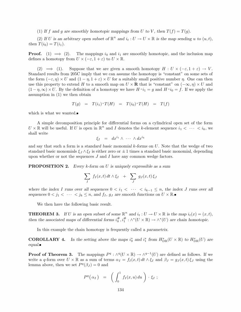
(1) If f and g are smoothly homotopic mappings from U to V , then T (f) = T (g).
(2) If U is an arbitrary open subset of Rn and it : U → U × R is the map sending u to (u, t),
then T (i0) = T (i1).
Proof. (1) =⇒ (2). The mappings i0 and i1 are smoothly homotopic, and the inclusion mapdefines a homotopy from U × (−ε, 1 + ε) to U × R.
(2) =⇒ (1). Suppose that we are given a smooth homotopy H : U × (−ε, 1 + ε) → V .Standard results from 205C imply that we can assume the homotopy is “constant” on some sets ofthe form (−ε, η) × U and (1− η, 1 + ε) × U for a suitably small positive number η. One can thenuse this property to extend H to a smooth map on U ×R that is “constant” on (−∞, η)× U and(1− η,∞)×U . By the definition of a homotopy we have H oi1 = g and H oi0 = f . If we apply theassumption in (1) we then obtain
T (g) = T (i1) oT (H) = T (i0) oT (H) = T (f)
which is what we wanted.
A simple decomposition principle for differential forms on a cylindrical open set of the formU × R will be useful. If U is open in Rn and I denotes the k-element sequence i1 < · · · < ik, weshall write
ξI = dxi1 ∧ · · · ∧ dxik
and say that such a form is a standard basic monomial k-forms on U . Note that the wedge of twostandard basic monomials ξJ ∧ ξI is either zero or ± 1 times a standard basic monomial, dependingupon whether or not the sequences J and I have any common wedge factors.
PROPOSITION 2. Every k-form on U is uniquely expressible as a sum
∑
I
fI(x, t) dt ∧ ξI +∑
J
gJ (x, t) ξJ
where the index I runs over all sequences 0 < i1 < · · · < ik−1 ≤ n, the index J runs over allsequences 0 < j1 < · · · < jk ≤ n, and fI , gJ are smooth functions on U × R.
We then have the following basic result.
THEOREM 3. If U is an open subset of some Rn and it : U → U ×R is the map it(x) = (x, t),
then the associated maps of differential forms i#0 , i#1 : ∧∗(U × R)→ ∧∗(U) are chain homotopic.
In this example the chain homotopy is frequently called a parametrix.
COROLLARY 4. In the setting above the maps i∗0 and i∗1 from H∗DR(U × R) to H∗DR(U) areequal.
Proof of Theorem 3. The mappings P q : ∧q(U × R) → ∧q−1(U) are defined as follows. If wewrite a q-form over U × R as a sum of terms αI = fI(x, t) dt ∧ ξI and βJ = gJ (x, t) ξJ using thelemma above, then we set P q(βJ ) = 0 and
P q(αI)
=
( ∫ 1
0
fI(x, u) du
)· ξI ;
134

we can then extend the definition to an arbitrary form, which is expressible as a sum of such terms,by additivity.
We must now compare the values of dP + Pd and i#1 − i#0 on the generating forms αI and βJdescribed above. It follows immediately that i#1 (αI )− i#0 (αI) = 0 and
i#1 (βJ ) − i#0 (βJ ) = [g(x, 1) − g(x, 0)]βJ .
Next, we have d oP (βJ ) = d(0) = 0 and
d oP (αI) = d
(∫ 1
0
fI(x, u)du)
)· ξI =
∑
j
(∫ 1
0
∂fI∂xj
(x, u) du
)∧ dxj ∧ ωI .
Similarly, we have
P od(αI) = P
∑
j
∂fI∂xj
dxj ∧ dt ∧ ξI +∂fI∂t
dt ∧ dt ∧ ξI
in which the final summand vanishes because dt ∧ dt = 0. If we apply the definition of P tothe nontrivial summation on the right hand side of the displayed equation and use the identitydxj ∧ dt = −dt ∧ dxj , we see that the given expression is equal to −d oP (αI); this shows that the
values of both dP + Pd and i#1 − i#0 on αI are zero. It remains to compute P od(βJ ) and verify
that it is equal to i#1 (βJ )− i#0 (βJ ). However, by definition we have
P od(gJ ξJ ) = P
(∑
i
∂gJ∂xi
dxi ∧ ξJ +∂gJ∂t
dt ∧ ξJ)
and in this case P maps the summation over i into zero because each form dxi ∧ ξJ is either zeroor ± 1 times a standard basic monomial, depending on whether or not dxi appears as a factor ofξJ . Thus the right hand side collapses to the final term and is given by
P
(∂gJ∂t
dt ∧ ξJ)
=
(∫ 1
0
∂gJ∂u
(x, u) du
)ξJ =
[ g(x, 1) − g(x, 0) ] ξJ
which is equal to the formula for i#1 (βJ ) − i#0 (βJ ) which we described at the beginning of theargument.
COROLLARY 5. If U is a convex open subset of some Rn, then HqDR(U) is isomorphic to R if
q = 0 and is trivial otherwise.
This follows because the constant map from U to R0 is a smooth homotopy equivalence if U isconvex, so that the de Rham cohomology groups of U are isomorphic to the de Rham cohomology
135

groups of R0, and by construction the latter are isomorphic to the groups described in the statementof the Corollary.
COROLLARY 6. (Poincare Lemma) Let U be a convex open subset of some Rn and let q > 0.The a differential q-form ω on U is closed (dω = 0) if and only if it is exact (ω = dθ for some θ).
Both of the preceding also hold if we merely assume that U is star-shaped with respect tosome point v (i.e., if x ∈ U , then the closed line segment joining x and v is contained in U), for inthis case the constant map is again a smooth homotopy equivalence.
The Mayer-Vietoris sequence
Here is the main result:
THEOREM 7. Let U and V be open subsets of Rn. Then there is a long exact Mayer-Vietorissequence in de Rham cohomology
· · · → Hq−1DR (U ∩ V )→ Hq
DR(U ∪ V )→ HqDR(U)⊕Hq
DR(V )→ HqDR(U ∩ V )→ Hq+1
DR (U ∪ V )→ · · ·
and a commutative ladder diagram relating the long exact Mayer-Vietoris sequences for U, V inde Rham cohomology and smooth singular cohomology with real coefficients.
Proof. The existence of the Mayer-Vietoris sequence will follow if we can show that there is ashort exact sequence of chain complexes
0→ ∧∗(U ∪ V ) −→ ∧∗(U)⊕ ∧∗(V ) −→ ∧∗(U ∩ V )→ 0
where the map from ∧∗(U ∪ V ) is given on the first factor by the i#U (where iU denotes inclusion)
and on the second factor by −i#V , and the map into ∧∗(U ∩ V ) is given by the maps j#U and j#Vdefined by inclusion of U ∩ V into U and V .
The exactness of this sequence at all points except ∧∗(U ∩ V ) follows immediately. Thereforethe only thing to prove is that the map to ∧∗(U ∩ V ) is surjective. This turns out to be less trivialthan one might first expect (in contrast to singular cochains, a differential form on U ∩ V neednot extend to either U or V ), but it can be done using smooth partitions of unity. Specifically, letϕU , ϕV be a smooth partition of unity subordinate to the open covering U, V of U ∪ V , andlet ω ∈ ∧p(U ∩ V ). Consider the forms ϕU · ω and ϕV · ω on U ∩ V . By definition of a partition ofunity there are open subsets U0 ⊂ U and V0 ⊂ V whose closures in U ∪ V are contained in U andV respectively, and such that ϕU and ϕV are zero off the closures of U0 and V0. This means thatwe can define a smooth form θU on U such that
θU |U ∩ V = ϕU · ω , θU |U − U0
because both restrict to zero on U ∩ V − U0. The same reasoning also yields a similar form θV onV , and it follows that
(θU , θV ) ∈ ∧p(U) ⊕ ∧p(V )
maps to ω ∈ ∧p(U ∩ V ). Additional details are given in Conlon (specifically, the last four lines ofthe proof for Lemma 8.5.1 on page 267).
136
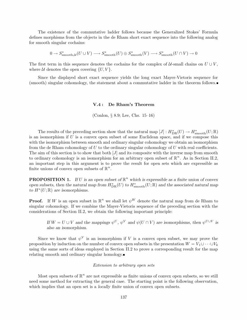
The existence of the commutative ladder follows because the Generalized Stokes’ Formuladefines morphisms from the objects in the de Rham short exact sequence into the following analogfor smooth singular cochains:
0→ S∗smooth,U(U ∪ V ) −→ S∗smooth(U)⊕ S∗smooth(V ) −→ S∗smooth(U ∩ V )→ 0
The first term in this sequence denotes the cochains for the complex of U -small chains on U ∪ V ,where U denotes the open covering U, V .
Since the displayed short exact sequence yields the long exact Mayer-Vietoris sequence for(smooth) singular cohomology, the statement about a commutative ladder in the theorem follows.
V.4 : De Rham’s Theorem
(Conlon, § 8.9; Lee, Chs. 15–16)
The results of the preceding section show that the natural map [J ] : H ∗DR(U)→ H∗smooth(U ; R)is an isomorphism if U is a convex open subset of some Euclidean space, and if we compose thiswith the isomorphism between smooth and ordinary singular cohomology we obtain an isomorphismfrom the de Rham cohomology of U to the ordinary singular cohomology of U with real coefficients.The aim of this section is to show that both [J ] and its composite with the inverse map from smoothto ordinary cohomology is an isomorphism for an arbitrary open subset of Rn. As in Section II.2,an important step in this argument is to prove the result for open sets which are expressible asfinite unions of convex open subsets of Rn.
PROPOSITION 1. If U is an open subset of Rn which is expressible as a finite union of convex
open subsets, then the natural map from H∗DR(U) to H∗smooth(U ; R) and the associated natural mapto H∗(U ; R) are isomorphisms.
Proof. If W is an open subset in Rn we shall let ψW denote the natural map from de Rham tosingular cohomology. If we combine the Mayer-Vietoris sequence of the preceding section with theconsiderations of Section II.2, we obtain the following important principle:
If W = U ∪ V and the mappings ψU , ψV and ψ(U ∩ V ) are isomorphisms, then ψU∪V isalso an isomorphism.
Since we know that ψV is an isomorphism if V is a convex open subset, we may prove theproposition by induction on the number of convex open subsets in the presentation W = V1∪ · · ·∪Vkusing the same sorts of ideas employed in Section II.2 to prove a corresponding result for the maprelating smooth and ordinary singular homology.
Extension to arbitrary open sets
Most open subsets of Rn are not expressible as finite unions of convex open subsets, so we stillneed some method for extracting the general case. The starting point is the following observation,which implies that an open set is a locally finite union of convex open subsets.
137

THEOREM 2. If U is an open subset of Rn, then U is a union of open subsets Wn indexed bythe positive integers such that the following hold:
(1) Each Wn is a union of finitely many convex open subsets.
(2) If |m− n| ≥ 3, then Wn ∩Wm is empty.
Proof. Results from 205C imply that U can be expressed as an increasing union of compactsubsets Kn such that Kn is contained in the interior of Kn+1 and K1 has a nonempty interior(?).Define An = Kn− Int(Kn−1), where K−1 is the empty set; it follows that An is compact. Let Vnbe the open subset Int(Kn+1)−Kn−1. By construction we know that Vn contains An and Vn∩Vmis empty if |n−m| ≥ 3. Clearly there is an open covering of An by convex open subsets which arecontained in Vn, and this open covering has a finite subcovering; the union of this finite family ofconvex open sets is the open set Wn that we want; by construction we have An ⊂ Wn, and sinceU = ∪n An we also have U = ∪n Wn. Furthermore, since Wn ⊂ Vn, and Vn ∩ Vm is empty if|n−m| ≥ 3, it follows that Wn ∩Wm is also empty if |n−m| ≥ 3.
We shall also need the following result:
PROPOSITION 3. Suppose that we are given an open subset U in Rn which is expressible asa countable union of pairwise disjoint subset Uk. If the map from de Rham cohomology to singularcohomology is an isomorphism for each Uk, then it is also an isomorphism for U .
Proof. By construction the cochain and differential forms mappings determined by the inclusionsik : Uk → U define morphisms from ∧∗(U) to the cartesian product Πk ∧∗(Uk) and from S∗smooth(U)to Πk S
∗smooth(Uk). We claim that these maps are isomorphisms. In the case of differential forms,
this follows because an indexed set of p-forms ωk ∈ ∧p(Uk) determine a unique form on U (existencefollows because the subsets are pairwise disjoint), and in the case of singular cochains it followsbecause every singular chain is uniquely expressible as a sum
∑k ck, where ck is a singular chain
on Uk and all but finitely many ck’s are zero (since the image of a singular simplex T : ∆q → U ispathwise connected and the open sets Uk are pairwise disjoint, there is a unique m such that theimage of T is contained in Um).
If we are given an abstract family of cochain complexes Ck then it is straightforward to verifythat there is a canonical homomorphism
H∗ (∏k Ck ) −→∏
k H∗(Ck)
defined by the projection mapsπj :
∏k Ck −→ Cj
and that this mapping is an isomorphism. Furthermore, it is natural with respect to families ofcochain complex mappings fk : Ck → Ek.
The proposition follows by combining the observations in the preceding two paragraphs(?).
We are now ready to prove the main result, which G. de Rham (1903–1990) first proved in1931:
THEOREM 4. (de Rham’s Theorem. ) The natural maps from de Rham cohomology to smoothand ordinary singular cohomology are isomorphisms for every open subset U in an arbitrary Rn.
138
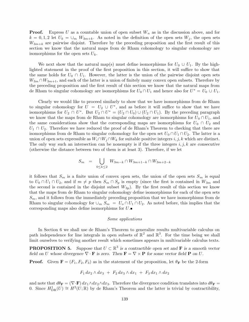
Proof. Express U as a countable union of open subset Wn as in the discussion above, and fork = 0, 1, 2 let Uk = ∪m W3m+k. As noted in the definition of the open sets Wj , the open setsW3m+k are pairwise disjoint. Therefore by the preceding proposition and the first result of thissection we know that the natural maps from de Rham cohomology to singular cohomology areisomorphisms for the open sets Uk.
We next show that the natural map(s) must define isomorphisms for U0 ∪ U1. By the high-lighted statement in the proof of the first proposition in this section, it will suffice to show thatthe same holds for U0 ∩ U1. However, the latter is the union of the pairwise disjoint open setsW3m∩W3m+1, and each of the latter is a union of finitely many convex open subsets. Therefore bythe preceding proposition and the first result of this section we know that the natural maps fromde Rham to singular cohomology are isomorphisms for U0 ∩ U1 and hence also for U ∗ = U0 ∪ U1.
Clearly we would like to proceed similarly to show that we have isomorphisms from de Rhamto singular cohomology for U = U2 ∪ U∗, and as before it will suffice to show that we haveisomorphisms for U2 ∩ U∗. But U2 ∩ U∗ = (U2 ∩ U0) ∪ (U2 ∩ U1). By the preceding paragraphwe know that the maps from de Rham to singular cohomology are isomorphisms for U0 ∩ U1, andthe same considerations show that the corresponding maps are isomorphisms for U0 ∩ U2 andU1 ∩ U2. Therefore we have reduced the proof of de Rham’s Theorem to checking that there areisomorphisms from de Rham to singular cohomology for the open set U0 ∩U1 ∩U2. The latter is aunion of open sets expressible as Wi∩Wj∩Wk for suitable positive integers i, j, k which are distinct.The only way such an intersection can be nonempty is if the three integers i, j, k are consecutive(otherwise the distance between two of them is at least 3). Therefore, if we let
Sm =⋃
0≤k≤2
W3m−k ∩W3m+1−k ∩W3m+2−k
it follows that Sm is a finite union of convex open sets, the union of the open sets Sm is equalto U0 ∩ U1 ∩ U2, and if m 6= p then Sm ∩ Sp is empty (since the first is contained in W3m andthe second is contained in the disjoint subset W3p). By the first result of this section we knowthat the maps from de Rham to singular cohomology define isomorphisms for each of the open setsSm, and it follows from the immediately preceding proposition that we have isomorphisms from deRham to singular cohomology for ∪m Sm = Uo ∩ U1 ∩ U2. As noted before, this implies that thecorresponding maps also define isomorphisms for U .
Some applications
In Section 6 we shall use de Rham’s Theorem to generalize results multivariable calculus onpath independence for line integrals in open subsets of R2 and R3. For the time being we shalllimit ourselves to verifying another result which sometimes appears in multivariable calculus texts.
PROPOSITION 5. Suppose that U ⊂ R3 is a contractible open set and F is a smooth vectorfield on U whose divergence ∇ · F is zero. Then F = ∇×P for some vector field P on U .
Proof. Given F = (F1, F2, F3) as in the statement of the proposition, let θF be the 2-form
F1 dx2 ∧ dx3 + F2 dx3 ∧ dx1 + F3 dx1 ∧ dx2
and note that dθF = (∇·F) dx1∧dx2∧dx3. Therefore the divergence condition translates into dθF =0. Since H1
DR(U) ∼= H2(U ; R) by de Rham’s Theorem and the latter is trivial by contractibility,
139

it follows that θF = dω for some 1-form ω. Expand ω as∑
i Pi dxi and write ω = ωP to reflectthis expansion. Then direct calculation shows that dωP is the 2-form θ∇×P in the notation at thebeginning of the proof. Therefore θF = θ∇×P, and by construction this means that F = ∇×P.
Generalization to arbitrary smooth manifolds
In fact, one can state and prove de Rham’s Theorem for every (second countable) smoothmanifold if we use Conlon’s approach to define differential forms (and related constructions) moregenerally; details are given in Chapters 6–8 of Conlon. The details of this generalization are beyondthe scope of this course, so we shall only give a purely formal method for deriving the general caseof de Rham’s Theorem from the special case of open sets in Rn and a generalization of differentialforms satisfying a few simple properties.
FACT 6. The category of (second countable) smooth manifolds and smooth mappings has thefollowing properties:
(i) It contains the category of open sets in Rn as a full subcategory.
(ii) The cochain complex functors ∧∗ and S∗smooth extend to this category, and likewise for thenatural transformation θ∗ : ∧∗ → S∗smooth.
(iii) Every smooth manifold Mm is a smooth retract of some open set U ⊂ RN for sufficientlylarge values of N .
Property (i) follows directly from the construction of the category of smooth manifolds andsmooth mappings, while (ii) clearly must hold in any reasonable extension of differential formsto smooth manifolds. Finally, (iii) is an immediate consequence of the Tubular NeighborhoodTheorem for a smooth embedding of M in some RN ; one reference is Lee, Proposition 10.20, page256.
In view of the preceding discussion, the general case of de Rham’s Theorem will be a conse-quence of the following very general result:
THEOREM 7. Let A be a category, let W ⊂ A be a full subcategory, and assume that everyobject in A is an A-retract of an object in W. Assume further that E and F are contravariantfunctors from A to the category of abelian groups and that θ : E → F is a natural transformation.Then θ(X) is an isomorphism for all objects X in A if and only if it is an isomorphism for allobjects X in W.
Proof. One implication is trivial, so we shall only look at the other case in which θ(X) is anisomorphism for all objects X in W.
Suppose that X is an object of A, choose a retract i : X → Y , where Y is an object of W, andlet r : Y → x be such that r oi = id(X). Consider the following commutative diagram:
E(Y )i∗−→ E(X)
r∗−→ E(Y )yθY
yθXyθX
F (Y )i∗−→ F (X)
r∗−→ F (Y )
Since i∗ or∗ is the identity on E(X) and F (X), it follows that i∗ is onto and r∗ is 1–1. To see thatθX is 1–1, notice that θX(u) = θX(v) implies θY r
∗(u) = r∗θX(u) = r∗θX(v) = θY r∗(v). Since θY
is an isomorphism it follows that r∗(u) = r∗(v), which in turn implies u = v because r∗ is 1–1. To
140

see that θX is onto, given u ∈ F (X) use the surjectivity of i∗ to write u = i∗(v). Since θY is anisomorphism it follows that v = θY (w) for some w, and thus we have u = i∗θY (v) = θXi
∗(w).
V.5 : Multiplicative properties of de Rham cohomology
(Hatcher, §§ 3.1–3.2; Conlon, § D.3; Lee, Ch. 15)
DEFAULT HYPOTHESIS. Unless specifically stated otherwise, all cochain complexes, modules inthis section are vector spaces over the real numbers, all algebraic morphisms are linear transforma-tions, and all tensor products are taken over the real numbers.
As in the case of simplicial cup products, the Leibniz rule for for differential forms
d(ω1 ∧ ω2) = (dω1) ∧ ω2 ± ω1 ∧ d(ω2)
implies that the wedge of two closed forms is closed and the wedge of a closed form with an exactform is exact. Consequently there is a well defined (bilinear) cohomology wedge product
HpDR(M)⊗R H
qDR(M) −→ Hp+q
DR (M)
sending [ω]⊗ [θ] to [ω∧θ] (where ω and θ are closed forms). It follows imeediately that this productmakes the de Rham cohomology of a smooth manifold into a graded algebra and this structure isfunctorial. Since the de Rham and singular cohomology groups of a smooth manifold are isomorphic,it is natural to ask if the wedge product and cup product correspond under the isomorphism inde Rham’s theorem, and it turns out that this is the case. We shall not give all the details of theargument; the references mentioned at appropriate points contain the omitted steps. Our approachwill involve some explicit constructions involving simplicial chains and cochains which are takenfrom Eilenberg and Steenrod and also from the following classic text (which we shall simply callHomology):
S. MacLane. Homology (Reprint of the first edition). Grundlehren der mathematischenWissenschaften Bd. 114. Springer-Verlag, Berlin-New York, 1967.
LEMMA 1. Let A be a p-simplex in Rn with vertices a0, · · · , ap, and let B be a p-simplex in Rm
with vertices b0, · · · , bq . Then there is a simplicial decomposition of A×B ⊂ Rn × Rm such thatevery point likes on at one (p + q)-simplex and an arbitrary (p+ q)-simplex of the decompositionhas vertices
(ai0 , bj0), · · · , (aip+q, bjp+q
)
where it ≥ it+1, jt ≥ jt+1 for all t and exactly one of these two inequalities is strict for each t.
For future reference, we note that the vertices of this decomposition for A×B have a standardlexicographic ordering obtained from the given orderings for the vertices of A and B.
Lemma 1 is a special case of the construction appearing in Section II.8 of Eilenberg andSteenrod.
We shall also need an explicit singular (in fact, simplicial) chain
X(p, q) ∈ Cp+q(Λp × Λq) ⊂ Sp+q(Λp × Λq)
141

defined on page 243 of Homology . This chain contains plus or minus each of the affine orderedsimplices mentioned in Lemma 1, and the sign is that of det Tα, where Tα is the unique affinemap sending the vertices of ∆p+q monotonically to those of the (p+ q)-simplex α ⊂ Λp × Λq (theassertion about signs requires a little work). The choice of signs leads to the following result:
LEMMA 2. Let f be a smooth real valued function defined on an open neighborhood ofΛp × Λq ⊂ Rp × Rq. Then
∫
Λp×Λq
f(t) dt =
∫
X(p,q)
f(t) dt1 ∧ · · · ∧ dtp+q
where the left hand side is the usual Riemann or Lebesgue integral and the right hand side is thedifferential forms integral.
Again turning to page 743 of Homology , we see that there is a natural chain transformation
γ : Ssmooth∗ (M)⊗ Ssmooth
∗ (N) −→ Ssmooth∗ (M ×N)
such that if M and N are open neighborhoods of Λp and Λq in Rp and Rq respectively and
σk : Λk → Rk is the standard inclusion, then γ(σp⊗σq) = X(p, q); in fact, the map γ is an explicitchain inverse to the Alexander-Whitney map (see pages 743–744 of Homology).
NOTATIONAL CONVENTIONS. Given forms ω ∈ ∧p(M) and η ∈ ∧q(N), the external wedgeω × η ∈ ∧p+q(M × n) is equal to
(p#Mω)∧(p#Mω)∈ ∧p+q(M ×N) .
In coordinates, if ω = f(x) dx1 ∧ · · · ∧ dxp and η = g(y) dy1 ∧ · · · ∧ dyq, then
ω × η = f(x) g(y) dx1 ∧ · · · ∧ dxp ∧ dy1 ∧ · · · ∧ dyq .
Given a chain complex S∗, a commutative ring with unit R, and cochains f : Sp → R, g : Sq → R,define the map f ./ g : Sp ⊗ Sq → R by the formula
f ./ g(u⊗ v) = f(u) · g(v) .
We can now state and prove a key fact relating the cross product in singular cohomology and theexternal wedge product in de Rham cohomology.
PROPOSITION 3. The following diagram is commutative:
∧p(M)⊗ ∧q(N)×−→ ∧p+q(M ×N)
yθM ⊗ θNyθM×N
Spsmooth(M)⊗ Sqsmooth(N) −→ Sp+qsmooth(M ×N)y./
y(γ|Sp ⊗ Sq)∗
[Sp ⊗ Sq]∗ =−→ [Sp ⊗ Sq]∗
In this diagram W ∗ denotes the dual space to the vector space W .
142

Proof. By the naturality properties of the constructions in the diagram, it suffices to consider thecase in which M and N are open neighborhoods of the simplices Λp, Λq ∈ Rp,Rq and to evaluateboth composites applied to a tensor product of forms ω ⊗ η on the universal example σp ⊗ σq.Assume ω and η are given as in the notational conventions. Then the value of the composite./ o (θM ⊗ θN ) o(ω ⊗ η) at σp ⊗ σq is equal to
∫
σp
ω ·∫
σq
η =
∫
Λp
f(x) dx ·∫
Λq
g(y) dy =
∫
Λp×Λq
f(x) · g(y) dx dy
(the last equation follows from Fubini’s Theorem). By Lemma 2, the last integral in the display isequal to ∫
X(p,q)
f(x) g(y) dx1 ∧ · · · ∧ dyq =
∫
X(p,q)
ω × η
and by definition the latter is equal to
(γ|Sp ⊗ Sq)∗ oθM×N o(ω ⊗ η) evaluated at σp ⊗ σq
which is what we wanted to prove.
The next result is nearly as important as the previous one for relating the cup and wedgeproducts.
PROPOSITION 4. Suppose that r+t = p+q but (s, t) 6= (p, q). Then (γ|Sr⊗St)∗θ(ω⊗η) = 0.
Proof. Again by naturality it suffices to consider the case whereM andN are open neighborhoodsof the simplices Λr, Λt ∈ Rr,Rt and to evaluate at σr ⊗ σt. The hypothesis implies that eitherr < p or t < q. Since dimM = r and dimN = t, it follows that either ∧p(M) or ∧q(N) is trivial.
The preceding results give us a cochain level formula relating the cross and external wedgeproducts (and thus also for the cup and ordinary wedge products).
PROPOSITION 5. In the setting above, let ψ : S∗(M × N) → S∗(M) ⊗ S∗(N) be theAlexander-Whitney map. Then θM (ω)× θN (η) = ψ∗ oγ∗ oθM×N (ω × η).Proof. The left hand side is equal to ψ∗ oρ(p, q) oθM ⊗ θN (ω ⊗ η), where ρ(p, q) projects[Ssmooth∗ (M) ⊗ Ssmooth
∗ (N)]p+q onto the direct summand Ssmoothp (M) ⊗ Ssmooth
q (N). By Propo-sition 4 the composite ψ∗ oγ∗ oθM×N(ω × η) is equal to ρ(p, q)∗ o(γ|Sp ⊗ Sq)∗ oθM×N (ω × η), andtherefore θM (ω)× θN(η) = ψ∗ oγ∗ oθM×N(ω × η) by Proposition 3.
We can now state and prove the main result of this section:
THEOREM 6. Let θ : H∗DR(M)→ H∗(M) be the isomorphism in de Rham’s Theorem, and letω and η be closed forms on M . Then θM ([ω] ∧ [η]) = θM ([ω]) ∪ θM ([η]).
Proof. Let M = N in the preceding discussion, and let ∆M : M → M × M be the di-agonal. Applying the cochain mapping ∆#
M to the right hand side of the equation in Proposi-
tion 5, we get θM (ω) ∪ θM (η) on the cochain level. Applying ∆#M to the left hand side, we get
∆#M
oψ∗ oγ∗ oθM×M (ω× η). Since γ oψ is chain homotopic to the identity (γ is a a chain homotopyinverse to ψ), the conditions dω = dη = 0 imply that
ψ∗ oγ∗ oθM×M (ω × η) = θM×M (ω × η) + δz for some z .
Therefore we haveθM (ω) ∪ θM (η) = ∆#
M (θM×M (ω × η) + δz) =
143

θM o∆#M (ω × η) + δ∆#
Mz = θM (ω ∧ η) + δ∆#Mz
where the last equation follows because ω ∧ η = ∆#M (ω× η). This means that if ω and η are closed
forms, then the closed forms θM (ω∧η) and θM (ω)∪θM (η) determine the same singular cohomologyclass.
V.6 : Path independence of line integrals
(Conlon, § 8.2; Lee, Chs. 11, 16)
In Section VIII.6 of fundgp-notes.pdf we proved that if U is an open subset of R2 and Pand Q are functions with continuous partial derivatives in U satisfying
∂P
∂y=
∂Q
∂x
at every point of U , then for each closed rectifiable curve Γ in U the line integral
∫
Γ
P dx + Qdy
depend only on the (based or free) homotopy class of Γ, and that if Γ and Γ′ are two piecewisesmooth curves in U with the same endpoints p and q such that Γ and Γ′ are homotopic by anendpoint preserving homotopy. Then
∫
Γ
P dx+Qdy =
∫
Γ′
P dx+Qdy .
In fact, we showed that both of these results followed from the following result which is simultane-ously a special case of both:
THEOREM 0. Let U be a connected open subset of R2, and let P and Q be smooth functions
on U with continuous partial derivatives which satsify the condition
∂P
∂y=
∂Q
∂x
at all points of U . If Γ is a piecewise smooth closed curve which starts and ends at p0 ∈ U whichis basepoint preservingly homotopic to a constant in U , then
∫
Γ
P dx+Qdy = 0.
The goal of this section is to prove generalizations of the results from Section VIII.6 of thenotes fundgp-notes.pdf to line integrals in open subsets of Rn for higher values of n; we shalldo so by the combining the methods employed in the 2-dimensional case with the machinery ofdifferential forms, the generalized Stokes’ Theorem proved in this unit, and de Rham’s Theorem.
144

As in the 2-dimensional case, it will be convenient to center the exposition around the followingversion of the main results:
THEOREM 1. Let U be a connected open subset of Rn, and let P1 · · · , Pn be smooth functionson U with continuous partial derivatives which satsify the conditions
∂Pi∂xj
=∂Pj∂xi
at all points of U for all i 6= j. If Γ is a piecewise smooth closed curve which starts and ends atp0 ∈ U which is basepoint preservingly homotopic to a constant in U , then
∫
Γ
∑i Pi dxi = 0.
Before proving this result, we shall state a few alternate versions and derive them from Theorem1. The exposition is completely analogous to the corresponding material in the 205A notes.
THEOREM 2. Let U and Pi be given as in Theorem 1, but suppose now that Γ and Γ′ are twopiecewise smooth curves in U with the same endpoints p and q such that Γ and Γ′ are homotopicby an endpoint preserving homotopy. Then
∫
Γ
∑i Pi dxi =
∫
Γ′
∑i Pi dxi .
Proof that Theorem 1 implies Theorem 2. In the setting of Theorem 2 the curve Γ′+(−Γ) isa closed piecewise smooth curve that is homotopic to a constant because Γ ' Γ′ implies [Γ′+(−Γ)] =[Γ + (−Γ)] = [constant]. Therefore Theorem 1 implies that the line integral over this curve is zero.On the other hand, by the three properties of line integrals listed above, the line integral overΓ′+(−Γ) is equal to the difference of the line integrals over Γ′ and Γ. Combining these observations,we see that the line integrals over Γ′ and Γ must be equal.
The next result is often also found in multivariable calculus texts.
COROLLARY 3. If in the setting preceding theorems we also know that the region U is simplyconnected, then the following hold:
(i) for every piecewise smooth closed curve Γ in U we have
∫
Γ
∑i Pi dxi = 0 .
(ii) for every pair of piecwise smooth curves Γ, Γ′ with the same endpoints we have
∫
Γ
∑i Pi dxi =
∫
Γ′
∑i Pi dxi .
The first part of the corollary follows from the triviality of the fundamental group of U , theconclusion of Theorem 1, and the triviality of line integrals over constant curve. The second partfollows formally from the first in the same way that the Theorem 2 follows from Theorem 1.
Finally, we have the following result concerning freely homotopic closed curves.
145

THEOREM 4. Let U and Pi be given as in Theorems 1 and 2, but suppose now that Γ and Γ′
are two piecewise smooth closed curves in U such that Γ and Γ′ are freely homotopic. Then
∫
Γ
∑i Pi dxi =
∫
Γ′
∑i Pi dxi .
In analogy with the 2-dimensional case, this proof will require some additional input, so theargument will be postponed until after the proof of Theorem 1 is completed.
Restatements using differential forms
The proof in the 2-dimensional case was based upon some consequences of Green’s Theorem inthe plane. In higher dimensions, it is more efficient to translate everything into differential formsand use the Generalized Stokes’ Theorem of this unit instead. From this perspective, the integrands∑
i Pi dxi correspond to differential 1-forms, and the line integral over a reasonable curve Γ canbe written as the integral
∫Γω, where ω =
∑i Pi dxi. Once again, the Fundamental Theorem of
Calculus and the Chain Rule imply that if Γ is a regular piecewise smooth curve defined on [0, 1]and f is a smooth function on U then
∫
Γ
∑
i
∂Pi∂xi
dxi = f oΓ(1) − f oΓ(0)
and this is merely the 0-dimensional case of the Generalized Stokes’ Formula.
Proof of Theorem 1. As in the preceding discussion, let ω denote the integrand of the lineintegrals under consideration. Then the conditions on the partial derivatives of the functions Pitranslate into the vanishing of the exterior derivative dω.
Given (U, u0) as in the statement of the theorem, let Θ(U, u0) denote the set of all pairs (γ,∆)where γ : [0, 1]→ U is a regular piecewise smooth curves such that γ(0) = γ(1) = u0 and
∆ = 0 = t0 < · · · < tm = 1
defines a partition of [0, 1] into subintervals such that the restriction of γ to each subinterval [ti−1, ti]is a regular smooth curve. For each i let Ti be the regular smooth curve defined by composingγ|[ti−1, ti] with the standard endpoint and order preserving linear map [0, 1]→ [ti−1, ti], and definea mapping
Chain(U,u0) : Θ(U, u0) −→ Ssmooth1 (U)
sending (γ,∆) to∑
i Ti. Since γ is a closed curve the boundary of the chain∑
i Ti is zero,and therefore the image of Chain(U,u0) lies in the subgroup Zsmooth
1 (U) of cycles in Ssmooth1 (U).
Therefore Chain(U,u0) yields a mapping η(U,u0) from Θ(U, u0) to Hsmooth1 (U).
We can now define a concatenation operation on Θ(U, u0) which sends the ordered pair((γ,∆), (γ′,∆′)
)to (γ′,∆′) where γ + γ′ is the concatenated curve and ∆ + ∆′ is the corre-
sponding partition of [0, 1] given by shrinking ∆ and ∆′ to [0, 12 ] and [ 12 , 1] respectively, and it
follows immediately that the previously constructed mapping η(U,u0) sends (γ,∆) + (γ′,∆′) toη(U,u0)(γ,∆) + η(U,u0)(γ
′,∆′).
146

Consider now the following commutative diagram, in which the vertical map at the left sends(γ,∆) to the homotopy class [γ] and the map h is the Hurewicz homomorphism:
Θ(U, u0)η−→ Hsmooth
1 (U))y
y
π1(U, u0)h−→ H1(U))
We can now complete the proof as follows: The basic properties of line integrals imply that the lineintegral of ω along γ is equal to the integral of γ with respect to the chain Chain(γ,∆) =
∑i Ti.
Since dω = 0, the Generalized Stokes’ Theorem implies that the integral∫Chain(γ,∆)
ω only depends
on the image of (γ,∆) in H smooth1 (U). If γ is basepoint preserving homotopic to the constant map
whose value everywhere is u0, then the class of γ in π1(U, u0) is trivial and hence we can use thediagram to conclude that h o [γ] = 0 and hence η(γ,∆) = 0, and therefore by the preceding sentencewe know that
∫γω = 0, which is what we wanted to prove.
Proof that Theorem 1 implies Theorem 4. We do not know whether or not the freelyhomotopic closed curves γ0 and γ1 start and end at the same point, so assume that γi starts andends at ui for i = 0, 1. Choose appropriate partitions ∆i such that γi is smooth on each subintervaldetermined by ∆i for i = 0, 1. Since γ0 and γ1 are freely homotopic, the commutative diagramimplies that
η(U,u0)(γ0,∆0) = η(U,u1)(γ1,∆1) in Hsmooth1 (U) .
As in the proof of Theorem 1, the integrand∑
i Pi dxi corresponds to a closed 1-form ω, andtherefore in this case the Generalized Stokes’ Theorem implies that the integrals of ω over thechains
∫Chain(γ0,∆0)
ω and∫Chain(γ1,∆1)
ω are equal As in the proof of Theorem 1, we know that
these inegrals are respectively equal to the line integrals∫γ0
ω and∫γ1
ω, and therefore these twoline integrals must also be equal.
Some classical implications
Frequently one sees the 3-dimensional case of the following result in multivariable calculustexts:
THEOREM 5. Let n ≥ 3, and suppose that U is obtained from Rn by removing finitely manypoints. If F = (P1, · · · , Pn) is a smooth vector field on U such that
∂Pi∂xj
=∂Pj∂xi
for all i 6= j, then there is a smooth function g on U such that ∇g = F. In particular, if Γ is aregular piecewise smooth curve in U , then the value of the line integral
∫
Γ
∑i Pi dxi
depends only upon the endpoints of the curve Γ.
In particular, a result of this type is formulated as Theorem 7 on page 551 of Marsden andTromba.
147

Theorem 5 contrasts sharply with the case n = 2, and the easiest way to explain the differenceis to note that the complement of a finite subset in Rn is simply connected if n = 3 but is not simplyconnected if n = 2. We shall give a simpler (but less elementary) argument which only requires usto know that H1(U ; R) is trivial if n ≥ 3. By the Universal Coefficient Theorem relating integralhomology to real cohomology, we only need to prove the following:
LEMMA 6. Let n ≥ 3, and suppose that U is obtained from Rn by removing a set X whichcontains exactly k points. Then the singular homology groups of U = Rn − X are given byHj(R
n −X) ∼= Z if k = 0, Hj(Rn −X) ∼= Zk if k = n− 1, and Hj(R
n −X) ∼= 0 otherwise.
Proof that Lemma 6 implies Theorem 5. By Lemma 10 we know that H1(U = Rn − X)is trivial because n ≥ 3, and by the Universal Coefficient Theorem we know that H 1(U ; R) ∼=Hom (H1(U),R); therefore H1(U ; R) is trivial. Since H∗DR(U) ∼= H∗(U ; R) by de Rham’s Theorem,it follows that H1
DR(U) is trivial and therefore every closed 1-form over U is exact; i.e., if dω = 0then ω = dg for some g.
Let ω be the 1-form∑
i Pi dxi; the hypothesis on the functions Pi is equivalent to the identitydω = 0, and therefore if this identity holds we can apply the preceding paragraph to conclude thatω = dg for some smooth function g. If we translate this back into the language of vector fields, wesee that the original vector field F is equal to ∇g, proving the first assertion in the conclusion ofthe theorem. The second assertion now follows because the line integral in question has the form∫Γ∇g · dx and we have already noted that the values of such line integrals only depend upon the
endpoints of Γ.
Proof of Lemma 6. For each x ∈ X let Vx be the open neighborhood of radius r centered at x;choose r to be smaller than half the minimum distance between points of X (the minimum existsby the finiteness of X, and let V = ∪x Ux, so that Rn = V ∪ (Rn −X)) and V ∩X = ∪x Vx−x.Then by excision, the splitting of the homology of X into the homology of its arc componenents,and Theorem VII.1.7 in algtop-notes.pdf we know that
Hj(Rn,Rn −X) ∼= Hj(U,U −X) ∼= Hj (∪x Vx, ∪x Vx − x) ∼=
⊕
x
Hj ( Vx, Vx − x) ∼= Zk or 0
where the group is zero unless j = n, in which case it is isomorphic to Zk. We can now recover thehomology groups Rn − X from the long exact homology sequence for (Rn,Rn − X) and the factthat Hj(R
n) is Z if j = 0 and zero otherwise.
Similar conclusions hold if U is obtained from Rn (where n ≥ 3) by deleting an infinite sequence
of isolated points p1,p2, · · · . The main difference in the argument is that the open disk Vkcentered at pk must have a radius rk such that for each j 6= k we have |pj − pk| > rk; we canalways find such positive radii if we have a sequence of isolated points.
148