Mathematical Theories of Interaction withOracles

Liu YangOctober 2013

CMU-ML-13-111

Mathematical Theories of Interaction with

Oracles

Liu Yang

October 2013

CMU-ML-13-111

School of Computer Science

Machine Learning Department

Carnegie Mellon University

Pittsburgh, PA

Thesis Committee:

Avrim Blum, Chair

Jaime Carbonell, Chair

Manuel Blum

Sanjoy Dasgupta

Yishay Mansour

Joel Spencer

Submitted in partial fulfillment of the requirements

for the degree of Doctor of Philosophy.

Copyright c© 2013 Liu Yang

This research was sponsored by the National Science Foundation under grant numbers DBI0640543, IIS0713379,

IIS1065251; the Defense Intelligence Agency under grant number FA872105C0003; and a grant from Google Inc.

The views and conclusions contained in this document are those of the author and should not be interpreted as

representing the official policies, either expressed or implied, of any sponsoring institution, the U.S. government or

any other entity.

Keywords: Property Testing, Active Learning, Computational Learning Theory, Learning

DNF, Statistical Learning Theory, Transfer Learning, Prior Estimation, Bayesian Theory, Surro-

gate Losses, Preference Elicitation,Concept Drift, Algorithmic Mechanism Design, Economies

of Scale

This thesis is dedicated to all Mathematicians.

Acknowledgments

I would like to thank my advisor Avrim Blum for so many stimulating discussions (research

problems and other fun math problems), for the inspiration I experienced during our discussions,

for his amazingly accurate-with-high-probability sense of the directions that are worth trying,

and for the many valuable bits of feedback and advice he has provided me. I also thank my

other advisor Jaime Carbonell for always being supportive and encouraging me to push on with

one problem after another. I am grateful to Manuel Blum for so many ingenious discussions all

through these years when I am at CMU, which have broadened my mind, and given me a great

taste of research problems and a faith in the ability of Mathematics to uncover interesting and

mysterious truths, such as the nature of consciousness. I appreciate the exhilarating experience of

working with Yishay Mansour on an algorithmic economics problem; through these interactions,

I have learned many insights about axiomatic approaches to algorithmic economics.

One of my great experiences has been interacting with many wonderful mathematicians. I

thank Ryan O’Donnell for input on my research on learning DNF, and insights on the analysis of

boolean functions. I appreciate discussions with Steven Rudich on interactive proof systems, and

for his counseling on Fourier techniques; he has also helped sharpen my skills of giving good

talks and lectures. I thank Venkatesan Guruswami for discussions on information theory and cod-

ing theory related to my work in Bayesian active learning; I also highly enjoyed his complexity

theory class. I want to thank Tuomas Sandholm for sharing his knowledge of Bayesian auction

design. I thank Anupam Gupta for discussions on approximation algorithms. I would also like

to thank all the other faculty that I’ve interacted with in my time at CMU. Thanks especially

to my co-author Silvio Micali for extending my philosophical and implementational insights on

auction design. I thank Shafi Goldwasser for encouragement on my work in property testing and

computational learning theory. I thank Leslie Valiant for input on my project on learning DNF

with representation-specific queries.

There are also several mathematicians who, though our interactions have been only brief,

have made a lasting impact on my mathematical perspective. I am grateful for the wonderful and

stimulating discussion I had with Alan Frieze on combinatorics. I appreciate the one sentence

of advice from John Nash when I happened to be at Princeton for a summer workshop. I am

grateful to Scott Aaronson and Avi Wigderson for a few email conversations on interactive proof

systems with restricted provers, which is a project I am actively pursuing. I also thank all the

theorists I met in conferences, and the many friends and peers that made my time as a graduate

student quite enjoyable, including Eric Blais and Paul Valiant. Finally, I want to cite Fan Chung

Graham’s advice for grad students “Coauthorship is a closer relationship than friendship.” Yes,

indeed, the co-authorship with all my collaborators is to be cherished year after year.

iv

Contents

1 Summary 1

1.1 Bayesian Active Learning . . . . . . . . . . . . . . . . . . . . . . . . . . . . . . 1

1.1.1 Arbitrary Binary-Valued Queries . . . . . . . . . . . . . . . . . . . . . . 2

1.1.2 Self-Verifying Active Learning . . . . . . . . . . . . . . . . . . . . . . . 2

1.2 Active Testing . . . . . . . . . . . . . . . . . . . . . . . . . . . . . . . . . . . . 3

1.3 Theory of Transfer Learning . . . . . . . . . . . . . . . . . . . . . . . . . . . . 4

1.4 Active Learning with Drifting Distributions and Targets . . . . . . . . . . . . . . 6

1.5 Efficiently Learning DNF with Representation-Specific Queries . . . . . . . . . 8

1.6 Online Allocation with Economies of Scale . . . . . . . . . . . . . . . . . . . . 9

2 Active Testing 10

2.1 Introduction . . . . . . . . . . . . . . . . . . . . . . . . . . . . . . . . . . . . . 11

2.1.1 The Active Property Testing Model . . . . . . . . . . . . . . . . . . . . 14

2.1.2 Our Results . . . . . . . . . . . . . . . . . . . . . . . . . . . . . . . . . 16

2.2 Testing Unions of Intervals . . . . . . . . . . . . . . . . . . . . . . . . . . . . . 19

2.3 Testing Linear Threshold Functions . . . . . . . . . . . . . . . . . . . . . . . . 22

2.4 Testing Disjoint Unions of Testable Properties . . . . . . . . . . . . . . . . . . . 25

2.5 General Testing Dimensions . . . . . . . . . . . . . . . . . . . . . . . . . . . . 26

2.5.1 Application: Dictator functions . . . . . . . . . . . . . . . . . . . . . . 29

2.5.2 Application: LTFs . . . . . . . . . . . . . . . . . . . . . . . . . . . . . 30

2.6 Proof of a Property Testing Lemma . . . . . . . . . . . . . . . . . . . . . . . . . 31

2.7 Proofs for Testing Unions of Intervals . . . . . . . . . . . . . . . . . . . . . . . 32

2.8 Proofs for Testing LTFs . . . . . . . . . . . . . . . . . . . . . . . . . . . . . . . 35

2.9 Proofs for Testing Disjoint Unions . . . . . . . . . . . . . . . . . . . . . . . . . 37

2.10 Proofs for Testing Dimensions . . . . . . . . . . . . . . . . . . . . . . . . . . . 39

2.10.1 Passive Testing Dimension (proof of Theorem 2.15) . . . . . . . . . . . 39

2.10.2 Coarse Active Testing Dimension (proof of Theorem 2.17) . . . . . . . . 41

2.10.3 Active Testing Dimension (proof of Theorem 2.19) . . . . . . . . . . . . 42

2.10.4 Lower Bounds for Testing LTFs (proof of Theorem 2.20) . . . . . . . . . 42

2.11 Testing Semi-Supervised Learning Assumptions . . . . . . . . . . . . . . . . . . 49

3 Testing Piecewise Real-Valued Functions 54

3.1 Piecewise Constant . . . . . . . . . . . . . . . . . . . . . . . . . . . . . . . . . 54

v

4 Learnability of DNF with Representation-Specific Queries 58

4.1 Introduction . . . . . . . . . . . . . . . . . . . . . . . . . . . . . . . . . . . . . 59

4.1.1 Our Results . . . . . . . . . . . . . . . . . . . . . . . . . . . . . . . . . 60

4.2 Learning DNF with General Queries: Hardness Results . . . . . . . . . . . . . . 60

4.3 Learning DNF with General Queries : Positive . . . . . . . . . . . . . . . . . . . 63

4.3.1 Methods . . . . . . . . . . . . . . . . . . . . . . . . . . . . . . . . . . 63

4.3.2 Positive Results . . . . . . . . . . . . . . . . . . . . . . . . . . . . . . . 66

4.4 Learning DNF under the Uniform Distribution . . . . . . . . . . . . . . . . . . . 68

4.5 More Powerful Queries . . . . . . . . . . . . . . . . . . . . . . . . . . . . . . . 72

4.6 Learning DNF with General Queries: Open Questions . . . . . . . . . . . . . . . 75

4.7 Generalizations . . . . . . . . . . . . . . . . . . . . . . . . . . . . . . . . . . . 76

4.7.1 Learning Unions of Halfspaces . . . . . . . . . . . . . . . . . . . . . . . 76

4.7.2 Learning Voronoi with General Queries . . . . . . . . . . . . . . . . . . 76

5 Bayesian Active Learning with Arbitrary Binary Valued Queries 78

5.1 Introduction . . . . . . . . . . . . . . . . . . . . . . . . . . . . . . . . . . . . . 78

5.2 Definitions . . . . . . . . . . . . . . . . . . . . . . . . . . . . . . . . . . . . . . 81

5.2.1 Definition of Packing Entropy . . . . . . . . . . . . . . . . . . . . . . . 82

5.3 Main Result . . . . . . . . . . . . . . . . . . . . . . . . . . . . . . . . . . . . . 83

5.4 Proof of Theorem 5.6 . . . . . . . . . . . . . . . . . . . . . . . . . . . . . . . . 84

5.5 Application to Bayesian Active Learning . . . . . . . . . . . . . . . . . . . . . . 88

5.6 Open Problems . . . . . . . . . . . . . . . . . . . . . . . . . . . . . . . . . . . 90

6 The Sample Complexity of Self-Verifying Bayesian Active Learning 91

6.1 Introduction and Background . . . . . . . . . . . . . . . . . . . . . . . . . . . . 91

6.2 Definitions and Preliminaries . . . . . . . . . . . . . . . . . . . . . . . . . . . . 95

6.3 Prior-Independent Learning Algorithms . . . . . . . . . . . . . . . . . . . . . . 97

6.4 Prior-Dependent Learning: An Example . . . . . . . . . . . . . . . . . . . . . . 99

6.5 A General Result for Self-Verifying Bayesian Active Learning . . . . . . . . . . 101

6.6 Dependence on D in the Learning Algorithm . . . . . . . . . . . . . . . . . . . 105

6.7 Inherent Dependence on π in the Sample Complexity . . . . . . . . . . . . . . . 106

7 Prior Estimation for Transfer Learning 108

7.1 Introduction . . . . . . . . . . . . . . . . . . . . . . . . . . . . . . . . . . . . . 108

7.1.1 Outline of the paper . . . . . . . . . . . . . . . . . . . . . . . . . . . . 111

7.2 Definitions and Related Work . . . . . . . . . . . . . . . . . . . . . . . . . . . . 112

7.2.1 Relation to Existing Theoretical Work on Transfer Learning . . . . . . . 113

7.3 Estimating the Prior . . . . . . . . . . . . . . . . . . . . . . . . . . . . . . . . . 117

7.3.1 Identifiability from d Points . . . . . . . . . . . . . . . . . . . . . . . . 127

7.4 Transfer Learning . . . . . . . . . . . . . . . . . . . . . . . . . . . . . . . . . . 129

7.4.1 Proof of Theorem 7.8 . . . . . . . . . . . . . . . . . . . . . . . . . . . . 132

7.5 Conclusions . . . . . . . . . . . . . . . . . . . . . . . . . . . . . . . . . . . . . 134

vi

8 Prior Estimation 135

8.1 Introduction . . . . . . . . . . . . . . . . . . . . . . . . . . . . . . . . . . . . . 135

8.2 The Setting . . . . . . . . . . . . . . . . . . . . . . . . . . . . . . . . . . . . . 137

8.3 An Upper Bound . . . . . . . . . . . . . . . . . . . . . . . . . . . . . . . . . . 139

8.4 A Minimax Lower Bound . . . . . . . . . . . . . . . . . . . . . . . . . . . . . . 143

8.5 Future Directions . . . . . . . . . . . . . . . . . . . . . . . . . . . . . . . . . . 148

9 Estimation of Priors with Applications to Preference Elicitation 149

9.1 Introduction . . . . . . . . . . . . . . . . . . . . . . . . . . . . . . . . . . . . . 149

9.2 Notation . . . . . . . . . . . . . . . . . . . . . . . . . . . . . . . . . . . . . . . 152

9.3 Maximizing Customer Satisfaction in Combinatorial Auctions . . . . . . . . . . 161

10 Active Learning with a Drifting Distribution 166

10.1 Introduction . . . . . . . . . . . . . . . . . . . . . . . . . . . . . . . . . . . . . 166

10.2 Definition and Notations . . . . . . . . . . . . . . . . . . . . . . . . . . . . . . 167

10.2.1 Assumptions . . . . . . . . . . . . . . . . . . . . . . . . . . . . . . . . 169

10.3 Related Work . . . . . . . . . . . . . . . . . . . . . . . . . . . . . . . . . . . . 170

10.4 Active Learning in the Realizable Case . . . . . . . . . . . . . . . . . . . . . . . 171

10.4.1 Learning with a Fixed Distribution . . . . . . . . . . . . . . . . . . . . . 173

10.4.2 Learning with a Drifting Distribution . . . . . . . . . . . . . . . . . . . 173

10.5 Learning with Noise . . . . . . . . . . . . . . . . . . . . . . . . . . . . . . . . 176

10.5.1 Noise Conditions . . . . . . . . . . . . . . . . . . . . . . . . . . . . . . 177

10.5.2 Agnostic CAL . . . . . . . . . . . . . . . . . . . . . . . . . . . . . . . 177

10.5.3 Learning with a Fixed Distribution . . . . . . . . . . . . . . . . . . . . . 179

10.5.4 Learning with a Drifting Distribution . . . . . . . . . . . . . . . . . . . 179

10.6 Querying before Predicting . . . . . . . . . . . . . . . . . . . . . . . . . . . . . 180

10.7 Discussion . . . . . . . . . . . . . . . . . . . . . . . . . . . . . . . . . . . . . . 182

10.8 Proof of Theorem 10.4 . . . . . . . . . . . . . . . . . . . . . . . . . . . . . . . 182

10.9 Proof of Theorem 10.15 . . . . . . . . . . . . . . . . . . . . . . . . . . . . . . . 183

10.10Proof of Theorem 10.17 . . . . . . . . . . . . . . . . . . . . . . . . . . . . . . . 186

11 Active Learning with a Drifting Target Concept 189

11.1 Introduction . . . . . . . . . . . . . . . . . . . . . . . . . . . . . . . . . . . . . 189

11.2 Definitions and Notations . . . . . . . . . . . . . . . . . . . . . . . . . . . . . . 191

11.3 General Analysis under Constant Drift Rate: Inefficient Passive Learning . . . . 191

11.4 General Analysis under Constant Drift Rate: Sometimes-Efficient Passive Learning193

11.4.1 Lower Bounds . . . . . . . . . . . . . . . . . . . . . . . . . . . . . . . 195

11.4.2 Random Drifts . . . . . . . . . . . . . . . . . . . . . . . . . . . . . . . 199

11.5 Linear Separators under the Uniform Distribution . . . . . . . . . . . . . . . . . 200

11.6 General Analysis of Sublinear Mistake Bounds: Passive Learning . . . . . . . . 211

11.7 General Analysis under Varying Drift Rate: Inefficient Passive Learning . . . . . 214

vii

12 Surrogate Losses in Passive and Active Learning 218

12.1 Introduction . . . . . . . . . . . . . . . . . . . . . . . . . . . . . . . . . . . . . 219

12.1.1 Related Work . . . . . . . . . . . . . . . . . . . . . . . . . . . . . . . . 221

12.2 Definitions . . . . . . . . . . . . . . . . . . . . . . . . . . . . . . . . . . . . . . 222

12.2.1 Surrogate Loss Functions for Classification . . . . . . . . . . . . . . . . 224

12.2.2 A Few Examples of Loss Functions . . . . . . . . . . . . . . . . . . . . 228

12.2.3 Empirical ℓ-Risk Minimization . . . . . . . . . . . . . . . . . . . . . . . 229

12.2.4 Localized Sample Complexities . . . . . . . . . . . . . . . . . . . . . . 230

12.3 Methods Based on Optimizing the Surrogate Risk . . . . . . . . . . . . . . . . . 235

12.3.1 Passive Learning: Empirical Risk Minimization . . . . . . . . . . . . . . 235

12.3.2 Negative Results for Active Learning . . . . . . . . . . . . . . . . . . . 235

12.4 Alternative Use of the Surrogate Loss . . . . . . . . . . . . . . . . . . . . . . . 237

12.5 Applications . . . . . . . . . . . . . . . . . . . . . . . . . . . . . . . . . . . . . 242

12.5.1 Diameter Conditions . . . . . . . . . . . . . . . . . . . . . . . . . . . . 243

12.5.2 The Disagreement Coefficient . . . . . . . . . . . . . . . . . . . . . . . 245

12.5.3 Specification of φℓ . . . . . . . . . . . . . . . . . . . . . . . . . . . . . 246

12.5.4 VC Subgraph Classes . . . . . . . . . . . . . . . . . . . . . . . . . . . . 248

12.5.5 Entropy Conditions . . . . . . . . . . . . . . . . . . . . . . . . . . . . . 257

12.5.6 Remarks on VC Major and VC Hull Classes . . . . . . . . . . . . . . . . 261

12.6 Proofs . . . . . . . . . . . . . . . . . . . . . . . . . . . . . . . . . . . . . . . . 263

12.7 Results for Efficiently Computable Updates . . . . . . . . . . . . . . . . . . . . 273

12.7.1 Proof of Theorem 12.16 under (12.34) . . . . . . . . . . . . . . . . . . . 274

13 Online Allocation and Pricing with Economies of Scale 280

13.1 Introduction . . . . . . . . . . . . . . . . . . . . . . . . . . . . . . . . . . . . . 281

13.1.1 Our Results and Techniques . . . . . . . . . . . . . . . . . . . . . . . . 283

13.1.2 Related Work . . . . . . . . . . . . . . . . . . . . . . . . . . . . . . . . 285

13.2 Model, Definitions, and Notation . . . . . . . . . . . . . . . . . . . . . . . . . . 286

13.2.1 Utility Functions . . . . . . . . . . . . . . . . . . . . . . . . . . . . . . 286

13.2.2 Production cost . . . . . . . . . . . . . . . . . . . . . . . . . . . . . . . 286

13.2.3 Allocation problems . . . . . . . . . . . . . . . . . . . . . . . . . . . . 287

13.3 Structural Results and Allocation Policies . . . . . . . . . . . . . . . . . . . . . 287

13.3.1 Permutation and pricing policies . . . . . . . . . . . . . . . . . . . . . . 288

13.3.2 Structural results . . . . . . . . . . . . . . . . . . . . . . . . . . . . . . 288

13.4 Uniform Unit Demand and the Allocate-All problem . . . . . . . . . . . . . . . 291

13.4.1 Generalization Result . . . . . . . . . . . . . . . . . . . . . . . . . . . . 294

13.4.2 Generalized Performance Guarantees . . . . . . . . . . . . . . . . . . . 297

13.4.3 Generalization for β-nice costs . . . . . . . . . . . . . . . . . . . . . . . 298

13.5 General Unit Demand Utilities . . . . . . . . . . . . . . . . . . . . . . . . . . . 304

13.5.1 Generalization . . . . . . . . . . . . . . . . . . . . . . . . . . . . . . . 307

13.6 Properties of β-nice cost . . . . . . . . . . . . . . . . . . . . . . . . . . . . . . 308

Bibliography 310

viii

Chapter 1

Summary

The key insight underlying this thesis is that the right kind of interaction is the key to making

the intractable tractable. This work specifically investigates this insight in the context of learn-

ing theory. While much of the learning theory literature has traditionally focused on protocols

that are either non-interactive or involving unrealistically strong forms of interaction, there have

recently been several exciting advances in the design and analysis of methods for realistic inter-

active learning protocols.

Perhaps one of the most interesting of these is active learning. In active learning, a learning

algorithm is given access to a large pool of unlabeled examples, and is allowed to sequentially

request their labels so as to learn how to accurately predict the labels of new examples. This

thesis contains a number of interesting advances in our understanding of the capabilities of active

learning methods. Specifically, I summarize the main contributions below.

1.1 Bayesian Active Learning

While most of the recent advances in our understanding of active learning have focused on the

traditional PAC model (or noisy variants thereof), similar advnaces specific to the Bayesian learn-

ing setting have largely been lacking. Specifically, suppose that in addition to the data itself, the

1

learner additionally has access to a prior distribution for the target function, and we are inter-

ested in achieving a guarantee of low expected error rate, where the expectation is over both the

draw of the data and the draw of the target concept from the given prior. This setting has been

studied in depth for the passive learning protocol, but aside from the well-known work on the

query-by-committee algorithm, little was known about this setting for the active learning proto-

col. This lack of knowledge is particularly troubling in light of the fact that most of the active

learning methods used in practice have Bayesian interpretations, selecting their label requests

based on Bayesian notions such as label entropy, expected error reduction, or reduction in the

total probability mass of the version space.

1.1.1 Arbitrary Binary-Valued Queries

In this thesis, we present work that makes progress in understanding the Bayesian active learning

setting. To begin, we study the most basic question: how many queries are necessary if we

are able to ask arbitrary binary-valued queries. While label requests are only a special type of

binary-valued query, a general lower bound for arbitrary binary-valued queries will also hold for

label request queries, and thus provides a lower bound on the intrinsic query complexity of the

learning problem. Not surprisingly, we find that the number of binary-valued queries necessary

for learning is characterized by a kind of entropy quantity: namely, the entropy of the Voronoi

partition induced by a maximal ǫ-packing.

1.1.2 Self-Verifying Active Learning

Our next contribution is a study of a special type of active learning, characterized by the stopping-

criterion used in the learning algorithm. Specifically, consider a protocol in which the input to

the active learning algorithm is the desired error rate guarantee ǫ, and the algorithm then makes

a number of queries and then halts. For the algorithm to be considered “correct”, it must have

the guarantee that the expected error rate of the classifier it produces after halting is at most

2

the value of ǫ provided as input. We refer to this family of algorithms as self-verifying. The

label complexity of learning in this protocol is generally higher than in some other protocols

(e.g., budget-based), since the algorithm must not only find a classifier with good error rate, but

must also somehow be self-aware of the fact that it has found such a good classifier. Indeed, it

is known that prior-independent self-verifying algorithms may often have label complexities no

better than that of passive learning, which is Θ(1/ǫ) for VC classes. However, we prove that

in Bayesian active learning, for any VC class and prior, there is a prior-dependent method that

always achieves an expected label complexity that is o(1/ǫ). Thus, this represents a concrete

result on the advantages of having access to the target’s prior distribution.

1.2 Active Testing

One of the major challenges facing active learning is that of model selection. Specifically, given

a number of hypothesis classes, how does one decide which one to use? In passive learning, the

solution is simple: try them all, and then pick from among the resulting hypotheses using cross-

validation. But such solutions are not available to active learning, since the methods tailored to

each hypothesis class will generally make very different label requests, so that the label com-

plexity of producing a hypothesis from all of the classes is close to the sum of their individual

label complexities.

Thus, to avoid this problem, there is a need for procedures that quickly dermine whether the

target concept is within (or approximated by) a given concept class, by asking a much smaller

number of label requests than required for learning with that class: that is, for testing methods

that operate in the active learning protocol, which we therefore refer to as active testing. This

way, we can simply go through each class and test whether the target is in the class or not, and

only run the full learning method on some simplest class that passes the test. The questions then

become how many fewer queries are required for testing compared to learning, as this quantifies

the savings from using this approach. Following the traditional literature on property testing,

3

the primary focus of such an analysis is on the dependence of the query complexity on the VC

dimension of the hypothesis class being tested. Since learning typically required a number of

queries linear in the VC dimension, a sublinear dependence is considered an improvement, while

a query complexity independent of the VC dimension is considered superb.

There is much existing literature on property testing. However, the standard model of prop-

erty testing makes use of membership queries, which are effectively label requests for feature

vectors of our own construction, rather than feature vectors from a given polynomial-sized sam-

ple of unlabeled examples from the data distribution. Such methods are unrealistic for our model

selection purposes, since it is well-known in the machine learning community that the feature

vectors constructed by membership queries are often unintelligible by the human experts charged

with labeling the examples. However, the results from this literature on membership queries do

provide us a useful additional reference point, since we are certain that the query complexity of

active testing is no smaller than that of testing with membership queries, and no larger than that

of testing from random labeled examples (passive testing).

In our work on active testing, we study a number of interesting concept classes, and find

that in some cases the query complexity is nearly the same as that of testing with membership

queries, while other times it is closer to that of passive testing. However, in most (though not all)

cases, we do find that the query complexity of active testing is significantly smaller than that of

active learning, so that this approach to model selection can indeed be quite effective at reducing

the total query complexity.

1.3 Theory of Transfer Learning

Given the positive results mentioned above on the advantages of active learning with access to

the target’s prior distribution, the next natural quesiton is, “How does one gain access to the

target’s prior distribution?” Traditionally, there have been a variety of answers to this question

given by the Bayesian Statistics community, ranging from subjective beliefs, to computationally-

4

motivated assumptions, to estimation. Perhaps one of the most appealing, from a practical per-

spective, it the Empirical Bayes perspective, which says that we gain access to an approximation

of the prior based on analysis of past experience. In the learning context, this idea of gaining in-

sights for a new learning problem, based on experience with past learning problems, goes by the

name Transfer Learning. The specific model of transfer learning relevant to this Empirical Bayes

setting is the following. We suppose that we are tasked with a sequence of T learning problems,

or tasks. For each task, the unlabeled data are sampled i.i.d. according to some distribution D,

independently across the tasks. Furthermore, for each task the target function is sampled accord-

ing to some prior distribution π, again independently across tasks. We then approach each task as

usual, making a number of label requests and then halting with guaranteed expected error rate at

most ǫ. The hope is that, after solving a number of learning problems t < T , the label complexity

of solving task t + 1 should be smaller than that of solving the first task, due to gaining some

information about the distribution π.

The challenge in this problem is that we do not get direct observations of the target functions

from each task. Rather, we may only observe a small number of labeled examples. So the

question is how to extract useful information about π from these limited observations. This

situation is further complicated by the fact that we are interested in minimizing the number of

samples per-task, and that the active learning method’s queries might be highly task-specific.

Indeed, in many transfer learning settings, each task is approached by a different agent, who may

be non-altruistic with respect to the other agents; thus, she may be unwilling to make very many

additional label requests merely to aid the learners that will solve future tasks.

In our work, we show that it is possible to gain benefits from transfer learning, while limiting

the number of additional queries (other than those used directly for learning) required from each

task. Specifically, we use a number of extra queries per task equal the VC dimension of the

concept class. Using these queries, we are able to consistently estimate π, assuming only that

it resides in a known totally bounded class of distributions. We are then able to use this esti-

5

mate in the context of a prior-dependent learning method to asymptotically achieve an average

label complexity equal to that of learning with direct knowledge of π. Thus, we have realized

the aforementioned benefits of having knowledge of the target’s prior, including the guaranteed

o(1/ǫ) expected label complexity for self-verifying active learning. We further show that no

method taking fewer than VC dimension number of samples per task can match this guarantee at

this level of generality.

Interestingly, under smoothness conditions on π, we also provide explicit bounds on the rate

of convergence of our estimator to π, and we additionally derive lower bounds on the minimax

rate of convergence. This has implications for non-asymptotic guarantees on the benefits of

transfer learning.

We also extend these results to real-valued functions, where the VC dimension is replaced

by the pseudo-dimension of the function class. In addition to transfer learning, we also find that

this technique for estimating a prior distribution over real-valued functions has applications to

the preference elicitation problem in a certain type of combinatorial auction.

1.4 Active Learning with Drifting Distributions and Targets

In addition to the work on Bayesian active learning, I have additionally studied the setting of

active learning without access to a prior. Work in this area is presently more mature, so that

there are known methods that are robust to noise, and have well-understood label complexities.

However, all of the previous theoretical work on active learning supposed the data were sampled

i.i.d. from some fixed (though unknown) distribution. But many realistic applications of active

learning involve distributions that change over time, so that we require some understanding of

how active learning methods behave under drifting distributions.

In my work on this topic, I study a model of distribution drift in which the conditional distri-

bution of label given features remains fixed (i.e., no target drift), while the marginal distribution

over the feature vectors can change arbitrarily within a given totally bounded family of distribu-

6

tions from one observation to the next. I then analyze a stream-based active learning setting, in

which the learner is at each time required to make a prediction for the label of a new example,

and then decide whether to request the label or not. We are then interested in the expected num-

ber of mistakes and number of label requests, as a function of how many data points have been

observed.

Interestingly, I find that even with such drifting distributions, it is still possible to guarantee

a number of mistakes on par with fully-supervised learning, while only requesting a sublinear

number of labels, as long as the disagreement coefficient is sublinear in the reciprocal of its

argument under all distributions in the given family. I prove this, both under the realizable case,

and under Tsybakov noise conditions. I further provide a more detailed analysis of the frequency

of label requests and mistakes, as a function of the Tsybakov noise parameters, the supremum of

the disagreement coefficient over the given family of distributions, and the covering numbers of

the family of distributions. To complement this, I also provide lower bounds on the number of

label requests required of any active learning method whose number of mistakes is on par with

the optimal performance of fully-supervised learning.

We have also studied the related problem of active learning with a drifting target concept, in

which the target function itself changes over time. In this setting, the distribution over unlabeled

samples remains fixed, while the function providing labels changes over time at a specified rate.

We then express bounds on the expected number of mistakes and queries, as a function of this

rate of change and the number of samples.

In any learning context, the problem of efficient learning in the presence of noise is a constant

challenge. Toward addressing this challenge, we have proposed an active learning algorithm that

makes use of a convex surrogate loss function, in place of the 0-1 loss, while still providing

guarantees on the obtained error rate (under the 0-1 loss) and number of queries made in the

active learning context, under the assumption that the surrogate loss is classification-calibrated,

and the minimizer of the surrogate loss resides in the function class used by the algorithm.

7

1.5 Efficiently Learning DNF with Representation-Specific Queries

In addition to the basic active learning protocol, based on label requests, we have also studied

an interesting new type of learning protocol, in which the algorithm is allowed queries regarding

specific aspects of the representation of the target function. This setting is motivated by appli-

cations in which there are essentially sub-labels for the examples, which may be difficult for an

expert to explicitly produce, but for which they can easily recognize commonality. For instance,

in fraud detection, we may be able to ask an expert whether two given examples of fraudulent

transactions are representative of the same type of fraud.

To study this idea in formality, we specifically look at the classic problem of efficiently

learning a DNF formula. Certain variants of this problem are known to be NP-Hard if we are

permitted only labeled data (e.g., proper learning), and there are no known efficient methods for

the general problem of learning DNF, even with membership queries. In fact, under the uniform

distribution, there are no such general results known even for the problem of learning monotone

DNF from labeled data alone. Thus, there is a real need for new ideas to approach the problem

of learning DNF if the class of DNF functions is to be used for practical applications.

In our work, we suppose access to a polynomial-sized sample of labeled examples, and for

any pair of positive examples from that sample, we allow queries of the type, “Do these two

examples satisfy a term in common in the target DNF?” It turns out that the problem of learning

arbitrary DNF under arbitrary distributions is no easier with this type of query than with labeled

examples alone. However, using queries of this type, we are able to efficiently learn several

interesting sub-families of DNF, including solving some problems known to be NP-Hard from

labeled data alone (properly learning 2-term DNF). Additionally, under the uniform distribu-

tion, we find many more interesting families of DNF that are efficient learnable with queries of

this type, including the well-studied family of O(log(n))-juntas, and any DNF for which each

variable appears in at most O(log(n)) terms.

We further study several generalizations of this type of query. In particular, if we allow the

8

algorithm to ask “How many terms do these two examples satisfy in common in the target DNF?”

then we can significantly broaden the collection of subfamilies of DNF that are efficiently learn-

able. In particular, O(log(n))-juntas become efficiently learnable under arbitrary distributions,

as does the family of DNF with O(log(n)) terms.

With a further strengthening to allow the query to involve an arbitrary number of examples,

rather than just two, we find we can efficiently (properly) learn an arbitrary DNF under an arbi-

trary distribution. This is also the case if we restrict to just two examples in the query, but we

allow the algorithm to construct the feature vectors for those two examples, rather than selecting

them from a polynomial-sized sample.

Overall, we feel this is an important topic, in that it makes real progress on the practically-

important problem of efficiently learning DNF, which has otherwise been essentially stagnant for

a number of years.

1.6 Online Allocation with Economies of Scale

In addition to all of the above work on computational learning theory, this dissertation also in-

cludes work on allocations problems in which the cost of allocating each additional copy of a

good is decreasing in the number of copies already allocated. This model captures the natural

economies of scale that arise in many real-world contexts. In this context, we derive meth-

ods capable of allocating goods to a set of customers in a unit-demand setting, while achieving

near-optimal cost guarantees. We study this problem both in an offline setting, in which all of

the customer valuation functions are known in advance, and also in a type of online setting, in

which the customers arrive one-at-a-time, so that we do not know in advance what their valuation

functions will be. In the online variant of the problem, working under the assumption that the

valuation functions are i.i.d. samples, we make use of generalization guarantees from statistical

learning theory, in combination to the algorithmic solutions to the offline problem, to obtain the

approximation guarantees.

9

Chapter 2

Active Testing

Abstract

1 One of the motivations for property testing of boolean functions is the idea that testing can

serve as a preprocessing step before learning. However, in most machine learning applications,

the ability to query functions at arbitrary points in the input space is considered highly unrealistic.

Instead, the dominant query paradigm in applied machine learning, called active learning, is one

where the algorithm may ask for examples to be labeled, but only from among those that exist

in nature. That is, the algorithm may make a polynomial number of draws from the underlying

distribution D and then query for labels, but only of points in its sample. In this work, we bring

this well-studied model in learning to the domain of testing, calling it active testing.

We show that for a number of important properties, testing can still yield substantial benefits

in this setting. This includes testing unions of intervals, testing linear separators, and testing

various assumptions used in semi-supervised learning. For example, we show that testing unions

of d intervals can be done with O(1) label requests in our setting, whereas it is known to require

Ω(√d) labeled examples for passive testing (where the algorithm must pay for labels on every

example drawn from D) and Ω(d) for learning. In fact, our results for testing unions of intervals

1Joint work with Maria-Florina Balcan, Eric Blais, and Avrim Blum.

10

also yield improvements on prior work in both the membership query model (where any point

in the domain can be queried) and the passive testing model [Kearns and Ron, 2000] as well. In

the case of testing linear separators in Rn, we show that both active and passive testing can be

done with O(√n) queries, substantially less than the Ω(n) needed for learning and also yielding

a new upper bound for the passive testing model. We also show a general combination result that

any disjoint union of testable properties remains testable in the active testing model, a feature

that does not hold for passive testing.

In addition to these specific results, we also develop a general notion of the testing dimension

of a given property with respect to a given distribution. We show this dimension characterizes

(up to constant factors) the intrinsic number of label requests needed to test that property; we do

this for both the active and passive testing models. We then use this dimension to prove a number

of lower bounds. For instance, interestingly, one case where we show active testing does not help

is for dictator functions, where we give Ω(log n) lower bounds that match the upper bounds for

learning this class.

Our results show that testing can be a powerful tool in realistic models for learning, and

further that active testing exhibits an interesting and rich structure. Our work in addition develops

new characterizations of common function classes that may be of independent interest.

2.1 Introduction

One of the motivations for property testing of boolean functions is the idea that testing can serve

as a preprocessing step before learning – to determine whether learning with a given hypothesis

class is worthwhile [Goldreich, Goldwasser, and Ron, 1998]. Indeed, query-efficient testers have

been designed for many common hypothesis classes in machine learning such as linear thresh-

old functions [Matulef, O’Donnell, Rubinfeld, and Servedio, 2009], unions of intervals [Kearns

and Ron, 2000], juntas [Blais, 2009, Fischer, Kindler, Ron, Safra, and Samorodnitsky, 2004],

DNFs [Diakonikolas, Lee, Matulef, Onak, Rubinfeld, Servedio, and Wan, 2007], and decision

11

trees [Diakonikolas, Lee, Matulef, Onak, Rubinfeld, Servedio, and Wan, 2007]. (See Ron’s

survey [Ron, 2008] for much more on the connection between learning and property testing.)

Most property testing algorithms, however, rely on the ability to query functions on arbitrary

points – an assumption that is unrealistic in most machine learning applications. For example,

in classifying documents by topic, while selecting an existing document on the web and asking

a user “is this about sports or business?” may make perfect sense, taking an existing sports

document (represented in Rn as a vector of word-counts), corrupting a random fraction of the

entries, and asking “is this still about sports?” does not. Early experiments yielded similar

failures for membership-query learning algorithms in vision applications when asking human

users about corrupted images [Baum and Lang, 1993]. As a result, the dominant query paradigm

in machine learning has instead been the model of active learning where the algorithm may

query for labels of examples of its choosing, but only among those that exist in nature [Balcan,

Beygelzimer, and Langford, 2006, Balcan, Broder, and Zhang, 2007a, Balcan, Hanneke, and

Wortman, 2008, Beygelzimer, Dasgupta, and Langford, 2009, Castro and Nowak, 2007, Cohn,

Atlas, and Ladner, 1994a, Dasgupta, 2005, Dasgupta, Hsu, and Monteleoni, 2007b, Hanneke,

2007a, Seung, Opper, and Sompolinsky, 1992, Tong and Koller., 2001].

In this work, we bring this well-studied model in learning to the domain of testing. In par-

ticular, we assume that as in active learning, our algorithm can make a polynomial number of

draws of unlabeled examples from the underlying distribution D (these unlabeled examples are

viewed as cheap), and then can make a small number of label queries but only over the unlabeled

examples drawn (these label queries are viewed as expensive). The question we ask is whether

testing in this setting is sufficient to still yield significant benefit in terms of label requests over

the number of labeled examples needed for learning.

What we show is that for a number of interesting properties relevant to learning, this capa-

bility indeed allows for a substantial reduction in the number of labels required. This includes

testing unions of intervals, testing linear separators, and testing various assumptions about the

12

separation of data used in semi-supervised learning. For example, we show that testing unions

of d intervals can be done with O(1) label requests in our setting, whereas it is known to require

Ω(√d) labeled examples for passive testing (where the algorithm must pay for labels on every

example drawn from D) and Ω(d) for learning. In the case of testing linear separators in Rn,

we show that both active and passive testing can be done with O(√n) queries, substantially less

than the Ω(n) needed for learning and also yielding a new upper bound for the passive testing

model as well. These results use a generalization of Arcones Theorem on the concentration of

U-statistics. For the case of unions of intervals, our results even improve on prior work in the

membership query and passive models of testing [Kearns and Ron, 2000], and are based on a

characterization of this class in terms of noise sensitivity that may be of independent interest.

We also show that any disjoint union of testable properties remains testable in the active testing

model, allowing one to build testable properties out of simpler components; this is a feature that

does not hold for passive testing.

In addition to the above results, we also develop a general notion of the testing dimension of a

given property with respect to a given distribution. We show this dimension characterizes (up to

constant factors) the intrinsic number of label requests needed to test that property; we do this for

both passive and active testing models. We then make use of this notion of dimension to prove

a number of lower bounds. For instance, one interesting case where we show active testing does

not help is for dictator functions, a classic property where membership queries can allow testing

with O(1) label requests, but where we show active testing requires Ω(log n) labels, matching

the bounds for learning.

Our results show that a number of important properties for learning can be tested with a

small number of label requests in a realistic model, and furthermore that active testing exhibits

an interesting and rich structure. We further point out that unlike the case of passive learning,

there are no known strong Structural Risk Minimization bounds for active learning, which makes

the use of testing in this setting even more compelling.2 Our techniques are quite different from

2In passive learning, if one has a collection of algorithms or hypothesis classes to try, there is little advantage

13

those used in the active learning literature.

2.1.1 The Active Property Testing Model

Before discussing our results in more detail, let us first introduce the model of active testing. A

property P of boolean functions is simply a subset of all boolean functions. We will also refer

to properties as classes of functions. The distance of a function f to the property P over a distri-

bution D on the domain of the function is distD(f,P) := ming∈P Prx∼D[f(x) 6= g(x)]. A tester

for P is a randomized algorithm that must distinguish (with high probability) between functions

in P and functions that are far from P . In the standard property testing model introduced by

Rubinfeld and Sudan [Rubinfeld and Sudan, 1996], a tester is allowed to query the value of the

function on any input in order to make this decision. We consider instead a model in which we

add restrictions to the possible queries:

Definition 2.1 (Property tester). An s-sample, q-query ǫ-tester for P over the distribution D is a

randomized algorithm A that draws s samples from D, sequentially queries for the value of f on

q of those samples, and then

1. Accepts w.p. at least 23

when f ∈ P , and

2. Rejects w.p. at least 23

when distD(f,P) ≥ ǫ.

We will use the terms “label request” and “query” interchangeably. Definition 2.1 coincides

with the standard definition of property testing when the number of samples is unlimited and the

distribution’s support covers the entire domain. In the other extreme case where we fix q = s, our

definition then corresponds to the passive testing model, where the inputs queried by the tester

are sampled from the distribution. Finally, by setting s to be polynomial in some appropriate

measure of the input domain, we obtain the active testing model that is the focus of this paper:

asymptotically to being told which of these is best in advance, since one can simply apply all of them and use an

appropriate union bound. In contrast, this is much less clear for active learning algorithms that each might ask for

labels on different examples.

14

Definition 2.2 (Active tester). A randomized algorithm is a q-query active ǫ-tester for P ⊆

0, 1n → 0, 1 over D if it is a poly(n)-sample, q-query ǫ-tester for P over D.

Remark 2.1. We emphasize that the name active tester is chosen to reflect the connection with

active learning. It is not meant to imply that this model of testing is somehow “more active” than

the standard property testing model.

In some cases, the domain of our functions is not 0, 1n. In those cases, we require s to be

polynomial in some other appropriate measure of complexity that we specify explicitly.

Note that in Definition 2.1, since we do not have direct membership query access (at arbitrary

points), our tester must accept w.p. at least 23

when f is such that distD(f,P) = 0, even if f does

not satisfy P over the entire input space. This, in fact, is one crucial difference between our

model and the distribution-free testing model introduced by Halevy and Kushilevitz [Halevy and

Kushilevitz, 2007] and further studied in [Dolev and Ron, 2010, Glasner and Servedio, 2009,

Halevy and Kushilevitz, 2004, 2005]. In the distribution-free model, the tester can sample inputs

from some unknown distribution and can query the target function on any input of its choosing.

It must then distinguish between the case where f ∈ P from the case where f is far from the

property over the distribution. Most testers in this model strongly rely on the ability to query any

input3 and, therefore, these algorithms are not valid active testers.

In fact, the case of dictator functions, functions f : 0, 1n → 0, 1 such that f(x) = xi

for some i ∈ [n], helps to illustrate the distinction between active testing and the standard

(membership query) testing model. The dictatorship property is testable with O(1) member-

ship queries [Bellare, Goldreich, and Sudan, 1998, Parnas, Ron, and Samorodnitsky, 2003]. In

contrast, with active testing, the query complexity is the same as needed for learning:

Theorem 2.3. Active testing of dictatorships under the uniform distribution requires Ω(log n)

queries. This holds even for distinguishing dictators from random functions.

3Indeed, Halevy and Kushilevitz’s original motivation for introducing the model was to better model PAC learn-

ing in the membership query model [Halevy and Kushilevitz, 2007].

15

This result, which we prove in Section 2.5.1 as an application of the active testing dimension

defined in Section 2.5, points out that the constraints imposed by active testing present real

challenges. Nonetheless, we show that for a number of interesting properties we can indeed

perform active testing with substantially fewer queries than needed for learning or passive testing.

In some cases, we will even provide improved bounds for passive testing in the process as well.

2.1.2 Our Results

We have two types of results. Our first results, on the testability of unions of intervals and linear

threshold functions, show that it is indeed possible to test properties of interest to the learning

community efficiently in the active model. Our next results, concerning the testing of disjoint

unions of properties and a new notion of testing dimension, examine the active testing model

from a more abstract point of view. We describe these results and some of their applications

below.

Testing Unions of Intervals. The function f : [0, 1] → 0, 1 is a union of d intervals if there

are at most d non-overlapping intervals (ℓ1, u1), . . . , (ℓd, ud) such that f(x) = 1 iff ℓi ≤ x ≤ ui

for some i ∈ [d]. The VC dimension of this class is 2d, so learning a union of d intervals requires

at least Ω(d) queries. By contrast, we show that testing unions of d intervals can be done with a

number of label requests that is independent of d, for any distribution D:

Theorem 2.4. Testing unions of d intervals in the active testing model can be done using only

O(1/ǫ3) queries. In the case of the uniform distribution, we further need only O(√d/ǫ5) unla-

beled examples.

We note that Theorem 2.4 not only gives the first result for testing unions of intervals in the

active testing model, but it also improves on the previous best results for testing this class in the

membership query and passive models. Previous testers used O(1) queries in the membership

query model and O(√d) samples in the passive model, but applied only to a relaxed setting

in which only functions that were ǫ far from unions of d′ = d/ǫ intervals had to be rejected

16

with high probability [Kearns and Ron, 2000]. Our tester immediately yields the same query

bound as a function of d (active testing with O(√d) unlabeled examples directly implies passive

testing with O(√d) labeled examples) but rejects any function that is ǫ-far from unions of d′ = d

intervals. Note also that Kearns and Ron [Kearns and Ron, 2000] show that Ω(√d) samples are

required to test unions of d intervals in the passive model, and so our bound on the number of

unlabeled examples in Theorem 2.4 is optimal in terms of d.

The proof of Theorem 2.4 relies on a new noise sensitivity characterization of the class of

unions of d intervals. That is, we show that all unions of d intervals have low noise sensitivity

while all functions that are far from this class have noticeably larger noise sensitivity and intro-

duce a tester that estimates the noise sensitivity of the input function. We describe these results

in Section 2.2.

Testing Linear Threshold Functions. We next study the problem of testing linear threshold

functions (or LTFs), namely the class of boolean functions f : Rn → 0, 1 of the form f(x) =

sgn(w1x1 + · · ·+wnxn − θ) where w1, . . . , wn, θ ∈ R. LTFs can be tested with O(1) queries in

the membership query model [Matulef, O’Donnell, Rubinfeld, and Servedio, 2009]. While we

show this is not possible in the active testing model, we nonetheless show we can substantially

improve over the number of label requests needed for learning. In particular, learning LTFs

requires Θ(n) labeled examples, even over the Gaussian distribution [Long, 1995]. We show

that the query and sample complexity for testing LTFs is significantly better:

Theorem 2.5. We can efficiently test LTFs under the Gaussian distribution with O(√n) labeled

examples in both active and passive testing models. Furthermore, we have lower bounds of

Ω(n1/3) and Ω(√n) on the number of labels needed for active and passive testing respectively.

The proof of the upper bound in the theorem relies on a recent characterization of LTFs by the

Hermite weight distribution of the function [Matulef, O’Donnell, Rubinfeld, and Servedio, 2009]

as well as a new concentration of measure result for U-statistics. The proof of the lower bound

involves analyzing the distance between the label distribution of an LTF formed by a Gaussian

17

weight vector and the label distribution of a random noise function. See Section 2.3 for details.

Testing Disjoint Unions of Testable Properties. Given a collection of properties Pi, a natural

way to combine them is via their disjoint union. E.g., perhaps our data falls intoN well-separated

regions, and while we suspect our data overall may not be linearly separable, we believe it may

be linearly separable (by a different separator) in each region. We show that if each individual

property Pi is testable (in this case, Pi is the LTF property) then their disjoint union P is testable

as well, with only a very small increase in the total number of queries. It is worth noting that this

property does not hold for passive testing. We present this result in Section 2.4, and use it inside

our testers for semi-supervised learning properties discussed below.

Testing Semi-Supervised Learning Assumptions. Two common assumptions considered in

semi-supervised learning [Chapelle, Schlkopf, and Zien, 2006] and active learning [Dasgupta,

2011] are (a) if data happens to cluster then points in the same cluster should have the same label,

and (b) there should be some large margin γ of separation between the positive and negative

region (but without assuming the target is necessarily a linear threshold function). Here, we

show that for both properties, active testing can be done with O(1) label requests, even though

these classes contain functions of high complexity so learning (even semi-supervised or active)

requires substantially more labeled examples. Our results for the margin assumption use the

cluster tester as a subroutine, along with analysis of an appropriate weighted graph defined over

the data. We present our results in Section 2.4 but for space reasons, defer analysis to Appendix

2.11.

General Testing Dimensions. We develop a general notion of the testing dimension of a given

property with respect to a given distribution. We do this for both passive and active testing

models. We show these dimensions characterize (up to constant factors) the intrinsic number of

label requests needed to test the given property with respect to the given distribution in the corre-

sponding model. For the case of active testing we also provide a simpler notion that characterizes

18

whether testing with O(1) label requests is possible. We present the dimension definitions and

analysis in Section 2.5.

The lower bounds in this paper are given by proving lower bounds on these dimension quan-

tities. In Section 2.5.1, we prove (as mentioned above) that for the class of dictator functions,

active testing cannot be done with fewer queries than the number of examples needed for learn-

ing, even for the problem of distinguishing dictator functions from truly random functions. This

result additionally implies that any class that contains dictator functions (and is not so large as

to contain almost all functions) requires Ω(log n) queries to test in the active model, including

decision trees, functions of low Fourier degree, juntas, DNFs, etc. In Section 2.5.2, we complete

the proofs of the lower bounds in Theorem 2.5 on the number of queries required to test linear

threshold functions.

2.2 Testing Unions of Intervals

In this section, we prove Theorem 2.4 that we can test unions of d intervals in the active testing

model using only O(1/ǫ3) label requests, and furthermore, over the uniform distribution, using

only O(√d/ǫ5) unlabeled samples. We begin with the case that the underlying distribution is

uniform over [0, 1], and afterwards show how to generalize to arbitrary distributions. Our tester

exploits the fact that unions of intervals have a noise sensitivity characterization.

Definition 2.6. Fix δ > 0. The local δ-noise sensitivity of the function f : [0, 1] → 0, 1 at

x ∈ [0, 1] is NSδ(f, x) = Pry∼δx[f(x) 6= f(y)], where y ∼δ x represents a draw of y uniform in

(x− δ, x+ δ) ∩ [0, 1]. The noise sensitivity of f is

NSδ(f) = Prx,y∼δx

[f(x) 6= f(y)]

or, equivalently, NSδ(f) = ExNSδ(f, x).

A simple argument shows that unions of d intervals have (relatively) low noise sensitivity:

19

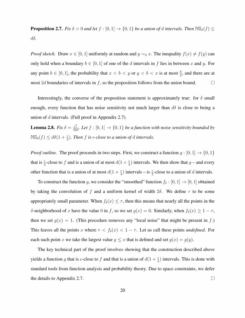
Proposition 2.7. Fix δ > 0 and let f : [0, 1]→ 0, 1 be a union of d intervals. Then NSδ(f) ≤

dδ.

Proof sketch. Draw x ∈ [0, 1] uniformly at random and y ∼δ x. The inequality f(x) 6= f(y) can

only hold when a boundary b ∈ [0, 1] of one of the d intervals in f lies in between x and y. For

any point b ∈ [0, 1], the probability that x < b < y or y < b < x is at most δ2, and there are at

most 2d boundaries of intervals in f , so the proposition follows from the union bound.

Interestingly, the converse of the proposition statement is approximately true: for δ small

enough, every function that has noise sensitivity not much larger than dδ is close to being a

union of d intervals. (Full proof in Appendix 2.7).

Lemma 2.8. Fix δ = ǫ2

32d. Let f : [0, 1]→ 0, 1 be a function with noise sensitivity bounded by

NSδ(f) ≤ dδ(1 + ǫ4). Then f is ǫ-close to a union of d intervals.

Proof outline. The proof proceeds in two steps. First, we construct a function g : [0, 1]→ 0, 1

that is ǫ2-close to f and is a union of at most d(1 + ǫ

4) intervals. We then show that g – and every

other function that is a union of at most d(1 + ǫ4) intervals – is ǫ

2-close to a union of d intervals.

To construct the function g, we consider the “smoothed” function fδ : [0, 1]→ [0, 1] obtained

by taking the convolution of f and a uniform kernel of width 2δ. We define τ to be some

appropriately small parameter. When fδ(x) ≤ τ , then this means that nearly all the points in the

δ-neighborhood of x have the value 0 in f , so we set g(x) = 0. Similarly, when fδ(x) ≥ 1− τ ,

then we set g(x) = 1. (This procedure removes any “local noise” that might be present in f .)

This leaves all the points x where τ < fδ(x) < 1 − τ . Let us call these points undefined. For

each such point x we take the largest value y ≤ x that is defined and set g(x) = g(y).

The key technical part of the proof involves showing that the construction described above

yields a function g that is ǫ-close to f and that is a union of d(1 + ǫ4) intervals. This is done with

standard tools from function analysis and probability theory. Due to space constraints, we defer

the details to Appendix 2.7.

20

The noise sensitivity characterization of unions of intervals obtained by Proposition 2.7 and

Lemma 2.8 suggest a natural approach for building a tester: design an algorithm that estimates

the noise sensitivity of the input function and accepts iff this noise sensitivity is small enough.

This is indeed what we do:

UNION OF INTERVALS TESTER( f , d, ǫ )

Parameters: δ = ǫ2

32d, r = O(ǫ−3).

1. For rounds i = 1, . . . , r,

1.1 Draw x ∈ [0, 1] uniformly at random.

1.2 Draw samples until we obtain y ∈ (x− δ, x+ δ).

1.3 Set Zi = 1[f(x) 6= f(y)].

2. Accept iff 1r

∑

Zi ≤ dδ(1 + ǫ8).

The algorithm makes 2r = O(ǫ−3) queries to the function. Since a draw in Step 1.2 is in the

desired range with probability 2δ, the number of samples drawn by the algorithm is a random

variable with very tight concentration around r(1 + 12δ) = O(d/ǫ5). The draw in Step 1.2 also

corresponds to choosing y ∼δ x. As a result, the probability that f(x) 6= f(y) in a given round is

exactly NSδ(f), and the average 1r

∑

Zi is an unbiased estimate of the noise sensitivity of f . By

Proposition 2.7, Lemma 2.8, and Chernoff bounds, the algorithm therefore errs with probability

less than 13

provided that r > c · 1/dδǫ = c · 32/ǫ3 for some suitably large constant c.

Improved unlabeled sample complexity: Notice that by changing Steps 1.1-1.2 slightly to

pick the first pair (x, y) such that |x − y| < δ, we immediately improve the unlabeled sample

complexity toO(√d/ǫ5) without affecting the analysis. In particular, this procedure is equivalent

to picking x ∈ [0, 1] then y ∼δ x.4 As a result, up to poly(1/ǫ) terms, we also improve over

the passive testing bounds of Kearns and Ron [Kearns and Ron, 2000] which are able only to

distinguish the case that f is a union of d intervals from the case that f is ǫ-far from being a

4Except for events of O(δ) probability mass at the boundary.

21

union of d/ǫ intervals. (Their results use O(√d/ǫ1.5) examples.) Kearns and Ron [Kearns and

Ron, 2000] show that Ω(√d) examples are necessary for passive testing, so in terms of d this is

optimal.

Active Tester Over Arbitrary Distributions: We can reduce the problem of testing over general

distributions to that of testing over the uniform distribution on [0, 1] by using the CDF of the

distribution D. In particular, given point x, define px = Pry∼D[y ≤ x]. So, for x drawn from D,

px is uniform in [0, 1].5 As a result we can just replace Step 1.2 in the tester with sampling until

we obtain y such that py ∈ (px − δ, px + δ). The only issue is that we do not know the px and

py values exactly. However, VC-dimension bounds for initial intervals on the line imply that if

we sampleO(ǫ−6δ−2) unlabeled examples, with high probability the estimates px computed with

respect to the sample (the fraction of points in the sample that are ≤ x) will be within O(ǫ3δ) of

the correct px values for all points x. This in turn implies that the noise-sensitivity estimates are

sufficiently accurate that the procedure works as before.

Putting these results together, we have Theorem 2.4.

2.3 Testing Linear Threshold Functions

In the last section, we saw how unions of intervals are characterized by a statistic of the function

– namely, its noise sensitivity – that can be estimated with few queries and used this to build

our tester. In this section, we follow the same high-level approach for testing linear threshold

functions. In this case, however, the statistic we will estimate is not noise sensitivity but rather

the sum of squares of the degree-1 Hermite coefficients of the function.

Definition 2.9. The Hermite polynomials are a set of polynomials h0(x) = 1, h1(x) = x, h2(x) =

1√2(x2− 1), . . . that form a complete orthogonal basis for (square-integrable) functions f : R→

R over the inner product space defined by the inner product 〈f, g〉 = Ex[f(x)g(x)], where

5We are assuming here that D is continuous and has a pdf. If D has point masses, then instead define pLx =

Pry[y < x] and pUx = Pry[y ≤ x] and select px uniformly in [pLx , pUx ].

22

the expectation is over the standard Gaussian distribution N (0, 1). For any S ∈ Nn, define

HS =∏n

i=1 hSi(xi). The Hermite coefficient of f : Rn → R corresponding to S is f(S) =

〈f,HS〉 = Ex[f(x)HS(x)] and the Hermite decomposition of f is f(x) =∑

S∈Nn f(S)HS(x).

The degree of the coefficient f(S) is |S| :=∑ni=1 Si.

The connection between linear threshold functions and the Hermite decomposition of func-

tions is revealed by the following key lemma of Matulef et al. [Matulef, O’Donnell, Rubinfeld,

and Servedio, 2009].

Lemma 2.10 (Matulef et al. [Matulef, O’Donnell, Rubinfeld, and Servedio, 2009]). There is an

explicit continuous function W : R → R with bounded derivative ‖W ′‖∞ ≤ 1 and peak value

W (0) = 2π

such that every linear threshold function f : Rn → −1, 1 satisfies∑n

i=1 f(ei)2 =

W (Exf). Moreover, every function g : Rn → −1, 1 that satisfies |∑ni=1 g(ei)

2 −W (Exg)| ≤

4ǫ3, is ǫ-close to being a linear threshold function.

In other words, Lemma 2.10 shows that∑

i f(ei)2 characterizes linear threshold functions.

To test LTFs, it suffices to estimate this value (and the expected value of the function) with

enough accuracy. Matulef et al. [Matulef, O’Donnell, Rubinfeld, and Servedio, 2009] showed

that∑

i f(ei)2 can be estimated with a number of queries that is independent of n by querying f

on pairs x, y ∈ Rn where the marginal distributions on x and y are both the standard Gaussian

distribution and where 〈x, y〉 = η for some small (but constant) η > 0. Unfortunately, the

same approach does not work in the active testing model since with high probability, all pairs

of samples that we can query have inner product |〈x, y〉| ≤ O( 1√n). Instead, we rely on the

following result.

Lemma 2.11. For any function f : Rn → R, we have∑n

i=1 f(ei)2 = Ex,y[f(x)f(y) 〈x, y〉]

where 〈x, y〉 =∑ni=1 xiyi is the standard vector dot product.

Proof. Applying the Hermite decomposition of f and linearity of expectation,

Ex,y[f(x)f(y) 〈x, y〉] =n∑

i=1

∑

S,T∈Nn

f(S)f(T )Ex[HS(x)xi]Ey[HT (y)yi].

23

By definition, xi = h1(xi) = Hei(x). The orthonormality of the Hermite polynomials therefore

guarantees that Ex[HS(x)Hei(x)] = 1[S=ei]. Similarly, Ey[HT (y)yi] = 1[T =ei].

A natural idea for completing our LTF tester is to simply sample pairs x, y ∈ Rn indepen-

dently at random and evaluating f(x)f(y) 〈x, y〉 on each pair. While this approach does give

an unbiased estimate of Ex,y[f(x)f(y) 〈x, y〉], it has poor query efficiency: To get enough accu-

racy, we need to repeat this sampling strategy Ω(n) times. (That is, the query complexity of this

sampling approach is the same as that of learning LTFs.)

We can improve the query complexity of the sampling strategy by instead using U-statistics.

The U-statistic (of order 2) with symmetric kernel function g : Rn × Rn → R is

Umg (x1, . . . , xm) :=

(

m

2

)−1∑

1≤i<j≤m

g(xi, xj).

Tight concentration bounds are known for U-statistics with well-behaved kernel functions. In

particular, by setting g(x, y) = f(x)f(y) 〈x, y〉1[|〈x, y〉| < τ ] to be an appropriately truncated

kernel for estimating E[f(x)f(y) 〈x, y〉], we can apply a Bernstein-type inequality due to Ar-

cones [Arcones, 1995] to show that O(√n) samples are sufficient to estimate

∑

i f(ei)2 with

sufficient accuracy. As a result, the following algorithm is a valid tester for LTFs.

LTF TESTER( f , ǫ )

Parameters: τ =√

4n log(4n/ǫ3), m = 800τ/ǫ3 + 32/ǫ6.

1. Draw x1, x2, . . . , xm independently at random from Rn.

2. Query f(x1), f(x2), . . . , f(xm).

3. Set µ = 1m

∑mi=1 f(x

i).

4. Set ν =(

m2

)−1∑

i 6=j f(xi)f(xj) 〈xi, xj〉 · 1[|〈xi, xj〉| ≤ τ ].

5. Accept iff |ν −W (µ)| ≤ 2ǫ3.

The algorithm queries the function only on inputs that are all independently drawn at random

from the n-dimensional Gaussian distribution. As a result, this tester works in both the active

24

and passive testing models. For the complete proof of the correctness of the algorithm, see

Appendix 2.8.

2.4 Testing Disjoint Unions of Testable Properties

We now show that active testing has the feature that a disjoint union of testable properties is

testable, with a number of queries that is independent of the size of the union; this feature does

not hold for passive testing. In addition to providing insight into the distinction between the

two models, this fact will be useful in our analysis of semi-supervised learning-based properties

mentioned below and discussed more fully in Appendix 2.11.

Specifically, given properties P1, . . . ,PN over domains X1, . . . , XN , define their disjoint

union P over domain X = (i, x) : i ∈ [N ], x ∈ Xi to be the set of functions f such that

f(i, x) = fi(x) for some fi ∈ Pi. In addition, for any distribution D over X , define Di to be the

conditional distribution over Xi when the first component is i. If each Pi is testable over Di then

P is testable over D with only small overhead in the number of queries:

Theorem 2.12. Given properties P1, . . . ,PN , if each Pi is testable overDi with q(ǫ) queries and

U(ǫ) unlabeled samples, then their disjoint union P is testable over the combined distribution D

with O(q(ǫ/2) · (log3 1ǫ)) queries and O(U(ǫ/2) · (N

ǫlog3 1

ǫ)) unlabeled samples.

Proof. See Appendix 2.9.

As a simple example, consider Pi to contain just the constant functions 1 and 0. In this case,

P is equivalent to what is often called the “cluster assumption,” used in semi-supervised and

active learning [Chapelle, Schlkopf, and Zien, 2006, Dasgupta, 2011], that if data lies in some

number of clearly identifiable clusters, then all points in the same cluster should have the same

label. Here, each Pi individually is easily testable (even passively) with O(1/ǫ) labeled samples,

so Theorem 2.12 implies the cluster assumption is testable with poly(1/ǫ) queries.6 However, it

6Since the Pi are so simple in this case, one can actually test with only O(1/ǫ) queries.

25

is not hard to see that passive testing with poly(1/ǫ) samples is not possible and in fact requires

Ω(√N/ǫ) labeled examples.7

We build on this to produce testers for other properties often used in semi-supervised learning.

In particular, we prove the following result about testing the margin property (See Appendix 2.11

for definitions and analysis).

Theorem 2.13. For any γ, γ′ = γ(1− 1/c) for constant c > 1, for data in the unit ball in Rd for

constant d, we can distinguish the case that Df has margin γ from the case that Df is ǫ-far from

margin γ′ using Active Testing withO(1/(γ2dǫ2)) unlabeled examples andO(1/ǫ) label requests.

2.5 General Testing Dimensions

The previous sections have discussed upper and lower bounds for a variety of classes. Here,

we define notions of testing dimension for passive and active testing that characterize (up to

constant factors) the number of labels needed for testing to succeed, in the corresponding testing

protocols. These will be distribution-specific notions (like SQ dimension in learning), so let us

fix some distribution D over the instance space X , and furthermore fix some value ǫ defining our

goal. I.e., our goal is to distinguish the case that distD(f,P) = 0 from the case distD(f,P) ≥ ǫ.

For a given set S of unlabeled points, and a distribution π over boolean functions, define πS

to be the distribution over labelings of S induced by π. That is, for y ∈ 0, 1|S| let πS(y) =

Prf∼π[f(S) = y]. We now use this to define a distance between distributions. Specifically, given

a set of unlabeled points S and two distributions π and π′ over boolean functions, define

DS(π, π′) = (1/2)

∑

y∈0,1|S|

|πS(y)− π′S(y)|,

7Specifically, suppose region 1 has 1− 2ǫ probability mass with f1 ∈ P1, and suppose the other regions equally

share the remaining 2ǫ probability mass and either (a) are each pure but random (so f ∈ P) or (b) are each 50/50

(so f is ǫ-far from P). Distinguishing these cases requires seeing at least two points with the same index i 6= 1,

yielding the Ω(√N/ǫ) bound.

26

to be the variation distance between π and π′ induced by S. Finally, let Π0 be the set of all

distributions π over functions in P , and let set Πǫ be the set of all distributions π′ in which a

1− o(1) probability mass is over functions at least ǫ-far from P . We are now ready to formulate

our notions of dimension.

Definition 2.14. Define the passive testing dimension, dpassive, as the largest q ∈ N such that,

supπ∈Π0

supπ′∈Πǫ

PrS∼Dq

(DS(π, π′) > 1/4) ≤ 1/4.

That is, there exist distributions π and π′ such that a random set S of dpassive examples has a

reasonable probability (at least 3/4) of having the property that one cannot reliably distinguish

a random function from π versus a random function from π′ from just the labels of S. From the

definition it is fairly immediate that Ω(dpassive) examples are necessary for passive testing; in

fact, O(dpassive) are sufficient as well.

Theorem 2.15. The sample complexity of passive testing is Θ(dpassive).

Proof. See Appendix 2.10.

For the case of active testing, there are two complications. First, the algorithms can examine

their entire poly(n)-sized unlabeled sample before deciding which points to query, and secondly

they may in principle determine the next query based on the responses to the previous ones (even

though all our algorithmic results do not require this feature). If we merely want to distinguish

those properties that are actively testable with O(1) queries from those that are not, then the

second complication disappears and the first is simplified as well, and the following coarse notion

of dimension suffices.

Definition 2.16. Define the coarse active testing dimension, dcoarse, as the largest q ∈ N such

that,

supπ∈Π0

supπ′∈Πǫ

PrS∼Dq

(DS(π, π′) > 1/4) ≤ 1/nq.

Theorem 2.17. If dcoarse = O(1) the active testing of P can be done with O(1) queries, and if

dcoarse = ω(1) then it cannot.

27

Proof. See Appendix 2.10.

To achieve a more fine-grained characterization of active testing we consider a slightly more

involved quantity, as follows. First, recall that given an unlabeled sample U and distribution π

over functions, we define πU as the induced distribution over labelings of U . We can view this as

a distribution over unlabeled examples in 0, 1|U |. Now, given two distributions over functions

π, π′, define Fair(π, π′, U) to be the distribution over labeled examples (y, ℓ) defined as: with

probability 1/2 choose y ∼ πU , ℓ = 1 and with probability 1/2 choose y ∼ π′U , ℓ = 0. Thus, for

a given unlabeled sample U , the sets Π0 and Πǫ define a class of fair distributions over labeled

examples. The active testing dimension, roughly, asks how well this class can be approximated

by the class of low-depth decision trees. Specifically, let DTk denote the class of decision trees

of depth at most k. The active testing dimension for a given number u of allowed unlabeled

examples is as follows:

Definition 2.18. Given a number u = poly(n) of allowed unlabeled examples, we define the

active testing dimension, dactive(u), as the largest q ∈ N such that

supπ∈Π0

supπ′∈Πǫ

PrU∼Du

(err∗(DTq,Fair(π, π′, U)) < 1/4) ≤ 1/4,

where err∗(H,P ) is the error of the optimal function in H with respect to data drawn from

distribution P over labeled examples.

Theorem 2.19. Active testing with failure probability 18

using u unlabeled examples requires

Ω(dactive(u)) label queries, and furthermore can be done with O(u) unlabeled examples and

O(dactive(u)) label queries.

Proof. See Appendix 2.10.

We now use these notions of dimension to prove lower bounds for testing several properties.

28

2.5.1 Application: Dictator functions

We now prove Theorem 2.3 that active testing of dictatorships over the uniform distribution re-

quires Ω(log n) queries by proving a Ω(log n) lower bound on dactive(u) for any u = poly(n); in

fact, this result holds even for the specific choice of π′ as random noise (the uniform distribution

over all functions).

Proof of Theorem 2.3. Define π and π′ to be uniform distributions over the dictator functions and

over all boolean functions, respectively. In particular, π is the distribution obtained by choosing

i ∈ [n] uniformly at random and returning the function f : 0, 1n → 0, 1 defined by f(x) =

xi. Fix S to be a set of q vectors in 0, 1n. This set can be viewed as a q × n boolean-valued

matrix. We write c1(S), . . . , cn(S) to represent the columns of this matrix. For any y ∈ 0, 1q,

πS(y) =|i ∈ [n] : ci(S) = y|

nand π′

S(y) = 2−q.

By Lemma 2.21, to prove that dactive ≥ 12log n, it suffices to show that when q < 1

2log n

and U is a set of nc vectors chosen uniformly and independently at random from 0, 1n, then

with probability at least 34, every set S ⊆ U of size |S| = q and every y ∈ 0, 1q satisfy

πS(y) ≤ 652−q. (This is like a stronger version of dcoarse where DS(π, π

′) is replaced with an L∞

distance.)

Consider a set S of q vectors chosen uniformly and independently at random from 0, 1n.

For any vector y ∈ 0, 1q, the expected number of columns of S that are equal to y is n2−q.

Since the columns are drawn independently at random, Chernoff bounds imply that

Pr[

πS(y) >652−q]

≤ e−( 15)2n2−q/3 < e−

175

n2−q

.

By the union bound, the probability that there exists a vector y ∈ 0, 1q such that more than

65n2−q columns of S are equal to y is at most 2qe−

175

n2−q. Furthermore, when U is defined as

above, we can apply the union bound once again over all subsets S ⊆ U of size |S| = q to obtain

Pr[∃S, y : πS(y) >652−q] < ncq · 2q · e− 1

75n2−q

. When q ≤ 12log n, this probability is bounded

29

above by ec2log2 n+ 1

2logn− 1

75

√n, which is less than 1

4when n is large enough, as we wanted to

show.

2.5.2 Application: LTFs

The testing dimension also lets us prove the lower bounds in Theorem 2.5 regarding the query

complexity for testing linear threshold functions. Specifically, those bounds follow directly from

the following result.

Theorem 2.20. For linear threshold functions under the standard n-dimensional Gaussian dis-

tribution, dpassive = Ω(√

n/ log(n)) and dactive = Ω((n/ log(n))1/3).

Let us give a brief overview of the strategies used to obtain the dpassive and dactive bounds.

The complete proofs for both results, as well as a simpler proof that dcoarse = Ω((n/ log n)1/3),

can be found in Appendix 2.10.4.

For both results, we set π to be a distribution over LTFs obtained by choosingw ∼ N (0, In×n)

and outputting f(x) = sgn(w · x). Set π′ to be the uniform distribution over all functions—i.e.,

for any x ∈ Rn, the value of f(x) is uniformly drawn from 0, 1 and is independent of the value

of f on other inputs.

To bound dpassive, we bound the total variation distance between the distribution of Xw/√n

given X , and the standard normal N (0, In×n). If this distance is small, then so must be the

distance between the distribution of sgn(Xw) and the uniform distribution over label sequences.

Our strategy for bounding dactive is very similar to the one we used to prove the lower bound

on the query complexity for testing dictator functions in the last section. Again, we want to

apply Lemma 2.21. Specifically, we want to show that when q ≤ o((n/ log(n))1/3) and U is a

set of nc vectors drawn independently from the n-dimensional standard Gaussian distribution,

then with probability at least 34, every set S ⊆ U of size |S| = q and almost all x ∈ R

q, we have

πS(x) ≤ 652−q. The difference between this case and the lower bound for dictator functions is

that we now rely on strong concentration bounds on the spectrum of random matrices [Vershynin,

30

2012] to obtain the desired inequality.

2.6 Proof of a Property Testing Lemma

The following lemma is a generalization of a lemma that is widely used for proving lower bounds

in property testing [Fischer, 2001, Lem. 8.3]. We use this lemma to prove the lower bounds on

the query complexity for testing dictator functions and testing linear threshold functions.

Lemma 2.21. Let π and π′ be two distributions on functions X → R. Fix U ⊆ X to be a set

of allowable queries. Suppose that for any S ⊆ U , |S| = q, there is a set ES ⊆ Rq (possibly

empty) satisfying πS(ES) ≤ 152−q such that

πS(y) <65π′S(y) for every y ∈ R

q \ ES.

Then err∗(DTq,Fair(π, π′, U)) > 1/4.

Proof. Consider any decision tree A of depth q. Each internal node of the tree consists of a

query y ∈ U and a subset T ⊆ R such that its children are labeled by T and R \ T , respectively.

The leaves of the tree are labeled with either “accept” or “reject”, and let L be the set of leaves

labeled as accept. Each leaf ℓ ∈ L corresponds to a set Sℓ ⊆ U q of queries and a subset Tℓ ⊆ Rℓ,

where f : X → R leads to the leaf ℓ iff f(Sℓ) ∈ Tℓ. The probability that A (correctly) accepts

an input drawn from π is

a1 =∑

ℓ∈L

∫

Tℓ

πSℓ(y)dy.

Similarly, the probability that A (incorrectly) accepts an input drawn from π′ is

a2 =∑

ℓ∈L

∫

Tℓ

π′Sℓ(y)dy.

The difference between the two rejection probabilities is bounded above by

a1 − a2 ≤∑

ℓ∈L

∫

Tℓ\ESℓ

πSℓ(y)− π′

Sℓ(y)dy +

∑

ℓ∈L

∫

Tℓ∩ESℓ

πSℓ(y)dy.

31

The conditions in the statement of the lemma then imply that

a1 − a2 <∑

ℓ∈L

∫

Tℓ

16πSℓ

(y)dy + 56

∑

ℓ

∫

ESℓ

πSℓ(y)dy ≤ 1

3.

To complete the proof, we note thatA errs on an input drawn from Fair(π, π′, U) with probability

12(1− a1) + 1

2a2 =

12− 1

2(a1 − a2) > 1

3.

2.7 Proofs for Testing Unions of Intervals

In this section we complete the proofs of the technical results in Section 2.2.

Proposition 2.7 (Restated). Fix δ > 0 and let f : [0, 1]→ 0, 1 be a union of d intervals. Then

NSδ(f) ≤ dδ.

Proof. For any fixed b ∈ [0, 1], the probability that x < b < y when x ∼ U(0, 1) and y ∼

U(x− δ, x+ δ) is

Prx,y

[x < b < y] =

∫ δ

0

Pry∼U(b−t−δ,b−t+δ)

[y ≥ b]dt =

∫ δ

0

δ − t2δ

dt =δ

4.

Similarly, Prx,y[y < b < x] = δ4. So the probability that b lies between x and y is at most δ

2.

When f is the union of d intervals, f(x) 6= f(y) only if at least one of the boundaries

b1, . . . , b2d of the intervals of f lies in between x and y. So by the union bound, Pr[f(x) 6=

f(y)] ≤ 2d(δ/2) = dδ. Note that if b is within distance δ of 0 or 1, the probability is only

lower.

Lemma 2.8 (Restated). Fix δ = ǫ2

32d. Let f : [0, 1]→ 0, 1 be any function with noise sensitivity

NSδ(f) ≤ dδ(1 + ǫ4). Then f is ǫ-close to a union of d intervals.

Proof. The proof proceeds in two steps: We first show that f is ǫ2-close to a union of d(1 + ǫ

2)

intervals, then we show that every union of d(1+ ǫ2) intervals is ǫ

2-close to a union of d intervals.

32

Consider the “smoothed” function fδ : [0, 1]→ [0, 1] defined by

fδ(x) = Ey∼δxf(y) =1

2δ

∫ x+δ

x−δ

f(y)dy.

The function fδ is the convolution of f and the uniform kernel φ : R → [0, 1] defined by

φ(x) = 12δ1[|x| ≤ δ].

Fix τ = 4ǫNSδ(f). We introduce the function g∗ : [0, 1]→ 0, 1, ∗ by setting

g∗(x) =

1 when fδ(x) ≥ 1− τ ,

0 when fδ(x) ≤ τ , and

∗ otherwise

for all x ∈ [0, 1]. Finally, we define g : [0, 1] → 0, 1 by setting g(x) = g∗(y) where y ≤ x is

the largest value for which g(y) 6= ∗. (If no such y exists, we fix g(x) = 0.)

We first claim that dist(f, g) ≤ ǫ2. To see this, note that

dist(f, g) = Prx[f(x) 6= g(x)]

≤ Prx[g∗(x) = ∗] + Pr

x[f(x) = 0 ∧ g∗(x) = 1] + Pr

x[f(x) = 1 ∧ g∗(x) = 0]

= Prx[τ < fδ(x) < 1− τ ] + Pr

x[f(x) = 0 ∧ fδ(x) ≥ 1− τ ] + Pr

x[f(x) = 1 ∧ fδ(x) ≤ τ ].

We bound the three terms on the RHS individually. For the first term, we observe that NSδ(f, x) =

minfδ(x), 1− fδ(x) and that ExNSδ(f, x) = NSδ(f). From these identities and Markov’s in-

equality, we have that

Prx[τ < fδ(x) < 1− τ ] = Pr

x[NSδ(f, x) > τ ] <

NSδ(f)

τ=ǫ

4.

For the second term, let S ⊆ [0, 1] denote the set of points x where f(x) = 0 and fδ(x) ≥ 1− τ .

Let Γ ⊆ S represent a δ-net of S. Clearly, |Γ| ≤ 1δ. For x ∈ Γ, let Bx = (x − δ, x + δ) be a

ball of radius δ around x. Since fδ(x) ≥ 1 − τ , the intersection of S and Bx has mass at most

|S ∩ Bx| ≤ τδ. Therefore, the total mass of S is at most |S| ≤ |Γ|τδ = τ . By the bounds on the

33

noise sensitivity of f in the lemma’s statement, we therefore have

Prx[f(x) = 0 ∧ fδ(x) ≥ 1− τ ] ≤ τ ≤ ǫ

8.

Similarly, we obtain the same bound on the third term. As a result, dist(f, g) ≤ ǫ4+ ǫ

8+ ǫ

8= ǫ

2,

as we wanted to show.

We now want to show that g is a union of m ≤ dδ(1 + ǫ2) intervals. Each left boundary of an

interval in g occurs at a point x ∈ [0, 1] where g∗(x) = ∗, where the maximum y ≤ x such that

g∗(y) 6= ∗ takes the value g∗(y) = 0, and where the minimum z ≥ x such that g∗(z) 6= ∗ has

the value g∗(z) = 1. In other words, for each left boundary of an interval in g, there exists an

interval (y, z) such that fδ(y) ≤ τ , fδ(z) ≥ 1 − τ , and for each y < x < z, fδ(x) ∈ (τ, 1 − τ).

Fix any interval (y, z). Since fδ is the convolution of f with a uniform kernel of width 2δ, it

is Lipschitz continuous (with Lipschitz constant 12δ

). So there exists x ∈ (y, z) such that the

conditions fδ(x) =12, x− y ≥ 2δ(1

2− τ), and z − x ≥ 2δ(1

2− τ) all hold. As a result,

∫ z

y

NSδ(f, t) dt =

∫ x

y

NSδ(f, t) dt+

∫ z

x

NSδ(f, t) dt ≥ 2δ(12− τ)2.

Similarly, for each right boundary of an interval in g, we have an interval (y, z) such that

∫ z

y

NSδ(f, t) dt ≥ 2δ(12− τ)2.

The intervals (y, z) for the left and right boundaries are all disjoints, so

NSδ(f) ≥2m∑

i=1

∫ zi

yiNSδ(f, t) dt ≥ 2m

δ

2(1− 2τ)2.

This means that

m ≤ dδ(1 + ǫ/4)

δ(1− 2τ)2≤ d(1 + ǫ

2)

and g is a union of at most d(1 + ǫ2) intervals, as we wanted to show.

Finally, we want to show that any function that is the union of m ≤ d(1 + ǫ2) intervals is ǫ

2-

close to a union of d intervals. Let ℓ1, . . . , ℓm represent the lengths of the intervals in g. Clearly,

34

ℓ1 + · · ·+ ℓm ≤ 1, so there must be a set S of m− d ≤ dǫ/2 intervals in f with total length

∑

i∈Sℓi ≤

m− dm

≤ dǫ/2

d(1 + ǫ2)<ǫ

2.

Consider the function h : [0, 1] → 0, 1 obtained by removing the intervals in S from g (i.e.,

by setting h(x) = 0 for the values x ∈ [b2i−1, b2i] for some i ∈ S). The function h is a union

of d intervals and dist(g, h) ≤ ǫ2. This completes the proof, since dist(f, h) ≤ dist(f, g) +

dist(g, h) ≤ ǫ.

2.8 Proofs for Testing LTFs

We complete the proof that LTFs can be tested with O(√n) samples in this section.

For a fixed function f : Rn → R, define g : Rn × Rn → R to be g(x, y) = f(x)f(y) 〈x, y〉.

Let g∗ : Rn × Rn → R be the truncation of g defined by setting

g∗(x, y) =

f(x)f(y) 〈x, y〉 if | 〈x, y〉 | ≤√

4n log(4n/ǫ3)

0 otherwise.

Our goal is to estimate Eg. The following lemma shows that Eg∗ provides a good estimate of

this value.

Lemma 2.22. Let g, g∗ : Rn × Rn → R be defined as above. Then |Eg − Eg∗| ≤ 1

2ǫ3.

Proof. For notational clarity, fix τ =√

4n log(4n/ǫ3). By the definition of g and g∗ and with

the trivial bound |f(x)f(y) 〈x, y〉 | ≤ n we have

|Eg−Eg∗| =∣

∣

∣

∣

Prx,y

[

|〈x, y〉| > τ]

· Ex,y

[

f(x)f(y) 〈x, y〉∣

∣ |〈x, y〉| > τ]

∣

∣

∣

∣

≤ n ·Prx,y

[

|〈x, y〉| > τ]

.

The right-most term can be bounded with a standard Chernoff argument. By Markov’s inequality

and the independence of the variables x1, . . . , xn, y1, . . . , yn,

Prx,y

[

〈x, y〉 > τ]

= Pr[

et〈x,y〉 > etτ]

≤ Eet〈x,y〉

etτ=

∏ni=1 Ee

txiyi

etτ.

35

The moment generating function of a standard normal random variable is Eety = et2/2, so

Exi,yi

[

etxiyi]

= Exi

[

Eyietxiyi]

= Exie(t

2/2)x 2i .

When x ∼ N (0, 1), the random variable x2 has a χ2 distribution with 1 degree of freedom. The

moment generating function of this variable is Eetx2=√

11−2t

=√

1 + 2t1−2t

for any t < 12.

Hence,

Exie(t

2/2)x 2i ≤

√

1 +t2

1− t2 ≤ et2

2(1−t2)

for any t < 1. Combining the above results and setting t = τ2n

yields

Prx,y

[

〈x, y〉 > τ]

≤ ent2

2(1−t2)−tτ ≤ e−

τ2

4n = ǫ3

4n.

The same argument shows that Pr[〈x, y〉 < −τ ] ≤ ǫ3

4nas well.

The reason we consider the truncation g∗ is that its smaller ℓ∞ norm will enable us to apply

a strong Bernstein-type inequality on the concentration of measure of the U-statistic estimate of

Eg∗.

Lemma 2.23 (Arcones [Arcones, 1995]). For a symmetric function h : Rn × Rn → R, let Σ2 =

Ex[Ey[h(x, y)]2] − Ex,y[h(x, y)]

2, let b = ‖h − Eh‖∞, and let Um(h) be a random variable ob-

tained by drawing x1, . . . , xm independently at random and settingUm(h) =(

m2

)−1∑

i<j h(xi, xj).

Then for every t > 0,

Pr[|Um(h)− Eh| > t] ≤ 4 exp

(

mt2

8Σ2 + 100bt

)

.

We are now ready to complete the proof of the upper bound of Theorem 2.5.

Theorem 2.24 (Upper bound in Theorem 2.5, restated). Linear threshold functions can be tested

over the standard n-dimensional Gaussian distribution with O(√n log n) queries in both the

active and passive testing models.

Proof. Consider the LTF-TESTER algorithm. When the estimates µ and ν satisfy

|µ− Ef | ≤ ǫ3 and |ν − E[f(x)f(y) 〈x, y〉]| ≤ ǫ3,

36

Lemmas 2.10 and 2.11 guarantee that the algorithm correctly distinguishes LTFs from functions

that are far from LTFs. To complete the proof, we must therefore show that the estimates are

within the specified error bounds with probability at least 2/3.

The values f(x1), . . . , f(xm) are independent −1, 1-valued random variables. By Hoeffd-

ing’s inequality,

Pr[|µ− Ef | ≤ ǫ3] ≥ 1− 2e−ǫ6m/2 = 1− 2e−O(√n).

The estimate ν is a U-statistic with kernel g∗ as defined above. This kernel satisfies

‖g∗ − Eg∗‖∞ ≤ 2‖g∗‖∞ = 2√

4n log(4n/ǫ3)

and

Σ2 ≤ Ey

[

Ex[g∗(x, y)]2

]

= Ey

[

Ex[f(x)f(y) 〈x, y〉1[|〈x, y〉| ≤ τ ]]2]

.

For any two functions φ, ψ : Rn → R, when ψ is 0, 1-valued the Cauchy-Schwarz in-

equality implies that Ex[φ(x)ψ(x)]2 ≤ Ex[φ(x)]Ex[φ(x)ψ(x)

2] = Ex[φ(x)]Ex[φ(x)ψ(x)] and

so Ex[φ(x)ψ(x)]2 ≤ Ex[φ(x)]. Applying this inequality to the expression for Σ2 gives

Σ2 ≤ Ey

[

Ex[f(x)f(y) 〈x, y〉]2]

= Ey

[(

n∑

i=1

f(y)yiEx[f(x)xi])2]

=∑

i,j

f(ei)f(ej)Ey[yiyj] =n∑

i=1

f(ei)2.

By Parseval’s identity, we have∑

i f(ei)2 ≤ ‖f‖22 = ‖f‖22 = 1. Lemmas 2.22 and 2.23 imply

that

Pr[|ν − Eg| ≤ ǫ3] = Pr[|ν − Eg∗| ≤ 12ǫ3] ≥ 1− 4e

− mt2

8+200√

n log(4n/ǫ3)t ≥ 1112.

The union bound completes the proof of correctness.

2.9 Proofs for Testing Disjoint Unions

Theorem 2.12 (Restated). Given properties P1, . . . ,PN , if each Pi is testable over Di with q(ǫ)

queries and U(ǫ) unlabeled samples, then their disjoint union P is testable over the combined

distribution D with O(q(ǫ/2) · (log3 1ǫ)) queries and O(U(ǫ/2) · (N

ǫlog3 1

ǫ)) unlabeled samples.

37

Proof. Let p = (p1, . . . , pN) denote the mixing weights for distribution D; that is, a random

draw from D can be viewed as selecting i from distribution p and then selecting x from Di. We

are given that each Pi is testable with failure probability 1/3 using using q(ǫ) queries and U(ǫ)

unlabeled samples. By repetition, this implies that each is testable with failure probability δ using

qδ(ǫ) = O(q(ǫ) log(1/δ)) queries and Uδ(ǫ) = O(U(ǫ) log(1/δ)) unlabeled samples, where we

will set δ = ǫ2. We now test property P as follows:

For ǫ′ = 1/2, 1/4, 1/8, . . . , ǫ/2 do:

Repeat O( ǫ′

ǫlog(1/ǫ)) times:

1. Choose a random (i, x) from D.

2. Sample until either Uδ(ǫ′) samples have been drawn from Di or (8N/ǫ)Uδ(ǫ

′)

samples total have been drawn from D, whichever comes first.

3. In the former case, run the tester for property Pi with parameter ǫ′, making

qδ(ǫ′) queries. If the tester rejects, then reject.

If all runs have accepted, then accept.

First to analyze the total number of queries and samples, since we can assume q(ǫ) ≥ 1/ǫ and

U(ǫ) ≥ 1/ǫ, we have qδ(ǫ′)ǫ′/ǫ = O(qδ(ǫ/2)) and Uδ(ǫ

′)ǫ′/ǫ = O(Uδ(ǫ/2)) for ǫ′ ≥ ǫ/2. Thus,

the total number of queries made is at most

∑

ǫ′

qδ(ǫ/2) log(1/ǫ) = O

(

q(ǫ/2) · log3 1ǫ

)

and the total number of unlabeled samples is at most

∑

ǫ′

8N

ǫUδ(ǫ/2) log(1/ǫ) = O

(

U(ǫ/2)N

ǫlog3

1

ǫ

)

.

Next, to analyze correctness, if indeed f ∈ P then each call to a tester rejects with probability

at most δ so the overall failure probability is at most (δ/ǫ) log2(1/ǫ) < 1/3; thus it suffices to

analyze the case that distD(f,P) ≥ ǫ.

38

If distD(f,P) ≥ ǫ then∑

i:pi≥ǫ/(4N) pi · distDi(fi,Pi) ≥ 3ǫ/4. Moreover, for indices i such that

pi ≥ ǫ/(4N), with high probability Step 2 draws Uδ(ǫ′) samples, so we may assume for such

indices the tester for Pi is indeed run in Step 3. Let I = i : pi ≥ ǫ/(4N) and distDi(fi,Pi) ≥

ǫ/2. Thus, we have

∑

i∈Ipi · distDi

(fi,Pi) ≥ ǫ/4.

Let Iǫ′ = i ∈ I : distDi(fi,Pi) ∈ [ǫ′, 2ǫ′]. Bucketing the above summation by values ǫ′ in this

way implies that for some value ǫ′ ∈ ǫ/2, ǫ, 2ǫ, . . . , 1/2, we have:

∑

i∈Iǫ′pi ≥ ǫ/(8ǫ′ log(1/ǫ)).

This in turn implies that with probability at least 2/3, the run of the algorithm for this value of ǫ′

will find such an i and reject, as desired.

2.10 Proofs for Testing Dimensions

2.10.1 Passive Testing Dimension (proof of Theorem 2.15)

Lower bound: By design, dpassive is a lower bound on the number of examples needed for

passive testing. In particular, if DS(π, π′) ≤ 1/4, and if the target is with probability 1/2 chosen

from π and with probability 1/2 chosen from π′, even the Bayes optimal tester will fail to identify

the correct distribution with probability 12

∑

y∈0,1|S| min(πS(y), π′S(y)) =

12(1 − DS(π, π

′)) ≥

3/8. The definition of dpassive implies that there exist π ∈ Π0, π′ ∈ Πǫ such that PrS(DS(π, π′) ≤

1/4) ≥ 3/4. Since π′ has a 1 − o(1) probability mass on functions that are ǫ-far from P , this

implies that over random draws of S and f , the overall failure probability of any tester is at least

(1− o(1))(3/8)(3/4) > 1/4. Thus, at least dpassive + 1 random labeled examples are required if

we wish to guarantee error at most 1/4. This in turn implies Ω(dpassive) examples are needed to

guarantee error at most 1/3.

39

Upper bound: We now argue that O(dpassive) examples are sufficient for testing as well. Toward

this end, consider the following natural testing game. The adversary chooses a function f such

that either f ∈ P or distD(f,P) ≥ ǫ. The tester picks a function A that maps labeled samples

of size k to accept/reject. That is, A is a deterministic passive testing algorithm. The payoff to

the tester is the probability that A is correct when S is chosen iid from D and labeled by f .

If k > dpassive then (by definition of dpassive) we know that for any distribution π over f ∈ P

and any distribution π′ over f that are ǫ-far from P , we have PrS∼Dk(DS(π, π′) > 1/4) > 1/4.

We now need to translate this into a statement about the value of the game. The key fact we can

use is that if the adversary uses distribution απ + (1 − α)π′ (i.e., with probability α it chooses

from π and with probability 1−α it chooses from π′), then the Bayes optimal predictor has error

exactly

∑

y

min(απS(y), (1− α)π′S(y)) ≤ max(α, 1− α)

∑

y

min(πS(y), π′S(y)),

while

∑

y

min(πS(y), π′S(y)) = 1− (1/2)

∑

y

|πS(y)− π′S(y)| = 1−DS(π, π

′),

so that the Bayes risk is at most max(α, 1− α)(1−DS(π, π′)). Thus, for any α ∈ [7/16, 9/16],

if DS(π, π′) > 1/4, the Bayes risk is less than (9/16)(3/4) = 27/64. Furthermore, any α /∈

[7/16, 9/16] has Bayes risk at most 7/16. Thus, since DS(π, π′) > 1/4 with probability > 1/4

(and if DS(π, π′) ≤ 1/4 then the error probability of the Bayes optimal predictor is at most

1/2), for any mixed strategy of the adversary, the Bayes optimal predictor has risk less than

(1/4)(7/16) + (3/4)(1/2) = 31/64.

Now, applying the minimax theorem we get that for k = dpassive + 1, there exists a mixed

strategy A for the tester such that for any function chosen by the adversary, the probability the

tester is correct is at least 1/2 + γ for a constant γ > 0 (namely, 1/64). We can now boost the

correctness probability using a constant-factor larger sample. Specifically, letm = c·(dpassive+1)

for some constant c, and consider a sample S of size m. The tester simply partitions the sample

40

S into c pieces, runs A separatately on each piece, and then takes majority vote. This gives us

that O(dpassive) examples are sufficient for testing with any desired constant success probability

in (1/2, 1).

2.10.2 Coarse Active Testing Dimension (proof of Theorem 2.17)

Lower bound: First, we claim that any nonadaptive active testing algorithm that uses≤ dcoarse/c

label requests must use more than nc unlabeled examples (and thus no algorithm can succeed

using o(dcoarse) labels). To see this, suppose algorithm A draws nc unlabeled examples. The

number of subsets of size dcoarse/c is at most ndcoarse/6 (for dcoarse/c ≥ 3). So, by definition of

dcoarse and the union bound, with probability at least 5/6, all such subsets S satisfy the property

that DS(π, π′) < 1/4. Therefore, for any sequence of such label requests, the labels observed will

not be sufficient to reliably distinguish π from π′. Adaptive active testers can potentially choose

their next point to query based on labels observed so far, but the above immediately implies that

even adaptive active testers cannot use an o(log(dcoarse)) queries.

Upper bound: For the upper bound, we modify the argument from the passive testing dimension

analysis as follows. We are given that for any distribution π over f ∈ P and any distribution π′

over f that are ǫ-far fromP , for k = dcoarse+1, we have PrS∼Dk(DS(π, π′) > 1/4) > n−k. Thus,

we can sample U ∼ Dm withm = Θ(k ·nk), and partition U into subsamples S1, S2, . . . , Scnk of

size k each. With high probability, at least one of these subsamples Si will have DS(π, π′) > 1/4.

We can thus simply examine each subsample, identify one such that DS(π, π′) > 1/4, and query

the points in that sample. As in the proof for the passive bound, this implies that for any strategy

for the adversary in the associated testing game, the best response has probability at least 1/2+γ

of success for some constant γ > 0. By the minimax theorem, this implies a testing strategy with

success probability 1/2+γ which can then be boosted to 2/3. The total number of label requests

used in the process is only O(dcoarse).

Note, however, that this strategy uses a number of unlabeled examples Ω(ndcoarse+1). Thus,

41

this only implies an active tester for dcoarse = O(1). Nonetheless, combining the upper and lower

bounds yields Theorem 2.17.

2.10.3 Active Testing Dimension (proof of Theorem 2.19)

Lower bound: for a given sample U , we can think of an adaptive active tester as a decision

tree, defined based on which example it would request the label of next given that the previous

requests have been answered in any given way. A tester making k queries would yield a decision

tree of depth k. By definition of dactive(u), with probability at least 3/4 (over choice of U ), any

such tester has error probability at least (1/4)(1 − o(1)) over the choice of f . Thus, the overall

failure probability is at least (3/4)(1/4)(1− o(1) > 1/8.

Upper bound: We again consider the natural testing game. We are given that for any mixed

strategy of the adversary with equal probability mass on functions in P and functions ǫ-far from

P , the best response of the tester has expected payoff at least (1/4)(3/4) + (3/4)(1/2) = 9/16.

This in turn implies that for any mixed strategy at all, the best response of the tester has expected

payoff at least 33/64 (if the adversary puts more than 17/32 probability mass on either type

of function, the tester can just guess that type with expected payoff at least 17/32, else it gets

payoff at least (1 − 1/16)(9/16) > 33/64). By the minimax theorem, this implies existence of

a randomized strategy for the tester with at least this payoff. We then boost correctness using

c · u samples and c · dactive(u) queries, running the tester c times on disjoint samples and taking

majority vote.

2.10.4 Lower Bounds for Testing LTFs (proof of Theorem 2.20)

We complete the proofs for the lower bounds on the query complexity for testing linear threshold

functions in the active and passive models. This proof has three parts. First, in Section 2.10.4, we

introduce some preliminary (technical) results that will be used to prove the lower bounds on the

passive and coarse dimensions of testing LTFs. In Section 2.10.4, we introduce some more pre-

42

liminary results regarding random matrices that we will use to bound the active dimension of the

class. Finally, in Section 2.10.4, we put it all together and complete the proof of Theorem 2.20.

Preliminaries for dpassive and dcoarse

Fix any K. Let the dataset X = x1, x2, · · · , xK be sampled iid according to the uniform

distribution on −1,+1n and let X ∈ RK×n be the corresponding data matrix.

Suppose w ∼ N(0, In×n). We let

z = Xw,

and note that the conditional distribution of z given X is normal with mean 0 and (X-dependent)

covariance matrix, which we denote by Σ. Further applying threshold function to z gives y as

the predicted label vector of an LTF.

Lemma 2.25. For any matrix B, log(det(B)) = Tr(log(B)), where log(B) is the matrix expo-

nential of B.

Proof. From [Higham, 2008], we know since every eigenvalue of A corresponds to the eigen-

value of exp(A), thus

det(exp(A)) = exp(Tr(A)) (2.1)

where exp(A) is the matrix exponential of A. Taking logarithm of both sides of (2.1), we get

log(det(exp(A))) = Tr(A) (2.2)

Let B = exp(A) (thus A = log(B)). Then (2.2) can rewritten as log(det(B)) = Tr(logB).

Lemma 2.26. For sufficiently large n, and a value K = Ω(√

n/ log(K/δ)), with probability at

least 1− δ (over X),

‖P(z/√n)|X −N(0, I)‖ ≤ 1/4.

43

Proof. Let l be the feature index. For a pair xi and xj ,

P(∣

∣

∣|l : xil = xjl| −

n

2

∣

∣

∣>

√

n log 2δ

2) ≤ δ

By Hoeffding Inequality, with probability 1− δ,

xTi xj = |l : xil = xjl| − |l : xil 6= xjl|

= 2|l : xil = xjl| − n ∈

−2

√

n log 2δ

2, 2

√

n log 2δ

2

By union bound,

P

(

∃i, j, such that xTi xj 6∈

[

−√

2n log2K2

δ,

√

2n log2K2

δ

])

≤ K2 δ

K2= δ (2.3)

For the remainder of the proof we suppose the (probability 1− δ) event

∀i, j,xTi xj ∈

[

−√

2n log(2K2/δ),√

2n log(2K2/δ)]

occurs.

Cov(zi/√n, zj/

√n|X) =

E[zizj|X]

n

=1

nE

[

(n∑

l=1

wl · xil)(n∑

l=1

wl · xjl)|X]

=1

nE

[

n,n∑

l,m=1,1

wlwmxilxjm|X]

=1

nE

[

∑

l

w2l xilxjl|X

]

=1

nE

[

∑

l

xilxjl|X]

=1

n

∑

l

xilxjl =1

nxTi xj ∈

[

−√

2 log(2K2/δ)

n,

√

2 log(2K2/δ)

n

]

because E[wlwm] = 0 (for l 6= m) and E[w2l ] = 1. Let β =

√

2 log(2K2/δ)n

. Thus Σ is a K ×K

matrix, with Σii = 1 for i = 1, · · · , K and Σij ∈ [−β, β] for all i 6= j.

Let P1 = N(0,ΣK×K) and P2 = N(0, IK×K). As the density

p1(z) =1

√

(2π)Kdet(Σ)exp(−1

2zTΣ−1z)

44

and the density

p2(z) =1

√

(2π)Kexp(−1

2zTz)

Then L1 distance between the two distributions P1 and P2

|dP2 − dP1| ≤ 2√

K(P1, P2) = 2√

(1/2) log det(Σ),

where this last equality is by [Davis and Dhillon, 2006]. By Lemma 2.25, log(det(Σ)) =

Tr(log(Σ)). Write A = Σ− I . By the Taylor series

log(I + A) = −∞∑

i=1

1

i(I − (I + A))i = −

∞∑

i=1

1

i(−A)i

Thus Tr(log(I + A)) =∞∑

i=1

1

iT r((−A)i). (2.4)

Every entry in Ai can be expressed as a sum of at most Ki−1 terms, each of which can

be expressed as a product of exactly i entries from A. Thus, every entry in Ai is in the range

[−Ki−1βi, Ki−1βi]. This means Tr(Ai) ≤ Kiβi. Therefore, if Kβ < 1/2, since Tr(A) = 0,

the expansion of Tr(log(I + A)) ≤∑∞i=2K

iβi = O(

K2 log(K/δ)n

)

.

In particular, for some K = Ω(√

n/ log(K/δ)), Tr(log(I +A)) is bounded by the appropri-

ate constant to obtain the stated result.

Preliminaries for dactive

Given an n×m matrix A with real entries ai,ji∈[n],j∈[m], the adjoint (or transpose – the two are

equivalent since A contains only real values) of A is the m × n matrix A∗ whose (i, j)-th entry

equals aj,i. Let us write λ1 ≥ λ2 ≥ · · · ≥ λm to denote the eigenvalues of√A∗A. These values

are the singular values of A. The matrix A∗A is positive semidefinite, so the singular values of

A are all non-negative. We write λmax(A) = λ1 and λmin(A) = λm to represent its largest and

smallest singular values. Finally, the induced norm (or operator norm) of A is

‖A‖ = maxx∈Rm\0

‖Ax‖2‖x‖2

= maxx∈Rm:‖x‖22=1

‖Ax‖2.

45

For more details on these definitions, see any standard linear algebra text (e.g., [Shilov, 1977]).

We will also use the following strong concentration bounds on the singular values of random

matrices.

Lemma 2.27 (See [Vershynin, 2012, Cor. 5.35]). Let A be an n × m matrix whose entries are

independent standard normal random variables. Then for any t > 0, the singular values of A

satisfy

√n−√m− t ≤ λmin(A) ≤ λmax(A) ≤

√n+√m+ t (2.5)

with probability at least 1− 2e−t2/2.

The proof of this lemma follows from Talagrand’s inequality and Gordon’s Theorem for

Gaussian matrices. See [Vershynin, 2012] for the details. The lemma implies the following

corollary which we will use in the proof of our theorem.

Corollary 2.28. Let A be an n × m matrix whose entries are independent standard normal

random variables. For any 0 < t <√n−√m, them×mmatrix 1

nA∗A satisfies both inequalities

∥

∥

1nA∗A− I

∥

∥ ≤ 3

√m+ t√n

and det(

1nA∗A

)

≥ e−m

(

(√m+t)2

n+2

√m+t√n

)

(2.6)

with probability at least 1− 2e−t2/2.

Proof. When there exists 0 < z < 1 such that 1 − z ≤ 1√nλmax(A) ≤ 1 + z, the identity

1√nλmax(A) = ‖ 1√

nA‖ = max‖x‖22=1 ‖ 1√

nAx‖2 implies that

1− 2z ≤ (1− z)2 ≤ max‖x‖22=1

∥

∥

∥

1√nAx∥

∥

∥

2

2≤ (1 + z)2 ≤ 1 + 3z.

These inequalities and the identity ‖ 1nA∗A − I‖ = max‖x‖22=1 ‖ 1√

nAx‖22 − 1 imply that −2z ≤

‖ 1nA∗A− I‖ ≤ 3z. Fixing z =

√m+t√n

and applying Lemma 2.27 completes the proof of the first

inequality.

Recall that λ1 ≤ · · · ≤ λm are the eigenvalues of√A∗A. Then

det( 1nA∗A) =

det(√A∗A)2

n=

(λ1 · · ·λm)2n

≥(

λ 21

n

)m

=

(

λmin(A)2

n

)m

.

46

Lemma 2.27 and the elementary inequality 1+x ≤ ex complete the proof of the second inequal-

ity.

Proof of Theorem 2.20

Theorem 2.20 (Restated). For linear threshold functions under the uniform distribution on

−1, 1n, dpassive = Ω(√

n/ log(n)) and dactive = Ω((n/ log(n))1/3).

Proof. Let K be as in Lemma 2.26 for δ = 1/4. Let D = (x1, y1), . . . , (xK , yK) denote

the sequence of labeled data points under the random LTF based on w. Furthermore, let D′ =

(x1, y′1), . . . , (xK , y′K) denote the sequence of labeled data points under a target function that

assigns an independent random label to each data point. Also let zi = (1/√n)wTxi, and let

z′ ∼ N(0, IK×K). Let E = (x1, z1), . . . , (xK , zK) and E ′ = (x1, z′1), . . . , (xK , z′K). Note

that we can think of yi and y′i as being functions of zi and z′i, respectively. Thus, letting X =

x1, . . . , xK, by Lemma 2.26, with probability at least 3/4,

‖PD|X − PD′|X‖ ≤ ‖PE|X − PE′|X‖ ≤ 1/4.

This suffices for the claim that dpassive = Ω(K) = Ω(√

n/ log(n)).

Next we turn to the lower bound on dactive. Let us now introduce two distributions Dyes

and Dno over linear threshold functions and functions that (with high probability) are far from

linear threshold functions, respectively. We draw a function f from Dyes by first drawing a

vector w ∼ N (0, In×n) from the n-dimensional standard normal distribution. We then define

f : x 7→ sgn( 1√nx · w). To draw a function g from Dno, we define g(x) = sgn(yx) where each

yx variable is drawn independently from the standard normal distribution N (0, 1).

Let X ∈ Rn×q be a random matrix obtained by drawing q vectors from the n-dimensional

normal distributionN (0, In×n) and setting these vectors to be the columns of X. Equivalently, X

is the random matrix whose entries are independent standard normal variables. When we view X

as a set of q queries to a function f ∼ Dyes or a function g ∼ Dno, we get f(X) = sgn( 1√nXw)

47

and g(X) = sgn(yX). Note that 1√nXw ∼ N (0, 1

nX∗X) and yX ∼ N (0, Iq×q). To apply

Lemma 2.21 it suffices to show that the ratio of the pdfs for both these random variables is

bounded by 65

for all but 15

of the probability mass.

The pdf p : Rq → R of a q-dimensional random vector from the distribution Nq×q(0,Σ) is

p(x) = (2π)−q2 det(Σ)−

12 e−

12xTΣ−1x.

Therefore, the ratio function r : Rq → R between the pdfs of 1√nXw and of yX is

r(x) = det( 1nX∗X)−

12 e

12xT (( 1

nX

∗X)−1−I)x.

Note that

xT (( 1nX∗X)−1 − I)x ≤ ‖( 1

nX∗X)−1 − I‖‖x‖22 = ‖ 1nX∗X− I‖‖x‖22,

so by Lemma 2.27 with probability at least 1− 2e−t2/2 we have

r(x) ≤ eq2

(

(√q+t)2

n+2

√q+t√n

)

+3√

q+t√n

‖x‖22.

By a union bound, for U ∼ N (0, In×n)u, u ∈ N with u ≥ q, the above inequality for r(x) is true

for all subsets of U of size q, with probability at least 1 − uq2e−t2/2. Fix q = n13/(50(ln(u))

13 )

and t = 2√

q ln(u). Then uq2e−t2/2 ≤ 2u−q, which is < 1/4 for any sufficiently large n. When

‖x‖22 ≤ 3q then for large n, r(x) ≤ e74/625 < 65. To complete the proof, it suffices to show that

when x ∼ N (0, Iq×q), the probability that ‖x‖22 > 3q is at most 152−q. The random variable ‖x‖22

has a χ2 distribution with q degrees of freedom and expected value E‖x‖22 =∑q

i=1 Ex2i = q.

Standard concentration bounds for χ2 variables imply that

Prx∼N (0,Iq×q)

[‖x‖22 > 3q] ≤ e−43q < 1

52−q,

as we wanted to show. Thus, Lemma 2.21 implies err∗(DTq,Fair(π, π′, U)) > 1/4 holds when-

ever this r(x) inequality is satisfied for all subsets of U of size q; we have shown this happens

with probabiliity greater than 3/4, so we must have dactive ≥ q.

48

If we are only interested in bounding dcoarse, the proof can be somewhat simplified. Specifi-

cally, taking δ = n−K in Lemma 2.26 implies that with probability at least 1− n−K ,

‖PD|X − PD′|X‖ ≤ ‖PE|X − PE′|X‖ ≤ 1/4,

which suffices for the claim that dcoarse = Ω(K), where K = Ω(√

n/K log(n)): in particular,

dcoarse = Ω((n/ log(n))1/3).

2.11 Testing Semi-Supervised Learning Assumptions

We now consider testing of common assumptions made in semi-supervised learning [Chapelle,

Schlkopf, and Zien, 2006], where unlabeled data, together with assumptions about how the target

function and data distribution relate, are used to constrain the search space. As mentioned in

Section 2.4, one such assumption we can test using our generic disjoint-unions tester is the

cluster assumption, that if data lies in N identifiable clusters, then points in the same cluster

should have the same label. We can in fact achieve the following tighter bounds:

Theorem 2.29. We can test the cluster assumption with active testing using O(N/ǫ) unlabeled

examples and O(1/ǫ) queries.

Proof. Let pi1 and pi0 denote the probability mass on positive examples and negative examples

respectively in cluster i, so pi1 + pi0 is the total probabilty mass of cluster i. Then dist(f,P) =∑

i min(pi1, pi0). Thus, a simple tester is to draw a random example x, draw a random example

y from x’s cluster, and check if f(x) = f(y). Notice that with probability exactly dist(f,P),

point x is in the minority class of its own cluster, and conditioned on this event, with probability

at least 1/2, point y will have a different label. It thus suffices to repeat this process O(1/ǫ)

times. One complication is that as stated, this process might require a large unlabeled sample,

especially if x belongs to a cluster i such that pi0+ pi1 is small, so that many draws are needed to

find a point y in x’s cluster. To achieve the given unlabeled sample bound, we initially draw an

unlabeled sample of size O(N/ǫ) and simply perform the above test on the uniform distribution

49

U over that sample, with distance parameter ǫ/2. Standard sample complexity bounds [Vapnik,

1998] imply that O(N/ǫ) unlabeled points are sufficient so that if distD(f,P) ≥ ǫ then with

high probability, distU(f,P) ≥ ǫ/2.

We now consider the property of a function having a large margin with respect to the un-

derlying distribution: that is, the distribution D and target f are such that any point in the

support of D|f=1 is at distance γ or more from any point in the support of D|f=0. This is a

common property assumed in graph-based and nearest-neighbor-style semi-supervised learning

algorithms [Chapelle, Schlkopf, and Zien, 2006]. Note that we are not additionally requiring

the target to be a linear separator or have any special functional form. For scaling, we assume

that points lie in the unit ball in Rd, where we view d as constant and 1/γ as our asymptotic

parameter.8 Since we are not assuming any specific functional form for the target, the number

of labeled examples needed for learning could be as large as Ω(1/γd) by having a distribution

with support over Ω(1/γd) points that are all at distance γ from each other (and therefore can

be labeled arbitrarily). Furthermore, passive testing would require Ω(1/γd/2) samples as this

specific case encodes the cluster-assumption setting with N = Ω(1/γd) clusters. We will be able

to perform active testing using only O(1/ǫ) label requests.

First, one distinction between this and other properties we have been discussing is that it

is a property of the relation between the target function f and the distribution D; i.e., of the

combined distribution Df = (D, f) over labeled examples. As a result, the natural notion of

distance to this property is in terms of the variation distance of Df to the closest D∗ satisfying

the property.9 Second, we will have to also allow some amount of slack on the γ parameter as

8Alternatively points could lie in a d-dimensional manifold in some higher-dimensional ambient space, where the

property is defined with respect to the manifold, and we have sufficient unlabeled data to “unroll” the manifold using

existing methods [Chapelle, Schlkopf, and Zien, 2006, Roweis and Saul, 2000, Tenenbaum, Silva, and Langford,

2000].9As a simple example illustrating the issue, consider X = [0, 1], a target f that is negative on [0, 1/2) and

positive on [1/2, 1], and a distribution D that is uniform but where the region [1/2, 1/2 + γ] is downweighted to

50

well. Specifically, our tester will distinguish the case that Df indeed has margin γ from the case

that the Df is ǫ-far from having margin γ′ where γ′ = γ(1− 1/c) for some constant c > 1; e.g.,

think of γ′ = γ/2. This slack can also be seen to be necessary (see discussion following the

proof of Theorem 2.13). In particular, we have the following.

Theorem 2.13 (Restated). For any γ, γ′ = γ(1 − 1/c) for constant c > 1, for data in the unit

ball inRd for constant d, we can distinguish the case thatDf has margin γ from the case thatDf

is ǫ-far from margin γ′ using Active Testing with O(1/(γ2dǫ2)) unlabeled examples and O(1/ǫ)

label requests.

Proof. First, partition the input space X (the unit ball in Rd) into regions R1, R2, . . . , RN of

diameter at most γ/(2c). By a standard volume argument, this can be done using N = O(1/γd)

regions (absorbing “c” into the O()). Next, we run the cluster-property tester on these N regions,

with distance parameter ǫ/4. Clearly, if the cluster-tester rejects, then we can reject as well.

Thus, we may assume below that the total impurity within individual regions is at most ǫ/4.

Now, consider the following weighted graph Gγ . We have N vertices, one for each of the N

regions. We have an edge (i, j) between regions Ri and Rj if diam(Ri ∪ Rj) < γ. We define

the weight w(i, j) of this edge to be min(D[Ri], D[Rj ]) where D[R] is the probability mass in

R under distribution D. Notice that if there is no edge between region Ri and Rj , then by the

triangle inequality every point in Ri must be at distance at least γ′ from every point in Rj . Also,

note that each vertex has degreeO(cd) = O(1), so the total weight over all edges isO(1). Finally,

note that while algorithmically we do not know the edge weights precisely, we can estimate all

edge weights to ±ǫ/(4M), where M = O(N) is the total number of edges, using the unlabeled

sample size bounds given in the Theorem statement. Let w(i, j) denote the estimated weight of

edge (i, j).

Let Ewitness be the set of edges (i, j) such that one endpoint is majority positive and one is

have total probability mass only 1/2n. Such a Df is 1/2n-close to the property under variation distance, but would

be nearly 1/2-far from the property if the only operation allowed were to change the function f .

51

majority negative. Note that if Df satisfies the γ-margin property, then every edge in Ewitness

has weight 0. On the other hand, if Df is ǫ-far from the γ′-margin property, then the total weight

of edges in Ewitness is at least 3ǫ/4. The reason is that otherwise one could convert Df to D′f

satisfying the margin condition by zeroing out the probability mass in the lightest endpoint of

every edge (i, j) ∈ Ewitness, and then for each vertex, zeroing out the probability mass of points

in the minority label of that vertex. (Then, renormalize to have total probability 1.) The first step

moves distance at most 3ǫ/4 and the second step moves distance at most ǫ/4 by our assumption

of success of the cluster-tester. Finally, if the true total weight of edges in Ewitness is at least 3ǫ/4

then the sum of their estimated weights w(i, j) is at least ǫ/2. This implies we can perform our

test as follows. For O(1/ǫ) steps, do:

1. Choose an edge (i, j) with probability proportional to w(i, j).

2. Request the label for a random x ∈ Ri and y ∈ Rj . If the two labels disagree, then reject.

If Df is ǫ-far from the γ′-margin property, then each step has probability w(Ewitness)/w(E) =

O(ǫ) of choosing a witness edge, and conditioned on choosing a witness edge has probability at

least 1/2 of detecting a violation. Thus, overall, we can test using O(1/ǫ) labeled examples and

O(1/(γ2dǫ2)) unlabeled examples.

On the necessity of slack in testing the margin assumption: Consider an instance space X =

[0, 1]2 and two distributions over labeled examples D1 and D2. Distribution D1 has probability

mass 1/2n+1 on positive examples at location (0, i/2n) and negative examples at (γ′, i/2n) for

each i = 1, 2, . . . , 2n, for γ′ = γ(1 − 1/22n). Notice that D1 is 1/2-far from the γ-margin

property because there is a matching between points in the support of D1|f=1 and points in the

support of D1|f=0 where the matched points have distance less than γ. On the other hand, for

each i = 1, 2, . . . , 2n, distributionD2 has probability mass 1/2n at either a positive point (0, i/2n)

or a negative point (γ′, i/2n), chosen at random, but zero probability mass at the other location.

DistributionD2 satisfies the γ-margin property, and yetD1 andD2 cannot be distinguished using

52

a polynomial number of unlabeled examples.

53

Chapter 3

Testing Piecewise Real-Valued Functions

Abstract

This chapter extends the model of the previous chapter to the setting of testing properties of real-

valued functions. Specifically, it establishes a technique for testing d-piecewise constantness of

a real-valued function.

3.1 Piecewise Constant

For this section, let NSδ = NS1δ =

∫ 1

0NS

1δ(x)dx, where NS

1δ(x) =

12δ

∫ x+δ

x−δI[f(x) 6= f(y)]dy.

Proposition 3.1. Fix δ > 0 and let f : [0, 1] → R be a d-piecewise constant function. Then

NSδ(f) ≤ (d− 1) δ2.

Proof. For any fixed b ∈ [0, 1], the probability that x < b < y when x ∼ U(0, 1) and y ∼

U(x− δ, x+ δ) is

Prx,y

[x < b < y] =

∫ δ

0

Pry∼U(b−t−δ,b−t+δ)

[y ≥ b]dt =

∫ δ

0

δ − t2δ

dt =δ

4.

Similarly, Prx,y[y < b < x] = δ4. So the probability that b lies between x and y is at most δ

2.

When f is a d-piecewise constant function, f(x) 6= f(y) only if at least one of the boundaries

b1, . . . , bd−1 of the regions of f lie in between x and y. So by the union bound, Pr[f(x) 6=

54

f(y)] ≤ (d − 1)(δ/2). Note that if b is within distance δ of 0 or 1, the probability is only

lower.

Lemma 3.2. Fix δ = ǫ2

32d. Let f : [0, 1] → R be any function with noise sensitivity NSδ(f) ≤

(d− 1) δ2(1 + ǫ

4). Then f is ǫ-close to a d-piecewise constant function.

Proof. The proof proceeds in two steps: We first show that f is ǫ2-close to a (1+(d−1)(1+ ǫ

2))-

piecewise constant function, and then we show that every (1+(d−1)(1+ ǫ2))-piecewise constant

function is ǫ2-close to a d-piecewise constant function.

For eacy y ∈ R, consider the function f yδ : [0, 1]→ [0, 1] defined by

f yδ (x) =

1

2δ

∫ x+δ

x−δ

I[f(t) = y]dt.

The function f yδ is the convolution of f y = I[f = y] and the uniform kernel φ : R → [0, 1]

defined by φ(x) = 12δ1[|x| ≤ δ].

Note that for any x, there is at most one value y ∈ R for which f yδ (x) > 1/2. Fix τ =

4ǫNSδ(f). We introduce the function g∗ : [0, 1]→ R ∪ ∗ by setting

g∗(x) =

argmaxy∈R fyδ (x) when supy∈R f

yδ (x) ≥ 1− τ ,

∗ otherwise

for all x ∈ [0, 1]. Finally, we define g : [0, 1] → 0, 1 by setting g(x) = g∗(z) where z ≤ x is

the largest value for which g∗(z) 6= ∗. (If no such z exists, we let g(x) = g∗(z) for the smallest

value z ≥ x with g∗(z) 6= ∗; if that does not exist, then for completeness define g(x) = 0

everywhere, though this case will not come up).

We first claim that dist(f, g) ≤ ǫ4. To see this, note that

dist(f, g) = Prx[f(x) 6= g(x)]

≤ Prx[g∗(x) = ∗] + Pr

x[∗ 6= g∗(x) 6= f(x)]

= Prx[supy∈R

f yδ (x) < 1− τ ] + Pr

x[ supy∈R\f(x)

f yδ (x) ≥ 1− τ ].

55

Because τ < 1/2, at most one y can have f yδ (x) ≥ 1 − τ , so that both supy∈R f

yδ (x) < 1 − τ

and supy∈R\f(x) fyδ (x) ≥ 1 − τ imply f

f(x)δ (s) < 1 − τ ; thus, since these events are disjoint,

the above sum of probabilities is at most

Prx[f

f(x)δ (x) < 1− τ ].

Now observe that NSδ(f, x) = 1 − ff(x)δ (x) and that ExNSδ(f, x) = NSδ(f). From these

identities and Markov’s inequality, we have that

Prx[f

f(x)δ (x) < 1− τ ] = Pr

x[1− f f(x)

δ (x) > τ ] = Prx[NSδ(f, x) > τ ] <

NSδ(f)

τ=ǫ

4.

We now want to show that g is m-piecewise constant, for some m ≤ d(1+ ǫ2). Since each f y

δ

is the convolution of I[f = y] with a uniform kernel of width 2δ, it is Lipschitz continuous (with

Lipschitz constant 12δ

). Also recall that τ < 1/2, and at most one value y can have f yδ (x) ≥ 1− τ

for any given x. Thus, if we consider any two points x, z ∈ [0, 1] with ∗ 6= g∗(x) 6= g∗(z) 6= ∗

and x < z, it must be that |x − z| ≥ 2δ2(12− τ), and that there is at least one point t ∈ (x, z)

with supy∈R fyδ (t) = 1/2. Since each f y

δ is 12δ

-Lipschitz, so is supy∈R fyδ , so that we have

∫ t+2δ( 12−τ)

t−2δ( 12−τ)

ff(s)δ (s)ds ≤

∫ t+2δ( 12−τ)

t−2δ( 12−τ)

supy∈R

f yδ (s)ds

≤ 2

∫ 2δ( 12−τ)

0

(1

2+

s

2δ)ds = 2δ(

1

2− τ)(3

2− τ).

Therefore,

∫ z

x

NSδ(f, s)ds =

∫ z

x

(1− f f(s)δ (s))ds ≥ (z − x)− 2δ(

1

2− τ)(3

2− τ)

≥ 2δ2(1

2− τ)− 2δ(

1

2− τ)(3

2− τ) = 2δ(

1

2− τ)(1

2+ τ)) = 2δ(

1

4− τ 2).

Since any x with g∗(x) 6= ∗ has g(x) = g∗(x), and since g is defined to be continuous from

the right on [0, 1], for every transition point x > 0 for g (i.e., a point x for which there exist

arbitrarily close points z having g(z) 6= g(x)), there is a point z < x such that every t ∈ (z, x)

56

has g(t) = g∗(z) 6= g∗(x) = g(x); combined with the above, we have that∫ x

zNSδ(f, s)ds ≥

2δ(14− τ 2). Altogether, if g has m such transition points, then

NSδ(f) =

∫ 1

0

NSδ(f, s)ds ≥ m2δ(1

4− τ 2).

By assumption, NSδ(f) ≤ (d− 1) δ2(1 + ǫ

4). Therefore, we must have

m ≤ (d− 1)δ(1 + ǫ4)

4δ(14− τ 2) ≤ (d− 1)

1 + ǫ4

1− 4τ 2≤ (d− 1)

1 + ǫ4

(1− 2τ)2≤ (d− 1)(1 +

ǫ

2).

In particular, this means g is (m+ 1)-piecewise constant, for an m ≤ (d− 1)(1 + ǫ2).

Finally, we want to show that any (m+1)-piecewise constant function, form ≤ (d−1)(1+ ǫ2),

is ǫ2-close to a d-piecewise constant function. Let ℓ1, . . . , ℓm+1 represent the lengths of the m

regions in g. Clearly, ℓ1 + · · ·+ ℓm+1 = 1, so there must be a set S of (m+1)− d ≤ (d− 1)ǫ/2

regions in g with total length

∑

i∈Sℓi ≤

(m+ 1)− d(m+ 1)

≤ (d− 1)ǫ/2

1 + (d− 1)(1 + ǫ2)<ǫ

2.

Consider the function h : [0, 1] → 0, 1 obtained by removing the regions in S from g (i.e.,

for each x in a region indexed by i ∈ S, setting h(x) = h(z) for z a point in the nearest region

to x that is not indexed by some j ∈ S). The function h is then d-piecewise constant, and

dist(g, h) ≤ ǫ2. This completes the proof, since dist(f, h) ≤ dist(f, g) + dist(g, h) ≤ ǫ.

With these results, applying the same technique as used in the unions of intervals method in

the previous chapter yields a tester for d-piecewise constant functions.

57

Chapter 4

Learnability of DNF with

Representation-Specific Queries

Abstract

1We study the problem of PAC learning the space of DNF functions with a type of query specific

to the representation of the target DNF. Specifically, given a pair of positive examples from a

polynomial-sized sample, our query asks whether the two examples satisfy a term in common in

the target DNF. We show that a number of interesting special types of DNF targets are efficiently

properly learnable with this type of query, though the general problem of learning an arbitrary

DNF target under an arbitrary distribution is no easier than in the traditional PAC model. Specif-

ically, we find that 2-term DNF are efficiently properly learnable under arbitrary distributions, as

are disjoint DNF. We further study the special case of learning under the uniform distribution,

and find that several other general families of DNF functions are efficiently properly learnable

with these queries, including functions with O(log(n)) relevant variables, and monotone DNF

functions for which each variable appears in at most O(log(n)) terms.

We also study a variety of generalizations of this type of query. For instance, consider in-

1Joint work with Avrim Blum and Jaime Carbonell.

58

stead the ability to ask how many terms a pair of examples satisfy in common, where the exam-

ples are again taken from a polynomial-sized sample. In this case, we can efficiently properly

learn several more general classes of DNF, including DNF having O(log(n)) terms, DNF having

O(log(n)) relevant variables, DNF for which each example can satisfy at most O(1) terms, all

under arbitrary distributions. Other possible generalizations of the query include allowing the

algorithm to ask the query for an arbitrary number of examples from the sample at once (rather

than just two), or allowing the algorithm to ask the query for examples of its own construction;

we show that both of these generalizations allow for efficient proper learnability of arbitrary DNF

functions under arbitrary distributions.

4.1 Introduction

Consider a bank aiming to use machine learning to identify instances of financial fraud. To

do so, the bank would have experts label past transactions as fraudulent or not, and then run a

learning algorithm on the resulting labeled data. However, this learning problem might be quite

difficult because of the existence of multiple intrinsic types of fraud, with each positive example

perhaps involving multiple types. That is, the target might be a DNF formula, a class for which

no efficient algorithms are known.

Yet in such a case, perhaps the experts performing the labeling could be called on to provide a

bit more information. In particular, suppose that given two positive examples of fraud, the experts

could indicate whether or not the two examples are similar in the sense of having at least one

intrinsic type of fraud (at least one term) in common. Or perhaps the experts could indicate how

similar the examples are (how many terms in common they satisfy). This is certainly substantially

more information. Can it be used to learn DNF formulas and their natural subclasses efficiently?

In our work, we study the problem of learning DNF formulas and other function classes

using such pairwise, representation-dependent queries. Specifically, we consider queries of the

form, “Do these two positive examples satisfy at least one term in common in the target DNF

59

formula?” (we call these boolean similarity queries) and “How many terms in common do these

two positive examples satisfy?” (we call these numerical similarity queries).

4.1.1 Our Results

We begin with a somewhat surprising negative result, that learning general DNF formulas under

arbitrary distributions from boolean similarity queries is as hard as PAC-learning DNF formulas

without them. This result uses the equivalence between group learning, weak learning, and

strong learning. In contrast, learning disjoint DNF (a class that contains decision trees) with

such queries is quite easy. We in addition show that it helps in a number of other important

cases, including properly learning “parsimonious” DNF formulas (formulas for which no term

can be deleted without appreciably changing the function) as well as any 2-term DNF, a class

known to be NP-Hard to properly learn from labeled data alone.

Under the uniform distribution, we can properly learn any DNF formula for which each vari-

able appears in O(log(n)) terms, as well as any DNF formula with O(log(n)) relevant variables.

If we are allowed to ask numerical similarity queries, then we show we can properly learn

any DNF formula having O(log(n)) terms, under arbitrary distributions, or any DNF formula

having O(log(n)) relevant variables, again under arbitrary distributions. If we are allowed to ask

“Do these k examples satisfy any term in common?” for arbitrary (poly-sized) k, we can even

properly learn arbitrary DNF formulas under arbitrary distributions.

This topic of learning with representation-specific queries is interesting, even beyond the

DNF case, and we have explored a variety of other learning problems of this type as well.

4.2 Learning DNF with General Queries: Hardness Results

Theorem 4.1. Learning DNF from random data under arbitrary distributions with boolean sim-

ilarity queries is as hard as learning DNF from random data under arbitrary distributions with

60

only the labels (no queries).

Proof. [Kearns, 1989] and [Kearns, Li, and Valiant, 1994] proved that “group learning” is equiv-

alent to “weak learning”.

In group learning, at each round we are given poly(n) examples that are either all iid from

D+ or all iid from D− (i.e. all positive or all negative) and our goal is to figure out which

case it is. Later, of course, Schapire [Schapire, 1990] proved that weak-learning is equivalent to

strong-learning. So, if DNF is hard to PAC-learn, then DNF is also hard to group-learn.

Now, consider the following reduction from group-learning DNF in the standard model to

learning DNF in the extended queries model. In particular, given an algorithm A for learning

from a polynomial number of examples in the extended queries model, we show how to use A to

group-learn as follows:

Given a set S of m = poly(n) examples x1, x2, ..., xm (we will use m = tn where t is the

number of terms in the target), construct a new example by just concatenating them together. So

overall we now have nm variables. We present this concatenated example to A with label equal

to the label of S. If A makes a similarity query between two positive examples [x1, x2, ..., xm]

and [x′1, x′2, ..., x

′m], we simply output yes (i.e., that they do indeed share a term in common).

We now argue that with high probability, the labels and our responses to A are all fully

consistent with some DNF formula of size mt. In particular, we claim they will be consistent

with a target function that is just the AND of m copies of the original target function.

First of all, note that the AND of m copies of the original target function will produce the

correct labels since by assumption either all xi ∈ S are positive or all xi ∈ S are negative.

Next, we claim that whp, any two of these concatenated positive examples will share a term

in common. Specifically, if the original DNF formula has t terms, then for two random positive

examples fromD+ there is probability at least 1/t that they share a common term. So, the chance

of failure for two concatenated examples is at most (1− 1/t)m. (Because the only way that two

of these big concatenated examples [x1, x2, ..., xm] and [x′1, x′2, ..., x

′m] can fail to share a term in

61

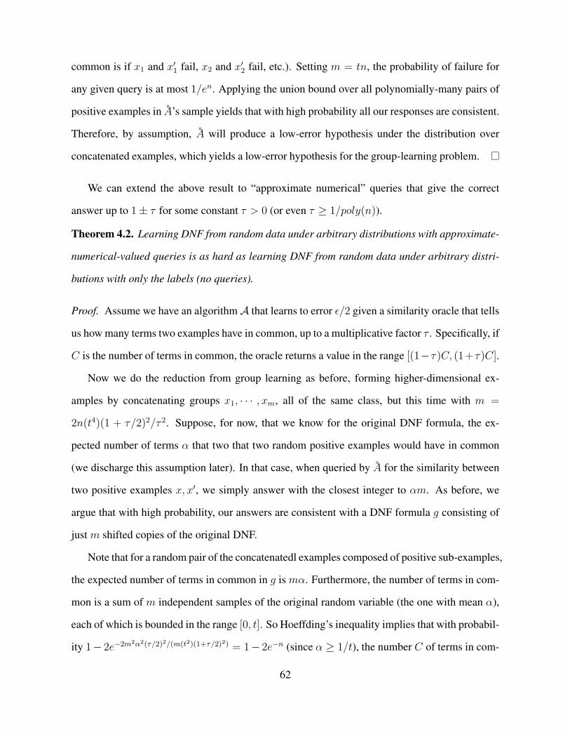
common is if x1 and x′1 fail, x2 and x′2 fail, etc.). Setting m = tn, the probability of failure for

any given query is at most 1/en. Applying the union bound over all polynomially-many pairs of

positive examples in A’s sample yields that with high probability all our responses are consistent.

Therefore, by assumption, A will produce a low-error hypothesis under the distribution over

concatenated examples, which yields a low-error hypothesis for the group-learning problem.

We can extend the above result to “approximate numerical” queries that give the correct

answer up to 1± τ for some constant τ > 0 (or even τ ≥ 1/poly(n)).

Theorem 4.2. Learning DNF from random data under arbitrary distributions with approximate-

numerical-valued queries is as hard as learning DNF from random data under arbitrary distri-

butions with only the labels (no queries).

Proof. Assume we have an algorithmA that learns to error ǫ/2 given a similarity oracle that tells

us how many terms two examples have in common, up to a multiplicative factor τ . Specifically, if

C is the number of terms in common, the oracle returns a value in the range [(1−τ)C, (1+τ)C].

Now we do the reduction from group learning as before, forming higher-dimensional ex-

amples by concatenating groups x1, · · · , xm, all of the same class, but this time with m =

2n(t4)(1 + τ/2)2/τ 2. Suppose, for now, that we know for the original DNF formula, the ex-

pected number of terms α that two that two random positive examples would have in common

(we discharge this assumption later). In that case, when queried by A for the similarity between

two positive examples x, x′, we simply answer with the closest integer to αm. As before, we

argue that with high probability, our answers are consistent with a DNF formula g consisting of

just m shifted copies of the original DNF.

Note that for a random pair of the concatenatedl examples composed of positive sub-examples,

the expected number of terms in common in g is mα. Furthermore, the number of terms in com-

mon is a sum of m independent samples of the original random variable (the one with mean α),

each of which is bounded in the range [0, t]. So Hoeffding’s inequality implies that with probabil-

ity 1− 2e−2m2α2(τ/2)2/(m(t2)(1+τ/2)2) = 1− 2e−n (since α ≥ 1/t), the number C of terms in com-

62

mon satisfies |C−mα| ≤ mα(τ/2)/(1+τ/2), which implies (1−τ/2)C ≤ mα ≤ (1+τ/2)C.

Thus, for a poly(n)-sized sample of data points, with high probability, all of the pairs of

positive concatenated examples have the nearest integer to mα within these factors of their true

number of terms in common. It therefore suffices to respond to A’s similarity queries with the

nearest integer to mα.

Now the only trouble is that we do not know α. So we just try all positive integers i from

1 to mt and then use a validation set to select among the hypotheses produced. That is, we

run A on the constructed data set and respond to all similarity queries with a single value i,

getting back a classifier for these concatenated examples, and then repeat for each i. Then we

take O((1/ǫ) log(mt/δ)) additional higher-dimensional samples (with labels) and choose the

classifier among these mt returned classifiers, having the smallest number of mistakes there-on.

At least one of these mt values of i is the closest integer to mα, so at least one of these mt

classifiers is ǫ/2-good, and our validation set will identify one whose error is at most ǫ. So we

can use this classifier to identify whether a random m-sized group of examples is composed of

all positives or all negatives, with error rate epsilon: i.e., we can do group learning.

If the algorithm A only has a “high probability” guarantee on success, we can repeat this sev-

eral times with independent data sets, to boost the confidence that there will be a good classifier

among those we choose from at the end, and slightly increase the size of the validation set to

compensate for this larger number of classifiers.

4.3 Learning DNF with General Queries : Positive

4.3.1 Methods

The Neighborhood Method

We refer to the following simple procedure as the “neighborhood method”. Takem = poly(n, 1/ǫ, log(1/δ))

samples. First, among the positive examples, query all pairs (with the binary-valued query) to

63

construct a graph, in which examples are adjacent if they satisfy a term in common. For each

positive example, construct a minimal conjunction consistent with that example and all of its

neighbors (i.e., the consistent conjunction having largest number of literals in it). Next, discard

any of these conjunctions that make mistakes on any negative examples. Then sequentially re-

move any conjunction c1 such that some other remaining conjunction c2 subsumes it (contains a

subset of the variables). Form a DNF from the remaining conjunctions. Produce this resultant

DNF as the output hypothesis.

Lemma 4.3. Suppose the target DNF has t = poly(n) terms. For an appropriate (t-dependent)

polynomial sample size m, the neighborhood method will, with probability at least 1 − delta,

produce an ǫ-accurate DNF if, for each term Ti in the target DNF having a probability of satis-

faction at least ǫ/2t, there is at least a p = 1/poly(n, 1/ǫ) probability that a random example

satisfies term Ti and no other term (we call such an example a “nice seed” for Ti).

Proof. Under these conditions, m = O((1/p) log(t/δ) + (t/ǫ) log(1/ǫδ)) samples suffice to

guarantee each Ti with probability of satisfaction at least ǫ/2t has at least one nice seed, with

probability at least 1− δ/2.

In the second phase, we remove any conjunction inconsistent with the negative examples. The

conjunctions guarnateed by the above argument survive this pruning due to their minimality, and

the fact that they are learned from a set of examples that actually are consistent with some term

in the target DNF (due to the nice seed). The final pruning step, which removes any redundancies

in the set of conjunctions, leaves at most t conjunctions.

The terms that do not have nice seeds compose at most ǫ/2 total probability mass, and m is

large enough so that with probability at least 1− δ/4, at most an ǫ/4-fraction of the data satisfy

these terms. Thus, since the result of the neighborhood method is a DNF formula with at most

t terms, which correctly labels a 1 − ǫ/2 fraction of the m examples, the standard PAC bounds

imply that with probability at least 1 − δ/4, the resulting DNF has error rate at most ǫ. A union

bound over the above events implies this holds with probability at least 1− δ.

64

The Common Profile Approach

In the case of numerical queries, we have some additional flexibility in designing a method. In

this context, we refer to the following procedure as the “common profiles approach”.

Consider a sample of m = poly(n, 1/ǫ, log(1/δ)) random labeled examples, and for each

pair of positive examples x, y, we request the number K(x, y) of terms they satisfy in common;

we additionally request K(x, x) for each positive example x. For each positive example x, we

identify the set S of examples y such that the numerical value of K(x, y) is equal K(x, x). So

these points satisfy at least all the terms x satisfies. For each such set S, we learn a minimal

conjunction consistent with these examples. Then for each of these conjunctions, if it is a spe-

cialization of some other one of the conjunctions, we discard it. Then we form our hypothesis

DNF with the remaining conjunctions as the terms.

For any example x, relative to a particular target DNF, we refer to the “profile” of x as the set

of terms Ti in the target DNF satisfied by x.

Lemma 4.4. If the target DNF has at most p = poly(n) possibel profiles, then the common

profile approach, with an appropriate (p-dependent) sample size m, will with probability at least

1− δ, produce a DNF having error rate at most ǫ.

Proof. Note that this procedure produces a DNF that correctly labels the entire data set, since

K(x, y) = K(x, x) implies x and y have the same profiles, so that in particular the set S has some

term in common to all the examples. If there are only a poly(n) number of possible profiles,

then the above will only produce at most as many distinct terms in its hypothesis DNF, so that a

sufficiently large poly(n)-sized data set will be sufficient to guarantee good generalization error.

Specifically, m = O((pn/ǫ) log(1/ǫδ)) examples are enough to guarantee with probability at

least 1− δ, any DNF consistent with the data having at most p terms will have error rate at most

ǫ, so this is sufficient for the common profile approach.

65

4.3.2 Positive Results

Theorem 4.5. With numerical-valued queries, we can properly learn any DNF havingO(log(n))

relevant variables, under arbitrary distributions.

Proof. These targets have poly(n) possible profiles, so the common profiles approach will be

successful.

Theorem 4.6. If the target DNF has onlyO(log(n)) terms, then we can efficiently properly learn

from random data under any distribution using numerical-valued queries.

Proof. There are only poly(n) number of possible profiles, so the “common profiles” approach

will work.

The above result is interesting particularly because proper learning (even for 2-term DNF) is

known to be hard from labeled data alone.

Theorem 4.7. If the target DNF has t = poly(n) terms, and is such that any example can satisfy

at most O(1) terms, then we can efficiently properly learn from random data using numerical-

valued queries.

Proof. There are at most poly(t) = poly(n) possible profiles, so the “common profiles” ap-

proach will work.

Corollary 4.8. We can properly learn any k-term DNF with numerical-valued queries, where k

is constant.

Proof. This follows from either Theorem 4.6 or Theorem 4.7.

Corollary 4.9. If the DNF is such that any example can satisfy at most 1 term (a so-called

“disjoint” DNF), then we can efficiently properly learn from random data using binary-valued

queries.

Proof. A numerical query whose value can be at most 1 is just a binary query anyway.

66

In particular, Decision Trees can be thought of as a DNF where each example satisfies at

most 1 term.

Lemma 4.10. If it happens that the target DNF is parsimonious (no redundant terms) for some

random Ω((tn/ǫ) log(1/ǫ) + (1/ǫ) log(1/δ))-sized data set (for any distribution), then we can

efficiently produce a DNF consistent with it having at most t terms using binary-valued queries.

Proof. (Sketch) Parsimonious, in this case, means that we cannot remove any terms without

changing some labels. But this means that every term has some example that satisfies only that

term (i.e., a nice seed). So as described in the proof of Lemma 4.3 above, the “neighborhood

method,” produces a DNF with terms for the neighborhoods of each of these nice seeds, which

in the parsimonious case, covers all of the positive examples.

Theorem 4.11. We can properly learn 2-term DNF with binary queries.

Proof. Take O((n/ǫ) log(1/ǫ) + (1/ǫ) log(1/δ)) random labeled examples and make the binary

query for all pairs of positive examples. First, find a minimal conjunction consistent with all

of the positive examples; if this conjunction does not misclassify any negative examples, return

it. By classic PAC bounds, a conjunction consistent with this many random labeled examples

will, with probabiliy at least 1 − δ, have error rate at most ǫ. Otherwise, if this conjunction

misclassifies some negatives, then we are assured the target DNF is parsimonious for this data

set, and thus Lemma 4.10 guarantees we can efficiently identify a 2-term DNF consistent with it

using the binary-valued queries. Again, the classic PAC bounds imply the sample size is large

enough to, with probability at least 1 − δ, guarantee that any consistent 2-term DNF has error

rate at most ǫ.

Theorem 4.11 gives a concrete result where using this type of query overturns a known hard-

ness result for supervised learning.

Open problem Can this idea be extended to learning 3-term DNF or higher, still using only

the binary-valued queries? Or is there a hardness result for properly learning 3-term DNF with

67

these binary-valued pairwise queries?

4.4 Learning DNF under the Uniform Distribution

In this section, we investigate the problem of learning DNF under a uniform distribution on

0, 1n, using the binary-valued queries.

Definition 4.12. Fix a constant c ∈ (0,∞). We say a term t in the target DNF is “relatively

distinct” if it contains a variable v which occurs in at most c log(n) other terms. We say v is a

witness to t being relatively distinct.

Definition 4.13. For a term t in the target DNF, and a variable v in t, we say v is “sometimes

nonredundant” for t if, given a random example that satisfies t, there is at least an ǫ probability

that every term in the target DNF that the example satisfies also contains v.

Theorem 4.14. Suppose no term in the target DNF is logically entailed from any other term

in the target DNF, every term t is relatively distinct, and that some variable v that is a witness

to t being relatively distinct is sometimes nonredundant for t. Then we can properly learn any

monotone DNF of this type under a uniform distribution on 0, 1n with binary pairwise queries.

Proof. By Lemma 4.3, it suffices to show that every term having at least ǫ/(2T ) probability of

being satisfied will, with high probability, have some example satisfying only that term, given a

polynomial-sized data set.

Consider a given term t in the target DNF, and choose the v that witnesses relative distinctness

which is sometimes nonredundant. Note that every other term in the target DNF contains some

variable not present in t, and in particular this is true for the (at most) c log(n) terms containing

v. So under the conditional distribution given that t is satisfied and that v is nonredundant, with

probability at least 2−c log(n) = n−c, none of these other terms containing v are satisfied, so that t

is the only term satisfied. Thus, since t has probability at least ǫ/(2T ) of being satisfied, and v has

probability at least ǫ of being nonredundant given that t is satisfied, we have that with probability

68

at least (ǫ2/T )n−c, a random example satisfies t and no other terms in the target DNF.

Since this is the case for all terms in the target, a sample of size O((T/ǫ2)nc log(T/δ)) guar-

antees every term has some example satisfying only that term, with probability at least 1−δ.

We can also consider the class of DNF function having only a small number of relevant

variables. In this context, it is interesting to observe that if the ith variable is irrelevant, then

P (K(x, y) = 1 and xi 6= yi) = P (K(x, y) = 1 and xi = yi), where x and y are independent

uniformly-distributed samples, and K(x, y) = 1 iff x and y are positive examples that satisfy at

least one term in common. However, as the following lemma shows, this is not true for relevant

variables.

Lemma 4.15. For x and y independent uniformly-distributed samples, if the target function has

r relevant variables, and the ith variable is relevant in the target function, then P (K(x, y) =

1 and xi = yi)− P (K(x, y) = 1 and xi 6= yi) ≥ (1/4)r.

Proof. For each pair (x, y) with xi 6= yi, there is a unique corresponding pair (x′, y) with x′j = xj

for j 6= i, and x′i = yi. Let Mi be the number of x, y pairs with xi 6= yi and K(x, y) = 1. Then

note that for every x, y pair with xi 6= yi and K(x, y) = 1, we also have K(x′, y) = 1, since

whatever term x and y satisfy in common cannot contain variable i anyway, so flipping that

feature in x does not change whether x and y share a term or not. In particular, this implies

the number of x, y pairs with xi = yi and K(x, y) = 1 is at least Mi. However, we can also

argue it is strictly larger, as follows. By definition of “relevant”, each of the 2r settings of the

relevant variables corresponds to an equivalence class of feature vectors, all of which have the

same label, and if that label is positive, then all of which have the same profile. Since variable i

is relevant, at least one of the 2r settings of the relevant variables yields an equivalence class of

positive examples whose profile contains only terms with variable i in them (these are positive

examples such that flipping variable i makes them negative). The probability that both x and y

(chosen at random) are in this equivalence class is (1/4)r. Note that for the (x, y) pairs of this

type, we have K(x, y) = 1; however, if we flip feature xi, then x would become negative, and

69

hence K(x, y) would no longer be 1; this means this (x, y) pair is not included among those Mi

pairs constructed above by flipping xi starting from some (x, y) with xi 6= yi and K(x, y) = 1.

So P (K(x, y) = 1 and xi = yi)−P (K(x, y) = 1 and xi 6= yi) = (Mi/4n+(1/4)r)−Mi/4

n =

(1/4)r.

Theorem 4.16. Under the uniform distribution, with binary pairwise queries, we can properly

learn any DNF having O(log(n)) relevant variables.

Proof. We can use the property in Lemma 4.15 to design an algorithm as follows. For each i,

sample Ω(8r log(n/δ)) random pairs (x, y), and evaluate K(x, y) for each pair. Then calculate

the difference of empirical probabilities (fraction of pairs (x, y) for which K(x, y) = 1 and

xi = yi minus fraction of pairs (x, y) for which K(x, y) = 1 and xi 6= yi). If this difference

is > (1/2)(1/4)r, decide variable i is relevant, and otherwise decide variable i is irrelevant.

By Hoeffding and union bounds, with probability 1 − δ/2, this will find exactly the r relevant

variables. Now enumerate all 2r = poly(n) possible conjunctions that can be formed from

using all of these r relevant variables. Considering this as a 2r-dimensional feature space, take

Ω((2r/ǫ)log(1/δ)) random labeled data points and learn a disjunction over this 2r-dimensional

feature space; since the VC dimension of this set of disjunctions is 2r, the usual PAC analysis

implies this will learn an ǫ-good disjunction with probability 1 − δ/2. A union bound implies

both stages (finding variables and learning the disjunction) will succeed with probability at least

1− δ.

An alternative approach to the second stage in the proof would be to take Ω(2r log(2r/δ))

random samples, so that with probability at least 1−δ/2, we have at least one data point satisfying

each of the 2r possible conjunctions on the relevant variables; then for each of the conjunctions,

we check the label of the example that satisfies it, and if that label is positive, we include that

conjunction as a term in our DNF, and otherwise we do not include it. This has the property that,

altogether, with probability 1− δ, we construct a DNF that has error rate zero.

70

Another family of DNF studied in the literature are those with a sublinear number of terms.

Specifically, [Servedio, 2004] proved that the class of 2O(√logn)-term monotone DNF are learn-

able under the uniform distribution from labeled data alone. As the following theorem states,

we can extend this result to include general 2O(√logn)-term DNF (including non-monotone) given

access to our binary pairwise queries.

Theorem 4.17. Under the uniform distribution, with binary pairwise queries, we can learn any

2O(√log n)-term DNF (supposing ǫ to be a constant).

First, we review some known results from [Servedio, 2004]. For any function g : 0, 1n →

−1,+1, define the gi,1 and gi,0 functions by the property that any x with xi = 1 has gi,1(x) =

g(x), and gi,0(x) = g(y), where yj = xj for j 6= i and yi = 0. Then define the influence

function Ii(g) = P (gi,0(x) 6= gi,1(x)). [Servedio, 2004] developed a procedure, FindVariable,

which uses a poly(n, 1/γ, log(1/η)) number of random labeled samples, labeled according to

any monotone DNF g having at most t terms, and with probability 1 − η, returns a set S of

variables (indices in 1, . . . , n) such that every i /∈ S has Ii(g) ≤ γ and every i ∈ S has

Ii(g) ≥ γ/2 and the ith variable is contained in some term in g with at most log 32tnγ

variables in

it.

Furthermore, [Servedio, 2004] showed that, for any t-term DNF f , if we are provided with

a set Sf ⊆ 1, . . . , n such that every i /∈ Sf has Ii(f) ≤ ǫ/4n, then we can learn f in time

polynomial in n, |Sf |O(log tǫlog 1

ǫ), and log(1/δ). In particular, for |Sf | = O(t log tn

ǫ) and t =

2O(√log n), this is polynomial in n (though not necessarily in ǫ). Given the set Sf , the learning

procedure simply estimates the Fourier coefficients for small subsets of Sf .

Proof of Theorem 4.17. To prove Theorem 4.17, we consider the following procedure. First

sample m labeled examples x(1), . . . , x(m) at random. Then, for each j ≤ m, define Kj(·) =

K(x(j), ·). Now note that, if we define ϕj(y) = (ϕj1(y), . . . , ϕjn(y)) by ϕji(y) = 2I[yi =

x(j)i ]−1, then we can represent Kj(·) = (K ′

j(ϕj(·))+1)/2, where K ′j is a monotone DNF (map-

ping into −1,+1); specifically, the terms in K ′j correspond to the terms in the target satisfied

71

by x(j), except none of the literals are negated. We then run FindVariable for each of these K ′j ,

with γ = ǫ/m and η = δ/2m. Let Sf denote the union (over j ≤ m) of the returned sets of vari-

ables. It remains only to show this Sf satisfies the requirements for the procedure of [Servedio,

2004], including the size requirement.

Taking m = Ω( ctǫlog t

δ), with probability at least 1 − δ/4, every term in the target having

probability at least ǫ/2ct will have at least one of the m examples satisfying it. Suppose this

event happens. In particular, this means error(maxj Kj) < ǫ/2c. Note that

Ii(f) = P (fi,0(x) 6= fi,1(x)) ≤ 2P (maxjKj(x) 6= f(x)) + P ((max

jKj)i,0(x) 6= (max

jKj)i,1(x))

< ǫ/c+∑

j

P ((K ′j)i,0(x) 6= (K ′

j)i,1(x)) = ǫ/c+∑

j

Ij(K′j).

Thus, by a union bound, with probability 1 − δ/2, any variable i /∈ Sf has Ii(f) < ǫ/c +mγ,

and any variable i ∈ Sf appears in a term in some K ′j of size at most log 32tn

γ, and therefore

also appear in a corresponding term of this size in f . Suppose this happens. Letting c = 8n and

γ = ǫ/8nm, we have that any i /∈ Sf has Ii(f) < ǫ/4n, while any i ∈ Sf appears in a term of

size at most log 256tn2mǫ

= O(log tn log(1/δ)ǫ

). In particular, this implies |Sf | = O(t log tn log(1/δ)ǫ

),

and Sf satisfies the requirements of the method of [Servedio, 2004].

Thus, running the procedure from [Servedio, 2004] with confidence parameter δ/4, a union

bound implies the total probability of successfully producing an ǫ-good classifier is at least 1−δ.

The above process of constructing Sf is clearly polynomial-time. Then, if t = 2O(√logn), the

procedure of [Servedio, 2004] runs in time polynomial in n, log(1/δ), and |Sf |O(log(t/ǫ) log(1/ǫ)),

which is polynomial in n and log(1/δ) (though not necessarily in ǫ).

4.5 More Powerful Queries

Theorem 4.18. If we can construct our own feature vectors in addition to getting random data,

then under any distribution we can efficiently properly learn DNF using binary-valued queries.

72

Proof. Suppose we can adaptively construct our own examples. Suppose the target DNF has

T = poly(n) terms. Oracle(x, x′) gives the number of terms that x and x′ have in common. For

any x, let x−i be x but with the ith bit flipped. Let x be the negative of x.

Below is an algorithm. Move(x, x′) moves x′ away from x by one bit, while trying to main-

tain at least one common term. LearnTerm(x) returns a term in the target function.

0. Move(x, x′)

1. x′′ ← x

2. For i = 1, 2, ..., n s.t. xi = x′i

3. If (Oracle(x, x′′) ≤ Oracle(x, x′−i))

4. x′′ ← x′−i

5. Return x′′

0. LearnTerm(x)

1. Replicate x to get x′

2. While (Oracle(x, Move(x, x′)) ! = ∅)

3. x′ ←Move(x, x′)

4. Let I ← i : Oracle(x, x′−i) = ∅

5. Return xI (i.e. a conjunction with the literals indexed by I , either positive or negative so

that x satisfies it)

0. LearnDNF

1. Initialize all-negative DNF h

2. Take M = poly(n)≫ nT random examples S

73

3. For each x ∈ S

4. If Oracle(x,x) > 0 (positive example) and h(x) = negative

5. Add term LearnTerm(x) to h

6. Return h (a DNF with at most T terms, consistent with all M examples)

When we reach x′ such that we can’t flip any more bits (not already flipped) without making

it so they don’t satisfy any terms in common anymore, then the bits these two have in common

must form a term in the target DNF, so LearnTerm(x) should still find a term in the target DNF.

If we can ask about k-tuples of examples (do they all jointly satisfy a term in common?), we

have the following result:

Theorem 4.19. If we can use query sets of arbitrary sizes (instead of just 2 points), then under

any distribution we can efficiently properly learn DNF using binary-valued queries from random

data.

Proof. We take any set of examples and ask the oracle the number of terms all examples in the

set have in common. Let S be the query set. The idea is to greedily add the examples to S while

keeping some terms in common.

Algorithm:

0. Input : dataset D

1. Initialize S to be an empty set

2. Do

3. Do

4. rmax ← 0

5. For each example x in the dataset D

6. add x to the set S

74

7. query the combined set S, and let r = Oracle(S), rmax ← maxrmax, r

8. If r = 0, remove x from S, and otherwise leave it in S and remove x from D

9. Until(rmax = 0)

10. Learn a “most-specific” conjunction from S and add that term to the hypothesis DNF

11. Reset S to empty set

12. Until (|D| = 0)

Each time we add a term to the DNF, the examples in S satisfy some term in the target DNF,

because we only add each example if by adding it S still has at least one term in common. So the

”most-specific” conjunction consistent with S (i.e., the one with most literals in it, still labeling

all of S positive) will not misclassify any negative point as positive. Since whenever we add a

new term, there were no additional examples in D that could have satisfied a term in common

with the examples in S, after adding the term we have removed from D all examples that satisfy

the term S has in common. Therefore, the number of terms in our learnt DNF is at most the

number of terms T in the true DNF. If the total number of examples is ≫ nT (and say T is

poly(n)), it will get us a DNF that has at most T terms and correctly labels a poly(n) ≫ nT

sized dataset. Since the training dataset size is much larger than the size of the classifier, by the

Occam bound, the learnt DNF will have small generalization error.

4.6 Learning DNF with General Queries: Open Questions

• Is it possible to efficiently learn an arbitrary DNF from random data under arbitrary distri-

butions with numerical-valued queries?

• Is it possible to efficiently learn a DNF with O(1) terms from random data under arbitrary

distributions with binary-valued queries?

75

• Is it possible to efficiently learn a monotone DNF from random data under a uniform

distribution with numerical-valued queries? If so, what about binary-valued queries?

4.7 Generalizations

4.7.1 Learning Unions of Halfspaces

Several of the above results generalize nicely to the more general problem of learning unions of

halfspaces. Specifically, the queries are of the type “do these two examples satisfy a halfspace in

common?” or “how many halfspaces do these two examples satisfy in common?” The general-

ized forms of Theorem 4.19 and Lemma 4.10 follow by the exact same arguments. In each case,

the algorithm finds sets of examples that satisfy some halfspace, such that none of the remaining

examples satisfy that halfspace, so for each such set we simply find a linear separator to separate

those examples from the rest, and take their union to form our final classifier. A sufficiently

large (poly(n,1/ǫ)-sized) set suffices to guarantee this works. It is not so clear how to generalize

Theorem 4.7, since it is not clear how to use the sets of examples with the common profiles to

learn the halfspaces. The generalized version of Theorem 4.6 actually follows from the result

below on learning Voronoi diagrams. The generalized version of Theorem 4.18 is simple, since

it is even known that labeled data plus membership queries are sufficient.

4.7.2 Learning Voronoi with General Queries

Consider the space of Voronoi diagrams (vector quantizers); specifically, the target function is

constant within each cell of the Voronoi diagram, and there are poly(n) such cells for a given

target function. We define a “same cell” query as asking, for a pair of examples x and y, whether

x and y occur in the same cell of the target function. With this type of query, we can efficiently

properly learn Voronoi partitions from random data, under arbitrary distributions. To prove this,

we simply group the examples in a sufficiently large sample into equivalence classes based on

76

these same-cell queries. For each pair of such equivalence classes, we find a linear separator that

separates them. For each test point, we evaluate these linear separators, which thereby associates

the test point with one of the equivalence classes from the training data, and we predict as a label

for that point the label associated with that equivalence class. If we have a sufficiently large

training set, then there is only a small probability the test point gets placed into a different set of

points from those in its own cell.

77

Chapter 5

Bayesian Active Learning with Arbitrary

Binary Valued Queries

Abstract

1We investigate the minimum expected number of bits sufficient to encode a random variable X

while still being able to recover an approximation of X with expected distance from X at most

D: that is, the optimal rate at distortion D, in a one-shot coding setting. We find this quantity is

related to the entropy of a Voronoi partition of the values of X based on a maximal D-packing.

5.1 Introduction

In this work, we study the fundamental complexity of lossy coding. We are particularly interested

in identifying a key quantity that characterizes the expected number of bits (called the rate)

required to encode a random variable so that we may recover an approximation within expected

distance D (called the distortion). This topic is a generalization of the well-known analysis of

exact coding by Shannon [Shannon, 1948], where it is known that the optimal expected number

1Joint work with Jaime Carbonell and Steve Hanneke.

78

of bits is precisely characterized by the entropy. There are many problems in which exact coding

is not practical or not possible, so that lossy coding becomes necessary: particularly for random

variables taking values in uncountably infinite spaces. The topic of code lengths for lossy coding

is interesting, both for its direct applications to compression, and also as a general setting in

which to derive lower bounds for specializations of the setting.

There is much existing work on lossy binary codes. In the present work, we are interested

in a “one-shot” analysis of lossy coding [Kieffer, 1993], in which we wish to encode a single

random variable, in contrast to the analysis of “asymptotic” source coding [Cover and Thomas,

2006], in which one wishes to simultaneously encode a sequence of random variables. Of par-

ticular relevance to the one-shot coding problem is the analysis of quantization methods that

balance distortion with entropy [Gersho, 1979, Kieffer, 1993, Zador, 1982]. In particular, it is

now well-known that this approach can yield codes that respect a distortion contraint while nearly

minimizing the rate, so that there are near-optimal codes of this type [Kieffer, 1993]. Thus, we

have an alternative way to think of the optimal rate, in terms of the rate of the best distortion-

constrained quantization method. While this is interesting, in that it allows us to restrict our focus

in the design of effective coding techniques, it is not as directly helpful if we wish to understand

the behavior of the optimal rate itself. That is, since we do not have an explicit description of the

optimal quantizer, it may often be difficult to study the behavior of its rate under various interest-

ing conditions. There exist classic results lower bounding the achievable rates, most notably the

famous Shannon lower bound [Shannon, 1959], which under certain restrictions on the source

and the distortion metric, is known to be fairly tight in the asymptotic analysis of source coding

[Linder and Zamir, 1994]. However, there are few general results explicitly and tightly charac-

terizing the (non-asymptotic) optimal rates for one-shot coding. In particular, to our knowledge,

only a few special-case calculations of the exact value of this optimal rate have been explicitly

carried out, such as vectors of independent Bernoulli or Gaussian random variables [Cover and

Thomas, 2006].

79

Below, we discuss a particular distortion-constrained quantizer, based on a Voronoi partition

induced by a maximal packing. We are interested in the entropy of this quantizer, as a quantity

used to characterize the optimal rate for codes of a given distortion. While it is clear that this

entropy upper bounds the optimal rate, as this is the case for any distortion-constrained quantizer

[Kieffer, 1993], the novelty of our analysis lies in noting the remarkable fact that the entropy

of any quantizer constructed in this way also lower bounds the optimal rate. In particular, this

provides a method for approximately calculating the optimal rate without the need to optimize

over all possible quantizers. Our result is general, in that it applies to an arbitrary distribution

and an arbitrary distortion measure from a general class of finite-dimensional pseudo-metrics.

This generality is noteworthy, as it leads to interesting applications in statistical learning theory,

which we describe below.

Our analysis is closely related to various notions that arise in the study of ǫ-entropy [Posner

and Rodemich, 1971, Posner, Rodemich, and Rumsey, Jr., 1967], in that we are concerned with

the entropy of a Voronoi partition induced by an ǫ-cover. The notion of ǫ-entropy has been

related to the optimal rates for a given distortion (under a slightly different model than studied

here) [Posner and Rodemich, 1971, Posner, Rodemich, and Rumsey, Jr., 1967]. However, there

are some important distinctions, perhaps the most significant of which is that calculating the

ǫ-entropy requires a prohibitive optimization of the entropy over all ǫ-covers; in contrast, the

entropy term in our analysis can be calculated based on any maximal ǫ-packing (which is a

particular type of ǫ-cover). Maximal ǫ-packings are easy to construct by greedily adding arbitrary

new elements to the packing that are ǫ-far from all elements already added; thus, there is always

a straightforward algorithmic approach to applying our results.

80

5.2 Definitions

We suppose X ∗ is an arbitrary (nonempty) set, equipped with a separable pseudo-metric ρ :

X ∗×X ∗ → [0,∞). 2 We supposeX ∗ is accompanied by its Borel σ-algebra induced by ρ. There

is additionally a (nonempty, measurable) set X ⊆ X ∗, and we denote by ρ = suph1,h2∈X

ρ(h1, h2).

Finally, there is a probability measure π with π(X ) = 1, and an X -valued random variable X

with distribution π, referred to here as the “target.” As the distribution is essentially arbitrary, the

results below will hold for any π.

A code is a pair of (measurable) functions (φ, ψ). The encoder, φ, maps any element x ∈ X

to a binary sequence φ(x) ∈ ⋃∞q=00, 1q (the codeword). The decoder, ψ, maps any element

c ∈ ⋃∞q=00, 1q to an element ψ(c) ∈ X ∗. For any q ∈ 0, 1, . . . and c ∈ 0, 1q, let |c| = q

denote the length of c. A prefix-free code is any code (φ, ψ) such that no x1, x2 ∈ X have

c(1) = φ(x1) and c(2) = φ(x2) with c(1) 6= c(2) but ∀i ≤ |c(1)|, c(2)i = c(1)i : that is, no codeword is

a prefix of another (longer) codeword. Let PF denote the set of all prefix-free binary codes.

Here, we consider a setting where the code (φ, ψ) may be lossy, in the sense that for some

values of x ∈ X , ρ(ψ(φ(x)), x) > 0. Our objective is to design the code to have small expected

loss (in the ρ sense), while maintaining as small of an expected codeword length as possible.

Formally, we have the following definition, which essentially describes a notion of optimality

for a lossy code.

Definition 5.1. For any D > 0, define the optimal rate at distortion D

R(D) = inf

E

[

|φ(X)|]

: (φ, ψ) ∈ PF with

E

[

ρ(

ψ(φ(X)), X)]

≤ D

,

where the random variable in both expectations is X ∼ π.

For our analysis, we will require a notion of dimensionality for the pseudo-metric ρ. For this,

2The set X ∗ will not play any significant role in the analysis, except to allow for improper learning scenarios to

be a special case of our setting.

81

we adopt the well-known doubling dimension [Gupta, Krauthgamer, and Lee, 2003].

Definition 5.2. Define the doubling dimension d as the smallest value d such that, for any x ∈ X ,

and any ǫ > 0, the size of the minimal ǫ/2-cover of the ǫ-radius ball around x is at most 2d.

That is, for any x ∈ X and ǫ > 0, there exists a set xi2di=1 of 2d elements of X such that

x′ ∈ X : ρ(x′, x) ≤ ǫ ⊆2d⋃

i=1

x′ ∈ X : ρ(x′, xi) ≤ ǫ/2.

Note that, as defined here, d is a constant (i.e., has no dependence on the x or ǫ in its defini-

tion). In the analysis below, we will always assume d < ∞. The doubling dimension has been

studied for a variety of spaces, originally by Gupta, Krauthgamer, & Lee [Gupta, Krauthgamer,

and Lee, 2003], and subsequently by many others. In particular, Bshouty, Li, & Long [Bshouty,

Li, and Long, 2009] discuss the doubling dimension of spaces X of binary classifiers, in the

context of statistical learning theory.

5.2.1 Definition of Packing Entropy

Our main result concerns the relation between the optimal rate at a given distortion with the

entropy of a certain quantizer. We now turn to defining this latter quantity.

Definition 5.3. For any D > 0, define Y(D) ⊆ X as a maximal D-packing of X . That is,

∀x1, x2 ∈ Y(D), ρ(x1, x2) ≥ D, and ∀x ∈ X \ Y(D), minx′∈Y(D) ρ(x, x′) < D.

For our purposes, if multiple maximal D-packings are possible, we can choose to define

Y(D) arbitrarily from among these; the results below hold for any such choice. Recall that any

maximal D-packing of X is also a D-cover of X , since otherwise we would be able to add to

Y(D) the x ∈ X that escapes the cover. That is, ∀x ∈ X , ∃y ∈ Y(D) s.t. ρ(x, y) < D.

Next we define a complexity measure, a type of entropy, which serves as our primary quantity

of interest in the analysis of R(D). It is specified in terms of a partition induced by Y(D), defined

as follows.

82

Definition 5.4. For any D > 0, define

Q(D) =

x ∈ X : z = argminy∈Y(D)

ρ(x, y)

: z ∈ Y(D)

,

where we break ties in the argmin arbitrarily but consistently (e.g., based on a predefined pref-

erence ordering of Y(D)).

Definition 5.5. For any finite (or countable) partition S of X into measurable regions (subsets),

define the entropy of S

H(S) = −∑

S∈Sπ(S) log2 π(S).

In particular, we will be interested in the quantityH(Q(D)) in the analysis below.

5.3 Main Result

Our main result can be summarized as follows. Note that, since we took the distribution π to be

arbitrary in the above definitions, this result holds for any given π.

Theorem 5.6. If d <∞ and ρ <∞, then there is a constant c = O(d) such that ∀D ∈ (0, ρ/2),

H (Q (D log2(ρ/D)))− c ≤ R(D) ≤ H (Q (D)) + 1.

It should not be surprising that entropy terms play a key role in this result, as the entropy is

essential to the analysis of exact coding [Shannon, 1948]. Furthermore, R(D) is tightly charac-

terized by the minimum achievable entropy among all quantizers of distortion at most D [Kieffer,

1993]. The interesting aspect of Theorem 5.6 is that we can explicitly describe a particular quan-

tizer with near-optimal rate, and its entropy can be explicitly calculated for a variety of scenarios

(X , ρ, π). As for the behavior of R(D) within the range between the upper and lower bounds

of Theorem 5.6, we should expect the upper bound to be tight when high-probability subsets of

the regions in Q(D) are point-wise well-separated, while R(D) may be much smaller (perhaps

closer to the lower bound) when this is violated to a large degree, for reasons described in the

proof below.

83

20 40 60 80 1001D

5

10

15

HHPHDLL

BetaH2,5L

Χ2H1L

NH0,1L

Figure 5.1: Plots ofH(Q(D)) as a function of 1/D, for various distributions π on X = R.

Although this result is stated for bounded psuedo-metrics ρ, it also has implications for un-

bounded ρ. In particular, the proof of the upper bound holds as-is for unbounded ρ. Furthermore,

we can always use this lower bound to construct a lower bound for unbounded ρ, simply restrict-

ing to a bounded subset of X with constant probability and calculating the lower bound for that

region. For instance, to get a lower bound for π as a Gaussian distribution on R, we might note

that π([−1/2, 1/2]) times the expected loss under the conditional π(·|[−1/2, 1/2]) lower bounds

the total expected loss. Thus, calculating the lower bound of Theorem 5.6 under the conditional

π(·|[−1/2, 1/2]) while replacing D with D/π([−1/2, 1/2]) provides a lower bound on R(D).

To get a feel for the behavior ofH (Q (D)), we have plotted it as a function of 1/D for several

distributions, in Figure 5.1.

5.4 Proof of Theorem 5.6

We first state a lemma, due to Gupta, Krauthgamer, & Lee [Gupta, Krauthgamer, and Lee, 2003],

which will be useful in the proof of Theorem 5.6.

Lemma 5.7. [Gupta, Krauthgamer, and Lee, 2003] For any γ ∈ (0,∞), δ ∈ [γ,∞), and x ∈ X ,

|x′ ∈ Y(γ) : ρ(x′, x) ≤ δ| ≤(

4δ

γ

)d

.

In particular, note that this lemma implies that the minimum of ρ(x, y) over y ∈ Y(D) is

always achieved in Definition 5.4, so that Q(D) is well-defined.

84

We are now ready for the proof of Theorem 5.6.

Proof of Theorem 5.6. Throughout the proof, we will consider a set-valued random quantity

QD(X) with value equal to the set inQ(D) containingX , and a corresponding X -valued random

quantity YD(X) with value equal the sole point in QD(X) ∩ Y(D): that is, the target’s nearest

representative in the D-packing. Note that, by Lemma 5.7, |Y(D)| < ∞ for all D ∈ (0, 1). We

will also adopt the usual notation for entropy (e.g., H(QD(X))) and conditional entropy (e.g.,

H(QD(X)|Z)) [Cover and Thomas, 2006], both in base 2.

To establish the upper bound, we simply take φ as the Huffman code for the random quantity

QD(X) [Cover and Thomas, 2006, Huffman, 1952]. It is well-known that the expected length

of a Huffman code for QD(X) is at most H(QD(X)) + 1 (in fact, is equal H(QD(X)) when

the probabilities are powers of 2) [Cover and Thomas, 2006, Huffman, 1952], and each possible

value ofQD(X) is assigned a unique codeword so that we can perfectly recoverQD(X) (and thus

also YD(X)) based on φ(X). In particular, define ψ(φ(X)) = YD(X). Finally, recall that any

maximal D-packing is also a D-cover. Thus, since every element of the setQD(X) has YD(X) as

its closest representative in Y(D), we must have ρ(X,ψ(φ(X))) = ρ(X, YD(X)) < D. In fact,

as this proof never relies on ρ <∞, this establishes the upper bound even in the case ρ =∞.

The proof of the lower bound is somewhat more involved, though the overall idea is simple

enough. Essentially, the lower bound would be straightforward if the regions ofQ(D log2(ρ/D))

were separated by some distance, since we could make an argument based on Fano’s inequality

to say that since any X = ψ(φ(X)) is “close” to at most one region, the expected distance

from X is at least as large as half this inter-region distance times a quantity proportional to the

conditional entropyH(QD(X)|φ(X)), so thatH(φ(X)) can be related toH(QD(X)).

However, the general case is not always so simple, as the regions can generally be quite close

to each other (even adjacent), so that it is possible for X to be close to multiple regions. Thus, the

proof will first “color” the regions ofQ(D log2(ρ/D)) in a way that guarantees no two regions of

the same color are within distance D log2(ρ/D) of each other. Then we apply the above simple

85

argument for each color separately (i.e., lower bounding the expected distance from X under the

conditional given the color of QD log2(ρ/D)(X) by a function of the conditional entropy under the

conditional), and average over the colors to get a global lower bound. The details follow.

Fix any D ∈ (0, ρ/2), and for brevity let α = D log2(ρ/D). We suppose (φ, ψ) is some

prefix-free binary code.

Define a function K : Q(α)→ N such that ∀Q1, Q2 ∈ Q(α),

K(Q1) = K(Q2) =⇒ infx1∈Q1,x2∈Q2

ρ(x1, x2) ≥ α, (5.1)

and suppose K has minimumH(K(Qα(X))) subject to (5.1). We will refer to K(Q) as the color

of Q.

Now we are ready to bound the expected distance from X . Let X = ψ(φ(X)), and let

Qα(X;K) denote the set Q ∈ Q(α) having K(Q) = K with smallest infx∈Q ρ(x, X) (breaking

ties arbitrarily). We know

E[ρ(X,X)] = E

[

E[ρ(X,X)|K(Qα(X))]]

. (5.2)

Furthermore, by (5.1) and a triangle inequality, we know no X can be closer than α/2 to more

than one Q ∈ Q(α) of a given color. Therefore,

E[ρ(X,X)|K(Qα(X))]

≥ α

2P(Qα(X;K(Qα(X))) 6= Qα(X)|K(Qα(X))). (5.3)

By Fano’s inequality, we have

E

[

P(Qα(X;K(Qα(X))) 6= Qα(X)|K(Qα(X)))]

≥ H(Qα(X)|φ(X),K(Qα(X)))− 1

log2 |Y(α)|. (5.4)

It is generally true that, for a prefix-free binary code φ(X), φ(X) is a lossless prefix-free

binary code for itself (i.e., with the identity decoder), so that the classic entropy lower bound on

average code length [Cover and Thomas, 2006, Shannon, 1948] implies H(φ(X)) ≤ E[|φ(X)|].

86

Also, recalling that Y(α) is maximal, and therefore also an α-cover, we have that any Q1, Q2 ∈

Q(α) with infx1∈Q1,x2∈Q2

ρ(x1, x2) ≤ α have ρ(Yα(x1), Yα(x2)) ≤ 3α (by a triangle inequality).

Therefore, Lemma 5.7 implies that, for any given Q1 ∈ Q(α), there are at most 12d sets Q2 ∈

Q(α) with infx1∈Q1,x2∈Q2

ρ(x1, x2) ≤ α. We therefore know there exists a function K′ : Q(α)→ N

satisfying (5.1) such that maxQ∈Q(α)

K′(Q) ≤ 12d (i.e., we need at most 12d colors to satisfy (5.1)).

That is, if we consider coloring the setsQ ∈ Q(α) sequentially, for any givenQ1 not yet colored,

there are < 12d sets Q2 ∈ Q(α) \ Q1 within α of it, so there must exist a color among

1, . . . , 12d not used by any of them, and we can choose that for K′(Q1). In particular, by our

choice of K to minimizeH(K(Qα(X))) subject to (5.1), this implies

H(K(Qα(X))) ≤ H(K′(Qα(X))) ≤ log2(12d) ≤ 4d.

Thus,

H(Qα(X)|φ(X),K(Qα(X)))

= H(Qα(X), φ(X),K(Qα(X)))

−H(φ(X))−H(K(Qα(X))|φ(X))

≥ H(Qα(X))−H(φ(X))−H(K(Qα(X)))

≥ H(Qα(X))− E [|φ(X)|]− 4d

= H(Q(α))− E [|φ(X)|]− 4d. (5.5)

Thus, combining (5.2), (5.3), (5.4), and (5.5), we have

E[ρ(X,X)] ≥ α

2

H(Q(α))− E [|φ(X)|]− 4d− 1

log2 |Y(α)|

≥ α

2

H(Q(α))− E [|φ(X)|]− 4d− 1

d log2(4ρ/α),

where the last inequality follows from Lemma 5.7.

Thus, for any code with

E [|φ(X)|] < H(Q(α))− 4d− 1− 2dlog2(4ρ/D)

log2(ρ/D),

87

we have E[ρ(X,X)] > D, which implies

R(D) ≥ H(Q(α))− 4d− 1− 2dlog2(4ρ/D)

log2(ρ/D).

Since log2(4ρ/D)/ log2(ρ/D) ≤ 3, we have

R(D) ≥ H(Q(α))−O(d).

5.5 Application to Bayesian Active Learning

As an example, in the special case of the problem of learning a binary classifier, as studied by

[Haussler, Kearns, and Schapire, 1994a] and [Freund, Seung, Shamir, and Tishby, 1997], X ∗ is

the set of all measurable classifiers h : Z → −1,+1, X is called the “concept space,” X is

called the “target function,” and ρ(X1, X2) = P(X1(Z) 6= X2(Z)), where Z is some Z-valued

random variable. In particular, ρ(X1, X) is called the “error rate” of X1.

We may then discuss a learning protocol based on binary-valued queries. That is, we sup-

pose some learning machine is able to pose yes/no questions to an oracle, and based on the

responses it proposes a hypothesis X . We may ask how many such yes/no questions must the

learning machine pose (in expectation) before being able to produce a hypothesis X ∈ X ∗ with

E[ρ(X,X)] ≤ ǫ, known as the query complexity.

If the learning machine is allowed to pose arbitrary binary-valued queries, then this setting is

precisely a special case of the general lossy coding problem studied above. That is, any learning

machine that asks a sequence of yes/no questions before terminating and returning some X ∈ X ∗

can be thought of as a binary decision tree (no = left, yes = right), with the return X values stored

in the leaf nodes. Transforming each root-to-leaf path in the decision tree into a codeword (left

= 0, right = 1), we see that the algorithm corresponds to a prefix-free binary code. Conversely,

given any prefix-free binary code, we can construct an algorithm based on sequentially asking

88

queries of the form “what is the first bit in the codeword φ(X) forX?”, “what is the second bit in

the codeword φ(X) for X?”, etc., until we obtain a complete codeword, at which point we return

the value that codeword decodes to. From this perspective, the query complexity is precisely

R(ǫ).

This general problem of learning with arbitrary binary-valued queries was studied previously

by Kulkarni, Mitter, & Tsitsiklis [Kulkarni, Mitter, and Tsitsiklis, 1993], in a minimax analysis

(studying the worst-case value of X). In particular, they find that for a given distribution for

Z, the worst-case query complexity is essentially characterized by log |Y(ǫ)|. The techniques

employed are actually far more general than the classifier-learning problem, and actually apply

to any pseudo-metric space. Thus, we can abstractly think of their work as a minimax analysis

of lossy coding.

In addition to being quite interesting in their own right, the results of Kulkarni, Mitter, &

Tsitsiklis [Kulkarni, Mitter, and Tsitsiklis, 1993] have played a significant role in the recent

developments in active learning with label request queries for binary classification [Dasgupta,

2005, Hanneke, 2007a,b], in which the learning machine may only ask questions of the form,

“What is the value X(z)?” for certain values z ∈ Z . Since label requests can be viewed as

a type of binary-valued query, the number of label requests necessary for learning is naturally

lower bounded by the number of arbitrary binary-valued queries necessary for learning. We

therefore always expect to see some term relating to log |Y(ǫ)| in any minimax query complexity

results for active learning with label requests (though this factor is typically represented by its

upper bound: ∝ V · log(1/ǫ), where V is the VC dimension).

Similarly to how the work of Kulkarni, Mitter, & Tsitsiklis [Kulkarni, Mitter, and Tsitsiklis,

1993] can be used to argue that log |Y(ǫ)| is a lower bound on the minimax query complexity of

active learning with label requests, Theorem 5.6 can be used to argue that H(Q(ǫ log2(1/ǫ))) −

O(d) is a lower bound on the query complexity of learning relative to a given distribution for

X (called a prior, in the language of Bayesian statistics), rather than the worst-case value of X .

89

Furthermore, as with [Kulkarni, Mitter, and Tsitsiklis, 1993], this lower bound remains valid for

learning with label requests, since label requests are a type of binary-valued query. Thus, we

should expect a term related to H(Q(ǫ)) or H(Q(ǫ log2(1/ǫ))) to appear in any tight analysis of

the query complexity of Bayesian learning with label requests.

5.6 Open Problems

In our present context, there are several interesting questions, such as whether the log(ρ/D) factor

in the entropy argument of the lower bound can be removed, whether the additive constant in the

lower bound might be improved, and in particular whether a similar result might be obtained

without assuming d < ∞ (e.g., in the statistical learning special case, by making a VC class

assumption instead).

90

Chapter 6

The Sample Complexity of Self-Verifying

Bayesian Active Learning

Abstract

1We prove that access to a prior distribution over target functions can dramatically improve the

sample complexity of self-terminating active learning algorithms, so that it is always better than

the known results for prior-dependent passive learning. In particular, this is in stark contrast to

the analysis of prior-independent algorithms, where there are simple known learning problems

for which no self-terminating algorithm can provide this guarantee for all priors.

6.1 Introduction and Background

Active learning is a powerful form of supervised machine learning characterized by interaction

between the learning algorithm and supervisor during the learning process. In this work, we

consider a variant known as pool-based active learning, in which a learning algorithm is given

access to a (typically very large) collection of unlabeled examples, and is able to select any of

1Joint work with Jaime Carbonell and Steve Hanneke.

91

those examples, request the supervisor to label it (in agreement with the target concept), then after

receiving the label, selects another example from the pool, etc. This sequential label-requesting

process continues until some halting criterion is reached, at which point the algorithm outputs

a function, and the objective is for this function to closely approximate the (unknown) target

concept in the future. The primary motivation behind pool-based active learning is that, often,

unlabeled examples are inexpensive and available in abundance, while annotating those examples

can be costly or time-consuming; as such, we often wish to select only the informative examples

to be labeled, thus reducing information-redundancy to some extent, compared to the baseline of

selecting the examples to be labeled uniformly at random from the pool (passive learning).

There has recently been an explosion of fascinating theoretical results on the advantages of

this type of active learning, compared to passive learning, in terms of the number of labels re-

quired to obtain a prescribed accuracy (called the sample complexity): e.g., [Balcan, Broder, and

Zhang, 2007a, Balcan, Beygelzimer, and Langford, 2009, Balcan, Hanneke, and Vaughan, 2010,

Beygelzimer, Dasgupta, and Langford, 2009, Castro and Nowak, 2008, Dasgupta, 2004, 2005,

Dasgupta, Hsu, and Monteleoni, 2007b, Dasgupta, Kalai, and Monteleoni, 2009, Freund, Seung,

Shamir, and Tishby, 1997, Friedman, 2009, Hanneke, 2007a,b, 2009, 2011, Kaariainen, 2006,

Koltchinskii, 2010, Nowak, 2008, Wang, 2009]. In particular, [Balcan, Hanneke, and Vaughan,

2010] show that in noise-free binary classifier learning, for any passive learning algorithm for a

concept space of finite VC dimension, there exists an active learning algorithm with asymptoti-

cally much smaller sample complexity for any nontrivial target concept. In later work, [Hanneke,

2009] strengthens this result by removing a certain strong dependence on the distribution of the

data in the learning algorithm. Thus, it appears there are profound advantages to active learning

compared to passive learning.

However, the ability to rapidly converge to a good classifier using only a small number of

labels is only one desirable quality of a machine learning method, and there are other qualities

that may also be important in certain scenarios. In particular, the ability to verify the performance

92

of a learning method is often a crucial part of machine learning applications, as (among other

things) it helps us determine whether we have enough data to achieve a desired level of accuracy

with the given method. In passive learning, one common practice for this verification is to hold

out a random sample of labeled examples as a validation sample to evaluate the trained classifier

(e.g., to determine when training is complete). It turns out this technique is not feasible in active

learning, since in order to be really useful as an indicator of whether we have seen enough la-

bels to guarantee the desired accuracy, the number of labeled examples in the random validation

sample would need to be much larger than the number of labels requested by the active learning

algorithm itself, thus (to some extent) canceling the savings obtained by performing active rather

than passive learning. Another common practice in passive learning is to examine the training er-

ror rate of the returned classifier, which can serve as a reasonable indicator of performance (after

adjusting for model complexity). However, again this measure of performance is not necessarily

reasonable for active learning, since the set of examples the algorithm requests the labels of is

typically distributed very differently from the test examples the classifier will be applied to after

training.

This reasoning indicates that performance verification is (at best) a far more subtle issue in

active learning than in passive learning. Indeed, [Balcan, Hanneke, and Vaughan, 2010] note that

although the number of labels required to achieve good accuracy is significantly smaller than

passive learning, it is often the case that the number of labels required to verify that the accuracy

is good is not significantly improved. In particular, this phenomenon can dramatically increase

the sample complexity of active learning algorithms that adaptively determine how many labels

to request before terminating. In short, if we require the algorithm both to learn an accurate

concept and to know that its concept is accurate, then the number of labels required by active

learning is often not significantly smaller than the number required by passive learning.

We should note, however, that the above results were proven for a learning scenario in which

the target concept is considered a constant, and no information about the process that generates

93

this concept is known a priori. Alternatively, we can consider a modification of this problem, so

that the target concept can be thought of as a random variable, a sample from a known distribution

(called a prior) over the space of possible concepts. Such a setting has been studied in detail

in the context of passive learning for noise-free binary classification. In particular, [Haussler,

Kearns, and Schapire, 1994a] found that for any concept space of finite VC dimension d, for

any prior and distribution over data points, O(d/ε) random labeled examples are sufficient for

the expected error rate of the Bayes classifier produced under the posterior distribution to be at

most ε. Furthermore, it is easy to construct learning problems for which there is an Ω(1/ε) lower

bound on the number of random labeled examples required to achieve expected error rate at most

ε, by any passive learning algorithm; for instance, the problem of learning threshold classifiers

on [0, 1] under a uniform data distribution and uniform prior is one such scenario.

In the context of active learning (again, with access to the prior), [Freund, Seung, Shamir, and

Tishby, 1997] analyze the Query by Committee algorithm, and find that if a certain information

gain quantity for the points requested by the algorithm is lower-bounded by a value g, then the

algorithm requires onlyO((d/g) log(1/ε)) labels to achieve expected error rate at most ε. In par-

ticular, they show that this is satisfied for constant g for linear separators under a near-uniform

prior, and a near-uniform data distribution over the unit sphere. This represents a marked im-

provement over the results of [Haussler, Kearns, and Schapire, 1994a] for passive learning, and

since the Query by Committee algorithm is self-verifying, this result is highly relevant to the

present discussion. However, the condition that the information gains be lower-bounded by a

constant is quite restrictive, and many interesting learning problems are precluded by this re-

quirement. Furthermore, there exist learning problems (with finite VC dimension) for which the

Query by Committee algorithm makes an expected number of label requests exceeding Ω(1/ε).

To date, there has not been a general analysis of how the value of g can behave as a function of

ε, though such an analysis would likely be quite interesting.

In the present paper, we take a more general approach to the question of active learning with

94

access to the prior. We are interested in the broad question of whether access to the prior bridges

the gap between the sample complexity of learning and the sample complexity of learning with

verification. Specifically, we ask the following question.

Can a prior-dependent self-terminating active learning algorithm for a concept class of finite

VC dimension always achieve expected error rate at most ε using o(1/ε) label requests?

After some basic definitions in Section 6.2, we begin in Section 6.4 with a concrete example,

namely interval classifiers under a uniform data density but arbitrary prior, to illustrate the general

idea, and convey some of the intuition as to why one might expect a positive answer to this

question. In Section 6.5, we present a general proof that the answer is always “yes.” As the

known results for the sample complexity of passive learning with access to the prior are typically

∝ 1/ε [Haussler, Kearns, and Schapire, 1994a], and this is sometimes tight, this represents

an improvement over passive learning. The proof is simple and accessible, yet represents an

important step in understanding the problem of self-termination in active learning algorithms, and

the general issue of the complexity of verification. Also, as this is a result that does not generally

hold for prior-independent algorithms (even for their “average-case” behavior induced by the

prior) for certain concept spaces, this also represents a significant step toward understanding the

inherent value of having access to the prior.

6.2 Definitions and Preliminaries

First, we introduce some notation and formal definitions. We denote by X the instance space,

representing the range of the unlabeled data points, and we suppose a distribution D on X ,

which we will refer to as the data distribution. We also suppose the existence of a sequence

X1, X2, . . . of i.i.d. random variables, each with distribution D, referred to as the unlabeled

data sequence. Though one could potentially analyze the achievable performance as a function

of the number of unlabeled points made available to the learning algorithm (cf. [Dasgupta,

2005]), for simplicity in the present work, we will suppose this unlabeled sequence is essentially

95

inexhaustible, corresponding to the practical fact that unlabeled data are typically available in

abundance as they are often relatively inexpensive to obtain. Additionally, there is a set C of

measurable classifiers h : X → −1,+1, referred to as the concept space. We denote by d

the VC dimension of C, and in our present context we will restrict ourselves to spaces C with

d < ∞, referred to as a VC class. We also have a probability distribution π, called the prior,

over C, and a random variable h∗ ∼ π, called the target function; we suppose h∗ is independent

from the data sequence X1, X2, . . .. We adopt the usual notation for conditional expectations

and probabilities [Ash and Doleans-Dade, 2000]; for instance, E[A|B] can be thought of as an

expectation of the value A, under the conditional distribution of A given the value of B (which

itself is random), and thus the value of E[A|B] is essentially determined by the value of B. For

any measurable h : X → −1,+1, define the error rate er(h) = D(x : h(x) 6= h∗(x)).

So far, this setup is essentially identical to that of [Freund, Seung, Shamir, and Tishby, 1997,

Haussler, Kearns, and Schapire, 1994a].

The protocol in active learning is the following. An active learning algorithm A is given as

input the prior π, the data distribution D (though see Section 6.6), and a value ε ∈ (0, 1]. It

also (implicitly) depends on the data sequence X1, X2, . . ., and has an indirect dependence on

the target function h∗ via the following type of interaction. The algorithm may inspect the values

Xi for any initial segment of the data sequence, select an index i ∈ N to “request” the label of;

after selecting such an index, the algorithm receives the value h∗(Xi). The algorithm may then

select another index, request the label, receive the value of h∗ on that point, etc. This happens

for a number of rounds, N(A, h∗, ε,D, π), before eventually the algorithm halts and returns a

classifier h. An algorithm is said to be correct if E[

er(

h)]

≤ ε for every (ε,D, π); that is,

given direct access to the prior and the data distribution, and given a specified value ε, a correct

algorithm must be guaranteed to have expected error rate at most ε. Define the expected sample

complexity of A for (X ,C,D, π) to be the function SC(ε,D, π) = E[N(A, h∗, ε,D, π)]: the

expected number of label requests the algorithm makes.

96

6.3 Prior-Independent Learning Algorithms

One may initially wonder whether we could achieve this o(1/ε) result merely by calculating

the expected sample complexity of some prior-independent method, thus precluding the need

for novel algorithms. Formally, we say an algorithm A is prior-independent if the conditional

distribution of the queries and return value ofA(ε,D, π) given (X1, X(X1)), (X2, X(X2)), . . .

is functionally independent of π. Indeed, for some C and D, it is known that there are prior-

independent active learning algorithms A that have E[N(A, X, ε,D, π)|X] = o(1/ε) (always);

for instance, threshold classifiers have this property under anyD, homogeneous linear separators

have this property under a uniform D on the unit sphere in k dimensions, and intervals with

positive width on X = [0, 1] have this property under D = Uniform([0, 1]) (see e.g., [Dasgupta,

2005]). It is straightforward to show that any such A will also have SC(A, ε,D, π) = o(1/ε)

for every π. In particular, the law of total expectation and the dominated convergence theorem

imply

limε→0

εSC(A, ε,D, π) = limε→0

εE[E[N(A, X, ε,D, π)|X]]

= E

[

limε→0

εE[N(A, X, ε,D, π)|X]]

= 0.

In these cases, we can think of SC as a kind of average-case analysis of these algorithms. How-

ever, as we discuss next, there are also many C and D for which there is no prior-independent

algorithm achieving o(1/ε) sample complexity for all priors. Thus, any general result on o(1/ε)

expected sample complexity for π-dependent algorithms would indicate that there is a real ad-

vantage to having access to the prior, beyond the apparent smoothing effects of an average-case

analysis.

As an example of a problem where no prior-independent self-verifying algorithm can achieve

o(1/ε) sample complexity, considerX = [0, 1],D = Uniform([0, 1]), and C as the concept space

of interval classifiers: C = I±(a,b) : 0 ≤ a ≤ b ≤ 1, where I±(a,b)(x) = +1 if x ∈ (a, b) and

−1 otherwise. Note that because we allow a = b, there is a classifier h− ∈ C labeling all of X

97

negative. For 0 ≤ a ≤ b ≤ 1, let π(a,b) denote the prior with π(a,b)(I±(a,b)) = 1. We now show

any correct prior-independent algorithm has Ω(1/ε) sample complexity for π(0,0), following a

technique of [Balcan, Hanneke, and Vaughan, 2010]. Consider any ε ∈ (0, 1/144) and any

prior-independent active learning algorithm A with SC(A, ε,D, π(0,0)) < s = 1144ε

. Then define

Hε =

(12iε, 12(i+ 1)ε) : i ∈

0, 1, . . . ,⌊

1−12ε12ε

⌋

. Let h(a,b) denote the classifier returned

by A(ε,D, ·) when queries are answered with X = I±(a,b), for 0 ≤ a ≤ b ≤ 1, and let R(a,b)

denote the set of examples (x, y) for which A(ε,D, ·) requests labels (including their y = X(x)

labels). The point of this construction is that, with such a small number of queries, for many

of the (a, b) ∈ Hε, the algorithm must behave identically for X = I±(a,b) as for X = I

±(0,0) (i.e.,

R(a,b) = R(0,0), and hence h(a,b) = h(0,0)). These π(a,b) priors will then witness the fact that A is

not a correct self-verifying algorithm. Formally,

max(a,b)∈Hε

E

[

D(x : h(a,b)(x) 6= I±(a,b)(x))

]

≥ 1

|Hε|∑

(a,b)∈Hε

E

[

D(x : h(a,b)(x) 6= I±(a,b)(x))

]

≥ 1

|Hε|E

∑

(a,b)∈Hε:R(a,b)=R(0,0)

D(x : h(a,b)(x) 6= I±(a,b)(x))

≥ 1

|Hε|E

∑

(a,b)∈Hε:R(a,b)=R(0,0)

(

12ε−minD(x : h(a,b)(x) 6= −1), 12ε)

. (6.1)

Since the summation in (6.1) is restricted to (a, b) with R(a,b) = R(0,0), these (a, b) must also

have h(a,b) = h(0,0), so that (6.1) equals

1

|Hε|E

∑

(a,b)∈Hε:R(a,b)=R(0,0)

(

12ε−minD(x : h(0,0)(x) 6= −1), 12ε)

. (6.2)

Furthermore, for a given X1, X2, . . . sequence, the only (a, b) ∈ Hε with R(a,b) 6= R(0,0) are

those for which some (x,−1) ∈ R(0,0) has x ∈ (a, b); since the (a, b) ∈ Hε are disjoint, the

98

above summation has at least |Hε| − |R(0,0)| elements in it. Thus, (6.2) is at least

E

[( |Hε| −min|R(0,0)|, |Hε||Hε|

)

(

12ε−minD(x : h(0,0)(x) 6= −1), 12ε)

]

≥ E

[

I[

|R(0,0)| ≤ 3s]

I

[

D(x : h(0,0)(x) 6= −1) ≤ 6ε]

( |Hε| − 3s

|Hε|

)

(12ε− 6ε)

]

≥ 3εP(

|R(0,0)| ≤ 3s,D(x : h(0,0)(x) 6= −1) ≤ 6ε)

. (6.3)

By Markov’s inequality,

P(

|R(0,0)| > 3s)

≤ E[|R(0,0)|]/(3s) = SC(A, ε,D, π(0,0))/(3s) < 1/3,

and P

(

D(x : h(0,0)(x) 6= −1) > 6ε)

≤ E

[

D(x : h(0,0)(x) 6= −1)]

/(6ε), and if A is a correct

self-verifying algorithm, then E

[

D(x : h(0,0)(x) 6= −1)]

/(6ε) ≤ 1/6. Thus, by a union bound,

(6.3) is at least 3ε(1− 1/3− 1/6) = (3/2)ε > ε. Therefore,A cannot be a correct self-verifying

learning algorithm.

6.4 Prior-Dependent Learning: An Example

We begin our exploration of π-dependent active learning with a concrete example, namely inter-

val classifiers under a uniform data density but arbitrary prior, to illustrate how access to the prior

can make a difference in the sample complexity. Specifically, consider X = [0, 1], D uniform

on [0, 1], and the concept space C of interval classifiers specified in the previous section. For

each classifier h ∈ C, define w(h) = D(x : h(x) = +1) (the width of the interval h). Note that

because we allow a = b in the definition of C, there is a classifier h− ∈ C with w(h−) = 0.

For simplicity, in this example (only) we will suppose the algorithm may request the label

of any point in X , not just those in the sequence Xi; the same ideas can easily be adapted

to the setting where queries are restricted to Xi. Consider an active learning algorithm that

sequentially requests the labels X(x) for points x at 1/2, 1/4, 3/4, 1/8, 3/8, 5/8, 7/8, 1/16,

3/16, etc., until (case 1) it encounters an example x with X(x) = +1 or until (case 2) the set of

99

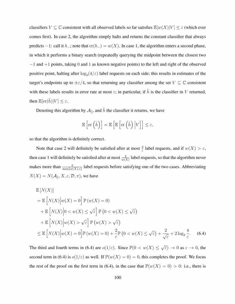
classifiers V ⊆ C consistent with all observed labels so far satisfies E[w(X)|V ] ≤ ε (which ever

comes first). In case 2, the algorithm simply halts and returns the constant classifier that always

predicts−1: call it h−; note that er(h−) = w(X). In case 1, the algorithm enters a second phase,

in which it performs a binary search (repeatedly querying the midpoint between the closest two

−1 and +1 points, taking 0 and 1 as known negative points) to the left and right of the observed

positive point, halting after log2(4/ε) label requests on each side; this results in estimates of the

target’s endpoints up to ±ε/4, so that returning any classifier among the set V ⊆ C consistent

with these labels results in error rate at most ε; in particular, if h is the classifier in V returned,

then E[er(h)|V ] ≤ ε.

Denoting this algorithm by A[], and h the classifier it returns, we have

E

[

er(

h)]

= E

[

E

[

er(

h) ∣

∣

∣V]]

≤ ε,

so that the algorithm is definitely correct.

Note that case 2 will definitely be satisfied after at most 2ε

label requests, and if w(X) > ε,

then case 1 will definitely be satisfied after at most 2w(X)

label requests, so that the algorithm never

makes more than 2maxw(X),ε label requests before satisfying one of the two cases. Abbreviating

N(X) = N(A[], X, ε,D, π), we have

E [N(X)]

= E

[

N(X)∣

∣

∣w(X) = 0]

P (w(X) = 0)

+ E

[

N(X)∣

∣

∣0 < w(X) ≤ √ε

]

P(

0 < w(X) ≤ √ε)

+ E

[

N(X)∣

∣

∣w(X) >√ε]

P(

w(X) >√ε)

≤ E

[

N(X)∣

∣

∣w(X) = 0]

P (w(X) = 0) +2

εP(

0 < w(X) ≤ √ε)

+2√ε+ 2 log2

4

ε. (6.4)

The third and fourth terms in (6.4) are o(1/ε). Since P(0 < w(X) ≤ √ε) → 0 as ε → 0, the

second term in (6.4) is o(1/ε) as well. If P(w(X) = 0) = 0, this completes the proof. We focus

the rest of the proof on the first term in (6.4), in the case that P(w(X) = 0) > 0: i.e., there is

100

nonzero probability that the target X labels the space all negative. Letting V denote the subset

of C consistent with all requested labels, note that on the event w(X) = 0, after n label requests

(for n + 1 a power of 2) we have maxh∈V w(h) ≤ 1/n. Thus, for any value γ ∈ (0, 1), after at

most 2γ

label requests, on the event that w(X) = 0,

E

[

w(X)∣

∣

∣V]

≤ E [w(X)I [w(X) ≤ γ]]

π(V )≤ E [w(X)I [w(X) ≤ γ]]

P(w(X) = 0). (6.5)

Now note that, by the dominated convergence theorem,

limγ→0

E

[

w(X)I [w(X) ≤ γ]

γ

]

= E

[

limγ→0

w(X)I [w(X) ≤ γ]

γ

]

= 0.

Therefore, E [w(X)I [w(X) ≤ γ]] = o(γ). If we define γε as the largest value of γ for which

E [w(X)I [w(X) ≤ γ]] ≤ εP(w(X) = 0) (or, say, half the supremum if the maximum is not

achieved), then we have γε ≫ ε. Combined with (6.5), this implies

E

[

N(X)∣

∣

∣w(X) = 0

]

≤ 2

γε= o(1/ε).

Thus, all of the terms in (6.4) are o(1/ε), so that in total E[N(X)] = o(1/ε).

In conclusion, for this concept space C and data distribution D, we have a correct active

learning algorithm A achieving a sample complexity SC(A, ε,D, π) = o(1/ε) for all priors π

on C.

6.5 A General Result for Self-Verifying Bayesian Active Learn-

ing

In this section, we present our main result for improvements achievable by prior-dependent

self-verifying active learning: a general result stating that o(1/ε) expected sample complexity

is always achievable for some appropriate prior-dependent active learning algorithm, for any

(X ,C,D, π) for which C has finite VC dimension. Since the known results for the sample com-

plexity of passive learning with access to the prior are typically Θ(1/ε) [Haussler, Kearns, and

101

Schapire, 1994a], and since there are known learning problems (X ,C,D, π) for which every pas-

sive learning algorithm requires Ω(1/ε) samples, this o(1/ε) result for active learning represents

an improvement over passive learning.

The proof is simple and accessible, yet represents an important step in understanding the

problem of self-termination in active learning algorithms, and the general issue of the complexity

of verification. Also, since there are problems (X ,C,D) where C has finite VC dimension but

for which no prior-independent correct active learning algorithm (of the self-terminating type

studied here) can achieve o(1/ε) expected sample complexity for every π, this also represents a

significant step toward understanding the inherent value of having access to the prior in active

learning.

First, we have a small lemma.

Lemma 6.1. For any sequence of functions φn : C→ [0,∞) such that, ∀f ∈ C, φn(f) = o(1/n)

and ∀n ∈ N, φn(f) ≤ c/n (for an f -independent constant c ∈ (0,∞)), there exists a sequence

φn in [0,∞) such that

φn = o(1/n) and limn→∞

P(

φn(X) > φn

)

= 0.

Proof. For any constant γ ∈ (0,∞), we have (by Markov’s inequality and the dominated con-

vergence theorem)

limn→∞

P (nφn(X) > γ) ≤ 1

γlimn→∞

E [nφn(X)]

=1

γE

[

limn→∞

nφn(X)]

= 0.

Therefore (by induction), there exists a diverging sequence ni in N such that

limi→∞

supn≥ni

P(

nφn(X) > 2−i)

= 0.

Inverting this, let in = maxi ∈ N : ni ≤ n, and define φn(X) = (1/n) ·2−in . By construction,

P(

φn(X) > φn

)

→ 0. Furthermore, ni →∞ =⇒ in →∞, so that we have

limn→∞

nφn = limn→∞

2−in = 0,

102

implying φn = o(1/n).

Theorem 6.2. For any VC class C, there is a correct active learning algorithmAa that, for every

data distribution D and prior π, achieves expected sample complexity

SC(Aa, ε,D, π) = o(1/ε).

Our approach to proving Theorem 6.2 is via a reduction to established results about (prior-

independent) active learning algorithms that are not self-verifying. Specifically, consider a

slightly different type of active learning algorithm than that defined above: namely, an algo-

rithm Ab that takes as input a budget n ∈ N on the number of label requests it is allowed to

make, and that after making at most n label requests returns as output a classifier hn. Let us refer

to any such algorithm as a budget-based active learning algorithm. Note that budget-based active

learning algorithms are prior-independent (have no direct access to the prior). The following re-

sult was proven by [Hanneke, 2009] (see also the related earlier work of [Balcan, Hanneke, and

Vaughan, 2010]).

Lemma 6.3. [Hanneke, 2009] For any VC class C, there exists a constant c ∈ (0,∞), a function

E(n; f,D), and a budget-based active learning algorithm Ab such that

∀D, ∀f ∈ C, E(n; f,D) ≤ c/n and E(n; f,D) = o(1/n),

and E

[

er (Ab(n))∣

∣

∣X]

≤ E(n;X,D) (always).2

That is, equivalently, for any fixed value for the target function, the expected error rate is

o(1/n), where the random variable in the expectation is only the data sequence X1, X2, . . .. Our

task in the proof of Theorem 6.2 is to convert such a budget-based algorithm into one that is

correct, self-terminating, and prior-dependent, taking ε as input.

Theorem 6.2. Consider Ab, E , and c as in Lemma 6.3, let hn denote the classifier returned by

Ab(n), and define

nπ,ε = min

n ∈ N : E[

er(

hn

)]

≤ ε

.

2Furthermore, it is not difficult to see that we can take this E to be measurable in the X argument.

103

This value is accessible based purely on access to π and D. Furthermore, we clearly have (by

construction) E[

er(

hnπ,ε

)]

≤ ε. Thus, letting Aa denote the active learning algorithm taking

(D, π, ε) as input, which runs Ab(nπ,ε) and then returns hnπ,ε , we have that Aa is a correct

learning algorithm (i.e., its expected error rate is at most ε).

As for the expected sample complexity SC(Aa, ε,D, π) achieved byAa, we have SC(Aa, ε,D, π) ≤

nπ,ε, so that it remains only to bound nπ,ε. By Lemma 6.1, there is a π-dependent function

E(n; π,D) such that

π (f ∈ C : E(n; f,D) > E(n; π,D))→ 0

and E(n; π,D) = o(1/n).

Therefore, by the law of total expectation,

E

[

er(

hn

)]

= E

[

E

[

er(

hn

) ∣

∣

∣X]]

≤ E [E(n;X,D)]

≤ c

nπ (f ∈ C : E(n; f,D) > E(n; π,D)) + E(n; π,D)

= o(1/n).

If nπ,ε = O(1), then clearly nπ,ε = o(1/ε) as needed. Otherwise, since nπ,ε is monotonic in ε,

we must have nπ,ε ↑ ∞ as ε ↓ 0. In particular, in this latter case we have

limε→0

ε · nπ,ε

≤ limε→0

ε ·(

1 + max

n ≥ nπ,ε − 1 : E[

er(

hn

)]

> ε)

= limε→0

ε · maxn≥nπ,ε−1

nI[

E

[

er(

hn

)]

/ε > 1]

≤ limε→0

ε · maxn≥nπ,ε−1

nE[

er(

hn

)]

/ε

= limε→0

maxn≥nπ,ε−1

nE[

er(

hn

)]

= lim supn→∞

nE[

er(

hn

)]

= 0,

so that nπ,ε = o(1/ε), as required.

Theorem 6.2 implies that, if we have direct access to the prior distribution ofX , regardless of

what that prior distribution π is, we can always construct a self-verifying active learning algorithm

104

Aa that has a guarantee of E [er (Aa(ε,D, π))] ≤ ε and its expected number of label requests

is o(1/ε). This guarantee is not possible for prior-independent self-verifying active learning

algorithms.

6.6 Dependence on D in the Learning Algorithm

The dependence on D in the algorithm described in the proof of Theorem 6.2 is fairly weak, and

we can eliminate any direct dependence onD by replacing er(

hn

)

by a 1−ε/2 confidence upper

bound based onMε = Ω(

1ε2log 1

ε

)

i.i.d. unlabeled examplesX ′1, X

′2, . . . , X

′Mε

independent from

the examples used by the algorithm (e.g., set aside in a pre-processing step, where the bound is

calculated via Hoeffding’s inequality and a union bound over the values of n that we check,

of which there are at most O(1/ε)). Then we simply increase the value of n (starting at some

constant, such as 1) until

1

Mε

Mε∑

i=1

π(

f ∈ C : f (X ′i) 6= hn (X

′i))

≤ ε/2.

The expected value of the smallest value of n for which this occurs is o(1/ε). Note that this

only requires access to the prior π, not the data distribution D (the budget-based algorithm Ab

of [Hanneke, 2009] has no direct dependence on D); if desired for computational efficiency, this

dependence may also be estimated by a 1 − ε/4 confidence upper bound based on Ω(

1ε2log 1

ε

)

independent samples of X values with distribution π, where for each sample we simulate the

execution of Ab(n) for that (simulated) target function in order to obtain the returned classifier.

In particular, note that no actual label requests to the oracle are required during this process of

estimating the appropriate label budget nπ,ε, as all executions of Ab are simulated.

105

6.7 Inherent Dependence on π in the Sample Complexity

We have shown that for every prior π, the sample complexity is bounded by a o(1/ε) function.

One might wonder whether it is possible that the asymptotic dependence on ε in the sample

complexity can be prior-independent, while still being o(1/ε). That is, we can ask whether

there exists a (π-independent) function s(ε) = o(1/ε) such that, for every π, there is a correct

π-dependent algorithm A achieving a sample complexity SC(A, ε,D, π) = O(s(ε)), possibly

involving π-dependent constants. Certainly in some cases, such as threshold classifiers, this is

true. However, it seems this is not generally the case, and in particular it fails to hold for the

space of interval classifiers.

For instance, consider a prior π on the space C of interval classifiers, constructed as follows.

We are given an arbitrary monotonic g(ε) = o(1/ε); since g(ε) = o(1/ε), there must exist

(nonzero) functions q1(i) and q2(i) such that limi→∞ q1(i) = 0, limi→∞ q2(i) = 0, and ∀i ∈

N, g(q1(i)/2i+1) ≤ q2(i) · 2i; furthermore, letting q(i) = maxq1(i), q2(i), by monotonicity of

g we also have ∀i ∈ N, g(q(i)/2i+1) ≤ q(i) · 2i, and limi→∞ q(i) = 0. Then define a function

p(i) with∑

i∈N p(i) = 1 such that p(i) ≥ q(i) for infinitely many i ∈ N; for instance, this can

be done inductively as follows. Let α0 = 1/2; for each i ∈ N, if q(i) > αi−1, set p(i) = 0

and αi = αi−1; otherwise, set p(i) = αi−1 and αi = αi−1/2. Finally, for each i ∈ N, and each

j ∈ 0, 1, . . . , 2i − 1, define π(

I±(j·2−i,(j+1)·2−i)

)

= p(i)/2i.

We let D be uniform on X = [0, 1]. Then for each i ∈ N s.t. p(i) ≥ q(i), there is a

p(i) probability the target interval has width 2−i, and given this any algorithm requires ∝ 2i

expected number of requests to determine which of these 2i intervals is the target, failing which

the error rate is at least 2−i. In particular, letting εi = p(i)/2i+1, any correct algorithm has sample

complexity at least ∝ p(i) · 2i for ε = εi. Noting p(i) · 2i ≥ q(i) · 2i ≥ g(q(i)/2i+1) ≥ g(εi), this

implies there exist arbitrarily small values of ε > 0 for which the optimal sample complexity is

at least ∝ g(ε), so that the sample complexity is not o(g(ε)).

For any s(ε) = o(1/ε), there exists a monotonic g(ε) = o(1/ε) such that s(ε) = o(g(ε)).

106

Thus, constructing π as above for this g, we have that the sample complexity is not o(g(ε)),

and therefore not O(s(ε)). So at least for the space of interval classifiers, the specific o(1/ε)

asymptotic dependence on ε is inherently π-dependent. This argument also illustrates that the

o(1/ε) result in Theorem 6.2 is essentially the strongest possible at this level of generality (i.e.,

without saying more about C, D, or π).

107

Chapter 7

Prior Estimation for Transfer Learning

Abstract

1We explore a transfer learning setting, in which a finite sequence of target concepts are sampled

independently with an unknown distribution from a known family. We study the total number of

labeled examples required to learn all targets to an arbitrary specified expected accuracy, focusing

on the asymptotics in the number of tasks and the desired accuracy. Our primary interest is

formally understanding the fundamental benefits of transfer learning, compared to learning each

target independently from the others. Our approach to the transfer problem is general, in the

sense that it can be used with a variety of learning protocols.

7.1 Introduction

Transfer learning reuses knowledge from past related tasks to ease the process of learning to

perform a new task. The goal of transfer learning is to leverage previous learning and experience

to more efficiently learn novel, but related, concepts, compared to what would be possible with-

out this prior experience. The utility of transfer learning is typically measured by a reduction in

1Joint work with Jaime Carbonell and Steve Hanneke

108

the number of training examples required to achieve a target performance on a sequence of re-

lated learning problems, compared to the number required for unrelated problems: i.e., reduced

sample complexity. In many real-life scenarios, just a few training examples of a new concept

or process is often sufficient for a human learner to grasp the new concept given knowledge of

related ones. For example, learning to drive a van becomes much easier a task if we have already

learned how to drive a car. Learning French is somewhat easier if we have already learned En-

glish (vs Chinese), and learning Spanish is easier if we know Portuguese (vs German). We are

therefore interested in understanding the conditions that enable a learning machine to leverage

abstract knowledge obtained as a by-product of learning past concepts, to improve its perfor-

mance on future learning problems. Furthermore, we are interested in how the magnitude of

these improvements grows as the learning system gains more experience from learning multiple

related concepts.

The ability to transfer knowledge gained from previous tasks to make it easier to learn a new

task can potentially benefit a wide range of real-world applications, including computer vision,

natural language processing, cognitive science (e.g., fMRI brain state classification), and speech

recognition, to name a few. As an example, consider training a speech recognizer. After training

on a number of individuals, a learning system can identify common patterns of speech, such as

accents or dialects, each of which requires a slightly different speech recognizer; then, given a

new person to train a recognizer for, it can quickly determine the particular dialect from only a

few well-chosen examples, and use the previously-learned recognizer for that particular dialect.

In this case, we can think of the transferred knowledge as consisting of the common aspects of

each recognizer variant and more generally the distribution of speech patterns existing in the

population these subjects are from. This same type of distribution-related knowledge transfer

can be helpful in a host of applications, including all those mentioned above.

Supposing these target concepts (e.g., speech patterns) are sampled independently from a

fixed population, having knowledge of the distribution of concepts in the population may often

109

be quite valuable. More generally, we may consider a general scenario in which the target con-

cepts are sampled i.i.d. according to a fixed distribution. As we show below, the number of

labeled examples required to learn a target concept sampled according to this distribution may

be dramatically reduced if we have direct knowledge of the distribution. However, since in many

real-world learning scenarios, we do not have direct access to this distribution, it is desirable to be

able to somehow learn the distribution, based on observations from a sequence of learning prob-

lems with target concepts sampled according to that distribution. The hope is that an estimate

of the distribution so-obtained might be almost as useful as direct access to the true distribution

in reducing the number of labeled examples required to learn subsequent target concepts. The

focus of this paper is an approach to transfer learning based on estimating the distribution of

the target concepts. Whereas we acknowledge that there are other important challenges in trans-

fer learning, such as exploring improvements obtainable from transfer under various alternative

notions of task relatedness [Ben-David and Schuller, 2003, Evgeniou and Pontil, 2004], or alter-

native reuses of knowledge obtained from previous tasks [Thrun, 1996], we believe that learning

the distribution of target concepts is a central and crucial component in many transfer learning

scenarios, and can reduce the total sample complexity across tasks.

Note that it is not immediately obvious that the distribution of targets can even be learned

in this context, since we do not have direct access to the target concepts sampled according to

it, but rather have only indirect access via a finite number of labeled examples for each task; a

significant part of the present work focuses on establishing that as long as these finite labeled

samples are larger than a certain size, they hold sufficient information about the distribution over

concepts for estimation to be possible. In particular, in contrast to standard results on consistent

density estimation, our estimators are not directly based on the target concepts, but rather are

only indirectly dependent on these via the labels of a finite number of data points from each

task. One desideratum we pay particular attention to is minimizing the number of extra labeled

examples needed for each task, beyond what is needed for learning that particular target, so that

110

the benefits of transfer learning are obtained almost as a by-product of learning the targets. Our

technique is general, in that it applies to any concept space with finite VC dimension; also, the

process of learning the target concepts is (in some sense) decoupled from the mechanism of

learning the concept distribution, so that we may apply our technique to a variety of learning

protocols, including passive supervised learning, active supervised learning, semi-supervised

learning, and learning with certain general data-dependent forms of interaction [Hanneke, 2009].

For simplicity, we choose to formulate our transfer learning algorithms in the language of active

learning; as we show, this problem can benefit significantly from transfer. Formulations for other

learning protocols would follow along similar lines, with analogous theorems; these results are

particularly interested when composed with the results on prior-dependent active learning from

the previous chapter.

Transfer learning is related at least in spirit to much earlier work on case-based and analog-

ical learning [Carbonell, 1983, 1986, Kolodner (Ed), 1993, Thrun, 1996, Veloso and Carbonell,

1993], although that body of work predated modern machine learning, and focused on symbolic

reuse of past problem solving solutions rather than on current machine learning problems such as

classification, regression or structured learning. More recently, transfer learning (and the closely

related problem of multitask learning) has been studied in specific cases with interesting (though

sometimes heuristic) approaches [Baxter, 1997, Ben-David and Schuller, 2003, Caruana, 1997,

Micchelli and Pontil, 2004, Silver, 2000]. This paper considers a general theoretical framework

for transfer learning, based on an Empirical Bayes perspective, and derives rigorous theoretical

results on the benefits of transfer. We discuss the relation of this analysis to existing theoretical

work on transfer learning below.

7.1.1 Outline of the paper

The remainder of the paper is organized as follows. In Section 7.2 we introduce basic notation

used throughout, and survey some related work from the existing literature. In Section 7.3, we

111

describe and analyze our proposed method for estimating the distribution of target concepts, the

key ingredient in our approach to transfer learning, which we then present in Section 7.4.

7.2 Definitions and Related Work

First, we state a few basic notational conventions. We denote N = 1, 2, . . . and N0 = N ∪

0. For any random variable X , we generally denote by PX the distribution of X (the induced

probability measure on the range of X), and by PX|Y the regular conditional distribution of X

given Y . For any pair of probability measures µ1, µ2 on a measurable space (Ω,F), we define

‖µ1 − µ2‖ = supA∈F|µ1(A)− µ2(A)|.

Next we define the particular objects of interest to our present discussion. Let Θ be an

arbitrary set (called the parameter space), (X ,BX ) be a Borel space [Schervish, 1995] (where

X is called the instance space), and D be a fixed distribution on X (called the data distribution).

For instance, Θ could be Rn and X could be R

m, for some n,m ∈ N, though more general

scenarios are certainly possible as well, including infinite-dimensional parameter spaces. Let C

be a set of measurable classifiers h : X → −1,+1 (called the concept space), and suppose

C has VC dimension d < ∞ [Vapnik, 1982] (such a space is called a VC class). C is equipped

with its Borel σ-algebra B, induced by the pseudo-metric ρ(h, g) = D(x ∈ X : h(x) 6= g(x)).

Though all of our results can be formulated for general D in slightly more complex terms, for

simplicity throughout the discussion below we suppose ρ is actually a metric, in that any h, g ∈ C

with h 6= g have ρ(h, g) > 0; this amounts to a topological assumption on C relative to D.

For each θ ∈ Θ, πθ is a distribution on C (called a prior). Our only (rather mild) assumption

on this family of prior distributions is that πθ : θ ∈ Θ be totally bounded, in the sense that

∀ε > 0, ∃ finite Θε ⊆ Θ s.t. ∀θ ∈ Θ, ∃θε ∈ Θε with ‖πθ − πθε‖ < ε. See [Devroye and Lugosi,

2001] for examples of categories of classes that satisfy this.

The general setup for the learning problem is that we have a true parameter value θ⋆ ∈ Θ, and

112

a collection of C-valued random variables h∗tθt∈N,θ∈Θ, where for a fixed θ ∈ Θ the h∗tθt∈Nvariables are i.i.d. with distribution πθ.

The learning problem is the following. For each θ ∈ Θ, there is a sequence

Zt(θ) = (Xt1, Yt1(θ)), (Xt2, Yt2(θ)), . . .,

where Xtit,i∈N are i.i.d. D, and for each t, i ∈ N, Yti(θ) = h∗tθ(Xti). For k ∈ N we denote by

Ztk(θ) = (Xt1, Yt1(θ)), . . . , (Xtk, Ytk(θ)). Since the Yti(θ) are the actual h∗tθ(Xti) values, we

are studying the non-noisy, or realizable-case, setting.

The algorithm receives values ε and T as input, and for each t ∈ 1, 2, . . . , T in increas-

ing order, it observes the sequence Xt1, Xt2, . . ., and may then select an index i1, receive label

Yti1(θ⋆), select another index i2, receive label Yti2(θ⋆), etc. The algorithm proceeds in this fash-

ion, sequentially requesting labels, until eventually it produces a classifier ht. It then increments

t and repeats this process until it produces a sequence h1, h2, . . . , hT , at which time it halts. To be

called correct, the algorithm must have a guarantee that ∀θ⋆ ∈ Θ, ∀t ≤ T,E[

ρ(

ht, h∗tθ⋆

)]

≤ ε,

for any values of T ∈ N and ε > 0 given as input. We will be interested in the expected number

of label requests necessary for a correct learning algorithm, averaged over the T tasks, and in

particular in how shared information between tasks can help to reduce this quantity when direct

access to θ⋆ is not available to the algorithm.

7.2.1 Relation to Existing Theoretical Work on Transfer Learning

Although we know of no existing work on the theoretical advantages of transfer learning for

active learning, the existing literature contains several analyses of the advantages of transfer

learning for passive learning. In his classic work, Baxter ([Baxter, 1997] section 4) explores a

similar setup for a general form of passive learning, except in a full Bayesian setting (in contrast

to our setting, often referred to as “empirical Bayes,” which includes a constant parameter θ⋆ to be

estimated from data). Essentially, [Baxter, 1997] sets up a hierarchical Bayesian model, in which

(in our notation) θ⋆ is a random variable with known distribution (hyper-prior), but otherwise the

113

specialization of Baxter’s setting to the pattern recognition problem is essentially identical to our

setup above. This hyper-prior does make the problem slightly easier, but generally the results

of [Baxter, 1997] are of a different nature than our objectives here. Specifically, Baxter’s results

on learning from labeled examples can be interpreted as indicating that transfer learning can

improve certain constant factors in the asymptotic rate of convergence of the average of expected

error rates across the learning problems. That is, certain constant complexity terms (for instance,

related to the concept space) can be reduced to (potentially much smaller) values related to πθ⋆ by

transfer learning. Baxter argues that, as the number of tasks grows large, this effectively achieves

close to the known results on the sample complexity of passive learning with direct access to θ⋆.

A similar claim is discussed by Ando and Zhang [Ando and Zhang, 2004] (though in less detail)

for a setting closer to that studied here, where θ⋆ is an unknown parameter to be estimated.

There are also several results on transfer learning of a slightly different variety, in which,

rather than having a prior distribution for the target concept, the learner initially has several

potential concept spaces to choose from, and the role of transfer is to help the learner select from

among these concept spaces [Ando and Zhang, 2005, Baxter, 2000]. In this case, the idea is

that one of these concept spaces has the best average minimum achievable error rate per learning

problem, and the objective of transfer learning is to perform nearly as well as if we knew which

of the spaces has this property. In particular, if we assume the target functions for each task all

reside in one of the concept spaces, then the objective of transfer learning is to perform nearly

as well as if we knew which of the spaces contains the targets. Thus, transfer learning results

in a sample complexity related to the number of learning problems, a complexity term for this

best concept space, and a complexity term related to the diversity of concept spaces we have to

choose from. In particular, as with [Baxter, 1997], these results can typically be interpreted as

giving constant factor improvements from transfer in a passive learning context, at best reducing

the complexity constants, from those for the union over the given concept spaces, down to the

complexity constants of the single best concept space.

114

In addition to the above works, there are several analyses of transfer learning and multitask

learning of an entirely different nature than our present discussion, in that the objectives of the

analysis are somewhat different. Specifically, there is a branch of the literature concerned with

task relatedness, not in terms of the underlying process that generates the target concepts, but

rather directly in terms of relations between the target concepts themselves. In this sense, several

tasks with related target concepts should be much easier to learn than tasks with unrelated target

concepts. This is studied in the context of kernel methods by [Evgeniou and Pontil, 2004, Evge-

niou, Micchelli, and Pontil, 2005, Micchelli and Pontil, 2004], and in a more general theoretical

framework by [Ben-David and Schuller, 2003]. As mentioned, our approach to transfer learning

is based on the idea of estimating the distribution of target concepts. As such, though interesting

and important, these notions of direct relatedness of target concepts are not as relevant to our

present discussion.

As with [Baxter, 1997], the present work is interested in showing that as the number of

tasks grows large, we can effectively achieve a sample complexity close to that achievable with

direct access to θ⋆. However, in contrast, we are interested in a general approach to transfer

learning and the analysis thereof, leading to concrete results for a variety of learning protocols

such as active learning and semi-supervised learning. In particular, our analysis of active learning

reveals the interesting phenomenon that transfer learning can sometimes improve the asymptotic

dependence on ε, rather than merely the constant factors as in the analysis of [Baxter, 1997].

Our work contrasts with [Baxter, 1997] in another important respect, which significantly

changes the way we approach the problem. Specifically, in Baxter’s analysis, the results (e.g.,

[Baxter, 1997] Theorems 4, 6) regard the average loss over the tasks, and are stated as a function

of the number of samples per task. This number of samples plays a dual role in Baxter’s analysis,

since these samples are used both by the individual learning algorithm for each task, and also for

the global transfer learning process that provides the learners with information about θ⋆. Baxter

is then naturally interested in the rates at which these losses shrink as the sample sizes grow

115

large, and therefore formulates the results in terms of the asymptotic behavior as the per-task

sample sizes grow large. In particular, the results of [Baxter, 1997] involve residual terms which

become negligible for large sample sizes, but may be more significant for smaller sample sizes.

In our work, we are interested in decoupling these two roles for the sample sizes; in partic-

ular, our results regard only the number of tasks as an asymptotic variable, while the number of

samples per task remains bounded. First, we note a very practical motivation for this: namely,

non-altruistic learners. In many settings where transfer learning may be useful, it is desirable

that the number of labeled examples we need to collect from each particular learning problem

never be significantly larger than the number of such examples required to solve that particular

problem (i.e., to learn that target concept to the desired accuracy). For instance, this is the case

when the learning problems are not all solved by the same individual (or company, etc.), but

rather a coalition of cooperating individuals (e.g., hospitals sharing data on clinical trials); each

individual may be willing to share the data they used to learn their particular concept, in the

interest of making others’ learning problems easier; however, they may not be willing to collect

significantly more data than they themselves need for their own learning problem. We should

therefore be particularly interested in studying transfer as a by-product of the usual learning pro-

cess; failing this, we are interested in the minimum possible number of extra labeled examples

per task to gain the benefits of transfer learning.

The issue of non-altruistic learners also presents a further technical problem in that the in-

dividuals solving each task may be unwilling to alter their method of gathering data to be more

informative for the transfer learning process. That is, we expect the learning process for each

task is designed with the sole intention of estimating the target concept, without regard for the

global transfer learning problem. To account for this, we model the transfer learning problem in

a reduction-style framework, in which we suppose there is some black-box learning algorithm to

be run for each task, which takes a prior as input and has a theoretical guarantee of good perfor-

mance provided the prior is correct. We place almost no restrictions whatsoever on this learning

116

algorithm, including the manner in which it accesses the data. This allows remarkable generality,

since this procedure could be passive, active, semi-supervised, or some other kind of query-based

strategy. However, because of this generality, we have no guarantee on the information about θ⋆

reflected in the data used by this algorithm (especially if it is an active learning algorithm). As

such, we choose not to use the label information gathered by the learning algorithm for each

task when estimating the θ⋆, but instead take a small number of additional random labeled ex-

amples from each task with which to estimate θ⋆. Again, we want to minimize this number of

additional samples per task; indeed, in this work we are able to make due with a mere constant

number of additional samples per task. To our knowledge, no result of this type (estimating θ⋆

using a bounded sample size per learning problem) has previously been established at the level

of generality studied here.

7.3 Estimating the Prior

The advantage of transfer learning in this setting is that each learning problem provides some

information about θ⋆, so that after solving several of the learning problems, we might hope to be

able to estimate θ⋆. Then, with this estimate in hand, we can use the corresponding estimated

prior distribution in the learning algorithm for subsequent learning problems, to help inform

the learning process similarly to how direct knowledge of θ⋆ might be helpful. However, the

difficulty in approaching this is how to define such an estimator. Since we do not have direct

access to the h∗t values, but rather only indirect observations via a finite number of example

labels, the standard results for density estimation from i.i.d. samples cannot be applied.

The idea we pursue below is to consider the distributions on Ztk(θ⋆). These variables are di-

rectly observable, by requesting the labels of those examples. Thus, for any finite k ∈ N, this dis-

tribution is estimable from observable data. That is, using the i.i.d. values Z1k(θ⋆), . . . ,Ztk(θ⋆),

we can apply standard techniques for density estimation to arrive at an estimator of PZtk(θ⋆). Then

the question is whether the distribution PZtk(θ⋆) uniquely characterizes the prior distribution πθ⋆ :

117

that is, whether πθ⋆ is identifiable from PZtk(θ⋆).

As an example, consider the space of half-open interval classifiers on [0, 1]: C = 1±[a,b) :

0 ≤ a ≤ b ≤ 1, where 1±[a,b)(x) = +1 if a ≤ x < b and −1 otherwise. In this case, πθ⋆ is

not necessarily identifiable from PZt1(θ⋆); for instance, the distributions πθ1 and πθ2 characterized

by πθ1(1±[0,1)) = πθ1(1±

[0,0)) = 1/2 and πθ2(1±[0,1/2)) = πθ2(1±

[1/2,1)) = 1/2 are not dis-

tinguished by these one-dimensional distributions. However, it turns out that for this half-open

intervals problem, πθ⋆ is uniquely identifiable from PZt2(θ⋆); for instance, in the θ1 vs θ2 sce-

nario, the conditional probability P(Yt1(θi),Yt2(θi))|(Xt1,Xt2)((+1,+1)|(1/4, 3/4)) will distinguish

πθ1 from πθ2 , and this can be calculated from PZt2(θi). The crucial element of the analysis below

is determining the appropriate value of k to uniquely identify πθ⋆ from PZtk(θ⋆) in general. As we

will see, k = d (the VC dimension) is always sufficient, a key insight for the results that follow.

We will also see this is not the case for any k < d.

To be specific, in order to transfer knowledge from one task to the next, we use a few labeled

data points from each task to gain information about θ⋆. For this, for each task t, we simply take

the first d data points in the Zt(θ⋆) sequence. That is, we request the labels

Yt1(θ⋆), Yt2(θ⋆), . . . , Ytd(θ⋆)

and use the points Ztd(θ⋆) to update an estimate of θ⋆.

The following result shows that this technique does provide a consistent estimator of πθ⋆ .

Again, note that this result is not a straightforward application of the standard approach to con-

sistent estimation, since the observations here are not the h∗tθ⋆ variables themselves, but rather a

number of the Yti(θ⋆) values. The key insight in this result is that πθ⋆ is uniquely identified by the

joint distribution PZtd(θ⋆) over the first d labeled examples; later, we prove this is not necessarily

true for PZtk(θ⋆) for values k < d. This identifiability result is stated below in Corollary 7.6;

as we discuss in Section 7.3.1, there is a fairly simple direct proof of this result. However,

for our purposes, we will actually require the stronger condition that any θ ∈ Θ with small

‖PZtk(θ)−PZtk(θ⋆)‖ also has small ‖πθ− πθ⋆‖. This stronger requirement adds to the complexity

118

of the proofs. The results in this section are purely concerned with relating distances in the space

of PZtd(θ) distributions to the corresponding distances in the space of πθ distributions; as such,

they are not specific to active learning or other learning protocols, and hence are of independent

interest.

Theorem 7.1. There exists an estimator θTθ⋆ = θT (Z1d(θ⋆), . . . ,ZTd(θ⋆)), and functions R :

N0 × (0, 1] → [0,∞) and δ : N0 × (0, 1] → [0, 1], such that for any α > 0, limT→∞

R(T, α) =

limT→∞

δ(T, α) = 0 and for any T ∈ N0 and θ⋆ ∈ Θ,

P

(

‖πθTθ⋆− πθ⋆‖ > R(T, α)

)

≤ δ(T, α) ≤ α.

One important detail to note, for our purposes, is that R(T, α) is independent from θ⋆, so

that the value of R(T, α) can be calculated and used within a learning algorithm. The proof of

Theorem 7.1 will be established via the following sequence of lemmas. Lemma 7.2 relates dis-

tances in the space of priors to distances in the space of distributions on the full data sets. In turn,

Lemma 7.3 relates these distances to distances in the space of distributions on a finite number of

examples from the data sets. Lemma 7.4 then relates the distances between distributions on any

finite number of examples to distances between distributions on d examples. Finally, Lemma 7.5

presents a standard result on the existence of a converging estimator, in this case for the distri-

bution on d examples, for totally bounded families of distributions. Tracing these relations back,

they relate convergence of the estimator for the distribution of d examples to convergence of the

corresponding estimator for the prior itself.

Lemma 7.2. For any θ, θ′ ∈ Θ and t ∈ N,

‖πθ − πθ′‖ = ‖PZt(θ) − PZt(θ′)‖.

Proof. Fix θ, θ′ ∈ Θ, t ∈ N. Let X = Xt1, Xt2, . . ., Y(θ) = Yt1(θ), Yt2(θ), . . ., and for

k ∈ N let Xk = Xt1, . . . , Xtk. and Yk(θ) = Yt1(θ), . . . , Ytk(θ). For h ∈ C, let cX(h) =

(Xt1, h(Xt1)), (Xt2, h(Xt2)), . . ..

For h, g ∈ C, define ρX(h, g) = limm→∞

1m

∑mi=1 1[h(Xti) 6= g(Xti)] (if the limit exists), and

ρXk(h, g) = 1

k

∑ki=1 1[h(Xti) 6= g(Xti)]. Note that since C has finite VC dimension, so does

119

the collection of sets x : h(x) 6= g(x) : h, g ∈ C, so that the uniform strong law of

large numbers implies that with probability one, ∀h, g ∈ C, ρX(h, g) exists and has ρX(h, g) =

ρ(h, g) [Vapnik, 1982].

Consider any θ, θ′ ∈ Θ, and any A ∈ B. Then since B is the Borel σ-algebra induced by ρ,

any h /∈ A has ∀g ∈ A, ρ(h, g) > 0. Thus, if ρX(h, g) = ρ(h, g) for all h, g ∈ C, then ∀h /∈ A,

∀g ∈ A, ρX(h, g) = ρ(h, g) > 0 =⇒ ∀g ∈ A, cX(h) 6= cX(g) =⇒ cX(h) /∈ cX(A).

This implies c−1X(cX(A)) = A. Under these conditions,

PZt(θ)|X(cX(A)) = πθ(c−1X(cX(A))) = πθ(A),

and similarly for θ′.

Any measurable set C for the range of Zt(θ) can be expressed as C = cx(h) : (h, x) ∈ C ′

for some appropriate C ′ ∈ B ⊗ B∞X . Letting C ′

x = h : (h, x) ∈ C ′, we have

PZt(θ)(C) =

∫

πθ(c−1x (cx(C

′x)))PX(dx) =

∫

πθ(C′x)PX(dx) = P(h∗

tθ,X)(C ′).

Likewise, this reasoning holds for θ′. Then

‖PZt(θ) − PZt(θ′)‖ = ‖P(h∗tθ,X)− P(h∗

tθ′ ,X)‖

= supC′∈B⊗B∞

X

∣

∣

∣

∣

∫

(πθ(C′x)− πθ′(C ′

x))PX(dx)

∣

∣

∣

∣

≤∫

supA∈B|πθ(A)− πθ′(A)|PX(dx) = ‖πθ − πθ′‖.

Since h∗tθ and X are independent, forA ∈ B, πθ(A) = Ph∗tθ(A) = Ph∗

tθ(A)PX(X∞) = P(h∗

tθ,X)(A×

X∞). Analogous reasoning holds for h∗tθ′ . Thus, we have

‖πθ − πθ′‖ = ‖P(h∗tθ,X)

(· × X∞)− P(h∗tθ′ ,X)

(· × X∞)‖

≤ ‖P(h∗tθ,X)− P(h∗

tθ′ ,X)‖ = ‖PZt(θ) − PZt(θ′)‖.

Combining the above, we have ‖PZt(θ) − PZt(θ′)‖ = ‖πθ − πθ′‖.

120

Lemma 7.3. There exists a sequence rk = o(1) such that ∀t, k ∈ N, ∀θ, θ′ ∈ Θ,

‖PZtk(θ) − PZtk(θ′)‖ ≤ ‖πθ − πθ′‖ ≤ ‖PZtk(θ) − PZtk(θ′)‖+ rk.

Proof. The left inequality follows from Lemma 7.2 and the basic definition of ‖ · ‖, since

PZtk(θ)(·) = PZt(θ)(· × (X × −1,+1)∞), so that

‖PZtk(θ) − PZtk(θ′)‖ ≤ ‖PZt(θ) − PZt(θ′)‖ = ‖πθ − πθ′‖.

The remainder of this proof focuses on the right inequality. Fix θ, θ′ ∈ Θ, let γ > 0, and let

B ⊆ (X × −1,+1)∞ be a measurable set such that

‖πθ − πθ′‖ = ‖PZt(θ) − PZt(θ′)‖ < PZt(θ)(B)− PZt(θ′)(B) + γ.

LetA be the collection of all measurable subsets of (X ×−1,+1)∞ representable in the form

A′ × (X × −1,+1)∞, for some measurable A′ ⊆ (X × −1,+1)k and some k ∈ N. In

particular, since A is an algebra that generates the product σ-algebra, Caratheodory’s extension

theorem [Schervish, 1995] implies that there exist disjoint sets Aii∈N in A such that B ⊆⋃

i∈NAi and

PZt(θ)(B)− PZt(θ′)(B) <∑

i∈NPZt(θ)(Ai)−

∑

i∈NPZt(θ′)(Ai) + γ.

Additionally, as these sums are bounded, there must exist n ∈ N such that

∑

i∈NPZt(θ)(Ai) < γ +

n∑

i=1

PZt(θ)(Ai),

so that

∑

i∈NPZt(θ)(Ai)−

∑

i∈NPZt(θ′)(Ai) < γ +

n∑

i=1

PZt(θ)(Ai)−n∑

i=1

PZt(θ′)(Ai)

= γ + PZt(θ)

(

n⋃

i=1

Ai

)

− PZt(θ′)

(

n⋃

i=1

Ai

)

.

121

As⋃n

i=1Ai ∈ A, there exists k′ ∈ N and measurableA′ ⊆ (X×−1,+1)k′ such that⋃n

i=1Ai =

A′ × (X × −1,+1)∞, and therefore

PZt(θ)

(

n⋃

i=1

Ai

)

− PZt(θ′)

(

n⋃

i=1

Ai

)

= PZtk′ (θ)(A′)− PZtk′ (θ

′)(A′)

≤ ‖PZtk′ (θ) − PZtk′ (θ′)‖ ≤ lim

k→∞‖PZtk(θ) − PZtk(θ′)‖.

In summary, we have ‖πθ − πθ′‖ ≤ limk→∞ ‖PZtk(θ) − PZtk(θ′)‖ + 3γ. Since this is true for an

arbitrary γ > 0, taking the limit as γ → 0 implies

‖πθ − πθ′‖ ≤ limk→∞‖PZtk(θ) − PZtk(θ′)‖.

In particular, this implies there exists a sequence rk(θ, θ′) = o(1) such that

∀k ∈ N, ‖πθ − πθ′‖ ≤ ‖PZtk(θ) − PZtk(θ′)‖+ rk(θ, θ′).

This would suffice to establish the upper bound if we were allowing rk to depend on the par-

ticular θ and θ′. However, to guarantee the same rates of convergence for all pairs of parameters

requires an additional argument. Specifically, let γ > 0 and let Θγ denote a minimal subset of Θ

such that, ∀θ ∈ Θ, ∃θγ ∈ Θγ s.t. ‖πθ − πθγ‖ < γ: that is, a minimal γ-cover. Since |Θγ| < ∞

by assumption, defining rk(γ) = maxθ,θ′∈Θγ rk(θ, θ′), we have rk(γ) = o(1). Furthermore, for

any θ, θ′ ∈ Θ, letting θγ = argminθ′′∈Θγ‖πθ−πθ′′‖ and θ′γ = argminθ′′∈Θγ

‖πθ′ −πθ′′‖, we have

(by triangle inequalities)

‖πθ − πθ′‖ ≤ ‖πθ − πθγ‖+ ‖πθγ − πθ′γ‖+ ‖πθ′γ − πθ′‖

< 2γ + rk(γ) + ‖PZtk(θγ) − PZtk(θ′γ)‖.

By triangle inequalities and the left inequality from the lemma statement (established above), we

122

also have

‖PZtk(θγ) − PZtk(θ′γ)‖

≤ ‖PZtk(θγ) − PZtk(θ)‖+ ‖PZtk(θ) − PZtk(θ′)‖+ ‖PZtk(θ′) − PZtk(θ′γ)‖

≤ ‖πθγ − πθ‖+ ‖PZtk(θ) − PZtk(θ′)‖+ ‖πθ′ − πθ′γ‖

< 2γ + ‖PZtk(θ) − PZtk(θ′)‖.

Defining rk = infγ>0 (4γ + rk(γ)), we have the right inequality of the lemma statement, and

since rk(γ) = o(1) for each γ > 0, we have rk = o(1).

Lemma 7.4. ∀t, k ∈ N, ∀θ, θ′ ∈ Θ,

‖PZtk(θ) − PZtk(θ′)‖ ≤ 4 · 22k+dkd√

‖PZtd(θ) − PZtd(θ′)‖.

Proof. Fix any t ∈ N, and let X = Xt1, Xt2, . . . and Y(θ) = Yt1(θ), Yt2(θ), . . ., and for

k ∈ N let Xk = Xt1, . . . , Xtk and Yk(θ) = Yt1(θ), . . . , Ytk(θ).

If k ≤ d, then PZtk(θ)(·) = PZtd(θ)(· × (X × −1,+1)d−k), so that

‖PZtk(θ) − PZtk(θ′)‖ ≤ ‖PZtd(θ) − PZtd(θ′)‖,

and therefore the result trivially holds.

Now suppose k > d. For a sequence z and I ⊆ N, we will use the notation zI = zi : i ∈ I.

Note that, for any k > d and xk ∈ X k, there is a sequence y(xk) ∈ −1,+1k such that no

h ∈ C has h(xk) = y(xk) (i.e., ∀h ∈ C, ∃i ≤ k s.t. h(xki ) 6= yi(xk)). Now suppose k > d and

take as an inductive hypothesis that there is a measurable set A∗ ⊆ X∞ of probability one with

the property that ∀x ∈ A∗, for every finite I ⊂ N with |I| > d, for every y ∈ −1,+1∞ with

‖yI − y(xI)‖1/2 ≤ k − 1,

∣

∣PYI(θ)|XI(yI |xI)− PYI(θ′)|XI

(yI |xI)∣

∣

≤ 2k−1 · maxyd∈−1,+1d,D∈Id

∣

∣PYd(θ)|Xd(yd|xD)− PYd(θ′)|Xd

(yd|xD)∣

∣ .

123

This clearly holds for ‖yI − y(xI)‖1/2 = 0, since PYI(θ)|XI(yI |xI) = 0 in this case, so this

will serve as our base case in the inductive proof. Next we inductively extend this to the value

k > 0. Specifically, let A∗k−1 be the A∗ guaranteed to exist by the inductive hypothesis, and fix

any x ∈ A∗, y ∈ −1,+1∞, and finite I ⊂ N with |I| > d and ‖yI − y(xI)‖1/2 = k. Let i ∈ I

be such that yi 6= yi(xI), and let y′ ∈ −1,+1 have y′j = yj for every j 6= i, and y′i = −yi.

Then

PYI(θ)|XI(yI |xI) = PYI\i(θ)|XI\i(yI\i|xI\i)− PYI(θ)|XI

(y′I |xI), (7.1)

and similarly for θ′. By the inductive hypothesis, this means

∣

∣PYI(θ)|XI(yI |xI)− PYI(θ′)|XI

(yI |xI)∣

∣

≤∣

∣

∣PYI\i(θ)|XI\i(yI\i|xI\i)− PYI\i(θ′)|XI\i(yI\i|xI\i)

∣

∣

∣

+∣

∣PYI(θ)|XI(y′I |xI)− PYI(θ′)|XI

(y′I |xI)∣

∣

≤ 2k · maxyd∈−1,+1d,D∈Id

∣

∣PYd(θ)|Xd(yd|xD)− PYd(θ′)|Xd

(yd|xD)∣

∣ .

Therefore, by the principle of induction, this inequality holds for all k > d, for every x ∈ A∗,

y ∈ −1,+1∞, and finite I ⊂ N, where A∗ has D∞-probability one.

In particular, we have that for θ, θ′ ∈ Θ,

‖PZtk(θ) − PZtk(θ′)‖

≤ 2kE

[

maxyk∈−1,+1k

∣

∣PYk(θ)|Xk(yk|Xk)− PYk(θ′)|Xk

(yk|Xk)∣

∣

]

≤ 22kE

[

maxyd∈−1,+1d,D∈1,...,kd

∣

∣PYd(θ)|Xd(yd|XD)− PYd(θ′)|Xd

(yd|XD)∣

∣

]

≤ 22k∑

yd∈−1,+1d

∑

D∈1,...,kdE[∣

∣PYd(θ)|Xd(yd|XD)− PYd(θ′)|Xd

(yd|XD)∣

∣

]

.

Exchangeability implies this is at most

22k∑

yd∈−1,+1d

∑

D∈1,...,kdE[∣

∣PYd(θ)|Xd(yd|Xd)− PYd(θ′)|Xd

(yd|Xd)∣

∣

]

≤ 22k+dkd maxyd∈−1,+1d

E[∣

∣PYd(θ)|Xd(yd|Xd)− PYd(θ′)|Xd

(yd|Xd)∣

∣

]

.

124

To complete the proof, we need only bound this value by an appropriate function of ‖PZtd(θ) −

PZtd(θ′)‖. Toward this end, suppose

E[∣

∣PYd(θ)|Xd(yd|Xd)− PYd(θ′)|Xd

(yd|Xd)∣

∣

]

≥ ε,

for some yd. Then either

P(

PYd(θ)|Xd(yd|Xd)− PYd(θ′)|Xd

(yd|Xd) ≥ ε/4)

≥ ε/4,

or

P(

PYd(θ′)|Xd(yd|Xd)− PYd(θ)|Xd

(yd|Xd) ≥ ε/4)

≥ ε/4.

For which ever is the case, let Aε denote the corresponding measurable subset of X d, of proba-

bility at least ε/4. Then

‖PZtd(θ) − PZtd(θ′)‖ ≥∣

∣PZtd(θ)(Aε × yd)− PZtd(θ′)(Aε × yd)∣

∣

≥ (ε/4)PXd(Aε) ≥ ε2/16.

Therefore,

E[∣

∣PYd(θ)|Xd(yd|Xd)− PYd(θ′)|Xd

(yd|Xd)∣

∣

]

≤ 4√

‖PZtd(θ) − PZtd(θ′)‖,

which means

22k+dkd maxyd∈−1,+1d

E[∣

∣PYd(θ)|Xd(yd|Xd)− PYd(θ′)|Xd

(yd|Xd)∣

∣

]

≤ 4 · 22k+dkd√

‖PZtd(θ) − PZtd(θ′)‖.

The following lemma is a standard result on the existence of converging density estima-

tors for totally bounded families of distributions. For our purposes, the details of the estimator

achieving this guarantee are not particularly important, as we will apply the result as stated. For

completeness, we describe a particular estimator that does achieve the guarantee after the lemma.

125

Lemma 7.5. [Devroye and Lugosi, 2001, Yatracos, 1985] Let P = pθ : θ ∈ Θ be a totally

bounded family of probability measures on a measurable space (Ω,F), and let Wt(θ)t∈N,θ∈Θbe Ω-valued random variables such that Wt(θ)t∈N are i.i.d. pθ for each θ ∈ Θ. Then there

exists an estimator θTθ⋆ = θT (W1(θ⋆), . . . ,WT (θ⋆)) and functions RP : N0 × (0, 1] → [0,∞)

and δP : N0× (0, 1]→ [0, 1] such that ∀α > 0, limT→∞RP(T, α) = limT→∞ δP(T, α) = 0, and

∀θ⋆ ∈ Θ and T ∈ N0,

P

(

‖pθTθ⋆− pθ⋆‖ > RP(T, α)

)

≤ δP(T, α) ≤ α.

In many contexts (though certainly not all), even a simple maximum likelihood estimator

suffices to supply this guarantee. However, to derive results under the more general condi-

tions we consider here, we require a more involved method: specifically, the minimum dis-

tance skeleton estimate explored by [Devroye and Lugosi, 2001, Yatracos, 1985], specified as

follows. Let Θε ⊆ Θ be a minimal-cardinality ε-cover of Θ: that is, a minimal-cardinality sub-

set of Θ such that ∀θ ∈ Θ, ∃θε ∈ Θε with ‖pθε − pθ‖ < ε. For each θ, θ′ ∈ Θε, let Aθ,θ′

be a set in F maximizing pθ(Aθ,θ′) − pθ′(Aθ,θ′), and let Aε = Aθ,θ′ : θ, θ′ ∈ Θε, known

as a Yatracos class. Finally, for A ∈ F , let pT (A) = T−1∑T

t=1 1A(Wt(θ⋆)). The mini-

mum distance skeleton estimate is θTθ⋆ = argminθ∈ΘεsupA∈Aε

|pθ(A)− pT (A)|. The reader

is referred to [Devroye and Lugosi, 2001, Yatracos, 1985] for a proof that this method satis-

fies the guarantee of Lemma 7.5. In particular, if εT is a sequence decreasing to 0 at a rate

such that T−1 log(|ΘεT |) → 0, and δT is a sequence bounded by α and decreasing to 0 with

δT = ω(εT +√

T−1 log(|ΘεT |)), then the result of [Devroye and Lugosi, 2001, Yatracos, 1985],

combined with Markov’s inequality, implies that to satisfy the condition of Lemma 7.5, it suffices

to take RP(T, α) = δ−1T

(

3εT +√

8T−1 log(2|ΘεT |2 ∨ 8))

and δP(T, α) = δT . For instance,

εT = 2 inf

ε > 0 : log(|Θε|) ≤√T

and δT = α ∧ (√εT + T−1/8) suffice.

We are now ready for the proof of Theorem 7.1

Theorem 7.1. For ε > 0, let Θε ⊆ Θ be a finite subset such that ∀θ ∈ Θ, ∃θε ∈ Θε with

‖πθε − πθ‖ < ε; this exists by the assumption that πθ : θ ∈ Θ is totally bounded. Then

126

Lemma 7.3 implies that ∀θ ∈ Θ, ∃θε ∈ Θε with ‖PZtd(θε) − PZtd(θ)‖ ≤ ‖πθε − πθ‖ < ε,

so that PZtd(θε) : θε ∈ Θε is a finite ε-cover of PZtd(θ) : θ ∈ Θ. Therefore, PZtd(θ) :

θ ∈ Θ is totally bounded. Lemma 7.5 then implies that there exists an estimator θTθ⋆ =

θT (Z1d(θ⋆), . . . ,ZTd(θ⋆)) and functions Rd : N0 × (0, 1]→ [0,∞) and δd : N0 × (0, 1]→ [0, 1]

such that ∀α > 0, limT→∞Rd(T, α) = limT→∞ δd(T, α) = 0, and ∀θ⋆ ∈ Θ and T ∈ N0,

P

(

‖PZ(T+1)d(θTθ⋆ )|θTθ⋆− PZ(T+1)d(θ⋆)‖ > Rd(T, α)

)

≤ δd(T, α) ≤ α. (7.2)

Defining

R(T, α) = mink∈N

(

rk + 4 · 22k+dkd√

Rd(T, α))

,

and δ(T, α) = δd(T, α), and combining (7.2) with Lemmas 7.4 and 7.3, we have

P

(

‖πθTθ⋆− πθ⋆‖ > R(T, α)

)

≤ δ(T, α) ≤ α.

Finally, note that limk→∞

rk = 0 and limT→∞

Rd(T, α) = 0 imply that limT→∞

R(T, α) = 0.

7.3.1 Identifiability from d Points

Inspection of the above proof reveals that the assumption that the family of priors is totally

bounded is required only to establish the estimability and bounded minimax rate guarantees. In

particular, the implied identifiability condition is, in fact, always satisfied, as stated formally in

the following corollary.

Corollary 7.6. For any priors π1, π2 on C, if h∗i ∼ πi, X1, . . . , Xd are i.i.d. D independent from

h∗i , and Zd(i) = (X1, h∗i (X1)), . . . , (Xd, h

∗i (Xd)) for i ∈ 1, 2, then PZd(1) = PZd(2) =⇒

π1 = π2.

Proof. The described scenario is a special case of our general setting, with Θ = 1, 2, in which

case PZd(i) = PZ1d(i). Thus, if PZd(1) = PZd(2), then Lemma 7.4 and Lemma 7.3 combine to

imply that ‖π1 − π2‖ ≤ infk∈N rk = 0.

127

Since Corollary 7.6 is interesting in itself, it is worth noting that there is a simple direct proof

of this result. Specifically, by an inductive argument based on the observation (7.1) from the

proof of Lemma 7.4, we quickly find that for any k ∈ N, PZtk(θ⋆) is identifiable from PZtd(θ⋆).

Then we merely recall that PZt(θ⋆) is always identifiable from PZtk(θ⋆) : k ∈ N [Kallenberg,

2002], and the argument from the proof of Lemma 7.2 shows πθ⋆ is identifiable from PZt(θ⋆).

It is natural to wonder whether identifiability of πθ⋆ from PZtk(θ⋆) remains true for some

smaller number of points k < d, so that we might hope to create an estimator for πθ⋆ based on

an estimator for PZtk(θ⋆). However, one can show that d is actually the minimum possible value

for which this remains true for all D and all families of priors. Formally, we have the following

result, holding for every VC class C.

Theorem 7.7. There exists a data distribution D and priors π1, π2 on C such that, for any pos-

itive integer k < d, if h∗i ∼ πi, X1, . . . , Xk are i.i.d. D independent from h∗i , and Zk(i) =

(X1, h∗i (X1)), . . . , (Xk, h

∗i (Xk)) for i ∈ 1, 2, then PZk(1) = PZk(2) but π1 6= π2.

Proof. Note that it suffices to show this is the case for k = d − 1, since any smaller k is a

marginal of this case. Consider a shatterable set of points Sd = x1, x2, . . . , xd ⊆ X , and let

D be uniform on Sd. Let C[Sd] be any 2d classifiers in C that shatter Sd. Let π1 be the uniform

distribution on C[S]. Now let Sd−1 = x1, . . . , xd−1 and C[Sd−1] ⊆ C[Sd] shatter Sd−1 with

the property that ∀h ∈ C[Sd−1], h(xd) =∏d−1

j=1 h(xj). Let π2 be uniform on C[Sd−1]. Now

for any k < d and distinct indices t1, . . . , tk ∈ 1, . . . , d, h∗i (xt1), . . . , h∗i (xtk) is distributed

uniformly in −1,+1k for both i ∈ 1, 2. This implies PZd−1(1)|X1,...,Xd−1= PZd−1(2)|X1,...,Xd−1

,

which implies PZd−1(1) = PZd−1(2). However, π1 is clearly different from π2, since even the sizes

of the supports are different.

128

7.4 Transfer Learning

In this section, we look at an application of the techniques from the previous section to transfer

learning. Like the previous section, the results in this section are general, in that they are ap-

plicable to a variety of learning protocols, including passive supervised learning, passive semi-

supervised learning, active learning, and learning with certain general types of data-dependent

interaction (see [Hanneke, 2009]). For simplicity, we restrict our discussion to the active learning

formulation; the analogous results for these other learning protocols follow by similar reasoning.

The result of the previous section implies that an estimator for θ⋆ based on d-dimensional joint

distributions is consistent with a bounded rate of convergence R. Therefore, for certain prior-

dependent learning algorithms, their behavior should be similar under πθTθ⋆to their behavior

under πθ⋆ .

To make this concrete, we formalize this in the active learning protocol as follows. A prior-

dependent active learning algorithm A takes as inputs ε > 0, D, and a distribution π on C. It

initially has access to X1, X2, . . . i.i.d. D; it then selects an index i1 to request the label for,

receives Yi1 = h∗(Xi1), then selects another index i2, etc., until it eventually terminates and

returns a classifier. Denote by Z = (X1, h∗(X1)), (X2, h

∗(X2)), . . .. To be correct, A must

guarantee that for h∗ ∼ π, ∀ε > 0, E [ρ(A(ε,D, π), h∗)] ≤ ε. We define the random variable

N(A, f, ε,D, π) as the number of label requests A makes before terminating, when given ε, D,

and π as inputs, and when h∗ = f is the value of the target function; we make the particular

data sequence Z the algorithm is run with implicit in this notation. We will be interested in the

expected sample complexity SC(A, ε,D, π) = E [N(A, h∗, ε,D, π)].

We propose the following algorithm Aτ for transfer learning, defined in terms of a given

correct prior-dependent active learning algorithm Aa. We discuss interesting specifications for

Aa in the next section, but for now the only assumption we require is that for any ε > 0 and

D, there is a value sε < ∞ such that for every π and f ∈ C, N(Aa, f, ε,D, π) ≤ sε; this

is a very mild requirement, and any active learning algorithm can be converted into one that

129

satisfies this without significantly increasing its sample complexities for the priors it is already

good for [Balcan, Hanneke, and Vaughan, 2010]. We additionally denote by mε = 16dεln(

24ε

)

,

and B(θ, γ) = θ′ ∈ Θ : ‖πθ − πθ′‖ ≤ γ.

Algorithm 1Aτ (T, ε): an algorithm for transfer learning, specified in terms of a generic subrou-

tine Aa.

for t = 1, 2, . . . , T do

Request labels Yt1(θ⋆), . . . , Ytd(θ⋆)

if R(t− 1, ε/2) > ε/8 then

Request labels Yt(d+1)(θ⋆), . . . , Ytmε(θ⋆)

Take ht as any h ∈ C s.t. ∀i ≤ mε, h(Xti) = Yti(θ⋆)

else

Let θtθ⋆ ∈ B(

θ(t−1)θ⋆ , R(t− 1, ε/2))

be such that

SC(Aa, ε/4,D, πθtθ⋆ ) ≤ minθ∈B(θ(t−1)θ⋆ ,R(t−1,ε/2))

SC(Aa, ε/4,D, πθ) + 1/t

Run Aa(ε/4,D, πθtθ⋆ ) with data sequence Zt(θ⋆) and let ht be the classifier it returns

end if

end for

Recall that θ(t−1)θ⋆ , which is defined by Theorem 7.1, is a function of the labels requested

on previous rounds of the algorithm; R(t − 1, ε/2) is also defined by Theorem 7.1, and has no

dependence on the data (or on θ⋆). The other quantities referred to in Algorithm 1 are defined

just prior to Algorithm 1. We suppose the algorithm has access to the value SC(Aa, ε/4,D, πθ)

for every θ ∈ Θ. This can sometimes be calculated analytically as a function of θ, or else can

typically be approximated via Monte Carlo simulations. In fact, the result below holds even if

SC is merely an accessible upper bound on the expected sample complexity.

Theorem 7.8. The algorithm Aτ is correct. Furthermore, if ST (ε) is the total number of label

requests made by Aτ (T, ε), then lim supT→∞

E[ST (ε)]T≤ SC(Aa, ε/4,D, πθ⋆) + d.

The implication of Theorem 7.8 is that, via transfer learning, it is possible to achieve al-

130

most the same long-run average sample complexity as would be achievable if the target’s prior

distribution were known to the learner. We will see in the next section that this is sometimes

significantly better than the single-task sample complexity. As mentioned, results of this type for

transfer learning have previously appeared whenAa is a passive learning method [Baxter, 1997];

however, to our knowledge, this is the first such result where the asymptotics concern only the

number of learning tasks, not the number of samples per task; this is also the first result we know

of that is immediately applicable to more sophisticated learning protocols such as active learning.

The algorithm Aτ is stated in a simple way here, but Theorem 7.8 can be improved with

some obvious modifications to Aτ . The extra “+d” in Theorem 7.8 is not actually necessary,

since we could stop updating the estimator θtθ⋆ (and the corresponding R value) after some o(T )

number of rounds (e.g.,√T ), in which case we would not need to request Yt1(θ⋆), . . . , Ytd(θ⋆)

for t larger than this, and the extra d · o(T ) number of labeled examples vanishes in the average

as T →∞. Additionally, the ε/4 term can easily be improved to any value arbitrarily close to ε

(even (1 − o(1))ε) by running Aa with argument ε − 2R(t − 1, ε/2) − δ(t − 1, ε/2) instead of

ε/4, and using this value in the SC calculations in the definition of θtθ⋆ as well. In fact, for many

algorithms Aa (e.g., with SC(Aa, ε,D, πθ⋆) continuous in ε), combining the above two tricks

yields lim supT→∞

E[ST (ε)]T≤ SC(Aa, ε,D, πθ⋆).

Returning to our motivational remarks from Subsection 7.2.1, we can ask how many extra la-

beled examples are required from each learning problem to gain the benefits of transfer learning.

This question essentially concerns the initial step of requesting the labels Yt1(θ⋆), . . . , Ytd(θ⋆).

Clearly this indicates that from each learning problem, we need at most d extra labeled examples

to gain the benefits of transfer. Whether these d label requests are indeed extra depends on the

particular learning algorithmAa; that is, in some cases (e.g., certain passive learning algorithms),

Aa may itself use these initial d labels for learning, so that in these cases the benefits of trans-

fer learning are essentially gained as a by-product of the learning processes, and essentially no

additional labeling effort need be expended to gain these benefits. On the other hand, for some

131

active learning algorithms, we may expect that at least some of these initial d labels would not

be requested by the algorithm, so that some extra labeling effort is expended to gain the benefits

of transfer in these cases.

One drawback of our approach is that we require the data distribution D to remain fixed

across tasks (this contrasts with [Baxter, 1997]). However, it should be possible to relax this

requirement in the active learning setting in many cases. For instance, if X = Rk, then as long

as we are guaranteed that the distribution Dt for each learning task has a strictly positive density

function, it should be possible to use rejection sampling for each task to guarantee the d queried

examples from each task have approximately the same distribution across tasks. This is all we

require for our consistency results on θTθ⋆ (i.e., it was not important that the d samples came

from the true distribution D, only that they came from a distribution under which ρ is a metric).

We leave the details of such an adaptive method for future consideration.

7.4.1 Proof of Theorem 7.8

Recall that, to establish correctness, we must show that ∀t ≤ T , E[

ρ(

ht, h∗tθ⋆

)]

≤ ε, regardless

of the value of θ⋆ ∈ Θ. Fix any θ⋆ ∈ Θ and t ≤ T . If R(t − 1, ε/2) > ε/8, then classic

results from passive learning indicate that E[

ρ(

ht, h∗tθ⋆

)]

≤ ε [Vapnik, 1982]. Otherwise, by

Theorem 7.1, with probability at least 1−ε/2, we have ‖πθ⋆−πθ(t−1)θ⋆‖ ≤ R(t−1, ε/2). On this

event, ifR(t−1, ε/2) ≤ ε/8, then by a triangle inequality ‖πθtθ⋆−πθ⋆‖ ≤ 2R(t−1, ε/2) ≤ ε/4.

Thus,

E

[

ρ(

ht, h∗tθ⋆

)]

≤ E

[

E

[

ρ(

ht, h∗tθ⋆

) ∣

∣

∣θtθ⋆

]

1

[

‖πθtθ⋆ − πθ⋆‖ ≤ ε/4]]

+ ε/2. (7.3)

For θ ∈ Θ, let htθ denote the classifier that would be returned by Aa(ε/4,D, πθtθ⋆ ) when

run with data sequence (Xt1, h∗tθ(Xt1)), (Xt2, h

∗tθ(Xt2)), . . .. Note that for any θ ∈ Θ, any

measurable function F : C→ [0, 1] has

E[

F (h∗tθ⋆)]

≤ E [F (h∗tθ)] + ‖πθ − πθ⋆‖. (7.4)

132

In particular, supposing ‖πθtθ⋆ − πθ⋆‖ ≤ ε/4, we have

E

[

ρ(

ht, h∗tθ⋆

) ∣

∣

∣θtθ⋆

]

= E

[

ρ(

htθ⋆ , h∗tθ⋆

) ∣

∣

∣θtθ⋆

]

≤ E

[

ρ(

htθtθ⋆ , h∗tθtθ⋆

) ∣

∣

∣θtθ⋆

]

+ ‖πθtθ⋆ − πθ⋆‖ ≤ ε/4 + ε/4 = ε/2.

Combined with (7.3), this implies E[

ρ(

ht, h∗tθ⋆

)]

≤ ε.

We establish the sample complexity claim as follows. First note that convergence of R(t −

1, ε/2) implies that limT→∞∑T

t=1 1 [R(t, ε/2) > ε/8] /T = 0, and that the number of labels

used for a value of t with R(t−1, ε/2) > ε/8 is bounded by a finite function mε of ε. Therefore,

lim supT→∞

E[ST (ε)]

T

≤ d+ lim supT→∞

T∑

t=1

E

[

N(Aa, h∗tθ⋆ , ε/4,D, πθtθ⋆ )

]

1[R(t− 1, ε/2) ≤ ε/8]/T

≤ d+ lim supT→∞

T∑

t=1

E

[

N(Aa, h∗tθ⋆ , ε/4,D, πθtθ⋆ )

]

/T. (7.5)

By the definition of R, δ from Theorem 7.1, we have

limT→∞

1

T

T∑

t=1

E

[

N(Aa, h∗tθ⋆ , ε/4,D, πθtθ⋆ )1

[

‖πθ(t−1)θ⋆− πθ⋆‖ > R(t− 1, ε/2)

]]

≤ limT→∞

1

T

T∑

t=1

sε/4P(

‖πθ(t−1)θ⋆− πθ⋆‖ > R(t− 1, ε/2)

)

≤ sε/4 limT→∞

1

T

T∑

t=1

δ(t− 1, ε/2) = 0.

Combined with (7.5), this implies

lim supT→∞

E[ST (ε)]

T≤ d+

lim supT→∞

1

T

T∑

t=1

E

[

N(Aa, h∗tθ⋆ , ε/4,D, πθtθ⋆ )1

[

‖πθ(t−1)θ⋆− πθ⋆‖ ≤ R(t− 1, ε/2)

]]

.

For any t ≤ T , on the event ‖πθ(t−1)θ⋆− πθ⋆‖ ≤ R(t − 1, ε/2), we have (by the property (7.4)

133

and a triangle inequality)

E

[

N(Aa, h∗tθ⋆ ,ε/4,D, πθtθ⋆ )

∣

∣

∣θtθ⋆

]

≤ E

[

N(Aa, h∗tθtθ⋆

, ε/4,D, πθtθ⋆ )∣

∣

∣θtθ⋆

]

+ 2R(t− 1, ε/2)

= SC(

Aa, ε/4,D, πθtθ⋆)

+ 2R(t− 1, ε/2)

≤ SC (Aa, ε/4,D, πθ⋆) + 1/t+ 2R(t− 1, ε/2),

where the last inequality follows by definition of θtθ⋆ . Therefore,

lim supT→∞

E[ST (ε)]

T

≤ d+ lim supT→∞

1

T

T∑

t=1

SC (Aa, ε/4,D, πθ⋆) + 1/t+ 2R(t− 1, ε/2)

= d+ SC (Aa, ε/4,D, πθ⋆) .

7.5 Conclusions

We have shown that when learning a sequence of i.i.d. target concepts from a known VC class,

with an unknown distribution from a known totally bounded family, transfer learning can lead

to amortized average sample complexity close to that achievable by an algorithm with direct

knowledge of the the targets’ distribution.

134

Chapter 8

Prior Estimation

Abstract

1We study the optimal rates of convergence for estimating a prior distribution over a VC class

from a sequence of independent data sets respectively labeled by independent target functions

sampled from the prior. We specifically derive upper and lower bounds on the optimal rates

under a smoothness condition on the correct prior, with the number of samples per data set equal

the VC dimension. These results have implications for the improvements achievable via transfer

learning.

8.1 Introduction

In the transfer learning setting, we are presented with a sequence of learning problems, each

with some respective target concept we are tasked with learning. The key question in transfer

learning is how to leverage our access to past learning problems in order to improve performance

on learning problems we will be presented with in the future.

Among the several proposed models for transfer learning, one particularly appealing model

1Joint work with Jaime Carbonell and Steve Hanneke

135

supposes the learning problems are independent and identically distributed, with unknown distri-

bution, and the advantage of transfer learning then comes from the ability to estimate this shared

distribution based on the data from past learning problems [Baxter, 1997, Yang, Hanneke, and

Carbonell, 2011]. For instance, when customizing a speech recognition system to a particu-

lar speaker’s voice, we might expect the first few people would need to speak many words or

phrases in order for the system to accurately identify the nuances. However, after performing

this for many different people, if the software has access to those past training sessions when

customizing itself to a new user, it should have identified important properties of the speech

patterns, such as the common patterns within each of the major dialects or accents, and other

such information about the distribution of speech patterns within the user population. It should

then be able to leverage this information to reduce the number of words or phrases the next user

needs to speak in order to train the system, for instance by first trying to identify the individual’s

dialect, then presenting phrases that differentiate common subpatterns within that dialect, and so

forth.

In analyzing the benefits of transfer learning in such a setting, one important question to ask

is how quickly we can estimate the distribution from which the learning problems are sampled.

In recent work, Yang, Hanneke, and Carbonell [2011] have shown that under mild conditions on

the family of possible distributions, if the target concepts reside in a known VC class, then it is

possible to estimate this distribtion using only a bounded number of training samples per task:

specifically, a number of samples equal the VC dimension. However, we left open the question

of quantifying the rate of convergence. This rate of convergence can have a direct impact on how

much benefit we gain from transfer learning when we are faced with only a finite sequence of

learning problems. As such, it is certainly desirable to derive tight characterizations of this rate

of convergence.

The present work continues that of Yang, Hanneke, and Carbonell [2011], bounding the rate

of convergence for estimating this distribution, under a smoothness condition on the distribution.

136

We derive a generic upper bound, which holds regardless of the VC class the target concepts

reside in. The proof of this result builds on our earlier work, but requires several interesting

innovations to make the rate of convergence explicit, and to dramatically improve the upper

bound implicit in the proofs of those earlier results. We further derive a nontrivial lower bound

that holds for certain constructed scenarios, which illustrates a lower limit on how good of a

general upper bound we might hope for in results expressed only in terms of the number of tasks,

the smoothness conditions, and the VC dimension.

8.2 The Setting

Let (X ,BX ) be a Borel space [Schervish, 1995] (where X is called the instance space), and

let D be a distribution on X (called the data distribution). Let C be a VC class of measurable

classifiers h : X → −1,+1 (called the concept space), and denote by d the VC dimension of

C [Vapnik, 1982]. We suppose C is equipped with its Borel σ-algebra B induced by the pseudo-

metric ρ(h, g) = D(x ∈ X : h(x) 6= g(x)). Though our results can be formulated for general

D (with somewhat more complicated theorem statements), to simplify the statement of results

we suppose ρ is actually a metric, which would follow from appropriate topological conditions

on C relative toD. For any two probability measures µ1, µ2 on a measurable space (Ω,F), define

the total variation distance

‖µ1 − µ2‖ = supA∈F

µ1(A)− µ2(A).

Let ΠΘ = πθ : θ ∈ Θ be a family of probability measures on C (called priors), where Θ

is an arbitrary index set (called the parameter space). We additionally suppose there exists a

probability measure π0 on C (called the reference measure) such that every πθ is absolutely con-

tinuous with respect to π0, and therefore has a density function fθ given by the Radon-Nikodym

derivative dπθ

dπ0[Schervish, 1995].

We consider the following type of estimation problem. There is a collection of C-valued ran-

137

dom variables h∗tθ : t ∈ N, θ ∈ Θ, where for any fixed θ ∈ Θ the h∗tθ∞t=1 variables are i.i.d.

with distribution πθ. For each θ ∈ Θ, there is a sequenceZt(θ) = (Xt1, Yt1(θ)), (Xt2, Yt2(θ)), . . .,

where Xtit,i∈N are i.i.d. D, and for each t, i ∈ N, Yti(θ) = h∗tθ(Xti). We additionally denote

by Ztk = (Xt1, Yt1(θ)), . . . , (Xtk, Ytk(θ)) the first k elements of Zt(θ), for any k ∈ N, and

similarly Xtk = Xt1, . . . , Xtk and Ytk(θ) = Yt1(θ), . . . , Ytk(θ). Following the terminol-

ogy used in the transfer learning literature, we refer to the collection of variables associated

with each t collectively as the tth task. We will be concerned with sequences of estimators

θTθ = θT (Z1k(θ), . . . ,ZTk(θ)), for T ∈ N, which are based on only a bounded number k of

samples per task, among the first T tasks. Our main results specifically study the case of k = d.

For any such estimator, we measure the risk as E[

‖πθTθ⋆− πθ⋆‖

]

, and will be particularly inter-

ested in upper-bounding the worst-case risk supθ⋆∈Θ E

[

‖πθTθ⋆− πθ⋆‖

]

as a function of T , and

lower-bounding the minimum possible value of this worst-case risk over all possible θT estima-

tors (called the minimax risk).

In previous work, Yang, Hanneke, and Carbonell [2011] we showed that, if ΠΘ is a totally

bounded family, then even with only d number of samples per task, the minimax risk (as a func-

tion of the number of tasks T ) converges to zero. In fact, we also proved this is not necessarily

the case in general for any number of samples less than d. However, the actual rates of con-

vergence were not explicitly derived in that work, and indeed the upper bounds on the rates of

convergence implicit in that analysis may often have fairly complicated dependences on C, ΠΘ,

and D, and furthermore often provide only very slow rates of convergence.

To derive explicit bounds on the rates of convergence, in the present work we specifically

focus on families of smooth densities. The motivation for involving a notion of smoothness in

characterizing rates of convergence is clear if we consider the extreme case in which ΠΘ contains

two priors π1 and π2, with π1(h) = π2(g) = 1, where ρ(h, g) is a very small but nonzero

value; in this case, if we have only a small number of samples per task, we would require many

tasks (on the order of 1/ρ(h, g)) to observe any data points carrying any information that would

138

distinguish between these two priors (namely, points x with h(x) 6= g(x)); yet ‖π1 − π2‖ = 1,

so that we have a slow rate of convergence (at least initially). A total boundedness condition

on ΠΘ would limit the number of such pairs present in ΠΘ, so that for instance we cannot have

arbitrarily close h and g, but less extreme variants of this can lead to slow asymptotic rates of

convergence as well.

Specifically, in the present work we consider the following notion of smoothness. For L ∈

(0,∞) and α ∈ (0, 1], a function f : C→ R is (L, α)-Holder smooth if

∀h, g ∈ C, |f(h)− f(g)| ≤ Lρ(h, g)α.

8.3 An Upper Bound

We now have the following theorem, holding for an arbitrary VC class C and data distribution

D; it is the main result of this work.

Theorem 8.1. For ΠΘ any class of priors on C having (L, α)-Holder smooth densities fθ : θ ∈

Θ, for any T ∈ N, there exists an estimator θTθ = θT (Z1d(θ), . . . ,ZTd(θ)) such that

supθ⋆∈Θ

E‖πθT − πθ⋆‖ = O

(

LT− α2

2(d+2α)(α+2(d+1))

)

.

Proof. By the standard PAC analysis [Blumer, Ehrenfeucht, Haussler, and Warmuth, 1989, Vap-

nik, 1982], for any γ > 0, with probability greater than 1−γ, a sample of k = O((d/γ) log(1/γ))

random points will partition C into regions of width less than γ. For brevity, we omit the t sub-

script on quantities such as Ztk(θ) throughout the following analysis, since the claims hold for

any arbitrary value of t.

For any θ ∈ Θ, let π′θ denote a (conditional on X1, . . . , Xk) distribution defined as follows.

Let f ′θ denote the (conditional on X1, . . . , Xk) density function of π′

θ with respect to π0, and for

any g ∈ C, let f ′θ(g) =

πθ(h∈C:∀i≤k,h(Xi)=g(Xi))π0(h∈C:∀i≤k,h(Xi)=g(Xi)) (or 0 if π0(h ∈ C : ∀i ≤ k, h(Xi) = g(Xi)) =

0). In other words, π′θ has the same probability mass as πθ for each of the equivalence classes

induced by X1, . . . , Xk, but conditioned on the equivalence class, simply has a constant-density

139

distribution over that equivalence class. Note that, by the smoothness condition, with probability

greater than 1− γ, we have everywhere

|fθ(h)− f ′θ(h)| < Lγα.

So for any θ, θ′ ∈ Θ, with probability greater than 1− γ,

‖πθ − πθ′‖ = (1/2)

∫

|fθ − fθ′ |dπ0 < Lγα + (1/2)

∫

|f ′θ − f ′

θ′ |dπ0.

Furthermore, since the regions that define f ′θ and f ′

θ′ are the same (namely, the partition induced

by X1, . . . , Xk), we have

(1/2)

∫

|f ′θ − f ′

θ′ |dπ0

= (1/2)∑

y1,...,yk∈−1,+1|πθ(h ∈ C : ∀i ≤ k, h(Xi) = yi)− πθ′(h ∈ C : ∀i ≤ k, h(Xi) = yi)|

= ‖PYk(θ)|Xk− PYk(θ′)|Xk

‖.

Thus, we have that with probability at least 1− γ,

‖πθ − πθ′‖ < Lγα + ‖PYk(θ)|Xk− PYk(θ′)|Xk

‖.

Following analogous to the inductive argument of Yang, Hanneke, and Carbonell [2011],

suppose I ⊆ 1, . . . , k, fix xI ∈ X |I| and yI ∈ −1,+1|I|. Then the yI ∈ −1,+1|I| for

which no h ∈ C has h(xI) = yI for which ‖yI − yI‖1 is minimal, has ‖yI − yI‖1 ≤ d + 1, and

for any i ∈ I with yi 6= yi, letting y′j = yj for j ∈ I \ i and y′i = yi, we have

PYI(θ)|XI(yI |xI) = PYI\i(θ)|XI\i(yI\i|xI\i)− PYI(θ)|XI

(y′I |xI),

and similarly for θ′, so that

|PYI(θ)|XI(yI |xI)− PYI(θ′)|XI

(yI |xI)|

≤ |PYI\i(θ)|XI\i(yI\i|xI\i)− PYI\i(θ′)|XI\i(yI\i|xI\i)|

+ |PYI(θ)|XI(y′I |xI)− PYI(θ′)|XI

(y′I |xI)|.

140

Now consider that these two terms inductively define a binary tree. Every time the tree branches

left once, it arrives at a difference of probabilities for a set I of one less element than that of its

parent. Every time the tree branches right once, it arrives at a difference of probabilities for a

yI one closer to an unrealized yI than that of its parent. Say we stop branching the tree upon

reaching a set I and a yI such that either yI is an unrealized labeling, or |I| = d. Thus, we

can bound the original (root node) difference of probabilities by the sum of the differences of

probabilities for the leaf nodes with |I| = d. Any path in the tree can branch left at most k − d

times (total) before reaching a set I with only d elements, and can branch right at most d + 1

times in a row before reaching a yI such that both probabilities are zero, so that the difference is

zero. So the depth of any leaf node with |I| = d is at most (k − d)d. Furthermore, at any level

of the tree, from left to right the nodes have strictly decreasing |I| values, so that the maximum

width of the tree is at most k − d. So the total number of leaf nodes with |I| = d is at most

(k − d)2d. Thus, for any y ∈ 1, . . . , k and x ∈ X k,

|PYk(θ)|Xk(y|x)− PYk(θ′)|Xk

(y|x)|

≤ (k − d)2d · maxyd∈−1,+1d

maxD∈1,...,kd

|PYd(θ)|Xd(yd|xD)− PYd(θ′)|Xd

(yd|xD)|.

Since

‖PYk(θ)|Xk− PYk(θ′)|Xk

‖ = (1/2)∑

yk∈−1,+1k|PYk(θ)|Xk

(yk)− PYk(θ′)|Xk(yk)|,

and by Sauer’s Lemma this is at most

(ek)d maxyk∈−1,+1k

|PYk(θ)|Xk(yk)− PYk(θ′)|Xk

(yk)|,

we have that

‖PYk(θ)|Xk− PYk(θ′)|Xk

‖ ≤ (ek)dk2d maxyd∈−1,+1d

maxD∈1,...,kd

|PYd(θ)|XD(yd)− PYd(θ′)|XD

(yd)|.

141

Thus, we have that

‖πθ − πθ′‖ = E‖πθ − πθ′‖

< γ + Lγα + (ek)dk2dE

[

maxyd∈−1,+1d

maxD∈1,...,kd

|PYd(θ)|XD(yd)− PYd(θ′)|XD

(yd)|]

.

Note that

E

[

maxyd∈−1,+1d

maxD∈1,...,kd

|PYd(θ)|XD(yd)− PYd(θ′)|XD

(yd)|]

≤∑

yd∈−1,+1d

∑

D∈1,...,kdE[

|PYd(θ)|XD(yd)− PYd(θ′)|XD

(yd)|]

≤ (2k)d maxyd∈−1,+1d

maxD∈1,...,kd

E[

|PYd(θ)|XD(yd)− PYd(θ′)|XD

(yd)|]

,

and by exchangeability, this last line equals

(2k)d maxyd∈−1,+1d

E[

|PYd(θ)|Xd(yd)− PYd(θ′)|Xd

(yd)|]

.

Yang, Hanneke, and Carbonell [2011] showed that

E[

|PYd(θ)|Xd(yd)− PYd(θ′)|Xd

(yd)|]

≤ 4√

‖PZd(θ) − PZd(θ′)‖,

so that in total we have

‖πθ − πθ′‖ < (L+ 1)γα + 4(2ek)2d+2√

‖PZd(θ) − PZd(θ′)‖.

Plugging in the value of k = c(d/γ) log(1/γ), this is

(L+ 1)γα + 4

(

2ecd

γlog

(

1

γ

))2d+2√

‖PZd(θ) − PZd(θ′)‖.

So the only remaining question is the rate of convergence of our estimate of PZd(θ⋆). If N(ε)

is the ε-covering number of PZd(θ) : θ ∈ Θ, then taking θTθ⋆ as the minimum distance skele-

ton estimate of Devroye and Lugosi [2001], Yatracos [1985] achieves expected total variation

distance ε from πθ⋆ , for some T = O((1/ε2) logN(ε/4)). We can partition C into O((L/ε)d/α)

cells of diameter O((ε/L)1/α), and set a constant density value within each cell, on an O(ε)-grid

142

of density values, and every prior with (L, α)-Holder smooth density will have density within

ε of some density so-constructed; there are then at most (1/ε)O((L/ε)d/α) such densities, so this

bounds the covering numbers of ΠΘ. Furthermore, the covering number of ΠΘ upper bounds

N(ε) [Yang, Hanneke, and Carbonell, 2011], so that N(ε) ≤ (1/ε)O((L/ε)d/α).

Solving T = O(ε−2(L/ε)d/α log(1/ε)) for ε, we have ε = O

(

L(

log(TL)T

) αd+2α

)

. So this

bounds the rate of convergence for E‖PZd(θT ) − PZd(θ⋆)‖, for θT the minimum distance skeleton

estimate. Plugging this rate into the bound on the priors, combined with Jensen’s inequality, we

have

E‖πθT − πθ⋆‖ < (L+ 1)γα + 4

(

2ecd

γlog

(

1

γ

))2d+2

O

(

L

(

log(TL)

T

) α2d+4α

)

.

This holds for any γ > 0, so minimizing this expression over γ > 0 yields a bound on the rate.

For instance, with γ = O(

T− α2(d+2α)(α+2(d+1))

)

, we have

E‖πθT − πθ⋆‖ = O

(

LT− α2

2(d+2α)(α+2(d+1))

)

.

8.4 A Minimax Lower Bound

One natural quesiton is whether Theorem 8.1 can generally be improved. While we expect this to

be true for some fixed VC classes (e.g., those of finite size), and in any case we expect that some

of the constant factors in the exponent may be improvable, it is not at this time clear whether

the general form of T−Θ(α2/(d+α)2) is sometimes optimal. One way to investigate this question is

to construct specific spaces C and distributions D for which a lower bound can be obtained. In

particular, we are generally interested in exhibiting lower bounds that are worse than those that

apply to the usual problem of density estimation based on direct access to the h∗tθ⋆ values (see

Theorem 8.3 below).

Here we present a lower bound that is interesting for this reason. However, although larger

than the optimal rate for methods wtih direct access to the target concepts, it is still far from

143

matching the upper bound above, so that the question of tightness remains open. Specifically, we

have the following result.

Theorem 8.2. For any integer d ≥ 1, any L > 0, α ∈ (0, 1], there is a value C(d, L, α) ∈ (0,∞)

such that, for any T ∈ N, there exists an instance space X , a concept space C of VC dimension

d, a distribution D over X , and a distribution π0 over C such that, for ΠΘ a set of distributions

over C with (L, α)-Holder smooth density functions with respect to π0, any estimator θT =

θT (Z1d(θ⋆), . . . ,ZTd(θ⋆)) (T = 1, 2, . . .), has

supθ⋆∈Θ

E[

‖πθT − πθ⋆‖]

≥ C(d, L, α)T− α2(d+α) .

Proof. (Sketch) We proceed by a reduction from the task of determining the bias of a coin from

among two given possibilities. Specifically, fix any γ ∈ (0, 1/2), n ∈ N, and letB1(p), . . . , Bn(p)

be i.i.d Bernoulli(p) random variables, for each p ∈ [0, 1]; then it is known that, for any (possibly

nondeterministic) decision rule pn : 0, 1n → (1 + γ)/2, (1− γ)/2,

1

2

∑

p∈(1+γ)/2,(1−γ)/2P(pn(B1(p), . . . , Bn(p)) 6= p) ≥ (1/32) · exp

−128γ2n/3

. (8.1)

This easily follows from the results of Bar-Yossef [2003], Wald [1945], combined with a result

of Poland and Hutter [2006] bounding the KL divergence.

To use this result, we construct a learning problem as follows. Fix some m ∈ N with m ≥ d,

let X = 1, . . . ,m, and let C be the space of all classifiers h : X → −1,+1 such that

|x ∈ X : h(x) = +1| ≤ d. Clearly the VC dimension of C is d. Define the distribution D

as uniform over X . Finally, we specify a family of (L, α)-Holder smooth priors, parameterized

by Θ = −1,+1(md), as follows. Let γm = (L/2)(1/m)α. First, enumerate the(

md

)

distinct

d-sized subsets of 1, . . . ,m as X1,X2, . . . ,X(md). Define the reference distribution π0 by the

property that, for any h ∈ C, letting q = |x : h(x) = +1|, π0(h) = (12)d(

m−qd−q

)

/(

md

)

.

For any b = (b1, . . . , b(md)) ∈ −1, 1(md), define the prior πb as the distribution of a random

variable hb specified by the following generative model. Let i∗ ∼ Uniform(1, . . . ,(

md

)

), let

Cb(i∗) ∼ Bernoulli((1 + γmbi∗)/2); finally, hb ∼ Uniform(h ∈ C : x : h(x) = +1 ⊆

144

Xi∗ ,Parity(|x : h(x) = +1|) = Cb(i∗)), where Parity(n) is 1 if n is odd, or 0 if n is even.

We will refer to the variables in this generative model below. For any h ∈ C, letting H =

x : h(x) = +1 and q = |H|, we can equivalently express πb(h) = (12)d(

md

)−1∑(md)i=1 1[H ⊆

Xi](1+γmbi)Parity(q)(1−γmbi)1−Parity(q). From this explicit representation, it is clear that, letting

fb = dπb

dπ0, we have fb(h) ∈ [1 − γm, 1 + γm] for all h ∈ C. The fact that fb is Holder

smooth follows from this, since every distinct h, g ∈ C have D(x : h(x) 6= g(x)) ≥ 1/m =

(2γm/L)1/α.

Next we set up the reduction as follows. For any estimator πT = πT (Z1d(θ⋆), . . . ,ZTd(θ⋆)),

and each i ∈ 1, . . . ,(

md

)

, let hi be the classifier with x : hi(x) = +1 = Xi; also, if

πT (hi) > (12)d/(

md

)

, let bi = 2Parity(d) − 1, and otherwise bi = 1 − 2Parity(d). We

use these bi values to estimate the original bi values. Specifically, let pi = (1 + γmbi)/2 and

pi = (1 + γmbi)/2, where b = θ⋆. Then

‖πT − πθ⋆‖ ≥ (1/2)

(md)∑

i=1

|πT (hi)− πθ⋆(hi)|

≥ (1/2)

(md)∑

i=1

γm

2d(

md

) |bi − bi|/2 = (1/2)

(md)∑

i=1

1

2d(

md

) |pi − pi|.

Thus, we have reduced from the problem of deciding the biases of these(

md

)

independent

Bernoulli random variables. To complete the proof, it suffices to lower bound the expectation

of the right side for an arbitrary estimator.

Toward this end, we in fact study an even easier problem. Specifically, consider an estimator

qi = qi(Z1d(θ⋆), . . . ,ZTd(θ⋆), i∗1, . . . , i

∗T ), where i∗t is the i∗ random variable in the generative

model that defines h∗tθ⋆ ; that is, i∗t ∼ Uniform(1, . . . ,(

md

)

), Ct ∼ Bernoulli((1 + γmbi∗t )/2),

and h∗tθ⋆ ∼ Uniform(h ∈ C : x : h(x) = +1 ⊆ Xi∗t ,Parity(|x : h(x) = +1|) =

Ct), where the i∗t are independent across t, as are the Ct and h∗tθ⋆ . Clearly the pi from above

can be viewed as an estimator of this type, which simply ignores the knowledge of i∗t . The

knowledge of these i∗t variables simplifies the analysis, since given i∗t : t ≤ T, the data

can be partitioned into(

md

)

disjoint sets, Ztd(θ⋆) : i∗t = i : i = 1, . . . ,(

md

)

, and we can

145

use only the set Ztd(θ⋆) : i∗t = i to estimate pi. Furthermore, we can use only the subset

of these for which Xtd = Xi, since otherwise we have zero information about the value of

Parity(|x : h∗tθ⋆(x) = +1|). That is, given i∗t = i, any Ztd(θ⋆) is conditionally independent

from every bj for j 6= i, and is even conditionally independent from bi when Xtd is not completely

contained in Xi; specifically, in this case, regardless of bi, the conditional distribution of Ytd(θ⋆)

given i∗t = i and given Xtd is a product distribution, which deterministically assigns label −1 to

those Ytk(θ⋆) with Xtk /∈ Xi, and gives uniform random values to the subset of Ytd(θ⋆) with their

respective Xtk ∈ Xi. Finally, letting rt = Parity(|k ≤ d : Ytk(θ⋆) = +1|), we note that given

i∗t = i, Xtd = Xi, and the value rt, bi is conditionally independent from Ztd(θ⋆). Thus, the set of

values CiT (θ⋆) = rt : i∗t = i,Xtd = Xi is a sufficient statistic for bi (hence for pi). Recall that,

when i∗t = i and Xtd = Xi, the value of rt is equal to Ct, a Bernoulli(pi) random variable. Thus,

we neither lose nor gain anything (in terms of risk) by restricting ourselves to estimators qi of

the type qi = qi(Z1d(θ⋆), . . . ,ZTd(θ⋆), i∗1, . . . , i

∗T ) = q′i(CiT (θ⋆)), for some q′i [Schervish, 1995]:

that is, estimators that are a function of the NiT (θ⋆) = |CiT (θ⋆)| Bernoulli(pi) random variables,

which we should note are conditionally i.i.d. given NiT (θ⋆).

Thus, by (8.1), for any n ≤ T ,

1

2

∑

bi∈−1,+1E

[

|qi − pi|∣

∣

∣NiT (θ⋆) = n

]

=1

2

∑

bi∈−1,+1γmP

(

qi 6= pi

∣

∣

∣NiT (θ⋆) = n

)

≥ (γm/32) · exp

−128γ2mNi/3

.

Also note that, for each i, E[Ni] =d!(1/m)d

(md)T ≤ (d/m)2dT = d2d(2γm/L)

2d/αT , so that Jensen’s

inequality, linearity of expectation, and the law of total expectation imply

1

2

∑

bi∈−1,+1E [|qi − pi|] ≥ (γm/32) · exp

−43(2/L)2d/αd2dγ2+2d/αm T

.

146

Thus, by linearity of the expectation,

(

1

2

)(md) ∑

b∈−1,+1(md)

E

(md)∑

i=1

1

2d(

md

) |qi − pi|

=

(md)∑

i=1

1

2d(

md

)

1

2

∑

bi∈−1,+1E [|qi − pi|]

≥ (γm/(32 · 2d)) · exp

−43(2/L)2d/αd2dγ2+2d/αm T

.

In particular, taking

m =

⌈

(L/2)1/α(

T

43(2/L)2d/αd2d

) 12(d+α)

⌉

,

we have

γm = Θ

(

(

43(2/L)2d/αd2d

T

)

α2(d+α)

)

,

so that

(

1

2

)(md) ∑

b∈−1,+1(md)

E

(md)∑

i=1

1

2d(

md

) |qi − pi|

= Ω

(

2−d

(

43(2/L)2d/αd2d

T

)

α2(d+α)

)

.

In particular, this implies there exists some b for which

E

(md)∑

i=1

1

2d(

md

) |qi − pi|

= Ω

(

2−d

(

43(2/L)2d/αd2d

T

)

α2(d+α)

)

.

Applying this lower bound to the estimator pi defined above yields the result.

In the extreme case of allowing arbitrary dependence on the data samples, we merely recover

the known results lower bounding the risk of density estimation from i.i.d. samples from a

smooth density, as indicated by the following result.

Theorem 8.3. For any integer d ≥ 1, there exists an instance space X , a concept space C of

VC dimension d, a distribution D over X , and a distribution π0 over C such that, for ΠΘ the

set of distributions over C with (L, α)-Holder smooth density functions with respect to π0, any

sequence of estimators, θT = θT (Z1(θ⋆), . . . ,ZT (θ⋆)) (T = 1, 2, . . .), has

supθ⋆∈Θ

E[

‖πθT − πθ⋆‖]

= Ω(

T− αd+2α

)

.

147

The proof is a simple reduction from the problem of estimating πθ⋆ based on direct access to

h∗1θ⋆ , . . . , h∗Tθ⋆

, which is essentially equivalent to the standard model of density estimation, and

indeed the lower bound in Theorem 8.3 is a well-known result for density estimation from T i.i.d.

samples from a Holder smooth density in a d-dimensional space [see e.g., Devroye and Lugosi,

2001].

8.5 Future Directions

There are several interesting questions that remain open at this time. Can either the lower bound

or upper bound be improved in general? If, instead of d samples per task, we instead use m ≥ d

samples, how does the minimax risk vary with m? Related to this, what is the optimal value of

m to optimize the rate of convergence as a function of mT , the total number of samples? More

generally, if an estimator is permitted to use N total samples, taken from however many tasks it

wishes, what is the optimal rate of convergence as a function of N?

148

Chapter 9

Estimation of Priors with Applications to

Preference Elicitation

Abstract

1We extend the work of [Yang, Hanneke, and Carbonell, 2013] on estimating prior distributions

over VC classes to the case of real-valued functions in a VC subgraph class. We then apply this

technique to the problem of maximizing customer satisfaction using a minimal number of value

queries in an online preference elicitation scenario.

9.1 Introduction

Consider an online travel agency, where customers go to the site with some idea of what type of

travel they are interested in; the site then poses a series of questions to each customer, and iden-

tifies a travel package that best suits their desires, budget, and dates. There are many options of

travel packages, with options on location, site-seeing tours, hotel and room quality, etc. Because

of this, serving the needs of an arbitrary customer might be a lengthy process, requiring many

1This chapter is based on joint work with Steve Hanneke

149

detailed questions. Fortunately, the stream of customers is typically not a worst-case sequence,

and in particular obeys many statistical regularities: in particular, it is not too far from reality

to think of the customers as being independent and identically distributed samples. With this

assumption in mind, it becomes desirable to identify some of these statistical regularities so that

we can pose the questions that are typically most relevant, and thereby more quickly identify

the travel package that best suits the needs of the typical customer. One straightforward way

to do this is to directly estimate the distribution of customer value functions, and optimize the

questioning system to minimize the expected number of questions needed to find a suitable travel

package.

One can model this problem in the style of Bayesian combinatorial auctions, in which each

customer has a value function for each possible bundle of items. However, it is slightly differ-

ent, in that we do not assume the distribution of customers is known, but rather are interested in

estimating this distribution; the obtained estimate can then be used in combination with methods

based on Bayesian decision theory. In contrast to the literature on Bayesian auctions (and subjec-

tivist Bayesian decision theory in general), this technique is able to maintain general guarantees

on performance that hold under an objective interpretation of the problem, rather than merely

guarantees holding under an arbitrary assumed prior belief. This general idea is sometimes re-

ferred to as Empirical Bayesian decision theory in the machine learning and statistics literatures.

The ideal result for an Empirical Bayesian algorithm is to be competitive with the corresponding

Bayesian methods based on the actual distribution of the data (assuming the data are random,

with an unknown distribution); that is, although the Empirical Bayesian methods only operate

with a data-based estimate of the distribution, the aim is to perform nearly as well as methods

based on the true (unobservable) distribution. In this work, we present results of this type, in the

context of an abstraction of the aforementioned online travel agency problem, where the measure

of performance is the expected number of questions to find a suitable package.

The technique we use here is rooted in the work of [Yang, Hanneke, and Carbonell, 2013] on

150

transfer learning with a VC class. The component of that work of interest here is the estimation

of prior distributions over VC classes. Essentially, there is a given class of functions, from which

a sequence of functions is sampled i.i.d. according to an unknown distribution. We observe

a number of values of each of these functions, evaluated at points chosen at random, and are

then tasked with estimating the distribution of these functions. This is more challenging than

the traditional problem of nonparametric density estimation, since we are not permitted direct

access to these functions, but rather only a limited number of evaluations of the function (i.e.,

a number of (x, f(x)) pairs). The work of [Yang, Hanneke, and Carbonell, 2013] develops a

technique for estimating the distribution of these functions, given that the functions are binary-

valued, the class of functions has finite VC dimension, and the class of distributions is totally

bounded. In this work, we extend this technique to classes of real-valued functions having finite

pseudo-dimension, a natural generalization of VC dimension for real-valued functions [Haussler,

1992].

The specific application we are interested in here may be expressed abstractly as a kind of

combinatorial auction with preference elicitation. Specifically, we suppose there is a collection

of items on a menu, and each possible bundle of items has an associated fixed price. There is

a stream of customers, each with a valuation function that provides a value for each possible

bundle of items. The objective is to serve each customer a bundle of items that nearly-maximizes

his or her surplus value (value minus price). However, we are not permitted direct observation

of the customer valuation functions; rather, we may query for the value of any given bundle of

items; this is referred to as a value query in the literature on preference elicitation in combinato-

rial auctions (see Chapter 14 of [Cramton, Shoham, and Steinberg, 2006], [Zinkevich, Blum, and

Sandholm, 2003]). The objective is to achieve this near-maximal surplus guarantee, while mak-

ing only a small number of queries per customer. We suppose the customer valuation function

are sampled i.i.d. according to an unknown distribution over a known (but arbitrary) class of real-

valued functions having finite pseudo-dimension. Reasoning that knowledge of this distribution

151

should allow one to make a smaller number of value queries per customer, we are interested in

estimating this unknown distribution, so that as we serve more and more customers, the number

of queries per customer required to identify a near-optimal bundle should decrease. In this con-

text, we in fact prove that in the limit, the expected number of queries per customer converges

to the number required of a method having direct knowledge of the true distribution of valuation

functions.

9.2 Notation

Let B denote a σ-algebra on X × R, let BX denote the σ-algebra on X . Also let ρ(h, g) =∫

|h− g|dPX , where PX is a marginal distribution over X . Let F be a class of functions X → R

with Borel σ-algebra BF induced by ρ. Let Θ be a set of parameters, and for each θ ∈ Θ, let πθ

denote a probability measure on (F ,BF). We suppose πθ : θ ∈ Θ is totally bounded in total

variation distance, and that F is a uniformly bounded VC subgraph class with pseudodimension

d. We also suppose ρ is a metric when restricted to F .

Let Xtit,i∈N be i.i.d. PX random variables. For each θ ∈ Θ, let h∗tθt∈N be i.i.d. πθ random

variables, independent from Xtit,i∈N. For each t ∈ N and θ ∈ Θ, let Yti(θ) = h∗tθ(Xti) for

i ∈ N, and let Zt(θ) = (Xt1, Yt1(θ)), (Xt2, Yt2(θ)), . . ., Xt = Xt1, Xt2, . . ., and Yt(θ) =

Yt1(θ), Yt2(θ), . . .; for each k ∈ N, define Ztk(θ) = (Xt1, Yt1(θ)), . . . , (Xtk, Ytk(θ)), Xtk =

Xt1, . . . , Xtk, and Ytk(θ) = Yt1(θ), . . . , Ytk(θ).

For any probability measures µ, µ′, we denote the total variation distance by

‖µ− µ′‖ = supAµ(A)− µ′(A),

where A ranges over measurable sets.

Lemma 9.1. For any θ, θ′ ∈ Θ and t ∈ N,

‖πθ − πθ′‖ = ‖PZt(θ) − PZt(θ′)‖.

152

Proof. Fix θ, θ′ ∈ Θ, t ∈ N. Let X = Xt1, Xt2, . . ., Y(θ) = Yt1(θ), Yt2(θ), . . ., and for

k ∈ N let Xk = Xt1, . . . , Xtk. and Yk(θ) = Yt1(θ), . . . , Ytk(θ). For h ∈ F , let cX(h) =

(Xt1, h(Xt1)), (Xt2, h(Xt2)), . . ..

For h, g ∈ F , define ρX(h, g) = limm→∞

1m

∑mi=1 |h(Xti) − g(Xti)| (if the limit exists), and

ρXk(h, g) = 1

k

∑ki=1 |h(Xti) − g(Xti)|. Note that since F is a uniformly bounded VC subgraph

class, so is the collection of functions |h − g| : h, g ∈ F, so that the uniform strong law of

large numbers implies that with probability one, ∀h, g ∈ F , ρX(h, g) exists and has ρX(h, g) =

ρ(h, g) [Vapnik, 1982].

Consider any θ, θ′ ∈ Θ, and any A ∈ BF . Then any h /∈ A has ∀g ∈ A, ρ(h, g) > 0 (by the

metric assumption). Thus, if ρX(h, g) = ρ(h, g) for all h, g ∈ F , then ∀h /∈ A,

∀g ∈ A, ρX(h, g) = ρ(h, g) > 0 =⇒ ∀g ∈ A, cX(h) 6= cX(g) =⇒ cX(h) /∈ cX(A).

This implies c−1X(cX(A)) = A. Under these conditions,

PZt(θ)|X(cX(A)) = πθ(c−1X(cX(A))) = πθ(A),

and similarly for θ′.

Any measurable set C for the range of Zt(θ) can be expressed as C = cx(h) : (h, x) ∈ C ′

for some appropriate C ′ ∈ BF ⊗ B∞X . Letting C ′

x = h : (h, x) ∈ C ′, we have

PZt(θ)(C) =

∫

πθ(c−1x (cx(C

′x)))PX(dx) =

∫

πθ(C′x)PX(dx) = P(h∗

tθ,X)(C ′).

Likewise, this reasoning holds for θ′. Then

‖PZt(θ) − PZt(θ′)‖ = ‖P(h∗tθ,X)− P(h∗

tθ′ ,X)‖

= supC′∈BF⊗B∞

X

∣

∣

∣

∣

∫

(πθ(C′x)− πθ′(C ′

x))PX(dx)

∣

∣

∣

∣

≤∫

supA∈BF

|πθ(A)− πθ′(A)|PX(dx) = ‖πθ − πθ′‖.

Since h∗tθ and X are independent, for A ∈ BF , πθ(A) = Ph∗tθ(A) = Ph∗

tθ(A)PX(X∞) =

153

P(h∗tθ,X)

(A×X∞). Analogous reasoning holds for h∗tθ′ . Thus, we have

‖πθ − πθ′‖ = ‖P(h∗tθ,X)

(· × X∞)− P(h∗tθ′ ,X)

(· × X∞)‖

≤ ‖P(h∗tθ,X)− P(h∗

tθ′ ,X)‖ = ‖PZt(θ) − PZt(θ′)‖.

Combining the above, we have ‖PZt(θ) − PZt(θ′)‖ = ‖πθ − πθ′‖.

Lemma 9.2. There exists a sequence rk = o(1) such that, ∀t, k ∈ N, ∀θ, θ′ ∈ Θ,

‖PZtk(θ) − PZtk(θ′)‖ ≤ ‖πθ − πθ′‖ ≤ ‖PZtk(θ) − PZtk(θ′)‖+ rk.

Proof. This proof follows identically to a proof of [Yang, Hanneke, and Carbonell, 2013], but is

included here for completeness. Since PZtk(θ)(A) = PZt(θ)(A × (X × R)∞) for all measurable

A ⊆ (X × R)k, and similarly for θ′, we have

‖PZtk(θ) − PZtk(θ′)‖ = supA∈Bk

PZtk(θ)(A)− PZtk(θ′)(A)

= supA∈Bk

PZt(θ)(A× (X × R)∞)− PZt(θ′)(A× (X × R)∞)

≤ supA∈B∞

PZt(θ)(A)− PZt(θ′)(A) = ‖PZt(θ) − PZt(θ′)‖,

which implies the left inequality when combined with Lemma 9.1.

Next, we focus on the right inequality. Fix θ, θ′ ∈ Θ and γ > 0, and let B ∈ B∞ be such that

‖πθ − πθ′‖ = ‖PZt(θ) − PZt(θ′)‖ < PZt(θ)(B)− PZt(θ′)(B) + γ.

Let A = A × (X × R)∞ : A ∈ Bk, k ∈ N. Note that A is an algebra that generates B∞.

Thus, Caratheodory’s extension theorem [Schervish, 1995] implies that there exist disjoint sets

Aii∈N in A such that B ⊆ ⋃i∈NAi and

PZt(θ)(B)− PZt(θ′)(B) <∑

i∈NPZt(θ)(Ai)−

∑

i∈NPZt(θ′)(Ai) + γ.

Since these Ai sets are disjoint, each of these sums is bounded by a probability value, which

implies that there exists some n ∈ N such that

∑

i∈NPZt(θ)(Ai) < γ +

n∑

i=1

PZt(θ)(Ai),

154

which implies

∑

i∈NPZt(θ)(Ai)−

∑

i∈NPZt(θ′)(Ai) < γ +

n∑

i=1

PZt(θ)(Ai)−n∑

i=1

PZt(θ′)(Ai)

= γ + PZt(θ)

(

n⋃

i=1

Ai

)

− PZt(θ′)

(

n⋃

i=1

Ai

)

.

As⋃n

i=1Ai ∈ A, there exists m ∈ N and measurable Bm ∈ Bm such that⋃n

i=1Ai = Bm× (X ×

R)∞, and therefore

PZt(θ)

(

n⋃

i=1

Ai

)

− PZt(θ′)

(

n⋃

i=1

Ai

)

= PZtm(θ)(Bm)− PZtm(θ′)(Bm)

≤ ‖PZtm(θ) − PZtm(θ′)‖ ≤ limk→∞‖PZtk(θ) − PZtk(θ′)‖.

Combining the above, we have ‖πθ − πθ′‖ ≤ limk→∞ ‖PZtk(θ) − PZtk(θ′)‖ + 3γ. By letting γ

approach 0, we have

‖πθ − πθ′‖ ≤ limk→∞‖PZtk(θ) − PZtk(θ′)‖.

So there exists a sequence rk(θ, θ′) = o(1) such that

∀k ∈ N, ‖πθ − πθ′‖ ≤ ‖PZtk(θ) − PZtk(θ′)‖+ rk(θ, θ′).

Now let γ > 0 and let Θγ be a minimal γ-cover of Θ. Define the quantity rk(γ) = maxθ,θ′∈Θγ rk(θ, θ′).

Then for any θ, θ′ ∈ Θ, let θγ = argminθ′′∈Θγ‖πθ − πθ′′‖ and θ′γ = argminθ′′∈Θγ

‖πθ′ − πθ′′‖.

Then a triangle inequality implies that ∀k ∈ N,

‖πθ − πθ′‖ ≤ ‖πθ − πθγ‖+ ‖πθγ − πθ′γ‖+ ‖πθ′γ − πθ′‖

< 2γ + rk(θγ , θ′γ) + ‖PZtk(θγ) − PZtk(θ′γ)‖

≤ 2γ + rk(γ) + ‖PZtk(θγ) − PZtk(θ′γ)‖.

155

Triangle inequalities and the left inequality from the lemma statement (already established) imply

‖PZtk(θγ) − PZtk(θ′γ)‖

≤ ‖PZtk(θγ) − PZtk(θ)‖+ ‖PZtk(θ) − PZtk(θ′)‖+ ‖PZtk(θ′γ) − PZtk(θ′)‖

≤ ‖πθγ − πθ‖+ ‖PZtk(θ) − PZtk(θ′)‖+ ‖πθ′γ − πθ′‖

< 2γ + ‖PZtk(θ) − PZtk(θ′)‖.

So in total we have

‖πθ − πθ′‖ ≤ 4γ + rk(γ) + ‖PZtk(θ) − PZtk(θ′)‖.

Since this holds for all γ > 0, defining rk = infγ>0(4γ + rk(γ)), we have the right inequality

of the lemma statement. Furthermore, since each rk(θ, θ′) = o(1), and |Θγ| < ∞, we have

rk(γ) = o(1) for each γ > 0, and thus we also have rk = o(1).

Lemma 9.3. ∀t, k ∈ N, there exists a monotone function Mk(x) = o(1) such that, ∀θ, θ′ ∈ Θ,

‖PZtk(θ) − PZtk(θ′)‖ ≤Mk

(

‖PZtd(θ) − PZtd(θ′)‖)

.

Proof. Fix any t ∈ N, and let X = Xt1, Xt2, . . . and Y(θ) = Yt1(θ), Yt2(θ), . . ., and for

k ∈ N let Xk = Xt1, . . . , Xtk and Yk(θ) = Yt1(θ), . . . , Ytk(θ).

If k ≤ d, then PZtk(θ)(·) = PZtd(θ)(· × (X × −1,+1)d−k), so that

‖PZtk(θ) − PZtk(θ′)‖ ≤ ‖PZtd(θ) − PZtd(θ′)‖,

and therefore the result trivially holds.

Now suppose k > d. Fix any γ > 0, and let Bθ,θ′ ⊆ (X × R)k be a measurable set such that

PZtk(θ)(Bθ,θ′)− PZtk(θ′)(Bθ,θ′) ≤ ‖PZtk(θ) − PZtk(θ′)‖

≤ PZtk(θ)(Bθ,θ′)− PZtk(θ′)(Bθ,θ′) + γ.

By Caratheodory’s extension theorem, there exists a disjoint sequence of sets Bi∞i=1 such that

PZtk(θ)(Bθ,θ′)− PZtk(θ′)(Bθ,θ′) < γ +∞∑

i=1

PZtk(θ)(Bi)−∞∑

i=1

PZtk(θ′)(Bi),

156

and such that each Bi(θ, θ′) is representable as follows; for some ℓi(θ, θ

′) ∈ N, and sets Cij =

(Aij1 × (−∞, tij1]) × · · · × (Aijk × (−∞, tijk]), for j ≤ ℓi(θ, θ′), where each Aijp ∈ BX ,

the set Bi(θ, θ′) is representable as

⋃

s∈Si

⋂ℓi(θ,θ′)

j=1 Dijs, where Si ⊆ 0, . . . , 2ℓi(θ,θ′) − 1, each

Dijs ∈ Cij, Ccij, and s 6= s′ ⇒ ⋂ℓi(θ,θ

′)j=1 Dijs ∩

⋂ℓi(θ,θ′)

j=1 Dijs′ = ∅. Since the Bi(θ, θ′) are

disjoint, the above sums are bounded, so that there exists mk(θ, θ′, γ) ∈ N such that every

m ≥ mk(θ, θ′, γ) has

PZtk(θ)(Bθ,θ′)− PZtk(θ′)(Bθ,θ′)

< 2γ +m∑

i=1

PZtk(θ)(Bi(θ, θ′))−

m∑

i=1

PZtk(θ′)(Bi(θ, θ′)),

Now define Mk(γ) = maxθ,θ′∈Θγ mk(θ, θ′, γ). Then for any θ, θ′ ∈ Θ, let θγ , θ

′γ ∈ Θγ be

such that ‖πθ − πθγ‖ < γ and ‖πθ′ − πθ′γ‖ < γ, which implies ‖PZtk(θ) − PZtk(θγ)‖ < γ and

‖PZtk(θ′) − PZtk(θ′γ)‖ < γ by Lemma 9.2. Then

‖PZtk(θ) − PZtk(θ′)‖ < ‖PZtk(θγ) − PZtk(θ′γ)‖+ 2γ

≤ PZtk(θγ)(Bθγ ,θ′γ )− PZtk(θ′γ)(Bθγ ,θ′γ ) + 3γ

≤Mk(γ)∑

i=1

PZtk(θγ)(Bi(θγ, θ′γ))− PZtk(θ′γ)(Bi(θγ, θ

′γ)) + 5γ.

Again, since the Bi(θγ, θ′γ) are disjoint, this equals

5γ + PZtk(θγ)

Mk(γ)⋃

i=1

Bi(θγ, θ′γ)

− PZtk(θ′γ)

Mk(γ)⋃

i=1

Bi(θγ , θ′γ)

≤ 7γ + PZtk(θ)

Mk(γ)⋃

i=1

Bi(θγ , θ′γ)

− PZtk(θ′)

Mk(γ)⋃

i=1

Bi(θγ, θ′γ)

= 7γ +

Mk(γ)∑

i=1

PZtk(θ)(Bi(θγ, θ′γ))− PZtk(θ′)(Bi(θγ , θ

′γ))

≤ 7γ + Mk(γ) maxi≤Mk(γ)

∣

∣PZtk(θ)(Bi(θγ, θ′γ))− PZtk(θ′)(Bi(θγ, θ

′γ))∣

∣ .

Thus, if we can show that each∣

∣PZtk(θ)(Bi(θγ, θ′γ))− PZtk(θ′)(Bi(θγ, θ

′γ))∣

∣ is bounded by a o(1)

157

function of ‖PZtd(θ)−PZtd(θ′)‖, then the result will follow by substituting this relaxation into the

above expression and defining Mk by minimizing the resulting expression over γ > 0.

Toward this end, let Cij be as above from the definition of Bi(θγ, θ′γ), and note that IBi(θγ ,θ′γ)

is representable as a function of the ICijindicators, so that

∣

∣PZtk(θ)(Bi(θγ, θ′γ))− PZtk(θ′)(Bi(θγ, θ

′γ))∣

∣

= ‖PIBi(θγ,θ′γ )(Ztk(θ)) − PIBi(θγ,θ′γ )(Ztk(θ′))‖

≤ ‖P(ICi1(Ztk(θ)),...,IC

iℓi(θγ,θ′γ )(Ztk(θ))) − P(ICi1

(Ztk(θ′)),...,ICiℓi(θγ,θ′γ )

(Ztk(θ′)))‖

≤ 2ℓi(θγ ,θ′γ) max

J⊆1,...,ℓi(θγ ,θ′γ)E

[(

∏

j∈JICij

(Ztk(θ))

)

∏

j /∈J

(

1− ICij(Ztk(θ))

)

−(

∏

j∈JICij

(Ztk(θ′))

)

∏

j /∈J

(

1− ICij(Ztk(θ

′))

)]

≤ 2ℓi(θγ ,θ′γ)

∑

J⊆1,...,2ℓi(θγ,θ′γ )

∣

∣

∣

∣

∣

E

[

∏

j∈JICij

(Ztk(θ))−∏

j∈JICij

(Ztk(θ′))

]∣

∣

∣

∣

∣

≤ 4ℓi(θγ ,θ′γ) max

J⊆1,...,2ℓi(θγ,θ′γ )

∣

∣

∣

∣

∣

E

[

∏

j∈JICij

(Ztk(θ))−∏

j∈JICij

(Ztk(θ′))

]∣

∣

∣

∣

∣

= 4ℓi(θγ ,θ′γ) max

J⊆1,...,2ℓi(θγ,θ′γ )

∣

∣

∣

∣

∣

PZtk(θ)

(

⋂

j∈JCij

)

− PZtk(θ′)

(

⋂

j∈JCij

)∣

∣

∣

∣

∣

.

Note that⋂

j∈J Cij can be expressed as some (A1 × (−∞, t1])× · · · × (Ak × (−∞, tk]), where

each Ap ∈ BX and tp ∈ R, so that, letting ℓ = maxθ,θ′∈Θγ maxi≤Mk(γ)ℓi(θ, θ

′) and Ck = (A1 ×

(−∞, t1])× · · · × (Ak × (−∞, tk]) : ∀j ≤ k,Aj ∈ BX , tk ∈ R, this last expression is at most

4ℓ supC∈Ck

∣

∣PZtk(θ)(C)− PZtk(θ′)(C)∣

∣ .

Next note that for any C = (A1 × (−∞, t1]) × · · · × (Ak × (−∞, tk]) ∈ Ck, letting C1 =

A1 × · · · × Ak and C2 = (−∞, t1]× · · · × (−∞, tk],

PZtk(θ)(C)− PZtk(θ′)(C) = E[(

PYtk(θ)|Xtk(C2)− PYtk(θ′)|Xtk

(C2))

IC1(Xtk)]

≤ E[∣

∣PYtk(θ)|Xtk(C2)− PYtk(θ′)|Xtk

(C2)∣

∣

]

.

158

For p ∈ 1, . . . , k, let C2p = (−∞, tp]. Then note that, by definition of d, for any given

x = (x1, . . . , xk), the class Hx = xp 7→ IC2p(h(xp)) : h ∈ F is a VC class over x1, . . . , xk

with VC dimension at most d. Furthremore, we have

∣

∣PYtk(θ)|Xtk(C2)− PYtk(θ′)|Xtk

(C2)∣

∣

=∣

∣

∣P(IC21(h∗

tθ(Xt1)),...,IC2k(h∗

tθ(Xtk)))|Xtk((1, . . . , 1))

− P(IC21(h∗

tθ′ (Xt1)),...,IC2k(h∗

tθ′ (Xtk)))|Xtk((1, . . . , 1))

∣

∣

∣.

Therefore, the results of [Yang, Hanneke, and Carbonell, 2013] (in the proof of their Lemma 3)

imply that

∣

∣PYtk(θ)|Xtk(C2)− PYtk(θ′)|Xtk

(C2)∣

∣

≤ 2k maxy∈0,1d

maxD∈1,...,kd

∣

∣

∣PIC2j

(h∗tθ(Xtj))j∈D|Xtjj∈D

(y)

− PIC2j(h∗

tθ′ (Xtj))j∈D|Xtjj∈D(y)

∣

∣

∣.

Thus, we have

E[∣

∣PYtk(θ)|Xtk(C2)− PYtk(θ′)|Xtk

(C2)∣

∣

]

≤ 2kE

[

maxy∈0,1d

maxD∈1,...,kd

∣

∣

∣PIC2j(h∗

tθ(Xtj))j∈D|Xtjj∈D(y)

− PIC2j(h∗

tθ′ (Xtj))j∈D|Xtjj∈D(y)

∣

∣

∣

]

≤ 2k∑

y∈0,1d

∑

D∈1,...,kdE

[

∣

∣

∣PIC2j(h∗

tθ(Xtj))j∈D|Xtjj∈D(y)

− PIC2j(h∗

tθ′ (Xtj))j∈D|Xtjj∈D(y)

∣

∣

∣

]

≤ 2d+kkd maxy∈0,1d

maxD∈1,...,kd

E

[

∣

∣

∣PIC2j(h∗

tθ(Xtj))j∈D|Xtjj∈D(y)

− PIC2j(h∗

tθ′ (Xtj))j∈D|Xtjj∈D(y)

∣

∣

∣

]

.

159

Exchangeability implies this is at most

2d+kkd maxy∈0,1d

supt1,...,td∈R

E

[

∣

∣

∣PI(−∞,tj ](h∗

tθ(Xtj))dj=1|Xtd(y)

− PI(−∞,tj ](h∗

tθ′ (Xtj))dj=1|Xtd(y)

∣

∣

∣

]

= 2d+kkd maxy∈0,1d

supt1,...,td∈R

E

[

∣

∣

∣PI(−∞,tj ](Ytj(θ))dj=1|Xtd

(y)

− PI(−∞,tj ](Ytj(θ′))dj=1|Xtd

(y)∣

∣

∣

]

.

[Yang, Hanneke, and Carbonell, 2013] argue that for all y ∈ 0, 1d and t1, . . . , td ∈ R,

E

[∣

∣

∣PI(−∞,tj ]

(Ytj(θ))dj=1|Xtd(y)− PI(−∞,tj ]

(Ytj(θ′))dj=1|Xtd(y)

∣

∣

∣

]

≤ 4√

‖PI(−∞,tj ](Ytj(θ))dj=1,Xtd

− PI(−∞,tj ](Ytj(θ′))dj=1,Xtd

‖.

Noting that

‖PI(−∞,tj ](Ytj(θ))dj=1,Xtd

− PI(−∞,tj ](Ytj(θ′))dj=1,Xtd

‖ ≤ ‖PZtd(θ) − PZtd(θ′)‖

completes the proof.

We can use the above lemmas to design an estimator of πθ⋆ . Specifically, we have the follow-

ing result.

Theorem 9.4. There exists an estimator θTθ⋆ = θT (Z1d(θ⋆), . . . ,ZTd(θ⋆)), and functions R :

N0 × (0, 1] → [0,∞) and δ : N0 × (0, 1] → [0, 1] such that, for any α > 0, limT→∞

R(T, α) =

limT→∞

δ(T, α) = 0 and for any T ∈ N0 and θ⋆ ∈ Θ,

P

(

‖πθTθ⋆− πθ⋆‖ > R(T, α)

)

≤ δ(T, α) ≤ α.

Proof. The estimator θTθ⋆ we will use is precisely the minimum-distance skeleton estimate of

PZtd(θ⋆) [Devroye and Lugosi, 2001, Yatracos, 1985]. [Yatracos, 1985] proved that if N(ε) is

160

the ε-covering number of PZtd(θ⋆) : θ ∈ Θ, then taking this θTθ⋆ estimator, then for some

Tε = O((1/ε2) logN(ε/4)), any T ≥ Tε has

E

[

‖PZtd(θTθ⋆ )− PZtd(θ⋆)‖

]

< ε.

Thus, taking GT = infε > 0 : T ≥ Tε, we have

E

[

‖PZtd(θTθ⋆ )− PZtd(θ⋆)‖

]

≤ GT = o(1).

Letting R′(T, α) be any positive sequence with GT ≪ R′(T, α)≪ 1 and R′(T, α) ≥ GT/α, and

letting δ(T, α) = GT/R′(T, α) = o(1), Markov’s inequality implies

P

(

‖PZtd(θTθ⋆ )− PZtd(θ⋆)‖ > R′(T, α)

)

≤ δ(T, α) ≤ α. (9.1)

Letting R(T, α) = mink (Mk (R′(T, α)) + rk), since R′(T, α) = o(1) and rk = o(1), we have

R(T, α) = o(1). Furthermore, composing (9.1) with Lemmas 9.1, 9.2, and 9.3, we have

P

(

‖πθTθ⋆− πθ⋆‖ > R(T, α)

)

≤ δ(T, α) ≤ α.

Remark: Although the above result makes use of the minimum-distance skeleton estimator,

which is typically not computationally efficient, it is often possible to achieve this same result

(for certain families of distributions) using a simpler estimator, such as the maximum likelihood

estimator. All we require is that the risk of the estimator converges to 0 at a known rate that

is independent of θ⋆. For instance, see [van de Geer, 2000b] for conditions on the family of

distributions sufficient for this to be true of the maximum likelihood estimator.

9.3 Maximizing Customer Satisfaction in Combinatorial Auc-

tions

We can use Theorem 9.4 in the context of various applications. For instance, consider the fol-

lowing application to the problem of serving a sequence of customers so as to maximize their

161

satisfaction.

Suppose there is a menu of n items [n] = 1, . . . , n, and each bundle B ⊆ [n] has an

associated price p(B) ≥ 0. Suppose also there is a sequence of customers, each with a valuation

function vt : 2[n] → R. We suppose these vt functions are i.i.d. samples. We can then calculate

the satisfaction function for each customer as st(x), where x ∈ 0, 1n, and st(x) = vt(Bx) −

p(Bx), where Bx ⊆ [n] contains element i ∈ [n] iff xi = 1.

Now suppose we are able to ask each customer a number of questions before serving up a

bundle Bxt to that customer. More specifically, we are able to ask for the value st(x) for any

x ∈ 0, 1n. This is referred to as a value query in the literature on preference elicitation in

combinatorial auctions (see Chapter 14 of [Cramton, Shoham, and Steinberg, 2006], [Zinkevich,

Blum, and Sandholm, 2003]). We are interested in asking as few questions as possible, while

satisfying the guarantee that E[st(xt)−maxx st(x)] ≤ ε.

Now suppose, for every π and ε, we have a methodA(π, ε) such that, given that π is the actual

distribution of the st functions, A(π, ε) guarantees that the xt value it selects has E[maxx st(x)−

st(xt)] ≤ ε; also let Nt(π, ε) denote the actual (random) number of queries the method A(π, ε)

would ask for the st function, and let Q(π, ε) = E[Nt(π, ε)]. We suppose the method never

queries any st(x) value twice for a given t, so that its number of queries for any given t is

bounded.

Also suppose F is a VC subgraph class of functions mapping X = 0, 1n into [−1, 1] with

pseudodimension d, and that πθ : θ ∈ Θ is a known totally bounded family of distributions

over F such that the st functions have distribution πθ⋆ for some unknown θ⋆ ∈ Θ. For any θ ∈ Θ

and γ > 0, let B(θ, γ) = θ′ ∈ Θ : ‖πθ − πθ′‖ ≤ γ.

Suppose, in addition to A, we have another method A′(ε) that is not π-dependent, but still

provides the ε-correctness guarantee, and makes a bounded number of queries (e.g., in the

worst case, we could consider querying all 2n points, but in most cases there are more clever

π-independent methods that use far fewer queries, such as O(1/ε2)). Consider the following

162

method; the quantities θTθ⋆ , R(T, α), and δ(T, α) from Theorem 9.4 are here considered with

respect PX taken as the uniform distribution on 0, 1n.

Algorithm 2 An algorithm for sequentially maximizing expected customer satisfaction.

for t = 1, 2, . . . , T do

Pick points Xt1, Xt2, . . . , Xtd uniformly at random from 0, 1n

if R(t− 1, ε/2) > ε/8 then

Run A′(ε)

Take xt as the returned value

else

Let θtθ⋆ ∈ B(

θ(t−1)θ⋆ , R(t− 1, ε/2))

be such that

Q(πθtθ⋆ , ε/4) ≤ minθ∈B(θ(t−1)θ⋆ ,R(t−1,ε/2))

Q(πθ, ε/4) + 1/t

Run A(πθtθ⋆ , ε/4) and let xt be its return value

end if

end for

The following theorem indicates that this method is correct, and furthermore that the long-

run average number of queries is not much worse than that of a method that has direct knowledge

of πθ⋆ .

Theorem 9.5. For the above method, ∀t ≤ T,E[maxx st(x)−st(xt)] ≤ ε. Furthermore, if ST (ε)

is the total number of queries made by the method, then

lim supT→∞

E[ST (ε)]

T≤ Q(πθ⋆ , ε/4) + d.

Proof. By Theorem 9.4, for any t ≤ T , if R(t − 1, ε/2) ≤ ε/8, then with probability at least

1− ε/2, ‖πθ⋆ − πθ(t−1)θ⋆‖ ≤ R(t− 1, ε/2), so that a triangle inequality implies ‖πθ⋆ − πθtθ⋆‖ ≤

2R(t− 1, ε/2) ≤ ε/4. Thus,

E

[

maxx

st(x)− st(xt)]

≤ E

[

E

[

maxx

st(x)− st(xt)∣

∣

∣θtθ⋆

]

1

[

‖πθtθ⋆ − πθ⋆‖ ≤ ε/2]]

+ ε/2. (9.2)

163

For θ ∈ Θ, let xtθ denote the point x that would be returned by A(πθtθ⋆ , ε/4) when queries are

answered by some stθ ∼ πθ instead of st (and supposing st = stθ⋆). If ‖πθtθ⋆ − πθ⋆‖ ≤ ε/4, then

E

[

maxx

st(x)− st(xt)∣

∣

∣θtθ⋆

]

= E

[

maxx

stθ⋆(x)− stθ⋆(xt)∣

∣

∣θtθ⋆

]

≤ E

[

maxx

stθtθ⋆ (x)− stθtθ⋆ (xtθtθ⋆ )∣

∣

∣θtθ⋆

]

+ ‖πθtθ⋆ − πθ⋆‖ ≤ ε/4 + ε/4 = ε/2.

Plugging into (9.2), we have

E

[

maxx

st(x)− st(xt)]

≤ ε.

For the result on ST (ε), first note that R(t − 1, ε/2) > ε/8 only finitely many times (due

to R(t, α) = o(1)), so that we can ignore those values of t in the asymptotic calculation (as the

number of queries is always bounded), and rely on the correctness guarantee of A′ for correct-

ness. For the remaining t values, let Nt denote the number of queries made by A(πθtθ⋆ , ε/4).

then

lim supT→∞

E[ST (ε)]

T≤ d+ lim sup

T→∞

T∑

t=1

E [Nt] /T.

Since

limT→∞

1

T

T∑

t=1

E

[

Nt1[‖πθ(t−1)θ⋆− πθ⋆‖ > R(t− 1, ε/2)]

]

≤ limT→∞

1

T

T∑

t=1

2nP(

‖πθ(t−1)θ⋆− πθ⋆‖ > R(t− 1, ε/2)

)

≤ 2n limT→∞

1

T

T∑

t=1

δ(t− 1, ε/2) = 0,

we have

lim supT→∞

T∑

t=1

E [Nt] /T = lim supT→∞

1

T

T∑

t=1

E

[

Nt1[‖πθ(t−1)θ⋆− πθ⋆‖ ≤ R(t− 1, ε/2)]

]

.

For any t ≤ T , let Nt(θtθ⋆) denote the number of queries A(πθtθ⋆ , ε/4) would make if queries

were answered with stθtθ⋆ instead of st. On the event ‖πθ(t−1)θ⋆− πθ⋆‖ ≤ R(t− 1, ε/2), we have

E

[

Nt

∣

∣

∣θtθ⋆

]

≤ E

[

Nt(θtθ⋆)∣

∣

∣θtθ⋆

]

+ 2R(t− 1, ε/2)

= Q(πθtθ⋆ , ε/4) + 2R(t− 1, ε/2) ≤ Q(πθ⋆ , ε/4) + 2R(t− 1, ε/2) + 1/t.

164

Therefore,

lim supT→∞

1

T

T∑

t=1

E

[

Nt1[‖πθ(t−1)θ⋆− πθ⋆‖ ≤ R(t− 1, ε/2)]

]

≤ Q(πθ⋆ , ε/4) + lim supT→∞

1

T

T∑

t=1

2R(t− 1, ε/2) + 1/t = Q(πθ⋆ , ε/4).

Note that in many cases, this result will even continue to hold with an infinite number of

goods (n = ∞), since the general results of the previous section have no dependence on the

cardinality of the space X .

165

Chapter 10

Active Learning with a Drifting

Distribution

Abstract

We study the problem of active learning in a stream-based setting, allowing the distribution of

the examples to change over time. We prove upper bounds on the number of prediction mistakes

and number of label requests for established disagreement-based active learning algorithms, both

in the realizable case and under Tsybakov noise. We further prove minimax lower bounds for

this problem.

10.1 Introduction

Most existing analyses of active learning are based on an i.i.d. assumption on the data. In this

work, we assume the data are independent, but we allow the distribution from which the data

are drawn to shift over time, while the target concept remains fixed. We consider this problem

in a stream-based selective sampling model, and are interested in two quantities: the number of

mistakes the algorithm makes on the first T examples in the stream, and the number of label

166

requests among the first T examples in the stream.

In particular, we study scenarios in which the distribution may drift within a fixed totally

bounded family of distributions. Unlike previous models of distribution drift [Bartlett, 1992,

Koby Crammer and Vaughan, 2010], the minimax number of mistakes (or excess number of

mistakes, in the noisy case) can be sublinear in the number of samples.

We specifically study the classic CAL active learning strategy [Cohn, Atlas, and Ladner,

1994b] in this context, and bound the number of mistakes and label requests the algorithm makes

in the realizable case, under conditions on the concept space and the family of possible distribu-

tions. We also exhibit lower bounds on these quantities that match our upper bounds in certain

cases. We further study a noise-robust variant of CAL, and analyze its number of mistakes and

number of label requests in noisy scenarios where the noise distribution remains fixed over time

but the marginal distribution on X may shift. In particular, we upper bound these quantities un-

der Tsybakov’s noise conditions [Mammen and Tsybakov, 1999]. We also prove minimax lower

bounds under these same conditions, though there is a gap between our upper and lower bounds.

10.2 Definition and Notations

As in the usual statistical learning problem, there is a standard Borel space X , called the instance

space, and a set C of measurable classifiers h : X → −1,+1, called the concept space. We

additionally have a space D of distributions on X , called the distribution space. Throughout, we

suppose that the VC dimension of C, denoted d below, is finite.

For any µ1, µ2 ∈ D, let ‖µ1 − µ2‖ = supA µ1(A)− µ2(A) denote the total variation pseudo-

distance between µ1 and µ2, where the set A in the sup ranges over all measurable subsets of X .

For any ǫ > 0, let Dǫ denote a minimal ǫ-cover of D, meaning that Dǫ ⊆ D and ∀µ1 ∈ D, ∃µ2 ∈

Dǫ s.t. ‖µ1 − µ2‖ < ǫ, and that Dǫ has minimal possible size |Dǫ| among all subsets of D with

this property.

In the learning problem, there is an unobservable sequence of distributions D1,D2, . . ., with

167

each Dt ∈ D, and an unobservable time-independent regular conditional distribution, which

we represent by a function η : X → [0, 1]. Based on these quantities, we let Z = (Xt, Yt)∞t=1

denote an infinite sequence of independent random variables, such that ∀t,Xt ∼ Dt, and the con-

ditional distribution of Yt givenXt satisfies ∀x ∈ X ,P(Yt = +1|Xt = x) = η(x). Thus, the joint

distribution of (Xt, Yt) is specified by the pair (Dt, η), and the distribution of Z is specified by

the collection Dt∞t=1 along with η. We also denote by Zt = (X1, Y1), (X2, Y2), . . . , (Xt, Yt)

the first t such labeled examples. Note that the η conditional distribution is time-independent,

since we are restricting ourselves to discussing drifting marginal distributions on X , rather than

drifting concepts. Concept drift is an important and interesting topic, but is beyond the scope of

our present discussion.

In the active learning protocol, at each time t, the algorithm is presented with the value

Xt, and is required to predict a label Yt ∈ −1,+1; then after making this prediction, it may

optionally request to observe the true label value Yt; as a means of book-keeping, if the algorithm

requests a label Yt on round t, we define Qt = 1, and otherwise Qt = 0.

We are primarily interested in two quantities. The first, MT =∑T

t=1 I

[

Yt 6= Yt

]

, is the

cumulative number of mistakes up to time T . The second quantity of interest, QT =∑T

t=1Qt,

is the total number of labels requested up to time T . In particular, we will study the expectations

of these quantities: MT = E

[

MT

]

and QT = E

[

QT

]

. We are particularly interested in the

asymptotic dependence of QT and MT−M∗T on T , where M∗

T = infh∈C E[

∑Tt=1 I [h(Xt) 6= Yt]

]

.

We refer to QT as the expected number of label requests, and to MT −M∗T as the expected excess

number of mistakes. For any distribution P on X , we define erP (h) = EX∼P [η(X)I[h(X) =

−1] + (1− η(X))I[h(X) = +1]], the probability of h making a mistake for X ∼ P and Y with

conditional probability of being +1 equal η(X). Note that, abbreviating ert(h) = erDt(h) =

P(h(Xt) 6= Yt), we have M∗T = infh∈C

∑Tt=1 ert(h).

Scenarios in which both MT −M∗T and QT are o(T ) (i.e., sublinear) are considered desirable,

as these represent cases in which we do “learn” the proper way to predict labels, while asymp-

168

totically using far fewer labels than passive learning. Once establishing conditions under which

this is possible, we may then further explore the trade-off between these two quantities.

We will additionally make use of the following notions. For V ⊆ C, let diamt(V ) =

suph,g∈V Dt(x : h(x) 6= g(x)). For h : X → −1,+1, ers:t(h) = 1t−s+1

∑tu=s eru(h),

and for finite S ⊆ X × −1,+1, er(h;S) = 1|S|∑

(x,y)∈S I[h(x) 6= y]. Also let C[S] = h ∈

C : er(h;S) = 0. Finally, for a distribution P on X and r > 0, define BP (h, r) = g ∈ C :

P (x : h(x) 6= g(x)) ≤ r.

10.2.1 Assumptions

In addition to the assumption of independence of the Xt variables and that d < ∞, each result

below is stated under various additional assumptions. The weakest such assumption is that D is

totally bounded, in the following sense. For each ǫ > 0, let Dǫ denote a minimal subset of D

such that ∀D ∈ D, ∃D′ ∈ Dǫ s.t. ‖D − D′‖ < ǫ: that is, a minimal ǫ-cover of D. We say that D

is totally bounded if it satisfies the following assumption.

Assumption 10.1. ∀ǫ > 0, |Dǫ| <∞.

In some of the results below, we will be interested in deriving specific rates of convergence.

Doing so requires us to make stronger assumptions about D than mere total boundedness. We

will specifically consider the following condition, in which c,m ∈ [0,∞) are constants.

Assumption 10.2. ∀ǫ > 0, |Dǫ| < c · ǫ−m.

For an example of a class D satisfying the total boundedness assumption, consider X =

[0, 1]n, and let D be the collection of distributions that have uniformly continuous density func-

tion with respect to the Lebesgue measure on X , with modulus of continuity at most some value

ω(ǫ) for each value of ǫ > 0, where ω(ǫ) is a fixed real-valued function with limǫ→0 ω(ǫ) = 0.

As a more concrete example, when ω(ǫ) = Lǫ for some L ∈ (0,∞), this corresponds to the

family of Lipschitz continuous density functions with Lipschitz constant at most L. In this case,

we have |Dǫ| ≤ O (ǫ−n), satisfying Assumption 10.2.

169

10.3 Related Work

We discuss active learning under distribution drift, with fixed target concept. There are several

branches of the literature that are highly relevant to this, including domain adaptation [Mansour,

Mohri, and Rostamizadeh, 2008, 2009], online learning [Littlestone, 1988], learning with con-

cept drift, and empirical processes for independent but not identically distributed data [van de

Geer, 2000a].

Streamed-based Active Learning with a Fixed Distribution [Dasgupta, Kalai, and Mon-

teleoni, 2009] show that a certain modified perceptron-like active learning algorithm can achieve

a mistake bound O(d log(T )) and query bound O(d log(T )), when learning a linear separator

under a uniform distribution on the unit sphere, in the realizable case. [Dekel, Gentile, and Srid-

haram, 2010] also analyze the problem of learning linear separators under a uniform distribution,

but allowing Tsybakov noise. They find that with QT = O(

d2αα+2T

2α+2

)

queries, it is possible to

achieve an expected excess number of mistakes MT −M∗T = O

(

dα+1α+2 · T 1

α+2

)

. At this time, we

know of no work studying the number of mistakes and queries achievable by active learning in a

stream-based setting where the distribution may change over time.

Stream-based Passive Learning with a Drifting Distribution There has been work on learn-

ing with a drifting distribution and fixed target, in the context of passive learning. [Bartlett, 1992,

Barve and Long, 1997] study the problem of learning a subset of a domain from randomly cho-

sen examples when the probability distribution of the examples changes slowly but continually

throughout the learning process; they give upper and lower bounds on the best achievable prob-

ability of misclassification after a given number of examples. They consider learning problems

in which a changing environment is modeled by a slowly changing distribution on the product

space. The allowable drift is restricted by ensuring that consecutive probability distributions are

close in total variation distance. However, this assumption allows for certain malicious choices of

distribution sequences, which shift the probability mass into smaller and smaller regions where

170

the algorithm is uncertain of the target’s behavior, so that the number of mistakes grows linearly

in the number of samples in the worst case. More recently, [Freund and Mansour, 1997] have

investigated learning when the distribution changes as a linear function of time. They present

algorithms that estimate the error of functions, using knowledge of this linear drift.

10.4 Active Learning in the Realizable Case

Throughout this section, suppose C is a fixed concept space and h∗ ∈ C is a fixed target function:

that is, ert(h∗) = 0. The family of scenarios in which this is true are often collectively referred

to as the realizable case. We begin our analysis by studying this realizable case because it

greatly simplifies the analysis, laying bare the core ideas in plain form. We will discuss more

general scenarios, in which ert(h∗) ≥ 0, in later sections, where we find that essentially the same

principles apply there as in this initial realizable-case analysis.

We will be particularly interested in the performance of the following simple algorithm, due

to [Cohn, Atlas, and Ladner, 1994b], typically referred to as CAL after its discoverers. The

version presented here is specified in terms of a passive learning subroutine A (mapping any

sequence of labeled examples to a classifier). In it, we use the notation DIS(V ) = x ∈ X :

∃h, g ∈ V s.t. h(x) 6= g(x), also used below.

171

CAL

1. t← 0, Q0 ← ∅, and let h0 = A(∅)

2. Do

3. t← t+ 1

4. Predict Yt = ht−1(Xt)

5. If maxy∈−1,+1

minh∈C

er(h;Qt−1 ∪ (Xt, y)) = 0

6. Request Yt, let Qt = Qt−1 ∪ (Xt, Yt)

7. Else let Y ′t = argmin

y∈−1,+1minh∈C

er(h;Qt−1 ∪ (Xt, y)), and let

Qt ← Qt−1 ∪ (Xt, Y′t )

8. Let ht = A(Qt)

Below, we let A1IG denote the one-inclusion graph prediction strategy of [Haussler, Little-

stone, and Warmuth, 1994b]. Specifically, the passive learning algorithm A1IG is specified as

follows. For a sequence of data points U ∈ X t+1, the one-inclusion graph is a graph, where each

vertex represents a distinct labeling of U that can be realized by some classifier in C, and two

vertices are adjacent if and only if their corresponding labelings for U differ by exactly one label.

We use the one-inclusion graph to define a classifier based on t training points as follows. Given

t labeled data points L = (x1, y1), . . . , (xt, yt), and one test point xt+1 we are asked to predict

a label for, we first construct the one-inclusion graph on U = x1, . . . , xt+1; we then orient the

graph (give each edge a unique direction) in a way that minimizes the maximum out-degree, and

breaks ties in a way that is invariant to permutations of the order of points in U ; after orienting

the graph in this way, we examine the subset of vertices whose corresponding labeling of U is

consistent with L; if there is only one such vertex, then we predict for xt+1 the corresponding

label from that vertex; otherwise, if there are two such vertices, then they are adjacent in the

one-inclusion graph, and we choose the one toward which the edge is directed and use the label

for xt+1 in the corresponding labeling of U as our prediction for the label of xt+1. See [Haussler,

Littlestone, and Warmuth, 1994b] and subsequent work for detailed studies of the one-inclusion

graph prediction strategy.

172

10.4.1 Learning with a Fixed Distribution

We begin the discussion with the simplest case: namely, when |D| = 1.

Definition 10.3. [Hanneke, 2007a, 2011] Define the disagreement coefficient of h∗ under a dis-

tribution P as

θP (ǫ) = supr>ǫ

P (DIS(BP (h∗, r))) /r.

Theorem 10.4. For any distribution P on X , if D = P, then running CAL with A =

A1IG achieves expected mistake bound MT = O (d log(T )) and expected query bound QT =

O(

θP (ǫT )d log2(T )

)

, for ǫT = d log(T )/T .

For completeness, the proof is included in the supplemental materials.

10.4.2 Learning with a Drifting Distribution

We now generalize the above results to any sequence of distributions from a totally bounded

space D. Throughout this section, let θD(ǫ) = supP∈D θP (ǫ).

First, we prove a basic result stating that CAL can achieve a sublinear number of mistakes,

and under conditions on the disagreement coefficient, also a sublinear number of queries.

Theorem 10.5. If D is totally bounded (Assumption 10.1), then CAL (with A any empirical risk

minimization algorithm) achieves an expected mistake bound MT = o(T ), and if θD(ǫ) = o(1/ǫ),

then CAL makes an expected number of queries QT = o(T ).

Proof. As mentioned, given that erQt−1(h∗) = 0, we have that Y ′

t in Step 7 must equal h∗(Xt),

so that the invariant erQt(h∗) = 0 is maintained for all t by induction. In particular, this implies

Qt = Zt for all t.

Fix any ǫ > 0, and enumerate the elements of Dǫ so that Dǫ = P1, P2, . . . , P|Dǫ|. For each

t ∈ N, let k(t) = argmink≤|Dǫ| ‖Pk −Dt‖, breaking ties arbitrarily. Let

L(ǫ) =

⌈

8√ǫ

(

d ln

(

24√ǫ

)

+ ln

(

4√ǫ

))⌉

.

173

For each i ≤ |Dǫ|, if k(t) = i for infinitely many t ∈ N, then let Ti denote the smallest value of

T such that |t ≤ T : k(t) = i| = L(ǫ). If k(t) = i only finitely many times, then let Ti denote

the largest index t for which k(t) = i, or Ti = 1 if no such index t exists.

Let Tǫ = maxi≤|Dǫ| Ti and Vǫ = C[ZTǫ ]. We have that ∀t > Tǫ, diamt(Vǫ) ≤ diamk(t)(Vǫ)+ǫ.

For each i, let Li be a sequence of L(ǫ) i.i.d. pairs (X, Y ) with X ∼ Pi and Y = h∗(X), and let

Vi = C[Li]. Then ∀t > Tǫ,

E[

diamk(t)(Vǫ)]

≤ E[

diamk(t)(Vk(t))]

+∑

s≤Ti:k(s)=k(t)

‖Ds−Pk(s)‖ ≤ E[

diamk(t)(Vk(t))]

+L(ǫ)ǫ.

By classic results in the theory of PAC learning [Anthony and Bartlett, 1999, Vapnik, 1982] and

our choice of L(ǫ), ∀t > Tǫ,E[

diamk(t)(Vk(t))]

≤ √ǫ.

Combining the above arguments,

E

[

T∑

t=1

diamt(C[Zt−1])

]

≤ Tǫ +T∑

t=Tǫ+1

E [diamt(Vǫ)] ≤ Tǫ + ǫT +T∑

t=Tǫ+1

E[

diamk(t)(Vǫ)]

≤ Tǫ + ǫT + L(ǫ)ǫT +T∑

t=Tǫ+1

E[

diamk(t)(Vk(t))]

≤ Tǫ + ǫT + L(ǫ)ǫT +√ǫT.

Let ǫT be any nonincreasing sequence in (0, 1) such that 1≪ TǫT ≪ T . Since |Dǫ| <∞ for

all ǫ > 0, we must have ǫT → 0. Thus, noting that limǫ→0 L(ǫ)ǫ = 0, we have

E

[

T∑

t=1

diamt(C[Zt−1])

]

≤ TǫT + ǫTT + L(ǫT )ǫTT +√ǫTT ≪ T. (10.1)

The result on MT now follows by noting that for any ht−1 ∈ C[Zt−1] has ert(ht−1) ≤

diamt(C[Zt−1]), so

MT = E

[

T∑

t=1

ert

(

ht−1

)

]

≤ E

[

T∑

t=1

diamt(C[Zt−1])

]

≪ T.

Similarly, for r > 0, we have

P(Request Yt) = E [P(Xt ∈ DIS(C[Zt−1])|Zt−1)] ≤ E [P(Xt ∈ DIS(C[Zt−1] ∪ BDt(h∗, r)))]

≤ E [θD(r) ·max diamt(C[Zt−1]), r] ≤ θD(r) · r + θD(r) · E [diamt(C[Zt−1])] .

174

Letting rT = T−1E

[

∑Tt=1 diamt(C[Zt−1])

]

, we see that rT → 0 by (10.1), and since θD(ǫ) =

o(1/ǫ), we also have θD(rT )rT → 0, so that θD(rT )rTT ≪ T . Therefore, QT equals

T∑

t=1

P(Request Yt) ≤ θD(rT )·rT ·T+θD(rT )·E[

T∑

t=1

diamt(C[Zt−1])

]

= 2θD(rT )·rT ·T ≪ T.

We can also state a more specific result in the case when we have some more detailed infor-

mation on the sizes of the finite covers of D.

Theorem 10.6. If Assumption 10.2 is satisfied, then CAL (withA any empirical risk minimization

algorithm) achieves an expected mistake bound MT and expected number of queries QT such that

MT = O(

Tm

m+1d1

m+1 log2 T)

and QT = O(

θD (ǫT )Tm

m+1d1

m+1 log2 T)

, where ǫT = (d/T )1

m+1 .

Proof. Fix ǫ > 0, enumerate Dǫ = P1, P2, . . . , P|Dǫ|, and for each t ∈ N, define k(t) =

argmin1≤k≤|Dǫ| ‖Dt−Pk‖. Let X ′t∞t=1 be a sequence of independent samples, with X ′

t ∼ Pk(t),

and let Z ′t = (X ′

1, h∗(X ′

1)), . . . , (X′t, h

∗(X ′t). Then

E

[

T∑

t=1

diamt(C[Zt−1])

]

≤ E

[

T∑

t=1

diamt(C[Z ′t−1])

]

+T∑

t=1

‖Dt − Pk(t)‖

≤ E

[

T∑

t=1

diamt(C[Z ′t−1])

]

+ ǫT ≤T∑

t=1

E

[

diamPk(t)(C[Z ′

t−1])]

+ 2ǫT.

The classic convergence rates results from PAC learning [Anthony and Bartlett, 1999, Vapnik,

1982] imply

T∑

t=1

E

[

diamPk(t)(C[Z ′

t−1])]

=T∑

t=1

O(

d log t|i≤t:k(i)=k(t)|

)

≤ O(d log T ) ·T∑

t=1

1|i≤t:k(i)=k(t)| ≤ O(d log T ) · |Dǫ| ·

⌈T/|Dǫ|⌉∑

u=1

1u≤ O

(

d|Dǫ| log2(T ))

.

Thus,∑T

t=1 E [diamt(C[Zt−1])] ≤ O(

d|Dǫ| log2(T ) + ǫT)

≤ O(

d · ǫ−m log2(T ) + ǫT)

.

Taking ǫ = (T/d)−1

m+1 , this is O(

d1

m+1 · T mm+1 log2(T )

)

. We therefore have

MT ≤ E

[

T∑

t=1

suph∈C[Zt−1]

ert(h)

]

≤ E

[

T∑

t=1

diamt(C[Zt−1])

]

≤ O(

d1

m+1 · T mm+1 log2(T )

)

.

175

Similarly, letting ǫT = (d/T )1

m+1 , QT is at most

E

[

T∑

t=1

Dt(DIS(C[Zt−1]))

]

≤ E

[

T∑

t=1

Dt (DIS (BDt (h∗,max diamt(C[Zt−1]), ǫT)))

]

≤ E

[

T∑

t=1

θD (ǫT ) ·max diamt(C[Zt−1]), ǫT]

≤ E

[

T∑

t=1

θD (ǫT ) · diamt(C[Zt−1])

]

+ θD (ǫT )TǫT ≤ O(

θD (ǫT ) · d1

m+1 · T mm+1 log2(T )

)

.

We can additionally construct a lower bound for this scenario, as follows. Suppose C contains

a full infinite binary tree for which all classifiers in the tree agree on some point. That is, there is

a set of points xb : b ∈ 0, 1k, k ∈ N such that, for b1 = 0 and ∀b2, b3, . . . ∈ 0, 1, ∃h ∈ C

such that h(x(b1,...,bj−1)) = bj for j ≥ 2. For instance, this is the case for linear separators (and

most other natural “geometric” concept spaces).

Theorem 10.7. For any C as above, for any active learning algorithm, ∃ a set D satsifying

Assumption 10.2, a target function h∗ ∈ C, and a sequence of distributions DtTt=1 in D such

that the achieved MT and QT satisfy MT = Ω(

Tm

m+1

)

, and MT = O(

Tm

m+1

)

=⇒ QT =

Ω(

Tm

m+1

)

.

The proof is analogous to that of Theorem 10.17 below, and is therefore omitted for brevity.

10.5 Learning with Noise

In this section, we extend the above analysis to allow for various types of noise conditions com-

monly studied in the literature. For this, we will need to study a noise-robust variant of CAL,

below referred to as Agnostic CAL (or ACAL). We prove upper bounds achieved by ACAL, as

well as (non-matching) minimax lower bounds.

176

10.5.1 Noise Conditions

The following assumption may be referred to as a strictly benign noise condition, which es-

sentially says the model is specified correctly in that h∗ ∈ C, and though the labels may be

stochastic, they are not completely random, but rather each is slightly biased toward the h∗ label.

Assumption 10.8. h∗ = sign(η − 1/2) ∈ C and ∀x, η(x) 6= 1/2.

A particularly interesting special case of Assumption 10.8 is given by Tsybakov’s noise con-

ditions, which essentially control how common it is to have η values close to 1/2. Formally:

Assumption 10.9. η satisfies Assumption 10.8 and for some c > 0 and α ≥ 0,

∀t > 0, P (|η(x)− 1/2| < t) < c · tα.

In the setting of shifting distributions, we will be interested in conditions for which the above

assumptions are satisifed simultaneously for all distributions in D. We formalize this in the

following.

Assumption 10.10. Assumption 10.9 is satisfied for all D ∈ D, with the same c and α values.

10.5.2 Agnostic CAL

The following algorithm is essentially taken from [Dasgupta, Hsu, and Monteleoni, 2007a, Han-

neke, 2011], adapted here for this stream-based setting. It is based on a subroutine: LEARN(L,Q) =

argminh∈C:er(h;L)=0

er(h;Q) if minh∈C

er(h;L) = 0, and otherwise LEARN(L,Q) = ∅.

177

ACAL

1. t← 0, Lt ← ∅, Qt ← ∅, let ht be any element of C

2. Do

3. t← t+ 1

4. Predict Yt = ht−1(Xt)

5. For each y ∈ −1,+1, let h(y) = LEARN(Lt−1,Qt−1)

6. If either y has h(−y) = ∅ or

er(h(−y);Lt−1 ∪ Qt−1)− er(h(y);Lt−1 ∪ Qt−1) > Et−1(Lt−1,Qt−1)

7. Lt ← Lt−1 ∪ (Xt, y), Qt ← Qt−1

8. Else Request Yt, and let Lt ← Lt−1, Qt ← Qt−1 ∪ (Xt, Yt)

9. Let ht = LEARN(Lt,Qt)

10. If t is a power of 2

11. Lt ← ∅, Qt ← ∅

The algorithm is expressed in terms of a function Et(L,Q), defined as follows. Let δi

be a nonincreasing sequence of values in (0, 1). Let ξ1, ξ2, . . . denote a sequence of inde-

pendent Uniform(−1,+1) random variables, also independent from the data. For V ⊆

C, let Rt(V ) = suph1,h2∈V1

t−2⌊log2(t−1)⌋∑t

m=2⌊log2(t−1)⌋+1 ξm · (h1(Xm) − h2(Xm)), Dt(V ) =

suph1,h2∈V1

t−2⌊log2(t−1)⌋∑t

m=2⌊log2(t−1)⌋+1 |h1(Xm)−h2(Xm)|, Ut(V, δ) = 12Rt(V )+34√

Dt(V ) ln(32t2/δ)

t+

752 ln(32t2/δ)t

. Also, for any finite sets L,Q ⊆ X × Y , let C[L] = h ∈ C : er(h;L) =

0, C(ǫ;L,Q) = h ∈ C[L] : er(h;L ∪ Q) − ming∈C[L] er(g;L ∪ Q) ≤ ǫ. Then define

Ut(ǫ, δ;L,Q) = Ut(Ct(ǫ;L,Q), δ), and (letting Zǫ = j ∈ Z : 2j ≥ ǫ)

Et(L,Q) = inf

ǫ > 0 : ∀j ∈ Zǫ,minm∈N

Ut(ǫ, δ⌊log(t)⌋;L,Q) ≤ 2j−4

.

178

10.5.3 Learning with a Fixed Distribution

The following results essentially follow from [Hanneke, 2011], adapted to this stream-based

setting.

Theorem 10.11. For any strictly benign (P, η), if 2−2i ≪ δi ≪ 2−i/i, ACAL achieves an ex-

pected excess number of mistakes MT −M∗T = o(T ), and if θP (ǫ) = o(1/ǫ), then ACAL makes

an expected number of queries QT = o(T ).

Theorem 10.12. For any (P, η) satisfying Assumption 10.9, if D = P, ACAL achieves an ex-

pected excess number of mistakes MT −M∗T = O

(

d1

α+2 · T α+1α+2 log

(

1δ⌊log(T )⌋

)

+∑⌊log(T )⌋

i=0 δi2i)

.

and an expected number of queries QT = O(

θP (ǫT ) · d2

α+2 · T αα+2 log

(

1δ⌊log(T )⌋

)

+∑⌊log(T )⌋

i=0 δi2i)

.

where ǫT = T− αα+2 .

Corollary 10.13. For any (P, η) satisfying Assumption 10.9, if D = P and δi = 2−i in ACAL,

the algorithm achieves an expected number of mistakes MT and expected number of queries QT

such that, for ǫT = T− αα+2 , MT−M∗

T = O(

d1

α+2 · T α+1α+2

)

, and QT = O(

θP (ǫT ) · d2

α+2 · T αα+2

)

.

10.5.4 Learning with a Drifting Distribution

We can now state our results concerning ACAL, which are analogous to Theorems 10.5 and 10.6

proved earlier for CAL in the realizable case.

Theorem 10.14. If D is totally bounded (Assumption 10.1) and η satisfies Assumption 10.8, then

ACAL with δi = 2−i achieves an excess expected mistake bound MT − M∗T = o(T ), and if

additionally θD(ǫ) = o(1/ǫ), then ACAL makes an expected number of queries QT = o(T ).

The proof of Theorem 10.14 essentially follows from a combination of the reasoning for

Theorem 10.5 and Theorem 10.15 below. Its proof is omitted.

Theorem 10.15. If Assumptions 10.2 and 10.10 are satisfied, then ACAL achieves an expected

excess number of mistakes MT − M∗T = O

(

T(α+2)m+1(α+2)(m+1) log

(

1δ⌊log(T )⌋

)

+∑⌊log(T )⌋

i=0 δi2i)

, and

an expected number of queries QT = O(

θD(ǫT )T(α+2)(m+1)−α(α+2)(m+1) log

(

1δ⌊log(T )⌋

)

+∑⌊log(T )⌋

i=0 δi2i)

,

where ǫT = T− α(α+2)(m+1) .

179

The proof of this result is in many ways similar to that given above for the realizable case,

and is included among the supplemental materials.

We immediately have the following corollary for a specific δi sequence.

Corollary 10.16. With δi = 2−i in ACAL, the algorithm achieves expected number of mistakes

M and expected number of queries QT such that, for ǫT = T− α(α+2)(m+1) ,

MT −M∗T = O

(

T(α+2)m+1(α+2)(m+1)

)

and QT = O(

θD(ǫT ) · T(α+2)(m+1)−α(α+2)(m+1)

)

.

Just as in the realizable case, we can also state a minimax lower bound for this noisy setting.

Theorem 10.17. For any C as in Theorem 10.7, for any active learning algorithm, ∃ a set D

satisfying Assumption 10.2, a conditional distribution η, such that Assumption 10.10 is satisfied,

and a sequence of distributions DtTt=1 in D such that the MT and QT achieved by the learning

algorithm satisfy MT − M∗T = Ω

(

T1+mα

α+2+mα

)

and MT −M∗T = O

(

T1+mα

α+2+mα

)

=⇒ QT =

Ω(

T2+mα

α+2+mα

)

.

The proof is included in the supplemental material.

10.6 Querying before Predicting

One interesting alternative to the above framework is to allow the learner to make a label request

before making its label predictions. From a practical perspective, this may be more desirable

and in many cases quite realistic. From a theoretical perspective, analysis of this alternative

framework essentially separates out the mistakes due to over-confidence from the mistakes due

to recognized uncertainty. In some sense, this is related to the KWIK model of learning of [Li,

Littman, and Walsh, 2008].

Analyzing the above procedures in this alternative model yields several interesting details.

Specifically, consider the following natural modifications to the above procedures. We refer to

the algorithm LAC as the same sequence of steps as CAL, except with Step 4 removed, and

180

an additional step added after Step 8 as follows. In the case that we requested the label Yt, we

predict Yt, and otherwise we predict ht(Xt). Similarly, we define the algorithm ALAC as having

the same sequence of steps as ACAL, except with Step 4 removed, and an additional step added

after Step 11 as follows. In the case that we requested the label Yt, we predict Yt, and otherwise

we predict ht(Xt).

The analysis of the number of queries made by LAC in this setting remains essentially un-

changed. However, if we consider running LAC in the realizable case, then the total number of

mistakes in the entire sequence will be zero. As above, for any example for which LAC does

not request the label, every classifier in the version space agrees with the target function’s label,

and therefore the inferred label will be correct. For any example that LAC requests the label of,

in the setting where queries are made before predictions, we simply use the label itself as our

prediction, so that LAC certainly does not make a mistake in this case.

On the other hand, the the analysis of ALAC in this alternative setting when we have noisy

labels can be far more subtle. In particular, because the version space is only guaranteed to

contain the best classifier with high confidence, there is still a small probability of making a

prediction that disagrees with the best classifier h∗ on each round that we do not request a label.

So controlling the number of mistakes in this setting comes down to controlling the probability of

removing h∗ from the version space. However, this confidence parameter appears in the analysis

of the number of queries, so that we have a natural trade-off between the number of mistakes and

the number of label requests.

Formally, for any given nonincreasing sequence δi in (0, 1), under Assumptions 10.2 and

10.10, ALAC achieves an expected excess number of mistakes MT −M∗T ≤

∑⌊log(T )⌋i=1 δi2

i, and

an expected number of queries QT = O(

θD(ǫT ) · T(α+2)(m+1)−α(α+2)(m+1) log

(

1δ⌊log(T )⌋

)

+∑⌊log(T )⌋

i=0 δi2i)

,

where ǫT = T− α(α+2)(m+1) . In particular, given any nondecreasing sequence MT , we can set this

δi sequence to maintain MT −M∗T ≤MT for all T .

181

10.7 Discussion

What is not implied by the results above is any sort of trade-off between the number of mis-

takes and the number of queries. Intuitively, such a trade-off should exist; however, as CAL

lacks any parameter to adjust the behavior with respect to this trade-off, it seems we need a

different approach to address that question. In the batch setting, the analogous question is the

trade-off between the number of label requests and the number of unlabeled examples needed.

In the realizable case, that trade-off is tightly characterized by Dasgupta’s splitting index anal-

ysis [Dasgupta, 2005]. It would be interesting to determine whether the splitting index tightly

characterizes the mistakes-vs-queries trade-off in this stream-based setting as well.

In the batch setting, in which unlabeled examples are considered free, and performance is

only measured as a function of the number of label requests, [Balcan, Hanneke, and Vaughan,

2010] have found that there is an important distinction between the verifiable label complexity

and the unverifiable label complexity. In particular, while the former is sometimes no better than

passive learning, the latter can always provide improvements for VC classes. Is there such a thing

as unverifiable performance measures in the stream-based setting? To be concrete, we have the

following open problem. Is there a method for every VC class that achieves O(log(T )) mistakes

and o(T ) queries in the realizable case?

10.8 Proof of Theorem 10.4

Proof of Theorem 10.4. First note that, by the assumption that ∀t, ert(h∗) = 0, with probability

1 we have that ∀t,Qt = Zt. Thus, since the stated bound on MT for the one-inclusion graph

algorithm has been established when using the true sequence of labeled examples ZT [Haussler,

Littlestone, and Warmuth, 1994b], it must hold here as well.

The remainder of the proof focuses on the bound on QT . This proof is essentially based on a

related proof of [Hanneke, 2011], but reformulated for this stream-based model.

182

Let Vt denote the set of classifiers h ∈ C with er(h;Qt) = 0 (with V0 = C). Classic results

from statistical learning theory [Blumer, Ehrenfeucht, Haussler, and Warmuth, 1989, Vapnik,

1982] imply that for t > d, with probability at least 1− δ,

diamt(Vt−1) ≤ cdlog(2e(t− 1)/d) + log(4/δ)

t− 1, (10.2)

for some universal constant c ∈ (1,∞).

In particular, for d < t ≤ T , since the probability CAL requests the label Yt is P (Xt ∈

DIS(Vt−1)), (10.2) implies that this probability satisfies

P (Xt ∈ DIS(Vt−1)) ≤ P

(

Xt ∈ DIS

(

BP

(

h∗, cdlog(2e(t− 1)/d) + log(4/δ)

t− 1

)))

+ δ

≤ θP (d log(T )/T ) cdlog(2e(t− 1)/d) + log(4/δ)

t− 1+ δ.

Taking δ = d/(t− 1), this implies

P (Xt ∈ DIS(Vt−1)) ≤ θP (d log(T )/T ) 2cdlog(8e(t− 1)/d)

t− 1.

Thus, for T > d,

QT =T∑

t=1

P (Xt ∈ DIS(Vt−1)) ≤ d+ 1 +T−1∑

t=d+1

θP (d log(T )/T ) 2cdlog(8et/d)

t

≤ d+ 1 + θP (d log(T )/T ) 2cd log(8eT/d)

∫ T

d

1

tdt

= d+ 1 + θP (d log(T )/T ) 2cd log(8eT/d) log(T/d).

10.9 Proof of Theorem 10.15

The following lemma is similar to a result proven by [Hanneke, 2011], based on the work of

[Koltchinskii, 2006], except here we have adapted the result to the present setting with changing

distributions. The proof is essentially identical to the proof of the original result of [Hanneke,

2011], and is therefore omitted here.

183

Lemma 10.18. [Hanneke, 2011] Suppose η satisfies Assumption 10.8. For every i ∈ N, on an

event Ei with P(Ei) ≥ 1− δi, ∀t ∈ 2i + 1, . . . , 2i+1, letting t(i) = t− 2i,

• er(h∗;Lt−1) = 0,

• ∀h ∈ C s.t. er(h;Lt−1) = 0 and er(h;Lt−1 ∪ Qt−1)− er(h∗;Lt−1 ∪ Qt−1) ≤ Et−1(Lt−1,Qt−1),

we have er2i+1:t−1(h)− er2i+1:t−1(h∗) ≤ 2Et−1(Lt−1,Qt−1),

• if Assumption 10.10 is satisifed, Et−1(Lt−1,Qt−1) ≤ K ·(

d log(t(i)/δi)

t(i)

)α+1α+2

,

for some (c, α)-dependent constant K ∈ (1,∞).

We can now prove Theorem 10.15.

Proof of Theorem 10.15. Fix any i ∈ N, and we will focus on bounding the expected excess

number of mistakes and expected number of queries for the values t ∈ 2i + 1, . . . , 2i+1. The

result will then follow from this simply by summing this over values of i ≤ log(T ).

The predictions for t ∈ 2i + 1, . . . , 2i+1 are made by ht−1. Lemma 10.18 implies that with

probability at least 1 − δi, every t ∈ 2i + 1, . . . , 2i+1 has ∀h ∈ C[Lt−1] with er(h;Lt−1 ∪

Qt−1)− er(h∗;Lt−1 ∪ Qt−1) ≤ Et−1(Lt−1,Qt−1) (and therefore in particular for ht−1)

t−1∑

s=2i+1

ers(h)− ers(h∗) ≤ K1 · (t− 2i) ·

(

d log((t− 2i)/δi)

t− 2i

)α+1α+2

≤ K1 · t1

α+2 · (d log(t/δi))α+1α+2 . (10.3)

for some finite constant K1.

Fix some value ǫ > 0, and enumerate the elements of Dǫ = P1, P2, . . . , P|Dǫ|. Then let

Dǫ,k = P ∈ D : k = argminj≤|Dǫ| ‖Pj − P‖, breaking ties arbitrarily in the argmin. This

induces a (Voronoi) partition Dǫ,k : k ≤ |Dǫ| of D.

Rewriting (10.3) in terms of this partition, we have

|Dǫ|∑

k=1

∑

s∈2i+1,...,t−1:Ds∈Dǫ,k

ers(h)− ers(h∗) ≤ K1 · (t)

1α+2 · (d log(t/δi)) .

184

This means that, for any k ≤ |Dǫ|, we have

(erPk(h)− erPk

(h∗)) ·∣

∣

s ∈ 2i + 1, . . . , t− 1 : Ds ∈ Dǫ,k

∣

∣

+t−1∑

s=2i+1

(ers(h)− ers(h∗)) · ID\Dǫ,k

(Ds)

≤ K1 · (t)1

α+2 · (d log(t/δi)) + 2ǫ∣

∣

s ∈ 2i + 1, . . . , t− 1 : Ds ∈ Dǫ,k

∣

∣ .

Abbreviating by k(s) the value of k ≤ |Dǫ| with Ds ∈ Dǫ,k, we have that

ert(h)− ert(h∗)

≤ 2ǫ+ erPk(t)(h)− erPk(t)

(h∗)

≤ 2ǫ+2ǫ |s ∈ 2i + 1, . . . , t− 1 : k(s) = k(t)|+K1 · (t)

1α+2 · (d log(t/δi))

max 1, |s ∈ 2i + 1, . . . , t− 1 : k(s) = k(t)|

≤ 4ǫ+2K1 · (t)

1α+2 · (d log(t/δi))

|s ∈ 2i + 1, . . . , t : k(s) = k(t)| . (10.4)

Applying (10.4) simultaneously for all t ∈ 2i + 1, . . . , 2i+1 for h = ht−1, we have

MT −M∗T ≤ 4ǫT +

⌊log(T )⌋∑

i=0

2iδi+

2K1 · T1

α+2 · log(T )(

d log(T/δ⌊log(T )⌋))

⌊log(T )⌋∑

i=0

|Dǫ|∑

k=1

|t∈2i+1,...,2i+1:k(t)=k|∑

u=1

1

u

≤ 4ǫT +

⌊log(T )⌋∑

i=0

2iδi+

2K1 · T1

α+2 · log(T )(

d log(T/δ⌊log(T )⌋))

log2(2T )|Dǫ|.

= O

ǫT + ǫ−mT1

α+2d log3(T ) log(1/δ⌊log(T )⌋) +

⌊log(T )⌋∑

i=0

2iδi

.

Taking ǫ = T− α+1(α+2)(m+1) , this shows that

MT −M∗T = O

T(α+2)m+1(α+2)(m+1)d log3(T ) log(1/δ⌊log(T )⌋) +

⌊log(T )⌋∑

i=0

δi2i

.

185

We can bound QT in a similar fashion as follows. Fix any i ≤ log(T ). Lemma 10.18

implies that with probability at least 1 − δi, for every t ∈ 2i + 1, . . . , 2i+1, letting Et =

4ǫ+2K1·t

1α+2 d log(t/δ⌊log(t)⌋)

|s∈2i+1,...,t:k(s)=k(t)| , we have

P(request Yt|Lt−1,Qt−1)

≤ P

(

Xt ∈ DIS(

h ∈ C[Lt−1] : er(h;Lt−1 ∪ Qt−1)− er(h∗;Lt−1 ∪ Qt−1) ≤ Et−1(Lt−1,Qt−1)) ∣

∣

∣Lt−1,Qt−1

)

≤ P(

Xt ∈ DIS(

h ∈ C : ert(h)− ert(h∗) ≤ Et

))

≤ P

(

Xt ∈ DIS(

h ∈ C : Pt(x : h(x) 6= h∗(x)) ≤ K2 · Eα

α+1

t

))

≤ θD

(

E

αα+1

t

)

·K3 · Eα

α+1

t ,

where the third inequality above is due to Assumption 10.10.

Applying this simultaneously to all i ≤ log(T ) and t ∈ 2i + 1, . . . , 2i+1, we have, for

ǫT = ǫ+ T−α+1α+2 ,

QT ≤⌊log(T )⌋∑

i=0

δi2i + θD

(

ǫα

α+1

T

)

K4d log(T/δ⌊log(T )⌋)

⌊log(T )⌋∑

i=0

|Dǫ|∑

k=1

|t∈2i+1,...,2i+1:k(t)=k|∑

u=1

(

max

ǫ, T1

α+21

u

) αα+1

≤⌊log(T )⌋∑

i=0

δi2i + θD

(

ǫα

α+1

T

)

·K5 · d log(1/δ⌊log(T )⌋) log2(T ) ·

(

ǫα

α+1T + |Dǫ|Tα

(α+2)(α+1)

(

T

|Dǫ|

) 1α+1

)

= O

⌊log(T )⌋∑

i=0

δi2i + θD

(

ǫα

α+1

T

)

log(1/δ⌊log(T )⌋) log2(T ) ·

(

ǫα

α+1T + ǫ−m αα+1T

2α+2

)

.

Taking ǫ = ǫα+1α

T = T− α+1(α+2)(m+1) , we have

QT = O

⌊log(T )⌋∑

i=0

δi2i + θD (ǫT ) log(1/δ⌊log(T )⌋) log

2(T ) · T(α+2)(m+1)−α(α+2)(m+1)

.

10.10 Proof of Theorem 10.17

Proof of Theorem 10.17. Fix any T ∈ N, and any particular active learning algorithm A. We

construct a set of distributions tailored for these, as follows. Let κ = (α + 1)/α. Let ǫ =

186

T− κ2κ−1+m , M = T

m2κ+m−1 = ǫ−m/κ, and K = T

2κ−12κ+m−1 = T/M .

Inductively define a sequence bk∞k=1 as follows. Let b1 = 0, b2 = 1. For any integer k ≥ 3,

given that values of b1, b2, . . . , bk−1, η3, . . . , ηk−1, D3, . . . Dk−1, and X1, X2, . . . , X(k−3)K have

already been defined, it is known [Hanneke, 2011] that for any active learning algorithm (possibly

randomized) there exists a value bk such that, for the distribution Dk with Dk(xb1,b2,...,bk−1) =

ǫ1/κ = 1−Dk(xb1), there is a label distribution ηk(x) = P (Y = 1|X = x) having ηk(xb1) = 1

and inducing h∗(xb1,b2,...,bk−1) = bk, which also satisfies Tsybakov noise with parameters c and α

under distribution Dk: namely, ηk(xb1,b2,...,bk−1) = 1

2

(

1 + (2bk − 1)ǫκ−1κ

)

. Furthermore, [Han-

neke, 2011] shows that this bk can be chosen so that, for some N = Ω(

ǫ2κ−2)

, after observing

any number fewer than N random labeled observations (X, Y ) with X = xb1,b2,...,bk−1, if hn is

the algorithm’s hypothesis, then E[er(hn) − er(h∗)] > ǫ, where the error rate is evaluated under

ηk and Dk. In particular, this means that if the unlabeled samples are distributed according to

Dk, then with any fewer than N label requests, the expected excess error rate will be greater

than ǫ. But this also means that with any fewer than Ω(ǫ−1/κN) = Ω(ǫ1κ−2) = Ω(K) unlabeled

examples sampled according to Dk, the expected excess error rate will be greater than ǫ.

Thus, to define the value bk given the already-defined values b1, b2, . . . , bk−1, we consider

X(k−3)K+1, X(k−3)K+2, . . ., X(k−2)K i.i.d. Dk, independent from the other X1, . . . , X(k−3)K vari-

ables, and consider the values of bk and ηk mentioned above, but defined for the active learning

algorithm that feeds the stream X1, X2, . . . , X(k−3)K into A before feeding in the samples from

Dk. Thus, in this perspective, these X1, X2, . . . , X(k−3)K random variables, and their labels

(which A may request), are considered internal random variables in this active learning algo-

rithm we have defined. This completes the inductive definition.

Now for the original learning problem we are interested in, we take as our fixed label distribu-

tion an η with η(xb1) = 1 and ∀k ≥ 2, η(xb1,b2,...,bk−1) = ηk(xb1,b2,...,bk−1

), and defined arbitrariliy

elsewhere. Thus, for any Dk, this satisfies Tsybakov noise with the given c and α parameters.

We define the family D of distributions as D3, , D4, . . . , DM+2 for M = Tm

2κ+m−1 = ǫ−m/κ

187

as above. Since these Di are each separated by distance exactly ǫ1/κ, D satisfies the constraint on

its cover sizes.

The sequence of data points will be the X1, X2, . . . , XT sequence defined above, and the

corresponding sequence of distributions has D1 = D2 = · · · = DK = D3, DK+1 = DK+2 =

· · · = D2K = D4, and so on, up to D(M−1)K+1 = D(M−1)K+2 = · · · DT = DM+2.

Now applying the stated result of [Hanneke, 2011] used in the definition of the sequence, for

any 1 ≤ t ≤ minǫ−1/κN,K, and any k < M , denoting by hkK+t−1 the classifier produced by

A after processing kK+t−1 examples from this stream, E[

erDkK+t(hkK+t−1)

]

−erDkK+t(h∗) >

ǫ = T− κ2κ+m−1 .

Since minǫ−1/κN,K = Ω(K), the expected excess number of mistakes is

MT −M∗T =

M−1∑

k=0

K∑

t=1

E

[

erDkK+t(hkK+t−1)

]

− erDkK+t(h∗)

≥M−1∑

k=0

minǫ−1/κN,K∑

t=1

E

[

erDkK+t(hkK+t−1)

]

− erDkK+t(h∗) ≥

M−1∑

k=0

minǫ−1/κN,K∑

t=1

ǫ

= Ω(M ·K · ǫ) = Ω(

M · (T/M) · T− κ2κ+m−1

)

= Ω(

Tκ+m−12κ+m−1

)

.

Similarly, applying the stated result of [Hanneke, 2011] regarding the number of samples

of labels for the point xb1,b2,...,bk−1to achieve excess error ǫ being larger than N , we see that in

order to achieve this MT −M∗T = O

(

Tκ+m−12κ+m−1

)

, we need that at least some constant fraction

of these M segments receive an expected number of queries Ω(N), so that we will need QT =

Ω(M ·N) = Ω(

T2κ+m−22κ+m−1

)

.

188

Chapter 11

Active Learning with a Drifting Target

Concept

Abstract

1 This chapter describes results on learning in the presence of a drifting target concept. Specif-

ically, we provide bounds on the expected number of mistakes on a sequence of i.i.d. points,

labeled according to a target concept that can change by a given amount on each round. Some

of the results also describe an active learning variant of this setting, and provide bounds on the

number of queries for the labels of points in the sequence sufficient to obtain the stated bounds

on the number of mistakes.

11.1 Introduction

At this time, the work on active learning has focused on learning settings in which the concept

to be learned is static over time. However, in many real-world applications, such as webpage

classification, spam filtering, and face recognition, the data distribution and the concept itself

1This chapter is based on joint work with Steve Hanneke and Varun Kanade.

189

change over time. Our existing work in the previous chapter addresses the problem of active

learning with a drifting distribution, providing theoretical guarantees on the number of mistakes

and label requests made by a particular active learning algorithm in a stream-based learning set-

ting. However, that work left open the question of a drifting target concept. To bridge this gap,

we propose to study the problem of active learning (and passive learning) with a drifting target

concept. Specifically, consider a statistical learning setting, in which data arrive i.i.d. in a stream,

and for each data point the learner is required to predict a label for the data point at that time,

and then optionally request the true (target) label of that point. We are then interested in making

a small number of queries and mistakes (including mistakes on unqueried labels) as a function

of the number of points processed so far at any given time. The target labels are generated from

a function known to reside in a given concept space, and at each time the target function is al-

lowed to change by a distance ǫ (that is, the probability the new target function disagrees with

the old target function on a random sample is at most ǫ). The recent work of [Koby Crammer

and Vaughan, 2010] studies this problem in the context of passive learning of linear separators.

In this theoretical study, we intend to broaden the scope of that work, to other concept spaces

and distributions, improve the guarantees on performance, establish lower bounds on achievable

performance, and extend the framework to study the number of labels requested by an active

learning algorithm while maintaining the performance guarantees established for passive learn-

ing. In particular, we will be interested in bounding the number of queries and mistakes made

by a particular algorithm, as a function of ǫ, the VC dimension of the concept space, and the

number of time steps so far. We will also consider variants of this in which ǫ is also allowed to

change over time, and then the bounds on the number of mistakes and queries should depend on

the sequence of ǫ values.

190

11.2 Definitions and Notations

Formally, in this setting, there is a sequence of data i.i.d. unlabeled data X1, X2, . . ., each with

marginal distribution P over the instance space X . There is also a sequence of target functions

h∗1, h∗2, . . . in C, with P(x : h∗t (x) 6= h∗t+1(x)) ≤ ǫt+1 for each t ∈ N. Each t has an associated

target label Yt = h∗t (Xt). A prediction Yt is counted as a “mistake” if Yt 6= Yt. We suppose

each h∗t is chosen independently from Xt, Xt+1, . . . (i.e., h∗t is chosen prior to the “draw” of

Xt, Xt+1, . . . ∼ P). For the purposes of the results below, we do not necessarily require h∗t to be

independent from X1, . . . , Xt−1. Additionally, for any x ∈ (0,∞), define Log(x) = ln(x) ∨ 1.

11.3 General Analysis under Constant Drift Rate: Inefficient

Passive Learning

The following Lemma is due to [Vapnik and Chervonenkis, 1971].

Lemma 11.1. There exists a universal constant c ∈ [1,∞) such that, for any class C of VC

dimension d, ∀m ∈ N ∀δ ∈ (0, 1), with probability at least 1− δ, every h, g ∈ C have

∣

∣

∣

∣

∣

P(x : h(x) 6= g(x))− 1

m

m∑

t=1

I[h(Xt) 6= g(Xt)]

∣

∣

∣

∣

∣

≤ c

√

√

√

√

(

1

m

m∑

t=1

I[h(Xt) 6= g(Xt)]

)

d log(m/d) + log(1/δ)

m+ c

d log(m/d) + log(1/δ)

m.

Consider the following algorithm.

0. Predict arbitrary values Y1, . . . , Ym for Y1, . . . , Ym, respectively.

1. For T = m+ 1,m+ 2, . . .

2. Let hT = ERM(C, (XT−m, YT−m), . . . , (XT−1, YT−1))

3. Predict YT = hT (XT ) as the prediction for the value of YT

The bound in the following theorem is a generalization of one given by [Koby Crammer and

Vaughan, 2010] for finite concept classes (which they claimed could be extended to spaces of

191

infinite VC dimension, presumably yielding something resembling the result stated here).

Theorem 11.2. If every ǫt = ǫ, for some constant value ǫ ∈ (0, 1), then the above algorithm,

with m = ⌊√

d/ǫ⌋, makes an expected number of mistakes among the first T instances that is

O(√dǫ log(1/dǫ)T ).

Proof. The statement is trivial for any ǫ ≥ 1/(ed), so suppose ǫ < 1/(ed). Let us bound

ert(ht) := P(x : ht(x) 6= h∗t (x)) for an arbitrary t > m. By a Chernoff bound, with probability

at least 1− δ,

1

m

t−1∑

i=t−m

I[h∗t−m(Xi) 6= h∗i (Xi)] ≤log2(1/δ) + 2em2ǫ

m≤ (2 log2(1/δ) + 2ed)

√

ǫ/d.

In particular, this means

1

m

t−1∑

i=t−m

I[ht(Xi) 6= h∗t−m(Xi)] ≤ 2(2 log2(1/δ) + 2ed)√

ǫ/d.

By Lemma 11.1, on an additional event of probability at least 1− δ,

P(x : ht(x) 6= h∗t−m(x))

≤ 2(2 log2(1/δ)+2ed)√

ǫ/d+c

√

2(2 log2(1/δ) + 2ed)√

ǫ/d(d log(1/√dǫ) + log(1/δ))2

√

ǫ/d

+ c(d log(1/√dǫ) + log(1/δ))2

√

ǫ/d.

Taking δ =√dǫ, this is at most

2√dǫ(

(√

1/d log2(1/dǫ) + 2e) + 2c√

1/d log2(1/dǫ) + 2c√

2e log(1/dǫ) + c log(1/dǫ))

≤ 14(c+ 1)√dǫ log(1/dǫ)

Since this holds with probability 1− 2δ = 1− 2√dǫ, and ert(ht) ≤ 1 always, we have

E

[

ert(ht)]

≤ P(x : ht(x) 6= h∗t−m(x)) + P(x : h∗t−m(x) 6= h∗t (x))

≤ 14(c+ 1)√dǫ log(1/dǫ) + 2

√dǫ+mǫ ≤ (14c+ 17)

√dǫ log(1/dǫ).

192

Therefore,

E

[

T∑

t=1

I[ht(Xt) 6= h∗t (Xt)]

]

≤ m+ (14c+ 17)√dǫ log(1/dǫ)(T −m) = O(

√dǫ log(1/dǫ)T ).

It may be possible to remove the log(1/dǫ) factor in some cases (e.g., homogeneous half-

spaces under a uniform distribution on the sphere); it’s not yet clear whether or not it should

sometimes belong there in the optimal number of mistakes.

11.4 General Analysis under Constant Drift Rate: Sometimes-

Efficient Passive Learning

The following method is often (though certainly not always) computationally efficient. For in-

stance, it is efficient for linear separators.

0. Let h0 be an arbitrary classifier in C

1. For T = 1, 2, . . .

2. If T > m⌈log2(1/ǫ)⌉, let mT ∈ m, . . . ,m⌈log2(1/ǫ)⌉ be minimal s.t.

minh∈C∑T−mT+m−1

t=T−mTI[h(Xt) 6= Yt] = 0 (if it exists)

3. If mT exists, let hT = argminh∈C∑T−mT+m−1

t=T−mTI[h(Xt) 6= Yt]

4. Else let hT = hT−1

5. Predict YT = hT (XT ) as the prediction for the value of YT

Theorem 11.3. If every ǫt = ǫ, for some constant value ǫ ∈ (0, 1), then the above algorithm,

with m =⌊

12√ǫ⌈log2(1/ǫ)⌉

⌋

, makes an expected number of mistakes among the first T instances

that is O(d√ǫ log2(1/ǫ)T ).

Proof. The statement is trivial for any ǫ ≥ 1/(ed)2, so suppose ǫ < 1/(ed)2. Let us bound

E[ert(ht)] := E[P(x : ht(x) 6= h∗t (x))] for an arbitrary t > m log2(1/√ǫ).

193

Fix any M ∈ m, . . . ,m⌈log2(1/ǫ)⌉. By a Chernoff bound, with probability at least 1 −

ǫ/(m⌈log2(1/ǫ)⌉),

1

m

t−M+m−1∑

k=t−M

I[h∗t−m⌈log2(1/ǫ)⌉(Xk) 6= h∗k(Xk)] ≤1

mlog2((m⌈log2(1/ǫ)⌉)/ǫ) + 2eǫ⌈log2(1/ǫ)⌉m.

Combined with Lemma 11.1, this implies that with probability at least 1 − 2ǫ/(m⌈log2(1/ǫ)⌉),

for any h ∈ C witht−M+m−1∑

k=t−M

I[h(Xk) 6= h∗k(Xk)] = 0,

it must have

1

m

t−M+m−1∑

k=t−M

I[h∗t−m⌈log2(1/ǫ)⌉(Xk) 6= h(Xk)] ≤1

mlog2((m⌈log2(1/ǫ)⌉)/ǫ) + 2eǫ⌈log2(1/ǫ)⌉m,

and therefore

P(x : h(x) 6= h∗t−m⌈log2(1/ǫ)⌉(x))

≤(

1

mlog2((m⌈log2(1/ǫ)⌉)/ǫ) + 2eǫ⌈log2(1/ǫ)⌉m

)

+ c

√

(

1

mlog2((m⌈log2(1/ǫ)⌉)/ǫ) + 2eǫ⌈log2(1/ǫ)⌉m

)

d log(m/d) + log((m⌈log2(1/ǫ)⌉)/ǫ)m

+ cd log(m/d) + log((m⌈log2(1/ǫ)⌉)/ǫ)

m

≤ 19√ǫ log22(1/ǫ) + 12c

√dǫ log22(1/ǫ) + 24cd

√ǫ log22(1/ǫ)

≤ 55cd√ǫ log22(1/ǫ).

If this is the case, then

ert(h) ≤ P(x : h∗t−m⌈log2(1/ǫ)⌉(x) 6= ht(x)) + P(x : h(x) 6= h∗t−m⌈log2(1/ǫ)⌉(x))

≤ ǫm⌈log2(1/ǫ)⌉+ 55cd√ǫ log22(1/ǫ)

≤ 56cd√ǫ log22(1/ǫ).

Thus, by a union bound, with probability at least 1− 2ǫ, if mt exists, then

ert(ht) ≤ 56cd√ǫ log22(1/ǫ).

194

For any given i ∈ 1, . . . , ⌈log2(1/ǫ)⌉, by a union bound, the probability that

t−m(i−1)−1∑

k=t−mi

I[h∗t−m⌈log2(1/ǫ)⌉(Xk) 6= h∗k(Xk)] > 0

is at most ǫ⌈log2(1/ǫ)⌉m2 < 1/2. Since these sums are independent over values of i, we have

that with probability at least 1 − ǫ, at least one of these values of i ∈ 1, . . . , ⌈log2(1/ǫ)⌉ will

have∑t−m(i−1)−1

k=t−mi I[h∗t−m⌈log2(1/ǫ)⌉(Xk) 6= h∗k(Xk)] = 0. In particular, on this event, this implies

mt exists in Step 2.

Altogether, since ert(ht) ≤ 1 always, we have

E[ert(ht)] ≤ 56cd√ǫ log22(1/ǫ) + 3ǫ ≤ 59cd

√ǫ log22(1/ǫ).

Therefore,

E

[

T∑

t=1

I

[

ht(Xt) 6= h∗t (Xt)]

]

≤ m⌈log2(1/ǫ)⌉+ 59cd√ǫ log22(1/ǫ)T = O

(

d√ǫ log2(1/ǫ)T

)

.

11.4.1 Lower Bounds

In this section, we establish a lower bound on the number of mistakes that can be achieved when

the target function may drift by ǫ, at each step.

Thresholds

For simplicity, we first consider the case where the distribution is uniform over [−1, 1], and the

concept class is threshold functions. Between each time-step the threshold may move to the left

or right by ǫ.

Theorem 11.4. For any ǫ < 1/16, any algorithm for learning under drifting targets makes at

least√ǫT/4e in expectation.

195

Proof. Consider the following strategy that the adversary uses to define the drifting thresholds.

For simplicity assume that 2/√ǫ is an even integer and T is divisible by 2/

√ǫ. The game is

divided into k = T/(2/√ǫ) epochs, each consisting of 2/

√ǫ time steps. We have the following:

• At the beginning of each epoch, the threshold is at 0. The adverary tosses an unbiased

coin.

• If the outcome is heads, for the next 1/√ǫ time-steps, the threshold increase by ǫ at each

time-step. Then for the next 1/√ǫ it decreases by ǫ at each time-step. Thus, at the begin-

ning of the next epoch, the threshold is again at 0.

• If the outcome is tails, the adversary first decreases the threshold by ǫ for the first 1/√ǫ

time-steps; then increases again. Thus, in either case, at the end of the epoch the threshold

is again at 0.

We first assume that the algorithm knows the strategy of the adversary (but not the coin

tosses). This can only make the algorithm more powerful. Since at the end of each epoch, the

algorithm knows exactly where the threshold is, the total (expected) number of mistakes is k

times the expected number of mistakes in each epoch. Without loss of generality consider the

first epoch, i.e., time-steps 1 to 2/√ǫ. For t <

√t, let Zt denote the random variable that is 1 if

at time-step t, the random example xt is inside the interval [−ǫt, ǫt]. Note that Pr[Zt = 1] = ǫt.

Let Mt denote the random variable that is 1 if the algorithm makes a mistake at time-step t

and 0 otherwise. (Here the expectation is over the randomness of the examples as well as the

adversary’s coin toss). Then, consider the following:

E[Mt | Z1 = 0, . . . , Zt−1 = 0, Zt = 1] =1

2

This is because, the only information the algorithm has at this time is that the threshold is either

at −ǫt or ǫt, each with equal probability. Therefore,

E[Mt] ≥ǫt(1−√ǫ)t−1

2

196

Let S = 1/√ǫ. Then, the expected number of mistakes between the time-steps 1 to S is

E[∑S

t=1Mt] =∑S

t=1 E[Mt]. Then, we have

S∑

t=1

E[Mt] ≥1

2

S∑

t=1

ǫt(1−√ǫ)t−1

Using the fact that∑S

t=1 txt−1 ≥ (1− xS)/(1− x) for small enough x, we get

S∑

t=1

E[Mt] ≥ǫ

2· 1− (1−√ǫ)S(1− (1−√ǫ))2

≥ 1

2e

In the last line we used the fact that (1 − x)1/x ≤ 1/e. Now, it must be the case that the total

(expected) number of mistakes is at least k/2e =√ǫT/(4e).

Halfspaces

Now consider the case where X = Rk for k ∈ N, and where the concept space C is the set of

halfspaces (linear separators): that is, for every h ∈ C, ∃w ∈ Rk and b ∈ R such that ∀x ∈ R

k,

h(x) = +1 iff w · x+ b ≥ 0. In this case, we have the following result.

Theorem 11.5. For any k ∈ N, forX = Rk and C the class of halfspaces on R

k, for any ǫ < 1/k,

for any algorithm for learning under ǫ-drifting targets, there exists a distribution P over Rk and

a sequence of ǫ-drifting (w.r.t. P) targets h∗1, h∗2, . . . in C such that, for any T ∈ N, the expected

number of mistakes made by the algorithm among the first T rounds is at least√ǫkT/8.

Proof. Consider the distribution P that is uniform over the set

k⋃

i=1

0i−1 × [0, 1]× 0k−i :

that is, P is uniform in [0, 1] along each of the axes. Now, by the probabilistic method, it suffices

to show that there exists a way to randomly set the sequence of target functions so that the ex-

pected number of mistakes is at least the stated lower bound. We will choose the target functions

197

from among the subset of C consisting of halfspaces whose respective separating hyperplanes

intersection all k axes in [0, 1]: that is, ∀i ≤ k, x : w ·x+b = 0∩(0i−1×[0, 1]×0k−i) 6= ∅.

Note that each halfspace of this type can be specified by k values, (z1, . . . , zk), corresponding

to the k intersection values with the axes: that is, ∀i ≤ k, the x ∈ 0i−1 × [0, 1] × 0k−i has

xi = zi ∈ [0, 1].

Consider the following strategy that the adversary uses to define the drifting targets. For sim-

plicity assume that 2√

k/ǫ is an even integer and T is divisible by 2√

k/ǫ. The game is divided

into ℓ = T/(2√

k/ǫ) epochs, each consisting of 2√

k/ǫ time steps. We have the following:

• At the beginning of each epoch, the target function has zi = 1/2 for all i ≤ k. The adverary

tosses k unbiased coins c1, . . . , ck.

• For each i ≤ k, if the outcome of tossing ci is heads, for the next√

k/ǫ time-steps, the

value of zi is increased by ǫ at each time-step, and then for the following√

k/ǫ time-steps

it decreases by ǫ. Thus, at the beginning of the next epoch, the target once again has

zi = 1/2 for all i ≤ k.

• For each i, if the outcome of ci is tails, the adversary first decreases the value of zi by ǫ

for the next√

k/ǫ time-steps, and then increases again by ǫ on each round. Thus, in either

case, at the end of the epoch the target again has ∀i ≤ k, zi = 1/2.

We first assume that the algorithm knows the strategy of the adversary (but not the coin

tosses). This can only make the algorithm more powerful. Since at the end of each epoch, the

algorithm knows exactly where the threshold is, the total (expected) number of mistakes is ℓ

times the expected number of mistakes in each epoch. Without loss of generality consider the

first epoch, i.e., time-steps 1 to 2√

k/ǫ. For t ≤√

k/ǫ and i ≤ k, let Zit denote the random

variable that is 1 if at time-step t, the ith coordinate of the random variable xt is inside the interval

[1/2 − ǫt, 1/2 + ǫt]. Note that Pr[Zit = 1] = 2ǫt/k. Let Mt denote the random variable that

is 1 if the algorithm makes a mistake at time-step t and 0 otherwise. (Here the expectation is

over the randomness of the examples as well as the adversary’s coin tosses). Then, consider the

198

following:

E[Mt | Zi1 = 0, . . . , Zi(t−1) = 0, Zit = 1] =1

2.

For any i ≤ k, if any Zit = 1 for t ≤√

k/ǫ, then there must exist a first such t, in which case

the above equality holds at that time t. Therefore,

E

√k/ǫ∑

t=1

Mt

≥

k∑

i=1

1

2P

(

∃t ≤√

k/ǫ : Zit = 1)

=k

2

1−

√k/ǫ∏

t=1

(1− 2ǫt/k)

≥ k

2

1− exp

−2(ǫ/k)

√k/ǫ∑

t=1

t

≥ k

2

(

1− e−1)

≥ k/4.

Now, it must be the case that the total (expected) number of mistakes is at least ℓk/4 = T√ǫk/8.

11.4.2 Random Drifts

In this section, we consider a very simple case of “random drift”. We consider the class of

homogeneous linear separators in R2, say C2 and let µ be any radially symmetric measure on R

2.

We show a simple lower bound that the achievable target drift rate in this setting is O(ǫ2/3T ).

Proposition 11.6. Let C2 be the class of homogeneous linear separators in R2 and let µ be any

radially symmetric measure on R2. Then, if c1, c2, . . . , cT is a (random) sequence of concepts

from C2, where ci+1 is chosen uniformly at random from one of the two concepts in C2, such that

errµ(ci, ci+1) = ǫ. Then, for any algorithm the expected number of mistakes is Ω(ǫ2/3T ). (Here

the expectation is taken over the randomness of the sequence ci and the examples drawn from µ.)

Proof. This follows from the anti-concentration of the standard random walk.

Proposition 11.7. Under conditions of the above proposition – the algorithm above achieves a

mistake bound of O(ǫ2/3T ).

199

Proof. The main idea is that because of random drift, the expected number of examples that are

consistent with a fixed classifier is actually 1/ǫ1/3, instead of 1/√ǫ.

11.5 Linear Separators under the Uniform Distribution

For the special case of learning linear separators in Rk, the results of Section 11.4 imply that

it is possible to achieve an expected number of mistakes and queries O(d√ǫT ) among the first

T instances, using an algorithm that runs in time poly(d, 1/ǫ) (and independent of T ) for each

prediction. In the special case of learning homogeneous linear separators under the uniform

distribution on a unit sphere, it is possible to improve this result; specifically, we show there exists

an efficient algorithm that achieves a bound on the expected number of mistakes and queries that

is O(√dǫT ), as was possible with the inefficient algorithm of Section 11.3. The technique is

based on a modification of the algorithm presented in Section 11.3, replacing ERM with (a

modification of) the computationally-efficient algorithm of [Awasthi, Balcan, and Long, 2013].

Formally, define the class of homogeneous linear separators as the set of classifiers hw :

Rd → −1,+1, for w ∈ R

d with ‖w‖ = 1, such that hw(x) = sign(w · x) for every x ∈ Rd.

We have the following result.

Theorem 11.8. When C is the space of homogeneous linear separators (with d ≥ 4) and P

is the uniform distribution on the surface of the origin-centered unit sphere in Rd, when ǫt =

ǫ > 0 (constant) for all t ∈ N, there is an algorithm that runs in time poly(d, 1/ǫ) for each

prediction, which makes an expected number of mistakes among the first T instances that is

O(√

ǫd log3/2(

1ǫd

)

T)

. Furthermore, the expected number of labels requested by the algorithm

among the first T instances is O(√

ǫd log3/2(

1ǫd

)

T)

.

Before stating the proof, we have a few additional definitions and lemmas that will be needed.

For τ > 0 and x ∈ R, define ℓτ (x) = max

0, 1− xτ

. Consider the following algorithm and

subroutine; parameters δk, mk, τk, rk, bk, α, and κ will all be specified below; we suppose

M =∑⌈log2(1/α)⌉

k=0 mk.

200

Algorithm: DriftingHalfspaces

0. Let w0 be an arbitrary element of Rd with ‖w0‖ = 1

1. For i = 1, 2, . . .

2. ABL(M(i− 1))

Subroutine: ModPerceptron(t)

0. Let wt be any element of Rd with ‖wt‖ = 1

1. For m = t+ 1, t+ 2, . . . , t+m0

2. Predict Ym = hwm−1(Xm) as the prediction for the value of Ym

3. Request the label Ym

4. If Ym 6= Ym

5. wm ← wm−1 − 2(wm−1 ·Xm)Xm

6. Else wm ← wm−1

7. Return wt+m0

Subroutine: ABL(t)

0. Let w0 be the return value of ModPerceptron(t)

1. For k = 1, 2, . . . , ⌈log2(1/α)⌉

2. Wk ←

3. For s = t+∑k−1

j=0 mj + 1, . . . , t+∑k

j=0mj

4. Predict Ys = hwk−1(Xs) as the prediction for the value of Ys

5. If |wk−1 ·Xs| ≤ bk−1, Request the label Ys

6. and let Wk ← Wk ∪ (Xs, Ys)

7. Find vk ∈ Rd with ‖vk − wk−1‖ ≤ rk, 0 < ‖vk‖ ≤ 1, and

8.∑

(x,y)∈Wk

ℓτk(y(vk · x)) ≤ infv:‖v−wk−1‖≤rk

∑

(x,y)∈Wk

ℓτk(y(v · x)) + κ|Wk|

9. Let wk =1

‖vk‖vk

The following result for ModPerceptron was proven by [Koby Crammer and Vaughan,

2010].

Lemma 11.9. Suppose ǫ < 1512

. Consider the values wm obtained during the execution of

201

ModPerceptron(t). ∀m ∈ t + 1, . . . , t +m0, P(x : hwm(x) 6= h∗m(x)) ≤ P(x : hwm−1(x) 6=

h∗m(x)). Furthermore, letting c1 = π2

d·400·215 , if P(x : hwm−1(x) 6= h∗m(x)) ≥ 1/32, then with

probability at least 1/64, P(x : hwm(x) 6= h∗m(x)) ≤ (1− c1)P(x : hwm−1(x) 6= h∗m(x)).

This implies the following.

Lemma 11.10. Suppose ǫ ≤ π2

400·227d . For m0 = max⌈

512 ln(

1√dǫ

)⌉

, ⌈128(1/c1) ln(32)⌉

,

with probability at least 1 −√dǫ, ModPerceptron(t) returns a vector w with P(x : hw(x) 6=

h∗t+m0+1(x)) ≤ 1/16.

Proof. By Lemma 11.9 and a union bound, in general we have

P(x : hwm(x) 6= h∗m+1(x)) ≤ P(x : hwm−1(x) 6= h∗m(x)) + ǫ. (11.1)

Furthermore, if P(x : hwm−1(x) 6= h∗m(x)) ≥ 1/32, then wth probability at least 1/64,

P(x : hwm(x) 6= h∗m+1(x)) ≤ (1− c1)P(x : hwm−1(x) 6= h∗m(x)) + ǫ. (11.2)

In particular, this implies that the number N of values m ∈ t + 1, . . . , t + m0 with either

P(x : hwm−1(x) 6= h∗m(x)) < 1/32 or P(x : hwm(x) 6= h∗m+1(x)) ≤ (1 − c1)P(x : hwm−1(x) 6=

h∗m(x)) + ǫ is lower-bounded by a Binomial(m, 1/64) random variable. Thus, a Chernoff bound

implies that with probability at least 1 − exp−m0/512 ≥ 1 −√dǫ, we have N ≥ m0/128.

Suppose this happens.

Since ǫm0 ≤ 1/32, if any m ∈ t + 1, . . . , t +m0 has P(x : hwm−1(x) 6= h∗m(x)) < 1/32,

then inductively applying (11.1) implies P(x : hwt+m0(x) 6= h∗t+m0+1(x)) ≤ 1/32+ǫm0 ≤ 1/16.

On the other hand, if all m ∈ t+ 1, . . . , t+m0 have P(x : hwm−1(x) 6= h∗m(x)) ≥ 1/32, then

in particular we have N values of m ∈ t + 1, . . . , t + m0 satisfying (11.2). Combining this

fact with (11.1) inductively, we have that

P(x : hwt+m0(x) 6= h∗t+m0+1(x)) ≤ (1− c1)NP(x : hwt(x) 6= h∗t+1(x)) + ǫm0

≤ (1− c1)(1/c1) ln(32)P(x : hwt(x) 6= h∗t+1(x)) + ǫm0 ≤1

32+ ǫm0 ≤

1

16.

202

Next, we consider the execution of ABL(t), and let the sets Wk be as in that execution. We

will denote by w∗ the weight vector with ‖w∗‖ = 1 such that h∗t+m0+1 = hw∗ . Also denote by

M1 =M −m0.

The proof relies on a few results proven in the work of [Awasthi, Balcan, and Long, 2013],

which we summarize in the following lemmas. Although the results were proven in a slightly

different setting in that work (namely, agnostic learning under a fixed joint distribution), one can

easily verify that their proofs remain valid in our present context as well.

Lemma 11.11. [Awasthi, Balcan, and Long, 2013] Fix any k ∈ 1, . . . , ⌈log2(1/α)⌉. Suppose

bk−1 = c721−k/√d for a universal constant c7 > 0, and let zk =

√

r2k/(d− 1) + b2k−1. For a

universal constant c1 > 0, if ‖w∗ − wk−1‖ ≤ rk,

∣

∣

∣

∣

∣

∣

E

∑

(x,y)∈Wk

ℓτk(|w∗ · x|)∣

∣

∣wk−1, |Wk|

− E

∑

(x,y)∈Wk

ℓτk(y(w∗ · x))

∣

∣

∣wk−1, |Wk|

∣

∣

∣

∣

∣

∣

≤ c1|Wk|√

2kǫM1zkτk.

Lemma 11.12. [Balcan and Long, 2013] For any c > 0, there is a constant c′ > 0 depending

only on c (i.e., not depending on d) such that, for any u, v ∈ Rd with ‖u‖ = ‖v‖ = 1, letting

∆ = P(x : hu(x) 6= hv(x)), if ∆ < 1/2, then

P(

x : hu(x) 6= hv(x) and |v · x| ≥ c′∆√d

)

≤ c∆.

The following is a well-known lemma concerning concentration around the equator for the

uniform distribution (see e.g., [Awasthi, Balcan, and Long, 2013, Balcan, Broder, and Zhang,

2007b, Dasgupta, Kalai, and Monteleoni, 2009]); for instance, it easily follows from the formulas

for the area in a spherical cap derived by [Li, 2011].

Lemma 11.13. For any constant C > 0, there are constants c2, c3 > 0 depending only on C

(i.e., independent of d) such that, for any w ∈ Rd with ‖w‖ = 1, ∀γ ∈ [0, C/

√d],

c2γ√d ≤ P (x : |w · x| ≤ γ) ≤ c3γ

√d.

203

Based on this lemma, [Awasthi, Balcan, and Long, 2013] prove the following.

Lemma 11.14. [Awasthi, Balcan, and Long, 2013] For X ∼ P , for any w ∈ Rd with ‖w‖ = 1,

for any C > 0 and τ, b ∈ [0, C/√d], for c2, c3 as in Lemma 11.13,

E

[

ℓτ (|w∗ ·X|)∣

∣

∣|w ·X| ≤ b

]

≤ c3τ

c2b.

The following is a slightly stronger version of a result of [Awasthi, Balcan, and Long, 2013]

(specifically, the size of mk, and consequently the bound on |Wk|, are both improved by a factor

of d compared to the original result).

Lemma 11.15. Fix any δ ∈ (0, 1/e). For universal constants c4, c5, c6, c7, c8, c9, c10 ∈ (0,∞),

for an appropriate choice of κ ∈ (0, 1) (a universal constant), if α = c9

√

ǫd log(

1κδ

)

, for

every k ∈ 1, . . . , ⌈log2(1/α)⌉, if bk−1 = c721−k/√d, τk = c82

−k/√d, rk = c102

−k, δk =

δ/(⌈log2(4/α)⌉ − k)2, and mk =⌈

c52k

κ2d log(

1κδk

)⌉

, and if P(x : hwk−1(x) 6= hw∗(x)) ≤

2−k−3, then with probability at least 1 − (4/3)δk, |Wk| ≤ c61κ2d log

(

1κδk

)

and P(x : hwk(x) 6=

hw∗(x)) ≤ 2−k−4.

Proof. By Lemma 11.13, and a Chernoff and union bound, for an appropriately large choice of

c5 and any c7 > 0, letting c2, c3 be as in Lemma 11.13 (with C = c7 ∨ (c8/2)), with probability

at least 1− δk/3,

c2c72−kmk ≤ |Wk| ≤ 4c3c72

−kmk. (11.3)

The claimed upper bound on |Wk| follows from this second inequality.

Next note that, if P(x : hwk−1(x) 6= hw∗(x)) ≤ 2−k−3, then

maxℓτk(y(w∗ · x)) : x ∈ Rd, |wk−1 · x| ≤ bk−1, y ∈ −1,+1 ≤ c11

√d

for some universal constant c11 > 0. Furthermore, since P(x : hwk−1(x) 6= hw∗(x)) ≤ 2−k−3,

we know that the angle between wk−1 and w∗ is at most 2−k−3π, so that

‖wk−1 − w∗‖ =√

2− 2wk−1 · w∗ ≤√

2− 2 cos(2−k−3π)

≤√

2− 2 cos2(2−k−3π) =√2 sin(2−k−3π) ≤ 2−k−3π

√2.

204

For c10 = π√22−3, this is rk. By Hoeffding’s inequality (under the conditional distribution given

|Wk|), the law of total probability, Lemma 11.11, and linearity of conditional expectations, with

probability at least 1− δk/3, for X ∼ P ,

∑

(x,y)∈Wk

ℓτk(y(w∗ · x)) ≤ |Wk|E

[

ℓτk(|w∗ ·X|)∣

∣

∣wk−1, |wk−1 ·X| ≤ bk−1

]

+ c1|Wk|√

2kǫM1zkτk

+√

|Wk|(1/2)c211d ln(3/δk). (11.4)

We bound each term on the right hand side separately. By Lemma 11.14, the first term is at most

|Wk| c3τkc2bk−1

= |Wk| c3c82c2c7. Next,

zkτk

=

√

c2102−2k/(d− 1) + 4c272

−2k/d

c82−k/√d

≤√

2c210 + 4c27c8

,

while 2k ≤ 2/α so that the second term is at most

√2c1

√

2c210 + 4c27c8

|Wk|√

ǫm

α.

Noting that

M1 =

⌈log2(1/α)⌉∑

k′=1

mk′ ≤32c5κ2

1

αd log

(

1

κδ

)

, (11.5)

we find that the second term on the right hand side of (11.4) is at most

√

c5c9

8c1κ

√

2c210 + 4c27c8

|Wk|

√

ǫd log(

1κδ

)

α2=

8c1√c5

κ

√

2c210 + 4c27c8c9

|Wk|.

Finally, since d ln(3/δk) ≤ 2d ln(1/δk) ≤ 2κ2

c52−kmk, and (11.3) implies 2−kmk ≤ 1

c2c7|Wk|, the

third term on the right hand side of (11.4) is at most

|Wk|c11κ√c2c5c7

.

Altogether, we have

∑

(x,y)∈Wk

ℓτk(y(w∗ · x)) ≤ |Wk|

(

c3c82c2c7

+8c1√c5

κ

√

2c210 + 4c27c8c9

+c11κ√c2c5c7

)

.

205

Taking c9 = 1/κ3 and c8 = κ, this is at most

κ|Wk|(

c32c2c7

+ 8c1√c5

√

2c210 + 4c27 +c11√c2c5c7

)

.

Next, note that because hwk(x) 6= y ⇒ ℓτk(y(vk · x)) ≥ 1, and because (as proven above)

‖w∗ − wk−1‖ ≤ rk,

|Wk|erWk(hwk

) ≤∑

(x,y)∈Wk

ℓτk(y(vk · x)) ≤∑

(x,y)∈Wk

ℓτk(y(w∗ · x)) + κ|Wk|.

Combined with the above, we have

|Wk|erWk(hwk

) ≤ κ|Wk|(

1 +c3

2c2c7+ 8c1

√c5

√

2c210 + 4c27 +c11√c2c5c7

)

.

Let c12 = 1 + c32c2c7

+ 8c1√c5√

2c210 + 4c27 +c11√c2c5c7

. Furthermore,

|Wk|erWk(hwk

) =∑

(x,y)∈Wk

I[hwk(x) 6= y]

≥∑

(x,y)∈Wk

I[hwk(x) 6= hw∗(x)]−

∑

(x,y)∈Wk

I[hw∗(x) 6= y].

For an appropriately large value of c5, by a Chernoff bound, with probability at least 1− δk/3,

t+∑k

j=0 mj∑

s=t+∑k−1

j=0 mj+1

I[hw∗(Xs) 6= Ys] ≤ 2eǫM1mk + log2(3/δk).

In particular, this implies

∑

(x,y)∈Wk

I[hw∗(x) 6= y] ≤ 2eǫM1mk + log2(3/δk),

so that

∑

(x,y)∈Wk

I[hwk(x) 6= hw∗(x)] ≤ |Wk|erWk

(hwk) + 2eǫM1mk + log2(3/δk).

Noting that (11.5) and (11.3) imply

ǫM1mk ≤ ǫ32c5κ2

d log(

1κδ

)

c9

√

ǫd log(

1κδ

)

2k

c2c7|Wk| ≤

32c5c2c7c9κ2

√

ǫd log

(

1

κδ

)

2k|Wk|

=32c5

c2c7c29κ2α2k|Wk| =

32c5κ4

c2c7α2k|Wk| ≤

32c5κ4

c2c7|Wk|,

206

and (11.3) implies log2(3/δk) ≤ 2κ2

c2c5c7|Wk|, altogether we have

∑

(x,y)∈Wk

I[hwk(x) 6= hw∗(x)] ≤ |Wk|erWk

(hwk) +

64ec5κ4

c2c7|Wk|+

2κ2

c2c5c7|Wk|

≤ κ|Wk|(

c12 +64ec5κ

3

c2c7+

2κ

c2c5c7

)

.

Letting c13 = c12 +64ec5c2c7

+ 2c2c5c7

, and noting κ ≤ 1, we have∑

(x,y)∈WkI[hwk

(x) 6= hw∗(x)] ≤

c13κ|Wk|.

Lemma 11.1 (applied under the conditional distribution given |Wk|) and the law of total

probability imply that with probability at least 1− δk/3,

|Wk|P(

x : hwk(x) 6= hw∗(x)

∣

∣

∣|wk−1 · x| ≤ bk−1

)

≤∑

(x,y)∈Wk

I[hwk(x) 6= hw∗(x)] + c14

√

|Wk|(d log(|Wk|/d) + log(1/δk)),

for a universal constant c14 > 0. Combined with the above, and the fact that (11.3) implies

log(1/δk) ≤ κ2

c2c5c7|Wk| and

d log(|Wk|/d) ≤ d log

8c3c5c7 log(

1κδk

)

κ2

≤ d log

(

8c3c5c7κ3δk

)

≤ 3 log(8maxc3, 1c5)c5d log(

1

κδk

)

≤ 3 log(8maxc3, 1)κ22−kmk ≤3 log(8maxc3, 1)

c2c7κ2|Wk|,

we have

|Wk|P(

x : hwk(x) 6= hw∗(x)

∣

∣

∣|wk−1 · x| ≤ bk−1

)

≤ c13κ|Wk|+ c14

√

|Wk|(

3 log(8maxc3, 1)c2c7

κ2|Wk|+κ2

c2c5c7|Wk|

)

= κ|Wk|

c13 + c14

√

3 log(8maxc3, 1)c2c7

+1

c2c5c7

.

Thus, letting c15 =

(

c13 + c14

√

3 log(8maxc3,1)c2c7

+ 1c2c5c7

)

, we have

P(

x : hwk(x) 6= hw∗(x)

∣

∣

∣|wk−1 · x| ≤ bk−1

)

≤ c15κ. (11.6)

207

Next, note that ‖vk−wk−1‖ =√

‖vk‖2 + 1− 2‖vk‖ cos(πP(x : hwk(x) 6= hwk−1

(x))). Thus,

one implication of the fact that ‖vk − wk−1‖ ≤ rk is that‖vk‖2

+1−r2k2‖vk‖ ≤ cos(πP(x : hwk

(x) 6=

hwk−1(x))); since the left hand side is positive, we have P(x : hwk

(x) 6= hwk−1(x)) < 1/2. Addi-

tionally, by differentiating, one can easily verify that for φ ∈ [0, π], x 7→√

x2 + 1− 2x cos(φ) is

minimized at x = cos(φ), in which case√

x2 + 1− 2x cos(φ) = sin(φ). Thus, ‖vk − wk−1‖ ≥

sin(πP(x : hwk(x) 6= hwk−1

(x))). Since ‖vk − wk−1‖ ≤ rk, we have sin(πP(x : hwk(x) 6=

hwk−1(x))) ≤ rk. Since sin(πx) ≥ x for all x ∈ [0, 1/2], combining this with the fact (proven

above) that P(x : hwk(x) 6= hwk−1

(x)) < 1/2 implies P(x : hwk(x) 6= hwk−1

(x)) ≤ rk.

In particular, we have that both P(x : hwk(x) 6= hwk−1

(x)) ≤ rk and P(x : hw∗(x) 6=

hwk−1(x)) ≤ 2−k−3 ≤ rk. Now Lemma 11.12 implies that, for any universal constant c > 0,

there exists a corresponding universal constant c′ > 0 such that

P(

x : hwk(x) 6= hwk−1

(x) and |wk−1 · x| ≥ c′rk√d

)

≤ crk

and

P(

x : hw∗(x) 6= hwk−1(x) and |wk−1 · x| ≥ c′

rk√d

)

≤ crk,

so that (by a union bound)

P(

x : hwk(x) 6= hw∗(x) and |wk−1 · x| ≥ c′

rk√d

)

≤ P(

x : hwk(x) 6= hwk−1

(x) and |wk−1 · x| ≥ c′rk√d

)

+ P(

x : hw∗(x) 6= hwk−1(x) and |wk−1 · x| ≥ c′

rk√d

)

≤ 2crk.

In particular, letting c7 = c′c10/2, we have c′ rk√d= bk−1. Combining this with (11.6), Lemma 11.13,

208

and a union bound, we have that

P (x : hwk(x) 6= hw∗(x))

≤ P (x : hwk(x) 6= hw∗(x) and |wk−1 · x| ≥ bk−1) + P (x : hwk

(x) 6= hw∗(x) and |wk−1 · x| ≤ bk−1)

≤ 2crk + P(

x : hwk(x) 6= hw∗(x)

∣

∣

∣|wk−1 · x| ≤ bk−1

)

P (x : |wk−1 · x| ≤ bk−1)

≤ 2crk + c15κc3bk−1

√d =

(

25cc10 + c15κc3c725)

2−k−4.

Taking c = 126c10

and κ = 126c3c7c15

, we have P(x : hwk(x) 6= hw∗(x)) ≤ 2−k−4, as required.

By a union bound, this occurs with probability at least 1− (4/3)δk.

Proof of Theorem 11.8. If ǫ > π2

400·227d , the result trivially holds, since then T ≤ 400·227π2

√ǫdT .

Otherwise, suppose ǫ ≤ π2

400·227d .

Fix any i ∈ N. Lemma 11.10 implies that, with probability at least 1−√ǫd, the w0 returned

in Step 0 of ABL(M(i− 1)) satisfies P(x : hw0(x) 6= h∗M(i−1)+m0+1(x)) ≤ 1/16. Taking this as

a base case, Lemma 11.15 (with δ =√ǫd) then inductively implies that, with probability at least

1−√ǫd−

⌈log2(1/α)⌉∑

k=1

(4/3)

√ǫd

(⌈log2(4/α)⌉ − k)2

≥ 1−√ǫd

(

1 + (4/3)∞∑

ℓ=2

1

ℓ2

)

≥ 1− 2√ǫd,

every k ∈ 0, 1, . . . , ⌈log2(1/α)⌉ has

P(x : hwk(x) 6= h∗M(i−1)+m0+1(x)) ≤ 2−k−4, (11.7)

and furthermore the number of labels requested during ABL(M(i − 1)) total to at most (for

appropriate universal constants c1, c2)

m0 +

⌈log2(1/α)⌉∑

k=1

|Wk| ≤ c1

d+ ln

(

1

ǫd

)

+

⌈log2(1/α)⌉∑

k=1

d log

(

(⌈log2(4/α)⌉ − k)2√ǫd

)

≤ c2d log2

(

1

ǫd

)

.

209

In particular, by a union bound, (11.7) implies that for every k ∈ 1, . . . , ⌈log2(1/α)⌉, every

m ∈

M(i− 1) +∑k−1

j=0 mj + 1, . . . ,M(i− 1) +∑k

j=0mj

has

P(x : hwk−1(x) 6= h∗m(x))

≤ P(x : hwk−1(x) 6= h∗M(i−1)+m0+1(x)) + P(x : h∗M(i−1)+m0+1(x) 6= h∗m(x))

≤ 2−k−3 + ǫM.

Thus, noting that

M =

⌈log2(1/α)⌉∑

k=0

mk = Θ

d+ log

(

1

ǫd

)

+

⌈log2(1/α)⌉∑

k=1

2kd log

(

1

ǫd

)

= Θ

(

1

αd log

(

1

ǫd

))

= Θ

(√

d

ǫlog

(

1

ǫd

)

)

,

we have that the expected number of labels requested among yM(i−1)+1, . . . , yMi is at most

c2d log2

(

1

ǫd

)

+ 2√ǫdM = O

(√ǫd log3/2

(

1

ǫd

)

M

)

,

and the expected number of mistaken predictions among points xM(i−1)+1, . . . , xMi is at most

2√ǫdM + (1− 2

√ǫd)

m0 +

⌈log2(1/α)⌉∑

k=1

(2−k−3 + ǫM)mk

= O

(√ǫdM + d log2

(

1

ǫd

)

+ ǫM2

)

= O

(√ǫd log3/2

(

1

ǫd

)

M

)

.

These imply that the expected number of labels requested among y1, . . . , yT, for any given

T , is at most

O

(√ǫd log3/2

(

1

ǫd

)

M

⌈

T

M

⌉)

= O

(√ǫd log3/2

(

1

ǫd

)

T

)

,

and the expected number of mistaken predictions among points x1, . . . , xT is at most

O

(√ǫd log3/2

(

1

ǫd

)

M

⌈

T

M

⌉)

= O

(√ǫd log3/2

(

1

ǫd

)

T

)

.

210

Remark: The original work of [Koby Crammer and Vaughan, 2010] additionally allowed for

some number K of “jumps”: times t at which ǫt = 1. Note that, in the above algorithm, since the

influence of each sample is localized to the predictors trained within that “batch” ofM instances,

the effect of allowing such jumps would only change the bound on the number of mistakes to

O(√

dǫT +√

dǫK)

. This compares favorably to the result of [Koby Crammer and Vaughan,

2010], which is roughly O(

(dǫ)1/4T + d1/4

ǫ3/4K)

. However, the result of [Koby Crammer and

Vaughan, 2010] was proven for a slightly more general setting, allowing distributions P that

are not quite uniform (though they do require a relation between the angle between any two

separators and the probability mass they disagree on, similar to that holding for the uniform

distribution, which seems to require the distributions are not too far from uniform). It is not clear

whether Theorem 11.8 can be generalized to this larger family of distributions.

11.6 General Analysis of Sublinear Mistake Bounds: Passive

Learning

First, consider the following general lemma.

Lemma 11.16. Suppose ǫt → 0. Then there exists an increasing sequence Ti∞i=1 in N with

T1 = 1 such that limi→∞ Ti+1 − Ti =∞ while limi→∞∑Ti+1−1

t=Tiǫt = 0.

Proof. Let T1 = 1, T2 = 2, and γ2 = ǫ1. Inductively, for each i > 2, if∑Ti−1+2(Ti−1−Ti−2)−1

t=Ti−1ǫt ≤

γi−1/2, set Ti = Ti−1 + 2(Ti−1 − Ti−2) and γi =∑Ti−1

t=Ti−1ǫt; otherwise, set Ti = Ti−1 + (Ti−1 −

Ti−2) and γi = γi−1. Since any fixed value k ∈ N has limT→∞∑T+k

t=T ǫt = 0, we know there

exist an infinite number of values i ∈ N with γi ≤ γi−1/2, at which point we then also have

Ti − Ti−1 = 2(Ti−1 − Ti−2) > Ti−1 − Ti−2; together these facts imply the stated properties.

Suppose C is the concept space, and that C has finite VC dimension d. Consider the following

passive learning algorithm, based on the sequnce Ti implied by Lemma 11.16.

211

0. Let h1 be any element of C

1. For i = 1, 2, . . .

2. For t = Ti, . . . , Ti+1 − 1

3. Predict Yt = hi(Xt) as the prediction for the value of Yt

4. Let hi+1 = ERM(C, (XTi, YTi

), . . . , (XTi+1−1, YTi+1−1))Theorem 11.17. If ǫt → 0, and Ti∞i=1 is the sequence guaranteed to exist by Lemma 11.16,

then the above algorithm has an expected cumulative number of mistakes o(T ).

Proof. Consider any value i ∈ N, and let hi+1 = h∗Ti+1. By a Chernoff bound, with probability

at least 1− 1/(Ti+1 − Ti),Ti+1−1∑

t=Ti

I[hi+1(Xt) 6= h∗t (Xt)] ≤ log2(Ti+1 − Ti) + 2e

Ti+1∑

t=Ti+1

Ti+1∑

k=t

ǫk.

Furthermore, standard VC analysis implies that, with probability at least 1 − 1/(Ti+1 − Ti),

∀h, g ∈ C,

Ti+1−1∑

t=Ti

I[h(Xt) 6= g(Xt)] ≥ (Ti+1 − Ti)P(x : h(x) 6= g(x))− c√

(d log(Ti+1 − Ti))(Ti+1 − Ti),

for some numerical constant c > 0. Thus, on these events, any h ∈ C with P(x : h(x) 6=

hi+1(x)) > 2log2(Ti+1−Ti)+2e

∑Ti+1t=Ti+1

∑Ti+1k=t ǫk

Ti+1−Ti+ c√

d log(Ti+1−Ti)Ti+1−Ti

must have

Ti+1−1∑

t=Ti

I[h(Xt) 6= h∗t (Xt)]

≥Ti+1−1∑

t=Ti

I[h(Xt) 6= hi+1(Xt)]−Ti+1−1∑

t=Ti

I[hi+1(Xt) 6= h∗t (Xt)]

> log2(Ti+1 − Ti) + 2e

Ti+1∑

t=Ti+1

Ti+1∑

k=t

ǫk

≥Ti+1−1∑

t=Ti

I[hi+1(Xt) 6= h∗t (Xt)]

≥Ti+1−1∑

t=Ti

I[hi+1(Xt) 6= h∗t (Xt)].

212

Therefore, by a union bound, with probability at least 1− 2/(Ti+1 − Ti),

P(x : hi+1(x) 6= hi+1(x)) ≤ 2log2(Ti+1 − Ti) + 2e

∑Ti+1

t=Ti+1

∑Ti+1

k=t ǫk

Ti+1 − Ti+ c

√

d log(Ti+1 − Ti)Ti+1 − Ti

,

so that

E

[

P(x : hi+1(x) 6= hi+1(x))]

≤ 2log2(Ti+1 − Ti) + 2e

∑Ti+1

t=Ti+1

∑Ti+1

k=t ǫk

Ti+1 − Ti+ c

√

d log(Ti+1 − Ti)Ti+1 − Ti

+2

Ti+1 − Ti.

Denote by pi+1 the value on the right hand side of this inequality. Since Ti+1 − Ti → ∞

and 1Ti+1−Ti

∑Ti+1

t=Ti+1

∑Ti+1

k=t ǫk ≤∑Ti+1

t=Ti+1 ǫt → 0 (guaranteed by Lemma 11.16), we have

limi→∞ pi+1 = 0. Since E[∑Ti+2−1

t=Ti+1I[hi+1(Xt) 6= h∗t (Xt)]] ≤

∑Ti+2−1t=Ti+1+1

∑tk=Ti+1+1 ǫk, we

have

E

Ti+2−1∑

t=Ti+1

I[hi+1(Xt) 6= h∗t (Xt)]

≤ E

Ti+2−1∑

t=Ti+1

I[hi+1(Xt) 6= hi+1(Xt)]

+ E

Ti+2−1∑

t=Ti+1

I[hi+1(Xt) 6= h∗t (Xt)]

≤ (Ti+2 − Ti+1)E[P(x : hi+1(x) 6= hi+1(x))] +

Ti+2−1∑

t=Ti+1+1

t∑

k=Ti+1+1

ǫk

≤ (Ti+2 − Ti+1)pi+1 +

Ti+2−1∑

t=Ti+1+1

t∑

k=Ti+1+1

ǫk.

Since pi+1 → 0, we have (Ti+2 − Ti+1)pi+1 = o(Ti+2 − Ti+1), and since Ti+2 − Ti+1 → ∞,

we have∑j

i=1(Ti+2−Ti+1)pi+1 = o(Tj). Furthermore, since∑Ti+2−1

t=Ti+1+1

∑tk=Ti+1+1 ǫk ≤ (Ti+2−

Ti+1)∑Ti+2−1

t=Ti+1+1 ǫt = o(Ti+2−Ti+1), and Ti+2−Ti+1 →∞, we have∑j

i=1

∑Ti+2−1t=Ti+1+1

∑tk=Ti+1+1 ǫk =

o(Tj). Altogether, we have that the expected sum of mistakes up to time T (which is the sum

of the expected numbers of mistakes within the component segments Ti+1, . . . , Ti+2 − 1) grows

sublinearly in T .

213

11.7 General Analysis under Varying Drift Rate: Inefficient

Passive Learning

Consider the following algorithm.

0. For T = 1, 2, . . .

1. Let mT = argminm∈1,...,T−1∑T

t=T−m+1 ǫt +d log(m/d)

m

2. Let hT = ERM(C, (XT−mT, YT−mT

), . . . , (XT−1, YT−1))

3. Predict YT = hT (XT ) as the prediction for the value of YT

Theorem 11.18. The above algorithm makes an expected number of mistakes among the first T

instances that is

O

(

T∑

t=1

minm∈1,...,t−1

t∑

s=t−m+1

ǫs +d log(m/d)

m

)

.

Proof. It suffices to show that, for any T ∈ N, and any m ∈ 1, . . . , T − 1, the classifier

h = ERM(C, (XT−m, YT−m), . . . , (XT−1, YT−1)) has

E[P(x : h(x) 6= h∗T (x))] ≤ c′(

T∑

t=T−m+1

ǫt +d log(m/d)

m

)

,

for some universal constant c′ ∈ (0,∞). Minimization over m in the theorem statement then

follows from the fact that mT minimizes this expression over m by definition. The result will

then follow by linearity of expectations.

Let E =∑T

t=T−m+1 ǫt. By a Chernoff bound, with probability at least 1− δ,

1

m

T−1∑

i=T−m

I[h∗T−m(Xi) 6= h∗i (Xi)] ≤log2(1/δ) + 2emE

m=

log2(1/δ)

m+ 2eE.

In particular, this means

1

m

T−1∑

i=T−m

I[h(Xi) 6= h∗T−m(Xi)] ≤2 log2(1/δ)

m+ 4eE.

214

By Lemma 11.1, on an additional event of probability at least 1− δ,

P(x : h(x) 6= h∗T−m(x))

≤ 2 log2(1/δ)

m+4eE+c

√

(

2 log2(1/δ)

m+ 4eE

)

d log(m/d) + log(1/δ)

m+c

d log(m/d) + log(1/δ)

m

≤ c′′(

E+

√

Ed log(m/d) + log(1/δ)

m+d log(m/d) + log(1/δ)

m

)

,

for an appropriate numerical constant c′′ ∈ [1,∞). Taking δ = d/m, this is at most

2c′′(

E+

√

Ed log(m/d)

m+d log(m/d)

m

)

.

Since this holds with probability 1− 2δ = 1− 2d/m, and P(x : h(x) 6= h∗T−m(x)) ≤ 1 always,

we have

E

[

P(x : h(x) 6= h∗T (x))]

≤ E

[

P(x : h(x) 6= h∗T−m(x))]

+ P(x : h∗T−m(x) 6= h∗T (x))

≤ 2c′′(

E+

√

Ed log(m/d)

m+d log(m/d)

m

)

+ 2d

m+ E

≤ 4c′′(

E+

√

Ed log(m/d)

m+d log(m/d)

m

)

≤ 4c′′(

√E+

√

d log(m/d)

m

)2

≤ 16c′′ max

E,d log(m/d)

m

≤ 16c′′(

E+d log(m/d)

m

)

.

In particular, we have the following corollary.

Corollary 11.19. If∑T

t=1 ǫt = o(T ), then the expected number of mistakes made by the above

algorithm is also o(T ).

215

Proof. Let βt(m) = max

∑ts=t−m+1 ǫs,

d log(m/d)m

, and note that

t∑

s=t−m+1

ǫs +d log(m/d)

m≤ 2βt(m),

so that Theorem 11.18 (combined with the fact that the probability of a mistake on a given round

is at most 1) implies the expected number of mistakes is O(∑T

t=1minm∈1,...,t−1 βt(m)∧ 1). Let

m′t = argminm∈1,...,t−1 βt(m).

Fix any M ∈ N. For a given t, if m′t < M , then it must be that

∑ts=t−M+1 ǫs >

d log(M/d)M

.

Also, sinceT∑

t=M

t∑

s=t−M+1

ǫs =M−1∑

t=1

tǫt +MT∑

t=M

ǫt = o(T ),

andT∑

t=M

I

[

t∑

s=t−M+1

ǫs >d log(M/d)

M

]

≤ M

d log(M/d)

T∑

t=M

t∑

s=t−M+1

ǫs,

we have thatT∑

t=M

I [m′t < M ] = o(T ).

Furthermore, consider any t for which m′t ≥M . Then

minm∈1,...,t−1

βt(m) ≤ maxt∑

s=t−M+1

ǫs,d log(M/d)

M.

As established above,

T∑

t=M

I

[

t∑

s=t−M+1

ǫs >d log(M/d)

M

]

= o(T ),

so that

T∑

t=1

minm∈1,...,t−1

βt(m) ∧ 1

≤ d log(M/d)

MT +

T∑

t=1

I

[

m′t < M or m′

t ≥M and

t∑

s=t−M+1

ǫs >d log(M/d)

M

]

≤ d log(M/d)

MT +

T∑

t=1

I

[

t∑

s=t−M+1

ǫs >d log(M/d)

M

]

=d log(M/d)

MT + o(T ).

216

Since this is true of any M ∈ N, we have that

limT→∞

1

T

T∑

t=1

minm∈1,...,t−1

βt(m) ∧ 1 ≤ limM→∞

d log(M/d)

M= 0,

so that the expected number of mistakes is o(T ), as claimed.

217

Chapter 12

Surrogate Losses in Passive and Active

Learning

Abstract

1 Active learning is a type of sequential design for supervised machine learning, in which the

learning algorithm sequentially requests the labels of selected instances from a large pool of

unlabeled data points. The objective is to produce a classifier of relatively low risk, as measured

under the 0-1 loss, ideally using fewer label requests than the number of random labeled data

points sufficient to achieve the same. This work investigates the potential uses of surrogate loss

functions in the context of active learning. Specifically, it presents an active learning algorithm

based on an arbitrary classification-calibrated surrogate loss function, along with an analysis of

the number of label requests sufficient for the classifier returned by the algorithm to achieve a

given risk under the 0-1 loss. Interestingly, these results cannot be obtained by simply optimizing

the surrogate risk via active learning to an extent sufficient to provide a guarantee on the 0-1 loss,

as is common practice in the analysis of surrogate losses for passive learning. Some of the results

have additional implications for the use of surrogate losses in passive learning.

1The chapter is based on joint work with Steve Hanneke.

218

12.1 Introduction

In supervised machine learning, we are tasked with learning a classifier whose probability of

making a mistake (i.e., error rate) is small. The study of when it is possible to learn an accurate

classifier via a computationally efficient algorithm, and how to go about doing so, is a subtle and

difficult topic, owing largely to nonconvexity of the loss function: namely, the 0-1 loss. While

there is certainly an active literature on developing computationally efficient methods that suc-

ceed at this task, even under various noise conditions, it seems fair to say that at present, many

of these advances have not yet reached the level of robustness, efficiency, and simplicity required

for most applications. In the mean time, practitioners have turned to various heuristics in the

design of practical learning methods, in attempts to circumvent these tough computational prob-

lems. One of the most common such heuristics is the use of a convex surrogate loss function

in place of the 0-1 loss in various optimizations performed by the learning method. The con-

vexity of the surrogate loss allows these optimizations to be performed efficiently, so that the

methods can be applied within a reasonable execution time, even with only modest computa-

tional resources. Although classifiers arrived at in this way are not always guaranteed to be good

classifiers when performance is measured under the 0-1 loss, in practice this heuristic has often

proven quite effective. In light of this fact, most modern learning methods either explicitly make

use of a surrogate loss in the formulation of optimization problems (e.g., SVM), or implicitly

optimize a surrogate loss via iterative descent (e.g., AdaBoost). Indeed, the choice of a surrogate

loss is often as fundamental a part of the process of approaching a learning problem as the choice

of hypothesis class or learning bias. Thus it seems essential that we come to some understanding

of how best to make use of surrogate losses in the design of learning methods, so that in the

favorable scenario that this heuristic actually does work, we have methods taking full advantage

of it.

In this work, we are primarily interested in how best to use surrogate losses in the context

of active learning, which is a type of sequential design in which the learning algorithm is pre-

219

sented with a large pool of unlabeled data points (i.e., only the covariates are observable), and

can sequentially request to observe the labels (response variables) of individual instances from

the pool. The objective in active learning is to produce a classifier of low error rate while access-

ing a smaller number of labels than would be required for a method based on random labeled

data points (i.e., passive learning) to achieve the same. We take as our starting point that we

have already committed to use a given surrogate loss, and we restrict our attention to just those

scenarios in which this heuristic actually does work. We are then interested in how best to make

use of the surrogate loss toward the goal of producing a classifier with relatively small error rate.

To be clear, we focus on the case where the minimizer of the surrogate risk also minimizes the

error rate, and is contained in our function class.

We construct an active learning strategy based on optimizing the empirical surrogate risk over

increasingly focused subsets of the instance space, and derive bounds on the number of label

requests the method requires to achieve a given error rate. Interestingly, we find that the basic

approach of optimizing the surrogate risk via active learning to a sufficient extent to guarantee

small error rate generally does not lead to as strong of results. In fact, the method our results

apply to typically does not optimize the surrogate risk (even in the limit). The insight leading

to this algorithm is that, if we are truly only interested in achieving low 0-1 loss, then once we

have identified the sign of the optimal function at a given point, we need not optimize the value

of the function at that point any further, and can therefore focus the label requests elsewhere. As

a byproduct of this analysis, we find this insight has implications for the use of certain surrogate

losses in passive learning as well, though to a lesser extent.

Most of the mathematical tools used in this analysis are inspired by recently-developed tech-

niques for the study of active learning [Hanneke, 2009, 2011, Koltchinskii, 2010], in conjunction

with the results of Bartlett, Jordan, and McAuliffe [2006] bounding the excess error rate in terms

of the excess surrogate risk, and the works of Koltchinskii [2006] and Bartlett, Bousquet, and

Mendelson [2005] on localized Rademacher complexity bounds.

220

12.1.1 Related Work

There are many previous works on the topic of surrogate losses in the context of passive learning.

Perhaps the most relevant to our results below are the work of Bartlett, Jordan, and McAuliffe

[2006] and the related work of Zhang [2004]. These develop a general theory for converting

results on excess risk under the surrogate loss into results on excess risk under the 0-1 loss.

Below, we describe the conclusions of that work in detail, and we build on many of the basic

definitions and insights pioneered in these works.

Another related line of research, initiated by Audibert and Tsybakov [2007], studies “plug-in

rules,” which make use of regression estimates obtained by optimizing a surrogate loss, and are

then rounded to −1,+1 values to obtain classifiers. They prove results under smoothness as-

sumptions on the actual regression function, which (remarkably) are often better than the known

results for methods that directly optimize the 0-1 loss. Under similar conditions, Minsker [2012]

studies an analogous active learning method, which again makes use of a surrogate loss, and

obtains improvements in label complexity compared to the passive learning method of Audibert

and Tsybakov [2007]; again, the results for this method based on a surrogate loss are actually

better than those derived from existing active learning methods designed to directly optimize

the 0-1 loss. The works of Audibert and Tsybakov [2007] and Minsker [2012] raise interesting

questions about whether the general analyses of methods that optimize the 0-1 loss remain tight

under complexity assumptions on the regression function, and potentially also about the design

of optimal methods for classification when assumptions are phrased in terms of the regression

function.

In the present work, we focus our attention on scenarios where the main purpose of using the

surrogate loss is to ease the computational problems associated with minimizing an empirical

risk, so that our statistical results are typically strongest when the surrogate loss is the 0-1 loss

itself. Thus, in the specific scenarios studied by Minsker [2012], our results are generally not

optimal; rather, the main strength of our analysis lies in its generality. In this sense, our results

221

are more closely related to those of Bartlett, Jordan, and McAuliffe [2006] and Zhang [2004]

than to those of Audibert and Tsybakov [2007] and Minsker [2012]. That said, we note that

several important elements of the design and analysis of the active learning method below are

already present to some extent in the work of Minsker [2012].

There are several interesting works on active learning methods that optimize a general loss

function. Beygelzimer, Dasgupta, and Langford [2009] and Koltchinskii [2010] have both pro-

posed active learning methods, and analyzed the number of label requests the methods make

before achieving a given excess risk for that loss function. The former method is based on

importance weighted sampling, while the latter makes clear an interesting connection to local

Rademacher complexities. One natural idea for approaching the problem of active learning with

a surrogate loss is to run one of these methods with the surrogate loss. The results of Bartlett,

Jordan, and McAuliffe [2006] allow us to determine a sufficiently small value γ such that any

function with excess surrogate risk at most γ has excess error rate at most ε. Thus, by evalu-

ating the established bounds on the number of label requests sufficient for these active learning

methods to achieve excess surrogate risk γ, we immediately have a result on the number of label

requests sufficient for them to achieve excess error rate ε. This is a common strategy for con-

structing and analyzing passive learning algorithms that make use of a surrogate loss. However,

as we discuss below, this strategy does not generally lead to the best behavior in active learning,

and often will not be much better than simply using a related passive learning method. Instead,

we propose a new method that typically does not optimize the surrogate risk, but makes use of it

in a different way so as to achieve stronger results when performance is measured under the 0-1

loss.

12.2 Definitions

Let (X ,BX ) be a measurable space, where X is called the instance space; for convenience, we

suppose this is a standard Borel space. Let Y = −1,+1, and equip the space X × Y with its

222

product σ-algebra: B = BX⊗2Y . Let R = R∪−∞,∞, letF∗ denote the set of all measurable

functions g : X → R, and let F ⊆ F∗, where F is called the function class. Throughout, we fix

a distribution PXY over X ×Y , and we denote by P the marginal distribution of PXY over X . In

the analysis below, we make the usual simplifying assumption that the events and functions in the

definitions and proofs are indeed measurable. In most cases, this holds under simple conditions

on F and PXY [see e.g., van der Vaart and Wellner, 2011]; when this is not the case, we may

turn to outer probabilities. However, we will not discuss these technical issues further.

For any h ∈ F∗, and any distribution P over X × Y , denote the error rate by er(h;P ) =

P ((x, y) : sign(h(x)) 6= y); when P = PXY , we abbreviate this as er(h) = er(h;PXY ). Also,

let η(X;P ) be a version of P(Y = 1|X), for (X, Y ) ∼ P ; when P = PXY , abbreviate this as

η(X) = η(X;PXY ). In particular, note that er(h;P ) is minimized at any h with sign(h(x)) =

sign(η(x;P )− 1/2) for all x ∈ X . In this work, we will also be interested in certain conditional

distributions and modifications of functions, specified as follows. For any measurable U ⊆ X

withP(U) > 0, define the probability measurePU(·) = PXY (·|U×Y) = PXY (·∩U×Y)/P(U):

that is, PU is the conditional distribution of (X, Y ) ∼ PXY given that X ∈ U . Also, for any

h, g ∈ F∗, define the spliced function hU ,g(x) = h(x)IU(x) + g(x)IX\U(x). For a set H ⊆ F∗,

denoteHU ,g = hU ,g : h ∈ H.

For any H ⊆ F∗, define the region of sign-disagreement DIS(H) = x ∈ X : ∃h, g ∈

H s.t. sign(h(x)) 6= sign(g(x)), and the region of value-disagreement DISF(H) = x ∈

X : ∃h, g ∈ H s.t. h(x) 6= g(x), and denote by DIS(H) = DIS(H) × Y and DISF(H) =

DISF(H) × Y . Additionally, we denote by [H] = f ∈ F∗ : ∀x ∈ X , infh∈H h(x) ≤ f(x) ≤

suph∈H h(x) the minimal bracket set containingH.

Our interest here is learning from data, so letZ = (X1, Y1), (X2, Y2), . . . denote a sequence

of independentPXY -distributed random variables, referred to as the labeled data sequence, while

X1, X2, . . . is referred to as the unlabeled data sequence. For m ∈ N, we also denote Zm =

(X1, Y1), . . . , (Xm, Ym). Throughout, we will let δ ∈ (0, 1/4) denote an arbitrary confidence

223

parameter, which will be referenced in the methods and theorem statements.

The active learning protocol is defined as follows. An active learning algorithm is initially

permitted access to the sequenceX1, X2, . . . of unlabeled data. It may then select an index i1 ∈ N

and request to observe Yi1; after observing Yi1 , it may select another index i2 ∈ N, request to

observe Yi2 , and so on. After a number of such label requests not exceeding some specified bud-

get n, the algorithm halts and returns a function h ∈ F∗. Formally, this protocol specifies a type

of mapping that maps the random variable Z to a function h, where h is conditionally indepen-

dent of Z given X1, X2, . . . and (i1, Yi1), (i2, Yi2), . . . , (in, Yin), where each ik is conditionally

independent of Z and ik+1, . . . , in given X1, X2, . . . and (i1, Yi1), . . . , (ik−1, Yik−1).

12.2.1 Surrogate Loss Functions for Classification

Throughout, we let ℓ : R→ [0,∞] denote an arbitrary surrogate loss function; we will primarily

be interested in functions ℓ that satisfy certain conditions discussed below. To simplify some

statements below, it will be convenient to suppose z ∈ R⇒ ℓ(z) <∞. For any g ∈ F∗ and dis-

tribution P over X ×Y , let Rℓ(g;P ) = E [ℓ(g(X)Y )], where (X, Y ) ∼ P ; in the case P = PXY ,

abbreviate Rℓ(g) = Rℓ(g;PXY ). Also define ℓ = 1∨ supx∈X suph∈F maxy∈−1,+1 ℓ(yh(x)); we

will generally suppose ℓ <∞. In practice, this is more often a constraint on F than on ℓ; that is,

we could have ℓ unbounded, but due to some normalization of the functions h ∈ F , ℓ is bounded

on the corresponding set of values.

Throughout this work, we will be interested in loss functions ℓ whose point-wise minimizer

necessarily also optimizes the 0-1 loss. This property was nicely characterized by Bartlett, Jor-

dan, and McAuliffe [2006] as follows. For η0 ∈ [0, 1], define ℓ⋆(η0) = infz∈R(η0ℓ(z) + (1 −

η0)ℓ(−z)), and ℓ⋆−(η0) = infz∈R:z(2η0−1)≤0(η0ℓ(z) +(1− η0)ℓ(−z)).

Definition 12.1. The loss ℓ is classification-calibrated if, ∀η0 ∈ [0, 1] \ 1/2, ℓ⋆−(η0) > ℓ⋆(η0).

In our context, for X ∼ P , ℓ⋆(η(X)) represents the minimum value of the conditional ℓ-risk

atX , so that E[ℓ⋆(η(X))] = infh∈F∗ Rℓ(h), while ℓ⋆−(η(X)) represents the minimum conditional

224

ℓ-risk at X , subject to having a sub-optimal conditional error rate at X: i.e., sign(h(X)) 6=

sign(η(X)− 1/2). Thus, being classification-calibrated implies the minimizer of the conditional

ℓ-risk at X necessarily has the same sign as the minimizer of the conditional error rate at X .

Since we are only interested here in using ℓ as a reasonable surrogate for the 0-1 loss, throughout

the work below we suppose ℓ is classification-calibrated.

Though not strictly necessary for our results below, it will be convenient for us to suppose

that, for all η0 ∈ [0, 1], this infimum value ℓ⋆(η0) is actually obtained as η0ℓ(z⋆(η0)) + (1 −

η0)ℓ(−z⋆(η0)) for some z⋆(η0) ∈ R (not necessarily unique). For instance, this is the case

for any nonincreasing right-continuous ℓ, or continuous and convex ℓ, which include most of

the cases we are interested in using as surrogate losses anyway. The proofs can be modified in a

natural way to handle the general case, simply substituting any z with conditional risk sufficiently

close to the minimum value. For any distribution P , denote h∗P (x) = z⋆(η(x;P )) for all x ∈

X . In particular, note that h∗P obtains Rℓ(h∗P ;P ) = infg∈F∗ Rℓ(g;P ). When P = PXY , we

abbreviate this as h∗ = h∗PXY. Furthermore, if ℓ is classification-calibrated, then sign(h∗P (x)) =

sign(η(x;P )−1/2) for all x ∈ X with η(x;P ) 6= 1/2, and hence er(h∗P ;P ) = infh∈F∗ er(h;P )

as well.

For any distribution P over X ×Y , and any h, g ∈ F∗, define the loss distance Dℓ(h, g;P ) =√

E[

(ℓ(h(X)Y )− ℓ(g(X)Y ))2]

, where (X, Y ) ∼ P . Also define the loss diameter of a class

H ⊆ F∗ as Dℓ(H;P ) = suph,g∈HDℓ(h, g;P ), and the ℓ-risk ε-minimal set ofH asH(ε; ℓ, P ) =

h ∈ H : Rℓ(h;P )− infg∈H Rℓ(g;P ) ≤ ε. When P = PXY , we abbreviate these as Dℓ(h, g) =

Dℓ(h, g;PXY ), Dℓ(H) = Dℓ(H;PXY ), and H(ε; ℓ) = H(ε; ℓ,PXY ). Also, for any h ∈ F∗,

abbreviate hU = hU ,h∗ , and for anyH ⊆ F∗, defineHU = hU : h ∈ H.

We additionally define related quantities for the 0-1 loss, as follows. Define the distance

∆P (h, g) = P(x : sign(h(x)) 6= sign(g(x))) and radius radius(H;P ) = suph∈H ∆P (h, h∗P ).

Also define the ε-minimal set of H as H(ε; 01, P ) = h ∈ H : er(h;P )− infg∈H er(g;P ) ≤ ε,

and for r > 0, define the r-ball centered at h in H by BH,P (h, r) = g ∈ H : ∆P (h, g) ≤ r.

225

When P = PXY , we abbreviate these as ∆(h, g) = ∆PXY(h, g), radius(H) = radius(H;PXY ),

H(ε; 01) = H(ε; 01,PXY ), and BH(h, r) = BH,PXY(h, r); when H = F , further abbreviate

B(h, r) = BF(h, r).

We will be interested in transforming results concerning the excess surrogate risk into results

on the excess error rate. As such, we will make use of the following abstract transformation.

Definition 12.2. For any distribution P over X × Y , and any ε ∈ [0, 1], define

Γℓ(ε;P ) = supγ > 0 : F∗(γ; ℓ, P ) ⊆ F∗(ε; 01, P ) ∪ 0.

Also, for any γ ∈ [0,∞), define the inverse

Eℓ(γ;P ) = inf ε > 0 : γ ≤ Γℓ(ε;P ) .

When P = PXY , abbreviate Γℓ(ε) = Γℓ(ε;PXY ) and Eℓ(γ) = Eℓ(γ;PXY ).

By definition, Γℓ has the property that

∀h ∈ F∗, ∀ε ∈ [0, 1], Rℓ(h)− Rℓ(h∗) < Γℓ(ε) =⇒ er(h)− er(h∗) ≤ ε. (12.1)

In fact, Γℓ is defined to be maximal with this property, in that any Γ′ℓ for which (12.1) is satisfied

must have Γ′ℓ(ε) ≤ Γℓ(ε) for all ε ∈ [0, 1].

In our context, we will typically be interested in calculating lower bounds on Γℓ for any

particular scenario of interest. Bartlett, Jordan, and McAuliffe [2006] studied various lower

bounds of this type. Specifically, for ζ ∈ [−1, 1], define ψℓ(ζ) = ℓ⋆−(

1+ζ2

)

− ℓ⋆(

1+ζ2

)

, and

let ψℓ be the largest convex lower bound of ψℓ on [0, 1], which is well-defined in this context

[Bartlett, Jordan, and McAuliffe, 2006]; for convenience, also define ψℓ(x) for x ∈ (1,∞)

arbitrarily subject to maintaining convexity of ψℓ. Bartlett, Jordan, and McAuliffe [2006] show

ψℓ is continuous and nondecreasing on (0, 1), and in fact that x 7→ ψℓ (x) /x is nondecreasing on

(0,∞). They also show every h ∈ F∗ has ψℓ(er(h)−er(h∗)) ≤ Rℓ(h)−Rℓ(h∗), so that ψℓ ≤ Γℓ,

and they find this inequality can be tight for a particular choice of PXY . They further study more

subtle relationships between excess ℓ-risk and excess error rate holding for any classification-

calibrated ℓ. In particular, following the same argument as in the proof of their Theorem 3, one

226

can show that if ℓ is classification-calibrated, every h ∈ F∗ satisfies

∆(h, h∗) · ψℓ

(

er(h)− er(h∗)

2∆(h, h∗)

)

≤ Rℓ(h)− Rℓ(h∗).

The implication of this in our context is the following. Fix any nondecreasing function Ψℓ :

[0, 1]→ [0,∞) such that ∀ε ≥ 0,

Ψℓ(ε) ≤ radius(F∗(ε; 01))ψℓ

(

ε

2radius(F∗(ε; 01))

)

. (12.2)

Any h ∈ F∗ with Rℓ(h)−Rℓ(h∗) < Ψℓ(ε) also has ∆(h, h∗)ψℓ

(

er(h)−er(h∗)2∆(h,h∗)

)

< Ψℓ(ε); combined

with the fact that x 7→ ψℓ(x)/x is nondecreasing on (0, 1), this implies radius(F∗(er(h) −

er(h∗); 01))ψℓ

(

er(h)−er(h∗)2radius(F∗(er(h)−er(h∗);01))

)

< Ψℓ(ε); this means Ψℓ(er(h) − er(h∗)) < Ψℓ(ε), and

monotonicity of Ψℓ implies er(h)− er(h∗) < ε. Altogether, this implies Ψℓ(ε) ≤ Γℓ(ε). In fact,

though we do not present the details here, with only minor modifications to the proofs below,

when h∗ ∈ F , all of our results involving Γℓ(ε) will also hold while replacing Γℓ(ε) with any

nondecreasing Ψ′ℓ such that ∀ε ≥ 0,

Ψ′ℓ(ε) ≤ radius(F(ε; 01))ψℓ

(

ε

2radius(F(ε; 01))

)

, (12.3)

which can sometimes lead to tighter results.

Some of our stronger results below will be stated for a restricted family of losses, originally

explored by Bartlett, Jordan, and McAuliffe [2006]: namely, smooth losses whose convexity

is quantified by a polynomial. Specifically, this restriction is characterized by the following

condition.

Condition 12.3. F is convex, with ∀x ∈ X , supf∈F |f(x)| ≤ B for some constant B ∈ (0,∞),

and there exists a pseudometric dℓ : [−B, B]2 → [0, dℓ] for some constant dℓ ∈ (0,∞), and con-

stants L,Cℓ ∈ (0,∞) and rℓ ∈ (0,∞] such that ∀x, y ∈ [−B, B], |ℓ(x)− ℓ(y)| ≤ Ldℓ(x, y) and

the function δℓ(ε) = inf

12ℓ(x) + 1

2ℓ(y)− ℓ(1

2x+ 1

2y) : x, y ∈ [−B, B], dℓ(x, y) ≥ ε

∪ ∞

satisfies ∀ε ∈ [0,∞), δℓ(ε) ≥ Cℓεrℓ .

227

In particular, note that if F is convex, the functions in F are uniformly bounded, and ℓ is

convex and continuous, Condition 12.3 is always satisfied (though possibly with rℓ = ∞) by

taking dℓ(x, y) = |x− y|/(4B).

12.2.2 A Few Examples of Loss Functions

Here we briefly mention a few loss functions ℓ in common practical use, all of which are

classification-calibrated. These examples are taken directly from the work of Bartlett, Jor-

dan, and McAuliffe [2006], which additionally discusses many other interesting examples of

classification-calibrated loss functions and their corresponding ψℓ functions.

Example 1 The exponential loss is specified as ℓ(x) = e−x. This loss function appears in

many contexts in machine learning; for instance, the popular AdaBoost method can be viewed as

an algorithm that greedily optimizes the exponential loss [Freund and Schapire, 1997]. Bartlett,

Jordan, and McAuliffe [2006] show that under the exponential loss, ψℓ(x) = 1−√1− x2, which

is tightly approximated by x2/2 for small x. They also show this loss satisfies the conditions on

ℓ in Condition 12.3 with dℓ(x, y) = |x− y|, L = eB , Cℓ = e−B/8, and rℓ = 2.

Example 2 The hinge loss, specified as ℓ(x) = max 1− x, 0, is another common surrogate

loss in machine learning practice today. For instance, it is used in the objective of the Support

Vector Machine (along with a regularization term) [Cortes and Vapnik, 1995]. Bartlett, Jordan,

and McAuliffe [2006] show that for the hinge loss, ψℓ(x) = |x|. The hinge loss is Lipschitz con-

tinuous, with Lipschitz constant 1. However, for the remaining conditions on ℓ in Condition 12.3,

any x, y ≤ 1 have 12ℓ(x) + 1

2ℓ(y) = ℓ(1

2x+ 1

2y), so that δℓ(ε) = 0; hence, rℓ =∞ is required.

Example 3 The quadratic loss (or squared loss), specified as ℓ(x) = (1 − x)2, is often used

in so-called plug-in classifiers [Audibert and Tsybakov, 2007], which approach the problem of

learning a classifier by estimating the regression function E[Y |X = x] = 2η(x) − 1, and then

228

taking the sign of this estimator to get a binary classifier. The quadratic loss has the convenient

property that for any distribution P overX×Y , h∗P (·) = 2η(·;P )−1, so that it is straightforward

to describe the set of distributions P satisfying the assumption h∗P ∈ F . Bartlett, Jordan, and

McAuliffe [2006] show that for the quadratic loss, ψℓ(x) = x2. They also show the quadratic

loss satisfies the conditions on ℓ in Condition 12.3, with L = 2(B + 1), Cℓ = 1/4, and rℓ = 2.

In fact, they study the general family of losses ℓ(x) = |1 − x|p, for p ∈ (1,∞), and show that

ψℓ(x) and rℓ exhibit a range of behaviors varying with p.

Example 4 The truncated quadratic loss is specified as ℓ(x) = (max1 − x, 0)2. Bartlett,

Jordan, and McAuliffe [2006] show that in this case, ψℓ(x) = x2. They also show that, under

the pseudometric dℓ(a, b) = |mina, 1 − minb, 1|, the truncated quadratic loss satisfies the

conditions on ℓ in Condition 12.3, with L = 2(B + 1), Cℓ = 1/4, and rℓ = 2.

12.2.3 Empirical ℓ-Risk Minimization

For anym ∈ N, g : X → R, and S = (x1, y1), . . . , (xm, ym) ∈ (X×Y)m, define the empirical

ℓ-risk as Rℓ(g;S) = m−1∑m

i=1 ℓ(g(xi)yi). At times it will be convenient to keep track of the

indices for a subsequence of Z , and for this reason we also overload the notation, so that for

any Q = (i1, y1), . . . , (im, ym) ∈ (N × Y)m, we define S[Q] = (Xi1 , y1), . . . , (Xim , ym)

and Rℓ(g;Q) = Rℓ(g;S[Q]). For completeness, we also generally define Rℓ(g; ∅) = 0. The

method of empirical ℓ-risk minimization, here denoted by ERMℓ(H,Zm), is characterized by

the property that it returns h = argminh∈H Rℓ(h;Zm). This is a well-studied and classical

passive learning method, presently in popular use in applications, and as such it will serve as our

baseline for passive learning methods.

229

12.2.4 Localized Sample Complexities

The derivation of localized excess risk bounds can essentially be motivated as follows. Suppose

we are interested in bounding the excess ℓ-risk of ERMℓ(H,Zm). Further suppose we have a

coarse guarantee Uℓ(H,m) on the excess ℓ-risk of the h returned by ERMℓ(H,Zm): that is,

Rℓ(h)− Rℓ(h∗) ≤ Uℓ(H,m). In some sense, this guarantee identifies a setH′ ⊆ H of functions

that a priori have the potential to be returned by ERMℓ(H,Zm) (namely,H′ = H(Uℓ(H,m); ℓ)),

while those in H \ H′ do not. With this information in hand, we can think of H′ as a kind of

effective function class, and we can then think of ERMℓ(H,Zm) as equivalent to ERMℓ(H′,Zm).

We may then repeat this same reasoning for ERMℓ(H′,Zm), calculating Uℓ(H′,m) to determine

a set H′′ = H′(Uℓ(H′,m); ℓ) ⊆ H′ of potential return values for this empirical minimizer, so

that ERMℓ(H′,Zm) = ERMℓ(H′′,Zm), and so on. This repeats until we identify a fixed-point

set H(∞) of functions such that H(∞)(Uℓ(H(∞),m); ℓ) = H(∞), so that no further reduction is

possible. Following this chain of reasoning back to the beginning, we find that ERMℓ(H,Zm) =

ERMℓ(H(∞),Zm), so that the function h returned by ERMℓ(H,Zm) has excess ℓ-risk at most

Uℓ(H(∞),m), which may be significantly smaller than Uℓ(H,m), depending on how refined the

original Uℓ(H,m) bound was.

To formalize this fixed-point argument for ERMℓ(H,Zm), Koltchinskii [2006] makes use of

the following quantities to define the coarse bound Uℓ(H,m) [see also Bartlett, Bousquet, and

Mendelson, 2005, Gine and Koltchinskii, 2006]. For any H ⊆ [F ], m ∈ N, s ∈ [1,∞), and any

distribution P on X × Y , letting Q ∼ Pm, define

φℓ(H;m,P ) = E

[

suph,g∈H

(Rℓ(h;P )− Rℓ(g;P ))− (Rℓ(h;Q)− Rℓ(g;Q))

]

,

Uℓ(H;P,m, s) = K1φℓ(H;m,P ) + K2Dℓ(H;P )√

s

m+K3ℓs

m,

Uℓ(H;P,m, s) = K

(

φℓ(H;m,P ) + Dℓ(H;P )√

s

m+ℓs

m

)

,

where K1, K2, K3, and K are appropriately chosen constants.

We will be interested in having access to these quantities in the context of our algorithms;

230

however, since PXY is not directly accessible to the algorithm, we will need to approximate

these by data-dependent estimators. Toward this end, we define the following quantities, again

taken from the work of Koltchinskii [2006]. For ε > 0, let Zε = j ∈ Z : 2j ≥ ε. For any

H ⊆ [F ], q ∈ N, and S = (x1, y1), . . . , (xq, yq) ∈ (X × −1,+1)q, let H(ε; ℓ, S) = h ∈

H : Rℓ(h;S) − infg∈H Rℓ(g;S) ≤ ε; then for any sequence Ξ = ξkqk=1 ∈ −1,+1q, and

any s ∈ [1,∞), define

φℓ(H;S,Ξ) = suph,g∈H

1

q

q∑

k=1

ξk · (ℓ(h(xk)yk)− ℓ(g(xk)yk)) ,

Dℓ(H;S)2 = suph,g∈H

1

q

q∑

k=1

(ℓ(h(xk)yk)− ℓ(g(xk)yk))2 ,

Uℓ(H;S,Ξ, s) = 12φℓ(H;S,Ξ) + 34Dℓ(H;S)√

s

q+

752ℓs

q.

For completeness, define φℓ(H; ∅, ∅) = Dℓ(H; ∅) = 0, and Uℓ(H; ∅, ∅, s) = 752ℓs.

The above quantities (with appropriate choices of K1, K2, K3, and K) can be formally related

to each other and to the excess ℓ-risk of functions in H via the following general result; this

variant is due to Koltchinskii [2006].

Lemma 12.4. For any H ⊆ [F ], s ∈ [1,∞), distribution P over X × Y , and any m ∈ N, if

Q ∼ Pm and Ξ = ξ1, . . . , ξm ∼ Uniform(−1,+1)m are independent, and h∗ ∈ H has

Rℓ(h∗;P ) = infh∈H Rℓ(h;P ), then with probability at least 1− 6e−s, the following claims hold.

∀h ∈ H,Rℓ(h;P )− Rℓ(h∗;P ) ≤ Rℓ(h;Q)− Rℓ(h

∗;Q) + Uℓ(H;P,m, s),

∀h ∈ H,Rℓ(h;Q)− infg∈H

Rℓ(g;Q) ≤ Rℓ(h;P )− Rℓ(h∗;P ) + Uℓ(H;P,m, s),

Uℓ(H;P,m, s) < Uℓ(H;Q,Ξ, s) < Uℓ(H;P,m, s).

We typically expect the U , U , and U quantities to be roughly within constant factors of each

other. Following Koltchinskii [2006] and Gine and Koltchinskii [2006], we can use this result

to derive localized bounds on the number of samples sufficient for ERMℓ(H,Zm) to achieve a

given excess ℓ-risk. Specifically, for H ⊆ [F ], distribution P over X × Y , values γ, γ1, γ2 ≥ 0,

231

s ∈ [1,∞), and any function s : (0,∞)2 → [1,∞), define the following quantities.

Mℓ(γ1, γ2;H, P, s) = min

m ∈ N : Uℓ(H(γ2; ℓ, P );P,m, s) < γ1

,

Mℓ(γ;H, P, s) = supγ′≥γ

Mℓ(γ′/2, γ′;H, P, s(γ, γ′)),

Mℓ(γ1, γ2;H, P, s) = min

m ∈ N : Uℓ(H(γ2; ℓ, P );P,m, s) ≤ γ1

,

Mℓ(γ;H, P, s) = supγ′≥γ

Mℓ(γ′/2, γ′;H, P, s(γ, γ′)).

These quantities are well-defined for γ1, γ2, γ > 0 when limm→∞ φℓ(H;m,P ) = 0. In other

cases, for completeness, we define them to be∞.

In particular, the quantity Mℓ(γ;F ,PXY , s) is used in Theorem 12.6 below to quantify the

performance of ERMℓ(F ,Zm). The primary practical challenge in calculating Mℓ(γ;H, P, s)

is handling the φℓ(H(γ′; ℓ, P );m,P ) quantity. In the literature, the typical (only?) way such

calculations are approached is by first deriving a bound on φℓ(H′;m,P ) for every H′ ⊆ H

in terms of some natural measure of complexity for the full class H (e.g., entropy numbers)

and some very basic measure of complexity for H′: most often Dℓ(H′;P ) and sometimes a

seminorm of an envelope function for H′. After this, one then proceeds to bound these basic

measures of complexity for the specific subsetsH(γ′; ℓ, P ), as a function of γ′. Composing these

two results is then sufficient to bound φℓ(H(γ′; ℓ, P );m,P ). For instance, bounds based on an

entropy integral tend to follow this strategy. This approach effectively decomposes the problem

of calculating the complexity ofH(γ′; ℓ, P ) into the problem of calculating the complexity ofH

and the problem of calculating some much more basic properties of H(γ′; ℓ, P ). See [Bartlett,

Jordan, and McAuliffe, 2006, Gine and Koltchinskii, 2006, Koltchinskii, 2006, van der Vaart and

Wellner, 1996], or Section 12.5 below, for several explicit examples of this technique.

Another technique often (though not always) used in conjunction with the above strategy

when deriving explicit rates of convergence is to relax Dℓ(H(γ′; ℓ, P );P ) to Dℓ(F∗(γ′; ℓ, P );P )

or Dℓ([H](γ′; ℓ, P );P ). This relaxation can sometimes be a source of slack; however, in many

interesting cases, such as for certain losses ℓ [e.g., Bartlett, Jordan, and McAuliffe, 2006], or

232

even certain noise conditions [e.g., Mammen and Tsybakov, 1999, Tsybakov, 2004], this relaxed

quantity can still lead to nearly tight bounds.

For our purposes, it will be convenient to make these common techniques explicit in the

results. In later sections, this will make the benefits of our proposed methods more explicit,

while still allowing us to state results in a form abstract enough to capture the variety of specific

complexity measures most often used in conjunction with the above approach. Toward this end,

we have the following definition.

Definition 12.5. For every distribution P over X × Y , let φℓ(σ,H;m,P ) be a quantity defined

for every σ ∈ [0,∞],H ⊆ [F ], and m ∈ N, such that the following conditions are satisfied when

h∗P ∈ H.

If 0 ≤ σ ≤ σ′,H ⊆ H′ ⊆ [F ],U ⊆ X , and m′ ≤ m,

then φℓ(σ,HU ,h∗P;m,P ) ≤ φℓ(σ

′,H′;m′, P ). (12.4)

∀σ ≥ Dℓ(H;P ), φℓ(H;m,P ) ≤ φℓ(σ,H;m,P ). (12.5)

For instance, most bounds based on entropy integrals can be made to satisfy this. See Sec-

tion 12.5.3 for explicit examples of quantities φℓ from the literature that satisfy this definition.

Given a function φℓ of this type, we define the following quantity for m ∈ N, s ∈ [1,∞),

ζ ∈ [0,∞],H ⊆ [F ], and a distribution P over X × Y .

Uℓ(H, ζ;P,m, s)

= K

(

φℓ(Dℓ([H](ζ; ℓ, P );P ),H;m,P ) + Dℓ([H](ζ; ℓ, P );P )√

s

m+ℓs

m

)

.

Note that when h∗P ∈ H, since Dℓ([H](γ; ℓ, P );P ) ≥ Dℓ(H(γ; ℓ, P );P ), Definition 12.5 im-

plies φℓ(H(γ; ℓ, P );m,P ) ≤ φℓ(Dℓ([H](γ; ℓ, P );P ),H(γ; ℓ, P );P,m), and furthermoreH(γ; ℓ, P ) ⊆

H so that φℓ(Dℓ([H](γ; ℓ, P );P ),H(γ; ℓ, P );P,m) ≤ φℓ(Dℓ([H](γ; ℓ, P );P ),H;P,m). Thus,

Uℓ(H(γ; ℓ, P );P,m, s) ≤ Uℓ(H(γ; ℓ, P ), γ;P,m, s) ≤ Uℓ(H, γ;P,m, s). (12.6)

233

Furthermore, when h∗P ∈ H, for any measurable U ⊆ U ′ ⊆ X , any γ′ ≥ γ ≥ 0, and any

H′ ⊆ [F ] withH ⊆ H′,

Uℓ(HU ,h∗P, γ;P,m, s) ≤ Uℓ(H′

U ′,h∗P, γ′;P,m, s). (12.7)

Note that the fact that we use Dℓ([H](γ; ℓ, P );P ) instead of Dℓ(H(γ; ℓ, P );P ) in the defini-

tion of Uℓ is crucial for these inequalities to hold; specifically, it is not necessarily true that

Dℓ(HU ,h∗P(γ; ℓ, P );P ) ≤ Dℓ(HU ′,h∗

P(γ; ℓ, P );P ), but it is always the case that [HU ,h∗

P](γ; ℓ, P ) ⊆

[HU ′,h∗P](γ; ℓ, P ) when h∗P ∈ [H], so that Dℓ([HU ,h∗

P](γ; ℓ, P );P ) ≤ Dℓ([HU ′,h∗

P](γ; ℓ, P );P ).

Finally, for H ⊆ [F ], distribution P over X × Y , values γ, γ1, γ2 ≥ 0, s ∈ [1,∞), and any

function s : (0,∞)2 → [1,∞), define

Mℓ(γ1, γ2;H, P, s) = min

m ∈ N : Uℓ(H, γ2;P,m, s) ≤ γ1

,

Mℓ(γ;H, P, s) = supγ′≥γ

Mℓ(γ′/2, γ′;H, P, s(γ, γ′)).

For completeness, define Mℓ(γ1, γ2;H, P, s) = ∞ when Uℓ(H, γ2;P,m, s) > γ1 for every m ∈

N.

It will often be convenient to isolate the terms in Uℓ when inverting for a sufficient m, thus

arriving at an upper bound on Mℓ. Specifically, define

Mℓ(γ1, γ2;H, P, s) = min

m ∈ N : Dℓ([H](γ2; ℓ, P );P )√

s

m+ℓs

m≤ γ1

,

Mℓ(γ1, γ2;H, P ) = min

m ∈ N : φℓ (Dℓ([H](γ2; ℓ, P );P ),H;P,m) ≤ γ1

.

This way, for c = 1/(2K), we have

Mℓ(γ1, γ2;H, P, s) ≤ max

Mℓ(cγ1, γ2;H, P ), Mℓ(cγ1, γ2;H, P, s)

. (12.8)

Also note that we clearly have

Mℓ(γ1, γ2;H, P, s) ≤ s ·max

4Dℓ([H](γ2; ℓ, P ); ℓ, P )2γ21

,2ℓ

γ1

, (12.9)

so that, in the task of bounding Mℓ, we can simply focus on bounding Mℓ.

234

We will express our main abstract results below in terms of the incremental values Mℓ(γ1, γ2;H,PXY , s);

the quantity Mℓ(γ;H,PXY , s) will also be useful in deriving analogous results for ERMℓ. When

h∗P ∈ H, (12.6) implies

Mℓ(γ;H, P, s) ≤ Mℓ(γ;H, P, s) ≤ Mℓ(γ;H, P, s). (12.10)

12.3 Methods Based on Optimizing the Surrogate Risk

Perhaps the simplest way to make use of a surrogate loss function is to try to optimize Rℓ(h) over

h ∈ F , until identifying h ∈ F with Rℓ(h)− Rℓ(h∗) < Γℓ(ε), at which point we are guaranteed

er(h) − er(h∗) ≤ ε. In this section, we briefly discuss some known results for this basic idea,

along with a comment on the potential drawbacks of this approach for active learning.

12.3.1 Passive Learning: Empirical Risk Minimization

In the context of passive learning, the method of empirical ℓ-risk minimization is one of the most-

studied methods for optimizing Rℓ(h) over h ∈ F . Based on Lemma 12.4 and the above defini-

tions, one can derive a bound on the number of labeled data pointsm sufficient for ERMℓ(F ,Zm)

to achieve a given excess error rate. Specifically, the following theorem is due to Koltchinskii

[2006] (slightly modified here, following Gine and Koltchinskii [2006], to allow for general s

functions). It will serve as our baseline for comparison in the applications below.

Theorem 12.6. Fix any function s : (0,∞)2 → [1,∞). If h∗ ∈ F , then for any m ≥

Mℓ(Γℓ(ε);F ,PXY , s), with probability at least 1 −∑j∈ZΓℓ(ε)6e−s(Γℓ(ε),2

j), ERMℓ(F ,Zm) pro-

duces a function h such that er(h)− er(h∗) ≤ ε.

12.3.2 Negative Results for Active Learning

As mentioned, there are several active learning methods designed to optimize a general loss

function [Beygelzimer, Dasgupta, and Langford, 2009, Koltchinskii, 2010]. However, it turns

235

out that for many interesting loss functions, the number of labels required for active learning to

achieve a given excess surrogate risk value is not significantly smaller than that sufficient for

passive learning by ERMℓ.

Specifically, consider a problem with X = x0, x1, let z ∈ (0, 1/2) be a constant, and for

ε ∈ (0, z), letP(x1) = ε/(2z), P(x0) = 1−P(x1), and supposeF and ℓ are such that for

η(x1) = 1/2 + z and any η(x0) ∈ [4/6, 5/6], we have h∗ ∈ F . For this problem, any function h

with sign(h(x1)) 6= +1 has er(h)−er(h∗) ≥ ε, so that Γℓ(ε) ≤ (ε/(2z))(ℓ⋆−(η(x1))−ℓ⋆(η(x1)));

when ℓ is classification-calibrated and ℓ <∞, this is cε, for some ℓ-dependent c ∈ (0,∞). Any

function h with Rℓ(h)−Rℓ(h∗) ≤ cε for this problem must have Rℓ(h;Px0)−Rℓ(h

∗;Px0) ≤

cε/P(x0) = O(ε). Existing results of Hanneke and Yang [2010] (with a slight modification

to rescale for η(x0) ∈ [4/6, 5/6]) imply that, for many classification-calibrated losses ℓ, the

minimax optimal number of labels sufficient for an active learning algorithm to achieve this is

Θ(1/ε). Hanneke and Yang [2010] specifically show this for losses ℓ that are strictly positive,

decreasing, strictly convex, and twice differentiable with continuous second derivative; however,

that result can easily be extended to a wide variety of other classification-calibrated losses, such

as the quadratic loss, which satisfy these conditions in a neighborhood of 0. It is also known

[Bartlett, Jordan, and McAuliffe, 2006] (see also below) that for many such losses (specifically,

those satisfying Condition 12.3 with rℓ = 2), Θ(1/ε) random labeled samples are sufficient for

ERMℓ to achieve this same guarantee, so that results that only bound the surrogate risk of the

function produced by an active learning method in this scenario can be at most a constant factor

smaller than those provable for passive learning methods.

In the next section, we provide an active learning algorithm and a general analysis of its per-

formance which, in the special case described above, guarantees excess error rate less than εwith

high probability, using a number of label requests O(log(1/ε) log log(1/ε)). The implication is

that, to identify the improvements achievable by active learning with a surrogate loss, it is not

sufficient to merely analyze the surrogate risk of the function produced by a given active learning

236

algorithm. Indeed, since we are not particularly interested in the surrogate risk itself, we may

even consider active learning algorithms that do not actually optimize Rℓ(h) over h ∈ F (even

in the limit).

12.4 Alternative Use of the Surrogate Loss

Given that we are interested in ℓ only insofar as it helps us to optimize the error rate with compu-

tational efficiency, we should ask whether there is a method that sometimes makes more effective

use of ℓ in terms of optimizing the error rate, while maintaining essentially the same computa-

tional advantages. The following method is essentially a relaxation of the methods of Koltchin-

skii [2010] and Hanneke [2012]. Similar results should also hold for analogous relaxations of the

related methods of Balcan, Beygelzimer, and Langford [2006], Dasgupta, Hsu, and Monteleoni

[2007a], Balcan, Beygelzimer, and Langford [2009], and Beygelzimer, Dasgupta, and Langford

[2009].

Algorithm 1:

Input: surrogate loss ℓ, unlabeled sample budget u, labeled sample budget n

Output: classifier h

0. V ← F , Q← , m← 1, t← 0

1. While m < u and t < n

2. m← m+ 1

3. If Xm ∈ DIS(V )

4. Request label Ym and let Q← Q ∪ (m,Ym), t← t+ 1

5. If log2(m) ∈ N

6. V ←

h ∈ V : Rℓ(h;Q)− infg∈V Rℓ(g;Q) ≤ Tℓ(V ;Q,m)

7. Q←

8. Return h = argminh∈V Rℓ(h;Q)

237

The intuition behind this algorithm is that, since we are only interested in achieving low

error rate, once we have identified sign(h∗(x)) for a given x ∈ X , there is no need to further

optimize the value E[ℓ(h(X)Y )|X = x]. Thus, as long as we maintain h∗ ∈ V , the data points

Xm /∈ DIS(V ) are typically less informative than those Xm ∈ DIS(V ). We therefore focus the

label requests on thoseXm ∈ DIS(V ), since there remains some uncertainty about sign(h∗(Xm))

for these points. The algorithm updates V periodically (Step 6), removing those functions h

whose excess empirical risks (under the current sampling distribution) are relatively large; by

setting this threshold Tℓ appropriately, we can guarantee the excess empirical risk of h∗ is smaller

than Tℓ. Thus, the algorithm maintains h∗ ∈ V as an invariant, while focusing the sampling

region DIS(V ).

In practice, the set V can be maintained implicitly, simply by keeping track of the constraints

(Step 6) that define it; then the condition in Step 3 can be checked by solving two constraint sat-

isfaction problems (one for each sign); likewise, the value infg∈V Rℓ(g;Q) in these constraints,

as well as the final h, can be found by solving constrained optimization problems. Thus, for

convex loss functions and convex classes of function, these steps typically have computationally

efficient realizations, as long as the Tℓ values can also be obtained efficiently. The quantity Tℓ in

Algorithm 1 can be defined in one of several possible ways. In our present abstract context, we

consider the following definition. Let ξ′kk∈N denote independent Rademacher random variables

(i.e., uniform in −1,+1), also independent from Z; these should be considered internal ran-

dom bits used by the algorithm, which is therefore a randomized algorithm. For any q ∈ N∪0

and Q = (i1, y1), . . . , (iq, yq) ∈ (N × −1,+1)q, let S[Q] = (Xi1 , y1), . . . , (Xiq , yq),

Ξ[Q] = ξ′ikqk=1. For s ∈ [1,∞), define

Uℓ(H;Q, s) = Uℓ(H;S[Q],Ξ[Q], s).

Then we can define the quantity Tℓ in the method above as

Tℓ(H;Q,m) = Uℓ(H;Q, s(m)), (12.11)

238

for some s : N→ [1,∞). This definition has the appealing property that it allows us to interpret

the update in Step 6 in two complementary ways: as comparing the empirical risks of functions in

V under the conditional distribution given the region of disagreement PDIS(V ), and as comparing

the empirical risks of the functions in VDIS(V ) under the original distribution PXY . Our abstract

results below are based on this definition of Tℓ. This can sometimes be problematic due to the

computational challenge of the optimization problem in the definitions of φℓ and Dℓ. There has

been considerable work on calculating and bounding φℓ for various classes F and losses ℓ [e.g.,

Bartlett and Mendelson, 2002, Koltchinskii, 2001], but it is not always feasible. However, the

specific applications below continue to hold if we instead take Tℓ based on a well-chosen upper

bound on the respective Uℓ function, such as those obtained in the derivations of those respective

results below; we provide descriptions of such efficiently-computable relaxations for each of the

applications below (though in some cases, these bounds have a mild dependence on PXY via

certain parameters of the specific noise conditions considered there).

We have the following theorem, which represents our main abstract result. The proof is

included in Appendix 12.6.

Theorem 12.7. Fix any function s : N→ [1,∞). Let jℓ = −⌈log2(ℓ)⌉, define ujℓ−2 = ujℓ−1 = 1,

and for each integer j ≥ jℓ, let Fj = F(Eℓ(22−j); 01)DIS(F(Eℓ(22−j);01)), Uj = DIS(Fj), and

suppose uj ∈ N satisfies log2(uj) ∈ N and

uj ≥ 2Mℓ(2−j−1, 22−j ;Fj,PXY , s(uj)) ∨ uj−1 ∨ 2uj−2. (12.12)

Suppose h∗ ∈ F . For any ε ∈ (0, 1) and s ∈ [1,∞), letting jε = ⌈log2(1/Γℓ(ε))⌉, if

u ≥ ujε and n ≥ s+ 2e

jε∑

j=jℓ

P(Uj)uj,

then, with arguments ℓ, u, and n, Algorithm 1 uses at most u unlabeled samples and makes at

most n label requests, and with probability at least

1− 2−s −log2(ujε )∑

i=1

6e−s(2i),

239

returns a function h with er(h)− er(h∗) ≤ ε.

The number of label requests indicated by Theorem 12.7 can often (though not always) be sig-

nificantly smaller than the number of random labeled data points sufficient for ERMℓ to achieve

the same, as indicated by Theorem 12.6. This is typically the case when P(Uj)→ 0 as j →∞.

When this is the case, the number of labels requested by the algorithm is sublinear in the number

of unlabeled samples it processes; below, we will derive more explicit results for certain types of

function classes F , by characterizing the rate at which P(Uj) vanishes in terms of a complexity

measure known as the disagreement coefficient.

For the purpose of calculating the values Mℓ in Theorem 12.7, it is sometimes convenient to

use the alternative interpretation of Algorithm 1, in terms of sampling Q from the conditional

distribution PDIS(V ). Specifically, the following lemma allows us to replace calculations in terms

of Fj and PXY with calculations in terms of F(Eℓ(21−j); 01) and PDIS(Fj). Its proof is included

in Appendix 12.6

Lemma 12.8. Let φℓ be any function satisfying Definition 12.5. Let P be any distribution over

X × Y . For any measurable U ⊆ X × Y with P (U) > 0, define PU(·) = P (·|U). Also, for any

σ ≥ 0,H ⊆ [F ], and m ∈ N, if P(

DISF(H))

> 0, define

φ′ℓ(σ,H;m,P ) =

32

infU=U ′×Y:

U ′⊇DISF(H)

P (U)φℓ

(

σ√

P (U),H; ⌈(1/2)P (U)m⌉, PU

)

+ℓ

m+ σ

√

1

m

, (12.13)

and otherwise define φ′ℓ(σ,H;m,P ) = 0. Then the function φ′

ℓ also satisfies Definition 12.5.

Plugging this φ′ℓ function into Theorem 12.7 immediately yields the following corollary, the

proof of which is included in Appendix 12.6.

Corollary 12.9. Fix any function s : N → [1,∞). Let jℓ = −⌈log2(ℓ)⌉, define ujℓ−2 = ujℓ−1 =

1, and for each integer j ≥ jℓ, let Fj and Uj be as in Theorem 12.7, and if P(Uj) > 0, suppose

240

uj ∈ N satisfies log2(uj) ∈ N and

uj ≥ 4P(Uj)−1Mℓ

(

2−j−7

P(Uj),22−j

P(Uj);Fj,PUj

, s(uj)

)

∨ uj−1 ∨ 2uj−2. (12.14)

If P(Uj) = 0, let uj ∈ N satisfy log2(uj) ∈ N and uj ≥ Kℓs(uj)2j+2 ∨ uj ∨ 2uj−2. Suppose

h∗ ∈ F . For any ε ∈ (0, 1) and s ∈ [1,∞), letting jε = ⌈log2(1/Γℓ(ε))⌉, if

u ≥ ujε and n ≥ s+ 2e

jε∑

j=jℓ

P(Uj)uj,

then, with arguments ℓ, u, and n, Algorithm 1 uses at most u unlabeled samples and makes at

most n label requests, and with probability at least

1− 2−s −log2(ujε )∑

i=1

6e−s(2i),

returns a function h with er(h)− er(h∗) ≤ ε.

Algorithm 1 can be modified in a variety of interesting ways, leading to related methods that

can be analyzed analogously. One simple modification is to use a more involved bound to define

the quantity Tℓ. For instance, for Q as above, and a function s : (0,∞)× Z× N→ [1,∞), one

could define

Tℓ(H;Q,m) = (3/2)q−1 inf

λ > 0 : ∀k ∈ Zλ,

Uℓ

(

H(

3q−12k−1; ℓ, S[Q])

;Q, s(λ, k,m))

≤ 2k−4q−1

,

for which one can also prove a result similar to Lemma 12.4 [see Gine and Koltchinskii, 2006,

Koltchinskii, 2006]. This definition shares the convenient dual-interpretations property men-

tioned above about Uℓ(H;Q, s(m)); furthermore, results analogous to those above for Algorithm

1 also hold under this definition (under mild restrictions on the allowed s functions), with only a

few modifications to constants and event probabilities (e.g., summing over the k ∈ Zλ argument

to s in the probability, while setting the λ argument to 2−j for the largest j with uj ≤ 2i).

The update trigger in Step 5 can also be modified in several ways, leading to interesting re-

lated methods. One possibility is that, if we have updated the V set k − 1 times already, and

241

the previous update occurred at m = mk−1, at which point V = Vk−1, Q = Qk−1 (before

the update), then we could choose to update V a kth time when log2(m − mk−1) ∈ N and

Uℓ(V ;Q, s(γk−1,m − mk−1))|Q|∨1

m−mk−1≤ γk−1/2, for some function s : (0,∞) × N → [1,∞),

where γk−1 is inductively defined as γk−1 = Uℓ(Vk−1;Qk−1, s(γk−2,mk−1 −mk−2))|Qk−1|∨1

mk−1−mk−2

(and γ0 = ℓ), and we would then use Uℓ(V ;Q, s(γk−1,m − mk−1)) for the Tℓ value in the up-

date; in other words, we could update V when the value of the concentration inequality used in

the update has been reduced by a factor of 2. This modification leads to results quite similar

to those stated above (under mild restrictions on the allowed s functions), with only a change

to the probability (namely, summing the exponential failure probabilities e−s(2−j ,2i) over values

of j between jℓ and jε, and values of i between 1 and log2(uj)); additionally, with this modifi-

cation, because we check for log2(m − mk−1) ∈ N rather than log2(m) ∈ N, one can remove

the “∨uj−1 ∨ 2uj−2” term in (12.12) and (12.14) (though this has no effect for the applications

below). Another interesting possibility in this vein is to update when log2(m − mk−1) ∈ N

and Uℓ(V ;Q, s(Γℓ(2−k),m −mk−1))

|Q|∨1m−mk−1

< Γℓ(2−k). Of course, the value Γℓ(2

−k) is typi-

cally not directly available to us, but we could substitute a distribution-independent lower bound

on Γℓ(2−k), for instance based on the ψℓ function of Bartlett, Jordan, and McAuliffe [2006];

in the active learning context, we could potentially use unlabeled samples to estimate a P-

dependent lower bound on Γℓ(2−k), or even diam(V )ψℓ(2

−k/2diam(V )), based on (12.3), where

diam(V ) = suph,g∈V ∆(h, g).

12.5 Applications

In this section, we apply the abstract results from above to a few commonly-studied scenarios:

namely, VC subgraph classes and entropy conditions, with some additional mention of VC major

classes and VC hull classes. In the interest of making the results more concise and explicit, we

express them in terms of well-known conditions relating distances to excess risks. We also

express them in terms of a lower bound on Γℓ(ε) of the type in (12.2), with convenient properties

242

that allow for closed-form expression of the results. To simplify the presentation, we often omit

numerical constant factors in the inequalities below, and for this we use the common notation

f(x) . g(x) to mean that f(x) ≤ cg(x) for some implicit universal constant c ∈ (0,∞).

12.5.1 Diameter Conditions

To begin, we first state some general characterizations relating distances to excess risks; these

characterizations will make it easier to express our results more concretely below, and make

for a more straightforward comparison between results for the above methods. The following

condition, introduced by Mammen and Tsybakov [1999] and Tsybakov [2004], is a well-known

noise condition, about which there is now an extensive literature [e.g., Bartlett, Jordan, and

McAuliffe, 2006, Hanneke, 2011, 2012, Koltchinskii, 2006].

Condition 12.10. For some a ∈ [1,∞) and α ∈ [0, 1], for every g ∈ F∗,

∆(g, h∗) ≤ a (er(g)− er(h∗))α .

Condition 12.10 can be equivalently expressed in terms of certain noise conditions [Bartlett,

Jordan, and McAuliffe, 2006, Mammen and Tsybakov, 1999, Tsybakov, 2004]. Specifically,

satisfying Condition 12.10 with some α < 1 is equivalent to the existence of some a′ ∈ [1,∞)

such that, for all ε > 0,

P (x : |η(x)− 1/2| ≤ ε) ≤ a′εα/(1−α),

which is often referred to as a low noise condition. Additionally, satisfying Condition 12.10 with

α = 1 is equivalent to having some a′ ∈ [1,∞) such that

P (x : |η(x)− 1/2| ≤ 1/a′) = 0,

often referred to as a bounded noise condition.

For simplicity, we formulate our results in terms of a and α from Condition 12.10. However,

for the abstract results in this section, the results remain valid under the weaker condition that

243

replaces F∗ by F , and adds the condition that h∗ ∈ F . In fact, the specific results in this section

also remain valid using this weaker condition while additionally using (12.3) in place of (12.2),

as remarked above.

An analogous condition can be defined for the surrogate loss function, as follows. Similar

notions have been explored by Bartlett, Jordan, and McAuliffe [2006] and Koltchinskii [2006].

Condition 12.11. For some b ∈ [1,∞) and β ∈ [0, 1], for every g ∈ [F ],

Dℓ (g, h∗P ;P )

2 ≤ b (Rℓ(g;P )− Rℓ(h∗P ;P ))

β .

Note that these conditions are always satisfied for some values of a, b, α, β, since α = β = 0

trivially satisfies the conditions. However, in more benign scenarios, values of α and β strictly

greater than 0 can be satisfied. Furthermore, for some loss functions ℓ, Condition 12.11 can

even be satisfied universally, in the sense that a value of β > 0 is satisfied for all distributions. In

particular, Bartlett, Jordan, and McAuliffe [2006] show that this is the case under Condition 12.3,

as stated in the following lemma [see Bartlett, Jordan, and McAuliffe, 2006, for the proof].

Lemma 12.12. Suppose Condition 12.3 is satisfied. Let β = min1, 2rℓ and b = (2Cℓd

minrℓ−2,0ℓ )−βL2.

Then every distribution P over X ×Y with h∗P ∈ [F ] satisfies Condition 12.11 with these values

of b and β.

Under Condition 12.10, it is particularly straightforward to obtain bounds on Γℓ(ε) based on

a function Ψℓ(ε) satisfying (12.2). For instance, since x 7→ xψℓ(1/x) is nonincreasing on (0,∞)

[Bartlett, Jordan, and McAuliffe, 2006], the function

Ψℓ(ε) = aεαψℓ

(

ε1−α/(2a))

(12.15)

satisfies Ψℓ(ε) ≤ Γℓ(ε) [Bartlett, Jordan, and McAuliffe, 2006]. Furthermore, for classification-

calibrated ℓ, Ψℓ in (12.15) is strictly increasing, nonnegative, and continuous on (0, 1) [Bartlett,

Jordan, and McAuliffe, 2006], and has Ψℓ(0) = 0; thus, the inverse Ψ−1ℓ (γ), defined for all γ > 0

by

Ψ−1ℓ (γ) = infε > 0 : γ ≤ Ψℓ(ε) ∪ 1, (12.16)

244

is strictly increasing, nonnegative, and continuous on (0,Ψℓ(1)). Furthermore, one can easily

show x 7→ Ψ−1ℓ (x)/x is nonincreasing on (0,∞). Also note that ∀γ > 0,Eℓ(γ) ≤ Ψ−1

ℓ (γ).

12.5.2 The Disagreement Coefficient

In order to more concisely state our results, it will be convenient to bound P(DIS(H)) by a linear

function of radius(H), for radius(H) in a given range. This type of relaxation has been used

extensively in the active learning literature [Balcan, Hanneke, and Vaughan, 2010, Beygelzimer,

Dasgupta, and Langford, 2009, Dasgupta, Hsu, and Monteleoni, 2007a, Friedman, 2009, Han-

neke, 2007a, 2009, 2011, 2012, Koltchinskii, 2010, Mahalanabis, 2011, Raginsky and Rakhlin,

2011, Wang, 2011], and the coefficient in the linear function is typically referred to as the dis-

agreement coefficient. Specifically, the following definition is due to Hanneke [2007a, 2011];

related quantities have been explored by Alexander [1987] and Gine and Koltchinskii [2006].

Definition 12.13. For any r0 > 0, define the disagreement coefficient of a function h : X → R

with respect to F under P as

θh(r0) = supr>r0

P(DIS(B(h, r)))r

∨ 1.

If h∗ ∈ F , define the disagreement coefficient of the class F as θ(r0) = θh∗(r0).

The value of θ(ε) has been studied and bounded for various function classes F under various

conditions on P . In many cases of interest, θ(ε) is known to be bounded by a finite constant

[Balcan, Hanneke, and Vaughan, 2010, Friedman, 2009, Hanneke, 2007a, 2011, Mahalanabis,

2011], while in other cases, θ(ε) may have an interesting dependence on ε [Balcan, Hanneke,

and Vaughan, 2010, Raginsky and Rakhlin, 2011, Wang, 2011]. The reader is referred to the

works of Hanneke [2011, 2012] for detailed discussions on the disagreement coefficient.

245

12.5.3 Specification of φℓ

Next, we recall a few well-known bounds on the φℓ function, which leads to a more concrete

instance of a function φℓ satisfying Definition 12.5. Below, we let G∗ denote the set of measurable

functions g : X ×Y → R. Also, for G ⊆ G∗, let F(G) = supg∈G |g| denote the minimal envelope

function for G, and for g ∈ G∗ let ‖g‖2P =∫

g2dP denote the squared L2(P ) seminorm of g; we

will generally assume F(G) is measurable in the discussion below.

Uniform Entropy: The first bound is based on the work of van der Vaart and Wellner [2011];

related bounds have been studied by Gine and Koltchinskii [2006], Gine, Koltchinskii, and Well-

ner [2003], van der Vaart and Wellner [1996], and others. For a distribution P over X × Y ,

a set G ⊆ G∗, and ε ≥ 0, let N (ε,G, L2(P )) denote the size of a minimal ε-cover of G (that

is, the minimum number of balls of radius at most ε sufficient to cover G), where distances are

measured in terms of the L2(P ) pseudo-metric: (f, g) 7→ ‖f − g‖P . For σ ≥ 0 and F ∈ G∗,

define the function

J(σ,G,F) = supQ

∫ σ

0

√

1 + lnN (ε‖F‖Q,G, L2(Q))dε,

where Q ranges over all finitely discrete probability measures.

Fix any distribution P over X × Y and anyH ⊆ [F ] with h∗P ∈ H, and let

GH = (x, y) 7→ ℓ(h(x)y) : h ∈ H,

and GH,P = (x, y) 7→ ℓ(h(x)y)− ℓ(h∗P (x)y) : h ∈ H. (12.17)

Then, since J(σ,GH,F) = J(σ,GH,P ,F), it follows from Theorem 2.1 of van der Vaart and

Wellner [2011] (and a triangle inequality) that for some universal constant c ∈ [1,∞), for any

m ∈ N, F ≥ F(GH,P ), and σ ≥ Dℓ(H;P ),

φℓ(H;P,m) ≤ (12.18)

cJ

(

σ

‖F‖P,GH,F

)

‖F‖P

1√m

+J(

σ‖F‖P ,GH,F

)

‖F‖P ℓσ2m

.

246

Based on (12.18), it is straightforward to define a function φℓ that satisfies Definition 12.5.

Specifically, define

φ(1)ℓ (σ,H;m,P ) =

infF≥F(GH,P )

infλ≥σ

cJ

(

λ

‖F‖P,GH,F

)

‖F‖P

1√m

+J(

λ‖F‖P ,GH,F

)

‖F‖P ℓλ2m

, (12.19)

for c as in (12.18). By (12.18), φ(1)ℓ satisfies (12.5). Also note that m 7→ φ

(1)ℓ (σ,H;m,P ) is non-

increasing, while σ 7→ φ(1)ℓ (σ,H;m,P ) is nondecreasing. Furthermore, H 7→ N (ε,GH, L2(Q))

is nondecreasing for all Q, so that H 7→ J(σ,GH,F) is nondecreasing as well; since H 7→

F(GH,P ) is also nondecreasing, we see that H 7→ φ(1)ℓ (σ,H;m,P ) is nondecreasing. Similarly,

for U ⊆ X , N (ε,GHU,h∗P, L2(Q)) ≤ N (ε,GH, L2(Q)) for all Q, so that J(σ,GHU,h∗P

,F) ≤

J(σ,GH,F); because F(GHU,h∗P ,P ) ≤ F(GH,P ), we have φ(1)ℓ (σ,HU ,h∗

P;m,P ) ≤ φ

(1)ℓ (σ,H;m,P )

as well. Thus, to satisfy Definition 12.5, it suffices to take φℓ = φ(1)ℓ .

Bracketing Entropy: Our second bound is a classic result in empirical process theory. For func-

tions g1 ≤ g2, a bracket [g1, g2] is the set of functions g ∈ G∗ with g1 ≤ g ≤ g2; [g1, g2] is called

an ε-bracket under L2(P ) if ‖g1− g2‖P < ε. ThenN[](ε,G, L2(P )) denotes the smallest number

of ε-brackets (under L2(P )) sufficient to cover G. For σ ≥ 0, define the function

J[](σ,G, P ) =∫ σ

0

√

1 + lnN[](ε,G, L2(P ))dε.

Fix any H ⊆ [F ], and let GH and GH,P be as above. Then since J[](σ,GH, P ) = J[](σ,GH,P , P ),

Lemma 3.4.2 of van der Vaart and Wellner [1996] and a triangle inequality imply that for some

universal constant c ∈ [1,∞), for any m ∈ N and σ ≥ Dℓ(H;P ),

φℓ(H;P,m) ≤ cJ[] (σ,GH, P )(

1√m

+J[] (σ,GH, P ) ℓ

σ2m

)

. (12.20)

As-is, the right side of (12.20) nearly satisfies Definition 12.5 already. Only a slight modification

is required to fulfill the requirement of monotonicity in σ. Specifically, define

φ(2)ℓ (σ,H;P,m) = inf

λ≥σcJ[] (λ,GH, P )

(

1√m

+J[] (λ,GH, P ) ℓ

λ2m

)

, (12.21)

247

for c as in (12.20). Then taking φℓ = φ(2)ℓ suffices to satisfy Definition 12.5.

Since Definition 12.5 is satisfied for both φ(1)ℓ and φ

(2)ℓ , it is also satisfied for

φℓ = min

φ(1)ℓ , φ

(2)ℓ

. (12.22)

For the remainder of this section, we suppose φℓ is defined as in (12.22) (for all distributions P

over X × Y), and study the implications arising from the combination of this definition with the

abstract theorems above.

12.5.4 VC Subgraph Classes

For a collection A of sets, a set z1, . . . , zk of points is said to be shattered by A if |A ∩

z1, . . . , zk : A ∈ A| = 2k. The VC dimension vc(A) of A is then defined as the largest

integer k for which there exist k points z1, . . . , zk shattered by A [Vapnik and Chervonenkis,

1971]; if no such largest k exists, we define vc(A) = ∞. For a set G of real-valued functions,

denote by vc(G) the VC dimension of the collection (x, y) : y < g(x) : g ∈ G of subgraphs

of functions in G (called the pseudo-dimension [Haussler, 1992, Pollard, 1990]); to simplify

the statement of results below, we adopt the convention that when the VC dimension of this

collection is 0, we let vc(G) = 1. A set G is said to be a VC subgraph class if vc(G) < ∞

[van der Vaart and Wellner, 1996].

Because we are interested in results concerning values of Rℓ(h) − Rℓ(h∗), for functions h

in certain subsets H ⊆ [F ], we will formulate results below in terms of vc(GH), for GH defined

as above. Depending on certain properties of ℓ, these results can often be restated directly in

terms of vc(H); for instance, this is true when ℓ is monotone, since vc(GH) ≤ vc(H) in that case

[Dudley, 1987, Haussler, 1992, Nolan and Pollard, 1987].

The following is a well-known result for VC subgraph classes [see e.g., van der Vaart and

Wellner, 1996], derived from the works of Pollard [1984] and Haussler [1992].

Lemma 12.14. For any G ⊆ G∗, for any measurable F ≥ F(G), for any distribution Q such that

248

‖F‖Q > 0, for any ε ∈ (0, 1),

N (ε‖F‖Q,G, L2(Q)) ≤ A(G)(

1

ε

)2vc(G).

where A(G) . (vc(G) + 1)(16e)vc(G).

In particular, Lemma 12.14 implies that any G ⊆ G∗ has, ∀σ ∈ (0, 1],

J (σ,G,F) ≤∫ σ

0

√

ln(eA(G)) + 2vc(G) ln(1/ε)dε (12.23)

≤ 2σ√

ln(eA(G)) +√

8vc(G)∫ σ

0

√

ln(1/ε)dε

= 2σ√

ln(eA(G)) + σ√

8vc(G) ln(1/σ) +√

2πvc(G)erfc(

√

ln(1/σ))

.

Since erfc(x) ≤ exp−x2 for all x ≥ 0, (12.23) implies ∀σ ∈ (0, 1],

J(σ,G,F) . σ√

vc(G)Log(1/σ). (12.24)

Applying these observations to bound J(σ,GH,P ,F) for H ⊆ [F ] and F ≥ F(GH,P ), noting

J(σ,GH,F) = J(σ,GH,P ,F) and vc(GH,P ) = vc(GH), and plugging the resulting bound into

(12.19) yields the following well-known bound on φ(1)ℓ due to Gine and Koltchinskii [2006]. For

any m ∈ N and σ > 0,

φ(1)ℓ (σ,H;m,P )

. infλ≥σ

λ

√

√

√

√

vc(GH)Log(

‖F(GH,P )‖Pλ

)

m+

vc(GH)ℓLog(

‖F(GH,P )‖Pλ

)

m. (12.25)

Specifically, to arrive at (12.25), we relaxed the infF≥F(GH,P ) in (12.19) by taking F ≥ F(GH,P )

such that ‖F‖P = maxσ, ‖F(GH,P )‖P, thus maintaining λ/‖F‖P ∈ (0, 1] for the minimizing

λ value, so that (12.24) remains valid; we also made use of the fact that Log ≥ 1, which gives us

Log(‖F‖P/λ) = Log(‖F(GH,P )‖P/λ) for this case.

In particular, (12.25) implies

Mℓ(γ1, γ2;H, P )

. infσ≥Dℓ([H](γ2;ℓ,P );P )

(

σ2

γ21+

ℓ

γ1

)

vc(GH)Log(‖F(GH,P )‖P

σ

)

. (12.26)

249

Following Gine and Koltchinskii [2006], for r > 0, define BH,P (h∗P , r; ℓ) = g ∈ H :

Dℓ(g, h∗P ;P )

2 ≤ r, and for r0 ≥ 0, define

τℓ(r0;H, P ) = supr>r0

∥

∥F(

GBH,P (h∗P ,r;ℓ),P

)∥

∥

2

P

r∨ 1.

When P = PXY , abbreviate this as τℓ(r0;H) = τℓ(r0;H,PXY ), and when H = F , further

abbreviate τℓ(r0) = τℓ(r0;F ,PXY ). For λ > 0, when h∗P ∈ H and P satisfies Condition 12.11,

(12.26) implies that,

supγ≥λ

Mℓ(γ/(4K), γ;H(γ; ℓ, P ), P )

.

(

b

λ2−β+ℓ

λ

)

vc(GH)Log(

τℓ(

bλβ;H, P))

. (12.27)

Combining this observation with (12.6), (12.8), (12.9), (12.10), and Theorem 12.6, we arrive

at a result for the sample complexity of empirical ℓ-risk minimization with a general VC subgraph

class under Conditions 12.10 and 12.11. Specifically, for s : (0,∞)2 → [1,∞), when h∗ ∈ F ,

(12.6) implies that

Mℓ(Γℓ(ε);F ,PXY , s) ≤ Mℓ(Γℓ(ε);F ,PXY , s)

= supγ≥Γℓ(ε)

Mℓ(γ/2, γ;F(γ; ℓ),PXY , s(Γℓ(ε), γ))

≤ supγ≥Γℓ(ε)

Mℓ(γ/2, γ;F(γ; ℓ),PXY , s(Γℓ(ε), γ)). (12.28)

Supposing PXY satisfies Conditions 12.10 and 12.11, applying (12.8), (12.9), and (12.27) to

(12.28), and taking s(λ, γ) = Log(

12γλδ

)

, we arrive at the following theorem, which is implicit in

the work of Gine and Koltchinskii [2006].

Theorem 12.15. For a universal constant c ∈ [1,∞), if PXY satisfies Condition 12.10 and

Condition 12.11, ℓ is classification-calibrated, h∗ ∈ F , and Ψℓ is as in (12.15), then for any

ε ∈ (0, 1), letting τℓ = τℓ(

bΨℓ(ε)β)

, for any m ∈ N with

m ≥ c

(

b

Ψℓ(ε)2−β+

ℓ

Ψℓ(ε)

)

(vc(GF)Log (τℓ) + Log (1/δ)) , (12.29)

with probability at least 1− δ, ERMℓ(F ,Zm) produces h with er(h)− er(h∗) ≤ ε.

250

As noted by Gine and Koltchinskii [2006], in the special case when ℓ is itself the 0-1 loss, the

bound in Theorem 12.15 simplifies quite nicely, since in that case ‖F(GBF,PXY(h∗,r;ℓ),PXY

)‖2PXY=

P (DIS (B (h∗, r))), so that τℓ(r0) = θ(r0); in this case, we also have vc(GF) ≤ vc(F) and

Ψℓ(ε) = ε/2, and we can take β = α and b = a, so that it suffices to have

m ≥ caεα−2 (vc(F)Log (θ) + Log (1/δ)) , (12.30)

where θ = θ (aεα) and c ∈ [1,∞) is a universal constant. It is known that this is sometimes the

minimax optimal number of samples sufficient for passive learning [Castro and Nowak, 2008,

Hanneke, 2011, Raginsky and Rakhlin, 2011].

Next, we turn to the performance of Algorithm 1 under the conditions of Theorem 12.15.

Specifically, suppose PXY satisfies Conditions 12.10 and 12.11, and for γ0 ≥ 0, define

χℓ(γ0) = supγ>γ0

P (DIS (B (h∗, aEℓ (γ)α)))

bγβ∨ 1.

Note that ‖F(GFj ,PXY)‖2PXY

≤ ℓ2P (DIS (F (Eℓ (22−j) ; 01))). Also, note that vc(GFj

) ≤

vc(GF(Eℓ(22−j);01)) ≤ vc(GF). Thus, by (12.26), for jℓ ≤ j ≤ ⌈log2(1/Ψℓ(ε))⌉,

Mℓ(2−j−2K−1, 22−j ;Fj,PXY ) .

(

b2j(2−β) + ℓ2j)

vc(GF)Log(

χℓ (Ψℓ(ε)) ℓ)

. (12.31)

With a little additional work to define an appropriate s function and derive closed-form

bounds on the summation in Theorem 12.7, we arrive at the following theorem regarding the

performance of Algorithm 1 for VC subgraph classes. For completeness, the remaining techni-

cal details of the proof are included in Appendix 12.6

Theorem 12.16. For a universal constant c ∈ [1,∞), if PXY satisfies Condition 12.10 and Con-

dition 12.11, ℓ is classification-calibrated, h∗ ∈ F , and Ψℓ is as in (12.15), for any ε ∈ (0, 1), let-

ting θ = θ (aεα), χℓ = χℓ(Ψℓ(ε)),A1 = vc(GF)Log(χℓℓ)+Log(1/δ),B1 = min

11−2(α+β−2) ,Log(ℓ/Ψℓ(ε))

,

and C1 = min

11−2(α−1) ,Log(ℓ/Ψℓ(ε))

, if

u ≥ c

(

b

Ψℓ(ε)2−β+

ℓ

Ψℓ(ε)

)

A1 (12.32)

251

and

n ≥ cθaεα(

b(A1 + Log(B1))B1

Ψℓ(ε)2−β+ℓ(A1 + Log(C1))C1

Ψℓ(ε)

)

, (12.33)

then, with arguments ℓ, u, and n, and an appropriate s function, Algorithm 1 uses at most u

unlabeled samples and makes at most n label requests, and with probability at least 1 − δ,

returns a function h with er(h)− er(h∗) ≤ ε.

To be clear, in specifying B1 and C1, we have adopted the convention that 1/0 = ∞ and

min∞, x = x for any x ∈ R, so that B1 and C1 are well-defined even when α = β = 1,

or α = 1, respectively. Note that, when α + β < 2, B1 = O(1), so that the asymptotic

dependence on ε in (12.33) is O(

θεαΨℓ(ε)β−2Log(χℓ)

)

, while in the case of α = β = 1, it is

O (θLog(1/ε)(Log(θ) + Log(Log(1/ε)))). It is likely that the logarithmic and constant factors

can be improved in many cases (particularly the Log(χℓℓ), B1, and C1 factors).

Comparing the result in Theorem 12.16 to Theorem 12.15, we see that the condition on

u in (12.32) is almost identical to the condition on m in (12.29), aside from a change in the

logarithmic factor, so that the total number of data points needed is roughly the same. However,

the number of labels indicated by (12.33) may often be significantly smaller than the condition

in (12.29), reducing it by a factor of roughly θaεα. This reduction is particularly strong when θ

is bounded by a finite constant. Moreover, this is the same type of improvement that is known to

occur when ℓ is itself the 0-1 loss [Hanneke, 2011], so that in particular these results agree with

the existing analysis in this special case, and are therefore sometimes nearly minimax [Hanneke,

2011, Raginsky and Rakhlin, 2011]. Regarding the slight difference between (12.32) and (12.29)

from replacing τℓ by χℓℓ, the effect is somewhat mixed, and which of these is smaller may depend

on the particular class F and loss ℓ; we can generally bound χℓ as a function of θ(aεα), ψℓ, a, α,

b, and β. In the special case of ℓ equal the 0-1 loss, both τℓ and χℓℓ are equal to θ(a(ε/2)α).

We note that the values s(m) used in the proof of Theorem 12.16 have a direct dependence on

the parameters b, β, a, α, and χℓ. Such a dependence may be undesirable for many applications,

where information about these values is not available. However, one can easily follow this same

252

proof, taking s(m) = Log(

12 log2(2m)2

δ

)

instead, which only leads to an increase by a log log

factor: specifically, replacing the factor of A1 in (12.32), and the factors (A1 + Log(B1)) and

(A1 + Log(C1)) in (12.33), with a factor of (A1 + Log(Log(ℓ/Ψℓ(ε)))). It is not clear whether

it is always possible to achieve the slightly tighter result of Theorem 12.16 without having direct

access to the values b, β, a, α, and χℓ in the algorithm.

As mentioned above, though convenient in the sense that it offers a completely abstract and

unified approach, the choice of Tℓ(V ;Q,m) given by (12.11) may often make Algorithm 1 com-

putationally inefficient. However, for each of the applications studied here, we can relax this Tℓ

function to a computationally-accessible value, which will then allow the algorithm to be effi-

cient under convexity conditions on the loss and class of functions. In particular, in the present

application to VC Subgraph classes, Theorem 12.16 remains valid if we instead define Tℓ as fol-

lows. If we let V (m) and Qm denote the sets V and Q upon reaching Step 5 for any given value

of m with log2(m) ∈ N realized in Algorithm 1, then consider defining Tℓ in Step 6 inductively

by letting γm/2 =8(|Qm/2|∨1)

m

(

Tℓ(V(m/2);Qm/2,m/2) ∧ ℓ

)

(or γm/2 = ℓ if m = 2), and taking

(with a slight abuse of notation to allow Tℓ to depend on sets V (m′) and Qm′ with m′ < m)

Tℓ(V(m);Qm,m) =

c0m/2

|Qm| ∨ 1

√

√

√

√γβm/2

b

m

(

vc(GF)Log(

ℓ(|Qm|+ s(m))

mbγβm/2

)

+ s(m)

)

+ℓ

m

(

vc(GF)Log(

ℓ(|Qm|+ s(m))

mbγβm/2

)

+ s(m)

)

, (12.34)

for an appropriate universal constant c0. This value is essentially derived by upper bounding

m/2|Q|∨1 Uℓ(VDIS(V );PXY ,m/2, s(m)) (which is a bound on (12.11) by Lemma 12.4), based on

(12.25) and Condition 12.11 (along with a Chernoff bound to argue |Qm| ≈ P(DIS(V ))m/2);

since the sample sizes derived for u and n in Theorem 12.16 are based on these relaxations

anyway, they remain sufficient (with slight changes to the constant factors) for these relaxed Tℓ

253

values. For brevity, we defer a more detailed proof that these values of Tℓ suffice to achieve

Theorem 12.16 to Appendix 12.7. Note that we have introduced a dependence on b and β in

(12.34). These values would indeed be available for some applications, such as when they are

derived from Lemma 12.12 when Condition 12.3 is satisfied; however, in other cases, there may

be more-favorable values of b and β than given by Lemma 12.12, dependent on the specific

PXY distribution, and in these cases direct observation of these values might not be available.

Thus, there remains an interesting open question of whether there exists a function Tℓ(V ;Q,m),

which is efficiently computable (under convexity assumptions) and yet preserves the validity of

Theorem 12.16; this same question applies to each of the results below as well.

In the special case when ℓ satisfies Condition 12.3, we can derive a sometimes-stronger result

via Corollary 12.9. Specifically, we can combine (12.26), (12.8), (12.9), and Lemma 12.12, to

get that if h∗ ∈ F and Condition 12.3 is satisfied, then for j ≥ jℓ in Corollary 12.9,

Mℓ

(

2−j−7

P(Uj),22−j

P(Uj);Fj,PUj

, s

)

(12.35)

.(

b(

2jP(Uj))2−β

+ 2j ℓP(Uj))

(

vc(GF)Log(

ℓ2jβP(Uj)β/b)

+ s)

,

where b and β are as in Lemma 12.12. Plugging this into Corollary 12.9, with s defined analogous

to that used in the proof of Theorem 12.16, and bounding the summation in the condition for n

in Corollary 12.9, we arrive at the following theorem. The details of the proof proceed along

similar lines as the proof of Theorem 12.16, and a sketch of the remaining technical details is

included in Appendix 12.6.

Theorem 12.17. For a universal constant c ∈ [1,∞), if PXY satisfies Condition 12.10, ℓ is

classification-calibrated and satisfies Condition 12.3, h∗ ∈ F , Ψℓ is as in (12.15), and b and β

are as in Lemma 12.12, then for any ε ∈ (0, 1), letting θ = θ(aεα), A2 =

vc(GF)Log(

(

ℓ/b)

(aθεα/Ψℓ(ε))β)

+Log (1/δ), B2 = min

11−2(α−1)(2−β) ,Log

(

ℓ/Ψℓ(ε))

, and

C2 = min

11−2(α−1) ,Log

(

ℓ/Ψℓ(ε))

, if

u ≥ c

(

b (aθεα)1−β

Ψℓ(ε)2−β+

ℓ

Ψℓ(ε)

)

A2, (12.36)

254

and

n ≥ c

(

b(A2 + Log(B2))B2

(

aθεα

Ψℓ(ε)

)2−β

+ ℓ(A2 + Log(C2))C2

(

aθεα

Ψℓ(ε)

)

)

, (12.37)

then, with arguments ℓ, u, and n, and an appropriate s function, Algorithm 1 uses at most u

unlabeled samples and makes at most n label requests, and with probability at least 1 − δ,

returns a function h with er(h)− er(h∗) ≤ ε.

Examining the asymptotic dependence on ε in the above result, the sufficient number of un-

labeled samples is O

(

(θεα)1−β

Ψℓ(ε)2−βLog

(

(

θεα

Ψℓ(ε)

)β))

, and the sufficient number of label requests is

O

(

(

θεα

Ψℓ(ε)

)2−β

Log

(

(

θεα

Ψℓ(ε)

)β))

in the case that α < 1, orO(

θ2−βLog(1/ε)Log(

θβLog(1/ε)))

in the case that α = 1. This is noteworthy in the case α > 0 and rℓ > 2, for at least two rea-

sons. First, the number of label requests indicated by this result can often be smaller than that

indicated by Theorem 12.16, by a factor of roughly O(

(θεα)1−β)

; this is particularly interesting

when θ is bounded by a finite constant. The second interesting feature of this result is that even

the sufficient number of unlabeled samples, as indicated by (12.36), can often be smaller than

the number of labeled samples sufficient for ERMℓ, as indicated by Theorem 12.15, again by a

factor of roughly O(

(θεα)1−β)

. This indicates that, in the case of a surrogate loss ℓ satisfying

Condition 12.3 with rℓ > 2, when Theorem 12.15 is tight, even if we have complete access to a

fully labeled data set, we may still prefer to use Algorithm 1 rather than ERMℓ; this is somewhat

surprising, since (as (12.37) indicates) we expect Algorithm 1 to ignore the vast majority of the

labels in this case. That said, it is not clear whether there exist natural classification-calibrated

losses ℓ satisfying Condition 12.3 with rℓ > 2 for which the indicated sufficient size of m in

Theorem 12.15 is ever competitive with the known results for methods that directly optimize the

empirical 0-1 risk (i.e., Theorem 12.15 with ℓ the 0-1 loss); thus, the improvements in u and n re-

flected by Theorem 12.17 may simply indicate that Algorithm 1 is, to some extent, compensating

for a choice of loss ℓ that would otherwise lead to suboptimal label complexities.

We note that, as in Theorem 12.16, the values s used to obtain this result have a direct

dependence on certain values, which are typically not directly accessible in practice: in this

255

case, a, α, and θ. However, as was the case for Theorem 12.16, we can obtain only slightly

worse results by instead taking s(m) = Log(

12 log2(2m)2

δ

)

, which again only leads to an increase

by a log log factor: replacing the factor of A2 in (12.36), and the factors (A2 + Log(B2)) and

(A2+Log(C2)) in (12.37), with a factor of (A2+Log(Log(ℓ/Ψℓ(ε)))). As before, it is not clear

whether the slightly tighter result of Theorem 12.17 is always available, without requiring direct

dependence on these quantities.

As was also true of Theorem 12.16, while the above choice of Tℓ(V ;Q,m) given by (12.11)

provides an elegant unifying perspective, it may often be infeasible to calculate efficiently. How-

ever, as was possible in that case, we can define an alternative that is specialized to the conditions

of Theorem 12.17, for which the theorem statement remains valid. Specifically, consider instead

defining Tℓ in Step 6 as

Tℓ(V(m);Qm,m)

= c0

(

b

|Qm| ∨ 1

(

vc(GF)Log(

ℓ

b

( |Qm|bvc(GF)

)β

2−β

)

+ s(m)

))

12−β

∧ ℓ, (12.38)

for b and β as in Lemma 12.12, and for an appropriate universal constant c0. This value is essen-

tially derived by bounding Uℓ(V ;PDIS(V ), s(m)), which is informative in Step 6 via Lemma 12.4.

Since Theorem 12.17 is proven by considering concentration under the conditional distributions

PUjvia Corollary 12.9, and (12.38) represents the concentration bound one gets from directly

applying Lemma 12.4 to the samples from the conditional distribution PDIS(V (m)), one can show

that the conclusions of Theorem 12.17 remain valid for this specification of Tℓ in place of (12.11).

For brevity, the details of the proof are omitted. Note that, unlike the analogous result for The-

orem 12.16 based on (12.34) above, in this case all of the quantities in Tℓ(V ;Q,m) are directly

observable (in particular, b and β), aside from any possible dependence arising in the specifica-

tion of s.

256

12.5.5 Entropy Conditions

Next we turn to problems satisfying certain entropy conditions. In particular, the following

represent two commonly-studied conditions, which allow for concise statement of results below.

Condition 12.18. For some q ≥ 1, ρ ∈ (0, 1), and F ≥ F(GF ,PXY), either ∀ε > 0,

lnN[](ε‖F‖PXY,GF , L2(PXY )) ≤ qε−2ρ, (12.39)

or for all finitely discrete P , ∀ε > 0,

lnN (ε‖F‖P ,GF , L2(P )) ≤ qε−2ρ. (12.40)

In particular, note that when F satisfies Condition 12.18, for 0 ≤ σ ≤ 2‖F‖PXY,

φℓ(σ,F ;PXY ,m) . max

√q‖F‖ρPXY

σ1−ρ

(1− ρ)m1/2,ℓ

1−ρ1+ρ q

11+ρ‖F‖

2ρ1+ρ

PXY

(1− ρ) 21+ρm

11+ρ

. (12.41)

Since Dℓ([F ]) ≤ 2‖F‖PXY, this implies that for any numerical constant c ∈ (0, 1], for every

γ ∈ (0,∞), if PXY satisfies Condition 12.11, then

Mℓ(cγ, γ;F ,PXY ) .q‖F‖2ρPXY

(1− ρ)2 max

b1−ργβ(1−ρ)−2, ℓ1−ργ−(1+ρ)

. (12.42)

Combined with (12.8), (12.9), (12.10), and Theorem 12.6, taking s(λ, γ) = Log(

12γλδ

)

, we arrive

at the following classic result [e.g., Bartlett, Jordan, and McAuliffe, 2006, van der Vaart and

Wellner, 1996].

Theorem 12.19. For a universal constant c ∈ [1,∞), if PXY satisfies Condition 12.10 and

Condition 12.11, F and PXY satisfy Condition 12.18, ℓ is classification-calibrated, h∗ ∈ F , and

Ψℓ is as in (12.15), then for any ε ∈ (0, 1) and m with

m ≥ cq‖F‖2ρPXY

(1− ρ)2(

b1−ρ

Ψℓ(ε)2−β(1−ρ)+

ℓ1−ρ

Ψℓ(ε)1+ρ

)

+ c

(

b

Ψℓ(ε)2−β+

ℓ

Ψℓ(ε)

)

Log

(

1

δ

)

,

with probability at least 1− δ, ERMℓ(F ,Zm) produces h with er(h)− er(h∗) ≤ ε.

257

Next, turning to the analysis of Algorithm 1 under these same conditions, combining (12.42)

with (12.8), (12.9), and Theorem 12.7, we have the following result. The details of the proof

follow analogously to the proof of Theorem 12.16, and are therefore omitted for brevity.

Theorem 12.20. For a universal constant c ∈ [1,∞), if PXY satisfies Condition 12.10 and

Condition 12.11, F and PXY satisfy Condition 12.18, ℓ is classification-calibrated, h∗ ∈ F , and

Ψℓ is as in (12.15), then for any ε ∈ (0, 1), letting B1 and C1 be as in Theorem 12.16, B3 =

min

11−2(α+β(1−ρ)−2) ,Log(ℓ/Ψℓ(ε))

, C3 = min

11−2(α−(1+ρ)) ,Log(ℓ/Ψℓ(ε))

, and θ = θ (aεα),

if

u ≥ cq‖F‖2ρPXY

(1− ρ)2(

b1−ρ

Ψℓ(ε)2−β(1−ρ)+

ℓ1−ρ

Ψℓ(ε)1+ρ

)

+ c

(

b

Ψℓ(ε)2−β+

ℓ

Ψℓ(ε)

)

Log

(

1

δ

)

(12.43)

and

n ≥ cθaεαq‖F‖2ρPXY

(1− ρ)2(

b1−ρB3

Ψℓ(ε)2−β(1−ρ)+

ℓ1−ρC3

Ψℓ(ε)1+ρ

)

+ cθaεα(

bB1Log(B1/δ)

Ψℓ(ε)2−β+ℓC1Log(C1/δ)

Ψℓ(ε)

)

, (12.44)

then, with arguments ℓ, u, and n, and an appropriate s function, Algorithm 1 uses at most u

unlabeled samples and makes at most n label requests, and with probability at least 1 − δ,

returns a function h with er(h)− er(h∗) ≤ ε.

The sufficient size of u in Theorem 12.20 is essentially identical (up to the constant factors)

to the number of labels sufficient for ERMℓ to achieve the same, as indicated by Theorem 12.19.

In particular, the dependence on ε in these results is O(

Ψℓ(ε)β(1−ρ)−2

)

. On the other hand, when

θ(εα) = o(ε−α), the sufficient size of n in Theorem 12.20 does reflect an improvement in the

number of labels indicated by Theorem 12.19, by a factor with dependence on ε of O (θεα).

As before, in the special case when ℓ satisfies Condition 12.3, we can derive sometimes

stronger results via Corollary 12.9. In this case, we will distinguish between the cases of (12.40)

and (12.39), as we find a slightly stronger result for the former.

258

First, suppose (12.40) is satisfied for all finitely discrete P and all ε > 0, with F ≤ ℓ. Then

following the derivation of (12.42) above, combined with (12.9), (12.8), and Lemma 12.12, for

values of j ≥ jℓ in Corollary 12.9,

Mℓ

(

2−j−7

P(Uj),22−j

P(Uj);Fj,PUj

, s

)

.qℓ2ρ

(1− ρ)2(

b1−ρ(

2jP(Uj))2−β(1−ρ)

+ ℓ1−ρ(

2jP(Uj))1+ρ

)

+(

b(

2jP(Uj))2−β

+ ℓ2jP(Uj))

s,

where q and ρ are from Lemma 12.12. This immediately leads to the following result by reason-

ing analogous to the proof of Theorem 12.17.

Theorem 12.21. For a universal constant c ∈ [1,∞), if PXY satisfies Condition 12.10, ℓ is

classification-calibrated and satisfies Condition 12.3, h∗ ∈ F , Ψℓ is as in (12.15), b and β are as

in Lemma 12.12, and (12.40) is satisfied for all finitely discrete P and all ε > 0, with F ≤ ℓ, then

for any ε ∈ (0, 1), lettingB2 andC2 be as in Theorem 12.17,B4 = min

11−2(α−1)(2−β(1−ρ)) ,Log(ℓ/Ψℓ(ε))

,

C4 = min

11−2(α−1)(1+ρ) ,Log(ℓ/Ψℓ(ε))

, and θ = θ (aεα), if

u ≥ c

(

qℓ2ρ

(1− ρ)2)

(

(

b1−ρ

Ψℓ(ε)

)(

aθεα

Ψℓ(ε)

)1−β(1−ρ)

+

(

ℓ1−ρ

Ψℓ(ε)

)(

aθεα

Ψℓ(ε)

)ρ)

+ c

(

(

b

Ψℓ(ε)

)(

aθεα

Ψℓ(ε)

)1−β

+ℓ

Ψℓ(ε)

)

Log(1/δ)

and

n ≥ c

(

qℓ2ρ

(1− ρ)2)

(

B4b1−ρ

(

aθεα

Ψℓ(ε)

)2−β(1−ρ)

+ C4ℓ1−ρ

(

aθεα

Ψℓ(ε)

)1+ρ)

+ c

(

B2Log(B2/δ)b

(

aθεα

Ψℓ(ε)

)2−β

+ C2Log(C2/δ)ℓ

(

aθεα

Ψℓ(ε)

)

)

,

then, with arguments ℓ, u, and n, and an appropriate s function, Algorithm 1 uses at most u

unlabeled samples and makes at most n label requests, and with probability at least 1 − δ,

returns a function h with er(h)− er(h∗) ≤ ε.

259

Compared to Theorem 12.20, in terms of the asymptotic dependence on ε, the sufficient

sizes for both u and n here may be smaller by a factor of O(

(θεα)1−β(1−ρ))

, which sometimes

represents a significant refinement, particularly when θ is much smaller than ε−α. In particular,

as was the case in Theorem 12.17, when θ(ε) = o(1/ε), the size of u indicated by Theorem 12.21

is smaller than the known results for ERMℓ(F ,Zm) from Theorem 12.19.

The case where (12.39) is satisfied can be treated similarly, though the result we obtain here

is slightly weaker. Specifically, for simplicity suppose (12.39) is satisfied with F = ℓ constant. In

this case, we have ℓ ≥ F(GFj ,PUj) as well, whileN[](εℓ,GFj

, L2(PUj)) = N[](εℓ

√

P(Uj),GFj, L2(PXY )),

which is no larger than N[](εℓ√

P(Uj),GF , L2(PXY )), so that Fj and PUjalso satisfy (12.39)

with F = ℓ; specifically,

lnN[]

(

εℓ,GFj, L2(PUj

))

≤ qP(Uj)−ρε−2ρ.

Thus, based on (12.42), (12.8), (12.9), and Lemma 12.12, we have that if h∗ ∈ F and Condi-

tion 12.3 is satisfied, then for j ≥ jℓ in Corollary 12.9,

Mℓ

(

2−j−7

P(Uj),22−j

P(Uj);Fj,PUj

, s

)

.

(

qℓ2ρ

(1− ρ)2)

P(Uj)−ρ(

b1−ρ(

2jP(Uj))2−β(1−ρ)

+ ℓ1−ρ(

2jP(Uj))1+ρ

)

+(

b(

2jP(Uj))2−β

+ ℓ2jP(Uj))

s,

where b and β are as in Lemma 12.12. Combining this with Corollary 12.9 and reasoning analo-

gously to the proof of Theorem 12.17, we have the following result.

Theorem 12.22. For a universal constant c ∈ [1,∞), if PXY satisfies Condition 12.10, ℓ is

classification-calibrated and satisfies Condition 12.3, h∗ ∈ F , Ψℓ is as in (12.15), b and β

are as in Lemma 12.12, and (12.39) is satisfied with F = ℓ constant, then for any ε ∈ (0, 1),

letting B2 and C2 be as in Theorem 12.17, B5 = min

11−2(α−1)(2−β(1−ρ))−αρ ,Log

(

ℓΨℓ(ε)

)

, C5 =

260

min

11−2α−1−ρ ,Log

(

ℓΨℓ(ε)

)

, and θ = θ (aεα), if

u ≥ c

(

qℓ2ρ

(1− ρ)2)

(

(

b1−ρ

Ψℓ(ε)1+ρ

)(

aθεα

Ψℓ(ε)

)(1−β)(1−ρ)

+ℓ1−ρ

Ψℓ(ε)1+ρ

)

+ c

(

(

b

Ψℓ(ε)

)(

aθεα

Ψℓ(ε)

)1−β

+ℓ

Ψℓ(ε)

)

Log(1/δ)

and

n ≥ c

(

qℓ2ρ

(1− ρ)2)

(

(

B5b1−ρ

Ψℓ(ε)ρ

)(

aθεα

Ψℓ(ε)

)1+(1−β)(1−ρ)

+C5ℓ

1−ρaθεα

Ψℓ(ε)1+ρ

)

+ c

(

bB2Log(B2/δ)

(

aθεα

Ψℓ(ε)

)2−β

+ ℓC2Log(C2/δ)

(

aθεα

Ψℓ(ε)

)

)

,

then, with arguments ℓ, u, and n, and an appropriate s function, Algorithm 1 uses at most u

unlabeled samples and makes at most n label requests, and with probability at least 1 − δ,

returns a function h with er(h)− er(h∗) ≤ ε.

In this case, compared to Theorem 12.20, in terms of the asymptotic dependence on ε, the

sufficient sizes for both u and n here may be smaller by a factor of O(

(θεα)(1−β)(1−ρ))

, which

may sometimes be significant, though not quite as dramatic a refinement as we found under

(12.40) in Theorem 12.21. As with Theorem 12.21, when θ(ε) = o(1/ε), the size of u indicated

by Theorem 12.22 is smaller than the known results for ERMℓ(F ,Zm) from Theorem 12.19.

12.5.6 Remarks on VC Major and VC Hull Classes

Another widely-studied family of function classes includes VC Major classes. Specifically, we

say G is a VC Major class with index d if d = vc(z : g(z) ≥ t : g ∈ G, t ∈ R) < ∞.

We can derive results for VC Major classes, analogously to the above, as follows. For brevity,

we leave many of the details as an exercise for the reader. For any VC Major class G ⊆ G∗

with index d, by reasoning similar to that of Gine and Koltchinskii [2006], one can show that if

F = ℓIU ≥ F(G) for some measurable U ⊆ X × Y , then for any distribution P and ε > 0,

lnN (ε‖F‖P ,G, L2(P )) .d

εlog

(

ℓ

ε

)

log

(

1

ε

)

.

261

This implies that for F a VC Major class, and ℓ classification-calibrated and either nonincreasing

or Lipschitz, if h∗ ∈ F and PXY satisfies Condition 12.10 and Condition 12.11, then the condi-

tions of Theorem 12.7 can be satisfied with the probability bound being at least 1 − δ, for some

u = O(

θ1/2εα/2

Ψℓ(ε)2−β/2 +Ψℓ(ε)β−2)

and n = O(

θ3/2ε3α/2

Ψℓ(ε)2−β/2 + θεαΨℓ(ε)β−2)

, where θ = θ(aεα), and

O(·) hides logarithmic and constant factors. Under Condition 12.3, with β as in Lemma 12.12,

the conditions of Corollary 12.9 can be satisfied with the probability bound being at least 1− δ,

for some u = O

(

(

1Ψℓ(ε)

)(

θεα

Ψℓ(ε)

)1−β/2)

and n = O

(

(

θεα

Ψℓ(ε)

)2−β/2)

.

For example, for X = [0, 1] and F the class of all nondecreasing functions mapping X to

[−1, 1], F is a VC Major class with index 1, and θ(0) ≤ 2 for all distributions P . Thus, for

instance, if η is nondecreasing and ℓ is the quadratic loss, then h∗ ∈ F , and Algorithm 1 achieves

excess error rate ε with high probability for some u = O (ε2α−3) and n = O(

ε3(α−1))

.

VC Major classes are contained in special types of VC Hull classes, which are more generally

defined as follows. Let C be a VC Subgraph class of functions onX , with bounded envelope, and

for B ∈ (0,∞), let F = Bconv(C) =

x 7→ B∑

j λjhj(x) :∑

j |λj| ≤ 1, hj ∈ C

denote the

scaled symmetric convex hull of C; then F is called a VC Hull class. For instance, these spaces

are often used in conjunction with the popular AdaBoost learning algorithm. One can derive

results for VC Hull classes following analogously to the above, using established bounds on the

uniform covering numbers of VC Hull classes [see van der Vaart and Wellner, 1996, Corollary

2.6.12], and noting that for any VC Hull class F with envelope function F, and any U ⊆ X , FU

is also a VC Hull class, with envelope function FIU . Specifically, one can use these observations

to derive the following results. For a VC Hull class F = Bconv(C) with d = 2vc(C), if ℓ is

classification-calibrated and Lipschitz, h∗ ∈ F , and PXY satisfies Condition 12.10 and Condi-

tion 12.11, then the conditions of Theorem 12.7 can be satisfied with the probability bound being

at least 1− δ, for some u = O(

(θεα)d

d+2 Ψℓ(ε)2βd+2

−2)

and n = O(

(θεα)2d+2d+2 Ψℓ(ε)

2βd+2

−2)

. Un-

der Condition 12.3, with β as in Lemma 12.12, the conditions of Corollary 12.9 can be satisfied

with the probability bound being at least 1 − δ, for some u = O

(

(

1Ψℓ(ε)

)(

θεα

Ψℓ(ε)

)1− 2βd+2

)

and

262

n = O

(

(

θεα

Ψℓ(ε)

)2− 2βd+2

)

. However, it is not clear whether these results for VC Hull classes have

any practical implications, since we do not know of any examples of VC Hull classes where these

results reflect an improvement over a more direct analysis of ERMℓ for these scenarios.

12.6 Proofs

Proof of Theorem 12.7. Fix any ε ∈ (0, 1), s ∈ [1,∞), values uj satisfying (12.12), and consider

running Algorithm 1 with values of u and n satisfying the conditions specified in Theorem 12.7.

The proof has two main components: first, showing that, with high probability, h∗ ∈ V is main-

tained as an invariant, and second, showing that, with high probability, the set V will be suffi-

ciently reduced to provide the guarantee on h after at most the stated number of label requests,

given the value of u is as large as stated. Both of these components are served by the following

application of Lemma 12.4.

Let S denote the set of values of m obtained in Algorithm 1 for which log2(m) ∈ N. For

each m ∈ S, let V (m) and Qm denote the values of V and Q (respectively) upon reaching

Step 5 on the round that Algorithm 1 obtains that value of m, and let V (m) denote the value

of V upon completing Step 6 on that round; also denote Dm = DIS(V (m)) and Lm = (1 +

m/2, Y1+m/2), . . . , (m,Ym), and define V (1) = F and D1 = DIS(F).

Consider any m ∈ S, and note that ∀h, g ∈ V (m),

(|Qm| ∨ 1) (Rℓ(h;Qm)− Rℓ(g;Qm))

=m

2(Rℓ(hDm ;Lm)− Rℓ(gDm ;Lm)) , (12.45)

and furthermore that

(|Qm| ∨ 1)Uℓ(V(m);Qm, s(m)) =

m

2Uℓ(V

(k)Dm

;Lm, s(m)). (12.46)

Applying Lemma 12.4 under the conditional distribution given V (m), combined with the law of

total probability, we have that, for every m ∈ N with log2(m) ∈ N, on an event of probability

263

at least 1 − 6e−s(m), if h∗ ∈ V (m) and m ∈ S, then letting Um = Uℓ

(

V(m)Dm

;Lm, s(m))

, every

hDm ∈ V (m)Dm

has

Rℓ(hDm)− Rℓ(h∗) < Rℓ(hDm ;Lm)− Rℓ(h

∗;Lm) + Um, (12.47)

Rℓ(hDm ;Lm)− mingDm∈V (m)

Dm

Rℓ(gDm ;Lm) < Rℓ(hDm)− Rℓ(h∗) + Um, (12.48)

and furthermore

Um < Uℓ

(

V(m)Dm

;PXY ,m/2, s(m))

. (12.49)

By a union bound, on an event of probability at least 1 −∑log2(ujε )i=1 6e−s(2i), for every m ∈ S

with m ≤ ujε and h∗ ∈ V (m), the inequalities (12.47), (12.48), and (12.49) hold. Call this event

E.

In particular, note that on the event E, for any m ∈ S with m ≤ ujε and h∗ ∈ V (m), since

h∗Dm = h∗, (12.45), (12.48), and (12.46) imply

(|Qm| ∨ 1)

(

Rℓ(h∗;Qm)− inf

g∈V (m)Rℓ(g;Qm)

)

=m

2

(

Rℓ(h∗;Lm)− inf

gDm∈V (m)Dm

Rℓ(gDm ;Qm)

)

<m

2Um = (|Qm| ∨ 1)Uℓ(V

(m);Qm, s(m)),

so that h∗ ∈ V (m) as well. Since h∗ ∈ V (2), and every m ∈ S with m > 2 has V (m) = V (m/2),

by induction we have that, on the event E, every m ∈ S with m ≤ ujε has h∗ ∈ V (m) and

h∗ ∈ V (m); this also implies that (12.47), (12.48), and (12.49) all hold for these values of m on

the event E.

We next prove by induction that, on the event E, ∀j ∈ jℓ − 2, jℓ − 1, jℓ, . . . , jε, if uj ∈

S ∪ 1, then V(uj)Duj⊆ [F ](2−j; ℓ) and V (uj) ⊆ F (Eℓ(2

−j); 01). This claim is trivially satisfied

for j ∈ jℓ − 2, jℓ − 1, since in that case [F ](2−j; ℓ) = [F ] ⊇ V(uj)Duj

and F(Eℓ(2−j); 01) = F ,

so that these values can serve as our base case. Now take as an inductive hypothesis that, for

some j ∈ jℓ, . . . , jε, if uj−2 ∈ S ∪ 1, then on the event E, V(uj−2)Duj−2

⊆ [F ](22−j ; ℓ) and

264

V (uj−2) ⊆ F (Eℓ(22−j); 01), and suppose the event E occurs. If uj /∈ S, the claim is trivially

satisfied; otherwise, suppose uj ∈ S, which further implies uj−2 ∈ S ∪ 1. Since uj ≤ ujε , for

any h ∈ V (uj), (12.47) implies

uj2

(

Rℓ(hDuj)− Rℓ(h

∗))

<uj2

(

Rℓ(hDuj;Luj

)− Rℓ(h∗;Luj

) + Uuj

)

.

Since we have already established that h∗ ∈ V (uj), (12.45) and (12.46) imply

uj2

(

Rℓ(hDuj;Luj

)− Rℓ(h∗;Luj

) + Uuj

)

= (|Quj| ∨ 1)

(

Rℓ(h;Quj)− Rℓ(h

∗;Quj) + Uℓ(V

(uj);Quj, s(uj))

)

.

The definition of V (uj) from Step 6 implies

(|Quj| ∨ 1)

(

Rℓ(h;Quj)− Rℓ(h

∗;Quj) + Uℓ(V

(uj);Quj, s(uj))

)

≤ (|Quj| ∨ 1)

(

2Uℓ(V(uj);Quj

, s(uj)))

.

By (12.46) and (12.49),

(|Quj| ∨ 1)

(

2Uℓ(V(uj);Quj

, s(uj)))

= ujUuj< ujUℓ

(

V(uj)Duj

;PXY , uj/2, s(uj))

.

Altogether, we have that, ∀h ∈ V (uj),

Rℓ(hDuj)− Rℓ(h

∗) < 2Uℓ

(

V(uj)Duj

;PXY , uj/2, s(uj))

. (12.50)

By definition of Mℓ, monotonicity of m 7→ Uℓ(·, ·; ·,m, ·), and the condition on uj in (12.12), we

know that

Uℓ

(

Fj, 22−j ;PXY , uj/2, s(uj)

)

≤ 2−j−1.

The fact that uj ≥ 2uj−2, combined with the inductive hypothesis, implies

V (uj) ⊆ V (uj−2) ⊆ F(

Eℓ(22−j); 01

)

.

This also implies Duj⊆ DIS(F(Eℓ(2

2−j); 01)). Combined with (12.7), these imply

Uℓ

(

V(uj)Duj

, 22−j ;PXY , uj/2, s(uj))

≤ 2−j−1.

265

Together with (12.6), this implies

Uℓ

(

V(uj)Duj

(22−j ; ℓ);PXY , uj/2, s(uj))

≤ 2−j−1.

The inductive hypothesis implies V(uj)Duj

= V(uj)Duj

(22−j ; ℓ), which means

Uℓ

(

V(uj)Duj

;PXY , uj/2, s(uj))

≤ 2−j−1.

Plugging this into (12.50) implies, ∀h ∈ V (uj),

Rℓ(hDuj)− Rℓ(h

∗) < 2−j. (12.51)

In particular, since h∗ ∈ F , we always have V(uj)Duj⊆ [F ], so that (12.51) establishes that V

(uj)Duj⊆

[F ](2−j; ℓ). Furthermore, since h∗ ∈ V (uj) on E, sign(hDuj) = sign(h) for every h ∈ V (uj), so

that every h ∈ V (uj) has er(h) = er(hDuj), and therefore (by definition of Eℓ(·)), (12.51) implies

er(h)− er(h∗) = er(hDuj)− er(h∗) ≤ Eℓ

(

2−j)

.

This implies V (uj) ⊆ F (Eℓ(2−j); 01), which completes the inductive proof. This implies that, on

the event E, if ujε ∈ S, then (by monotonicity of Eℓ(·) and the fact that Eℓ(Γℓ(ε)) ≤ ε)

V (ujε ) ⊆ F(Eℓ(2−jε); 01) ⊆ F(Eℓ(Γℓ(ε)); 01) ⊆ F(ε; 01).

In particular, since the update in Step 6 always keeps at least one element in V , the function

h in Step 8 exists, and has h ∈ V (ujε ) (if ujε ∈ S). Thus, on the event E, if ujε ∈ S, then

er(h) − er(h∗) ≤ ε. Therefore, since u ≥ ujε , to complete the proof it suffices to show that

taking n of the size indicated in the theorem statement suffices to guarantee ujε ∈ S, on an event

(which includes E) having at least the stated probability.

Note that for any j ∈ jℓ, . . . , jε with uj−1 ∈ S ∪ 1, every m ∈ uj−1 + 1, . . . , uj ∩ S

has V (m) ⊆ V (uj−1); furthermore, we showed above that on the event E, if uj−1 ∈ S, then

V (uj−1) ⊆ F(Eℓ(21−j); 01), so that DIS(V (m)) ⊆ DIS(V (uj−1)) ⊆ DIS(F(Eℓ(2

1−j); 01)) ⊆ Uj .

Thus, on the event E, to guarantee ujε ∈ S, it suffices to have

n ≥jε∑

j=jℓ

uj∑

m=uj−1+1

IUj(Xm).

266

Noting that this is a sum of independent Bernoulli random variables, a Chernoff bound implies

that on an event E ′ of probability at least 1− 2−s,

jε∑

j=jℓ

uj∑

m=uj−1+1

IUj(Xm) ≤ s+ 2e

jε∑

j=jℓ

uj∑

m=uj−1+1

P(Uj)

= s+ 2e

jε∑

j=jℓ

P(Uj)(uj − uj−1) ≤ s+ 2e

jε∑

j=jℓ

P(Uj)uj.

Thus, for n satisfying the condition in the theorem statement, on the event E ∩ E ′, we have

ujε ∈ S, and therefore (as proven above) er(h)− er(h∗) ≤ ε. Finally, a union bound implies that

the event E ∩ E ′ has probability at least

1− 2−s −log2(ujε )∑

i=1

6e−s(2i),

as required.

Proof of Lemma 12.8. If P(

DISF(H))

= 0, then φℓ(H;m,P ) = 0, so that in this case, φ′ℓ

trivially satisfies (12.5). Otherwise, suppose P(

DISF(H))

> 0. By the classic symmetrization

inequality [e.g., van der Vaart and Wellner, 1996, Lemma 2.3.1],

φℓ(H,m, P ) ≤ 2E[∣

∣

∣φℓ(H;Q,Ξ[m])

∣

∣

∣

]

,

where Q ∼ Pm and Ξ[m] = ξ1, . . . , ξm ∼ Uniform(−1,+1m) are independent. Fix any

measurable U ⊇ DISF(H). Then

E

[∣

∣

∣φℓ(H;Q,Ξ[m])

∣

∣

∣

]

= E

[

∣

∣

∣φℓ(H;Q ∩ U ,Ξ[|Q∩U|])

∣

∣

∣

|Q ∩ U|m

]

, (12.52)

where Ξ[q] = ξ1, . . . , ξq for any q ∈ 0, . . . ,m. By the classic desymmetrization inequality

[see e.g., Koltchinskii, 2008], applied under the conditional distribution given |Q ∩ U|, the right

hand side of (12.52) is at most

E

[

2φℓ(H, |Q ∩ U|, PU)|Q ∩ U|m

]

+ suph,g∈H

|Rℓ(h;PU)− Rℓ(g;PU)|E

[

√

|Q ∩ U|]

m. (12.53)

267

By Jensen’s inequality, the second term in (12.53) is at most

suph,g∈H

|Rℓ(h;PU)− Rℓ(g;PU)|√

P (U)m≤ Dℓ(H;PU)

√

P (U)m

= Dℓ(H;P )√

1

m.

Decomposing based on |Q ∩ U|, the first term in (12.53) is at most

E

[

2φℓ(H, |Q ∩ U|, PU)|Q ∩ U|m

I [|Q ∩ U| ≥ (1/2)P (U)m]

]

+ 2ℓP (U)P (|Q ∩ U| < (1/2)P (U)m) . (12.54)

Since |Q∩U| ≥ (1/2)P (U)m⇒ |Q∩U| ≥ ⌈(1/2)P (U)m⌉, and φℓ(H, q, PU) is nonincreasing

in q, the first term in (12.54) is at most

2φℓ(H, ⌈(1/2)P (U)m⌉, PU)E

[ |Q ∩ U|m

]

= 2φℓ(H, ⌈(1/2)P (U)m⌉, PU)P (U),

while a Chernoff bound implies the second term in (12.54) is at most

2ℓP (U) exp −P (U)m/8 ≤ 16ℓ

m.

Plugging back into (12.53), we have

φℓ(H,m, P ) ≤ 4φℓ(H, ⌈(1/2)P (U)m⌉, PU)P (U) +32ℓ

m+ 2Dℓ(H;P )

√

1

m. (12.55)

Next, note that, for any σ ≥ Dℓ(H;P ), σ√P (U)

≥ Dℓ(H;PU). Also, if U = U ′ × Y for some

U ′ ⊇ DISF(H), then h∗PU = h∗P , so that if h∗P ∈ H, (12.5) implies

φℓ(H, ⌈(1/2)P (U)m⌉, PU) ≤ φℓ

(

σ√

P (U),H; ⌈(1/2)P (U)m⌉, PU

)

. (12.56)

Combining (12.55) with (12.56), we see that φ′ℓ satisfies the condition (12.5) of Definition 12.5.

Furthermore, by the fact that φℓ satisfies (12.4) of Definition 12.5, combined with the mono-

tonicity imposed by the infimum in the definition of φ′ℓ, it is easy to check that φ′

ℓ also satisfies

(12.4) of Definition 12.5. In particular, note that any H′′ ⊆ H′ ⊆ [F ] and U ′′ ⊆ X have

DISF(H′′U ′′) ⊆ DISF(H′), so that the range of U in the infimum is never smaller for H = H′′

U ′′

relative to that forH = H′.

268

Proof of Corollary 12.9. Let φ′ℓ be as in Lemma 12.8, and define for any m ∈ N, s ∈ [1,∞),

ζ ∈ [0,∞], andH ⊆ [F ],

U ′ℓ(H, ζ;PXY ,m, s)

= K

(

φ′ℓ(Dℓ([H](ζ; ℓ)),H;m,PXY ) + Dℓ([H](ζ; ℓ))

√

s

m+ℓs

m

)

.

That is, U ′ℓ is the function Uℓ that would result from using φ′

ℓ in place of φℓ. Let U = DISF(H),

and suppose P(U) > 0. Then since DISF([H]) = DISF(H) implies

Dℓ([H](ζ; ℓ)) = Dℓ([H](ζ; ℓ);PU)√

P(U)

= Dℓ([H](ζ/P(U); ℓ,PU);PU)√

P(U),

a little algebra reveals that for m ≥ 2P(U)−1,

U ′ℓ(H, ζ;PXY ,m, s) ≤ 33P(U)Uℓ(H, ζ/P(U);PU , ⌈(1/2)P(U)m⌉, s). (12.57)

In particular, for j ≥ jℓ, taking H = Fj , we have (from the definition of Fj) U = DISF(H) =

DIS(H) = Uj , so that when P(Uj) > 0, any

m ≥ 2P(Uj)−1Mℓ

(

2−j−1

33P(Uj),22−j

P(Uj);Fj,PUj

, s(2m)

)

suffices to make the right side of (12.57) (with s = s(2m) and ζ = 22−j) at most 2−j−1; in

particular, this means taking uj equal to 2m ∨ uj−1 ∨ 2uj−2 for any such m (with log2(m) ∈

N) suffices to satisfy (12.12) (with the Mℓ in (12.12) defined with respect to the φ′ℓ function);

monotonicity of ζ 7→ Mℓ

(

ζ, 22−j

P(Uj);Fj ,PUj

, s(2m))

implies (12.14) is a sufficient condition

for this. In the special case where P(Uj) = 0, U ′ℓ(Fj, 2

2−j ;PXY ,m, s) = K ℓsm

, so that taking

uj ≥ Kℓs(uj)2j+2∨uj−1∨2uj−1 suffices to satisfy (12.12) (again, with the Mℓ in (12.12) defined

in terms of φ′ℓ). Plugging these values into Theorem 12.7 completes the proof.

Proof of Theorem 12.16. Let jε = ⌈log2(1/Ψℓ(ε))⌉. For jℓ ≤ j ≤ jε, let sj = Log

(

48(2+jε−j)2

δ

)

,

and define uj = 2⌈log2(u′j)⌉, where

u′j = c′(

b2j(2−β) + ℓ2j) (

vc (GF) Log(

χℓℓ)

+ sj)

, (12.58)

269

for an appropriate universal constant c′ ∈ [1,∞). A bit of calculus reveals that for jℓ + 2 ≤

j ≤ jε, u′j ≥ u′j−1 and u′j ≥ 2u′j−2, so that uj ≥ uj−1 and uj ≥ 2uj−2 as well; this is also

trivially satisfied for j ∈ jℓ, jℓ + 1 if we take uj−2 = 1 in these cases (as in Theorem 12.7).

Combining this fact with (12.31), (12.8), and (12.9), we find that, for an appropriate choice of

the constant c′, these uj satisfy (12.12) when we define s such that, for every j ∈ jℓ, . . . , jε,

∀m ∈ 2uj−1, . . . , uj with log2(m) ∈ N,

s(m) = Log

(

12 log2 (4uj/m)2(

2 + jε − j)2

δ

)

.

Additionally, let s = log2(2/δ).

Next, note that, since Ψℓ(ε) ≤ Γℓ(ε) and uj is nondecreasing in j,

ujε ≤ ujε ≤ 26c′(

b

Ψℓ(ε)2−β+

ℓ

Ψℓ(ε)

)

(

vc (GF) Log(

χℓℓ)

+ Log(1/δ))

,

so that, for any c ≥ 26c′, we have u ≥ uiε , as required by Theorem 12.7.

For Uj as in Theorem 12.7, note that by Condition 12.10 and the definition of θ,

P (Uj) = P(

DIS(

F(

Eℓ

(

22−j)

; 01

)))

≤ P(

DIS(

B(

h∗, aEℓ

(

22−j)α)))

≤ θmax

aEℓ

(

22−j)α, aεα

≤ θmax

aΨ−1ℓ

(

22−j)α, aεα

.

Because Ψℓ is strictly increasing on (0, 1), for j ≤ jε, Ψ−1ℓ (22−j)≥ ε, so that this last expression

is equal to θaΨ−1ℓ (22−j)

α. This implies

jε∑

j=jℓ

P (Uj) uj ≤jε∑

j=jℓ

P (Uj) uj

.

jε∑

j=jℓ

aθΨ−1ℓ

(

22−j)α (

b2j(2−β) + ℓ2j) (

A1 + Log(

2 + jε − j))

. (12.59)

We can change the order of summation in the above expression by letting i = jε−j and summing

from 0 to N = jε − jℓ. In particular, since 2jε ≤ 2/Ψℓ(ε), (12.59) is at most

N∑

i=0

aθΨ−1ℓ

(

22−jε2i)α(

4b2i(β−2)

Ψℓ(ε)2−β+

2ℓ2−i

Ψℓ(ε)

)

(A1 + Log(i+ 2)) . (12.60)

270

Since x 7→ Ψ−1ℓ (x)/x is nonincreasing on (0,∞), Ψ−1

ℓ

(

22−jε2i)

≤ 2i+2Ψ−1ℓ

(

2−jε)

, and

since Ψ−1ℓ is increasing, this latter expression is at most 2i+2Ψ−1

ℓ (Ψℓ(ε)) = 2i+2ε. Thus, (12.60)

is at most

16aθεαN∑

i=0

(

b2i(α+β−2)

Ψℓ(ε)2−β+ℓ2i(α−1)

Ψℓ(ε)

)

(A1 + Log(i+ 2)) . (12.61)

In general, Log(i + 2) ≤ Log(N + 2), so that∑N

i=0 2i(α+β−2) (A1 + Log(i+ 2)) ≤ (A1 +

Log(N+2))(N+1) and∑N

i=0 2i(α−1) (A1 + Log(i+ 2)) ≤ (A1+Log(N+2))(N+1). When α+

β < 2, we also have∑N

i=0 2i(α+β−2) ≤∑∞

i=0 2i(α+β−2) = 1

1−2(α+β−2) and∑N

i=0 2i(α+β−2)Log(i+

2) ≤∑∞i=0 2

i(α+β−2)Log(i+2) ≤ 21−2(α+β−2)Log

(

11−2(α+β−2)

)

. Similarly, if α < 1,∑N

i=0 2i(α−1) ≤

∑∞i=0 2

i(α−1) = 11−2(α−1) and likewise

∑Ni=0 2

i(α−1)Log(i + 2) ≤ ∑∞i=0 2

i(α−1)Log(i + 2) ≤2

1−2(α−1)Log(

11−2(α−1)

)

. By combining these observations (along with a convention that 11−2(α−1) =

∞ when α = 1, and 11−2(α+β−2) =∞ when α = β = 1), we find that (12.61) is

. aθεα(

b(A1 + Log(B1))B1

Ψℓ(ε)2−β+ℓ(A1 + Log(C1))C1

Ψℓ(ε)

)

.

Thus, for an appropriately large numerical constant c, any n satisfying (12.33) has

n ≥ s+ 2e

jε∑

j=jℓ

P(Uj)uj,

as required by Theorem 12.7.

Finally, we need to show the success probability from Theorem 12.7 is at least 1 − δ, for s

and s as above. Toward this end, note that

log2(ujε )∑

i=1

6e−s(2i)

≤jε∑

j=jℓ

log2(uj)∑

i=log2(uj−1)+1

δ

2 (2 + log2(uj)− i)2(

2 + jε − j)2

=

jε∑

j=jℓ

log2(uj/uj−1)−1∑

t=0

δ

2(2 + t)2(

2 + jε − j)2

<

jε∑

j=jℓ

δ

2(

2 + jε − j)2 <

∞∑

t=0

δ

2(2 + t)2< δ/2.

271

Noting that 2−s = δ/2, we find that indeed

1− 2−s −log2(ujε )∑

i=1

6e−s(2i) ≥ 1− δ.

Therefore, Theorem 12.7 implies the stated result.

Proof Sketch of Theorem 12.17. The proof follows analogously to that of Theorem 12.16, with

the exception that now, for each integer j with jℓ ≤ j ≤ jε, we replace the definition of u′j from

(12.58) with the following definition. Letting cj = vc(GF)Log(

(

ℓ/b) (

aθ2jΨ−1ℓ (22−j)α

)β)

,

define

u′j = c′(

b2j(2−β)(

aθΨ−1ℓ (22−j)α

)1−β+ ℓ2j

)

(cj + sj) ,

where c′ ∈ [1,∞) is an appropriate universal constant, and sj is as in the proof of Theorem 12.16.

With this substitution in place, the values uj and s, and function s, are then defined as in the proof

of Theorem 12.16. Since x 7→ xΨ−1ℓ (1/x) is nondecreasing, a bit of calculus reveals uj ≥ uj−1

and uj ≥ 2uj−2. Combined with (12.35), (12.9), (12.8), and Lemma 12.12, this implies we can

choose the constant c′ so that these uj satisfy (12.14). By an identical argument to that used in

Theorem 12.16, we have

1− 2−s −log2(ujε )∑

i=1

6e−s(2i) ≥ 1− δ.

It remains only to show that any values of u and n satisfying (12.36) and (12.37), respectively,

necessarily also satisfy the respective conditions for u and n in Corollary 12.9.

Toward this end, note that since x 7→ xΨ−1ℓ (1/x) is nondecreasing on (0,∞), we have that

ujε ≤ ujε .

(

b (aθεα)1−β

Ψℓ(ε)2−β+

ℓ

Ψℓ(ε)

)

A2.

Thus, for an appropriate choice of c, any u satisfying (12.36) has u ≥ ujε , as required by Corol-

lary 12.9.

272

Finally, note that for Uj as in Theorem 12.7, and ij = jε − j,

jε∑

j=jℓ

P(Uj)uj ≤jε∑

j=jℓ

aθΨ−1ℓ (22−j)αuj

.

jε∑

j=jℓ

b(

aθ2jΨ−1ℓ (22−j)α

)2−β(A2 + Log (ij + 2))

+

jε∑

j=jℓ

ℓaθ2jΨ−1ℓ (22−j)α (A2 + Log (ij + 2)) .

By changing the order of summation, now summing over values of ij from 0 toN = jε−jℓ ≤

log2(4ℓ/Ψℓ(ε)), and noting 2jε ≤ 2/Ψℓ(ε), and Ψ−1ℓ (2−jε22+i) ≤ 22+iε for i ≥ 0, this last

expression is

.

N∑

i=0

b

(

aθ2i(α−1)εα

Ψℓ(ε)

)2−β

(A2 + Log (i+ 2)) (12.62)

+N∑

i=0

ℓaθ2i(α−1)εα

Ψℓ(ε)(A2 + Log (i+ 2)) .

Considering these sums separately, we have∑N

i=0 2i(α−1)(2−β)(A2+Log(i+2)) ≤ (N+1)(A2+

Log(N + 2)) and∑N

i=0 2i(α−1)(A2 + Log(i+ 2)) ≤ (N + 1)(A2 + Log(N + 2)). When α < 1,

we also have∑N

i=0 2i(α−1)(2−β)(A2 + Log(i + 2)) ≤ ∑∞

i=0 2i(α−1)(2−β)(A2 + Log(i + 2)) ≤

21−2(α−1)(2−β)Log

(

11−2(α−1)(2−β)

)

+ 11−2(α−1)(2−β)A2, and similarly

∑Ni=0 2

i(α−1)(A2+Log(i+2)) ≤1

1−2(α−1)A2 +2

1−2(α−1)Log(

11−2(α−1)

)

. Thus, generally∑N

i=0 2i(α−1)(2−β)(A2 + Log(i + 2)) .

B2(A2+Log(B2)) and∑N

i=0 2i(α−1)(A2+Log(i+2)) . C2(A2+Log(C2)). Plugging this into

(12.62), we find that for an appropriately large numerical constant c, any n satisfying (12.37) has

n ≥∑jεj=jℓP(Uj)uj , as required by Corollary 12.9.

12.7 Results for Efficiently Computable Updates

Here we include more detailed sketches of the arguments leading to computationally efficient

variants of Algorithm 1, for which the specific results proven above for the given applications

273

remain valid. Throughout this section, we adopt the notational conventions introduced in the

proof of Theorem 12.7 (e.g., V (m), V (m), Qm, Lm, S), except in each instance here these are

defined in the context of applying Algorithm 1 with the respective stated variant of Tℓ.

12.7.1 Proof of Theorem 12.16 under (12.34)

We begin with the application to VC Subgraph classes, first showing that if we specify Tℓ(V ;Q,m)

as in (12.34), the conclusions of Theorem 12.16 remain valid. Fix any s function (to be specified

below), and fix any value of ε ∈ (0, 1). First note that, for any m with log2(m) ∈ N, by a Cher-

noff bound and the law of total probability, on an event E ′′m of probability at least 1− 21−s(m), if

m ∈ S, then

(1/2)mP(Dm)−√

s(m)mP(Dm) ≤ |Qm| ≤ s(m) + emP(Dm). (12.63)

Also recall that, for any m with log2(m) ∈ N, by Lemma 12.4 and the law of total probability,

on an event Em of probability at least 1− 6e−s(m), if m ∈ S and h∗ ∈ V (m), then

(|Qm| ∨ 1)

(

Rℓ(h∗;Qm)− inf

g∈V (m)Rℓ(g;Qm)

)

=m

2

(

Rℓ(h∗;Lm)− inf

gDm∈V (m)Dm

Rℓ(gDm ;Lm)

)

<m

2Uℓ

(

V(m)Dm

;PXY ,m/2, s(m))

(12.64)

and ∀h ∈ V (m),

m

2(Rℓ(hDm)− Rℓ(h

∗))

<m

2

(

Rℓ(hDm ;Lm)− Rℓ(h∗;Lm) + Uℓ

(

V(m)Dm

;PXY ,m/2, s(m))

∧ ℓ)

= |Qm| (Rℓ(h;Qm)− Rℓ(h∗;Qm)) +

m

2

(

Uℓ

(

V(m)Dm

;PXY ,m/2, s(m))

∧ ℓ)

≤ (|Qm| ∨ 1)Tℓ(

V (m);Qm,m)

+m

2

(

Uℓ

(

V(m)Dm

;PXY ,m/2, s(m))

∧ ℓ)

. (12.65)

274

Fix a value iε ∈ N (an appropriate value for which will be determined below), and let χℓ =

χℓ(Ψℓ(ε)). For m ∈ N with log2(m) ∈ N, let

Tℓ(m) = c2

(

b

m

(

vc(GF)Log(χℓℓ) + s(m))

) 12−β

+ c2ℓ

m

(

vc(GF)Log(χℓℓ) + s(m))

,

for an appropriate universal constant c2 ∈ [1,∞) (to be determined below); for completeness,

also define Tℓ(1) = ℓ. We will now prove by induction that, for an appropriate value of the

constant c0 in (12.34), for any m′ with log2(m′) ∈ 1, . . . , iε, on the event

⋂log2(m′)−1

i=1 E2i ∩

E ′′2i+1 , if m′ ∈ S, then h∗ ∈ V (m′),

V(m′)Dm′ ⊆ [F ](γm′/2; ℓ) ⊆ [F ](2Tℓ(m′/2) ∨Ψℓ(ε); ℓ),

V (m′) ⊆ F(Eℓ(γm′/2); 01) ⊆ F(Eℓ(2Tℓ(m′/2) ∨Ψℓ(ε)); 01),

Uℓ

(

V(m′)Dm′ ;PXY ,m

′/2, s(m′))

∧ ℓ ≤ |Qm′ | ∨ 1

m′/2

(

Tℓ

(

V (m′);Qm′ ,m′)

∧ ℓ)

,

and if γm′/2 ≥ Ψℓ(ε),

|Qm′ | ∨ 1

m′/2

(

Tℓ

(

V (m′);Qm′ ,m′)

∧ ℓ)

≤ Tℓ(m′).

As a base case for this inductive argument, we note that for m′ = 2, we have (by definition)

γm′/2 = ℓ, and furthermore (if c0 ∧ c2 ≥ 2) Tℓ(V(2);Q2, 2) ≥ ℓ and Tℓ(1) ≥ ℓ, so that the

claimed inclusions and inequalities trivially hold. Now, for the inductive step, take as an inductive

hypothesis that the claim is satisfied form′ = m for somem ∈ N with log2(m) ∈ 1, . . . , iε−1.

Suppose the event⋂log2(m)

i=1 E2i ∩ E ′′2i+1 occurs, and that 2m ∈ S. By the inductive hypothesis,

combined with (12.64) and the fact that (|Qm| ∨ 1)Rℓ(h∗;Qm) ≤ (m/2)ℓ, we have

(|Qm| ∨ 1)

(

Rℓ(h∗;Qm)− inf

g∈V (m)Rℓ(g;Qm)

)

≤ m

2

(

Uℓ

(

V(m)Dm

;PXY ,m/2, s(m))

∧ ℓ)

≤ (|Qm| ∨ 1)Tℓ(

V (m);Qm,m)

.

275

Therefore, h∗ ∈ V (m) as well, which implies h∗ ∈ V (2m) = V (m). Furthermore, by (12.65), the

inductive hypothesis, and the definition of V (m) from Step 6, ∀h ∈ V (2m) = V (m),

Rℓ(hDm)− Rℓ(h∗) < 2

|Qm| ∨ 1

m/2

(

Tℓ(

V (m);Qm,m)

∧ ℓ)

,

and if γm/2 ≥ Ψℓ(ε), then this is at most 2Tℓ(m).

Since γm = 2 |Qm|∨1m/2

(

Tℓ(

V (m);Qm,m)

∧ ℓ)

, and Rℓ(hD2m) ≤ Rℓ(hDm) for every h ∈

V (2m)d, we have V(2m)D2m

⊆ [F ](γm; ℓ) ⊆ [F ](2Tℓ(m) ∨ Ψℓ(ε); ℓ). By definition of Eℓ(·), we

also have er(hD2m) − er(h∗) ≤ Eℓ(γm) for every h ∈ V (2m); since h∗ ∈ V (2m), we have

sign(hD2m) = sign(h), so that er(h)−er(h∗) ≤ Eℓ(γm) as well: that is, V (2m) ⊆ F(Eℓ(γm); 01) ⊆

F(Eℓ(2Tℓ(m) ∨Ψℓ(ε)); 01). Combining these facts with (12.5), (12.25), Condition 12.11, mono-

tonicity of vc(GHU ) in both U and H, and the fact that ‖F(GV

(2m)D2m

,PXY)‖2PXY

≤ ℓ2P(D2m), we

have that

Uℓ

(

V(2m)D2m

;PXY ,m, s(2m))

≤ c1

√

√

√

√

bγβmvc(GF)Log

(

ℓP(D2m)

bγβm

)

+ s(2m)

m

+ c1ℓvc(GF)Log

(

ℓP(D2m)

bγβm

)

+ s(2m)

m, (12.66)

for some universal constant c1 ∈ [1,∞). By (12.63), we have P(D2m) ≤ 3m(|Q2m|+ s(2m)), so

that the right hand side of (12.66) is at most

c1

√

√

√

√

bγβmvc(GF)Log

(

ℓ6(|Q2m|+s(2m))

2mbγβm

)

+ s(2m)

m

+ c1ℓvc(GF)Log

(

ℓ6(|Q2m|+s(2m))

2mbγβm

)

+ s(2m)

m

≤ 8c1

√

√

√

√

bγβmvc(GF)Log

(

ℓ(|Q2m|+s(2m))

2mbγβm

)

+ s(2m)

2m

+ 8c1ℓvc(GF)Log

(

ℓ(|Q2m|+s(2m))

2mbγβm

)

+ s(2m)

2m.

Thus, if we take c0 = 8c1 in the definition of Tℓ in (12.34), then we have

Uℓ

(

V(2m)D2m

;PXY ,m, s(2m))

∧ ℓ ≤ |Q2m| ∨ 1

m

(

Tℓ(

V (2m);Q2m, 2m)

∧ ℓ)

.

276

Furthermore, (12.63) implies |Q2m| ≤ s(2m)+2emP(D2m). In particular, if s(2m) > 2emP(D2m),

then

|Q2m| ∨ 1

m

(

Tℓ(

V (2m);Q2m, 2m)

∧ ℓ)

≤ s(2m) + 2emP(D2m)

mℓ ≤ 2s(2m)ℓ

m,

and taking any c2 ≥ 4 guarantees this last quantity is at most Tℓ(2m). On the other hand,

if s(2m) ≤ 2emP(D2m), then |Q2m| ≤ 4emP(D2m), and we have already established that

V (2m) ⊆ F(Eℓ(γm); 01), so that

|Q2m| ∨ 1

m

(

Tℓ(

V (2m);Q2m, 2m)

∧ ℓ)

≤ 8c1

√

√

√

√

bγβmvc(GF)Log

(

ℓ3eP(DIS(F(Eℓ(γm);01)))

bγβm

)

+ s(2m)

2m

+ 8c1ℓvc(GF)Log

(

ℓ3eP(DIS(F(Eℓ(γm);01)))

bγβm

)

+ s(2m)

2m. (12.67)

If γm ≥ Ψℓ(ε), then this is at most

8c1

√

bγβmvc(GF)Log

(

3eχℓℓ)

+ s(2m)

2m+ ℓ

vc(GF)Log(

3eχℓℓ)

+ s(2m)

2m

≤ 48c1

√

bγβmvc(GF)Log

(

χℓℓ)

+ s(2m)

2m+ ℓ

vc(GF)Log(

χℓℓ)

+ s(2m)

2m

.

For brevity, let K = vc(GF )Log(χℓℓ)+s(2m)2m

. As argued above, γm ≤ 2Tℓ(m), so that the right hand

side of the above inequality is at most

48√2c1

(√

bTℓ(m)βK + ℓK

)

.

Then since s(m) ≤ 2s(2m), the above expression is at most

48 · 4c1√c2

(√

b(

(bK)1

2−β ∨ ℓK)β

K + ℓK

)

. (12.68)

If ℓK ≤ (bK)1

2−β , then (12.68) is equal

48 · 4c1√c2

(

(bK)1

2−β + ℓK)

.

277

On the other hand, if ℓK > (bK)1

2−β , then (12.68) is equal

48 · 4c1√c2

(

√

bK(ℓK)β + ℓK

)

< 48 · 4c1√c2

(

√

(ℓK)2−β(ℓK)β + ℓK

)

= 48 · 8c1√c2ℓK.

In all of the above cases, taking c2 = 9 · 214c21 in the definition of Tℓ yields

|Q2m| ∨ 1

m

(

Tℓ(

V (2m);Q2m, 2m)

∧ ℓ)

≤ Tℓ(2m).

This completes the inductive step, so that we have proven that the claim holds for all m′ with

log2(m′) ∈ 1, . . . , iε.

Let jℓ = −⌈log2(ℓ)⌉, jε = ⌈log2(1/Ψℓ(ε))⌉, and for each j ∈ jℓ, . . . , jε, let sj =

log2

(

144(2+jε−j)2

δ

)

, define

m′j = 32c22

(

b2j(2−β) + ℓ2j) (

vc(GF)Log(χℓℓ) + sj)

,

and let mj = 2⌈log2(m′j)⌉. Also define mjℓ−1 = 1. Using this notation, we can now define

the relevant values of the s function as follows. For each j ∈ jℓ, . . . , jε, and each m ∈

mj−1 + 1, . . . ,mj with log2(m) ∈ N, define

s(m) = log2

(

16 log2(4mj/m)2(2 + jε − j)2δ

)

.

In particular, taking iε = log2(mjε), we have that 2Tℓ(2

iε−1) ≤ Ψℓ(ε), so that on the event

⋂iε−1i=1 E2i ∩ E ′′

2i+1 , if we have 2iε ∈ S, then h ∈ V (2iε ) ⊆ F(Eℓ(2Tℓ(2iε−1) ∨ Ψℓ(ε)); 01) =

F(Eℓ(Ψℓ(ε)); 01) ⊆ F(Ψ−1ℓ (Ψℓ(ε)); 01) = F(ε; 01), so that er(h)− er(h∗) ≤ ε.

Furthermore, we established above that, on the event⋂iε−1

i=1 E2i ∩ E ′′2i+1 , for every j ∈

jℓ, . . . , jε with mj ∈ S, and every m ∈ mj−1 + 1, . . . ,mj with log2(m) ∈ N, V (m) ⊆

F(Eℓ(2Tℓ(m/2) ∨ Ψℓ(ε)); 01) ⊆ F(Eℓ(2Tℓ(mj−1) ∨ Ψℓ(ε)); 01). Noting that 2Tℓ(mj−1) ≤ 21−j ,

we have∑

m∈S:m≤mjε

|Qm| ≤jε∑

j=jℓ

mj∑

m=mj−1+1

IDIS(F(Eℓ(21−j);01))(Xm).

278

A Chernoff bound implies that, on an event E ′ of probability at least 1− δ/2, the right hand side

of the above inequality is at most

log2(2/δ) + 2e

jε∑

j=jℓ

(mj −mj−1)P(DIS(F(Eℓ(21−j); 01)))

≤ log2(2/δ) + 2e

jε∑

j=jℓ

mjP(DIS(F(Ψ−1ℓ (21−j); 01))).

By essentially the same reasoning used in the proof of Theorem 12.16, the right hand side of this

inequality is

. aθεα(

b(A1 + Log(B1))B1

Ψℓ(ε)2−β+ℓ(A1 + Log(C1))C1

Ψℓ(ε)

)

.

Since

mjε.

(

b

Ψℓ(ε)2−β+

ℓ

Ψℓ(ε)

)

A1,

the conditions on u and n stated in Theorem 12.16 (with an appropriate constant c) suffice to

guarantee er(h)−er(h∗) ≤ ε on the event E ′∩⋂iε−1i=1 E2i ∩E ′′

2i+1 . Finally, the proof is completed

by noting that a union bound implies the event E ′ ∩⋂iε−1i=1 E2i ∩ E ′′

2i+1 has probability at least

1− δ

2−

iε−1∑

i=1

21−s(2i+1) + 6e−s(2i)

≥ 1− δ

2−

jε∑

j=jℓ

log2(mj)∑

i=log2(mj−1)+1

δ

2(2 + log2(mj)− i)2(2 + jε − j)2

≥ 1− δ

2−

jε∑

j=jℓ

∞∑

k=0

δ

2(2 + k)2(2 + jε − j)2

≥ 1− δ

2−

jε∑

j=jℓ

δ

2(2 + jε − j)2≥ 1− δ

2−

∞∑

t=0

δ

2(2 + t)2≥ 1− δ.

Note that, as in Theorem 12.16, the function s in this proof has a direct dependence on a,

α, and χℓ, in addition to b and β. As before, with an alternative definition of s, similar to that

mentioned in the discussion following Theorem 12.16, it is possible to remove this dependence,

at the expense of the same logarithmic factors mentioned above.

279

Chapter 13

Online Allocation and Pricing with

Economies of Scale

Abstract

1Allocating multiple goods to customers in a way that maximizes some desired objective is a

fundamental part of Algorithmic Mechanism Design. We consider here the problem of offline

and online allocation of goods that have economies of scale, or decreasing marginal cost per item

for the seller. In particular, we analyze the case where customers have unit-demand and arrive

one at a time with valuations on items, sampled iid from some unknown underlying distribution

over valuations. Our strategy operates by using an initial sample to learn enough about the

distribution to determine how best to allocate to future customers, together with an analysis of

structural properties of optimal solutions that allow for uniform convergence analysis. We show,

for instance, if customers have binary valuations over items, and the goal of the allocator is to

give each customer an item he or she values, we can efficiently produce such an allocation with

cost at most a constant factor greater than the minimum over such allocations in hindsight, so

long as the marginal costs do not decrease too rapidly. We also give a bicriteria approximation

1This chapter is based on joint work with Avrim Blum and Yishay Mansour.

280

to social welfare for the case of more general valuation functions when the allocator is budget

constrained.

13.1 Introduction

Imagine it is the Christmas season, and Santa Claus is tasked with allocating toys. There is a

sequence of children coming up with their Christmas lists of toys they want. Santa wants to give

each child some toy from his or her list (for simplicity, assume all children have been good this

year). But of course, even Santa Claus has to be cost-conscious, so he wants to perform this

allocation of toys to children at a near-minimum cost to himself (call this the Thrifty Santa Claus

Problem). Now if it was the case that every toy had a fixed price, this would be easy: simply

allocate to each child the cheapest toy on his or her list and move on to the next child. But here

we are interested in the case where goods have economies of scale. For example, producing a

millon toy cars might be cheaper than a million times the cost of producing one toy car. Thus,

even if producing a single toy car is more expensive than a single Elmo doll, if a much larger

number of children want the toy car than the Elmo doll, the minimum-cost allocation might give

toy cars to many children, even if some of them also have the Elmo doll on their lists.

The problem faced by Santa (or by any allocator that must satisfy a collection of disjunctive

constraints in the presence of economies of scale) makes sense in both offline and online settings.

In the offline setting, in the extreme case of goods such as software where all the cost is in the first

copy, this is simply weighted set-cover, admitting a Θ(log n) approximation to the minimum-cost

allocation. We will be interested in the online case where customers are iid samples from some

arbitrary distribution over subsets of item-set I (i.e., Christmas lists), where the allocator must

make allocation decisions online, and where the marginal cost of goods does not decrease so

sharply. We show that for a range of cost curves, including the case that the marginal cost of copy

t of an item is t−α, for some α ∈ [0, 1), we will be able to get a constant-factor approximation so

long as the number of customers is sufficiently large compared to the number of items.

281

One basic observation we show is that, if the marginal costs are non-increasing, there is al-

ways an optimal allocation that can be described as an ordering of the possible toys, so that as

each child comes, Santa simply gives the child the first toy in the ordering that appears on the

child’s list. Another observation we prove is that, if the marginal costs do not drop too quickly,

then if we are given the lists of all the children before determining the allocation, we can effi-

ciently find an allocation that is within a constant factor of the minimum-cost allocation, as op-

posed to the logarithmic factor required for the set-cover problem. Since, however, the problem

we are interested in does not supply the lists before the allocations, but rather requires a decision

for each child in sequence, we rely on the iid assumption and use ideas from machine learning,

as follows: after processing a small initial number of children (with no nontrivial guarantees on

allocation costs for these), we take their wish lists as representative of the future children, and

find the optimal solution (in hindsight) for those, while treating each of these children as repre-

senting many future children (supposing we know the total number of children ahead of time).

We then take the ordered list of toys from this solution, and allocate according to this preference

ordering in the future (allocating to each child the earliest toy in the ordering that is also on his

or her list). We show that, as long as we take a sufficiently large number of initial children, this

procedure will find an ordering that will be near-optimal for allocating to the remaining children.

More generally, we can imagine the case where, rather than simple lists of items, the lists

also provide valuations for each item, and we are interested in the trade-off between maximizing

the total of valuations for allocated items while minimizing the total cost of the allocation. In this

case, we might think of the allocator as being a large company with many different projects, and

each project has some valuations over different resources (e.g., types of laptops for employees

involved in that project), where it could use one or another resource but prefers some resources

over others. One natural quantity to consider in this context is the social welfare: the difference

between the happiness (total of valuations for the allocation) minus the total cost of the allocation.

In this case, it turns out the optimal allocation rule can be described by a pricing scheme. In

282

another words, whatever the optimal allocation is, there always exist prices such that if the buyers

purchase what they most want at those prices, they will actually produce that allocation. We note

that, algorithmically, this is a harder problem than the list-based problem (which corresponds to

binary valuations).

Aside from social welfare, it is also interesting to consider a variant in which we have a

budget constraint, and are interested in maximizing the total valuation of the allocation, subject

to that budget constraint on the total cost of the allocation. It turns out this latter problem can be

reduced to a problem known as the weighted budget maximum coverage problem. Technically,

this problem is originally formulated for the case in which the marginal cost of a given item

drops to zero after the first item of that type is allocated (as in the set cover reduction mentioned

above); however, viewed appropriately, we are able to formulate this reduction for arbitrary

decreasing marginal cost functions. What we can then do is run an algorithm for the weighted

budget maximum coverage problem, and then convert the solution into a pricing. As before, this

strategy will be effective for the offline problem, in which all of the valuations are given ahead of

time. However, we can extend it to the online setting with iid valuation functions by generating

a pricing based on an appropriately-sized initial sample of valuation functions, and then apply

that pricing to sequentially generate allocations for the remaining valuations. Again, as long as

the marginal costs are not decreasing too rapidly, we can obtain an allocation strategy for which

the sum of valuations of the allocated items will be within a constant factor of the maximum

possible, subject to the budget constraint on the cost.

13.1.1 Our Results and Techniques

We consider this problem under two, related, natural objectives. In the first (the “thrifty Santa

Claus” objective) we assume customers have binary 0, 1 valuations, and the goal of the seller is

to give each customer a toy of value 1, but in such a way that minimizes the total cost to the seller.

We show that so long as the number of buyers n is large compared to the number of items r, and

283

so long as the marginal costs do not decrease too rapidly (e.g., a rate 1/tα for some 0 ≤ α < 1),

we can efficiently perform this allocation task with cost at most a constant factor greater than that

of the optimal allocation of items in hindsight. Note that if costs decrease much more rapidly,

then even if all customers’ valuations were known up front, we would be faced with (roughly)

a set-cover problem and so one could not hope to achieve cost o(log n) times optimal. The

second objective we consider, which we apply to customers of arbitrary unit-demand valuation,

is that of maximizing total social welfare of customers subject to a cost bound on the seller; for

this, we also give a strategy that is constant-competitive with respect to the optimal allocation in

hindsight.

Our algorithms operate by using initial buyers to learn enough about the distribution to de-

termine how best to allocate to the future buyers. In fact, there are two main technical parts of

our work: the sample complexity and the algorithmic aspects. From the perspective of sample

complexity, one key component of this analysis is examining how complicated the allocation

rule needs to be in order to achieve good performance, because simpler allocation rules require

fewer samples in order to learn. We do this by providing a characterization of what the op-

timal strategies look like. For example, for the thrifty Santa Claus version, we show that the

optimal solution can be assumed wlog to have a simple permutation structure. In particular, so

long as the marginal costs are nonincreasing, there is always an optimal strategy in hindsight of

this form: order the items according to some permutation and for each bidder, give it the ear-

liest item of its desire in the permutation. This characterization is used inside both our sample

complexity results and our algorithmic guarantees. Specifically, we prove that for cost function

cost(t) =∑t

τ=1 1/τα, for α ∈ [0, 1), running greedy weighted set cover incurs total cost at

most 11−α

OPT. More generally, if the average cost is within some factor of the marginal cost,

we have a greedy algorithm that achieves constant approximation ratio. To allocate to new buy-

ers, we simply give it the earliest item of its desire in the learnt permutation. For the case of

general valuations, we give a characterization showing that the optimal allocation rule in terms

284

of social welfare can be described by a pricing scheme. That is, there exists a pricing scheme

such that if buyers purchased their preferred item at these prices, the optimal allocation would

result. Algorithmically, we show that we can reduce to a weighted budgeted maximum coverage

problem with single-parameter demand for which there is a known constant-approximation-ratio

algorithm [Khuller, Moss, and Naor, 1999].

13.1.2 Related Work

In this work we focus on the case of decreasing marginal cost. There have been a large body

of research devoted to unlimited supply, which is implicitly constant marginal cost (e.g., [Nisan,

Roughgarden, Tardos, and Vazirani, 2007] Chapter 13), where the goal is to achieve a constant

competitive ratio in both offline and online models. The case of increasing marginal cost was

studies in [Blum, Gupta, Mansour, and Sharma, 2011] where constant competitive ratio where

given.

We analyze an online setting where buyers arrive one at a time, sampled iid from some

unknown underlying distribution over valuations. Other related online problems with stochastic

inputs such as matching problems have been studied in ad auctions [Goel and Mehta, 2008,

Mehta, Saberi, Vazirani, and Vazirani, 2007]. Algorithmically, our work is related to the online

set cover body of work where [Alon, Awerbuchy, Azarz, Buchbinder, and Naor, 2009] gave the

first O(logm log n) competitive algorithm (here n is the number of elements in the ground set

and m is size of a family of subsets of the ground set). The problems we study are also related to

online matching problems [Devanur and Hayes, 2009, Devanur and Jain, 2012, Karp, Vazirani,

and Vazirani, 1990] in the iid setting; however our problem is a bit like the “opposite” of online

matching in that the cumulative cost curve for us is concave rather than convex.

285

13.2 Model, Definitions, and Notation

We have a set I of r items. We have a set N = 1, . . . , n indexing n unit demand buyers. Our

setting can then generally be formalized in the following terms.

13.2.1 Utility Functions

Each buyer j ∈ N has a weight uj,i for each item i ∈ I. We suppose the vectors uj,· are sampled

i.i.d. according to a fixed (but arbitrary and unknown) distribution. In the online setting we are

interested in, the buyers’ weight vectors uj,· are observed in sequence, and for each one (before

observing the next) we are required to allocate a set of items Tj ⊆ I to that buyer. The utility

of buyer j for this allocation is then defined as uj(Tj) = maxi∈Tjuj,i. A few of our results

consider a slight variant of this model, in which we are only required to begin allocating goods

after some initial o(n) number of customers has been observed (to whom we may allocate items

retroactively).

This general setting is referred to as the weighted unit demand setting. We will also be

interested in certain special cases of this problem. In particular, many of our results are for the

uniform unit demand setting, in which every j ∈ N and i ∈ I have uj,i ∈ 0, 1. In this case,

we may refer to the set Sj = i ∈ I : uj,i = 1 as the list of items buyer j wants (one of).

13.2.2 Production cost

We suppose there are cumulative cost functions costi : N → [0,∞] for each item i ∈ I, where

for t ∈ N, the value of costi(t) represents the cost of producing t copies of item i. We suppose

each costi(·) is nondecreasing.

We would like to consider the case of decreasing marginal cost, where t 7→ costi(t + 1) −

costi(t) is nonincreasing for each i ∈ I.

A natural class of decreasing marginal costs we will be especially interested in are of the

286

form t−α for α ∈ [0, 1). That is, costi(t) = c0∑t

τ=1 τ−α.

13.2.3 Allocation problems

After processing the n buyers, we will have allocated some set of items T , consisting ofmi(T ) =

∑

j∈N ITj(i) copies of each item i ∈ I. We are then interested in two quantities in this setting:

the total (production) cost cost(T ) =∑

i∈I costi(mi(T )) and the social welfare SW (T ) =

∑

j∈N uj(Tj).

We are interested in several different objectives within this setting, each of which is some

variant representing the trade-off between reducing total production cost while increasing social

welfare.

In the allocate all problem, we have to allocate to each buyer j ∈ N one item i ∈ Sj (in the

uniform demand setting): that is, SW (T ) = n. The goal is to minimize the total cost cost(T ),

subject to this constraint.

The allocate with budget problem requires our total cost to never exceed a given limit b (i.e.,

cost(T ) ≤ b). Subject to this constraint, our objective is to maximize the social welfare SW (T ).

For instance, in the uniform demand setting, this corresponds to maximizing the number of

satisfied buyers (that get an item from their set Sj).

The objective in the maximize social surplus problem is to maximize the difference of the

social welfare and the total cost (i.e., SW (T )− cost(T )).

13.3 Structural Results and Allocation Policies

We now present several results about the structure of optimal (and non-optimal but “reasonable”)

solutions to allocation problems in the setting of decreasing marginal costs. These will be impor-

tant in our sample-complexity analysis because they allow us to focus on allocation policies that

have inherent complexity that depends only on the number of items and not on the number of

287

customers, allowing for the use of uniform convergence bounds. That is, a small random sample

of customers will be sufficient to uniformly estimate the performance of these policies over the

full set of customers.

13.3.1 Permutation and pricing policies

A permutation policy has a permutation π over I and is applicable in the case of uniform unit

demand. Given buyer j arriving, we allocate to him the minimal (first) demanded item in the

permutation, i.e., argmini∈Sjπ(i). A pricing policy assigns a price pricei to each item i and is

applicable to general quasilinear utility functions. Given buyer j arriving, we allocate to him

whatever he wishes to purchase at those prices, i.e., argmaxTjuj(Tj)−

∑

i∈Tjpricei.

2

We will see below that for uniform unit demand buyers, there always exists a permutation

policy that is optimal for the allocate-all task, and for general quasilinear utilities there always

exists a pricing policy that is optimal for the task of maximizing social surplus. We will also

see that for weighted unit demand buyers, there always exists a pricing policy that is optimal

for the allocate-with-budget task; moreover, for any even non-optimal solution (e.g., that might

be produced by a polynomial-time algorithm) there exists a pricing policy that sells the same

number of copies each item and has social welfare at least as high (and can be computed in

polynomial time given the initial solution).

13.3.2 Structural results

Theorem 13.1. For general quasilinear utilities, any allocation that maximizes social surplus

can be produced by a pricing policy. That is, if T = T1, . . . , Tn is an allocation maximizing

SW (T ) − cost(T ) then there exist prices price1, . . . , pricer such that buyers purchasing their

most-demanded bundle recovers T , assuming that the marginal cost function is strictly decreas-

2When more that one subset is applicable, we assume we have the freedom to select any such set.

288

ing.3

Proof. Consider the optimal allocation OPT. Define pricei to be the marginal cost of the next

copy of item i under OPT, i.e., pricei = costi(#i(OPT)+1). Suppose some buyer j is assigned

set Tj in OPT but prefers set T ′j under these prices. Then,

uj(T′j)−

∑

i∈T ′j

pricei ≥ uj(Tj)−∑

i∈Tj

pricei,

which implies

uj(T′j)− uj(Tj) +

∑

i∈Tj\T ′j

pricei −∑

i∈T ′j\Tj

pricei ≥ 0. (13.1)

Now, consider modifying OPT by replacing Tj with T ′j . This increases buyer j’s utility by

uj(T′j) − uj(Tj), incurs an extra purchase cost exactly

∑

i∈T ′j\Tj

pricei and a savings of strictly

more than∑

i∈Tj\T ′jpricei (because marginal costs are decreasing). Thus, by (13.1) this would

be a strictly preferable allocation, contradicting the optimality of OPT.

Corollary 13.2. For uniform unit demand buyers there exists an optimal allocation that is a

permutation policy, for the allocate all task.

Proof. Imagine each buyer j had valuation vmax on items in Sj where vmax is greater than the

maximum cost of any single item. The allocation OPT that maximizes social surplus would

then minimize cost subject to allocating exactly one item to each buyer and therefore would

be optimal for the allocate-all task. Consider the pricing associated to this allocation given by

Theorem 13.1. Since each buyer j is uniform unit demand, he will simply purchase the cheapest

item in Sj . Therefore, the permutation π that orders items according to increasing price according

to the prices of Theorem 13.1 will produce the same allocation.

We now present a structural statement that will be useful for the allocate-with-budget task.

3If the marginal cost function is only non-increasing, we can have the same result, assuming we can select

between the utility maximizing bundles.

289

Theorem 13.3. For weighted unit-demand buyers, for any allocation T there exists a pricing

policy that allocates the same multiset of items T (or a subset of T ) and has social welfare at

least as large as T . Moreover, this pricing can be computed efficiently from T and the buyers’

valuations.

Proof. Let T be the multiset of items allocated by T . Weighted unit-demand valuations satisfy

the gross-substitutes property, so by the Second Welfare Theorem (e.g., see [Nisan, Roughgar-

den, Tardos, and Vazirani, 2007] Theorem 11.15) there exists a Walrasian equilibrium: a set of

prices for the items in T that clears the market. Moreover, these prices can be computed effi-

ciently from demand queries (e.g., [Nisan, Roughgarden, Tardos, and Vazirani, 2007], Theorem

11.24), which can be evaluated efficiently for weighted unit-demand buyers. Furthermore, these

prices must assign all copies of the same item in T the same price (else the pricing would not be

an equilibrium) so it corresponds to a legal pricing policy. Thus, we have a legal pricing such

that if all buyers were shown only the items represented in T , at these prices, then the market

would clear perfectly (breaking any ties in our favor). We can address the fact that there may be

items not represented in T (i.e., they had zero copies sold) by simply setting their price to infinity.

Finally, by the First Welfare Theorem (e.g., [Nisan, Roughgarden, Tardos, and Vazirani, 2007]

Theorem 11.13), this pricing maximizes social welfare over all allocations of T , and therefore

achieves social welfare at least as large as T , as desired.

The above structural results will allow us to use the following sketch of an online algorithm.

First sample an initial set of ℓ buyers. Then, for the allocate-all problem, compute the best

(or approximately best) permutation policy according to the empirical frequencies given by the

sample. Or, for the allocate-with budget task, compute the best (or approximately best) allocation

according to these empirical frequencies and convert it into a pricing policy. Then run this

permutation or pricing policy on the remainder of the customers. Finally, using the fact that

these policies have low complexity (they are lists or vectors in a space that depends only on the

number of items and not on the number of buyers) compute the size of initial sample needed to

290

ensure that the estimated performance is close to true performance uniformly over all policies in

the class.

13.4 Uniform Unit Demand and the Allocate-All problem

Here we consider the allocate-all problem for the setting of uniform unit demand. For intuition,

we begin by considering the following simple class of decreasing marginal cost curves.

Definition 13.4. We say the cost function cost(t) is α-poly if the marginal cost of item t is 1/tα

for α ∈ [0, 1). That is, cost(t) =∑t

τ=1 1/τα.

Theorem 13.5. If each cost function is α-poly, then there exists an efficient offline algorithm that

given a set X of buyers produces a permutation policy that incurs total cost at most 11−α

OPT.

Proof. We run the greedy set-cover algorithm. Specifically, we choose the item desired by the

most buyers and put it at the top of the permutation π. We then choose the item desired by

the most buyers who did not receive the first item and put it next, and so on. For notational

convenience assume π is the identity, and let Si denote the set of buyers that receive item i, For

any set S ⊆ X , let OPT(S) denote the cost of the optimal solution to the subproblem S (i.e., the

problem in which we are only required to cover buyers in S). Clearly OPT(Sr) = cost(|Sr|) =∑|Sr|

τ=1 1/τα ≥ ∑|Sr|

t=1

∫ |St|1

x−αdx = 11−α|Sr|1−α − 1, since any solution using more than one set

to cover the elements of Sr has at least as large a cost.

Now, for the purpose of induction, suppose that some k ∈ 2, . . . , r has OPT(⋃r

t=k St) ≥∑r

t=k |St|1−α. Then, since Sk−1 was chosen to be the largest subset of⋃r

t=k−1 St that can be

covered by a single item, it must be that the sets used by any allocation for the⋃r

t=k−1 St sub-

problem achieving OPT(⋃r

t=k−1 St) have size at most |Sk−1|, and thus the marginal costs for

each of the elements of Sk−1 in the OPT(⋃r

t=k−1 St) solution is at least 1/|Sk−1|α.

This implies OPT(⋃r

t=k−1 St) ≥ OPT(⋃r

t=k St) +∑

x∈Sk−11/|Sk−1|α = OPT(

⋃rt=k St) +

|Sk−1|1−α. By the inductive hypothesis, this latter expression is at least as large as∑r

t=k−1 |St|1−α.

291

By induction, this implies OPT(X) = OPT(⋃r

t=1 St) ≥∑r

t=1 |St|1−α. On the other hand,

the total cost incurred by the greedy algorithm is∑r

t=1

∑|Sr|τ=1 1/τ

α ≤ ∑rt=1

∫ |St|0

x−αdx =

11−α

∑rt=1 |St|1−α. By the above argument, this is at most 1

1−αOPT(X).

More general cost curves We can generalize the above result to a natural class of smoothly de-

creasing cost curves. Define the average cost of item i given to set Si of buyers asAvgC(i, |Si|) =cost(|Si|)

|Si| . Define the marginal cost MarC(i, t) = costi(t)− costi(t− 1). Here is a greedy algo-

rithm.

Algorithm: GreedyGeneralCost(S)

0. i = argminAvgC(i, |Si|)

1. Call GreedyGeneralCost(S − Si)

We make the following assumption:

Assumption 13.6. ∀i, t, AvgC(i, t) ≤ βMarC(i, t), for some β > 0.

For example, for the case of an α-poly cost, we have: MarC(t) = 1tα

and AvgC =

1t

∑tτ=1

1τα≈ t−α

1−α; so, therefore we have β = 1

1−α.

Theorem 13.7. The algorithm GreedyGeneralCost achieves approximation ratio β.

Proof. Order the elements in the order that GreedyGeneralCost allocates them. Let Nj be the

set of consumers that receive item j, and N = ∪Nj in GreedyGeneralCost. For consumer

i let itemopt(i) be the item that OPT allocates to consumer i. Let ℓopt(j) be the number of

consumers that are allocated item j. By Assumption 13.6 we have MarC(j, l) ≤ AvgC(j, l) ≤

βMarC(j, l) (the first inequality is due to having decreasing marginal cost).

292

We would like to consider the influence of the consumers in N1 on the cost of OPT . Let

OPT(N)−OPT(N −N1) ≥∑

i∈N1MarC(itemopt(i), ℓopt(itemopt(i)))

≥ ∑

i∈N1

1βAvgC(itemopt(i), ℓopt(itemopt(i)))

≥ 1β|N1|AvgC(1, |N1|) = 1

βGreedyCost(N1)

The first inequality follows since taking the final marginal cost can only reduce the cost (decreas-

ing marginal cost). The second inequality follows from Assumption 13.6. The third inequality

follows since GreedyGeneralCost selects the lowest average cost of any allocated item .

We can now continue inductively. Let T0 = N , T1 = N −N1, and Ti = Ti−1 −Ni. We can

show similarly that,

OPT(Ti−1)−OPT(Ti) ≥1

βGreedyCost(Ni)

Summing over all i we have

OPT (T )−OPT (∅) =∑

i

OPT(Ti−1)−OPT(Ti) ≥1

β

∑

i

GreedyCost(Ni)

=1

βGreedyCost(N)

Corollary 13.8. If the cost function is α-poly, then for β = 11−α

, Assumption 13.6 holds. Thus

GreedyCost(Sj)

OPTCost(Sj)≤ 1

1−α.

Additionally, the following property is satisfied for these β-nice cost functions.

Lemma 13.9. For cost satisfying Assumption 13.6, ∀x ∈ N, ∀ǫ ∈ (0, 1), ∀i ≤ r, costi(ǫx) ≤

ǫlog2(1+12β

)costi(x).

Proof. By the fact that marginal costs are non-negative, AvgC(2ǫx) ≥ costi(ǫx)/(2ǫx). There-

fore, by Assumption 13.6, MarC(2ǫx) ≥ costi(ǫx)/(2ǫxβ). By the decreasing marginal cost

property, we have

costi(2ǫx) ≥ costi(ǫx) + ǫxMarC(2ǫx) ≥ costi(ǫx) + costi(ǫx)/(2β) = (1 +1

2β)costi(ǫx).

293

Applying this argument log2(1/ǫ) times, we have

costi(x) ≥ (1 +1

2β)log2(1/ǫ)costi(ǫx) = (

1

ǫ)log2(1+

12β

)costi(ǫx).

Multiplying both sides by ǫlog2(1+12β

)completes the proof.

13.4.1 Generalization Result

Say n is the total number of customers; ℓ is the size of subsample where we do estimate on;

r is the total number of items; α ∈ (0, 1] is some constant, and the cost is α-poly, so that

cost(t) =∑t

τ=1 1/τα ≃

∫ t

0y−αdy =

[

y1−α

1−α

]t

0= t1−α

1−α. We have the following generalization

result:

Theorem 13.10. Suppose n ≥ ℓ and the cost function is α-poly. With probability at least 1−δ(ℓ),

for any permutations Π,

cost(Π, ℓ)(1 + ǫ)−2(n

ℓ

)1−α

≤ cost(Π, n) ≤ cost(Π, ℓ)(1 + ǫ)2(1−α)(n

ℓ

)1−α

,

where δ(ℓ) = r2r(δ1 + δ2 + δ3) and δ1 = exp−ǫ2(

ǫr

) 11−α n/3, δ2 = exp−ǫ2ℓ

(

ǫr

) 11−α /3,

δ3 = exp−(

ǫr

) 11−α nǫ2/2.

Proof. Fix a permutation Π. Let πj denote the event that a customer buys item Πj and not

covered by items Π1 through Πj−1. Namely, the probability that the consumer set of desired

items include j and none of the items 1, . . . , j − 1. Let qj denote Pr[πj], and let qj denote the

fraction of Πj on the initial ℓ-sample.

Item j to is a “Low probability item” if qj <(

ǫr

) 11−α ; and “High probability items” if qj ≥

(

ǫr

) 11−α . Let the set “Low” include all “Low probability items”; and the set “High” include all

“High probability items”.

First we address the case of item j of low probability. The quantity of item j that we

will sell is at most(

ǫr

) 11−α n(1 + ǫ) (Chernoff bound) with probability at least 1 − δ1 with

δ1 = exp−ǫ2(

ǫr

) 11−α n/3. By a union bound, this holds for all low probability item j, with

probability at least 1− |Low|δ1.

294

Next, we suppose j has high probability. In this case, the quantity of item j we will sell is at

most qjn(1 + ǫ), with probability at least 1 − exp−ǫ2qjn/3 ≥ 1 − δ1. Again, a union bound

implies this holds for all high probability j with probability at least 1− |High|δ1.

We have that (by Chernoff bounds), with probability at least 1−exp−ǫ2ℓqj/3 ≥ 1−δ2, we

have qj/qj ≤ (1+ ǫ). A union bound implies this holds for all high probability j with probability

1− rδ2.

Furthermore, noting that qjn(1 + ǫ) = qjn(1 + ǫ)qjqj

, and upper boundingqjqj

by 1 + ǫ, we get

that qjn(1 + ǫ) ≤ (1 + ǫ)2qjn, with probability 1− δ2. Thus,

cost(Π, n) ≤ cost(Low) + cost(High)

≤ r

(

( ǫ

r

) 11−α

n(1 + ǫ)

)1−α

+∑

j∈High

(

(1 + ǫ)2qjn)1−α

≤ ǫ(1 + ǫ)1−αn1−α + (1 + ǫ)2(1−α)n1−α∑

j∈High

(qj)1−α .

Note that the total cost of all low probability items is at most ǫ-fraction of OPT which is at least

n1−α

1−α. Also,

(1 + ǫ)2(1−α)n1−α∑

j∈High

(qj)1−α = (1 + ǫ)2(1−α)

(n

ℓ

)1−α∑

j

(qjℓ)1−α

= (1 + ǫ)2(1−α)(n

ℓ

)1−α

cost(Π, ℓ)

by definition of cost(Π, ℓ).

Therefore we showed,

cost(Π, n) ≤ ǫ(1 + ǫ)1−αℓ1−α(n

ℓ

)1−α

+ (1 + ǫ)2(1−α)(n

ℓ

)1−α

cost(Π, ℓ)

≤ (1 + 5ǫ)(n

ℓ

)1−α

cost(Π, ℓ)

The lower bound is basically similar. For j ∈ Low, we have qj <(

ǫr

) 11−α and qj <

295

(

ǫr

) 11−α (1 + ǫ) (by Chernoff bounds). So we have

∑

j

(qjℓ)1−α ≤

∑

j

(

( ǫ

r

) 11−α

(1 + ǫ)ℓ

)1−α

= rǫ

r(1 + ǫ)1−αℓ1−α

= ǫ(1 + ǫ)1−αn1−α

(

ℓ

n

)1−α

≤ ǫ(1 + ǫ)1−αcost(Π, n)

(

ℓ

n

)1−α

Thus,

cost(Π, ℓ) =∑

j∈Low

(qjℓ)1−α +

∑

j∈High

(qjℓ)1−α

≤ cost(Π, n)ǫ

(

ℓ

n

)1−α

(1 + ǫ)1−α +∑

j∈High

(qjn)1−α

(

ℓ

n

)1−α(qjqj

)1−α

≤ cost(Π, n)ǫ

(

ℓ

n

)1−α

(1 + ǫ) +∑

j∈High

(qjn)1−α

(

ℓ

n

)1−α

(1 + ǫ)

≤ (1 + ǫ)2cost(Π, n)

(

ℓ

n

)1−α

with probability at least 1 − exp −qjnǫ2/2 ≥ 1 − δ3. For low-probability j, the number of

item j sold is ≥(

ǫr

) 11−α n(1 − ǫ) with probability at least 1 − δ3. A union bound extends these

to all j with combined probability 1− rδ3.

Thus we obtain the upper bound: cost(Π, n) ≤ cost(Π, ℓ)(1 + ǫ)2(1−α)(

nℓ

)1−αand the lower

bound: cost(Π, n) ≥ cost(Π, ℓ)(1 + ǫ)−2(

nℓ

)1−α, with probability at least 1− r2r(δ1 + δ2 + δ3).

A naive union bound can be done over all the permutations, which will add a factor of r!,

we can reduce the factor to r2r by noticing that we are only interested in events of the type πj ,

namely a given item (say, j) is in the set of desired items, and another set (say, 1, . . . , j − 1) is

not in that set. This has only r2r different events we need to perform the union over.

296

13.4.2 Generalized Performance Guarantees

We define GreedyGeneralCost(ℓ, n) as follows. For the first ℓ customers it allocates arbi-

trary items they desire, and observed their desired sets. Give the sets of the first ℓ customers,

it runs GreedyGeneralCost and computes a permutation Π of the items. For the remaining

customers it allocates using permutation Π. Namely, each customer is allocated the first item in

the permutation Π that is in its desired set. The following theorem bounds the performance of

GreedyGeneralCost(ℓ, n) for α-poly cost functions.

Theorem 13.11. With probability 1− δ(ℓ) (for δ(ℓ) as in Theorem 13.10), the cost of

GreedyGeneralCost(ℓ, n) is at most

ℓ+(1 + ǫ)4−2α

1− α OPT

Proof. Let Π be the permutation policy produced by GreedyGeneralCost, after the ℓ first cus-

tomers. By Theorem 13.7,

cost(Π, ℓ) ≤ 1

1− α minΠ

cost(Π, ℓ).

By Theorem 13.10, with probability 1− δ(ℓ),

minΠ

cost(Π, ℓ) ≤ minΠ

cost(Π, n)(1 + ǫ)2(

ℓ

n

)1−α

.

Additionally, on this same event,

cost(Π, n) ≤ cost(Π, ℓ)(1 + ǫ)2(1−α)(n

ℓ

)1−α

.

Altogether, this implies

cost(Π, n) ≤ (1 + ǫ)2(1−α)

1− α(n

ℓ

)1−α

minΠ

cost(Π, n)(1 + ǫ)2(

ℓ

n

)1−α

=(1 + ǫ)4−2α

1− α minΠ

cost(Π, n).

297

Corollary 13.12. For any fixed constant δ ∈ (0, 1), for any

ℓ ≥ 3

ǫ2

(r

ǫ

) 11−α

ln

(

3r2r

δ

)

,

and

n ≥(

ℓ

ǫ

) 11−α

with probability at least 1− δ we have GreedyGeneralCost(n, ℓ) is at most

(

(1 + ǫ)4−2α

1− α + ǫ

)

OPT

13.4.3 Generalization for β-nice costs

Toward extending the offline-model results under Assumption 13.6 to the online setting, consider

the following lemma.

Lemma 13.13. For any cost cost satisfying Assumption 13.6 with a given β, for any k ≥ 1, the

cost cost′ with cost′i(x) = costi(kx) also satisfies Assumption 13.6 with the same β.

Proof.

costi(kx)

x= k

costi(kx)

kx≤ βk(costi(kx)− costi(kx− 1)).

Also, the property of nonincreasing marginal costs implies ∀t ∈ 1, . . . , k,

costi(kx)− costi(kx− 1) ≤ costi(kx− (t− 1))− costi(kx− t),

so that

k(costi(kx)−costi(kx−1)) ≤k∑

t=1

(costi(kx−(t−1))−costi(kx−t)) = costi(kx)−costi(k(x−1)).

Therefore,

costi(kx)

x≤ β(costi(kx)− costi(k(x− 1))).

298

Now the strategy is to run GreedyGeneralCost with the rescaled cost function cost′i(x) =

costi(nℓx). This provides a β-approximation guarantee for the rescaled problem. The following

theorem describes the generalization capabilities of this strategy.

Theorem 13.14. Suppose n ≥ ℓ and the cost function satisfies Assumption 13.6, and that ∀i,

costi(1) ∈ [1, B], where B ≥ 1 is constant. Let cost′i(x) = costi(nℓx). With probability at least

1− δ(ℓ), for any permutations Π,

cost′(Π, ℓ)1− ǫ

1 + 2ǫ− ǫ2 ≤ cost(Π, n) ≤ cost′(Π, ℓ)(1 + ǫ)2

1− ǫ ,

where δ(ℓ) = r22r+1(δ1 + δ2), δ1 = exp−ǫ3nlog2(1+12β

)/(3rB(1 + ǫ)), and

δ2 = exp−ǫ2ℓ ǫrB(1+ǫ)

nlog2(1+12β

)−1/3. It is not necessary for the set of ℓ customers to be

contained in the set of n customers for this.

Proof. Fix a permutation Π. Let πj denote the event that a customer buys item Πj and not

covered by items Π1 through Πj−1. Namely, the probability that the consumer set of desired

items include j and none of the items 1, . . . , j − 1. Let qj denote Pr[πj], and let qj denote the

fraction of Πj on the initial ℓ-sample.

Let q∗ = ǫrB(1+ǫ)

nc−1, where c = log2(1+12β). Item j is a “Low probability item” if qj < q∗,

and is called a “High probability item” if qj ≥ q∗. Let the set “Low” include all “Low probability

items”; and the set “High” include all “High probability items”.

First we address the case of item j of low probability. By a Chernoff bound, the quantity of

item j that we will sell when applying Π to n customers is at most q∗n(1 + ǫ), with probability

at least 1− exp−ǫ2q∗n/3 = 1− δ1. By a union bound, this holds for all low probability items

j with probability at least 1− |Low|δ1.

Next, suppose j has high probability. In this case, the quantity of item j we will sell when

applying Π to n customers is at most qjn(1 + ǫ), with probability at least 1− exp−ǫ2qjn/3 ≥

1− δ1. Again, a union bound implies this holds for all high probability j with probability at least

1− |High|δ1.

299

We have that (by Chernoff bounds), with probability at least 1−exp−ǫ2ℓqj/3 ≥ 1−δ2, we

have qj/qj ≤ (1+ ǫ). A union bound implies this holds for all high probability j with probability

1− rδ2.

Furthermore, noting that qjn(1 + ǫ) = qjn(1 + ǫ)qjqj

, and upper boundingqjqj

by 1 + ǫ, we get

that qjn(1 + ǫ) ≤ (1 + ǫ)2qjn, with probability at least 1 − δ2. Thus, with probability at least

1− rδ1 − rδ2,

cost(Π, n) ≤ cost(Low) + cost(High)

≤∑

j∈Low

costj (q∗n(1 + ǫ)) +

∑

j∈High

costj(

(1 + ǫ)2qjn)

≤ rBq∗n(1 + ǫ) + (1 + ǫ)2∑

j∈High

costj (qjn)

= rBq∗n(1 + ǫ) + (1 + ǫ)2∑

j∈High

cost′j(Π, ℓ).

Note that Lemma 13.9 (with ǫ = 1/x) implies that on n customers, OPT ≥ minj costj(n) ≥

nlog2(1+12β

)minj costj(1) ≥ nlog2(1+12β

) = nc, where the third inequality is by the assumption on

the range of costi(1). Thus, rBq∗n(1 + ǫ) = ǫnc ≤ ǫOPT.

We showed that

cost(Π, n) ≤ ǫOPT + (1 + ǫ)2∑

j∈High

cost′j(Π, ℓ)

≤ ǫcost(Π, n) + (1 + ǫ)2∑

j∈High cost′j(Π, ℓ).

Therefore,

cost(Π, n) ≤ (1 + ǫ)2

1− ǫ∑

j∈High

cost′j(Π, ℓ)

≤ (1 + ǫ)2

1− ǫ cost′(Π, ℓ).

The lower bound is basically similar. For j ∈ Low, a Chernoff bound implies we have

300

qj < q∗(1 + ǫ) with probability at least 1− exp−ǫ2q∗ℓ/3 ≥ 1− δ2. So we have

∑

j∈Low

costj(qjn) ≤∑

j∈Low

costj(q∗(1 + ǫ)n)

≤ rB(1 + ǫ)q∗n

= ǫnc

≤ ǫOPT

≤ ǫcost(Π, n).

For j ∈ High, again by a Chernoff bound, we have qj/qj ≤ (1 + ǫ) with probability at least

1− exp−ǫ2qjℓ/3 ≥ 1− δ2. Thus, by a union bound, with probability at least 1− rδ2,

cost′(Π, ℓ) =∑

j∈Low

costj(qjn) +∑

j∈High

costj(qjn)

≤ ǫcost(Π, n) +∑

j∈High

costj(qjn(1 + ǫ)).

By another application of Chernoff and union bounds, with probability at least 1−∑j∈High exp−ǫ2qjn/2 ≥

1 − rδ1, for every j ∈ High, the number of j we will sell when applying Π to n customers is at

least qin(1− ǫ). Thus,

∑

j∈High

costj(qjn(1 + ǫ)) =∑

j∈High

costj(qjn(1− ǫ)1 + ǫ

1− ǫ) ≤1 + ǫ

1− ǫ∑

j∈High

costj(qjn(1− ǫ)) ≤1 + ǫ

1− ǫcost(Π, n).

Altogether, we have proven that with probability at least 1− r(δ1 + δ2),

cost′(Π, ℓ) ≤(

ǫ+1 + ǫ

1− ǫ

)

cost(Π, n)

=1 + 2ǫ− ǫ2

1− ǫ cost(Π, n),

which implies

1− ǫ1 + 2ǫ− ǫ2 cost

′(Π, ℓ) ≤ cost(Π, n).

A naive union bound can be done over all the permutations, which will add a factor of r!;

we can reduce the factor to r2r by noticing that we are only interested in events of the type πj ,

301

namely a given item (say, j) is in the set of desired items, and another set (say, 1, . . . , j − 1) is

not in that set. This has only r2r different events we need to perform the union over. Thus, the

above inequalities hold for all permutations with probability at least 1− r22r+1(δ1 + δ2).

Let n0 = 0, n1 = 2(

3rB(1+ǫ)ǫ3

ln(

4r22r+2

δ

)) 1

log2(1+12β

). For each integer i ≥ 2, define

ni =

(∑i−1

j=1 nj)ǫ3

3rB(1 + ǫ) ln(

(i+2)2r22r+2

δ

)

1

1−log2(1+12β

)

.

We define GreedyGeneralCostβ(n) as follows. Allocate arbitrary (valid) items to the first

n1 customers. For each i ≥ 2 with∑i

j=1 ni ≤ n, run GreedyGeneralCost(S) with cost func-

tion cost′, where S is the set of buyers 1, 2, . . . ,∑i−1

j=1 nj , and ∀j, cost′j(x) = costj(xni/∑i−1

t=1 nt);

this produces a permutation policy Π. We then allocate to the customers (∑i−1

j=1 nj)+1, . . . ,∑i

j=1 nj

using the permutation policy Π.

The following theorem bounds the performance of GreedyGeneralCostβ(n).

Theorem 13.15. If cost satisfies Assumption 13.6, and has costj(1) ∈ [1, B] for every j ≤ r,

with probability at least 1− δ, the cost of GreedyGeneralCostβ(n) is at most

Bn1 + β(1 + ǫ)2(1 + 2ǫ− ǫ2)

(1− ǫ)2∑

i:∑i

j=1 nj≤n

OPT(ni).

Proof. By Theorem 13.7, Lemma 13.13, and Theorem 13.14 and a union bound, with probability

at least 1−δ, for every i, the cost ofGreedyGeneralCostβ on customers 1+∑i−1

j=1 nj , . . . ,∑i

j=1 nj

is at most

cost′(

Π,i−1∑

j=1

nj

)

(1 + ǫ)2

1− ǫ ≤ βminΠ

cost′(

Π,i−1∑

j=1

nj

)

(1 + ǫ)2

1− ǫ

≤ βminΠ

cost(Π, ni)(1 + ǫ)2(1 + 2ǫ− ǫ2)

(1− ǫ)2

= β(1 + ǫ)2(1 + 2ǫ− ǫ2)

(1− ǫ)2 OPT(ni).

Summing over i yields the result.

302

If we are allowed to preview the utilities of some initial o(n) set of buyers, then we can get

the following simpler result.

Theorem 13.16. If cost satisfies Assumption 13.6, and has costj(1) ∈ [1, B] for every j ≤ r, with

probability at least 1−δ, the cost of applying the policy found byGreedyGeneralCost(1, . . . , ℓ)

to all n customers is at most

β(1 + ǫ)2(1 + 2ǫ− ǫ2)

(1− ǫ)2 OPT(n),

where ℓ =⌈

n1−log2(1+12β

) 3rB(1+ǫ)ǫ3

ln(

r22r+2

δ

)⌉

= o(n).

Proof. By Theorem 13.7, Lemma 13.13, and Theorem 13.14, with probability at least 1− δ, the

cost of applying the policy Π found by GreedyGeneralCost(1, . . . , ℓ) to customers 1, . . . , n

is at most

cost′(Π, ℓ)(1 + ǫ)2

1− ǫ ≤ βminΠ

cost′(Π, ℓ)(1 + ǫ)2

1− ǫ≤ βmin

Πcost(Π, n)

(1 + ǫ)2(1 + 2ǫ− ǫ2)(1− ǫ)2

= β(1 + ǫ)2(1 + 2ǫ− ǫ2)

(1− ǫ)2 OPT(n).

Also consider the following lemma.

Lemma 13.17. If cost satisfies Assumption 13.6, then for any n ∈ N, OPT(2n) ≥(

1 + 12β

)

OPT(n).

Proof.

We define GreedyGeneralCost′β(n) as follows. Allocate an arbitrary (valid) item to the first

customer. For each i ≥ 1 with i ≤ log2(n), run GreedyGeneralCost(S), where S is the set of

buyers 1, 2, . . . , 2i−1; this produces a permutation policy Π. We then allocate to the customers

2i−1 + 1, . . . , 2i using the permutation policy Π.

The following theorem bounds the performance of GreedyGeneralCost′β(n).

303

Theorem 13.18. If cost satisfies Assumption 13.6, and has costj(1) ∈ [1, B] for every j ≤ r, let-

ting ℓ denote the smallest power of 2 greater than(

3rB(1+ǫ)ǫ3

ln(

4r22r+2

δ

)) 1

log2(1+12β

), with proba-

bility at least 1−∑log2(n)−1i=log2(ℓ)

r22r+2(

δ4r22r+2

)2(i−log2(ℓ)) log2(1+

12β

)

, the cost ofGreedyGeneralCost′β(n)

is at most

Bℓ+(1 + ǫ)2(1 + 2ǫ− ǫ2)

(1− ǫ)2 (2β)2OPT(n).

Proof. By Theorem 13.7, Theorem 13.14 and a union bound, with the stated probability, for

every i > log2(ℓ), the cost of GreedyGeneralCost′β on customers 2i−1 + 1, . . . , 2i is at most

cost(

Π, 1, . . . , 2i−1) (1 + ǫ)2

1− ǫ ≤ βminΠ

cost(

Π, 1, . . . , 2i−1) (1 + ǫ)2

1− ǫ≤ βmin

Πcost(Π, 2i−1 + 1, . . . , 2i)(1 + ǫ)2(1 + 2ǫ− ǫ2)

(1− ǫ)2

= β(1 + ǫ)2(1 + 2ǫ− ǫ2)

(1− ǫ)2 OPT(2i−1 + 1, . . . , 2i).

By Lemma 13.17,

OPT(2i−1 + 1, . . . , 2i) = OPT(2i−1) ≤ OPT(2n2i−1−⌈log2(n)⌉)

≤(

1

1 + 12β

)⌈log2(n)⌉+1−i

2OPT(n).

Summing this over i ∈ log2(ℓ) + 1, . . . , ⌈log2(n)⌉ is at most 4βOPT(n). Plugging this into

the above bound on the cost supplies the stated result.

13.5 General Unit Demand Utilities

In this section we show how to give a constant approximation for the case of general unit demand

buyers in the offline setting in the case when we have a budget B to bound the cost we incur and

we would like to maximize the buyers social welfare given this budget constraint. The main tool

would be a reduction of our problem to the budgeted maximum coverage problem.

Definition 13.19. An instance of the budgeted maximum coverage problem has a universe X

of m elements where each xi ∈ X has an associated weight wi; there is a collection of m sets

304

S such that each sets Sj ∈ S has a cost cj; and there is a budget L. A feasible solution is a

collection of sets S ′ ⊂ S such that∑

Sj∈S′ cj ≤ L. The goal is to maximize the weight of the

elements in S ′, i.e., w(S ′) =∑

xi∈∪S∈S′S wi.

While the budgeted maximum coverage problem is NP-complete there is a (1−1/e) approx-

imation algorithm [Khuller, Moss, and Naor, 1999]. Their algorithm is a variation of the greedy

algorithm, where on the one hand it computes the greedy allocation, where each time a set which

maximizes the ratio between weight of the elements covered and the cost of the set is added, as

long as the budget constraint is not violated. On the other hand the single best set is computed.

The output is the best of the two alternative (either the single best set of the greedy allocation).

Before we show the reduction from a general unit demand utility to the budgeted maximum

coverage problem, we show a simpler case where for each buyer j has a value vj such that of any

item i either vj = uj,i or uj,i = 0, which we call buyer-uniform unit demand.

Lemma 13.20. There is a reduction from the budgeted buyer-uniform unit demand buyers prob-

lem to the budgeted maximum coverage problem. In addition the greedy algorithm can be com-

puted in polynomial time on the resulting instance.

Proof. For each buyer j we create an element xj with weight vj . For each item k and any

subsets of buyers S we create a set TS,k = xj : j ∈ S and has cost costk(|S|). The budget is

set to be L = B. Clearly any feasible allocation of the budgeted maximum coverage problem

TS1,k1 , . . . TSr ,kr can be translated to a solution of the budgeted buyer-uniform unit demand buyers

by simply producing item ki for all the buyers in TSi,ki . The welfare is the sum of the weight of

the elements covered which is the social welfare, and the cost is exactly the production cost.

Note that the reduction generates an exponential number of sets, if we do it explicitly. How-

ever,we can run the Greedy algorithm easily, without generating the sets explicitly. Assume

we have m′ remaining buyers. For each item i and any ℓ ∈ [1,m′] we compute the cost

costi(ℓ)/gaini(ℓ), where gaini(ℓ) is the weight of the ℓ buyers with highest valuation for item i.

Greedy select the item i and number of buyers ℓ which have the highest ratio and adding this set

305

still satisfies the budget constraint. Note that given that greedy selects TS,k where |S| = ℓ then

its cost is costk(ℓ) and its weigh is w(TS,k) ≤ gaink(ℓ), and hence Greedy will always select one

of the sets we are considering.

In the above reduction we used very heavily the fact that each buyer j has a single valuation

vj regardless of which desired item it gets. In the following we show a slightly more involved

reduction which handles the general unit demand buyers.

Lemma 13.21. There is a reduction from the budgeted general unit demand buyers problem to

the budgeted maximum coverage problem. In addition the greedy algorithm can be computed in

polynomial time on the resulting instance.

Proof. For each buyer j we sort its valuations uj,i1 ≤ · · · ≤ uj,im . We set vj,i1 = uj,i1 and

vj,ir = uj,ir − uj,ir−1 . Note that∑r

s=1 vj,is = uj,ir . For each buyer j we create m elements xj,r,

1 ≤ r ≤ m. For a buyer j and item k let Xj,k be all the elements that represent lower valuation

than uj,k, i.e., Xj,k = xj,r : uj,ir ≤ uj,k. For each item k and any subsets of buyers S we create

a set TS,k = ∪j∈SXj,k and has cost costk(|S|). The budget is set to be L = B.

Any feasible allocation of the budgeted maximum coverage problem TS1,k1 , . . . TSl,kr can be

translated to a solution of the budgeted general unit demand buyers producing item ki for all the

buyers in TSi,ki . We call buyer j as winner if there exists some b such that xj,b ∈ ∪ri=1TSi,ki . Let

Winners we the set of all winner buyers. For any winner buyer j ∈ Winner let item(j) = s

such that s = maxb : xj,b ∈ ∪ri=1TSi,ki.

The cost of our allocation is by definition at most L = B. The social welfare is

∑

xj,b∈∪ri=1TSi,ki

vj,b =∑

j∈Winner

uj,item(j)

Again, note that the reduction generates an exponential number of sets, if we do it explicitly.

However, we can run the Greedy algorithm easily, without generating the sets explicitly. For

each item i and any ℓ ∈ [1,m] we compute the cost costi(ℓ)/gaini(ℓ), where gaini(ℓ) is the

weight of the ℓ buyers with highest valuation for item i. Greedy selects the item i and number

306

of buyers ℓ which have the highest ratio which still satisfies the budget constraint. Note that

given that greedy selects TS,k where |S| = ℓ then its production cost is costk(ℓ) and its weight

is w(TS,k) ≤ gaink(ℓ), and hence Greedy will always select one of the sets we are considering.

Once the Greedy selects a set TS,k we need to update the utility of any buyer j ∈ S for any

other item i, by setting uj,i = maxuj,i− uj,k, 0, which is the residual valuation buyer j has for

getting item i in addition to item k.

Combining our reduction with approximation algorithm of [Khuller, Moss, and Naor, 1999]

we have the following theorem.

Theorem 13.22. There exists a poly-time algorithm for the budgeted general unit demand buyers

problem which achieves social welfare at least (1− 1/e)OPT.

13.5.1 Generalization

To extend these results to the online setting, we will use Theorem 13.3 to represent allocations

by pricing policies, and then use the results from above to learn a good pricing policy based on

an initial sample.

Theorem 13.23. Suppose every uj,i ∈ [0, B]. With ℓ = O((1/ǫ2)(r3 log(rB/ǫ) + log(1/δ)))

random samples, with probability at least 1 − δ, the empirical per-customer social welfare is

within±ǫ of the expected per-customer social welfare, uniformly over all price vectors in [0, B]r.

Proof. We will show that, for any distribution P and value ǫ > 0, there exist N = 2O(r3 log(rB/ǫ))

functions f1, . . . , fN such that, for every price vector price ∈ [0, B]r, the function g(x) =

xargmaxi≤r xi−pricei has mink≤N

∫

|fk − g|dP ≤ ǫ. This value N is known as the uniform ǫ-

covering number. The result then follows from standard uniform convergence bounds (see e.g.,

[Haussler, 1992]).

The function x 7→ maxi≤r xi − pricei is a hyperplane with slope 1 in coordinate i and slope

0 in all other coordinates. So the subgraph (i.e., the set of r + 1-dimensional points (x, y) for

307

which maxi≤r xi − pricei ≥ y is a union of r halfspaces in r + 1 dimensions. The space of

unions of r halfspaces in r+ 1 dimensions has VC dimension r(r+ 2), so this upper bounds the

pseudo-dimension of the space of functions maxi≤r xi− pricei, parametrized by the price vector

price. Therefore, the uniform ǫ-covering number of this class is 2O(r2 log(B/ǫ)).

For each i ≤ r, the set of vectors x ∈ [0, B]r such that i = argmaxk xk − pricek is an

intersection of r halfspaces in r dimensions. Thus, the function x 7→ priceargmaxi xi−priceiis

contained in the family of linear combinations of r disjoint intersections of r halfspaces. The

VC dimension of an intersection of r halfspaces in r dimensions is r(r + 1). So assuming the

prices are bounded in a range [0, B], the uniform ǫ-covering number for linear combinations (with

weights in [0, B]) of r disjoint intersections of r halfspaces is 2O(r3 log(rB/ǫ)). To prove this, we

can take an ǫ/(2rB) cover (of 0, 1-valued functions) of intersections of r halfspaces, which

has size (rB/ǫ)O(r2), and then take an ǫ/(2r) grid in [0, B] and multiply each function in the

cover by each of these values to get a space of real-valued functions; there are (rB/ǫ)O(r2) total

functions in this cover, and for each term in the linear combination of r disjoint intersections of

r halfspaces, at least one of these real-valued functions will be within ǫ/r of it. Thus, taking the

set of sums of r functions from this cover forms an ǫ-cover of the space of linear combinations

of r disjoint intersections of r halfspaces, with size (rB/ǫ)O(r3).

Now note that xargmaxi(xi−pricei) = maxi(xi−pricei)+priceargmaxi(xi−pricei). So the uniform

ǫ-covering number for the space of possible functions xargmaxi(xi−pricei) is at most the produce

of the uniform (ǫ/2)-covering number for the space of functions x 7→ maxi(xi − pricei) and

the uniform (ǫ/2)-covering number for the space of functions x 7→ priceargmaxi(xi−pricei); by the

above, this produce is 2O(r3 log(rB/ǫ)).

13.6 Properties of β-nice cost

Let cost(n) be a β-nice cost function. We show a few properties of it.

308

Claim 13.24.

cost(2n) ≥ cost(n)

(

1 +1

2β

)

Proof. Let a = cost(n)/n be the average cost of the first n items. Then the cost of the first 2n

items is at least an, and has an average cost of at least a/2. The marginal cost of item 2n is at

least a/(2β). Therefore the cost of the items n+ 1 to 2n is at least an/(2β).

We can get a better bound by a more refine analysis.

Claim 13.25. Let an = cost(n)/n be the average cost of the first n items. Then,

an+1 ≥ ann

n+ 1

(

1 +1

β(n+ 1)

)

and

an ≥ a11

n

n∏

t=1

(

1 +1

β(t+ 1)

)

≥ e1/β2 · a1n−1+(1/β)

Proof. The marginal cost of item n+1 is at least an/β. Therefore the cost of the first items n+1

is at least nan + an/(β), which gives the first expression.

We get the expression of an as a function of a1 by repeatedly using the recursion. The

approximation follows from,

ln(an) ≥ ln(a1)− ln(n) +n∑

t=1

ln(1 +1

β(n+ 1))

≥ ln(a1)− ln(n) +n∑

t=1

1

β(t+ 1)− 1

(β(t+ 1))2

≥ ln(a1)− ln(n) +1

βln(n)− 1

β2

where we used the identity x− x2 ≤ ln(1 + x).

309

Bibliography

K. S. Alexander. Rates of growth and sample moduli for weighted empirical processes indexed

by sets. Probability Theory and Related Fields, 75:379–423, 1987. 12.5.2

N. Alon, B. Awerbuchy, Y. Azarz, N. Buchbinder, and J. Naor. The online set cover problem.

SIAM Journal on Computing, 39(2):361–370, 2009. 13.1.2

R. K. Ando and T. Zhang. A framework for learning predictive structures from multiple tasks and

unlabeled data. Technical Report RC23462, IBM T.J. Watson Research Center, 2004. 7.2.1

R. K. Ando and T. Zhang. A framework for learning predictive structures from multiple tasks

and unlabeled data. Journal of Machine Learning Research, 6:1817–1853, 2005. 7.2.1

M. Anthony and P. L. Bartlett. Neural Network Learning: Theoretical Foundations. Cambridge

University Press, 1999. 10.4.2, 10.4.2

M. A. Arcones. A Bernstein-type inequality for U-statistics and U-processes. Statistics & Prob-

ability Letters, 22(3):239 – 247, 1995. 2.3, 2.23

R. B. Ash and C. A. Doleans-Dade. Probability & Measure Theory. Academic Press, 2000. 6.2

J.-Y. Audibert and A. B. Tsybakov. Fast learning rates for plug-in classifiers. The Annals of

Statistics, 35(2):608–633, 2007. 12.1.1, 12.2.2

P. Awasthi, M.-F. Balcan, and P. M. Long. The power of localization for efficiently learning

linear separators with noise. arXiv:1307.8371v2, 2013. 11.5, 11.5, 11.11, 11.5, 11.5, 11.14,

11.5

310

M.-F. Balcan and P. M. Long. Active and passive learning of linear separators under log-concave

distributions. In Proceedings of the 26th Conference on Learning Theory, 2013. 11.12

M. F. Balcan, A. Beygelzimer, and J. Langford. Agnostic active learning. In Proceedings of the

23rd International Conference on Machine Learning (ICML), 2006. 2.1, 12.4

M.-F. Balcan, A. Broder, and T. Zhang. Margin based active learning. In Proceedings of the 20th

Annual Conference on Computational Learning Theory (COLT), 2007a. 2.1, 6.1

M.-F. Balcan, A. Broder, and T. Zhang. Margin based active learning. In Proceedings of the 20th

Conference on Learning Theory, 2007b. 11.5

M.-F. Balcan, S. Hanneke, and J. Wortman. The true sample complexity of active learning. In

Proceedings of the 21st Annual Conference on Computational Learning Theory (COLT), 2008.

2.1

M.-F. Balcan, A. Beygelzimer, and J. Langford. Agnostic active learning. Journal of Computer

and System Sciences, 75(1):78–89, 2009. 6.1, 12.4

M.-F. Balcan, S. Hanneke, and J. W. Vaughan. The true sample complexity of active learning.

Machine Learning, 80(2–3):111–139, September 2010. 6.1, 6.3, 6.5, 7.4, 10.7, 12.5.2, 12.5.2

Z. Bar-Yossef. Sampling lower bounds via information theory. In Proceedings of the 35th Annual

ACM Symposium on the Theory of Computing, pages 335–344, 2003. 8.4

P. Bartlett, M. I. Jordan, and J. McAuliffe. Convexity, classification, and risk bounds. Journal of

the American Statistical Association, 101:138–156, 2006. 12.1, 12.1.1, 12.2.1, 12.2.1, 12.2.1,

12.2.2, 12.2.2, 12.2.2, 12.2.2, 12.2.2, 12.2.4, 12.3.2, 12.4, 12.5.1, 12.5.1, 12.5.1, 12.5.1,

12.5.1, 12.5.5

P. L. Bartlett. Learning with a slowly changing distribution. In Proceedings of the fifth annual

workshop on Computational learning theory, COLT ’92, pages 243–252, 1992. 10.1, 10.3

P. L. Bartlett and S. Mendelson. Rademacher and Gaussian complexities: Risk bounds and

structural results. Journal of Machine Learning Research, 3(11):463–482, 2002. 12.4

311

P. L. Bartlett, O. Bousquet, and S. Mendelson. Local rademacher complexities. The Annals of

Statistics, 33(4):1497–1537, 2005. 12.1, 12.2.4

R. D. Barve and P. M. Long. On the complexity of learning from drifting distributions. Inf.

Comput., 138(2):170–193, 1997. 10.3

E. Baum and K. Lang. Query learning can work poorly when a human oracle is used. In

Proceedings of the IEEE International Joint Conference on Neural Networks, 1993. 2.1

J. Baxter. A Bayesian/information theoretic model of learning to learn via multiple task sampling.

Machine Learning, 28:7–39, 1997. 7.1, 7.2.1, 7.4, 8.1

J. Baxter. A model of inductive bias learning. Journal of Artificial Intelligence Research, 12:

149–198, 2000. 7.2.1

M. Bellare, O. Goldreich, and M. Sudan. Free bits, PCPs and non-approximability – towards

tight results. SIAM J. Comput., 27(3):804–915, 1998. 2.1.1

S. Ben-David and R. Schuller. Exploiting task relatedness for multiple task learning. In Confer-

ence on Learning Theory, 2003. 7.1, 7.2.1

A. Beygelzimer, S. Dasgupta, and J. Langford. Importance weighted active learning. In Pro-

ceedings of the 26th International Conference on Machine Learning (ICML), 2009. 2.1, 6.1,

12.1.1, 12.3.2, 12.4, 12.5.2

E. Blais. Testing juntas nearly optimally. In Proc. 41st Annual ACM Symposium on the Theory

of Computing, pages 151–158, 2009. 2.1

A. Blum, A. Gupta, Y. Mansour, and A. Sharma. Welfare and profit maximization with produc-

tion costs. In FOCS, pages 77–86, 2011. 13.1.2

A. Blumer, A. Ehrenfeucht, D. Haussler, and M. Warmuth. Learnability and the Vapnik-

Chervonenkis dimension. Journal of the Association for Computing Machinery, 36(4):929–

965, 1989. 8.3, 10.8

N. H. Bshouty, Y. Li, and P. M. Long. Using the doubling dimension to analyze the generalization

312

of learning algorithms. Journal of Computer and System Sciences, 75(6):323–335, 2009. ISSN

0022-0000. 5.2

J. G. Carbonell. Learning by analogy: Formulating and generalizing plans from past experience.

In R. S. Michalski, J. G.Carbonell, and T. M. Mitchell, editors, Machine Learning, An Artificial

Intelligence Approach. Tioga Press, Palo Alto, CA, 1983. 7.1

J. G. Carbonell. Derivational analogy: A theory of reconstructive problem solving and expertise

acquisition. In R. S. Michalski, J. G. Carbonell, and T. M. Mitchell, editors, Machine Learning,

An Artificial Intelligence Approach, Volume II. Morgan Kaufmann, 1986. 7.1

R. Caruana. Multitask learning. Machine Learning, 28:41–75, 1997. 7.1

R. Castro and R. Nowak. Minimax bounds for active learning. In Proceedings of the 20th Annual

Conference on Computational Learning Theory (COLT), 2007. 2.1

R. Castro and R. Nowak. Minimax bounds for active learning. IEEE Transactions on Information

Theory, 54(5):2339–2353, July 2008. 6.1, 12.5.4

O. Chapelle, B. Schlkopf, and A. Zien. Semi-Supervised Learning. MIT press, 2006. 2.1.2, 2.4,

2.11, 2.11, 8

D. Cohn, L. Atlas, and R. Ladner. Improving generalization with active learning. In Proceedings

of the 15th International Conference on Machine Learning (ICML), pages 201–221, 1994a.

2.1

D. Cohn, L. Atlas, and R. Ladner. Improving generalization with active learning. Machine

Learning, 15(2):201–221, 1994b. 10.1, 10.4

C. Cortes and V. Vapnik. Support-vector networks. Machine Learning, 20:273–297, 1995. 12.2.2

T. M. Cover and J. A. Thomas. Elements of Information Theory. John Wiley & Sons, Inc., 2006.

5.1, 5.4, 5.4

P. Cramton, Y. Shoham, and R. Steinberg. Combinatorial Auctions. The MIT Press, 2006. 9.1,

9.3

313

S. Dasgupta. Analysis of a greedy active learning strategy. In Advances in Neural Information

Processing Systems, pages 337–344. MIT Press, 2004. 6.1

S. Dasgupta. Coarse sample complexity bounds for active learning. In Advances in Neural

Information Processing Systems, volume 18, 2005. 2.1, 5.5, 6.1, 6.2, 6.3, 10.7

S. Dasgupta. Two faces of active learning. Theoretical Computer Science, 2011. To appear.

2.1.2, 2.4

S. Dasgupta, D. Hsu, and C. Monteleoni. A general agnostic active learning algorithm. Tech-

nical Report CS2007-0898, Department of Computer Science and Engineering, University of

California, San Diego, 2007a. 10.5.2, 12.4, 12.5.2

S. Dasgupta, D. Hsu, and C. Monteleoni. A general agnostic active learning algorithm. Advances

in Neural Information Processing Systems, 20, 2007b. 2.1, 6.1

S. Dasgupta, A. Kalai, and C. Monteleoni. Analysis of perceptron-based active learning. Journal

of Machine Learning Research, 10:281–299, 2009. 6.1, 10.3, 11.5

J. V. Davis and I. Dhillon. Differential entropic clustering of multivariate gaussians. In Advances

in Neural Information Processing Systems 19, 2006. 2.10.4

O. Dekel, C. Gentile, and K. Sridharam. Robust selective sampling from single and multiple

teachers. In Conference on Learning Theory, 2010. 10.3

N. R. Devanur and T. P. Hayes. The adwords problem: Online keyword matching with budgeted

bidders under random permutations. In Proc. ACM EC, EC ’09, pages 71–78, 2009. 13.1.2

N. R. Devanur and K. Jain. Online matching with concave returns. In Proc. STOC, pages 137–

144, 2012. 13.1.2

L. Devroye and G. Lugosi. Combinatorial Methods in Density Estimation. Springer, New York,

NY, USA, 2001. 7.2, 7.5, 7.3, 8.3, 8.4, 9.2

I. Diakonikolas, H. Lee, K. Matulef, K. Onak, R. Rubinfeld, R. Servedio, and A. Wan. Testing for

concise representations. In Proc. 48th Annual IEEE Symposium on Foundations of Computer

314

Science, pages 549–558, 2007. 2.1

E. Dolev and D. Ron. Distribution-free testing algorithms for monomials with a sublinear number

of queries. In Proceedings of the 13th international conference on Approximation, and 14 the

International conference on Randomization, and combinatorial optimization: algorithms and

techniques, APPROX/RANDOM’10, pages 531–544. Springer-Verlag, 2010. 2.1.1

R. M. Dudley. Universal Donsker classes and metric entropy. The Annals of Probability, 15(4):

1306–1326, 1987. 12.5.4

T. Evgeniou and M. Pontil. Regularized multi-task learning. In ACM SIGKDD Conference on

Knowledge Discovery and Data Mining, 2004. 7.1, 7.2.1

T. Evgeniou, C. Micchelli, and M. Pontil. Learning multiple tasks with kernel methods. Journal

of Machine Learning Research, 6:615–637, 2005. 7.2.1

E. Fischer. The art of uninformed decisions. Bulletin of the EATCS, 75:97–126, 2001. 2.6

E. Fischer, G. Kindler, D. Ron, S. Safra, and A. Samorodnitsky. Testing juntas. J. Comput. Syst.

Sci., 68:753–787, 2004. 2.1

Y. Freund and Y. Mansour. Learning under persistent drift. In Proceedings of the Third European

Conference on Computational Learning Theory, EuroCOLT ’97, pages 109–118, 1997. ISBN

3-540-62685-9. 10.3

Y. Freund and R. E. Schapire. A decision-theoretic generalization of on-line learning and an

application to boosting. Journal of Computer and System Sciences, 55(1):119–139, 1997.

12.2.2

Y. Freund, H. S. Seung, E. Shamir, and N. Tishby. Selective sampling using the query by com-

mittee algorithm. Machine Learning, 28(2):133–168, 1997. 5.5, 6.1, 6.2

E. Friedman. Active learning for smooth problems. In Proceedings of the 22nd Conference on

Learning Theory, 2009. 6.1, 12.5.2, 12.5.2

A. Gersho. Asymptotically optimal block quantization. IEEE Transactions on Information The-

315

ory, 25(4):373–380, 1979. 5.1

E. Gine and V. Koltchinskii. Concentration inequalities and asymptotic results for ratio type

empirical processes. The Annals of Probability, 34(3):1143–1216, 2006. 12.2.4, 12.2.4, 12.3.1,

12.4, 12.5.2, 12.5.3, 12.5.4, 12.5.4, 12.5.4, 12.5.4, 12.5.6

E. Gine, V. Koltchinskii, and J. Wellner. Ratio limit theorems for empirical processes. In Stochas-

tic Inequalities, pages 249–278. Birkhauser, 2003. 12.5.3

D. Glasner and R. A. Servedio. Distribution-free testing lower bound for basic boolean functions.

Theory of Computing, 5(1):191–216, 2009. 2.1.1

G. Goel and A. Mehta. Online budgeted matching in random input models with applications to

adwords. In Proc. SODA, pages 982–991, 2008. 13.1.2

O. Goldreich, S. Goldwasser, and D. Ron. Property testing and its connection to learning and

approximation. J. ACM, 45(4):653–750, 1998. 2.1

A. Gupta, R. Krauthgamer, and J. R. Lee. Bounded geometries, fractals, and low-distortion em-

beddings. In In Proceedings of the 44th Annual IEEE Symposium on Foundations of Computer

Science, 2003. 5.2, 5.2, 5.4, 5.7

S. Halevy and E. Kushilevitz. Distribution-free connectivity testing. In Approximation, Random-

ization, and Combinatorial Optimization. Algorithms and Techniques, volume 3122 of Lecture

Notes in Computer Science, pages 393–404. Springer Berlin / Heidelberg, 2004. 2.1.1

S. Halevy and E. Kushilevitz. A lower bound for distribution-free monotonicity testing. In Ap-

proximation, Randomization and Combinatorial Optimization, volume 3624 of Lecture Notes

in Computer Science, pages 612–612. Springer Berlin / Heidelberg, 2005. 2.1.1

S. Halevy and E. Kushilevitz. Distribution-free property-testing. SIAM Journal on Computing,

37(4):1107–1138, 2007. 2.1.1, 3

S. Hanneke. A bound on the label complexity of agnostic active learning. In Proceedings of

the 24th Annual International Conference on Machine Learning (ICML), 2007a. 2.1, 5.5, 6.1,

316

10.3, 12.5.2, 12.5.2

S. Hanneke. Teaching dimension and the complexity of active learning. In In Proceedings of the

20th Annual Conference on Learning Theory, 2007b. 5.5, 6.1

S. Hanneke. Theoretical Foundations of Active Learning. PhD thesis, Machine Learning Depart-

ment, School of Computer Science, Carnegie Mellon University, 2009. 6.1, 6.5, 6.3, 6.6, 7.1,

7.4, 12.1, 12.5.2

S. Hanneke. Rates of convergence in active learning. The Annals of Statistics, 39(1):333–361,

2011. 6.1, 10.3, 10.5.2, 10.5.3, 10.8, 10.9, 10.18, 10.10, 12.1, 12.5.1, 12.5.2, 12.5.2, 12.5.4,

12.5.4

S. Hanneke. Activized learning: Transforming passive to active with improved label complexity.

Journal of Machine Learning Research, 13:1469–1587, 2012. 12.4, 12.5.1, 12.5.2, 12.5.2

S. Hanneke and L. Yang. Negative results for active learning with convex losses. In Proceedings

of the 13th International Conference on Artificial Intelligence and Statistics, 2010. 12.3.2

D. Haussler. Decision theoretic generalizations of the PAC model for neural net a nd other

learning applications. Information and Computation, 100:78–150, 1992. 9.1, 12.5.4, 13.5.1

D. Haussler, M. Kearns, and R. Schapire. Bounds on the sample complexity of Bayesian learning

using information theory and the VC dimension. Machine Learning, 14(1):83–113, 1994a. 5.5,

6.1, 6.2, 6.5

D. Haussler, N. Littlestone, and M. Warmuth. Predicting 0, 1-functions on randomly drawn

points. Information and Computation, 115:248–292, 1994b. 10.4, 10.8

N. J. Higham. Functions of Matrices: Theory and Computation. Society for Industrial and

Applied Mathematics, Philadelphia, PA, USA, 2008. ISBN 978-0-898716-46-7. 2.10.4

D. A. Huffman. A method for the construction of minimum-redundancy codes. In Proceedings

of the I.R.E., pages 1098–1102, 1952. 5.4

M. Kaariainen. Active learning in the non-realizable case. In In Proc. of the 17th International

317

Conference on Algorithmic Learning Theory, 2006. 6.1

O. Kallenberg. Foundations of Modern Probability, 2nd Edition. Springer Verlag, New York,

2002. 7.3.1

R. M. Karp, U. V. Vazirani, and V. V. Vazirani. An optimal algorithm for on-line bipartite

matching. In Proc. STOC, pages 352–358, 1990. 13.1.2

M. Kearns. The Computational Complexity of Machine Learning. PhD thesis, Department of

Computer Science, Harvard University, 1989. 4.2

M. Kearns and D. Ron. Testing problems with sublearning sample complexity. Journal of

Computer and System Sciences, 61(3):428 – 456, 2000. 2, 2.1, 2.1.2, 2.2

M. Kearns, M. Li, and L. Valiant. Learning boolean formulas. J. ACM, 41:1298–1328, November

1994. 4.2

S. Khuller, A. Moss, and J. Naor. The budgeted maximum coverage problem. Inf. Process. Lett.,

70(1):39–45, 1999. 13.1.1, 13.5, 13.5

J. C. Kieffer. A survey of the theory of source coding with a fidelity criterion. IEEE Transactions

on Information Theory, 39(5):1473–1490, 1993. 5.1, 5.3

E. E.-D. Koby Crammer, Yishay Mansour and J. W. Vaughan. Regret minimization with concept

drift. In COLT, pages 168–180, 2010. 10.1, 11.1, 11.3, 11.5, 11.5

J. Kolodner (Ed). Case-Based Learning. Kluwer Academic Publishers, The Netherlands, 1993.

7.1

V. Koltchinskii. Rademacher penalties and structural risk minimization. IEEE Transactions on

Information Theory, 47(5):1902–1914, 2001. 12.4

V. Koltchinskii. Local rademacher complexities and oracle inequalities in risk minimization. The

Annals of Statistics, 34(6):2593–2656, 2006. 10.9, 12.1, 12.2.4, 12.2.4, 12.3.1, 12.4, 12.5.1,

12.5.1

318

V. Koltchinskii. Oracle inequalities in empirical risk minimization and sparse recovery problems:

Lecture notes. Technical report, Ecole d’ete de Probabilites de Saint-Flour, 2008. 12.6

V. Koltchinskii. Rademacher complexities and bounding the excess risk in active learning. Jour-

nal of Machine Learning Research, To Appear, 2010. 6.1, 12.1, 12.1.1, 12.3.2, 12.4, 12.5.2

S. R. Kulkarni, S. K. Mitter, and J. N. Tsitsiklis. Active learning using arbitrary binary valued

queries. Machine Learning, 11(1):23–35, 1993. 5.5

L. Li, M. L. Littman, and T. J. Walsh. Knows what it knows: A framework for self-aware

learning. In International Conference on Machine Learning, 2008. 10.6

S. Li. Concise formulas for the area and volume of a hyperspherical cap. Asian Journal of

Mathematics and Statistics, 4(1):66–70, 2011. 11.5

T. Linder and R. Zamir. One the asymptotic tightness of the shannon lower bound. IEEE Trans-

actions on Information Theory, 40(6):2026–2031, 1994. 5.1

N. Littlestone. Learning quickly when irrelevant attributes abound: A new linear-threshold algo-

rithm. Machine Learning, 2:285–318, 1988. 10.3

P. M. Long. On the sample complexity of PAC learning halfspaces against the uniform distribu-

tion. IEEE Transactions on Neural Networks, 6(6):1556–1559, 1995. 2.1.2

S. Mahalanabis. A note on active learning for smooth problems. arXiv:1103.3095, 2011. 12.5.2,

12.5.2

E. Mammen and A. Tsybakov. Smooth discrimination analysis. The Annals of Statistics, 27:

1808–1829, 1999. 10.1, 12.2.4, 12.5.1, 12.5.1

Y. Mansour, M. Mohri, and A. Rostamizadeh. Domain adaptation with multiple sources. In In

Advances in Neural Information Processing Systems (NIPS), pages 1041–1048, 2008. 10.3

Y. Mansour, M. Mohri, and A. Rostamizadeh. Domain adaptation: Learning bounds and algo-

rithms. In COLT, 2009. 10.3

319

K. Matulef, R. O’Donnell, R. Rubinfeld, and R. A. Servedio. Testing halfspaces. In Proc. 20th

Annual ACM-SIAM Symposium on Discrete Algorithms, pages 256–264, 2009. 2.1, 2.1.2,

2.1.2, 2.3, 2.10, 2.3

A. Mehta, A. Saberi, U. Vazirani, and V. Vazirani. Adwords and generalized online matching. J.

ACM, 54(5), 2007. 13.1.2

C. Micchelli and M. Pontil. Kernels for multi–task learning. In Advances in Neural Information

Processing 18, 2004. 7.1, 7.2.1

S. Minsker. Plug-in approach to active learning. Journal of Machine Learning Research, 13(1):

67–90, 2012. 12.1.1

N. Nisan, T. Roughgarden, E. Tardos, and V. V. Vazirani. Algorithmic Game Theory. Cambridge

University Press, 2007. ISBN 0521872820. 13.1.2, 13.3.2

D. Nolan and D. Pollard. U-processes: Rates of convergence. The Annals of Statistics, 15(2):

780–799, 1987. 12.5.4

R. D. Nowak. Generalized binary search. In Proceedings of the 46th Annual Allerton Conference

on Communication, Control, and Computing, 2008. 6.1

M. Parnas, D. Ron, and A. Samorodnitsky. Testing basic boolean formulae. SIAM J. Discret.

Math., 16(1):20–46, 2003. 2.1.1

J. Poland and M. Hutter. MDL convergence speed for Bernoulli sequences. Statistics and Com-

puting, 16:161–175, 2006. 8.4

D. Pollard. Convergence of Stochastic Processes. Springer-Verlag, Berlin / New York, 1984.

12.5.4

D. Pollard. Empirical Processes: Theory and Applications. NSF-CBMS Regional Conference

Series in Probability and Statistics, Vol. 2, Institute of Mathematical Statistics and American

Statistical Association, 1990. 12.5.4

E. C. Posner and E. R. Rodemich. Epsilon entropy and data compression. The Annals of Mathe-

320

matical Statistics, 42(6):2079–2125, 1971. 5.1

E. C. Posner, E. R. Rodemich, and H. Rumsey, Jr. Epsilon entropy of stochastic processes. The

Annals of Mathematical Statistics, 38(4):1000–1020, 1967. 5.1

M. Raginsky and A. Rakhlin. Lower bounds for passive and active learning. In Advances in

Neural Information Processing Systems 24, 2011. 12.5.2, 12.5.2, 12.5.4, 12.5.4

D. Ron. Property testing: A learning theory perspective. Foundations and Trends in Machine

Learning, 1(3):307–402, 2008. 2.1

S. Roweis and L. Saul. Nonlinear dimensionality reduction by locally linear embedding. Science,

290:2323–2326, 2000. 8

R. Rubinfeld and M. Sudan. Robust characterizations of polynomials with applications to pro-

gram testing. SIAM J. Comput., 25:252–271, 1996. 2.1.1

R. E. Schapire. The strength of weak learnability. Mach. Learn., 5:197–227, July 1990. 4.2

M. J. Schervish. Theory of Statistics. Springer, New York, NY, USA, 1995. 7.2, 7.3, 8.2, 8.4, 9.2

R. A. Servedio. On learning monotone DNF under product distributions. Information and Com-

putation, 193:57–74, 2004. 4.4, 4.4

H. Seung, M. Opper, and H. Sompolinsky. Query by committee. In Proceedings of the 5th

Annual ACM workshop on Computational learning theory, pages 287–294, 1992. 2.1

C. E. Shannon. A mathematical theory of communication. Bell System Technical Journal, 27:

379–423,623–656, 1948. 5.1, 5.3, 5.4

C. E. Shannon. Coding theorems for a discrete source with a fidelity criterion. IRE National

Convention Rec., Part 4, pages 142–163, 1959. 5.1

G. E. Shilov. Linear Algebra. Dover, 1977. 2.10.4

D. L. Silver. Selective Transfer of Neural Network Task Knowledge. PhD thesis, Computer

Science, University of Western Ontario, 2000. 7.1

321

J. Tenenbaum, V. Silva, and J. Langford. A global geometric framework for nonlinear dimen-

sionality reduction. Science, 290:2319–2323, 2000. 8

S. Thrun. Is learning the n-th thing any easier than learning the first? In In Advances in Neural

Information Processing Systems 8, 1996. 7.1

S. Tong and D. Koller. Support vector machine active learning with applications to text classifi-

cation. Journal of Machine Learning Research, 4:45–66, 2001. 2.1

A. B. Tsybakov. Optimal aggregation of classifiers in statistical learning. The Annals of Statistics,

32(1):135–166, 2004. 12.2.4, 12.5.1, 12.5.1

S. van de Geer. Empirical Processes in M-Estimation (Cambridge Series in Statistical and Prob-

abilistic Mathematics). Cambridge University Press, 2000a. 10.3

S. van de Geer. Empirical Processes in M-Estimation. Cambridge University Press, 2000b. 9.2

A. van der Vaart and J. A. Wellner. A local maximal inequality under uniform entropy. Electronic

Journal of Statistics, 5:192–203, 2011. 12.2, 12.5.3, 12.5.3

A. W. van der Vaart and J. A. Wellner. Weak Convergence and Empirical Processes. Springer,

1996. 12.2.4, 12.5.3, 12.5.3, 12.5.4, 12.5.5, 12.5.6, 12.6

V. Vapnik. Estimation of Dependencies Based on Empirical Data. Springer-Verlag, New York,

1982. 7.2, 7.3, 7.4.1, 8.2, 8.3, 9.2, 10.4.2, 10.4.2, 10.8

V. Vapnik and A. Chervonenkis. On the uniform convergence of relative frequencies of events to

their probabilities. Theory of Probability and its Applications, 16:264–280, 1971. 11.3, 12.5.4

V. N. Vapnik. Statistical Learning Theory. John Wiley and Sons, 1998. 2.11

M. M. Veloso and J. G. Carbonell. Derivational analogy in prodigy: Automating case acquisition,

storage and utilization. Machine Learning, 10:249–278, 1993. 7.1

R. Vershynin. Introduction to the non-asymptotic analysis of random matrices. In

Y. Eldar and G. Kutyniok, editors, Compressed Sensing: Theory and Applica-

322

tions, chapter 5, pages 210–268. Cambridge University Press, 2012. Available at

http://arxiv.org/abs/1011.3027. 2.5.2, 2.27, 2.10.4

A. Wald. Sequential tests of statistical hypotheses. The Annals of Mathematical Statistics, 16(2):

117–186, 1945. 8.4

L. Wang. Sufficient conditions for agnostic active learnable. In Advances in Neural Information

Processing Systems 22, 2009. 6.1

L. Wang. Smoothness, disagreement coefficient, and the label complexity of agnostic active

learning. Journal of Machine Learning Research, 12:2269–2292, 2011. 12.5.2, 12.5.2

L. Yang, S. Hanneke, and J. Carbonell. Identifiability of priors from bounded sample sizes with

applications to transfer learning. In 24th Annual Conference on Learning Theory, 2011. 8.1,

8.2, 8.3

L. Yang, S. Hanneke, and J. Carbonell. A theory of transfer learning with applications to active

learning. Machine Learning, 90(2):161–189, 2013. 9, 9.1, 9.2, 9.2

Y. G. Yatracos. Rates of convergence of minimum distance estimators and Kolmogorov’s en-

tropy. The Annals of Statistics, 13:768–774, 1985. 7.5, 7.3, 8.3, 9.2

P. L. Zador. Asymptotic quantization error of continuous signals and the quantization dimension.

IEEE Transactions on Information Theory, 28(2):139–149, 1982. 5.1

T. Zhang. Statistical behavior and consistency of classification methods based on convex risk

minimization. The Annals of Statistics, 32(1):56–134, 2004. 12.1.1

M. Zinkevich, A. Blum, and T. Sandholm. On polynomial-time preference elicitation with value

queries. In Proceedings of the 4th ACM Conference on Electronic Commerce, pages 175–185,

2003. 9.1, 9.3

323

Carnegie Mellon University does not discriminate in admission, employment, or administration of its programs or activities on the basis of race, color, national origin, sex, handicap or disability, age, sexual orientation, gender identity, religion, creed, ancestry, belief, veteran status, or genetic information. Futhermore, Carnegie Mellon University does not discriminate and if required not to discriminate in violation of federal, state, or local laws or executive orders.

Inquiries concerning the application of and compliance with this statement should be directed to the vice president for campus affairs, Carnegie Mellon University, 5000 Forbes Avenue, Pittsburgh, PA 15213,telephone, 412-268-2056

Carnegie Mellon University5000 Forbes AvenuePittsburgh, PA 15213