mathematical statistics, lecture 2 statistical models · 18.655 mathematical statistics spring 2016

Statistical Models

Statistical Models

MIT 18.655

Dr. Kempthorne

Spring 2016

1 MIT 18.655 Statistical Models

Statistical Models

Definitions Examples Modeling Issues Regression Models Time Series Models

Outline

1 Statistical Models Definitions Examples Modeling Issues Regression Models Time Series Models


Statistical Models


Statistical Models: Definitions

Def: Statistical Model

Random experiment with sample space Ω.

Random vector X = (X1, X2, . . . , Xn) defined on Ω. ω ∈ Ω: outcome of experiment X (ω): data observations

Probability distribution of X X : Sample Space = {outcomes x}FX : sigma-field of measurable events P(·) defined on (X , FX )

Statistical Model P = {family of distributions }


Statistical Models


Statistical Models: Definitions

Def: Parameters / Parametrization

Parameter θ identifies/specifies distribution in P.

P = {Pθ, θ ∈ Θ}

Θ = {θ}, the Parameter Space


Statistical Models


Outline



Statistical Models


Statistical Models: Examples

Example 1.1.1 Sampling Inspection

Shipment of manufactured items inspected for defects

N = Total number of items

Nθ = Number of defective items

Sample n < N items without replacement and inspect for defects

X = Number of defective items in the sample


Statistical Models


Statistical Models: Sampling Inspection Example

Probability Model for X

X = {x} = {0, 1, . . . , n}. Parameter θ: proportion of defective items in shipment

1 2 NΘ = {θ} = {0, }., , . . . , N N N

Probability distribution of X⎛ ⎞⎛ ⎞ Nθ N − Nθ⎝ ⎠⎝ ⎠ k n − k

P(X = k) = ⎛ ⎞ N⎝ ⎠ n


Statistical Models


Statistical Models: Sampling Inspection Example

Probability Model for X (continued)

Range of X depends on θ, n, and N k ≤ n and k ≤ Nθ (n − k) ≤ n and (n − k) ≤ N(1 − θ)

=⇒ max(0, n − N(1 − θ)) ≤ k ≤ min(n, Nθ).

X ∼ Hypergeometric(Nθ, N, n).


Statistical Models



Example 1.1.2 One-Sample Model

X1, X2, . . . , Xn i.i.d. with distribution function F (·). E.g., Sample n members of a large population at random and measure attribute X E.g., n independent measurements of a physical constant µ in a scientific experiment.

Probability Model: P = {distribution functions F (·)}

Measurement Error Model: Xi = µ + Ei , i = 1, 2, . . . , n µ is constant parameter (e.g., real-valued, positive) E1, E2, . . . , En i.i.d. with distribution function G (·)

(G does not depend on µ.)


Statistical Models



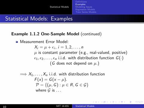
Example 1.1.2 One-Sample Model (continued)

Measurement Error Model: Xi = µ + Ei , i = 1, 2, . . . , n µ is constant parameter (e.g., real-valued, positive) E1, E2, . . . , En i.i.d. with distribution function G (·)

(G does not depend on µ.)

=⇒ X1, . . . , Xn i.i.d. with distribution function F (x) = G (x − µ). P = {(µ, G ) : µ ∈ R, G ∈ G} where G is . . .


Statistical Models


Example: One-Sample Model

Special Cases:

Parametric Model: Gaussian measurement errors {Ej } are i.i.d. N(0, σ2), with σ2 > 0, unknown.

Semi-Parametric Model: Symmetric measurement-error distributions with mean µ {Ej } are i.i.d. with distribution function G (·), where G ∈ G, the class of symmetric distributions with mean 0.

Non-Parametric Model: X1, . . . , Xn are i.i.d. with distribution function G (·) where

G ∈ G, the class of all distributions on the sample space X (with center µ)


Statistical Models



Example 1.1.3 Two-Sample Model

X1, X2, . . . , Xn i.i.d. with distribution function F (·) Y1, Y2, . . . , Ym i.i.d. with distribution function G (·) E.g., Sample n members of population A at random and m members of population B and measure some attribute of population members. Probability Model: P = {(F , G ), F ∈ F , and G ∈ G}

Specific cases relate F and G Shift Model with parameter δ

{Xi } i.i.d. X ∼ F (·), response under Treatment A. {Yj } i.i.d. Y ∼ G (·), response under Treatment B. Y =X + δ, i.e., G (v) = F (v − δ) δ is the difference in response with Treatment B instead of Treatment A.


Statistical Models


Outline



Statistical Models


Statistical Modeling Issues

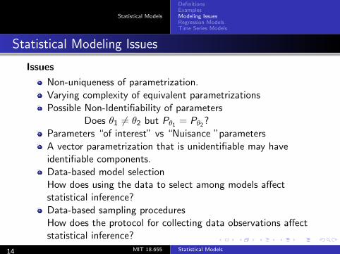
Issues

Non-uniqueness of parametrization. Varying complexity of equivalent parametrizations Possible Non-Identifiability of parameters

Does θ1 = Pθ2 ?= θ2 but Pθ1

Parameters “of interest” vs “Nuisance ”parameters A vector parametrization that is unidentifiable may have identifiable components. Data-based model selection How does using the data to select among models affect statistical inference? Data-based sampling procedures How does the protocol for collecting data observations affect statistical inference?


Statistical Models


Regular Models

Notation:

θ: a parameter specifying a probability distribution Pθ.

F (· | θ) : Distributon function of Pθ

Eθ[·]: Expectation under the assumption X ∼ Pθ. For a measurable function g(X ),

Eθ[g(X )] = g(x)dF (x | θ).X

p(x | θ) = p(x ; θ): density or probability-mass function of X

Assumptions:

Either All of the Pθ are continuous with densities p(x | θ), Or All of the Pθ are discrete with pmf’s p(x | θ) The set {x : p(x | θ) > 0} is the same for all θ ∈ Θ.


Statistical Models


Outline



Statistical Models


Regression Models

n cases i = 1, 2, . . . , n

1 Response (dependent) variable yi , i = 1, 2, . . . , n

p Explanatory (independent) variables xi = (xi ,1, xi ,2, . . . , xi ,p)T , i = 1, 2, . . . , n

Goal of Regression Analysis:

Extract/exploit relationship between yi and xi .

Examples

Prediction

Causal Inference

Approximation

Functional Relationships


Statistical Models


General Linear Model: For each case i , the conditional distribution [yi | xi ] is given by

yi = yi + Ei where

yi = β1xi ,1 + β2xi ,2 + · · · + βi ,pxi ,p

β = (β1, β2, . . . , βp)T are p regression parameters

(constant over all cases)

Ei Residual (error) variable (varies over all cases)

Extensive breadth of possible models Polynomial approximation (xi,j = (xi )

j , explanatory variables are different powers of the same variable x = xi )

Fourier Series: (xi,j = sin(jxi ) or cos(jxi ), explanatory variables are different sin/cos terms of a Fourier series expansion)

Time series regressions: time indexed by i , and explanatory variables include lagged response values.

Note: Linearity of yi (in regression parameters) maintained with non-linear x .


Statistical Models


Steps for Fitting a Model

(1) Propose a model in terms of

Response variable Y (specify the scale) Explanatory variables X1, X2, . . . Xp (include different functions of explanatory variables if appropriate) Assumptions about the distribution of E over the cases

(2) Specify/define a criterion for judging different estimators.

(3) Characterize the best estimator and apply it to the given data.

(4) Check the assumptions in (1).

(5) If necessary modify model and/or assumptions and go to (1).


Statistical Models


Specifying Assumptions in (1) for Residual Distribution

Gauss-Markov: zero mean, constant variance, uncorrelated

Normal-linear models: Ei are i.i.d. N(0, σ2) r.v.s

Generalized Gauss-Markov: zero mean, and general covariance matrix (possibly correlated,possibly heteroscedastic)

Non-normal/non-Gaussian distributions (e.g., Laplace, Pareto, Contaminated normal: some fraction (1 − δ) of the Ei are i.i.d. N(0, σ2) r.v.s the remaining fraction (δ) follows some contamination distribution).


Statistical Models


Normal Linear Regression Model

Y = Xβ + E ⎤⎡⎞⎛ ⎞⎛Y1 x1,1 x1,2 · · · x1,p β1

Y = ⎜⎜⎜⎝

Y2 . . .

⎟⎟⎟⎠ X =

⎢⎢⎢⎣

⎥⎥⎥⎦ β =

x2,1 x2,2 · · · x2,p . . ..

⎜⎝ ⎟⎠

. . .. . . . .. . . βpYn xn,1 xn,2 · · · xp,n

E = (E1, E2, . . . , En)T and Ej are i.i.d. N(0, σ2)

1with density f (E) = (2πσ2)− 12 exp(− · E2)

2σ2

Multivariate Normal Probability Model Y ∼ Nn(µ, σ

2Inp(Y1, Y2, . . . , Yn | θ) =

with parameter θ = (β, σ2) ∈ Θ = Rp × R+

)i=1

) where µ = Xβ and σ2 > 0. n Tf (Yj − x β),j


Statistical Models


Outline



Statistical Models


Statistical Models: Dependent Responses

Example 1.1.5 Measurement Model with Autoregressive Errors

X1, X2, . . . , Xn are n successive measurements of a physical constant µ

Xi = µ + ei , i = 1, 2, . . . , n

ei = βei−1 + Ei , i = 2, 3, . . . , n, and e0 = 0 where Ei are i.i.d. with density f (·).

Note:

The ei are not i.i.d. (they are dependent).

The Xi are dependent Xi = µ(1 − β) + βXi−1 + Ei , i = 2, . . . , n X1 = µ + E1


Statistical Models


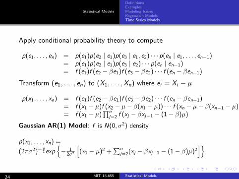
Apply conditional probability theory to compute

p(e1, . . . , en) = p(e1)p(e2 | e1)p(e3 | e1, e2) · · · p(en | e1, . . . , en−1) = p(e1)p(e2 | e1)p(e3 | e2) · · · p(en | en−1) = f (e1)f (e2 − βe1)f (e3 − βe2) · · · f (en − βen−1)

Transform (e1, . . . , en) to (X1, . . . , Xn) where ei = Xi − µ

p(x1, . . . , xn) = f (e1)f (e2 − βe1)f (e3 − βe2) · · · f (en − βen−1) = f (x1 − µ)f (x2 − µ − β(x1 − µ)) · · · f (xn − µ − β(xn−1 − µ)))n = f (x1 − µ) j=2 f (xj − βxj−1 − (1 − β)µ)

Gaussian AR(1) Model: f is N(0, σ2) density

p(x1, . . . , xn) = = n1(2πσ2)− n 2 exp − (x1 − µ)2 + (xj − βxj−1 − (1 − β)µ)22σ2 j=2


Statistical Models


Problems

Problem 1.1.3 Identifiable parametrizations.

Problem 1.1.4 Stochastically larger distributions in two-sample Models.

Problem 1.1.7 Symmetric distributions and their properties.

Problem 1.1.9 Collinearity: What conditions on X are required for the regression parameter β to be identifiable?

Problem 1.1.11 Scale Models and Shift Models.

Problem 1.1.12 Hazard rates and Cox proportional hazard model.

Problem 1.1.14 The Pareto distribution.


MIT OpenCourseWarehttp://ocw.mit.edu

18.655 Mathematical StatisticsSpring 2016

For information about citing these materials or our Terms of Use, visit: http://ocw.mit.edu/terms.

http://ocw.mit.edu/terms

http://ocw.mit.edu/

mathematical statistics, lecture 2 statistical models · 18.655 mathematical statistics spring 2016

Documents