mathematical programming - department of civil ... · mathematical programming lecture notes ce...

Math Programming 1 1/10/2003

Mathematical Programming Lecture Notes

CE 385D - McKinney Water Resources Planning and Management

Department of Civil Engineering The University of Texas at Austin

Section page

1. Introduction 2

2. General Mathematical Programming Problem 2

3. Constraints 3

4. Typical Forms of Math Programming Problems 4 4.1 Linear Programming 4 4.2 Classical Programming 5 4.3 Nonlinear Programming 6

5. Types of Solutions 6

6. Classical Programming 8 6.1 Unconstrained Scalar Case 8 6.2 Unconstrained Vector Case 9 6.3 Constrained Vector Case - Single Constraint 10 6.5 Constrained Vector Case – Multiple Constraints 14 6.6 Nonlinear Programming and the Kuhn-Tucker Conditions 16

Exercises 17

References 21

Appendix A. Mathematics Review 22 A.1 Linear Algebra 22 A.2 Calculus 29 A.3 Vectors Calculus 32


1. Introduction An optimization problem (mathematical program) is to determine the values of a vector of decision variables

=

nx

xM1

x

(1.1) which optimize (maximize or minimize) the value of an objective function

),x,,x f(x) f( nL21=x (1.2) The decision variables must also satisfy a set of constraints X which describe the system being optimized and any restrictions on the decision variables. The decision vector x is feasible if X iffeasibleis ∈xx (1.3) The feasible region X, an n-dimensional subset of nR , is defined by the set of all feasible vectors. An optimal solution *x has the properties (for minimization): (1) X *∈x (1.4) (2) * )( *)( xxxx ≠∀≤ ff (1.5) i.e., the solution is feasible and attains a value of the objective function which is less than or equal to the objective function value resulting from any other feasible vector.

2. General Mathematical Programming Problem The general mathematical programming problem can be stated as

X

)f(

∈x

xx

subject to

maximize

(2.1) In words this says,


maximize the objective function f(x) by choice of the decision variables x while ensuring that the optimal decision variables satisfy all of the constraints or restrictions of the problem

The objective function of the math programming problem can be either a linear or nonlinear function of the decision variables. Note that: )f(x maximize (2.2) is equivalent to

0, minimize

or,0, maximize

<+

>+

b)bf(a

b)bf(a

x

x

(2.3) That is, optimizing if a linear operator; multiplying by a scalar or adding a constant does not change the result and maximizing a negative is the same as minimizing a positive function.

3. Constraints The constraint set X of the math program can consist of combinations of:

(1) Linear equalities: b Ax = (3.1)

m,i b xa i

n

jjij L1

1==∑

= (3.2)

where the nm, j, iaij LL 11 == are the elements of the matrix A, and b is a vector of right-hand-side constants. For a review of matrix arithmetic and notation, linear equalities and inequalities, please see Section 7.1.

(2) Linear inequalities: b Ax ≤ (3.3)

m,i b xa i

n

jjij L1

1=≤∑

= (3.4)


(3) Nonlinear inequalities: 0 xg ≤)( (3.5)

r,j g j L1)( =≤ 0x

(3.6)

where the functions g(x) are nonlinear functions of the decision variables.

(4) Nonlinear equalities: 0 xh =)( (3.7)

m,i hi L1)( =≤ 0x (3.8) where the functions h(x) are nonlinear functions of the decision variables.

4. Typical Forms of Math Programming Problems Different forms of the objective function and constraints give rise to different classes of mathematical programming problems:

4.1 Linear Programming The objective function is linear and the constraints are linear equalities, inequalities, or both and non-negativity restrictions apply.

0xbAx

xcx

≥≤

⋅

tosubject

Maximize

(4.1)

Example:

1357195976

5tosubject

532 Maximize

321

321

321

321

≤+−

−=−+−−≥−+

++

xxxxxx

xxx

xxx


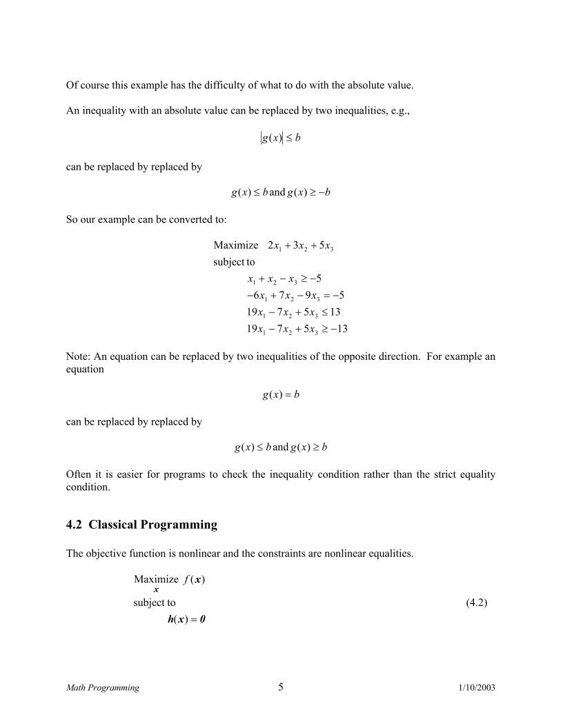
Of course this example has the difficulty of what to do with the absolute value. An inequality with an absolute value can be replaced by two inequalities, e.g.,

bxg ≤)(

can be replaced by replaced by

bxgbxg −≥≤ )(and)( So our example can be converted to:

135719135719

59765

tosubject532 Maximize

321

321

321

321

321

−≥+−≤+−

−=−+−−≥−+

++

xxxxxxxxx

xxx

xxx

Note: An equation can be replaced by two inequalities of the opposite direction. For example an equation

bxg =)( can be replaced by replaced by

bxgbxg ≥≤ )(and)( Often it is easier for programs to check the inequality condition rather than the strict equality condition.

4.2 Classical Programming The objective function is nonlinear and the constraints are nonlinear equalities.

0xh

xx

=)(tosubject

)(Maximize f

(4.2)


Example:

( ) ( )

02subject to

21 Minimize

21

22

21

=−

−+−

xx

xx

4.3 Nonlinear Programming The objective function is linear or nonlinear and the constraints are linear or nonlinear equalities, inequalities, or both.

0xg0xh

xx

≤=

)()(

tosubject

)(Maximize f

(4.3)

Example:

( )

0,032

subject to1xln Maximize

21

21

21

≥≥≤+

++

xxxx

x

5. Types of Solutions Solutions to the general mathematical programming problem are classified as either global or local solutions depending upon certain characteristics of the solution. A solution x* is a global solution (for maximization) if it is:

1. Feasible; and 2. Yields a value of the objective function less than or equal to that obtained by any other

feasible vector, or

Xff

X∈∀≥

∈xxx

x)(*)(

and,* (5.1)

A solution x* is a local solution (for maximization) if it is:

1. Feasible; and


2. Yields a value of the objective function greater than or equal to that obtained by any feasible vector x sufficiently close to it, or

*))(()(*)(

and,*xxxxx

x

εNXffX

∈∩∈∀≥∈

(5.2)

In this case multiple optima may exist for the math program and we have only established that x* is the optimum within the neighborhood searched. Extensive investigation of the program to find additional optima may be necessary. Sometimes we can establish the local or global nature of the solution to a math program. The following two theorems give some examples. Weierstras Theorem: (Sufficient conditions for a global solution)

If X is non-empty and compact (closed and bounded) and f(x) is continuous on X, then f(x) has a global maximum either in the interior or on the boundary of X.

Local - Global Theorem: (Sufficient conditions for a local solution to be global)

If X is a non-empty, compact and convex and f(x) is continuous on X and a concave (convex) function over X, then a local maximum is a global maximum.

The Figure 5.1 shows a non-convex function defined over a convex feasible region so we have no assurance that local maxima are global maxima. We must assume that they are local maxima. Figure 5.2 shows a concave (non-convex) function maximized over a convex constraint set, so we are assured that a local maximum is a global maximum (if we can find one) by the Local-Global Theorem.

x

f( x ) Global Max

Global Min

Local Max

Local Min

X

Figure 5.1. Illustration of global and local solutions.


x

f( x )

Global Max

X

Figure 5.2. Concave function maximized over a convex constraint set

6. Classical Programming

)(Maximize xx

f (6.1)

0xh =)(tosubject (6.2)

6.1 Unconstrained Scalar Case In this case, there are no constraints (Equation 6.2 is not present) and we consider only the objective function for a single decision variable, the scalar x )(Maximize xf

x (6.1.1)

The necessary conditions for a local minimum are

0)(=

dxxdf (first-order conditions) (6.1.2)

and

0)(2

2≤

dxxfd (second-order conditions) (6.1.3)

The first-order conditions represent an equation which can be solved for x* the optimal solution for the problem. But what if the decision variable was constrained to be greater than or equal to zero (non-negativity restriction), e.g., 0≥x ? In this case there are two possibilities, either (1) the solution


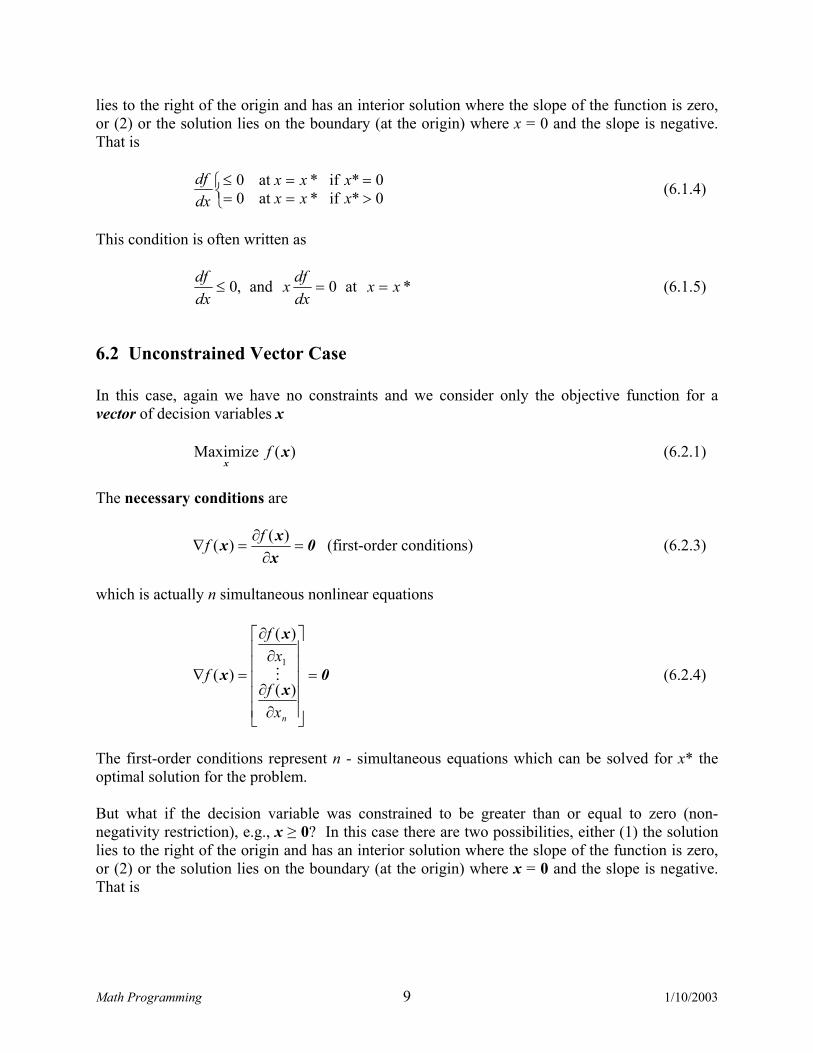
lies to the right of the origin and has an interior solution where the slope of the function is zero, or (2) or the solution lies on the boundary (at the origin) where x = 0 and the slope is negative. That is

>====≤

0*if*at00*if*at0

xxxxxx

dxdf (6.1.4)

This condition is often written as

*at0and,0 xxdxdfx

dxdf

==≤ (6.1.5)

6.2 Unconstrained Vector Case In this case, again we have no constraints and we consider only the objective function for a vector of decision variables x )(Maximize x

xf (6.2.1)

The necessary conditions are

0

xxx =

∂∂

=∇)()( ff (first-order conditions) (6.2.3)

which is actually n simultaneous nonlinear equations

0x

x

x =

∂∂

∂∂

=∇

nxf

xf

f)(

)(

)(1M (6.2.4)

The first-order conditions represent n - simultaneous equations which can be solved for x* the optimal solution for the problem. But what if the decision variable was constrained to be greater than or equal to zero (non-negativity restriction), e.g., x ≥ 0? In this case there are two possibilities, either (1) the solution lies to the right of the origin and has an interior solution where the slope of the function is zero, or (2) or the solution lies on the boundary (at the origin) where x = 0 and the slope is negative. That is


>====≤

∂∂

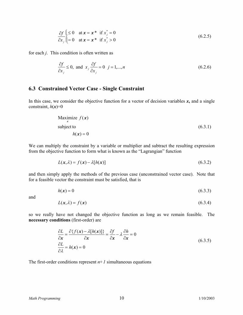
0if*at00if*at0

*

*

j

j

j xx

xf

xxxx

(6.2.5)

for each j. This condition is often written as

njxfx

xf

jj

j

,...,10and,0 ==∂∂

≤∂∂ (6.2.6)

6.3 Constrained Vector Case - Single Constraint In this case, we consider the objective function for a vector of decision variables x, and a single constraint, h(x)=0

0)(

tosubject

)(Maximize

=x

xx

h

f

(6.3.1)

We can multiply the constraint by a variable or multiplier and subtract the resulting expression from the objective function to form what is known as the “Lagrangian” function )]([)(),( xxx hfL λλ −= (6.3.2) and then simply apply the methods of the previous case (unconstrained vector case). Note that for a feasible vector the constraint must be satisfied, that is 0)( =xh (6.3.3) and )(),( xx fL =λ (6.3.4) so we really have not changed the objective function as long as we remain feasible. The necessary conditions (first-order) are

0)(

0)]}([)({

==∂∂

=∂∂

−∂∂

=∂−∂

=∂∂

x

xxxxx

x

hL

hfhfL

λ

λλ

(6.3.5)

The first-order conditions represent n+1 simultaneous equations


0)(

0

0

0

22

11

=

=∂∂

−∂∂

=∂∂

−∂∂

=∂∂

−∂∂

xhxh

xf

xh

xf

xh

xf

nn

λ

λ

λ

M (6.3.6)

which must be solved for the optimal values of x* and λ*. Example (adapted from Loucks et al., 1981, Section 2.6, pp. 23-28) Consider a situation where there is a total quantity of water R to be allocated to a number of different uses. Let the quantity of water to be allocated to each use be denoted by xi, i=1,…, I. The objective is to determine the quantity of water to be allocated to each use such that the total net benefits of all uses is maximized. We will consider an example with three uses I = 3.

R

User 1

S

User 2 User 3 Reservoir

x1 x2 x3

B1 B2B3

Figure 6.4.1. Reservoir release example. The net-benefit resulting from an allocation of xi to use i is given by

3,2,1)( 2 =−= ixbxaxB iiiiii (6.4.1) where ai and bi are given positive constants. These net-benefit (benefit minus cost) functions are of the form shown in Figure 6.4.2.


Net economic benefit to user i

0

5

10

15

20

25

30

35

0 2 4 6 8 10

B1B2B3

Figure 6.4.2. Net-benefit function for user i.

The three allocation variables xi are unknown decision variables. The values that these variables can take on are restricted between 0 (negative allocation is meaningless) and values whose sum, x1 + x2 + x3, does not exceed the available supply of water R minus the required downstream flow S. The optimization model to maximize net-benefits can be written as

0

subject to

)(maximize

3

1

2

=−+

−

∑

∑

=

=

RSx

xbxa

ii

3

1iiiii

x

(6.4.2) The Lagrangian function is

( )

−+−−= ∑∑

==

RSxxbxa,Li

i

3

1iiiii )(

3

1

2 λλx (6.4.3)

There are now four unknowns in the problem, xi , i = 1, 2, 3 and λ . Solution of the problem is obtained by applying the first-order conditions, setting the first partial derivatives of the Lagrangian function with respect to each of the variables equal to zero:


0

02

02

02

321

3333

2222

1111

=−+++=∂∂

=−−=∂∂

=−−=∂∂

=−−=∂∂

RSxxxL

xbaxL

xbaxL

xbaxL

λ

λ

λ

λ

(6.4.4)

These equations are the necessary conditions for a local maximum or minimum ignoring the nonnegativity conditions. Since the objective function involves the maximization of the sum of concave functions (functions whose slopes are decreasing), any local optima will also be the global maxima (by the Local-Global Theorem). The optimal solution of this problem is found by solving for each xi , i = 1, 2, 3 in terms of λ .

3,2,12

=−

= ib

ax

i

ii

λ (6.4.5)

Then solve for λ by substituting the xi , i = 1, 2, 3 into the constraint

0

3

1=−+∑

=RSx

ii

(6.4.6)

02

3

1=−+∑

−

=RS

ba

i i

i λ (6.4.7)

and solve for λ

∑

∑

=

=

−+

= 3

1

3

1

12

2

i i

i i

i

b

RSb

a

λ (6.4.8)

Hence knowing R, S, ai and bi this last equation can be solved for λ . Substitution of this value into the equation for the xi , i = 1, 2, 3, we can solve for the optimal allocations, provided that all of the allocations are nonnegative.


6.5 Constrained Vector Case – Multiple Constraints In this case, we consider the objective function for a vector of decision variables x, and a vector of constraints, h(x)=0

0xh

xx

=)(tosubject

)(Maximize f

(6.5.1)

We can multiply the constraints by a vector of variables or multipliers ),...,,( 21 mλλλλ = or

)(xh⋅λ and subtract the resulting expression from the objective function to form what is known as the “Lagrangian” function

∑=

−=⋅−=m

iii )(hffL

1)()()(),( xxxhxx λλλ (6.5.2)

and then simply apply the methods of the previous case (unconstrained vector case). The necessary conditions (first-order) are 0xhxx, =∇⋅−∇=∇ )()()( xxx fL λλ (6.5.3) or

0)]()([1

=∑∂∂

−∂∂

=∂

⋅−∂=

∂∂

=

m

i

ii

hffLxxx

xhxx

λλ (6.5.4)

and 0x, =∇ )( λλ L (6.5.5) or 0xh =)( (6.5.6) The first-order conditions (Eq. 6.5.4 and Eq. 6.5.6) represent n+m simultaneous equations must be solved for the optimal values of the vectors of decision variables and the Lagrange multipliers, x* and λ*. Example (after Haith, 1982, Example 4-2): Solve the following optimization problem using Lagrange multipliers.


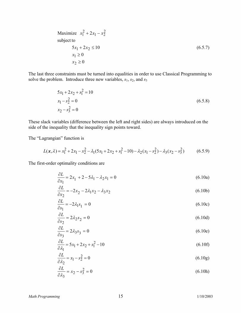
00

1025tosubject

2Maximize

2

1

21

221

21

≥≥

≤+

−+

xx

xx

xxx

(6.5.7)

The last three constraints must be turned into equalities in order to use Classical Programming to solve the problem. Introduce three new variables, s1, s2, and s3

0

0

1025

232

221

2121

=−

=−

=++

sx

sx

sxx

(6.5.8)

These slack variables (difference between the left and right sides) are always introduced on the side of the inequality that the inequality sign points toward. The “Lagrangian” function is )()()1025(2),( 2

3232212

21211

221

21 sxsxsxxxxxL −−−−−++−−+= λλλλx (6.5.9)

The first-order optimality conditions are

0522 12111

=−−+=∂∂ xxxL λλ (6.10a)

232122

22 xxxxL λλ −−−=

∂∂ (6.10b)

02 111

=−=∂∂ ssL λ (6.10c)

02 222

==∂∂ ssL λ (6.10d)

02 333

==∂∂ ssL λ (6.10e)

1025 2121

1−++=

∂∂ sxxLλ

(6.10f)

0221

2=−=

∂∂ sxLλ

(6.10g)

0232

3=−=

∂∂ sxLλ

(6.10h)


Equations 6.10c-e require that λi or si be equal to zero. There can be several solutions to the problem depending on whether one or another of the λi or si are equal to zero.

6.6 Nonlinear Programming and the Kuhn-Tucker Conditions In this case, we consider the objective function for a vector of decision variables x, a vector of equality constraints, h(x)=0, and a vector of inequality constraints, g(x)≤0

0xg0xh

xx

≤=

)()(

tosubject

)(Maximize f

(6.6.1)

We can multiply the constraints by vectors of variables or multipliers ),...,,( 21 mλλλλ = or

)(xh⋅λ and ),...,,( 21 ruuu=u or )(xgu ⋅ and subtract the resulting expression from the objective function to form what is known as the “Lagrangian” function

∑−∑−===

r

jjj

m

iii )(gu)(hfL

11)(),,( xxxux λλ (6.6.2)

and then simply apply the methods of the previous case (unconstrained vector case). The necessary conditions (first-order) are the Kuhn-Tucker Conditions

nk

xg

uxh

xfx

xg

uxh

xf

r

j k

jj

m

i k

ii

kk

r

j k

jj

m

i k

ii

k,...,1for*,at

0

0

11

*

11==

=

∑

∂

∂−∑

∂∂

−∂∂

≤∑∂

∂−∑

∂∂

−∂∂

==

==xx

λ

λ

(6.6.3)

rjgu

g

jj

j,...,1for

0*)(

0*)(=

=

≤

x

x (6.6.4)

mihi ,...,1for,0*)( ==x (6.6.5)

rjunkx

jk

,...,1,0,...,1,0*

=≥=≥ (6.6.6)


Exercises 1. (after Mays and Chung, 1992, Exercise 3.4.5) Water is available at supply points 1, 2, and 3 in quantities 4, 8, and 12 thousand units, respectively. All of this water must be shipped to destinations A, B, C, D, and E, which have requirements of 1, 2, 3, 8, and 10 thousand units, respectively. The following table gives the cost of shipping one unit of water from the given supply point to the given destination. Find the shipping schedule which minimizes the total cost of transportation.

Destination Source A B C D E

1 7 10 5 4 122 3 2 0 9 1 3 8 13 11 6 14

A

B

C

D

E

1

2

3Supply Destination

A

B

C

D

E

1

2

3Supply Destination

2. (adapted from Mays and Tung, 1992, Exercise 3.1.1) Solve the following Linear Program

1357195976

5tosubject

532 Maximize

321

321

321

321

≤+−

−=−+−−≥−+

++

xxxxxx

xxx

xxx


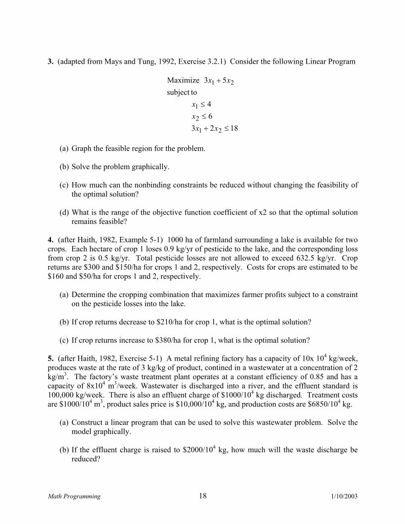
3. (adapted from Mays and Tung, 1992, Exercise 3.2.1) Consider the following Linear Program

182364

tosubject53 Maximize

21

2

1

21

≤+≤≤

+

xxxx

xx

(a) Graph the feasible region for the problem.

(b) Solve the problem graphically.

(c) How much can the nonbinding constraints be reduced without changing the feasibility of

the optimal solution?

(d) What is the range of the objective function coefficient of x2 so that the optimal solution remains feasible?

4. (after Haith, 1982, Example 5-1) 1000 ha of farmland surrounding a lake is available for two crops. Each hectare of crop 1 loses 0.9 kg/yr of pesticide to the lake, and the corresponding loss from crop 2 is 0.5 kg/yr. Total pesticide losses are not allowed to exceed 632.5 kg/yr. Crop returns are $300 and $150/ha for crops 1 and 2, respectively. Costs for crops are estimated to be $160 and $50/ha for crops 1 and 2, respectively.

(a) Determine the cropping combination that maximizes farmer profits subject to a constraint on the pesticide losses into the lake.

(b) If crop returns decrease to $210/ha for crop 1, what is the optimal solution? (c) If crop returns increase to $380/ha for crop 1, what is the optimal solution?

5. (after Haith, 1982, Exercise 5-1) A metal refining factory has a capacity of 10x 104 kg/week, produces waste at the rate of 3 kg/kg of product, contined in a wastewater at a concentration of 2 kg/m3. The factory’s waste treatment plant operates at a constant efficiency of 0.85 and has a capacity of 8x104 m3/week. Wastewater is discharged into a river, and the effluent standard is 100,000 kg/week. There is also an effluent charge of $1000/104 kg discharged. Treatment costs are $1000/104 m3, product sales price is $10,000/104 kg, and production costs are $6850/104 kg.

(a) Construct a linear program that can be used to solve this wastewater problem. Solve the model graphically.

(b) If the effluent charge is raised to $2000/104 kg, how much will the waste discharge be

reduced?


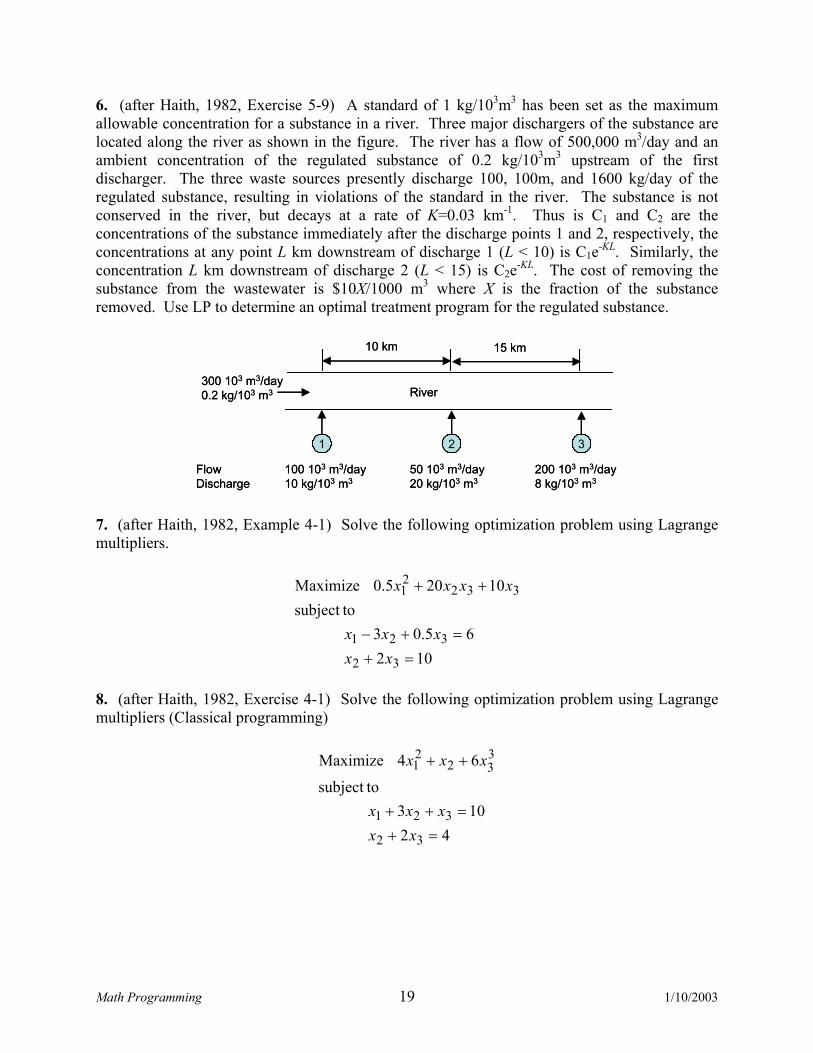
6. (after Haith, 1982, Exercise 5-9) A standard of 1 kg/103m3 has been set as the maximum allowable concentration for a substance in a river. Three major dischargers of the substance are located along the river as shown in the figure. The river has a flow of 500,000 m3/day and an ambient concentration of the regulated substance of 0.2 kg/103m3 upstream of the first discharger. The three waste sources presently discharge 100, 100m, and 1600 kg/day of the regulated substance, resulting in violations of the standard in the river. The substance is not conserved in the river, but decays at a rate of K=0.03 km-1. Thus is C1 and C2 are the concentrations of the substance immediately after the discharge points 1 and 2, respectively, the concentrations at any point L km downstream of discharge 1 (L < 10) is C1e-KL. Similarly, the concentration L km downstream of discharge 2 (L < 15) is C2e-KL. The cost of removing the substance from the wastewater is $10X/1000 m3 where X is the fraction of the substance removed. Use LP to determine an optimal treatment program for the regulated substance.

1 2 3

River300 103 m3/day0.2 kg/103 m3

100 103 m3/day10 kg/103 m3

50 103 m3/day20 kg/103 m3

200 103 m3/day8 kg/103 m3

FlowDischarge

10 km 15 km

1 2 3

River300 103 m3/day0.2 kg/103 m3

100 103 m3/day10 kg/103 m3

50 103 m3/day20 kg/103 m3

200 103 m3/day8 kg/103 m3

FlowDischarge

10 km 15 km

7. (after Haith, 1982, Example 4-1) Solve the following optimization problem using Lagrange multipliers.

10265.03

tosubject10205.0 Maximize

32

321

33221

=+=+−

++

xxxxx

xxxx

8. (after Haith, 1982, Exercise 4-1) Solve the following optimization problem using Lagrange multipliers (Classical programming)

42103

tosubject

64 Maximize

32

321

332

21

=+=++

++

xxxxx

xxx


9. (after Haith, 1982, Exercise 4-2) Solve the following optimization problem using Lagrange multipliers (Classical programming)

066

tosubject4 Maximize

1

21

221

≥=−

−−

xxx

xe x

10. (after Willis, 2002) A waste storage facility consists of a right circular cylinder of radius 5 units and a conical cap. The volume of the storage facility is V. Determine H, the height of the storage facility, and h, the height of the conical cap, such that the total surface area is minimized.


References Haith, D.A., Environmental Sytems Optimization, John Wiley & Sons, New York, 1982 Loucks, D. P. et al., Water Resource Systems Planning and Analysis, Prentice Hall, Englewood Cliffs, 1981 Mays, L.W., and Y-K, Tung, Hydrosystems Engineering and Management, McGraw Hill, 1992 Mathematical Programming and Optimization Texts Bradley, S.P., Hax, A.C., And Magnanti, T.L., Applied Mathematical Programming, Addison-Wesley, Reading, 1977 Fletcher, Practical Methods of Optimization, ... Gill, P.E., W. Murray, and M.H. Wright, Practical Optimization, Academic Press, London, 1981 Hadley, G., Linear Programing, Addison Wesley, Reading, 1962 Hadley, G., Nonlinear and Dynamic Programming, Addison Wesley, Reading, 1962 Hillier, F. S. and G.J. Lieberman, Introduction to Operation Research, McGraw-Hill, Inc., New York, 1990. Intrilligator, M.D., Mathematical Optimizatiron and Economic Theory, Prentice-Hall, Inc., Englewood Cliffs, 1971. Luenberger, D.G., Linear and Nonlinear Programming, Addison Wesley, New York, 1984. McCormick, G.P., Nonlinear Programming: Theory, Algorithms, and Applications, John Wiley and Sons, 1983. Taha, H.A., Operations Research: An Introduction, MacMillan, New York, 1987. Wagner, H.M., Principles of Operations Research, Prentice-Hall, Inc., Englewood Cliffs, 1975.


Appendix A. Mathematics Review

A.1 Linear Algebra

A.1.1 Introduction An important tool in many areas of scientific and engineering analysis and computation is matrix theory or linear algebra. A wide variety of problems lead ultimately to the need to solve a linear system of equations Ax = b. There are two general approaches to the solution of linear systems.

A.1.2 Matrix Notation

A matrix is an array of real numbers. Consider an (m x n) matrix Arr

with m rows and n columns:

=

mnmmm

nn

aaaa

aaaaaaaa

KMOM

L

321

22322211131211

A

(A.1.2.1) The horizontal elements of the matrix are the rows and the vertical elements are the columns. The first subscript of an element designates the row, and the second subscript designates the column. A row matrix (or row vector) is a matrix with one row, i.e., the dimension m = 1. For example

( )nrrrr L321=r (A.1.2.2) A column vector is a matrix with only one column, e.g.,

`

=

mc

cc

M21

c

(A.1.2.3) When the row and column dimensions of a matrix are equal (m = n) then the matrix is called square

=

nnnn

nn

aaa

aaaaaa

LOM

L

21

2222111211

A

(A.1.2.4) The transpose of the (m x n) matrix A is the (n x m)


=

mnnn

mm

T

aaa

aaaaaa

LOM

L

21

2221212111

A

(A.1.2.5) A symmetric matrix is one where AT = A. An example of a symmetric matrix is

= 21

12 A (A.1.2.6)

A diagonal matrix is a square matrix where elements off the main diagonal are all zero

=

nna

aa

0

0

22

11

OA

(A.1.2.7) An identity matrix is a diagonal matrix where all the elements are one’s

=

10

101

O

I

(A.1.2.8) An upper triangular matrix is one where all the elements below the main diagonal are zero

=

nn

n

n

a

aaaaa

0

222

11211

O

L

A

(A.1.2.9) A lower triangular matrix is one where all the elements above the main diagonal are zero

=

nnnn aaa

aaa

L

OM

21

2221

11 0

A

(A.1.2.10)


A.1.3 Matrix Arithmetic Two (m x n) matrices A and B are equal if and only if each of their elements are equal. That is A = B if and only if aij = bij for i = 1,...,m and j = 1,...,n (A.1.3.1) The addition of vectors and matrices is allowed whenever the dimensions are the same. The sum of two (m x 1) column vectors a and b is

=

+

=+

mmmm + ba

+ ba + ba

b

bb

a

aa

MMM

22

11

2

1

2

1

ba

(A.1.3.2) Example:

Let )4,2,3,1( −=u and )2,1,5,3( −−=v . Then

)2,1,2,4()24,12,53,31( =−−+−+=+ vu

)20,10,15,5()4*5,2*5),3(*5,1*5(5 −=−=u

)14,7,21,7()6,3,15,9()8,4,6,2(32 −−=−−+−=− vu The sum of two (m x n) matrices A and B is

+++

++++++

=

+

=+

mnmnmmmm

nn

nn

mnmm

n

n

mnmm

n

n

b a b a b a

b a b a b a b a b a b a

bbb

bbbbbb

aaa

aaaaaa

K

MOM

L

K

MOM

L

K

MOM

L

2211

1122222121

1112121111

21

12221

11211

21

12221

11211

BA

(A.1.3.3)


Multiplication of a matrix A by a scalar α is defined as

=

mnmm

n

n

αaαaαa

αaαaαaαaαaαa

α

K

OM

L

21

22221

11211

A

(A.1.3.4) The product of two matrices A and B is defined only if the number of columns of A is equal to the number of rows of B. If A is (n x p) and B is (p x m), the product is an (n x m) matrix C

++++++

++++++++++++

=

=

mnmnnmmmnmmnm

mnnnmnmn

mnnnmnmn

mnmm

n

n

mnmm

n

n

babababababa

babababababababababababa

bbb

bbbbbb

aaa

aaaaaa

=

LKLL

MOM

LLL

LLLL

K

MOM

L

K

MOM

L

11212111111

2121221221121121

1111211211111111

21

12221

11211

21

12221

11211

ABC

(A.1.3.5) The ij element of the matrix C is given by

kj

p

kikij ba c ∑

=

=1 (A.1.3.6)

That is the cij element is obtained by adding the products of the individual elements of the i-th row of the first matrix by the j-th column of the second matrix (i.e., “row-by-column”). The following figure shows an easy way to check if two matrices are compatible for multiplication and what the dimensions of the resulting matrix will be:

mppnmn xxx BAC = (A.1.3.7) Example:

Let ),,,( 21 naaa L=a and

=

nb

bb

M2

1

b , then


nn

n

n bababa

b

bb

aaa +++=

=⋅ LM

L 22112

1

21 ),,,(ba

Example:

Let

=

nnnn

n

n

aaa

aaaaaa

L

MM

L

L

21

22221

11211

A and

=

nb

bb

M2

1

b , then

nnnnn

nn

nn

nnnnn

n

n

bababa

babababababa

b

bb

aaa

aaaaaa

L

L

L

M

L

MM

L

L

++

++++

=

=

2211

2222111

1212111

2

1

21

22221

11211

Ab

Matrix division is not a defined operation. The identity matrix has the property that IA=A and AI = A. If A is an (n x n) square matrix and there is a matrix X with the property that AX = I (A.1.3.8) where I is the identity matrix, then the matrix X is defined to be the inverse of A and is denoted A-1. That is AA-1 = I and A-1A = I (A.1.3.9) The inverse of a (2 x 2) matrix A can be represented simply as

−

−−

=−

1121

1222

21122211

1 1aaaa

aaaa A

(A.1.3.10)

Example

If

=

2112

A , then

−

−=

−

−−

=−

3/23/13/13/2

2112

)1(1)2(21 1A

A.1.4 Systems of Linear Equations Consider the linear system of equations


bAx = (A.1.4.1) where A is an (n x n) matrix, b is a column vector of constants, called the right-hand-side, and x is the unknown solution vector to be determined. This system can be written out as

=

nnnnnn

n

n

b

bb

x

xx

aaa

aaaaaa

MM

L

OM

L

2

1

2

1

21

22221

11211

(A.1.4.2) Performing the matrix multiplication and writing each equation out separately, we have

nnnnnn

nn

nn

b x a x a xa

b x a x a xa b x a x a xa

=+++

=+++=+++

L

M

L

L

2211

22222121

11212111

(A.1.4.3a) This system can also be written in the following manner

n,i b xa i

n

jjij L1

1==∑

= (A.1.4.3b) A formal way to obtain a solution using matrix algebra is to multiply each side of the equation by the inverse of A to yield bAAxA 11 −− = (A.1.4.4) or, since IAA 1 =− bA x 1−= (A.1.4.5) Thus, we have obtained the solution to the system of equations. Unfortunately, this is not a very efficient way of solving the system of equations. We will discuss more efficient ways in the following sections. Example: Consider the following two equations in two unknowns:

2 2x x18 2x 3x

21

21

=+−=+

Solve the first equation for x2


923

12 x x +−

=

which is a straight line with an intercept of 9 and a slope of (-3/2). Now, solve the second equation for x2

121

12 x x +=

which is also a straight line, but with an intercept of 1 and a slope of (1/2). These lines are plotted in the following Figure. The solution is the intersection of the two lines at x1 = 4 and x2 = 3.

2

4

6

8

2 4 6 8 x1

x 2

3x1 + 2x2 = 18

-x1 + 2x2 = 2

Solut ion: x1 = 4 ; x2 = 3

Figure A.1.4.1. Graphical solution of two simultaneous linear equations. Each linear equation

ininii b x a x a xa =+++ L2211 (A.1.4.6) represents a hyperplane in an n-dimensional Euclidean space (Rn), and the system of equations Ax = b represents m hyperplanes. The solution of the system of equations is the intersection of all of the m hyperplanes, and can be

- the empty set (no solution) - a point (unique solution)


- a line (non-unique solution) - a plane (non-unique solution)

A.1.5 Systems of Linear Inequalities A system of m linear inequalities in n unknowns can be written as bAx ≤ (A.1.5.1) or

nnnnnn

nn

nn

b x a x a xa

b x a x a xa b x a x a xa

≤+++

≤+++≤+++

L

M

L

L

2211

22222121

11212111

(A.1.5.2a) This system of inequalities can also be written in the following manner

n,i b xa i

n

jjij L1

1=≤∑

= (A.1.5.2b) Each linear inequality

ininii b x a x a xa ≤+++ L2211 (A.1.5.3) represents a half-space in Rn, and the system of inequalities Ax ≤ b represents the intersection of m half-spaces which is a polyhedral convex set or, if bounded, a polyhedron.

A.2 Calculus

A.2.1 Functions A function )(xf of n variables can be written as )(xfy = (A.2.1.1)

)();( 11

scalarRyvectorcolumnRx

xn

n

∈∈

= Mx (A.2.1.2)


A linear function of n variables is written as

nn

n

iii xcxcxcxcfy +++==⋅== ∑

=

L22111

)( xcx (A.2.1.3)

where c is a vector of coefficients.

A.2.2 Sets, Neighborhoods and Distance The distance between two points x and y in Rn is defined as

∑=

−=n

iii yxd

1

2)(),( yx (A.2.2.1)

A neighborhood around a point x in Rn is defined as the set of all points y less than some distance ε from the point x or { }εε <∈= ),(:)( yxyx dRN n (A.2.2.2) A closed set is a set which contains all of the points on its boundary, for example a closed interval on the real line (R1). In a bounded set, the distance between two points contained in the set is finite. A compact set is closed and bounded, examples are any finite interval [a,b] on the real line or any bounded sphere in R3. A set S is a convex set if for any two points x and y in the set, the point yxz )1( aa −+= (A.2.2.3) is also in the set for all a, where 0 ≤ a ≤ 1. That is, all weighted averages of two points in the set are also points in the set. For example, all points on a line segment joining two points in a convex set are also in the set. Straight lines, hyperplanes, closed halfspaces are all convex sets. Figure 2 below illustrates a convex and a non-convex set. A real valued function f(x) defined on a convex set S is a convex function if given any two points x and y in S, )()1()()]()1()([ yxyx faaffaaff −+≤−+ (A.2.2.4) for all a, where 0 ≤ a ≤ 1. Figure 3 illustrates the fact that the line segment joining two points in a convex function does not lie below the function. Figure 4 shows general examples of convex and non-convex (or concave) functions. An example of a convex function is a parabola which opens upward. Linear functions (lines, planes, hyperplanes, half-spaces) are both convex and non-convex functions.


x

xy

y

convex

non-convex

Figure A.2.2.1. General diagram of convex and non-convex sets.

yx ax + (1-a)y

X

x

f( x )

f( a x + (1-a) y )

f( x )

f( y )

af(x) + (1-a)f(y)

Figure A.2.2.2. General diagram of a convex function.

x

f( x )

Convex Concave

Figure A.2.2.3. General diagram of a convex function and a concave function.


A.2.3 Derivatives The derivative of a function of a single scalar variable f(x) is defined as

x

xfxxfdxdfxf

x ∆−∆+

==′→∆

)()(lim)(0

(A.2.3.1)

The partial derivatives of a function f of the variables x and y are defined as

yyxfyyxf

yf

xyxfyxxf

xf

y

x

∆−∆+

=∂∂

∆−∆+

=∂∂

→∆

→∆

),(),(lim

),(),(lim

0

0 (A.2.3.2)

That is, to find the partial derivative of a multivariable function with respect to one independent variable xi, regard all other independent variables as fixed and find the usual derivative with respect to xi. The partial derivative of a function of several variables f(x) with respect to a particular component of x, xi, evaluated at a point xo is

oii x

fxf

x

x∂

∂=

∂∂ )( (A.2.3.3)

The partial derivative of f(x) with respect to the vector x is a row vector of partial derivatives of the function or the gradient vector

∂∂

∂∂

=∂∂

=∇nx

fxfff L1

)(x

x (A.2.3.4)

A.3 Vectors Calculus

A.3.1 Coordinate Systems Typical coordinate systems used in groundwater problems include: Rectangular: x, y, z; and Cylindrical: r, θ, z where x = rcosθ and y = rsinθ. Let A be a vector function of (x, y, z) or (r, θ, z), respectively, then kθrkjiA zrzyx AAAAAA ++=++= θ (A.3.1.1) where (i, j, k) and (r, θ, k) are unit vectors in the (x, y, z) or (r, θ, z) directions, respectively.


A.3.2 Basic Operators The gradient operator, del (from the Greek nabla) or ∇ , is defined in rectangular coordinates as the vector

kjizyx

z

y

x

∂⋅∂

+∂

⋅∂+

∂⋅∂

=

∂⋅∂

∂⋅∂

∂⋅∂

=⋅∇)()()(

)(

)(

)(

)( (A.3.2.1)

The major operators: Gradient, “del” or , )(⋅∇ ; Divergence, “div” or )(⋅⋅∇ ; and Laplacian, “del dot del” or )()( 2 ⋅∇=⋅∇⋅∇ can be defined in the rectangular and cylindrical coordinate systems as:

Gradient (Rectangular) kjizyx ∂⋅∂

+∂

⋅∂+

∂⋅∂

=⋅∇)()()()( (A.3.2.2)

(Cylindrical) kθrzrr ∂⋅∂

+∂

⋅∂+

∂⋅∂

=⋅∇)()(1)()(

θ (A.3.2.3)

Divergence (Rectangular) z

Ay

Ax

A zyx∂

∂+

∂

∂+

∂∂

=⋅∇ A (A.3.2.4)

Proof:

[ ]

zA

yA

xA

zA

zA

zA

yA

yA

yA

xA

xA

xA

zA

zA

zA

yA

yA

yA

xA

xA

xA

AAAzyx

zyx

zyx

zyx

zyx

zyx

zyx

zyx

zyx

∂∂

+∂

∂+

∂∂

=

∂∂

+∂

∂+

∂∂

+

∂∂

+∂

∂+

∂∂

+

∂∂

+∂

∂+

∂∂

=

⋅∂

∂+⋅

∂

∂+⋅

∂∂

+

⋅∂

∂+⋅

∂

∂+⋅

∂∂

+

⋅∂

∂+⋅

∂

∂+⋅

∂∂

=

++⋅

∂

⋅∂+

∂⋅∂

+∂

⋅∂=⋅∇

)1()0()0(

)0()1()0(

)0()0()1(

)()()(

kkjkik

kjjjij

kijiii

kjikjiA


(Cylindrical) z

AArr

rAr

zr

∂∂

+∂∂

+∂

∂=⋅∇

θθ1)(1A (A.3.2.5)

Laplacian (Rectangular) 2

2

2

2

2

22 )()()()()(

zyx ∂⋅∂

+∂

⋅∂+

∂⋅∂

=⋅∇=⋅∇⋅∇ (A.3.2.6)

e.g., 2

2

2

2

2

22

zA

yA

xA zyx

∂∂

+∂

∂+

∂∂

=∇=∇⋅∇ AA

(Cylindrical) 2

2

2

2

22 )()(1))((1)()(

zrrr

rr ∂⋅∂

+∂

⋅∂+

∂⋅∂

∂∂

=⋅∇=⋅∇⋅∇θ

(A.3.2.7)

e.g., 2

2

2

2

22 1)(1

zAA

rrAr

rrzr

∂∂

+∂∂

+∂

∂∂∂

=∇=∇⋅∇θ

θAA

A.3.3 Various Groundwater Relations The Piezometric head, zph += γ/ , is a scalar quantity and the gradient of this quantity is a column vector

kjizh

yh

xh

zhyhxh

h∂∂

+∂∂

+∂∂

=

∂∂∂∂∂∂

=∇ (A.3.3.1)

The hydraulic conductivity, K, is a tensor whose common form in three dimensions is

=

z

y

x

KK

K

000000

K (A.3.3.2)

The term h∇⋅K is the product of the matrix K with the vector h∇ or (using “row by column” multiplication)

kjiKzhK

yhK

xhK

zhK

yhKxhK

zhyhxh

KK

Kh zyx

z

y

x

z

y

x

∂∂

+∂∂

+∂∂

=

∂∂∂∂∂∂

=

∂∂∂∂∂∂

⋅

=∇⋅

000000

(A.3.3.3)


Now h∇⋅⋅∇ K is the dot product of the vector )(⋅∇ with the vector h∇⋅K or

∂∂

∂∂

+

∂∂

∂∂

+

∂∂

∂∂

=

∂∂

+∂∂

+∂∂

⋅

∂

⋅∂+

∂⋅∂

+∂

⋅∂=

∂∂∂∂∂∂

⋅

∂⋅∂

∂⋅∂

∂⋅∂

=∇⋅⋅∇

zhK

zyhK

yxhK

x

zhK

yhK

xhK

zyx

zhK

yhKxhK

z

y

xh

zyx

zyx

z

y

x

kjikji

K

)()()(

)(

)(

)(

(A.3.3.4)

mathematical programming - department of civil ... · mathematical programming lecture notes ce...

Documents