mathematical models of membranes - department of...

MATHEMATICAL MODELS OF MEMBRANES

ELIZABETH BLACK

Abstract. This paper outlines molecular dynamics simulations and their lim-

itations when modeling large-scale shape dynamics of cellular membranes. We

explore concepts from differential geometry and cellular-mechanics to describecellular membranes in terms of Helfrich’s equation of generalized shape energy,

which provides the theoretical framework for understanding shape changes in

liposome vesicles. We present an outline of the derivation of Helfrich’s shapeequation in order to illustrate how these equations can be used to model large-

scale shape changes in biological cells. We conclude by discussing biological

applications of the equations in modeling red blood cell shape.

Contents

1. Introduction 12. Modeling 32.1. MD Simulations 32.2. Continuum Models 42.3. Curves, Orientation, and Curvature 52.4. Surfaces 72.5. Surface curvature 72.6. The First Fundamental Form 92.7. Second fundamental form 112.8. Normal, Principal, Mean, and Gaussian Curvature 123. Helfrich’s Equation of Generalized Shape Energy 144. The Shape Equation 155. Biological Applications: Red blood Cells 17Acknowledgments 19References 19

1. Introduction

The behavior of biological systems, such as lipid bilayers and cellular membranes,can be fundamentally tied to mathematical concepts through theoretical models.Scientists have been using theoretical models to develop a better understandingof biological systems. Computational simulations and free energy functionals uti-lize mathematics to define abstract physical concepts into concrete mathematicalexpressions and help us understand how components of the biomolecular systemsinteract with each other. By solving these expressions, we may model overall mem-brane dynamics, including cell movement and undulations in cell shape. In this

Date: October 13, 2013.

1

2 ELIZABETH BLACK

present work, we focus on how molecular dynamics simulations and Helfrich’s equa-tion of generalized shape energy use mathematics to depict the dynamics of lipidbilayer systems, and how they have been used to explain biomolecular phenomenaassociated with cellular membranes such as the shape of human red blood cells.

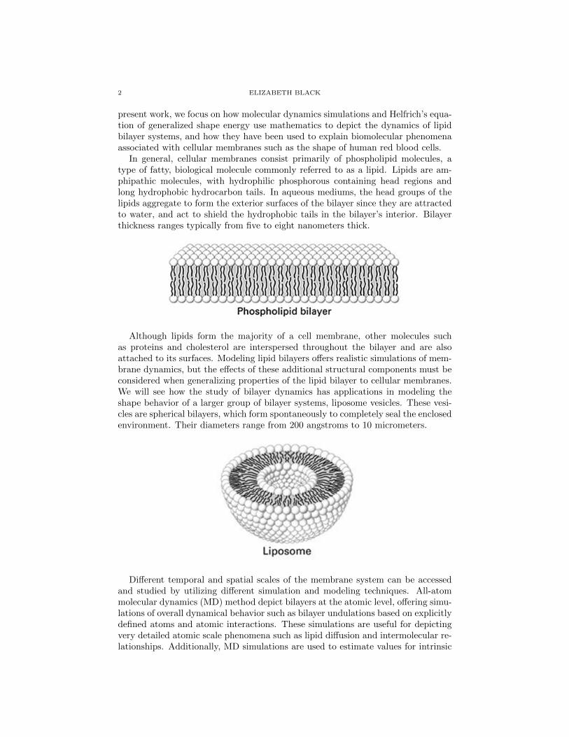
In general, cellular membranes consist primarily of phospholipid molecules, atype of fatty, biological molecule commonly referred to as a lipid. Lipids are am-phipathic molecules, with hydrophilic phosphorous containing head regions andlong hydrophobic hydrocarbon tails. In aqueous mediums, the head groups of thelipids aggregate to form the exterior surfaces of the bilayer since they are attractedto water, and act to shield the hydrophobic tails in the bilayer’s interior. Bilayerthickness ranges typically from five to eight nanometers thick.

Although lipids form the majority of a cell membrane, other molecules suchas proteins and cholesterol are interspersed throughout the bilayer and are alsoattached to its surfaces. Modeling lipid bilayers offers realistic simulations of mem-brane dynamics, but the effects of these additional structural components must beconsidered when generalizing properties of the lipid bilayer to cellular membranes.We will see how the study of bilayer dynamics has applications in modeling theshape behavior of a larger group of bilayer systems, liposome vesicles. These vesi-cles are spherical bilayers, which form spontaneously to completely seal the enclosedenvironment. Their diameters range from 200 angstroms to 10 micrometers.

Different temporal and spatial scales of the membrane system can be accessedand studied by utilizing different simulation and modeling techniques. All-atommolecular dynamics (MD) method depict bilayers at the atomic level, offering simu-lations of overall dynamical behavior such as bilayer undulations based on explicitlydefined atoms and atomic interactions. These simulations are useful for depictingvery detailed atomic scale phenomena such as lipid diffusion and intermolecular re-lationships. Additionally, MD simulations are used to estimate values for intrinsic

MATHEMATICAL MODELS OF MEMBRANES 3

properties of cell membranes, such as membrane elasticity, as direct experimenta-tion with lipid bilayers is difficult or impossible, due in part to their microscopicsize and limitations of current experimental technology.

Free energy functionals, which are continuum representations of physical behav-ior in the system of interest, can be utilized to describe larger scale dynamics ofmembranes, such as the shape behavior of liposome vesicles. In this work, we willfocus on functionals that model the effects of stresses on the shape of the liposome.These models are formulated based on fluctuations in equilibrium shape influencedby bending, pressure, and volume deformations and the resistance of the membraneto those fluctuations. We will see how these continuum models offer insights intobiological phenomena such as the equilibrium biconcave shape of human red bloodcells.

This paper offers a background of MD simulation and their limitations, explain-ing the necessity of a continuum approach to characterize the shape behavior oflarger liposome systems. Before offering a background on the Helfrich equation forshape energy, it discusses methods that are used to describe the bilayer through thelanguage of differential geometry. The paper provides a brief outline of the deriva-tion of the shape equation, subsequently discussing the biological applications ofthe free energy models and shape equation used in this work.

2. Modeling

2.1. MD Simulations. MD simulations utilize the following classical equations ofmotion to iteratively evolve the movements of a biomolecular system based on themovements of the atoms it contains:

Fi = miai Fi = − ∂

∂riU

The interactions between atoms are pre-defined and are represented by potentialenergy functions, U as a function of atomic position, ri. The force acting on eachatom, Fi is derived from U by the second equation above. Changes in atomicposition and may be calculated by the first equation in small enough windows oftime from this force as the initial positions, masses mi and velocities vi of eachatom are known. Repeating this proscess over small frames of time produces acollection of atomic positions which may be viewed together as a trajectory of thesystem’s movements over time. Trajectories with time lengths of picoseconds tonanoseconds are generally accessible using the current computational resources.

To illustrate this process more clearly, let us consider a flat patch of a lipidbilayer, spanning the x and y directions of a three dimensional box of space withside lengths of 10 micrometers. To simulate a more realistic bilayer system, we willenforce periodic boundary conditions in the x and y directions. In doing so, thesimulation box is replicated to form an infinite lattice in these directions, portrayingan edgeless bilayer patch. If a molecule leaves the boundaries of the central box inthe x or y direction, it will enter through the respective opposite periodic boundary.

Every atom defining the lipid bilayer is represented by a mass and position in thesimulation box. From here, we must also define the initial velocities of the atomsand the interactions between them before we begin calculating their movements.The initial velocities of the atoms are obtained by defining the temperature ofthe simulation, and setting the total momentum of the system, Σmivi, to zero,which guarantees that there are no external forces on the box. The interactions

4 ELIZABETH BLACK

between atoms are defined by potential energy functions based on the nature of theinteraction. For example, a single covalent bond interaction between two atoms Aand B can be represented by the following potential energy functional:

U(rAB) =1

2kAB(rAB − rAB,eq)2

where rAB = rA − rB is the distance between A and B, rAB,eq is the distancebetween A and B at which U has a minimum, and kAB is a constant dependenton the identity of the atoms involved. In this interaction, the bond interaction isrepresented as a spring and models the potential energy characteristic of a simpleharmonic oscillator; the further the atoms are apart, the more the string is stretchedthe more potential energy it has and wants to snap back to its original position.

After interactions between and the initial positions and velocities of the atomsare defined, simulation begins by calculating the force acting on each atom, wherethis force is the negative derivative of the potential energy function describing theinteractions which the atom is involved in. From the force, each atoms velocityfor the next timestep can be found by integrating and solving Newtons secondequation of motion, Fi = miai, as acceleration is the derivative of velocity andmass is defined.

In small enough windows of time ranging from femto- to picoseconds, new atomicposition can be generated based on the calculated velocities. The length of thesetimesteps is chosen to ensure the distances traveled by the atoms are no greaterthan the length of the shortest bond in the system to ensure realistic atomic dy-namics. If the timestep was longer, atoms contained in the shortest bond couldmove unrealistically outside the small bond length, resulting in a large restoringforce acting to counter this relatively large bond ”stretch” away from its equilib-rium length. Additionally, timesteps are chosen to be smaller than the shortestvibrational wavelength of a bond, as steps too large could gloss over importantdynamical information happening at these smaller wavelengths.

By repeating the calculations described above for subsequent timesteps, snap-shots of the atoms’ positions as a function of timesteps can compiled into tra-jectories. These trajectories model fluctuations and dynamics of the bilayer as awhole by describing the movements of its atoms, with bilayer phenomena such asundulations appearing on scales of several nanoseconds.

2.2. Continuum Models. Computational limitations can be prohibitive when all-atom MD simulations are used to model large liposome membranes, which mayrequire solving for millions of degree of freedom. A modest sized, 100-nanometerliposome consists of tens of thousands of lipid molecules, with each lipid consistingof up to one hundred and fifty atoms. Even if the configuration and the vastamount and variety of interactions between the millions of atoms contained in theliposome were defined, the computational power required to perform the associatedcalculations would take months to generate even a modest trajectory.

To realistically model and study the behavior of larger bilayer systems, theymust be simplified without losing relevant information. In Helfrich’s Equation ofGeneralized Shape Energy, the overall shape of an entire liposome is not modeledas a function of small scale changes in the millions of atoms it contains, but utilizeslarger scale membrane properties to parameterize a continuous scalar property ofthe system: free energy.


Parameters of this free energy model generalize physical characteristics and prop-erties associated with the lipid bilayer system and together offer a description ofthe relative stability of a membrane in a particular physical configuration. Many ofthese parameters can be expressed mathematically, utilizing the language of differ-ential geometry. Other parameters are constants quantifying the relative intensityof intrinsic properties of the bilayer, such as elasticity, and may be approximatedfrom analysis of MD simulations. Through outlining the derivation of the shapeequation, we will see how Helfrich’s equation mathematically models the equilib-rium shape and dynamics of the liposome, as they both seek a shape configurationthat minimizes the liposome’s free energy.

Before discussing the free energy model and how it models liposome shape, wemust first become familiar with the bilayer system as a mathematical surface, uti-lizing differential geometry to describe the physical conformations its surface maytake.

2.3. Curves, Orientation, and Curvature. Curves and surfaces can be ex-pressed implicitly or explicitly, but for this discussion we will focus on their para-metric representation.

Definition 2.1. A smooth parameterized plane curve is a subset of R2 describedby the positional vector ~r : [a, b] → R2 and scalar value t ∈ [a, b] such that theposition of the curve in R2 may be represented as functions of t:

~r(t) = (x(t), y(t))

where x and y are continuous and have continuous derivatives for all values oft ∈ (a, b) A plane curve is said to be of class r if x and y have continuous derivativesup to order r, inclusive.

Definition 2.2. A smooth parameterized space curve is subset R3 described bythe positional vector ~r: [a, b] →R3 and scalar value t ∈ [a, b] such that position ofthe curve may be represented as functions of t:

~r(t) = (x(t), y(t), z(t))

where the functions x, y and z are continuous and have continuous derivatives forall values of t ∈ (a, b) A space curve is said to be of class r if x, y and z havecontinuous derivatives up to order r, inclusive.

As t increases from a to b, the positional vector traces out a path of points inspace, which, when taken together, form the curve. If the parameter of the curve istaken to be the arc length of the curve, it is said to have a natural parameterization,and we will denote the arc length parameter as s. Planar curves may also exist inR3, having at least one constant parameterization for its coordinates.

At any point along its parameterization, the orientation of a curve may be de-scribed by three mutually orthogonal unit vectors called the unit tangent, unit mainnormal, and bi-normal vectors. We find the vectors of a naturally parameterizedcurve by differentiating the curve’s parameterization with respect to arc length, s.

Definition 2.3. The unit tangent vector ~t(s) of a naturally parameterized curve~r(s) is

~t(s) =~r ′(s)

||~r ′(s)||

6 ELIZABETH BLACK

Definition 2.4. The unit main normal vector ~m(s) of a naturally parameterizedcurve described by ~r(s) is

~m(s) =~t ′(s)

||~t ′(s)||=

~r ′′(s)

||~r ′′(s)||

Definition 2.5. The bi-normal ~b(s) vector of a naturally parameterized curvedescribed by ~r(s) is

~b(s) = ~t(s)× ~m(s)

The triple vectors define a moving frame and a local coordinate system at eachpoint along the curve. This frame is referred to as the Frenet Frame with theosculating plane defined by ~m and ~t. Properties and characteristics of curves canbe described by changes in these vectors and this frame, geometrically symbolizingthe relative strengths in which the curve is bent and twisted in space.

The tangent vector has a simple geometric interpretation. The vector ~r(s+ ∆s)- ~r(s) offers the directionality from ~r(s) to ~r(s + ∆s). By dividing this vector bychanges in arc length ∆s , and taking the limit as ∆s goes to zero, we converge ata finite magnitude vector describing the directionality of the curve at a point: thetangent vector:

lim∆s→0

~r(s+ ∆s)− ~r(s)∆s

= ~r ′(s)

The unit tangent vector is found by normalizing the magnitude of the tangentvector.

Changes in the tangent vector are used to characterize the curvature of a curve,and offer a scalar value representing how much the curve bends, or the relativeextent to which a curve in not contained in a straight line. Curvature intuitivelyleads us to the normal vector, as this vector describes the relative rate of the changeof tangent vector along the curve.

Definition 2.6. The curvature k(s) of curve at a point s along its parameteriza-tion is defined as

k(s) = ||~t ′(s)|| = 1

γ

where γ is the radii of the circle tangent to the curve at that point, known as theosculating circle.

Curvature can be also quantified by the angular speed of rotation of a curve’smain normal vector as a function of s. Let ~r(s) describe a plane curve. As wemove from point P = ~r(s) to point Q = ~r(s + ∆s) the tangent vectors at thosepoints, ~r ′(s) and ~r ′(s+ ∆s) and the vector describing their difference, ~r ′(s+ ∆s)- ~r ′(s) form an isosceles triangle, following from the fact that ~r ′(s) and ~r ′(s−∆s)are both vectors of the same unit length. Let us denote ∆Φ as the angle between~r ′(s + ∆s) and ~r ′(s). It follows that the length of the third side of the triangle,~r ′(s + ∆s) - ~r ′(s) is related to the curvature in the following way as ∆s goes tozero:

||~r ′(s+ ∆s)− ~r ′(s)|| = ∆Φ · 1 = ∆Φ = ||~r ′′∆s||Thus, the curvature can also be represented as:

k(s) = ||~r ′′(s)|| = lim∆s→0

|∆Φ

∆s|


For space curves, another means of curvature must be defined, as the curve notonly bends but twists in space. This twisting is measured by the curve’s torsion.The torsion quantifies the extent to which curve deviates from the osculating plane.

Definition 2.7. The torsion τ(s) of a naturally parameterized space curve at apoint s along its parameterization is defined as

τ(s) = −~m(s) · dds~b(s)

Geometrically, the torsion characterizes the angular speed of rotation of the bi-normal vector as a function of s and may be expressed as:

τ(s) = lim∆s→0

|∆ϕ∆s|

where ∆ϕ is the angle between the bi-normal vectors ~b(s+ ∆s) and ~b(s)

2.4. Surfaces. The lipid bilayer can be represented as a smooth, two dimensionalsurface embedded in a three dimensional Euclidean space.

Definition 2.8. A smooth surface in R3 is a subset S ⊂ R3 such that each pointin S has a neighborhood U ⊂ S and is described by a map ~r : V → R3 from anopen set V ⊂ R2 such that

• V and U are homeomorphic, meaning ~r : V → U is a bijection that continu-ously maps V into U , and its inverse function, ~r −1 exists and is continuous.• ~r(u, v) = (x(u, v), y(u, v), z(u, v)) has continuous partial derivatives of all

orders.• For all points in S, ~r is a regular parameterization, meaning the first partial

derivatives ~ru and ~rv are linearly independent.

Before continuing, it is convenient to notate the partial derivatives of a smoothsurface described by ~r(u, v) in the following manner:

~rv =d~r

dv, ~ruu =

d2~r

du2, ~ruv =

d2~r

dudv, and ~rvv =

d2~r

dv2

We may describe the orientation of a surface at a point by generalizing theorientation of the curves passing through that point. We define a tangent plane ata point on the surface by generalizing the tangent vectors of the curves on a surfacethrough that point and we specify a new surface normal vector with respect to thetangent plane.

Definition 2.9. The tangent space of a smooth parameterized surface S at pointp = ~r(u, v) contains all the tangent vectors of curves through that point. This spacedefines a tangent plane to that point on a surface.

Definition 2.10. The unit surface normal ~n of a smooth parameterized surfaceat a point p = ~r(u, v) is the vector orthogonal to the tangent plane at point p:

~n =~ru × ~rv| ~ru × ~rv|

8 ELIZABETH BLACK

2.5. Surface curvature. As with surface orientation, a natural way to investigatehow much a surface curves at a point is to look at the curvature of the curvespassing though that point on the surface. We relate the curves’ curvature to thesurface’s by projecting the curvature of specific curves into regions described by theDarboux frame.

Definition 2.11. The Darboux frame at a point p on a smooth surface withrespect to a smooth curve on the surface passing through p, ~r(s) = ~r(u(s), v(s)), isdefined by the surface normal vector ~n, unit tangent vector ~t of the curve, and a

tangent normal vector ~g = ~N × ~t, which is orthogonal to the surface normal andthe curve’s tangent vector.

The vectors in this plane are perpendicular to each other, and the frame formsan orthonormal basis for R3. It follows that the smooth curve, ~r can be written aslinear combination of the vectors in this frame.

Definition 2.12. The normal curvature κn and geodesic curvature κg of a

smooth surface S at point p in the direction specified by the unit tangent, ~t andmain normal, ~m vectors of a smooth curve ~r(s) = ~r(u(s), v(s)) on S at p are definedby

κn(s) = ~m(s) · ~n(s)

κg(s) = ~m(s) · ~g(s)

and are related to the curve’s curvature κ by

κ · ~n = κn + κg

κn is positive if ~r(s) bends towards the surface normal vector ~n, and κg is positiveif ~r(s) bends towards the tangent normal vector ~g.

Geometrically κn measures the magnitude of the projection of curvature of thecurve, κ onto the surface normal, ~n, at that point. Similarly, kg measures themagnitude of κ projected onto the tangent vector. In this way, κn describes thecomponent of the curve’s curvature, κ in the surface normal direction of the Dar-boux frame, while κg describes the curvature in the tangent normal direction.


Definition 2.13. Given a naturally parameterized smooth curve ~c : s→ S(u(s), v(s))on a smooth surface S, geodesic torsion τg at a point p is given by:

τg = τ − δθ

δswhere τ is the torsion of c at p, and θ is the angle between surface normal and theprincipal normal of c at s.

The geodesic torsion describes the rate of change of the surface normal around thecurve’s tangent vector, giving us another means of describing the extent of surfacecurvature by looking at its curves.

Definition 2.14. The normal section of the surface at a point p along adirection specified by a vector ~x is the plane generated by and containing thesurface normal at that point, ~n, and ~x.

Definition 2.15. Principal curvatures, c1 and c2 of a surface S at point p arethe extremal values of kn of the smooth curves generated by the intersection of thenormal section of the surface with S. The directionality of the normal section isgiven by the curves’ tangent vectors, and called the principal directions. c1 istaken as the maximum and c2, the minimum.

Definition 2.16. The Gaussian curvature, K at a point p of a surface is definedas the product of the principal curvatures:

K = c1c2

Definition 2.17. The mean curvature H at a point p of a surface is defined as

H =c1 + c2

2

2.6. The First Fundamental Form. Describing surface curvature more rigor-ously requires a discussion of the first and second fundamental forms of a surface.These forms define important metric properties of a surface and can be used todescribe curvature in terms of how much Euclidean length and volume is deformedat points on a surface. The first fundamental form acts as the surface metric, en-abling calculations of lengths and area on surface as it defines a unit of length onthe surface.

Definition 2.18. Let p be a point on a smooth surface S. The first fundamentalform at p is defined as

I = < ~V , ~U >

where ~V and ~U are elements of the tangent space at p.

Since the inner product on R3 is defined as the dot product, the first fundamentalform may be expressed in quadratic from:

Edu2 + 2Fdudv +Gdv2

where the coefficients of the first fundamental form, E, F , and G are

E = ~ru · ~ru, F = ~ru · ~rv, and, G = ~rv · ~rvWe will see later that it is also convenient to express the coefficients of the first

fundamental form in a matrix:

Iu,v =

∣∣∣∣ E FF G

∣∣∣∣

10 ELIZABETH BLACK

denoting its determinant as |g|=EG− F 2

We now will see how the first fundamental form defines the surface metric ona surface by considering its relation to the differential arc length ∆s of a smoothparameterized curve on a smooth surface S. The differential arc length defineslength on the surface metric by defining the the arc length between two infinitelyclose points of a curve on a surface.

Definition 2.19. The differential arc length ∆s of a smooth curve, ~r(t) is thedistance along the contour of the curve as t1 → t2, where t1 and t2 are parametersused to describe points of the curve.

The differential arc length may be approximated by the Euclidean distance, orchord length, between two points of the curve, p = ~r(t) and q = ~r(t + ∆t) as ∆tgoes to zero. To find this infinitely small chord length, we take a first order Taylorexpansion of the magnitue of the vector ∆~r = ~r(t)− ~r(t+ ∆t) as ∆t goes to zero:

∆s ' |∆~r | = |~r(t)− ~r(t+ ∆t)| = |d~rdt

∆t+1

2

d2~r

dt2(∆t)2| ' |d~r

dt|∆t

As p approaches q or ∆t goes to zero (utilizing slightly different notation) the lengthof ∆r becomes the differential arc length, ds, of the curve:

ds = |d~rdt|dt = |~r ′|dt =

√~r ′ · ~r ′dt

The first fundamental form shows itself when we compute the differential arclength for the smooth curve ~r(u(t), v(t)) on a surface ~r(u, v):

ds =√~r ′ · ~r ′dt

=√

( ~ruu′(t) + ~rvv′(t)) · ( ~ruu′(t) + ~rvv′(t))dt

=√

( ~ru · ~ru)(u′(t))2 + 2( ~ru · ~rv)u′(t)v′(t) + (~rv · ~rv)(v′(s))2dt

=√

(E(u′(t))2 + 2Fu′(t)v′(t) +G(v′(t))2)dt

=√Edu2 + 2Fdudv +Gdv2

=√I

Thus the first fundamental form encodes information about the surface metricby describing small changes in length on a surface as a function of small changesin the surface’s parameterization:

ds2 = I

It follows the arc length of a naturally parameterized smooth curve, r(s) =r(u(s), v(s)) with values of s ranging from a to b on a smooth surface is:∫ b

a

|~r ′(s)ds| =∫ b

a

√(Eu′(s)2 + 2Fu′(s)v′(s) +Gv′(s)2)ds

As the first fundamental form describes length on a parameterized surface, itintuitively follows that it is related to area on a surface. Just as the ds offers adescription of length by approximating the arc length between two infinitesimally


close points ~r(u, v) and ~r(u + du, v + dv) on a parameterized surface, the areaelement,

dA = |~ru × ~rv|approximates the area of an infinitesimally small parallelogram with vertices ~r(u, v), ~r(u+du), ~r(u, v + dv) and ~r(u+ du, v + dv) and can be used to calculate area of regionson a surface.

Definition 2.20. The surface area of a bounded region, ~r(Q) on a smooth pa-rameterized surface, ~r is given by∫ ∫

Q

|~ru × ~rv| du dv =

∫ ∫Q

dAdu dv.

The first fundamental form and dA are related through the determinant of thefirst fundamental form, g = EG− F 2

EG− F 2 = ( ~ru · ~ru)(~rv · ~rv)− ( ~ru · ~rv)2 = |~ru × ~rv|2

ThusdA =

√|g|

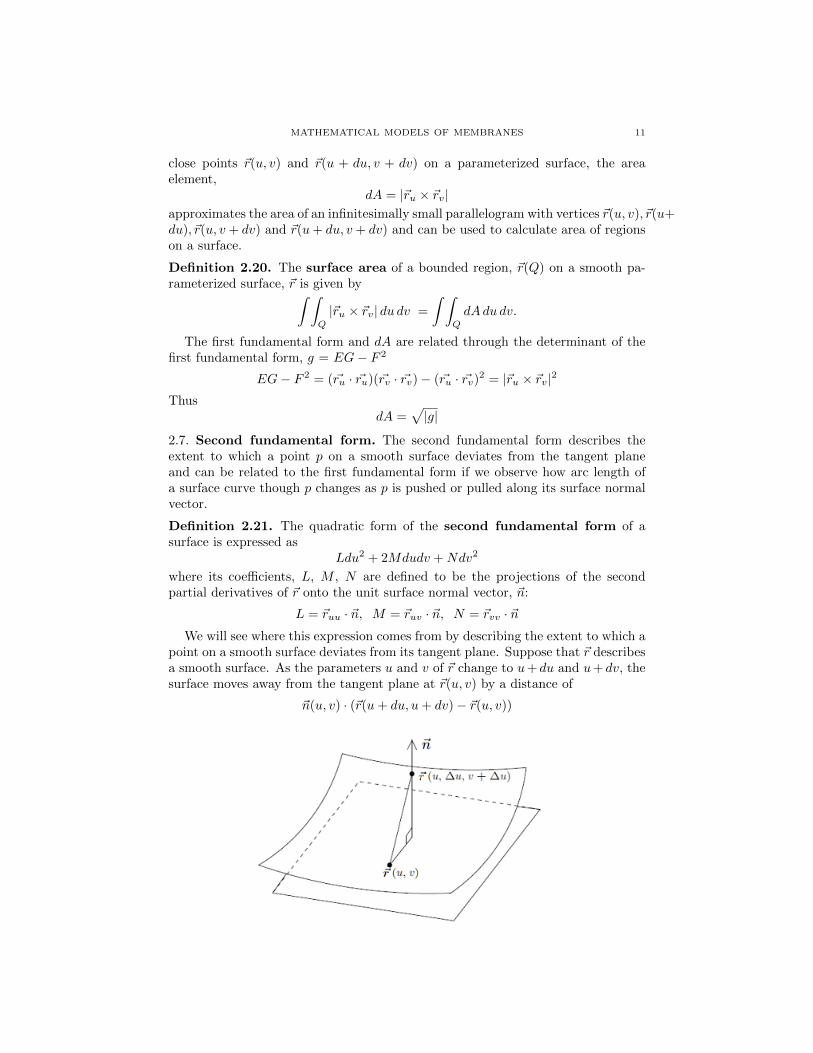
2.7. Second fundamental form. The second fundamental form describes theextent to which a point p on a smooth surface deviates from the tangent planeand can be related to the first fundamental form if we observe how arc length ofa surface curve though p changes as p is pushed or pulled along its surface normalvector.

Definition 2.21. The quadratic form of the second fundamental form of asurface is expressed as

Ldu2 + 2Mdudv +Ndv2

where its coefficients, L, M , N are defined to be the projections of the secondpartial derivatives of ~r onto the unit surface normal vector, ~n:

L = ~ruu · ~n, M = ~ruv · ~n, N = ~rvv · ~nWe will see where this expression comes from by describing the extent to which a

point on a smooth surface deviates from its tangent plane. Suppose that ~r describesa smooth surface. As the parameters u and v of ~r change to u+ du and u+ dv, thesurface moves away from the tangent plane at ~r(u, v) by a distance of

~n(u, v) · (~r(u+ du, u+ dv)− ~r(u, v))

12 ELIZABETH BLACK

By the two variable form of Taylors theorem, ~r(u+ du, u+ dv)− ~r(u, v) is equalto

~rudu+ ~rvdv +1

2(~ruudu

2 + 2~ruvdudv + ~rvvdv2) + remainder

where remainderdu2+dv2 tends to zero as du2 + dv2 tends to zero. As ~ru and ~rv are tangent

vectors, they are perpendicular to ~n(u, v) thus the deviation of the surface from itstangent plane may be expressed as

1

2(Ldu2 + 2Mdudv +Ndv2) + remainder

The second fundamental form can also be expressed in a matrix, where:

IIuv =

∣∣∣∣ L MM N

∣∣∣∣The relation of the second fundamental form to the first can be seen by con-

sidering changes in the surface metric, or first fundamental form, as is a point isdeformed about the surface normal. Suppose we have a surface S described by theparameterization ~r(u, v). Deformational changes in this surface along the surface

normal, ~n can be described by a family of surfaces, ~R(u, v, t) = ~r(u, v) - t~r(u, v),

where the first fundamental form of ~R is expressed as

IR = E(t)du2 + 2F (t)dudv +G(t)dv2

where ~Ru = ~ru− t~nu, ~Rv=~rv− t~nv. The second fundamental form of ~r = ~R(u, v, 0)is found to be

IIR =1

2

d

dtIR

It should be noted that this expression corresponds to the second fundamental

form only for the surface ~r(u, v) = ~R(u, v, 0) and not of the entire family of surfaces~R(u, v, t) as we considered the change in arc length deformation expressed by 1

2ddtIR

only at time t=0 along the normal. Derivatives at different points correspond to

the second fundamental form of different surfaces in the family ~R(u, v, t).

2.8. Normal, Principal, Mean, and Gaussian Curvature. The curvature ofa surface can be expressed in terms of the first and second fundamental forms of asurface.

Theorem 2.22. If ~r:(u, v)→ R3 describes a smooth surface S and ~r(s) = ~r(u(s), v(s)),a smooth curve on S at point p, then the normal curvature, κn is given by

κn =IIrIr

=L+ 2MΛ +N2

E + 2FΛ +GΛ2

where Λ = dudv is the direction of the tangent line at ~r(s)

Proof. Let ~r:(u, v) → R3 describe a smooth surface S, and ~r(s) = ~r(u(s), v(s))a smooth curve on S through point p. We know by definition ~n · ~t = 0, and bydifferentiating this expression along the curve with respect to s, we obtain

d~t

ds· ~n+ ~t · d~n

ds= 0


Thus, we arrive at the following expression for the normal curvature at s by defini-tion of the triple unit vectors, ds and the first fundamental form:

κn(s) = ~m(s) · ~n(s) =d~t

ds· ~n = −~t · d~n

ds= −dr

ds· dnds

= −dr · dndr · dr

=Ldu2 + 2Mdudv +Ndv2

Edu2 + 2Fdudv +Gdv2

where

L = −~ru · ~nu M = −1

2(~ru · ~nv + ~rv · ~nu) = −~ru · ~nv = −~rv · ~nu N = −~rv · ~nv

and E, F and G are the coefficients of the first fundamental form. Since ~ru and~rv are perpendicular to ~n we may write an alternative expression for L, M and Ncorresponding to the coefficients of the second fundamental form: we have ~ru · ~n =0 and ~rv · ~n = 0.

0 = (~ru · ~n)u = ~ruu · ~n+ ~ru · ~nu =⇒ L = −~ruu · ~n

0 = (~rv · ~n)v = ~rvv · ~n+ ~rv · ~nv =⇒ [N = ~rvv · ~n

0 = (~ru · ~n)v = ~ruv · ~n+ ~ru · ~nv =⇒ M = ~ruvN

Therefore, the normal curvature is given by:

κn(s) =IIrIr

=L+ 2MΛ +N2

E + 2FΛ +GΛ2

�

The above theorem enables us to calculate the extreme values, or principal cur-vatures, of a smooth surface at point p by evaluating dκn

dΛ =0. which gives:

(2.23) (E + 2FΛ +GΛ2)(NΛ +M)− (L+ 2MΛ +NΛ2)(GΛ + F ) = 0

Thus

κn =L+ 2MΛ +N2

E + 2FΛ +GΛ2=M +NΛ

F +GΛFurthermore, since

E + 2FΛ +GΛ2 = (E + FΛ) + Λ(F +GΛ)

L+ 2MΛ +NΛ2 = (L+MΛ) + Λ(M +NΛ)

We may reduce (2.24) to

(E + FΛ)(M +NΛ) = (L+MΛ)(F +GΛ)

Thus, the extreme values of κn must satisfy both

(L− κnE)du+ (M − κnF )dv = 0

(M − κnF )du+ (N − κnG)dv = 0

Therefor, the principal curvatures c1 and c2 are the roots of the following systemof equations

det(II − cI) = 0 det

∣∣∣∣ L− κnE M − κnFM − κnF N − κnG

∣∣∣∣ = 0

14 ELIZABETH BLACK

which may also be expressed in quadratic form as:

(EG− F 2)κ2n − (NE + LG− 2MF )κn + (LN −M2) = 0

Expressions of the Gaussian and mean curvatures may be similarly expressed interms of the first and second fundamental forms:

Theorem 2.24. The Gaussian curvature K of a surface is

K =LN −M2

EG− F 2

Theorem 2.25. The mean curvature H of a surface is

H =LG− 2FM +NE

2(EG− F 2)

3. Helfrich’s Equation of Generalized Shape Energy

We saw how differential geometry offers a more rigorous means of describingcurvature and metric properties of lipid bilayers by representing them as mathe-matical surfaces. Fluctuations in overall lipid bilayer shape can be represented froma more unified point of by view by associating free energy with deformations dueto bending, pressure differences, and surface tension.

The free energy of a system may be thought of as its capacity to do work, and canbe used to describe the energetic stability of a system. Higher values of free energyare energetically unfavorable, and the system, in this case the liposome membranes,will seek to lower its free energy by moving into a more favorable conformation.The membrane’s movement may be thought of as work.

The general equation relating curvature, pressure, and volume deformations ofa liposome’s shape to free energy is given below:

Definition 3.1. Helfrich’s Equation of Generalized Shape Energy describesthe free energy of a liposome represented as a smooth parameterized surface, ~r andis given by

FHelfrich =kc2

∮(2H − c0)2dA+ ∆P

∮dV + λ

∮dA

where dA is the area element, dV is the volume element, ∆P is the pressure dif-ference between the inside and outside of the liposome, kc is the bending modulus,λ is the tensile stress acting on the surface, and c0 is the spontaneous curvature ofthe membrane, which is the value of mean curvature that minimizes the free energyof the system.

The first part of the equation, kc2∮

(2H−c0)2dA expresses the total elastic energyof the membrane, or the free energy associated with bending deformations on thesurface of the membrane. We arrive at the total elastic energy of the membraneby integrating the elastic energy of curvature per unit area over the surface of themembrane, utilizing the area element dA which we previously discussed.

Definition 3.2. Theelastic energy of curvature per unit area of a membrane Fc is given by

Fc =kc2

(2H − c0)2 + k̄K

where K Gaussian curvature, kc is the bending modulus, c0 is the spontaneouscurvature, and k̄ is the elastic modulus of Gaussian curvature.


Since we have described the membrane as a smooth mathematical surface, wemay describe bending deformations on the membranes in terms of curvature. Wesee that the elastic energy of curvature per unit area utilizes both mean and Gauss-ian curvature to represent membrane shape in terms of free energy at a particularpoint on a membrane. The expression quantifies the extent to which the curva-ture deviates from the most energetically favorable curvature, or the equilibriumcurvature. Doing so describe the relative stability of the liposome’s conformation.

The first part of the curvature free energy accounts for energetic differences inmean curvature. It relates the mean curvature to free energy using a functionalform similar to one we saw earlier:

U(rAB) =1

2kAB(rAB − rAB,eq)2

Here however, instead of describing the potential energy associated with stretch-ing the bond length of two atoms from its equilibrium length, we describe thepotential energy associated with deviating from the equilibrium value of mean cur-vature. C0 represents the mean curvature at which the shape free energy is at itsequilibrium value, or the mean curvature a membrane naturally assumes if sub-jected to no deformations.

The bending modulus, kc is a constant which quantifies the extent to how muchthe bending free energy is affected from a deviation from the spontaneous curvatureand can be thought of as the rigidity of a membrane. A membrane with a smallvalue for kc is a flexible membrane since there is a small scaling effect associatedwith deforming the membrane’s curvature from its optimum value. Higher valuesfor kc result in a more rigid membrane, as higher values causes even the small defor-mations to be energetically unfavorable. Gaussian curvature contributions to freeenergy are accounted for by kK, with the elastic modulus of Gaussian curvature, kdescribing the relative rigidity of the membrane with respect to Gaussian curvaturedeformations.

Pressure and volume deformations are also accounted for in the general shapeequation. ∆P

∫dV describes the free energy associated with volume deformations

induced by pressure differences, where ∆P is the Lagrange multiplier due to theconstraint of constant volume of the system and denotes the osmotic pressure dif-ference between the inside and outside of the membrane. The volume element, dVat a point on the membrane is expressed in terms of the determinant of the firstfundamental form |g|=EG − F 2, the surface’s parameterization, and the surfacenormal:

dV =1

3

√g(~r · ~n)dudv

In nature, we see the effects of ∆P∫dV arising if the liposome in a salty environ-

ment. The semipermeable nature of the bilayer allows water but does not readilyallow salt atoms to diffuse through the bilayer. In an attempt to equilibrate thedifference in salt concentrations, water leaves the membrane’s interior, creating anosmotic pressure difference. This pressure difference may be assumed to charac-terize the extent to which the liposome’s volume is reduced in size as water leavesthe membrane. Similarly, the final term, λ accounts for free energy associated withdeformations induced by surface or other interfacial tensions, where λ this Lagrangemultiplier due to the constraint of area.

16 ELIZABETH BLACK

4. The Shape Equation

An expression for the equilibrium shape of the liposome vesicle is found byminimizing the shape energy of an insignificantly perturbed liposome, which isdone by calculating the first variation of Helfrich’s equation of generalized shapeenergy and setting it equal to zero. In this way, the derivation acts to modelthe dynamics of a liposome, as they both also seek to find the most energeticallyfavorable configuration of the liposome in space. We will outline the derivationthe shape equation by presenting the steps for calculating the first variation ofFHelfrich, denoted δ(1)FHelfrich.

Theorem 4.1. The general shape equation of a liposome vesicle represented bya smooth parameterized surface is denoted:

∆p− 2λH + kc(2H + c0)(2H2 − 2K − c0H) + 2kc 52 (2H + c0) = 0

Where H is surface’s mean curvature, kc is bending modulus, c0 is spontaneouscurvature, K is Gaussian curvature, and 5 is the Laplace-Beltrami operator on thesurface

Proof. Let ~r : (u, v) → R3 describe a smooth surface representing the liposome.We will consider a new surface r created by slightly deforming ~r with respect to itssurface normals:

r = ~r + Ψ · ~nwhere Ψ(u, v) is a sufficiently small and smooth function representing a slight per-turbation to the liposome. We begin calculating the first variation of FHelfrich bycalculating the first variation of Fc:

(4.2) δ(1)Fc =kc2

∮(2H − c0)2δ(1)(dA) +

kc2

∮4(2H − c0)2dA(δ(1)H)dA

One may find the first variation of area element dA, mean curvature H, and volumeelement dV for r by writing dA, H and dV in terms of ~r and Ψ. The first ordervariation gives us δ(1)dA, δ(1)dV and δ(1)H as:

(4.3) δ(1)dA = −2HΨ√gdudv

(4.4) δ(1)dV = Ψ√gdudv

(4.5) [δ(1)H = (2H2 −K)Ψ +1

2gij(Ψij − ΓkijΨk)]dudv

where gij is the inverse of the matrix of first fundamental form of ~r, Ψuv and Ψk

are defined as:

Ψuv =d

duΨ · d

dvΨ

Ψk =d

dkΨ

where k = u, v, and the Christoffel symbol, Γkij is used to expand ~rij :

~rij = Γkij · ~rk + ~rk · ~nThe following expression can be found by plugging (4.3) and (4.4) into (4.2) and

simplifying:

δ(1)Fc = kc

∮[(2H+c0)(2H2−c0H−2K)Ψ+

1

2gij(2H+c0)ψij−gijΓkij(2H+c0)Ψk]g1/2dudv


By integrating Ψu and Ψuv by parts, noting the two relations:∮fψkdudv = −

∮fkψdudv

∮fψuvdudv =

∮fuvψdudv

One may obtain:

δ(1)Fc = kc

∮ {(2H + c0)(2H2 − c0H − 2K)g1/2 + [g1/2gij(2H + c0)]ij + [g1/2gij(2H + c0)Γkij ]k

}ψdudv

This equation can be simplified by considering the following relations:

• [g1/2gij(2H + c0)]ij may be rewritten as

[g1/2gij(2H + c0)]ij = [(g1/2gij)j(2H + c0)]i + [g1/2gij(2H + c0)Γkij ]kψdudv

• For functions f(u, v) where u, v = i, j one may prove:

[(g1/2gij)jf ]i = −(Γkijg1/2gijf)k

• If we define the Laplace-Beltrami operator on the surface ~r(u, v) as

52 = g1/2 ∂

∂i(g1/2gij

∂

∂j)

We can rewrite [g1/2gij(2H + c0)j ]i as

[g1/2gij(2H + c0)j ]i = g1/2 52 (2H + c0)

These relations lead to the following expression for the first variation of Fc:

δ(1)Fc = kc

∮[(2H + c0)(2H2 − c0H − 2K) +52(2H + c0)]ψg1/2dudv

Using similar methods, one may find the the first variation of F ,

δ(1)F = δ(1)Fc + δ(1)(∆p

∫dV ) + δ(1)(λ

∫dA)

to be

δ(1)F =

∮[∆p− 2λH + kc(2H + c0)(2H2 − c0 − 2K) + kc52 (2H + c0)]ψg1/2dudv

If r describes an equilibrium configuration of a vesicle, δ(1)F must vanish forany significantly small and smooth function Ψ as an equilibrium configuration hasshape free energy at a minimum value. This minimization condition of δ(1)F leadsto the following expression for shape free energy:

∆p− 2λH + kc(2H + c0)(2H2 − c0H − 2K) + 2kc 52 (2H + c0) = 0

�

18 ELIZABETH BLACK

5. Biological Applications: Red blood Cells

The shape equation is a fourth order highly non-linear partial differential equa-tion and finding any non-trivial solution is not an easy task. Deuling and Helfrich[5] have found several particular solutions by assuming the vesicles are surfacesof revolution, reducing the shape equation to a third order non-linear ordinarydifferential equation, which may be further simplified and expressed as a secondorder ordinary differential equation upon integration. Under additional restraintsto pressure and surface tension, this simplified equation offers solutions agree wellwith unique biconcave disc shape of normal human red blood cells, which may beconsidered as liposome vesicles as they do not contain nuclei in their mature form.Below we outline Deuling and Helfrich’s derivation of a simplified shape equation.

The simplified parameterization of the red blood cell is given by the plane curvez : x→ R2. Only positive values of x are considered as the z axis is taken to be thecell’s axis of rotational symmetry. In this parameterization, the principal curvaturesare along the cell’s meridians, cm and parallels of latitude, cl and expressed:

(5.1) cp =sinψ

x

(5.2) cm =dψ

dxcosψ

and the surface contour obtained by integration of the first order equation:

dz

dx= −tanψ

where ψ denotes the angle between the rotational axis, z, and the surface normalof the cell.

The contour for which the total elastic energy is minimal at a given volume andsurface area may be found by solving the respective shape equation for this system:

(5.3) δ(1)[(1

2kc

∫(cm + cp − c0)2dA+ ∆p

∫dV + λ

∫dA] = 0

Expressing dV and dA as

dV = π · x3 · cp(1− x2 · c2p)−1/2dx

dA = 2 · π · x3 · (1− x2 · c2p)−1/2dx

and utilizing the relation obtained from combining (5.1) and (5.2):

dcpdx

=(cm − cp)

x

to eliminate cm gives a new version of (5.3):

δ

∫ xm

0

x(1−x2 · c2p)−1/2 · [[x(dcp/dx) + 2 · cp− c0]2 + (∆p/kc) ·x2 · cp+ 2λ/kc]dx = 0

where cp(x) is the function to be varied. Preforming the variation gives us:

dcpdx

= x · (1− x2 · c2p)−1 · [(1

2)cp[(cp − co)2 − c2m] +

λ

kc· cp + (

1

2) ·∆p/kc]−

(cmcp)

x

This equation may be solved numerically resulting in a relation which yields thecontour, z(x), upon a further integration:


z(x)− z(0) = −∫

tanτdx = −∫x · cp · (1− x2 · c2p)−1/2dx

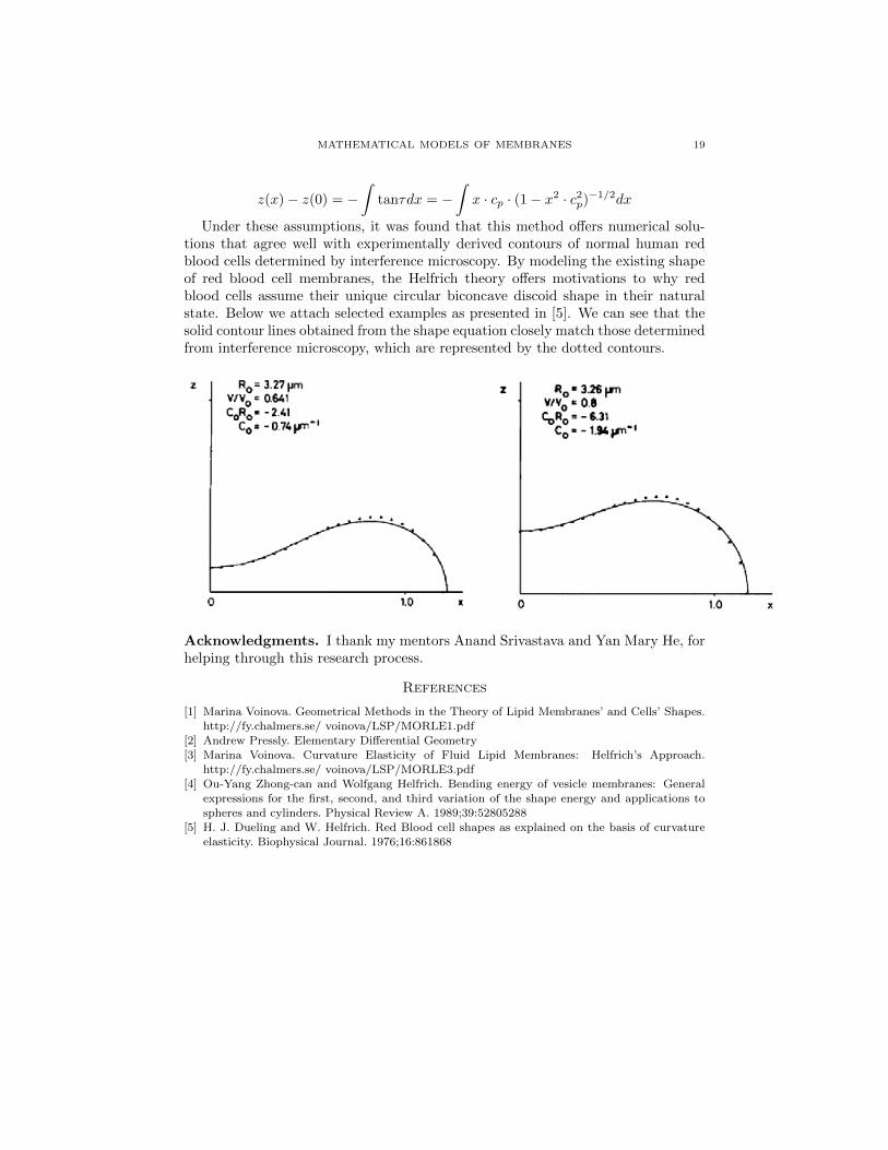
Under these assumptions, it was found that this method offers numerical solu-tions that agree well with experimentally derived contours of normal human redblood cells determined by interference microscopy. By modeling the existing shapeof red blood cell membranes, the Helfrich theory offers motivations to why redblood cells assume their unique circular biconcave discoid shape in their naturalstate. Below we attach selected examples as presented in [5]. We can see that thesolid contour lines obtained from the shape equation closely match those determinedfrom interference microscopy, which are represented by the dotted contours.

Acknowledgments. I thank my mentors Anand Srivastava and Yan Mary He, forhelping through this research process.

References

[1] Marina Voinova. Geometrical Methods in the Theory of Lipid Membranes’ and Cells’ Shapes.

http://fy.chalmers.se/ voinova/LSP/MORLE1.pdf

[2] Andrew Pressly. Elementary Differential Geometry[3] Marina Voinova. Curvature Elasticity of Fluid Lipid Membranes: Helfrich’s Approach.

http://fy.chalmers.se/ voinova/LSP/MORLE3.pdf[4] Ou-Yang Zhong-can and Wolfgang Helfrich. Bending energy of vesicle membranes: General

expressions for the first, second, and third variation of the shape energy and applications tospheres and cylinders. Physical Review A. 1989;39:52805288

[5] H. J. Dueling and W. Helfrich. Red Blood cell shapes as explained on the basis of curvature

elasticity. Biophysical Journal. 1976;16:861868

mathematical models of membranes - department of...

Documents