mathematical models for the efficiency of flotation
TRANSCRIPT

MATHEMATICAL MODELS FOR THE EFFICIENCY OF FLOTATION PROCESS FOR
NORTH WAZIRISTAN COPPER
By
SARDAR ALI Ph.D. Scholar
UNIVERSITY OF EDUCATION LAHORE
PAKISTAN 2007

i
MATHEMATICAL MODELS FOR THE EFFICIENCY OF FLOTATION PROCESS FOR
NORTH WAZIRISTAN COPPER
By
SARDAR ALI University Registration No. 87-03
A thesis submitted to the University of Education Lahore (Pakistan) in partial fulfillment of the requirements for the award of degree of
Doctor of Philosophy in Mathematics
with specialization in Mathematical Statistics at the Division of Science and Technology, University of Education Lahore.
SUPERVISOR CO-SUPERVISOR
JUNE 2007

ii
In the Name of
Allah,
Most Merciful and Compassionate the
Most Gracious and Beneficent
Whose help and guidance I always solicit at
every step, at every moment.

iii
DEDICATED
To my Wife and Children

iv
(ACCEPTANCE BY THE THESIS OF EXAMINATION COMMITTEE)
Thesis entitled
MATHEMATICAL MODELS FOR THE EFFICIENCY OF FLOTATION PROCESS FOR NORTH WAZIRISTAN COPPER
Submitted by
MR. SARDAR ALI
Accepted by the Division of Science and Technology, University of Education, in partial fulfillment of the requirements for degree of Doctor of Philosophy in Mathematics with specialization in Flotation Process.
Thesis Examination Committee:
Director External Examiner Supervisor Member Member
Date: ___________

v
ABSTRACT
The objectives of this research are to analyze empirically the effects of different
explanatory variables on recovery and grade of copper from ore found in North
Waziristan and to develop mathematical models for the enrichment of copper in
Pakistan.
This study is based on the primary data from flotation process experiment for
enrichment of copper. Seven variables were studied in experiments. The variable were
type and dosage of collector (X1g/ton) pH (X2), depressant sodium cyanide (X3 g/ton)
sulfidizer Na2S(X4g/ton), frother dosage (X5 g/ton), pulp density (X6 w/v) and
conditioning time (X7 minute) and consists of 31 observations. Flotation process
parameters were studied to concentrate the copper content of chalocopyrite the North
Waziristan copper ore. Mathematical models were developed using various model
selection procedures. Regression parameters were estimated by applying Ordinary
Least Squares (OLS) method for regression analysis and adopted general to simple
modeling procedure. In this study we found that the variables X1, X3, X4 and X6 of
equation (5.57) are statistically significant and concluded that an increase in these
variables there is increase in recovery of copper.
Maximum grade were obtained from equation (6.65) the combined significance
variable X1, X3, and X7.

vi
ACKNOWLEDGEMENTS
All praise and thanks for Almighty Allah, Who has given me power to
complete this report successfully.
I am extremely grateful to Dr. Ghulam M. Mustafa, Vice-Chancellor,
Education University Lahore for his expert guidance, incisive and scholarly advice
and very useful suggestion which were of great help in making this report.
I am also greatly thankful to my supervisor Dr. Mir Asad Ullah, COMSAT,
Abbottabad, for his constant help at each stage, with out which I probably would not
have been able to execute this project with such professional excellence.
Heartedly thanks are due to my Co-supervisor, Prof. Dr. Muhammad Mansoor
Khan, Dean N-W.F.P, University of Engineering & Technology, Peshawar.
My sincere thanks goes to Prof. Dr. Mian Izhar ul Haq, Director, Ph.D
Programme, Education University, Lahore, for his timely help, encouragement and
cooperation.
I am unable to find words for paying thanks to my wife and my children who
were so helpful and extending warm co-operation whenever called upon.
Last but not the least, I would like to thanks Mr. Syed Sajid, Alias (Doctor),
Supervisor, Words’ Masters, U.O.P, for compiling this stuff in such a short period of
time.
SARDAR ALI

vii
TABLE OF CONTENTS
Abstract v
Acknowledgements vi
List of Tables x
List of Figures xi
CHAPTER NO. 1: INTRODUCTION 1
1.1 Introduction 1
1.2 Why Mathematical Models are required in Flotation Process? 3
1.3 Benefits of the Present Research 4
1.4. Objectives of the Research 5
1.5 Scope of the Research 6
1.6 Sources of the data 7
1.7 Background of the Problem 8
1.8 Significance of the Research 8
1.9 Outline of the Study 9
CHAPTER NO.2: REVIEW OF LITERATURE 10
CHAPTER NO. 3: EXPERIMENTS 18
3.1 Previous Work 18
3.2 Geology of North Waziristan Copper 19
3.3 Location and Accessibility of North Waziristan Copper Ore 19
3.4 Uses of Copper 20
3.5 World Occurrences 21
3.6 World Mine Production and Reserves 22
3.7 More New Discoveries 25
3.7.1 Copper of Occurrences in Pakistan 25
3.7.2 Gilgit Agency (Northern Areas) 25
3.7.3 Punjab Province 25
3.7.4 Baluchistan Province 26
3.8 Basic Information About Chalcopyrite Mineral 26
3.9 Occurrences of North Waziristan Copper Ore 28

viii
3.9.1 Shinkai Area 28
3.9.2 Degan area 28
CHAPTER NO. 4: METHODOLOGY 29
4.1 The Principle of Least Squares 30
4.2 Estimation Techniques 32
4.3 Estimation Of Model Parameters 33
4.3.1 Least Squares Estimation of the Regression Coefficients 33
4.3.2 Properties of the Least-Squares Estimators 38
4.3.3 Estimation of 2 39
4.3.4 Test for Significance of Regression 40
4.3.5 Stepwise Regression Procedure 41
4.3.6 Studentized Residuals 41
4.3.7 Test Statistic for Skewness 42
4.3.8 Testing for Heteroscedasticity 42
4.3.9 The t-statistic - Normal Approximation 44
4.4 Collection of Copper Ore Samples and their Analysis for Pilot Scale Studies 45
4.5 Justification of the Explanatory Variables 46
4.5.1 Collector types & dosage 46
4.5.2 pH value 46
4.5.3 Depressant 47
4.5.4 Sulphidizer (Na2S) 47
4.5.5 Frothers Dosage 47
4.5.6 Frother 47
4.5.7 Effect of pulp density 48
4.5.8 Flotation time 48
CHAPTER NO. 5: MODEL BUILDING
5.1 General Model For Recovery: 51
5.2 General Description: 51
5.3 Mathematical Model For Optimum Recovery about the Data for recovery of copper 53
5.3.1 Effect of variation in collector dosage NaPX (X1). 53
5.3.2 Effect of variation in pH (X2) 55

ix
5.3.3 Effect of variation in depressant-NaCN (X3) 55
5.3.4 Effect of variation in Sulfidizer Na2S (X4) 55
5.3.5 Effect of Pine Oil (X5) 56
5.3.6 Effect of Pulp density (X6) 56
5.3.7 Effect of conditioning time (X7) 56
5.4 Modeling Effect Of Individual Variable For Recovery 59
5.5 Modeling Combined Effect Of Variables On Recovery 72
5.6 Forward selection procedure for model building or simple to general. 73
5.7 Backward elimination or general to simple procedure for model building 74
5.8 Best Subset For Recovery 75
5.9 Multiple Regression Model for Recovery 81
5.9.1 Jarque – Bera: A Combined Test: 85
5.9.2 Testing for Heteroscedasticity 86
5.10 Reduced model for recovery 87
5.10.1 Tests for basic assumptions: 89
5.10.2 Other tests for Normality 90
CHAPTER – 6: MATHEMATICAL MODEL FOR OPTIMUM GRADE 94
6.1 Mathematical model for optimum grade. 94
6.2 Modeling effect of individual Variable for grade 97
6.3 Modeling Combined Effect Of Variables On Grade 110
6.4 Forward Selection 110
6.5 Backward Elimination 112
6.6 Best Subset For Grade 112
6.7 Model development for grade: 120
6.8 General Remarks about the Model 123
6.8.1 Statistical Significance 123
6.8.2 Sample Size? 123
6.9 Specific Remarks about the Model 124
6.10 Discussion of size of coefficients and scientific judgment of coefficient 125
CHAPTER – 7: CONCLUSION 127
References 129 Appendix (1-7) 137

x
LIST OF TABLES
Table No. Title Page
Table – 1: World Refined Copper Consumption 22
Table – 2: World copper mined production 23
Table – 3: Data for the recovery of Copper 54
Table – 4: Mathematical models involving one predictor variable for recovery of copper by flotation.
59
Table – 5: Coefficient Analysis and model fitness statistic 82
Table – 6: Analysis of Variance 82
Table – 7: Test for normality of residuals: 84
Table – 8: Skew ness E. Kurtosis Jarque-Bera 85
Table – 9: Coefficient Analysis and model fitness statistic for four variables
88
Table – 10: Analysis of Variance for four variables 89
Table – 11: Tests for skewness, kurtosis and Jarque bera for four variables 90
Table – 12: Bin Frequency 90
Table – 13: Mathematical models involving one predictor variable for grade of copper.
98
Table – 14: Primary data on grad of copper 111
Table – 15: Coefficient Analysis for grad and model fitness statistic for
Seven variables
119
Table – 16 OLS estimates121 for three significant variables 120
Table – 17 Analysis of Variance 121

xi
LIST OF FIGURES
Figure No. Title Page
Figure 1: Effect o1f collector (NaPX) on recovery of copper 57
Figure 2: Effect of pH on recovery of copper 57
Figure 3: Effect of depressant (NaCN) on recovery of copper 57
Figure 4: Effect of sulfidizer (Na2S) on recovery of copper 57
Figure 5: Effect of frother (pine oil) on recovery of copper 58
Figure 6: Effect of pulp density on recovery of copper 58
Figure 7: Effect of conditioning time on recovery of copper 58
Figure 8: (a). Linear, (b) Logarithmic (c) quadratic (d) power (e) exponential and (f) two straight-line models fitted to the recovery of copper data from five levels of collector type and dosage in the flotation process.
63
Figure 9: (a) Linear, (b) Logarithmic (c) quadratic (d) power (e) exponential (f) and two straight-line models fitted to the recovery of copper data from five levels of pH of pulp in the flotation process.
65
Figure 10: (a) Linear, (b) Logarithmic (c) quadratic (d) power (e) exponential (f) and two straight-line models fitted to the recovery of copper data from five levels of depressant in the flotation process.
66
Figure 11: (a) Linear, (b) Logarithmic (c) quadratic (d) power (e) exponential (f) and two straight-line models fitted to the recovery of copper data from five levels of sulphidizer in the flotation process.
67
Figure 12: (a) Linear, (b) Logarithmic (c) power (d) and exponential models fitted to the recovery of copper data from three levels of frother dosage in the flotation process.
68
Figure 13: (a) Linear, (b) Logarithmic (c) quadratic (d) power (e) exponential (f) and two straight-line models fitted to the recovery of copper data from four levels of Pulp density in the flotation process.
69
Figure 14: (a) Linear, (b) Logarithmic (c) quadratic (d) power (e) exponential (f) and two straight-line models fitted to the recovery of copper data from four levels of conditioning time in the flotation process.
71
Figure 15: Effect of sodium cyanide (X3) on the recovery of copper. 77
Figure 16: Effect of sodium sulphide (X4) on the recovery of copper 77
Figure 17: Copper recovery (YR) response surface for sodium cyanide (X3) and sodium sulphide (X4).
78

xii
Figure 18: Copper recovery (YR) response surface for sodium sulphide (X4), and frother dosage (X5).
79
Figure 19: The figure (5.19) shows visual test for standard residuals of seven variables.
83
Figure 20: Histogram 84
Figure 21: Standard Residual Plot 86
Figure 22: Plot of residuals 89
Figure 23: Histogram 91
Figure 24: Standard Residual Plot 91
Figure 25: Effect of collector (NaPX) on grade of copper 96
Figure 26: Effect of pH on grade of copper 96
Figure 27: Effect of depressant (NaCN) on grade of copper 96
Figure 28: Effect of sulfidizer (Na2S) on grade of copper 96
Figure 29: Effect of frother (pine oil) on grade of copper 96
Figure 30: Effect of pulp density on grade of copper 96
Figure 31: Effect of conditioning time on grade of copper 97
Figure 32: (a) Linear, (b) Logarithmic (c) quadratic (d) power (e) exponential (f) and two straight-line models fitted to the grade of copper data from five levels of collector use in the flotation process.
101
Figure 33: (a) Linear, (b) Logarithmic (c) quadratic (d) power (e) exponential (f) and two straight-line models fitted to the grade of copper data from four levels of pH in the flotation process.
103
Figure 34: (a) Linear, (b) Logarithmic (c) quadratic (d) power (e) exponential (f) and two straight-line models fitted to the grade of copper data from four levels of sulfidizer in the flotation process.
104
Figure 35: (a) Linear, (b) Logarithmic (c) quadratic (d) power (e) exponential (f) and two straight-line models fitted to the grade of copper data from five levels of depressant in the flotation process.
105
Figure 36: (a) Linear, (b) Logarithmic (c) quadratic (d) power (e) exponential (f) and two straight-line models fitted to the grade of copper data from four levels of frother dosage in the flotation process.
106
Figure 37: (a) Linear, (b) Logarithmic (c) quadratic (d) power (e) exponential (f) and two straight-line models fitted to the grade of copper data from four levels of pulp density in the flotation process.
107
Figure 38: (a) Linear, (b) Logarithmic (c) quadratic (d) power (e) exponential (f) and two straight-line models fitted to the grade of copper data from four levels of flotation time in the flotation process.
109

xiii
Figure 39: Effect of sodium cyanide (X3) on the grade of copper. 114
Figure 40: Effect of sodium Sulphide (X4grams/ton) on the grade of copper.
114
Figure 41: Copper grade (YG) response surface for sodium cyanide (X3) conditioning time (X7).
116
Figure 42: Copper grade (YG) response surface for sodium Sulphid (X4) conditioning time (X7).
117
Figure 43 Histogram 121
Figure 44 Testing for heteroscedasticity 122
Figure 45 Residuals are normal. It qualifies the visual test of normality.
122
Figure 46 Conceptual general model for recovery and grad 126

CHAPTER – 1 INTRODUCTION
1.1 Introduction
Mineral processing is the art and science of processing ores to separate
valuable minerals from waste by physical means (crushing, grinding, screening,
gravity separation, magnetic separation and flotation) and of doing it for a profit. To
maximize profitability, accurate simulations of mineral processing unit operations
have been actively pursued as minerals processing technology has matured. The
modeling and simulation of mineral processing systems are inherently difficult
because they are multiphase (particles, fluids and air) and because the ore particles are
heterogeneous (size, shape, composition and texture). From the beginning, the rate of
development in mineral processing modeling was controlled by limitations in ones
understanding of the basic sub processes in each unit operation and in the
computational relationship required to solve model1 equations.
Mathematical statistics is an interdisciplinary subject aimed at developing
models and analytical methods for systems containing a substantial element of
random variation, often the motivation for the research is a practical problem
involving the development and analysis of a mathematical statistical model.
1 A model can simply be defined as a representation or a description of the physical phenomenon occurring in any activity.

2
A model explains the phenomenon either mechanistically (theoretically) or
statistically (empirically), which can be used for prediction of the phenomenon
(Pekkanen, 1998b). The development of a new process typically involves a lot of
experiments on several scales: Laboratory, bench scale and pilot stages.
This dissertation is mainly focusing on the state of mathematical modeling and
also to formulate mathematical models for grade and recovery of the North Waziristan
copper ore in Pakistan. The North-Waziristan copper ore is chalcopyrite. The ore is
of low grade within economic limit, therefore it must be upgraded before it can be
subjected to metallurgical treatment to obtain blister copper. The experimental work
was undertaken to upgrade the lean copper ore through flotation technique to make it
suitable for further metallurgical treatment to obtain blister copper. Extensive
flotation test work was carried out to investigate effects of various process variables
on recovery (YR) and grade (YG) of copper. Effects of collector dosage; pH,
Sulfidizer dosage; depressant levels, frother dosage, pulp density and conditioning
time were investigated in flotation tests. The results of the pilot scale studies showed
that the copper content in the ore can be upgraded from 0.9 % to 22-25 % in a staged
cleaning flotation with recoveries up to 80%. The grade can be further enhanced by
improving the machine efficiency and conducting more research on reagents.
The important information on some flotation results of copper were obtained
from the Department of Mining Engineering, N.W.F.P University of Engineering and
Technology, Peshawar, and used to develop mathematical models for grade and
recovery of copper.

3
1.2 Why Mathematical Models are Required in Flotation Process?
Mathematical Models are required because;
More time and money consumes during systematic experimentation or by hit
and trial
Scientific way to improve the efficiency of the process is to develop a correct
mathematical model
It is the only course of action available for the improvement in the system
Once we successfully construct mathematical model for a process it can be
used in future for any alteration for improvement in the process
It will help to improve the process of extraction of copper from the copper ore.
The study of mathematical models, simulation and optimization are important
because of the following reasons.
Modeling reduce manufacturing costs
Reduce research and development expenditure and save time.
Increase efficiency.
Greater understanding of the problem
Decision support
Knowledge management
Ability to handle complex problems
Technology transfer
Improve the safety of the plants

4
Bring new products to market faster
Reduce waste in process development
Improve product quality
Reduce need for potentially hazardous experiments.
Gives precise and accurate results
Mathematical models have been used in mineral processing system design
optimization in control for more than 32 years. All major technological innovations
involve information technology and mathematical modeling, and apparently
computerized mathematical model play an increasingly decisive role within
engineering sciences, i.e. within industrial production, within planning and
economics, within mineral processing. Mathematical modeling activities are aimed at
methodologies enabling one to deal with today’s ever increasing quantities
information.
1.3 Benefits of the Present Research
Saving of foreign exchange
Meet the demand of indigenous industry
To utilize the 122 million ton of copper ore of North Waziristan area.
In order to upgrade the copper content by mathematical model to make it
suitable for metallurgical treatment
To improve the quality and quantity of copper ore in concentrate

5
This model can be utilized specially in glass, ceramics industry, copper
concentrator, saindak (Baluchistan) process of bentonite clay, enrichement of
uranium, purification of soap, stone and fertilizer industries.
Optimization of flotation parameters.
1.4 Objectives of the Research
1. To develop mathematical models for the enrichment of copper in Pakistan.
2. To examine how to improve and increase the efficiency of the process by
scientific way.
3. To analyze empirically the effect of different explanatory variables2 on
recovery and grade of copper in the research area of Pakistan.
4. To give appropriate suggestions in the light of our findings.
The North Waziristan copper ore is chalcopyrite (CuFeS2). Chemistry of
chalcopyrite is such that it can be efficiently concentrated by the froth flotation from
associated gangue minerals. Flotation process parameters were studied using
chalcopyrite Copper ore of North Waziristan to obtain a copper concentrate suitable
for further metallurgical treatment. The important flotation variables examined were,
collector, depressant, pH, frothers, Sulphidizer (Na2S), pulp density and conditioning
time. By stage wise optimization of flotation variables, copper were upgraded from
0.9% to 10% and 20% in roughing stage and to as high as 22% in a cleaning stage
with recoveries up to 80 to 90% in experimental work done by the Department of
2 Seven important explanatory variables, e.g. type and dosage of collector (X1gms/ton) PH (X2), depressant sodium cyanide (X3gms/ton) sulfidizer Na2 S (X4gms/ton) frother dosage (X5gms/ton), pulp density (X6) and conditioning time (X7 minute).

6
Mining Engineering, NWFP University of Engineering & Technology Peshawar,
Pakistan.
To improve and increase the efficiency of the process by scientific way and to
develop a correct mathematical model, so that in future any alteration or change in the
process can be improved by utilizing the mathematical models. Now-a-days every
chemical, mechanical and electrical process is governed by mathematical or statistical
models. These 5.67 and 6.65 models are the first mathematical models, which have
been developed for the mineral industry in Pakistan and of course these will pave the
way to run our mineral based Industry. Using such mathematical models to improve
their products quantity and quality. These models can be utilized specially in glass,
ceramics industry copper concentrator Saindak (Baluchistan) process of bentonite
clay, enrichment of Uranium, purification of soap, stone and fertilizer industries.
1.5 Scope of the Research
Copper is one of the very essential minerals in modern industry. It is a good
conductor and is used in electrical networks, various equipments and weapons. The
United States, the world’s largest consumer (1999), uses between 2.5 and 3.0 million
tons of copper annually. Most wires and electrical equipment are made of pure copper
and considerable alloys of copper such as brass and bronze. The brasses are Cu – Zn
alloys (55%-99% Cu, 45%-1% Zn) and the bronzes are Cu – Sn – Zn (88% Cu, 10%
Sn and 2% Zn). There are also Ni, Al, and steel alloys of Cu; minor special alloys
utilize arsenic; beryllium, cadmium, chromium, cobalt, iron, lead, magnesium,
manganese and silicon. Copper sulphide deposits of North – Waziristan vary in grade
from 0.3% to as high as 1.0%. Due to its low grade it cannot be directly subjected to

7
metallurgical treatment for producing blister copper. Pakistan is still meeting its
requirement through import from other countries. Successful development of
mathematical model will provide optimum parameters for the enrichment of copper in
the final product. In this way it will save cost for further experimentation and time to
achieve similar objectives.
1.6 Sources of the data
The study is based on primary data from flotation process experiments on
samples collected by the Department of Mining Engineering, NWFP University of
Engineering and Technology, Peshawar Pakistan with the assistance of the political
authorities of North Waziristan agency and Federally Administered Tribal Area
Development Corporation (FATA DC). Other relevant information about copper
deposits were also obtained from FATA DC. An inventory of the ore samples was
prepared and each sample was tagged with a number and weighted.
Both the chemical and mineralogical analysis of the samples were carried out
at Department of Mining Engineering Laboratories (MEL) and Mineral Testing
Laboratories, Sarhad Development Authorities (SDA), Peshawar. The mineralogical
investigations include X-Ray Diffraction, X-Ray Fluorescence and ore microscopy.
The chemical constituents were determined by classical and instrumental methods of
analyses. On site the samples were collected by blasting irregularly spaced holes
within the regularly spaced rows for minimum chances of errors. A total of 30 tons of
samples were collected, comprising of six sub samples weighing five tons each from
six different locations. The rows of holes drilled on each location were spaced at an
equal interval of 300 feet. The collected samples were transported to the NWFP,
University of Engineering and Technology Peshawar, through trucks.

8
1.7 Background of the Problem
Extraction of copper from the available copper ore in Pakistan is important.
The metal has many uses and ranks fifth amongst the metals in tonnage consumed.
God has blessed Pakistan with abundant copper ore and its occurrences have been
reported throughout the country. However, the occurrences at Saindak and Ricodak in
Baluchistan and North Waziristan Agency in NWFP are of more importance. The
survey conducted by Federally administrated tribal areas (FATA) development
corporation has confirmed a minimum of 122 million tons of reserves of copper ore in
Boya-Datta Khel area (about 40km from Miran Shah), having copper contents better
than that found at Saindak at some places and in some layers.
Thus an extensive study of North Waziristan copper ore was carried out by the
Department of Mining Engineering, N.W.F.P, University of Engineering &
Technology, Peshawar, through a research proposal sponsored by Board of Advanced
Studies and Research (BOASAR). The laboratory evaluations of raw ore were made
in Phase-1 of the project and in order to confirm these evaluations, a study of flotation
process by a single stage pilot plant was carried out in Phase-II. These studies have
generated sufficient data for constructing mathematical models for the processes.
1.8 Significance of the Research
For obtaining optimum level of variables for efficient flotation process to
extract copper from raw ore, experimentation by systematic or by hit and trial
procedures takes a lot of time and costs enormous amount of money. The standard
scientific way to improve and increase the efficiency of the flotation process for
enrichment of copper ore is to develop a mathematical model for the process. It

9
should be remembered that in some cases mathematical modeling is the only course
of action available for the improvement in the system. Once we successfully construct
mathematical model for a process, it can be improved and used in future for any
alteration for improvement in the process. Thus mathematical models to be developed
will reduce the extent of further experimentation to achieve certain desired objectives.
These will help to improve the process of extraction of copper from the copper ore
and will save sizeable amount of money for the country.
1.9 Outline of the study
Outline or organization of the study is as follows. Chapter one deals with
introduction regarding mathematical modeling for the efficiency of mineral
processing of North Waziristan copper ore, benefits of the present study, main
objective, scope, background and significance of the study. Chapter two presents
review of literature. Chapter three explains experiments, previous work, geology of
North Waziristan copper ore, location and accessibility Waziristan copper ore, and
occurrences of North Waziristan copper ore. Chapter four deals with methodology,
justification of the explanatory variables and flotation process. Chapter five presents
building of mathematical models. Chapter six consist mathematical models for grade.
Final and the last chapter seven consist of summary, conclusion and
recommendations.

10
CHAPTER – 2 REVIEW OF LITERATURE
In the literature, the construction of mathematical models for flotation process
in mineral processing has been approached in various ways depending on the
philosophy of the researcher as well as the expected usage of the model and the
allowable investment in personnel and time. The goal of using these models is to
undertake plant scale tests on batch laboratory evaluations. Flotation tests were
carried out on samples of a US porphyry ore (Pinto Valley, AZ) by Dowling et al.
(1985). The ore was tested using various collector and frother system to produce
different time recovery profiles these were used to calculate flotation rate and ultimate
recovery parameters for each model. The models were then evaluated statistically to
determine the over all fit of the calculated to the observed data and to test the range of
significance of the parameters in each model.
Each flotation model will have an associated error. This error will effect and
can be measured by both the fit to the observed data and the range of statistical
significance of each parameters. Two types of errors were found due to experiment
and due to model. The researcher found the model variance S2r and compared the
optimal model variance to the model variance from a given change in the parameter
being assessed and F-value calculated. To determine the optimal flotation model
parameters, a generalized parameters estimation computer program was used (Klimpl
1980”) by Dowling in his study. The criteria used for estimation of parameters value

11
is the minimization of the absolute sum of the square of deviation at a given time
between observed in calculated recovery.
Wills (1986) studied simple nodal sensitivity analysis in complex circuit
analysis were found by using matrices and statistical techniques. The researcher
worked to develop a best-fit material balance model. The method described makes use
of the minimum number of sampled streams and analysis of only one component,
such as metal assay or dilution ratio, on each stream one involved in a unit process.
He found that plant flow sheet was reduced to a series of nodes, where process either
join or separate. Simple nodes have either one input and two outputs (a separator ) or
two inputs and one output ( a junction ).
Munn (1998) investigated that metal recovery in mineral processing plants is
often linearly correlated with feed or concentrate grade, particularly in flotation. This
correlation can be used to analyze the data form plant trials in which two operating
conditions are being compared, such as different reagent regimes or circuit
configurations. The method involves the statistical comparison of the two linear
recovery –grade regression lines corresponding to the two operating conditions.
Although not as efficient as a formal experimental design, the method can be used
where such designs are impractical, or in the analysis of historical data.
Khan (1999) studied flotation process parameters to concentrate the copper
content of chalcopyrite, the North Waziristan copper ore, in pilot-scale to obtain a
copper concentrate suitable for further metallurgical treatment. The important
flotation parameters, e.g. type and dosage of collector, dosage of depressant, and
frother and conditioning time for collector were examined. During stepwise
optimization of flotation parameters, the copper content was upgraded from 0.9% to

12
20% in roughing stage, and to as high as 22% in a single-stage cleaning with
recoveries of over 83%. A flow sheet depicting different products of flotation, for an
industrial concentrator, has also been suggested.
Elzinga E.J. Van J.J.M and Swartjes. F.A. (1999) worked on General purpose
Freundlich isotherms for cadmium, copper and zinc in soils. They have tried to derive
generally applicable isotherm for cd, zn and zn using data from batch sorption
experiments on a wide range of soils and experimental conditions. They used a
linearized logarithmic transformation of the Freundlich sorption equation.
Freundlich derived equations for cd, zn and zn using multiple linear regression
on batch sorption data. The equations were based both total dissolved metal
concentrations and free metal activities in solution. He calculated free metal activities
from total metal concentration talking into account ionic activity. The logarithmic
transformation of the Freundlich constant for cadmium was regressed on the
logarithmic transformations of cation exchange capacity. He used Minitab for
statistically analysis.
They used step-wise forward regression by evaluating the t–ratios, stepwise
improvement of 2adjR could be attributed either to addition of an argument or to
reduction of data. A best model was selected based on 2adjR t-ratio and the number of
data points considered. The regression co-efficient of the best models were significant
at the P = 0.001 level. All sorption point were considered as independent
observations.
Sripriya et al. (2002) examined the kinetic model based on time recovery data,
which uses the extra dimension of rate and has been in vogue since time immemorial

13
for scaling up of laboratory data. The air flow number and the froth number were used
as a basis for scale up. The performance of the froth flotation circuit, an efficiency
parameter (co-efficient of separation c s) was used. The yield from the flotation circuit
improved, the froth ash reduced and the rejects ash went up. Various empirical and
kinetic models were evaluated.
Sripriya developed regression equations for predicting the combustible
recovery ash recovery and Ks for combustibles and ash. The effects of three most
important reagents for coal flotation namely sodium meta silicate, collector (kerosene)
and frother were studied using 23 full factorial design. The regression models were
developed using factorial experiment data to quantify the effect of sodium meta
silicate, collector and frother and to predict grade and recovery of combustible
material for different reagent conditions. The addition of sodium meta silicate
increased the recovery without affecting the grade significantly. The MIBC addition
reduce the surface tension at the liquid–vapor interface, which results in the
production of finer bubble size distribution and thus improves flotation rates and
recovery values. However, a finer bubble size is tribution also increases water
recovery, which results in a greater recovery of certain able ash bearing particles and
thus degradation of the product grade. The interaction between OH group of MIBC
and hydrated mineral matter improves floatability of high ash coal particles and
degrades the product grade further. The negative effect of kerosene and MIBC
interaction on both grade and recovery could be due to the recovery of high ash coal
particles in preference to low ash coal particles. The highest possible grade of product
is 94.19% combustibles with 25.33% recovery. A product with 91.11% combustibles

14
grade at 95.58% recovery was obtained at 0.1 g/kg sodium silicate, 0.4 g/kg collector
and 0.075 g/kg frother from the coal fines tested.
Ziyadanogullari (2003) worked on flotation of oxidized copper ore obtained
from Ergani Copper Mining Company in Turkey. The ore contained 2.03% copper,
0.15% cobalt and 3.73% sulfur. An effective processing method has not been found to
recover copper and cobalt from this ore, which has been stockpiled for 40-45 years in
a idled plant. It was established that recovery of copper and cobalt from this ore with
hydrometallurgical treatment is not economical, so using flotation to increase the
concentration of copper and cobalt was chosen. When flotation of the oxidized copper
ore was performed under standard operating conditions in the plant, good results were
not obtained. Because of this, the flotation of samples obtained from sulfurized
medium containing different ratios of H2S+ H2O gases was done under the same
conditions. Following flotation, it was seen that copper, cobalt and sulfur present in
the medium were concentrated. In this solution, concentration of copper and cobalt
were found five times higher than normal level.
Elemental sulfur produced by chloride leaching of sulfide ores or concentrates
contains selenium and tellurium usually too high to be used in various industrial or
agricultural uses. The sulfur in the leaching residue can be upgraded to 90% in grade
by froth flotation and the sulfur concentration can be followed by sulfur purification
and selenium and tellurium removal. The sulfur in the leaching is in a form of discrete
particles with a size range of 5 to 10 microns. The sulfur particles tend to agglomerate
in the pulp and hence mechanically entrap gangue minerals. With sodium silicate as
the dispersant as well as the depressant for siliceous material, a sulfur concentrate of
90% in grade and 90% in recovery can be obtained with a single-stage froth flotation.

15
The flotation reagent consumptions are minimum. The majority of chalcopyrite
remains in the sulfur flotation tailings and can be readily recovered by flotation with
different flotation reagents. When amyl xanthate is used, 85% of chalcopyrite can be
recovered with a copper grade of 14.5% in a single-stage froth flotation. The
chalcopyrite flotation concentrate can be sent back to chloride leaching circuits.
Cilek (2004) combined the classical first order kinetic model with a properly
built statistical model based on a factorial experimental design. In order to accurately
predict the rougher flotation efficiency for various flotation conditions, a three-level,
three factor experimental design was used to develop statistical model to predict each
of the kinetic model parameters as a function of the air flow rate, the feed grade and
the froth thickness. The statistical evaluation of the experimental results indicated that
the ultimate recovery, the rate constant and time correlation are not constant, but each
of these kinetic model parameters can be defined as a function of variables
considered. The rate of change in the kinetic parameters due to the feed grade
fluctuation and their effects on the metallurgical performance can accurately be
predicted by using the models developed. To reduce the detrimental feed grade
fluctuations on the metallurgical performance, the operating variables of the flotation
can be manipulated to obtain the desired concentrate grade. Cilek obtained the results
of the statistical evaluation; the rate data were used to build a statistical model
considering the variables.
Among all models the following models, which were built by using piece wise
(or breakpoint) linear regression method were selected.
Km = (0.4273-0.52 f+0.0051Qa+0.617Tf-0.05QaTf) , km2.24
Km= (3.565+0.38f-0.31Tf+0.104Qa+0.003QaTf), km<2.24,R2=0.9431........……….(1)

16
bm = (0.2012-0.09f+67.10-3Qa+0.074Tf+0.014 f Tf-0.011QaTf), b0.406
bm= (3.695-3.75f-0.08Qa+0.348Tf-0.694fTf+0.097QaTf),b<0.406, R2 = 0.8945.....…(2)
RIm= [27.973f-1.337Qa+0.89Tf(25.33-8.64f-Qa)-9.592Qa-0.549], RIm69.3
RIm= [75.284-4.811f+0.015Qa+0.654Tf(9.896+f-Qa)-0.115fQa],Im69.3,R2=0.9022..(3)
topt = [0.538+0.77f-0.112f Tf+0.02Qa(2.2+Tf-2.4f)] topt 2.32
topt=[4.097-0.867f+0.2fTf+0.051Qa(1.47-Tf+1.087f)],topt<2.32, R2=0.9087.........…..(4)
The high R2 values for all the responses reveal that the experimental data
provide evidence to indicate that the developed models satisfactorily predict the
Kinetic Parameters, where topt RI, k and b are the optimum flotation, time ultimate
recovery, the rate constant and the time correction factor also Tf, f, Qa denotes pulp
level, feed grade and factor respectively.
Barbaro and Piga (1998), adopted statistical approach to evaluate the Pb-Zn
selectivity of various organic collectors of the Mercaptobenzothiazole (MBT) and
aminothiophenol (ATP) types, in the flotation of lead and zinc minerals. Six
replicated tests were performed using each collector in order to obtain an estimate of a
statistical population characterized by an average and a variance. Comparison of these
statistical populations indicated the most selective collectors. The selectivity exhibited
by the collectors was then related to their molecular structure.
Horbstand and Potapov (2004), reported that mathematical simulation have
been used in mineral processing system design, optimization and control for more
than 30 years. Presently a new set of simulation tools based on the physics of the
underlying processes has been developed. Because these models provide accurate
micro scale simulations of equipment and process behavior, these high-fidelity

17
simulation (HFS) tools are deemed to constitute a radical innovation of great
importance to the mineral processing industry.

18
CHAPTER – 3
EXPERIMENTS
3.1 Previous Work
The commercial copper deposits occur in variable sizes. However, the ores
containing 0.3% and more copper are deemed feasible for exploitation on commercial
scale. With the state of the art mineral processing techniques the ores with lower
grades can be economically beneficiated as well. Undoubtedly large area of Federally
Administered Tribal Area (FATA) abounds in mineral resources. The survey
conducted by FATA development corporation has confirmed a minimum of 122
million tons of inferred reserves of copper ore varying in depth upto 30m in Boya-
Datta Khel area about 40 kms from Miran-Shah. The average content of this copper
ore is 0.3865%. The copper content increases with depth and at places it is 0.90%
which is better than that found at Saindak (Baluchistan). This low grade raw copper is
of little value unless it is enriched to a higher grade concentrate. The Department of
Mining Engineering through a research proposal (Beneficiation of North Waziristan
Copper Ore) sponsored by Board of Advance Studies and Research (BASAR) carried
out laboratory evaluation of raw ore. Based on the encouraging results of phase-I,
further work on the project was considered necessary. In the phase II of the project, it
was proposed to install a flexible single stage pilot plant for flotation process to study
the laboratory results at the pilot scale. The pilot plant, locally fabricated, has been

19
installed in the premises of NWFP University of Engineering and Technology,
Peshawar.
3.2 Geology of North Waziristan Copper Ore
North Waziristan area remained unexplored before seventies. It was in 1985,
that Federally Administered Tribal Area Development Corporation prepared a
geological base map of about 2350 sq. km on 1:50,000. Investigation resulted in
delineating certain prospective areas having copper mineralization. Detailed
topographical mapping on scales 1:10,000, 1:1000 and 1:500 were conducted in the
mineralized zones. Petrographic study of the representative rock samples was made
before starting pilot plant operations. Geochemical studies of grid samples had
already been carried out at laboratory scale. Probe core drilling in two copper
mineralized bodies has just been completed in collaboration with the technical
expertise of China. According to the estimates given by the Chinese geologist there
are 80 million tons of confirmed reserves of copper ore having an average copper
content of 0.8%. The grade increases with depth and at some places it is 1%,
sometimes approaching 2 to 5%.
3.3 Location and Accessibility of North Waziristan Copper Ore
The tribal belt lies at the Pak-Afghan Border. This belt is divided into seven
units (Agencies) namely Bajaur, Mohmand, Khyber, Aurakzai, Kurram, North
Waziristan and South Waziristan and four frontier regions attached to Peshawar,
Kohat, Bannu and Dera Ismail Khan.
Investigation in the southern region have revealed the presence of copper
mineralization at various places in North Waziristan. Boya, an important locality, is

20
located at longitude 69o 55/ 06// and latitude 32o 57/ 09// N on the right bank of Tochi
River. It lies at a distance of 19 km from Miranshah, the Agency Headquarters and the
local business center. Miranshah is fairly connected to the down districts. It is
accessible by about 270 km of Peshawar-Bannu-Miranshah mettalled road and also
through Peshawar-Tal-Miranshah road. Peshawar is connected by road, rail and air to
Islamabad, the distance being 167 km, similar communication links are available to
Bannu(District Headquarters), that falls at a distance of 61 km to the east of Miran
Shah. Bannu is also connected by about 141 km length of metalled road to D.I.Khan
(Divisional Headquarters) in the south. Tal and Bannu are connected by metalled
roads. The former is also connected to Kalabagh by a metalled road.
3.4 Uses of Copper
The tremendous growth in the use of copper is indicated by the fact that of the
total world production of copper during the last 100 year, about 80% was mined in the
last 25 years and more than one half of it in the last 12 years copper consumption by
major countries and regions is given in table-1. Annual world production ranges
around 20 million metric tons of metallic copper. In spite of the significant number of
closures in United States and Canada, Western world copper mine production rose
3.8% due to projects that came on stream in 1999. In Chile, the Pelambres project
came on stream, with its main impact to be felt during 2000. Similarly, Collahuasi
started up in late 1998 and reached full capacity in 1999, as did Andina expansion and
Escondida’s SX-EW operation. In Australia the Olympic dam expansion started up, as
did the Cuajone expansion in Peru, then Indonesia’s Batu Hijau mine began to
produce (Enrique, 2000). Copper ranks fifth among the metals in tonnage consumed.
It has a variety of uses and the important one is in electrical supply, use and

21
manufacturing industries due to its good conductivity that gives it an advantage over
most metals. It is extensively used in communications equipment including cables and
television transmitters and receivers. The second important use of copper is in
construction worm, particularly in plumbing and hardware and decorative purposes. It
is also a substance used in non-electrical industrial applications such as alloy with
nickel for tubing used in sea water desalination plants. It is used in heat exchangers,
pollution control, and liquid waste disposal. Automobile radiator cores are made of
copper; it is also used in air conditioners, heaters, gas and oil line, and bearings and
bushings.
Military uses of copper are fourth in rank, and the price usually go up during
periods of military spending. This is one of the incremental uses which can rapidly
increase consumption. Coinage, jewellery, chemicals, pigments, brass and bronze
wares and a multitude of minor uses also demand copper in variable amounts.
Copper is essential for plant growth, if copper content falls below 10ppm in
soils, good growth is not possible. On the other hand, if a large amount of copper is
present in the soil it is toxic to some plants.
3.5 World Occurrences
There are hundreds of copper minerals and dozens of settings for copper
deposits. By far the most important mineral is chalcopyrite and the large portion of
this mineral and of copper production comes from the porphyry deposits.
The term porphyry refers to a rock which has an intergrowth of distinctly large
and small crystals. Porphyries are considered to have intruded as molten rock or
magma from depth of ten to hundreds of kilometers. To form the texture of porphyry,

22
it should have approached to within about 3km of the surface before crystallizing as
rock. The texture of mixed coarse and fine crystals is brought to indicate fairly rapid
cooling. Copper deposits the world over can be classified according to the nature of
the deposits.
3.6 World Mine Production And Reserves
Reserves and reserve based estimates for Australia, Chile, China and Poland
have been revised upward based on new information from official country sources.
Revisions to other countries were based on updated tabulations of resources reported
by companies or individual proprietors. Table 2 shows the world mine production and
reserves of Copper.
Table 1: World Refined Copper Consumption (in 1000 tons of Cu)
Area 1994 1995 1996 1997 1998 1999 (e)
Western Europe 3341 3388 3345 3536 3751 3710
Africa 123 117 115 118 110 115
Japan 1375 1415 1480 1441 1255 1260
Other Asia 1833 1955 2126 2240 2148 2420
Canada 199 190 218 225 245 270
United States 2560 2534 2621 2790 2905 2935
Latin America 503 511 619 734 828 820
Oceania 148 174 170 166 161 160
Total 10082 10283 10691 11250 11403 11690
Annual Growth (%) 8 2 4 5 1 3
Source: (Enrique, 2000), (e) Estimate

23
Other Asia includes China, Taiwan, India South Korea, Thailand, Malaysia,
and Philippines.
North America
There are some greatest concentrations of copper in Arizona and Cordilleran
parts of the United States, Canada and Mexico and includes all the well known North
American “porphyry coppers” and a host of other famous districts. All the ores are
associated with felsic types of intrusions. There is another very productive copper
province in Montana at Butte. Other areas where copper can be found include the
Appalachian, the fruitful take Superior district, and Cascadian – Coast Range belt
extending from Yukon Territories through northern British Columbia to the state of
Washington.
Canada
Copper deposits extend from Manitoba to New Brunswick includes the
Hudson Bay, Sodbury, Noranda, heath Steele, Kidd Creek, and other deposits.
Table 2: World Copper Mine Production (in 1000 tons of Cu) (Enrique, 2000)
Area 1994 1995 1996 1997 1998 1999 (e)
Western Europe 304 323 290 317 305 260
Africa 647 618 585 577 563 491
Asia 674 806 798 810 1054 1034
Australasia 614 598 660 625 730 871
Latin America 2853 3198 3884 4280 4658 5316
North America 2399 2534 2537 2544 2495 2211
Total 7491 8077 8754 9153 9805 10183
(e) Estimate

24
South America
Andean copper belt is the most renown in this region. It extends from Chile to
Panama and includes large deposits like Chuquickamata, Braden, Potrerillos, El
Salvador, Cerro Colorado, Rio Blanca, Toquepala, Cerro de Pasco deposits, and many
more. The copper deposits found in these areas are normally associated with
monzonitic intrusives.
Central Africa
The central Africa province constitutes the most concentrated copper belt in
the world and includes the most productive mines of Zambia and adjacent Zaire.
These are strata bound deposits where the metals precipitated from sea with the
sediments.
Several new copper porphyries have been discovered in New Zealand, Fiji,
New Hebrides, Buganville, British Solomon Island protectorate, the territory of
Papua, New Guinea, and West Irian. Some of the copper producing deposits is
Penguna, Ok Tedi, Frieda, and the high grade deposits of Carstenz.
Other copper belts include Uralian province of Russia, the outer Japanese
Island arc, Spain – Portugal (Rio Tinto), Bor in Yugoslavia, Mansfeld in Germany,
Outokumpu in Finland, and Boliden in Sweden.
In Australia there are various copper centers such as Mount Lyell, Mount
Morgan, Mount Isa, Cobar, Tennant Creek, and Mount Oxide.

25
3.7 More New discoveries
Few more new discoveries have been made in Australia, Chile, Peru, British
Columbia, Panama, New Guinea, Fiji, New Idria, Brazil, Puerto Rico, New
Brunswick, Philippines, Solomon Islands, North western Brazil (John, 1984).
3.7.1 Copper of Occurrences in Pakistan
Several copper occurrences have been reported in Pakistan. They are available
in numerous geological settings and contain a variety of copper minerals. However,
the occurrences at Saindak (Baluchistan) and North Waziristan (FATA) are of much
importance. Minor occurrences have been reported from various other places of the
country.
Investment oriented study on Minerals and Mineral based Industries, Expert
advisory cell, Ministry of Industries & Production, Govt. of Pakistan. April, 2004
3.7.2 Gilgit Agency (Northern Areas)
Copper minerals have been located in quartz veins in the northeastern regions
of the area. Similarly chalcopyrite has been reported in alluvial sands in Indus, Gilgit,
Nagar and Hunza rivers.
3.7.3 Punjab Province
Small occurrences of copper have also been reported in Northern Punjab at
Kattha, Mussa Khel and Nilawahan Gorge in salt range. In these areas oxide copper
minerals are found in sandstone beds with malachite and cuprite as the major copper
minerals. Up till now these findings has no economic value. No detail exploration
work has been carried out to access the potential of these deposits.
26
3.7.4 Baluchistan Province
Copper mineralization has been reported in Chagai (Saindak), Loralai and
Zhob districts. Both copper sulphide and oxide minerals as well as native copper have
been reported in Chaghi district. Copper minerals in these areas occur mainly as
sulphides, oxides, silicates and carbonates. The minerals are found in disseminated
form in association with quartz, galena, hematite, siderite and monazite (Zaki, 1969).
In chaghi the amount of potential deposits of copper is reported as 729mt (0.64% Cu
and 0.39g/t Au (Malik,2003). Saindak copper deposits comprise of copper carbonate,
chalcopyrite, chalcocite and malachite minerals. These copper minerals are in
disseminate form and present in association with hydrothermally altered shales,
volcanic tuffs and shales, and limestone of Eocene age.
3.8 Basic information about Chalcopyrite Mineral
Chalcopyrite looks like, and is easily confused with pyrite and is also one of
the minerals referred to as “Fool’s Gold” because of its bright golden color, but it is
brittle, dissolves in acid and has a dark green streak. It is distinguished from pyrite by
ease of scractching, and by copper tests. The color is slightly more yellow than that of
pyrite or is often tarnished in brilliant iridescent hues, which is also called “peacock
copper ore”. Pyrite will frequently show striated cubes or pyritohedra, whereas
chalcopyrite, if not massive, has the characteristic sphenoidal or disphenoid crystals.
Chalcopyrite is the primary minerals, which by alteration and successive
enrichment with copper produces the series starting with chalcopyrite and going
through bornite (Cu5SFeS4), covellite (CuS), chalcocite (Cu2S), and ending rarely as
native copper (Cu). Its structure is so closely related to that sphalerite that it forms
intergrowths with mineral, and isolated free-growing crystals perched on crystals of

27
sphalerite are all parallel. The same face on all the chalcopyrite gives simultaneous
reflections. (It Sparkles) from the Greek words chalkos, “copper” and pyrites, “strike
fire”
Following are the various physical properties of chalcopyrite ore
Composition: CuFeS2 (34.5% Cu, 30.5% Fe, 35% S)
Class: Sulfides
Group: Chalcopyrite
Crystal system: Tetragonal
Fracture: Conchoidal and brittle
Hardness: 3.4-4
Specific gravity: 4.2
Luster: Metallic
Streak: Dark green
Cleavage: Poor in one direction
Color: Brassy yellow, greens, yellows and purples.
Transparency: Opaque
Associated Minerals: Barite, calcite, fluorite, galena, pyrite, pyrrhotite, quartz
and Siderite. Sphalerite and tetrahedrite are a few of the
most Common.
Chalcopyrite is usually massive, but crystals are also common. Often they are
large and the faces usually are somewhat uneven or may have striations on most
crystal faces. Chalcopyrite is often tarnished in brilliant iridescent hues. Spheroidal

28
crystals are common. Also common are disphenoid crystals, which are like two
opposing wedges that resemble a tetrahedron. Crystals are sometimes twinned and can
also be botryoidal.
On charcoal, chalcopyrite fuses to magnetic black globule, touched with HCl tints
flame with blue flash. Solution with strong nitric acid is green; ammonia precipitates
red iron hydroxide and leaves a blue solution.
3.9 Occurrences of North Waziristan Copper Ore
3.9.1 Shinkai Area
The host rocks in this area are normally breccia composed of fragments of
lava flow, ultra basic and intermediate igneous rocks. At some places breccia occurs
with altered andesitic, rhyodacitic, granodioritic, ultrabasic, doleritic and jesperitic
rock fragments. Still at some other places it is a simple breccia. The associated rocks
commonly found are ultrabsic, dolerite, volcanic, andesite, and lava flow. Jerositic is
the gossan type found in the area. The associated minerals are malachite, azurite,
pyrite, chalcopyrite and chalcocite. The extension of mineralized bodies varies from
960-17400 square meters.
3.9.2 Degan area
The host rocks in this area are normally composed of breccia. The associated
rocks commonly found are lava flow, andesite, interbedded limestone, shale, diorite,
and dolerite. Jerositic is the gossan type found in the area, the same as found in the
shinkai area. The associated minerals are malachite, azurite, pyrite, chalcopyrite and
manganese. The extension of mineralized bodies varies from 2604-108800 square
meters.

29
CHAPTER – 4 METHODOLOGY
Data from the following seven variables of flotation process were used to
develop mathematical models for recovery and enrichment of copper from North
Waziristan copper ore.
S. No. Name of Variable Level used
1. Propylxanthate 50, 100, 150, 200, 250
2. pH 10, 10.3, 11, 11.58, 12
3. Sodium Cyanide 10, 15, 20 ,25, 30
4. Sodium Sulphide 10, 30, 40, 50, 60
5. Frother (Pineoil) 25, 46, 70
6. Pulp Density 15, 25, 30, 35
7. Conditioning time 10, 13, 16, 18
Experiments conducted by the Department of Mining Engineering NWFP
University of Engineering and Technology Peshawar. The least square fitting
procedure is used for data analysis as purely descriptive technique. Computer
algorithms Minitab statistical software and Microsoft Excel were used for developing
best mathematical models for the efficiency of seven process variables.

30
Mathematical models were developed to observe the effects of process
variable on recovery and grade of copper. Simple and multiples regression were used
for developing the models.
The most general type of linear mathematical models can be described with
variables X1, X2, -----, Xp. in the form as follows where stands for variation caused
by other than X1, X2, -------.
Y= βo + β1 X1 + β2 X2 + ………. βp Xp + €
4.1 The Principle of Least Squares.
The principle of least squares (LS) consists of determining the values for the
unknown parameters that will minimize the sum of squares of errors (or residuals)
where errors are defined as the difference between observed values and the
corresponding values predicted or estimated by the fitted model equation.
The parameters values thus determined, will give the least sum of the squares
of errors and are known as least squares estimates. The method of least squares that
gets its name from the minimization of a sum of squared deviations, is attributed to
Gauss (1777-1855) some believed that the method was discovered at the same time by
Legendre (1952-1833).
Laplace (1749-1827) and other mar Kov’s name is also mentioned in
connection with its further development this method is used as one of the important
methods of estimating the population parameters.
The best regression line is the one, which minimizes the sum of the squares of
the vertical deviations between the observed values yi and the corresponding values yi
(hat) predicted by the regression model iioi exy 1ˆˆ –––––––––––– (4.1)
31
The set of observations (xi, yi), i = 1,2,...n, where yi are the values of y
randomly drawn from a population and xi and fixed values. Then the observed yi may
be expressed in a linear form of the population parameters as
iii xy
or in terms of sample data iioi exy 1ˆˆˆ …… (4.2)
Where 0 and 1 are the least-squares estimates of and , commonly called
residual is the deviation of the observed yi from its estimate. Provided by
iiii xy ….. (4.3)
In general the response y may be related to k regressor or Predictor variable.
The model y = 0 + 1x1 + 2x2,+ 3x3+,……….+ pxp … (4.4)
is called a multiple linear regression model with P regressors. A regression model
that involves more than one regressor variables. The parameters j, j = 0,1,2,----,p are
called the regression coefficients.
This model describes a hyper plane in the k – dimensional space of the
regressor variables xj. The parameters j represents the expected change in the
response y per unit change in xj when all of the remaining regressor variables xi
(i j) are held constant.
For this reason the parameters j, j = 1, 2, …..p, are often called partial
regression coefficients. Multiple linear regression models are often used as empirical
models or approximating functions. That is the true functional relationship between y
and x1, x2, …., xp known, but over certain ranges of the regressor variables the linear
regression model is an adequate approximate to true unknown function.

32
Models that are more complex in structure than equation (4.4) may often still
be analyzed by multiple linear regression techniques.
4.2 Estimation Techniques
The following techniques and test statistics were use in this study.
1. Ordinary Least Square Method (OLS) for parameters estimation
2. Coefficient of Determination (R-squared)
3. Adjusted R-squared
4. Standard Error Test
5. F-statistics
6. Stepwise regression procedure
7. Correlation Matrix
8. Visual normal test for standard residuals
9. Histograms
10. Test for Jarquebera
11. Test Statistic for Skewness
12. Test Statistic for Kurtosis
13. Testing for Heteroscedasticity
14. The Gold feld-Quandt Statistic (GQ-Test)
15. The t-statistic - Normal Approximation

33
4.3 Estimation of Model Parameters
4.3.1 Least Squares Estimation of the Regression Coefficients:
The method of least squares can be used to estimate the regression coefficients
in eq. (4.2) suppose that n>k observations are available, and let yi denote the i-th
observed response and xij denote the i-th observation or level of regressor xj. The data
is given in table 4.1. Assuming that the error term in the model has E() = 0, Var
() = 2 and that the errors are uncorrelated.
Data for multiple linear regression
Observation
I
Response
Y
Regression
x1, x2, …… xp
1 Y1 x11 x12 x1p
2 Y2 x21 x22 x2p
. . . . .
. . . . .
. . . . .
. . . . .
N YN xn1 xn2 xnp
Assume that the regressor variables x1, x2, ….xp, are fixed. (i.e., mathematical
or nonrandom) variables, measured without error. All the simple linear regression
models of our results are valid for the case where the regressors are random variables.
This is certainly important, because when regression data arises from an observational
study, some or most of the regressors will be random variables. When the data result
from a designed experiment.

34
It is more likely that the x’s will be fixed variables. When the x’s are random
variables it is only necessary that the observations on each regressor be independent
and that the distribution not depend on the regression coefficients (the ’s) or on 2.
When the testing hypotheses or constructing confidence intervals, Assume that the
conditional distribution of y given x1, x2, ….. xp be normal with mean
yi = 0 + 1x1 + 2x2,+ 3x3,-----------+ pxp and variance 2.
The sample regression model corresponding to equation (4.2) as
yi = 0 + 1xi1 + 2xi2,+ 3xi3 +,----+ pxip + i = 0 +
p
j 1
jxij, + i ––– (4.5)
i = 1,2,….n
The least-square function is
S (0, 1, ……,p) =
n
i
p
jijji
n
ii xy
1
2
10
1
2 )( –––––––––––––––––– (4.6)
The function S must be minimized with respect to 0, 1, …..,p. The least –
squares estimations of 0, 1, …..,p must satisfy.
0ˆˆ21 1
0ˆ,.......ˆ,ˆ0
10
n
iij
P
jji xy
S
p
–––––––––––––––––––––– (4.7)
and
0ˆˆ21 1
0
ˆ,.......ˆ,ˆ10
ij
n
iij
P
jji
j
xxYS
p
for p = 1,2,......p –––––– (4.8)
Simplifying equation (4.8) obtaining the least square normal equations.

35
n
i
n
iiipp
n
ii
n
ii yxxxn
1 1122
1110
ˆ..........ˆˆˆ
n
i
n
iiiipip
n
iii
n
ii
n
ii yxxxxxxx
1 111
1212
1
211
110
ˆ..........ˆˆˆ
– – –
– – –
n
i
n
iiipipp
n
iiip
n
iiip
n
iip yxxxxxxx
1 1
2
122
111
10
ˆ..........ˆˆˆ ––––––––– (4.9)
These k = (p +1) equations are called the normal equations, one for each of
the unknown regression coefficients. The solution to the normal equations will be the
least-square estimators ( p ˆ,......,ˆ,ˆ10 ). It is more convenient to deal with multiple
regression models, if they are expressed in matrix notation. This allows a very
compact display of the model, data, and results. In matrix notation, the model given
by Equation (4.5) is
Y = X +
where
ppn
nPn
P
P
y
y
y
Y
xx
xx
xx
X
.
.
.,
.
.
.,
.
.
.,
.........1
:::
.........1
..........1 2
1
1
0
2
1
1
221
111

36
In general Y is an n x 1 vector of the observations, X is an n x K matrix of the
levels of the regressor variables. is a k x 1 vector of the regression co-efficient and
is an (n x 1) vector of random errors.
To find the vector of least-square estimators. , that minimizes
S() =
n
ii XyXy
1
2 )()(
S() may be expressed as
S() = XXXyyXyy = XXyXyy 2
Since yX is 1 x 1 matrix and its transpose ( yX )/ = Xy is the same
scalar. The least square estimator must satisfy.
0ˆ22ˆ
XXyXS
which become
yXXX –––––––––––––––––––––––––––––––––––––––––––––– (4.10)
Equation (4.10) are the least-squares normal equations. To solve the normal
equations, multiply both sides of (4.10) by the inverse of X/X. Thus the least-square
estimator of is;
yXXX 1)( ––––––––––––––––––––––––––––––––––––––––––– (4.11)
provided that the inverse matrix (X/X)-1 exists. The (X/X)-1 matrix will always exist if
the regressors are linearly dependent, that is, if no column of the X matrix is a linear
combination of the other columns.

37
The matrix form of the normal equation (4.10) is identical to the scalar form
(4.9).
The normal equation can be written as
n
i
n
iIP
n
i
n
iiPiPiiPiiP
n
i
n
iIPiPiii
n
ii
n
ii
n
iIP
n
ii
n
ii
xxxxxxx
xxxxxxx
xxxn
1 1 1 121
1 1121
11
11
112
11
........
....
....
....
....
..........
P
ˆ
.
.
ˆ
ˆ
1
0
=
n
iiiP
n
iii
n
ii
yx
yx
y
1
11
1
.
.
If the indicated matrix multiplication is performed the scalar form of the
normal equation (4.9) is obtained. In this display we see that X/X symmetric matrix
and X/y is a k x *1 column vector. The special structure of the X/X matrix. The
diagonal elements of X/X are the sums of squares of the elements in the columns of X,
and the off-diagonal elements are the sums of cross products of the elements in the
columns of X. The elements of X/y are the sums of cross products of the columns of X
and the observations yi.
The fitted regression model corresponding to the levels of the regressors
variables x/ = [1, x1, x2, …, xp] is
p
jjj xxy
10
ˆˆˆˆ
The vector of fitted value iy corresponding to the observed values yi is

38
HyyXXXXXy 1)(ˆˆ –––––––––––––––––––––––––––––––– (4.12)
The n x n matrix H = X (X/X)-1X/ is usually called the hat matrix. It maps the
vector of observed values into a vector of fitted values. The hat matrix and its
properties play a central role in regression analysis.
The difference between the observed value yi and the corresponding fitted
value iy is the residual iii yye ˆ . The n residuals may be conveniently written in
matrix notation as:
e = y – ŷ ––––––––––––––––––––––––––––––––––––––––––– (4.13a)
There are several other ways to express the vector of residuals e that will
prove useful, including
yHIHyyXye )(ˆ –––––––––––––––––––––––––––– (4.13b)
4.3.2 Properties of the Least-Squares Estimators
The statistical properties of the least-squares estimators may be easily
demonstrated. Consider first bias:
E( ) = E[(X/X)-1X/y] = E [(X/X)-1X/(X + )]
= E[(X/X)-1X/X +(X/X)-1X/]=
since E() = 0 and (X/X)-1 X/X = I. Thus, is an unbiased estimator of .
The variance property of is expressed by the covariance matrix.
Cov ( ) = E{[ -E( )][ - E ( )]/}

39
Which is a k x k symmetric matrix whose j-th diagonal element is the variance
of j and whose (ij)th off-diagonal element is the covariance between i and j.
the covariance matrix of is
Cov ( ) = 2(X/X)-1
Therefore, if we let C = (X/X)-1, the variance of j is 2Cjj and the covariance
between i and j is 2Cjj. The least-square estimator is the best linear unbiased
estimator of (the Gauss-Markov theorem).
4.3.3 Estimation of 2
As in simple linear regression, we may develop an estimator of 2 from the
residual sum of squares
eeeyySSn
ii
n
iiis
1
2
1
2Re )ˆ(
substituting e = y - X , we have
SSRes = (y - X )/(y-X )
= y/y – /X/y – y/X + /X/X
= y/y –2 /X/y + /X/X
since X/X = X/y, this last equation becomes
SSRes = y/y – /X/y ––––––––––––––––––––––––––––––––––––– (4.14)

40
The residual sum of squares has n – k degrees of freedom associated with it
since p parameters are estimated in the regression model. The residual mean squares
is
MSRes = kn
SS s
Re –––––––––––––––––––––––––––––––––––––––––– (4.15)
The expected value of MSRes is 2, so an unbiased estimator of 2 is given by
sMSRe2ˆ –––––––––––––––––––––––––––––––––––––––––––– (4.16)
In the simple linear regression case, this estimator of 2 is model dependent.
4.3.4 Test for Significance of Regression:
The test for significance of regression is a test to determine if there is a linear
relationship between the response y and any of the regressor variables
x1, x2, ……, xk. This procedure is often thought of as an overall or global test of model
adequacy. The appropriate hypotheses are:
H0: 1 = 1 = ….. = p = 0
H1: j 0 for at least one j
Rejection of this null hypothesis implies that at least one of the regressor
x1, x2, …..xp contributes significantly to the model.
The test procedure is a generalization of the analysis of variance used in
simple linear regression. The total sum of squares SST is partitioned into a sum of
squares due to regression, SSR, and a residual sum of squares, SSRes. Thus,
SST = SSR + SSRes

41
If the null hypothesis is true, then SSR/2 follows a 2i distribution, which has
the same number of degrees of freedom as number of regressor variables in the
model. Also SSRes/2 ~ 21knX and that SSRes and SSR are independent. By the
definition of an F statistic.
s
R
s
R
MS
MS
pnSS
pSSF
ReRe0 )1/(
/
follows the Fk, n – p – 1 distribution
also E(MSRes) = 2
E(MSR) = 2 + 2
/ **
p
XX cc
4.3.5 Stepwise Regression Procedure
Stepwise regression procedure is one of the most popular algorithms of
Efroymson (1960). Stepwise regression is a modification of forward selection in
which at each step all regressors entered into the models are tested.
A regressor added at an earlier step may now be redundant because of the
relation ship between it and regressor now in the equation. If the partial F-statistic for
a variable is less than Fout that variable is dropped from the model. Stepwise
regression requires two cut off values, FIN and Fout. Some analysists prefer to choose
FIN = Fout, although this is not necessary. Frequently choosing FIN > Fout, making it
relatively more difficult to add a regressor than to delete one.
4.3.6 Studentized Residuals
Studentized residuals are helpful in identify outliers which do not appear to be
consistent with the rest of other data the hat matrix is used to identify “high leverage”

42
points which are outliers among the independent variables, the two concepts are
related.
In the case of studentized residuals, large deviations from the regression line
are identified since the residuals from a regression will generally not be independently
distributed (even if the disturbances in the regression model are), it is advisable to
weight the residuals by their standard deviations.
4.3.7 Test Statistic for Skewness
Let r*=(r(1),…,r(T)) be the vector of OLS residuals. Since the mean of the
OLS residuals is zero, the test statistic for skewness can be written as:
SK(r*) =
T
t SER
Tr
T 1
3)(1
We want to test if this is close enough to 0. To do this, we need to know the
usual range of variation of SK(r*) under the null hypothesis that the regression errors
are normal. If the observed statistic falls within the usual range of variation, we will
accept the null hypothesis of normal errors. If it falls outside the usual range then we
will reject the null hypothesis.
4.3.8 Testing for Heteroscedasticity
The assumption that the errors all have the same distribution (identical
distributions) also needs to be tested. The basic lesson is this: we must make sure that
our assumptions about the error term are valid. One assumption we have already
discussed earlier is that of homoscadasticity. We now study violations of this
assumption in greater detail.

43
Whenever one of our assumptions fails in a regression model, we say that we have
a misspecified model. There are generally three goals in misspecification analysis:
1. What happens if a misspecification occurs and is ignored?
2. How do we detect when this misspecification occurs?
3. How do we fix problems created by this misspecification?
In the standard regression model, we assume that the error terms are i.i.d. with
common distribution N(0,2). The assumption that all errors have the same variance is
called homoscadasticity. What happens when this assumption is violated? It is
possible that the t-th error (t) has variance 2 (t). When the errors have different
variances, we say that the errors are heteroscadastic. In this situation, the OLS
estimates continue to be unbiased. They are also consistent - this means that as the
sample size increases to infinity, the OLS estimates will converge to the true
parameters. However, the SER for the regression, and the SE’s for the parameters
(and therefore the t-statistics) are incorrectly computed and hence misleading.
We have discussed how OLS analysis is damaged by the presence of
heteroscedasticity. Next we consider the issue of how we can detect if
heteroscedasticity is present. In the type of case under discussion, where
heteroscedasticity increases with X(t), it is relatively easy to detect. One simple test is
the Goldfeld-Quandt test. This consists of splitting the sample into two halves, and
estimating the regression separately on both halves. Let SER(1) and SER(2) be the
Standard Error of Regression for the first half and the second half of the data set
respectively. If the ratio SER(1)/SER(2) is close to 1 then the SE’s on both halves of
the data set are similar. If the ratio is far from 1 than the two SE’s are different (which

44
is what we expect in the case of heteroscedasticity). Next, the issue is: how do we find
the critical values? That is, at what point can we say that the ratio is too far from 1 for
the null hypothesis of equal variances in both halves to be valid?
The Goldfeld-Quandt statistic is based on the ratio of variances (not SE’s):
GQ = [SER(2)/SER(1)]2
4.3.9 The t-statistic - Normal Approximation
A very important issue in the regression model is to find out whether a
regressor has any effect on the dependent variable or not. Consider the regression
model
Y(t) = 1 + 2 X2 + 3 X3 + … + k Xk + (t)………….. (4.17)
The null hypothesis that 3=0 says that X3 does not belong in the regression
equation. Equivalently, it says that X3 has no effect on the dependent variable Y(t).
This situation arises when we do not know which variables have an effect of Y
and which do not. We often have a list of variables all of which are potential
candidates for explanatory variables for Y. In this case, we are genuinely interested in
the null hypothesis, and wish to find out whether or not X3 affects Y. The t-test
provides a way of doing this. In such situations, it is often the case that if we find out
that X3 is not significant, we take it out of the regression. We might then try some
other variable. There are a number of ways of including and excluding regressors on
the basis of t tests to try to arrive at a particular set of best explanatory variables. Such
procedures are called “stepwise regression” procedures.

45
4.4 Collection of Copper Ore Samples and their Analysis for Pilot
Scale Studies
This research work is based on primary data. The representative samples were
collected by the Department of Minerals Engineering, NWFP University of
Engineering and Technology, Peshawar, with the assistance of the political authorities
of North Wazirsitan agency and Federally Administrated Tribal Area Development
Corporation (FATA DC). Other relevant information about copper deposits was
obtained from FATA DC. The survey conducted by FATA DC his conformed a
minimum of 122 million tons of inferred reserves of copper ore Boya-Datta Khel area
about 40 kms from Miran Shah. The average content of this copper ore is 0.3865%
varying from 0 to 100 feet. The Copper content increases with depth and at places it is
.90% which is better than that found at Saindak (Baluchistan) (Badshah 1983, 1985,
1996). An inventory of the ore samples was prepared. Each sample was tagged with a
number and weighed.
Both the chemical and mineralogical analyses of the sample were carried out
at Mining Engineering Laboratories (MEL) and Mineral Testing Laboratories (SDA),
Peshawar. The mineralogical investigation include X-Rays Diffraction, X-Rays
Fluorescence and ore microscopy. These chemical constituents were determined by
classical and instrumental methods of analyses. On site the samples were collected by
blasting the irregularly spaced holes within the regularly spaced rows for minimum
chances of errors. A total of 30 tons of sample was collected, comprising of six sub
sample weighing five tons each from six different locations. The rows of holes drilled
on each location were spaced at an equal interval of 300 feet. The collected samples

46
were transported to the NWFP, University of Engineering and Technology, through a
truck.
4.5 Justification of the Explanatory Variables
4.5.1 Collector dosage (X1)
Collectors, some time called promoters, are organic substance. Collectors are
the organic chemicals, which are able to selectively adsorb onto the mineral surface,
and render the mineral surface hydrophobic. Commercial collectors should ideally
possess the following character ristics:
1. They can be easily produced from broadly available materials.
2. They are cheap and convenient for users to handle them
3. They are well soluble, less toxic, and chemically stable
4. They have strong collecting capability
5. They provide higher selectivity, being expected to adsorb only one specific
minerals.
4.5.2 pH value (X2)
Control of solution pH is one of the most widely used methods, for regulating
complex separations in flotation. The depressant action of alkalis results from an
increase in the rate of dissolution or oxidation of the mineral surface. Pulp pH value
plays a significant role in flotation through its influence both on mineral flotability
and reagent function.

47
4.5.3 Depressant (X3)
Chemical used to modify the surface of gangue to prevent it from
hydrophobacity.
4.5.4 Sulphidizer (Na2S) (X4):
Sodium sulphide is a major modifier used for the activation of oxide minerals.
It is a salt produced from reaction between strong alkali and weak acid.
Na2S + H2O 2Na+ + H2S + OH-
As a result of hydrolysis, hydroxide ions and hydrogen sulphide appear in
solution. The latter is disassociated with the formation of hydrosulphide ion.
4.5.5 Frothers Dosage (X5):
Chemical used to modify the surface of copper to make it suitable for
hydrophobicity.
4.5.6 Frothers:
The function of frother is to disperse air into fine bubbles and to form a stable
froth. Frothing action is thus due to the ability of the frother to adsorb on the air water
interface because of its surface activity and to reduce the surface tension. Thus
stabilizing the air bubble interface. Bubbles undue merge or breakage is harmful to
flotation through destroying bubble-particle attachment and dropping the collected
valuables back to pulp before the froth carrying them is removed.
Bubbles strength i.e. their stability is required which can be realized by
increasing aeration and frother proper frother. Frother acts entirely in liquid phase and
does not influences, the state of the mineral surface.

48
1. Prevent coalescence of separate air bubbles
2. Decrease the rate at which air bubbles rise in the flotation machine to the
surface of the pulp.
3. Affect the action of the collectors
4.5.7 Effect of pulp density (X6):
An increase in pulp density the recovery and grade curves show an upward
trend due to hindered setting conditions upto 30%.
4.5.8 Flotation time (X7):
Increasing flotation time increases recovery but at the cost of decrease in
concentrate grade. Flotation time is dependent on mineral floatability, grinding
fineness, reagent scheme and other conditions.
In flotation process the raw ore is ground with water, the thick pulp 30% water
is prepared by adding various reagents having specific purposes, the copper particles
are floated and/recovered materials is called % recovery and % copper content in it is
called % grade.
Mathematically if C is the concentrate, c is the metal weight in the
concentrate, if f is the average feed and F is the feed weight then % recovery =
(Cc/Ff) x 100
Flotation is one of the most important mineral concentration techniques. It is
known that the appearance of the froth in the flotation cells tells much about the state
of the flotation process. A machine vision measurement device was used to compute
dynamical, morphological and colour variables of the froth on the top of a flotation

49
cell during a set of experiments. In order to examine the dependencies between the
state of the process and the separated image variables, a set of experiments was
carried out. The behaviour of the froth state variables imply that these image variables
are useful in the control and monitoring of the complex process. In process industry
one of the most frequently use method for separation of valuable substances from the
waste is flotation. Especially in the mining industry flotation is widely used. Flotation
means the use of air bubbles to concentrate small mineral grains from the ore
suspension. Relatively heavy mineral grains attach themselves to the air bubbles due
to surface chemical phenomena and are transported to the froth. Concentrated froth is
collected for further treatments as it flows over the shoulder into the gutter.
Information of the state of a flotation process can be seen from the appearance of the
froth layer on the top of the flotation cell. Operators at the flotation plant shave
applied this information in manual control of the flotation process for ages. They use
the colour, speed and shape information of the froth layer. Development of image
processing methods has made it possible to acquire real-time numerical data of the
froth for control purposes. The possibility of utilizing image information in mineral
flotation has aroused a lot of interest in the mineral engineering community. Up to
now, however, the research has been mainly concentrating on image analysis
problems, i.e. how to extract a certain image feature from the froth images. To really
investigate whether the image data can be utilized in the monitoring and control of
flotation process or not, a set of experiments was designed, carried out and analyzed.
As a result information would be obtained about the appearance of the froth and the
behaviour of a flotation process in different control circumstances. Experiments were
carried out in the zinc flotation circuit of the flotation plant at Pyhäsalmi, Finland, in
October 1998.

50
In flotation the efficiency of mineral enrichment is determined by properties of
the minerals; these properties can be modified by the use of suitable chemical
treatment. Chemicals that are used in the flotation process can be roughly divided into
three different categories: collectors, frothing agents and regulators. The task of
collector chemicals is to make valuable minerals hydrophobic. The frothing agent is
used for lowering the surface tension of water; this makes froth, which forms on the
top of the flotation cell, viscous and stable enough. The regulator chemicals control
the selectivity of the flotation process. These chemicals are divided into two
subgroups depending on whether they ease flotation of certain minerals, in which case
they are called activators, or make more difficult the flotation of unwanted minerals,
in which case they are called depressants.

51
CHAPTER – 5 MODELS BUILDING
5.1 General Model For Recovery:
General to simple strategy was used to construct mathematical models to
maximize the efficiency of flotation process for the recovery (YR) and grade (YG) of
copper ore. The response variables YR and YG were regressed on seven variables X1,
X2, …. X7 as shown in the following model:
So that Y = 0 + 1X1 + 2X2 +……….+7X7 +
(Where Y = YR and Y = YG)
The above is a multiple linear regression model because more than one
regressor is involved when Xi are called the independent variable or response
variables. The adjective linear is employed to indicat that the model is linear in the
parameters 0, 1, …… 7 not because YR and YG is a linear function of the Xi’s. An
important objective of regression analysis is to estimate the unknown parameters in
the regression model. This process is also called fitting the model to the data.
5.2 General Description:
Brief Discussion About The Model
Models are often used to decide issues in situations marked by uncertainty.
However, statistical inferences about data depend upon assumptions about the process

52
which generated the data. If the assumptions do not hold, the inferences may not be
reliable. The limitation is often ignored by the applied workers who fail to identify
crucial assumptions or subject them to any kind of empirical testing. In such
circumstances, using statistical procedures may compound the uncertainty. Therefore
developing models by checking some of the assumptions.
To fit a model, to a set of data, one or both of the following methods are employed.
1) Start with the general model for YR (the dependent variable) that contains all
available independent variables, then simplify the model by eliminating the
independent variables that do not contribute significantly to the variability in
the dependent variable;
2) Start with a simple model and elaborate on it by adding additional independent
variables. The variable highly correlated with dependant variable is used to
develop simple one variable model, the partial correlations of the remaining
independent variables with dependent variable are calculated and the variable
with highest partial correlation is then included in the simple model and so on.
Here we have employed both the methods in our study.

53
Mathematical Model For Optimum Recovery
5.3 About the data for recovery of copper
The data given in Table – 3 were recorded in a series of seven experiments
with a total of 31 different treatments. The experiments were carried out in the
Department of Mining Engineering, NWFP University of Engineering and
Technology, Peshawar.
The data consist of values for grade and recovery as affected by the different
values of seven flotation process variables; collector NaPX (X1), PH(X2), depressant-
NaCN (X3), sulphadizer Na2S (X4), frother pine oil (X5), pulp density (X6), and
conditioning time (X7). The whole data are made up of seven sub groups. In each sub
group only one of the process variables was varied and others were kept constant.
5.3.1 Effect of variation in collector dosage, NaPX (X1).
The first experiment was conducted to investigate the effect of five levels of
collector, sodium propylxanthate, on the recovery of copper, while keeping all the
other six variables constant. Effect of collector dosage on recovery is given in Figure
1. The trend of recovery presented in Figure 1 shows that with an increase in level of
sodium propylxanthate up to 200 g/ton of feed, there was a corresponding increase in
recovery of copper; with further increase in the level of collector there was a slight
decrease in recovery. This decrease might be due to the nonspecific absorption of
collector by the gangue particles. Therefore, 200g of Prophylxanthate per ton feed is
the optimum level for recovery of copper.

54
Table – 3: Primary Data On Recovery (YR) Of Copper As Affected By Seven Flotation Process Variables (X1 to X7)
X1 X2 X3 X4 X5 X6 X7 YR
50 11 0 0 75 30 10 32
100 11 0 0 75 30 10 32.7
150 11 0 0 75 30 10 38
200 11 0 0 75 30 10 41.5
250 11 0 0 75 30 10 41
200 10 0 0 75 30 10 35
200 10.3 0 0 75 30 10 36
200 11 0 0 75 30 10 42
200 11.58 0 0 75 30 10 45.2
200 12 0 0 75 30 10 40
200 11.58 10 0 75 30 10 49
200 11.58 15 0 75 30 10 50
200 11.58 20 0 75 30 10 55
200 11.58 25 0 75 30 10 63
200 11.58 30 0 75 30 10 60
200 11.58 25 10 75 30 10 60
200 11.58 25 30 75 30 10 63
200 11.58 25 40 75 30 10 67
200 11.58 25 50 75 30 10 73
200 11.58 25 60 75 30 10 59.4
200 11.58 25 50 25 30 10 70
200 11.58 25 50 46 30 10 74
200 11.58 25 50 70 30 10 71.56
200 11.58 25 50 46 15 10 56
200 11.58 25 50 46 25 10 64
200 11.58 25 50 46 30 10 75
200 11.58 25 50 46 35 10 68
200 11.58 25 50 46 30 10 69.77
200 11.58 25 50 46 30 13 73.3
200 11.58 25 50 46 30 16 68
200 11.58 25 50 46 30 18 64

55
5.3.2 Effect of variation in pH (X2)
The next experiment was conducted to investigate the effect of variation in pH
of pulp (X2) on the recovery of copper, while keeping collector level at the optimum
found in experiment one, and all the other five variables constant. Five levels of pH
were used in the experiment. It is evident from Figure 2 that increase in pH from 10 to
11.58 increased recovery, the fourth level of pH studied gave the highest recovery and
thus pH of 11.58 is optimum for better recovery because pH beyond 11.58, decreased
recovery. This decrease is due to the deactivation of NaOH on the copper minerals.
5.3.3 Effect of variation in depressant, NaCN (X3)
The third experiments was conducted to investigate the effect of variation in
depressant NaCN (X3) on the recovery of copper, while keeping all other variables
constant. The effect of depressant on recovery of copper ore is shown in Figure 3. The
figure clearly shows that recovery increased with increase in depressant dosage upto
25g/ton. Levels of depressant higher than 25 g/ton decreased recovery of copper. This
decrease might be due to the deactivation of copper particles in the pulp by sodium
cyanide as complex cyanides. From the figure 3 it is clear that the optimum dosage of
depressant is 25g/ton.
5.3.4 Effect of variation in sulfidizer, Na2S (X4)
The fourth experiment was conducted to investigate the effect of variation in
sulfadizer (Na2S) on the recovery of copper, while keeping the first three variables at
the optimum levels found in the previous experiments and the other three variables
constant. The effect of sulfidizer on recovery of copper ore is shown in Figure 4. The
curve in Figure 4 shows that recovery was maximum at 50g sulfidizer per ton of feed;

56
with further increase in the level of suplfidizer, there was a drastic decrease in
recovery of copper. This decrease may be attributed to depressive action of sodium
sulphide.
5.3.5 Effect of Variation in Frother Pine Oil (X5)
The next experiment was conducted to investigate the effect of variation in
pine oil (X5) on the recovery of copper, while keeping the first four variables at the
optimum levels found in first four experiments, and variables six and seven constant.
The effect of frother dosage investigated in the fourth experiment is shown in Figure
5. Frother imparts stability to the mineral froth and helps in achieving maximum
recovery.
The optimum frother dosage was found to be 46g of pine oil per ton of feed.
5.3.6 Effect of Pulp density (X6)
Four levels of pulp density were studied in the sixth experiment to investigate
the effect of variation in pulp density (X6) on the recovery of copper. The first five
variables were kept at the levels giving highest recoveries in the previous experiments
while variable seven, conditioning time was kept at 10 minute. Figure 6 shows that
with an increase in pulp density the recovery showed an upward trend due to hindered
setting condition up to 30% Pulp density. Recovery decreased with further increase in
pulp density beyond 30%. The recovery showed marked decrease with the highest
pulp density of 35% due to the entrapped fine slime particles.
5.3.7 Effect of conditioning time (X7)
The next experiment was conducted to investigate the effect of variation in
conditioning time (X7) on the recovery of copper, while keeping all other variables at

57
the optimum levels which were found in the previous experiments. The conditioning
time was varied between 10 to 18 minutes. Effect of conditioning time on recovery of
copper is presented in Figure 7. It is evident from the Figure 7 that 13 minutes
conditioning time was optimum, since beyond this, recovery markedly decreasing due
to dissolution of copper xanthate ions in the equilibrium system.
(a)
10
15
20
25
30
35
40
45
50 100 150 200 250 300
PropylXanthate (g/ton)
% R
eco
very
(b)
20
25
30
35
40
45
50
9 10 11 12 13
pH%
Rec
ove
ry
Figure1: EFFECT OF COLLECTOR
(NaPX) ON RECOVERY OF COPPER Figure-2: EFFECT OF pH ON RECOVERY
OF COPPER
(c)
30
40
50
60
70
0 5 10 15 20 25 30 35
Sodium Cyanide(g/ton)
% R
eco
very
(d)
20
40
60
80
0 20 40 60 80
Sodium Sulphide (g/ton)
% R
eco
very
Figure 3: EFFECT OF DEPRESSANT (NaCN) ON RECOVERY OF COPPER
Figure-4: EFFECT OF SULFIDIZER (Na2S) ON RECOVERY OF COPPER

58
(e)
10
30
50
70
90
0 20 40 60 80
Pineoil (g/ton)
% R
eco
very
(f)
20
30
40
50
60
70
80
10 20 30 40
Pulp Density (%wt/vol)
% R
eco
very
Figure-5: EFFECT OF FROTHER (PINE OIL) ON RECOVERY OF COPPER
Figure-6: EFFECT OF PULP DENSITY ON RECOVERY OF COPPER
(g)
20
30
40
50
60
70
80
0 5 10 15 20
Conditioning time (minutes)
% R
eco
very
Figure-7: EFFECT OF CONDITIONING TIME ON RECOVERY OF COPPER

59
5.4. Modeling effect of individual variable for recovery
To develop mathematical models for recovery of copper involving one
variable, four to six models were fitted for each of the seven variables. The models
fitted were linear, logarithmic, quadratic, power, exponential and two straight-line for
each of the seven independent variables; quadratic model was not used for variable
five because it will lead to over fitting and will pass through all the three points.
Minitab statistical analysis was used to fit the forty mathematical models in
single predictor variable. The fitted equations and co-efficient of determination are
given in Table 4 below.
Table – 4: Mathematical Models Involving One Predictor Variable For Recovery Of Copper By Flotation.
YR = 0.0536X1 + 29, R2 = 0.8897 (5.1)
YR = 6.5631Ln(X1) + 5.0807, R2 = 0.8619 (5.2)
YR = -0.0001X21 + 0.0896X1 + 26.9, R2 = 0.9053 (5.3)
YR = 15.289X10.1805, R2 = 0.8678 (5.4)
YR = 29.541e0.0015X1, R2 = 0.8884 (5.5)
YR = 27.6 + 0.06 X – 3.5X’ R2 = 0.9503 (5.6)
Graphical representation of above six equations are given in figure-8
YR= 3.815X2 –2.237, R2= .5757 (5.7)
YR = 42.465Ln(X2) - 61.994, R2 = 0.5940 (5.8)

60
YR = -5.1611X22 + 117.21X2 - 622.2, R2 = 0.8568 (5.9)
YR = 2.9069X21.0898, R2 = 0.6161 (5.10)
YR = 13.468e0.0979X2, R2 = 0.5975 (5.11)
YR = -33.52 + 6.81 X – 8.27 X’ R2 = 0.9868 (5.12)
Graphical representation of above six equations are given in figure-9
YR = 0.7X3 + 41.4 R2 = 0.8210 (5.13)
YR = 12.69Ln(X3) + 18.277 R2 = 0.8123 (5.14)
YR = -0.0143X23 + 1.2714X3 + 36.4 R2 = 0.8330 (5.15)
YR = 28.043X30.2311 R2 = 0.8302 (5.16)
YR = 42.746e0.0127X3 R2 = 0.8360 (5.17)
YR = 37.8 + 0.94X – 6X’ R2 = 0.9176 (5.18)
Graphical representation of above six equations are given in figure-10
YR = 0.0897X4 + 61.07 R2 = 0.0938 (5.19)
YR = 3.2386Ln(X4) + 53.2 R2 = 0.1652 (5.20)
YR = -0.0107X24 + 0.8295X4 + 51.563 R2 = 0.4242 (5.21)
YR = 54.228X40.048 R2 = 0.1634 (5.22)

61
YR = 61.129e0.0013X4 R2 = 0.0889 (5.23)
YR = 55.62 + 0.31 X – 14.9 X’ R2 = 0.9222 (5.24)
Graphical representation of above six equations are given in figure-11
YR = 0.0314X5 + 70.376 R2 = 0.1233 (5.25)
YR = 1.8784Ln(X5) + 64.781 R2 = 0.2327 (5.26)
YR = 65.03X50.0264 R2 = 0.2391 (5.27)
YR = 70.347e0.0004X5 R2 = 0.1283 (5.28)
Graphical representation of above four equations are given in figure-12
YR = 0.76X6 + 45.8 R2 = 0.6694 (5.29)
YR = 18.224Ln(X6) + 7.0532 R2 = 0.7168 (5.30)
YR = -0.0509X26 + 3.2691X6 + 17.8 R2 = 0.7773 (5.31)
YR = 25.854X60.2881 R2 = 0.7542 (5.32)
YR = 47.704e0.012X6 R2 = 0.7040 (5.33)
YR = 37.0 + 1.20 X – 11.0 X’ R2 = 0.9258 (5.34)
Graphical representation of above six equations are given in figure-13
YR = -0.7931 X7 + 80.07 R2 = 0.5153 (5.35)

62
YR = -9.8924Ln(X7) + 94.811 R2 = 0.4352 (5.36)
YR = -0.3245X27 + 8.274X7 + 19.746 R2 = 0.9533 (5.37)
YR = 100.95X7-0.1463 R2 = 0.4463 (5.38)
YR = 81.159e-0.0117X7 R2 = 0.5269 (5.39)
YR = 88.29 – 1.85 X + 9.16X’ R2 = 0.9988 (5.40)
Graphical representation of above six equations are given in figure-14
Information presented in Figure 8, reveals that all the models gave good fit to
the data. Two straight line model had the highest R2 of 0.9503, followed by quadratic
model, the simple linear regression model also gave good fit as it had the third highest
R2. Two straight line model is best because the X-maximum calculated from the
quadratic model, 448 gram per ton, is much out of the range used in the study. The
recovery of copper increased at the rate of 0.0536 per gram increase in sodium
propylxanthate considering linear model. The equation for two straight lines show that
recovery increased at the rate of 0.0676% per one gram increase in collector up to
200g/ton, there after the recovery remained the same upto 250 g/ton of collector.

63
(a)
y = 0.0536x + 29
R2 = 0.889720
30
40
50
40 90 140 190 240 290
PropylXanthate (g/ton)
% R
ecov
ery
(b)
y = 6.5631Ln(x) + 5.0807R2 = 0.8619
0
10
20
30
40
50
0 100 200 300
PropylXanthate
% R
ecov
ery
(c)
y = -0.0001x2 + 0.0896x + 26.9R2 = 0.9053
0
10
20
30
40
50
0 100 200 300
ProphylXanthate
% R
eco
very
(d)
y = 15.289x0.1805
R2 = 0.8678
0
10
20
30
40
50
0 50 100 150 200 250 300
ProphylXanthate
% R
eco
very
(e)
y = 29.541e0.0015x
R2 = 0.8884
20
30
40
50
40 90 140 190 240 290
ProphylXanthate (g/ton)
% R
eco
very
Figure-8: (a) LINEAR (b) LOGARITHMIC (c) QUADRATIC (d) POWER (e) EXPONENTIAL AND (f) TWO STRAIGHT-LINE MODELS FITTED TO THE
RECOVERY OF COPPER DATA FROM FIVE LEVELS OF COLLECTOR TYPE AND DOSAGE IN THE FLOTATION PROCESS.
20
30
40
50
40 90 140 190 240Sodium propylxanthate (g/ton)
% R
eco
very
(f)
Y = 27.6 + 0.0676X - 3.5X'R2 = 0.9503

64
Two straight lines gave the best fit followed by quadratic model gave best fit
followed by power model, and the other three models also gave good fit to the data
for copper recovery as affected by pH of pulp in flotation process (Fig. 9) the X-max
calculated from the quadratic equation show that 11.3 pH of the pulp will result in
maximum recovery, however, the two straight lines model show that pH of 11.6 is the
joining point with the highest recovery.
(a)
y = 3.8154x - 2.2376
R2 = 0.5757
20
30
40
50
9.8 10.3 10.8 11.3 11.8
pH
% R
eco
very
(b)
y = 42.465Ln(x) - 61.994
R2 = 0.594
20
30
40
50
9.8 10.3 10.8 11.3 11.8
pH
% R
eco
very
(c)
y = -5.1611x2 + 117.21x - 622.2
R2 = 0.8568
20
30
40
50
9.8 10.3 10.8 11.3 11.8
pH
% R
eco
very
(d)
y = 2.9069x1.0898
R2 = 0.6161
20
30
40
50
9.8 10.3 10.8 11.3 11.8
pH
% R
eco
very

65
(e)
y = 13.468e0.0979x
R2 = 0.5975
20
25
30
35
40
45
50
9.8 10.3 10.8 11.3 11.8
pH
% R
eco
very
Figure-9: (a) LINEAR (b) LOGARITHMIC (c) QUADRATIC (d) POWER (e) EXPONENTIAL (f) AND TWO STRAIGHT-LINE MODELS FITTED TO THE RECOVERY OF COPPER DATA FROM FIVE LEVELS OF PH OF PULP IN
THE FLOTATION PROCESS.
The two straight lines model gave best fit. All the other five models gave good
fit to the data for copper recovery as affected by depressant (Fig. 10) the differences
in the R2’s of the models are very small. Though the original data points show
maximum recovery at 25, the quadratic X-max is beyond the range used, the
maximum recovery may be obtained around the last 2 data points i.e. 25 and 30 g/ton
of depressant. The two straight lines model gave in figure 10 show a joining point at
25 g/ton of depressant with decrease on both sides thus 25g depressant per ton is
optimum for recovery of copper.
20
30
40
50
9.8 10.3 10.8 11.3 11.8pH
% R
eco
very
Y = -33.52 + 6.8165X - 8.2751X'R2 = 0.9868
(f)

66
(a)
y = 0.7x + 41.4
R2 = 0.821
30
40
50
60
70
8 12 16 20 24 28 32
Sodium Cyanide(g/ton)
% R
eco
very
(b)
y = 12.69Ln(x) + 18.277
R2 = 0.8123
30
40
50
60
70
8 12 16 20 24 28 32
Sodium Cyanide(g/ton)
% R
eco
very
(c)
y = -0.0143x2 + 1.2714x + 36.4R2 = 0.8330
30
40
50
60
70
8 12 16 20 24 28 32
Sodium Cyanide(g/ton)
% R
eco
very
(d)
y = 28.043x0.2311
R2 = 0.8302
30
40
50
60
70
8 12 16 20 24 28 32
Sodium Cyanide(g/ton)
% R
eco
very
(e)
y = 42.746e0.0127x
R2 = 0.836
30
40
50
60
70
8 12 16 20 24 28 32
Sodium Cyanide(g/ton)
% R
eco
very
Figure-10: (a) LINEAR (b) LOGARITHMIC (c) QUADRATIC (d) POWER (e) EXPONENTIAL (f) AND TWO STRAIGHT-LINE MODELS FITTED TO THE
RECOVERY OF COPPER DATA FROM FIVE LEVELS OF DEPRESSANT IN THE FLOTATION PROCESS.
Equations and coefficient of determinations given in Figure 11 show that two
straight lines model which gave best fit followed by quadratic model which gave good
fit to the copper recovery data as affected by sulphidizer in the flotation process X-
30
40
50
60
70
8 12 16 20 24 28 32Sodium Cyanide (g/ton)
% R
eco
vry
(f)
Y = 37.8 + 0.94X - 6X'R2 = 0.9176

67
max calculated from the quadratic equation is 38 g/ton. However, the two straight
lines model show that the joint point at 50 g/ton of sulphidizer will give maximum
recovery of copper.
(a)
y = 0.0897x + 61.07
R2 = 0.0938
20304050607080
5 10 15 20 25 30 35 40 45 50 55 60 65
Sodium Sulphide (g/ton)
% R
eco
very
(b)
y = 3.2386Ln(x) + 53.21
R2 = 0.1652
20304050607080
5 10 15 20 25 30 35 40 45 50 55 60 65
Sodium Sulphide (g/ton)
% R
eco
very
8
(c)
y = -0.0107x2 + 0.8295x + 51.563
R2 = 0.4242
20
30
40
50
60
70
80
5 10 15 20 25 30 35 40 45 50 55 60 65
Sodium Sulphide (g/ton)
% R
eco
very
(d)
y = 54.228x0.0489
R2 = 0.1634
20
30
40
50
60
70
80
5 10 15 20 25 30 35 40 45 50 55 60 65
Sodium Sulphide (g/ton)
% R
eco
very
(e)
y = 61.129e0.0013x
R2 = 0.0889
20
30
40
50
60
70
80
5 10 15 20 25 30 35 40 45 50 55 60 65
Sodium Sulphide (g/ton)
% R
eco
very
Figure-11: (a) LINEAR (b) LOGARITHMIC (c) QUADRATIC (d) POWER (e) EXPONENTIAL (f) AND TWO STRAIGHT-LINE MODELS FITTED TO THE RECOVERY OF COPPER DATA FROM FIVE LEVELS OF SULPHIDIZER
IN THE FLOTATION PROCESS.
20
30
40
50
60
70
80
5 10 15 20 25 30 35 40 45 50 55 60 65
Sodium Sulphide (g/ton)
% R
eco
very
Y = 55.62 + 0.3114X - 14.914X'R2 = 0.9222
(f)

68
Power and logarithmic models gave fair fit to the copper recovery data on
frother dosage from flotation process. The other two models gave poor fit which is
given in (Figure-12). It seems that maximum recovery will be obtained when the
dosage of frother (pine oil) is around 50 (vol/wt). Further data is needed in this case,
as R2 is low.
(b)
y = 1.8784Ln(x) + 64.781
R2 = 0.232769
70
71
72
73
74
75
0 20 40 60 80Frother (g/ton)
% R
eco
very
(c)
y = 65.03x0.0264
R2 = 0.239169
70
71
72
73
74
75
0 20 40 60 80Frother (g/ton)
% R
eco
very
(d)
y = 70.347e0.0004x
R2 = 0.128369707172737475
0 20 40 60 80
Frother (g/ton)
% R
eco
very
Figure-12: (a) LINEAR (b) LOGARITHMIC (c) POWER (d) AND EXPONENTIAL MODELS FITTED TO THE RECOVERY OF COPPER
DATA FROM THREE LEVELS OF FROTHER DOSAGE IN THE FLOTATION PROCESS.
Figure 13 show that two straight lines, quadratic and power function gave fit
than the other models in case of copper recovery data as affected by the pulp density
in the flotation process for enrichment of copper ore. Two straight lines give the next
(a)
y = 0.0314x + 70.376R2 = 0.1233
69
70
71
72
73
74
75
0 20 40 60 80Frother (g/ton)
% R
eco
very

69
best fit quadratic equation also gave good fit and X-max was 32 showing that pulp
density of 32 will gave maximum recovery, though the trend of other functions show
that recovery increased with increase in pulp density.
(a)
y = 0.76x + 45.8
R2 = 0.6694
20304050607080
10 20 30 40
Pulp density (%wt/vol)
% R
eco
very
(b)
y = 18.224Ln(x) + 7.0532
R2 = 0.7168
20
30
40
50
60
70
80
10 15 20 25 30 35 40
Pulp density(%wt/vol)
% R
eco
very
(c)
y = -0.0509x2 + 3.2691x + 17.8
R2 = 0.777320304050607080
10 20 30 40
Pulp density(%wt/vol)
% R
eco
very
(d)
y = 25.854x0.2881
R2 = 0.7542
10
20
30
40
50
60
70
80
10 15 20 25 30 35 40
Pulp density(%wt/vol)
% R
eco
very
(e)
y = 47.704e0.012x
R2 = 0.70420
30
40
50
60
70
80
10 20 30 40Pulp density(%wt/vol)
% R
eco
very
Figure-13: (a) LINEAR (b) LOGARITHMIC (c) QUADRATIC (d) POWER (e) EXPONENTIAL (f) AND TWO STRAIGHT-LINE MODELS FITTED TO THE RECOVERY OF COPPER DATA FROM FOUR LEVELS OF PULP DENSITY
IN THE FLOTATION PROCESS.
20304050
607080
10 20 30 40Pulp Density (%wt/vol)
% R
ec
ov
ery
Y = 37.0 + 1.20X - 11.0X'R2 = 0.9258
(f)

70
The coefficient of determination for the six models given in Figure 14 show
that all the models gave good fit to the data on recovery of copper as affected by
conditioning time. The recovery decreased with increase in the flotation time, beyond
13 minutes. Quadratic model gave better fit the X-max from quadratic equation is
about 11 minutes. However the two straight line model gave best fit with R2 = 0.9988;
there was not much effect of conditioning time in the range of 10-12 minutes beyond
13 minutes the recovery decrease.
(a)
y = -0.7931x + 80.07
R2 = 0.515320
30
40
50
60
70
80
8 12 16 20
Conditioning time (minute)
% R
eco
very
(b)
y = -9.8924Ln(x) + 94.811
R2 = 0.435220
30
40
50
60
70
80
8 12 16 20
Conditioning time (minute)
% R
eco
very
(c)
y = -0.3245x2 + 8.274x + 19.746
R2 = 0.953320
30
40
50
60
70
80
8 12 16 20
Conditioning time (minute)
% R
eco
very
(d)
y = 100.95x-0.1463
R2 = 0.4463
20
30
40
50
60
70
80
8 12 16 20
Conditioning time (minute)
% R
eco
very

71
(e)
y = 81.159e-0.0117x
R2 = 0.5269
20
30
40
50
60
70
80
8 12 16 20
Conditioning time (minute)
% R
eco
very
Figure –14: (a) LINEAR (b) LOGARITHMIC (c) QUADRATIC (d) POWER (e) EXPONENTIAL (f) AND TWO STRAIGHT-LINE MODELS FITTED TO THE
RECOVERY OF COPPER DATA FROM FOUR LEVELS OF CONDITIONING TIME IN THE FLOTATION PROCESS.
Summing up the results of modeling individual variable effects, the graphs
reveals that the predicted values are with in the range when not extrapolated. The
most suitable models for the effect of the seven individual variables on recovery for
enrichment of copper are models 5.6,5.12,5.18,5.24,5.27,5.34 and 5.40 for X1, X2, ----
-, X7 respectively based on R2. In other words, two straight line equation give best fit
for X1,X2, X3, X4 and X7 while power model give good fit for X5, and exponential
give best fit for variable X6.
20.0
30.0
40.0
50.0
60.0
70.0
80.0
8 12 16 20
Conditioning Time
Gra
de
of
co
pp
er
(%)
Y = 88.29 - 1.8526X + 9.16X'R2 = 0.9988
20
30
4050
60
70
80
8 12 16 20Conditioning Time (minutes)
% R
eco
very
Y = 88.29 - 1.8526X + 9.16X'R2 = 0.9988
(f)

72
5.5. Modeling combined effect of variables on recovery
The data from all experiments were used to construct models for recovery of
copper ore. The following four strategies were followed for model selection.
1. Forward selection procedure or simple to general model building strategy.
2. Back ward elimination procedure or general to simple model building strategy.
3. Stepwise selection procedure
4. Best subset procedure
5. Modeling effect of pairs of variables with interaction from best subset
procedure.
6. Multiple regression model with testing Apt mess of model and checking the
assumptions.

73
5.6 Forward selection or simple to general procedure for model
building
The forward stepwise selection procedure was used to select variables for
modeling recovery of copper using the seven variables. The equations selected at each
step are given below. The details of each step are given in appendix-1
YR =38.254+1.101 X3 (5.41)
YR=38.493+0.837 X3+0.168 X4 (5.42)
YR =15.65 +0.835 X3+0.185 X4+0.76 X6 (5.43)
YR=6.132 +0.054 X1+0.779X3 +0.188X4+0.76 X6 (5.44)
YR =-35.026+0.053X1+3.7X2+0.688 X3+0.191 X4+0.76X6 (5.45)
In the forward selection procedure or simple to general model building
strategy, the model involving X3 was the first model fitted. The program then selected
X4 and the next model involved X3 and X4. The process was continued till no more
variable met the criteria of entering in the model. The final model had intercept and
five variables, X1, X2, X3, X4, and X6. In five variables model intercept and X2, are
not important so we drop intercept and X2. Thus model involving X1, X3, X4, and X6
without intercept is the best model.The improvement in R2 of model five over model
four is very meager to 0.
When stepwise procedure was used for model selection, it gave the same
result as forward selection.

74
However, when no intercept option was used the stepwise first included X2
then X3, X4, X6 and X1 but finally removed X2 as its probability was greater than
alpha to remove and thus the final model from stepwise procedure was the same as
forward selection with out intercept option.
5.7 Backward elimination or general to simple procedure for
model building
The backward elimination procedure or general to simple model building
strategy was used to select best model for recovery of copper ore.
The following equations, were fitted at each step. The details of each step are
given in appendix – 2.
YR=-25.20+0.053X1+3.7X2+0.69X3+0.158X4-0.098X5+0.83X6-0.45X7 (5.46)
YR=-29.93+0.053X1+3.7X2+0.69X3+0.155X4-0.080X5+0.79X6 (5.47)
YR=-35.03+0.053X1+3.7X2+0.69X3+0.191X4+0.76X6 (5.48)
YR = 6.132+0.053X1+0.779X3+0.188X4+0.762X6 (5.49)
By adopting backward elimination procedure or general to simple procedure
the full model with seven variables was fitted first Variable X7 had not much
contribution so it was eliminated first, X5 was eliminated next. In model including five
variables intercept, X2 were not statistically significant so we drop intercept and X2
from this model and we obtained the best fit model as given in the forward selection
procedure.

75
5.8 Best subset for recovery
The total all possible regression models involving seven variable are 128, it is
very difficult to check all these models so the best subset procedure was used to select
two best models involving one, two, three, four, five and six, variables. Using best
subset method (Minitab), we got thirteen models, two in each subset and the full
model for recovery of copper. The summary of best subset models are given below.
Models with one variable are:
M1: YR = 0 + 1X3
M2: YR = 0+ 1X4
Models with two variable are:
M3: YR = 0+ 1X3 + 2 X4
M4: YR = 0 + 1X3 + 2 X5
Models with three variable are:
M5: YR = 0 + 1X1 + 2 X3 + 3 X4
M6: YR = 0 + 1X3 + 2 X4 + 3 X6
Models with four variable are:
M7: YR = 0 + 1X1 + 2 X3 + 3 X4 + 4 X6
M8: YR = 0 + 1X2 + 2 X3 + 3 X4 + 4 X6
M9: YR =1X2 + 2 X3 + 3 X4 + 4 X6
Models with five variables are:

76
M10: YR = 0 + 1X1 + 2 X2 + 3 X3 + 4 X4 + 5 X6
M11: YR = 0 + 1X1 + 2 X3 + 3 X4 + 4 X6 + 5 X7
Models with six variables are:
M12: YR = 0 + 1X1 + 2 X2 + 3 X3 + 4 X4 + 5 X6 + 6 X7
M13: YR = 0 + 1X1 + 2 X2 + 3 X3 + 4 X4 + 5 X5 +6 X6
Models with seven variables are:
M14: YR = + 1X1 + 2 X2 + 3 X3 + 4 X4 + 5 X5 +6 X6 + 7 X7
Among the subset with single predictors.
The regression equations with single predictors for recovery of copper
obtained from least square analysis are as follows:
YR = 41.4 + 0.7 X3 ………………..…(5.50)
YR = 61.07 + 0.089 X4 ………………(5.51)
The R2 show that the first equation explained 85.2% of the variation and the
second equation explained 67.3% variation in the recovery of copper using flotation
process. The coefficients of equation (5.50) are different from coefficients of equation
(5.13), though both have X3 as independent variable. The differences in coefficients of
the two equations for X3, are due to the fact that equation (5.13) is based on the data
from one experiment and equation (5.50) is based on combined data from seven
experiments. Similarly, the differences in coefficient of equation (5.19) and (5.51) are
due to the same reason as above; equation (5.19) is based on data from one
experiment and equation (5.51) is based on data from seven experiments.

77
010203040506070
0 10 20 30 40Sodium Cyanide (g/ton)
% R
eco
very
58596061626364
0 20 40 60 80Sodium Sulphide (g/ton)
% R
eco
very
Figure-15: EFFECT OF SODIUM CYANIDE (X3)ON THE RECOVERY OF
COPPER.
Figure-16: EFFECT OF SODIUM SULPHIDE (X4)ON THE RECOVERY OF
COPPER.
In a single predictor variable models involving X3 and X4 were found as better
model than other five models. Based on R2, F-value, t-statistics and P-value (as shown
in the output, given in appendix – 3) model having X3 is better than model having X4.
The first model show that thirty g/ton of depressant gave maximum recovery 71.3%
and Recovery increased at the rate 1.10% per one-gram increase in depressant. The
second model show that recovery increased at the rate of 0.465% per one gram
increase in sulfidizer.
Among the twenty-one models in the subset with two predictor variables, the
two best regression equation involving two predictor variables are:
YR = 38.5 + 0.837 X3 + 0.168 X4……………………………………(5.52)
YR = 50.7 + 0.991 X3 - 0.164 X5…………………………………….(5.53)
The equation (5.52) involving X3 and X4 explained 89.2% and the equation
(5.53) involving X3 and X5 explained 87.5% of the variation in the recovery of
copper.

78
Response surfaces were developed for the variables involved in the above two
equations.
Figure -17: COPPER RECOVERY (YR) RESPONSE SURFACE FOR SODIUM
CYANIDE (X3) AND SODIUM SULPHIDE (X4).
The combine response surface for sodium cyanide (X3 g/ton) and depressant
sodium sulphide (X4 g/ton) on the recovery of copper reveals that the maximum peak
of surface shows the estimated maximum recovery of 73.69% with 30 gram per ton of
sodium cyanide and 60 gram per ton of sodium sulphide.
X4
X3
YR

79
Figure-18: COPPER RECOVERY (YR) RESPONSE SURFACE FOR SODIUM
SUPHIDE (X4), AND FROTHER DOSAGE (X5).
The combine response surface for sodium sulphide (X4 g/ton) and frother
dosage (X5 g/ton) on the estimated recovery of copper is given in the Figure 18. The
maximum peak of surface show the maximum recovery of 76.33% with 30 gram per
ton of sodium sulphide and 68-70 grams per ton of frother.
The best subset program picked the following two best regression equations
involving three predictor variables among the fifty-five, 3-variable models in the
subset with 3-predictors:
YR = 29.0 + 0.053 X1 + 0.782 X3 + 0.171 X4 ………………………………….(5.54)
YR = 15.6 + 0.835 X3 + 0.185 X4 + 0.762 X6 ………………………………….(5.55)
The two equations (5.54) and (5.55) explained 91.7% and 90.7% of the total
variation in recovery of copper.
X3
X5
YR
80
Among the next subset with 4 predictors, the following two best regression
equations involving four predictor variables were selected by the program.
YR = 6.13 + 0.0539 X1 + 0.779 X3 + 0.188 X4 + 0.762 X6 ……………………..(5.56)
YR = 0.0615 X1 + 0.777 X3 + 0.191 X4 + 0.918 X6 ……………………………..(5.57)
YR = - 26.6 + 3.83 X2 + 0.741 X3 + 0.189 X4 + 0.762 X6 …………………………………..(5.58)
Equation (5.56) explained 93.2% of the total variation in recovery; This model
all variables are collectively important except intercept. Equation (5.58) explained
92.4% of the variation in the data for recovery of copper, but the intercept and X2 are
not statistically significant so we drop this model. As intercept in equation (5.56) was
not significant a model with no intercept (model equation 5.57) was fitted to the data
which gave very good fit.
The following two best regression equations involving five predictor variables
were selected by the program:
YR = - 35.0 + 0.0534 X1 + 3.74 X2 + 0.688 X3 + 0.191 X4 + 0.762 X6………(5.59)
YR = 8.56 + 0.054 X1 + 0.778 X3 + 0.196 X4 + 0.782 X6 - 0.305 X7 ………..(5.60)
In both equations (5.59) and (5.60), the inclusion X2 and X7 did not improve
the fit significantly.
The improvement in R2 from equations with five predictor variables
(equations 5.59 and 5.60) over equations with four predictors (equations
5.56,5.57,5.58) are very small and not significant, so the models with four predictors
sufficiently explained the variation in copper recovery.

81
The two best regression equations involving six predictor variables are given
below:
YR = - 32.6 + 0.053 X1 + 3.75 X2 + 0.687 X3 + 0.200 X4 + 0.783 X6 -0.306 X7 ….. (5.61)
YR = -29.9 + 0.053X1 + 3.73X2 + 0.694X3 + 0.155X4 - 0.079X5 + 0.795X6 ……(5.62)
There improvements with equations (5.61) and (5.62) as compared to
equations (5.59) and (5.60) are not statistically significant. The full model is given
below, the improvement in R2 is very small over model (5.61) and (5.62).
YR = - 25.2 + 0.053 X1 + 3.74 X2 + 0.693 X3 + 0.158 X4 -0.0982 X5 + 0.833 X6 -
0.450 X7………………………………………………………………………….(5.63)
From the information provided by the best subset procedure, it is concluded
that equations with four predictor variables explains sufficient variation in the
recovery of copper ore data from all the experiments. The best equation involves
variables sodium propylxanthate, sodium sulphide, sodium cyanide and pulp density.
The second best equation involves pH, sodium sulphide, sodium cyanide and pulp
density. The equation without intercept involving the variables sodium
propylxanthate, sodium sulphide, sodium cyanide and pulp density explains almost
99% of the variation in recovery of copper.
5.9 Multiple Regression Model for Recovery
An other approached followed was that the full model was fitted and based on
significance of the parameters reduced model was fitted excluding the variables with
probability greater than 0.05 and the detail study was made about assumption of the
full and reduced model.

82
The recovery data was regressed on the seven flotation process independent
variables. The Excel out put is given Tables 5 and 6 are given below.
Regression output of copper recovery on seven independent variables
Table 5: Coefficient Analysis And Model Fitness Statistic For Seven Variables
Predictor Coef SE Coef T P Standard Error 3.752,
Constant -25.20 25.81 -0.98 0.339 R-Square 94.6%,
X1 0.053 0.021 2.53 0.019 (Adjusted) R-Square 92.9%
X2 3.735 2.162 1.73 0.097 Press 680.517,
X3 0.693 0.104 6.67 0.000 Observation 31%
X4 0.158 0.051 3.05 0.006
X5 -0.098 0.069 -1.42 0.168
X6 0.833 0.237 3.51 0.002
X7 -0.450 0.412 -1.09 0.287
Table 6: Analysis Of Variance
Source DF SS MS F P
Regression 7 5629.65 804.24 57.14 0.000
Residual Error 23 323.71 14.07
Total 30 5953.35
The residuals are independent identically normally distributed (i.i.d), so here
we use t-statistic. The t-statistic, and its probability show that intercept, X2, X5, and

83
X7 are not statistically significant, therefore, we dropped these insignificant variables,
and fitted a reduced model check the assumptions of the full model tests to nosuality
of residuals give some description.
Visual normal test for standard residuals for seven process parameters
0
0.2
0.4
0.6
0.8
1
1.2
1 3 5 7 9 11 13 15 17 19 21 23 25 27 29 31
Number of Observation
Re
sid
ua
ls
Figure-19: VISUAL NORMAL TEST FOR STANDARD RESIDUALS FOR SEVEN PROCESS PARAMETERS MODEL.
The Figure (19) shows visual test for standard residuals of seven variables and
it has little deviation from 45-degree line yet it does not give vital evidence against
the normality.

84
Table – 7: Test for normality of residuals:
Bin Frequency Cumulative %
-2 1 3.33%
-1 2 10.00%
0 14 56.67%
1 7 80.00%
2 6 100.00%
3 0 100.00%
More 0 100.00%
Histogram
0
2
4
6
8
10
12
14
16
-2 -1 0 1 2 3 More
Bin
Fre
qu
ency
0.00%
20.00%
40.00%
60.00%
80.00%
100.00%
120.00%
Co
mm
ula
tive
%Frequency Cumulative %
Figure-20: HISTOGRAM OF SEVEN VARIABLES
It is obvious from the histogram that the distribution of the error terms is
symmetric but not normal. In this study the co-efficient of skewness for standard
residual is –0.47, which is inside the 96% confidence interval. Thus the data is note
skewed and therefore satisfies one of the normality conditions. Also E.Kurtosis is
1.107, which is inside the 96% confidence interval and hence satisfies normality
condition.

85
5.9.1 Jarque – Bera: A Combined Test:
Instead of using the two tests separately, one can use a linear combination of
the two. The Jarque – Bera test was devised as an optimal test against a certain class
of alternative to the null distribution. The test statistic is:
JB = T{EK2/24 + (SK)^2/6}
In this study the value of Jarque – Bera (JB) is 2.747, in the table given below
here are calculated values of different tests and also there critical values calculated by
simulation.
EK=kurtosis of any distribution –3= k-3
Kurtosis is measure of heaviness of tail K for normal distribution.
Skew ness (SK) a non-symmetric distribution is known as skewed distribution.
Table – 8: Skew ness E. Kurtosis Jarque-Bera for seven variables
Test Calculated Lower critical
value
Upper critical
value
Results
Skew ness -0.47 -.7 .7 Pass
E.Kurtosis 1.1 -.99 1.55 Pass
Jarque-Bera 2.7 N.A 462 Pass

86
Standard Residual Plot
-4
-3
-2
-1
0
1
2
3
1 2 3 4 5 6 7 8 9 10 11 12 13 14 15 16 17 18 19 20 21 22 23 24 25 26 27 28 29 30 31
Figure-21: STANDARD RESIDUAL PLOT FOR SEVEN VARIABLES
From the standard residual plot it is clear that approximately 68% data is
inside the interval [-1.1] and approximately 95% data is in the interval [-2, 2], which
is a sign of normality. If we look it more deeply we can see that the variation in the
first half is different than the second half, which is indicating heteroscedasticity
problem.
5.9.2 Testing for Heteroscedasticity
Let SER(1) and SET(2) be the Standard Error of Regression for the first half
and the second half of the data set respectively. If the ratio SER(1)/SER/2) is close to
1 then the two SE’s are different. The Goldfled-Quandt statistic is based on the ratio
of variances (not Se’s)
2[ (2) / (1)]GQ SER SER
Now in study Var1 (Variance of first half)=0.654, Var2 (Variance of second
half) =1.298, GQ test=0.254, p-value=0.995. The value of GQ test is 0.28, which is

87
very much different from 1. This can also be seen from the p-value of GQ test.
Standard residuals are normal but are not identically distributed, so it fails to be i.i.d
random variables. Thus R2 is meaningless.
Table-5 show’s that R2 of the full model is high and have a low Standard
Error. It means that 94% variation in YR can be explained by the regressors with ± 7
units with 95% confidence if the residuals are identity independent Normal. But
residuals are not identity independent Normal so these statistics are meaningless.
Regression coefficients, their standard errors, t-values and probability are
given in Table-5.
From Table-5 we have write the following equation
YR = -25.2049 + 0.053 X1 +3.73 X2 + 0.69 X3 + 0.15 X4 -0.09 X5 + 0.833 X6 –0.45X7
…………………………………………………………………………………. (5.64)
T-statistics and probability given in the Table-4 shows that intercept, X2, X5
and X7 are not significant at 5% level so a reduced model excluding these was tried.
5.10 Reduced model for recovery
We discard intercept, X2, X5 and X7, which are not significant therefore our
reduced model is
YR = δ1X1+ + δ3X3+ δ4X4+ δ6X6+ R’ ………………………………………… (5.65)
Here are true parameters that we want to conjecture and residuals is identity
independent Normal with mean 0 and variance σ2.
Note that the “stepwise regression” procedures is a little bit risky procedure
there is a chance of loosing some valuable information but over all performance can

88
be tested by different ways. First we check the basic assumptions about the model and
then will compare both the models, for example By F-test etc. Also before discarding
variables we must consult the theory. Note that when we say that we are discarding
one agent it does not mean that that agent is not involved in the process. It simply
means that it is kept constant, usually on its critical value because its variation is not
effecting the dependent variable and its effect is very slight. Using the reduced model
given above, the recovery was regressed on X1, X2 X3 X4 and X6 with no intercept.
The Excel out put of the fitted model is given in the table 6 to 8. The information in
table 9, show that R2 of (5.65) is slightly less and standard error is slightly more then
model (5.65). It is important to examine the optness of the model (5.65).
Table – 9: Coefficient Analysis And Model Fitness Statistic For Four Variables
Predictor Coef SE Coef T P Standard Error 3.9
Constant 0.0 0.0 0.0 0.0 R-Square 99.60%
X1 0.061 0.019 3.16 0.004 (Adjusted) R-Square 99.55%
X3 0.776 0.093 8.34 0.000 Press 526.202,
X4 0.191 0.043 4.44 0.000 Observation 31
X6 0.917 0.118 7.78 0.000

89
Table -10: Analysis of Variance for four variables
Source DF SS MS F P
Regression 4 102807 25702 1688.93 0.000
Residual Errors 27 411 15
Total 31 103218
5.10.1 Tests for basic assumptions:
(i) F-test of the P- value suggests that all variables are collectively important. As
compared to the full model the F-value is more showing better fit.
The regression equation is
YR = 0.061 X1 + 0.777 X3 + 0.191 X4 + 0.918 X6
(ii) The t-statistics
The P-value of t-statistic of each variable shows that all variables are
individually important.
iii. Test for normality of residuals
0
0.2
0.4
0.6
0.8
1
1 4 7 10 13 16 19 22 25 28 31
No. of observations
resi
du
als
Figure 22: PLOT OF RESIDUALS OF REDUCED MODEL

90
Figure 22 shows normal test for standard residuals of seven variables. Though
it has little deviation from 45 degree line yet it does not give vital evidence against the
normality.
5.10.2 Other tests for normality:
i) Tests for skewness, kurtosis and Jarque bera for four variables
Table 11:
Test Calculated
value
Lower critical
value
Upper
critical value
Result
Skewness -0.6 -.7 .7 Pass
Kurtosis E-.89 -.99 1.55 Pass
Jarque bera -1.8 N.A 4.62 Pass
ii) Histogram
Table-12:
Bin Frequency
-3 0
-2 1
-1 4
0 9
1 11
2 6
3 0
More 0

91
Histogram
01
4
9
11
6
0 00
2
4
6
8
10
12
-3 -2 -1 0 1 2 3 More
Bin
Fre
qu
ency
Figure 23: HISTOGRAM FOR FOUR SIGNIFICANT VARIABLES
Frequency table and histogram shows that data is normal.
Another way of checking the normality is as follows:
iii) Standard Residual Plot
-3.5
-3
-2.5
-2
-1.5
-1
-0.5
0
0.5
1
1.5
2
1 3 5 7 9
11 13 15 17 19 21 23 25 27 29 31
Figure 24: STANDARD RESIDUAL PLOT
From the standard residual plot it is clear that approximately 68% data is in
side [-1, 1] and 95% data is in the interval [-2, 2] which is the evidence that data is
normal.

92
iv) For identical distribution we again use the GQ test
Var-1 Var-2 GQ-Test P-value
0.8 1.21 0.43 0.94
It qualifies the GQ test. So residuals are identically distributed
v. Structural stability:
Chow Test 2.015
P. significance 0.048
So Model is structurally stable.
Next natural question is that can we really drop few variables and whether our
new model is better than before.
We can perform F-test to see if the removal of the three theoretically least
important regressors X2, X5, and X7 has made any significant difference.
The later of F-statistic can be computed as follows:
F = [(CRSS-URSS)/2]/[URSS/(T-K)]
= [(382.5-311.05)/2]/[311.05/(31-4] = 3.1004,
where CRSS=Constrained residuals sum of square.
and URSS=Unconstrained residuals sum of square, T=Number of observations=31
K = Number of regressors = 4
This has degrees of freedom 2 and 27

93
Using FDIST (3.1,2,27) we get the p-value 0.0641. Which is not significant.
This means that collectively these three regresors X2, X5, X7 have no collective
importance. It has a simpler theoretical structure. By using this model one can
estimate YR within +3.704 with 68% probability and U+ 7.4 with 9.8% probability
result, drop these variables one by one t-statistics suggest that they are not important.
So our final model is
YR = 0.061*X1 + 0.776*X3 + 0.191*X4 + 0.917*X6 …………………………..(5.67)
It is clear from the model that curve passes through the origin it is obvious
from this model that if we increase one unit of X1, YR will increase 0.061 unit keeping
all other variables constant. We can define the other entire coefficient in the same
fashion. These coefficients (slopes) give partial value.

94
CHAPTER – 6 MODEL BUILDING FOR GRADE
6.1 MATHEMATICAL MODEL FOR OPTIMUM GRADE.
PREVIOUS STUDIES
First experiment was carried out to investigate the effect of variation in
collector propylxanthate (X1) on the grade of copper, while keeping all the other
regressors constant. The response of propylxanthate to grade of the chalcopyrite ore is
shown graphically in Figure 25 with increase in dosage of propylxanthate there was a
corresponding increase in grade of copper. Beyond the dosage of 200g/ton of
propylxanthate there was no increase rather decrease in grade occurred as shown in
Figure 25. Next experiment was conducted to investigate the effect of variation in
collector pH (X2) on the grade of copper, while keeping all other variables constant
Figure 26, shows that pH (X2) at 11.58 gives the maximum grade. But pH greater then
11.58 decreased the grade. The third experiment was carried to investigate the effect
of variation in depressant sodium cyanide (X3), on the grade of copper, while keeping
all other variables constant. The results are given in Figure 27. Grade increase within
increase in sodium cyanide up to 25/gon, however, further increase in depressant
caused decrease in grade. Grade was maximum at 50g/ton dosage of sulfidizer (X4)
and beyond that dosage there was a slight decrease in grade of copper as shown in
Figure 28. The next experiment was conducted to investigate the effect of variation in
pine oil (X5) on the grade of copper, while keeping all other regressors constant. The

95
maximum grade of copper was noted when frother, the pine oil, was used at the rate
of 46 g/ton. Beyond 46g/ton of pine oil the grade was reduced as shown in Figure 29
graphically. The optimum pulp density (X6) is of great importance, as in general the
more dilute the pulp, the cleaner the separation. The effect of pulp density on the
grade of chalcopyrite ore has been shown in Figure 30. The curve shows that
maximum values of grade was obtained at 30% solids by weight. However, beyond
that level of pulp density, the grade markedly decreased due to the entrapped fine slim
particles. Next test was conducted to find out the effect of conditioning time of
collectors ranging from 10 to 18 minutes on grade. The graph in Figure 31 indicates
that 13 minutes conditioning time was optimum for obtaining better grade of copper.
Conditioning time greater than 13 minutes reduces the grade due to dissolution of
copper xanthate ions in the equilibrium system.

96
(a)
5
7
9
11
13
15
17
0 100 200 300
PropylXanthate (g/ton)
% G
rad
e
(b)
12.513
13.514
14.515
15.516
9.5 10 10.5 11 11.5 12 12.5
pH
% G
rad
e
Figure-25: EFFECT OF COLLECTOR ROPYLXANTHATE ON GRADE OF
COPPER
Figure 26: EFFECT OF PH ON GRADE OF COPPER
(c)
13.5
14
14.5
15
15.5
16
16.5
17
0 10 20 30 40
Sodium Cyanide (g/ton)
% G
rad
e
(d)
15
15.5
16
16.5
17
17.5
18
0 20 40 60 80
Sodium Sulphide (g/ton)
% G
rad
e
Figure-27: EFFECT OF DEPRESSANT ON GRADE OF COPPER
Figure-28: EFFECT OF SULFIDIZER ON GRADE OF COPPER
(e)
16
16.5
17
17.5
18
18.5
0 20 40 60 80
Pineoil (g/ton)
% G
rad
e
(f)
579
1113151719
0 10 20 30 40
Pulp density (%wt/vol)
% G
rad
e
Figure-29: EFFECT OF FROTHER (PINE OIL) ON GRADE OF COPPER
Figure-30: EFFECT OF PULP DENSITY ON GRADE OF COPPER

97
(g)
5
7
9
11
13
15
17
19
5 10 15 20
Conditioning time(minutes)
% G
rad
e
Figure-31: EFFECT OF CONDITIONINGTIME ON GRADE OF COPPER
6.2 Modeling effect of individual variable for grade
For developing single variable mathematical models for the grade of copper,
forty one models were fitted to select suitable models based on F-test, and R2 of the
model and t-test of the model parameters.
The models and their R2 are given in Table 13 and graphically presented in
Figures (1 to 7). Mathematical models 6.6, 6.13, 6.18, 6.24, 6.29, 6.35 and 6.41 were
best for X1, X2, X3, X4, X5, X6 and X7 respectively among the forty one single predictor
models.

98
Table-13: Mathematical models involving one predictor variable for
grade of copper.
YG = 0.0182X1 + 10.67 R2 = 0.65 (6.1)
YG = 2.4687Ln(X1) + 1.3788 R2 = 0.7728 (6.2)
YG = -0.0002X21 + 0.0756X1 + 7.32 R2 = 0.9017 (6.3)
YG = 5.1995X10.1929 R2 = 0.7965 (6.4)
YG = 10.748e0.0014X1 R2 = 0.6687 (6.5)
YG = 9.45 + 0.03X – 3.05X’ R2 = 0.9421 (6.6)
Graphical representation of above Six equations are given in figure-32
YG = -0.1495X2 + 16.04 R2 = 0.0169 (6.7)
YG = -1.4068Ln(X2) + 17.767 R2 = 0.0124 (6.8)
YG = -1.7788X22 + 38.933X2 - 197.63 R2 = 0.6541 (6.9)
YG = 16.534e-0.0128X2 R2 = 0.0248 (6.10)
YG = 19.32X2-0.1236 R2 = 0.0194 (6.11)
YG = 5.014 + 0.90X – 2.90 X’ R2 = 0.9868 (6.12)
Graphical representation of above six equations are given in figure-33
YG = -0.044X3 + 16.38 R2 = 0.1066 (6.13)
YG = -0.5273Ln(X3) + 17.042 R2 = 0.0461 (6.14)

99
YG = -0.0177X23 + 0.6646X3 + 10.18 R2 = 0.7114 (6.15)
YG = 17.339X3-0.039 R2 = 0.0574 (6.16)
YG = 16.471e-0.0031X3 R2 = 0.1233 (6.17)
YG = 14.49 + 0.082 X – 3.15 X’ R2 = 0.9808 (6.18)
Graphical representation of above six equations are given in figure-34
YG = 0.0158X4 + 15.516 R2 = 0.1047 (6.19)
YG = 0.5068Ln(X4) + 14.352 R2 = 0.1459 (6.20)
YG = -0.0013X24 + 0.1032X4 + 14.393 R2 = 0.2709 (6.21)
YG = 14.469X40.0306 R2 = 0.1460 (6.22)
YG = 15.529e0.0009X4 R2 = 0.1025 (6.23)
YG = 14.696 + 0.049 X – 2.248 X’ R2 = 0.7835 (6.24)
Graphical representation of above six equations are given in figure-35
YG = -0.0154X5 + 18.011 R2 = 0.201 (6.25)
YG = -0.4706Ln(X5) + 19.058 R2 = 0.0992 (6.26)
YG = 19.207X5-0.0282 R2 = 0.1067 (6.27)
YG = 18.03e-0.0009X5 R2 = 0.2111 (6.28)
YG = 17.94 – 0.02 X + 1.40 X’ R2 = 0.3567 (6.29)

100
Graphical representation of above five equations are given in figure-36
YG = -0.1829X6 + 21.6 R2 = 0.4213 (6.30)
YG = -3.6902Ln(X6) + 28.686 R2 = 0.3196 (6.31)
YG = -0.0329X26 + 1.4391X6 + 3.5 R2 = 0.9115 (6.32)
YG = 36.157X6-0.2406 R2 = 0.326 (6.33)
YG = 22.761e-0.0119X6 R2 = 0.4276 (6.34)
YG = 17.6 + 0.0171 X – 5X’ R2 = 0.9973 (6.35)
Graphical representation of above six equations are given in figure-37
YG = -0.9143X7 + 28.229 R2 = 0.8491 (6.36)
YG = 11.961Ln(X7) + 46.689 R2 = 0.7890 (6.37)
YG = -0.1557X27
+ 3.436 X7 –0.7142 R2 = 0.9741 (6.38)
YG = 129.66X7-0.8222 R2 = 0.7805 (6.39)
YG = 36.521e-0.063X7 R2 = 0.8436 (6.40)
YG = 32.3473 – 1.444X – 5 X’ R2 = 0.9994 (6.41)
Graphical representation of above five equations are given in figure-38
The various models with R2 for collector are presented in Figure 32. Though
quadratic model had better fit, all other models also gave good fit based on R2. The X-
max calculated from the quadratic equation was 189 gram per ton which shows that
collector level of about 190 gram per ton will gave the highest grade of copper. The

101
two straight line model give best fit, showing that the joining point at 200 g/ton of
collection will give the highest grade.
(a)
y = 0.0182x + 10.67
R2 = 0.65
10
11
12
13
14
15
16
40 90 140 190 240
PropylXanthate (g/ton)
% G
rad
e
(b)
y = 2.4687Ln(x) + 1.3788
R2 = 0.7728
10
11
12
13
14
15
16
40 90 140 190 240 290ProphylXanthate (g/ton)
% G
rad
e
(c)
y = -0.0002x2 + 0.0756x + 7.32
R2 = 0.9017
10
11
12
13
14
15
16
40 90 140 190 240 290
PropylXanthate (g/ton)
% G
rad
e
(d)
y = 5.1995x0.1929
R2 = 0.7965
10
11
12
13
14
15
16
40 90 140 190 240 290PropylXanthate (g/ton)
% G
rad
e
(e)
y = 10.748e0.0014x
R2 = 0.6687
10
11
12
13
14
15
16
40 90 140 190 240 290ProphylXanthate (g/ton)
% G
rad
e
Figure-32: (a) LINEAR (b) LOGARITHMIC (c) QUADRATIC (d) POWER (e) EXPONENTIAL (f) AND TWO STRAIGHT-LINE MODELS FITTED TO THE
GRADE OF COPPER DATA FROM FIVE LEVELS OF COLLECTOR USE IN THE FLOTATION PROCESS.
10111213
141516
40 90 140 190 240Propylxanthate (g/ton)
% G
rad
e
(f)
Y = 9.45 + 0.0304X - 3.05X'R2 = 0.9421

102
The R2’s of the different models given in Figure 33 show that only quadratic
model gave good fit. The X-max calculated from the function is 10.9 showing that pH
of 10.9 that will give the highest grade of copper. The two straight lines gave much
better fit with the highest R2, it show that pH of 11.5 will give the highest grade of
copper.
(a)
y = -0.1495x + 16.04
R2 = 0.01691011121314151617181920
9.8 10.8 11.8 12.8
pH
% G
rad
e
(b)
y = -1.4068Ln(x) + 17.767
R2 = 0.01241011121314151617181920
9.8 10.8 11.8 12.8
pH
% G
rad
e
(c)
y = -1.7788x2 + 38.933x - 197.63
R2 = 0.65411011121314151617181920
9.8 10.8 11.8 12.8
pH
% G
rad
e
(d)
y = 16.534e-0.0128x
R2 = 0.024812.5
13
13.5
14
14.5
15
15.5
16
9.5 10 10.5 11 11.5 12 12.5
pH
% G
rad
e

103
(e)
y = 19.32x-0.1236
R2 = 0.01941011121314151617181920
9.8 10.8 11.8 12.8
pH
% G
rad
e
Figure-33: (a) LINEAR (b) LOGARITHMIC (c) QUADRATIC (d) POWER (e) EXPONENTIAL (f) AND TWO STRAIGHT-LINE MODELS FITTED TO THE
GRADE OF COPPER DATA FROM FOUR LEVELS OF PH IN THE FLOTATION PROCESS.
Coefficient of determinations given in Figure 34 show that quadratic equation
give good fit while the other models gave poor fit. The calculated X-max show that 18
gram per ton of sulfidizer will give the highest grade of copper. The two straight lines
model gave excellent fit with an R2 of 0.9808 indicating that it explained 98% of the
variation in data for grade of copper.
(a)
y = -0.044x + 16.38
R2 = 0.10661011121314151617
8 12 16 20 24 28 32
Sodium Cyanide (g/ton)
% G
rad
e
(b)
y = -0.5273Ln(x) + 17.042R2 = 0.0461
1011121314151617
0 10 20 30 40Sodium Cyanide (g/ton)
% G
rad
e
10
11
12
13
14
15
16
9.8 10.3 10.8 11.3 11.8pH
% G
rad
e
(f)
Y = 5.0419 + 0.9056X - 2.9091X'R2 = 0.9868

104
(c)
y = -0.0177x2 + 0.6646x + 10.18
R2 = 0.7114
1011121314151617
8 12 16 20 24 28 32
Sodium Cyanide (g/ton)
% G
rad
e
(d)
y = 17.339x-0.039
R2 = 0.0574
1011121314151617
8 12 16 20 24 28 32Sodium Cyanide (g/ton)
% G
rad
e
(e)
y = 16.471e-0.0031x
R2 = 0.1233
1011121314151617
8 12 16 20 24 28 32
Sodium Cyanide (g/ton)
% G
rad
e
Figure-34: (a) LINEAR (b) LOGARITHMIC (c) QUADRATIC (d) POWER (e) EXPONENTIAL (f) AND TWO STRAIGHT-LINE MODELS FITTED TO THE
GRADE OF COPPER DATA FROM FOUR LEVELS OF SULFIDIZER IN THE FLOTATION PROCESS.
Except the two straight line model, none of the models presented in Figure 35
gave good fit to the observed data for grade as affected by levels of depressant. The
original data points show that highest grade of copper was obtained when 50 g per ton
of depressant was used though X-max from quadratic function was about 40 gram per
ton of depressant. The two straight line model also how that X-max is 50 g/ton.
1011121314151617
8 12 16 20 24 28 32Sodium Cyanide (g/ton)
% G
rad
e
(f)
Y = 14.49 + 0.082X - 3.15X'R2 = 0.9808

105
(a)
y = 0.0158x + 15.516
R2 = 0.1047
10111213141516171819
5 10 15 20 25 30 35 40 45 50 55 60 65
Sodium sulphide (g/ton)
% G
rad
e
(b)
y = 0.5068Ln(x) + 14.352
R2 = 0.1459
10111213141516171819
5 10 15 20 25 30 35 40 45 50 55 60 65
Sodium sulphide (g/ton)
% G
rad
e
(c)
y = -0.0013x2 + 0.1032x + 14.393
R2 = 0.2709
10111213141516171819
5 10 15 20 25 30 35 40 45 50 55 60 65
Sodium sulphide (g/ton)
% G
rad
e
(d)
y = 14.469x0.0306
R2 = 0.146
10111213141516171819
5 10 15 20 25 30 35 40 45 50 55 60 65Sodium sulphide (g/ton)
% G
rad
e
Figure-35: (a) LINEAR (b) LOGARITHMIC (c) QUADRATIC (c) POWER (e) EXPONENTIAL (f) AND TWO STRAIGHT-LINE MODELS FITTED TO THE
GRADE OF COPPER DATA FROM FIVE LEVELS OF DEPRESSANT IN THE FLOTATION PROCESS.
None of the models given in figure 36 gave good fit to the observed data on
grade of copper as affected by frother dosage. The original data points show that 46
gram per ton of frother gave maximum grade of copper, the two straight lines who
show the same result regarding X-max. The two straight line gave much better fit than
the other models.
(a)
y = -0.0154x + 18.011
R2 = 0.201
10111213141516171819
20 30 40 50 60 70 80Frother (g/ton)
% G
rad
e
(b)
y = -0.4706Ln(x) + 19.058
R2 = 0.0992
10111213141516171819
20 30 40 50 60 70 80
Frother (g/ton)
% G
rad
e

106
(c)
y = 19.207x-0.0282
R2 = 0.1067
10
11
12
13
14
15
16
17
18
19
20 30 40 50 60 70 80
Frother (g/ton)
% G
rad
e
(d)
y = 18.03e-0.0009x
R2 = 0.2111
10111213141516171819
20 30 40 50 60 70 80Frother (g/ton)
% G
rad
e
Figure-36: (a) LINEAR (b) LOGARITHMIC (c) QUADRATIC (d) POWER (e) EXPONENTIAL (f) AND TWO STRAIGHT-LINE MODELS FITTED TO THE GRADE OF COPPER DATA FROM FOUR LEVELS OF FROTHER DOSAGE
IN THE FLOTATION PROCESS.
The model for grade of copper as effected by pulp density are given Figure 37.
Quadratic regression gave best fit followed by linear regression to the data on grade of
copper as affected by pulp density. However two straight lines give excellent fit with
fit with an R2 of 0.9993. X-max from quadratic equations was 21.8 g per ton X-max
from two straight lines is 30 g per ton.
10111213141516171819
20 30 40 50 60 70 80Frother (g/ton)
% G
rad
e
(e)
Y = 17.943 - 0.0297X + 1.4046X'R2 = 0.3567

107
(a)
y = -0.1829x + 21.6
R2 = 0.4213
10111213141516171819
10 20 30 40Pulp density (%wt/vol)
% G
rad
e
(b)
y = -3.6902Ln(x) + 28.686
R2 = 0.3196111213141516171819
10 20 30 40Pulp density (%wt/vol)
% G
rad
e
(c)
y = -0.0329x2 + 1.4391x + 3.5
R2 = 0.9115
1011121314151617181920
10 20 30 40
Pulp density (%wt/vol)
% G
rad
e
(d)
y = 36.157x-0.2406
R2 = 0.32610111213141516171819
10 20 30 40
Pulp density(%wt/vol)
% G
rad
e
(e)
y = 22.761e-0.0119x
R2 = 0.4276
10111213141516171819
10 20 30 40
Pulp density (%wt/vol)
% G
rad
e
Figure-37: (a) LINEAR (b) LOGARITHMIC (c) QUADRATIC (d) POWER (e) EXPONENTIAL (f) AND TWO STRAIGHT-LINE MODELS FITTED TO THE GRADE OF COPPER DATA FROM FOUR LEVELS OF PULP DENSITY IN
THE FLOTATION PROCESS.
The models for grade of copper as affected by conditioning time are present in
Figure 38. Coefficients of determination of models presented in Figure 38 show that
10111213141516171819
10 20 30 40Pulp Density
% G
rad
e
(f)
Y = 17.6 + 0.01714X - 5X'R2 = 0.9973

108
all the models give good fit to data of copper grade as affected by flotation time.
Grade of copper decreased with increase in time of flotation. Two straight line model
gave excellent fit with an R2 of 0.9994 showing that it explained almost all the
variation in data for grade. The graph for two straight line show that there was no
significant difference in grade when conditioning time was 10 to 13 minutes but
conditioning time greater that 13 minute reduce grade of copper.
(a)
y = -0.9143x + 28.229
R2 = 0.8491
1011121314151617181920
8 12 16 20Conditioning time (minute)
% G
rad
e
(b)
y = -11.961Ln(x) + 46.689
R2 = 0.7891011121314151617181920
8 12 16 20Conditioning time (minute)
% G
rad
e
(c)
y = -0.1557x2 + 3.436x - 0.7142
R2 = 0.97411011121314151617181920
8 12 16 20
Conditioning time (minute)
% G
rad
e
(d)
y = 129.66x-0.8222
R2 = 0.780510
11
12
13
14
15
16
17
18
19
20
8 12 16 20Conditioning time (minute)
% G
rad
e

109
(e)
y = 36.521e-0.063x
R2 = 0.84361011121314151617181920
8 12 16 20Conditioning time (minute)
% G
rad
e
Figure-38: (a) LINEAR (b) LOGARITHMIC (c) QUADRATIC (d) POWER (e) EXPONENTIAL (f) AND TWO STRAIGHT-LINE MODELS FITTED TO THE GRADE OF COPPER DATA FROM FOUR LEVELS OF FLOTATION TIME
IN THE FLOTATION PROCESS.
10111213141516171819
8 12 16 20Conditioning Time (minutes)
% G
rad
e
(f)
Y = 32.3473 - 1.4447X - 5X'R2 = 0.9994

110
6.3 Modeling Combined Effect Of Variables On Grade
The data from all experiments were used to construct models for grade of
copper ore. The following four strategies were followed for models selection.
1. Forward selection procedure or simple to general strategy
2. Back ward elimination procedure or general to simple strategy
3. Best subset procedure
4. Modeling effect of pairs of variables with interaction from best subset
procedure
6.4 Forward Selection
The forward stepwise selection procedure was used to select variables for
modeling grade of copper using seven independent variables. The details of steps are
given in appendix – 4. The equations selected at each step are given below.
YG = 14.01 + 0.085 X3 (6.42)
YG = 19.26 + 0.104 X3 –0.53 X7 (6.43)
YG = 15.88 + 0.019 X1 + 0.086 X3 - 0.52 X7 (6.44)
YG = 20.16+ 0.019 X1+0.06X3 -0.044 X5 - 0.63 X7 (6.45)
Equation (6.42) in one predictor variable, equation (6.43) in two-predictor
variable, equation (6.44) in three-predictor variable, equation (6.45) in four-predictor
variables were selected for the grade of copper by forward selected procedure.

111
Table–14: Primary Data On Grade (YG) Of Copper As Affected By Seven Flotation Process Variables (X1 To X7).
X1 X2 X3 X4 X5 X6 X7 YG
50 11 0 0 75 30 10 11
100 11 0 0 75 30 10 12.1
150 11 0 0 75 30 10 14.7
200 11 0 0 75 30 10 15.2
250 11 0 0 75 30 10 14
200 10 0 0 75 30 10 14.2
200 10.3 0 0 75 30 10 14.2
200 11 0 0 75 30 10 15.1
200 11.58 0 0 75 30 10 15.5
200 12 0 0 75 30 10 13
200 11.58 10 0 75 30 10 15.4
200 11.58 15 0 75 30 10 15.5
200 11.58 20 0 75 30 10 16.3
200 11.58 25 0 75 30 10 16.5
200 11.58 30 0 75 30 10 13.8
200 11.58 25 10 75 30 10 15.51
200 11.58 25 30 75 30 10 15.78
200 11.58 25 40 75 30 10 16.2
200 11.58 25 50 75 30 10 17.7
200 11.58 25 60 75 30 10 15.4
200 11.58 25 50 25 30 10 17.2
200 11.58 25 50 46 30 10 18.1
200 11.58 25 50 70 30 10 16.56
200 11.58 25 50 46 15 10 17.8
200 11.58 25 50 46 25 10 18.2
200 11.58 25 50 46 30 10 18
200 11.58 25 50 46 35 10 13.2
200 11.58 25 50 46 30 10 17.9
200 11.58 25 50 46 30 13 18.2
200 11.58 25 50 46 30 16 13.7
200 11.58 25 50 46 30 18 11

112
6.5 Backward elimination
Backward elimination procedure or general to simple model building strategy
was used to select model for grade of copper using data combined over all
experiments. The following models were fitted at each step. The details are given in
appendix – 5.
YG = 21.58 + 0.0194X1 + 0.07X2 + 0.038X3 + 0.018X4 -0.024X5 - 0.130X6 - 0.60X7….. (6.46)
YG = 22.30 + 0.019X1 + 0.04X3 + 0.018X4-0.024X5-0.130X6 - 0.60X7……………….. (6.47)
YG = 20.55 + 0.019X1 + 0.039X3 + 0.028X4 - 0.142X6 -0.57X7 ……………………… (6.48)
YG = 20.43 + 0.0216X1 + 0.041X4 - 0.141X6 - 0.57X7………………………………. (6.49)
YG = 16.48 + 0.021X1 + 0.045X4 - 0.60X7…………………………………………… . (6.50)
Equation (6.46), (6.47), (6.48) and (6.49), are not statistically significant these
models are not good fit. While equation (6.50), is a best fit model.
The forward selection and backward elimination selected at different
equations. So we will look at the best subset procedure and the model from that
procedure which correspond to any of the model from forward or backward will be
the approximate model-1.
6.6 Best subset for grade
It difficult to fit and test all the possible regression models involving seven
variables therefore the best subset procedure was used to select models involving one,
two, three, four, five and six variables. The best subset procedure (Minitab), produced
the following thirteen models two in each subset and the full model for grade of
copper.

113
Models with one variable are:
M1: YG = + 1X3
M2: YG = + 1X4
Models with two variable are:
M3: YG = + 1X4 + 2 X7
M4: YG = + 1X3 + 2 X7
Models with three variable are:
M5: YG = + 1X1 + 2 X4 + 3 X7
M6: YG = + 1X1 + 2 X3 + 3 X7
Models with four variable are:
M7: YG = + 1X1 + 2 X3 + 3 X5 + 4 X7
M8: YG = + 1X1 + 2 X4 + 3 X6 + 4 X7
Models with five variable are:
M9: YG = + 1X1 + 2 X3 + 3 X4 + 4 X6 + 5 X7
M10: YG = + 1X1 + 2 X3 + 3 X5 + 4 X6 + 5 X7
Models with six variable are:
M11: YG = + 1X1 + 2 X3 + 3 X4 + 4 X5 + 5 X6+6 X7
M12: YG = + 1X1 + 2 X2 + 3 X3 + 4 X4 + 5 X6+6 X7

114
Models with seven variable are:
M13: YG = + 1X1 + 2 X2 + 3 X3 + 4 X4 + 5 X5+ 6 X6+7X7
The regression equations for single predictors for recovery of copper obtained
form least square analysis are as follows:
YG = 14.0 + 0.0854 X3………………………………………………………. (6.51)
YG = 14.5 + 0.0374 X4………………………………………………………. (6.52)
The R2 show that the first equation explained 24.3% of the variation and the
second equation explained 20.7% variation in the grade of copper using flotation
equation process. The coefficient of equation (6.51) are different then coefficient of
(6.13), because the equation (6.13) is based on data from on experiment and equation
(6.51) is based on data from all experiments. Similarly the coefficients of equations
(6.19) and (6.52) are different because one is based on data from a single experiment
having five treatments and the other is based on combined data from seven
experiment having thirty-one treatment.
15
15.5
16
16.5
17
17.5
18
0 10 20 30 40
Sodium Cyanide (g/ton)
% G
rad
e
0
5
10
15
20
0 20 40 60 80
Sodium Sulphide (g/ton)
%Grade
Figure-39: EFFECT OF SODIUM CYANIDE (X3) ON THE GRADE OF
COPPER.
Figure-40: EFFECT OF SODIUM SULPHIDE (X4) ON THE GRADE OF
COPPER.

115
In the subset with single predictor variable, models involving X3 and X4 were
found as better model than others for grade of copper. Based on R2, F-value, t-
statistics and P-value (as shown in the output), model having X3 is better than model
having X4.
Grade increased at the rate 0.0854% per one gram increase in depressant.
Sixty gram per ton of sulfidizer gave maximum grade 19.12%. Grade increased at the
rate of 0.0854% per one gram increase in sulphidizer.
Among the twenty-one models in the subset with two predictor variables, the
two best regression equations involving two predictor variables are:
YG = 20.5 + 0.0518 x4 - 0.599 X7 (6.53)
YG = 19.3 + 0.104 X3 - 0.527 X7 (6.54)
The equation involving X4 and X7 explained 46.1% and the equation involving
X3 and X7 explained 45.1% of the variation in the grade of copper.
Response surfaces were developed for the variables involved in the above two
equations.

116
Figure 41: COPPER GRADE (YG) RESPONSE SURFACE FOR SODIUM CYANIDE (X3) AND CONDITIONING TIME (X7).
The combine response surface for sodium cyanide and conditioning time on
the grade of copper is shown in Figure 41. The maximum peak of surface shows the
estimated maximum grade of 16.42% with 28 gram per ton of sodium sulphide and 11
minutes conditioning time.
X3
X7
YG
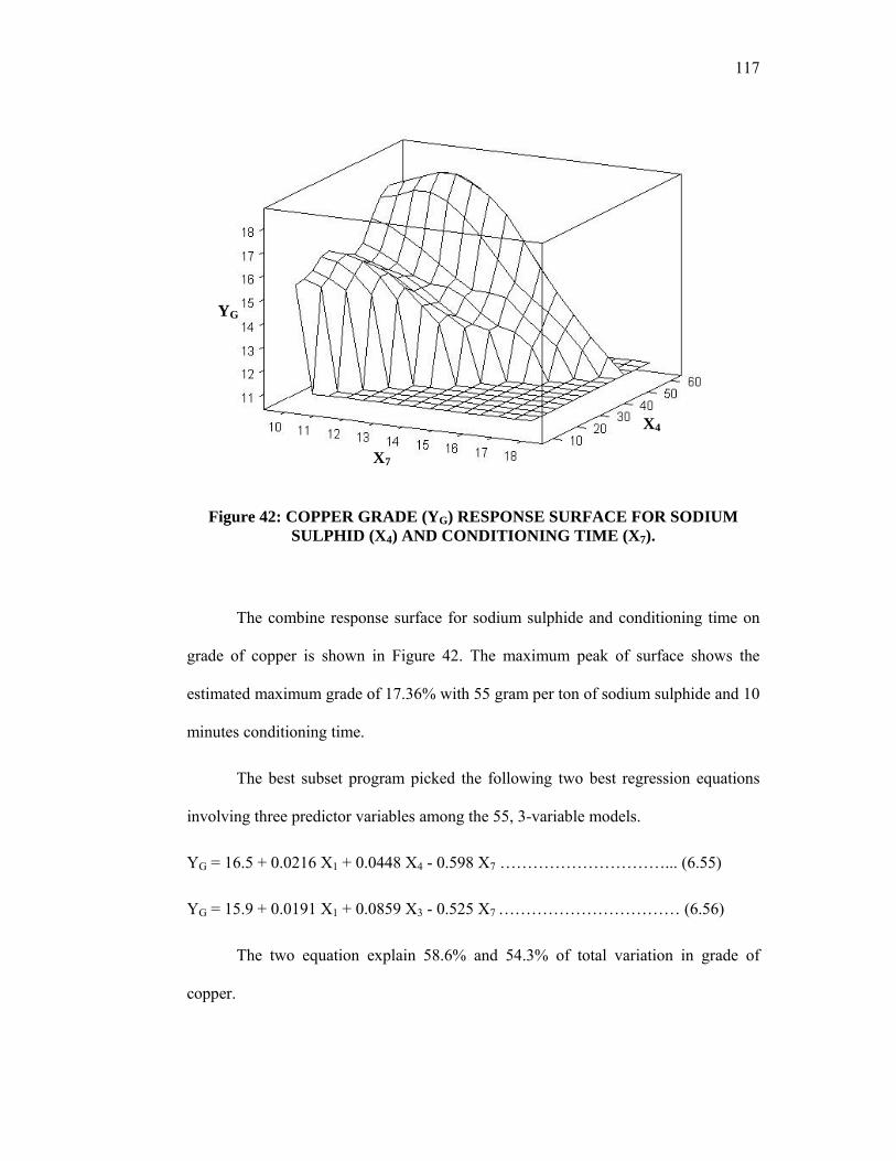
117
Figure 42: COPPER GRADE (YG) RESPONSE SURFACE FOR SODIUM SULPHID (X4) AND CONDITIONING TIME (X7).
The combine response surface for sodium sulphide and conditioning time on
grade of copper is shown in Figure 42. The maximum peak of surface shows the
estimated maximum grade of 17.36% with 55 gram per ton of sodium sulphide and 10
minutes conditioning time.
The best subset program picked the following two best regression equations
involving three predictor variables among the 55, 3-variable models.
YG = 16.5 + 0.0216 X1 + 0.0448 X4 - 0.598 X7 …………………………... (6.55)
YG = 15.9 + 0.0191 X1 + 0.0859 X3 - 0.525 X7 …………………………… (6.56)
The two equation explain 58.6% and 54.3% of total variation in grade of
copper.
X4
X7
YG

118
Among the next subset with four predictors, the follow two best regression
equations involving four predictor variables were selected by the program:
YG = 20.4 + 0.0216 X1 + 0.0411 X4 - 0.141 X6 - 0.570 X7 (6.57)
YG = 20.2 + 0.0193 X1 + 0.0601 X3 - 0.0437 X5 - 0.626 X7 (6.58)
Equation (6.57) explained 62.7% but in this model the contribution X6 is not
important. Equation (6.58) explained 61.1% of the variation in the data, all variables
in this model are collectively important so this is a good fit model for grade of copper.
The following two best regression equation involving five predictor variables
were selected by the program:
YG = 20.5 + 0.0194 X1 + 0.0386 X3 + 0.0281 X4 - 0.142 X6 - 0.567 X7 (6.59)
YG = 23.3 + 0.0193 X1 + 0.0591 X3 - 0.0371 X5 - 0.133 X6 - 0.593 X7 (6.60)
The improvement in R2 from equations with five predictor variables over
equations with four predictor variables is small so the models (6.57) and (6.58) are
better for data on grade of copper.
Both the above models are not significant different then model (6.57) and
(6.58).
The two best regression equations involving six predictor variables are given
below:
YG = 22.3 + 0.019 X1 + 0.039 X3 + 0.018 X4 - 0.023 X5 - 0.130 X6 - 0.602 X7…(6.61)
YG= 19.8+ 0.019 X1 +0.068 X2 +0.036 X3 +0.028 X4 -0.142 X6-0.567 X7…….. (6.62)
Both the above models are not statistically significant.

119
The full model involving seven predictor variables is:
YG=21.6+0.0194X1+0.066X2+0.0383X3+0.0182X4-0.0236X5-0.130X6-0.602X7 (6.63)
Full model was fitted for the grade of copper the excel out put is given below:
Table:– 15: Coefficient Analysis for Grad And Model Fitness Statistic For Seven
Variables
Table – 16: Analysis of Variance
Source DF SS MS F P
Regression 7 82.926 11.847 6.39 0.000
Residual Error 23 42.637 1.854
Total 30 125.563
From Statistical Analysis from Table (15), the regressors X2, X3, X4, X5, and X6 are
insignificant but collectively we cannot exclude these all regressors.
Predictor Coef SE Coef T P Standard
Error
1.362
Constant 21.577 9.366 2.30 0.031 R-Square 66.0%
X1 0.019390 0.007662 2.53 0.019 R-Square
(Adjusted)
55.7%
X2 0.0658 0.7846 0.08 0.934 Press 129.905
X3 0.03834 0.03773 1.02 0.320
X4 0.01824 0.01885 0.97 0.343
X5 -0.02360 0.02505 -0.94 0.356
X6 -0.13009 0.08607 -1.51 0.144
X7 -0.6017 0.1499 -4.02 0.001

120
Subset F (4,23) = 1.998 [0.1296] so we can exclude X2, X4, X5, and X6 on statistical
basis. So our new significant models is YG=15.9+0.019X1+0.0859X3-0.525X7.
Subset F (3,27) = 10.68 [0.0000] all regressors are collectively important.
6.7 Model development for grade:
To find out the best fit model for grade, a full model was filled first that
contain all available candidates as predictor, then the model was simplify by
discarding the variables that did not contribute to explaining the variability in the
dependent variable.
After working with different full and reduced models the following final
model was selected. The model gave good fit as judged by the adjusted R2 and it has
the required criteria– independence, normality etc of residual to some extent:
YG = 15.9 + 0.0191 X1 + 0.0859 X3 - 0.525 X7 ………………………………… (6.64)
The excel output for the model is given in table 15 and 16.
Table 16: OLS estimates for three significant variables
Predictor Coef SECoef T P S.E 1.458
Constant 15.876 2.135 7.44 0.000 R.Sq 54.3%
X1 0.019072 0.008204 2.32 0.028 R-Sq(adj) 49.2%
X3 0.08593 0.02450 3.51 0.002 Press
X7 -0.5249 0.1502 -3.49 0.002

121
Table – 17: Analysis of Variance
Source DF SS MS F P
Regression 3 68.147 22.716 10.68 0.000
Residual Error 27 57.416 2.127
Total 30 125.563
T-state in column 4 of table 15 for each coefficient suggests that each variable
is individually significant.
F statistics given below tells that collectively, all regressors are important
Significance F = 0.0043
Graphical Analysis:
Histogram of Residuals
Figure 43
The histogram looks normal

122
Testing for heteroscedasticity using squares
Figure 44
Residuals are heteroscedastic
Residuals are normal. It qualifies the visual test of normality.
0
0.2
0.4
0.6
0.8
1
1.2
0 1 2 3 4 5 6 7 8 9 10 11 12 13 14
Figure-45: RESIDUALS ARE NORMAL

123
6.8 General remarks about the model
For each regressor, a regression produces
A point estimate
A standard error
The point estimate helps us determine economic significance.
6.8.1 Statistical significance
A particular result is explained by chance if a coin is flipped five times in a
row and comes up heads each time, should I suspect that the coin is not a fair one with
equal chance of heads and tails?
In engineering data, we usually don’t have the luxury of adding more
observations to help us decide whether a result is due to chance. So we perform a
hypothesis test.
First, statistical significance. The difference is statistically significant, by
definition, if the 95% confidence interval does not overlap zero, or if the p value for
the effect is less than 0.05. Values of 95% or 0.05 are also equivalent to a type one
error rate of 5%: in other words, the rate of false alarms in the absence of any
population effect will be 5%. It has to be 5%, or less preferably, but like most
researchers I opted for 5%.
6.8.2 Sample Size?
The traditional approach for estimation of sample size is based on statistical
significance of outcome measure. We have to specify the smallest effect we want to

124
detect, the Type I and type II error rates, and design of the study. But unfortunately
we have limited observation.
Few agents who are not included are important for conducting experiment so
their constant values are present that are clear from the intercept.
Usually we need to exercise judgment to decide whether an estimated effect is
economically significant but in our case we can produce high quality copper grade by
just looking the model.
Usually if an estimated effect is economically and statically significant, we
need to weigh our results against those of other researchers but again it is our
misfortune that we don’t have any mathematical model to compare the results.
In analysis few times we face a problem that data are unusual. Because you
did things in a slightly different way than did others? If so, is our method one that is
knowledge and time? But in our case data is from control experiment so it can’t be
unusual.
6.9 Specific Remarks about the Model
We have the model
YG = 16.41 + 0.019 X1 + 0.048 X4 – 0.58 X7 ………………………………..… (6.65)
Here we have a linear model with the constraints of upper limits, which are
obvious from the data. We are choosing variable for inclusion solely on the basis of
statistical significance because we are not removing any regressor entirely. All or
their few combinations are necessary for experiments.

125
Here we have a statistically significant intercept in the model and it is
justifiable. If X1, X4, X7 all are collectively zero even though we can get copper grade
because other four regressors (here working as a constant) are presents.
In the model we have a negative coefficient of regressor X7 conditioning time
theory suggests the maximum values of grade 18.2 g/ton at 13 minutes can be
obtained. However, beyond that, the grade has markedly decreased due to the
entrapped of fine slim particles. That if we increase the optimum pulp density we will
get poor copper grade.
6.10 Discussion of size of coefficients and scientific judgment of
coefficient
If we generate the data from the model then this generated data will be
meaningless, as it can’t be compared with any other set of data because no such data
is available.
Though we have tested a lot of assumptions about the validity of the model
still we are uncertain about its results.
To overcome this problem one can randomly removed few observations from
the given set of data and again built model over same assumptions and then predict
the values that he had removed.
By simulation we checked that the coefficients are reasonable.

126
Figure 46: CONCEPTUAL GENERAL MODEL FOR RECOVERY / GRADE
If out of the seven inputs only one is varied then its variation will effect the
recovery/Grade YR/YG. Above figure demonstrates a conceptual model of this
phenomena only when input X is varied.
X
Recovery / Grade
PROCESS

127
CHAPTER-7
CONCLUSION
I understand that in Pakistan this is the first ever attempt to develop
Mathematical models both for recovery (YR) and grade (YG) of copper from the
copper ore.
Mathematical model for recovery
YR = 0.061X1+0.776X3 +0.191X4+0.917X6
Indicate that out of seven variables X1,X2, --, X7 only four of them Propylxanthate
(X1), Sodium Cyanide (X 3), Sodium Sulphide (X4) and pulp density (X6) are significant.
This model not only gives overall picture of the variables but also shows that X6 and
X3 play dominant role.
For Grade (YG) the mathematical model
YG = 0.019X1+0.0858X3-0.525 X7+15.9
Indicate that out of seven variables only three variables Propylxanthate (X1),
Sodium Cyanide (X3) and conditioning time (X7) are significant. Conditioning time
(X7) is the most dominant variables.
For Grade (YG) the variable X7 gives optimum results at 12 minute. For this fixed
value of X7, YG is further modified and YG = 0.019X1+0.0858X3+9.6
These mathematical models for recovery and grade, are strictly based on the
data provided by the Department of Mining Engineering N.W.F.P University of
Engineering and technology Peshawar. These models may not be valid for another
data if that do not conform to over data.

128
It is suggested that more experimental data may be generated against which
the above mathematical models and conclusions drawn from the models may be
verified.
A proposal amounting to Rs. 200 million was prepared by Prof. Dr.
Muhammad Mansoor Khan, Dean, Faculty of Engineering and was submitted for
approval to the Pakistan Science Foundation for enrichment and production of 99.9%
pure copper of North Waziristan Copper Ore.

129
REFERENCES
Acherman, P. K., Harris, G. H., Klimpel, R.R., Aplan, F. F., 2000. Int. J.
Miner. Process (Elsevier), Vol. 58, No. 1.
Agar, G.E., 1987. Simulation in mineral processing. Mineral processing
design. In: Yarar, B., Dogan, Z.M. (Eds.), NATO ASI Series E, 122. Martinus
Nijhoff Pub., Dordrecht, pp. 269–287.
Agar, G.E., Chia, J., Requis-c, L., 1998. Flotation rate measurements to
optimize an operating circuits. Minerals Engineering Vol. 11, No. 4,
pp. 347-360.
Agar, G.F, Stralton-Crawly, R., and Bruee, T.J. 1986. “Optimizing the design
of flotation circuits”. CIM Bulletin 73, pp. 173-181.
Ahmed, N., Jameson, G.J, 1989. Flotation kinetics. Mineral Processing and
Extractive Metallurgy Review 5, pp. 77–99.
Akhanazarova, S., Kafarov, V., 1982. Experiment Optimization in Chemistry
and Chemical Engineering. Mir Publishers, Moscow.
Aplan, F.F., 1976. Coal flotation. In: Fuerstenau, M.C. (Ed.), Flotation—A.M.
Gaudin Memorial, Vol. 2. SME, pp. 1235–1264.
Arbiter, N., Weiss, N.L., 1970. Design of Flotation Cells and Circuits, Society
of Mining Engineers, Preprint 70-B-89, AIME annual meeting.
Arbiter, N., Harris, C.C., and Yap, R.F.1967, In: Hydrodynamic of Flotation
cells Society of Mining Engineers, Transactions, Vol. 244, pp.134-148.

130
Arnold, B.J., Aplan, F.F., 1989. Application of rate models to pilot and
commercial scale coal froth flotation circuits. Presented at the SME, Annual
Meeting, Las Vegas, NV.
Arnold, B.J., Aplan, F.F., Arnold and Aplan, 1988. A practical view of rate
and residence time in industrial coal froth flotation circuits. In: Processing
Fifth Annual International, Pittsburgh Coal Conference, Pittsburgh, PA. Vol.
12, No. 16, pp. 328-341.
Badshah, S.M, 1983. Development Potential of Waziristan copper, record of
FATA development corporation, vol-11, pp. 2-13.
Badshah, S.M., 1985. Development Potential of Waziristan copper, record of
FATA development corporation, vol-3, pp. 14-18.
Banerjee, P.K., Choudhury, B.R., Ramu, A., Rao, P.V.T., Sripriya, R., 1998.
Plant trials with alternative to pine oil at West Bokaro. R & D Internal Report,
Tata steel.
Baro, M. and Piga, L., 1998. Mineral Processing Institute CNR Via Bolognola,
7-00138 Rome, Italy “Comparison of pb-zn selective collectors using
Statistical Methods”.
Cilek, E.C., 2004. “Estimation of flotation kinetic parameters by considering
interactions of the operating variables. “ Mineral Processing Division
Department of Mining Engineering, Faculty of Engineering, Suleyman
Demirel University, Isparta, TR 32260, Turkey. Vol. 17, No. 1. Pp. 81-85.
Dalton, R. F., Price, R., Hermana, E., and Hoffman, B., 1988. “Cuprex-New
Chloridebased Hydrometallurgy to Recover Copper from Sulfide Ores”.

131
Mining Engineering, Vol. 40, No. 1, pp. 24-28. Vol. 2, No.1 Characterization
and Flotation of Sulfur from Chalcopyrite Concentrate Leaching.
Deglon, D.A., Sawyerr, F., O., Connor, C.T., 1999. A model to relate the
flotation rate constant and the bubble surface area flux in mechanical flotation
cells. Minerals Engineering Vol. 12 No. 6, Pp. 599–608.
Dowling, E. C., Klimpel, R.R. and Aplan, F.F., 1985. Model discrimination in
the floation of a porphyry copper ore. Minerals and Metallurgical Processing,
pp.87-101.
Dowling, E. C., Klimpel, R.R. and Aplan, F.F., 1987. Use of kinetic model to
analyze industrial flotation circuits. In: D.R Gaskell et a,:. International
Symposium on Innovative Technology and Reactor Design in Extractive
Metallugy, TMS-AIME, Warrendale, PA, pp.533-552.
Dutrizac, J. E., and MacDonald, R. J. C., 1974. “Ferric Ion as a Leaching
Medium”, Minerals Science. Engineering, Vol. 6, No 2, pp. 59-100.
Edmonson, N., 1994. “North American Sulfur Market: Structure and
Outlook”, Mining Engineering, Vol. 46, No. 6, pp. 563-567.
Faulkner, B.P., 1966. “Computer control improves metallurgy at Tennessee
copper flotation” Plan Mining Engineering, pp. 53-57.
Fuerstenau, D.W. (Ed.), 1981. Mathematical Models of Flotation. Mineral
Coal Flotation Circuits—Their Simulation and Control. Elsevier, New York,
vol. 3, pp. 57– 70.
Harris, C.C., 1974. Impeller speed, air and power requirements in floatation
machine scale-up. International journal of Mineral processing, pp.51-64.

132
Harris, C.C., Rimmer, H.W., 1966. Study of a two phase model of the flotation
process. Institution of Mining and Metallurgy, pp. 153– 161.
Haver, F. P., and Wong, W. W., 1971. “Recovery of Copper, Iron and Sulfur
from Chalcopyrite Concentrate Using a Ferric Chloride Leach”, Journal of
Metals, Vol. 23, No 2, pp. 25-29.
Haver, F. P., Baker, R. D., and Wong, M. M., 1975. “Improvements in Ferric
Chloride Leaching of Chalcopyrite Concentrate”, U. S. Bureau of Mines,
RI8007.
Horbstand, J.A., et al., 2004. “Radical innovations in mineral processing
simulation” Society for mining, Metallurgy, and exploration, INC. vol. 21. No.
2. pp. 57-63.
Huber-Panu, I., Ene-Danalance, E., Cojocariu, D.G., 1976. Mathematical
models of batch and continuous flotation. In: Fuerstenau, D.W. (Ed.),
Flotation-A.M. Gaudin Memorial Volume, AIME, pp. 675–724.
Jaisen, N.2002, Thesis on “Improving efficiencies in water-Based separators
using Mathematical Analysis tool” Kohmuench U.S.A.
Kelsall, D.F., 1961. Application of probability in the assessment of flotation
systems. Transactions of the Institution of Mining and Metallurgy Vol. 70, pp.
191– 204.
Khan et al., 1984. “Flotation studies on North Waziristan copper ore
Proceeding of Seminar on prospects in problem of mineral based industry in
Pakistan”, Peshawar published by the Department of Mining Engineering,
NWFP University of Engineering and Technology Peshawar.

133
Khan, et al. 2000. “Flotation of copper minerals from North Wazirsitan copper
ore on pilot-scale”. Quarterly science vision vol. 6. No. 1, pp. 10-20.
Khan, M.M., Proceedings of the first seminar on problems and prospects on
mineral based industries in Pakistan.
Klimpel, R.R., 1987. “Use of mathematical modeling to analyze collectors
dosage effects in forth flotation”, in the mathematical modeling of Metals
Processing Operation. Extractive and Process Metallurgy Fall Meeting., Palm
Springs, CA, p.12.
Klimpel, R.R., 2000. Optimizing the industrial flotation performance of
sulfide minerals having some natural floatability. International Journal of
Mineral Processing Vol. 58 No. (1–4), pp. 77–84.
Klimpel, R.R., Mular, A.L., and Bhappu R.B., Editors, 1980. Selection of
Chemical Reagents for Flotataion mineral Processing Plant Design (2nd ed.),
AIME, New York, pp. 930-934.
Kuopanportti, H., Suorsa, T., Dahl, O., Niinimaki, J., 2000. A model of
conditioning in the flotation of a mixture of pyrite and chalcopyrite ores.
International Journal of Mineral Processing Vol. 59 No. 4, pp. 327–338.
Lin, H.K., 2003. “Characterization and Flotation of Sulfur from Chalcopyrite
Concentrate Leaching Residue”. Minerals & Materials Journal of
Characterization & Engineering, Vol. 2, No.1, pp1-9.
Mao, L., Yoon, R.H., 1997. Predicting flotation rates using a rate equation
derived from first principles. International Journal of Mineral Processing Vol.
51, pp. 171–181.

134
Oliveira, J.F., Saraiva, S.M., Pimenta, J.S., Oliveira, A.P.A., 2001. Kinetics of
pyrochlore flotation from Arax_a mineral deposits. Minerals Engineering Vol.
14 No. 1, pp. 99–105.
Rau, M. F., and Fuerstenau, M. C., 1981. “Rate Phenomena Involved in the
Dissolution of Chalcopyrite in Chloride-bearing Lixiviants”, Metallurgical
Transaction, Vol. 12B, pp. 595-601,
Parker, A. J., Paul R. L., and Power G. C., 1981. “Electrochemical Aspects of
Leaching Copper from Chalcopyrife in Ferric and Cupric Salt Solutions”,
Aust. J. of Chemistry, Vol. 34, pp. 13-34.
Pitt, J.C., 1968. “The development of system for continuous optimal control of
flotation plants. In: Computer Systems Dynamics and Automatic Control in
Basic Industries”, I.F.R.C Symposium, Sydney, pp. 165-171.
Polat, M., Chander, S., 2000. First-order flotation kinetics models and
methods for estimation of the true distribution of flotation rate constants.
International Journal of Mineral Processing Vol. 58, No. (1–4), pp. 145–166.
Smith, H.W., Lewis, C.L., 1969. Computer control experiments at lake
default. Canadian IMM Bulletin Vol. 62, No. 682, pp. 109–115.
Sripriya, R., P.V.T. Rao, Choudhry, B.R., Rao, M.V.S., and Sensharma, S.,
1997. Increasing the Yield in flotation-scale up of laboratory data and
commercialization. Fuel Scinece and Technology Vol. 16, No. 3, pp. 71-77.
Sripriya, R. P.V.T. Rao , Chaudhry, B.R. 2003 R and D Division Tata steel,
Jamshedpur, Jharkhand 831 007, India.. “Optimization of operating variables
of fine coal flotation using a combination of modified flotation parameters and

135
Statistical Techniques”. International journal mineral processing Vol. 68,
No.(1-4), pp. 109-127.
Tidwell, P.W., G.E.P Box, 1962. “Transformation of Independent Variable”,
techno metrics, Vol. 4, pp. 531-550.
U.S. Bureau of Mines, 1990. “Mineral Industry Surveys”, Copper Monthly, p.
20.
Van Orden, P.R., 1986. “Simulation of continuous flotation cells using
observed residence time distributions”. In: P. Somasundaran, Editor, Advances
in Mineral Processing, SME-AIME, Littleton, Co, pp.714-725.
Vera, N.A. The Modeling of froth zone Recovery in Batch and continuously
operated Laboratory flotation cells” N.A. the University of Queens Land
Brisbane, QLD Australia.
Wang, Z., 1996. Lecture on Distribution and Metallogenic Models of large
copper deposits of the world in North Waziristan copper ore.
Weiss, N. L., 1985. “SME Mineral Processing Handbook”, Society of Mining
Wills, B.A., 1986. Camborne school of mines, Red Ruth, Corn Wall, TR 15
3SE, Great Britain “Complex circuit mass balancing-A simple, practical,
sensitivity Analysis Method”.
Wills, B.A., 1997. Mineral Processing Technology, sixth ed. Butterworth-
Heinemann, Oxford. pp. 284–316.
Xu, M., 1998. “Modified flotation rate constant and selectivity index”.
Minerals engineering Vol. 11 No. 3, pp. 271-278.
136
Yianatos, J.B., Bergh, L.G., Condori, P., Aguilera, J., 2001. Hydrodynamic
and metallurgical characterization of industrial flotation banks for control
purposes. Minerals Engineering Vol. 14, No. 9, pp. 1033–1046.
Ziyadanogullari, Firat Aydin. 2005. “A New Application For Flotation of
Oxidized Copper ore” Journal of Minerals & Materials Characterization &
Engineering, Vol. 4, No. 2, pp 67-73.

137
APPENDIX-1
General model for Recovery and Grade of copper using E-view
software:
YR = -25.2 + 0.05334*X1 + 3.735*X2 + 0.6932*X3 + 0.1583*X4
(SE) (25.8) (0.0211) (2.16) (0.104) (0.0519)
- 0.09816*X5 + 0.8331*X6 - 0.4502*X7 ---------- (a)
(0.069) (0.237) (0.413)
Since the t-ratio of following regressors are insignificant so we now try to observe
whether we can collectively drop all these variables or not.
Test for excluding:
[0] = Constant
[1] = X2
[2] = X5
[3] = X7
Subset F (4,23) = 1.5485 [0.2216]
So we can collectively drop them
Now our new model will be
YR = + 0.06148*X1 + 0.7765*X3 + 0.1911*X4 + 0.9176*X6 ---------- (b)
(SE) (0.0194) (0.0932) (0.0431) (0.118)
T-ratio shows that all above regressors are individually important.
Subset F (4,27) = 1688.9 [0.0000]**
So collectively they are important.
R2 = 99.60

138
R2 is very high but we know that t-ratio, F-stat and R2 etc give meaningful values if
residuals are identically independent normal. So we check that whether these
variables are identically independent normal or not.
Graphical Analysis For recovery of Copper:
Figure (A)
It looks almost normal.
Normality test for Residuals
Observations 31
Mean 0.043489
Std. Devn. 3.6404
Skewness -0.78933
Excess Kurtosis 1.1999
Minimum -11.304
Maximum 6.2073
Asymptotic test: Chi^2(2) = 5.0787 [0.0789]
Normality test: Chi^2(2) = 4.8027 [0.0906]
So residuals qualify normality test.

139
Actual and fitted values
Figure (B)
Standard Residual graph
Figure (C)
Residuals look independent.

140
Autocorrelation of residuals
Figure (D)
No significant autocorrelation present
Therefore residuals are identically independent normal.
General Model for Grad of Copper
YG = 21.58 + 0.01939*X1 + 0.06566*X2 + 0.03842*X3 + 0.01821*X4
(SE) (9.37) (0.00766) (0.785) (0.0377) (0.0188)
- 0.02359*X5 - 0.1301*X6 - 0.6017*X7 ------------- (c)
(0.025) (0.0861) (0.15)
Test for excluding:
[0] = X2
[1] = X3
[2] = X4
[3] = X5
[4] = X6
Subset F (5,23) = 4.4172 [0.0058]**

141
We can’t collectively exclude the all above regressors
Test for excluding:
[0] = X2
[1] = X4
[2] = X5
[3] = X6
Subset F (4,23) = 1.9908 [0.1296]
So we can exclude these regressors on totally statistical basis
YG = + 15.88 + 0.01907*X1 + 0.08596*X3 - 0.525*X7 ----------- (d)
(SE) (2.13) (0.0082) (0.0245) (0.15)
R2 = 0.542911
Subset F (3,27) = 10.68 [0.0000]**
All variables are collectively important.
Figure (E)

142
It looks normal
Normality test for Residuals
Observations 31
Mean 0.00000
Std.Devn. 1.3607
Skewness -0.41587
Excess Kurtosis 0.62105
Minimum -3.3897
Maximum 3.1853
Asymptotic test: Chi^2(2) =1.3918 [0.4986]
Normality test: Chi^2(2) = 3.1105 [0.2111]
Residuals qualify normality test
Figure (F)

143
Testing for heteroscedasticity using squares
Chi^2(8) = 29.292 [0.0003]** and F-form F (8,18) = 38.580 [0.0000]**
Residuals are heteroscedastic.
Now we take other possible model
Test for excluding:
[0] = X2
[1] = X3
[2] = X5
[3] = X6
Subset F (4,23) =1.2639 [0.3127]
So we can exclude these variables
YG = + 16.48 + 0.02159*X1 + 0.04478*X4 - 0.598*X7 -------- (e)
(SE) (2.06) (0.00758) (0.0111) (0.147)
T-ratio shows that all variables are individually important.
F (3,27) = 12.73 [0.000]**
F stat shows that all variables are collectively important
R2 = 0.585837
T-ratio, F-stat and R2 etc give meaningful values if residuals are identically
independent normal. So we check that whether these variables are identical
independent normal or not.

144
Graphical analysis of residuals
Testing for heteroscedasticity using squares
Chi^2(6) = 5.8926 [0.4353] and F-form F (6,20) = 0.78232 [0.5937]
So residuals are homoscedastics
Normality test for Residuals
Normality test for Residuals
Observations 31
Mean 0.00000
Std.Devn 1.2952
Skewness -0.65212
Excess Kurtosis 1.1558
Minimum -3.8576
Maximum 2.9363
Asymptotic test: Chi^2(2) = 3.9228 [0.1407]
Normality test: Chi^2(2) = 4.8522 [0.0884]
Residuals histogram
Figure (G)

145
Actual fitted values.
Figure (H)
Standard residuals for above model
Figure (I)
Residual looks independent

146
APPENDIX – 2
FORWARD SELECTION
Output from forward model selection procedure used for data on copper
recovery by the flotation process with seven variables (Alpha-to-enter: 0.25, N = 31)
Table – A
Step 1 2 3 4 5 6
Constant 38.254 38.493 15.650 6.132 -35.026 -29.933
X3 1.101 0.837 0.835 0.779 0.688 0.694
T-Value 12.94 7.52 8.41 8.29 6.55 6.65
P-Value 0.000 0.000 0.000 0.000 0.000 0.000
X4 0.168 0.185 0.188 0.191 0.155
T-Value 3.18 3.90 4.29 4.53 2.97
P-Value 0.004 0.001 0.000 0.000 0.007
X6 0.76 0.76 0.76 0.79
T-Value 2.87 3.12 3.23 3.38
P-Value 0.008 0.004 0.003 0.003
X1 0.054 0.053 053
T-Value 2.44 2.50 2.52
P-Value 0.022 0.019 0.019
X2 3.7 3.7
T-Value 1.71 1.72
P-Value 0.099 0.098
X5 -0.080
T-Value -1.19
P-Value 0.247
S 5.50 4.80 4.28 3.94 3.80 3.77
R-Sq 85.25 89.17 91.69 93.24 93.95 94.28
R-Sq(adj) 84.74 88.39 90.77 92.20 92.74 92.85
C-p 35.4 20.8 12.1 7.6 6.6 7.2
Press 1000.40 787.710 672.060 565.64 537.56 632.9
R-Sq(Pred) 83.20 86.77 88.71 90.50 90.97 89.37

147
APPENDIX – 3
BACKWARD ELIMINATION
Minitab out from backward elimination model selection procedure used for the
combined data for copper recovery in the flotation process with seven variables
(Alpha-to-Remove: 0.1, N = 31)
Table – B
Step 1 2 3
Constant -25.20 -29.93 -35.03
X1 0.053 0.053 0.053
T-Value 2.53 2.52 2.50
P-Value 0.019 0.019 0.019
X2 3.7 3.7 3.7
T-Value 1.73 1.72 1.71
P-Value 0.097 0.098 0.099
X3 0.69 0.69 0.69
T-Value 6.67 6.65 6.55
P-Value 0.000 0.000 0.000
X4 0.158 0.155 0.191
T-Value 3.05 2.97 4.53
P-Value 0.006 0.007 0.000
X5 -0.098 -0.080
T-Value -1.42 -1.19
P-Value 0.168 0.247
X6 0.83 0.79 0.76
T-Value 3.51 3.38 3.23
P-Value 0.002 0.003 0.003
X7 -0.45
T-Value -1.09
P-Value 0.287

148
S 3.75 3.77 3.80
R-Sq 94.56 94.28 93.95
R-Sq(adj) 92.91 92.85 92.74
C-p 8.0 7.2 6.6
Press 680.517 632.917 537.569
R-Sq(pred) 88.57 89.37 90.97

149
APPENDIX – 4
Minitab out from best subset procedure used for the combined data for copper
recovery by the flotation process with seven variables.
i. One variable best model YR = 38.254 + 1.101X3
Table – A: S = 5.504, R-Sq = 85.2%, R-Sq(adj) = 84.7%, Press = 1000.40
Predictor Coef SECoef T P
Constant 38.254 1.691 22.62 0.000
X3 1.101 0.085 12.94 0.000
Table – B: Analysis of Variance
Source DF SS MS F P
Regression 1 5075.0 5075.0 167.55 0.000
Residual Errors 29 878.4 30.3
Total 30 5953.4
ii. One variable second best model YR = 44.9 + 0.465X4
Table – A: S = 8.19, R-Sq = 67.3%, R-Sq(adj) = 66.1%, Press = 2236.53
Redictor Coef SE Coef T P
Constant 44.919 2.058 21.83 0.000
X4 0.464 0.060 7.72 0.000
Table – B: Analysis of Variance
Source DF SS MS F P
Regression 1 4004.3 4004.3 59.58 0.000
Residual Errors 29 1949.0 67.2
Total 30 5953.4

150
iii. Two variables best model YR = 38.5 + 0.837 X3 + 0.168X4
Table – A: S = 4.800, R-Sq = 89.2%, R-Sq(adj) = 88.4%, Press = 787.710
Predictor Coef SE Coef T P
Constant 38.493 1.477 26.07 0.000
X3 0.837 0.111 7.52 0.000
X4 0.168 0.052 3.18 0.004
Table – B: Analysis of Variance
Source DF SS MS F P
Regression 2 5308.4 2654.2 115.22 0.000
Residual Errors 28 645.0 23.0
Total 30 5953.4
iv. Two variables second best model YR = 50.7+ 0.991 X3 –0.164 X5
Table – A: S = 5.153, R-Sq = 87.5%, R-Sq(adj) = 86.6%, Press = 910.345
Predictor Coef SE Coef T P
Constant 50.675 5.736 8.84 0.000
X3 0.991 0.093 10.61 0.000
X5 -0.164 0.072 -2.25 0.032
Table – B: Analysis of Variance
Source DF SS MS F P
Regression 2 5209.8 2604.9 98.09 0.000
Residual Errors 28 743.6 26.6
Total 30 5953.4

151
v. Three variables best model YR = 29.0+ 0.053 X1 + 0.782 X3 + 0.171 X4
Table – A: S = 4.526, R-Sq = 90.7%, R-Sq(adj) = 89.7%, Press = 681.242
Predictor Coef SE Coef T P
Constant 28.983 4.702 6.16 0.000
X1 0.053 0.025 2.12 0.044
X3 0.781 0.108 7.23 0.000
X4 0.170 0.049 3.42 0.002
Table – B: Analysis of Variance
Source DF SS MS F P
Regression 3 5400.2 1800.1 87.87 0.000
Residual 27 553.1 20.5
Total 30 5953.4
vi. Three variables second best model YR=15.6+ 0.835X3 + 0.185X4 + 0.762 X6
Table – A: S = 4.280, R-Sq = 91.7%, R-Sq(adj) = 90.8%, Press = 672.060
Predictor Coef SE Coef T P
Constant 15.650 8.078 1.94 0.063
X3 0.834 0.099 8.41 0.000
X4 0.185 0.047 3.90 0.001
X6 0.761 0.265 2.87 0.008

152
Table – B: Analysis of Variance
Source DF SS MS F P
Regression 3 5458.8 1819.6 99.34 0.000
Residual Errors 27 494.5 18.3
Total 30 5953.4
vii. Four variables best model YR=6.13+0.0539X1+0.779X3 +0.188X4+0.762 X6
Table – A: S = 3.935, R-Sq = 93.2%, R-Sq(adj) = 92.2%, Press = 565.649
Predictor Coef SE Coef T P
Constant 6.132 8.392 0.73 0.472
X1 0.053 0.022 2.44 0.022
X3 0.779 0.094 8.29 0.000
X4 0.187 0.043 4.29 0.000
X6 0.761 0.244 3.12 0.004
Table – B: Analysis of Variance
Source DF SS MS F P
Regression 4 5550.7 1387.7 89.61 0.000
Residual Errors 26 402.6 15.5
Total 30 5953.4

153
viii. Four variables second best model with out intercept YR = 0.0615X1 +
0.777X3 +0.191X4 + 0.918X6
Table – A: S = 3.9, R-Sq = 99.60%, R-Sq(adj) = 92.74%, Press = 526.202
Predictor Coef SE Coef T P
Constant 0 0 0 0
X1 0.061 0.019 3.16 0.004
X3 0.776 0.093 8.34 0.000
X4 0.191 0.043 4.44 0.000
X6 0.917 0.118 7.78 0.000
Table – B: Analysis of Variance
Source DF SS MS F P
Regression 4 102807 25702 1688.93 0.000
Residual Errors 27 411 15
Total 31 103218
ix. Four variables third best model YR=-26.6+3.83X2+0.741X3+0.189X4+0.782X6
Table – A: S = 4.16, R-Sq = 92.4%, R-Sq(adj) = 91.3%, Press = 63.69
Predictor Coef SE Coef T P
Constant -26.57 27.57 -0.96 0.344
X2 3.831 2.398 1.60 0.122
X3 0.741 0.112 6.57 0.000
X4 0.189 0.046 4.09 0.000
X6 0.761 0.258 2.95 0.007

154
Table – B: Analysis of Variance
Source DF SS MS F P
Regression 4 5503.0 1375.8 79.43 0.000
Residual Errors 26 450.3 17.3
Total 30 5953.4
x. Five variables best model YR = -35.0+ 0.0534X1 + 3.74X2 +0.688X3 +
0.191X4 + 0.762X6
Table – A: S = 3.79, R-Sq = 93.9%, R-Sq(adj) = 92.7%, Press = 537.569
Predictor Coef SE Coef T P
Constant -35.03 25.38 -1.38 0.180
X1 0.053 0.021 2.50 0.019
X2 3.744 2.188 1.71 0.099
X3 0.688 0.105 6.55 0.000
X4 0.191 0.042 4.53 0.000
X6 0.761 0.235 3.23 0.003
Table – B: Analysis of Variance
Source DF SS MS F P
Regression 5 5592.9 1118.6 77.59 0.000
Residual 25 360.4 14.4
Total 30 5953.4

155
xi. Five variables second best model YR = 8.56+ 0.054X1 + 0.778X3 +0.196X4
+ 0.826X6-0.305X7
Table – A: S = 3.972, R-Sq = 93.4%, R-Sq(adj) = 92.0%, Press = 617.656
Predictor Coef SE Coef T P
Constant 8.563 9.118 0.94 0.357
X1 0.053 0.022 2.41 0.023
X3 0.778 0.094 8.20 0.000
X4 0.195 0.045 4.30 0.000
X6 0.782 0.248 3.15 0.004
X7 -0.305 0.423 -0.72 0.478
Table – B: Analysis of Variance
Source DF SS MS F P
Regression 5 5558.9 1111.8 70.47 0.000
Residual Error 25 394.4 15.8
Total 30 5953.4
xii. Six variables second best model YR = -32.6+ 0.053X1 + 3.75X2 +0.687X3 +
0.200X4 + 0.783X6 –0.306X7
Table – A: S = 3.831, R-Sq = 94.1%, R-Sq(adj) = 92.6%, Press = 589.660
Predictor Coef SE Coef T P
Constant -32.61 25.81 -1.26 0.219
X1 0.053 0.021 2.48 0.021
X2 3.746 2.207 1.70 0.103
X3 0.687 0.106 6.48 0.000
X4 0.199 0.043 4.54 0.000
X6 0.782 0.239 3.27 0.003
X7 -0.306 0.408 -0.75 0.461

156
Table – B: Analysis of Variance
Source DF SS MS F P
Regression 6 5601.18 933.53 63.62 0.000
Residual Error 24 352.17 14.67
Total 30 5953.35
xiii. Six variables best model YR = -29.9+ 0.053X1 + 3.73X2 +0.694X3 + 0.155X4
+ 0.079X5 –0.795X6
Table – A: S = 3.766, R-Sq = 94.3%, R-Sq(adj) = 92.9%, Press = 632.917
Predictor Coef SE Coef T P
Constant -29.93 25.54 -1.17 0.253
X1 0.053 0.021 2.52 0.019
X2 3.735 2.170 1.72 0.098
X3 0.693 0.104 6.65 0.000
X4 0.154 0.052 2.97 0.007
X5 -0.079 0.067 -1.19 0.247
X6 0.794 0.235 3.38 0.003
Table – B: Analysis of Variance
Source DF SS MS F P
Regression 6 5612.92 935.49 65.95 0.000
Residual Error 24 340.43 14.18
Total 30 5953.35

157
xiv. Seven variables i.e full model YR = -25.2+ 0.053X1 + 3.74X2 +0.693X3 +
0.158X4 - 0.0982X5 +0.833X6-0.450X7
Table – A: S = 3.752, R-Sq = 94.6%, R-Sq(adj) = 92.9%, Press = 680.517
Predictor Coef SE Coef T P
Constant -25.20 25.81 -0.98 0.339
X1 0.053 0.021 2.53 0.019
X2 3.735 2.162 1.73 0.097
X3 0.693 0.104 6.67 0.000
X4 0.158 0.051 3.05 0.006
X5 -0.098 0.069 -1.42 0.168
X6 0.833 0.237 3.51 0.002
X7 -0.450 0.412 -1.09 0.287
Table – B: Analysis of Variance
Source DF SS MS F P
Regression 7 5629.65 804.24 57.14 0.000
Residual Error 23 323.71 14.07
Total 30 5953.35

158
APPENDIX – 5
FORWARD SELECTION FOR GRADE
Minitab output from forward model selection procedure used for data on grade
by the flotation process with seven variables. (Alpha – to – enter 0.1, N=31)
Table - A
Step 1 2 3 4 5
Constant 14.01 19.26 15.88 20.16 23.33
X3 0.085 0.104 0.086 0.060 0.059
T-Value 3.05 4.19 3.51 2.31 2.34
P-Value 0.005 0.000 0.002 0.029 0.028
X7 -0.53 -0.52 -0.63 -0.59
T-Value -3.26 -3.49 -4.21 -4.05
P-Value 0.003 0.002 0.000 0.000
X1 0.0191 0.0193 0.0193
T-Value 2.32 2.50 2.57
P-Value 0.028 0.019 0.017
X5 -0.044 -0.037
T-Value -2.14 -1.83
P-Value 0.042 0.080
X6 -0.133
T-Value -1.58
P-Value 0.126
S 1.81 1.57 1.46 1.37 1.33
R-Sq 24.31 45.12 54.27 61.11 64.66
R-Sq(adj) 21.70 41.20 49.19 55.13 57.59
C-p 24.3 12.2 8.0 5.3

159
APPENDIX – 6
BACKWARD ELIMINATION. ALPHA-TO-REMOVE: 0.1
Minitab output from backward elimination model selection procedure used for
the combined data for copper on grade in the flotation process with seven variables.
(Alpha–to–remove 0.1,N = 31)
Table - A
Step 1 2 3 4 5 Constant 21.58 22.30 20.55 20.43 16.48 X1 0.0194 0.0194 0.0194 0.0216 0.0216 T-Value 2.53 2.59 2.59 2.95 2.85 P-Value 0.019 0.016 0.016 0.007 0.008 X2 0.07 T-Value 0.08 P-Value 0.934 X3 0.038 0.040 0.039
T-Value 1.02 1.25 1.21
P-Value 0.320 0.223 0.237
X4 0.018 0.018 0.028 0.041 0.045 T-Value 0.97 0.99 1.84 3.76 4.05 P-Value 0.343 0.334 0.078 0.001 0.000 X5 -0.024 -0.024 T-Value -0.94 -0.96 P-Value 0.356 0.345 X6 -0.130 -0.130 -0.142 -0.141
T-Value -1.51 -1.54 -1.71 -1.68 P-Value 0.144 0.136 0.100 0.105 X7 -0.60 -0.60 -0.57 -0.57 -0.60 T-Value -4.02 -4.10 -3.99 -3.98 -4.07 P-Value 0.001 0.000 0.001 0.000 0.000 S 1.36 1.33 1.33 1.34 1.39 R-Sq 66.04 66.03 64.72 62.65 58.59 R-Sq(adj) 55.71 57.54 57.67 56.90 53.99 C-p 8.0 6.0 4.9 4.3 5.1 Press 129.905 124.851 118.041 116.114 73.6739

160
APPENDIX – 7
Minitab out from best subset procedure used for the combined data copper
grade by the flotation process with seven variables.
I. One variable best model YG = 14.0 + 0.0854 X3
Table – A: S = 1.810, R-Sq = 24.3%, R-Sq(adj) = 21.7%, Press = 108.113
Predictor Coef SE Coef T P
Constant 14.0078 0.5563 25.18 0.000
X3 0.08539 0.02798 3.05 0.005
Table – B: Analysis of Variance
Source DF SS MS F P
Regression 1 30.522 30.522 9.31 0.005
Residual Error 29 95.041 3.277
Total 30 125.563
ii. One variable second best model YG = 14.5 + 0.0374 X4
Table – A: S = 1.853, R-Sq = 20.7%, R-Sq(adj) = 17.9%, Press = 114.609
Predictor Coef SE Coef T P
Constant 14.4922 0.4652 31.15 0.000
X4 0.03741 0.01361 2.75 0.010
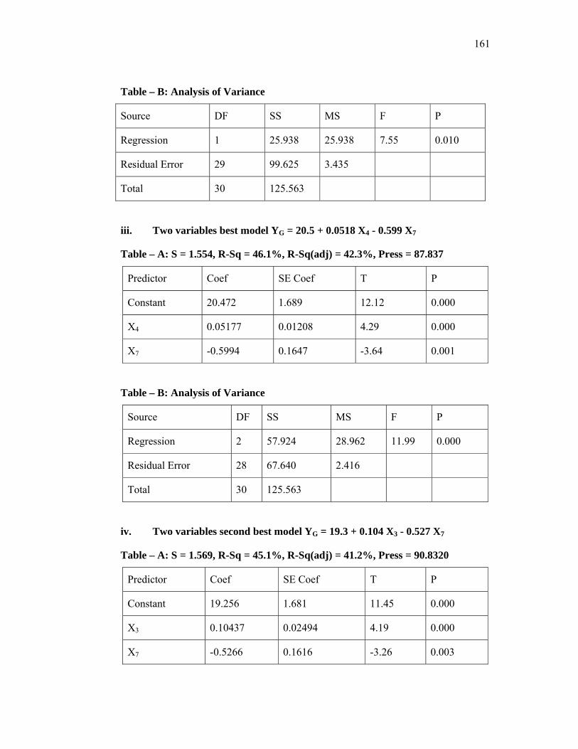
161
Table – B: Analysis of Variance
Source DF SS MS F P
Regression 1 25.938 25.938 7.55 0.010
Residual Error 29 99.625 3.435
Total 30 125.563
iii. Two variables best model YG = 20.5 + 0.0518 X4 - 0.599 X7
Table – A: S = 1.554, R-Sq = 46.1%, R-Sq(adj) = 42.3%, Press = 87.837
Predictor Coef SE Coef T P
Constant 20.472 1.689 12.12 0.000
X4 0.05177 0.01208 4.29 0.000
X7 -0.5994 0.1647 -3.64 0.001
Table – B: Analysis of Variance
Source DF SS MS F P
Regression 2 57.924 28.962 11.99 0.000
Residual Error 28 67.640 2.416
Total 30 125.563
iv. Two variables second best model YG = 19.3 + 0.104 X3 - 0.527 X7
Table – A: S = 1.569, R-Sq = 45.1%, R-Sq(adj) = 41.2%, Press = 90.8320
Predictor Coef SE Coef T P
Constant 19.256 1.681 11.45 0.000
X3 0.10437 0.02494 4.19 0.000
X7 -0.5266 0.1616 -3.26 0.003

162
Table – B: Analysis of Variance
Source DF SS MS F P
Regression 2 56.653 28.327 11.51 0.000
Residual Error 28 68.910 2.461
Total 30 125.563
v. Three variables best model YG = 16.5 + 0.0216 X1 + 0.0448 X4 - 0.598 X7
Table – A: S = 1.388, R-Sq = 58.6%, R-Sq(adj) = 54.0%, Press = 73.673
Predictor Coef SE Coef T P
Constant 16.480 2.058 8.01 0.000
X1 0.021587 0.007575 2.85 0.008
X4 0.04479 0.01106 4.05 0.000
X7 -0.5979 0.1471 -4.07 0.000
Table – B: Analysis of Variance
Source DF SS MS F P
Regression 3 73.563 24.521 12.73 0.000
Residual Error 27 52.000 1.926
Total 30 125.563
vi. Three variables second best model YG = 15.9 + 0.0191 X1 + 0.0859 X3 - 0.525 X7
Table – A: S = 1.458, R-Sq = 54.3%, R-Sq(adj) = 49.2%, Press = 80.260
Predictor Coef SECoef T P
Constant 15.876 2.135 7.44 0.000
X1 0.019072 0.008204 2.32 0.028
X3 0.08593 0.02450 3.51 0.002
X7 -0.5249 0.1502 -3.49 0.002

163
Table – B: Analysis of Variance
Source DF SS MS F P
Regression 3 68.147 22.716 10.68 0.000
Residual Error 27 57.416 2.127
Total 30 125.563
vii. Four variables best model YG = 20.4 + 0.0216 X1 + 0.0411 X4 - 0.141 X6 -
0.570 X7
Table – A: S = 1.343, R-Sq = 62.7%, R-Sq(adj) = 56.9%, Press = 116.114
Predictor Coef SE Coef T P
Constant 20.435 3.082 6.63 0.000
X1 0.021614 0.007331 2.95 0.007
X4 0.04112 0.01092 3.76 0.001
X6 -0.14119 0.08395 -1.68 0.105
X7 -0.5700 0.1433 -3.98 0.000
Table – B: Analysis of Variance
Source DF SS MS F P
Regression 4 78.666 19.666 10.90 0.000
Residual Error 26 46.898 1.804
Total 30 125.563

164
viii. Four variables second best model YG = 20.2 + 0.0193 X1 + 0.0601 X3
- 0.0437 X5 - 0.626 X7
Table – A: S = 1.370, R-Sq = 61.1%, R-Sq(adj) = 55.1%, Press = 73.70
Predictor Coef SE Coef T P
Constant 20.163 2.836 7.11 0.000
X1 0.019256 0.007710 2.50 0.019
X3 0.06011 0.02600 2.31 0.029
X5 -0.04375 0.02046 -2.14 0.042
X7 -0.6264 0.1489 -4.21 0.000
Table – B: Analysis of Variance
Source DF SS MS F P
Regression 4 76.735 19.184 10.22 0.000
Residual Error 26 48.828 1.878
Total 30 125.563
ix. Five variables best model YG = 20.5 + 0.0194 X1 + 0.0386 X3 + 0.0281 X4 -
0.142 X6 - 0.567 X7
Table – A: S = 1.331, R-Sq = 64.7%, R-Sq(adj) = 57.7%, Press = 118.04
Predictor Coef SE Coef T P
Constant 20.547 3.056 6.72 0.000
X1 0.019410 0.007490 2.59 0.016
X3 0.03855 0.03182 1.21 0.237
X4 0.02809 0.01526 1.84 0.078
X6 -0.14219 0.08320 -1.71 0.100
X7 -0.5671 0.1420 -3.99 0.001

165
Table – B: Analysis of Variance
Source DF SS MS F P
Regression 5 81.267 16.253 9.17 0.000
Residual Error 25 44.296 1.772
Total 30 125.563
x. Five variables best model YG = 23.3 + 0.0193 X1 + 0.0591 X3 - 0.0371 X5 -
0.133 X6 - 0.593 X7
Table – A: S = 1.332, R-Sq = 64.7%, R-Sq(adj) = 57.6%, Press = 120.67
Predictor Coef SE Coef T P
Constant 23.325 3.405 6.85 0.000
X1 0.019264 0.007496 2.57 0.017
X3 0.05909 0.02528 2.34 0.028
X5 -0.03712 0.02032 -1.83 0.080
X6 -0.13327 0.08416 -1.58 0.126
X7 -0.5926 0.1464 -4.05 0.000
Table – B: Analysis of Variance
Source DF SS MS F P
Regression 5 81.187 16.237 9.15 0.000
Residual Error 25 44.377 1.775
Total 30 125.563

166
xi. Six variables best model YG = 22.3 + 0.019 X1 + 0.039 X3 + 0.018 X4 - 0.023
X5 - 0.130 X6 - 0.602 X7
Table – A: S = 1.333, R-Sq = 66.0%, R-Sq(adj) = 57.5%, Press = 124.58
Predictor Coef SE Coef T P
Constant 22.300 3.562 6.26 0.000
X1 0.0194 0.007 2.59 0.016
X3 0.039 0.031 1.25 0.223
X4 0.018 0.018 0.99 0.334
X5 -0.02360 0.02453 -0.96 0.345
X6 -0.13009 0.08427 -1.54 0.136
X7 -0.6017 0.1467 -4.10 0.000
Table – B: Analysis of Variance
Source DF SS MS F P
Regression 6 82.913 13.819 7.78 0.000
Residual Error 24 42.650 1.777
Total 30 125.563
xii. Six variables second best model YG= 19.8+ 0.019 X1 +0.068 X2 +0.036 X3
+0.028 X4 -0.142 X6-0.567 X7
Table – A: S = 1.358, R-Sq = 64.7%, R-Sq(adj) = 55.9%, Press = 123.102
Predictor Coef SE Coef T P
Constant 19.796 9.152 2.16 0.041
X1 0.019400 0.007644 2.54 0.018
X2 0.0682 0.7828 0.09 0.931
X3 0.03690 0.03761 0.98 0.336
X4 0.02816 0.01559 1.81 0.084
X6 -0.14218 0.08491 -1.67 0.107
X7 -0.5671 0.1450 -3.91 0.001

167
Table – B: Analysis of Variance
Source DF SS MS F P
Regression 6 81.281 13.547 7.34 0.000
Residual Error 24 44.282 1.845
Total 30 125.563
xiii. Seven variables best model YG = 21.6 + 0.0194 X1 + 0.066X2+0.0383
X3+0.0182 X4-0.0236X5 -0.130 X6 - 0.602 X7
Table – A: S = 1.362, R-Sq = 66.0%, R-Sq(adj) = 55.7%, Press = 129.905
Predictor Coef SE Coef T P
Constant 21.577 9.366 2.30 0.031
X1 0.019390 0.007662 2.53 0.019
X2 0.0658 0.7846 0.08 0.934
X3 0.03834 0.03773 1.02 0.320
X4 0.01824 0.01885 0.97 0.343
X5 -0.02360 0.02505 -0.94 0.356
X6 -0.13009 0.08607 -1.51 0.144
X7 -0.6017 0.1499 -4.02 0.001
Table – B: Analysis of Variance
Source DF SS MS F P
Regression 7 82.926 11.847 6.39 0.000
Residual Error 23 42.637 1.854
Total 30 125.563

PAPER PUBLISHED

2
* Sardar Ali, M. Izhar ul Haq
** M. Mansoor Khan
***Mir Asad ullah
MATHEMATICAL MODELS FOR THE EFFICIENCY OF FLOTATION PROCESS FOR THE RECOVERY OF NORTH
WAZIRISTAN COPPER.
Abstract
Mathematical models were developed to give an insight to see the effect of process
variables propylxanthat (X1 g/ton), pH (X2), sodium sulphide (X3,g/ton) and sodium
cyanide (X4g/ton) on the recovery (YR) of copper.
The optimum recovery (YR) 62.95%, at X4=60g/ton were obtained (6,7)
Introduction
The simulation of mineral processing system design optimization of flotation
parameter and control is used for the least 30 years. (1-5, 9-11, 14, 20-23). Federally
Administrated Tribal Area Development Corporation carried out exploration work
and confirmed 122 million tons of estimated reserves.
The North – Waziristan ore is a sulphide ore body, which contains chalcopyrite as the
ore mineral. The ore is of low grade within economic limit (6,8,17) therefore it must
be upgraded before it can be subjected to metallurgical treatment to obtain blister
copper. Extensive floatation test work were carried out to investigate effects of
various process parameters on recovery of copper. Effects of collector type and
dosage; pH, sulfidizer dosage; depressant were investigated during flotation test. The
results of the pilot scale studies showed that the copper content in the ore was
upgraded from 0.9% to 22-25% in a staged cleaning flotation with recoveries up to
80%. The recovery can be further enhanced by improving the machine efficiency and
conducting more research on reagents. (7,19,24).
______________________ * University of Education Lahore ** Department of Mining Engineering , N.W.F.P, U.E.T. Peshawar. *** Department of Mathematics, COMSAT,Abbottabad.

3
EXPERIMENTAL WORK
Twenty tests were carried out to evaluate the flotation response, using different
dosages and type of collector. Five tests were conducted out each to investigate the
effect of individual parameter such as the collector type dosage NapX, pH, depressant
and sulphidizer on the grade and recovery of final concentrate copper.
Methodology
Applying Regression Analysis for enrichment of copper ore experiments were
conducted to study the effect of the collector type dosage, depressant, sulphidizer and
frother dosage on recovery of North Waziristan copper ore.
The most general type of linear mathematical model can be described with variables
Z1,Z2, ….., Zp in the form as follows where € stands for variations caused by other
than Z1, Z2 …..,
Y = βoZo + β1 Z1 + β2 Z2 + ……….. βp Zp + € …….. (1*)
Zo = 1 and stands for effects of the regression model
However, it is some times convenient to have a Zo in the model.
The following four mathematical models were used to estimate recovery of copper ore
in the final product based on first order, second order, logarithmic and exponential.
1. First Order Mathematical Model
1. If p = 1 and Z1 = X in eq. (1*)
we get the simple first-order mathematical model with one predictor variable.
Y = βo + β1 X + € …………………. (2*)
2. Second-order Mathematical Model:
We obtain a second order-variable mathematical model with one predictor
variable:
Y = βo + β1 X + β11 X2 +€……………….. (3*)

4
3. The Logarithmic Transformation:
By taking P = 2, Z1 = In X1, Z2 = In X2 eq. (1*) becomes
Y = βo + β1 In X1 + β2 In X2 ………….. (4*)
4. The Exponential Mathematical Models:
Y = eβo + β1
X1
+ β2
X2 + € ……………taking natural logarithms of both sides we get
In Y = βo + β1X1 + β2 X2 + In € …………….(5*)
Results and discussions
Fifteen mathematical models were developed by using statistical techniques for
recovery of North Waziristan copper.
The following first order and second order mathematical model were derived with one
predictor variable i.e. Linear, logarithmic, polynomial and exponential.
YR = 0.0536X1 + 29, R2 = 0.8897 Eq. (1)
YR = 6.5631Ln(X1) + 5.0807, R2 = 0.8619 Eq. (2)
YR = -0.0001X21 + 0.0896X1 + 26.9, R2 = 0.9053 Eq. (3)
YR = 29.541e0.0015X1, R
2 = 0.8884 Eq. (4)
Graphical representation of above five equations are given in figure-1
YR= 4.0591X2 –5.1084, R2= 0.5837 Eq.(5)
YR = 45.116Ln(X2) - 68.534, R2 = 0.6005 Eq. (6)
YR = -5.0413X22 + 114.83X2 - 610.69, R2 = 0.8239 Eq. (7)
Graphical representation of above five equations are given in figure-2
YR = 0.7X3 + 41.4, R2 = 0.821 Eq. (8)
YR = 12.69Ln(X3) + 18.277, R2 = 0.8123 Eq. (9)
YR = -0.0143X23 + 1.2714X3 + 36.4, R2 = 0.833
Eq(10)
YR = 42.746e0.0127X3, R
2 = 0.836 Eq(11)

5
Graphical representation of above five equations are given in figure-3
YR = 0.0720X4 + 58.4, R2 = 0.9348 Eq(12)
YR = 1.8153Ln(X4) + 54.903, R2 = 0.7821 Eq(13)
YR = 0.0013X24 + 0.0212X4 + 59.544, R2 = 0.9938 Eq(14)
YR = 59.467e0.0012X4, R
2 = 0.9367 Eq(15)
Graphical representation of above five equations are given in figure-4
Using X1, in equations 1,2,3 and 4 we obtained equation 3 is the appropriate model is
equation 10 which is quadratic.
Using X2 the models 5,6 and 7 we get the suitable fit model 7 which is again quadratic
using X3 in equations 8,9,10 and 11 the comparatively better quadratic model in using
X4 in equations 12,13,14 and 15we obtained the best fit model 14.
CONCLUSION
Suitable models for the effect of individual variable X1,X2,X3, and X4 on the recovery
YR, for the enrichment of copper are the equations 3,7,10 and 14 with high value of
R2. These all equations are quadratic one predictor variable. It was concluded with
high degree of confidence that the effect of processes parameters can be predicated by
these equation within the given rang. Maximum copper recovery were obtained when
the value of X1 is 200mg/ton, X2 is 11.58, X3 is 30gm/ton and the value of X4 is 60
gm/ton. Comparing the results of recovery of all above four parameters, the best
model is which gives the maximum recovery among all the parameters with high
value of R2 and is significant at the level of probability. However it will be more
appropriate if further models may be derived to have combined effect of these
parameters on the recovery of copper concentrate in the treatment of copper ore by
flotation process. Optimum copper recovery were obtained when X1 = 200g/ton, X2 =
11.58, X3 = 30 g/ton and X4 = 60 g/ton.
X4 gives the maximum recovery 62.95%. More models will be derived to have
combine effect of these parameters.

Figure-1: Showing the effect of NaPX on recovery.
y = 0.0536x1 + 29R2 = 0.8897
01020304050
0 100 200 300
%R
Dosage gm/ton
figure a figure by = 6.5631Ln(x1) + 5.0807
R2 = 0.8619
01020
304050
0 50 100 150 200 250 300
Dosage gm/ton
%R
figure cy = -0.0001x2
1 + 0.0896x1 + 26.9
R2 = 0.9053
0
10
20
30
40
50
0 50 100 150 200 250 300
Dosage gm/ton
R%
figure d y = 29.541e0.0015x
R2 = 0.8884
0
10
20
30
40
50
0 100 200 300
Dosage gm/ton
R%
Figure-2: Showing effect of pH on recovery
figure a y = 4.0591x2 - 5.1084R2 = 0.5837
0
10
20
30
40
50
9.5 10 10.5 11 11.5 12 12.5
pH
R%
figure b y = 45.116Lnx2 - 68.534
R2 = 0.6005
0
10
20
30
40
50
9.5 10 10.5 11 11.5 12 12.5
pH
R%
figure c y = -5.0413x22 + 114.83x2 - 610.69
R2 = 0.8239
0
10
20
30
40
50
9.5 10 10.5 11 11.5 12 12.5
pH
R%

7
Figure-3: Showing the effect Na2S on recovery
figure a y = 0.7x3 + 41.4
R2 = 0.821
0
20
40
60
80
0 10 20 30 40
Na2S gm/ton
R%
figure b y = 12.69Lnx3 + 18.277
R2 = 0.8123
010203040506070
0 10 20 30 40
Na2S gm/ton
R%
figure cy = -0.0143x3 + 1.2714x3 + 36.4
R2 = 0.833
010203040506070
0 10 20 30 40
Na2S gm/ton
R%
figure d y = 42.746e0.0127x
R2 = 0.836
010203040506070
0 10 20 30 40
Na2S gm/ton
R%
Figure-4: Showing the effect NaCN on recovery
figure a y = 0.072x4 + 58.424
R2 = 0.9348
58596061626364
0 20 40 60 80
NaCN gm/ton
R%
figure b y = 1.8153Lnx4 + 54.903
R2 = 0.7831
58596061626364
0 20 40 60 80
NaCN gm/ton
R%
figure c y = 0.0013x42 - 0.0212x4 + 59.544
R2 = 0.9938
59
60
61
62
63
64
0 20 40 60 80
NaCN gm/ton
R%
figure d y = 58.467e0.0012x
R2 = 0.9367
58596061626364
0 20 40 60 80
NaCN gm/ton
R%

8
REFERENCES
1. G.E.P Box and P.W Tidwell “Transformation of Independent Variable”,
techno metrics, 4, 1962, (531-550)
2. Faulkner, 1966. B.P. Faulkner, “Computer control improves metallurgy at
Tennessee copper flotation” plan Mining Engineering 18 11 (1966), pp. 53-57.
3. Pitt, 1968. J.C Pitt, “the development of system for continuous optimal control
of flotation plants. In: Computer Systems Dynamics and Automatic Control in
Basic Industries”, I.F.R.C Symposium, Sydney (1968), pp. 165-171.
4. Smith and Lewis, 1969. H.W. and C.L. Lewis, “Computer control experiments
at lake default”. Canadian IMM Bulletin 62 682 (1969), pp. 109-115.
5. Fuerstenau, 1981. D.W. Fuestenau, Editor, “Mathematical models of Flotation
Mineral Coal Flotation Circuits-Their Simulation and control” vol.3,. Elsevier,
New York (1981), pp. 51-64.
6. S.M, Badshah, 1983 Development Potential of Wazirsitan copper, record of
FATA development corporation, vol-11, pp 2-13.
7. Khan etc.al., 1984,” flotation studies on North Waziristan copper ore
Proceeding of Seminar on prospects in problem of mineral based industry in
Pakistan”, Peshawar published by the Department of Mining Engineering,
NWFP University of Engineering and Technology Peshawar.
8. S.M. Badshah, 1985 development Potential of Waziristan copper, record of
FATA development corporation, vol-3, pp 14-18.
9. Dowling et al., 1985. E.C Dowling, R.R. Klimpel and F.F Aplan, “model
discrimination in the flotation of a porphyry copper ore”. Minerals and
metallurgical processing 2 (1985), pp.
10. E.C Dowling, R.R.K limped, and F.F Aplan “Model Discrimination in the
flotation of a porphyry copper ore” May 1985, P 87-101.
11. Van Orden, 1986. P.R. Van Orden, “Simulation of continuous flotation cells
using observed residence time distributions”. In: P. Somasundaran, Editor,

9
Advances in Mineral Processing, SME-AIME, Littleton, CO (1986), pp.714-
725.
12. Agar et al., 1986 G.F, Agar, r. Stralton-Crawly and T.J. Bruee, “Optimizing
the design of flotation circuits”. CIM Bulletin 73 (1986), pp. 173-181.
13. Dowling et al., 1987. E.C Dowling, R.R. Klimpel and F.F Aplan, “use of
kinetic model to analyze industrial flotation circuits”. In: D.R Gaskell et a,:.
International Symposium on Innovative Technology and Reactor Design in
Extractive Metallugy, TMS-AIME, Warrendale, PA(1987), pp.533-552.
14. Klimple 1987. R.R Klimpel, the “use of mathematical modeling to analyze
collectors dosage effects in forth flotation”, in the mathematical modeling of
Metals Processing Operation”, 1978. Extractive and Process Metallurgy Fall
Meeting., Palm Springs, CA, Nov. 29-Dec.2 (1987), p.12.
15. Arnold and Aplan, 1988. B.J. Arnold and F.F. Aplan, “A practical view of rate
and residence time in industrial coal froth flotation circuits”. In: Processing
Fifth Annual International, Pittsburgh Coal Conference, Pittsburgh, PA.
September 12 16(1988), pp.328-341.
16. Arnold and Aplan, 1989. B.J Arnold and F.F. “Application of rate models to
pilot and commercial scale coal froth flotation circuits” presented at the, In:
(1989).
17. Wang, Z, 1996, Lecture on Distribution and Metallogenic Models of large
copper deposits of the world in North Waziristan copper ore.
18. Xu, 1998, M. Xu, “Modified flotation rate constant and selectivity index”.
Minerals engineering 11 (3) (1998), pp. 271-278.
19. Khan, etc. al (2000). “Flotation of copper minerals from North Wazirsitan
copper ore on pilot-scale”. Quarterly science vision vol 6(1) July-September
2000. pp. 10-20.
20. R. Sripriya, P.V.T.Rao and B.Roy Chaudhry R and D Division Tata steel,
Jamshedpur, Jharkhand 831 007, India. “Optimization of operating variables
of fine coal flotation using a combination of modified flotation parameters and

10
Statistical Techniques”. International journal mineral processing vol 68,issues
1-4,Jan 2003 pages 109-127.
21. E.C. Cilek (January 2004) “Estimation of flotation kinetic parameters by
considering interactions of the operating variables. “ Mineral Processing
Division Department of Mining Engineering, Faculty of Engineering,
Suleyman Demirel University, Isparta, TR 32260, Turkey. Volume 17(1)pp
81-85.
22. J.A Herbst etc.al (May 2004) “Radical innovations in mineral processing
simulation” Society for mining, Metallurgy, and exploration, INC. vol 21(2)
pp. 57-63.
23. M.Baro and L.Piga Mineral Processing Institute CNR Via Bolognola, 7-00138
Rome, Italy “Comparison of pb-zn selective collectors using Statistical
Methods”.
24. Khan, proceedings of the first seminar on problems and prospects on mineral
based industries in Pakistan.