mathematical modelling and numerical simulation …cdn.intechweb.org/pdfs/20907.pdfthe boilers used...

26

Mathematical Modelling and Numerical Simulation of the Dynamic Behaviour

of Thermal and Hydro Power Plants

Flavius Dan Surianu Politechnica University of Timisoara

Romania

1. Introduction

The global economic and social development process has brought about increasing capacities of electric energy production, transportation and distribution. This fact has required both the development of the national power systems and the interconnection of most of them, leading to real expanded continental power systems. But technological development and territorial expansion have generated new problems concerning their running and monitoring. Planning, designing, leading and running such huge systems has turned to very complex activities, indissolubly linked with their operating stability. The problem of power system stability has got new spatial and temporal dimensions implying the reconsideration of the means and methods of analysis through revising and expanding mathematical modelling in order to get a most accurate numerical simulation of the operating regime1. The operating experience shows that the synchronism of synchronous generators in networking power plants can be lost even at a few minutes after a disturbance has appeared. In this case the phenomena are much more complex and they refer to slow power oscillations on the interconnecting electric lines among large areas which lead to a decrease in frequency and loss of synchronism among these regions. Such phenomena can appear due to the poor performance of the frequency - exchange power control and the unsatisfactory answer of the slow action of the governing elements as, for example, those of the boilers, turbines, charging valves, feeding pumps, hydro units etc. In this respect, they speak about Long Term Dynamic (LTD) stability or slow phenomena stability2. From the point of view of time scale analysis, the phenomena which are manifest in Long Term Dynamic processes are minute long, comprising a part of the time allotted to the variation of consumers` electric loading and the values of the time constants of the boilers and steam turbines as well as those of the primary installations of the hydro units. Therefore it is necessary to increase the number of the system elements whose mathematical modelling has to be considered in simulation, so that the main components of the power system be included starting from the thermal, hydro and mechanical primary installations up to the consumers, including the characteristics of the respective elements and the functional relationships between the input and the output values and the assembly as a whole.

1 (Ernst et al., 2004) 2 (Hongesombut et al., 2005)

www.intechopen.com

Numerical Simulations of Physical and Engineering Processes

552

2. The mathematical modelling of the primary installations of a thermal power plant

In Long Term Dynamics, due to the expansion of the time scale analysis, the slow

thermal- mechanical processes will appear and influence the behaviour of the electric

power system.

2.1 The mathematical modelling of the steam boiler

Two aspects have to be considered in this case: on one hand, it is the realization of the

mathematical model, which automatically represents a storing element, inducing an

important delay of the output signal and, on the other hand, the determination of the

mathematical model of the boiler control system which, from the point of view of

automation, is a chain of proportionally integrating and proportionally derivative elements

with multiple delays and limitations3.

The boilers used in thermal power plants are drum type boilers and once-through boilers. In

the case of the former, their dynamics is dominated by fuels and air, and for the latter the

feed water is dominant on the main parameter, which changes in large limits and can

influence the power of the corresponding turbine, namely the pressure of the live steam, tp .

The boiler aggregate, as a controlled object, having pressure as an output value is

considered to be made of two cascaded elements: the combustion chamber and the steam

generator (figure 1). In the case of boilers without coal dust hopper there appears a third

element, the coal mill (figure 2).

Combustion chamber

Steam generator

ΔB

ΔA

ΔBz

ΔAz

ΔptΔQ

ΔD

Fig. 1. The diagram of the steam boiler as a controlled object

The controlled value, pressure, changes with the variation of the heat quantity, QΔ ,

produced by the combustion chamber, as a result of the modification of the fuel flow rate,

BΔ and that of the air, AΔ , at the entry into the combustion chamber. The main

disturbances which operate on the steam pressure are the variation of the steam load

required by the consumer, DΔ , which acts as an external disturbance and the variation of

the fuel flow rate, zBΔ , which acts as an internal disturbance. The variation of the air flow

rate, zAΔ , although, from a quantitative point of view, having an effect similar with

zBΔ , has got a much less effect on the steam pressure because the air excess in the

combustion chamber leads to the increase of heat losses through the evacuated gases, and its

excessive reduction determines the increase of losses due to imperfect chemical combustion.

Steam pressure, tp , remains constant if the thermal and mass balance are undisturbed.

3 (Surianu, 2008)

www.intechopen.com

Mathematical Modelling and Numerical Simulation of the Dynamic Behaviour of Thermal and Hydro Power Plants

553

Combustion chamber

Steam generator

ΔB

ΔA

ΔBz

ΔAz

ΔptΔQ

ΔD

Coalmill

B

Fig. 2. The diagram of the steam boiler without coal dust hopper

If we consider that the mass balance between the feed water flow rate and steam flow rate is satisfied, the pressure variation process is described approximately through the differential equation:

ta q

dpT D D

dt= − ; (1)

where: qD - is the boiler thermal load; D - is the steam load; Ta [kg/at] – is the accumulation

constant. By means of Ta, there can be calculated the boiler inertia time as following:

max

tnp a

pT T

D= ; (2)

For the modern boilers, (125 300)pT = ÷ seconds. If there are used per units related to the

boiler nominal values, steam load, D, becomes td p= and from expressions (1) and (2) there

follows:

tp q t t

dpT d m p

dt= − − ; (3)

where: dq represents the boiler thermal load in per unit and tm is the steam flow rate, in per

unit (p.u.). Expression (3) allows the representation of the steam generator through a transfer

function having a first order delay, if the operational operator,d

sdt

= , is introduced, namely:

1

1c

p

Hs T

=+ ⋅

. (4)

The mathematical model of the boiler, described by transfer function (4) has got for input

value (figure 3) the algebraic sum of the signals of the load and the steam flow rate, tm (if

there is no thermo-mechanical control system), or the algebraic sum between the load signal

and the load reference signal of the synchronous generator (if there is a thermo-mechanical

control system).

mt

Pg

dq pt

dq1 1

1 + sTp

.

Fig. 3. The diagram of the mathematical model of the steam boiler.

www.intechopen.com


554

The output value is represented by steam pressure, pt. This mathematical model has the advantage of simplicity but it implies a more detailed representation of the control system. Though simple, it approximates fairly well the dynamic behaviour of any type of steam generator, both from a quantitative and from a qualitative point of view. As to the combustion chamber, its influence on the dynamic behaviour of the boiler depends on its construction and on the combustion method. The heat evolved by the combustion chamber is determined by the control system of the combustion process, which contains a fuel feeding system and a fuel control. The fuel controller reacts to the steam flow rate and steam pressure and to other parameters depending on its construction and it emits a modification impulse of the fuel flow rate. After emitting the impulse, after a certain period of time, depending on the delay in the fuel feeding system, there starts the modification of thermal load, Dq. In the case of drum type boilers, the modification process of the thermal load can be described by the differential equation:

F

tq T

c q B

dDT D e

dt

−

+ = µ ⋅ ; (5)

where: (20 25)FT = ÷ s is the time constant of the combustion chamber and (6 60)cT = ÷ s is

the time constant of the fuel carriage which depends on the control type and on the type of

the fuel that is used. The position of the control device of the fuel feeding system has been

assigned to Bµ . In the case of once-through boilers, as the dynamics of the boiler is

determined by the rapid water-steam flow, the influence of the steam generator is much

diminished versus the delay introduced by the water feed pumps, which can be represented

by the following transfer function:

=+ ⋅

p

1H

1 M s (6)

where: (20 25)M = ÷ s represents the time constant of the boiler-water feed pumps4.

2.2 The mathematical modelling of the steam boiler automation The automatic control of the steam boiler has to solve a set of problems connected with the synchronous control of more values: load control, combustion control, keeping constant the water level in the drum type boilers, keeping constant steam temperature and negative pressure in the combustion chamber. The control of these values means modelling the types of control equipments, namely the pressure of steam, the fuel and air, the feed water and the temperature. As temperature modifications and control are very slow, their modelling can be neglected. As to the fuel and air control and feed water control equipments, these will determine boiler load Dq. The main components which influence the boiler response being fuel dynamics and the dynamics of the air introduced in the ventilators as well as the response of the feed water pumps and of the associated control equipments, the dynamic dependences will be manifest through two distinct ways: a slow one (fuel-air) and a quick one (water-steam). The two ways have no direct physical correspondence, but they can be used together to simulate either drum type boilers (where the dominant effect on pressure belongs to fuel and air) or once-through boilers (where the boiler load dynamics is

4 (Surianu, 2009)

www.intechopen.com


555

dominated by the boiler feed water parameters); there can also be combinations of both

effects, depending on the value adopted for a weight factor 0 1K≤ ≤ , introduced into the

calculation programs, which simulate steam boiler behaviour in dynamic processes. The block diagram of the steam boiler automation is represented in figure 4.

KP

KI

s

1- sTR

10

1+TRsΔP CP

CP1

From the generator

From the boiler

P pt

Pressure control

CP11

CP12

From the generator

1 - Kf

0.2

0.1

From the steam turbine

mHP

K

1-K

11+Kps

e-sTe

Kw1

Kw2

s

1.0

1.0 1

1+Ms

Cpm

Cw

CKw1

CKw

Dq2

Dq1

Dq

Water-steam way

Fuel-air way

P0

pt0

.

Fig. 4. The block diagram of the steam boiler automation

The pressure control equipments have been represented through a P I− type, followed by a

differential control unit (figure 4). At the entrance into the control equipment there has been

applied the signal of pressure error at the admission valve versus the pressure reference value,

balanced with the load error of the generator. The output signal can be balanced with the

generator load signal or with the signal of the turbine steam flow rate, when there is no

coordinating thermo-mechanical control system and it has got both superior and inferior

limits. Fuel-air dynamics (the case of the drum type boilers) is represented through a delay of

( )( )1 / 1 FT s+ ⋅ and ( )csTe− type smoothness, due to fuel feed, smoothness that can be

neglected if the boiler is fed with burning oil and gas. Water- steam dynamics (the case of the

once-through boilers) is simulated through a P I− control unit described by

expression ( )1 2

/W WK K s+ , with a corresponding limitation and by a first order delay

function, I, due to the water feed pumps ( )( )1 / 1 M s+ ⋅ , where M is the time constant of the

water feed pumps. The action signal of the boiler load, Dq, has been got from adding up the

output signals of the two ways (fuel-air and water-steam). The mathematical model described

in figure 4 allows simulating automation for both types of boilers, drum type boilers and once-

through boilers, through values 1, respectively, 0, assigned to weighting factor K.

2.3 The mathematical modelling of the steam turbine The changes in the energetic status of a steam turbine can be generated by the following disturbing values:

Load variations (the electric power and the voltage at the synchronous generator terminals); Live steam flow variation (the boiler steam flow); Live steam pressure variation (due to the modification of the fuel heating power); Live steam flow variation at the turbine’s steam bleeding.

2.3.1 The transfer function of the steam turbine The nominal electric power of the steam turbine-synchronous generator aggregate operating in steady regime is given by the expression:

www.intechopen.com


556

T eP M D H= Ω = η⋅ η ⋅ ⋅ ; (7)

where: η is the real efficiency of the turbine, eη is the electric energy efficiency, D is the

steam flow rate at the entrance of the turbine and H is the enthalpy variation in the turbine5.

The difference between the instantaneous values of mechanical torque MT, of the turbine

and the synchronous generator electric torque MG, modifies the aggregate dynamic torque,

according to the second principle of Newtonian mechanics:

T G

dM M M J

dt

Δω= − = . (8)

In the transitory regimes of the electric power systems, the deviations of pulsation versus

the synchronous pulsation ( )nΔω = ω − ω do not exceed (20-30) %. In this scale, the

characteristics turbine torque-pulsation can be approximated through tangent lines in the

point corresponding to the rated speed. In figure 5 there is represented such a family of

characteristics having µ as position parameter of the steam admission valve of the speed

control system. In this case, the equation of the characteristic turbine torque-pulsation is expressed in per units as following:

T nM = α − β ⋅ ω ; (9)

where: α and β are constant coefficients which, according to figure 5, satisfy the expression:

1α = + β ; (10)

and ( )0.7 1.2β = ÷ for different types of turbines.

Fig. 5. The diagram of the characteristics turbine torque - pulsation

Experimentally there has been observed that, when the turbine power varies, the slope of the characteristics turbine torque-pulsation varies depending on the torque corresponding to the rated speed, namely:

( )T nM M= α − βω . (11)

5 (Zhiyong et al., 2008)

www.intechopen.com


557

In expression (11) coefficient nM kβ = ϕ is the turbine automatic control coefficient and it is

equal with the slope of the characteristic. If the variation of the torque and pulsation in

expression (8) are related to the corresponding nominal values, the following result is

obtained:

n n

n n

dM

JM M dt

Δω

ω ωΔ= ; (12)

where: factor /n nJ Mω has a temporal dimension and represents the starting time constant

or the launching time of the turbine - synchronous generator aggregate, namely:

2

n nl

n n

T J JM P

ω ω= = . (13)

Launching time, lT , does not modify proportionally with the machine power as inertia

moment J, due to constructive reasons, does not increase proportionally with the increase in

the machine power. Equation (12) can be rewritten in an operational form, as a transfer function H(s),

considering the operator d

sdt

= , namely:

( )1

l

H sT s

=⋅

. (14)

Relation (14) shows that the aggregate behaves like an integral unit whose output value has a linear variation in time, at a step variation of the input value.

2.3.2 The mathematical modelling of the boiler with steam re-heater The presence of the steam re-heater modifies the behaviour in the case of turbines built with three pressure units. The use of steam re-heater in this case allows increasing the aggregate power and efficiency but it leads to a worsened dynamic behaviour because

the steam re-heater follows with some delay the power variations generated by the control valve of the intermediate and low pressure units (IPU+LPU), introducing a dead time in the transmission of the variations of the steam flow rate at the entrance6. At the same time, the large volume of steam leads, through pressure release in (IPU+LPU),

to large super-adjustments of speed and rapid power variations. This is due to the fact that the contribution to power of (IPU+LPU) is about (70÷80) % of the nominal value while that of the high pressure unit (HPU) is only (20÷30) %. A simplified representation

of the turbine-synchronous generator aggregate, having a steam re-heater is given in figure 6. The steam generated by the boiler flows through HPU, where it releases part of its thermal energy, determining a torque MT1 at the turbine axis, then flows through the

connecting pipe and enters the steam re-heater where it receives an excess of thermal

6 (Dimo et al., 1980)

www.intechopen.com


558

energy and from here it flows through the connecting pipe with IPU+LPU, where determines torque MT2 at the turbine axis. The rotors of units HPU, IPU and LPU being rigidly coupled, the total torque will be the sum of the torques developed in each unit. In

the studies of Long Term Dynamic stability the mathematical modelling of the turbine with three pressure units and steam re-heater can be described through the block diagram in figure 7.

Fig. 6. Block diagram of the boiler with steam re-heater

Fig. 7. The block diagram of the steam turbine aggregate.

The input value of the mathematical model of the steam turbine in figure 7 is steam flow

rate CVm , at the output of the assembly of pipes – admission valves – speed governor. The

steam flow rate, CVm , is calculated in per units, multiplying the position signal of the

admission valve, Sp, by the pressure at admission valve, Vp , ( Vp being calculated through

the algebraic summing of the steam pressure given by the boiler with the output value of

the proportional reaction given by the assembly of high pressure pipes). There follows:

( )2CV p t PD CVm S p K m= − ⋅ ; (15)

where: KPD is the amplifying factor corresponding to the drop pressure in the high pressure

pipes. To the steam flow rate, CVm , there is applied a delay described by a transfer function

with a first order delay 1/(1+sTCV), where TCV is the steam time constant through pipes and

valves, resulting in steam flow rate HPm at the entrance of the high pressure unit of the

turbine. The steam turbine is modelled through two serially connected first order delay

elements representing the delays given by the steam re-heater having time constant TOH and

by the steam transfer between the intermediate and low pressure units with time constant TIL,

as well as three proportional elements corresponding to the mechanical power weight of the

www.intechopen.com


559

high, intermediate and low pressure units. The generally accepted values7 of the constants

of the mathematical model are given in Table 2. The amplifying factors are given in per units

and the time constants, in seconds. The output value of the mathematical model is the

mechanical power at turbine axle, Pm, expressed in per units, too.

Aggregate type PDK HPP IPP LPP CVT [s] OHT [s] ILT [s]

Turbine with 3 units of pressure and steam re-heater

0 ÷ 1 0.3 0.4 0.3 0.1÷0.4 4 ÷ 11 0.3÷0.5

Table 2. The values of the constants of the steam turbine

The mathematical model of the steam turbine represented in the block diagram in figure 7 is described by the following set of algebraic and differential equations:

( )2CV p t PD CVm S p K m= − ⋅ ;

( )1HPCV CV HP

dmT m m

dt−= −

;

( )1IPOH HP IP

dmT m m

dt−= −

; (16)

( )1LPIL IP LP

dmT m m

dt−= −

;

m HP HP IP IP LP LPP P m P m P m= + + .

The initial values of the variables are obtained from the pre-disturbance steady state, which

results from annulling the derivatives in expression (16), this fact leading to the system of

above mentioned algebraic equations. Though, there has to be mentioned that the steam

turbine, as an assembly, behaves like a derivative element of first order delay, the modelling

described as a transfer function ( )/ 1T TK sT+ , is legitimate if constants TK and TT are

chosen appropriately. But we consider that such a representation is too general to be valid in

the case of interconnecting the steam turbine with the steam boiler upstream and the

synchronous generator downstream.

3. The mathematical modelling of the primary installations of a hydro power plant

The theoretical study of the behaviour and stability of hydro power plants is complex and highly difficult due to the large number of variables, to the fact that hydro units cannot be standardized (each of them depending on the geographical situation of the area where it is placed) and to the non-linearity of the hydro power system8. That is why the first research works in the field have been directed to realizing the linearity of the system around the

7 (Surianu, 2009) 8 (Fraile-Ardanuy et al., 2006)

www.intechopen.com


560

operating point. In order to be able to analyze the stability of a hydro power plant, this should be theoretically divided into two subsystems: the hydro subsystem (from the reservoir to the turbine) and the electro-mechanical one (comprising the turbine, the admission valves control system and the speed governor). The assembly of the two subsystems is represented in figure 8.

Fig. 8. The block diagram of a hydro power plant.

3.1 The simple mathematical modelling of a hydro power plant The hydro power plant comprises the reservoir, the influent conduit, the surge tank, the raceway and the hydro turbine. The mathematical modelling of the hydro power plant implies writing the characteristic operating equations for each unit separately, established for common operating conditions and assembling the equations in a mathematical system which is solved at each simulation step. The problem is highly difficult and that is why, for the largest number of the power system stability studies, the modelling of the hydro power plant is reduced to modelling the hydro turbine whose transitory characteristics are deduced from the dynamics of the water in the raceway. The following mathematical model is obtained and it is presented in figure 9.

Fig. 9. The ideal model of the hydro turbine

In this mathematical model, the whole hydro power plant is considered practically through the value attributed to constant, TW, which represents the water launching time or the water time constant. It is associated with the water acceleration time in the raceway between the dam and the turbine and it can be determined with the following expression:

W

t

L vT

g H

⋅=

⋅ ; (17)

where: L is the length of the raceway, v is the water speed, g is the gravity acceleration and Ht is the net head of water in the raceway. The longer the net head of water is the shorter the water launching time and, usually, TW = (0.5 ÷ 7) s. This mathematical model is simple and easy to handle but it is too general and cannot be applied to long raceways.

www.intechopen.com


561

3.2 The complex mathematical model of the hydro power plant In order to obtain the complex mathematical model of a hydro power plant9 we need some explanations and preliminary calculations. Thus: a. All the values are expressed in per units related to the absolute values corresponding to

the operating point in the pre-disturbance steady state. b. Considering the problem of a hydro unit stability implies that with a relatively short

time variation , Δt, all the values vary only in the vicinity of their operating point in steady state, fact accepted physically due to the big inertia of the system and of the corresponding large time constants. This way, the infinitesimal quantities of a rank higher than 2 are neglected and only the first terms in the series development around the steady state point are kept, namely the equations describing the behaviour in time of the different elements of the hydro power plants are smoothed.

c. There are defined the following values for the hydro turbine and hydro unit according to the turbine mechanical, hydro and geometrical parameters. These values are presented in Table 3:

Physical values Mathematical formula Observations

Turbine energy value 2 2

2 ng H

R n

⋅ ⋅ε =

⋅

R– turbine radius;n– turbine speed.

Turbine water flow rate value 3

nQ

S R nγ =

⋅ ⋅ nQ – nominal flow rate;

S – turbine section.

Turbine power value 5 3

2 mnP

S R n

⋅ψ =

ρ ⋅ ⋅ ⋅ mnP –nominal mechanical power;

ρ – water density.

Turbine efficiency value mn

n n

P

g H Qη =

ρ ⋅ ⋅ ⋅ nH – the net head of water.

Relationship among the 4 values

ψ = ε ⋅ γ ⋅ η

Reference section of the turbine

2r

Ss

R=

where: ( )2 2nS R R= π −

2eS R= π

S – turbine section; R – turbine radius (Francis, Kaplan

turbines);

eR - Pelton turbines.

The maximum water level in the surge tank

g ggo

ch

L SZ v

g S

⋅=

⋅

chS –surge tank section;

,g gL S – geometry of the influent

conduit;

0gv – water speed.

The time constant of the raceway

g gg

ch

L ST

g S

⋅=

⋅

Table 3. Basic values for the turbine and the hydro power plant.

9 (Huimin & Chao, 2006)

www.intechopen.com


562

3.2.1 The determination of the basic hydro parameters of the hydro turbine In steady state, if the cavitation is neglected, the hydro behaviour of a turbine is determined by the following expressions:

( ), , 0F ε γ η = and ( ), , 0G Aε γ = ; (18)

which in the spatial Cartesian system represent two surfaces. But, if plan representation is

used, we get functions ε = f(γ), with η parameter and ε = f(γ), with A parameter, representing

the position of the wicket and the turbine blades. These functions can be represented in plan

( , )ε γ according to figure 10. If we consider point P, as the operating point in steady state,

the behaviour of the turbine, from the point of view of stability, is wholly determined by

two tangent plans in point P, to the surfaces described in expressions (18). But the orientation

of each plan is determined by two slopes, then, theoretically, it suffices to know 4 of the

slopes to approach any stability problem of the turbine around the point corresponding to

the steady state10. Practically, these 4 slopes are obtained in per units, as following:

0

1 ;A

tδγ

=δε

02t

Aε

∂γ=

∂;

0

3 ;A

tδη

=δε

04t

Aε

∂η=

∂. (19)

Fig. 10. The diagram of the operating characteristics of the hydro turbine.

The 4 slopes represent the basic hydro values of a hydro turbine. But their values cannot be calculated unless the surfaces which characterize the hydro behaviour of the turbine are expressed analytically. That is why for solving this problem we use statistical data obtained from a large number of turbines of all types (Pelton, Francis, spiral and Kaplan), resulting in

variation curves of the basic hydro values depending on the speed value, given in Figure 11. The turbine speed value is defined by the expression:

( )

3/2r n

Qv n

s g H=

⋅ ⋅ ; (20)

where: Q – the turbine water flow rate; n – the turbine speed; rs – the reference section;

nH – the net head of water and g – gravity acceleration.

10 (Surianu & Dilertea, 2004)

www.intechopen.com


563

0,8

0,6

0,4

0,2

0

-0,2

-0,4

-0.6

0,1 0,2 0,3 0,4 0,5 0,6 0,7 0,8 ν

t 4

t 2

t 1

t 3

Fig. 11. The statistical relationships among the basic hydro values and speed value v .

By means of the basic hydro values, the following auxiliary hydro values are defined:

5 1 31t t t= + + ; 6 2 4t t t= + ; 7 11 2t t= − ; 8 2 5t t t= ⋅ ; 9 1 31 2 2t t t= − − ; 11 32t t= − . (21)

These values, together with the basic hydro ones define completely the hydro turbine

behaviour in terms of stability, the differentials of functions ( ),r rf aγ = ε ; ( ),r rf aη = ε ; and

r r r rψ = ε ⋅ γ ⋅ η are expressed as following:

1 2 3 4 5 6; ; .r r r r r rd t d t da d t d t da d t d t daγ = ⋅ ε + ⋅ η = ⋅ ε + ⋅ ψ = ⋅ ε + ⋅ (22)

3.2.2 The operating equations of the hydro power plant The operating equations of the hydro power plant are presented in Table 4, in the order corresponding to the water flow sense, from the water reservoir to the hydro turbine.

Equation type Mathematical expression

Equation of losses in the influent conduit

22gg Vh qΔ = Δ

Δhg – variation of the water height losses; ΔqVg – variation of the water flow rate.

Equation of the kinetic energy in the point of the

surge tank insertion

2gch Ve qΔ = ⋅ Δ

Equation of surge tank filling

ch ch

dXS Q

dt=

Sch– surge tank section; dX– water height variation; Qch– water flow rate.

Surge tank equation

ch ch

dXT Q

dt= , where:

( )go

ch bo go

chV

S H HT

Q

−=

Tch – surge tank time constant; Hbo – water height in the reservoir; Hgo – water height in the influent conduit.

www.intechopen.com


564

Equation type Mathematical expression

Water flow rate equation

ch Vg cQ Q Q= −

Qch – water flow rate at the basis of the surge tank; QVg – water flow rate in the influent conduit Qc – water flow rate in the raceway.

Influent conduit equation

( )

( ) ( )

2

2 42

2 4 2

2

2 1

ch gi ch

cgi c b

d X dXT T c c T X

dtdtd q

T c c q c g hdt

⋅ + + + =

Δ= − − + Δ + + ⋅ Δ

with: 02

0

pc

h= and

( )

2

4

0 02

ch

b g

vc

g H H=

−

where: 0

0gH

pZ

= and 0 0

0b gH H

hZ

−=

Tgi – time constant of the influent conduit; c2 – load loss in the influent conduit in steady state; c4 – kinetic energy in the point of surge tank insertion;

0 0b b gh H HΔ = − , is the water height variation in the

reservoir (p.u.).

Equation of specific energy related to the mass in the

point of surge tank insertion

( )

( )

2 4

2 4 2

2

2 2 1

agi a

gi b

d eT c c e

dtdX

T c X c c g hdt

Δ+ + Δ =

= + + + Δ

Δea – variation of specific energy related to the mass.

Equation of load losses in the raceway

2c ce qΔ = Δ

ceΔ − variation of the water energy in the raceway;

cqΔ − variation of water flow rate in the raceway.

Water hammer equation in the raceway

cp c

d qe T

dt

Δ= − , where:

00

cL

c c

cno

v dLT

gH=

ep – specific energy related to mass (p.u.) due to the water hammer; Tc – hydro inertia time constant of the raceway.

Equation of the net specific energy related to mass

( )2 21 2 ck a c c

d qe h e h q T

dt

ΔΔ = + Δ − Δ −

keΔ − variation of net specific energy related to mass;

h2 – load loss in the raceway in steady state.

Equation of the turbine water flow rate

7 1 2r kq t n t e t aΔ = Δ + Δ + Δ

where: cq qΔ = Δ ( continuity law)

Equation of the hydro turbine efficiency 11 3 4r r kt n t e t aΔη = Δ + Δ + Δ

Equation of the hydro turbine mechanical power 9 5 6m r kp t n t e t aΔ = Δ + Δ + Δ

Table 4. Operating equations of the hydro power plant in dynamic regime

www.intechopen.com


565

3.2.3 The expression of the complex mathematical model of the hydro power plant Starting from the above mentioned equations, there can be written a system of differential and algebraic equations to synthesize the mathematical models of the different elements within the hydro power plant equipped with influent conduit and surge tank and which, together with the equation of rotor (turbine & generator) movement and the equations of the speed control system of the power generating unit characterize completely the behaviour of a hydro power plant in dynamic stability11. The set of differential and algebraic equations consists of:

the equation of the water level in the surge tank; the equation of the net specific energy in the point of surge tank insertion; the equation of the net specific energy; the equation of the hydro turbine flow rate; the equation of the hydro turbine mechanical power.

To make the set of equations easier to approach through integrating the differential equations and solving the algebraic ones, the equations are ranked and displayed in a form to allow applying Runge-Kutta integration methods. Thus, the following system is obtained:

( ) ( )2 4 2 4 22 21 1 1;b

gi gi ch gi ch ch gi ch

c c c c d qdB cB X q g h

dt T T T T T T dt T T

+ + Δ += − − − Δ − + Δ

;dX

Bdt

= ( ) ( )2 4 4 22 2 2 12;a

a bgi gi gi

c c c cd e cB X e g h

dt T T T

+ +Δ= + − Δ + Δ

( )2 21 2 1a k

c c c

hd q he q e

dt T T T

+Δ= Δ − Δ − Δ ;

7 21

1( )k re q t n t a

tΔ = Δ − ⋅ Δ − ⋅ Δ (23)

9 5 6m r kp t n t e t aΔ = Δ + Δ + Δ .

To the set of equations (23) we have added the movement equation of the assembly of rotors

(turbine & synchronous generator) and the equations of the speed governor system (SG),

which give the values of speed variation rnΔ and the value of the variation of valve position,

aΔ . Figure 12 presents the block diagram of an operating hydro-mechanical installation

equipped with influent conduit and surge tank. Equations (23) and the corresponding block

diagram in figure 12 have a general character describing the behaviour of the whole hydro-

mechanic installation around the steady state point. If the hydro power plant has no influent

conduit and surge tank, equations (23) stay valid but they are particularized through

annulling the constants corresponding to these elements, and, in figure 12, the

corresponding blocks disappear from the diagram.

3.3 The mathematical modelling of the speed governor

Frequency, as a unique parameter of the electric power system, plays a special role in its

reliable and economic operation. If the reactive current component is neglected (for

cos 0.8ϕ = ) there can be stated that the active power losses in the electric power systems

are proportional to frequency increased to the power of four:

11 (Surianu & Barbulescu, 2008)

www.intechopen.com


566

4EPS PP K fΔ ≅ ⋅ ; (24)

and then an increase in frequency leads to increasing power losses, and a decrease in

frequency leads to a diminished consumers` productivity. There has also to be mentioned

that keeping frequency at a constant level is a “must” in the case of the interconnection of

large power systems, frequency variations being incompatible between partners.

In real circumstances, frequency is not kept strictly constant, but variable in pre-established

limits, slightly depending on disturbance, which in this case is represented by the active

power variation ( PΔ ) consumed in electric power systems. That is why there are realized

static characteristics of the speed to allow a univocal distribution of the disturbing values on

the power units set in parallel, either in the same power plant or in different points of the

power system.

Fig. 12. The block diagram of a hydro-mechanical installation equipped with influent conduit and surge tank.

3.3.1 The block diagram and the mathematical models for the speed governors of the thermal and hydro power plants The speed control of the power units is realized by means of turbine automatic control systems, namely speed governors (SG). To make possible univocal distribution and necessity based modification of the disturbing values distribution, the automatic control of speed is a static one, with offset characteristics between (1 – 7) %. There are a large number of SG types, with mechanical, electrical, electronic elements with which turbines are

www.intechopen.com


567

equipped12, but no matter the type, SG’s mainly consist of the following elements: a measuring element for speed (or frequency), amplifying elements (servo-engines) which take over the shifting of the pendulum and shift the heavy control units of the turbine, and reaction devices which insure the control stability and quality of transitory processes. From Long Term Dynamics studies there have been chosen two different general models to describe SG behaviour for thermal, respectively hydro-mechanical installations, these types being described in the block diagram in figure 13.

a) thermal installations;

b) hydro installations

Fig. 13. The diagrams of general SG models:

The equations which describe SG behaviour in figure 13 are: for the thermal model:

1

1 1 1 1 21

1pc p

dS dK K S K T

dt T dt

ω = ω − ω − − ; ( )1

3

1ppc p p

dSS S S

dt T= + − ; (25)

with :

pm p PMS S S≤ ≤ ; pm p PMS S S≤ ≤ .

for the hydro model:

21

1c

dz dz T

dt T dt

ω = ω − ω − − ; 1

1 1 1 23

1da dzK z a K T

dt T dt

= ⋅ − + ; (26)

with:

1ra a aΔ = + ; m Ma a a≤ Δ ≤ .

To equations (25) and (26) the movement equation of rotors is added. As to the values of the coefficients in equations (25) and (26), these can have the following

values: ( )1 0.2 2.8T = − s; ( )2 0 1.0T = − s; ( )3 0.025 0.15T = − s; ( )1 10; 15; 25K = ; 0.1pmS = −

p.u./s;

12 (Hanmandlu et al., 2006)

www.intechopen.com


568

0.1PMS = p.u./s; 0.0pmS = p.u.; 1.0PMS = p.u.; 0.1ma = p.u.; 1.1Ma = p.u.

3.4 Numerical simulations of the primary installations of the power plants For the numerical simulation of power plants in dynamic regimes, the mathematical

models of the components of the primary installations have to be assembled according to

their causal links and there have to be written the corresponding systems of equations.

Conceiving the algorithms and writing the calculation programs for each type of power

plant and, finally applying them to real operating power plants turns hypotheses to

certainty13.

3.4.1 The model of the primary installations of a thermal power plant Based on the mathematical models of the elements of a thermal power plant, there has been

conceived an assembly operating block diagram of the thermal unit of a power plant. It is

represented in figure 14. The diagram allows modelling both types of primary installations,

either those provided with drum type boilers or those with once-through boilers.

Fig. 14. The operating block diagram of the primary installations of a thermal power plant

The assembly operation is described by a set of algebraic and differential equations which are added to the inequalities of the corresponding limitations, as following:

13 (Surianu, 2009)

www.intechopen.com


569

0p tc tC P p P p= + − − ; 11p p pC K C= ⋅ ;

12pI p

dCK C

dt= ;

( )

1 11 12

1

2

2

;

10 10;

;

1 ;

p p p

pR R

p R

pm p f HP

C C C

dGG C

dt T T

dGC G T

dt

C C K m

= +

= − +

= +

= + −

( ) ( )

11 1 1 1 2

1

13

1 1;

1 1;

1;

11 ;

tq t

p p

mL L

pc p

Ppc p p PT HP

dpD p

dt T T

dP P

dt T T

dS dK K S K T

dt T dt

dSS S S K m

dt T

ω

ωω ω

= −

= −

= − − −

= − − − −

( )

( )

2

11

2

1 1

0.2 1.0;

1;

1 ;

;

p

q cpm q

F F

w pm q

kw w w

C

dD K t TC D

dt T T

C K C D

C K C

≤ ≤

−= −

= − −

=

22

2

1 2

;

0.0 1.0;

;

0.0 1.0;

kww w

kw

kw kw kw

kw

dCK C

dtC

C C C

C

=

≤ ≤

= +

≤ ≤

22

1 2

1 1;

;

qkw q

q q q HP

dDC D

dt M MD D D m

= −

= + −

;

;

pm p pM

pm p pM

S S S

S S S

≤ ≤

≤ ≤

2 ;

;

1( );

1( );

1( );

.

V t PD CV

CV p V

HPCV HP

CV

IPHP IP

OH

LPIP LP

IL

m HP HP IP IP LP LP

p p K m

m S p

dmm m

dt T

dmm m

dt T

dmm m

dt T

P P m P m P m

= − ⋅

= ⋅

= −

= −

= −

= ⋅ + ⋅ + ⋅

(27)

3.4.2 The model of the primary installations of the hydro power plant The operational block diagram for the primary installations of a hydro power plant has been presented in figure 12 and the equations corresponding to the mathematical model are expressions (23). If to this block diagram there is added the general representation of SG and the block corresponding to the mechanical inertia of the assembly of the turbine & synchronous generator rotors, we get the complete operational block diagram in figure 15. The equations describing the operation of the primary installations of the hydro power plants equipped with speed governors are:

( ) ( )2 4 2 4 22 21 1 1;b

gi gi ch gi ch ch gi ch

c c c c d qdB cB X q g h

dt T T T T T T dt T T

+ + Δ += − − − Δ − + Δ

;dX

Bdt

= ( ) ( )2 4 4 22 2 2 12

;aa b

gi gi gi

c c c cd e cB X e g h

dt T T T

+ +Δ= + − Δ + Δ

( )2 21 2 1a k

c c c

hd q he q e

dt T T T

+Δ= Δ − Δ − Δ ;

www.intechopen.com


570

Q Q q= + Δ ; ( )7 21

1;k re q t n t a

tΔ = Δ − Δ − Δ

k k kE E e= + Δ ; 5 9 6m k rp t e t n t aΔ = Δ + Δ + Δ ; (28)

m m mP P p= + Δ ; 1 1

ml l

dp p

dt T T

ω= Δ − Δ ;

r cnΔ = ω − ω ; 21

1c

dz dz T

dt T dt

ω = ω − ω − − ;

11 2

3

1da dzK z a KT

dt T dt

= ⋅ − + ;

1ra a aΔ = + ; m Ma a a≤ Δ ≤ .

Fig. 15. The operating block diagram of the primary installations of a hydro power plant

3.4.3 Applications and the interpretation of the results of the computer simulation of thermal and hydro primary installations For simulating the dynamic processes in power plants, using the mathematical models of the primary thermal and hydro installations, there have been conceived two calculation programs, named THERMO and HYDRO, whose flow charts are described in figure 16, a and b. The programs have been written in DELPHI. They have aimed at studying the way in which the systems of equations satisfy the initial conditions corresponding to a pre-disturbance steady state and they allow the calculus of the initial values of variables. We have studied the way in which the models respond to a given disturbance, the adjustment of the models according to the response to disturbances as well as checking the stability of the mathematical models having in view the possibility of linking them to the mathematical

www.intechopen.com


571

models of the synchronous generators and electric networks14. The validity of the mathematical models has been demonstrated by applying them to the operating parameters of two real big power installations of the electric power system of Romania. These installations belong to Thermal Power Plant Mintia, equipped with six power units of 210 MW each and Hydro Power Plant Raul Mare, equipped with two power units of 167.5 MW each. The analysis of the components has been made for a single power unit of each type.

START

INITIAL DATA UNIT IS LAUNCHED

COMPUTE THE DIFFERENTIAL AND

ALGEBRAIC EQUATION COEFFICIENTS

INITIAL VARIABLE VALUES UNIT IS

LAUNCHED

RESULTS PRINTING UNIT IS LAUCHED

TIME = 0.0

DIFFERENTIAL EQUATION ARE INTEGRATED

ALGEBRAIC EQUATION ARE SOLVED TIME = TIME + DT

TIME = TMAX

STOP

YES

NO

START

INITIAL DATA UNIT IS LAUNCHED

COMPUTE THE DIFFERENTIAL AND

ALGEBRAIC EQUATION COEFFICIENTS VALUE

INITIAL VARIABLE VALUES UNIT IS

LAUNCHED

RESULTS PRINTING UNIT IS LAUCHED

TIME = 0.0

DIFFERENTIAL EQUATION ARE INTEGRATED

ALGEBRAIC EQUATION ARE SOLVED

TIME = TIME + DT

TIME = TMAX

STOP

YES

NO

NO

RE-COMPUTE THE DIFFERENTIAL AND

ANGEBRICAL EQUATION COEFFICIENT VALUE

TIME = 0.0

a) b)

Fig. 16. The flow charts of the calculation programs. a) THERMO; b) HYDRO

By means of THERMO there has been analyzed the response in time of a thermal-

mechanical installation equipped with a once-through boiler at a sudden electric load

increase of 5 % at the synchronous generator terminals. There has been considered the boiler

having a nominal steam pressure of 140tp at= and a normal steam flow rate of

630 /tm t h= , supplying with steam an assembly turbine & synchronous generator of a power

14 (Surianu, 2009)

www.intechopen.com


572

unit having a nominal electric power 210nP MW= and operating at an electric power

0.8 nP P= ⋅ . The launching time of the assembly is 6.5lT s= at the nominal frequency,

50f Hz= . The boiler inertia time constant is 300pT s= , and the principal automation constants

of the boiler on the feed water way are: 1 1.5wK = ; 2 0.5wK = ; 5M = s. The turbine with

three pressure units and re-heater has got the following parameters: 0.5CVT = s, 7OHT = s;

0.4ILT = s; 0.3HPP = ; 0.4IPP = ; 0.3LPP = . The analysis of the dynamic evolution of the

thermal-mechanical system has been made for a time of 100 s, with an increasing step of

1tΔ = s. All the values have been written in per units. In Figure 17, there have been

presented synthetically the main thermal - mechanical installations of Thermal Power Plant

Mintia, Romania to which dynamic simulation has been applied and the results of the dynamic

behaviour analysis are represented in Figure 18, having an operating once-through boiler.

Fig. 17. Representation of the main thermal-mechanical installations of the power plant

Caption: ------- mP ; ------ HPm ; ------ pt ; - ----- Spt ; ------ ω .

Fig. 18. The diagram of the simulation of the dynamic behaviour of the thermo-mechanical installations of Thermal Power Plant Mintia, Romania

Analyzing the curves obtained, there has been observed that at a sudden increase in the

power necessity of the power system, there starts opening the steam admission valves, ptS .

Thus the steam flow rate at the turbine increases rapidly, HPm and the mechanical

power, mP , starts increasing. Steam pressure tp varies slowly due to the oscillatory

movement of the steam admission valve and the big inertia of the primary fuel feeding

www.intechopen.com


573

installation. The slow pressure oscillation at the admission valve is longer than 100 seconds.

In the first five seconds after the disturbance moment, the pulsation, ω , slightly decreases

due to the increase in electric power, which determines a retarding torque at the

synchronous generator axle coupled to the steam turbine. After this decreasing tendency,

the pulsation recovers slowly at a relatively constant value, a little bit higher than the initial

one, and after 60 seconds, due to the action of the speed governor, the initial speed is

reached, simultaneously with reaching the balance of the mechanical power with the electric

one. The analysis of the dynamics of the thermo-mechanic installations for a period of 100

seconds points out the stabilization tendency of the thermo-mechanic operating system

through a damped oscillatory process of all the thermal and mechanical values.

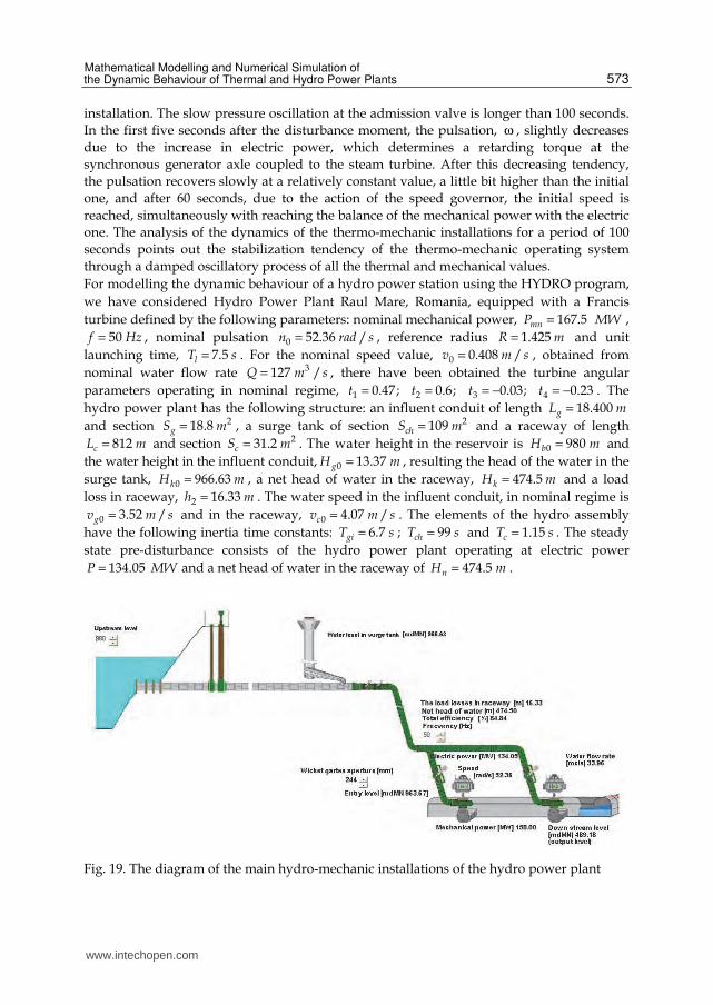
For modelling the dynamic behaviour of a hydro power station using the HYDRO program,

we have considered Hydro Power Plant Raul Mare, Romania, equipped with a Francis

turbine defined by the following parameters: nominal mechanical power, 167.5mnP MW= ,

50f Hz= , nominal pulsation 0 52.36 /n rad s= , reference radius 1.425R m= and unit

launching time, 7.5lT s= . For the nominal speed value, 0 0.408 /v m s= , obtained from

nominal water flow rate 3127 /Q m s= , there have been obtained the turbine angular

parameters operating in nominal regime, 1 0.47;t = 2 0.6;t = 3 0.03;t = − 4 0.23t = − . The

hydro power plant has the following structure: an influent conduit of length 18.400gL m=

and section 218.8gS m= , a surge tank of section 2109chS m= and a raceway of length

812cL m= and section 231.2cS m= . The water height in the reservoir is 0 980bH m= and

the water height in the influent conduit, 0 13.37gH m= , resulting the head of the water in the

surge tank, 0 966.63kH m= , a net head of water in the raceway, 474.5kH m= and a load

loss in raceway, 2 16.33h m= . The water speed in the influent conduit, in nominal regime is

0 3.52 /gv m s= and in the raceway, 0 4.07 /cv m s= . The elements of the hydro assembly

have the following inertia time constants: 6.7giT s= ; 99chT s= and 1.15cT s= . The steady

state pre-disturbance consists of the hydro power plant operating at electric power

134.05P MW= and a net head of water in the raceway of 474.5nH m= .

Fig. 19. The diagram of the main hydro-mechanic installations of the hydro power plant

www.intechopen.com


574

The dynamic behaviour of the hydro-mechanic installation has been analyzed for a

disturbance consisting of 10% increase of electric power versus the steady state at the

synchronous generator’s terminals, represented by the hydro power station operating with a

single generating unit loaded with 80 % of the nominal power. There has been studied the

evolution in time of the mechanic and hydro values on an interval of 200 seconds, with a time

incremental step of 1t sΔ = . In Figure 19 there are presented synthetically the main hydro-

mechanic installations of the hydro power plant to which the dynamic simulation is applied.

The results of the dynamic behaviour are represented in Figure 20. There has been observed

that a sudden increase in the electric power required at the terminals of the synchronous

generator results in a rapid decrease in speed, n, due to the appearance of a strong braking

couple. The speed governor registers the speed decrease and initiates the opening of the

wicket gates. At the beginning, the wicket gates open very quickly and mechanical power Pm

increases, surpassing the value of the electric power, this fact leading to the appearance of an

accelerating mechanical torque and, this way, speed n starts increasing. But as soon as the

wicket gates open an increase in water flow rate Q of the turbine is registered and this cannot

be compensated by the water leaking through the dam, through the influent conduit and

water level, Hk, in the surge tank starts decreasing, leading to a diminishing of the net head of

water and, correspondingly, to a decrease in the net specific energy, kE .

Caption: ----- Q ----- mP ------ P ------ kE ------ n ------- kH

Fig. 20. Mathematical simulation of the dynamic behaviour the hydro-mechanic installations of Hydro Power Plant Raul Mare, Romania

This dynamic process in the hydro power plant, due to its big inertia, is produced much more slowly than the control dynamic process given by the speed governor which now, registering the speed increase, initiates the closing of the wicket gates and reduces the mechanical power under the value of the electric one. The speed decreases and re-starts opening the wicket gates but, as the water level in the surge tank is diminished and the net head of water is shorter, in order to get the corresponding mechanical power, there is needed a bigger water flow rate on a longer period of time. After having balanced the powers, the closing of the wicket gates is initiated, this leading to an increase in the water level of the surge tank and in the corresponding net specific energy.

4. Conclusions

The analysis of the simulation results has shown concordance with the evolution of the dynamics of thermal and hydro-mechanic primary installations in real circumstances. The

www.intechopen.com


575

simulation represents realistically the physical phenomena both in pre- disturbance steady state and in the dynamic processes following the disturbances in the electric power system. These models have proved to be useful for experts to draw up contiguities leading to optimum operating regimes and appreciate the necessary measures to be taken in critical circumstances. They also provide instruments for the operating regimes and for further studies concerning the expansion of the existing electric power systems.

5. Referances

Dimo, P.; Constantinescu, J.; Pomarleanu, M; Radu, I. (1980). Determination of the

Power Systems Behaviour in Long Term Dynamics, Produced by Successive

Perturbations in System, Energetica Revue, Vol. 28, No. 10-11, November, 1980, pp.

443-448

Ernst, D.; Glavic, M. & Wehenkel, L. (2004). Power Systems Stability Control: Reinforcement

Learning Framework, IEEE Transactions on Power Systems, Vol.19, No.1, (February

2004), pp. 427–435, ISSN: 0885-8950

Fraile-Ardanuy, J.; Wilhelmi, J.R.; Fraile-Mora, J.J. & Perez, J.I. (2006). Variable-speed hydro

generation: operational aspects and control, IEEE Transaction on Energy Conversion,

Vol. 21, No. 2, (June 2006), pp. 569 – 574, ISSN: 0885-8969

Hanmandlu, M., Goyal, H. & Kothari D.P. (2006). An Advanced Control Scheme for Micro

Hydro Power Plants, International Conference on Power Electronics, Drives and Energy

Systems, (PEDES '06), December 2006, pp. 1-7. ISBN: 0-7803-9772-X, New Delhi,

India

Hongesombut, K.; Mitani, Y.; Tada, M.Y.; Takazawa, T.& Shishido, T. (2005). Object-

Oriented Modelling for Advanced Power System Simulations, IEEE Power

Tech Conference, pp. 1–6, ISBN: 978-5-93208-034-4, St. Petersburg, Russia, June 27-30,

2005

Huimin G.; Chao W. (2006). Effect of Detailed Hydro Turbine Models on Power System

Analysis, Power Systems Conference and Exposition (PSCE'06) IEEE PES, pp. 1577-1581,

ISBN: 1-4244-0177-1, Atlanta, USA, October 28-November, 1, 2006

Surianu F.D.; Dilertea F. (2004). Using “HYDRO” Mathematical Model in Simulating

Dynamic Behaviour of Hydro Mechanical Equipment of Hydro Power Plant Raul

Mare- Retezat, Scientific Bulletin of the “Politehnica” University of Timisoara,

Romania, Transactions on Engineering, Vol.50 (64), No.1-2, (November 2005), pp.

553-560, ISSN: 1582-7194

Surianu F.D.; Bărbulescu C. (2008). Complete Dynamic Behaviour Mathematical Modelling

of Hydro Mechanical Equipment. Case study: Hydro Power Plant Raul Mare-

Retezat, Romania, WSEAS Transactions on Power Systems, Volume 3, Issue 7,

August, 2008, pp. 517-526, ISSN 1790-5060

Surianu F.D. (2008). Experimental Determination and Numerical Simulation of the Dynamic

Insulation of a Large Consumer Unit, Proceedings of WSEAS International Conference

on Electric Power Systems, High Voltages, Electric Machines, (POWER’08), November,

2008, pp. 239-246, ISBN 978-960-474-026-0, Venice, Italy

Surianu, F.D. (2009). Modelling and Identification of Power System Elements. (in Romanian)

Orizonturi Universitare, ISBN: 978-973-638-457-8, Timisoara, Romania.

www.intechopen.com


576

Zhiyong, H; Renmu, H.& Yanhui, X. (2008). Effect of steam pressure fluctuation in turbine

steam pipe on stability of power system, Third International Conference on Electric

Utility Deregulation and Restructuring and Power Technologies (DRPT 2008), pp. 1127-

1131, ISBN: 978-7-900714-13-8, Nanjuing, China, 6-9 April, 2008

www.intechopen.com

Numerical Simulations of Physical and Engineering ProcessesEdited by Prof. Jan Awrejcewicz

ISBN 978-953-307-620-1Hard cover, 594 pagesPublisher InTechPublished online 26, September, 2011Published in print edition September, 2011

InTech EuropeUniversity Campus STeP Ri Slavka Krautzeka 83/A 51000 Rijeka, Croatia Phone: +385 (51) 770 447 Fax: +385 (51) 686 166www.intechopen.com

InTech ChinaUnit 405, Office Block, Hotel Equatorial Shanghai No.65, Yan An Road (West), Shanghai, 200040, China

Phone: +86-21-62489820 Fax: +86-21-62489821

Numerical Simulations of Physical and Engineering Process is an edited book divided into two parts. Part Idevoted to Physical Processes contains 14 chapters, whereas Part II titled Engineering Processes has 13contributions. The book handles the recent research devoted to numerical simulations of physical andengineering systems. It can be treated as a bridge linking various numerical approaches of two closely inter-related branches of science, i.e. physics and engineering. Since the numerical simulations play a key role inboth theoretical and application oriented research, professional reference books are highly needed by pureresearch scientists, applied mathematicians, engineers as well post-graduate students. In other words, it isexpected that the book will serve as an effective tool in training the mentioned groups of researchers andbeyond.

How to referenceIn order to correctly reference this scholarly work, feel free to copy and paste the following:

Flavius Dan Surianu (2011). Mathematical Modelling and Numerical Simulation of the Dynamic Behaviour ofThermal and Hydro Power Plants, Numerical Simulations of Physical and Engineering Processes, Prof. JanAwrejcewicz (Ed.), ISBN: 978-953-307-620-1, InTech, Available from:http://www.intechopen.com/books/numerical-simulations-of-physical-and-engineering-processes/mathematical-modelling-and-numerical-simulation-of-the-dynamic-behaviour-of-thermal-and-hydro-power-

mathematical modelling and numerical simulation …cdn.intechweb.org/pdfs/20907.pdfthe boilers used...

Documents