mathematical modelling and applications of particle...
TRANSCRIPT
Master’s Thesis
Mathematical Modelling and Simulation
Thesis no: 2010:8
Mathematical Modelling and Applications
of Particle Swarm Optimization
by
Satyobroto Talukder
Submitted to the School of Engineering at
Blekinge Institute of Technology
In partial fulfillment of the requirements for the degree of
Master of Science
February 2011

ii
Contact Information:
Author:
Satyobroto Talukder
E-mail: [email protected]
Co-supervisor:
Efraim Laksman, BTH E-mail: [email protected]
Phone: +46455385684
School of Engineering
Blekinge Institute of Technology
SE – 371 79 Karlskrona
Sweden
Internet : www.bth.se/com
Phone : +46 455 38 50 00
Fax : +46 455 38 50 57
University advisor:
Prof. Elisabeth Rakus-Andersson
Department of Mathematics and Science, BTH E-mail: [email protected]
Phone: +46455385408

ABSTRACT
Optimization is a mathematical technique that concerns the
finding of maxima or minima of functions in some feasible
region. There is no business or industry which is not involved
in solving optimization problems. A variety of optimization
techniques compete for the best solution. Particle Swarm
Optimization (PSO) is a relatively new, modern, and powerful
method of optimization that has been empirically shown to
perform well on many of these optimization problems. It is
widely used to find the global optimum solution in a complex
search space. This thesis aims at providing a review and
discussion of the most established results on PSO algorithm as
well as exposing the most active research topics that can give
initiative for future work and help the practitioner improve
better result with little effort. This paper introduces a
theoretical idea and detailed explanation of the PSO algorithm,
the advantages and disadvantages, the effects and judicious
selection of the various parameters. Moreover, this thesis
discusses a study of boundary conditions with the invisible wall
technique, controlling the convergence behaviors of PSO,
discrete-valued problems, multi-objective PSO, and
applications of PSO. Finally, this paper presents some kinds of
improved versions as well as recent progress in the
development of the PSO, and the future research issues are also
given.
Keywords: Optimization, swarm intelligence, particle swarm,
social network, convergence, stagnation, multi-objective.

ii
CONTENTS Page
Chapter 1- Introduction 8
1.1 PSO is a Member of Swarm Intelligence ………………………………………..… 9
1.2 Motivation………………………………………………………..…………… 9
1.3 Research Questions ……………………………………………….…………… 10
Chapter 2- Background 11
2.1 Optimization…………………………………………………………...……… 11
2.1.1 Constrained Optimization………………………………………………… 11
2.1.2 Unconstrained Optimization……………………………………………… 12
2.1.3 Dynamic Optimization………………………………………………...… 12
2.2 Global Optimization…………………………………………………….……… 12
2.3 Local Optimization……………………………………………………..……… 12
2.4 Uniform Distribution…………………………………………………………… 14
2.5 Sigmoid function………………………………………………………….…… 15
Chapter 3- Basic Particle Swarm Optimization 16
3.1 The Basic Model of PSO algorithm.......................................................................... 16
3.1.1 Global Best PSO…………………………………………………...……… 17
3.1.2 Local Best PSO……………………………………………………….…… 19
3.2 Comparison of ‘gbest’ to ‘lbest’…………………………………………………… 21
3.3 PSO Algorithm Parameters………………………………………………..……… 21
3.3.1 Swarm size………………………………………………………..……… 21
3.3.2 Iteration numbers…………………………………………………..……… 21
3.3.3 Velocity components………………………………………………….…… 21
3.3.4 Acceleration coefficients…………………………………………………… 22
3.4 Geometrical illustration of PSO…………………………………………………… 23
3.5 Neighborhood Topologies……….……………………………………………….. 24
3.6 Problem Formulation of PSO algorithm…………………………………………….. 26
3.7 Advantages and Disadvantages of PSO……………………………………………... 30
Chapter 4- Empirical Analysis of PSO Characteristics 31
4.1 Rate of Convergence Improvements……………………………………………….. 31
4.1.1 Velocity clamping…………………………………………………………. 31
4.1.2 Inertia weight……………………………………………………………... 33
4.1.3 Constriction Coefficient…………………….………………………………. 34
4.2 Boundary Conditions…………………………………………………………….. 35
4.3 Guaranteed Convergence PSO (GCPSO) …………………………………………... 37
4.4 Initialization, Stopping Criteria, Iteration Terms and Function Evaluation………………. 39
4.4.1 Initial Condition …………………………………………………………... 39
4.4.2 Iteration Terms and Function Evaluation……………………………………… 40
4.4.3 Stopping Condition………………………………………………………… 40
Chapter 5- Recent Works and Advanced Topics of PSO 42
5.1 Multi-start PSO (MSPSO) ……………………………………………………….. 42
5.2 Multi-phase PSO (MPPSO) ……………………………………………………… 45
5.3 Perturbed PSO (PPSO) ………………………………………………………….. 45
5.4 Multi-Objective PSO (MOPSO) ………………………………………………….. 47
5.4.1 Dynamic Neighborhood PSO (DNPSO) ……………………………………… 48
5.4.2 Multi-Objective PSO (MOPSO) …………………………………………….. 48
5.4.3 Vector Evaluated PSO (VEPSO) ……………………………………………. 49
5.5 Binary PSO (BPSO) ……………………………………………………………. 49
5.5.1 Problem Formulation (Lot Sizing Problem) ………………………………………. 51

iii
Chapter 6- Applications of PSO 56
Chapter 7- Conclusion 59
References 60
Appendix A 63
Appendix B 64

iv
List of Figures
Page
Figure 2.1: Illustrates the global minimizer and the local minimize………………………. 13
Figure 2.2: Sigmoid function……………………………………………………….. 15
Figure 3.1: Plot of the functions f1 and f2 ……………………………………………... 16
Figure 3.2: Velocity and position update for a particle in a two-dimensional search space…… 23
Figure 3.3: Velocity and Position update for Multi-particle in gbest PSO………………….. 23
Figure 3.4: Velocity and Position update for Multi-particle in lbest PSO…………………... 24
Figure 3.5: Neighborhood topologies………………………………………………… 25 Figure 4.1: Illustration of effects of Velocity Clampnig for a particle in a two-dimensinal
search space………………………………………………………………………
31
Figure 4.2: Various boundary conditions in PSO………………………………………. 36
Figure 4.3: Six different boundary conditions for a two-dimensional search space. x´ and v´
represent the modified position and velocity repectively, and r is a random factor [0,1]……... 36
List of Flowcharts
Flowchart 1: gbest PSO............................................................................................ 19
Flowchart 2: lbest PSO............................................................................................. 20
Flowchart 3: Self-Organized Criticality PSO…………………………………………. 44
Flowchart 4: Perturbed PSO...................................................................................... 46
Flowchart 5: Binary PSO.......................................................................................... 50

1
ACKNOWLEDGEMENT
Thanks to my supervisor Prof. Elisabeth Rakus-Andersson
for her guidance and for helping me present my ideas clearly.
2
CHAPTER 1
Introduction
Scientists, engineers, economists, and managers always have to take many
technological and managerial decisions at several times for construction and
maintenance of any system. Day by day the world becomes more and more
complex and competitive so the decision making must be taken in an optimal way.
Therefore optimization is the main act of obtaining the best result under given
situations. Optimization originated in the 1940s, when the British military faced
the problem of allocating limited resources (for example fighter airplanes,
submarines and so on) to several activities [6]. Over the decades, several
researchers have generated different solutions to linear and non-liner optimization
problems. Mathematically an optimization problem has a fitness function,
describing the problem under a set of constraints which represents the solution
space for the problem. However, most of the traditional optimization techniques
have calculated the first derivatives to locate the optima on a given constrained
surface. Due to the difficulties in evaluation the first derivative for many rough
and discontinuous optimization spaces, several derivatives free optimization
methods have been constructed in recent time [15].
There is no known single optimization method available for solving all
optimization problems. A lot of optimization methods have been developed for
solving different types of optimization problems in recent years. The modern
optimization methods (sometimes called nontraditional optimization methods) are
very powerful and popular methods for solving complex engineering problems.
These methods are particle swarm optimization algorithm, neural networks,
genetic algorithms, ant colony optimization, artificial immune systems, and fuzzy
optimization [6] [7].
The Particle Swarm Optimization algorithm (abbreviated as PSO) is a novel
population-based stochastic search algorithm and an alternative solution to the
complex non-linear optimization problem. The PSO algorithm was first introduced
by Dr. Kennedy and Dr. Eberhart in 1995 and its basic idea was originally inspired
by simulation of the social behavior of animals such as bird flocking, fish
schooling and so on. It is based on the natural process of group communication to
share individual knowledge when a group of birds or insects search food or
migrate and so forth in a searching space, although all birds or insects do not know
where the best position is. But from the nature of the social behavior, if any
member can find out a desirable path to go, the rest of the members will follow
quickly.
The PSO algorithm basically learned from animal’s activity or behavior to solve
optimization problems. In PSO, each member of the population is called a particle
and the population is called a swarm. Starting with a randomly initialized
population and moving in randomly chosen directions, each particle goes through
3
the searching space and remembers the best previous positions of itself and its
neighbors. Particles of a swarm communicate good positions to each other as well
as dynamically adjust their own position and velocity derived from the best
position of all particles. The next step begins when all particles have been moved.
Finally, all particles tend to fly towards better and better positions over the
searching process until the swarm move to close to an optimum of the fitness
function
The PSO method is becoming very popular because of its simplicity of
implementation as well as ability to swiftly converge to a good solution. It does
not require any gradient information of the function to be optimized and uses only
primitive mathematical operators.
As compared with other optimization methods, it is faster, cheaper and more
efficient. In addition, there are few parameters to adjust in PSO. That’s why PSO
is an ideal optimization problem solver in optimization problems. PSO is well
suited to solve the non-linear, non-convex, continuous, discrete, integer variable
type problems.
1.1 PSO is a Member of Swarm Intelligence
Swarm intelligence (SI) is based on the collective behavior of decentralized, self-
organized systems. It may be natural or artificial. Natural examples of SI are ant
colonies, fish schooling, bird flocking, bee swarming and so on. Besides multi-
robot systems, some computer program for tackling optimization and data analysis
problems are examples for some human artifacts of SI. The most successful swarm
intelligence techniques are Particle Swarm Optimization (PSO) and Ant Colony
Optimization (ACO). In PSO, each particle flies through the multidimensional
space and adjusts its position in every step with its own experience and that of
peers toward an optimum solution by the entire swarm. Therefore, the PSO
algorithm is a member of Swarm Intelligence [3].
1.2 Motivation
PSO method was first introduced in 1995. Since then, it has been used as a robust
method to solve optimization problems in a wide variety of applications. On the
other hand, the PSO method does not always work well and still has room for
improvement.
This thesis discusses a conceptual overview of the PSO algorithm and a number of
modifications of the basic PSO. Besides, it describes different types of PSO
algorithms and flowcharts, recent works, advanced topics, and application areas of
PSO.

4
1.3 Research Questions
This thesis aims to answer the following questions:
Q.1: How can problems of premature convergence and stagnation in the PSO
algorithm be prevented?
Q.2: When and how are particles reinitialized?
Q.3: For the PSO algorithm, what will be the consequence if
a) the maximum velocity Vmax is too large or small?
b) the acceleration coefficients c1 and c2 are equal or not?
c) the acceleration coefficients c1 and c2 are very large or small?
Q.4: How can the boundary problem in the PSO method be solved?
Q.5: How can the discrete-valued problems be solved by the PSO method?
Q.1 is illustrated in Section 4.1 and 4.3; Q.2 in Section 5.1; Q.3 (a) in Section
4.1.1; Q.3 (b) and (c) in Section 3.3.5; Q.4 and Q.5 in Section 4.2 and 5.5
respectively.

5
CHAPTER 2
Background
This chapter reviews some of the basic definitions related to this thesis.
2.1 Optimization
Optimization determines the best-suited solution to a problem under given
circumstances. For example, a manager needs to take many technological and
managerial plans at several times. The final goal of the plans is either to minimize
the effort required or to maximize the desired benefit. Optimization refers to both
minimization and maximization tasks. Since the maximization of any function is
mathematically equivalent to the minimization of its additive inverse , the term
minimization and optimization are used interchangeably [6]. For this reason, now-
a-days, it is very important in many professions.
Optimization problems may be linear (called linear optimization problems) or non-
linear (called non-linear optimization problems). Non-linear optimization
problems are generally very difficult to solve.
Based on the problem characteristics, optimization problems are classified in the
following:
2.1.1 Constrained Optimization
Many optimization problems require that some of the decision variables satisfy
certain limitations, for instance, all the variables must be non-negative. Such types
of problems are said to be constrained optimization problems [4] [8] [11] and
defined as
(2.1)
where are the number of inequality and equality constraints
respectively.
Example: Minimize the function
Then, the global optimum is , with

6
2.1.2 Unconstrained Optimization
Many optimization problems place no restrictions on the values of that can be
assigned to variables of the problem. The feasible space is simply the whole search
space. Such types of problems are said to be unconstrained optimization problems
[4] and defined as
(2.2)
where is the dimension of .
2.1.3 Dynamic Optimization
Many optimization problems have objective functions that change over time and
such changes in objective function cause changes in the position of optima. These
types of problems are said to be dynamic optimization problems [4] and defined as
(2.3)
where is a vector of time-dependent objective function control parameters,
and is the optimum found at time step .
There are two techniques to solve optimization problems: Global and Local
optimization techniques.
2.2 Global Optimization
A global minimizer is defined as such that
(2.4)
where is the search space and for unconstrained problems.
Here, the term global minimum refers to the value , and is called the
global minimizer. Some global optimization methods require a starting point
and it will be able to find the global minimizer if .
2.3 Local Optimization
A local minimizer of the region , is defined as
(2.5)
where
Here, a local optimization method should guarantee that a local minimizer of the
set is found.

7
Finally, local optimization techniques try to find a local minimum and its
corresponding local minimizer, whereas global optimization techniques seek to
find a global minimum or lowest function value and its corresponding global
minimizer.
Example: Consider a function ,
and then the following figure 2.1.1 illustrates the difference between the global
minimizer and the local minimizer .
Figure 2.1 : Illustration of the local minimizer xL* and the global minimizer x*.
-1 0 1 2 3 4 5 6 7-80
-70
-60
-50
-40
-30
-20
-10
x
y
x*
xL
*
L

8
2.4 Uniform Distribution
A uniform distribution, sometimes called a rectangular distribution, is a
distribution where the probability of occurrence is the same for all values of , i.e.
it has constant probability. For instance, if a die is thrown, then the probability of
obtaining any one of the six possible outcomes is 1/6. Now, since all outcomes are
equally probable, the distribution is uniform.
Therefore, if a uniform distribution is divided into equally spaced intervals, there
will be an equal number of members of the population in each interval. The
distribution is defined by , where are its minimum and maximum
values respectively.
A uniform distribution A nonuniform distribution
The probability density function (PDF) and cumulative distribution function
(CDF) for a continuous uniform distribution on the interval are respectively
(2.6)
and
(2.7)
Uniform PDF
)(xf
x
)/(1 ab
a bUniform CDF
)(xF
x
1
a b
is called a standard uniform distribution.

9
2.5 Sigmoid function
Sigmoid function, sometimes called a logistic function, is an ’S’ shape curve and
defined by the formula
(2.8)
It is a monotonically increasing function with
(2.9)
S
-10 -8 -6 -4 -2 0 2 4 6 8 100
0.1
0.2
0.3
0.4
0.5
0.6
0.7
0.8
0.9
1
tFigure 2.2: Sigmoid function.
Since, sigmoid function is monotonically increasing, we can write
(2.10)

10
CHAPTER 3
Basic Particle Swarm Optimization
This chapter discusses a conceptual overview of the PSO algorithm and its
parameters selection strategies, geometrical illustration and neighborhood
topology, advantages and disadvantages of PSO, and mathematical explanation.
3.1 The Basic Model of PSO algorithm
Kennedy and Eberhart first established a solution to the complex non-linear
optimization problem by imitating the behavior of bird flocks. They generated the
concept of function-optimization by means of a particle swarm [15]. Consider the
global optimum of an n-dimensional function defined by
(3.1)
where is the search variable, which represents the set of free variables of the
given function. The aim is to find a value such that the function is either
a maximum or a minimum in the search space.
Consider the functions given by
(3.2)
and (3.3)
(b) Multi-model
Figure 3.1: Plot of the functions f1 and f2.
(a) Unimodel-2
0
2
-2
0
2
0
2
4
6
8
-2
0
2
-2
0
2
-4
-2
0
2
4
6
From the figure 3.1 (a), it is clear that the global minimum of the function is
at , i.e. at the origin of function in the search space. That means
it is a unimodel function, which has only one minimum. However, to find the
global optimum is not so easy for multi-model functions, which have multiple local
minima. Figure 3.1 (b) shows the function which has a rough search space with
multiple peaks, so many agents have to start from different initial locations and

11
continue exploring the search space until at least one agent reach the global
optimal position. During this process all agents can communicate and share their
information among themselves [15]. This thesis discusses how to solve the multi-
model function problems.
The Particle Swarm Optimization (PSO) algorithm is a multi-agent parallel search
technique which maintains a swarm of particles and each particle represents a
potential solution in the swarm. All particles fly through a multidimensional search
space where each particle is adjusting its position according to its own experience
and that of neighbors. Suppose denote the position vector of particle in the
multidimensional search space (i.e. ) at time step , then the position of each
particle is updated in the search space by
with
(3.4)
where,
is the velocity vector of particle that drives the optimization process
and reflects both the own experience knowledge and the social
experience knowledge from the all particles;
is the uniform distribution where are its
minimum and maximum values respectively.
Therefore, in a PSO method, all particles are initiated randomly and evaluated to
compute fitness together with finding the personal best (best value of each
particle) and global best (best value of particle in the entire swarm). After that a
loop starts to find an optimum solution. In the loop, first the particles’ velocity is
updated by the personal and global bests, and then each particle’s position is
updated by the current velocity. The loop is ended with a stopping criterion
predetermined in advance [22].
Basically, two PSO algorithms, namely the Global Best (gbest) and Local Best
(lbest) PSO, have been developed which differ in the size of their neighborhoods.
These algorithms are discussed in Sections 3.1.1 and 3.1.2 respectively.
3.1.1 Global Best PSO
The global best PSO (or gbest PSO) is a method where the position of each
particle is influenced by the best-fit particle in the entire swarm. It uses a star
social network topology (Section 3.5) where the social information obtained from
all particles in the entire swarm [2] [4]. In this method each individual particle,
, has a current position in search space , a current
velocity, , and a personal best position in search space, . The personal best
position corresponds to the position in search space where particle had the
smallest value as determined by the objective function , considering a
minimization problem. In addition, the position yielding the lowest value amongst
all the personal best is called the global best position which is denoted

12
by [20]. The following equations (3.5) and (3.6) define how the personal and
global best values are updated, respectively.
Considering minimization problems, then the personal best position at the
next time step, , is calculated as
(3.5)
where is the fitness function. The global best position at time
step is calculated as
, (3.6)
Therefore it is important to note that the personal best is the best position
that the individual particle has visited since the first time step. On the other hand,
the global best position is the best position discovered by any of the particles
in the entire swarm [4].
For gbest PSO method, the velocity of particle is calculated by
(3.7)
where
is the velocity vector of particle in dimension at time ;
is the position vector of particle in dimension at time ;
is the personal best position of particle in dimension found
from initialization through time t;
is the global best position of particle in dimension found from
initialization through time t;
and are positive acceleration constants which are used to level the
contribution of the cognitive and social components respectively;
and
are random numbers from uniform distribution at time t.
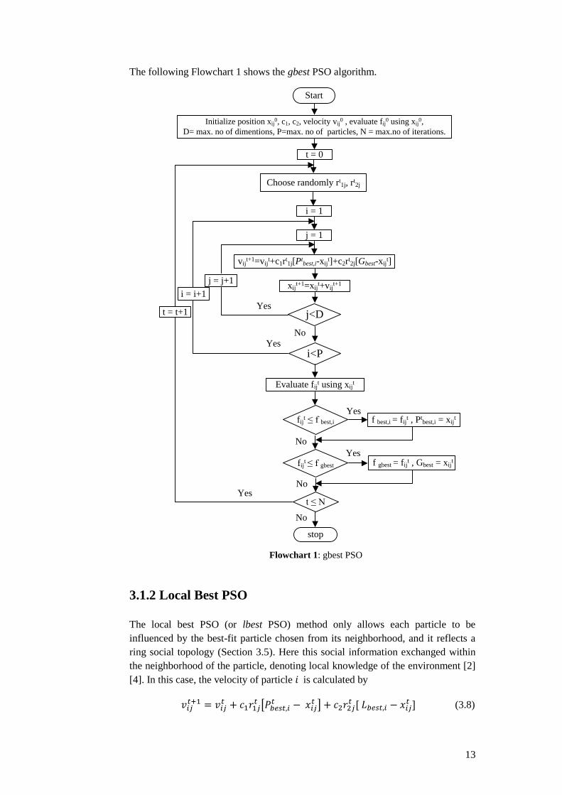
13
The following Flowchart 1 shows the gbest PSO algorithm.
Initialize position xij0, c1, c2, velocity vij
0 , evaluate fij0 using xij
0,
D= max. no of dimentions, P=max. no of particles, N = max.no of iterations.
fijt ≤ f best,i f best,i = fij
t , Ptbest,i = xij
t
fijt ≤ f gbest f gbest = fij
t , Gbest = xijt
vijt+1=vij
t+c1rt1j[Pt
best,i-xijt]+c2rt
2j[Gbest-xijt]
j = j+1xij
t+1=xijt+vij
t+1
t ≤ N
stop
j = 1
No
Yes
No
Flowchart 1: gbest PSO
Start
Yes
Evaluate fijt using xij
t
t = 0
j<D
No
i<P
No
i = i+1
t = t+1
Yes
Yes
Yes
i = 1
Choose randomly rt1j, rt
2j
3.1.2 Local Best PSO
The local best PSO (or lbest PSO) method only allows each particle to be
influenced by the best-fit particle chosen from its neighborhood, and it reflects a
ring social topology (Section 3.5). Here this social information exchanged within
the neighborhood of the particle, denoting local knowledge of the environment [2]
[4]. In this case, the velocity of particle is calculated by
(3.8)

14
where, is the best position that any particle has had in the neighborhood of
particle found from initialization through time t.
The following Flowchart 2 summarizes the lbest PSO algorithm:
Initialize position xij0, c1, c2, velocity vij
0 , evaluate fij0 using xij
0,
D= max. no of dimentions, P=max. no of particles, N = max.no of iterations.
fijt ≤ f best,i f best,i = fij
t , Ptbest,i = xij
t
( f tbest,i-1, ft best,i , ft best,i+1) ≤ f lbest f lbest = fijt,Lbest,i = xij
t
vijt+1=vij
t+c1rt1j[Pbest,i
t-xijt]+c2rt
2j[Lbest,i-xijt]
j = j+1xij
t+1=xijt+vij
t+1
stop
j = 1
No
Yes
Flowchart 2: lbest PSO
Start
Yes
Evaluate fijt using xij
t
t = 0
j<D
No
i<P
No
i = i+1
Yes
Yes
i = 1
t ≤ N
No
Yes
t = t+1
Choose randomly rt1j,rt
2j
Finally, we can say from the Section 3.1.1 and 3.1.2 respectively, in the gbest PSO
algorithm every particle obtains the information from the best particle in the entire
swarm, whereas in the lbest PSO algorithm each particle obtains the information
from only its immediate neighbors in the swarm [1].

15
3.2 Comparison of ‘gbest’ to ‘lbest’
Originally, there are two differences between the ‘gbest’ PSO and the ‘lbest’ PSO:
One is that because of the larger particle interconnectivity of the gbest PSO,
sometimes it converges faster than the lbest PSO. Another is due to the larger
diversity of the lbest PSO, it is less susceptible to being trapped in local minima
[4].
3.3 PSO Algorithm Parameters
There are some parameters in PSO algorithm that may affect its performance. For
any given optimization problem, some of these parameter’s values and choices
have large impact on the efficiency of the PSO method, and other parameters have
small or no effect [9]. The basic PSO parameters are swarm size or number of
particles, number of iterations, velocity components, and acceleration coefficients
illustrated bellow. In addition, PSO is also influenced by inertia weight, velocity
clamping, and velocity constriction and these parameters are described in Chapter
IV.
3.3.1 Swarm size
Swarm size or population size is the number of particles n in the swarm. A big
swarm generates larger parts of the search space to be covered per iteration. A
large number of particles may reduce the number of iterations need to obtain a
good optimization result. In contrast, huge amounts of particles increase the
computational complexity per iteration, and more time consuming. From a number
of empirical studies, it has been shown that most of the PSO implementations use
an interval of for the swarm size.
3.3.2 Iteration numbers
The number of iterations to obtain a good result is also problem-dependent. A too
low number of iterations may stop the search process prematurely, while too large
iterations has the consequence of unnecessary added computational complexity
and more time needed [4].
3.3.3 Velocity Components
The velocity components are very important for updating particle’s velocity. There
are three terms of the particle’s velocity in equations (3.7) and (3.8):
1. The term is called inertia component that provides a memory of the previous
flight direction that means movement in the immediate past. This component
represents as a momentum which prevents to drastically change the direction of
the particles and to bias towards the current direction.

16
2. The term
is called cognitive component which measures the
performance of the particles relative to past performances. This component looks
like an individual memory of the position that was the best for the particle. The
effect of the cognitive component represents the tendency of individuals to return
to positions that satisfied them most in the past. The cognitive component referred
to as the nostalgia of the particle.
3. The term
for gbest PSO or
for lbest PSO
is called social component which measures the performance of the particles
relative to a group of particles or neighbors. The social component’s effect is
that each particle flies towards the best position found by the particle’s
neighborhood.
3.3.4 Acceleration coefficients
The acceleration coefficients and , together with the random values and
, maintain the stochastic influence of the cognitive and social components of the
particle’s velocity respectively. The constant expresses how much confidence a
particle has in itself, while expresses how much confidence a particle has in its
neighbors [4]. There are some properties of and :
●When , then all particles continue flying at their current speed until
they hit the search space’s boundary. Therefore, from the equations (3.7) and (3.8),
the velocity update equation is calculated as
(3.9)
●When and , all particles are independent. The velocity update
equation will be
(3.10)
On the contrary, when and , all particles are attracted to a single
point in the entire swarm and the update velocity will become
for gbest PSO, (3.11)
or,
for lbest PSO. (3.12)
●When , all particles are attracted towards the average of and .
●When , each particle is more strongly influenced by its personal best
position, resulting in excessive wandering. In contrast, when then all
particles are much more influenced by the global best position, which causes all
particles to run prematurely to the optima [4] [11].
17
Normally, are static, with their optimized values being found
empirically. Wrong initialization of may result in divergent or cyclic
behavior [4]. From the different empirical researches, it has been proposed that the
two acceleration constants should be
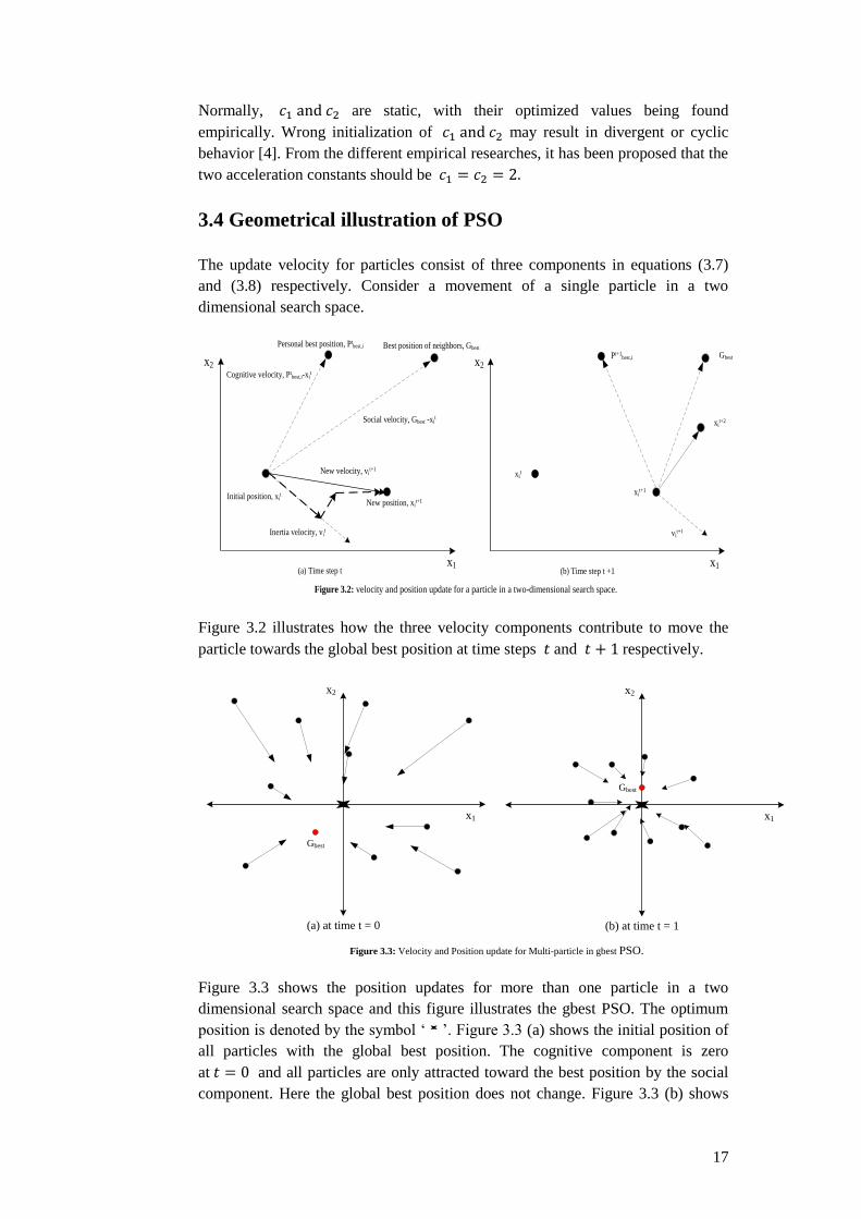
3.4 Geometrical illustration of PSO
The update velocity for particles consist of three components in equations (3.7)
and (3.8) respectively. Consider a movement of a single particle in a two
dimensional search space.
(a) Time step t
Cognitive velocity, Ptbest,i-xi
t
Social velocity, Gbest -xit
Inertia velocity, vit
New velocity, vit+1
New position, xit+1
Personal best position, Ptbest,i Best position of neighbors, Gbest
x1
x2
Initial position, xit
(b) Time step t +1
vit+1
xit+1
Pt+1best,i Gbest
x1
x2
xit
xit+2
Figure 3.2: velocity and position update for a particle in a two-dimensional search space.
Figure 3.2 illustrates how the three velocity components contribute to move the
particle towards the global best position at time steps and respectively.
Gbest
x2
x1
(a) at time t = 0
Gbest
x2
x1
(b) at time t = 1
Figure 3.3: Velocity and Position update for Multi-particle in gbest PSO.
Figure 3.3 shows the position updates for more than one particle in a two
dimensional search space and this figure illustrates the gbest PSO. The optimum
position is denoted by the symbol ‘ ’. Figure 3.3 (a) shows the initial position of
all particles with the global best position. The cognitive component is zero
at and all particles are only attracted toward the best position by the social
component. Here the global best position does not change. Figure 3.3 (b) shows

18
the new positions of all particles and a new global best position after the first
iteration i.e. at .
Lbest
x2
x1
(a) at time t = 0
i
jh
a
g
f
e
d
c b
Lbest
Lbest
3
2 1 Lbest
x2
x1
(b) at time t = 1
ij
h
a
g
f
e
d
c
bLbest
Lbest
3
2 1
Figure 3.4: Velocity and Position update for Multi-particle in lbest PSO.
Figure 3.4 illustrates how all particles are attracted by their immediate neighbors in
the search space using lbest PSO and there are some subsets of particles where one
subset of particles is defined for each particle from which the local best particle is
then selected. Figure 3.4 (a) shows particles a, b and c move towards particle d,
which is the best position in subset 1. In subset 2, particles e and f move towards
particle g. Similarly, particle h moves towards particle i, so does j in subset 3 at
time step . Figure 3.4 (b) for time step , the particle d is the best
position for subset 1 so the particles a, b and c move towards d.
3.5 Neighborhood Topologies
A neighborhood must be defined for each particle [7]. This neighborhood
determines the extent of social interaction within the swarm and influences a
particular particle’s movement. Less interaction occurs when the neighborhoods in
the swarm are small [4]. For small neighborhood, the convergence will be slower
but it may improve the quality of solutions. For larger neighborhood, the
convergence will be faster but the risk that sometimes convergence occurs earlier
[7]. To solve this problem, the search process starts with small neighborhoods size
and then the small neighborhoods size is increased over time. This technique
ensures an initially high diversity with faster convergence as the particles move
towards a promising search region [4].
The PSO algorithm is social interaction among the particles in the entire swarm.
Particles communicate with one another by exchanging information about the
success of each particle in the swarm. When a particle in the whole swarm finds a
better position, all particles move towards this particle. This performance of the
particles is determined by the particles’ neighborhood [4]. Researchers have
worked on developing this performance by designing different types of
neighborhood structures [15]. Some neighborhood structures or topologies are
discussed below:

19
(a) Star or gbest. (b) Ring or lbest.
(c) Wheel.
Focal particle
(d) Four Clusters.
Figure 3.5: Neighborhood topologies.
Figure 3.5 (a) illustrates the star topology, where each particle connects with every
other particle. This topology leads to faster convergence than other topologies, but
there is a susceptibility to be trapped in local minima. Because all particles know
each other, this topology is referred to as the gbest PSO.
Figure 3.5 (b) illustrates the ring topology, where each particle is connected only
with its immediate neighbors. In this process, when one particle finds a better
result, this particle passes it to its immediate neighbors, and these two immediate
neighbors pass it to their immediate neighbors, until it reaches the last particle.
Thus the best result found is spread very slowly around the ring by all particles.
Convergence is slower, but larger parts of the search space are covered than with
the star topology. It is referred as the lbest PSO.
Figure 3.5 (c) illustrates the wheel topology, in which only one particle (a focal
particle) connects to the others, and all information is communicated through this
particle. This focal particle compares the best performance of all particles in the
swarm, and adjusts its position towards the best performance particle. Then the
new position of the focal particle is informed to all the particles.
Figure 3.5 (d) illustrates a four clusters topology, where four clusters (or cliques)
are connected with two edges between neighboring clusters and one edge between
opposite clusters.

20
There are more different neighborhood structures or topologies (for instance,
pyramid topology, the Von Neumann topology and so on), but there is no the best
topology known to find the optimum for all kinds of optimization problems.
3.6 Problem Formulation of PSO algorithm
Problem: Find the maximum of the function
with
using the PSO algorithm. Use 9 particles with the initial positions
, , , , ,
and . Show the detailed computations for iterations 1, 2 and 3.
Solution:
Step1: Choose the number of particles: , , ,
, , and .
The initial population (i.e. the iteration number ) can be represented
as
,
, ,
,
,
,
, .
Evaluate the objective function values as
Let
Set the initial velocities of each particle to zero:
Step2: Set the iteration number as and go to step 3.
Step3: Find the personal best for each particle by

21
So,
,
.
Step4: Find the global best by
Since, the maximum personal best is thus
Step5: Considering the random numbers in the range (0, 1) as and
and find the velocities of the particles by
so
,
,
,
,
.
Step6: Find the new values of by
So
,
, ,
,
, ,
,
, .
Step7: Find the objective function values of
.
Step 8: Stopping criterion:
If the terminal rule is satisfied, go to step 2,
Otherwise stop the iteration and output the results.

22
Step2: Set the iteration number as , and go to step 3.
Step3: Find the personal best for each particle.
.
Step4: Find the global best.
Step5: By considering the random numbers in the range (0, 1) as
and
find the velocities of the particles by
.
so
, ,
,
, .
Step6: Find the new values of by
so
,
,
, ,
1.9240,
.
Step7: Find the objective function values of
Step 8: Stopping criterion:
If the terminal rule is satisfied, go to step 2,
Otherwise stop the iteration and output the results.

23
Step2: Set the iteration number as , and go to step 3.
Step3: Find the personal best for each particle.
.
Step4: Find the global best.
Step5: By considering the random numbers in the range (0, 1) as
and
find the velocities of the particles by
.
so
, ,
,
, .
Step6: Find the new values of by
so
,
,
, ,
,
.
Step7: Find the objective function values of
Step 8: Stopping criterion:
If the terminal rule is satisfied, go to step 2,
Otherwise stop the iteration and output the results.

24
Finally, the values of did not converge, so we increment
the iteration number as and go to step 2. When the positions of all particles
converge to similar values, then the method has converged and the corresponding
value of is the optimum solution. Therefore the iterative process is continued
until all particles meet a single value.
3.7 Advantages and Disadvantages of PSO
It is said that PSO algorithm is the one of the most powerful methods for solving
the non-smooth global optimization problems while there are some disadvantages
of the PSO algorithm. The advantages and disadvantages of PSO are discussed
below:
Advantages of the PSO algorithm [14] [15]:
1) PSO algorithm is a derivative-free algorithm.
2) It is easy to implementation, so it can be applied both in scientific research
and engineering problems.
3) It has a limited number of parameters and the impact of parameters to the
solutions is small compared to other optimization techniques.
4) The calculation in PSO algorithm is very simple.
5) There are some techniques which ensure convergence and the optimum
value of the problem calculates easily within a short time.
6) PSO is less dependent of a set of initial points than other optimization
techniques.
7) It is conceptually very simple.
Disadvantages of the PSO algorithm [13]:
1) PSO algorithm suffers from the partial optimism, which degrades the
regulation of its speed and direction.
2) Problems with non-coordinate system (for instance, in the energy field)
exit.
25
CHAPTER 4
Empirical Analysis of PSO Characteristics
This chapter discusses a number of modifications of the basic PSO, how to
improve speed of convergence, to control the exploration-exploitation trade-off, to
overcome the stagnation problem or the premature convergence, the velocity-
clamping technique, the boundary value problems technique, the initial and
stopping conditions, which are very important in the PSO algorithm.
4.1 Rate of Convergence Improvements
Usually, the particle velocities build up too fast and the maximum of the objective
function is passed over. In PSO, particle velocity is very important, since it is the
step size of the swarm. At each step, all particles proceed by adjusting the velocity
that each particle moves in every dimension of the search space [9]. There are two
characteristics: exploration and exploitation. Exploration is the ability to explore
different area of the search space for locating a good optimum, while exploitation
is the ability to concentrate the search around a searching area for refining a
hopeful solution. Therefore these two characteristics have to balance in a good
optimization algorithm. When the velocity increases to large values, then particle’s
positions update quickly. As a result, particles leave the boundaries of the search
space and diverge. Therefore, to control this divergence, particles’ velocities are
reduced in order to stay within boundary constraints [4]. The following techniques
have been developed to improve speed of convergence, to balance the exploration-
exploitation trade-off, and to find a quality of solutions for the PSO:
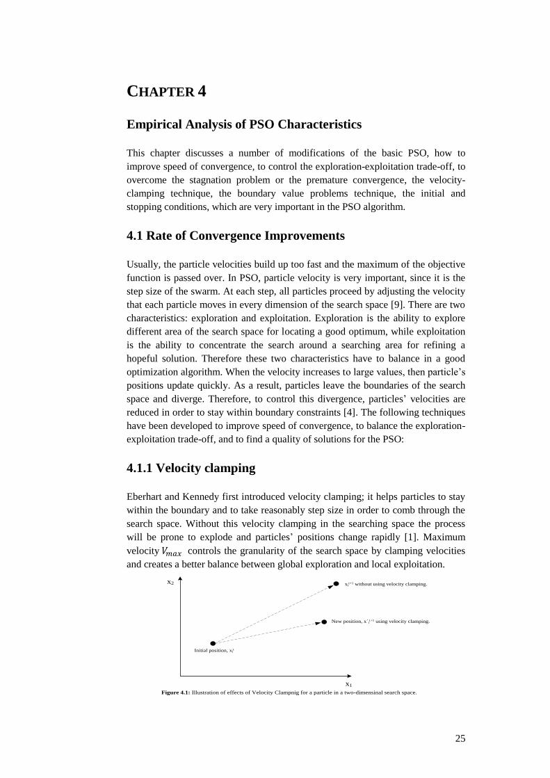
4.1.1 Velocity clamping
Eberhart and Kennedy first introduced velocity clamping; it helps particles to stay
within the boundary and to take reasonably step size in order to comb through the
search space. Without this velocity clamping in the searching space the process
will be prone to explode and particles’ positions change rapidly [1]. Maximum
velocity controls the granularity of the search space by clamping velocities
and creates a better balance between global exploration and local exploitation.
New position, x´it+1 using velocity clamping.
x1
x2
Initial position, xit
Figure 4.1: Illustration of effects of Velocity Clampnig for a particle in a two-dimensinal search space.
xit+1 without using velocity clamping.

26
Figure 4.1 illustrates how velocity clamping changes the step size as well as the
search direction when a particle moves in the process. In this figure, and
denote respectively the position of particle i without using velocity
clamping and the result of velocity clamping [4].
Now if a particle’s velocity goes beyond its specified maximum velocity ,
this velocity is set to the value and then adjusted before the position update
by,
(4.1)
where,
is calculated using equation (3.7) or (3.8).
If the maximum velocity is too large, then the particles may move erratically
and jump over the optimal solution. On the other hand, if is too small, the
particle’s movement is limited and the swarm may not explore sufficiently or the
swarm may become trapped in a local optimum.
This problem can be solved when the maximum velocity is calculated by a
fraction of the domain of the search space on each dimension by subtracting the
lower bound from the upper bound, and is defined as
(4.2)
where, are respectively the maximum and minimum values of
and . For example, if and on each
dimension of the search space, then the range of the search space is 300 per
dimension and velocities are then clamped to a percentage of that range according
to equation (4.2), then the maximum velocity is
There is another problem when all velocities are equal to the maximum
velocity . To solve this problem can be reduced over time. The initial
step starts with large values of , and then it is decreased it over time. The
advantage of velocity clamping is that it controls the explosion of velocity in the
searching space. On the other hand, the disadvantage is that the best value of
should be chosen for each different optimization problem using empirical
techniques [4] and finding the accurate value for for the problem being
solved is very critical and not simple, as a poorly chosen can lead to
extremely poor performance [1].
Finally, was first introduced to prevent explosion and divergence. However,
it has become unnecessary for convergence because of the use of inertia-weight ω
(Section 4.1.2) and constriction factor χ (Section 4.1.3) [15].

27
4.1.2 Inertia weight
The inertia weight, denoted by ω, is considered to replace by adjusting the
influence of the previous velocities in the process, i.e. it controls the momentum of
the particle by weighing the contribution of the previous velocity. The inertia
weight ‘ω’ will at every step be multiplied by the velocity at the previous time
step, i.e. . Therefore, in the gbest PSO, the velocity equation of the particle
with the inertia weight changes from equation (3.7) to
(4.3)
In the lbest PSO, the velocity equation changes in a similar way as the above
velocity equation do.
The inertia weight was first introduced by Shi and Eberhart in 1999 to reduce the
velocities over time (or iterations), to control the exploration and exploitation
abilities of the swarm, and to converge the swarm more accurately and efficiently
compared to the equation (3.7) with (4.3). If then the velocities increase
over time and particles can hardly change their direction to move back towards
optimum, and the swarm diverges. If then little momentum is only saved
from the previous step and quick changes of direction are to set in the process. If
particles velocity vanishes and all particles move without knowledge of
the previous velocity in each step [15].
The inertia weight can be implemented either as a fixed value or dynamically
changing values. Initial implementations of used a fixed value for the whole
process for all particles, but now dynamically changing inertia values is used
because this parameter controls the exploration and exploitation of the search
space. Usually the large inertia value is high at first, which allows all particles to
move freely in the search space at the initial steps and decreases over time.
Therefore, the process is shifting from the exploratory mode to the exploitative
mode. This decreasing inertia weight has produced good results in many
optimization problems [16]. To control the balance between global and local
exploration, to obtain quick convergence, and to reach an optimum, the inertia
weight whose value decreases linearly with the iteration number is set according to
the following equation [6] [14]:
, (4.4)
where,
are the initial and final values of the inertia weight
respectively,
is the maximum iteration number,
and is the current iteration number.
Commonly, the inertia weight decreases linearly from 0.9 to 0.4 over the entire
run.

28
Van den Bergh and Engelbrecht, Trelea have defined a condition that
(4.5)
guarantees convergence [4]. Divergent or cyclic behavior can occur in the process
if this condition is not satisfied.
Shi and Eberhart defined a technique for adapting the inertia weight dynamically
using a fuzzy system [11]. The fuzzy system is a process that can be used to
convert a linguistic description of a problem into a model in order to predict a
numeric variable, given two inputs (one is the fitness of the global best position
and the other is the current value of the inertia weight). The authors chose to use
three fuzzy membership functions, corresponding to three fuzzy sets, namely low,
medium, and high that the input variables can belong to. The output of the fuzzy
system represents the suggested change in the value of the inertia weight [4] [11].
The fuzzy inertia weight method has a greater advantage on the unimodal function.
In this method, an optimal inertia weight can be determined at each time step.
When a function has multiple local minima, it is more difficult to find an optimal
inertia weight [11].
The inertia weight technique is very useful to ensure convergence. However there
is a disadvantage of this method is that once the inertia weight is decreased, it
cannot increase if the swarm needs to search new areas. This method is not able to
recover its exploration mode [16].
4.1.3 Constriction Coefficient
This technique introduced a new parameter ‘χ’, known as the constriction factor.
The constriction coefficient was developed by Clerc. This coefficient is extremely
important to control the exploration and exploitation tradeoff, to ensure
convergence behavior, and also to exclude the inertia weight ω and the maximum
velocity [19]. Clerc’s proposed velocity update equation of the particle for
the j dimension is calculated as follows:
(4.6)
where
, , and .
If then all particles would slowly spiral toward and around the best solution
in the searching space without convergence guarantee. If then all particles
converge quickly and guaranteed [1].
The amplitude of the particle’s oscillation will be decreased by using the
constriction coefficient and it focuses on the local and neighborhood previous best
points [7] [15]. If the particle’s previous best position and the neighborhood best
position are near each other, then the particles will perform a local search. On the
other hand, if their positions are far from each other then the particles will perform

29
a global search. The constriction coefficient guarantees convergence of the
particles over time and also prevents collapse [15]. Eberhart and Shi empirically
illustrated that if constriction coefficient and velocity clamping are used together,
then faster convergence rate will be obtained [4].
The disadvantage of the constriction coefficient is that if a particle’s personal best
position and the neighborhood best position are far apart from each other, the
particles may follow wider cycles and not converge [16].
Finally, a PSO algorithm with constriction coefficient is algebraically equivalent to
a PSO algorithm with inertia weight. Equation (4.3) and (4.6) can be transformed
into one another by the mapping and [19].
4.2 Boundary Conditions
Sometimes, the search space must be limited in order to prevent the swarm from
exploding. In other words, the particles may occasionally fly to a position beyond
the defined search space and generate an invalid solution. Traditionally, the
velocity clamping technique is used to control the particle’s velocities to the
maximum value . The maximum velocity , the inertia weight , and the
constriction coefficient value do not always confine the particles to the solution
space. In addition, these parameters cannot provide information about the space
within which the particles stay. Besides, some particles still run away from the
solution space even with good choices for the parameter .
There are two main difficulties connected with the previous velocity techniques:
first, the choice of suitable value for can be nontrivial and also very
important for the overall performance of the method, and second, the previous
velocity techniques cannot provide information about how the particles are
enforced to stay within the selected search space all the time [18]. Therefore, the
method must be generated with clear instructions on how to overcome this
situation and such instructions are called the boundary condition (BC) of the PSO
algorithm which will be parameter-free, efficient, and also reliable.
To solve this problem, different types of boundary conditions have been
introduced and the unique features that distinguish each boundary condition are
showed in Figure 4.2 [17] [18]. These boundary conditions form two groups:
restricted boundary conditions (namely, absorbing, reflecting, and damping) and
unrestricted boundary conditions (namely, invisible, invisible/reflecting,
invisible/damping) [17].

30
Particle outside
Boundaries?
Boundary condition
not needed
Relocate errant
particle?
How to modify
velocity?
At the boundary
Invisible/damping
v´= -rand()*v
Invisible/reflecting
v´= -v
Invisible
v´= vDamping
v´= -rand()*v
Reflecting
v´= -v
Absorbing
v´= 0
UnrestrictedRestricted
Figure 4.2: Various boundary conditions in PSO.
How to modify
velocity?
No
No
Yes
Yes
The following Figure 4.3 shows how the position and velocity of errant particle is
treated by boundary conditions.
x
yxt
xt+1
x´t+1
vt = vx.x+vy.y
v´t = 0.x+vy.y
(a) Absorbingx
yxt
xt+1
x´t+1
vt = vx.x+vy.y
(b) Reflecting
v´t = -vx.x+vy.y
x
yxt
xt+1
x´t+1
vt = vx.x+vy.y
(c) Damping
v´t = -r.vx.x+vy.y
x
yxt
xt+1
vt = vx.x+vy.y
v´t = vt
(d) Invisible
x
yxt
xt+1
vt = vx.x+vy.y
(e) Invisible/Reflecting
v´t = -vx.x+vy.y
x
yxt
xt+1
vt = vx.x+vy.y
(f) Invisible/Damping
v´t = -r.vx.x+vy.y
Figure 4.3: Six different boundary conditions for a two-dimensional search space. x´ and v´ represent
the modified position and velocity repectively, and r is a random factor [0,1].
The six boundary conditions are discussed below [17]:
● Absorbing boundary condition (ABC): When a particle goes outside the
solution space in one of the dimensions, the particle is relocated at the wall of the
solution space and the velocity of the particle is set to zero in that dimension as
illustrated in Figure 4.3(a). This means that, in this condition, such kinetic energy
of the particle is absorbed by a soft wall so that the particle will return to the
solution space to find the optimum solution.
● Reflecting boundary condition (RBC): When a particle goes outside the
solution space in one of the dimensions, then the particle is relocated at the wall of

31
the solution space and the sign of the velocity of the particle is changed in the
opposite direction in that dimension as illustrated in Figure 4.3(b). This means
that, the particle is reflected by a hard wall and then it will move back toward the
solution space to find the optimum solution.
● Damping boundary condition (DBC): When a particle goes outside the
solution space in one of the dimensions, then the particle is relocated at the wall of
the solution space and the sign of the velocity of the particle is changed in the
opposite direction in that dimension with a random coefficient between 0 and 1 as
illustrated in Figure 4.3(c). Thus the damping boundary condition acts very similar
as the reflecting boundary condition except randomly determined part of energy is
lost because of the imperfect reflection.
● Invisible boundary condition (IBC): In this condition, a particle is considered
to stay outside the solution space, while the fitness evaluation of that position is
skipped and a bad fitness value is assigned to it as illustrated in Figure 4.3(d). Thus
the attraction of personal and global best positions will counteract the particle’s
momentum, and ultimately pull it back inside the solution space.
● Invisible/Reflecting boundary condition (I/RBC): In this condition, a particle
is considered to stay outside the solution space, while the fitness evaluation of that
position is skipped and a bad fitness value is assigned to it as illustrated in Figure
4.3(e). Also, the sign of the velocity of the particle is changed in the opposite
direction in that dimension so that the momentum of the particle is reversed to
accelerate it back toward in the solution space.
● Invisible/Damping boundary condition (I/DBC): In this condition, a particle
is considered to stay outside the solution space, while the fitness evaluation of that
position is skipped and a bad fitness value is assigned to it as illustrated in Figure
4.3(f). Also, the velocity of the particle is changed in the opposite direction with a
random coefficient between 0 and 1 in that dimension so that the reversed
momentum of the particle which accelerates it back toward in the solution space is
damped.
4.3 Guaranteed Convergence PSO (GCPSO)
When the current position of a particle coincides with the global best position, then
the particle moves away from this point if its previous velocity is non-zero. In
other words, when
, then the velocity update depends only on
the value of . Now if the previous velocities of particles are close to zero, all
particles stop moving once and they catch up with the global best position, which
can lead to premature convergence of the process. This does not even guarantee
that the process has converged to a local minimum, it only means that all particles
have converged to the best position in the entire swarm. This leads to stagnation of
the search process which the PSO algorithm can overcome by forcing the global
best position to change when
[11].

32
To solve this problem a new parameter is introduced to the PSO. Let be the
index of the global best particle, so that
(4.7)
A new velocity update equation for the globally best positioned particle, , has
been suggested in order to keep moving until it has reached a local minimum.
The suggested equation is
(4.8)
where
‘ ’ is a scaling factor and causes the PSO to perform a random search in an
area surrounding the global best position . It is defined in equation
(4.10) below,
‘ ’ resets the particle’s position to the position
,
‘ ’ represents the current search direction,
‘ ’ generates a random sample from a sample space with side
lengths .
Combining the position update equation (3.4) and the new velocity update
equation (4.8) for the global best particle yields the new position update equation
(4.9)
while all other particles in the swarm continue using the usual velocity update
equation (4.3) and the position update equation (3.4) respectively.
The parameter controls the diameter of the search space and the value of is
adapted after each time step, using
(4.10)
where and respectively denote the number of consecutive
successes and failures, and a failure is defined as
. The
following conditions must also be implemented to ensure that equation (4.10) is
well defined:
and
(4.11)
Therefore, when a success occurs, the failure count is set to zero and similarly
when a failure occurs, then the success count is reset.

33
The optimal choice of values for and depend on the objective function. It is
difficult to get better results using a random search in only a few iterations for
high- dimensional search spaces, and it is recommended to use and
. On the other hand, the optimal values for and can be found
dynamically. For instance, may be increased every time that
i.e. it becomes more difficult to get the success if failures occur frequently
which prevents the value of from fluctuating rapidly. Such strategy can be used
also for [11].
GCPSO uses an adaptive to obtain the optimal of the sampling volume given the
current state of the algorithm. If a specific value of repeatedly results in a
success, then a large sampling volume is selected to increase the maximum
distance traveled in one step. On the other hand, when produces consecutive
failures, then the sampling volume is too large and must be consequently reduced.
Finally, stagnation is totally prevented if for all steps [4].
4.4 Initialization, Stopping Criteria, Iteration Terms and
Function Evaluation
A PSO algorithm includes particle initialization, parameters selection, iteration
terms, function evaluation, and stopping condition. The first step of the PSO is to
initialize the swarm and control the parameters, the second step is to calculate the
fitness function and define the iteration numbers, and the last step is to satisfy
stopping condition. The influence and control of the PSO parameters have been
discussed in Sections 3.3 and 4.1 respectively. The rest of the conditions are
discussed below:
4.4.1 Initialization
In PSO algorithm, initialization of the swarm is very important because proper
initialization may control the exploration and exploitation tradeoff in the search
space more efficiently and find the better result. Usually, a uniform distribution
over the search space is used for initialization of the swarm. The initial diversity of
the swarm is important for the PSO’s performance, it denotes that how much of the
search space is covered and how well particles are distributed. Moreover, when the
initial swarm does not cover the entire search space, the PSO algorithm will have
difficultly to find the optimum if the optimum is located outside the covered area.
Then, the PSO will only discover the optimum if a particle’s momentum carries
the particle into the uncovered area. Therefore, the optimal initial distribution is to
located within the domain defined by which represent the
minimum and maximum ranges of for all particles in dimension respectively
[4]. Then the initialization method for the position of each particle is given by
(4.12)
where

34
The velocities of the particles can be initialized to zero, i.e. since
randomly initialized particle’s positions already ensure random positions and
moving directions. In addition, particles may be initialized with nonzero velocities,
but it must be done with care and such velocities should not be too large. In
general, large velocity has large momentum and consequently large position
update. Therefore, such large initial position updates can cause particles to move
away from boundaries in the feasible region, and the algorithm needs to take more
iterations before settling the best solution [4].
4.4.2 Iteration Terms and Function Evaluation
The PSO algorithm is an iterative optimization process and repeated iterations will
continue until a stopping condition is satisfied. Within one iteration, a particle
determines the personal best position, the local or global best position, adjusts the
velocity, and a number of function evaluations are performed. Function evaluation
means one calculation of the fitness or objective function which computes the
optimality of a solution. If n is the total number of particles in the swarm, then n
function evaluations are performed at each iteration [4].
4.4.3 Stopping Criteria
Stopping criteria is used to terminate the iterative search process. Some stopping
criteria are discussed below:
1) The algorithm is terminated when a maximum number of iterations or
function evaluations (FEs) has been reached. If this maximum number of
iterations (or FEs) is too small, the search process may stop before a good
result has been found [4].
2) The algorithm is terminated when there is no significant improvement
over a number of iterations. This improvement can be measured in
different ways. For instance, the process may be considered to have
terminated if the average change of the particles’ positions are very small
or the average velocity of the particles is approximately zero over a
number of iterations [4].
3) The algorithm is terminated when the normalized swarm radius is
approximately zero. The normal swarm radius is defined as
(4.13)
where diameter(S) is the initial swarm’s diameter and is the
maximum radius,
with
, ,
and is a suitable distance norm.

35
The process will terminate when . If is too large, the process
can be terminated prematurely before a good solution has been reached
while if is too small, the process may need more iterations [4].

36
CHAPTER 5
Recent Works and Advanced Topics of PSO
This chapter describes different types of PSO methods which help to solve
different types of optimization problems such as Multi-start (or restart) PSO for
when and how to reinitialize particles, binary PSO (BPSO) method for solving
discrete-valued problems, Multi-phase PSO (MPPSO) method for partition the
main swarm of particles into sub-swarms or subgroups, Multi-objective PSO for
solving multiple objective problems.
5.1 Multi-Start PSO (MSPSO)
In the basic PSO, one of the major problems is lack of diversity when particles
start to converge to the same point. To prevent this problem of the basic PSO,
several methods have been developed to continually inject randomness, or chaos,
into the swarm. These types of methods are called the Multi-start (or restart)
Particle Swarm Optimizer (MSPSO). The Multi-start method is a global search
algorithm and has as the main objective to increase diversity, so that larger parts of
the search space are explored [4] [11]. It is important to remember that continual
injection of random positions will cause the swarm never to reach an equilibrium
state that is why, in this algorithm, the amount of chaos reduces over time.
Kennedy and Eberhart first introduced the advantages of randomly reinitializing
particles and referred to as craziness. Now the important questions are when to
reinitialize, and how are particles reinitialized? These aspects are discussed below
[4]:
Randomly initializing position vectors or velocity vectors of particles can increase
the diversity of the swarm. Particles are physically relocated to a different random
position in the solution space by randomly initializing positions. When position
vectors are kept constant and velocity vectors are randomized, particles preserve
their memory of current and previous best solutions, but are forced to search in
different random directions. When randomly initialized particle’s velocity cannot
found a better solution, then the particle will again be attracted towards its
personal best position. When the positions of particles are reinitialized, then the
particles’ velocities are typically set to zero and to have a zero momentum at the
first iteration after reinitialization. On the other hands, particle velocities can be
initialized to small values. To ensure a momentum back towards the personal best
position, G. Venter and J. Sobieszczanski-Sobieski initialize particle velocities to
the cognitive component before reinitialization. Therefore the question is when to
consider the reinitialization of particles. Because, when reinitialization occurs too
soon, then the affected particles may have too short time to explore their current
regions before being relocated. If the reinitialization time is too long, however it
may happen that all particles have already converged [4].

37
A probabilistic technique has been discussed to decide when to reinitialize
particles. X. Xiao, W. Zhang, and Z. Yang reinitialize velocities and positions of
particles based on chaos factors which act as probabilities of introducing chaos in
the system. Let denote the chaos factors for velocity and location. If
then the particle velocity component is reinitialized to
where is random number for each particle and each
dimension . Again, if then the particle position component is
initialized to . In this technique, start with large chaos
factors that decrease over time to ensure that an equilibrium stat can be reached.
Therefore the initial large chaos factors increase diversity in the first stages of the
solution space, and allow particles to converge in the final steps [4].
A convergence criterion is another technique to decide when to reinitialize
particles, where particles are allowed to first exploit their local regions before
being reinitialized [4]. All particles are to initiate reinitialization when particles do
not improve over time. In this technique, a variation is to evaluate in particle
fitness of the current swarm, and if the variation is small, then particles are close to
the global best position. Otherwise, particles that are at least two standard
deviations away from the swarm center are reinitialized.
M. Løvberg and T. Krink have developed reinitialization of particles by using self-
organized criticality (SOC) which can help control the PSO and add diversity [21].
In SOC, each particle maintains an additional variable, , where is the
criticality of the particle . If two particles are closer than a threshold distance ,
from one another, then both particles have their criticality increased by one. The
particles have no neighborhood restrictions and this neighborhood is full
connected network (i.e. star type) so that each particle can affect all other particles
[21].
In SOCPSO model the velocity of each particle is updated by
(5.1)
where χ is known as the constriction factor, ω is the inertia-weight, and are
random values different for each particle and for each dimension [21].
In each iteration, each is decreased by a fraction to prevent criticality from
building up [21]. When , is the global criticality limit, then the criticality
of the particle is distributed to its immediate neighbors and is reinitialized. The
authors also consider the inertia weight value of each particle to
, this forces the particle to explore more when it is too similar to other
particles [4].

38
Flowchart 3 shows criticality measures for SOCPSO.
Initialize position xij0, Ci=0, ϕ1, ϕ2, χ, ω, velocity vij
0 , evaluate fij0 using xij
0,
D= max. no of dimentions, P=max. no of particles, N = max.no of iterations.
fijt ≤ f best,i f best,i = fij
t , Ptbest,i = xij
t
fijt ≤ f gbest f gbest = fij
t , Gbest = xijt
vijt+1=χ[ωvij
t+ϕ1(Pbest,it-xij
t)+ϕ2(Gbest-xijt)]
j = j+1
xijt+1=xij
t+vijt+1
t ≤ N
stop
j = 1
No
Yes
No
Flowchart 3: Self-Organized Criticality PSO
Start
Yes
Evaluate fijt using xij
t
t = 0
j<D
No
i<P
No
i = i+1
t = t+1
Yes
Yes
Yes
i = 1
Calculate criticality for all particles
Reduce criticality for each particle
Ci > C
Disperse criticality of particle i
Reinitialize xij
No
Yes

39
5.2 Multi-phase PSO (MPPSO)
Multi-phase PSO (MPPSO) method partitions the main swarm of particles into
sub-swarms or subgroups, where each sub-swarm performs a different task,
exhibits a different behavior and so on. This task or behavior performed by a sub-
swarm usually changes over time and information are passed among sub-swarms
in this process.
In 2002, B. Al-Kazemi and C. Mohan described the MPPSO method and they
divided the main swarm into two sub-swarms with the equal size. In this
algorithm, particles are randomly assigned, and each sub-swarm may be in one of
two phases [4]. These phases are discussed below:
● Attraction phase: in this phase, the particles of the corresponding sub-swarm
are influenced to move towards the global best position.
● Repulsion phase: in this phase, the particles of the corresponding sub-swarm go
away from the global best position [4].
In MPPSO algorithm, the particle velocity updating equation is presented as
follows:
(5.2)
where ω is the inertia-weight, and are acceleration coefficients respectively.
In this method, the personal best position is eliminated from the main velocity
equation (4.3), since a particle’s position is only updated when the new position
improves the performance in the solution space [4] [23].
Another MPPSO algorithm is based on the groups PSO and multi-start PSO
algorithm, and it was introduced by H. Qi et al [23]. The advantage of the MPPSO
algorithm is that when the fitness of a particle doesn’t changed any more, then the
particle’s flying speed and direction in the searching space are changed by the
adaptive velocity strategy. Therefore, MPPSO differ from basic PSO in three
ways:
1. Particles divide into multiple groups to increase the diversity of the swarm
and extensiveness of the exploration space.
2. Different phases introduce in the algorithm which have different searching
ways and flying directions.
3. Searching direction will increase particle’s fitness [23].
5.3 Perturbed PSO (PPSO)
The basic particle swarm optimization (PSO) has some disadvantages, for
example, high speed of convergence frequently generates a quick loss of diversity
during the process of optimization. Then, the process leads to undesirable
premature convergence. To overcome this disadvantage, Zhao Xinchao described a

40
perturbed particle swarm algorithm which is based upon a new particle updating
strategy and the concept of perturbed global best (p-gbest) within the swarm. The
perturbed global best (p-gbest) updating strategy is based on the concept of
possibility measure to model the lack of information about the true optimality of
the gbest [24]. In PPSO, the particle velocity is rewritten by
(5.3)
where
(5.4)
is the -th dimension of p-gbest in iteration .
Here, is the normal distribution, and represents the degree of
uncertainty about the optimality of the gbest and is modeled as some non-
increasing function of the number of iterations, defined as
(5.5)
where
and are manually set parameters.
The Flowchart 4 shows the perturbed PSO algorithm.
Initialize ω, σmax, σmin, α, position xij0, c1, c2, velocity vij
0 , evaluate fij0 using xij
0,
D= max. no of dimentions, P=max. no of particles, N = max.no of iterations.
fijt ≤ f best,i f best,i = fij
t , Ptbest,i = xij
t
fijt ≤ f gbest f gbest = fij
t , G´best = xijt
vijt+1=ωvij
t+c1rt1j[Pbest,i
t-xijt]+c2rt
2j[G´best-xijt]
j = j+1
xijt+1=xij
t+vijt+1
t ≤ N
stop
j = 1
No
Yes
No
Flowchart 4: Perturbed PSO
Start
Yes
Evaluate fijt using xij
t
t = 0
j<D
No
i<P
No
i = i+1
t = t+1
Yes
Yes
Yes
i = 1
Calculate σ using equation (5.5)
Calculate G´best using equation (5.4)
Choose randomly rt1j,rt
2j
41
The p-gbest function encourages the particles to explore a solution space beyond
that defined by the search trajectory. If is large, then the p-gbest algorithm
generates a simple and efficient exploration at the initial stage, while it encourages
a local fine-tuning at the latter stage when is small. Moreover, the p-gbest
function reduces the likelihood of premature convergence and also helps to direct
the search toward the most promising search area [24].
5.4 Multi-Objective PSO (MOPSO)
Multi-objective optimization problems have several objective functions that need
to be optimized simultaneously. In multiple-objectives cases, due to lack of
common measure and confliction among objective functions, there does not
necessarily exist a solution that is best with respect to all objectives. There exist a
set of solutions for the multi-objective problem which cannot normally be
compared with each other. Such solutions are called non-dominated solutions (or
Pareto optimal solutions) only when no improvement is possible in any objective
function without sacrificing at least one of the other objective functions [25].
Concepts of Multi-Objective Optimization: Consider is an n-
dimensional search space, and is -objective functions defined
over . Then, a general multi-objective minimization optimization problem can be
expressed as:
(5.6)
subject to:
(5.7)
(5.8)
where is the decision-making vector on the search
space; is the goal vector ; and are the constraint functions(or
bound conditions) of the problem. The objective functions can be conflicting
with each other so that the detection of a single global minimum cannot possibly
be at the same point in . To solve this problem, optimality of a solution in multi-
objective problems needs to be redefined properly.
Let be two vectors of the search
space . Therefore, (denoted by ) if and only if
( ) for all , and for at least one
component. This property is called Pareto dominance. Now a solution, , of the
multi-objective problem is said to be Pareto optimal, if and only if there is no
other solution, , in such that dominates , that means is not
dominated such that . The set of non-dominated (or all Pareto optimal)
solutions of a problem in the solution space is called the Pareto optimal set,
denoted by , and the set
(5.9)
is called the Pareto front [26].

42
In multi-objective optimization algorithms, these cases are considered the most
difficult. From the definition of Pareto optimality, it is true that the main goal in
multi-objective optimization problems is the detection of all Pareto optimal
solutions. Since the Pareto optimal set may be infinite and all the computational
problems are time and space limited, we are compelled to set more realistic goals
[26].
A number of approaches have been proposed to extend the PSO for multiple
objective problems. Some approaches will be discussed in this section.
5.4.1 Dynamic Neighborhood PSO (DNPSO)
This method for solving multi-objective optimization problems was first proposed
by Hu and Eberhart. In this algorithm, the multiple objectives are divided into two
groups: and , where is defined as the neighborhood objective, and is
defined as the optimization objective. The choices of and are arbitrary. In each
iteration, each particle dynamically determines a new neighborhood by calculating
the distance to all other particles and choosing the nearest neighbors. The
distance is discribed as the difference between fitness values for the first group of
objective functions . When the neighborhood has been determined, the best local
value is selected among the neighbors in terms of the fitness value of the second
objective functions . Finally, the global best updating system considers only the
solution that dominates the current personal best value [16]. The main drawback is
that it is useful only for two objectives [27].
5.4.2 Multi-Objective PSO (MOPSO)
The MOPSO algorithm was developed by Coello-Coello et. al. There are two main
fundamental approaches in this algorithm [26]. The first approach is that each
particle is evaluated only by one objective function at a time, and the finding of the
best positions is performed similarly to the single-objective optimization case. In
such cases, the main challenge is the proper management of the information
coming from each objective function so that the particles go toward Pareto optimal
solutions. For maintaining the identified Pareto optimal solutions, the most trivial
solution would be to store non-dominated solutions as the particles’ best positions.
The second approach is that each particle is evaluated by all objective functions
and based on the concept of Pareto optimality, and they produce non-dominated
best positions (called leaders). Nevertheless, there can be many non-dominated
solutions in the neighborhood of a particle, and the determination of leaders is not
easy. On the other hand, only the one that will be used as the best position of a
particle is usually selected to participate in the velocity update. Therefore, the
selection of the best position is an important task in making particles move to the
Pareto optimal front. To solve this problem, consider an additional set that is called
external archive for storing the non-dominated solutions discovered during search
[26].
43
5.4.3 Vector Evaluated PSO (VEPSO)
The vector evaluated particle swarm optimization (VEPSO) algorithm was first
proposed by Parsopoulos and Vrahatis [26]. In VEPSO algorithm, one swarm is
evaluated only for one objective function and the information is exchanged among
other swarms. As a result in the swarm update, the best position of one swarm is
used for the velocity update of another swarm that corresponds to a different
objective function. Therefore, in this algorithm swarms are used for objective
functions and the velocity update equation for an -objective function problem can
be defined as
(5.10)
where
defines the swarm number( );
corresponds to the particle number( );
is the velocity of the -th particle in the -th swarm;
is the best position found for any particle in the -th swarm
which is evaluated with the -th objective function.
The VEPSO algorithm is called parallel VEPSO because this algorithm also
enables the swarms to be implemented in parallel computers that are connected in
an Ethernet network [16].
In 2005, Raquel and Naval first introduced Multi-Objective PSO with Crowing
Distance (MOPSO-CD). This algorithm is based on a crowding distance
mechanism for the selection of the global best particle and also for the deletion of
non-dominated solutions from the external archive. The MOPSOCD method has a
constraint handling technique for solving constrained optimization problems.
5.5 Binary PSO (BPSO)
In the beginning, PSO algorithm was developed for continuous-valued search
spaces and most of its modified versions worked in the continuous space, which
could not be used to optimize for a discrete-valued search spaces. In 1997,
Kennedy and Eberhart firstly extended the basic PSO algorithm to the discrete
space to solve this problem [4]. They developed the PSO to operate on the binary
search spaces, because real-valued domains can be transformed into the binary-
valued domains. The proposed algorithm is called binary PSO (BPSO) algorithm
where the particles represent position in binary space and particle’s position
vectors can take on the binary value 0 or 1 i.e. . In this case, it maps
from the n-dimensional binary space (i.e. bit strings of the length n) to the real
numbers (where is a fitness function and a real number set
respectively). That means a particle’s positions must belong to in order to be
calculated by [15].
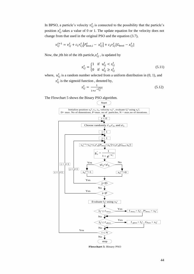
44
In BPSO, a particle’s velocity is connected to the possibility that the particle’s
position takes a value of 0 or 1. The update equation for the velocity does not
change from that used in the original PSO and the equation (3.7),
Now, the bit of the particle, is updated by
(5.11)
where, is a random number selected from a uniform distribution in (0, 1), and
is the sigmoid function , denoted by,
(5.12)
The Flowchart 5 shows the Binary PSO algorithm.
Initialize position xij0, c1, c2, velocity vij
0 , evaluate fij0 using xij
0,
D= max. No of dimentions, P=max. no of particles, N = max.no of iterations.
fijt ≤ f best,i f best,i = fij
t , Ptbest,i = xij
t
fijt ≤ f gbest f gbest = fij
t , Gbest = xijt
vijt+1=vij
t+c1rt1j[Pbest,i
t-xijt]+c2rt
2j[Gbest-xijt]
j = j+1
xijt+1=1
t ≤ N
stop
j = 1
No
Yes
NoYes
No
Flowchart 5: Binary PSO
Start
Yes
Evaluate fijt using xij
t
t = 0
es
vt
ij
t
ij 1
1
1
utij<st
ij
xijt+1=0
j<D
No
i<P
No
i = i+1
t = t+1
Yes
Yes
Yes
i = 1
Choose randomly rt1j,rt
2j, and utij

45
Now if the bit is not flipped into a 1 at the iteration, then the velocity increases
again at the iteration, along with a greater probability of to flip the bit.
In continuous valued problems of the PSO, the maximum velocity can be
large number for the particles exploration. On the other hand, in binary PSO the
maximum velocity will be small numbers for exploration, even if a good
solution is found [12]. It is suggested that the maximum velocity , which
corresponds to a maximum probability of 0.997 that a bit is flipped into 1, whereas
the minimum velocity , corresponds to a minimum probability of 0.002
that the bit remains 0. Since each bit of is always binary-valued in the solution
space, so no boundary conditions need to be specified in BPSO [10].
The velocity is a probability for the particle position
to be 0 or 1. For
instance, if , then
(or 50%). On the other hand,
if , then
, and if , then
.
Besides, it is true that
. Due to the random number
in the above equation (5.11), can change even if the value of does not
change [4].
The binary PSO algorithm is very important to practical and commercial use in
discrete problems solving, therefore this algorithm completely needs a lot more
attention in the future. Finally, in the following section the Lot sizing problem is
used to illustrate the details of computations for iterations 1 and 2 using the BPSO
method.
5.5.1 Problem Formulation (Lot Sizing Problem)
The problem is to find order quantities that will minimize total ordering and
holding costs of an ordering budget. I wish to find the solution of the following
problem by the Binary PSO method:
(1)
(2)
(3)
(4)
(5)
(6)
where,

46
The objective function equation (1) is to minimize the total cost with constraints
that include some limits, no initial inventory is available equation (2),equation (3)
represents the inventory balance equation in which the order quantity covers all the
requirements until the next order, equation (4) shows that projected inventory is
always positive, equation (5) satisfies the condition that no shortages are allowed,
and finally equation (6) denotes the decision variable that is either 1 (place an
order) or 0 (not place an order) [22].
Solution:
The various steps of the procedure are illustrated using the binary particle swarm
optimization:
Step1: Consider the number of particles ; the number of dimensions or
periods ; the ordering cost per period ; the holding
cost per unit per period ; also the net requirements , the lot size of
the particles , the initial particles positions
and corresponding
velocities , the inventory balance of particles
are given below and
finally evaluate each particle in the swarm using the objective function
in period at iteration .
1 2 3 4 5
80 60 40 30 70
140 100 70 100 80
1 0 1 0 0
3.50 1.50 3.80 -2.20 -1.00
60 30
260 + 230 = 490
120 80 50 40 90
1 1 0 0 0
2.80 3.00 -1.20 -3.00 2.5
40 20
240 + 220 = 460
100 70 30 25 95
1 0 0 1 1
3.40 -2.50 -1.00 1.50 3.00
20 15 25
220 + 215 + 225 =660

47
Find the personal best for each particle in the swarm:
1 2 3 4 5
1 0 1 0 0 490
1 1 0 0 0 460
1 0 0 1 1 660
Find the global best in the entire swarm:
1 2 3 4 5
1 1 0 0 0 460
Step 2: Set the iteration number as and go to step 3.
Step 3: By considering and the random numbers in the range (0, 1)
as
find the update velocities of the particles by
So
,
,
,
, ,
,
, ,
,
Step 4: Find the values of by the following equation
So
,
, ,
, .
,
, ,
,
,
, ,
,

48
Step 5: Update the particle’s position by using the sigmoid function,
Where, is a random number selected from a uniform distribution in (0, 1).
The following table is given the particles update position after completing the first
iteration:
1 2 3 4 5
1 1 0 0 0
3.50 1.50 3.55 -2.20 -1.00
0.96 0.82 0.98 0.10 0.27
0.60 0.10 0.99 0.35 0.53
120 40
0 1 0 0 1
2.80 3.00 -1.20 -3.00 2.5
0.94 0.95 0.24 0.04 0.92
0.96 0.70 0.99 0.05 0.30
40 20
1 0 0 0 1
3.15 -2.50 -1.00 1.25 2.75
0.96 0.08 0.27 0.78 0.94
0.56 0.70 0.80 0.85 0.35
40 50
Step 6: Evaluate using
in the swarm:
Step 7: Update the personal best for each particle in the swarm:
Since
then with
.
then with
.
then with
.

49
The new positions of particles are
1 2 3 4 5
1 0 1 0 0 490
0 1 0 0 1 460
1 0 0 0 1 490
Step 8: Update the global best in the entire swarm:
Since
then with
1 2 3 4 5
0 1 0 0 1 460
Step 9: Stopping criterion:
If the terminal rule is satisfied, go to step 2,
Otherwise stop the iteration and output the results.

50
CHAPTER 6
Applications of PSO
This chapter discusses the various application areas of PSO method.
Kennedy and Eberhart established the first practical application of Particle Swarm
Optimization in 1995. It was in the field of neural network training and was
reported together with the algorithm itself. PSO have been successfully used
across a wide range of applications, for instance, telecommunications, system
control, data mining, power systems, design, combinatorial optimization, signal
processing, network training, and many other areas. Nowadays, PSO algorithms
have also been developed to solve constrained problems, multi-objective
optimization problems, problems with dynamically changing landscapes, and to
find multiple solutions, while the original PSO algorithm was used mainly to solve
unconstrained, single-objective optimization problems [29].Various areas where
PSO is applied are listed in Table1 [5]:
Table 1. Application areas of Particle Swarm Optimization
Antennas
Design
The optimal control and design of phased arrays, broadband
antenna design and modeling, reflector antennas, design of
Yagi-Uda arrays, array failure correction, optimization of a
reflect array antenna, far-field radiation pattern
reconstruction, antenna modeling, design of planar
antennas, conformal antenna array design, design of patch
antennas, design of a periodic antenna arrays, near-field
antenna measurements, optimization of profiled corrugated
horn antennas, synthesis of antenna arrays, adaptive array
antennas, design of implantable antennas.
Signal
Processing
Pattern recognition of flatness signal, design of IIR filters,
2D IIR filters, speech coding, analogue filter tuning,
particle filter optimization, nonlinear adaptive filters, Costas
arrays, wavelets, blind detection, blind source separation,
localization of acoustic sources, distributed odour source
localization, and so on.
Networking
Radar networks, bluetooth networks, auto tuning for
universal mobile telecommunication system networks,
optimal equipment placement in mobile communication,
TCP network control, routing, wavelength division-
multiplexed network, peer-to-peer networks, bandwidth and
channel allocation, WDM telecommunication networks,
wireless networks, grouped and delayed broadcasting,
bandwidth reservation, transmission network planning,
voltage regulation, network reconfiguration and expansion,
economic dispatch problem, distributed generation,

51
microgrids, congestion management, cellular neural
networks, design of radial basis function networks, feed
forward neural network training, product unit networks,
neural gas networks, design of recurrent neural networks,
wavelet neural networks, neuron controllers, wireless sensor
network design, estimation of target position in wireless
sensor networks, wireless video sensor networks
optimization.
Biomedical
Human tremor analysis for the diagnosis of Parkinson’s
disease, inference of gene regulatory networks, human
movement biomechanics optimization, RNA secondary
structure determination, phylogenetic tree reconstruction,
cancer classification, and survival prediction, DNA motif
detection, biomarker selection, protein structure prediction
and docking, drug design, radiotherapy planning, analysis
of brain magneto encephalography data,
electroencephalogram analysis, biometrics and so on.
Electronics and
electromagnetic
On-chip inductors, configuration of FPGAs and parallel
processor arrays, fuel cells, circuit synthesis, FPGA-based
temperature control, AC transmission system control,
electromagnetic shape design, microwave filters, generic
electromagnetic design and optimization applications,
CMOS RF wideband amplifier design, linear array antenna
synthesis, conductors, RF IC design and optimization,
semiconductor optimization, high-speed CMOS, frequency
selective surface and absorber design, voltage flicker
measurement, shielding, digital circuit design.
Robotics
Control of robotic manipulators and arms, motion planning
and control, odour source localization, soccer playing, robot
running, robot vision, collective robotic search, transport
robots, unsupervised robotic learning, path planning,
obstacle avoidance, swarm robotics, unmanned vehicle
navigation, environment mapping, voice control of robots,
and so forth.
Design and
Modelling
Conceptual design, electromagnetics case, induction heating
cooker design, VLSI design, power systems, RF circuit
synthesis, worst case electronic design, motor design, filter
design, antenna design, CMOS wideband amplifier design,
logic circuits design, transmission lines, mechanical design,
library search, inversion of underwater acoustic models,
modeling MIDI music, customer satisfaction models,
thermal process system identification, friction models,
model selection, ultrawideband channel modeling,
identifying ARMAX models, power plants and systems,
chaotic time series modeling, model order reduction.
Image segmentation, autocropping for digital photographs,
synthetic aperture radar imaging, locating treatment
52
Image and
Graphics
planning landmarks in orthodontic x-ray images, image
classification, inversion of ocean color reflectance
measurements, image fusion, photo time-stamp recognition,
traffic stop-sign detection, defect detection, image
registration, microwave imaging, pixel classification,
detection of objects, pedestrian detection and tracking,
texture synthesis, scene matching, contrast enhancement,
3D recovery with structured beam matrix, character
recognition, image noise cancellation.
Power
generation and
Controlling
Automatic generation control, power transformer
protection, power loss minimization, load forecasting,
STATCOM power system, fault-tolerant control of
compensators, hybrid power generation systems, optimal
power dispatch, power system performance optimization,
secondary voltage control, power control and optimization,
design of power system stabilizers, operational planning for
cogeneration systems, control of photovoltaic systems,
large-scale power plant control, analysis of power quality
signals, generation planning and restructuring, optimal
strategies for electricity production, production costing,
operations planning.
Fuzzy systems,
Clustering, data
mining
Design of neurofuzzy networks, fuzzy rule extraction, fuzzy
control, membership functions optimization, fuzzy
modeling, fuzzy classification, design of hierarchical fuzzy
systems, fuzzy queue management, clustering, clustering in
large spatial databases, document and information
clustering, dynamic clustering, cascading classifiers,
classification of hierarchical biological data, dimensionality
reduction, genetic-programming-based classification, fuzzy
clustering, classification threshold optimization, electrical
wader sort classification, data mining, feature selection.
Optimization
Electrical motors optimization, optimization of internal
combustion engines, optimization of nuclear electric
propulsion systems, floor planning, travelling-sales man
problems, n-queens problem, packing and knapsack,
minimum spanning trees, satisfiability, knights cover
problem, layout optimization, path optimization, urban
planning, FPGA placement and routing.
Prediction and
forecasting
Water quality prediction and classification, prediction of
chaotic systems, streamflow forecast, ecological models,
meteorological predictions, prediction of the floe stress in
steel, time series prediction, electric load forecasting,
battery pack state of charge estimation, predictions of
elephant migrations, prediction of surface roughness in end
milling, urban traffic flow forecasting, and so on.

53
CHAPTER 7
Conclusion
This thesis discussed the basic Particle Swarm Optimization algorithm,
geometrical and mathematical explanation of PSO, particles’ movement and the
velocity update in the search space, the acceleration coefficients and particles’
neighborhood topologies in Chapter 3.
In Chapter 4, a set of convergence techniques, i.e. velocity clamping, inertia
weight and constriction coefficient techniques which can be used to improve speed
of convergences and control the exploration and exploitation abilities of the entire
swarm, was illustrated. The Guaranteed Convergence PSO (GCPSO) algorithm
was analyzed. This algorithm is very important to solve a problem when all
particles face premature convergence or stagnation in the search process.
Boundary conditions were presented which are very useful in the PSO algorithm.
Chapter 5 presented five different types of PSO algorithms which solve different
types of optimization problems. The Multi-Start PSO (MSPSO) algorithm attempts
to detect when the PSO has found lack of diversity. Once lack of diversity is
found, the algorithm re-starts the algorithm with new randomly chosen initial
positions for the particles. The Multi-phase PSO (MPPSO) algorithm partitions the
main swarm into sub-swarms or subgroups, where each sub-swarm performs a
different task, exhibits a different behavior and so on. Then the swarms cooperate
to solve the problem by sharing the best solutions they have discovered in their
respective sub-swarms. During the optimization process, high speed of
convergence sometimes generates a quick loss of diversity which lead to
undesirable premature convergence. To solve this problem, the perturbed particle
swarm algorithm (PPSO) illustrated in this chapter. The Multi-Objective PSO
(MOPSO) algorithm is very important when an optimization problem has several
objective functions. One discrete optimization problem was solved by the Binary
PSO (BPSO) algorithm.
The PSO algorithm has some problems that ought to be resolved. Therefore, the
future works on the PSO algorithm will probably concentrate on the following:
1. Find a particular PSO algorithm which can be expected to provide good
performance.
2. Combine the PSO algorithm with other optimization methods to improve the
accuracy.
3. Use this algorithm to solve the non-convex optimization problems.

54
REFERENCES
[1] D. Bratton and J. Kennedy, "Defining a Standard for Particle Swarm
Optimization ," in IEEE Swarm Intelligence Symposium, 2007, pp. 120-127.
[2] X. Li and K. Deb, "Comparing lbest PSO Niching algorithms Using Different
Position Update Rules," in In Proceedings of the IEEE World Congress on
Computational Intelligence, Spain, 2010, pp. 1564-1571.
[3] M. Dorigo and M. Birattar, "Swarm intelligence," in Scholarpedia, 2007, pp.
2(9):1462.
[4] Andries P. Engelbrecht, Computational Intelligence: An Introduction.: John
Wiley and Sons, 2007, ch. 16, pp. 289-358.
[5] Riccardo Poli, "Review Article-Analysis of the Publications on the Applications
of Particle Swarm Optimisation," Journal of Artificial Evolution and
Applications, p. 10, 2008.
[6] Singiresu S. Rao, Engineering Optimization Theory and Practice, 4th edition,
Ed.: John Wiley and Sons, 2009.
[7] El-Ghazali Talbi, Metaheuristics-From Design to Implementation.: John Wiley
and Sons, 2009.
[8] George I. Evers, An Automatic Regrouping Mechanism to Deal with Stagnation
in Particle Swarm Optimization(Master’s thesis), The University of Texas-Pan
American., 2009, Department of Electrical Engineering.
[9] Anthony Carlisle and Gerry Dozier, "An Off-The-Shelf PSO," in Workshop
Particle Swarm Optimization, Indianapolis, 2001.
[10] Nanbo Jin and Yahya Rahmat-Samii, "Advances in Particle Swarm
Optimization for Antenna Designs: Real-Number, Binary, Single-Objective and
Multiobjective Implementations," IEEE TRANSACTIONS ON ANTENNAS AND
PROPAGATION, vol. 55, no. 3, pp. 556-567, MARCH 2007.
[11] F. van den bergh, An Analysis of Perticle Swarm Optimizers. PhD thesis,
Department of Computer Science., 2006, University of Pretoria, Pretoria, South
Africa.
[12] Mohammad Teshnehlab and Mahdi Aliyari Shoorehdeli Mojtaba Ahmadieh
Khanesar, "A Novel Binary Particle Swarm Optimization," in Proceedings of
the 15th Mediterranean Conference on Control and Automation, Greece, July

55
,2007, p. 6.
[13] V.Selvi and R.Umarani, "Comparative Analysis of Ant Colony and Particle
Swarm Optimization techniques," International Journal of Computer
Applications, , vol. 5, no. 4, pp. 1-6, 2010.
[14] Kwang Y. Lee and Jong-Bae Park, "Application of Particle Swarm Optimization
to Economic Dispatch Problem: Advantages and Disadvantages," IEEE, 2010.
[15] Ajith Abraham, and Amit Konar Swagatam Das. (2008)
www.softcomputing.net. [Online]. http://www.softcomputing.net/aciis.pdf
[16] Ganesh Kumar,Salman Mohagheghi,Jean-Carlos Hernandez Yamille delValle,
"Particle Swarm Optimization: Basic Concepts, Variants and Applications in
Power Systems.," in IEEE, 2008, pp. 171-195.
[17] Y. Rahamat-Samii and Shenheng Xu, "Boundary Conditions in Particle Swarm
Optimization Revisited," IEEE TRANSACTIONS ON ANTENNAS AND
PROPAGATION, vol. 55, no. 3, pp. 760-765, March 2007.
[18] S. M. Mikki and Ahmed A. Kishk, "Hybrid Periodic Boundary Condition for
Particle Swarm Optimization," IEEE TRANSACTIONS ON ANTENNAS AND
PROPAGATION, vol. 55, no. 11, pp. 3251-3256, NOVEMBER 2007.
[19] James Kennedy and Tim Blackwell Riccardo Poli, "Particle swarm optimization
An overview," Swarm Intelligence, vol. 1, no. 1, pp. 33–57, 2007.
[20] A. P. Engelbrecht F. van den Bergh, "A New Locally Convergent Particle
Swarm Optimiser," IEEE Conference onSystems, Man and Cybernetics, Tunisia,
2002.
[21] Morten Løvbjerg and Thiemo Krink, "Extending Particle Swarm Optimisers
with Self-Organized Criticality," IEEE Int.Congr. Evolutionary Computation,
vol. 2, pp. 1588-1593, May 2002.
[22] M. Fatih Tasgetiren and Yun-Chia Liang, "A Binary Particle Swarm
Optimization Algorithm for Lot Sizing Problem," Journal of Economic and
Social Research, vol. 5, no. 2, pp. 1-20, 2003.
[23] L.M. Ruan, M. Shi, W. An and H.P. Tan H. Qi, "Application of multi-phase
particle swarm optimization technique to inverse radiation problem," Journal of
Quantitative Spectroscopy & Radiative Transfer 109 (3), pp. 476-493, 2008.
[24] Zhao Xinchao, "A perturbed particle swarm algorithm for numerical
optimization," Applied Soft Computing 10, pp. 119–124, 2010.

56
[25] Lihua Gong and Zhengyuan Jia, "Multi-criteria Human Resource Allocation for
Optimization Problems Using Multi-objective particle Swarm Optimization
Algorithm," International Conference on Computer Science and Software
Engineering, vol. 1, pp. 1187-1190, 2008.
[26] Konstantinos E. Parsopoulos and Michael N. Vrahatis, Multi-Objective Particles
Swarm Optimization Approaches, 2008.
[27] M. R. Pontes, C. J. A. Bastos-Filho R. A. Santana, "A Multiple Objective
Particle Swarm Optimization Approach using Crowding Distance and Roulette
Wheel," IEEE Ninth International Conference on Intelligent Systems Design
and Applications, pp. 237-242, 2009.
[28] Tsung-Ying Sun, Sheng-Ta Hsieh, and Cheng-Wei Lin Shih-Yuan Chiu,
"Cross-Searching Strategy for Multi-objective Particle Swarm Optimization,"
IEEE Congress on Evolutionary Computation, pp. 3135-3141, 2007.
[29] Marco Dorigo et al., "Particle swarm optimization," Scholarpedia, vol. 3, no. 11,
p. 1486, 2008.

57
Appendix A
Glossary terms of this thesis:
ABC: Absorbing boundary condition.
BPSO: Binary Particle Swarm Optimization.
CSS-MOPSO: Cross-Searching Strategy Multi-Objective
DBC: Damping boundary condition.
DNPSO: Dynamic Neighborhood Particle Swarm Optimization.
gbest PSO: Global Best Particle Swarm Optimization.
GCPSO: Guaranteed Convergence Particle Swarm Optimization.
IBC: Invisible boundary condition.
I/DBC: Invisible/Damping boundary condition.
I/RBC: Invisible/Reflecting boundary condition.
lbest PSO: Local Best Particle Swarm Optimization.
: Pareto front.
PPSO: Perturbed Particle Swarm Optimization.
PSO: Particle Swarm Optimization.
RBC: Reflecting boundary condition.
MOPSO: Multi-Objective Particle Swarm Optimization.
MPPSO: Multi-phase Particle Swarm Optimization.
MSPSO: Multi-Start Particle Swarm Optimization.
VEPSO: Vector Evaluated Particle Swarm Optimization.

58
Appendix B
Commonly-used symbols of this thesis:
The function being minimized or maximized. It takes a vector input
and returns a scalar value.
The velocity vector of particle in dimension at time
The position vector of particle in dimension at time
The personal best position of particle in dimension found from
initialization through time t.
The global best position of particle in dimension found from
initialization through time t.
, Positive acceleration constants which are used to level the
contribution of the cognitive and social components respectively.
,
Random numbers from uniform distribution at time t.
: Two chosen (local guides) for each particle in
iteration .
The swarm size or number of particles.
Denotes time or time steps.
D: The maximum no. of dimensions.
P: The maximum no. of particles.
N: Total number of iterations.
The maximum velocity.
ω The inertia weight.
χ The constriction coefficient.
The parameter controls the diameter of the search space.
The criticality of the particle .
The global criticality limit.
The -th dimension of p-gbest in iteration .

59
The normal distribution.
The degree of uncertainty about the optimality of the gbest and is
modeled as some non-increasing function of the number of
iterations.
The velocity of the -th particle in the -th swarm.
The best position found for any particle in the -th swarm which is
evaluated with the -th objective function.
The sigmoid function.