mathematical model for pore development during physical ...a mathematical model for pore development...

MATHEMATICAL MODEL FOR PORE DEVELOPMENT DURING

PHYSICAL ACTIVATION OF CHARS

ERIKA ARENAS CASTIBLANCO

UNIVERSIDAD NACIONAL DE COLOMBIA

FACULTY OF MINES

DOCTORAL ENGINEERING PROGRAM

ENERGY SYSTEMS

MEDELLIN

2009

2

MATHEMATICAL MODEL FOR PORE DEVELOPMENT DURING

PHYSICAL ACTIVATION OF CHARS

BY

ERIKA ARENAS CASTIBLANCO

A dissertation submitted to the Faculty of Mines of Universidad Nacional

de Colombia in partial fulfillment of the requireme nts for the Degree of

Doctor

Advisor

Ph.D. FARID CHEJNE JANNA

UNIVERSIDAD NACIONAL DE COLOMBIA

FACULTY OF MINES

DOCTORAL ENGINEERING PROGRAM

ENERGY SYSTEMS

MEDELLIN

2009

3

ACKNOWLEDGMENT

The author wish to thank to:

Ph.D. Farid Chejne for his guidance throughout this research, and in many

other times in my Life.

Professor Suresh Bhatia, who received me at the University of Queensland in

his research group and let me to discuss with him part of this job. I met very

special people in his group.

Ph.D. Whady Florez for his precise support through the building of the program

in Fortran.

M.Sc. Zulamita Zapata for her collaboration during the experimental job.

COLCIENCIAS and Universidad Nacional de Colombia for their financial

support through the grant “Apoyo a Doctorados Nacionales" and to the

Universidad Pontificia Bolivariana that permitted I had taken time to do my

Doctoral Program.

To all those persons that had knowledge about this job, and they collaborated to

me in different ways.

4

ABSTRACT

A mathematical model for pore development during physical distribution of

chars was proposed. This model combines the Random Pore Model, proposed

by Bhatia and Perlmutter and the population balance for the pore size

distribution proposed by Hashimoto and Silveston. The equations of the model

were solved using the orthogonal collocation method and the method of

moments applying at this point two techniques: the maximum entropy method

and the use of a priori distribution shape with its parameters obtained from the

moments. The shape of the pore size distributions obtained by the method of

the use of a priori distribution was closer to the experimental distributions than

those obtained by the method of maximum entropy.

The results were compared with experimental data obtained by the activation

with CO2 of three coal chars: La Capotera, La Grande and El Sol that exhibit

different reactivity. By using two adjustable parameters φ and α, the theoretical

model allows establishing the occurrence and prevalence of phenomenon of

formation and combination of pores during the activation. However, the model

does not take into account the effect of the closed pores that are present at the

beginning of the process of gasification. These closed pores can have an

important effect on the pore size distribution as the shape of the pore size

distribution at low carbon conversion is different when compared to the

distribution at higher carbon conversion degree. This phenomenon should be

considered as an additional term in future refinements of our model.

5

TABLE OF CONTENT

CHAPTER ONE.......................................................................................................... 10

LITERATURE REVIEW .................................. ............................................................ 10

1.1. MODELS FOR CHAR REACTIONS..................................................................................... 10

1.1.1. CONTINUUM MODELS.................................................................................................... 11

1.1.2. DISCRETE MODELS......................................................................................................... 15

1.2. PORE SIZE DISTRIBUTION............................................................................................... 21

1.3. REVIEW ON EVOLUTION OF PORE SIZE DISTRIBUTION................................................ 24

1.4. MAXIMUM ENTROPY METHOD ...................................................................................... 31

1.5. CONCLUSIONS .................................................................................................................. 35

LIST OF REFERENCES.......................................................................................................... 37

CHAPTER TWO......................................................................................................... 42

EXPERIMENTAL PORE SIZE DISTRIBUTION................ .......................................... 42

2.1. MATERIALS AND PROCEDURE ........................................................................................ 42

2.2. RESULTS ........................................................................................................................... 47

2.3. SEM MICROGRAPHS........................................................................................................ 62

2.4. PORE SIZE DISTRIBUTION EVOLUTION IN THE LITERATURE. ....................................... 66

2.5. CONCLUSIONS .................................................................................................................. 67


CHAPTER THREE ..................................................................................................... 72

THEORETICAL MODEL FOR PREDICTION OF PORE SIZE DISTR IBUTION.......... 72

3.1. MODEL EQUATIONS: MASS AND ENTROPY BALANCES................................................. 72

6

3.2. MODEL EQUATIONS: PORE SIZE DISTRIBUTION .......................................................... 78

3.3. MODEL SOLUTION ........................................................................................................... 82

3.3.1 THE ORTHOGONAL COLLOCATION METHOD.................................................................. 82

3.3.2 THE MAXIMUM ENTROPY TECHNIQUE............................................................................. 85


CHAPTER FOUR ....................................................................................................... 89

RESULTS AND VALIDATION OF THE MODEL FOR PREDICTION OF PORE SIZE

DISTRIBUTION .......................................................................................................... 89

4.1. SENSITIVITY ANALYSIS FOR THE MODEL .................................................................... 100

4.2. VALIDATION OF THE MODEL FOR LA CAPOTERA, LA GRANDE AND EL SOL CHARS 105

4.3. CONCLUSIONS ................................................................................................................ 116

LIST OF REFERENCES........................................................................................................ 117

CHAPTER FIVE ....................................................................................................... 118

CONCLUSIONS ....................................................................................................... 118

APPENDIX A. EXPERIMENTAL DATA .................... ............................................. 120

APPENDIX B. FLOW CHART FOR MODEL SOLUTION PROGRAM ................... 145

APPENDIX C. EXECUTIVE SUMMARY.................... ............................................. 147

7

LIST OF TABLES

Table 1. Analysis of coals ........................................................................................... 43

Table 2. Input parameters for model solution .............................................................. 89

Table 3. Initial value of moments ................................................................................ 95

Table 4. General parameters for distributions as functions of moments ...................... 98

Table 5. Parameters values for Sensitivity Analysis .................................................. 101

Table 6. Parameter for validation of the model with La Capotera char ...................... 106

Table 7. Parameter for validation of the model with La Grande char ......................... 108

Table 8. Parameter for validation of the model with El Sol char ................................ 111

8

LIST OF FIGURES

Figure 1. Diagram of fixed bed reactor........................................................................ 44

Figure 2. Carbon conversion versus time at 850°C. .. .................................................. 48

Figure 3. Carbon conversion function versus time. Unreacted shrinking Core Model .. 49

Figure 4. Carbon conversion function versus time. Volumetric Model ....................... 49

Figure 5. PSD based on CO2 Isotherm. La Capotera char at different carbon

conversion levels ................................................................................................ 51

Figure 6. PSD based on CO2 Isotherm. La Grande char at different carbon conversion

levels................................................................................................................... 51

Figure 7. PSD based on CO2 Isotherm. El Sol char at different carbon conversion levels

............................................................................................................................ 52

Figure 8. N2 adsorption isotherms for La Capotera char at different burn-off levels..... 54

Figure 9. N2 adsorption isotherms for La Grande char at different burn-off levels........ 55

Figure 10. N2 adsorption isotherms for El Sol char at different burn-off levels ............. 55

Figure 11. PSD based on N2 Isotherm. La Capotera char at different carbon conversion

levels................................................................................................................... 56

Figure 12. PSD based on N2 Isotherm. La Grande char at different carbon conversion

levels................................................................................................................... 57

Figure 13. PSD based on N2 Isotherm. El Sol char at different carbon conversion levels

............................................................................................................................ 57

Figure 14 . Pore size evolution throughout activation. ................................................. 58

Figure 15. Evolution of pore volume versus Burn-off. La Capotera char. .................... 59

Figure 16. Evolution of pore volume versus Burn-off. La Grande char. ....................... 60

Figure 17. Evolution of pore volume versus Burn-off. El Sol char................................ 60

Figure 18. SEM micrographs. La Capotera char at different carbon conversion levels.

............................................................................................................................ 63

Figure 19. SEM micrographs. La Grande char at different carbon conversion levels... 64

Figure 20. SEM micrographs. El Sol char at different carbon conversion levels. ........ 65

Figure 21. Scheme of char particle ............................................................................. 72

Figure 22. Conversion vs. Radial Position. k= 1e-6..................................................... 90

9

Figure 23. Entropy generation vs. Radial position. k=1e-6 .......................................... 91

Figure 24. Pore size distribution. Maximum Entropy Method. k=1e-6.......................... 92

Figure 25. Conversion vs. Radial Position. k= 1e-2..................................................... 93

Figure 26. Entropy generation vs. Radial position. k= 1e-2 ......................................... 93

Figure 27. Pore Size Distribution. Maximum entropy method. k= 1e-2 ........................ 94

Figure 28. Pore Size Distribution. Maximum entropy method. Run 1 .......................... 96

Figure 29. Pore Size Distribution. Maximum entropy method. Run 2. ......................... 96

Figure 30. Pore Size Distribution. Maximum entropy method. Run 3. ......................... 97

Figure 31. Pore Size Distribution. Log-normal distribution. k= 1e-6............................. 99

Figure 32 . Pore Size Distribution. Log-normal distribution. k= 1e-4............................ 99

Figure 33. Pore Size Distribution. Log-normal distribution. k= 1e-2........................... 100

Figure 34. Kf: Krxn,Krxn,0, Alpha: 0.75,0.75,0.75, Phi: 0.5 ...................................... 102

Figure 35. Kf: Krxn,Krxn,Krxn, Alpha: 0.75, 0.75,0.75, Phi: 0.3,0.6,0.9 .................... 102

Figure 36. Kf: 10000Krxn,Krxn,0, Alpha: 0.75, 0.75,0.75, Phi: 0.3,0.6,0.9................. 103

Figure 37. Kf: Krxn,Krxn,0, Alpha: 0.5, 0.5,0.5, Phi: 0.3,0.6,0.9 ............................... 103

Figure 38. Kf: Krxn,Krxn,0, Alpha: 0.75, 0.5,1.0, Phi: 0.3,0.6,0.9 ............................. 104

Figure 39. Theoretical pore size distribution for La Capotera char ............................ 106

Figure 40. Carbon conversion profile for La Capotera char....................................... 107

Figure 41. Entropy generation profile for La Capotera char....................................... 107

Figure 42. Theoretical pore size distribution for La Grande char ............................... 109

Figure 43. Carbon conversion profile for La Grande char.......................................... 109

Figure 44. Entropy generation profile for La Grande char ......................................... 110

Figure 45. Theoretical pore size distribution for El Sol char....................................... 112

Figure 46. Carbon conversion profile for El Sol char ................................................. 112

Figure 47. Entropy generation profile for El Sol char ................................................ 113

Figure 48. Flow chart for model solution program ..................................................... 146

10

CHAPTER ONE

LITERATURE REVIEW

The global concern for pollution control has lead to develop efficient and low

cost pollution control systems. Systems based on activated carbons represent

an alternative. Activated carbons are porous materials that can be obtained

from different raw materials such as coal, wood, coconut shells, etc. These raw

materials are activated using steam or carbon dioxide (physically activation) or

using some chemical substances such as ZnCL2 or H3PO4 (chemical

activation).

One of the criteria for selecting an activated carbon for a particular application is

the pore size distribution (PSD). The porosity development is affected by

different parameters such as the raw material, the activating agent,

temperature, activation time among others. A theoretical model that explains

changes in porosity and surface area throughout the activation process could

be a valuable tool in order to establish the value of the parameters required for

the fabrication of an activated carbon for a specific application.

1.1. Models for Char reactions

According to Bhatia and Gupta (1992) the mathematical models for gas-solid

reactions, one of which is the physical activation by gasification, can be

presented in terms of an unified framework that accommodates shrinking core

reactions as well as the internal reaction-diffusion formulation with an arbitrary

structural model.

11

The Shrinking Core Model takes into account for gas-solid reaction in the

shrinking front of the external surface of the particle. This model was first

developed by Yagi and Kunii (1955, cited by Bhatia and Gupta, 1992). This

model considers that the gaseous reactant has to go through three resistances

to reach the external surface of the solid: 1) Diffusion through the gas film

around the particle, 2) Diffusion through the ash layer that is formed around the

nuclei and 3) Chemical reaction on the surface. This model does not consider

the role of the internal structure in the reaction.

In the reaction-diffusion regime, the various models differ primarily in terms of

the assumed structural representation of the solid. Sahimi et al (1990) classified

the models for transport and reaction in porous media as continuum models and

discrete models. Continuum models represent the classical engineering

approach to describe materials of complex and irregular geometry characterized

by several length scales. The porous material is treated as a continuum in

which temperature, fluid species concentrations and solid species

concentrations are defined as smooth functions of time and position. In a

discrete model the material is treated as a collection of elements such as voids,

crystallites etc. The fluid and solid concentrations are defined for each element

and are governed by energy and material balances as in the continuum models.

1.1.1. Continuum Models

Two classes of models for representing a porous medium have been used

frequently in continuum modeling: grain models and capillary models. The grain

model considers the solid compounds of small spherical particles or grains. The

space between grains constitutes the porous network. The grains are usually

taken as initially nonporous but the product layer developing could be porous or

nonporous. This model was proposed by Szekely and Evans (1970). The gas

concentration C and solid conversion X are functions of time; position R of the

12

grain within the pellet, and position r within the grain. By making a pseudo-

steady-state simplification and the assumption that reaction within the grains

proceeds in a shrinking-core fashion controlled by interface, the governing

equations are reduced to a second order differential equation in R coupled to a

first order differential equation in time for the solid conversion. However the

grain model predicts a monotonically decreasing in surface area and reaction

rate (Lu and Do, 1994). Some experimental studies have shown that reaction

rate and surface area evolution has a maximum (Adschiri and Furusawa, 1986)

or in other cases the surface area has a tendency to increase during

gasification. (Feng and Bhatia, 2003). Adschiri and Furusawa calculate the

specific surface area based on the initial mass of the solid, whereas Feng and

Bhatia calculate the specific surface area based on the residual carbon at any

conversion level. It could be more practical to calculate the specific surface area

based on the initial mass of the solid. In this way, it is known the surface area

and pore sizes developed per mass unit of coal or char fed to a reactor at

different burn-off levels.

Capillary models conceive the porous structure constituted by capillaries or

cylinders. One of the first capillary models was proposed by Petersen (1957)

who considered networks of infinitely long, uniform, cylindrical capillaries with

axes located randomly on a single plane and calculated the evolution of surface

area and volume with conversion. This author assumed that the pores enlarge

uniformly and developed a model based on this consideration and the

conservation of mass applied to a system conformed by a cylindrical rod with

cylindrical pores. This model has served as a starting point for some models

developed later.

Simons and Finson (1979) proposed a pore tree model. The pores are assumed

to be cylindrical tubes of length lp and radius rp. The number of pores whose

radius is between rp and rp+drp is denoted by a pore distribution function. The

authors obtained an approximate form for the pore size distribution based on

13

pore branching sequence as a tree. The pore length is expressed as a collision

integral over the distribution function and is shown to be proportional to the pore

radius. Each pore that reaches the exterior surface of the char particle is

depicted as the trunk of a tree. Each tree trunk of radius rt is associated with an

internal structure whose surface area is proportional to rt3.

Simons and Finson assume that the pore structure occurs randomly and the

pore length is determined by an arbitrary intersection with another pore. At such

an intersection, the smaller pore is terminated and the larger pore retains its

structure, then the largest pores must terminate at either the exterior surface of

the particle or at an internal void. These can be interpreted as pores near to the

external surface are larger than pores within the particle. It should be noted that

the pore tree structure was previously assumed, not in an explicit way but

implicit, and the authors derived equations to model this assumption. This

model tries to explain the change in pore distribution by considering phenomena

such as pore combination and pore growing due to chemical reaction.

Robau-Sanchez et al (2003) activated char spheres obtained by pelletizing

Quercus agrifolia powdered char, using CO2 and measured the porosity by

physical adsorption of N2 in samples taken from different layers of the sphere:

core, middle and outer layer at different burn-off. These authors determined

micropore and mesopore volume and they found, for activation at 820°C, the

total pore volume at low conversions decreases from the external since CO2

first access external layers than internal sections. For activation at 860°C,

microporosity is higher in the core of the particle at conversion beyond 60%.

This behavior is explained based on the pore formation mechanism proposed

by Wigmans (cited by the Robau-Sanchez et al,2003). Pore deepening is

favored by high temperatures causing the formation of micro and mesopores. At

high conversion levels, more intense gasification reaction is favored by the high

temperatures. This could cause that the external layer to be more rigorously

attacked by the reacting gas increasing its mesoporosity and decreasing its

14

microporosity. This behavior is in accordance with the pore tree model.

However Robau-Sanchez et al found that the total pore volume does not show

the same trend at low conversions as for 820°C. The authors attribute this result

to the fact that macropore volume was not measured and propose that the

macropore volume should be determined in order to give a better description of

the structural changes during activation as a function of the radial position.

Another aspect that should be pointed out is that these authors used N2 but

they did not use CO2 in the characterization of microporosity volume and it is

known that N2 is subject to very slow diffusion in small pores. CO2 at 273 K is

sensitive to narrow pores not accessible to N2 at 77 K, and hence, it is an

adequate complement to N2 at 77 K (Cazorla-Amorós et al, 1998)

A random pore model (Bhatia and Perlmutter, 1980) considers that the overlap

between void elements of arbitrary shape can be described exactly when the

location of the voids is completely random, i.e. it obeys the Poisson distribution.

The Poisson distribution in this model is derived from the use of the model of

Avrami (1940, cited by Bhatia) that proposed that the average of the increment

in the volume enclosed by the overlapped system (dV) is only a fraction of the

growth in the nonoverlapped cylindrical system (dVE). This fraction is (1-V).

Then dV=(1-V)dVE and with the observation that V→0 as VE→0 the integration

of the equation gives: V=1-exp(-VE) and the function exp(-VE) can be

associated with a Poisson distribution and can be explained as the probability of

not having any pore volume at a point.

In the Random Pore Model the evolution of surface area with conversion is

expressed in terms of a structural adjustable parameter Ψ that according to the

authors can be derived from experimental measurements of surface area, pore

length per mass and true density of the non reacted char. Gavalas (1980)

independently arrived at a similar model but with a different interpretation of the

structural parameter ψ. For Bhatia and Perlmutter is a parameter that relates

the initial surface area and total pore length Ψ= 4πLg/(ρtSgo2), where Lg is pore

15

length [m/g], ρt is the true density of the carbon and Sgo2 is the initial pore

surface area [m2/g]. For Gavalas ψ is a parameter relates to pore size

distribution ψ = Σλi/2πΣλirio where λi is the surface density of intersections of the

capillary axes with a fixed plane within the particle. The interpretation of Bhatia

is easier to test experimentally but determination of pore length implies to

assume a specific pore shape that leads to discrepancies with the true pore

length.

Experimental measurements made by Chi and Perlmutter (1989) and Feng and

Bhatia (2003) have found there is no coincidence between theoretical and

experimental values of the parameter Ψ. Bhatia has tried to improve his model

taking into account some characteristics of the char such as high microporosity

by including a discreteness parameter α that accounts for the finiteness of the

size of the reacting solid units (Bhatia and Vartak, 1996) and different

reactivities in the interior of the particles (Bhatia, 1998).

Based on the Random Pore Model Su and Perlmutter (1984) proposed an

equation that predicts the evolution of pore volume distribution taking into

account pore enlargement as well as pore intersections.

In general any model tries to adjust experimental observations on a curve with

equations that describe that curve. This curve can be described by known

equations such as distribution functions. The difference lies on the adjustable

parameters that appear when one or another equation is used and in the

physical meaning attributed to these parameters

1.1.2. Discrete models

As it was mentioned, in discrete models the material is treated as a collection of

voids, crystallites, etc. In these models concentrations and temperatures are

defined by energy and material balances.

16

Miura and Hashimoto (1984) , taking into account the differences in reactivity

proposed a model dividing the carbonaceous material in two parts, the

nonorganized carbons and the stacks consisting of graphitic layers of carbon

(crystallite). When the carbonaceous material is activated the more reactive

nonorganized carbon is gasified, rapidly forming a reaction interface and the

less reactive crystallite is gasified gradually, thus forming micropores within the

crystallite. The number of pores created in the crystallite is calculated on the

basis of the probability concept used by Wolff (1959, cited by Miura and

Hashimoto) that assumes a random removal of the crystallite layers. The

particle is comprised of grains of spherical shape and uniform size; each grain

is composed of nonorganized and organized carbon. The spaces between the

grains are the macropores.

Other discrete models are based on the percolation theory thought as the

spread of a fluid through a random medium resembled by flow of a coffee in a

percolator. The medium is defined as an infinite set of objects called sites. For

porous media applications sites are equivalent to pore bodies. These pore

bodies are points where pore throats join each other. It is a point of intersection

of pores. The opened connections between these points build a cluster. The

porosity is related to the size of the clusters, low porosities small clusters and

high porosities big clusters. Percolation processes are characterized by a

transition point (percolation threshold) at which a sudden change in the

properties of a disordered medium occurs when its’ previously disconnected

regions or phases coalesce to form a continuous path. For porosities smaller

than the percolation threshold, there is not accessible porosity and surface

area; consequently there is no mass transport into the structure.

The percolation threshold is a value that depends on the structure of the

network that is assumed. It is a theoretical value and theoretically, this threshold

marks a limit between the existence, or not, of clusters of accessible porosity.

17

Then the values of the threshold are different, they could be as low as 0.199 for

a face centered cubic tessellation (three dimensional) as high as 0.6962 for a

honeycomb network (two dimensional). Sahimi and Tsotsis (1988) proposed the

use of three dimensional networks that is a more realistic representation of the

solid than two-dimensional or Bethe networks. These three dimensional

networks have lower values of the percolation that other kind of networks. Then,

in order to select an appropriate network, its percolation threshold should be

inferior to true values of porosities of carbon, or chars, in order to have a more

realistic model avoiding the simulation of deep transition between non

accessible and accessible porosity.

When porosity is increased by randomly distributing pores throughout the solid,

a continuous path of pores is generated when the porosity reaches the

percolation threshold. As porosity continues to increase, past percolation

threshold, more pores are incorporated into the accessible region. The values of

the percolation threshold depend on the representation of the pore space, which

is divided or tessellated in polyhedra or another volumetric form.

One of the early models based on the percolation theory was proposed by

Reyes and Jensen (1986). According to these authors percolation theory

provides a natural framework for modeling pore opening, enlargement and

coalescence in the evolution of porosity and internal accessible area with solid

conversion. The space is represented based on Bethe lattices that are two-

dimensional representations and completed characterized by their coordination

number z, that is, the number of bonds connected to a site. These authors take

some results developed by Fisher and Essam(1961, cited by Reyes and

Jensen), for the percolation threshold Φc of a coordinated network that is given

by:

1 z-1cΦ =

18

And the accessible porosity ΦA is evaluated from

( )(2 2) /( 2) c

0

1 /

cA

z zR − −

Φ < ΦΦ = Φ ≥ Φ Φ − Φ Φ

Where ΦR is the root of the equation:

( )( 2) ( 2)1 (1 ) 0zR R z− −Φ − Φ − Φ − Φ =

and Φ = ΦA + ΦI where Φ is the total porosity and ΦI is the isolated porosity.

The model for the internal surface area includes a constant K that is obtained by

matching the accessible surface area to a single surface area measurement.

SvA = KΦ (1-Φ)-ΦI(1-ΦI)

Shah and Ottino (1987) proposed a model based on percolation. It was applied

to a gasification of a spherical particle and included an energy balance due to

the consideration of the process of gasification to be non-isothermal because

the gasification reaction is generally endothermic in nature and the thermal

diffusivity of the particle is not very high. Again in this model adjustable

parameters appear, these are obtained by fitting with experimental results

Sahimi and Tsotsis (1988) proposed a model also based on the percolation

theory but, according to the authors, it is different from the earlier models due

to the inclusion of concepts on dynamic scaling, to describe the evolution of the

size of the fragments, which are produced as a result of the reaction. The

dynamics of the process cannot be described by percolation concepts alone,

since percolation models are inherently static. This model is based on a body-

centered cubic network. This network has a coordination number of 14 and its

19

site percolation threshold is about 0.16. At porosity higher than 0 a randomness

is introduced into the model by a random assignment of the sites, as the open

space generates clusters of open pores. If this random assignment of the sites

of the network, as either solid or open space, generates isolated and finite

clusters of solid sites, they are removed from the network, so that one starts

with a single sample-spanning cluster of solid sites. The method of

Alexandrowicz (1980, cited by Sahimi and Tsotsis) can be used to generate

only the sample-spanning cluster of the solid sites and avoid formation of

isolated clusters. One identifies the solid sites at the perimeter of the open

cluster, which are connected to the particle surface. The process time is then

set as t=0. The perimeter solid sites are consumed and redesignated as open

space (pores) and the process time is increased by one unit. The new perimeter

solid sites are now identified and consumed and the process time is again

increased by one unit and so on. In this model a random factor appears to

generate a network (cluster) and the way in which time is increased is not very

clear.

Kantorovich and Bar-Ziv (1994) proposed a model to describe the evolution of

porous structure of highly porous chars and the shrinkage phenomenon

(diameter reduction of a particle). Porous char is a three dimensional network of

randomly distributed interconnected solid bodies “microrods” (finite cylinders of

equal radii with a distribution of lengths).The skeleton of the microrods holds the

whole micropore and macropore structure. Micropores are voids between the

microrods and macropores are great voids that interrupt this network and its

shape is assumed cylindrical. Macropores with a dead-end, as well as isolated

macropores are not considered in this model. According to these authors this

assumption can be made due to isolated fact that pores practically do not

contribute to the total porosity and to internal surface, for materials with a

porosity higher than 60% which corresponds to the range of porosities of char

particles exhibiting shrinkage.

20

The shrinkage is explained by different reactivities, that is, preferential

consumption of the edges of microrods. The porous evolution is explained by

the “Subskeleton model” that assumes that all microrods can be divided in two

groups: Group 1-long microrods that do not coalesce, Group 2-short microrods

that can coalesce to other microrods of both groups. Shrinkage occurs due to

shortening of long microrods but they retain their original position in the

subskeleton by attraction forces. Small microrods form the fine structure of the

micromedium which changes during conversion. The macropore radius

increases with conversion due to reaction with the macropore walls. However,

as the dimensions of the macropores are much larger than those of microrods,

the macropore changes due to reaction with their walls can be neglected. In

other words, the factor for shrinkage of the macropores and the entire material

is equal to the shrinkage factor of the microrod network. As shrinkage of

macropores is caused by processes in the microstructure, macroporosity does

not change with conversion. Therefore, the topological features of the

macropore structure would retain a similar shape during conversion. The

variations of porosity, surface area are expressed in terms of these changes of

pore length. The expressions for variations of length, derived from considering

the geometrical structure –subskeleton-, are complex as it is indicated by the

authors. By other hand, some parameters that appear in the equations, such as

surface number density of pores of a specific size and pore length of each size,

must be obtained by experimental fitting because it is not possible to measure

it.

Borrelli et al (1996) proposed a kinetic model of gasification of porous carbon

particles. The model considers the configurational diffusion mechanism, which

dominates transport in pores whose size is of the order of the diffusing molecule

size. The pores space is modeled by using branching self-similar pore

networks. Pores are hierarchically arranged in a sequence of levels i>0. Each

pore is characterized by lateral size 2rj. The sequence of pore levels is

constructed so as to keep constant the reduction ratio: ri+1/ri=α<1. The authors

21

compare this topological model, which is not fractal in strict sense but have a

fractal behavior with a topological model that is a classical prototype of the

fractal structures, i.e. the Menger Sponge. The formation of both types of

porous structures is based on an iterative application of the Thiele analysis.

This is based on the definition of an effective reaction rate constant ki per unit

surface of the pores belonging to the ith level. It is calculated as the sum of

contributions to the reaction rate from pores smaller than ri divided by the

concentration of the gaseous reactant at the ith level and by the surface area ai

of pores of size ri . It is assumed that the solid is characterized by a uniform

reactivity Ks. The results presented by the authors use in both models different

fractal dimensions that are used to calculate ratios between of areas and sizes

of the ith levels. This model is static in the way that a porous structure is built

adjusting parameters according to an apparent reaction rate. Time evolution

had to be derived changing apparent reaction rate and adjusting again the

porous structure. This kind of fractal models can be classified as continuum

since fractal theory is used to built a porous structure with not regular shapes as

the case of model with cylindrical pores but the porous medium can be treated

as a continuum

1.2. Pore Size Distribution

The International Union of Pure Applied Chemistry proposed to classify pores

by their internal pore width in: Micropore with pore width less than 2 nm,

Mesopore with pore width between 2 and 50 nm and Macropore with pore width

greater than 50 nm. Additional, micropores are classified into ultramicropores,

pore width less than 0.7 nm, and supermicropores, pore width between 0.7 and

2 nm.

The sorption behavior is different according to the size of pores. In Micropores,

the sorption is dominated by the interaction between molecules and pore walls.

In Mesopores, sorption depends on fluid-wall interactions and on interactions

22

between fluid molecules, which may lead to the occurrence of capillary

condensation (Lowell et al,2006).

One of the most used characterizations for porous carbons is the pore size

distribution that is defined as:

( )dV

f wdw

= (1)

Where w is a characteristic dimension of the regular model pore and V is the

volume of that pore (Davies and Seaton, 1998).

Several theories have been proposed to characterize the pore size distribution.

In the case of Mesopores, the most common are the methods based on the

Kelvin equation. In these methods is assumed that condensation occurs in

pores when a critical relative pressure is reached corresponding to the Kelvin

radius, rk. Based on this radius and the absorbed film thickness is calculated

the actual pore radius, rp, and then it is possible to build the curve Vp/∆r versus

rp that is the representation of the pore size distribution. Vp is the actual pore

volume and ∆r is the difference between successive pore radius obtained from

successive relative pressures. Between these methods, the BJH, Barrett-

Joyner-Halenda method is the most popular.

Other methods for mesopore analysis are based on microscopic analysis using

the Density Functional Theory or computer simulations based on Monte Carlo

and Molecular Dynamics techniques. These methods are also used for

micropore analysis. These methods emerge as a need to improve the results

obtained from the classical Kelvin equation and they consider a microscopic

approach of the adsorption phenomenon. In these methods the pore size

distribution is obtained by solving the adsorption integral equation:

23

0

N(p) ( ) ( , )f w p w dwρ∞

= ∫ (2)

Where N(p) is the experimental isotherm and ρ(p,w) is the adsorption isotherm

obtained theoretically.

The density functional theory was first applied by Seaton et al (cited by

Lastoskie et al,1993) to calculate the pore size distribution. Their approach was

called the Local Density Functional Theory. Lastoskie et al (1993) proposed a

modified method called Non-local Density Functional Theory that it is the most

used method. In both cases, using statistical thermodynamics, the local density

of the pore fluid is determined by minimizing of the correspondent grand

potential that is given by the equation:

[ ] [ ] [ ]ext(r) (r) (r) V (r)ρ ρ ρ µΩ = − −∫L L LF (3)

where F[ ( )ρL r ] is the intrinsic Helmholtz free energy functional, µ is the

chemical potential and Vext is a potential imposed by walls. The pore geometry

is represented by two semiinfinite parallel graphitic slabs separated by a

distance H, and then it is implicitly assumed that the aspect ratio of pore length

to pore width is large. This assumption leads to neglect the influence of

connectivity in the pore model.

The grand potential functional is minimized with respect to the local density:

[ ( )]0

ρ ρ

ρρ

=

∂Ω =∂

L Leq

L

L

r (4)

The local density varies in the z direction only. The minimization condition is

solved for ( )ρL z over a range of chemical potentials µ for selected values of H.

24

The chemical potential is related to the reduced pressure P/P0 through the bulk

fluid equation of state. The mean pore fluid density ρ is calculated as

0

1( )ρ ρ= ∫

H

L z dzH

(5)

The pore size distribution is obtained by solving the adsorption integral equation

0

N(P)= ( ) (P, )dH f H Hρ∞

∫ (6)

Where N(P) is the measured isotherm of the material and ρ(P,H) is the

theoretical uptake of adsorbate in a slit pore of width H at pressure P (Equation

(5)).

In the Monte Carlo method, the theoretical adsorption isotherm is obtained from

simulations of movement of molecules got by using a random number generator

and thermodynamic criteria. This method is in general accepted as the most

accurate method but it is also more complicated especially because it demands

large computer time for simulations.

Besides the DFT and Monte Carlo methods, the Micropore analysis (MP), the

Horvath-Kawazoe (HK) and the Dubinin-Stoeckli (DS) are other methods to

determine micropore size distribution (Lowell et al,2006).

Research on pore size distribution has been mainly focused on characterization

and improvement of the different methods, especially in microscopic methods

through considering for example different formulations for interactions between

molecules: fluid-fluid and wall-fluid.

1.3. Review on Evolution of Pore Size Distribution

Little work has been done on prediction of evolution of pore size distribution.

The models presented on section 1.1 have been focused on prediction of

25

surface area evolution and carbon consumption although some authors have

considered the problem of pore size distribution. Based on the Random Pore

Model, Su and Perlmutter (1984) proposed an equation for the evolution of pore

volume distribution during isothermal gasification. The pore radius (rp) evolution

is described by Equation (7)

p po sr r k Rt= + (7)

Where rpo is the initial pore radius, ks a rate constant for surface reaction, R

reaction rate per unit surface area and t is reaction time. Pore volume

distribution of the non-overlapped system (νE) is defined by

2( , ) ( , )E p p pr t r f r tν π= (8)

Total pore length of the non-overlapped system LE is defined by:

0

( , )E p pL f r t dr∞

= ∫ (9)

The proposal of these authors is that the total pore length holds constant as

reaction proceeds. In this way pore volume evolution is given as:

( , ) ( ) ( , )E p po s pv r t r k Rt f r tπ= + (10)

Or in terms of the initial pore volume distribution:

2

00

( , ) 1 ( ,0)sE p E p

p

k Rtv r t v r

r

= +

(11)

26

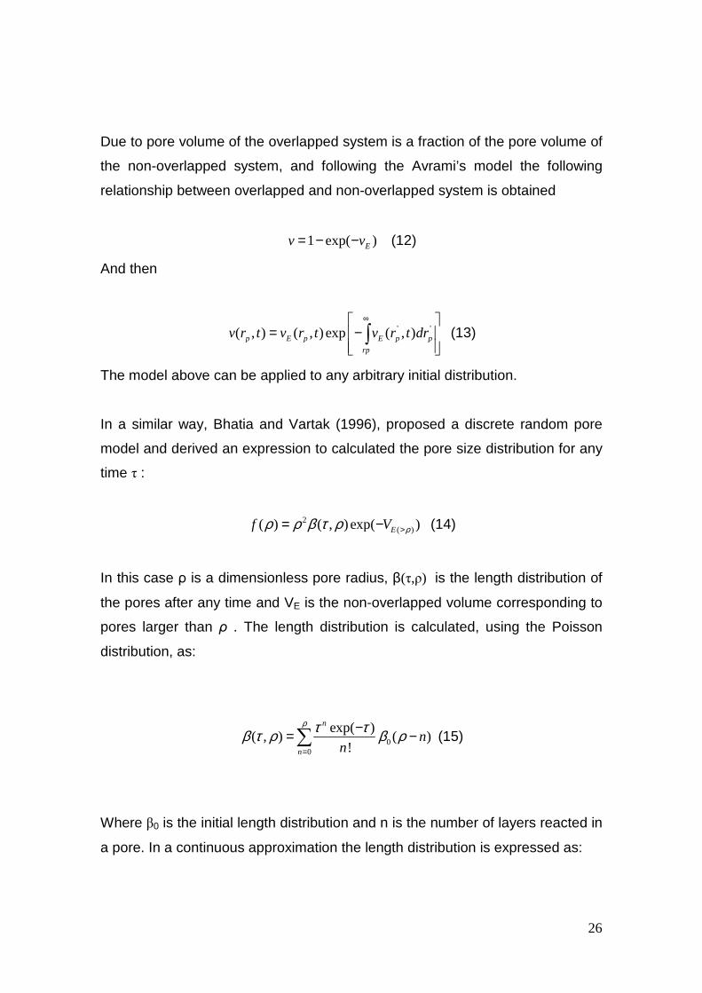
Due to pore volume of the overlapped system is a fraction of the pore volume of

the non-overlapped system, and following the Avrami’s model the following

relationship between overlapped and non-overlapped system is obtained

1 exp( )Ev v= − − (12)

And then

' '( , ) ( , )exp ( , )p E p E p p

rp

v r t v r t v r t dr∞

= − ∫ (13)

The model above can be applied to any arbitrary initial distribution.

In a similar way, Bhatia and Vartak (1996), proposed a discrete random pore

model and derived an expression to calculated the pore size distribution for any

time τ :

2

( )( ) ( , )exp( )Ef V ρρ ρ β τ ρ >= − (14)

In this case ρ is a dimensionless pore radius, β(τ,ρ) is the length distribution of

the pores after any time and VE is the non-overlapped volume corresponding to

pores larger than ρ . The length distribution is calculated, using the Poisson

distribution, as:

00

exp( )( , ) ( )

!

n

n

nn

ρ τ τβ τ ρ β ρ=

−= −∑ (15)

Where β0 is the initial length distribution and n is the number of layers reacted in

a pore. In a continuous approximation the length distribution is expressed as:

27

0 0 0( , ) ( , / ) ( )P dβ τ ρ τ ρ ρ β ρ ρ= ∫ (16)

With 0

00

exp( )( , / )

( 1)P

ρ ρτ ττ ρ ρρ ρ

− −=Γ − +

The form of the initial length distribution is assumed by using different kind of

distributions. Bhatia and Vartak used Rayleigh and log-normal distributions.

Hashimoto and Silveston (1973) proposed a population balance for the change

in the distribution with time due to gas-solid reactions:

0p

p

rff B D

t r t

∂ ∂ ∂+ − + = ∂ ∂ ∂ (17)

In Equation (17) f is a density distribution function, rp is pore radius, t is time, B

is the rate of introduction of new pores of the radius range into the unit volume

at time t and D is the rate of removal of pores through coalescence. Equation

(17) is transformed into moment equations and the moments M0, M1, and M2

are related to local solid properties. The moment equations are combined with a

local mass balance equation for solid in order to obtain an expression for solid

conversion but the form of the pore size distribution is not determined.

These authors proposed the birth of pores as a contribution of two phenomena:

formation of new pores due to an etching phenomenon and formation of pores

due to combination of smaller pores. The expressions proposed are given by

equations (18) and (19) respectively.

( )f f g s p prB k C r rρ δ= − (18)

28

1 1 1

0

1( )

2

rp

p p p

rBc f r f r drφ

α

= −

∫ (19)

Where kf is a specific rate constant for pore initiation, δ is a Dirac delta function

taking a nonzero value only when the pore radius is rf that is the value of the

pore radius of the new micropores that are formed. φ is the probability that

adjacent pores grow sufficiently in the time period dt to come in contact.

1 1( )pp p

rf r f rφ

α

−

accounts for the rate of combination of pores of size rp1 and

rp2 to yield pores of size rp. rp is related with rp1 and rp2 by Equation (20)

( )1 2p p pr r rα= + (20)

where 0.5<α <1.0 with α = 0.5 if rp1≈rp2 and α=1.0 if r1>>r2.

The death term is the rate of combination of pores of radius rp with pores of all

other radii:

1 1

0

( ) ( )p p pD f r f r drφ∞

= ∫ (21)

Simons and Finson (1979) and Simons (1979) based also on a population

balance, derived an expression for the pore volume distribution. These authors

proposed, from empirical facts, that pore radius increases as porosity θ

according to Equation (22) :

1/3

pr θ≈ (22)

29

Two function distributions are proposed. f(rp) that accounts for the number of

pores between rp and rp+drp, and g(rp,Ф) that accounts for the number of pores

in an arbitrary cross section. Both functions are related. The terms for birth and

death represent the change in function g(rp,Ф) due to pore combination but the

birth and death rates are constrained in that the total porosity must be

conserved. The terms for birth and death are given by Equations (23) and (24).

0

min

2 ( , )ln

3p pmg r r d

Br dt

φ θβ

=

(23)

0 max2 ( , )

ln3

p

p

mg r r dD

r dt

φ θβ

=

(24)

where rpmin minimum pore radius, rpmax maximum pore radius, m is a pore shape

factor that takes into account the roughness of the wall of cylindrical pores, θ

porosity and Ф is the angle between pores and an arbitrary cross section. β is a

ratio given by Equation (25):

max

min

(0)ln

(0)

r

rβ

=

(25)

The expression for specific porous volume between rpmin and rp obtained by

Simons is given by Equation(26):

30

( ) ( )min

2 2min 2min max2

ln( / )ln( / ) ln( / )

3

prp p p

p p p

r

v r r mvdv r r r r

εβ

β β = + + − ∫ (26)

Where ε is total porosity and vp the total specific porous volume.

As an attempt to explain evolution, Simons derived an expression for porosity

evolution as a function of pore growing ξg according to Equation (27):

2

2min min

2(0)(0)

(0) 2 (0)g g

p pr r

ξ ξεε εβ

= + +

(27)

The pore growing is not expressed explicitly but is indicated that the change of

pore radius is given by Equation (28) :

( )p po gr r tξ= + (28)

Simons concludes that the pore growth during gasification may be the most

important single parameter in predicting the time evolution of the distribution

function.

Recently, Navarro et al (2007) proposed a model also based on a population

balance for the evolution of the pore size distribution. In their model the rate of

change of the number density function with respect to time and pore size is

given by the Equation(29):

( )' ( , )'( , )0

G n w tn w t

t w

∂∂ + =∂ ∂

(29)

31

Where n’(w,t) is a function proportional to the number density function and is

given by Equation(30):

( , )( , )

f w tn w t

w= (30)

G is the growth rate considered to be constant and independent of the pore

size. These authors applied their model to the activation of a lignite char. The

growth rate is obtained by adjusting to the experimental data. These authors

conclude that other processes, additional to pore growth, should be taken into

account in the model of PSD evolution.

1.4. Maximum Entropy Method

The maximum entropy method (MEM) is an approach that has been used by

different authors to predict probability functions in some processes. This method

was firstly proposed by Jaynes (1957) in his paper “Information theory and

Statistical mechanics” based on the work developed by Shannon (1948) who

stated that the only function able of measuring how uncertain we are of the

outcome of a process, that has a set of events with different probabilities of

occurrence, is the function H defined in Equation (31):

logj jH K p p= − ∑ (31)

where K is a positive constant. In information theory, the function H is a

measure of information, choice and uncertainty. The form of H is the same for

entropy in statistical mechanics. Jaynes took this concept of H from the

information theory and proposed the use of entropy as a tool to infer

distributions in statistical mechanics interpreting entropy as a synonymous of

uncertainty. In this sense, Jaynes affirmed “The great advance provided by

information theory is a unique, unambiguous criterion for the amount of

32

uncertainty represented by a discrete probability distribution, which agrees with

our intuitive notions that a broad distribution represents more uncertainty than

does a sharply peaked one, and satisfies all other conditions which make it

reasonable”. The prediction of the most probable value for a function, that is the

answer to some proposed problem, is based on the determination of the

probability distribution that has the maximum entropy subject to whatever is

known. The information that is known is represented through the constraints of

the problem.

The constraints emerge from the previous knowledge of expected values of

several quantities fr(x), expressed as :

1

( ) ( )n

r i r ii

f x p f x=

=∑ (32)

Another constraint arises from the normalization of the set of probabilities:

1ip =∑ (33)

The interest is to find the probability distribution pi to calculate the expectation

value of a function g(x).

Knowing that mathematical entropy is expressed as:

i iiS K p lnp= − ∑ (34)

And the most probable distribution is that which has maximum entropy;

Equation (34) must be maximized subject to constraints (32) and (33) in order to

get the distribution pi. This is accomplished introducing Lagrangian multipliers

λm, thus:

33

[ ]0 1 1 2 2( ( ) ( ) .... ( ) )i i m m if x f x f xip e λ λ λ λ− + + + += (35)

The constants λm are determined by substituting (35) into (32) and (33)Jaynes

made an extension of the method to make possible the application to

phenomena depending on the time (Jaynes,1957).

The Maximum entropy method has been used for different authors to calculate

density function distributions. Babinsky and Sojka (2002) present a review on

application of different methods for modelling drop size distributions in sprays,

one of these methods is the MEM. Sellens and Brzustowski (cited by Babinsky

and Sojka) were the first to apply the MEM to predict drop size distributions

taking the equations of conservation of mass, conservation of momentum,

conservation of surface energy, conservation of kinetic energy and

normalization as constraints. Although the results that were obtained did not

agree well with the experimental, it was a first step in the application of the

MEM to this kind of problems. Other authors such as Sellens, Li and Tankin

between others cited by Babinsky and Sojka have applied the MEM changing

the formulation of the constraints and the number of constraints that are taking

into account.

Elgarayhi (2002) applied the method of the maximum entropy for the solution of

the aerosol dynamic equation. In this case the function distribution, representing

the number of particles per unit volume, is determined as a function of time. The

function distribution is the solution of the mass conservation, Equation(36):

[ ] [ ]

[ ]

( , , ). ( , , ) ( , , ) . ( , , ) ( , , )

+ ( , , ) ( , , ) ( , , ) ( , , ) ( , , )coag

n r tU r t n r t D r t n r t

tn

I r t n r t R r t n r t S r tt

υ υ υ υ υ

υ υ υ υ υυ

∂ + ∇ − ∇ ∇∂∂ ∂ + = + ∂ ∂

(36)

34

In equation (36) ( , , )υ υn r t d is the distribution function that represents the

number of particles per unit volume in the point r, at time t with particle volume

between υ and υ + dυ . U is the vector sum of the fluid and particle velocities, D

is the Brownian diffusion coefficient, I is the rate of growth of an individual

particle due to evaporation or condensation, R is the removal rate of particles

due to Brownian deposition, gravity and leakage through a hole or crack, S is an

independent source term and [ ]coagn t∂ ∂ denotes the coagulation that is a

function of K(υ, υ) that is a coagulation coefficient for particles of volumes υ and

υ. Elgarayhi used the MEM to solve the particular case in which only

condensation growth rate, removal of particles and coagulation processes are

taken into account. The constraints come from normalization and moments

derived from the mass conservation equation.

The MEM has also been applied to determine particle size distribution of

comminution products (Otwinowski,2006). A balance on the fed material

particles is done. Two constraints are used to solve the system of equations:

normalization and the energy balance of the particles in the comminution

process. John et al (2007) cite the MEM as one of the methods for the

reconstruction of a distribution from its moments where the moments are the

constraints of the problem in the same way as it was used by Elgarayhi (2002).

Other methods are presented in this paper but some of them need a priori

prescribed shape functions or can be applied only to simple problems that

consider only birth or growth. The method of reconstruction of distributions by

splines is also proposed.

In general, the papers mentioned above determine function distributions based

on population balance equations and the maximum entropy is one method used

to solve these equations. Population balances were proposed for chemical

35

engineers purposes by Hulburt and Katz in 1964 (cited by Wynn and

Hounslow,1997). A very general population balance is:

( ).n

nu B Dt

∂ + ∇ = −∂

(37)

where n is a density function distribution, u is the vector of velocities which

includes spatial coordinates and “internal” coordinates such as size and B and

D are terms related to birth and death processes. Hashimoto and Silveston

(1973) proposed a population balance for pore distribution and got expressions

for three moments of the balance: zero, first and second moment. However,

they did not obtain the form of the function; the Maximum Entropy Method can

be applied to the Hashimoto and Silveston equations in order to get the form of

the distribution function (See Chapter 3).

1.5. Conclusions

There are different char-solid reaction models, such as those proposed by

Szekely, Bhatia and Perlmutter, Kantorovich and Bar-Ziv among others. These

models have been applied to gasification reactions and can predict evolution of

surface area in terms of carbon conversion or can be adjusted to experimental

data to obtained kinetic parameters. However there are few models that explain

the evolution of pore size distribution in activation processes. Although the

work of Hashimoto and Silveston in 1973 gave a starting point by proposing a

model to interpret different phenomena that occur throughout the activation

process, it can be said that the problem of calculating and predicting evolution

pore size distributions still exists. Most of the models for predicting evolution of

pore size distribution are mainly based on population balance approach due to

it is being a technique that has been applied with some success to get

36

distribution functions in other processes. The main differences between these

models lie in the way as terms of birth, death and growth of pores are

considered.

37

LIST OF REFERENCES

1. ADSCHIRI T. and FURUSAWA T., “Relation between CO2-reactivity of coal

char and BET surface area” . Fuel, v.65, 1986, p. 927-931.

2. BABINSKY and SOJKA. “Modeling drop size distributions”. Progress in

Energy and Combustion science. Vol. 28. 2002. p.303-329

3. BHATIA S.K. and GUPTA J.S. “Mathematical modelling of gas-solid

reactions: Effect of pore structure”. Reviews in Chem. Eng. v 8. No 3-4.

1992. p.177-258.

4. BHATIA S.K. “Reactivity of chars and carbons: New insights through

molecular modelling”. AIChE Journal. v. 44. No. 11. 1998. p. 2478-2493.

5. BHATIA S.K. and PERLMUTTER D.D. “A random pore model for fluid-solid

reactions: I. isothermal, kinetic control”. AIChE J. v. 26. No 3. 1980. p 379-

386

6. BHATIA S.K. and VARTAK B.J. “Reaction of microporous solids: the

discrete random pore model”. Carbon. v. 34. 1996. p. 1383-1391

7. BORRELLI S. GIORDANO M. and SALATINO P. “Modelling diffusion-limited

gasification of carbons by branching pore models”. Chem. Eng. Journal. v.

64. 1996. p. 77-84

8. CAZORLA-AMORÓS D., ALCAÑIZ-MONGE J., De la CASA-LILLO M.A and

LINARES-SOLANO A. “CO2 as an adsorptive to characterize carbon

molecular sieves and activated carbons”. Langmuir. v. 14. 1998. p.4589-

4596.

38

9. CHEJNE F. et al. “Obtención de carbones a partir de carbones colombianos.

Fase II” Final Report. Minercol, Ingeominas, Univ. Nacional de Colombia.

Univ. Pontificia Bolivariana. 2001. 350 p.

10. CHI W.K. and PERLMUTTER D.D. “The effect of pore structure on the char

steam reaction”. AIChE Journal v. 35. 1989. p. 1791

11. DAVIES G.M and SEATON N.A. “The effect of the choice of pore model on

the characterization of the internal structure of microporous carbons using

pore size distributions”. Carbon. V 36. 1998 p. 1473-1490.

12. ELGARAYHI A. “Solution of the dynamic equation of aerosols by means of

maximum entropy technique”. Journal of Quantitative spectroscopy &

Radiative transfer. Vol. 75. 2002. p.1-11

13. FENG B. and BHATIA S.K. “Variation of pore structure of coal chars during

gasification”. Carbon. V. 41. 2003. p.507-523

14. GAVALAS G. “A random capillary model with application to char gasification

at chemically controlled rates”. AIChE Journal. v 26. No 4. 1980. p. 577-

585.

15. GUPTA J. and BHATIA S. “A modified discrete random pore model allowing

for different initial surface reactivity”. Carbon. v 38. 2000. p. 47-58

16. HASHIMOTO K. and SILVESTON P.L. “Gasification: Part I. Isothermal,

Kinetic Control Model for solid with a pores size distribution”. AIChE J. v. 19.

No 2. 1973. p. 259-268

17. JAYNES E.T. “Information theory and Statistical mechanics”. The Physical

Review. Vol.106, No 4, 1957. p.620-630

39

18. JAYNES E.T. “Information theory and Statistical mechanics. II. The Physical

Review. Vol.108, No 2, 1957. p.171-190.

19. JOHN V. et al. “Techniques for the reconstruction of a distribution from a

finite number of its moments”. Chem. Eng. Sci. v. 62. 2007. p.2890-2904.

20. KANTOROVICH I. and BAR-ZIV E. “Processes in highly porous chars under

kinetically controlled conditions: I. Evolution of the porous structure”. Comb.

and Flame. 97. 1994. p.61-78

21. LASTOSKIE C. GUBBINS K and QUIRKE N. “Pore Size Distribution

Analysis of Microporous Carbons: A Density Functional Theory Approach”.

J. Phys.Chem. V. 97. 1993. p. 4789-4796.

22. LIZZIO A.A, PIOTROWSKI A. and RADOVIC L.R. “Effect of oxygen

chemisorption on char gasification reactivity profiles obtained by

thermogravimetric analyses”. Fuel. v. 67 1988. p. 1691-1695.

23. LOWELL, S. SHIELDS, J. THOMAS, M. and THOMMES M.

Characterization of porous solids and powders: surface area, pore size and

density. Springer, 1st reprint , 2006. 347 p.

24. LU G.Q and DO D.D. “Comparison of structural models for high-ash char

gasification”. Carbon. v.32 .1994. p.247-263

25. MIURA K. and HASHIMOTO K. “A model representing the change of pore

structure during the activation of carbonaceous materials”. Ind. Eng. Chem.

Process Des. Dev. 1984. P. 138-145.

40

26. NAVARRO M.V, SEATON N.A., MASTRAL A.M. and MURILLO R.

“Assessment of the development of the pore size distribution during carbon

activation: a population balance approach”. Studies in surface science and

catalysis, 160. 2007. p. 551-558.

27. OTWINOWSKI H. “Energy and population balances in comminution process

modelling based on the informational entropy”. Powder Techn. V. 167.

2006. p 33-44.

28. PETERSEN E.E. “Reaction of porous solids”. AIChE J. v 3. 1957. p.443-448

29. REYES S. and JENSEN K.F. “Percolation concepts in modelling of gas-

solid reactions- I. Application to char gasification in the kinetic regime”.

Chem. Eng. Sci. v. 41. No 2. 1986. p. 333-343

30. ROBAU-SANCHEZ A. AGUILAR-ELGUEZABAL A., DE LA TORRE-SAENZ

L., and LARDIZABAL-GUTIERREZ D. “Radial distribution of porosity in

spherical activated carbon particles”. Carbon. v 41. 2003. p.693-698.

31. SAHIMI M. and TSOTSIS T. “Statistical modelling of gas solid reaction with

pore volume growth: kinetic regime”. Chem. Eng. Sci. v. 43. No 1.1988 p.

113-121

32. SAHIMI M., GAVALAS G. and TSOTSIS T. “Statistical and continuum

models of fluid-solid reactions in porous media”. Chemical Engineering

Science. v. 45. 1990. p. 1443-1502

33. SHAH N. and OTTINO J.M. “Transport and reaction in evolving, disordered

composites-I. Gasification of porous solids”. Chem. Eng. Sci. v. 42. No 1.

1987. p. 63-72

41

34. SHANNON C.E. “A mathematical theory of information”. Reprinted with

corrections from The Bell System technical journal. Vol. 27. 1948. p.379-

423, 623-656

35. SIMONS G.A and FINSON M.L. “The structure of coal char: Part I. Pore

branching”. Combustion Science Technology. v.19. 1979. p. 217-225

36. SIMONS G.A. “The structure of coal char: Part II. Pore combination”.

Combustion Science Technology. v.19. 1979. p. 227-235

37. SU J.L. and PERLMUTTER D.D. “Evolution of pore volume distribution

during gasification”. AIChE J. v. 30. No 6. 1984. p.967-973

38. SZEKELY J. and EVANS J.W. “A structural model for gas-solid reactions

with a moving boundary”. Chem. Eng. Sci. v. 25. 1970. p. 1091-1107.

39. WYNN E.J.W and HOUNSLOW M.J. “Integral balance population equations

for growth”. Chem. Eng. Sci. v. 52. 1997. p. 733-746.

42

CHAPTER TWO

EXPERIMENTAL PORE SIZE DISTRIBUTION

With the aim of studying the evolution of pore size distribution during the

activation process, some experiments were carried out. Three coals from

Amagá-Titiribí region in Antioquia (Colombia) were activated with CO2 at 850°C

in a fixed bed reactor. The coals are identified as La Capotera, La Grande and

El Sol. The temperature was selected based on a previous work done by

Chejne et al (2001) where different Colombian coals were activated with CO2 at

different temperatures and it was found that the most of coals showed the

higher porosity development at 850°C.

2.1. Materials and Procedure

In Table 1 the proximate and ultimate analysis of the coals are shown. The

coals are of different rank. La Capotera is the coal of lowest rank, has the

highest moisture content and the lowest fixed carbon content whereas El Sol is

the coal of highest rank and has the highest fixed carbon content and the lowest

moisture and volatile matter contents. Due to its different rank and different

composition, it is expected that these coals have different behavior during

gasification.

43

Table 1. Analysis of coals

Coal Ultimate analysis Proximate analysis

C 58.9 (%) Moisture 13.8 (%)

H 5.59 (%) Ash 7.6 (%)

N 1.23 (%) Volatile Matter 34.4 (%)

O 24.7 (%) Fixed Carbon 44.2 (%)

La Capotera

S 1.99 (%) ASTM clasif. Subbituminous B

C 68.2 (%) Moisture 4.5 (%)

H 5.18 (%) Ash 6.5 (%)


O 18.14 (%) Fixed Carbon 47.0 (%)

La Grande(1)

S 0.56 (%) ASTM clasif. Bituminous High

Volatile C

C 82.03 (%) Moisture 1.4 (%)

H 3.84 (%) Ash 7.4 (%)


O 4.19 (%) Fixed Carbon 76.2 (%)

El Sol

S 0.81 (%) ASTM clasif. Bituminous Low

Volatile

(1) This coal had to be oxidized due to it showed a trend to agglomerate. Analysis

correspond to oxidized coal

Before activation, all samples were devolatililized during 1 hour in inert

atmosphere (N2, 99.5% purity) at 850°C in fixed bed. After devol atililization the

N2 flow was changed by CO2 flow. (CO2 99.5% purity). The devolatililized

samples were activated at 850°C during different re action time in order to get

different carbon conversion degree (batch process). In Figure 1 is shown a

diagram of the equipment used.

44

Figure 1. Diagram of fixed bed reactor The equipment is a vertical tubular furnace, inner diameter 2.5 cm, heated by

electrical resistances. Sample was put on a steel mesh. The particle size was

between sieves +30/-60. CO2 flow was 0.6 l/min and N2 flow was 0.3 l/min.

These flows were selected after some experiments with different flows in which

flow was varied to avoid fluidization. Initial coal sample weight, before

devolatilization, was 15.0 gr. For each coal different activated samples with

different carbon conversion degree were obtained. Conversion was obtained

according to Equation (38):

0

0(1 )f

ash

w wX

w f

−=

− (38)

Where X is carbon conversion, w0 is the initial sample weight, wf is the final

sample weight, fash is the fraction of ash in the initial sample.

Surface area and pore volume of all samples were characterized by CO2 and N2

adsorption isotherms at 273K and 77K. These isotherms were obtained using a

NOVA3200 Quantachrome analyzer.

Surface area was obtained by the Brunauer-Emmett-Teller (BET) method. This

method is based on the assumption that multilayer adsorption occurs on an

N2

CO2

FlowmeterGas flue

sampleBy-pass

Temperaturecontrol

850

N2

CO2

FlowmeterGas flue

sampleBy-pass

Temperaturecontrol

850

45

array of surface sites of uniform energy, molecules in the first layer act as sites

for molecules in the second and higher layers. The upper layer is equilibrium

with the vapor then the rates of adsorption and desorption are equal. Based on

these assumptions the BET equation (39) is obtained :

0 0

1 1

( ) m m

P C P

n P P n C n C P

−= +−

(39)

Where n and nm are the number of molecules in the incomplete and complete

monolayer, respectively. C is a constant that is related to the heat of first layer

adsorption. According to Equation(39), the plot P/n(P0-P) versus P/P0 should be

linear and from the slope and intercept it is possible to calculated the surface

area. In many cases the range of linearity extends over P/P0 ≈ 0.05-0.3 but with

graphitized and microporous carbons linear BET plots are given only at P/P0

<0.1 (Patrick,1995).

Although Nitrogen at 77K is the most used adsorptive for micropore analysis of

microporous materials, its performance for ultramicropore (pore widths<0.7nm)

analysis is not satisfactory. This is due to diffusion problems caused by the low

energy that nitrogen molecules have at 77K, and then nitrogen molecules can

not pass energetic barriers of narrow pores. Argon and CO2 are alternative

adsorptives to ultramicropore analysis. Argon at 87K fills micropores of

dimensions 0.4nm-0.8nm. CO2 adsorption at 273,15K can eliminate diffusion

problems but due to CO2 saturation pressure is high at 273,15K when the

analysis is carried out in a conventional sorption analyzer, such as the case of

the NOVA3200, the measurable pore size range is limited to pore sizes up to

1.5 nm (Lowell et al, 2006).

Pore size distributions were calculated by Density Functional Theory Method

(DFT) where, as it was mentioned in Chapter 1, the pore size distribution is

obtained by solving the adsorption integral equation:

46

0

N(p) ( ) ( , )f w p w dwρ∞

= ∫

Here f(w) is the pore size distribution, N(p) is the experimental isotherm and

ρ(p,w) is the adsorption isotherm obtained theoretically through minimization of

the grand potential functional Ω. For a fluid in the presence of a spatially varying

external potential Vext(r), the grand potential functional can be written as

(Lastoskie et al,1993) :

[ ] [ ] [ ]( ) ( ) ( ) ( )L L L extr F r dr r V rρ ρ ρ µΩ = − −∫ (40)

Here F is the intrinsic Helmholtz free energy functional, ρL is the local fluid

density at position r and µ is the chemical potential. The different terms of

Equation (40) are derived from the assumption that each pore is represented as

two semi-infinite parallel graphitic slabs separated by a physical width w, the

distance between the centers of the surface carbon atoms. The interaction fluid-

fluid is calculated by the Lennard-Jones 12-6 potential and the interaction solid-

fluid by the Steele 10-4-3 potential. The fitting parameters in these potentials

are obtained from experimental observations. The external potential is due to

interactions solid-fluid. The intrinsic Helmholtz energy is formed by the

contribution of the hard sphere Helmholtz free energy functional, the pair

distribution function and the attractive portion of the fluid-fluid potential.

The equilibrium density profile is obtained from minimization of the grand

potential with respect to density:

[ ],

( )0

( )L L

L

L

r

rρ ρ

δ ρδρ

∞=

Ω=

47

The mean pore fluid density ρ is calculated according to:

0

1( )

w

L z dzw

ρ ρ= ∫

The Quantachrome® software Autosorb® 1 for windows 1.20 was used to get

the DFT pore size distributions. The software has different kernels to calculated

PSD; in this work the CO2_nldf.gai and the N2_carb.gai kernels were used.

2.2. Results

The behavior of carbon conversion of the different chars versus time is shown in

Figure 2. The reactivity can be calculated using the unreacted shrinking core

model that is one of the most applied models to char gasification (Kwon et al,

1988, Osafune and Marsh 1988, Shufen and Ruizheng 1994, ,Ye et al 1998)

and shows a good fitting to experimental data. This model assumes that

gaseous reactants diffuse through a gas film surrounding the particles, then

diffuse through the ash layer and react on the reacted core surface. As the

reaction progresses, the unreacted core keeps shrinking. In the unreacted

shrinking core model the carbon conversion with time is described as:

1/31 (1 )− − =X Kt

Where X is the carbon conversion at time t and K is an apparent rate constant.

Another kinetic model that is commonly used for describing gasification is the

homogenous or volumetric model that assumes that the carbon gas reactions

occur at active sites distributed uniformly throughout the whole particle.(Ye et al,

1998). In the volumetric model the carbon conversion with time is described as:

(1 )Ln X Kt− − =

In Figures 3 and 4, the plots 1-(1-X)1/3 against time and Ln(1-X) versus time for

each coal char, are shown. It can be observed that experimental data exhibit

48

best fitting to the unreacted shrinking core model. According to this model, it

can be seen that La Capotera char, the parent coal of lowest rank, exhibits the

higher reactivity (K=3.2e-3 1/min) and El Sol char, the parent coal of higher

rank, exhibits the lower reactivity (K=3.0e-4 1/min). Although coal rank is not

always an adequate parameter to predict the reactivity of coal char, some works

have found that the reactivity of char generally increases with a decrease in the

rank of the parent coal (Kabe et al, 2004).

0

10

20

30

40

50

60

70

80

90

100

0 200 400 600 800 1000

Time [min]

Con

vers

ion

[%]

La Capotera La Grande El Sol

Figure 2. Carbon conversion versus time at 850°C.

49

y = 0.0032x - 0.0128

R2 = 0.9962

y = 0.0008x + 0.0245

R2 = 0.9719

y = 0.0003x + 0.0007

R2 = 0.9707

0.00

0.10

0.20

0.30

0.40

0.50

0 200 400 600 800 1000

Time [min]

1-(1

-X)1

/3


Figure 3. Carbon conversion function versus time. U nreacted shrinking Core Model

y = 0.0131x - 0.1279

R2 = 0.9862

y = 0.0028x + 0.0515

R2 = 0.9754

y = 0.001x - 0.0168

R2 = 0.9571

0.00

0.40

0.80

1.20

1.60

2.00

0 200 400 600 800 1000

Time [min]

-LN

(1-X

)


Figure 4. Carbon conversion function versus time. Volumetric Model

50

Studies carried out by methods such as Nuclear Magnetic Resonance (NMR)

have shown that the aromaticity, that is an index of the number of aromatic ring

in coal, increases as the coal rank increase. The graphite, which is constituted

completely by aromatic rings, has an aromaticity equal to 1.0 (Kabe et al, 2004).

These aromatic structures present less active site. El Sol coal is the coal with

the higher rank showed the lower reactivity. Reactivity is also related with the

content of amorphous carbon that refers to any non-aromatic carbon. Lu et al,

2002, suggested that amorphous carbon concentration is one of the strongest

indicators of char reactivity with higher amorphous concentration most likely

indicating a better reactivity. Lu et al ,2001 showed , as it was known, that

there is a strong linear relationship between amorphous carbon concentration

and volatile matter, increasing the amorphous carbon as the volatile matter

increases. The results agreed with this affirmation, the reactivity index

increased as the volatile matter content increased in the parent coal: La

Capotera > La Grande > El Sol.

The pore size distributions for the different samples calculated by DFT analysis,

using the software supplied by Quantachrome®, for CO2 and N2 isotherms are

shown for La Capotera, El Sol and La Grande chars. For CO2 isotherm the

CO2_nldf.gai kernel file was chosen. For N2 isotherm the N2_carb.gai kernel file

was chosen. In Figures 3-5, the pore size distributions calculated from CO2

isotherms are compared for the different chars at different conversion degree.

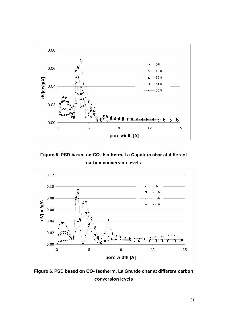
51

0.00

0.02

0.04

0.06

0.08

3 6 9 12 15

pore width [A]

dV[c

c/g/

A]

0%

19%

35%

61%

85%

Figure 5. PSD based on CO 2 Isotherm. La Capotera char at different

carbon conversion levels

0.00

0.02

0.04

0.06

0.08

0.10

0.12

3 6 9 12 15

pore width [A]

dV[c

c/g/

A]

0%

29%

55%

72%

Figure 6. PSD based on CO 2 Isotherm. La Grande char at different carbon

conversion levels

52

0.00

0.01

0.02

0.03

0.04

0.05

3 6 9 12 15

pore width [A]

dV[c

c/g/

A]

0%

16%

34%

63%

Figure 7. PSD based on CO 2 Isotherm. El Sol char at different carbon

conversion levels

In Figure 5, La Capotera char, it can be seen that 0% burn-off there are two

peaks at 5.2 and 6.3Ǻ after the devolatilization process. At the following

conversion degrees there is a peak around 3.6Ǻ that could be attributed to

formation of new pores due to the chemical reactions. This peak initially

increases as the carbon conversion increases but at carbon conversion 61%

this peak decreases indicating that the phenomenon of formation of new pores

does not have an important contribution at this stage of the activation process.

Also, it can be seen that the values of the function distribution for pore width

between 5 and 6Å increases as carbon conversion increases but it decreases at

carbon conversion 61%. This behavior could be attributed to pore enlargement

and/or pore combination. Then, according to these experimental results, it can

be establish an important contribution of the formation of new small pores (3.6

Å, 5-6 Å) up to around 35% carbon conversion. At 61% carbon conversion and

after, formation of new pores is not important and prevalence the pore

enlargement.

53

In Figure 6, La Grande char, at 0%, two low peaks at 5 and 6 Ǻ are formed as

consequence of devolatilization. At 29% three peaks at 3.6, 5 and 5.7Ǻ are

presented that could be attributed to formation of new pores and pore

enlargement and/or pore combination. Also there is a low peak at 7.5Ǻ. At 72%

the peaks are almost at the same positions, but the peaks on the larger pore

widths, that is 5.7 and 7.5Ǻ, are higher than the peaks at smaller pore widths.

This behavior could be interpreted as a prevalence of pore enlargement and/or

pore combination. As in the case of La Capotera Char, experimental data

indicate an important contribution of the formation of new pores up to carbon

conversion around 30% and after that a possible prevalence of pore

enlargement phenomenon.

In Figure 7, El Sol char at 0% burn-off shows little pore development. There are

peaks at 3.8Å, 5-6Å and 7.8Å. At higher burn-off, 29%, the peaks are on the

same positions and are higher that could indicate formation of new pores and

pore enlargement. At 63% the peaks still keep on the same pore widths but the

peak at 3.8Å is lower and the peaks at 5.7Å and 7.8Å are higher, this behavior

could indicate prevalence of pore enlargement.

The N2 adsorption isotherms for La Capotera, La Grande and El Sol chars at

different burn-off are shown in Figures 8-10. The shape of the isotherms can

give information about the type of porosity that has been developed (Linares-

Solano et al, 2000, Carrasco-Marin et al, 1996). In Figure 8, La Capotera char,

since 19% burn-off and higher percentages of burn-off, isotherms show wide

knees that indicate a wide micropore distribution and a light slope for higher

relative pressures values, indicating widening of the micropores into

mesopores.

In Figure 9, La Grande char, isotherms up to 29% burn-off are rectangular,

indicating microporous character with narrow microporosity. At higher

54

percentages of burn-off, the knee becomes broader, which indicates the

presence of wider micropores and a wide micropore distribution. In Figure 10, El

Sol char, the isotherms are highly rectangular indicating that the activated

carbons are microporous with very narrow microporosity. Isotherm for 63%

carbon conversion shows a small increase of the knee that suggests the

development of wider micropores.

0

40

80

120

160

0.0 0.2 0.4 0.6 0.8 1.0

P/P0

VN

2 [cc

ST

P/g

]

0% 19% 35% 61% 85%

Figure 8. N 2 adsorption isotherms for La Capotera char at diffe rent burn-off levels

55

0

100

200

300

400

0.0 0.2 0.4 0.6 0.8 1.0

P/P0

VN

2 [cc

ST

P/g

]

0% 29% 55% 72%

Figure 9. N 2 adsorption isotherms for La Grande char at differe nt burn-off levels

0

20

40

60

80

100

0.0 0.2 0.4 0.6 0.8 1.0

P/P0

VN

2 [cc

ST

P/g

]

9% 16% 34% 63%

Figure 10. N 2 adsorption isotherms for El Sol char at different burn-off levels

56

In Figures 11-13, the pore size distributions obtained from N2 isotherms for the

activated carbons obtained from the three coals are presented. In Figure 11, La

Capotera char, 0% burn-off, there are pores of different pore width although the

maximum value of the pore size distribution corresponds to 4Ǻ. As conversion

increases, the maximum value of the pore size distribution keeps on 4Ǻ but this

maximum value increased. However a high conversion degree this maximum

value decreases although it still keeps at the same pore width. Also it can be

seen that since the first stages of activation, a peak around 20Ǻ is presented. A

possible explanation for this behavior is that at the first stages of activation,

there is a predominance of the phenomenon of formation of new pores but also

the phenomenon of pore enlargement occurs. A high conversion degree, there

is a prevalence of pore enlargement or pore combination phenomena but still

the formation of new pores is important.

0.000

0.005

0.010

0.015

0.020

0 10 20 30 40 50 60

Pore width [A]

dV [c

c/g/

A]

0%

19%

35%

61%

85%

Figure 11. PSD based on N 2 Isotherm. La Capotera char at different carbon conversion levels

57

0.00

0.01

0.02

0.03

0.04

0.05

0 10 20 30 40 50 60

pore width [A]

dV [c

c/g/

A]

0%

29%

55%

72%

Figure 12. PSD based on N 2 Isotherm. La Grande char at different carbon conversion levels

0.000

0.003

0.006

0.009

0.012

0.015

0.018

0.021

0 10 20 30 40 50 60

pore width [A]

dV [c

c/g/

A]

9%

16%

34%

63%

Figure 13. PSD based on N2 Isotherm. El Sol char at different carbon conversion levels

58

In Figure 12, La Grande char, it can be seen that at low carbon conversion

there is a prevalence of formation of new pores. There is a maximum value of

the pore size distribution around 4Ǻ. However at higher carbon conversion the

maximum value of the pore size distribution is displaced to larger pore sizes,

around 11Ǻ, that could be interpreted as a prevalence of the pore enlargement

phenomenon over the formation of new pores. It can be seen that the value of

pore size distribution on small pore widths is low that could be interpreted as a

not significant contribution of formation of new pores.

In Figure 13, El Sol Char, the maximum value of pore size distribution increases

as carbon conversion increases and it keeps on the same pore size. The

contribution of the larger pores to the distribution is smaller compare to the

smaller pores. This behavior is in accordance with the microporous character

deduced from the shape of the isotherms. This behavior could be interpreted as

there is always an important contribution of the formation of new pores over the

pore enlargement and/or pore combination.

As a conclusion, experimental results of the PSD for the three chars could be

depicted in the way as it is shown in Figure 14.

Low carbon conversion. Prevalence of the formation of new pores

Intermediate carbon conversion. Both phenomena:the formation of new pores and pore enlargement are important

High Carbon Conversion. Prevalence of pore enlargement even though the formation of new pores still occurs

Figure 14 . Pore size evolution throughout activati on.

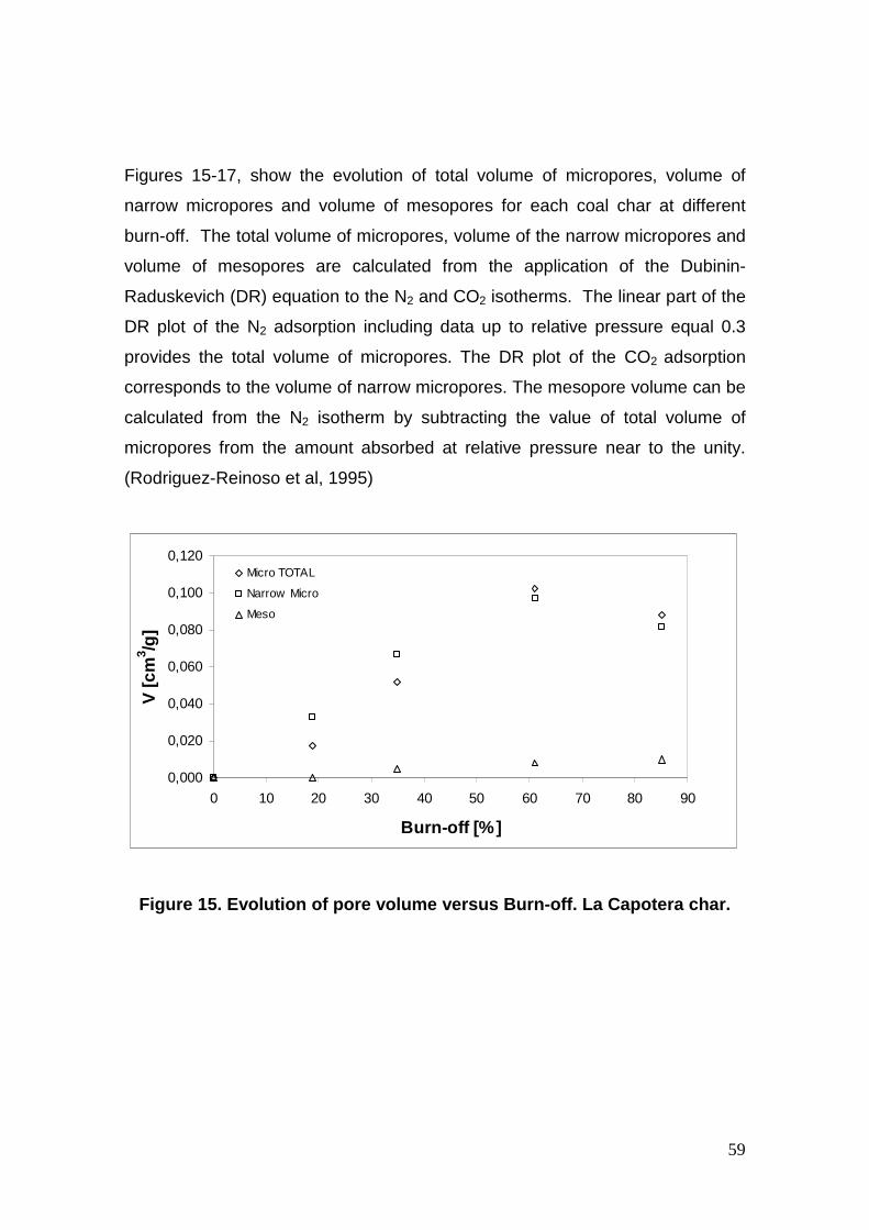
59

Figures 15-17, show the evolution of total volume of micropores, volume of

narrow micropores and volume of mesopores for each coal char at different

burn-off. The total volume of micropores, volume of the narrow micropores and

volume of mesopores are calculated from the application of the Dubinin-

Raduskevich (DR) equation to the N2 and CO2 isotherms. The linear part of the

DR plot of the N2 adsorption including data up to relative pressure equal 0.3

provides the total volume of micropores. The DR plot of the CO2 adsorption

corresponds to the volume of narrow micropores. The mesopore volume can be

calculated from the N2 isotherm by subtracting the value of total volume of

micropores from the amount absorbed at relative pressure near to the unity.

(Rodriguez-Reinoso et al, 1995)

0,000

0,020

0,040

0,060

0,080

0,100

0,120

0 10 20 30 40 50 60 70 80 90

Burn-off [%]

V [c

m3 /g

]

Micro TOTAL

Narrow Micro

Meso

Figure 15. Evolution of pore volume versus Burn-off . La Capotera char.

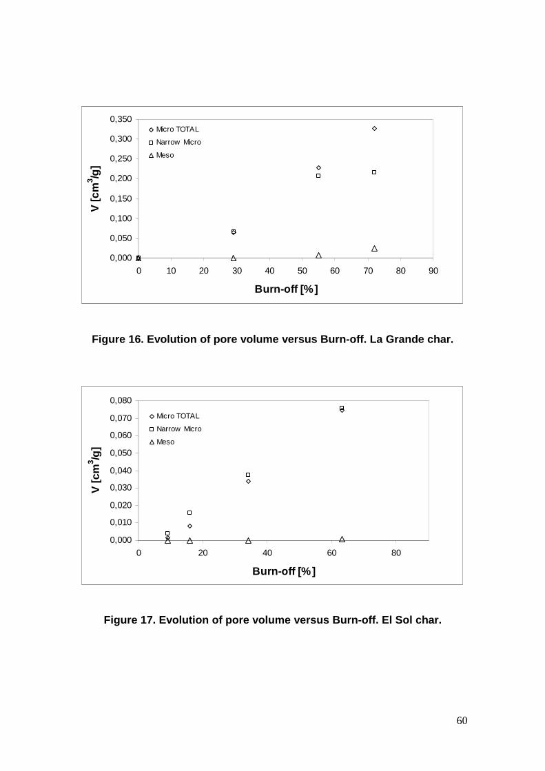
60

0,000

0,050

0,100

0,150

0,200

0,250

0,300

0,350

0 10 20 30 40 50 60 70 80 90

Burn-off [%]

V [c

m3 /g

]

Micro TOTAL

Narrow Micro

Meso

Figure 16. Evolution of pore volume versus Burn-off . La Grande char.

0,000

0,010

0,020

0,030

0,040

0,050

0,060

0,070

0,080

0 20 40 60 80

Burn-off [%]

V [c

m3 /g

]

Micro TOTAL

Narrow Micro

Meso

Figure 17. Evolution of pore volume versus Burn-off . El Sol char.

61

In Figure 15, La Capotera char, the evolution of the total micropore volume and

the narrow microporosity show similar trend. There is development of both type

of porosity up to 60% burn-off and the volume of micropores and narrow

micropores tend to decreases. Also, it should be noted that the development of

mesopores begins since earlier stages of the activation, around 30% burn-off.

After the microporosity and narrow microporosity decrease, the mesoporosity

tends to increase even more. This behavior indicates the presence of pore

enlargement or pore combination phenomenon since early stages of the

activation, and a predominance of this phenomenon a the latest stage of the

activation.

In Figure 16, La Grande char, there is a continuous increasing of the total

volume of micropores throughout of the activation process that was done (up to

72% burn-off). The volume of narrow microporosity increases up to 55% burn-

off but then it keeps almost constant. At this stage, the volume of mesopores

shows an increase. This behavior can be attributed to pore enlargement

In Figure 17, El Sol char, the volume of narrow microporosity is always

increasing. At the highest carbon conversion, 63%, is not observed a

significant volume of micropores although the isotherm for this conversion

(Figure 10) shows a slight broadening of the knee indicating an incipient

occurrence of wider micropores.

According to the above results the evolution of the pore size distribution has

different behavior depending on the characteristics of the activated material and

different phenomena are present at the different stages of the activation

process. A material with high reactivity, such as La Capotera, shows since the

first stages of activation the phenomena of formation of new pores and pore

enlargement. This behavior leads to the presence of pore of different widths,

since small pores, around 4Ǻ, to larger pores around 20Ǻ. A material with low

reactivity, such as El Sol, shows prevalence of development of small pores

62

throughout the activation. A material with an intermediate reactivity such as La

Grande exhibits a prevalence of formation of new pores in the first stages of

activation and a prevalence of pore enlargement through high carbon

conversions. This behavior could allow producing an activated carbon with

prevalence of small pores at low carbon conversion and an activated carbon

with prevalence of larger pores at higher carbon conversion.

Franklin (1951) in a study on crystallite growth in carbons, classified carbons in

two main groups: non-graphitic and graphitic carbons. Non-graphitic carbons

are those carbons that during thermal treatment show the graphite-like layers in

parallel groups but not orientated as the crystalline structure of graphite. In

Graphitic carbons the graphite-like layers show a tendency to become mutually

orientated as in crystalline graphite. Non-graphitic carbons are divided in two

groups: Non-graphitizing and graphitizing carbons. The graphitizing carbons

can be converted into graphitic carbons by heat treatment whereas non-

graphitizing carbons can not be transformed into a graphitic carbon solely by

heat treatment. Oxygen-rich low-rank coals belong to non-graphitizing carbons

whereas coking coals belong to graphitizing carbons. Franklin also explained

the formation of fine pores, during carbonization, as due to the rigid cross-

linking of neighboring nuclei of carbon. The formation of a strongly cross-linked,

open-structured, non-graphitizing carbon is favored by the presence of oxygen

or by a shortage of hydrogen in the raw material. La Capotera coal has the

highest oxygen content whereas El Sol coal has the lowest oxygen content;

then El Sol Coal could tend to show graphite like structure than the other

carbons.

2.3. SEM micrographs.

Scanning Electron Microscope (SEM) is a technique that has been used to

observe the porosity development of activated carbons. (Gergova and Eser,

1996, Teng et al, 1997, Sharma et al,2001) . It is used as a qualitative method

63

and not as a quantitative method. This is due to its resolution does not permit to

see microporosity. In order to observe the porosity development some SEM

micrographs of activated samples from La Grande, La Capotera and El Sol

coals were taken. Due to activated carbons have low electrical conductivity;

gold dust had to be used to increase electrical conductivity and to make

possible the observation through SEM. A JEOL-JSM 5910LV model was used

to take the micrographs. These micrographs are shown in Figures 18-20.

Carbon conversion 19%.


Carbon conversion 61%. Carbon conversion 85%.

Figure 18. SEM micrographs. La Capotera char at different carb on conversion levels.

64




Figure 19. SEM micrographs. La Grande char at different carbon conversion levels.

65




Figure 20. SEM micrographs. El Sol char at differe nt carbon conversion levels.

In the case of La Capotera char, Figure 18, a very roughness surface can be

observed since the first stages of activation. This coal showed the higher

reactivity and the development of roughness surface can be attributed to this

high reactivity.

For La Grande char, Figure 19, it can be seen that devolatilized coal, 0%

carbon conversion, shows some roughness surface and there are presented

some large pores. As carbon conversion increases the amount of larger pores

66

also increases. At 72% carbon conversion a totally attacked surface can be

seen.

In Figure 20, El Sol char, shows the more smoothness surface at the first

stages of the activation. This behavior is in agreement with the lower reactivity

of this coal and the slow variation of the development of the porosity as it could

be seen in the PSDs.

2.4. Pore size distribution evolution in the litera ture.

Many papers report pore size evolution. Feng and Bhatia (2003) showed pore

volume evolution of Yarrabee (a semianthracite coal) coal chars gasified to

various conversions in air at 653K, determined from argon adsorption isotherms

obtained at 87K. At the first stages of gasification a peak below 10Å is formed

and increases as conversion increases up to 15%, after this conversion this

peak decreases. Above 10Å other peaks are presented and they increases as

carbon conversion increases. The authors explain this behavior as due to the

fact that the gasification reactions occurs predominantly in the larger pores (>10

Å).

Navarro et al (2006) in their paper on the analysis of the evolution of the pore

size distribution and the pore network connectivity of a porous carbon during

activation, present the evolution of PSD obtained from lignite chars activated

with CO2 at different burn-off degree. As it is indicated by these authors, the

PSDs obtained from nitrogen adsorption, the activation seems to be focused on

three main pore-size regions around 7, 12 and 15Å. They also point out that the

smallest pores are mainly produced at the beginning of the activation process

and disappear later; hence this peak appears in the first activated sample with

17% burn-off and decreases continuously afterwards. The other two regions of

the PSD also have a maximum in the mean pore size as a function of burn-off

67

but for a different degree of activation. For the region around 12Å, the maximum

is reached with a burn-off of 40% and the maximum for the third peak is

obtained by the sample with 60% burn-off. The authors indicate that one

possible explanation for this behavior is a linear growth of the pores but

according to a theoretical work previously developed by these authors, this

phenomenon can not be the only process involved in the pore evolution and

other processes should also be considered.

Junpirom et al (2005) developed a carbon activation model and it was applied to

longan seed char gasification. The model assumes that the char is composed of

bundles of graphite-like layers and the porosity is created via the consumption

of carbon by the gasification reaction. Their model can predict pore volume

evolution and information to calculate PSD. After applied this model to Logan

seed activated with CO2 and from N2 adsorption isotherms the authors present

PSDs for activated chars with different burn-off. According to the analysis of the

authors, they describe three stages in the pore development. First stage

(creation stage) only fine pores are evolved and the volume increases as the

pore width remains constant. This stage is for burn-off less than 5%. In the

second stages, burn-off between 5-60%, fine pores are continually created and

there is the onset of the medium pores. The main mechanism in this period is

the increase in the length of each pore resulting in larger volume but the pore

size remains fairly constant. In the third stage, burn-off higher than 60%, the

volume of fine pores decreases but the medium and large pores continue to

evolve at expenses of fine pores. In this stage two processes are possible, the

coalescence of smaller pores to form larger pores and the collapse of pores due

to the complete removal of the pore walls of some pores.

2.5. Conclusions

The evolution of pore size distribution throughout activation is different for each

material but in general the phenomena of formation of new pores (fine pores)

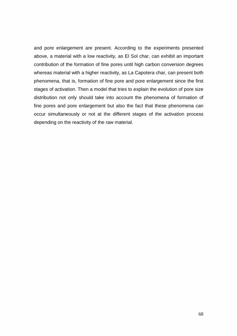
68

and pore enlargement are present. According to the experiments presented

above, a material with a low reactivity, as El Sol char, can exhibit an important

contribution of the formation of fine pores until high carbon conversion degrees

whereas material with a higher reactivity, as La Capotera char, can present both

phenomena, that is, formation of fine pore and pore enlargement since the first

stages of activation. Then a model that tries to explain the evolution of pore size

distribution not only should take into account the phenomena of formation of

fine pores and pore enlargement but also the fact that these phenomena can

occur simultaneously or not at the different stages of the activation process

depending on the reactivity of the raw material.

69

LIST OF REFERENCES

1. CHEJNE F. et al. “Obtención de carbones a partir de carbones colombianos.

Fase II” Final Report. Minercol, Ingeominas, Univ. Nacional de Colombia.

Univ. Pontificia Bolivariana. 2001. 350 p.

2. CARRASCO-MARÍN F., ALVAREZ-MERINO M.A., MORENO-CASTILLA C.

”Microporous activated carbons from a bituminous coal”. Fuel v. 75. 1996.

p.966-970

3. FRANKLIN R. “Crystallite growth in graphitizing and non-graphitizing

carbons” . Proc. Royal Society of London. Series A, Mathematical and

Physical sciences. v 209. 1951. p. 196-218

4. FENG B. and BHATIA S.K. “Variation of the pore structure of coal chars

during gasification”. Carbon. v 41. 2003. p.507-523.

5. GERGOVA K. and ESER S. “Effects of activation method on the pore

structure of activated carbons from apricot stones”. Carbon. v 34. 1996.

p.879-888.

6. JUNPIROM S., DO D.D., TANGSATHITKULCHAI C. and

TANGSATHITKULCHAI M. “A carbon activation model with application to

longan seed char gasification”. Carbon. V 43. 2005. p.1936-1943.

7. KABE T., ISHIARA A., QIAN E.W., SUTRISNA I.P., and KABE Y. “COAL

AND COAL-RELATED COMPOUNDS Structures, Reactivity and Catalytic

reactions”. Tokyo, Elsevier. 2004. 341 p.

70

8. KWON T., KIM S.D., and FUNG D. “Reaction kinetics of char-CO2

gasification”. Fuel. V 67. 1988. p 530-535.

9. LASTOSKIE C. GUBBINS K and QUIRKE N. “Pore Size Distribution

Analysis of Microporous Carbons: A Density Functional Theory Approach”.

J. Phys.Chem. V. 97. 1993. p. 4789-4796.

10. LINARES-SOLANO A., MARTIN-GULLÓN I., SALINAS-MARTINEZ DE

LECEA C., SERRANO-TALAVERA B. “Activated carbons from bituminous

coal: effect of mineral matter content “. Fuel v. 79. 2000. p 635-643

11. LOWELL, S. SHIELDS, J. THOMAS, M. and THOMMES M.

Characterization of porous solids and powders: surface area, pore size and

density. Springer, 1st reprint , 2006. 347 p.

12. LU L., SAHAJWALL V., KONG C., HARRIS D. “Quantitative X-ray

diffraction analysis and its application to various coals”. Carbon v.39. 2001.

p. 1821-1833.

13. LU L., KONG C., SAHAJWALL V., HARRIS D. “Char structural ordering

during pyrolysis and combustion and its influence on char reactivity”. Fuel

v.81. 2002 .p.1215-1225.

14. NAVARRO M.V, SEATON N.A, MASTRAL A.M and MURILLO R. “Analysis

of the evolution of the pore size distribution and the pore network

connectivity of a porous carbon during activation”. Carbon v. 44. 2006. p.

2281-2288.

15. OSAFUNE K. and MARSH H. “Gasification kinetics of coal chars in carbon

dioxide”. Fuel. V. 67.1988. p.384-388

71

16. PATRICK J.W. Porosity in Carbons. New York. Halsted Press .1995. 331

p.

17. RODRIGUEZ-REINOSO F., MOLINA-SABIO M., GONZALEZ M.T. “The

use of steam and CO2 as activating agent in the preparation of activated

carbons”. Carbon 33. (1995) p 15-23

18. SHARMA R.K. et al. “Characterization of chars from biomass-derived

materials: pectin chars”. Fuel v. 80. 2001. p.1825-1836.

19. SHUFEN L. and RUIZHENG S. “Kinetic studies of a lignite char

pressurized gasification with CO2, H2 and steam”. Fuel. V.73. 1994. p. 413-

416.

20. TENG H., HO J-A.,and HSU F-A. “Preparation of activated carbons from

bituminous coals with CO2 activation-Influence of coal oxidation”. Carbon. v

35. 1997. p.275-283.

21. YE D.P., AGNEW J.B. and ZHANG D.K. “Gasification of a South Australian

low-rank coal with carbon dioxide and steam: kinetics and reactivity

studies”. Fuel. V. 77. 1998. p. 1209-1219.

72

CHAPTER THREE

THEORETICAL MODEL FOR PREDICTION OF PORE SIZE DISTRIBUTION

According to the literature review, a theoretical model based on mass and

entropy balance equations and the Maximum Entropy Method is proposed for

prediction of pore size distribution. The orthogonal collocation method is used to

obtain the numerical solution of the equation system.

3.1. Model Equations: Mass and entropy balances

Consider a spherical char particle (Figure 21) following the chemical reaction:

C + CO2(g) = 2CO(g)

Figure 21. Scheme of char particle

CO2

∆∆∆∆r

73

Taking into account only mass transfer in direction r, the mass balance for the

different species, in a differential volume as shown in Figure 21, can be

expressed as:

consumption/Mass mass transfer by

= + generation byaccumulation diffusion

chemical reaction

• Balance for CO2, equations (41)

( )2

2 2

22 2 2

(4 )4 4 4co

CO COr r r

C r rN r N r R r r

t

π επ π π

+∆

∂ ∆= − − ∆

∂ɺ

2 2

2

2

( )1co COC N rR

t r r

ε∂ ∂= − −

∂ ∂ɺ (41)

2 2

2

22

1CO CO

co COe

C CD r R

t r r r

ε−

∂ ∂ ∂= − ∂ ∂ ∂ ɺ

• Balance for CO, equations (42)

( )2

2 2 2(4 )4 4 2 4co

CO COr r r

C r rN r N r R r r

t

π ε π π π+∆

∂ ∆ = − + ∆∂

ɺ

2

2

( )12co COC N r

Rt r r

ε∂ ∂= − +∂ ∂

ɺ (42)

2

22

12

CO CO

co COe

C CD r R

t r r r

ε−

∂ ∂∂ = + ∂ ∂ ∂ ɺ

74

• Balance for carbon, equation (43)

cCR

t

∂ = −∂

ɺ (43)

Here Rɺ is a rate reaction per volume unit [kmol/m3]. Generally the accumulation

term could be eliminated because it is several orders of magnitude smaller than

the other terms, however it will be kept trying to get more accurate results :

Expressing the effective diffusivity as :

2ef

t

DD D

ε ετ

= =

Here D is the molecular diffusivity and τ t =1/ε is the tortuosity factor. Equations

(41) and (41) can be written as:

2 2

2

2 22

1CO CO

co COC CD r R

t r r r

εε

−

∂ ∂ ∂= − ∂ ∂ ∂ ɺ for CO2 (44)

2

2 22

12

CO CO

co COC CD r R

t r r r

ε ε−

∂ ∂∂ = + ∂ ∂ ∂ ɺ for CO (45)

The main difference between models reported in literature is the way Rɺ is

taken, particularly the function for surface area evolution. One of these models

is the Random Pore Model (Bhatia and Perlmutter, 1980,1981) that will be used

here. This model was selected due to the fact that it has few adjustable

parameters and is very simple compared to other models as it was presented in

Chapter 1.

75

According to the Random Pore Model, the expression for surface area evolution

is given by equation (46)

0 1 ln(1 )g gS S X= − Ψ − (46)

Here 0

20

4 g

t g

L

S

πρ

Ψ = is a structural parameter that, according to the authors, is

related to the initial total pore length Lg0 (m/g) and the initial specific surface

area Sg0.

Then the reaction rate [kmol/m3] will be

Then mass balance equations (43), (44) and (45) can be written as:

2 2

2

2 22 02

1(1 ) 1 ln(1 )

CO CO

co COco t g

C CD r kC S X

t r r r

εε ρ ε

−

∂ ∂ ∂= − − − Ψ − ∂ ∂ ∂ (47)

2

2 22 02

12 (1 ) 1 ln(1 )

CO CO

co COco t g

C CD r kC S X

t r r r

ε ε ρ ε−

∂ ∂∂ = + − − Ψ − ∂ ∂ ∂ (48)

2 0(1 ) 1 ln(1 )cco t g

CkC S X

tρ ε∂ = − − − Ψ −

∂ (49)

In dimensionless form:

2 22 2

* 1 1 **(1 ) 1 ln(1 )

C CC X

ε ξ ε ετ φ ξ ξ ξ

∂ ∂ ∂= − − − Ψ − ∂ ∂ ∂ (50)

2 0(1 ) 1 ln(1 )co t gR kC S Xρ ε= − − Ψ −ɺ

76

2 22 2

" 1 1 "2 *(1 ) 1 ln(1 )

C CC X


∂ ∂ ∂= + − − Ψ − ∂ ∂ ∂ (51)

( )( )01 1 * 1 ln(1 )*

Xq X C Xε

τ∂ = − − − Ψ −∂

(52)

With

22

2 0 0

Ct g0

C 0

C (1 ) * =k S q=

C (1 )Scoco

co s C

CCrC t

R C C

εξ τ ρε

−= = =−

2,s

CcoC"=

Cco

0

2

t g

co co

k SR

D

ρφ

−

=

And k(m/s) is the intrinsic reaction rate constant.

Boundary conditions

* (1 *) at 1

ef

C Sh C

Dξ

ξ∂ −= =∂

where Sh is Sherwood number

*0 at 0

C ξξ

∂ = =∂

Initial condition

X=0, 0ε ε= at t =0

77

Entropy balance.

The entropy balance is given by equation (53):

( )( ) ( )( )2 2

2 2

( ) 1 1

co co co coc cgen

N s N sC s

t r r r rσ

∂ × ∂ ×∂ = − − +∂ ∂ ∂

∑ ∑

(53)

2

2 2 2

2 2 2 22 2

( ) 1 1

CO CO CO CO

CO COc cco co gen

C CC sD r s D r s

t r r r r r rε ε σ

− −

∂ ∂ ∂ ∂ ∂= × + × + ∂ ∂ ∂ ∂ ∂

Here cs is the entropy of the solid, 2cos is the entropy of CO2, cos is the entropy

of CO and genσ is the term of entropy generation. Considering an isothermal

particle with not changes of temperature 2cos and cos are constant and the

entropy balance will be:

2

( )2 c c

co co gen

C sR s R s

tσ∂ − × + × =

∂ɺ ɺ

(54)

Using the expression for Rɺ according to the random pore model the equation

for entropy balance is given by equation (55):

( )22 0(1 ) 1 ln(1 ) 2co t g c co co genkC S X s s sρ ε σ− − − Ψ − + − = (55)

Then, the entropy generation can be calculated from the above equation and it

could be used to follow the natural evolution of the activation process.

78

3.2. Model Equations: Pore Size Distribution

A population balance equation can be used to express the change in the

number of pores in a particle. According to an expression of this kind, the

change of the number of pores is due to process of birth, death and growing as

shown in equation(56):

0p

p

rff B D

t r t

∂ ∂ ∂+ − + = ∂ ∂ ∂ (56)

Hashimoto and Silveston (1973) used a population balance equation to

describe the development of surface area, volume and porosity during

gasification. The expressions proposed by these authors to birth and death of

pores are:

Formation of new pores (Bf) :

( )f f g s p rB k C r rρ δ= −

Formation of pores of radii r due to combination of r1 and r2 pores (Bc):

1 1 1

0

1( )

2

rpr

Bc f r f r drφα

= −

∫

Removal of pores due to combination of pores of radii r with pores of all radii

(D):

1 1

0

( ) ( )pD f r f r drφ∞

= ∫

Replacing in equation (56)

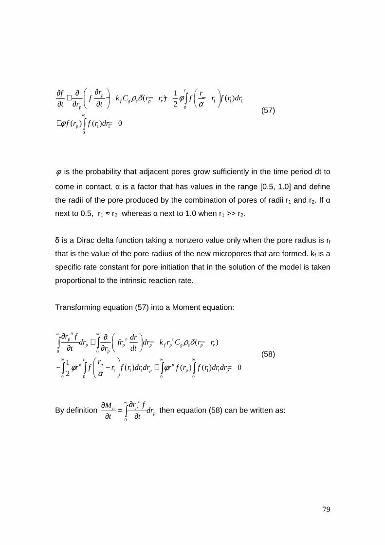
79

1 1 1

0

1 1

0

1( ) ( )

2

( ) ( ) 0

rp

f g s p rp

p

rf rf k C r r f r f r dr

t r t

f r f r dr

ρ δ φα

φ∞

∂ ∂ ∂ + − − − − ∂ ∂ ∂

+ =

∫

∫ (57)

φ is the probability that adjacent pores grow sufficiently in the time period dt to

come in contact. α is a factor that has values in the range [0.5, 1.0] and define

the radii of the pore produced by the combination of pores of radii r1 and r2. If α

next to 0.5, r1 ≈ r2 whereas α next to 1.0 when r1 >> r2.

δ is a Dirac delta function taking a nonzero value only when the pore radius is rf

that is the value of the pore radius of the new micropores that are formed. kf is a

specific rate constant for pore initiation that in the solution of the model is taken

proportional to the intrinsic reaction rate.

Transforming equation (57) into a Moment equation:

0 0

1 1 1 1 1

0 0 0 0

( )

1( ) ( ) ( ) 0

2

nn np

p p p f p g s p rp

rpn n

p p p

r f drdr fr dr k r C r r

t r dt

rr f r f r dr dr r f r f r dr dr

ρ δ

φ φα

∞ ∞

∞ ∞ ∞

∂ ∂ + − − ∂ ∂

− − + =

∫ ∫

∫ ∫ ∫ ∫ (58)

By definition 0

npn

p

r fMdr

t t

∞ ∂∂ =∂ ∂∫ then equation (58) can be written as:

80

1

0

1 1 1

0 0

1( ) 0

2

n npnp p f p g s

rn p

p p o n

drMn r fdr k r C

t dt

rr f r f r dr dr M M

ρ

φ φα

∞−

∞

∂ + −∂

− − + =

∫

∫ ∫ (59)

Zero Moment: n=0

01 1 1 1 1

0 0 0 0

1( ) ( ) ( ) 0

2

rp

f g s p p p

rMk C f r f r dr dr f r dr f r dr

tρ φ φ

α

∞ ∞ ∞ ∂ − − − + = ∂ ∫ ∫ ∫ ∫ (60)

First Moment: n=1

11 1 1

0 0 0

1 1

0 0

1( )

2

( ) ( ) 0

rp p

p f p g s p p

p p p

dr rMfdr k r C r f r f r dr dr

t dt

f r dr r f r dr

ρ φα

φ

∞ ∞

∞ ∞

∂ + − − − ∂

+ =

∫ ∫ ∫

∫ ∫ (61)

Second Moment: n=2

2 221 1 1

0 0 0

21 1

0 0

12 ( )

2

( ) ( ) 0

rp p

p p f p g s p p

p p p

dr rMr fdr k r C r f r f r dr dr

t dt

f r dr r f r dr

ρ φα

φ

∞ ∞

∞ ∞

∂ + − − − ∂

+ =

∫ ∫ ∫

∫ ∫ (62)

Third Moment: n=3

81

2 3 331 1 1

0 0 0

31 1

0 0

13 ( )

2

( ) ( ) 0

rp p

p p f p g s p p

p p p

dr rMr fdr k r C r f r f r dr dr

t dt

f r dr r f r dr

ρ φα

φ

∞ ∞

∞ ∞

∂ + − − − ∂

+ =

∫ ∫ ∫

∫ ∫ (63)

In order to eliminate function distribution and the double integral, a change in

the integration limits is done:

1 1 1

0 0

1( )

2

r

n pp p

rBc r f r f r dr dr

α

φα

∞ = −

∫ ∫

Expressing the integral as an expansion, the term for birth due to pore

combination can be written as

1

0

1

2

nn

n i ii

nBc M M

iα φ+

−=

=

∑

And the moment equations (60), (61) and (62) can be written as:

2 200 0

10

2f g s

Mk C M M

tρ αφ φ∂ − − + =

∂ (64)

210 1 0 0 1 0f f g s

M drM k r C M M M M

t dtρ α φ φ∂ + − Θ − + =

∂ (65)

2 3 3 221 2 0 1 0 22 0f f g s

M drM k r C M M M M M

t dtρ α φ α φ φ∂ + − Θ − − + =

∂ (66)

82

3 4 432 3 0 1 2 0 33 3 0f f g s

M drM k r C M M M M M M

t dtρ α φ α φ φ∂ + − Θ − − + =

∂ (67)

Here 1 0 and =0 >0gen gens sΘ = ≤ Θ

Hashimoto and Silveston (1973) used the above expressions to obtain the

evolution of surface area, volume and average pore radius. However these

authors did not obtain pore size distribution.

3.3. Model Solution

To obtain the pore size distribution, the maximum entropy method was applied

to the moment equations (64), (65) and (66). The mass and entropy balance

equations ((50) – (66)), are solved by the orthogonal collocation method.

3.3.1 The Orthogonal Collocation Method

The orthogonal collocation method was proposed by Villadsen and Stewart

(1967) for solving boundary-value problems. In this method the function y(x),

that is the dependent variable, is approximated by a series expansion y(n)

containing n undetermined parameters. These parameters are determined

applying the differential equation or the boundary conditions to n points (the

collocation points). In the collocation method it is only necessary to evaluate

the residual at the collocation points. In the orthogonal collocation method the

collocation points are taken as the roots to orthogonal polynomials. The residual

function is defined as the function obtained by substituting the trial function

expansion into the original problem: Lv(y)=0.

For the case of problems in which the solution is sought on the domain [0,1] and

is required to be symmetric about x=0, y(x) can be expanded in terms of powers

83

of x2. Also consider a boundary condition in which the value of the solution is

given, y=y(1) at x2=1. The approximation function is chosen such as the

boundary conditions are satisfied. A possible choice of trial function is:

( )1

( ) 2 ( ) 2

0

(1) (1 )n

n ni i

i

y y x a P x−

== + − ∑ (68)

Here Pi(x2) are polynomials of degree i in x2. The residual function contains a

polynomial factor Gn(x2) of degree n in x2, whose zeros are the collocation

points. Then the collocation points are chosen by specifying that Gn(x2) be

orthogonal to all the functions (1-x2)Pi(x2) in equation (68). This specification is

satisfied by taking Gn(x2) and Pi(x

2) from the orthogonal polynomial set defined

by:

( ) ( ) ( )1

2 2 2 1

0

1 ai n i inx P x P x x dx C δ−− =∫ (69)

Where the elemental volume dV is replaced by 1ax dx− , a =1 for slabs, a =2 for

cylinders and a =3 for spheres. The polynomials given by equation (69) are the

Jacobi polynomials that explicitly are:

( )( )

2 2 2

1 ( )( 1)..( 1) 1 ....2 2 2

1 ....1! ! 1 ... 1

2 2 2 2

ii

a a ai i i i i i i

P x x xa a a a

i i

− + + − − + − + + + + = + + + + + −

(70)

84

The collocation points are given by the zeros of Pn(x2). The gradient and

Laplacian operators for the function y(n) given by equation (68) are:

1( ) ( ) ( )

1

( )n

n n nij j

jx xi

dyA y x

dx

+

==

=

∑ (71)

1( )1 1 ( ) ( )

1

( )n

na a n nij j

jx xi

dydx x B y x

dx dx

+− −

==

=

∑ (72)

Equations (71) and (72) have to be used for rewritten the original differential

equation as a set of differential equations at the collocation points. The

operators for i=n+1 are not needed when in the boundary the solution is known

but are useful when there are derivatives in the boundary conditions, in this

latter case the boundary is also a collocation point. The coefficients Aij and Bij

are obtained by writing equations (71) and (72) for functions y=x0, y=x2,….,y=x2n

and solving the resulting systems of equations for the arrays A and B.

( ) ( )

( ) ( )

1 1

1 1

0 21

( )

0 2

/ /

...

/ /n n

n

x x

nij

n

x x

dx dx dx dx

A Q

dx dx dx dx+ +

− =

…

⋮ ⋮

⋯

( ) ( )

( ) ( )

1 1

1 1

2 0 2 21

( )

2 0 2 2

...

n n

n

x x

nij

n

x x

x x

B Q

x x+ +

− ∇ ∇ = ∇ ∇

…

⋮ ⋮

⋯

(73)

85

[ ]

2 21 1

2 21 1

1 ...

. . ... .

. . ... .

1 ...

n

nn n

x x

Q

x x+ +

=

x2i with i=0, 1,…n

The collocation points, x1, x2, ….,xn are the roots of Pn(x2)=0 and xn+1 is unity (it

means xn+1=1)

3.3.2 The maximum entropy technique

The reconstruction of a distribution from its moments is a problem for which

different techniques of solution have been proposed (John et al, 2007). One of

the techniques is the Maximum Entropy Method that finds the most probable

value for a function that is the answer to some problem based on the

determination of the probability distribution that has the maximum entropy

subject to some constraints (Jaynes 1957). Let be Pi the probability of state i,

then the Shannon entropy is represented by Equation (74):

lni iS P P= −∑ (74)

The constraints are expected values of several quantities. Applying the

Lagrange multipliers method, the probability distribution is found maximizing the

entropy function subject to constraints. In the case, where the n-moments are

used as constraints, the function that is obtained is given by Equation(75):

20 1 2( , ) exp .... n

p p p n pf r t r r rλ λ λ λ = − + + + + (75)

Where λi are the Lagrange multipliers and the number i of these multipliers

depend on the number of moments that are used.

86

The above equation is obtained applying the Lagrange multipliers method

where a function F is built by multiplying each constraint by an unknown

constant λi. Each one of these term is added to the entropy function :

1 1 1 2 2 2F ( ) [ ( ) ( )] [ ( ) ( )] .... [ ( ) ( )]i p i p p i p n n p i n pS P f r P f r f r P f r f r P f rλ λ λ= + ⟨ ⟩ − + ⟨ ⟩ − + + ⟨ ⟩ −∑ ∑ ∑

The value of the multipliers is found by an equation system obtained from

maximizing the function F respect to each unknown parameter:

0 0 i i

F F

P λ∂ ∂= =∂ ∂

The use of the moments must have into account some considerations as it is

noted by John et al (2007). Mathematically, all moments up to infinity are

requested in order to obtain a perfect reconstruction of a distribution; moreover,

the knowledge of all moments is only sufficient if the class of functions in which

the reconstruction is sought is restricted appropriately.

Besides the above considerations, there is the problem of the reconstruction of

distributions with more than one peak. According to the results presented in

Chapter 2, the shape of the pore size distribution is different for each raw

material. Some pore size distributions, such as El Sol, show only one peak

whereas other can present two peaks or even three peaks at different stages of

the activation process. A way to model distributions with more than one peak is

to reconstruct the distribution function corresponding to each peak therefore

each peak has its specific set of moment equations and the maximum entropy

method is applied to each set of moments.

87

LIST OF REFERENCES


reactions: I. Isothermal, kinetic control”. AIChE J. v. 26, 1980, p. 379-386.


reactions: II. Diffusion and transport effects”. AIChE J. v. 27, 1981, p. 247-

254.

3. FINLAYSON B. “The method of weighted residuals and variational

principles with application in fluid, mechanics and mass transfer”. Academic

Press, New York, 1972.

4. HASHIMOTO K. and SILVESTON P.L. “Gasification: Part I. Isothermal,

Kinetic Control Model for solid with a pores size distribution”. AIChE J. v. 19.

No 2. 1973. p. 259-268

5. JAYNES E.T. “Information theory and Statistical mechanics”. The Physical

Review. Vol.106, No 4, 1957. p.620-630

6. JOHN V., ANGELOV I., ONCUL A.A., and THEVENIN D. “Techniques for

the reconstruction of a distribution from a finite number of its moments”.

Chem. Eng. Sci. v.62, 2007. p. 2890-2904

7. VILLADSEN J.D. and STEWART W.E. “Solution of boundary-value

problems by orthogonal collocation”. Chem. Eng. Science. 3981-3996

(reprinted from Chem. Eng. Science 22, 1967).

88

NOMENCLATURE

2coC :CO2 concentration [kmol/m3]

Nco2 :CO2 molar flux [kmol/s-m2]

Cc : Carbon concentration [kmol/m3]

Rɺ : Reaction rate per volume [kmol/s-m3]

t: time [s]

r: particle radii [m]

rp: pore radius [m]

ε porosity

Def: Effective diffusivity [m2/s]

D: diffusivity [m2/s]

τ: tortuosity factor

ρp : particle density [g/m3]

Sg: specific surface area [m2/g]

k: intrinsic reaction rate [m/s]

ρt: true density [g/m3]

A: pre-exponential factor

E: activation energy [kJ/kmol-K]

R: universal gas constant

T: temperature [K]

2cos : specific entropy of CO2 [kJ/kmol-K]

cs : specific entropy of solid Carbon [kJ/kmol-K]

genσɺ : entropy generation per volume [kJ/m3-s-K]

89

CHAPTER FOUR

RESULTS AND VALIDATION OF THE MODEL FOR PREDICTION OF PORE SIZE DISTRIBUTION

Initially, the model was solved for two different intrinsic reaction rates (k) in

order to evaluate the effect of reactivity on the carbon conversion and pore size

distribution. Two sets of moments where used in order to simulate the

development of two peaks in the distribution. The initial value of the moments

(zero, first, second and third moment) were obtained by setting experimental

data of the pore size distribution of the char (La Capotera char was chosen)

with the lowest burn-off, but not 0%. Char with 0% burn-off can not be used due

to pore development is poor and it is not possible to get appropriate functions

that show peaks in different pore widths. The pore size distribution was divided

in two parts: the first part represents development of fine pores while the

second part represents the larger pores. Two sets of moments corresponding to

each part of the pore size distribution were calculating by setting the value of

the first moment of each part, which is related to the mean pore width, to 4 and

25Å respectively. Other values of parameters involved in the model are

presented in Table 2.

Table 2. Input parameters for model solution

Peak 1

Moment Zero 1.0 Ψ 5.0

First moment 4.0 φ 0.8

Second moment 25.5 α 0.75

Third moment 192.5 Rpartícula [m] 4.0e-3

90

Peak 2


First moment 25.8 φ 0.8

Second moment 672.6 α 0.75


In Figure 22, carbon conversion versus radial position for k=1e-6 at different

time, is shown. It can be seen that reaction occurs all over the particle indicating

that diffusion predominates over chemical reaction.

0.0

0.2

0.4

0.6

0.8

1.0

0.00 0.20 0.40 0.60 0.80 1.00

Position

Car

bon

conv

ersi

on

1.20E+00

1.68E+013.36E+01

5.16E+016.84E+01

8.52E+01

Krxn:1e-6

Figure 22. Conversion vs. Radial Position. k= 1e-6

In Figure 23 entropy generation (Sgen) versus radial position at different time, is

shown. It can be seen that the entropy generation decreases as the process

advances that is an expected behavior.

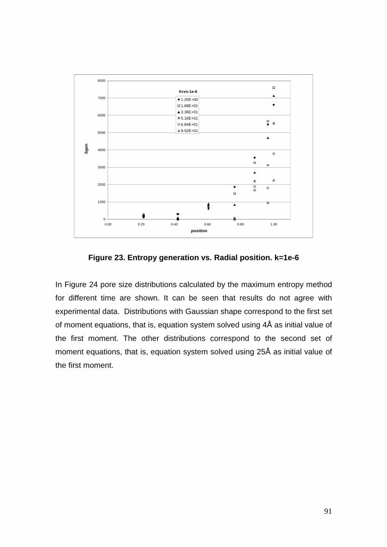
91

0

1000

2000

3000

4000

5000

6000

7000

8000

0.00 0.20 0.40 0.60 0.80 1.00

position

Sge

n

1.20E+00

1.68E+01

3.36E+01

5.16E+01

6.84E+01

8.52E+01

Krxn:1e-6

Figure 23. Entropy generation vs. Radial position. k=1e-6

In Figure 24 pore size distributions calculated by the maximum entropy method

for different time are shown. It can be seen that results do not agree with

experimental data. Distributions with Gaussian shape correspond to the first set

of moment equations, that is, equation system solved using 4Å as initial value of

the first moment. The other distributions correspond to the second set of

moment equations, that is, equation system solved using 25Å as initial value of

the first moment.

92

0.000

0.100

0.200

0.300

0.400

0.500

0.600

0.700

0.0 50.0 100.0 150.0 200.0

Pore width [A]

f(r)

5.16E+01

6.84E+01

8.52E+01

5.16E+01

6.84E+01

8.52E+01

Figure 24. Pore size distribution. Maximum Entropy Method. k=1e-6

In Figure 25, carbon conversion versus radial position for k=1.0e-2, is shown. In

this case it can be seen that conversion is higher on the particle surface and

nodes near to the particle centre exhibit less carbon conversion. This behavior

indicates that chemical reaction predominates and the reactant gas does not

reach the particle centre.

93

0

10000000

20000000

30000000

40000000

50000000

60000000

70000000

80000000

0.00 0.20 0.40 0.60 0.80 1.00

position

Sge

n

1.20E+00

1.68E+01

3.36E+01

5.16E+01

6.84E+01

8.52E+01

Krxn:1e-2

0.0

0.2

0.4

0.6

0.8

1.0

0.00 0.20 0.40 0.60 0.80 1.00

position

Car

bon

conv

ersi

on

1.20E+00

1.68E+01

3.36E+01

5.16E+01

6.84E+01

8.52E+01

Krxn:1e-2

Figure 25. Conversion vs. Radial Position. k= 1e-2

Figure 26. Entropy generation vs. Radial position. k= 1e-2

94

In Figure 26 the entropy generation versus radial position for k=1e-2 is shown.

Again entropy generation decreases as the process goes forward. Entropy

generation is higher on the surface that is the zone where the chemical reaction

takes place.

0.00

0.10

0.20

0.30

0.40

0.50

0.60

0.70

0.0 50.0 100.0 150.0 200.0

Pore width [A]

f(r)

5.16E+01

6.84E+01

8.52E+01

5.16E+01

6.84E+01

8.52E+01

Figure 27. Pore Size Distribution. Maximum entropy method. k= 1e-2

In Figure 27, the pore size distribution calculated by the maximum entropy

method for k=1e-2 has the same behavior as the case k=1e-6. Then the model

as it is initially proposed does not reflect the effect of the reactivity of the raw

material and either it does not reproduce in some way the shape of the

experimental distribution functions.

The solution of the equations moments by the maximum entropy method is very

sensitive to the initial value of the moments. A series of runs were carried out

95

with different values of the initial moments to observe the response of the

solution to initial values. The conditions were the same as for k=1e-6 except the

initial value of the moments. In Table 3 the initial value of the moments for each

run are shown.

Table 3. Initial value of moments

Run 1 Run 2 Run 3

Peak 1

Moment Zero 1.0 1.0 1.0

First moment 1.0 1.0 1.0

Second moment 10.0 5.0 3.0

Third moment 100.0 30.0 10.0

Peak 2

Moment Zero 1.0 1.0 1.0

First moment 1.0 1.0 1.0

Second moment 10.0 10.0 10.0

Third moment 100.0 100.0 100.0

In Figures 28-30 , the pore size distributions for each run are shown.

96

0.000

0.020

0.040

0.060

0.080

0.0 50.0 100.0 150.0 200.0

Pore width [A]

f(r)

5.16E+01

6.84E+01

8.52E+01

5.16E+01

6.84E+01

8.52E+01

0.000

0.020

0.040

0.060

0.080

0.100

0.0 50.0 100.0 150.0 200.0

Pore width [A]

f(r)

5.16E+01

6.84E+01

8.52E+01

5.16E+01

6.84E+01

8.52E+01

Figure 28. Pore Size Distribution. Maximum entropy method. Run 1

Figure 29. Pore Size Distribution. Maximum entropy method. Run 2.

97

0.000

0.020

0.040

0.060

0.080

0.0 50.0 100.0 150.0 200.0

Pore width [A]

f(r)

5.16E+01

6.84E+01

8.52E+01

5.16E+01

6.84E+01

8.52E+01

Figure 30. Pore Size Distribution. Maximum entropy method. Run 3.

The initial values of the moments were changed for the first peak in each run.

For the second peak the initial value of the moments were kept constant. In

Figure 28, the pore size distributions for the first peak show a mean pore size

around 48Å and the maximum value of the function tends to increases as the

process takes place. In Figure 29, the mean pore size is around 40Å and there

is a slight tendency to increase the maximum value of the distribution as the

activation takes place. In Figure 30 the mean pore size is around 28Å and the

maximum of the distribution tends to decrease as the activation takes place.

According to the above results the Maximum entropy method is not very reliable

when there is not a reliable knowledge of several moments. At this point it is

necessary to use other technique for the reconstruction of the distribution from

its moments. An alternative is to use a priori distribution shape and the

moments are used to find properties such as mean size, standard deviation and

coefficient of variation that are related to the parameters of the distribution

98

(John et al, 2007). In Table 4 is shown the relation between moments and

properties of a distribution.

Table 4. General parameters for distributions as fu nctions of moments

Parameter Relation

Mean size 1 0/x M M=

Coefficient of variation 0 2

21

1v

M Mc

M= −

Standard deviation 0 21

20 1

1M MM

M Mσ = −

In the Figures 31-32 the results using the log-normal distribution, for different

reactivities, are shown. The initial values of the moments are the same that

were calculated from the fitting of experimental data of the pore size distribution

of the char with the lowest burn-off (Table 2). Due to log-normal distribution

shows a long tail in the direction of the larger sizes, this distribution is one of the

most used to represent size distributions. The function of log-normal

distribution is shown in Equation (76):

2

2

ln ( / )1( ) exp

2lnln 2g

gg

x xf x

x σσ π

= −

(76)

Where ( )2g v2

=exp ln(c 1)exp(0.5ln )g

g

xx σ

σ= +

99

0.00

0.02

0.04

0.06

0.08

0.10

0.12

0.0 10.0 20.0 30.0 40.0 50.0 60.0 70.0 80.0 90.0 100.0

Pore Width [A]

f(r)

5.16E+01

6.84E+01

8.52E+01

Figure 31. Pore Size Distribution. Log-normal distr ibution. k= 1e-6

0.00

0.02

0.04

0.06

0.08

0.10

0.12

0.0 10.0 20.0 30.0 40.0 50.0 60.0 70.0 80.0 90.0 100.0

Pore Width [A]

f(r)

5.16E+01

6.84E+01

8.52E+01

Figure 32 . Pore Size Distribution. Log-normal dist ribution. k= 1e-4

100

0.00

0.02

0.04

0.06

0.08

0.10

0.12

0.0 10.0 20.0 30.0 40.0 50.0 60.0 70.0 80.0 90.0 100.0

Pore Width [A]

f(r)

5.16E+01

6.84E+01

8.52E+01

Figure 33. Pore Size Distribution. Log-normal distr ibution. k= 1e-2

In the above figures it can be observed that the shape of the peaks is close to

the shape of the experimental pore size distributions. Also, the behavior

indicates a trend to decrease the maximum value of the distribution as the

reaction takes place, although there is not any effect of the reactivity on the

pore size distribution.

4.1. Sensitivity Analysis for the Model

To analyze the effect of some parameters on the PSD evolution, some runs

were carried out. The model was solved using a priori distribution shape, the

log-normal distribution. The values of probability of pore combination (φ), factor

for the pore radii combination (α) and rate of formation of pores (Kf) were varied.

Additionally, as an attempt to simulate the different stages observed in the

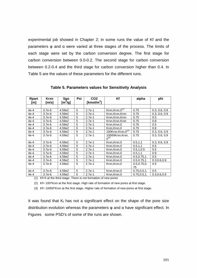
101

experimental job showed in Chapter 2; in some runs the value of Kf and the

parameters φ and α were varied at three stages of the process. The limits of

each stage were set by the carbon conversion degree. The first stage for

carbon conversion between 0.0-0.2. The second stage for carbon conversion

between 0.2-0.4 and the third stage for carbon conversion higher than 0.4. In

Table 5 are the values of these parameters for the different runs.

Table 5. Parameters values for Sensitivity Analysis

Rpart [m]

Krxn [m/s]

Sgo [m 2/g]

Psi CO2 [kmol/m 3]

Kf alpha phi

4e-4 3.7e-6 4.59e2 5 2.7e-1 Krxn,Krxn,0(1) 0.75 0.3, 0.6, 0.9 4e-4 3.7e-6 4.59e2 5 2.7e-1 Krxn,Krxn,Krxn 0.75 0.3, 0.6, 0.9 4e-4 3.7e-6 4.59e2 5 2.7e-1 Krxn,Krxn,Krxn 0.75 0.5 4e-4 3.7e-6 4.59e2 5 2.7e-1 Krxn,Krxn,Krxn 0.75 0.8 4e-4 3.7e-6 4.59e2 5 2.7e-1 Krxn,Krxn,0 0.75 0.5 4e-4 3.7e-6 4.59e2 5 2.7e-1 Krxn,Krxn,0 0.75 0.8 4e-4 3.7e-6 4.59e2 5 2.7e-1 100Krxn,Krxn,0(2) 0.75 0.3, 0.6, 0.9 4e-4 3.7e-6 4.59e2 5 2.7e-1 10000Krxn,Krxn,

0(3) 0.75 0.3, 0.6, 0.9

4e-4 3.7e-6 4.59e2 5 2.7e-1 Krxn,Krxn,0 0.5,1,1 0.3, 0.6, 0.9 4e-4 3.7e-6 4.59e2 5 2.7e-1 Krxn,Krxn,0 0.5,1,1 0.5 4e-4 3.7e-6 4.59e2 5 2.7e-1 Krxn,Krxn,0 0.5,1,0.5 0.5 4e-4 3.7e-6 4.59e2 5 2.7e-1 Krxn,Krxn,0 0.5,1,1 0.9 4e-4 3.7e-6 4.59e2 5 2.7e-1 Krxn,Krxn,0 0.5,0.75,1 0.5 4e-4 3.7e-6 4.59e2 5 2.7e-1 Krxn,Krxn,0 0.5,0.75,1 0.3,0.6,0.9 4e-4 3.7e-6 4.59e2 5 2.7e-1 Krxn,Krxn,0 0.5,0.75,0.

75 0.5

4e-4 3.7e-6 4.59e2 5 2.7e-1 Krxn,Krxn,0 0.75,0.5,1. 0.5 4e-4 3.7e-6 4.59e2 5 2.7e-1 Krxn,Krxn,0 0.75,0.5,1. 0.3,0.6,0.9

(1) Kf=0 at the third stage. There is not formation of new pores

(2) Kf= 100*Krxn at the first stage. High rate of formation of new pores at first stage.

(3) Kf= 10000*Krxn at the first stage. Higher rate of formation of new pores at first stage.

It was found that Kf has not a significant effect on the shape of the pore size

distribution evolution whereas the parameters φ and α have significant effect. In

Figures some PSD’s of some of the runs are shown.

102

0.00

0.02

0.04

0.06

0.08

0.10

0.0 10.0 20.0 30.0 40.0 50.0

Pore width [A]

f(r)

0.90%

4.60%

9.30%

16.80%

22.30%

40.30%

59.20%

Figure 34. Kf: Krxn,Krxn,0, Alpha: 0.75,0.75,0.75, Phi: 0.5

0.00

0.02

0.04

0.06

0.08

0.10

0.0 10.0 20.0 30.0 40.0 50.0

Pore width [A]

f(r)

0.90%

4.60%

9.30%

16.80%

22.30%

40.30%

59.20%

Figure 35. Kf: Krxn,Krxn,Krxn, Alpha: 0.75, 0.75,0 .75, Phi: 0.3,0.6,0.9

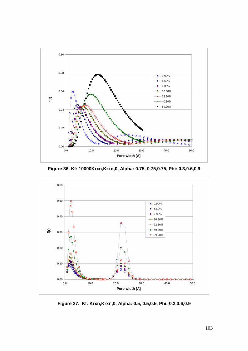
103

0.00

0.02

0.04

0.06

0.08

0.10

0.0 10.0 20.0 30.0 40.0 50.0

Pore width [A]

f(r)

0.90%

4.60%

9.30%

16.80%

22.30%

40.30%

59.20%

Figure 36. Kf: 10000Krxn,Krxn,0, Alpha: 0.75, 0.75, 0.75, Phi: 0.3,0.6,0.9

0.00

0.10

0.20

0.30

0.40

0.50

0.60

0.0 10.0 20.0 30.0 40.0 50.0

Pore width [A]

f(r)

0.90%

4.60%

9.30%

16.80%

22.30%

40.30%

59.20%

Figure 37. Kf: Krxn,Krxn,0, Alpha: 0.5, 0.5,0.5, P hi: 0.3,0.6,0.9

104

0.00

0.02

0.04

0.06

0.08

0.10

0.12

0.14

0.0 10.0 20.0 30.0 40.0 50.0

Pore width [A]

f(r)

0.90%

4.60%

9.30%

16.80%

22.30%

40.30%

59.20%

Figure 38. Kf: Krxn,Krxn,0, Alpha: 0.75, 0.5,1.0, Phi: 0.3,0.6,0.9

The parameter α has an important effect on the evolution of the PSD due to this

parameter determines the pore size. For instance, in Figures 34-36, α is

constant with a value of 0.75, that is, the pores that are combining have

different widths and it leads to a continuous increasing of the pore size. In

Figure 37, α is constant with a value of 0.5, that is, the size of pores that are

combining is similar. For this reason the mean pore size remains almost

constant at the different conversion. In Figure 38, α changes at different stages

of the process. In the first stage, carbon conversion between 0-0.2% and

α=0.75, there is a continuous increase of the pore size . In the second stage,

α=0.75, the mean pore size remains almost constant and in the third stage,

carbon conversion higher than 0.4%, α=1.0, the pore size increases faster

than in the first stage.

105

If Figure 38 is compared with experimental PSD’s results in Chapter 2, it can be

observed that the behavior is similar. Then, at the first stages of the activation

process, there is combination of pores of equal or comparable size. After that,

there is combination of pores of different size.

The parameter φ has effect on the height of the different peaks, that is, the

value of the function of pore size distribution. At higher probability of pore

combination leads to a higher production of pores of a new size whereas a low

probability of pore combination leads to a lower production of pores by this

mechanism and then it leads to lower peaks.

4.2. Validation of the model for La Capotera, La Gr ande and El Sol chars

In the above item, the model was solved for initial value of the moments (zero,

first, second and third moment) obtained by setting experimental data of the

pore size distribution of the La Capotera char with the lowest burn-off, but not

0%. As it was mentioned, char with 0% burn-off cannot be used because its

pore development is poor and it is not possible to get appropriate functions that

show peaks in different pore widths. Applying the DFT method and the BET

method on the N2 isotherm for the char with 19% burn-off, micropore volume,

pore width and the surface area were calculated. The values obtained are

0.0933 cc/g, 4.17Å and 458.7 m2/g, respectively. Based on these values and a

true density 2.0 g/cc (obtained from literature review), the parameter Ψ was

calculated as 20.4. The intrinsic reaction rate was calculated by using the un-

reacted shrinking core model, the value obtained was 3.7e-6 m/s. The model

was run for parameters shown in Table 6.

The value of parameters φ and α was changed at different stages of the

process, as it was done before (item 4.1).

106

In Figures 39-41 the theoretical pore size distribution obtained from the

simulation, conversion profile and entropy generation profile are shown.

Table 6. Parameter for validation of the model with La Capotera char

Peak 1


First moment 4.0 φ 0.3, 0.6, 0.9

Second moment 25.5 α 0.75, 0.5, 1.0


K [m/s] 3.7e-6 Kf 3.7e-6

Peak 2


First moment 25.8 φ 0.3, 0.6, 0.9

Second moment 672.6 α 0.75, 0.5, 1.0


K [m/s] 3.7e-6 Kf 3.7e-6

0.00

0.02

0.04

0.06

0.08

0.10

0.12

0.0 10.0 20.0 30.0 40.0 50.0

Pore width [A]

f(r)

0.90%

5.20%

11.40%

21.70%

29.00%

46.40%

54.90%

Figure 39. Theoretical pore size distribution for L a Capotera char

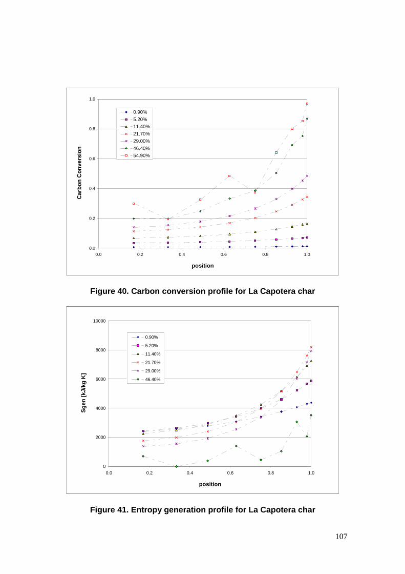
107

0.0

0.2

0.4

0.6

0.8

1.0

0.0 0.2 0.4 0.6 0.8 1.0

position

Car

bon

Con

vers

ion

0.90%

5.20%

11.40%

21.70%

29.00%

46.40%

54.90%

Figure 40. Carbon conversion profile for La Capoter a char

0

2000

4000

6000

8000

10000

0.0 0.2 0.4 0.6 0.8 1.0

position

Sge

n [k

J/kg

K]

0.90%

5.20%

11.40%

21.70%

29.00%

46.40%

Figure 41. Entropy generation profile for La Capote ra char

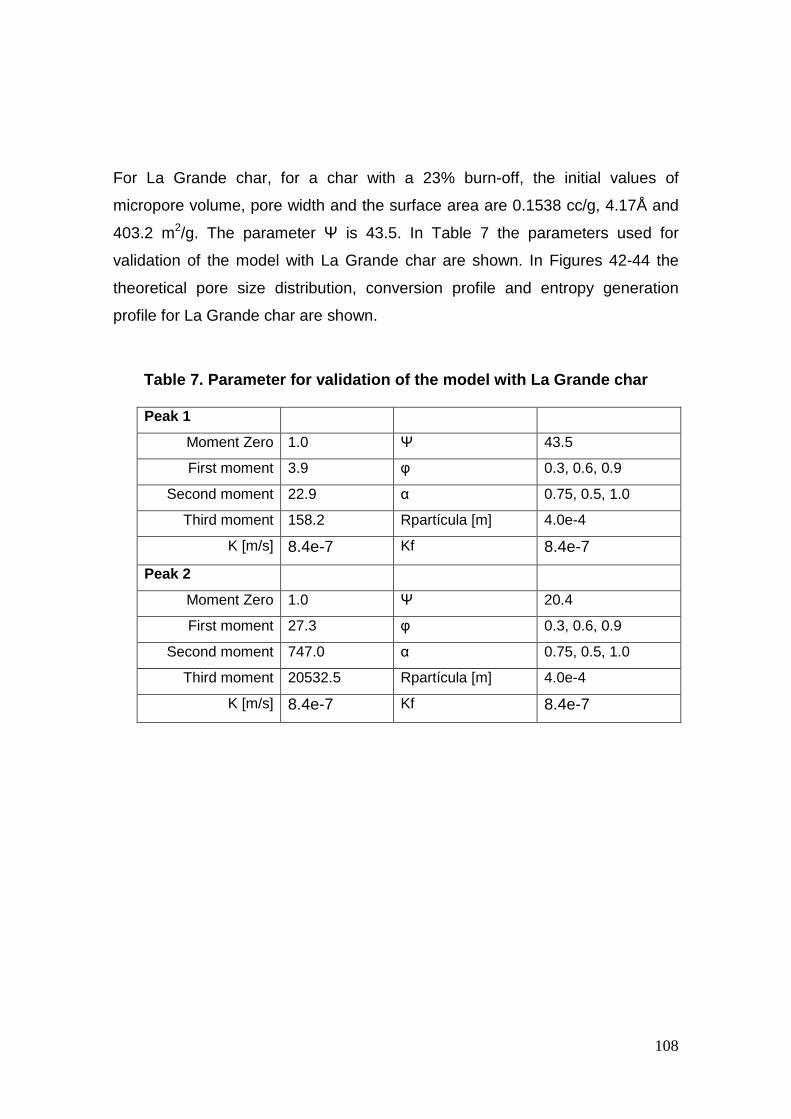
108

For La Grande char, for a char with a 23% burn-off, the initial values of

micropore volume, pore width and the surface area are 0.1538 cc/g, 4.17Å and

403.2 m2/g. The parameter Ψ is 43.5. In Table 7 the parameters used for

validation of the model with La Grande char are shown. In Figures 42-44 the

theoretical pore size distribution, conversion profile and entropy generation

profile for La Grande char are shown.

Table 7. Parameter for validation of the model with La Grande char

Peak 1


First moment 3.9 φ 0.3, 0.6, 0.9

Second moment 22.9 α 0.75, 0.5, 1.0


K [m/s] 8.4e-7 Kf 8.4e-7

Peak 2


First moment 27.3 φ 0.3, 0.6, 0.9

Second moment 747.0 α 0.75, 0.5, 1.0


K [m/s] 8.4e-7 Kf 8.4e-7

109

0.00

0.02

0.04

0.06

0.08

0.10

0.12

0.0 10.0 20.0 30.0 40.0 50.0

Pore width [A]

f(r)

1.20%

7.90%

19.10%

38.70%

51.20%

73.30%

Figure 42. Theoretical pore size distribution for L a Grande char

0.0

0.2

0.4

0.6

0.8

1.0

0.0 0.2 0.4 0.6 0.8 1.0

position

Car

bon

Con

vers

ion

1.20%7.90%19.10%38.70%51.20%

73.30%

Figure 43. Carbon conversion profile for La Grande char

110

0

500

1000

1500

2000

2500

3000

0.0 0.2 0.4 0.6 0.8 1.0

position

Sge

n [k

J/kg

K]

1.20%

7.90%19.10%38.70%51.20%

73.30%

Figure 44. Entropy generation profile for La Grande char

For El Sol char, for a char with a 16% burn-off, the initial values of micropore

volume, pore width and the surface area are 0.0486 cc/g, 4.17Å and 125.9

m2/g. The parameter Ψ is 150.2. In Table 8 the parameters used for validation

of the model with El Sol char are shown. In Figures 45-47 the theoretical pore

size distribution, conversion profile and entropy generation profile for El Sol char

are shown. Due to experimental PSD’s with El Sol char showed little change in

the mean pore size, it was assumed a parameter α=0.5. Several runs were

carried changing the value of the parameter φ. The best fitting was got with

φ=0.1 for the different stages of the activation process.

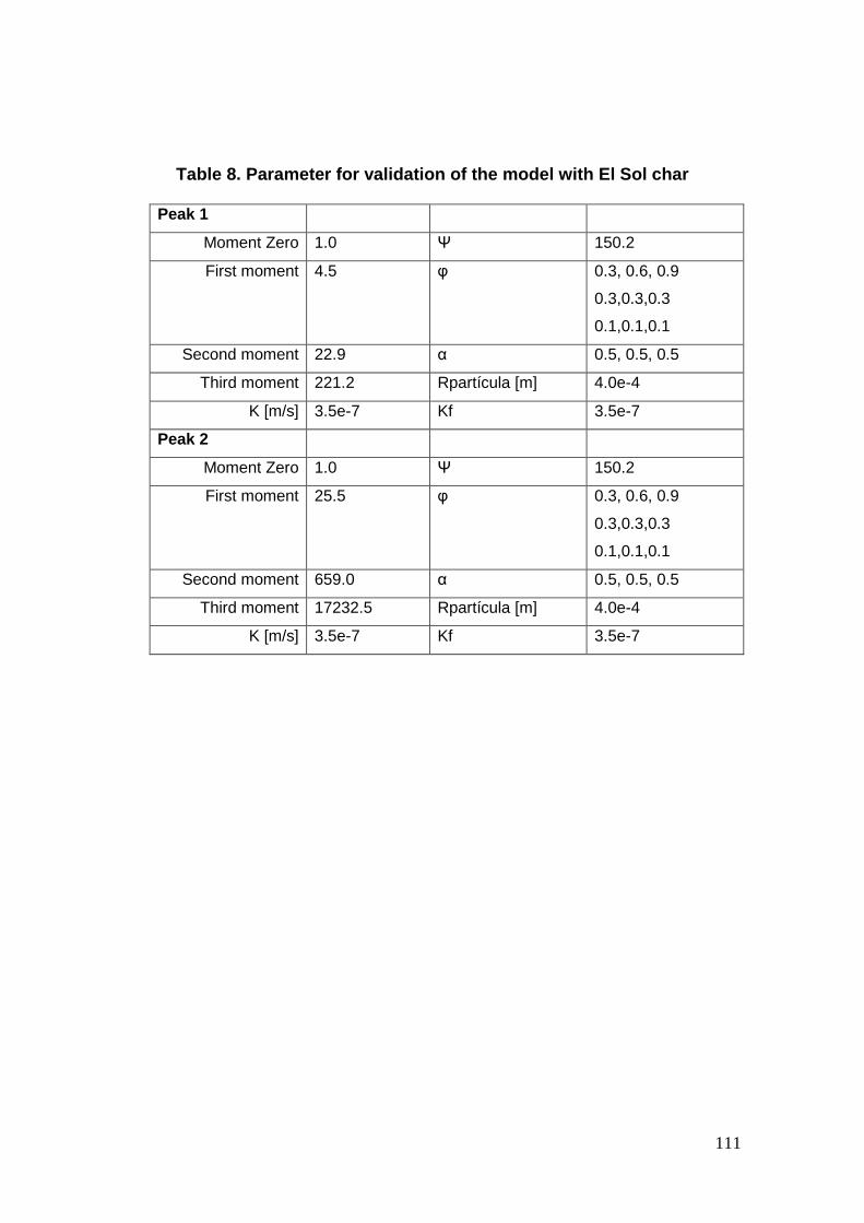
111

Table 8. Parameter for validation of the model with El Sol char

Peak 1


First moment 4.5 φ 0.3, 0.6, 0.9

0.3,0.3,0.3

0.1,0.1,0.1

Second moment 22.9 α 0.5, 0.5, 0.5


K [m/s] 3.5e-7 Kf 3.5e-7

Peak 2


First moment 25.5 φ 0.3, 0.6, 0.9

0.3,0.3,0.3

0.1,0.1,0.1

Second moment 659.0 α 0.5, 0.5, 0.5


K [m/s] 3.5e-7 Kf 3.5e-7

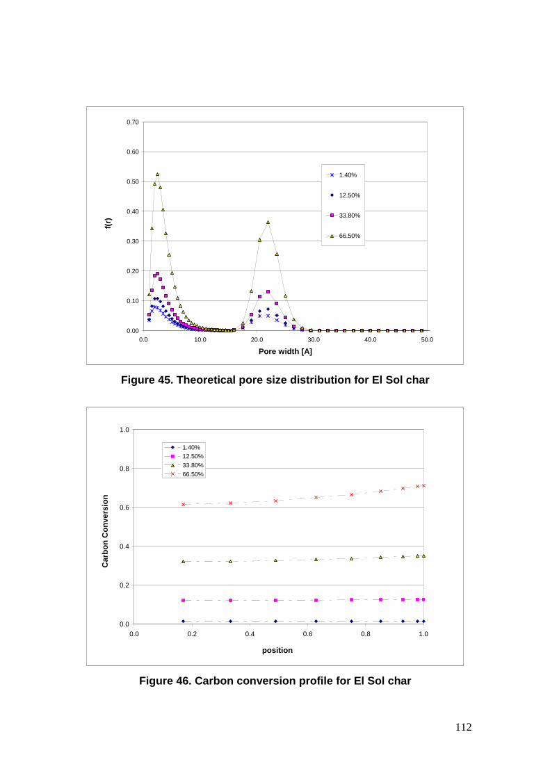
112

0.00

0.10

0.20

0.30

0.40

0.50

0.60

0.70

0.0 10.0 20.0 30.0 40.0 50.0

Pore width [A]

f(r)

1.40%

12.50%

33.80%

66.50%

Figure 45. Theoretical pore size distribution for E l Sol char

0.0

0.2

0.4

0.6

0.8

1.0

0.0 0.2 0.4 0.6 0.8 1.0

position

Car

bon

Con

vers

ion

1.40%12.50%

33.80%

66.50%

Figure 46. Carbon conversion profile for El Sol cha r

113

0

500

1000

1500

2000

0.0 0.2 0.4 0.6 0.8 1.0

position

Sge

n [k

J/kg

K]

1.40%

12.50%

33.80%

66.50%

Figure 47. Entropy generation profile for El Sol c har

Comparing the theoretical results with experimental results it can be seen that

there are deviations between experiments and results of the theoretical model.

Although the theoretical model can follow the trend in the evolution of PSD’s, a

better fitting for each char must be done by adjusting parameters such as φ

and α.

Experimentally, La Capotera char showed almost a constant mean pore size

and the value of the function for pore size distribution increased at carbon

conversion up to 60% and then decreased. With parameters showed in Table 6,

the theoretical model showed an increasing in the value of the function of PSD

at carbon conversion up to around 5%, but quickly the function of PSD

decreases.

114

Experimentally, La Grande char showed an increasing of the mean pore size for

the different carbon conversion. The results of the theoretical model, with

parameters presented in Table 7, also showed an increasing of the mean pore

size but again there is difference at the carbon conversion where the PSD

showed the maximum value. Experimentally, the maximum value of the PSD

was reached at 55% whereas with the theoretical model was reached at carbon

conversion around 40%.

For El Sol char, the theoretical model showed a continuous increasing of the

value of the PSD as it was found experimentally. However the theoretical

maximum values of the PSD are considerable higher than the experimental

values.

However, the results of theoretical model allow establishing a theory about the

occurrence of phenomenon of formation and combination of pores. For

instance, for La Capotera and La Grande chars can be established that at the

early stages of the activation process there is combination of pores of similar

size and at final stages there is combination of pores of different size. For El

Sol char, there is a low probability of pore combination then the formation of

new pores is the phenomenon that prevalence.

Another aspect to be analyzed is the deviation between the experimental and

theoretical carbon conversion at which the maximum PSD’s are reached. This

deviation could be attributed to the fact that the initial moments for the

simulations are taken from isotherms of chars with higher carbon burn-off (19%

and 23%). Nevertheless, it was pointed out that it is not possible to use an

isotherm of a char with very low carbon conversion because the shape of the

pore size distribution is very different compare to the pore size distributions of

chars with a high carbon conversion. At very low carbon conversion it is

possible an important effect of the opening of closed pores. This closure of

pores is caused by the presence of disordered carbon. Some authors (Calo et

115

al, 2001, Feng and Bhatia, 2003) indicate the existence of this phenomenon

after some degree of gasification. The opening of the closed pores occurs

through different carbon conversion degree for each type of char. For instance,

Calo et al (2001) used a Wyodak coal char in which the limit is 9.2% burn-off

and a phenolic resin char in which the development of porosity has a strong

effect of the opening of closed pores even at high carbon burn-off degree. Feng

and Bhatia (2003) gasified Yarrabee coal chars with air and found that closed

pores are reopened before 20% conversion. Tran et al (2008) gasified carbon

anodes in air and CO2. Based on their results, these authors proposed the

consumption of disordered carbon in the initial 15% conversion. This effect of

the opening of closed pores leads to a different behavior of the porosity

development at the first stage of gasification that was not taken into account in

the mathematical model.

As it was mentioned before, there is not effect of the reaction rate on the pore

size distribution, the changes on the maximum values depends on the initial

moments. However, there is an effect of reaction rate on the conversion and

entropy generation profiles. The theoretical conversion profile of La Capotera

char that has the higher reaction rate shows a higher conversion on the surface

and a lower conversion near to the center of the particle. This difference

increases as the reaction takes place. This behavior indicates a prevalence of

diffusion resistance over chemical resistance. In La Grande char, the

conversion profile tends to be more homogeneous and the difference between

carbon conversion on the surface and the center is not so deep. El Sol char

showed a horizontal carbon conversion profile indicating a prevalence of

chemical resistance over diffusion resistance.

The behavior of the entropy generation is associated with the reaction rate. For

La Capotera char, the entropy generation tends to zero more quickly than for La

Grande char. Theoretically, there was not possible to establish a relationship

between entropy generation and porosity development. Nevertheless, if the

116

theoretical results of the entropy generation are compared with the experimental

pore size distributions, it can be seen that the global conversion at which the

entropy generation profile is not stable, that is, the profile is not homogeneous,

is close to the global conversion at which the peaks on the pore widths around

4-7 Å began to decrease. The changes in the entropy generation profile could

be used as a restriction to determine limits of carbon conversion where there is

a change in the prevalence of the different phenomena, formation an

combination of pores. This behavior could be a coincidence then it is necessary

to do more research at this point.

4.3. Conclusions

The population balance model for pore size distribution model considers

phenomena such as pore formation and pore combination however these

phenomena occur at different stages of the gasification process then the model

should include some restrictions in order to give prevalence of each

phenomenon at different stage of the process.

Besides, the model does not take into account the effect of the closed pores

that are present at the beginning of the process of gasification. These closed

pores have an important effect on the pore size distribution due to the shape of

the pore size distribution at low carbon conversion is different compare to

distribution at higher carbon conversion degree. A best understanding of this

phenomenon would allow setting the carbon burn-off at which all pores are

opened and the possibility of including an additional term in the model that

could improve the results.

The adjustable parameters φ and α, have significant impact on the theoretical

evolution of the pore size distribution. These parameters allow establishing

theoretically which phenomenon has prevalence throughout of the different

stages of the activation process.

117

LIST OF REFERENCES

1. CALO J.M, HALL P and ANTXUSTEGI M. “Carbon porosity characterization

via small angle neutron scattering”. Colloids and Surface A. 2001. p. 219-

232.

2. FENG B. and BHATIA S.K. “Variation of pore structure of coal chars during

gasification”. Carbon. V. 41. 2003. p.507-523.

3. JOHN V., ANGELOV I., ONCUL A.A., and THEVENIN D. “Techniques for

the reconstruction of a distribution from a finite number of its moments”.

Chem. Eng. Sci. v.62, 2007. p. 2890-2904

4. JUNPIROM S., DO D.D., TANGSATHITKULCHAI C. and

TANGSATHITKULCHAI M. “A carbon activation model with application to

longan seed char gasification”. Carbon. v 43. 2005. p.1936-1943.

5. TRAN K.N., BERKOVICH A., TOMSETT A. and BHATIA S. “Crystalline

structure transformation of carbon anodes during gasification”. Energy &

Fuels. v 22. 2008. p.1902-1910.

118

CHAPTER FIVE

CONCLUSIONS

The evolution of pore size distribution throughout activation is different for each

material but in general the phenomena of formation of new pores (fine pores)

and pore enlargement are present. A material with a low reactivity, as El Sol

coal, exhibit an important contribution of the formation of fine pores until high

carbon conversion degrees whereas material with a higher reactivity, as La

Capotera coal, present both phenomena, that is, formation of fine pore and pore

enlargement since the first stages of activation.

The population balance model for pore size distribution model considers the

phenomena of pore formation and pore combination. The model proposed by

Miura and Hashimoto includes two parameters: φ that indicates the probability

of pore combination and α that indicates the difference between the widths of

the pores that are combined. These parameters have important effect on the

shape of pore size distribution and its evolution; also, these parameters allow

establishing theoretically which phenomenon has prevalence throughout of the

different stages of the activation process. The model developed in this thesis

make possible this prediction.

As recommendation, experiments on effect of particle size and use of a different

activating agent should be done in order to establish the importance of the

different phenomena throughout activation. For instance, for using steam, that

is known has a higher reactivity, it could be expected a less significant effect of

formation of new fine pores than pore enlargement. Also, experiments should

be done using other materials as precursors. In this way it will be possible to

119

establish a possible correlation between these parameters and precursor

properties, such as reactivity.

Another aspect that should be considered in the future is the fact that the model


beginning of the process of gasification. These closed pores have an important

effect on the pore size distribution due to the shape of the pore size distribution

at low carbon conversion is different compare to distribution at higher carbon

conversion degree. A best understanding of this phenomenon would allow

setting the carbon burn-off at which all pores are opened and the possibility of

including an additional term in the model that could improve the results.

120

APPENDIX A. EXPERIMENTAL DATA

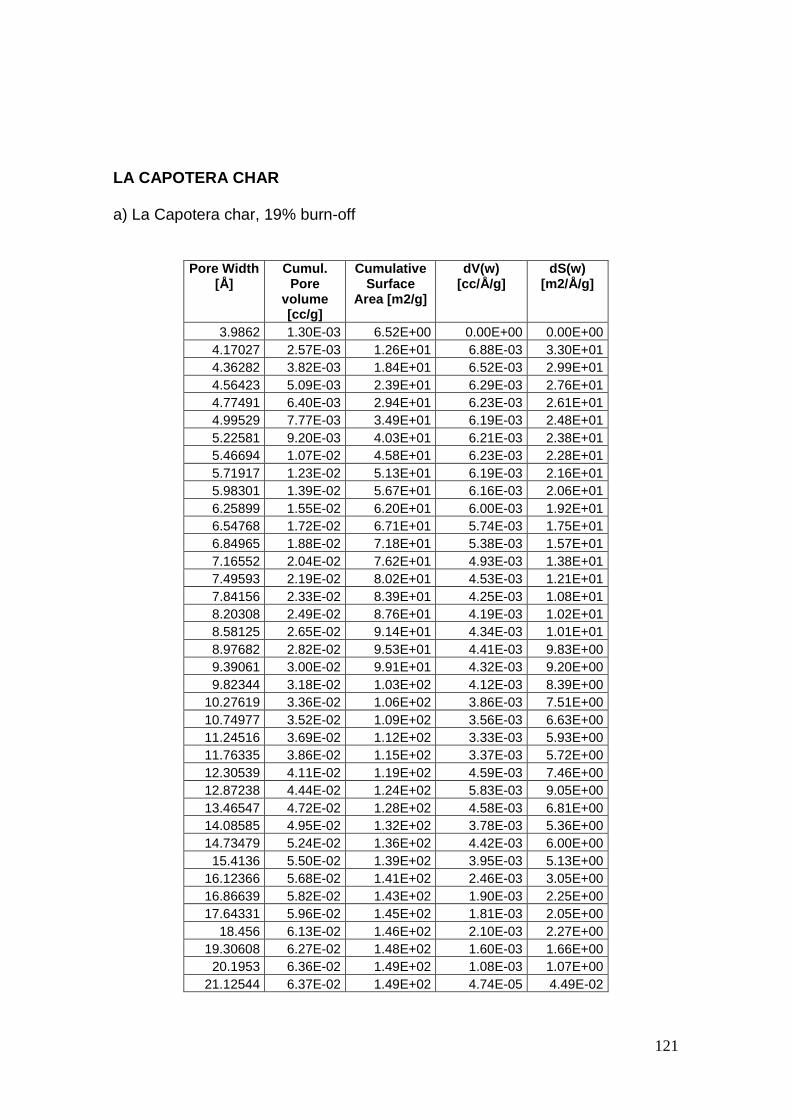
121

LA CAPOTERA CHAR a) La Capotera char, 19% burn-off

Pore Width [Å]

Cumul. Pore

volume [cc/g]

Cumulative Surface

Area [m2/g]

dV(w) [cc/Å/g]

dS(w) [m2/Å/g]

3.9862 1.30E-03 6.52E+00 0.00E+00 0.00E+00 4.17027 2.57E-03 1.26E+01 6.88E-03 3.30E+01 4.36282 3.82E-03 1.84E+01 6.52E-03 2.99E+01 4.56423 5.09E-03 2.39E+01 6.29E-03 2.76E+01 4.77491 6.40E-03 2.94E+01 6.23E-03 2.61E+01 4.99529 7.77E-03 3.49E+01 6.19E-03 2.48E+01 5.22581 9.20E-03 4.03E+01 6.21E-03 2.38E+01 5.46694 1.07E-02 4.58E+01 6.23E-03 2.28E+01 5.71917 1.23E-02 5.13E+01 6.19E-03 2.16E+01 5.98301 1.39E-02 5.67E+01 6.16E-03 2.06E+01 6.25899 1.55E-02 6.20E+01 6.00E-03 1.92E+01 6.54768 1.72E-02 6.71E+01 5.74E-03 1.75E+01 6.84965 1.88E-02 7.18E+01 5.38E-03 1.57E+01 7.16552 2.04E-02 7.62E+01 4.93E-03 1.38E+01 7.49593 2.19E-02 8.02E+01 4.53E-03 1.21E+01 7.84156 2.33E-02 8.39E+01 4.25E-03 1.08E+01 8.20308 2.49E-02 8.76E+01 4.19E-03 1.02E+01 8.58125 2.65E-02 9.14E+01 4.34E-03 1.01E+01 8.97682 2.82E-02 9.53E+01 4.41E-03 9.83E+00 9.39061 3.00E-02 9.91E+01 4.32E-03 9.20E+00 9.82344 3.18E-02 1.03E+02 4.12E-03 8.39E+00

10.27619 3.36E-02 1.06E+02 3.86E-03 7.51E+00 10.74977 3.52E-02 1.09E+02 3.56E-03 6.63E+00 11.24516 3.69E-02 1.12E+02 3.33E-03 5.93E+00 11.76335 3.86E-02 1.15E+02 3.37E-03 5.72E+00 12.30539 4.11E-02 1.19E+02 4.59E-03 7.46E+00 12.87238 4.44E-02 1.24E+02 5.83E-03 9.05E+00 13.46547 4.72E-02 1.28E+02 4.58E-03 6.81E+00 14.08585 4.95E-02 1.32E+02 3.78E-03 5.36E+00 14.73479 5.24E-02 1.36E+02 4.42E-03 6.00E+00

15.4136 5.50E-02 1.39E+02 3.95E-03 5.13E+00 16.12366 5.68E-02 1.41E+02 2.46E-03 3.05E+00 16.86639 5.82E-02 1.43E+02 1.90E-03 2.25E+00 17.64331 5.96E-02 1.45E+02 1.81E-03 2.05E+00

18.456 6.13E-02 1.46E+02 2.10E-03 2.27E+00 19.30608 6.27E-02 1.48E+02 1.60E-03 1.66E+00

20.1953 6.36E-02 1.49E+02 1.08E-03 1.07E+00 21.12544 6.37E-02 1.49E+02 4.74E-05 4.49E-02

122

Pore Width [Å]

Cumul. Pore

volume [cc/g]

Cumulative Surface

Area [m2/g]

dV(w) [cc/Å/g]

dS(w) [m2/Å/g]

22.0984 6.43E-02 1.49E+02 6.24E-04 5.65E-01 23.11614 6.60E-02 1.51E+02 1.74E-03 1.50E+00 24.18073 6.79E-02 1.52E+02 1.71E-03 1.42E+00 25.29431 6.98E-02 1.54E+02 1.73E-03 1.37E+00 26.45915 7.20E-02 1.56E+02 1.92E-03 1.45E+00 27.67761 7.42E-02 1.57E+02 1.77E-03 1.28E+00 28.95215 7.62E-02 1.59E+02 1.57E-03 1.09E+00 30.28536 7.79E-02 1.60E+02 1.28E-03 8.43E-01 31.67992 7.94E-02 1.61E+02 1.06E-03 6.68E-01 33.13868 8.08E-02 1.61E+02 1.00E-03 6.05E-01 34.66458 8.21E-02 1.62E+02 8.14E-04 4.70E-01 36.26072 8.32E-02 1.63E+02 7.34E-04 4.05E-01 37.93032 8.43E-02 1.63E+02 6.03E-04 3.18E-01 39.67677 8.51E-02 1.64E+02 5.05E-04 2.55E-01

41.5036 8.63E-02 1.64E+02 6.64E-04 3.20E-01 43.41452 8.76E-02 1.65E+02 6.34E-04 2.92E-01 45.41339 8.88E-02 1.65E+02 5.97E-04 2.63E-01 47.50428 8.99E-02 1.66E+02 5.62E-04 2.37E-01 49.69139 9.09E-02 1.66E+02 4.64E-04 1.87E-01 51.97918 9.18E-02 1.67E+02 3.89E-04 1.50E-01 54.37227 9.25E-02 1.67E+02 2.74E-04 1.01E-01 56.87551 9.30E-02 1.67E+02 1.95E-04 6.86E-02

Pore volume: 0.093 cc/g

Pore width (mode): 4.17 Å

123

b) La Capotera char, 35% burn-off

Pore Width [Å]

Cumul. Pore

volume [cc/g]

Cumulative Surface

Area [m2/g]

dV(w) [cc/Å/g]

dS(w) [m2/Å/g]




18.456 1.13E-01 2.90E+02 2.92E-03 3.16E+00 19.30608 1.15E-01 2.92E+02 2.14E-03 2.21E+00

20.1953 1.16E-01 2.93E+02 1.41E-03 1.39E+00 21.12544 1.16E-01 2.93E+02 3.10E-05 2.93E-02

22.0984 1.17E-01 2.94E+02 6.78E-04 6.13E-01 23.11614 1.19E-01 2.96E+02 2.17E-03 1.88E+00 24.18073 1.22E-01 2.98E+02 2.19E-03 1.81E+00

124

25.29431 1.24E-01 3.00E+02 2.29E-03 1.81E+00 26.45915 1.27E-01 3.02E+02 2.45E-03 1.85E+00 27.67761 1.30E-01 3.04E+02 2.28E-03 1.65E+00 28.95215 1.32E-01 3.06E+02 2.06E-03 1.42E+00 30.28536 1.35E-01 3.07E+02 1.65E-03 1.09E+00 31.67992 1.37E-01 3.08E+02 1.41E-03 8.90E-01 33.13868 1.39E-01 3.10E+02 1.38E-03 8.33E-01 34.66458 1.40E-01 3.11E+02 1.14E-03 6.60E-01 36.26072 1.42E-01 3.12E+02 1.06E-03 5.87E-01 37.93032 1.44E-01 3.12E+02 8.86E-04 4.67E-01 39.67677 1.45E-01 3.13E+02 7.36E-04 3.71E-01




125

c) La Capotera char, 61% burn-off

Pore Width [Å]

Cumul. Pore

volume [cc/g]

Cumulative Surface

Area [m2/g]

dV(w) [cc/Å/g]

dS(w) [m2/Å/g]




18.456 1.32E-01 3.45E+02 2.97E-03 3.21E+00 19.30608 1.34E-01 3.47E+02 2.28E-03 2.36E+00

20.1953 1.35E-01 3.48E+02 1.54E-03 1.53E+00 21.12544 1.35E-01 3.48E+02 1.03E-05 9.71E-03

22.0984 1.36E-01 3.49E+02 6.07E-04 5.49E-01 23.11614 1.38E-01 3.51E+02 2.12E-03 1.83E+00 24.18073 1.40E-01 3.53E+02 2.06E-03 1.71E+00

126

Pore Width [Å]

Cumul. Pore

volume [cc/g]

Cumulative Surface

Area [m2/g]

dV(w) [cc/Å/g]

dS(w) [m2/Å/g]

25.29431 1.43E-01 3.55E+02 2.27E-03 1.79E+00 26.45915 1.45E-01 3.57E+02 2.39E-03 1.81E+00 27.67761 1.48E-01 3.59E+02 2.26E-03 1.63E+00 28.95215 1.51E-01 3.60E+02 1.97E-03 1.36E+00 30.28536 1.53E-01 3.62E+02 1.50E-03 9.89E-01 31.67992 1.54E-01 3.63E+02 1.30E-03 8.23E-01 33.13868 1.56E-01 3.64E+02 1.37E-03 8.25E-01 34.66458 1.58E-01 3.65E+02 1.13E-03 6.51E-01 36.26072 1.60E-01 3.66E+02 9.41E-04 5.19E-01 37.93032 1.61E-01 3.67E+02 7.53E-04 3.97E-01 39.67677 1.62E-01 3.67E+02 6.58E-04 3.32E-01




127

d) La Capotera char, 85% burn-off

Pore Width [Å]

Cumul. Pore

volume [cc/g]

Cumulative Surface

Area [m2/g]

dV(w) [cc/Å/g]

dS(w) [m2/Å/g]




18.456 7.82E-02 2.06E+02 1.85E-03 2.01E+00 19.30608 7.94E-02 2.07E+02 1.44E-03 1.49E+00

20.1953 8.03E-02 2.08E+02 9.77E-04 9.68E-01 21.12544 8.03E-02 2.08E+02 3.78E-05 3.58E-02

22.0984 8.06E-02 2.08E+02 2.88E-04 2.61E-01 23.11614 8.20E-02 2.09E+02 1.33E-03 1.15E+00

128

Pore Width [Å]

Cumul. Pore

volume [cc/g]

Cumulative Surface

Area [m2/g]

dV(w) [cc/Å/g]

dS(w) [m2/Å/g]

24.18073 8.36E-02 2.11E+02 1.50E-03 1.24E+00 25.29431 8.54E-02 2.12E+02 1.64E-03 1.30E+00 26.45915 8.75E-02 2.14E+02 1.81E-03 1.37E+00 27.67761 8.97E-02 2.15E+02 1.77E-03 1.28E+00 28.95215 9.17E-02 2.17E+02 1.61E-03 1.11E+00 30.28536 9.35E-02 2.18E+02 1.34E-03 8.88E-01 31.67992 9.52E-02 2.19E+02 1.22E-03 7.71E-01 33.13868 9.70E-02 2.20E+02 1.22E-03 7.35E-01 34.66458 9.86E-02 2.21E+02 1.04E-03 6.02E-01 36.26072 1.00E-01 2.22E+02 9.23E-04 5.09E-01 37.93032 1.01E-01 2.22E+02 7.97E-04 4.20E-01 39.67677 1.03E-01 2.23E+02 7.51E-04 3.78E-01




129

LA GRANDE CHAR a) La Grande char, 23% burn-off

Pore Width [Å]

Cumul. Pore

volume [cc/g]

Cumulative Surface

Area [m2/g]

dV(w) [cc/Å/g]

dS(w) [m2/Å/g]



15.4136 1.44E-01 4.04E+02 3.80E-03 4.93E+00 16.12366 1.45E-01 4.05E+02 1.60E-03 1.98E+00 16.86639 1.45E-01 4.06E+02 7.92E-04 9.39E-01 17.64331 1.46E-01 4.06E+02 6.32E-04 7.17E-01

18.456 1.47E-01 4.07E+02 8.69E-04 9.41E-01 19.30608 1.47E-01 4.08E+02 6.23E-04 6.45E-01

20.1953 1.47E-01 4.08E+02 4.19E-04 4.15E-01 21.12544 1.48E-01 4.08E+02 1.59E-04 1.50E-01

130

Pore Width [Å]

Cumul. Pore

volume [cc/g]

Cumulative Surface

Area [m2/g]

dV(w) [cc/Å/g]

dS(w) [m2/Å/g]

22.0984 1.48E-01 4.09E+02 8.06E-04 7.30E-01 23.11614 1.49E-01 4.10E+02 1.03E-03 8.92E-01 24.18073 1.50E-01 4.11E+02 7.08E-04 5.85E-01 25.29431 1.51E-01 4.11E+02 4.75E-04 3.76E-01 26.45915 1.51E-01 4.11E+02 4.54E-04 3.43E-01 27.67761 1.52E-01 4.12E+02 3.03E-04 2.19E-01 28.95215 1.52E-01 4.12E+02 2.42E-04 1.67E-01 30.28536 1.52E-01 4.12E+02 1.77E-04 1.17E-01 31.67992 1.52E-01 4.12E+02 8.14E-05 5.14E-02 33.13868 1.52E-01 4.12E+02 4.23E-05 2.55E-02 34.66458 1.52E-01 4.12E+02 5.41E-05 3.12E-02 36.26072 1.52E-01 4.12E+02 5.91E-05 3.26E-02 37.93032 1.53E-01 4.12E+02 5.16E-05 2.72E-02 39.67677 1.53E-01 4.12E+02 2.31E-05 1.17E-02




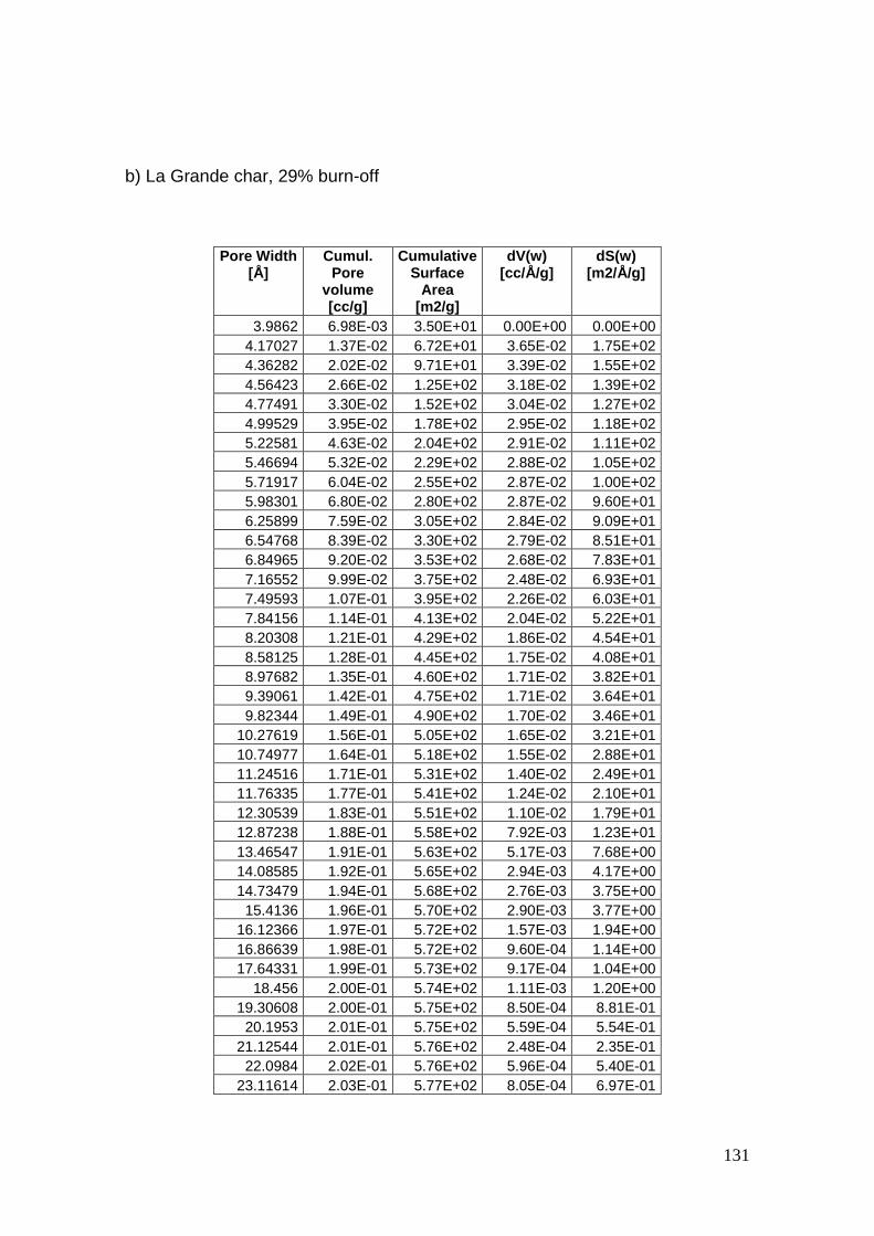
131

b) La Grande char, 29% burn-off

Pore Width [Å]

Cumul. Pore

volume [cc/g]

Cumulative Surface

Area [m2/g]

dV(w) [cc/Å/g]

dS(w) [m2/Å/g]




18.456 2.00E-01 5.74E+02 1.11E-03 1.20E+00 19.30608 2.00E-01 5.75E+02 8.50E-04 8.81E-01

20.1953 2.01E-01 5.75E+02 5.59E-04 5.54E-01 21.12544 2.01E-01 5.76E+02 2.48E-04 2.35E-01

22.0984 2.02E-01 5.76E+02 5.96E-04 5.40E-01 23.11614 2.03E-01 5.77E+02 8.05E-04 6.97E-01

132

Pore Width [Å]

Cumul. Pore

volume [cc/g]

Cumulative Surface

Area [m2/g]

dV(w) [cc/Å/g]

dS(w) [m2/Å/g]

24.18073 2.03E-01 5.77E+02 6.00E-04 4.96E-01 25.29431 2.04E-01 5.78E+02 5.38E-04 4.26E-01 26.45915 2.04E-01 5.78E+02 5.29E-04 4.00E-01 27.67761 2.05E-01 5.79E+02 4.17E-04 3.02E-01 28.95215 2.05E-01 5.79E+02 3.34E-04 2.31E-01 30.28536 2.06E-01 5.79E+02 2.38E-04 1.57E-01 31.67992 2.06E-01 5.79E+02 1.75E-04 1.11E-01 33.13868 2.06E-01 5.80E+02 1.68E-04 1.02E-01 34.66458 2.06E-01 5.80E+02 1.21E-04 6.99E-02 36.26072 2.06E-01 5.80E+02 9.95E-05 5.49E-02 37.93032 2.07E-01 5.80E+02 7.79E-05 4.11E-02 39.67677 2.07E-01 5.80E+02 4.97E-05 2.50E-02




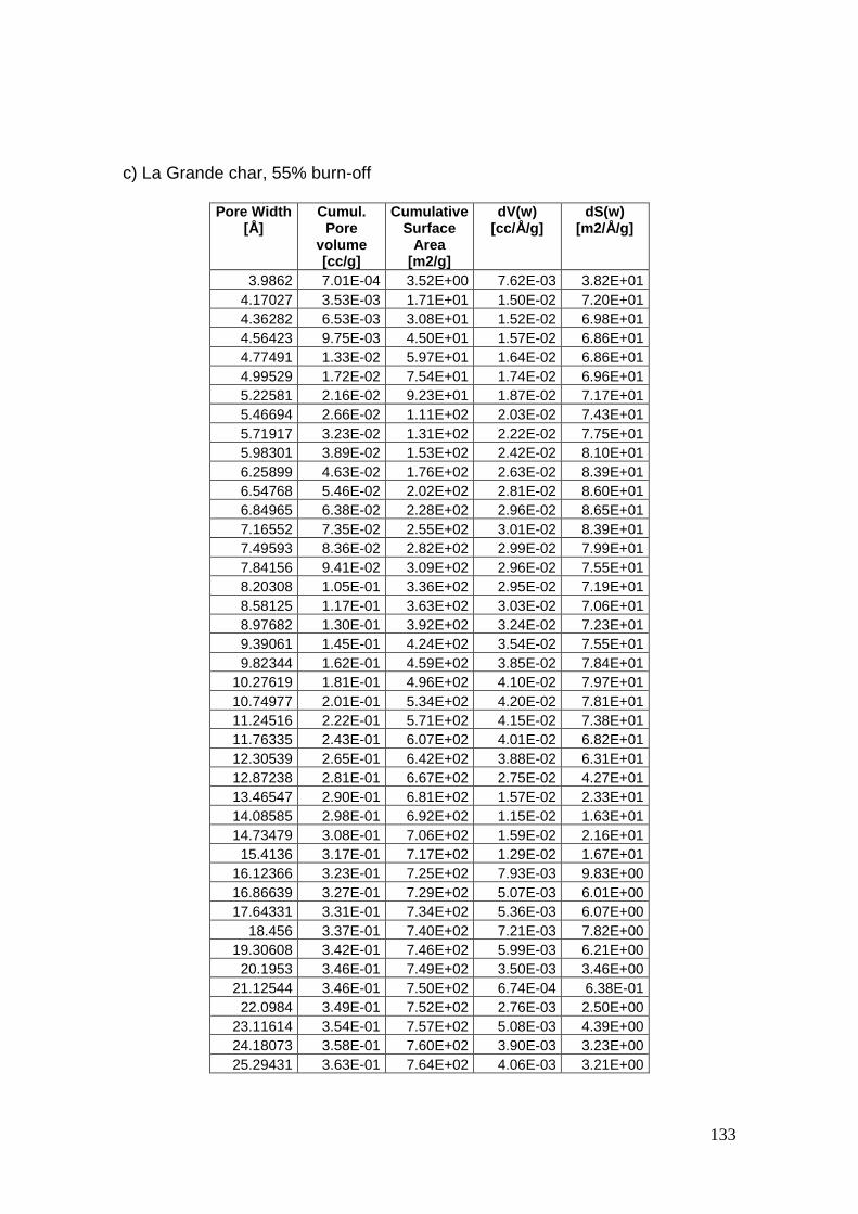
133

c) La Grande char, 55% burn-off

Pore Width [Å]

Cumul. Pore

volume [cc/g]

Cumulative Surface

Area [m2/g]

dV(w) [cc/Å/g]

dS(w) [m2/Å/g]

3.9862 7.01E-04 3.52E+00 7.62E-03 3.82E+01 4.17027 3.53E-03 1.71E+01 1.50E-02 7.20E+01 4.36282 6.53E-03 3.08E+01 1.52E-02 6.98E+01 4.56423 9.75E-03 4.50E+01 1.57E-02 6.86E+01 4.77491 1.33E-02 5.97E+01 1.64E-02 6.86E+01 4.99529 1.72E-02 7.54E+01 1.74E-02 6.96E+01 5.22581 2.16E-02 9.23E+01 1.87E-02 7.17E+01 5.46694 2.66E-02 1.11E+02 2.03E-02 7.43E+01 5.71917 3.23E-02 1.31E+02 2.22E-02 7.75E+01 5.98301 3.89E-02 1.53E+02 2.42E-02 8.10E+01 6.25899 4.63E-02 1.76E+02 2.63E-02 8.39E+01 6.54768 5.46E-02 2.02E+02 2.81E-02 8.60E+01 6.84965 6.38E-02 2.28E+02 2.96E-02 8.65E+01 7.16552 7.35E-02 2.55E+02 3.01E-02 8.39E+01 7.49593 8.36E-02 2.82E+02 2.99E-02 7.99E+01 7.84156 9.41E-02 3.09E+02 2.96E-02 7.55E+01 8.20308 1.05E-01 3.36E+02 2.95E-02 7.19E+01 8.58125 1.17E-01 3.63E+02 3.03E-02 7.06E+01 8.97682 1.30E-01 3.92E+02 3.24E-02 7.23E+01 9.39061 1.45E-01 4.24E+02 3.54E-02 7.55E+01 9.82344 1.62E-01 4.59E+02 3.85E-02 7.84E+01



18.456 3.37E-01 7.40E+02 7.21E-03 7.82E+00 19.30608 3.42E-01 7.46E+02 5.99E-03 6.21E+00

20.1953 3.46E-01 7.49E+02 3.50E-03 3.46E+00 21.12544 3.46E-01 7.50E+02 6.74E-04 6.38E-01


134

Pore Width [Å]

Cumul. Pore

volume [cc/g]

Cumulative Surface

Area [m2/g]

dV(w) [cc/Å/g]

dS(w) [m2/Å/g]

26.45915 3.68E-01 7.68E+02 4.19E-03 3.17E+00 27.67761 3.72E-01 7.71E+02 3.34E-03 2.41E+00 28.95215 3.76E-01 7.73E+02 2.72E-03 1.88E+00 30.28536 3.78E-01 7.75E+02 1.83E-03 1.21E+00 31.67992 3.80E-01 7.76E+02 1.18E-03 7.48E-01 33.13868 3.82E-01 7.77E+02 1.27E-03 7.67E-01 34.66458 3.83E-01 7.78E+02 8.58E-04 4.95E-01 36.26072 3.84E-01 7.78E+02 6.13E-04 3.38E-01 37.93032 3.85E-01 7.79E+02 4.53E-04 2.39E-01 39.67677 3.85E-01 7.79E+02 2.25E-04 1.13E-01

41.5036 3.86E-01 7.79E+02 4.07E-04 1.96E-01 43.41452 3.87E-01 7.80E+02 3.78E-04 1.74E-01 45.41339 3.88E-01 7.80E+02 3.66E-04 1.61E-01 47.50428 3.88E-01 7.80E+02 3.12E-04 1.31E-01 49.69139 3.89E-01 7.80E+02 1.99E-04 8.02E-02 51.97918 3.89E-01 7.81E+02 2.29E-04 8.82E-02 54.37227 3.90E-01 7.81E+02 4.08E-04 1.50E-01 56.87551 3.98E-01 7.84E+02 6.18E-03 2.17E+00



135

d) La Grande char, 72% burn-off

Pore Width [Å]

Cumul. Pore

volume [cc/g]

Cumulative Surface

Area [m2/g]

dV(w) [cc/Å/g]

dS(w) [m2/Å/g]

3.9862 6.17E-04 3.10E+00 6.71E-03 3.36E+01 4.17027 3.11E-03 1.50E+01 1.32E-02 6.34E+01 4.36282 5.75E-03 2.72E+01 1.34E-02 6.16E+01 4.56423 8.60E-03 3.97E+01 1.38E-02 6.06E+01 4.77491 1.17E-02 5.27E+01 1.45E-02 6.07E+01 4.99529 1.52E-02 6.67E+01 1.54E-02 6.17E+01 5.22581 1.91E-02 8.17E+01 1.66E-02 6.37E+01 5.46694 2.36E-02 9.80E+01 1.81E-02 6.61E+01 5.71917 2.87E-02 1.16E+02 1.97E-02 6.89E+01 5.98301 3.45E-02 1.35E+02 2.15E-02 7.20E+01 6.25899 4.11E-02 1.56E+02 2.33E-02 7.45E+01 6.54768 4.84E-02 1.79E+02 2.49E-02 7.62E+01 6.84965 5.65E-02 2.02E+02 2.62E-02 7.65E+01 7.16552 6.51E-02 2.26E+02 2.66E-02 7.42E+01 7.49593 7.41E-02 2.50E+02 2.65E-02 7.06E+01 7.84156 8.33E-02 2.74E+02 2.63E-02 6.70E+01 8.20308 9.31E-02 2.98E+02 2.63E-02 6.41E+01 8.58125 1.04E-01 3.22E+02 2.72E-02 6.35E+01 8.97682 1.15E-01 3.49E+02 2.92E-02 6.52E+01 9.39061 1.29E-01 3.77E+02 3.19E-02 6.79E+01 9.82344 1.44E-01 4.08E+02 3.45E-02 7.03E+01



18.456 3.42E-01 7.13E+02 1.23E-02 1.33E+01 19.30608 3.50E-01 7.21E+02 9.40E-03 9.74E+00

20.1953 3.56E-01 7.27E+02 6.31E-03 6.25E+00 21.12544 3.56E-01 7.27E+02 1.43E-04 1.35E-01

22.0984 3.58E-01 7.30E+02 2.52E-03 2.28E+00 23.11614 3.67E-01 7.37E+02 8.09E-03 7.00E+00

136

Pore Width [Å]

Cumul. Pore

volume [cc/g]

Cumulative Surface

Area [m2/g]

dV(w) [cc/Å/g]

dS(w) [m2/Å/g]

24.18073 3.74E-01 7.43E+02 6.88E-03 5.69E+00 25.29431 3.83E-01 7.50E+02 7.86E-03 6.21E+00 26.45915 3.94E-01 7.58E+02 8.87E-03 6.70E+00 27.67761 4.04E-01 7.65E+02 7.99E-03 5.77E+00 28.95215 4.13E-01 7.72E+02 7.08E-03 4.89E+00 30.28536 4.20E-01 7.76E+02 5.24E-03 3.46E+00 31.67992 4.26E-01 7.80E+02 4.25E-03 2.68E+00 33.13868 4.32E-01 7.84E+02 4.13E-03 2.49E+00 34.66458 4.36E-01 7.86E+02 2.53E-03 1.46E+00 36.26072 4.40E-01 7.88E+02 2.52E-03 1.39E+00 37.93032 4.44E-01 7.90E+02 2.08E-03 1.09E+00 39.67677 4.45E-01 7.91E+02 9.11E-04 4.59E-01

41.5036 4.48E-01 7.92E+02 1.32E-03 6.34E-01 43.41452 4.50E-01 7.93E+02 1.09E-03 5.00E-01 45.41339 4.52E-01 7.94E+02 8.44E-04 3.72E-01 47.50428 4.53E-01 7.95E+02 7.12E-04 3.00E-01 49.69139 4.54E-01 7.95E+02 4.89E-04 1.97E-01 51.97918 4.55E-01 7.96E+02 4.23E-04 1.63E-01 54.37227 4.57E-01 7.96E+02 6.85E-04 2.52E-01 56.87551 4.65E-01 7.99E+02 6.25E-03 2.20E+00



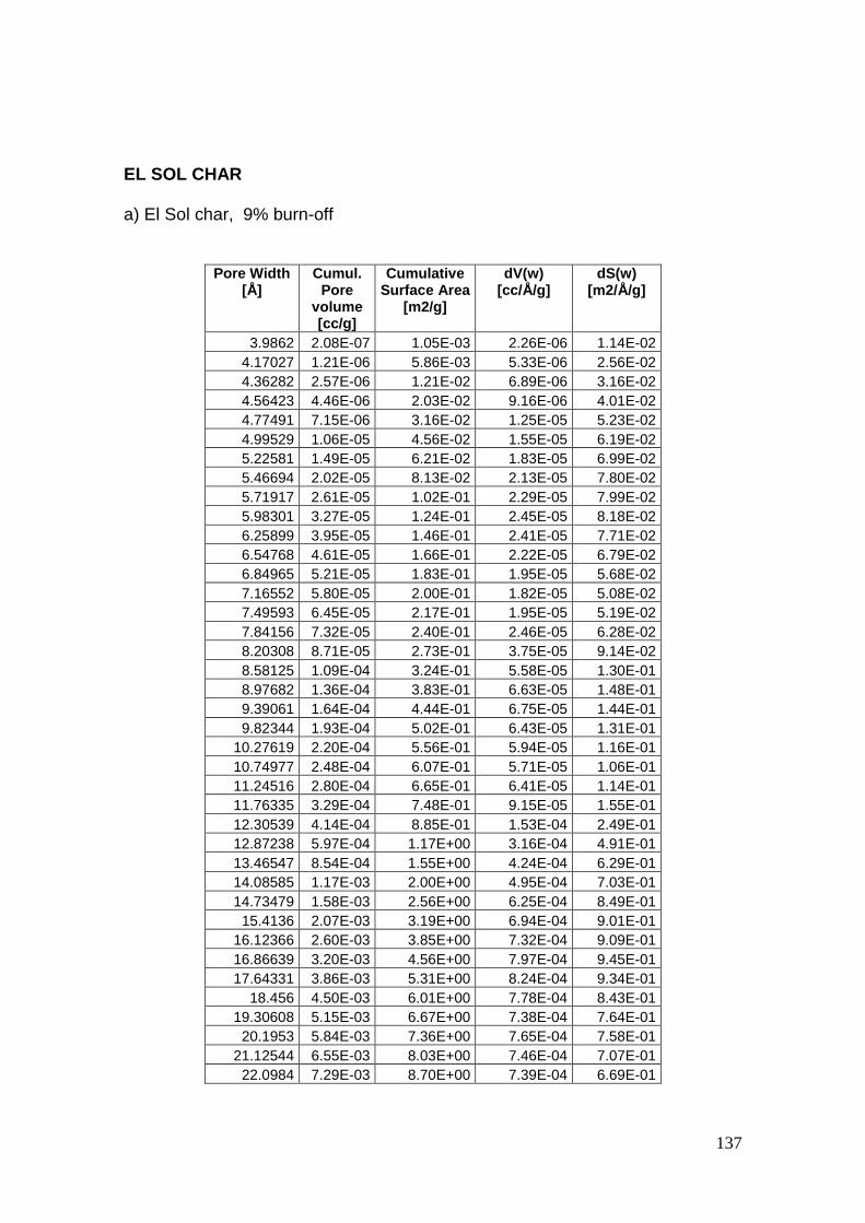
137

EL SOL CHAR a) El Sol char, 9% burn-off

Pore Width [Å]

Cumul. Pore

volume [cc/g]

Cumulative Surface Area

[m2/g]

dV(w) [cc/Å/g]

dS(w) [m2/Å/g]

3.9862 2.08E-07 1.05E-03 2.26E-06 1.14E-02 4.17027 1.21E-06 5.86E-03 5.33E-06 2.56E-02 4.36282 2.57E-06 1.21E-02 6.89E-06 3.16E-02 4.56423 4.46E-06 2.03E-02 9.16E-06 4.01E-02 4.77491 7.15E-06 3.16E-02 1.25E-05 5.23E-02 4.99529 1.06E-05 4.56E-02 1.55E-05 6.19E-02 5.22581 1.49E-05 6.21E-02 1.83E-05 6.99E-02 5.46694 2.02E-05 8.13E-02 2.13E-05 7.80E-02 5.71917 2.61E-05 1.02E-01 2.29E-05 7.99E-02 5.98301 3.27E-05 1.24E-01 2.45E-05 8.18E-02 6.25899 3.95E-05 1.46E-01 2.41E-05 7.71E-02 6.54768 4.61E-05 1.66E-01 2.22E-05 6.79E-02 6.84965 5.21E-05 1.83E-01 1.95E-05 5.68E-02 7.16552 5.80E-05 2.00E-01 1.82E-05 5.08E-02 7.49593 6.45E-05 2.17E-01 1.95E-05 5.19E-02 7.84156 7.32E-05 2.40E-01 2.46E-05 6.28E-02 8.20308 8.71E-05 2.73E-01 3.75E-05 9.14E-02 8.58125 1.09E-04 3.24E-01 5.58E-05 1.30E-01 8.97682 1.36E-04 3.83E-01 6.63E-05 1.48E-01 9.39061 1.64E-04 4.44E-01 6.75E-05 1.44E-01 9.82344 1.93E-04 5.02E-01 6.43E-05 1.31E-01

10.27619 2.20E-04 5.56E-01 5.94E-05 1.16E-01 10.74977 2.48E-04 6.07E-01 5.71E-05 1.06E-01 11.24516 2.80E-04 6.65E-01 6.41E-05 1.14E-01 11.76335 3.29E-04 7.48E-01 9.15E-05 1.55E-01 12.30539 4.14E-04 8.85E-01 1.53E-04 2.49E-01 12.87238 5.97E-04 1.17E+00 3.16E-04 4.91E-01 13.46547 8.54E-04 1.55E+00 4.24E-04 6.29E-01 14.08585 1.17E-03 2.00E+00 4.95E-04 7.03E-01 14.73479 1.58E-03 2.56E+00 6.25E-04 8.49E-01

15.4136 2.07E-03 3.19E+00 6.94E-04 9.01E-01 16.12366 2.60E-03 3.85E+00 7.32E-04 9.09E-01 16.86639 3.20E-03 4.56E+00 7.97E-04 9.45E-01 17.64331 3.86E-03 5.31E+00 8.24E-04 9.34E-01

18.456 4.50E-03 6.01E+00 7.78E-04 8.43E-01 19.30608 5.15E-03 6.67E+00 7.38E-04 7.64E-01

20.1953 5.84E-03 7.36E+00 7.65E-04 7.58E-01 21.12544 6.55E-03 8.03E+00 7.46E-04 7.07E-01

22.0984 7.29E-03 8.70E+00 7.39E-04 6.69E-01

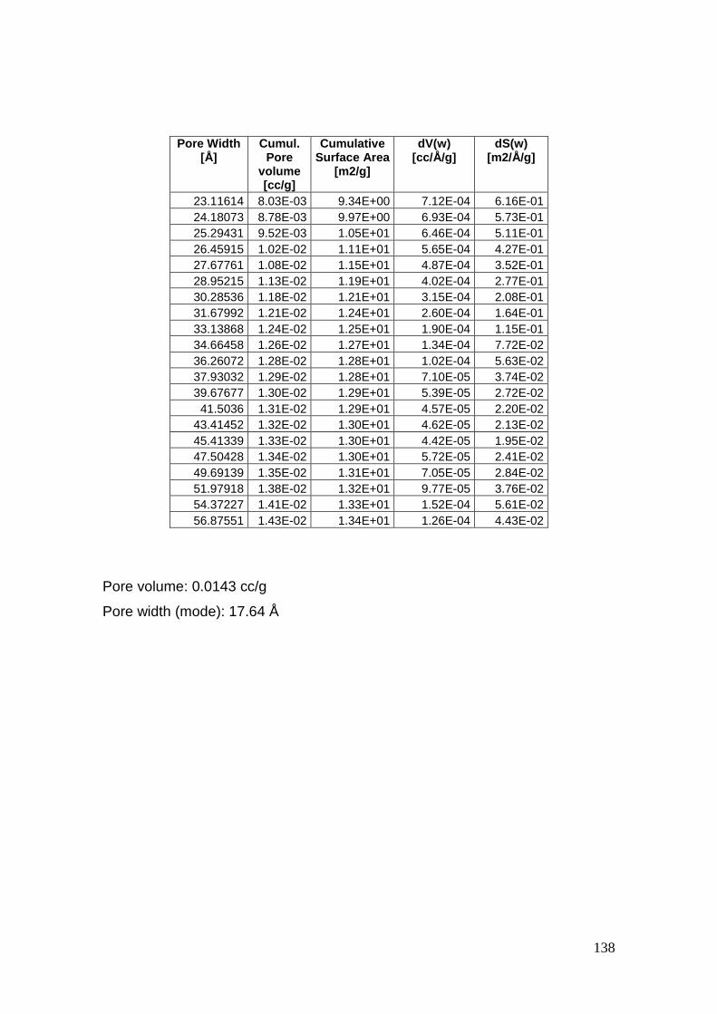
138

Pore Width [Å]

Cumul. Pore

volume [cc/g]


[m2/g]

dV(w) [cc/Å/g]

dS(w) [m2/Å/g]

23.11614 8.03E-03 9.34E+00 7.12E-04 6.16E-01 24.18073 8.78E-03 9.97E+00 6.93E-04 5.73E-01 25.29431 9.52E-03 1.05E+01 6.46E-04 5.11E-01 26.45915 1.02E-02 1.11E+01 5.65E-04 4.27E-01 27.67761 1.08E-02 1.15E+01 4.87E-04 3.52E-01 28.95215 1.13E-02 1.19E+01 4.02E-04 2.77E-01 30.28536 1.18E-02 1.21E+01 3.15E-04 2.08E-01 31.67992 1.21E-02 1.24E+01 2.60E-04 1.64E-01 33.13868 1.24E-02 1.25E+01 1.90E-04 1.15E-01 34.66458 1.26E-02 1.27E+01 1.34E-04 7.72E-02 36.26072 1.28E-02 1.28E+01 1.02E-04 5.63E-02 37.93032 1.29E-02 1.28E+01 7.10E-05 3.74E-02 39.67677 1.30E-02 1.29E+01 5.39E-05 2.72E-02




139

b) El Sol char, 16% burn-off

Pore Width [Å]

Cumul. Pore

volume [cc/g]


[m2/g]

dV(w) [cc/Å/g]

dS(w) [m2/Å/g]



15.4136 4.39E-02 1.22E+02 1.32E-03 1.71E+00 16.12366 4.44E-02 1.22E+02 6.44E-04 7.99E-01 16.86639 4.46E-02 1.23E+02 3.49E-04 4.14E-01 17.64331 4.49E-02 1.23E+02 3.02E-04 3.43E-01

18.456 4.52E-02 1.23E+02 3.53E-04 3.83E-01 19.30608 4.54E-02 1.24E+02 2.34E-04 2.43E-01

20.1953 4.55E-02 1.24E+02 1.22E-04 1.21E-01 21.12544 4.55E-02 1.24E+02 9.39E-06 8.89E-03

22.0984 4.58E-02 1.24E+02 3.81E-04 3.45E-01 23.11614 4.64E-02 1.24E+02 5.55E-04 4.80E-01 24.18073 4.68E-02 1.25E+02 3.76E-04 3.11E-01

140

Pore Width [Å]

Cumul. Pore

volume [cc/g]


[m2/g]

dV(w) [cc/Å/g]

dS(w) [m2/Å/g]

25.29431 4.71E-02 1.25E+02 2.50E-04 1.98E-01 26.45915 4.73E-02 1.25E+02 2.04E-04 1.54E-01 27.67761 4.75E-02 1.25E+02 1.67E-04 1.21E-01 28.95215 4.77E-02 1.25E+02 1.32E-04 9.09E-02 30.28536 4.78E-02 1.26E+02 9.14E-05 6.03E-02 31.67992 4.79E-02 1.26E+02 5.57E-05 3.52E-02 33.13868 4.79E-02 1.26E+02 3.80E-05 2.29E-02 34.66458 4.80E-02 1.26E+02 2.19E-05 1.27E-02 36.26072 4.80E-02 1.26E+02 2.31E-05 1.27E-02 37.93032 4.81E-02 1.26E+02 2.40E-05 1.26E-02 39.67677 4.81E-02 1.26E+02 2.07E-05 1.04E-02




141

c) El Sol char, 29% burn-off

Pore Width [Å]

Cumul. Pore

volume [cc/g]

Cumulative Surface

Area [m2/g]

dV(w) [cc/Å/g]

dS(w) [m2/Å/g]



15.4136 8.06E-02 2.33E+02 1.27E-03 1.65E+00 16.12366 8.11E-02 2.34E+02 6.52E-04 8.09E-01 16.86639 8.13E-02 2.34E+02 3.75E-04 4.45E-01 17.64331 8.16E-02 2.34E+02 3.28E-04 3.71E-01

18.456 8.19E-02 2.35E+02 4.13E-04 4.47E-01 19.30608 8.22E-02 2.35E+02 3.56E-04 3.69E-01

20.1953 8.24E-02 2.35E+02 2.33E-04 2.31E-01 21.12544 8.25E-02 2.35E+02 9.04E-05 8.56E-02

22.0984 8.29E-02 2.36E+02 4.18E-04 3.78E-01 23.11614 8.35E-02 2.36E+02 5.69E-04 4.92E-01 24.18073 8.39E-02 2.37E+02 3.66E-04 3.03E-01

142

Pore Width [Å]

Cumul. Pore

volume [cc/g]

Cumulative Surface

Area [m2/g]

dV(w) [cc/Å/g]

dS(w) [m2/Å/g]

25.29431 8.42E-02 2.37E+02 2.34E-04 1.85E-01 26.45915 8.44E-02 2.37E+02 1.97E-04 1.49E-01 27.67761 8.46E-02 2.37E+02 1.54E-04 1.11E-01 28.95215 8.47E-02 2.37E+02 1.23E-04 8.47E-02 30.28536 8.49E-02 2.37E+02 8.24E-05 5.44E-02 31.67992 8.49E-02 2.37E+02 3.87E-05 2.44E-02 33.13868 8.49E-02 2.37E+02 1.75E-05 1.06E-02 34.66458 8.50E-02 2.37E+02 2.41E-05 1.39E-02 36.26072 8.50E-02 2.37E+02 2.26E-05 1.24E-02 37.93032 8.50E-02 2.37E+02 1.85E-05 9.75E-03 39.67677 8.51E-02 2.37E+02 1.04E-05 5.25E-03




143

d) El Sol char, 63% burn-off

Pore Width [Å]

Cumul. Pore

volume [cc/g]

Cumulative Surface

Area [m2/g]

dV(w) [cc/Å/g]

dS(w) [m2/Å/g]



15.4136 1.04E-01 2.95E+02 2.18E-03 2.82E+00 16.12366 1.05E-01 2.97E+02 1.18E-03 1.46E+00 16.86639 1.06E-01 2.97E+02 7.11E-04 8.44E-01 17.64331 1.06E-01 2.98E+02 5.85E-04 6.64E-01

18.456 1.07E-01 2.98E+02 6.33E-04 6.86E-01 19.30608 1.07E-01 2.99E+02 4.41E-04 4.57E-01

20.1953 1.07E-01 2.99E+02 2.47E-04 2.44E-01 21.12544 1.07E-01 2.99E+02 1.42E-04 1.35E-01

22.0984 1.08E-01 2.99E+02 3.65E-04 3.30E-01 23.11614 1.08E-01 3.00E+02 4.35E-04 3.76E-01

144

Pore Width [Å]

Cumul. Pore

volume [cc/g]

Cumulative Surface

Area [m2/g]

dV(w) [cc/Å/g]

dS(w) [m2/Å/g]

24.18073 1.09E-01 3.00E+02 2.81E-04 2.32E-01 25.29431 1.09E-01 3.00E+02 1.94E-04 1.53E-01 26.45915 1.09E-01 3.00E+02 1.57E-04 1.19E-01 27.67761 1.09E-01 3.00E+02 1.17E-04 8.43E-02 28.95215 1.09E-01 3.00E+02 1.04E-04 7.17E-02 30.28536 1.09E-01 3.00E+02 7.33E-05 4.84E-02 31.67992 1.09E-01 3.01E+02 4.84E-05 3.06E-02 33.13868 1.09E-01 3.01E+02 3.04E-05 1.83E-02 34.66458 1.09E-01 3.01E+02 2.51E-05 1.45E-02 36.26072 1.10E-01 3.01E+02 3.39E-05 1.87E-02 37.93032 1.10E-01 3.01E+02 3.13E-05 1.65E-02 39.67677 1.10E-01 3.01E+02 4.05E-07 1.92E-04




145

APPENDIX B. FLOW CHART FOR MODEL SOLUTION PROGRAM

146

The program for model solution was done in Fortran. The flow chart for the

program is shown in Figure 48.

Figure 48. Flow chart for model solution program

Input parameters: intrinsic reaction rate, temperature, particle radii, true density, psi, alpha, phi.

Input initial values: gas concentration profile, carbon conversion profile, porosity

Calculate initial moments

Calculate Jacobi roots, Aij, Bij

Set NN=1

Solve Mass balance equations (Solve differential equations by Adams Moulton Method using IVPAG routine)

new: gas concentration profile, carbon conversion profile, porosity

Calculate new moments by solving population balance equations (Solve differential equations by Adams Moulton Method using IVPAG routine)

Calculate standard deviation, variance and other parameters for log-normal distribution (A priori distribution shape)

Calculate pore size distribution as a function of pore radii

Set NN=2…..J

T=NN*∆T

147

APPENDIX C. EXECUTIVE SUMMARY

148

A mathematical model for pore development during physical distribution of

chars was proposed. The model is based on mass balance and population

balance equations. The reaction rate is calculated according to the Random

Pore Model , proposed by Bhatia and Perlmutter and the population balance for

the pore size distribution is developed following the equations proposed by

Hashimoto and Silveston.

• Balance for CO2

2 2

2

2 '''2

1CO CO

co COef

C CD r R

t r r r

ε−

∂ ∂ ∂= − ∂ ∂ ∂ (C1)

• Balance for CO

2

2 '''2

12

CO CO

co COef

C CD r R

t r r r

ε−

∂ ∂∂ = + ∂ ∂ ∂ (C2)

• Balance for Carbon

'''cCR

t

∂ = −∂

(C3)

Here '''R is a reaction rate per volume unit. Generally the accumulation term

could be eliminated because it is several orders of magnitude smaller than the

other terms, however it will be kept trying to get more accurate results :

Expressing the effective diffusivity as:

149

2

2

CO CO

CO COeft

DD

ετ

−

−=

Where DCO2-CO is the molecular diffusivity and τ t =1/ε is the tortuosity factor. For

calculate the reaction rate, the Random Pore Model was selected. This model

was selected due to it has few adjustable parameters and is very simple.

According to the Random Pore Model the expression for surface area evolution

is given by equation (C4)

0 1 ln(1 )g gS S X= − Ψ − (C4)

Where 0

20

4 g

t g

L

S

πρ

Ψ = is a structural parameter that is related to the initial total pore

length Lg0 (m/g) and the initial specific surface area Sg0.

Then the reaction rate will be

Where k is the intrinsic reaction rate constant, ρt is the true density of the solid

and ε is the porosity.

Then mass balance equations (C1-C3), can be written in dimensionless form

as:

2 22 2

* 1 1 **(1 ) 1 ln(1 )

C CC X


∂ ∂ ∂= − − − Ψ − ∂ ∂ ∂ (C5)

'''2 0(1 ) 1 ln(1 )co t gR kC S Xρ ε= − − Ψ −

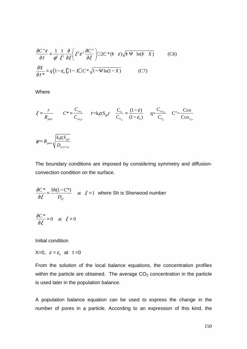
150

2 22 2

" 1 1 "2 *(1 ) 1 ln(1 )

C CC X


∂ ∂ ∂= + − − Ψ − ∂ ∂ ∂ (C6)

( )( )01 1 * 1 ln(1 )*

Xq X C Xε

τ∂ = − − − Ψ −∂

(C7)

Where

22

2 0 0

Ct g0

C 0

C (1 ) * =k S q=

C (1 )Scoco

part co s C

CCrC t

R C C

εξ τ ρε

−= = =−

2,s

CcoC"=

Cco

0

2

t gpart

co co

k SR

D

ρφ

−

=

The boundary conditions are imposed by considering symmetry and diffusion-

convection condition on the surface.

* (1 *) at 1

ef

C Sh C

Dξ

ξ∂ −= =∂

where Sh is Sherwood number

*0 at 0

C ξξ

∂ = =∂

Initial condition

X=0, 0ε ε= at t =0

From the solution of the local balance equations, the concentration profiles

within the particle are obtained. The average CO2 concentration in the particle

is used later in the population balance.

A population balance equation can be used to express the change in the

number of pores in a particle. According to an expression of this kind, the

151

change of the number of pores is due to process of birth (B), death (D) and

growing as it is shown in equation (C8):

0p

p

rff B D

t r t

∂ ∂ ∂+ − + = ∂ ∂ ∂ (C8)

Hashimoto and Silveston used a population balance equation to describe the

development of surface area, volume and porosity during gasification. The

expressions proposed by these authors to birth and death of pores are:

Formation of new pores (Bf) :

( )f f g s p rB k C r rρ δ= −

Formation of pores due to combination of pores (Bc):

1 1 1

0

1( )

2

rpr

Bc f r f r drφα

= −

∫

Removal of pores due to combination of pores (D):

1 1

0

( ) ( )pD f r f r drφ∞

= ∫

Considering all these terms in equation (C8), the population balance equation

can be written as:

152

2 1 1 1

0

1 1

0

1( ) ( )

2

( ) ( ) 0

rp

f CO s p rp

p

rf rf k C r r f r f r dr

t r t

f r f r dr

ρ δ φα

φ∞

∂ ∂ ∂ + − − − − ∂ ∂ ∂

+ =

∫

∫ (C9)

φ is the probability that adjacent pores grow sufficiently in the time period dt to

come in contact. δ is Dirac delta function taking a nonzero value only when the

pore radius is rf that is the value of the pore radius of the new fine pores that are

formed. kf is a specific rate constant for pore initiation that in the solution of the

model is taken proportional to the intrinsic reaction rate and α is a parameter

that indicates the average pore size of the new pores formed by pore

combination. Then the value of α is in the range [0.5, 1.0]

Multiplying by rpn , and by definition

0

npn

p

r fMdr

t t

∞ ∂∂ =∂ ∂∫ then equation can be

written as:

12 1 1 1

0 0 0

1( ) 0

2

rn n np pn

p p f p CO s p p o n

dr rMn r fdr k r C r f r f r dr dr M M

t dtρ φ φ

α

∞ ∞− ∂ + − − − + = ∂

∫ ∫ ∫

(C10)

n takes its value depending on the order of the moment. To eliminate the double

integral, a change in the integration limits is done and the integral is expressed

as an expansion. Then the term for birth due to pore combination can be written

as

1

0

1

2

nn

n i ii

nBc M M

iα φ+

−=

=

∑

153

And the moment equations can be written as:

2 202 0 0

10

2f CO s

Mk C M M

tρ αφ φ∂ − − + =

∂ (C11)

210 2 1 0 0 1 0p

f f CO s

drMM k r C M M M M

t dtρ α φ φ∂ + − − + =

∂ (C12)

2 3 3 221 2 2 0 1 0 22 0p

f f CO s

drMM k r C M M M M M

t dtρ α φ α φ φ∂ + − − − + =

∂ (C13)

3 4 432 2 3 0 1 2 0 33 3 0p

f f CO s

drMM k r C M M M M M M

t dtρ α φ α φ φ∂ + − − − + =

∂ (C14)

The expression to calculate the variation of rp is given by:

2 2Mwp CO CO

t

dr kC

dt ρ=

Here MwCO2 is the molecular weight of CO2. CCO2 is the average concentration

of the reactant gas inside the particle. It is calculated based on the gas

concentration profile obtained from the mass balance equations.

Hashimoto and Silveston used the above expressions to obtain the evolution of

surface area, volume and average pore radius. However these authors did not

obtain pore size distribution. In this work, the above equations system is solved

to obtain the pore size distribution as the reaction takes place. As initial

conditions the first, second and third moments of a function obtained by fitting

the experimental pore size distribution of a low carbon conversion char to a

polynomial equation, were used.

154

Equations (C5-C7) were solved by the Orthogonal Collocation Method. The

Equations (C11-C14) were solved by the reconstruction of the distribution from

its moments using a priori distribution shape.In this technique the moments are

related to the parameters of the distribution; in this case the Log-normal

distribution was selected due to its shape represents in good agreement the

typical size distributions. In Table C1 the parameters of this distribution and

their relation with the different moments are shown.

2

2

ln ( / )1( ) exp

2lnln 2g

gg

x xf x

x σσ π

= −

(C15)

Where ( )2g v2

=exp ln(c 1)exp(0.5ln )g

g

xx σ

σ= +

Table C1. General Parameters of Log-normal distrib ution

Parameter Relation

Mean size 1 0/x M M=

Coefficient of variation 0 2

21

1v

M Mc

M= −

Standard deviation 0 21

20 1

1M MM

M Mσ = −

The results were compared with experimental data obtained by the activation

with CO2 of three coal chars: La Capotera, La Grande and El Sol that exhibit

different reactivity. By using two adjustable parameters, the probability of pore

combination (φ) and a factor for the pore radii combination (α), the theoretical

155

model allows establishing the occurrence and prevalence of phenomenon of

formation and combination of pores during the activation. However, the model


beginning of the process of gasification. These closed pores can have an

important effect on the pore size distribution as the shape of the pore size

distribution at low carbon conversion is different when compared to the

distribution at higher carbon conversion degree. This phenomenon should be

considered as an additional term in future refinements of our model.

mathematical model for pore development during physical ...a mathematical model for pore development...

Documents