mathematical epidemiology - univ-lorraine.frgauthier.sallet/lecture-notes-pretoria-2018.pdf · and...
TRANSCRIPT

Mathematical Epidemiology
Gauthier SalletEmeritus Professor
Institut Elie Cartan, UMR CNRS 7502Universite de Lorraine
March 2018

2

Contents
0.1 Preface . . . . . . . . . . . . . . . . . . . . . . . . . . . . . . . 7
1 Introduction and Important Concepts 9
1.1 Mathematical modeling of infectious diseases . . . . . . . . . . 9
1.2 Deterministic epidemic models : compartmental approach . . . 12
1.2.1 Compartmental equations . . . . . . . . . . . . . . . . 14
1.2.2 Graphic representations . . . . . . . . . . . . . . . . . 18
1.2.3 An example : The Kermack–McKendrick Model . . . . 18
1.2.4 Transfer rates . . . . . . . . . . . . . . . . . . . . . . . 20
2 Some Classical Examples 23
2.1 Introduction . . . . . . . . . . . . . . . . . . . . . . . . . . . 23
2.2 Natural history of Malaria . . . . . . . . . . . . . . . . . . . . 26
2.2.1 In Liver . . . . . . . . . . . . . . . . . . . . . . . . . . 27
2.2.2 In blood . . . . . . . . . . . . . . . . . . . . . . . . . . 28
2.2.3 The vector . . . . . . . . . . . . . . . . . . . . . . . . 31
2.3 Building the model . . . . . . . . . . . . . . . . . . . . . . . . 32
2.3.1 Infectious human evolution . . . . . . . . . . . . . . . 34
2.3.2 Infectious mosquito population . . . . . . . . . . . . . 36
2.3.3 Ross model, final form . . . . . . . . . . . . . . . . . . 37
2.4 Ross model analysis . . . . . . . . . . . . . . . . . . . . . . . . 39
3

4 CONTENTS
2.5 Malaria intra-host model . . . . . . . . . . . . . . . . . . . . . 40
2.6 SEIR model . . . . . . . . . . . . . . . . . . . . . . . . . . . 41
3 Basic Mathematical Tools and Techniques 45
3.1 Well-posedness of a model . . . . . . . . . . . . . . . . . . . . 45
3.1.1 Examples . . . . . . . . . . . . . . . . . . . . . . . . . 52
3.1.2 Kermack-McKendrick model . . . . . . . . . . . . . . . 52
3.1.3 Ross model . . . . . . . . . . . . . . . . . . . . . . . . 53
3.2 Lyapunov techniques . . . . . . . . . . . . . . . . . . . . . . . 53
3.2.1 Problematics . . . . . . . . . . . . . . . . . . . . . . . 53
3.2.2 Lyapunov functions . . . . . . . . . . . . . . . . . . . . 56
3.2.3 Theorems . . . . . . . . . . . . . . . . . . . . . . . . . 56
3.2.4 Examples . . . . . . . . . . . . . . . . . . . . . . . . . 59
3.2.5 How to find a Lyapunov function ? . . . . . . . . . . . 61
3.2.6 Lyapunov and Ross model . . . . . . . . . . . . . . . . 63
3.3 Proofs of the Theorems . . . . . . . . . . . . . . . . . . . . . . 67
3.4 SEIR example . . . . . . . . . . . . . . . . . . . . . . . . . . 72
3.4.1 Stability of the DFE . . . . . . . . . . . . . . . . . . . 73
3.4.2 Stability of the DFE . . . . . . . . . . . . . . . . . . . 73
3.4.3 Stability of the EE . . . . . . . . . . . . . . . . . . . . 74
3.5 Last example . . . . . . . . . . . . . . . . . . . . . . . . . . . 76
3.6 Reduction of systems and Vidyasagar’s Theorem . . . . . . . . 77
4 The concept of basic reproduction ratio R0 83
4.1 Introduction . . . . . . . . . . . . . . . . . . . . . . . . . . . . 83
4.2 The structure of compartmental epidemiological models . . . . 85
4.2.1 Definition of R0 . . . . . . . . . . . . . . . . . . . . . 90
4.2.2 Biological interpretation of R0 . . . . . . . . . . . . . . 91

CONTENTS 5
4.3 R0 is a threshold . . . . . . . . . . . . . . . . . . . . . . . . . 92
4.3.1 Varga’s Theorem . . . . . . . . . . . . . . . . . . . . . 93
4.4 Examples . . . . . . . . . . . . . . . . . . . . . . . . . . . . . 95
5 Monotone systems in Epidemiology 97
5.1 Generalities . . . . . . . . . . . . . . . . . . . . . . . . . . . . 97
5.1.1 Introduction . . . . . . . . . . . . . . . . . . . . . . . 97
5.1.2 Generalities and Notations. Cones and Ordered rela-
tion . . . . . . . . . . . . . . . . . . . . . . . . . . . . 98
5.2 Monotone application and Monotone vector field . . . . . . . . 101
5.2.1 Monotone linear applications . . . . . . . . . . . . . . . 102
5.2.2 Metzler Matrices: Dynamical properties . . . . . . . . 103
5.2.3 Characterization of Hurwitz Metzler matrices . . . . . 104
5.3 Perron-Frobenius Theorems . . . . . . . . . . . . . . . . . . . 106
5.4 Irreducible Matrices . . . . . . . . . . . . . . . . . . . . . . . 108
5.4.1 Irreducible Metzler Matrices . . . . . . . . . . . . . . 110
5.4.2 Perron-Frobenius . . . . . . . . . . . . . . . . . . . . . 112
5.4.3 Stability modulus and order . . . . . . . . . . . . . . . 116
5.5 Characterization of Monotone Dynamical Systems . . . . . . . 119
5.6 Strongly monotone vector fields . . . . . . . . . . . . . . . . . 123
5.6.1 Linear vector fields strongly monotone . . . . . . . . . 123
5.7 A Convergence Criteria . . . . . . . . . . . . . . . . . . . . . . 125
5.8 Looking for invariant sets and equilibria . . . . . . . . . . . . 127
5.9 Sublinearity, positive invariance and equilibria . . . . . . . . . 129
5.10 A Theorem on stability . . . . . . . . . . . . . . . . . . . . . . 132
5.11 A Theorem from Hirsch . . . . . . . . . . . . . . . . . . . . . 133
5.12 Hirsch’s Theorem modified . . . . . . . . . . . . . . . . . . . . 134
5.13 Example : Gonnorhea . . . . . . . . . . . . . . . . . . . . . . 136

6 CONTENTS
5.14 Ross model in a patchy environment . . . . . . . . . . . . . . 138
5.14.1 The migration model . . . . . . . . . . . . . . . . . . 138
5.14.2 The Ross-Macdonald model on n patches . . . . . . . 138
5.14.3 Properties of the model . . . . . . . . . . . . . . . . . 140
5.14.4 Reduction of the system . . . . . . . . . . . . . . . . . 141
5.14.5 Main theorem . . . . . . . . . . . . . . . . . . . . . . 145
5.15 Wolbachia . . . . . . . . . . . . . . . . . . . . . . . . . . . . . 149
5.15.1 Monotonicity . . . . . . . . . . . . . . . . . . . . . . . 150
5.15.2 Strong monotonicity . . . . . . . . . . . . . . . . . . . 150
5.15.3 Equilibria . . . . . . . . . . . . . . . . . . . . . . . . . 151
5.15.4 Basic reproduction ratio . . . . . . . . . . . . . . . . . 152
5.15.5 Stability of the CWIE . . . . . . . . . . . . . . . . . . 153
5.15.6 Global analysis . . . . . . . . . . . . . . . . . . . . . . 153
5.16 Brucellosis . . . . . . . . . . . . . . . . . . . . . . . . . . . . . 155
5.17 Population dynamics of mosquito . . . . . . . . . . . . . . . . 157
5.17.1 The model . . . . . . . . . . . . . . . . . . . . . . . . . 158
5.17.2 Analysis of the model . . . . . . . . . . . . . . . . . . . 160
5.18 A schistosomiasis model . . . . . . . . . . . . . . . . . . . . . 161
5.19 Notes . . . . . . . . . . . . . . . . . . . . . . . . . . . . . . . . 164
6 Models with continuous delays 165
6.1 Introduction . . . . . . . . . . . . . . . . . . . . . . . . . . . . 165
6.2 Some historical background . . . . . . . . . . . . . . . . . . . 168
6.3 The Linear Chain Trick . . . . . . . . . . . . . . . . . . . . . . 169
6.4 Generalized linear chain trick . . . . . . . . . . . . . . . . . . 173
6.5 Application . . . . . . . . . . . . . . . . . . . . . . . . . . . . 176
6.5.1 Notations . . . . . . . . . . . . . . . . . . . . . . . . . 177
6.5.2 Hypotheses . . . . . . . . . . . . . . . . . . . . . . . . 178

0.1. PREFACE 7
6.6 Stability analysis for the one chain system . . . . . . . . . . . 179
6.6.1 Background . . . . . . . . . . . . . . . . . . . . . . . . 179
6.6.2 Basic reproduction ratio and Equilibria of the system . 180
6.6.3 Stability analysis . . . . . . . . . . . . . . . . . . . . . 181
6.7 Stability for the complete system . . . . . . . . . . . . . . . . 186
7 Identification of parameters. 187
7.1 Introduction . . . . . . . . . . . . . . . . . . . . . . . . . . . . 187
7.1.1 A non identifiable linear system . . . . . . . . . . . . . 187
7.1.2 Historical Background . . . . . . . . . . . . . . . . . . 189
7.2 Concepts from control theory . . . . . . . . . . . . . . . . . . 189
7.2.1 Observability . . . . . . . . . . . . . . . . . . . . . . . 189
7.2.2 Identifiability . . . . . . . . . . . . . . . . . . . . . . . 194
7.2.3 Observability, identifiability and augmented system . . 194
7.3 Examples . . . . . . . . . . . . . . . . . . . . . . . . . . . . . 196
7.3.1 Identification for an intra-host model of Malaria . . . 196
7.3.2 Identification for the Macdonald’s model of schistoso-
miasis transmission . . . . . . . . . . . . . . . . . . . . 199
7.3.3 Identification for Ross’ s model of malaria transmission 201
7.4 Identifiability and observers . . . . . . . . . . . . . . . . . . . 202
7.4.1 Definition . . . . . . . . . . . . . . . . . . . . . . . . . 202
7.4.2 An example : within-host model of Malaria . . . . . . 203
0.1 Preface
The origin of these lectures notes comes from a series of courses taught in
the University of Pretoria in Match 2018. There are, now, many books in

8 CONTENTS
mathematical epidemiology [14, 13, 20, 6, 57, 78] to cite a few. These lectures
notes consider only finite dimensional deterministic system, ODE for short.
In these lectures notes we have addressed some issues which are not commonly
treated elsewhere.
1. We have given detailed exposition on Lyapunov and LaSalle techniques
with examples from the literature. The reduction techniques of Vidyasagar
are given. They are used throughout these lectures, simplifying the
models by dimension reduction.
2. The exposition on R0 is now classical, but we try to clear the notion
of threshold in relation with Varga’s theorem;
3. We think that our exposition on Monotone systems with applications
to large scale epidemiological systems is original. All the results are
proven in details, results which are dispersed in the literature.
4. The linear chain trick is exposed and show how to deal with delays only
with ODE
5. The problem of parameters, identification and identifiability is intro-
duced with a control theory approach.
I would like to thanks the department of mathematics of UP, the staff and
their students for their warm welcome and to permit this opportunity to give
these lectures.

Chapter 1
Introduction and ImportantConcepts
1.1 Mathematical modeling of infectious dis-
eases
A disease is infectious if the causative agent, whether a virus, bacterium,
protozoa, or toxin, can be passed from one host to another through modes of
transmission such as direct physical contact, airborne droplets, water or food,
disease vectors, or mother to newborns. The objective of a mathematical
model of an infectious disease is to describe the transmission process of the
disease, which can be defined generally as follows: when infectious individuals
are introduced into a population of susceptibles, the disease is passed to other
individuals through its modes of transmission, and the disease spreads in the
group. An infected individual may remain asymptomatic at the early stage
of infection, only later developing clinical symptoms and being diagnosed as
a disease case.
Mathematical modeling can provide an understanding of the underlying
mechanisms of disease transmission and spread, help to pinpoint key factors
in the disease transmission process, suggest effective control and preventive
9

10 1. INTRODUCTION AND IMPORTANT CONCEPTS
measures, and provide an estimate for the severity and potential scale of the
epidemic. Put it simply, mathematical modeling should become part of the
toolbox of public health research and decision making.
The next question we would like to answer is: what is the general pro-
cess of mathematical modeling? Generally speaking, the modeling process
involves the following six stages:
1. Make assumptions about the disease transmission process based on the
best available biological knowledge on the pathogenesis of the infection
and epidemiology of the disease.
2. Set up mathematical models for the transmission process based on these
assumptions. This usually starts from drawing the transfer diagram
and then deriving the mathematical equations.
3. Perform mathematical analysis on the model to understand all possi-
ble qualitatively distinct model outcomes. This is typically done by
applying existing mathematical theories on stability and bifurcations
in conjunction with numerical simulations.
4. Interpret the mathematical findings within the modeling context. These
interpretations form our understanding of the disease transmission pro-
cess entailed by the set of assumptions made in Step (1).
5. Collect available disease data from public health agencies and from
research publications. Validate the model using data.
6. Improve the model by modifying the earlier assumptions in Step (1),
and produce a more accurate understanding of the disease process.
It is important to keep in mind that a mathematical model is always an
approximation of the real disease process. It is a mathematical translation of

1.1. MATHEMATICAL MODELING OF INFECTIOUS DISEASES 11
our hypotheses about the disease transmission process. Another important
role for mathematical models is hypothesis testing: by comparing the model
outcomes with existing knowledge or data of the disease, we can use the model
to test various hypotheses about the disease. Compared to experimental
approaches, the modeling approach has the advantage of saving enormous
amounts of time and resources.
There are three general approaches to mathematical modeling of infec-
tious diseases.
1. Statistical models. These models are very data oriented and are con-
structed to deal with a specific set of data.
• Advantages: statistical models widely used in epidemiology and
public health research.
• Drawbacks: statistical models requires large samples of data.
2. Deterministic models. These are typically models using differential and
difference equations of various forms. The key assumption is that the
size of susceptible and infectious population are continuous functions
of time. The models describe the dynamic inter-relations among the
rates of change and population sizes.
• Advantages: the mathematical theories for this type of model are
more mature in comparison to stochastic models; the derivation
of mathematical models are less data dependent in comparison to
statistical models; and mathematical models are suited for making
predictions.
• Drawbacks: these models are not expected to be valid if the pop-
ulation sizes are very small, in which case stochastic disturbances
become nonnegligible.

12 1. INTRODUCTION AND IMPORTANT CONCEPTS
3. Stochastic models. In this type of model, disease infection is treated as
a stochastic process. The models describe dynamic interrelations of its
probability distributions.
• Advantages: stochastic models are suitable to deal with small
population groups such as a small community or a single hospital,
or where a few infected individuals are highly active and have a
high number of infectious contacts.
• Drawbacks: mathematical analysis of stochastic models is difficult
due to a lack of mathematical machinery; model analysis largely
relies on observations from large amount of numerical simulations.
1.2 Deterministic epidemic models : compart-
mental approach
Dynamic models of many processes in pharmacokinetics;metabolism, epi-
demiology, ecology, and other areas are derived from mass balance consider-
ations
As a result, these models lead to particular systems of ordinary differential
equations–many of them nonlinear–that are called compartmental systems.
The equations of compartmental systems are subject to such strong struc-
tural constraints that it seems likely that their solutions may also be strongly
constrained.
The conservation law that dominates such systems is the law of conser-
vation of mass : there are also called mass balance systems. A compartment
is an amount of some material that is kinetically homogeneous.
By kinetically homogeneous we mean the material of a compartment is
at all times homogeneous; any material entering it is instantaneously mixed
1.2. DETERMINISTIC EPIDEMIC MODELS : COMPARTMENTAL APPROACH 13
with the material of the compartment.
• A space or a region limited by barriers
• Or a substance or a physical quantity ,without precise localization
An example is the presence of lead in an living organism :
Lead in an organisme gives rise to a disease : lead poisoning (also call
saturnism)
a part of lead absorbed is excreted, but the remaining accumulate es-
sentially in bones; 80 to 95%. In bones lead has a mean half life of 20–25
years.
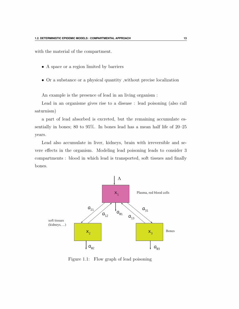
Lead also accumulate in liver, kidneys, brain with irreversible and se-
vere effects in the organism. Modeling lead poisoning leads to consider 3
compartments : blood in which lead is transported, soft tissues and finally
bones.
x1
x2
a21a12
a01
a02 a03
a31
a13
x3
Λ
soft tissues (kidneys, ...)
Plasma, red blood cells
Bones
Figure 1.1: Flow graph of lead poisoning

14 1. INTRODUCTION AND IMPORTANT CONCEPTS
1.2.1 Compartmental equations
The box in the following figure represents the i-th compartment of an n
compartment system.
Ii
qi FjiFij
F0i
From j
Outside Input
Going to j
Outside output
Figure 1.2: A comparment
Arrows represents the input and output flows in the compartment.
qi = Ii − F0i +∑j 6=i
Fij − Fji
Inputs : the flows into the compartment
Ii(t) ∆t+
(∑j
Fij
)∆t
Outputs : the outflows leaving the compartment
F0i ∆t+
(∑j 6=i
Fji
)∆t
1.2. DETERMINISTIC EPIDEMIC MODELS : COMPARTMENTAL APPROACH 15
Instantaneous mass balance equations
qi(t) = Ii(t) +
(∑j 6=i
Fij
)− F0i −
(∑j 6=i
Fji
)
The functions Fij and Ii are flows : quantity of material by unit of time.
The functions Ii, F0i, Fij can be functions of q1, . . . ,qn and possibly t.
So we can write the functions Fij(t, q)
These are nonnegative quantity Ii ≥ 0, F0i ≥ 0, Fij ≥ 0
If there is no material un a compartment, nothing can leave the compartment.
Mathematically
qi = 0⇒ Fji = 0 and F0i = 0
To summarize we have
•
Fij ≥ 0 F0i ≥ 0 Ii ≥ 0
•
qi = 0⇒ Fji = 0 et F0i = 0
Now we will suppose that these functions are C1
Proposition 1.2.1 If f is a function from Rn into Rm of class Ck, s.t.
f(x∗) = 0 there exists A(x) of class Ck−1, from Rn in matrices m × n such
that for any x ∈ Rn we have

16 1. INTRODUCTION AND IMPORTANT CONCEPTS
f(x) = A(x) (x− x∗)
Proof
we consider C1 from R into Rm
ϕ(t) = f(x∗ + t (x− x∗))
f(x) = ϕ(1)− ϕ(0) =
∫ 1
0
ϕ′(s) ds
=
∫ 1
0
Df(x∗ + s (x− x∗) . (x− x∗) ds
=
(∫ 1
0
Df(x∗ + s (x− x∗) ds)
(x− x∗)
Then A(x) =
(∫ 1
0
Df(x∗ + s (x− x∗) ds)
of class C1.
Consequence for our functions there exists a function fij such that
Fij = fij qj
qi = Ii − F0i +∑j 6=i
Fij − Fij
qi = −
(f0i +
∑j 6=i
fji
)qi +
∑j 6=i
fij qj + Ii
We now introduce a matrix A defined by
• A(i, j) = fij

1.2. DETERMINISTIC EPIDEMIC MODELS : COMPARTMENTAL APPROACH 17
• A(i, i) = −f0i −∑j 6=i
fji
• and the vector I = (I1, · · · , In)T
The equations can now be written in a linearized way
q = Aq + I
Functions fij are called fractional transfer coefficients. Dimension of these
functions are t−1. Depending generally for q and t.
The entries of the matrix A have some properties : the off-diagonal entries
are nonnegative.
Definition 1.2.1 (Metzler Matrix ) A matrix A whose off diagonal en-
tries are nonnegative, i.e. if i 6= j then aij ≥ 0 is called a Metzler matrix.
But we have more properties for our matrices A
q = A(t,q) q + I(t,q)
a diagonal entry is given by A(i, i) = −f0i −∑j 6=i
fji ≤ 0. In other words
A(i, i) is equal to minus the sum of entries of columnn i and subtracting the
term −f0i. Then for the matrix A, each column sum is non positive.
A Metzler matrix, which satisfies that the column sum are nonpositive (this
implies that the diagonal terms are non positive) diagonale) is called a com-
partmental.

18 1. INTRODUCTION AND IMPORTANT CONCEPTS
1.2.2 Graphic representations
A standard graphical representation of compartmental systems uses nodes for
compartments and directed arcs labeled with fractional transfer coefficients
for transfers between compartments, and for excretions.
Inputs are labeled with the input function. Such representations are called
compartmental system connection diagrams or simply connection diagrams
or flow-graphs. Actually these are digraphs with weight on each arc : these
are also called un Coates graph.
1.2.3 An example : The Kermack–McKendrick Model
We formulate our descriptions as compartmental models, with the pop-
ulation under study being divided into compartments and with assumptions
about the nature and time rate of transfer from one compartment to another.
Diseases that confer immunity have a different compartmental structure
from diseases without immunity
In order to model such an epidemic we divide the population being stud-
ied into three classes labeled S, I, and R. We let S(t) denote the number
of individuals who are susceptible to the disease, that is, who are not (yet)
infected at time t. I(t) denotes the number of infected individuals, assumed
infectious and able to spread the disease by contact with susceptibles. R(t)
denotes the number of individuals who have been infected and then removed
from the possibility of being infected again or of spreading infection. Re-
moval is carried out either through isolation from the rest of the population
or through immunization against infection or through recovery from the dis-
ease with full immunity against reinfection or through death caused by the
disease.In formulating models in terms of the derivatives of the sizes of each
compartment we are assuming that the number of members in a compartment
1.2. DETERMINISTIC EPIDEMIC MODELS : COMPARTMENTAL APPROACH 19
is a differentiable function of time. This may be a reasonable approximation
if there are many members in a compartment, but it is certainly suspect
otherwise. The basic compartmental models to describe the transmission of
communicable diseases are contained in a sequence of three papers by W.O.
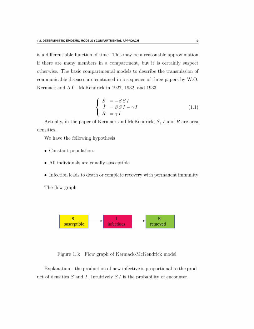
Kermack and A.G. McKendrick in 1927, 1932, and 1933S = −β S II = β S I − γ IR = γ I
(1.1)
Actually, in the paper of Kermack and McKendrick, S, I and R are area
densities.
We have the following hypothesis
• Constant population.
• All individuals are equally susceptible
• Infection leads to death or complete recovery with permanent immunity
The flow graph
SS I Rsusceptiblesusceptible infectiousinfectives
removedremoved
Figure 1.3: Flow graph of Kermack-McKendrick model
Explanation : the production of new infective is proportional to the prod-
uct of densities S and I. Intuitively S I is the probability of encounter.

20 1. INTRODUCTION AND IMPORTANT CONCEPTS
This is the mass action law, when the variables are densities.
Another way to formulate is : we assume that any individual makes β
adequate contact by unit of time with others. If N is the total population
and S, I and R prevalence (i.e., % relatively to the population), we have
I N infectious individuals, then the number of encounter of an infective by
unit of time is (β N) I. Among this encounters, only the encounters with a
susceptible, will produce a new infective
Then the number of new infections in unit time per infective is equal to
(β N) I S = β,N S I = β S I
Note : the hypothesis of homogeneity.
1.2.4 Transfer rates
For the simple Kermack-McKendrick model described in the previous section,
we assumed that the recovery rate, or the rate of transfer from compartment
I to R, is given by γ I . This is equivalent to assuming the following:
(H) the fraction of the infectious population that recovers per unit time
is a constant.
Proportional transfer rates as assumed in (H) are often used for transfers
between compartments in simple compartmental models. However, we need
to understand that this is only one of many assumptions we can make about
population transfers.
In fact, our assumption that recovery rate is in proportion to the size of the
infectious population is by no means universal. In the following, we develop
a better mathematical understanding of the proportional transfer rate, and
consider other possible alternatives. Consider a general compartment C of
total population size N(t), where individuals leave the compartment at a rate
rN(t) (r > 0). Then the size N(t) satisfies

1.2. DETERMINISTIC EPIDEMIC MODELS : COMPARTMENTAL APPROACH 21
dN(t)
dt= −r N(t), r > 0,
and thus N(t) = N0 e−r t, or
N(t)
N0
= e−r t.
Therefore, e−r t gives the fraction of the population that remains in the
compartment C. In probability terms, e−r t is the probability of an individual
entering C at time t = 0 and remaining in C at time t > 0. Since we are
interested in the population transfer out of C, we consider
F (t) =
1− e−r t, t ≥ 0
0, t < 0
which gives the fraction of the population that has left C during the time
period [0, t), or the probability of an individual who has left C during [0, t).
Here we see that F (t) has the characteristics of a probability distribution.
In fact, let X denote the random variable of the residence time of an
individual in compartment C, the time period from entrance to exit, we see
that
F (t) = Prob[ X ≤ t ].
In other words, F (t) is the probability distribution function of individual
residence time in C, and it satisfies the following properties:
• F (t) ≥ 0
• F (t)→ 0, as t→ −∞
• F (t)→ 1, as t→ +∞

22 1. INTRODUCTION AND IMPORTANT CONCEPTS
Now we see that the assumption of proportional exit rate is the same as
the following: (H0) the residence time of an individual in compartment C
has an exponential distribution. We can also describe the random variable
X in terms of probability density function f(t) =d
dtF (t), namely:
f(t) =
r e−r t, t ≥ 0
0, t < 0,
with the following properties
• f(t) ≥ 0
•∫ +∞
−∞f(t) dt = 1
• F (t) = Prob[ X ≤ t ] =
∫ t
−∞f(s) ds.
The expected value, also called the mean value, of X is
E(X) =
∫ +∞
−∞t f(t) dt =
1
r
For transfers from compartment I toR, the residence time is the period
between time of infection and time of recovery, which is the infectious period.
Then1
γis the mean infectious period.

Chapter 2
Some Classical Examples
2.1 Introduction
Ronald Ross discovers the transmission of Malaria by mosquitoes Anophe-
les. Ross proves this transmission in 1898 and was awarded Nobel prize in
1902. Ross is better known to the medical community as the discoverer of the
mosquito transmission of malaria than as the author of a far-reaching theo-
retical approach to the study of disease in populations. We need little wonder
that towards the end of his life, Ronald Ross, the man who incriminated the
mosquito in the transmission of malaria, would write:
’In my own opinion my principal work has been to establish the
general laws of epidemics’
This section will present the so-called Ross model. This model has been
published in the appendix of in 1911 in Prevention of Malaria and also in
Nature Nature the same year . This model is interesting since
• It shows how to model, what are the hypotheses taken into account
and the hypotheses neglected.
23

24 2. SOME CLASSICAL EXAMPLES
• this model is really seminal : the so-called famous model of Lotka-
Volterra, also quadratic equations in the plane, is dated of 1925;
• despite its simplicity it captures the dynamics of Malarai;
• this model was used by Ross to found the justification of anti-vectorial
measures.
Before considering the modeling, it is valuable to present the historic
context.
Are mathematics useful in epidemiology ? we will quote Ross again
In the appendix ( prevention of Malaria, 1911), where the model is pre-
sented Ross says,
The mathematical treatment adopted in section 28 has been met
with some questioning by critics. Some have approved of it, but
others think that it is scarcely feasible owing to the large num-
bers of variables which must be considered. As a matter of fact
all epidemiology concerned as it is with the variation of disease
from time to time or from place to place, must be considered
mathematically, however many variables are implicated, if it is to
be considered scientifically at all. To say that a disease depends
upon certain factors is not to say much, until we can also form an
estimate as to how largely each factor influences the whole result.
And the mathematical method of treatment is really nothing but
the application of careful reasoning to the problems at issue
Ross insists on the qualitative nature of the studies
Then how us eMathematics ?

2.1. INTRODUCTION 25
Ronald Ross is not the first to use mathematics to study some problems in
epidemiology. Daniel Bernoulli considers the problem of smallpox relatively
to the techniques of variolation in 1760. P.D. Enko published some studies on
transmission in 1889. But it can be said that Ross is the first to systematically
use the mathematical approach . In the introduction of An Application of
the Theory of Probabilities to the Study of a priori Pathometry. Part I Ross
writes
The whole subject (i.e., Epidemiology) is capable of study by
two distinct methods which are used in other branches of science,
which are complementary of each other, and which should con-
verge towards the same results – the a posteriori and the a priori
methods. In the former we commence with observed statistics,
endeavour to fit analytical laws to them, and so work backwards
to the underlying cause (as done in much statistical work of the
day) ; and in the latter we assume a knowledge of the cause, we
construct our differential equations on that supposition, follow up
the logical consequences, and finally test the calculated results by
comparing them with the observed statistics
Ross is the first to use the a priori method and the cited text, dating
back to 1916 !, could introduce a course on modeling.
The rest of the chapter is organized as follows. In accordance with the a
priori method first we will describe the natural history of malaria. In other
words, how does it work? Then we will discuss in detail the construction of
Ross model and continue with his analytic study to state what Ross called
the mosquito theorem (which also shows Ross state of mind). To conclude on
malaria we will present a simple model intra-host, ie a model that describes
the infection in an individual.

26 2. SOME CLASSICAL EXAMPLES
2.2 Natural history of Malaria
To be established Malaria needs three ingredients :
• A human host
• a mosquito of Anopheles type
• a hematophagous protozoan.
The causative agent, le Plasmodium was discovered in 1880, in Algeria at
Constantine, by a french military doctor Alphonse Laveran. Laveran was
awarded in 1907 by the Nobel prize.
4 parasitic species for man :
• Plasmodium vivax,
• Plasmodium falciparum,
• Plasmodium malariae,
• Plasmodium ovale.
All have an asexual cycle in man schizogony and a sexual cycle in
mosquito called sporogony. The most dangerous and frequent in Africa is
P. falciparum. Parasite cycle is divided in 3 parts. Two in man and one in
mosquito. The first part occurs in liver, the second occurs in red blood cells

2.2. NATURAL HISTORY OF MALARIA 27
Figure 2.1: Le cycle du parasite du paludisme Plasmodium falciparum(D’apres C. Rogier)
2.2.1 In Liver
Parasite is inoculated in the peripheral blood with the anticoagulant saliva
of moquito. . These parasites are called sporozoites. There are mobile and
are moved by the blood flow to penetrate liver cells. It takes less than 45
minutes
Each sporozoite enters in a hepatocyte (liver cell); and from these moment
unable to move Sporozoite transforms, grews and divides. After a mean

28 2. SOME CLASSICAL EXAMPLES
duration between 8 to 15 days the hepatocyte is invaded by several thousands
of nucleus called schizonte. Once matured the schizonte bursts and releases
m erozoites which pass in blood. The duration of this period is around 15
days
This Liver cycle was only discovered in 1948 seulement with teh works pf
James, Tate, Shortt and Garnham.
2.2.2 In blood
Merozoites invade Erythrocytes (Red Blood Cell) taking the characteristic
aspect for P. falciparum of a kitten ring. They becomes trophozoites feeding
from hemoglobin. At the end trophozoites becomes pigmented schizontes.,
Once mature the red blood cell burst and releases new merozoites which will
parasite healthy RBC.
Several similar evolutions succeed one another as well. After few weeks
(10-12 days for P. falciparum ) some schizonts will turn into male sexed cells
or females: the gametocytes. We distinguish macrogametocytes (females) et
des microgametocytes (males). This cells stays in the blood being a reservoir
for the mosquito

2.2. NATURAL HISTORY OF MALARIA 29
Figure 2.2: Different form of Plasmodium falciparum in Erythrocyte cycle(Laveran Drawings).

30 2. SOME CLASSICAL EXAMPLES
Figure 2.3: Laveran Drawings planche I [55]
sporogony in mosquito
If a female mosquito bites an infected individual it ingests gametocytes in
his gut. The gametes increase in size. In 10 minutes the male and female ga-
metes have left their envelope. The male produced 8 flagellated microgametes
mobile. This event, the formation of vigorous mobile male gametes from a
previously quiet gamete is called exflagellation. This striking phenomenon
has fascinated malariologists since the observation by Laveran himself.

2.2. NATURAL HISTORY OF MALARIA 31
Fertilization produces a mobile ookinete that will establish itself as oocyst
on the inside of the digestive tract.
Inside the oocyst will form sporocysts that will give several hundred sporo-
zoites. The sporozoites migrate to the salivary glands of the mosquito, where
they develop in vacuoles and can stay up to 59 days. During their develop-
ment, sporozoites can become up to 1000 times more infectious than when
their presence in the oocyst.
2.2.3 The vector
Only the female bite the host, usually after sunset. A blood meal is necessary
before laying eggs singly on liquid surfaces.
Figure 2.4: anopheles
Eggs give larvae (Figure 2.5), then nymph and finally the winged insect

32 2. SOME CLASSICAL EXAMPLES
Figure 2.5: larvae ias parallel to surface
The flight of the mosquito does not exceed, in principle, one or two kilo-
meters.
There are more than 300 species of Anopheles, only 60 are human plas-
modium vectors.
2.3 Building the model
With Ross, we will make some simplifying hypotheses. It is assumed that the
human population is constant as well as that of female anopheles. In other
words, mortality is equal to the birth rate. A hypothesis of homogeneity
is admitted: that humans and mosquitoes are equally distributed. In other
words, a mosquito has an equal probability of biting a determined human.
The mosquito population is divided into two fictitious compartments: healthy
mosquitoes, we say susceptible, and infectious mosquitoes. We do the same
for the human population.

2.3. BUILDING THE MODEL 33
Ssusceptibles
Iinfectieux
Sv vsusceptibles
Iinfectieux
h h Humains
Anophèlesfemelles
Figure 2.6: Les compartiments
These assumptions are simplifications. On the episode on which we study the
transmission we can admit that the populations are approximately constant.
In any model, there are simplifying hypotheses, e.g. when we write the
equations of the pendulum we neglect the friction and the resistance of the
air.
Sh(t) and Ih(t) are the respective populations of humans in the susceptible
and infectious compartment.
We will write the balance of transfers between each compartment. We con-
sider a time interval ∆t, supposedly small. In this interval of time we will
write the movements of populations between each compartment. There are
some hidden hypotheses here: we neglect the incubation time, we also make
the implicit assumption that there is no superinfection.

34 2. SOME CLASSICAL EXAMPLES
2.3.1 Infectious human evolution
W evaluate Ih(t+ ∆t).
Input These are the new infectious individuals.
• To become infectious you must have been bitten by an infectious
mosquito.
• A mosquito bites a human per unit of time.
• It is assumed that the probability of becoming infectious after an
infectious bite is b1.
• There are Iv(t) infectious mosquitoes, they will induce a Iv ∆t
bites.
• In all these bites, only those made on a susceptible human will
produce a new infectious. The proportion is ShH
= H−IhH
where H
is the constant human population.
• Therefore the number of new infectious is
b1 a IvH − IhH
∆t
Output It’s the infectious ones that heal and regain the susceptible com-
partment. It is therefore assumed that there is no immunity.
• It is assumed that the average speed for a healing individual is
γH per unit of time. Mortality is assumed to be µH . This is the
number of deaths per person per unit of time.
• Therefore it disappears
(γH + µH) Ih ∆t
infectious either by cure or by death.

2.3. BUILDING THE MODEL 35
Balance Finally
Ih(t+ ∆t) = Ih(t) + b1 a IvH − IhH
∆t− (γH + µH) Ih ∆t
Susceptibles balance Since the human population is constant , Sh(t) =
H − Ih(t) we have
Sh(t+ ∆(t) = Sh(t)− b1 a IvH − IhH
∆t+ (γH + µH) Ih ∆t
Actually it is sufficient to know Ih(t) to immediately know by difference Sh(t).
The first relation can also be written
Ih(t+ ∆t)− Ih(t)∆t
= b1 a IvH − IvH
− (γH + µH) Ih
When ∆t goes to 0 we obtain the following ODE
d Ih(t)
dt= Ih(t) = b1 a Iv(t)
H − Ih(t)H
− (γH + µH) Ih(t)
which is written writes more simply, omitting the time t in the functions
Ih and Iv.
Ih = b1 a IvH − IhH
− (γH + µH) Ih (2.1)
This gives the following graph

36 2. SOME CLASSICAL EXAMPLES
Ssusceptibles
Iinfectieux
S v vsusceptibles
Iinfectieux
h h Humains
Anophèlesfemelles
ab1 Iv /H
γH
μH μH
Figure 2.7: Human
2.3.2 Infectious mosquito population
The principle is the same. A new infectious mosquito will appear after the
bite of a susceptible mosquito biting an infectious human. The probability
of becoming infected, for the mosquito biting an infectious host, is b2. We
will have aSv bites, where a SvIhH
will give rise to an infectious mosquito. If
we denote by V the vector population (Anopheles females) Sv = V − Iv. We
will thus have, by introducing the speed of recovering of the mosquito and
its mortality
Iv = b2 a (V − Iv)IhH− (γV + µV ) Iv (2.2)
which gives the flow graph

2.3. BUILDING THE MODEL 37
Ssusceptibles
Iinfectieux
Sv vsusceptibles
Iinfectieux
h h Humains
Anophèlesfemelles
ab1 Iv /H
ab2 Ih /H
γH
γV
μH
μH H
μV V
μH
μVμV
Figure 2.8: Complete flow graph
We see that in the human susceptible compartment, deaths are µH Sh and
births µH H = µH (Sh + Ih). Newborns are born susceptible. It is also an
implicit assumption and it is actually true. The gain in the compartment of
susceptible is in fact µH Ih, in other words Sh = −Ih. Which is another way
of saying that the H population is constant: H = 0.
2.3.3 Ross model, final form
We have a system of ODE
Ih = b1 a Iv
H − IhH
− (γH + µH) Ih
Iv = b2 a (V − Iv)IhH− (γV + µV ) Iv
(2.3)

38 2. SOME CLASSICAL EXAMPLES
In epidemiology, it is often the percentages, in other words the prevalences,
that are measured. As the population is constant we will introduce the
percentage of infectious individuals:
x =IhH
for human hosts and y =IvV
for mosquitoes
Since H et V are constant we have x =IhH
et y = IvV
. We prepare, a litlle bit
(2.3)
Ih = b1 a
IvVV
(1− Ih
H
)− (γH + µH) Ih
Iv = b2 a V (1− IvV
)IhH− (γV + µV ) Ih
(2.4)
dividing the first equation by H and the second by V , by setting m = VH
we
get x = ma b1 y (1− x)− (γH + µH)x
y = b2 a (1− y)x− (γV + µV ) y(2.5)
To obtain the final model, two more approximations are made: the rate of
recovering is the inverse of the average duration of the time spent in the
infectious status. In other words, an infectious individual remains infectious
on a mean time
1
γtime units
In particular mortality is negligible in the face of healing time in humans. If
conservatively we take between 2 and 6 months for a recovery
µH ≈ 1/(60× 365) j−1 ≈ 4.56 10−5
et γV ≈ 1/(2× 60) j−1 ≈ 0.008

2.4. ROSS MODEL ANALYSIS 39
µVγV≈ 1
360≈ 0.0027
Similarly, the mosquito’s recovering time is assumed to be negligible com-
pared to life expectancy of the mosquito. In all the entomological literature
it is admitted that the mosquito remains infected all his life. We therefore
neglect µH and γV . Which finally gives
x = ma b1 y (1− x)− γ x
y = b2 a (1− y)x− µ y(2.6)
As a result of this model Ross stated what he called his mosquito theorem.
Formulated in a contemporary way, this theorem would be read now
Theorem 2.3.1 (Mosquito theorem, Ross)
For the system (2.6)
• Si on ama2 b1 b2
γ µ≤ 1,
the disease free equilibrium (0, 0) is globally asymptotically stable on
[0, 1] × [0, 1].
• Sima2 b1 b2
γ µ> 1,
then there exists a unique equilbrium (x, y) ∈]0, 1[×]0, 1[ ]0, 1]×]0, 1]
which is is globally asymptotically stable on ]0, 1[×]0, 1[ .
2.4 Ross model analysis
We will postpone this analysis, waiting for the tools needed.
40 2. SOME CLASSICAL EXAMPLES
2.5 Malaria intra-host model
Ross model is a model for the spread of a disease. It may be useful to study
the spread of pathogens within an individual. The model we will present was
introduced by Anderson, May and Gupta in 1989.
Let x the concentration in the blood of healthy erythrocytes, y the con-
centration of parasitized erythrocytes and m the concentration of merozoites
circulating freely in the bloodstream.
x = Λ− µx x− βxm
y = β xm− µy y
m = r µy y − µmm− β xm.
In the absence of parasites, the concentration of red blood cells is con-
stant. The number of red blood cells in the blood is normally between 4.5 -
5.5 million / mm3, their lifespan is 120 days, they are produced by the bone
marrow. This explains the choice of x = Λ− µx x in the absence of parasite.
Now the term β xm represents the penetration rate of merozoites in ery-
throcytes An infected erythrocyte passes into the infected compartment The
mortality of infected erythrocytes is µy. For P. falciparum the average cycle
time is 48 hours When a red blood cell bursts it releases r merozoites. A
merozoite if it does succeed to enter a RBC will be eliminated in the spleen.
The term β xm which appears in the last equation represents the passage of
the merozoite circulating in the red blood cell. If this term was not present,
the model would allow a single merozoite to infect several RBC!
The term r µy is the mean number of sporozoites produced by a infected
erythrocyte by unit of time. Since an erythrocyte has a mean life of1
µyand
since when bursting it gives r merozoites, the number by unit of time is

2.6. SEIR MODEL 41
r1µy
= r µy
In this model the unknown parameter is β, for the others we have at least
an approximate knowledge.
This model, without the quadratic term in m, is baptized as a model of
viral dynamics ( May et al)
In fact this model is also a model of HIV infection. It is proposed by
Perelson in the 1990s. The only difference is that recruitment, instead of
being constant is represented by a logistic function. In this case, the variable
x represents the concentration of CD4 + lymphocyte cells. and we would
have
x = Λ + p x
(1− x
xmax
)− µx x− β xm.
In this form y is the concentration of infected lymphocytes and m the
concentration of free circulating virion.
With this model Perelson has said
While the mathematics involved was trivial, the application of
mathematics in this manner was novel and set off what has been
described as a revolution in thinking about HIV
2.6 SEIR model
Disease infection begins with the transmission of the pathogen from one host
to another. After pathogens invade the host body, they need to be able to
evade or overcome the host immune response, and be able to multiply or
replicate. When the pathogens accumulate sufficiently large numbers and

42 2. SOME CLASSICAL EXAMPLES
reach the targeted organs, they begin to cause sufficient damage to the host
body so that the host becomes symptomatic, and the host is then capable
to transmit the pathogens to others. The period from time of infection to
time of onset of symptoms is called the incubation period. The period from
time of infection to time of being contagious or infectious is called the latent
period. The period from the beginning to the end of being infectious is called
the infectious period. See the illustration (2.9) for an example of relations
between these periods. During the latent period, a host may or may not show
symptoms, but the host is not capable of transmitting pathogens to other
hosts.
Time of infectionBeginning of infectiousness
Onset of symptoms
End of infectiousness
Recovery
Latent period Infectious period
Incubation period
Figure 2.9: SEIR model
We have the following flow graph

2.6. SEIR MODEL 43
Ssusceptibles
Iinfectives
ELatents
Rremoved
μS μE
α γ
μI μR
βI/N
Figure 2.10: Scheme of infection
S = Λ− µS S − βS I
N
E = β I S − (µE + α)E
I = α I − (γ + µI) I
R = γ I − µRR
(2.7)
In this model S, E, I, R andN = S+E+I+R are numbers. It is assumed,
under the hypothesis of homogeneity that any individual makes β adequate
contact by unit of time. Then I infectious will make β I adequate contacts.
But in all these contacts, only the contact with susceptible individuals will
give rise to latent (E) individual. The proportion of susceptibles in the whole
population isS
N. Then the new latent will be
β IS
N
This law is called true mass action or frequency-dependent transmission.
The mean period for latency is1
α, for recovery
1
γ

44 2. SOME CLASSICAL EXAMPLES

Chapter 3
Basic Mathematical Tools andTechniques
3.1 Well-posedness of a model
We consider the Kermack-McKendrick model (1.1)
S = −β S I
I = β S I − γ I
R = γ I
(3.1)
with initial condition (S0, I0, R0). We claim that nonnegative initial condi-
tions leads to nonnegative solutions. In other word, any trajectory beginning
in the nonnegative orthant R3+ stays in this orthant. In other words the non-
negative orthant is positively invariant for the dynamical system. It is what
we mean by well-posedness. Recall that the variables are either numbers or
densities, then in the nonnegative orthant.
To study the well-posedness of a system we will give a Theorem. This
Theorem seems to be intuitively evident, but it has to be proved ...
This Theorem will allows to study well-posedness for epridemiological or
45
46 3. BASIC MATHEMATICAL TOOLS AND TECHNIQUES
biological models.
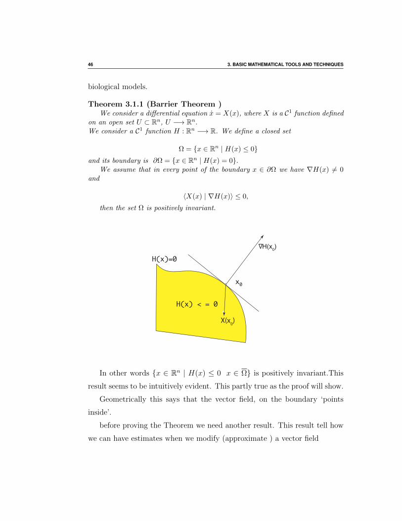
Theorem 3.1.1 (Barrier Theorem )We consider a differential equation x = X(x), where X is a C1 function defined
on an open set U ⊂ Rn, U −→ Rn.We consider a C1 function H : Rn −→ R. We define a closed set
Ω = x ∈ Rn | H(x) ≤ 0and its boundary is ∂Ω = x ∈ Rn | H(x) = 0.
We assume that in every point of the boundary x ∈ ∂Ω we have ∇H(x) 6= 0and
〈X(x) | ∇H(x)〉 ≤ 0,
then the set Ω is positively invariant.
H(x)=0
x0
H(x) < = 0
X(x0)
∇H(x0)
In other words x ∈ Rn | H(x) ≤ 0 x ∈ Ω is positively invariant.This
result seems to be intuitively evident. This partly true as the proof will show.
Geometrically this says that the vector field, on the boundary ‘points
inside’.
before proving the Theorem we need another result. This result tell how
we can have estimates when we modify (approximate ) a vector field
3.1. WELL-POSEDNESS OF A MODEL 47
Lemma 3.1.1
Let X a Lipschitz vector vector with Lipschitz constant L. We consider
the approximation Xε of X, in other words for any x we have
‖Xε(x)−X(x)‖ ≤ ε
‖ ‖ being any norm on Rn.
Then for any t where the quantities are defined
‖Xεt (x
ε0)−Xt(x0)‖ ≤ ‖xε0 − x0‖ eLt + ε
eLt − 1
L
proof of the Theorem
Actually we will prove the theorem for a Locally Lipschitz vector field.
The case C1 is then contained in it. To go out from the set
G = x ∈ Rn | H(x) ≤ 0 x ∈ Ω
the trajectory, by the intermediate value theorem, must pass through he
boundary ∂G = x ∈ Ω | H(x) = 0 We will distinguish two cases.
In the first case
we suppose that in x0, H(x0) = 0. We have
〈X(x0) | ∇H(x0)〉 < 0
Let ε < 0 such that 〈X(x0) | ∇H(x0)〉 < ε < 0, with a continuity
argument, there is a ball centered in x0 and of radius η > 0, such that for all
y ∈ B(x0, η) we have
48 3. BASIC MATHEMATICAL TOOLS AND TECHNIQUES
〈X(y) | ∇H(y)〉 < ε < 0
We consider the trajectory Xt(x0) from x0. For t ≥ 0 small enough
0 ≤ t < α, the trajectory remains in the ball B(x0, η). We have
d
dtH(Xt(x0)) = 〈∇H(Xt(x0)) | X (Xt(x0))〉 < ε < 0
The function H(Xt(x0)) is strictly decreasing and so H(Xt(x0)) < 0 for
0 < t < α.
Which proves that Xt(x0) ∈G
Second case
we suppose now that 〈X(x0) | ∇H(x0)〉 = 0. We consider the vector field
Xε(x) = X(x)− ε ∇H(x)
‖∇H(x)‖
This vector field satisfies for all ε > 0, the hypothesis of first case on
Ω ∪ ∂G. Let η small enough such that in the closed ball B(x0, η) the vector
field Xε satisfies the required inequality. We choose t ≤ T sufficiently small
such that Xt(x0) ∈ B(x0, η/2). Since Xε is a ε approximate field of X, we
apply the lemma (3.1.1), which gives us the increase
‖Xεt (x0)−Xt(x0)‖ ≤ ε
eLT − 1
L
This proves that by choosing ε small enough such that eLT−1L
< η/2 we
will have

3.1. WELL-POSEDNESS OF A MODEL 49
Xεt (x0) ∈ B(x0, η)
From the previous demonstration Xεt (x0) ∈
G, so Xt(x0) is the limit of
points of G which is closed, so in G. The path from x0 can not leave G
locally. Since this is true for every x0 point of ∂G we have shown the result
on Ω.
Proof of the lemma
We use the fondamental identity
Xt(x0) = x0 +
∫ t
0
X (Xs(x0)) ds
then
‖Xεt (x
ε0)−Xt(x0)‖ ≤ ‖xε0 − x0‖+
∫ t
0
‖Xε (Xεs (x
ε0))−X((Xs(x0)) ‖ds
Writting∫ t
0
‖Xε (Xεs (x
ε0))−X((Xs(x0)) ‖ds ≤∫ t
0
‖Xε (Xεt (x
ε0))−X((Xε
s (x0)) ‖ds+
∫ t
0
‖X (Xεt (x
ε0))−X((Xs(x0)) ‖ds
we get
‖Xεt (x
ε0)−Xt(x0)‖ ≤ ‖xε0 − x0‖+ ε t+ L
∫ t
0
‖Xεs (x
ε0)−Xs(x0)‖ ds
If we set u(t) = ‖Xεt (x
ε0)−Xt(x0)‖ we have

50 3. BASIC MATHEMATICAL TOOLS AND TECHNIQUES
u(t) ≤ u(0) + ε t+ L
∫ t
0
u(s) ds
The inequality is immediate by Gronwall’s lemma.
Lemma 3.1.2 (Gronwall 2) Let t u : [0, α] −→ R+ a continuous and non-
negative function. We assume that there exists constants C, ε and L such
that for any t ∈ [0, α] we have
u(t) ≤ C + ε t+ L
∫ t
0
u(s) ds (3.2)
Then we have
u(t) ≤ C eLt +ε
L(eLt − 1)
Proof
Let y(t) = L
∫ t
0
u(s) ds et z(t) = e−Lt y(t). From inequality 3.2.
y ≤ L (C + ε t) + Ly
and
z = e−Lt(y − Ly) ≤ Le−Lt(C + εt)
which gives integrating from 0 to t
or equivalently
z(t) ≤∫ t
0
Le−Ls(C + εs) ds

3.1. WELL-POSEDNESS OF A MODEL 51
y(t) ≤ eLt∫ t
0
Le−Ls(C + εs) ds
taking into account the inequality satisfied by u
u(t) ≤ C + εt+ eLt∫ t
0
Le−Ls(C + εs) ds
A straighforward computation leads to
eLt∫ t
0
Le−Ls(C + εs) ds = −C − εt+ CeLt +ε
L(eLt − 1)
Which is the inequality to prove
Remark 3.1.1
If the vector field is not Lipschitzian, the theorem is no more true. For
example for the equation x = −3 |x|23 on R, origine is a barrier however
some solutions can go through. For this vector fiels R+ is not positively
invariant.
The same applies to the vector field given by the ODE x = −√
2 g x, the
origin is a barrier and R− should be positively invariant. This is not the case
as can be seen on the figure 3.1.

52 3. BASIC MATHEMATICAL TOOLS AND TECHNIQUES
0.0
0.1
0.2
0.3
0.4
0.5
0.6
0.7
0.8
0.9
1.0
0.0 0.5 1.0 1.5 2.0 2.5 3.0
(2)(1)
(3) (4)
(5)
Figure 3.1: Different solutions of x = −√
2 g x
3.1.1 Examples
3.1.2 Kermack-McKendrick modelS = −β S I
I = β S I − γ I
R = γ I
We prove that the nonnegative orthant is positively invariant. The bound-
ary of R3+ is given by 3 hyperplane cone : R+ × R+ × 0, 0 × R+ × R+

3.2. LYAPUNOV TECHNIQUES 53
and R+ × 0 × R+.
When S = 0 we have S = 0, the vector field is tangent to the RI-
plane hence the conditions of theTheorem are satisfied. Identically if I = 0
then I = 0. When R = 0, R = γ I ≥ 0, since we are in the nonnegative
orthant. Note that to be in accordance with the notations of the Theorem,
the nonnegative orthant is defined by −S ≤ 0 ;−I ≤ 0 ;−R ≤ 0.
3.1.3 Ross model
3.2 Lyapunov techniques
Lyapunov method also called direct method or second method of Lyapunov
has been introduced in 1892 in Lyapunov’s thesis and published in french in
1897.
Probleme general de la stabilite du mouvement. Annales de la faculte des
sciences de Toulouse 9(2) (1907): 203-474
This method allow to establish stability of the equilibrium of a system,
without integrate this EDO.
This method was forgotten and rediscovered in USSR in the 1944
This method was ignored in the West till 1950. From this date, this
method was the prerogative of the russian mathematician and control engi-
neers. Its importance was rediscovered first in control theory and popularized
by LaSalle and Lefschetz in 1959.
It is now well funded that Lyapunov is a very fundamental method.
3.2.1 Problematics x = f(x)
x ∈ Rn
x(0) = x0
(3.3)

54 3. BASIC MATHEMATICAL TOOLS AND TECHNIQUES
The unique solution for the initial value x0, is denoted by Φt(x0). By
renormalizing f , we can always suppose that the vector field is complete, i.e.,
the function Φt(x0) is defined for any t.
Now we suppose that x0 is an equilibrium,
f(x0) = 0
We have the following well known property : for any (t, s) ∈ R2
Φt (Φs(x)) = Φt+s(x)
One parameter group property
We recall properties of equilibria
Definition 3.2.1 (stability) We say that x0, an equilibrium of x = f(x)
is stable (in Lyapunov’s sense) iff for any open set U containing x0, it exists
an open set V of initial values , V ⊂ U such that for any y ∈ V and for any
t ≥ 0 we have Φt(y) ∈ U
x0
∀ U
∃ V
Figure 3.2: Stable equilibrium

3.2. LYAPUNOV TECHNIQUES 55
Definition 3.2.2 (attractivity) We say that x0 is attractive in the open
set V if for any y ∈ V
limt→+∞
Φt(y) = x0
x0
V
Figure 3.3: attractive equilibrium
Definition 3.2.3 ( asymptotic stability) We say that x0 is asymptoti-
cally stable (locallly ) if x0 is stable and if there exists an open set V of x0
in which x0 is attractive.
Remark 3.2.1 Beware : attractivity does not imply stability. However this
is true for linear systems. x = Ax.

56 3. BASIC MATHEMATICAL TOOLS AND TECHNIQUES
-2
-1
0
1
2
-2 -1 1 2.P x
y
Figure 3.4: attractivity without stability
3.2.2 Lyapunov functions
Definition 3.2.4 ( Lyapunov fonction ) We call Lyapunov function in
x0, an equilibrium of x = f(x), a function V such that there is an open set
U containing x0, and such that the following properties are satisfied
• V (x) ≥ 0 sur U
• V (x) = 0 iff x = x0
• On U we have
V (x) = 〈∇V (x) | f(x)〉 ≤ 0
A function satisfying the two first properties in x0 is said definite positive.
3.2.3 Theorems
Theorem 3.2.1 (Lyapunov first theorem) If x0 is an equilibrium of x =
f(x), if there exists a Lyapunov function in x0 for this system then x0 is a

3.2. LYAPUNOV TECHNIQUES 57
stable equilibrium.
Lyapunov second theorem
If moreover V is negative definite , i.e. si V (x) = 0 iff x = x0, then x0
is an asymptotically stable equilibrium
The attraction basin of x0 is contained in U where the 3 properties of V
are satisfied.
Theorem 3.2.2 (Lasalle) If V is a Lyapunov function the greatest invari-
ant set contained in
L = x | V (x) = 0
is an attractive set. This assertion is called LaSalle’s principle of invariance
and is true even is V is only nonnegative and non necessarily positive definite.
If L = x0 then x0 is asymptotically stable.
Theorem 3.2.3 (Lasalle) We consider the ODE with an equilibrium x0,
defined on a compact positively invariant set Ω.
If we have a nonnegative function V , such that V ≤ 0 on Ω and moreover
the largest invariant set contained in L = x ∈ Ω | V (x) = 0 is reduced to
x0
Then x0 is globally asymptotically stable in Ω
Note: V is not a Lyapunov function : not positive definite.
Theorem 3.2.4 (Poincare-Lyapunov) We consider a C1 ODE , x = f(x)
and x0 and equilibrium.
1. If Df(x0) has all its eigenvalues with negative real part, i.e., s(Df(x0)) <
0, then x0 est asymptotically (locally ) stable.

58 3. BASIC MATHEMATICAL TOOLS AND TECHNIQUES
2. if Df(x0) has (at least ) one eigenvalue with a positive real part, i.e.,
s(Df(x0)) > 0, then x0 is unstable.
Avantage of Lyapunov over Poincare : Lyapunov can give a conclusion
when Poincare fails
example :
x = −x2
y = −y
The positive orthant is est positively invariant. The origin is stable in the
domain R+ × R+.
-1 0 1
-3
-2
-1
1
2
3
..x
y
Figure 3.5: Saddle-Node
Il is sufficient to choose for Lyapunov function on sur R+ × R+
V (x, y) = x+1
2y2

3.2. LYAPUNOV TECHNIQUES 59
3.2.4 Examples
Lotka-Volterra model introduced by Pielou : n the prey , p the predator n = r n(1− n
K
)− a n p
p = b n p− µ p
This can be also considered as an intra-host model for a disease. n can
represent a concentrationof target cells, e.g. red blood cells and p a parasit
destroying red blood cells. . .
It is easy to determine a coexistence equilibrium
n∗ =µ
bp∗ =
r
a
(1− µ
bK
)This equilibrium has a biological meaning if p∗ > 0 or bK
µ> 1
This coefficient is a basic reproduction ratio : it is the mean number
of predator fathered by one predator introduced in a population of preys
(without predator) during its life :
Prey Population at Equilibrium : K , mean life of a predator 1µ, basic
repruction ration bK 1µ.
Proof of the Stability of the coexistence equilibrium when R0 = bKµ> 1.
we consider
f(n, p) = b (n− n∗ lnn) + a (p− p∗ ln p)
and the Lyapunov function R∗+ × R∗+
V (n, p) = b (n− n∗ lnn) + a (p− p∗ ln p)− f(n∗, p∗)
V =b r n(1− nK )−a b np−b r n∗ (1− n
K )+a b n∗p+a b n p−aµ p−a p∗ (b n−µ)
Taking into account b n∗ = µ we get
60 3. BASIC MATHEMATICAL TOOLS AND TECHNIQUES
V = b r(
1− n
K
)(n− n∗)− a b p∗ (n− n∗)
Using again a p∗ = r(1− n∗
K
)we obtain
V = b (n− n∗) r(
1− n
K− 1 +
n∗
K
)= −b r
K(n− n∗)2 ≤ 0
This proves stability . Now consider the set L defined by
L = (n, p) ≥ 0 | n = n∗
To be invariant in this set, n must be constant equal to n∗ must be
constant, then n = 0. Hence
n = r n∗(
1− n∗
K
)− a n∗ p = 0
Precisely p = p∗. The greatest invariant set L is (n∗, p∗).
We conclude by LaSalle ’s invariance principle to the asymptotic stability
on R∗+ × R∗+.
Stability of the predator free equilibrium when R0 = bKµ≤ 1.
Lyapunov function
V (n, p) = b (n−K lnn) + a p
Which gives
V = −b rK
(n−K)2 + a µ p (R0 − 1) ≤ 0
3.2. LYAPUNOV TECHNIQUES 61
3.2.5 How to find a Lyapunov function ?
Bad news
More an art than a science
Good news :
Some ingenuity, astuteness and tricks are needed
How do you find this dawn Lyapunov function for the Lotka-Volterra
Model ?
Back to classical Lotka-Volterran = r n − a n p
p = b n p− µ p
Dividing the two equations
dn
dp=r n − a n pb n p− µ p
We can separate the variables
(b− µ
n) dn = (−a+
r
p) dp
Equivalently
(b− µ
n) dn− (−a+
r
p) dp = 0
Integrating this relation shows that
f(n, p) = b(n− µ
blnn)
+ a(p− r
aln p)

62 3. BASIC MATHEMATICAL TOOLS AND TECHNIQUES
is a first integral, i.e., the derivative of f on the trajectories are zero,
or this function is constant on the trajectories of the ODE. Recall : the
coexistence equilibrium is n∗ =µ
b, p∗ =
r
aInterlude : the function s−s∗ ln s, defined on R+\0 has a unique minimum
s∗. Hence
s− s∗ ln s− s∗ + s∗ ln s∗
is definite positive for s∗
Recall
f(n, p) = b(n− µ
blnn)
+ a(p− r
aln p)
Tada !!!
f(n, p)− f(n∗, p∗)
is a Lyapunov function for (n∗, p∗)
The function
f(n, p) = b (n− n∗ lnn) + a (p− p∗ ln p)
is a Lyapunov function for the classical Lotka-Volterra. For the Pielou
Lotka-Volterra we use the same function, evidently with modified value for
the equilibrium.
If bKµ> 1
n∗ =µ
bp∗ =
r
a
(1− µ
bK
)

3.2. LYAPUNOV TECHNIQUES 63
If
bKµ< 1
n∗ = K and p∗ = 0 which makes disappear the p∗ ln p term.
3.2.6 Lyapunov and Ross model
Theorem 3.2.5 Let G an open set, containing origin, positively invariant
for the system
x = A(x).x,
where A(x) is a Metzler matrix depending continuously of x.
We suppose there exists cT 0 such that cT A(x) 0 for any x ∈ G,
x 6= 0.
Then the origin is GAS in G.
Consider on G Lyapunov function.
V (x) =n∑i=1
ci | xi | .
We define εz = sign(z), i.e. |xi| = εxi xi.
The function V is locally Lipschitz : we can defined Dini derivative.
V =∑n
i=1 ci εxi xi
=∑n
i=1 ci εxi∑n
j=1 aij xj
=∑n
i=1
∑nj=1 ci εxi aij xj
=∑n
j=1 εxjxj∑n
i=1 ci εxjεxi aij
=∑n
j=1 εxjxj
[cj ajj +
∑i 6=j ci εxjεxi aij
]≤∑n
j=1 εxjxj
[cj ajj +
∑i 6=j ci aij
]=∑n
j=1 |xj| (cT A)j ≤ 0.

64 3. BASIC MATHEMATICAL TOOLS AND TECHNIQUES
Since cT A(x) 0 sur G, function V is definite negative.x = ma b1 y (1− x)− γ x
y = b2 a (1− y)x− µ yTwo equilibria : DFE : (0, 0) and
x =
ma2 b1 b2µγ
− 1
ma2 b1 b2µγ
+ b2 aµ
y =
ma2 b1 b2µγ
− 1
ma2 b1 b2µγ
+ mb1 aγ
This equilibrium has a biological meaning iff
R0 =ma2 b1 b2
µ γ> 1
x = α y (1− x)− γ x
y = β (1− y)x− µ yTwo equilibria (DFE) : (0, 0) and
x =
αβµγ− 1
αβµγ
+ b2 aµ
y =
αβµγ− 1
αβµγ
+ mb1 aγ
Make sense iff
R0 =αβ
µ γ> 1
We can write xy
=
−γ α (1− x)
β (1− y) −µ
xy
Which is
X = A(X)X

3.2. LYAPUNOV TECHNIQUES 65
Stability of the DFE
R0 =αβ
µ γ≤ 1
A(x, y) =
−γ α (1− x)
β (1− y) −µ
We set
cT =[β + µ γ + α]
]
[β+µ γ+α]
] −γ α(1−x)
β (1−y) −µ
=[γ µ (R0−1)−(α+γ)β y γ µ (R0−1)−(β+µ)αx
]We choose
V (x, y) = 〈X | c〉
where we denote X = (x, y)T .
V = 〈X | c〉 = 〈A(X)X | c〉 = 〈X | A(X)T c〉
V =
⟨[x
y
]|[γ µ (R0−1)−(α+γ)β y
γ µ (R0−1)−(β+µ)αx
]⟩
V = γ µ (x+ y) (R0 − 1)− (2αβ + αµ+ β γ)x y ≤ 0
Conclusion : LaSalle

66 3. BASIC MATHEMATICAL TOOLS AND TECHNIQUES
Stability of the EE
R0 =αβ
µ γ> 1
We know that an endemic equilibirum (x, y) 0 exists
We use the variable change xnew = x− x et ynew = y − y
xnew = α (ynew + y) (1− x− xnew)− γ (xnew + x)
ynew = β (1− y − ynew) (xnew + x)− µ (ynew + y)
To simplify we write again x for xnew and y for ynew.
Taking into account
α (1− x) y − γ x = 0
β (1− y) x− µ y = 0
we obtain x = −(α y + γ)x+ α (1− x− x) y
y = β (1− y − y)x− (β x+ µ) y
A(x, y) =
−(α y + γ) α (1− x− x)
β (1− y − y) −(β x+ µ)
α (1− x) y − γ x = 0 in other words − (α y + γ) x = −α y
β (1− y) x− µ y = 0 in other words − (β x+ µ) y = −β x
A(x, y) =
−α yx
α− α (x+ x)
β − β (y + y) −β xy

3.3. PROOFS OF THE THEOREMS 67
[β x α y
] [ −α yx
α−α (x+x)
β−β (y+y) −β xy
]=[−αβ y (y+y) −αβ x (x+x)
] 0
On
]x, 1− x[ ×] − y, 1− y[
Proof Finished with the preceding theorem.
3.3 Proofs of the Theorems
LaSalle theorem encompasses second theorem of Lyapunov. We prove Lya-
punov fist theorem, and after LaSalle.
Let U be an open set, B(x0, ε) a closed ball, centered in x0 contained in
U .
0
∀ U
B(0,ε)
Let
δ = min‖x−x0‖=ε
V (x) > 0
and
Wδ = x ∈ B(x0, ε) | V (x) < δ

68 3. BASIC MATHEMATICAL TOOLS AND TECHNIQUES
Wδ is an open set, x0 ∈ Wδ 6= ∅. Since V is decreasing on trajectories, a
trajectory starting in Wδ cannot cross the sphere of radius ε. Remark : Wδ
is positively invariant.
0
∀ U
B(0,ε)W
δ
To prove LaSalle’s invariance principle we need some concepts.
Definition 3.3.1 (invariant set ) We say that M is positively invariant
for x = f(x), if for any x0 ∈M we have Φt(x0) ∈M for any t ≥ 0
negatively invariant is defined similarly. A set is invariant if it is positively
and negatively invariant.
Definition 3.3.2 A point p is called an ω-limit point of the l’orbitγ(x0), if
there exists a strictly increasing sequence of real numbers t1< . . .<tk such
that
limk→+∞
x(tk, x0) = p
Theorem 3.3.1 If the positive orbit γ+(x0) is bounded then the set of ω-
limits points, ω(γ) points is a non empty invariant compact, connected set.
We can now prove the LaSalle’s invariance principle

3.3. PROOFS OF THE THEOREMS 69
Let U a compact neighborhood containing x0, on which V is a Lyapunov
function.
m = minx∈U
V (x)
And let
W = x ∈ U | V (x) ≤ m
W is an invariant compact set. Any trajectory γ+(x) for x ∈ W is
bounded. The set of Omega-limit points of γ+(x) is an invariant compact
set Ωx contained in W .
The set
Ω =⋃x∈W
Ωx
Is a positively invariant set.
The set Ω is an invariant set, constituted of Omega-limit point, attracting
trajectories of W .
What is the value of V on Ω ?
Let ω ∈ Ωx for x ∈ W .
ω = limk→+∞
Φtk(x)
V (ω) = limk→+∞
V (Φtk(x))
V (ω) is a a limit value (adherence value) of V (Φt(x)). This function
is decreasing, lower bounded (by 0). Hence admits a limit c. Therefore
V (ω) = c, for any point of Ωx.
V (ω) =d
dtV (Φt(ω)|t=0

70 3. BASIC MATHEMATICAL TOOLS AND TECHNIQUES
V (ω) =d
dtV (Φt(ω)|t=0
By invariance Φt(ω) is an Omega-limit point. Φt(ω) ∈ Ωx. Hence
V (Φt(ω)) = c. Fonction V is constant on trajectories starting fromω.
Therefore
V (ω) =d
dtV (Φt(ω)|t=0 = 0
The set Ω satisfies
Ω ⊂ L = x ∈ W | V = 0
This ends the proof of Theorem (3.2.2)
Now we have to prove the Theorem (3.2.3), i.e., Lasalle’s Theorem for semi-
definite functions.
From the proof of LaSalle’s invariance principe we know that x0 is attractive.
The difficult part is to prove the stability in x0
We restrain to G which is positively invariant and we consider the dy-
namical system on this compact.
L = x ∈ G | V (x) = 0 = x0
Assume x0 is not stable. We denote, as usual φt() the flow associated to the
ODE. It is complete since all trajectories are bounded.
This means that we can find an ε > 0, a sequence of initial states xn in
G and a sequence of positive time tn, such that
‖xn − x0‖ <1
net ‖ φtn(xn)− x0‖ = ε

3.3. PROOFS OF THE THEOREMS 71
We construct these element in the following way : by unstability, we know
that there is ball of radius ε, such that for any ball B(x0,1
n), there exists
a xn in this ball, such that the trajectory starting from xn leaves the ball
B(x0,1
n). By the crossing borders theorem, there exists a time tn such that
‖ φtn(xn)− x0‖ = ε.
By extracting a subsequence (we are in a compact set) φtn(xn), we can
assume that que φtn(xn) converge toward a z with ‖z − x0‖ = ε.
We claim that the sequence tn goes to infinity, tn → +∞. If it would not
the case, sequence tn is bounded and we can extract a subsequence tnk which
converges, tnk → T . But in one hand, by hypothesis
limk→∞
φtnk (xnk) = z,
and in the other hand by continuity
limk→∞
φtnk (xnk) = φT (x0) = x0
Recall that x0 is an equilibrium then for any t > 0 φt(x0) = x0.
This is a contradiction since ‖z − x0‖ = ε. Hence we have proved tn → +∞when n→∞
Since tn → +∞, for a given t ∈ R, there exists a tn large enough such that
tn + t > 0. Since V is decreasing on the trajectories (V ≤ 0) we have
V (φt+tn(xn) = V (φt(φtn(xn)) ≤ V (xn)

72 3. BASIC MATHEMATICAL TOOLS AND TECHNIQUES
going to the limit we obtain
V (φt(z) ≤ V (x0) (3.4)
Now for any s ≥ 0, again by the argument of V decreasing on trajectories
we have
V (φs(φt(z)) ≤ V (φt(z)) (3.5)
By attractivity of x0, φs(φt(z)) → x0 when s → +∞, passing to the limit ,
the inequality (3.5) becomes
V (x0) ≤ V (φt(z)) (3.6)
From ( 3.4) and ( 3.6) we deduce that for any t ∈ R, V (x0) = V (φt(z)). On
the orbit of z ,
γ(z) = φt(z) | t ∈ R
V est constant.The orbit of z is invariant, hence in M , this a contradiction
with avec M = x0.The equilibrium is stable and attractive G.
3.4 SEIR example
S E I RγΙ α
Ε
μS μE μI μR
Λ β I
S = Λ− β S I − µS SE = β S I − αE E − µE EI = αE E − µI I − γI IR = γI I − µRR
(3.7)
3.4. SEIR EXAMPLE 73
R does not occur in the 3 first equations. Then we can discard the last
equation
3.4.1 Stability of the DFE
DFE : (Λ
µS, 0, 0) = (S∗, 0, 0)
R0 =β αE
(αE + µE) (γ1 + µI)
Λ
µS=
β αE(αE + µE) (γ1 + µI)
S∗
Endemic equilibrium (S, I , E) where
S =(αE + µE) (γ1 + µI)
β αE=S∗
R0I =
Λ (1− 1
R0)
β SE =
µI + γIαE
I
assume (natural hypothesis)
µS ≤ min(µE , µI)
If we denote N = S + E + I we have
N = Λ− µS S − µE E − (µI + γI) I ≤ Λ− µS N
as a consequence the compact set of R3+ defined by
Ω = (S,E, I) ∈ R3+ | S + E + I ≤ Λ
µS= S∗
is a positively compact invariant absorbing set
Absorbing means that any ω-limit set is in Ω.
Then we will restrict our analysis to this compact set
3.4.2 Stability of the DFE
The DFE is in Ω. Consider the Lyapunov function
V (S,E, I) = (µI + γI)E + β S∗ I
a simple computation gives

74 3. BASIC MATHEMATICAL TOOLS AND TECHNIQUES
V = [ β αE S∗ − (αE + µE) (γ1 + µI)]E + β (µI + γI) (S − S∗) I
= (αE + µE) (γ1 + µI) [R0 − 1)]E + β (µI + γI) (S − S∗) I ≤ 0
Since S ≤ N ≤ S∗ on Ω and R0 ≤ 1.
What is the largest invariant set in L = (S,E, I) ∈ Ω | V (S,E, I) = 0If R0 < 1, necessarily E = 0 in L. Invariance implies I = 0 hence S = S∗.
R0 = 1 idem
3.4.3 Stability of the EE
Recall R0 > 1.
V (S,E, I) = (S − S)− S lnS
S+
[(E − E)− E ln
E
E
]+µE + αE
αE[ (I − I)− I ln
I
I]
V = Λ− µS S−β S I − ΛS
S+ µS S + β S I
+β S I−(αE + µE)E − β S I EE
+ (αE + µE) E
(µE + αE)E − (µI + γI)µE + αEαE
I − (µE + αE)I
IE + (µI + γI)
µE + αEαE
I
V = Λ− µS S − ΛS
S+ µS S + β S I
− β S I EE
+ (αE + µE) E
− (µI + γI)µE + αEαE
I − (µE + αE)I
IE + (µI + γI)
µE + αEαE
I
But recall
β S = (µI + γI)µE + αEαE

3.4. SEIR EXAMPLE 75
another simplification
V = Λ−µS S − ΛS
S+ µS S
− β S I EE
+ (αE + µE) E
−(µE + αE)I
IE + β S I
we write
−β S I EE
= −β S I EE
S
S
I
I(αE + µE) E = β S I et
−(µE + αE)I
IE = −β S I I
I
E
Eto get
V = β S I + µS S − µSSS
S− β S I S
S− µS S
S
S+ µS S
− β S I EE
S
S
I
I+ β S I
− β S I II
E
E+ β S I
Factoring β S I and µS S we get
V = µS S
[2− S
S− S
S
]+ β S I
[3− S
S− E
E
S
S
I
I− I
I
E
E
]Claim : The expressions between brackets are negative definite
We have something like 2− x− y with xy = 1 and
3− a− b− c with abc = 1
Function ln is concave hence
1
n[ lnx1 + · · ·+ lnxn] = ln n
√x1 · · ·xn ≤ ln[
1
n(x1 + · · ·xn)]
taking exponential n n√x1 · · ·xn − (x1 + · · ·xn) ≤ 0
if x1 · · ·xn = 1 we get
n− (x1 + · · ·xn) ≤ 0
We have equality iff if all xi = 1
76 3. BASIC MATHEMATICAL TOOLS AND TECHNIQUES
V = µS S
[2− S
S− S
S
]+ β S I
[3− S
S− E
E
S
S
I
I− I
I
E
E
]This function is definite negative, this ends the proof.
blacksquare
3.5 Last example
We consider what is known a generalized Lotka-Volterra equations. This a popu-lation model. The model consist of n equations
xi =
(ri +
n∑i=1
aij xj
)xi (3.8)
It is convenient to vectorialize these equations
x = diag(x) (r +Ax)
Wherer diag(x) is the diagonal matrix whose diagonal terms are the compo-nents of x.
The term aij represent the represente the incidence of species j on species i. Vectorr is the birth-rate. Generaly the aii are negative, representing the intra-specificcompetition, as it appears in Logistic equation (also known as Pearl-VerhulstODE).
We assume that A is a Hurwitz Metzler matrix. This mutualism. Each specieshas a positive incidence on the other species. Furthermore we assumer 0.
Then we know that there exists x 0 such that Ax + r = 0. It is sufficient toapply ( 5.2.2). Indeed since −A−1 ≥ 0, r 0 and −A−1 invertible we deducex = −A−1 r 0.
We have an equilibrium in the interior of the nonnnegative orthant x. Now we canrewrite (3.8) as
xi =
(n∑i=1
aij (xj − xj)
)xi
Since A is Hurwitz, there exists c 0 such that Ac 0. We now consider theLyapunov function on the ortha,t
V (x) = maxi=1,··· ,n
|xi − xi|ci

3.6. REDUCTION OF SYSTEMS AND VIDYASAGAR’S THEOREM 77
Let i an index where|xi − xi|
ciis maximum.
V = εxi−xixici
= εxi−xixici
n∑j=1
aij (xj − xj)
=xici
aii |xi − xi|+ ∑j 6=i
εxi−xi aij (xj − xj)
≤ xici
aii |xi − xi|+ ∑j 6=i
aij |xj − xj |
≤ xici
aii |xi − xi|+ ∑j 6=i
aijcjci|xi − xi|
=xic2i
|xi − xi|
aii ci +∑j 6=i
aij cj
=xiciV (x) (Ac)i ≤ 0
Function V is negative definite. this end s the proof of the GAS of the equilibrium..
3.6 Reduction of systems and Vidyasagar’s
Theorem
We consider a triangular system, more precisely this is a system on Rn×Rm whichcan be written in the following form
x1 = f1(x1)x2 = f2(x1, x2)
(3.9)
where f1 is an application from Rn into Rn and f2 from Rn×Rm into Rm. We willassume that the conditions for existence and uniqueness are satisfied(for examplef1 and f2 of class C1).
The trajectories have the same projection on Rn×0, these are the ones of systemx1 = f1(x1) sur Rn.

78 3. BASIC MATHEMATICAL TOOLS AND TECHNIQUES
It is clear why they are called triangular. Actually the Jacobian is lower blocktriangular. Theses systems are also called hierarchical. We will give a resultobtain by Vidyasagar [83]. We give the autonomous version which is more simple.However this theorem is also valid, with some extra-hypothesis for non-autonomoussystems.
Theorem 3.6.1 [Vidyasagar]
We consider a C1 system x1 = f1(x1)x2 = f2(x1, x2)
(3.10)
such that the origin of Rn is globally asymptotically stable (GAS) for the isolatedsystem x1 = f1(x1) on Rn and such that the origin of Rm is GAS pour x2 =f2(0, x2).
Then the origin is asymptotically stable.
If all the positive trajectories are bounded then the origin is GAS on Rn × Rm.
This theorem is very convenient because it allows to “reduce” the system. Forexample if the stability of the isolated system is obvious, it remains to study thereduced system x2 = f2(0, x2).
Remark 3.6.1 If all the positive trajectories are not bounded, only the local asymp-totic stability can be obtained. The following example in R2, from Seibert andSuarez [70], is a counter-example.
x = −xy = y (x2 y2 − 1)
(3.11)
It is clear that 0 is GAS for the first system y = −y. Since we have symmetries,we consider the system in the nonnegative orthant. Let the functions HK(x, y) =x y − k
Hk =
⟨∇Hk
[
−xy (x y − 1)
]⟩= x y (x2 y2 − 2)
Hyperbolas xy −√
2 = 0 are invariant. These hyperbolas xy − a where a >√
2are boundaries where the vector field points toward the increasing xy. The originis not GAS.

3.6. REDUCTION OF SYSTEMS AND VIDYASAGAR’S THEOREM 79
0.0 0.5 1.0 1.5 2.0 2.5 3.00.0
0.5
1.0
1.5
2.0
2.5
3.0
Figure 3.6: Local Asymptotic Stability only
ProofWe prove stability. Let
B(0, ε) = (x1, x2) | ‖x1‖ ≤ ε, ‖x2‖ ≤ ε a neighborhood of the origin.Since the equilibria of the isolated systems are GAS, since these systems are C1 theconverse of Lyapunov Theorems can be applied. Then it exist C1 positive definitefunctions V1(x1) and V2(x2) such that
V1 = 〈∇V1(x1)|f1(x1)〉 ≤ 0
V2 = 〈∇V2(x2)|f2(0, x2)〉 ≤ 0
These functions V1 et V2 are negative definite on B(0, ε) for ε small enough.Since f1 et V1 are C1 let
L = max(x1,x2)∈B(0,ε)
∂f1
∂x1(x1, x2)
and
M = max(x1,x2)∈B(0,ε)
∇V2(x2)
80 3. BASIC MATHEMATICAL TOOLS AND TECHNIQUES
Since V2 is a Lyapunov function, we can choose δ1 <ε2 small enough such that
max‖x2‖≤δ1
V2(x2) < minε2≤‖x2‖≤ε
V2(x2)
We have
V2(x2) = 〈∇V2(x2)|f2(x1, x2)〉 = 〈∇V2(x2)|f2(0, x2)〉+〈∇V2(x2)|f2(x1, x2)−f2(0, x2)〉
With the relation
f2(x1, x2)− f2(0, x2) =
∫ 1
0
∂f2
∂x1(t x1, x2)x1 dt
which gives in B(0, ε)
‖f2(x1, x2)− f2(0, x2)‖ ≤ L ‖x1‖
and
V2(x2) ≤ 〈∇V2(x2)|f2(0, x2)〉+ LM ‖x1‖ (3.12)
Function 〈∇V2(x2)|f2(0, x2)〉 is negative definite, therefore if we define ϕ by
ϕ(c) = minc≤‖x2‖≤ε
−〈∇V2(x2)|f2(0, x2)〉
The function ϕ, defined in R, is continuously increasing , tends to 0 when c tendsto 0 and satisfies ϕ(c) > 0 pour tout c > 0.Since x1 = f1(x1) is AS, we can choose δ2 ≤ δ1 such that, if the initial condition
satisfies ‖x1(0)‖ ≤ δ2, we will have for any t ≥ 0, the inequality ‖x1(t)‖ ≤ ϕ(δ1)LM .
If we have ‖x1‖ ≤ δ2 and ‖x2‖ ≥ δ1, with the inequality (3.12), we deduce
〈∇V2(x2)|f2(0, x2)〉+ LM ‖x1‖ < 0 (3.13)
Let now δ3 be such that 0 < δ3 < δ2 and such that
max‖x1‖≤δ3
V1(x1) < minδ2≤‖x1‖≤ε
V1(x1)
Let U the open set defined by
U = (x1, x2)| ‖x1‖ ≤ δ3; ‖x2‖ ≤ δ3

3.6. REDUCTION OF SYSTEMS AND VIDYASAGAR’S THEOREM 81
If x1(0) ≤ δ3, since V1 is decreasing, the preceding inequaltiy shows that ‖x1(t)‖ ≤δ2. In other words no trajectory can reach the sphere of radius δ2 in Rn).
Let now ‖x2(0)‖ ≤ δ3. Since
max‖x2‖≤δ3
V2(x2) ≤ max‖x2‖≤δ1
V2(x2) < minε2≤‖x2‖≤ε
V2(x1)
the trajectory starting from (x1(0), x2(0)) as long it verifies ‖x2(t)‖ ≤ δ1
V2(x2(t)) ≤ minδ1≤‖x2‖≤ε
V2(x1)
We have seen above that we have ‖x1(t)‖ ≤ δ2. This implies, as long as ‖x2(t)‖ ≥δ1, from the inequality (3.13), and inequality V2(x2) ≤ 0.
Since V2 is non-increasing on the trajectories in the ring defined by ‖x1‖ ≤ δ2,δ1 ≤ ‖x2‖ ≤ ε
2 , we conclude that any trajectory cannot reach the sphere of radiusε2 in Rm. We proved ‖x1(t)‖ ≤ δ2 < ε and ‖x2(t)‖ ≤ ε
2 . This ends the stabilityproof.
We will show the local attractivity by LaSalle’s invariance principle.
Since the origin is stable, there exists a compact neighborhood of the origin U ,positively invariant. we will restrict ourselves to this neighborhood U .
Let V1 a Lyapunov-LaSalle functionBy hypothesis
V1 = 〈∇V1(x1)|f1(x1)〉 ≤ 0
Let E = (x1, x2) ∈ U | V1(x1) = 0 and the greatest invariant set contained in E.This is clearly (0×Rm)∩U . By hypothesis x2 = f2(0, x2) is GAS on 0×Rm.We claim that this implies that any negative trajectory from U \ 0 goes out ofU .
Indeed, if it is not the case, we will have a complete trajectory γ in U . The setof α-limit points of γ is invariant. By asymptotic stability and invariance, this setcontain the origin. This means that trajectory starts as close as we want of theorigin to going back to this origin. The closure of this trajectory is compact, whichcontradicts the stability. This proves our claim.
This means that the the greatest invariant set contained in E is reduced to 0.This proves the attractiveness of the origin in U .
If a trajectory is relatively compact, then the ω-limit points are in 0 × Rm.Indeed for tn → ∞ we have x1(tn) → 0. If all trajectories are relatively compactthe ω-limits points are in 0 × Rm. By asymptotic stability on 0 × Rm the

82 3. BASIC MATHEMATICAL TOOLS AND TECHNIQUES
origin is an ω-limit point. Any trajectory approaches as close as we wont to theorigin. By stability it is trapped in U above. The tends to the origin.

Chapter 4
The concept of basicreproduction ratio R0
4.1 Introduction
This chapter consists essentially of two parts. A mathematical part, which usesmathematical theorems and demonstrations. Finally, examples to understand thenotion.
We denote by R0 the basic reproduction rate. This concept is now unanimouslyrecognized as a key concept in epidemiology. It is defined ”heuristically” as theaverage number of new cases of infection, caused by an average infected individual(during the infective period), in a population entirely composed of susceptible.
For about twenty years, R0 is part of the majority of research articles using math-ematical modeling.
Originally, this concept comes from demography and ecology. This is the averagenumber of girls (females) born of a female (female) during her life. The use of R0
is relatively recent in epidemiology.
The first to have introduced this concept in 1886 is undoubtedly Richard Bockh,the director of the statistics office of Berlin. Using a life table for women from1879, it summed the probability of survival products by the birth rate of girls. Heconcludes that, on average, 2,172 girls will be born to a woman. He corrects thisfigure using the sex ratio and comes up with, what we would call R0, an estimateof 1.06.
It is Dublin and Lotka (1925) and Kuczynski (1928), which introduce, in thedemographic context, the notion and calculation of R0. In a summary in 1939, inFrench, of his contribution Lotka writes
83

84 4. THE CONCEPT OF BASIC REPRODUCTION RATIO R0
The net reproductivity, R0, introduced by Boeckh, has more merit,since it gives a measure essentially independent of the age distributionof the population.
If F(a) is the probability for a woman to survive at a, if β(a) is the birth rate ofgirls, at age a for a woman then
R0 =
∫ +∞
0F(a)β(a) da.
This is the approximation calculation done by Bockh. This is the mean number ofgirls that woman will have during all her life.One wonders where the 0 index comes from. We can define the order time n forthe function F(a)β(a)
Rn =
∫ ∞0
anF(a)β(a) da
The basic reproduction rate is the 0 moment of order.The concept of threshold has been used by Ross in his elementary mosquito theo-rem. Neither Ross nor Kermack and McKendrick have attached a name or symbolto their threshold concept. From 1911, Ross, Ross and Hudson developed a theoryof epidemics between 1916 and 1917. Ross calls it a priori pathometry or theoryof ”happenings”. It should be noted that Lotka was very interested in Ross papersand solves several of the problems posed by Ross in 1919 in ”a contribution toquantitative epidemiology”. He also devotes 120 pages ”contribution to malariaepidemiology” to the model of Ross [62]. In his article on the history of R0 [32],Heesterbeek regrets that Lotka, who introduced R0 demographer and biomathe-matician, missed out on this concept in epidemiology.McKendrick was also a military doctor. He served under Ross in the 1901 SierraLeone eradication campaign. It was Ross who encouraged McKendrick to learnmathematics and apply it to medical problems. In his correspondence with McK-endrick, Ross makes clear his desire to establish the general law of epidemics. In1911 he wrote a letter to McKendrick
We shall end by establishing a new science. But first let you and meunlock the door and then anybody can go in who likes.
The following basic paper is still that of Kermack and McKendrick [50]. They es-tablish in the continuity of Ross a threshold of critical density Nc for the populationin the form
1
Nc=
∫ ∞0
φtBt dt

4.2. THE STRUCTURE OF COMPARTMENTAL EPIDEMIOLOGICAL MODELS 85
The next step is given by McDonald in 1952. George McDonald is the first professorof Tropical Medicine and Hygiene and director of the Ross Institute in 1947. He hashad a considerable influence on the use of modeling in malariology. It introducesthe term basic reproduction rate.
In 1975 Dietz and Hethcote rediscover the R0 concept for direct transmissiondiseases. Dahlem’s 1982 conference, initiated by May and Anderson, serves topromote the concept. We must finally wait for Diekmann et al. to give a pre-cise mathematical definition It is defined an operator, called the ”next generationoperator”. The largest eigenvalue defined R0. This operator is for a generation.
The classical and non-mathematical definition ofR0 is, as given in the introduction,the average number of secondary cases of infectious disease, generated by a typicalindividual in a population consisting entirely of susceptible individuals throughouttheir entire period of infectivity.
This is a heuristic definition. Diekmann and Heesterbeek gave a mathematicaldefinition. In these notes we will treat the case of compartmental deterministicmodels in finite dimension.
4.2 The structure of compartmental epidemi-
ological models
We will make an essential assumption: there is no immigration of infected individ-uals. Indeed, if this were the case, there would be no balance without disease.
We will consider that the population is divided into n compartments. The numberof individuals in the i compartment is given by xi (or xi can be a prevalence , i.e.the percentage of individuals contained in the i compartment relative to the totalpopulation, or a density)
It is assumed that the compartments are marked in such a way that the first pconsist of ”uninfected”individuals, more specifically non-carriers of the germ (virus,protozoan, parasite, dots). In fact all those who will not evolve to a compartmentof infectious individuals. In these compartments may have susceptible, vaccinated,quarantined individuals in such a way that they can transmit neither horizontallynor vertically.
The essential concept is that these compartments will never be able to give trans-mitters of their own.
The rest of the compartments are infected. For example infectious, latent, asymp-tomatic carrier.
we denote by
x = (x1, x2, · · · , xn)T

86 4. THE CONCEPT OF BASIC REPRODUCTION RATIO R0
the state of the system
"Healthy""Diseased"
Figure 4.1: infected and non infected
We can now describe the dynamics of the systemIn other words we will rewrite the ODE x = f(x). Let the compartment xi.
Vi+(x)
Vi-
Fi(x)
(x)
xi
Figure 4.2: Le bilan
We will now describe the dynamics of this infectious disease.

4.2. THE STRUCTURE OF COMPARTMENTAL EPIDEMIOLOGICAL MODELS 87
In other words, we will write the differential equation x = f(x). Let the compart-ment xi.We consider the balance of what comes in and what comes out in each compart-ment:
1. We denote by Fi(x) the speed of appearance of new infected, in the com-partment i. They are new infected, obtained by transmission of any kind.Horizontal, i.e., from individual to individual or vertical from mother tochild.
2. We denote by V+i (x) is from other compartments by any other cause (moving,
aging, healing etc . . . )
3. We denote by V−i (x) the speed of what leaves the i compartment. Forexample by mortality, change of epidemiological status, movement etc . . .
We finally have
xi = Fi(x) + V+i (x)− V−i (x)
Xs are states without disease, i.e.
Xs = x | xp+1 = · · · = xn = 0.
The nature of the epidemiological characteristics implies the following propertiesfor the introduced functions:
H1 x ≥ 0 and F(x) ≥ 0, V+i (x) ≥ 0, V−i (x) ≥ 0
Indeed this is flows of materials.
H2 If xi = 0 then V−i (x) = 0
If there is nothing in a compartment, nothing can come out of it, it is theessential property of a compartmental model.
H3 If i ≤ p then Fi(x) = 0
Compartments with an index of less than p are ”uninfected”. By definition,it can not appear in these compartments ”infected”.
H4 If x ∈ Xs then Fi(x) = 0 and for i ≥ p we have V+i (x) = 0
Recall that we have assumed that there is no immigration of infectives.Since we are in a state in Xs this means that we are in the state withno infected anywhere. V+
i (x) is infectious coing from other compartment.

88 4. THE CONCEPT OF BASIC REPRODUCTION RATIO R0
Nothing can move from a uninfected compartment in i, since it is an infectedcompartment. And all the infected compartment are empty.
If there are no carriers of germs, in the population, no new ”infected” canappears. This is Lavoisier’s principle. There is no spontaneous generation.
We will consider a point of equilibrium without disease, which is also a point ofequilibrium of the system. For example, in the case of demographic dynamics, thismeans that the population is not moving. In fact, every x∗i is fixed and is zero fori > p. In other words, a ”disease-free” equilibrium, x∗ ∈ Xs is such that f(x∗) = 0Such an equilibrium is called a disease-free equilibrium (DFE).We denote , for any state, by x1 = (x1, · · · , xp)T the ”non infected” componentsx2 = (xp+1, · · · , xn)T ) the ”infected” one.The system x = f(x) can be rewritten
x1 = f1(x1,x2)x2 = f2(x1,x2)
(4.1)
By definition x∗ = (x∗1, 0) where
f1(x∗1, 0) = 0
and for any x1 we have
f2(x1, 0) = 0
Indeed if (x1, 0) is a state without disease state, any new infected can appear.If we assume that f is C1 then there are matrices A11(x), A12(x), and A22(x) suchthat
f1(x1,x2) = A11(x).(x1 − x∗1) +A12(x).x2
andf2(x1,x2) = A22(x).x2
These two results result from the proposition 1.2.1 applied to the functions f1(x1, x2)and f2(x1, x2). According to this proposition we know that there exists a matrixA1(x) of size p× n such that
f1(x) = f1(x1, x2) = A1(x)
[x1 − x∗1x2
]We break A1 into a block A11 of size p× p and a block A12 of size p× n− p
A1 =[A11 A12
]

4.2. THE STRUCTURE OF COMPARTMENTAL EPIDEMIOLOGICAL MODELS 89
This gives the first statement.The second relationship comes from the proposition applied to the function f2(x),considered as a function of x2, which vanishes in 0.The system is rewritten
x1 = A11(x).(x1 − x∗1) +A12(x).x2
x2 = A22(x).x2(4.2)
The Jacobian at the point of equilibrium (x∗1, 0) is written
Jac(x∗) =
[A11(x∗) A12(x∗)
0 A22(x∗)
]noindent We will make an additional assumption We suppose that
H5 The DFE is x∗ = (x∗1, 0). If F(x) is set to zero, the matrix Df(x∗) is Hurwitz.
It simply means that when there is no disease, the population admits a locallyasymptotically stable equilibrium, the DFE.We have J(x∗) = DF(x∗) + DV+(x∗) + DV−(x∗) . Moreover, since the Fi com-ponents of the function F are identically zero for i ≤ p we have
DF(x∗) =
[0 00 F
]and
D(V+ − V−)(x∗) =
[J3 J4
0 V
]
Theorem 4.2.1 F ≥ 0 and V is an asymptotically stable Metzler matrix
ProofWe denote by ei the i-th vector of the canonical basis of Rn. For i > p and j > psince Fi(x∗) = 0
∂Fi∂xj
(x∗) = limh→0+
Fi(x∗ + h ej)
h≥ 0
For indices satisfying i > p and j > p and i 6= j we have V−i (x∗+h ej) = 0. Indeedx∗ + h ej is a state wher we add to x∗, h element from the infected compartmentsj, with j 6= i. So there is nothing in the compartment i when system is in statex∗+h ej , therefore nothing can go out. Hence Vi(x∗+h ej) = V+
i (x∗+h ej). Nowsince i > p we have x∗i = 0 ( x∗ is a DFE)

90 4. THE CONCEPT OF BASIC REPRODUCTION RATIO R0
We deduce
∂Vi∂xj
(x∗) = limh→0+
V+i (x∗ + h ej)
h≥ 0
This proves that V is Metzler. By H5 matrices J3 and V are asymptoticallystable . Matrix V is an asymptotically stable matrix..
4.2.1 Definition of R0
Definition 4.2.1 (spectral radius) :
We call the spectral radius of a matrix A, the maximum value of the module of theeigenvalues ?? of A.
ρ(A) = maxλ∈Sp(A)
|λ |
Definition 4.2.2 (R0)
R0 = ρ(−F V −1)
First like F ≥ 0 and V is an asymptotically stable Metzler, then −V −1 ≥ 0.This is demonstrated in the theorem 5.2.2. This proves that −F V −1 is a positivematrix. According to the classic Perron-Frobenius theorem, the spectral radius isan eigenvalue of this matrix.
This definition is purely mathematical.
Remark 4.2.1 The definition of ”next generation matrix” given here differs froma − sign compared to that of van den Driessche [80]. We use Metzler matrices,which appear naturally in compartmental systems, whereas in [80] the M -matricesare used. Which leads van den Driessche to note V+
i what comes in, V−i what comesout and to note
xi = Fi − Vi
with Vi = V−i − V+i !!!
This is absolutely unnatural, but it is to bring up the opposites of the stable Metzlermatrices, the M -matrices

4.2. THE STRUCTURE OF COMPARTMENTAL EPIDEMIOLOGICAL MODELS 91
4.2.2 Biological interpretation of R0
We will now give the biological interpretation of the definition of R0.A small number of infectious individuals are introduced into a susceptible popula-tion. We are therefore at equilibrium at the DFE.To determine the fate of a small number of infected individuals, we consider thedynamics of the system, with reinfection suppressed, since we are interested in theevolution of the introduced infectious individuals. As we want their immediatefuture, we consider the system approached by its linearization at equilibrium. Ifone is close to equilibrium the behavior of the system is approximated by thelinearized system.Since Df = DF +DV+ −DV− the system becomes
x = (DV+ −DV−).x =
[J3 J4
0 V
].x
If (0,x02) is a small number of infected individuals at time t we have, by integrating
the linear system, to the time etV .x02 infectious people. This represents the state
of the infected in the infected compartments.In the end we will have obtained∫ ∞
0(0, etV .x0
2) dt = (0,−V −1.x02)
This set of infected will generate new cases by transmission. The number of newcases will be
−F V −1.x02
We will interpret the components of
−F V −1
If we consider an infected in the j compartment, then the (i, j) entry of −V −1
is the average time that this individual will stay in the i compartment during its”infective period”. The (k, i) entry of F is the speed with which an individual in thei compartment produces new infections in the k compartment. Therefore the (k, j)entry of −FV −1 is the average number of new infections in the k compartmentproduced by an infected individual in the j compartment.If K is the next generation matrix, we have just seen that Ki,j is the averagenumber of infected individuals of type i produced by an infected individual of typej. The K matrix is a positive square matrix of the size dimension of the type ofinfected.

92 4. THE CONCEPT OF BASIC REPRODUCTION RATIO R0
The matrix−FV −1 is called the ”next generation matrix”. Approximately−FV −1 x0,vectorially expressed, the ”number”of new secondary cases. We are led to consider,at generation n, the quantity (−FV −1)n x0. In other words Mn.x0 where M is apositive operator. It is a discreet positive system. The importance of dominantmodes in these positive systems is well known. The term mode is the term of theengineers or physicists to designate the eigenvalues. Dominant mode is simply thespectral radius. By the Perron-Frobenius theorem ref Perron, it is a proper value.Hence the definition of mathcalR0. The system is stable and converges to 0 ifmathcalR0 < 1. The system is unstable and the state of the system tends to in-finity, and is aligned with the eigenvector corresponding to the largest eigenvalue.This is an intuitive result. But we have a lot more. This is the subject of the nextpart.
4.3 R0 is a threshold
For a dynamic system, we call threshold at the point of equilibrium a functionof the parameters of the system T such that if T < 1 then the system is locallyasymptotically stable and unstable if T > 1.
Theorem 4.3.1 The epidemiological system is asymptotically stable to the DFEif R0 < 1 and unstable if R0 > 1.
ProofWe apply the Poincare-Lyapunov theorem of linearization Just look at the Jacobianin x∗:Proof
We apply Poincare-Lyapunov linearization theorem. It is sufficient to consider theJacobian at x∗ :
Jac(x∗) =
[A11(x∗) A12(x∗)
0 A22(x∗)
]=
[J3 J4
0 F + V
]By the hypothesis H5 A11(x∗) = J3 is Hurwitz. Therefore it is sufficient to provethat F +V is Hurwitz. But F +V is a regular decomposition (see definition 4.3.1)of A22(x∗).
A regular decomposition of a matrix is the decomposition of this matrix in thesum of a nonnegative matrix ( here F ) with a Hurwitz Metzler matrix (here V ).Varga’s theorem (See Theorem 4.3.2 ) gives the equivalence :
s(F + V ) < 0 is equivalent to ρ(−FV −1) < 1 .By continuity s(F + V ) ≤ 0 is equivalent to ρ(−FV −1) ≤ 1. This implies
s(F + V ) > 0 is equivalent to ρ(−FV −1) > 1.Conclusion is obtain by Poincare-Lyapunov theorem.
4.3. R0 IS A THRESHOLD 93
4.3.1 Varga’s Theorem
We will prove a theorem of Varga [81, 82] which is closely related to R0.
Definition 4.3.1 (regular decomposition)Let A a Metzler matrix.A regular decomposition of A is any decomposition of A
A = F + V
where F ≥ 0 and V is Hurwitz Metzler matrix.
Theorem 4.3.2For any regular decomposition of a Metzler matrix A, the following assertions areequivalent
• A is Hurwitz
• ρ(−F V −1) < 1
Remark 4.3.1Any regular decomposition gives a threshold
ProofSuppose that A is Hurwitz, then we claim −A−1 ≥ 0 (see below)Matrices V = A − F and A being invertible (note that a Hurwitz matrix is non-singular) we have using A− F = (I − F A−1)A
−F V −1 = −F (A− F )−1 = −F A−1 (I − F A−1)−1
Let G = −F A−1. This is a nonnegative matrix. To obtain its spectral radius,from Perron-Frobenius, it s sufficient to consider only nonnegative vectors. Letv > 0 an eigenvector of G associated to the eigenvalue λ ≥ 0, such that Gv = λ v.We have
−F V −1 v = G(I +G)−1 v =λ
1 + λv.
Matrix −F V −1 is nonnegative. Reciprocally let µ ≥ 0 an eigenvalue of −F V −1
associated to an eigenvector v > 0 . Then G(I + G)−1 v = µ v. Since G and(I+G)−1 commute, we deduce Gv = µ (I+G) v or (1−µ)Gv = µ v. This impliesthat necessarily µ 6= 1 and v is an eigenvector of G associated to the eigenvector
toµ
1− µ.

94 4. THE CONCEPT OF BASIC REPRODUCTION RATIO R0
The function from R+ into [0, 1[, defined by par x 7→ x
1 + xis a bijection from the
eigenvalues of G = −F A−1 onto the eigenvalues of −F V −1. This a monotonousfunction. Therefore
ρ(−F V −1) =ρ(G)
1 + ρ(G)< 1
Reciprocally suppose that ρ(−F V −1) < 1. Then −I − F V −1 is invertible, and isa Metzler matrix. Since ρ(−F V −1) < 1 we have s(−I − F V −1) < 1. This is aHurwitz Metzler. Then the opposite of its inverse is nonnegative therefore
−A−1 = (−I − F V −1)−1 V −1 ≥ 0
This proves that A est Hurwitz. This ends the proof.
Lemma 4.3.1Let A a Metzler matrix, the following assertions are equivalent
• A is Hurwitz
• −A−1 ≥ 0.
ProofAssume A is Hurwitz then
−A−1 =
∫ +∞
0etA dt =
[A−1etA
]+∞0
Let ei the canonical basis of Rn
(−A−1)i,j = 〈−1A ej | ei〉 =
∫ +∞
0〈etA ej | ei〉 dt ≥ 0
We have used that etA let invariant the nonnegative orthant ( use barrierTheorem 3.1.1)Reciprocally assume −A−1 ≥ 0. Let c 0 then v = −A−1 c 0 this givesAv = −c 0.Consider the ODE x = AT x.
Let now V (x) = 〈v | x〉. This is a Lyapunov function on the nonnegativeorthant. For x ≥ 0
V (x) = 〈v | AT x〉 = 〈Av | x〉 = −〈c | x〉 ≤ 0

4.4. EXAMPLES 95
and V is definite negative on Rn+. Hence the ODE is asymptotically stable onthe nonnegative orthant.
Now let x ∈ Rn and x = x+ − x−. We have etA = etA x+ − etA x− → 0 whent→ +∞. This proves that A is Hurwitz. (The origin is attractive, and A is linear)
We have more, by continuity of the functions s and ρ we obtain
s(F + V ) ≤ 0⇐⇒ ρ(−FV −1) ≤ 1
By contraposition we obtain
s(F + V ) > 0⇐⇒ ρ(−FV −1) > 1.
4.4 Examples
We give examples to illustrate the computation of R0. We will consider classicalexamples.
Ross model
We consider the model with prevalences. in other words x represent the % ofinfected humans and y the % of infected mosquitoes.
x = mab1 y (1− x)− γ x
y = b2 a (1− y)x− µ y(4.3)
With the preceding noations
F =
[mab1 y (1− x)b2 a (1− y)x
]V =
[−γ x−µ y
]then
F =
[0 mab1b2 a 0
]V =
[−γ x−µ y
]Therefore

96 4. THE CONCEPT OF BASIC REPRODUCTION RATIO R0
F V −1 =
0mab1µ
b2 a
γ0
Then
R20 =
ma2 b1 b2γ µ
Chapter 5
Monotone systems inEpidemiology
5.1 Generalities
5.1.1 Introduction
We have this chapter on monotone system applied to epidemiology for many rea-sons. The first one is to have a self-contained lectures notes. The second reasonis that this is rarely taught in the academic lectures and moreover there are noelementary references.
However it exists two excellent references : [42, 37].
The following notes in this chapter are devoted to monotonous systems, aconcept introduced by M. W. Hirsch in a series of founding articles [36, 38, 39, 40].These systems appear quite often in biology.
We cannot speak of monotonous systems, without using the Perron-Frobeniustheorem. The Perron-Frobenius theorem manifests a certain ubiquity in appliedmathematics. We will see this further. In this chapter w e will give the proof ofthese fundamental theorem. The notion of R0 is based on this theorem.
A Metzler matrix is a matrix whose terms outside the diagonal are nonnegative.Economists (Arrow 1966) gave this name to this type of matrix because of theirstudy by L. Metzler. These matrices have many applications in economics but alsoin all areas where we mode with compartmental systems. We can also speak ofthe ubiquity of Metzler’s matrices. In fact there are two competing schools: Thosewho use the matrices of Metzler, still called quasi-positive matrices [72, 74, 78], and
97

98 5. MONOTONE SYSTEMS IN EPIDEMIOLOGY
those using the opposite matrices, called Z -matrices [10, 80, 82]. The Z-matricescontain the M -matrices for which there is an abundant literature.The positive matrices have the characteristic of leaving invariant, as applications,the nonnegative orthant. In other words, A is positive if, and only if, ARn+ ⊂ Rn+.For discrete dynamic systems we will consider xn+1 = Axn.We must be careful not to confuse this notion of positive matrix with the notionof positive symmetric matrix. Here it will means that the entries of the matrix arenonnegative.If we consider differential equations and if one looks for matrices such that the dy-namic system x = Ax leaves invariant the nonnegative orthant we obtain naturallyMetzler matrices. There are a strong similarity between linear discrete systems andlinear differential systems. We will exploit the dynamic properties of these lineardifferential systems to make the dictionary work in the other direction. In otherwords, A is nonnegative if, and only if, ARn+ ⊂ Rn+.For discrete dynamic systems we will consider xn+1 = Axn.
5.1.2 Generalities and Notations. Cones and Orderedrelation
The ordered space Rn
In a standard way if x ∈ Rn is a vector, we denote by xi its i-th component.
Definition 5.1.1 We define an order on Rn by x ≥ y if for any index i theinequality xi ≥ yi is satisfied
It is easy to see that this relation is an order relation that makes Rn an orderedvector space. Note that this is partial order. In an ordered vector space of finitedimension, the nonnegative elements form a closed convex cone. This role is played,for the standard order, by the nonnegative orthant.
The following notation are now well recognized.We write Rn+ the nonnegative orthant. We have the equivalence x ≥ y and x−y ∈Rn+, especially
x ≥ 0 ⇐⇒ for any index i we have xi ≥ 0
Notation x > 0 means x ≥ 0 and x 6= 0We will denote x 0 if x is in the interior of Rn+, in other words
x 0 ⇐⇒ for any index i xi > 0

5.1. GENERALITIES 99
Remark 5.1.1 These notations are now well admitted [10, 42, 74, 37], but it wasnot always the case. For example in some papers x < y will means what we denoteby x y [36, 73]. So when reading or citing the literature pay attention to thenotations used
Similarly, we extend these notations to matrices by assimilating the vectorspace of matrices M(n, n),R) with Rn2
. We write A ≥ B if for every couple ofindex (i, j) we have ai,j ≥ bi,j and we have the analog for A > B and A B.
For this order on Rn we define the closed interval
[[a,b]] = x ∈ Rn | a ≤ x ≤ b = [a1,b1]× · · · × [an,bn]
This notation is used for not to be confused with the notation for segment
[a, b] = ta+ (1− t)b | 0 ≤ t ≤ 1,
which is used in convexity.
In the same manner is defined the open interval
]]a,b[[= x ∈ Rn | a x b =]a1,b1[× · · ·×]an,bn[
If E and F are subspaces of Rn we define
R+E = λx | λ ∈ R+ x ∈ E
and
E + F = x+ y | x ∈ E y ∈ F
We will denote 〈x | y〉 the euclidean inner product of two vectors. If A is a matrixAT will denote the transpose. If vectors of Rn are identified with column matricesn× 1, then the inner product is expressed by 〈x | y〉 = xT y
We denote by ei le i-th vector of the canonical basis of Rn.
Cones and Order
The nonnegative orthant is Rn+ is a pointed convex cone (that means that 0 is inthe cone).

100 5. MONOTONE SYSTEMS IN EPIDEMIOLOGY
Definition 5.1.2 (Cone)
A cone in a real vector space is a set K which satisfies
R∗+K ⊂ K
In other words it is a set invariant by homotheties
A cone is said salient if it does not contain a pair of non zero opposite vectors, orequivalently does not contains a vectorial line/
K⋂−K = 0
Definition 5.1.3 A closed convex salient cone is a non empty convex set K, sat-isfying
1. K +K ⊂ K
2. R+K ⊂ K
3. K ∩ −K = 0
It is easy to show that such a set is convex.
In the remaining cone will means : closed convex salient cone
An order relation is said to be compatible with the structure of vector space if
for any z x ≤ y =⇒ x+ z ≤ y + z (5.1)
for any λ ≥ 0 x ≤ 0 =⇒ λx ≥ 0 (5.2)
If moreover we have
xn ≤ yn =⇒ limn→∞
xn ≤ limn→∞
yn
we will say that the order is compatible with the topology. If these 3 propertiesare satisfied then we say that we have a ordered topological vector space.
Proposition 5.1.1
An order is compatible with the vector space if the set of elements ≥ 0 is a closeconvex salient cone. Reciprocally a cone define an order.
A topological vector space is ordered iff the set of elements ≥ 0 is .close convexsalient cone

5.2. MONOTONE APPLICATION AND MONOTONE VECTOR FIELD 101
Orthant and faces
Definition 5.1.4 A subset F of the orthant is a face of the orthant if F is a coneand for any x ∈ F the relation 0 ≤ y ≤ x implies y ∈ F
A face F is said proper if F 6= 0 and F 6= Rn+.
It is easy to see that faces are
FI = x ∈ Rn+ | xi = 0 si i ∈ I ⊂ [1, · · · , n]
Face FI is the convex cone generated by ei for index in I.
The dimension of a face F is the dimension of the vector space generated bythis face, in other words the vector space generated by the ei for i ∈ I. As a faceis a convex cone, the generated vector space is also F − F . The faces 0 and Rn+are called the trivial faces. The faces of dimension 1 are the half-lines R+ei.
If x is an element of the orthant the set R+[[0, x]] is the face generated by theelement x.
We have two ways of defining a face. By a system of equations. This is what wechose here, with the notation FI . If we denote J = [1, n] \ I, FI is defined by theset of equations
xj = 0 pour tout j ∈ J.
But if we consider FI as the convex cone generated by the vector of the canonicalbasis ei for i ∈ I, this correspond to the parmetric defintion :
x ∈ FI ⇐⇒ x =∑i∈I
λi ei λi ≥ 0
The positive orthant is an intersection of half-space hyperplanes. This is calleda polyhedron. The faces are the faces of this polyhedron.
5.2 Monotone application and Monotone vec-
tor field
Definition 5.2.1
The application f : Rn −→ Rn is said to monotone nondecreasing if for any pair(x, y) we have

102 5. MONOTONE SYSTEMS IN EPIDEMIOLOGY
x ≤ y =⇒ f(x) ≤ f(y)
Application f is said strongly monotone if
x < y =⇒ f(x) f(y)
If F class C1 vector field ( or an ODE) we can associate to the vector field thelocal flow φt(x0), i.e., the value of the system
x = F (x)x(0) = x0
at time t is defined en t.
Definition 5.2.2 ( Monotone nondecreasing vector field)A vector fiels is said monotone nondecreasing (monotone for short) if the associatedflow φt(.)is monotone nondecreasing i.e.,
x ≤ y =⇒ φt(x) ≤ φt(y)
Definition 5.2.3 ( Strongly Monotone nondecreasing vector field)A vector fiels is said strongly monotone nondecreasing if the associated flow φt(.)isstrongly monotone nondecreasing i.e.,
x < y =⇒ φt(x) φt(y)
5.2.1 Monotone linear applications
Nonnegative matrices are characterized by an invariance property.
Proposition 5.2.1Linear monotone applications correspond to nonnegative matrices.A matrix is nonnegative, if and only if, it leaves invariant the nonnegative orthantRn+.
Indeed, if x 7→ Ax is monotone, then for all x ≤ y we have Ax ≤ Ay. Equivalently,y− x ≥ 0 results in A (y− x) ≥ 0. A leaves invariant the nonnegative orthant. Sofor every vector of the canonical basis ej , Aej ≥ 0 and consequently
A(ei, ej) = 〈Aej | ei〉 ≥ 0
Conversely if A ≥ 0 then for all x ≥ 0 we have Ax ≥ 0.

5.2. MONOTONE APPLICATION AND MONOTONE VECTOR FIELD 103
5.2.2 Metzler Matrices: Dynamical properties
We will show that the Metzler matrices leave ”dynamically” invariant the nonneg-ative orthant and this characterizes them. More precisely we will study the linearsystems x = Ax and search among these systems those which leave positivelyinvariant the nonnegative orthant.
Theorem 5.2.1The linear system x = Ax has the nonnegative orthant positively invariant iff A isMetzler
ProofSufficient : we prove that et A ≥ 0, for any t ≥ 0, if A is Metzler.We have
et A = e−c t et(A+c I
For c big enough B = A+ c I ≥ 0, then et(A+c I ≥ 0. Indeed if B ≥ 0 we have,from the result with nonnegative matrices :
〈etB ej | ei〉 =∑k≥0
tk
k!〈Bk ej | ei〉 ≥ 0
Necessarily if et A ≥ 0, for any t ≥ 0, we will shiw that A is Metzler.We have
A =d
dt(et A)|t=0
= limt→0t>0
etA − It
Therfeore for i 6= j
〈Aej | ei〉 = limt→0t>0
〈etA ej | ei〉 − 〈 ej | ei〉t
= limt→0t>0
〈etA ej | ei〉t
≥ 0
Proposition 5.2.2 Linear system x = Ax+ b leaves positively invariant the non-negative orthant iff A is Metzler and b ≥ 0
Analogous proof as before.
This result is atrributed to a Karlin by economy Nobel prize K. Arrow [5] andBellman however never published by Karlin.

104 5. MONOTONE SYSTEMS IN EPIDEMIOLOGY
There is a discret analogue of this result. One wonders what are the matricesA, such that for the discrete system xn+1 = Axn leaves positively invariant thenonnegative orthant. It is clear that if we look for the matrices A which leaveinvariant the orthant ARn + subsetRn+. It is immediate that these are the non-negative matrices A ≥ 0
5.2.3 Characterization of Hurwitz Metzler matrices
A book by Berman et Plemmons (1979) gives 50 equivalent condition for a Metzlermatrix to be stable [10].Actually this is a convenient abuse of language actually we want that x = Ax,asymptotically stable at the origin.
Here we will give some of the most important and prove them. In fact we willonly need property 2, the others are classical and not expensive to demonstrate.The proofs given by [10] are generally lengthy algebraic proofs. using the powerof Lyapaunov and LaSalle techniques it becomes easy, elagant and short
Theorem 5.2.2If A is Metzler, the the following assertions are equivalent
1. Metzler matrix A is asymptotically stable (i.e., s(A) < 0)
2. Metzler matrix A is invertible and et −A−1 ≥ 0
3. If b is a vector such that b 0 then there exists x 0 such that Ax+ b = 0
4. It exists c > 0 tel que Ac 0
5. Il existe c 0 tel que Ac 0
Proof
(1⇒ 2) :Let any norm on Rn. Since A is AS, we know that [41] ther exists a constant Ksuch that for any t x0 and for any t ≥ 0 we have
‖etA x0‖ ≤ K es(A) t x0
This implies that the integral ∫ +∞
0etA x0 dt

5.2. MONOTONE APPLICATION AND MONOTONE VECTOR FIELD 105
is normally convergent for any x0.
We deduce the existence of
∫ +∞
0etA dt
Matrix being A Hurwitz we have limt→+∞
etA = 0.Since A is invertible
−A−1 =
∫ +∞
0etA dt =
[A−1etA
]+∞0
Using component (i, j) of −A−1 given by 〈−A−1 ej | ei〉 we get
(−A−1)i,j =
∫ +∞
0〈etA ej | ei〉 dt ≥ 0
Indeed from 5.2.1 we have etA ej ≥ 0
(2⇒ 3) :La solution de Ax + b = 0 est donnee, si A est inversible, par −A−1b. Commeb 0 et −A−1 ≥ 0 et qu’aucune ligne de −A−1 ne peut etre identiquement nulleon en deduit x = −A−1b 0
(3⇒ 4) :WE choose b 0 from 3, thers exists c > 0 such that Ac+ b = 0 (we weaken theassertion ) therfore Ac = −b 0
(4⇒ 5) :It is sufficient to perturb 4. Indeed let ε > 0 an c1 = c+ ε
∑ni=1 ei 0.
Then Ac1 = Ac+ε∑n
i=1Aei. By a continuity argument we can choose ε > 0 smallenough such that Ac1 0.
(5⇒ 1) :We consider on the nonnegative orthant the ODE x = AT x. Choosing
V (x) = 〈c | x〉Since c 0 lfunction V is definite positive on Rn+.
V = 〈c | Ax〉 = 〈AT c | x〉This last quantity is zero iff x = 0. This prove the GAS of AT on Rn+ by Lyapunov
theorem. Since any initial condition x0 can be written x0 = x+0 − x
−0 with x+
0 andx−0 in the nonnegative orthant we deduce that etAx0 converges to the origin .Thisprove that AT hence Ais Hurwitz.

106 5. MONOTONE SYSTEMS IN EPIDEMIOLOGY
5.3 Perron-Frobenius Theorems
We will prove Perron’sTheorem. Before we recall two definitions for matrices :
Definition 5.3.1
If we denote by spec(A) the set of eigenvalues of A, i.e., the spectrum, we definethe stability modulus, denoted s(A) the real number
s(A) = maxλ∈spec(A)
Re(λ)
The spectral radius ρ(A) is
ρ(A) = maxλ∈spec(A)
|λ|
We can now state the weak form of Frobenius’ s Theorem
Theorem 5.3.1
The spectral radius ρ(A) of a nonnegative matrix A is an eigenvalue of A andthere exists a corresponding nonnegative eigenvector.
In other words
If A ≥ 0 ∃v > 0 such that Av = ρ(A) v
We get immediately the corollary
Theorem 5.3.2
The stability modulus s(A) of a Metzler matrix A is an eigenvalue of A anthere exists a corresponding nonnegative eigenvector.
In other words
If A is Metzler ∃v > 0 such that Av = s(A) v
To prove Perron, we need a fix point theorem, Brouwer’s Theorem
Theorem 5.3.3 ( Brouwer) Any continuous application of a compact convex setK ⊂ Rn into K has a fix point.

5.3. PERRON-FROBENIUS THEOREMS 107
This theorem is still when Rn is replaced by a Banach space: Schauder’s Theorem
It has a generalization to locally convex topological vector spaces vectoriels topologiqueslocalement convexes : Tychonoff-Kakutani ’s Theorem
Perron-Frobenius ProofConsider K
K = x ≥ 0 | ‖x‖1 = 1 et ρ(A)x ≤ Ax
Let v such that Av = λ v with |λ| = ρ(A). By dividing by the 1-norm, we canassume ‖v‖1 = 1.
ρ(A) |v| = |ρ(A) v| = |Av| ≤ A |v|
v ∈ K, then K is non empty. Now it is easy to check that K is compact andconvex.If there exists x ∈ K tel que Ax = 0, we are finished (and ρ(A) = 0)Otherwise we define a function on K
f(x) =1
‖Ax‖1Ax
f(x) =1
‖Ax‖1Ax
This function is continuous and
Af(x) =1
‖Ax‖1AAx ≥ ρ(A)
‖Ax‖1Ax = ρ(A) f(x)
In other words f send K in K, then f admit a fix point y ∈ K, by Brouwer ’sTheorem
1
‖Ay‖1Ay = y
This means that y is an eigenvector of A of eigenvalue ‖Ay‖1.Bur since y ∈ K, we have
‖Ay‖1 y = Ay ≥ ρ(A) y
from y > 0, we deuce ‖Ay‖1 ≥ ρ(A).therefore ρ(A) = ‖Ay‖1
Perron’s Theorem is for nonnegative matrices. Le theoreme de Perron-Frobenius’s Theorem improve Perron’s Theorem conclusion at the price of a supplementary

108 5. MONOTONE SYSTEMS IN EPIDEMIOLOGY
hypothesis.To state Perron-Frobenius’s Theorem we have to introduce anothernotion for matrices
5.4 Irreducible Matrices
This term was coined in 1912 by Frobenius.
Definition 5.4.1 A square matrix n × n, for n ≥ 2, denoted A = (aij) is irre-ducible if for any proper subset of the set I of indices 1, · · · , n, there exists oneindex j ∈ I and one index i /∈ I such that aij 6= 0. A matrix 1× 1 is irreducible ifit is nonzero.
The geometrical interpretation is that A has no invariant subspace VI of formVI = x ∈ Rn | for any j ∈ I xj = 0. Indeed VI is generated by the set linearlyindependent of vectors ej | j ∈ I. This subspace will not be invariant if thereexists a vector Aej for j ∈ I which cannot be expressed as a linear combination ofei for i ∈ I
This means there is no permutation Pof coordinates such that in this new coordi-nates P−1AP is not in block form
P−1AP =
[E F0 G
]where diagonal blocks are at least of dimension 1.
The irreducibility cannot be characterized by a beautiful graph theoretic interpre-tation
Definition 5.4.2 A digraph (for directed graph) G = (X,U) is a pair of n pointsX = x1, · · · , xn with a subset U of X ×XElements of X are called nodes (also called vertices) of the graph. An element(x, y) ∈ U is called an edge , x is the origin and y its end. It said that the edgeleads x to y
A graph is a set of nodes with edges connecting some nodes. The edges are oriented
Definition 5.4.3 A path is a sequence of edges (u1, · · · , up) such that each ui hasfor end the origin of ui+1. We say that the origin of u1 is connected to the end ofupA graph is strongly connected if any pair (x, y) of vertices there is path which leadsx to y
5.4. IRREDUCIBLE MATRICES 109
Associating a graph to a matrix
Definition 5.4.4 If A = (aij) is a n × n matrix, we consider the graph with nvertices X = 1, · · · , n. An edge leads vertice i to vertice j if aji 6= 0. We saythat aji is the weight of the edge (i, j) .Conversely to any n graph we can associate a matrix n× n, where aij = 1 if thereis an edge from i to j and aij = 0 otherwise.
You will note the inversion of indices, this is to stick to the representation ofcompartmental model. In our definition aji is the flow from i to j. It is clear thatthe irreducibility of A is equivalent to the irreducibility of AT .
Remark 5.4.1The diagonal terms has no role in irreducibility
Theorem 5.4.1 :A irreducible iff its associated graph G(A) is strongly connected
ProofCondition is necessary
Assume A irreducible. Let i a vertice. We define by I the set of vertices,different of i, accessible by a path from i, i.e. the set of vertices j 6= i such thatthere is path which leads i to j.
The set I is non empty. Indeed let J the complement set of the singleton i.Since A is irreducible there exists k /∈ J and j ∈ J such that ajk 6= 0. But with thedefinition of J this means that there exists j 6= i such that aji 6= 0. There exists apath from i to j.
We assume, argument by absurdity, that I 6= 1, · · · , n. By irreducibility ofA there exists j ∈ I and t k /∈ I such that akj 6= 0. Hence we have a path leadingfrom j to k. Since j ∈ I, j is accessible from i, hence ki is accessible from i. Acontradiction.
Sufficient condition. Assume again by an argument of absurdity that the associatedgraph is strongly connected and A reducible. Then there exists a proper subset ofindices I, such that if J is its complement, we have aji = 0 for any i ∈ I and anyj ∈ J . We have simply taken the negation of the property of irreducibility. Wechoose and index i ∈ I and an index j ∈ J . This is possible since I is proper. Nowwe know that there is path from i to j. Then there exists indices k1, · · · , kp suchthat the following entries are non zero
aj,k1 , ak1,k2 , · · · , akp,i

110 5. MONOTONE SYSTEMS IN EPIDEMIOLOGY
With hypothesis on I and J we deduce that since akp,i 6= 0, kp /∈ J , soit kp ∈ I.But if kp ∈ I the same argument applied to akp−1,kp proves that kp−1 ∈ I. A finiteinduction argument proves j ∈ I, a contradiction.
Corollary 5.4.1If a nonnegative matrix A is irreducible, then for any pair of indices (i, j), if i 6= jthere exists k ∈ N such that
Ak(j, i) 6= 0
Conversely if Ak(i, j) 6= 0 there exists a path of length k leading from i to j.
ProofConsider A2(i, j)
A2(j, i) =
n∑k=1
aj,k ak,i
ajk is non zero if there exists an edge from k to j, entry ak,i is non zero if there isan edge from i to k. Since the sum is a sum of nonnegative terms, A2(j, i) will benon zero if there exists a path of length 2 from i to k.By Ak(j, i) is non zero if there exists a path of length k leading from i to j.Irreducibility implying strong connectedness, the proof is finished.
An reducible matrix A can be transformed in block form
P T AP =
A11 A12 · · · A1p
0 A22 · · · A2p...
.... . .
...0 0 · · · App
Where diagonal Aii are irreducible matrices and P a permutation matrix.Apply reduction process by induction
5.4.1 Irreducible Metzler Matrices
On va caracteriser par une propriete dynamique l’irreductibilite des matrices deMetzler. Une matrice de Metzler laisse positivement invariant l’orthant positif.Que se passe t-il a la frontiere, autrement dit sur les faces de l’orthant ?
We will characterize by a dynamic property the irreducibility of Metzler matri-ces. An linear ODE with Metzler matrix let positively invariant the nonnegativeorthant. What is happening at the border, in other words on the faces of theorthant?

5.4. IRREDUCIBLE MATRICES 111
Proposition 5.4.1 :
If A is an irreducible Metzler matrix, no trajectory can remain in a face of thenonnegative orthant.
More precisely
A is an irreducible Metzler matrix then for ant alors t > 0 we have etA 0.
Particularly if x0 > 0 then etA x0 0.
Proof
We will begin to bring back to a nonnegative matrix. For c ≥ 0 large enoughmatrix A+ c I is nonnegative. Since
et A = e−c t et(cI+A)
and e−c t > 0, it is sufficient to prove the proposition for cI + A ≥ 0. Wealready know that diagonal terms does not count in irreducibility. Then A+ c I isirreducible if A is .
We can assume that A ≥ 0. Then we have, by analyticity
〈et A ej | ei〉 =∑k≥0
tk
k!〈Ak ej | ei〉
This series is a sum of nonnegative terms. The sum will be positive if one termis positive. Since the matrix is irreducible nonnegative there exists from corollary(5.4.1) a natural number k such that
Ak(j, i) = 〈Ak ej | ei〉 6= 0
This ends the proof of et A 0.
Therefore if x is a vector x > 0 then et A x 0. Any positive trajectory startingfrom the orthant is immediately in the interior. This ends the proof.
This shows that etA, corresponding to irreducible Metzler matrices , is a stronglymonotone application.
Proposition 5.4.2
Linear system x = Ax, is strongly monotone, i.e., the linear application etA isstrongly monotone iff A is an irreducible Metzler matrix.

112 5. MONOTONE SYSTEMS IN EPIDEMIOLOGY
Proof
Condition is sufficient : this is the preceding proposition.
Condition is necessary. We know that A is necessarily Metzler since etA 0 ≥ 0.This is 5.2.1. We will give a contrapositive proof. Again writing
etA = e−st e((sI+A)
we can assume esI+A 0. Then we assume that A ≥ 0. Assuming A reducible,it exists a proper face F , invariant by A, i.e.,
A F ⊂ F
By induction we observe that An leave F invariant. Since F is a cone, we have forany t ≥ 0
F + t A F +t2
2!A2 F + · · ·+ tn
n!A2 F ⊂ F
Face F is a closed set, a we just prove that etA F ⊂ F . A contradiction withetA 0.
5.4.2 Perron-Frobenius
We will give another characterization of irreducility for Metzler matrices
Proposition 5.4.3 (Irreducible Metzler Matrices )
The Metzler matrix A is irreducible iff for any vector x > 0 in a face F of Rn+,where F is defined by
F = x ≥ 0 | i ∈ I 〈ei | x〉 = 0,
there exists an index i ∈ I such that 〈ei | Ax〉 > 0.
This means, geometrically, that for any face of the nonnegative orthant, the vectorfield associated to A , for any point of F is never tangent to F .
Proof
The condition is necessary
Again we can replace A by A+λ In, wher In is the identity matrix, for λ largeenough. Indeed if there exists i such that 〈ei | x〉 = 0 and 〈ei | Ax〉 > 0 this is

5.4. IRREDUCIBLE MATRICES 113
equivalent to 〈ei | x〉 = 0 and 〈ei | (A+ λIn )x〉 > 0. Then we will assume A ≥ 0.We will give a contrapositive proof.
Assume i that for any i ∈ I 〈ei | x〉 = 0 we have 〈ei | Ax〉 = 0.
Let Fx = R+ [[0, x]] the face generated by par x. (Exercise show that this is thesmallest face containing x)
Since A ≥ 0 we have AFx = R+ [0, Ax]. Fx is characterized by a set if indices I.
We have Fx = x ≥ 0 | 〈ei | x〉 = 0. For these indices we have 〈ei | Ax〉 = 0.Therefore AFx ⊂ Fx. A face is invariant by A, then the matrix is not irreducuble.
Necessary condition.
Again by a contrapositive argument.
If A is reducible, there exists a face, which can be written Fx, such that AFx ⊂Fx. For any index such that 〈ei | x〉 = 0 we then have 〈ei | Ax〉 = 0.
Theorem 5.4.2 (Characterization)
A nonnegative matrix is irreducible iff one of the following assertions is satisfied
1. An eigenvector of A cannot belong to a face of the nonnegative orthant.
2. Matrix A has exactly one eigenvector v 0 (up to a positive multiplicativefactor). It is associated to the stability modulus
3. Condition x > 0 with Ax ≤ αx implies x 0.
4. (I +A)n−1 0.
Proof of condition (1) and (3)
We prove condition (1). Condition (1) is sufficient by a contrapositive argument.Assume A leaves invariant a subspace VI generated by a face. We consider therestriction A|V of application A to V . This is again a Metzler Matrix.Therefore,Perron’s Theorem can be applied to a A|V : there exists an eigenvalue v > 0 ofA|V , therefore of A, in VI , hence v ∈ ∂Rn+.
Condition (1) is necessary. Let v ∈ ∂Rn+ an eigenvector of A and a canonical basisvector ei such that 〈v|ei〉 = 0. We j-have et A v = etλ v. Then ϕ(t) = 〈et A v|ei〉 = 0.Function ϕ is differentiable and we have
ϕ′(t) = 〈Aet A v|ei〉 = 〈λ et λ v|ei〉 = 0
Therefore ϕ′(0) = 〈A v| ei〉 = 0, this proves that A is reducible from proposition(5.4.3).

114 5. MONOTONE SYSTEMS IN EPIDEMIOLOGY
we will now prove condition (3). If A is reducible there is an invariant face andan eigenvector v in this face : this is obtained by applying Frobenius Theorem tothe restriction of A to F . Then there exists v > 0 with Av = λ v ≤ s(A) v andhowever v does not satisfies v 0.Conversely for A + τ I ≤ 0, for any x satisfying the inequality , the face Fx =R+ [[0, x]] generated by x satisfies AFx ⊂ Fx. Since no face can be positivelyinvariant by A, we deduce x 0.end of proof condition (1) and (3)To prove condition (2) we need some technical results
Lemma 5.4.1If the nonnegative matrix A, has two eigenvectors in the interior of the nonnegativeorthant, the associated eigenvalues are equal and there exists an eigenvector on theboundary of the orthant.
Proof
We need some technical results on a generalization of the infinity norm ‖ ‖∞.
Proposition 5.4.4 (Weighted infinity norm) :To any vector v 0, we associate the norm defined by
‖x‖v = maxi
|xi|vi
This is clearly a norm on Rn. If we denote by |x| the vector whose componentsare |xi|, we have
‖x‖v = inf
v−|x|λ≥0
λ = inft≥0 |x|≤t u
t
The unit ball for ‖ ‖v is Bv = [[−v, v]]. The unit sphere is a polyhedron., withfaces parallel to the faces of the nonnegative orthant.The vector x
‖x‖v belongs to the unit sphere as is v. This implies that for any x > 0we haveImportant remark
v − x
‖x‖v∈ ∂Rn+
It also can be checked by considering the components.We can now prove the lemma

5.4. IRREDUCIBLE MATRICES 115
Let Av1 = λ1 v1 and Av2 = λ2 v2 with v1 0 and v2 0.
Since A ≥ 0 eigenvalues λ1 and λ2 are nonnegative.
Assume λ2 ≥ λ1 ≥ 0. Let
v3 = v1 −1
‖v2‖v1
v2
We have seen in the properties of the weighted norms that v3 ∈ ∂Rn+. ThereforeAv3 ≥ 0.
Av3 = λ1 v1 − λ21
‖v2‖v1
v2 ≥ 0.
If λ1 = 0, then λ2 = 0, we are finished
Otherwise
Av3 = λ1
[v1 −
λ2
λ1
1
‖v2‖v1
v2
]≥ 0
With the definition of ‖v2‖v1 , necessarily we have λ1 ≥ λ2. (Compute the coordi-nates ofAv3, look for the index where the maximum is reached, and use Av3 ≥ 0
This prove λ1 = λ2 with v3 ∈ ∂Rn+ eigenvalue of A.
Back to Proof of Theorem (5.4.2)
Condition (2) of Theorem (5.4.2) is sufficient : assumeA is nonnegative irreducible,it admits an eigenvector in the orthant from Perron’s Theorem and with condition(1), already proved, of the Theorem, it cannot be in the boundary of the orthant.It is necessarily unique from the preceding lemma.
Conversely assume A has a exactly one eigenvector v 0, Av = λ v. Since A ≥ 0we have λ ≥ 0. By Perron’s Theorem we have a nonnegative eigenvector x such
that Ax = ρ(A)x. If we consider v − x
‖x‖v∈ ∂Rn+, then
A
(v − x
‖x‖v
)= λ v − ρ(A)
x
‖x‖v≥ 0.
Let i0 such thatxi0vi0
= maxixivi
= ‖x‖v, then
λ vi0 − ρ(A)xi0(xi0vi0
) = (λ− ρ(A)) vi0 ,
which implies λ ≥ ρ(A) hence λ = ρ(A). This proves that x and v are eigenvectorsfor the same eigenvalue ρ(A). But t x+ (1− t) v are also eigenvectors for ρ(A) andfor t small enough be in the interior of the nonnegative orthant.
We have two eigenvectors 0. a contradiction. Necessarily x = v

116 5. MONOTONE SYSTEMS IN EPIDEMIOLOGY
Condition (4) of Theorem (5.4.2). If A is reducible it exists v > 0, v ∈ ∂Rn+such that Av = λ v. We have (I + A)n−1 = (1 + λ)n−1 v in the boundary of thenonnegative orthant. Conversely if A is irreducible, let v > 0 in the boundaryof the orthant. Then (I + A) v /∈ Fv. The set (I + A)Fv is necessarily in aface of dimension strictly greater than the dimension of Fv. By a finite induction(I +A)n−1 v 0.
Therefore for any vector of the canonical basis ei we have (I+An−1) ei 0, whichproves
(I +An−1) 0.
Theorem 5.4.2 contain the following theorem
Theorem 5.4.3 (Perron-Frobenius)
Let A be an irreducible nonnegative matrix, then the spectral radius is a simpleeigenvalue of A and its associated eigenvector v is positive. This vector is unique(up to a positive multiplicative factor)
In other words
If A ≥ 0 irreducible then ∃ v 0 such that Av = ρ(A) v
We get immediately
Theorem 5.4.4 (Perron-Frobenius)
Let A an irreducible Metzler matrix, then the stability modulus is a simple eigen-value of A and its associated eigenvector v is positive. Conversely A has exactlyone eigenvector v 0 (up to a positive multiplicative factor). It is associated tothe stability modulus
If A is an irreducible Metzler matrix then ∃ v 0 such that Av = s(A) v
5.4.3 Stability modulus and order
The stability modulus is an increasing function on the set of Metzler matrices.
Theorem 5.4.5
1. If theres exists v 0 such that Av ≤ β v then s(A) ≤ β.
2. If moreover A is irreducible then if v > 0 and Av < β v imply s(A) < β.Actually we have necessarily v 0.

5.4. IRREDUCIBLE MATRICES 117
3. If it exists v > 0 such that α v ≤ Av then α < s(A).
This theorem, for its nonnegative version and spectral radius is proved in [10] in aalgebraic way (theoremes 2.1.11, 1.3.34 et 1.3.35). We will give a short proof usingLyapaunov and LaSalle.
Proof
Let v 0 such that Av ≤ β v. This is equivalent to (A− β I) v ≤ 0.
Considering on the nonnegative orthant the definite positive function V (x) = 〈c|x〉it appears that system x = (A− β In)T x is stable. The trajectories starting froma nonnegative point are bounded. taking the proof argument of 5.2.2, i.e., thenonnegative orthant generate Rn, it is clear that all trajectories are bounded.This linear system is not unstable hence its stability modulus in non positive, inother words
s(A− β In) = s(A)− β ≤ 0.
If moreover A is irreducible, and v > 0 we consider the same function V . From5.4.2 property 3, A irreducible and Av < β v implies v 0. V is definite positive.We look for the greatest invariant set E in L defined by par V = 0, i.e.,
L = x ≥ 0 |〈(A− β In) v|x〉 = 0
Let x ∈ E then any trajectory from x denote φt(x) stays in L. Therefore forany t > 0
〈(A− β In) v|φt(x)〉 = 0
then
d
dt〈(A− β In) v|x〉 = 〈(A− β In) v|x〉 = 〈(A− β In)2 v| x〉 = 0
By induction we prove that for any k, if x ∈ E, we have 〈(A − β In)k v| x〉 = 0.This implies by lemma (5.4.1) that
〈exp(t (A− β In) v| x〉 = 0
Since (A−β In) is irreducible exp(t (A−β In) 0, hence exp(t (A−β In) v 0,which in turn implies that x = 0. Then the greatest invariant set contained in Lis 0. By LaSalle ’s invvaraint principle (A − β, In is Hurwitz. Which provess(A− β In) < 0

118 5. MONOTONE SYSTEMS IN EPIDEMIOLOGY
E is simply Since A− β In is irreducible, no face can be invariant, since v 0 wehave (A− β In) v 0. This means that V is negative definite. By Lyapunov, theorigin is GAS in the nonnegative orthant.This proves that the origin is GAS, hence
s(A− β I) = s(A)− β < 0.
For the other inequalities if v 0 arguments are identical. We simply considerthe system x = (α In −A)x. We prove that this system is stable by an analogousargument, which proves α ≤ s(A) Hurwitz. When v > 0 There is, here, a differencesince we cannot ascertain that v 0. We must use LaSalle’s principle. Letconsider the greatest invariant set E contained in L such that
L = x ∈ Rn+ | 〈(α In −A)) v|x〉 = 0
By a similar argument as before, we obtain if x ∈ E, for any t ≥ 0
〈exp t (α In −A)) v|x〉 = 0
Since (−α In + A) is Metzler a matrix (note the sign change), exp t (−α In +A)) ≥ 0, this matrix is invertible, with v > 0 it implies that exp t (−α In+A)) v 0, hence
〈exp t (α In −A)) v|x〉 = 0
iff x = 0. Then the origin is attractive and because we are with linear systems,the matrix (α In −A) is Hurwitz, implying α ≤ s(A)
Theorem 5.4.6Let A and B two Metzler matrices
1. If A ≤ B then s(A) ≤ s(B)
2. If A is irreducible A < B implies s(A) < s(B).
ProofLet v > 0 such that Av = s(A) v. Then we have Av = s(A) v ≤ B v. FromTheorem (5.4.5 3), we deduce s(A) ≤ s(B).
If A is irreducible, there exist v 0 such that Av = s(A) v. We have A < B, whichimplies Av < B v, let s(A) v < B v. If A is irreducible A ≤ B, B is irreducible.We conclude with (5.4.5 4).

5.5. CHARACTERIZATION OF MONOTONE DYNAMICAL SYSTEMS 119
Corollary 5.4.2If B is a principal matrix of A then s(B) ≤ s(A)If a Metzler matrix is Hurwitz its diagonal is negative.
Proof as an exercise.
5.5 Characterization of Monotone Dynami-
cal Systems
We will see that actually the Metzler matrices are the infinitesimal version of themonotone vector fields
Definition 5.5.1 (Kamke-Muller condition)The vector field F is said of type K if for any i and for any pair (x, y) such thatx ≤ y and xi = yi we have Fi(x) ≤ Fi(y).
This definition extends to non-autonomous vector fields F (t, x). We consider theassociated flow φt,t0(x0) pour t ≥ t0, associated to non-autonomous ODE.
x = F (t, x)x(t0) = x0
Properties considered in the assertions must be true for any t. We have the fol-lowing theorem
Theorem 5.5.1Let F be a class C1 vector field on a convex open set Ω. We use the order from thenonnegative orthant. Then the following are equivalent
1. F is monotone
2. F is of type K
3. F is such that, for any x ∈ Ω, the Jacobian DF (x), computed at x, is aMetzler matrix.
A vector field satisfying condition (3) is said to be cooperative. We assume Ωconvex, Actually it is sufficient to have a weaker condition. We say that Ω is orderconvex : if for any pair x and y in Ω satisfying x ≤ y then t x + (1 − t) y ∈ Ω forany t ∈ [0, 1].
Proof

120 5. MONOTONE SYSTEMS IN EPIDEMIOLOGY
1⇒ 2
Let x ≤ y et xi = yi, by hypothesis, for any t ≥ 0 : φt(x) ≤ φt(y). Let ei the i-thvector of the canonical basis. We have
〈ei | φt(y)〉 − 〈ei | φt(y)〉 ≥ 0.
Since 〈ei | φ0(y)〉 − 〈ei | φ0(y)〉 = yi − xi = 0, we deduce
d
dt[〈ei | φt(y)〉 − 〈ei | φt(y)〉]|t=0
= Fi(y)− Fi(x) ≥ 0
This proves 1⇒ 2.
2⇒ 3
We have x + t ej ≥ x for any t > 0 and the i-components of x + t ej and x fori 6= j are equal. If F is of type K, then if i 6= j, we have Fi(x + t ej) − Fi(x) ≥ 0therefore i 6= j
limt→∞t>0
Fi(x+ t ej)− Fi(x)
t=∂Fi∂xj
(x) ≥ 0
Matrix DF (x) is Metzler
3⇒ 2
Let x ≤ y, such that xi = yi. Since Ω is order-convex for s ∈ [0, 1] we have(1− s)x+ s y ∈ Ω. Therefore
Fi(y)− Fi(x) =
[(∫ 1
0DF ((1− s)x+ s y) ds
)(y − x)
]i
=∑j 6=i
∫ 1
0
∂Fi∂xj
((1− s)x+ s y) ds (yj − xj) ≤ 0
2⇒ 1
Let x ≤ y and assume φt(x) and φt(y) are defined for t > 0. We wont to getφt(x) ≤ φt(y).
Let v 0. For example v = e1 + · · · en and consider the ODE
x = F (x) + ε v

5.5. CHARACTERIZATION OF MONOTONE DYNAMICAL SYSTEMS 121
We denote by φεt ( ) the associated flow. We know that for ε > 0 small enough,the flow φεs(y + ε v) will be defined on [0, t]. Furthermore φεs(y + ε v) uniformlyconverges on [0, t]. See lemma 3.1, chap 1 [31].
We will show that for ε small enough, for any s ∈ [0, t] we have φs(x) φεs(y+ε v)
We have φ0(x) φε0(y + ε v), therefore this inequality is still satisfied, by a con-tinuity argument, for s small enough. We will use an absurdity argument. If thiswere not true, it exists s0 > 0 and an index i such that
〈ei | φs0(x)〉 = 〈ei | φεs0(y + ε v)〉,
with φs0(x) ≤ φεs0(y + ε v) and for any s < s0
φs(x) ≤ φεs(y + ε v)
Which implies for 0 ≤ s < s0
〈ei | φs(x)〉 ≤ 〈ei | φεs(y + ε v)〉
Consequently
d
ds〈ei | φεs(y + ε v)− φs(x)〉|s=s0 = lim
s→s0s<s0
1
s− s0〈ei| (φεs(y + ε v)− φs(x))〉
= Fi(φεs0(y + ε v)) + ε vi − Fi(φs0(x))
≤ 0
We deduce
Fi(φεs0(y + ε v)) < Fi(φ
εs0(y + ε v)) + ε vi ≤ Fi(φs0(x))
But in the other hand since F is of type K, with the hypotheses in s0, we have
Fi(φs0(x)) ≤ Fi(φεs0(y + ε v))
A contradiction which proves our claim, namely
φs(x) φεs(y + ε v),
for any s ∈ [0, t]. Since φεt (y + ε v)→ φt(y) when ε→ 0, by going to the limitwe get

122 5. MONOTONE SYSTEMS IN EPIDEMIOLOGY
φt(x) ≤ φt(y)
This ends the proof
Remark 5.5.1 Theorem is still true for non-autonomous systems.
Remark 5.5.2 Let F a class C1, monotone vector fiels. We denote by ≺ any ofthe relations ≤, < and . If i x ≺ y then φt(x) ≺ φt(y).
ProofIf x ≤ y we know that φt(x) ≤ φt(y) by definition. Since φt() is a diffeomorphism,it is bijection therefore x < y implies φt(x) 6= φt(y and consequently φt(x) < φt(y.If x y since we have φt() monotone,the interval
[x, y] = z | x ≤ z ≤ y
is sent in [φt(x), φt(y)]. Since x y the set [x, y] has is interior empty and thereforet [φt(x), φt(y)] also, since φt()is a diffeomorphism. we deduce φt(x) φt(y).
Corollary 5.5.1A monotone vector field, with the origin as a fix point leaves the nonnegative or-thant and its interior positively invariant
ProofIt is sufficient to remark that if x ≥ 0 then φt(x) ≥ φt(0) = 0.Int he same manner x 0 implies φt(x) φt(0) = 0.
The following proposition will extend to monotone linear non-autonomous vectorfields.
Proposition 5.5.1 We consider a non-autonomous linear equation, where for anyt ≥ t0 matrix A(t) is Metzler.
x = A(t)xx(t0) = x0
Then the nonnegative orthant and its interior are positively invariant by the flowassociated to the ODE.

5.6. STRONGLY MONOTONE VECTOR FIELDS 123
Proof
The matrix A(t) is Metzler, we claim that A(t)x is of type K.
Indeed if xi = yi et x ≤ y then
〈ei|A(t) (y − x)〉 ≥ 0
therefore
〈ei|A(t) y〉 ≥ 〈ei|A(t)x〉
The vector field (non-autonomous ) is monotone: from the preceding remark ifx > 0 we have aφt,t0(x) > φt,t0(0) = 0. This proves the positive invariance of thenonnegative orthant. Moreover if x 0 then φt,t0(x) 0, this proves the positiveinvariance of the interior of nonnegative orthant.
Remark 5.5.3 We can now prove directly 3⇒ 1
5.6 Strongly monotone vector fields
Monotone Linear vector field are associated to Metzler matrices. We will seethat Strongly Monotone Linear vector field are associated to irreducible Metzlermatrices Indeed we see A irreducible Metzleri, iff et A 0. If x < y, or equivalentlyy − x > 0 with et A 0 implies et A (y − x) 0.
5.6.1 Linear vector fields strongly monotone
We prove the result for the linear non-autonomous vector fields.
Theorem 5.6.1
Let R(t, t0) the fundamental solution of the following ODEX = A(t)XX(t0) = I
We assume that A(t) is Metzler for any t ≥ t0 that it exists a tile s ∈ [t0, t1] suchthat A(s) is irreducible.
Then R(t1, t0) 0 For any t1 > t0.

124 5. MONOTONE SYSTEMS IN EPIDEMIOLOGY
Proof
By an absurdity argument. Assume it is false for a time t1 ≥ t0. Then it ex-ists x > 0 such that R(t1, t0)x ∈ ∂Rn+. Since R(t1, s) is invertible and non-negative for any s ≤ t1 and since we have the one parameter group relation wehave R(t1, s)R(s, t0) = R(t1, t0). We see that R(s, t0) cannot be strongly posi-tive and R(s, t0)x is in the boundary of the nonnegative orthant : The interiorof the orthant is invariant. Since A(s) is irreducible, there exists ei such that〈ei|R(s, t0)x〉 = 0 and such that 〈ei|A(s)R(s, t0)x〉 > 0. But since R(t, t0) ≥ 0,the function ϕ(t) = 〈ei|R(t, t0)x〉 is nonnegative for any t ∈ [t0, t1]. By hypothesisϕ(s) = 0. It is a minimum. Therefore ϕ′(s) = 0, but in the other hand, also byhypothesis ϕ′(s) = 〈ei|A(s)R(s, t0)x〉 > 0. A contradiction.
Corollary 5.6.1
Let the linear equation x = A(t)x. We assume that A(t) is an irreducible Metzlermatrix, the flow is strongly monotone.
Proof
Immediately from the preceding theorem. The solution ofx = A(t)Xxx(t0) = x0
is given by x(t, t0, x0) = R(t, t0)x0. Preceding theorem shows that R(t, t0) 0.Therefore if x > y then R(t, t0)x R(t, t0) y. Following Theorem is a sufficient condition for the strong monotonicity
Theorem 5.6.2
Let F a class C1 vector field on open convex set Ω. If the Jacobian ∂F∂x is an
irreducible Metzler, the vector field F is strongly monotone.
Proof
We use the relation
x(t, t0, x1)− x(t, t0, x0) =
(∫ 1
0
∂x
∂x0(t, t0, s x1 + (1− s)x0) ds
)(x1 − x0)
We denote by ∂x∂x0
(t, t0, x0) the derivative of the solution of x = F (x) with respectto the initial condition.

5.7. A CONVERGENCE CRITERIA 125
We know that ∂x∂x0
(t, t0, x0) is the fundamental solution of the non-autonomousODE
X = ∂F∂x (x(t, t0, x0)) X
X(t0) = I
By hypothesis ∂F∂x (x(t, t0, x0)) is irreducible Metzler, hence from the corollary
(5.6.1) the flow, in other words ∂x∂x0
(t, t0, x0) is strongly monotone. Since x1 > x0
we deduce the strong inequality in the integral and therefore for the integral, , i.e.x(t, t0, x1) x(t, t0, x0).
5.7 A Convergence Criteria
WE have the following proposition
Proposition 5.7.1 : [Hirsch [36]]We consider a monotone vector fiels and an initial condition x, such that thepositive trajectory from x is bounded. Assume that there exits T > 0 such that
φT (x) ≥ x ou φT (x) ≤ x
Then the ω-limit set of the trajectory is periodic, with period T .
ProofAssume φT (x) ≥ x. If φT (x) = x we are finished. If x is not a fix-point, thenφT (x) is different of x, i.e., x < φt(x). Since the trajectory is relatively compact,we can extract a convergent subsequence from the sequence φnT (x), that we willdenote by φnk T (x), in such a manner that nk is strictly increasing and
limk→∞
φnk T (x) = y
This limit is a point of the y omega-limit set ω(x) of the trajectory.Since the vector fiels is monotone, and since by hypothesis φT (x) > x, we deduceby induction, that for any pair of natural number n > p owe have
φnT (x) > φp T (x)
Therfeore
φnk+1 T (x) ≥ φ(nk+1)T (x) = φT [φnk T (x)] > φnk T (x)

126 5. MONOTONE SYSTEMS IN EPIDEMIOLOGY
going to the limit, from the inequalities we deduce
y = φT (y)
The ω-limit point y is on a trajectory of period T . It remains to show that thetrajectory is exactly the omega-limit set .
Let z ∈ ω(x) a strictly increasing sequence tp such that limp→∞
φtp(x) = z. Let for
any p be the index nk(p) of the defining sequence of y such that
nk(p) T ≤ tp < (nk(p) + 1)T
The sequence of real tp − nk(p) T is abounded sequence. Then a convergent sub-sequence can be extracted. To simplify we will denote in an identical way. Thenlimp→∞
(tp − nk(p) T ) = τ . Which gives
φtp(x) = φnk(p) T
[φtp−nk(p)T
(x)]
= φtp−nk(p)T
[φnk(p) T (x)
]Sequence nk(p) T being an extracted sequence of nk T defining y we deduce, passingto the limit that
z = φτ (y)
The omega-limit point is therefore on the periodic trajectory from y.
We can now state an useful theorem for existence of an equilbrium
Theorem 5.7.1 [ Hirsch [36]]
We consider a monotone vector field. Let φt(x) | t ≥ 0 a relatively compactpositive trajectory. If there exists a positive T > 0 such that
φT (x) x ou φT (x) x
then φt(x) converge to an equilibrium when t tends to infinity.
If the field is strongly monotone, it is sufficient to have x < φt(x) or φt(x) < x toconlude.

5.8. LOOKING FOR INVARIANT SETS AND EQUILIBRIA 127
ProofAssume φT (x) x. Other case is similar. Due to this strict inequality and bycontinuity of the solution of an ODE, it exists ε such that φs(x) x if s ∈[T − ε, T + ε].From proposition 5.7.1, we know that the omega-limit set is periodic trajectory ofperiod s for any s 6= 0, s ∈]T − ε, T + ε[. It is known that the set of period is anadditive sub-semigroup of the semigroup (R+,+)
This semigroup is dense (we can have a period as small as we want). Thissemigroup is closed ( continuity of the trajectory), hence this R, i.e., 0 is a period.The omega-limite set is reduced to point. Q.E.D.
5.8 Looking for invariant sets and equilibria
Proposition 5.8.1Let F be a class C1 monotone vector field. We denote by ≺ any of the following
binary relation ≤, < and . If x ≺ y then φt(x) ≺ φt(y).
ProofIf x ≤ y we have φt(x) ≤ φt(y)by definition. Since φt() is diffeomorphism, it isbijection therefore if x < y then φt(x) 6= φt(y and consequently φt(x) < φt(y.If x y since φt() is monotone, the interval
[x, y] = z | x ≤ z ≤ y
is send in [φt(x), φt(y)]. Since x y the set [x, y] has a non empty interiorand therefore [φt(x), φt(y)] also, because φt() is a diffeomorphism.. We deduceφt(x) φt(y).
Lemma 5.8.1Let f a monotone field . Let denotes by ≺ one of the relation <, ≤ or .Then the set
A+ = x ∈ Rn|f(x) 0
is positively invariant and the flow is nondecreasing on this set.The set
A− = x ∈ Rn|f(x) ≺ 0
is positively invariant and the flow is nonincreasing on this set.

128 5. MONOTONE SYSTEMS IN EPIDEMIOLOGY
Proof
Let φt(x) the flow associated to the vector field.
Let z(t) = f(φt(x)). We have z(t) = Df(φt(x) f(φt(x)) = Df(z(t)) z(t). Thisproves that f(φt(x)) is the unique solution of the system
x = Df(x)xx(0) = f(x)
This system is monotone, then let positively invariant the 3 sets Rn+, Rn+ \ 0 andthe interior of Rn+, i.e., Rn+,∗.Then if x ∈ A+, f(x) belongs to one of this three set, say e.g. K. The solutionof the linearized system, starting from f(x) stays in K, hence φ(f(x) ∈ K . Thisproves that A+ is positively invariant.
Then φt(x) is nonincreasing if x ∈ A+, at least locally, but this is true necessarilyby positive invariance for all the trajectory.
Proposition 5.8.2
Consider a monotone system in Rn, x = f(x) with f being C1.
Let a b such that f(a) ≥ 0 and f(b) ≤ 0, then [a, b] is positively invariant. Thetrajectories from a and b are convergents.
If there is an unique equilibrium p in [a, b] then p is GAS in [a, b]
Proof
Let x ∈ [a, b], since f(a) ≥ 0, by the preceding theorem φt(a) is non decreasing,hence a ≤ φt(a) and by monotonicity φt(a) ≤ φt(x). This gives a ≤ φt(a) ≤φt(x). By the same argument with b, this proves that [a, b] is positively invariant.Now φt(a) is a nondecreasing function, by lemma (5.8.1), which is bounded henceconverging to a limit.
If there is an unique equilibrium p then φt(a) and φt(b) converge to p. Hence
a ≤ φt(a) ≤ φt(x) ≤ φt(b) ≤ b,
proves the convergence to p. The stability is obtained by considering the orderinterval [φt(a), φt(b)] which are positively invariant and as small as we want for tlarge enough.

5.9. SUBLINEARITY, POSITIVE INVARIANCE AND EQUILIBRIA 129
5.9 Sublinearity, positive invariance and equi-
libria
Definition 5.9.1 (Hirsch-Smith [42])
A map T : Rn+ −→ Rn+ is sublinear if
0 < λ < 1 , x > 0 ⇒ λT (x) ≤ T (λx),
strictly sublinear if
0 < λ < 1, x 0⇒ λT (x) < T (λx),
and strongly sublinear if
0 < λ < 1, x 0⇒ λT (x) T (λx).
Strong sublinearity is the strong concavity assumption of Krasnosel′skiı [51].
Proposition 5.9.1
If the application T is C1 then the condition
x y 0 =⇒ DT (x) < DT (y)
implies the strict sublinearity if T (0) ≥ 0.
This is called the strict anti-monotonicity of DT
Proof
Let x 0 and λ ∈ (0, 1) let Φ(s) = T (λ s x)− λ (T (s x)).
We have Φ(1)− Φ(0) = T (λx)− λT (x)− (1− λ)T (0) and therefore
T (λx)− λT (x) = (1− λ)T (0) +
[∫ 1
0(DT (λ t x)−DT (t x)) dt
](λx) > 0
Remark 5.9.1
The condition is sufficient but not necessary. The Ricker function αx e−β x isstrictly sublinear but its derivative is not anti-monotone.

130 5. MONOTONE SYSTEMS IN EPIDEMIOLOGY
Proposition 5.9.2Let F be a C1 vector field in Rn, whose flow φ preserves Rn+ for t ≥ 0 monotoneand strictly sublinear in Rn+. Then the flow φt( ) associated to F is monotone andstrictly sublinear.Moreover if F is strongly monotone and strictly sublinear, then φt( ) is stronglymonotone and strongly sublinear.
ProofThe application φt is monotone since the vector field is monotone (Theorem (5.6.2)).To prove the strict sublineariry we consider, for λ ∈ (0, 1) and x 0, the quantity
y(t) = φt(λx)− λφt(x).
We consider the time derivative y
y = F (φt(λx))− λF (φt(x))
= F (φt(λx))− F (λφt(x)) + [F (λφt(x))− λF (φt(x))]
= A(t) y +B(t).
With
A(t) =
∫ 1
0DF (s φt(λx)) + (1− s)λφt(x)) ds,
andB(t) = F (λφt(x))− λF (φt(x))
In other words y(t) is the solution of a linear equation with a second term B(t),and initial condition y(0) = 0. We denote by R(t, t0) the fundamental solution of
X = A(t)XX(t0) = In
Since φt( ) preserves the nonnegative orthant we have φt(0) ≥ 0 and since x 0 bymonotonicity 0 ≤ φt(0) φt(x) ( proposition (5.8.1)). Hence, since F is strictlysublinear, B(t) > 0 for any t ≥ 0.Then by the variation of constant formula we have
y(t) =
∫ t
0R(t, τ)B(τ) dτ.
Since for any z ≥ 0, DF (z) is Metzler, the same is true for A(t). Hence R(t, t0) ≥0 for t ≥ t0 and is a nonsingular matrix. By hypothesis B(τ) > 0, hence

5.9. SUBLINEARITY, POSITIVE INVARIANCE AND EQUILIBRIA 131
R(t, τ)B(τ) > 0, therefore y(t) 0 for t > 0. Which proves that φt is strictlysublinear.
The second assertion comes from the observation that φt( ) is strongly monotoneby Theorem (5.6.2) and by noticing that since DF ((x) is Metzler irreducible, thenR(t, t0 is positive, which implies that, with B(t) > 0, R(t, τ)B(τ) 0. Thisproves the strong sublinearity.
The sublinear application have nice properties. They will be detailed in the nextpropositions.
Proposition 5.9.3 (Krasnosel′skiı sublinearity trick)
Let F be a C1 vector field in Rn, whose flow φ preserves Rn+ for t ≥ 0 and isstrongly monotone strictly sublinear in Rn+. Assume that all trajectories are for-ward complete.
Then F cannot have two distinct positive equilibria in the interior of the nonneg-ative orthant Rn+
Proof
Denote by φ( ) the flow of F . The fact that φt( ) is strongly monotone and stronglysublinear proves the uniqueness of any positive equilibrium p, by Krasnosel′skiısublinearity trick [35, 51] :
Let p1 and p2 two different positive equilibrium. There are fix points of φt. Let rbe defined by
r = min
1
‖p1‖p2
,1
‖p2‖p1
,
such that p1 ≥ r p2 and p2 ≥ r p1. We have r ∈ (0, 1) since ‖p1‖p2 ‖p2‖p1 > 1.Indeed let i0 and j0 indices realizing the maximum for each of the two weighted
norms, thenp1,i0
p2,i0
p2,j0
p1,j0>p1,i0
p2,i0
p2,i0
p1,i0= 1.
Actually r is the maximum number such that simultaneously p1 ≥ r p2 and p2 ≥r p1.
By strong sublinearity and monotonicity we have
p1 = φt(p1) ≥ φt(r p2) r φt(p2) = r p2.
Similarly we have p2 r p1. This contradicts the maximality of r.
Now we will revisit proposition (5.8.2) with the additional hypothesis of sublinear-ity.

132 5. MONOTONE SYSTEMS IN EPIDEMIOLOGY
Proposition 5.9.4Consider a C1 vector field F strongly monotone and strictly sublinear in the non-negative orthant.We assume that there exists 0 a b such that F (a) ≥ 0 and F (b) ≤ 0.Then the nonnegative orthant is positively invariant and there is an unique positiveequilibrium which is GAS on the interior of the nonnegative orthant.
ProofWe know that [a, b] is positively invariant. But we have, by sublinearity, for 0 <
λ < 1 the inequalities F (λ a) > λF (a) ≥ 0 and λF
(1
λb
)< F (b) ≤ 0. Hence for
any 1 > ε > 0 and ξ > 1 the order interval [ ε a, ξ b] is positively invariant. Thisproves that the interior of the nonnegative orthant is positively invariant and thatall the forward trajectories are bounded, hence F is a complete vector field.By proposition (5.8.2) φt(a) converge to an equilibrium, which is unique by sub-linearity. This ends the proof.
.
5.10 A Theorem on stability
The following theorem generalizes Theorem 6.1 proved by Hirsch [37] and also atheorem with the weaker condition given by Smith [73]. The strict antimonotonic-ity of the Jacobian of the vector field in [37] is replaced by strict sublinearity ofthe vector field. Strict sublinearity implies strict antimonotonicity of the Jacobian[51, 52].
Theorem 5.10.1 [Hirsch 1984]Let F be a C1 vector field in Rn, whose flow φ preserves Rn+ for t ≥ 0 and iscooperative, irreducible and strictly sublinear in Rn+. Assume that all trajectoriesin Rn+ are bounded.
• If F (0) = 0, the origin is an equilibrium, then either all trajectories in Rn+tend to the origin, or else there is a unique equilibrium p 0 which isglobally asymptotically stable on Rn+ \ 0.
• If F (0) > 0, there is a unique equilibrium p 0 which is globally asymptot-ically stable on Rn+.
ProofConsider the case that the trajectory of some x ∈ Rn+ does not tend to 0. Byhypothesis this trajectory is forward bounded. The omega limit set ω(x) of x has
5.11. A THEOREM FROM HIRSCH 133
a least upper bound Y in Rn+ \ 0, for the ordering on Rn. Let z be a point ofω(x). Since ω(x) is an invariant set, φ−t(z) ∈ ω(x) for any t ≥ 0. Since φ isa monotone flow, from φ−t(z) ≤ Y we deduce z ≤ φt(Y ) for any t ≥ 0. Thisproves that φt(Y ) is an upper bound of ω(x), whence Y ≤ φt(Y ). If Y is anequilibrium, we have finished, otherwise Y < φt(Y ), and by strong monotonicityof the flow we deduce that, for a T > 0, we have Y φT (Y ). By theorem 5.7.1,since the system is monotone and the trajectories bounded, φt(Y ) converges toan equilibrium p > 0 as t → +∞. Moreover by strong monotonicity since p > 0implies p = φt(p) φt(0) ≥ 0.
This proves that any trajectory, which does not tend to the origin, converges to apositive equilibrium, which is unique by sublinearity (proposition (5.9.3))By sublinearity, for any s ∈ (0, 1), F (s p) > sF (p) = 0. Hence [s p, p] is positivelyinvariant. This proves that ]]0, p[[ is postively invariant. By strong monotonicity,any trajectory, starting from a face of the orthant, except at the origin, enters thepositive orthant. Then no trajectory of Rn+ tends to zero, hence tends to p.The asymptotic stability follows by strong monotonicity (Theorem 3.14 of [42]).
5.11 A Theorem from Hirsch
Theorem 5.11.1Assume that X is a strongly ordered separable topological vector space. Assume φstrongly monotone in X (or SOP) and that every orbit of φ is closure compact. Letp, q be equilibria with p q, with no other equilibria in the order interval [p, q].Then: either every trajectory in [ p, q] \ p approaches q, or else every trajectoryin [ p, q] \ q approaches p.
comments:This theorem has to be applied on a strongly ordered separable topological vectorspace.
We say φ is order-compact if φt(S) has compact closure whenever t > 0 and Sin the domain D(φt() of φt() is order-bounded.
D(φt) is the domain of φt an open subset of X.
The set of equilibria is denoted by E.
A point x ∈ X is quasiconvergent if ω(x) ∈ E; the set of quasiconvergent points isdenoted by Q.
We call x convergent when ω(x) is a singleton p; in this case φt(x) −→ p ∈ E.
The set of convergent points is denoted by C.

134 5. MONOTONE SYSTEMS IN EPIDEMIOLOGY
When all orbit closures are compact and E is totally disconnected (e.g., countable),then Q = C; because in this case every omega limit set, being a connected subsetof E, is a singleton.
We call φ strongly order preserving, SOP for short, if it is monotone and wheneverx < y there exists open subsets U and V of x,y respectively, and t0 > 0 such that
φt0(U) ≤ φt0(V )
Monotonicity of φ then implies that for any t ≥ t0 φt(U) ≤ φt(V ).
We say that φ is eventually strongly monotone if it is monotone and wheneverx < y there exists t0 > 0 such that
t ≥ t0 =⇒ φt(x) φt(y)
If φ is eventually strongly monotone then it is SOP.
5.12 Hirsch’s Theorem modified
Some preliminary definitions. We denote by K = Rn+ ( some other cone to see . . . )the nonnegative orthant.
Definition 5.12.1
A subset F of K is called a face if F is a cone and if for any x ∈ F
0 ≤ y ≤ x =⇒ y ∈ F
Definition 5.12.2
We consider a order interval [p, q] with p q. We have
[p, q] = p+K ∩ q −K
[p, q] is a convex polytope, i.e, the finite intersection of half-spaces. A hyperplaneH of Rn is supporting [p, q] if one of the two closed halfspaces of H contains [p, q].
A subset F of [p, q] is called a face of [p, q] if it is either ∅, [p, q] itself or theintersection of [p, q] with a supporting hyperplane.

5.12. HIRSCH’S THEOREM MODIFIED 135
Theorem 5.12.1
We consider a C1 monotone system x = f(x), whose flow φ preserve Rn+ for t ≥ 0.
We have two equilibria p q, with no other equilibrium in [p, q].
We assume that p is asymptotically stable for φ and that there exists a positivelyinvariant face F of [p, q] containing p which is in the basin of p. We also assumethat some other faces F1, F2, · · · , FK are positively invariant, and for any point xof each Fi, the omega-limit set satisfies ω(x) ∩ F 6= ∅.We assume that the system is strongly monotone on the complement
[p, q] \ (F ∪ F1 ∪ · · · ∪ Fk).
Then any trajectory of [p, q] \ q converges to p. Hence the equilibrium q is un-stable.
Proof
Consider the totally ordered arc in [p, q], J = x = (1 − t) p + t q | 0 ≤ t ≤ 1. Ifpoint x ∈ I converges to p then by monotonicity [x, p] is in the basin of p. Since pis asymptotically stable there exists x 6= p in J converging to p. Let a = supx ∈J | x converges to p. Similarly let b = infx ∈ J | x converges to q. The orderinterval [[a, b]] is composed of points converging neither to p, neither to q.
The ordered interval [p, a]] is an open subset of [p, q], containing p in the basin ofp.
We will show that a = b = q which will prove the theorem.
Before this we show that any face Fi is in the basin of p. We know that for anyx in Fi, ω(x) ∩ F 6= ∅. Since any point of F converges to p, by invariance of theomega limit set, we have p ∈ ω(x), which implies that the trajectory from x enters[p, a]] proving that x converges to p.
We proceed by contradiction assuming a b. By definition of a, any point of[[a, b]] does not converge to p. Let
W = φR+([[a, b]] ∪ J).
Continuity of φ implies that W is a separable metric space positively invariantunder φ. Moreover W ∩ (F ∪ F1 ∪ · · · ∪ Fk) = ∅, otherwise this will implies thata point of [[a, b]] converges to p, a contradiction. It follows that W is an orderedspace, with a strongly monotone semiflow φ. By Theorem 1.14 of [42], if Q is theset of quasiconvergent points, ([[a, b]] ∪ J) \Q is at most countable. Then there isa point in [[a, b]] ∪ J converging to p or to q. A contradiction, hence a = b.
We will now prove that a = q. We proceed by contradiction, assuming that a q.
We already know that p a. The point a cannot converge to p. If not, since thebasin of an asymptotically stable point is open, this will contradict the definition

136 5. MONOTONE SYSTEMS IN EPIDEMIOLOGY
of a. If a converges to q, this will implies that in [p, q] the point q is asymptoticallystable, by the preceding argument we obtain again a contradiction. This provesthat a is a nonconvergent point. The set X = φR+(a) is a positively invariantcompact ordered set with a strongly monotone semiflow φ without equilibrium.By lemma 1.1 of [42], X has a maximal element z. For any t ≥ 0, φt(z) is anupper bound of X, hence z = φt(z) is an equilibrium, a contradiction. This endsthe proof of the Theorem.
5.13 Example : Gonnorhea
Gonorrhea is a sexually transmitted disease caused by the bacterium Neisseriagonorrhoeae manifested primarily by urethritis in men, vaginitis, cervicitis andmetritis in women.Neisseria gonorrhoeae is a strict human parasite, host of the mucous membranesof the genital tract of man and woman. Transmission is mainly direct (this germbeing fragile) and almost venereal.This is one of the most common infectious diseases with more than 200 millionannual cases worldwide. It primarily affects the poor.A person treated may again be contaminated. There ’s no immunization for gon-orrhea.The following model is a seminal paper from Lajmanovitch and Yorke [53] in 1976.In 1984 Hirsch remarks the monotonicity of the system [37].We consider n groups (patches). We begin with a model in one isolated group :SIS model
S = Λ− µS − β SN I + γ I
I = β SN I − (γ + µ) I
(5.3)
N is the total populationN = Λ− µNI = β S
N I − (γ + µ) I(5.4)
This system is triangular, N∗ = Λµ and we can apply Vidyasagar’s Theorem (3.6.1).
It is sufficient to study the reduced system :
I =β
N∗(N∗ − I) I − (γ + µ) I
x =I
N∗x = β x(1− x)− γ x

5.13. EXAMPLE : GONNORHEA 137
Model in n groups : multigroup model. n equations i = 1, . . . , n.
xi = (1− xi)∑j
βi, j xj − αi xi (5.5)
βi, j xj visiting infectious from patch j coming in patch i
x =[D +B − diag(x)B
]x
B = (βi,j),D = −diag(αi).
x =[D +B − diag(x)B
]x
rewritten in Scilab/Matlab notations
x =[D + diag(1− x)B
]x
f(x) =[D + diag(1− x)B
]x
Jacf(x) = D + diag(1− x)B − diag(Bx)
B irreducible, system is strongly monotone and strictly sublinear.Remark
B +D stable⇐⇒ s(B +D) < 0⇐⇒ R0 = ρ(−BD−1) > 1
Varga : B +D regular splitting B ≥ 0 D stable Metzler matrix.Diekmann, van den Driessche-Watmough : −BD−1 next generation matrix.
All the condition of Hirsch’s Theorem are satisfied hence
Theorem 5.13.1If ρ(−B−1) < 1 the origin (DFE) is GAS for system (5.5).If ρ(−B−1) > 1 there exists a unique positive endemic equilibrium, which is GASfor system (5.5) on [0, 1] \ 0.
Remark 5.13.1What happens when ρ(−B−1) = 1 ? It can be shown that the DFE is GAS usingLyapunov techniques [24].

138 5. MONOTONE SYSTEMS IN EPIDEMIOLOGY
5.14 Ross model in a patchy environment
5.14.1 The migration model
This model does not keep track of where an individual usually resides, but justconsiders where he is at time t. As in the Ross model, the demography is neglected,i.e., there is no death or birth. The transfer rate from patch i to patch j, for i 6= j,is denoted by mji ≥ 0. The total host population on patch i is denoted Ni. Hence,for i = 1, · · · , n, the dynamics is given by
Ni =n∑
j=1 j 6=imij Nj −Ni
n∑j=1 j 6=i
mji .
This system can be written
N = M N . (5.6)
Where N is the column vector (N1, · · · , Nn)T , the superscript T denotes transpose,and the matrix M is defined by M(i, j) = mij , for i 6= j and
M(i, i) = −n∑
j=1 j 6=imji .
5.14.2 The Ross-Macdonald model on n patches
We use the following notations :
• Ih,i is the infectious host population on patch i.
• p is the number of patches harboring vectors. Iv,i, Vi are respectively theinfectious vector population and the constant vector population on patch i.If i > p there is no vector on patch i, i.e., Vi = 0.
• a is the man biting rate of vectors.
• b1 is the proportion of infectious bites on hosts that produce a patent infec-tion.
• b2 is the proportion of bites by susceptible vectors on infectious hosts thatproduce a patent infection.
• µ is the per capita rate of vector mortality.

5.14. ROSS MODEL IN A PATCHY ENVIRONMENT 139
• γ is the per capita rate of host recovery from infection.
As in the classical Ross-MacDonald model the total population of hosts is constantwhen we consider all the patches. On the other hand since there are no migrationof vectors, the population of vectors is constant on each patch.
Remark 5.14.1 For sake of simplicity, we assume that the parameters b1, b2, γand µ are the same for all patches. However, the analysis presented here can beextended when these parameters differ from patch to patch.
We number the patches in such a way that only the p first patches, 1 ≤ p ≤ n, areinfested by vectors. On the patches i for i > p, we have Vi = 0 hence, Iv,i = 0.Since we already know the dynamics of the host population on patches by system(5.6), it is sufficient to model the dynamics of the population of infectious hosts.Similarly the population of vectors being constant on each patch we only need tostudy the dynamics of the population of infectious vectors.For patches such that i ≤ p, i.e., where vectors are present, we have
Ih,i = b1 a Iv,i
Ni − Ih,iNi
− γ Ih,i +n∑
j=1,j 6=imij Ih,j − Ih,i
n∑j=1,j 6=i
mji
Iv,i = b2 a (Vi − Iv,i)
Ih,iNi− µ Iv,i .
(5.7)
In the equations for infectious hosts, the term b1 a Iv,iNi−Ih,iNi
corresponds to theinfection of susceptible hosts bitten by infectious vectors, using the classical fre-quency dependent transmission, with a varying host population on patch i. Theterm −γ Ih,i is the recovery term. The other terms account for migration. In
the equations for infectious vectors, b2 a (Vi − Iv,i)Ih,iNi
corresponds to the infec-tion of susceptible vectors, when biting an infected host. The last term −µ Iv,icorresponds to mortality.For i > p, there are no vector on patch i and the equations for infectious hostsonly have recovery and migration terms. The equation governing the evolution ofIh,i is the following
Ih,i = −γ Ih,i +n∑
j=1,j 6=imij Ih,j − Ih,i
n∑j=1,j 6=i
mji
. (5.8)
The complete system of 2n + p equations is obtained by incorporating to theprevious system, the n equations N = M N .

140 5. MONOTONE SYSTEMS IN EPIDEMIOLOGY
We are going to “vectorialize” the model, using the following vectors of Rn :Ih = (Ih,1, · · · , Ih,n)T , Iv = (Iv,1, · · · , Iv,p, 0, · · · , 0)T andV = (V1, . . . , Vp, 0, · · · , 0) ∈ Rn.
We denote β1 = b1 a and β2 = b2 a. If X is a vector, with either X ∈ Rp orX ∈ Rq, we denote by diag(X, p, q) the p × q matrix whose diagonal is given bythe components of X and the other terms are zero. The short notation diag(X)denotes, if X ∈ Rp, the p× p diagonal matrix diag(X, p, p).
We use the notation π to denote the projection of Rn on Rp, p ≤ n;
π : (x1, . . . , xn)T 7−→ (x1, . . . , xp)T
With these notations and conventions, the complete system becomesN = M N
Ih = β1 diag(N)−1 diag(N − Ih) Iv − γ Ih +M Ih
πIv = β2 diag(πN)−1 diag(π(V − Iv))πIh − µπIv .
(5.9)
This system evolves on the affine hyperplane of R2n+p, whose equation is∑
iNi =H, where H is the total host population.
Remark 5.14.2 In the case where the parameters β1, β2, γ and µ are not thesame for all patches, they are replaced in system (5.9) by diagonal nonnegativematrices and this does not change the fundamental structure of the system.
5.14.3 Properties of the model
The model is such that the entire population H = N1 + · · ·+Nn is constant.Let 1 be the vector (1, · · · , 1)T of Rn. The vector (H, · · · , H) will be denoted H 1.
Proposition 5.14.1 :The Parallelepiped
P = (N, Ih, π Iv) ∈ R2n+p| 0 ≤ N ≤ H 1; 0 ≤ Ih ≤ H 1 ; 0 ≤ Iv ≤ V .
is positively invariant for system (5.9).
ProofIt is sufficient to consider the system on the faces of P and to show that on
each face, the vector fields associated to the system points into the nonnegativeorthant.

5.14. ROSS MODEL IN A PATCHY ENVIRONMENT 141
If Ih,i = 0 then
Ih,i = b1 a Iv,iNi
Ni+
n∑j=1,j 6=i
mij Ih,j ≥ 0.
If Ih,i = H then for all j 6= i we have Ih,j = 0, since the entire population is Hand
Ih,i = −γ H −H
n∑j=1,j 6=i
mji
< 0.
If Iv,i = 0, then
Iv,i = b2 a (Vi)Ih,iNi≥ 0.
If Iv,i = Vi then
Iv,i = −µVi < 0.
Finally, since M is a Metzler matrix [46], the nonnegative orthant is positivelyinvariant by the system N = M N .
5.14.4 Reduction of the system
We will reduce the stability analysis of (5.9), to the study of a smaller and simplersystem.
Let us show that matrix M can be assumed to be irreducible. In other words,we can assume that the graph of the patches is strongly connected. If M is notirreducible, then by renumbering the patches, it can be given the following blocktriangular structure
M =
M11 0 · · · 0M21 M22 0 0
.... . .
. . ....
Mk1 Mk2 · · · Mkk
,where the diagonal blocks are irreducible.
Let us consider the blocks Mii corresponding to traps, i.e., groups of compartmentsfor which there are no transfers to the environment. It is easily seen that asymp-totically, all the material will be transfered into the traps of the system. From this

142 5. MONOTONE SYSTEMS IN EPIDEMIOLOGY
moment the traps will behave as irreducible groups. For studying the asymptoticproperties of the system, it is therefore sufficient to restrain the study to traps.This shows that M can be assumed to be irreducible.
Theorem of Vidyasagar (3.6.1) will permit us to reduce the stability analysis to asmaller system
If we prove that the system N = M N has an equilibrium, which is globallyasymptotically stable, then we can apply theorem ??. Recall that the stabilitymodulus s(M) of a matrix M is the largest real part of the elements of the spectrumSpec(M) of M .
s(M) = maxλ∈Spec(M)
Re(λ).
By Perron-Frobenius Theorem (5.4.4) if M is an irreducible Metzler matrix, thenthere exists a positive eigenvector w 0 of M such that M w = s(M) w, and anypositive eigenvector is a multiple of w. Moreover the multiplicity of the eigenvalues(M) is 1.
The Metzler matrix M satisfies 1T M = 0 or equivalently MT 1 = 0. This impliesthat s(M) = 0 and all the other eigenvalues are with negative real part. Animmediate consequence of the relation 1T M = 0 is that any trajectory of thesystem N = M N remains in the affine hyperplane orthogonal to vector 1 andcontaining the initial condition N(0).
From the preceding remark on irreducible Metzler matrices, there exists w 0such that M w = 0. Hereafter we denote by w the unique vector w 0, definedby
M w = 0 andn∑i=1
wi = 1. (5.10)
Hence H w = (Hw1, · · · , Hwn)T is in the hyperplane orthogonal to 1, and con-taining N(0). It is the unique equilibrium of the system in this hyperplane. Sinceall the nonzero eigenvalues of M have a negative real part, this equilibrium isglobally asymptoticaly stable on the hyperplane.
Hereafter we denote by N = H w this equilibrium. By application of Vidyasagar’stheorem the stability analysis of (5.9) is now reduced to the stability analysis ofthe system
Ih = β1 diag(N)−1 diag(N − Ih) Iv − γ Ih +M Ih
π Iv = β2 diag(π N)−1 diag(π (V − Iv))π Ih − µ π Iv.(5.11)
The dimension of this reduced system is n+ p.

5.14. ROSS MODEL IN A PATCHY ENVIRONMENT 143
Since the populations in the patches are constant, we will now rewrite the systemusing the prevalence variables xi = Ih,i/Ni, yi = Iv,i/Vi and the vectorial densityon each patch denoted by mi = Vi/Ni. Clearly the vectorial densities on the lastn − p patches are 0. Accordingly the vectors x, y and m are in Rn. With thesenotations the system (5.11) can be rewritten as follows
x = β1 diag(m) diag(1− x) y − γ x+Dx
π y = β2 diag(1− π y)π x− µπ y.(5.12)
The matrix D is defined by D(i, j) =1
N i
M(i, j)N j . In other words
D = diag(N)−1M diag(N).
Since Mw = M N = 0, it follows that
D.1 = diag(N)−1M diag(N).1 = 0.
In other words, if we denote by dij ≥ 0 the (i, j) entry of D for i 6= j and −dii ≤ 0the (i, i) entry of D, then
−dii +n∑j 6=i
dij = 0.
In this form system (5.12) is clearly a generalization on n patches of the classicalRoss-Macdonald model, with Dx as the migration term.We have the straightforward property
Proposition 5.14.2 :The unit cube [0, 1]n+p is positively invariant for system ( 5.12).
We will simplify this system one step further. Hereafter X = (x, π y) ∈ Rn+p ,where In is the n× n identity matrix and we set the block matrices
B =
0 0 Ip0 In−p 0Ip 0 0
,∆ =
[D − γ In 0
0 −µ Ip
],
Λ =
[β1 diag(m) 0
0 β2 Ip
].
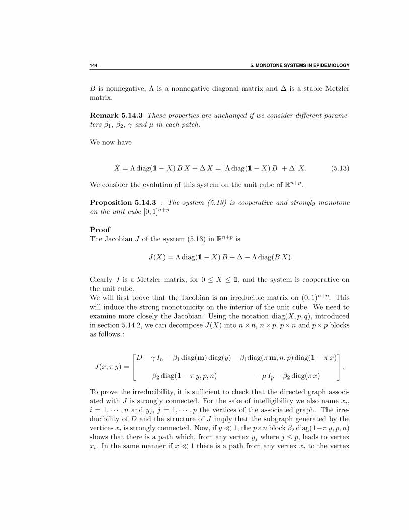
144 5. MONOTONE SYSTEMS IN EPIDEMIOLOGY
B is nonnegative, Λ is a nonnegative diagonal matrix and ∆ is a stable Metzlermatrix.
Remark 5.14.3 These properties are unchanged if we consider different parame-ters β1, β2, γ and µ in each patch.
We now have
X = Λ diag(1−X)BX + ∆X = [Λ diag(1−X)B + ∆]X. (5.13)
We consider the evolution of this system on the unit cube of Rn+p.
Proposition 5.14.3 : The system (5.13) is cooperative and strongly monotoneon the unit cube [0, 1]n+p
ProofThe Jacobian J of the system (5.13) in Rn+p is
J(X) = Λ diag(1−X)B + ∆− Λ diag(BX).
Clearly J is a Metzler matrix, for 0 ≤ X ≤ 1, and the system is cooperative onthe unit cube.We will first prove that the Jacobian is an irreducible matrix on (0, 1)n+p. Thiswill induce the strong monotonicity on the interior of the unit cube. We need toexamine more closely the Jacobian. Using the notation diag(X, p, q), introducedin section 5.14.2, we can decompose J(X) into n×n, n× p, p×n and p× p blocksas follows :
J(x, π y) =
D − γ In − β1 diag(m) diag(y) β1diag(πm, n, p) diag(1− π x)
β2 diag(1− π y, p, n) −µ Ip − β2 diag(π x)
.To prove the irreducibility, it is sufficient to check that the directed graph associ-ated with J is strongly connected. For the sake of intelligibility we also name xi,i = 1, · · · , n and yj , j = 1, · · · , p the vertices of the associated graph. The irre-ducibility of D and the structure of J imply that the subgraph generated by thevertices xi is strongly connected. Now, if y 1, the p×n block β2 diag(1−π y, p, n)shows that there is a path which, from any vertex yj where j ≤ p, leads to vertexxi. In the same manner if x 1 there is a path from any vertex xi to the vertex

5.14. ROSS MODEL IN A PATCHY ENVIRONMENT 145
yj (necessarily j ≤ p). It is now clear that between any couple of vertices thereexists a path. This proves the strong monotonicity on the unit cube except on thefaces, i.e., for x 6 1 and y 6 1. Now if an initial point is on one of these faces,the trajectory of the system leaves immediately the face. This implies the strongmonotonicity of the flow of the system.
5.14.5 Main theorem
In this section we will give an analytic expression for R0 and completely answerto the stability question.As usual ρ(M) is the spectral radius of a matrix M. To express the basic reproduc-tion ratio, we need a notation to extract blocks from matrices. If M is a matrix,we denote by M(1 : p, 1 : q) the submatrix consisting of p first rows and the q firstcolumns of M . With this notation
Proposition 5.14.4 :The origin is the DFE of (5.12) and
R20 =
β1 β2
µρ (− diag(πm)Z) ,
where Z = (D − γ I)−1 (1 : p, 1 : p), i.e., the submatrix of the p first rows and pfirst columns of (D − γ I)−1.
ProofThe Jacobian, computed at the DFE, is J(0) = ΛB + ∆. The part coming frominfection is ΛB and the part coming from other transfers is ∆. Hence R0 =ρ(−ΛB∆−1). If Ip,n is the p× n identity matrix, we set
F =
[0 β1 diag(πm, n, p)
β2 Ip,n 0
].
V =
[D − γ In 0
0 −µ Ip
].
We have R0 = ρ(−F V −1) = ρ(−V −1 F ). We can compute F V −1. We remarkthat the product Ip,n . (D − γ In)−1 is the block (p, n) extracted from the matrix(D − γ In)−1.
−F V 1 =
0β1
µdiag(πm, n, p)
−β2 (D − γ n)−1(1 : p, 1 : n) 0
.

146 5. MONOTONE SYSTEMS IN EPIDEMIOLOGY
If A and B are two n× p and p× n matrices, we have the relation
det
[λ In −A−B λ Ip
]= λn−p det(λ2 Ip −BA) = λp−n det(λ2 Ip −AB)
The last relation implying simply that, in the characteristic polynomial of AB,there are (n−p) roots equal to zero. Then, using again the structure of diag(m, n, p)and Cayley reduction, we have
R20 = ρ
(−β1 β2
µdiag(πm)
[(D − γ In)−1(1 : p, 1 : p)
]),
where (D − γ I)−1(1 : p, 1 : p) is the block of the p first rows and p first columnsof (D − γ I)−1.
For the classical Ross-Macdonald model, this formula gives the intended result
R20 =
ma2 b1 b2γ µ
. We have now reduced the study of the stability of the complete
system (5.9) to the study the stability of (5.13).
Remark 5.14.4 The expression of R0 can be rendered more geometrical if we usethe projection π.This is useful if the reordering of coordinates is not done.
R20 = ρ
(−β1 β2
µdiag(πm)π (D − γ I)−1 πT
).
Finally, using the definition of D and the fact that diagonal matrices commute, wehave the following expression of R0 for the original system (5.9)
R20 =
β1 β2
µρ(− diag(π V ) diag(π N)−2 π (M − γ I)−1 πT diag(π N)
). (5.14)
We know from [21, 80] that ifR0 < 1 then the DFE is locally asymptotically stable,and if R0 > 1 then the DFE is unstable. Our main result is a global stability resultof the DFE , which holds for R0 ≤ 1 and a global stability result for R0 > 1.
Theorem 5.14.1 :If R0 ≤ 1, then all the trajectories of (5.13) tend to the disease free equilibrium,which is globally asymptotically stable on the unit cube. If R0 > 1, then there existsa unique endemic equilibrium (x, y) 0, and all the trajectories of the unit cube,minus the origin, tend to this equilibrium which is GAS on the unit cube minusthe origin.

5.14. ROSS MODEL IN A PATCHY ENVIRONMENT 147
ProofWe recall the system (5.13)
X = Λ diag(1−X)BX + ∆X = [Λ diag(1−X)B + ∆]X.
To prove the first assertion we assume R0 = ρ(−ΛB∆−1) ≤ 1.The Jacobian at the origin is J = ΛB + ∆. Since ∆ is a nonsingular Metzlermatrix and Λ ≥ 0, this expression is a regular splitting of J . Then we have seenthat we have the equivalence between s(J) ≤ 0 and ρ(−ΛB∆−1) ≤ 1.We have seen that the Jacobian at the origin is an irreducible Metzler matrix andthat there exists a positive vector c 0 such that
cT (ΛB + ∆) = s(J) cT ≤ 0.
We use on the unit cube the Liapunov proper function
V (X) = 〈c |X〉,
where 〈 | 〉 denotes the usual inner product. Since c 0 this function is positivedefinite in the nonnegative orthant. We compute the derivative V of V along thetrajectories of (5.13)
V = 〈c |(Λ diag(1−X)B + ∆)X〉 ≤ 〈c |(ΛB + ∆)X〉 = 〈(ΛB + ∆)T c |X〉
= 〈s(J) c|X〉 = s(J) 〈c|X〉 ≤ 0
This proves the stability of the DFE. We now consider the asymptotic stability.
V (X) = 〈c |(Λ diag(1−X)B + ∆)X〉 = 〈c |(ΛB + ∆)X〉 − 〈c |Λ diag(X)BX〉.
If R0 < 1, then s(ΛB + ∆) < 0 whence
V (X) ≤ 〈c |(ΛB + ∆)X〉 = s(ΛB + ∆) 〈c |X〉 < 〈c|X〉 < 0.
When R0 = 1, we have α(ΛB + ∆) = 0, and V reduces to
V (X) = −〈c |Λ diag(X)BX〉 ≤ 0.
We consider the set E = X ∈ [0, 1]n+p| V (X) = 0. Since c 0 and Λ diag(X)BX ≥0, this set is composed of points for which xi yi = 0, for all the indexes i ≤ p. Weshow that the largest invariant set L, contained in E is reduced to 0. The proof

148 5. MONOTONE SYSTEMS IN EPIDEMIOLOGY
hinges on the irreducibility of the system. There exists at least a point in L suchthat xi = 0 or yi = 0 with i ≤ p.
If xi = 0 considering
xi = β1mi (1− xi) yi − γ xi + (M x)i
= β1mi yi +∑j 6=i
mij xj = 0.
This shows that yi = 0, and all the xj for which mij 6= 0 i.e., all the xj “con-nected” to xi are equal to zero. A finite recursion argument, with the irreducibilityhypothesis, concludes that all the xi and the yi are equal to zero. The set L isreduced to the origin.
If yi = 0 considering
yi = β2 (1− yi)xi − µ yi = β2 xi = 0.
the invariance of L shows that xi = 0, and we are back to the preceding situation.In any case L is reduced to the origin. By LaSalle’s invariance principle [54] wededuce the global asymptotic stability of the DFE.
which proves the asymptotic stability of the DFE.
For the second assertion of the Theorem, when R0 > 1 then the DFE is unstable.It is straightforward to check that the system is strongly sublinear. Let 0 < λ < 1and
T (X) = Λ diag(1−X)BX + ∆X
Then if X 0, BX 0
T (λX) = Λ diag(1−λX)B λX+∆λX Λ diag(1−X)B λX+∆λX = λT (X).
This proves the strong sublinearity, hence all the hypothesis of Hirsch’s Theorem(5.10.1) are satisfied, therefore there exists an unique positive equilibrium whichis GAS on [0, 1]n+p \ 0.
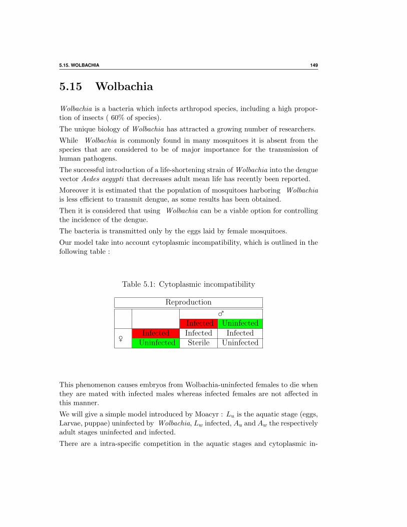
5.15. WOLBACHIA 149
5.15 Wolbachia
Wolbachia is a bacteria which infects arthropod species, including a high propor-tion of insects ( 60% of species).
The unique biology of Wolbachia has attracted a growing number of researchers.
While Wolbachia is commonly found in many mosquitoes it is absent from thespecies that are considered to be of major importance for the transmission ofhuman pathogens.
The successful introduction of a life-shortening strain of Wolbachia into the denguevector Aedes aegypti that decreases adult mean life has recently been reported.
Moreover it is estimated that the population of mosquitoes harboring Wolbachiais less efficient to transmit dengue, as some results has been obtained.
Then it is considered that using Wolbachia can be a viable option for controllingthe incidence of the dengue.
The bacteria is transmitted only by the eggs laid by female mosquitoes.
Our model take into account cytoplasmic incompatibility, which is outlined in thefollowing table :
Table 5.1: Cytoplasmic incompatibility
Reproduction
Infected Uninfected
Infected Infected Infected
Uninfected Sterile Uninfected
This phenomenon causes embryos from Wolbachia-uninfected females to die whenthey are mated with infected males whereas infected females are not affected inthis manner.
We will give a simple model introduced by Moacyr : Lu is the aquatic stage (eggs,Larvae, puppae) uninfected by Wolbachia, Lw infected, Au and Aw the respectivelyadult stages uninfected and infected.
There are a intra-specific competition in the aquatic stages and cytoplasmic in-

150 5. MONOTONE SYSTEMS IN EPIDEMIOLOGY
compatibility is modeled in equation 2 and 4.
Au = λLu − µuAu
Lu = r AuAu
Au +Aw− [ λ+ ν + d (Lu + Lw)] Lu
Aw = λLw − µiAw
Lw = r Aw − [ λ+ ν + d (Lu + Lw)] Lw
(5.15)
This system is defined on the nonnegative orthant, by Lipschitz prolongation. Thenonnegative orthant is clearly positively invariant.
5.15.1 Monotonicity
We consider the Jacobian of this system
Jac =
−µu λ 0 0
r − r A2w
(Aw+Au)2−λ− ν − dLw − 2 dLu − r A2
u
(Aw+Au)2−dLu
0 0 −µw λ
0 −dLw r −λ− ν − 2dLw − dLu
If we consider the permutation matrix
P =
−1 0 0 00 −1 0 00 0 1 00 0 0 1
The matrix P JacP is aMetzler matrix. This means that the system is monotonefor the cone K = −R+ ×−R+ × R+ × R+.
5.15.2 Strong monotonicity
The system is irreducible. If we draw the graph of the Jacobian we obtain

5.15. WOLBACHIA 151
Au ≠0
Au ≠0
Lw ≠0
Lu ≠0
Figure 5.1: Graph of Jacobian
The system will be strongly monotone if Lw 6= 0 and Au 6= 0.
5.15.3 Equilibria
We have three equilibria.
A DFE
L∗u =(rλ− µu(λ+ ν))
dµuA∗u =
λ (rλ− µu(λ+ ν))
dµ2u
This equilibrium exists if the basic offspring number, for uninfected, satisfies
Roffsp,u =r λ
µu (λ+ ν)> 1
A Wolbachia completely infected equilibrium (WCIE)
L∗w =(rλ− µw(λ+ ν))
dµwA∗w =
λ (rλ− µw(λ+ ν))
dµ2w
This equilibrium exists if the basic offspring number, for infected, satisfies
Roffsp,w =r λ
µi (λ+ ν)> 1

152 5. MONOTONE SYSTEMS IN EPIDEMIOLOGY
A coexistence equilibrium
Lu =µ2u [ r λ− µw (λ+ ν)]
dµw (µ2u − µw µu + µ2
w)Au =
λ [ r λ− µu (λ+ ν))
dµ2u
Lw =(µw − µu) [ r λ− µw (λ+ ν)]
d (µ2u − µw µu + µ2
w)Aw =
λ [ rλ− µw(λ+ ν)]
dµ2w
This equilibrium exists if Roffsp,w > 1Since Wolbachia is life shortening we assume that µw > µu. Hence if Roffsp,w >
1 we have three equilibria.
5.15.4 Basic reproduction ratio
We will now consider the basic reproduction ratio for the infection R0.The Jacobian at the DFE is
J(A∗u, L∗u, 0, 0) =
−µu λ 0 0
r −2rλµu
+ λ+ ν −r − rλµu
+ λ+ ν
0 0 −µi λ
0 0 r − rλµu
This is a block upper triangular matrix. The upper block diagonal is
J1 =
−µu λ
r −2rλµu
+ λ+ ν
The trace of this matrix is − rλ
µu+ λ + ν − µu − rλ
µu< 0, if Roffsp,u > 1. The
determinant of J1 is rλ − µu(λ + ν) > 0. This block is Hurwitz. Thereforehypothesis H5 is satisfied.We can now look at the Jacobian of the transmission in the infected compartment
F =
[0 0r 0
]The Jacobian of the other terms is
V =
[−µi λ
0 − rλµu
]

5.15. WOLBACHIA 153
Hence the next generation matrix is
K =
[0 0rµw
µuµw
]and
R0 =µuµw
< 1
Which proves the asymptotic stability of the DFE.
5.15.5 Stability of the CWIE
Consider the Jacobian at the CWIE
J(0, 0, A∗w, L∗w) =
−µu λ 0 0
0 − rλµw
0 0
0 0 −µw λ
0 − rλµw
+ λ+ ν r −2rλµw
+ λ+ ν
This a lower block triangular matrix. The lower diagonal block is
J4 =
−µw λ
r −2rλµw
+ λ+ ν
which is clearly Hurwitz if Roffsp,w > 1.
The upper diagonal block is
J1 =
[−µu λ
0 − rλµw
]which is Hurwitz without any condition.
The Jacobian J(CWIE) is then Hurwitz, which proves the asymptotic stability ofthe CWIE.
5.15.6 Global analysis
We have 3 equilbria, we will use Hirsch’s Theorem (5.11.1). We must prove thatthe trajectories are forward bounded

154 5. MONOTONE SYSTEMS IN EPIDEMIOLOGY
Solutions are forward bounded
we denote Xu = (Au, Lu) and Xw = (Aw, Lw). The vector field on R4+ defined by
(5.15) will be denoted by f(Au, Lu, Aw, Lw) = (fu(Au, Lu, Aw, Lw), fw(Au, Lu, Aw, Lw))on R2+ × R2
+.The equilibria will be denoted by
XDFE = (A∗u, L∗u, 0, 0) XWCIE = (0, 0, A∗w, L
∗w) Xcoex = (Au, Lu, Aw, Lw, )
and
X∗u = (A∗u, L∗u) X∗w = (A∗w, L
∗w)
Recall that the order is given by the cone K = −R+×−R+×R+×R+. We denoteby ≤ the classical order given by the nonnegative orthant and by ≤K the orderassociated to K.We have
XDFE K Xcoex K XWCIE
Since f(XDFE) = 0 and f(XWCIE) = 0, by proposition (5.8.2) the order interval(for K-order) [XDFE, XWCIE]K is positively invariant.We can obtain more : if ξ > 1 we have fu(ξ A∗u, ξ L
∗u, 0, 0) < ξ fu(A∗u, L
∗u, 0, 0) = 0
and fw(0, 0, ξ A∗w, ξ L∗w) < ξ fu(0, 0, A∗w, L
∗w) = 0. For the K-order
ξ XDFE = (ξ A∗u, ξ L∗u, 0, 0)K ξ XWCIE = (0, 0, ξ A∗w, ξ L
∗w) with
f(ξ XDFE) >K 0 and f(ξ XWCIE) <K 0
This proves by proposition (5.8.2) that [ ξ XDFE, ξ XWCIE]K is positively invariant.For ξ large enough any element of the nonnegative orthant can be included in thisorder interval. Therefore any trajectory is bounded.
Stability analysis
We consider the order interval [XDFE, Xcoex]K and the 2-face defined by Aw =Lw = 0. The 2-face is positively invariant and we claim that XDFE is GAS on thisface. It is sufficient to note that this system on the 2-face is strongly monotone,strictly sublinear and that X∗u is asymptotically stable. By Hirsch theorem (5.10.1)X∗u is GAS. We know thatXDFE is asymptotically stable becauseR0 > 1. Hence allthe hypothesis of Theorem (5.11.1) are satisfied. All trajectories in [XDFE, Xcoex]K

5.16. BRUCELLOSIS 155
converge to XDFE and Xcoex is unstable. This result is obtained without anycomputation.Actually [ ξ XDFE, Xcoex]K is in the basin of attraction ofXcoex. Left as an exercise.
u
Increasing order for u
Increasing order for w
X*u
Xu,coex
ξ X*u
ξ X*wX*wXw,coex
Xcoex
R2
R2
Figure 5.2: Order interval and equilibria
5.16 Brucellosis
We consider the following model for ovine brucellosis incorporating direct andindirect transmission from
B. Ainseba, C. Benosman and P. MagalJournal of Biological Dynamics, vol 4, n° 1, 2010 pp 2-11
This section left as an exercise has for objective to give easily the stability analysisof the model. Compare with the original paper !
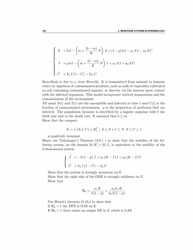
156 5. MONOTONE SYSTEMS IN EPIDEMIOLOGY
S = b S −(m+
(b−m)
KN
)S + (1− p) b I − a1 S I − a2 S C
I = p b I −(m+
(b−m)
KN
)I + a1 S I + a2 S C
C = k1 I (1− C) − k2, C
Brucellosis is due to a virus Brucella. It is transmitted from animals to humanseither by ingestion of contaminated products, such as milk or vegetables cultivatedon soil containing contaminated manure, or directly via the mucosa upon contactwith the infected organisms. This model incorporate vertical transmission and thecontamination of the environment.
AS usual S(t) and I(t) are the susceptible and infected at time t and C(t) is thefraction of contaminated environment. p is the proportion of newborns that areinfected. The population dynamic is described by a logistic equation with b thebirth rate and m the death rate. It assumed that b ≥ m.
Show that the compact
K = (S, I, C) ∈ R3+ | 0 ≤ S + I ≤ N 0 ≤ C ≤ 1
is positively invariant.
Hence use Vidyasagar’s Theorem (3.6.1 ) to show that the stability of the fol-lowing system, on the domain [0,K] × [0, 1], is equivalent to the stability of the3-dimensional system
I = −b (1− p) I + a1 (K − I) I + a2 (K − I)C
C = k1 I (1− C) − k2C
Show that the system is strongly monotone on KShow that the right side of the ODE is strongly sublinear on K.
Show that
R0 =a1K
b (1− p)+
a2 k1K
k2 b (1− p)
Use Hirsch’s theorem (5.10.1 to show that
if R0 < 1 the DFE is GAS on KIf R0 > 1 there exists an unique EE in K which is GAS.

5.17. POPULATION DYNAMICS OF MOSQUITO 157
If R0 = 1 , consider the candidate Lyapunov function V (I, C) = k2 I + a2K C.Show that the origin is stable.Use again Hirsch’s Theorem Hirsch’s theorem (5.10.1 to exclude an endemic EEand to the stability of the DFE. You can also use LaSalle’s principle.
5.17 Population dynamics of mosquito
The life cycle of a mosquito consists of two main stages: aquatic (egg, larva, pupa)and adult (with males and females). After emergence from pupa, a female mosquitoneeds to mate and get a blood meal before it starts laying eggs. Then every 4−−5days it will take a blood meal and lay 100−−150 eggs at different places (10−−15per place). For the mathematical description, our model is inspired by the modelconsidered in [23, 4].However we will consider three aquatic stages, where the authors [23, 4] lumpthe three stages into a single aquatic stage. The rationale is to prepare for asubsequent model with infection by Wolbachia. Furthermore, we split the adultstage into three sub-compartments, males, immature female and mature femalewhich leads to the following compartments:
• Eggs E;
• Larvae L;
• Pupae P ;
• Males M ;
• Young immature females Y ; We consider a female to be in the Y compart-ment from its emergence from pupa until her gonotrophic cycle has began,that is the time of mating and taking the first blood meal, which takestypically 3−−4 days.
• Mature females F , i.e., fertilized female. A female needs to mate successfullyonly once and rarely remate.
The parameters µE , µP , µY , µF and µM are respectively the death rate of eggs,larvae, pupae, immature female, mature females and males. The parameters ηE ,ηL,ηP , β are the respective rate of transfer to the next compartment. The param-eter ν is the sex ratio. In this model, we use a density dependent death rate forthe larvae stage since mosquitoes larvae (anopheles and aedes) are density sen-sitive, which imply an additional density mortality rate µ2 L . The equation forL can be considered as a logistic equation. Such an hypothesis is appropriate

158 5. MONOTONE SYSTEMS IN EPIDEMIOLOGY
since mosquitoes only have access to a finite number of potential breeding sites,and density-dependent larval survival has been demonstrated at such sites. Theparameter φ is the average amount of eggs laid per fertilized female per unit oftime.
Mating is a complex process that is not fully understood. However, as discussedin [4] and references therein, the male mosquito can mate practically through allits life. A female mosquito needs one successful mating to breed lifelong. It isadmitted that mosquitoes locate themselves in space and time to ensure they areavailable to mate. Therefore, it is reasonable to assume that in any case theimmature female will mate and afterwards move to compartment F , or die. Thusa parameter like 1
β+µYcan represents the mean time given by length of the first
gonotrophic cycle of a female, i.e., the interval from immediately after the matingto the first blood meal.
We assume that all the parameters are constant. In reality, the mosquito popula-tion varies seasonally. Nevertheless, such a model should be a good approximationfor a definite season.
5.17.1 The model
E
L
P
YM
F
Eggs
Larvae
Pupae
Immature FemalesMales
Mature Females
μEηE
ηL
νηP
(1−ν)ηP
β
μL
μP
μYμM

5.17. POPULATION DYNAMICS OF MOSQUITO 159
E = φF − (µE + ηE)E
L = ηE E − (µL + ηL + µ2 L)L
P = ηL L− (µP + ηP )P
Y = ν ηP P − (β + µY )Y
F = β Y − µF F
M = (1− ν) ηP P − µM M.
(5.16)
If we denote by X a vector of the state space of this systems.
XT = (E,L, P, Y, F,M),
then the systems can be written
X = A(X)X,
For (5.16) the matrix is given by
A(X) =
−(µE + ηE) 0 0 0 φ 0
ηE −(µL + ηL + µ2 L) 0 0 0 0
0 ηL −(µP + ηP ) 0 0 0
0 0 ν ηP −(β + µY ) 0 0
0 0 0 β −µF 0
0 0 (1− ν) ηP 0 0 −µM
.
The matrix A(X) is a Metzler matrix, this implies that the nonnegative orthantis positively invariant for (5.16).
Actually A(X) depends only of L, so we will denote the matrix A(X) simply byA(L).

160 5. MONOTONE SYSTEMS IN EPIDEMIOLOGY
5.17.2 Analysis of the model
We can define a basic offspring number, using the techniques of R0, where thetransmission term is given by φF ) :Using (5.16) shows that
R0,offsp =φ
µF
ηEµE + ηE
ηLµL + ηL
ν ηPµP + ηP
β
β + µY.
When R0,offsp ≤ 1 the only equilibrium is the origin. When R0,offsp > 1 a secondpositive equilibrium exists X∗ = (E∗, L∗, P ∗, Y ∗, F ∗,M∗)T .We can express all the components as positive linear expressions of P ∗
L∗ =µp + ηpηL
P ∗, Y ∗ =ν ηPβ + µY
P ∗, (5.17)
F ∗ =β
β + µY
ν ηPµF
P ∗, M∗ =(1− ν) ηP
µMP ∗ (5.18)
E∗ =φ
µE + ηE
β
β + µY
ν ηPµF
P ∗. (5.19)
Finally, replacing in the equation L = 0, we get
P ∗ =ηL (µL + ηL)
µ2 (µP + ηP )
(ηE ν φ ηL ηP
µF (µE + ηE) (µL + ηL) (µP + ηP )− 1
)=ηL (µL + ηL)
µ2 (µP + ηP )(R0,offsp − 1) > 0. (5.20)
The system is monotone
Jac =
−ηE − µE 0 0 0 φ 0ηE −ηL − µ2 − µL 0 0 0 00 ηL −ηP − µP 0 0 00 0 ν ηP −β − µY 0 00 0 0 β −µF 00 0 (1− ν) ηP 0 0 −µM
Then by proposition (5.8.2) the order interval [0, x∗] is positively invariant.The system is strictly sublinear. Denote by T (X) = A(X)X, then for 0 < λ < 1and X 0
λT (X) = λA(L)L < λA(λL)L = T (λX)

5.18. A SCHISTOSOMIASIS MODEL 161
Let now λ > 1, then by sublinearity1
λT (λX∗) < T (X∗) = 0. Therefore the order
interval [0, λX∗] is positively invariant by proposition (5.8.2). We conclude thatall the trajectories are forward bounded. Then we can us Vidyasagar’s Theoremto reduce the system, suppressing the equation for the males.
The Jacobian for the reduced system is now−ηE − µE 0 0 0 φ
ηE −ηL − µ2 − µL 0 0 00 ηL −ηP − µP 0 00 0 ν ηP −β − µY 00 0 0 β −µF
This matrix is clearly irreducible and the system is strongly monotone and strictlysublinear. We conclude with Hirsch’s Theorem
Theorem 5.17.1
If the basic reproduction ratio R0,offsp > 1 then there is an unique positive equilib-rium X∗ which is GAS on R6
+ \ 0.
5.18 A schistosomiasis model
We consider the following model from
Allen, E J and Victory, H D Jr, Modelling and simulation of a schistosomiasisinfection with biological control. Acta Tropica, 2 vol 87, pp 251–267 (2003).
We consider the following system with variables :
• Ih infected human by schistosomes
• Es the latent snails
• Is infectious snails releasing cercariae
• Im infected mammals
• Nh the human population
• Ns the snail population for transmission for schistosomiasis
• Nrs a resistant snail population, competitor for the first population
• Nm a mammals population.

162 5. MONOTONE SYSTEMS IN EPIDEMIOLOGY
Two subsystem. A demographic model
Nh = Λ− µhNn
Ns = rsNs
(1− Ns
Ks− λrsNrs
)
Nrs = rrsNrs
(1− Nrs
Krs− λsNs
)
Nm = rmNm
(1− Nm
Km
)and a transmission model
Ih = βhs (Nh − Ih) Is − γh Ih
Es = (βsh Ih + βsm Im) (Ns − Es − Is)− (µs + αs +Ns
Ks+ λrsNrs)Es
Is = αsEs − (µs +Ns
Ks+ λrsNrs) Is
Im = βms (Nm − Im) Is − (µm +rmKm
Nm) Im
It is immediate that the nonnegative orthant is positively invariant. By consideringthe population dynamics equations, the compact
K = X ∈ R8+|Nh ≤
Λ
µh, Ns ≤ Ks, Nrs ≤ Krs, Nm ≤ Km,
is positively invariant and absorbing. Absorbing means that any trajectorytends to K when t→ +∞. Therefore any trajectory is forward bounded.
Considering the population dynamics it is clear that N∗h =Λ
µhand N∗m = Km
are GAS equilibria. For the equations giving (Ns, Nm) we have a classical Lotka-Volterra competition model. This is analyzed for example in [41, 84].
We assume that λsKs > 1 and λrsKrs < 1. In this case the positive coexistenceequilibrium exists (N∗s , N
∗rs) and is GAS on the interior of the nonnegative orthant.
We can apply Vidyasagar’s Theorem to obtain a reduced system.
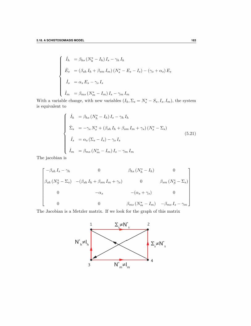
5.18. A SCHISTOSOMIASIS MODEL 163
Ih = βhs (N∗h − Ih) Is − γh Ih
Es = (βsh Ih + βsm Im) (N∗s − Es − Is)− (γs + αs)Es
Is = αsEs − γs Is
Im = βms (N∗m − Im) Is − γm ImWith a variable change, with new variables (Ih,Σs = N∗s − Ss, Is, Im), the systemis equivalent to
Ih = βhs (N∗h − Ih) Is − γh Ih
Σs = −γsN∗s + (βsh Ih + βsm Im + γs) (N∗s − Σs)
Is = αs (Σs − Is)− γs Is
Im = βms (N∗m − Im) Is − γm Im
(5.21)
The jacobian is
−βsh Is − γh 0 βhs (N∗h − Ih) 0
βsh (N∗S − Σs) −(βsh Ih + βsm Im + γs) 0 βsm (N∗S − Σs)
0 −αs −(αs + γs) 0
0 0 βms (N∗m − Im) −βms Is − γm
The Jacobian is a Metzler matrix. If we look for the graph of this matrix
1 2
34
Σs≠N*s
Σs≠N*s
N*h≠Ih
N*m≠Im

164 5. MONOTONE SYSTEMS IN EPIDEMIOLOGY
The system is strongly monotone excepted in two points Σs = N∗s ,i.e., all thesnail are infected and/or infectious and Im = N∗m, i.e., all the mammal are infected.These two points are immediately leaved by any trajectory.
Left as an exercise, we compute R0 for the DFE (0, 0, 0, 0)
R20 =
αs γm βhs βshN∗h N
∗s + αs γh βsm βmsN
∗mN
∗s
γhγmαsγs + γhγmγ2s
.
It is not difficult to check that the system is strictly sublinear.We have, denoting by F the vector field defined by the system (??)
F (N∗h , N∗s , N
∗s , N
∗m) = (−γnN∗h ,−γs, N∗s ,−γsN∗s ,−γmN∗m)T 0
Hence by Hirsch’s Theorem if R0 > 1 there exists a unique positive equilibriumwhich is GAS on the nonnegative orthant minus the origin. We can also use theproposition using sublinearity.
5.19 Notes
To quote H. Thieme
The theory of (quasi-)positive matrices (i.e., Metzler) and of the as-sociated dynamical system, as rarely as it is taught in standard lin-ear algebra or ordinary differential equations courses, is a immenselypowerful tool in population models with some kind of structures . . . H.Thieme pp 418 [78]
The Perron-Frobenius theorem appears everywhere in applied mathematics: insolutions using iterative methods linear systems [82], in finite Markov chain the-ory [71], input-output analysis in economics, Lotka-Volterra models [77], Google’spage rank algorithm, in demographics (Leslie Models) and even in the ranking ofAmerican Football teams [49] . . .
It is an important theorem and also a little forgotten in the academic courses.The theory of monotonic systems, seen from the angle of dynamical systems, wasintroduced by Hirsch in a series of papers in the 1980s [36, 38, 39, 40]. In fact theywere called cooperative systems. The two terms still coexist. The book ”theoryof the chemostat” [72] gives some applications of monotonous systems. We haveincluded this theory in this course, because on one hand there are applications inepidemiology and on the other hand there is no elementary references as remarkedby H. Thieme.

Chapter 6
Models with continuous delays
6.1 Introduction
Dynamic models of many processes in mathematical epidemiology give systems ofordinary differential equations called compartmental systems. Often, these systemsinclude time lags; in this context, continuous probability density functions (pdfs)of lags are far more important than discrete lags.
Consider the already seen example of an intra-host modelx = Λ− µx x− β x vy = β x v − µy vm = r µy y − µvm− β x v
(6.1)
variables :
• x Concentration of target cells, namely CD+ T-cells
• y Concentration of cells invade by virions (HIV)
• m Concentration fo free circulating virions
This a classical Model : Perelson (1993), Nowak (1996), May-Anderson-Gupta(1989) said fundamental model of immunology.
The binding of a parasite particle to a receptor on a target cell initiates a cascade of
events that can ultimately lead to the target cell becoming productively infected,i.e. producing new parasite.
However, in reality there is a time delay between initial viral entry into a celland subsequent viral production Fixed delays (of which a zero delay is a specialcase) are not biologically realistic.
165

166 6. MODELS WITH CONTINUOUS DELAYS
For example conversion of a newly infected cell into a productively infected cell is amulti-step process that requires viral entry into the host cell, reverse transcriptionof viral RNA into DNA, transport of the newly made DNA into the nucleus,integration of the viral DNA into the chromosome, production of viral RNA andprotein, and the creation of new virus from these newly synthesized RNA moleculesand proteins.
Even in a homogeneous population of target cells, it is unreasonable to expect thatthe time to complete all of these processes will be the same for every infected cell.
If we consider biologically realistic differences in cell activation state, metabolism,position of the cell in the cell cycle, pre-existing stores of nucleotides and otherprecursors needed for the production of new virions, along with generic variationin the viral population, variation in infection delay times becomes a near certainty.
To incorporate a delay, we consider the following modified model
x = Λ− µx x− β x v
y = β
∫ ∞0
g(τ)x(t− τ) v(t− τ) dτ − µy y
m = r µy y − µv v − β x v
(6.2)
This is an integrodifferential equation. The function g(t) is the probability thata individual infected is infectious t unit of time later. This a probability densityfunction (pdf). A pdf g satisfies
• g(t) ≥ 0
•∫ +∞
−∞g(t) dt = 1
• F (t) = Prob[ X ≤ t ] =
∫ t
−∞g(s) ds.
A very useful pdf is the Erlang distribution
gn,σ =tn−1 e−
tσ
σn (n− 1)!(6.3)
The characteristics are : mean nσ, deviation nσ2, maximum (n − 1)σ ; This
function is also defined with the parameter k =1
σ. The parameter n is called the
shape parameter and σ the rate parameter.

6.1. INTRODUCTION 167
This gamma distribution can reproduce a variety of biological delay distributionsand is amenable enough to allow for analytical solutions.
It is a ‘tunable’ distribution that can mimic both exponential declines andmore general bell-shaped distributions
This distribution was developed by Agner Krarup Erlang to model the number ofsimultaneous phone calls. The Erlang distribution can be used to model the timeto complete n operations in series, where each operation requires an exponentialperiod of time to complete. In a Poisson process the sum of n inter-arrival timeshas an Erlang distribution with parameters n and σ. We will show that theErlang distribution is the distribution of the sum of k independent and identicallydistributed random variables each having an exponential distribution..
0 0.5 1 1.5 2 2.5 3 3.5 4 4.5 50
0.5
1
1.5
2
2.5
3
3.5
4
4.5
5
t
n=5
n=25
n=125
Figure 6.1: Erlang distribution
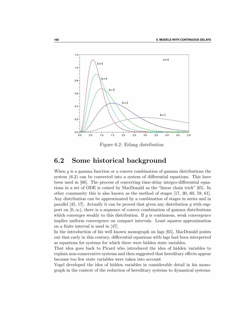
168 6. MODELS WITH CONTINUOUS DELAYS
0.0 0.5 1.0 1.5 2.0 2.5 3.0 3.5 4.0 4.5 5.00.0
0.2
0.4
0.6
0.8
1.0
1.2
k=5
k=4
k=3
k=2
k=1
n=4
Figure 6.2: Erlang distribution
6.2 Some historical background
When g is a gamma function or a convex combination of gamma distributions thesystem (6.2) can be converted into a system of differential equations. This havebeen used in [66]. The process of converting time-delay integro-differential equa-tions in a set of ODE is coined by MacDonald as the “linear chain trick” [65]. Inother community this is also known as the method of stages [17, 30, 60, 59, 61].Any distribution can be approximated by a combination of stages in series and inparallel [45, 17]. Actually it can be proved that given any distribution g with sup-port on [0,∞), there is a sequence of convex combination of gamma distributionswhich converges weakly to this distribution. If g is continuous, weak convergenceimplies uniform convergence on compact intervals. Least squares approximationon a finite interval is used in [47].In the introduction of his well known monograph on lags [65], MacDonald pointsout that early in this century, differential equations with lags had been interpretedas equations for systems for which there were hidden state variables.That idea goes back to Picard who introduced the idea of hidden variables toexplain non-conservative systems and then suggested that hereditary effects appearbecause too few state variables were taken into accountVogel developed the idea of hidden variables in considerable detail in his mono-graph in the context of the reduction of hereditary systems to dynamical systems.

6.3. THE LINEAR CHAIN TRICK 169
The use of a catenary chain of compartments with one-way flow to generate a dis-tribution of lags is well known. Gyori gives two references in the Russian literatureon this chain method and MacDonald used it extensively in his monograph, callingit the ‘linear chain trick’, and pointing to it as an example of hidden variables.
6.3 The Linear Chain Trick
Suppose that the material leaving a compartment j has a pdf of delay hij(τ)before entering the compartment i. At time t a fraction hij(t − τ) dτ will entercompartment i during the interval [τ, t + dτ ] for τ ≤ t. Then the total materialcoming from j at time t is
fij
∫ t
−∞qj(τ)hij(t− τ) dτ
To fix the idea consider the following SIR model, where to be infectious has adelay, modeled by a pdf.
S = Λ− β S(t)
∫ +∞
0f(τ) I(t− τ) dτ − µS(t)
I = β S(t)
∫ +∞
0f(τ) I(t− τ) dτ − (µ+ γ) I(t)
When the pdf is an Erlang function or a convex linear combination of Erlangfunctions this system is equivalent to a system of ODE [16, 25].
Consider the following input-ouput linear system, which a catenary compartmentalsystem
y1 y2 y3 yninput output
1!
1!
1!
1!
1!
Figure 6.3: Catenary system
The system of ODE is given by

170 6. MODELS WITH CONTINUOUS DELAYS
x1 = u− 1σx1
x2 = 1σ (x1 − x2)
· · ·xn = 1
σ (xn−1 − xn)
output = y = h(x) = 1σ xn =
1
σ〈en|x〉
If we denote by ei the canonical basis of Rn+, let define C =1
σeTn , B = e1 and
A =1
σ
−1 0 0 · · · 01 −1 0 · · · 00 1 −1 · · · 0...
. . .. . .
. . ....
0 · · · 0 1 −1
Then the linear system is now
x = Ax+B u
y = C x
The output is given, for x0 = 0, by
y(t) =
∫ t
0C e(t−s)AB u(s) ds =
∫ +∞
0C e(t−s)AB Y (t− s)u(s) ds
where Y (t) is the Heaviside function
Y (t) =
1 t ≥ 0
0, t < 0
We recall the convolution of functions :
Definition 6.3.1
If f and g are two locally integrable functions, their convolution, denoted by f ? g,is defined by

6.3. THE LINEAR CHAIN TRICK 171
f ? g(t) =
∫Rf(t− s) g(s) ds =
∫Rf(t) g(t− s) ds
Then the output y(t) is simply
y(t) = [CetAB Y (t)] ? u(t),
and a delay with pdf h(τ)
∫ t
−∞qj(τ)hij(t− τ) dτ =
∫Rqj(τ)hij(t− τ)Y (t− τ) dτ = [ hij Y ? qj ] (t)
We will now compute CetAB for the catenary system. First of all we remark that
A =1
σ(−In +N). The matrix N is a well known nilpotent matrix with 1 on the
first sub-diagonal, Np is the matrix with 1 on the p sub-diagonal. Therefore Nn−1
is simply the matrix with only 1 in the (n, 1) entry and Nn = 0.The second remark is
CetAB =1
σ〈en|etA e1〉 =
1
σetA(n, 1)
Using the fact that N and In are commuting
1
σetA(n, 1) = e
−t
σtn−1
(n− 1)!σn= gn,σ
Finally
y(t) = gn,σ(t) ? u(t)
This means that introducing such a catenary chain of compartments between twocompartments generates a continuous distribution of delays with density function(6.3).If one introduces a unit impulse, i.e., a Dirac function δ, into the first compartmentof the catenary chain at t = 0, the density function for time of exit is exactly theErlang function. We will precise this now.We consider a linear control system
x = Ax+B u
y = C x(6.4)

172 6. MODELS WITH CONTINUOUS DELAYS
Definition 6.3.2 (Impulse response) :
The matrix
h(t) = C etAB,
is called the impulse response of the linear system (6.4)
Proposition 6.3.1 :
The impulse response is the output of a linear control system for a nul initialcondition, to a Dirac input.
Proof Consider the following sequences of functionsfn(t) = n if 0 ≤ t ≤ 1
nfn(t) = 0 otherwise
These functions are called unit pulse (∫R fn(s)ds = 1)
If we use fn as an input we obtain
yn(t) = CetA n
∫ 1n
0e−sAB ds
= CetA ne
1nA − IA
B
Therefore
limn→+∞
ne
1nA − IA
= I
The limit is CetAB.
This result is obtained immediately with the language of distributions, since δ isa unit for the convolution.
y(t) = h(t) ? δ = h(t)
The limit of fn in distributions sens is the Dirac function δ. It can be shown that,for σ fixed, the sequence of Erlang function (6.3) converges to the Dirac functionwhen n→ +∞.

6.4. GENERALIZED LINEAR CHAIN TRICK 173
6.4 Generalized linear chain trick
We will show how to generates a convex combination of Erlang functions.
We consider a dynamic system where a peculiar one dimensional feedback u(x)has been distinguished. For example the xv term appearing in the second equationof the system (6.1).
x = f(x, u(x)) (6.5)
The function f is an application from Rn × R into R. The function u is definedfrom Rn to R. The functions f and u are supposed to satisfy conditions whichensure that for any initial state x(0) = x0 the system (6.5) has a unique solution.Usually a system x = f(x, u) is called a controlled system.
x = f(x,u)ux
Figure 6.4: Control system
When the function u depends only of time t it is called a control or an input.When u depends on x(t) it is called a feedback.
x = f(x,u)x
x u(x)u
Figure 6.5: Feedback
Let us consider the following controlled linear system ( in control theory’s sense[75, 63]).
y = Ay + wBz = C x
(6.6)
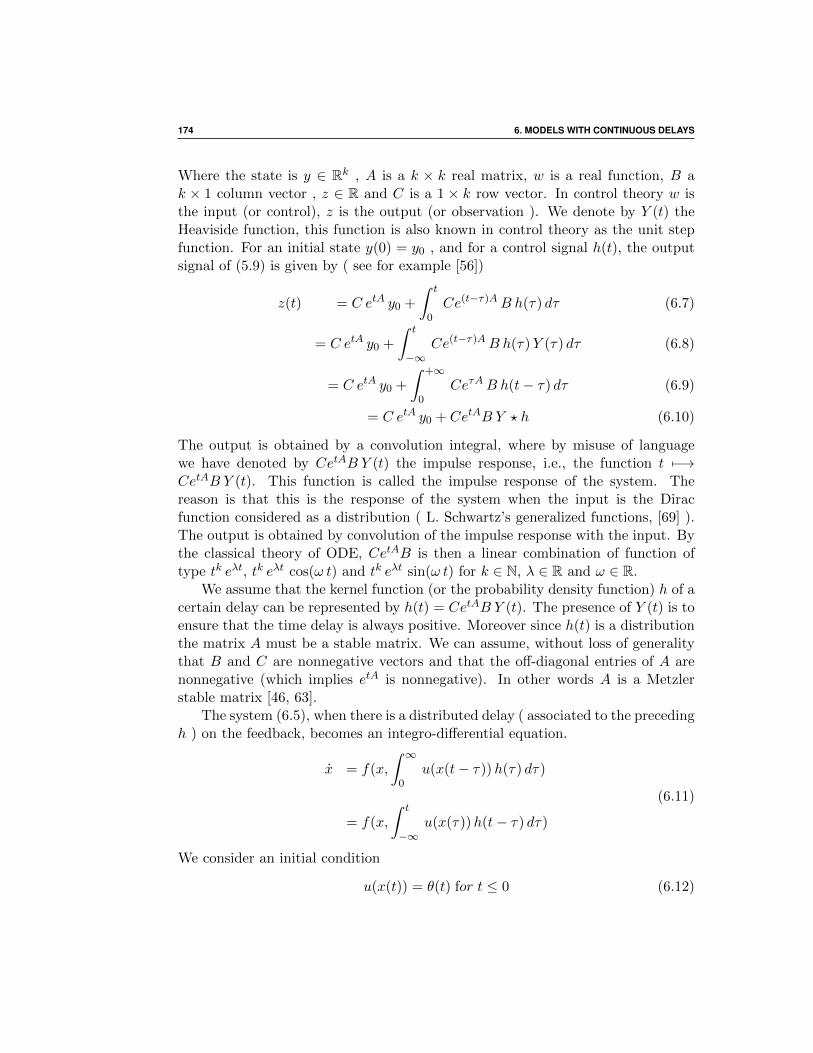
174 6. MODELS WITH CONTINUOUS DELAYS
Where the state is y ∈ Rk , A is a k × k real matrix, w is a real function, B ak × 1 column vector , z ∈ R and C is a 1 × k row vector. In control theory w isthe input (or control), z is the output (or observation ). We denote by Y (t) theHeaviside function, this function is also known in control theory as the unit stepfunction. For an initial state y(0) = y0 , and for a control signal h(t), the outputsignal of (5.9) is given by ( see for example [56])
z(t) = C etA y0 +
∫ t
0Ce(t−τ)AB h(τ) dτ (6.7)
= C etA y0 +
∫ t
−∞Ce(t−τ)AB h(τ)Y (τ) dτ (6.8)
= C etA y0 +
∫ +∞
0CeτAB h(t− τ) dτ (6.9)
= C etA y0 + CetAB Y ? h (6.10)
The output is obtained by a convolution integral, where by misuse of languagewe have denoted by CetAB Y (t) the impulse response, i.e., the function t 7−→CetAB Y (t). This function is called the impulse response of the system. Thereason is that this is the response of the system when the input is the Diracfunction considered as a distribution ( L. Schwartz’s generalized functions, [69] ).The output is obtained by convolution of the impulse response with the input. Bythe classical theory of ODE, CetAB is then a linear combination of function oftype tk eλt, tk eλt cos(ω t) and tk eλt sin(ω t) for k ∈ N, λ ∈ R and ω ∈ R.
We assume that the kernel function (or the probability density function) h of acertain delay can be represented by h(t) = CetAB Y (t). The presence of Y (t) is toensure that the time delay is always positive. Moreover since h(t) is a distributionthe matrix A must be a stable matrix. We can assume, without loss of generalitythat B and C are nonnegative vectors and that the off-diagonal entries of A arenonnegative (which implies etA is nonnegative). In other words A is a Metzlerstable matrix [46, 63].
The system (6.5), when there is a distributed delay ( associated to the precedingh ) on the feedback, becomes an integro-differential equation.
x = f(x,
∫ ∞0
u(x(t− τ))h(τ) dτ)
= f(x,
∫ t
−∞u(x(τ))h(t− τ) dτ)
(6.11)
We consider an initial condition
u(x(t)) = θ(t) for t ≤ 0 (6.12)

6.4. GENERALIZED LINEAR CHAIN TRICK 175
where θ is a continuous function defined on )−∞, 0].
Now we define
y(t) =
∫ 0
−∞e(t−τ)AB u(x(τ)) dτ
and
y0 = y(0) =
∫ 0
−∞e(−τ)AB u(x(τ)) dτ =
∫ 0
−∞e(−τ)AB θ(τ) dτ
We have the relation∫ t
−∞u(x(t− τ))h(τ) dτ =
∫ t
−∞C e(t−τ)AB u(x(τ)) dτ = z(t) = C y(t)
Then for any initial state x(0) = x0 and an initial condition u(t) = θ(t) on R−,the integro-differential equation (6.11) is equivalent to
x = f(x,Cy)y = Ay + u(x)B
(6.13)
with initial condition x(0) = x0 y(0) = y0. More precisely any solution of (6.11)becomes a solution of (6.13) (see [9] for example).
The general linear chain trick can replace system with delays with a pdf which islinear combination of gamma functions, by a system of ODE. Realization theoryis a part of linear control theory which gives explicit means of constructing sucha matrix A when the distribution is known. The delay is obtained in insertingbetween the feedback and the original system a linear system.
x = f(x,u)x
x u(x)u
y= A y + w bz= C y
z
Figure 6.6: Linear chain trick
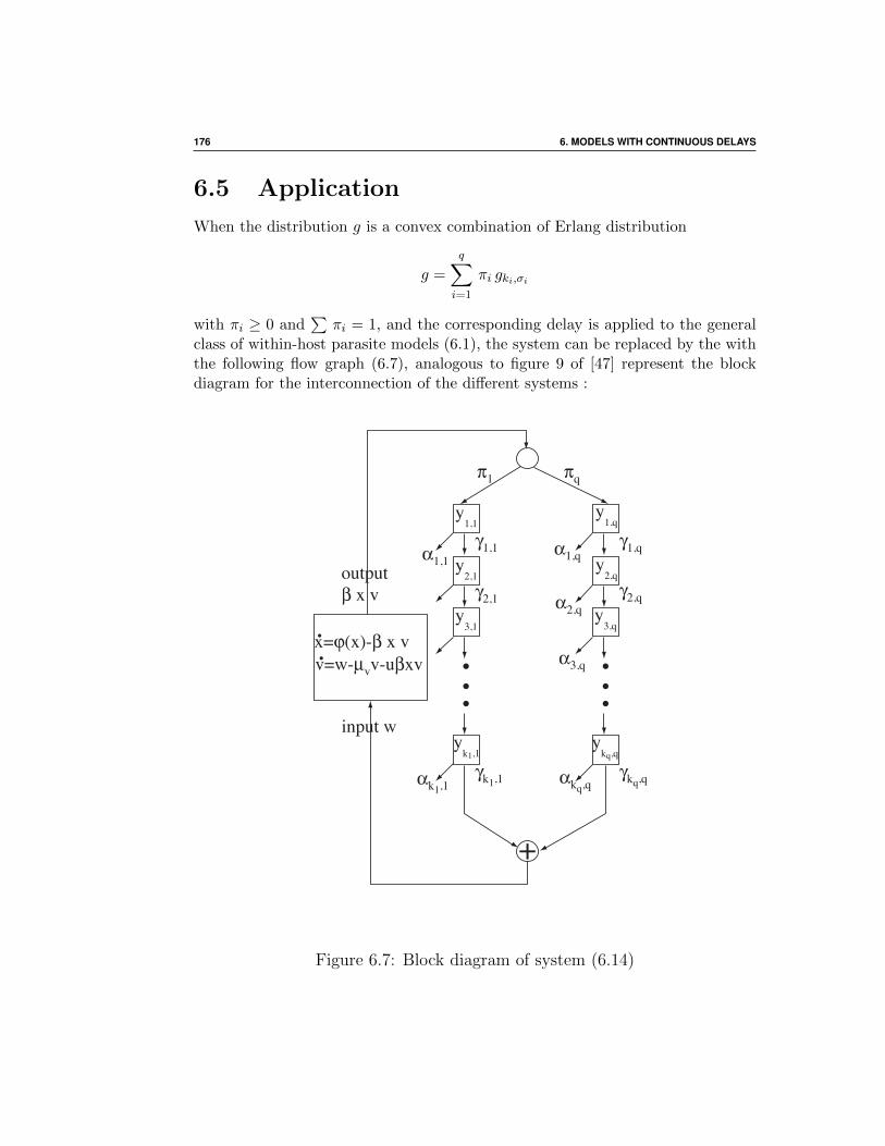
176 6. MODELS WITH CONTINUOUS DELAYS
6.5 Application
When the distribution g is a convex combination of Erlang distribution
g =
q∑i=1
πi gki,σi
with πi ≥ 0 and∑
πi = 1, and the corresponding delay is applied to the generalclass of within-host parasite models (6.1), the system can be replaced by the withthe following flow graph (6.7), analogous to figure 9 of [47] represent the blockdiagram for the interconnection of the different systems :
..... ...
y1,1
y2,1
y3,1
yk1,1
ykq,q
y3,q
y2,q
y1,q
γ1,1α1,1
γ2,1
γk1,1αk1,1γkq,qαkq,q
γ1,qα1,q
γ2,qα2,q
α3,q
+
output β x v
input w
π1 πq
x=ϕ(x)-β x vv=w-µvv-uβxv
Figure 6.7: Block diagram of system (6.14)

6.5. APPLICATION 177
We draw reader’s attention to the fact that this block diagram is not strictlyspeaking a compartmental model, since this is not a mass-balance system. From apseudo-compartment j is globally leaving a quantity αjyj of material, and enteringγj−1 yj−1. This γj−1 yj−1 quantity entering in the j compartment has not to besubtracted to the amount of material of the j − 1 compartment. The coefficientsγj can be considered as yield coefficients. We only assume that the coefficients arepositive. The arrows are only to symbolize what material is entering (or leaving).This picture is more a signal flow graph in control theory’s spirit.From the flow graph the system of ODE is simply
x = ϕ(x)− β x v
and for i = 1, · · · q
y1,i = πi β x v − α1,i y1,i
y2,i = γ1,i y1,i − α2,i y2,i
. . .yki,i = γki−1,i yki−1,i − αki,i yk,i
v =∑n
i=1 γki,i yki,i − µv v − uβ x v
(6.14)
The system (6.14) can be written in a condensed form.x = ϕ(x)− β x vy = Ay + β x v Bv = C y − µv v − uβ x v
(6.15)
6.5.1 Notations
To simplify the exposition we need some notations. We will adopt some conve-nient notations from MATLAB or SCILAB. Matrices will be represented by entriesbetween brackets, listed by rows, each element is separated by commas and thesemicolon indicates end of the rows.
We denote by ek(n) the kth-vector of the canonical basis of Rn. In other wordsfor example the vector e1(n) is the column vector of length n written with ournotations e1(n) = [1; 0; · · · ; 0]. We will use the notation eend(n) for the last vectorof the canonical basis. We use the same convention to define block matrices, forexample M = [E,F ;G,H] is the block matrix
M =
[E FG H
]

178 6. MODELS WITH CONTINUOUS DELAYS
provided the matrices E,F ,G and H have compatible dimensions. We denoteby AT the transpose of the matrix A. For a vector x of length n we denote bydiag(x) the n × n diagonal matrix with the elements of x on the diagonal. Wealso consider diag(A1, · · · , An) which is a diagonal block matrix, the Ai being thediagonal blocks.
We can now define A, B and C of (6.15):
The matrix A is a n × n diagonal block matrix with n =∑q
i=1 ki. A =diag(A1, · · · , Aq). The ki × ki block Ai is
Ai =
−α1,i 0 0 · · · 0 0γ1,i −α2,i 0 · · · 0 00 γ2,i −α3,i · · · 0 0...
. . .. . .
. . ....
...0 · · · 0 γki−2,i −αk 00 · · · 0 0 γki−1,i −αki,i
The vector B is the column vector of length n
B = [π1 e1(k1);π2 e1(k2); . . . ;πq e1(kq)]
The matrix C is a 1× n row vector
C = [γk1,1 eend(k1)T , γk2,2 eend(k2)T , . . . , γkq ,q eend(kq)T ]
The block decompositions of A, B and C are compatible.
6.5.2 Hypotheses
We start to analyze the system with minimal hypothesis on ϕ but neverthelessplausible from the biological point of view. The function ϕ(x) describes the pop-ulation dynamics of target cells in absence of parasites. The target cells have afinite lifetime. The function ϕ models in some way homeostasis. We assume thatϕ is a C1 function. Since homeostasis is maintained we assume the system
x = ϕ(x)
has a globally asymptotically stable equilibrium x∗ > 0, that is,
ϕ(x∗) = 0 ϕ(x) > 0 for 0 ≤ x < x∗, and ϕ(x) < 0 for x > x∗. (6.16)

6.6. STABILITY ANALYSIS FOR THE ONE CHAIN SYSTEM 179
6.6 Stability analysis for the one chain sys-
tem
To simplify we will examine the system given by a single chain of k elements. Wewill use the computations of this special case to study the complete system (6.14).In the case of a single chain the system is reduced to
x = ϕ(x)− β x vy = Ay + β x v Bv = C y − µv v − uβ x v
(6.17)
with
A =
−α1 0 0 · · · 0γ1 −α2 0 · · · 00 γ2 −α3 · · · 0...
. . .. . .
. . ....
0 · · · 0 γk−1 −αk
C = γk eend(k)T and B = e1(k)
It is clear that the nonnegative orthant is positively invariant by (6.17). The matrixA is a stable Metzler matrix.
6.6.1 Background
For later references we need the expression of the nonnegative matrix (−A−1) (Ais Metzler stable ). Using the fact that A = −D + N where D is the diagonalmatrix D = diag(α1, · · · , αk), N is the nilpotent matrix N = A + D. We denoteby I the identity matrix, we have (−A)−1 = D−1(I − ND−1)−1. Using the factthat ND−1 is nilpotent we get
(I −ND−1)−1 = I +ND−1 + (ND−1)2 + · · ·+ (ND−1)k−1
Finally
−A−1 =
1α1
0 0 · · · 0
γ1
α1 α2
1α2
0 · · · 0
γ1 γ2
α1 α2 α3
γ2
α2 α3
1α3
· · · 0...
. . .. . .
. . ....
γ1···γk−1
α1···αk · · · · · · γk−1
αk−1αk1αk

180 6. MODELS WITH CONTINUOUS DELAYS
The matrix −A−1 is a lower triangular matrix, the i-term on the diagonal is givenby 1
αi, the entry (i, j) with i > j is
(−A−1)(i, j) =γj · · · γi−1
αj · · ·αi−1
1
αi(6.18)
If we use the usual convention that an empty product has value 1, this expressionis also valid for the entries on the diagonal.
6.6.2 Basic reproduction ratio and Equilibria of thesystem
As usual the basic reproduction number is the expected number of secondary casesproduced in a completely susceptible population, by a typical infected individualduring its entire period of infectiousness [34, 80, 20, 21]. From the structure of thesystem the computation of R0 is straightforward. Indeed one parasite during themean duration of its life generates a Dirac input β x∗
µv+uβ x∗ in the second controlledsystem y = Ay + wB. Hence this input generates secondary cases given by theformula
β x∗
µv + uβ x∗
∫ +∞
0CetAB dt =
β x∗
µv + uβ x∗C (−A−1)B
This proves
R0 =β x∗
µv + uβ x∗C (−A−1)B (6.19)
With our definition we have C(−A−1)B = γk eend(k)T (−A−1)e1(k) which is simplythe entry of the last row , first column of −A−1 multiplied by γk. Finally
R0 =β x∗
µv + uβ x∗γ1 · · · γkα1 · · ·αk
. (6.20)
We also define a threshold T0 by
T0 =β[γ1···γkα1···αk − u
]x∗
µv(6.21)
We call T0 a threshold since T0 ≤ 1 is equivalent to R0 ≤ 1.The system has two nonnegative equilibria. The first, called the parasite free
equilibrium, is (x∗, 0 · · · , 0). The second is called the endemic equilibrium and isdenoted by (x, y, v).We have necessarily y = β x v(−A−1) e1 and
µv v + uβ x v = γk β x v eTend(−A−1) e1

6.6. STABILITY ANALYSIS FOR THE ONE CHAIN SYSTEM 181
If v 6= 0 we deduce
x =µv
β[γk e
Tend (−A−1) e1 − u
] =x∗
T0
With this expression we get v = ϕ(x)β x . Hence, with the hypothesis (6.16), x and
v are positive iff T0 > 1 or equivalently iff R0 > 1. Now y = ϕ(x)(−A−1) e1. Inother words y is the first column of (−A−1) multiplied by ϕ(x). The first column of(−A−1) is a positive vector, hence v is in the positive orthant, classically denotedby v 0.To summarize the endemic equilibrium is in the positive orthant iff R0 > 1 and itis given by
x = µv
β[γ1···γkα1···αk
−u] = x
T0 < x∗
y = ϕ(x) (−A)−1e1
v = ϕ(x)β x
(6.22)
6.6.3 Stability analysis
We give the main result of the section
Theorem 6.6.1 We consider the system (6.15) with the hypothesis on ϕ (6.16)satisfied. The basic reproduction ratio of the system is given by (6.20).
1. The system (6.15) is globally asymptotically stable on Rk+2+ at the parasite
free equilibrium (PFE) (x∗, 0, · · · , 0) if and only if R0 ≤ 1.
2. If R0 > 1 then the PFE is unstable and there exists a unique endemic equi-librium (EE) in the positive orthant, (x, y, v) 0 given by (6.22)
3. If R0 > 1, denoting α∗ = −maxx∈[0,x∗] (ϕ′(x) ), and if
uβ ϕ(x) ≤ α∗ µv (6.23)
then the endemic equilibrium is globally asymptotically stable on the nonneg-ative orthant, excepted for initial conditions on the x-axis.
Remark 6.6.1 If ϕ increases on some part of its domain, the relation (6.23) isnever satisfied. In this happens, it may lead to limit cycle for this model as in [18].
Remark 6.6.2 When u = 0 and ϕ(x) = Λ − µx x the sufficient condition isautomatically satisfied. This is the case of numerous models of the literature. Seefor example the general model (1) of [67] or the model in [60].

182 6. MODELS WITH CONTINUOUS DELAYS
Proof. We need some dissipativity properties of system (6.15). In a first stepwe show that there exists in the nonnegative orthant Rk+2
+ a forward invariantcompact absorbing neighborhood Ω of the PFE (x∗, 0, · · · , 0). An absorbing setD is a neighborhood of the PFE such that the trajectory of the system startingfrom any initial condition enters and remains in D for a sufficiently large time T .The entrance time depends on the initial condition. If the initial conditions arecontained in a compact set F then there exits a uniform T for F . A system is pointdissipative if there exists a compact absorbing set. The above definition coincideswith dissipativity given by [15].
Let ε ≥ 0 be a given nonnegative real. With the hypothesis (6.16) on ϕ thereexists a time T such that, for any initial condition in the nonnegative orthant andfor t ≥ T we have x(t) ≤ x∗+ ε. Let Mϕ be the maximum of the function ϕ(x) onR+. Let A a positive real such that α1A > Mϕ + ε.
We claim that the set Dε defined by
Dε =
(x, y, v) ∈ Rk+2+ | x ≤ x∗ + ε, x+ y1 ≤ A+ x∗ + ε, and for i = 2 · · · k
yi ≤ γ2···γi−1
α2···αi (A+ x∗ + iε), v ≤ γ1···γkα2···αk µv (A+ x∗ + kε)
is a forward invariant compact absorbing set for the system for ε > 0, and thatthe set D0 (ε = 0) is a forward invariant compact set.
The set Dε is the intersection of halfspaces defined by some hyperplanes. Toprove the positive invariance of a set, it is sufficient to prove that the vector fieldassociated to the system is tangent or pointing to the set on the boundary ofthis set. See Theorem (3.1.1). This is immediate for the faces of the nonnegativeorthant and for the halfspace defined by Dε,1 = (x, y, v) | x ≤ x∗ + ε. Fromthe properties of ϕ this set is also clearly absorbing. We define Dε,2 = (x, y, v) ∈Dε,1 | x + y1 ≤ A + x∗ + 2 ε. We have just to look at the boundary of Dε,2contained in Dε,1. On this part of the boundary we have y1 ≥ A. Then on thisboundary we have x+ y1 ≤ Mϕ − α1 y1 < ε. The vector is re-entrant, hence Dε,2is positively invariant. The inequality x+ y1 < ε proves that Dε,2 is absorbing inDε,1. A finite induction process, with similar arguments, ends the proof for Dε.
In a second step we will prove that, if R0 ≤ 1, the PFE is globally asymp-totically stable on the compact forward invariant set D0. It is well known that ifR0 > 1 then the PFE is unstable [21, 80] . Thus the condition R0 ≤ 1 is necessary.
To prove the sufficiency we consider the following Liapunov function on thepositive orthant.
VPFE(y, v) = bT y + v (6.24)
where the column vector b = [b1; b2; · · · ; bk] is the transpose of the last row of−A−1 multiplied by γk. In other words b = γk (−A−T ) eend.

6.6. STABILITY ANALYSIS FOR THE ONE CHAIN SYSTEM 183
We also define for further reference a = b1 − u. If we use (6.22) we obtain forthe parameter a the equivalent relation
a = b1 − u =µvβ x
=
[γ1 · · · γkα1 · · ·αk
− u]
(6.25)
If we compute the derivative of VPFE along the trajectories of (6.15) we get
VPFE = bT y + v= γk e
Tend (−A−1)Ay + γk e
Tend (−A−1)β x v e1 + v
= −γk yk + β x v b1 + γk yk − µv v − uβ x v= v[(b1 − u)βx− µv] = v[a β x− µv]= v[µv xx − µv]= µv
x (x− x)v
= β[γ1···γkα1···αk − u
](x− x)v
If R0 ≤ 1, or equivalently T0 ≤ 1, we distinguish two cases :
1. On one hand if ( γ1···γkα1···αk − u) < 0 then x < 0 and all the other quantities are
nonnegative in the expression of V . Therefore V ≤ 0.
2. On the other hand if ( γ1···γkα1···αk − u) ≥ 0, then from T0 ≤ 1 and since we are in
D0 we deduce 0 ≤ x ≤ x∗ ≤ x it follows that V ≤ 0.
In both cases V ≤ 0. It is easy to see that the maximum invariant set in (x, y, v) ∈D0 | V = 0 is reduced to the PFE. Therefore the global asymptotic stability ofthe PFE on the compact positively invariant set D0 follows from ([11], Theorem3.7.11, page 346). Now, We will prove the global asymptotic stability on theorthant Rk+2
+ . It is sufficient to prove that any forward trajectory converges tothe PFE. Since D1 ( i.e Dε for ε = 1 ) is a forward compact absorbing set anytrajectory entersD1. If a trajectory enters the interior ofD0 we have already provedthat it converges toward the PFE. Now assume that a trajectory, in D1 stays inD1 ∩ x∗ ≤ x ≤ x∗ + 1. Consider the Liapunov function W (x) = 1
2(x − x∗)2 onthis trajectory. By the hypothesis (6.16) on ϕ and the hypothesis on the trajectorywe have W = (x−x∗)ϕ(x)−(x−x∗)βx v ≤ 0 on any point of the trajectory in D1.By LaSalle’s principle it follows from W ≤ 0 that the PFE is the largest invariantset contained in x ∈ D1, x
∗ ≤ x ≤ x∗ + 1 | W = 0. This ends the proof of theGAS of the PFE.
Now we assume that R0 > 1. The equilibria (x, y, v) of the system, differentfrom the PFE, is given by (6.22) is in the positive orthant since R0 > 1.

184 6. MODELS WITH CONTINUOUS DELAYS
We will now prove a sufficient condition for the GAS of the EE. To this endwe define the following Liapunov function on the positive orthant.
VEE(x, y, v) = a(x− x lnx) +k∑i=1
bi (yi − yi ln yi) + (v − v ln v) (6.26)
where the column vector b and the coefficient a have been previously defined bythe relation (6.25). Since R0 > 1 we deduce a > 0, hence the coefficients of VEEare positive. In this case this function has a unique minimum, the EE, in thepositive orthant.
This function has a linear part LEE(x, y, v) = a x+∑k
i=1 bi yi + v. This linearpart can be expressed as
LEE(x, y, v) = a x+ bT y + v = a x+ γk eend (−A−1) y + v
If we compute the derivative LEE of LEE along the trajectories of (6.15), consid-ering the definition of b and the relation a+ u = b1, we get
LEE(x, y, v) = a x+ γk eend (−A−1) y + v= a x+ γk eend (−A−1)Ay + β x v eend (−A−1)B + v= a x− γk eend y + β x v eend (−A−1) e1 + v= aϕ(x)− aβxv − γk yk + b1 β x v + γk yk − µv v − uβ x v= aϕ(x)− µv v
If we collect in VEE the terms in v we obtain (aβx− µv)v. From (6.25) the termsin v cancel . With these simplifications we can now express VEE
VEE =. aϕ(x)(1− x
x
)− b1 βy1
xvy1−∑k
i=2 biγi−1yi−1yiyi
+
+k∑i=1
biαiyi − γkykv
v+ uβvx+ µvv.
This can also be written
VEE = aϕ(x)(
1− x
x
)− b1 βx v
x
x
v
v
y1
y1−
k∑i=2
bi γi−1 yi−1yi−1
yi−1
yiyi
+
+k∑i=1
biαiyi − γk ykykyk
v
v+ uβx v
x
x+ µvv
We now compare some coefficients appearing in this formula. We have ϕ(x) = β xv.Using the fact that y is the first column of −A−1 multiplied by ϕ(x), b is the

6.6. STABILITY ANALYSIS FOR THE ONE CHAIN SYSTEM 185
transpose of the last row multiplied by γk of the same matrix and accordingly tothe relation (6.18), we can now consider bi γi−1yi−1 :
bi γi−1yi−1 = γk (−A−1)(k, i) γi−1 ϕ(x) (−A−1)(i− 1, 1)
= ϕ(x) γkγi · · · γk−1
αi . . . αk−1
1
αkγi−1
γ1 · · · γi−2
α1 · · ·αi−2
1
αi−1
=γ1 · · · γkα1 · · · γk
ϕ(x) = b1 ϕ(x) = b1 β xv
In the same way
bi αiyi = γk (−A−1)(k, i)αi ϕ(x) (−A−1)(i, 1)
= ϕ(x) γkγi · · · γk−1
αi . . . αk−1
1
αkαi
γ1 · · · γi−1
α1 · · ·αi−1
1
αi=γ1 · · · γkα1 · · · γk
ϕ(x) = b1 ϕ(x)
and γk yk = γk (−A−1)(k, i)ϕ(x) = ϕ(x) γkγ1 · · · γk−1
α1 . . . αk−1
1
αk= b1 ϕ(x).
According to (6.25) we also have µvv = a β x v = aϕ(x)
Using all these relations between the coefficients we get for VEE
VEE = aϕ(x)(
1− x
x
)+
b1 ϕ(x)
[k − x
x
v
v
y1
y1−
k∑i=2
yi−1
yi−1
yiyi− ykyk
v
v
]+ uϕ(x)
x
x+ aϕ(x)
Adding 2− xx in the expression between brackets and subtracting the same expres-
sion outside the brackets, using u = b1 − a we obtain
VEE = aϕ(x)(
1− x
x
)+
b1 ϕ(x)
[k + 2− x
x− x
x
v
v
y1
y1−
k∑i=2
yi−1
yi−1
yiyi− ykyk
v
v
]+b1 ϕ(x)
( xx
+x
x− 2)
+ aϕ(x)(
1− x
x
)If we factor, in this expression, x−x
x x we obtain
VEE =x− xxx
(a x ϕ(x)− a xϕ(x) + b1 ϕ(x)(x− x)) +
b1 ϕ(x)
[k + 2− x
x− x
x
v
v
y1
y1−
k∑i=2
yi−1
yi−1
yiyi− ykyk
v
v
]

186 6. MODELS WITH CONTINUOUS DELAYS
Now we will use the fact that there exists ξ in the open interval ]x, x[ such thatϕ(x) = ϕ(x) + (x− x)ϕ′(ξ). Replacing in the preceding expression gives
VEE =(x− x)2
xx
(−aϕ(x) + a x ϕ′(ξ) + b1 ϕ(x)
)+
b1 ϕ(x)
[k + 2− x
x− x
x
v
v
y1
y1−
k∑i=2
yi−1
yi−1
yiyi− ykyk
v
v
]Finally since a− b1 = u
VEE =(x− x)2
xx
(uϕ(x) + a x ϕ′(ξ)
)+
b1 ϕ(x)
[k + 2− x
x− x
x
v
v
y1
y1−
k∑i=2
yi−1
yi−1
yiyi− ykyk
v
v
]
The term between brackets in the last expression of V is non positive by theinequality between the arithmetical mean and the geometrical mean. Therefore asufficient condition for V ≤ 0 is
uϕ(x) + a x ϕ′(ξ) ≤ 0
Or equivalently since ax = µvβ
uβ ϕ(x) ≤ −ϕ′(ξ)µv
Moreover with this condition V is negative excepted at the EE for the system(6.15). If
Since VEE is a proper function on the positive orthant, this proves the GAS ofthe EE on the positive orthant for the system (6.15).
The vector field associated with the system is strictly entrant on the faces ofthe orthant except on the x-axis where it is tangent. The basin of attraction of theEE is then the orthant excepted the one-dimensional face contained in the x-axisof the orthant, which is the stable manifold of the PFE.
Setting α∗ = − maxx∈[0,x∗]
ϕ′(x), a sufficient condition for the GAS of the EE is
R0 > 1 and uβ ϕ(x) ≤ µvα∗
This ends the proof of the theorem.
6.7 Stability for the complete system
The proof use the same line of ideas. This is proven in [43].

Chapter 7
Identification of parameters.
7.1 Introduction
ODE has been widely used to model epidemics of infectious diseases or the intra-host dynamics of a parasite. The analysis of such models, their simulation hasattracted a great attention and are the topics of many research papers. Thisis the problem of predicting the result of measurement, modelization, simulationproblems. However, less effort has been devoted to the so-called inverse problem.The inverse problem consists of using the actual results of some measurement toinfer the values of the parameters that characterize the system.
This problem, depending of the scientific community, has also received differentnames : data assimilation, estimation of parameters or identification. In thischapter we will use the concept emanating from control theory of identification ofparameters.
Actually, before parameter estimation algorithms can be used to an ODE modelto estimate the model parameters based measurements, a serious lock must beovercome : how to verify whether the model parameters are identifiable based onthe measurements of output variables. In other words, with the knowledge of somemeasurements, is there a unique set of parameters which gives these measures ?Does the inverse problem have a unique solution ?
This is the problem of identifiability : whether or not is it possible to distinguishdifferent sets of parameters from the measurement of the output. Before the in-troduction of precise definitions we will provide a simple example.
7.1.1 A non identifiable linear system
We consider the following system, whose flow graph is
187
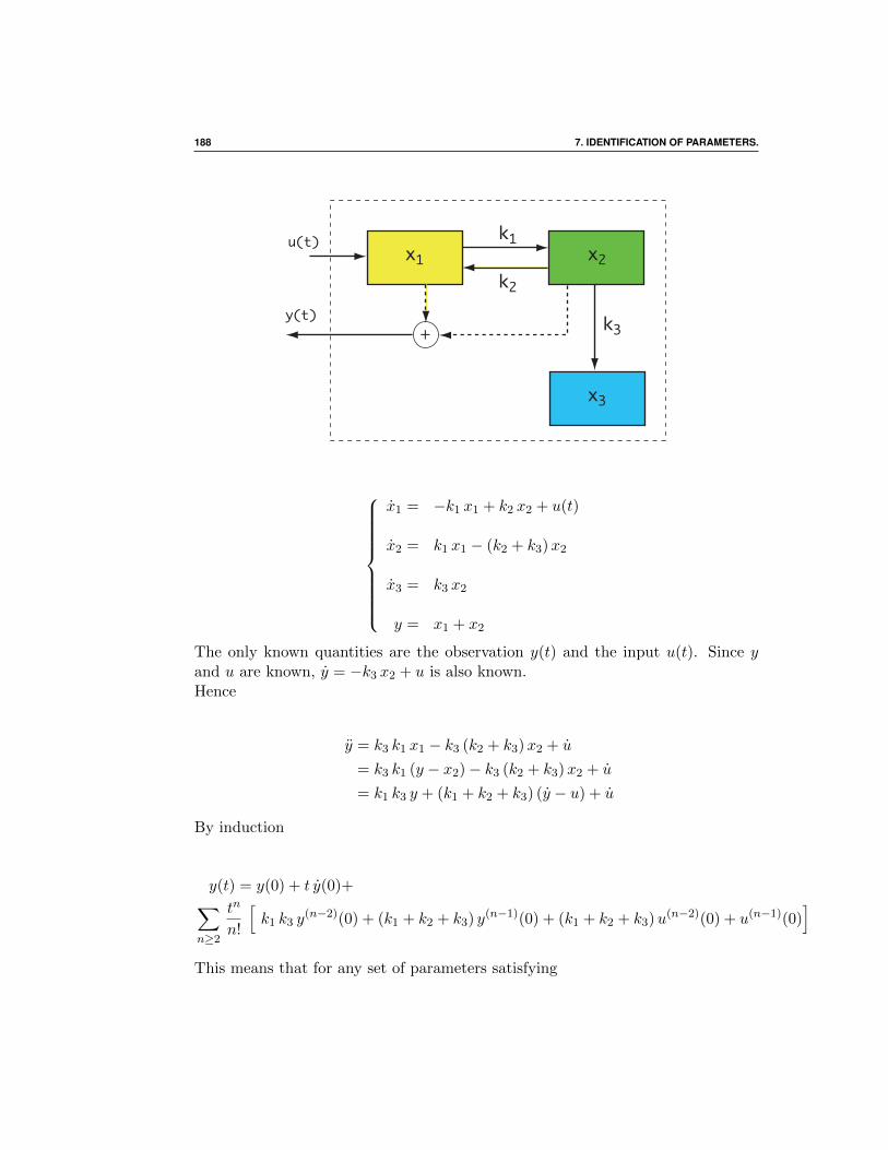
188 7. IDENTIFICATION OF PARAMETERS.
x1k1
k2
k3
x2
x3
u(t)
y(t)+
x1 = −k1 x1 + k2 x2 + u(t)
x2 = k1 x1 − (k2 + k3)x2
x3 = k3 x2
y = x1 + x2
The only known quantities are the observation y(t) and the input u(t). Since yand u are known, y = −k3 x2 + u is also known.Hence
y = k3 k1 x1 − k3 (k2 + k3)x2 + u
= k3 k1 (y − x2)− k3 (k2 + k3)x2 + u
= k1 k3 y + (k1 + k2 + k3) (y − u) + u
By induction
y(t) = y(0) + t y(0)+∑n≥2
tn
n!
[k1 k3 y
(n−2)(0) + (k1 + k2 + k3) y(n−1)(0) + (k1 + k2 + k3)u(n−2)(0) + u(n−1)(0)]
This means that for any set of parameters satisfying

7.2. CONCEPTS FROM CONTROL THEORY 189
(k1 + k2 + k3) = (k1 + k2 + k3) and k1 k3 = k1 k3
will gives the same input-output behavior. The system is not identifiable withthe output.
7.1.2 Historical Background
For system of ODE it is Kalman [48] who for the first time mentioned, in a rathercryptic way, the notion of identifiability.
The paper of Belmann and Astrom [8] in 1970 gives precise definitions of structuralidentifiability for linear control systems. The first systematic treatment in 1987for nonlinear system is by Tunali and Tarn [79].
Identifiability is simply, as we have try in the preceding example, to express param-eters as functions of the known quantities of the system, such as input and output.In this aspect, an algebraic definition, its relationship to observability, and algorith-mic procedures based on differential algebraic polynomial systems were rigorouslystudied in [22, 26, 58].
7.2 Concepts from control theory
In this section we will consider the following systemx = X(x, θ, u) = Xu,θ(x)
y = h(x)(7.1)
We assume that the application X : Rn × Rp × Rk −→ Rn is C∞ or analytic ash : Rn −→ Rm. The variable x is the state of the system in the state space Rn, θis a parameter in Rp, and u ∈ Rk is a control. The function h is the observation oroutput of the system. For any initial state x0 we denote by Xu,θ
t (x0) the solution
at time t and by y(x0, u, t) = h(Xu,θt (x0)) the corresponding output.
7.2.1 Observability
Definition 7.2.1 (indistinguishability) Two states x1 and x2 are said indis-tinguishable for system (7.1) iff for any time t ≥ 0 and any input u(t)
y(x1, u(), t) = y(x2, u(), t)

190 7. IDENTIFICATION OF PARAMETERS.
Indistinguishability I is an equivalence relation on Rn .Two states x1, x2, x1 6= x2 are said to be distinguishable if there exists an ad-missible control (or input) u and a time t ≥ 0 such that y(x1, u, t) 6= y(x2, u, t).An admissible input which distinguishes every pair of states is called an universalinput.Roughly speaking, this means that the information provided by the measurableoutput is not enough to tell us if the evolution of the system is given by the solutionemanating from the state x1 or by the one emanating from the state x2.
Definition 7.2.2 (Observability)A system is said observable if any pair of distinct states (x1, x2) are distinguishable.
The system (7.1) is observable if I(x) = x on Rn
Consider the following model of a chemostat
input:rate of flow u
output
pump
pump
Sin
Biomass
Figure 7.1: Chemostat
x = µ(s)x− ux
s = −k µ(s)− u (s− sin)
y = x
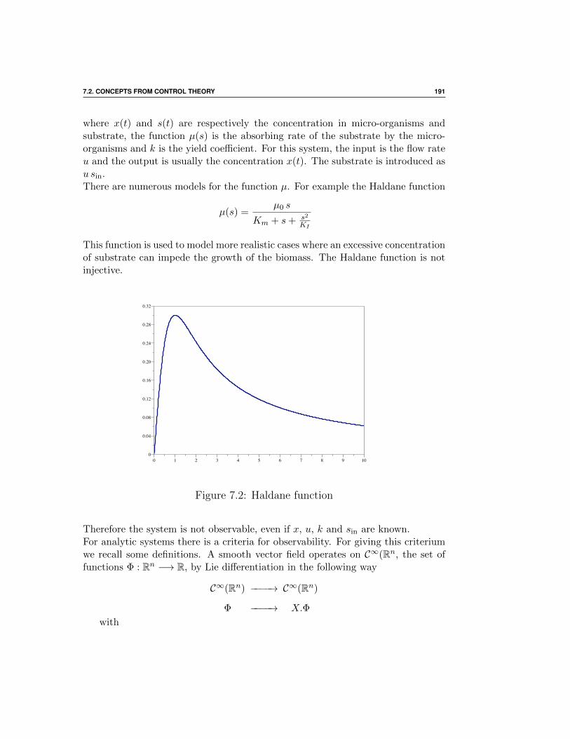
7.2. CONCEPTS FROM CONTROL THEORY 191
where x(t) and s(t) are respectively the concentration in micro-organisms andsubstrate, the function µ(s) is the absorbing rate of the substrate by the micro-organisms and k is the yield coefficient. For this system, the input is the flow rateu and the output is usually the concentration x(t). The substrate is introduced asu sin.There are numerous models for the function µ. For example the Haldane function
µ(s) =µ0 s
Km + s+ s2
KI
This function is used to model more realistic cases where an excessive concentrationof substrate can impede the growth of the biomass. The Haldane function is notinjective.
0 1 2 3 4 5 6 7 8 9 100
0.04
0.08
0.12
0.16
0.20
0.24
0.28
0.32
Figure 7.2: Haldane function
Therefore the system is not observable, even if x, u, k and sin are known.For analytic systems there is a criteria for observability. For giving this criteriumwe recall some definitions. A smooth vector field operates on C∞(Rn, the set offunctions Φ : Rn −→ R, by Lie differentiation in the following way
C∞(Rn) −−−−→ C∞(Rn)
Φ −−−−→ X.Φ
with

192 7. IDENTIFICATION OF PARAMETERS.
X.Φ (x) =d
dt(Φ(Xt(x)))
∣∣∣∣t=0
As usual Xt(x) denotes the flow of X initiating from x at time t.The function X.Φ is called the Lie derivative of Φ along the vector field X. We
have the following relation
X.Φ (x) = 〈∇Φ(x) | X(x)〉
The Lie derivative of order k is defined by induction
Xk.Φ = X.(Xk−1.Φ)
Definition 7.2.3 (Observation space) The observation space O of system (7.1)is the linear subspace over R of functions of C∞(Rn), containing the observationfunction h and closed under the Lie differentiation by all elements of
X = f(., θ, u)|u ∈ Rp.
We have the description of O
O = spanR
(Xul,θ)kl . . . . (Xu1,θ)k1 .h | l ≥ 0, u1, . . . , ul ∈ U, ki ∈ N
Theorem 7.2.1 For analytic systems the observability is equivalent to the factthat the observation space separates the points of Rn, i.e., if x1 6= x2 there existsg ∈ O such that g(x1) 6= g(x2).
ProofBy analyticity for one constant control u
y(x0, u, t) = h(Xu,θt (x0)) =
∑n≥0
tn
n!
dn
dtnh(Xu,θ
t (x0))
∣∣∣∣t=0
But
d
dth(Xu,θ
t (x0))
∣∣∣∣t=0
= 〈∇h(x0)|Xu,θ(x0)〉 = Xu,θ.h (x0)

7.2. CONCEPTS FROM CONTROL THEORY 193
By induction
dn
dtnh(Xu,θ
t (x0))
∣∣∣∣t=0
= (Xu,θ)n.h (x0)
Then it is necessary and sufficient for two distincts initial states x1 6= x2, forhaving different outputs, that there exists an index n such that
(Xu,θ)n.h (x1) 6= (Xu,θ)n.h (x2)
in other words be separated by a function of O
Notice that observability is a global concept since it might be necessary totravel a considerable distance or for a long time to distinguish between pointsof Rn. Therefore we introduce a local concept which is stronger than observ-ability from [33]. Let U be a subset of Rn and x1, x2 ∈ U . We say x1 is U-indistinguishable from x2 (denoted x1 IU x2 ) if for every control u, whose trajec-
tories Xθ,ut (x1) and Xθ,u
t (x2) both lie in U , fails to distinguish between x1 and x2.U -indistinguishability is not, in general, an equivalence relation on U because itfails to be transitive.
However, we can still define (7.1) to be locally observable at x0 if for every openneighborhood U of x0, IU (x0) = x0 and locally observable if it is so on Rn.
On the other hand one can weaken the concept of observability; in practice it maysuffice to be able to distinguish x0 from its neighbors. Therefore we define (7.1)to be weakly observable at x0 if there exists a neighborhood U of x0 such thatI(x0) ∩ U = x0 and (7.1) is weakly observable if it is so on Rn
Notice once again that it may be necessary to travel considerably far from Uto distinguish points of U , so we make a last definition, (7.1) is locally weaklyobservable at x0 if there exists an open neighborhood U of x0 such that for everyopen neighborhood V of x0 contained in U , IV (x0) = xo and is locally weaklyobservable if it is so in Rn. Intuitively, (7.1) is locally weakly observable if one caninstantaneously distinguish each point from its neighbors.
We have the following relations between these concepts [33] :
Locally Observable Observable
Locally Weakly Observable Weakly Observable

194 7. IDENTIFICATION OF PARAMETERS.
7.2.2 Identifiability
Definition 7.2.4The system (7.1) is said to be locally identifiable at θ if there exists a neighborhoodNθ of θ ∈ Rp such that for any θ1 6= θ2 in Nθ, there exists an admissible input usuch that for a nonnegative time t we have y(t, θ1, u) 6= y(t, θ2, u).If Nθ = Rp the system is said globally identifiable.
There is also a notion of identifiability almost everywhere. To introduce To intro-duce such a concept, we need a topology for the input function space. For anyT > 0 and a positive integer n, the space Cn[0, T ] is the space of all functions on[0, T ] which have continuous derivatives up to the order n. A topology of the spaceis the one associated with following well-defined norm, for f ∈ Cn[0, T ], we define‖ f‖ =
∑ni=1 maxt∈[0,T ] ‖f (i)(t)‖.
Definition 7.2.5The system (7.1) is said to be structurally identifiable if there exists a time T > 0,a positive integer n, and open and dense subset of Rn, Rp and Cn[0, T ] such thatthe system is identifiable at θ for every x0, θ and u in these open dense sets.
This characterizes the one-to-one property (almost everywhere) of the map fromthe parameters to the system output.
In these definitions, the initial state is unknown. However, sometimes an initialcondition is known (or partially known). Then we can define x0-identifiabilityeasily, the output is then limited from a common initial state x0.
7.2.3 Observability, identifiability and augmented sys-tem
The augmented system is simply the original system in an enlarged state-spacewith parameters treated as constant states :
x = X(x, θ, u) = Xu,θ(x)
θ = 0
y = h(x)
(7.2)
The system (7.1) is said observable and identifiable iff the enlarged system (7.2) isobservable.The algebraic identifiability is about construction of parameters from algebraicequations of the system input and output. This concept was f defined in [22] in

7.2. CONCEPTS FROM CONTROL THEORY 195
the differential algebraic framework. We adapt the definition into the followingone.
Definition 7.2.6A system is said to be algebraically identifiable if it is possible to construct theparameters from solving algebraic equations depending only on the information ofthe input and output.
We will give a more precise definition by using the formalism of differential algebra.Differential algebra can be seen as a generalization to differential equations of theconcepts of commutative algebra and algebraic geometry. This theory, foundedby Ritt, is an appropriate framework for the definition of algebraic observabilityintroduced by Diop and Fliess [22].A differential ring R is a commutative ring, with an unity 1 6= 0 equipped with
one derivation R → R a → a, such that˙︷ ︸︸ ︷
(a+ b) = a + b and˙︷︸︸︷
(a.b) = a.b + a.b. Aconstant of R is an element c such that c = 0Let K and L two differential fields such that K ⊂ L. If each element of L satis-fies an algebraic differential equation with coefficients in K, then L is said to bedifferential algebraic extension of K. The differential field generated by K and asubset S of L is denoted by K〈S〉.Let k a differential field. Denote byk〈u〉 the differential field generated by k anda finite set u = (u1, . . . , um) of differential quantities. The set u plays the role ofcontrol variables or input, which may be assumed to be independent. This meansthat u is differentially k- algebraically independent.
A dynamic is is a finitely generated differential extension D/k〈u〉This means that any element of D, satisfies an algebraic differential equation
with coefficients which are rational functions over k in the components of u anda finite number of their derivatives. As output variables can be viewed as sensorson the dynamics, we formally define an output as a finite set y = (y1, . . . , yp) ∈ D
Definition 7.2.7A dynamic D/k〈u〉, with output y is said to be algebraically observable iff thedifferentail extension D/k〈u, y〉 is algebraic
The intuitive meaning is the following: x the state variable can be expressedas an algebraic function of the components of u, y and a finite number of theirderivatives.
Definition 7.2.8Parameters π are algebraically identifiable if they are observable with respect tou, y, i.e., if they are algebraic over k〈u, y〉. The parameters are rationally iden-tifiable if they belongs to k〈u, y〉.

196 7. IDENTIFICATION OF PARAMETERS.
The intuitive meaning is clear: In the algebraic case, several values of theparameters are possible as algebraic equations must be solved, whereas in therational case one is always insured of a single value. This rational identifiability isequivalent to the global identifiability of Glad and Ljung [58].
We will now give Theorems for algebraic identifiability [85].
Theorem 7.2.2 ( Xia and Moog, 2003 )
Let K the differential field consisting of meromorphix function of x, θ, u and finitederivatives of u and define E = spanKdK. A vector is in E if it is a finite linearcombination of one forms dx, dθ, du, . . . , duk, . . . , with coefficients in K.
Denote Y =⋃∞k=0 spandy, dy, · · · , dyk, U =
⋃∞k=0 spandu, du, · · · , duk and
X = spandx
The system is algebraically identifiable iff
Θ ⊂ Y + U
Recall for a function h we define h = Xu,θ.h. Similarly for a one form ω in E if
ω = κx dx+ κθ dθ +∑
ηi dui ∈ E
we define (Leibnitz rule)
ω = κx dx+ κθ dθ +∑
ηi dui + κxX
u,θ(x) +∑
ηi dui+1
7.3 Examples
7.3.1 Identification for an intra-host model of Malaria
We consider the intra-host model of Malaria we have already encountered in theselectures
x = Λ− µx x− β xm,
y = β xm− µy y,
m = r µy y − µmm− β xm.
(7.3)
7.3. EXAMPLES 197
Observability and Identifiability
In case of malaria, only the concentration of infected erythrocytes are measured[27, 29, 28]. For this system the parameters Λ, µx, µy, µm and r are known or atleast widely accepted. However the infection rate is unknown. Then the problem,when y is measured, is to reconstruct the states x, m and identify the parameterβ.
Proposition 7.3.1
System (7.3) , with observation h(x, y,m) = y and parameters Λ, µx, µy, µm andr known, is observable and identifiable.
We assume, in relation to the plausible biological parameters, that we have theinequalities µx < µy < µm and r > 1.
Proof
We define h1 = y. Then
y = β xm− µy y = β xm− µy h1.
We define the known function h2 by h2 = β xm = h1 + µy h1.
We now have
h2 = (Λ− h2)β m+ (r µy h1 − h2)β x− (µx + µm)h2
Again, setting h3 = (Λ− h2)β m+ (r µy h1 − h2)β x, we obtain
h3 = −[µm (Λ− h2) + h2
]β m−
[µx (r µy h1 − h2)− (r µy h1 − h2)
]β x
+ 2 [(Λ− h2) (r µy h1 − h2) ] β
We define two known functions A = Λ− h2 and B = r µy h1 − h2.
Consider the two equationsAβm+B β x = −A + (µx + µm)h2
(µmA− A)β m+ (µxB − B)β x = −h3 + 2AB β(7.4)
These equations can be considered as a linear system in β m, β x with constantterms depending on β. Let ∆ the determinant of this system
∆ = −AB + AB + (µx − µm)AB
The function ∆ is analytic. Then either ∆ is zero or its zeroes are isolated. Weclaim that ∆ cannot be zero on a trajectory of system (7.3).

198 7. IDENTIFICATION OF PARAMETERS.
Moreover A = Λ − h2 cannot be zero an a trajectory. If it is the case thenx = −µx x and x goes to zero, which is impossible for system (7.3) : x convergeseither to the first component of the DFE or the endemic equilibrium, which is,in any case, non zero. In the same spirit B = r µy h1 − h2 cannot be zero on atrajectory, otherwise y = (r − 1) y which is a contradiction with the boundednessof the trajectories of (7.3).
If ∆ = 0, dividing by AB we have
−BB
+A
A= (µm − µx).
Integrating this relation gives
lnB0
A0
A
B= (µm − µx) t.
Where A0 and B0 are the initial value of A and B. Then
B0
A0
A
B= e(µm−µx) t
Since µm > µx the right hand side of this relation converges infinity, and the
left hand side converges toB0
A0
µx x
µm m, where we denote by (x, y m) either the DFE
or the EE of system (7.3). In any case the left hand side does not converge toinfinity, a contradiction.
Now with ∆ 6= 0 we obtain for β x and β mβm = M +N β
βx = P +Qβ.(7.5)
where M , N , P and Q are algebraic functions of the known functions h1, h2,h1,h2, h3.
From this relations we obtain, deriving one more time,
βm = M + N β
βm = (r µy h1 − h2)β − β µmmβm = (r µy h1 − h2)β − µm(M +N β)
(7.6)
Hence
M + N β = (r µy h1 − h2)β − µm(M +N β)

7.3. EXAMPLES 199
(B − N − µmN
)β = M + µmM.
Since M = [ −A+ (µx +µm)h2] (µmA− A) +A h3, a similar argument, as theprevious one, shows that M + µmM cannot be zero on a trajectory. Finally weobtain an expression for β as a rational expression of the derivative of the measuredoutput y. Note that we derive 4 times, corresponding to 3 states and one unknownparameter.
We prove the identifiability and observability of our system.
7.3.2 Identification for the Macdonald’s model of schis-tosomiasis transmission
In this section we consider the very well known model of MacDonald for the trans-mission of Schistosomiasis [64, 7]
This model can be written asw = α y − γ w
y = β (1− y)w − µ y(7.7)
The variable w is the average burden in the definitive host (e.g; humans) andthe variable y is the prevalence of infection in snails. We assume that the averageburden w is measured and that the transmission parameters α and β are unknown.γ the per capita death rate of parasites and µ the per capita death rate of infectedsnails are known.
Observability and identifiability
Proposition 7.3.2
System (7.7), with w measured, γ and µ known, is observable and identifiable,
excepted at the equilibria (0, 0) and
(α
γ
(1− 1
R0
), 1− 1
R0
)with R0 =
αβ
γ µ> 1
Proof
Observation is h(w, y) = w then

200 7. IDENTIFICATION OF PARAMETERS.
h = α y − γ w (7.8)
= α y − γ h, (7.9)
therefore
α y = h+ γ h (7.10)
α y = αβ (1− y)h− αµ y (7.11)
= αβ (1− y)h− µ (h+ γ h) (7.12)
= h+ γ h (7.13)
Function h is never identically zero (otherwise we are at the disease free equilib-rium)
αβ (1− y) =h+ γ h+ µ (h+ γ h)
h= g (7.14)
Function g is known and is rationally expressed with the derivatives of h. We get
−αβ y = g (7.15)
−β (h+ γ h) = g (7.16)
Parameter β has an rational expression in the derivatives of h, up to order 3.If h + γ h = 0 on a trajectory, we have y = 0, hence y is constant, which gives wconstant. We are on an equilibria. Since h 6= 0 we are at the endemic equilibrium.
w∗ =α
γy∗ and y∗ = 1− µγ
αµ= 1− 1
R0
In this case the system is non identifiable (we only know the product αβ).Otherwise
β = − g
h+ γ h(7.17)
Using (7.14) we obtain
αβ (1− y) = αβ − β (h+ γ h) = g

7.3. EXAMPLES 201
which gives
α =g + β (h+ γ h)
β(7.18)
finally
y =h+ γ h
α(7.19)
System (7.7 ) is rationally observable and identifiable.
7.3.3 Identification for Ross’ s model of malaria trans-mission
We consider the classical Ross model of malaria transmissionx = α y (1− x)− γ x
y = β (1− y)x− µ y(7.20)
The variable x represents the prevalence of malaria in humans, variable y is theprevalence of infection in mosquitoes. Parameter γ is the recovery rate of infectedhumans and µ is the death rate of mosquitoes. Parameters α and β are compositeparameter. Classically α = mab1 where m is the vectorial density, i.e., meannumber of mosquitoes by human, a is the biting rate and b1 is the probability thata bite by an infectious mosquito infects a susceptible human. Similarly β = a b2with b2 is the probability that a bite by a susceptible mosquito of an infectedhuman gives an infected mosquito.This is Ross model of 1911 [68, 3]. If we set α = mab1 e
−µ τ with τ the mosquitoincubation period, we obtain a version of Ross-Macdonald model.Parameters γ and µ are known, at least locally, and α and β has to be identified.Again we assume that x is measured.
Observability and Identifiability
Proposition 7.3.3Ross model (7.20 ) with x measured, parameters µ and γ known is observable andidentifiable, excepted at the equilibria which are the disease free equilibrium (0, 0)and the endemic equilibrium (if R0 > 1)

202 7. IDENTIFICATION OF PARAMETERS.
(R0 − 1
R0 + βµ
,R0 − 1
R0 + αγ
)
with R0 =αβ
γ µ.
ProofWe set the observation h1(x, y) = x. The function h1 is never identically equal to1, since if y = 1 then y = −µ. We define
h2 = α y =h1 + γ h1
1− h1
Deriving h2 gives
h2 = α y = αβ(1− y)h1 − µh2 = αβ h1 − β h2 h1 − µh2.
The function h2 cannot be identically zero unless at the origin.Then set
h3 =h2 + µh2
h1= αβ − β h2,
then
h3 = −β h2.
Excepted at one of the equilibria, h2 cannot be identically zero, therefore
β = − h3
h2
.
Finally
α =h3 + β h2
βand y =
h2
α
7.4 Identifiability and observers
7.4.1 Definition
When a system is observable initial points are distinguishable. Is it possible toreconstruct the state of the system from the measurement ? Observability deemsto be a natural requirement.

7.4. IDENTIFIABILITY AND OBSERVERS 203
We consider an inout-output systemx = X(x, u) = Xu(x)
y = h(x)
y
u
u
xSystem
Observer
From control theory, a system which gives an estimation of the state, is calledan observer. To be more precise an observer is a dynamical system, whose inputare the known quantities fo the control system, i.e., u and y :
˙x = g(x, u, u),
with the property that
limt→+∞
‖ x(t)− x(t)‖ = 0
The observer is called an asymptotic observer if the error satisfies for constantsK > 0 a > 0 and for ant t > 0
‖ x(t)− x(t)‖ ≤ K ‖ x(0)− x(0)‖ e−a t
7.4.2 An example : within-host model of Malaria
We have already seen this type of model. The observation is the concentrationof infected red blood cells. Actually what is observed are the young parasites inperipheral blood. This the phenomenon of sequestration : At the half-way pointof parasite development, the infected erythrocyte leaves the circulating blood andbinds to endothelium in the microvasculature.
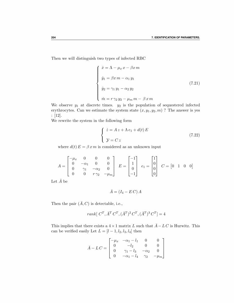
204 7. IDENTIFICATION OF PARAMETERS.
Then we will distinguish two types of infected RBC
x = Λ− µx x− βxm
y1 = βxm− α1 y1
y2 = γ1 y1 − α2 y2
m = r γ2 y2 − µmm− β xm
(7.21)
We observe y1 at discrete times. y2 is the population of sequestered infectederythrocytes. Can we estimate the system state (x, y1, y2,m) ? The answer is yes: [12].We rewrite the system in the following form
z = Az + Λ e1 + d(t)E
Y = C z(7.22)
where d(t)E = β xm is considered as an unknown input
A =
−µx 0 0 0
0 −α1 0 00 γ1 −α2 00 0 r γ2 −µm
E =
−110−1
e1 =
1000
C =[0 1 0 0
]Let A be
A = (I4 − E C)A
Then the pair (A, C) is detectable, i.e.,
rank[ CT , AT CT , (AT )2CT , (AT )3CT ] = 4
This implies that there exists a 4× 1 matrix L such that A−LC is Hurwitz. Thiscan be verified easily Let L = [l − 1, l2, l3, l4] then
A− LC =
−µx −α1 − l1 0 0
0 −l2 0 00 γ1 − l3 −α2 00 −α1 − l4 γ2 −µm

7.4. IDENTIFIABILITY AND OBSERVERS 205
Eigenvalues of this matrix are −µx, −l2, −α2 a,d −µm. It is sufficient to choosel2 > 0 to have A− LC is Hurwitz.With this condition we claim that
w = (A− LC)w +[L+ (A− LC)E
]Y + Λ e1
z = w(t) + E Y,
To prove this claim we set the error e = z − z. Some remarks are in order
E C E = E and C e1 = 0
e = ˙z − z= w + E Y − z= w + E Y −Az − Λ e1 − d(t)E
= w + E Y − (I − LC)Az − E C [ Az + Λ e1 + d(t)E] − Λ e1
= w + E Y − A z − E Y − Λ e1
= w − A z − Λ e1
= (A− LC)w +[L+ (A− LC)E
]Y + Λ e1 − A z − Λ e1
= (A− LC)w +[L+ (A− LC)E
]Y − A z
= (A− LC) z + LY − A z= (A− LC) z + LC z − A z= (A− LC) (z − z)= (A− LC) e
Since A − LC is Hurwitz this proves the claim. Our observer is asymptotic.The speed of convergence is given by the stability modulus, namely −µx if l2 ischosen large enough.This observer is known as an observer with unknown input. The state of thesystem is estimated without knowledge of the parameter β. Asa by-product wecan now estimates this parameter. For this
We have
y1 = β xm− (γ1 + µ1) y1
Constant variation formula for linear system gives
y1(t) = exp (−(γ1 + µ1)(t− t0)) y1(t0) + β
∫ t
t0
x(s)m(s) exp (−(γ1 + µ1)(s− t)) ds

206 7. IDENTIFICATION OF PARAMETERS.
We replace the unknown values by their estimations
y1(t) = exp (−(γ1 + µ1)(t− t0)) y1(t0) + β
∫ t
t0
x(s) m(s) exp (−(γ1 + µ1)(s− t)) ds
therefore
exp ((γ1 + µ1)t) y1(t)−exp ((γ1 + µ1) t0) y1(t0) = β
∫ t
t0
x(s) m(s) exp (−(γ1 + µ1) s) ds
Discretizing [tinit, tf ] in [ti, ti+1] applying preceding relation and choosing tinit suchthat the observer gives a good estimation (practically that means waiting a little,giving time for the observer to converge
exp ((γ1 + µ1)ti+1) y1(ti+1)− exp ((γ1 + µ1) ti) y1(ti)
= β
∫ ti+1
ti
x(s) m(s) exp (−(γ1 + µ1) s) ds
For each i we set
Ui = exp ((γ1 + µ1)ti+1) y1(ti+1)− exp ((γ1 + µ1) ti) y1(ti)
and
Vi =
∫ ti+1
ti
x(s) m(s) exp (−(γ1 + µ1) s) ds
this gives
U = β V
An estimation of β is obtained in solving by least square method this linearsystem.

7.4. IDENTIFIABILITY AND OBSERVERS 207
Malariatherapy
During the pre-penicillin era, there was no efficient treatment for syphilis. Duringthe natural evolution of the disease, patients sometimes developed neurosyphilis10 to 25 years after the initial infection. The curative effect of fevers has beenreported since Hippocrates’ time. Wagner-Jauregg, the father of malaria therapy,described in detail experiments with induced fever in patients.In 1917 the inoculation of malaria parasites, which proved to be very successful inthe case of dementia paralytica (also called general paresis of the insane), causedby neurosyphilis, at that time a terminal disease. It had been observed that somewho develop high fevers could be cured of syphilis. Thus, from 1917 to the mid1940s, malaria induced by the least aggressive parasite, Plasmodium vivax, wasused as treatment for tertiary syphilis because it produced prolonged and highfevers (a form of pyrotherapy). This was considered an acceptable risk becausethe malaria could later be treated with quinine, which was available at that time.This discovery earned to Wagner-Jauregg the Nobel Prize in Medicine in 1927.The technique was known as malariatherapy; however, it was dangerous, killingabout 15% of patients, so it is no longer in use.Data were collected by the US Public Health Service between 1940 and 1963, whenmalaria therapy was a recommended treatment for neurosyphilis. Infections withdifferent strains of P. falciparum, P. vivax, P. ovale, and P. malariae were inducedin patients for the treatment of neurosyphilis.Afroamericans were however found to be refractory, and so they were treated withdifferent strains of P. falciparum under close medical supervision. They were in-oculated either with sporozoites (generally through mosquito bite) or with infectedblood. Inoculations were preceded by variable sequences of blood and mosquitopassages of the strain. Microscopic examination of the blood was performed on analmost daily basis.
Is the malaria therapy model identifiable ?
When the initial condition is partially known the system can be observable andidentifiable [79, 85].If we consider the case of malariatherapy the initial condition is partially known.Sporozoites are introduced and measured was performed daily.
Hence (x0 =Λ
µ, y2(0) = 0,m(0) = 0 are known. Only the value of y1(0) is
unknown.Now y1(t) is known, hence y1 + α1 y1 = β xm is also known. Consequently
x(t) = e−µx t∫ t
0(Λ− β x(s)m(s)) ds+ e−µx t x0,

208 7. IDENTIFICATION OF PARAMETERS.
is also known.Then we know β m. Similarly
y2(t) = e−α2 t γ1
∫ t
0y1(s) ds+ e−α2 t y2(0) = e−α2 t γ1
∫ t
0y1(s) ds
is known. Finally
m(t) = e−µm t
∫ t
0[ r2 γ2 y2(s)− β x(s)m(s)] ds+ e−µm tm(0)
= e−µm t
∫ t
0[ r2 γ2 y2(s)− β x(s)m(s)] ds,
is known. Since we can know x, y1, y2,m and β xm, betais known.
This proves that the system (7.21) is observable and identifiable.
Numerical observers
If we prove that the system under consideration is observable and identifiable howcan we reconstruct the states and the unknown parameters. Dynamical observerscan be designed, but it is a difficult task. recently some advances have beenobtained [12, 19, 44, 85]. However we will propose something else.
We will consider observability, since we have seen that the identifiability can be,with the augmented system, analyzed as an observability problem.
x = f(x, u)y = h(x)
Measures are discrete, with a time interval of ∆t :
(y0, y1, . . . , yk),
with corresponding time
(0,∆t, · · · , k∆t)
The principle is very simple : for a initial condition (this is a guess) we computethe ouptput
(h(x0), h(x(∆t, x0, u) ), · · · , h(x(k∆t, x0, u) ).
Then is evaluated the difference between what is predicted and what is measured

7.4. IDENTIFIABILITY AND OBSERVERS 209
Φ(x0) = minx0
k∑i=0
‖yi − y(i∆t, x0, u)‖22.
This a function of x0. Using an algorithm of minimization we compute
x0 = arg minx0
Φ(x0)
By a numerical integration we obtain
x(t) = x(t, x0, u)
As the number of measurements grows, the size of the optimization increases. Tobound the size of the optimization, the least squares objective can be modified toemploy a fixed-size moving window in which the number of measurements that webase our estimate on (and hence the size of the optimization) remains constant.
Practically that means that, if our horizon is of length N , we will estimate x0 usingthe N first measures. The we will have an estimation x(N ∆t). This estimationwill be the guess for the next time window [ (N + 1) ∆t, · · · , 2N ∆t)] giving anew x(N ∆t) and an estimation for x(2N ∆t) . . . .
The use of a finite horizon and moving windows is motivated by two reasons. Thefirst one is the limited amount of memory, which limits the size of the optimizationproblem. The second one is that generally measures are corrupted by noise. Hencetaking many measures will add many noise to the data used in computation.
What is the size of the window ? This is an engineering problem, but we have somehints. E. Sontag has proved that For differential equations with r parameters 2 r+1experiments are enough for identification. Aeyels has shown that in n-dimensions2n + 1 samples are necessary to observe observability [76, 1, 2]. Then for theaugmented system with n states and p parameters the size of the window shouldnot be less than 2 (n+ p) + 1.
A program
Here a routine, written in Scilab ( like MATLAB but free)
1 function Xob=numobs3(dyn ,output ,Tm,N,x0_est , x0_reel)
2 // Numerical observer
3 // comparion with real measures
4 //
5
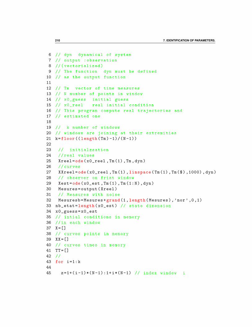
210 7. IDENTIFICATION OF PARAMETERS.
6 // dyn dynamical of system
7 // output :observation
8 //(vectorialized)
9 // The function dyn must be defined
10 // as the output function
11
12 // Tm vector of time measures
13 // N number of points in window
14 // x0_guess initial guess
15 // x0_reel real initial condition
16 // This program compute real trajectories and
17 // estimated one
18
19 // k number of windows
20 // windows are joining at their extremities
21 k=floor(( length(Tm)-1)/(N-1))
22
23 // initialzsation
24 //real values
25 Xreel=ode(x0_reel ,Tm(1),Tm,dyn)
26 // curves
27 XXreel=ode(x0_reel ,Tm(1), linspace(Tm(1),Tm($),1000),dyn)
28 // observer on frist window
29 Xest=ode(x0_est ,Tm(1),Tm(1:N),dyn)
30 Mesures=output(Xreel)
31 // Measures with noise
32 Mesuresb=Mesures+grand(1,length(Mesures),’nor’ ,0,1)
33 nb_etat=length(x0_est) // state dimension
34 x0_guess=x0_est
35 // intial conditions in memory
36 //in each window
37 X=[]
38 // curves points in memory
39 XX=[]
40 // curves times in memory
41 TT=[]
42 //
43 for i=1:k
44
45 z=1+(i-1)*(N -1):1+i*(N-1) // index window i
7.4. IDENTIFIABILITY AND OBSERVERS 211
46
47 T=Tm(z);
48 mesureF=Mesuresb(z)
49 x0_opt=optimize(dyn ,output ,mesureF ,x0_guess)
50 Z=ode(x0_opt ,T(1),T,dyn)
51 sol=ode(x0_opt ,T(1), linspace(T(1),T($)),dyn);
52 TT=[TT,linspace(T(1),T($))]
53 XX=[XX,sol]
54 X=[X,Z(:,1:$-1)]
55 x0_guess=Z(:,$)
56
57 end
58
59 // If the windows has not taken all the points
60 // one last window
61
62 if pmodulo(length(Tm),N -1)~=1
63 T=Tm(1+k*(N-1):$)
64 mesureFi=Mesuresb (1+k*(N-1):$)
65 x0_opt=optimize(dyn ,output ,mesureFi ,x0_guess)
66 Z=ode(x0_opt ,T(1),T,dyn)
67 sol=ode(x0_opt ,T(1), linspace(T(1),T($)),dyn);
68 TT=[TT,linspace(T(1),T($))]
69 XX=[XX,sol]
70 X=[X,Z(:,1:$)]
71 end
72
73
74 Xob=X;
75
76 for j=1: nb_etat
77 xset("window",j)
78 clf
79 plot(Tm ’,[Xreel(j,:); Xob(j,:)]’,’+’)
80 plot(TT’,XX(j,:)’,’b’)
81 plot(linspace(Tm(1),Tm($),1000)’, XXreel(j,:)’,’g:’)
82 end
83
84 xset("window",nb_etat +1)
85 clf

212 7. IDENTIFICATION OF PARAMETERS.
86 plot(Tm ’,[Mesures;Mesuresb]’,’o’)
87
88 endfunction
89
90 // ///////////////////////////////////
91 function x0_opt=optimize(fun ,output ,mesureF ,x0_guess ,T)
92 m=length(mesureF)
93 x0_opt=lsqrsolve(x0_guess ,crit ,m)
94 endfunction
95
96 // ////////////////////
97 function y=crit(x,m)
98 z=ode(x,T(1),T,fun);
99 y=output(z)
100 y=y-mesureF
101 y=y(:)
102 endfunction
Example for the Schistosome example
0.04
0.06
0.08
0.10
0.12
0.14
0.16
0 100 200 300 400 500 600 700 800 900
Figure 7.3: Measures w : blue real measures, green with noise

7.4. IDENTIFIABILITY AND OBSERVERS 213
0.05
0.06
0.07
0.08
0.09
0.10
0.11
0.12
0.13
0.14
0.15
0 100 200 300 400 500 600 700 800 900
Figure 7.4: Estimation of w : noise is filtered
0.0
0.1
0.2
0.3
0.4
0.5
0.6
0.7
0.8
0 100 200 300 400 500 600 700 800 900
Figure 7.5: Estimation of y

214 7. IDENTIFICATION OF PARAMETERS.

Bibliography
[1] D. Aeyels, Generic observability of differentiable systems, SIAM J. ControlOptim., 19 (1981), pp. 595–603.
[2] , On the number of samples necessary to achieve observability, SystemsControl Lett., 1 (1981/82), pp. 92–94.
[3] R. M. Anderson and R. M. May, Infectious Diseases of Humans. Dynam-ics and Control, Oxford science publications, 1991.
[4] R. Anguelov, Y. Dumont, and J. Lubuma, Mathematical modeling ofsterile insect technology for control of anopheles mosquito, Comput. Math.Appl., 64 (2012), pp. 374–389.
[5] K. Arrow, A “Dynamic” Proof of the Frobenius-Perron Theorem for Met-zler Matrices, in Probability, Statistics and Mathematics. Papers in honor ofSamuel Karlin, Academic Press, 1989, pp. 17–25.
[6] N. Bailey, The Mathematical Theory of Infectious Diseases and its Applica-tions, Griffin,London, 1975.
[7] A. D. Barbour, Macdonald’s model and the transmission of bilharzia., TransR Soc Trop Med Hyg, 72 (1978), pp. 6–15.
[8] Bellman, R. and Astrom, K.J., On structural identifiability, Math.Biosci., 7 (1970), pp. 329–339.
[9] E. Beretta and Y. Takeuchi, Global stability of Lotka-Volterra diffusionmodels with continuous time delay., SIAM J. Appl. Math., 48 (1988), pp. 627–651.
[10] A. Berman and R. J. Plemmons, Nonnegative matrices in the mathemat-ical sciences, vol. 9 of Classics in Applied Mathematics, Society for Industrialand Applied Mathematics (SIAM), Philadelphia, PA, 1994. Revised reprintof the 1979 original.
215

216 BIBLIOGRAPHY
[11] N. P. Bhatia and G. P. Szego, Dynamical systems: Stability theory andapplications, vol. 35 of Lecture Notes in Mathematics, Springer-Verlag, 1967.
[12] D. Bichara, N. Cozic, and A. Iggidr, On the estimation of sequestered in-fected erythrocytes in plasmodium falciparum malaria patients, Math. Biosci.Eng., 11 (2014), pp. 741–759.
[13] F. Brauer and C. Castillo-Chavez, Mathematical models in populationbiology and epidemiology, vol. 40 of Texts in Applied Mathematics, Springer-Verlag, New York, 2001.
[14] F. Brauer, J. Wu, and P. van den Driessche, eds., Mathematical Epi-demiology, no. 1945 in Lectures Notes in Math., Springer-Verlag, 2008.
[15] G. Butler and P. Waltman, Persistence in dynamical systems, J. Differ-ential Equations, 63 (1986), pp. 255–263.
[16] K. L. Cooke and Z. Grossman, Discrete delay, distributed delay and sta-bility switches, J. Math. Anal. Appl., 86 (1982), pp. 592–627.
[17] D. Cox and H. Miller, The theory of stochastic processes, Chapman andHall, 1965.
[18] P. De Leenheer and H. L. Smith, Virus dynamics: A global analysis.,SIAM J. Appl. Math., 63 (2003), pp. 1313–1327.
[19] M. Diaby, A. Iggidr, and M. Sy, Observer design for a schistosomiasismodel, Math. Biosci., 269 (2015), pp. 17–29.
[20] O. Diekmann and J. A. P. Heesterbeek, Mathematical epidemiology ofinfectious diseases, Wiley Series in Mathematical and Computational Biology,John Wiley & Sons Ltd., Chichester, 2000. Model building, analysis andinterpretation.
[21] O. Diekmann, J. A. P. Heesterbeek, and J. A. J. Metz, On the def-inition and the computation of the basic reproduction ratio R0 in models forinfectious diseases in heterogeneous populations, J. Math. Biol., 28 (1990),pp. 365–382.
[22] S. Diop and M. Fliess, Nonlinear observability, identifiability, and persis-tent trajectories, in proceedings 36th IEEE-CDC, 1991, pp. 714–719.
[23] Y. Dumont and J. M. Tchuenche, Mathematical studies on the sterileinsect technique for the chikungunya disease and aedes albopictus., J MathBiol, (2011).

BIBLIOGRAPHY 217
[24] A. Fall, A. Iggidr, G. Sallet, and J. J. Tewa, Epidemiological modelsand Lyapunov functions, Math. Model. Nat. Phenom., 2 (2007), pp. 55–73.
[25] D. Fargue, Reductibilite des systemes hereditaires a des systemes dy-namiques., C. R. Math. Acad. Sci. Ser B, 277 (1973), pp. 471–473.
[26] M. Fliess, Nonlinear control theory and differential algebra, in Modellingand adaptive control (Sopron, 1986), vol. 105 of Lect. Notes Control Inf. Sci.,Springer, Berlin, 1988, pp. 134–145.
[27] M. B. Gravenor, A. L. Lloyd, P. G. Kremsner, M. A. Missinou,M. English, K. Marsh, and D. Kwiatkowski, A model for estimatingtotal parasite load in falciparum malaria patients., J Theor Biol, 217 (2002),pp. 137–48.
[28] M. B. Gravenor, A. R. McLean, and D. Kwiatkowski, The regula-tion of malaria parasitaemia: parameter estimates for a population model.,Parasitology, 110 ( Pt 2) (1995), pp. 115–22.
[29] M. B. Gravenor, M. B. van Hensbroek, and D. Kwiatkowski, Es-timating sequestered parasite population dynamics in cerebral malaria., ProcNatl Acad Sci U S A, 95 (1998), pp. 7620–4.
[30] Z. Grossman, M. Feinberg, K. Kuznetsov, D. Dimitrov, andW. Paul, Hiv infection : how effective is drug combination treatment, Im-munol. Today, 19 (1998), pp. 528–532.
[31] J. Hale, Ordinary differential equations, Krieger, 1980.
[32] J. A. P. Heesterbeek, A brief history of R0 and a recipe for its calculation,Acta Biotheorica, 50 (2002), pp. 189–204.
[33] R. Hermann and A. J. Krener, Nonlinear controllability and observabil-ity., IEEE Trans. Autom. Control, 22 (1977), pp. 728–740.
[34] H. W. Hethcote, The mathematics of infectious diseases, SIAM Rev., 42(2000), pp. 599–653 (electronic).
[35] H. W. Hethcote and H. R. Thieme, Stability of the endemic equilibriumin epidemic models with subpopulations, Math. Biosci., 75 (1985), pp. 205–227.
[36] M. Hirsch, Systems of differential equations that are competitive or cooper-ative i: limit sets, SIAM J. Math. Anal., 13 (1982), pp. 167–179.

218 BIBLIOGRAPHY
[37] , The dynamical system approach to differential equations, Bull. AMS,11 (1984), pp. 1–64.
[38] , Systems of differential equations that are competitive or cooperative ii :convergence almost everywhere, SIAM J. Math. Anal., 16 (1985), pp. 423–439.
[39] , Systems of differential equations that are competitive or cooperative iii:Competing species, Nonlinearity, 1 (1988), pp. 51–71.
[40] , Systems of differential equations that are competitive or cooperative. iv:Structural stability in three-dimensional systems, SIAM J. Appl. Math., 21(1990), pp. 1125–1234.
[41] M. Hirsch and S. Smale, Differential equations, dynamical systems, andlinear algebra, Pure and applied mathematics, Academic Press, 1974.
[42] M. W. Hirsch and H. Smith, Monotone dynamical systems, in Handbookof differential equations: ordinary differential equations. Vol. II, Elsevier B.V., Amsterdam, 2005, pp. 239–357.
[43] A. Iggidr, J. Mbang, and G. Sallet, Stability analysis of within-hostparasite models with delays, Math. Biosci., 209 (2007).
[44] A. Iggidr and M. Souza, State estimators for some epidemiological sys-tems, J. Math. Biol., to appear (2018).
[45] J. A. Jacquez, Compartmental analysis in Biology and Medicine, BioMed-ware, 1996.
[46] J. A. Jacquez and C. P. Simon, Qualitative theory of compartmental sys-tems, SIAM Rev., 35 (1993), pp. 43–79.
[47] , Qualitative theory of compartmental systems with lags, Math. Biosci.,180 (2002), pp. 329–362.
[48] R. E. Kalman, Mathematical description of linear dynamical systems, J.SIAM Control Ser. A, 1 (1963), pp. 152–192 (1963).
[49] J. P. Keener, The Perron-Frobenius theorem and the ranking of footballteams, SIAM Rev., 35 (1993), pp. 80–93.
[50] W. Kermack and A. McKendrick, A contribution to the mathematicaltheory of epidemics, Proc. R. Soc., A115 (1927), pp. 700–721.

BIBLIOGRAPHY 219
[51] Krasnosel‘skiı, M. A., Positive solutions of operator equations, Translatedfrom the Russian by Richard E. Flaherty; edited by Leo F. Boron, P. Noord-hoff Ltd. Groningen, 1964.
[52] Krasnosel′skiı, M. A., The operator of translation along the trajectoriesof differential equations, Translations of Mathematical Monographs, Vol. 19.Translated from the Russian by Scripta Technica, American MathematicalSociety, Providence, R.I., 1968.
[53] A. Lajmanovich and J. Yorke, A deterministic model for gonorrhea in anonhomogeneous population., Math. Biosci., 28 (1976), pp. 221–236.
[54] J. P. LaSalle, The stability of dynamical systems, CBMS conferences, 25,SIAM, Philadelphia, Pa., 1976. With an appendix: “Limiting equations andstability of nonautonomous ordinary differential equations” by Z. Artstein,Regional Conference Series in Applied Mathematics.
[55] A. Laveran, , A. Bull.Acad. N. Med, 9 (1880), p. 1235.
[56] E. Lee and L. Markus, Foundations of optimal control theory, John Wiley& Sons Ltd., 1967.
[57] M. Li, An introduction to Mathematical Modeling of Infectious diseases,Springer, 2018.
[58] L. Ljung and T. Glad, On global identifiability for arbitrary modelparametrizations, Automatica J. IFAC, 30 (1994), pp. 265–276.
[59] A. L. Lloyd, The dependance of viral parameter estimates on the assumedviral life cycle : limitations of studies of viral load data, Proc R Soc Lond BBiol Sci, (2001), pp. 847–854.
[60] A. L. Lloyd, Destabilization of epidemic models with the inclusion of realisticdistributions of infectious periods., Proc R Soc Lond B Biol Sci, 268 (2001),pp. 985–93.
[61] , Realistic distributions of infectious periods in epidemic models: chang-ing patterns of persistence and dynamics., Theor Popul Biol, 60 (2001),pp. 59–71.
[62] A. Lotka, contribution to the analysis of malaria epidemiology, Am. J. Trop.Med. Hyg., 3 (1923), pp. 1–121.
[63] D. G. Luenberger, Introduction to dynamic systems. Theory, models, andapplications., John Wiley & Sons Ltd., 1979.

220 BIBLIOGRAPHY
[64] G. Macdonald, The dynamics of helminth infections, with special referenceto schistosomes., Trans R Soc Trop Med Hyg, 59 (1965), pp. 489–506.
[65] N. MacDonald, Time lags in biological models, no. 27 in Lecture Notes inBiomath., Springer-Verlag, 1978.
[66] J. E. Mittler, B. Sulzer, A. U. Neumann, and A. S. Perelson, Influ-ence of delayed viral production on viral dynamics in HIV-1 infected patients.,Math. Biosci., 152 (1998), pp. 143–163.
[67] P. W. Nelson and A. S. Perelson, Mathematical analysis of delay differ-ential equation models of HIV-1 infection., Math. Biosci., 179 (2002), pp. 73–94.
[68] R. Ross, The prevention of malaria, John Murray, 1911.
[69] L. Schwartz, Methods of mathematical physics, Addison-Wesley, ReadingMass., 1964.
[70] P. Seibert and R. Suarez, Global stabilization of nonlinear cascade sys-tems, Syst. Control Lett., 14 (1990), pp. 347–352.
[71] E. Seneta, Non-negative matrices and Markov chains, Springer Series inStatistics, Springer, New York, 2006. Revised reprint of the second (1981)edition [Springer-Verlag, New York; MR0719544].
[72] H. Smith and P. Waltman, The theory of the chemostat. Dynamics of mi-crobial competition., Cambridge Studies in Mathematical Biology, CambridgeUniversity Press, 1995.
[73] H. L. Smith, Cooperative systems of differential equations with concave non-linearities, Nonlinear Anal., 10 (1986), pp. 1037–1052.
[74] , Monotone dynamical systems: an introduction to the theory of compet-itive and cooperative systems., Mathematical Surveys and Monographs. 41.Providence, RI: American Mathematical Society (AMS). x, 174 p. , 1995.
[75] E. D. Sontag, Mathematical control theory, deterministic finite dimensionalsystems, no. 6 in Texts in Applied Mathematics, Springer-Verlag, 1990.
[76] , For differential equations with r parameters, 2r + 1 experiments areenough for identification, J. Nonlinear Sci., 12 (2002), pp. 553–583.
[77] Y. Takeuchi, Global dynamical properties of Lotka-Volterra systems, WorldScientific Publishing Co. Inc., River Edge, NJ, 1996.

BIBLIOGRAPHY 221
[78] H. R. Thieme, Mathematics in population biology, Princeton Series in The-oretical and Computational Biology, Princeton University Press, Princeton,NJ, 2003.
[79] E. T. Tunali and T. J. Tarn, New results for identifiability of nonlinearsystems, IEEE Trans. Automat. Control, 32 (1987), pp. 146–154.
[80] P. van den Driessche and J. Watmough, reproduction numbers and sub-threshold endemic equilibria for compartmental models of disease transmis-sion, Math. Biosci., (2002), pp. 29–48.
[81] R. Varga, Factorization and normalized iterative methods, in Boundaryproblems in differential equations, R. Langer, ed., university of WisconsinPress, 1960, pp. 121–142.
[82] , matrix iterative analysis, Prentice-Hall, 1962.
[83] M. Vidyasagar, Decomposition techniques for large-scale systems with non-additive interactions: Stability and stabilizability., IEEE Trans. Autom. Con-trol, 25 (1980), pp. 773–779.
[84] P. Waltman, Competition models in population biology, vol. 45 of CBMS-NSF Regional Conference Series in Applied Mathematics, Society for Indus-trial and Applied Mathematics (SIAM), Philadelphia, PA, 1983.
[85] X. Xia and C. H. Moog, Identifiability of nonlinear systems with applicationto HIV/AIDS models, IEEE Trans. Automat. Control, 48 (2003), pp. 330–336.