mathematical analysis of the effect of a pulse vaccination...

Mathematical analysis of the effect of a pulsevaccination to an HBV mutation model

Plaire Tchinda Mouofoa,e,* — J.J. Tewab,e — B. Mewoli c,e — S. Bowongd,e

a Department of Mathematics, University of Yaounde I,PO Box 812 Yaounde, [email protected] National Advanced School of EngineeringUniversity of Yaounde I, Department of Mathematics and PhysicsP.O. Box 8390 Yaounde, Cameroonc Department of Mathematics, University of Yaounde I,PO Box 812 Yaounde, [email protected] Department of Mathematics and Computer Science, Faculty of Science,University of Douala, P.O. Box 24157 Douala, Cameroon,[email protected] UMI 209 IRD/UPMC UMMISCO, University of Yaounde I, Faculty of Science,LIRIMA Project team GRIMCAPE, University of Yaounde I, Faculty of ScienceP.O. Box 812, Yaounde, Cameroon* Corresponding authorTel.+(237) 99 36 36 20; [email protected]

ABSTRACT. It has been proven that vaccine can play an important role for eradication of hepatitis Binfection. When the mutant strain of virus appears, it changes all treatments strategies. The currentproblem is to find the critical vaccine threshold which can stimulate the immune system for eradicatethe virus, or to find conditions at which mutant strain of the virus can persist in the presence of a CTLvaccine. In this paper, the dynamical behavior of a new hepatitis B virus model with two strains ofvirus and CTL immune responses is studied. We compute the basic reproductive ratio of the modeland show that the dynamic depend of this threshold. After that, we extend the model incorporatingpulse vaccination and we find conditions for eradication of the disease. Our result indicates that if thevaccine is sufficiently strong, both strains are driven to extinction, assuming perfect adherence.

RÉSUMÉ. Il a été démontré que le vaccin peut jouer un rôle très important dans le processusd’éradication de l’hépatite B. Lorsque la souche mutante apparait, elle modifie les stratégies de luttes.Le problème courant est celui de déterminer le seuil vaccinal capable de stimuler le système immuni-taire pour éliminer le virus, ou de trouver les conditions pour lesquelles la souche mutante persisteraen présence du vaccin. Dans ce travail, nous considérons un nouveau modèle d’hépatite B dans le-quel nous prenons en compte une souche de virus sauvage et une souche mutante et leur interactionavec les cellules du système immunitaire. Nous calculons le taux de reproduction de base et montronsque la dynamique dépend de ce seuil. Une extension de ce modèle est faite afin d’inclure un schémaimpulsionnel de vaccination et de déterminer les conditions pour éliminer la maladie. Nos résultatsmontrent que si le vaccin est suffisamment puissant, les deux souches pourront être éliminées.

KEYWORDS : Mutant strains, pulse vaccination, Hepatitis B.

MOTS-CLÉS : Souche mutante, vaccination par impulsion, hépatite B.

Special issue, CARI'14 Eric Badouel, Moussa Lo, Mokhtar Sellami, Editors.

ARIMA Journal, vol. 21, pp. 3-19 (2015)

1. IntroductionHepatitis B virus (HBV) infection is a disease of global health. According to the data

of World Health Organization (WHO), approximately 30% of world’s population, i.e.about 2 billion people have been infected with HBV at some time in their lives. Of these,about 350 million remain infected chronically and become carriers of the virus. Everyyear, there are over 4 million acute clinical cases of HBV, and about 25% of carriers.Hepatitis B causes about 1 million people to die from chronic active hepatitis, cirrhosis,or primary liver cancer annually [13].

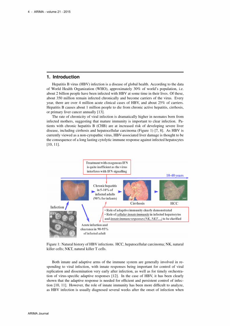
The rate of chronicity of viral infection is dramatically higher in neonates born frominfected mothers, suggesting that mature immunity is important to clear infection. Pa-tients with chronic hepatitis B (CHB) are at increased risk of developing severe liverdisease, including cirrhosis and hepatocellular carcinoma (Figure 1) [7, 8]. As HBV iscurrently viewed as a non-cytopathic virus, HBV-associated liver damage is thought to bethe consequence of a long lasting cytolytic immune response against infected hepatocytes[10, 11].

Figure 1: Natural history of HBV infections. HCC, hepatocellular carcinoma; NK, naturalkiller cells; NKT, natural killer T cells.

Both innate and adaptive arms of the immune system are generally involved in re-sponding to viral infection, with innate responses being important for control of viralreplication and dissemination very early after infection, as well as for timely orchestra-tion of virus-specific adaptive responses [12]. In the case of HBV, it has been clearlyshown that the adaptive response is needed for efficient and persistent control of infec-tion [10, 11]. However, the role of innate immunity has been more difficult to analyze,as HBV infection is usually diagnosed several weeks after the onset of infection when

4 - ARIMA - volume 21 - 2015

ARIMA Journal

viremia is already high; thus the role of innate immunity in defense against HBV remainscontroversial.

HBV mutants have recently been identified in patients with acute, fulminant, or chronicinfections. Sequence analysis of virus isolates from many individual patients has revealedthe occurrence of certain mutational hot spots in the genome, some of which appear tocorrelate with the patient’s immunological and/or disease status; however, cause and ef-fect are not always easily discernible [5]. This holds particularly for the issue of whethervirus variants exist that have an increased pathogenic potential; due to the scarcity of ap-propriate in vivo experiment models, such hypotheses are difficult to prove. Similarly,because of the compact organization of the HBV genome, almost every single mutationmay have pleiotropic phenotypic effects.

Naturally occurring mutations have been identified in all viral genes and regulatoryelements, most notably in the genes coding for the structural envelope and nucleocapsidproteins [6]. Mutations in the gene coding for the HBsAg may result in infection orviral persistence despite the presence of antibodies against HBsAg (anti-HBs). Mutationsin the gene encoding the pre-core/core protein (pre-core stop codon mutant) result in aloss of HBeAg (HBeAg minus mutant) and seroconversion to antibodies to HBeAg (anti-HBe) with persistence of HBV replication [5]. Mutations in the core gene may leadamong others to an “immune escape" due to a T cell receptor antagonism [5]. Mutationsin the gene coding for the polymerase/reverse transcriptase can be associated with viralpersistence or resistance to nucleoside analogues [5]. Thus, HBV mutations may affectthe natural course of infection, viral clearance and response to antiviral therapy. The exactcontribution of specific mutations to diagnosis and therapy of HBV infection as well aspatient management in clinical practice remain to be established. In addition, despite theavailability of an effective prophylactic vaccine, further extensive efforts are required tomonitor the emergence of vaccination and therapy-resistant HBV variants and to preventtheir spread in the general population.

Current treatment options for chronic hepatitis B depend on interferon (IFN) α anddirect antivirals, i.e. nucleoside or nucleotide analogues. Although there now are sevenapproved therapies for HBV infection (two IFN formulations and five nucleoside ana-logues) [18, 19]. HBV cannot be cleared by currently available antiviral therapy andtherefore requires long-term antiviral treatment, which is costly, often selects for drugresistant viral variants and may have long-term side effects [18]. So there is a need foralternative treatment approaches. For HBV highly effective and safe prophylactic vac-cines are available. These, however, showed no effect in the setting of chronic infection[20, 21, 22, 23], indicating the need for a specific therapeutic vaccine design. We herefocus on the options to design and develop a therapeutic hepatitis B vaccine.

Since its widespread introduction in 1983, the hepatitis B vaccine has become an es-sential part of infant immunization programmes globally, and is the key component ofthe global hepatitis B control programme for the World Health Organization (WHO)[1].Infection with hepatitis B virus (HBV) can cause acute liver disease, as well as chronicinfection that may lead to liver failure or hepatocellular carcinoma. The vaccine has beenparticularly important for countries where the incidence of HBV-related hepatocellularcarcinoma is high. In effect, the hepatitis B vaccine was the world’s first anticancer vac-cine.

Therapeutic vaccines are currently developed for chronic viral infections, such as hu-man papillomavirus (HPV), human immunodeficiency virus (HIV), herpes virus and hep-atitis B (HBV) and C (HCV) virus infections. As an alternative to antiviral treatment orto support only partially effective therapy a therapeutic vaccine shall activate the patient’s

Mathematical analysis of the effect of a pulse vaccination to an HBV mutation model - 5

ARIMA Journal

immune system to fight and finally control or ideally even eliminate the virus. HBV canbe eliminated by the immune system after acute infection or sometimes even when theimmune balance in chronic infection tips. Since shifting this balance towards immunecontrol is the aim of therapeutic vaccination, those viruses are primary targets for a proof-of-concept of therapeutic vaccination.

Within-host models are used for different purposes : explanation of observations, topredict impact of interventions (antimalarial drugs), estimate hidden states or parameters.Experimental results show that one of the main reasons for CTL response failure is viralescape from CTLs [2]. Moreover, if escape mutation to the vaccine occurs, then either thewild type or the mutant can outcompete the other strain [14]. In this paper, we investigatethe effect of viral mutation on the ability of CTLs to control the viral infection when apost-infection vaccine is administered at regular intervals. The novelty in our model isthat its not only takes into account two strains of virus, but also assumes that a regulatorynegative feedback force, operates to suppress immune population growth at a net rateproportional to the square of its density. This implies regulation of the response at hightantigen concentration.

This work is organized as follows. In the next Section, we propose our model. Weanalyze the model in Section 3. We extend this model in Section 4 to incorporate pulsevaccination and to find conditions for eradication of the viruses. We give some numericalsimulations in Sect. 5 to explain our mathematical results. We end this paper with a briefdiscussion and conclusion.

2. The model formulationWe begin by introducing the model constructed by Nowak and Bangham [9] when

there is no mutation. This model is given by

x = λ− dxx− βxv,y1 = βxv − dyy − ρyI,v1 = ky − dvv,

I = αyI − γI.

(1)

where x is the number of susceptible host cells, y1 is the number of infected cells, v1 is thenumber of free virus, and I is the number of CTL cells. All the parameters λ, dx, β, dy ,ρy , ky , dv , α and γ are positive. dx, dy , dv , and γ are the death rates of uninfected cells,infected cells, free virus, and CTL cells, respectively. λ represents a constant productionof the target cells. β is the contact rate between uninfected cells and free virus. Infectedcells are removed at rate ρI by CTL immune responses. The virus-specific CTL cellsproliferate at rate αy by contact with infected cells. Free virus is produced from infectedcells at rate ky.

Now we include mutant virus and we use a special function to describe immune re-sponses. This function assume a regulatory negative feedback force, which operates tosuppress immune population growth at a net rate proportional to the square of its density.

6 - ARIMA - volume 21 - 2015

ARIMA Journal

This implies regulation of the response at hight antigen concentration. So, the model weconsider in this paper is given as follows:

x = λ− dxx− β1v1x− β2v2x,v1 = k1y1 − dvv1,v2 = k2y2 − dvv2,y1 = (1− ε)β1v1x− ρ1y1I − dyy1,y2 = εβ1v1x+ β2v2x− ρ2y2I − dyy2,

I = α(y1 + y2)I + pI − qI2.

(2)

where x is the number of uninfected liver cells, v1 is the number of wild-type virus, v2 isthe number of mutant virus, y1 is the number of liver cells infected with wild-type, y2 isthe number of liver cells infected with mutant strains, and I is the number of CTL cells.All the parameters λ, dx, β1, β2, k1, dv , ε, k2, dy , α, p, and q are positive. Uninfected livercells are produced with constant rate λ and die with rate dx. They are infected with wild-type and mutant strains respectively at rate β1 and β2. The chance of the novo mutation isε. Free virus particles and infected liver cells die at rate dv and dy respectively. Infectedliver cells are also cleared by the body’s defensive CTLs; this happens respectively atrate ρ1 and ρ2. CTLs reproduced in the presence of infected liver cells at rate α. Theparameter p denotes the proliferation rate of immune cells and q the density-dependentrate of immune cells suppression. New virus particles are produced at rate k1 by wild-typevirus and k2 by mutant virus respectively.

3. Mathematical analysis of the modelHerein, we present some basic results, such as the positive invariance of model system

(2), the boundedness of solutions, the existence of equilibria and its stability analysis.

3.1. Positivity and boundedness of solutionsThe following result guarantees that model system (2) is biologically well behaved andits dynamics is concentrated on a bounded region of R6

+. More precisely, the followingresult holds.

Theorem 3.1. Let R6+ = {(x, v1, v2, y1, y2, I) ∈ R6 : x ≥ 0, v1 ≥ 0, v2 ≥ 0, y1 ≥

0, y2 ≥ 0, I ≥ 0}. Then, R6+ is positively invariant under the flow induced by model

system (2). Moreover, the region

∆ ={(x, v1, v2, y1, y2, I) ∈ R6 : x+ y1 + y2 ≤ λ

µ, v1 + v2 ≤ (k1 + k2)λ

µdv,

p

q≤ I ≤ pµ+ αλ

µq

}.

is positively invariant and absorbing with respect to model system (2), whereµ = min{dx, dy}.

Proof. Let µ = min{dx, dy}. No solution of model system (2) with initial conditions(x(0), v1(0), v2(0), y1(0), y2(0), I(0)) ∈ R6

+ is negative. In fact, for(x(t), v1(t), v2(t), y1(t), y2(t), I(t)) ∈ R6

+, we have x |x=0= λ > 0, v1 |v1=0= k1y1 ≥0, v2 |v2=0= k2y2 ≥ 0, y1 |y1=0= (1− ε)β1v1x ≥ 0, y2 |y2=0= εβ1v1x+ β2v2x ≥ 0,


ARIMA Journal

I |I=0= 0 ≥ 0, this immediately implies that all solutions of model system (2) with initialcondition (x(0), v1(0), v2(0), y1(0), y2(0), I(0)) ∈ R6

+ stay in the first quadrant.For the invariance property of ∆, it suffices to show that the vector field, on the bound-

ary, does not point to the exterior. Adding the first, fourth and fifth and second equationsof model system(2) yields on the boundary of ∆:

d(x+ y1 + y2)

dt

∣∣∣∣x+y1+y2=

λµ

= λ− dxx− dyy1 − dyy2 − (ρ1y1 + ρ2y2)I |x+y1+y2=λµ

≤ (λ− µ(x+ y1 + y2))|x+y1+y2=λµ= 0

Similarly, we get

d(v1 + v2)

dt

∣∣∣∣v1+v2=

(k1+k2)λµdv

≤ (k1+k2)λµ − dv(v1 + v2)

∣∣∣v1+v2=

(k1+k2)λµdv

= 0,

dI

dt

∣∣∣∣I= p

q

≥ (p− qI) I|I= pq= 0 i.e I(t) ≥ p

q , ∀t ≥ 0,

anddI

dt

∣∣∣∣I= pµ+αλ

µq

≤(αλ

µ+ p− qI

)I

∣∣∣∣I= pµ+αλ

µq

= 0

Therefore, solutions starting in ∆ will remain there for t ≥ 0.Now, we prove the attractiveness of the trajectories of model system (2). To do so,

from model system (2), one hasd(x+ y1 + y2)

dt≤ λ − µ(x + y1 + y2). Therefore,

lim supt→∞

(x+ y1+ y2)(t) ≤λ

µ. Similarly, since

d(v1 + v2)

dt≤ (k1 + k2)λ

µ− dv(v1+ v2),

one has lim supt→∞

(v1(t)+ v2(t)) ≤(k1 + k2)λ

µdv. Concerning the variable I , we have

dI

dt≤(

αλ

µ+ p

)I − qI2 which implies that I(t) ≤ 1

µqpµ+αλ +

(1

I(0) −µq

pµ+αλ

)e−(p+

αλµ )t

.

So, I is bounded and hence, ∆ is attracting, that is, all solutions of model system (2)eventually enters ∆. This concludes the proof.

3.2. Basic reproduction number and equilibriaThe basic reproduction number is defined as the average number of secondary infec-

tions produced by one infected cell during the period of infection when all cells are unin-fected. This threshold is obtained at the virus free equilibrium. The virus free equilibriumis obtained by setting v1 = 0 in all equations of model system (2) at the equilibrium.We obtain that the virus free equilibrium is P1(x

∗, 0, 0, 0, 0, 0, I∗), where x∗ = λdx

andI∗ = p

q . We use the method of van den Driessche[3] to compute the basic reproductionnumber. Using the notations of van den Driessche and Watmough[3], for model system(2), we have

F =

0 0 k1 00 0 0 k2

(1− ε)β1x∗ 0 0 0

εβ1x∗ β2x

∗ 0 0

and

8 - ARIMA - volume 21 - 2015

ARIMA Journal

V =

dv 0 0 00 dv 0 00 0 ρ1I

∗ + dy 00 0 0 ρ2I

∗ + dy

.

Thus, the basic reproduction number is given by:

R0 = max {R01 ; R02} . (3)

where R01 =k1(1− ε)β1x

∗

dv(dy + ρ1I∗)and R02 =

k2β2x∗

dv(dy + ρ2I∗). From theorem 2 of Van Den

Driessche[3], we have the following result.

Lemma 3.1. The virus-free equilibrium P1 of the model system (2) is locally asymptoti-cally stable (LAS) if R0 < 1, and unstable if R0 > 1.

We now study the existence of equilibria of model system (2). Setting the right-handsides of model system (2) equals to zero gives

λ− dxx− β1v1x− β2v2x = 0, (4)

k1y1 − dvv1 = 0, (5)

k2y2 − dvv2 = 0, (6)

(1− ε)β1v1x− ρ1y1I − dyy1 = 0. (7)

εβ1v1x+ β2v2x− ρ2y2I − dyy2 = 0, (8)

α(y1 + y2)I + pI − qI2 = 0. (9)

Model system (2) has always equilibrium P1 = (x∗, 0, 0, 0, 0, I∗) which is the virus freeequilibrium and represents the state when the viruses are absent. If R02 > 1, then themodel has one mutant-only equilibrium P2(x, 0, v2, 0, y2, I), where x = λdv

dxdv+β2k2y2,

v2 = k2

dvy2, I = p

q +αq y2, and y2 is the unique positive solution of the following equation:

ρ2αβ2k2q

y22 +

(dyβ2k2 +

ρ2αdxdv + ρ2pβ2k2q

)y2 + (1−R02)dxdv(dy + ρ2I

∗) = 0

(10)In what follows, we study the existence of the third equilibrium P = (x, v1, v2, y1, y2, I),which is obtained when the two virus strains coexist. From equations (4), (5), (6) and (9),we have

x =λdv

dxdv + β1k1y1 + β2k2y2, v1 =

k1dv

y1, v2 =k2dv

y2, and I =p

q+α

q(y1+y2).

Substituting the above relations in Eqs. (7)−(8),we obtain the following system:y1 =

dx(1− ε)β1k1x∗y1

(dxdv + β1k1y1 + β2k2y2)[dy + ρ1

(pq + α

q (y1 + y2))]

y2 =εdxβ1k1x

∗y1 + β2k2y2x∗dx

(dxdv + β1k1y1 + β2k2y2)[dy + y2ρ2

(pq + α

q (y1 + y2))] (11)

Solving the above fixed point problem, we obtain the following result:


ARIMA Journal

Proposition 3.1. If R0 > 1, then the model has a unique endemic equilibrium P =(x, v1, v2, y1, y2, I).

Remark 3.1. 1) The proof of Proposition 3.1 is given in Appendix C.

2) Due to mutation, there is no wild-type-only equilibrium. In fact, when v2 = 0in (4)-(9), then v1 = 0.

3.3. Stability of equilibriaHere, we analyze the stability of equilibria obtained in the previous section. We have

the following result.

Lemma 3.2. If R01 < 1, thenk1(1− ε)β1x

dv(ρ1I + dy)< 1.

Proof : If R01 < 1, then k1(1 − ε)β1x∗ < dv(ρ1I

∗ + dy). since x∗ > x andI∗ < I , we have the result. �Theorem 3.2. Let us consider the model system (2). If R01 < 1 and R02 > 1, then themutant-only equilibrium P2 exists and is locally asymptotically stable in ∆.

Proof : The characteristic equation of the jacobian matrix evaluated at P is givenby

P (ξ) =

[ξ2 + ξ(ρ1I + dy + dv) + dv(ρ1I + dy)

(1− k1(1− ε)β1x

dv(ρ1I + dy)

)](4∑

i=0

aiξ4−i

)(12)

where the coefficients a0, a1, a2, a3 and a4 are positive and are given in the appendix A.The Maple program shows that a1a2a3 > a23 + a21a4. It follows that the stability of P2 isdetermined by the solution of equation:

ξ2 + ξ(ρ1I + dy + dv) + dv(ρ1I + dy)

(1− k1(1− ε)β1x

dv(ρ1I + dy)

)= 0. (13)

Since the discriminant is delta = (dv − ρ1I − dy)2 + 4k1(1 − ε)β1x > 0, if R01 < 1

then from lemma 3.2, equation (13) has two negative solutions. So, it follows from theRouth-Hurwitz criterion that if R01 < 1 then P2 is locally asymptotically stable. �

Using the Routh-Hurwitz criterion, about the stability of equilibrium P when the twovirus co-exist, we have the following result.

Theorem 3.3. If R0 > 1, there exists one endemic equilibrium P = (x, v1, v2, y1, y2, I)for the model system (2) which is locally asymptotically stable in ∆ if the following con-ditions holds:

1) ui > 0, i = 2, ..., 6 since u1 > 0,

2) u1u2u3 > u23 + u2

1u4,

3) (u1u4 − u5)(u1u2u3 − u23 − u2

1u4) > u5(u1u2 − u3)2 + u1u

25,

4) u5(u1u2u3u4+2u21u2u6+u1u4u5+u1u5u4+u2u3u5)+u3u6(u

21u4+u3) >

u5(3u1u3u6 + u21u

24 + u1u

22u5 + u2

3u4 + u25) + u1u6(u2u

23 + u2

1u6).where ui, i = 1, ..., 6 are given in Appendix D.

10 - ARIMA - volume 21 - 2015

ARIMA Journal

4. The model with pulse vaccinationIn this section, we consider the previous model and we extend that model by incor-

porating pulse vaccination. We suppose that at fixed vaccination times tk, k = 1, 2, ...vaccination increases CTL cells by a fixed amount I which is proportional to the totalnumber of CTLs the vaccine stimulates. This hypothesis is make to determine the criticalvaccine threshold for eradication of the virus or to find conditions at which mutant strainof the virus can persist in the presence of a CTL vaccine. For t = tk, the model is

x = λ− dxx− β1v1x− β2v2x,v1 = k1y1 − dvv1,v2 = k2y2 − dvv2,y1 = (1− ε)β1v1x− ρ1y1I − dyy1,y2 = εβ1v1x+ β2v2x− ρ2y2I − dyy2,

I = α(y1 + y2)I + pI − qI2,

(14)

and for t = tk,∆I ≡ I(t+k )− I(t−k ) = I (15)

where I(t−k ) is the CTL concentration immediately before the impulse and I(t+k ) is theCTL concentration immediately after the impulse.

4.1. Impulsive orbit and local stabilityBecause of the impulsive effect in I, there are no classical equilibria for System (14).

In this case, we have the impulse orbit which are obtained when x = y1 = y2 = v1 =y2 = 0 and I = 0. Let r1 = ρ1I + dy and r2 = ρ2I + dy . We obtain the disease-free

orbit P0 =(

λdx, 0, 0, 0, 0

), the mutant-only orbit P1 = (x, 0, v2, 0, y2), where x = r2dv

β2k2,

v2 = λβ2k2−dxr2dv

β2r2dv, y2 = λβ2k2−dxr2dv

β2r2k2. Due to mutation, there is no wild-type only

orbit. For both strains of the virus to be eradicated, the disease-free orbit must be locallystable. If both the disease-free and mutant-only orbits are locally unstable, then the twovirus strains will coexist in the presence of the vaccine.

Definition 4.1. Let I∗1 be the value of I such that dxdvr1 = (1 − ε)β1k1λ. That isI∗1 =

(1−ε)β1k1λ−dxdvdy

dxdvρ1. Let I∗2 be the value of I such that dxdvr2 = β2k2λ. That is

I∗2 =β2k2λ−dxdvdy

dxdvρ2. Finally, let I∗3 be the value of I such that (1− ε)β1k1r2 = β2k2r1.

That is I∗3 =(1−ε)β1k1dy−β2k2dy

β2k2ρ1−(1−ε)β1k1ρ2. The value I∗1 determines the long-term behavior of the

wild-type strain, while I∗2 determines the long-term behavior of the mutant strain. Theparameter I∗3 can take any sign and is critical in the analysis of the competition betweenthe two virus strains.

Lemma 4.1. Either I∗1 = I∗2 = I∗3 or I∗3 > I∗1 > I∗2 or I∗2 > I∗1 > I∗3 .

Remark 4.1. The proof of the previous lemma is given in the appendix B.

About the local stability of the disease free orbit and mutant-only orbit, we have thefollowing result:

Theorem 4.2. The disease-free orbit is locally stable if and only if I > I∗1 and I > I∗2 .The mutant-only orbit is locally stable if and only if I∗3 < I < I∗2 .


ARIMA Journal

Proof : The characteristic polynomial of the jacobian matrix at the disease-free P0

orbit is given by

P (ζ) = (−dx − ζ)(ζ2 + (dv + r1)ζ + dvr1 − r1(1− ε)β1

λdx

)×(

ζ2 + (dv + r2)ζ + dvr2 − k2β2λdx

).

(16)

At the disease free orbit, −dx is an eigenvalue which is negative. From equation (16),the equilibrium P is locally asymptotically stable if dvr1 − r1(1 − ε)β1

λdx

> 0 anddvr2 − k2β2

λdx

> 0; i.e I > I∗1 and I > I∗2 .The characteristic polynomial of the jacobian matrix at the mutant-only orbit P1 is

given by:

Q(ζ) = −(ζ2 + (dv + r1)ζ + dvr1 − k1(1− ε)β1

r2dvβ2k2

)(ζ3+b1ζ

2+b2ζ+b3

)(17)

where b1 = r2 + dv + λβ2k2

r2dv, b2 = (r2 + dv)

λβ2k2

r2dvand b3 = λβ2k2 − dxr2dv . Since

b1 > 0 and b1b2 > b3, from the Routh-Hurwitz criterion, the equilibrium P1 is locallyasymptotically stable if only if dvr1 − k1(1 − ε)β1

r2dv

β2k2> 0 and b3 > 0. These lead to

I > I∗3 and I < I∗2 ; that is I∗3 < I < I∗2 . �

Remark 4.2. 1) By Lemma 4.1, for stability of mutant only orbit, either I∗3 <I∗1 < I < I∗2 or I∗3 < I < I∗1 < I∗2 .

2) The condition for eradication of the both strains of the virus is I > I∗1 andI > I∗2 . So, it is important for the vaccine to be strong enough to guarantee I > I∗1 andI > I∗2 . Moreover, if I∗2 > I∗1 and if the vaccine is such that I∗3 < I < I∗2 , then the mutantstrain may become dominant. The both strains coexist when 0 ≤ I < I∗3 < I∗1 < I∗2 . Thecoexistence both strains can also exists when 0 < I < I∗3 < I∗1 < I∗2 or I2 < I < I1 <I∗3 .

This remark is summarized in Figure 2.

4.2. Perfect adherence of vaccineWe have established in the previous section, the critical level of CTLs necessary to

control the virus. Here, we determine the maximal time between the vaccinations, de-pending on the vaccine strength, to ensure that the CTL amount always exceeds the de-sired level. Establishing this maximal time frame allows us to recommend a CTL vaccinetreatment.

The vaccination is operate at time tk and I(t+k ) ( is the CTL concentration immediatelyafter the impulse. From the impulsive differential equation for I , we have: I = α(y1 +y2)I + pI − qI2 > pI − qI2 as y1 and y2 are positive. So, we obtain

I(t) > 1

pq+

(1

I(t+k

)− p

q

)e−p(t−tk)

for tk < t < tk+1.

Let us suppose that vaccination is successful (y1 and y2 are very small) and let us considerthe following approximaltion of I(t):

I(t) = 1

pq+

(1

I(t+k

)− p

q

)e−p(t−tk)

for tk < t < tk+1.

12 - ARIMA - volume 21 - 2015

ARIMA Journal

(a)

(b)

Figure 2: Regions of stability of impulsive orbits. When I∗2 < I∗1 , if I > I∗1 , the disease-freeorbit becomes stable and the mutant cannot survive on its own (see Fig. 2 (a)). Conversely,if I < I∗1 , both strains coexist. If I∗2 > I∗1 The disease-free orbit is stable if I > I∗2 andunstable otherwise. When I∗3 < I < I∗2 , the mutant survives on its own, while if 0 ≤ I < I∗3 ,both strains coexist.

Let us suppose that I(0)) = 0 and the vaccine is taken at regular intervals with length τ .Then, we haveI(t+1 ) = I , I(t−2 ) =

pI

qI+(p−qI)e−pτ, I(t+2 ) =

(p+q)I+I(p−qI)e−pτ

qI+(p−qI)e−pτ, .... We will show

numerically that trajectories converge to an impulsive periodic orbit.

5. Numerical simulationIn this section, we use numerical simulations to illustrate the results. The parameter

values are taken as: λ = 252666.6667, dx = 0.0039, β1 = 7 × 10−5, β2 = 7 × 10−5;k1 = 100; dv = 0.021; k2 = 100, ε = 3 × 10−5, dy = 0.0693, ρ1 = 0.03, ρ2 = 0.042,α = 0.03, p = 0.5, q = 0.03 and I = 50 (these data based on [4, 15, 16], others valuesare assumed) in the following simulations except as noted in the figures.

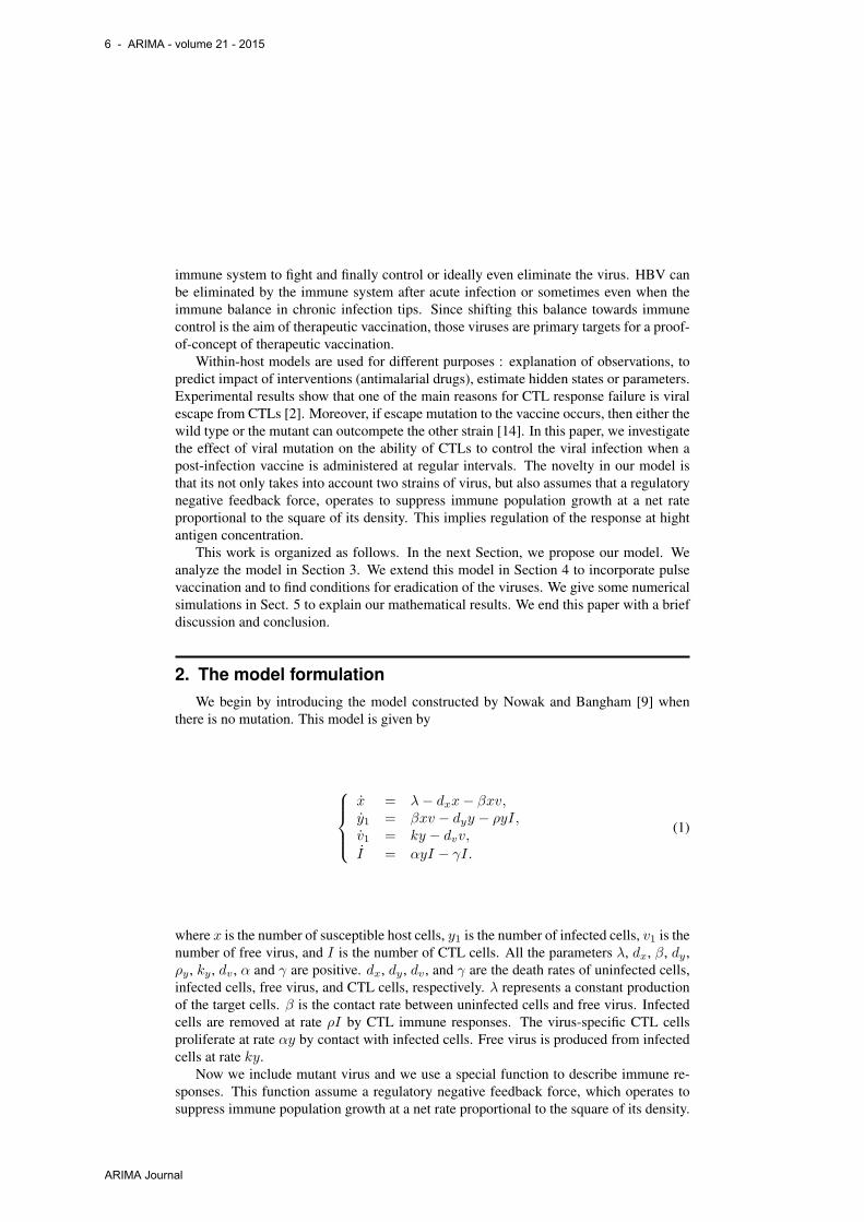
Firstly, Fig. 3(a) illustrates that under regular vaccinations, the CTL count oscillatesin an impulsive periodic orbit. If the vaccine is sufficiently strong, both strains are drivento extinction, assuming perfect adherence (see Fig. 3.(b)). In this figure we have alsoincrease the value of dv . So, if the vaccine can reduce the life span of viruses, the twostrains can be eradicated.

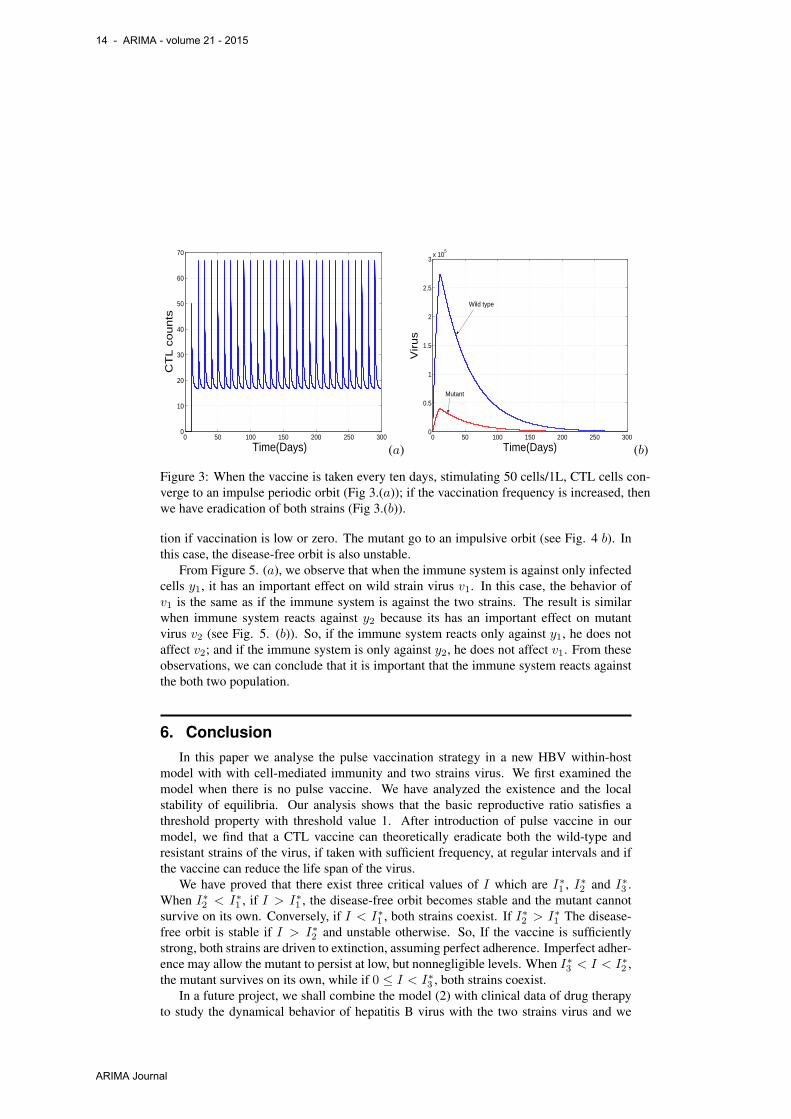
Fig. 4(a) show that the mutant and wild type can coexist if vaccination is low, butnonzero, and if we increase the time life of virus. Both values approach a stable orbit.When I∗3 < I∗2 , the mutant persists at high levels, while the wild type is driven to extinc-


ARIMA Journal

0 50 100 150 200 250 3000

10

20

30

40

50

60

70

Time(Days)

CT

L c

ounts

(a)0 50 100 150 200 250 300

0

0.5

1

1.5

2

2.5

3x 10

5

Time(Days)

Virus

Wild type

Mutant

(b)

Figure 3: When the vaccine is taken every ten days, stimulating 50 cells/1L, CTL cells con-verge to an impulse periodic orbit (Fig 3.(a)); if the vaccination frequency is increased, thenwe have eradication of both strains (Fig 3.(b)).

tion if vaccination is low or zero. The mutant go to an impulsive orbit (see Fig. 4 b). Inthis case, the disease-free orbit is also unstable.

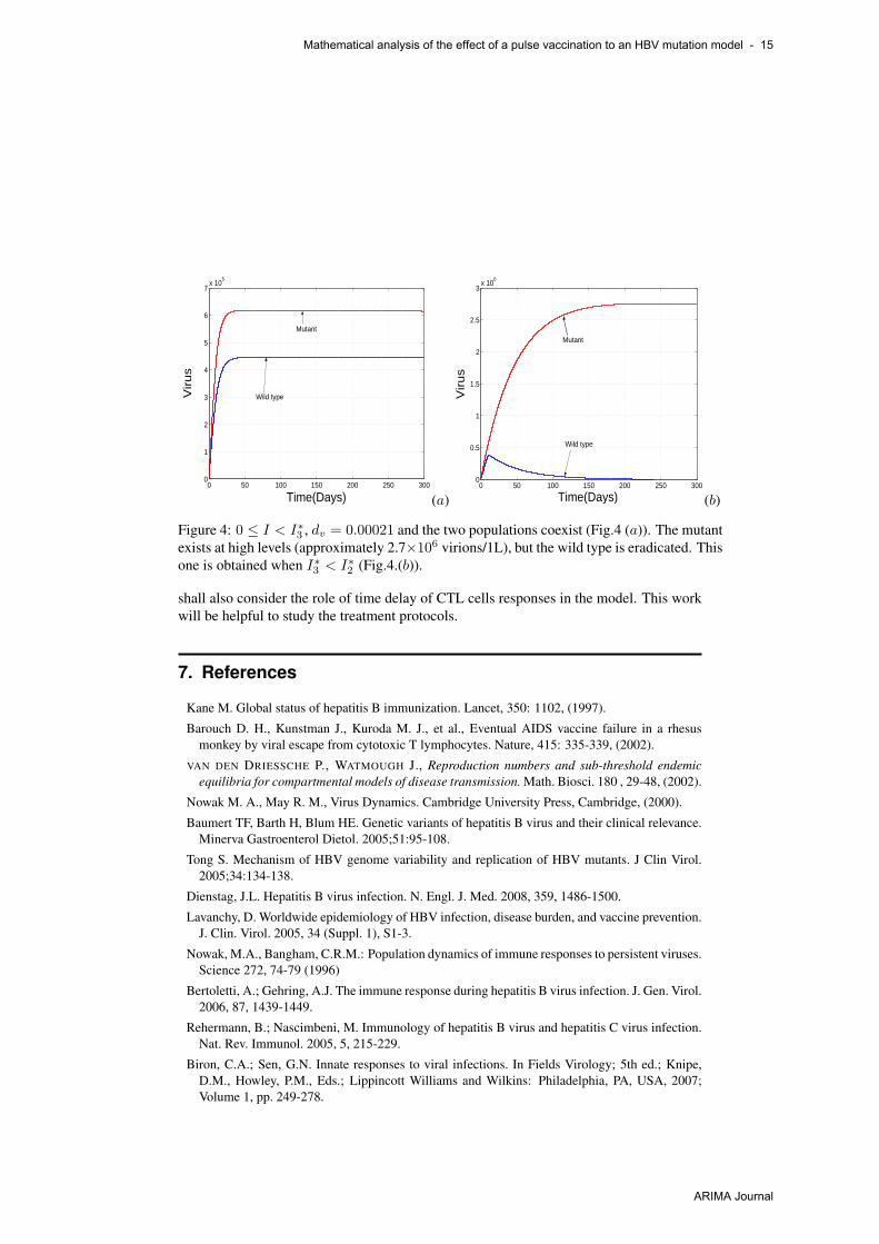
From Figure 5. (a), we observe that when the immune system is against only infectedcells y1, it has an important effect on wild strain virus v1. In this case, the behavior ofv1 is the same as if the immune system is against the two strains. The result is similarwhen immune system reacts against y2 because its has an important effect on mutantvirus v2 (see Fig. 5. (b)). So, if the immune system reacts only against y1, he does notaffect v2; and if the immune system is only against y2, he does not affect v1. From theseobservations, we can conclude that it is important that the immune system reacts againstthe both two population.

6. ConclusionIn this paper we analyse the pulse vaccination strategy in a new HBV within-host

model with with cell-mediated immunity and two strains virus. We first examined themodel when there is no pulse vaccine. We have analyzed the existence and the localstability of equilibria. Our analysis shows that the basic reproductive ratio satisfies athreshold property with threshold value 1. After introduction of pulse vaccine in ourmodel, we find that a CTL vaccine can theoretically eradicate both the wild-type andresistant strains of the virus, if taken with sufficient frequency, at regular intervals and ifthe vaccine can reduce the life span of the virus.

We have proved that there exist three critical values of I which are I∗1 , I∗2 and I∗3 .When I∗2 < I∗1 , if I > I∗1 , the disease-free orbit becomes stable and the mutant cannotsurvive on its own. Conversely, if I < I∗1 , both strains coexist. If I∗2 > I∗1 The disease-free orbit is stable if I > I∗2 and unstable otherwise. So, If the vaccine is sufficientlystrong, both strains are driven to extinction, assuming perfect adherence. Imperfect adher-ence may allow the mutant to persist at low, but nonnegligible levels. When I∗3 < I < I∗2 ,the mutant survives on its own, while if 0 ≤ I < I∗3 , both strains coexist.

In a future project, we shall combine the model (2) with clinical data of drug therapyto study the dynamical behavior of hepatitis B virus with the two strains virus and we

14 - ARIMA - volume 21 - 2015

ARIMA Journal

0 50 100 150 200 250 3000

1

2

3

4

5

6

7x 10

5

Time(Days)

Virus

Wild type

Mutant

(a)0 50 100 150 200 250 300

0

0.5

1

1.5

2

2.5

3x 10

6

Time(Days)

Virus

Mutant

Wild type

(b)

Figure 4: 0 ≤ I < I∗3 , dv = 0.00021 and the two populations coexist (Fig.4 (a)). The mutantexists at high levels (approximately 2.7×106 virions/1L), but the wild type is eradicated. Thisone is obtained when I∗3 < I∗2 (Fig.4.(b)).

shall also consider the role of time delay of CTL cells responses in the model. This workwill be helpful to study the treatment protocols.

7. References

Kane M. Global status of hepatitis B immunization. Lancet, 350: 1102, (1997).

Barouch D. H., Kunstman J., Kuroda M. J., et al., Eventual AIDS vaccine failure in a rhesusmonkey by viral escape from cytotoxic T lymphocytes. Nature, 415: 335-339, (2002).

VAN DEN DRIESSCHE P., WATMOUGH J., Reproduction numbers and sub-threshold endemicequilibria for compartmental models of disease transmission. Math. Biosci. 180 , 29-48, (2002).

Nowak M. A., May R. M., Virus Dynamics. Cambridge University Press, Cambridge, (2000).

Baumert TF, Barth H, Blum HE. Genetic variants of hepatitis B virus and their clinical relevance.Minerva Gastroenterol Dietol. 2005;51:95-108.

Tong S. Mechanism of HBV genome variability and replication of HBV mutants. J Clin Virol.2005;34:134-138.

Dienstag, J.L. Hepatitis B virus infection. N. Engl. J. Med. 2008, 359, 1486-1500.

Lavanchy, D. Worldwide epidemiology of HBV infection, disease burden, and vaccine prevention.J. Clin. Virol. 2005, 34 (Suppl. 1), S1-3.

Nowak, M.A., Bangham, C.R.M.: Population dynamics of immune responses to persistent viruses.Science 272, 74-79 (1996)

Bertoletti, A.; Gehring, A.J. The immune response during hepatitis B virus infection. J. Gen. Virol.2006, 87, 1439-1449.

Rehermann, B.; Nascimbeni, M. Immunology of hepatitis B virus and hepatitis C virus infection.Nat. Rev. Immunol. 2005, 5, 215-229.

Biron, C.A.; Sen, G.N. Innate responses to viral infections. In Fields Virology; 5th ed.; Knipe,D.M., Howley, P.M., Eds.; Lippincott Williams and Wilkins: Philadelphia, PA, USA, 2007;Volume 1, pp. 249-278.


ARIMA Journal

0 50 100 150 200 250 3000

1

2

3

4

5

6x 10

5

Time(Days)

wild

−ty

pe

v1

Immunity against y1 and y

2Immunity against y

1Immunity against y

2No immunity

(a)0 50 100 150 200 250 300

0

0.5

1

1.5

2

2.5

3

3.5

4

4.5x 10

5

Time(Days)

Muta

nt st

rain

t vi

rus

v 2

immunity against both y1 and y

2Immunity against y

1Immunity against y

2No immunity

(b)

Figure 5: 0 ≤ I < I∗3 , dv = 0.00021 and the two populations coexist (Fig.5 (a)) and Fig.5.(b). The two strains population exist. The target of immune response strongly influences theoutcome of infection in HBV model with two strains.

World Health Organization: Hepatitis B. WHO/CDS/CSR/ LYO/2002.2: Hepatitis B.This document has been downloaded from the WHO/CSR Web site. http://www.who.int/csr/disease/hepatitis/whocdscsrlyo20022/en/ (2002).

Bernhard P. K., Naveen K. V., Robert J. S., Modelling Mutation to a Cytotoxic T-lymphocyte HIVVaccine, Mathematical Population Studies, 18: 122-149, (2011)

Whalley S. A., Murray J. M. , Brown D., Webster G. J. M., Emery V. C., Dusheiko G. M. andPerelson A. S., Kinetics of Acute Hepatitis B Virus Infection in Humans. J. Exp. Med., 193:847−853, (2001).

Murray J. M., Purcell R. H., Wieland S. F., The half-life of hepatitis B virions. Hepatology, 44:1117−1121, (2006).

Hethcote H. W., Thieme H. R., Stability of the Endemic Equilibrium in Epidemic Models withSubpopulations, Math. Biosci. 75 205-277, (1985).

Cornberg M, Protzer U, Petersen J, Wedemeyer H, Berg T, Jilg W, Erhardt A, Wirth S, Sarrazin C,Dollinger MM, Schirmacher P, Dathe K, Kopp IB, Zeuzem S, Gerlich WH, Manns MP, AWMF,Prophylaxis, diagnosis and therapy of hepatitis B virus infection - the German guideline. ZGastroenterol. PubMed; 49(7) : 871-930, (2011).

Kwon H, Lok AS Hepatitis B therapy. Nat Rev Gastroenterol Hepatol.; 8(5) : 275-284, (2011).

Dienstag JL, Stevens CE, Bhan AK, Szmuness W, Hepatitis B vaccine administered to chroniccarriers of hepatitis b surface antigen. Ann Intern Med. 96 (5) : 575-579, (1982) .

Heintges T, Petry W, Kaldewey M, Erhardt A, Wend UC, Gerlich WH, Niederau C, HäussingerD. Combination therapy of active HBsAg vaccination and interferon-alpha in interferon-alphanonresponders with chronic hepatitis B. Dig Dis Sci. 46 (4) 901-906, (2001)

Dahmen A, Herzog-Hauff S, Böcher WO, Galle PR, Löhr HF. Clinical and immunological efficacyof intradermal vaccine plus lamivudine with or without interleukin-2 in patients with chronichepatitis B. J Med Virol. 66 (4) : 452-460, (2002).

Hildesheim A, Herrero R, Wacholder S, Rodriguez AC, Solomon D, Bratti MC, Schiller JT, Gon-zalez P, Dubin G, Porras C, Jimenez SE, Lowy DR. Effect of human papillomavirus 16/18 L1viruslike particle vaccine among young women with preexisting infection: a randomized trial.Costa Rican HPV Vaccine Trial Group JAMA. 15; 298 (7) : 743-753, (2007).

16 - ARIMA - volume 21 - 2015

ARIMA Journal

Appendix A : Coefficients of the characteristic polynomial at P

a4 = (dx + β2v2)[dvqIdy + qIk2β2x+ ρ2dvpI] + β22 v2xk2qI

a3 = (dx + β2v2)[(ρ2I + dy + qI)dv + qIdy + k2β2x+ ρ2pI]

+ dvqIdy + qIk2β2x+ ρ2dvpI + β22 v2xk2

a2 = (dx + β2v2)(dv + ρ2I + dy + qI) + dv(ρ2I + dy + qI) + qIdy + k2β2x

+ ρ2pI

a1 = dx + dv + dy + β2v2 + (ρ2 + q)Ia0 = 1

Appendix B : Proof of lemma 4.1.Proof : Case 1: Suppose that I∗1 = I∗2 = I . Since λ

dxdv= r1

(1−ε)β1k1and λ

dxdv= r2

k2β2,

we obtain r1(1−ε)β1k1

= r2k2β2

⇒ r2(1− ε)β1k1 = r1β2k2 ⇒ I = I∗3 .

Case 2: Let us suppose that I∗1 > I∗2 . Set I = I∗2 then I < I∗1 ⇔ r1 < (1−ε)β1k1λdxdv

⇔I < I∗3 . Hence I∗3 > I2∗. By the same method, we establish that I∗3 > I∗2 . The case 3 isobtained by the same method as in case 2. �

Appendix C : Proof of Proposition 3.1.We use a theorem for the existence and uniqueness of a positive fixed point of a multi-

variable function. We labeled this theorem as follows.

Theorem 7.1. (Thieme [17], theorem 2.1) Let F (x) be a continuous, monotone non-decreasing, strictly sub linear, bounded function which maps the non-negative orthantRn

+ = [0,+∞) into itself. Let F (0) = 0 and F ′(0) exists and be irreducible. Then F (x)does not have a non-trivial fixed point on the boundary of Rn

+. Moreover, F (x) has apositive fixed point iff ρ(F ′(0)) > 1. If there is a positive fixed point, then it is unique.

Let us show that the system (11) has a positive solution. (11) can be written as:Y = F (Y ) where Y = (y1, y2)

T and

F =

dx(1− ε)β1k1x

∗

(dxdv + β1k1y1 + β2k2y2)[dy + ρ1

(pq + α

q (y1 + y2))]

εdxβ1k1x∗y1 + β2k2y2x

∗dx

(dxdv + β1k1y1 + β2k2y2)[dy + y2ρ2

(pq + α

q (y1 + y2))]

,(

F1(Y )F2(Y )

)

We have F1(Y ) ≤ dx(1− ε)β1k1x∗y1

(dxdv + β1k1y1)(dy + ρ1

pq

) ≤ M1 and

F2(Y ) ≤ εdxβ1k1x∗y1


pq

) +β2k2y2x

∗dx


pq

) ≤ M2.

In this case, F (Y ) is continuous, bounded function which maps

Γ = {(y1, y2) : 0 < y1 < M1, 0 < y2 < M2}


ARIMA Journal

It is easy to find that F (Y ) is infinitely differentiable and is a monotone nondecreasingfunction. Moreover, F (0, 0) = (0, 0) and

F ′(0, 0) =

R01 0

εβ1k1x∗

dv(dy + ρ2I∗)R02

Hence ρ(F ′(0, 0)) = max{R01,R02} = R0 > 1. Thanks to the graph theory, weclaim that F ′(0, 0) is irreducible because the associated graph of the matrix is stronglyconnected.

Let us now prove that F is strictly sub linear in Γ, i.e., F (rY ) > rF (Y ), for anyY ∈ Γ. with Y > 0, and r ∈ (0; 1). Some calculations give

r1F1(Y )

F1(r1Y )=

(dxdv + r1β1k1y1 + r1β2k2y2)[dy + ρ1

(pq + r1

αq (y1 + y2)

)](dxdv + β1k1y1 + β2k2y2)

[dy + ρ1

(pq + α

q (y1 + y2))] < 1,

r2F2(Y )

F2(r2Y )=

(dxdv + r2β1k1y1 + r2β2k2y2)[dy + ρ2

(pq + r2

αq (y1 + y2)

)](dxdv + β1k1y1 + β2k2y2)

[dy + ρ2

(pq + α

q (y1 + y2))] < 1

So the function F (Y ) is strictly sub linear with r = min(r1; r2). This ends the proof ofProposition 3.1.

Appendix D : Coefficients ui (i = 1, ..., 6) of the characteristicpolynomial at P

The characteristic polynomial at P is given by

Q(λ) = λ6 + u1λ5 + u2λ

4 + u3λ3 + u4λ

2 + u5λ+ u6

18 - ARIMA - volume 21 - 2015

ARIMA Journal

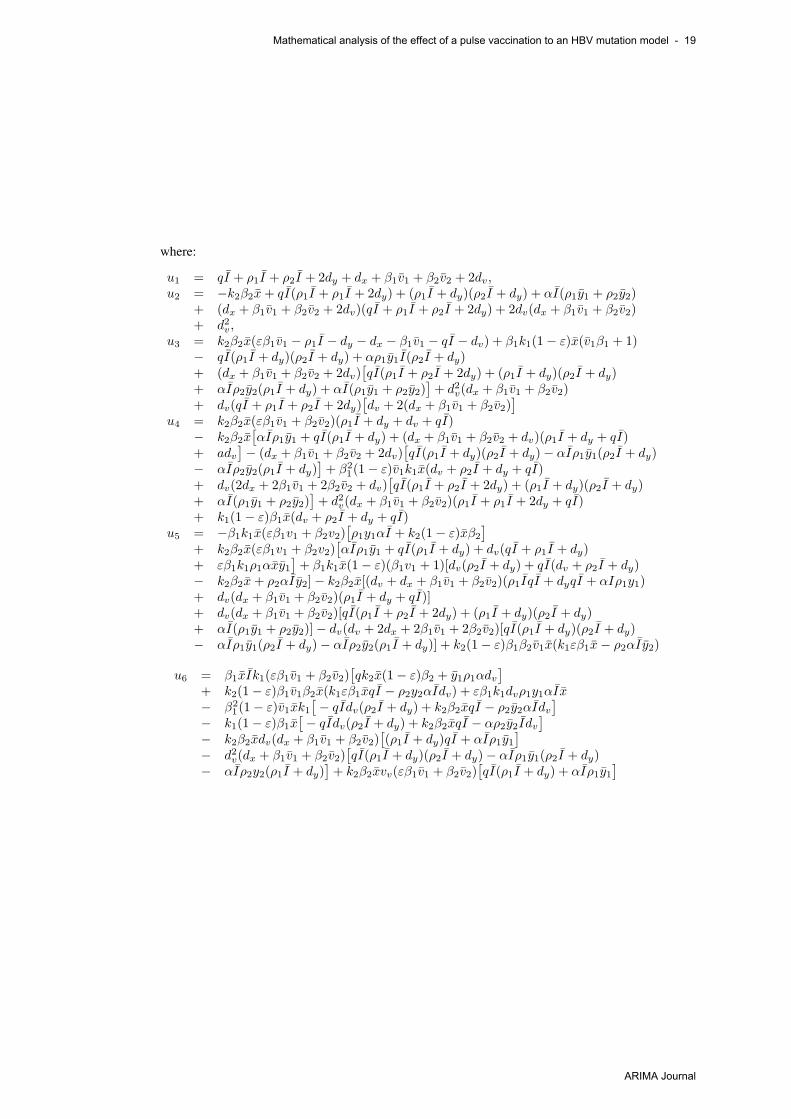
where:

u1 = qI + ρ1I + ρ2I + 2dy + dx + β1v1 + β2v2 + 2dv,u2 = −k2β2x+ qI(ρ1I + ρ1I + 2dy) + (ρ1I + dy)(ρ2I + dy) + αI(ρ1y1 + ρ2y2)

+ (dx + β1v1 + β2v2 + 2dv)(qI + ρ1I + ρ2I + 2dy) + 2dv(dx + β1v1 + β2v2)+ d2v,

u3 = k2β2x(εβ1v1 − ρ1I − dy − dx − β1v1 − qI − dv) + β1k1(1− ε)x(v1β1 + 1)− qI(ρ1I + dy)(ρ2I + dy) + αρ1y1I(ρ2I + dy)+ (dx + β1v1 + β2v2 + 2dv)

[qI(ρ1I + ρ2I + 2dy) + (ρ1I + dy)(ρ2I + dy)

+ αIρ2y2(ρ1I + dy) + αI(ρ1y1 + ρ2y2)]+ d2v(dx + β1v1 + β2v2)

+ dv(qI + ρ1I + ρ2I + 2dy)[dv + 2(dx + β1v1 + β2v2)

]u4 = k2β2x(εβ1v1 + β2v2)(ρ1I + dy + dv + qI)

− k2β2x[αIρ1y1 + qI(ρ1I + dy) + (dx + β1v1 + β2v2 + dv)(ρ1I + dy + qI)

+ adv]− (dx + β1v1 + β2v2 + 2dv)

[qI(ρ1I + dy)(ρ2I + dy)− αIρ1y1(ρ2I + dy)

− αIρ2y2(ρ1I + dy)]+ β2

1(1− ε)v1k1x(dv + ρ2I + dy + qI)+ dv(2dx + 2β1v1 + 2β2v2 + dv)

[qI(ρ1I + ρ2I + 2dy) + (ρ1I + dy)(ρ2I + dy)

+ αI(ρ1y1 + ρ2y2)]+ d2v(dx + β1v1 + β2v2)(ρ1I + ρ1I + 2dy + qI)

+ k1(1− ε)β1x(dv + ρ2I + dy + qI)u5 = −β1k1x(εβ1v1 + β2v2)

[ρ1y1αI + k2(1− ε)xβ2

]+ k2β2x(εβ1v1 + β2v2)

[αIρ1y1 + qI(ρ1I + dy) + dv(qI + ρ1I + dy)

+ εβ1k1ρ1αxy1]+ β1k1x(1− ε)(β1v1 + 1)[dv(ρ2I + dy) + qI(dv + ρ2I + dy)

− k2β2x+ ρ2αIy2]− k2β2x[(dv + dx + β1v1 + β2v2)(ρ1IqI + dyqI + αIρ1y1)+ dv(dx + β1v1 + β2v2)(ρ1I + dy + qI)]+ dv(dx + β1v1 + β2v2)[qI(ρ1I + ρ2I + 2dy) + (ρ1I + dy)(ρ2I + dy)+ αI(ρ1y1 + ρ2y2)]− dv(dv + 2dx + 2β1v1 + 2β2v2)[qI(ρ1I + dy)(ρ2I + dy)− αIρ1y1(ρ2I + dy)− αIρ2y2(ρ1I + dy)] + k2(1− ε)β1β2v1x(k1εβ1x− ρ2αIy2)

u6 = β1xIk1(εβ1v1 + β2v2)[qk2x(1− ε)β2 + y1ρ1αdv

]+ k2(1− ε)β1v1β2x(k1εβ1xqI − ρ2y2αIdv) + εβ1k1dvρ1y1αIx− β2

1(1− ε)v1xk1[− qIdv(ρ2I + dy) + k2β2xqI − ρ2y2αIdv

]− k1(1− ε)β1x

[− qIdv(ρ2I + dy) + k2β2xqI − αρ2y2Idv

]− k2β2xdv(dx + β1v1 + β2v2)

[(ρ1I + dy)qI + αIρ1y1

]− d2v(dx + β1v1 + β2v2)

[qI(ρ1I + dy)(ρ2I + dy)− αIρ1y1(ρ2I + dy)

− αIρ2y2(ρ1I + dy)]+ k2β2xvv(εβ1v1 + β2v2)

[qI(ρ1I + dy) + αIρ1y1

]


ARIMA Journal

mathematical analysis of the effect of a pulse vaccination...

Documents