Four Node Test System with Induction Motor

3 4Delta LoadY Load

Motor

1 2Reg Line

s R

VLL4VLG3VLG2VLGRVLG1VLGS

IS IR I 2 I3I t

I 4abcIM

I4ldI3ld

Define standard matrices:

Symmetrical Componenttransformation matrix

as 1 ej 120⋅ deg⋅⋅:= As

1

1

1

1

as2

as

1

as

as2

⎛⎜⎜⎜⎜⎝

⎞⎟⎟⎟⎟⎠

:=

Phase shift matrix usedfor three-phase Inductionmachine modeling

ts1

3ej 30⋅ deg⋅⋅:= T

1

0

0

0

ts⎯

0

0

0

ts

⎛⎜⎜⎜⎝

⎞⎟⎟⎟⎠

:=

Matrix used to compute equivalentline-to-neutral knowing line-to-linevoltages.

W13

2

0

1

1

2

0

0

1

2

⎛⎜⎜⎝

⎞⎟⎟⎠

⋅:=

Matrix used to convert line-to-neutralvoltages to line-to-line voltages.

D

1

0

1−

1−

1

0

0

1−

1

⎛⎜⎜⎝

⎞⎟⎟⎠

:=

Unity matrix U

1

0

0

0

1

0

0

0

1

⎛⎜⎜⎝

⎞⎟⎟⎠

:=

Matrix used to compute line currentsinto a delta connected load. DI

1

1−

0

0

1

1−

1−

0

1

⎛⎜⎜⎝

⎞⎟⎟⎠

:=

C:\Milsoft 2009 Evaluation\Student test feeder\Try 2.xmcd 1

Line data:

4.0'

2.5' 4.5'

3.0'

a b c

n

25.0'

Phase Conductors: 336,400 26/7 ACSR

Neutral Conductor: 4/0 6/1 ACSR

Length of line: 2.0 miles

Dist 2.0:= miles

Define conductor positions:

d1 0 j 29⋅+:= d2 2.5 j 29⋅+:= d3 7.0 j 29⋅+:= d4 4.0 j 25⋅+:=

Compute self and image distances:

n 1 4..:= m 1 4..:=

Dxn m, dn dm−:= Dx

0

2.5

7

5.6569

2.5

0

4.5

4.272

7

4.5

0

5

5.6569

4.272

5

0

⎛⎜⎜⎜⎜⎝

⎞⎟⎟⎟⎟⎠

=

Sxn m, dn dm⎯

−:= Sx

58

58.0539

58.4209

54.1479

58.0539

58

58.1743

54.0208

58.4209

58.1743

58

54.0833

54.1479

54.0208

54.0833

50

⎛⎜⎜⎜⎜⎝

⎞⎟⎟⎟⎟⎠

=

Input conductor data:

i 1 3..:= GMRi .0244:= ri .306:= Diai 0.741:= RDi

Diai

24:= RD1 0.0309=

j 1 3..:= GMR4 .00814:= r4 .592:= Dia4 0.563:= RD4

Dia4

24:= RD4 0.0235=

C:\Milsoft 2009 Evaluation\Student test feeder\Try 2.xmcd 2

Define diagonal term of distance matrix:

Dxi i, GMRi:= Dx4 4, GMR4:=

Display final distance matrix:

Dx

0.0244

2.5

7

5.6569

2.5

0.0244

4.5

4.272

7

4.5

0.0244

5

5.6569

4.272

5

0.0081

⎛⎜⎜⎜⎜⎝

⎞⎟⎟⎟⎟⎠

= ft.

Carson's equations:

zpn m, 0.0953 j .12134⋅ ln1

Dxn m,

⎛⎜⎝

⎞⎟⎠

7.93402+⎛⎜⎝

⎞⎟⎠

⋅+:=

zpn n, rn zpn n,+:=

Display primitive impedance matrix:

zp

0.4013 1.4133j+

0.0953 0.8515j+

0.0953 0.7266j+

0.0953 0.7524j+

0.0953 0.8515j+

0.4013 1.4133j+

0.0953 0.7802j+

0.0953 0.7865j+

0.0953 0.7266j+

0.0953 0.7802j+

0.4013 1.4133j+

0.0953 0.7674j+

0.0953 0.7524j+

0.0953 0.7865j+

0.0953 0.7674j+

0.6873 1.5465j+

⎛⎜⎜⎜⎜⎝

⎞⎟⎟⎟⎟⎠

=

Partition zp to set up for Kron reduction:

zij submatrix zp 1, 3, 1, 3,( ):= zij

0.4013 1.4133j+

0.0953 0.8515j+

0.0953 0.7266j+

0.0953 0.8515j+

0.4013 1.4133j+

0.0953 0.7802j+

0.0953 0.7266j+

0.0953 0.7802j+

0.4013 1.4133j+

⎛⎜⎜⎝

⎞⎟⎟⎠

=

zin submatrix zp 1, 3, 4, 4,( ):= zin

0.0953 0.7524j+

0.0953 0.7865j+

0.0953 0.7674j+

⎛⎜⎜⎝

⎞⎟⎟⎠

=

znj submatrix zp 4, 4, 1, 3,( ):= znj 0.0953 0.7524j+ 0.0953 0.7865j+ 0.0953 0.7674j+( )=

znn submatrix zp 4, 4, 4, 4,( ):= znn 0.6873 1.5465j+( )=

C:\Milsoft 2009 Evaluation\Student test feeder\Try 2.xmcd 3

Kron Reduction:

zabc zij zin znn 1−⋅ znj⋅−:=

Display phase impedance matrix:

zabc

0.4576 1.078j+

0.156 0.5017j+

0.1535 0.3849j+

0.156 0.5017j+

0.4666 1.0482j+

0.158 0.4236j+

0.1535 0.3849j+

0.158 0.4236j+

0.4615 1.0651j+

⎛⎜⎜⎝

⎞⎟⎟⎠

= Ω/mile

Admittance calculations:

Compute potential coefficient matrix:

Pn m, 11.17689 lnSxn m,

Dxn m,

⎛⎜⎜⎝

⎞⎟⎟⎠

⋅:= Pn n, 11.17689 lnSxn n,

RDn

⎛⎜⎜⎝

⎞⎟⎟⎠

⋅:=

Display potential coefficient matrix:

P

84.2542

35.1522

23.7147

25.2469

35.1522

84.2542

28.6058

28.359

23.7147

28.6058

84.2542

26.6131

25.2469

28.359

26.6131

85.6659

⎛⎜⎜⎜⎜⎝

⎞⎟⎟⎟⎟⎠

=

Partition P to set up for Kron reduction:

pij submatrix P 1, 3, 1, 3,( ):= pij

84.2542

35.1522

23.7147

35.1522

84.2542

28.6058

23.7147

28.6058

84.2542

⎛⎜⎜⎝

⎞⎟⎟⎠

=

pin submatrix P 1, 3, 4, 4,( ):= pin

25.2469

28.359

26.6131

⎛⎜⎜⎝

⎞⎟⎟⎠

=

pnj submatrix P 4, 4, 1, 3,( ):= pnj 25.2469 28.359 26.6131( )=

pnn submatrix P 4, 4, 4, 4,( ):= pnn 85.6659( )=

C:\Milsoft 2009 Evaluation\Student test feeder\Try 2.xmcd 4

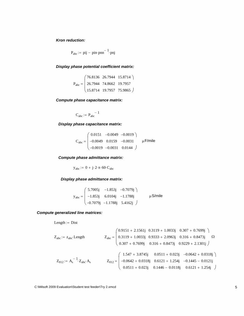
Kron reduction:

Pabc pij pin pnn 1−⋅ pnj⋅−:=

Display phase potential coefficient matrix:

Pabc

76.8136

26.7944

15.8714

26.7944

74.8662

19.7957

15.8714

19.7957

75.9865

⎛⎜⎜⎝

⎞⎟⎟⎠

=

Compute phase capacitance matrix:

Cabc Pabc1−

:=

Display phase capacitance matrix:

Cabc

0.0151

0.0049−

0.0019−

0.0049−

0.0159

0.0031−

0.0019−

0.0031−

0.0144

⎛⎜⎜⎝

⎞⎟⎟⎠

= μF/mile

Compute phase admittance matrix:

yabc 0 j 2⋅ π⋅ 60⋅ Cabc⋅+:=

Display phase admittance matrix:

yabc

5.7005j

1.853j−

0.7079j−

1.853j−

6.0104j

1.1788j−

0.7079j−

1.1788j−

5.4162j

⎛⎜⎜⎝

⎞⎟⎟⎠

= μS/mile

Compute generalized line matrices:

Length Dist:=

Zabc zabc Length⋅:= Zabc

0.9151 2.1561j+

0.3119 1.0033j+

0.307 0.7699j+

0.3119 1.0033j+

0.9333 2.0963j+

0.316 0.8473j+

0.307 0.7699j+

0.316 0.8473j+

0.9229 2.1301j+

⎛⎜⎜⎝

⎞⎟⎟⎠

= Ω

Z012 As1− Zabc⋅ As⋅:= Z012

1.547 3.8745j+

0.0642− 0.0318j+

0.0511 0.023j+

0.0511 0.023j+

0.6121 1.254j+

0.1446 0.0118j−

0.0642− 0.0318j+

0.1445− 0.0121j−

0.6121 1.254j+

⎛⎜⎜⎝

⎞⎟⎟⎠

=

C:\Milsoft 2009 Evaluation\Student test feeder\Try 2.xmcd 5

Yabc yabc Length⋅ 10 6−⋅:= Yabc

1.1401j 10 5−×

3.706j− 10 6−×

1.4159j− 10 6−×

3.706j− 10 6−×

1.2021j 10 5−×

2.3575j− 10 6−×

1.4159j− 10 6−×

2.3575j− 10 6−×

1.0832j 10 5−×

⎛⎜⎜⎜⎜⎝

⎞⎟⎟⎟⎟⎠

= S

aline U12

Zabc⋅ Yabc⋅+:=

aline

0.99999011 0.00000442j+

0.00000124− 0.00000018j−

0.00000131− 0.00000051j+

0.00000113− 0.00000018j−

0.99999026 0.00000466j+

0.00000116− 0.00000024j+

0.00000146− 0.00000065j+

0.00000141− 0.00000039j+

0.99999001 0.00000441j+

⎛⎜⎜⎝

⎞⎟⎟⎠

=

bline Zabc:= bline

0.9151 2.1561j+

0.3119 1.0033j+

0.307 0.7699j+

0.3119 1.0033j+

0.9333 2.0963j+

0.316 0.8473j+

0.307 0.7699j+

0.316 0.8473j+

0.9229 2.1301j+

⎛⎜⎜⎝

⎞⎟⎟⎠

=

cline Yabc14

Yabc⋅ Zabc⋅ Yabc⋅+:=

cline

2.5166− 10 11−× 1.1401j 10 5−

×+

9.8471 10 12−× 3.706j 10 6−

×−

1.5637 10 13−× 1.4159j 10 6−

×−

9.8471 10 12−× 3.706j 10 6−

×−

2.8054− 10 11−× 1.2021j 10 5−

×+

4.0481 10 12−× 2.3575j 10 6−

×−

1.5637 10 13−× 1.4159j 10 6−

×−

4.0481 10 12−× 2.3575j 10 6−

×−

2.2962− 10 11−× 1.0832j 10 5−

×+

⎛⎜⎜⎜⎜⎝

=

dline aline:=

Aline aline1−

:=

Aline

1.00000989 0.00000442j−

0.00000124 0.00000018j+

0.00000131 0.00000051j−

0.00000113 0.00000018j+

1.00000974 0.00000466j−

0.00000116 0.00000024j−

0.00000146 0.00000065j−

0.00000141 0.00000039j−

1.00000999 0.00000441j−

⎛⎜⎜⎝

⎞⎟⎟⎠

=

Bline aline1− bline⋅:= Bline

0.9151 2.1561j+

0.3119 1.0034j+

0.307 0.7699j+

0.3119 1.0034j+

0.9333 2.0963j+

0.316 0.8473j+

0.307 0.7699j+

0.316 0.8473j+

0.923 2.1301j+

⎛⎜⎜⎝

⎞⎟⎟⎠

=

C:\Milsoft 2009 Evaluation\Student test feeder\Try 2.xmcd 6

Read in substation transformer data:

kVA 12000:= kVLLhi 115:= Delta kVLLlo 12.47:= Wye

kVLNlokVLLlo

3:= kVLNlo 7.1996=

Zpusub .01 j .1⋅+:= Per-unit

Compute transformer Z on low side:

ZbaselokVLLlo

2 1000⋅

kVA:= Zbaselo 12.9584=

Zsub Zpusub Zbaselo⋅:= Zsub 0.1296 1.2958j+=

Define Zt matrix:

Zsubabc

Zsub

0

0

0

Zsub

0

0

0

Zsub

⎛⎜⎜⎜⎝

⎞⎟⎟⎟⎠

:=

Compute turns ratio:

ntkVLLhi

kVLNlo:= nt 15.9732=

Compute substation transformer matrices:

asubnt−

3

0

1

2

2

0

1

1

2

0

⎛⎜⎜⎝

⎞⎟⎟⎠

⋅:= asub

0

5.3244−

10.6488−

10.6488−

0

5.3244−

5.3244−

10.6488−

0

⎛⎜⎜⎝

⎞⎟⎟⎠

=

bsub asub Zsubabc⋅:=

bsub

0

0.69− 6.8996j−

1.3799− 13.7992j−

1.3799− 13.7992j−

0

0.69− 6.8996j−

0.69− 6.8996j−

1.3799− 13.7992j−

0

⎛⎜⎜⎝

⎞⎟⎟⎠

=

csub

0

0

0

0

0

0

0

0

0

⎛⎜⎜⎝

⎞⎟⎟⎠

:=

C:\Milsoft 2009 Evaluation\Student test feeder\Try 2.xmcd 7

dsub1nt

1

0

1−

1−

1

0

0

1−

1

⎛⎜⎜⎝

⎞⎟⎟⎠

⋅:= dsub

0.0626

0

0.0626−

0.0626−

0.0626

0

0

0.0626−

0.0626

⎛⎜⎜⎝

⎞⎟⎟⎠

=

Bsub asub1− bsub⋅:= Bsub

0.1296 1.2958j+

0

0

0

0.1296 1.2958j+

0

0

0

0.1296 1.2958j+

⎛⎜⎜⎝

⎞⎟⎟⎠

=

Asub1nt

1

1−

0

0

1

1−

1−

0

1

⎛⎜⎜⎝

⎞⎟⎟⎠

⋅:= Asub

0.0626

0.0626−

0

0

0.0626

0.0626−

0.0626−

0

0.0626

⎛⎜⎜⎝

⎞⎟⎟⎠

=

Read in data for three type B step voltage regulators connected inwye.

Potential transformer ratio: Npt7200120

:= Npt 60=

Current transformer primary rating:

CTp 500:= CTc 0.1:= CTCTp

CTc:= CT 5000=

Compensator settings:

RComp 4.9:= XComp 10.0:= volts

ZohmsRComp j XComp⋅+

CTc:= Zohms 49 100j+= Ohms

Set desired voltage level:

Vset 125:=

Vlevel

Vset

Vset

Vset

⎛⎜⎜⎜⎝

⎞⎟⎟⎟⎠

:=

Set initial tap positions:

Tap

0

0

0

⎛⎜⎜⎝

⎞⎟⎟⎠

:=

Compute initial matrices:

ari1 .00625 Tapi⋅−:= ar

1

1

1

⎛⎜⎜⎝

⎞⎟⎟⎠

=

C:\Milsoft 2009 Evaluation\Student test feeder\Try 2.xmcd 8

aR

ar1

0

0

0

ar2

0

0

0

ar3

⎛⎜⎜⎜⎜⎝

⎞⎟⎟⎟⎟⎠

:= aR

1

0

0

0

1

0

0

0

1

⎛⎜⎜⎝

⎞⎟⎟⎠

=

dR aR1−

:= dR

1

0

0

0

1

0

0

0

1

⎛⎜⎜⎝

⎞⎟⎟⎠

=

AR dR:= AR

1

0

0

0

1

0

0

0

1

⎛⎜⎜⎝

⎞⎟⎟⎠

=

Read in equivalent system data:

kVLLs 115:= kVLNskVLLs

3:= kVLNs 66.3953=

Vpus 1.05000:=

Z1sys 5.6261 j 27.408⋅+:= Ω on 115 kV side

Z0sys 18.5865 j 122.4028⋅+:= Ω on 115 kV side

Build system sequence impedance matrix:

Zsys012

Z0sys

0

0

0

Z1sys

0

0

0

Z1sys

⎛⎜⎜⎜⎝

⎞⎟⎟⎟⎠

:= Zsys012

18.5865 122.4028j+

0

0

0

5.6261 27.408j+

0

0

0

5.6261 27.408j+

⎛⎜⎜⎝

=

Compute system phase impedance matrix:

Zsysabc As1− Zsys012⋅ As⋅:= Zsysabc

9.9462 59.0729j+

4.3201 31.6649j+

4.3201 31.6649j+

4.3201 31.6649j+

9.9462 59.0729j+

4.3201 31.6649j+

4.3201 31.6649j+

4.3201 31.6649j+

9.9462 59.0729j+

⎛⎜⎜⎝

⎞

⎠=

Compute system phase matrices:

asys U:= asys

1

0

0

0

1

0

0

0

1

⎛⎜⎜⎝

⎞⎟⎟⎠

=

bsys Zsysabc:= bsys

9.9462 59.0729j+

4.3201 31.6649j+

4.3201 31.6649j+

4.3201 31.6649j+

9.9462 59.0729j+

4.3201 31.6649j+

4.3201 31.6649j+

4.3201 31.6649j+

9.9462 59.0729j+

⎛⎜⎜⎝

⎞⎟⎟⎠

=

C:\Milsoft 2009 Evaluation\Student test feeder\Try 2.xmcd 9

csys

0

0

0

0

0

0

0

0

0

⎛⎜⎜⎝

⎞⎟⎟⎠

:=

dsys asys:=

Asys U:=

Bsys bsys:=

Input node 3 wye connected load data:

kW312000:= PF31

.95:= Lagging

kW321500:= PF32

.95:= Lagging

kW331000:= PF33

.90:= Lagging

SL3i

kW3i

PF3i

ej acos PF3i( )⋅

⋅:= SL3

2000 657.3682j+

1500 493.0262j+

1000 484.3221j+

⎛⎜⎜⎝

⎞⎟⎟⎠

=

Input the motor transformer data

kVAx 2500:= kVLLxhi 12.470:= Y kVLLxlo .480:= Y

Zpux .010 j .050⋅+:=

Compute abcd transformer parameters:

kVLNxhikVLLxhi

3:= kVLNxlo

kVLLxlo

3:=

nxkVLNxhi

kVLNxlo:= nx 25.9792= ax

kVLLxhi

kVLLxlo:= ax 25.9792=

ZbasekVLLxlo

2 1000⋅

kVAx:= Zbase 0.0922=

Zt Zpux Zbase⋅:= Zt 0.0009 0.0046j+=

Ztabc

Zt

0

0

0

Zt

0

0

0

Zt

⎛⎜⎜⎜⎝

⎞⎟⎟⎟⎠

:= Ztabc

0.0009 0.0046j+

0

0

0

0.0009 0.0046j+

0

0

0

0.0009 0.0046j+

⎛⎜⎜⎝

⎞⎟⎟⎠

=

C:\Milsoft 2009 Evaluation\Student test feeder\Try 2.xmcd 10

AV nx U⋅:= AV

25.9792

0

0

0

25.9792

0

0

0

25.9792

⎛⎜⎜⎝

⎞⎟⎟⎠

=

ax AV:= ax

25.9792

0

0

0

25.9792

0

0

0

25.9792

⎛⎜⎜⎝

⎞⎟⎟⎠

=

dx ax1−

:= dx

0.0385

0

0

0

0.0385

0

0

0

0.0385

⎛⎜⎜⎝

⎞⎟⎟⎠

=

bx AV Ztabc⋅:= bx

0.0239 0.1197j+

0

0

0

0.0239 0.1197j+

0

0

0

0.0239 0.1197j+

⎛⎜⎜⎝

⎞⎟⎟⎠

=

cx

0

0

0

0

0

0

0

0

0

⎛⎜⎜⎝

⎞⎟⎟⎠

:=

Ax AV 1−:= Ax

0.0385

0

0

0

0.0385

0

0

0

0.0385

⎛⎜⎜⎝

⎞⎟⎟⎠

=

Bx Ztabc:= Bx

0.0009 0.0046j+

0

0

0

0.0009 0.0046j+

0

0

0

0.0009 0.0046j+

⎛⎜⎜⎝

⎞⎟⎟⎠

=

Input delta connected node 4 load:

kVA41400:= PF41

.9:= Lagging

kVA42500:= PF42

.85:= Lagging

kVA43300:= PF43

.95:= Lagging

SL4ikVA4i

ej acos PF4i( )⋅

⋅:= SL4

360 174.356j+

425 263.3913j+

285 93.675j+

⎛⎜⎜⎝

⎞⎟⎟⎠

=

C:\Milsoft 2009 Evaluation\Student test feeder\Try 2.xmcd 11

Input the three-phase Hp (kVA) and line-to-line voltage rating of the machine

kVA 1200:= VLL 480:= Prot 0:=

Rs 0.0053:= Xs 0.106:= per-unit

Rr 0.007:= Xr 0.12:= per-unit

Xm 4.0:= per-unit

Compute motor impedance in ohms:

ZbaseVLL2

kVA 1000⋅:= Zbase 0.192=

Rs Rs Zbase⋅:= Rs 0.001018= Xs Xs Zbase⋅:= Xs 0.020352=

Rr Rr Zbase⋅:= Rr 0.001344= Xr Xr Zbase⋅:= Xr 0.02304=

Xm Xm Zbase⋅:= Xm 0.768=

Define impedances:

Zs Rs j Xs⋅+:= Zs 0.001 0.0204j+=

Zr Rr j Xr⋅+:= Zr 0.0013 0.023j+=

Ym j−1

Xm⋅:= Ym 1.3021j−=

Zm1

Ym:= Zm 0.768j=

Input the desired slip:

s1 0.005:=

Positive Sequence Network: RL1

1 s1−

s1

⎛⎜⎜⎝

⎞⎟⎟⎠

Rr⋅:= RL1 0.2675=

Negative Sequence Network: s2 2 s1−:= s2 1.995= RL2

1 s2−

s2Rr⋅:= RL2 0.0007−=

ZR1 Zr RL1+:= ZR2 Zr RL2+:=

C:\Milsoft 2009 Evaluation\Student test feeder\Try 2.xmcd 12

Zm 0.768j=ZR1 0.2688 0.023j+= ZR2 0.0007 0.023j+=

ZM1 Zs

Zm ZR1⋅

Zm ZR1++:= ZM1 0.2282 0.1199j+=

ZM2 Zs

Zm ZR2⋅

Zm ZR2++:= ZM2 0.0017 0.0427j+=

Compute phase admittance matrix:

YM11

ZM1:= YM2

1ZM2

:=

YT

1

0

0

0

ts⎯

YM1⋅

0

0

0

ts YM2⋅

⎛⎜⎜⎜⎝

⎞⎟⎟⎟⎠

:=

YMabc As YT⋅ As1−

⋅:= YMabc

3.1318 4.4397j−

1.6856 3.9527j+

3.8174− 0.4869j+

3.8174− 0.4869j+

3.1318 4.4397j−

1.6856 3.9527j+

1.6856 3.9527j+

3.8174− 0.4869j+

3.1318 4.4397j−

⎛⎜⎜⎝

⎞⎟⎟⎠

=

Define source voltages:

nominal phase A-B voltage: ELL 115000 ej 30⋅ deg⋅⋅:=

operating PU voltage: Epu 1.05:=

operating A-B voltage: ELL ELL Epu⋅:= ELL 120750=arg ELL( )

deg30=

Define source voltage array:

ELLABC

ELL

as2 ELL⋅

as ELL⋅

⎛⎜⎜⎜⎝

⎞⎟⎟⎟⎠

:= ELLABCi

120750

120750

120750

=arg ELLABCi( )

deg30

-90

150

=

C:\Milsoft 2009 Evaluation\Student test feeder\Try 2.xmcd 13

ELGABC W ELLABC⋅:= ELGABCi

69715.045

69715.045

69715.045

=arg ELGABCi( )

deg0

-120

120

=

Tol .0000001:=

Istart

0

0

0

⎛⎜⎜⎝

⎞⎟⎟⎠

:=

Iter IS Istart←

IR Istart←

I2 Istart←

I3 Istart←

I4 Istart←

Vold 0 ELGABC⋅←

Told

0

0

0

⎛⎜⎜⎝

⎞⎟⎟⎠

←

VRLG Asub ELGABC⋅ Bsub IR⋅−←

V2LG AR VRLG⋅←

V3LG Aline V2LG⋅ Bline I3⋅−←

V4LG Ax V3LG⋅ Bx I4⋅−←

V4LL D V4LG⋅←

break

1

3

k

V4LLkVoldk

−∑=

Tol<if

Vold V4LL←

IMabc YMabc V4LL⋅←

I3ldi

SL3i1000⋅

V3LGi

⎯

←

I4deli

SL4i1000⋅

V4

⎯

←

i 1 3..∈for

n 1 200..∈for

m 1 3..∈for

:=

C:\Milsoft 2009 Evaluation\Student test feeder\Try 2.xmcd 14

i V4LLi

I4ld DI I4del⋅←

I4 IMabc I4ld+←

It cx V4LG⋅ dx I4⋅+←

I3 It I3ld+←

I2 cline V3LG⋅ dline I3⋅+←

IR dR I2⋅←

IS csub V2LG⋅ dsub I2⋅+←

nm n m⋅←

VcompV2LG

Npt←

IcompI2

CT←

Vrelay Vcomp Zohms Icomp⋅−←

Tpk VlevelkVrelayk

−←

Tapk Toldk round Tpk( )+←

ark 1 .00625 Tapk⋅−←

k 1 3..∈for

AR

1ar1

0

0

0

1ar2

0

0

0

1ar3

⎛⎜⎜⎜⎜⎜⎜⎜⎝

⎞⎟⎟⎟⎟⎟⎟⎟⎠

←

dR AR←

Told Tap←

Out1 1, VRLG←

Out1 2, Vrelay←

Out1 3, Tap←

Out2 1, V2LG←

Out2 2, V3LG←

Out2 3, V4LG←

Out V4←C:\Milsoft 2009 Evaluation\Student test feeder\Try 2.xmcd 15

Out2 4, V4LL←

Out3 1, IS←

Out3 2, IR←

Out3 3, I2←

Out3 4, I3←

Out3 5, I3ld←

Out3 6, It←

Out3 7, I4←

Out3 8, I4ld←

Out3 9, I4del←

Out3 10, IMabc←

Out3 11, Vcomp←

Out3 12, Icomp←

Out4 1, nm←

Out4 2, AR←

Out

C:\Milsoft 2009 Evaluation\Student test feeder\Try 2.xmcd 16

Final ResultsIterations:

Iterationstotal Iter4 1,:= Iterationstotal 39=

Compensator results:

Vcomp Iter3 11,:= Vcompi

131.4111

129.6442

129.0842

=arg Vcompi( )

deg-33.5411

-152.8346

87.954

=

Icomp Iter3 12,:= Icompi

0.0754

0.0621

0.0487

=arg Icompi( )

deg-56.1665

-176.3531

57.5493

=

Vrelay Iter1 2,:= Vrelayi

125.2262

124.4575

124.5935

=arg Vrelayi( )

deg-36.0745

-154.8971

86.5765

=

Final tap settings:

Tap Iter1 3,:= Tap

12

10

8

⎛⎜⎜⎝

⎞⎟⎟⎠

=

Final Regulator matrices:

AR Iter4 2,:= AR

1.0811

0

0

0

1.0667

0

0

0

1.0526

⎛⎜⎜⎝

⎞⎟⎟⎠

=

dR AR:= dR

1.0811

0

0

0

1.0667

0

0

0

1.0526

⎛⎜⎜⎝

⎞⎟⎟⎠

=

C:\Milsoft 2009 Evaluation\Student test feeder\Try 2.xmcd 17

Node Voltages: 120 Volt Base

VRLG Iter1 1,:= VRLGi

7293.3183

7341.1016

7357.8005

=arg VRLGi( )

deg-33.5411

-152.8346

87.954

=VRLGi

Npt

121.5553

122.3517

122.63

=

V2LG Iter2 1,:= V2LGi

7884.6685

7778.6507

7745.0531

=arg V2LGi( )

deg-33.5411

-152.8346

87.954

=V2LGi

Npt

131.4111

129.6442

129.0842

=

V3LG Iter2 2,:= V3LGi

7341.6238

7611.8194

7484.1398

=arg V3LGi( )

deg-36.5216

-155.3708

87.1687

=V3LGi

Npt

122.3604

126.8637

124.7357

=

Motor transformer CT ratios:

NLNpt

480

3

120:= NLNpt 2.3094= NLLpt

480120

:= NLLpt 4=

Motor node voltages:

V4LG Iter2 3,:= V4LGi

276.3107

285.3829

279.6403

=arg V4LGi( )

deg-38.3838

-157.3778

85.5233

=V4LGi

NLNpt

119.646

123.5744

121.0878

=

C:\Milsoft 2009 Evaluation\Student test feeder\Try 2.xmcd 18

V4LL Iter2 4,:= V4LLi

483.9787

482.0254

490.6663

=arg V4LLi( )

deg-7.3357

-126.2834

113.3869

=V4LLi

NLLpt

120.9947

120.5063

122.6666

=

Line currents:

IS Iter3 1,:= ISi

37.3522

30.9828

32.8437

=arg ISi( )

deg-29.4378

-152.9058

98.6629

=

IR Iter3 2,:= IRi

407.3344

328.9488

256.5368

=arg IRi( )

deg-56.1665

-176.3531

57.5493

=

I2 Iter3 3,:= I2i

376.7843

310.4454

243.71

=arg I2i( )

deg-56.1665

-176.3531

57.5493

=

I3 Iter3 4,:= I3i

376.8376

310.4806

243.7526

=arg I3i( )

deg-56.1807

-176.3733

57.5288

=

It Iter3 6,:= Iti

90.4713

103.7945

96.121

=arg Iti( )

deg-60.8263

178.0088

51.6566

=

I4 Iter3 7,:= I4i

2350.3688

2696.4947

2497 1423

=arg I4i( )

deg-60.8263

178.0088

51 6566

=

C:\Milsoft 2009 Evaluation\Student test feeder\Try 2.xmcd 19

2497.1423 51.6566

Load currents:

I3ld Iter3 5,:= I3ldi

286.7572

207.4336

148.4621

=arg I3ldi( )

deg-54.7165

-173.5657

61.3268

=

I4ld Iter3 8,:= I4ldi

1297.7829

1655.2656

1347.2413

=arg I4i( )

deg-60.8263

178.0088

51.6566

=

I4del Iter3 9,:= I4deli

826.4827

1037.2898

611.4134

=arg I4deli( )

deg-33.1776

-158.0718

95.1921

=

IMabc Iter3 10,:= IMabci

1068.1972

1041.272

1156.8943

=arg IMabci( )

deg-68.0882

178.4162

56.2792

=

C:\Milsoft 2009 Evaluation\Student test feeder\Try 2.xmcd 20

Compute motor operating complex power:

V4LG W V4LL⋅:=

SMi

V4LGiIMabci

⎯

1000:= SM

258.8482 154.8569j+

262.382 120.7152j+

288.4544 150.5724j+

⎛⎜⎜⎝

⎞⎟⎟⎠

=

PFi

Re SMi( )SMi

:= PF

0.8582

0.9085

0.8865

⎛⎜⎜⎝

⎞⎟⎟⎠

=

SMtotal

1

3

k

SMk∑=

:= SMtotal 809.6846 426.1445j+=

SMtotal 914.9799=

PFtotalRe SMtotal( )

SMtotal:= PFtotal 0.8849=

Compute complex power out of motor transformer:

STi

V4LGiI4i

⎯⋅

1000:= ST

608.0488 266.0076j+

677.229 317.4288j+

594.4067 374.1303j+

⎛⎜⎜⎝

⎞⎟⎟⎠

=

STtotal

1

3

k

STk∑=

:= STtotal 1879.6846 957.5667j+=

STtotal 2109.5374=

C:\Milsoft 2009 Evaluation\Student test feeder\Try 2.xmcd 21

Short Circuit Calculations for Faults at Node 4

Determine Thevenin Equivalent Z of the system relative to the 12.47 side of the transformer..

Zlosys Asub Zsysabc⋅ dsub⋅ Bsub+:=

Zlosys

0.1737 1.5107j+

0.0221− 0.1074j−

0.0221− 0.1074j−

0.0221− 0.1074j−

0.1737 1.5107j+

0.0221− 0.1074j−

0.0221− 0.1074j−

0.0221− 0.1074j−

0.1737 1.5107j+

⎛⎜⎜⎝

⎞⎟⎟⎠

=

Calculate equivalent impedance up to node 2:

Zth2 Zlosys Zsub+:=

Zth2

0.3033 2.8065j+

0.1075 1.1884j+

0.1075 1.1884j+

0.1075 1.1884j+

0.3033 2.8065j+

0.1075 1.1884j+

0.1075 1.1884j+

0.1075 1.1884j+

0.3033 2.8065j+

⎛⎜⎜⎝

⎞⎟⎟⎠

=

Compute Thevenin voltage at node 2:

Eth2 AsubELGABC

Epu⋅:= Eth2i

7199.5579

7199.5579

7199.5579

= arg Eth2i( )deg-30

-150

90

=

Calculate Thevenin equivalent impedance to node 3:

Zth3 Zth2 Zabc+:=

Zth3

1.2184 4.9626j+

0.4194 2.1918j+

0.4145 1.9583j+

0.4194 2.1918j+

1.2365 4.9029j+

0.4235 2.0357j+

0.4145 1.9583j+

0.4235 2.0357j+

1.2262 4.9366j+

⎛⎜⎜⎝

⎞⎟⎟⎠

=

Compute Thevenin voltage at node 3:

Eth3 Aline Eth2⋅:= Eth3i

7199.6249

7199.615

7199.6193

=arg Eth3i( )

deg-30.0002

-150.0003

89.9998

=

C:\Milsoft 2009 Evaluation\Student test feeder\Try 2.xmcd 22

Calculate Thevenin equivalent impedance to node4:

Zth4 Ax Zth3⋅ dx⋅ Bx+:=

Zth4

0.0027 0.012j+

0.0006 0.0032j+

0.0006 0.0029j+

0.0006 0.0032j+

0.0028 0.0119j+

0.0006 0.003j+

0.0006 0.0029j+

0.0006 0.003j+

0.0027 0.0119j+

⎛⎜⎜⎝

⎞⎟⎟⎠

=

Calculate Thevenin equivalent voltage at node 4:

Eth4 Ax Eth3⋅:= Eth4i

277.1307

277.1303

277.1305

=arg Eth4i( )

deg-30.0002

-150.0003

89.9998

=

Compute equivalent admittance matrix:

Y Zth41−

:= Y

20.7927 88.695j−

5.4835− 19.6812j+

3.9269− 16.4868j+

5.4835− 19.6812j+

21.4616 89.6582j−

4.4587− 17.7159j+

3.9269− 16.4868j+

4.4587− 17.7159j+

20.5351 88.09j−

⎛⎜⎜⎝

⎞⎟⎟⎠

=

Compute constant current matrix

IPabc Y Eth4⋅:= IPabci

30249.8889

31040.9507

30004.7781

=arg IPabci( )

deg-104.993

132.7553

12.6243

=

Compute sum of row terms:

IMi =IMYsi1

3

k

Yi k,∑=

:= Ys

11.3824 52.527j−

11.5194 52.2611j−

12.1495 53.8874j−

⎛⎜⎜⎝

⎞⎟⎟⎠

=

C:\Milsoft 2009 Evaluation\Student test feeder\Try 2.xmcd 23

Define source vector:

IPs

IPabc1

IPabc2

IPabc3

0

0

0

0

⎛⎜⎜⎜⎜⎜⎜⎜⎜⎜⎝

⎞⎟⎟⎟⎟⎟⎟⎟⎟⎟⎠

:=

Define coefficient matrix for three-phase fault:

C

1

0

0

0

0

0

1

0

1

0

0

0

0

1

0

0

1

0

0

0

1

Y1 1,

Y2 1,

Y3 1,

1

0

0

0

Y1 2,

Y2 2,

Y3 2,

0

1

0

0

Y1 3,

Y2 3,

Y3 3,

0

0

1

0

Ys1

Ys2

Ys3

0

0

0

0

⎛⎜⎜⎜⎜⎜⎜⎜⎜⎜⎝

⎞⎟⎟⎟⎟⎟⎟⎟⎟⎟⎠

:=

Solve Equation:

X C 1− IPs⋅:=

Define primary currents:

Ifabc4iXi:=

Display short circuit currents for a-b-c fault at node 4:

Ifabc4i

30323.7013

31095.0381

29868.831

=arg Ifabc4i( )

deg-105.2026

132.9785

12.5949

=

Ifabcline dx Ifabc4⋅:= Ifabclinei

1167.2315

1196.9221

1149.7224

=arg Ifabclinei( )

deg-105.2026

132.9785

12.5949

=

C:\Milsoft 2009 Evaluation\Student test feeder\Try 2.xmcd 24

Ifabcsource dsub Ifabcline⋅:= Ifabcsourcei

129.3399

127.4826

124.2033

=arg Ifabcsourcei( )

deg-75.7117

162.1265

43.9574

=

Define coefficient matrix for a-b fault at node 4:

C

1

0

0

0

0

1

0

0

1

0

0

0

1

0

0

0

1

0

0

0

1

Y1 1,

Y2 1,

Y3 1,

1

0

0

0

Y1 2,

Y2 2,

Y3 2,

0

1

0

0

Y1 3,

Y2 3,

Y3 3,

0

0

0

0

Ys1

Ys2

Ys3

0

0

0

0

⎛⎜⎜⎜⎜⎜⎜⎜⎜⎜⎝

⎞⎟⎟⎟⎟⎟⎟⎟⎟⎟⎠

:=

SolveEquation:

X C 1− IPs⋅:=

Define primarycurrents:

Ifab4iXi:=

Display primary short circuitcurrents:

Ifab4i

26892.9605

26892.9605

0

=arg Ifab41( )

deg76.266−=

Ifabline dx Ifab4⋅:= Ifablinei

1035.1741

1035.1741

0

=arg Ifabline1( )

deg76.266−=

C:\Milsoft 2009 Evaluation\Student test feeder\Try 2.xmcd 25

Ifabsource dsub Ifabline⋅:= Ifabsourcei

129.6138

64.8069

64.8069

=arg Ifabsourcei( )

deg-76.266

103.734

103.734

=

Define coefficient matrix for b-c fault at node 4:

C

1

0

0

0

0

1

0

0

1

0

0

0

0

1

0

0

1

0

0

0

1

Y1 1,

Y2 1,

Y3 1,

0

0

0

0

Y1 2,

Y2 2,

Y3 2,

1

0

0

0

Y1 3,

Y2 3,

Y3 3,

0

1

0

0

Ys1

Ys2

Ys3

0

0

0

0

⎛⎜⎜⎜⎜⎜⎜⎜⎜⎜⎝

⎞⎟⎟⎟⎟⎟⎟⎟⎟⎟⎠

:=

SolveEquation:

X C 1− IPs⋅:=

Define primarycurrents:

Ifbc4iXi:=

Display primary short circuitcurrents:

Ifbc4i

0

26286.1799

26286.1799

=arg Ifbc42( )

deg163.4164=

Ifbcline dx Ifbc4⋅:= Ifbclinei

0

1011.8177

1011.8177

=arg Ifbcline2( )

deg163.4164=

Ifbcsource dsub Ifbcline⋅:= Ifbcsourcei

63.3447

126.6894

63 3447

=arg Ifbcsourcei( )

deg-16.5836

163.4164

-16 5836

=

C:\Milsoft 2009 Evaluation\Student test feeder\Try 2.xmcd 26

63.3447 16.5836

Define Coefficient matrix for c-a fault at node 4:

C

1

0

0

0

0

0

1

0

1

0

0

0

1

0

0

0

1

0

0

0

1

Y1 1,

Y2 1,

Y3 1,

1

0

0

0

Y1 2,

Y2 2,

Y3 2,

0

0

0

0

Y1 3,

Y2 3,

Y3 3,

0

1

0

0

Ys1

Ys2

Ys3

0

0

0

0

⎛⎜⎜⎜⎜⎜⎜⎜⎜⎜⎝

⎞⎟⎟⎟⎟⎟⎟⎟⎟⎟⎠

:=

Solve Equation:

X C 1− IPs⋅:=

Define primary currents:

Ifca4iXi:=

Display short circuit currents:

Ifca4i

25848.2264

0

25848.2264

=arg Ifca41( )

deg136.8115−=

Ifcaline dx Ifca4⋅:= Ifcalinei

994.9598

0

994.9598

=arg Ifcaline1( )

deg136.8115−=

Ifcasource dsub Ifcaline⋅:= Ifcasourcei

62.2893

62.2893

124.5786

=arg Ifcasourcei( )

deg-136.8115

-136.8115

43.1885

=

C:\Milsoft 2009 Evaluation\Student test feeder\Try 2.xmcd 27

Define coefficient matrix for a-g fault at node 4:

C

1

0

0

0

0

0

0

0

1

0

0

0

1

0

0

0

1

0

0

0

1

Y1 1,

Y2 1,

Y3 1,

1

0

0

0

Y1 2,

Y2 2,

Y3 2,

0

0

0

0

Y1 3,

Y2 3,

Y3 3,

0

0

0

0

Ys1

Ys2

Ys3

0

1

0

0

⎛⎜⎜⎜⎜⎜⎜⎜⎜⎜⎝

⎞⎟⎟⎟⎟⎟⎟⎟⎟⎟⎠

:=

SolveEquation:

X C 1− IPs⋅:=

Define primarycurrents:

Ifag4iXi:=

Display primary short circuitcurrents:

Ifag4i

22590.118

0

0

=arg Ifag41( )

deg107.1576−=

Ifagline dx Ifag4⋅:= Ifaglinei

869.5474

0

0

=arg Ifagline1( )

deg107.1576−=

Ifagsource dsub Ifagline⋅:= Ifagsourcei

54.4379

0

54.4379

=arg Ifagsource1( )

deg107.1576−=

C:\Milsoft 2009 Evaluation\Student test feeder\Try 2.xmcd 28

Define coefficient matrix for b-g fault at node 4:

C

1

0

0

0

0

1

0

0

1

0

0

0

0

0

0

0

1

0

0

0

1

Y1 1,

Y2 1,

Y3 1,

0

0

0

0

Y1 2,

Y2 2,

Y3 2,

1

0

0

0

Y1 3,

Y2 3,

Y3 3,

0

0

0

0

Ys1

Ys2

Ys3

0

1

0

0

⎛⎜⎜⎜⎜⎜⎜⎜⎜⎜⎝

⎞⎟⎟⎟⎟⎟⎟⎟⎟⎟⎠

:=

SolveEquation:

X C 1− IPs⋅:=

Define primarycurrents:

Ifbg4iXi:=

Display primary short circuitcurrents:

Ifbg4i

0

22738.8125

0

=arg Ifbg42( )

deg133.0582=

Ifbgline dx Ifbg4⋅:= Ifbglinei

0

875.271

0

=arg Ifbgline2( )

deg133.0582=

Ifbgsource dsub Ifbgline⋅:= Ifbgsourcei

54.7962

54.7962

0

=arg Ifbgsource1( )

deg46.9418−=

C:\Milsoft 2009 Evaluation\Student test feeder\Try 2.xmcd 29

Define Coefficient matrix for c-g fault at node 4:

C

1

0

0

0

0

1

0

0

1

0

0

0

0

1

0

0

1

0

0

0

0

Y1 1,

Y2 1,

Y3 1,

0

0

0

0

Y1 2,

Y2 2,

Y3 2,

0

0

0

0

Y1 3,

Y2 3,

Y3 3,

1

0

0

0

Ys1

Ys2

Ys3

0

1

0

0

⎛⎜⎜⎜⎜⎜⎜⎜⎜⎜⎝

⎞⎟⎟⎟⎟⎟⎟⎟⎟⎟⎠

:=

Solve Equation:

X C 1− IPs⋅:=

Define primary currents:

Ifcg4iXi:=

Display short circuit currents:

Ifcg4i

0

0

22654.536

=arg Ifcg43( )

deg12.9355=

Ifcgline dx Ifcg4⋅:= Ifcglinei

0

0

872.027

=arg Ifcgline3( )

deg12.9355=

Ifcgsource dsub Ifcgline⋅:= Ifcgsourcei

0

54.5931

54.5931

=arg Ifcgsource2( )

deg167.0645−=

C:\Milsoft 2009 Evaluation\Student test feeder\Try 2.xmcd 30

Summary of Short Circuit Currents

Motor transformer output currents for faults at node4:

Ifabc4i

30323.7013

31095.0381

29868.831

= Ifab4i

26892.9605

26892.9605

0

= Ifbc4i

0

26286.1799

26286.1799

= Ifca4i

25848.2264

0

25848.2264

=

Ifag4i

22590.118

0

0

= Ifbg4i

0

22738.8125

0

= Ifcg4i

0

0

22654.536

=

Line currents for faults at node 4:

Ifabclinei

1167.2315

1196.9221

1149.7224

= Ifablinei

1035.1741

1035.1741

0

= Ifbclinei

0

1011.8177

1011.8177

= Ifcalinei

994.9598

0

994.9598

=

Ifaglinei

869.5474

0

0

= Ifbglinei

0

875.271

0

= Ifcglinei

0

0

872.027

=

Source currents for faults at node 4:

Ifabcsourcei

129.3399

127.4826

124.2033

= Ifabsourcei

129.6138

64.8069

64.8069

= Ifbcsourcei

63.3447

126.6894

63.3447

= Ifcasourcei

62.2893

62.2893

124.5786

=

Ifagsourcei

54.4379

0

54.4379

= Ifbgsourcei

54.7962

54.7962

0

= Ifcgsourcei

0

54.5931

54 5931

=

C:\Milsoft 2009 Evaluation\Student test feeder\Try 2.xmcd 31

54.5931

C:\Milsoft 2009 Evaluation\Student test feeder\Try 2.xmcd 32