math2041/2042 statistics for civil and environmental ...sks/teach/math2019/amas.pdf ·...
TRANSCRIPT

Math2041/2042 Statistics for Civil
and Environmental Engineering
Sujit K. Sahu
School of Mathematics,
University of Southampton, UK.
February 2009

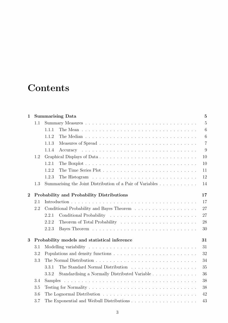
Contents
1 Summarising Data 5
1.1 Summary Measures . . . . . . . . . . . . . . . . . . . . . . . . . . . . . . . . 5
1.1.1 The Mean . . . . . . . . . . . . . . . . . . . . . . . . . . . . . . . . . 6
1.1.2 The Median . . . . . . . . . . . . . . . . . . . . . . . . . . . . . . . . 6
1.1.3 Measures of Spread . . . . . . . . . . . . . . . . . . . . . . . . . . . . 7
1.1.4 Accuracy . . . . . . . . . . . . . . . . . . . . . . . . . . . . . . . . . 9
1.2 Graphical Displays of Data . . . . . . . . . . . . . . . . . . . . . . . . . . . . 10
1.2.1 The Boxplot . . . . . . . . . . . . . . . . . . . . . . . . . . . . . . . . 10
1.2.2 The Time Series Plot . . . . . . . . . . . . . . . . . . . . . . . . . . . 11
1.2.3 The Histogram . . . . . . . . . . . . . . . . . . . . . . . . . . . . . . 12
1.3 Summarising the Joint Distribution of a Pair of Variables . . . . . . . . . . . 14
2 Probability and Probability Distributions 17
2.1 Introduction . . . . . . . . . . . . . . . . . . . . . . . . . . . . . . . . . . . . 17
2.2 Conditional Probability and Bayes Theorem . . . . . . . . . . . . . . . . . . 27
2.2.1 Conditional Probability . . . . . . . . . . . . . . . . . . . . . . . . . 27
2.2.2 Theorem of Total Probability . . . . . . . . . . . . . . . . . . . . . . 28
2.2.3 Bayes Theorem . . . . . . . . . . . . . . . . . . . . . . . . . . . . . . 30
3 Probability models and statistical inference 31
3.1 Modelling variability . . . . . . . . . . . . . . . . . . . . . . . . . . . . . . . 31
3.2 Populations and density functions . . . . . . . . . . . . . . . . . . . . . . . . 32
3.3 The Normal Distribution . . . . . . . . . . . . . . . . . . . . . . . . . . . . . 34
3.3.1 The Standard Normal Distribution . . . . . . . . . . . . . . . . . . . 35
3.3.2 Standardising a Normally Distributed Variable . . . . . . . . . . . . . 36
3.4 Samples . . . . . . . . . . . . . . . . . . . . . . . . . . . . . . . . . . . . . . 38
3.5 Testing for Normality . . . . . . . . . . . . . . . . . . . . . . . . . . . . . . . 38
3.6 The Lognormal Distribution . . . . . . . . . . . . . . . . . . . . . . . . . . . 42
3.7 The Exponential and Weibull Distributions . . . . . . . . . . . . . . . . . . . 43
3

4
3.8 Return Periods, Design Life and Reliability . . . . . . . . . . . . . . . . . . . 47
3.9 Extreme value distributions . . . . . . . . . . . . . . . . . . . . . . . . . . . 49
4 Estimation and Hypothesis Testing 53
4.1 Introduction . . . . . . . . . . . . . . . . . . . . . . . . . . . . . . . . . . . . 53
4.2 Estimating a mean . . . . . . . . . . . . . . . . . . . . . . . . . . . . . . . . 53
4.3 Confidence interval for a mean . . . . . . . . . . . . . . . . . . . . . . . . . . 56
4.4 Estimating other parameters . . . . . . . . . . . . . . . . . . . . . . . . . . . 61
4.5 Hypothesis Tests for the Mean of a Population . . . . . . . . . . . . . . . . . 63
4.6 Comparing Two Distributions . . . . . . . . . . . . . . . . . . . . . . . . . . 66
4.6.1 Case 1: The Two Sample t Test under equal variance assumption . . 67
4.6.2 Case 2: An approximate two Sample t-test when variances are unequal 67
4.6.3 The paired t Test . . . . . . . . . . . . . . . . . . . . . . . . . . . . . 69
5 Regression 71
5.1 Introduction . . . . . . . . . . . . . . . . . . . . . . . . . . . . . . . . . . . . 71
5.2 Linear Regression . . . . . . . . . . . . . . . . . . . . . . . . . . . . . . . . . 73
5.2.1 Introduction . . . . . . . . . . . . . . . . . . . . . . . . . . . . . . . . 73
5.2.2 Least squares estimation . . . . . . . . . . . . . . . . . . . . . . . . . 73
5.2.3 Confidence intervals and Hypothesis tests . . . . . . . . . . . . . . . . 75
5.2.4 Prediction . . . . . . . . . . . . . . . . . . . . . . . . . . . . . . . . . 76
5.2.5 Goodness-of-fit . . . . . . . . . . . . . . . . . . . . . . . . . . . . . . 77
5.2.6 Checking assumptions . . . . . . . . . . . . . . . . . . . . . . . . . . 79
5.2.7 Linear Regression in MINITAB . . . . . . . . . . . . . . . . . . . . . 80
5.3 Multiple Regression . . . . . . . . . . . . . . . . . . . . . . . . . . . . . . . . 82
5.4 Fitting Curves . . . . . . . . . . . . . . . . . . . . . . . . . . . . . . . . . . . 85

Chapter 1
Summarising DataIn statistical data analysis, the number of experimental or observational units (and the
number of variables) is often large. For presentation purposes, it is impractical to present
the whole data. Furthermore, the data are often not particularly informative when presented
as a complete list of observations. A better way of presenting data is to pick out the important
features using summary measures or graphical displays.
1.1 Summary Measures
The data in the file silt2.dat were collected as part of an investigation into soil variability.
Soil samples were obtained in each of 4 sites in the province of Murcia, Spain, and the
percentage of clay was determined. At each site, 11 observations were made (at random
points in a 10m×10m area). The eleven observations for each of the first four sites are
presented in the dotplot below.
.... . . .. . . .
-------+---------+---------+---------+---------+---------Site 1
: . ...: : .
-------+---------+---------+---------+---------+---------Site 2
.
. : . :. . . .
-------+---------+---------+---------+---------+---------Site 3
. .. .. . .:. .
-------+---------+---------+---------+---------+---------Site 4
28.0 35.0 42.0 49.0 56.0 63.0
Clearly there are some differences in the distributions of the observations at each of the
sites. These differences can be described in terms of the location and spread of the data.
5
6
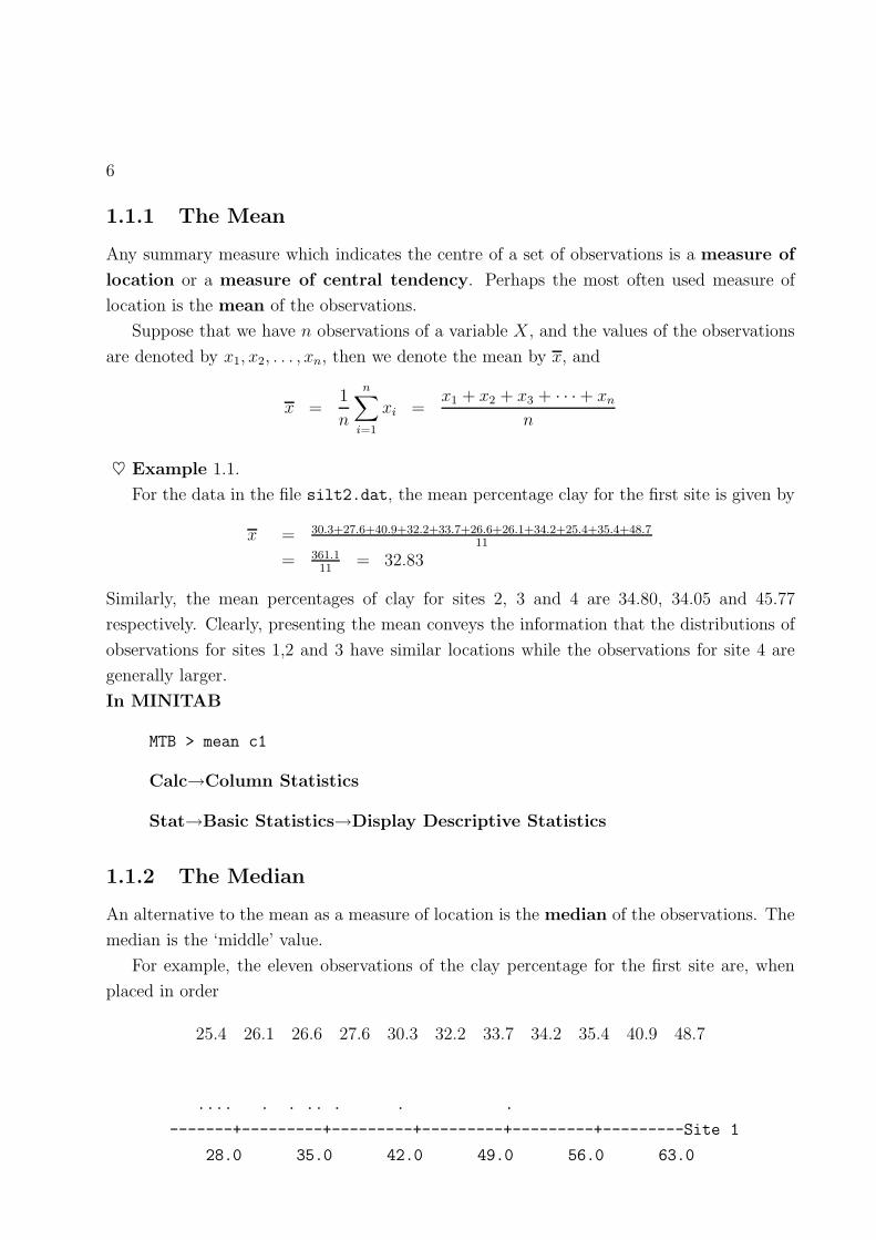
1.1.1 The Mean
Any summary measure which indicates the centre of a set of observations is a measure of
location or a measure of central tendency. Perhaps the most often used measure of
location is the mean of the observations.
Suppose that we have n observations of a variable X, and the values of the observations
are denoted by x1, x2, . . . , xn, then we denote the mean by x, and
x =1
n
n∑
i=1
xi =x1 + x2 + x3 + · · · + xn
n
♥ Example 1.1.
For the data in the file silt2.dat, the mean percentage clay for the first site is given by
x = 30.3+27.6+40.9+32.2+33.7+26.6+26.1+34.2+25.4+35.4+48.711
= 361.111
= 32.83
Similarly, the mean percentages of clay for sites 2, 3 and 4 are 34.80, 34.05 and 45.77
respectively. Clearly, presenting the mean conveys the information that the distributions of
observations for sites 1,2 and 3 have similar locations while the observations for site 4 are
generally larger.
In MINITAB
MTB > mean c1
Calc→Column Statistics
Stat→Basic Statistics→Display Descriptive Statistics
1.1.2 The Median
An alternative to the mean as a measure of location is the median of the observations. The
median is the ‘middle’ value.
For example, the eleven observations of the clay percentage for the first site are, when
placed in order
25.4 26.1 26.6 27.6 30.3 32.2 33.7 34.2 35.4 40.9 48.7
.... . . .. . . .
-------+---------+---------+---------+---------+---------Site 1
28.0 35.0 42.0 49.0 56.0 63.0

MATH2041/2042 Stats for Engineering Year: 08–09 Dr S. K. Sahu 7
Similarly, the median percentages of clay for sites 2, 3 and 4 are 35.9, 34.5 and 44.5 re-
spectively. Again, the median conveys the information that the distributions of observations
for sites 1,2 and 3 have similar locations while the observations for site 4 are generally larger.
If there are an even number of observations, then there isn’t a single ‘middle observation’
and the median is defined to be half way between the ‘middle two’ observations.
In general:
if we have an odd number of observations, then the median is the value of the n+12
th
largest.
if we have an even number of observations, then the median is the mean of (half way
between) the n2th largest and the (n
2+ 1)th largest.
In MINITAB
MTB > median c1
Calc→Column Statistics
Stat→Basic Statistics→Display Descriptive Statistics
Why use the median rather than the mean?
The mean is the summary of location which is most often calculated and quoted. However,
there are situations where the median provides a better summary of location.
The median is much less sensitive (more robust) in situations where there are a small
number of extreme observations. It is a better measure of a ‘typical observation’. (Indeed,
it often is the value of an actual observation). However, the mean has many nice ‘statistical
properties’ which we shall discuss later.
1.1.3 Measures of Spread
Any summary measure which indicates the amount of dispersion of a set of observations is
a measure of spread.
The easiest measure of spread to calculate is the range of the data, the difference between
the smallest and largest observations. For example, consider the eleven observations of the
clay percentage for the first site.

8
.... . . .. . . .
-------+---------+---------+---------+---------+---------Site 1
28.0 35.0 42.0 49.0 56.0 63.0
The range for the percentages of clay for sites 2, 3 and 4 are 11.4, 11.3 and 21.4 re-
spectively. This conveys the information that the observations for sites 2 and 3 have a very
similar spread, which is somewhat smaller to that for sites 1 or 4.
However, the range is not a very useful measure of spread, as it is extremely sensitive to
the values of the two extreme observations. Furthermore, it gives little information about
the distribution of the observations between the two extremes.
A more robust measure of spread is the interquartile range (or quartile range). This
is the difference between the lower quartile and upper quartile.
The lower and upper quartiles, together with the median, divide the observations up into
four sets of equal size.
For example, for the eleven observations of the clay percentage for the first site
.... . . .. . . .
-------+---------+---------+---------+---------+---------Site 1
28.0 35.0 42.0 49.0 56.0 63.0
In general:
the upper quartile is the value of the 34(n + 1)th largest.
the lower quartile is the value of the 14(n + 1)th largest
If n + 1 is not divisible by 4 then some interpolation is required. However, MINITAB does
this for us.
The interquartile range may be interpreted as the range in which the ‘middle half’ of the
observations lie.
For the sets of observations of clay percentages for the four sites, the interquartile ranges
are 8.8, 4.9, 6.5 and 8.7, which again illustrates the difference in spread between the obser-
vations for sites 1 and 4, and those for sites 2 and 3.
Although the range and the interquartile range are easy to calculate and interpret, they
do not have nice statistical properties. For future use, we shall define a further measure of
spread called the standard deviation.
Recall that we denote the n observations by x1, x2, . . . , xn and the mean of the sample
by x. Then for each observation xi, i = 1, 2, . . . , n, xi − x is the difference between that
observation and the mean.
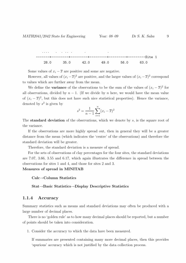
MATH2041/2042 Stats for Engineering Year: 08–09 Dr S. K. Sahu 9
.... . . .. . . .
-------+---------+---------+---------+---------+---------Site 1
28.0 35.0 42.0 49.0 56.0 63.0
Some values of xi − x are positive and some are negative.
However, all values of (xi −x)2 are positive, and the larger values of (xi −x)2 correspond
to values which are further away from the mean.
We define the variance of the observations to be the sum of the values of (xi − x)2 for
all observations, divided by n − 1. (If we divide by n here, we would have the mean value
of (xi − x)2, but this does not have such nice statistical properties). Hence the variance,
denoted by s2 is given by
s2 =1
n − 1
n∑
i=1
(xi − x)2
The standard deviation of the observations, which we denote by s, is the square root of
the variance.
If the observations are more highly spread out, then in general they will be a greater
distance from the mean (which indicates the ‘centre’ of the observations) and therefore the
standard deviation will be greater.
Therefore, the standard deviation is a measure of spread.
For the sets of observations of clay percentages for the four sites, the standard deviations
are 7.07, 3.66, 3.55 and 6.17, which again illustrates the difference in spread between the
observations for sites 1 and 4, and those for sites 2 and 3.
Measures of spread in MINITAB
Calc→Column Statistics
Stat→Basic Statistics→Display Descriptive Statistics
1.1.4 Accuracy
Summary statistics such as means and standard deviations may often be produced with a
large number of decimal places.
There is no ‘golden rule’ as to how many decimal places should be reported, but a number
of points should be taken into consideration.
1. Consider the accuracy to which the data have been measured.
If summaries are presented containing many more decimal places, then this provides
‘spurious’ accuracy which is not justified by the data collection process.
10
If summaries are presented containing many fewer decimal places, then important
information may be lost.
2. For continuous data, consider the variability of the data.
For example, if all the observations are the same up to and including the first decimal
place, with variability occuring in the second decimal place and beyond, then clearly
at least two, and probably more decimal places, are required.
3. For discrete data, there is no need for summaries to be reported on the same scale as
the data.
For example, it is perfectly reasonable that the mean of a set of counts may not be a
whole number.
4. Do not truncate trailing zeros.
Once you have decided on a certain number of decimal places to report, then report
them all, even if the last one is a zero. Otherwise you are throwing away information.
1.2 Graphical Displays of Data
Often, a simple graphical display provides a more easily interpretable summary of the dis-
tribution of the observations than a collection of summary statistics.
One graphical display, which is easy to construct, and incorporates many of the fea-
tures of the summary measures introduced in §1.1 is the box-and-whisker plot (or simply
boxplot).
1.2.1 The Boxplot
We will illustrate this using data in the file quake.dat which represent the time in days
between successive serious earthquakes worldwide, between 16th December 1902 and 4th
March 1977.
Constructing a boxplot involves the following steps:
1. Draw a vertical (or horizontal) axis representing the interval scale on which the obser-
vations are made.
2. Calculate the median, and upper and lower quartiles (Q1, Q3) as described in §1.1.
Calculate the interquartile range (or ‘midspread’) H = Q3 − Q1.
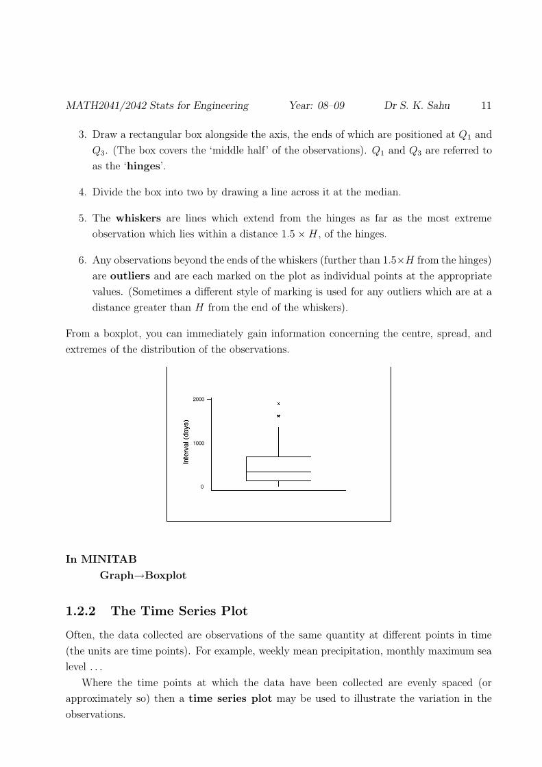
MATH2041/2042 Stats for Engineering Year: 08–09 Dr S. K. Sahu 11
3. Draw a rectangular box alongside the axis, the ends of which are positioned at Q1 and
Q3. (The box covers the ‘middle half’ of the observations). Q1 and Q3 are referred to
as the ‘hinges’.
4. Divide the box into two by drawing a line across it at the median.
5. The whiskers are lines which extend from the hinges as far as the most extreme
observation which lies within a distance 1.5 × H, of the hinges.
6. Any observations beyond the ends of the whiskers (further than 1.5×H from the hinges)
are outliers and are each marked on the plot as individual points at the appropriate
values. (Sometimes a different style of marking is used for any outliers which are at a
distance greater than H from the end of the whiskers).
From a boxplot, you can immediately gain information concerning the centre, spread, and
extremes of the distribution of the observations.
2000
1000
0
In MINITAB
Graph→Boxplot
1.2.2 The Time Series Plot
Often, the data collected are observations of the same quantity at different points in time
(the units are time points). For example, weekly mean precipitation, monthly maximum sea
level . . .
Where the time points at which the data have been collected are evenly spaced (or
approximately so) then a time series plot may be used to illustrate the variation in the
observations.

12
A time series plot is simply a plot of each observation xi, i = 1, 2, . . . , n on the y-axis
against its index i on the x-axis, in other words a plot of the points (i, xi), i = 1, 2, . . . , n.
Consecutive points are joined together to illustrate the way in which the observations
vary over time.
For example, the data in the file flow.dat represent the mean monthly flow (in cms) of
the Fraser River at Hope, B.C., Canada between January 1981 and December 1990.
1990198919881987198619851984198319821981
9000
800070006000
50004000
30002000
10000
Year (June)
In MINITAB
Graph→Time Series Plot
Time series plots may be used to detect trend or seasonal behaviour (or both).
Note that in many practical examples, there is no natural time ordering of the observa-
tions (for example, observations where the units are individuals). In such examples, time
series plots are meaningless.
1.2.3 The Histogram
Histograms have the following properties.
1. The horizontal axis represents the scale on which the observations are measured, and
the bars of the histogram adjoin each other with the boundaries between bars repre-
senting the boundaries between the categories.
2. If bars are not of equal width, then care must be taken when determining the height
of each bar (particularly with MINITAB ) to ensure that the area of each bar is
proportional to the number of observations in each category.
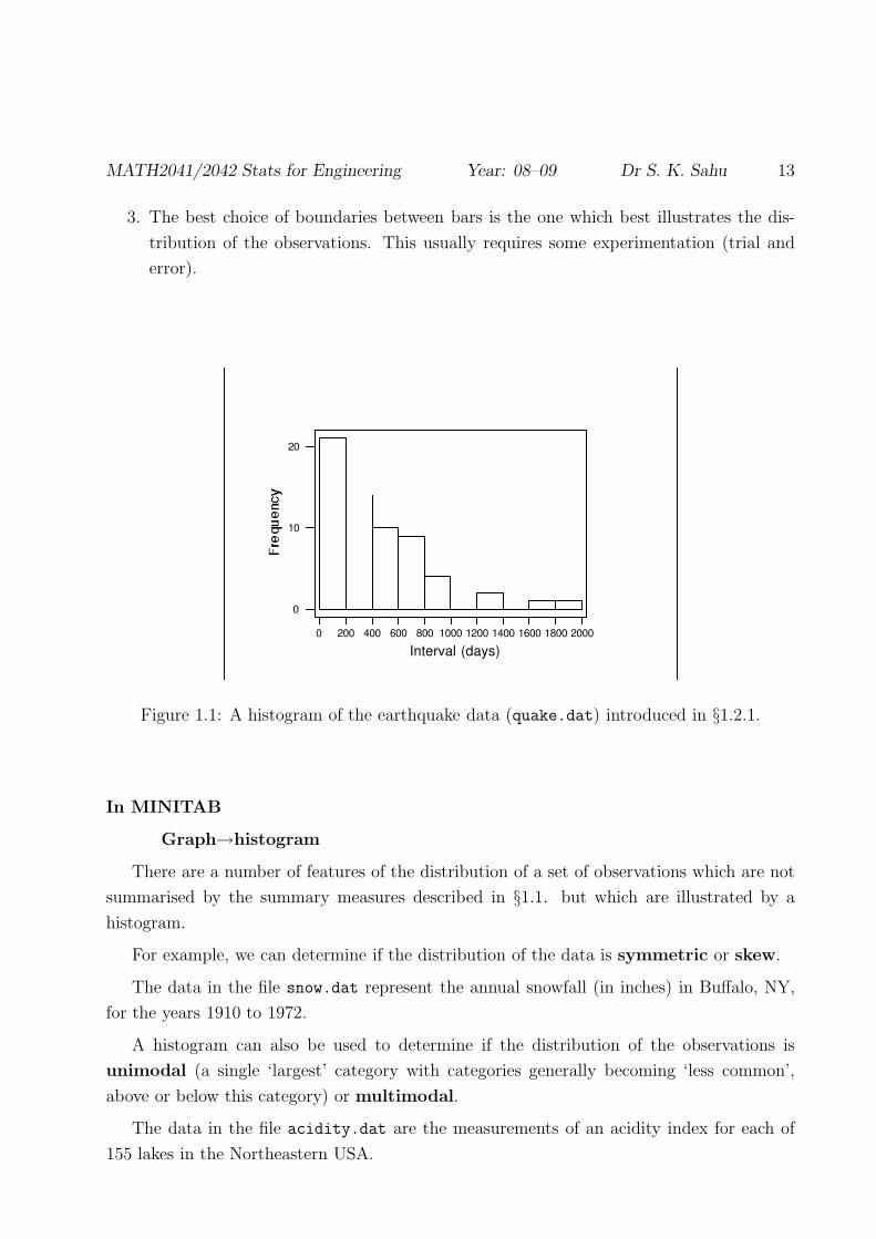
MATH2041/2042 Stats for Engineering Year: 08–09 Dr S. K. Sahu 13
3. The best choice of boundaries between bars is the one which best illustrates the dis-
tribution of the observations. This usually requires some experimentation (trial and
error).
2000180016001400120010008006004002000
20
10
0
Interval (days)
Figure 1.1: A histogram of the earthquake data (quake.dat) introduced in §1.2.1.
In MINITAB
Graph→histogram
There are a number of features of the distribution of a set of observations which are not
summarised by the summary measures described in §1.1. but which are illustrated by a
histogram.
For example, we can determine if the distribution of the data is symmetric or skew.
The data in the file snow.dat represent the annual snowfall (in inches) in Buffalo, NY,
for the years 1910 to 1972.
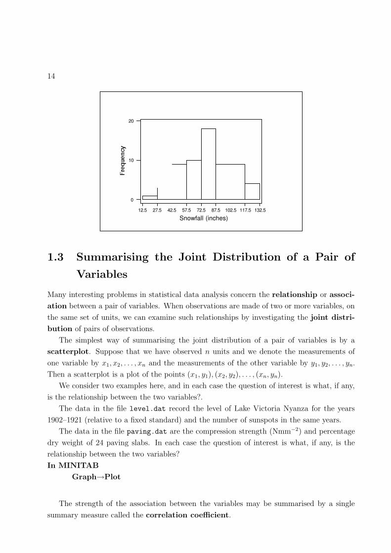
A histogram can also be used to determine if the distribution of the observations is
unimodal (a single ‘largest’ category with categories generally becoming ‘less common’,
above or below this category) or multimodal.
The data in the file acidity.dat are the measurements of an acidity index for each of
155 lakes in the Northeastern USA.
14
132.5117.5102.587.572.557.542.527.512.5
20
10
0
Snowfall (inches)
1.3 Summarising the Joint Distribution of a Pair of
Variables
Many interesting problems in statistical data analysis concern the relationship or associ-
ation between a pair of variables. When observations are made of two or more variables, on
the same set of units, we can examine such relationships by investigating the joint distri-
bution of pairs of observations.
The simplest way of summarising the joint distribution of a pair of variables is by a
scatterplot. Suppose that we have observed n units and we denote the measurements of
one variable by x1, x2, . . . , xn and the measurements of the other variable by y1, y2, . . . , yn.
Then a scatterplot is a plot of the points (x1, y1), (x2, y2), . . . , (xn, yn).
We consider two examples here, and in each case the question of interest is what, if any,
is the relationship between the two variables?.
The data in the file level.dat record the level of Lake Victoria Nyanza for the years
1902–1921 (relative to a fixed standard) and the number of sunspots in the same years.
The data in the file paving.dat are the compression strength (Nmm−2) and percentage
dry weight of 24 paving slabs. In each case the question of interest is what, if any, is the
relationship between the two variables?
In MINITAB
Graph→Plot
The strength of the association between the variables may be summarised by a single
summary measure called the correlation coefficient.

MATH2041/2042 Stats for Engineering Year: 08–09 Dr S. K. Sahu 15
7.06.56.05.55.04.54.03.53.0
40
30
20
10
0
Acidity
To calculate the correlation coefficient, we first need to calculate the mean and standard
deviation of the observations x1, x2, . . . , xn of the first variable (call these x and sx), and the
mean and standard deviation of the observations y1, y2, . . . , yn of the second variable (call
these y and sy). The correlation coefficient (denoted by r) is given by
r =1
n − 1
n∑
i=1
(xi − x)(yi − y)
sxsy.
The correlation coefficient, which must lie between −1 and 1, measures the strength of
the linear (straight line) relationship between the variables. It determines to what extent
values of one variable increase as values of the other variable increase, and how close this
relationship is to being a perfect straight line.
Hence, the correlation coefficient provides a measure of the extent of linear association.
For example, the correlation coefficients for the two examples illustrated by scatterplots on
the previous page are 0.526 between ‘strength’ and ‘dry weight’ and 0.879 between ‘lake
level’ and ‘number of sunspots’. Therefore, both data sets show positive linear association,
stronger between lake level and number of sunspots.
In MINITAB
Stat→Basic Statistics→Correlation

16
21201918171615
80
70
60
50
40
30
Percentage dry weight

Chapter 2
Probability and Probability
Distributions
2.1 Introduction
Most of us have an idea about probability from games of chance, from the lottery and from
general statements about the likelihood of a particular event occurring. The probability of it
raining in Southampton tomorrow might be given or the chance that a particular team will
win a given match. It will be necessary to clarify ideas about probability a little in order to
tackle the kind of problems that we shall meet later, but you will not be required to delve
very deeply into the theory of probability.
Firstly, we shall identify a probability of zero with some event which cannot happen and
a probability of unity for something which is certain to occur. All other probabilities will be
between zero and one and will reflect the “chance” of an event occurring. For a repeatable
event, the probability may be interpreted as the proportion of times the event will occur in
the “long run”. For other kinds of event, probability may be interpreted as a measure of
subjective belief reflecting the likelihood of the event occuring.
In this chapter, we consider tightly controlled situations, where it is possible to calculate
probabilities precisely. More generally, we cannot know probabilities precisely, but we can
use observed data to learn about probabilities – this is statistical inference and is the subject
of later chapters.
For example, suppose that electronic resistors of a similar appearance are either 5 ohms
or 10 ohms, and we put 100 of the 5 ohm resistors in a box together with 50 of the 10 ohm
resistors. A resistor is then chosen from the box. What is the probability that it is a 5 ohm
resistor?
It is not immediately possible to answer this question since we are not told enough about
17

18
the conduct of the experiment. If we are told that the 150 resistors are shaken up in the
box and that the resistor is chosen “at random” from the box, then we can argue that each
of the resistors has an equal probability of being selected. Since there are now 150 resistors
in total and they are all equally likely to be chosen, the probability that a 5 ohm resistor is
chosen will be given by 100/150 = 2/3. Thus the probability of choosing a 5 ohm resistor is
formally given by
P (5 ohm resistor being chosen) =Number of 5 ohm resistors in the box
Total number of resistors in the box=
2
3
Similarly, P (10 ohm resistor being chosen)= 50/150 = 1/3
Suppose now we take out a second resistor at random from those left in the box. What
is the probability of getting two 5 ohm resistors?
To answer this, consider the experiment in two stages.
(a) Select the first resistor. The probability of a 5 ohm resistor is 2/3.
(b) Now, assuming that a 5 ohm resistor has been selected, choose the second resistor.
There are only 149 resistors left and 99 of them are 5 ohm resistors, so the probability
of a 5 ohm resistor being selected is 99/149.
The probability of getting two 5 ohm resistors is now given by
2
3× 99
149=
66
149= 0.443.
Similarly, the probability of two 10 ohm resistors is
1
3× 49
149=
49
447= 0.110.
The other possibility is that we choose one 5 ohm and one 10 ohm resistor. The probability
of this is slightly more involved since we could choose the 5 ohm first and then the 10 ohm
resistor or the 10 ohm first and then the 5 ohm resistor. The probability is given by(
2
3× 50
149
)
+
(
1
3× 100
149
)
=200
447= 0.447.
Note that 0.443 + 0.110 + 0.447 = 1, i.e. P (two 5 ohm) + P (two 10 ohm) + P (one of each)
= 1. Since these are the only possible outcomes, the probabilities must sum to 1.
The above example illustrates sampling without replacement, in that the first selected
resistor was not replaced in the box before the second was selected.
If we had decided to replace the first resistor, whatever its resistance, before selecting the
second, then the probabilities of two 5 ohm, two 10 ohm or one of each would be given by
P (two 5 ohm) = 23× 2
3= 4
9= 0.444
P (two 10 ohm) = 13× 1
3= 1
9= 0.111
P (one of each) =(
23× 1
3
)
+(
13× 2
3
)
= 49
= 0.444.

MATH2041/2042 Stats for Engineering Year: 08–09 Dr S. K. Sahu 19
These probabilities for the with replacement scheme are slightly different but, as before,
these three situations include all possibilities so the three probabilities must sum to 1.
Notice that we have multiplied probabilities together where considering events occurring
together, such as choosing a 5 ohm resistor on the first selection and a 5 ohm on the second
selection. We have added together probabilities when a situation could arise in two different
ways, such as “one of each” could be obtained either as a 5 ohm selected first and a 10 ohm
second or a 10 ohm selected first and a 5 ohm resistor selected second.
S
A B
More generally, if we have events A and B, then
P (A or B) = P (A ∪ B) = P (A) + P (B) − P (A and B)
and
P (A and B) = P (A ∩ B) = P (A) × P (B given that A has occured).
If the occurence, or otherwise, of A does not affect the probability of B, then we say that A
and B are independent events, and we can write P (B given that A has occured) = P (B).
In this case
P (A and B) = P (A ∩ B) = P (A) × P (B).
These simple multiplication and addition rules for probabilities are very important for
most problems. The rest of this Section is devoted to a series of examples illustrating the
calculation of probabilities using these rules. We shall consider conditional probability in
more detail in Section 2.2.
♥ Example 2.1. Ten items are available and 4 are defective and 6 are satisfactory. A
random sample of 3 items is taken from these 10, what is the probability that exactly one is
defective?
One way to tackle a problem like this is to construct a probability tree diagram to see
what is going on. Consider selecting one item at a time until all three are selected and
illustrate the results and the associated probabilities in each case. (D = defective, S =
satisfactory).
So the probability for DDD will be: 410× 3
9× 2
8= 1
30. All the remaining probabilities can
be found similarly.

20
D
S
D
D
S
S
D
S
D
S
D
S
D
S
4/10
6/10
3/9
6/9
5/9
4/9
2/8
6/8
3/8
4/8
5/8
5/8
3/8
4/8
DDD
DDS
DSD
DSS
SDD
SDS
SSD
SSS
There are eight possible sequences with the probabilities as given in the table above.
Note that the sequences DSS, SDS and SSD all have one defective, so the probability of
obtaining one defective is given by(
4
10× 6
9× 5
8
)
+
(
6
10× 4
9× 5
8
)
+
(
6
10× 5
9× 4
8
)
= 3 × 6 × 5 × 4
10 × 9 × 8=
1
2
Similarly, the probability of two defectives is
P (DDS) + P (DSD) + P (SDD) =(
410
× 39× 6
8
)
+(
410
× 69× 3
8
)
+(
610
× 49× 3
8
)
= 3 × 6×4×310×9×8
= 310
,
the probability of no defectives is
P (SSS) =6
10× 5
9× 4
8=
1
6
and the probability of three defectives is
P (DDD) =4
10× 3
9× 2
8=
1
30.
Note that these four probabilities must sum to 1, i.e.
P (0 defectives) +P (1 defective) +P (2 defectives)+ P (3 defectives) =1
6+
1
2+
3
10+
1
30= 1.

MATH2041/2042 Stats for Engineering Year: 08–09 Dr S. K. Sahu 21
In fact, we can calculate these probabilities without constructing a probability tree dia-
gram. To do this, we need to know something about combinations.
Suppose that we have n items from which we select r without replacement. The order in
which the items are selected does not matter, just which r items comprise the final selection.
We denote by(
nr
)
the number of such distinct combinations of r items which can be selected.
It can be shown that(
n
r
)
=n!
r!(n − r)!=
n × (n − 1) × · · · × (n − r + 1)
1 × 2 × · · · × r
where a! (“a factorial”) is defined to be a! = a × (a − 1)× (a − 2)× · · · × 3 × 2 × 1. Hence,
in particular(
n1
)
= n(
n2
)
= n(n−1)2
(
n3
)
= n(n−1)(n−2)6
.
As we have a total of 10 items, 4 defective and 6 satisfactory. The number of possible ways
of selecting 3 items from 10 is
(
10
3
)
=10 × 9 × 8
6= 120
In order to get one defective and two satisfactory in the sample, the defective must be
selected from one of the four defectives and the two satisfactory ones from the six which
are satisfactory. Therefore, the number of different selections of one defective and two
satisfactory is(
4
1
)
×(
6
2
)
= 4 × 6 × 5
2= 60
Therefore, the probability of choosing one defective in the sample of three is
P (one defective) =Number of ways of choosing 1 defective and 2 satisfactory
Number of ways of choosing 3 items
=(41)×(6
2)(10
3 )
= 60120
= 12.
Similarly
P (two defectives) =(42)×(6
1)(10
3 )
= 6×6120
= 310
.
Either method will produce the answer, but the tree-diagram method can get a bit cumber-
some with larger problems.

22
♥ Example 2.2. The National Lottery In the National Lottery, the winning ticket
has six numbers from 1 to 49 exactly matching those on the balls drawn on a Wednesday
or Saturday evening. The ‘experiment’ consists of drawing the balls. The ‘randomness’, the
equal probability of any set of six numbers being drawn, is ensured by the Lottery machine,
which mixes the balls during the selection process.
The probability associated with the winning selection is given by
P (Jackpot) =Number of winning selections
Number of possible selections
The total number of possible selections is given by
(
49
6
)
=49 × 48 × 47 × 46 × 45 × 44
1 × 2 × 3 × 4 × 5 × 6= 13 983 816
(i.e. nearly 14 million). Since there is only one winning selection, the probability of matching
the jackpot sequence is 1/13 983 816 = 0.0000000715.
Other prizes are given for fewer matches. The corresponding probabilities can be evalu-
ated as follows:
P (5 matches) = Number of selections with 5 matchesNumber of possible selections
=(65)×(43
1 )(49
6 )
=6!
5!1!× 43!
1!42!
13 983 816
= 6×4313 983 816
= 0.00001845
≈ 154 200
Similarly,
P (4 matches) =(64)×(43
2 )(49
6 )
= 15×90313 983 816
= 0.0009686
≈ 11 032
P (3 matches) =(63)×(43
3 )(49
6 )
= 20×12 34113 983 816
= 0.01765
≈ 157
There is one other way of winning, using the bonus ball. Matching five of the selected
six balls plus matching the bonus ball gives a share in a prize substantially less than the

MATH2041/2042 Stats for Engineering Year: 08–09 Dr S. K. Sahu 23
jackpot. The probability of this is given by
P (Matching 5 and the bonus ball) =Number of selections of this type
Number of possible selections= 6
(496 )
= 0.000000429
≈ 12 331 000
Adding all these probabilities of winning some kind of prize together gives
P (Winning) = 0.0188 ≈ 1
53
so that a player buying one ticket each week would expect to win a prize about once a year.
Without further information, it is not possible to work out the expected return on this kind
of investment since this involves the amounts of the prizes as well as the probabilities of
winning. In the National Lottery, the prize money, (except for the $10 prize), depends on
the number of winners and the number of tickets sold.
One of the most common applications of probability calculations in Engineering is in
evaluating reliability. The remaining examples focus on this area.
♥ Example 2.3. If a communications satellite is to be launched and positioned in space
to receive and transmit telephone and data transmissions, various stages of the process are
said to succeed or fail with certain probabilities. For example, it may be that the launch will
be successful with a probability of 0.9. The reliability, which is the probability that it works,
is therefore 0.9 or 90%. Obviously, the probability that the launch will fail is 1 − 0.9 = 0.1.
Suppose such a satellite has a successful launch with a probability of 0.9 and after launch,
the satellite is to be positioned in a suitable orbit with a probability of 0.8. Small retro-
rockets on the satellite can then be used to adjust the position, if this is not initially correct,
and the probability of success here is 0.5. Once in position, the solar powered batteries are
expected to last at least a year with probability 0.7. What is the probability that a satellite
due to be launched will still be working in a year’s time?
In order to work out this probability, it is necessary to assume that all the different ways
of failing are acting independently of each other. This might not be so, of course. if the
batteries were used to power the retro-rockets. A simple tree-diagram helps here.
Let L represent a successful launch and L represent a failure, with P, R and B representing
successful position, retro-rocket adjustment and battery life, respectively.
The probability of overall success is given by
(0.9 × 0.8 × 0.7) + (0.9 × 0.2 × 0.5 × 0.7) = 0.504 + 0.063
= 0.567.
The overall reliability is 56.7%.
24
L
L
P
P
B
B
R
0.9
0.1
0.8
0.2
0.7
0.3
0.5
0.5
B
B
0.7
0.3
R
Overall success
Overall success
Note that whenever a system is affected by a series of different reasons for failure, the
overall reliability of the system is reduced. Another example of this follows.
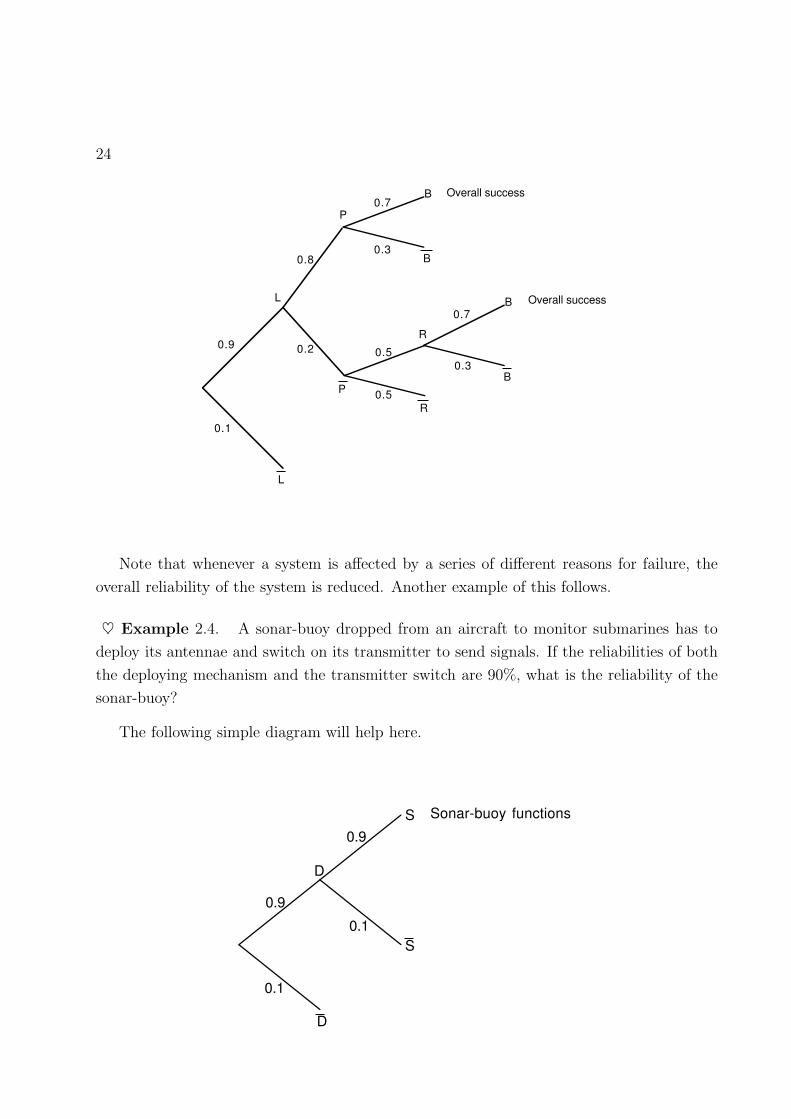
♥ Example 2.4. A sonar-buoy dropped from an aircraft to monitor submarines has to
deploy its antennae and switch on its transmitter to send signals. If the reliabilities of both
the deploying mechanism and the transmitter switch are 90%, what is the reliability of the
sonar-buoy?
The following simple diagram will help here.
0.9
0.1
0.1
0.9
D
S
S
D
Sonar-buoy functions

MATH2041/2042 Stats for Engineering Year: 08–09 Dr S. K. Sahu 25
P (sonar-buoy functions) = P (deploys antennae) × P (switch works)
= 0.9 × 0.9
= 0.81
Therefore the reliability of sonar-buoy is 81%. Although 9 out of 10 of the deploying
mechanisms work and 9 out of 10 of the switches work, only 4 out of 5 sonar-buoys work.
To achieve a 90% reliability for the buoys, we need to have individual reliabilities of√0.9 = 0.9487 for the switches and deployment mechanisms.
The more components which are required to function to make a system work, the lower
the overall reliability. For example, a set of four elements, each with reliability 90%, produces
a system with reliability 0.94 = 65.6%.
Standby redundancy can be used to improve the reliability of a system. It is common
practice, when high reliability is required to introduce parallel systems which ‘cut-in’ if the
initial system fails. Some aircraft systems can have as many as three parallel systems, any
one of which would be sufficient to fly the plane safely.
♥ Example 2.5. Suppose a system consists of two independent switches S1 and S2, each
with reliability 90% and is arranged so that the system operates if either of the switches, S1
or S2, operates. What is the reliability of this system?
This can be represented as below.
S1
A B
S2
This diagram indicates that the system operates if there is a link from A to B created by
the switches operating. The system operates if either or both of the switches are operating.
In other words, the system fails only if both switches fail.
P (system fails) = P (switch S1 fails) × P (switch S2 fails)
= 0.1 × 0.1
= 0.01
Therefore, the reliability of the system is 99%.
By introducing a ‘spare’ switch, the reliability has increased from 90% to 99%, a sub-
stantial gain for the potentially small cost of an extra switch.
26
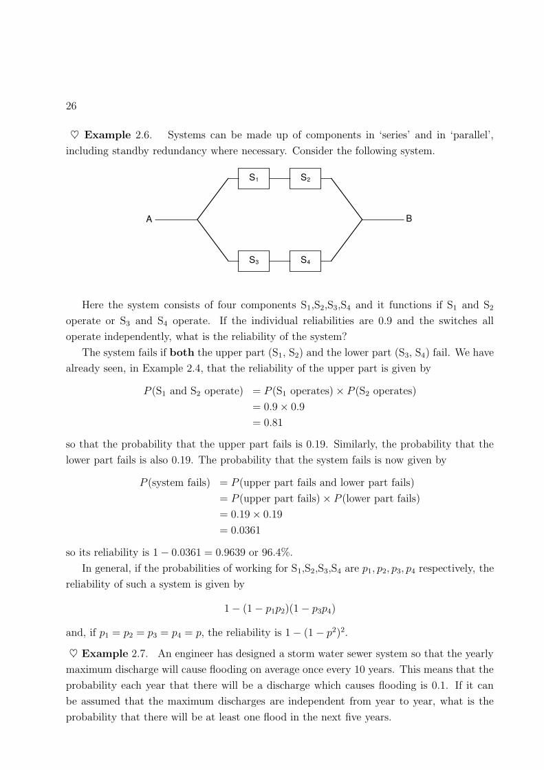
♥ Example 2.6. Systems can be made up of components in ‘series’ and in ‘parallel’,
including standby redundancy where necessary. Consider the following system.
S1
A B
S2
S4S3
Here the system consists of four components S1,S2,S3,S4 and it functions if S1 and S2
operate or S3 and S4 operate. If the individual reliabilities are 0.9 and the switches all
operate independently, what is the reliability of the system?
The system fails if both the upper part (S1, S2) and the lower part (S3, S4) fail. We have
already seen, in Example 2.4, that the reliability of the upper part is given by
P (S1 and S2 operate) = P (S1 operates) × P (S2 operates)
= 0.9 × 0.9
= 0.81
so that the probability that the upper part fails is 0.19. Similarly, the probability that the
lower part fails is also 0.19. The probability that the system fails is now given by
P (system fails) = P (upper part fails and lower part fails)
= P (upper part fails) × P (lower part fails)
= 0.19 × 0.19
= 0.0361
so its reliability is 1 − 0.0361 = 0.9639 or 96.4%.
In general, if the probabilities of working for S1,S2,S3,S4 are p1, p2, p3, p4 respectively, the
reliability of such a system is given by
1 − (1 − p1p2)(1 − p3p4)
and, if p1 = p2 = p3 = p4 = p, the reliability is 1 − (1 − p2)2.
♥ Example 2.7. An engineer has designed a storm water sewer system so that the yearly
maximum discharge will cause flooding on average once every 10 years. This means that the
probability each year that there will be a discharge which causes flooding is 0.1. If it can
be assumed that the maximum discharges are independent from year to year, what is the
probability that there will be at least one flood in the next five years.
MATH2041/2042 Stats for Engineering Year: 08–09 Dr S. K. Sahu 27
Whenever we require “the probability of at least one”, it is simpler to determine “the
probability of none” and then subtract this from 1. In this case, the probability of no flood
in any particular year is 1 − 0.1 = 0.9, so that the probability of no flood in 5 years is
P (No flood in 5 years) = P (No flood in year 1 and no flood in year 2 and · · ·· · · and no flood in year 5)
= P (No flood in year 1) × P (No flood in year 2) × · · ·· · · × P (No flood in year 5)
= 0.9 × 0.9 × 0.9 × 0.9 × 0.9 = 0.95 = 0.59
and therefore
P (At least one flood in 5 years) = 1 − 0.59 = 0.41
Although the sewer system has been designed to withstand a flood which occurs on
average once every 10 years, the probability that this will occur within the next 5 years is
just over 0.4.
The ideas of design life, reliability and return period will be covered in more detail
in a later chapter.
2.2 Conditional Probability and Bayes Theorem
2.2.1 Conditional Probability
The probability of an event B occurring when it is known that some event A has already
occurred is called a conditional probability and it is denoted by P (B|A). The symbol
P (B|A) is usually read as “the probability that B occurs given that A has already occurred’,
or simply, the probability of B given A.
The formula for finding the conditional probability is:
P (B|A) =P (A ∩ B)
P (A), provided P (A) > 0. (2.1)
♥ Example 2.8. The probability that a plane departs on time is P (D) = 0.83; the
probability that it arrives on time is P (A) = 0.82; and the probability that it arrives and
departs on time is P (D ∩ A) = 0.78.
The probability that a plane departed on time given that it arrived on time is:
P (D|A) =P (D ∩ A)
P (A)=
0.78
0.82= 0.95.
The probability that a plane arrives on time given that it departed on time is:
P (A|D) =P (D ∩ A)
P (D)=
0.78
0.83= 0.94.

28
2.2.2 Theorem of Total Probability
Two events B1 and B2 are called mutually exclusive if they cannot occur simultaneously.
For example, let B1 denote the event that head turns up and B2 denote the event that tail
turns up when a coin is tossed. Here P (B1 ∩ B2) = 0.
Sometimes we partition (i.e. divide) the sample space by mutually exclusive events. Often
a set of such events covering the entire sample space, called a set of exhaustive events,
are considered. For example, suppose that B1, . . . , Bk denote a set of mutually exclusive
and exhaustive events. So B1 ∪ B2 ∪ · · · ∪ Bk = S where S is the sample space. In the coin
tossing example, B1 and B2 provide a set of mutually exclusive and exhaustive events.PSfrag replacements
B1
B2
B3
B4
B5 B6
B7
To find the probability of another event A (other than the B1, . . . , Bk), intuition suggests
that we can find the intersection probability of A with each of B1, . . . , Bk and add them up.
The theorem of total probability is exactly that and is as follows:
If the events B1, . . . , Bk form a partition of the sample space such that P (Bi) 6= 0, i =
1, . . . , k, then for any event A in the sample space S:
P (A) =
k∑
i=1
P (Bi ∩ A).
However, using the definition of conditional probability in (2.1) we have:
P (Bi ∩ A) = P (Bi)P (A|Bi).
Hence we have:
P (A) =
k∑
i=1
P (Bi ∩ A) =
k∑
i=1
P (Bi)P (A|Bi).PSfrag replacements
B1
B2
B3
B4
B5 B6
B7
A

MATH2041/2042 Stats for Engineering Year: 08–09 Dr S. K. Sahu 29
♥ Example 2.9. In a certain assembly plant, three machines B1, B2, and B3 make 30%,
45%, and 25%, respectively of the products. It is known from past experience that 2%, 3%
and 2% of the products made by each machine, respectively, are defective. Now suppose
that a finished product is randomly selected. What is the probability that it is defective?
Consider the following events:
A: the product is defective,
B1: the product is made by machine B1,
B2: the product is made by machine B2,
B3: the product is made by machine B3,
Using the theorem of total probability:
P (A) = P (B1)P (A|B1) + P (B2)P (A|B2) + P (B3)P (A|B3).
0.30
0.020.006
0.45 0.03 0.0135
0.25
0.020.005
But we have:P (B1) = 0.30, P (A|B1) = 0.02
P (B2) = 0.45, P (A|B1) = 0.03
P (B3) = 0.25, P (A|B3) = 0.02
HenceP (B1) P (A|B1) = (0.30)(0.02) = 0.006
P (B2) P (A|B2) = (0.45)(0.03) = 0.0135
P (B3) P (A|B3) = (0.25)(0.02) = 0.005.
and hence:
P (A) = 0.006 + 0.00135 + 0.0005 = 0.0245.
If instead, we wanted to find the inverse probability that P (B1|A), i.e. the probability
that a randomly selected product was made by machine B1 given that it is defective? We
apply the Bayes theorem to find the inverse probability.

30
2.2.3 Bayes Theorem
Let B1, B2, . . . , Bk be a set of mutually exclusive and exhaustive events. For any new event
A,
P (Br|A) =P (Br ∩ A)
P (A)=
P (A|Br)P (Br)∑k
i=1 P (A|Bi)P (Bi), r = 1, . . . , k. (2.2)
♥ Example 2.10. For the above example with three machines:
P (B1|A) =P (B1)P (A|B1)
P (A)=
(0.30)(0.02)
0.0245= 0.2449.
So, although there was a 30% chance that a randomly selected product was made by machine
B1, the probability that a randomly selected product was made by machine B1 given that the
product was defective reduces to 24.49%. This is to be expected since machine B1 produces
less defective products than some others.
If, instead, we suppose that machine B1 produces 5% defective items. Then
P (A) = (0.30)(0.05) + 0.00135 + 0.0005 = 0.01685, and
P (B1|A) =P (B1)P (A|B1)
P (A)=
(0.30)(0.05)
0.01685= 0.471.
Here the probability that a randomly selected product was made by machine B1 given that
the product was defective increases to 47.10%.
P (B1) and P (B1|A) are called the prior and posterior probability, respectively.
♥ Example 2.11. Consider a disease that is thought to occur in 1% of the population.
Using a particular blood test a physician observes that out of the patients with disease 98%
possess a particular symptom. Also assume that 0.1% of the population without the disease
have the same symptom. A randomly chosen person from the population is blood tested and
is shown to have the symptom. What is the conditional probability that the person has the
disease?
Let B1 be the event that a randomly chosen person has the disease and B2 is the com-
plement of B1. Let A be the event that a randomly chosen person has the symptom. The
problem is to determine P (B1|A).
We have P (B1) = 0.01 since 1% of the population has the disease, and P (A|B1) = 0.98.
Also P (B2) = 0.99 and P (A|B2) = 0.001. Now
P (disease | symptom) = P (B1|A) = P (A|B1) P (B1)P (A|B1) P (B1)+P (A|B2) P (B2)
= 0.98×0.010.98×0.01+0.001×0.99
= 0.9082.
So the unconditional probability of disease, P (B1) = 0.01 = 1%, has increased to 90.82%
when the symptom is present, P (B1|A).
Chapter 3
Probability models and statistical
inference
3.1 Modelling variability
Just as we use mathematical models for deterministic physical and environmental processes,
so we use mathematical models for physical and environmental processes or systems which
display variability or randomness. Models allow us to calculate probabilities of the process
being in a particular state, or of a particular output of the process being observed. We call
these models probability models or stochastic models.
Chapter 2 contained several examples of probability models for variable physical systems.
We do not expect probability models to be true, in the sense that, many of the processes
we model are not truly random – the outputs are the results of many small innovations,
mostly unobserved, which combine in an unknown way to produce the output. The proba-
bility model is an approximation which replaces our ignorance about the innovations, and
the mechanism by which they produce the output, by a random process.
Typically probability models depend on a number of parameters. In Example 2.4 of
Chapter 2, the model had two parameters, the probability of successful deployment of the
antennae and the probability of correct operation of the transmitter switch. In Chapter 2, we
assumed that these parameters were known. However, it is more usual, when we construct a
probability model for a process, that the parameters of the process are not known precisely.
When a probability model contains unknown parameters, then we need to try to find out
about the parameters. This is achieved by making observations of the outputs of the process,
or of parts of the process. For example, we might test a number of transmitter switches and
estimate the probability of correct operation of a transmitter switch by the proportion of
switches in our test sample which operate correctly. We might also use sample data to
31

32
validate our model. In Example 2.4 of Chapter 2 we assumed that successful deployment of
the antennae was independent of correct operation of the transmitter switch. We might use
sample data to determine whether this is a reasonable assumption, or whether our model
needs to be modified.
This process, using sample data to learn about a probability model, is called statistical
inference. The subject of Statistics concerns how we should use sample data to learn about
probability models.
Perhaps the most straightforward probability model, but nevertheless one of the most
widely applicable is where our interest is focussed on a single variable. The remainder of
this chapter is devoted to models for this situation.
3.2 Populations and density functions
When we talk about a population in Statistics, we mean the totality of the observations
obtainable from all units possessing some common characteristics. Therefore, a population
is not a set of objects or individuals but a set of possible values of a variable. Populations
may be finite, when there are a maximum number of possible observations which can ever
be made; or infinite, when no such upper bound exists.
Occasionally, for a finite population, the data collected consist of the entire population.
Such a data set is called a census. When the data comprise the entire population, then
statistical data analysis merely involves presentation and summary of the data,
using methods such as those discussed in Chapter 1.
Populations consist of observations (or potential observations) of variables, and we
construct statistical models for the process of making observations from the population.
A statistical model for a population takes the form of a probability distribution. The
probability distribution tells us how likely we are to observe the various possible observations
of the variable concerned.
The simplest example is where each observation may take only two possible values. For
example, our population of interest may be the correct operation, or otherwise, of all sonar
buoy transmitter switches, including those which have not yet been manufactured. Each
member of the population takes one of two values (‘correct’ or ‘incorrect’), so a probability
model for the population is that any individual switch is taken at random from the population
and operates correctly with probability p and incorrectly with probability 1− p. This model
(probability distribution) depends on a single parameter p.
For data which consist of continuous measurements, populations may be summarised
by using some of the summary measures described in Chapter 1. Throughout the rest of
this course, we will concentrate on three of these: the mean, the median and the standard

MATH2041/2042 Stats for Engineering Year: 08–09 Dr S. K. Sahu 33
deviation.
In statistical data analysis, it is important to distinguish between quantities which have
been calculated based on an entire population, and those which have just been calculated
using an arbitrary sample of units. We denote the population mean, median and standard
deviation, by the Greek letters µ (mu), η (eta) and σ (sigma) respectively.
However, individual measures such as this are only a summary. They are extremely
important for many of the statistical methods which we shall consider later, but give only
partial information about the population and do not completely describe it.
For populations which are measurements of a continuous variable, we model the pop-
ulation by a continuous probability distribution. A continuous probability distribution is
defined by a probability density function.
0 5 10 15 20
0.0
0.05
0.10
0.15
PSfrag replacements
a b
This function completely describes the distribution (population). The area under
the whole curve is equal to one, and the area under the curve between any two points is
the probability of observing a value between those points. In other words if we denote the
variable of interest by X, which has probability density function f(x),
P (a ≤ X ≤ b) =
∫ b
a
f(x)dx.
If a and b are the points where the shading starts and ends respectively in the above figure,
then the probability, P (a ≤ X ≤ b), is the area of the shaded region.
We can also calculate the mean µ and standard deviation σ of the distribution (popula-
tion) directly from the density function, using
µ =∫∞−∞ xf(x)dx,
σ2 =∫∞−∞(x − µ)2f(x)dx =
∫∞−∞ x2f(x)dx − µ2.

34
3.3 The Normal Distribution
One particular form of probability density curve which describes many populations, in prac-
tice, is the density curve of the normal distribution.
All normal distribution density curves possess a distinctive bell shape. The location
and spread of the curve are determined by the population mean (µ), and the population
standard deviation (σ) and a normal model for a population is completely specified by these
two parameters.
µ − 3σ µ − 2σ µ − σ µ µ + σ µ + 2σ µ + 3σ
The normal distribution curve is centred at µ, and most of the population (99.8%) lie
between µ − 3σ and µ + 3σ. In fact, the exact mathematical form for the normal density
curve is
f(x) = 1√2πσ2
exp(
− (x−µ)2
2σ2
)
= 1√2πσ2
e−(x−µ)2
2σ2
The normal curve seems intuitively reasonable for describing a population. It is symmetric
about the population mean µ, where the curve is at its maximum (so µ is the ‘most common’
observation in the population). The curve decreases rapidly away from µ without ever
touching the axis (so no values are totally ruled out although values far away from µ are
extremely rare).
The usual shorthand for the normal distribution with mean µ and standard deviation σ
(variance σ2) is N(µ, σ2).

MATH2041/2042 Stats for Engineering Year: 08–09 Dr S. K. Sahu 35
3.3.1 The Standard Normal Distribution
The normal distribution with mean 0 and standard deviation 1, N(0, 1), is called the stan-
dard normal distribution. For the standard normal distribution, tables are available in
all published books of statistical tables (For example, table 4 of ‘New Cambridge Statisti-
cal Tables’, 2nd Edition, by D. V. Lindley and W. F. Scott.) giving the probability of the
distribution in selected regions.
Most tables give areas under the curve to the left of a specified value, i.e. the probability
of observing a standard normal value less than or equal to a specified value, P (Z ≤ z).
PSfrag replacementsz
Table gives values of P (Z ≤ z)
2nd decimal place of z
z 0 1 2 3 4 5 6 7 8 9
0.0 0.5000 0.5040 0.5080 0.5120 0.5160 0.5199 0.5239 0.5279 0.5319 0.5359
0.1 0.5398 0.5438 0.5478 0.5517 0.5557 0.5596 0.5636 0.5675 0.5714 0.5753
0.2 0.5793 0.5832 0.5871 0.5910 0.5948 0.5987 0.6026 0.6064 0.6103 0.6141
0.3 0.6179 0.6217 0.6255 0.6293 0.6331 0.6368 0.6406 0.6443 0.6480 0.6517
0.4 0.6554 0.6591 0.6628 0.6664 0.6700 0.6736 0.6772 0.6808 0.6844 0.6879
0.5 0.6915 0.6950 0.6985 0.7019 0.7054 0.7088 0.7123 0.7157 0.7190 0.7224
0.6 0.7257 0.7291 0.7324 0.7357 0.7389 0.7422 0.7454 0.7486 0.7517 0.7549
0.7 0.7580 0.7611 0.7642 0.7673 0.7704 0.7734 0.7764 0.7794 0.7823 0.7852
0.8 0.7881 0.7910 0.7939 0.7967 0.7995 0.8023 0.8051 0.8078 0.8106 0.8133
0.9 0.8159 0.8186 0.8212 0.8238 0.8264 0.8289 0.8315 0.8340 0.8365 0.8389
1.0 0.8413 0.8438 0.8461 0.8485 0.8508 0.8531 0.8554 0.8577 0.8599 0.8621
1.1 0.8643 0.8665 0.8686 0.8708 0.8729 0.8749 0.8770 0.8790 0.8810 0.8830
1.2 0.8849 0.8869 0.8888 0.8907 0.8925 0.8944 0.8962 0.8980 0.8997 0.9015
1.3 0.9032 0.9049 0.9066 0.9082 0.9099 0.9115 0.9131 0.9147 0.9162 0.9177
1.4 0.9192 0.9207 0.9222 0.9236 0.9251 0.9265 0.9279 0.9292 0.9306 0.9319
1.5 0.9332 0.9345 0.9357 0.9370 0.9382 0.9394 0.9406 0.9418 0.9429 0.9441
1.6 0.9452 0.9463 0.9474 0.9484 0.9495 0.9505 0.9515 0.9525 0.9535 0.9545
1.7 0.9554 0.9564 0.9573 0.9582 0.9591 0.9599 0.9608 0.9616 0.9625 0.9633
1.8 0.9641 0.9649 0.9656 0.9664 0.9671 0.9678 0.9686 0.9693 0.9699 0.9706
1.9 0.9713 0.9719 0.9726 0.9732 0.9738 0.9744 0.9750 0.9756 0.9761 0.9767
2.0 0.9772 0.9778 0.9783 0.9788 0.9793 0.9798 0.9803 0.9808 0.9812 0.9817
2.1 0.9821 0.9826 0.9830 0.9834 0.9838 0.9842 0.9846 0.9850 0.9854 0.9857
2.2 0.9861 0.9864 0.9868 0.9871 0.9875 0.9878 0.9881 0.9884 0.9887 0.9890
2.3 0.9893 0.9896 0.9898 0.9901 0.9904 0.9906 0.9909 0.9911 0.9913 0.9916
2.4 0.9918 0.9920 0.9922 0.9925 0.9927 0.9929 0.9931 0.9932 0.9934 0.9936
2.5 0.9938 0.9940 0.9941 0.9943 0.9945 0.9946 0.9948 0.9949 0.9951 0.9952
2.6 0.9953 0.9955 0.9956 0.9957 0.9959 0.9960 0.9961 0.9962 0.9963 0.9964
2.7 0.9965 0.9966 0.9967 0.9968 0.9969 0.9970 0.9971 0.9972 0.9973 0.9974
2.8 0.9974 0.9975 0.9976 0.9977 0.9977 0.9978 0.9979 0.9979 0.9980 0.9981
2.9 0.9981 0.9982 0.9982 0.9983 0.9984 0.9984 0.9985 0.9985 0.9986 0.9986
3.0 0.9987 0.9987 0.9987 0.9988 0.9988 0.9989 0.9989 0.9989 0.9990 0.9990
3.1 0.9990 0.9991 0.9991 0.9991 0.9992 0.9992 0.9992 0.9992 0.9993 0.9993
3.2 0.9993 0.9993 0.9994 0.9994 0.9994 0.9994 0.9994 0.9995 0.9995 0.9995
3.3 0.9995 0.9995 0.9995 0.9996 0.9996 0.9996 0.9996 0.9996 0.9996 0.9997
3.4 0.9997 0.9997 0.9997 0.9997 0.9997 0.9997 0.9997 0.9997 0.9997 0.9998
36
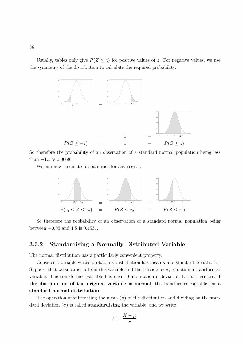
Usually, tables only give P (Z ≤ z) for positive values of z. For negative values, we use
the symmetry of the distribution to calculate the required probability.
−4 −2 0 2 4
0.0
0.1
0.2
0.3
0.4
PSfrag replacementszz −z = −4 −2 0 2 4
0.0
0.1
0.2
0.3
0.4
PSfrag replacementsz
z−z
= 1 − −4 −2 0 2 4
0.0
0.1
0.2
0.3
0.4
PSfrag replacementsz
z−z
P (Z ≤ −z) = 1 − P (Z ≤ z)
So therefore the probability of an observation of a standard normal population being less
than −1.5 is 0.0668.
We can now calculate probabilities for any region.
−4 −2 0 2 4
0.0
0.1
0.2
0.3
0.4
PSfrag replacementszz−z
z1 z2 = −4 −2 0 2 4
0.0
0.1
0.2
0.3
0.4
PSfrag replacementszz−z
z1 z2 − −4 −2 0 2 4
0.0
0.1
0.2
0.3
0.4
PSfrag replacementszz−z
z1z2
P (z1 ≤ Z ≤ z2) = P (Z ≤ z2) − P (Z ≤ z1)
So therefore the probability of an observation of a standard normal population being
between −0.05 and 1.5 is 0.4531.
3.3.2 Standardising a Normally Distributed Variable
The normal distribution has a particularly convenient property.
Consider a variable whose probability distribution has mean µ and standard deviation σ.
Suppose that we subtract µ from this variable and then divide by σ, to obtain a transformed
variable. The transformed variable has mean 0 and standard deviation 1. Furthermore, if
the distribution of the original variable is normal, the transformed variable has a
standard normal distribution.
The operation of subtracting the mean (µ) of the distribution and dividing by the stan-
dard deviation (σ) is called standardising the variable, and we write
Z =X − µ
σ.

MATH2041/2042 Stats for Engineering Year: 08–09 Dr S. K. Sahu 37
By standardising, we can calculate probabilities for any normal distribution using tables
of the standard normal distribution.
Suppose that the atmospheric SO2 (sulphur dioxide) concentration at a particular loca-
tion is, under usual conditions, normally distributed with mean 25.8 micrograms per cubic
metre and standard deviation 5.5 micrograms per cubic metre. What is the probability of a
SO2 concentration between 20 and 30 micrograms per cubic metre?
If we denote the SO2 concentration by X then Z = (X − 25.8)/5.5 is a variable with a
standard normal distribution.
We require P (20 ≤ X ≤ 30).
When x = 20, z = −1.05
When x = 30, z = 0.76
P (20 ≤ X ≤ 30) = P (−1.05 ≤ Z ≤ 0.76) = 0.7764 − (1 − 0.8531) = 0.6295.
10 20 30 400.0
0.02
0.04
0.06
PSfrag replacements
z
z
−z
z1
z2 =−4 −2 0 2 4
0.0
0.1
0.2
0.3
0.4PSfrag replacements
z
z
−z
z1
z2
The fact that a normally distributed population is completely specified by its mean
and standard deviation means that it is easy to make useful statements and predictions
about normal populations.
For example, suppose that on one particular day the SO2 concentration was measured
as 44.3 micrograms per cubic metre. Is this unusually high?
When x = 44.3, z = 44.3−25.85.5
= 3.36
Now P (X ≥ 44.3) = P (Z ≥ 3.36) = 1 − P (Z ≤ 3.36) = 1 − 0.9996 = 0.0004
This observation, 44.3, does seem high. Only about 1 in 2500 observations from this
population are as high, or higher than this. This might lead us to suspect that conditions for
this measurement were unusual, and to seek some explanation as to why the measurement
is so high.
Note that in MINITAB we can calculate probabilities for any (not just standard) normal
distribution using

38
Calc→Probability Distributions →Normal
but remember to ask for Cumulative probability
If we have a normal model for a particular population (and the normal distribution does
provide a reasonable model for many populations) and we know the mean and standard
deviation of the normal distribution, useful statements and predictions can be made about
the variable of interest.
In practice we will rarely know any of these things precisely, but we can use a sample
of observations from the population to estimate the mean and standard deviation and check
to see if the assumption of a normal distribution is sensible.
3.4 Samples
A set of observations which consists of the whole population is a census. In practice, we
rarely observe the whole population. Therefore we collect data on a sample from the
population and use the sample to make inferences about the population. A sample is a
set of observations which constitutes part of a population.
Most statistical data analysis (§4 onwards) concerns how to use a sample to make in-
ferences about a population and how accurate conclusions made about populations using
sample data are likely to be (as a sample only contains part of the population, using a sample
to make conclusions about a population is subject to error).
Next, we consider how to use sample data to determine whether or not a normal model
may be appropriate for a particular population. This is particularly relevant, as if we can
be confident about our model for a population, then useful statements and predictions can
be made about the variable of interest.
The further use of sample data to make inferences about populations, for example to
estimate model parameters, will be discussed in Chapter 4.
3.5 Testing for Normality
Suppose that we have a sample of n observations from a particular population, and a normal
model is proposed for the population. One may produce a histogram of the observations,
and examine if the distribution is approximately ‘bell-shaped’. However, there is a more
straightforward procedure to check whether a sample of observations have come from a
normal distribution.
For any sample size n, MINITAB can calculate normal scores. These are the typical
values one would expect to obtain if one had a sample of size n from a standard normal
distribution. For example, if n = 20

MATH2041/2042 Stats for Engineering Year: 08–09 Dr S. K. Sahu 39
-3 -2 -1 0 1 2 3
PSfrag replacements
z
z
−z
z1
z2
These are the mean values of the ordered observations when repeated samples of size
20 are taken from a standard normal distribution.
A normal probability plot is a plot of the observed data (n values) against the normal
scores for a sample of size n. The smallest value in the sample is plotted against the smallest
normal score, the second smallest value in the sample is plotted against the against the
second smallest normal score, . . . , the largest value in the sample is plotted against the
largest normal score.
If the sample is from a normally distributed population, then the plot will be approxi-
mately a straight line. although the variation in the data will ensure that the plot is not a
perfect straight line.
There are two ways of producing a normal probability plot in MINITAB.
1. Calc→Calculator allows you to put normal scores corresponding to the column of data
of interest into a new column so that the two columns are the same length and are ordered
correctly. Then it is straightforward to produce the plot using
Graph→Scatterplot. If you plot the data of interest along the y-axis, and the normal
scores along the x-axis, then, if the data are from a normally distributed population, the
resulting straight line will have an intercept (value of y at x = 0) approximately equal to the
population mean, and a gradient approximately equal to the population standard deviation.
2. Graph→Probability plot produces the normal probability plot directly
(choose Normal in the distribution panel of the dialogue box).
40
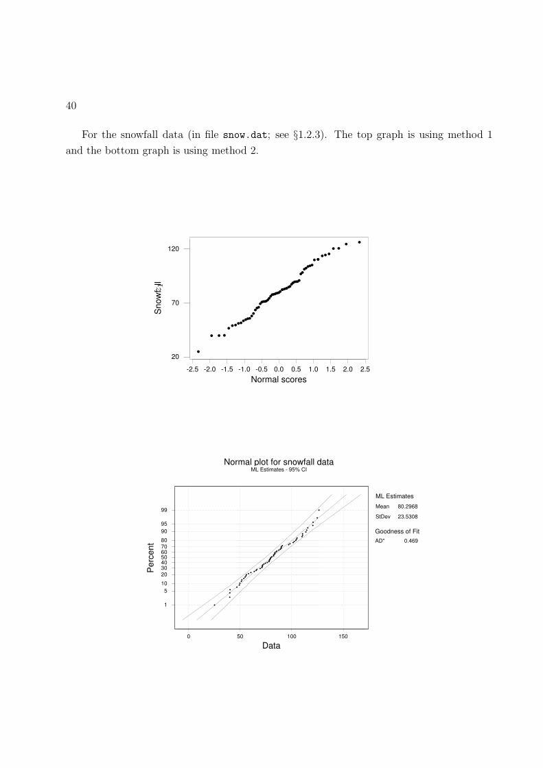
For the snowfall data (in file snow.dat; see §1.2.3). The top graph is using method 1
and the bottom graph is using method 2.
2.52.01.51.00.50.0-0.5-1.0-1.5-2.0-2.5
120
70
20
Normal scores
Snow
fll
PSfrag replacements
z
z
−z
z 1
z2
150100500
99
95908070605040302010 5
1
Data
Perc
ent 0.469AD*
Goodness of Fit
Normal plot for snowfall dataML Estimates - 95% CI
Mean
StDev
80.2968
23.5308
ML Estimates
PSfrag replacements
z
z
−z
z1
z2

MATH2041/2042 Stats for Engineering Year: 08–09 Dr S. K. Sahu 41
The following normal probability plot is for the data in rain.dat which are 30 successive
values of March precipitation (in inches) for Minneapolis/St Paul.
420
99
9590
80706050403020
10 5
1
Data
Perc
ent 0.947AD*
Goodness of Fit
Normal plot for rainfall dataML Estimates - 95% CI
Mean
StDev
1.675
0.983798
ML Estimates
PSfrag replacements
z
z
−z
z1
z2
The following normal probability plot is for the data in acidity data (in acidity.dat which
are measurements of an acidity index for each of 155 lakes in the Northeastern USA.
8.57.56.55.54.53.52.51.5
99
95908070605040302010 5
1
Data
Perc
ent 6.361AD*
Goodness of Fit
Normal plot for acidity dataML Estimates - 95% CI
Mean
StDev
5.10510
1.03846
ML Estimates
PSfrag replacements
z
z
−z
z1
z2

42
3.6 The Lognormal Distribution
If a normal probability plot produces a result which is clearly not a straight line, then a
normal model is inappropriate for the variable of interest, and an alternative model needs to
be specified. When the variable of interest can only take positve values, it is quite common
for the distribution to be skewed so that more observations lie to the right of (are greater
than) the peak (or mode) of the distribution than lie to the left. This kind of behaviour is
typical when the variable of interest is a concentration.
The symmetric normal distribution fails as a model for such variables. However, it is
often the case that by creating a transformed variable, by taking the logarithm of the original
variable, that the transformed variable seems to have a normal distribution. Suppose that
X is the original variable and that Y = log X has a normal distribution. Then we say that
X has a lognormal distribution. The lognormal distribution has density function
f(x) =1
x√
2πσ2exp
(
−(log x − µ)2
2σ2
)
.
0.0 0.2 0.4 0.6 0.8 1.0
PSfrag replacements
z
z
−z
z1
z2
The base to which the logarithm is taken is not important, because
loga x = loga b logb x = k logb x.
In other words, any logarithm can be obtained from any other by multipication by a constant,
and if a normally distributed variable is multiplied by a constant, its distribution remains
normal. Therefore, if taking logarithms to one particular base transforms a variable to a
normal distribution, so will taking logarithms to any other base.
There are two ways in MINITAB of checking to see if a lognormal distribution is appro-
priate for the variable of interest.
MATH2041/2042 Stats for Engineering Year: 08–09 Dr S. K. Sahu 43
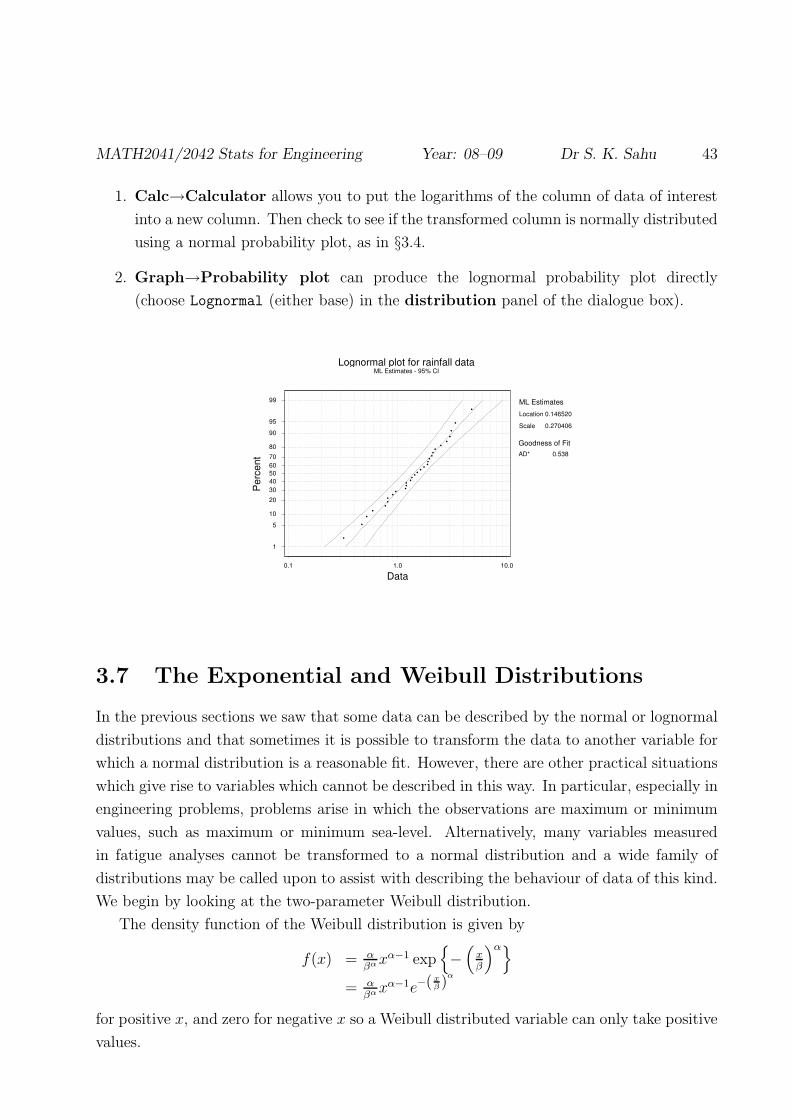
1. Calc→Calculator allows you to put the logarithms of the column of data of interest
into a new column. Then check to see if the transformed column is normally distributed
using a normal probability plot, as in §3.4.
2. Graph→Probability plot can produce the lognormal probability plot directly
(choose Lognormal (either base) in the distribution panel of the dialogue box).
10.01.00.1
99
9590
80706050403020
10 5
1
Data
Perc
ent 0.538AD*
Goodness of Fit
Lognormal plot for rainfall dataML Estimates - 95% CI
Location
Scale
0.146520
0.270406
ML Estimates
PSfrag replacements
z
z
−z
z1
z2
3.7 The Exponential and Weibull Distributions
In the previous sections we saw that some data can be described by the normal or lognormal
distributions and that sometimes it is possible to transform the data to another variable for
which a normal distribution is a reasonable fit. However, there are other practical situations
which give rise to variables which cannot be described in this way. In particular, especially in
engineering problems, problems arise in which the observations are maximum or minimum
values, such as maximum or minimum sea-level. Alternatively, many variables measured
in fatigue analyses cannot be transformed to a normal distribution and a wide family of
distributions may be called upon to assist with describing the behaviour of data of this kind.
We begin by looking at the two-parameter Weibull distribution.
The density function of the Weibull distribution is given by
f(x) = αβα xα−1 exp
{
−(
xβ
)α}
= αβα xα−1e−( x
β )α
for positive x, and zero for negative x so a Weibull distributed variable can only take positive
values.

44
The parameters are α and β, where the value of α determines the shape of the distribution
and β its scale. The figure below illustrates this distribution for some different combinations
of values of α and β.
0.0 0.2 0.4 0.6 0.8 1.0
PSfrag replacements
z
z
−z
z1
z2
When the parameter α = 1, the density function takes the form
f(x) =1
βe−
xβ
which is also known as the exponential or negative exponential distribution. This distribution
often occurs in such practical problems as the waiting time between events in some random
process of events or as the time between failures in some process where the failures are
occurring at random. The figure below illustrates this distribution for β = 0.2.
0.0 0.2 0.4 0.6 0.8 1.0
PSfrag replacements
z
z
−z
z1
z2

MATH2041/2042 Stats for Engineering Year: 08–09 Dr S. K. Sahu 45
The simple form of this particular distribution makes it possible to determine the mean
(µ) and standard deviation (σ), by integration as follows
µ =∫∞0
x 1βe−
xβ dx = β
σ2 =∫∞0
x2 1βe−
xβ dx − β2 = β2.
Other properties of this distribution, such as the probability of an exponentially dis-
tributed variable lying in any region, may also be found using integration. For example, if
the variable is X, then
P (X ≤ t) =
∫ t
0
1
βe−
xβ dx = 1 − e−
tβ .
This probability may be calculated directly in MINITAB using
Calc→Probability Distributions→Exponential, asking for Cumulative probability.
Hence
P (s ≤ X ≤ t) = e−sβ − e−
tβ .
As with the normal distribution, if we propose an exponential distribution as a model for a
variable of interest, we can use sample data to check whether the model is appropriate. Again,
we use a probability plot to perform the check. The ordered sample data are plotted, not
against the normal scores, but against the equivalent values for an exponential distribution.
Graph→Probability plot produces the exponential probability plot (if you choose
Exponential in the distribution panel of the dialogue box).
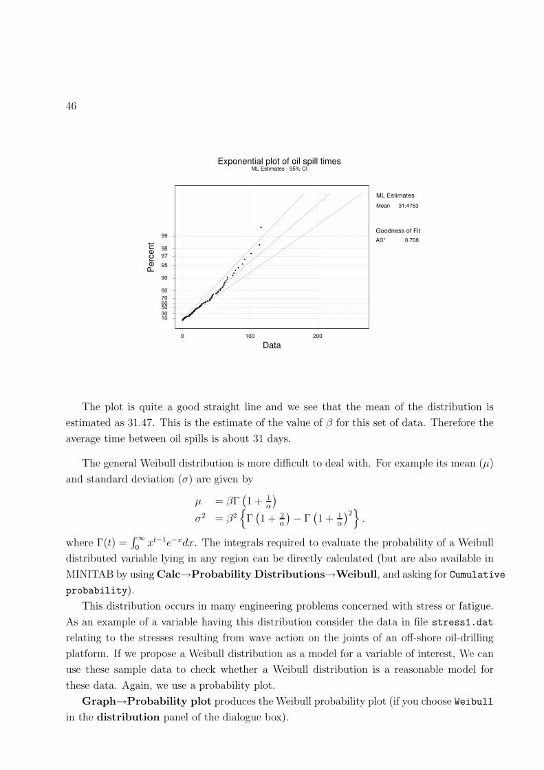
For example, consider the data in the file oilspill.dat which are the times between oil
spills in or around an oil terminal entrance.
46
2001000
99
989795
90
807060503010
Data
Perc
ent 0.708AD*
Goodness of Fit
Exponential plot of oil spill timesML Estimates - 95% CI
Mean 31.4763ML Estimates
PSfrag replacements
z
z
−z
z1
z2
The plot is quite a good straight line and we see that the mean of the distribution is
estimated as 31.47. This is the estimate of the value of β for this set of data. Therefore the
average time between oil spills is about 31 days.
The general Weibull distribution is more difficult to deal with. For example its mean (µ)
and standard deviation (σ) are given by
µ = βΓ(
1 + 1α
)
σ2 = β2{
Γ(
1 + 2α
)
− Γ(
1 + 1α
)2}
.
where Γ(t) =∫∞0
xt−1e−xdx. The integrals required to evaluate the probability of a Weibull
distributed variable lying in any region can be directly calculated (but are also available in
MINITAB by using Calc→Probability Distributions→Weibull, and asking for Cumulative
probability).
This distribution occurs in many engineering problems concerned with stress or fatigue.
As an example of a variable having this distribution consider the data in file stress1.dat
relating to the stresses resulting from wave action on the joints of an off-shore oil-drilling
platform. If we propose a Weibull distribution as a model for a variable of interest, We can
use these sample data to check whether a Weibull distribution is a reasonable model for
these data. Again, we use a probability plot.
Graph→Probability plot produces the Weibull probability plot (if you choose Weibull
in the distribution panel of the dialogue box).

MATH2041/2042 Stats for Engineering Year: 08–09 Dr S. K. Sahu 47
100.010.01.00.1
99959080706050403020
10
5
3 2
1
Data
Perc
ent 0.679AD*
Goodness of Fit
Weibull plot for oil platform stress dataML Estimates - 95% CI
Shape
Scale
0.983219
21.8543
ML Estimates
PSfrag replacements
z
z
−z
z1
z2
Note that the analysis produces estimates of the parameters in the Weibull model. In
this case these are α = 0.98 and β = 21.8. These can be substituted into the expressions
above to estimate the population mean and standard deviation if required. Alternatively
the probability of the stress taking a value in a particular range can be calculated by using
these values of α and β in Calc→Probability Distributions→Weibull in MINITAB.
Estimation is considered in further detail in Chapter 4.
3.8 Return Periods, Design Life and Reliability
One of the main applications of a probability model for a particular variable is often to
extrapolate into the tails of the distribution to determine the value exceeded with a specified
probability, say p = 0.01.
For example, suppose that the random variable X represents the maximum annual flow
rate of a river at a particular location. If we have a probability model for X, and we have
estimated the parameters of this model, we can use the density function to find the value x
such that P (X > x) = p, or alternatively P (X ≤ x) = 1 − p.
The reciprocal of this probability T = 1/p, (for example T = 100 if p = 0.01) is known
as the corresponding Return Period. There is often, however, some confusion about the
appropriate interpretation of statements of the form “The flow x has a return period of 100
years.” This statement does not mean that the flow x will be exceeded once in every 100
years, or that it will take 100 years for x to be exceeded, or that any structure designed to
withstand a flow of x will last 100 years.
In order to be able to appreciate the meaning of a return period, particularly the need
48
sometimes to use large return periods of say 500 years, 1000 years or even 2000 years, we
should consider the concepts of design life and reliability of a structure.
The design life of a structure is the time that the designer hopes that it will survive.
The reliability is the probability that it will survive for that length of time.
The usual position is that the structure under discussion has a design life of a specified
number of years and the engineer is prepared to accept a risk, again of specified magnitude,
that the structure will fail at some time during its design life. For example, the design life
for an irrigation project could be 50 years and an acceptable risk could be 5 per cent. This
means that there is a 95% chance that it will survive for 50 years. An alternative acceptable
risk not uncommonly used is 10%. We shall observe the effects of modifying risk later.
The problem now is to relate the design life, the specified risk and the return period.
Suppose that the structure is to be built at a point in the river where data has been
collected for a period of time. Since we are interested in the extreme flows when designing
structures, it is common to consider the annual maximum or the annual minimum flows
as the basic data with these values recorded for a number of years. We shall consider the
distributions of extremes in the next section, but for the moment suppose that the data
consist of annual maximum river flows at that point on the river and that these values are
denoted by x1, x2, . . . , xn, where n is the number of years of data.
Suppose that the distribution of these annual maxima has density function f(x), and
define F (x) by
F (x) = P (X ≤ x) =
∫ x
−∞f(x)dx.
We call F (x) the distribution function of the random variable. Then
P (X > x) = 1 − F (x) = p
where p is the probability that the value x is exceeded.
Consider a design life of m years over which the structure is expected to be operational,
and that if the flow exceeds x, the structure fails. Each year of the design life the probability
that the structure fails is p and therefore the probability that it does not fail is (1−p) = F (x).
Assuming that values of X over succesive years are independent, then the probability
that the structure does not fail over its design life of m years is
P (X ≤ x, every year) = (1 − p)m
and therefore the probability that x is exceeded at some time during the design life, (thus
causing a failure of the structure), is β = 1 − (1 − p)m.
This is the risk of failure and may be set equal to any specified risk such as 5% or 10%.
Therefore, specifying a risk β and a design life m acceptable to the engineer, is equivalent to
specifying a value of p = 1 − F (x) and this in turn is equivalent to specifying a value of x.
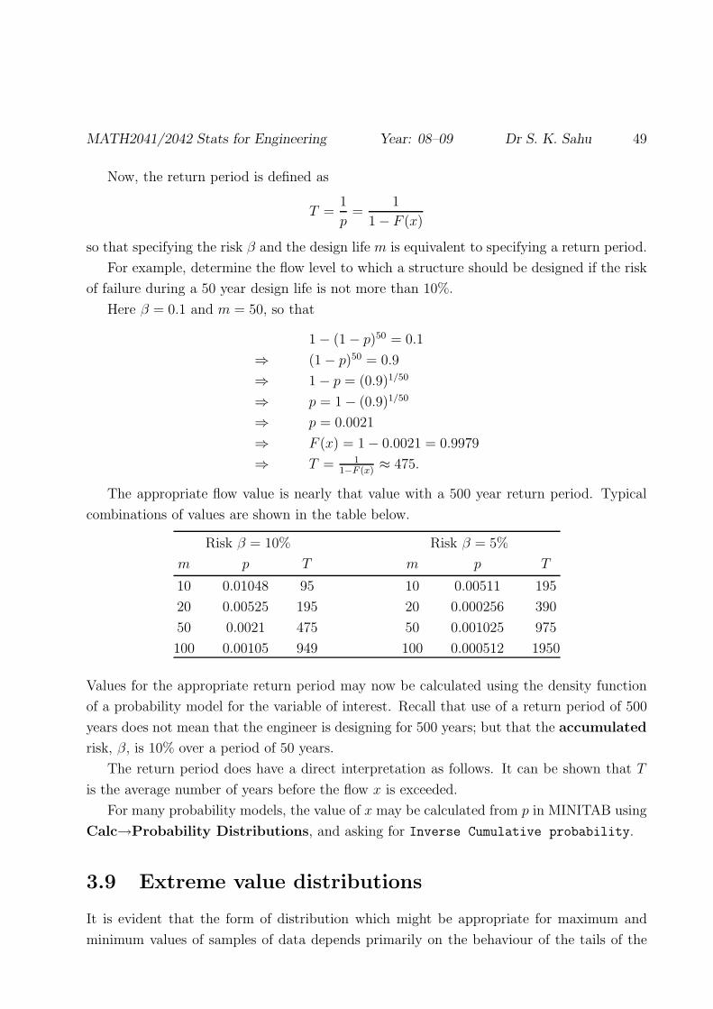
MATH2041/2042 Stats for Engineering Year: 08–09 Dr S. K. Sahu 49
Now, the return period is defined as
T =1
p=
1
1 − F (x)
so that specifying the risk β and the design life m is equivalent to specifying a return period.
For example, determine the flow level to which a structure should be designed if the risk
of failure during a 50 year design life is not more than 10%.
Here β = 0.1 and m = 50, so that
1 − (1 − p)50 = 0.1
⇒ (1 − p)50 = 0.9
⇒ 1 − p = (0.9)1/50
⇒ p = 1 − (0.9)1/50
⇒ p = 0.0021
⇒ F (x) = 1 − 0.0021 = 0.9979
⇒ T = 11−F (x)
≈ 475.
The appropriate flow value is nearly that value with a 500 year return period. Typical
combinations of values are shown in the table below.
Risk β = 10% Risk β = 5%
m p T m p T
10 0.01048 95 10 0.00511 195
20 0.00525 195 20 0.000256 390
50 0.0021 475 50 0.001025 975
100 0.00105 949 100 0.000512 1950
Values for the appropriate return period may now be calculated using the density function
of a probability model for the variable of interest. Recall that use of a return period of 500
years does not mean that the engineer is designing for 500 years; but that the accumulated
risk, β, is 10% over a period of 50 years.
The return period does have a direct interpretation as follows. It can be shown that T
is the average number of years before the flow x is exceeded.
For many probability models, the value of x may be calculated from p in MINITAB using
Calc→Probability Distributions, and asking for Inverse Cumulative probability.
3.9 Extreme value distributions
It is evident that the form of distribution which might be appropriate for maximum and
minimum values of samples of data depends primarily on the behaviour of the tails of the
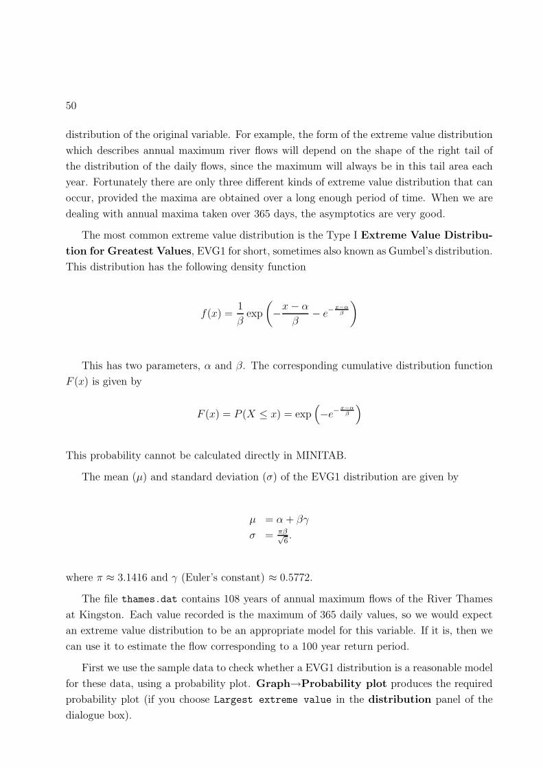
50
distribution of the original variable. For example, the form of the extreme value distribution
which describes annual maximum river flows will depend on the shape of the right tail of
the distribution of the daily flows, since the maximum will always be in this tail area each
year. Fortunately there are only three different kinds of extreme value distribution that can
occur, provided the maxima are obtained over a long enough period of time. When we are
dealing with annual maxima taken over 365 days, the asymptotics are very good.
The most common extreme value distribution is the Type I Extreme Value Distribu-
tion for Greatest Values, EVG1 for short, sometimes also known as Gumbel’s distribution.
This distribution has the following density function
f(x) =1
βexp
(
−x − α
β− e−
x−αβ
)
This has two parameters, α and β. The corresponding cumulative distribution function
F (x) is given by
F (x) = P (X ≤ x) = exp(
−e−x−α
β
)
This probability cannot be calculated directly in MINITAB.
The mean (µ) and standard deviation (σ) of the EVG1 distribution are given by
µ = α + βγ
σ = πβ√6.
where π ≈ 3.1416 and γ (Euler’s constant) ≈ 0.5772.
The file thames.dat contains 108 years of annual maximum flows of the River Thames
at Kingston. Each value recorded is the maximum of 365 daily values, so we would expect
an extreme value distribution to be an appropriate model for this variable. If it is, then we
can use it to estimate the flow corresponding to a 100 year return period.
First we use the sample data to check whether a EVG1 distribution is a reasonable model
for these data, using a probability plot. Graph→Probability plot produces the required
probability plot (if you choose Largest extreme value in the distribution panel of the
dialogue box).

MATH2041/2042 Stats for Engineering Year: 08–09 Dr S. K. Sahu 51
PSfrag replacements
z
z
−z
z1
z2
The estimated values for the parameters α and β are 271.1 and 96.98.
It would seem that this distribution is reasonable for these data, even though one point
is a bit out of line with the others. We can accept this distribution and use it to estimate
the flow corresponding to a 100 year return period. This could be obtained from the graph
or calculated from the formula developed above. The flow, x, corresponding to a return
period of 100 years is such that the probability of exceeding x, p = 1−F (x), is 0.01, so that
F (x) = P (X < x) = 0.99. This means that
exp(
−e−x−α
β
)
= 0.99
⇒ e−x−α
β = − log 0.99
⇒ x−αβ
= − log[− log 0.99]
⇒ x = α − β log[− log 0.99]
If we plug in the estimates for α (271.1) and β (96.98), provided by the probability plotting
routine, into this expression, we obtain an estimate for x of 717.2 m3s−1. This means that we
need to design any structure at this point of the Thames to withstand a flow of 717 m3s−1,
if it is to have a return period of 100 years.
More generally, for EVG1 distributions, we can write the expression
x = α − β log[− log(1 − p)]
where p is the probability of exceeding thhreshold value x. Therefore, as the return period
T = 1/p, we can write
x = α − β log
[
− log
(
1 − 1
T
)]

52
Now letu = − log
[
− log(
1 − 1T
)]
e−u = − log(
1 − 1T
)
e−u = 1T
+ 12T 2 + · · ·
e−u = 1T
[
1 + 12T
+ · · ·]
eu = T 1
[1+ 12T
+··· ]
eu ≈ T[
1 − 12T
]
provided that T is reasonably large. Therefore
eu = T − 1
2.
If we ignore the 1/2, which is relatively insignificant if T is large, we have that
u ≈ log T
and therefore
x = α + β log T.
This is known as the fundamental formula for flood control. Once the estimates of the
two parameters α and β have been obtained from the available data, they can be substituted
into this equation so that the value of x corresponding to any return period T can be found.
For example, here the estimates of α and β for the annual flows data for Kingston are
α = 271.1 and β = 96.98, so that the estimate of the annual maximum flows corresponding
to the 100, 200, 500 and 1000 year return periods are as follows.
Return period T in years Flow x in m3s−1
100 717.7
200 784.9
500 873.8
1000 941.0

Chapter 4
Estimation and Hypothesis Testing
4.1 Introduction
A probability model for the distribution of variable of interest will usually depend on one
or more unknown parameters. For example, if we propose a normal distribution for a par-
ticular variable, then we need to know the mean µ and standard deviation σ of that normal
distribution, in order to use our model to make predictions about future observations.
Just as we used sample data in §3, to assess whether a particular distributional model is
appropriate for a variable of interest, we can also use sample data to estimate the parameters
of our model.
4.2 Estimating a mean
The most straightforward situation is where the parameter of interest is the mean of the
population distribution, for example the normal parameter µ or the exponential parameter
β. There are also cases where it may be sufficient to estimate the mean of a population
without necessarily specifying a complete distributional model for the population.
Suppose that we have a sample of size n, x1, . . . xn from a population of interest. It
seems obvious that we should use the sample mean (x) to estimate the population mean µ.
This procedure, estimating a population quantity using a sample quantity, is called point
estimation.
When we calculate a point estimate, it is important that we have some idea how accurate
that estimate is likely to be. So how accurate are we, when we use the mean of a sample of
size n to estimate the mean of a population distribution?
Samples from a population are variable, and therefore estimates calculated using sample
data are also variable, and we can consider their distribution. When a sample of size n is
53

54
observed from a distribution, the sample mean x is a single observation from the distribution
of x for all such samples. An important question is ‘What does the distribution of x look like?’
and in particular ‘How does it compare with the distribution of the original observations
x1, x2, . . .?’
The following example is artificial, but serves to illustrate the point
♥ Example 4.1. Suppose that the distribution of interest consists of the integers from 1 to
49, each with probability 1/49. Twice a week a ‘sample’ of six observations is taken from this
distribution in the National Lottery. From §2, we know that there are 13 983 816 possible
samples of size 6. We can illustrate the distribution of x across these possible samples by a
histogram.
0 10 20 30 40 50
PSfrag replacements
z
z
−z
z1
z2
We can also calculate the mean and standard deviation of this distribution, 25 and 5.7735
respectively.
Note that the mean and standard deviation of the original distribution (the numbers 1
to 49, each with probability 1/49) are 25 and 14.1421 respectively.
We immediately notice three facts about the distribution of x
1. It has the same mean as the original distribution.
2. It has a smaller standard deviation than the original distribution.
3. The histogram seems ‘bell-shaped’ suggesting that the distribution may be close to a
normal distribution, even though the original distribution is far from normal.
In general Suppose also that x1, . . . , xn is a sample of size n from a distribution with
mean µ and standard deviation σ.
Then the distribution of x, the sample mean has the following three properties.
MATH2041/2042 Stats for Engineering Year: 08–09 Dr S. K. Sahu 55
1. It also has mean µ.
2. It has standard deviationσ√n
.
For larger sample sizes n, the distribution of sample means has smaller standard devi-
ation, so the sample means for larger samples are less variable and generally closer to
µ.
3. It is approximately normally distributed if n is large, regardless of the shape of
the original distribution.
• This is surprising and remarkable. It is the Central Limit Theorem, and one of the
reasons why the normal distribution is so important for data analysis.
How large must a sample be before we can assume that the sample mean x is from a
normal distribution?
There is no ready answer to this question. If the original distribution is ‘close to normal’,
then quite small samples may be adequate. Indeed if the original distribution is exactly
normal, then this assumption is appropriate for any size of sample. However, for highly
non-normal distributions (very skew or multimodal) larger samples will be required.
What remains true for all distributions is that the larger the sample size, the closer the
distribution of sample means is to a normal distribution.
Now, when we use a sample mean x to estimate the mean µ of the underlying distribution,
we know that x can be considered as a single observation from the distribution of sample
means for samples of size n.
We know that the mean of this distribution is also µ, but that its standard deviation is
σ/√
n. Therefore, ‘on average’, x is equal to µ, the quantity which we want to estimate, so
x is a sensible estimate. (This property, being ‘correct on average’, is called unbiased).
Furthermore, σ/√
n, the standard deviation, is a measure of the spread of possible sample
means around µ, and gives an indication of the error involved when we use a single sample
mean x to estimate µ.
Unfortunately, σ/√
n, the standard deviation of the distribution of x, is not known, as it
depends on the σ, the standard deviation of the original distribution, which is an unknown
quantity. However, if we use the standard deviation, s, of the sample to estimate σ, we can
use s/√
n as a measure of the accuracy of x as an estimate of µ.
The quantity s/√
n is called the standard error of the mean and should be quoted
whenever a sample mean x is used to estimate a population mean µ, as an indication of the
accuracy of the estimate.
In MINITAB
Stat→Basic Statistics→ Display Descriptive Statistics

56
4.3 Confidence interval for a mean
A better approach to estimating µ than using a single point estimate x, together with the
standard error s/√
n as a measure of precision, is to combine the two quantities to give a
range of plausible values for µ. A confidence interval provides this.
Suppose that x is the mean of a sample of observations x1, . . . , xn from a distribution
with mean µ and standard deviation σ.
Furthermore, suppose that either the sample size n is ‘large’, or the distribu-
tion of interest is close to normal.
Then we know that x is a single observation from (approximately) a normal distribution
with mean µ and standard deviation σ/√
n. We can standardise the variable x by subtracting
µ and dividing by σ/√
n. The standardised sample mean will have a standard normal
distribution. We can write
z =x − µ
σ/√
n
However, as σ is not known, we need to estimate it by the sample standard deviation s.
Then,
t =x − µ
s/√
n
is an observation from a t distribution ‘with n − 1 degrees of freedom’.
The t distribution is a known distribution, with a density curve which looks similar to
the standard normal distribution, but has a standard deviation larger than 1. The mean
of a t distribution is always zero, but the standard deviation depends on the degrees of
freedom, and is larger if the degrees of freedom is small.
When the degrees of freedom is large, the t distribution is very similar to the standard
normal distribution, and its standard deviation is very close to one.
To distinguish between different t distributions (with different degrees of freedom), we
denote the t distribution with k degrees of freedom by tk.

MATH2041/2042 Stats for Engineering Year: 08–09 Dr S. K. Sahu 57
values
dens
ity
-4 -2 0 2 4
0.0
0.1
0.2
0.3
0.4
Std normal and t density with 1 df
values
dens
ity
-4 -2 0 2 4
0.0
0.1
0.2
0.3
0.4
Std normal and t density with 8 df
values
dens
ity
-4 -2 0 2 4
0.0
0.1
0.2
0.3
0.4
Std normal and t density with 15 df
values
dens
ity
-4 -2 0 2 4
0.0
0.1
0.2
0.3
0.4
Std normal and t density with 30 df
PSfrag replacements
z
z
−z
z1
z2
Because the t distribution is well understood, we can make statements about observations
from a t distribution. As
t =x − µ
s/√
n
is an observation from a tn−1 distribution. then we can (in principle), by calculating areas
under the density curve of the tn−1 distribution, find the value c such that
P
(
−c ≤ x − µ
s/√
n≤ c
)
= 0.95.
0.025 0.025
shaded area=0.95
0.025
PSfrag replacements
z
z
−z
z1
z2
c−c

58
Therefore
P
(
x − cs√n
≤ µ ≤ x + cs√n
)
= 0.95.
or, in other words, for 95% of samples of size n, drawn from a distribution with mean µ,
the interval between
x − cs√n
and x + cs√n
will include µ.
Hence, we can calculate the endpoints of an interval, which will, for 95% of samples,
include the population mean µ.
(The endpoints of the interval are often written as x ± cs/√
n).
We call this interval a 95% confidence interval for µ.
It is an interval within which we can be ‘95% certain’ that µ lies. It provides a suumary
of the ‘most plausible’ values for the population mean µ in light of the observed data.
Statistical tables can be used to find c for any sample size n.
Because the tk distribution is similar to the standard normal distribution for large values
of k, then if the sample size n is large, in which case n − 1, the degrees of freedom will also
be large, then c can be calculated using a standard normal distribution.PSfrag replacements
z
z
−z
z1
z2
c
−c c
Table gives values of c for some P (tk ≤ c)
P (tk ≤ c) P (tk ≤ c)
k 0.9 0.95 0.975 0.99 0.995 k 0.9 0.95 0.975 0.99 0.995
1 3.08 6.31 12.71 31.82 63.66 11 1.36 1.80 2.20 2.72 3.11
2 1.89 2.92 4.30 6.96 9.92 12 1.36 1.78 2.18 2.68 3.05
3 1.64 2.35 3.18 4.54 5.84 15 1.34 1.75 2.13 2.60 2.95
4 1.53 2.13 2.78 3.75 4.60 20 1.33 1.72 2.09 2.53 2.85
5 1.48 2.02 2.57 3.36 4.03 25 1.32 1.71 2.06 2.49 2.79
6 1.44 1.94 2.45 3.14 3.71 30 1.31 1.70 2.04 2.46 2.75
7 1.41 1.89 2.36 3.00 3.50 40 1.30 1.68 2.02 2.42 2.70
8 1.40 1.86 2.31 2.90 3.36 50 1.30 1.68 2.01 2.40 2.68
9 1.38 1.83 2.26 2.82 3.25 60 1.30 1.67 2.00 2.39 2.66
10 1.37 1.81 2.23 2.76 3.17 100 1.29 1.66 1.98 2.36 2.63
∞ 1.28 1.64 1.96 2.33 2.58
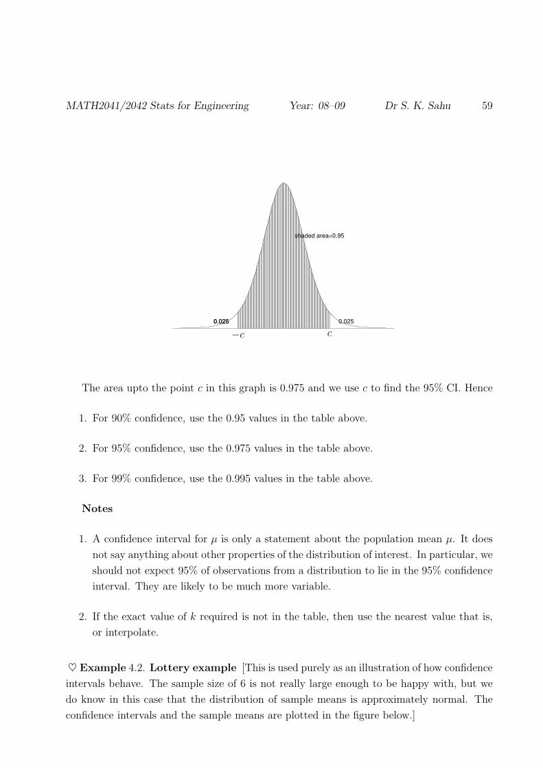
MATH2041/2042 Stats for Engineering Year: 08–09 Dr S. K. Sahu 59
0.025 0.025
shaded area=0.95
0.025
PSfrag replacements
z
z
−z
z1
z2
c
−c
cc−c
The area upto the point c in this graph is 0.975 and we use c to find the 95% CI. Hence
1. For 90% confidence, use the 0.95 values in the table above.
2. For 95% confidence, use the 0.975 values in the table above.
3. For 99% confidence, use the 0.995 values in the table above.
Notes
1. A confidence interval for µ is only a statement about the population mean µ. It does
not say anything about other properties of the distribution of interest. In particular, we
should not expect 95% of observations from a distribution to lie in the 95% confidence
interval. They are likely to be much more variable.
2. If the exact value of k required is not in the table, then use the nearest value that is,
or interpolate.
♥ Example 4.2. Lottery example [This is used purely as an illustration of how confidence
intervals behave. The sample size of 6 is not really large enough to be happy with, but we
do know in this case that the distribution of sample means is approximately normal. The
confidence intervals and the sample means are plotted in the figure below.]

60
Date Sample x
7/3/98 4 11 14 39 43 44 25.83
4/3/98 6 28 30 34 41 45 30.67
28/2/98 1 7 15 18 30 31 17.00
25/2/98 9 21 27 36 42 48 30.50
21/2/98 2 16 25 27 37 45 25.33
18/2/98 1 5 10 13 25 32 14.33
14/2/98 8 13 14 17 20 28 16.67
11/2/98 11 32 38 42 46 49 36.33
7/2/98 9 25 27 31 42 45 29.83
4/2/98 13 17 32 35 42 45 30.67
31/1/98 17 22 30 40 46 48 33.83
28/1/98 4 12 15 31 32 47 23.50
24/1/98 1 4 6 14 24 49 16.33
21/1/98 5 12 24 35 36 38 25.00
17/1/98 14 31 33 38 46 48 35.00
14/1/98 20 27 28 31 33 41 30.00
10/1/98 3 10 11 27 47 49 24.50
7/1/98 7 14 25 32 36 38 25.33
3/1/98 1 13 26 28 35 45 24.67
31/12/98 8 13 18 21 23 29 18.67
Week
5 10 15 20
010
2030
4050
*
*
*
*
*
**
*
* **
*
*
*
*
*
* **
*
PSfrag replacements
z
z
−z
z1
z2
c
−c
c
c
−c
MATH2041/2042 Stats for Engineering Year: 08–09 Dr S. K. Sahu 61
In MINITAB
Stat→Basic Statistics→ 1-sample t
Real examples
♥ Example 4.3. The file concrete.dat contains the compression strength (Nmm−2)
of 180 concrete cubes. Suppose that we are interested in the mean of the distribution of
compression strength of all such cubes. The sample size of 180 is large, so there is no
problem here.
The sample mean is x = 61.098, the sample standard deviation is s = 3.963, and therefore,
as the sample size n = 180, the standard error s/√
n = 0.295. The value of the constant c
for a t179 distribution is 1.9733 (approximately the same as for a standard normal).
Therefore, a 95% confidence interval for µ, the mean compression strength of all such
cubes is (60.515, 61.681).
This interval may also be presented as
60.515 ≤ µ ≤ 61.681 or 61.098 ± 0.583
A 99% confidence interval for µ is (60.329, 61.867).
A 90% confidence interval for µ is (60.609, 61.586).
♥ Example 4.4. Consider the data in the file latent.dat (also presented on the intro-
ductory handout), which are measurements of the latent heat of water using two methods.
Measurements subject to error are often assumed to be normally distributed with mean µ
equal to the ‘true’ value. Normal probability plots of the sample data produce straight lines
for both samples, we can assume that the distribution of measurements is approximately
normal, and calculate a confidence interval for the true value µ without any concerns.
Using sample data for method A, the sample mean is x = 80.021, the sample standard
deviation is s = 0.024, and therefore, as the sample size n = 13, the standard error s/√
n =
0.007, and c = 2.18 using the tables. Therefore, a 95% confidence interval for µ, the true
latent heat of water is (80.006, 80.035).
Using sample data for method B, the sample mean is x = 79.979, the sample stan-
dard deviation is s = 0.031, and therefore, as the sample size n = 8, the standard error
s/√
n = 0.011. Therefore, a 95% confidence interval for µ, the true latent heat of water is
(79.953, 80.005).
4.4 Estimating other parameters
When estimating the mean µ of a distribution, a sample mean is an obvious estimator.
However, for other parameters, a convenient estimator may not be quite so obvious. For
example, how should we estimate the parameters α and β of a Weibull or EVG1 distribution?
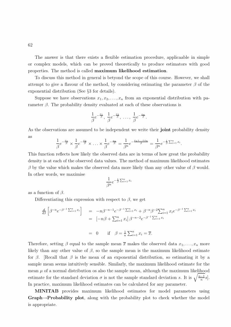
62
The answer is that there exists a flexible estimation procedure, applicaable in simple
or complex models, which can be proved theoretically to produce estimators with good
properties. The method is called maximum likelihood estimation.
To discuss this method in general is betyond the scope of this course. However, we shall
attempt to give a flavour of the method, by considering estimating the parameter β of the
exponential distribution (See §3 for details).
Suppose we have observations x1, x2, . . . , xn from an exponential distribution with pa-
rameter β. The probability density evaluated at each of these observations is
1
βe−
x1β ,
1
βe−
x2β , . . . ,
1
βe−
xnβ .
As the observations are assumed to be independent we write their joint probability density
as1
βe−
x1β × 1
βe−
x2β × . . . × 1
βe−
xnβ =
1
βne−
x1+...+xnβ =
1
βne−
1β
Pni=1 xi.
This function reflects how likely the observed data are in terms of how great the probability
density is at each of the observed data values. The method of maximum likelihood estimates
β by the value which makes the observed data more likely than any other value of β would.
In other words, we maximise1
βne−
1β
Pni=1 xi
as a function of β.
Differentiating this expression with respect to β, we get
ddβ
[
β−ne−β−1Pn
i=1 xi
]
= −nβ−n−1e−β−1Pn
i=1 xi + β−nβ−2∑n
i=1 xie−β−1
Pni=1 xi
= [−nβ +∑n
i=1 xi]β−n−2e−β−1
Pni=1 xi
= 0 if β = 1n
∑ni=1 xi = x.
Therefore, setting β equal to the sample mean x makes the observed data x1, . . . , xn more
likely than any other value of β, so the sample mean is the maximum likelihood estimate
for β. [Recall that β is the mean of an exponential distribution, so estimating it by a
sample mean seems intuitively sensible. Similarly, the maximum likelihood estimate for the
mean µ of a normal distribution os also the sample mean, although the maximum likelihood
estimate for the standard deviation σ is not the sample standard deviation s. It is√
n−1n
s].
In practice, maximum likelihood estimates can be calculated for any parameter.
MINITAB provides maximum likelihood estimates for model parameters using
Graph→Probability plot, along with the probability plot to check whether the model
is appropriate.

MATH2041/2042 Stats for Engineering Year: 08–09 Dr S. K. Sahu 63
Ideally, we would also like to be able to get standard errors or (even better) confidence
intervals for these parameters but MINITAB does not provide these in general. However,
what MINITAB does provide are estimates of the distribution function F (x) = P (X ≤ x)
based on the parameter estimates.
In particular, for a number of values of p (and more can be specified using Options),
estimates of the value of x for which P (X ≤ x) = p are given. Furthermore, the uncertainty
in these estimates is represented by confidence intervals.
♥ Example 4.5. Consider the data in file stress1.dat relating to the stresses resulting
from wave action on the joints of an off-shore oil-drilling platform. In §3 we used a Weibull
distribution as a model for this variable, and estimated the parameters as α = 0.98 and
β = 21.8. Suppose, for design purposes we want to estimate the value of stress which is
exceeded with probability 0.01. Then the relevant MINITAB output is as follows.
Percentile Estimates
95% CI 95% CI
Approximate Approximate
Percent Percentile Lower Limit Upper Limit
1 0.203 0.0374 1.104
2 0.413 0.0950 1.796
...
98 87.508 52.2537 146.548
99 103.300 59.5150 179.299
Hence, although the stress value exceeded with probability 0.01 is estimated to be 103.3,
there is considerable uncertainty, as the 95% confidence interval (59.5, 179.3) is very wide.
4.5 Hypothesis Tests for the Mean of a Population
Sometimes, sample data are collected with the purpose of examining a conjecture or hy-
pothesis concerning a distribution. For example, data may be collected to ensure that
certain standards are being satisfied, or a change may have been made to a process and
data is collected on an output of that process to see if its distribution has changed from the
(known) previous distribution.

64
We will focus on hypotheses which concern the (unknown) distribution mean µ, although
in principle a hypothesis may concern any property of the distribution which might be of
interest (for example, any parameter of the distribution).
Again, we suppose that x is the mean of a sample of n observations x1, . . . , xn from a
distribution with mean µ and standard deviation σ. Let the hypothesised value of µ be
denoted by µ0.
A confidence interval gives a range of plausible values of µ, based on the observed data,
so a sensible procedure would seem to be to reject the hypothesis that µ = µ0 if the value of
µ0 does not lie inside our confidence interval.
For example, if we have a 95% confidence interval, and the mean of the distribution is
indeed equal to µ0, then for 95% of samples, the confidence interval will include µ0. If it
does not then, either we have been unlucky, and observed one of the 5% of samples with
erroneous confidence intervals, or the mean of the distribution is not, in fact, equal to µ0.
Therefore, if the hypothesised value, µ0 does not lie in the 95% confidence interval, we
use this fact as evidence against the hypothesis that µ = µ0 and reject the hypothesis at
the 5% level of significance. Another way of saying this is that the evidence against the
hypothesis µ = µ0 is statistically significant at the 5% level.
More generally, the significance level for the test is 1− the confidence level of the associ-
ated interval. Smaller significance levels correspond to wider confidence intervals, so require
greater evidence in order to reject.
Recall that, for large samples, or distributions which are close to normal, we calculate
confidence intervals based on the fact that
t =x − µ
s/√
n
is an observation from a tn−1 distribution. Hence, if our hypothesis that µ = µ0 is true, then
T =x − µ0
s/√
n
is an observation from a tn−1 distribution.
The hypothesised mean µ0 will fall inside the confidence interval if
x − cs√n
≤ µ0 ≤ x + cs√n
⇒ −c ≤ x − µ0
s/√
n≤ c
⇒ −c ≤ T ≤ c
where c is the relevant value calculated using the tn−1 distribution
If |T | > c, then µ0 is outside the confidence interval and the hypothesis is rejected.
MATH2041/2042 Stats for Engineering Year: 08–09 Dr S. K. Sahu 65
Therefore, a hypothesis test involves calculating the test statistic T and seeing if it
falls in the rejection region |T | > c evaluated using the tn−1 distribution together with the
significance (confidence) level for the test. This is intuitively sensible. The test will reject
when the sample mean x and the hypothesised distribution mean µ0 are far apart.
Sometimes we calculate a p-value for a hypothesis test. A p-value is the highest sig-
nificance level at which the hypothesis would not be rejected. Therefore the p-value is
the significance value of the test for which T lies right on the edge of the rejection region
i.e. |T | = c. Hence the p-value is the probability that an observation from a tn−1 distribution
is greater than |T | or less than −|T |.Recall that smaller significance levels require greater evidence, so if the p-value is small,
the data are providing strong evidence against the hypothesis, because the hypothesis is
rejected, even at small significance levels.
Usually, we reject the hypothesis if the p-value p < 0.05. In other words, we tend to use
a 5% significance level. Other values of significance which are commonly used are 1% and
0.1%. These imply even stronger evidence against H0.
If the hypothesis is not rejected, then that is exactly what has happened – we have not
rejected it. This does not mean that we have accepted it. Try to avoid using the word
‘accept’ when talking about statistical hypotheses. The reason that we have not rejected
the hypothesis may be simply that we have not observed a sufficiently large sample for the
evidence against it to be statistically significant.
Another issue to be aware of is the difference between statistical and practical significance.
We reject a hypothesised mean µ0 because the data provide strong evidence that the true
distribution mean µ is not equal to µ0. However, this does not necessarily mean that there
is a large discrepancy between µ and µ0. Indeed, in practical terms it is possible for the
discrepancy between µ and µ0 to be of a magnitude which is relatively unimportant in the
application concerned. What constitutes a practically significant discrepancy depends on
the application and is not a statistical issue. A confidence interval is a particularly useful
summary, as it enables you to assess both statistical significance (is the hypothesised value
in the interval) and practical significance (how far is the interval away from the hypothesised
value).
♥ Example 4.6. The file concrete.dat contains the compression strength (Nmm−2) of
180 concrete cubes. Suppose that the cubes are required to be manufactured with a mean
compression strength of 62 Nmm−2. Test the hypothesis that the process is manufacturing
cubes to the required standard.
Here we are required to test the hypothesis that µ = 62 (cubes are of the required
standard).
Recall that a 95% confidence interval for µ is (60.515, 61.681). As this interval does not
66
include 62, we reject the hypothesis that µ = 62 at the 5% level of significance. Furthermore,
as a 99% confidence interval for µ is (60.329, 61.867), and this we also reject the hypothesis
that µ = 62 at the 1% level of significance.
The test statistic for this test is
T =x − 62
s/√
n=
61.098 − 62
0.295= −3.05
which gives a p-value of 0.003. This is a very small p-value, indicating that these data provide
extremely strong evidence against the hypothesis that µ = 62.
On the other hand, if the required standard for the mean of the distribution is 61.5
Nmm−2, this value falls inside the 90% confidence interval so, even at the 10% level of
significance, there is no evidence that µ is not equal to 61.5. The test statistic for this test
is
T =x − 61.5
s/√
n=
61.098 − 61.5
0.295= −1.36
which gives a p-value of 0.175. This is quite a moderate p-value, indicating that these data
provide no significant evidence against the hypothesis that µ = 61.5.
In MINITAB
Stat→Basic Statistics→1-sample t
4.6 Comparing Two Distributions
Often, the most interesting hypotheses arise when we are comparing two (or more) distribu-
tions. Usually, we are interested in whether the observations of one distribution are larger
than those of the other.
To investigate this, we again focus on the distribution means, and use samples from each
of the distributions concerned to test a hypothesis concerning the distribution means.
Suppose that we observe a sample of n observations x1, . . . , xn, from the distribution of
variable X and a sample of m observations y1, . . . , ym, from the distribution of variable Y .
We assume that the distribution of X has mean µx and standard deviation σx, and that
the sample x1, . . . , xn has sample mean x and sample standard deviation sx. Similarly, the
distribution of Y has mean µy and standard deviation σy, and the sample y1, . . . , ym has
sample mean y and sample standard deviation sy.
Two cases arise depending on whether we can assume that σx = σy.

MATH2041/2042 Stats for Engineering Year: 08–09 Dr S. K. Sahu 67
4.6.1 Case 1: The Two Sample t Test under equal variance as-
sumption
Suppose we can assume that σx = σy. We can check this assumption by considering a
normal-probability plot. We need to see if the slopes of the two probability plots are roughly
same or not. (Recall that the slopes are standard deviations in a normal probability plot.)
We calculate the following to test if the two means are equal,
T =x − y
√
1m
+ 1n
√
(n−1)s2x+(m−1)s2
y
m+n−2
,
follows the t− distribution with m + n − 2 degrees of freedom.
In MINITAB
Stat→Basic Statistics→ 2-sample t
and check the box for equal variances. For the latent.dat we get T = 3.47 on 19 degrees
of freedom. The 95% confidence interval for µx − µy is (0.0167, 0.0673). Since this does not
include zero we reject the hypothesis that the mean are equal at 5% level of significance.
4.6.2 Case 2: An approximate two Sample t-test when variances
are unequal
If we cannot assume that σx = σy we do not have an exact general solution. However,
provided that either
(a) the sample sizes n and m are large, or
(b) the distributions of X and Y are approximately normal, (this may need to be checked
using normal probability plots)
it can be shown that
T =x − y − (µx − µy)
√
s2x
n+
s2y
m
is an observation from a distribution which has (approximately) a t distribution with k
degrees of freedom where
k =
(
s2x
n+
s2y
m
)2
(s2x/n)2
n−1+
(s2y/m)2
m−1
.
Hence, using the tk distribution, we can find c such that
P
−c ≤ x − y − (µx − µy)√
s2x
n+
s2y
m
≤ c
= 0.95.

68
⇒ P
(
x − y − c
√
s2x
n+
s2y
m≤ µx − µy ≤ x − y + c
√
s2x
n+
s2y
m
)
= 0.95.
so the endpoints of a 95% confidence interval for the difference between the means, µx − µy
are
x − y ± c
√
s2x
n+
s2y
m
where c is evaluated using the tk distribution, with k calculated as above.
Most commonly, we are interested in whether the distributions of X and Y are the
same, or whether the data provide significant evidence that they differ. Hence a common
hypothesis of interest is µx = µy, or equivalently µx − µy = 0. To test this hypothesis at
the 5% level of significance, all that is required is to check whether or not zero falls in the
confidence interval for µx − µy, or equivalently whether the test statistic T given above falls
in the rejection region |T | > c. Again, a p-value for the test gives the largest significance
level at which the hypothesis is not rejected, and small p-values indicate strong evidence
against the hypothesis.
♥ Example 4.7. Consider the data in the file latent.dat, which are measurements of the
latent heat of water using two methods. As measurements subject to error are often assumed
to be normally distributed, and normal probability plots of the sample data produce straight
lines for both samples, we assume that the population of measurements are approximately
normal, for both methods.
A question of interest is whether there is a systematic difference between the measuring
methods. We might conclude that there is a systematic difference if µx, the mean of all
possible measurements made using method A was different from µy, the mean of all possible
measurements made using method B. To determine this we test the hypothesis µx = µy.
Here, x = 80.021, sx = 0.024, n = 13, y = 79.979, sy = 0.031, m = 8, so T = 3.25 and
k = 12 (rounded), and a 95% confidence interval for µx − µy is (0.0138, 0.0702), which does
not include zero. Therefore, we reject the hypothesis that the means are equal at the 5%
significance level.
The p-value for this test is 0.007 so there is highly significant evidence of a systematic
difference between the measurement methods.
Recall that the 95% confidence interval for µx−µy in under the equal variance assumption
is (0.0167, 0.0673) and this is wider than the interval (0.0138, 0.0702). This is expected since
we get tighter inferences under more assumptions (the equality of variances).
In real life problems the choice between the two tests depends on which assumptions we
can justify, i.e. can we assume that the variances are equal? Are the sample sizes large?

MATH2041/2042 Stats for Engineering Year: 08–09 Dr S. K. Sahu 69
4.6.3 The paired t Test
The two sample t test is carried out under the assumption that the samples from the two
distributions are independent of one another. In some situations this assumption is
clearly violated. For example, consider the data in the file labs.dat.
♥ Example 4.8. In the USA, municipal wastewater treatment plants are required by
law to monitor their discharges into rivers and streams on a regular basis. Concern about
the reliability of data from one of these self-monitoring programs led to a study in which 11
volumes of effluent were divided and set to two laboratories for testing. One half of each
volume was sent to the Wisconsin State Laboratory of Hygiene and one half was sent to
a private commercial laboratory routinely used in the monitoring program. The data in
the file labs.dat are measurements of biochemical oxygen demand (BOD – c1; commercial
laboratory, c3; state laboratory) and suspended solids (SS – c2; commercial laboratory, c4;
state laboratory) for each of the 11 volumes.
To investigate whether there is a systematic difference between the state and commercial
laboratories we can test whether µx, the mean of the distribution of X, the BOD as measured
by the commercial laboratory differs from µy, the mean of the distribution of Y , the BOD
as measured by the state laboratory.
However, we have not observed independent samples from these two distributions, as
the 11 volumes analysed by each of the two laboratories were not obtained as 22 independent
volumes, but by splitting 11 larger volumes.
The observations of one sample are paired with the observations of the other sample.
Therefore, we ought to expect x1, the first measurement from the commercial laboratory, to
be more closely related to y1, the first measurement from the state laboratory, than to any
other measurement, as these measurements were made on (essentially) the same volume of
effluent.
In general, assume that we have n observations from each of the two populations, and
that these observations have been collected in such a way that they are clearly paired, so
that the samples are not independent. Denote the pairs of observations (x1, y1), . . . , (xn, yn).
In this situation, we consider the variable D = X − Y , the difference between a pair
of observations. This distribution has mean µd and standard deviation σd. We rewrite our
hypothesis of interest µx = µy, as µd = 0, a hypothesis concerning the distribution of D.
A sample of differences d1, . . . dn from the distribution of D is calculated using the paired
observations.
d1 = x1 − y1 d2 = x2 − y2 . . . dn = xn − yn.
We can test a hypothesis about the mean µd, of the distribution of D using a sample
d1, . . . dn, from that population, using the methods of §4.5.

70
♥ Example 4.9. Consider the data in labs.dat. Is there a systematic difference between
the laboratories in the way in which they measure biochemical oxygen demand?
To examine this, we test the hypothesis that µd, the mean of the distribution of D, the
difference between BOD measurements of a volume of water split and analysed by the two
laboratories is zero (µd = 0; no difference between laboratories).
We have a sample
−19 − 22 − 18 − 27 − 4 − 10 − 14 17 9 4 − 19
of differences (values of D). Here d = −9.36, s/√
n = 4.26, and T = −2.20. A 95%
confidence interval for µd is (−18.85, 0.12). This includes the hypothesised value, µd = 0 so
we do not reject the hypothesis at the 5% significance level.
The p-value is 5.2% so the evidence of a difference between the laboratories is very close
to being significant, but not quite. Is there a systematic difference between the laboratories
in the way in which they measure suspended solids?
To examine this, we test the hypothesis that µd, the mean of the distribution of D, the
difference between SS measurements of a volume of water split and analysed by the two
laboratories is zero (µd = 0; no difference between laboratories).
We have a sample
12 10 42 15 − 1 11 − 4 60 − 2 10 − 7
from the population of differences. Here d = 13.27, s/√
n = 6.17, and T = 2.15. A 95%
confidence interval for µd is (−0.47, 27.02). This includes the hypothesised value, µd = 0 so
we do not reject the hypothesis at the 5% significance level.
The p-value is 5.7% so, again, the evidence of a difference between the laboratories is
close to being significant, but not quite. In this example, it seems clear that collecting more
data might lead one to conclude that there was a difference but, with the data available, we
have not observed significant evidence of a difference.
In MINITAB
Stat→Basic Statistics→ Paired t

Chapter 5
Regression
5.1 Introduction
In §1.3 we used graphical methods to examine the association between a pair of variables.
Regression is the formal statistical analysis of association between variables. A regression
analysis uses sample data to determine if two variables are associated, and if so, exactly
what form that relationship takes.
The most common form of regression analysis concerns the relationship between two
variables, which we will call X and Y , measured on a continuous underlying scale. Suppose
that we have observed n units (pairs of X and Y ) and we denote the measurements of X by
x1, x2, . . . , xn and the measurements of Y by y1, y2, . . . , yn.
A regression analysis is concerned with using the sample data to answer the questions
Is there a relationship between X and Y ?
and if so
What is the form of the relationship?
and
Can we use the relationship to predict one variable using another?
Often, in a scientific study, the investigator specifies the values of one of the variables
X (perhaps an experimental setting) and observes the values of the other variable Y which
arise. In other situations, neither variable is specified, but the intention of the analysis is to
be able to predict the value of one variable Y using the other variable X.
Then, we call Y the response (or outcome or dependent) variable and X the explana-
tory (or predictor or independent) variable.
A regression analysis assumes that for every possible value x of the explanatory variable
X, the value of the response variable Y can be predicted by the function µ(x), evaluated at
x. We can plot the value of µ(x) for each possible value of X. This is the regression line,
71

72
which explains the relationship between Y and X.
0 5 10 15 200.0
0.5
1.0
1.5
2.0
2.5
3.0
PSfrag replacements
z
z
−z
z1
z2
c
−c
c
c
−c
However, variability is present, so the prediction is not perfect; for the same value of X,
we may observe different values of Y . In other words, when we observe a pair of observations
of X and Y we do not expect them to lie exactly on the regression line. The relationship
between Y and X, given by the function µ(x) is disguised by residual variation. Therefore,
we write the relationship between observed values y and x as
y = µ(x) + ε
Here, ε is a random variable, representing the residual variability about the regression line.
We assume that the distribution of ε has mean zero, so that, on average, for a given value
of X, the value of Y is perfectly described by the regression equation y = µ(x). However,
the closeness of observed data points to the regression line will depend on the standard
deviation, σ of the distribution of ε. If σ is small, then observations will generally be close
to the regression line, but if σ is large, then this may not be the case.
0 5 10 15 200.0
0.5
1.0
1.5
2.0
2.5
3.0
•
•
•
•
••• • •
•
•
••
•
•
••
•• •
•
•
•••
••
•
• •
•
••
••
••
••
•
•
• ••
•
•
•
•
• ••
•
•
•• ••
•
•
•
•
•
•
•
•••
•
•
••
•••
••
•
•
• •
PSfrag replacements
z
z
−z
z1
z2
c
−c
c
c
−c0 5 10 15 20
0.0
0.5
1.0
1.5
2.0
2.5
3.0
••• •
•
•
•
••
•
•
•
•
•
•
•
•
•
•
•
•
•
••
•
•
•
•
•
•
• ••
•
•
•
••
•
•
•
•
•
•
•
•
•
•
•
•
•
•
•
•
•
••
•
•
•
•
•
•
•
•
•
• • •
•
••
•
•
•
•
•
•
•
•
PSfrag replacements
z
z
−z
z1
z2
c
−c
c
c
−c
In practice, we do not know the regression line. A regression analysis uses sample data
to estimate the form of the regression line.

MATH2041/2042 Stats for Engineering Year: 08–09 Dr S. K. Sahu 73
5.2 Linear Regression
5.2.1 Introduction
It is usually assumed that the regression line has a reasonably simple shape. The most
obvious shape is a straight line. The mathematical equation of a straight line is
µ(x) = α + βx.
The coefficients (or parameters) of the regression line, α and β represent the intercept
and slope (gradient) of the line. Alternatively, we might write a linear regression as
y = α + βx + ε
[Sometimes this expression is written in a shorthand form as Y = α + βX. This is a little
sloppy, as Y and X are not exactly related by the regression equation. The relationship is
hidden by the residual variation.]
For the remainder of this section we will consider the data in the file level.dat which
are the level of Lake Victoria Nyanza for the years 1902–1921 (relative to a fixed standard)
and the number of sunspots in the same years. Is there a relationship between these two
variables, and can we use the number of sunspots (X) to predict the level of the lake (Y )?
PSfrag replacements
z
z
−z
z1
z2
c
−c
c
c
−c
5.2.2 Least squares estimation
As we do not observe the whole population of possible values of X and Y , we do not know
the coefficients α and β of the regression line. A linear regression analysis uses sample data

74
to estimate the coefficients, α and β, of the regression line. This is sometimes referred to
as fitting the line to the data. To do this, we use the method of least squares.
The observed sample data is a set of n pairs, (x1, y1), . . . , (xn, yn). For any line of the
form y = a + bx, we define the sum of squares of the sample data about the line to be
D =
n∑
i=1
(yi − [a + bxi])2
The least squares estimates α and β of α and β, the coefficients of the regression line, are
the values of a and b which minimise the sum of squares D.
By partially differentiating D with respect to a and b, it can be shown that the values of
α and β are given D are given by
β =
∑ni=1 xiyi − nx y∑n
i=1 x2i − nx2 = r
sy
sxand α = y − βx.
Therefore, we can calculate α and β using the mean and standard deviation x and sx of the
sample of values of X, the mean and standard deviation y and sy of the sample of values of
Y , and the sample correlation coefficient r (see §1.3).
PSfrag replacements
z
z
−z
z1
z2
c
−c
c
c
−c
The estimated regression line is
µ(x) = α + βx
(or, in shorthand form, Y = α + βX).
For the data in the file level.dat, α = −8.042, β = 0.4128.

MATH2041/2042 Stats for Engineering Year: 08–09 Dr S. K. Sahu 75
5.2.3 Confidence intervals and Hypothesis tests
The least squares estimates α and β depend on the sample values of X and Y . Different
samples lead to different estimates, and therefore we consider the estimates as variables.
What can we say about the distribution of α and β?
We assume (throughout the remainder of this chapter) that
1. The residual variable ε has a normal distribution (with zero mean).
2. The standard deviation σ of the distribution of ε is the same for any value of X.
Then
α − α
sαis an observation from a tn−2 distribution.
β − β
sβ
is an observation from a tn−2 distribution.
Here sα and sβ are the standard errors of α, and β, and summarise the variability
involved in the process of least squares estimation. Note the similarities with §4.3. There,
x was used as an estimate of µ, and (x− µ)/sx was an observation from a tn−1 distribution,
where sx = s/√
n, the standard error of x. Now, just as in §4.3, we can use the results above
to calculate confidence intervals for the unknown regression coefficients α and β.
α ± csα are the end points of a confidence interval for α
β ± csβ are the end points of a confidence interval for β
The appropriate value of c depends on the level of confidence required, and on the sample
size n.
0.025 0.025
shaded area=0.95
0.025
PSfrag replacements
z
z
−z
z1
z2
c
−c
c
c
−c
c−c
For the data in the file level.dat, sa = 2.556, sb = 0.05275 and n = 20. Therefore a
95% confidence interval for α is (−13.412,−2.672) and a 95% confidence interval for β is
(0.3020, 0.5236).

76
The confidence intervals allow us to test hypotheses concerning the regression coefficients
α and β. One such hypothesis which is of particular interest is whether β = 0. The reason
this hypothesis is interesting is that if it is true then µ(x) = α, and does not depend on x.
In other words, Y does not depend on X and therefore there is no relationship between
Y and X. On the other hand, if we reject the hypothesis and conclude that β 6= 0, we are
concluding that the data do provide significant evidence of a relationship between Y and X.
For the data in the file level.dat, the hypothesis of β = 0 is clearly rejected at the
5% level of significance, as zero is not in the confidence interval (0.3020, 0.5236). Indeed,
the p-value for this test is given by MINITAB, as being less than 0.001. There is highly
significant evidence of a relationship between sunspots and level of the lake.
5.2.4 Prediction
Often, the motivation for performing a regression analysis is to be able to predict Y from
X. In other words, given a future value x of X, what would we predict the corresponding
value of Y to be, and how confident would we be about that prediction? For example, what
would we predict the level of Lake Victoria Nyanza to be in a year in which there were 50
sunspots?
Recall that we can write the regression equation as
y = µ(x) + ε = α + βx + ε.
Therefore, given a particular value x, we can use this equation to predict y. We do not know
α, β or ε, but we can use the estimates α and β for α and β. In other words, we replace
µ(x) = α + βx with µ(x) = α + βx. As the distribution of ε is assumed to have mean zero,
we estimate ε for a future observation to be zero.
Therefore, our prediction for future observation y is
y = α + βx.
So we use the estimated regression equation µ(x) to predict y.
In a year in which there were 50 sunspots we would predict the level of Lake Victoria
Nyanza to be
y = −8.042 + 0.4128 × 50 = 12.6.
Uncertainty about the prediction y arises from two sources. Firstly, we are using estimates
α and β in place of α and β (using µ(x) rather than µ(x)). Secondly, we are estimating
the residual variation ε to be zero, when it is a normally distributed with mean zero and
standard deviation σ.

MATH2041/2042 Stats for Engineering Year: 08–09 Dr S. K. Sahu 77
PSfrag replacements
z
z
−z
z1
z2
c
−c
c
c
−c
c
−c
The error involved in using µ(x) rather than µ(x) is determined by the variability of
µ(x), which is summarised by sµ(x) the standard error of µ(x). We can use the prediction,
together with its standard error, to obtain a confidence interval for µ(x) using µ(x)± csµ(x),
where c is again determined using a tn−2 distribution. This confidence interval summarises
our uncertainty, in light of the sample data, about the value of the regression line at a
particular value x.
As far as our prediction is concerned, we have still to incorporate the uncertainty asso-
ciated with the residual variation. A confidence interval for the value y which we are trying
to predict incorporates both the uncertainty about µ(x) as above, together with the uncer-
tainty associated with the residual variation for our predicted observation. We call such a
confidence interval a predictive interval.
Confidence intervals for µ(x) and predictive intervals for y at any value x of X may be
displayed as bands on a plot.
5.2.5 Goodness-of-fit
A linear regression is a statistical model for the variables X and Y . The statistical mod-
elling process involves (at least) three important stages. Firstly, estimation of the unknown
coefficients of the model, and assessment of uncertainty about these estimates. For a linear
regression model, we have discussed these in §5.2.2 and §5.2.3. The final stage is using the
model for prediction, and we have discussed this in §5.2.4.
The intermediate stage is assessment of the quality of the model. How well does the
model describe the observed sample data, and how valid are the assumptions required by the
modelling process. Here we focus on how well the model fits the data. Checking assumptions
is discussed in §5.2.6.

78
A regression model which fits the data well is one where we would expect predictions
provided by the model to be highly accurate. Good regression models have small residual
variation. Poor regression models have large residual variation.
0 5 10 15 200.0
0.5
1.0
1.5
2.0
2.5
3.0
•
•
•
•
•
•
••
••
•• ••
••
•
•
•
•
••
••
•
•••
•
••
•
•
•
•
•
•
•
•
••
•
•
•
••
•
•
•
•
•
•
•
•
• •
••
•
•
•
•
••
•
•
•
••
•
•
••
•
•
•
•
•••
PSfrag replacements
z
z
−z
z1
z2
c
−c
c
c
−c
c
−c0 5 10 15 20
0.0
0.5
1.0
1.5
2.0
2.5
3.0
•
•
•
•
••
•
•
•
• •
•
•
••
•
•
•
•
••
•
•
•
••
•
•
•
•
•
•
• •
••
•
• ••
•
•
•
•
•
•
•
•
•
• •
•
•
•
•
•
•
•
•
•
••
•
•
•
•
•
••
•
•
•
••
•
•
••
•
•
PSfrag replacements
z
z
−z
z1
z2
c
−c
c
c
−c
c
−c
Therefore, any measure of residual variation provides a measure of goodness-of-fit of the
model to the data. The most straightforward measure of residual variation is the sum of
squares
D =n∑
i=1
(yi − [α + βxi])2
(Recall that α and β were chosen so as to make D as small as possible for the observed
data).
However, it is not straightforward to interpret what large and small values of D are. In
particular, if the scale of measurement of the Y values is changed (from metres to centimetres,
say) then the value of D will change, even though the regression model will still explain the
data in the same way.
In order to interpret D, we compare it with (n − 1)s2y =
∑ni=1(yi − y)2 which is the sum
of the squares of the distances of each observation of Y from y. The value of (n − 1)s2y
represents the natural variation in Y , whereas D represents the variation in Y , when we
have estimated the regression relationship between Y and X.
Therefore the difference in these quantities represents the amount of the natural variation
in Y which has been explained by the regression relationship between Y and X. The
quantity
R2 =(n − 1)s2
y − D
(n − 1)s2y
is the proportion of the natural variation in Y which has been explained by the regression
relationship between Y and X.
Therefore R2 provides an easily interpretable measure of how well the regression model
fits the data. If R2 is close to 1 (100%), then the regression explains most of the natural
variation, whereas if it is close to 0, then the regression line is a poor fit to the data.

MATH2041/2042 Stats for Engineering Year: 08–09 Dr S. K. Sahu 79
For a linear regression model, it happens that R2 is just the square of the correlation
coefficient r, introduced in §1.3. This seems sensible, as we recall that r measures the
strength of linear relationship between Y and X, and is close to ±1 (so R2 is close to 1)
when the relationship between Y and X is close to a straight line.
For the data in the file level.dat, the value of R2 is 0.773, so 77.3% of the natural
variation in level of the lake is explained by the number of sunspots. This figure is quite
high, so we might describe this regression as a reasonable fit to the data. In order to make
accurate predictions using a regression line, high values of R2 are required (at least 90%).
Many examples in science and engineering exhibit a significant relationship between two
variables, but not one which can be described as very close. Values of R2 of less than 50%
are common. While one may conclude that there is an association in these cases, and be
reasonably confident about the form of the association (coefficients of the regression line).
accurate prediction is prohibited by the large residual variation.
5.2.6 Checking assumptions
We can use the sample data to check whether the assumptions we have made in the modelling
process are valid. Recall that the regression model can be written as
y = µ(x) + ε = α + βx + ε.
Our sample data consists of n pairs of observations (x1, y1), . . . , (xn, yn). Therefore, for
each pair of observations
yi = α + βxi + εi.
where εi represents the residual variation for the ith pair of observations. As we do not know
α or β, we do not know ε, but we can estimate it for each observation using
εi = yi − (α + βxi).
We call the n values of εi the residuals. We can use the residuals to assess how reasonable
our model assumptions are. We have made two key assumptions
1. The residual variable ε has a normal distribution (with zero mean).
2. The standard deviation σ of the distribution of ε is the same for any value of X.
If the first assumption is true, then the residuals are observations from a normal distribu-
tion. We can check this assumption by inspecting a normal probability plot of the residuals.
If the plot is approximately a straight line, then the assumption is justified.
The second assumption is more difficult to assess. However the most common departure
from this assumption occurs when the standard deviation of the distribution of ε has a larger

80
standard deviation when the regression function µ(x) is larger. We can check this by plotting
each residual εi against the estimated value of the regression line µ(xi) corresponding to that
residual. This plot should be a random scatter. Behaviour to beware of is ‘funnelling’.
0 5 10 15 20-3
-2
-1
0
1
2
3
••
•
•
•
••
•
•
••
••
• • •
•
•
•
•
••
•
•
• •
•
•
•
•
•
•
•
••
•
• •••
•
•
•
•• •
•
•
•
•• ••
•
•
•
••
•
•
•
•
•
•
•
•
•
•
•
•
•
•
••
•
••••
•
PSfrag replacements
z
z
−z
z1
z2
c
−c
c
c
−c
c
−c0 5 10 15 20
-3
-2
-1
0
1
2
3
•
•
•
•
• •
•
•
••
•
•
•
••
•
•
•
•
•
•
•
•
•
•
•
•••
•
• •••
•
•
•
•
•
•
•
•
•••
•
•
•
•
•
•
••
••
•
•
•
•
•
•
••
•
•
•
••
•
•
•
•
•
•
•
•
••
••
PSfrag replacements
z
z
−z
z1
z2
c
−c
c
c
−c
c
−c
A third assumption required is that the observations are made independently of one
another. Again, this is very difficult to assess, but in situations where the data have been
collected in a particular serial (time) order (and only in such situations) a time series plot
of the residuals may help to detect departures from this assumption. The time series plot
should be a random scatter. Beware of examples where each residual is more closely related
to the previous one than might be expected.
0 20 40 60 80-3
-2
-1
0
1
2
3
•
••
•
••
•
•••
••
•
••
••••
•
•
•
•
•
•
•
••••
•
••
••
•
•••
••
•
•
•
••
•••••
•
•
•
•
••
••••
•
•••
•
•••••
•
•
••
•
••
•
•
PSfrag replacements
z
z
−z
z1
z2
c
−c
c
c
−c
c
−c
For the data in the file level.dat (where the data have been presented year by year in
serial order) there is nothing in the residual plots which casts doubt on any of the assump-
tions.
5.2.7 Linear Regression in MINITAB
In MINITAB
Stat→Regression→Regression
Stat→Regression→Fitted Line Plot
Regression Analysis: level versus sunspots
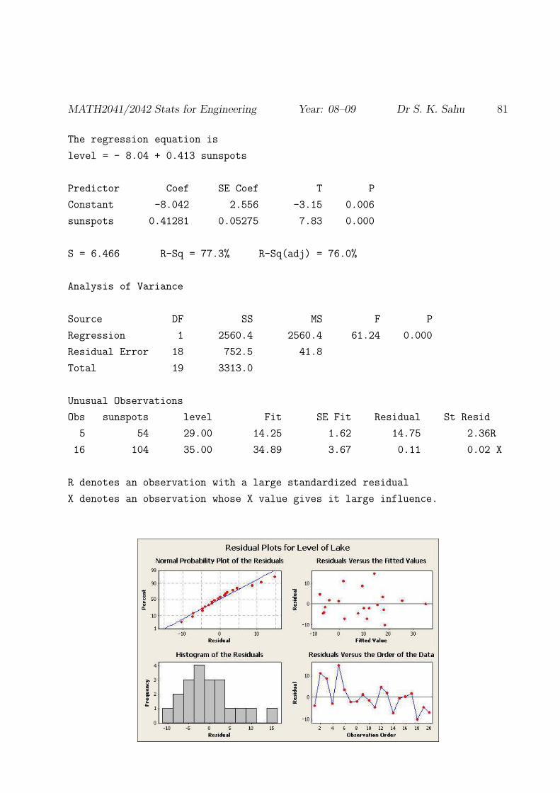
MATH2041/2042 Stats for Engineering Year: 08–09 Dr S. K. Sahu 81
The regression equation is
level = - 8.04 + 0.413 sunspots
Predictor Coef SE Coef T P
Constant -8.042 2.556 -3.15 0.006
sunspots 0.41281 0.05275 7.83 0.000
S = 6.466 R-Sq = 77.3% R-Sq(adj) = 76.0%
Analysis of Variance
Source DF SS MS F P
Regression 1 2560.4 2560.4 61.24 0.000
Residual Error 18 752.5 41.8
Total 19 3313.0
Unusual Observations
Obs sunspots level Fit SE Fit Residual St Resid
5 54 29.00 14.25 1.62 14.75 2.36R
16 104 35.00 34.89 3.67 0.11 0.02 X
R denotes an observation with a large standardized residual
X denotes an observation whose X value gives it large influence.
PSfrag replacements
z
z
−z
z1
z2
c
−c
c
c
−c
c
−c

82
5.3 Multiple Regression
In many practical examples, the variability in the response variable Y is influenced by more
than one explanatory variable. For example, consider the data in the file soil.dat which
arise from the study of the phosphorus content of soil. Interest was focussed on how the
plant-available phosphorus (Y in ppm; c3) was related to two explanatory variables, the
inorganic phosphorus (X1 in ppm; c1) and a component of the organic phosphorus (X2 in
ppm; c2) of the soil.
It is very straightforward to extend the linear regression model when there is more than
one explanatory variable. Recall that for a single explanatory variable the linear regression
equation was
y = α + βx + ε
When we have two explanatory variables X1 and X2, we use the multiple regression
equation
y = α + β1x1 + β2x2 + ε
where the residual ε is a normally distributed random variable with zero mean and constant
standard deviation σ. (We can easily extend this to three or more explanatory variables).
Again, the coefficients α, β1 and β2 of the regression equation are unknown, so we estimate
them using the method of least squares, that is, we find estimates α, β1 and β2 which give
the smallest value of the sum of squares
D =
n∑
i=1
(yi − [α + β1x1i + β2x2i])2.
Here y1, . . . yn are the n values of the response variable and (x11, x21), . . . , (x1n, x2n) are
the corresponding n pairs of values of the explanatory variables.
The estimated regression equation
y = α + β1x1 + β2x2
can be used to predict future values of Y , at specified values of X1 and X2. In all
other aspects, multiple regression proceeds in exactly the same way as linear regression.
Confidence intervals for coefficients of the regression equation, or for predictions, can be
made. Confidence intervals are based on the t distribution with n−p−1 degrees of freedom,
where p is the number of explanatory variables.
Goodness-of-fit can still be assessed using the R2 coefficient, calculated and interpreted
in the same way, as the ‘proportion of natural variation in the response variable which has
been explained by the regression equation’. Residuals, now calculated using
εi = yi − (α + β1x1i + β2x2i)
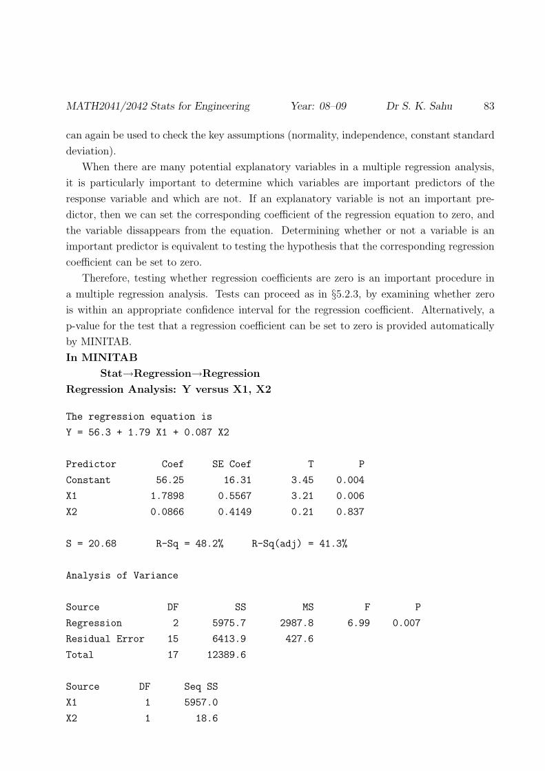
MATH2041/2042 Stats for Engineering Year: 08–09 Dr S. K. Sahu 83
can again be used to check the key assumptions (normality, independence, constant standard
deviation).
When there are many potential explanatory variables in a multiple regression analysis,
it is particularly important to determine which variables are important predictors of the
response variable and which are not. If an explanatory variable is not an important pre-
dictor, then we can set the corresponding coefficient of the regression equation to zero, and
the variable dissappears from the equation. Determining whether or not a variable is an
important predictor is equivalent to testing the hypothesis that the corresponding regression
coefficient can be set to zero.
Therefore, testing whether regression coefficients are zero is an important procedure in
a multiple regression analysis. Tests can proceed as in §5.2.3, by examining whether zero
is within an appropriate confidence interval for the regression coefficient. Alternatively, a
p-value for the test that a regression coefficient can be set to zero is provided automatically
by MINITAB.
In MINITAB
Stat→Regression→Regression
Regression Analysis: Y versus X1, X2
The regression equation is
Y = 56.3 + 1.79 X1 + 0.087 X2
Predictor Coef SE Coef T P
Constant 56.25 16.31 3.45 0.004
X1 1.7898 0.5567 3.21 0.006
X2 0.0866 0.4149 0.21 0.837
S = 20.68 R-Sq = 48.2% R-Sq(adj) = 41.3%
Analysis of Variance
Source DF SS MS F P
Regression 2 5975.7 2987.8 6.99 0.007
Residual Error 15 6413.9 427.6
Total 17 12389.6
Source DF Seq SS
X1 1 5957.0
X2 1 18.6

84
Unusual Observations
Obs X1 Y Fit SE Fit Residual St Resid
17 26.8 168.00 109.24 9.24 58.76 3.18R
R denotes an observation with a large standardized residual
There are many strategies for determining which explanatory variables are important pre-
dictors. One reasonable strategy is to fit the model with all possible predictors, determine if
any are not required (high p-value, so corresponding regression coefficient is not significantly
different from zero) and if so, ignore the explanatory variable which is least useful (highest
p-value). Then refit the model without this explanatory variable. Proceed like this until all
explanatory variables are useful predictors (low p-values, so corresponding regression coef-
ficients are significantly different from zero). Use this final model as your ‘best’ regression
model for prediction etc.
It is important that each time you decide to omit an explanatory variable, you refit the
regression before making another decision, as estimates and p-values will change.
The regression equation is
Y = 59.3 + 1.84 X1
Predictor Coef SE Coef T P
Constant 59.259 7.420 7.99 0.000
X1 1.8434 0.4789 3.85 0.001
S = 20.05 R-Sq = 48.1% R-Sq(adj) = 44.8%
Analysis of Variance
Source DF SS MS F P
Regression 1 5957.0 5957.0 14.82 0.001
Residual Error 16 6432.6 402.0
Total 17 12389.6
Unusual Observations
Obs X1 Y Fit SE Fit Residual St Resid
17 26.8 168.00 108.66 8.54 59.34 3.27R
R denotes an observation with a large standardized residual

MATH2041/2042 Stats for Engineering Year: 08–09 Dr S. K. Sahu 85
Note that there is not necessarily a single best model. You may find that two different
sets of explanatory variables provide similar explanantions of the variability in the response
variable. Then other considerations (such as scientific reasoning) may determine which
regression equation you prefer.
5.4 Fitting Curves
A regression analysis can also be used when the regression equation describing the way in
which the response variable Y depends on an explanatory variable X is not a straight line.
0 5 10 15 200.0
0.5
1.0
1.5
2.0
2.5
3.0
•
•
•
•
••• • •
•
•
••
•
•
••
•• •
•
•
•••
••
•
• •
•
••
••
••
••
•
•
• ••
•
•
•
•
• ••
•
•
•• ••
•
•
•
•
•
•
•
•••
•
•
••
•••
••
•
•
• •
PSfrag replacements
z
z
−z
z1
z2
c
−c
c
c
−c
c
−c0 5 10 15 20
0.0
0.5
1.0
1.5
2.0
2.5
3.0
••• •
•
•
•
••
•
•
•
•
•
•
•
•
•
•
•
•
•
••
•
•
•
•
•
•
• ••
•
•
•
••
•
•
•
•
•
•
•
•
•
•
•
•
•
•
•
•
•
••
•
•
•
•
•
•
•
•
•
• • •
•
••
•
•
•
•
•
•
•
•
PSfrag replacements
z
z
−z
z1
z2
c
−c
c
c
−c
c
−c
The simplest way to fit a curve is by using a polynomial regression equation. For
example
y = α + βx + γx2 + ε
y = α + βx + γx2 + δx3 + ε.
(More complicated polynomials are possible, but are rarely required in practice).
Again, the coefficients α, β, γ (and δ if required) of the regression equation are unknown,
so we estimate them using the method of least squares, that is, we find the values of the
coefficients which minimise the sum of squares of the distances between the data points and
the regression curve.
We can fit polynomial regression models in exactly the same way as we fitted multiple
regression models in §5.3. For example, for the quadratic model, we create a ‘new variable’ X 2
containing the values of x2 for each observation x of explanatory variable X. [In MINITAB,
Calc→Calculator can be used to achieve this.] Then, a quadratic regression is just a
multiple regression with explanatory variables X and X2.
Polynomial models can be fitted, confidence intervals calculated, predictions made, and
the model assessed by using R2 and residual plots, exactly as described in §5.2 and §5.3.
It is important to determine what kind of polynomial is required to describe the depen-
dence of Y on X. It is usual practice to start with a linear regression model and successively

86
add terms (X2, X3 etc.) until the coefficient of the term you are trying to add is not sig-
nificantly different from zero. (Note that is is rarely sensible to fit a polynomial model with
‘missing lower order terms’ e.g. if X3 is in the model, then X and X2 should be as well.)
PSfrag replacements
z
z
−z
z1
z2
c
−c
c
c
−c
c
−c
The regression equation is
level = - 8.24 + 0.427 sunspots - 0.00016 sunspots^2
Predictor Coef SE Coef T P
Constant -8.244 3.343 -2.47 0.025
sunspots 0.4275 0.1594 2.68 0.016
sunspots -0.000164 0.001671 -0.10 0.923
S = 6.651 R-Sq = 77.3% R-Sq(adj) = 74.6%
Analysis of Variance
Source DF SS MS F P
Regression 2 2560.9 1280.4 28.94 0.000
Residual Error 17 752.1 44.2
Total 19 3313.0
Source DF Seq SS
sunspots 1 2560.4
sunspots 1 0.4

MATH2041/2042 Stats for Engineering Year: 08–09 Dr S. K. Sahu 87
Unusual Observations
Obs sunspots level Fit SE Fit Residual St Resid
5 54 29.00 14.36 2.03 14.64 2.31R
16 104 35.00 34.44 5.92 0.56 0.18 X
R denotes an observation with a large standardized residual
X denotes an observation whose X value gives it large influence.
The estimated regression line (and associated confidence and predictive intervals) may
again be obtained, in MINITAB, using Stat→Regression→Fitted Line Plot.
PSfrag replacements
z
z
−z
z1
z2
c
−c
c
c
−c
c
−c
One additional way of determining whether or not you require further polynomial terms
in your model is to plot the residuals εi against the values xi of the explanatory variable X.
If any kind of pattern is evident, then further polynomial terms may help. Otherwise, the
plot should appear as a random scatter.
There are many other ways of fitting curves to data, outside the scope of this course.
One popular way is to consider transforming the data. For example, if the regression curve
takes the form
Y = αXβ
then we can write
log Y = log α + β log X.
Hence, if we transform our data points by taking logs, the relationship between the trans-
formed variables log Y and log X is described by a straight line, with intercept log α and
slope β.
88
Similarly if the regression curve takes the form
Y = αβX
then we can write
log Y = log α + X log β.
Hence, if we transform our data points by taking logs of the response variable Y (only), the
relationship between the transformed variable log Y and X is described by a straight line,
with intercept log α and slope log β.
The key to these approaches is transforming an awkward problem, based on complicated
curves, to a simple problem based on linear regression. If the relationship between Y and X
seems to be described by a curve, and a polynomial model does not fit well, then it may be
worth invesigating possible linear relationships between log Y and X or between log Y and
log X.
In MINITAB, Calc→Calculator can be used to create the transformed variables log Y
and log X.