math1051 calculus and linear algebra i - school of
TRANSCRIPT

MATH1051
CALCULUSAND
LINEAR ALGEBRA I
Semester 1, 2008Lecture Workbook Solutions
How to use this workbook
This book should be taken to lectures, tutorials and lab sessions. In the lectures,you will be expected to fill in the blanks in any incomplete definitions, theoremsetc, and any examples which appear. The lecturer will make it clear when theyare covering something that you need to complete.
The completed workbook will act as a study guide designed to assist you inworking through assignments and preparing for the mid-semester and final ex-ams. For this reason, it is very important to attend lectures.
The text for the calculus part of the course is “Calculus” by James Stewart,6th edition, 2008. We often refer to the text in this workbook, and many of thedefinitions, theorems, and examples come from the text. (References are alsoprovided for the 5th edition). It is strongly advised that you purchase a copy.
Although there is no set text for the linear algebra part of the course, thereare several books in the library which cover the material well (see the coursewebsite).
c©Mathematics, School of Physical Sciences, The University of Queensland, Brisbane QLD 4072, Australia
Edited by Phil Isaac, Birgit Loch, Joseph Grotowski, Mary Waterhouse, Victor Scharaschkin, Barbara Maen-
haut. July 2007.
1
Contents
1 Complex Numbers 9
1.1 Notation . . . . . . . . . . . . . . . . . . . . . . . . . . . . . . . 9
1.2 Complex Numbers . . . . . . . . . . . . . . . . . . . . . . . . . 9
1.3 Polar form . . . . . . . . . . . . . . . . . . . . . . . . . . . . . . 10
1.4 Euler’s formula . . . . . . . . . . . . . . . . . . . . . . . . . . . 12
2 Vectors 13
2.1 Revision . . . . . . . . . . . . . . . . . . . . . . . . . . . . . . . 13
2.2 Review Problems . . . . . . . . . . . . . . . . . . . . . . . . . . 20
3 Matrices and Linear Transformations 24
3.1 2× 2 matrices . . . . . . . . . . . . . . . . . . . . . . . . . . . . 24
3.2 Transformations of the plane . . . . . . . . . . . . . . . . . . . . 24
3.3 Translations . . . . . . . . . . . . . . . . . . . . . . . . . . . . . 25
3.4 Linear transformations . . . . . . . . . . . . . . . . . . . . . . . 26
3.5 Visualizing linear transformations . . . . . . . . . . . . . . . . . 27
3.6 Scalings . . . . . . . . . . . . . . . . . . . . . . . . . . . . . . . 28
3.7 Rotations . . . . . . . . . . . . . . . . . . . . . . . . . . . . . . 30
3.8 Reflections . . . . . . . . . . . . . . . . . . . . . . . . . . . . . . 31
3.9 Composing Linear Transformations; Matrix Multiplication . . . 34
3.10 Vectors in Rn . . . . . . . . . . . . . . . . . . . . . . . . . . . . 35
3.11 Properties of Dot Product . . . . . . . . . . . . . . . . . . . . . 37
3.12 Definition: Matrix . . . . . . . . . . . . . . . . . . . . . . . . . 37
3.13 Equality . . . . . . . . . . . . . . . . . . . . . . . . . . . . . . . 38
3.14 Addition . . . . . . . . . . . . . . . . . . . . . . . . . . . . . . . 38
3.15 Scalar Multiplication . . . . . . . . . . . . . . . . . . . . . . . . 38
3.16 Matrix Multiplication . . . . . . . . . . . . . . . . . . . . . . . . 39
3.17 Transposition . . . . . . . . . . . . . . . . . . . . . . . . . . . . 41
2

4 Vector Spaces 43
4.1 Linear combinations . . . . . . . . . . . . . . . . . . . . . . . . 43
4.2 Linear Independence . . . . . . . . . . . . . . . . . . . . . . . . 44
4.3 How to test for linear independence . . . . . . . . . . . . . . . . 44
4.4 Vector spaces . . . . . . . . . . . . . . . . . . . . . . . . . . . . 47
4.5 The span of vectors . . . . . . . . . . . . . . . . . . . . . . . . . 50
4.6 Bases . . . . . . . . . . . . . . . . . . . . . . . . . . . . . . . . . 52
4.7 Dimension . . . . . . . . . . . . . . . . . . . . . . . . . . . . . . 54
4.8 Components . . . . . . . . . . . . . . . . . . . . . . . . . . . . . 55
4.9 Further Properties of Bases . . . . . . . . . . . . . . . . . . . . 56
4.10 Orthogonal and Orthonormal . . . . . . . . . . . . . . . . . . . 57
4.11 Gram-Schmidt Algorithm . . . . . . . . . . . . . . . . . . . . . 59
5 Inverses 62
5.1 The Identity Matrix . . . . . . . . . . . . . . . . . . . . . . . . 62
5.2 Definition: Inverse . . . . . . . . . . . . . . . . . . . . . . . . . 63
5.3 Invertible Matrices and Linear Independence . . . . . . . . . . . 65
6 Gaussian elimination 71
6.1 Simultaneous equations . . . . . . . . . . . . . . . . . . . . . . . 71
6.2 Gaussian elimination . . . . . . . . . . . . . . . . . . . . . . . . 72
6.3 The general solution . . . . . . . . . . . . . . . . . . . . . . . . 82
6.4 Gauss-Jordan elimination . . . . . . . . . . . . . . . . . . . . . 85
7 Determinants 90
7.1 Definition: Determinant . . . . . . . . . . . . . . . . . . . . . . 90
7.2 Properties of Determinants . . . . . . . . . . . . . . . . . . . . . 92
7.3 Connection with inverses and systems of linear equations . . . . 97
8 Vector Products in 3-Space 99
8.1 Definition: Cross product . . . . . . . . . . . . . . . . . . . . . 99
8.2 Application: area of a triangle . . . . . . . . . . . . . . . . . . . 102
8.3 Scalar Triple Product . . . . . . . . . . . . . . . . . . . . . . . . 104
8.4 Geometrical Interpretation . . . . . . . . . . . . . . . . . . . . . 104
3

9 Eigenvalues and eigenvectors 106
9.1 Eigenvalues . . . . . . . . . . . . . . . . . . . . . . . . . . . . . 106
9.2 Eigenspace . . . . . . . . . . . . . . . . . . . . . . . . . . . . . . 107
9.3 How to find eigenvalues . . . . . . . . . . . . . . . . . . . . . . . 107
10 Numbers 114
10.1 Number systems . . . . . . . . . . . . . . . . . . . . . . . . . . 114
10.2 Real number line and ordering on R . . . . . . . . . . . . . . . . 114
10.3 Definition: Intervals . . . . . . . . . . . . . . . . . . . . . . . . . 115
10.4 Absolute value . . . . . . . . . . . . . . . . . . . . . . . . . . . 116
11 Functions 119
11.1 Notation . . . . . . . . . . . . . . . . . . . . . . . . . . . . . . . 119
11.2 Definition: Function, domain, range . . . . . . . . . . . . . . . . 119
11.3 Graphs . . . . . . . . . . . . . . . . . . . . . . . . . . . . . . . . 120
11.4 Convention (domain) . . . . . . . . . . . . . . . . . . . . . . . . 121
11.5 Caution (non-functions) . . . . . . . . . . . . . . . . . . . . . . 121
11.6 Vertical line test . . . . . . . . . . . . . . . . . . . . . . . . . . . 122
11.7 Exponential functions . . . . . . . . . . . . . . . . . . . . . . . . 123
11.8 Trigonometric functions (sin, cos, tan) . . . . . . . . . . . . . . 126
11.9 Composition of functions . . . . . . . . . . . . . . . . . . . . . . 131
11.10One-to-one (1-1) functions - Stewart, 6ed. pp. 385-388; 5ed.pp. 413-417 . . . . . . . . . . . . . . . . . . . . . . . . . . . . . 131
11.11Inverse Functions . . . . . . . . . . . . . . . . . . . . . . . . . . 133
11.12Logarithms - Stewart, 6ed. p. 405; 5ed. p. 434 . . . . . . . . . . 135
11.13Natural logarithm . . . . . . . . . . . . . . . . . . . . . . . . . . 135
11.14Inverse trigonometric functions . . . . . . . . . . . . . . . . . . 138
12 Limits 146
12.1 Definition: Limit - Stewart, 6ed. p. 66; 5ed. p. 71 . . . . . . . . 146
12.2 One-sided limits . . . . . . . . . . . . . . . . . . . . . . . . . . . 150
12.3 Theorem: Squeeze principle . . . . . . . . . . . . . . . . . . . . 152
12.4 Limits as x approaches infinity . . . . . . . . . . . . . . . . . . . 153
12.5 Some important limits . . . . . . . . . . . . . . . . . . . . . . . 157
4

13 Continuity 163
13.1 Definition: Continuity . . . . . . . . . . . . . . . . . . . . . . . 163
13.2 Definition: Continuity on intervals . . . . . . . . . . . . . . . . . 165
13.3 Properties . . . . . . . . . . . . . . . . . . . . . . . . . . . . . . 166
13.4 Intermediate Value Theorem (IVT) - Stewart, 6ed. p. 104; 5ed.p. 109 . . . . . . . . . . . . . . . . . . . . . . . . . . . . . . . . 167
13.5 Application of IVT (bisection method) . . . . . . . . . . . . . . 167
14 Derivatives 171
14.1 Tangents . . . . . . . . . . . . . . . . . . . . . . . . . . . . . . . 171
14.2 Definition: Derivative, differentiability . . . . . . . . . . . . . . 172
14.3 Theorem: Differentiability implies continuity . . . . . . . . . . . 174
14.4 Rates of change - Stewart, 6ed. p. 117; 5ed. p. 117 . . . . . . . 174
14.5 Higher derivatives . . . . . . . . . . . . . . . . . . . . . . . . . . 176
14.6 Rules for differentiation . . . . . . . . . . . . . . . . . . . . . . . 176
14.7 The chain rule - Stewart, 6ed. p. 156; 5ed. p. 176 . . . . . . . . 178
14.8 Derivative of inverse function . . . . . . . . . . . . . . . . . . . 180
14.9 L’Hopital’s rule - Stewart, 6ed. p. 472; 5ed. p. 494 . . . . . . . . 182
14.10The Mean Value Theorem (MVT) . . . . . . . . . . . . . . . . . 183
14.11Definition: Increasing/Decreasing . . . . . . . . . . . . . . . . . 184
14.12Increasing/Decreasing test - Stewart, 6ed. p. 221; 5ed. p. 240 . . 184
14.13Definition: Local maxima and minima . . . . . . . . . . . . . . 185
14.14First derivative test . . . . . . . . . . . . . . . . . . . . . . . . . 187
14.15Second derivative test . . . . . . . . . . . . . . . . . . . . . . . . 188
14.16Extreme value theorem - Stewart, 6ed. p. 206; 5ed. p. 225 . . . 192
14.17Optimization problems . . . . . . . . . . . . . . . . . . . . . . . 193
15 Integration 199
15.1 Definition: Anti-derivative - Stewart, 6ed. p. 274; 5ed. p. 300 . . 199
15.2 Definition: Indefinite integral . . . . . . . . . . . . . . . . . . . 200
15.3 Area under a curve - Stewart, 6ed. pp. 289-296; 5ed. p. 315-322 200
5

15.4 Fundamental Theorem of Calculus . . . . . . . . . . . . . . . . 203
15.5 Approximate integration (trapezoidal rule) . . . . . . . . . . . . 207
15.6 Improper integrals - Stewart, 6ed. pp. 544-551; 5ed. pp. 566-573 208
15.7 Techniques of integration - Stewart, 6ed. ch. 8; 5ed. ch. 8 . . . . 210
15.8 Integrals involving ln function . . . . . . . . . . . . . . . . . . . 215
15.9 Integration of rational functions by partial fractions . . . . . . . 215
15.10Volumes of revolution . . . . . . . . . . . . . . . . . . . . . . . . 222
16 Sequences 226
16.1 Formal Definition: Sequence . . . . . . . . . . . . . . . . . . . . 226
16.2 Representations . . . . . . . . . . . . . . . . . . . . . . . . . . . 226
16.3 Application: Rabbit population - Stewart, 6ed. p. 722 ex. 71;5ed. p. 748 ex. 65 . . . . . . . . . . . . . . . . . . . . . . . . . . 229
16.4 Limits . . . . . . . . . . . . . . . . . . . . . . . . . . . . . . . . 229
16.5 Theorem: Limit laws . . . . . . . . . . . . . . . . . . . . . . . . 231
16.6 Theorem: Squeeze . . . . . . . . . . . . . . . . . . . . . . . . . 231
16.7 Theorem: Continuous extension . . . . . . . . . . . . . . . . . . 232
16.8 Useful sequences to remember . . . . . . . . . . . . . . . . . . . 233
16.9 Application: Logistic sequence . . . . . . . . . . . . . . . . . . . 233
17 Series 237
17.1 Infinite sums (notation) . . . . . . . . . . . . . . . . . . . . . . 237
17.2 Motivation . . . . . . . . . . . . . . . . . . . . . . . . . . . . . . 237
17.3 Definition: Convergence - Stewart, 6ed. p. 724; 5ed. p. 750 . . . 238
17.4 Theorem: p test . . . . . . . . . . . . . . . . . . . . . . . . . . . 239
17.5 Theorem: nth term test - Stewart, 6ed. p. 728; 5ed. p. 754 . . . 240
17.6 Test for divergence (nth term test) . . . . . . . . . . . . . . . . 240
17.7 Example: Geometric series . . . . . . . . . . . . . . . . . . . . . 241
17.8 Application: Bouncing ball - Stewart, 6ed. p. 731 qn 58; 5ed.p. 756 qn 52 . . . . . . . . . . . . . . . . . . . . . . . . . . . . . 244
17.9 Convergence theorem and limit laws . . . . . . . . . . . . . . . . 247
6
17.10Comparison tests . . . . . . . . . . . . . . . . . . . . . . . . . . 248
17.11Theorem: Comparison test - Stewart, 6ed. p. 741; 5ed. p. 767 . 248
17.12Alternating series . . . . . . . . . . . . . . . . . . . . . . . . . . 249
17.13Theorem: Alternating series test - Stewart, 6ed. p. 746; 5ed. p. 772250
17.14Definition: Absolute/conditional convergence . . . . . . . . . . . 252
17.15Theorem: Ratio test - Stewart, 6ed. p. 752; 5ed. p. 778 . . . . . 254
18 Power series and Taylor series 258
18.1 Definition: Power series . . . . . . . . . . . . . . . . . . . . . . . 258
18.2 Theorem: Defines radius of convergence - Stewart, 6ed. p. 752;5ed. p. 787 . . . . . . . . . . . . . . . . . . . . . . . . . . . . . 259
18.3 Radius of convergence . . . . . . . . . . . . . . . . . . . . . . . 260
18.4 Taylor series . . . . . . . . . . . . . . . . . . . . . . . . . . . . . 261
18.5 Theorem: Formula for Taylor series . . . . . . . . . . . . . . . . 262
18.6 Binomial series . . . . . . . . . . . . . . . . . . . . . . . . . . . 267
19 Appendix - Practice Problems 271
19.1 Numbers . . . . . . . . . . . . . . . . . . . . . . . . . . . . . . . 271
19.2 Functions . . . . . . . . . . . . . . . . . . . . . . . . . . . . . . 271
19.3 Limits . . . . . . . . . . . . . . . . . . . . . . . . . . . . . . . . 273
19.4 Continuity . . . . . . . . . . . . . . . . . . . . . . . . . . . . . . 274
19.5 Derivatives . . . . . . . . . . . . . . . . . . . . . . . . . . . . . . 274
19.6 Integration . . . . . . . . . . . . . . . . . . . . . . . . . . . . . . 277
19.7 Sequences . . . . . . . . . . . . . . . . . . . . . . . . . . . . . . 279
19.8 Series . . . . . . . . . . . . . . . . . . . . . . . . . . . . . . . . . 279
19.9 Power series and Taylor series . . . . . . . . . . . . . . . . . . . 281
19.10Vectors . . . . . . . . . . . . . . . . . . . . . . . . . . . . . . . . 282
19.11Matrix Algebra . . . . . . . . . . . . . . . . . . . . . . . . . . . 285
20 Appendix - Mathematical notation 289
7

21 Appendix - Basics 290
21.1 Powers . . . . . . . . . . . . . . . . . . . . . . . . . . . . . . . . 290
21.2 Multiplication/Addition of real numbers . . . . . . . . . . . . . 291
21.3 Fractions . . . . . . . . . . . . . . . . . . . . . . . . . . . . . . . 292
21.4 Solving quadratic equations . . . . . . . . . . . . . . . . . . . . 292
21.5 Surds . . . . . . . . . . . . . . . . . . . . . . . . . . . . . . . . . 295
8

1 Complex Numbers
1.1 Notation
The symbol ∈ means “is an element of”. Thus we write
x ∈ R
to mean x is an element of R. That is, x is a real number. Hence, we can write,for example, 2 ∈ R, π ∈ R, −
√3 ∈ R, and so forth.
1.2 Complex Numbers
Complex numbers were introduced in the 16th century to obtain roots of poly-nomial equations. A complex number is of the form
z = x + iy
where x, y ∈ R and i is (formally) a symbol satisfying i2 = −1. The quantity xis called the real part of z and y is called the imaginary part of z.
The set of all complex numbers is denoted C. Thus 3− 2i ∈ C.
1.2.1 Example
The real part of 3− 2i is 3 and the imaginary part is −2 (not −2i).
Complex numbers can be added and multiplied by replacing i2 everywhere with−1. For example (2i)2 = 4i2 = −4.
1.2.2 Example
Simplify (3− 2i)(1 + i).
(3− 2i)(1 + i) = 3 + 3i− 2i− 2i2
= 3 + i + 2 = 5 + i
1.2.3 Example
Suppose a, b ∈ R. Simplify (a + bi)(a− bi).
(a + bi)(a− bi) = a2 − abi + abi − b2i2
= a2 + b2
9

1.2.4 Example
Simplify3− 2i
1− i.
3− 2i
1− i=
3− 2i
1− i× (1 + i)
(1 + i)
=(3− 2i)(1 + i)
12 + 12
=1
2(3− 2i)(1 + i)
=1
2(5 + i)
=5
2+
1
2i
It is a fact that if we consider complex roots of polynomials and count themwith their correct multiplicity, then a polynomial of degree n always has n roots.For example, every quadratic has two roots.
1.2.5 Example
Find the roots of x2 + 2x + 2 = 0.
x2 + 2x + 2 = (x + 1)2 + 1 = 0
⇐⇒ (x + 1)2 = −1 = i2
⇐⇒ x + 1 = ±i
∴ x = −1± i are the roots.
Alternatively use the quadratic formula:
x =1
2(−2±
√4− 8) =
1
2(−2± 2i)
= −1± i.
1.3 Polar form
A complex number z = x + iy may be represented by a point in the complexplane where the vertical axis is the imaginary axis and the horizontal axis is thereal axis.
10
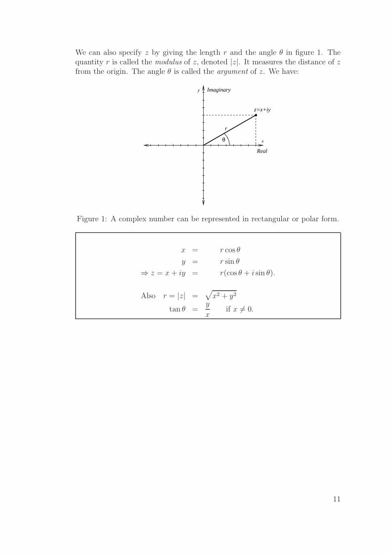
We can also specify z by giving the length r and the angle θ in figure 1. Thequantity r is called the modulus of z, denoted |z|. It measures the distance of zfrom the origin. The angle θ is called the argument of z. We have:
x
y
Real
Imaginary
θ
z=x+iy
r
Figure 1: A complex number can be represented in rectangular or polar form.
x = r cos θ
y = r sin θ
⇒ z = x + iy = r(cos θ + i sin θ).
Also r = |z| =√
x2 + y2
tan θ =y
xif x 6= 0.
11

1.3.1 Example
Write z = 1 + i in polar form.
First find the modulus:|z| =
√1 + 1 =
√2.
We have for the argument tan θ =y
x, so we can take
θ = arctany
x= arctan 1
=π
4
∴ z =√
2(
cosπ
4+ i sin
π
4
)
.
1.4 Euler’s formula
Euler’s formula states for any real number θ:
cos θ + i sin θ = eiθ.
(To make sense of this, one has to define the exponential function for complexarguments. This may be done using a series.)
Thus every complex number z = x + iy can be represented in polar form
z = reiθ.
12

2 Vectors
• A vector quantity has both a magnitude and a direction; force and velocityare two examples of vector quantities.
• A scalar quantity has only a magnitude (it has no direction); time, areaand temperature are examples of scalar quantities.
2.1 Revision
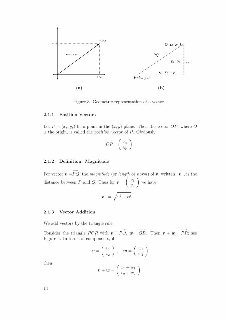
A vector is represented geometrically in the (x, y) plane or in (x, y, z) space bya directed line segment (arrow). The direction of the arrow is the direction ofthe vector, and the length of the arrow is proportional to the magnitude of thevector. Only the length and direction of the arrow are significant: it can beplaced anywhere convenient in the (x, y) plane.
x
y
Figure 2: Vector of unit length at 45◦ to x-axis has many representations asshown.
If P , Q are points in 2-space or 3-space,−→PQ denotes the vector from P to Q.
A vector v =−→PQ in the (x, y) plane may be represented by a pair of numbers
v =
(v1
v2
)
=
(xQ − xP
yQ − yP
)
which is the same for all representations−→PQ of v. We call v1, v2 the components
of the vector v.
We call the vector
(00
)
the zero vector. It is denoted by 0.
13
21v=<v ,v >
2
21
1x=v
(v ,v )y=v
2
1 v
= v
=
P
PQ
Q
PP
y −y
x −x
Q=(x ,y )
P=(x ,y )
PQ
(a) (b)
Figure 3: Geometric representation of a vector.
2.1.1 Position Vectors
Let P = (xp, yp) be a point in the (x, y) plane. Then the vector−→OP , where O
is the origin, is called the position vector of P . Obviously
−→OP=
(xp
yp
)
.
2.1.2 Definition: Magnitude
For vector v =−→PQ, the magnitude (or length or norm) of v, written ‖v‖, is the
distance between P and Q. Thus for v =
(v1
v2
)
we have
‖v‖ =√
v21 + v2
2.
2.1.3 Vector Addition
We add vectors by the triangle rule.
Consider the triangle PQR with v =−→PQ, w =
−→QR. Then v + w =
−→PR; see
Figure 4. In terms of components, if
v =
(v1
v2
)
, w =
(w1
w2
)
then
v + w =
(v1 + w1
v2 + w2
)
.
14

P
Q
R
Figure 4:−→PQ +
−→QR=
−→PR
It follows from the component description that vector addition satisfies thefollowing properties:
v + w = w + v (commutative law)
u + (v + w) = (u + v) + w (associative law)
v + 0 = 0 + v = v
2.1.4 Scalar multiplication
α
2
1
2
1
v
v
v
v
α
αv
v
Figure 5: We can multiply the vector v by a number α (scalar).
With α ∈ R a number (called a scalar), we define αv to be the vector ofmagnitude
‖αv‖ = |α| · ‖v‖in the same direction as v if α > 0 and opposite direction if α < 0.
Using similar triangles it follows that if v =
(v1
v2
)
then αv =
(αv1
αv2
)
.
15

Note that if we multiply any vector v =
(v1
v2
)
by zero we obtain the zero
vector:
0 · v =
(00
)
= 0
2.1.5 Unit Vectors
A unit vector is a vector of unit length. If v 6= 0 is a vector, then
v
‖v‖
determines a unit vector in the direction of v.
In particular
i =
(10
)
, j =
(01
)
determine unit vectors along the x and y axes respectively.
x
y
ij
Figure 6: Unit vectors i and j in the x and y directions respectively.
For any vector v =
(v1
v2
)
we have
v =
(v1
0
)
+
(0v2
)
= v1i + v2j,
Hence we can decompose v into a vector v1i along the x-axis and v2j along they-axis. Then v1 and v2 are called the components of v with respect to i and j.
16

2.1.6 Vectors in 3-space
Similarly in 3-space a vector v =−→PQ is represented in component form by
v =
v1
v2
v3
=
xQ − xP
yQ − yP
zQ − zP
which is the same for all representations−→PQ of v.
P
N
3
2
1
v
v
v
z
y
x
v
Figure 7: A vector in 3-space.
For v =−→OP=
v1
v2
v3
the magnitude of the vector v is
‖v‖ =√
ON2 + NP 2 =√
v21 + v2
2 + v23.
As before, we add vectors component by component. We also define multipli-cation by a scalar α. So if
v =
v1
v2
v3
, w =
w1
w2
w3
are vectors then
v + w =
v1 + w1
v2 + w2
v3 + w3
and αv =
αv1
αv2
αv3
, for α ∈ R.
17
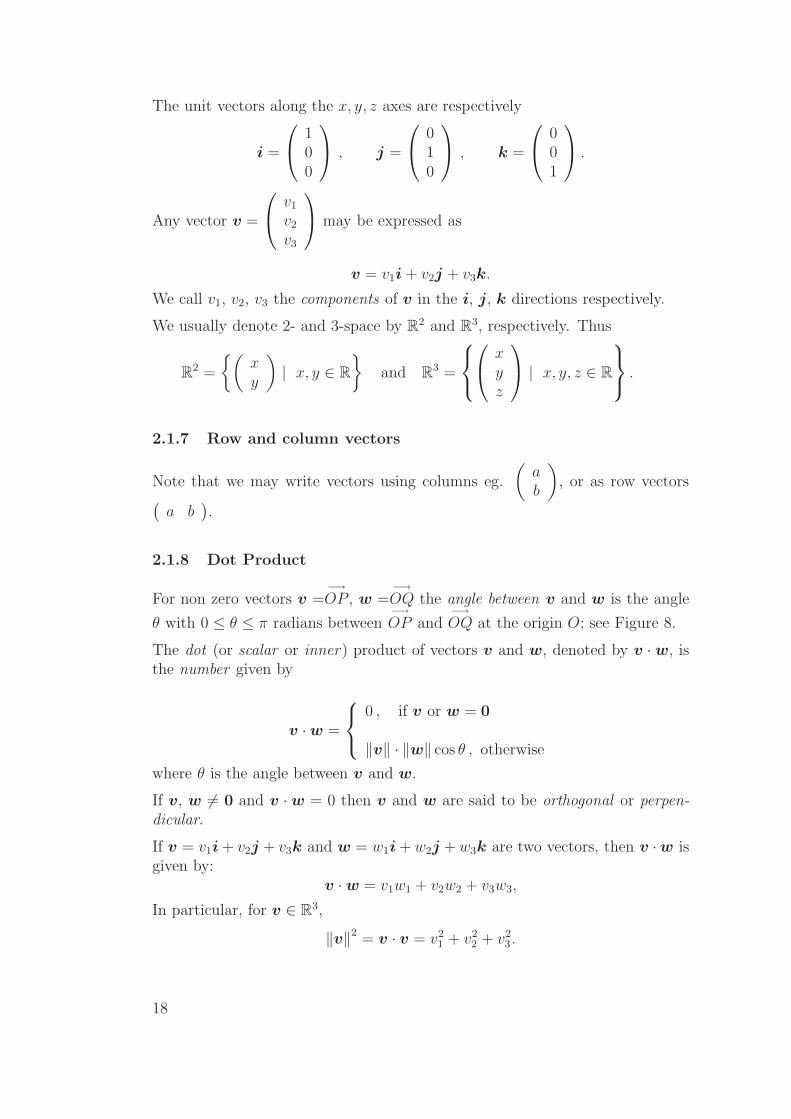
The unit vectors along the x, y, z axes are respectively
i =
100
, j =
010
, k =
001
.
Any vector v =
v1
v2
v3
may be expressed as
v = v1i + v2j + v3k.
We call v1, v2, v3 the components of v in the i, j, k directions respectively.
We usually denote 2- and 3-space by R2 and R3, respectively. Thus
R2 =
{(xy
)
| x, y ∈ R
}
and R3 =
xyz
| x, y, z ∈ R
.
2.1.7 Row and column vectors
Note that we may write vectors using columns eg.
(ab
)
, or as row vectors(
a b).
2.1.8 Dot Product
For non zero vectors v =−→OP , w =
−→OQ the angle between v and w is the angle
θ with 0 ≤ θ ≤ π radians between−→OP and
−→OQ at the origin O; see Figure 8.
The dot (or scalar or inner) product of vectors v and w, denoted by v ·w, isthe number given by
v ·w =
0 , if v or w = 0
‖v‖ · ‖w‖ cos θ , otherwise
where θ is the angle between v and w.
If v, w 6= 0 and v ·w = 0 then v and w are said to be orthogonal or perpen-dicular.
If v = v1i + v2j + v3k and w = w1i + w2j + w3k are two vectors, then v ·w isgiven by:
v ·w = v1w1 + v2w2 + v3w3,
In particular, for v ∈ R3,
‖v‖2 = v · v = v21 + v2
2 + v23.
18

x
y
θ
vw
Figure 8: θ is the angle between v and w.
2.1.9 The Projection Formula
Fix a vector v. Given another vector w we can write it as
w = w1 + w2,
where w1 is in the direction of v and w2 is perpendicular to v; see Figure 9.
y
x
2
1w
w
w
v
Figure 9: w can be decomposed into a component w1 in the direction of v anda component w2 perpendicular to v.
Then we have the projection formula:
w1 =(w · v)
‖v‖2v , w2 = w − (w · v)
‖v‖2v. (2.1)
19

2.2 Review Problems
2.2.1 Example
A zeppelin is directed NE at 20 km/h into a 10 km/h wind in direction E60◦S.Find the actual speed and direction of the airship.
θ
v
o60
10
o45
20
Figure 10: v gives the velocity vector of the zeppelin.
There holds:
z = 20 cos 45◦i + 20 sin 45◦j
= 10√
2i + 10√
2j;
w = 10 cos 60◦i− 10 sin 60◦j
= 5i− 5√
3j.
20

So v = z + w = (10√
2 + 5)i + (10√
2− 5√
3)jTherefore the magnitude of v is
‖v‖ =
√
(10√
2 + 5)2 + (10√
2− 5√
3)2
=
√
500 + 100√
2(1−√
3)
≈ 19.91.
To calculate the angle θ we use
tan θ =10√
2− 5√
3
10√
2 + 5
⇒ θ ≈ 15.98◦
So v = 19.9kmh−1 at E16◦N.
21

2.2.2 Example
Find the angle θ between the following pairs of vectors:
(i) v =
001
, w =
022
(ii) v =
1−5
4
, w =
333
Note cos θ =v ·w
‖v‖ · ‖w‖ . So:
(i)
‖v‖ = 1
‖w‖ =√
0 + 4 + 4 = 2√
2
v ·w = 0 + 0 + 2 = 2
∴ cos θ =2
2√
2=
1√2
⇒ θ =π
4
(ii) v ·w = 1 · 3− 5 · 3 + 4 · 3 = 0
So the vectors are perpendicular, i.e. θ =π
2.
2.2.3 Example
If P = (2, 4,−1), Q = (1, 1, 1), R = (−2, 2, 3), find the angle θ = PQR.
−→QP =
24−1
−
111
=
13−2
,
−→QR =
−223
−
111
=
−312
.
∴
∥∥∥
−→QP
∥∥∥ =
∥∥∥
−→QR
∥∥∥ =√
1 + 9 + 4 =√
14.
22

−→QP ·
−→QR =
13−2
·
−312
= −3 + 3− 4 = −4
∴ cos θ =
−→QP ·
−→QR
∥∥∥
−→QP
∥∥∥ ·
∥∥∥
−→QR
∥∥∥
=−4
14⇒ θ ≃ 107◦.
23

3 Matrices and Linear Transformations
3.1 2× 2 matrices
Recall that a 2× 2 array of numbers
A =
(a bc d
)
is called a 2×2 matrix. Suppose v =
(xy
)
is a 2 element column vector. Then
the product Av is defined to be the 2 element column vector whose entries aregiven by taking the dot product of each row of A with the vector v:
Av =
(a bc d
)(xy
)
=
(ax + bycx + dy
)
.
3.1.1 Example
Let A =
(1 23 4
)
, and let v =
(56
)
. Calculate Av.
Av =
(1 23 4
) (56
)
=
(1 · 5 + 2 · 63 · 5 + 4 · 6
)
=
(1739
)
.
3.2 Transformations of the plane
• In computer graphics there is often a need to transform a set of points,or a figure, that appears on the screen. For example, moving the figureto another part of the screen, rotating the figure about a central point,reflecting the figure in a line, scaling the figure to a new size, or shootingat moving things.
• Moving a figure about in the (x, y)-plane can be described by the additionof a vector (the translation vector) to each of the position vectors of thepoints making up the figure.
24

• Transformations such as rotations, reflections and scalings, are examplesof a special class of transformations called linear transformations.
• A linear transformation of the (x, y)-plane can be represented by a 2× 2matrix, and we can use matrix multiplication to calculate the effect of thetransformation on the points of the plane (using position vectors).
• Transformations of the plane have important applications in computergraphics and other areas.
3.2.1 Transformations of the plane
• A transformation of the (x, y)-plane is an operation (function) that mapseach point of the (x, y)-plane to some other point of the (x, y)-plane.
• If a transformation maps the point P with coordinates (x, y) to the pointP ′ with coordinates (x′, y′), then we call P the original point and P ′ theimage point.
• For particular transformations, we are given, or can determine, a formulafor x′ and y′ in terms of x and y.
3.2.2 Example
Find the coordinates of the image points of A = (2, 1) and B = (−1, 3) underthe transformation defined by
x′ = 2x− y and y′ = x2 + y,
and sketch the points and their images.
3.3 Translations
• A translation is a transformation that involves shifting each point of theplane a certain distance in the same direction.
• The translation in which each point is shifted a units in the x-directionand b units in the y-direction can be described by the equations x′ =x + a and y′ = y + b.
• This translation can be described in terms of vectors. If p is the positionvector of the original point P = (x, y), p′ is the position vector of the
image point P ′ = (x′, y′), and t =
(ab
)
is the translation vector, then
p′ = p + t, that is,
(x′
y′
)
=
(xy
)
+
(ab
)
.
25

• A translation shifts each point the same distance in the same direction, sothe shape of figures is preserved.
3.3.1 Example
Draw the triangle with vertices A = (1, 3), B = (−2, 1) and C = (0,−2). Then
draw its image under the translation having translation vector t =
(4−1
)
.
3.4 Linear transformations
• A linear transformation of the plane is a transformation that maps thepoint (x, y) to the point (x′, y′) where
x′ = ax + by and y′ = cx + dy,
for some real numbers a, b, c and d.
• Such a linear transformation can be represented by the 2× 2 matrix A =(a bc d
)
as follows:
• If p is the position vector of the original point P = (x, y) and p′ is the posi-tion vector of the image point P ′ = (x′, y′), then the linear transformationrepresented by the matrix A can be described by the equation
p′ = Ap, that is,
(x′
y′
)
=
(a bc d
) (xy
)
.
• A linear transformation preserves straight lines. When a linear transfor-mation is applied to a figure, points that are collinear in the original figuremap to collinear points in the new figure.
• A linear transformation preserves parallelism. When a linear transforma-tion is applied to a figure, lines that are parallel in the original figure mapto lines that are parallel in the new figure.
• A linear transformation maps the origin to itself, since A0 = 0. Note thattranslations are not linear transformations, except for translatoin by 0,i.e., the identity transformation.
3.4.1 Example
Are the following transformations linear? If so, write down the matrix repre-senting the transformation, if not, explain why not.
26

(a) x′ = x + 2y y′ = y − x
(b) x′ = x + 2 y′ = y − 1
(c) x′ = 0 y′ = 0
(d) x′ = 2 y′ = −3
(a) This is linear, represented by the matrix
(1 2−1 1
)
.
(b) This is not linear. The origin is not mapped to the origin:
T
(00
)
=
(2−1
)
6=(
00
)
.
(c) This is linear, represented by the zero matrix
(0 00 0
)
.
(d) This is not linear:
T
(00
)
=
(2−3
)
6=(
00
)
.
3.5 Visualizing linear transformations
• The linear transformation represented by the matrix A maps (1, 0) and(0, 1) to points whose position vectors are the first and second columns ofA, respectively, since
Ai =
(a bc d
) (10
)
=
(ac
)
and
Aj =
(a bc d
) (01
)
=
(bd
)
.
• Let a and b be the position vectors given by the first and second columnsof A, respectively.
Thus a =
(ac
)
and b =
(bd
)
.
27
• The linear transformation represented by A will map the point (x, y) to
(a bc d
) (xy
)
=
(ax + bycx + dy
)
= x
(ac
)
+ y
(bd
)
.
Thus the point (x, y) is mapped to the point whose position vector isxa + yb = xAi + yAj. The linear transformation will be determined oncewe know where i and j map to.
• These facts, along with the knowledge that linear transformations pre-serve linearity and parallelism, allow us to visualize the effect of a lineartransformation by considering the effect of the transformation on the unitgrid.
3.6 Scalings
• A scaling of the plane is a stretching (or shrinking) of the plane in twodirections, horizontally and vertically.
• A scaling (or dilation) of the plane is a linear transformation.
• The amount of stretching (or shrinking) of a figure under a scaling isdetermined by two parameters, the scaling factor in the x-direction andthe scaling factor in the y-direction. When listing the two scaling factors,we will always list the factor in the x-direction first.
• If one (or both) of the scaling factors is negative, then the image will bereflected in one (or both) of the axes as well as being scaled.
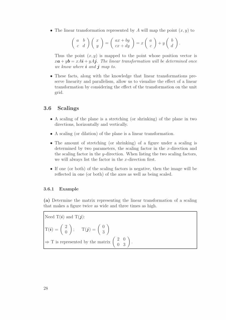
3.6.1 Example
(a) Determine the matrix representing the linear transformation of a scalingthat makes a figure twice as wide and three times as high.
Need T(i) and T(j):
T(i) =
(20
)
; T(j) =
(03
)
⇒ T is represented by the matrix
(2 00 3
)
.
28

(b) Use the matrix from part a) to determine the image of the point (2, 3) underthis scaling.
(x′
y′
)
= A
(xy
)
=
(a bc d
) (xy
)
=
(2 00 3
) (23
)
=
(49
)
.
We now determine the matrix representing a scaling with factor g in the x-direction and factor h in the y-direction.
First we must find the images of the position vectors i and j.
g i
hj
i
j
y
x
The image of i is the position vector(
g
0
)
. The image of j is(
0h
)
.
Thus the matrix representing a scaling with factors g and h is
Dg,h =
(g 00 h
)
.
29

3.7 Rotations
• A rotation of the plane about the origin is a linear transformation. A ro-tation about any other point is not, because the origin will not be mappedto the origin.
• A rotation of the plane through an angle θ will mean an anti-clockwiserotation of the plane about the origin through an angle θ.
3.7.1 Example
(a) Determine the matrix that represents the linear transformation of anti-clockwise rotation through an angle of π/2 radians about the origin.
T(i) = j =
(01
)
; T(j) = −i =
(−10
)
.
Hence the transform is represented by the matrix
(0 −11 0
)
.
(b) Use the matrix from part a) to determine the image of (2, 3) under thisrotation.
The point (2, 3) is sent to
(0 −11 0
) (23
)
=
(−32
)
.
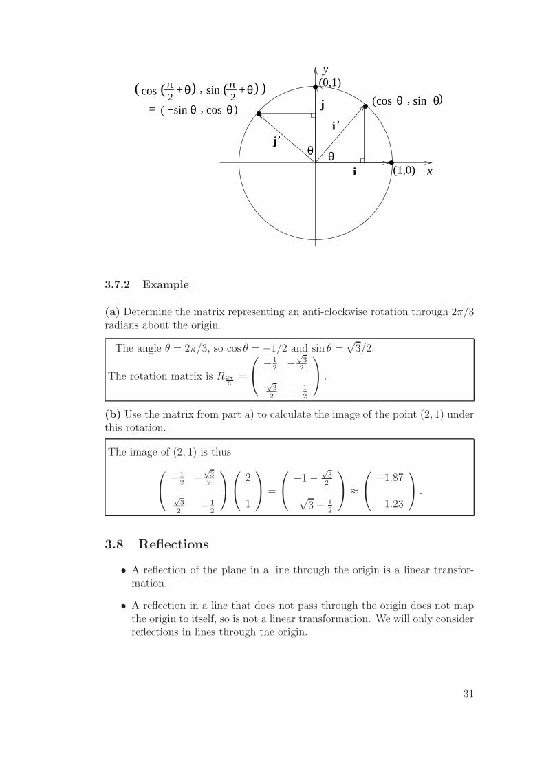
We now determine the general matrix that represents an anti-clockwise rotationthrough an angle θ about the origin.
We must find the images of the position vectors i and j. Recall the definitionof sin θ and cos θ in terms of the unit circle.
The image of i is the position vector
(cos θsin θ
)
. The image of j is
(− sin θ
cos θ
)
.
Thus the matrix representing an anti-clockwise rotation through an angle θabout the origin is
Rθ =
(cos θ − sin θsin θ cos θ
)
.
30
i ’
cos θ sin θ,( )
j’
__π2
+ θ( ) __π2
+ θ( )cos , sin )(
cos θ−sin θ ,( )
xθ
i (1,0)
θ
j
(0,1)y
=
3.7.2 Example
(a) Determine the matrix representing an anti-clockwise rotation through 2π/3radians about the origin.
The angle θ = 2π/3, so cos θ = −1/2 and sin θ =√
3/2.
The rotation matrix is R 2π3
=
−12−
√3
2
√3
2−1
2
.
(b) Use the matrix from part a) to calculate the image of the point (2, 1) underthis rotation.
The image of (2, 1) is thus
−12−
√3
2
√3
2−1
2
2
1
=
−1−√
32
√3− 1
2
≈
−1.87
1.23
.
3.8 Reflections
• A reflection of the plane in a line through the origin is a linear transfor-mation.
• A reflection in a line that does not pass through the origin does not mapthe origin to itself, so is not a linear transformation. We will only considerreflections in lines through the origin.
31
• When the plane is reflected in a line through the origin, points on theline of reflection remain fixed. A point P not on the line of reflection ismapped to a point P ′ on the opposite side of the line, such that the pointsP and P ′ are equidistant from the line of reflection and the line throughP and P ′ is perpendicular to the line of reflection.
3.8.1 Example
Determine the matrix representing the linear transformation of reflection in thex-axis.
T(i) =
(10
)
; T(j) =
(0−1
)
.
Hence A =
(1 00 −1
)
.
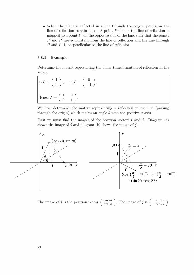
We now determine the matrix representing a reflection in the line (passingthrough the origin) which makes an angle θ with the positive x-axis.
First we must find the images of the position vectors i and j. Diagram (a)shows the image of i and diagram (b) shows the image of j.
i ’
cos 2 θ( sin 2 θ),
y
xθ
sin 2 θ( ,−cos 2 θ)=
__π2
2θ( ) __π2
2θ( )cos , −sin( )j’
__π2 θ
__π2
i (1,0)
θj
(0,1)
y
xθ
2θ
The image of i is the position vector(
cos 2θ
sin 2θ
)
. The image of j is(
sin 2θ
− cos 2θ
)
.
32
Thus the matrix representing a reflection in the line through the origin, thatmakes an angle θ with the positive x-axis is
Qθ =
(cos 2θ sin 2θsin 2θ − cos 2θ
)
.
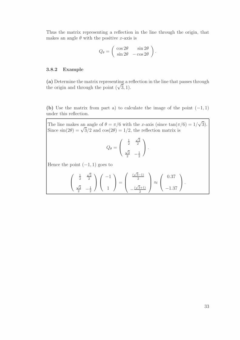
3.8.2 Example
(a) Determine the matrix representing a reflection in the line that passes throughthe origin and through the point (
√3, 1).
(b) Use the matrix from part a) to calculate the image of the point (−1, 1)under this reflection.
The line makes an angle of θ = π/6 with the x-axis (since tan(π/6) = 1/√
3).Since sin(2θ) =
√3/2 and cos(2θ) = 1/2, the reflection matrix is
Qθ =
12
√3
2
√3
2−1
2
.
Hence the point (−1, 1) goes to
12
√3
2
√3
2−1
2
−1
1
=
(√
3−1)2
− (√
3+1)2
≈
0.37
−1.37
.
33
3.9 Composing Linear Transformations; Matrix Multi-plication
Suppose we perform two linear transformations, one after the other. Suppose
the first transformation we perform is given by the matrix B =
(s tu v
)
, and
the second is given by the matrix A =
(a bc d
)
. A vector v =
(xy
)
is first
sent to
Bv =
(s tu v
) (xy
)
=
(sx + tyux + vy
)
.
Then this vector is sent to
A
(sx + tyux + vy
)
=
(a bc d
) (sx + tyux + vy
)
=
(a(sx + ty) + b(ux + vy)c(sx + ty) + d(ux + vy)
)
=
((as + bu)x + (at + bv)y(cs + du)x + (ct + dv)y
)
=
(as + bu at + bvcs + du ct + dv
) (xy
)
.
We define the product AB to be the 2× 2 matrix
AB =
(a bc d
) (s tu v
)
=
(as + bu at + bvcs + du ct + dv
)
.
The effect of performing the transformation represented by B and then thetransformation represented by A is to perform the transformation representedby AB. In symbols
A(Bv) = (AB)v.
Mnemonic: we can view B as consisting of two column vectors v =
(su
)
and
w =
(tv
)
. Then AB has columns Av, Aw.
3.9.1 Non-commutativity of matrix multiplication
In general AB 6= BA. That is, matrix multiplication is not commutative.
3.9.2 Example
Let A =
(0 12 −1
)
, B =
(1 23 4
)
. Then
34
AB =
(0 12 −1
) (1 23 4
)
=
(0 · 1 + 1 · 3 0 · 2 + 1 · 42 · 1− 1 · 3 2 · 2− 1 · 4
)
=
(3 4−1 0
)
but
BA =
(1 23 4
) (0 12 −1
)
=
(4 −18 −1
)
Note that AB 6= BA.
3.10 Vectors in Rn
In a similar way, 3×3 matrices can be used to transform images in 3 dimensionalspace, by rotating, reflecting etc.
We are familiar with vectors in two and three dimensional space, R2 and R3.These generalize to n dimensional space, denoted Rn. A vector v in Rn isspecified by n components:
v =
v1
v2...
vn
vi ∈ R.
We define addition of vectors and multiplication by a scalar α component-wise.
Thus if w =
w1
w2...
wn
is another vector then
v + w =
v1 + w1
v2 + w2...
vn + wn
= w + v, αv =
αv1
αv2...
αvn
α ∈ R,
We may also define the dot (or scalar) product between v and w as
v ·w = v1w1 + v2w2 + · · · · · ·+ vnwn
=n∑
k=1
vkwk.
35
The length or norm of the vector v is
‖v‖ =√
v · v=
√
v21 + v2
2 + · · ·+ v2n
As for R2 and R3, every vector v is expressible in terms of the coordinate vectors
ei =
0...010...0
← ith spot. (3.1)
Proof:
An arbitrary vector v ∈ Rn can be written as
v =
v1
v2...
vn
=
v1
00...0
+
0v2
0...0
+ · · · · · ·+
00...0vn
= v1e1 + v2e2 + · · · · · ·+ vnen.
3.10.1 Notation
(1) E.g. in R3 we have
i = e1 , j = e2 , k = e3.
(2) We have also the zero vector
0 =
00...0
satisfying
0 + v = v + 0 = v, 0 · v = 0, for every vector v.
36
(3) If v 6= 0, w 6= 0, we say that vectors v, w are perpendicular (or orthogo-nal) if
v ·w = 0.
3.11 Properties of Dot Product
If u, v and w ∈ Rn and α ∈ R then
(1) u · v = v · u.
(2) v · (w + u) = v ·w + v · u.
(3) (αv) ·w = α(v ·w) = v · (αw).
(4) v · v ≥ 0 and v · v = 0 if and only if v = 0.
3.12 Definition: Matrix
A rectangular array of numbers
A =
a11 a12 · · · · · · a1n
a21 a22 · · · · · · a2n...
...am1 am2 · · · · · · amn
is called an m× n matrix – made up of m rows and n columns. Entries of thejth column may be assembled into a vector
a1j
a2j...amj
called the jth column vector of A. Similarly the ith row vector of A is
(ai1 ai2 · · · · · ·ain).
Note that an m×1 matrix is a column vector and a 1×n matrix is a row vector.The number aij in the ith row and j column of A is called the (i, j)th entry ofA. For brevity we write A = (aij).
3.12.1 Example
The 2× 3 matrix with entries aij = i− j is
A =
(0 −1 −21 0 −1
)
.
37
3.12.2 Example
The m×n matrix A whose entries are all zero is called the zero matrix, denotedO; eg. the zero 3× 2 matrix is
O =
0 00 00 0
.
3.13 Equality
Matrices A, B are said to be equal, written A = B, if they are the same sizeand aij = bij , for all i, j.
3.14 Addition
The sum of two m × n matrices A and B is defined to be the m × n matrixA + B with entries
(A + B)ij = aij + bij
We add matrices element wise, as for vectors.
Addition is only defined between matrices of the same size.
3.14.1 Properties
For matrices A, B, C of the same size we have
A + B = B + A
(A + B) + C = A + (B + C).
3.15 Scalar Multiplication
Let A be an m × n matrix and α ∈ R. We define αA to be the m × n matrixwith entries
(αA)ij = α · aij , for all i, j.
Throughout we write −A for (−1) ·A. We may then define subtraction betweenmatrices of the same size by
A− B = A + (−B).
38
3.15.1 Example
Let
A =
(−4 6 3
0 1 2
)
, B =
(5 −1 03 1 0
)
.
Then
A + B =
(1 5 33 2 2
)
, A−B =
(−9 7 3−3 0 2
)
.
3.15.2 Example
If A =
(6 02 −1
)
then A + A =
(12 04 −2
)
= 2A.
3.16 Matrix Multiplication
Let A = (aij) be an m × n and B = (bjk) an n × r matrix. Then AB is them× r matrix with ik entry
(ab)ik = ai1b1k + ai2b2k + · · · · · ·+ ainbnk :
a11 a12 · · · · · · a1n...
......
ai1 ai2 · · · · · · ain...
......
am1 am2 · · · · · · amn
A(m× n)
b11 · · · · b1k · · · · b1r
b21 · · · · b2k · · · · b2r...
......
...bn1 · · · · bnk · · · · bnr
B(n× r)
= AB(m× r)
where (ab)ik = dot product between ith row of A and kth column of B.
AB is only defined if the number of columns A = the number of rows of B.
3.16.1 Example
• Let A = (−1 0 1)1× 3
and B =
0 −11 2−2 1
2
3× 2
• Then AB is defined, but B3×2
A1×3
is not defined.
Calculate AB.
39
AB = (−1 0 1)
0 −11 2−2 1
2
=
(
−1 · 0 + 0 · 1 + 1 · −2 − 1 · 1 + 0 · 2 + 1 · 12
)
= (−2 3/2)
3.16.2 Example
A = (1 3 9) , B =
217
.
Calculate AB and BA.
(1 3 9)1×3
217
3×1
= 2 + 3 + 63 = 68
217
3×1
(1 3 9
)
1×3
=
2 6 181 3 97 21 63
.
3.16.3 Properties
For matrices of appropriate size
(1) (AB)C = A(BC), Associativity
(2) (A+B)C = AC +BC, A(B +C) = AB +AC Distributive Laws
Another unusual property of matrices is that AB = 0 does not imply A = 0 orB = 0. It is possible for the product of two non-zero matrices to be zero:
(1 12 2
) (−1 1
1 −1
)
=
(0 00 0
)
40

Also, if AC = BC, or CA = CB then it is not true in general that A = B. (IfAC = BC, then AC − BC = 0 and (A − B)C = 0, but this does not implyA−B = 0 or C = 0.)
3.17 Transposition
The transpose of an m×n matrix A = (aij) is the n×m matrix AT with entries
aji = aTij , for all i, j
ie.
a11 a12 · · · · · · a1n
a21 a22 · · · · · · a2n...
...am1 am2 · · · · · · amn
T
=
a11 a21 · · · · · · am1
a12 a22 · · · · · · am2...
...a1n a2n · · · · · · amn
So the row vectors of A become column vectors of AT and vice versa.
3.17.1 Examples
(5 −8 14 0 0
)T
=
5 4−8 0
1 0
(1 −12 0
)T
=
(1 2−1 0
)
(7 5 − 2)T =
75−2
3.17.2 Properties
For matrices of appropriate size
(1) (αA)T = α · AT , α ∈ R
(2) (A + B)T = AT + BT
(3) (AT )T = A
(4) (AB)T = BT AT (not AT BT !).
41

3.17.3 Dot product expressed as matrix multiplication
A column vector
v =
v1
v2...vn
∈ Rn
may be interpreted as an n× 1 matrix. Then the dot product (for two columnvectors v and w) may be expressed using matrix multiplication:
v ·w = v1w1 + v2w2 + · · ·+ vnwn = (v1 v2 · · · vn)1× n
w1
w2...
wn
n× 1
= vT w.
Also
v · v = v21 + v2
2 + · · ·+ v2n = ‖v‖2
= vT v.
42

4 Vector Spaces
In this chapter we consider sets of vectors with special properties, called vectorspaces.
4.1 Linear combinations
4.1.1 Definition: Linear combination
If v1, v2, ..., vm ∈ Rn, a vector of the form
v = α1v1 + α2v2 + · · ·+ αmvm , αi ∈ R
is called a linear combination of the vectors v1, v2, ..., vm.
4.1.2 Example
Every v =
v1
v2...vn
is a linear combination of the coordinate vectors ei:
v = v1e1 + v2e2 + · · ·+ vnen.
4.1.3 Example
Show that each of the vectors
w1 =
(1
0
)
, w2 =
(0
1
)
and w3 =
(3
3
)
are a linear combination of
v1 =
(2
2
)
and v2 =
(3
2
)
.
Write
w1 = α1
(2
2
)
+ α2
(3
2
)
.
Equating components:
2α1 + 3α2 = 1,
2α1 + 2α2 = 0
43

Solving, α2 = 1 and α1 = −1. Similarly we get:
w1 =
(1
0
)
= (−1)
(2
2
)
+ 1
(3
2
)
= −v1 + v2,
w2 =
(0
1
)
=3
2
(2
2
)
− 1
(3
2
)
=3
2v1 − v2,
w3 =
(3
3
)
=3
2
(2
2
)
+ 0
(3
3
)
=3
2v1 + 0v2.
4.2 Linear Independence
4.2.1 Definition: Linear independence
Consider the linear combination
α1v1 + α2v2 + · · ·+ αmvm
with α1 = α2 = · · · = αn = 0. Obviously this gives the 0 vector.
A set of vectors S = {v1, v2, ..., vm} ⊆ Rn is linearly dependent if there existscalars α1, ..., αm not all zero such that
α1v1 + α2v2 + · · ·+ αmvm = 0.
S is called linearly independent if no such scalars exist, i.e. if the only linearcombination adding up to 0 is with all the scalars 0. So S is linearly independentif
α1v1 + α2v2 + · · ·+ αmvm = 0 ⇒ α1 = α2 = · · · = αm = 0
4.3 How to test for linear independence
Given vectors v1, . . . , vm, solve the vector equation
α1v1 + · · ·+ αmvm = 0.
If the only solution is α1, . . . , αm = 0 then the vectors are linearly independent.
If there is any other solution, the vectors are linearly dependent.
44

4.3.1 Example
Show that in R2, the vectors
(11
)
,
(1−1
)
are linearly independent.
α
(11
)
+ β
(1−1
)
=
(00
)
⇒(
α + βα− β
)
=
(00
)
⇒ α + β = 0α− β = 0
}
⇒ α = β = 0.
4.3.2 Example
Show that in Rn the coordinate vectors ei are linearly independent.
α1e1 + α2e2 + · · ·+ αnen = 0
⇒
α1
0...0
+
0α2...0
+ · · ·+
0...0αn
=
α1
α2...
αn
=
00...0
.
⇒ α1 = 0, α2 = 0, . . . , αn = 0.
4.3.3 Example
Show that in R3, the vectors
131
,
111
,
010
are linearly dependent.
α1
131
+ α2
111
+ α3
010
=
000
⇒
α1 + α2 = 03α1 + α2 + α3 = 0
α1 + α2 = 0
Note that the first and third equations are the same, so we effectively onlyhave 2 equations in 3 unknowns.α2 = −α1 and α3 = −3α1 − α2 = −2α1. α1 is not determined: it can beanything. For example if we choose α1 = 1 then α2 = −1 and α3 = −2.
45

Check:
131
−
111
− 2
010
=
000
.
We have found a non-trivial linear combination summing to 0, so the vectorsare linearly dependent.
4.3.4 Example
Show that any finite set of vectors containing the zero vector 0 is linearly de-pendent.
Write S = {v1, ..., vm, 0} ⊆ Rn. Then
0 · v1 + · · ·+ 0 · vm + 1 · 0 = 0
⇒ S linearly dependent.
Special cases:
(i) If two vectors v1, v2 are linearly dependent, then there exist scalars α1,α2 ∈ R, not both 0, with
α1v1 + α2v2 = 0.
If α2 6= 0 then v2 = (−α1/α2)v1, so v2 is a scalar multiple of v1. If α2 = 0then α1 6= 0 so v1 = 0 = 0v2, and v2 is a scalar multiple of v2.
So two vectors are linearly dependent if and only if one of them is amultiple of the other.
(ii) If one vector v is linearly dependent then αv = 0 with α 6= 0, so v = 0.Thus a single vector is linearly dependent if and only if it is the zero vector.
46
4.4 Vector spaces
4.4.1 Definition: Vector space, subspace
A subset V ⊆ Rn is called a vector space if it satisfies the following
(o) V is non-empty.
(i) If v ∈ V and w ∈ V then v + w ∈ V (closure under vector addition).
(ii) If v ∈ V and α ∈ R then αv ∈ V (closure under scalar multiplication).
If V is a vector space, W ⊆ V and W is also a vector space, we call W a subspaceof V . Note: V is a subspace of itself.
If V ⊆ Rn is a vector space and v ∈ V , then by property (ii)
0 = 0v ∈ V
that is, the zero vector belongs to every vector space.
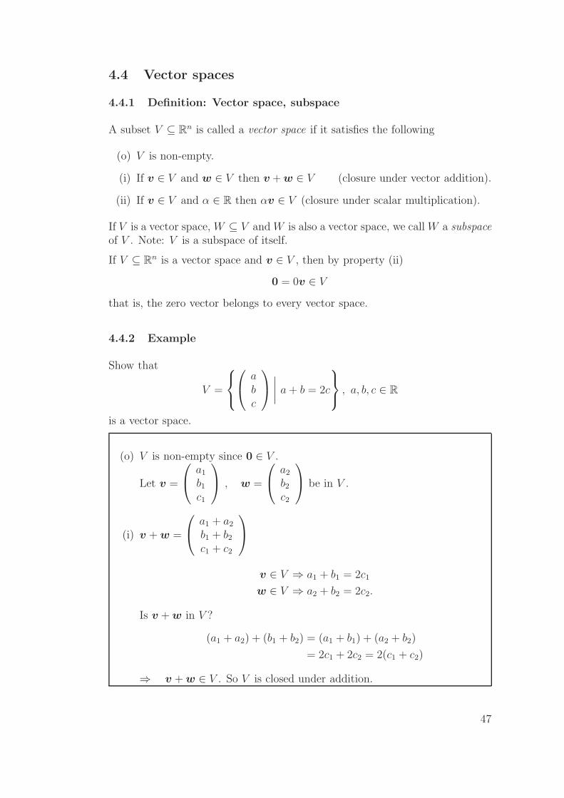
4.4.2 Example
Show that
V =
abc
∣∣∣∣a + b = 2c
, a, b, c ∈ R
is a vector space.
(o) V is non-empty since 0 ∈ V .
Let v =
a1
b1
c1
, w =
a2
b2
c2
be in V .
(i) v + w =
a1 + a2
b1 + b2
c1 + c2
v ∈ V ⇒ a1 + b1 = 2c1
w ∈ V ⇒ a2 + b2 = 2c2.
Is v + w in V ?
(a1 + a2) + (b1 + b2) = (a1 + b1) + (a2 + b2)
= 2c1 + 2c2 = 2(c1 + c2)
⇒ v + w ∈ V . So V is closed under addition.
47

Consider v =
a1
b1
c1
, w =
a2
b2
c2
∈ V .
(ii) If α is any scalar then αv =
αa1
αb1
αc1
αa1 + αb1 = α(a1 + b1) = α2c1 = 2(αc1)
⇒ αv ∈ V. So V is closed under scalar multiplication.
Hence V is a vector space.
4.4.3 Example
Is V = {0} a vector space?
(o) 0 ∈ V ⇒ V is non-empty.
(i) If v, w ∈ V then v = w = 0 and v + w = 0 ∈ V .
(ii) If α ∈ R, then α0 = 0 ∈ V .
4.4.4 Example
Show that V = Rn is a vector space.
(o) 0 ∈ V
(i) v, w ∈ V ⇒ v + w ∈ Rn = V
(ii) v ∈ V ⇒ αv ∈ Rn = V
So V is a vector space.
48

4.4.5 Example
Is V =
{(12
)}
a vector space?
No, since 0 /∈ V .
4.4.6 Example
Is V =
{
α
(12
)
| α ∈ R
}
a vector space?
(o) α = 0⇒ 0 ∈ V .
(i) If v, w ∈ V then v = α
(12
)
and w = β
(12
)
for suitable α, β ∈ R.
Then v + w =
(α2α
)
+
(β2β
)
=
(α + β
2(α + β)
)
= (α + β) ·(
12
)
∈ V.
(ii) If γ ∈ R, then γv = γα
(12
)
∈ V .
Therefore V is a vector space.
Geometrically, all these vectors can be viewed as lying along a single line throughthe origin.
49
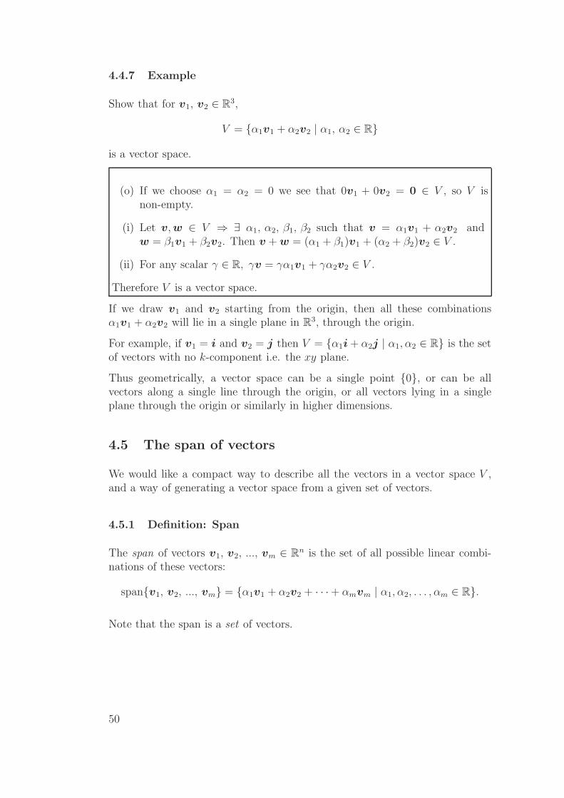
4.4.7 Example
Show that for v1, v2 ∈ R3,
V = {α1v1 + α2v2 | α1, α2 ∈ R}
is a vector space.
(o) If we choose α1 = α2 = 0 we see that 0v1 + 0v2 = 0 ∈ V , so V isnon-empty.
(i) Let v, w ∈ V ⇒ ∃ α1, α2, β1, β2 such that v = α1v1 + α2v2 andw = β1v1 + β2v2. Then v + w = (α1 + β1)v1 + (α2 + β2)v2 ∈ V .
(ii) For any scalar γ ∈ R, γv = γα1v1 + γα2v2 ∈ V .
Therefore V is a vector space.
If we draw v1 and v2 starting from the origin, then all these combinationsα1v1 + α2v2 will lie in a single plane in R3, through the origin.
For example, if v1 = i and v2 = j then V = {α1i + α2j | α1, α2 ∈ R} is the setof vectors with no k-component i.e. the xy plane.
Thus geometrically, a vector space can be a single point {0}, or can be allvectors along a single line through the origin, or all vectors lying in a singleplane through the origin or similarly in higher dimensions.
4.5 The span of vectors
We would like a compact way to describe all the vectors in a vector space V ,and a way of generating a vector space from a given set of vectors.
4.5.1 Definition: Span
The span of vectors v1, v2, ..., vm ∈ Rn is the set of all possible linear combi-nations of these vectors:
span{v1, v2, ..., vm} = {α1v1 + α2v2 + · · ·+ αmvm | α1, α2, . . . , αm ∈ R}.
Note that the span is a set of vectors.
50

4.5.2 The Span of vectors is a Vector Space
The span of any non-empty set of vectors is a vector space.
We proved this for two vectors in Example 4.4.7. The general proof is similar.
If span{v1, v2, ..., vm} = V then we say that v1, . . . , vm span V , or that theyform a spanning set for V .
4.5.3 Example
Find a spanning set for V =
{
α
(12
)
| α ∈ R
}
.
Every vector in V is a linear combination of
(12
)
, so a spanning set is{(
12
)}
.
This answer is not unique. For example
{(−1−2
)}
is another spanning set
for V .
4.5.4 Example
The coordinate vectors ei =
0...010...0
← i span Rn since every vector v ∈ Rn
is a linear combination of these vectors (see equation 3.1).
4.5.5 Example
The vector space {0} is spanned by the zero vector 0 ∈ Rn is and called thezero vector space.
51
4.6 Bases
We have seen that we can describe a vector space by giving a spanning set.When we do this, we usually like to choose a spanning set that is as small aspossible (contains no redundancies). We ensure this as follows.
4.6.1 Definition: Basis
Let V be a vector space. We say that a set of vectors B = {v1, ..., vm} ⊆ V isa basis for V if:
1. B spans V ;
2. B is linearly independent.
To prove that a set of vectors is a basis, we must prove both properties.
Sometimes we are just given a vector space V , and asked to find a basis. Prob-lems like this are solved by finding a spanning set for V , and then checking thatthe set is linearly independent.
A single vector space V may have many different bases.
4.6.2 Example
We have seen that the coordinate vectors ei, i = 1, ..., n, are linearly indepen-dent (section 4.3.2) and span Rn (section 4.5.4). Therefore they form a basisfor Rn, called the standard basis.
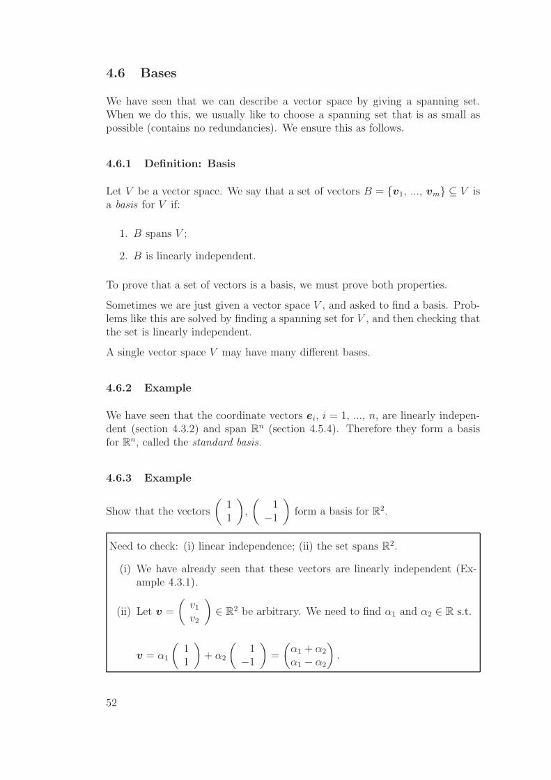
4.6.3 Example
Show that the vectors
(11
)
,
(1−1
)
form a basis for R2.
Need to check: (i) linear independence; (ii) the set spans R2.
(i) We have already seen that these vectors are linearly independent (Ex-ample 4.3.1).
(ii) Let v =
(v1
v2
)
∈ R2 be arbitrary. We need to find α1 and α2 ∈ R s.t.
v = α1
(11
)
+ α2
(1−1
)
=
(α1 + α2
α1 − α2
)
.
52

So we need:{
v1 = α1 + α2
v2 = α1 − α2
⇒
α1 =1
2(v1 + v2)
α2 =1
2(v1 − v2)
.
Hence
v =
(v1
v2
)
=1
2
(v1 + v2
)(
11
)
+1
2
(v1 − v2
)(
1−1
)
.
Note that this basis differs from the standard
{(10
)
,
(01
)}
basis of R2,
but still has two elements.
4.6.4 Example
Find a basis for the vector space of 4.4.2
V =
abc
∣∣∣∣a + b = 2c
, a, b, c ∈ R
Any vector in V is of the form
v =
2c− bbc
=
2c0c
+
−bb0
= cv1 + bv2
with c, b ∈ R. Thus {v1, v2} is a spanning set for V . For {v1, v2} to be abasis, we need to show v1 and v2 are linearly independent. If α1v1 +α2v2 = 0then from the second coordinate α2 = 0 and from the first α1 = 0, so {v1, v2}is also linearly independent.
53
4.7 Dimension
Suppose B = {v1, ..., vm} is a basis for V . Then it can be shown that everybasis for V has m vectors. We call m the dimension of V and write m = dim V .(By convention, the zero vector space {0} has dimension zero.)
4.7.1 Example
We have seen that the coordinate vectors ei, form a basis for Rn, so
dim Rn = n.
4.7.2 Example
The vector space
V =
{
α
(12
)
| α ∈ R
}
⊆ R2
is spanned by a single vector
(12
)
(example 4.5.3) which thus constitutes a
basis for V . Hence dim V = 1.
Geometrically, V consists of vectors along a single line, which is a one dimen-sional object.
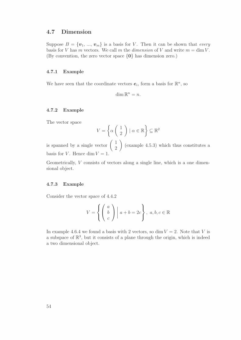
4.7.3 Example
Consider the vector space of 4.4.2
V =
abc
∣∣∣∣a + b = 2c
, a, b, c ∈ R
In example 4.6.4 we found a basis with 2 vectors, so dimV = 2. Note that V isa subspace of R3, but it consists of a plane through the origin, which is indeeda two dimensional object.
54
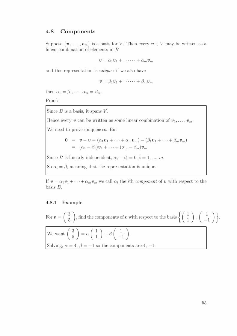
4.8 Components
Suppose {v1, . . . , vm} is a basis for V . Then every v ∈ V may be written as alinear combination of elements in B
v = α1v1 + · · · · · ·+ αmvm
and this representation is unique: if we also have
v = β1v1 + · · · · · ·+ βmvm
then α1 = β1, . . . , αm = βm.
Proof:
Since B is a basis, it spans V .
Hence every v can be written as some linear combination of v1, . . . , vm.
We need to prove uniqueness. But
0 = v − v = (α1v1 + · · ·+ αmvm)− (β1v1 + · · ·+ βmvm)
= (α1 − β1)v1 + · · ·+ (αm − βm)vm.
Since B is linearly independent, αi − βi = 0, i = 1, ..., m.
So αi = βi meaning that the representation is unique.
If v = α1v1 + · · ·+ αmvm we call αi the ith component of v with respect to thebasis B.
4.8.1 Example
For v =
(35
)
, find the components of v with respect to the basis
{(11
)
,
(1−1
)}
.
We want
(35
)
= α
(11
)
+ β
(1−1
)
.
Solving, α = 4, β = −1 so the components are 4, −1.
55
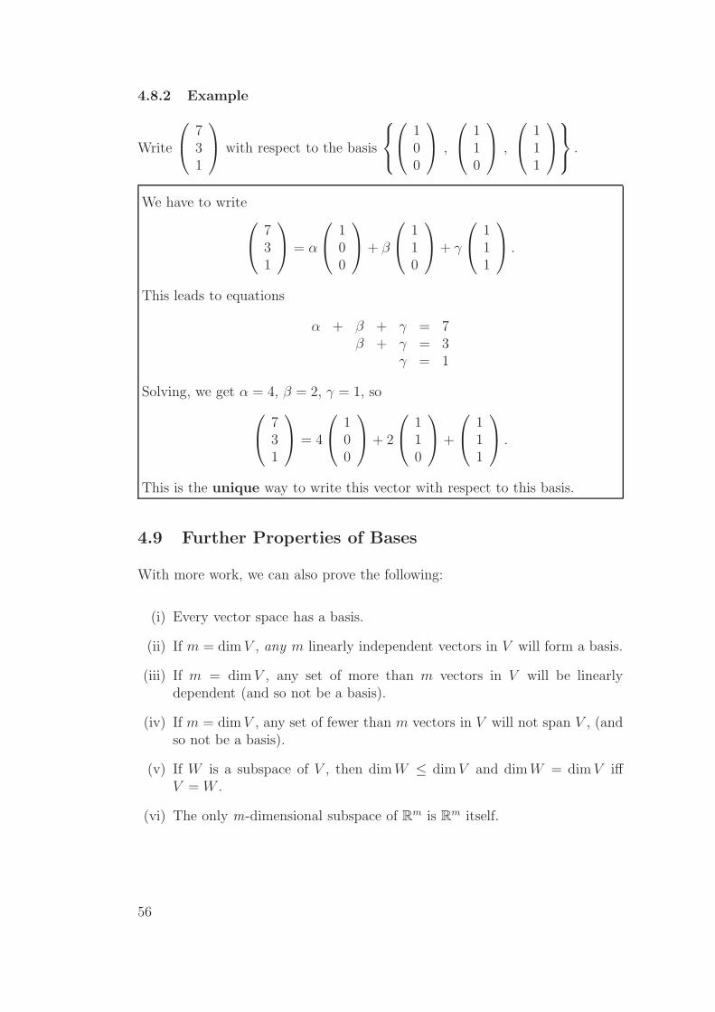
4.8.2 Example
Write
731
with respect to the basis
100
,
110
,
111
.
We have to write
731
= α
100
+ β
110
+ γ
111
.
This leads to equations
α + β + γ = 7β + γ = 3
γ = 1
Solving, we get α = 4, β = 2, γ = 1, so
731
= 4
100
+ 2
110
+
111
.
This is the unique way to write this vector with respect to this basis.
4.9 Further Properties of Bases
With more work, we can also prove the following:
(i) Every vector space has a basis.
(ii) If m = dim V , any m linearly independent vectors in V will form a basis.
(iii) If m = dim V , any set of more than m vectors in V will be linearlydependent (and so not be a basis).
(iv) If m = dim V , any set of fewer than m vectors in V will not span V , (andso not be a basis).
(v) If W is a subspace of V , then dim W ≤ dim V and dim W = dim V iffV = W .
(vi) The only m-dimensional subspace of Rm is Rm itself.
56

4.9.1 Example
Show that in R3, the vectors
v1 =
100
, v2 =
110
v3 =
111
are linearly independent and hence form a basis for R3.
Setting αv1 + βv2 + γv3 = 0 implies
α
100
+ β
110
+ γ
111
=
000
⇒
α + β + γβ + γ
γ
=
000
⇒ γ = 0⇒ β = 0⇒ α = 0
Therefore the vectors are linearly independent.Because we already know dim R3 = 3 and we have found 3 linearly independentvectors, they must form a basis, by (vi) above.
Check: in R3, v =
abc
⇒ v =
abc
= (a− b)
100
+ (b− c)
110
+ c
111
The shortcut in this example is fine if we already know the dimension of V . Ifwe are just given a space like
V =
abc
∣∣∣∣a + b = 2c
, a, b, c ∈ R
it is often not obvious what the dimension is (2? 3?).
4.10 Orthogonal and Orthonormal
As we have seen, a single vector space can have many different bases. One reasonwe like the standard basis {ei} of Rn is that the basis vectors are mutuallyorthogonal (perpendicular). The Gram-Schmidt process is a method of using agiven basis for a vector space to obtain a new basis in which the basis vectorsare orthogonal.
57

4.10.1 Definition: Orthogonal set, orthonormal set
A set S of vectors is orthogonal or mutually orthogonal if each pair of distinctvectors in S are orthogonal. It is orthonormal if additionally, all the vectorshave norm 1.
Note: in an orthogonal set all the vectors must be non-zero, because the 0-vectoris not considered to be orthogonal to other vectors.
In symbols, {v1, . . . , vn} is orthogonal if
vi · vj = 0 for all i 6= j
It is orthonormal if also
vi · vi = 1 for all i
4.10.2 Example
The standard basis {i, j} in R2 is an orthonormal set, because each vector hasnorm 1, and i · j = 0. More generally the standard basis {e1, . . . , en} of Rn isan orthonormal set.
4.10.3 Example
The set
v1 =
010
, v2 =
101
, v3 =
10−1
is an orthogonal set in R3 but is not orthonormal. We have v1 · v2 = v2 · v3 =v3 · v1 = 0, but ‖v2‖ =
√2, ‖v3‖ =
√2.
4.10.4 Converting Orthogonal to Orthonormal
It is easy to convert an orthogonal set into an orthonormal one: just make eachvector into a unit vector, by dividing by its norm. (This does not change theangle between the vectors, so the set is still orthogonal.)
4.10.5 Example
The set
u1 =
010
, u2 =1√2v2 =
1/√
20
1/√
2
, u3 =1√2v3 =
1/√
20
−1/√
2
is an orthonormal set made from the orthogonal set in the previous example.
58

4.10.6 Orthogonal implies Linearly Independent
Any orthogonal set of vectors is linearly independent.
Proof: Let {v1, . . . , vn} be an orthogonal set. Suppose
α1v1 + · · ·+ αnvn = 0. (4.1)
We must show α1 = α2 = · · · = αn = 0. Take the dot product of equation 4.1with v1:
0 = (α1v1 + · · ·+ αnvn) · v1
= α1(v1 · v1) + α2(v2 · v1) + · · ·+ αn(vn · v1)
= α1‖v1‖2
where we used orthogonality: v1 ·v2 = 0, v1 ·v3 = 0 etc. Since v1 6= 0, we musthave α1 = 0.
Taking dot product of equation 4.1 with v2, v3 etc similarly we get α2 = 0,α3 = 0 etc.
So if we can find an orthogonal set, it is automatically linearly independent.
4.11 Gram-Schmidt Algorithm
Suppose {u1, . . . , un} is any set of linearly independent vectors. We form anorthogonal set {v1, . . . , vn} with the same span.
Stage 1: Letv1 = u1.
Stage 2: We want a vector orthogonal to u1, so we take the component of u2
orthogonal to u1. By the projection formula (equation 2.1) this is
v2 = u2 −u2 · v1
v1 · v1v1.
Then v2 is orthogonal to v1, by construction. Note that u2·v1
v1·v1is just a scalar.
Check of orthogonality:
v1 · v2 = v1 ·(
u2 −u2 · v1
v1 · v1v1
)
= v1 · u2 −u2 · v1
v1 · v1
(v1 · v1)
= v1 · u2 − u2 · v1
= 0
59

Since v1 = u1 and v2 is given as a linear combination of u1, v2 by the formulaabove, v1 and v2 are contained in the 2 dimensional space spanned by {u1, u2}.But orthogonal vectors are linearly independent, so we have found 2 linearlyindependent vectors in a 2 dimensional space. Thus {v1, v2} is a basis forspan{u1, u2}. So span{u1, u2} = span{v1, v2}.At stage 2 we have found a orthogonal set {v1, v2} of 2 vectors, with the samespan as the first two given vectors u1, u2.
Stage 3:
v3 = u3 −u3 · v1
v1 · v1
v1 −u3 · v2
v2 · v2
v2.
One can check that then {v1, v2, v3} is an orthogonal set of 3 vectors with thesame span as {u1, u2, u3}.Stage 4:
v4 = u4 −u4 · v1
v1 · v1v1 −
u4 · v2
v2 · v2v2 −
u4 · v3
v3 · v3v3.
Etc.
The set produced is orthogonal. If we want to make it orthonormal, we canreplace each vi by vi/‖vi‖ at the end.
4.11.1 Example
Let u1 =
210−1
, u2 =
102−1
, u3 =
0−210
in R4. Find an orthogonal
set of vectors with the same span.
Let v1 = u1 =
210−1
.
60

Let
v2 = u2 − u2 · v1
v1 · v1v1
=
102−1
− 3
6
210−1
=
0−1/2
2−1/2
Now let
v3 = u3 − u3 · v1
v1 · v1v1 − u3 · v2
v2 · v2v2
=
0−210
− −2
6
210−1
− 3
9/2
0−1/2
2−1/2
=
2/3−4/3−1/3
0
So an orthogonal set of vectors with the same span as {u1, u2, u3} is{v1, v2, v3
}
An orthonormal basis is{w1, w2, w3
}where wi = vi
‖vi‖ , i = 1, 2, 3.
Since ‖v1‖ =√
6, ‖v2‖ =√
18/2 = 3√
2/2, ‖v3‖ =√
213
we get the or-thonormal basis
{w1, w2, w3
}=
1√6
210−1
,1
3√
2
0−14−1
,1√21
2−4−10
.
4.11.2 Orthogonal Bases Exist
Every finite-dimensional vector space has an orthogonal basis.
Proof: Pick any basis and apply the Gram-Schmidt process above.
61

5 Inverses
5.1 The Identity Matrix
An n × n matrix (m = n) is called a square matrix of order n. The diagonalcontaining the entries
a11, a22, · · · , ann
is called the principal diagonal (or main diagonal) of A. If the entries abovethis diagonal are all zero then A is called lower triangular. If all the entriesbelow the diagonal are zero, A is called upper triangular
a11 0 0 · · · 0... a22 0 · · · 0
. . .. . .
......
. . . 0an1 · · · · · · ann
lower triangular
a11 · · · · · · a1n
0 a22...
0 0. . .
......
. . .. . .
...0 0 · · · 0 ann
upper triangular
If elements above and below the principal diagonal are zero, so
aij = 0 , i 6= j
then A is called a diagonal matrix.
5.1.1 Example
A =
1 0 00 −3 00 0 2
is a diagonal 3× 3 matrix.
5.1.2 Definition: Identity matrix
The n×n identity matrix I = In, is the diagonal matrix whose entries are all 1:
I =
1 0 0 · · · 00 1 0 · · · 00 0 1 · · · 0...
. . ....
0 0 · · · · · · 1
.
62

5.1.3 Comments on the identity matrix
(1) It is easily checked that I acts as the multiplicative identity for n×n matrices:
IA = AI = A
Eg. for 2× 2 case we have
IA =
(1 00 1
) (a11 a12
a21 a22
)
=
(a11 a12
a21 a22
)
= A = AI.
(2) The jth column vector of I is the coordinate vector
ej =
0...010...0
← j.
5.2 Definition: Inverse
Let I denote the identity matrix.
A square matrix A is invertible (or non-singular) if there exists a matrix B suchthat
AB = BA = I.
B is called the inverse of A and is denoted A−1. A matrix that is not invertibleis also said to be singular.
5.2.1 Inverse for the 2 × 2 case
Let A be a 2× 2 matrix A =
(a bc d
)
. Set B =
(d −b−c a
)
. Then
AB =
(a bc d
) (d −b−c a
)
=
(ad− bc 0
0 ad− bc
)
= BA.
Let∆ = ad− bc.
If ∆ 6= 0, then
A−1 =1
∆B =
1
∆
(d −b−c a
)
We call ∆ the determinant of A. We will consider determinants in more detaillater (chapter 7). The problem of obtaining inverses of larger square matriceswill also be considered later (section 6.4.3).
63

5.2.2 Example
Find the inverse matrix of A =
(1 23 5
)
. Check your answer.
∆ = 1× 5− 2× 3 = −1.
⇒ A−1 =1
−1
(5 −2−3 1
)
=
(−5 2
3 −1
)
.
Check whether AA−1 = A−1A = I:Multiplying the two matrices A and A−1 gives
(1 23 5
) (−5 2
3 −1
)
=
(1 00 1
)
,
(−5 2
3 −1
) (1 23 5
)
=
(1 00 1
)
So A is invertible with inverse(−5 2
3 −1
)
.
5.2.3 Example
Show that A =
(1 23 6
)
is not invertible.
Suppose A has inverse
(a bc d
)
.
Then
(1 23 6
) (a bc d
)
=
(1 00 1
)
⇒
a + 2c = 1 (1)b + 2d = 0 (2)3a + 6c = 0 (3)3b + 6d = 1 (4)
.
Hence 3 · (1)− (3)⇒ 0 = 3. This is impossible, so A can’t have an inverse.Note that ∆ = 6− 2 · 3 = 0 in this case.
64

5.2.4 Example: Inverse of a 3× 3 Matrix
There is no simple formula for the inverse of a 3× 3 (or larger) matrix.
Let A =
2 −3 −11 −2 −3−2 2 −5
and B =
16 −17 711 −12 5−2 2 −1
. Show that B is the
inverse of A.
Just multiply the two matrices together.
AB =
2 −3 −11 −2 −3−2 2 −5
16 −17 711 −12 5−2 2 −1
=
1 0 00 1 00 0 1
.
And, similarly
BA =
16 −17 711 −12 5−2 2 −1
2 −3 −11 −2 −3−2 2 −5
=
1 0 00 1 00 0 1
.
We will learn a systematic way of finding B later (section 6.4.3).
5.3 Invertible Matrices and Linear Independence
As we have seen, not every square matrix has an inverse.
5.3.1 Theorem (existence of inverse)
A square matrix A has an inverse if and only if the columns of A are linearlyindependent.
Proof:
Suppose A is invertible. We must show its columns are linearly independent.We can isolate the columns with the following technique:
65

Aej =
a11 · · · a1j · · · a1n
a21 · · · a2j · · · a2n...
......
an1 · · · anj · · · ann
0...010...0
← j
=
a1j
a2j...anj
=jth columnvector ofA.
Now suppose there is a linear relation among the columns of A. By the previouscalculation, we can write this relation as
0 = α1Ae1 + α2Ae2 + · · ·+ αnAen
Factorize A:
0 = A(α1e1 + α2e2 + · · ·+ αnen)
= A
α1
0...
0
+ A
0α2
0...0
+ . . . + A
00...0αn
= A
α1
α2...
αn−1
αn
.
Multiplication on the left by A−1 gives
0 = A−1A︸ ︷︷ ︸
I
α1
α2...
αn
= I
α1
α2...
αn
=
α1
α2...
αn
⇒ α1 = α2 = · · · = αn = 0
so the column vectors of A are linearly independent.
Conversely, it can be shown that if columns of A are linearly independent thenA is invertible.
66

5.3.2 Example
From example 4.3.3, the columns of
A =
1 1 03 1 11 1 0
are linearly dependent. Therefore A is not invertible.
5.3.3 Example
From example 4.9.1 the columns of
A =
1 1 10 1 10 0 1
are linearly independent, and therefore A has an inverse.
5.3.4 Another Linear Independence Test
Theorem 5.3.1 can also be used in the other direction to give another method oftesting if n vectors in Rn are linearly independent. Put the vectors (as columns)into a matrix A. If A is invertible, then the vectors are linearly independent. IfA is not invertible, they are linearly dependent.
Disadvantage of this method: only works for n vectors in Rn (otherwise thematrix is not square).
5.3.5 Example
Determine whether vectors
v1 =
21−2
, v2 =
−3−22
, v3 =
−1−3−5
are linearly independent.
Put the vectors into the columns of a matrix: A =(v1| v2| v3
).
So, let
A =
2 −3 −11 −2 −3−2 2 −5
.
67
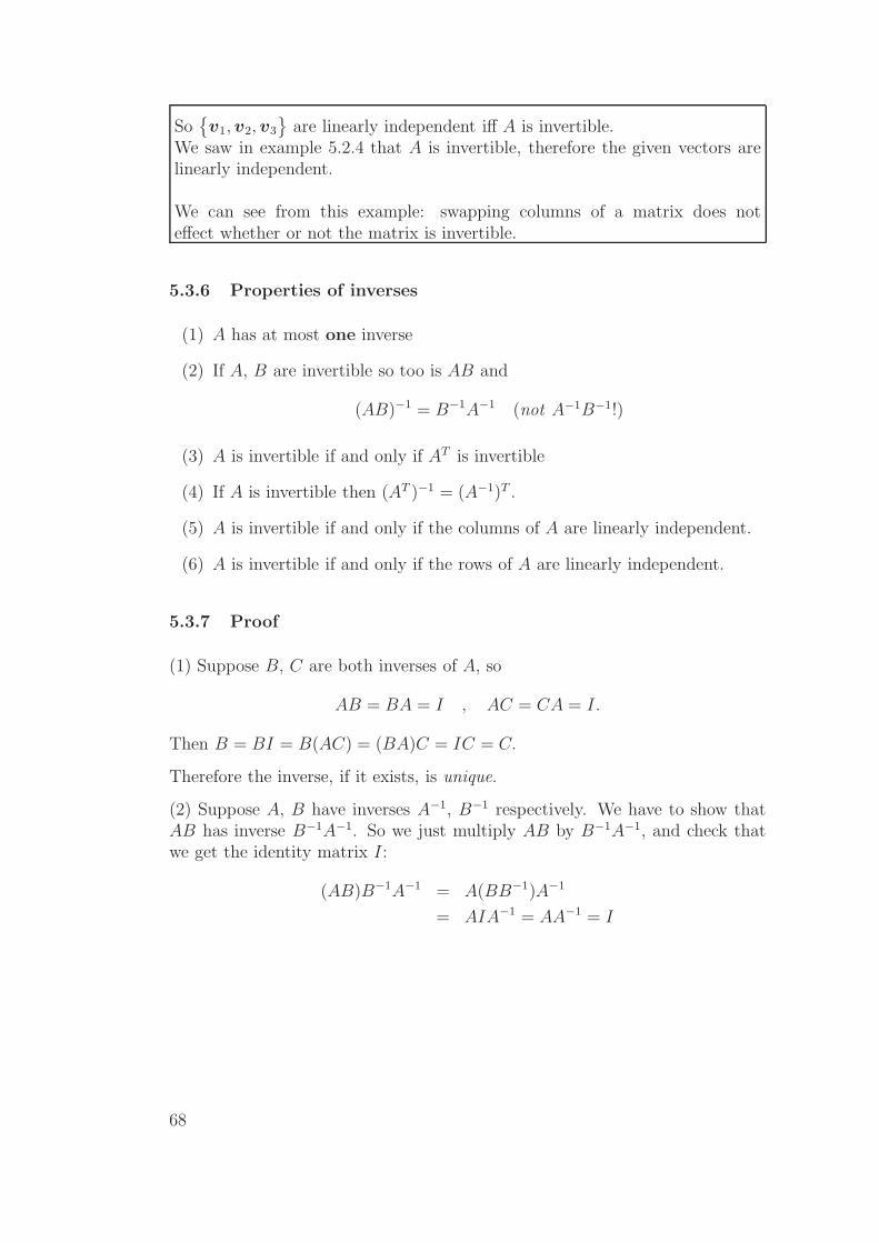
So{v1, v2, v3
}are linearly independent iff A is invertible.
We saw in example 5.2.4 that A is invertible, therefore the given vectors arelinearly independent.
We can see from this example: swapping columns of a matrix does noteffect whether or not the matrix is invertible.
5.3.6 Properties of inverses
(1) A has at most one inverse
(2) If A, B are invertible so too is AB and
(AB)−1 = B−1A−1 (not A−1B−1!)
(3) A is invertible if and only if AT is invertible
(4) If A is invertible then (AT )−1 = (A−1)T .
(5) A is invertible if and only if the columns of A are linearly independent.
(6) A is invertible if and only if the rows of A are linearly independent.
5.3.7 Proof
(1) Suppose B, C are both inverses of A, so
AB = BA = I , AC = CA = I.
Then B = BI = B(AC) = (BA)C = IC = C.
Therefore the inverse, if it exists, is unique.
(2) Suppose A, B have inverses A−1, B−1 respectively. We have to show thatAB has inverse B−1A−1. So we just multiply AB by B−1A−1, and check thatwe get the identity matrix I:
(AB)B−1A−1 = A(BB−1)A−1
= AIA−1 = AA−1 = I
68
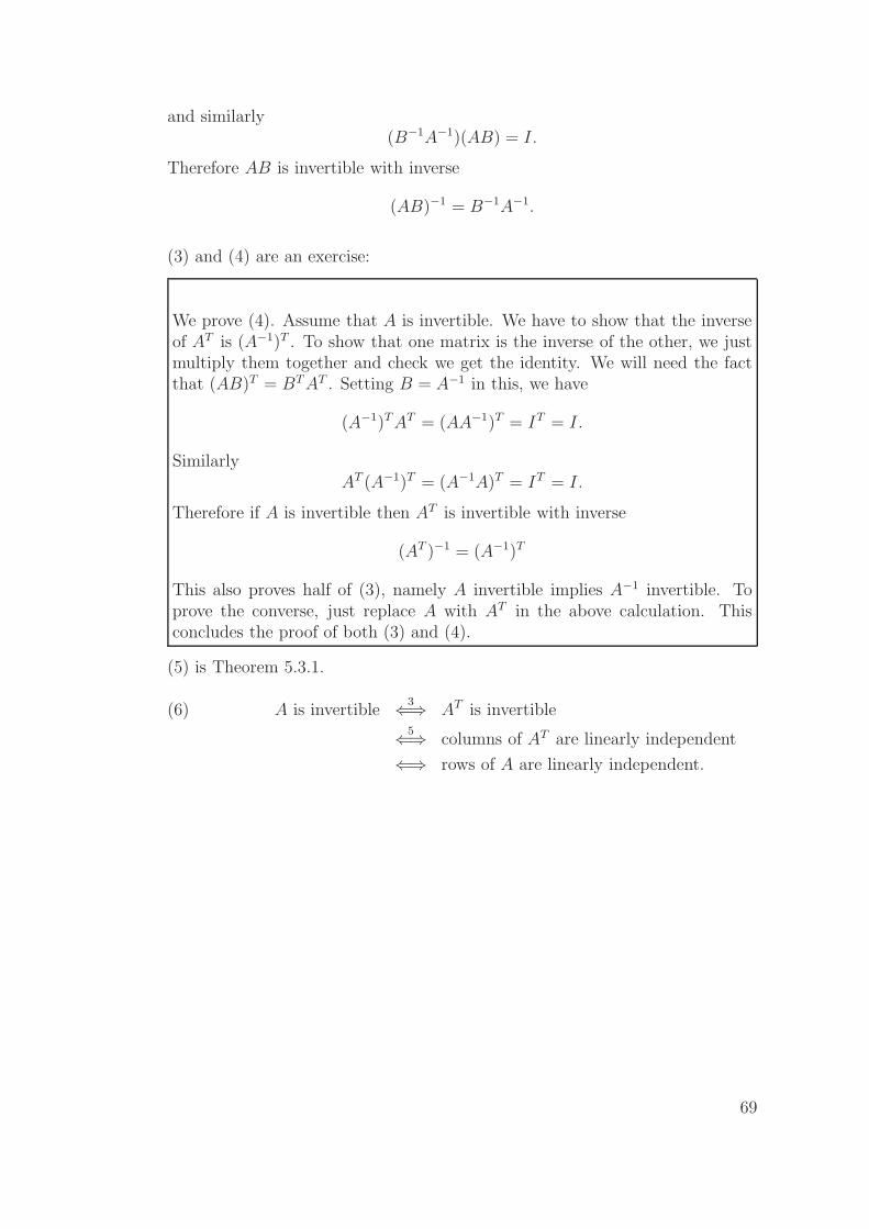
and similarly(B−1A−1)(AB) = I.
Therefore AB is invertible with inverse
(AB)−1 = B−1A−1.
(3) and (4) are an exercise:
We prove (4). Assume that A is invertible. We have to show that the inverseof AT is (A−1)T . To show that one matrix is the inverse of the other, we justmultiply them together and check we get the identity. We will need the factthat (AB)T = BT AT . Setting B = A−1 in this, we have
(A−1)T AT = (AA−1)T = IT = I.
SimilarlyAT (A−1)T = (A−1A)T = IT = I.
Therefore if A is invertible then AT is invertible with inverse
(AT )−1 = (A−1)T
This also proves half of (3), namely A invertible implies A−1 invertible. Toprove the converse, just replace A with AT in the above calculation. Thisconcludes the proof of both (3) and (4).
(5) is Theorem 5.3.1.
(6) A is invertible3⇐⇒ AT is invertible5⇐⇒ columns of AT are linearly independent
⇐⇒ rows of A are linearly independent.
69

Notes
70
6 Gaussian elimination
6.1 Simultaneous equations
One of the main applications of matrices is solving simultaneous equations ofthe form
a11x1 + a12x2 + · · · + a1nxn = b1
a21x1 + a22x2 + · · · + a2nxn = b2...
...am1x1 + am2x2 + · · · + amnxn = bm.
Here x1, x2, · · · · · · , xn are the variables (unknowns) and the coefficients aij andbi are given real numbers.
This set of equations can be written using matrix multiplication as
Ax = b (6.1)
where x =
x1
x2...
xn
is a column vector of unknowns, b =
b1
b2...
bm
is a given
m× 1 matrix (column vector) and A = (aij) is the m× n matrix of coefficients.
6.1.1 Special case: n equations in n unknowns.
In the special case that A is n× n and invertible, we may solve (6.1) by multi-plication on the left by A−1 to give
A−1A︸ ︷︷ ︸
I
x = A−1b⇒ unique solution x = A−1b.
So if A is invertible, then the system Ax = b has a unique solution, for each b.This is often inaccurately remembered as “n equations in n unknowns have aunique solution”. This statement is only true if A is invertible.
The method of multiplying by A−1 only works if A is square and A is invertible.
We return to consideration of the general case. An efficient way of solving asystem is by Gaussian elimination.
71

6.2 Gaussian elimination
We now illustrate the process of Gaussian elimination. Given a set of equations,the idea is to performs operations, called elementary row operations, in order tosimplify the equations to the point where the solution may be obtained easily.
Solve the following system of equations:
2x1 − 3x2 − x3 = 1x1 − 2x2 − 3x3 = 2
−2x1 + 2x2 − 5x3 = 3
Swap the order of the first two equations:
x1 − 2x2 − 3x3 = 22x1 − 3x2 − x3 = 1−2x1 + 2x2 − 5x3 = 3
Subtract 2 times first equation from second:
x1 − 2x2 − 3x3 = 2x2 + 5x3 = −3
−2x1 + 2x2 − 5x3 = 3
Add 2 times first equation to third:
x1 − 2x2 − 3x3 = 2x2 + 5x3 = −3
− 2x2 − 11x3 = 7
Add 2 times second equation to third:
x1 − 2x2 − 3x3 = 2x2 + 5x3 = −3− x3 = 1
Multiply third equation by −1:
x1 − 2x2 − 3x3 = 2x2 + 5x3 = −3
x3 = −1
Now we can solve by back substitution:Third equation gives x3 = −1.Substitute x3 into second: x2 − 5 = −3 so x2 = 2.Substitute x2, x3 into first: x1 − 4 + 3 = 2 so x1 = 3.
72
This process is called Gaussian elimination. We call this simplified set of equa-tions
x1 − 2x2 − 3x3 = 2x2 + 5x3 = −3
x3 = −1
the reduced form of the equations. Once in reduced form the set of equations iseasily solved by back substitution.
In this example we repeatedly performed the following operations:
(1) Interchange the order of two equations: swap the ith and j equations.
(2) Multiply an equation through by a non-zero number α.
(3) Add α times the jth equation to the ith equation (where i 6= j).
Performing these operations does not change the solution of the equations. Buteventually we obtained such a simple system that we could easily find the solu-tion.
6.2.1 Gaussian elimination using matrices
The above procedure may be described most conveniently in terms of matrices.The information present in a set of simultaneous equations
Am×n
xn×1
= bm×1
may be summarized by constructing a new matrix
(A | b)
A with one extra column, b. This is called the augmented matrix. Instead ofmanipulating equations we manipulate the corresponding augmented matrix.This way we keep writing to a minimum.
The augmented matrix for the set of equations in the previous example 6.2 maybe written
2 −3 −1 11 −2 −3 2−2 2 −5 3
Always keep in mind that each row of the augmented matrix represents anequation. The last column is the rhs. The other columns are the coefficients ofthe variables. Eg the last row above corresponds to −2x1 + 2x2 − 5x3 = 3.
Another advantage of the augmented matrix notation is that if we want to solvethe equations
Ax = b, and Ay = c,
we can do both at once by forming the augmented matrix
(A | b | c).
73
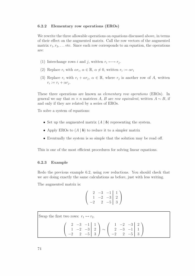
6.2.2 Elementary row operations (EROs)
We rewrite the three allowable operations on equations discussed above, in termsof their effect on the augmented matrix. Call the row vectors of the augmentedmatrix r1, r2, . . . etc. Since each row corresponds to an equation, the operationsare:
(1) Interchange rows i and j, written ri ←→ rj.
(2) Replace ri with αri, α ∈ R, α 6= 0, written ri := αri
(3) Replace ri with ri + αrj , α ∈ R, where rj is another row of A, writtenri := ri + αrj.
These three operations are known as elementary row operations (EROs). Ingeneral we say that m× n matrices A, B are row equivalent, written A ∼ B, ifand only if they are related by a series of EROs.
To solve a system of equations:
• Set up the augmented matrix (A | b) representing the system.
• Apply EROs to (A | b) to reduce it to a simpler matrix
• Eventually the system is so simple that the solution may be read off.
This is one of the most efficient procedures for solving linear equations.
6.2.3 Example
Redo the previous example 6.2, using row reductions. You should check thatwe are doing exactly the same calculations as before, just with less writing.
The augmented matrix is:
2 −3 −1 11 −2 −3 2−2 2 −5 3
Swap the first two rows: r1 ↔ r2.
2 −3 −1 11 −2 −3 2−2 2 −5 3
∼
1 −2 −3 22 −3 −1 1−2 2 −5 3
74

Subtract 2 times row 1 from row 2: r2 → r2 − 2r1.
∼
1 −2 −3 20 1 5 −3−2 2 −5 3
Add 2 times row 1 to row 3: r3 → r3 + 2r1.
∼
1 −2 −3 20 1 5 −30 −2 −11 7
Add 2 times row 2 to row 3: r3 → r3 + 2r2.
∼
1 −2 −3 20 1 5 −30 0 −1 1
Multiply row 3 by −1: r3 → −r3.
∼
1 −2 −3 20 1 5 −30 0 1 −1
This is called a Gauss reduced form, or row-echelon form. The solution cannow be read off directly by back substitution as before.r3 gives x3 = −1.Substitute x3 into r2: x2 − 5 = −3 so x2 = 2.Substitute x2, x3 into r1: x1 − 4 + 3 = 2 so x1 = 3.
75

6.2.4 The Gaussian algorithm
To solveA
m×nx
n×1= b
m×1,
first set up the augmented matrix
(A | b) .
Then
- Find a row with entry α 6= 0 in column 1. (If none go to column 2)
- Multiply row by 1α
to make leading entry 1
- Swap rows to bring the 1 to the top
1 · · ·∗ · · ·∗ · · ·...
- Subtract appropriate multiples of row 1 to clear out the first column
1 · · ·0 · · ·0 · · ·...
First column is now done.
Repeat on second column:
Find a row (not the first) with entry α 6= 0 in column 2. (If none exists, go onto third column). Make the leading entry 1, and clear out all the entries belowthis 1:
1 · · ·0 1 · ·0 0 · ·...
Then go on to the third column etc.
76

6.2.5 Gauss reduced form or row echelon form
When solving a system Ax = b, we can stop doing EROs on (A|b) once Ais “simple enough” to find the solution by back substitution. This means wereduce (A|b) until:
• All rows consisting entirely of 0’s are at the bottom.
• The first non-zero entry (leading entry) of each row is 1, and appears in acolumn to the right of the leading entry of the row above it.
• All entries in a column below a leading entry are zeros.
The reduced matrix is called the Gauss reduced form (or row echelon form) ofA. For example:
1 · · · ·0 1 · · ·0 0 0 1 ·0 0 0 0 0
∣∣∣∣∣∣∣∣
····
The leading entries 1 leading entry (pivot), must be 1 and must have zerosbelow them. Not every column must have a pivot. Above, the third column hasno pivot.
The leading entries must form a “stair case” from top left to bottom right.
(Note that a matrix A may have more than one Gauss reduced form. Eg theentries marked · above are not unique. It doesn’t matter which is used.) Tips:
• Try to do row reductions that lead to the easiest algebra.
• Try to avoid fractions.
• Do not neglect row swaps to take advantage of existing 1’s in the matrix.
6.2.6 Example
Which of the following matrices are in Gauss reduced form (row echelon form)?
A =
1 2 3 40 0 1 40 0 0 1
, B =
0 1 0 20 0 1 −20 0 0 0
, C =
0 1 0 21 0 0 00 0 0 1
A, B are row-reduced. C is not because the leading 1 in the second column isnot to the right of the leading 1 in the 1st column.
77
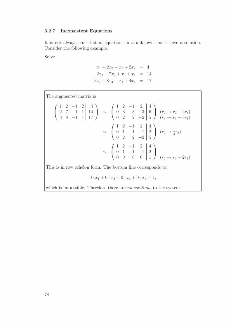
6.2.7 Inconsistent Equations
It is not always true that m equations in n unknowns must have a solution.Consider the following example.
Solve
x1 + 2x2 − x3 + 2x4 = 4
2x1 + 7x2 + x3 + x4 = 14
3x1 + 8x2 − x3 + 4x4 = 17
The augmented matrix is
1 2 −1 2 42 7 1 1 143 8 −1 4 17
∼
1 2 −1 2 40 3 3 −3 60 2 2 −2 5
(r2 → r2 − 2r1)(r3 → r3 − 3r1)
∼
1 2 −1 2 40 1 1 −1 20 2 2 −2 5
(r2 → 13r2)
∼
1 2 −1 2 40 1 1 −1 20 0 0 0 1
(r3 → r3 − 2r2)
This is in row echelon form. The bottom line corresponds to:
0 · x1 + 0 · x2 + 0 · x3 + 0 · x4 = 1,
which is impossible. Therefore there are no solutions to the system.
78

6.2.8 How to recognize an inconsistent system
The Gauss reduced form of the augmented matrix will have one or more rowsof the form (0 0 . . . 0 | a) where a 6= 0. This leads to an impossible equation0x1 + 0x2 + · · ·+ 0xn = a 6= 0.
Geometrically, a linear equation in R2 represents a line. An equation in R3
represents a plane etc. Solving 2 equations in R2 thus corresponds to findingthe intersection of 2 lines in R2. Usually two lines in R2 have a unique point ofintersection. But not always: parallel lines do not.
In fact parallel lines do not intersect at all, so there are no solutions—unlessthe lines are right on top of each other, in which case they intersect in infinitelymany points.
Solving 3 equations in R3 corresponds to finding the intersection of 3 planes.Usually three planes have a unique point of intersection, but not always. Simi-larly for equations in more variables. This underlies the next two examples.
6.2.9 Example
A system of equations may have more than one solution, i.e. infinitely manysolutions.
Solve
x1 + x2 = 0
3x1 + 3x2 + x3 = 0.
The augmented matrix is
(1 1 0 03 3 1 0
)
∼(
1 1 0 00 0 1 0
)
Thus our reduced system is
x1 + x2 = 0
x3 = 0
Take x2 = α. Then
x1 = −x2 = −α, x2 = α, x3 = 0
So the solution is: x = α
−110
, for any α ∈ R.
79
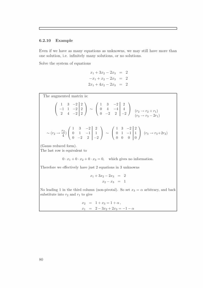
6.2.10 Example
Even if we have as many equations as unknowns, we may still have more thanone solution, i.e. infinitely many solutions, or no solutions.
Solve the system of equations
x1 + 3x2 − 2x3 = 2
−x1 + x2 − 2x3 = 2
2x1 + 4x2 − 2x3 = 2
The augmented matrix is:
1 3 −2 2−1 1 −2 22 4 −2 2
∼
1 3 −2 20 4 −4 40 −2 2 −2
(r2 → r2 + r1)(r3 → r3 − 2r1)
∼ (r2 →r2
4)
1 3 −2 20 1 −1 10 −2 2 −2
∼
1 3 −2 20 1 −1 10 0 0 0
(r3 → r3+2r2)
(Gauss reduced form).The last row is equivalent to
0 · x1 + 0 · x2 + 0 · x3 = 0, which gives no information.
Therefore we effectively have just 2 equations in 3 unknowns
x1 + 3x2 − 2x3 = 2
x2 − x3 = 1
No leading 1 in the third column (non-pivotal). So set x3 = α arbitrary, and backsubstitute into r2 and r1 to give
x2 = 1 + x3 = 1 + α ,
x1 = 2− 3x2 + 2x3 = −1− α
80

This means, for any choice of α ∈ R, a solution is:
x =
x1
x2
x3
=
−1− α
1 + α
α
=
−110
+ α
−111
.
The last equation is the equation of a line in R3: x is given by a position vector
p =
−110
plus α times a vector v =
−111
indicating direction.
Thus geometrically the three planes intersect along a common line rather than at
a single point. Every solution x corresponds to a point on this line obtained by a
particular choice of α.
6.2.11 How to recognize non-unique solutions
The system is consistent, and the Gauss reduced matrix will have one or morecolumns without a pivot (leading entry).
For example, if the second column does not have a leading 1 then there willnever be an equation we can use to isolate x2, so x2 will be a free variable: wewill be able to assign it any value (α say), and still solve the system. In a bigsystem we may have several free variables.
81

6.3 The general solution
6.3.1 General form of solutions
In general a system of equations
Am×n
xn×1
= bm×1
will have one of the following
• A unique solution
• An infinite number of solutions
• No solution.
Which behaviour occurs can be seen from the Gauss reduced form of the matrix.
We shall show that if there are an infinite number of solutions, they will all beof the form p+y where p is a particular solution and y is the part arising fromthe free variables. We shall show that y is a solution of Ax = 0.
It is useful to introduce some notation.
6.3.2 The Nullspace of a matrix
Let A be a matrix. The set of vectors x with Ax = 0 is called the nullspace ofA, denoted N (A).
Theorem: N (A) is a vector space.
Proof:
(o) A0 = 0 ⇒ 0 ∈ N (A) ⇒ N (A) is non-empty.
(i) v, w ∈ N (A) ⇒ Av = 0, Aw = 0⇒ A(v + w) = Av + Aw = 0 + 0 = 0 ⇒ v + w ∈ N (A)
(ii) If v ∈ N (A), α ∈ R then Av = 0⇒ A(αv) = αAv = α0 = 0 ⇒ αv ∈ N (A)
Hence N (A) is a vector space.
Notice that this means either N (A) = {0} or else it is infinite. If there is anynon-zero solution v of Av = 0, there will be infinitely many solutions.
The linear system Ax = 0 is called a homogeneous system. (Homogeneousmeans “all the same”.) Thus the nullspace of A is the set of solutions of thehomogeneous system.
A linear system Ax = b with b 6= 0 is called inhomogeneous.
82
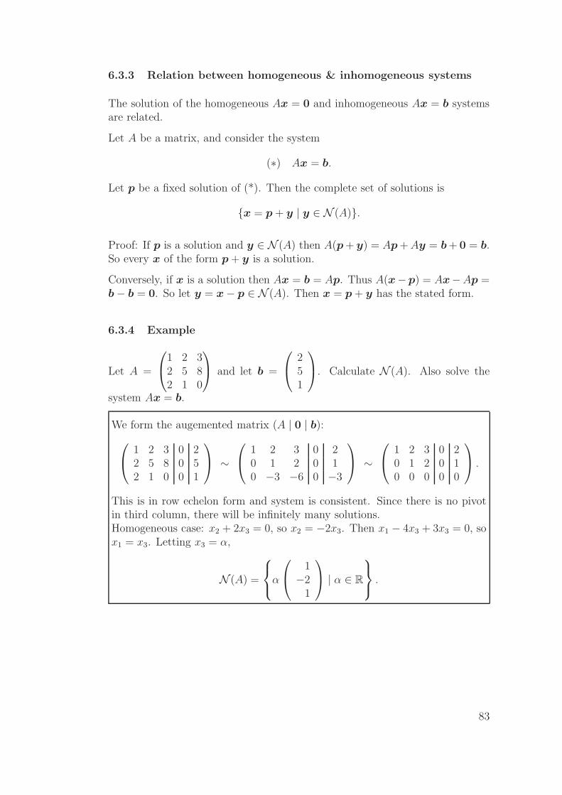
6.3.3 Relation between homogeneous & inhomogeneous systems
The solution of the homogeneous Ax = 0 and inhomogeneous Ax = b systemsare related.
Let A be a matrix, and consider the system
(∗) Ax = b.
Let p be a fixed solution of (*). Then the complete set of solutions is
{x = p + y | y ∈ N (A)}.
Proof: If p is a solution and y ∈ N (A) then A(p + y) = Ap + Ay = b + 0 = b.So every x of the form p + y is a solution.
Conversely, if x is a solution then Ax = b = Ap. Thus A(x−p) = Ax−Ap =b− b = 0. So let y = x− p ∈ N (A). Then x = p + y has the stated form.
6.3.4 Example
Let A =
1 2 32 5 82 1 0
and let b =
251
. Calculate N (A). Also solve the
system Ax = b.
We form the augemented matrix (A | 0 | b):
1 2 3 0 22 5 8 0 52 1 0 0 1
∼
1 2 3 0 20 1 2 0 10 −3 −6 0 −3
∼
1 2 3 0 20 1 2 0 10 0 0 0 0
.
This is in row echelon form and system is consistent. Since there is no pivotin third column, there will be infinitely many solutions.Homogeneous case: x2 + 2x3 = 0, so x2 = −2x3. Then x1 − 4x3 + 3x3 = 0, sox1 = x3. Letting x3 = α,
N (A) =
α
1−2
1
| α ∈ R
.
83

Inhomogeneous case: x3 = α
1 2 3 20 1 2 10 0 0 0
x2 + 2α = 1 ⇒ x2 = 1− 2α
x1 + 2x2 + 3α = 2⇒ x1 + 2(1− 2α) + 3x2 = 2
⇒ x1 − α = 0
⇒ x1 = α.
Then
x =
α1− 2α
α
=
010
+ α
1−2
1
= p + y,
where p =
010
is a particular solution of Ax = b and y ∈ N (A).
6.3.5 Summary
There are 3 possible behaviours for a system:
1. The system Ax = b may have no solutions. (Inconsistent case.)
2. If a solution to Ax = b exists and N (A) = {0} then Ax = b has a uniquesolution.
3. If Ax = b has a solution x = p and N (A) 6= {0} then there are infinitelymany solutions: all x of the form x = p + y with y ∈ N (A).
Important: Note that a homogeneous system is always consistent, because the0-vector is always a solution.
84

6.3.6 Invertibility and the Nullspace
Now suppose A is a square matrix. We add some further conditions equivalentto A being invertible:
Theorem: The following are equivalent for a square matrix A:
1. A is invertible.
2. For every b, the system Ax = b has a unique solution
3. N (A) = {0}
Proof: (1) ⇒ (2) Done earlier: in section 6.1.1.
(2) ⇒ (3) If (2) is true then Ax = 0 has a unique solution, which must bex = 0. So N (A) = {0}.(3) ⇒ (1) We use the same trick to isolate the columns of A that we saw inTheorem 5.3.1. Ax = 0 can be expressed as
Ax = A(x1e1 + · · · · · ·+ xnen) = 0
orx1Ae1 + x2Ae2 + · · · · · ·+ xnAen = 0
where Aej = jth column vector of A. Therefore x = 0 unique solution ⇐⇒column vectors of A linearly independent ⇔ A is invertible by Theorem 5.3.1.
6.4 Gauss-Jordan elimination
Gauss-Jordan (or simply Jordan) reduction involves performing more EROs onthe Gauss reduced form of a matrix until it has the additional property thateach leading 1 is the only non-zero entry in its column.
Solve2x1 − 3x2 − x3 = 1x1 − 2x2 − 3x3 = 2
−2x1 + 2x2 − 5x3 = 3
6.4.1 Solution
This is example 6.2.3 again. The augmented matrix is:
2 −3 −1 11 −2 −3 2−2 2 −5 3
∼
1 −2 −3 20 1 5 −30 0 1 −1
85
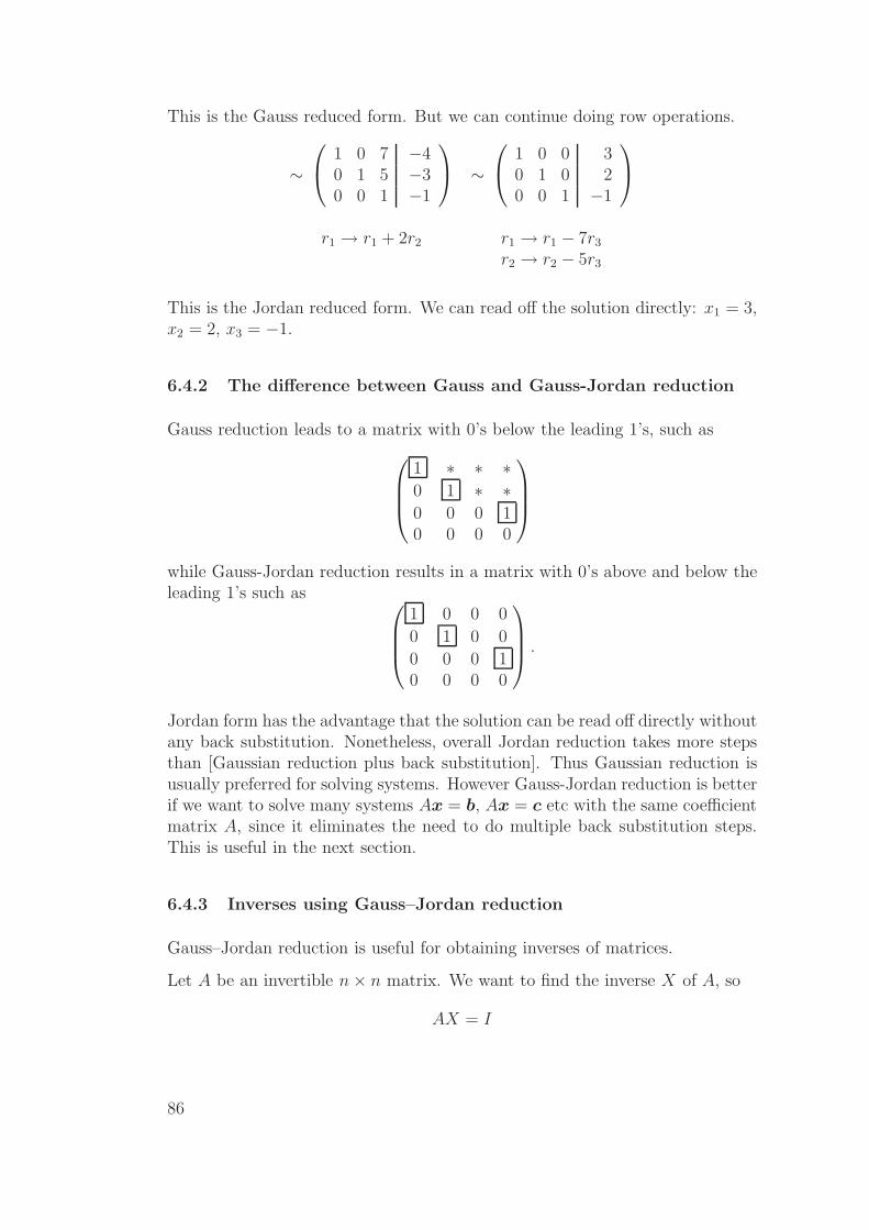
This is the Gauss reduced form. But we can continue doing row operations.
∼
1 0 7 −40 1 5 −30 0 1 −1
∼
1 0 0 30 1 0 20 0 1 −1
r1 → r1 + 2r2 r1 → r1 − 7r3
r2 → r2 − 5r3
This is the Jordan reduced form. We can read off the solution directly: x1 = 3,x2 = 2, x3 = −1.
6.4.2 The difference between Gauss and Gauss-Jordan reduction
Gauss reduction leads to a matrix with 0’s below the leading 1’s, such as
1 ∗ ∗ ∗0 1 ∗ ∗0 0 0 10 0 0 0
while Gauss-Jordan reduction results in a matrix with 0’s above and below theleading 1’s such as
1 0 0 0
0 1 0 0
0 0 0 10 0 0 0
.
Jordan form has the advantage that the solution can be read off directly withoutany back substitution. Nonetheless, overall Jordan reduction takes more stepsthan [Gaussian reduction plus back substitution]. Thus Gaussian reduction isusually preferred for solving systems. However Gauss-Jordan reduction is betterif we want to solve many systems Ax = b, Ax = c etc with the same coefficientmatrix A, since it eliminates the need to do multiple back substitution steps.This is useful in the next section.
6.4.3 Inverses using Gauss–Jordan reduction
Gauss–Jordan reduction is useful for obtaining inverses of matrices.
Let A be an invertible n× n matrix. We want to find the inverse X of A, so
AX = I
86
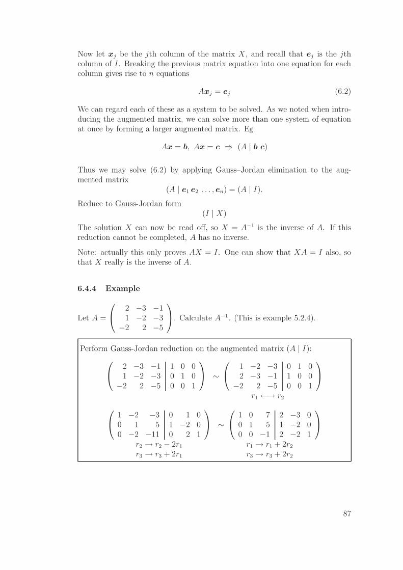
Now let xj be the jth column of the matrix X, and recall that ej is the jthcolumn of I. Breaking the previous matrix equation into one equation for eachcolumn gives rise to n equations
Axj = ej (6.2)
We can regard each of these as a system to be solved. As we noted when intro-ducing the augmented matrix, we can solve more than one system of equationat once by forming a larger augmented matrix. Eg
Ax = b, Ax = c ⇒ (A | b c)
Thus we may solve (6.2) by applying Gauss–Jordan elimination to the aug-mented matrix
(A | e1 e2 . . . , en) = (A | I).
Reduce to Gauss-Jordan form(I | X)
The solution X can now be read off, so X = A−1 is the inverse of A. If thisreduction cannot be completed, A has no inverse.
Note: actually this only proves AX = I. One can show that XA = I also, sothat X really is the inverse of A.
6.4.4 Example
Let A =
2 −3 −11 −2 −3−2 2 −5
. Calculate A−1. (This is example 5.2.4).
Perform Gauss-Jordan reduction on the augmented matrix (A | I):
2 −3 −1 1 0 01 −2 −3 0 1 0−2 2 −5 0 0 1
∼
1 −2 −3 0 1 02 −3 −1 1 0 0−2 2 −5 0 0 1
r1 ←→ r2
1 −2 −3 0 1 00 1 5 1 −2 00 −2 −11 0 2 1
∼
1 0 7 2 −3 00 1 5 1 −2 00 0 −1 2 −2 1
r2 → r2 − 2r1 r1 → r1 + 2r2
r3 → r3 + 2r1 r3 → r3 + 2r2
87
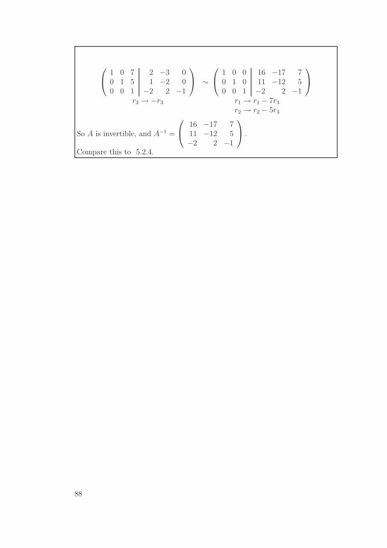
1 0 7 2 −3 00 1 5 1 −2 00 0 1 −2 2 −1
∼
1 0 0 16 −17 70 1 0 11 −12 50 0 1 −2 2 −1
r3 → −r3 r1 → r1 − 7r3
r2 → r2 − 5r3
So A is invertible, and A−1 =
16 −17 711 −12 5−2 2 −1
.
Compare this to 5.2.4.
88

Notes
89

7 Determinants
7.1 Definition: Determinant
Associated to each square matrix A is a number called the determinant of Aand denoted |A| or det(A). It is defined as follows.
• If A = (aij) is 2× 2 then
|A| =∣∣∣∣
a11 a12
a21 a22
∣∣∣∣= a11a22 − a12a21
We already encountered this in 5.2.1.
• In general if A = (aij) is n× n, first set
Cij = (−1)i+j
∣∣∣∣∣∣∣∣∣∣∣∣∣∣∣
a11 a12 .... a1 j−1 a1 j+1 .... a1n
a21 a22 .... a2 j−1 a2 j+1 .... a2n...
......
......
ai−1 1 ai−1 2 .... ai−1 j−1 ai−1 j+1 .... ai−1 n
ai+1 1 ai+1 2 .... ai+1 j−1 ai+1 j+1 .... ai+1 n...
......
......
an1 an2 .... an j−1 an j+1 .... ann
∣∣∣∣∣∣∣∣∣∣∣∣∣∣∣
called the cofactor of aij . The (n−1)× (n−1) determinant is obtained byomitting the ith row and jth column from A (indicated by the horizontaland vertical lines in the matrix).
We then define
|A| = a11C11 + a12C12 + · · · · · ·+ a1nC1n
which gives a recursive definition of the determinant.
Observe that (−1)i+j gives the pattern
+ − + − · · · ·− + − + · · · ·+ − + − · · · ····
Thus for a 3× 3 matrix A we have
|A| =
∣∣∣∣∣∣
a11 a12 a13
a21 a22 a23
a31 a32 a33
∣∣∣∣∣∣
= a11C11 + a12C12 + a13C13
where
C11 =
∣∣∣∣
a22 a23
a32 a33
∣∣∣∣, C12 = −
∣∣∣∣
a21 a23
a31 a33
∣∣∣∣
, C13 =
∣∣∣∣
a21 a22
a31 a32
∣∣∣∣.
90

7.1.1 Example
Find the cofactors C13 and C23 of the matrix
3 5 71 0 20 3 0
.
C13 = (−1)1+3M13 = 1 ·∣∣∣∣
1 00 3
∣∣∣∣= 3,
C23 = (−1)2+3M23 = −1 ·∣∣∣∣
3 50 3
∣∣∣∣= −9.
7.1.2 Example
Calculate the determinant
∣∣∣∣∣∣
3 5 71 0 20 3 0
∣∣∣∣∣∣
.
∣∣∣∣∣∣
3 5 71 0 20 3 0
∣∣∣∣∣∣
= (1) · (3) ·∣∣∣∣
0 23 0
∣∣∣∣+ (−1) · (5) ·
∣∣∣∣
1 20 0
∣∣∣∣+ (1) · (7) ·
∣∣∣∣
1 00 3
∣∣∣∣
= 3(0− 6)− 5(0− 0) + 7(3− 0)
= 3.
91

7.2 Properties of Determinants
Property (1): |A| =∣∣AT
∣∣
Consider for example the 2× 2 case. Then
A =
(a11 a12
a21 a22
)
⇒ AT =
(a11 a21
a12 a22
)
Thus |A| = a11a22 − a12a21 =∣∣AT
∣∣. This holds in general.
This means that any results about the rows in a general determinant is alsotrue about the columns (since the rows of AT are the columns of A).
Property (2): The determinant may by taking cofactors along any row (notjust the first) or down any column. Eg. for a 3× 3 matrix A
|A| = a11C11 + a12C12 + a13C13 (definition, expansion along 1st row)= a21C21 + a22C22 + a23C23 (expansion along 2nd row)= a13C13 + a23C23 + a33C33 (expansion down 3rd column) etc.
This is useful if one row or column contains a larger number of zeros.
7.2.1 Examples
(i) Calculate
∣∣∣∣∣∣
3 5 71 0 20 3 0
∣∣∣∣∣∣
by (a) expanding down the third column, (b) ex-
panding along the third row. Which is more efficient?
∣∣∣∣∣∣
3 5 71 0 20 3 0
∣∣∣∣∣∣
= 7
∣∣∣∣
1 00 3
∣∣∣∣− 2
∣∣∣∣
3 50 3
∣∣∣∣= 21− 18 = 3
(exp. down3rd. col.
)
= −3
∣∣∣∣
3 71 2
∣∣∣∣= −3(6− 7) = 3
(exp. along
r3
)
92

(ii) Find∣∣∣∣∣∣
3 6 90 0 02 4 5
∣∣∣∣∣∣
.
∣∣∣∣∣∣
3 6 90 0 02 4 5
∣∣∣∣∣∣
= 0 · C21 + 0 · C22 + 0 · C23
= 0 (expanding along r2)
In general any determinant with a row or column of zeros vanishes.
7.2.2 Effect of Elementary Row Operations on Determinants
The calculation of large determinants from the definition is very tedious. It ismuch easier to calculate the determinant after row reducing a matrix, becausethe reduced matrix will contain many zeros. However, performing elementaryrow operations changes the value of a determinant. Luckily the changes aresimple:
Property (3): From (2), a common factor in all entries of a row (or column)can be taken out as a factor of the determinant.
7.2.3 Example
∣∣∣∣∣∣
3 6 90 1 23 4 5
∣∣∣∣∣∣
= 3C11 + 6C12 + 9C13 (expanding along r1)
= 3[C11 + 2C12 + 3C13]
= 3 ·
∣∣∣∣∣∣
1 2 30 1 23 4 5
∣∣∣∣∣∣
(check!)
Property (4): If 2 rows (or columns) of A are interchanged (ri ←→ rj or ci ←→cj), |A| changes sign.
93
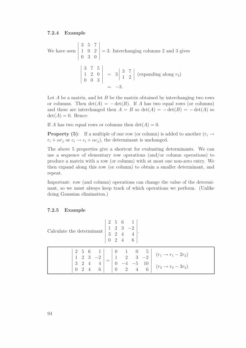
7.2.4 Example
We have seen
∣∣∣∣∣∣
3 5 71 0 20 3 0
∣∣∣∣∣∣
= 3. Interchanging columns 2 and 3 gives
∣∣∣∣∣∣
3 7 51 2 00 0 3
∣∣∣∣∣∣
= 3
∣∣∣∣
3 71 2
∣∣∣∣
(expanding along r3)
= −3.
Let A be a matrix, and let B be the matrix obtained by interchanging two rowsor columns. Then det(A) = − det(B). If A has two equal rows (or columns)and these are interchanged then A = B so det(A) = − det(B) = − det(A) sodet(A) = 0. Hence:
If A has two equal rows or columns then det(A) = 0.
Property (5): If a multiple of one row (or column) is added to another (ri →ri + αrj or ci → ci + αcj), the determinant is unchanged.
The above 5 properties give a shortcut for evaluating determinants. We canuse a sequence of elementary row operations (and/or column operations) toproduce a matrix with a row (or column) with at most one non-zero entry. Wethen expand along this row (or column) to obtain a smaller determinant, andrepeat.
Important: row (and column) operations can change the value of the determi-nant, so we must always keep track of which operations we perform. (Unlikedoing Gaussian elimination.)
7.2.5 Example
Calculate the determinant
∣∣∣∣∣∣∣∣
2 5 6 11 2 3 −23 2 4 40 2 4 6
∣∣∣∣∣∣∣∣
.
∣∣∣∣∣∣∣∣
2 5 6 11 2 3 −23 2 4 40 2 4 6
∣∣∣∣∣∣∣∣
=
∣∣∣∣∣∣∣∣
0 1 0 51 2 3 −20 −4 −5 100 2 4 6
∣∣∣∣∣∣∣∣
(r1 → r1 − 2r2)
(r3 → r3 − 3r2)
94
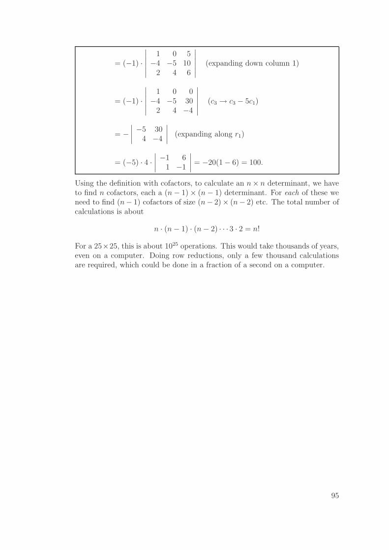
= (−1) ·
∣∣∣∣∣∣
1 0 5−4 −5 10
2 4 6
∣∣∣∣∣∣
(expanding down column 1)
= (−1) ·
∣∣∣∣∣∣
1 0 0−4 −5 30
2 4 −4
∣∣∣∣∣∣
(c3 → c3 − 5c1)
= −∣∣∣∣
−5 304 −4
∣∣∣∣
(expanding along r1)
= (−5) · 4 ·∣∣∣∣
−1 61 −1
∣∣∣∣= −20(1− 6) = 100.
Using the definition with cofactors, to calculate an n× n determinant, we haveto find n cofactors, each a (n− 1)× (n− 1) determinant. For each of these weneed to find (n− 1) cofactors of size (n− 2)× (n− 2) etc. The total number ofcalculations is about
n · (n− 1) · (n− 2) · · · 3 · 2 = n!
For a 25×25, this is about 1025 operations. This would take thousands of years,even on a computer. Doing row reductions, only a few thousand calculationsare required, which could be done in a fraction of a second on a computer.
95
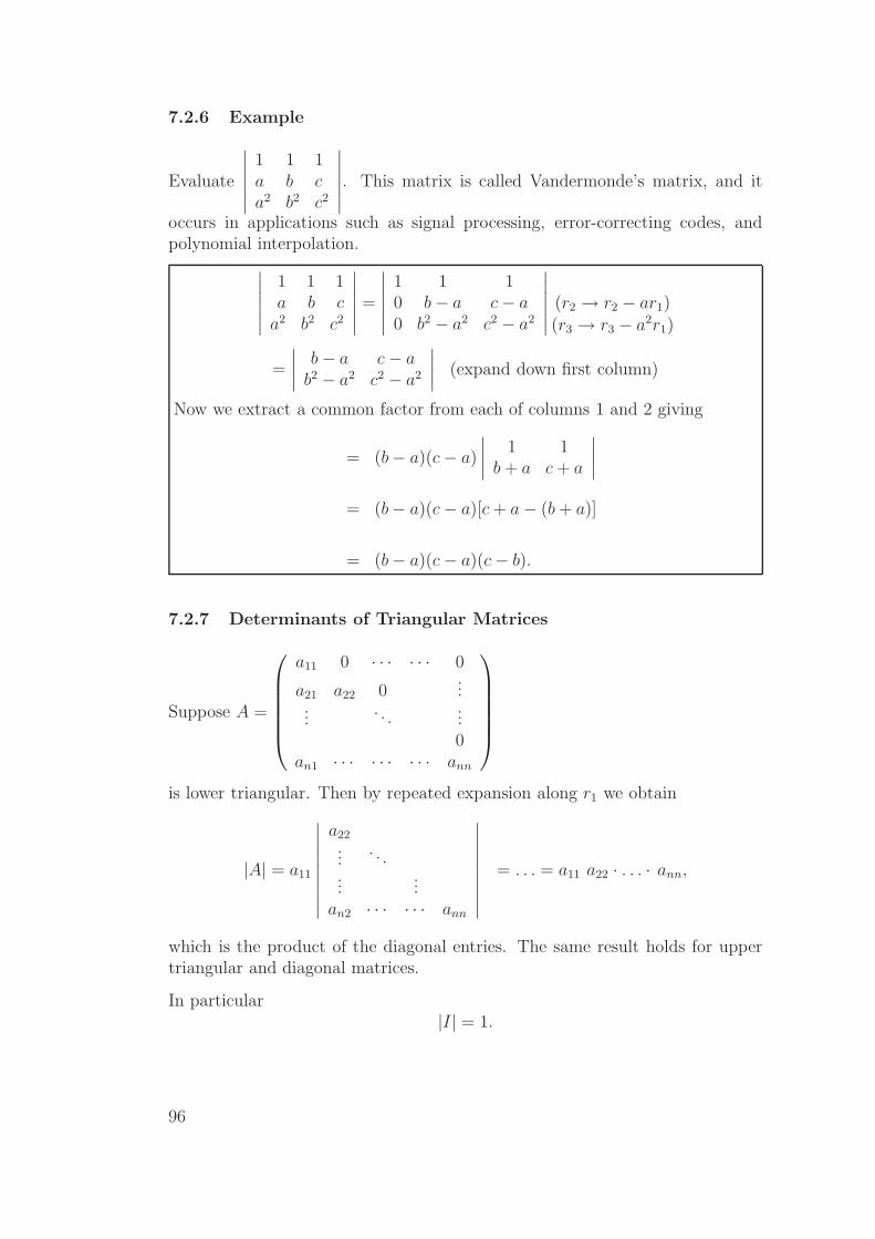
7.2.6 Example
Evaluate
∣∣∣∣∣∣
1 1 1a b ca2 b2 c2
∣∣∣∣∣∣
. This matrix is called Vandermonde’s matrix, and it
occurs in applications such as signal processing, error-correcting codes, andpolynomial interpolation.
∣∣∣∣∣∣
1 1 1a b c
a2 b2 c2
∣∣∣∣∣∣
=
∣∣∣∣∣∣
1 1 10 b− a c− a0 b2 − a2 c2 − a2
∣∣∣∣∣∣
(r2 → r2 − ar1)
(r3 → r3 − a2r1)
=
∣∣∣∣
b− a c− ab2 − a2 c2 − a2
∣∣∣∣
(expand down first column)
Now we extract a common factor from each of columns 1 and 2 giving
= (b− a)(c− a)
∣∣∣∣
1 1b + a c + a
∣∣∣∣
= (b− a)(c− a)[c + a− (b + a)]
= (b− a)(c− a)(c− b).
7.2.7 Determinants of Triangular Matrices
Suppose A =
a11 0 · · · · · · 0
a21 a22 0...
.... . .
...0
an1 · · · · · · · · · ann
is lower triangular. Then by repeated expansion along r1 we obtain
|A| = a11
∣∣∣∣∣∣∣∣∣
a22...
. . ....
...an2 · · · · · · ann
∣∣∣∣∣∣∣∣∣
= . . . = a11 a22 · . . . · ann,
which is the product of the diagonal entries. The same result holds for uppertriangular and diagonal matrices.
In particular|I| = 1.
96

7.3 Connection with inverses and systems of linear equa-tions
An important property of determinants is the following.
7.3.1 Fact (product of determinants)
Let A, B be n× n matrices. Then
|AB| = |A| · |B| .
7.3.2 Theorem: Invertible matrices
A is invertible ⇐⇒ |A| 6= 0.
7.3.3 Proof
=⇒ If A is invertible, then
I = AA−1
⇒ 1 = |I| = |AA−1| = |A| |A−1| ,So |A| 6= 0.
⇐= Follows from 7.3.4.
Remark: It follows immediately from the proof that if A is invertible, then
|A−1| = 1
|A| ,
i.e., the inverse of the determinant is the determinant of the inverse.
7.3.4 A Theoretical Formula
Actually there is an explicit formula for the inverse of A. If Cij is the cofactorof the i, j entry of A, let C be the matrix of cofactors C = (Cij). Then
A−1 =1
|A|CT .
Here CT is called the adjoint matrix of A. This formula is useful for sometheoretical problems, but is useless as a tool for calculations because it is sotime consuming to calculate all the cofactors.
Never use this formula for calculating inverses!
97
7.3.5 Example
In the 2× 2 case we have
|A| =∣∣∣∣
a11 a12
a21 a22
∣∣∣∣= a11a22 − a12a21
and co-factors
C11 = a22 , C12 = −a21 , C21 = −a12 , C22 = a11
∴ |A| 6= 0⇒ A−1 = 1|A|
(C11 C21
C12 C22
)
= 1|A|
(a22 −a12
−a21 a11
)
in agreement with a previous result, 5.2.1.
7.3.6 Summary of conditions equivalent to invertibility
Let A be an n× n matrix. Give a summary of all the conditions we have foundthat are equivalent to A being invertible.
1. A is invertible.
2. There exists an n × n matrix X with AX = XA = I [Definition ofinvertible, § 5.2].
3. AT is invertible [§ 5.3.6(3)].
4. The columns of A are linearly independent [Theorem 5.3.1 and§ 5.3.6(5)].
5. The rows of A are linearly independent [§ 5.3.6(6)].
6. Ax = b has a unique solution x for any b ∈ R [§ 6.3.6].
7. N (A) = {0} [§ 6.3.6].
8. The row reduced form of A is I [§ 6.4].
9. det(A) 6= 0 [Theorem 7.3.2].
98
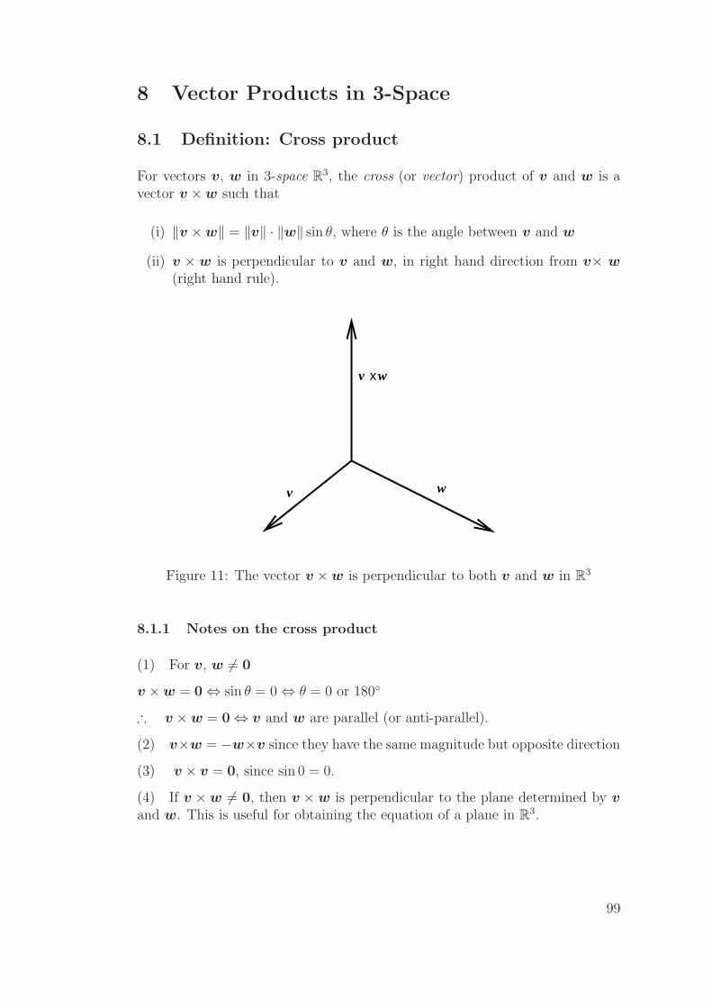
8 Vector Products in 3-Space
8.1 Definition: Cross product
For vectors v, w in 3-space R3, the cross (or vector) product of v and w is avector v ×w such that
(i) ‖v ×w‖ = ‖v‖ · ‖w‖ sin θ, where θ is the angle between v and w
(ii) v × w is perpendicular to v and w, in right hand direction from v× w
(right hand rule).
x
v w
v w
Figure 11: The vector v ×w is perpendicular to both v and w in R3
8.1.1 Notes on the cross product
(1) For v, w 6= 0
v ×w = 0⇔ sin θ = 0⇔ θ = 0 or 180◦
∴ v ×w = 0⇔ v and w are parallel (or anti-parallel).
(2) v×w = −w×v since they have the same magnitude but opposite direction
(3) v × v = 0, since sin 0 = 0.
(4) If v ×w 6= 0, then v ×w is perpendicular to the plane determined by v
and w. This is useful for obtaining the equation of a plane in R3.
99

8.1.2 Example
i× i = j × j = k × k = 0
i× j = k = −j × i , j × k = i = −k × j
k × i = j = −i× k
i
jk
Figure 12: This diagram is an aid in remembering the cross product betweenunit vectors.
8.1.3 Application: angular momentum
Vector products also arise naturally in physics and engineering eg. a particleof unit charge moving with velocity v in a magnetic field B experiences a forceF = v × B. The angular momentum of a particle of mass m moving withvelocity v is given by L = m(r × v) where r is the position vector of theparticle. This is important for central force problems.
8.1.4 Properties
We have seen thatv ×w = −w × v
so the commutative law fails. Also we do not have the associative law: ie. ingeneral
v × (w × u) 6= (v ×w)× u
For example, (i× i)× k = 0× k = 0, but i× (i× k) = i× (−j) = −k.
However, it can be shown that
v × (w + u) = v ×w + v × u
(v + w)× u = v × u + w × u
v × (αw) = (αv)×w = α(v ×w) , α ∈ R.
Using the above results we have the following theorem in terms of components.
100

8.1.5 Theorem: Calculating the cross product
Suppose v =
v1
v2
v3
, w =
w1
w2
w3
. Then
v ×w = (v2w3 − v3w2)i + (v3w1 − v1w3)j + (v1w2 − v2w1)k
ie. v ×w =
∣∣∣∣∣∣
i j k
v1 v2 v3
w1 w2 w3
∣∣∣∣∣∣
=
∣∣∣∣
v2 v3
w2 w3
∣∣∣∣i−
∣∣∣∣
v1 v3
w1 w3
∣∣∣∣
j +
∣∣∣∣
v1 v2
w1 w2
∣∣∣∣
k
can be evaluated by expanding above determinant along the first row.
8.1.6 Proof
This follows directly by expanding:
v ×w = (v1i + v2j + v3k)× (w1i + w2j + w3k)
= v1i× (w1i + w2j + w3k)
+ v2j × (w1i + w2j + w3k)
+ v3k × (w1i + w2j + w3k)
= v1w2(i× j)− v1w3(k × i)
− v2w1(i× j) + v2w3(j × k)
+ v3w1(k × i)− v3w2(j × k)
= (v2w3 − v3w2)i− (v1w3 − v3w1)j + (v1w2 − v2w1)k.
101

8.1.7 Example
Let v = (1, 2, 3), w = (4, 5, 6). Find a (non-zero) vector orthogonal to both v
and w.
The vector v ×w will do:
v ×w =
∣∣∣∣∣∣
i j k
1 2 34 5 6
∣∣∣∣∣∣
= i
∣∣∣∣
2 35 6
∣∣∣∣− j
∣∣∣∣
1 34 6
∣∣∣∣+ k
∣∣∣∣
1 24 5
∣∣∣∣
= i(12− 15)− j(6− 12) + k(5− 8)
= −3i + 6j − 3k.
This is orthogonal to both v and w.
8.2 Application: area of a triangle
Find area of the ∆ABC with vectors v, w along edges as shown in Figure 13.
θv
w
A
B
C
h
Figure 13: Find the area of the triangle ABC
Area =1
2base · perpendicular height
=1
2‖v‖ · ‖w‖ sin θ =
1
2‖v ×w‖ .
102

8.2.1 Example
Find the area of a triangle with vertices A = (0, 1, 3), B = (1, 2, 1), C = (4, 1, 0)and obtain a vector perpendicular to the plane of ∆ABC.
w =−→AB =
11−2
, v =−→AC =
40−3
Hence a vector perpendicular to the plane of ∆ABC is
v ×w =
∣∣∣∣∣∣
i j k
4 0 −31 1 −2
∣∣∣∣∣∣
= 3i + 5j + 4k.
Area of the triangle
1
2‖v ×w‖ =
1
2‖3i + 5j + 4k‖
=1
2
√9 + 25 + 16
=1
2
√50
=5√
2
2.
103

8.3 Scalar Triple Product
The number u · (v ×w) is called the scalar triple product of u, v, w.
Using the result of the previous theorem, express this product in terms of com-ponents.
Set u = u1i + u2j + u3k. Then
u · (v ×w) = (u1i + u2j + u3k) ·(∣
∣∣∣
v2 v3
w2 w3
∣∣∣∣i−
∣∣∣∣
v1 v3
w1 w3
∣∣∣∣j +
∣∣∣∣
v1 v2
w1 w2
∣∣∣∣k
)
= u1
∣∣∣∣
v2 v3
w2 w3
∣∣∣∣− u2
∣∣∣∣
v1 v3
w1 w3
∣∣∣∣+ u3
∣∣∣∣
v1 v2
w1 w2
∣∣∣∣
=
∣∣∣∣∣∣
u1 u2 u3
v1 v2 v3
w1 w2 w3
∣∣∣∣∣∣
.
This is a 3× 3 determinant.
8.4 Geometrical Interpretation
The volume V of a parallelepiped determined by vectors u, v, w along edgesas shown is given by
V = |u · (v ×w)|
CD
BA
xv w
w
v
u
Figure 14: Parallelepiped determined using vectors.
104

8.4.1 Proof
V = (area of base ABCD)× h where
h = perpendicular height
= size of component of u in direction of v ×w
=
∣∣∣∣
u · (v ×w)
‖v ×w‖2(v ×w)
∣∣∣∣=|u · (v ×w)|‖v ×w‖
From previous example,
area of the base ABCD = 2× (area ∆ ABD)
= ‖v ×w‖
⇒ V = ‖v ×w‖ · h = |u · (v ×w)| .
8.4.2 Example
Find the volume V of the parallelepiped determined by the vectors
a =
121
, b =
111
, c =
001
.
V = |a · (b× c)|, where
a · (b× c) =
∣∣∣∣∣∣
1 2 11 1 10 0 1
∣∣∣∣∣∣
= 1 ·∣∣∣∣
1 21 1
∣∣∣∣= 1− 2 = −1 (expanded along r3)
⇒ V = |−1| = 1.
The volume V of a parallepiped determined by the vectors u, v, w vanishes iffvectors are co-planar; therefore vectors are co-planar iff
∣∣∣∣∣∣
u1 u2 u3
v1 v2 v3
w1 w2 w3
∣∣∣∣∣∣
= 0 − this gives a useful method for determiningwhen 3 vectors are co-planar.
105

9 Eigenvalues and eigenvectors
Let A be an n× n matrix and consider the equation
Ax = λx (9.1)
with λ a number (possibly complex). It is clear that x = 0 is always a solutionto (9.1). A value λ, for which (9.1) has solution x 6= 0 is called an eigenvalueof A. The corresponding solution vector x 6= 0 is called an eigenvector of Acorresponding to the eigenvalue λ.
9.1 Eigenvalues
9.1.1 Example
Let
A =
(1 34 2
)
,
One eigenvalue is λ = −2 with corresponding eigenvector
(−1
1
)
since
(1 34 2
) (−1
1
)
=
(2−2
)
= −2
(−1
1
)
,
another eigenvalue is λ = 5 with corresponding eigenvector
(34
)
.
9.1.2 Note
Usually Ax is related to x in a much more complicated way,
e.g.
(1 34 2
) (12
)
=
(78
)
6= λ
(12
)
.
106

9.2 Eigenspace
9.2.1 Proposition (eigenspace is a vector space)
Let λ be an eigenvalue of A. Then the set of solutions to (9.1) forms a vectorspace called the eigenspace of A corresponding to eigenvalue λ, denoted Nλ. SoNλ = {x ∈ Rn : Ax = λx}.
9.2.2 Proof
(o) Note that 0 is always a solution to (9.1), so 0 ∈ Nλ.
Take x, y ∈ Nλ, α ∈ R.
(i) Then
A(x + y) = Ax + Ay
= λx + λy
= λ(x + y)
⇒ x + y ∈ Nλ.
(ii)
A(αx) = αAx
= αλx
= λ(αx)
⇒ αx ∈ Nλ.
Hence the set of solutions to (9.1) forms a vector space.
9.3 How to find eigenvalues
We haveAx = λx
⇐⇒ Ax = λ(Ix)⇐⇒ Ax− λIx = 0⇐⇒ (A− λI)x = 0.
We seek a non-zero solution x of this equation. Recall that an n × n systemBx = 0 has a solution x 6= 0 iff B is not invertible iff |B| = 0.
Thus A has eigenvalue λ if and only if
|A− λI| = 0.
107
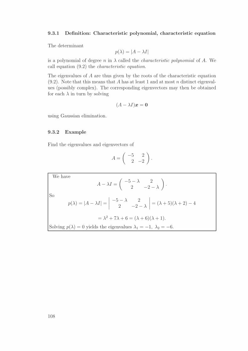
9.3.1 Definition: Characteristic polynomial, characteristic equation
The determinantp(λ) = |A− λI|
is a polynomial of degree n in λ called the characteristic polynomial of A. Wecall equation (9.2) the characteristic equation.
The eigenvalues of A are thus given by the roots of the characteristic equation(9.2). Note that this means that A has at least 1 and at most n distinct eigenval-ues (possibly complex). The corresponding eigenvectors may then be obtainedfor each λ in turn by solving
(A− λI)x = 0
using Gaussian elimination.
9.3.2 Example
Find the eigenvalues and eigenvectors of
A =
(−5 2
2 −2
)
.
We have
A− λI =
(−5− λ 2
2 −2− λ
)
.
So
p(λ) = |A− λI| =∣∣∣∣
−5− λ 22 −2− λ
∣∣∣∣= (λ + 5)(λ + 2)− 4
= λ2 + 7λ + 6 = (λ + 6)(λ + 1).
Solving p(λ) = 0 yields the eigenvalues λ1 = −1, λ2 = −6.
108
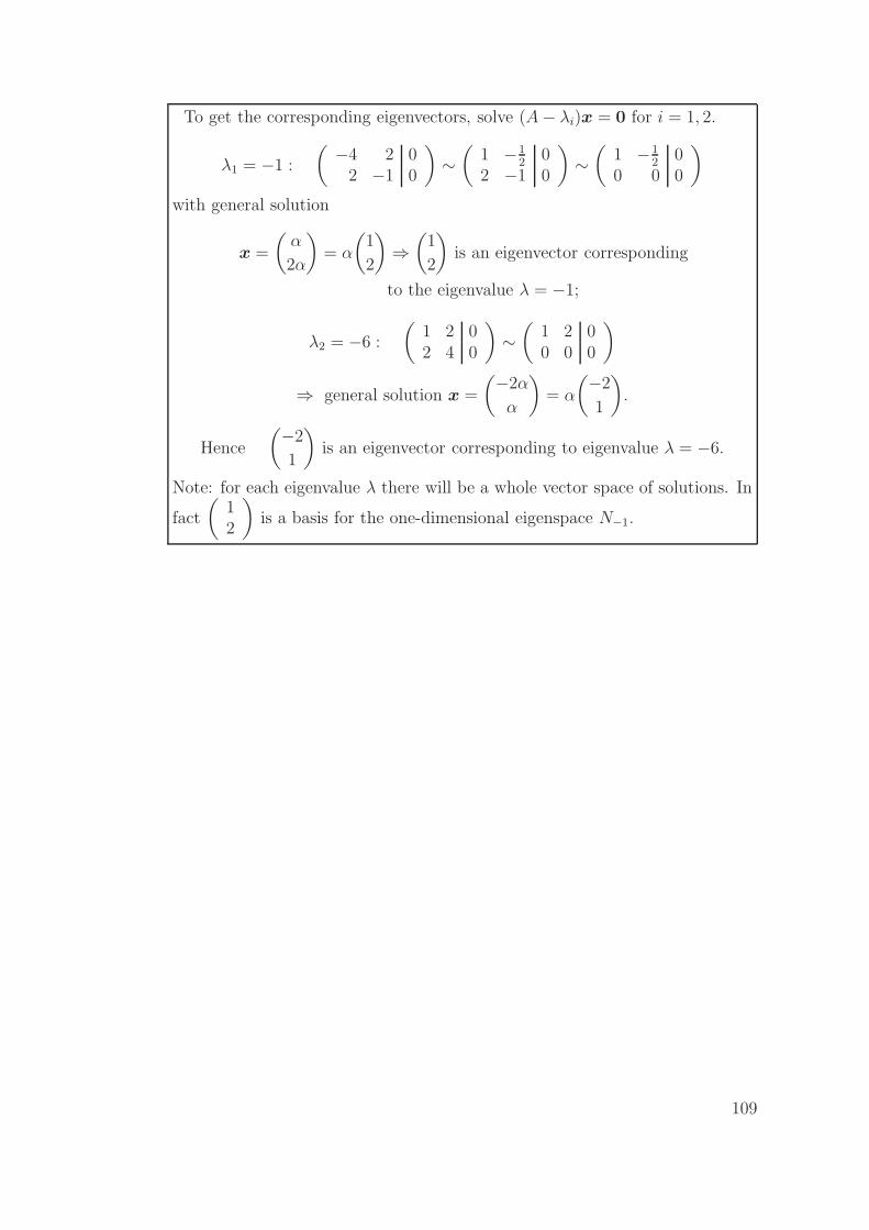
To get the corresponding eigenvectors, solve (A− λi)x = 0 for i = 1, 2.
λ1 = −1 :
(−4 2 0
2 −1 0
)
∼(
1 −12
02 −1 0
)
∼(
1 −12
00 0 0
)
with general solution
x =
(α
2α
)
= α
(1
2
)
⇒(
1
2
)
is an eigenvector corresponding
to the eigenvalue λ = −1;
λ2 = −6 :
(1 2 02 4 0
)
∼(
1 2 00 0 0
)
⇒ general solution x =
(−2α
α
)
= α
(−2
1
)
.
Hence
(−2
1
)
is an eigenvector corresponding to eigenvalue λ = −6.
Note: for each eigenvalue λ there will be a whole vector space of solutions. In
fact
(12
)
is a basis for the one-dimensional eigenspace N−1.
109
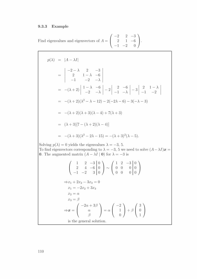
9.3.3 Example
Find eigenvalues and eigenvectors of A =
−2 2 −32 1 −6−1 −2 0
.
p(λ) = |A− λI|
=
∣∣∣∣∣∣
−2− λ 2 −32 1− λ −6−1 −2 −λ
∣∣∣∣∣∣
= −(λ + 2)
∣∣∣∣
1− λ −6−2 −λ
∣∣∣∣− 2
∣∣∣∣
2 −6−1 −λ
∣∣∣∣− 3
∣∣∣∣
2 1− λ−1 −2
∣∣∣∣
= −(λ + 2)(λ2 − λ− 12)− 2(−2λ− 6)− 3(−λ− 3)
= −(λ + 2)(λ + 3)(λ− 4) + 7(λ + 3)
= (λ + 3)[7− (λ + 2)(λ− 4)]
= −(λ + 3)(λ2 − 2λ− 15) = −(λ + 3)2(λ− 5).
Solving p(λ) = 0 yields the eigenvalues λ = −3, 5.To find eigenvectors corresponding to λ = −3, 5 we need to solve (A−λI)x =0. The augmented matrix (A− λI | 0) for λ = −3 is
1 2 −3 02 4 −6 0−1 −2 3 0
∼
1 2 −3 00 0 0 00 0 0 0
⇒x1 + 2x2 − 3x3 = 0
x1 = −2x2 + 3x3
x2 = α
x3 = β
⇒x =
−2α + 3βαβ
= α
−210
+ β
301
is the general solution.
110

So
−210
,
301
are linearly independent eigenvectors for λ1 = −3, and
they form a basis of the eigenspace.
For λ2 = 5 the augmented matrix is
−7 2 −3 02 −4 −6 0−1 −2 −5 0
∼
1 2 5 02 −4 −6 0−7 2 −3 0
∼
1 2 5 00 −8 −16 00 16 32 0
∼
1 2 5 00 1 2 00 0 0 0
So:
x1 + 2x2 + 5x3 = 0 ⇒ x1 = −2x2 − 5x3
x2 + 2x3 = 0 ⇒ x2 = −2x3
x3 = α
⇒ x1 = 4α− 5α = −α
x2 = −2α, x3 = α.
The vector x =
−α−2α
α
= α
−1−2
1
is the general solution,
so
−1−2
1
is an eigenvector with eigenvalue λ = 5.
111
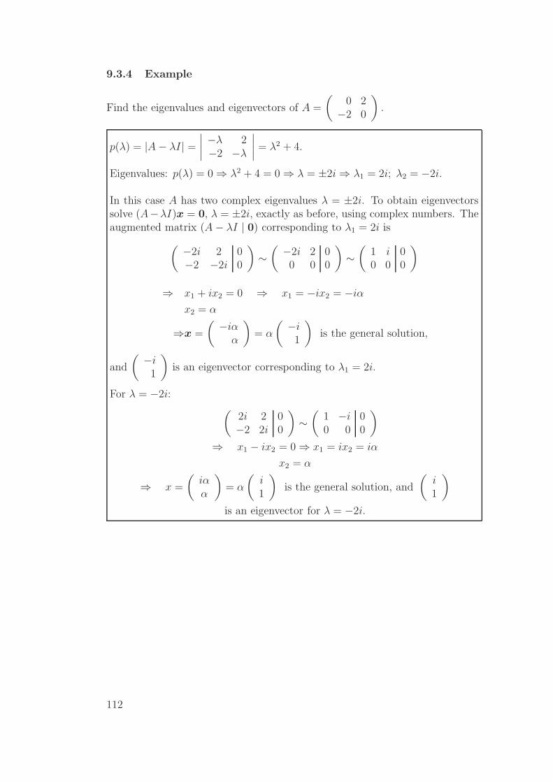
9.3.4 Example
Find the eigenvalues and eigenvectors of A =
(0 2−2 0
)
.
p(λ) = |A− λI| =∣∣∣∣
−λ 2−2 −λ
∣∣∣∣= λ2 + 4.
Eigenvalues: p(λ) = 0⇒ λ2 + 4 = 0⇒ λ = ±2i⇒ λ1 = 2i; λ2 = −2i.
In this case A has two complex eigenvalues λ = ±2i. To obtain eigenvectorssolve (A−λI)x = 0, λ = ±2i, exactly as before, using complex numbers. Theaugmented matrix (A− λI | 0) corresponding to λ1 = 2i is
(−2i 2 0−2 −2i 0
)
∼(−2i 2 00 0 0
)
∼(
1 i 00 0 0
)
⇒ x1 + ix2 = 0 ⇒ x1 = −ix2 = −iα
x2 = α
⇒x =
(−iα
α
)
= α
(−i1
)
is the general solution,
and
(−i1
)
is an eigenvector corresponding to λ1 = 2i.
For λ = −2i:(
2i 2 0−2 2i 0
)
∼(
1 −i 00 0 0
)
⇒ x1 − ix2 = 0⇒ x1 = ix2 = iα
x2 = α
⇒ x =
(iαα
)
= α
(i1
)
is the general solution, and
(i1
)
is an eigenvector for λ = −2i.
112
9.3.5 Note
Solving the system (A− λI)x = 0 to find eigenvectors always leads to at leastone row of zeros when A − λI is row reduced. This is because λ is chosen sothat (A− λI)x = 0 has a solution x 6= 0.
∴ A− λI is not invertible. ∴ A− λI does not reduce to I.
9.3.6 A note on applications
Eigenvalues and eigenvectors have many applications e.g. in Quantum Mechan-ics the energy of a system is represented by a matrix whose eigenvalues givethe allowed energies. This is why discrete energy levels are observed. Anothersituation where they are used is in modelling the population dynamics of apredator-prey system in biology. The eigenvalues and eigenvectors determinethe stability and dynamics of a population in such models.
There are many other applications in Mathematics, Physics, Chemistry andBiology.
113

10 Numbers
Mathematics uses structures at a fundamental level. These basic structures in-clude numbers, sets (e.g. intervals), shapes, vectors, complex numbers, quater-nions and many more strange and exotic things. Numbers are very importantin mathematics as building blocks as they lead to equations and inequalitieswhich we can use as a tool to solve many abstract and applied problems.
10.1 Number systems
R : set of real numbers - represented by a finite or infinite decimal expansion
The following are commonly used subsets of R:
N : set of natural numbers {1, 2, 3, . . .}
Z : set of integers {0, 1,−1, 2,−2, 3,−3, . . .}
Q : set of rational numbers - of the formp
qwhere p, q ∈ Z, q 6= 0
Irrational numbers are real numbers which cannot be represented as a ratio ofintegers. For example,
√2,√
3,√
5, π = 3.14159 . . ., e = 2.71828 . . . are allirrational. Note: proving rationality or irrationality of a given number can bequite subtle!
10.2 Real number line and ordering on R
The real number system can be visualised by imagining each real number as apoint on a line, with the positive direction being to the right, and an arbitraryorigin being chosen to represent 0 (see Figure 15).
0 1 2 3−1−2−3
−1.5 πe
Figure 15: The real number line.
114

The real numbers are ordered, i.e. given any 2 real numbers a and b there holdsprecisely one of the following: a > b, a < b or a = b. This means we can use thesymbols ‘<’, ‘>’, ‘≤’ and ‘≥’ to write statements such as 1 ≤ 2 and 3 >
√3.
Geometrically, a < b means that a lies to the left of b on the real number line.Note also that a ≤ b means that either a < b or a = b.
10.3 Definition: Intervals
An interval is a set of real numbers that can be thought of as a segment of thereal number line. For a < b, the open interval from a to b is given by
(a, b) = {x ∈ R| a < x < b}.
This notation is interpreted as
(a, b) is the set of all real numbers x such that a < x < b.
Note here that the end points are not included. If we wanted to include theendpoints, we would have a closed interval from a to b, denoted
[a, b] = {x ∈ R| a ≤ x ≤ b}.
In this notation it is important to distinguish between the round brackets (a, b)for an open interval (excluding the end points) and the square brackets [a, b] fora closed interval (including the end points).
We also have half-open intervals (or half-closed depending on how you feel),denoted
[a, b) = {x ∈ R| a ≤ x < b}, and
(a, b] = {x ∈ R| a < x ≤ b}.
There are also semi-infinite intervals such as
(−∞, a] = {x ∈ R | x ≤ a}, and
(a,∞) = {x ∈ R | a < x}.
There are other possible types of semi-infinite intervals: Stewart, 6ed. p. A4;5ed. p. A4.
115

10.4 Absolute value
We define
|x| ={
x, if x ≥ 0−x, if x < 0
10.4.1 Examples
|3| = 3
| − 4| = 4
|1− π| = π − 1
10.4.2 Properties of absolute value
(i) |a|2 = a2 ⇒ |a| =√
a2 (positive square root)
(ii) |ab| = |a||b|
(iii) |a + b| ≤ |a|+ |b| (triangle inequality)
(iv) |an| = |a|n, n ∈ Z, with a 6= 0 for nonpositive n.
It is worth emphasising that in general |a + b| 6= |a| + |b|, but the triangleinequality does hold:
|a + b| ≤ |a|+ |b|.
For example, set a = 1 and b = −2. We have l.h.s = |1 + (−2)| = | − 1| = 1,r.h.s = |1|+ | − 2| = 1 + 2 = 3.
10.4.3 Convention for√
For a > 0,√
a always denotes the positive square root. Thus√
4 = 2 and so on.For a > 0, solutions to x2 = a are x = ±√a.
116

Notes
117

Notes
118

11 Functions
11.1 Notation
Let X and Y be subsets of R. The notation f : X → Y means “f maps fromX into Y ”.
11.2 Definition: Function, domain, range
A function f : X → Y is a rule which assigns to every element x ∈ X exactlyone element f(x) ∈ Y called the value of f at x. X is called the domain of fand
f(X) = {f(x)| x ∈ X}is called the range of f .
The range of f , f(X), is a subset of Y . In other words, you can take any xvalue from X, plug it into f , and return the value f(x), which is in Y . Therange is the set of all possible values of f(x) as x varies throughout the domain.Note that f(X) is not necessarily equal to all of Y .
11.2.1 Example
The function f : R→ R, such that f(x) = x2 is a function with domain R. Therange is given by
f(R) = {f(x) | x ∈ R}
= {x2 | x ∈ R}
= {y ∈ R | y ≥ 0} = [0,∞) ⊆ R
11.2.2 Example
The following is a perfectly good example of a function, g : (−6, 7)→ R
g(x) =
−5 , −6 < x < 0−π , x = 0
x , 0 < x < 7
Piecewise defined functions are discussed in Stewart, 6ed. p. 17; 5ed. p. 18.
119

Clearly the domain of g is the open interval (−6, 7), but what about the range?Looking at the algebraic expression for g given above, the range can be expressedas
g((−6, 7)) = {−5} ∪ {−π} ∪ (0, 7).
11.3 Graphs
We can represent a function by drawing its graph which is the set of all points(x, y) in a plane where y = f(x).
11.3.1 Example
Let’s plot the previous two functions:
x
y
Figure 16: Graph of f(x) = x2 from Example 11.2.1
��������
−6
y
x7
−5
7
−π
Figure 17: Graph of g(x) from Example 11.2.2.
120
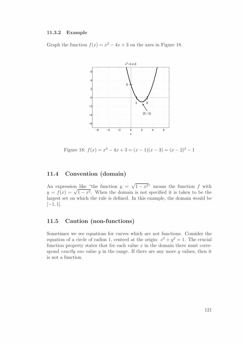
11.3.2 Example
Graph the function f(x) = x2 − 4x + 3 on the axes in Figure 18.
−6 −4 −2 0 2 4 6
−6
−4
−2
0
2
4
6
x
x2−4 x+3
3
3 1
(2,−1)
Figure 18: f(x) = x2 − 4x + 3 = (x− 1)(x− 3) = (x− 2)2 − 1
11.4 Convention (domain)
An expression like “the function y =√
1− x2” means the function f withy = f(x) =
√1− x2. When the domain is not specified it is taken to be the
largest set on which the rule is defined. In this example, the domain would be[−1, 1].
11.5 Caution (non-functions)
Sometimes we see equations for curves which are not functions. Consider theequation of a circle of radius 1, centred at the origin: x2 + y2 = 1. The crucialfunction property states that for each value x in the domain there must corre-spond exactly one value y in the range. If there are any more y values, then itis not a function.
121

11.6 Vertical line test
In the graph of a function, the vertical line x =constant must cut the graph inat most one point. The graph for the circle x2 + y2 = 1 is given in Figure 19.We can clearly see that the vertical line intersects the circle at two points. Inthis case the two y values are given by y = ±
√1− x2. Therefore x2 + y2 = 1
does not give rise to a function on any domain intersecting (−1, 1).
x
y
1
1
Figure 19: The circle x2 + y2 = 1 with a vertical line intersecting at two points.This shows that the equation for a circle does not give rise to a function.
11.6.1 Example
Both y =√
1− x2 (the top half of the circle) and y = −√
1− x2 (the bottomhalf of the circle) are functions of x. What are the domains and ranges of thesetwo functions?
Put f(x) =√
1− x2; g(x) = −√
1− x2.Then dom(f) = dom(g) = [−1, 1],and range(f) = [0,1]; range(g) = [−1, 0].
122
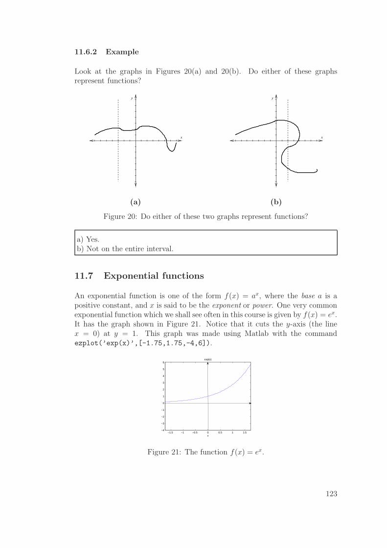
11.6.2 Example
Look at the graphs in Figures 20(a) and 20(b). Do either of these graphsrepresent functions?
x
y
x
y
(a) (b)
Figure 20: Do either of these two graphs represent functions?
a) Yes.b) Not on the entire interval.
11.7 Exponential functions
An exponential function is one of the form f(x) = ax, where the base a is apositive constant, and x is said to be the exponent or power. One very commonexponential function which we shall see often in this course is given by f(x) = ex.It has the graph shown in Figure 21. Notice that it cuts the y-axis (the linex = 0) at y = 1. This graph was made using Matlab with the commandezplot(’exp(x)’,[-1.75,1.75,-4,6]).
−1.5 −1 −0.5 0 0.5 1 1.5−4
−3
−2
−1
0
1
2
3
4
5
6
x
exp(x)
Figure 21: The function f(x) = ex.
123
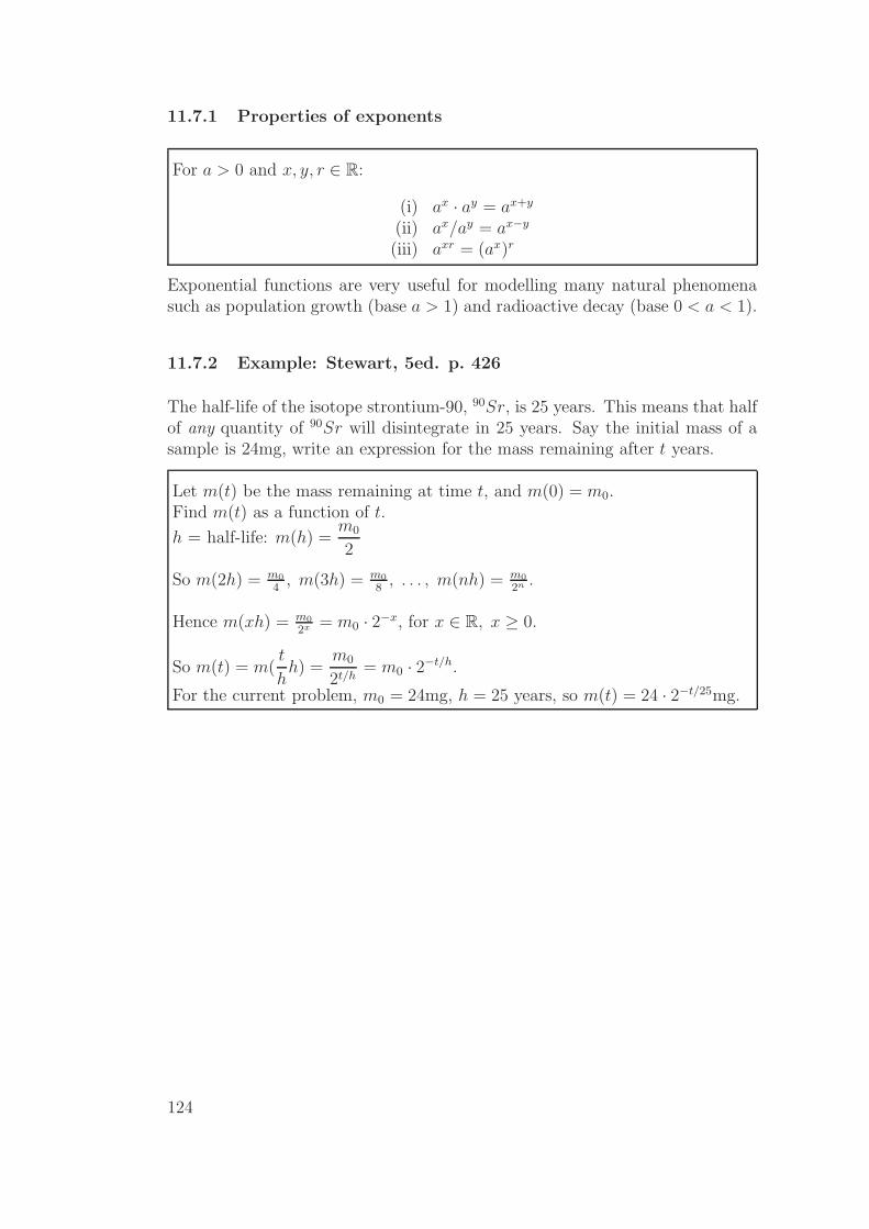
11.7.1 Properties of exponents
For a > 0 and x, y, r ∈ R:
(i) ax · ay = ax+y
(ii) ax/ay = ax−y
(iii) axr = (ax)r
Exponential functions are very useful for modelling many natural phenomenasuch as population growth (base a > 1) and radioactive decay (base 0 < a < 1).
11.7.2 Example: Stewart, 5ed. p. 426
The half-life of the isotope strontium-90, 90Sr, is 25 years. This means that halfof any quantity of 90Sr will disintegrate in 25 years. Say the initial mass of asample is 24mg, write an expression for the mass remaining after t years.
Let m(t) be the mass remaining at time t, and m(0) = m0.Find m(t) as a function of t.
h = half-life: m(h) =m0
2
So m(2h) = m0
4, m(3h) = m0
8, . . . , m(nh) = m0
2n .
Hence m(xh) = m0
2x = m0 · 2−x, for x ∈ R, x ≥ 0.
So m(t) = m(t
hh) =
m0
2t/h= m0 · 2−t/h.
For the current problem, m0 = 24mg, h = 25 years, so m(t) = 24 · 2−t/25mg.
124
In general, if the rate of change of a function is proportional to the value of thefunction, that is
df(t)
dt= kf(t),
thenf(t) = f(0)ekt,
where f(0) is the initial value of the function and k is the rate of exponentialgrowth or decay.
11.7.3 Example
Suppose that there are 1000 rabbits frollicking in your expansive yard on Jan-uary 1, 2006. Thirty days later there are 1500 rabbits. Find an expression forthe rabbit population and then determine how many rabbits there will be 60days after January 1, 2006.
Let n(t) be the number of rabbits at time t. Then n(t) = n(0)ekt, wheren(0) = 1000. We now use the fact that n(30) = 1500 to solve for the rate ofexponential growth, k.
n(30) = 1500 = 1000e30k,1500
1000= e30k.
Hence (see §11.13):
ln
(3
2
)
= 30k,
k =1
30ln
(3
2
)
,
≈ 0.0135.
Therefore, n(t) = 1000e0.0135t, and n(60) = 2250.
125

11.8 Trigonometric functions (sin, cos, tan)
In calculus, we measure angles in radians. One radian is defined as the anglesubtended at the centre of a circle of radius 1 by a segment of arc length 1.
1
1
1
1 rad
Figure 22: Angle in radians.
By definition, 2π radians = 360◦. To convert between the two measures use thefollowing formulae:For x angle in radians, θ angle in degrees,
x× 360◦
2π= θ, θ × 2π
360◦= x.
The point on the unit circle x2 + y2 = 1 making an angle θ (in radians) anti-clockwise from the x-axis has coordinates (cos θ, sin θ), so cos2 θ + sin2 θ = 1.This defines the cos and sin functions. This relationship is shown in Figure 23.
x
y
θ
(cos , sin )θ θ
sin
cos
θ
θ 1
1
−1
−1
Figure 23: The relationship between the cosine and sine functions.
126
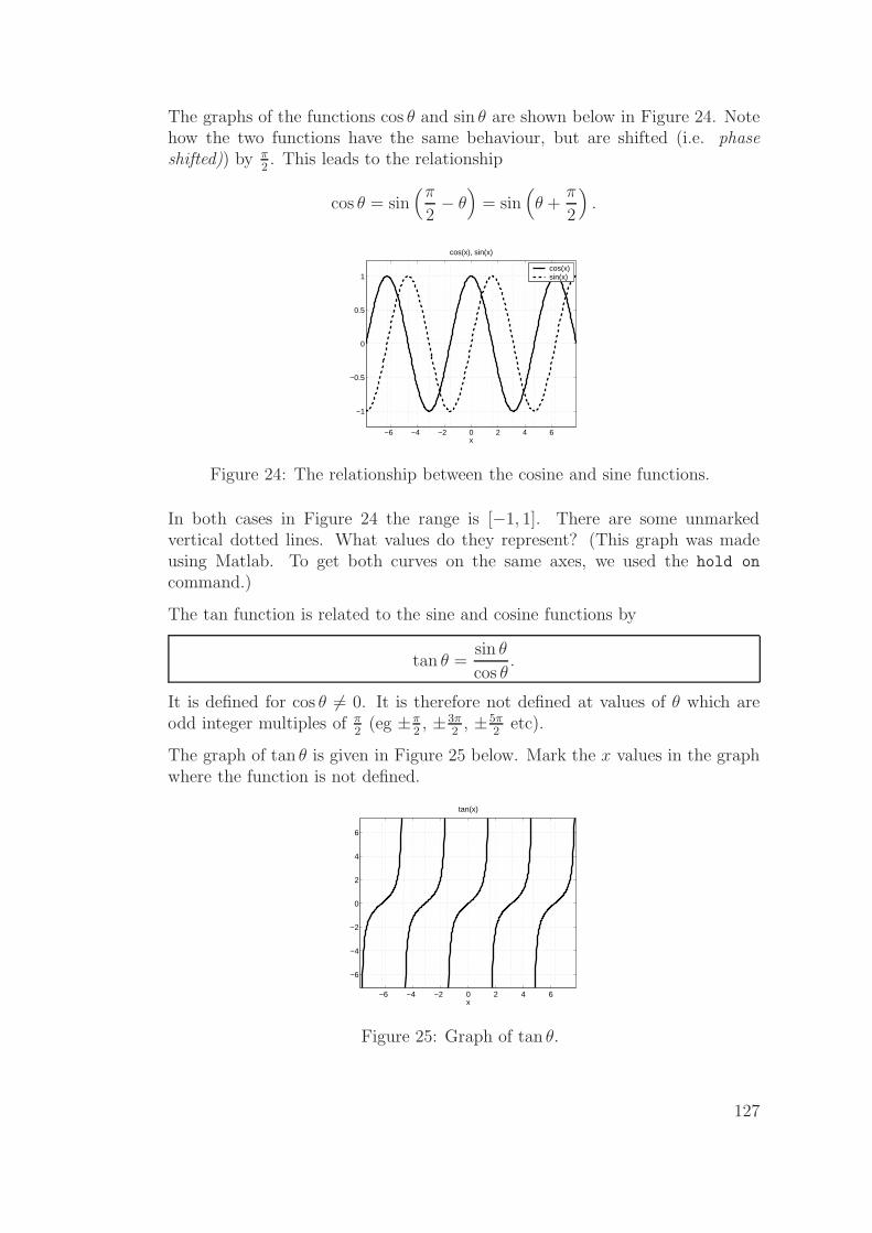
The graphs of the functions cos θ and sin θ are shown below in Figure 24. Notehow the two functions have the same behaviour, but are shifted (i.e. phaseshifted)) by π
2. This leads to the relationship
cos θ = sin(π
2− θ
)
= sin(
θ +π
2
)
.
−6 −4 −2 0 2 4 6
−1
−0.5
0
0.5
1
x
cos(x), sin(x)
cos(x)sin(x)
Figure 24: The relationship between the cosine and sine functions.
In both cases in Figure 24 the range is [−1, 1]. There are some unmarkedvertical dotted lines. What values do they represent? (This graph was madeusing Matlab. To get both curves on the same axes, we used the hold on
command.)
The tan function is related to the sine and cosine functions by
tan θ =sin θ
cos θ.
It is defined for cos θ 6= 0. It is therefore not defined at values of θ which areodd integer multiples of π
2(eg ±π
2, ±3π
2, ±5π
2etc).
The graph of tan θ is given in Figure 25 below. Mark the x values in the graphwhere the function is not defined.
−6 −4 −2 0 2 4 6
−6
−4
−2
0
2
4
6
x
tan(x)
Figure 25: Graph of tan θ.
127
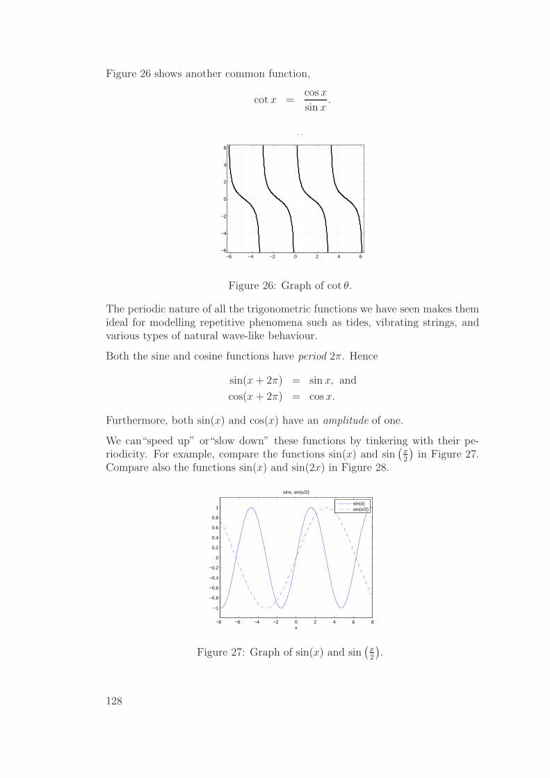
Figure 26 shows another common function,
cot x =cos x
sin x.
−6 −4 −2 0 2 4 6−6
−4
−2
0
2
4
6
x
cot (x)
Figure 26: Graph of cot θ.
The periodic nature of all the trigonometric functions we have seen makes themideal for modelling repetitive phenomena such as tides, vibrating strings, andvarious types of natural wave-like behaviour.
Both the sine and cosine functions have period 2π. Hence
sin(x + 2π) = sin x, and
cos(x + 2π) = cos x.
Furthermore, both sin(x) and cos(x) have an amplitude of one.
We can“speed up” or“slow down” these functions by tinkering with their pe-riodicity. For example, compare the functions sin(x) and sin
(x2
)in Figure 27.
Compare also the functions sin(x) and sin(2x) in Figure 28.
−8 −6 −4 −2 0 2 4 6 8
−1
−0.8
−0.6
−0.4
−0.2
0
0.2
0.4
0.6
0.8
1
x
sinx, sin(x/2)
sin(x)sin(x/2)
Figure 27: Graph of sin(x) and sin(
x2
).
128
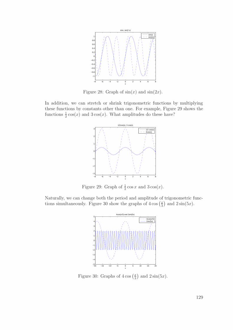
−8 −6 −4 −2 0 2 4 6 8
−1
−0.8
−0.6
−0.4
−0.2
0
0.2
0.4
0.6
0.8
1
x
sinx, sin(2 x)
sin(x)sin(2x)
Figure 28: Graph of sin(x) and sin(2x).
In addition, we can stretch or shrink trigonometric functions by multiplyingthese functions by constants other than one. For example, Figure 29 shows thefunctions 1
2cos(x) and 3 cos(x). What amplitudes do these have?
−8 −6 −4 −2 0 2 4 6 8
−3
−2
−1
0
1
2
3
x
1/2cos(x), 3 cos(x)
1/2 cos(x)3cos(x)
Figure 29: Graph of 12cos x and 3 cos(x).
Naturally, we can change both the period and amplitude of trigonometric func-tions simultaneously. Figure 30 show the graphs of 4 cos
(x3
)and 2 sin(5x).
−20 −15 −10 −5 0 5 10 15 20−5
−4
−3
−2
−1
0
1
2
3
4
5
x
4cos(x/3) and 2sin(5x)
4cos(x/3)2sin(5x)
Figure 30: Graphs of 4 cos(
x3
)and 2 sin(5x).
129

11.8.1 Example
Suppose that the temperature in Brisbane is periodic, peaking at 32 degreesCelsius on January 1, and sinking to 8 degrees Celsius in June; see Figure 31.Use the cosine function to model temperature as a function of time (in days).
0 50 100 150 200 250 300 3500
5
10
15
20
25
30
35
time, (t)
tem
pera
ture
(T)
Figure 31: Graph of temperature fluctuations in Brisbane.
First note that the amplitude of this cosine function is 12(32− 8) = 12. Thus,
we guess that our function will be of the form T = 12 cos(t), where T is thetemperature and t corresponds to time.
However, because we are measuring time in days the period of our modelshould be 365 days, while the period of T = 12 cos(t) is 2π. We take care ofthis by horizontally scaling our function to give T = 12 cos
(2π365
t).
Finally, we shift our model up by 20, because we want it to give temperaturesbetween 8 and 32 degrees, not -12 and 12 degrees.
Thus, the function which describes Brisbane’s temperature as a function oftime (measured in days) is
T = 20 + 12 cos
(2π
365t
)
.
130

11.9 Composition of functions
Let f and g be two functions. Then the composition of f and g, denoted f ◦ g,is the function defined by
(f ◦ g)(x) = f(g(x)).
Note: dom(f ◦ g) = {x ∈ dom(g) | g(x) ∈ dom(f)}
11.9.1 Example
f(x) = x2 + 1, g(x) =1
x. Their compositions f ◦ g and g ◦ f are given by
(f ◦ g)(x) = f(g(x)) = f
(1
x
)
=1
x2+ 1, x 6= 0,
(g ◦ f)(x) = g(f(x)) = g(x2 + 1)
=1
x2 + 1, x ∈ R.
Notice how these two composite functions are not equal. In general, f ◦g 6= g◦f .
11.10 One-to-one (1-1) functions - Stewart, 6ed. pp. 385-
388; 5ed. pp. 413-417
A function f : X → Y is said to be one-to-one (usually written as 1-1) if, forall x1, x2 ∈ X,
f(x1) = f(x2)⇒ x1 = x2.
Equivalently:x1 6= x2 ⇒ f(x1) 6= f(x2).
On the graph y = f(x), 1-1 means that any horizontal line y =constant cutsthrough the curve in at most one place; see Figure 32.
131

x
y
x
y
(a) (b)
Figure 32: Are either of these functions 1-1?
a) Yes.b) No.
11.10.1 Example
Show from the definition that the function f(x) = e2x−5 is 1-1 on its domain.
The domain of the function is R.
We need to show that
f(x1) = f(x2)⇒ x1 = x2 for any x1, x2 ∈ R.
Let x1, x2 ∈ R. Then
f(x1) = f(x2) ⇒ e2x1−5 = e2x2−5
⇒ 2x1 − 5 = 2x2 − 5
⇒ 2x1 = 2x2
⇒ x1 = x2
Therefore e2x−5 is 1-1.
132

11.11 Inverse Functions
Let f : X → Y be a 1-1 function. Then we can define the inverse function,f−1 : f(X)→ X by
f−1(f(x)) = x, ∀ x ∈ X,
f(f−1(y)) = y, ∀ y ∈ f(X).
By definition,
domain f−1 = range f, and
range f−1 = domain f.
Note that y = f(x)⇔ x = f−1(y), and that (f−1(y))−1 = f(x). The function fmust be 1-1 in order that f−1 satisfy the crucial function property. In order toobtain the graph of f−1(x), we reflect the graph of f(x) about the line y = x;for example, see Figure 33 below.
x
y
y=f(x)
y=xy=f (x)−1
Figure 33: The dashed line represents the graph of the inverse function, havingbeenreflected about the line y = x.
133

11.11.1 Example
Draw the graph of the inverse function of f(x) = x3 (the cube root functionf−1(x) = x1/3) on the same axes given below in Figure 34.
3
1/3xx
y
x
Figure 34: f(x) = x3. Draw in the graph of f−1(x) = x1/3.
11.11.2 Example
f : R → R, f(x) = x2 is not 1-1 and therefore has no inverse. However,the positive half (x ≥ 0) gives a 1-1 function f : [0,∞) → R, f(x) = x2
with range [0,∞). The inverse of this function is then f−1 : [0,∞) → [0,∞),f−1(x) =
√x. Similarly the negative half of the function f(x) = x2 is 1-1, with
inverse f−1 : [0,∞)→ (−∞, 0], f−1(x) = −√x.
This technique is often used when the function is not 1-1 over its entire domain:just take a part where it is 1-1 and determine the inverse for that part.
For further discussion on how to find the inverse function of a 1-1 function, seeStewart, 6ed. p. 388 box 5; 5ed. p. 416 box 5.
134
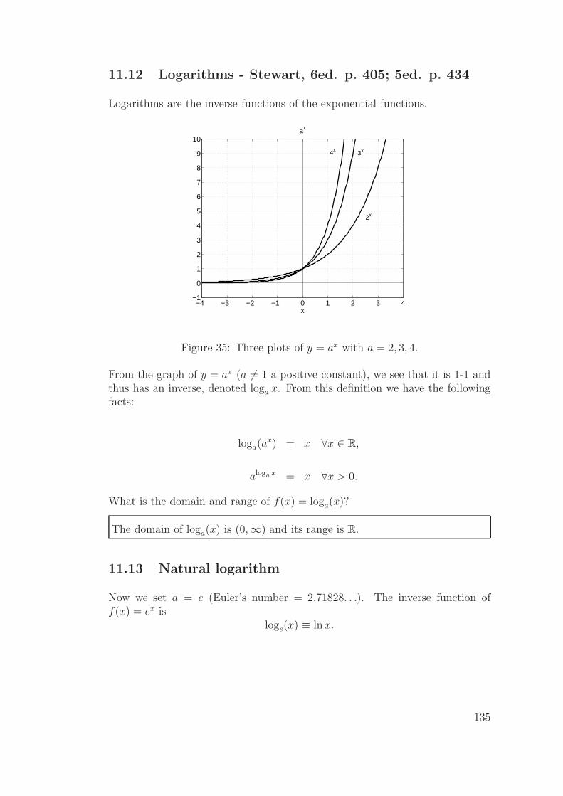
11.12 Logarithms - Stewart, 6ed. p. 405; 5ed. p. 434
Logarithms are the inverse functions of the exponential functions.
−4 −3 −2 −1 0 1 2 3 4−1
0
1
2
3
4
5
6
7
8
9
10
x
ax
2x
3x 4x
Figure 35: Three plots of y = ax with a = 2, 3, 4.
From the graph of y = ax (a 6= 1 a positive constant), we see that it is 1-1 andthus has an inverse, denoted loga x. From this definition we have the followingfacts:
loga(ax) = x ∀x ∈ R,
aloga x = x ∀x > 0.
What is the domain and range of f(x) = loga(x)?
The domain of loga(x) is (0,∞) and its range is R.
11.13 Natural logarithm
Now we set a = e (Euler’s number = 2.71828. . .). The inverse function off(x) = ex is
loge(x) ≡ lnx.
135
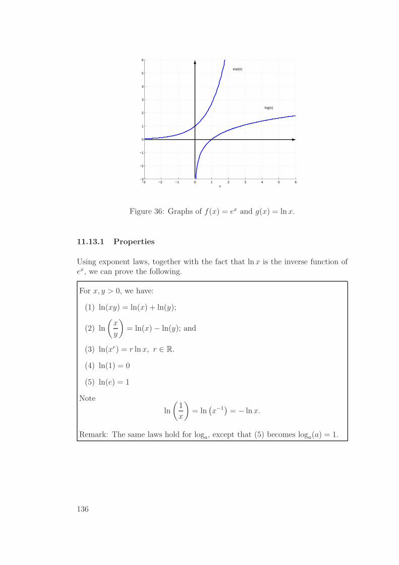
−3 −2 −1 0 1 2 3 4 5 6−3
−2
−1
0
1
2
3
4
5
6
x
exp(x)
log(x)
Figure 36: Graphs of f(x) = ex and g(x) = ln x.
11.13.1 Properties
Using exponent laws, together with the fact that ln x is the inverse function ofex, we can prove the following.
For x, y > 0, we have:
(1) ln(xy) = ln(x) + ln(y);
(2) ln
(x
y
)
= ln(x)− ln(y); and
(3) ln(xr) = r ln x, r ∈ R.
(4) ln(1) = 0
(5) ln(e) = 1
Note
ln
(1
x
)
= ln(x−1
)= − ln x.
Remark: The same laws hold for loga, except that (5) becomes loga(a) = 1.
136

11.13.2 Example: Bacteria population - Stewart, 6ed. p. 440 qn 49;5ed. p. 440 qn 49
If a bacteria population starts with 100 bacteria and doubles every 3 hours, thenthe number of bacteria n after t hours is given by the formula
n = f(t) = 100 · 2t/3.
(a) Find the inverse of this function and explain its meaning.
(b) When will the population reach 50000?
(a) If n = 100 · 2t/3, thenn
100= 2t/3.
Taking the natural logarithm of both sides gives
ln( n
100
)
= ln(2t/3
)
=t
3ln(2) (using 11.13.1)
so that
t = 3 · ln(n/100)
ln 2.
It describes how long it will take to obtain n bacteria.
(b) Substituting n = 50, 000 gives t ≈ 26.9 hours.
137

11.14 Inverse trigonometric functions
The function y = sin x is 1-1 if we just define it over the interval [−π/2, π/2];see Figure 24. The inverse function for this part of sin x is denoted arcsin x.Thus arcsin x is defined on the interval [−1, 1] and takes values in the range[−π/2, π/2]. The graph can easily be obtained by reflecting the graph of sin xabout the line y = x over the appropriate interval; see Figure 37.
−1.5 −1 −0.5 0 0.5 1 1.5−1.5
−1
−0.5
0
0.5
1
1.5
x
sin x
arcsin x
sin x, arcsin x
Figure 37: f(x) = sin x defined on [−π/2, π/2] reflected about the line y = x togive f−1(x) = arcsin x.
Similarly y = cos x is 1-1 on the interval [0, π] and its inverse function is denotedarccos x. The function arccos x is defined on [−1, 1] and takes values in therange [0, π]. Figure 38 below shows the graphs of f(x) = cos x before and afterreflection about the line y = x. This gives the graph of f−1(x) = arccos x.
−1 −0.5 0 0.5 1 1.5 2 2.5 3−1
−0.5
0
0.5
1
1.5
2
2.5
3
x
cos x, acos x
cos x
arccos x
Figure 38: f(x) = cos x defined on [0, π] reflected about the line y = x to givef−1(x) = arccosx (written in MATLAB as acos(x)).
138

Also, tanx is 1-1 on the open interval (−π/2, π/2) with inverse function denotedby arctan x. Hence arctan has the domain (−∞,∞) with values in the range(−π/2, π/2).
−10 −5 0 5 10
−10
−8
−6
−4
−2
0
2
4
6
8
10
x
tan x, atan(x)
tan x
arctan x
Figure 39: f(x) = tanx.
139

Notes
140

Notes
141

Notes
142

Notes
143

Notes
144

Notes
145

12 Limits
Limits arise when we want to find the tangent to a curve or the velocity ofan object, for example. Once we understand limits, we can proceed to study-ing continuity and calculus in general. You should be aware that limits are afundamental notion to calculus, so it is important to understand them clearly.
12.1 Definition: Limit - Stewart, 6ed. p. 66; 5ed. p. 71
Let f(x) be a function and ℓ ∈ R. We say f(x) approaches the limit ℓ (orconverges to the limit ℓ) as x approaches a if we can make the value of f(x)arbitrarily close to ℓ (as close to ℓ as we like) by taking x to be sufficiently closeto a (on either side of a) but not equal to a.
We writelimx→a
f(x) = ℓ.
Roughly speaking, f(x) is close to ℓ for all x values sufficiently close to a, withx 6= a. The limit “predicts” what should happen at x = a by looking at x valuesclose to but not equal to a.
12.1.1 Precise Definition
Let f be a function defined on some open interval that contains the number a,except possibly a itself. Then we write
limx→a
f(x) = ℓ
if for every number ε > 0 there is a number δ > 0 such that
|f(x)− ℓ| < ε whenever 0 < |x− a| < δ.
Detailed discussion on the precise definition of a limit can be found in Stewart,6ed. p. 88; 5ed. p. 93. This is not directly examinable in MATH1051, but youwill need it in later courses.
We can sometimes determine the limit of a function by looking at its graph.Figure 40 shows two functions with the same limit at 5.
146

2
x108642
4
Function 2Function 1
yy
14
12
10
8
6
4
2
x108642
14
12
10
8
6
Figure 40: Two functions with limit equal to 10 as x→ 5.
Function 1 is described by
y =
{2x for 0 ≤ x ≤ 5,−2x + 20 for 5 < x ≤ 10,
while function 2 is described by
y =
2x for 0 ≤ x < 5,2 for x = 5,−2x + 20 for 5 < x ≤ 10.
Each function has a limit of 10 as x approaches 5. It does not matter thatthe value of the second function is 2 when x equals 5 since, when dealing withlimits, we are only interested in the behaviour of the function as x approaches5.
12.1.2 Example: Stewart, 6ed. p. 69; 5ed. p. 74
Investigate limx→0
sinπ
x.
sin(π/x) oscillates rapidly between −1 and 1 as x → 0, so the limit does notexist.
147

12.1.3 Properties
Suppose that c is a constant and the limits ℓ = limx→a
f(x) and m = limx→a
g(x) exist
for some fixed a ∈ R. Then
limx→a
(f(x)± g(x)) = limx→a
f(x)± limx→a
g(x) = ℓ±m
limx→a
cf(x) = c · limx→a
f(x) = c · ℓ
limx→a
f(x) · g(x) = limx→a
f(x) · limx→a
g(x) = ℓ ·m
limx→a
f(x)
g(x)=
limx→a
f(x)
limx→a
g(x)=
ℓ
mif m 6= 0
148
12.1.4 Example
Find the value of limx→1
(x2 + 1).
limx→1
(x2 + 1) = 1 + 1 = 2
12.1.5 Example: Stewart, 6ed. p. 67 ex. 1; 5ed. p. 71 ex. 1
Determine the value of limx→1
x− 1
x2 − 1.
limx→1
x− 1
x2 − 1= lim
x→1
x− 1
(x + 1)(x− 1)remember x 6= 1
= limx→1
1
x + 1=
1
2.
Note: this means
f(x) =
x− 1
(x + 1)(x− 1)x 6= 1
1
2x = 1.
is a continuous function.
149
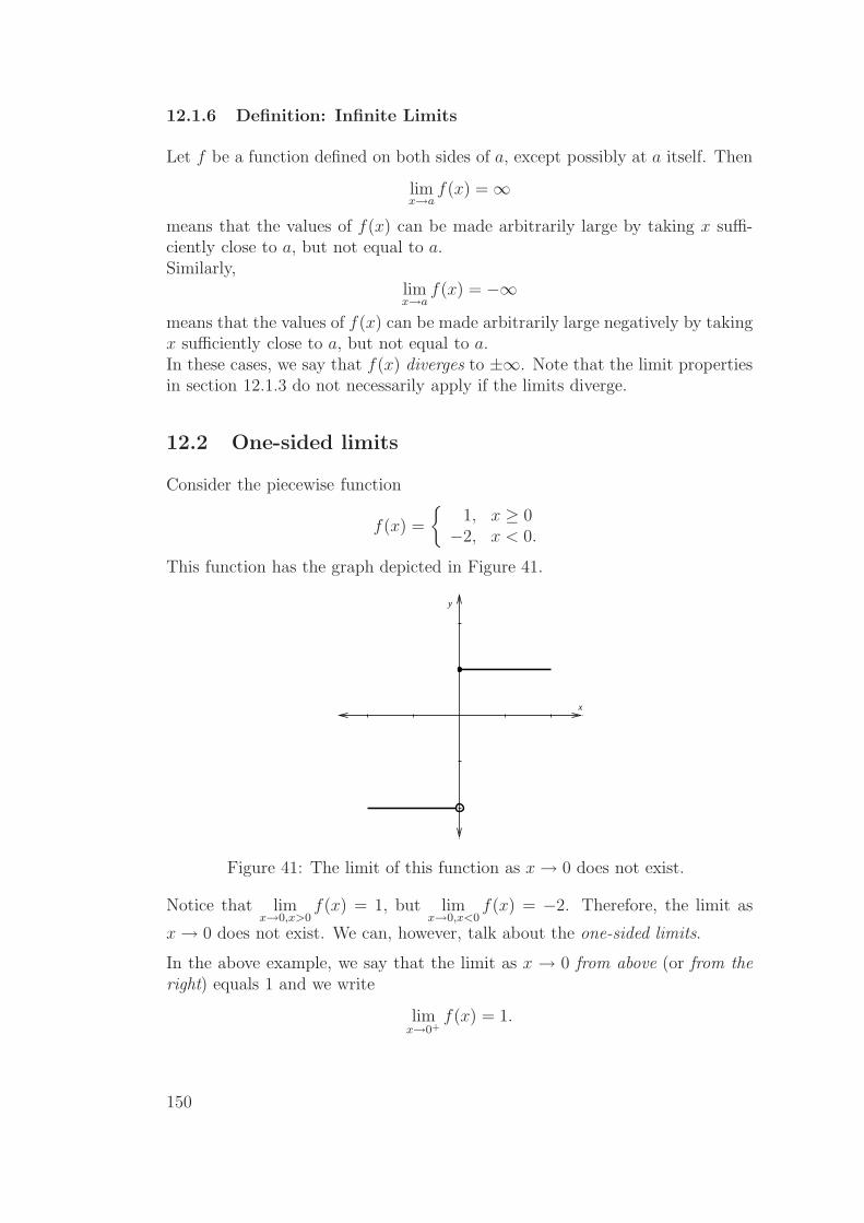
12.1.6 Definition: Infinite Limits
Let f be a function defined on both sides of a, except possibly at a itself. Then
limx→a
f(x) =∞
means that the values of f(x) can be made arbitrarily large by taking x suffi-ciently close to a, but not equal to a.Similarly,
limx→a
f(x) = −∞means that the values of f(x) can be made arbitrarily large negatively by takingx sufficiently close to a, but not equal to a.In these cases, we say that f(x) diverges to ±∞. Note that the limit propertiesin section 12.1.3 do not necessarily apply if the limits diverge.
12.2 One-sided limits
Consider the piecewise function
f(x) =
{1, x ≥ 0−2, x < 0.
This function has the graph depicted in Figure 41.
x
y
Figure 41: The limit of this function as x→ 0 does not exist.
Notice that limx→0,x>0
f(x) = 1, but limx→0,x<0
f(x) = −2. Therefore, the limit as
x→ 0 does not exist. We can, however, talk about the one-sided limits.
In the above example, we say that the limit as x → 0 from above (or from theright) equals 1 and we write
limx→0+
f(x) = 1.
150

Similarly, we say that the limit as x → 0 from below (or from the left) equals−2 and we write
limx→0−
f(x) = −2.
In general, for limx→a+
f(x) = ℓ, just consider x with x > a and similarly for
limx→a−
f(x) = ℓ, consider only x < a.
12.2.1 Example
Consider both limx→2+
√x− 2 and lim
x→2−
√x− 2. Based on your conclusion, does
the limx→2
√x− 2 exist?
limx→2+
√x− 2 = 0, however lim
x→2−
√x− 2 does not exist.
⇒ limx→2
√x− 2 does not exist.
12.2.2 Theorem
limx→a
f(x) = ℓ if and only if
limx→a−
f(x) = ℓ = limx→a+
f(x).
12.2.3 Example
Find limx→1
f(x) where f(x) =
{x2, x ≥ 1,
2− x, x < 1.
limx→1+
f(x) = limx→1+
x2 = 1,
limx→1−
f(x) = limx→1−
(2− x) = 2− 1 = 1,
⇒ limx→1
f(x) = 1.
151
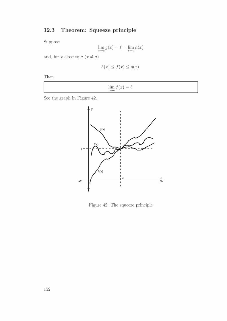
12.3 Theorem: Squeeze principle
Supposelimx→a
g(x) = ℓ = limx→a
h(x)
and, for x close to a (x 6= a)
h(x) ≤ f(x) ≤ g(x).
Then
limx→a
f(x) = ℓ.
See the graph in Figure 42.
y
x
l
a
h(x)
g(x)
f(x)
Figure 42: The squeeze principle
152
12.3.1 Example
Prove that limx→0
x2 sin
(1
x
)
= 0.
For x 6= 0,
−1 ≤ sin
(1
x
)
≤ 1.
Therefore,
−x2 ≤ x2 sin
(1
x
)
≤ x2.
Take g(x) = x2, and h(x) = −x2 in the squeeze theorem.As x→ 0, g(x)→ 0 and h(x)→ 0.
So by the squeeze principle ⇒
limx→0
x2 sin
(1
x
)
= 0.
12.4 Limits as x approaches infinity
If f(x) approaches ℓ as x gets larger and larger, we write
limx→∞
f(x) = ℓ.
That is, f(x) can be made arbitrarily close to ℓ by taking x sufficiently large.Similarly, we write
limx→−∞
f(x) = ℓ
if f(x) approaches ℓ as x becomes more and more negative.
12.4.1 Example
Find limx→∞
1x.
limx→∞
1
x= lim
x→−∞
1
x= 0.
153

Note: Since
limx→0+
1
x=∞ and lim
x→0−
1
x= −∞,
then limx→0
1
xdoesn’t exist. Furthermore, it is irrelevant that f(x) is not actually
defined at the point x = 0.
−10 −5 0 5 10−10
−8
−6
−4
−2
0
2
4
6
8
10
x
1/x
Figure 43: Graph of f(x) = 1/x.
12.4.2 Example
Determine limx→∞
sin x, or show that it does not exist.
This limit does not exist since sin x is a periodic function that oscillates between-1 and 1. (Compare with lim
x→0sin π
xin 3.1.4).
12.4.3 Example: ratio of two polynomials, numerator degree = de-nominator degree
Find limx→∞
2x2 + 3
3x2 + x.
Put f(x) = 2x2 + 3 and g(x) = 3x2 + x.
Then limx→∞
f(x) =∞ and limx→−∞
g(x) =∞
So the limit has the form∞∞ .
Technique: we divide top and bottom by the highest power of x in the denomi-nator. The result is two new functions in the numerator and the denominator,the limits of which are both finite.
154

limx→∞
2x2 + 3
3x2 + x= lim
x→∞
2 + 3x2
3 + 1x
= limx→∞
(2x2 + 3)/x2
(3x2 + x)/x2
= limx→∞
2 + 3x2
3 + 1x
=2
3
12.4.4 Example
Find limx→∞
8x3 + 6x2
4x3 − x + 12.
In this case, we divide the top and bottom by x3, and proceed as before.
limx→∞
8x3 + 6x2
4x3 − x + 12= lim
x→∞
(8x3 + 6x2)/x3
(4x3 − x + 12)/x3
= limx→∞
8 + 6x
4− 1x2 + 12
x3
=8
4
= 2
155

12.4.5 Example: ratio of two polynomials, numerator degree > de-nominator degree
Find limx→∞
x2 + 5
x + 1.
The highest power of x in the denominator is 1, so we have
limx→∞
x2 + 5
x + 1= lim
x→∞
x + 5x
1 + 1x
=∞.
12.4.6 Example: ratio of two polynomials, numerator degree < de-nominator degree
Find limx→∞
x + 1
x2 + 1
limx→∞
x + 1
x2 + 1= lim
x→∞
1x
+ 1x2
1 + 1x2
= 0
The general method in the four previous examples has been to:
1. divide the numerator and denominator by the highest power of x in thedenominator; and then
2. determine the limits of the numerator and denominator separately.
156
12.5 Some important limits
The following limits are fundamental. Combined with the properties given in12.1.3 and the Squeeze Principle given in 12.3, these will enable you to computea range of other limits.
Here a ∈ R is arbitrary.
(1) limx→a
1 = 1 (2) limx→a
x = a (3) limx→0
sin x
x= 1
(4) limx→0
1− cos(x)
x2=
1
2(5) lim
x→0
ex − 1
x= 1.
157

Notes
158

Notes
159

Notes
160

Notes
161

Notes
162
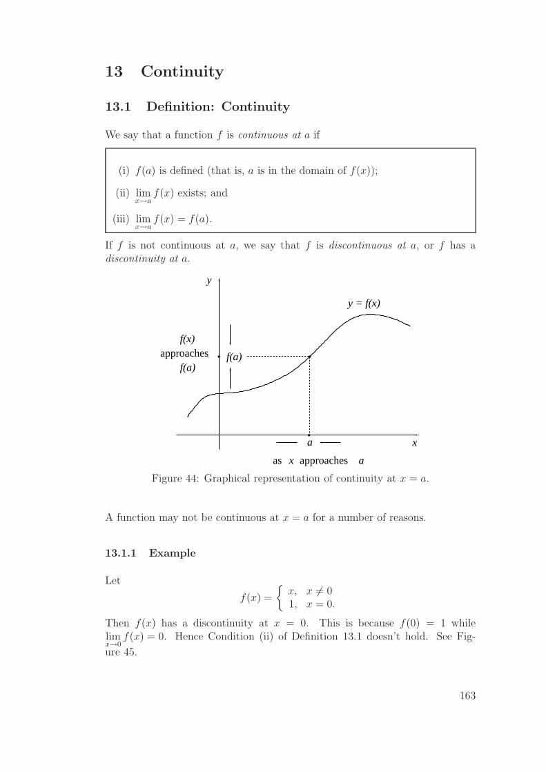
13 Continuity
13.1 Definition: Continuity
We say that a function f is continuous at a if
(i) f(a) is defined (that is, a is in the domain of f(x));
(ii) limx→a
f(x) exists; and
(iii) limx→a
f(x) = f(a).
If f is not continuous at a, we say that f is discontinuous at a, or f has adiscontinuity at a.
f(a)f(a)
a
f(x)
y
y = f(x)
approaches
as x approaches a
x
Figure 44: Graphical representation of continuity at x = a.
A function may not be continuous at x = a for a number of reasons.
13.1.1 Example
Let
f(x) =
{x, x 6= 01, x = 0.
Then f(x) has a discontinuity at x = 0. This is because f(0) = 1 whilelimx→0
f(x) = 0. Hence Condition (ii) of Definition 13.1 doesn’t hold. See Fig-
ure 45.
163
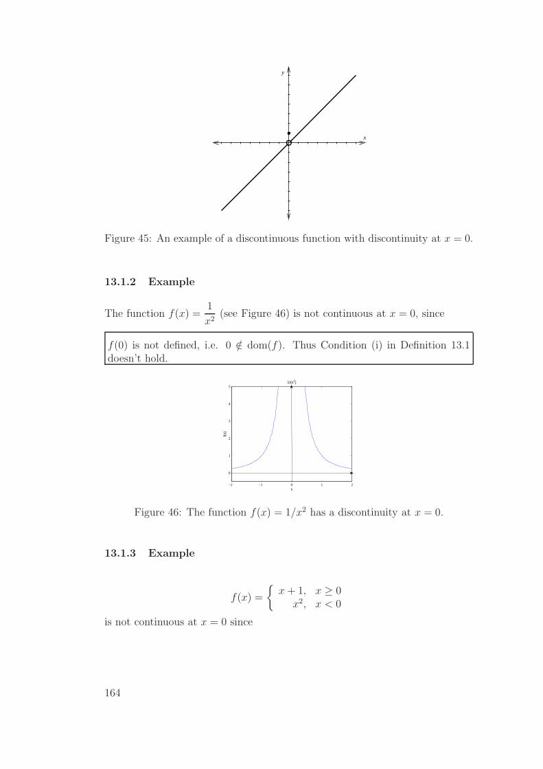
x
y
Figure 45: An example of a discontinuous function with discontinuity at x = 0.
13.1.2 Example
The function f(x) =1
x2(see Figure 46) is not continuous at x = 0, since
f(0) is not defined, i.e. 0 /∈ dom(f). Thus Condition (i) in Definition 13.1doesn’t hold.
−2 −1 0 1 2
0
1
2
3
4
5
x
1/(x2)
f(x)
Figure 46: The function f(x) = 1/x2 has a discontinuity at x = 0.
13.1.3 Example
f(x) =
{x + 1, x ≥ 0
x2, x < 0
is not continuous at x = 0 since
164

limx→0
f(x) doesn’t exist:
limx→0+
f(x) = limx→0+
(x + 1) = 1
limx→0−
f(x) = limx→0−
x2 = 0
The limit from above is different to the limit from below.
13.2 Definition: Continuity on intervals
If f is continuous on the open interval (a, b), then
f is continuous at c, for all c ∈ (a, b).
If f is continuous on the closed interval [a, b], then f is continuous on (a, b) and
limx→a+
f(x) = f(a), limx→b−
f(x) = f(b).
The graph of a function that is continuous on an interval can be drawn withoutlifting the pen.
13.2.1 Examples
• Any polynomial in x is continuous on R. For example, f(x) = ax2 +bx+cis continuous on R.
• ex, |x|, sin x, cos x and arctanx are continuous on R.
• f(x) = ln x is continuous on (0,∞).
165
13.3 Properties
If f(x) and g(x) are continuous at x = a and c is a constant, then
(1) f(x)± g(x),
(2) c · f(x),
(3) f(x) · g(x), and
(4)f(x)
g(x), where g(a) 6= 0,
are all continuous at x = a.
13.3.1 Theorem: Limit of a composite function - Stewart, 6ed. p. 103Thm 8; 5ed. p. 107 Thm 8
If f is continuous at b and limx→a
g(x) = b, then limx→a
f(g(x)) = f(b). In other
words,
limx→a
f(g(x)) = f(limx→a
g(x)).
Similarly if limx→∞
g(x) = b and f is continuous at x = b, then
limx→∞
f(g(x)) = f(b).
13.3.2 Corollary: Stewart, 6ed. p. 103 Thm 9; 5ed. p. 108 Thm 9
If g is continuous at a and f is continuous at g(a) then f ◦ g is continuous at a.
166

13.4 Intermediate Value Theorem (IVT) - Stewart, 6ed.p. 104; 5ed. p. 109
Suppose that f is continuous on the closed interval [a, b] and let N be anynumber between f(a) and f(b), where f(a) 6= f(b). Then there exists a numberc ∈ (a, b) such that f(c) = N .
N
c
f(b)
f(a)
ba
y
x
Figure 47: The IVT states that a continuous function takes on every interme-diate value between the function values f(a) and f(b). That is, we can chooseany N between f(a) and f(b) which corresponds to a value c between a and b.Note that this is not necessarily true if f is discontinuous.
13.5 Application of IVT (bisection method)
The bisection method is a procedure for approximating the zeros of a continuousfunction. It first cuts the interval [a, b] in half (say, at a point c), and then decidesin which of the smaller intervals ([a, c] or [c, b]) the zero lies. This process isrepeated until the interval is small enough to give a significant approximationto the zero itself.
We can present this bisection method as an algorithm:
(1) Given [a, b] such that f(a)f(b) < 0, let c =a + b
2.
(2) If f(c) = 0 then quit; c is a zero of f .
167

(3) If f(c) 6= 0 then:
(a) If f(a)f(c) < 0, replace b by c.
(b) If f(a)f(c) > 0, replace a by c.
(4) If the interval [a, b] is small enough to give a precise enough approximationthen quit. Otherwise, go to step (1).
y
x
f(a)
f(b)
a
b
Figure 48: The bisection method is an application of the IVT.
Note that:
f(a)f(c) < 0 ⇐⇒ f(a) < 0 and f(c) > 0
or f(a) > 0 and f(c) < 0
f(a)f(c) > 0 ⇐⇒ f(a) > 0 and f(c) > 0
or f(a) < 0 and f(c) < 0
We will investigate the bisection method in more detail in the lab sessions withMATLAB.
168

Notes
169

Notes
170
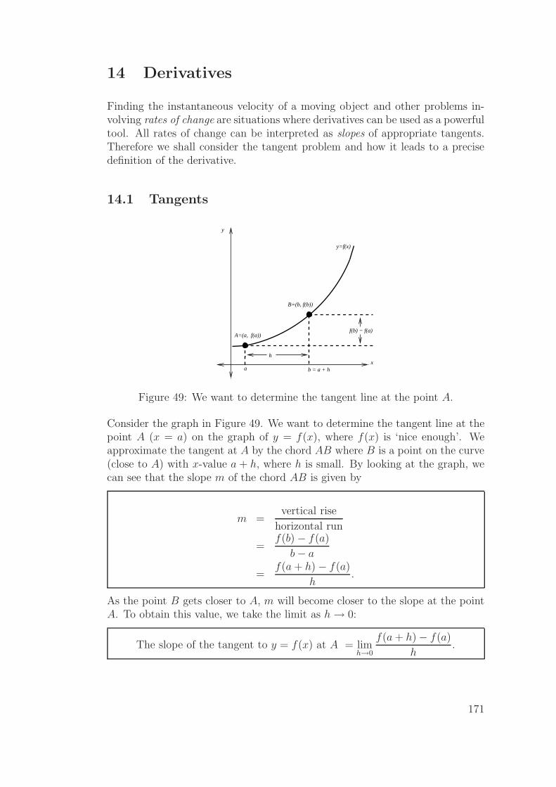
14 Derivatives
Finding the instantaneous velocity of a moving object and other problems in-volving rates of change are situations where derivatives can be used as a powerfultool. All rates of change can be interpreted as slopes of appropriate tangents.Therefore we shall consider the tangent problem and how it leads to a precisedefinition of the derivative.
14.1 Tangents
f(b) − f(a)
b = a + h
h
a
A=(a, f(a))
B=(b, f(b))
y=f(x)
y
x
Figure 49: We want to determine the tangent line at the point A.
Consider the graph in Figure 49. We want to determine the tangent line at thepoint A (x = a) on the graph of y = f(x), where f(x) is ‘nice enough’. Weapproximate the tangent at A by the chord AB where B is a point on the curve(close to A) with x-value a + h, where h is small. By looking at the graph, wecan see that the slope m of the chord AB is given by
m =vertical rise
horizontal run
=f(b)− f(a)
b− a
=f(a + h)− f(a)
h.
As the point B gets closer to A, m will become closer to the slope at the pointA. To obtain this value, we take the limit as h→ 0:
The slope of the tangent to y = f(x) at A = limh→0
f(a + h)− f(a)
h.
171
14.2 Definition: Derivative, differentiability
The derivative of f at x is defined by
f ′(x) = limh→0
f(x + h)− f(x)
h.
We say that f is differentiable at some point x if this limit exists. Further, wesay that f is differentiable on an open interval if it is differentiable at everypoint in the interval. Note that f ′(a) is the slope of the tangent line to thegraph of y = f(x) at x = a.
We have thus defined a new function f ′, called the derivative of f . Sometimes
we use the Leibniz notationdy
dxor
df
dxin place of f ′(x).
Note that if f is differentiable at a, there holds:
f ′(a) = limx→a
f(x)− f(a)
x− a.
14.2.1 Example
Using the definition of the derivative (i.e. calculating ‘by first principles’), showthat if f(x) = x2 + x, then f ′(x) = 2x + 1.
Using the definition for a derivative, we find:
f ′(x) = limh→0
f(x + h)− f(x)
h
= limh→0
(x + h)2 + (x + h)− (x2 + x)
h
= limh→0
x2 + 2xh + h2 + x + h− x2 − x
h
= limh→0
2xh + h2 + h
h
= limh→0
(2x + h + 1)
= 2x + 1
172

14.2.2 Example
Show that if f(x) = ex, then f ′(x) = ex.
As discussed earlier, we have from the definition of Euler’s number e:
limh→0
eh − 1
h− 0= 1, i.e. lim
h→0
eh − 1
h= 1.
Using the definition of the derivative, we then have
f ′(x) = limh→0
f(x + h)− f(x)
h
= limh→0
ex+h − ex
h
= limh→0
exeh − ex
h
= limh→0
ex · eh − 1
h
= ex limh→0
eh − 1
h= ex
14.2.3 Some useful derivatives
Other useful derivatives are
d
dx(constant) = 0
d
dx(x) = 1
d
dx(xα) = αxα−1, for α ∈ R, x ≥ 0 or for x ∈ R if α ∈ R+
d
dx(sin x) = cos x
d
dx(cos x) = − sin x
173
14.3 Theorem: Differentiability implies continuity
If f is differentiable at a, then
f is continuous at a.
The converse, however, is false. That is, if f is continuous at a, then it is notnecessarily differentiable. (See the following example.)
14.3.1 Example
The function f(x) = |x| is continuous, but not differentiable in x = 0, since
limh→0+
f(0 + h)− f(0)
h= lim
h→0+
h− 0
h= 1
and
limh→0−
f(0 + h)− f(0)
h= lim
h→0−
−h− 0
h= −1 6= 1,
meaning that limh→0
f(0 + h)− f(0)
hdoesn’t exist.
14.4 Rates of change - Stewart, 6ed. p. 117; 5ed. p. 117
Recall that the slope of the tangent line to y = f(x) at x = a measures the rateof change of y with respect to x at the point x = a.
14.4.1 Example: Velocity
Velocity v is the rate at which displacement s changes with respect to time t, so
v(t) =ds
dt= s′(t) = s(t).
174
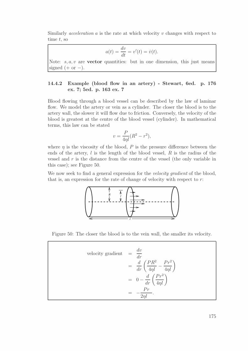
Similarly acceleration a is the rate at which velocity v changes with respect totime t, so
a(t) =dv
dt= v′(t) = v(t).
Note: s, a, v are vector quantities: but in one dimension, this just meanssigned (+ or −).
14.4.2 Example (blood flow in an artery) - Stewart, 6ed. p. 176ex. 7; 5ed. p. 163 ex. 7
Blood flowing through a blood vessel can be described by the law of laminarflow. We model the artery or vein as a cylinder. The closer the blood is to theartery wall, the slower it will flow due to friction. Conversely, the velocity of theblood is greatest at the centre of the blood vessel (cylinder). In mathematicalterms, this law can be stated
v =P
4ηl(R2 − r2),
where η is the viscosity of the blood, P is the pressure difference between theends of the artery, l is the length of the blood vessel, R is the radius of thevessel and r is the distance from the centre of the vessel (the only variable inthis case); see Figure 50.
We now seek to find a general expression for the velocity gradient of the blood,that is, an expression for the rate of change of velocity with respect to r:
l
rR
Figure 50: The closer the blood is to the vein wall, the smaller its velocity.
velocity gradient =dv
dr
=d
dr
(PR2
4ηl− Pr2
4ηl
)
= 0− d
dr
(Pr2
4ηl
)
= − Pr
2ηl.
175
This tells us at what rate the velocity of the blood decreases the further it isfrom the centre of the blood vessel.
These types of problems are studied in later courses on fluid mechanics andother related topics.
14.5 Higher derivatives
Differentiating a function y = f(x) n times, if possible, gives the nth derivative
of f , usually denoted f (n)(x),dnf
dxnor
dny
dxn.
Therefore acceleration can be represented as
a(t) =dv
dt
=d
dt
(ds
dt
)
=d2s
dt2
≡ s′′(t)
≡ s(2)(t)
≡ s(t).
Sometimes when we deal with time derivatives we write v(t) = s(t) or a(t) = s(t)and so on.
14.6 Rules for differentiation
Suppose that f(x) and g(x) are differentiable functions, and let c be a constant.Then we have the following rules:
(i) (cf)′ = cf ′;
(ii) (f ± g)′ = f ′ ± g′;
(iii) (fg)′ = f ′g + fg′ (the product rule); and
(iv)
(f
g
)′=
f ′g − fg′
g2, g 6= 0 (the quotient rule).
176

In the Leibniz notation, if f(x) and g(x) are both differentiable functions, andc is a constant, then the rules for differentiation can be expressed as:
(i)d
dx(cf) = c
df
dx;
(ii)d
dx(f ± g) =
df
dx± dg
dx;
(iii)d
dx(fg) =
df
dxg + f
dg
dx(the product rule); and
(iv)d
dx
(f
g
)
=dfdx
g − f dgdx
g2, for g 6= 0 (the quotient rule).
14.6.1 Example
Use the rules above to find the derivative of f(x) = tanx =sin x
cos x.
For x 6= (n + 12)π, n ∈ Z, there holds cos(x) 6= 0, so use the quotient rule:
f ′(x) =(sin x)′ cos x− sin x(cos x)′
cos2 x
=cos2 x + sin2 x
cos2 x
=1
cos2 x( since cos2 x + sin2 x = 1)
= sec2 x.
177

14.7 The chain rule - Stewart, 6ed. p. 156; 5ed. p. 176
If g and h are both differentiable and f = g◦h is the composite function definedby f(x) = g(h(x)), then f is differentiable and f ′ is given by the product
f ′(x) = g′(h(x))h′(x).
In the Leibniz notation, if y = g(u) and u = h(x) are both differentiable func-tions, then
dy
dx=
dy
du· du
dx.
14.7.1 Example
Differentiate y =√
sin x.
Let u = sin x. Then y = u1/2. Thus, we have
dy
dx=
dy
du· du
dx
=
(1
2u−1/2
)
(cos x)
=cos x
2√
u
=cos x
2√
sin x
178

14.7.2 Example: Rocket tracking application
A rocket is launched vertically and tracked by an observation station 5km fromthe launch pad. The angle of elevation θ is observed to be increasing at 3◦/swhen θ = 60◦. What is the velocity of the rocket at that instant?
Note thatθ =
π
3(radians)
and for θ =π
3:
dθ
dt= 3◦/s
=π
60radians/s
We have y = 5 tan θ, sody
dt= 5 sec2 θ.
By the chain rule:
dy
dt=
dy
dθ· dθ
dt
= (5 sec2 π
3)( π
60
)
=π
3km/s.
179

14.8 Derivative of inverse function
Suppose y = f−1(x), where f−1 is the inverse of f . To obtaindy
dxwe use
x = f(f−1(x)) = f(y).
Differentiating both sides with respect to x using the chain rule gives
1 =d
dx(x)
=d
dxf(y)
=df
dy· dy
dx
=dx
dy· dy
dx
Hence, ifdx
dy6= 0:
dy
dx=
1(
dxdy
) .
14.8.1 Example
Find the derivative of y = lnx.
y = ln x⇒ x = ey. Now (noting that ey is never 0)
dy
dx=
1(
dxdy
)
=1
ey
=1
x.
⇒ d(ln x)
dx=
1
x.
Important: Our goal is to find an explicit expression in terms of x.
180
14.8.2 Example
Find the derivative of y = arcsin x
First note that the domain for the arcsin function is (−1, 1) and the range is(−π
2, π
2).
We have x = sin y. Therefore
dy
dx=
1(
dxdy
)
=1
cos y,(
note cos(y) > 0 for y ∈ (−π
2,π
2))
=1
√
1− sin2 y
=1√
1− x2.
Therefore,d
dx(arcsin x) =
1√1− x2
, x ∈ (−1, 1).
14.8.3 Other useful derivatives
d
dx(arccos x) = − 1√
1− x2for x ∈ (−1, 1)
d
dx(arctan x) =
1
1 + x2for x ∈ R
181
14.9 L’Hopital’s rule - Stewart, 6ed. p. 472; 5ed. p. 494
Suppose that f and g are differentiable and g′(x) 6= 0 near a (except possiblyat a). Suppose that
limx→a
f(x) = 0 and limx→a
g(x) = 0
orlimx→a
f(x) = ±∞ and limx→a
g(x) = ±∞.
Then
limx→a
f(x)
g(x)= lim
x→a
f ′(x)
g′(x)
if the limit on the right exists.
14.9.1 Example
Verify limx→0
sin x
x= 1.
Note thatlimx→0
sin x = limx→0
x = 0.
Hence, we cannot use
limx→0
f(x)
g(x)=
limx→0
f(x)
limx→0
g(x).
Instead, we use L’Hopital’s rule to get:
limx→0
sin x
x= lim
x→0
cos x
1, if this limit exists,
= 1.
182
14.9.2 Example
Find limx→0+
x ln x.
Rewrite x ln x asln x
1/xand note that in this case
limx→0+
ln x = −∞ and limx→0+
1
x=∞.
Hence we use L’Hopital’s rule to give:
limx→0+
lnx
1/x= lim
x→0+
1/x
−1/x2
= limx→0+
(−x)
= 0.
14.9.3 Example
Verify that limh→0
eh−1h
= 1.
Begin by noting thatlimh→0
(eh − 1) = 0.
Hence,
limh→0
eh − 1
h= lim
h→0
eh
1
=1
1= 1.
14.10 The Mean Value Theorem (MVT)
Let f be continuous on [a, b] and differentiable on (a, b). Then
f(b)− f(a)
b− a= f ′(c)
for some c, where a < c < b.
Note f ′(c) is the slope of y = f(x) at x = c and f(b)−f(a)b−a
is the slope of thechord joining A = (a, f(a)) to B = (b, f(b)). (Stewart, 6ed. p. 216; 5ed. p. 236)
183

14.11 Definition: Increasing/Decreasing
A function f is called strictly increasing on an interval I if
f(x1) < f(x2) whenever x1 < x2,
while f is called strictly decreasing on I if
f(x1) > f(x2) whenever x1 < x2.
This leads to the following test.
14.12 Increasing/Decreasing test - Stewart, 6ed. p. 221;5ed. p. 240
Suppose that f is continuous on [a, b] and differentiable on (a, b).
(a) If f ′(x) > 0 on (a, b), then f is strictly increasing on [a, b].
(b) If f ′(x) < 0 on (a, b), then f is strictly decreasing on [a, b].
(c) If f ′(x) = 0 on (a, b), then f is constant on [a, b].
Proof of (a):Let a ≤ d < e ≤ b. It suffices to show f(e) > f(d). Applying the MVT to fon [d, e], there exists c ∈ (d, e) with
f(e)− f(d)
e− d= f ′(c)
> 0.
⇒ f(e)− f(d) > 0
i.e. f(e) > f(d).
The proofs of (b) and (c) are similar.
184

14.12.1 Example
Test to see on what intervals the function f(x) = x3 + x is increasing or de-creasing.
We have f(x) = x3 + x⇒ f ′(x) = 3x2 + 1 > 0 , for all x ∈ R
∴ f(x) is strictly increasing on R.
14.13 Definition: Local maxima and minima
A function f has a local maximum at a if
f(a) ≥ f(x) for all x in some open interval containing a (i.e. for x near a).
Similarly, f has a local minimum at b if
f(b) ≤ f(x) for all x in some open interval containing b.
14.13.1 Definition (critical point)
A function f is said to have a critical point at x = a, a ∈ dom(f) if
f ′(a) = 0 or if f ′(a) does not exist.
185
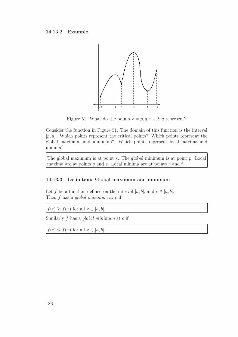
14.13.2 Example
utsrqp
Figure 51: What do the points x = p, q, r, s, t, u represent?
Consider the function in Figure 51. The domain of this function is the interval[p, u]. Which points represent the critical points? Which points represent theglobal maximum and minimum? Which points represent local maxima andminima?
The global maximum is at point s. The global minimum is at point p. Localmaxima are at points q and s. Local minima are at points r and t.
14.13.3 Definition: Global maximum and minimum
Let f be a function defined on the interval [a, b], and c ∈ [a, b].Then f has a global maximum at c if
f(c) ≥ f(x) for all x ∈ [a, b].
Similarly f has a global minimum at c if
f(c) ≤ f(x) for all x ∈ [a, b].
186

14.13.4 Theorem
If f has a local maximum/minimum at x = c and f ′(c) exists then f ′(c) = 0.
Proof (for max):
For x < c, x near c:
f(x)− f(c) ≤ 0
⇒ f(x)− f(c)
x− c≥ 0
⇒ f ′(c) = limx→c−
f(x)− f(c)
x− c≥ 0
Similarly for x > c, x near c:
f(x)− f(c) ≥ 0
⇒ f(x)− f(c)
x− c≤ 0
⇒ f ′(c) = limx→c−
f(x)− f(c)
x− c≤ 0
Thus f ′(c) = 0.
14.14 First derivative test
Let f be continuous on [a, b] and differentiable on (a, b), and let c ∈ (a, b).
(a) If f ′(x) > 0 for a < x < c and f ′(x) < 0 for c < x < b
then f has a local maximum at c.
(b) If f ′(x) < 0 for a < x < c and f ′(x) > 0 for c < x < b
then f has a local minimum at c.
Proof:
(a) Since f ′(x) > 0 for a < x < c and f continuous on (a, c], f is strictlyincreasing on (a, c] by 14.12(a). Thus f(c) > f(x) for x < c.
187
Similarly using 14.12(b), f(c) > f(x) for c < x < b.
Thus f(c) ≥ f(x) for all x ∈ R and f has a maximum at x = c.
(b)Analogous.
14.15 Second derivative test
Suppose f ′′ exists and is continuous near c.
(a) If f ′(c) = 0 and f ′′(c) > 0, then
f has a local minimum at c.
(b) If f ′(c) = 0 and f ′′(c) < 0, then
f has a local maximum at c.
(c) If f ′(c) = 0 and f ′′(c) = 0, then the test fails and we get no useful informa-tion. In this case the first derivative test should be used.
14.15.1 Example
Find local minima and maxima of f(x) = x3 on R.
second derivative test:
f ′(x) = 3x2 and f ′′(x) = 6x.
f ′(x) = 0⇒ 3x2 = 0⇒ x = 0.
f ′′(0) = 0⇒ no information, use first derivative test.
first derivative test:
f ′(x) = 3x2.
x < 0 : 3x2 > 0.
x > 0 : 3x2 > 0.
⇒ f(x) is always increasing,
therefore there is no extremal value at x = 0.
⇒ no local extrema (0 is a point of inflection).
188

14.15.2 Example
Find local extrema of f(x) = x4.
second derivative test:
f ′(x) = 4x3 and f ′′(x) = 12x2.
f ′(x) = 0⇒ 4x3 = 0⇒ x = 0.
f ′′(0) = 0⇒ no information, use first derivative test.
first derivative test:
f ′(x) = 4x3.
x < 0 : 4x3 < 0.
x > 0 : 4x3 > 0.
⇒ change of sign at x = 0, from negative to positive.
⇒ local minimum at x = 0, with value f(0) = 0.
14.15.3 Example: Beehive cell - Stewart, 6ed. p. 264 qn 43; 5ed.p. 285 qn 39
In a beehive, each cell is a regular hexagonal prism, open at one end with atrihedral angle at the other end (see Figure 52). It is believed that bees formtheir cells in such a way as to minimise the surface area for a given volume, thususing the least amount of wax in cell construction. Examination of these cellshas shown that the measure of the apex angle θ is amazingly consistent. Basedon the geometry of the cell, it can be shown that the surface area S is given by
S(θ) = 6sh +3s2
2 sin θ(√
3− cos θ)
where s, the length of the sides of the hexagon, and h, the height, are constants.
189

h
s
θ
Figure 52: The beehive cell. The open front is pictured on the bottom and theclosed end with the trihedral angle on top.
(a) CalculatedS
dθ
(b) What angle should the bees prefer?
Actual measurements of the angle θ in beehives have been made, and the mea-sures of these angles seldom differ from the calculated value by more than 2◦.
S(θ) = 6sh +3s2
2 sin θ(√
3− cos θ) s, h constant.
= 6sh +3s2
2·√
3− cos θ
sin θ
Then:
dS
dθ=
3s2
2· sin θ sin θ − (
√3− cos θ) cos θ
sin2 θ
=3s2
2· sin
2 θ + cos2 θ −√
3 cos θ
sin2 θ
=3s2
2 sin2 θ(1−
√3 cos θ).
190

dS
dθ= 0 ⇒ 3s2
2 sin2 θ(1−
√3 cos θ) = 0
⇒ 1−√
3 cos θ = 0
⇒ cos θ =1√3
(⇒ sin θ =√
2/3).
Note that the angle θ should satisfy 0 ≤ θ ≤ π2
(from a geometry argument).Therefore θ = arccos( 1√
3) ≈ 55◦ gives the critical point.
Using the second derivative test
d2S
dθ2=
3s2
2 sin3 θ(√
3 +√
3 cos2 θ − 2 cos θ) > 0 when cos θ =1√3.
Therefore we have a local minimum at θ ≃ 55◦. (This is in fact a globalminimum too.)
191

14.16 Extreme value theorem - Stewart, 6ed. p. 206;5ed. p. 225
If f is continuous on a closed interval [a, b], then
f attains its global maximum and a global minimum value on [a, b]. Thesevalues occur either at an end point or an interior critical point.
Calculate the value of f at each of these points and then work out the largestvalue (global maximum) and the smallest value (global minimum).
Bonus theorem: a) If f is differentiable on (a, b) and only has onecritical point, which is a local min; then the global minimum of f occurs atthis point.b) If f is differentiable on (a, b) and only has one critical point, which is alocal max; then the global maximum of f occurs at this point.
14.16.1 Example: Stewart, 6ed. p. 209 ex. 8; 5ed. p. 228 ex. 8
Find the global maximum and minimum of the function f(x) = x3− 3x2 +1 onthe interval [−1
2, 4].
Note thatf ′(x) = 3x2 − 6x = 3x(x− 2)
is defined everywhere and f ′(x) = 0 at x = 0 or 2. Both critical points thereforelie in (−1
2, 4).
Therefore the global maximum and minimum are either at the end points(x = −1
2or 4) or at the interior critical points (x = 0 or 2):
f(0) = 1
f(2) = −3
f
(
−1
2
)
=1
8
f(4) = 17
Therefore the global maximum is 17 at x = 4 and the global minimum is -3 atx = 2.
192

14.17 Optimization problems
14.17.1 Example: Optimal rowing
A rowing team launches a boat from point A on a bank of a straight river 3kmwide, and wants to reach point B, 8km downstream on the opposite bank asquickly as possible; see Figure 53. They could row their boat directly acrossthe river to a point C and then run to B, or they could row directly to B, orthey could row to some point D between C and B and then run to B. If theycan row 6km/h and run 8km/h, where should they land to reach B as soon aspossible? (Assume that the speed of the water is negligible compared to thespeed at which they row.)
8km
3km
DC B
A
Figure 53: How should the team travel from A to B in the shortest possibletime?
Let x = |CD| so |AD| =√
9 + x2 and |DB| = 8− x (km).
Aim: minimize the time taken. We need |AD| and |DB| ≥ 0, so 0 ≤ x ≤ 8.
t(x) =distance
speed
=1
6|AD|+ 1
8|DB|
=1
6
√9 + x2 +
1
8(8− x), 0 ≤ x ≤ 8.
So t′(x) =x
6√
9 + x2− 1
8.
193
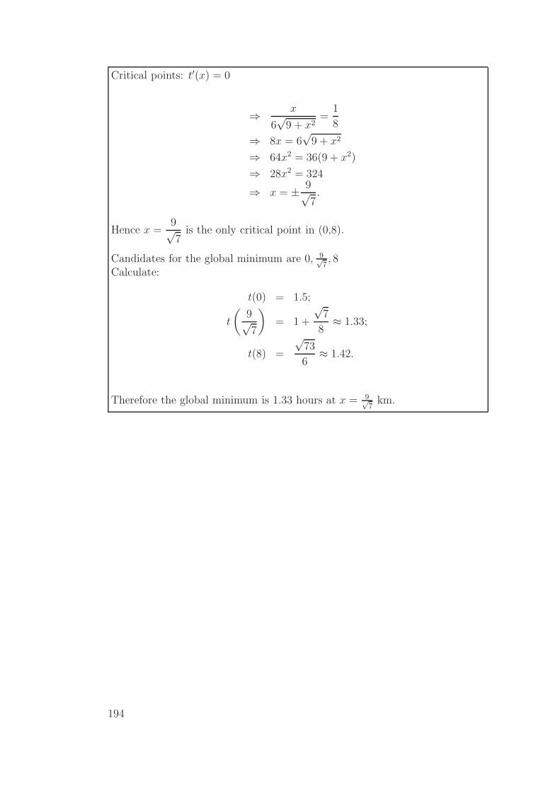
Critical points: t′(x) = 0
⇒ x
6√
9 + x2=
1
8
⇒ 8x = 6√
9 + x2
⇒ 64x2 = 36(9 + x2)
⇒ 28x2 = 324
⇒ x = ± 9√7.
Hence x =9√7
is the only critical point in (0,8).
Candidates for the global minimum are 0, 9√7, 8
Calculate:
t(0) = 1.5;
t
(9√7
)
= 1 +
√7
8≈ 1.33;
t(8) =
√73
6≈ 1.42.
Therefore the global minimum is 1.33 hours at x = 9√7
km.
194
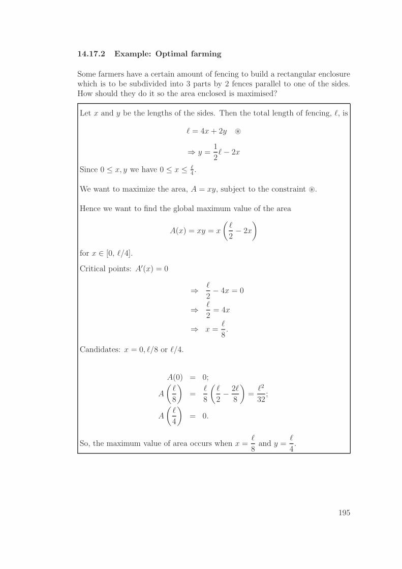
14.17.2 Example: Optimal farming
Some farmers have a certain amount of fencing to build a rectangular enclosurewhich is to be subdivided into 3 parts by 2 fences parallel to one of the sides.How should they do it so the area enclosed is maximised?
Let x and y be the lengths of the sides. Then the total length of fencing, ℓ, is
ℓ = 4x + 2y ⊛
⇒ y =1
2ℓ− 2x
Since 0 ≤ x, y we have 0 ≤ x ≤ ℓ4.
We want to maximize the area, A = xy, subject to the constraint ⊛.
Hence we want to find the global maximum value of the area
A(x) = xy = x
(ℓ
2− 2x
)
for x ∈ [0, ℓ/4].
Critical points: A′(x) = 0
⇒ ℓ
2− 4x = 0
⇒ ℓ
2= 4x
⇒ x =ℓ
8.
Candidates: x = 0, ℓ/8 or ℓ/4.
A(0) = 0;
A
(ℓ
8
)
=ℓ
8
(ℓ
2− 2ℓ
8
)
=ℓ2
32;
A
(ℓ
4
)
= 0.
So, the maximum value of area occurs when x =ℓ
8and y =
ℓ
4.
195

Notes
196

Notes
197

Notes
198
15 Integration
15.1 Definition: Anti-derivative - Stewart, 6ed. p. 274;
5ed. p. 300
A function F is called an anti-derivative of f or, a primitive of f on an intervalI if
F ′(x) = f(x), for all x ∈ I.
See the table below for some examples of anti-derivatives. We use the notationF ′ = f , G′ = g and c is a constant.
Function Antiderivative
cf(x) cF (x)
f(x) + g(x) F (x) + G(x)
xα, (α 6= −1)xα+1
α + 1
sin x − cos x
Function Antiderivative
cos x sin x
sec2 x tan x
1
xln x
ex ex
The most general anti-derivative can be obtained from those given in the table
by adding a constant. Notice that ifd
dxF (x) = f(x) then
d
dx(F (x) + C) = f(x)
is also true where C is any constant (independent of x).
15.1.1 Example
Find the most general anti-derivative of the function f(x) = x2 + 3x.
Using the table, we have
F (x) =1
3x3 +
3
2x2 + C,
where C is a constant.
199
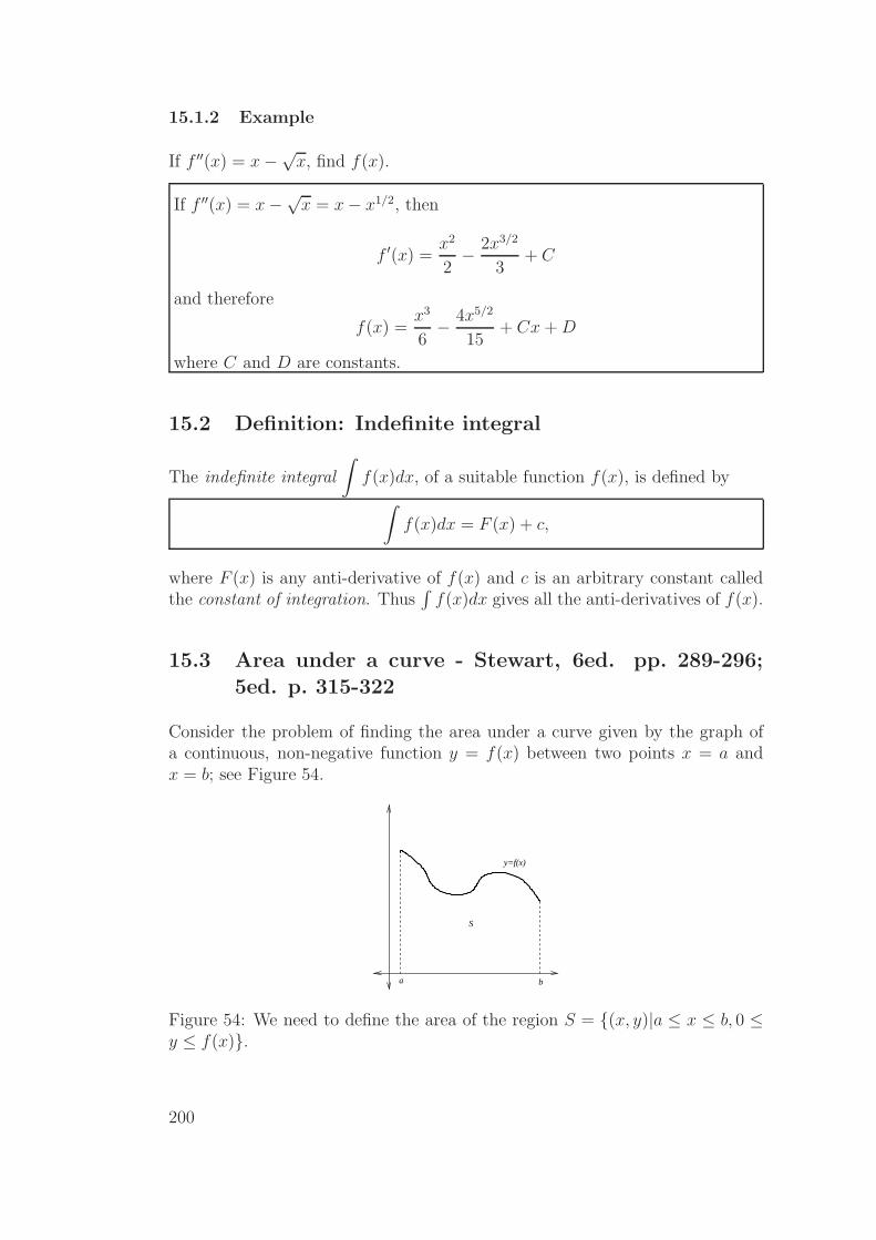
15.1.2 Example
If f ′′(x) = x−√x, find f(x).
If f ′′(x) = x−√x = x− x1/2, then
f ′(x) =x2
2− 2x3/2
3+ C
and therefore
f(x) =x3
6− 4x5/2
15+ Cx + D
where C and D are constants.
15.2 Definition: Indefinite integral
The indefinite integral
∫
f(x)dx, of a suitable function f(x), is defined by
∫
f(x)dx = F (x) + c,
where F (x) is any anti-derivative of f(x) and c is an arbitrary constant calledthe constant of integration. Thus
∫f(x)dx gives all the anti-derivatives of f(x).
15.3 Area under a curve - Stewart, 6ed. pp. 289-296;
5ed. p. 315-322
Consider the problem of finding the area under a curve given by the graph ofa continuous, non-negative function y = f(x) between two points x = a andx = b; see Figure 54.
y=f(x)
S
a b
Figure 54: We need to define the area of the region S = {(x, y)|a ≤ x ≤ b, 0 ≤y ≤ f(x)}.
200
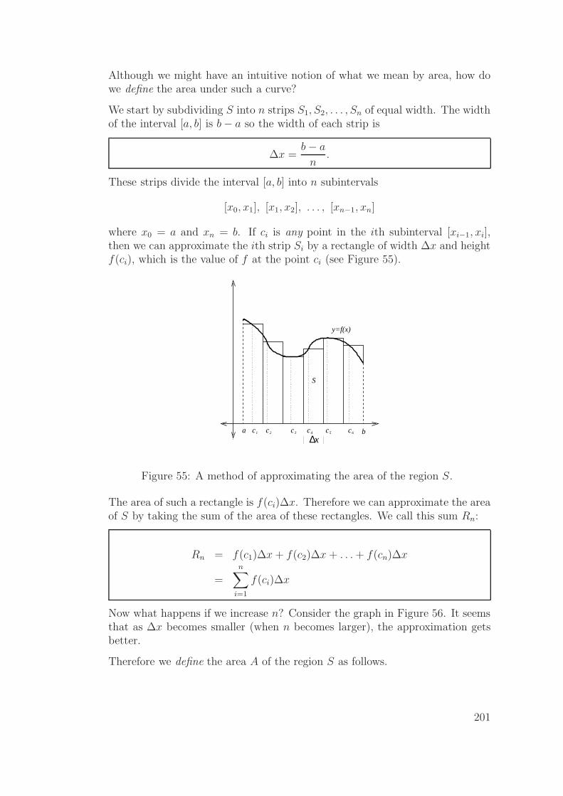
Although we might have an intuitive notion of what we mean by area, how dowe define the area under such a curve?
We start by subdividing S into n strips S1, S2, . . . , Sn of equal width. The widthof the interval [a, b] is b− a so the width of each strip is
∆x =b− a
n.
These strips divide the interval [a, b] into n subintervals
[x0, x1], [x1, x2], . . . , [xn−1, xn]
where x0 = a and xn = b. If ci is any point in the ith subinterval [xi−1, xi],then we can approximate the ith strip Si by a rectangle of width ∆x and heightf(ci), which is the value of f at the point ci (see Figure 55).
y=f(x)
a b2 3 4 61 5
S
c c c c c c∆x
Figure 55: A method of approximating the area of the region S.
The area of such a rectangle is f(ci)∆x. Therefore we can approximate the areaof S by taking the sum of the area of these rectangles. We call this sum Rn:
Rn = f(c1)∆x + f(c2)∆x + . . . + f(cn)∆x
=n∑
i=1
f(ci)∆x
Now what happens if we increase n? Consider the graph in Figure 56. It seemsthat as ∆x becomes smaller (when n becomes larger), the approximation getsbetter.
Therefore we define the area A of the region S as follows.
201

y=f(x)
a b
Figure 56: The smaller the width of the rectangle, the better the approximation,in general. Notice that in this diagram we chose ci = a + i∆x.
15.3.1 Definition: Area of a region, Riemann sum
The area A of the region S that lies under the graph of the continuous, non-negative function f is
A = limn→∞
Rn
= limn→∞
[f(c1)∆x + f(c2)∆x + . . . + f(cn)∆x]
= limn→∞
n∑
i=1
f(ci)∆x.
This limit always exists and is independent of the choice of ci. This can beproved using the fact that f is continuous on [a, b]. This sum Rn is called aRiemann sum.
Note that limn→∞
[f(c1)∆x + · · ·+ f(cn)∆x] is called the Riemann integral of f on
[a, b] and is denotedb∫
a
f(x)dx.
IMPORTANT: this definition can be carried over to functions which are notnecessarily non-negative. The intuitive interpretation of A as an area is then nolonger valid. The quantity A should then be viewed as a “signed area”, i.e.
A = area above x-axis, below graph − area below x-axis, above graph.
Stewart, 6ed. p. 301; 5ed. p. 328
202

15.4 Fundamental Theorem of Calculus
15.4.1 Theorem: Fundamental Theorem of Calculus
(a) If f is continuous on [a, b], a ≤ x ≤ b, then
A(x) =
x∫
a
f(t)dt
gives an antiderivative of f(x) such that A(a) = 0.
(b) If F (x) is any antiderivative of f(x), then
F (b)− F (a) =
b∫
a
f(t)dt.
15.4.2 Proof (outline)
(a) Consider f ≥ 0. Let A(x) =x∫
a
f(t)dt, that is let A(x) be the function
that describes the area below the graph of the function f above the interval[a, x]; thus A(a) = 0. For h > 0 small, consider
A(x + h)− A(x) = area above [a, x + h]− area above [a, x]
= area above [x, x + h] and below f
≈ h · f(x)
⇒ A(x + h)−A(x)
h≈ f(x)
Taking the limit h→ 0 then yields (this requires justification)
A′(x) = limh→0
A(x + h)− A(x)
h= f(x).
so that A(x) is an anti-derivative of f(x). General f is similar.
(b) Follows from (a).
203

15.4.3 Notation
We will writeF (x)|ba = [F (x)]ba = F (b)− F (a).
15.4.4 Properties of the definite integral
For some c ∈ R, f(x) continuous on [a, b] there holds:
•∫ a
b
f(x)dx = −∫ b
a
f(x)dx
•∫ b
a
cdx = c(b− a)
•∫ b
a
[f(x)± g(x)]dx =
∫ b
a
f(x)dx±∫ b
a
g(x)dx
•∫ b
a
cf(x)dx = c
∫ b
a
f(x)dx
•∫ c
a
f(x)dx +
∫ b
c
f(x)dx =
∫ b
a
f(x)dx
•∫ a
a
f(x)dx = 0
15.4.5 Examples
(1) Show that ln x =
x∫
1
1
tdt, for x > 0.
Set g(x) = ln x−∫ x
1
dt
tfor x > 0.
WTS: g(x) = 0 for all x > 0.
So g′(x) =d
dxlnx− d
dx
[∫ x
1
dt
t
]
=1
x− 1
xby Fundamental Theorem of Calculus
= 0
⇒ g(x) = C, for some constant C.
⇒ g(x) = g(1) = ln 1−∫ 1
1
dt
t= 0
204

(2) Evaluate
∫ 2
1
1
tdt.
∫ 2
1
1
tdt = [ln t]21
= ln 2− ln 1
= ln 2.
(3) Evaluate
∫ π/2
0
sin xdx.
∫ π/2
0
sin xdx = [− cos x]π/20
= − cosπ
2− (− cos 0)
= 0 + 1
= 1.
(4) If G(x) =sin x∫
2
dt√1+t2
, find G′(x).
Let F (u) =
u∫
2
dt√1 + t2
⇒ F ′(u) =1√
1 + u2(by the Fundamental Theorem of Calculus)
Now, G(x) = F (sin x) = F (u), with u = sin x. By the chain rule,
G′(x) =d
dxF (u)
=dF (u)
du· du
dx
=1√
1 + u2cos x
=cos x√
1 + sin2 x.
205
15.4.6 Example
Find the area between the x-axis and the curve y = sin x on [0, π].
There holds sin x ≥ 0 on [0, π], so
Area =
∫ π
0
sin xdx = [− cos x]π0
= − cos π − (− cos 0)
= −(−1) + 1
= 2.
15.4.7 Example
Find the area bounded by the curves y = x2 and y = x3 on the interval [0, 1].
There holds x2 ≥ x3 on [0, 1],
⇒ Area =
∫ 1
0
x2dx−∫ 1
0
x3dx
=
[1
3x3
]1
0
−[1
4x4
]1
0
=1
3− 1
4
=1
12.
15.4.8 Corollary
If f is non-negative and continuous on [a, b] then
∫ b
a
f(x)dx ≥ 0.
If f is non-positive and continuous on [a, b] then
∫ b
a
f(x)dx = −(area above graph below interval [a, b]) ≤ 0.
206

15.4.9 Example
Find the area enclosed by the curves y = x and y = x3.
First, we need to determine where the two curves intersect:
x3 = x ⇒ x3 − x = 0⇒ x(x + 1)(x− 1) = 0
⇒ x = −1, 0, 1.
There holds: x3 ≥ x on [−1, 0] and x ≥ x3 on [0, 1].
⇒ Area =
∫ 0
−1
(x3 − x)dx +
∫ 1
0
(x− x3)dx
=
[x4
4− x2
2
]0
−1
+
[x2
2− x4
4
]1
0
= −1
4+
1
2+
1
2− 1
4
=1
4+
1
4
=1
2.
15.5 Approximate integration (trapezoidal rule)
We can approximate the area under a curve by taking the sum of a finite numberof rectangles under the graph as outlined in the previous section. If we choosethe ci to be the left endpoints of each rectangle, we obtain the approximation
ℓn =n∑
i=1
f(xi−1)∆x.
If we choose the ci to be the right endpoints of each rectangle we obtain theapproximation
rn =
n∑
i=1
f(xi)∆x.
207
The trapezoidal rule is the approximation of the area under a curve which takesthe average value of ℓn and rn.
The formula for this approximation is therefore given by
area A ≈ ℓn + rn
2
=∆x
2
[n∑
i=1
(f(xi−1) + f(xi))
]
=∆x
2[(f(x0) + f(x1)) + (f(x1) + f(x2)) + . . . + (f(xn−1) + f(xn))]
=∆x
2[f(x0) + 2f(x1) + 2f(x2) + . . . + 2f(xn−1) + f(xn)]
where ∆x = (b− a)/n and xi = a + i∆x.
The trapezoidal rule will appear in a Matlab module.
15.6 Improper integrals - Stewart, 6ed. pp. 544-551; 5ed.pp. 566-573
If
∫ t
a
f(x)dx exists for every t ≥ a, then
∫ ∞
a
f(x)dx = limt→∞
∫ t
a
f(x)dx
provided the limit exists.
If
∫ b
t
f(x)dx exists for every t ≤ b, then
∫ b
−∞f(x)dx = lim
t→−∞
∫ b
t
f(x)dx
provided the limit exists.
208

The integrals
∫ ∞
a
f(x)dx and
∫ b
−∞f(x)dx are called convergent if the limit
exists and divergent otherwise.
If both
∫ ∞
a
f(x)dx and
∫ a
−∞f(x)dx are convergent, then we define
∫ ∞
−∞f(x)dx =
∫ a
−∞f(x)dx +
∫ ∞
a
f(x)dx for any real a.
Note that this must be independent of a. Note also that the usual propertiesof integrals apply provided all integrals are convergent.
15.6.1 Example
Find
∫ ∞
0
e−xdx.
For a > 0, ∫ a
0
e−xdx = [−e−x]a0 = 1− e−a.
As a→∞, 1− e−a → 1, so
∫ ∞
0
e−xdx = lima→∞
(1− e−a) = 1.
15.6.2 Note
It is still possible to define the integral for some classes of functions which arenot necessarily continuous: Stewart, 6ed. p. 548; 5ed. p. 570. Note also thatthere are other types of improper integral: Stewart, 6ed. p. 547; 5ed. p. 569.
209

15.7 Techniques of integration - Stewart, 6ed. ch. 8; 5ed.ch. 8
15.7.1 Substitution
If u = g(x) is a differentiable function whose range is an interval I and f iscontinuous on I, then
∫
f(g(x))g′(x)dx =
∫
f(u)du
dxdx =
∫
f(u)du.
If g′ is continuous on [a, b] and f is continuous on the range of u = g(x), then
∫ b
a
f(g(x))g′(x)dx =
∫ g(b)
g(a)
f(u)du.
15.7.2 Example: Stewart, 6ed. p. 334 ex. 1; 5ed. p. 361 ex. 1
Find
∫
x3 cos(x4 + 2)dx.
Substitute u = x4 + 2 sodu
dx= 4x3 and x3 =
14du
dx.
⇒∫
x3 cos(x4 + 2)dx =
∫1
4
du
dxcos u dx
=
∫cos u
4du
=1
4
∫
cos u du
=1
4sin u + c
=1
4sin(x4 + 2) + c.
210

15.7.3 Example: Stewart, 6ed. p. 337 ex. 7; 5ed. p. 364 ex. 7
Evaluate
∫ 2
1
dx
(5x− 3)2.
Substitute u = 5x− 3. Thendu
dx= 5 and dx =
1
5du.
Note also that u(2) = 7 and u(1) = 2. Therefore:
∫ 2
1
dx
(5x− 3)2=
∫ 7
2
1
u2· 15du
=1
5
∫ 7
2
u−2du
=1
5
[−u−1
]7
2
=1
5
(
−1
7+
1
2
)
=1
14.
15.7.4 Example: Trig substitution
Evaluate
∫dx√
a2 − x2.
Substitute x = a sin θ. Then dx = a cos θdθ. Hence:∫
dx√a2 − x2
=
∫a cos θdθ
√
a2 − a2 sin2 θ
=
∫a cos θdθ
a√
1− sin2 θ
=
∫cos θ
cos θdθ
=
∫
dθ
= θ + c
= arcsin(x
a
)
+ c.
211
15.7.5 Example
Evaluate
∫
cos x sin x dx.
Substitute u = sin x. Thendu
dx= cos x. Hence:
∫
cos x sin x dx =
∫
u du
=u2
2+ c
=sin2 x
2+ c.
15.7.6 Example
Evaluate
∫
(3x + 1)(3x2 + 2x)3 dx.
Substitute u = 3x2 + 2x. Thendu
dx= 6x + 2 and 3x + 1 =
1
2· du
dx. Hence:
∫
(3x + 1)(3x2 + 2x)3 dx =
∫1
2
du
dxu3 dx
=
∫u3
2du
=u4
8+ c
=1
8(3x2 + 2x)4 + c.
212
15.7.7 Integration by parts
Given two differentiable functions u(x) and v(x) we have a product rule fordifferentiation:
d
dx(uv) =
du
dxv + u
dv
dx= u′v + uv′.
Therefore uv is an antiderivative of uv′ + u′v. Hence
uv =
∫
(u′v + uv′) dx
=
∫
u′v dx +
∫
uv′ dx
⇒∫
uv′ dx = uv −∫
u′v dx.
The aim is to simplify the function that is integrated, i.e.∫
u′vdx should beeasier to find than
∫uv′dx. Also note that the antiderivative of v′ needs to be
found!
15.7.8 Example
Evaluate
∫
x3 ln xdx.
Set u = ln x and v′ = x3. Then u′ =1
xand v =
x4
4. Hence:
∫
x3 ln xdx =1
4x4 lnx−
∫1
4x4 · 1
xdx
=1
4x4 lnx− 1
4
∫
x3dx
=1
4x4 lnx− 1
16x4 + c.
Note that if u = x3 and v′ = ln x is chosen, then v =∫
ln xdx needs to befound.
213

15.7.9 Example
Evaluate
∫
xexdx.
Set u = x and v′ = ex. Then u′ = 1 and v = ex.
⇒∫
xexdx = xex −∫
exdx
= (x− 1)ex + c.
Note that for the choice u = ex and v′ = x, the integral becomes more com-plicated than before.
15.7.10 General rule
• For∫
(polynomial) · eax+bdx, choose u to be the polynomial and v′ = eax+b.
• For∫
(polynomial) · ln (ax + b)dx, choose u = ln (ax + b) and v′ to be thepolynomial.
• Note that sometimes integration by parts needs to be applied more thanonce.
15.7.11 Example
Evaluate
∫
x sin xdx.
Set u = x and v′ = sin x. Then u′ = 1 and v = − cos x.
⇒∫
x sin xdx = −x cos x−∫
− cos xdx
= −x cos x + sin x + c.
214

15.8 Integrals involving ln function
If y = ln x for x > 0, then
dy
dx=
1
x⇒
∫dx
x= ln x + c, for x > 0.
For x < 0, if y = ln(−x) we have
dy
dx=−1
−x=
1
x,
so we have ∫dx
x= ln(−x) + c, for x < 0.
We often combine these cases and write
∫dx
x= ln |x|+ c, x 6= 0.
15.9 Integration of rational functions by partial fractions
A ratio of two polynomials,
f(x) =P (x)
Q(x)
is called a rational function. Integration of a rational function is made possibleby expressing it as the sum of simpler fractions, called partial fractions.
(In the three examples which follow, we will only consider rational functions forwhich the degree of P (x) is less than the degree of Q(x).)
The general process for obtaining the sum of partial fractions is as follows:
• Factor the denominator Q(x) as much as possible;
• Express f(x) as a sum of fractions each of which take either the formA
(ax + b)ior
Ax + B
(ax2 + bx + c)j, where the denominators of these frac-
tions come from the factorisation of Q(x).
215
Consider the following examples.
15.9.1 Example
Evaluate
∫x + 2
x2 + xdx.
The general technique for solving intergrals of the form
∫cx + d
(x− a)(x− b)
is to writecx + d
(x− a)(x− b)=
A
x− 1+
B
x− b.
In this case:x + 2
x2 + x=
x + 2
x(x + 1).
We want:x + 2
x(x + 1)=
A
x+
B
x + 1
=A(x + 1) + Bx
x(x + 1).
equate numerators ⇒ x + 2 = A(x + 1) + Bx
= (A + B)x + A ⊛
equate coefficients ⇒ (A + B) = 1, and A = 2.
⇒ B = −1.
Hence ⇒∫
x + 2
x(x + 1)dx =
∫2
xdx−
∫dx
x + 1
= 2 ln |x| − ln |x + 1|+ C.
An alternate method at ⊛ would be to pick convenient values of x.
i.e. x = −1⇒ B = −1 x = 0 ⇒ A = 2
216
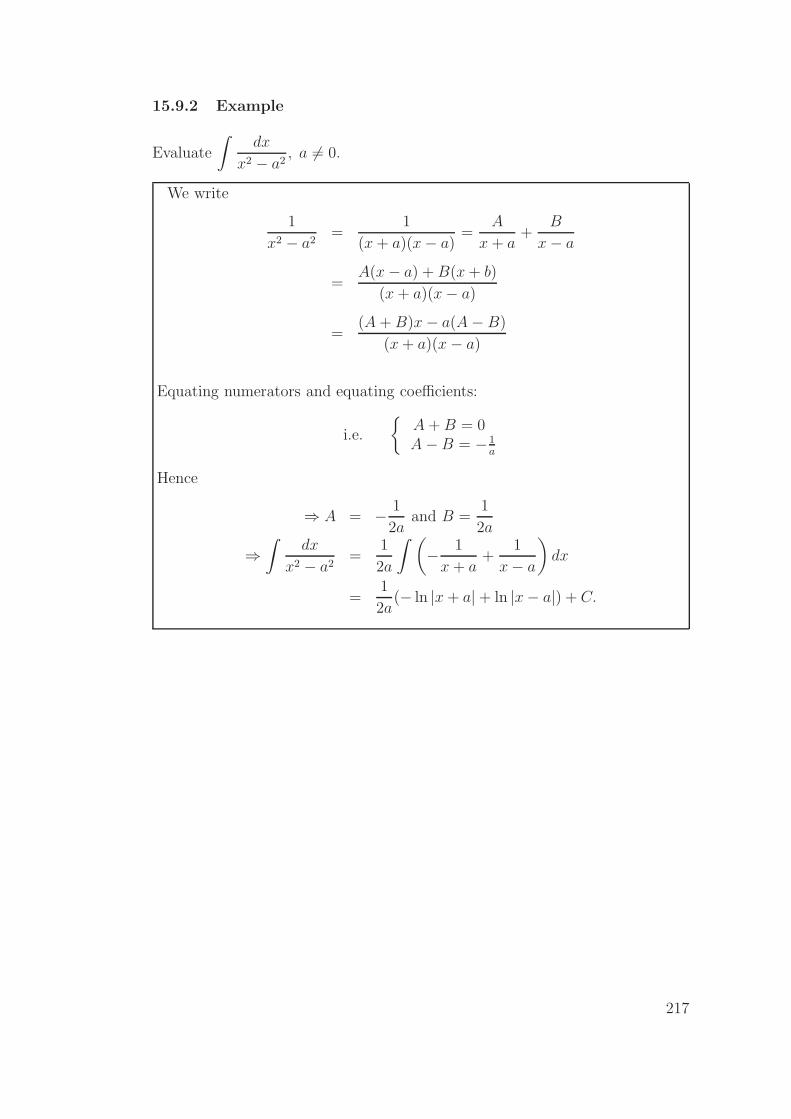
15.9.2 Example
Evaluate
∫dx
x2 − a2, a 6= 0.
We write
1
x2 − a2=
1
(x + a)(x− a)=
A
x + a+
B
x− a
=A(x− a) + B(x + b)
(x + a)(x− a)
=(A + B)x− a(A− B)
(x + a)(x− a)
Equating numerators and equating coefficients:
i.e.
{A + B = 0A−B = −1
a
Hence
⇒ A = − 1
2aand B =
1
2a
⇒∫
dx
x2 − a2=
1
2a
∫ (
− 1
x + a+
1
x− a
)
dx
=1
2a(− ln |x + a|+ ln |x− a|) + C.
217
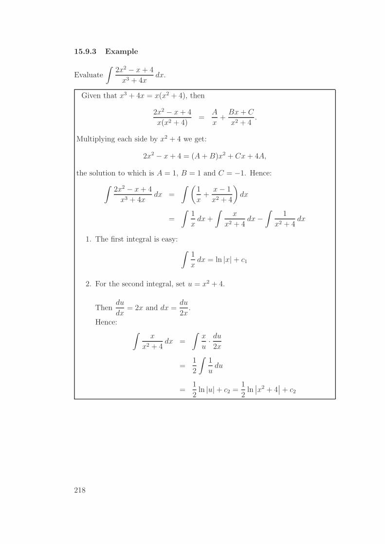
15.9.3 Example
Evaluate
∫2x2 − x + 4
x3 + 4xdx.
Given that x3 + 4x = x(x2 + 4), then
2x2 − x + 4
x(x2 + 4)=
A
x+
Bx + C
x2 + 4.
Multiplying each side by x2 + 4 we get:
2x2 − x + 4 = (A + B)x2 + Cx + 4A,
the solution to which is A = 1, B = 1 and C = −1. Hence:
∫2x2 − x + 4
x3 + 4xdx =
∫ (1
x+
x− 1
x2 + 4
)
dx
=
∫1
xdx +
∫x
x2 + 4dx−
∫1
x2 + 4dx
1. The first integral is easy:
∫1
xdx = ln |x| + c1
2. For the second integral, set u = x2 + 4.
Thendu
dx= 2x and dx =
du
2x.
Hence:∫
x
x2 + 4dx =
∫x
u· du
2x
=1
2
∫1
udu
=1
2ln |u|+ c2 =
1
2ln
∣∣x2 + 4
∣∣ + c2
218
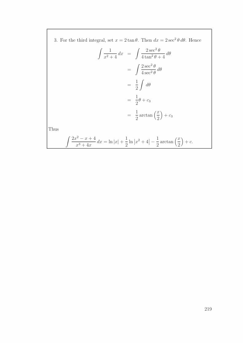
3. For the third integral, set x = 2 tan θ. Then dx = 2 sec2 θ dθ. Hence
∫1
x2 + 4dx =
∫2 sec2 θ
4 tan2 θ + 4dθ
=
∫2 sec2 θ
4 sec2 θdθ
=1
2
∫
dθ
=1
2θ + c3
=1
2arctan
(x
2
)
+ c3
Thus∫
2x2 − x + 4
x3 + 4xdx = ln |x| + 1
2ln
∣∣x2 + 4
∣∣− 1
2arctan
(x
2
)
+ c.
219
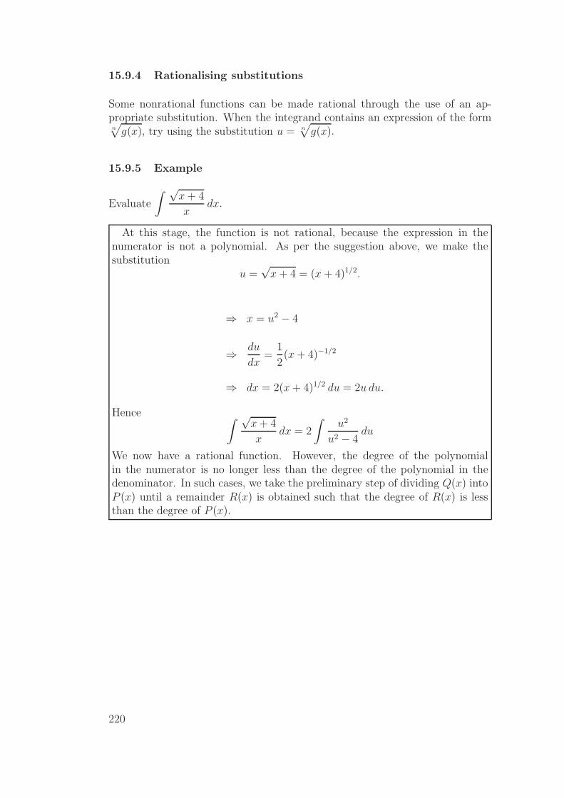
15.9.4 Rationalising substitutions
Some nonrational functions can be made rational through the use of an ap-propriate substitution. When the integrand contains an expression of the formn√
g(x), try using the substitution u = n√
g(x).
15.9.5 Example
Evaluate
∫ √x + 4
xdx.
At this stage, the function is not rational, because the expression in thenumerator is not a polynomial. As per the suggestion above, we make thesubstitution
u =√
x + 4 = (x + 4)1/2.
⇒ x = u2 − 4
⇒ du
dx=
1
2(x + 4)−1/2
⇒ dx = 2(x + 4)1/2 du = 2u du.
Hence ∫ √x + 4
xdx = 2
∫u2
u2 − 4du
We now have a rational function. However, the degree of the polynomialin the numerator is no longer less than the degree of the polynomial in thedenominator. In such cases, we take the preliminary step of dividing Q(x) intoP (x) until a remainder R(x) is obtained such that the degree of R(x) is lessthan the degree of P (x).
220

In this case, we get:u2
u2 − 4= 1 +
4
u2 − 4.
2
∫u2
u2 − 4du = 2
∫ (
1 +4
u2 − 4
)
du
= 2u + 2
∫4
(u + 2)(u− 2)du
= 2√
x + 4 + 2
∫ ( −1
u + 2+
1
u− 2
)
du
= 2√
x + 4− 2 ln |u + 2|+ 2 ln |u− 2|+ c
= 2√
x + 4− 2 ln∣∣∣
√x + 4 + 2
∣∣∣ + 2 ln
∣∣∣
√x + 4− 2
∣∣∣ + c
= 2√
x + 4 + 2 ln
∣∣∣∣
√x + 4− 2√x + 4 + 2
∣∣∣∣+ c.
221
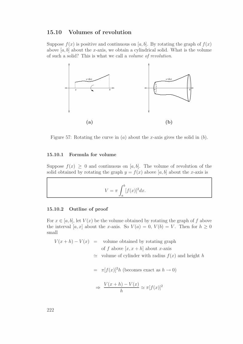
15.10 Volumes of revolution
Suppose f(x) is positive and continuous on [a, b]. By rotating the graph of f(x)above [a, b] about the x-axis, we obtain a cylindrical solid. What is the volumeof such a solid? This is what we call a volume of revolution.
a b
y=f(x)
b
y=f(x)
a
(a) (b)
Figure 57: Rotating the curve in (a) about the x-axis gives the solid in (b).
15.10.1 Formula for volume
Suppose f(x) ≥ 0 and continuous on [a, b]. The volume of revolution of thesolid obtained by rotating the graph y = f(x) above [a, b] about the x-axis is
V = π
∫ b
a
[f(x)]2dx.
15.10.2 Outline of proof
For x ∈ [a, b], let V (x) be the volume obtained by rotating the graph of f abovethe interval [a, x] about the x-axis. So V (a) = 0, V (b) = V . Then for h ≥ 0small
V (x + h)− V (x) = volume obtained by rotating graph
of f above [x, x + h] about x-axis
≃ volume of cylinder with radius f(x) and height h
= π[f(x)]2h (becomes exact as h→ 0)
⇒ V (x + h)− V (x)
h≃ π[f(x)]2
222

Taking the limit h→ 0 we obtain
V ′(x) = π[f(x)]2
so the Fundamental Theorem yields
∫ b
a
π[f(x)]2dx = [V (x)]ba = V (b)− V (a) = V (b) = V.
15.10.3 Example
Let a > 0. Find the volume of the solid obtained by rotating y = f(x) =√
xabout the x-axis over [0, a].
volume = π
∫ a
0
[√
x]2dx
= π
∫ a
0
xdx = π
[x2
2
]a
0
=1
2πa2.
15.10.4 Example
Determine the volume of the solid obtained by rotating y = x about the x-axisover [0, 1].
volume = π
∫ 1
0
(x)2 dx
=π
3
[x3
]1
0
=π
3.
223

15.10.5 Example
Determine the volume of the solid obtained by rotating y = x2 about the x-axisover [0, 1].
volume = π
∫ 1
0
(x2)2 dx
= π
∫ 1
0
x4 dx
=π
5
[x5
]1
0
=π
5.
15.10.6 Example
The region enclosed by the curves y = x and y = x2 is rotated about the x-axis.Find the volume of the resultant solid.
The curves y = x and y = x2 intersect at the points (0, 0) and (1, 1). Further-more, x ≥ x2 on [0, 1].
Hence, we can simply subtract the volume obtained by rotating y = x2 aboutthe x-axis over [0, 1] from the volume obtained by rotating y = x about thex-axis over [0, 1]:
volume =π
3− π
5
=2π
15.
224

Notes
225
16 Sequences
A sequence {an} is a list of numbers with a definite order:
a0, a1, a2, a3, . . . , an, . . .
In fact, sequences can be finite or infinite. Further, a sequence does not haveto consist of numbers, but might contain any sort of mathematical structure, orindeed any other objects.
16.1 Formal Definition: Sequence
More formally, a sequence is a function, with domain being N0 = {0, 1, 2, 3, . . .}.We can also take the domain as N = {1, 2, 3, ...} and start the sequence at a1
rather than a0.
16.1.1 Motivation
Infinite sequences of numbers are useful in many applications. The sequencemight represent approximations to the solution of a problem sduch as the bisec-tion method. Or the sequence might represent a time series, where the numbersrepresent the population each year. Mathematically, we are interested in howthe sequence behaves as the number of terms becomes large: does it convergeto a solution, or how fast does the population grow? Sequences can also appearfrom the partial sums in an infinite series, which comprises our next majortopic.
16.2 Representations
There are two main ways to represent the nth term in a sequence. Firstly, thereis a direct (or closed form or functional) representation. Secondly, there is arecursive (or indirect) representation.
In the direct form, we can write
an = f(n).
In the recursive form, we write
an = f(an−1, an−2, . . . , a2, a1, a0).
226

The recursive form can have a simpler structure. It might be that an =f(an−1, an−2) or even an = f(an−1). Depending on the problem, it can benatural to express the formula in one or the other way.
16.2.1 Example: Newton’s method
Newton’s method is a numerical procedure to approximate the roots of func-tions. Most programs which find roots of functions are based on this method.For example, consider the equation
48x(1 + x)60 − (1 + x)60 + 1 = 0.
How would you find the roots of this equation? It is impossible to solve analyt-ically (ie, precisely), but Newton’s method gives us a way of approximating theroots to some degree of accuracy.
The idea behind the geometry of this method is given in Figure 58. We musthave a starting guess (the value x1), then we find the tangent line to the curveat that point, and find where the tangent line cuts the x-axis. This gives us thenext point. We repeat the process until we have a close enough estimate.
xx 12p
Figure 58: Starting at x1, this gives you an idea of how Newton’s method iteratesto estimate the root p.
Mathematically, the slope of the tangent line to the curve at the point y = f(x1)is given by
f ′(x1) =f(x1)− 0
x1 − x2⇒ x2 = x1 −
f(x1)
f ′(x1).
Repeating this procedure leads to the iterative formula
xn+1 = xn −f(xn)
f ′(xn).
227

If the numbers xn become closer and closer to p as n becomes large, we say thesequence converges to p.
This method is very sensitive to the type of curve and the choice of startingpoint.
16.2.2 Example
List the first terms of the sequence an =n
n + 1.
0,1
2,2
3,3
4, . . .
16.2.3 Example
List the first terms of the recursive sequence an+1 =1
3− an
with a1 = 2.
2, 1,1
2,2
5, . . .
Note that for the recursive form, you must express one or more initial conditionsor starting values. The recursive form is actually a difference equation, and thereare similarities with differential equations that are studied in MATH1052.
16.2.4 Example: Fibonacci sequence
The Fibonacci sequence is defined through
an = f(an−1, an−2) = an−1 + an−2
with a0 = 0, a1 = 1. List the first 9 terms.
0, 1, 1, 2, 3, 5, 8, 13, 21, . . .
228

16.3 Application: Rabbit population - Stewart, 6ed. p. 722ex. 71; 5ed. p. 748 ex. 65
Suppose that rabbits live forever and that every month each pair produces anew pair which becomes productive at age 2 months. Starting with one newbornpair, how many pairs of rabbits will be there in the nth month?
Let an be the number of rabbit pairs in the nth month.
⇒ an = an−1 + an−2, with a0 = 0, a1 = 1.
16.4 Limits
Let {an}∞n=0 be a sequence. Then
limn→∞
an = ℓ , ℓ ∈ R , means :
an approaches ℓ as n gets larger and larger, ie. an is close to ℓ for n sufficientlylarge.
This is similar to limx→∞
f(x) = ℓ, except here an is defined only for natural
numbers n.
16.4.1 Convention
If a sequence {an}∞n=0 has limit ℓ ∈ R, we say that an converges to ℓ and thatthe sequence {an}∞n=0 is convergent. Otherwise the sequence is divergent.
229
16.4.2 Examples
Determine if the sequences {an}, with an as given below, are convergent and ifso find their limits.
1. an =1
n
limn→∞
an = limn→∞
1
n= 0
So {an} converges to 0, i.e. an → 0 as n→∞.
2. an =1
2an−1, a0 = −1.
In direct form:
an = − 1
2n, for n = 0, 1, . . .
⇒ limn→∞
an = limn→∞
(
− 1
2n
)
= 0
⇒ an → 0 as n→∞.
3. an = (−1)n
The first few terms are: 1,−1, 1,−1, . . .. This sequence oscillates between ±1and therefore does not converge ⇒ divergent sequence.
230
4. an = rn, for r =1
2, r = 1, r = 2
an = rn: 4 cases.(1) |r| < 1: lim
n→∞an = 0 ⇒ {an} converges to 0.
(2) |r| > 1: limn→∞
an =∞ ⇒ {an} diverges.
(3) r = 1: limn→∞
an = 1 ⇒ {an} converges to 1.
(4) r = −1: limn→∞
andoes not exist ⇒ {an} diverges.
So:r = 1
2: converges to 0.
r = 1: converges to 1.r = 2: converges to 2.
16.5 Theorem: Limit laws
The following limit laws apply provided that the separate limits exist (that is{an} and {bn} are convergent):
Suppose that {an} and {bn} are convergent sequences such that
limn→∞
an = ℓ and limn→∞
bn = m
and c is a constant. Then
• limn→∞
(an ± bn) = ℓ±m;
• limn→∞
can = cℓ;
• limn→∞
(anbn) = ℓm; and
• limn→∞
an
bn=
ℓ
m, provided m 6= 0.
16.6 Theorem: Squeeze
If an ≤ bn ≤ cn for n ≥ n0 for some n0 ∈ N and limn→∞
an = limn→∞
cn = ℓ, then
limn→∞
bn = ℓ.
231

16.6.1 Example
Use the squeeze theorem on {an}, where an =1
nsin(n).
Since−1 ≤ sin(n) ≤ 1, for n ≥ 1
we have
−1
n≤ an ≤
1
n, for n ≥ 1.
Now
limn→∞
−1
n= lim
n→∞
1
n= 0,
so the squeeze theorem gives limn→∞
an = 0.
16.7 Theorem: Continuous extension
Let f be a function on the real numbers such that limx→∞
f(x) exists. Let f(n) = an
for natural numbers n. Then:
limn→∞
an = limx→∞
f(x).
16.7.1 Example
Evaluate limn→∞
log nn
.
Define f(x) =ln x
x. Hence
limx→∞
f(x) = limx→∞
ln x
x
= limx→∞
1/x
1by L’Hopital’s rule
= 0
⇒ limn→∞
ln n
n= 0.
232

16.8 Useful sequences to remember
(1) For constant c, limn→∞
cn =
{0 , if |c| < 11 , if c = 1.
Sequence {cn}∞n=0 is divergent if c = −1 or |c| > 1.
(2) For constant c > 0, limn→∞
c1/n = limn→∞
n√
c = 1.
(3) Even limn→∞
n1/n = limn→∞
n√
n = 1.
(4) limn→∞
1
n!= 0.
(5) For constant c, limn→∞
cn
n!= 0.
(6) limn→∞
(
1 +1
n
)n
= e.
(7) limn→∞
(
1 +a
n
)n
= ea.
16.9 Application: Logistic sequence
Sequences which are bounded, but not convergent can be very interesting. Thestudy of chaos appears in these sequences. A famous recursive sequence is thelogistic sequence from population dynamics:
an = kan−1(1− an−1), with 0 ≤ an−1 ≤ 1.
For certain values of the coefficient k, the behaviour is regular: convergent,or periodic. But other values of k yield chaotic sequences which cannot bepredicted. You will explore the logistic equation in the Matlab Tutorials. Figure59 has some examples of the logistic sequence when k = 2.9, 3.5 and 3.9.
233

Figure 59: Logistic sequence, a0 = 12, k = 2.9, 3.5, 3.9
234

Notes
235

Notes
236

17 Series
17.1 Infinite sums (notation)
Recall that if we have an infinite sum we write
a0 + a1 + a2 + . . . + an + . . . =∞∑
n=0
an.
Note that the lower bound (n = 0) of the sum may vary.
17.2 Motivation
Series come from many fields.
1. Approximation to problem solutions:
• a0 zeroth order approximation
• a0 + a1 (a1 small) first order approximation
• a0 + a1 + a2 (a2 very small) second order approximation
• a0 + a1 + a2 + . . . + an nth order
• a0+a1+a2+. . .+an+. . . exact solution, provided the series converges
2. Current state of a process over infinite time horizon
3. Approximating function, e.g.,
ex = 1 + x +1
2x2 +
1
3!x3 + . . . ,
f(t) = c0 + c1 sin t + c2 sin(2t) + c3 sin(3t) + . . .
4. Measure the volume in a fractal process, like the amount of material in abotanic structure (Figure 60).
Figure 60: This is a graphical representation of a botanic fractal.
5. Riemann sums
237

17.3 Definition: Convergence - Stewart, 6ed. p. 724;5ed. p. 750
Given a series∞∑
n=0
an = a0 + a1 + a2 + . . ., let sn denote its nth partial sum:
s0 = a0
s1 = a0 + a1
s2 = a0 + a1 + a2
...
sn = a0 + a1 + . . . + an =
n∑
k=0
ak .
If the sequence {sn} is convergent (i.e. limn→∞
sn = s with s ∈ R), then the series∞∑
n=0
an is said to be convergent and we write
limn→∞
sn =∞∑
n=0
an = s.
The number s is called the sum of the series. Otherwise the series is said to bedivergent.
17.3.1 Example
Does the series∞∑
n=0
(−1)n converge or diverge?
s0 = (−1)0 = 1
s1 = (−1)0 + (−1)1 = 0
s2 = 1 etc.
Therefores2m = 1 and s2m+1 = 0
⇒ limn→∞
sn does not exist ⇒ {sn} diverges
So∞∑
n=0
(−1)n diverges.
238

17.3.2 Example
Show that the series
∞∑
n=0
1
(n + 1)(n + 2)is convergent and find its sum.
First note that
∞∑
n=0
1
(n + 1)(n + 2)=
∞∑
n=1
1
n(n + 1).
Then
sn =n∑
k=1
1
k(k + 1)
=n∑
k=1
(1
k− 1
k + 1
)
=
(1
1− 1
2
)
+
(1
2− 1
3
)
+ · · ·+(
1
n− 1
n + 1
)
= 1− 1
n + 1.
Therefore
limn→∞
sn = limn→∞
(
1− 1
n + 1
)
= 1.
Therefore the series is convergent and
∞∑
n=0
1
(n + 1)(n + 2)= 1.
17.4 Theorem: p test
For p ∈ R, the p-series
∞∑
n=1
1
npis
convergent if p > 1
and divergent if p ≤ 1.
Note the above sum is from n = 1. This is just a matter of taste since∞∑
n=1
1
np=
∞∑
n=0
1
(n + 1)p
239

17.5 Theorem: nth term test - Stewart, 6ed. p. 728; 5ed.p. 754
If∞∑
n=0
an is convergent then limn→∞
an = 0.
17.6 Test for divergence (nth term test)
If limn→∞
an 6= 0 then the series is divergent.
17.6.1 Caution
If limn→∞
an = 0 then we cannot say whether it is convergent or divergent.
For example,
limn→∞
1
n= 0
but the harmonic series
∞∑
n=1
1
n= 1 +
1
2+
1
3+
1
4+ . . .
diverges (p-series with p = 1).
17.6.2 Examples
Verify that these series diverge by the nth term test.
(i)∞∑
n=0
(−1)n
With an = (−1)n, limn→∞
an 6= 0⇒ series is divergent.
240

(ii)∞∑
n=1
n2
5n2 + 4
limn→∞
n2
5n2 + 4= lim
n→∞
1
5 + 4n2
=1
56= 0
⇒ series is divergent.
17.7 Example: Geometric series
The series ∞∑
n=0
arn
is convergent if |r| < 1 with
∞∑
n=0
arn =a
1− rand divergent if |r| ≥ 1.
17.7.1 Proof
Firstly, let’s prove that
sn =
{
a + ar + · · ·+ arn =a(1−rn+1)
1−r, if r 6= 1
(n + 1)a, if r = 1
Let sn =
n∑
k=0
ark. Then
sn = a + ar + ar2 + . . . + arn
and rsn = ar + ar2 + . . . + arn + arn+1.
Therefore
rsn − sn = (r − 1)sn =n+1∑
k=1
ark −n∑
k=0
ark
= arn+1 − a
= a(rn+1 − 1
).
241

Hence
sn =a (rn+1 − 1)
r − 1
=a (1− rn+1)
1− r, for r 6= 1.
We now consider four cases.
case 1: |r| < 1
limn→∞
sn = limn→∞
a (1− rn+1)
1− r
=a
1− r(since lim
n→∞rn+1 = 0, when |r| < 1)
case 2: |r| > 1 limn→∞
sn does not exist. Hence the series is divergent.
case 3: r = 1 In this case, sn = (n + 1)a, and
limn→∞
sn = limn→∞
(n + 1)a
does not exist. Hence the series is divergent.
case 4: r = −1 In this case, sn = an∑
k=0
(−1)k. Hence limn→∞
sn does not
exist and therefore the series is divergent.
242
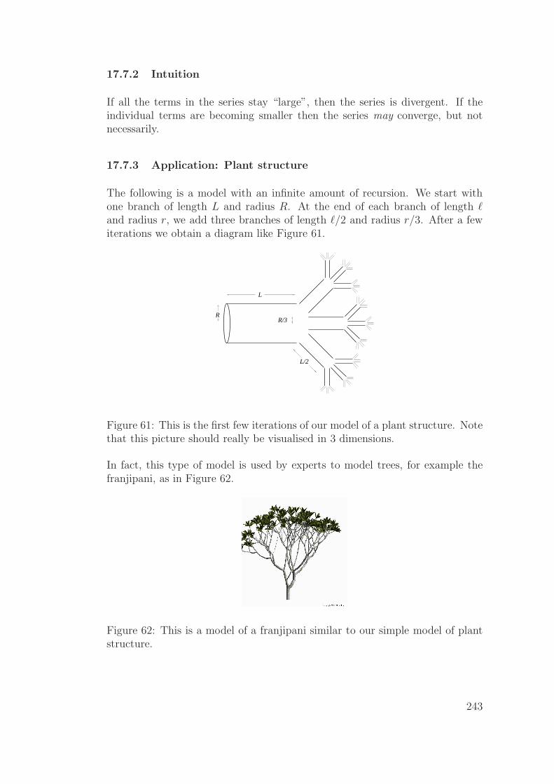
17.7.2 Intuition
If all the terms in the series stay “large”, then the series is divergent. If theindividual terms are becoming smaller then the series may converge, but notnecessarily.
17.7.3 Application: Plant structure
The following is a model with an infinite amount of recursion. We start withone branch of length L and radius R. At the end of each branch of length ℓand radius r, we add three branches of length ℓ/2 and radius r/3. After a fewiterations we obtain a diagram like Figure 61.
R/3
L/2
R
L
Figure 61: This is the first few iterations of our model of a plant structure. Notethat this picture should really be visualised in 3 dimensions.
In fact, this type of model is used by experts to model trees, for example thefranjipani, as in Figure 62.
Figure 62: This is a model of a franjipani similar to our simple model of plantstructure.
243

What is the volume of the infinitely iterated structure? Remember the formulafor the volume of a cylinder of radius r and length ℓ is πr2ℓ.
The volume is given by the sum
V = πr2ℓ + 3π(r
3
)2(
ℓ
2
)
+ 9π(r
9
)2(
ℓ
4
)
+ 27π( r
27
)2(
ℓ
8
)
+ . . .
= πr2ℓ
[
1 +1
6+
1
62+
1
63+ . . .
]
which is a geometric series with a = πr2ℓ and r = 1/6. Therefore it convergesto
V =a
1− r
=πr2ℓ
1− 16
=6πr2ℓ
5.
17.8 Application: Bouncing ball - Stewart, 6ed. p. 731
qn 58; 5ed. p. 756 qn 52
A certain ball has the property that each time it falls from a height h onto ahard, level surface, it rebounds to a height rh, where 0 < r < 1. Suppose thatthe ball is dropped from an initial height of H metres.
(a) Find the total distance that the ball travels.
Initially, the ball falls a distance H , then rebounds a distance rH , falls rH ,rebounds r2H , falls r2H , etc. The total distance it travels is
H + 2rH + 2r2H + 2r3H + . . . = H(1 + 2r + 2r2 + 2r3 + · · · )= H(1 + 2r(1 + r + r2 + . . .))
= H
[
1 + 2r
(1
1− r
)]
= H
(1 + r
1− r
)
metres.
244
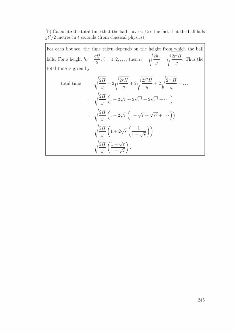
(b) Calculate the total time that the ball travels. Use the fact that the ball fallsgt2/2 metres in t seconds (from classical physics).
For each bounce, the time taken depends on the height from which the ball
falls. For a height hi =gt2i2
, i = 1, 2, . . . , then ti =
√
2hi
g=
√
2riH
g. Thus the
total time is given by
total time =
√
2H
g+ 2
√
2rH
g+ 2
√
2r2H
g+ 2
√
2r3H
g+ . . .
=
√
2H
g
(
1 + 2√
r + 2√
r2 + 2√
r3 + · · ·)
=
√
2H
g
(
1 + 2√
r(
1 +√
r +√
r2 + · · ·))
=
√
2H
g
(
1 + 2√
r
(1
1−√r
))
=
√
2H
g
(1 +√
r
1−√r
)
.
245

17.8.1 Example: Repeated drug dosage
A person with an ear infection is prescribed a treatment of ampicillin (a commonantibiotic) to be taken four times a day in 250mg doses. It is known that at theend of a six hour period, about 4% of the drug is still in the body (since thedrug is being excreted by the body between doses). What quantity of drug is inthe body after the tenth tablet? The fortieth? Predict what quantity of drugwill be in the body after long term treatment.
Let Qn represent the quantity of ampicillin in the blood right after the nthtablet. Then
Q1 = 250
Q2 = 250(1 + 0.04)
= 260
Q3 = 250(1 + 0.04 + 0.042
)
= 260.4
Qn = 250(1 + 0.04 + (0.04)2 + (0.04)3 + . . . + (0.04)n−1)
Note that the pattern is a geometric series with a = 250 and r = 0.04.
Therefore
limn→∞
Qn =250
1− 0.04≈ 260.42mg.
The amount of ampicillin in the blood appears to stabilize.
Note Q10 = 260.416666666664
Q40 = 260.416666666667
so Q40 −Q10 =
40∑
n=11
250(0.04)n−1
= 2.73× 10⁻¹² mg.
246

17.9 Convergence theorem and limit laws
If
∞∑
n=0
an = ℓ and
∞∑
n=0
bn = m are convergent series, then so are the series
∞∑
n=0
can
(where c is a constant),
∞∑
n=0
(an ± bn) and
∞∑
n=0
can = c
∞∑
n=0
an
∞∑
n=0
(an ± bn) =
∞∑
n=0
an ±∞∑
n=0
bn
17.9.1 Example
Evaluate
∞∑
n=0
xn(2x + 1), for |x| < 1.
∞∑
n=0
xn(2x + 1) = (2x + 1)∞∑
n=0
xn
Now∞∑
n=0
xn is a convergent geometric series (since |x| < 1) with a = 1. Hence
(2x + 1)
∞∑
n=0
xn = (2x + 1)1
1− x
=2x + 1
1− x.
247
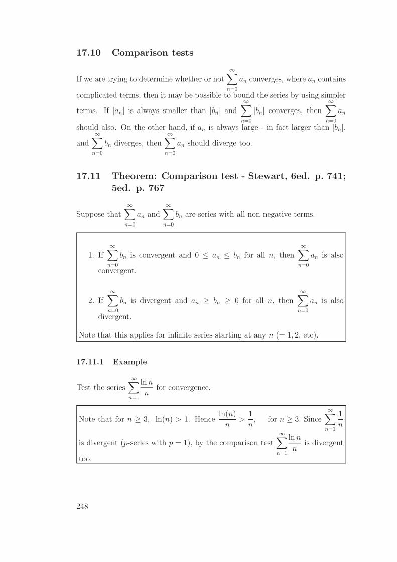
17.10 Comparison tests
If we are trying to determine whether or not
∞∑
n=0
an converges, where an contains
complicated terms, then it may be possible to bound the series by using simpler
terms. If |an| is always smaller than |bn| and
∞∑
n=0
|bn| converges, then
∞∑
n=0
an
should also. On the other hand, if an is always large - in fact larger than |bn|,
and
∞∑
n=0
bn diverges, then
∞∑
n=0
an should diverge too.
17.11 Theorem: Comparison test - Stewart, 6ed. p. 741;
5ed. p. 767
Suppose that
∞∑
n=0
an and
∞∑
n=0
bn are series with all non-negative terms.
1. If
∞∑
n=0
bn is convergent and 0 ≤ an ≤ bn for all n, then
∞∑
n=0
an is also
convergent.
2. If
∞∑
n=0
bn is divergent and an ≥ bn ≥ 0 for all n, then
∞∑
n=0
an is also
divergent.
Note that this applies for infinite series starting at any n (= 1, 2, etc).
17.11.1 Example
Test the series
∞∑
n=1
ln n
nfor convergence.
Note that for n ≥ 3, ln(n) > 1. Henceln(n)
n>
1
n, for n ≥ 3. Since
∞∑
n=1
1
n
is divergent (p-series with p = 1), by the comparison test∞∑
n=1
ln n
nis divergent
too.
248

17.11.2 Example
Test the series∞∑
n=0
5
2 + 3nfor convergence.
Note that
0 <5
2 + 3n<
5
3n, for all n ≥ 0.
Now ∞∑
n=0
5
3n=
∞∑
n=0
5
(1
3
)n
is a convergent geometric series with a = 5 and r =1
3. Hence, by the compar-
ison test,
∞∑
n=0
5
2 + 3nis also convergent.
17.12 Alternating series
The tests for convergence have so far required terms to be positive. However, ifterms alternate in sign +,−, +,−, . . . (or −, +,−, +, . . .) there are some specialresults. We call such a series an alternating series.
Here is quite an interesting result:
We have seen that the harmonic series
1 +1
2+
1
3+
1
4+ . . .
is divergent. However, the series
1− 1
2+
1
3− 1
4+ . . .
is convergent. Why?
249

17.13 Theorem: Alternating series test - Stewart, 6ed.p. 746; 5ed. p. 772
If the alternating series
∞∑
n=0
(−1)nbn = b0 − b1 + b2 − b3 + . . . (all bn > 0)
satisfies
(i) bn+1 ≤ bn, for all n ≥ 0 and
(ii) limn→∞
bn = 0
then the series is convergent.
17.13.1 Example
∞∑
n=0
(−1)n 1√n + 1
Clearly,
bn =1√
n + 1>
1√n + 2
= bn+1, for all n ≥ 0,
and
limn→∞
bn = limn→∞
1√n + 1
= 0.
Therefore, by the alternating series test
∞∑
n=0
(−1)n 1√n + 1
coverges.
250

17.13.2 Example
∞∑
n=1
(−1)n 3n
4n− 1
In this case bn =3n
4n− 1.
limn→∞
bn = limn→∞
(3n
4n− 1
)
= limn→∞
(3
4− 1/n
)
=3
4
Hence, the series diverges by the nth term test.
17.13.3 Example
1 +1
2− 1
3− 1
4+
1
5+
1
6− 1
7− 1
8+ . . .
1 +1
2− 1
3− 1
4+
1
5+
1
6− . . . =
(
1 +1
2
)
−(
1
3+
1
4
)
+
(1
5+
1
6
)
− . . .
=
∞∑
n=0
(−1)n
(1
2n + 1+
1
2n + 2
)
Consequently, this is an alternating series with bn =1
2n + 1+
1
2n + 2. Clearly,
bn > bn+1 (=1
2n + 4+
1
2n + 3),
for all n ≥ 0.
Furthermore,
limn→∞
bn = limn→∞
(1
2n + 1+
1
2n + 2
)
= 0
Hence, by the alternating series test, this series converges.
251

17.14 Definition: Absolute/conditional convergence
A series∞∑
n=0
an is called absolutely convergent if the series∞∑
n=0
|an| is convergent.
A series∞∑
n=0
an is called conditionally convergent if it is convergent, but not
absolutely convergent.
17.14.1 Examples
Are the following series conditionally or absolutely convergent?
(i)
∞∑
n=1
(−1)n 1
n
∞∑
n=1
(−1)n 1
nis an alternating series with bn =
1
n. Since bn > bn+1, for all n ≥ 1,
and limn→∞
bn = 0, then by the alternating series test, this series converges.
Now let an = (−1)n 1
n, for n ≥ 1. Then
∞∑
n=1
|an| =∞∑
n=1
1
n,
and this series is divergent (p-series with p = 1).
Consequently, the series is conditionally convergent.
252

(ii)
∞∑
n=1
(−1)n 1
n4
Let an = (−1)n 1
n4. Then
∞∑
n=1
|an| =∞∑
n=1
1
n4,
and this series converges (p-series with p = 4).
Hence the series is absolutely convergent.
(iii)∞∑
n=1
cos n
n2
Let an =cos n
n2and note that
−1 ≤ cos n ≤ 1 ⇒ − 1
n2≤ cos n
n2≤ 1
n2
⇒ | cos n|n2
≤ 1
n2.
Note also that the series∞∑
n=1
1
n2converges (p-series with p = 2). Consequently,
by the comparison test,∞∑
n=1
|an| =∞∑
n=1
|cos n|n2
converges.
Consequently, the series is absolutely convergent.
253

17.14.2 Theorem: Absolute convergence
If a series is absolutely convergent, then it is convergent.
17.14.3 Proof
Observe that0 ≤ an + |an| ≤ 2|an|
∴ If a series is absolutely convergent then∑
n
|an| converges and hence so too
does∑
n
2|an| = 2∑
n
|an|.∴ By the comparison test
∑
n
(an + |an|)
also converges. Thus
∑
n
an =∑
n
(an + |an|)−∑
n
|an|
must converge.
17.15 Theorem: Ratio test - Stewart, 6ed. p. 752; 5ed.p. 778
A powerful test for convergence of series is the ratio test. We will use it exten-sively in the following sections.
1. If limn→∞
∣∣∣∣
an+1
an
∣∣∣∣= L < 1, then the series
∞∑
n=1
an is absolutely convergent (and
therefore convergent).
2. If limn→∞
∣∣∣∣
an+1
an
∣∣∣∣= L > 1 or lim
n→∞
∣∣∣∣
an+1
an
∣∣∣∣=∞ , then the series
∞∑
n=1
an is diver-
gent.
3. If limn→∞
∣∣∣∣
an+1
an
∣∣∣∣= 1, then the ratio test is inconclusive.
4. If limn→∞
∣∣∣∣
an+1
an
∣∣∣∣
is not defined, then the ratio test is inconclusive.
Note that the ratio test only tests for absolute convergence. The ratio test doesnot give any estimates of the sum.
254
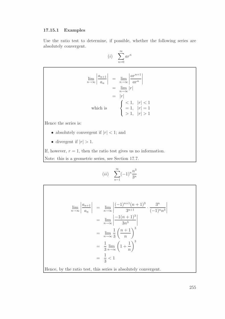
17.15.1 Examples
Use the ratio test to determine, if possible, whether the following series areabsolutely convergent.
(i)
∞∑
n=0
arn
limn→∞
∣∣∣∣
an+1
an
∣∣∣∣
= limn→∞
∣∣∣∣
arn+1
arn
∣∣∣∣
= limn→∞
|r|= |r|
which is
< 1, |r| < 1= 1, |r| = 1> 1, |r| > 1
Hence the series is:
• absolutely convergent if |r| < 1; and
• divergent if |r| > 1.
If, however, r = 1, then the ratio test gives us no information.
Note: this is a geometric series, see Section 17.7.
(ii)
∞∑
n=1
(−1)n n3
3n
limn→∞
∣∣∣∣
an+1
an
∣∣∣∣
= limn→∞
∣∣∣∣
(−1)n+1(n + 1)3
3n+1· 3n
(−1)nn3
∣∣∣∣
= limn→∞
∣∣∣∣
−1(n + 1)3
3n3
∣∣∣∣
= limn→∞
1
3
(n + 1
n
)3
=1
3lim
n→∞
(
1 +1
n
)3
=1
3< 1
Hence, by the ratio test, this series is absolutely convergent.
255
(iii)
∞∑
n=1
1
n!xn
limn→∞
∣∣∣∣
an+1
an
∣∣∣∣
= limn→∞
∣∣∣∣
xn+1
(n + 1)!· n!
xn
∣∣∣∣
= limn→∞
∣∣∣∣
x
n + 1
∣∣∣∣
= |x| limn→∞
1
n + 1= |x| · 0= 0 < 1
∴ Series is absolutely convergent for all x.
(iv)∞∑
n=0
(2x + 5)n
limn→∞
∣∣∣∣
an+1
an
∣∣∣∣
= limn→∞
∣∣∣∣
(2x + 5)n+1
(2x + 5)n
∣∣∣∣
= |2x + 5|
⇒ Series converges absolutely when |2x + 5| < 1 (ie when −3 < x < −2) anddiverges when |2x + 5| > 1 (ie when x < −3 or x > −2).
Note: the ratio test gives no information about convergence of the series whenx = −3, −2 (In fact, the series diverges at both these points).
256

Notes
257
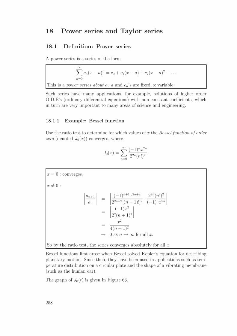
18 Power series and Taylor series
18.1 Definition: Power series
A power series is a series of the form
∞∑
n=0
cn(x− a)n = c0 + c1(x− a) + c2(x− a)2 + . . .
This is a power series about a. a and cn’s are fixed, x variable.
Such series have many applications, for example, solutions of higher orderO.D.E’s (ordinary differential equations) with non-constant coefficients, whichin turn are very important to many areas of science and engineering.
18.1.1 Example: Bessel function
Use the ratio test to determine for which values of x the Bessel function of orderzero (denoted J0(x)) converges, where
J0(x) =
∞∑
n=0
(−1)nx2n
22n(n!)2.
x = 0 : converges.
x 6= 0 :
∣∣∣∣
an+1
an
∣∣∣∣
=
∣∣∣∣
(−1)n+1x2n+2
22n+2[(n + 1)!]2· 22n(n!)2
(−1)nx2n
∣∣∣∣
=
∣∣∣∣
(−1)x2
22(n + 1)2
∣∣∣∣
=x2
4(n + 1)2
→ 0 as n→∞ for all x.
So by the ratio test, the series converges absolutely for all x.
Bessel functions first arose when Bessel solved Kepler’s equation for describingplanetary motion. Since then, they have been used in applications such as tem-perature distribution on a circular plate and the shape of a vibrating membrane(such as the human ear).
The graph of J0(t) is given in Figure 63.
258

0 5 10 15 20 25 30−1
−0.5
0
0.5
1
1.5
t
besselj(0,t)
Figure 63: The Bessel function J0(t) is represented as besselj(0,t) in MAT-LAB.
18.2 Theorem: Defines radius of convergence - Stewart,6ed. p. 752; 5ed. p. 787
For a given power series
∞∑
n=0
cn(x− a)n there are only three possibilities:
1. The series converges only when x = a.
2. The series converges for all x.
3. There is a positive number r (called the radius of convergence) such thatthe series converges if |x− a| < r and diverges if |x− a| > r.
In case (1), we say that the radius of convergence is 0, while in case (2) we saythat the radius of convergence is ∞.
The interval of convergence of a power series is the interval that consists of allvalues of x for which the series converges. In case (1) the interval is a singlepoint, a. In case (2) the interval is (−∞,∞). In case (3) the interval is either(a− r, a + r), (a− r, a + r], [a− r, a + r) or [a− r, a + r].
259
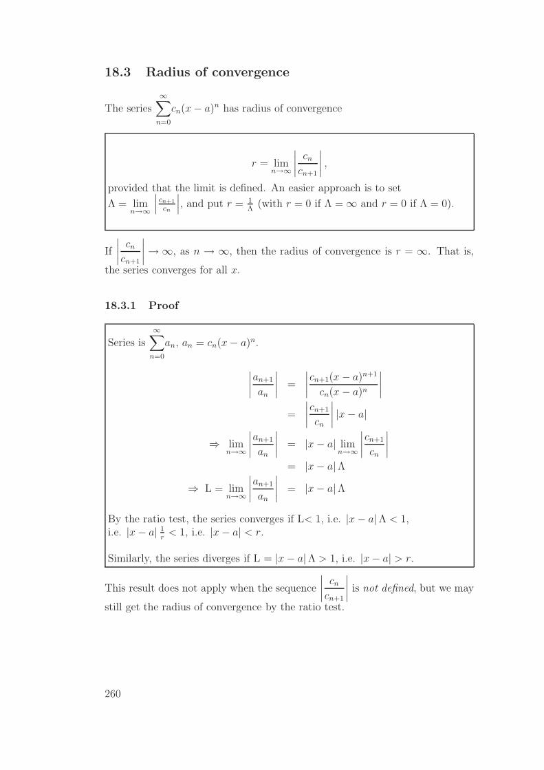
18.3 Radius of convergence
The series
∞∑
n=0
cn(x− a)n has radius of convergence
r = limn→∞
∣∣∣∣
cn
cn+1
∣∣∣∣,
provided that the limit is defined. An easier approach is to set
Λ = limn→∞
∣∣∣cn+1
cn
∣∣∣, and put r = 1
Λ(with r = 0 if Λ =∞ and r = 0 if Λ = 0).
If
∣∣∣∣
cn
cn+1
∣∣∣∣→∞, as n → ∞, then the radius of convergence is r = ∞. That is,
the series converges for all x.
18.3.1 Proof
Series is
∞∑
n=0
an, an = cn(x− a)n.
∣∣∣∣
an+1
an
∣∣∣∣
=
∣∣∣∣
cn+1(x− a)n+1
cn(x− a)n
∣∣∣∣
=
∣∣∣∣
cn+1
cn
∣∣∣∣|x− a|
⇒ limn→∞
∣∣∣∣
an+1
an
∣∣∣∣
= |x− a| limn→∞
∣∣∣∣
cn+1
cn
∣∣∣∣
= |x− a|Λ
⇒ L = limn→∞
∣∣∣∣
an+1
an
∣∣∣∣
= |x− a|Λ
By the ratio test, the series converges if L< 1, i.e. |x− a|Λ < 1,i.e. |x− a| 1
r< 1, i.e. |x− a| < r.
Similarly, the series diverges if L = |x− a|Λ > 1, i.e. |x− a| > r.
This result does not apply when the sequence
∣∣∣∣
cn
cn+1
∣∣∣∣is not defined, but we may
still get the radius of convergence by the ratio test.
260

18.3.2 Example
What is the radius of convergence for the series∞∑
n=0
(−3)nxn
√n + 1
? When does the
series converge/diverge?
The series is
∞∑
n=0
cnxn, cn =(−3)n
√n + 1
.
⇒∣∣∣∣
cn+1
cn
∣∣∣∣
=
∣∣∣∣
(−3)n+1
√n + 2
·√
n + 1
(−3)n
∣∣∣∣
= 3
√n + 1√n + 2
→ 3 as n→∞⇒ Λ = lim
n→∞
∣∣∣∣
cn+1
cn
∣∣∣∣= 3
⇒ r =1
Λ=
1
3
So the series converges absolutely for |x| < 13
and diverges for |x| < 13.
Remark: in fact the series also diverges at x = ±13.
18.4 Taylor series
Given a function f(x) it is sometimes possible to expand f(x) as a power series
f(x) =
∞∑
n=0
cn(x− a)n = c0 + c1(x− a) + c2(x− a)2 + c3(x− a)3 + . . .
How do we find the coefficients cn in general? Let us assume that f and all itsderivatives are defined at x = a.
First note thatf(a) = c0.
Now take the derivative of both sides. Assuming that we are justified in differ-entiating term by term on the right-hand side, this gives
f ′(x) = c1 + 2c2(x− a) + 3c3(x− a)2 + . . .
261

so thatf ′(a) = c1.
Taking the derivative again and again gives
f ′′(a) = 2c2 ⇒ c2 = f ′′(a)/2
f ′′′(a) = 6c3 ⇒ c3 = f ′′′(a)/3!
and, in generalcn = f (n)(a)/n!, with f (0)(x) ≡ f(x).
This leads to
f(x) =∞∑
n=0
f (n)(a)
n!(x− a)n.
The right-hand side is called the Taylor series of f(x) about x = a. So thisresult says that if f(x) has a power series representation (expansion) at x = a,then it must be a Taylor series.
18.4.1 Example: MacLaurin series
When a = 0 in the Taylor series we call the series a MacLaurin series.
18.4.2 Note
The function f and all its derivatives must be defined at x = a for the series toexist. In this case we say that f is infinitely differentiable at x = a.
18.5 Theorem: Formula for Taylor series
Suppose f(x) is infinitely differentiable at x = a. Then for f “sufficiently wellbehaved”,
f(x) =
∞∑
n=0
f (n)(a)
n!(x− a)n, for |x− a| < r,
where r is the radius of convergence.
(Note that if we define a sequence of numbers
bn = maxx∈[−r,r]
|f (n)(x)|, n ∈ N,
then the “sufficiently well behaved” means
limn→∞
bnrn
n!= 0.
Unless otherwise noted, all functions we consider in this section are “sufficientlywell behaved”.)
262

For |x− a| < r, we have approximately
f(x) ≃k∑
n=0
f (n)(a)
n!(x− a)n
which is a useful polynomial approximation. The smaller |x− a|, the better theapproximation. This approximation can be made accurate to arbitrary orderby taking k sufficiently large provided |x− a| < r.
This begins to address the question of whether or not f(x) has a power seriesrepresentation. The details are beyond the scope of this course, but for thoseinterested there is a good discussion about this issue and Taylor’s inequality inStewart, 6ed. pp. 772-774; 5ed. pp. 798-800.
18.5.1 Example
Find the Taylor series of f(x) = ln x about x = 1. Determine its radius ofconvergence.
f (0)(x) = f(x) = ln x
f ′(x) =1
x= x−1, f ′′(x) = −x−2, f ′′′(x) = 2x−3, and so on
n ≥ 2 : f (n)(x) = (−1)n−1(n− 1)! x−n
⇒ f (0)(1) = 0, f (1)(1) = 1, f (n)(1) = (−1)n−1(n− 1)!
So the Taylor series of f about 1 is
∞∑
n=0
cn(x− 1)n, where cn =fn(1)
n!.
⇒ c0 = 0, cn =(−1)n−1(n− 1)!
n!n ≥ 1
=(−1)n−1
n.
So the Taylor series of lnx is
∞∑
n=1
(−1)n−1
n(x− 1)n
⊛
263
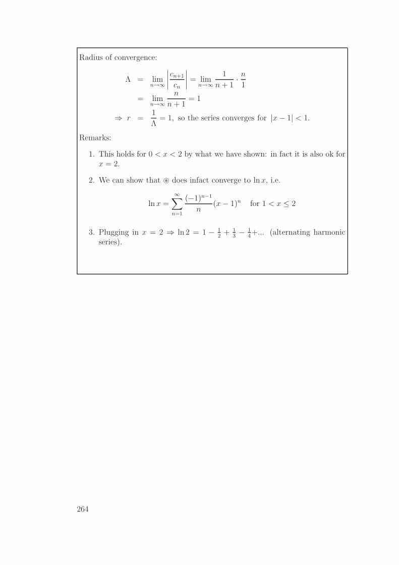
Radius of convergence:
Λ = limn→∞
∣∣∣∣
cn+1
cn
∣∣∣∣= lim
n→∞
1
n + 1· n
1
= limn→∞
n
n + 1= 1
⇒ r =1
Λ= 1, so the series converges for |x− 1| < 1.
Remarks:
1. This holds for 0 < x < 2 by what we have shown: in fact it is also ok forx = 2.
2. We can show that ⊛ does infact converge to lnx, i.e.
ln x =∞∑
n=1
(−1)n−1
n(x− 1)n for 1 < x ≤ 2
3. Plugging in x = 2 ⇒ ln 2 = 1 − 12
+ 13− 1
4+... (alternating harmonic
series).
264

18.5.2 Example
Find the Taylor series of f(x) = ex about x = a. Determine its radius ofconvergence.
f(x) ⇒ f (n)(x) = ex for all n ≥ 0
⇒ f (n)(a) = ea for all n ≥ 0
⇒ the Taylor series of f about x = a is
∞∑
n=0
f (n)(a)
n!(x− a)n =
∞∑
n=0
ea
n!(x− a)n
=
∞∑
n=0
cn(x− a)n
Radius of convergence:
Λ = limn→∞
∣∣∣∣
cn+1
cn
∣∣∣∣= lim
n→∞
∣∣∣∣
ea
(n + 1)!· n!
ea
∣∣∣∣
= limn→∞
1
n + 1= 0
Λ = 0 ⇒ r =∞.
Note:
1. Here, too, the Taylor series actually converges to the function, i.e.
ex =∞∑
n=0
ea
n!(x− a)n.
2. Taking a = 0 gives the MacLaurin series: ex =
∞∑
n=0
xn
n!
265

18.5.3 Example
Find the MacLaurin series for f(x) = sin x. Determine its radius of convergence.
f(x) = sin x ⇒ f ′(x) = cos x, f ′′(x) = − sin x, f ′′′(x) = − cos x,
f (4)(x) = sin x etc.
⇒ f(0) = 0, f ′(0) = 1, f ′′(0) = 0, f ′′′(0) = −1, f (4)(0) = (0) etc.
So f (n)(0) =
{0 n = 2m
(−1)m n = 2m + 1
⇒ MacLaurin series for sin x is:
∞∑
n=0
f (n)(0)
n!xn = x− x3
3!+
x5
5!− ....
=∞∑
m=0
(−1)m x2m+1
(2m + 1)!⊛
To determine the radius of convergence we use the ratio test on ⊛. So
L = limm→∞
∣∣∣∣
am+1
am
∣∣∣∣
= limm→∞
∣∣∣∣
(−1)m+1x2m+3
(2m + 3)!· (2m + 1)!
(−1)mx2m+1
∣∣∣∣
= limm→∞
∣∣∣∣
x2
(2m + 3)(2m + 2)
∣∣∣∣
= 0 < 1⇒ series converges for all x (i.e. r =∞).
Remarks :
1. The MacLaurin series converges to sin x.
2. The fith-order Taylor polynomial is T5(x) = x − x3
3!+
x5
5!: Suppose now
0 ≤ x ≤ π4: the the remainder R5 satisfies
|f(x)− R5(x)| = |T5(x)| =|f (6)(z)|
6!x6, for some z, 0 < z < x.
=| sin(z)|
6!x6 ≤ 1√
2· 1
6!(π
4)6 = 0.0023
NOTE: In fact T5 = T6 for this function, so we can improve the error estimateby using R6 instead of R5 to 0.000026.
266
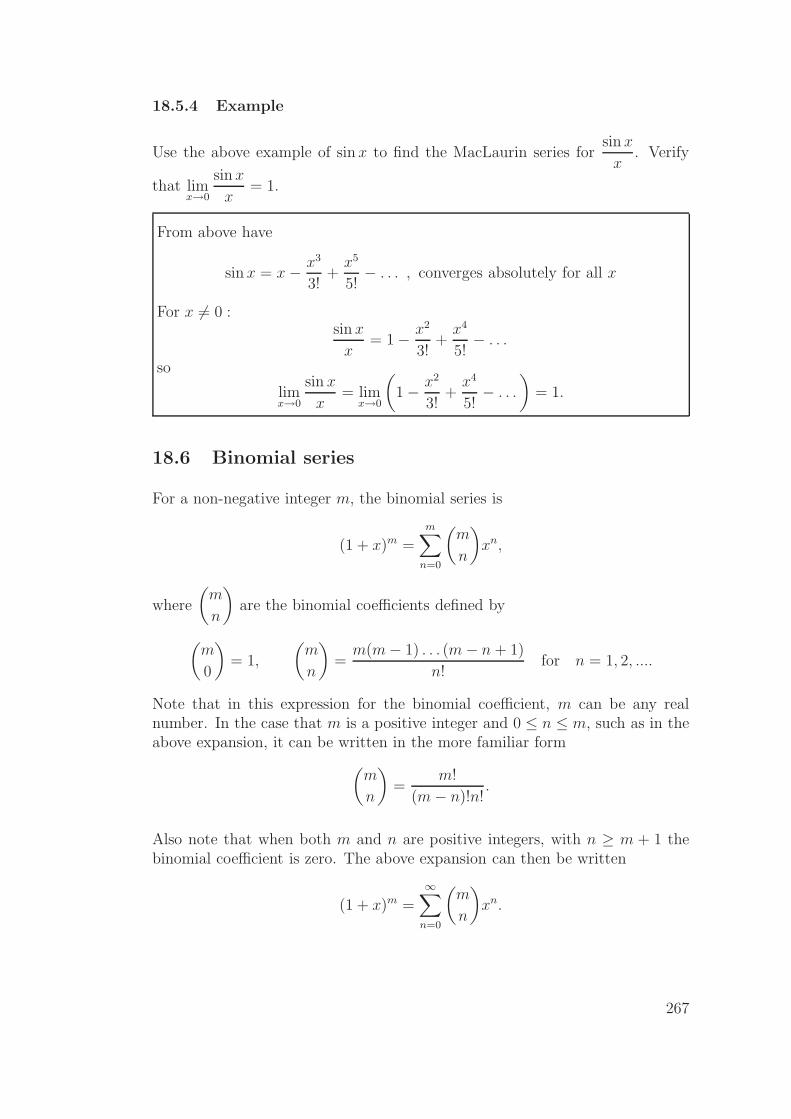
18.5.4 Example
Use the above example of sin x to find the MacLaurin series forsin x
x. Verify
that limx→0
sin x
x= 1.
From above have
sin x = x− x3
3!+
x5
5!− . . . , converges absolutely for all x
For x 6= 0 :sin x
x= 1− x2
3!+
x4
5!− . . .
so
limx→0
sin x
x= lim
x→0
(
1− x2
3!+
x4
5!− . . .
)
= 1.
18.6 Binomial series
For a non-negative integer m, the binomial series is
(1 + x)m =
m∑
n=0
(m
n
)
xn,
where
(m
n
)
are the binomial coefficients defined by
(m
0
)
= 1,
(m
n
)
=m(m− 1) . . . (m− n + 1)
n!for n = 1, 2, ....
Note that in this expression for the binomial coefficient, m can be any realnumber. In the case that m is a positive integer and 0 ≤ n ≤ m, such as in theabove expansion, it can be written in the more familiar form
(m
n
)
=m!
(m− n)!n!.
Also note that when both m and n are positive integers, with n ≥ m + 1 thebinomial coefficient is zero. The above expansion can then be written
(1 + x)m =
∞∑
n=0
(m
n
)
xn.
267
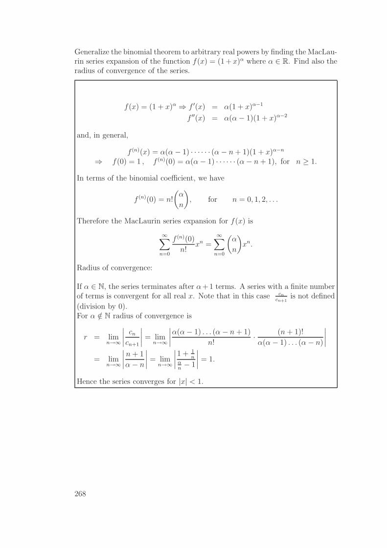
Generalize the binomial theorem to arbitrary real powers by finding the MacLau-rin series expansion of the function f(x) = (1+ x)α where α ∈ R. Find also theradius of convergence of the series.
f(x) = (1 + x)α ⇒ f ′(x) = α(1 + x)α−1
f ′′(x) = α(α− 1)(1 + x)α−2
and, in general,
f (n)(x) = α(α− 1) · · · · · · (α− n + 1)(1 + x)α−n
⇒ f(0) = 1 , f (n)(0) = α(α− 1) · · · · · · (α− n + 1), for n ≥ 1.
In terms of the binomial coefficient, we have
f (n)(0) = n!
(α
n
)
, for n = 0, 1, 2, . . .
Therefore the MacLaurin series expansion for f(x) is
∞∑
n=0
f (n)(0)
n!xn =
∞∑
n=0
(α
n
)
xn.
Radius of convergence:
If α ∈ N, the series terminates after α+1 terms. A series with a finite numberof terms is convergent for all real x. Note that in this case cn
cn+1is not defined
(division by 0).For α /∈ N radius of convergence is
r = limn→∞
∣∣∣∣
cn
cn+1
∣∣∣∣= lim
n→∞
∣∣∣∣
α(α− 1) . . . (α− n + 1)
n!· (n + 1)!
α(α− 1) . . . (α− n)
∣∣∣∣
= limn→∞
∣∣∣∣
n + 1
α− n
∣∣∣∣= lim
n→∞
∣∣∣∣
1 + 1n
αn− 1
∣∣∣∣= 1.
Hence the series converges for |x| < 1.
268

18.6.1 Relationship to geometric series
A familiar series is the geometric series
1
1− x= 1 + x + x2 + · · · , for |x| < 1.
This result follows from the binomial theorem. Taking α = −1 and replacing xwith −x we have
f(x) = (1− x)−1 =1
1− x.
The binomial coefficients in this case are
(−1
n
)
=(−1)(−2) . . . (−n)
n!= (−1)n, for n ≥ 1.
The binomial theorem then gives, for |x| < 1,
1
1− x= 1 +
∞∑
n=1
(−1)n(−x)n =
∞∑
n=0
xn,
which is the geometric series.
269

Notes
270

19 Appendix - Practice Problems
You should attempt the practice problems in this section while learning thematerial in the course. Try to solve all questions. Do at least questions markedwith a star (*) before attempting assignment questions. Have a look at thequestions before your tutorial. Try to solve them yourself first, and ask yourtutor at the tutorial if you need help. Solutions to questions on this sheet arenot to be handed in.
19.1 Numbers
1. Show that√
2 is irrational.
2. Solve for x.
(a) |x + 1| < 1
(b) |x + 1| > 1
(c) |3x + 5| ≤ 2
3. Simplify.
(a) 3+i3−i
(b) (2+3i)(3+2i)1+i
4. Write z = 1−√
3i in polar form.
∗ 5. Find the roots of x2 − 4x + 5 = 0.
19.2 Functions
1. Graph the following functions and give their domain and range.
(a) f(x) = x2 + 2∗(b) f(x) = 1
x−2
∗(c) f(x) = − 1x−2
(d) f(x) = 1x2+2
∗(e) f(x) = x+2x2−4
∗(f) f(x) =√
x2 − 9
(g) f(x) = −√
x2 + 9
(h) f(x) = ex+1
(i) f(x) = 1 + e2x+3.
271

2. Stewart ed 5, p.56 question 2
3. Stewart ed 5, p.23 question 36
4. Stewart ed 5, p.23 question 38
5. Two species of kangaroos inhabit a national park. There are currently4,500 grey kangaroos, whose population increases at a rate of 4% a year.There are only 3,000 red kangaroos, but they increase at a rate of 6%a year. In how many years will the red kangaroos outnumber the greykangaroos? Use logarithms to find the answer and draw a graph of thetwo populations.
6. Let P (t) be the amount of a radioactive material at time t. Experimentsindicate P (t) decays exponentially with time, so
P (t) = P0e−kt
where P0 is the amount of material at time t = 0 (initial amount) and k isa positive constant (called the decay constant). The half-life T is the timetaken for the material to decay to one half of its initial amount. ObtainT in terms of k.
7. If y = tan(x), 0 ≤ x < π/2, find cos(x) as a function of y.
∗ 8. Find the inverse of f(x) = 13cos(2x) and state its domain and range.
9. For f(x) = 3x + 2, g(x) = ln(x2 + 1) and h(x) = 3e2x+1, find
(a) f(g(x))
(b) g(f(x))
(c) f(h(x))
(d) h(f(x))
(e) g(h(x))
(f) f(g(h(x)))
(g) h(g(f(x))).
10. Show from the definition that the following two functions are 1-1 on theirdomains (a graph is not sufficient here). Find the inverse function, andstate the domain and range of both f and f−1.
(a) f(x) = e3x+1
∗ (b) f(x) = x+1x+2
.
272
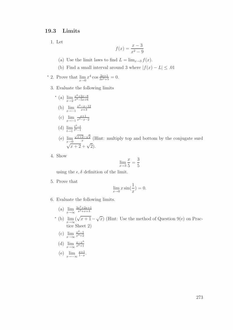
19.3 Limits
1. Let
f(x) =x− 3
x2 − 9
(a) Use the limit laws to find L = limx→3 f(x).
(b) Find a small interval around 3 where |f(x)− L| ≤ .01
∗ 2. Prove that limx→0
x4 cos 2x+13x2+5
= 0.
3. Evaluate the following limits
∗ (a) limx→2
x2+2x−8x2−5x+6
(b) limx→−1
x2−x−12x+3
(c) limx→−1
x+1x2−x−2
(d) limt→1
t3−tt2−1
(e) limx→0
√x+2−
√2
x(Hint: multiply top and bottom by the conjugate surd
√x + 2 +
√2).
4. Show
limx→3
x
5=
3
5
using the ǫ, δ definition of the limit.
5. Prove that
limx→0
x sin(1
x) = 0.
6. Evaluate the following limits.
(a) limx→∞
3x2+2x+1x2+x+3
∗ (b) limx→∞
(√
x + 1−√x) (Hint: Use the method of Question 9(e) on Prac-
tice Sheet 2)
(c) limx→∞
x2−1x3+2
(d) limx→∞
x−x3
x2+1
(e) limx→−∞
x+11−x
.
273
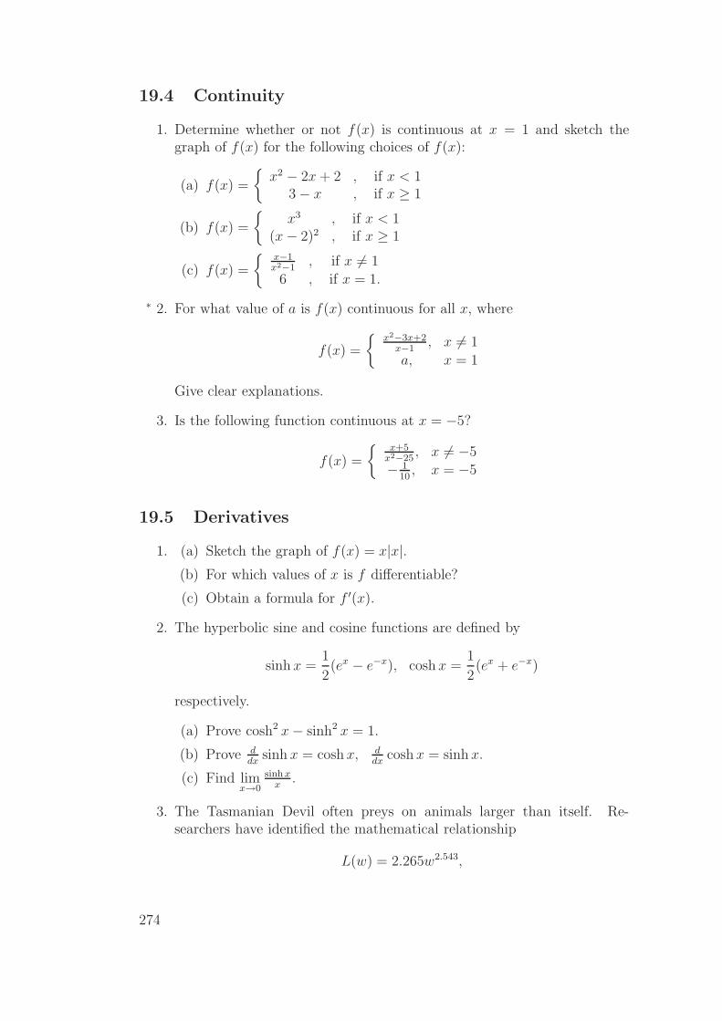
19.4 Continuity
1. Determine whether or not f(x) is continuous at x = 1 and sketch thegraph of f(x) for the following choices of f(x):
(a) f(x) =
{x2 − 2x + 2 , if x < 1
3− x , if x ≥ 1
(b) f(x) =
{x3 , if x < 1
(x− 2)2 , if x ≥ 1
(c) f(x) =
{x−1x2−1
, if x 6= 1
6 , if x = 1.
∗ 2. For what value of a is f(x) continuous for all x, where
f(x) =
{x2−3x+2
x−1, x 6= 1
a, x = 1
Give clear explanations.
3. Is the following function continuous at x = −5?
f(x) =
{x+5
x2−25, x 6= −5
− 110
, x = −5
19.5 Derivatives
1. (a) Sketch the graph of f(x) = x|x|.(b) For which values of x is f differentiable?
(c) Obtain a formula for f ′(x).
2. The hyperbolic sine and cosine functions are defined by
sinh x =1
2(ex − e−x), cosh x =
1
2(ex + e−x)
respectively.
(a) Prove cosh2 x− sinh2 x = 1.
(b) Prove ddx
sinh x = cosh x, ddx
cosh x = sinh x.
(c) Find limx→0
sinhxx
.
3. The Tasmanian Devil often preys on animals larger than itself. Re-searchers have identified the mathematical relationship
L(w) = 2.265w2.543,
274

where w (in kg) is the weight and L(w) (in mm) is the length of theTasmanian Devil. Suppose that the weight of a particular TasmanianDevil can be estimated by the function
w(t) = 0.125 + 0.18t,
where w(t) is the weight (in kg) and t is the age, in weeks, of a TasmanianDevil that is less than one year old. How fast is the length of a 30-week-oldTasmanian Devil changing?
4. Show that the equation of the tangent line to a point (x0, y0) on the ellipsex2
a2 + y2
b2= 1 is given by
x0x
a2+
y0y
b2= 1.
∗ 5. Consider the function f(x) = xx. Evaluate f ′(x) for x > 0.
6. A new car costing P dollars depreciates at an annual rate of r%, so thatafter t years the car will be worth C dollars where
C(t) = P (1− r
100)t.
(a) Find dCdt
(b) How much will the car be worth in the long run?
∗ 7. Findd
dθ
θ
cos(sin θ).
8. A spherical snowball is melting in such a way that its volume is decreasingat a rate of 1 cm3/min. At what rate is the diameter decreasing when thediameter is 10 cm?
9. Using L’Hopital’s rule evaluate the following limits
∗(a) limθ→0
1−cos θθ2
(b) limx→0
ex−1sinx
(c) limx→0
sinx−xx3
∗(d) limx→1
( 1ln x− 1
x−1)
(e) limx→∞
e−x ln x
(f) limθ→0
(sin θ)n
sin(θn), 1 ≤ n ∈ N.
275
10. Use the mean value theorem to prove the following (this is the secondderivative test).Suppose f : [a, b]→ R is continuous, and has continuous first and secondderivatives on [a, b]. Then if c ∈ (a, b) is a point with f ′(c) = 0 andf ′′(c) > 0 then f has a local minimum at c.
11. Determine where the following functions are increasing/decreasing.
(a) f(x) = (x− 1)(x + 2) = x2 + x− 2
(b) f(x) = x|x|.(c) f(x) = sin x, x ∈ (0, π)
(d) f(x) = e−x+1ex
12. Prove the following:
ex ≥ x + 1, for all x ≥ 0.
Hint: Consider f(x) = ex − x− 1.
13. Prove the following:sin x ≤ x, for all x ≥ 0.
14. Find the absolute maximum and minimum of the function f(x) = x3 −3x + 2 on the closed interval [0, 2].
15. Find all relative maxima and minima and thus sketch the graph of thefunction
f(x) = x +1
x.
∗ 16. Show that the function
f(x) =
{x ln x , x > 0
0 , x = 0
is continuous on [0,∞). What are the absolute maximum and minimumvalues of f(x) on [0, 2]?
17. To increase the velocity of the air flowing through the trachea when ahuman coughs, the body contracts the windpipe, producing a more effec-tive cough. Tuchinsky formulated that the velocity of air that is flowingthrough the trachea during a cough is
V = C(R0 − R)R2,
where C > 0 is a constant based on individual body characteristics, R0
is the radius of the windpipe before the cough, and R is the radius ofthe windpipe during the cough. Find the value of R that maximizes thevelocity. (Interestingly, Tuchinsky also states that X-rays indicate thatthe body naturally contracts the windpipe to this radius during a cough.)
276
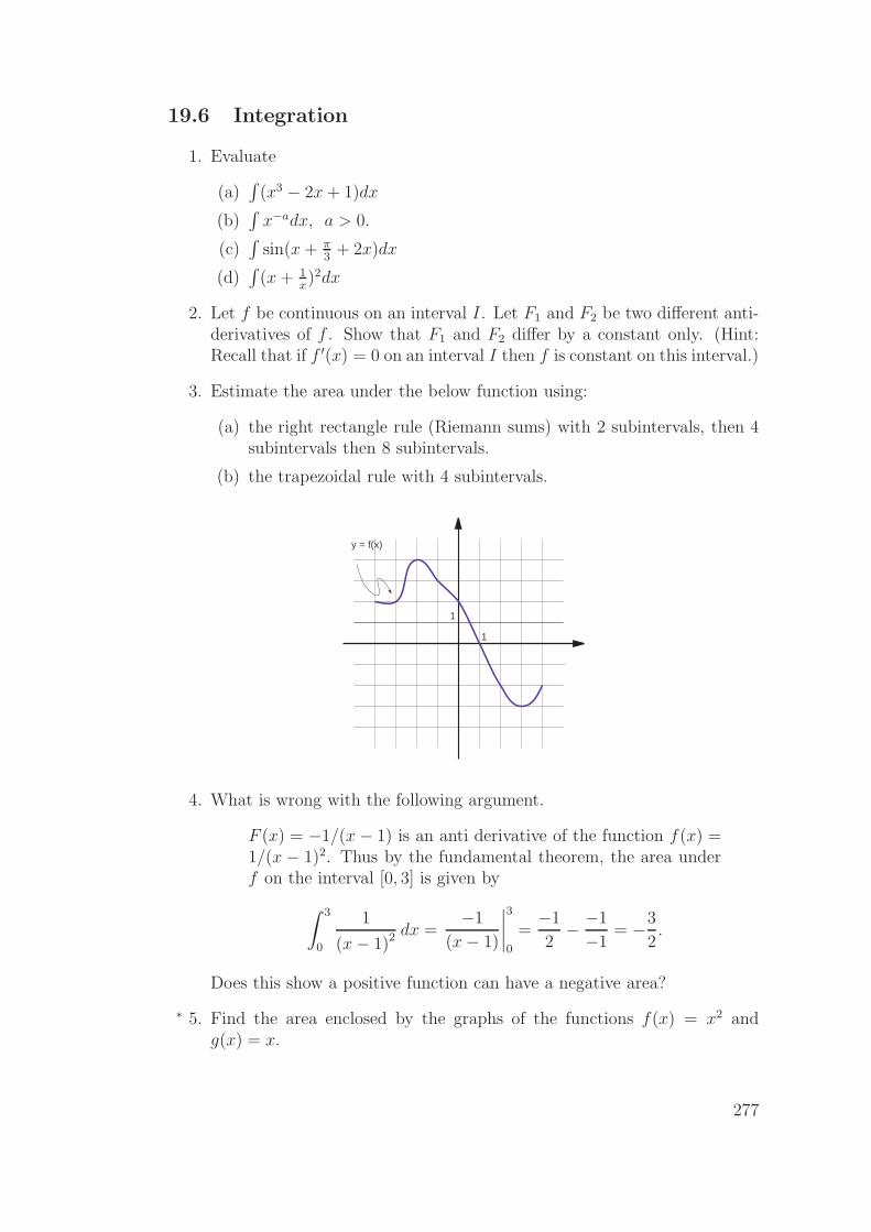
19.6 Integration
1. Evaluate
(a)∫
(x3 − 2x + 1)dx
(b)∫
x−adx, a > 0.
(c)∫
sin(x + π3
+ 2x)dx
(d)∫
(x + 1x)2dx
2. Let f be continuous on an interval I. Let F1 and F2 be two different anti-derivatives of f . Show that F1 and F2 differ by a constant only. (Hint:Recall that if f ′(x) = 0 on an interval I then f is constant on this interval.)
3. Estimate the area under the below function using:
(a) the right rectangle rule (Riemann sums) with 2 subintervals, then 4subintervals then 8 subintervals.
(b) the trapezoidal rule with 4 subintervals.
1
1
y = f(x)
4. What is wrong with the following argument.
F (x) = −1/(x− 1) is an anti derivative of the function f(x) =1/(x − 1)2. Thus by the fundamental theorem, the area underf on the interval [0, 3] is given by
∫ 3
0
1
(x− 1)2 dx =−1
(x− 1)
∣∣∣∣
3
0
=−1
2− −1
−1= −3
2.
Does this show a positive function can have a negative area?
∗ 5. Find the area enclosed by the graphs of the functions f(x) = x2 andg(x) = x.
277

6. Derive a formula for the area of the ellipse
x2
a2+
y2
b2= 1.
7. Find the area under the graph of
(a) y =√
4− x2 above [0, 1]
(b) y = sec x tan x above [0, π3].
8. Evaluate each of the following integrals by interpreting it in terms of areas:
(a)3∫
1
(1+2x)dx (b)0∫
−3
(1+√
9− x2)dx (c)2∫
−2
|x|dx (d)2∫
−2
√4− x2dx.
9. Determine∞∫
0
xe−x2
dx.
10. By finding a suitable substitution, evaluate the following indefinite inte-grals:
∗ (a)∫
ex
1+e2x dx
(b)∫
dxx2+4x+9
dx
(c)∫
cos x sin3 xdx.
11. Use integration by parts to find:
∗ (a)∫
x cos xdx
(b)∫
cos2 xdx
(c)∫
ex cos xdx
(d)∫
ln xdx (e)∫
x sec2 xdx
12. Use partial fractions to find
∗ (a)∫
x(x+1)(x+2)
dx
(b)∫
x+3x(x+2)
dx
(c)∫
4x+8x2+2x−3
dx.
13. Evaluate the following integrals:
(a)∫
xx2−1
dx (b)∫
1+ex
1−ex dx.
14. Evaluate the following indefinite integrals
(a)∫ sin(1/t2)
t3dt
(b)∫
sin(x) cos(cos(x)) dx
278
Check by explicitly differentating your answer to confirm it is indeed ananti-derivative.
15. Find the volume of the ellipsoid obtained by rotating the ellipse x2
a2 + y2
b2= 1
about the x-axis.
16. Let a > 0 be constant. Find the volume V of the solid of revolutionobtained by rotating y = f(x) above the interval [0, a] about the x-axis,for the following choices of f(x):
(a) y = x2
∗ (b) y =√
ln(x + 1).
17. Use Euler’s formula to express cos(2θ) and sin(2θ) in terms of cos(θ) andsin(θ).
19.7 Sequences
1. Use L’Hopital’s rule to find
limn→∞
sin(1/n)
log(1 + 1/n).
2. Evaluate the limit of the sequence {an}∞n=1 for the following choices of an:
(a) an = ncn, 0 ≤ c < 1∗ (b) an = 1+2n
1+3n .
∗ 3. Prove thatlim
n→∞n1/n = 1.
19.8 Series
∗ 1. It is known that a repeated decimal can always be expressed as a fraction.Consider, for example, the decimal 0.727272 . . . . Use the fact that
0.727272 · · · = 0.72 + 0.0072 + 0.000072 + . . .
to express the decimal as a geometric series. Hence show that
0.727272 · · · = 8
11.
2. Determine whether or not the following series converge:
(a)∞∑
n=1
nn
n!
279

(b) 11·2 + 1
2·3 + 13·4 + . . .
3. (a) Prove that∞∑
n=1
nxn = x(1−x)2
, for |x| < 1.
(Hint: Consider x ddx
( 11−x
))
(b) Hence, or otherwise, evaluate∞∑
n=1
n2n .
4. Consider the p = 1 case of the p-series (called the harmonic series):
∞∑
n=1
1
n= 1 + (
1
2) + (
1
3+
1
4) + (
1
5+
1
6+
1
7+
1
8) + (
1
9+
1
10+ · · ·+ 1
16) + . . .
and group together its terms as shown. Show that the sum of each group offractions is more than 1
2. Hence deduce that the harmonic series diverges.
∗ 5. Evaluate the following series:
(a)∞∑
n=1
( 1√n− 1√
n+1)
(b)∞∑
n=0
(−1)nxn.
6. (a) For p > 0, show that f(x) = xp is strictly increasing on [0,∞).
(b) For 0 < p < 1, show that
1
np≥ 1
n, n = 1, 2, 3 . . .
(c) Show that the p-series∞∑
n=1
1
np
diverges for 0 ≤ p ≤ 1.
7. Determine whether or not the following series converge.
(a)∞∑
n=1
(−1)n
n3n
∗ (b)∞∑
n=0
22n
(2n)!
∗ (c)∞∑
n=1
ln(n)n!
.
280
8. (a) Write down from the examples in lectures or the text book two seriesof positive terms
∑an &
∑bn satisfying the following conditions:
limn→∞
∣∣∣∣
an+1
an
∣∣∣∣
= 1 and the∑
m
an converges.
limn→∞
∣∣∣∣
bn+1
bn
∣∣∣∣
= 1 and∑
n
bn diverges.
This shows the ratio test gives no information if the limit is 1. Youcan accept any proofs of convergence in lectures or the text book butprove both the limits above.
9. Find an example of a sequence an with an = f(n)/g(n) for differentiablefunctions f and g, where limn→∞ an and limn→∞ f ′(n)/g′(n) both exist,and
limn→∞
an 6= limn→∞
f ′(n)
g′(n).
This shows before using L’Hopital’s rule we must remember to checkthat either limn→∞ f(n) = 0 = limn→∞ g(n) or limn→∞ f(n) = ±∞ =limn→∞ g(n)!
19.9 Power series and Taylor series
1. This question is about the MacLaurin series for
(1 + x)3/2 .
Find the first three terms of this series. If this series is written as∑∞
n=0 an,find the formula for an. Find a formula for cn so an+1 = cnan.
∗ 2. Obtain the MacLaurin series expansion for arctanx and its radius of con-vergence.(Hint: Use d
dx(arctanx) = 1
1+x2 ).
Using the fact that tan(π/6) = 1/√
3, show that
π = 2√
3
∞∑
n=0
(−1)n
(2n + 1)3n.
∗ 3. Obtain the MacLaurin series expansions and radius of convergence for thefollowing functions:
cosh x =1
2(ex + e−x) , sinh x =
1
2(ex − e−x).
∗ 4. Show that for |x| < 1,
281
(a)√
1 + x = 1 +
∞∑
n=0
(−1)n−1(2n− 2)!
22n−1n!(n− 1)!xn.
(b)
1√1 + x
=
∞∑
n=0
(−1)n(2n)!
22n(n!)2xn.
5. The theory of relativity predicts that the mass m of an object when it ismoving at a speed v is given by the formula
m =m0
√
1− v2/c2
where c is the speed of light and m0 is the mass of the object when it isat rest. Express m as a MacLaurin series in v
cand determine for which
values of v this series converges. (Hint: Use a result from the previousquestion.)
6. Show that the functions
(a) f(x) = (1 + x2)e−x2
(b) f(x) = x2 − ln(1 + x2)
both satisfy f ′(x) = f ′′(x) = 0 at x = 0 (so the second derivative test failshere). Show, using Taylor series, that (a) has a relative maximum and (b)a relative minimum at x = 0.
∗ 7. Find the sum of each of the following convergent series by recognizing itas a Taylor series evaluated at a particular value of x.
(a) 1 + 21!
+ 42!
+ 83!
+ · · ·+ 2n
n!+ . . .
(b) 1− 13!
+ 15!− 1
7!+ · · ·+ (−1)n
(2n+1)!+ . . .
(c) 1 + 14
+ (14)2 + (1
4)3 + · · ·+ (1
4)n + . . .
(d) 1− 1002!
+ 100004!
+ · · ·+ (−1)n·102n
(2n)!+ . . .
19.10 Vectors
1. A canoe travels at a speed 3km/h in a direction due west across a riverflowing due north at 4km/h. Find the actual speed and direction of thecanoe.
2. Draw a clock with vectors v1, v2, . . . , v12 pointing from the centre to eachof 1, 2, . . . , 12. Describe each of the following vectors.
282
(a) v1 + · · ·+ v12.
(b) v1 + v2 + 3v3 + v4 + v5 + v6 + v7 + v8 + 3v9 + v10 + v11 + v12.
(c) v1 + v2 + v3 + v4 + v6 + v7 + v9 + v10 + v12.
3. Find the lengths of the sides of the triangle ABC and determine whetherthe triangle is a right triangle.
(a) A = (4, 2, 0), B = (6, 6, 8), C = (10, 8, 6)
(b) A = (5, 5, 1), B = (6, 3, 2), C = (1, 4, 4).
4. (a) Suppose u and v are orthogonal vectors. Prove that‖u‖2 + ‖v‖2 = ‖u + v‖2. What geometric fact have you proved?
(b) Prove that ‖u + v‖2 + ‖u− v‖2 = 2(‖u‖2 + ‖v‖2). What geometricfact have you proved?
(c) Consider a triangle with side lengths a, b, c. Bisect side c, and drawa line connecting the midpoint to the opposite vertex. Let the lengthof this line be m. Using vectors prove that a2 + b2 = 2(m2 + (c/2)2).This is called Apollonius’ Theorem.
∗ 5. Find a non-zero vector in R3 orthogonal to
123
and
456
.
6. Given the point P = (2, −1, 4), find a point Q where→
PQ has the samedirection as v = 7i + 6j − 3k.
∗ 7. For what values of c is the angle between the vectors (1, 2, 1) and (1, 1, c)equal to 60◦? For what values of c are they orthogonal?
8. Determine whether or not each of the following sets of vectors are linearlyindependent.
(a)
120
,
−111
,
−121
.
(b) i + j, i + j + k, i− j.
(c)
1000
,
1200
,
1210
,
4410
.
9. Prove that the vectors
101
,
10−1
,
110
283

form a basis for R3. What are the components of the vector
210
in
this basis?
10. Given
v1 =
1−5−3
, v2 =
−216
, v3 =
2−9
h
,
for what values of h is v3 in span{v1, v2}, and for what values of h is{v1, v2, v3} linearly independent? Justify your answer.
∗ 11. Which of the following subsets of R3 are vector spaces? Find a basis ineach case.
(a) {(a, b, a + 2b) | a, b ∈ R}.(b) {(a, b, c)|a− b = 3c + 1}.
12. Suppose S = {v1, v2, . . . , vm} ⊂ Rn and let V be the set of all linearcombinations of the elements of S, so
V = {α1v1 + α2v2 + · · ·+ αmvm | α1, α2, . . . , αm ∈ R}.
Prove that V is a vector space.
13. If {a, b, c} forms a basis for a 3-dimensional vector space, could {a+b, b+c, c + a} also be a basis? Give your reasons.
∗ 14. Let u1 = (0, 0, 3), u2 = (−2,−1, 0), u3 = (1, 0, 0). Which of u1, u2, u3
are linear combinations of v1 = (1, 2, 3), v2 = (4, 5, 6), v3 = (7, 8, 9)? Do{v1, v2, v3} form a basis of R3?
15. Determine if the following vectors are a basis for R3. Justify your answer.
01−2
,
5−7
4
,
635
16. Let v1 = (1, 2, 3), v2 = (4, 5, 6), v3 = (−2,−1, 0). Do {v1, v2, v3} form abasis of R3? Explain.
∗ 17. Let v1 = (1, 4, 6), v2 = (2, 0, 1), v3 = (−1, 12, 16). Let V = span{v1, v2, v3}.Find dim V .
284

19.11 Matrix Algebra
1. Let A =
(cos θ sin θ− sin θ cos θ
)
. Find simple expressions for A2 and A3. What
do you notice?
2. Find 2× 2 matrices A, B such that (A + B)2 6= A2 + 2AB + B2.
∗ 3. Prove that (A + B)T = AT + BT for any m× n matrices A and B.
4. Let A =
(1 23 4
)
. Find all 2× 2 matrices B such that AB = BA.
5. Find a 2× 2 matrix A with no entry of A equal to 0 such that A2 = 0.
6. A matrix A is called idempotent if A2 = A.
(a) Find x so that A is idempotent:
A =
2/3 0 x0 1 0√2
30 1/3
(b) What is the smallest (integer) index N so that BN = 0? A matrixwith such a property is called nilpotent.
B =
0 1 0 00 0 2 10 0 0 10 0 0 0
.
7. Let C =
1 2 11 1 21 3 −1
. Show that C is invertible, ie show linear inde-
pendence of a certain set of vectors.
∗ 8. Let A =
4 -1 23 0 x8 -3 2
. For which value(s) of x is A not invertible?
9. Find the inverse matrix for:
(a)
(1 00 1
)
(b)
(1 23 4
)
285

(c)
1 2 30 1 20 0 1
∗ 10. Let
A =
15
25
35
35
15
25
0 0 15
and B =
−1 2 x3 −1 y0 0 z
.
Find real numbers x, y and z such that B = A−1.
11. A swimming pool can be filled by 3 pipes A,B and C. Pipe A can fill thepool by itself in 8 hours. Pipes A and C used together can fill the poolin 6 hours and pipes B and C used together can fill the pool in 10 hours.How long does it take to fill the pool if all 3 pipes are used?
∗ 12. Use Gaussian elimination to solve the following system of equations, andcheck your answer by substitution.
x1 − 2x2 + 3x3 = −6
4x1 + 2x3 = 2
3x1 + x2 + 2x3 = 3
13. Let xp be a particular solution of Ax = b. Show that every solution ofthis equation is of the form x = xp + h where h is a solution of thehomogeneous equation Ax = 0.
14. Show that the set of solutions of
Ax = b, with b = 0
form a vector space for A.If b 6= 0, does the set of solutions still form a vector space?
15. Show that A =
(2 11 2
)
satisfies A2 − 4A + 3I = 0. Hence deduce that
A is invertible with inverse A−1 = 13(4I −A).
16. Let a ∈ R. Use Gauss-Jordan elimination to find the inverses of thefollowing matrices. Check by multiplication if your inverse is correct.
∗ (a)
1 1 01 2 α2 1 1− α
(b)
0 0 −11 2 11 0 α
.
286
17. Find the inverses of the following matrices.
(a)
1 1 11 2 12 1 1
.
(b)
1 2 3 11 3 3 22 4 3 31 1 1 1
.
(c)
(1 11 2
)
.
18. Let A =
1 0 52 -1 23 1 2
. Calculate the determinant of A.
19. Determine for which values of x the following determinants vanish:
(a)
∣∣∣∣
1− x 23 2− x
∣∣∣∣
(b)
∣∣∣∣
1 2x2 x
∣∣∣∣
∗ (c)
∣∣∣∣∣∣
1 1 42 x 12x x2 x
∣∣∣∣∣∣
.
20. Evaluate the following determinants
(a)
∣∣∣∣
cos θ sin θ− sin θ cos θ
∣∣∣∣
(b)
∣∣∣∣∣∣
3 1 00 6 40 0 1
∣∣∣∣∣∣
(c)
∣∣∣∣∣∣∣∣
−1 1 3 43 2 4 −10 3 1 04 1 −1 −5
∣∣∣∣∣∣∣∣
(d)
∣∣∣∣∣∣
−1 1 22 1 −1−1 1 −1
∣∣∣∣∣∣
∗ 21. Use determinants to establish the linear dependence or independence ofthe following row vectors:
(a) (4, 1, 4), (2, 0, 4), (−1, 2, 2)
287

(b) (3,−3,−1), (6,−6, 0), (3,−3, 2)
(c) (1, 1, 1), (0, 1, 0), (0, 1,−1)
∗ 22. For an invertible matrix A, prove that An is also invertible, for all naturalnumbers n.
288

20 Appendix - Mathematical notation
> is strictly greater than e.g. 5 > 2< is strictly less than e.g. 2 < 5≥,≤ is greater/less than or equal to e.g. 2 ≤ 2, 4 ≥ 3∈ is an element of e.g. 3.5 ∈ R
/∈ is not an element of e.g. 3.5 /∈ N
⊆ is a subset of e.g. N ⊂ R
{x|...} set of all x for which a condition is fulfilled e.g. {x ∈ R|x > 0}∀ for all e.g. ∀x ∈ R
... continue the pattern e.g. 1, 2, 3, ..., 9, 10n! n factorial, n! = n · (n− 1) · ... · 3 · 2 · 1 e.g. 3! = 3 · 2 · 1 = 6⇒ implies, if ... then e.g. x = 2⇒ x2 = 4⇔ is equivalent to, if and only if e.g. x2 = 4⇔ x = 2 or x = −2
289
21 Appendix - Basics
This appendix contains some very important basic mathematical rules. Sincethis is highschool material, you must know and be able to apply all of themto successfully complete MATH1051. Go through the sections and check yourknowledge - do some additional exercises from textbooks if you encounter prob-lems, or check the MATH1040/MATH1050 material on the course websites.
21.1 Powers
21.1.1 Notation (product of two real numbers)
The product of two real numbers a and b can be written in either of the followingways:
a× b = a · b = ab.
21.1.2 Notation (powers)
The product after multiplying the same real number a n-times is
aa · · ·a︸ ︷︷ ︸
n factors
= an.
Note that an = aan−1 = an−1a.Then a0 = 1, a1 = a, aa = a2 = aa1, aaa = a3 = aa2.We also have 00 = 1 and 0n = 0, for n 6= 0.
21.1.3 Power rules
Let a, b, c ∈ R. We set
a−b =1
ab.
Thenabac = ab+c, a > 0 and
(ab
)c= abc.
We also havea
p
q = q√
ap,
with p, q ∈ Z and q > 0.These formulae also apply for some other values of a, p and q but care needs tobe taken.For example, a = −1, p = 1. If q = 3, then (−1)
1
3 = −1.
But if a = 2, then (−1)1
2 = i, which is not a real but a complex number!
290

21.1.4 Examples
1. (a× a)× (a× a)× (a× a) = (a2)3
= a2×3 = a6
2. a2 × a3 = a2+3 = a5
3. a1
2 =√
a
4. a1
3 = 3√
a
21.2 Multiplication/Addition of real numbers
21.2.1 Laws (multiplication and addition)
1. a + b = b + a and ab = ba (Commutative Law)
2. (a + b) + c = a + (b + c) and (ab)c = a(bc) (Associative Law)
3. a(c + d) = ac + ad = (c + d)a = ca + da (Distributive Law)
21.2.2 Examples (multiplications of sums)
1. (a + b)(c + d) = ac + ad + bc + bd,
as (a + b)(c + d) = a(c + d) + b(c + d) = ac + ad + bc + bd.
2. (a + b)2 = a2 + 2ab + b2
as (a + b)2 = (a + b)(a + b) = a(a + b) + b(a + b)= aa + ab + ba + bb = a2 + 2ab + b2.
3. (a + b)3 = a3 + 3a2b + 3ab2 + b3
as (a + b)3 = (a + b)(a + b)2 = (a + b)(a2 + 2ab + b2)= a(a2 + 2ab + b2) + b(a2 + 2ab + b2)= a3 + 3a2b + 3ab2 + b3.
4. (a− b)2 = a2 − 2ab + b2
5. (a + b)(a− b) = a2 − b2
291

21.3 Fractions
21.3.1 Rule (multiplying and dividing two fractions)
Let a, b, c, d ∈ Z. Thena
b· cd
=ac
bd
andabcd
=a
b· dc
=ad
bc.
21.3.2 Rule (adding two fractions)
Let a, b, c, d ∈ Z. Thena
c+
b
c=
a + b
c.
If the two fractions have different denominator, a common denominator needsto be found:
a
b+
c
d=
ad + bc
bd.
21.3.3 Examples
1.x2 + 1
x=
x2
x+
1
x= x +
1
x.
2.x
x + 1=
(x + 1)− 1
x + 1=
x + 1
x + 1− 1
x + 1= 1− 1
x + 1
3. Simplify1
x
(1
x + 1− 2
x + 2
)
Solution: First1
x + 1− 2
x + 2=
1(x + 2)− 2(x + 1)
(x + 1)(x + 2)=
−x
(x + 1)(x + 2)
⇒ 1
x
(1
x + 1− 2
x + 2
)
=1
x
( −x
(x + 1)(x + 2)
)
=−1
(x + 1)(x + 2)
21.4 Solving quadratic equations
A quadratic equation is an equation of the form ax2+bx+c = 0, or x2+bx+c = 0if all coefficients are divided by a. Here a, b and c are given. Quite often you willbe required to solve equations of this type, which means we try to determinex. There are many different ways of finding the solution. A few are listed here.They are completing the square, using a formula, or factorizing.
292

21.4.1 Completing the square
We may solve x2+bx+c = 0 by first writing the quadratic polynomial x2+bx+cin the form (x + d)2 + e, and then solving (x + d)2 + e = 0.
Applying the formula from example 21.2.2.(2),
x2 + bx = (x + b2)2 − ( b
2)2 (check!)
⇒ x2 + bx + c = (x + b2)2 − ( b
2)2 + c = (x + d)2 + e, with d = b
2and
e = c− ( b2)2 = c− d2.
To solve: (x+d)2 + e = 0⇔ (x+d)2 = −e⇔ x+d = ±√−e⇔ x = −d−√−eor x = −d +
√−e.
21.4.2 Examples
1. Express x2+6x+5 = (x+d)2+e. Then solve the equation x2+6x+5 = 0.
x2 + 6x + 5 = (x + 3)2 − 32 + 5 = (x + 3)2 − 4.We solve x2 + 6x + 5 = (x + 3)2 − 4 = 0⇔ (x + 3)2 = 4⇔ x + 3 = ±2⇔ x = −5 or x = −1.
2. The method of completing the square can also be used to find the turningpoint of a parabola.Express f(x) = x2 + 4x + 7 = (x + d)2 + e. Find the turning point of thisparabola.
Now b = 4 so d = 2.Also c = 7 so e = 7− 4 = 3. Thusx2 + 4x + 7 = (x + 2)2 + 3.The turning point of a parabola f(x) = (x + d)2 + e is at (−d, e).In this case the turning point is a minimum located at (−2, 3).
293

21.4.3 Formula (Solution to quadratic equation)
There is also a formula you can use to solve a quadratic equation.Let a, b, c ∈ R.The solution of the equation
ax2 + bx + c = 0
is
x =−b±
√b2 − 4ac
2a.
The solution of the equation
x2 + bx + c = 0
is
x = − b
2±
√
b2
4− c.
21.4.4 Factorizing
Another way of solving quadratic (and higher order polynomial) equations isby factorizing. We try to write the polynomial as a product of sums. Youcan sometimes use the formulas from Examples 21.2.2.(2),(4) or (5) for this.Factorizing is also used to simplify expressions.
If you cannot use one of the formulas from Examples 21.2.2.(2),(4) or (5), youcan sometimes factorize the following way. We would like to express x2+bx+c =(x + p)(x + q). Multiplying out we have x2 + bx + c = (x + p)(x + q) =x2 + (p + q) + pq. We now need to find p and q such that b = p + q and c = pq.Have a look at these examples.
21.4.5 Examples
1. Factorize f(x) = x2 + 6x + 5 using the formula from Example 21.2.2.(2).Then find the zeros.
x2 + 6x + 5 = (x + 3)2 − 22 = ([x + 3]− 2)([x + 3] + 2) = (x + 1)(x + 5).The zeros can be read directly from this expression:(x + 1)(x + 5) = 0⇒ x = −1 or x = −5.
2. Factorize x2 + 3x + 2 without using the formula from Example 21.2.2.(2).
x2+3x+2 = x2+bx+c. We must find p and q such that b = 3 = p+q andc = 2 = pq. A solution is p = 1 and q = 2, so x2 +3x+2 = (x+1)(x+2).
294
3. Factorize x2 − 7x + 6.
Now −7 = p + q and 6 = pq. A solution is p = −6 and q = −1, sox2 − 7x + 6 = (x− 6)(x− 1).
21.4.6 Factorizing using common factors
The following formula uses common factors to factorize :
a(x + d) + b(x + d) = (a + b)(x + d).
21.4.7 Examples
1. Factorize x(x + 3) + 2(x + 3).x(x + 3) + 2(x + 3) = (x + 2)(x + 3)setting a = x, b = 2, and d = 3 in the above formula.
2. Factorize (x + 4)(x + 3) + 2(x + 3).(x + 4)(x + 3) + 2(x + 3) = ([x + 4] + 2)(x + 3)setting a = [x + 4], b = 2, and d = 3.
21.5 Surds
The following formula is often used to ”simplify” surds:
√a−√
b =a− b√a +√
b.
To see this
√a−√
b =(√
a−√
b) √a +
√b√
a +√
b
=(√
a−√
b)(√
a +√
b)√a +√
b
=(√
a)2 − (√
b)2
√a +√
b=
a− b√
a +√
b.
Similarly,
√a +√
b =a− b√
a−√
b
295

21.5.1 Example
Simplify √2x + 1−
√x + 1
x, where x 6= 0
First
√2x + 1−
√x + 1 =
(√2x + 1
)2 −(√
x + 1)2
√2x + 1 +
√x + 1
=x√
2x + 1 +√
x + 1
⇒√
2x + 1−√
x + 1
x=
1
x
(x√
2x + 1 +√
x + 1
)
, where x 6= 0
=1√
2x + 1 +√
x + 1, where x 6= 0
296