math studio
TRANSCRIPT

MathStudio Manual
Abs(z)Returns the complex modulus (or magnitude) of a complex number.
abs(-3)
abs(-x)
abs(\im)
AiryAi(z)Returns the Airy function Ai(z).
AiryAi(2)
AiryAi(3-\im)
AiryAi(\pi/2)
AiryAi(-9)
Plot(AiryAi(x),x=[-10,1],numbers=0)
Page 1/187

MathStudio Manual
AiryBi(z)Returns the Airy function Bi(z).
AiryBi(0)
AiryBi(10)
AiryBi(1+\im)
Plot(AiryBi(x),x=[-10,1],numbers=0)
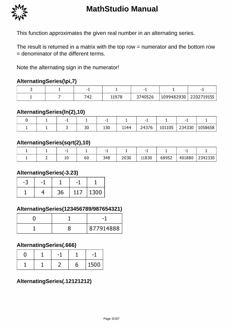
AlternatingSeries(n, [terms])
Page 2/187
MathStudio Manual
This function approximates the given real number in an alternating series.
The result is returned in a matrix with the top row = numerator and the bottom row= denominator of the different terms.
Note the alternating sign in the numerator!
AlternatingSeries(\pi,7)
AlternatingSeries(ln(2),10)
AlternatingSeries(sqrt(2),10)
AlternatingSeries(-3.23)
AlternatingSeries(123456789/987654321)
AlternatingSeries(.666)
AlternatingSeries(.12121212)
Page 3/187

MathStudio Manual
AlternatingSeries(.36363)
Angle(A, B)Returns the angle between the two vectors A and B.
Angle([a@1,b@1,c@1],[a@2,b@2,c@2])
Angle([1,2,3],[4,5,6])
Animate(variable, start, end, [step])This function creates an animated entry. The variable is initialized to the startvalue and at each frame is incremented by step and the entry is reevaluatedcreating animation.
When the variable is greater than the value end it is set back to start.
Animate(n,1,100) ImagePlot(Random(0,1,n,n))
Page 4/187

MathStudio Manual
Apart(f(x), x)Performs partial fraction decomposition on the polynomial function.
Apart performs the opposite operation of Together.
Apart((a+b)/(a*b),a)
Apart((a+b)/(a*b),b)
Apart((x^2+x+1)/((x-2)(x^2+3)))
Apart((2x^2+3x+5)/(x^2+2x+1))
Append(expression1, expression2)
Page 5/187
MathStudio Manual
Appends one expression to end of another expression.
Append([1,2,3],4)
Append([1,2,3],[4,5,6])
Append(ab,c)
Append(a,1)
Arg(z)Returns the argument (or phase) of a complex number.
The value is dependent on the angle setting which can be radians or degrees.You can manually set the angle mode per entry by using the keyword radians or degrees.
radians arg(2+2\im)
degrees arg(2+2\im)
Bernoulli(n, [z])Returns the nth Bernoulli number n.
If z is given, returns the nth Bernoulli polynomial of z.
Bernoulli(3,a)
Page 6/187

MathStudio Manual
Bernoulli(n,1/2)
Bernoulli(n,3)
Bernoulli(n,-z)
Bernoulli(n,5)
Bernoulli(n,-5)
Bernoulli(3,5)
Bernoulli(4,5)
BesselI(v, z)Returns the Modified Bessel function of the first kind.
BesselI(0,15\im)
Page 7/187

MathStudio Manual
BesselI(1,14.99)BesselI(-1,15)
BesselI(1,30)
BesselI(1/2,x)+BesselK(1/2,x)+BesselY(1/2,x)+BesselJ(1/2,x)
BesselI(3,x+1)
BesselI(3,x)
Plot([BesselI(0,x),BesselI(1,x),BesselI(2,x),BesselI(3,x)],colors=[red,blue,green,magenta])
BesselJ(v, z)Returns the Bessel function of the first kind.
Page 8/187

MathStudio Manual
BesselJ(0,1)
BesselJ(1,1)
BesselJ(2,1-\im)
BesselJ(2,x)
BesselJ(3,-x)
BesselJ(5/2,x)
Plot([BesselJ(0,x),BesselJ(1,x),BesselJ(2,x),BesselJ(3,x)])
Plot3D(BesselJ(1,sqrt(x^2+y^2)),x=[-10,10],y=[-10,10],z=[-2,2])
Page 9/187

MathStudio Manual
Diff(BesselJ(2,3z),z)
BesselK(v, z)Returns the Modified Bessel function of the second kind.
BesselK(0,0)
BesselK(0,2)
BesselK(2.3,1.5)
BesselK(3/2,x)
BesselK(3/2,-z)
Page 10/187

MathStudio Manual
BesselK(1,2+3\im)
Plot([BesselK(0,x),BesselK(1,x),BesselK(2,x),BesselK(3,x)],x=[-1,5])
BesselY(v, z)Returns the Bessel function of the second kind.
BesselY(0,1)
BesselY(2,x)
BesselY(1.23,45.67)
BesselY(3/2,x)
Page 11/187

MathStudio Manual
Plot([BesselY(0,x),BesselY(1,x),BesselY(2,x),BesselY(3,x)],x=[-1,6],y=[-2.5,2.5])
Beta(m, n)Calculates the Beta function of m, n both real or complex variables.
Beta(m,n)
Beta(2n,n)
Beta(n+3,n)
Page 12/187

MathStudio Manual
Beta(a/2,3)
Beta(a,-b)
Beta(5,2)-Beta(2,5)
Binomial(n, r)Finds the binomial coefficient. This function is the symbolic equivalent to nCr(n,r).
Binomial(n,3)
Binomial(1,4/5)
Binomial(2,1/2)
Binomial(n-5,n-7)
Binomial(n,7)
Page 13/187

MathStudio Manual
Binomial(n,5)
BinomialCDF(n, p, x)Computes the cumulative Binomial distribution at x with number of trials n andprobability of success p on each trial.
Plot(BinomialCDF(20,0.5,x),BinomialCDF(40,0.5,x),x=[0,20],y=[0,1],numbers=0)
BinomialPDF(n, p, x)Computes the binomial distribution at x with number of trials n and probability ofsuccess p on each trial.
Plot(BinomialPDF(0,0.5,x))
Page 14/187

MathStudio Manual
Plot(BinomialPDF(6,0.5,x),x=[0,10])
BodePlot(function, variable, minimum,maximum, mode)BodePlot creates a Bode plot for the given function.
The x-axis is a logarithmic scale and represents the frequency in rad/sec.
x = -2 : => ? = 0.01 rad/secx = -1 : => ? = 0.1 rad/secx = 0 : => ? = 1 rad/secx = 1 : => ? = 10 rad/secx = 2 : => ? = 100 rad/secx = 3 : => ? = 1000 rad/sec
When the frequency is not given, then ?min = 0.01 rad/sec and ?max = 1000rad/sec.
The y-axis is either the magnitude in dB (mode=0) or the phase in degrees(mode=1) or the phase in radians (mode=2).
BodePlot((0.1+s)/((0.001s+1)*(1+0.5s^2)),s,0.01,10000,0)
Page 15/187

MathStudio Manual
BodePlot((0.1+s)/((0.001s+1)*(1+0.5s^2)),s,0.01,10000,1)
BodePlot((30+s/10)^2/((s+10)^3),s,0.1,1000)
BodePlot((30+s/10)^2/((s+10)^3),s,0.1,1000,1)
Page 16/187

MathStudio Manual
BodePlot(1/(1+s^2),s,0.01,1000,1)
BodePlot((s+10)(s+1000)/((s+1)*(s+100)*(s+10000)),s,0.1,100000,0)
BodePlot((s+10)(s+1000)/((s+1)*(s+100)*(s+10000)),s,0.1,100000,1)
Call(function, parameter1, parameter2, ...)Executes a call to the given function and passes the included parameters to thefunction. The function is evaluated.
Call(sin,\pi/4)
Page 17/187

MathStudio Manual
Call(Binomial,10,2)
Caps(string, index, [mode])Tests for uppercase and lowercase letters in strings.
The mode parameter can be set to upper or lower.
Caps(Abc,1)
Caps(Abc,2)
Caps(Abc,2,upper)
Caps(Abc,1,lower)
Catalan(n)Returns the nth Catalan number.
Catalan(n)
Catalan(3)
Page 18/187
MathStudio Manual
Catalan(10)
Ceil(z)Returns the smallest integer of the given value.
If z is a complex number, then ceil works on both the real and the imaginary part.
ceil(1.234)
ceil(-9.8765)
ceil(-1.001)
ceil(0.5)
cFrac(n, [terms])Calculates the simple continued fraction representation of the given number n.
The result is given as a list, where the first term equals the constant term (a0) andthe others the fraction terms (a1, a2, a3, ...).
n = a0 + 1/( a1 + 1/ (a2 + 1/(a3 + .... )))
cFrac(\pi)
cFrac(sqrt(2),10)
Page 19/187

MathStudio Manual
cFrac(\e,10)
cFrac(BesselI(1,2)/BesselI(0,2))
cFrac(3.245)
cFrac(2.25)
Char(x)Returns the numerical ASCII value of a character or the character of a numericalASCII value.
char(97)
char(a)
char(A)
char(65)
ChebyshevT(n, z)Returns the Chebyshev polynomial of the first kind.
ChebyshevT(3,a)
Page 20/187

MathStudio Manual
ChebyshevT(7,x)
ChebyshevT(n,1)
ChebyshevT(n,x)
ChebyshevT(n,-1)
ChebyshevT(n,0)
ChebyshevT(n,-5)
ChebyshevT(3,5)
ChebyshevT(3,-5)
ChebyshevT(4,5)
ChebyshevT(4,-5)
Page 21/187

MathStudio Manual
ChebyshevU(n, z)Returns the Chebyshev polynomial of the second kind.
ChebyshevU(3,a)
ChebyshevU(7,x)
ChebyshevU(n,1)
ChebyshevU(n,x)
ChebyshevU(n,-1)
ChebyshevU(n,0)
ChebyshevU(n,-5)
ChebyshevU(3,5)
ChebyshevU(3,-5)
ChebyshevU(4,5)
Page 22/187
MathStudio Manual
ChebyshevU(4,-5)
CheckBox(variable, [value])This function dynamically changes the value of a variable or list of variables usinga check box control.
The value of the variable when the control is checked is 1 and 0 when unchecked.
Chi(z)Finds the Hyperbolic Cosine Integral of z.
Chi(-1)
Chi(2+\im)
Chi(-x)
ChiSquareCDF(lower, upper, df)Computes the ChiSquare distribution cumulative density function over the intervaldefined by lower and upper with degrees of freedom df.
ChiSquarePDF(x, df)
Plot(ChiSquarePDF(x,1),ChiSquarePDF(x,2),ChiSquarePDF(x,3),ChiSquareP
Page 23/187

MathStudio Manual
DF(x,4),ChiSquarePDF(x,5),x=[0,10],y=[0,0.5],numbers=0,colors=[black,blue,green,red,magenta])
Cholesky(A)Returns a list with singular values of a positive definite matrix A.
This routine uses the TNT library.
Cholesky([[10,5],[5,20]])
Cholesky([[5,2],[2,14]])
Choose(test1, value1, test2, value2, ...)Creates a piecewise-defined function.
Plot(Choose(x=0,sqrt(x)))
Page 24/187

MathStudio Manual
f(x)=Choose(x=0,sqrt(x)) f(9)
Ci(z)The Cosine Integral of z.
[Ci(0),Ci(\inf),Ci(-\inf),Ci(-x)]
a=list(3) b=list(3) loop(i,1,3) a(i)=Si(i) b(i)=Ci(i) end [a,b]
Ci(2+\im)
Plot([Si(x),Ci(x)],x=[-10,10],y=[-2,2])
Page 25/187

MathStudio Manual
Clear(variable, ...)Clears a variable or list of variables.
The variable must be entered using quotes. You can use the keyword all to clearall variables.
a=2 Clear("a") a
a=2;b=3;b=4 Clear("a", "b", "c") [a,b,c]
a=2;b=3;b=4 Clear(all) [a,b,c]
clip(x, [min], [max])Clips 2D plot functions. Min and max are optional parameters and set to [-1,1]when not given.
Plot(clip(HalfRectSineWave(x),0.5,1),x=[-20,20],y=[0,1.5])
Page 26/187

MathStudio Manual
Plot(clip(SawToothWave(x),0,0.5),x=[-6,12])
Plot(clip(TriangleWave(x),-0.5,0.2)
Coefficient(degree, x, f(x))Returns the coefficient of a term in a polynomial.
Coefficient(7x^3+5x^2+3x+6,x,3)
Page 27/187

MathStudio Manual
Coefficient(7x^3+5x^2+3x+6,x,2)
Coefficient(7x^3+5x^2+3x+6,x,1)
Coefficient(7x^3+5x^2+3x+6,x,0)
coFactor(matrix, i, j)Calculates the cofactor of the (i, j) entry of a matrix.
Command(setting)This function sets or gets options for the computer algebra system in an entry.Any changes to options only affect the entry locally. You cannot globally changethese options.
MatrixDetectionThis option automatically detects whether a list of equal-length lists is a matrix.
List MultiplicationCommand(MatrixDetection=0) [[1,2],[3,4]]*[[5,6],[7,8]]
Matrix MultiplicationCommand(MatrixDetection=1) [[1,2],[3,4]]*[[5,6],[7,8]]
Command(MatrixDetection)
Page 28/187

MathStudio Manual
Command(MatrixDetection=0) Command(MatrixDetection)
Conj(z)Returns the complex conjugate of a complex number.
Constant(name)Returns fundamental physical constants as a real number. The value of theconstant is given in SI-units
Speed of lightlight299792458 m s-1
Planck constant6.62607554e-34 J s
Planck constant eV4.135669212e-15 eV s
Planck hbarhbar1.0545726663e-34 J s
Planck hbar eVhbar eV6.58212202e-16 eV s
Planck massPmass2.1767114e-08 kg
Planck timePtime
Page 29/187

MathStudio Manual
5.3905634e-44 sec
Acceleration of gravitygravity9.80665 m s-2
Gravitation constantgravitation6.6725985e-11 m3 kg-1 s-2
Permeability of vacuummagnetic1.2566370614359172e-06 N A-2
Permittivity of vacuumelectric8.8541878176208e-12 F m-1
Avogadro constantAvogadro6.022136736e+23 mol-1
Boltzmann constantBoltzmann1.38065812e-23 J K-1
Boltzmann constant eVBoltzmann eV8.61738573e-05 eV K-1
Molar gas constantMolar gas8.3145107 J mol-1 K-1
Magnetic flux quantumflux2.0678346161e-15 Wb
Bohr magneton
Page 30/187

MathStudio Manual
9.274015431e-24 J T-1
Bohr magneton eV5.7883826352e-05 eV T-1
Bohr radius5.2917724924e-11 m
Rydberg constantRydberg10973731.53413 m-1
Faraday constantFaraday96485.30929 C mol-1
Stefan-Boltzmann constantStefan-Boltzmann5.6705119e-08 W m-2 K-4
Wien displacement constantWien0.00289775624 m K
Standard atmosphereatm101325 Pa
Elementary chargeelectron1.6021773349e-19 C
Electron mass9.109389754e-31 kg
Electron mass eV510999.0615 eV
Proton mass
Page 31/187

MathStudio Manual
1.67262311e-27 kg
Proton mass eV938272312.8 eV
Neutron mass1.67492861e-27 kg
Neutron mass eV939565632.8 eV
Constant("light")
Constant("electron")
G=Constant("gravitation") g=Constant("gravity") r=6.378\sci6Solve(G*m1*mass/r^2=m1*g,mass)
ContourPlot(expression, ...)Plots 2D contour graphs.
ContourPlot(x^2+y^2)
ContourPlot(sqrt(abs(x^2-y^2)))
Page 32/187

MathStudio Manual
Convergents(n, [mode=0], [terms])The Convergent of a given number or a given continued fraction is the rationalnumber obtained by keeping only a limited number of terms in the continuedfraction (or the continued fraction of the number).
Convergents([3,7,15,1,292,1,1])
Convergents([3,7,15,1,292,1,1],1)
Convergents(2/\pi,-1)
Convergents(\pi,1,10)
Convergents([1,1,1,1,1, 1,1,1,1,1, 1,1,1,1,1, 1,1,1,1,1, 1,1,1,1,1, 1,1,1,1,1,1,1,1,1,1, 1,1,1,1,1],-2)
Page 33/187

MathStudio Manual
Cross(A, B)Calculates the cross product of two 3-dimensional vectors A and B.
Cross([5,-8,3],[1,2,4])
Cross([sqrt(2)/2,1,sqrt(3)/2],[x@1,x@2,x@3])
Curl(vector, [varlist], [mode])Returns the curl of a vector field.
This is normally denoted as Curl(F) = ? x F
Curl([x/y,y/z,z/x])
Curl([t^2/u,u*v,v+t],[t,u,v])
Curl([x*exp(z),y^2/(x*z),cos(z)])
Page 34/187

MathStudio Manual
CylindricalPlot3D(expression, ...)Plots 3D parametric graphs in cylindrical coordinates.
CylindricalPlot3D((1+sin(\phi))r^2,r=[0,1],\phi=[0,2\pi])
D(f(x), x, [n])Finds the derivative of the expression to variable. The optional parameter n findsthe nth derivative of the expression.
See Diff for derivatives of both common and special functions.
D(x^6+3x^5-4x^3+x-1)
D(f(x),x)
D(exp(-s*t),t)
D(f(x)*g(x),x)
D(cos(x)*sin(x),x)
Page 35/187
MathStudio Manual
D(sin(a*x)/x,x)
D(a^(x^2),x)
D(sqrt(x)^sqrt(x),x)
Derivatives with optional nth parameter.D(sin(3x+6),x,3)
D(exp(-s*t),t,2)
D(tan(2x-4),x,3)
D(x^6-2x^4-3x^2+1,x,6)
Date(letter)Returns the current date.
date(h)
Page 36/187

MathStudio Manual
date(a)
date(y)
String(date(d),"-",date(m),"-",date(y))
Animate(500) String(date(h),":",date(i),":",date(s))
Dawson(z)Finds the Dawson Integral.
Dawson(0)
Dawson(1)
Dawson(2)
Plot(Dawson(x))
Page 37/187

MathStudio Manual
Degree(expression)Returns the degree of a polynomial.
Degree(x^2)
Degree(x^3+x^2)
Degree(x^10+3x+6)
Degree(x^10+y^6,y)
DEGtoDMS(angle, [digits])Converts an angle into a string represented the angle, minutes and seconds indegrees.
DEGtoDMS(90)
DEGtoDMS(90.123)
DEGtoDMS(12.5)
DEGtoDMS(12.345)
Delete(expression, position, [length])Deletes an expression in a list or a character in a string.
Page 38/187

MathStudio Manual
Delete([1,2,3,4,5],2)
Delete("Hello World",3,7)
Denominator(expression)Returns the denominator of an expression.
Denominator(a/b)
Denominator(1/2)
Denominator((x+1)/(x+2))
Denominator(f(x)/g(x))
Det(A)Finds the determinant of the square matrix A.
Det([[1,2,3],[1,8,6],[2,7,9]])
Det([[a,b],[c,d]])
Page 39/187

MathStudio Manual
Diff(f(x), x)Diff is equivalent to D and finds the first derivative to a function. Diff finds thederivative to both common and special functions.
Diff(FresnelCos(f(z))^3,z)
Diff(z^2*Zeta(z,a),z)
Expand(Diff(BesselJ(3,z),z))
Diff(Beta(f(z1),g(z2)),z2)
Diff(tan(x)/(-6x+7)+7*exp(2x+x^2/7)^5-ln(x)/(exp(y)*x^2),x)
Diff(Gamma(a,f(z))+Psi(h(z)),z)
Diff(Erf(3x)-Erfc(x),x)
Diff(Si(2z)+Ci(3z)+Ei(4z)+Li(5z),z)
Page 40/187

MathStudio Manual
DiGamma(z)Returns the logarithmic derivative of the gamma function.
Plot(DiGamma(x))
DiGamma(0)
DiGamma(2)
DiGamma(4)
DiLog(z)This function is the same as PolyLog(2,z).
Dirichlet_Eta(z)This function is closely related to the Riemann Zeta function.
Page 41/187

MathStudio Manual
Dirichlet_Eta(z)
Dirichlet_Eta(2z+1)
Dirichlet_Eta(1)
Dirichlet_Eta(3)
Dirichlet_Eta(-3)
Dirichlet_Eta(-10)
Dirichlet_Eta(-11)
Plot(Dirichlet_Eta(x),x=[-12,5],y=[-2,10])
Page 42/187

MathStudio Manual
Dirichlet_Lambda(z)Returns the Dirichlet L-series and is closely related to the Riemann Zeta function.
Dirichlet_Lambda(z)
Dirichlet_Lambda(2z+1)
Dirichlet_Lambda(1)
Dirichlet_Lambda(3)
Dirichlet_Lambda(-3)
Dirichlet_Lambda(-10)
Dirichlet_Lambda(-11)
Plot(Dirichlet_Lambda(x),x=[-12,5],y=[-2,10])
Page 43/187

MathStudio Manual
Divergence(vector, [varlist], [mode])Returns the divergence of a vector field.
This is normally denoted as Divergence(F) = ?.F
Divergence([3*x*y^2,y*z,y*z/x],[x,y,z])
Divergence([3*x*y^2,y*z,y*z/x])
Divergence([a*b^2,a^2*b],[a,b])
Divisors(n)Returns a list of integers that can be evenly divided into n without leaving aremainder.
Divisors(10)
Divisors(11)
Divisors(20)
Divisors(99)
ListPlot(Divisors(40))
Page 44/187

MathStudio Manual
ListPlot(Divisors(200))
DivisorSigma(n)Returns the sum of all factors of the given integer.
DivisorSigma(2)
DivisorSigma(7)
DivisorSigma(20)
DivisorSigma(100)
Page 45/187

MathStudio Manual
Dot(A, B)Calculates the dot product of the two vectors A and B. Vectors A and B can be ofany size, but should be equal to each other.
Euler anglesR1=[[cos(u),sin(u),0],[-sin(u),cos(u),0],[0,0,1]]R2=[[1,0,0],[0,cos(v),sin(v)],[0,-sin(v),cos(v)]]R3=[[cos(w),sin(w),0],[-sin(w),cos(w),0],[0,0,1]] Dot(R3,Dot(R2,R1))
Dot([[1,2],[3,4]],[[a,b],[c,d]])
Dot([3,2],[a,b])
Dot([5,-8],[1,2])
Draw(mode)Draws the colors with an optional mode. This mode parameter is reserved forfuture use and should be set to zero.
You can also plot images using ImagePlot but Draw is much faster because itbypasses the computer algebra system and draws directly to a block of memory.
width=100 height=100 DrawWindow(width,height) pixels=width*heightloop(i,1,pixels) DrawColor(i/pixels,0,1-i/pixels) end Draw(0)
Page 46/187
MathStudio Manual
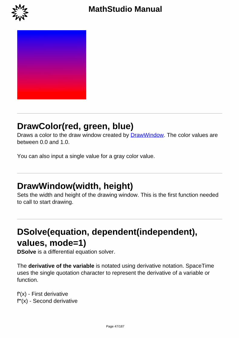
DrawColor(red, green, blue)Draws a color to the draw window created by DrawWindow. The color values arebetween 0.0 and 1.0.
You can also input a single value for a gray color value.
DrawWindow(width, height)Sets the width and height of the drawing window. This is the first function neededto call to start drawing.
DSolve(equation, dependent(independent),values, mode=1)DSolve is a differential equation solver.
The derivative of the variable is notated using derivative notation. SpaceTimeuses the single quotation character to represent the derivative of a variable orfunction.
f'(x) - First derivativef''(x) - Second derivative
Page 47/187

MathStudio Manual
f'''(x) - Third derivative
Derivative ExamplesSolve: y' + y = sin(t)DSolve(y'(t)+y(t)=sin(t), y(t), .....)
Solve: y'' + 2y' + y = xDSolve(y''(x)+2y'(x)+y(x)=x, y(x), .....)
The definite integral of the variable is represented by I(f(t), t) and denotes theintegral of the variable f(t) with lower bound 0 and upper bound t. These boundscannot be changed.
Integral Examples?(y) + y = sin(t)DSolve( I(y(t),t) + y(t) = sin(t), y(t), .....)
The upper case character I indicates the integral and is a mandatory condition.
Initial valuesWhen no initial values are given, then simple write the word no. The resultreturned contains the Constant C@1.
For first order differential equations the initial value can be given as y(t)=value.When you ommit y(t), then y(0) is assumed.
For higher order differential equations, the initial values should be given as a listand are always referred to zero : [y(0), y'(0), y''(0), ...]
Examples with different initial valuesSolve: y' + y = sin(t) with y(0) = 5DSolve(y'(t) + y(t) = sin(t) , y(t) , y(0) = 5)orDSolve(y(t)' + y(t) = sin(t) , y(t) , 5)
Solve: y' + y = sin(t) with y(2) = 5DSolve(y(t)' + y(t) = sin(t) , y(t) , y(2)=5)
Solve: y'' + 2y' + y = x with y(0) = 1 and y'(0) = 2
Page 48/187

MathStudio Manual
DSolve(y''(x) + 2y'(x) + y(x) = x, y(x), [1,2])
Solve: y'' + 2y' + y = x with no initial valuesDSolve(y''(x) + 2y'(x) + y(x) = x, y(x), no)
Different form for exact first order differential equations.Exact first order differential equation can be given with d@x , d@t , d@y, ect.
First Order ExamplesSolve: dy = sin(t) * dtDSolve(d@y = sin(t) * d@t, y(t), .....)
Of course, this can also be written as the following equation.DSolve(y'(t), t) = sin(t) , y(t), ...)Note: The variable to be solved should still be written as y(t).
ResultsNormally, DSolve tries to return the result as y(t) = function(t).
In case y(t) cannot be represented in a simple form then the result is returned in implicit form.function(y , t) = 0
In the latter case, the text Implicit result is added to call the users attention thatthe result is not of the form y(t)=function(t).
DSolve(y'(t)+y(t)=sin(t),y(t),no)
DSolve(y''(x)+2y'(x)+y(x)=x, y(x), no)
DSolve(y''(x)+2y'(x)+y(x)=x, y(x), [1, 5])
DSolve(R*q'(t)+q(t)/C=U*sin(t), q(t), no)
Page 49/187

MathStudio Manual
DSolve(4*q'(t)+2q(t)=U*sin(t), q(t), y(0)=0)
DSolve(d@y=sin(t)*d@t, y(t), no)
DSolve(d@y=sin(t)*d@t, y(t), y(0)=1)
DSolve(exp(x)*sin(y(x))*d@x+((y(x)+exp(x)*cos(y(x)))*d@y, y(x), no)
DSolve(x'(t)=-2*x(t)^2, x(t), no)
DSolve(x'(t)=-2*x(t)^2, x(t), y(1)=2)
DSolve(y'(t)=3t^2*exp(-y(t)), y(t), y(0)=1)
DSolve(x^2*y'(x)+3*x*y(x)=x^3, y(x), y(1)=A)
DSolve(x'(t)=6*sin(t)/x(t), x(t), no)
Page 50/187

MathStudio Manual
DSolve(x'(t)=6*sin(t)/x(t), x(t), y(\pi/4)=2)
DSolve(x'(t)=6*sin(t)/x(t), x(t), y(\pi/4)=2, 0)
DSolve(f(z)^2+2*z*f(z)*f'(z), f(z), no, 0)
DSolve(f(z)^2+2*z*f(z)*f'(z), f(z), no)
DSolve(f(z)^2+2*z*f(z)*f'(z), f(z), f(1)=5)
DSolve((a+b*x)*d@x+(e+x+c)*d@y, y(x), no)
DSolve((a+b*x)*d@x+(e+x+c)*d@y, y(x), a)
DSolve((a+b*x)+(e+x+c)*y'(x), y(x), no)
Page 51/187

MathStudio Manual
DSolve((a+b*x)+(e+x+c)*y'(x), y(x), a)
DSolve(x*f'(x)+x+f(x), f(x), f(1)=a, 0)
DSolve(y'(t)+2a*y(t)=t^2, y(t), y(1)=0)
Duf(function, [varlist], [point], [direction])Calculates the directional derivative of a given function.
Duf(x^2*y^2*z^2,[x,y,z],[1,2,3],[1,1,-2])
Duf(x^2*y^2*z^2)
Duf(f(x,y,z))
Duf(x^2*y*z,[x,y,z],[1,-1,1],[4,0,-3])
Page 52/187

MathStudio Manual
Duf(3x^2-3y^2,[x,y],[1,2],[0,1])
Duf(sqrt(x^2+y^2),[x,y,z],[0,-2,1],[2,2,1])
Duf(sin(x)+cos(y)+sin(z),[x,y,z],[\pi,0,\pi],[\pi,\pi,0])
Ei(z)Finds the Exponential Integral of z.
Eigenvalues(A)Returns the eigenvalues of matrix A.
This routine uses the TNT library.
Eigenvalues([[1,2],[2,3]])
Eigenvalues([[-1,-1,2],[0,2,-1],[4,-6,2]])
Eigenvectors(A)Returns the eigenvectors of matrix A.
Page 53/187

MathStudio Manual
This routine uses the TNT library.
Eigenvectors([[1, 2], [2, 3]])
Eigenvectors([[-1, -1, 2], [0, 2, -1], [4, -6, 2]])
Else If(condition)Evaluates a block of code if condition is a non-zero value.
This function was be preceded by an if code block or another else if code block.
n=5 if(n>0) result="Positive" else if(n
Erf(z)Returns the Error Function of z.
Erfc(z)Returns the Complementary Error Function of z.
Error(string)
Page 54/187

MathStudio Manual
This function stops all computations and displays an error message along with theline number where the error message occurred.
n=5 if(n>0) Error("Positive") else if(n
Euler(n, [z])If only n is given then Euler returns the Euler number n.
If z is also given then Euler returns the nth Euler polynomial of z.
Euler(3,a)
Euler(n,1/2)
Euler(n,1)
Euler(n,-1)
Euler(n,-5)
Euler(4,5)
Euler(4,-5)
Page 55/187

MathStudio Manual
Eulerian(n, k)Returns the number of permutations of {1,2,..n} having k permutation ascents.
The parameters n, k should both be positive integers > 0 with kEulerian(5,0)
Eulerian(5,1)
Eulerian(5,2)
Eulerian(5,3)
Eulerian(5,4)
Eulerian(5,5)
Eulerian(5,6)
Eulerian(10,3)
Eval(function, variable, value)Replaces the variable in the function with the new value.
Eval(sin(x),x,\pi/4)
Page 56/187

MathStudio Manual
Eval(3x^2+4x-6,x,3)
Eval([sin(x),cos(x)],x,\pi/3)
Eval(x^y+3x+2y,[x,y],[2,a])
Eval(x+sin(y)-cos(z),[x,z],[1,\pi/3])
Eval(Diff(a*x^3,x),a,5)
Exp(z)Exp(z) or e^z raises e (base of natural logarithm) to the power z.
exp(1)
Plot(exp(x))
Page 57/187
MathStudio Manual
Expand(expression)Returns the expanded form of a function.
Expand(3(x-2)(x+4))
Expand((2x^2-y)(x-y-z))
Expand((1+sin(z))^2)
Expand(3*(y+x)/sin(y))
ExpConvert(expression)Converts exponential functions to trigonometric functions.
ExpConvert(exp(x))
ExpConvert(exp(x^2))
ExpConvert(exp(2x))
ExpConvert(exp(3x))
Page 58/187

MathStudio Manual
Extract(expression, position, [length])Extracts an expression from a list or a substring from a string.
Extract([1,2,3,4,5],2,3)
Extract("abcde",2,3)
Extract("abcde",4)
Factor(expression)Returns the factored form of a polynomial. It does the reverse of what Expanddoes, but limited to polynomials.
For polynomials of degree > 2 this function makes use of pSolve. If pSolve canfind real roots, then Factor can return a factored form of the given function.
Factor(x^4-18x^2+81)
Factor(x^5+111105x^4+1121766570x^3+1118845033650x^2+108868944188565x+890011088900109)
Factor(x^12-21x^10+175x^8-735x^6+1624x^4-1764x^2+720)
Factor(x^8-26x^6+236x^4-886x^2+1155)
Factor(2x^6+18x^5+63x^4-324x^3-1620x^2+1458x+8019)
Page 59/187

MathStudio Manual
Factor(x^7-3x^6-27x^5+81x^4+243x^3-729x^2-729x+2187)
Factor(x^4+5x^2-6)
Factorial(n)Returns the number of ways n elements can be ordered.
n! = 1 * 2 * 3 * ..... (n-1) * n
Factorial(6)
6!
Fcdf(x, d1, d2)F-distribution cumulative density function.
fDiff(f(x,y,z,..), (x,y,z,...))Finds the exact differential of the given function.
fDiff(3*x*y+5x*z^2,[x,y,z])
fDiff(y^4+4y-3x^3sin(y)-2x-1,[x,y])
Page 60/187

MathStudio Manual
fDiff(x^2+5x-4y^2+3y+21,[x,y])
fDiff(x^3-7x^2y^3+4y^2+16,[x,y])
fDiff(sin(2x-7y)-16y,[x,y])
fDiff(y-x^(p/q),[x,y])
fDiff(a*x^3*y-2*y/z-z^2,[x,y])
fDiff([3sin(x)*cos(y),x^2-3y],[x,y])
fDiff([R*cos(\theta),R*sin(\theta)],[R,\theta])
fDiff(x^2+y^2,[x,y])
Fibonacci(n, [z])Returns the nth Fibonacci number of n.
Page 61/187

MathStudio Manual
If z is given, returns the nth Fibonacci polynomial of z.
Fibonacci(5,z)
Finance(PV, FV, Pmt, i, n, [mode=0])This is a simple financial function to calculate loan or investments. In case of loan,Pmt is a positive value. In case of investments, Pmt is a negative value.
Fill in the known values in the indicated order and use any variable name for theunknown. In the examples below, the unknown is indicated with it's own name butyou can use any variable name.
Based on the examples from Stan Brown, Oak Road Systems.
You have a $18,000 car load at 14.25% per year for a period of 36 months.Every month you pay $620. How big is the payoff amount after 24 months?Finance(18000, FV, 620, 14.25/12, 24)
You are buying a $250,000 house, with 10% down, on a 30-year mortgage ata fixed rate of 7.8%. What is the monthly payment?Finance(225000, 0, Pmt, 7.8/12, 30*12)
If you loan $3500 at 6% rate and and you pay back $100 per month. Howmany months do you have to pay?Finance(3500, 0, 100, 6/12, n)
In the above example, you will make payments for 38 month. How much willyou pay for the last month?Finance(3500,FV,100,6/12,38)
Page 62/187
MathStudio Manual
You have $15,000 in a 5% savings account, which is compounded monthly.How long can you withdraw $100 a month?Finance(15000,0, 100, 5/12, n)
If you deposit $100 per month over 5 years at 6% interest, how much moneywill you have at the end?Finance(0, FV, -100, 6/12, 60)
You want to purchase a 20-year annuity that will pay $500 a month. If theguaranteed interest rate is 4%, how much will the annuity cost?Finance(PV, 0, 500, 4/12, 20*12)
On the same day every year, you put $2000 into stocks. If the market rises8% a year, how many years will it take you to accumulate $40,000?Finance(0, 40000, -2000, 8, n)
Assume you want to set apart $50 at the end of each month for your childstarting the same month as the child was born. How much will be available ifthe child turns 19 years old. Assume an interest rate of 5% compoundedmonthly.Finance(0, FV, -50, 5/12, 18*12)
If you deposit $300 at the beginning of each month over 6 years at 10%interest, how much money will be in the fund at the end?Finance(0, FV, -300, 10/12, 72, 1)
The monthly rent on an apartment is $950 payable at the beginning of themonth. If the current interest is 12% compounded monthly, what singlepayment 12 months in advance would be equal to a year's rent.Finance(PV, 0, 950, 12/12, 12, 1)
Page 63/187

MathStudio Manual
To obtain an amount of $3,000 ten years from now, earning 10% annually,what amount would have to be invested on a yearly basis in an annuity dueform?Finance(0, -3000, Pmt, 10, 10, 1)
The time $1,500 is needed and you know in advance that you have 10 yearsto obtain it. What annual interest rate would a $100 annuity due have to earnfor you to achieve this goal?Finance(0, 1500, -100, i, 10, 1)
You are doing a one time investment of $2,500. What is accumulated valueafter 10 years at a fixed interest rate of 5%?Finance(2500, FV, 0, 5, 10)
You need $19,500 within 5 years from now. How much do you need todeposit today at a fixed interest rate of 3.25%?Finance(PV, 19500, 0, 3.25, 5)
What interest rate would be needed to receive $20,000 after 20 years whenyou deposit $8,000 now?Finance(8000, 20000, 0, i, 20)
Floor(z)Returns the greatest integer of the given value.
If z is a complex number, then floor works on both the real and the imaginary part.
floor(1.234)
Page 64/187

MathStudio Manual
floor(-9.8765)
floor(-1.001)
floor(0.5)
floor(7/2+7/3\im)
FourierCos(f(x), x, w)Takes the Fourier Cosine Transform of the given function.
Current implementation is very limited.
FourierCos(sin(x),x,w)
FourierCos(exp(t/2)*sin(t),t,w)
FourierCos(exp(-a*t),t,w)
FourierCos(sin(t),t,w)
Page 65/187

MathStudio Manual
FourierSeries(f(x), x, [n], [mode])Creates the Fourier series of a given function.
Trigonometric SeriesFourierSeries([[-1,-\pi,0],[1,0,\pi]],x,8)
FourierSeries([[-x,-\pi,0],[1,0,\pi]],x,6)
FourierSeries([-1,-\pi,\pi],x,6)
FourierSeries([-1,0,2\pi],x,6)
FourierSeries([sin(z),0,\pi],z,6)
FourierSeries([[0,-\pi,0],[\pi,0,\pi]],x,10)
FourierSeries([x^2,-\pi,\pi],x,6)
Page 66/187

MathStudio Manual
FourierSeries([[-cos(z),-\pi,0],[cos(z),0,\pi]],z,10)
Complex FormFourierSeries([[-1,-\pi,0],[1,0,\pi]],x,6,1)
FourierSeries([[-x,-\pi,0],[x,0,\pi]],x,6,1)
FourierSeries([[x,-\pi,\pi]],x,4,1)
FourierSeries([[t, 0,2\pi]],t,4,1)
FourierSeries([[sin(z),0,\pi],[0,\pi,2\pi]],z,6,1)
FourierSeries([[cos(z),-\pi/2,\pi/2],[0,\pi/2,3\pi/2]],z,6,1)
Single CoefficientFourierSeries([[sin(z),0,\pi],[0,\pi,2\pi]],z,0,1)
FourierSeries([[sin(z),0,\pi],[0,\pi,2\pi]],z,-1,1)
Page 67/187
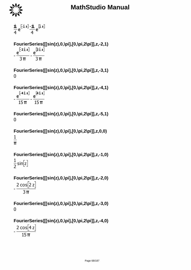
MathStudio Manual
FourierSeries([[sin(z),0,\pi],[0,\pi,2\pi]],z,-2,1)
FourierSeries([[sin(z),0,\pi],[0,\pi,2\pi]],z,-3,1)
FourierSeries([[sin(z),0,\pi],[0,\pi,2\pi]],z,-4,1)
FourierSeries([[sin(z),0,\pi],[0,\pi,2\pi]],z,-5,1)
FourierSeries([[sin(z),0,\pi],[0,\pi,2\pi]],z,0,0)
FourierSeries([[sin(z),0,\pi],[0,\pi,2\pi]],z,-1,0)
FourierSeries([[sin(z),0,\pi],[0,\pi,2\pi]],z,-2,0)
FourierSeries([[sin(z),0,\pi],[0,\pi,2\pi]],z,-3,0)
FourierSeries([[sin(z),0,\pi],[0,\pi,2\pi]],z,-4,0)
Page 68/187

MathStudio Manual
FourierSeries([[sin(z),0,\pi],[0,\pi,2\pi]],z,-5,0)
FormulaFourierSeries([[-1,\pi,0],[1,0,\pi]],x,f,1)
FourierSeries([[x,-\pi,\pi]],x,f,1)
FourierSeries([[t,0,2\pi]],x,f,1)
FourierSeries([[sin(z),0,\pi],[0,\pi,2\pi]],z,f,1)
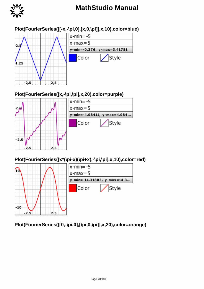
GraphsPlot(FourierSeries([[-1,-\pi,0],[1,0,\pi]],x,20),color=red)
Page 69/187
MathStudio Manual
Plot(FourierSeries([[-x,-\pi,0],[x,0,\pi]],x,10),color=blue)
Plot(FourierSeries([x,-\pi,\pi],x,20),color=purple)
Plot(FourierSeries([x*(\pi-x)(\pi+x),-\pi,\pi],x,10),color=red)
Plot(FourierSeries([[0,-\pi,0],[\pi,0,\pi]],x,20),color=orange)
Page 70/187

MathStudio Manual
Plot(FourierSeries([x^2,-\pi,\pi],x,20),color=blue)
FourierSin(f(x), x, w)Takes the Fourier Sine Transform of the given function.
Current implementation is very limited.
FourierSin(sin(x)^2,x,w)
FourierSin(exp(a*t)*sin(2t)*cos(t),t,w)
Page 71/187

MathStudio Manual
FourierSin(exp(a*t)*sin(t)*cos(t),t,w)
FourierSin(exp(-a*t),t,w)
FourierSin(cos(t),t,w)
FourierSin(k,t,w)
fPart(z)Returns the fractional part of z.
fPart(4/3)
fPart(1.234)
fPart(-9.8765)
Page 72/187

MathStudio Manual
Fpdf(x, d1, d2)F-distribution probability density function.
FractalPlot(expression, ...)Plots Mandelbrot set fractals.
FractalPlot(z^4+c)
FractalPlot(z^5+c)
FractalPlot(Real(c^9)+Imag(c^3)+z)
Page 73/187

MathStudio Manual
FresnelCos(z)Returns the Fresnel Cosine Integral of z.
FresnelCos(\inf)
FresnelCos(1)
FresnelCos(-2)
FresnelCos(1+3\im)
Plot(FresnelCos(x))
Page 74/187

MathStudio Manual
ParametricPlot(FresnelCos(u), FresnelSin(u), u=[-2\pi, 2\pi, 200], numbers=4)
FresnelSin(z)Returns the Fresnel Sine Integral of z.
FresnelSin(\inf)
FresnelSin(1)
FresnelSin(-2)
FresnelSin(1+3\im)
Diff(FresnelSin(f(z)),z)
Plot(FresnelSin(x))
Page 75/187

MathStudio Manual
ParametricPlot(FresnelCos(u), FresnelSin(u), u=[-2\pi, 2\pi, 200], numbers=4)
FullRectSineWave(x, [T])Creates a predefined 2D full rectified sine wave with period = T.
Plot(FullRectSineWave(x),color=red)
Page 76/187
MathStudio Manual
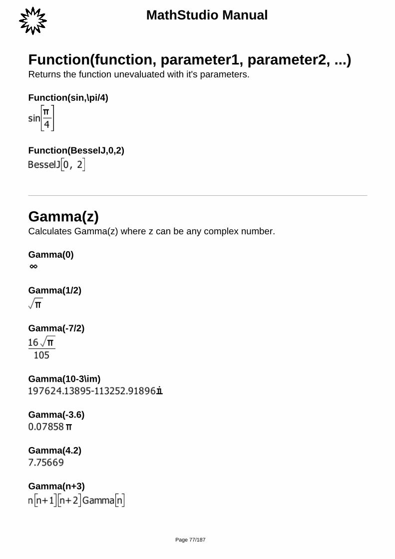
Function(function, parameter1, parameter2, ...)Returns the function unevaluated with it's parameters.
Function(sin,\pi/4)
Function(BesselJ,0,2)
Gamma(z)Calculates Gamma(z) where z can be any complex number.
Gamma(0)
Gamma(1/2)
Gamma(-7/2)
Gamma(10-3\im)
Gamma(-3.6)
Gamma(4.2)
Gamma(n+3)
Page 77/187

MathStudio Manual
Gamma(3z)
Gamma(2x+3)
Gamma(1-2n)
Plot(Gamma(z))
GCD(n1, n2)Finds the greatest common factor between two integers.
gcd(10,2)
gcd(12,8)
Page 78/187

MathStudio Manual
gcd(21,99)
gcd(1000, 15)
GegenbauerC(n, a, z)Returns the Gegenbauer polynomial.
GeoCDF(p, x)Computes the cumulative geometric distribution at x with probability of success p.
GeoPDF(p, x)Computes the geometric distribution at x with probability of success p.
Plot(GeoPDF(0.5,x))
Gradient(function, [varlist], [mode])
Page 79/187

MathStudio Manual
Returns the Gradient of the function.
This is normally denoted as Grad(F) = ?F
Gradient(x+y^2,[x,y])
Gradient(x^2*y^3,[x,y])
Gradient(1/sqrt(x^2+y^2+z^2))
Gradient(sin(x)*exp(y)*ln(z))
Gradient([a/b,c*d^2,a^2*c],[d,c])
Gradient([x*y/z,y*z^2,z^2*x])
Page 80/187

MathStudio Manual
Cartesian coordinate systemGradient(f(x,y,z))
Cylindrical coordinate systemGradient(f(r,\phi,z),[r,\phi,z],1)
Spherical coordinate systemGradient(f(r,\theta,\phi),[r,\theta,\phi],2)
Gudermannian(z)Returns the Gudermannian function of z.
Gudermannian(0)
Gudermannian(-\inf)
Gudermannian(\inf)
Gudermannian(3)
Page 81/187

MathStudio Manual
Gudermannian(3-2\im)
Diff(Gudermannian(x),x)
Plot(Gudermannian(x))
HalfRectSineWave(x, [T])Creates a predefined 2D half rectified sine wave with period = T.
Plot(HalfRectSineWave(x),color=red)
HankelH1(v, z)Calculates the Hankel function of the first kind.
Page 82/187

MathStudio Manual
HankelH1(0,z)
HankelH1(v,2)
HankelH1(0,5)
HankelH1(0,-5)
Expand(HankelH1(0,z)+HankelH2(0,z))
Diff(HankelH1(-1,z),z)
HankelH2(v, z)Calculates the Hankel function of the second kind.
HankelH2(0,z)
HankelH2(v,2)
HankelH2(0,5+\im)
Page 83/187

MathStudio Manual
HankelH2(0,-5-\im)
Expand(HankelH1(1,z)+HankelH2(1,z))
Diff(HankelH2(1/2,z),z)
Harmonic(z)Calculates the Harmonic Number of z.
Harmonic(2)
Harmonic(a+3)
Harmonic(1-2a)
Harmonic(3a)
Harmonic(100/3)
Page 84/187

MathStudio Manual
Harmonic(2+3\im)
Harmonic(-z)
Diff(Harmonic(x),x)
HermiteH(n, z)Returns the Hermite polynomial.
Plot(HermiteH(1, x), HermiteH(2, x), HermiteH(3, x), HermiteH(4, x), x=[-2, 2],y=[-30, 30], color=[red, yellow, green, blue], numbers=4)
Hessian(function, [varlist], [mode])Returns the Hessian matrix (mode=0) or Hessian determinant (mode=1) of agiven function.
Hessian(f(x,y,z))
Page 85/187

MathStudio Manual
Hessian(x^2*y^3/z^2)
Hessian(r^2*x^2+s^3*y^3,[r,s])
Hessian(r^2*x^2+s^3*y^3,[r,s],1)
HRStoHMS(hours, [digits])Converts a number representing hours into a string representation of hours,minutes and seconds.
HRStoHMS(5)
Page 86/187

MathStudio Manual
HRStoHMS(5.5)
HRStoHMS(1.234)
HRStoHMS(1.23456789,6)
Hypergeom_2F1(a, b, c, z, [mode])Calculates the Hyper Geometric 2F1 function.
Hypergeom_2F1(a,b,c,1)
Hypergeom_2F1(a,b,a,z)
Hypergeom_2F1(5,2,1,z)
Hypergeom_2F1(1,1,5,z)
Hypergeom_2F1(4,1,1/2,z)
Page 87/187

MathStudio Manual
Hypergeom_2F1(1/2,1,3/2,2.4)
Hypergeom_2F1(-1/2,1,1/2,z)
Hypergeom_2F1(1,1/2,3/4,z,8)
Identity(n)Returns the n x n identity matrix.
Identity(3)
Identity(4)*a
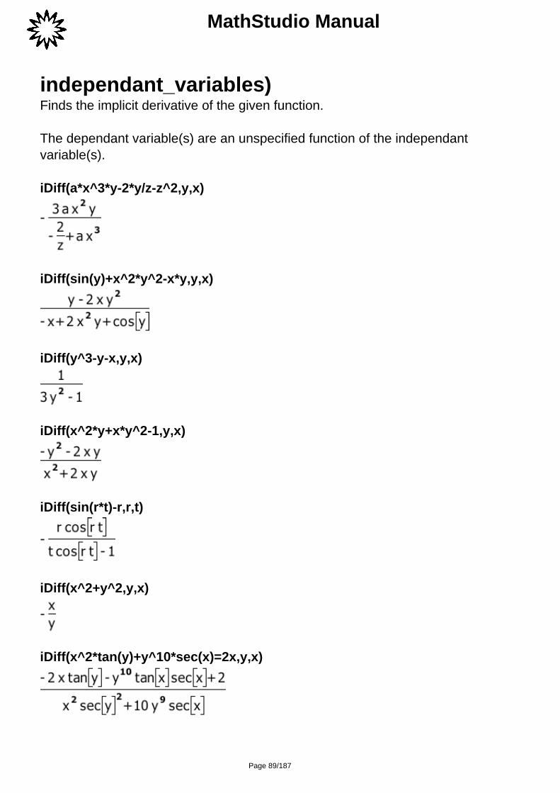
iDiff(f(x,y,z,..), dependant_variables,
Page 88/187
MathStudio Manual
independant_variables)Finds the implicit derivative of the given function.
The dependant variable(s) are an unspecified function of the independantvariable(s).
iDiff(a*x^3*y-2*y/z-z^2,y,x)
iDiff(sin(y)+x^2*y^2-x*y,y,x)
iDiff(y^3-y-x,y,x)
iDiff(x^2*y+x*y^2-1,y,x)
iDiff(sin(r*t)-r,r,t)
iDiff(x^2+y^2,y,x)
iDiff(x^2*tan(y)+y^10*sec(x)=2x,y,x)
Page 89/187

MathStudio Manual
iDiff(exp(2x+3y)+ln(x*y^3)=x^2,y,x)
If(condition)Evaluates a block of code if condition is a non-zero value. The end keyword isused to end the block of code.
This function can also be used with the else statement which will execute adifferent block of code if condition is zero for false.
The following comparisons are also typically used with If.(Equal to) ==(Not equal to) !=(Greater than) >(Greater than or equal to) >=(Less than)n=5 if(n>0) result="Positive" else if(n
iLaplace(F(s), s)Finds the Time function f(t) of the given Laplace function F(s).
iLaplace(10/p^(3/2),p)
iLaplace(b/\sqrt(a*s),s)
Page 90/187

MathStudio Manual
iLaplace(b/(a*s)^5,s)
iLaplace(2/s+3/s^2-4/s^4,s)
iLaplace(-1/(-s-3)+(c^3)/s,s)
iLaplace(1/s+1/(s^2)-4/(s^3)-18/(s^4)+(-a)/(a^2+s^2)+(-s)/(a^2+s^2),s)
iLaplace(-288b*s^2/(b^2+s^2)^4+24b/(b^2+s^2)^3+384b*s^4/(b^2+s^2)^5,s)
iLaplace(exp(k\sqrt(s)),s)
iLaplace(\sqrt(3)exp(3/s)/(7\sqrt(13)\sqrt(s)),s)
iLaplace(\sqrt(3)exp(3/s)/(\sqrt(b)s*\sqrt(s)),s)
iLaplace(exp(k/s),s)
Page 91/187
MathStudio Manual
iLaplace(3*a*b*exp(a*\sqrt(s)-b),s)
iLaplace(I(a/(s^3*(a^2+s^2)),s,3),s)
iLaplace(I(a/(a^2+s^2),s,3),s)
iLaplace(I(s/(a^2+s^2),s,4),s)
iLaplace(d(s/(s^2+1),s,3),s)
iLaplace(d(s/(s^2+1),s,-3),s)
iLaplace(d(F(s),s,2)+d(G(s),s,-3),s)
iLaplace(d(F(s),s,3)+d(G(s),s,-3)+I(H(s),s,3),s)
Page 92/187
MathStudio Manual
Im(z)Returns the imaginary part of a complex number.
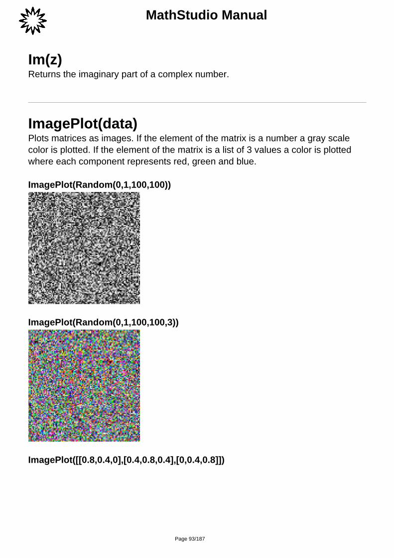
ImagePlot(data)Plots matrices as images. If the element of the matrix is a number a gray scalecolor is plotted. If the element of the matrix is a list of 3 values a color is plottedwhere each component represents red, green and blue.
ImagePlot(Random(0,1,100,100))
ImagePlot(Random(0,1,100,100,3))
ImagePlot([[0.8,0.4,0],[0.4,0.8,0.4],[0,0.4,0.8]])
Page 93/187
MathStudio Manual
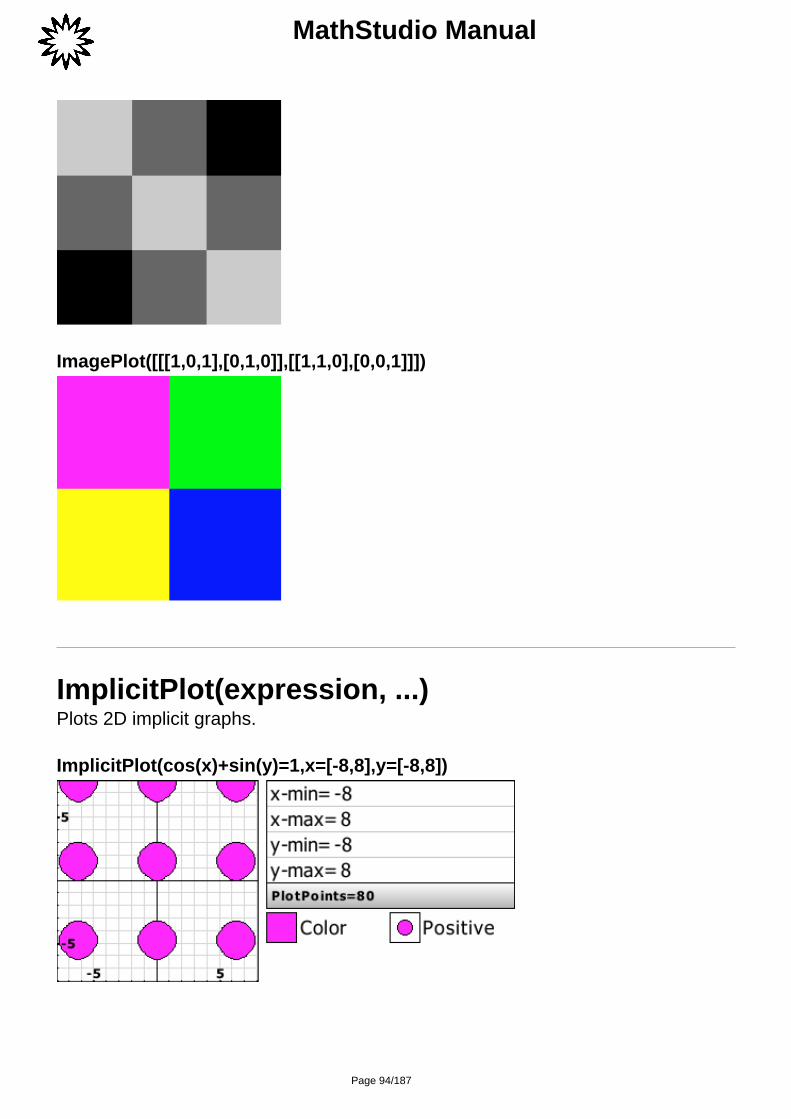
ImagePlot([[[1,0,1],[0,1,0]],[[1,1,0],[0,0,1]]])
ImplicitPlot(expression, ...)Plots 2D implicit graphs.
ImplicitPlot(cos(x)+sin(y)=1,x=[-8,8],y=[-8,8])
Page 94/187

MathStudio Manual
ImplicitPlot(sin(x^2+y^2)=0, numbers=0)
Include(filename)Includes the scripts from SpaceTime files.
Insert(expression, item, position)Inserts an expression into a list or string at the specified position.
Insert("acde",b,2)
Insert([1,2,4,5],333,3)
Integrate(f(x), x, [a], [b])Finds the indefinite integral of the given function.
If parameters a and b are given then Integrate returns the definite integral. Youcan also use NIntegrate for definite integrals.
Simple IntegralsIntegrate(x^2+3x-6,x)
Page 95/187

MathStudio Manual
Integrate(ln(x)+1/x,x)
Integrate(exp(x)*sin(x),x)
Integrate(sin(3x)*cos(4x-2),x)
Integrate((x+1)/(x^2+1),x)
Integrate(1/(a*x^2+b*x),x)
Integrate(1/cos(x),x)
Integrate(1/tan(x),x)
Integrate(sin(x)^2*cos(x),x)
Integrate(sin(3x)/sin(x),x)
Page 96/187

MathStudio Manual
Integrals with trigonometric functionsIntegrate(-3/x^2+sin(x)/(1-sin(x)),x)
Integrate((1+2cos(x))/(1+2sin(x)),x)
Integrate(cos(a*x+b)/x^3,x)
Integrate(2/sin(2x),x)
Integrate(sin(x)/sqrt(1+cos(x)),x)
Integrate(2sin(3x)/sqrt(5+cos(3x))^3,x)
Integrate(x*cos(x)^3/(3+sin(x)),x)
Integrals with reciprocalsIntegrate(1/(1+sqrt(x)),x)
Integrate(x+1/(x^(1/4)*sqrt(1+sqrt(x))),x)
Page 97/187
MathStudio Manual
Integrate(sqrt(x^2-y),x)
Integrate(sqrt(x)/sqrt(x-2),x)
Integrate(sqrt(2x)/sqrt(x-1),x)
Integrate(sqrt(2x-1)/sqrt(x+2),x)
Integrate((3x+2)/sqrt(x-9),x)
Integrate(x^(1/4)/(1+sqrt(x)),x)
Integrate(sqrt(x)/(sqrt(x)+sqrt(x+1)),x)
Integrate((1+x^4)/(1+x^3),x)
Page 98/187

MathStudio Manual
Integrate(1/(1+x^3),x)
Integrate(1/(a*x^2+b)^2,x)
Integrals with polynomialsIntegrate(1/sqrt(1+sqrt(x)),x)
Integrate(1/(x^2*sqrt(4+x^2)),x)
Integrate(1/(x^4+4),x)
Integrate(x/(x^2+2x+5),x)
Integrate(x^(2/3)/(x-1),x)
Page 99/187

MathStudio Manual
Integrate(x^2/(x^2+3x+1),x)
Integrate(x^3/(7x^2+2x-3),x)
Integrate(x^4*(x+1)^(5/3),x)
Integrals with logarithmic functionsIntegrate(ln(2*x+1),x)
Integrate((x^2+3x)*ln(x),x)
Integrate(ln(x)/(x+3)^2,x)
Integrate(sin(x)*ln(cos(x)),x)
Page 100/187

MathStudio Manual
Integrate(ln(x)/sqrt(x+1),x)
Integrate(ln(x^2+3)/(x+1)^2,x)
Integrate(x^4*ln(x)^(5/2),x)
Integrate(x^3/ln(x)^(5/2),x)
Integrals with exponential functionsIntegral(exp(x)/((exp(x)-1)*(exp(x)+3)),x)
Integral(exp(3x)/(1+exp(2x)),x)
Integral(exp(-2x)/(1+exp(-2x)),x)
Integral(1/(1+exp(2x)),x)
Page 101/187

MathStudio Manual
Integral(exp(5x)/(1+exp(2x)),x)
Integral(exp(x+a)/(1+exp(2x+1)),x)
Integral(sqrt(1+exp(3x)),x)
Integral(1/sqrt(1+exp(3x)),x)
Integrate(exp(-3*x^2),x)
Integrals with inverse trigonometric functionsIntegrate(asin(2x-1),x)
Integrate(x*asinh(x-7),x)
Integrate(x^2*asin(3x),x)
Page 102/187

MathStudio Manual
Integrate(x^3*atanh(x-1),x)
Integrate(x^4*atan(x),x)
Integrate((x+1/x^2)*atan(x),x)
Integrate(x*asin(x-2),x)
Integrals with forced substitutionIntegrate(sqrt(2+sqrt(4+sqrt(x))),x,u=2+sqrt(4+sqrt(x)))
Integrate(sqrt(2+sqrt(1+sqrt(x))),x,u=2+sqrt(1+sqrt(x)))
Integrate(sqrt(2+sqrt(4+sqrt(x))),x,u=2+sqrt(4+sqrt(x)))
Page 103/187

MathStudio Manual
Integrate((1+sqrt(x-3))^(1/3),x,u=sqrt(x-3))
Integrate(ln(x+1)^2*x,x,u=x+1)
Integrate(asin(sqrt(x)),x,u=sqrt(x),1)
Page 104/187

MathStudio Manual
Inverse(A)Calculates the inverse of a given square matrix A.
Inverse([[1,5,6],[2,4,5],[1,1,7]])
Inverse([[a,b],[c,d]])
InverseNormal(p, [mu], [sigma])Computes the x value to a corresponding area p using the inverse cumulativenormal distribution function.
invGudermannian(z)Returns the inverse Gudermannian function of z.
invGudermannian(0)
Page 105/187

MathStudio Manual
invGudermannian(-\pi/2)
invGudermannian(\pi/2)
invGudermannian(1)
number(invGudermannian(1))
invGudermannian(1.5)
Diff(invGudermannian(x),x)
Series(invGudermannian(x),x,8)
iPart(z)Returns the integer part of z.
iPart(4/3)
iPart(1.234)
iPart(-9.8765)
Page 106/187

MathStudio Manual
IsList(expression)Returns 1 if the expression is a list or returns 0 if the expression is not a list.
IsMatrix(expression)Returns 1 if the expression is a matrix or returns 0 if the expression is not amatrix.
IsNumber(expression)Returns 1 if the expression is a real or complex number otherwise it returns 0.
IsPoly(expression)Returns 1 if the expression is a polynomial or returns 0 if it is not a polynomial.
IsPrime(n)Returns 1 if the number is prime or 0 if it is not prime.
Jacobian(function, [varlist], [point])Returns either the Jacobian matrix or the Jacobian determinant of a function list function(varlist) evaluated at point.
Jacobian(x^2-y^2,[x,y],[u,v])
Jacobian([x^2-y^2,2x*y,3*x^2*y],[x,y],[a,b])
Page 107/187

MathStudio Manual
Jacobian([f(x,y,z),g(x,y,z),h(x,y,z)],[x,y,z])
Jacobian([x@1,5x3,4x@2^2-2*x@3,x@3*sin(x@1)],[x@1,x@2,x@3])
JuliaPlot(expression, ...)Plots a julia set fractal.
JuliaPlot(z^2+c,re=-0.7017,im=-0.3842)
Page 108/187

MathStudio Manual
JuliaPlot(z^3+c, re=-0.48, im=-0.61)
JuliaPlot(z^2+c,re=0.285,im=0.01)
JuliaPlot(z^2+c,re=-0.4,im=0.6)
Page 109/187

MathStudio Manual
KelvinBei(v, z)Calculates KelvinBei(v,z).
KelvinBei(0,z)
KelvinBei(1,z)
KelvinBei(1/2,z)
KelvinBei(3,2-\im)
KelvinBer(v, z)Calculates KelvinBer(v,z).
Page 110/187

MathStudio Manual
KelvinBer(0,z)
KelvinBer(1,z)
KelvinBer(1/2,z)
KelvinBer(3,5+\im)
Expand(Diff(KelvinBer(0,z),z))
KelvinKei(v, z)Calculates KelvinKei(v,z).
KelvinKei(0,z)
KelvinKei(-1,z)
Page 111/187

MathStudio Manual
KelvinKei(-1/2,z)
KelvinKei(3,sqrt(2)-\im/3)
KelvinKer(v, z)Calculates KelvinKer(v,z).
KelvinKer(0,z)
KelvinKer(-1,z)
KelvinKer(-1/2,z)
KelvinKer(3,sqrt(2)-\im/3)
Expand(Diff(KelvinKer(1,z),z))
Page 112/187

MathStudio Manual
LaguerreL(n, z)Returns the Laguerre polynomial.
Plot(LaguerreL(1,x),LaguerreL(2,x),LaguerreL(3,x),LaguerreL(4,x),LaguerreL(5,x),x=[-1,5],y=[-4,4],color=[red,yellow,green,blue,purple],numbers=2)
LambertW(z)Calculates the LambertW function of z.
LambertW(0)
LambertW(-1/\e)
LambertW(-\pi/2)
Solve(LambertW(x)=1.3267246652422002,x,1)
Diff(LambertW(3x+2),x)
Page 113/187
MathStudio Manual
Series(LambertW(2x),x,6)
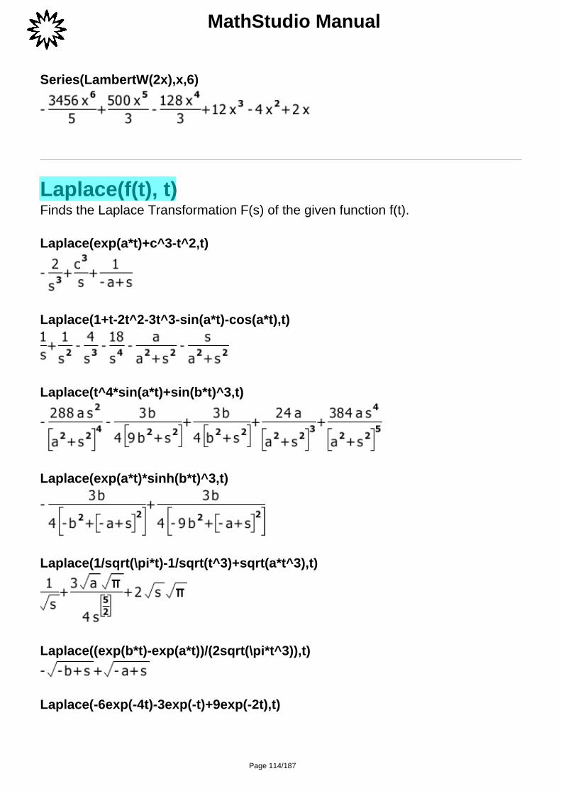
Laplace(f(t), t)Finds the Laplace Transformation F(s) of the given function f(t).
Laplace(exp(a*t)+c^3-t^2,t)
Laplace(1+t-2t^2-3t^3-sin(a*t)-cos(a*t),t)
Laplace(t^4*sin(a*t)+sin(b*t)^3,t)
Laplace(exp(a*t)*sinh(b*t)^3,t)
Laplace(1/sqrt(\pi*t)-1/sqrt(t^3)+sqrt(a*t^3),t)
Laplace((exp(b*t)-exp(a*t))/(2sqrt(\pi*t^3)),t)
Laplace(-6exp(-4t)-3exp(-t)+9exp(-2t),t)
Page 114/187

MathStudio Manual
Laplace(t^2*exp(-a*t)/2,t)
Laplace(Heaviside(t-3)*sin(c*(t-3)),t)
Laplace(BesselJ(0,a*t)+BesselJ(0,2sqrt(k*t)),t)
Laplace(BesselJ(1,a*t),t)
Laplace(BesselI(1,a*t),t)
Laplace(Erf(a*t),t)
Laplace(Erf(a*sqrt(t)),t)
Page 115/187

MathStudio Manual
Laplace(Erfc(a*sqrt(b*t)),t)
Expand(Laplace((t+3)^(3/2),t))
Laplace(f(t)/t,t)
Laplace(t^3*f(t),t)
Laplace(R*i(t)+L*d(i(t),t)=u(t),t)
Solve_Equation(Laplace(R*i(t)+L*d(i(t), t)=u(t), t), I(s))
Laplace(f(t)*sin(3t),t)
Laplace(t^4*f(t)*sin(3t),t)
Laplace(f(t)*cos(2t)/t,t)
Page 116/187

MathStudio Manual
Laplace(R*i(t)+1/C*I(i(t),t)=U,t)
Solve_Equation(Laplace(R*i(t)+1/C*I(i(t),t)=U(t),t),I(s))
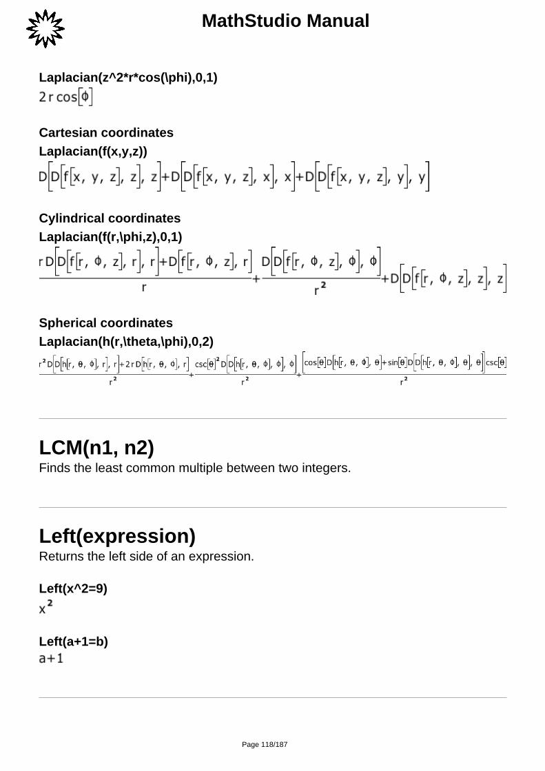
Laplacian(function, [varlist], [mode])Returns the Laplacian of the function.
This is normally denoted as Laplacian(F) = ?2F
Laplacian(x^2+y^2+z^2)
Laplacian(x*y/z)
Laplacian(sin(x)*exp(y)/ln(z))
Laplacian(r*sin(\theta)*cos(\phi),0,2)
Page 117/187
MathStudio Manual
Laplacian(z^2*r*cos(\phi),0,1)
Cartesian coordinatesLaplacian(f(x,y,z))
Cylindrical coordinatesLaplacian(f(r,\phi,z),0,1)
Spherical coordinatesLaplacian(h(r,\theta,\phi),0,2)
LCM(n1, n2)Finds the least common multiple between two integers.
Left(expression)Returns the left side of an expression.
Left(x^2=9)
Left(a+1=b)
Page 118/187

MathStudio Manual
LegendreP(n, z)Returns the Legendre polynomial or Legendre function of the first kind.
LegendreP(n,0)
LegendreP(n,1)
LegendreP(0,z)
LegendreP(1,z)
LegendreP(7,z)
LegendreP(7,1/2)
LegendreP(7,-1/2z)
LegendreP(4,z+1/2)
LegendreQ(n, z)
Page 119/187

MathStudio Manual
Returns the Legendre function of the second kind.
Plot(LegendreQ(1, x), LegendreQ(2, x), LegendreQ(3, x), LegendreQ(4, x),LegendreQ(5, x), x=[-1, 1], y=[-1, 1], color=[red, yellow, green, blue, purple],numbers=4)
Length(expression)Returns the length of the expression.
Length([1, 2, 3, 4, 5, 6])
Length([[1,2,3],[4,5,6]])
Length(a)
Length(a+b+c)
Li(x)Finds the Logarithmic Integral of x.
Li(3)
Page 120/187

MathStudio Manual
Plot(Li(x))
Limit(function, variable, point, [direction])Returns the limit of function as variable approaches point from the directiondirection.
The default value of direction is right side (+1).
Limit((3x-15)/\sqrt(x^2-10x+25),x,5,1)
Limit((3x-15)/\sqrt(x^2-10x+25),x,5,-1)
Limit((atan(x)-\pi/4)/\sqrt(1-x^2),x,1)
Limit((3-3tan(x))/(sin(x)-cos(x)),x,\pi/4)
Limit(-1/x,x,0)
Limit(1/x,x,\inf)
Page 121/187

MathStudio Manual
Limit(3z+p*(1+5m/x)^(a*x)+f*x^(1/x)-g*(1+1/x^2)^(d*x)-h*((x-7*n)/x)^(b*x),x,\inf)
Limit(-n^n/n!,n,\inf)
Limit(n!/4^n,n,\inf)
Limit(n!/n^n,n,\inf)
Limit(1^n/n^5,n,\inf)
Limit((3*sin(\pi*x) - sin(3*\pi*x))/x^3,x,0)
Limit(\sqrt(sin(3*\pi*x)/x^3 - 3*sin(\pi*x)/x^3),x,0)
Limit(cos(a*x)/x^2 - cos(b*x)/x^2,x,0)
Limit(2sin(a*x)/(x-sin(x))-sin(2a*x)/(x-sin(x)),x,0)
Limit((2sin(x)-sin(2x))/(b*x-sin(b*x))+(2sin(p*x)-sin(2p*x))/(q*x-sin(q*x)),x,0)
Page 122/187
MathStudio Manual
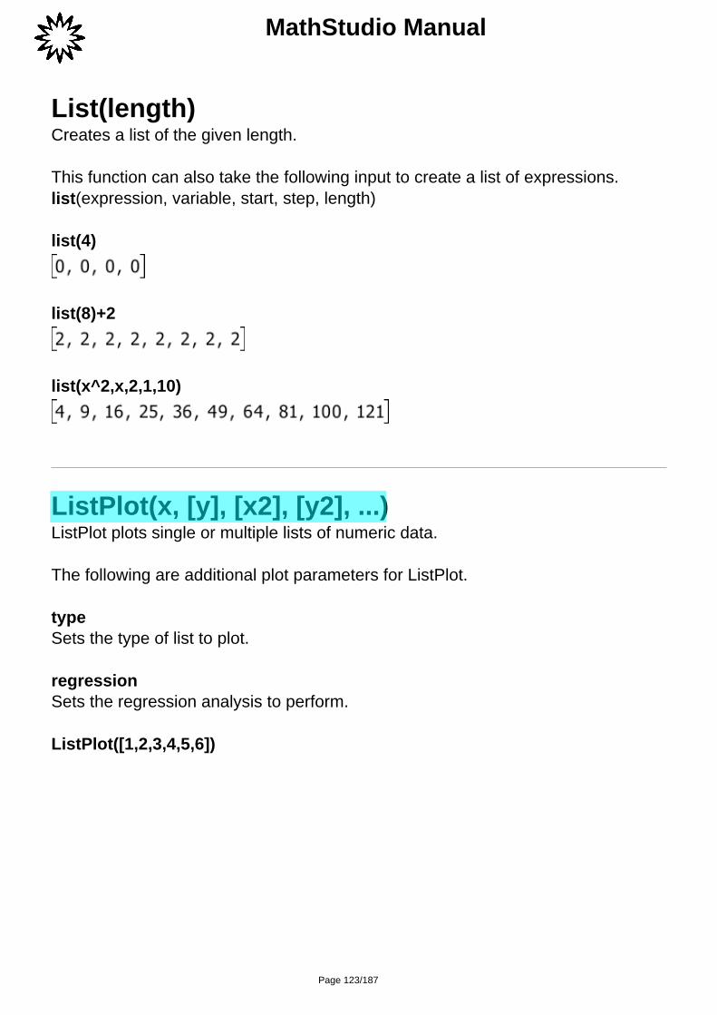
List(length)Creates a list of the given length.
This function can also take the following input to create a list of expressions.list(expression, variable, start, step, length)
list(4)
list(8)+2
list(x^2,x,2,1,10)
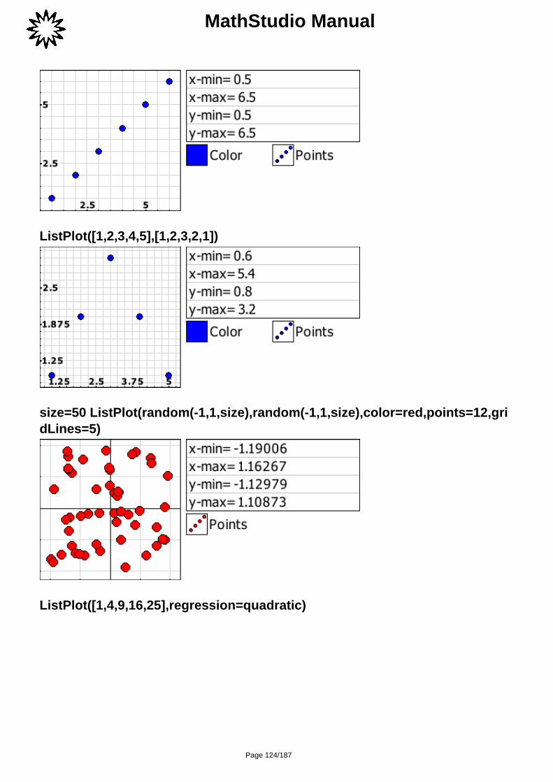
ListPlot(x, [y], [x2], [y2], ...)ListPlot plots single or multiple lists of numeric data.
The following are additional plot parameters for ListPlot.
typeSets the type of list to plot.
regressionSets the regression analysis to perform.
ListPlot([1,2,3,4,5,6])
Page 123/187
MathStudio Manual
ListPlot([1,2,3,4,5],[1,2,3,2,1])
size=50 ListPlot(random(-1,1,size),random(-1,1,size),color=red,points=12,gridLines=5)
ListPlot([1,4,9,16,25],regression=quadratic)
Page 124/187

MathStudio Manual
ListPlot([1,1,3,3,4,4,4,5,5,5,5,6,6,7,8],type=bar,color=red,gridLines=0,color=skyBlue,lineColor=blue)
ListPlot(random(2,10,40),type=box,numbers=0,gridLines=10)
ListPlot(random(0,2,20),type=probability)
Page 125/187

MathStudio Manual
ListPlot3D(x, y, z, [x2], [y2], [z2], ...)Plots 3D list data.
ListPlot3D(1:12,1:12,1:12)
ListPlot3D(Random(0,1,3,50), points=2)
Page 126/187

MathStudio Manual
Ln(z)Returns the natural logarithm (base: e) of the given number z.
Plot(ln(x),x=[-2,8],y=[-5,5])
ln(2)
ln(\e)
ln(-5)
LnGamma(z)Returns the Log Gamma(z) function.
LnGamma(z)
LnGamma(10)
LnGamma(20)
Page 127/187

MathStudio Manual
LnGamma(10000)
LnGamma(-5)
LnGamma(3z)
LnGamma(z-3)
LnGamma(2z+4)
LoadList(filename)This function loads data from a text file (.txt) and outputs a list. The data can betab or comma delineated.
LoadMatrix(filename)This function loads data from a text file (.txt) and outputs a matrix.
Log([n], z)
Page 128/187

MathStudio Manual
Returns the common or Briggs logarithm (base: 10) of the given number z.
log(2)
log(1000)
log(1\sci-5)
log(\e)
Loop(variable, start, end, [step=1])Loops through a block of code.
If the step is positive this functions loops until the variable initially set to start is greater than end.
If the step is negative this functions loops until the variable initially set to start is less than end.
length=10 a=list(length) loop(i,1,length) a(i)=i^2 end a
Lucas(n, [z])Returns the nth Lucas number.
If z is given, returns the Lucas polynomial of z.
Lucas(6,a)
Page 129/187

MathStudio Manual
LUDecomposition(matrix, [mode])Returns the matrix decomposition as the product of a lower triangular matrix andan upper triangular matrix.
LUDecomposition([[1,2],[3,4]])
Matrix(rows, [columns])Creates a matrix.
matrix(3)
matrix(2,3)
matrix(2,6)+2
Max(list)
Page 130/187
MathStudio Manual
Finds the largest number in a list.
Max([3,0,-5,0.5,4])
Mean(list)Finds the average of a given list of numbers.
Mean([3,0,-5,0.5,4])
Message(string)This will stop all computations and display a message.
n=5 if(n>0) Message("Positive") else if(n
Min(list)Finds the smallest number in a list.
Min([3,0,-5,0.5,4])
Mod(m, n)Calculates the following formula.m-n*floor(m/n)
Page 131/187

MathStudio Manual
The sign of mod(m,n) always equals the sign of n.
Multinomial(nList)Finds the Multinomial coefficient.
Multinomial([n@1,n@2,n@3])/Multinomial([n@1-1,n@2+2,n@3-1])
Multinomial([n@1,n@2,n@3])/Multinomial([n@1+1,n@2-1,n@3])
Multinomial([2+\im,-1+2\im,4.5-3\im])
Multinomial([7/2,5/2,3/2])
Multinomial([n,3,3])
Multinomial([n,3])
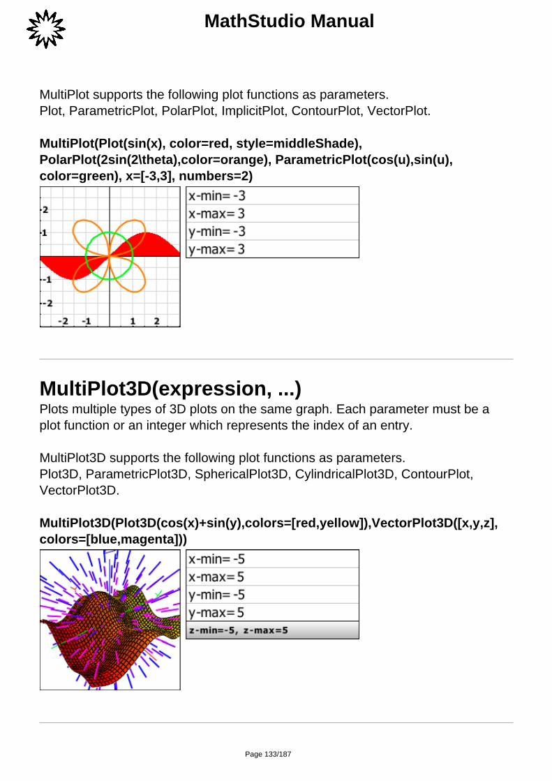
MultiPlot(plot1, plot2, ...)Plots multiple types of 2D plots on the same graph. Each parameter must be aplot function or an integer which represents the index of an entry.
Page 132/187
MathStudio Manual
MultiPlot supports the following plot functions as parameters.Plot, ParametricPlot, PolarPlot, ImplicitPlot, ContourPlot, VectorPlot.
MultiPlot(Plot(sin(x), color=red, style=middleShade),PolarPlot(2sin(2\theta),color=orange), ParametricPlot(cos(u),sin(u),color=green), x=[-3,3], numbers=2)
MultiPlot3D(expression, ...)Plots multiple types of 3D plots on the same graph. Each parameter must be aplot function or an integer which represents the index of an entry.
MultiPlot3D supports the following plot functions as parameters.Plot3D, ParametricPlot3D, SphericalPlot3D, CylindricalPlot3D, ContourPlot,VectorPlot3D.
MultiPlot3D(Plot3D(cos(x)+sin(y),colors=[red,yellow]),VectorPlot3D([x,y,z],colors=[blue,magenta]))
Page 133/187

MathStudio Manual
nCr(n, r)Returns the number of unordered subsets of r elements out of a set of n elements
nCr(n,r) = n! / ((n-r)! * r!)
nFactors(n)Finds all the dividing factors of the given number n. The result is returned as a list.
nFactors(6)
nFactors(99)
nFactors(997)
nFactors(12345)
NIntegrate(f(x), x, a, b)Finds the definite integral of the given function by a numerical integration method.The limits of integration are a (lower limit) and b (upper) limit.
NIntegrate(sin(x),x,0,\pi)
NIntegrate(cos(x),x,-\pi/2,\pi/2)
Page 134/187

MathStudio Manual
Norm(z)Returns the norm of the given vector A.
Norm([x,y,z])
Norm([1,5,6,3,6])
NormalCDF(lower, upper, [mu], [sigma])Computes the normal cumulative density function over the interval from lower to upper with mean mu and standard deviation sigma.
NormalPDF(x, mu, sigma)Computes either the normal probability density function at x with mean mu andstandard deviation sigma. The default values are mu = 0 and sigma = 1.
Plot(NormalPDF(x,0,0.2),NormalPDF(x,0,1.0),NormalPDF(x,-2,0.5),x=[-3,3],y=[-0.1,2.5])
nPr(n, r)
Page 135/187

MathStudio Manual
Returns the number of permutations of a subset of r elements from a set of nelements.
nPr(n,r) = n! / (n-r)!
nPrimes(n)Finds all prime factors and their exponent of a given number.
The result is returned as a nested list. The first number is the prime factor and thesecond number is the exponent.
1 * 2^1 * 5^1nPrimes(10)
1 * 31^1nPrimes(13)
1 * 2^3 * 5^2nPrimes(200)
1 * 3^2 * 11^1 * 101^1nPrimes(9999)
nRoot(z, n, [mode])Finds the nth root of a given value. All roots are returned as a list.
Page 136/187
MathStudio Manual
nRoot(z,n)
nRoot(-8,3)
nRoot(81,4)
nRoot(279841,4)
nRoot(279841,4,0)
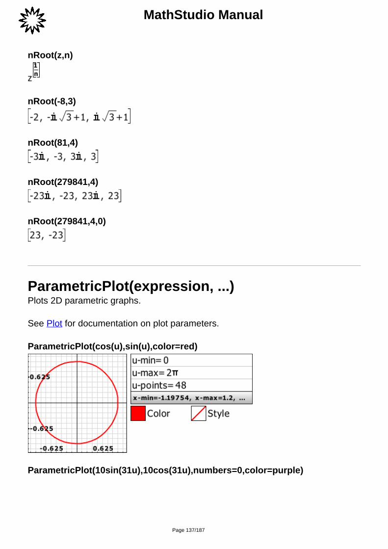
ParametricPlot(expression, ...)Plots 2D parametric graphs.
See Plot for documentation on plot parameters.
ParametricPlot(cos(u),sin(u),color=red)
ParametricPlot(10sin(31u),10cos(31u),numbers=0,color=purple)
Page 137/187

MathStudio Manual
ParametricPlot([sin(7u),sin(8u)], u=[0,2\pi,400], numbers=0, color=navyBlue)
ParametricPlot3D(expression, ...)Plots 3D parametric graphs.
c1=u/2 c2=v/2 c3=sin(c1) c4=sin(v) c5=cos(c1) c6=sin(2v) c7=2c8=c7+c5*c4-c3*c6 ParametricPlot3D(c8*cos(u),c8*sin(u),c3*c4+c5*c6,[u,0,2\pi,40],[v,0,2\pi,40],axis=0)
Page 138/187

MathStudio Manual
a=(1+0.4cos(v))cos(u) b=(1+0.4cos(v))sin(u) c=0.4sin(v)ParametricPlot3D([[c,b+1,a],[a,b,c]], colors=[[orange,red],[blue,skyBlue]],axis=0,u=[0,2\pi,30],v=[0,2\pi,30])
Part(expression, n)Returns the nth part of the expression.
This function can be used to iterate recursively through an entire expression.
When n=0 the part of the expression is returned as a string.
Part(a+b,1)
Part(a+b,2)
Part(a+b,0)
Part(sin(x),1)
Part(sin(x),0)
Part((x+1)^2,1)
Page 139/187
MathStudio Manual
Part((x+1)^2,0)
Part(a+b+c+d+e,3)
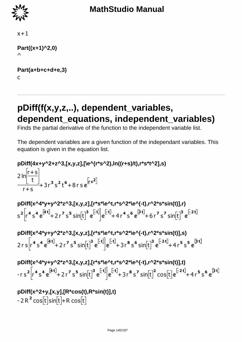
pDiff(f(x,y,z,..), dependent_variables,dependent_equations, independent_variables)Finds the partial derivative of the function to the independent variable list.
The dependent variables are a given function of the independant variables. Thisequation is given in the equation list.
pDiff(4x+y^2+z^3,[x,y,z],[\e^(r*s^2),ln((r+s)/t),r*s*t^2],s)
pDiff(x^4*y+y^2*z^3,[x,y,z],[r*s*\e^t,r*s^2*\e^(-t),r^2*s*sin(t)],r)
pDiff(x^4*y+y^2*z^3,[x,y,z],[r*s*\e^t,r*s^2*\e^(-t),r^2*s*sin(t)],s)
pDiff(x^4*y+y^2*z^3,[x,y,z],[r*s*\e^t,r*s^2*\e^(-t),r^2*s*sin(t)],t)
pDiff(x^2+y,[x,y],[R*cos(t),R*sin(t)],t)
Page 140/187

MathStudio Manual
pDiff(x^2+y^3-5,[x,y],[R*cos(t),R*sin(t)],t)
pDiff(f(x,y),[x,y],[g(t),h(t)],t)
pDiff(x^4*y^2,[x,y],[sin(t),t^2],t)
Pi_Digits(n)Calculates Pi up to the requested number of digits.
The maximum number of digits which can be calculated is 500.
Please note that the larger the number n, the slower the calculation.
Pi_Digits(10)
Pi_Digits(20)
Pi_Digits(30)
Pi_Digits(Scroll(n,1,50))
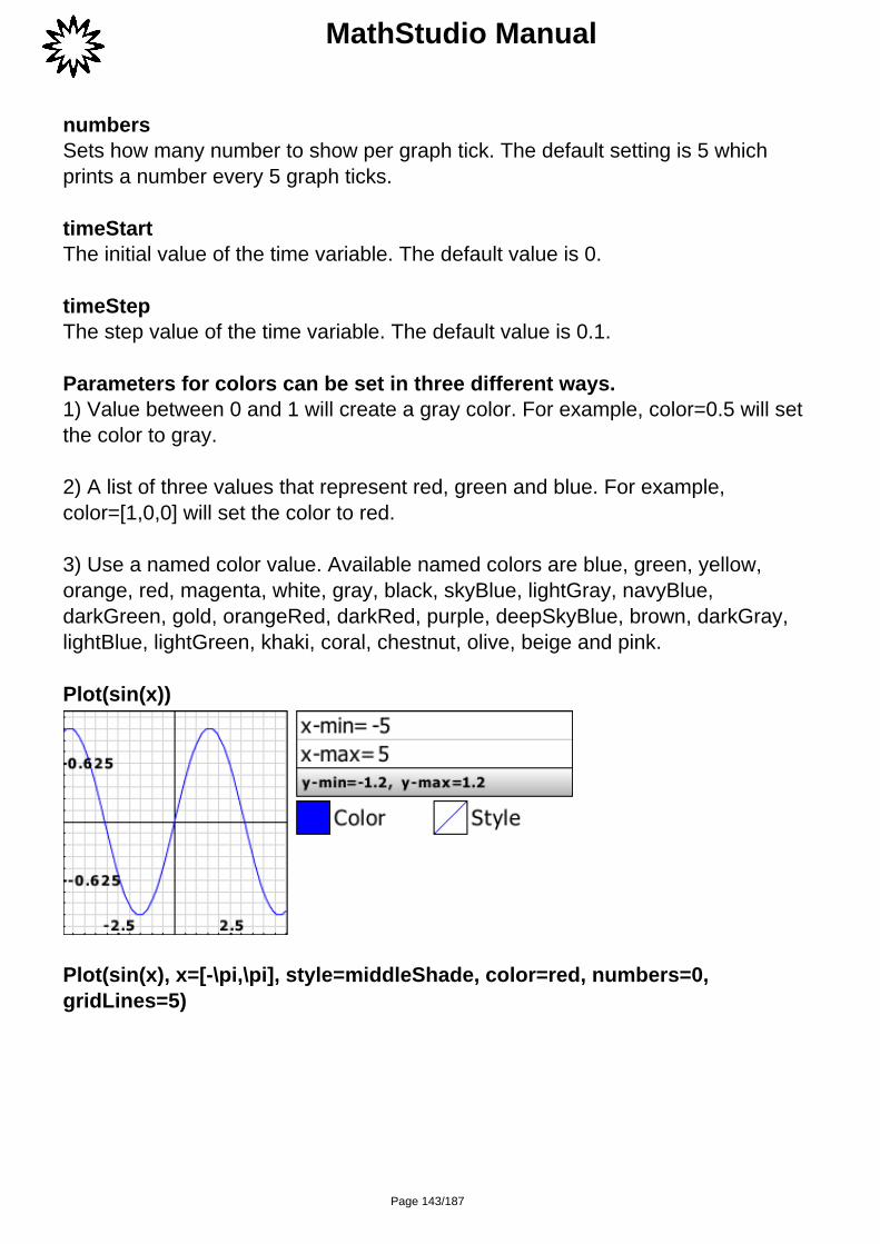
Plot(expression, ...)Plots 2D function graphs. This function can also have many additional parameters
Page 141/187

MathStudio Manual
which are entered in the form of parameter=value.
The following parameters can be set to a single value or a list of values formultiple plots.
alphaSets the transparency of the plot from 0 (completely transparent) to 1 (fullyopaque). The default value is 1.
colorSets the color of the plot.
pointsSets the size of the points.
linesSets the size of the lines.
styleSet the style of the plot.
The following parameters are used for the graph and can only be set to a singlevalue.
backgroundColorSets the background color of the graph.
axisColorSets the axis color of the graph.
textColorSets the text color of the graph.
gridLinesSets how many grid lines to show on the graph.
gridColorSets the color of the grid lines.
Page 142/187
MathStudio Manual
numbersSets how many number to show per graph tick. The default setting is 5 whichprints a number every 5 graph ticks.
timeStartThe initial value of the time variable. The default value is 0.
timeStepThe step value of the time variable. The default value is 0.1.
Parameters for colors can be set in three different ways.1) Value between 0 and 1 will create a gray color. For example, color=0.5 will setthe color to gray.
2) A list of three values that represent red, green and blue. For example,color=[1,0,0] will set the color to red.
3) Use a named color value. Available named colors are blue, green, yellow,orange, red, magenta, white, gray, black, skyBlue, lightGray, navyBlue,darkGreen, gold, orangeRed, darkRed, purple, deepSkyBlue, brown, darkGray,lightBlue, lightGreen, khaki, coral, chestnut, olive, beige and pink.
Plot(sin(x))
Plot(sin(x), x=[-\pi,\pi], style=middleShade, color=red, numbers=0,gridLines=5)
Page 143/187

MathStudio Manual
Plot([x^2,-x^2],colors=[navyBlue,deepSkyBlue],style=[topShade,bottomShade],alpha=0.7,gridLines=10,numbers=2)
Plot3D(expression, ...)Plots 3D function graphs. This function can also have many additional parameterswhich are entered in the form of parameter=value.
The following parameters can be set to a single value or a list of values formultiple plots.See examples below.
colorsSets the colors of the plot. This can be a list of up to 4 colors or a list of up to 6colors if the gradient parameter is set to height. See example below.
pointsSets the size of the points.
Page 144/187

MathStudio Manual
pointColorSets the color of the points.
linesSets the size of the lines.
lineColorSets the color of the lines.
solidSets whether to use solid shading. This takes a value of 0 or 1.
gradientSets how to color the graph.height colors the plot based on the height of the points.
The following parameters are used for the graph and can only be set to a singlevalue.
backgroundColorSets the background color of the graph.
axisColorXSets the x-axis color of the graph.
axisColorYSets the y-axis color of the graph.
axisColorZSets the z-axis color of the graph.
axisColorSets all axis colors of the graph.
shadeThis can take smooth for smooth shading or flat for flat shading. The default valueis smooth.
timeStart
Page 145/187

MathStudio Manual
The initial value of the time variable. The default value is 0.
timeStepThe step value of the time variable. The default value is 0.1.
Parameters for colors can be set in three different ways.
1) Value between 0 and 1 will create a gray color. For example, color=0.5 will setthe color to gray.
2) A list of three values that represent red, green and blue. For example,color=[1,0,0] will set the color to red.
3) Use a named color value. Available named colors are blue, green, yellow,orange, red, magenta, white, gray, black, skyBlue, lightGray, navyBlue,darkGreen, gold, orangeRed, darkRed, purple, deepSkyBlue, brown, darkGray,lightBlue, lightGreen, khaki, coral, chestnut, olive, beige and pink.
Plot3D(cos(x)+sin(y),colors=[yellow,red])
Plot3D(cos(x)+sin(y), gradient=height, axis=0,colors=[blue,green,yellow,red])
Page 146/187

MathStudio Manual
r=sqrt(x^2+y^2) Plot3D(sin(x^2+3y^2)/(0.1+r^2)+(x^2+5y^2)*exp(1-r^2)/2,gradient=height,colors=[red,yellow,green,skyBlue,blue],backgroundColor=black,x=[-3,3],y=[-3,3],z=[-3,3],axis=0)
Plot3D(sqrt(abs(x*y)),-sqrt(abs(x*y)),colors=[[red,yellow],[blue,green]])
Pochhammer(n, k)Finds the value of n*(n+1)*(n+2)*..*(n+k-1)
Page 147/187

MathStudio Manual
Pochhammer(n,5)
Pochhammer(n,-5)
Pochhammer(3,k)
Pochhammer(n,k)
Pochhammer(n,k-1)
Pochhammer(n-1,k)
Pochhammer(n-1,k-1)
Pochhammer(n-1,k)/Pochhammer(n-1,k-1)
Pochhammer(-10,5)
Pochhammer(5,-2)
Page 148/187

MathStudio Manual
PoissonCDF(mu, x)Computes the cumulative Poisson distribution at x with mean mu.
PoissonPDF(mu, x)Computes the Poisson distribution at x with mean mu.
Plot(PoissonPDF(1,x),PoissonPDF(1.2,x),PoissonPDF(1.3,x),PoissonPDF(1.4,x),PoissonPDF(1.5,x))
PolarPlot(expression, ...)Plots 2D polar plots.
See Plot for documentation on plot parameters.
PolarPlot(sin(2\theta))
Page 149/187

MathStudio Manual
PolarPlot(\e^sin(\theta)-2cos(4\theta)+sin(1/24(-\pi+2\theta))^5,\theta=[0,21\pi,1000], color=magenta)
PolyDivide(f(z), g(z))Returns both the quotient and remainder from the polynomial division ofnumerator f(z) and denominator g(z).
Both numerator and denominator should be polynomial functions.
The returned result is a list with the first term the quotient and the second term theremainder.
PolyDivide(x^2+x+6,x+7)
PolyDivide(4x^3-x^2+x+6,x+1)
Page 150/187

MathStudio Manual
PolyDivide(5x^7-3x^2+6,x^3-1)
PolyFit(pList, var)Finds a unique polynomial function of order N-1 through the given N data points.
Finds the line between the point [1,3] and [5,7]PolyFit([[1,3],[5,7]])
Plot(x+2)
Finds the parabolic curve through the points [2,4], [3,1], [5,7]PolyFit([[2,4],[3,1],[5,10]])
Plot(2.5x^2-15.5x+25)
Page 151/187

MathStudio Manual
Finds the cubic curve through the points [0,1], [2,5], [3,4], [5,7]PolyFit([[0,1],[2,5],[3,4],[5,7]])
Plot((11x^3)/30+(-17x^2)/6+(31x)/5+1)
PolyGamma(n, z)Returns the PolyGamma function.
PolyGamma(0,z)
PolyGamma(-1,z)
PolyGamma(2,2.5)
PolyGamma(3,-1/3)
PolyGamma(4,3z)
Page 152/187

MathStudio Manual
PolyGamma(2,z+3)
Diff(PolyGamma(n,z),z)
Solve(PolyGamma(1,x)=5)
Solve(PolyGamma(2,x)=10,x,[-1,0])
Plot(PolyGamma(1,x),x=[-10,10],y=[0,20])
Plot(PolyGamma(2,x),x=[-5,5],y=[-5,5])
Page 153/187

MathStudio Manual
PolyGCD(polynomial1, polynomial2)Finds the Greatest Common Divisor of two given polynomials.
The maximum number of polynomials that can be given inside PolyGCD isrestricted to two.
PolyGCD(3x^3-9x-6,x^2-4)
PolyGCD(75x^9-435x^8+852x^7-576x^6-663x^5+3027x^4-4911x^3+3402x^2-735x, 30x^6-192x^5+420x^4-354x^3+84x^2)
PolyGCD(x^4-1,x^3+1)
PolyGCD(x^2+2*x+1,x^2+3*x+2)
PolyGCD(x^2-2*x+1,x^3-1)
PolyGCD(s^4+s^3+12s^2+s+11,2s^3+5s^2+2s+5)
PolyGCD(t^4-59t^3-4560t^2+45500t+50000,t^2+31t+30)
PolyGCD(x^4+(sqrt(2)-3)x^3+(4-3sqrt(2))x^2+6(1+sqrt(2))x-12,x^3+(3+sqrt(2))x^2+(3sqrt(2)-2)x-6)
PolyLCM(polynomial1, polynomial2)Finds the Least Common Multiple of two given polynomials.
Page 154/187

MathStudio Manual
The maximum number of polynomials that can be given inside PolyLCM isrestricted to two.
PolyLCM(75x^9-435x^8+852x^7-576x^6-663x^5+3027x^4-4911x^3+3402x^2-735x,30x^6-192x^5+420x^4-354x^3+84x^2,0)
PolyLCM(x^3+x+1,x^2+3)
PolyLCM(4x^2-16,2x^2+2x-12)
PolyLCM(6x^3-5x^2-22x+24,6x^3-23x^2+29x-12)
PolyLCM(-x^2-x+6,-x^2+x+2)
PolyLCM(16x-4x^3,x^2+x-6)
PolyLog(n, z)Returns the Polylogarithm function of z.
PolyLog(-5,z)
PolyLog(-4,z)
Page 155/187

MathStudio Manual
PolyLog(-1,z)
PolyLog(0,z)
PolyLog(1,z)
PolyLog(1,5)
PolyLog(4,1)
PolyLog(n,1)
PowerExpand(expression)Expands powers.
PowerExpand(sqrt(a*b))
Page 156/187
MathStudio Manual
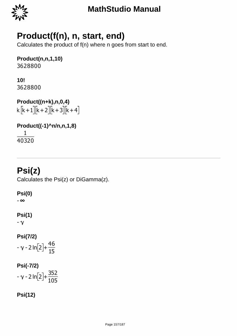
Product(f(n), n, start, end)Calculates the product of f(n) where n goes from start to end.
Product(n,n,1,10)
10!
Product((n+k),n,0,4)
Product((-1)^n/n,n,1,8)
Psi(z)Calculates the Psi(z) or DiGamma(z).
Psi(0)
Psi(1)
Psi(7/2)
Psi(-7/2)
Psi(12)
Page 157/187

MathStudio Manual
Psi(3-\im)
Psi(100/3)
Psi(2a+4)
Psi(2-3a)
Solve(Psi(x)=1,x,[0,5])
Solve(Psi(x)=-1/2,x,[-1,0])
Plot(Psi(x),x=[-5,5],y=[-20,20])
Page 158/187
MathStudio Manual
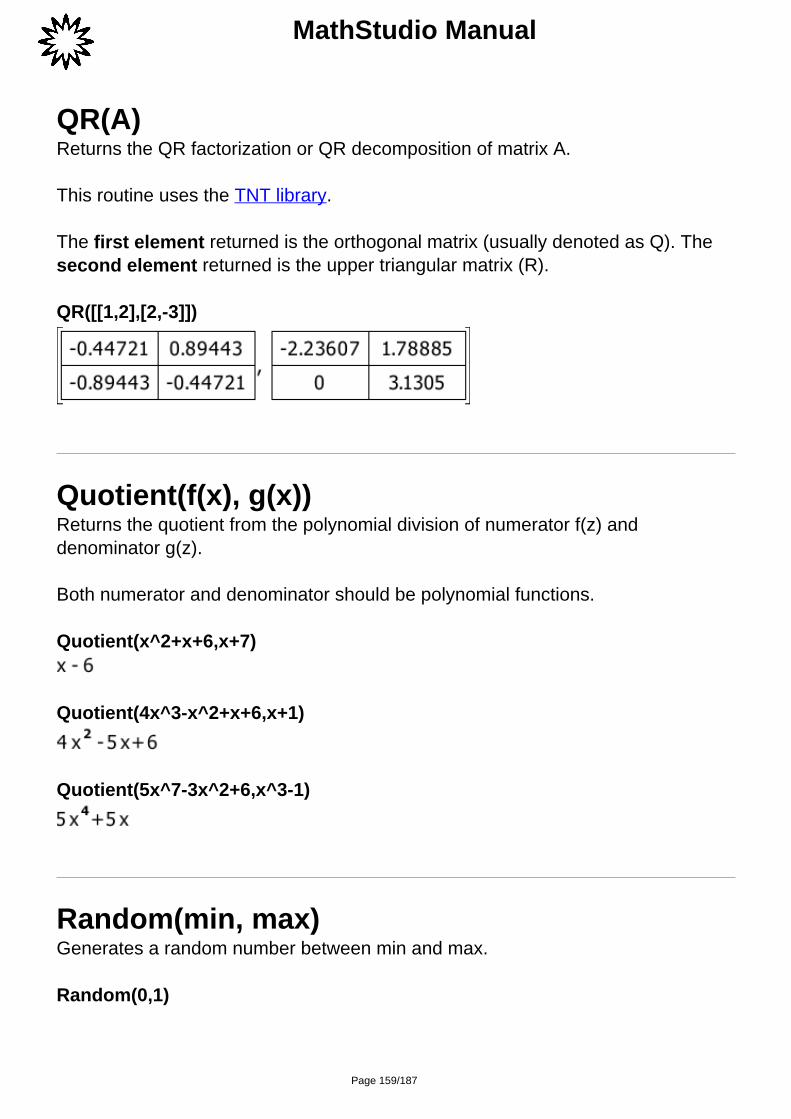
QR(A)Returns the QR factorization or QR decomposition of matrix A.
This routine uses the TNT library.
The first element returned is the orthogonal matrix (usually denoted as Q). The second element returned is the upper triangular matrix (R).
QR([[1,2],[2,-3]])
Quotient(f(x), g(x))Returns the quotient from the polynomial division of numerator f(z) anddenominator g(z).
Both numerator and denominator should be polynomial functions.
Quotient(x^2+x+6,x+7)
Quotient(4x^3-x^2+x+6,x+1)
Quotient(5x^7-3x^2+6,x^3-1)
Random(min, max)Generates a random number between min and max.
Random(0,1)
Page 159/187

MathStudio Manual
Random(0,1)
floor(Random(0,100))
Random(-1,1)
Re(z)Returns the real part of a complex number.
re(2+3\im)
Remainder(f(x), g(x))Returns the remainder from the polynomial division of numerator f(x) anddenominator g(x).
Both numerator and denominator should be polynomial functions.
Remainder(x^2+x+6,x+7)
Remainder(4x^3-x^2+x+6,x+1)
Remainder(5x^7-3x^2+6,x^3-1)
Page 160/187

MathStudio Manual
Replace(expression, old, new)Replaces an expression with another expression.
Replace(a+a^2,a^2,x^2)
Replace(sin(x),x,a^2)
Replace((x+1)(x+2),x+1,a)
Replace(sin(x)+cos(x),sin(x),tan(x))
Reshape(matrix)Reshapes a matrix to a different size. The new size of the matrix must have thesame number of elements as the original matrix.
Reshape([[1,2],[3,4]],1,4)
Reshape([[1,2],[3,4]],4,1)
Reshape([[1,2,3,4],[5,6,7,8],[9,10,11,12]],6,2)
Page 161/187

MathStudio Manual
Reshape([[1,2,3,4],[5,6,7,8],[9,10,11,12]],2,6)
Reverse(list)Sorts a list in descending order.
Reverse([3,2,1])
Reverse([a,A,b,B,c,C])
Right(expression)Returns the right side of an expression.
Right(x^2=9)
Right(a+1=b)
Page 162/187
MathStudio Manual
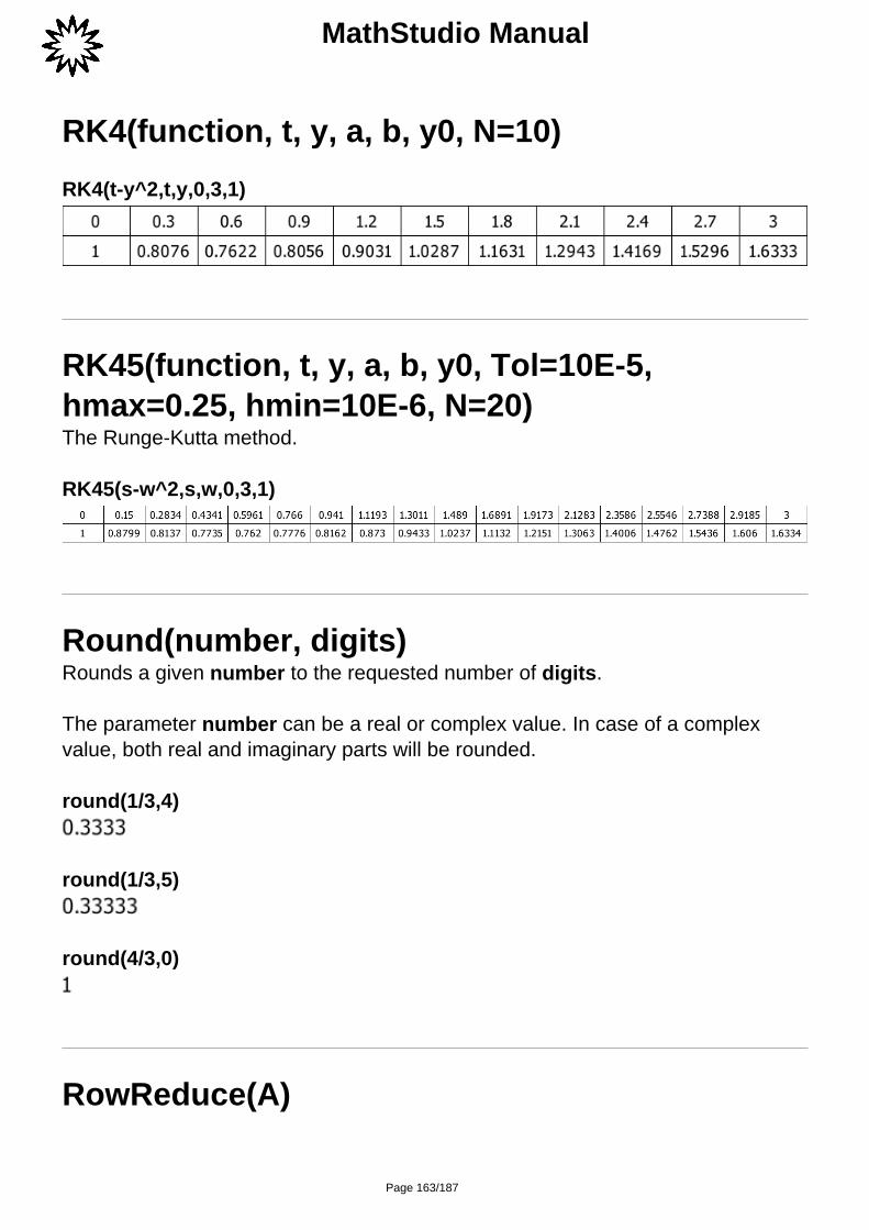
RK4(function, t, y, a, b, y0, N=10)
RK4(t-y^2,t,y,0,3,1)
RK45(function, t, y, a, b, y0, Tol=10E-5,hmax=0.25, hmin=10E-6, N=20)The Runge-Kutta method.
RK45(s-w^2,s,w,0,3,1)
Round(number, digits)Rounds a given number to the requested number of digits.
The parameter number can be a real or complex value. In case of a complexvalue, both real and imaginary parts will be rounded.
round(1/3,4)
round(1/3,5)
round(4/3,0)
RowReduce(A)
Page 163/187
MathStudio Manual
Performs a Gaussian elimination on the given matrix A.
Note: This function is equivalent to rref on the TI-Calculators.
RowReduce([[1,2,3],[2,5,6]])
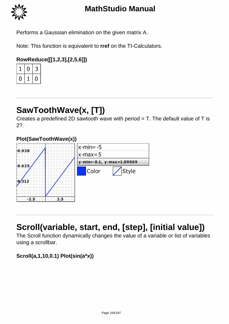
SawToothWave(x, [T])Creates a predefined 2D sawtooth wave with period = T. The default value of T is2?.
Plot(SawToothWave(x))
Scroll(variable, start, end, [step], [initial value])The Scroll function dynamically changes the value of a variable or list of variablesusing a scrollbar.
Scroll(a,1,10,0.1) Plot(sin(a*x))
Page 164/187

MathStudio Manual
Scroll(n, 1, 8) Expand((a+b)^n)
Sequence(f(x), x, start, end, step, [start term],[number of terms])Returns a sequence as a list.
Sequence(i,i,1,5)
Sequence(i^2,i,1,5)
Sequence(i,i,1,15,2)
Sequence(1/n^2,n,1,10)
Sequence(1/n^2,n,1,100,10,4,3)
Page 165/187

MathStudio Manual
Show sequence in reversed orderSequence(1/n^2,n,1,100,10,-4)
Show sequence in reversed orderSequence(1/n^2,n,1,100,10,-4,3)
Series(f(z), z, n)Finds the series expansion of a function around zero. This function is the same asthe Maclaurin series. This function can be used on all common and most specialfunctions.
Series(sin(x)+cos(x),x,8)
Series(exp(2z),z,10)
Series(tanh(3y),y,8)
Series(BesselJ(0,z),z,8)
Page 166/187

MathStudio Manual
Series(BesselJ(0,x)+BesselJ(1,x),x,6)
Series(asin(x),x,15)
Series(FresnelCos(z),z,8)
Series(Ei(x),x,7)
Shi(z)Finds the Hyperbolic Sine Integral of z.
Shi(1)
Shi(2+3\im)
Plot([Shi(x),Chi(x)],x=[-2,2],y=[-5,5])
Page 167/187

MathStudio Manual
Si(z)Sine Integral of z.
[Si(0), Si(\inf), Si(-\inf), Si(-x)]
a=list(3) b=list(3) loop(i, 1, 3) a(i)=Si(i) b(i)=Ci(i) end [a, b]
Si(2+\im)
Plot([Si(x), Ci(x)], x=[-10, 10], y=[-2, 2])
Sign(z)Returns the sign of a given value.
If z is a complex number, then sign returns z/abs(z).
sign(1.234)
sign(-9.8765)
Page 168/187
MathStudio Manual
sign(0)
sign(7/2+7/3\im)
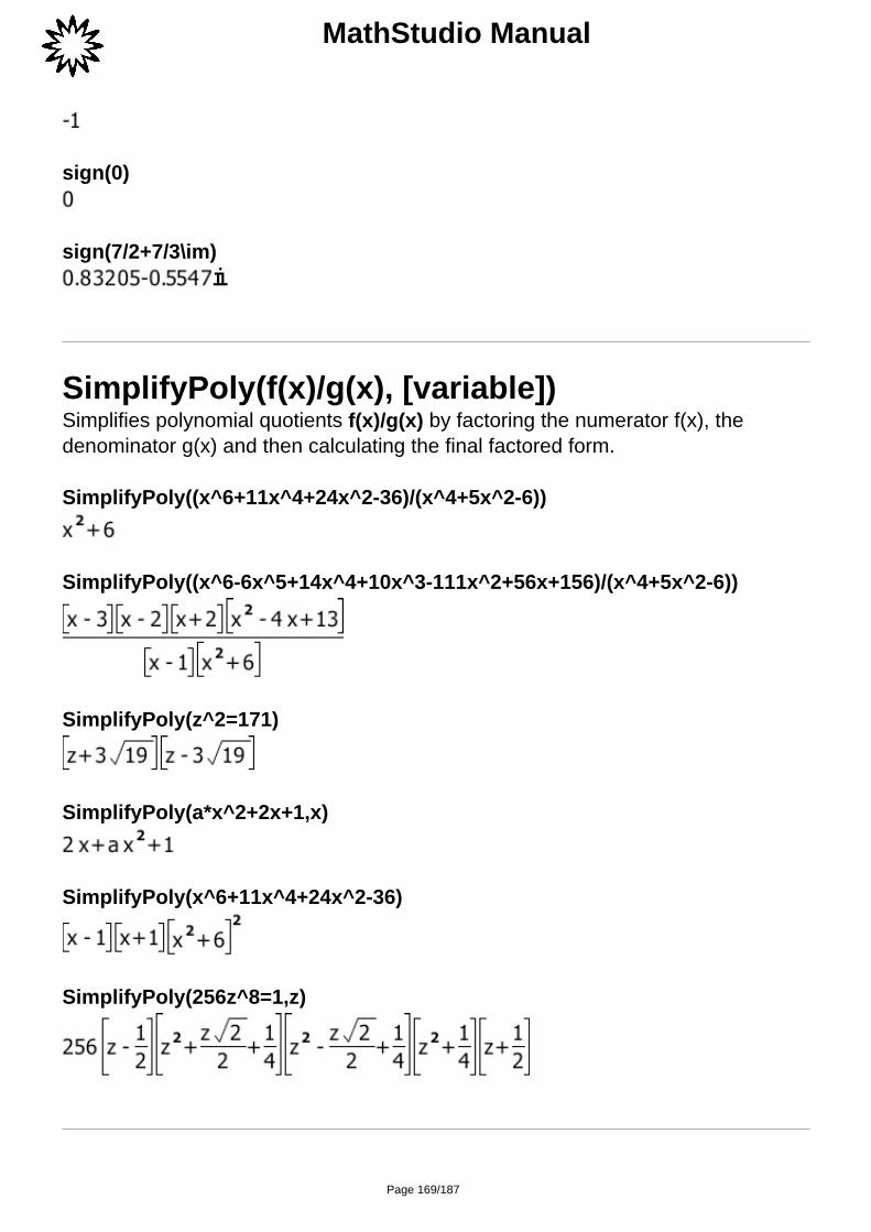
SimplifyPoly(f(x)/g(x), [variable])Simplifies polynomial quotients f(x)/g(x) by factoring the numerator f(x), thedenominator g(x) and then calculating the final factored form.
SimplifyPoly((x^6+11x^4+24x^2-36)/(x^4+5x^2-6))
SimplifyPoly((x^6-6x^5+14x^4+10x^3-111x^2+56x+156)/(x^4+5x^2-6))
SimplifyPoly(z^2=171)
SimplifyPoly(a*x^2+2x+1,x)
SimplifyPoly(x^6+11x^4+24x^2-36)
SimplifyPoly(256z^8=1,z)
Page 169/187

MathStudio Manual
Size(list)Returns the size of the list or matrix.
size([1,2,3,4,5,6])
size([[1,2,3],[4,5,6]])
Solve(f(x), x, [guess])Solves the expression for the given variable.
When no equals sign is given, Solve assumes the expression is equal to zero. Forexample, Solve(x^2-3) will solve the expression as x^2-3=0.
Quadratic expressions can be solved by entering each coefficient as a parameter.For instance, Solve(5x^2+3x+4) may also be entered as Solve(5,3,4).
Solve can also solve a system of linear equations with n unknowns.Solve(equation1, equation2, equation3, ...)See SolveSystem to solve a system of non-linear equations.
This optional parameter guess is the initial guess value to solve the equation. If alist of two values is given such as Solve(sin(x)=0,x,[0,6\pi]), Solve will return thesolutions within the given range.
Solve(3x+5=0,x)
Solve(3x+5)
Solve(3x^2+4x-3=0)
Page 170/187

MathStudio Manual
Solve(3,4,-3)
Solve(x+y+z=5,x+2y=6,z-x=3)
Solve(sin(3x)+cos(3x)=0)
Solve(3*tan(x)^2=1,x)
Solve(tan(x)^2=3)
Solve(x^6+16x^3+64,x)
Solve(asin(x)=\pi/4,x)
Solve(3sin(x)+exp(x)=2,x,[-2\pi,2\pi])
Solve(ln(x)=1,x)
Page 171/187

MathStudio Manual
Solve(exp(3x)=2,x)
Solve(4sin(x)^3+2sin(x)^2-2sin(x)=1,x)
Solve(Si(x)=1/2)
Solve(BesselJ(0,x)=2/3)
Solve(LegendreP(3,x)-1=0)
Solve(Gamma(x)=5040,x,[1,10])
SolveSystem(equations, [variables], [guesses])Solves a non-linear systems of equations.
SolveSystem([x+2y=1, x^2+y^2=10])
SolveSystem([x^2+y^2=25, y^2=x^2+3])
Page 172/187

MathStudio Manual
SolveSystem([x^2+y^2=25, y^2=x^2+3], [x,y], [-2,0])
SolveSystem([x^2+2y^2+cos(z)-w^2=0, 3x^2+y^2+sin(z)^2-w^2=0,-2x^2-y^2-cos(z)+w^2=0, -x^2-2y^2-cos(z)^2+w^2=0],[w,x,y,z],[-1,1,0,0])
Sort(list)Sorts a list in ascending order.
Sort([3,2,1])
Sort([2,5,3,4,1])
SphericalPlot3D(expression, ...)Plots 3D graphs in spherical coordinates.
SphericalPlot3D(1+1/5*sin(6*\theta)*sin(5*\phi), \theta=[0,\pi,60],\phi=[0,2\pi,60], axis=0)
Page 173/187
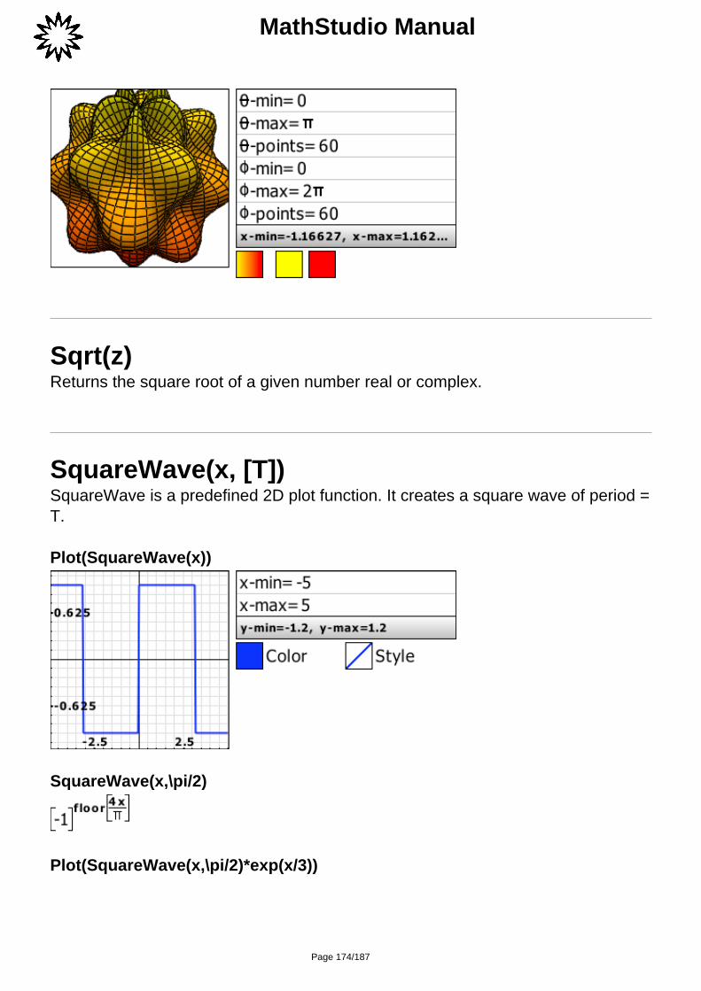
MathStudio Manual
Sqrt(z)Returns the square root of a given number real or complex.
SquareWave(x, [T])SquareWave is a predefined 2D plot function. It creates a square wave of period =T.
Plot(SquareWave(x))
SquareWave(x,\pi/2)
Plot(SquareWave(x,\pi/2)*exp(x/3))
Page 174/187

MathStudio Manual
StaircaseWave(x, [T])Creates a predefined 2D staircase wave with period = T.
Plot(StairCaseWave(x),x=[-20,20])
Plot(StairCaseWave(x)*SquareWave(x),x=[-20,26])
Page 175/187
MathStudio Manual
StandardDeviation(list)Finds the standard deviation of a list of numbers.
StandardDeviation([3,0,-5,0.5,4])
String(expression1, expression2, ...)Creates a string from a list of parameters.
String(A,1,B,2,C,3)
String("Hello", 123)
String(a,12)+String(b,12)
StudentTCDF(x, df)Computes the Student-t cumulative density function over the interval defined by lower and upper with degrees of freedom df.
StudentTPDF(x, df)Computes the Student-t probability density function at a value x with degrees offreedom df.
Plot(StudentTPDF(x,1))
Page 176/187

MathStudio Manual
Sum(f(n), n, start, end)Calculates the sum of f(n) where n goes from start to end.
Sum(n,n,1,10)
Sum(x^2,x,1,10)
Sum(1/a!,a,0,20)
\e
Sum(1/a^n,n,1,5)
f=Sum((-1)^n*x^(2n+1)/(2n+1)!,n,0,10)
Eval(f,x,\pi/4)
sin(\pi/4)
Page 177/187

MathStudio Manual
SurfaceNormal(function, [varlist], [point])Calculates the normal vector to the surface given by function at point.
Both the positive and negative normal vectors are returned.
SurfaceNormal(x*y^3-z-2,[x,y,z],[1,1,-1])
SurfaceNormal(x^2*y*z-1,[x,y,z],[1,1,1])
SurfaceNormal(x^2+y^2+z^2,[x,y,z],[5,0,12])
SurfaceNormal(x^2+y^2,[x,y],[a,b])
SVD(A)Returns a list with singular values of a matrix A.
This routine uses the TNT library.
SVD([[1,2],[3,4]])
Page 178/187

MathStudio Manual
Table(function, [independent, start, end, step],dependent)Prints a table of values.
Table(x^2,[x,2,10,1],y)
Together(expression)Finds a common denominator for each additive term of a polynomial function andreturns an equivalent expression with one numerator and one denominator. Itperforms the opposite operation as Apart.
Together(1/a+1/b)
Together(2-1/(x+1)+4/(x-2))
Page 179/187

MathStudio Manual
Together(2-1/(x+1)+4/(x+1)^2)
Together(exp(z)/a-exp(z)^2/b)
Trace(variable)This function is used for debugging scripts. It will output every instance when thespecified variable's value was changed.
Trace will only work inside a script.
Transpose(A)Calculates the transpose of a matrix A.
Transpose([[1,2,3,4],[5,6,7,8]])
TriangleWave(x, [T])
Page 180/187

MathStudio Manual
TriangleWave is a predefine 2D plotfunction which creates a triangle wave.
Plot(TriangleWave(x),color=red)
Plot(TriangleWave(x,\pi/2)*sin(x/5),color=magenta,x=[-15,15])
TrigCollect(expression)Equivalent of TrigReduce but even further reduces trigonometric functions.
TrigCollect(-(2*(cos(x)^2)-1)*sin(y)-2*cos(x)*cos(y)*sin(x)-4*(2*cos(y)*sin(x)*sin(y)+(2*(cos(y)^2)-1)*cos(x)))
TrigCollect(2*cos(y/3)*cos(x/9)*sin(y/3)+(2*(cos(y/3)^2)+-1)*sin(x/9))
TrigCollect((2*(2*(cos(z)^2)-1)*cos(u)*sin(u)+2*(2*(cos(u)^2)-1)*cos(z)*sin(z))*
Page 181/187

MathStudio Manual
cos((x+y)^0.5)+((2*(cos(u)^2)-1)*(2*(cos(z)^2)-1)-4*cos(u)*cos(z)*sin(u)*sin(z))*sin((x+y)^0.5))
TrigCollect(2*cos(x)*cos(y)*sin(x)+(2*(cos(x)^2)+-1)*sin(y)+1/(4*(cos(y)^3)+-3*cos(y)))
TrigConvert(expression)Converts trigonometric functions to exponential functions.
TrigConvert(sin(x))
TrigConvert(cos(x))
TrigConvert(tan(x))
TrigConvert(cot(x))
TrigExpand(expression)Splits up sums and integer multiples that appear in arguments of trigonometricfunctions and expands products of trigonometric functions into sums of powers.
Page 182/187

MathStudio Manual
TrigExpand(sin((x/3+2y)/3))
TrigExpand(cos(x^2+\sqrt(y)))
TrigExpand(tanh(2*x))
TrigExpand(tanh(x-y))
TrigReduce(expression)Rewrites products and powers of trigonometric functions in expr in terms oftrigonometric functions with combined arguments.
TrigReduce(sin(x)^2*cos(x) + 5*cos(x)^3 + 2*sin(x)*cos(x))
TrigReduce(-3cos(x)*sin(5)-cos(5)*sin(x)+4cos(x)^3*sin(5)+4cos(x)^2*cos(5)*sin(x))
TrigReduce(cos(x^2)*cos(\sqrt(y))-sin(\sqrt(y))*sin(x^2))
TrigReduce(3*sin(x)*cos(x)-sin(x)^2+cos(x)^2)
Page 183/187

MathStudio Manual
TrigReduce(cos(y)*sin(z)*sin(x)+cos(z)*cos(x)*cos(y)+cos(z)*sin(y)*sin(x)+-1*cos(x)*sin(z)*sin(y))
TrigReduce(4*(cos(x*y)^2)*sin(x*y)+-sin(x*y))
TrigReduce(32*(cos(x)^3)*sin(x)+-6*cos(x)*sin(x)+-32*(cos(x)^5)*sin(x))
TrigReduce(16*(cos(x*y)^4)*sin(x*y)+-12*(cos(x*y)^2)*sin(x*y)+sin(x*y))
Value(string)Converts a string to a value.
Variables(expression)Returns a list variables found in the expression.
Variables(2x^2+x+1)
Variables(x^2+y^2+z^2)
Variance(list)
Page 184/187

MathStudio Manual
Finds the variance of a list of numbers.
Variance([3,0,-5,0.5,4])
VectorPlot(list, ...)Plots 2D vector fields.
VectorPlot([y,-cos(x)])
VectorPlot3D(list, ...)Plots a 3D vector field.
VectorPlot3D([x,y,z])
Page 185/187

MathStudio Manual
While(condition)This will loop through and evaluate a block of code until condition evaluates tozero.
n=0 while(n
Zeta(z, [a])If a is not given, finds the Riemann Zeta.
If a is given, finds the Hurwitz Zeta function.
Zeta(0)
Zeta(1)
Zeta(-1)
Zeta(8)
Zeta(5+\im)
Zeta(-3.5)
Zeta(8)
Page 186/187
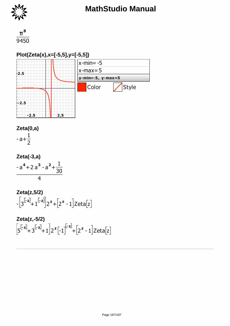
MathStudio Manual
Plot(Zeta(x),x=[-5,5],y=[-5,5])
Zeta(0,a)
Zeta(-3,a)
Zeta(z,5/2)
Zeta(z,-5/2)
Powered by TCPDF (www.tcpdf.org)
Page 187/187