math (p)refresher for political scientists - home | projects … · 2017-08-15 · math...
TRANSCRIPT

Math (P)refresher for Political Scientists∗
Harvard University
2017
∗The documents in this booklet are the product of generations of Math (P)refresher Instructors: Curt Signorino1996-1997; Ken Scheve 1997-1998; Eric Dickson 1998-2000; Orit Kedar 1999; James Fowler 2000-2001; Kosuke Imai2001-2002; Jacob Kline 2002; Dan Epstein 2003; Ben Ansell 2003-2004; Ryan Moore 2004-2005; Mike Kellermann2005-2006; Ellie Powell 2006-2007; Jen Katkin 2007-2008; Patrick Lam 2008-2009; Viridiana Rios 2009-2010; JenniferPan 2010-2011; Konstantin Kashin 2011-2012; Sole Prillaman 2013; Stephen Pettigrew 2013-2014; Anton Strezhnev2014-2015; Mayya Komisarchik 2015-2016; Connor Jerzak 2016-2017; Shiro Kuriwaki 2017
1

2
Schedule
Wednesday, August 16, 20179:00 - 9:30, Room K3541, Breakfast.9:30 - 11:30, K354, Introduction and lecture: Notation and functions (Connor)11:30 - 12:00, K354, Setting up computing software.
Please bring your laptops every day.12:00 - 1:00, K354, Lunch with Prof. Gary King.1:00 - 4:00, K354 or CGIS Computer Lab2, Practice Problems and R handling / visualizing data.
Thursday, August 17, 20179:00 - 9:30, K354, Breakfast.9:30 - 12:00, K354, Lecture: Linear algebra (Shiro)12:00 - 1:00, K354, Lunch with Steven Worthington and Ista Zahn.1:00 - 4:00, K354 or CGIS Computer Lab, Practice Problems and R handling matricies.
Friday, August 18, 20179:00 - 9:30, K354, Breakfast.9:30 - 12:00, K354, Lecture: Calculus I (Connor)12:00 - 1:00, Lunch with Prof. Jennifer Hochschild and Prof. Xiang Zhou.1:00 - 4:00, K354 or CGIS Computer Lab, Practice Problems and R building your own dataset.
Monday, August 21, 20179:00 - 9:30, K354, Breakfast.9:30 - 12:00, K354, Lecture: Calculus II and Optimization (Shiro)12:00 - 1:00, K354, Lunch on your own.1:00 - 4:00, K354 or CGIS Computer Lab, Practice Problems and R handling text
Tuesday, August 22, 20179:00 - 9:30, K354, Breakfast.9:30 - 12:00, K354, Lecture: Probability I (Shiro)12:00 - 1:00, K354, Lunch on your own.1:00 - 4:00, K354 or CGIS Computer Lab, Practice Problems and R handling stochastic systems.
Wednesday, August 23, 20179:00 - 9:30, K354, Breakfast.9:30 - 12:00, K354, Lecture: Probability II (Connor)12:00 - 1:00, K354, Lunch with Prof. Pia Raffler.1:00 - 4:00, K354 or CGIS Computer Lab, Practice Problems and LATEX, git, shell, markdown
1This location refers to Room K354 in CGIS Knafel, 1737 Cambridge St.2For all afternoons, students will switch between practice problems to computing or vice versa at 2:30

3
Syllabus
Math (P)refresher for Political Scientists
Wednesday, August 16 - Wednesday, August 23, 2017Breakfast 9am - 9:30am
Lecture 9:30am - 12:00pmSection 1:00pm - 4:00pm
Connor Jerzak (Instructor) Shiro Kuriwaki (Instructor)[email protected] [email protected]
Gary King (Faculty Adviser) Course [email protected] projects.iq.harvard.edu/prefresher
PURPOSE: Not only do the quantitative and formal modeling courses at Harvard require mathe-matics and computer programming — it’s becoming increasingly difficult to take courses in politicaleconomy, American politics, comparative politics, or international relations without encounteringgame-theoretic models or statistical analyses. One need only flip through the latest issues of the toppolitical science journals to see that mathematics have entered the mainstream of political science.Even political philosophy has been influenced by mathematical thinking. Unfortunately, most un-dergraduate political science programs have not kept up with this trend — and first-year graduatestudents often find themselves lacking in basic technical skills. This course is not intended to bean introduction to game theory or quantitative methods. Rather, it introduces basic mathematicsand computer skills needed for quantitative and formal modeling courses offered at Harvard.
PREREQUISITES: None. Students for whom the topics in this syllabus are completely foreignshould not be scared off. They have the perfect background for this course — the ones in mostneed of a “prefresh”ing before they take further courses with technical content. Students who havepreviously had some of this material, but have not used it in a while, should take this course to“refresh” their knowledge of the topics.
STRUCTURE & REQUIREMENTS: The class will meet twice a day, 9:00am – 12:00pm and1:00pm – 4:00pm. This course is not for credit and has no exams. No one but the student willknow how well he or she did. However, it still requires a significant commitment from students.Students are expected to do the reading assignments before the classes. Lectures will focus on majormathematical topics that are used in statistical and formal modeling in political science. Sectionswill be divided into two parts. During problem-solving sections, students are given exercises to workon (or as homework if not finished then) and students are encouraged to work on the exercisesin groups of two or three. You learn more quickly when everyone else is working on the sameproblems! During computing sections, we will introduce you to the computing environment andsoftware packages that are used in the departmental methods sequence. Math isn’t a spectatorsport — you have to do it to learn it.
COMPUTING: All of the methods courses in the department, and increasingly courses in formaltheory as well, make extensive use of the computational resources available at Harvard. Studentswill be introduced to LATEX (a typesetting language useful for producing documents with mathe-matical content) and R (the statistical computing language/environment used in the department’smethod courses). These resources are very powerful, but have something of a steep learning curve;one of the goals of the prefresher is to give students a head start on these programs.
TEXTS: There is no required textbook for the course. Instead of suggesting a text that you will

4
never use after the Prefresher, below we list some textbooks on the Prefresher material that somecourses list as their text or reference text. Students interested in a particular topic and plan totake courses in them may find it useful to refer to the textbooks during the Prefresher.
The list below is not intended to be comprehensive or reflective of future offerings of the course.
Texts for Mathematics
• (Gov 2000, MIT 17.800) Wooldridge, Jeffrey M. Introductory Econometrics
• (Gov 2000, Gov 2002, MIT 17.802) Angrist, Joshua D. and Jorn-Steffen Pischke. 2008. MostlyHarmless Econometrics: An Empiricists Companion. Princeton University Press.
• (Gov 2000, MIT 17.800) Berksekas, Dimitri P. and John N. Tsitsiklis. Introduction to Prob-ability. Athena Scientific.
• (Gov 2000) Diez, David M., Christopher D. Barr, and Mine Cetinkaya-Rundel. 2015. Open-Intro Statistics. 3rd edition. https://www.openintro.org/
• (Gov 2000) Gelman, Andrew and Jennifer Hill. 2007. Data Analysis Using Regression andMultilevel/Hierarchical Models. Cambridge University Press.
• (Stat 110) Blitzstein, Joseph K. and Jessica Hwang. 2014. Introduction to Probability, 1stedition. Chapman & Hall/CRC Texts in Statistical Science.
• (Stat 111) DeGroot, Morris H. and Mark J. Schervish. 2011 Probability and Statistics, 4thedition. Pearson.
• (Stat 210) Blitzstein, Joseph K. and Carl N. Morris. (unpublished manuscript). Probabilityfor Statistical Science.
• (Econ 2020a) Simon, Carl P. and Lawrence Blume. 1994. Mathematics for Economists. NewYork: Norton.
• (Econ 2020a, Gov 2006) Mas-Colell, Andreu, Michael D. Whinston, and Jerry R. Green.1995. Microeconomic Theory. Oxford University Press.
Texts for Programming
• Imai, Kosuke. 2017. Quantitative Social Science. Princeton University Press. (Supplemen-tary Information: https://github.com/kosukeimai/qss)
• Gentzkow, Matthew, and Jesse Shapiro. (online document). “Code and Data for the So-cial Sciences: A Practitioner’s Guide”. https://web.stanford.edu/~gentzkow/research/
CodeAndData.pdf
• Wickham, Hadley and Garrett Grolemund. 2017. R for Data Science. O’Reilly. http:
//r4ds.had.co.nz/

5
Lecture Schedule:
Wednesday, August 16
Lecture 1: Notation and FunctionsTutorial 1: Handling and Visualizing Data in R
Topics: Dimensionality. Interval Notation for R1.Neighborhoods: Intervals, Disks, and Balls.Sets, Sets, and More Sets.Introduction to Functions. Domain and Range.Logarthims, exponentials. Other Useful Functions.Solving for Variables. Finding Roots. Limit of a Function.Continuity.
Thursday, August 17
Lecture 2: Linear AlgebraTutorial 2: Matricies and Vectors in R
Topics: Working with Vectors. Linear Independence.Basics of Matrix Algebra. Square Matrices.Linear Equations. Systems of Linear Equations.Systems of Equations as Matrices. SolvingAugmented Matrices and Systems of Equations.Rank. The Inverse of a Matrix. Inverse of Larger Matrices.
Friday, August 18
Lecture 3: Calculus ITutorial 3: Open-ended R project: Building your own Time Series Cross-SecitonalDataset
Topics: Sequences. Limit of a Sequence. Series. Derivatives.Higher-Order Derivatives. Composite Functions and theChain Rule. Derivatives of Exp and Ln. Maxima and Minima.Partial Derivatives. L’Hospital’s Rule.Taylor Approximation.Derivative Calculus in 6 Steps.
Monday, August 21
Lecture 4: Calculus IITutorial 4: Text Data in R

6
Topics: The Indefinite Integral: The Antiderivative.Common Rules of Integration. The DefiniteIntegral: The Area under the Curve.Integration by Substitution. Integration by Parts.Optimization.Constrained Optimization.
Tuesday, August 22
Lecture 5: Probability ITutorial 5: Simulating data and stochastic processes in R
Topics: Sets. Probability.Conditional Probability. Bayes’ Rule. Independence.Random Variables.
Wednesday, August 23
Lecture 6: Probability IITutorial 6: LATEX, Command-line, Github, Markdown, and other software
Topics: Expectation. Covariance.Summarizing Observed Data.Probability Distributions of Random Variables.Important Distributions. Joint Distributions.Asymptotics.

Contents
1 Mathematics Notes 9
1.1 Functions and Notation . . . . . . . . . . . . . . . . . . . . . . . . . . . . . . . . . . 9
1.1.1 Dimensionality . . . . . . . . . . . . . . . . . . . . . . . . . . . . . . . . . . . 9
1.1.2 Interval Notation for R1 . . . . . . . . . . . . . . . . . . . . . . . . . . . . . . 9
1.1.3 Neighborhoods: Intervals, Disks, and Balls . . . . . . . . . . . . . . . . . . . 10
1.1.4 Introduction to Functions . . . . . . . . . . . . . . . . . . . . . . . . . . . . . 10
1.1.5 Domain and Range/Image . . . . . . . . . . . . . . . . . . . . . . . . . . . . . 10
1.1.6 Some General Types of Functions . . . . . . . . . . . . . . . . . . . . . . . . . 11
1.1.7 Log, Ln, and e . . . . . . . . . . . . . . . . . . . . . . . . . . . . . . . . . . . 12
1.1.8 Other Useful Functions . . . . . . . . . . . . . . . . . . . . . . . . . . . . . . 13
1.1.9 Graphing Functions . . . . . . . . . . . . . . . . . . . . . . . . . . . . . . . . 14
1.1.10 Solving for Variables and Finding Inverses . . . . . . . . . . . . . . . . . . . . 15
1.1.11 Finding the Roots or Zeroes of a Function . . . . . . . . . . . . . . . . . . . . 15
1.1.12 The Limit of a Function . . . . . . . . . . . . . . . . . . . . . . . . . . . . . . 16
1.1.13 Continuity . . . . . . . . . . . . . . . . . . . . . . . . . . . . . . . . . . . . . 17
1.1.14 Sets, Sets, and More Sets . . . . . . . . . . . . . . . . . . . . . . . . . . . . . 18
1.2 Linear Algebra . . . . . . . . . . . . . . . . . . . . . . . . . . . . . . . . . . . . . . . 20
1.2.1 Working with Vectors . . . . . . . . . . . . . . . . . . . . . . . . . . . . . . . 20
1.2.2 Linear Independence . . . . . . . . . . . . . . . . . . . . . . . . . . . . . . . . 21
1.2.3 Basics of Matrix Algebra . . . . . . . . . . . . . . . . . . . . . . . . . . . . . 21
1.2.4 Square Matrices . . . . . . . . . . . . . . . . . . . . . . . . . . . . . . . . . . 23
1.2.5 Linear Equations . . . . . . . . . . . . . . . . . . . . . . . . . . . . . . . . . . 24
1.2.6 Systems of Linear Equations . . . . . . . . . . . . . . . . . . . . . . . . . . . 24
1.2.7 Systems of Equations as Matrices . . . . . . . . . . . . . . . . . . . . . . . . . 25
1.2.8 Finding Solutions to Augmented Matrices and Systems of Equations . . . . . 26
1.2.9 Rank — and Whether a System Has One, Infinite, or No Solutions . . . . . . 28
1.2.10 The Inverse of a Matrix . . . . . . . . . . . . . . . . . . . . . . . . . . . . . . 29
1.2.11 Linear Systems and Inverses . . . . . . . . . . . . . . . . . . . . . . . . . . . . 31
1.2.12 Determinants . . . . . . . . . . . . . . . . . . . . . . . . . . . . . . . . . . . . 31
1.2.13 Getting Inverse of a Matrix using its Determinant and Matrix of Cofactors . 33
1.2.14 Inverse of Larger Matrices . . . . . . . . . . . . . . . . . . . . . . . . . . . . . 34
1.3 Calculus I . . . . . . . . . . . . . . . . . . . . . . . . . . . . . . . . . . . . . . . . . . 35
1.3.1 Sequences . . . . . . . . . . . . . . . . . . . . . . . . . . . . . . . . . . . . . . 35
1.3.2 The Limit of a Sequence . . . . . . . . . . . . . . . . . . . . . . . . . . . . . . 36
1.3.3 Series . . . . . . . . . . . . . . . . . . . . . . . . . . . . . . . . . . . . . . . . 37
1.3.4 Derivatives . . . . . . . . . . . . . . . . . . . . . . . . . . . . . . . . . . . . . 38
1.3.5 Higher-Order Derivatives or, Derivatives of Derivatives of Derivatives . . . . 39
1.3.6 Composite Functions and the Chain Rule . . . . . . . . . . . . . . . . . . . . 40
1.3.7 Derivatives of Euler’s number and natural logs . . . . . . . . . . . . . . . . . 41
1.3.8 Applications of the Derivative: Maxima and Minima . . . . . . . . . . . . . . 42

8
1.3.9 Partial Derivatives . . . . . . . . . . . . . . . . . . . . . . . . . . . . . . . . . 43
1.3.10 L’Hopital’s Rule . . . . . . . . . . . . . . . . . . . . . . . . . . . . . . . . . . 44
1.3.11 Taylor Series Approximation . . . . . . . . . . . . . . . . . . . . . . . . . . . 45
1.3.12 Summary: Derivative calculus in 6 steps . . . . . . . . . . . . . . . . . . . . . 46
1.4 Calculus II . . . . . . . . . . . . . . . . . . . . . . . . . . . . . . . . . . . . . . . . . 47
1.4.1 The Indefinite Integral: The Antiderivative . . . . . . . . . . . . . . . . . . . 47
1.4.2 Common Rules of Integration . . . . . . . . . . . . . . . . . . . . . . . . . . . 47
1.4.3 The Definite Integral: The Area under the Curve . . . . . . . . . . . . . . . . 48
1.4.4 Integration by Substitution . . . . . . . . . . . . . . . . . . . . . . . . . . . . 50
1.4.5 Integration by Parts, or Ultraviolet Voodoo . . . . . . . . . . . . . . . . . . . 51
1.5 Unconstrained and Constrained Optimization . . . . . . . . . . . . . . . . . . . . . . 53
1.5.1 Quadratic Forms . . . . . . . . . . . . . . . . . . . . . . . . . . . . . . . . . . 53
1.5.2 Concavity of Quadratic Forms . . . . . . . . . . . . . . . . . . . . . . . . . . 54
1.5.3 Definiteness of Quadratic Forms . . . . . . . . . . . . . . . . . . . . . . . . . 54
1.5.4 First Order Conditions . . . . . . . . . . . . . . . . . . . . . . . . . . . . . . . 56
1.5.5 Second Order Conditions . . . . . . . . . . . . . . . . . . . . . . . . . . . . . 57
1.5.6 Definiteness and Concavity . . . . . . . . . . . . . . . . . . . . . . . . . . . . 58
1.5.7 Global Maxima and Minima . . . . . . . . . . . . . . . . . . . . . . . . . . . . 58
1.5.8 Example . . . . . . . . . . . . . . . . . . . . . . . . . . . . . . . . . . . . . . . 59
1.5.9 Constrained Optimization . . . . . . . . . . . . . . . . . . . . . . . . . . . . . 60
1.5.10 Equality Constraints . . . . . . . . . . . . . . . . . . . . . . . . . . . . . . . . 61
1.5.11 Inequality Constraints . . . . . . . . . . . . . . . . . . . . . . . . . . . . . . . 63
1.5.12 Kuhn-Tucker Conditions . . . . . . . . . . . . . . . . . . . . . . . . . . . . . . 66
1.6 Probability I: Probability Theory . . . . . . . . . . . . . . . . . . . . . . . . . . . . . 70
1.6.1 Counting rules . . . . . . . . . . . . . . . . . . . . . . . . . . . . . . . . . . . 70
1.6.2 Sets . . . . . . . . . . . . . . . . . . . . . . . . . . . . . . . . . . . . . . . . . 71
1.6.3 Probability . . . . . . . . . . . . . . . . . . . . . . . . . . . . . . . . . . . . . 71
1.6.4 Conditional Probability and Bayes Law . . . . . . . . . . . . . . . . . . . . . 72
1.6.5 Random Variables . . . . . . . . . . . . . . . . . . . . . . . . . . . . . . . . . 76
1.6.6 Independence . . . . . . . . . . . . . . . . . . . . . . . . . . . . . . . . . . . . 77
1.7 Probability II: Distributions and Asymptotics . . . . . . . . . . . . . . . . . . . . . . 78
1.7.1 Types of Observed Data . . . . . . . . . . . . . . . . . . . . . . . . . . . . . . 78
1.7.2 Distributions . . . . . . . . . . . . . . . . . . . . . . . . . . . . . . . . . . . . 78
1.7.3 Expectation and Other Moments . . . . . . . . . . . . . . . . . . . . . . . . . 80
1.7.4 Special Distributions . . . . . . . . . . . . . . . . . . . . . . . . . . . . . . . . 82
1.7.5 Joint Distributions . . . . . . . . . . . . . . . . . . . . . . . . . . . . . . . . . 84
1.7.6 Summarizing Observed Events (Data) . . . . . . . . . . . . . . . . . . . . . . 85
1.7.7 Asymptotic Theory . . . . . . . . . . . . . . . . . . . . . . . . . . . . . . . . . 87
2 Guide to Greek Letters and Mathematical Symbols 89
2.1 Greek Letters . . . . . . . . . . . . . . . . . . . . . . . . . . . . . . . . . . . . . . . . 89
2.2 Mathematical Symbols . . . . . . . . . . . . . . . . . . . . . . . . . . . . . . . . . . . 89

Functions and Notation 9
1 Mathematics Notes
1.1 Functions and Notation
Topics :Dimensionality; Interval Notation for R1; Neighborhoods: Intervals, Disks, and Balls; Introductionto Functions; Domain and Range; Some General Types of Functions; Log, Ln, and e; Other UsefulFunctions; Graphing Functions; Solving for Variables; Finding Roots; Limit of a Function; Conti-nuity; Sets, Sets, and More Sets;
1.1.1 Dimensionality
• R1 is the set of all real numbers extending from −∞ to +∞ — i.e., the real number line.
• Rn is an n-dimensional space (often referred to as Euclidean space), where each of the n axesextends from −∞ to +∞.
Examples:
1. R1 is a one dimensional line.
2. R2 is a two dimensional plane.
3. R3 is a three dimensional space.
4. R4 could be 3-D plus time (or temperature, etc).
Points in Rn are ordered n-tuples, where each element of the n-tuple represents the coordinatealong that dimension.
R1: (3)
R2: (-15, 5)
R3: (86, 4, 0)
1.1.2 Interval Notation for R1
• Open interval: (a, b) ≡ x ∈ R1 : a < x < b
x is a one-dimensional element in which x is greater than a and less than b
• Closed interval: [a, b] ≡ x ∈ R1 : a ≤ x ≤ b
x is a one-dimensional element in which x is greater or equal to than a and less than orequal to b
• Half open, half closed: (a, b] ≡ x ∈ R1 : a < x ≤ b
x is a one-dimensional element in which x is greater than a and less than or equal to b
Much of the material and examples for this lecture are taken from Simon & Blume (1994) Mathematics for Economists,Boyce & Diprima (1988) Calculus, and Protter & Morrey (1991) A First Course in Real Analysis

Functions and Notation 10
1.1.3 Neighborhoods: Intervals, Disks, and Balls
• In many areas of math, we need a formal construct for what it means to be “near” a point cin Rn. This is generally called the neighborhood of c. It’s represented by an open interval,disk, or ball, depending on whether Rn is of one, two, or more dimensions, respectively. Giventhe point c, these are defined as
1. ε-interval in R1: x : |x− c| < εx is in the neighborhood of c if it is in the open interval (c− ε, c+ ε).
2. ε-disk in R2: x : ||x− c|| < εx is in the neighborhood of c if it is inside the circle or disc with center c and radius ε.
3. ε-ball in Rn: x : ||x− c|| < εx is in the neighborhood of c if it is inside the sphere or ball with center c and radius ε.
1.1.4 Introduction to Functions
• A function (in R1) is a mapping, or transformation, that relates members of one set tomembers of another set. For instance, if you have two sets: set A and set B, a function fromA to B maps every value a in set A such that f(a) ∈ B. Functions can be “many-to-one”,where many values or combinations of values from set A produce a single output in set B, orthey can be “one-to-one”, where each value in set A corresponds to a single value in set B.
Examples: Mapping notation
1. Function of one variable: f : R1 → R1
f(x) = x+ 1For each x in R1, f(x) assigns the number x+ 1.
2. Function of two variables: f : R2 → R1
f(x, y) = x2 + y2
For each ordered pair (x, y) in R2, f(x, y) assigns the number x2 + y2.
We often use one variable x as input and another y as output.Example: y = x+ 1
• Input variable also called independent or explanatory variable. Output variable also calleddependent or response variable.
1.1.5 Domain and Range/Image
Some functions are defined only on proper subsets of Rn.
• Domain: the set of numbers in X at which f(x) is defined.
• Range: elements of Y assigned by f(x) to elements of X, or
f(X) = y : y = f(x), x ∈ X
Most often used when talking about a function f : R1 → R1.

Functions and Notation 11
• Image: same as range, but more often used when talking about a function f : Rn → R1.
Examples:
1.f(x) = 3
1+x2
2. f(x) =
x+ 1, 1 ≤ x ≤ 20, x = 01− x, −2 ≤ x ≤ −1
3.f(x) = 1/x
4.f(x, y) = x2 + y2
1.1.6 Some General Types of Functions
• Monomials: f(x) = axk
a is the coefficient. k is the degree.Examples: y = x2, y = −1
2x3
• Polynomials: sum of monomials.Examples: y = −1
2x3 + x2, y = 3x+ 5
The degree of a polynomial is the highest degree of its monomial terms. Also, it’s often agood idea to write polynomials with terms in decreasing degree.
• Rational Functions: ratio of two polynomials.Examples: y = x
2 , y = x2+1x2−2x+1
• Exponential Functions: Example: y = 2x
• Trigonometric Functions: Examples: y = cos(x), y = 3 sin(4x)

Functions and Notation 12
• Linear: polynomial of degree 1.Example: y = mx+ b, where m is the slope and b is the y-intercept.
• Nonlinear: anything that isn’t constant or polynomial of degree 1.Examples: y = x2 + 2x+ 1, y = sin(x), y = ln(x), y = ex
1.1.7 Log, Ln, and e
• Relationship of logarithmic and exponential functions:
y = loga(x) ⇐⇒ ay = x
The log function can be thought of as an inverse for exponential functions. a is referred to asthe “base” of the logarithm.
• Common Bases: The two most common logarithms are base 10 and base e.
1. Base 10: y = log10(x) ⇐⇒ 10y = xThe base 10 logarithm is often simply written as “log(x)” with no base denoted.
2. Base e: y = loge(x) ⇐⇒ ey = xThe base e logarithm is referred to as the “natural” logarithm and is written as “ln(x)”.
• Properties of exponential functions:
1. axay = ax+y
2. a−x = 1/ax
3. ax/ay = ax−y
4. (ax)y = axy
5. a0 = 1

Functions and Notation 13
• Properties of logarithmic functions (any base):
Generally, when statisticians or social scientists write log(x) they mean loge(x). In otherwords: loge(x) ≡ ln(x) ≡ log(x)
loga(ax) = x and aloga(x) = x
1. log(xy) = log(x) + log(y)
2. log(xy) = y log(x)
3. log(1/x) = log(x−1) = − log(x)
4. log(x/y) = log(x · y−1) = log(x) + log(y−1) = log(x)− log(y)
5. log(1) = log(e0) = 0
• Change of Base Formula: Use the change of base formula to switch bases as necessary:
logb(x) =loga(x)
loga(b)
Example:
log10(x) =ln(x)
ln(10)
Examples:
1. log10(√
10) = log10(101/2) =
2. log10(1) = log10(100) =
3. log10(10) = log10(101) =
4. log10(100) = log10(102) =
5. ln(1) = ln(e0) =
6. ln(e) = ln(e1) =
1.1.8 Other Useful Functions
• Factorials!:x! = x · (x− 1) · (x− 2) · · · (1)
• Modulo:Tells you the remainder when you divide one number by another. Can be extremely usefulfor programming.
x mod y or x % y
Examples: 17 mod 3 = 2 100 % 30 = 10

Functions and Notation 14
• Summation:n∑i=1
xi = x1 + x2 + x3 + · · ·+ xn
Properties:
1.n∑i=1
cxi = cn∑i=1
xi
2.n∑i=1
(xi + yi) =n∑i=1
xi +n∑i=1
yi
3.n∑i=1
c = nc
• Product:n∏i=1
xi = x1x2x3 · · ·xn
Properties:
1.n∏i=1
cxi = cnn∏i=1
xi
2.n∏i=1
(xi + yi) = a total mess
3.n∏i=1
c = cn
You can use logs to go between sum and product notation. This will be particularly importantwhen you’re learning maximum likelihood estimation.
log
( n∏i=1
xi
)= log(x1 · x2 · x3 · · · · xn)
= log(x1) + log(x2) + log(x3) + · · ·+ log(xn)
=n∑i=1
log(xi)
Therefore, you can see that the log of a product is equal to the sum of the logs. We can writethis more generally by adding in a constant, c:
log
( n∏i=1
cxi
)= log(cx1 · cx2 · · · cxn)
= log(cn · x1 · x2 · · ·xn)
= log(cn) + log(x1) + log(x2) + · · ·+ log(xn)
= n log(c) +
n∑i=1
log(xi)
1.1.9 Graphing Functions
What can a graph tell you about a function?

Functions and Notation 15
1. Is the function increasing or decreasing? Over what part of the domain?
2. How “fast” does it increase or decrease?
3. Are there global or local maxima and minima? Where?
4. Are there inflection points?
5. Is the function continuous?
6. Is the function differentiable?
7. Does the function tend to some limit?
8. Other questions related to the substance of the problem at hand.
1.1.10 Solving for Variables and Finding Inverses
Sometimes we’re given a function y = f(x) and we want to find how x varies as a function ofy.
If f is a one-to-one mapping, then it has an inverse.
Use algebra to move x to the left hand side (LHS) of the equation and so that the righthand side (RHS) is only a function of y.
Examples: (we want to solve for x)
1. y = 3x+ 2 =⇒ −3x = 2− y =⇒ 3x = y − 2 =⇒ x = 13(y − 2)
2. y = 3x− 4z + 2 =⇒ y + 4z − 2 = 3x =⇒ x = 13(y + 4z − 2)
3. y = ex + 4 =⇒ y − 4 = ex =⇒ ln(y − 4) = ln(ex) =⇒ x = ln(y − 4)
Sometimes (often?) the inverse does not exist.
Example: We’re given the function y = x2 (a parabola). Solving for x, we get x = ±√y.For each value of y, there are two values of x.
1.1.11 Finding the Roots or Zeroes of a Function
Solving for variables is especially important when we want to find the roots of an equation:those values of variables that cause an equation to equal zero.
Especially important in finding equilibria and in doing maximum likelihood estimation.
• Procedure: Given y = f(x), set f(x) = 0. Solve for x.
• Multiple Roots:
f(x) = x2−9 =⇒ 0 = x2−9 =⇒ 9 = x2 =⇒ ±√
9 =√x2 =⇒ ±3 = x
• Quadratic Formula: For quadratic equations ax2 + bx + c = 0, usethe quadratic formula:
x =−b±
√b2 − 4ac
2a

Functions and Notation 16
Examples:
1. f(x) = 3x+ 2
2. f(x) = e−x − 10
3. f(x) = x2 + 3x− 4 = 0
1.1.12 The Limit of a Function
We’re often interested in determining if a function f approaches some number L as its inde-pendent variable x moves to some number c (usually 0 or ±∞). If it does, we say that thelimit of f(x), as x approaches c, is L: lim
x→cf(x) = L.
For a limit L to exist, the function f(x) must approach L from both the left and right.
• Limit of a function. Let f(x) be defined at each point in some open interval containingthe point c. Then L equals lim
x→cf(x) if for any (small positive) number ε, there exists a
corresponding number δ > 0 such that if 0 < |x− c| < δ, then |f(x)− L| < ε.
Note: f(x) does not necessarily have to be defined at c for limx→c
to exist.
• Uniqueness: limx→c
f(x) = L and limx→c
f(x) = M =⇒ L = M
• Properties: Let f and g be functions with limx→c
f(x) = A and limx→c
g(x) = B.
1. limx→c
[f(x) + g(x)] = limx→c
f(x) + limx→c
g(x)
2. limx→c
αf(x) = α limx→c
f(x)
3. limx→c
f(x)g(x) = [limx→c
f(x)][limx→c
g(x)]
4. limx→c
f(x)g(x) =
limx→c
f(x)
limx→c
g(x) , provided limx→c
g(x) 6= 0
Note: In a couple days we’ll talk about L’Hopital’s Rule, which uses simple calculus tohelp find the limits of functions like this.
Examples:
1. limx→c
k =
2. limx→c
x =
3. limx→0|x| =

Functions and Notation 17
4. limx→0
(1 + 1
x2
)=
5. limx→2
(2x− 3) =
6. limx→c
xn =
• Types of limits:
1. Right-hand limit: The value approached by f(x) when you move from right to left.Example: lim
x→0+
√x = 0
2. Left-hand limit: The value approached by f(x) when you move from left to right.
3. Infinity: The value approached by f(x) as x grows infinitely large. Sometimes this maybe a number; sometimes it might be ∞ or −∞.
4. Negative infinity: The value approached by f(x) as x grows infinitely negative. Some-times this may be a number; sometimes it might be ∞ or −∞.Example: lim
x→∞1/x =
limx→−∞
1/x = 0
1.1.13 Continuity
• Continuity: Suppose that the domain of the function f includes an open interval containingthe point c. Then f is continuous at c if lim
x→cf(x) exists and if lim
x→cf(x) = f(c). Further, f is
continuous on an open interval (a, b) if it is continuous at each point in the interval.
Examples: Continuous functions.
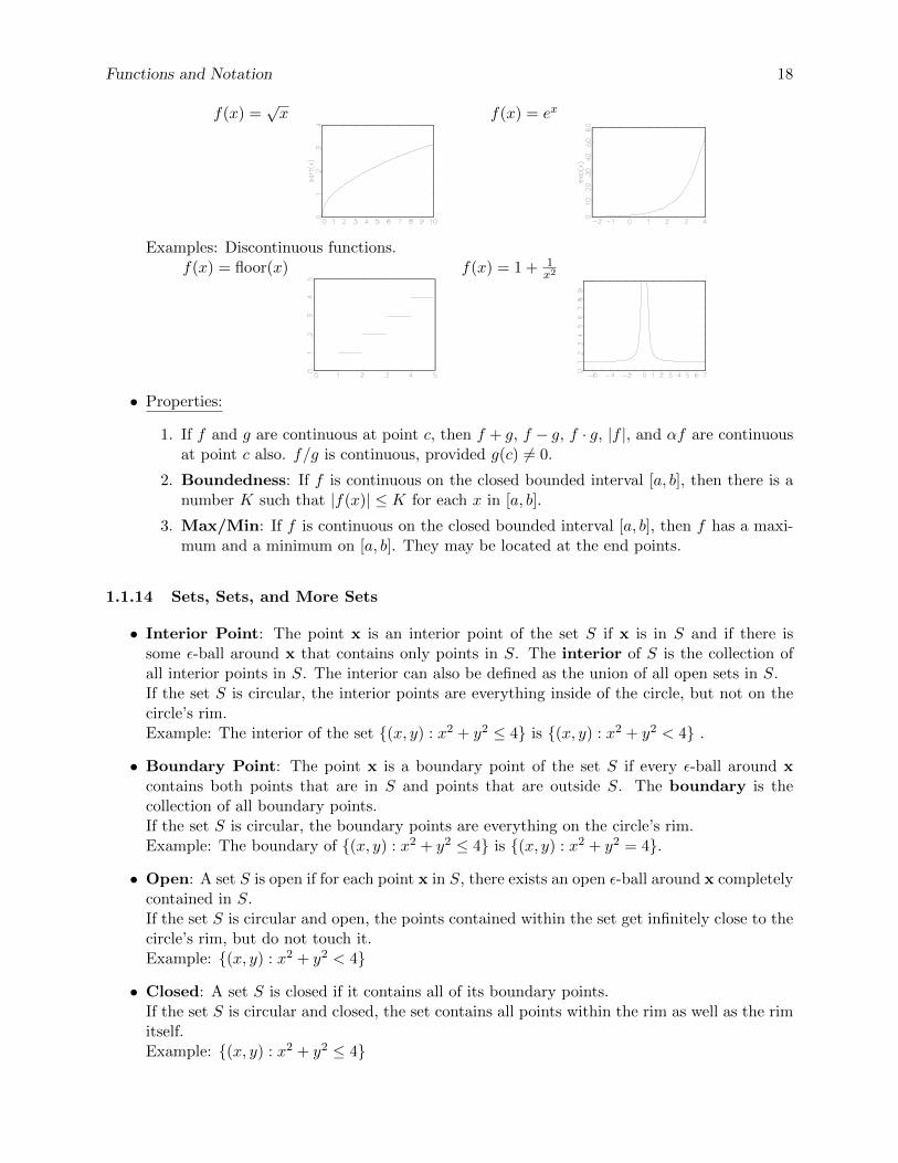
Functions and Notation 18
f(x) =√x f(x) = ex
Examples: Discontinuous functions.f(x) = floor(x) f(x) = 1 + 1
x2
• Properties:
1. If f and g are continuous at point c, then f + g, f − g, f · g, |f |, and αf are continuousat point c also. f/g is continuous, provided g(c) 6= 0.
2. Boundedness: If f is continuous on the closed bounded interval [a, b], then there is anumber K such that |f(x)| ≤ K for each x in [a, b].
3. Max/Min: If f is continuous on the closed bounded interval [a, b], then f has a maxi-mum and a minimum on [a, b]. They may be located at the end points.
1.1.14 Sets, Sets, and More Sets
• Interior Point: The point x is an interior point of the set S if x is in S and if there issome ε-ball around x that contains only points in S. The interior of S is the collection ofall interior points in S. The interior can also be defined as the union of all open sets in S.If the set S is circular, the interior points are everything inside of the circle, but not on thecircle’s rim.Example: The interior of the set (x, y) : x2 + y2 ≤ 4 is (x, y) : x2 + y2 < 4 .
• Boundary Point: The point x is a boundary point of the set S if every ε-ball around xcontains both points that are in S and points that are outside S. The boundary is thecollection of all boundary points.If the set S is circular, the boundary points are everything on the circle’s rim.Example: The boundary of (x, y) : x2 + y2 ≤ 4 is (x, y) : x2 + y2 = 4.
• Open: A set S is open if for each point x in S, there exists an open ε-ball around x completelycontained in S.If the set S is circular and open, the points contained within the set get infinitely close to thecircle’s rim, but do not touch it.Example: (x, y) : x2 + y2 < 4
• Closed: A set S is closed if it contains all of its boundary points.If the set S is circular and closed, the set contains all points within the rim as well as the rimitself.Example: (x, y) : x2 + y2 ≤ 4

Functions and Notation 19
Note: a set may be neither open nor closed.Example: (x, y) : 2 < x2 + y2 ≤ 4
• Complement: The complement of set S is everything outside of S.If the set S is circular, the complement of S is everything outside of the circle.Example: The complement of (x, y) : x2 + y2 ≤ 4 is (x, y) : x2 + y2 > 4.
• Closure: The closure of set S is the smallest closed set that contains S.Example: The closure of (x, y) : x2 + y2 < 4 is (x, y) : x2 + y2 ≤ 4
• Bounded: A set S is bounded if it can be contained within an ε-ball.Examples: Bounded: any interval that doesn’t have ∞ or −∞ as endpoints; any disk in aplane with finite radius.Unbounded: the set of integers in R1; any ray.
• Compact: A set is compact if and only if it is both closed and bounded.
• Empty: The empty (or null) set is a unique set that has no elements, denoted by or ø. 4
Examples: The set of squares with 5 sides; the set of countries south of the South Pole.
4The set, S, denoted by ø is technically not empty. That is because this set contains the empty set within it, so Sis not empty.

Linear Algebra 20
1.2 Linear Algebra
Topics5: • Working with Vectors • Linear Independence • Basics of Matrix Algebra • SquareMatrices • Linear Equations • Systems of Linear Equations • Systems of Equations as Matrices •Solving Augmented Matrices and Systems of Equations • Rank • The Inverse of a Matrix • Inverseof Larger Matrices
1.2.1 Working with Vectors
• Vector: A vector in n-space is an ordered list of n numbers. These numbers can be repre-sented as either a row vector or a column vector:
v(v1 v2 . . . vn
),v =
v1
v2...vn
We can also think of a vector as defining a point in n-dimensional space, usually Rn; eachelement of the vector defines the coordinate of the point in a particular direction.
• Vector Addition and Subtraction: If two vectors, u and v, have the same length (i.e.have the same number of elements), they can be added (subtracted) together:
u + v =(u1 + v1 u2 + v2 · · · uk + vn
)u− v =
(u1 − v1 u2 − v2 · · · uk − vn
)• Scalar Multiplication: The product of a scalar c (i.e. a constant) and vector v is:
cv =(cv1 cv2 . . . cvn
)• Vector Inner Product: The inner product (also called the dot product or scalar product)
of two vectors u and v is again defined iff they have the same number of elements
u · v = u1v1 + u2v2 + · · ·+ unvn =n∑i=1
uivi
If u · v = 0, the two vectors are orthogonal (or perpendicular).
• Vector Norm: The norm of a vector is a measure of its length. There are many different waysto calculate the norm, but the most common of is the Euclidean norm (which corresponds toour usual conception of distance in three-dimensional space):
||v|| =√
v · v =√v1v1 + v2v2 + · · ·+ vnvn
5Much of the material and examples for this lecture are taken from Gill (2006) Essential Mathematics for Politicaland Social Scientists, Simon & Blume (1994) Mathematics for Economists and Kolman (1993) Introductory LinearAlgebra with Applications.

Linear Algebra 21
1.2.2 Linear Independence
• Linear combinations: The vector u is a linear combination of the vectors v1,v2, · · · ,vk if
u = c1v1 + c2v2 + · · ·+ ckvk
• Linear independence: A set of vectors v1,v2, · · · ,vk is linearly independent if the onlysolution to the equation
c1v1 + c2v2 + · · ·+ ckvk = 0
is c1 = c2 = · · · = ck = 0. If another solution exists, the set of vectors is linearly dependent.
• A set S of vectors is linearly dependent iff at least one of the vectors in S can be written asa linear combination of the other vectors in S.
• Linear independence is only defined for sets of vectors with the same number of elements;any linearly independent set of vectors in n-space contains at most n vectors.
• Exercises: Are the following sets of vectors linearly independent?
1.
v1 =
100
,v2 =
101
,v3 =
111
2.
v1 =
32−1
,v2 =
−224
,v3 =
231
1.2.3 Basics of Matrix Algebra
• Matrix: A matrix is an array of real numbers arranged in m rows by n columns. Thedimensionality of the matrix is defined as the number of rows by the number of columns,mxn.
A =
a11 a12 · · · a1n
a21 a22 · · · a2n...
.... . .
...am1 am2 · · · amn
Note that you can think of vectors as special cases of matrices; a column vector of length kis a k × 1 matrix, while a row vector of the same length is a 1× k matrix.It’s also useful to think of matrices as being made up of a collection of row or column vectors.For example,
A =(a1 a2 · · · am
)• Matrix Addition: Let A and B be two m× n matrices.
A + B =
a11 + b11 a12 + b12 · · · a1n + b1na21 + b21 a22 + b22 · · · a2n + b2n
......
. . ....
am1 + bm1 am2 + bm2 · · · amn + bmn

Linear Algebra 22
Note that matrices A and B must have the same dimensionality, in which case they areconformable for addition.
• Example:
A =
(1 2 34 5 6
), B =
(1 2 12 1 2
)A + B =
• Scalar Multiplication: Given the scalar s, the scalar multiplication of sA is
sA = s
a11 a12 · · · a1n
a21 a22 · · · a2n...
.... . .
...am1 am2 · · · amn
=
sa11 sa12 · · · sa1n
sa21 sa22 · · · sa2n...
.... . .
...sam1 sam2 · · · samn
• Example:
s = 2, A =
(1 2 34 5 6
)sA =
• Matrix Multiplication: If A is an m×k matrix and B is a k×n matrix, then their productC = AB is the m× n matrix where
cij = ai1b1j + ai2b2j + · · ·+ aikbkj
• Examples:
1.
a bc de f
(A BC D
)=
2.
(1 2 −13 1 4
)−2 54 −32 1
=
Note that the number of columns of the first matrix must equal the number of rows of thesecond matrix, in which case they are conformable for multiplication. The sizes of thematrices (including the resulting product) must be
(m× k)(k × n) = (m× n)
Also note that if AB exists, BA exists only if dim(A) = m× n and dim(B) = n×m.This does not mean that AB = BA. AB = BA is true only in special circumstances, likewhen A or B is an identity matrix, A = B−1, or A = B and A is idempotent.
• Laws of Matrix Algebra:
1. Associative: (A + B) + C = A + (B + C)(AB)C = A(BC)
2. Commutative: A + B = B + A
3. Distributive: A(B + C) = AB + AC(A + B)C = AC + BC

Linear Algebra 23
• Commutative law for multiplication does not hold – the order of multiplication matters:
AB 6= BA
• Example:
A =
(1 2−1 3
), B =
(2 10 1
)AB =
(2 3−2 2
), BA =
(1 7−1 3
)• Transpose: The transpose of the m×n matrix A is the n×m matrix AT (also written A′)
obtained by interchanging the rows and columns of A.
• Examples:
1. A =
(4 −2 30 5 −1
), AT =
4 0−2 53 −1
2. B =
2−13
, BT =(2 −1 3
)• The following rules apply for transposed matrices:
1. (A + B)T = AT + BT
2. (AT )T = A
3. (sA)T = sAT
4. (AB)T = BTAT ; and by induction (ABC)T = CTBTAT
• Example of (AB)T = BTAT :
A =
(1 3 22 −1 3
), B =
0 12 23 −1
(AB)T =
(1 3 22 −1 3
)0 12 23 −1
T =
(12 75 −3
)
BTAT =
(0 2 31 2 −1
)1 23 −12 3
=
(12 75 −3
)
1.2.4 Square Matrices
• Square matrices have the same number of rows and columns; a k×k square matrix is referredto as a matrix of order k.
• The diagonal of a square matrix is the vector of matrix elements that have the same sub-scripts. If A is a square matrix of order k, then its diagonal is [a11, a22, . . . , akk]
′.
Linear Algebra 24
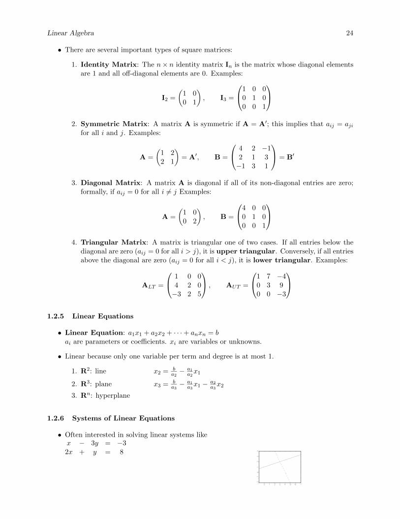
• There are several important types of square matrices:
1. Identity Matrix: The n× n identity matrix In is the matrix whose diagonal elementsare 1 and all off-diagonal elements are 0. Examples:
I2 =
(1 00 1
), I3 =
1 0 00 1 00 0 1
2. Symmetric Matrix: A matrix A is symmetric if A = A′; this implies that aij = aji
for all i and j. Examples:
A =
(1 22 1
)= A′, B =
4 2 −12 1 3−1 3 1
= B′
3. Diagonal Matrix: A matrix A is diagonal if all of its non-diagonal entries are zero;formally, if aij = 0 for all i 6= j Examples:
A =
(1 00 2
), B =
4 0 00 1 00 0 1
4. Triangular Matrix: A matrix is triangular one of two cases. If all entries below the
diagonal are zero (aij = 0 for all i > j), it is upper triangular. Conversely, if all entriesabove the diagonal are zero (aij = 0 for all i < j), it is lower triangular. Examples:
ALT =
1 0 04 2 0−3 2 5
, AUT =
1 7 −40 3 90 0 −3
1.2.5 Linear Equations
• Linear Equation: a1x1 + a2x2 + · · ·+ anxn = bai are parameters or coefficients. xi are variables or unknowns.
• Linear because only one variable per term and degree is at most 1.
1. R2: line x2 = ba2− a1
a2x1
2. R3: plane x3 = ba3− a1
a3x1 − a2
a3x2
3. Rn: hyperplane
1.2.6 Systems of Linear Equations
• Often interested in solving linear systems likex − 3y = −32x + y = 8

Linear Algebra 25
• More generally, we might have a system of m equations in n unknowns
a11x1 + a12x2 + · · · + a1nxn = b1a21x1 + a22x2 + · · · + a2nxn = b2
......
...am1x1 + am2x2 + · · · + amnxn = bm
• A solution to a linear system ofm equations in n unknowns is a set of n numbers x1, x2, · · · , xnthat satisfy each of the m equations.
1. R2: intersection of the lines.
2. R3: intersection of the planes.
3. Rn: intersection of the hyperplanes.
• Example: x = 3 and y = 2 is the solution to the above 2× 2 linear system. Notice from thegraph that the two lines intersect at (3, 2).
• Does a linear system have one, no, or multiple solutions?For a system of 2 equations in 2 unknowns (i.e., two lines):
1. One solution: The lines intersect at exactly one point.
2. No solution: The lines are parallel.
3. Infinite solutions: The lines coincide.
• Methods to solve linear systems:
1. Substitution
2. Elimination of variables
3. Matrix methods
1.2.7 Systems of Equations as Matrices
• Matrices provide an easy and efficient way to represent linear systems such as
a11x1 + a12x2 + · · · + a1nxn = b1a21x1 + a22x2 + · · · + a2nxn = b2
......
...am1x1 + am2x2 + · · · + amnxn = bm
asAx = b
where
1. The m × n coefficient matrix A is an array of mn real numbers arranged in m rowsby n columns:
A =
a11 a12 · · · a1n
a21 a22 · · · a2n...
. . ....
am1 am2 · · · amn

Linear Algebra 26
2. The unknown quantities are represented by the vector x =
x1
x2...xn
.
3. The right hand side of the linear system is represented by the vector b =
b1b2...bm
.
• Augmented Matrix: When we append b to the coefficient matrix A, we get the augmentedmatrix A = [A|b]
a11 a12 · · · a1n | b1a21 a22 · · · a2n | b2...
. . .... |
...am1 am2 · · · amn | bm
1.2.8 Finding Solutions to Augmented Matrices and Systems of Equations
• Row Echelon Form: Our goal is to translate our augmented matrix or system of equationsinto row echelon form. This will provide us with the values of the vector x which solve thesystem. We use the row operations to change coefficients in lower triangle of the augmentedmatrix to 0. An augmented matrix of the form
a′11 a′12 a′13 · · · a′1n | b′1
0 a′22 a′23 · · · a′2n | b′2
0 0 a′33 · · · a′3n | b′3
0 0 0. . .
... |...
0 0 0 0 a′mn | b′m
is said to be in row echelon form — each row has more leading zeros than the row precedingit.
• Reduced Row Echelon Form: We can go one step further and put the matrix into reducedrow echelon form. Reduced row echelon form makes the value of x which solves the systemvery obvious. For a system of m equations in m unknowns, with no all-zero rows, the reducedrow echelon form would be
1 0 0 0 0 | b∗10 1 0 0 0 | b∗20 0 1 0 0 | b∗3
0 0 0. . . 0 |
...
0 0 0 0 1 | b∗m
• Gaussian and Gauss-Jordan elimination: We can conduct elementary row operations
to get our augmented matrix into row echelon or reduced row echelon form. The methods oftransforming a matrix or system into row echelon and reduced row echelon form are referredto as Gaussian elimination and Gauss-Jordan elimination, respectively.

Linear Algebra 27
• Elementary Row Operations: To do Gaussian and Gauss-Jordan elimination, we usethree basic operations to transform the augmented matrix into another augmented matrixthat represents an equivalent linear system – equivalent in the sense that the same values ofxj solve both the original and transformed matrix/system:
1. Interchanging two rows. =⇒ Interchanging two equations.
2. Multiplying a row by a constant. =⇒ Multiplying both sides of an equationby a constant.
3. Adding two rows to each other. =⇒ Adding two equations to each other.
• Interchanging Rows: Suppose we have the augmented matrix
A =
(a11 a12 | b1a21 a22 | b2
)If we interchange the two rows, we get the augmented matrix(
a21 a22 | b2a11 a12 | b1
)which represents a linear system equivalent to that represented by matrix A.
• Multiplying by a Constant: If we multiply the second row of matrix A by a constant c,we get the augmented matrix (
a11 a12 | b1ca21 ca22 | cb2
)which represents a linear system equivalent to that represented by matrix A.
• Adding (subtracting) Rows: If we add (subtract) the first row of matrix A to the second,we obtain the augmented matrix(
a11 a12 | b1a11 + a21 a12 + a22 | b1 + b2
)which represents a linear system equivalent to that represented by matrix A.
• Exercises: Using Gaussian or Gauss-Jordan elimination, solve the following linear systems byputting them into row echelon or reduced row echelon form:
1.x − 3y = −32x + y = 8

Linear Algebra 28
1.2.9 Rank — and Whether a System Has One, Infinite, or No Solutions
• We previously noted that a 2 × 2 system had one, infinite, or no solutions if the two linesintersected, were the same, or were parallel, respectively. More generally, to determine howmany solutions exist, we can use information about (1) the number of equations m, (2) thenumber of unknowns n, and (3) the rank of the matrix representing the linear system.
• Rank: The row rank or column rank of a matrix is the number of nonzero rows or columnsin its row echelon form. The rank also corresponds to the maximum number of linearlyindependent row or column vectors in the matrix. For any matrix A, the row rank alwaysequals column rank, and we refer to this number as the rank of A.
• Examples:
1.
1 2 30 4 50 0 6
Rank=
2.
1 2 30 4 50 0 0
Rank=
3.
1 2 3 | b10 4 5 | b20 0 0 | b3
, bi 6= 0 Rank=
• Let A be the coefficient matrix and A = [A|b] be the augmented matrix. Then
1. rank A ≤ rank A Augmenting A with b can never result in more zero rowsthan originally in A itself. Suppose row i in A is all zerosand that bi is non-zero. Augmenting A with b will yield anon-zero row i in A.
2. rank A ≤ rows A By definition of “rank.”
3. rank A ≤ cols A Suppose there are more rows than columns (otherwise theprevious rule applies). Each column can contain at most onepivot. By pivoting, all other entries in a column below thepivot are zeroed. Hence, there will only be as many non-zerorows as pivots, which will equal the number of columns.
• Existence of Solutions:
1. Exactly one solution: rank A = rank A = rows A = cols A
Necessary condition for a system to have a unique solution:that there be exactly as many equations as unknowns.
2. Infinite solutions: rank A = rank A and cols A > rank A
If a system has a solution and has more unknowns than equa-tions, then it has infinitely many solutions.

Linear Algebra 29
3. No solution: rank A < rank A
Then there is a zero row i in A’s reduced echelon that corre-sponds to a non-zero row i in A’s reduced echelon. Row i ofthe A translates to the equation
0xi1 + 0xi2 + · · ·+ 0xin = b′i
where b′i 6= 0. Hence the system has no solution.
• Find the rank and number of solutions for the systems of equations below.:
1.x − 3y = −32x + y = 8
2.x + 2y + 3z = 62x − 3y + 2z = 143x + y − z = −2
3.x + 2y − 3z = −42x + y − 3z = 43x + 6y − 9z = −12
4.x + 2y + 3z + 4w = 5x + 3y + 5z + 7w = 11x − z − 2w = −6
1.2.10 The Inverse of a Matrix
• Inverse Matrix: An n× n matrix A is nonsingular or invertible if there exists an n× nmatrix A−1 such that
AA−1 = A−1A = In
where A−1 is the inverse of A. If there is no such A−1, then A is singular or noninvertible.

Linear Algebra 30
• Example: Let
A =
(2 32 2
), B =
(−1 3
21 −1
)Since
AB = BA = In
we conclude that B is the inverse, A−1, of A and that A is nonsingular.
• Properties of the Inverse:
1. If the inverse exists, it is unique.
2. A nonsingular =⇒ A−1 nonsingular (A−1)−1 = A
3. A nonsingular =⇒ (AT )−1 = (A−1)T
• Procedure to Find A−1: We know that if B is the inverse of A, then
AB = BA = In
Looking only at the first and last parts of this
AB = In
Solving for B is equivalent to solving for n linear systems, where each column of B is solvedfor the corresponding column in In. We can solve the systems simultaneously by augmentingA with In and performing Gauss-Jordan elimination on A. If Gauss-Jordan elimination on[A|In] results in [In|B], then B is the inverse of A. Otherwise, A is singular.
To summarize: To calculate the inverse of A
1. Form the augmented matrix [A|In]
2. Using elementary row operations, transform the augmented matrix to reduced row ech-elon form.
3. The result of step 2 is an augmented matrix [C|B].
(a) If C = In, then B = A−1.
(b) If C 6= In, then C has a row of zeros. A is singular and A−1 does not exist.
• Exercise: Find the inverse of A =
1 1 10 2 35 5 1

Linear Algebra 31
1.2.11 Linear Systems and Inverses
• Let’s return to the matrix representation of a linear system
Ax = b
If A is an n × n matrix,then Ax = b is a system of n equations in n unknowns. SupposeA is nonsingular =⇒ A−1 exists. To solve this system, we can premultiply each side byA−1 and reduce it as follows:
A−1(Ax) = A−1b
(A−1A)x = A−1b
Inx = A−1b
x = A−1b
Hence, given A and b and given that A is nonsingular, then x = A−1b is a unique solutionto this system.
• Notice also that the requirements for A to be nonsingular correspond to the requirements fora linear system to have a unique solution: rank A = rows A = cols A.
1.2.12 Determinants
• Singularity: Determinants can be used to determine whether a square matrix is nonsingular.
– A square matrix is nonsingular iff its determinant is not zero.
• Determinant of a 1× 1 matrix, A, equals a11
• Determinant of a 2× 2 matrix, A,
∣∣∣∣a11 a12
a21 a22
∣∣∣∣:(A) = |A|
= a11|a22| − a12|a21|= a11a22 − a12a21
Linear Algebra 32
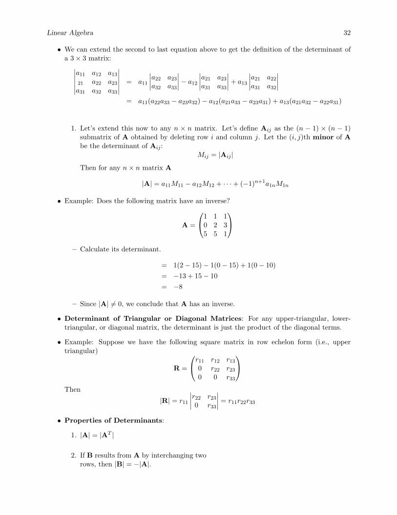
• We can extend the second to last equation above to get the definition of the determinant ofa 3× 3 matrix:∣∣∣∣∣∣
a11 a12 a13
21 a22 a23
a31 a32 a33
∣∣∣∣∣∣ = a11
∣∣∣∣a22 a23
a32 a33
∣∣∣∣− a12
∣∣∣∣a21 a23
a31 a33
∣∣∣∣+ a13
∣∣∣∣a21 a22
a31 a32
∣∣∣∣= a11(a22a33 − a23a32)− a12(a21a33 − a23a31) + a13(a21a32 − a22a31)
1. Let’s extend this now to any n × n matrix. Let’s define Aij as the (n − 1) × (n − 1)submatrix of A obtained by deleting row i and column j. Let the (i, j)th minor of Abe the determinant of Aij :
Mij = |Aij |
Then for any n× n matrix A
|A| = a11M11 − a12M12 + · · ·+ (−1)n+1a1nM1n
• Example: Does the following matrix have an inverse?
A =
1 1 10 2 35 5 1
– Calculate its determinant.
= 1(2− 15)− 1(0− 15) + 1(0− 10)
= −13 + 15− 10
= −8
– Since |A| 6= 0, we conclude that A has an inverse.
• Determinant of Triangular or Diagonal Matrices: For any upper-triangular, lower-triangular, or diagonal matrix, the determinant is just the product of the diagonal terms.
• Example: Suppose we have the following square matrix in row echelon form (i.e., uppertriangular)
R =
r11 r12 r13
0 r22 r23
0 0 r33
Then
|R| = r11
∣∣∣∣r22 r23
0 r33
∣∣∣∣ = r11r22r33
• Properties of Determinants:
1. |A| = |AT |
2. If B results from A by interchanging tworows, then |B| = −|A|.

Linear Algebra 33
3. If two rows of A are equal, then |A| = 0. (Notice that in this case rank A 6=rows A, which was one of the conditionsfor the existence of a unique solution.)
4. If a row of A consists of all zeros, then|A| = 0.
(Same as 3.)
5. If B is obtained by multiplying a row ofA by a scalar s, then |B| = s|A|.
6. If B is obtained from A by adding to theith row of A the jth row (i 6= j) multi-plied by a scalar s, then |B| = |A|.
(i.e., If the row isn’t simply multiplied bya scalar and left, then the determinantremains the same.)
7. If no row interchanges and no scalar mul-tiplications of a single row are used tocompute the row echelon form R fromthe n×n coefficient matrix A, then |A| =|R|.
(Implied by the previous properties.)
8. A square matrix is nonsingular iff its de-terminant 6= 0.
(Implied by the previous properties.)
9. |AB| = |A||B|
10. If A is nonsingular, then |A| 6= 0 and|A−1| = 1
|A| .
1.2.13 Getting Inverse of a Matrix using its Determinant and Matrix of Cofactors
• Thus far, we have a number of algorithms to
1. Find the solution of a linear system,
2. Find the inverse of a matrix
but these remain just that — algorithms. At this point, we have no way of telling how thesolutions xj change as the parameters aij and bi change, except by changing the values and“rerunning” the algorithms.
• With determinants, we can
1. Provide an explicit formula for the inverse, and
2. Provide an explicit formula for the solution of an n× n linear system.
Hence, we can examine how changes in the parameters and bi affect the solutions xj .
• Determinant Formula for the Inverse of a 2× 2: The determinant of a 2× 2 matrix A(a bc d
)is defined as:
1
det(A)
(d −b−c a
)

Linear Algebra 34
1.2.14 Inverse of Larger Matrices
• Cofactors and Adjoint Matrices:
– Define the (i, j)th cofactor Cij of A as (−1)i+jMij . Recall that Mij is the minor of A,defined as the determinant of the matrix that results from removing row i and columnj from A.
– Define the adjoint of A as the n×n matrix whose (i, j)th entry is Cji (notice the switchin indices!). In other words, adj(A) is the transpose of the cofactor matrix of A.
• Then the inverse of A is defined as the reciprocal of the determinant of A times its adjoint,given by the formula
A−1 =1
|A|adj A =
C11|A|
C21|A| · · ·
Cn1|A|
C12|A|
C22|A| · · ·
Cn2|A|
......
. . ....
C1n|A|
C2n|A| · · ·
Cnn|A|
• Exercises:
Let A =
5 1 30 2 35 5 1
1. Find the determinant of A.
det A =
=
=
=
2. Find the adjoint matrix of A.
adj(A) =
3. Find the inverse of A.
A−1 =

Calculus I 35
1.3 Calculus I
Topics:Sequences; Limit of a Sequence; Series; Derivatives; Higher-Order Derivatives; Composite Func-tions and The Chain Rule; Derivatives of Exp and Ln; Maxima and Minima; Partial Derivatives;L’Hopital’s Rule; Taylor Approximation; Derivative Calculus in 6 Steps
1.3.1 Sequences
• A sequence yn = y1, y2, y3, . . . , yn is an ordered set of real numbers, where y1 is thefirst term in the sequence and yn is the nth term. Generally, a sequence is infinite, that isit extends to n =∞. We can also write the sequence as yn∞n=1.
Examples:
1. yn =
2− 1n2
=
0 5 10 151
1.5
2
2. yn =n2+1n
=
0 5 10 15
10
20
3. yn =
(−1)n(1− 1
n
)=
0 20 40
1
1
Think of sequences like functions. Before, we had y = f(x) with x specified over some domain.Now we have yn = f(n) with n = 1, 2, 3, . . ..
• Three kinds of sequences:
1. Sequences like 1 above that converge to a limit.
2. Sequences like 2 above that increase without bound.
3. Sequences like 3 above that neither converge nor increase without bound — alternatingover the number line.
Much of the material and examples for this lecture are taken from Simon & Blume (1994) Mathematics for Economistsand from Boyce & Diprima (1988) Calculus

Calculus I 36
• Boundedness and monotonicity:
1. Bounded: if |yn| ≤ K for all n
2. Monotonically Increasing: yn+1 > yn for all n
3. Monotonically Decreasing: yn+1 < yn for all n
• Subsequence: choose an infinite collection of entries from yn, retaining their order.
1.3.2 The Limit of a Sequence
We’re often interested in whether a sequence converges to a limit. Limits of sequences areconceptually similar to the limits of functions addressed in the previous lecture.
• Limit of a sequence. The sequence yn has the limit L, that is limn→∞
yn = L, if for any
ε > 0 there is an integer N (which depends on ε) with the property that |yn−L| < ε for eachn > N . yn is said to converge to L. If the above does not hold, then yn diverges.
• Uniqueness: If yn converges, then the limit L is unique.
• Properties: Let limn→∞
yn = A and limn→∞
zn = B. Then
1. limn→∞
[αyn + βzn] = αA+ βB
2. limn→∞
ynzn = AB
3. limn→∞
ynzn
= AB , provided B 6= 0
Examples:
1. limn→∞
2− 1
n2
=
2. limn→∞
4n
n!
=
0 5 10 15
5
10
15
Finding the limit of a sequence in Rn is similar to that in R1.
• Limit of a sequence of vectors. The sequence of vectors yn has the limit L, that islimn→∞
yn = L, if for any ε there is an integer N where ||yn − L|| < ε for each n > N . The
sequence of vectors yn is said to converge to the vector L — and the distances between yn
and L converge to zero.
Think of each coordinate of the vector yn as being part of its own sequence over n. Then asequence of vectors in Rn converges if and only if all n sequences of its components converge.Examples:
1. The sequence yn where yn =(
1n , 2−
1n2
)converges to (0, 2).
2. The sequence yn where yn =(
1n , (−1)n
)does not converge, since (−1)n does not
converge.

Calculus I 37
• Bolzano-Weierstrass Theorem: Any sequence contained in a compact (i.e., closed andbounded) subset of Rn contains a convergent subsequence.
Example: Take the sequence yn = (−1)n, which has twoaccumulating points, but no limit. However, it is both closedand bounded.
0 10 20
1
1
The subsequence of yn defined by taking n = 1, 3, 5, . . .does have a limit: −1.
0 10 20
1
1
As does the subsequence defined by taking n = 2, 4, 6, . . .,whose limit is 1.
0 10 20
1
1
1.3.3 Series
• The sum of the terms of a sequence is a series. As there are both finite and infinite sequences,there are finite and infinite series.
The series associated with the sequence yn = y1, y2, y3, . . . , yn = yn∞n=1 is∑∞
n=1 yn.The nth partial sum Sn is defined as Sn =
∑nk=1 yk,the sum of the first n terms of the
sequence.
• Convergence: A series∑yn converges if the sequence of partial sums S1, S2, S3, ... con-
verges, i.e has a finite limit.
• A geometric series is a series that can be written as∑∞
n=0 rn, where r is called the ratio. A
geometric series converges to 11−r if |r| < 1 and diverges otherwise. For example,
∑∞n=0
12n = 2.
Examples of other series:
1.∑∞
n=01n! = 1 + 1
1! + 12! + 1
3! + · · · = e.This one is especially useful in statistics and probability.
2.∑∞
n=11n = 1
1 + 12 + 1
3 + · · · =∞ (harmonic series)
1.3.4 Derivatives
The derivative of f at x is its rate of change at x — i.e., how much f(x) changes with achange in x.

Calculus I 38
– For a line, the derivative is the slope.– For a curve, the derivative is the slope of the line tangent to the curve at x.
• Derivative: Let f be a function whose domain includes an open interval containing the pointx. The derivative of f at x is given by
f ′(x) = limh→0
f(x+ h)− f(x)
(x+ h)− x
= limh→0
f(x+ h)− f(x)
h
If f ′(x) exists at a point x, then f is said to be differentiable at x. Similarly, if f ′(x) existsfor every point a long an interval, then f is differentiable along that interval. For f to bedifferentiable at x, f must be both continuous and “smooth” at x. The process of calculatingf ′(x) is called differentiation.
• Notation for derivatives:
1. y′, f ′(x) (Prime or Lagrange Notation)
2. Dy, Df(x) (Operator Notation)
3. dydx , df
dx(x) (Leibniz’s Notation)
• Properties of derivatives: Suppose that f and g are differentiable at x and that α is a constant.Then the functions f ± g, αf , fg, and f/g (provided g(x) 6= 0) are also differentiable at x.Additionally,
1. Power rule: [xk]′ = kxk−1
2. Sum rule: [f(x)± g(x)]′ = f ′(x)± g′(x)
3. Constant rule: [αf(x)]′ = αf ′(x)
4. Product rule: [f(x)g(x)]′ = f ′(x)g(x) + f(x)g′(x)
5. Quotient rule: [f(x)/g(x)]′ = f ′(x)g(x)−f(x)g′(x)[g(x)]2
, g(x) 6= 0
Examples:
1. f(x) = cf ′(x) =
2.f(x) = xf ′(x) =
3.f(x) = x2
f ′(x) =

Calculus I 39
4.f(x) = x3
f ′(x) =
5. f(x) = 3x2 + 2x1/3
f ′(x) =
6. f(x) = (x3)(2x4)f ′(x) =
7. f(x) = x2+1x2−1
f ′(x) =
1.3.5 Higher-Order Derivatives or, Derivatives of Derivatives of Derivatives
We can keep applying the differentiation process to functions that are themselves derivatives.The derivative of f ′(x) with respect to x, would then be
f ′′(x) = limh→0
f ′(x+ h)− f ′(x)
h
and so on. Similarly, the derivative of f ′′(x) would be denoted f ′′′(x).
• First derivative: f ′(x), y′, df(x)dx , dy
dx
Second derivative: f ′′(x), y′′, d2f(x)dx2
, d2ydx2
nth derivative: dnf(x)dxn , dny
dxn
Example:f(x) = x3
f ′(x) = 3x2
f ′′(x) = 6xf ′′′(x) = 6f ′′′′(x) = 0
1.3.6 Composite Functions and the Chain Rule
• Composite functions are formed by substituting one function into another and are denotedby
(f g)(x) = f [g(x)]

Calculus I 40
To form f [g(x)], the range of g must be contained (at least in part) within the domain off . The domain of f g consists of all the points in the domain of g for which g(x) is in thedomain of f .
Examples:
1. f(x) = lnx,g(x) = x2
(f g)(x) = lnx2,(g f)(x) = [lnx]2,Notice that f g and g f are not the same functions.
2. f(x) = 4 + sinx,g(x) =
√1− x2,
(f g)(x) = 4 + sin√
1− x2,(gf)(x) does not exist.
√1− (4 + sin(x))2 is not a real number because 1−(4+sin(x))2
is always negative.
• Chain Rule: Let y = (f g)(x) = f [g(x)]. The derivative of y with respect to x is
d
dxf [g(x)] = f ′[g(x)]g′(x)
which can also be written asdy
dx=
dy
dg(x)
dg(x)
dx
(Note: the above does not imply that the dg(x)’s cancel out, as in fractions. They are partof the derivative notation and you can’t separate them out or cancel them.)The chain rule can be thought of as the derivative of the “outside” times the derivative of the“inside,” remembering that the derivative of the outside function is evaluated at the value ofthe inside function.
• Generalized Power Rule: If y = [g(x)]k, then dy/dx = k[g(x)]k−1g′(x).
Examples:
1. Find dy/dx for y = (3x2 + 5x − 7)6. Let f(z) = z6 and z = g(x) = 3x2 + 5x − 7.Then, y = f [g(x)] and
dy
dx=
2. Find dy/dx for y = sin(x3 + 4x). (Note: the derivative of sinx is cosx.) Letf(z) = sin z and z = g(x) = x3 + 4x. Then, y = f [g(x)] and
dy
dx=

Calculus I 41
1.3.7 Derivatives of Euler’s number and natural logs
• Derivatives of Exp or e:
1. ddxe
x = ex
2. ddxαe
x = αex
3. dn
dxnαex = αex
4. ddxe
u(x) = eu(x)u′(x)
Examples: Find dy/dx for
1. y = e−3x
2. y = ex2
3. y = esin 2x
• Derivatives of Ln:
1. ddx lnx = 1
x
2. ddx lnxk = d
dxk lnx = kx
3. ddx lnu(x) = u′(x)
u(x) (by the chain rule)
4. For any positive base b, ddxb
x = (ln b) (bx).
Examples: Find dy/dx for
1. y = ln(x2 + 9)
2. y = ln(lnx)
3. y = (lnx)2
4. y = ln ex
1.3.8 Applications of the Derivative: Maxima and Minima
The first derivative, f ′(x), identifies whether the function f(x) at the point x is increasing ordecreasing at x.
1. Increasing: f ′(x) > 0
2. Decreasing: f ′(x) < 0
3. Neither increasing nor decreasing: f ′(x) = 0i.e. a maximum, minimum, or saddle point
Examples:
1. f(x) = x2 + 2, f ′(x) = 2x

Calculus I 42
2. f(x) = x3 + 2, f ′(x) = 3x2
The second derivative f ′′(x) identifies whether the function f(x) at the point x is
1. Concave down: f ′′(x) < 0
2. Concave up: f ′′(x) > 0
• Maximum (Minimum): x0 is a local maximum (minimum) if f(x0) > f(x) (f(x0) <f(x)) for all x within some open interval containing x0. x0 is a global maximum (mini-mum) if f(x0) > f(x) (f(x0) < f(x)) for all x in the domain of f .
• Critical points: Given the function f defined over domain D, all of the following are definedas critical points:
1. Any interior point of D where f ′(x) = 0.
2. Any interior point of D where f ′(x) does not exist.
3. Any endpoint that is in D.
The maxima and minima will be a subset of the critical points.
• Second Derivative Test of Maxima/Minima: We can use the second derivative to tellus whether a point is a maximum or minimum of f(x).
Local Maximum: f ′(x) = 0 and f ′′(x) < 0
Local Minimum: f ′(x) = 0 and f ′′(x) > 0
Need more info: f ′(x) = 0 and f ′′(x) = 0
• Global Maxima and Minima. Sometimes no global max or min exists — e.g., f(x) notbounded above or below. However, there are three situations where we can fairly easilyidentify global max or min.
1. Functions with only one critical point. If x0 is a local max or min of f and it isthe only critical point, then it is the global max or min.
2. Globally concave up or concave down functions. If f ′′(x) is never zero, then thereis at most one critical point. That critical point is a global maximum if f ′′ < 0 and aglobal minimum if f ′′ > 0.
3. Functions over closed and bounded intervals must have both a global maximumand a global minimum.
Examples: Find any critical points and identify whether they’re a max, min, or saddlepoint:
1. f(x) = x2 + 2

Calculus I 43
2. f(x) = x3 + 2
3. f(x) = |x2 − 1|, x ∈ [−2, 2]
1.3.9 Partial Derivatives
Suppose we have a function f now of two (or more) variables and we want to determine therate of change relative to one of the variables. To do so, we would find it’s partial derivative,which is defined similar to the derivative of a function of one variable.
• Partial Derivative: Let f be a function of the variables (x1, . . . , xn). The partial derivativeof f with respect to xi is
∂f
∂xi(x1, . . . , xn) = lim
h→0
f(x1, . . . , xi + h, . . . , xn)− f(x1, . . . , xi, . . . , xn)
h
Only the ith variable changes — the others are treated as constants.
We can take higher-order partial derivatives, like we did with functions of a single variable,except now we the higher-order partials can be with respect to multiple variables.
Examples:
1. f(x, y) = x2 + y2
∂f∂x (x, y) =∂f∂y (x, y) =∂2f∂x2
(x, y) =∂2f∂x∂y (x, y) =
2. f(x, y) = x3y4 + ex − ln y∂f∂x (x, y) =∂f∂y (x, y) =∂2f∂x2
(x, y) =∂2f∂x∂y (x, y) =

Calculus I 44
1.3.10 L’Hopital’s Rule
In studying limits, we saw that limx→c
f(x)/g(x) =(
limx→c
f(x))/(
limx→c
g(x))
, provided that
limx→c
g(x) 6= 0.
• If both limx→c
f(x) = 0 and limx→c
g(x) = 0, then we get an indeterminate form of the type 0/0
as x→ c. However, a limit may still exist. We can use L’Hopital’s rule to find the limit.
• L’Hopital’s Rule: Suppose f and g are differentiable on some interval a < x < b and thateither
1. limx→a+
f(x) = 0 and limx→a+
g(x) = 0, or
2. limx→a+
f(x) = ±∞ and limx→a+
g(x) = ±∞
Suppose further that g′(x) is never zero on a < x < b and that
limx→a+
f ′(x)
g′(x)= L
then
limx→a+
f(x)
g(x)= L
And if limx→a
f ′(x)g′(x) = 0/0 or ±∞/±∞ then you can apply L’Hopital’s rule a second time, and
continue applying it until you have a solution.
Examples: Use L’Hopital’s rule to find the following limits:
1. limx→0+
ln(1+x2)x3
2. limx→0+
e1/x
1/x
3. limx→2
x−2(x+6)1/3−2

Calculus I 45
1.3.11 Taylor Series Approximation
• Taylor series (also known as the delta method) are used commonly to represent functionsas infinite series of the function’s derivatives at some point a. For example, Taylor series arevery helpful in representing nonlinear functions as linear functions. One can thus approximatefunctions by using lower-order, finite series known as Taylor polynomials. If a = 0, theseries is called a Maclaurin series.
• Specifically, a Taylor series of a real or complex function f(x) that is infinitely differentiablein the neighborhood of point a is:
f(x) = f(a) +f ′(a)
1!(x− a) +
f ′′(a)
2!(x− a)2 + · · ·
=∞∑n=0
f (n)(a)
n!(x− a)n
• Taylor Approximation: We can often approximate the curvature of a function f(x) atpoint a using a 2nd order Taylor polynomial around point a:
f(x) = f(a) +f ′(a)
1!(x− a) +
f ′′(a)
2!(x− a)2 +R2
R2 is the Lagrange remainder and often treated as negligible, giving us:
f(x) ≈ f(a) + f ′(a)(x− a) +f ′′(a)
2(x− a)2
Taylor series expansion is easily generalized to multiple dimensions.
• Curvature and The Taylor Polynomial as a Quadratic Form: The Hessian is used ina Taylor polynomial approximation to f(x) and provides information about the curvature off(x) at x — e.g., which tells us whether a critical point x∗ is a min, max, or saddle point.
1. The second order Taylor polynomial about the critical point x∗ is
f(x∗ + h) = f(x∗) +∇f(x∗)h +1
2hTH(x∗)h + R(h)
2. Since we’re looking at a critical point, ∇f(x∗) = 0; and for small h, R(h) is negligible.Rearranging, we get
f(x∗ + h)− f(x∗) ≈ 1
2hTH(x∗)h
3. The RHS is a quadratic form and we can determine the definiteness of H(x∗).
1.3.12 Summary: Derivative calculus in 6 steps
With these six rules (and decent algebra and trigonometry skills) you can figure out the derivativeof anything.
1. Sum rule: [f(x)± g(x)]′ = f ′(x)± g′(x)

Calculus I 46
2. Product rule: [f(x)g(x)]′ = f ′(x)g(x) + f(x)g′(x)
3. Power rule: [xk]′ = kxk−1
4. Chain rule: ddxf [g(x)] = f ′[g(x)]g′(x)
5. ex: ddxe
x = ex
6. Trig identity: ddx sin(x) = cos(x)

Calculus II 47
1.4 Calculus II
Today’s Topics: The Indefinite Integral: The Antiderivative; Common Rules of Integration; TheDefinite Integral: The Area under the Curve; Integration by Substitution; Integration by Parts
1.4.1 The Indefinite Integral: The Antiderivative
So far, we’ve been interested in finding the derivative g = f ′ of a function f . However,sometimes we’re interested in exactly the reverse: finding the function f for which g is itsderivative. We refer to f as the antiderivative of g.
Let DF be the derivative of F . And let DF (x) be the derivative of F evaluated at x. Thenthe antiderivative is denoted by D−1 (i.e., the inverse derivative). If DF = f , then F = D−1f .
• Indefinite Integral: Equivalently, if F is the antiderivative of f , then F is also called theindefinite integral of f and written F (x) =
∫f(x)dx.
Examples:
1.∫
1x2dx =
2.∫
3e3xdx =
3.∫
(x2 − 4)dx =
Notice from these examples that while there is only a single derivative for any function, thereare multiple antiderivatives: one for any arbitrary constant c. c just shifts the curve up ordown on the y-axis. If more info is present about the antiderivative — e.g., that it passesthrough a particular point — then we can solve for a specific value of c.
1.4.2 Common Rules of Integration
•∫af(x)dx = a
∫f(x)dx
•∫
[f(x) + g(x)]dx =∫f(x)dx+
∫g(x)dx
•∫xndx = 1
n+1xn+1 + c
•∫exdx = ex + c
•∫
1xdx = lnx+ c
•∫ef(x)f ′(x)dx = ef(x) + c
•∫
[f(x)]nf ′(x)dx = 1n+1 [f(x)]n+1 + c
•∫ f ′(x)
f(x) dx = ln f(x) + c
Much of the material and examples for this lecture are taken from Simon & Blume (1994) Mathematics for Economistsand from Boyce & Diprima (1988) Calculus

Calculus II 48
Examples:
1.∫
3x2dx =
2.∫
(2x+ 1)dx =
3.∫exee
xdx =
1.4.3 The Definite Integral: The Area under the Curve
• Riemann Sum: Suppose we want to determine the area A(R) of a region R defined by acurve f(x) and some interval a ≤ x ≤ b. One way to calculate the area would be to dividethe interval a ≤ x ≤ b into n subintervals of length ∆x and then approximate the region witha series of rectangles, where the base of each rectangle is ∆x and the height is f(x) at themidpoint of that interval. A(R) would then be approximated by the area of the union of therectangles, which is given by
S(f,∆x) =n∑i=1
f(xi)∆x
and is called a Riemann sum.
As we decrease the size of the subintervals ∆x, making the rectangles “thinner,” we wouldexpect our approximation of the area of the region to become closer to the true area. Thisgives the limiting process
A(R) = lim∆x→0
n∑i=1
f(xi)∆x
• Riemann Integral: If for a given function f the Riemann sum approaches a limit as ∆x→ 0,then that limit is called the Riemann integral of f from a to b. Formally,
b∫a
f(x)dx = lim∆x→0
n∑i=1
f(xi)∆x
• Definite Integral: We use the notationb∫af(x)dx to denote the definite integral of f from
a to b. In words, the definite integralb∫af(x)dx is the area under the “curve” f(x) from x = a
to x = b.
• First Fundamental Theorem of Calculus: Let the function f be bounded on [a, b] andcontinuous on (a, b). Then the function
F (x) =
x∫a
f(t)dt, a ≤ x ≤ b
has a derivative at each point in (a, b) and
F ′(x) = f(x), a < x < b
This last point shows that differentiation is the inverse of integration.

Calculus II 49
• Second Fundamental Theorem of Calculus: Let the function f be bounded on [a, b] andcontinuous on (a, b). Let F be any function that is continuous on [a, b] such that F ′(x) = f(x)on (a, b). Then
b∫a
f(x)dx = F (b)− F (a)
• Procedure to calculate a “simple” definite integralb∫af(x)dx:
1. Find the indefinite integral F (x).
2. Evaluate F (b)− F (a).
Examples:
1.3∫1
3x2dx =
2.2∫−2
exeexdx =
• Properties of Definite Integrals:
1.a∫af(x)dx = 0 There is no area below a point.
2.b∫af(x)dx = −
a∫b
f(x)dx Reversing the limits changes the sign of the integral.
3.b∫a
[αf(x) + βg(x)]dx = αb∫af(x)dx+ β
b∫ag(x)dx
4.b∫af(x)dx+
c∫b
f(x)dx =c∫af(x)dx
Examples:
1.1∫1
3x2dx =
2.4∫0
(2x+ 1)dx =
3.0∫−2
exeexdx+
2∫0
exeexdx =

Calculus II 50
1.4.4 Integration by Substitution
• Sometimes the integrand doesn’t appear integrable using common rules and antiderivatives.A method one might try is integration by substitution, which is related to the ChainRule.
Suppose we want to find the indefinite integral∫g(x)dx and assume we can identify a function
u(x) such that g(x) = f [u(x)]u′(x). Let’s refer to the antiderivative of f as F . Then thechain rule tells us that d
dxF [u(x)] = f [u(x)]u′(x). So, F [u(x)] is the antiderivative of g. Wecan then write ∫
g(x)dx =
∫f [u(x)]u′(x)dx =
∫d
dxF [u(x)]dx = F [u(x)] + c
• Procedure to determine the indefinite integral∫g(x)dx by the method of substi-
tution:
1. Identify some part of g(x) that might be simplified by substituting in a single variableu (which will then be a function of x).
2. Determine if g(x)dx can be reformulated in terms of u and du.
3. Solve the indefinite integral.
4. Substitute back in for x
Substitution can also be used to calculate a definite integral. Using the same procedure asabove,
b∫a
g(x)dx =
d∫c
f(u)du = F (d)− F (c)
where c = u(a) and d = u(b).
Examples:
1.∫x2√x+ 1dx
The problem here is the√x+ 1 term. However, if the integrand had
√x times some
polynomial, then we’d be in business. Let’s try u = x+ 1. Then x = u− 1 and dx = du.Substituting these into the above equation, we get∫
x2√x+ 1dx =
∫(u− 1)2√udu
=
∫(u2 − 2u+ 1)u1/2du
=
∫(u5/2 − 2u3/2 + u1/2)du
We can easily integrate this, since it’s just a polynomial. Doing so and substitutingu = x+ 1 back in, we get∫
x2√x+ 1dx = 2(x+ 1)3/2
[1
7(x+ 1)2 − 2
5(x+ 1) +
1
3
]+ c

Calculus II 51
2. For the above problem, we could have also used the substitution u =√x+ 1. Then
x = u2 − 1 and dx = 2udu. Substituting these in, we get∫x2√x+ 1dx =
∫(u2 − 1)2u2udu
which when expanded is again a polynomial and gives the same result as above.
3.1∫0
5e2x
(1+e2x)1/3dx
When an expression is raised to a power, it’s often helpful to use this expression asthe basis for a substitution. So, let u = 1 + e2x. Then du = 2e2xdx and we canset 5e2xdx = 5du/2. Additionally, u = 2 when x = 0 and u = 1 + e2 when x = 1.Substituting all of this in, we get
1∫0
5e2x
(1 + e2x)1/3dx =
5
2
1+e2∫2
du
u1/3
=5
2
1+e2∫2
u−1/3du
=15
4u2/3
∣∣∣∣1+e2
2
= 9.53
1.4.5 Integration by Parts, or Ultraviolet Voodoo
• Another useful integration technique is integration by parts, which is related to the ProductRule of differentiation. The product rule states that
d
dx(uv) = u
dv
dx+ v
du
dx
Integrating this and rearranging, we get∫udv
dxdx = uv −
∫vdu
dxdx
or ∫u(x)v′(x)dx = u(x)v(x)−
∫v(x)u′(x)dx
More frequently remembered as ∫udv = uv −
∫vdu
where du = u′(x)dx and dv = v′(x)dx.
For definite integrals:b∫au dvdxdx = uv|ba −
b∫av dudxdx
Calculus II 52
Our goal here is to find expressions for u and dv that, when substituted into the aboveequation, yield an expression that’s more easily evaluated.
Examples:
1.∫xeaxdx
2.∫xneaxdx
3.∫x3e−x
2dx

Unconstrained and Constrained Optimization 53
1.5 Unconstrained and Constrained Optimization
Topics8: • Quadratic Forms • Definiteness of Quadratic Forms • Maxima and Minima in Rn •First Order Conditions • Second Order Conditions • Global Maxima and Minima • ConstrainedOptimization • Equality Constraints • Inequality Constraints • Kuhn-Tucker Conditions
1.5.1 Quadratic Forms
• Quadratic forms important because
1. Approximates local curvature around a point — e.g., used to identify max vs min vssaddle point.
2. Simple, so easy to deal with.
3. Have a matrix representation.
• Quadratic Form: A polynomial where each term is a monomial of degree 2 in any numberof variables:
One variable: Q(x1) = a11x21
Two variables: Q(x1, x2) = a11x21 + a12x1x2 + a22x
22
N variables: Q(x1, · · · , xn) =∑i≤j
aijxixj
which can be written in matrix terms:
One variable: Q(x) = xT1 a11x1
N variables: Q(x) =(x1 x2 · · · xn
)a11
12a12 · · · 1
2a1n12a12 a22 · · · 1
2a2n...
.... . .
...12a1n
12a2n · · · ann
x1
x2...xn
= xTAx
Examples:
1. Quadratic on R2:
Q(x1, x2) =(x1 x2
)( a1112a12
12a12 a22
)(x1
x2
)= a11x
21 + a12x1x2 + a22x
22
2. Quadratic on R3: Q(x1, x2, x3) =
8Much of the material and examples for this lecture are taken from Simon & Blume (1994) Mathematics for Economistsand Ecker & Kupferschmid (1988) Introduction to Operations Research.
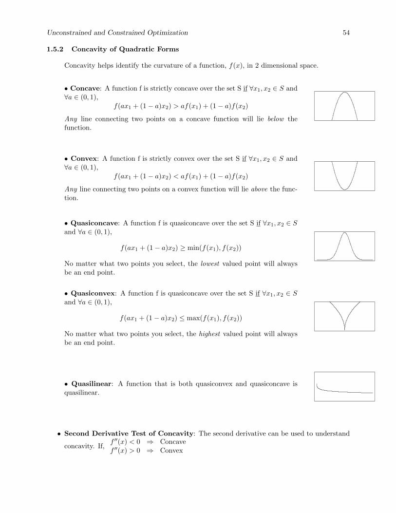
Unconstrained and Constrained Optimization 54
1.5.2 Concavity of Quadratic Forms
Concavity helps identify the curvature of a function, f(x), in 2 dimensional space.
• Concave: A function f is strictly concave over the set S if ∀x1, x2 ∈ S and∀a ∈ (0, 1),
f(ax1 + (1− a)x2) > af(x1) + (1− a)f(x2)
Any line connecting two points on a concave function will lie below thefunction.
• Convex: A function f is strictly convex over the set S if ∀x1, x2 ∈ S and∀a ∈ (0, 1),
f(ax1 + (1− a)x2) < af(x1) + (1− a)f(x2)
Any line connecting two points on a convex function will lie above the func-tion.
• Quasiconcave: A function f is quasiconcave over the set S if ∀x1, x2 ∈ Sand ∀a ∈ (0, 1),
f(ax1 + (1− a)x2) ≥ min(f(x1), f(x2))
No matter what two points you select, the lowest valued point will alwaysbe an end point.
• Quasiconvex: A function f is quasiconcave over the set S if ∀x1, x2 ∈ Sand ∀a ∈ (0, 1),
f(ax1 + (1− a)x2) ≤ max(f(x1), f(x2))
No matter what two points you select, the highest valued point will alwaysbe an end point.
• Quasilinear: A function that is both quasiconvex and quasiconcave isquasilinear.
• Second Derivative Test of Concavity: The second derivative can be used to understand
concavity. If,f ′′(x) < 0 ⇒ Concavef ′′(x) > 0 ⇒ Convex

Unconstrained and Constrained Optimization 55
1.5.3 Definiteness of Quadratic Forms
Definiteness helps identify the curvature of a function, Q(x), in n dimensional space.
• Definiteness: By definition, a quadratic form always takes on the value of zero when x = 0,Q(x) = 0 at x = 0. The definiteness of the matrix A is determined by whether the quadraticform Q(x) = xTAx is greater than zero, less than zero, or sometimes both over all x 6= 0.
1. Positive Definite xTAx > 0, ∀x 6= 0 Min
ex: Q(x1, x2) = x21 + x2
2
2. Positive Semidefinite xTAx ≥ 0, ∀x 6= 0
ex: Q(x1, x2) = x21 + 2x1x2 + x2
2
3. Negative Definite xTAx < 0, ∀x 6= 0 Max
ex: Q(x1, x2) = −x21 − x2
2
4. Negative Semidefinite xTAx ≤ 0, ∀x 6= 0
ex: Q(x1, x2) = −x21 − 2x1x2 − x2
2
5. Indefinite xTAx > 0 for some x 6= 0 andxTAx < 0 for other x 6= 0
Neither
ex: Q(x1, x2) = x21 − x2
2
Examples:
1. Positive Definite:
Q(x) = xT(
1 00 1
)x
= x21 + x2
2
2. Positive Semidefinite:
Q(x) = xT(
1 −1−1 1
)x
= (x1 − x2)2

Unconstrained and Constrained Optimization 56
3. Indefinite:
Q(x) = xT(
1 00 −1
)x
= x21 − x2
2
1.5.4 First Order Conditions
When we examined functions of one variable x, we found critical points by taking the firstderivative, setting it to zero, and solving for x. For functions of n variables, the critical pointsare found in much the same way, except now we set the partial derivatives equal to zero.9
• Gradient (∇f(x)): Given a function f(x) in n variables, the gradient ∇f(x) is a columnvector, where the ith element is the partial derivative of f(x) with respect to xi:
∇f(x) =
∂f(x)∂x1
∂f(x)∂x2...
∂f(x)∂xn
• Critical Point: x∗ is a critical point iff ∇f(x∗) = 0. If the partial derivative of f(x) with
respect to x∗ is 0, then x∗ is a critical point. To solve for x∗, find the gradient, set eachelement equal to 0, and solve the system of equations.
x∗ =
x∗1x∗2...x∗n
Example: Given a function f(x) = (x1 − 1)2 + x2
2 + 1, find the:
1. Gradient ∇f(x) =
2. Critical Point x∗ =
9We will only consider critical points on the interior of a function’s domain.

Unconstrained and Constrained Optimization 57
1.5.5 Second Order Conditions
When we found a critical point for a function of one variable, we used the second derivativeas an indicator of the curvature at the point in order to determine whether the point was amin, max, or saddle (second derivative test of concavity). For functions of n variables, weuse second order partial derivatives as an indicator of curvature.
• Hessian (H(x)): Given a function f(x) in n variables, the hessian H(x) is an n× n matrix,where the (i, j)th element is the second order partial derivative of f(x) with respect to xi andxj :
H(x) =
∂2f(x)∂x21
∂2f(x)∂x1∂x2
· · · ∂2f(x)∂x1∂xn
∂2f(x)∂x2∂x1
∂2f(x)∂x22
· · · ∂2f(x)∂x2∂xn
......
. . ....
∂2f(x)∂xn∂x1
∂2f(x)∂xn∂x2
· · · ∂2f(x)∂x2n
Note that the hessian will be a symmetric matrix because ∂f(x)
∂x1∂x2= ∂f(x)
∂x2∂x1.
Also note that given that f(x) is of quadratic form, each element of the hessian will be aconstant.
• Second Order Conditions:
Given a function f(x) and a point x∗ such that ∇f(x∗) = 0,
1. H(x∗) Positive Definite =⇒ Strict Local Min
2. H(x) Positive Semidefinite∀x ∈ B(x∗, ε)
=⇒ Local Min
3. H(x∗) Negative Definite =⇒ Strict Local Max
4. H(x) Negative Semidefinite∀x ∈ B(x∗, ε)
=⇒ Local Max
5. H(x∗) Indefinite =⇒Saddle Point
Example: We found that the only critical point of f(x) = (x1− 1)2 + x22 + 1 is at x∗ = (1, 0).
Is it a min, max, or saddle point?
1. Hessian H(x) =
2. Leading principal minors of H(x) =
3. Definiteness?
Unconstrained and Constrained Optimization 58
4. Maxima, Minima, or Saddle Point?
5. Alternate check of definiteness. Is H(x∗) ≥≤ 0 ∀ x 6= 0?
1.5.6 Definiteness and Concavity
Although definiteness helps us to understand the curvature of an n-dimensional function, itdoes not necessarily tell us whether the function is globally concave or convex.
We need to know whether a function is globally concave or convex to determine whether acritical point is a global min or max.
• Testing for Global Concavity: We can use the definiteness of the Hessian to determinewhether a function is globally concave or convex:
1. H(x) Positive Semidefinite ∀x =⇒ Globally Convex
2. H(x) Negative Semidefinite ∀x =⇒ Globally Concave
Notice that the definiteness conditions must be satisfied over the entire domain.
1.5.7 Global Maxima and Minima
• Global Max/Min Conditions: Given a function f(x) and a point x∗ such that∇f(x∗) = 0,
1. f(x) Globally Convex =⇒ Global Min
2. f(x) Globally Concave =⇒ Global Max
Note that showing that H(x∗) is negative semidefinite is not enough to guarantee x∗ is a localmax. However, showing that H(x) is negative semidefinite for all x guarantees that x∗ is aglobal max. (The same goes for positive semidefinite and minima.)
Example: Take f1(x) = x4 and f2(x) = −x4. Both have x = 0 as a critical point. Unfortu-nately, f ′′1 (0) = 0 and f ′′2 (0) = 0, so we can’t tell whether x = 0 is a min or max for either.However, f ′′1 (x) = 12x2 and f ′′2 (x) = −12x2. For all x, f ′′1 (x) ≥ 0 and f ′′2 (x) ≤ 0 — i.e., f1(x)is globally convex and f2(x) is globally concave. So x = 0 is a global min of f1(x) and aglobal max of f2(x).
1.5.8 Example
Given f(x) = x31 − x3
2 + 9x1x2, find any maxima or minima.
1. First order conditions.

Unconstrained and Constrained Optimization 59
(a) Gradient ∇f(x) =
(b) Critical Points x∗ =
2. Second order conditions.
(a) Hessian H(x) =
(b) Hessian H(x∗1) =
(c) Leading principal minors of H(x∗1) =
(d) Definiteness of H(x∗1)?
(e) Maxima, Minima, or Saddle Point for x∗1?
(f) Hessian H(x∗2) =
(g) Leading principal minors of H(x∗2) =
(h) Definiteness of H(x∗2)?
(i) Maxima, Minima, or Saddle Point for x∗2?

Unconstrained and Constrained Optimization 60
3. Global concavity/convexity.
(a) Is f(x) globally concave/convex?
(b) Are any x∗ global minima or maxima?
1.5.9 Constrained Optimization
We have already looked at optimizing a function in one or more dimensions over the wholedomain of the function. Often, however, we want to find the maximum or minimum of afunction over some restricted part of its domain.ex: Maximizing utility subject to a budget constraint
• Types of Constraints: For a function f(x1, . . . , xn), there are two types of constraints thatcan be imposed:
1. Equality constraints: constraints of the form c(x1, . . . , xn) = r. Budget constraintsare the classic example of equality constraints in social science.
2. Inequality constraints: constraints of the form c(x1, . . . , xn) ≤ r. These might arisefrom non-negativity constraints or other threshold effects.
In any constrained optimization problem, the constrained maximum will always be less thanor equal to the unconstrained maximum. If the constrained maximum is less than the uncon-strained maximum, then the constraint is binding. Essentially, this means that you can treatyour constraint as an equality constraint rather than an inequality constraint.
ex: The budget constraint binds when you spend your entire budget. This generallyhappens because we believe that utility is strictly increasing in consumption, i.e. youalways want more so you spend everything you have.
Any number of constraints can be placed on an optimization problem. When working withmultiple constraints, always make sure that the set of constraints are not pathological; itmust be possible for all of the constraints to be satisfied simultaneously.
• Set-up for Constrained Optimization:
maxx1,x2
f(x1, x2) s.t. c(x1, x2)
minx1,x2
f(x1, x2) s.t. c(x1, x2)

Unconstrained and Constrained Optimization 61
This tells us to maximize/minimize our function, f(x1, x2), with respect to the choice vari-ables, x1, x2, subject to the constraint.
Example:maxx1,x2
f(x1, x2) = −(x21 + 2x2
2) s.t. x1 + x2 = 4
It is easy to see that the unconstrained maximum occurs at (x1, x2) = (0, 0), but that doesnot satisfy the constraint. How should we proceed?
1.5.10 Equality Constraints
Equality constraints are the easiest to deal with because we know that the maximum orminimum has to lie on the (intersection of the) constraint(s).
The trick is to change the problem from a constrained optimization problem in n variablesto an unconstrained optimization problem in n + k variables, adding one variable for eachequality constraint. We do this using a lagrangian multiplier.
• Lagrangian function: The Lagrangian function allows us to combine the function we wantto optimize and the constraint function into a single function. Once we have this single func-tion, we can proceed as if this were an unconstrained optimization problem.
For each constraint, we must include a Lagrange multiplier (λi) as an additional variablein the analysis. These terms are the link between the constraint and the Lagrangian function.
Given a two dimensional set-up:
maxx1,x2
/ minx1,x2
f(x1, x2) s.t. c(x1, x2) = a
We define the Lagrangian function L(x1, x2, λ1) as follows:
L(x1, x2, λ1) = f(x1, x2)− λ1(c(x1, x2)− a)
More generally, in n dimensions:
L(x1, . . . , xn, λ1, . . . , λk) = f(x1, . . . , xn)−k∑i=1
λi(ci(x1, . . . , xn)− ri)
Getting the sign right:Note that above we subtract the lagrangian term and we subtract the constraint constantfrom the constraint function.Occasionally, you may see the following alternative form of the Lagrangian, which is equiva-lent :
L(x1, . . . , xn, λ1, . . . , λk) = f(x1, . . . , xn) +
k∑i=1
λi(ri − ci(x1, . . . , xn))
Here we add the lagrangian term and we subtract the constraing function from the constraintconstant.

Unconstrained and Constrained Optimization 62
• Using the Lagrangian to Find the Critical Points: To find the critical points, we takethe partial derivatives of lagrangian function, L(x1, . . . , xn, λ1, . . . , λk), with respect to each ofits variables (all choice variables x and all lagrangian multipliers λ). At a critical point, eachof these partial derivatives must be equal to zero, so we obtain a system of n + k equationsin n+ k unknowns:
∂L
∂x1=
∂f
∂x1−
k∑i=1
λi∂ci∂x1
= 0
... =...
∂L
∂xn=
∂f
∂xn−
k∑i=1
λi∂ci∂xn
= 0
∂L
∂λ1= c1(xi, . . . , xn)− r1 = 0
... =...
∂L
∂λk= ck(xi, . . . , xn)− rk = 0
We can then solve this system of equations, because there are n + k equations and n + kunknowns, to calculate the critical point (x∗1, . . . , x
∗n, λ∗1, . . . , λ
∗k).
• Second-order Conditions and Unconstrained Optimization: There may be more thanone critical point, i.e. we need to verify that the critical point we find is a maximum/minimum.Similar to unconstrained optimization, we can do this by checking the second-order conditions.
Example:maxx1,x2
f(x) = −(x21 + 2x2
2) s.t. x1 + x2 = 4
1. Begin by writing the Lagrangian:
L(x1, x2, λ) =
2. Take the partial derivatives and set equal to zero:
∂L
∂x1= = 0
∂L
∂x2= = 0
∂L
∂λ= = 0
3. Solve the system of equations:

Unconstrained and Constrained Optimization 63
Notice that when we take the partial derivative of L with respect to the lagranigian multiplierand set it equal to 0, we return exactly our constraint! This is why signs matter.
1.5.11 Inequality Constraints
Inequality constraints define the boundary of a region over which we seek to optimize thefunction. This makes inequality constraints more challenging because we do not know if themaximum/minimum lies along one of the constraints (the constraint binds) or in the interiorof the region.
We must introduce more variables in order to turn the problem into an unconstrained opti-mization.
• Slack: For each inequality constraint ci(x1, . . . , xn) ≤ ai, we define a slack variable s2i for
which the expression ci(x1, . . . , xn) ≤ ai − s2i would hold with equality. These slack variables
capture how close the constraint comes to binding. We use s2 rather than s to ensure thatthe slack is positive.
Slack is just a way to transform our constraints.
Given a two-dimensional set-up and these edited constraints:
maxx1,x2
/ minx1,x2
f(x1, x2) s.t. c(x1, x2) ≤ a1
Adding in Slack:maxx1,x2
/ minx1,x2
f(x1, x2) s.t. c(x1, x2) ≤ a1 − s21
We define the Lagrangian function L(x1, x2, λ1, s1) as follows:
L(x1, x2, λ1, s1) = f(x1, x2)− λ1(c(x1, x2) + s21 − a1)
More generally, in n dimensions:
L(x1, . . . , xn, λ1, . . . , λk, s1, . . . , sk) = f(x1, . . . , xn)−k∑i=1
λi(ci(x1, . . . , xn) + s2i − ai)
• Finding the Critical Points: To find the critical points, we take the partial derivativesof the lagrangian function, L(x1, . . . , xn, λ1, . . . , λk, s1, . . . , sk), with respect to each of itsvariables (all choice variables x, all lagrangian multipliers λ, and all slack variables s). At acritical point, each of these partial derivatives must be equal to zero, so we obtain a systemof n+ 2k equations in n+ 2k unknowns:

Unconstrained and Constrained Optimization 64
∂L
∂x1=
∂f
∂x1−
k∑i=1
λi∂ci∂x1
= 0
... =...
∂L
∂xn=
∂f
∂xn−
k∑i=1
λi∂ci∂xn
= 0
∂L
∂λ1= c1(xi, . . . , xn) + s2
1 − b1 = 0
... =...
∂L
∂λk= ck(xi, . . . , xn) + s2
k − bk = 0
∂L
∂s1= 2s1λ1 = 0
... =...
∂L
∂sk= 2skλk = 0
• Complementary slackness conditions: The last set of first order conditions of the form2siλi = 0 (the partials taken with respect to the slack variables) are known as complementaryslackness conditions. These conditions can be satisfied one of three ways:
1. λi = 0 and si 6= 0: This implies that the slack is positive and thus the constraint doesnot bind.
2. λi 6= 0 and si = 0: This implies that there is no slack in the constraint and the constraintdoes bind.
3. λi = 0 and si = 0: In this case, there is no slack but the constraint binds trivially,without changing the optimum.
Example: Find the critical points for the following constrained optimization:
maxx1,x2
f(x) = −(x21 + 2x2
2) s.t. x1 + x2 ≤ 4
1. Rewrite with the slack variables:
maxx1,x2
f(x) = −(x21 + 2x2
2) s.t. x1 + x2 ≤ 4− s21
2. Write the Lagrangian:
L(x1, x2, λ1, s1) = −(x21 + 2x2
2)− λ1(x1 + x2 + s21 − 4)
3. Take the partial derivatives and set equal to 0:
∂L
∂x1= −2x1 − λ1 = 0
∂L
∂x2= −4x2 − λ1 = 0
∂L
∂λ1= −(x1 + x2 + s2
1 − 4) = 0
∂L
∂s1= −2s1λ1 = 0

Unconstrained and Constrained Optimization 65
4. Consider all ways that the complementary slackness conditions are solved:
Hypothesis s1 λ1 x1 x2 f(x1, x2)
s1 = 0 λ1 = 0 No solutions1 6= 0 λ1 = 0 2 0 0 0 0s1 = 0 λ1 6= 0 0 −16
383
43 −32
3s1 6= 0 λ1 6= 0 No solution
This shows that there are two critical points: (0, 0) and (83 ,
43).
5. Find maximum: Looking at the values of f(x1, x2) at the critical points, we see thatf(x1, x2) is maximized at x∗1 = 0 and x∗2 = 0.
Example: Find the critical points for the following constrained optimization:
maxx1,x2
f(x) = −(x21 + 2x2
2) s.t.x1 + x2 ≤ 4x1 ≥ 0x2 ≥ 0
1. Rewrite with the slack variables:
2. Write the Lagrangian:
3. Take the partial derivatives and set equal to zero:
4. Consider all ways that the complementary slackness conditions are solved:

Unconstrained and Constrained Optimization 66
Hypothesis s1 s2 s3 λ1 λ2 λ3 x1 x2 f(x1, x2)
s1 = s2 = s3 = 0s1 6= 0, s2 = s3 = 0s2 6= 0, s1 = s3 = 0s3 6= 0, s1 = s2 = 0s1 6= 0, s2 6= 0, s3 = 0s1 6= 0, s3 6= 0, s2 = 0
s2 6= 0, s3 6= 0, s1 = 0
s1 6= 0, s2 6= 0, s3 6= 0
5. Find maximum:
1.5.12 Kuhn-Tucker Conditions
As you can see, this can be a pain. When dealing explicitly with non-negativity constraints,this process is simplified by using the Kuhn-Tucker method.
• Kuhn-Tucker conditions: Because the problem of maximizing a function subject to in-equality and non-negativity constraints arises frequently in economics, the Kuhn-Tucker ap-proach provides a method that often makes it easier to both calculate the critical points andidentify points that are (local) maxima.
Given a two-dimensional set-up:
maxx1,x2
/ minx1,x2
f(x1, x2) s.t.c(x1, x2) ≤ a1
x1 ≥ 0gx2 ≥ 0
We define the Lagrangian function L(x1, x2, λ1) the same as if we did not have the non-negativity constraints:
L(x1, x2, λ2) = f(x1, x2)− λ1(c(x1, x2)− a1)
More generally, in n dimensions:
L(x1, . . . , xn, λ1, . . . , λk) = f(x1, . . . , xn)−k∑i=1
λi(ci(x1, . . . , xn)− ai)
• Kuhn-Tucker and Complementary Slackness Conditions: To find the critical points,we first calculate the Kuhn-Tucker conditions by taking the partial derivatives of the la-grangian function, L(x1, . . . , xn, λ1, . . . , λk), with respect to each of its variables (all choicevariable sx and all lagrangian multipliers λ) and we calculate the complementary slack-ness conditions by multiplying each partial derivative by its respective variable and includenon-negativity conditions for all variables (choice variables x and lagrangian multipliersλ).

Unconstrained and Constrained Optimization 67
Kuhn-Tucker Conditions
∂L
∂x1≤ 0, . . . ,
∂L
∂xn≤ 0
∂L
∂λ1≥ 0, . . . ,
∂L
∂λm≥ 0
Complementary Slackness Conditions
x1∂L
∂x1= 0, . . . , xn
∂L
∂xn= 0
λ1∂L
∂λ1= 0, . . . , λm
∂L
∂λm= 0
Non-negativity Conditions
x1 ≥ 0 . . . xn ≥ 0
λ1 ≥ 0 . . . λm ≥ 0
Note that some of these conditions are set equal to 0, while others are set as inequalities!
Note also that to minimize the function f(x1, . . . , xn), the simplest thing to do is maximizethe function −f(x1, . . . , xn); all of the conditions remain the same after reformulating as amaximization problem.
There are additional assumptions (notably, f(x) is quasi-concave and the constraints areconvex) that are sufficient to ensure that a point satisfying the Kuhn-Tucker conditions is aglobal max; if these assumptions do not hold, you may have to check more than one point.
• Finding the Critical Points with Kuhn-Tucker Conditions: Given the above condi-tions, to find the critical points we solve the above system of equations. To do so, we mustcheck all border and interior solutions to see if they satisfy the above conditions.
In a two-dimensional set-up, this means we must check the following cases:
(1) x1 = 0, x2 = 0 Border Solution
(2) x1 = 0, x2 6= 0 Border Solution
(3) x1 6= 0, x2 = 0 Border Solution
(4) x1 6= 0, x2 6= 0 Interior Solution
Example:
maxx1,x2
f(x) = −(x21 + 2x2
2) s.t.x1 + x2 ≤ 4x1 ≥ 0x2 ≥ 0
1. Write the Lagrangian:
L(x1, x2, λ) = −(x21 + 2x2
2)− λ(x1 + x2 − 4)

Unconstrained and Constrained Optimization 68
2. Find the First Order Conditions:Kuhn-Tucker Conditions
∂L
∂x1= −2x1 − λ ≤ 0
∂L
∂x2= −4x2 − λ ≤ 0
∂L
∂λ= −(x1 + x2 − 4) ≥ 0
Complementary Slackness Conditions
x1∂L
∂x2= x1(−2x1 − λ) = 0
x2∂L
∂x2= x2(−4x2 − λ) = 0
λ∂L
∂λ= −λ(x1 + x2 − 4) = 0
Non-negativity Conditions
x1 ≥ 0
x2 ≥ 0
λ ≥ 0
3. Consider all border and interior cases:
Hypothesis λ x1 x2 f(x1, x2)
x1 = 0, x2 = 0 0 0 0 0x1 = 0, x2 6= 0 -16 0 4 -32x1 6= 0, x2 = 0 -8 4 0 -16x1 6= 0, x2 6= 0 −16
383
43 −32
3
4. Find Maximum:Three of the critical points violate the requirement that λ ≥ 0, so the point (0, 0, 0) isthe maximum.
Example:
maxx1,x2
f(x) =1
3log(x1 + 1) +
2
3log(x2 + 1) s.t.
x1 + 2x2 ≤ 4x1 ≥ 0x2 ≥ 0
1. Write the Lagrangian:
2. Find the First Order Conditions:Kuhn-Tucker Conditions

Unconstrained and Constrained Optimization 69
Complementary Slackness Conditions
Non-negativity Conditions
3. Consider all border and interior cases:
Hypothesis λ x1 x2 f(x1, x2)
x1 = 0, x2 = 0x1 = 0, x2 6= 0x1 6= 0, x2 = 0x1 6= 0, x2 6= 0
4. Find Maximum:

Probability I 70
1.6 Probability I: Probability Theory
Topics:Counting rules; Sets; Probability; Conditional Probability and Bayes’ Rule; Random Variables;Independence
1.6.1 Counting rules
• Fundamental Theorem of Counting: If an object has j different characteristics and eachcharacteristic has nj ways of being expressed, then there are
∏ji=1 nj possible unique objects.
Example: Cards can be either red or black and can take on any of 13 values.j = ncolor = nnumber = # Outcomes =
We often need to count the number of ways to choose a subset from some set of possibilities.The number of outcomes depends on two characteristics of the process: does the order matterand is replacement allowed?
• Sampling Table: If there are n objects and we select k < n of them, how many differentoutcomes are possible?
Sampling Table
Order Matters Order Doesn’t Matter
With Replacement nk(n+k−1
k
)Without Replacement n!
(n−k)!
(nk
)Where
(xy
)= x!
(x−y)!y! and 0! = 1
Example: There are five balls numbered from 1 through 5 in a jar. Three balls are chosen.How many possible choices are there?
1. Ordered, with replacement =
2. Ordered, without replacement =
3. Unordered, with replacement =
4. Unordered, without replacement =
Much of the material and examples for this lecture are taken from Gill (2006) Essential Mathematics for Politicaland Social Research, Wackerly, Mendenhall, & Scheaffer (1996) Mathematical Statistics with Applications, Degroot(1985) Probability and Statistics, Morrow (1994) Game Theory for Political Scientists, King (1989) Unifying PoliticalMethodology, and Ross (1987) Introduction to Probability and Statistics for Scientists and Engineers.

Probability I 71
1.6.2 Sets
• Set: A set is any well defined collection of elements. If x is an element of S, x ∈ S.
• Sample Space (S): A set or collection of all possible outcomes from some process. Out-comes in the set can be discrete elements (countable) or points along a continuous interval(uncountable).
Examples:
1. Discrete: the numbers on a die, the number of possible wars that could occur eachyear, whether a vote cast is republican or democrat.
2. Continuous: GNP, arms spending, age.
• Event: Any collection of possible outcomes of an experiment. Any subset of the full set ofpossibilities, including the full set itself. Event A ⊂ S.
• Empty Set: a set with no elements. S = ∅
• Set operations:
1. Union: The union of two sets A and B, A∪B, is the set containing all of the elementsin A or B.A1 ∪A2 ∪ ...An =
⋃ni=1Ai
2. Intersection: The intersection of sets A and B, A ∩ B, is the set containing all of theelements in both A and B.A1 ∩A2 ∩ ...An =
⋂ni=1Ai
3. Complement: If set A is a subset of S, then the complement of A, denoted AC , is theset containing all of the elements in S that are not in A.
• Properties of set operations:
1. Commutative: A ∪B = B ∪A; A ∩B = B ∩A2. Associative: A ∪ (B ∪ C) = (A ∪B) ∪ C; A ∩ (B ∩ C) = (A ∩B) ∩ C3. Distributive: A ∩ (B ∪ C) = (A ∩B) ∪ (A ∩ C); A ∪ (B ∩ C) = (A ∪B) ∩ (A ∪ C)
4. de Morgan’s laws: (A ∪B)C = AC ∩BC ; (A ∩B)C = AC ∪BC
• Disjointness: Sets are disjoint when they do not intersect, such that A ∩ B = ∅. A col-lection of sets is pairwise disjoint (mutually exclusive) if, for all i 6= j, Ai ∩ Aj = ∅. Acollection of sets form a partition of set S if they are pairwise disjoint and they cover set S,such that
⋃ki=1Ai = S.
1.6.3 Probability
• Probability: Many events or outcomes are random. In everyday speech, we say that we areuncertain about the outcome of random events. Probability is a formal model of uncertaintywhich provides a measure of uncertainty governed by a particular set of rules. A differentmodel of uncertainty would, of course, have a different set of rules and measures. Our focus onprobability is justified because it has proven to be a particularly useful model of uncertainty.

Probability I 72
• Probability Distribution Function (Pr(A)): a mapping of each event in the samplespace S to the real numbers that satisfy the following three axioms (also called Kolmogorov’sAxioms).
Axioms of Probability: Define Pr(A) as the probability of event A occurring in samplespace S, such that:
1. For any event A, Pr(A) ≥ 0.
2. Pr(S) = 1
3. For any sequence of disjoint (mutually exclusive) events A1, A2, . . . (of which theremay be infinitely many),
Pr
(k⋃i=1
Ai
)=
k∑i=1
Pr(Ai)
• Basic Rules of Probability: Using these three axioms, we can define all of the commonrules of probability.
1. Pr(∅) = 0
2. For any event A, 0 ≤ Pr(A) ≤ 1.
3. Pr(AC) = 1− Pr(A)
4. If A ⊂ B (A is a subset of B), then Pr(A) ≤ Pr(B).
5. For any two events A and B, Pr(A ∪B) = Pr(A) + Pr(B)− Pr(A ∩B)
6. Boole’s Inequality: For any sequence of n events (which need not be disjoint)A1, A2, . . . , An,
Pr
(n⋃i=1
Ai
)≤
n∑i=1
Pr(Ai)
Examples: Let’s assume we have an evenly-balanced, six-sided die. Then,
1. Sample space S =
2. Pr(1) = · · · = Pr(6) =
3. Pr(∅) = Pr(7) =
4. Pr (1, 3, 5) =
5. Pr(1, 2C
)= Pr (3, 4, 5, 6) =
6. Let A = 1, 2, 3, 4, 5 ⊂ S. Then Pr(A) = 5/6 < Pr(S) =
7. Let A = 1, 2, 3 and B = 2, 4, 6. Then A ∪B = 1, 2, 3, 4, 6, A ∩B = 2, and
Pr(A ∪B) = (1)
1.6.4 Conditional Probability and Bayes Law
• Conditional Probability: The conditional probability Pr(A|B) of an event A is the prob-ability of A, given that another event B has occurred. Conditional probability allows for

Probability I 73
the inclusion of other information into the calculation of the probability of an event. It iscalculated as
Pr(A|B) =Pr(A ∩B)
Pr(B)
Note that conditional probabilities are probabilities and must also follow the Kolmagorovaxioms of probability.
Example: Assume A and B occur with the following frequencies:
A AC
B nab naCbBC nabC n(ab)C
and let nab + naCb + nabC + n(ab)C = N . Then
1. Pr(A) =
2. Pr(B) =
3. Pr(A ∩B) =
4. Pr(A|B) = Pr(A∩B)Pr(B) =
5. Pr(B|A) = Pr(A∩B)Pr(A) =
Example: A six-sided die is rolled. What is the probability of a 1, given the outcome isan odd number?
• Multiplicative Law of Probability: The probability of the intersection of two events Aand B is Pr(A ∩B) = Pr(A) Pr(B|A) = Pr(B) Pr(A|B) which follows directly from the defi-nition of conditional probability. More generally,P (A1 ∩ ... ∩Ak) = P (Ak|Ak−1 ∩ ... ∩A1)× P (Ak−1|Ak−2 ∩ ...A1)...× P (A2|A1)× P (A1)
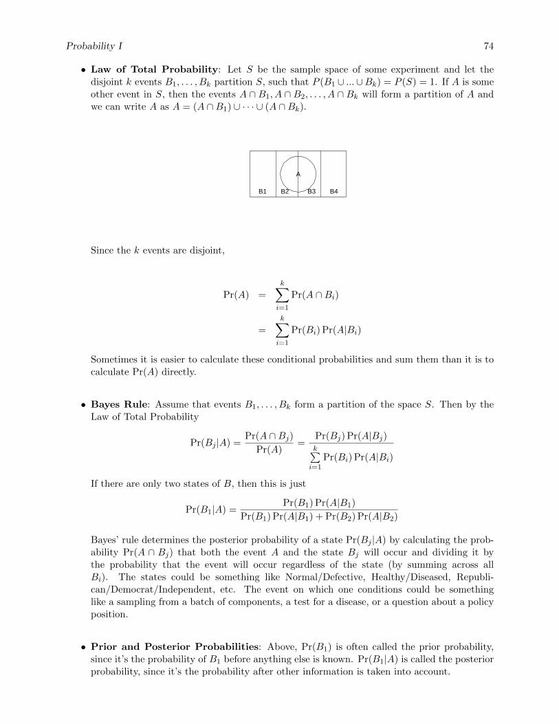
Probability I 74
• Law of Total Probability: Let S be the sample space of some experiment and let thedisjoint k events B1, . . . , Bk partition S, such that P (B1 ∪ ...∪Bk) = P (S) = 1. If A is someother event in S, then the events A ∩ B1, A ∩ B2, . . . , A ∩ Bk will form a partition of A andwe can write A as A = (A ∩B1) ∪ · · · ∪ (A ∩Bk).
B1 B2 B3 B4
A
Since the k events are disjoint,
Pr(A) =
k∑i=1
Pr(A ∩Bi)
=k∑i=1
Pr(Bi) Pr(A|Bi)
Sometimes it is easier to calculate these conditional probabilities and sum them than it is tocalculate Pr(A) directly.
• Bayes Rule: Assume that events B1, . . . , Bk form a partition of the space S. Then by theLaw of Total Probability
Pr(Bj |A) =Pr(A ∩Bj)
Pr(A)=
Pr(Bj) Pr(A|Bj)k∑i=1
Pr(Bi) Pr(A|Bi)
If there are only two states of B, then this is just
Pr(B1|A) =Pr(B1) Pr(A|B1)
Pr(B1) Pr(A|B1) + Pr(B2) Pr(A|B2)
Bayes’ rule determines the posterior probability of a state Pr(Bj |A) by calculating the prob-ability Pr(A ∩ Bj) that both the event A and the state Bj will occur and dividing it bythe probability that the event will occur regardless of the state (by summing across allBi). The states could be something like Normal/Defective, Healthy/Diseased, Republi-can/Democrat/Independent, etc. The event on which one conditions could be somethinglike a sampling from a batch of components, a test for a disease, or a question about a policyposition.
• Prior and Posterior Probabilities: Above, Pr(B1) is often called the prior probability,since it’s the probability of B1 before anything else is known. Pr(B1|A) is called the posteriorprobability, since it’s the probability after other information is taken into account.

Probability I 75
Examples:
1. A test for cancer correctly detects it 90% of the time, but incorrectly identifies aperson as having cancer 10% of the time. If 10% of all people have cancer at anygiven time, what is the probability that a person who tests positive actually hascancer?
2. In Boston, 30% of the people are conservatives, 50% are liberals, and 20%are independents. In the last election, 65% of conservatives, 82% of liberals,and 50% of independents voted. If a person in Boston is selected at random andwe learn that s/he did not vote last election, what is the probability s/he is a liberal?
Probability I 76
1.6.5 Random Variables
Most questions in the social sciences involve events, rather than numbers per se. To analyze andreason about events quantiatively, we need a way of mapping events to numbers. A random variabledoes exactly that.
A random variable is a measurable function X that maps from the sample space S to the setof real numbers R. It assigns a real number to every outcome s ∈ S.
It might seem strange to define a random variable as a function – which is neither random norvariable. The randomness comes from the realization of an event from the sample space s.
• Randomness means that the outcome of some experiment is not deterministic, i.e. there issome probability (0 < P (A) < 1) that the event will occur.
• Random Variable The support of a random variable is all values for which there is apositive probability of occurrence.
Example: Flip a fair coin two times.What is the sample space?A random variable must map events to the real line. For example, let a random variableX be the number of heads. The event (H,H) gets mapped to 2 X(s) = 2, and theevents (H,T ), (T,H) gets mapped to 1 (X(s) = 1), the event (T, T ) gets mapped to 0(X(s) = 0). Notice again that the while the mapping is not deterministic, what s ∈ Swill consist of is random. We often abbreviate the (s) from X(s) to refer to a randomvariable X, but all random variables are functions.What are other possible random variables?

Probability I 77
1.6.6 Independence
• Independence: If the occurrence or nonoccurrence of either events A and B have no effecton the occurrence or nonoccurrence of the other, then A and B are independent. If A and Bare independent, then
1. Pr(A|B) = Pr(A)
2. Pr(B|A) = Pr(B)
3. Pr(A ∩B) = Pr(A) Pr(B)Pr(⋂ki=1Ai) =
∏Ki=1 Pr(Ai)
Are mutually exclusive events independent of each other?
No. If A and B are mutually exclusive, then they cannot happen simultaneously. If we knowthat A occurred, then we know that B couldn’t have occurred. Because of this, A and Baren’t independent.
• Pairwise Independence: A set of more than two events A1, A2, . . . , Ak is pairwise inde-pendent if Pr(Ai ∩ Aj) = Pr(Ai) Pr(Aj), ∀i 6= j. Note that this does not necessarily implyindependence.
• Conditional Independence: If A and B are independent once you know the occurrence ofa third event C, then A and B are conditionally independent (conditional on C):
1. Pr(A|B ∩ C) = Pr(A|C)
2. Pr(B|A ∩ C) = Pr(B|C)
3. Pr(A ∩B|C) = Pr(A|C) Pr(B|C)
Probability II 78
1.7 Probability II: Distributions and Asymptotics
Today’s Topics:Levels of Measurement; Distributions; Expectation and Moments; Special Distributions; Joint Dis-tributions; Summarizing Observed Data; Asymptotics
1.7.1 Types of Observed Data
In empirical research, data can be classified along several dimensions. We can look at theprecision with which the underlying quantities are measured.
• Nominal (Categorical): Discrete data are nominal if there is no way to put the categoriesrepresented by the data into a meaningful order. Typically, this kind of data represents names(hence ‘nominal’) or attributes. Example: Republican or Democrat, Male or Female.
• Ordinal: Discrete data are ordinal if there is a logical order to the categories represented bythe data, but there is no common scale for differences between adjacent categories. Example:Party identification, common survey responses.
• Interval: Discrete or continuous data are interval if there is an order to the values andthere is a common scale, so that differences between two values have substantive meanings.Example: dates, temperature.
• Ratio: Discrete or continuous data are ratio if the data have the characteristics of intervaldata and zero is a meaningful quantity. This allows us to consider the ratio of two values aswell as difference between them. Allows direct ratio comparison because of the meaningfulbaseline of 0. Example: quantities measured in dollars, crime rates.
1.7.2 Distributions
The distribution of a random variable X is the probability function it induces on the real line. Itis given, roughly speaking, by p(s) = P (X ∈ s)
The formal definition of a random variable is easier to given by separating out two cases: discreterandom variables when the numeric summaries of the events are discrete, and continuous randomvariables whern they are continuous.
• Discrete Random Variable: Y is a discrete random variable if it can assume only a finiteor countably infinite number of distinct values. Examples: number of wars per year, headsor tails.
• Probability Mass Function (p(y)): For a discrete random variable Y , the probability massfunction12 (pmf), p(y) = Pr(Y = y), assigns probabilities to a countable number of distincty values such that
Much of the material and examples for this lecture are taken from Gill (2006) Essential Mathematics for Politicaland Social Research, Wackerly, Mendenhall, & Scheaffer (1996) Mathematical Statistics with Applications, Degroot(1985) Probability and Statistics, Morrow (1994) Game Theory for Political Scientists, and Ross (1987) Introductionto Probability and Statistics for Scientists and Engineers.12Also referred to simply as the “probability distribution.”

Probability II 79
1. 0 ≤ p(y) ≤ 1
2.∑yp(y) = 1
Example: For a fair six-sided die, there is an equal probability of rollingany number. Since there are six sides, the probability mass function is thenp(y) = 1/6 for y = 1, . . . , 6, 0 otherwise.
1 2 3 4 5 60
0.05
0.1
0.15
0.2
• Cumulative Density Function: The cumulative density function13, F (y) or Pr(Y ≤ y), isthe probability that Y is less than or equal to some value y, or
Pr(Y ≤ y) =∑i≤y
p(i)
Properties a CDF must satisfy:
1. F (y) is non-decreasing in y.
2. limy→−∞
F (y) = 0 and limy→∞
F (y) = 1
3. F (y) is right-continuous.
Note that P (Y > y) = 1− P (Y ≤ y).
Example: For a fair die,Pr(Y ≤ 1) =Pr(Y ≤ 3) =Pr(Y ≤ 6) =
1 2 3 4 5 60
0.25
0.5
0.75
1
We also have a similar definition for continuous random variables.
• Continuous Random Variable: Y is a continuous random variable if there exists anonnegative function f(y) defined for all real y ∈ (−∞,∞), such that for any interval A,Pr(Y ∈ A) =
∫A
f(y)dy. Examples: age, income, GNP, temperature.
• Probability Density Function: The function f above is called the probability densityfunction (pdf) of Y and must satisfy
1. f(y) ≥ 0
2.∞∫−∞
f(y)dy = 1
Note also that Pr(Y = y) = 0 — i.e., the probability of any point y is zero.
13Also referred to simply as the “cumulative distribution.”

Probability II 80
Example: f(y) = 1, 0 ≤ y ≤ 1
0 0.5 10
0.5
1
1.5
For both discrete and continous random variables, we have a unifying concept of anothermeasure: the cumulative distribution:
• Cumulative Density Function: Because the probability that a continuous random variablewill assume any particular value is zero, we can only make statements about the probabilityof a continuous random variable being within an interval. The cumulative distribution givesthe probability that Y lies on the interval (−∞, y) and is defined as
F (y) = Pr(Y ≤ y) =
y∫−∞
f(s)ds
Note that F (y) has similar properties with continuous distributions as it does with dis-crete - non-decreasing, continuous (not just right-continuous), and lim
y→−∞F (y) = 0 and
limy→∞
F (y) = 1.
We can also make statements about the probability of Y falling in an interval a ≤ y ≤ b.
Pr(a ≤ y ≤ b) =
b∫a
f(y)dy
• Link between PDF and CDF: f(y) = F ′(y) = dF (y)dy
Example: f(y) = 1, 0 < y < 1.F (y) =Pr(.5 < y < .75) =
0 0.5 10
0.5
1
1.5
1.7.3 Expectation and Other Moments
We often want to summarize some characteristics of the distribution of a random variable.The most important summary is the expectation (or expected value, or mean), in which thepossible values of a random variable are weighted by their probabilities.
• Expectation of a Discrete Random Variable: The expected value of a discrete randomvariable Y is
E(Y ) =∑y
yP (Y = y) =∑y
yp(y)
Probability II 81
In words, it is the weighted average of all possible values of Y , weighted by the probabilitythat y occurs. It is not necessarily the number we would expect Y to take on, but the averagevalue of Y after a large number of repetitions of an experiment.
Example: For a fair die, E(Y ) =
• Expectation of a Continuous Random Variable: The expected value of a continuousrandom variable is similar in concept to that of the discrete random variable, except thatinstead of summing using probabilities as weights, we integrate using the density to weight.Hence, the expected value of the continuous variable Y is defined by
E(Y ) =
∫y
yf(y)dy
Example: Find E(Y ) for f(y) = 11.5 , 0 < y < 1.5.
E(Y ) =
• Expected Value of a Function:
1. Discrete: E[g(Y )] =∑yg(y)p(y)
2. Continuous: E[g(Y )] =∞∫−∞
g(y)f(y)dy
• Properties of Expected Values:
1. E(c) = c
2. E[E[Y ]] = E[Y ]
3. E[cg(Y )] = cE[g(Y )]
4. Linearity: E[g(Y1) + · · ·+ g(Yn)] = E[g(Y1)] + · · ·+E[g(Yn)], regardless of independence
5. E[XY ] = E[X]E[Y ], if X and Y are independent
• Conditional Expectation: With joint distributions, we are often interested in the expectedvalue of a variable Y if we could hold the other variable X fixed. This is the conditionalexpectation of Y given X = x:
1. Y discrete: E(Y |X = x) =∑
y ypY |X(y|x)
2. Y continuous: E(Y |X = x) =∫y yfY |X(y|x)dy
The conditional expectation is often used for prediction when one knows the value of Xbut not Y ; the realized value of X contains information about the unknown Y so long asE(Y |X = x) 6= E(Y )∀x.

Probability II 82
• Variance: We can also look at other summaries of the distribution, which build on the ideaof taking expectations. Variance tells us about the “spread” of the distribution; it is theexpected value of the squared deviations from the mean of the distribution. The standarddeviation is simply the square root of the variance.
1. Variance: σ2 = Var(Y ) = E[(Y − E(Y ))2] = E(Y 2)− [E(Y )]2
2. Standard Deviation: σ =√
Var(Y )
• Covariance and Correlation: The covariance measures the degree to which two randomvariables vary together; if the covariance is positive, X tends to be larger than its mean whenY is larger than its mean. The covariance of a variable with itself is the variance of thatvariable.
Cov(X,Y ) = E[(X − E(X))(Y − E(Y ))] = E(XY )− E(X)E(Y )
The correlation coefficient is the covariance divided by the standard deviations of X and Y.It is a unitless measure and always takes on values in the interval [−1, 1].
ρ =Cov(X,Y )√
Var(X)Var(Y )=
Cov(X,Y )
SD(X)SD(Y )
• Properties of Variance and Covariance:
1. Var(c) = 0
2. Var[cY ] = c2Var[Y ]
3. Cov[Y, Y ] = Var[Y ]
4. Cov[X,Y ] = Cov[Y,X]
5. Cov[aX, bY ] = abCov[X,Y ]
6. Cov[X + a, Y ] = Cov[X,Y ]
7. Cov[X + Z, Y +W ] = Cov[X,Y ] + Cov[X,W ] + Cov[Z, Y ] + Cov[Z,W ]
8. Var[X + Y ] = Var[X] + Var[Y ] + 2Cov[X,Y ]
1.7.4 Special Distributions
Two discrete distributions used often are:
• Binomial Distribution: Y is distributed binomial if it represents the number of “successes”observed in n independent, identical “trials,” where the probability of success in any trial isp and the probability of failure is q = 1− p.
For any particular sequence of y successes and n − y failures, the probability of obtainingthat sequence is pyqn−y (by the multiplicative law and independence). However, there are(ny
)= n!
(n−y)!y! ways of obtaining a sequence with y successes and n − y failures. So thebinomial distribution is given by
p(y) =
(n
y
)pyqn−y, y = 0, 1, 2, . . . , n
with mean µ = E(Y ) = np and variance σ2 = V (Y ) = npq.

Probability II 83
Example: Republicans vote for Democrat-sponsored bills 2% of the time. What is theprobability that out of 10 Republicans questioned, half voted for a particular Democrat-sponsored bill? What is the mean number of Republicans voting for Democrat-sponsoredbills? The variance?
1. P (Y = 5) =
2. E(Y ) =
3. V (Y ) = 60 2 4 6 8 100
0.25
0.5
0.75
1
• Poisson Distribution: A random variable Y has a Poisson distribution if
p(y) =λy
y!e−λ, y = 0, 1, 2, . . . , λ > 0
The Poisson has the unusual feature that its expectation equals its variance: E(Y ) = V (Y ) =λ. The Poisson distribution is often used to model rare event counts: counts of the numberof events that occur during some unit of time. λ is often called the “arrival rate.”
Example: Border disputes occur between two countries at a rate of 2 per month. Whatis the probability of 0, 2, and less than 5 disputes occurring in a month?
1. P (Y = 0) =
2. P (Y = 2) =
3. Pr(Y < 5) =0 2 4 6 8 100
0.25
0.5
0.75
1
Two continuous distributions used often are:
• Uniform Distribution: A random variable Y has a continuous uniform distribution on theinterval (α, β) if its density is given by
f(y) =1
β − α, α ≤ y ≤ β
The mean and variance of Y are E(Y ) = α+β2 and V (Y ) = (β−α)2
12 .
Example: Y uniformly distributed over (1, 3).
1. P (Y = 2) =
2. f(2) =
3. P (Y ≤ 2) =
4. P (Y > 2) = 1 1.4 1.8 2.2 2.6 30
0.25
0.5
0.75
1

Probability II 84
• Normal Distribution: A random variable Y is normally distributed with mean E(Y ) = µand variance V (Y ) = σ2 if its density is
f(y) =1√2πσ
e−(y−µ)2
2σ2
Example: Y normally distributed with mean µ = 0 and varianceσ2 = .1
2 1 0 1 20
0.375
0.75
1.125
1.5
1.7.5 Joint Distributions
Often, we are interested in two or more random variables defined on the same sample space.The distribution of these variables is called a joint distribution. Joint distributions can bemade up of any combination of discrete and continuous random variables.
• Joint Probability Distribution: If both X and Y are random variable, their joint proba-bility mass/density function assigns probabilities to each pair of outcomes
Discrete: p(x, y) = Pr(X = x, Y = y)
s.t. p(x, y) ∈ [0, 1] and∑∑
p(x, y) = 1
Continuous: f(x, y); Pr((X,Y ) ∈ A) =∫∫A f(x, y)dxdy
s.t. f(x, y) ≥ 0 and∫∞−∞
∫∞−∞ f(x, y)dxdy = 1
If X and Y are independent, then P (X = x, Y = y) = P (X = x)P (Y = y) andf(x, y) = f(x)f(y)
• Marginal Probability Distribution: probability distribution of only one of the two vari-ables (ignoring information about the other variable), we can obtain the marginal distributionby summing/integrating across the variable that we don’t care about:
Discrete: pX(x) =∑
i p(x, yi)
Continuous: fX(x) =∫∞−∞ f(x, y)dy
• Conditional Probability Distribution: probability distribution for one variable, holdingthe other variable fixed. Recalling from the previous lecture that Pr(A|B) = Pr(A∩B)
Pr(B) , we canwrite the conditional distribution as
Discrete: pY |X(y|x) = p(x,y)pX(x) , pX(x) > 0
Continuous: fY |X(y|x) = f(x,y)fX(x) , fX(x) > 0
Probability II 85
Example: Suppose we are interested in the outcomes of flipping a coin and rolling a6-sided die at the same time. The sample space for this process contains 12 elements:
(H, 1), (H, 2), (H, 3), (H, 4), (H.5), (H, 6), (T, 1), (T, 2), (T, 3), (T, 4), (T, 5), (T, 6)
We can define two random variables X and Y such that X = 1 if heads and X = 0 iftails, while Y equals the number on the die. We can then make statements about thejoint distribution of X and Y .
1. P (X = x) =
2. P (Y = y) =
3. P (X = x, Y = y) =
4. P (X = x|Y = y) =
5. Are X and Y independent?
1.7.6 Summarizing Observed Events (Data)
So far, we’ve talked about distributions in a theoretical sense, looking at different properties ofrandom variables. We don’t observe random variables; we observe realizations of the randomvariable. These realizations of events are roughly equivalent to what we mean by “data”.
• Central tendency: The central tendency describes the location of the “middle” of theobserved data along some scale. There are several measures of central tendency.
1. Sample mean: This is the most common measure of central tendency, calculated bysumming across the observations and dividing by the number of observations.
x =1
n
n∑i=1
xi
The sample mean is an estimate of the expected value of a distribution.
2. Sample median: The median is the value of the “middle” observation. It is obtainedby ordering n data points from smallest to largest and taking the value of the n+ 1/2thobservation (if n is odd) or the mean of the n/2th and (n+ 1)/2th observations (if n iseven).
3. Sample mode: The mode is the most frequently observed value in the data:
mx = Xi : n(Xi) > n(Xj)∀j 6= i
When the data are realizations of a continuous random variable, it often makes senseto group the data into bins, either by rounding or some other process, in order to get areasonable estimate of the mode.
Example:

Probability II 86
X 6 3 7 5 5 5 6 4 7 2
Y 1 2 1 2 2 1 2 0 2 0
1. x = y =
2. median(x) = median(y) =
3. mx = my =
• Dispersion: We also typically want to know how spread out the data are relative to thecenter of the observed distribution. Again, there are several ways to measure dispersion.
1. Sample variance: The sample variance is the sum of the squared deviations from thesample mean, divided by the number of observations minus 1.
Var(X) =1
n− 1
n∑i=1
(xi − x)2
Again, this is an estimate of the variance of a random variable; we divide by n−1 insteadof n in order to get an unbiased estimate.
2. Standard deviation: The sample standard deviation is the square root of the samplevariance.
SD(X) =√
Var(X) =
√√√√ 1
n− 1
n∑i=1
(xi − x)2
3. Median absolute deviation (MAD): The MAD is a different measure of dispersion,based on deviations from the median rather than deviations from the mean.
MAD(X) = median(|xi −median(x)|)
Example: Using table above, calculate:
1. Var(X) = Var(Y ) =
2. SD(X) = SD(Y ) =
3. MAD(X) = MAD(Y ) =
• Covariance and Correlation: Both of these quantities measure the degree to which twovariables vary together, and are estimates of the covariance and correlation of two randomvariables as defined above.
1. Sample covariance: Cov(X,Y ) = 1n−1
∑ni=1(xi − x)(yi − y)
2. Sample correlation: r = Cov(X,Y )√Var(X)Var(Y )
Example: Using above table, calculate:
1. Cov(X,Y ) =
2. r =

Probability II 87
1.7.7 Asymptotic Theory
In theoretical and applied research, asymptotic arguments are often made. In this section we brieflyintroduce some of this material.
• What are asymptotics?
– In probability theory, asymptotic analysis is the study of limiting behavior. By limitingbehavior, we mean the behavior of some random process as the number of observationsgets larger and larger.
• Why is this important?
– We rarely know the true process governing the events we see in the social world. Itis helpful to understand how such unknown processes theoretically must behave andasymptotic theory helps us do this.
Examples.
• Central Limit Theorem. Let Xn = X1, X2, ..., Xn be a sequence of i.i.d. randomvariables with finite mean (µ) and variance (σ2). Then,
Xn =x1 + x2 + ...+ xn
n→ N
(µ,σ2
n
)as n→∞. This result, known as the Central Limit Theorem, is an important motivation formany quantitative methods, as well as for the widespread use of the Normal distribution.
– Intuitively, whenever a lot of small, independent processes somehow combine together toform the realized observations, practitioners often feel comfortable assuming Normality.
• Law of Large Numbers. Let Xn = X1, X2, ..., Xn be a sequence of i.i.d. randomvariables with a finite expected value of µ. Then,
Xn =x1 + x2 + ...+ xn
n
a.s.→ µ
as n→∞. In other words, Pr(limn→∞ Xn = µ) = 1. This theorem, known as the Strong Lawof Large Numbers, is an important motivation for the widespread use of the sample mean, aswell as the intuition link between averages and expected values.
– Important note: The Strong Law of Large Numbers holds so long as the expected valueexists; no other assumptions are needed. However, the rate of convergence will differgreatly depending on the distribution underlying the observed data. When extremeobservations occur often (i.e. kurtosis is large), the rate of convergence is much slower.Cf. The distribution of financial returns.
• Big O Notation. Some of you may encounter “big-OH”-notation. If f, g are two functions,we say that f = O(g) if there exists some constant, c, such that f(n) ≤ c × g(n) for largeenough n. This notation is useful for simplifying complex problems in game theory, computerscience, and statistics.
Example.

Probability II 88
– What is O(5 exp(0.5n) + n2 + n/2)? Answer: exp(n). Why? Because, for large n,
5 exp(0.5n) + n2 + n/2
exp(n)≤ c exp(n)
exp(n)= c.
whenever n > 4 and where c = 1.

Greek letters and math symbols 89
2 Guide to Greek Letters and Mathematical Symbols
2.1 Greek Letters
Name Lowercase Uppercase Typical usage
alpha α A often the intercept in a regressionbeta β B often denotes the parameters in a modelgamma γ Γ uppercase denotes a special counting functiondelta δ ∆ denotes a differenceepsilon ε, ε E denotes a very small number or errorzeta ζ Zeta η H sometimes denotes variance/standard deviationtheta θ, ϑ Θ often used for radiansiota ι Ikappa κ K can denote curvaturelambda λ Λ eigenvalues; parameter of a Poisson regressionmu µ M meannu ν Nxi ξ Ξomicron o Opi π, $ Π 3.1415...; a probability function; product functionrho ρ, % P correlationsigma σ, ς Σ variance/standard deviation; summation functiontau τ T sometimes denotes variance/standard deviationupsilon υ Υphi φ, ϕ Φ denotes the PDF and CDF of a normal distributionchi χ X denotes the chi-square distributionpsi ψ Ψomega ω Ω
2.2 Mathematical Symbols
Equivalency symbols
Symbol Meaning LATEX code
= equals =
6= not equal to \neq
> greater than >
< less than <
≥ greater than or equal to \geq
≤ less than or equal to \leq
∝ proportional to \propto
≈ approximately equal to \approx
∼ distributed as (or indifference) \sim
≡ equivalent to; set equal to; defined as \equiv
preferred to \succ

Greek letters and math symbols 90
Common mathematical symbols
Symbol Meaning LATEX code
∞ infinity \infty
± plus or minus \pm
∓ minus or plus \mp
⊥ perpendicular \perp
‖ parallel \parallel
| given \mid
· dot; times \cdot
· · · dots \cdots
R all real numbers \mathfrakR
x x bar \barx
x x hat \hatx
Function symbols
Symbol Meaning LATEX code√x square root \sqrtx
n√x nth root \sqrt[n]x
! factorial !n∑i=1
summation notation \sum\limits_i=1^n
n∏i=1
production notation \prod\limits_i=1^n
limn→∞
limits notation \lim\limits_n \to \infty∫integral \int
Set notation symbols
Symbol Meaning LATEX code
set \\
∈ is an element of \in
∅ empty set \emptyset
∪ union \cup
∩ intersection \cap
⊂ subset \subset
Logical symbols
Symbol Meaning LATEX code
∴ therefore \therefore
∀ for all \forall
∃ there exists \exists
=⇒ logical “then” statement \Longrightarrow
⇐⇒ if and only if \Longleftrightarrow

Greek letters and math symbols 91
Abbreviations
Symbol Meaning LATEX code
iff if any only if iff
s.t. such that s.t.
LHS Left-hand side of the equationRHS Right-hand side of the equationQED end of proof (quod erat demonstrandum)
W.R.T. with respect to
You can look up the LATEX code for other math symbols at http://detexify.kirelabs.org/classify.html