math and physics using sympy - jonathangross.de...
TRANSCRIPT

Math and Physics using SymPy
June 8, 2017
SymPyComputer Algebra System
A computer algebra system (CAS) is a program that allows thecomputation of mathematical expressions. In contrast to a simplecalculator, a CAS solves these problems not numerically, but usingsymbolic expressions, such as variables, functions, polynomials andmatrices.All CAS have essentially the same functionality. That means byunderstanding how one of them works, you will be able to use allthe others as well. Well known commercial systems include Maple,MATLAB, and Mathematica. Free ones are Octave, Magma, and ofcourse SymPy.
SymPySymbolical vs. numerical
In a symbolic CAS, numbers and operations are expressedsymbolically, so the obtained answers are exact. For example thenumber
√2 is represented in SymPy as the object Pow(2, 1/2).
In a numerical computer algebra system, such as Octave thenumber
√2 is represented as the approximation 1.41421356237310
(a float). For most cases this is fine, but these approximationscan lead to problems:float(sqrt(2)) ∗ float(sqrt(2)) = 2.0000000000000004 6= 2.Because SymPy uses the exact representation, such problems willnot appear! Pow(2, 1/2) ∗ Pow(2, 1/2) = 2

SymPyUsing SymPy
You can use SymPy right from the Python interpreter.$ pythonPython 2.7.3 (default , Mar 13 2014, 11:03:55)[GCC 4.7.2] on linux2Type "help", "copyright", "credits" or "license" for more information.>>> from sympy import *>>>
This imports all of SymPy’s methods and variables and you canstart using it right away.
SymPy
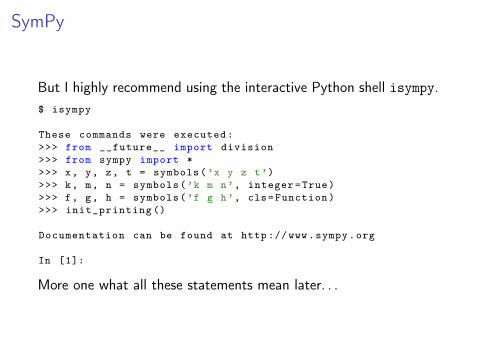
But I highly recommend using the interactive Python shell isympy.$ isympy
These commands were executed:>>> from __future__ import division>>> from sympy import *>>> x, y, z, t = symbols(’x y z t’)>>> k, m, n = symbols(’k m n’, integer=True)>>> f, g, h = symbols(’f g h’, cls=Function)>>> init_printing ()
Documentation can be found at http :// www.sympy.org
In [1]:
More one what all these statements mean later. . .

SymPyFundamentals of Mathematics
Let’s begin by learning about the basic SymPy objects andoperations. For example we’ll learn what it means “to solve” anequation, “to expand” an expression, and “to factor” a polynomial.

SymPyNumbers - from sympy import sympify, S, evalf, N
In Python there are two types of number objects: int and float.>>> 33 # an int>>> 3.03.0 # a float
Integer objects are a faithful representation of the set of integersZ = {. . . ,−2,−1, 0, 1, 2, . . . }.Floating point numbers are approximate representations of the realsR.

SymPyNumbers - from sympy import sympify, S, evalf, N
Special caution is needed when dealing with rational numbers,because integer division might not produce the answer you expect.Python 2 does not automatically convert to float, but rounds to theclosest integer. Python 3 on the other hand does! To get the samefunctionality in Python 2 we can import the future!# Python 21/2 --> 01.0/2 --> 0.51/2.0 --> 0.51.0/2.0 --> 0.5
# Python 31/2 --> 0.5
# Python 2 with future features!from __future__ import division1/2 --> 0.51//2 -> 0 # use // for integer division
SymPyNumbers - from sympy import sympify, S, evalf, N
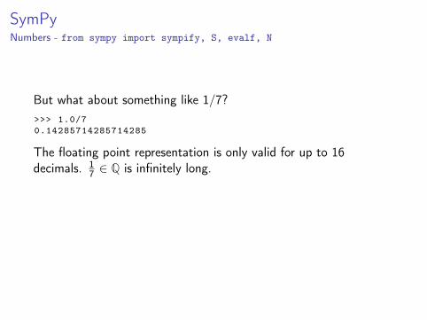
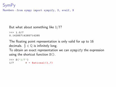
But what about something like 1/7?>>> 1.0/70.14285714285714285
The floating point representation is only valid for up to 16decimals. 1
7 ∈ Q is infinitely long.
To obtain an exact representation we can sympify the expressionusing the shortcut function S().>>> S(’1/7’)1/7 # = Rational (1,7)
SymPyNumbers - from sympy import sympify, S, evalf, N
But what about something like 1/7?>>> 1.0/70.14285714285714285
The floating point representation is only valid for up to 16decimals. 1
7 ∈ Q is infinitely long.To obtain an exact representation we can sympify the expressionusing the shortcut function S().>>> S(’1/7’)1/7 # = Rational (1,7)

SymPyNumbers - from sympy import sympify, S, evalf, N
The shortcut function S() takes a text string in quotes asargument. The same result could have been achieved usingS(′1′)/7, because a SymPy object divided by an int returns aSymPy object.Other math operators like addition +, subtraction −, andmultiplication ∗ work as well, so does exponentiation.>>> 2**10 # same as S(’2^10’)1024
SymPyNumbers - from sympy import sympify, S, evalf, N
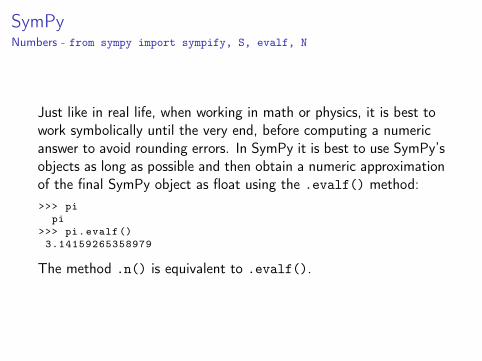
Just like in real life, when working in math or physics, it is best towork symbolically until the very end, before computing a numericanswer to avoid rounding errors. In SymPy it is best to use SymPy’sobjects as long as possible and then obtain a numeric approximationof the final SymPy object as float using the .evalf() method:>>> pi
pi>>> pi.evalf()3.14159265358979
The method .n() is equivalent to .evalf().

SymPy
You can also use the global SymPy method N() to get numericalvalues. By providing an integer as argument you can easily changethe number of digits of precision the approximations should return.>>> pi.n(400) # equivalent to N(pi, 400)3.141592653589793238462643383279502884197169399375105820974944592307816406286208998628034825342117067982148086513282306647093844609550582231725359408128481117450284102701938521105559644622948954930381964428810975665933446128475648233786783165271201909145648566923460348610454326648213393607260249141273724587006606315588174881520920962829254091715364367892590360011330530548820466521384146951941511609

SymPySymbols - from sympy import Symbol, symbols
When using isympy a number of commands are executed to setupa common environment for symbolic computation.>>> from __future__ import division # already discussed>>> from sympy import * # already discussed>>> x, y, z, t = symbols(’x y z t’)>>> k, m, n = symbols(’k m n’, integer=True)>>> f, g, h = symbols(’f g h’, cls=Function)
The last three lines define some generic symbols x , y , z , and t asvariables. k,m, and n as integer counting variables and f , g , and has function symbols.Note the difference between the following two statements:>>> x+2x+2>>> p+2NameError: name ’p’ is not defined
SymPySymbols - from sympy import Symbol, symbols
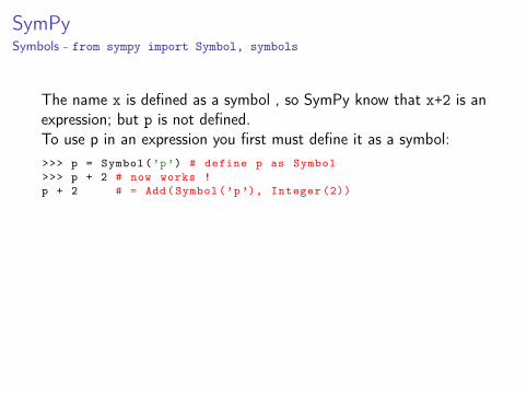
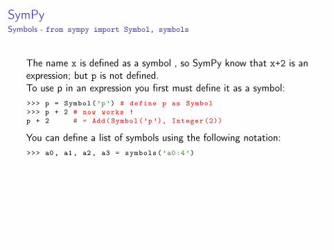
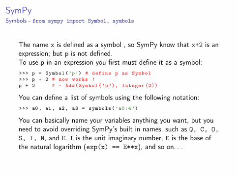
The name x is defined as a symbol , so SymPy know that x+2 is anexpression; but p is not defined.To use p in an expression you first must define it as a symbol:>>> p = Symbol(’p’) # define p as Symbol>>> p + 2 # now works !p + 2 # = Add(Symbol(’p ’), Integer (2))
You can define a list of symbols using the following notation:>>> a0 , a1 , a2 , a3 = symbols(’a0:4’)
You can basically name your variables anything you want, but youneed to avoid overriding SymPy’s built in names, such as Q, C, O,S, I, N, and E. I is the unit imaginary number, E is the base ofthe natural logarithm (exp(x) == E**x), and so on. . .
SymPySymbols - from sympy import Symbol, symbols
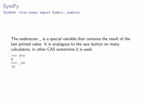
The underscore _ is a special variable that contains the result of thelast printed value. It is analogous to the ans button on manycalculators, in other CAS sometimes % is used.>>> 3+36>>> _*212

SymPyExpressions - from sympy import simplify, factor, expand, collect
You define expression by combining symbols with basic mathoperations and other functions:>>> myExpression = 2*x + 3*x - sin(x) - 3*x + 42>>> simplify(myExpression)2*x - sin(x) + 42
The function simplify can be used on any expression to simplifyit.
SymPyExpressions - from sympy import simplify, factor, expand, collect
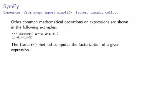
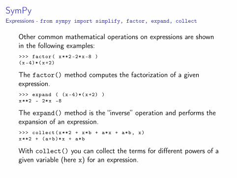
Other common mathematical operations on expressions are shownin the following examples:>>> factor( x**2 -2*x-8 )(x-4)*(x+2)
The factor() method computes the factorization of a givenexpression.
>>> expand ( (x -4)*(x+2) )x**2 - 2*x -8
The expand() method is the “inverse” operation and performs theexpansion of an expression.>>> collect(x**2 + x*b + a*x + a*b, x)x**2 + (a+b)*x + a*b
With collect() you can collect the terms for different powers of agiven variable (here x) for an expression.
SymPyExpressions - from sympy import simplify, factor, expand, collect
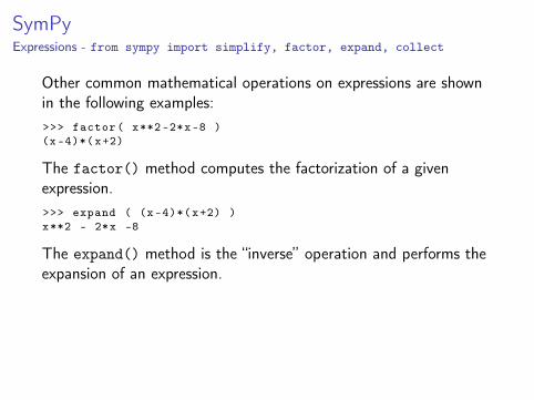
Other common mathematical operations on expressions are shownin the following examples:>>> factor( x**2 -2*x-8 )(x-4)*(x+2)
The factor() method computes the factorization of a givenexpression.>>> expand ( (x -4)*(x+2) )x**2 - 2*x -8
The expand() method is the “inverse” operation and performs theexpansion of an expression.
>>> collect(x**2 + x*b + a*x + a*b, x)x**2 + (a+b)*x + a*b
With collect() you can collect the terms for different powers of agiven variable (here x) for an expression.
SymPyExpressions - from sympy import simplify, factor, expand, collect
Other common mathematical operations on expressions are shownin the following examples:>>> factor( x**2 -2*x-8 )(x-4)*(x+2)
The factor() method computes the factorization of a givenexpression.>>> expand ( (x -4)*(x+2) )x**2 - 2*x -8
The expand() method is the “inverse” operation and performs theexpansion of an expression.>>> collect(x**2 + x*b + a*x + a*b, x)x**2 + (a+b)*x + a*b
With collect() you can collect the terms for different powers of agiven variable (here x) for an expression.
SymPyExpressions - from sympy import simplify, factor, expand, collect
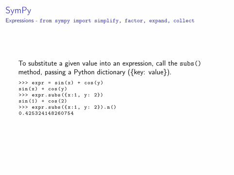
To substitute a given value into an expression, call the subs()method, passing a Python dictionary ({key: value}).>>> expr = sin(x) + cos(y)sin(x) + cos(y)>>> expr.subs({x:1, y: 2})sin (1) + cos(2)>>> expr.subs({x:1, y: 2}).n()0.425324148260754
SymPySolving equations - from sympy import solve
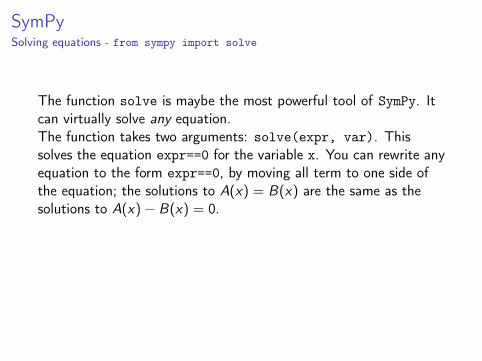
The function solve is maybe the most powerful tool of SymPy. Itcan virtually solve any equation.The function takes two arguments: solve(expr, var). Thissolves the equation expr==0 for the variable x. You can rewrite anyequation to the form expr==0, by moving all term to one side ofthe equation; the solutions to A(x) = B(x) are the same as thesolutions to A(x)− B(x) = 0.
For example let us solve the quadratic equation x2 + 2x − 8 = 0:>>> solve(x**2+2*x-8, x)[-4, 2]
The result is a list of solutions for x that satisfy the equation above.

SymPySolving equations - from sympy import solve
The function solve is maybe the most powerful tool of SymPy. Itcan virtually solve any equation.The function takes two arguments: solve(expr, var). Thissolves the equation expr==0 for the variable x. You can rewrite anyequation to the form expr==0, by moving all term to one side ofthe equation; the solutions to A(x) = B(x) are the same as thesolutions to A(x)− B(x) = 0.For example let us solve the quadratic equation x2 + 2x − 8 = 0:>>> solve(x**2+2*x-8, x)[-4, 2]
The result is a list of solutions for x that satisfy the equation above.

SymPySolving equations - from sympy import solve
The best part of solve is, that it also works with symbolicexpressions. For example let us look for the solution ofax2 + bx + c = 0.>>> a, b, c = symbols(’a b c’)>>> solve(a*x**2+b*x+c, x)[(-b + sqrt(-4*a*c + b**2))/(2*a),-(b + sqrt(-4*a*c + b**2))/(2*a)]
Here we used the symbols a, b, and c to solve the equation. Youshould recognize the solution of the quadratic formulax1,2 = −b±
√b2−4ac2a .
SymPySolving equations - from sympy import solve
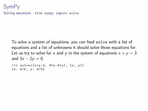
To solve a system of equations, you can feed solve with a list ofequations and a list of unknowns it should solve those equations for.Let us try to solve for x and y in the system of equations x + y = 3and 3x − 2y = 0.>>> solve([x+y-3, 3*x-2*y], [x, y]){x: 6/5, y: 9/5}

SymPyRational functions - from sympy import together, apart
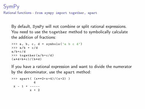
By default, SymPy will not combine or split rational expressions.You need to use the together method to symbolically calculatethe addition of fractions:>>> a, b, c, d = symbols(’a b c d’)>>> a/b + c/da/b+c/d>>> together(a/b+c/d)(a*d+b*c)/(b*d)
If you have a rational expression and want to divide the numeratorby the denominator, use the apart method:>>> apart( (x**2+x+4)/(x+2) )
6x - 1 + -----
x + 2
SymPyRational functions - from sympy import together, apart
By default, SymPy will not combine or split rational expressions.You need to use the together method to symbolically calculatethe addition of fractions:>>> a, b, c, d = symbols(’a b c d’)>>> a/b + c/da/b+c/d>>> together(a/b+c/d)(a*d+b*c)/(b*d)
If you have a rational expression and want to divide the numeratorby the denominator, use the apart method:>>> apart( (x**2+x+4)/(x+2) )
6x - 1 + -----
x + 2

SymPyPolynomials
Let us define a polynomial P with roots at x = 1, x = 2, andx = 3:>>> P = (x-1)*(x -2)*(x-3)(x-1)*(x-2)*(x-3)
To see the expanded version of the polynomial, call its expandmethod:>>> P.expand ()x**3 -6*x**2+11*x-6
If we start with the expanded form P(x) = x3 − 6x2 + 11x − 6, wecan get to the roots using either the factor or the simplifymethod:>>> P.factor ()(x-1)*(x-2)*(x-3)>>> P.simplify ()(x-1)*(x-2)*(x-3)
SymPyPolynomials
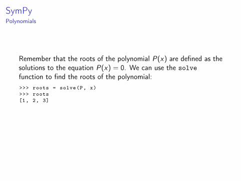
Remember that the roots of the polynomial P(x) are defined as thesolutions to the equation P(x) = 0. We can use the solvefunction to find the roots of the polynomial:>>> roots = solve(P, x)>>> roots[1, 2, 3]
# let’s check if P equals (x-1)(x-2)(x-3)>>> simplify(P - (x-roots [0])*(x-roots [1])*(x-roots [2]) )0
SymPyPolynomials
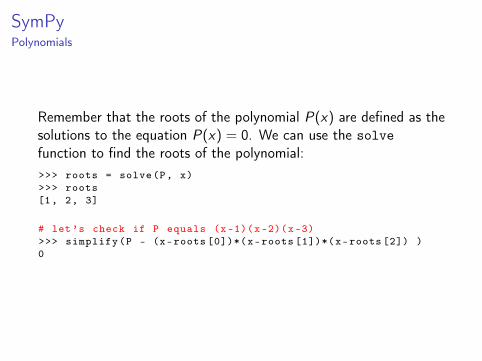
Remember that the roots of the polynomial P(x) are defined as thesolutions to the equation P(x) = 0. We can use the solvefunction to find the roots of the polynomial:>>> roots = solve(P, x)>>> roots[1, 2, 3]
# let’s check if P equals (x-1)(x-2)(x-3)>>> simplify(P - (x-roots [0])*(x-roots [1])*(x-roots [2]) )0

SymPyTrigonometry from sympy import sin, cos, tan, trigsimp, expand_trig
The trigonometric functions, such as sin and cos take inputs inradians. To call them with degree arguments you need theconversion factor π
180 or use numpy.radians or numpy.deg2rad.
SymPy is aware of several trigonometric identities.>>> sin(x) == cos(x-pi/2)True>>> simplify( sin(x)*cos(y)+cos(x)*sin(y) )sin(x+y)>>> e = 2*sin(x)**2+2* cos(x)**2>>> trigsimp(e)2>>> simplify(sin(x)**4 -2* cos(x)**2* sin(x)**2+ cos(x)**4)cos (4*x)/2 + 1/2
>>> expand_trig(sin(2*x))2*sin(x)*cos(x)
SymPyCalculus
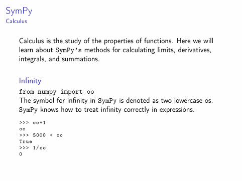
Calculus is the study of the properties of functions. Here we willlearn about SymPy’s methods for calculating limits, derivatives,integrals, and summations.
Infinityfrom numpy import ooThe symbol for infinity in SymPy is denoted as two lowercase os.SymPy knows how to treat infinity correctly in expressions.
>>> oo+1oo>>> 5000 < ooTrue>>> 1/oo0
SymPyCalculus
Calculus is the study of the properties of functions. Here we willlearn about SymPy’s methods for calculating limits, derivatives,integrals, and summations.
Infinityfrom numpy import ooThe symbol for infinity in SymPy is denoted as two lowercase os.SymPy knows how to treat infinity correctly in expressions.
>>> oo+1oo>>> 5000 < ooTrue>>> 1/oo0

SymPyCalculus - Limits - from sympy import limit, oo
With limits we can describe, with mathematical precision, infinitelylarge quantities, infinitely small quantities, and procedures withinfinitely many steps.For example the number e is defined as the limit
e ≡ limn→∞
(1 +
1n
)n
>>> limit( (1+1/n)**n, n, oo)E # = 2.71828182845905
Limits are also useful to describe the asymptotic behavior offunction. Consider the function f (x) = 1
x .
>>> limit( 1/x, x, 0, dir=’+’)oo>>> limit( 1/x, x, 0, dir=’-’)-oo>>> limit (1/x, x, oo)0
SymPyCalculus - Derivatives
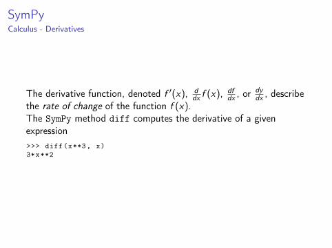
The derivative function, denoted f ′(x), ddx f (x), df
dx , ordydx , describe
the rate of change of the function f (x).The SymPy method diff computes the derivative of a givenexpression>>> diff(x**3, x)3*x**2
SymPyCalculus - Derivatives
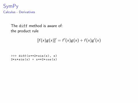
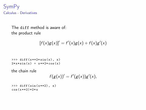
The diff method is aware of:the product rule
[f (x)g(x)]′ = f ′(x)g(x) + f (x)g ′(x)
>>> diff(x**2* sin(x), x)2*x*sin(x) + x**2* cos(x)
the chain rulef (g(x))′ = f ′(g(x))g ′(x),
>>> diff(sin(x**2), x)cos(x**2)*2*x
SymPyCalculus - Derivatives
The diff method is aware of:the product rule
[f (x)g(x)]′ = f ′(x)g(x) + f (x)g ′(x)
>>> diff(x**2* sin(x), x)2*x*sin(x) + x**2* cos(x)
the chain rulef (g(x))′ = f ′(g(x))g ′(x),
>>> diff(sin(x**2), x)cos(x**2)*2*x

SymPyCalculus - Derivatives
and, finally,the quotient rule[f (x)
g(x)
]′=
f ′(x)g(x)− f (x)g ′(x)
g(x)2 .
>>> diff(x**2/ sin(x), x)(2*x*sin(x) - x**2* cos(x))/sin(x)**2
SymPyCalculus - Differential equations
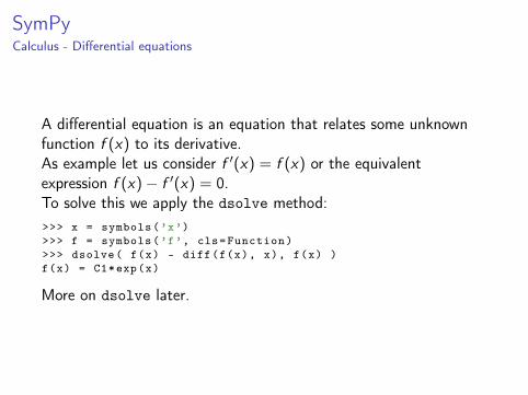
A differential equation is an equation that relates some unknownfunction f (x) to its derivative.As example let us consider f ′(x) = f (x) or the equivalentexpression f (x)− f ′(x) = 0.To solve this we apply the dsolve method:>>> x = symbols(’x’)>>> f = symbols(’f’, cls=Function)>>> dsolve( f(x) - diff(f(x), x), f(x) )f(x) = C1*exp(x)
More on dsolve later.
SymPyCalculus - Integrals
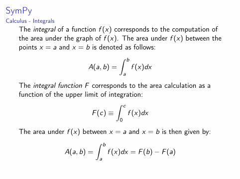
The integral of a function f (x) corresponds to the computation ofthe area under the graph of f (x). The area under f (x) between thepoints x = a and x = b is denoted as follows:
A(a, b) =
∫ b
af (x)dx
The integral function F corresponds to the area calculation as afunction of the upper limit of integration:
F (c) ≡∫ c
0f (x)dx
The area under f (x) between x = a and x = b is then given by:
A(a, b) =
∫ b
af (x)dx = F (b)− F (a)
SymPyCalculus - Integrals
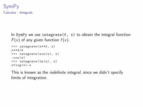
In SymPy we use integrate(f, x) to obtain the integral functionF (x) of any given function f (x).>>> integrate(x**3, x)x**4/4>>> integrate(sin(x), x)-cos(x)>>> integrate(ln(x), x)x*log(x)-x
This is known as the indefinite integral, since we didn’t specifylimits of integration.
SymPyCalculus - Integrals
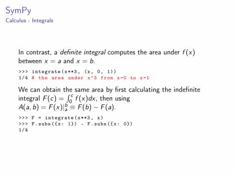
In contrast, a definite integral computes the area under f (x)between x = a and x = b.>>> integrate(x**3, (x, 0, 1))1/4 # the area under x^3 from x=0 to x=1
We can obtain the same area by first calculating the indefiniteintegral F (c) =
∫ c0 f (x)dx , then using
A(a, b) = F (x)|ba ≡ F (b)− F (a).>>> F = integrate(x**3, x)>>> F.subs({x: 1}) - F.subs({x: 0})1/4

SymPyCalculus - Fundamental theorem of calculus
The integral is the “inverse operation” of the derivative. If youperform the integral operation followed by the derivative operationon a function, you’ll obtain the same function:(
d
dx◦∫
dx
)f (x) ≡ d
dx
∫ x
cf (u)du = f (x)
>>> f = x**2>>> F = integrate(f, x)>>> Fx**3/3>>> diff(F, x)x**2

SymPyCalculus - Fundamental theorem of calculus
Alternatively, if you compute the derivative of a function followedby the integral, you will obtain the original function f (x) (up to aconstant):(∫
dx ◦ d
dx
)f (x) ≡
∫ x
cf ′(u)du = f (x) + C
>>> f = x**2>>> df = diff(f, x)>>> df2*x>>> integrate(df, x)x**2 # + C

SymPyCalculus - Fundamental theorem of calculus
The fundamental theorem of calculus is important because it tellsus how to solve differential equations. If we have to solve for f (x)in the differential equation d
dx f (x) = g(x), we can take the integralon both sides of the equation to obtain the answerf (x) =
∫g(x)dx + C .
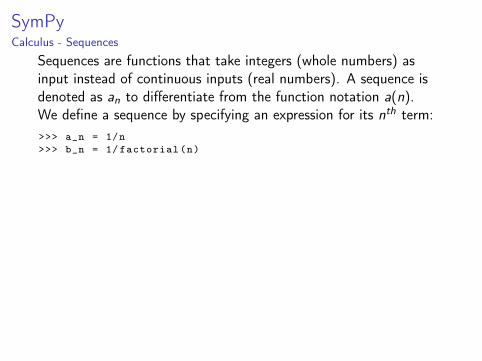
SymPyCalculus - Sequences
Sequences are functions that take integers (whole numbers) asinput instead of continuous inputs (real numbers). A sequence isdenoted as an to differentiate from the function notation a(n).We define a sequence by specifying an expression for its nth term:>>> a_n = 1/n>>> b_n = 1/ factorial(n)
Using Python’s list comprehension, we can generate the sequencefor some range of indices:>>> [a_n.subs({n: i}) for i in range(0, 8)][oo , 1, 1/2, 1/4, 1/4, 1/5, 1/6, 1/7]>>> [b_n.subs{n: i}) for i in range(0, 8)][1, 1, 1/2, 1/6, 1/24, 1/120, 1/720, 1/5040]
Both an = 1n and bn = 1
n! converge to 0 as n→∞.
>>> limit(a_n , n, oo)0>>> limit(b_n , n, oo)0
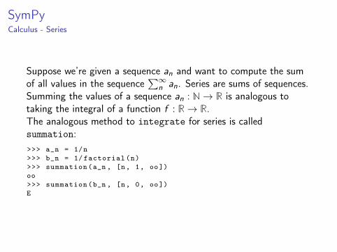
SymPyCalculus - Series
Suppose we’re given a sequence an and want to compute the sumof all values in the sequence
∑∞n an. Series are sums of sequences.
Summing the values of a sequence an : N→ R is analogous totaking the integral of a function f : R→ R.The analogous method to integrate for series is calledsummation:>>> a_n = 1/n>>> b_n = 1/ factorial(n)>>> summation(a_n , [n, 1, oo])oo>>> summation(b_n , [n, 0, oo])E
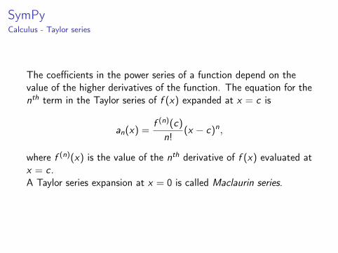
SymPyCalculus - Taylor series
The coefficients in the power series of a function depend on thevalue of the higher derivatives of the function. The equation for thenth term in the Taylor series of f (x) expanded at x = c is
an(x) =f (n)(c)
n!(x − c)n,
where f (n)(x) is the value of the nth derivative of f (x) evaluated atx = c .A Taylor series expansion at x = 0 is called Maclaurin series.

SymPyCalculus - Taylor series
Not only can we use series to approximate numbers, we can usethem to approximate functions!A power series is a series whose terms contain different powers ofthe variable x . For example, the power series of the functionexp(x) = ex :
exp(x) ≡ 1 + x +x2
2+
x3
3!+
x4
4!+
x5
5!+ · · · =
∞∑n=0
xn
n!
>>> exp_xn = x**n/factorial(n)# calculate exp(5)>>> summation = exp_xn.subs({x: 5}), [n, 0, oo]). evalf()148.413159102577
Actually SymPy is smart enough to recognize the series, so if weomit the evalf(), we get>>> summation = exp_xn.subs({x: 5}), [n, 0, oo])exp (5)
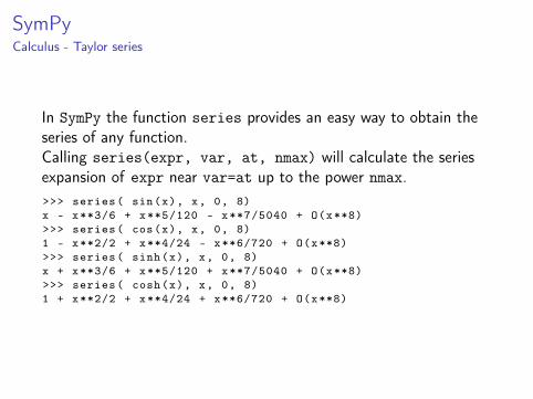
SymPyCalculus - Taylor series
In SymPy the function series provides an easy way to obtain theseries of any function.Calling series(expr, var, at, nmax) will calculate the seriesexpansion of expr near var=at up to the power nmax.>>> series( sin(x), x, 0, 8)x - x**3/6 + x**5/120 - x**7/5040 + O(x**8)>>> series( cos(x), x, 0, 8)1 - x**2/2 + x**4/24 - x**6/720 + O(x**8)>>> series( sinh(x), x, 0, 8)x + x**3/6 + x**5/120 + x**7/5040 + O(x**8)>>> series( cosh(x), x, 0, 8)1 + x**2/2 + x**4/24 + x**6/720 + O(x**8)

SymPyCalculus - Taylor series
If a function is not defined at x = 0, we can expand them at adifferent value of x .For example, the power series of ln(x) expanded at x = 1 is>>> series(ln(x), x, 1, 6)-1-(x -1)**2/2+(x-1)**3/3 -(x -1)**4/4+(x -1)**5/5+x+O((x -1)**6)
To get rid of the (x − 1) terms and to get a familiar result for theTaylor series we can do the following trick. Instead of expandingln(x) around x = 1, we obtain a more readable expression byexpanding ln(x + 1) around x = 0.>>> series(ln(x+1), x, 0, 6)x - x**2/2 + x**3/3 - x**4/4 + x**5/5 + O(x**6)
SymPyVectors and Matrices
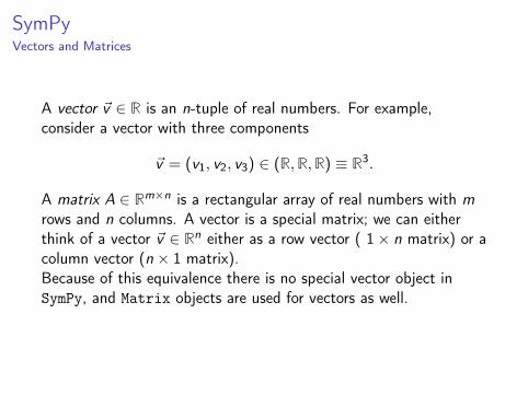
A vector ~v ∈ R is an n-tuple of real numbers. For example,consider a vector with three components
~v = (v1, v2, v3) ∈ (R,R,R) ≡ R3.
A matrix A ∈ Rm×n is a rectangular array of real numbers with mrows and n columns. A vector is a special matrix; we can eitherthink of a vector ~v ∈ Rn either as a row vector ( 1× n matrix) or acolumn vector (n × 1 matrix).Because of this equivalence there is no special vector object inSymPy, and Matrix objects are used for vectors as well.
SymPyVectors and Matrices
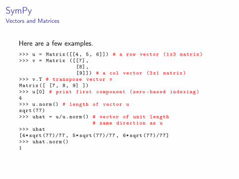
Here are a few examples.>>> u = Matrix ([[4, 5, 6]]) # a row vector (1x3 matrix)>>> v = Matrix ([[7],
[8],[9]]) # a col vector (3x1 matrix)
>>> v.T # transpose vector vMatrix ([ [7, 8, 9] ])>>> u[0] # print first component (zero -based indexing)4>>> u.norm() # length of vector usqrt (77)>>> uhat = u/u.norm() # vector of unit length
# same direction as u>>> uhat[4* sqrt (77)/77 , 5*sqrt (77)/77 , 6*sqrt (77)/77]>>> uhat.norm()1
SymPyVectors and Matrices
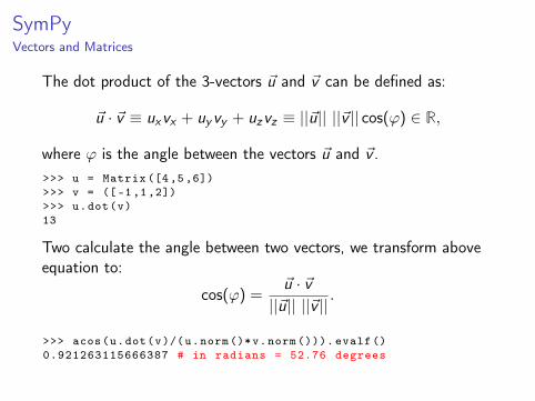
The dot product of the 3-vectors ~u and ~v can be defined as:
~u · ~v ≡ uxvx + uyvy + uzvz ≡ ||~u|| ||~v || cos(ϕ) ∈ R,
where ϕ is the angle between the vectors ~u and ~v .>>> u = Matrix ([4,5,6])>>> v = ([-1,1,2])>>> u.dot(v)13
Two calculate the angle between two vectors, we transform aboveequation to:
cos(ϕ) =~u · ~v||~u|| ||~v ||
.
>>> acos(u.dot(v)/(u.norm ()*v.norm ())). evalf ()0.921263115666387 # in radians = 52.76 degrees
SymPyVectors and Matrices
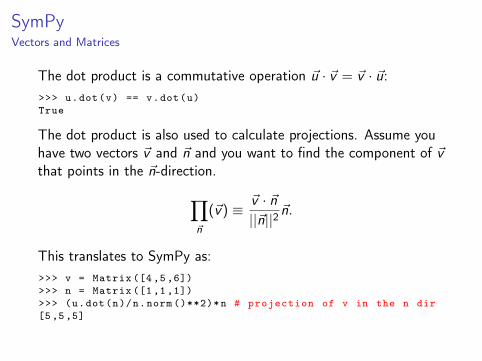
The dot product is a commutative operation ~u · ~v = ~v · ~u:>>> u.dot(v) == v.dot(u)True
The dot product is also used to calculate projections. Assume youhave two vectors ~v and ~n and you want to find the component of ~vthat points in the ~n-direction.∏
~n
(~v) ≡~v · ~n||~n||2
~n.
This translates to SymPy as:>>> v = Matrix ([4,5,6])>>> n = Matrix ([1,1,1])>>> (u.dot(n)/n.norm ()**2)*n # projection of v in the n dir[5,5,5]
SymPyVectors and Matrices
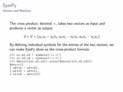
The cross product, denoted ×, takes two vectors as input andproduces a vector as output:
~u × ~v = (uyvz − uzvy , uzvx − uxvz , uxvy − uyvx)
By defining individual symbols for the entries of the two vectors, wecan make SymPy show us the cross-product formula:>>> u1 ,u2,u3 = symbols(’u1:4’)>>> v1 ,v2,v3 = symbols(’v1:4’)>>> Matrix ([u1 ,u2,u3]). cross(Matrix ([v1 ,v2 ,v3]))Matrix ([[ u2*v3 - u3*v2],[-u1*v3 + u3*v1],[ u1*v2 - u2*v1]])
SymPyVectors and Matrices
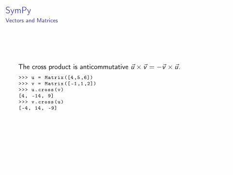
The cross product is anticommutative ~u × ~v = −~v × ~u.>>> u = Matrix ([4,5,6])>>> v = Matrix ([-1,1,2])>>> u.cross(v)[4, -14, 9]>>> v.cross(u)[-4, 14, -9]

SymPyVectors and Matrices
Let us look at some Matrix specifics.>>> A = Matrix ([ [ 2,-3,-8, 7],
[-2,-2, 2,-7],[ 1, 0,-3, 6] ])
We can use Python’s indexing to access elements and submatrices.>>> A[0,1] # row 0, col 1 of A-3>>> A[0:2, 0:3] # top -left 2x3 submatrix of A[ 2,-3,-8][-2, 1, 2]
Some commonly used matrices can be defined via shortcuts.>>> eye(2) # 2x2 identity matrix[1, 0][0, 1]>>> zeroes(2, 3) # 2x3 matrix with zeroes[0, 0, 0][0, 0, 0]
SymPyVectors and Matrices
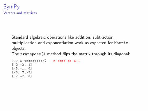
Standard algebraic operations like addition, subtraction,multiplication and exponentiation work as expected for Matrixobjects.The transpose() method flips the matrix through its diagonal:>>> A.transpose () # same as A.T[ 2,-2, 1][-3,-1, 0][-8, 2,-3][ 7,-7, 6]
SymPyVectors and Matrices
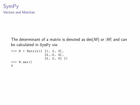
The determinant of a matrix is denoted as det(M) or |M| and canbe calculated in SymPy via:>>> M = Matrix ([ [1, 2, 3],
[2,-2, 4],[2, 2, 5] ])
>>> M.det()2
SymPyVectors and Matrices
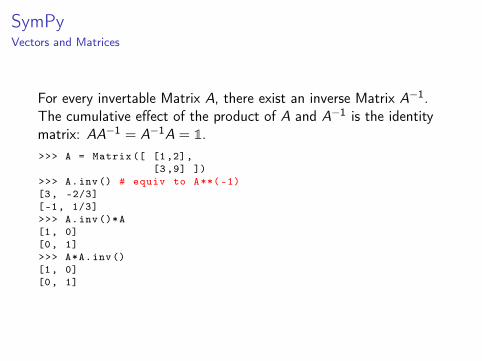
For every invertable Matrix A, there exist an inverse Matrix A−1.The cumulative effect of the product of A and A−1 is the identitymatrix: AA−1 = A−1A = 1.>>> A = Matrix ([ [1,2],
[3,9] ])>>> A.inv() # equiv to A**( -1)[3, -2/3][-1, 1/3]>>> A.inv()*A[1, 0][0, 1]>>> A*A.inv()[1, 0][0, 1]
SymPyVectors and Matrices
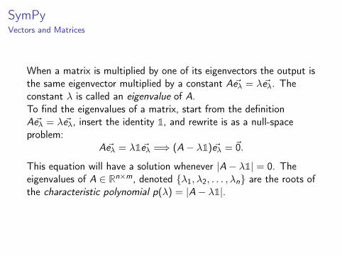
When a matrix is multiplied by one of its eigenvectors the output isthe same eigenvector multiplied by a constant A~eλ = λ~eλ. Theconstant λ is called an eigenvalue of A.To find the eigenvalues of a matrix, start from the definitionA~eλ = λ~eλ, insert the identity 1, and rewrite is as a null-spaceproblem:
A~eλ = λ1~eλ =⇒ (A− λ1)~eλ = ~0.
This equation will have a solution whenever |A− λ1| = 0. Theeigenvalues of A ∈ Rn×m, denoted {λ1, λ2, . . . , λn} are the roots ofthe characteristic polynomial p(λ) = |A− λ1|.

SymPyVectors and Matrices
This is how eigenvectors and eigenvalues work in SymPy.>>> A = Matrix ([ [ 9, -2],
[-2, 6] ])>>> A.eigenvals () # same as solve(det(A-eye (2)*x), x){5: 1, 10: 1} # eigenvalues 5 and 10 with multiplicity 1>>> A.eigenvects ()[(5, 1, [1]
[2]), (10, 1, [-2][1] ) ]
SymPyVectors and Matrices
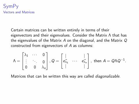
Certain matrices can be written entirely in terms of theireigenvectors and their eigenvalues. Consider the Matrix Λ that hasthe eigenvalues of the Matrix A on the diagonal, and the Matrix Qconstructed from eigenvectors of A as columns:
Λ =
λ1 · · · 0...
. . . 00 0 λn
,Q =
| |~eλ1 · · · ~eλn| |
, then A = QΛQ−1.
Matrices that can be written this way are called diagonalizable.

SymPyVectors and Matrices
To diagonalize a matrix A is to find its Q and Λ matrices:>>> A = Matrix ([ [ 9, -2], [-2, 6] ])>>> Q, L = A.diagonalize ()>>> Q # matrix of eigenvectors , as column[1,-2][2, 1]>>> Q.inv() # Q**(-1)[ 1/5, 2/5][-2/5, 1/5]>>> L[5, 0][0, 10]>>> Q*L*Q.inv() # eigendecomposition of A[ 9, -2][-2, 6]

SymPyVectors and Matrices
Not all matrices are diagonalizable. You can check if a matrix isdiagonalizable by calling its is_diagonalizable method:>>> A.is_diagonalizable ()True>>> B = Matrix ([ [1, 3], [0, 1] ])>>> B.is_diagonalizable ()False>>> B.eigenvals (){1: 2} # eigenvalue 1 with multiplicity 2>>> B.eigenvects ()[(1, 2 [1]
[0] )]
The matrix B is not diagonalizable, because it does not have a fullset of eigenvectors. Two diagonalize a 2× 2 matrix we need twoorthogonal eigenvectors, but B has only a single eigenvector.