math 536 - numerical solution of partial differential …pminev/courses/math_536/math536.pdf......
TRANSCRIPT

MATH 536 - Numerical Solution of Partial Differential Equations
Peter Minev
March 31, 2016

ii
Contents
1 Systems of Linear Equations 1
1.1 Direct Methods – Gaussian Elimination . . . . . . . . . . . . . . . . . . . . . . . . . . . . . . . . 11.1.1 Forward Elimination . . . . . . . . . . . . . . . . . . . . . . . . . . . . . . . . . . . . . . . 1
1.2 Gaussian Elimination with Pivoting . . . . . . . . . . . . . . . . . . . . . . . . . . . . . . . . . . 2
1.3 Special Cases . . . . . . . . . . . . . . . . . . . . . . . . . . . . . . . . . . . . . . . . . . . . . . . 4
1.3.1 Cholesky Decomposition . . . . . . . . . . . . . . . . . . . . . . . . . . . . . . . . . . . . . 41.3.2 Thomas Algorithm . . . . . . . . . . . . . . . . . . . . . . . . . . . . . . . . . . . . . . . . 6
1.4 Matrix Norms . . . . . . . . . . . . . . . . . . . . . . . . . . . . . . . . . . . . . . . . . . . . . . . 6
1.5 Error Estimates . . . . . . . . . . . . . . . . . . . . . . . . . . . . . . . . . . . . . . . . . . . . . . 8
1.6 Iterative Method Preliminaries . . . . . . . . . . . . . . . . . . . . . . . . . . . . . . . . . . . . . 81.7 Iterative Methods . . . . . . . . . . . . . . . . . . . . . . . . . . . . . . . . . . . . . . . . . . . . . 10
1.7.1 Jacobi’s Method . . . . . . . . . . . . . . . . . . . . . . . . . . . . . . . . . . . . . . . . . 10
1.7.2 Gauss-Seidel (GS) Iteration . . . . . . . . . . . . . . . . . . . . . . . . . . . . . . . . . . . 10
1.7.3 Successive Over-relaxation (SOR) Method . . . . . . . . . . . . . . . . . . . . . . . . . . . 111.7.4 Conjugate Gradient Method . . . . . . . . . . . . . . . . . . . . . . . . . . . . . . . . . . . 11
1.7.5 Steepest Descent Method . . . . . . . . . . . . . . . . . . . . . . . . . . . . . . . . . . . . 12
1.7.6 Conjugate Gradient Method (CGM) . . . . . . . . . . . . . . . . . . . . . . . . . . . . . . 13
1.7.7 Preconditioning . . . . . . . . . . . . . . . . . . . . . . . . . . . . . . . . . . . . . . . . . . 14
2 Solutions to Partial Differential Equations 23
2.1 Classification of Partial Differential Equations . . . . . . . . . . . . . . . . . . . . . . . . . . . . . 23
2.1.1 First Order linear PDEs . . . . . . . . . . . . . . . . . . . . . . . . . . . . . . . . . . . . . 232.1.2 Second Order PDE . . . . . . . . . . . . . . . . . . . . . . . . . . . . . . . . . . . . . . . . 23
2.2 Difference Operators . . . . . . . . . . . . . . . . . . . . . . . . . . . . . . . . . . . . . . . . . . . 24
2.2.1 Poisson Equation . . . . . . . . . . . . . . . . . . . . . . . . . . . . . . . . . . . . . . . . . 25
2.2.2 Neumann Boundary Conditions . . . . . . . . . . . . . . . . . . . . . . . . . . . . . . . . . 26
2.3 Consistency and Convergence . . . . . . . . . . . . . . . . . . . . . . . . . . . . . . . . . . . . . . 262.4 Advection Equation . . . . . . . . . . . . . . . . . . . . . . . . . . . . . . . . . . . . . . . . . . . 29
2.5 Von Neumann Stability Analysis . . . . . . . . . . . . . . . . . . . . . . . . . . . . . . . . . . . . 31
2.6 Sufficient Conditions for Convergence . . . . . . . . . . . . . . . . . . . . . . . . . . . . . . . . . 33
2.7 Parabolic PDEs – Heat Equation . . . . . . . . . . . . . . . . . . . . . . . . . . . . . . . . . . . . 342.7.1 FC Scheme . . . . . . . . . . . . . . . . . . . . . . . . . . . . . . . . . . . . . . . . . . . . 34
2.7.2 BC scheme . . . . . . . . . . . . . . . . . . . . . . . . . . . . . . . . . . . . . . . . . . . . 36
2.7.3 Crank-Nicolson Scheme . . . . . . . . . . . . . . . . . . . . . . . . . . . . . . . . . . . . . 36
2.7.4 Leapfrog Scheme . . . . . . . . . . . . . . . . . . . . . . . . . . . . . . . . . . . . . . . . . 372.7.5 DuFort-Frankel Scheme . . . . . . . . . . . . . . . . . . . . . . . . . . . . . . . . . . . . . 38
2.8 Advection-Diffusion Equation . . . . . . . . . . . . . . . . . . . . . . . . . . . . . . . . . . . . . . 38
2.8.1 FC Scheme . . . . . . . . . . . . . . . . . . . . . . . . . . . . . . . . . . . . . . . . . . . . 38
2.8.2 Upwinding Scheme (FB) . . . . . . . . . . . . . . . . . . . . . . . . . . . . . . . . . . . . . 40
iii
iv CONTENTS
3 Introduction to Finite Elements 413.1 Weighted Residual Methods . . . . . . . . . . . . . . . . . . . . . . . . . . . . . . . . . . . . . . . 41
3.1.1 Sobolev spaces . . . . . . . . . . . . . . . . . . . . . . . . . . . . . . . . . . . . . . . . . . 413.1.2 Weighted Residual Formulations . . . . . . . . . . . . . . . . . . . . . . . . . . . . . . . . 423.1.3 Collocation Methods . . . . . . . . . . . . . . . . . . . . . . . . . . . . . . . . . . . . . . . 43
3.2 Weak Methods . . . . . . . . . . . . . . . . . . . . . . . . . . . . . . . . . . . . . . . . . . . . . . 433.3 Finite Element Method (FEM) . . . . . . . . . . . . . . . . . . . . . . . . . . . . . . . . . . . . . 473.4 Gaussian Quadrature . . . . . . . . . . . . . . . . . . . . . . . . . . . . . . . . . . . . . . . . . . . 483.5 Error Estimates . . . . . . . . . . . . . . . . . . . . . . . . . . . . . . . . . . . . . . . . . . . . . . 493.6 Optimal Error Estimates . . . . . . . . . . . . . . . . . . . . . . . . . . . . . . . . . . . . . . . . . 50
3.6.1 Other Boundary Conditions . . . . . . . . . . . . . . . . . . . . . . . . . . . . . . . . . . . 523.7 Transient Problems . . . . . . . . . . . . . . . . . . . . . . . . . . . . . . . . . . . . . . . . . . . . 533.8 Finite Elements in Two Dimensions . . . . . . . . . . . . . . . . . . . . . . . . . . . . . . . . . . 58
3.8.1 Finite Element Basis Functions . . . . . . . . . . . . . . . . . . . . . . . . . . . . . . . . . 593.8.2 Discrete Galerkin Formulation . . . . . . . . . . . . . . . . . . . . . . . . . . . . . . . . . 60
Chapter 1
Systems of Linear Equations
1.1 Direct Methods – Gaussian Elimination
1.1.1 Forward Elimination
(k-th step):
a[k]ij = a
[k−1]ij − a[k−1]
k−1,jℓ[k−1]i,k−1, i = k, . . . , n, j = k − 1, . . . , n
ℓ[k−1]i,k−1 =
a[k−1]i,k−1
a[k−1]k−1,k−1
, k = 2, . . . , n i = k, . . . , n
b[k]i = b
[k−1]i − b[k−1]
k−1 ℓ[k−1]i,k−1, i = k, . . . , n
In n− 1 steps:
a[1]11 a
[1]12 . . . a
[1]1n
0 a[2]22 . . . a
[2]2n
......
. . ....
0 0 . . . a[n]nn
x1x2...xn
=
b[1]1
b[2]2...
b[n]n
or
[u] [x] = [c]
Operations Count
n−1∑
j=1
(n− j)︸ ︷︷ ︸
divisions
+2 (n− j) (n− j + 1)︸ ︷︷ ︸
multiply and sum
=
2n3
6+n2
2− 7n
6
Where we have usedm∑
j=1
j =m (m+ 1)
2,
m∑
j=1
j2 =m (m+ 1) (2m+ 1)
6
Backward Substitution
xi =1
a[i]ii
b[i]i −
n∑
j=i+1
a[i]ij xj
1
2 CHAPTER 1. SYSTEMS OF LINEAR EQUATIONS
Operation Count
n∑
i=1
2 (n− i)︸ ︷︷ ︸
Multiplication and Subtraction
+ 1︸︷︷︸
division
= n2
Matrix Representations
Define:
Lk =
1 0 . . . . . . . . . . . . . . . . 0
0. . . 0 . . . . . . 0
0 . . . 1 0 . . . 00 . . . −ℓk+1,k 1 . . . 0...
.... . .
0 . . . −ℓnk 0 . . . 1
Lemma 1.1.1
A[2] = L1A[1], b[2] = L1b
[1](
A[1] = A, b[1] = b)
Therefore,
A[n] = U = Ln−1Ln−2 · · ·L1A
or
A = L−11 L−1
2 · · ·L−1n−1U = LU
Proposition 1.1.2
L = L−11 · · ·L−1
n−1
is a lower triangular matrix with unit diagonal.
Definition A Permutation matrix is a matrix that has exactly one nonzero entry in each row and column, andthis entry is equal to 1. The elementary permutation matrix (EPM) is defined as a matrix produced from theidentity matrix by interchanging exactly one pair k,m of its columns. We denote it as Pkm
︸︷︷︸
k<m
= Pk.
For example:
P23 =
1 0 0 00 0 1 00 1 0 00 0 0 1
Proposition 1.1.3 If A ∈ Rn×n and Pk,m ∈ Rn×n is EPM, then Pk,mA differs from A by an interchange ofrows k and m.
1.2 Gaussian Elimination with Pivoting
A[n] = U = Ln−1Pn−1 . . . L1P1A
Where U is upper triangular, Lk is defined as before, and Pk = Pkm with m ≥ k. Equivalently,
A = P1L−11 P2L
−12 · · ·Pn−1L
−1n−1
︸ ︷︷ ︸
L∗
U
1.2. GAUSSIAN ELIMINATION WITH PIVOTING 3
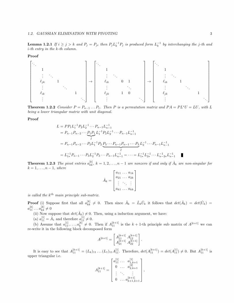
Lemma 1.2.1 If i ≥ j > k and Pj = Pji then PjL−1k Pj is produced form L−1
k by interchanging the j-th andi-th entry in the k-th column.
Proof
. . .
1...
. . .
ℓjk 1...
. . .
ℓik 1...
. . .
→
. . .
1...
. . .
ℓik 0 1...
. . .
ℓjk 1 0...
. . .
→
. . .
1...
. . .
ℓik 1...
. . .
ℓjk 1...
. . .
Theorem 1.2.2 Consider P = Pn−1 . . . P1. Then P is a permutation matrix and PA = PL∗U = LU , with Lbeing a lower triangular matrix with unit diagonal.
Proof
L = PP1L−11 P2L
−12 · · ·Pn−1L
−1n−1
= Pn−1Pn−2 · · ·P1P1︸ ︷︷ ︸
I
L−11 P2L
−12 · · ·Pn−1L
−1n−1
= Pn−1Pn−2 · · ·P2L−11 P2 P3 · · ·Pn−1Pn−1 · · ·P3
︸ ︷︷ ︸
I
L−12 · · ·Pn−1L
−1n−1
= L−11∗ Pn−1 · · ·P3L
−12 P3 · · ·Pn−1L
−1n−1 = · · · = L−1
1∗ L−12∗ · · ·L−1
n−2∗L−1n−1
Theorem 1.2.3 The pivot entries a[k]kk, k = 1, 2, . . . , n − 1 are nonzero if and only if Ak are non-singular for
k = 1, . . . , n− 1, where
Ak =
a11 . . . a1ka21 . . . a2k...
. . ....
ak1 . . . akk
is called the kth main principle sub-matrix.
Proof (i) Suppose first that all a[k]kk 6= 0. Then since Ak = LkUk it follows that det(Ak) = det(Uk) =
a[k]11 . . . a
[k]kk 6= 0
(ii) Now suppose that det(Ak) 6= 0. Then, using a induction argument, we have:
(a) a[1]11 = A1 and therefore a
[1]11 6= 0.
(b) Assume that a[1]11 , . . . , a
[k]k 6= 0. Then if A
[k+1]11 is the k + 1-th principle sub matrix of A[k+1] we can
re-write it in the following block decomposed form
A[k+1] =
[
A[k+1]11 A
[k+1]12
A[k+1]21 A
[k+1]22
]
.
It is easy to see that A[k+1]11 = (Lk)11 . . . (L1)11A
[1]11 . Therefore, det(A
[k+1]11 ) = det(A
[1]11) 6= 0. But A
[k+1]11 is
upper triangular i.e.
A[k+1]11 =
a[1]11 . . . a
[1]1,k+1
0 . . . a[2]2,k+1
.... . .
...
0 . . . a[k+1]k+1,k+1
,

4 CHAPTER 1. SYSTEMS OF LINEAR EQUATIONS
and then det(A[k+1]11 ) = a
[1]11 . . . a
[k+1]k+1,k+1. This, together with the induction hypothesis yields that a
[k+1]k+1,k+1 6= 0
which completes the induction proof.
Definition A matrix is strictly diagonally dominant if
|aii| >∑
j 6=i
|aij |
Corollary 1.2.4 If a matrix is strictly diagonally dominant then no pivoting is necessary.
Definition Matrix A is symmetric positive definite (spd) if
1. A = AT
2. vTAv ≥ 0 for all v ∈ Rn
3. vTAv = 0 if and only if v ≡ 0
Corollary 1.2.5 If a matrix is spd then no pivoting is necessary.
Definition The spectrum of a matrix A, S (A), is the set of all eigenvalues of the matrix.
Theorem 1.2.6 If A ∈ Rn×n is symmetric the following statements are equivalent
1. A is positive definite,
2. S (A) contains only positive real numbers, and
3. Every principle sub-matrix is positive definite.
Theorem 1.2.7 (Gershgorin) The spectrum S (A) is enclosed in
(n⋃
i=1
D′i
)⋂(
n⋃
i=1
D′′i
)
where
D′i =
z ∈ C : |z − aii| ≤
∑
j 6=i
|aij |
D′′i =
z ∈ C : |z − aii| ≤
∑
j 6=i
|aji|
1.3 Special Cases
1.3.1 Cholesky Decomposition
Theorem 1.3.1 If A ∈ Rn×n is spd then there exists a lower triangular matrix C such that CCT = A.Furthermore, the diagonal entries of C are positive.
Proof Use induction on n:n = 1 : C = [c11] =
√a11
Assume the theorem holds for all matrices in Rn×n.
A =
[An aaT an+1,n+1
]
1.3. SPECIAL CASES 5
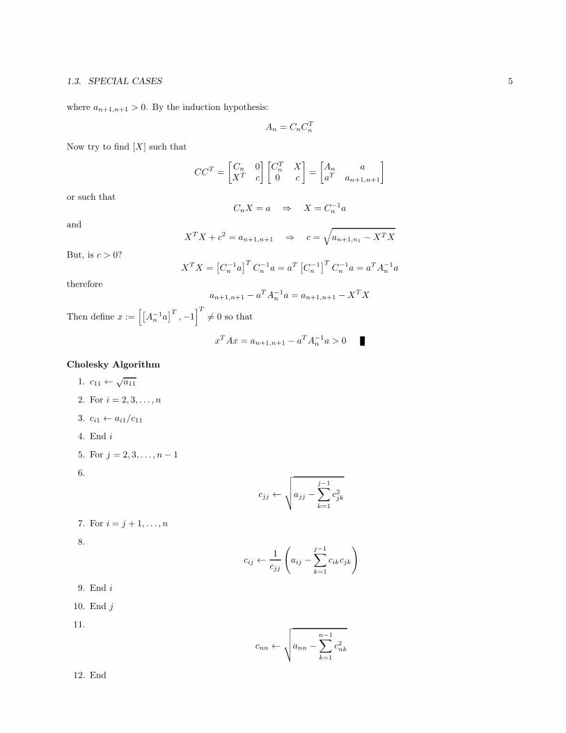
where an+1,n+1 > 0. By the induction hypothesis:
An = CnCTn
Now try to find [X ] such that
CCT =
[Cn 0XT c
] [CT
n X0 c
]
=
[An aaT an+1,n+1
]
or such thatCnX = a ⇒ X = C−1
n a
and
XTX + c2 = an+1,n+1 ⇒ c =√
an+1,n1 −XTX
But, is c > 0?
XTX =[C−1
n a]TC−1
n a = aT[C−1
n
]TC−1
n a = aTA−1n a
thereforean+1,n+1 − aTA−1
n a = an+1,n+1 −XTX
Then define x :=[[A−1
n a]T,−1
]T
6= 0 so that
xTAx = an+1,n+1 − aTA−1n a > 0
Cholesky Algorithm
1. c11 ←√a11
2. For i = 2, 3, . . . , n
3. ci1 ← ai1/c11
4. End i
5. For j = 2, 3, . . . , n− 1
6.
cjj ←
√√√√ajj −
j−1∑
k=1
c2jk
7. For i = j + 1, . . . , n
8.
cij ←1
cjj
(
aij −j−1∑
k=1
cikcjk
)
9. End i
10. End j
11.
cnn ←
√√√√ann −
n−1∑
k=1
c2nk
12. End

6 CHAPTER 1. SYSTEMS OF LINEAR EQUATIONS
1.3.2 Thomas Algorithm
Definition A band matrix is of the form
a11 a1,2 . . . a1,l 0 . . . . . . . . . . . . . . . . . . . . . . . . . . . 0
a21. . .
. . .. . .
. . ....
.... . .
. . .. . .
. . .. . .
...ak,1 . . . ak,k−1 akk ak,k+1 . . . ak,k+l−1 0 . . . 0
0. . .
. . .. . .
. . .. . .
. . ....
.... . .
. . .. . .
. . .. . .
. . . 0...
. . .. . .
. . .. . .
. . . an−l+1,n
.... . .
. . .. . .
. . .. . .
......
. . .. . .
. . .. . . an−1,n
0 . . . . . . . . . . . . . . . . . . . . . . . . . . 0 an,n−k+1 . . . an,n−1 an,n
A band matrix may be stored compactly as an l + k − 1× n matrix of the form:
k−1︷ ︸︸ ︷
0 . . . 0 a11 a12 . . . a1l. . . . . . . . . . . . . . . . . . . . . . . . . . . . . . . . . . . . . . . . . . . . . .ak1 . . . ak,k−1 akk ak,k+1 . . . ak,k+l−1
. . . . . . . . . . . . . . . . . . . . . . . . . . . . . . . . . . . . . . . . . . . . . .an,n−k+1 . . . an,n−1 ann 0 . . . 0
︸ ︷︷ ︸
l−1
Thomas Algorithm
For the linear system
b1 c1 0 . . . . . . . . . . . . . . . . 0a2 b2 c2 0 . . . . . . . . . . . 00 a3 b3 c3 0 . . . 0...
. . .. . .
. . .. . .
......
. . .. . .
. . .. . . 0
.... . . an−1 bn−1 cn−1
0 . . . . . . . . . . . . 0 an bn
x1x2...xn
=
d1d2...dn
1.
b[f ]j = bj − aj
c[f ]j−1
b[f ]j−1
and d[f ]j = dj − aj
d[f ]j−1
b[f ]j−1
, for j = 2, . . . , n
2.xj−1 = d
[f ]j−1 − b
[f ]j xj , for j = n, . . . , 2
1.4 Matrix Norms
Definition If A ∈ Rn×n then the mapping Rn×n → R is called a norm of A := ||A|| if and only if:
1. ||A|| ≥ 0 and ||A|| = 0 if and only if A = 0,
1.4. MATRIX NORMS 7
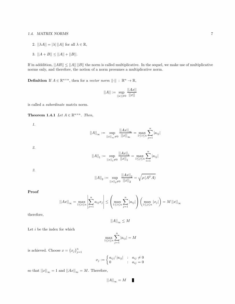
2. ||λA|| = |λ| ||A|| for all λ ∈ R,
3. ||A+B|| ≤ ||A||+ ||B||.
If in adddition, ||AB|| ≤ ||A|| ||B|| the norm is called multiplicative. In the sequel, we make use of multiplicativenorms only, and therefore, the notion of a norm presumes a multiplicative norm.
Definition If A ∈ Rn×n, then for a vector norm ||·|| : Rn → R,
||A|| := sup||x||6=0
||Ax||||x||
is called a subordinate matrix norm.
Theorem 1.4.1 Let A ∈ Rn×n. Then,
1.
||A||∞ := sup||x||
∞6=0
||Ax||∞||x||∞
= max1≤i≤n
n∑
j=1
|aij |
2.
||A||1 := sup||x||1 6=0
||Ax||1||x||1
= max1≤j≤n
n∑
i=1
|aij |
3.
||A||2 := sup||x||2 6=0
||Ax||2||x||2
=√
ρ (ATA)
Proof
||Ax||∞ = max1≤i≤n
∣∣∣∣∣∣
n∑
j=1
aijxj
∣∣∣∣∣∣
≤
max1≤i≤n
n∑
j=1
|aij |
(
max1≤j≤n
|xj |)
=M ||x||∞
therefore,
||A||∞ ≤M
Let i be the index for which
max1≤i≤n
n∑
j=1
|aij | =M
is achieved. Choose x = xjnj=1
xj :=
aij/ |aij | : aij 6= 00 : aij = 0
so that ||x||∞ = 1 and ||Ax||∞ =M . Therefore,
||A||∞ =M
8 CHAPTER 1. SYSTEMS OF LINEAR EQUATIONS
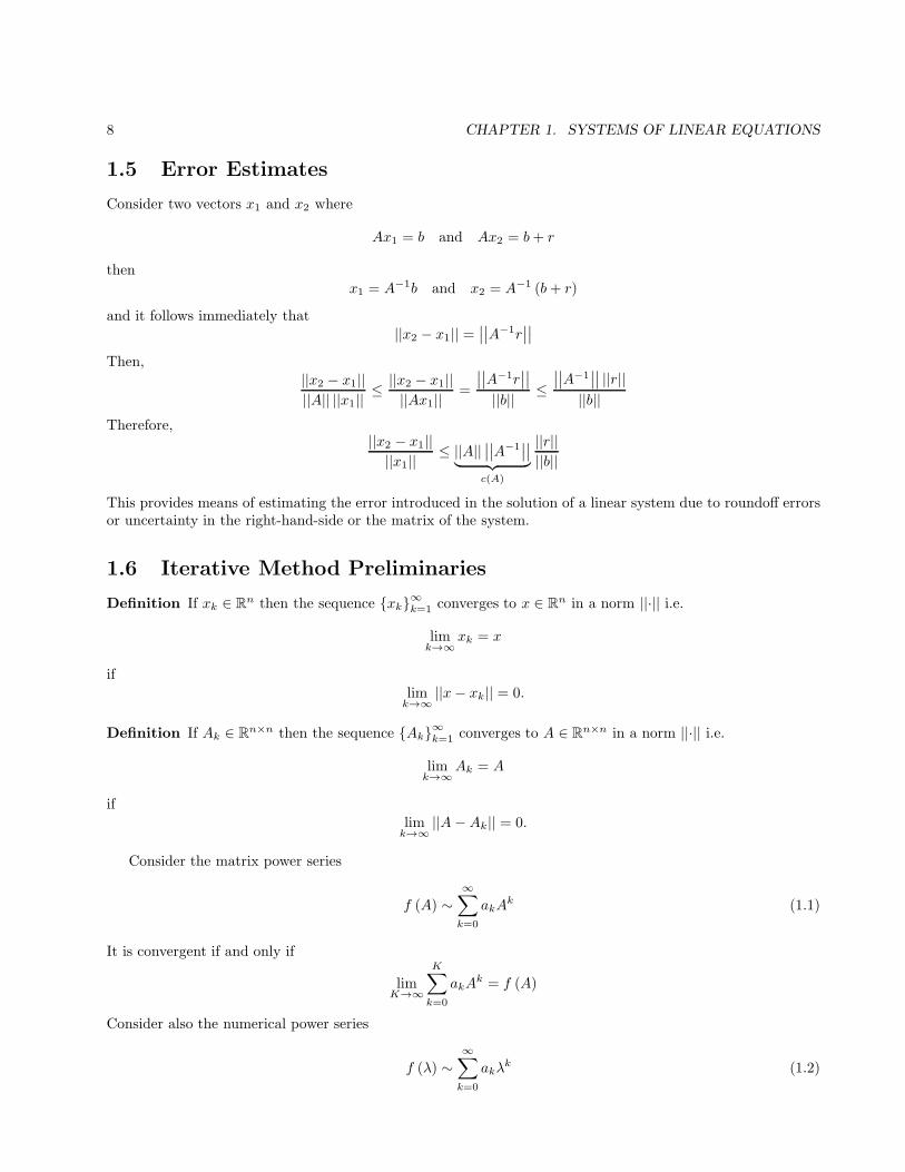
1.5 Error Estimates
Consider two vectors x1 and x2 where
Ax1 = b and Ax2 = b+ r
then
x1 = A−1b and x2 = A−1 (b+ r)
and it follows immediately that
||x2 − x1|| =∣∣∣∣A−1r
∣∣∣∣
Then,
||x2 − x1||||A|| ||x1||
≤ ||x2 − x1||||Ax1||=
∣∣∣∣A−1r
∣∣∣∣
||b|| ≤∣∣∣∣A−1
∣∣∣∣ ||r||
||b||Therefore,
||x2 − x1||||x1||
≤ ||A||∣∣∣∣A−1
∣∣∣∣
︸ ︷︷ ︸
c(A)
||r||||b||
This provides means of estimating the error introduced in the solution of a linear system due to roundoff errorsor uncertainty in the right-hand-side or the matrix of the system.
1.6 Iterative Method Preliminaries
Definition If xk ∈ Rn then the sequence xk∞k=1 converges to x ∈ Rn in a norm ||·|| i.e.
limk→∞
xk = x
if
limk→∞
||x− xk|| = 0.
Definition If Ak ∈ Rn×n then the sequence Ak∞k=1 converges to A ∈ Rn×n in a norm ||·|| i.e.
limk→∞
Ak = A
if
limk→∞
||A−Ak|| = 0.
Consider the matrix power series
f (A) ∼∞∑
k=0
akAk (1.1)
It is convergent if and only if
limK→∞
K∑
k=0
akAk = f (A)
Consider also the numerical power series
f (λ) ∼∞∑
k=0
akλk (1.2)

1.6. ITERATIVE METHOD PRELIMINARIES 9
Theorem 1.6.1 The matrix power series (1.1) is convergent if for all λi ∈ S (A) |λi| < ρ, where ρ is the radiusof convergence of (1.2) and S (A) is the spectrum of A. It is divergent if |λi| > ρ for some i.
Proof From Jordan’s theorem, there exists nonsingular C such that:
B = C−1AC, B = diag (Bk) , Bk =
λk 1 0 . . . 00 λk 1 . . . 0...
. . .. . .
. . ....
. . .. . . 1
0 . . . . . . . 0 λk
where Bk ∈ Rnk×nk and nk is the multiplicity of the eigenvalue λk. Then, f (A) is convergent if and only if
f (B) =
∞∑
k=0
akBk =
∞∑
k=0
akC−1AkC = C−1
( ∞∑
k=0
akAk
)
C
is convergent as well. Now, let’s look at Bik:
B2k =
λ2k 2λk 1 . . . 00 λ2k 2λk . . . 0. . . . . . . . . . . . . . . . . . . . . . .0 . . . . . . . . . . . . . . λ2k
, Bi
k =
λik(i1
)λi−1k . . . . . . . . . . . .
(i
nk−1
)λi−nk+1k
0 λik(i1
)λi−1k . . .
(i
nk−2
)λi−nk+2k
. . . . . . . . . . . . . . . . . . . . . . . . . . . . . . . . . . . . . . . . . . .0 . . . . . . . . . . . . . . . . . . . . . . λik
so that the i-th block of the m-th partial sum of f (B) is
fm (Bi) =
m∑
k=0
akBki =
fm (λi)11!f
′m (λi) . . . 1
(ni−1)!f(ni−1)m (λi)
0 fm (λi) . . . 1(ni−2)!f
(ni−2)m (λi)
. . . . . . . . . . . . . . . . . . . . . . . . . . . . . . . . . . . . . . . . . . .0 . . . 0 fm (λi)
where
f (B) =
m∑
k=0
akBk
Therefore, fm (B) is convergent if and only if
fm (λi) =
m∑
k=0
akλki
(and therefore f(l)m (λi)) is convergent for i = 1, . . . , n and l = 1, . . . , ni. fm (λi) is convergent if |λi| is smaller
than ρ, the radius of convergence of (1.2).
Corollary 1.6.2
f (A) = I +A+A2 + · · ·+Am + · · ·
is convergent if and only if |λk| < 1 for all k = 1, . . . , n and A ∈ Rn×n.
Corollary 1.6.3 Since |λk| ≤ ||A|| for any subordinate norm ||·|| then f (A) is convergent if ||A|| < 1.
10 CHAPTER 1. SYSTEMS OF LINEAR EQUATIONS
1.7 Iterative Methods
ConsiderAx = b
If A = B + C thenAx = b ⇔ x = x+ C−1 (b−Ax)
and in this form we may solve the problem iteratively:
xk+1 = xk + C−1(b−Axk
)(1.3)
Theorem 1.7.1 The iteration (1.3) is convergent if and only if ρ(I − C−1A
)< 1.
Proof
xk+1 =(I − C−1A
)
︸ ︷︷ ︸
D
xk + C−1b = D2xk−1 + (I +D)C−1b = . . .
= Dk+1x0 +(I +D +D2 + . . .+Dk
)C−1b
If ρ(I − C−1A
)< 1 then I +D + . . .+Dk + . . . is convergent and therefore
Dk →k→∞ 0
Definition R (D) = − log10 ρ (D) is called the convergence rate of the iteration.
1.7.1 Jacobi’s Method
C = diag (A)
D = I − C−1A =
0 −a12
a11−a13
a11· · · −a1n
a11
.... . .
...− an1
ann− an2
ann− an3
ann· · · 0
Theorem 1.7.2 If A is strictly diagonally dominant then Jacobi is convergent.
Proof
||D||∞ = maxi
∑
j 6=i
∣∣∣∣
aijaii
∣∣∣∣< 1.
Then|λi| ≤ ||D||∞ < 1 .
1.7.2 Gauss-Seidel (GS) Iteration
C = L =
a11 0...
. . .
a1n . . . ann
B = U = A− LXk+1 = Xk + C−1
(b−AXk
)
Theorem 1.7.3 If A is strictly diagonally dominant then Gauss-Seidel iteration is convergent.
1.7. ITERATIVE METHODS 11
Proof The formula for the i-th component of xk+1 is:
xk+1i = −
∑
j<i
aijaiixk+1j −
∑
j>i
aijaiixkj +
biaii
The exact solution clearly satisfies the iteration i.e.
xi = −∑
j<i
aijaii
xj −∑
j>i
aijaii
xj +biaii
The error ǫk+1 = xk+1 − x for Ax = B is found as
ǫk+1i = −
∑
j<i
aijaiiǫk+1j −
∑
j>i
aijaii
ǫkj
then∣∣ǫk+1
i
∣∣ ≤
∑
j<i
∣∣∣∣
aijaii
∣∣∣∣
∣∣ǫk+1
j
∣∣+∑
j>i
∣∣∣∣
aijaii
∣∣∣∣
∣∣ǫkj∣∣
Using induction on i we find that
∣∣ǫk+1
i
∣∣ ≤
∑
j 6=i
∣∣∣∣
aijaii
∣∣∣∣
∣∣∣∣ǫk∣∣∣∣∞ <
∣∣∣∣ǫk∣∣∣∣∞
Therefore,∣∣∣∣ǫk+1
i
∣∣∣∣∞ <
∣∣∣∣ǫk∣∣∣∣∞
so that the error must strictly decrease with each iteration. Then the error must go to zero because the exactsolution is the unique fixed point of the iteration (why is it unique?).
1.7.3 Successive Over-relaxation (SOR) Method
C = L+1
ωD
A = L+D + U
D = diag (A)
xk+1 = −(ω−1D + L
)−1 [(1− ω−1
)D + U
]xk +
(ω−1D + L
)−1b.
Note that in this case L has zeros on the main diagonal and is strictly lower triangular.
Theorem 1.7.4 (Ostrowski-Reich) If A ∈ Rn×n is spd then SOR is convergent iff 0 < ω < 2.
1.7.4 Conjugate Gradient Method
Theorem 1.7.5 If A ∈ Rn×n is spd then u is a solution to the linear system Au = b if and only if u minimizes
the function:
F (v) =1
2vTAv − bT v
Proof Let u∗ satisfy Au∗ = b then
F (u)− F (u∗) =1
2uTAu− bTu− 1
2u∗TAu∗ + bTu∗
=1
2uTAu− u∗TAu+
1
2u∗TAu∗ =
1
2(u− u∗)T A (u− u∗) ≥ 0
12 CHAPTER 1. SYSTEMS OF LINEAR EQUATIONS
then1
2(u− u∗)T A (u− u∗) = 0 ⇔ u = u∗
so that F (u) ≥ F (u∗) andF (u) = F (u∗) ⇔ u = u∗
Definition If A is spd then for any two vectors u, v ∈ Rn, uTAv defines the energy inner product induced byA denoted by:
〈u, v〉A = uTAv.
Note that in the rest of the notes at some occasions (u, v)A is also used to denote the energy inner product.
1.7.5 Steepest Descent Method
Note that any iteration for finding a solution to a linear system Au = b can be written in the form:
uk+1 = uk + αkpk
where αk ∈ R is called iteration step, pk ∈ Rn is called the search direction. For example, in the case of matrixsplitting methods the search direction is chosen to be pk = C−1rk, with rk = b−Auk being called the residualof the iterate uk, and αk = 1. The step does not need to be constant and the gradient-type methods choose it ateach iteration step so that this choice minimizes the function F (v). The basic gradient-type iterative algorithmtherefore can be written as:
1. Choose an initial search direction
p0 = r0 = b−Au0
2. For k = 1, 2, 3, . . . do:
(a) Find αk ∈ R such that
uk+1 = uk + αkpk
minimizes F over the line uk + αpk
(b) New iterate
uk+1 = uk + αkpk
(c) The new residual is
rk+1 = b−Auk+1
(d) Find the new search direction pk+1.
(e) Let k = k + 1 and repeat item 2 until convergence.
To find αk we minimize F along the search direction pk:
d
dαkF(uk + αkpk
)= ∇F
(uk + αkpk
)· d
dαk
(uk + αkpk
)
=[A(uk + αkpk
)− b]Tpk =
[Auk − b
]Tpk + αkp
TkApk
= −rTk pk + αkpTkApk = 0
so that
αk =rTk pk
pTkApk
1.7. ITERATIVE METHODS 13
Note that for this choice of αk we have:
Auk+1 − b︸ ︷︷ ︸
−rk+1
T
pk =
A(uk + αkpk
)
︸ ︷︷ ︸
uk+1
−b
T
pk = −rTk pk + αkpTkApk = 0
or
−rTk+1pk = ∇F (uk+1) pk = 0
In the steepest descent method we choose
pk = rk = b−Auk,
because this is the direction of the negative gradient and in this direction the function F (v) is clearly non-increasing. Unfortunately, this choice of search direction is not optimal. The basic reason for this is that thestep αk is chosen so that the iterate uk+1 is a minimum of F (v) along the direction pk. However, the nextminimum, along the direction pk+1, is not guaranteed to be smaller than or equal to the current one. This issueis discussed in the next section.
1.7.6 Conjugate Gradient Method (CGM)
Definition uk is optimal with respect to direction p 6= 0 iff F(uk)≤ F
(uk + λp
)for all λ ∈ R.
Lemma 1.7.6 uk is optimal with respect to p iff
pT rk = 0.
Proof uk is optimal with respect to p iff F(uk + λp
)has a minimum at λ = 0, i.e.
∂F
∂λ
(uk + λp
)∣∣∣∣λ=0
= pT(Auk − b
)
︸ ︷︷ ︸
−rk
+ λpTAp∣∣λ=0
= 0
This is obviously satisfied iff pT rk = 0.
We know that the choice of αk guarantees that uk+1 is optimal with respect to pk and this applies in particularto the steepest descent method for which pk = −rk. However, uk+2 may not be optimal with respect to pk i.e.the next iteration can undo some of the minimization work of the previous iteration. Indeed:
uk+2 = uk+1 + αk+1rk+1
which gives
rk+2 = rk+1 − αk+1Ark+1 ⇒ rTk rk+2 = rTk rk+1︸ ︷︷ ︸
=0
−αk+1rTk Ark+1 ⇒ pTk rk+2 = −αk+1r
Tk Ark+1 6= 0
unless A = cI. Note that rTk rk+1 = 0 for the steepest descent method since
rTk rk+1 = rTk (b−A(uk + αkrk)) = rTk (rk − αkArk) = rTk (rk −rTk rk||rk||2A
Ark) = 0.
To find a different search direction pk+1 that maintains the optimality of uk+2 w.r.t. pk, we multiply by pk theequation for the residual:
rk+2 = rk+1 − αk+1Apk+1
14 CHAPTER 1. SYSTEMS OF LINEAR EQUATIONS
and require the product to be zero:
0 = pTk rk+2 = pTk rk+1︸ ︷︷ ︸
=0
+αk+1pTkApk+1 ⇔ pTkApk+1 = 0.
For the conjugate gradient method we require that uk+2 is also optimal with respect to pk i.e. we choosethe search direction pk+1 from the condition pTkApk+1 = 0.
Definition If u, v ∈ Rn are such that 〈u, v〉A = 0 for A (which is spd) then u, v are A-conjugate.
This means that pk+1 should be A-conjugate to pk. We search for pk+1 in the form pk+1 = rk+1 + βkpk and
then from the condition pTkApk+1 = 0 we easily obtain that βk = −〈rk+1, pk〉A||pk||2A
Algorithm (Basic CGM procedure) If A ∈ Rn×n is spd and u0 is an initial guess:
1. r0 ← b− Au0
2. p0 = r0
3. For k = 1, 2, . . . ,m:
4. αk−1 ← rTk−1pk−1/ ||pk−1||2A5. uk ← uk−1 + αk−1pk−1
6. rk ← rk−1 − αk−1Apk−1
7.
pk ← rk −〈rk, pk−1〉A||pk−1||2A
pk−1
8. Next k
9. End
As it will be demonstrated below, if all arithmetic operations are exact, the algorithm computes the exactsolution in a finite number of steps (finite termination property).
Later, we will show that the error decreases as:
∣∣∣∣u− uk
∣∣∣∣A=∣∣∣∣ǫk∣∣∣∣A≤ 2 ||ǫ0||A
[√
c (A)− 1√
c (A) + 1
]k
If c (A) ≫ 1 then the convergence is slow. Therefore, the algorithm is often modified by formally multiplyingthe original system by a matrix that has a spectrum close to the spectrum of A and performing the CG methodon the modified system which has the same solution as the original one. This process is called preconditioning.
1.7.7 Preconditioning
Instead of Au = b we solve Au = b where
A =(B−1
)TAB−1, u = Bu, b =
(B−1
)Tb
Since the preconditioner BTB must be an approximation to the matrix A, a natural choice for B should be anapproximation to the square root of A. Since A is s.p.d. its square root is also s.p.d. and therefore we assumethat BT = B. The preconditioner B2 must satisfy somewhat contradicting requirements since on one hand it
1.7. ITERATIVE METHODS 15
should be a good approximation of A and on the other, it should be much easier to solve a linear system witha matrix B2 than with A. The second requirement follows from the fact that, as it will become clear below, oneach iteration of the CG method with preconditioning, we will need to solve one system with B2.
For the system Au = b we know that
u : F (u) = minv∈Rn
F (v)
Now, if v = Bv then
F (v) =1
2vTAv − bT v =
1
2
[B−1v
]TA[B−1v
]− bT
(B−1v
)
=1
2vT B−1AB−1︸ ︷︷ ︸
A
v −(B−1b
)
︸ ︷︷ ︸
b
v = F (v)
The preconditioned method should compute the new iterate from: uk = uk−1+αk−1pk−1, with αk−1 =rTk−1pk−1
||pk−1||A.
The search direction for the preconditioned method should be computed as pk = βk−1pk−1+rk where the residual
rk is given by rk = rk−1 − αk−1Apk−1, and βk = − 〈rk+1,pk〉A||pk||2A
. These formulae are not convenient for practical
computations since they require to somehow compute the inverse of the preconditioner, (B2)−1. Fortunately,it appears that the preconditioned method can be implemented almost exactly as the original CGM modifyingonly the computation of the search direction to:
pk =(B2)−1
rk︸ ︷︷ ︸
zk
−
zk︷ ︸︸ ︷(B2)−1
rk
T
Apk−1
pTk−1Apk−1pk−1, (1.4)
and defining the initial iterate as u0 = B−1u0 and the initial search direction as p0 = (B2)−1r0. With thismodification, the residuals rk, rk, search directions pk, pk, and iterates uk, uk, of the modified CG algorithmand the preconditioned CG algorithm, verify the relations: rk = Brk, pk = B−1pk, u
k = B−1uk. Indeed, usingthe assumption that rk−1 = Brk−1, pk−1 = B−1pk−1, and uk−1 = B−1uk−1 (these assumptions are triviallyverifiable at k = 1), we obtain that:
αk−1 =rTk−1pk−1
||pk−1||2A=
rTk−1B−1Bpk−1
(Bpk−1)TB−1AB−1Bpk−1
=rTk−1pk−1
||pk−1||2A= αk−1,
and subsequently that: rk = Brk and uk = B−1uk. For example,
uk = uk−1 + αk−1pk−1 = B(uk−1 + αk−1pk−1) = Buk.
This immediately yields that rk = Brk. Then, if pk is computed from (1.4) we obtain, multiplying it by B,that:
Bpk = B−1rk −rTk B
−1B−1AB−1Bpk−1
pTk−1BB−1AB−1Bpk−1
Bpk−1,
or, using the induction assumptions:
Bpk = rk −〈rk, pk−1〉A||pk−1||2A
pk−1 = pk
Thus, using an induction argument we establish that rk = Brk, pk = B−1pk, uk = B−1uk, and therefore,
αk = αk, for all positive integer k, Then, it is clear that the modified CG algorithm does not require theknowledge of A to proceed. It needs only one extra step for the computation of the new search direction.Instead of using rk for its computation, we need to use zk that is a solution of the system B2zk = rk. Theconjugate gradient method with preconditioning is given by:
16 CHAPTER 1. SYSTEMS OF LINEAR EQUATIONS
Algorithm Preconditioned CGM:
1. k← 0
2. r0 ← b− Au0
3. p0 = (B2)−1r0
4. For k = 1, 2, . . . ,m:
5. αk−1 ← rTk−1pk−1/ ||pk−1||2A6. uk ← uk−1 + αk−1pk−1
7. rk ← rk−1 − αk−1Apk−1
8. if ||rk||2 ≥ τ then
9. solve B2zk = rk
10.
pk ← zk −〈zk, pk−1〉A||pk−1||2A
pk−1
11. k = k + 1
12. Go to (5)
13. End if
14. End
Lemma 1.7.7 If A ∈ Rn×n is spd, then for m = 0, 1, 2, . . . we have
span p0, p1, . . . , pm = span r0, r1, . . . , rm = span r0, Ar0, . . . , Amr0
Proof 1. For m = 0, this is trivial.
2. Suppose that for m = k we have
span p0, p1, . . . , pk = span r0, r1, . . . , rk = spanr0, Ar0, . . . , A
kr0.
3. To complete the proof we should show that the same is true for m = k + 1 i.e.
span p0, p1, . . . , pk+1 = span r0, r1, . . . , rk+1 = spanr0, Ar0, . . . , A
k+1r0.
We have shown that
rk+1 = rk − αkApk
pk ∈ spanr0, Ar0, . . . , A
kr0
Apk ∈ spanAr0, A
2r0, . . . , Ak+1r0
this impliesrk+1 ∈ span
r0, Ar0, . . . , A
k+1r0
so thatspan r0, r1, . . . , rk+1 ⊂ span
r0, Ar0, . . . , A
k+1r0
1.7. ITERATIVE METHODS 17
Now,
Akr0 ∈ span p0, p1, . . . , pkAk+1r0 ∈ span Ap0, Ap1, . . . , Apkrk+1 = rk − αkApk
So that
Ak+1r ∈ span
Ap0︸︷︷︸
(r1−r0)
, Ap1︸︷︷︸
(r2−r1)
, . . . , Apk−1︸ ︷︷ ︸
c(rk−rk−1)
, rk+1 − rk
⊆ span r0, r1, . . . rk+1
ThereforeAk+1r0 ∈ span r0, r1, . . . , rk+1
and by inductionspan
r0, Ar0, . . . , A
k+1r0⊂ span r0, . . . rk+1
.
span p0, p1, . . . , pm = span r0, . . . , rmis proven using
pm = rm + βm−1pm−1
and the same arguments as above.
Definition Km := span r0, r1, . . . , rm−1 is the m-th Krylov space of A.
Theorem 1.7.8 If A is spd then:
(A) 〈pk, pm〉A = 0 for m 6= k and
(B) rTk rm = 0 for m 6= k.
Proof 1. For k,m ≤ 1:
rT1 r0 = 0
〈p1, p0〉A = 0
2. Assume:
(a) 〈pk, pm〉A = 0 for k 6= m and k,m ≤ l(b) rTk rm = 0 for k 6= m and k,m ≤ l
3. For m < l:rTl pm = rTl (c0r0 + c2r2 + · · ·+ cmrm) = 0
from (b) and therefore
rTl+1pm = (rl − αlApl)T pm = 0.
For m = l we haverTl+1pl = (rl − αlApl)
Tpl = rTl pl − αl 〈pl, pl〉A = 0
by the definition of αl. But rm ∈ span p0, . . . , pm for m = 1, . . . , l and therefore
rTl+1rm = 0, m = 0, 1, . . . , l,
18 CHAPTER 1. SYSTEMS OF LINEAR EQUATIONS
which proves (B).
To prove (A), we use:
pl+1 = rl+1 + βlpl
〈pl+1, pm〉A = 〈rl+1, pm〉A + βl 〈pl, pm〉A ; 〈pl, pm〉A = 0, m = 0, . . . , l − 1.
ButApm ∈ span r0, r1, . . . , rm+1
and from (B),〈rl+1, pm〉A = 0 ⇒ 〈pl+1, pm〉A = 0 for m = 0, 1, . . . , l− 1.
By the choice of pl+1 in the CGM,〈pl+1, pl〉A = 0
and so (A) holds.
From this theorem we can conclude thatdimKn ≤ n.
Corollary 1.7.9 If A ∈ Rn×n is spd then for some m ≤ n, rm = 0.
Theorem 1.7.10 If A is spd then uk+1 minimizes the error u− uk+1 = ǫk+1 over Kk+1 in ||·||A i.e.
||ǫk+1||A = minv∈Kk+1
||u− v||A (u : Au = b)
Proof Corollary 1.7.9 concluded that there exist some m + 1 ≤ n s.t. rm+1 = 0. Without loss of generalitywe can assume that u0 = 0 since any change of the initial iterate can be interpreted as a change in the righthand side vector b: A(u − u0) = b − Au0, and therefore it does not affect the estimates that follow. Then the
exact solution must be a linear combination of the search directions p1, . . . , pm i.e. u =m∑
i=0
αipi. Consider some
v ∈ Kk+1, k < m+ 1. It must have the form v =k∑
i=0
γipi. Then we have:
||u− v||2A = ||k∑
i=0
(αi − γi)pi +m∑
i=k+1
αipi||2A =
k∑
i=0
|αi − γi|2||pi||2A +
m∑
i=k+1
|αi|2||pi||2A,
since 〈pi, pj〉A = 0 if i 6= j. Therefore, ||u− v||A has its minimum for αi = γi, i = 1, . . . , k. But uk+1 =k∑
i=0
αipi
which concludes the proof.
Definition Πl denotes the set of all polynomials up to order l:
Πl =pl : alx
l + · · ·+ a0
Corollary 1.7.11 If A ∈ Rn×n is symmetric positive definite with a spectrum λini=1 then:
||ǫk+1||A ≤ ||ǫ0||A max1≤j≤n
|q (λj)|
for all polynomials q ∈ Πk+1 such that q (0) = 1
1.7. ITERATIVE METHODS 19
Proof From theorem 1.7.10 we have that:
||ǫk+1||A ≤ ||u− v||A , ∀v ∈ Kk+1.
But
v ∈ Kk+1 = spanr0, Ar0, . . . , A
kr0
Without loss of generality, we can assume that r0 = b i.e. u0 = 0 and then
v = α0b+ α1Ab+ · · ·+ αkAkb = p (A) b.
Therefore
||ǫk+1||A ≤ ||u− p (A) b||A , ∀p (A) ∈ Πk
but u0 = 0, b = Au, and ǫ0 = u so that
||ǫk+1||A ≤∣∣∣∣ǫ0 − p (A)A
(u− u0
)∣∣∣∣A= ||ǫ0 (I − p (A)A)||A
≤ ||ǫ0||
∣∣∣∣∣∣∣
∣∣∣∣∣∣∣
I − p (A)A︸ ︷︷ ︸
∈Πk+1
∣∣∣∣∣∣∣
∣∣∣∣∣∣∣A
= ||ǫ0|| ||q (A)||A , ∀q (A) ∈ Πk+1 s.t. q (0) = 1.
Now we will prove that
||q (A)||A = maxj|q (λj)| .
Since A is symmetric, there exists an orthonormal set of eigenvectors vjnj=1 of A i.e.
vTi vj =
0 if i 6= j1 if i = j
Take x ∈ Rn then
x =
n∑
i=1
civi
and therefore ||x||2A =n∑
i=1
c2iλi . Then we have
||q (A)||2A = sup||x||A=1
||q (A)x||A2= sup
n∑
i=1
c2iλi=1
(
q (A)n∑
j=1
cjvj
)T
A
(
q (A)n∑
i=1
civi
)
=
supn∑
i=1
c2iλi=1
n∑
i=1
q2 (λi) c2i λi ≤ max
1≤i≤nq2 (λi) .
If max1≤i≤n
q2 (λi) is achieved for some index l then it is clear that the equality in the last relation would be achieved
if we take x = vl/√λl, and this concludes the proof of the corollary.
From corollary 1.7.11 it is clear that the sharpest error estimate would be obtained if we pick q to be suchthat max
1≤j≤n|q (λj)| is minimal with respect to q. Let us denote the minimum and maximum eigenvalues of A
by λmin and λmax correspondingly. Before we construct such a polynomial on the interval [λmin, λmax] we firstconsider polynomials on [−1, 1] whose maximum is minimal among all possible polynomials of the same degreei.e. polynomials with a minimal infinity norm. To remind you:
20 CHAPTER 1. SYSTEMS OF LINEAR EQUATIONS
Definition The infinity norm of a polynomial on [−1, 1] is defined as
||p||L∞[−1,1] = supz∈[−1,1]
|p (z)|
If p (0) = 1 then ||p||L∞[−1,1] ≥ 1 so the minimum for such polynomials would be 1.
The polynomials that have a unit infinity norm on [−1, 1] are the Chebyshev polynomials. They are definedrecursively as follows:
Definition
T0 (z) = 1
T1 (z) = z
Tn+1 (z) = 2zTn (z)− Tn−1 (z)
Alternatively, we may represent the Chebyschev polynomials as
Tk (z) =1
2
[(
z +√
z2 − 1)k
+(
z −√
z2 − 1)k]
,
orTk (z) = cos(k arccos(z)).
The polynomials with a minimum infinity norm on [λmin, λmax], such that they equal 1 at 0, are given by theShifted Chebyshev polynomials:
Definition
Tk (z) =Tk
(
1− 2 z−λmin
λmax−λmin
)
Tk
(
1 + 2 λmin
λmax−λmin
)
Lemma 1.7.12 ∣∣∣
∣∣∣Tk (z)
∣∣∣
∣∣∣L∞[λmin,λmax]
= minp∈Πk,p(0)=1
||p(z)||L∞[λmin,λmax].
Proof Since Tk (z) = cos(k arccos(z)) it is clear that Tk has k+1 extrema Tk(zi) = (−1)i, i = 0, 1, . . . , k in thenodes zi = cos(iπ/k) i.e it has k + 1 alternating minima and maxima on [−1, 1]. Tk is just a scaled and shiftedversion of Tk so it must have exactly the same number of alternating maxima and minima on [λmin, λmax].
Now assume towards contradiction, that there is some pk(z) such that pk(0) = 1 and ||pk(z)||L∞[λmin,λmax]<
∣∣∣
∣∣∣Tk(z)
∣∣∣
∣∣∣L∞[λmin,λmax]
. Then, pk − Tk must also have at least the same number of alternating extrema as Tk
on [λmin, λmax] since max |pk| < max |Tk| on this interval. This means that pk − Tk has at least k zeros on[λmin, λmax]. But pk(0)− Tk(0) = 0 and 0 < λmin. So we reach the contradiction that the polynomial of k-thdegree pk − Tk has at least k + 1 zeros which concludes the proof.
From the corollary we have that||ǫk||A ≤ ||ǫ0||A max
λi
|p (λi)|
for any p (x) ∈ Πk such that p (0) = 1. Therefore,
||ǫk||A ≤ ||ǫ0||A supλmin<z<λmax
|pk (z)| = ||ǫ0||A ‖p‖L∞[λmin,λmax].
Since pk can be any polynomial such that p (0) = 1, the sharpest estimate would be obtained for polynomialswith a minimum infinity norm i.e. shifted Chebishev polynomials:
||ǫk||A ≤ ||ǫ0||A maxλmin<z<λmax
∣∣∣Tk (z)
∣∣∣

1.7. ITERATIVE METHODS 21
Then,
maxλmin<z<λmax
∣∣∣Tk (z)
∣∣∣ = max
∣∣∣∣∣∣
Tk
(
1− 2 z−λmin
λmax−λmin
)
Tk
(
1 + 2 λmin
λmax−λmin
)
∣∣∣∣∣∣
≤ 1∣∣∣Tk
(
1 + 2 λmin
λmax−λmin
)∣∣∣
≤ 2
(√λmax −
√λmin√
λmax +√λmin
)k
where we have used
∣∣∣∣Tk
(λmax + λmin
λmax − λmin
)∣∣∣∣=
1
2
((√λmax +
√λmin√
λmax −√λmin
)k
+
(√λmax −
√λmin√
λmax +√λmin
)k)
≥ 1
2
(√λmax +
√λmin√
λmax −√λmin
)k
.
Then
||ǫk||A ≤ 2 ||ǫ0||A(√
λmax −√λmin√
λmax +√λmin
)k
If A is spd then
c2 (A) = ||A||2∣∣∣∣A−1
∣∣∣∣2=λmax
λmin
and
||ǫk||A ≤ 2 ||ǫ0||A
(√
c2 (A)− 1√
c2 (A) + 1
)k
.
Let p(γ) be the smallest integer k > 0 such that ||ǫk||A ≤ γ ||ǫ0||A. Then, from the estimate above (which issharp) it follows that
2
(1− z1 + z
)k
≤ γ, ∀z ∈ [0, 1), where z = 1/√
c2(A),
or2
γ≤(1 + z
1− z
)k
.
Note that z = 0 corresponds to the limit c2(A)→∞. Then we get
ln2
γ≤ k ln 1 + z
1− z = 2k(z +1
3z3 +
1
5z5 + . . . ), z ∈ [0, 1)
or1
2zln
2
γ≤ k(1 + 1
3z2 +
1
5z4 + . . . ) = k
arctanh(z)
z.
But arctanh(z)/z is a monotonically increasing function on [0, 1) and its minimum is 1. Therefore, we have;
1
2
√
c2(A) ln2
γ≤ k,
which means that p(γ) ≤ 1/2√
c2(A) ln(2/γ) + 1, i.e. for all practical purposes, we need of order of√
c2(A)iterations for satisfying the convergence condition ||ǫk||A ≤ γ ||ǫ0||A.

22 CHAPTER 1. SYSTEMS OF LINEAR EQUATIONS
Chapter 2
Solutions to Partial DifferentialEquations
2.1 Classification of Partial Differential Equations
Suppose we have a pde of the form
φ
(
x, y, u,∂u
∂x,∂u
∂y,∂2u
∂x2,∂2u
∂x∂y,∂2u
∂y2
)
= 0
then we classify the equation in terms of the second order derivatives, if they are not present we then classifyin terms of the first order derivatives.
2.1.1 First Order linear PDEs
α (t, x)∂u
∂t+ β (t, x)
∂u
∂x= γ (t, x)
Let us try to reduce it to an ODE over some path (t (s) , x (s)) in the domain of the equation. We have that:
du
ds=∂u
∂t
dt
ds+∂u
∂x
dx
ds
If we can choose a path α = dtds and β = ∂x
∂s then
du
ds= γ
These paths are called characteristics.
2.1.2 Second Order PDE
α∂2u
∂x2+ β
∂2u
∂x∂y+ γ
∂2u
∂y2= ψ
(
x, y, u,∂u
∂x,∂u
∂y
)
We use a similar idea as in the first order case but now we try to reduce the equation to a system of ODEs forthe first derivatives of the solution i.e.
d
ds
(∂u
∂x
)
=∂2u
∂x2dx
ds+
∂2u
∂x∂y
dy
ds
d
ds
(∂u
∂y
)
=∂2u
∂x∂y
dx
ds+∂2u
∂y2dy
ds23
24 CHAPTER 2. SOLUTIONS TO PARTIAL DIFFERENTIAL EQUATIONS
Then we may write this system as
α β γdxds
dyds 0
0 dxds
dyds
∂2u∂x2
∂2u∂x∂y∂2u∂y2
=
ψdds
(∂u∂x
)
dds
(∂u∂y
)
If we require, similarly to the first-order case, that the original equation is a linear combination of the twoequations for the first partial derivative, i. e. this system is linearly dependent, then
α
(dy
ds
)2
− β dxds
dy
ds+ γ
(dx
ds
)2
= 0 and α
(dy
dx
)2
− β dydx
+ γ = 0.
We classify the equations based on the discriminant
β2 − 4αγ > 0 ⇒ hyperbolic (2 real characteristics)
β2 − 4αγ = 0 ⇒ parabolic (1 real characteristic)
β2 − 4αγ < 0 ⇒ elliptic (0 real characteristics)
2.2 Difference Operators
Suppose that we have a grid of nodes in an interval [a, b], ∆ = a = x0 < x1 < · · · < xN−1 < xN = b. Thefollowing mapping: uh : ∆→ R is called a grid function: uh = (uh,0, . . . , uh,N)T with uh,j = uh(xj). A classicalfunction u : [a, b] → R gives rise to an associated grid function and, abusing notation somewhat, we denotethis grid function by u and its value at a given node xj by uj . In addition we will make use of the followingoperators on such functions, that are used to approximate the corresponding derivatives:
δ+uj =1
hj+1(uj+1 − uj) , hj+1 = xj+1 − xj
δ−uj =1
hj(uj − uj−1)
δuj+ 12=
1
hj+1(uj+1 − uj) ,
δ2uj =1
hj+ 12
(uj+1 − ujhj+1
− uj − uj−1
hj
)
, hj+ 12=
1
2(hj + hj+1) .
We will also make use of the averaging operator:
uj+ 12=
1
2(uj + uj+1) .
Assuming that hj = h, ∀j, and enough regularity of the function u, and using Taylor expansions, we can derivethe following estimates for the error of these approximations:
δ+uj =1
h(uj+1 − uj) =
1
h
(
uj +∂uj∂x
h+∂2uj∂x2
h2
2+ . . .− uj
)
=∂uj∂x
+ h∂2uj∂x2
+ . . . =∂uj∂x
+O (h)
δ−uj =∂uj∂x
+O (h)
δ2uj =uj+1 − 2uj + uj−1
h2=∂2uj∂x2
+O(h2)
uj+ 12=
1
2(uj + uj+1) = u
(
xj+ 12
)
+O(h2).
Similar estimates can be derived for non-constant grid size hj , however, in the rest of the notes we will consideronly equidistant grids. The non-equidistant case requires more careful examination.

2.2. DIFFERENCE OPERATORS 25
2.2.1 Poisson Equation
−∇2u (u, y) = f (x, y) , (x, y) ∈ (0, 1)× (0, 1) = Ω
u (x, y) = g (x, y) , (x, y) ∈ ∂Ω
Consider the grid:
Ωh ≡ (xj , yl) ∈ [0, 1]× [0, 1] , xj = jh, yl = lh, i, l ∈ 0, . . . , NΩh ≡ (xj , yl) ∈ ∆, 1 ≤ j, l ≤ N − 1∂Ωh ≡ (x0, yl) , (xN , yl) , (xj , y0) , (xj , yN) , 1 ≤ j, l ≤ N − 1
A second order scheme for an approximation to the solution uh is given by:
−(δ2xuh,j,l + δ2yuh,j,l
)= fh,j,l, (xj , yl) ∈ Ωh
uj,l = gh,j,l, (xj , yl) ∈ ∂Ωh
where fh,j,l = fj,l, (xj , yl) ∈ Ωh; gh,j,l = gj,l, (xj , yl) ∈ ∂Ωh So that
− (uh,j−1,l + uh,j,l−1 − 4uh,j,l + uh,j,l+1 + uh,j+1,l) = h2fh,j,l
The left hand side is a discretization of ∇2u on the following stencil
yl+1
yl
yl−1
xj+1xjxj−1
T II T I
. . .
I T II T
uh,1uh,2...
uh,N−2
uh,N−1
= −h2
r1r2...
rN−2
rN−1
where
T ≡
−4 11 −4 1
. . .
1 −4 11 −4
, uh,j ≡
uh,j,1uh,j,2
...uh,j,N−1
, fj ≡
fj,1fj,2...
fj,N−1
, rj ≡ fj +
bjh2
bj ≡
gj,00...0gj,N
for j = 2, . . . , N − 2, b1 ≡
g0,1 + g1,0g0,2...
g0,N−2
g0,N−1 + g1,N
, bN−1 ≡
gN,1 + gN−1,0
gN,2
...gN,N−2
gN,N−1 + gN−1,N
26 CHAPTER 2. SOLUTIONS TO PARTIAL DIFFERENTIAL EQUATIONS
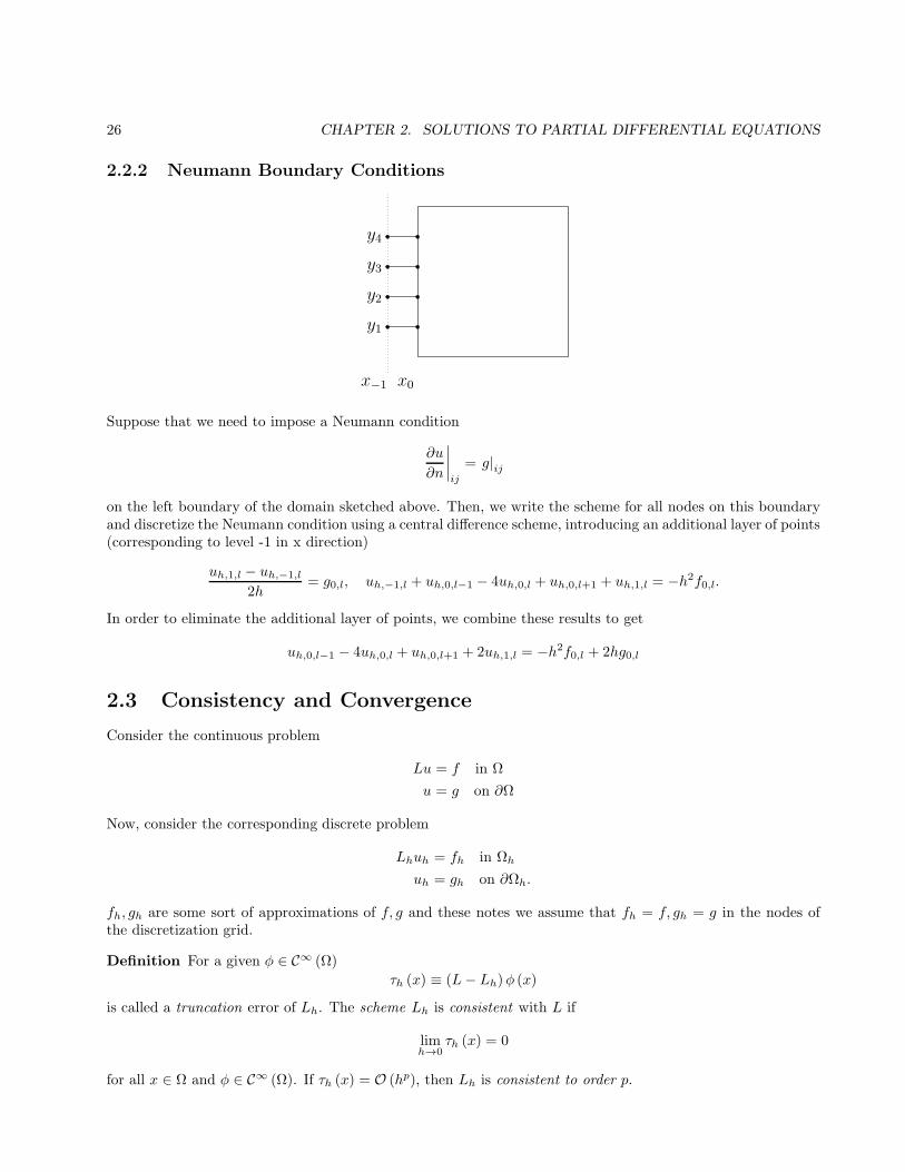
2.2.2 Neumann Boundary Conditions
y1
y2
y3
y4
x−1 x0
Suppose that we need to impose a Neumann condition
∂u
∂n
∣∣∣∣ij
= g|ij
on the left boundary of the domain sketched above. Then, we write the scheme for all nodes on this boundaryand discretize the Neumann condition using a central difference scheme, introducing an additional layer of points(corresponding to level -1 in x direction)
uh,1,l − uh,−1,l
2h= g0,l, uh,−1,l + uh,0,l−1 − 4uh,0,l + uh,0,l+1 + uh,1,l = −h2f0,l.
In order to eliminate the additional layer of points, we combine these results to get
uh,0,l−1 − 4uh,0,l + uh,0,l+1 + 2uh,1,l = −h2f0,l + 2hg0,l
2.3 Consistency and Convergence
Consider the continuous problem
Lu = f in Ω
u = g on ∂Ω
Now, consider the corresponding discrete problem
Lhuh = fh in Ωh
uh = gh on ∂Ωh.
fh, gh are some sort of approximations of f, g and these notes we assume that fh = f, gh = g in the nodes ofthe discretization grid.
Definition For a given φ ∈ C∞ (Ω)
τh (x) ≡ (L− Lh)φ (x)
is called a truncation error of Lh. The scheme Lh is consistent with L if
limh→0
τh (x) = 0
for all x ∈ Ω and φ ∈ C∞ (Ω). If τh (x) = O (hp), then Lh is consistent to order p.
2.3. CONSISTENCY AND CONVERGENCE 27
Proposition 2.3.1
−∇2h = −δ2x − δ2y
is consistent to order 2 with
−∇2 = − ∂2
∂x2− ∂2
∂y2
Definition uh converges to u in a given norm ||.|| if ||ǫh|| = ||u− uh|| satisfies
limh→0||ǫh|| = 0.
If ||ǫh|| = O (hp), then p is the order of convergence.
In the section on finite difference methods we use exclusively the infinity (or maximum) norm: ||ǫh|| = maxj|ǫh,j |.
Note that consistency does not guarantee that the difference between the solutions of the continuous anddiscrete problems also tends to zero. It only guarantees that the action of the difference between the differentialand discrete operators on a smooth enough function tends to zero.
Let us go back to the boundary value problem for the Poisson equation
−∇2u = f in Ω
u = g in ∂Ω (2.1)
with the corresponding discrete problem
−∇2huh = fh in Ωh
uh = gh in ∂Ωh. (2.2)
From the elliptic PDEs theory we know that the solution to (2.1) satisfies a maximum principle i.e. the solutionachieves its maximum on the boundary of the domain. Similarly (2.2) satisfies a Discrete Maximum Principle:
Theorem 2.3.2 (Discrete Maximum Principle) If
∇2hvj,l ≥ 0
for all (xj , yl) ∈ Ωh, then
max(xj,yl)∈Ωh
vj,l ≤ max(xj,yl)∈∂Ωh
vj,l
Proof
∇2hvj,l =
vj+1,l + vj−1,l + vj,l+1 + vj,l−1 − 4vj,lh2
≥ 0 ⇒ vj,l ≤1
4(vj+1,l + vj−1,l + vj,l+1 + vj,l−1) ∀(xj , yl) ∈ Ωh
Suppose that the maximum of v is achieved in an internal point (xJ , yL) ∈ Ωh, then:
vJ ,L ≥ vJ−1,L, vJ ,L ≥ vJ+1,L, vJ ,L ≥ vJ ,L−1, vJ ,L ≥ vJ ,L+1
so that
4vJ ,L ≥ vJ−1,L + vJ+1,L + vJ ,L−1 + vJ ,L+1 ⇒ 4vJ ,L = vJ−1,L + vJ+1,L + vJ ,L−1 + vJ ,L+1
Therefore, v must attain its maximum in all neighbouring points too. Applying this argument repeatedly tothe neighbours we eventually will reach a boundary point.
Corollary 2.3.3 The following two results follow from the discrete maximum principle:
28 CHAPTER 2. SOLUTIONS TO PARTIAL DIFFERENTIAL EQUATIONS
1.
∇2huh = 0 in Ωh
uh = 0 on ∂Ωh
has a unique solution uh = 0 in Ωh ∪ ∂Ωh.
2. For given fh and gh,
∇2huh = fh in Ωh
uh = gh on ∂Ωh
has a unique solution.
Definition Ifv : Ωh ∪ ∂Ωh → R
then
||v||Ω ≡ max(xj ,yl)∈Ωh
|vj,l|
||v||∂Ω ≡ max(xj ,yl)∈∂Ωh
|vj,l|
Lemma 2.3.4 If vj,l = 0 for all (xj , yl) ∈ ∂Ωh then
||v||Ω ≤M∆
∣∣∣∣∇2
hv∣∣∣∣Ω
for some M∆ > 0, that depends on Ω but not on h.
Proof Let∣∣∣∣∇2
hv∣∣∣∣Ω= ν ⇒ −ν ≤ ∇2
hv ≤ ν,and consider the function
w : wj,l =1
4
(x2j + y2l
)≥ 0.
Denote its norm on the boundary by M∆ i.e.
||w||∂Ω =M∆ > 0.
Note that ∇2hw = 1. Then
∇2h (v + νw) ≥ 0∇2
h (v − νw) ≤ 0
in Ω
From the maximum principle and since vh|∂Ωh= 0 we have:
vj,l ≤ vj,l + νwj,l ≤ ν ||wj,l||∂Ω =M∆
∣∣∣∣∇2
hvj,l∣∣∣∣Ω
vj,l ≥ vj,l − νwj,l ≥ −ν ||wj,l||∂Ω = −M∆
∣∣∣∣∇2
hvj,l∣∣∣∣Ω
∀(xj , yl) ∈ Ωh
Theorem 2.3.5 (error estimate) Let u be the solution of the boundary value problem (2.1) and uh is asolution to the discrete analog (2.2). Assuming that u ∈ C4
(Ω), then there exists a constant k > 0 such that:
||u− uh||Ω ≤ kMh2
where
M ≡ max
∣∣∣∣
∣∣∣∣
∂4u
∂x4
∣∣∣∣
∣∣∣∣L∞(Ω)
,
∣∣∣∣
∣∣∣∣
∂4u
∂y4
∣∣∣∣
∣∣∣∣L∞(Ω)
2.4. ADVECTION EQUATION 29
Proof From the proposition:
(∇2
h −∇2)uj,l =
h2
12
[∂4u
∂x4(ξj , yl) +
∂4u
∂y4(xj , ηl)
]
for some ξj , ηl s.t. xj−1 ≤ ξj ≤ xj+1, yl−1 ≤ ηl ≤ yl+1. Taking into account that u is the exact solution wehave:
−∇2huj,l = fj,l −
h2
12
[∂4u
∂x4(ξj , yl) +
∂4u
∂y4(xj , ηl)
]
Subtract −∇2huh,j,l = fh,j,l = fj,l and note that u− uh = 0 on ∂Ωh. Then
∇2h (uj,l − uh,j,l) =
h2
12
[∂4u
∂x4(ξj , yl) +
∂4u
∂y4(xj , ηl)
]
From the Lemma we get
||u− uh||Ω ≤M∆
∣∣∣∣∇2
h (u− uh)∣∣∣∣Ω≤ 2M∆
12︸ ︷︷ ︸
=k
Mh2 = kMh2
2.4 Advection Equation
Consider the initial value problem
∂u
∂t+ v
∂u
∂x= 0, −∞ < x <∞, t > 0
with v > 0, u (0, x) = f (x) for −∞ < x <∞. The exact solution is given by
u (t, x) = f (x− vt)
Consider a grid ∆ ≡ ∆t ×∆x:
∆t ≡ nk : n = 0, 1, 2, . . .∆x ≡ jh : j = 0,±1,±2, . . .
One possible discretization is
(δ+t + vδ−x
)unh,j =
un+1h,j − unh,j
k+ v
unh,j − unh,j−1
h= 0
or equivalently
un+1h,j = unh,j − C
(unh,j − unh,j−1
)
This is called the FB (Forwards Backwards) scheme where the Courant number is defined as
C ≡ vk
h
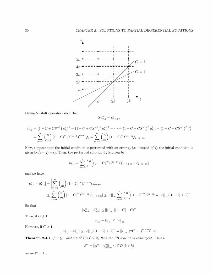
30 CHAPTER 2. SOLUTIONS TO PARTIAL DIFFERENTIAL EQUATIONS
t
x
h
2h
3h
4h
5h
...
k 2k 3k
C = 1
C > 1
Define S (shift operator) such thatSunh,j = unh,j+1
unh,j =(1− C + CS−1
)un−1h,j =
(1− C + CS−1
)2un−2h,j = · · · =
(1− C + CS−1
)nu0h,j =
(1− C + CS−1
)nf0j
=n∑
m=0
(n
m
)
(1− C)m(CS−1
)n−mfj =
n∑
m=0
(n
m
)
(1− C)m Cn−mfj−n+m
Now, suppose that the initial condition is perturbed with an error ǫj i.e. instead of fj the initial condition is
given byfj = fj + ǫj . Then, the perturbed solution uh is given by:
uh,j =
n∑
m=0
(n
m
)
(1− C)m Cn−m (fj−n+m + ǫj−n+m)
and we have
∣∣unh,j − unh,j
∣∣ =
∣∣∣∣∣
n∑
m=0
(n
m
)
(1− C)mCn−mǫj−n+m
∣∣∣∣∣
≤n∑
m=0
(n
m
)
|1− C|m Cn−m |ǫj−n+m| ≤ ||ǫ||∞n∑
m=0
(n
m
)
|1− C|m Cn−m = ||ǫ||∞ (|1− C|+ C)n
So that∣∣unh,j − unh,j
∣∣ ≤ ||ǫ||∞ (|1− C|+ C)
n
Then, if C ≤ 1:∣∣unh,j − unh,j
∣∣ ≤ ||ǫ||∞
However, if C > 1:∣∣unh,j − unh,j
∣∣ ≤ ||ǫ||∞ (|1− C|+ C)
n= ||ǫ||∞ (2C − 1)
n n→∞→ ∞
Theorem 2.4.1 If C ≤ 1 and u ∈ C2 ((0, t]× R) then the FB scheme is convergent. That is
En = ||un − unh||∞ ≤ tnO (k + h)
where tn = kn.

2.5. VON NEUMANN STABILITY ANALYSIS 31
Proof
δ+t u (t, x) =∂u
∂t(t, x) +
k
2
∂2u
∂t2(t, ξ)
δ−x u (t, x) =∂u
∂x(t, x)− h
2
∂2u
∂x2(η, x)
δ+t u+ vδ−x u = −τk,h (t, x) = O (k + h)
δ+t uh + vδ−x uh = 0
and letting ǫh = u− uh we get the following estimate:∣∣∣ǫn+1
h,j
∣∣∣ ≤
∣∣(1− C) ǫnh,j
∣∣+ C
∣∣ǫnh,j−1
∣∣+ k |τk,h (tn, xj)|
LetEn = ||ǫnh||∞ , T n = max
j|τk,h (tn, xj)|
Then we can rewrite the inequality in the form
En+1 ≤ (1− C)En + CEn + k |τk,h (tn, xj)| ≤ En + kT n ≤ En−1 + kT n + kT n−1 ≤ E0 + k
n∑
m=1
Tm
If E0 = 0 then
En+1 ≤ kn∑
m=1
Tm ≤ nk max1≤m≤n
Tm = tn maxm
Tm = tnO (k + h)
2.5 Von Neumann Stability Analysis
Definition Discrete L2 norm:
||v||22 ≡ h∞∑
j=−∞|vj |2
Definition A FD (Finite Difference) scheme for a time dependent PDE is stable if for any time T > 0, thereexists K > 0 such that for any initial data u0h, the sequence unh satisfies:
||unh||2 ≤ K∣∣∣∣u0h∣∣∣∣2
for 0 ≤ nk ≤ T . The constant K is independent of the time and space mesh size!
Consider the following grid on the real axes
∆x = . . . ,−2h,−h, 0, h, 2h, . . . .
Then the Fourier Transform of a given grid function v is defined as
(Fv) (τ) ≡ h√2π
∞∑
j=−∞e−ijhτvj
Inverse transform:
vj =1√2π
∫ πh
−πh
eijhξ (Fv) (ξ) dξ
Theorem 2.5.1 (Parseval Identity)
||Fv||2L2[−πh,πh ]
:=
∫ πh
−πh
(Fv)2 dξ = ||v||22
32 CHAPTER 2. SOLUTIONS TO PARTIAL DIFFERENTIAL EQUATIONS
Corollary 2.5.2 A finite difference scheme is stable if and only if ∃K > 0, independent of k, h, s.t.:
||Funh||L2[−πh,πh ]≤ K
∣∣∣∣Fu0h
∣∣∣∣L2[−π
h,πh ]
Consider the forward backwards scheme. Since we have:
unh,j = (1− C)un−1h,j + Cun−1
h,j−1
unh,j =h√2π
∫ πh
−πh
eijhξ (Funh) (ξ) dξ
un−1h,j−1 =
h√2π
∫ πh
−πh
ei(j−1)hξ(Fun−1
h
)(ξ) dξ,
we obtain:Funh =
(1− C + Ce−ihξ
)
︸ ︷︷ ︸
Amplification Factor
(Fun−1
h
)(ξ)
A (hξ) = 1− C + Ce−ihξ
Then, since we have
||Funh||2L2[−πh,πh ]
=
∫ πh
−πh
A (hξ)2 (Fun−1
h
)2dξ,
if |A (hξ)| ≤ 1, we obtain that:||Funh||L2[−π
h,πh ]≤∣∣∣∣Fun−1
h
∣∣∣∣L2[−π
h,πh ]
and recursive application gives:||Funh||L2[−π
h,πh ]≤∣∣∣∣Fu0h
∣∣∣∣L2[−π
h,πh ].
SinceA (θ) = 1− C + Ce−iθ
|A (θ)| = (1− C + C cos θ)2+ (−C sin θ)
2
= 1− 2C + C2 + 2C cos θ − 2C2 cos θ + C2 cos2 θ + C2 sin2 θ
= 1− 2C (1− cos θ) + 2C2 (1− cos θ) = 1 + 2C (1− cos θ) (C − 1)
≤ 1 + 4C (C − 1)
it follows that if C > 1 then |A (θ)| > 1, and if C ≤ 1 then |A (θ)| ≤ 1. Also,∣∣∣∣1− C + Ce−iθ
∣∣∣∣ ≤ |1− C|+ C
If a numerical scheme requires a solution of a linear system with a non-diagonal matrix then we call it an implicitscheme, otherwise it is called an explicit scheme.
Consider the following “Backwards Backwards” scheme
unh,j − un−1h,j
k+ v
unh,j − unh,j−1
h= 0
(1 + C) unh,j − Cunh,j−1 = un−1h,j
This is an implicit scheme.In order to study its stability (and the stability of any other FD scheme), it is enough, instead of considering
the full Fourier transform of the solution, to consider the ”action” of the scheme on a single mode of the form:
wneijhξ
2.6. SUFFICIENT CONDITIONS FOR CONVERGENCE 33
then plugging into the BB scheme:
wn[1 + C
(1− e−ihξ
)]
︸ ︷︷ ︸
A−1(hξ)
= wn−1
wn = A (hξ)wn−1
A (θ) =[1 + C
(1− e−iθ
)]−1
Then,∣∣1 + C
(1− e−ihξ
)∣∣ ≥ |1 + C| −
∣∣Ce−ihξ
∣∣ = 1
so that|A (θ)| ≤ 1 ∀θ
therefore the BB scheme is unconditionally stable.We may outline a procedure for von Neumann stability analysis:
1. Consider a single mode wneijhξ.
2. Derive conditions for A to satisfy |A (hξ)| ≤ 1
2.6 Sufficient Conditions for Convergence
Consider∂u
∂t= Lu, (t, x) ∈ (0, T )× R
where L is a linear spatial operator, with an initial condition
u (0, x) = f (x) .
We assume that the boundary conditions, in case of a finite spatial domain, are incorporated in the operator L.Then after discretization using a scheme that involves two time levels, in general we obtain a discrete systemthat can be written as:
Cun+1h − unh
k= Dun+1
h + Funh
where C,D, F are linear finite dimensional operators. The consistency error is obtained when we substitute theexact solution u in the discrete system i.e.
Cun+1 − un
k= Dun+1 + Fun + τn+1
k,h .
The last equation can be rewritten as:Bun+1 = Aun + kτn+1
k,h
whereB = C − kD, A = kF − C
If det (B) 6= 0 (otherwise the scheme would be inconsistent if the original problem is well posed) then
un+1 = B−1Aun + kB−1τn+1k,l = Eun + kB−1τn+1
k,l
where τn+1k,h is the truncation error.
Theorem 2.6.1 If the scheme is consistent to order (p, q) in time and space and is also stable then it isconvergent of order (p, q), that is
∣∣∣∣un+1 − un+1
h
∣∣∣∣2= O (kp + hq)
provided that the initial error is zero:∣∣∣∣u0 − u0h
∣∣∣∣2= 0
34 CHAPTER 2. SOLUTIONS TO PARTIAL DIFFERENTIAL EQUATIONS
Proofun+1 = Eun + kB−1τn+1
k,h , un+1h = Eunk
so that
un+1h − un+1 = E (unh − un)− kB−1τn+1
k,h = . . . = En+1(u0h − u0
)
︸ ︷︷ ︸
=0
−kn+1∑
m=1
En−m+1B−1τmk,h
Then,
∣∣∣∣un+1
h − un+1∣∣∣∣2≤ k
n+1∑
m=1
∣∣∣∣En−m+1B−1τmk,h
∣∣∣∣2≤ k
n+1∑
m=1
∣∣∣∣En−m+1
∣∣∣∣2
∣∣∣∣B−1
∣∣∣∣2
︸ ︷︷ ︸
≤M
∣∣∣∣τmk,h
∣∣∣∣2.
If the scheme is stable then for any positive integer l,∣∣∣∣ulh∣∣∣∣2≤ K
∣∣∣∣u0h∣∣∣∣2for some positive K. Since from
the scheme we have that∣∣∣∣ulh∣∣∣∣2≤∣∣∣∣El∣∣∣∣2
∣∣∣∣u0h∣∣∣∣2and this is a sharp inequality we can conclude that ∃k2 > 0
∣∣∣∣En−m+1
∣∣∣∣2≤ k2 and we have
∣∣∣∣un+1
h − un+1∣∣∣∣2≤ k
n+1∑
m=1
k2M∣∣∣∣τmk,h
∣∣∣∣2≤ RT max
m
∣∣∣∣τmk,h
∣∣∣∣2= RTO (kp + hq)
where T = k(n+ 1) is the final time and R = k2M .
Theorem 2.6.2 (Lax Theorem) Given a consistent scheme for a well-posed initial boundary value problem,then stability is a necessary and sufficient condition for convergence.
2.7 Parabolic PDEs – Heat Equation
∂u∂t = D ∂2u
∂x2 , (t, x) ∈ (0, T ]× R
u (0, x) = f (x) , x ∈ R
Which has the solution
u (t, x) =1√4πDt
∫ ∞
−∞f (ξ) e−
(x−ξ)2
4Dt dξ
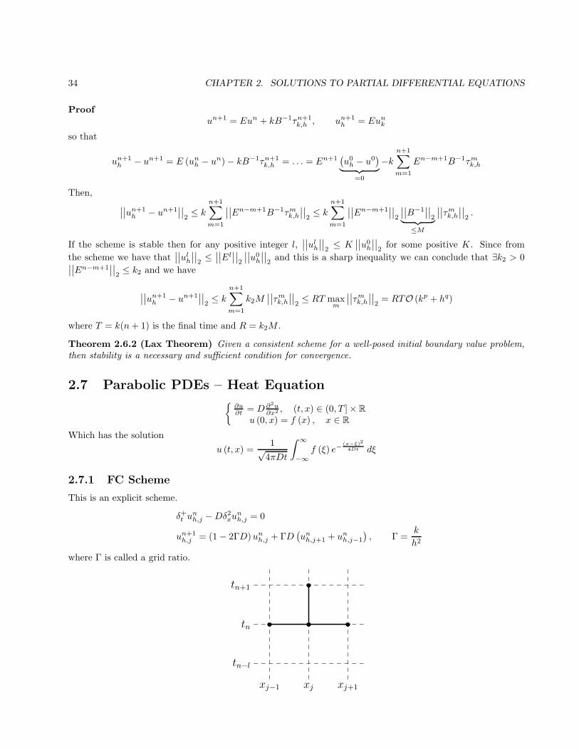
2.7.1 FC Scheme
This is an explicit scheme.
δ+t unh,j −Dδ2xunh,j = 0
un+1h,j = (1− 2ΓD)unh,j + ΓD
(unh,j+1 + unh,j−1
), Γ =
k
h2
where Γ is called a grid ratio.
tn+1
tn
tn−l
xj+1xjxj−1
2.7. PARABOLIC PDES – HEAT EQUATION 35
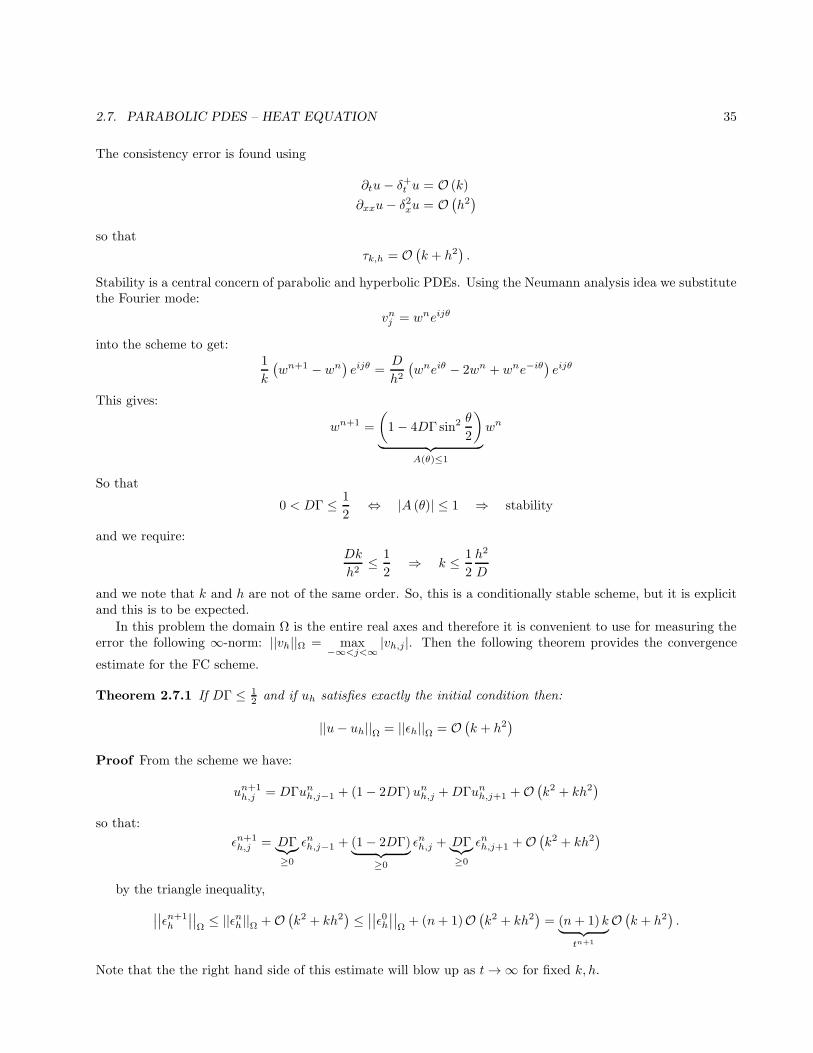
The consistency error is found using
∂tu− δ+t u = O (k)
∂xxu− δ2xu = O(h2)
so that
τk,h = O(k + h2
).
Stability is a central concern of parabolic and hyperbolic PDEs. Using the Neumann analysis idea we substitutethe Fourier mode:
vnj = wneijθ
into the scheme to get:1
k
(wn+1 − wn
)eijθ =
D
h2(wneiθ − 2wn + wne−iθ
)eijθ
This gives:
wn+1 =
(
1− 4DΓ sin2θ
2
)
︸ ︷︷ ︸
A(θ)≤1
wn
So that
0 < DΓ ≤ 1
2⇔ |A (θ)| ≤ 1 ⇒ stability
and we require:
Dk
h2≤ 1
2⇒ k ≤ 1
2
h2
D
and we note that k and h are not of the same order. So, this is a conditionally stable scheme, but it is explicitand this is to be expected.
In this problem the domain Ω is the entire real axes and therefore it is convenient to use for measuring theerror the following ∞-norm: ||vh||Ω = max
−∞<j<∞|vh,j|. Then the following theorem provides the convergence
estimate for the FC scheme.
Theorem 2.7.1 If DΓ ≤ 12 and if uh satisfies exactly the initial condition then:
||u− uh||Ω = ||ǫh||Ω = O(k + h2
)
Proof From the scheme we have:
un+1h,j = DΓunh,j−1 + (1− 2DΓ)unh,j +DΓunh,j+1 +O
(k2 + kh2
)
so that:
ǫn+1h,j = DΓ
︸︷︷︸
≥0
ǫnh,j−1 + (1− 2DΓ)︸ ︷︷ ︸
≥0
ǫnh,j + DΓ︸︷︷︸
≥0
ǫnh,j+1 +O(k2 + kh2
)
by the triangle inequality,
∣∣∣∣ǫn+1
h
∣∣∣∣Ω≤ ||ǫnh||Ω +O
(k2 + kh2
)≤∣∣∣∣ǫ0h∣∣∣∣Ω+ (n+ 1)O
(k2 + kh2
)= (n+ 1)k︸ ︷︷ ︸
tn+1
O(k + h2
).
Note that the the right hand side of this estimate will blow up as t→∞ for fixed k, h.
36 CHAPTER 2. SOLUTIONS TO PARTIAL DIFFERENTIAL EQUATIONS
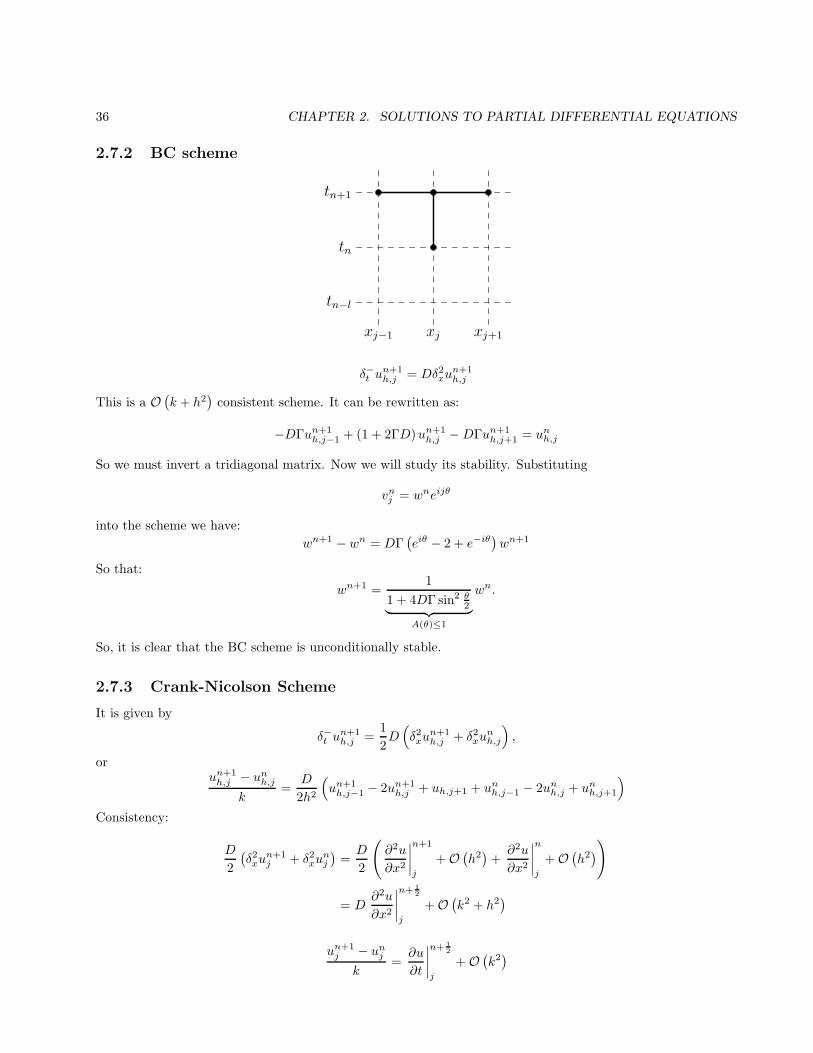
2.7.2 BC scheme
tn+1
tn
tn−l
xj+1xjxj−1
δ−t un+1h,j = Dδ2xu
n+1h,j
This is a O(k + h2
)consistent scheme. It can be rewritten as:
−DΓun+1h,j−1 + (1 + 2ΓD)un+1
h,j −DΓun+1h,j+1 = unh,j
So we must invert a tridiagonal matrix. Now we will study its stability. Substituting
vnj = wneijθ
into the scheme we have:
wn+1 − wn = DΓ(eiθ − 2 + e−iθ
)wn+1
So that:
wn+1 =1
1 + 4DΓ sin2 θ2
︸ ︷︷ ︸
A(θ)≤1
wn.
So, it is clear that the BC scheme is unconditionally stable.
2.7.3 Crank-Nicolson Scheme
It is given by
δ−t un+1h,j =
1
2D(
δ2xun+1h,j + δ2xu
nh,j
)
,
orun+1h,j − unh,j
k=
D
2h2
(
un+1h,j−1 − 2un+1
h,j + uh,j+1 + unh,j−1 − 2unh,j + unh,j+1
)
Consistency:
D
2
(δ2xu
n+1j + δ2xu
nj
)=D
2
(
∂2u
∂x2
∣∣∣∣
n+1
j
+O(h2)+∂2u
∂x2
∣∣∣∣
n
j
+O(h2)
)
= D∂2u
∂x2
∣∣∣∣
n+ 12
j
+O(k2 + h2
)
un+1j − unj
k=∂u
∂t
∣∣∣∣
n+ 12
j
+O(k2)

2.7. PARABOLIC PDES – HEAT EQUATION 37
tn+1
tn
tn−l
xj+1xjxj−1
Neumann stability analysis: First, rewrite the scheme in the following two-stage form
un+ 1
2
h,j − unh,jk2
= Dunh,j−1 − 2unh,j + unh,j+1
h2→ A1 (θ) = 1− 4D
Γ
2sin2
θ
2
un+1h,j − u
n+ 12
h,j
k2
= Dun+1h,j−1 − 2un+1
h,j + un+1h,j+1
h2→ A2 (θ) =
1
1 + 4D Γ2 sin2 θ
2
.
Then,wn+ 1
2 = A1 (θ)wn wn+1 = A2 (θ)w
n+ 12 = A1A2
︸ ︷︷ ︸
A(θ)
wn
So that A (θ) ≤ 1, so the system is unconditionally stable, and O(h2 + k2
).
2.7.4 Leapfrog Scheme
tn+1
tn
tn−l
xj+1xjxj−1
As we use central difference in both directions, the scheme is O(k2 + h2
). We may write the scheme as:
un+1h,j − un−1
h,j
2k= D
unh,j−1 − 2unh,j + unh,j+1
h2
Now we preform stability analysis: vnj = wneijθ
wn+1 − wn−1 = 2DΓ(e−iθ − 2 + eiθ
)wn
Then, assume that:wn = A (θ)wn−1 and wn+1 = A (θ)wn
so that(A2 − 1
)wn−1 = 4DΓ (cos θ − 1)Awn−1
38 CHAPTER 2. SOLUTIONS TO PARTIAL DIFFERENTIAL EQUATIONS
this gives
A1,2 = −4DΓ sin2θ
2±√
1 + 16D2Γ2 sin2θ
2
clearly |A2| ≥ 1, and |A2| > 1 for some θ, so the scheme is unconditionally unstable.
2.7.5 DuFort-Frankel Scheme
δtunh =
D
h2
[
unh,j+1 −(
un+1h,j + un−1
h,j
)
+ unh,j−1
]
Since1
2
(
un+1h,j + un−1
h,j
)
= unh,j +O(k2)
this scheme can be considered as a stabilized version of the Leapfrog scheme. The truncation error is then:
τk,h (t, x) = 2
(k
h
)2∂2u
∂t2(tn, xj) +
k3
3
∂2u
∂t2(tn, xj)−
h2
12
∂2u
∂x2(tn, xj) +O
(k3 + h3
)
and the system is conditionally consistant if kh → 0. If k, h go to zero but k
h → c2, then DF is consistent with:
∂u
∂t+ c2
∂2u
∂t2= D
∂2u
∂x2.
The stability analysis reveals that this scheme is unconditionally stable.
2.8 Advection-Diffusion Equation
∂u
∂t+ v
∂u
∂x= D
∂2u
∂x2(t, x) ∈ (0, T ]× (0, L)
and v,D > 0. Then define τ = vtL , ξ = x
L , and Peclet number Pe = vLD . So the PDE becomes:
∂u
∂τ+∂u
∂ξ=
1
Pe
∂2u
∂ξ2, (τ, ξ) ∈
(
0,vT
L
]
× (0, 1)
2.8.1 FC Scheme
un+1h,j − unh,j
k+unh,j+1 − unh,j−1
2h− 1
Pe
unh,j−1 − 2unh,j + unh,j+1
h2= 0
This scheme is consistant to O(k + h2
). Now preform stability analysis: vnj = wneijθ
wn+1 − wn + keiθ − e−iθ
2hwn − 1
Peke−iθ − 2 + eiθ
h2= 0
wn+1 = wn
(
−Ci sin θ + 2Γ
Pe(cos θ − 1) + 1
)
︸ ︷︷ ︸
A(θ)
So we may write,
|A (θ)|2 =
(
1− 4Γ
Pesin2
θ
2
)2
+ C2 sin2 θ
If Γ/Pe ≤ 1/2 the first term ≤ 1 and since C2 = kΓ then C2 sin2 θ ≤ Pek/2 =Mk,M > 0, i.e.
|A|2 ≤ 1 +Mk
2.8. ADVECTION-DIFFUSION EQUATION 39
Theorem 2.8.1 The FC scheme is stable if Γ ≤ Pe/2 i.e. if |A (θ)|2 ≤ 1 +Mk for some M > 0.
Proof
(Funh)2(ξ) = A2 (hξ)
(Fun−1
n
)2(ξ) = A2n (hξ)
(Fu0h
)2(ξ) ≤ (1 +Mk)
n (Fu0h
)2(ξ)
Therefore,
||Funh||22 ≤ (1 +Mk)n∣∣∣∣Fu0h
∣∣∣∣2 ≤ (1 +Mk)
nkMkM
∣∣∣∣Fu0h
∣∣∣∣2
2=(
(1 +Mk)1
kM
)Mtn ∣∣∣∣Fu0h
∣∣∣∣2
2≤ eMtn
∣∣∣∣Fu0h
∣∣∣∣2
2,
where tn = nk.
Theorem 2.8.2 Assume:Γ
Pe≤ 1
2
Then the solution of the FC scheme satisfies the maximum principle:
maxj
∣∣∣un+1
h,j
∣∣∣ ≤ max
j
∣∣unh,j
∣∣
for all n ≥ 1, if and only if h ≤ 2Pe .
Proof Let h ≤ 2Pe , then:
∣∣∣un+1
h,j
∣∣∣ ≤ Γ
Pe
(
1 +1
2hPe
)∣∣unh,j−1
∣∣+(1− 2ΓPe−1
) ∣∣unh,j
∣∣+
Γ
Pe
(
1− 1
2hPe
)∣∣unh,j+1
∣∣ ≤ max
j
∣∣unh,j
∣∣
because h ≤ 2Pe ,
ΓPe ≤ 1
2 .
Now, assume that
maxj
∣∣∣un+1
h,j
∣∣∣ ≤ max
j
∣∣unh,j
∣∣ .
Aiming towards a contradiction, assume that h > 2Pe . Then, choose the initial data as follows
u0h,j =
1, j = 0, 10, j > 1
so that
u1h,1 =Γ
Pe
(
1 +1
2hPe
)
+ 1− 2Γ
Pe>
Γ
Pe
(
1 +1
2
2
PePe− 2
)
+ 1 = 1
and this gives:
maxj
∣∣u1h,j
∣∣ > 1 = max
j
∣∣u0h,j
∣∣
so, by contradiction, the theorem holds.
Since violation of the maximum principle leads to unphysical solution then we must choose h ≤ 2/Pe and so,if the Peclet number Pe is very large then we need to use very small h, of the order of Pe−1. This correspondsto problems with boundary layers that need to be resolved by h. However, it is known from the properties ofthe corresponding boundary value problem that the thickness of such boundary layers is of the order of Pe−1/2
i.e. it can be resolved by h being of order of Pe−1/2. So, this scheme requires the use of a spatial step h muchless than what is needed to resolve the actual solution. The next scheme cures this problem at the expense ofloss of accuracy.
40 CHAPTER 2. SOLUTIONS TO PARTIAL DIFFERENTIAL EQUATIONS
2.8.2 Upwinding Scheme (FB)
un+1h,j − unh,j
k+unh,j − unh,j−1
h=
1
Pe
unh,j−1 − 2unh,j + unh,j+1
h2
Theorem 2.8.3 Assume that ΓPe ≤ 1
2 . Then the FB scheme satisfies a maximum principle provided that:
2Γ
Pe+ C ≤ 1,
(
C =k
h
)
The proof is left as an exercise. This theorem implies that the maximum principle is satisfied if k ≤ (Peh2)/(2+Peh). Note that in the limit Pe→∞, this restriction on k tends to h. On the other hand, the stability conditionk ≤ Peh2/2 implies that if Pe→∞ but Peh2 → const (i.e. h = O(Pe−1/2)), k is restricted by a constant. Inconclusion, if the Peclet number Pe is very large, the scheme guarantees that the solution satisfies a maximumprinciple, similar to the exact solution, and is stable if k ≤ h, but k can be of the order of h. And this is trueeven if h = O(Pe−1/2) that is sufficient to resolve boundary layers.
The scheme has a consistency errorτk,h (t, x) = O (k + h)
as
δ+t unj =
∂u
∂t(tn, xj) +O (k)
and
δ−x unj =
∂u
∂x(tn, xj)−
h
2
∂2u
∂x2(tn, xj) +O
(h2)
and
δ2xunj =
∂2u
∂x2(tn, xj) +O
(h2).
Combining these results we have:
δ+t unj + δ−x u
nj −
1
Peδ2xu
nj =
∂u
∂t+∂u
∂x−(
1
Pe+h
2
)∂2u
∂x2+O
(k + h2
)
i.e. up to terms that are O(k + h2), the scheme is consistent with the equation
∂u
∂t+∂u
∂x−(
1
Pe+h
2
)∂2u
∂x2= 0.
This means that the scheme adds an extra diffusion term that is of order of h. If the leading order term inthe spatial error is proportional to a derivative of an even order, we call the scheme dissipative since suchschemes usually dissipate sharp changes (large gradients) of the solution. If the leading order term of the erroris proportional to a derivative of an odd order, the scheme is called dispersive. This is because odd derivativesin PDEs lead to the so called dispersion in the solution. In terms of a Fourier decomposition of the solution,this effect is manifested in the fact that due to the presence of odd derivatives different Fourier modes travelwith a different speed.
Chapter 3
Introduction to Finite Elements
3.1 Weighted Residual Methods
3.1.1 Sobolev spaces
Sobolev space:
Hm (Ω) ≡
v : Ω→ R :
∫
Ω
(
v2 +(
v(1))2
+ . . .+(
v(m))2)
<∞
then
H0 (Ω) = L2 (Ω)
and Hm (Ω) is a Hilbert space:
(u, v)m =
∫
Ω
(
uv + u(1)v(1) + . . .+ u(m)v(m))
dx
and
||u||m =
√∫
Ω
(
u2 + . . .+(u(m)
)2)
dx
Proposition 3.1.1 1. Hm+1 (Ω) ⊂ H
m (Ω)
2. If v ∈ Hm (Ω) then:
||v||2m = ||v||20 +∣∣∣
∣∣∣v(1)
∣∣∣
∣∣∣
2
0+ . . .+
∣∣∣
∣∣∣v(m)
∣∣∣
∣∣∣
2
0
3. ||v||m+1 ≥ ||v||m and ||v||m+1 ≥∣∣∣∣v(1)
∣∣∣∣m.
4. If v, w ∈ Hm (Ω) then |(v, w)m| ≤ ||v||m ||v||m, this is the Cauchy-Schwartz inequality.
5. If v, w ∈ Hm (Ω) then
||v + w||m ≤ ||v||m + ||w||m
Proof We will prove the Cauchy-Schwartz inequality
|(u, v)m| ≤ ||u||m ||v||m
for u, v ∈ Hm (Ω). For any s ∈ R we have
0 ≤ (u− sv, u− sv)m = ||u||2m + s2 ||v||2m − 2s (u, v)m .
41
42 CHAPTER 3. INTRODUCTION TO FINITE ELEMENTS
Choose
s =(u, v)m||v||2m
so that:
0 ≤ (u− sv, u− sv)m = ||u||2m +(u, v)
2m
||v||2m− 2
(u, v)2m
||v||2m= ||u||2m −
(u, v)2m
||v||2mand, upon rearranging, we have:
(u, v)m ≤ ||u||m ||v||m
3.1.2 Weighted Residual Formulations
ConsiderLu = f, in Ω
withu = 0, on ∂Ω
where
L = − d2
dx2
so that:
−d2u
dx2= f in Ω = (0, 1)
withu = 0, on x = 0, 1
Define the “trial function” space, for example it can be chosen to be
U =u : u ∈ H
2 (Ω) , u = 0 on ∂Ω
and we introduce the “weight functions” (also called test) space, for this choice of U it can be chosen to be
W =w : w ∈ L2 (Ω) , w = 0 on ∂Ω
Now, find u ∈ U such that∫
Ω
(d2u
dx2+ f
)
w dΩ = 0, f ∈ L2 (Ω)
for all w ∈W . This is one “weighted residual formulation” of the original problem. This particular formulationis also usually called a strong formulation. It still defines a continuous problem and in order to discretize itwe need to discretize the corresponding functional spaces i.e. to define appropriate approximations for eachfunction in them. We select a subset Uh of U :
Uh ⊂ U, Uh = span φ0, . . . , φn−1and Wh, a subset of W :
Wh ⊂W, Wh = span ψ0, . . . , ψn−1and then, search for the discrete approximation uh in the form:
uh =
n−1∑
i=0
ciφi
so that:∫
Ω
(
d2
dx2
n−1∑
i=0
ciφi − f)
ψj dΩ = 0 ⇒n−1∑
i=0
ci
∫
Ω
d2φidx2
ψj =
∫
Ω
fψj dΩ, j = 0, 1, . . . , n− 1
This is a linear algebraic system Lc = F where:
Lij =
∫
Ω
d2φidx2
ψj dΩ, Fi =
∫
Ω
fψi dΩ

3.2. WEAK METHODS 43
3.1.3 Collocation Methods
Let
ψj (x) = δ (x− xj)
so that: Lij =d2φi
dx2 (xj) and Fj = f (xj) . Note that ψj are not in L2 however the formulation still makes sense
if φi ∈ C0 because the integrals are well defined. Next, we may approximate d2
dx2 ∼ δ2x, and this gives us afinite difference method or we may select Uh as the space spanned by certain sets of orthogonal polynomials(Legendre, Tchebishev etc.), and this gives us spectral collocation.
3.2 Weak Methods
By far, the most popular weighted residual methods are based on the so called weak formulation of the classicalproblem. To obtain it we start from
∫
Ω
(d2u
dx2+ f
)
w dΩ = 0 ∀ w ∈W
and choose the discrete test functions space to be
W =w : w ∈ H
10 (Ω)
. Here we define
H10 (Ω) =
u ∈ H
1 (Ω) , u = 0 on ∂Ω
. Then,
−∫
Ω
du
dx
dw
dx+
∫
∂Ω
du
dxw ds
︸ ︷︷ ︸
=0
= −∫
Ω
fw dΩ
Then the problem is reformulated as: Find u ∈ U such that:
∫
Ω
du
dx
dw
dx=
∫
Ω
fw dΩ
A natural choice for U which makes all integrals well defined and incorporates the Dirichlet boundary conditionsin the solution is U =W . Such formulation is called a Galerkin formulation. The space U can be discretized bymeans of piecewise polynomial functions, orthogonal polynomials, trigonometric polynomials, spline functionsetc. These choices yield various weak methods. In the remainder of the notes we will focus on the piecewisepolynomial approximations which yield the so called finite element methods.
Before we proceed with the discretization we shall prove some important results for the continuous Galerkinformulation: Find u ∈ U = H1
0(Ω) such that
∫
Ω
u′v′ dΩ =
∫
Ω
fv dΩ, ∀ v ∈ U.
Theorem 3.2.1 If u is a solution of the classical formulation
−u′′ = f in Ω
u = 0 on ∂Ω
then u is a solution of the Galerkin formulation. If u is a solution to the Galerkin Formulation then it is asolution to the classical formulation if u ∈ C2 ([0, 1]) and f ∈ C0 ([0, 1]).
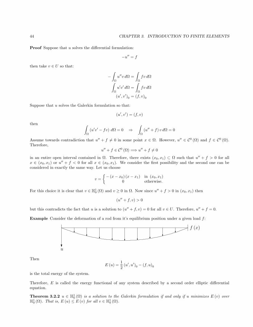
44 CHAPTER 3. INTRODUCTION TO FINITE ELEMENTS
Proof Suppose that u solves the differential formulation:
−u′′ = f
then take v ∈ U so that:
−∫
Ω
u′′v dΩ =
∫
Ω
fv dΩ
∫
Ω
u′v′ dΩ =
∫
Ω
fv dΩ
(u′, v′)0 = (f, v)0
Suppose that u solves the Galerkin formulation so that:
(u′, v′) = (f, v)
then ∫
Ω
(u′v′ − fv) dΩ = 0 ⇒∫
Ω
(u′′ + f) v dΩ = 0
Assume towards contradiction that u′′ + f 6= 0 in some point x ∈ Ω. However, u′′ ∈ C0 (Ω) and f ∈ C0 (Ω).Therefore,
u′′ + f ∈ C0 (Ω) =⇒ u′′ + f 6= 0
in an entire open interval contained in Ω. Therefore, there exists (x0, x1) ⊂ Ω such that u′′ + f > 0 for allx ∈ (x0, x1) or u′′ + f < 0 for all x ∈ (x0, x1). We consider the first possibility and the second one can beconsidered in exactly the same way. Let us choose
v =
− (x− x0) (x− x1) in (x0, x1)
0 otherwise.
For this choice it is clear that v ∈ H10 (Ω) and v ≥ 0 in Ω. Now since u′′ + f > 0 in (x0, x1) then
(u′′ + f, v) > 0
but this contradicts the fact that u is a solution to (u′′ + f, v) = 0 for all v ∈ U . Therefore, u′′ + f = 0.
Example Consider the deformation of a rod from it’s equilibrium position under a given load f :
u
f (x)
Then
E (u) =1
2(u′, u′)0 − (f, u)0
is the total energy of the system.
Therefore, E is called the energy functional of any system described by a second order elliptic differentialequation.
Theorem 3.2.2 u ∈ H10 (Ω) is a solution to the Galerkin formulation if and only if u minimizes E (v) over
H10 (Ω). That is, E (u) ≤ E (v) for all v ∈ H
10 (Ω).
3.2. WEAK METHODS 45
Proof 1. Suppose that u is a solution to the Galerkin formulation so that: (u′, v′)0 = (f, v) for all v ∈ H10 (Ω)
so that:
E (v) = E (u+ w) =1
2
((u+ w)
′, (u+ w)
′)0−(f, u+ w)0 =
1
2(u′, u′)0−(f, u)0+
1
2(w′, w′)0−(f, w)0+(u′, w′)0
Since(u′, w′)0 = (f, w)0
we have
E (v) = E (u) +1
2||w′||20 ≥ E (u)
2. Suppose that E (u) ≤ E (v) for all v ∈ H10 (Ω). Then if we take s ∈ R, E (u+ sw) has a min at s = 0, and
therefore:d
dsE (u+ sw)
∣∣∣∣s=0
= 0
which we expand as:
d
ds
(1
2
((u+ sw)′ , (u+ sw)′
)
0− (f, u+ sw)0
)∣∣∣∣s=0
= 0
d
ds
(
E (u) + s (u′, w′)0 − s (f, w)0 +1
2s2 (w′, w′)
)∣∣∣∣s=0
= (u′, w′)0 − (f, w)0 + s (w′, w′)︸ ︷︷ ︸
=0
∣∣∣∣∣∣s=0
= 0
So that:(u′, w′)0 = (f, w)0
for all w ∈ H10 (Ω). Therefore, u solves the Galerkin Formulation.
Consider a Hilbert space V equipped with the product (·, ·)V i..e. V is complete with respect to the norm||·||V induced by this product. Now, consider the mapping a : V × V → R (further called a bilinear form) suchthat:
1. a (αu+ βv, w) = αa (u,w) + βa (v, w),
2. a (w,αu + βv) = αa (w, u) + βa (w, v),
3. there exists β > 0 such that |a (u, v)| ≤ β ||u||V ||v||V (such bilinear form is called bounded w.r.t. ||.||V ),and
4. there exists ρ > 0 such thata (u, u) ≥ ρ ||u||2V
(such bilinear form is called coercive w.r.t. ||.||V )
Now, suppose that G (v) is a functional such that:
1. G (αu+ βv) = αG (u) + βG (v) (such a functional is called linear) and
2. there exists δ > 0 such that |G (u)| ≤ δ ||u||V (such functional is called bounded).
The following theorem is one version of a very well known result from functional analysis.
Theorem 3.2.3 (Riesz Theorem) If V is a Hilbert space with a given inner product (., .)∗ and if G (v) is abounded linear functional on V (w.r.t. the norm induced by its inner product), then there is a unique elementu ∈ V such that (u, v)∗ = G (v) for all v ∈ V .
This theorem almost directly yields the proof of a somewhat restricted version of the following fundamentalresult in PDE theory and their numerical analysis.
46 CHAPTER 3. INTRODUCTION TO FINITE ELEMENTS
Lemma 3.2.4 (Lax-Milgram) If a (u, v) and G (v) satisfy the six conditions stated above then there exists aunique solution u ∈ V for the following problem: Find u ∈ V s.t.
a (u, v) = G (v) ∀v ∈ V
If a (u, v) = a (v, u) (symmetric form) then u is the minimizer of
E (v) =1
2a (v, v)−G (v)
Proof We shall consider only the case where a (u, v) = a (v, u).
• The proof of the first claim is a direct consequence of the Riesz theorem if we prove that a (u, v) definesan inner product on V . We know that:
a (u, u) ≥ ρ ||u||2Vwhich guarantees that √
a (u, u) = ||u||ais a norm on V . It is not difficult then to verify that a(u, v) defines an inner product on V . Also, it isstraightforward to show that the norm ||.||a is equivalent to ||.||V i.e.:
√ρ ||u||V ≤ ||u||a ≤
√
β ||u||V .
Therefore, since V is complete with respect to ||·||V then it is complete with respect to the norm ||.||a i.e.V is a Hilbert space with respect to the product a(., .). As G (v) is bounded with respect to ||·||V , G (v)is bounded with respect to ||·||a. Since a(., .) is an inner product on V and G (v) is bounded w.r.t. thenorm induced by this inner product, the Riesz theorem implies the first claim of the lemma.
• Next we show that u minimizes E (v) = 12a (v, v)−G (v).
E (v) = E (u+ w) = E (u) + 1/2 a (w,w)︸ ︷︷ ︸
≥0
≥ E (u)
Example−∇2u = f in Ωu = 0 on ∂Ω
.
Its Galerkin formulation reads: Find u ∈ H10(Ω) s.t.:
(∇u,∇v)0 = (f, v)0 ∀v ∈ H10 (Ω) . (3.1)
Below we prove the so-called Poincare inequality which will guarantee that a(u, v) = (∇u,∇v)0 defines a bilinearform satisfying the conditions of the Lax-Milgram lemma.
Lemma 3.2.5 (Poincare Inequality) If Ω is a bounded domain and v ∈ H10 (Ω) then ∃C > 0, depending only
on the domain Ω, such that||v||20 ≤ C ||∇v||
20 .
Proof Consider first v ∈ C10(Ω) i.e. v is a continuously differentiable function defined on Ω that vanishes on
its boundary. We can always find a ∈ R large enough so that the cube Q = x ∈ Rn : |xj | < a, 1 ≤ j ≤ ncontains Ω. Integrating by parts in the x1 direction and taking into account that the surface integral vanishessince v = 0 on ∂Ω we obtain:
||v||20 =∫
Ω
v2dx =∫
Ω
1 · v2dx = −∫
Ω
x1∂v2
∂x1dx
= −2∫
Ω
x1v∂v∂x1
dx ≤ 2a∫
Ω
|v|∣∣∣∂v∂x1
∣∣∣ dx.
3.3. FINITE ELEMENT METHOD (FEM) 47
Using the Cauchy-Schwarz inequality for the L2 inner product on Ω, we obtain:
||v||20 ≤ 2a∫
Ω
|v|∣∣∣∂v∂x1
∣∣∣ dx ≤ 2a‖v‖0‖ ∂v
∂x1‖0 ≤ 2a‖v‖0‖∇v‖0.
Dividing by ‖v‖0 gives the desired result with C = (2a)2 and v ∈ C10(Ω). Due to some classical results in
functional analysis (see for example Ern, A. and Guermond, J.-L., Theory and Practice of Finite Elements,Applied Mathematical Sciences, v. 159, Springer, 2004, p. 485), we can claim that for each v ∈ H1
0(Ω) we canchoose a sequence of functions in vk∞k=1 ⊂ C
10(Ω) such that the sequence converges to v in the H
1Ω) normi.e. ‖v − vk‖0 ≤ ‖v − vk‖1 → 0 as k → ∞ and similarly ‖∇v −∇vk‖0 ≤ ‖v − vk‖1 → 0. Using the triangularinequality in the form ‖u−w‖0 ≥ ‖u‖0−‖w‖0 yields that ‖vk‖0 → ‖v‖0 and ‖∇vk‖0 → ‖∇v‖0. This allows usto take the limit in the Poincare inequality for vk ∈ C
10(Ω) to derive the inequality for any function in H
10(Ω).
Using this inequality we easily prove the following proposition.
Proposition 3.2.6 a (u, v) = (∇u,∇v)0 is a bilinear, bounded, and coercive form in H10 (Ω); G (v) = (f, v)0 is
bounded in H10 (Ω) if ||f ||0 <∞.
Proof
|a (u, v)| =
∣∣∣∣∣∣
∫
Ω
∇u∇vdx
∣∣∣∣∣∣
≤ ||∇u||0 ||∇v||0 ≤ ||u||1 ||v||1
as ||u||1 = ||∇u||0 + ||u||0 ≥ ||∇u||0. Then,
a (u, u) = (∇u,∇u) = ||∇u||20 =1
2
(
||∇u||20 + ||∇u||20
)
≥ 1
2
(
||u||20 + ||∇u||20
)
=1
2||u||21
The last proposition guarantee us that the bilinear form a (u, v) =∫
Ω
∇u∇vdx and the functional G (v) =
(f, v)0 satisfy the conditions of the Lax-Milgram lemma if ||f ||0 < ∞. This automatically guarantees that thecorresponding weak formulation (3.1) has a unique solution in H1
0 (Ω).
3.3 Finite Element Method (FEM)
Let us define a grid:
∆ = x0, . . . , xMand the following linear space of continuous piecewise linear functions on ∆:
M10 (∆) = span l0, l1, . . . , lM ∈ H
1 (Ω)
where
li =
x−xi−1
xi−xi−1, xi−1 ≤ x ≤ xi
x−xi+1
xi−xi+1, xi ≤ x ≤ xi+1
0 otherwise.
.
Define the discrete space:
Vh =v ∈M1
0 (∆) , v (0) = v (1) = 0⊂ H
10 (Ω)
which is equivalent toVh = span l1, . . . , lM−1
Let us now consider the following discrete problem: Find uh ∈ Vh such that:
(u′h, v′h)0 = (f, vh)0
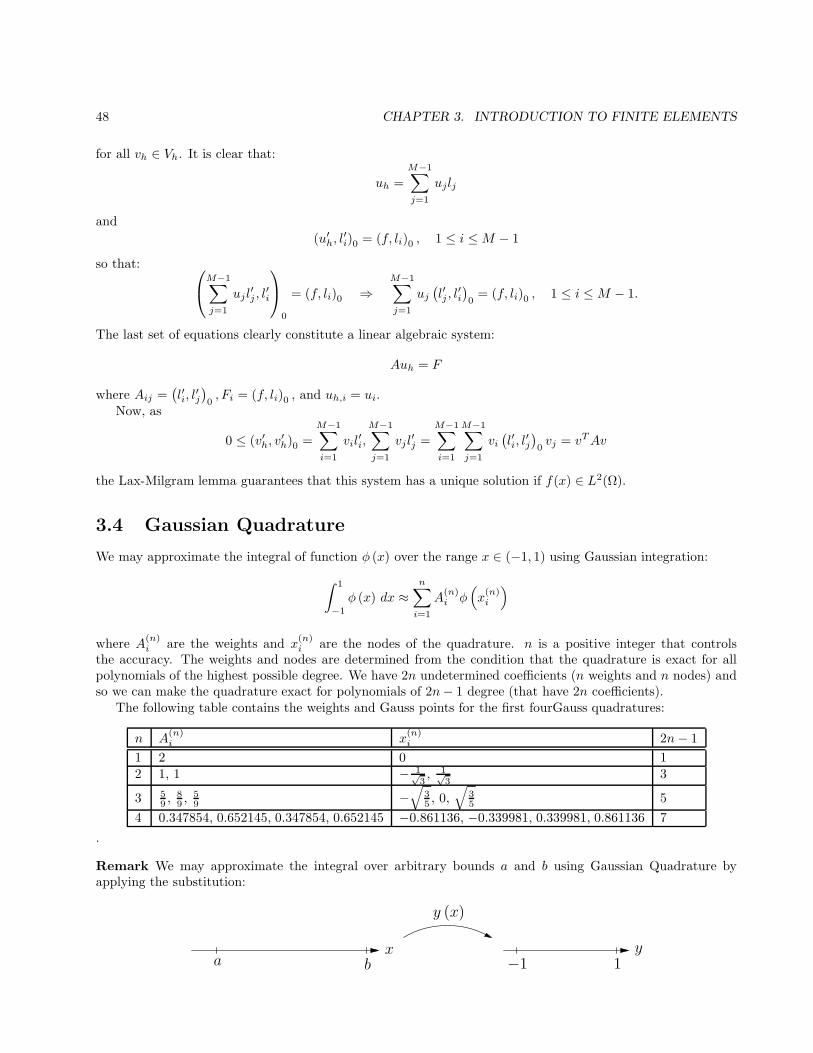
48 CHAPTER 3. INTRODUCTION TO FINITE ELEMENTS
for all vh ∈ Vh. It is clear that:
uh =
M−1∑
j=1
ujlj
and
(u′h, l′i)0 = (f, li)0 , 1 ≤ i ≤M − 1
so that:
M−1∑
j=1
uj l′j , l
′i
0
= (f, li)0 ⇒M−1∑
j=1
uj(l′j , l
′i
)
0= (f, li)0 , 1 ≤ i ≤M − 1.
The last set of equations clearly constitute a linear algebraic system:
Auh = F
where Aij =(l′i, l
′j
)
0, Fi = (f, li)0 , and uh,i = ui.
Now, as
0 ≤ (v′h, v′h)0 =
M−1∑
i=1
vil′i,
M−1∑
j=1
vj l′j =
M−1∑
i=1
M−1∑
j=1
vi(l′i, l
′j
)
0vj = vTAv
the Lax-Milgram lemma guarantees that this system has a unique solution if f(x) ∈ L2(Ω).
3.4 Gaussian Quadrature
We may approximate the integral of function φ (x) over the range x ∈ (−1, 1) using Gaussian integration:
∫ 1
−1
φ (x) dx ≈n∑
i=1
A(n)i φ
(
x(n)i
)
where A(n)i are the weights and x
(n)i are the nodes of the quadrature. n is a positive integer that controls
the accuracy. The weights and nodes are determined from the condition that the quadrature is exact for allpolynomials of the highest possible degree. We have 2n undetermined coefficients (n weights and n nodes) andso we can make the quadrature exact for polynomials of 2n− 1 degree (that have 2n coefficients).
The following table contains the weights and Gauss points for the first fourGauss quadratures:
n A(n)i x
(n)i 2n− 1
1 2 0 12 1, 1 − 1√
3, 1√
33
3 59 ,
89 ,
59 −
√35 , 0,
√35 5
4 0.347854, 0.652145, 0.347854, 0.652145 −0.861136, −0.339981, 0.339981, 0.861136 7
.
Remark We may approximate the integral over arbitrary bounds a and b using Gaussian Quadrature byapplying the substitution:
xa b
y−1 1
y (x)
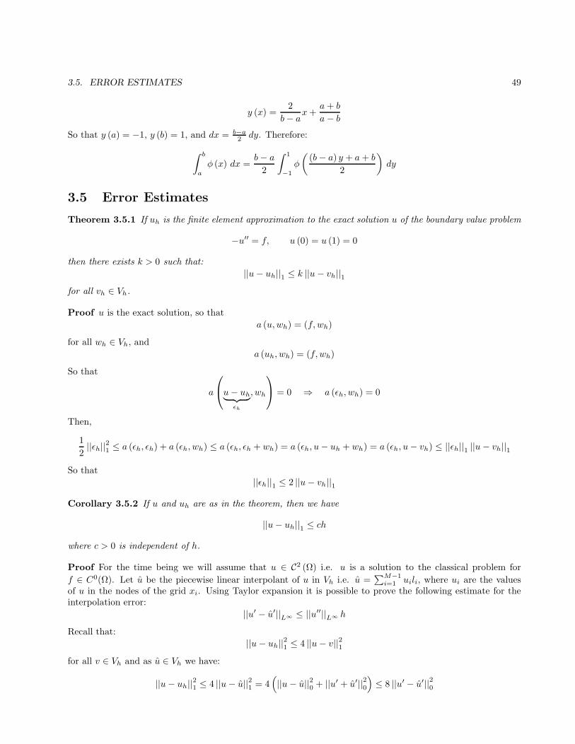
3.5. ERROR ESTIMATES 49
y (x) =2
b− ax+a+ b
a− bSo that y (a) = −1, y (b) = 1, and dx = b−a
2 dy. Therefore:
∫ b
a
φ (x) dx =b− a2
∫ 1
−1
φ
((b− a) y + a+ b
2
)
dy
3.5 Error Estimates
Theorem 3.5.1 If uh is the finite element approximation to the exact solution u of the boundary value problem
−u′′ = f, u (0) = u (1) = 0
then there exists k > 0 such that:
||u− uh||1 ≤ k ||u− vh||1for all vh ∈ Vh.
Proof u is the exact solution, so that
a (u,wh) = (f, wh)
for all wh ∈ Vh, anda (uh, wh) = (f, wh)
So that
a
u− uh︸ ︷︷ ︸
ǫh
, wh
= 0 ⇒ a (ǫh, wh) = 0
Then,
1
2||ǫh||21 ≤ a (ǫh, ǫh) + a (ǫh, wh) ≤ a (ǫh, ǫh + wh) = a (ǫh, u− uh + wh) = a (ǫh, u− vh) ≤ ||ǫh||1 ||u− vh||1
So that
||ǫh||1 ≤ 2 ||u− vh||1
Corollary 3.5.2 If u and uh are as in the theorem, then we have
||u− uh||1 ≤ ch
where c > 0 is independent of h.
Proof For the time being we will assume that u ∈ C2 (Ω) i.e. u is a solution to the classical problem for
f ∈ C0(Ω). Let u be the piecewise linear interpolant of u in Vh i.e. u =∑M−1
i=1 uili, where ui are the valuesof u in the nodes of the grid xi. Using Taylor expansion it is possible to prove the following estimate for theinterpolation error:
||u′ − u′||L∞ ≤ ||u′′||L∞ h
Recall that:
||u− uh||21 ≤ 4 ||u− v||21for all v ∈ Vh and as u ∈ Vh we have:
||u− uh||21 ≤ 4 ||u− u||21 = 4(
||u− u||20 + ||u′ + u′||20)
≤ 8 ||u′ − u′||20
50 CHAPTER 3. INTRODUCTION TO FINITE ELEMENTS
where, in the last step, we applied the Poincare inequality. Continuing, we have:
||u− uh||21 ≤ 8
∫ 1
0
(u′ − u′)2 dx ≤ 8 ||u′ − u′||2L∞ ≤ 8 ||u′′||2L∞ h2
where we have used the interpolation estimate ||u′ − u′||2L∞ ≤ ||u′′||2L∞ h2. This yields
||u− uh||1 ≤√8 ||u′′||L∞ h = O (h)
And, applying Poincare’s inequality, we have:
||u− uh||21 = ||u− uh||20 + ||u′ − u′h||20 ≥ 2 ||u− uh||20
so that:||u− uh||0 ≤ ch ||u′′||L∞ .
This is a suboptimal estimate because from interpolation theory we know that u can be approximated with apiecewise linear function with a second order accuracy in the L2 norm.
3.6 Optimal Error Estimates
Lemma 3.6.1 If u is the finite element interpolant of u ∈ H2 (Ω), i.e. u =
∑M−1j=1 u(xj)lj, then:
1. ||u− u||0 ≤(hπ
)2 ||u′′||02. ||u′ − u′||0 ≤ h
π ||u′′||0Proof The domain is subdivided into elements at points:
x0 = 0, x1, x2, . . . xi−1, xi, . . . xM−1, xM = 1
Consider the differenceu− u in [0, h] = [x0, x1]
and define η (x) = u− u ∈ H1 ([0, h]). Clearly,
η (0) = η (h) = 0.
Since η ∈ C0[0, h] it can be expanded in a uniformly convergent Fourier sine series:
η (x) =
∞∑
n=1
ηn sin(nπx
h
)
Then, using the Parceval identity,∫ h
0
η2 dx = ||η||2L2[0,h] =h
2
∞∑
n=1
η2n.
Differentiating term wise we get:
η′ (x) =∞∑
n=1
ηnnπ
hcos(nπx
h
)
⇒ ||η′||2L2[0,h] =h
2
∞∑
n=1
(
ηnnπ
h
)2
and differentiating again we have:
η′′ (x) = −∞∑
n=1
ηnn2π2
h2sin(nπx
h
)
⇒ ||η′′||2L2[0,h] =h
2
∞∑
n=1
η2n
(nπ
h
)4

3.6. OPTIMAL ERROR ESTIMATES 51
So that
||η′||2L2[0,h] =h
2
∞∑
n=1
η2n
(nπ
h
)2 (nπ
h
)2 h2
n2π2≤ h2
π2
h
2
∞∑
n=1
η2n
(nπ
h
)4
=h2
π2||η′′||2L2[0,h] =
h2
π2||u′′||2L2[0,h]
and
||η||2L2[0,h] =h
2
∞∑
n=1
η2n ≤h2
π2
h
2
∞∑
n=1
η2n
(nπ
h
)2
=h2
π2||η′||2L2[0,h] =
(h
π
)4
||u′′||2L2[0,h]
Applying the same for any subsequent subinterval and summing the resulting inequalities we complete theproof.
Corollary 3.6.2 1. ||u− u||1 ≤ h√2
π ||u′′||0
2. ||u− uh||1 ≤√8hπ ||u′′||0
Proof 1.
||u− u||21 = ||u− u||20 + ||u′ − u′||20 ≤ 2 ||u′ − u′||20 ≤ 2
(h
π
)2
||u′′||20
2. for all vh ∈ Vh in the finite element space we have:
||u− uh||1 ≤ 2 ||u− vh||1
Take vh = u, then:
||u− uh||1 ≤ 2 ||u− u||1 ≤h√8
π||u′′||0
So that||u− uh||1 ≤ Ch ||u′′||0
where C is independent of h.
Theorem 3.6.3 (L2 lifting theorem) If uh ∈ Vh is the Galerkin finite element approxitamion of:
u :
−u′′ = f (x) , x ∈ (0, 1)u (0) = u (1) = 0
then there exists Γ > 0 such that||u− uh||0 ≤ Γh2 ||u′′||0
Proof Define:ǫh = u− uh
then,(u′, v′h)0 = (f, vh)0
for all vh ∈ Vh or,a (u, vh) = (u′, v′h)0
so thata (u, vh) = (f, vh)0a (uh, vh) = (f, vh)0
a (ǫh, vh) = 0 (3.2)
Now, consider the auxiliary problem−φ′′ = ǫh, 0 < x < 1φ (0) = φ (1) = 0
52 CHAPTER 3. INTRODUCTION TO FINITE ELEMENTS
Then,||ǫh||20 = (ǫh, ǫh)0 = − (ǫh, φ
′′)0 = (ǫ′h, φ′)0 = a (ǫh, φ)
Now, taking vh = φ in (3.2), we get:
a(
ǫh, φ)
= 0,
and subtracting it from the above equation we obtain:
||ǫh||20 = a (ǫh, φ) = a (ǫh, φ)− a(
ǫh, φ)
= a(
ǫh, φ− φ)
=(
ǫ′h, φ′ − φ′
)
0=
∫ 1
0
ǫ′(
φ′ − φ′)
dx
≤ ||ǫ′h||0∣∣∣
∣∣∣φ′ − φ′
∣∣∣
∣∣∣0≤ ||ǫ′h||0
∣∣∣
∣∣∣φ− φ
∣∣∣
∣∣∣1≤ ||ǫ′h||0
√2h
π||φ′′||0 = ||ǫ′h||0
h√2
π||ǫh||0
≤ ||ǫh||1h√2
π||ǫh||0 ≤ Γh2 ||u′′||0 ||ǫh||0
So that
||ǫh||0 ≤ Γh2 ||u′′||0for some Γ > 0, independent of h.
3.6.1 Other Boundary Conditions
Let us consider an elliptic problem with more general boundary conditions:
−u′′ (x) = f, 0 < x < 1u (0) = β1, u′ (1) = β2.
Since we need to satisfy non-homogeneous boundary conditions of Dirichlet and Neumann type, this time wediscretize the solution with the expansion:
uh = β1l0 (x) +
M∑
j=1
uj lj (x) (3.3)
so that
uh (0) = β1l0 (0) = β1.
Now, consider the original equation:
−u′′ = f
multiply it by v ∈ V = H1 (Ω), and integrate over Ω to obtain:
(−u′′, v)0 = (f, v)0 ⇒ (u′, v′)0 + u′ (0) v (0)− u′ (1) v (1) = (f, v)0 .
If we approximate u with (3.3) and take the test functions to be vh ∈ Vh = span l1, . . . , lM, we have:
(u′h, lj)0 − u′h (1) v (1) = (f, lj)0 , j = 1, . . . ,M,
or (
β1l′0 +
M∑
n=1
unl′n, l
′j
)
− β2lj (1) = (f, lj)0 .
This yields:(
β1l′0 +
M∑
n=1
unl′n, l
′1
)
= (f, l1)0 ,
3.7. TRANSIENT PROBLEMS 53
(M∑
n=1
unl′n, l
′j
)
= (f, lj)
for j = 2, . . . ,M − 1 and finally,(
M∑
n=1
unl′n, l
′M
)
0
− β2 = (f, lM )0 .
3.7 Transient Problems
Consider the Initial Boundary Value Problem given by:
∂u∂t − ∂
∂x
[a (x) ∂u
∂x
]= f (x) for (t, x) ∈ (0, T ]× (0, 1)
u (t, 0) = u (t, 1) = 0 for t > 0u (0, x) = g (x) for x ∈ (0, 1)
For a (x) ∈ C1(Ω)such that 0 < α ≤ a (x) ≤ A <∞ and ||f (x) ||0 ≤ L <∞.
The Galerkin formulation of the problem is given by: Find u ∈ H10 (Ω) such that
(∂u
∂t, v
)
0
+ b (u, v) = (f (x) , v)0
for all v ∈ H10 (Ω), where b (u, v) =
(a (x) ∂u
∂x ,∂v∂x
)
0. Note that b(u, v) is a coercive and bounded bilinear form on
H10 (Ω) (why?). In order to discretize it we define
Vh = span l1, l2, . . . lM−1
and search for uh ∈ Vh such that: (∂uh∂t
, vh
)
0
+ b (uh, vh) = (f, vh)0
for all vh ∈ Vh. Then, taking into account that
uh (t, x) =
M−1∑
j=1
uj (t) lj (x)
we obtain the linear system∂
∂t(Mu) + Su = F
where
Aij =
∫
Ω
(li, lj) dx
︸ ︷︷ ︸
mass matrix M
+
∫
Ω
a (x)∂li∂x
∂lj∂x
dx
︸ ︷︷ ︸
stiffness S
for each i, l ∈ 1, . . . ,M − 1, and
Fj =
∫
Ω
flj dx
Then, as M is time-independent,
M∂
∂t(u) + Su = F
We may discretize this ODE system using for example a backward difference scheme (a good choice for suchproblems, as we know from the previous section)
Mun − un−1
k+ Sun = Fn + τk
54 CHAPTER 3. INTRODUCTION TO FINITE ELEMENTS
where τk = −∂u∂t
n
+un − un−1
kis the truncation error of the approximation of the time derivative of u by a
backward difference. Define
A =
(M
k+ S
)
,
where :
Mij =
∫
Ω
lilj
and
Sij =
∫
Ω
a (x)∂li∂x
∂lj∂x
dx ≥ α∫
Ω
∂li∂x
∂lj∂x
dx.
M,A are are spd (why?). If u is the exact solution, then
∂u
∂t− ∂
∂x
(
a (x)∂u
∂x
)
= f
Now we multiply by vh ∈ Vh and integrate:(∂u
∂t, vh
)
0
+ b (u, vh) = (f, vh)0
Applying the discretization, we get:
(un − un−1
k, vh
)
0
+ b (un, vh)0 = (fn, vh)0 −(∂u
∂t
n
, vh
)
0
+
(un − un−1
k, vh
)
0
which we may rewrite as:
(un − un−1
k, vh
)
0
+ b (un, vh) = (fn, vh)0 + (τk, vh)0 .
On the other hand we have for the finite element approximation to the solution that:
(unh − un−1
h
k, vh
)
0
+ b (unh, vh) = (fn, vh)0 .
Lettingun − unh = ǫnh
and subtracting the two preceding equations equations, we get:
(ǫnh − ǫn−1
h
k, vh
)
+ b (ǫnh, vh) = (τk, vh)0
Now, define wh such thatb (wh, vh) = b (u, vh) (3.4)
for all vh ∈ Vh. wh is called the elliptic projection of u onto Vh. Then we split the error ǫnh into ǫnh = ηn + ξn
where ηn = un − wnh is the error of the elliptic projection of u. Therefore, as we have already established for
the solution of (3.4)
||un − wnh ||0 ≤ Γh2
∣∣∣∣
∣∣∣∣
∂2u
∂x2
∣∣∣∣
∣∣∣∣0
But then, as ∂wh
∂t is the elliptic projection of ∂u∂t onto vh ∈ Vh,
∣∣∣∣
∣∣∣∣
(∂u
∂t
)n
−(∂wh
∂t
)n∣∣∣∣
∣∣∣∣0
≤ Γh2∣∣∣∣
∣∣∣∣
∂3u
∂t∂2x
∣∣∣∣
∣∣∣∣0
3.7. TRANSIENT PROBLEMS 55
Now,(ξn − ξn−1, vh
)
0+ kb (ξn, vh) = k (τnk , vh)0 −
(ηn − ηn−1, vh
)
0− kb (ηn, vh)
But, as ξn ∈ Vh,(ξn − ξn−1, ξn
)
0+ kb (ξn, ξn) = k (τnk , ξ
n)0 −(ηn − ηn−1, ξn
)
0− kb (ηn, ξn)
and, since since b (ξn, ξn) ≥ 0 and b (ηn, ξn) = 0, this leads to the inequality:(ξn − ξn−1, ξn
)
0≤ k (τnk , ξn)0 −
(ηn − ηn−1, ξn
)
0
which we may rewrite as:
||ξn||20 ≤(ξn−1, ξn
)
0+ k (τnk , ξ
n)0 −(ηn − ηn−1, ξn
)
0
Lemma 3.7.1(ξn−1, ξn
)
0≤ 1
2
∣∣∣∣ξn−1
∣∣∣∣2
0+
1
2||ξn||a0
Proof0 ≤
∣∣∣∣ξn − ξn−1
∣∣∣∣2
0= ||ξn||n0 − 2
(ξn, ξn−1
)
0+∣∣∣∣ξn−1
∣∣∣∣2
0
Upon rearranging, this yields the desired result.
Theorem 3.7.2 (Young Inequality)
(u, v)0 ≤ α2 ||u||20 +1
4α2||v||20
Lemma 3.7.3
k (τn, ξn) ≤ k2
2
∫ nk
(n−1)k
∣∣∣∣
∣∣∣∣
∂2u
∂t2
∣∣∣∣
∣∣∣∣
2
0
dt+k
2||ξn||20
Proof
k (τn, ξn) ≤ k
2||τn||20 +
k
2||ξn||20 .
Now using the integral form of the truncation error: τn =∂un
∂t− un − un−1
k=
1
k
∫ nk
(n−1)k
[t− (n− 1) k]∂2u
∂t2dt,
and the Cauchy-Schwartz inequality for the integral in time, we obtain:
||τn||20 =
∣∣∣∣
∣∣∣∣
∂un
∂t− un − un−1
k
∣∣∣∣
∣∣∣∣
2
0
=
∣∣∣∣∣
∣∣∣∣∣
1
k
∫ nk
(n−1)k
[t− (n− 1) k]∂2u
∂t2dt
∣∣∣∣∣
∣∣∣∣∣
2
0
≤
∣∣∣∣∣∣
∣∣∣∣∣∣
1
k
√∫ nk
(n−1)k
[t− (n− 1)]2dt
√∫ nk
(n−1)k
(∂2u
∂t2
)2
dt
∣∣∣∣∣∣
∣∣∣∣∣∣
2
0
≤
∣∣∣∣∣∣
∣∣∣∣∣∣
√k3
k
√∫ nk
(n−1)k
(∂2u
∂t2
)2
dt
∣∣∣∣∣∣
∣∣∣∣∣∣
2
0
= k
∫
Ω
∫ nk
(n−1)k
(∂2u
∂t2
)2
dt dx
= k
∫ nk
(n−1)k
∣∣∣∣
∣∣∣∣
∂2u
∂t2
∣∣∣∣
∣∣∣∣
2
0
dt
So then,
k(τk, ξn
)≤ k
2||τn||20 +
k
2||ξn||20 ≤
k2
2
∫ nk
(n−1)k
∣∣∣∣
∣∣∣∣
∂2u
∂t2
∣∣∣∣
∣∣∣∣
2
dt+k
2||ξn||20
56 CHAPTER 3. INTRODUCTION TO FINITE ELEMENTS
Lemma 3.7.4∣∣(ηn − ηn−1, ξn
)
0
∣∣ ≤ Γ2h4
2
∫ nk
(n−1)k
∣∣∣∣
∣∣∣∣
∂3u
∂t∂x2
∣∣∣∣
∣∣∣∣
2
0
dt+k
2||ξn||20
Proof Using the Cauchy-Schwartz inequality for the integral in time and subsequently, the Young’s inequalitywe obtain
∣∣(ηn − ηn−1, ξn
)
0
∣∣ =
∣∣∣∣∣
(∫ nk
(n−1)k
∂η
∂tdt, ξn
)
0
∣∣∣∣∣≤
∣∣∣∣∣∣
√∫ nk
(n−1)k
(∂η
∂t
)2
dt,√kξn
0
∣∣∣∣∣∣
≤ 1
2
∫
Ω
∫ nk
(n−1)k
(∂η
∂t
)2
dt+k
2||ξn||20 =
1
2
∫ nk
(n−1)k
∫
Ω
(∂η
∂t
)2
dt+k
2||ξn||20
=1
2
∫ nk
(n−1)k
∣∣∣∣
∣∣∣∣
∂η
∂t
∣∣∣∣
∣∣∣∣
2
0
dt+k
2||ξn||20
Then, applying the result∣∣∣∣
∣∣∣∣
∂wh
∂t− ∂u
∂t
∣∣∣∣
∣∣∣∣
2
0
≤ Γh2∣∣∣∣
∣∣∣∣
∂2
∂x2
(∂u
∂t
)∣∣∣∣
∣∣∣∣
2
0
= Γh2∣∣∣∣
∣∣∣∣
∂3u
∂x2∂t
∣∣∣∣
∣∣∣∣
2
0
,
we obtain the final claim of the lemma.
Lemma 3.7.5 Let k ≤ 14 , then:
||ξn||20 ≤ 2∣∣∣∣ξ0∣∣∣∣2
0+ 2k2
∣∣∣∣
∣∣∣∣
∂2u
∂t2
∣∣∣∣
∣∣∣∣L2(0,T,L2(Ω))
+ 2h4Γ2
∣∣∣∣
∣∣∣∣
∂3u
∂x2∂t
∣∣∣∣
∣∣∣∣
2
L2(0,T,L2(Ω))
+n−1∑
m=0
||ξm||20
Where we define
||f (t, x)||L2(0,T,L2(Ω)) =
∫ T
0
∫
Ω
f2, f ∈ L2 ((0, T )× Ω) .
Proof Using the results of the last three lemmas we easily obtain:
1
2||ξm||20 + kb (ξm, ξm) ≤ 1
2
∣∣∣∣ξm−1
∣∣∣∣2
0+k2
2
∫ mk
(m−1)k
∣∣∣∣
∣∣∣∣
∂2u
∂t2
∣∣∣∣
∣∣∣∣
2
0
dt+Γ2h4
2
∫ mk
(m−1)k
∣∣∣∣
∣∣∣∣
∂3u
∂x2∂t
∣∣∣∣
∣∣∣∣
2
0
dt+ k ||ξm||20
and, as b (ξm, ξm) ≥ 0,
||ξm||20 ≤∣∣∣∣ξm−1
∣∣∣∣2
0+ k2
∫ mk
(m−1)k
∣∣∣∣
∣∣∣∣
∂2u
∂t2
∣∣∣∣
∣∣∣∣
2
0
dt+ Γ2h4∫ mk
(m−1)k
∣∣∣∣
∣∣∣∣
∂3u
∂x2∂t
∣∣∣∣
∣∣∣∣
2
0
dt+ 2k ||ξm||20
Now we sum for m = 1, . . . , n to get:
||ξn||20 ≤∣∣∣∣ξ0∣∣∣∣2
0+ k2
∫ nk
0
∣∣∣∣
∣∣∣∣
∂2u
∂t2
∣∣∣∣
∣∣∣∣
2
0
dt+ Γ2h4∫ nk
0
∣∣∣∣
∣∣∣∣
∂3u
∂t∂x2
∣∣∣∣
∣∣∣∣
2
0
dt+ 2k
n−1∑
m=1
||ξm||20 + 2k ||ξn||20
(1− 2k) ||ξn||20 ≤∣∣∣∣ξ0∣∣∣∣2
0+ k2
∫ nk
0
∣∣∣∣
∣∣∣∣
∂2u
∂t2
∣∣∣∣
∣∣∣∣
2
0
+ Γ2h4∫ nk
0
∣∣∣∣
∣∣∣∣
∂3u
∂x2∂t
∣∣∣∣
∣∣∣∣
2
0
dt+ 2k
n−1∑
m=1
||ξm||20 .
Since k ≤ 1/4 then 1 − 2k ≥ 1/2. Also∣∣∣∣ξ0∣∣∣∣2
0≥ 0 so we can multiply it by 4k and add to the right hand side
of the last inequality to obtain:
||ξn||20 ≤ 2∣∣∣∣ξ0∣∣∣∣2
0+ 2k2
∫ nk
0
∣∣∣∣
∣∣∣∣
∂2u
∂t2
∣∣∣∣
∣∣∣∣
2
0
+ 2Γ2h4∫ nk
0
∣∣∣∣
∣∣∣∣
∂3u
∂x2∂t
∣∣∣∣
∣∣∣∣
2
0
dt+ 4k
n−1∑
m=0
||ξm||20 .
But k ≤ 1/4 and this competes the proof.

3.7. TRANSIENT PROBLEMS 57
Lemma 3.7.6 (Gronwall Lemma) If the sequence ξnNn=1 satisfies
|ξn| ≤ ν + µ
n−1∑
m=1
|ξm| , ν, µ ≥ 0
then,
|ξn| ≤ eµN(ν + µ
∣∣ξ0∣∣)
Proof Consider the sequence zn defined by
zn = ν + µ
n∑
m=1
|ξm| ⇒ zn − zn−1 = µ |ξn|
so that,
zn ≤ (1 + µ) zn−1
zn−1 ≤ (1 + µ) zn−2 ≤ . . . ≤ (1 + µ)(n−1)µ
µ z0 ≤ eµ(n−1)z0 ≤ eµNz0
because:
(1 + µ)1µ ≤ eµ.
Then,
|ξn| ≤ zn−1 ≤ eµNz0 = eµN(ν + µ
∣∣ξ0∣∣)
for n = 1, . . . , N .
Now let µ = 4k and
ν = 2∣∣∣∣ξ0∣∣∣∣2
0+ 2k2
∣∣∣∣
∣∣∣∣
∂2u
∂t2
∣∣∣∣
∣∣∣∣
2
L2(0,T ;L2(Ω))
+ 2Γ2h4∣∣∣∣
∣∣∣∣
∂2u
∂t∂x2
∣∣∣∣
∣∣∣∣
2
L2(0,T ;L2(Ω))
.
Denoting the final time instant by T = nk and using the results of lemma 3.7.5 we find that
||ξn||20 ≤ e4T(
3∣∣∣∣ξ0∣∣∣∣2
0+ 2k2
∣∣∣∣
∣∣∣∣
∂2u
∂t2
∣∣∣∣
∣∣∣∣
2
L2(0,T ;L2(Ω))
+ 2h4Γ2
∣∣∣∣
∣∣∣∣
∂3u
∂t∂x2
∣∣∣∣
∣∣∣∣
2
L2(0,T ;L2(Ω))
)
Let’s choose u0h = w0h i..e.
b(u0h, vh
)= a (g, vh)
for all vh ∈ Vh. Then ξ0 = 0. Therefore,
||ξn||20 ≤ e4T(
2k2∣∣∣∣
∣∣∣∣
∂2u
∂t2
∣∣∣∣
∣∣∣∣
2
L2(0,T ;L2(Ω))
+ 2Γ2h4∣∣∣∣
∣∣∣∣
∂3u
∂t∂x2
∣∣∣∣
∣∣∣∣
2
L2(0,T ;L2(Ω))
)
= O(k2 + h4
)
Theorem 3.7.7 Consider the scheme:
Mun − un−1
k+Aun = f
If k < 14 and u0h = w0
h, then
||ǫnh||0 ≤ O(k + h2
)
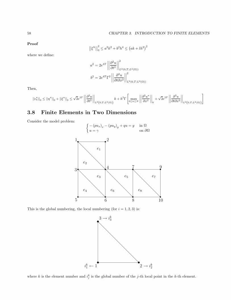
58 CHAPTER 3. INTRODUCTION TO FINITE ELEMENTS
Proof∣∣∣∣ξh∣∣∣∣2
0≤ a2k2 + b2h4 ≤
(ak + lh2
)2
where we define:
a2 = 2e4T∣∣∣∣
∣∣∣∣
∂2u
∂t2
∣∣∣∣
∣∣∣∣
2
L2(0,T ;L2(Ω))
b2 = 2e4TΓ2
∣∣∣∣
∣∣∣∣
∂3u
∂t∂x2
∣∣∣∣
∣∣∣∣
2
L2(0,T ;L2(Ω))
Then,
||ǫnh ||0 ≤ ||ηn||0 + ||ξn||0 ≤√2e2T
∣
∣
∣
∣
∣
∣
∣
∣
∂2u
∂t2
∣
∣
∣
∣
∣
∣
∣
∣
L2(0,T ;L2(Ω))k + h
2Γ
[
max0≤n≤N
∣
∣
∣
∣
∣
∣
∣
∣
∂2un
∂x2
∣
∣
∣
∣
∣
∣
∣
∣
0
+√2e2T
∣
∣
∣
∣
∣
∣
∣
∣
∂3u
∂t∂x2
∣
∣
∣
∣
∣
∣
∣
∣
L2(0,T ;L2(Ω))
]
3.8 Finite Elements in Two Dimensions
Consider the model problem:− (pux)x − (puy)y + qu = g in Ω
u = γ on ∂Ω
1 2
34 7 9
5 6 8 10
e1
e2
e3
e4
e5
e6
e7
e8
This is the global numbering, the local numbering (for i = 1, 2, 3) is:
3→ ik3
ik1 ← 1 2→ i
k2
where k is the element number and ikj is the global number of the j-th local point in the k-th element.
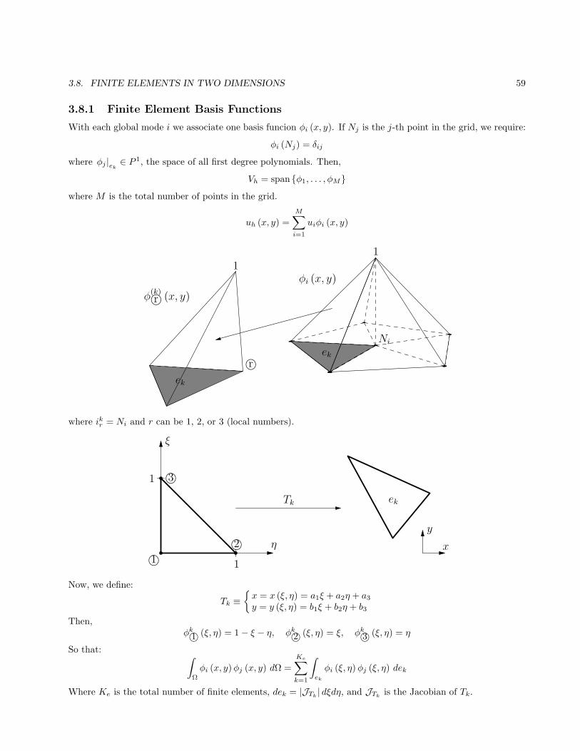
3.8. FINITE ELEMENTS IN TWO DIMENSIONS 59
3.8.1 Finite Element Basis Functions
With each global mode i we associate one basis funcion φi (x, y). If Nj is the j-th point in the grid, we require:
φi (Nj) = δij
where φj |ek ∈ P1, the space of all first degree polynomials. Then,
Vh = span φ1, . . . , φMwhere M is the total number of points in the grid.
uh (x, y) =
M∑
i=1
uiφi (x, y)
r©
ek
1
φ(k)r© (x, y)
Ni
ek
1
φi (x, y)
where ikr = Ni and r can be 1, 2, or 3 (local numbers).
ξ
η
1
11©
2©
3©
ekTk
y
x
Now, we define:
Tk ≡x = x (ξ, η) = a1ξ + a2η + a3y = y (ξ, η) = b1ξ + b2η + b3
Then,φk1© (ξ, η) = 1− ξ − η, φk2© (ξ, η) = ξ, φk3© (ξ, η) = η
So that:∫
Ω
φi (x, y)φj (x, y) dΩ =
Ke∑
k=1
∫
ek
φi (ξ, η)φj (ξ, η) dek
Where Ke is the total number of finite elements, dek = |JTk| dξdη, and JTk
is the Jacobian of Tk.
60 CHAPTER 3. INTRODUCTION TO FINITE ELEMENTS
3.8.2 Discrete Galerkin Formulation
Find uh ∈ Vh such that: ∫
Ω
puh,xvh,x +
∫
Ω
puh,yvh,y +
∫
Ω
quhvh =
∫
Ω
gvh
and, for simplicity, we choose γ ≡ 0, p = constant and q = constant. Then, substitutiting
uh =M∑
i=1
uiφi
and vh = φj for j = 1, . . . ,M yields the linear system:
(pS+ qM)uh = G
where:
Sij = p
∫
Ω
∇φi∇φj dΩ (the stiffness matrix)
Mij = q
∫
Ω
φiφj dΩ (the mass matrix)