math 524 – linear analysis on manifolds spring 2012

Math 524 – Linear Analysis on ManifoldsSpring 2012

Pierre Albin

Contents

Contents i

1 Differential operators on manifolds 3

1.1 Smooth manifolds . . . . . . . . . . . . . . . . . . . . . . . . . . . . . 3

1.2 Partitions of unity . . . . . . . . . . . . . . . . . . . . . . . . . . . . 5

1.3 Tangent bundle . . . . . . . . . . . . . . . . . . . . . . . . . . . . . . 5

1.4 Vector bundles . . . . . . . . . . . . . . . . . . . . . . . . . . . . . . 8

1.5 Pull-back bundles . . . . . . . . . . . . . . . . . . . . . . . . . . . . . 9

1.6 The cotangent bundle . . . . . . . . . . . . . . . . . . . . . . . . . . . 11

1.7 Operations on vector bundles . . . . . . . . . . . . . . . . . . . . . . 12

1.8 Sections of bundles . . . . . . . . . . . . . . . . . . . . . . . . . . . . 14

1.9 Differential forms . . . . . . . . . . . . . . . . . . . . . . . . . . . . . 16

1.10 Orientations and integration . . . . . . . . . . . . . . . . . . . . . . . 18

1.11 Exterior derivative . . . . . . . . . . . . . . . . . . . . . . . . . . . . 19

1.12 Differential operators . . . . . . . . . . . . . . . . . . . . . . . . . . . 21

1.13 Exercises . . . . . . . . . . . . . . . . . . . . . . . . . . . . . . . . . . 22

1.14 Bibliography . . . . . . . . . . . . . . . . . . . . . . . . . . . . . . . . 24

2 A brief introduction to Riemannian geometry 25

2.1 Riemannian metrics . . . . . . . . . . . . . . . . . . . . . . . . . . . . 25

2.2 Parallel translation . . . . . . . . . . . . . . . . . . . . . . . . . . . . 28

2.3 Levi-Civita connection . . . . . . . . . . . . . . . . . . . . . . . . . . 32

2.4 Associated bundles . . . . . . . . . . . . . . . . . . . . . . . . . . . . 33

i

ii CONTENTS

2.5 E-valued forms . . . . . . . . . . . . . . . . . . . . . . . . . . . . . . 34

2.6 Curvature . . . . . . . . . . . . . . . . . . . . . . . . . . . . . . . . . 36

2.7 Geodesics . . . . . . . . . . . . . . . . . . . . . . . . . . . . . . . . . 39

2.8 Complete manifolds of bounded geometry . . . . . . . . . . . . . . . 42

2.9 Riemannian volume and formal adjoint . . . . . . . . . . . . . . . . . 42

2.10 Hodge star and Hodge Laplacian . . . . . . . . . . . . . . . . . . . . 44

2.11 Exercises . . . . . . . . . . . . . . . . . . . . . . . . . . . . . . . . . . 47

2.12 Bibliography . . . . . . . . . . . . . . . . . . . . . . . . . . . . . . . . 50

3 Laplace-type and Dirac-type operators 53

3.1 Principal symbol of a differential operator . . . . . . . . . . . . . . . 53

3.2 Laplace-type operators . . . . . . . . . . . . . . . . . . . . . . . . . . 56

3.3 Dirac-type operators . . . . . . . . . . . . . . . . . . . . . . . . . . . 57

3.4 Clifford algebras . . . . . . . . . . . . . . . . . . . . . . . . . . . . . . 59

3.5 Hermitian vector bundles . . . . . . . . . . . . . . . . . . . . . . . . . 63

3.6 Examples . . . . . . . . . . . . . . . . . . . . . . . . . . . . . . . . . 68

3.6.1 The Gauss-Bonnet operator . . . . . . . . . . . . . . . . . . . 68

3.6.2 The signature operator . . . . . . . . . . . . . . . . . . . . . . 70

3.6.3 The Dirac operator . . . . . . . . . . . . . . . . . . . . . . . . 71

3.6.4 Twisted Clifford modules . . . . . . . . . . . . . . . . . . . . . 73

3.6.5 The ∂ operator . . . . . . . . . . . . . . . . . . . . . . . . . . 73

3.7 Exercises . . . . . . . . . . . . . . . . . . . . . . . . . . . . . . . . . . 76

3.8 Bibliography . . . . . . . . . . . . . . . . . . . . . . . . . . . . . . . . 78

4 Pseudodifferential operators on Rm 79

4.1 Distributions . . . . . . . . . . . . . . . . . . . . . . . . . . . . . . . 79

4.2 Examples . . . . . . . . . . . . . . . . . . . . . . . . . . . . . . . . . 84

4.2.1 Fundamental solutions . . . . . . . . . . . . . . . . . . . . . . 84

4.2.2 Principal values and finite parts . . . . . . . . . . . . . . . . . 85

4.3 Tempered distributions . . . . . . . . . . . . . . . . . . . . . . . . . . 86

CONTENTS 1

4.3.1 Convolution . . . . . . . . . . . . . . . . . . . . . . . . . . . . 86

4.3.2 Fourier transform . . . . . . . . . . . . . . . . . . . . . . . . . 88

4.4 Pseudodifferential operators on Rm . . . . . . . . . . . . . . . . . . . 92

4.4.1 Symbols and oscillatory integrals . . . . . . . . . . . . . . . . 92

4.4.2 Amplitudes and mapping properties . . . . . . . . . . . . . . . 98

4.5 Exercises . . . . . . . . . . . . . . . . . . . . . . . . . . . . . . . . . . 106

4.6 Bibliography . . . . . . . . . . . . . . . . . . . . . . . . . . . . . . . . 107

5 Pseudodifferential operators on manifolds 109

5.1 Symbol calculus and parametrices . . . . . . . . . . . . . . . . . . . . 109

5.2 Hodge decomposition . . . . . . . . . . . . . . . . . . . . . . . . . . . 114

5.3 The index of an elliptic operator . . . . . . . . . . . . . . . . . . . . . 118

5.4 Pseudodifferential operators acting on L2 . . . . . . . . . . . . . . . . 122

5.5 Sobolev spaces . . . . . . . . . . . . . . . . . . . . . . . . . . . . . . 127

5.6 Exercises . . . . . . . . . . . . . . . . . . . . . . . . . . . . . . . . . . 131

5.7 Bibliography . . . . . . . . . . . . . . . . . . . . . . . . . . . . . . . . 134

6 Spectrum of the Laplacian 135

6.1 Spectrum and resolvent . . . . . . . . . . . . . . . . . . . . . . . . . . 135

6.2 The heat kernel . . . . . . . . . . . . . . . . . . . . . . . . . . . . . . 139

6.3 Weyl’s law . . . . . . . . . . . . . . . . . . . . . . . . . . . . . . . . . 146

6.4 Long-time behavior of the heat kernel . . . . . . . . . . . . . . . . . . 148

6.5 Determinant of the Laplacian . . . . . . . . . . . . . . . . . . . . . . 149

6.6 The Atiyah-Singer index theorem . . . . . . . . . . . . . . . . . . . . 151

6.6.1 Chern-Weil theory . . . . . . . . . . . . . . . . . . . . . . . . 151

6.6.2 The index theorem . . . . . . . . . . . . . . . . . . . . . . . . 155

6.7 Examples . . . . . . . . . . . . . . . . . . . . . . . . . . . . . . . . . 157

6.8 Exercises . . . . . . . . . . . . . . . . . . . . . . . . . . . . . . . . . . 159

6.9 Bibliography . . . . . . . . . . . . . . . . . . . . . . . . . . . . . . . . 159

2 CONTENTS

Lecture 1

Differential operators on manifolds

1.1 Smooth manifolds

The m-dimensional Euclidean space Rm, the m-dimensional sphere Sm and the m-dimensional torus Tm = S1 × . . . × S1 are all examples of smooth manifolds, thecontext where our studies will take place. A general manifold is a space constructedfrom open sets in Rm by patching them together smoothly.

Formally, M is a manifold if it is a paracompact1 Hausdorff topological spacewith an ‘atlas’, i.e., a covering by open sets Vα together with homeomorphisms

φα : Uα −→ Vα

for some open subsets Uα of Rm. The integer m is known as the dimension ofM and the maps φα : Uα −→ Vα (or sometimes just the sets Vα) are known ascoordinate charts. An atlas is smooth if whenever Vαβ := Vα ∩ Vβ 6= ∅ the map

(1.1) ψαβ := φ−1β φα : φ−1

α (Vαβ) −→ φ−1β (Vαβ)

is a smooth diffeomorphism between the open sets φ−1α (Vαβ), φ−1

β (Vαβ) ⊆ Rm. (For

us smooth will always mean C∞.) If the maps ψαβ are all Ck-smooth, we say thatthe atlas is Ck.

If φα : Uα −→ Vα is a coordinate chart, it is typical to write

(y1, . . . , ym) = φ−1α : Vα −→ Uα

and refer to the yi as local coordinates of M on Vα.1 A topological space is paracompact if every open cover has a subcover in which each point is

covered finitely many times.

3

4 LECTURE 1. DIFFERENTIAL OPERATORS ON MANIFOLDS

Two smooth atlases are compatible (or equivalent) if their union is a smoothatlas. A smooth structure on M is an equivalence class of smooth atlases or,equivalently, a maximal smooth atlas on M. A manifold M together with a smoothstructure is a smooth manifold.

To indicate that a manifold M is m-dimensional we will sometimes write Mm

or, more often, we will refer to M as an m-manifold.

A more general notion than manifold is that of a manifold with boundary.The former is defined in the same way as a manifold, but the local model is

Rm− = (x1, . . . , xn) ∈ Rm : x1 ≤ 0.

If M is a smooth manifold with boundary, its boundary ∂M consists of those pointsin M that are in the image of ∂Rm

− for some (and hence all) local coordinate charts.It is easy to check that ∂M is itself a smooth manifold (without boundary). Theproduct of two manifolds with boundary is an example of a still more general notion,a manifold with corners.

A map between two smooth manifolds (with or without boundary)

F : M −→M ′

is smooth if it is smooth in local coordinates. That is, whenever

φα : Uα −→ Vα ⊆M, φ′γ : U ′γ −→ V ′γ ⊆M ′,

are coordinate charts, the map

(1.2) (φ′γ)−1 F φα : Uα −→ U ′γ

is smooth (whenever it is defined). Notice that this definition is equivalent to makingcoordinate charts diffeomorphisms.

The space of smooth maps between M and M ′ will be denoted C∞(M,M ′)and when M ′ = R, simply by C∞(M). Notice that a map F ∈ C∞(M,M ′) naturallyinduces a pull-back map

F ∗ : C∞(M ′) −→ C∞(M), F ∗(h)(p) = h(F (p)) for all h ∈ C∞(M ′), p ∈M.

(So we can think of C∞ as a contravariant functor on smooth manifolds.)

For us a manifold will mean a connected smooth manifold without boundary,unless otherwise specified. Similarly, unless we specify otherwise, a map betweenmanifolds will be smooth.

1.2. PARTITIONS OF UNITY 5

A subset X ⊆ M is a submanifold of M of dimension k if among the mcoordinates on M at each point of X there are k that restrict to give coordinates ofX. That is, at each point p ∈ X there is a coordinate chart of M, φ : U −→ V withq ∈ V , whose restriction to U ∩ Rk × 0 maps into X,

φ∣∣U∩Rk×0 : U ∩ Rk × 0 −→ V ∩X.

These restricted charts then define a smooth k-manifold structure on X.

1.2 Partitions of unity

A manifold is defined by patching together many copies of Rm. It is often useful totake a construction on Rm and transfer it to a manifold by carrying it out on eachpatch and then adding the pieces together.

For these constructions, it is very convenient that every open covering Vα of asmooth manifold carries a partition of unity. That is, a collection ωi of smoothfunctions ωi : M −→ R such that:i) At each p ∈M only finitely many ωi(p) are non-zeroii) Each ωi is supported inside some Vαiii) The sum of the ωi is the constant function equal to one at each point p ∈M.

One remarkable fact that follows easily from the existence of partitions of unityis that any compact smooth manifold can be identified with a smooth submanifoldof RN for some N. This is easy to show using a finite atlas with a correspondingpartition of unity. Whitney’s embedding theorem shows that any smooth manifoldM embeds into R2 dimM+1 and a compact smooth manifold into R2 dimM .

1.3 Tangent bundle

We know what a smooth function

f : M −→ R

is, what is its derivative? If γ is a smooth curve on M, that is, a smooth map

γ : R −→M,

then f γ is a map from R to itself so its derivative is unambiguously defined. Wecan take advantage of this to define the derivative of f at a point p ∈ M in termsof the curves through that point.


Indeed, let us say that two curves γ1 and γ2 are equivalent at p if γ1(0) =γ2(0) = p and

∂

∂t

∣∣∣∣t=0

(φ−1 γ1) =∂

∂t

∣∣∣∣t=0

(φ−1 γ2)

for some (and hence any) coordinate chart φ : U −→ V ⊆M containing p. It is easyto see that this is an equivalence relation and we refer to an equivalence class as atangent vector at p ∈M. The tangent space to M at p is the set of all tangentvectors at p and is denoted TpM.

For the case of Euclidean space, the tangent space to Rm at any point isanother copy of Rm,

TpRm = Rm.

The tangent space of the m-sphere is also easy to describe. By viewing Sm as theunit vectors in Rm+1, curves on Sm are then also curves in Rm+1 so we have

TpSm ⊆ TpRm+1 = Rm+1,

and a tangent vector at p will correspond to a curve on Sm precisely when it isorthogonal to p as a vector in Rm+1, thus

TpSm = v ∈ Rm+1 : v · p = 0.

Clearly if γ1 is equivalent to γ2 at p then

∂

∂t

∣∣∣∣t=0

(f γ1) =∂

∂t

∣∣∣∣t=0

(f γ2)

for all f : M −→ R, so we can think of the derivative of f at p as a map fromequivalence classes of curves through p to equivalence classes of curves throughf(p), thus

Dpf : TpM −→ Tf(p)R.

More generally, any smooth map F : M1 −→ M2 defines a map, known as itsdifferential,

DpF : TpM1 −→ TF (p)M2

by sending the equivalence class of a curve γ on M1 to the equivalence class of thecurve F γ on M2. When the point p is understood, we will omit it from the notation.

If the differential of a map is injective we say that the map is an immersion,if it is surjective we say that it is a submersion. If F : M1 −→ M2 is an injectiveimmersion which is a homeomorphism between M1 and F (M1) then we say that Fis an embedding. A connected subset X ⊆ M is a submanifold of M preciselywhen the inclusion map X →M is an embedding.

1.3. TANGENT BUNDLE 7

If F is both an immersion and a submersion, i.e., if DF is always a linearisomorphism, we say that it is a local diffeomorphism. By the inverse functiontheorem, if F is a local diffeomorphism then every point p ∈M1 has a neighborhoodV ⊆M1 such that F

∣∣V is a diffeomorphism onto its image. A diffeomorphism is a

bijective local diffeomorphism.

The chain rule is the fact that commutative diagrams

M1F1 //

F2F1 !!

M2

F2

M3

of smooth maps between manifolds induce, for each p ∈M1, commutative diagramsbetween the corresponding tangent spaces,

TpM1DF1 //

D(F2F1) &&

TF1(p)M2

DF2

TF2(F1(p))M3

i.e., that D(F2 F1) = DF2 DF1.

Taking differentials of coordinate charts of M, we end up with coordinatecharts on

TM =⋃p∈M

TpM

showing that TM, the tangent bundle of M, is a smooth manifold of twice thedimension of M. For Rm the tangent bundle is simply the product

TRm = Rm × Rm

where the first factor is thought of as a point in Rm and the second as a vector‘based’ at that point; the tangent bundle of an open set in Rm has a very similardescription, we merely restrict the first factor to that open set. (We can think ofM 7→ TM together with F 7→ DF as a covariant functor on smooth manifolds.)

If φ : U −→ V is a coordinate chart on M and p ∈ V ⊆M, then Dpφ identifiesTpM with Rm. A different choice of coordinate chart gives a different identificationof TpM with Rm, but these identifications differ by an invertible linear map. Thismeans that each TpM is naturally a vector space of dimension m, which howeverdoes not have a natural basis.

Now that we know the smooth structure of TM, note that the differential ofa smooth map between manifolds is a smooth map between their tangent bundles.


There is also a natural smooth projection map

π : TM −→M

that sends elements of TpM to p and when M = Rm is simply the projection ontothe first factor. It is typical, for any subset Z ⊆M, to use the notations

π−1(Z) =: TM∣∣Z

=: TZM.

1.4 Vector bundles

A coordinate chart φ : U −→ V on a smooth m-manifold M induces a coordinatechart on TM and an identification

(1.3) π−1(V)Dφ−1

−−−−→ TU = U × Rm φ×id−−−−→ V × Rm

which restricts to each fiber π−1(p) to a linear isomorphism. We say that a coordinatechart of M locally trivializes TM as a ‘vector bundle’.

A vector bundle over a manifold M is a locally trivial collection of vectorspaces, one for each point in M. Formally a rank k real vector bundle consists ofa smooth manifold E together with a smooth surjective map π : E −→ M suchthat the fibers π−1(p) form vector spaces over R and satisfying a local trivialitycondition: for any point p ∈ M and small enough neighborhood V of p there is adiffeomorphism

Φ : V × Rk −→ π−1(V)

whose restriction to any q ∈ V is a linear isomorphism

Φ∣∣q∈V : q × Rk −→ π−1(q).

We refer to the pair (V ,Φ) as a local trivialization of E.

We will often refer to a rank k real vector bundle as a Rk-bundle. The discus-sion below of Rk-vector bundles applies equally well to complex vector bundles,or Ck-vector bundles, which are the defined by systematically replacing Rk with Ck

above.

If X is a submanifold of M, and Eπ−−→M is a vector bundle, then

E∣∣X

π|X−−−→ X

is a vector bundle.

1.5. PULL-BACK BUNDLES 9

A subset of a vector bundle is a subbundle if it is itself a bundle in a consistentfashion. That is, E1 is a subbundle of E2 if E1 and E2 are both bundles over M,E1 ⊆ E2, and the projection map E1 −→M is the restriction of the projection mapE2 −→M.

A bundle morphism between two vector bundles

E1π1−−→M1, E2

π2−−→M2

is a mapF : E1 −→ E2

that sends fibers of π1 to fibers of π2 and acts linearly between fibers. Thus for anybundle morphism F there is a map F : M1 −→M2 such that the diagram

(1.4) E1F //

π1

E2

π2

M1

F //M2

commutes; we say that F covers the map F . An invertible bundle morphism is calleda bundle isomorphism.

The trivial Rk-bundle over a manifold M is the manifold Rk×M with projec-tion the map onto the second factor. We will use Rk to denote the trivial Rk-bundle.A bundle is trivial if it is isomorphic to Rk for some k. A manifold is said to be par-allelizable if its tangent bundle is a trivial bundle, e.g., Rm is parallelizable.

We will show later that Sm is not parallelizable when m is even. The circle S1

is parallelizable and hence (by exercise 1) so are all tori Tm. Some interesting factswhich we will not show is that any three dimensional manifold is parallelizable andthat the only parallelizable spheres are S1, S3 and S7. The fact that these sphereare parallelizable is easy to see by viewing them as the unit vectors in the complexnumbers, the quaternions, and the octionians, respectively; the fact that these arethe only parallelizable ones is not trivial.

1.5 Pull-back bundles

Any bundle morphism covers a map between manifolds (1.4). There is a sort ofconverse to this: given a map between manifolds f : M1 −→ M2, and a Rk-bundleE

π−−→M2 the set

f ∗E = (p, v) ⊆M1 × E : f(p) = π(v)


fits into the commutative diagram

f ∗Ef //

π

E

π

M1

f //M2

where, for any (p, v) ∈ f ∗E,

p (p, v)πoo f // v.

Moreover, if (U ,Φ) is a local trivialization of E and V is a coordinate chart in M1

such that f(V) ⊆ U then

f ∗E ∩ (V × π−1(U)) = (p, (Φ∣∣f(p)

)−1(x)) : p ∈ V , x ∈ Rk

and we can use this to introduce a C∞ manifold structure on f ∗E such that f ∗E ∩(V × π−1(U)) is diffeomorphic to V × Rk making f ∗E

π−−→ M1 a Rk-bundle. Thebundle f ∗E is called the pull-back of E along f .

The simplest example of a pull-back bundle is the restriction of a bundle. If

X is a submanifold of M, and Eπ−−→ M is a vector bundle, then E

∣∣X

π

∣∣X−−−−→ X is

(isomorphic to) the pull-back of E along the inclusion map X →M.

We see directly from the definition that the pull-back bundle of a trivial bundleis again trivial, but note that the converse is not true.

Given a smooth map f : M1 −→ M2, pull-back along f defines a functorbetween bundles on Y and bundles on X. Indeed, if E1 −→ Y and E2 −→ Y arebundles over Y and F : E1 −→ E2 is a bundle map between them then

f ∗F : f ∗E1 −→ f ∗E2, f ∗F (p, v) = (p, F (p)v) for all (p, v) ∈ f ∗E1

is a bundle map between f ∗E1 and f ∗E2.

Another useful relation between pull-backs and bundle maps is the following:If E1

π1−−→ M1 and E2π2−−→ M2 are vector bundles and F : E1 −→ E2 is a bundle

map so that

E1F //

π1

E2

π2

M1

F //M2

then F is equivalent to a bundle map between E1 −→M1 and F∗E2 −→M1, namely

E1 3 v 7→ (π1(v), F (π1(v))v) ∈ F ∗E2.

1.6. THE COTANGENT BUNDLE 11

We will show later (Remark 3) that if f : M1 −→ M2 and g : M1 −→ M2 arehomotopic smooth maps, i.e., if there is a smooth map

H : [0, 1]×M1 −→M2 s.t. H(0, ·) = f(·) and H(1, ·) = g(·)

then f ∗E ∼= g∗E for any vector bundle E −→ M2. In particular, this implies thatall vector bundles over a contractible space are trivial.

1.6 The cotangent bundle

Every real vector space V has a dual vector space

V ∗ = Hom(V,R)

consisting of all the linear maps from V to R. Given a linear map between vectorspaces

T : V −→ W

there is a dual map between the dual spaces

T ∗ : W ∗ −→ V ∗, T ∗(ω)(v) = ω(T (v)) for all ω ∈ W ∗, v ∈ V.

By taking the dual maps of the local trivializations of a vector bundle Eπ−−→

M, the manifold

E∗ = (p, ω) : p ∈M,ω ∈ (π−1(p))∗

with the obvious projection E∗ −→ M is seen to be a vector bundle, the dualbundle to E.

Every vector v ∈ Rk defines a dual vector v∗ ∈ (Rk)∗,

v∗ : Rk −→ R, v∗(w) = v · w,

and it is easy to see that the dual vectors of a basis of Rk form a basis of (Rk)∗ sothat in fact v 7→ v∗ is a vector space isomorphism. In particular the dual bundle ofan Rk-bundle is again a Rk-bundle.

Given vector bundles E1 −→M1 and E2 −→M2 and F : E1 −→ E2 a bundlemap, we get a dual bundle map

F ∗ : E∗2 −→ E∗1 .

Thus taking duals defines a contravariant functor on the category of vector bundles.


The dual of a bundle map F : E1 −→ E2 between two bundles Ei −→ M is amap between their duals

F ∗ : E∗2 −→ E∗1 .

Thus taking duals defines a contravariant functor on the category of vector bundleson M. It is easy to see that this functor commutes with pull-back along a smoothmap.

The dual bundle to the tangent bundle is the cotangent bundle

T ∗M −→M.

Remark 1. The assignation M 7→ T ∗M is natural, but is not a functor in the sameway that M 7→ TM is. Rather, a map F : M1 −→M2 between manifolds induces amap DF : TM1 −→ TM2 between their tangent bundles which, as explained above,we can interpret as a map DF : TM1 −→ F ∗(TM2) between bundles over M1. Nowwe can take duals and we get a bundle map (DF )∗ : F ∗(TM∗

2 ) −→ TM∗1 .

Thus we can view M 7→ T ∗M as a functor but its target category should consistof vector bundles where a morphism between E1 −→M1 and E2 −→M2 consists ofa map F : M1 −→M2 and a bundle map Φ : F ∗E2 −→ E1 and composition is

(F1,Φ1) (F2,Φ2) = (F1 F2,Φ1 (F ∗1 Φ2)).

This is called the category of star bundles in [Kolar-Michor-Slovak].

1.7 Operations on vector bundles

We constructed the vector bundle E∗ −→ M from the vector bundle E −→ Mby applying the vector space operation V 7→ V ∗ fiber-by-fiber. This works moregenerally whenever we have a smooth functor of vector spaces.

Let Vect denote the category of finite dimensional vector spaces with linearisomorphisms, and let T be a (covariant) functor on Vect. We say that T is smoothif for all V and W in Vect the map

Hom(V,W ) −→ Hom(T (V ),T (W ))

is smooth.

Let Eπ−−→M be a vector bundle over M, define

Tp(E) = T (π−1(p)), T (E) =⊔p∈M

Tp(E)

1.7. OPERATIONS ON VECTOR BUNDLES 13

and let T (π) : T (E) −→ M be the map that sends Tp(E) to p. We claim that

T (E)T (π)−−−−→M is a smooth vector bundle.

Applying T fibrewise to a local trivialization of E,

Φ : V × Rk −→ π−1(V),

we obtain a mapT (Φ) : V ×T (Rk) −→ T (π)−1(V),

and we can use these maps as coordinate charts on T (E) to obtain the structure ofa smooth manifold. Indeed, we only need to see that if two putative charts overlapthen the map

(V1 ∩ V2)×T (Rk)T (Φ1)−1T (Φ2)−−−−−−−−−−→ (V1 ∩ V2)×T (Rk)

is smooth, and this follows from the smoothness of T .

Thus T (E) is a smooth manifold, T (π) is a smooth function, and

T (E)T (π)−−−−→M

satisfies the local triviality condition, so we have a new vector bundle over M.

The same procedure works for contravariant functors (meaning that Hom(V,W )is sent to Hom(T (W ),T (V ))) as well as functors with several variables. Therefore,for instance, we can define for vector bundles E −→ M and F −→ M the vectorbundles:

i) Hom(E,F ) −→M with fiber over p, Hom(Ep, Fp).

ii) E ⊗ F −→M with fiber over p, Ep ⊗ Fp.

iii) S2E −→M whose fiber over p is the space of all symmetric bilinear transfor-mations from Ep × Ep to R.

iv) SkE −→M whose fiber over p is the space of all symmetric k-linear transfor-mations from Ek

p to R.

v) ΛkE −→ M whose fiber over p is the space of all antisymmetric k-lineartransformations from Ek

p to R.

We also obtain natural isomorphisms of vector bundles from isomorphisms ofvector spaces. Thus, for instance, for vector bundles E, F, and G over M, we have2

2Recall that R is the trivial R-bundle, R×M −→M.


i) E ⊕ F ∼= F ⊕ E

ii) E ⊗ R ∼= E

iii) E ⊗ F ∼= F ⊗ E

iv) E ⊗ (F ⊕G) ∼= (E ⊗ F )⊕ (E ⊗G)

v) Hom(E,F ) = E∗ ⊗ F (so E∗ ∼= Hom(E,R))

vi) Λk(E ⊕ F ) ∼=⊕i+j=k

(ΛiE ⊗ ΛjF )

vii) (ΛkE)∗ = Λk(E∗)

1.8 Sections of bundles

A section of a vector bundle Eπ−−→M is a smooth map s : M −→ E such that

Eπ

M

s

>>

id //M

commutes. We will denote the space of smooth sections of E by C∞(M ;E). Thisforms a vector space over R and, as such, it is infinite-dimensional (unless we are ina ‘trivial’ situation where (dimM)(rankE) = 0). However it is also a module overC∞(M) (with respect to pointwise multiplication) and here it is finitely generated.For instance, the sections of a trivial bundle form a free C∞(M) module,

C∞(M ;Rn) = (C∞(M))n .

We also introduce notation for functions and sections with compact support,

C∞c (M), C∞c (M ;E)

and point out that the latter is a module over the former. One consequence of themodule structure is that we can use a partition of unity on M to decompose a sectioninto a sum of sections supported on trivializations of E.

A section of the tangent bundle is known as a vector field. Thus a vectorfield on M is a smooth function that assigns to each point p ∈ M a tangent vectorin TpM. A vector field V ∈ C∞(M ;TM) naturally acts on a smooth function bydifferentiation

V : C∞(M) −→ C∞(M), (V f)(p) = Dpf(V (p)) for all f ∈ C∞(M), p ∈M.

1.8. SECTIONS OF BUNDLES 15

If Vα is a coordinate chart on M with local coordinates y1, . . . , ym then we can write

V∣∣Vα

=m∑i=1

ai(y1, . . . , ym)∂

∂yi.

Indeed, this is just the representation in the induced coordinates of TM with theidentification (1.3).

This action of V on C∞(M) is linear and satisfies

V (fh) = V (f)h+ fV (h), for all f, h ∈ C∞(M),

i.e., it is a derivation of C∞(M). In fact, it is possible to identify vector fields on Mwith the derivations of C∞(M). (see e.g., [Lee])

As maps on C∞(M), we can compose vector fields

(VW )(f) = V (W (f))

but the result is no longer a vector field. However, if we form the commutator oftwo vector fields,

[V,W ]f = V (W (f))−W (V (f))

then the result is again a vector field! In fact it is easy to check that this is aderivation on C∞(M). The commutator of vector fields satisfies the ‘Jacobi identity’

[[U, V ],W ] + [[V,W ], U ] + [[W,U ], V ] = 0

and hence the commutator, combined with the R-vector space structure, givesC∞(M,TM) the structure of a Lie algebra.

Remark 2. Whereas a smooth map F : M1 −→M2 induces a map DF : TM1 −→TM2, it is not always possible to ‘push-forward’ a vector field. We say that two vectorfields V ∈ C∞(M1;TM1), and W ∈ C∞(M2;TM2) are F -related if the diagram

TM1DF // TM2

M1

V

OO

F //M2

W

OO

commutes, i.e., if DF V = W F.If F is a diffeomorphism, then we can push-forward a vector field: the vector

fields V ∈ C∞(M1;TM1) and F∗V = DF V F−1 ∈ C∞(M2;TM2) are alwaysF -related. Moreover, F∗[V1, V2] = [F∗V1, F∗V2] for all V1, V2 ∈ C∞(M1;TM1), soM 7→ C∞(M ;TM) is a functor from smooth manifolds with diffeomorphisms to Liealgebras and isomorphisms.


1.9 Differential forms

Sections of the cotangent bundle of M, T ∗M, are known as differential 1-forms.More generally, sections of the k-th exterior power of the cotangent bundle, ΛkT ∗M,are known as differential k-forms. The typical notation for this space is

Ωk(M) = C∞(M ; ΛkT ∗M), Ω∗(M) =dimM⊕k=0

Ωk(M)

where by convention Ω0(M) = C∞(M). A differential form in Ωk(M) is said to havedegree k.

A differential k-form ω ∈ Ωk(M) can be evaluated on k-tuples of vector fields,

ω : C∞(M ;TM)k −→ R,

it is linear in each variable and has the property that

ω(Vσ(1), . . . , Vσ(k)) = sign(σ)ω(V1, . . . , Vk)

for any permutation σ of 1, . . . , k.Differential forms of all degrees Ω∗(M) form a graded algebra with respect to

the wedge product

Ωk(M)× Ω`(M) 3 (ω, η) 7→ ω ∧ η ∈ Ωk+`(M)

ω ∧ η(V1, . . . , Vk+`) =1

k!`!

∑σ

sign(σ)ω(Vσ(1), . . . , Vσ(k))η(Vσ(k+1), . . . , Vσ(k+`)).

This product is graded commutative (so sometimes commutative and sometimesanti-commutative)

ω ∈ Ωk(M), η ∈ Ω`(M) =⇒ ω ∧ η = (−1)k`η ∧ ω.

In particular if ω ∈ Ωk(M) with k odd, then ω ∧ ω = 0.

Given a differential k-form, ω, we will write the operator ‘wedge product withω, by

eω : Ω∗(M) −→ Ω∗+k(M), eω(η) = ω ∧ η, for all η ∈ Ω∗(M).

We say that a k-form is elementary if it is the wedge product of k 1-forms.Elementary k-forms are easy to evaluate

(ω1 ∧ · · · ∧ ωk)(V1, . . . , Vk) = det(ωi(Vj)).

1.9. DIFFERENTIAL FORMS 17

Let p be a point in a local coordinate chart V on M with coordinates y1, . . . , ym. Abasis of T ∗pM dual to the basis ∂y1 , . . . , ∂ym of TpM is given by

dy1, . . . , dym where dyi(∂yj) = δij.

A basis for the space of k-forms in T ∗pM is given by

dyi1 ∧ · · · ∧ dyik : i1 < · · · < ik.

Any k-form supported in V can be written as a sum of elementary k-forms. Usinga partition of unity we can write any k-form on M as a sum of elementary k-forms.Notice that anticommutativity of the wedge product implies that all elementary k-forms, and hence all k-forms, of degree greater than the dimension of the manifoldvanish.

There is also an interior product of a vector field and a differential form,which is simply the contraction of the differential form by the vector field. For everyW ∈ C∞(M ;TM), the interior product is a map

iW : Ω∗(M) −→ Ω∗−1(M)

(iWω)(V1, . . . , Vk−1) = ω(W,V1, . . . , Vk−1), for all ω ∈ Ωk, Vi ⊆ C∞(M ;TM).

We will also use the notationiWω = W yω.

Notice that antisymmetry of differential forms induces anticommutativity of theinterior product in that

iV iW = −iW iV

for any V,W ∈ C∞(M ;TM). In particular, (iV )2 = 0.

If F : M1 −→ M2 is a smooth map between manifolds, we can pull-backdifferential forms from M2 to M1,

F ∗ : Ωk(M2) −→ Ωk(M1),

F ∗ω(V1, . . . , Vk) = ω(DF (V1), . . . , DF (Vk)) for all ω ∈ Ωk(M2), Vi ∈ C∞(M ;TM1).

Pull-back respects the wedge product,

(1.5) F ∗(ω ∧ η) = F ∗ω ∧ F ∗η,

and the interior product,

F ∗(DF (W ) yω) = W yF ∗(ω).

In the particular case of Rm, the pull-back of an m-form by a linear map T is

(1.6) T ∗(dx1 ∧ · · · ∧ dxm) = (detT )(dx1 ∧ · · · ∧ dxm),

directly from the definition of the determinant.


1.10 Orientations and integration

If W is an m-dimensional vector space, and u1, . . . , um, v1, . . . , vm are bases ofW, we will say that they represent the same orientation if the linear map that sendsui to vi has positive determinant. Equivalently, since ΛmW is a one-dimensionalvector space, we know that u1 ∧ · · · ∧ um and v1 ∧ · · · vm differ by multiplication bya non-zero real number and we say that they represent the same orientation if thisnumber is positive. A representative ordered basis or non-zero m-form is said to bean orientation of W. The canonical orientation of Euclidean space Rm correspondsto the canonical ordered basis, e1, . . . , em.

An Rk-vector bundle E −→M is orientable if we can find a smooth orienta-tion of its fibers, i.e., if there is a nowhere vanishing section of ΛkE −→ M. Noticethat the latter is an R-bundle over M, so the existence of a nowhere vanishing sec-tion is equivalent to its being trivial. Thus E −→ M is orientable if and only ifΛkE −→ M is a trivial bundle. An orientation is a choice of trivializing section,and a manifold together with an orientation is said to be oriented. Note that, sinceΛk(E∗) = (ΛkE)∗, E is orientable if and only if E∗ is orientable.

An m-manifold M is orientable if and only if its tangent bundle is orientable.Equivalently, a manifold is orientable when its cotangent bundle is orientable, sowhen there is a nowhere vanishing m-form. A choice of nowhere vanishing m-formis called an orientation of M or also a volume form on M. A coordinate chartφ : U −→ V is oriented if it pulls-back the orientation of M to the canonicalorientation of Rm. A manifold is orientable precisely when it has an atlas of orientedcoordinate charts.

If M is oriented, there is a unique linear map the integral∫: C∞c (M ; ΛmM) −→ R

which is invariant under diffeomorphims and coincides in local coordinates with theLebesgue integral. That is, if ω ∈ ΩmM is supported in a oriented coordinate chartφ : U −→ V then φ∗ω ∈ Ωm(Rm) and so we can take its Lebesgue integral. Theassertion is that the result is independent of the choice of oriented coordinate chart,and the proof follows from (1.6) and the usual change of variable formula for theLebesgue integral. By using a partition of unity, integration of any m-form reducesto integration of m-forms supported in oriented coordinate charts. It is convenientto formally extend the integral to a functional on forms of all degrees, by setting itequal to zero on all forms of less than maximal degree.

What happens when a manifold is not orientable? At each point p ∈ M, theset of equivalence classes of orientations of TM, Op, has two elements, say o1(p) and

1.11. EXTERIOR DERIVATIVE 19

o2(p). We define the orientable double cover of M to be the set

Or(M) = (p, oi(p)) : p ∈M, oi(p) ∈ Op.

The manifold structure on M easily extends to show that M is a smooth manifold.Indeed, given a coordinate chart φ : U −→ V of M we set, for each q ∈ U ,

φ(q) = (φ(q), [φ−1(e1 ∧ · · · ∧ em)]) ∈ Or(M)

and we get a coordinate chart on M. The mapping π : M −→M that sends (p, oi(p))to p is smooth and surjective. Moreover if V is a coordinate neighborhood in Mthen π−1(V) = V1 ∪ V2 is the union of two disjoint open sets in Or(M) and πrestricted to each Vi is a diffeomorphism onto V , hence the term ‘double cover’.It is easy to see that Or(M) is always orientable (at each point (p, oi(p)) choosethe orientation corresponding to oi(p)). If M is connected and not orientable thenOr(M) is connected and orientable, and we can often pass to Or(M) if we needan orientation. If M is orientable, then the same construction of Or(M) yields adisconnected manifold consisting of two copies of M.

Orientations are one place where the theory of complex vector bundles dif-fers from that of general real vector bundles. Complex vector bundles are alwaysorientable.

Indeed, first note that a C-vector space W of complex dimension k has acanonical orientation as a R-vector space of real dimension 2k. We just take any basisof W over C, say b = v1, . . . , vk, and then take b = v1, iv1, v2, iv2, . . . , vk, ivk asa basis for W over R. The claim is that if b′ = w1, . . . , wk is any other basis of W

over C, then b′ = w1, iw1, . . . , wk, iwk gives us the same orientation for W as a R-

vector space, i.e., the change of basis matrix B from b to b′ has positive determinant.The proof is just to note that, if B is the complex change of basis matrix from b tob′ then

det B = (detB)(detB) > 0.

As the orientation is canonical, every Ck-vector bundle is orientable as a R2k-vectorbundle.

1.11 Exterior derivative

If f is a smooth function onM, its exterior derivative is a 1-form df ∈ C∞(M ;T ∗M)defined by

df(V ) = V (f), for all V ∈ C∞(M ;TM).


If ω ∈ C∞(M ;T ∗M), its exterior derivative is a 2-form dω ∈ C∞(M ; Λ2T ∗M) definedby

dω(V,W ) = V (ω(W ))−W (ω(V ))− ω([V,W ]), for all V,W ∈ C∞(M ;TM).

In the same way, if ω ∈ Ωk(M), we define its exterior derivative to be the (k+1)-formdω ∈ Ωk+1(M) defined by

dω(V0, . . . , Vk) =

p∑i=0

(−1)iVi(ω(V0, . . . , Vi, . . . , Vp))

+∑i<j

(−1)i+jω([Vi, Vj], V0, . . . , Vi, . . . , Vj, . . . , Vp)

The exterior derivative thus defines a graded map

d : Ω∗(M) −→ Ω∗(M).

It has the property that d2 = 0. It also distributes over the wedge product respectingthe grading, in that

(1.7) ω ∈ Ωk(M), η ∈ Ω`(M) =⇒ d(ω ∧ η) = (dω) ∧ η + (−1)kω ∧ dη.

The exterior derivative also commutes with pull-back along a smooth mapF : M1 −→ M2. Indeed, note that for a function on M2, f ∈ C∞(M2), this followsfrom the chain rule

d(F ∗f)(V ) = d(fF )(V ) = D(fF )(V ) = Df(DF (V )) = df(DF (V )) = F ∗(df)(V )

and, using this, it follows for forms of arbitrary degree from (1.5) and (1.7).

A k-form ω is called closed if dω = 0 and exact if there is a (k − 1)-form ηsuch that dη = ω. The space of k-forms is an infinite dimensional vector space overR, as are the spaces of closed and exact forms. However we will show that, for acompact manifold M and any k, the quotient vector space

HkdR(M) =

closed k-forms

exact k-forms=

ker(d : Ωk(M) −→ Ωk+1(M)

)im (d : Ωk−1(M) −→ Ωk(M))

is finite dimensional. This R-vector space is known as the k-th de Rham coho-mology group of M . These groups are one of the main objects of study in thiscourse. We will come back to them after we build up more tools.

If M is an oriented manifold with boundary, Stokes’ theorem is the fact that∫M

dω =

∫∂M

ω, for all ω ∈ Ωm−1c (M).

1.12. DIFFERENTIAL OPERATORS 21

This compact statement generalizes the fundamental theorem of calculus, Green’stheorem, and Gauss’ theorem. If M does not have boundary, then Stokes’ theoremsays that ∫

M

dω = 0, for all ω ∈ Ωm−1c (M).

1.12 Differential operators

It is clear what we mean by a differential operator of order n on Rm, namely apolynomial of degree n in the variables ∂y1 , ∂y2 , . . . , ∂ym ,

(1.8)∑

j1,j2,...,jmj1+...+jm=n

aj1,...,jm(y1, . . . , ym)∂j1y1∂j2y2· · · ∂jmym .

(The degree of this operator is the largest value of j1 + j2 + . . . + jm for whichaj1,...,jm is not zero, which we are assuming is n.) This operator is smooth when thecoefficient functions aj1,...,jm(y1, . . . , ym) are all smooth. The set of all differentialoperators of order at most n, is denoted Diffn(Rm).

This is a good moment to introduce multi-index notation. Let us agree, for allvectors α = (j1, . . . , jm), on the equivalence of the symbols

∂αy = ∂j1y1∂j2y2· · · ∂jmym ,

and let us use |α| to denote j1 + . . . + jm. Then we can write the expression abovemore succinctly as

P ∈ Diffn(Rm) ⇐⇒ P =∑|α|≤n

aα(y)∂αy .

On a manifold, a differential operator of order at most n is a linear map

P : C∞(M) −→ C∞(M)

that in any choice of local coordinates has the form (1.8). For instance, a vectorfield V induces a linear map (a derivation) on smooth functions

V : C∞(M) −→ C∞(M)

and this is exactly what we mean by a first order differential operator on M. In fact,a better description of differential operators of order at most n on M is to take thespan of powers of C∞(M ;TM),

Diffn(M) = span0≤j≤n

(C∞(M ;TM))j


where we agree that C∞(M ;TM)0 = C∞(M). Notice that the fact that the degreeof a differential operator is well-defined comes from the fact that the commutatorof two vector fields is again a vector field.

The exterior derivative is also a first order differential operator, but now be-tween sections of vector bundles over M, e.g., for each k,

d : C∞(M ; ΛkT ∗M) −→ C∞(M ; Λk+1T ∗M).

In general, a differential operator of order at most n acting between sections of twovector bundles E and F is a linear map

C∞(M ;E) −→ C∞(M ;F )

that in any local coordinates that trivialize both E and F has the form (1.8) wherewe now require the functions aα(y) to be sections of Hom(E,F ).

There is a very nice characterization (or definition if you prefer) of differentialoperators due to Peetre3. First, we say that a linear operator

T : C∞(M ;E) −→ C∞(M ;F )

is a local operator if whenever s ∈ C∞(M ;E) vanishes in an open set U ⊆M, Tsalso vanishes in that open set,

s∣∣U = 0 =⇒ (Ts)

∣∣U = 0.

Peetre showed that all linear local operators are differential operators.

1.13 Exercises

Exercise 1.Show that whenever M1 and M2 are smooth manifolds, M1×M2 is too. Prove thatT (M1 ×M2) = TM1 × TM2.

Exercise 2.Instead of defining the cotangent bundle in terms of the tangent bundle, we can dothings the other way around. At each point p of a manifold M, let

Ip = u ∈ C∞(M) : u(p) = 03 Peetre, Jaak Une caracterisation abstraite des operateurs differentiels. Math. Scand. 7

1959 211-218.

1.13. EXERCISES 23

be the ideal of functions vanishing at p. Let I2p be the linear span of products of

pairs of elements in Ip, and define

T ∗p M = Ip/I2p , T ∗M =

⋃p∈M

T ∗p M.

Show that, together with the obvious projection map, this defines a vector bundleisomorphic to the cotangent bundle.

Exercise 3.Show that a Rk-bundle E

π−−→M is trivial if and only if there are k sections s1, . . . , sksuch that, at each p ∈M,

s1(p), . . . , sk(p) is linearly independent.

Exercise 4.If E

πE−−−→M is a subbundle of FπF−−−→M show that there is a bundle F/E −→M

whose fiber over p ∈M is π−1F (p)/π−1

E (p)

Exercise 5.Given vector bundles E −→M and F −→M, assume that f ∈ C∞(M ; Hom(E,F ))is such that

dim ker f(p) is independent of p ∈M.

Prove that the kernels of f form a vector bundle over M (a subbundle of E) andthe cokernels of f also form a vector bundle over M (a quotient of F.)

Exercise 6.(Poincare’s Lemma for 1-forms.)Let

ω = a(x, y, z) dx+ b(x, y, z) dy + c(x, y, z) dz

be a smooth 1-form in R3 such that dω = 0. Define f : R3 −→ R by

f(x, y, z) =

∫ 1

0

(a(tx, ty, tz)x+ b(tx, ty, tz)y + c(tx, ty, tz)z) dt.

Show that df = ω.(Thus on R3 (also Rn) a 1-form ω satisfies dω = 0 ⇐⇒ ω = df for some f. It turnsout that this is a reflection of the ‘contractibility’ of Rn.)Hint: First use dω = 0 to show that

∂b

∂x=∂a

∂y,

∂c

∂x=∂a

∂z,

∂b

∂z=∂c

∂y

and then use the identity

a(x, y, z) =

∫ 1

0

∂

∂t(a(tx, ty, tz)t) dt

=

∫ 1

0

a(tx, ty, tz) dt+

∫ 1

0

t

(x∂a

∂x+ y

∂a

∂y+ z

∂a

∂z

)dt.


Exercise 7.Show that any smooth map F : M1 −→ M2 induces, for any k ∈ N0, a map incohomology

F ∗ : HkdR(M2) −→ Hk

dR(M1)

Exercise 8.Show that the wedge product and the integral descend to cohomology. That is,show that the value of

∫ω and the cohomology class of ω ∧ η only depends on the

cohomology classes of ω and η.

Exercise 9.Show that a linear map T : C∞(M ;E) −→ C∞(M ;F ) corresponds to a section ofC∞(M ; Hom(E,F )) if and only if T is linear over C∞(M).

1.14 Bibliography

There are many wonderful sources for differential geometry. The first volume ofSpivak, A comprehensive introduction to differential geometry is written in a con-versational style that makes it a pleasure to read. The other four volumes are alsovery good. I also recommend Lee, Introduction to smooth manifolds.

For vector bundles, the books Milnor and Stasheff, Characteristic classesand Atiyah, K-theory are written by fantastic expositors, as is the book Bott andTu, Differential forms in algebraic topology.

Lecture 2

A brief introduction toRiemannian geometry

2.1 Riemannian metrics

A metric on a vector bundle E −→M is a smooth family of inner products, one oneach fiber of E. We make sense of smoothness by using the bundle S2(E) −→M ofsymmetric bilinear forms on the fibers of E. Formally, a metric gE on E is a sectionof the vector bundle S2(E) −→ M that is non-degenerate and positive definite. Inparticular we have an C∞(M)-valued inner product on the sections of E, so a smoothmap

gE : C∞(M ;E)× C∞(M ;E) −→ C∞(M)

that is linear in each entry, symmetric, and satisfies

gE(s, s) ≥ 0 and gE(s, s) = 0 ⇐⇒ s = 0.

A metric g on the tangent bundle of M is called a Riemannian metric, and thepair (M, g) is called a Riemannian manifold.

Any vector bundle admits a metric. Indeed, on a local trivialization we can justput the Euclidean inner product. Covering the manifold with local trivializations,we can use a partition of unity to put these inner products together into a bundlemetric.

Given a metric gE on E we can use the inner product gE(p) to identify a vectorv ∈ Ep with a vector in E∗ by

(2.1) (gE(p))(v)(w) = gE(p)(v, w) for all w ∈ Ep.

25

26 LECTURE 2. A BRIEF INTRODUCTION TO RIEMANNIAN GEOMETRY

This extends to a bundle isomorphism

gE : E −→ E∗.

Conversely, any bundle isomorphism between E and E∗ defines by (2.1) an innerproduct on E (and on E∗), though not necessarily positive definite.

In particular a Riemannian metric g on M induces a bundle isomorphismbetween TM and T ∗M, known as the ‘musical isomorphism’. A vector field V isassociated a differential 1-form via g, denoted V [, and a 1-form ω is associated avector field via g, denoted ω].

Incidentally, this is how the gradient is defined on a Riemannian manifold.Given a function f ∈ C∞(M), we get a one form df ∈ C∞(M ;TM), and we use themetric to turn this into a vector field

∇f = (df)] ∈ C∞(M ;TM).

Thus, the gradient satisfies (and is defined by)

g(∇f, V ) = df(V ) = V (f), for all V ∈ C∞(M ;TM).

Let us look at the objects in local coordinates. Let V be a local coordinatechart of M trivializing E, so that we have coordinates

(2.2) y1, . . . , ym, s1, . . . , sk

where y1, . . . , ym are local coordinates on M, and s1, . . . , sk are linearly independentsections of E depending on y. A metric is a smooth family of k × k symmetricpositive definite matrices

y 7→ gE(y) = ((gE)ab(y)) , where (gE)ab = gE(sa, sb).

Any section of E, σ : V −→ E, can be written

σ(y) =k∑a=1

σa(y)sa

for some smooth functions σa. It is common to write this more succinctly using the‘Einstein summation convention’ as

σ(y) = σa(y)sa

2.1. RIEMANNIAN METRICS 27

with the understanding that a repeated index that occurs as both a subindex and asuperindex should be summed over. If σ = σasa and τ = τasa are two sections of E,their inner product with respect to gE is

gE(σ, τ) = σaτ b(gE)ab.

It is very convenient, with regards to the Einstein convention, to denote theentries of the inverse matrix of (gE)ab by (gE)ab, thus for instance we have

(gE)ab(gE)bc = δac .

The metric gE determines a metric gE∗ on E∗ by the relation

(2.3) gE∗(gE(σ), gE(τ)) = gE(σ, τ),

and in a local trivialization this corresponds to taking the inverse matrix of (gE)ab.Indeed, in these same coordinates (2.2) we have a natural local trivialization of E∗,namely

y1, . . . , ym, s1, . . . , sk, where sj ∈ C∞(V ;E∗) satisfy sisj = δij.

Then the map gE satisfies

(gE)(sa)(sb) = gE(sa, sb) = gab, so (gE)(sa) = (gE)absb

and hence sb = (gE)abgE(sa). Thus we have

(gE∗)ab = gE∗(sa, sb) = gE∗((gE)acgE(sc), (gE)bngE(sn))

= (gE)ac(gE)bn(gE)cn = (gE)acδbc = (gE)ab

as required.

Given a smooth map F : M1 −→ M2 we can pull-back a metric g on M2 todefine a section of S2(TM1) −→M1,

(F ∗g)(V1, V2) = g(DF (V1), DF (V2)).

If F is an immersion, then F ∗g is a metric on M1. In particular, submanifolds of aRiemannian manifold inherit metrics.

The simplest example of a Riemannian m-manifold is Rm with the usual Eu-clidean inner product on the fibers of

TRm = Rm × Rm −→ Rm.


From the previous paragraph it follows that all submanifolds of Rm inherit a metricfrom the one on Rm. A difficult theorem of Nash, the Nash embedding theorem,shows that all Riemannian manifolds can be embedded into RN for some N in sucha way that the metric coincides with the one inherited from RN . So we can think ofan arbitrary Riemannian manifold as a submanifold of a Euclidean space.

If (M1, g1) and (M2, g2) are Riemannian manifolds, a map F : M1 −→M2 is alocal isometry if it is a local diffeomorphism and F ∗g2 = g1. An isometry betweentwo Riemannian manifolds is a bijective local isometry. Riemannian geometry is thestudy of invariants of isometry classes of manifolds.

A metric on E −→M allows us to define the length of a vector v ∈ Ep by

|v|gE =√gE(p)(v, v)

and the angle θ between two vectors v, w ∈ Ep satisfies

gE(p)(v, w) = |v|gE |w|gE cos θ.

Given a curve γ : [a, b] −→ M on M, and a Riemannian metric g, the lengthof γ is defined to be

`(γ) =

∫ b

a

|γ′(t)|g dt.

This is independent of the chosen parametrization of γ. We can use the length ofcurves to define the distance between two points, p, q ∈M, to be

(2.4) d(p, q) = inf`(γ) : γ ∈ C∞([0, 1],M), γ(0) = p, γ(1) = q

it is easy to see that

d(p, q) ≥ 0, d(p, q) = d(q, p), d(p, q) ≤ d(p, r) + d(r, q)

and we will show below that d(p, q) = 0 =⇒ p = q, so that (M,d) is a metricspace.

2.2 Parallel translation

On Rm, and more generally on a parallelizable manifold, it is clear what we meanby a constant vector field. Given a tangent vector at a point in one of these spaces,we can ‘parallel translate’ it to the whole space just taking the constant vector field.

2.2. PARALLEL TRANSLATION 29

To try to make sense of this on a manifold, suppose we have a smooth curveγ : [0, 1] −→M and a vector field V ∈ C∞(M ;TM), we would like to say that V isconstant (or parallel) along γ if the map

V γ : [0, 1] −→ TM

is constant. The problem with making sense of this is that TM is not a vector spacebut a collection of vector spaces, so V (γ(t)) ∈ Tγ(t)M belongs to a different vectorspace for each t. The same problem occurs with trying to make sense of a constantsection of a vector bundle E −→M. The solution is to use a connection.

A connection on a vector bundle E −→M is a map

∇E : C∞(M ;TM)× C∞(M ;E) −→ C∞(M ;E)

which is denoted ∇E(V, s) = ∇EV s, is R-linear in both variables, i.e., for all ai ∈ R,

Vi ∈ C∞(M ;TM), si ∈ C∞(M ;E),

∇Ea1V1+a2V2

s = a1∇EV1s+ a2∇E

V2s, ∇E

V (a1s1 + a2s2) = a1∇EV s1 + a2∇E

V s2

and satisfies, for f ∈ C∞(M),

(2.5) ∇EfV s = f∇E

V s, ∇EV (fs) = V (f)s+ f∇E

V s.

It follows that the value of ∇EV s at a point p ∈ M depends only on the value of V

at p and the values of s in a neighborhood of p. We refer to ∇EV s as the covariant

derivative of s in the direction of V .

On a trivial bundle Rk ×M −→M, a vector field is a map M −→ Rk and theusual derivative on Rk defines a covariant derivative on Rk.

In a local trivialization of E,

y1, . . . , ym, s1, . . . , sk

the connection is determined by mk2 functions,

Γbia, where 1 ≤ i ≤ m, 1 ≤ a, b ≤ k

known as the Christoffel symbols, defined by

∇E∂yisa = Γbiasb

where we are using the Einstein summation convention as above. Once we know thefunctions Γbia we can find ∇V s at any point in this local trivialization by using (2.5).


We can answer our original question by saying that, for a given curve γ :[a, b] −→M a section of E, s : M −→ E, is parallel along γ (with respect to ∇E)if

∇Eγ′(t)s = 0

at all points γ(t). Let us see write this equation in local coordinates as above (2.2).We can write

s(t) := s(γ(t)) = σa(t)sa, γ′(t) = (γi)′(t)∂yi

and then

∇Eγ′(t)s = (∂tσ

a)sa + ((γi)′(t))σaΓbiasb

grouping together the coefficients of sa, we see that this will vanish precisely when

(2.6) ∂tσa + ((γi)′(t))σcΓaic = 0 for all a.

This local expression shows that it is always possible to extend a vector in Epto a covariantly constant section of E along any curve through p. Indeed, given anysuch curve γ : [a, b] −→ M, with p = γ(t0) and any vector s0 ∈ Eγ(t0), we can finds by solving (2.6) for its coefficients σ1, . . . , σk. As this is a linear system of ODE’s,there is a unique solution defined on all of [a, b]. We call this solution the paralleltransport of s0 along γ.

Parallel transport along γ defines a linear isomorphism between fibers of E −→M,

Tγ : Ea −→ Eb.

This is particularly interesting when γ is a loop at a point p ∈ M. The possiblelinear automorphisms of Ep resulting from parallel transport along loops at p form agroup, the holonomy group of ∇. Different points in M yield isomorphic groupsso, as long as M is connected, this group is independent of the base point p.

Remark 3. We can use parallel transport to show that pull-back bundles underhomotopic maps are isomorphic. Indeed, assume that f : M1 −→ M2 and g :M1 −→M2 are homotopic smooth maps, so that there is a smooth map

H : [0, 1]×M1 −→M2 s.t. H(0, ·) = f(·) and H(1, ·) = g(·)

and let E −→ M2 be a vector bundle. We want to show that f ∗E ∼= g∗E, and byconsidering H∗E we see that we can reduce to the case M2 = [0, 1]×M1, with

f = i0 : M1 −→ [0, 1]×M1, i0(p) = (0, p)

g = i1 : M1 −→ [0, 1]×M1, i1(p) = (1, p).

2.2. PARALLEL TRANSLATION 31

So let F −→ [0, 1]×M1 be a vector bundle. Choose a connection on F and for eachp ∈M1 let Tp be parallel transport along the curve t 7→ (t, p), then the map

Φ : i∗0F −→ i∗1F, Φ(p, v) = (p, Tp(v))

is a vector bundle isomorphism.

Next assume that we have both a metric gE and a connection ∇E on E. Wewill say that these objects are compatible if, for any sections σ and τ of E, and anyvector field V ∈ C∞(M ;TM),

(2.7) V (gE(σ, τ)) = gE(∇EV σ, τ) + gE(σ,∇E

V τ).

We also say in this case that ∇E is a metric connection.

Parallel transport with respect to a metric connection is an isometry. That is,if γ : [a, b] −→M is a curve on M and σ and τ are parallel along γ, then

∂tgE(σ(t), τ(t)) = 0.

In fact this follows immediately from the metric condition since the derivative withrespect to t is precisely the derivative with respect to the vector field γ′(t). In localcoordinates, the connection is metric if and only if the Christoffel symbols satisfy

∂yi(gE)ab = Γcia(gE)cb + Γcib(gE)ac.

Given the matrix-valued function gE, we can always find functions Γbia that satisfythese relations. In other words given a metric on a trivial bundle, there is alwaysa metric connection. Using a partition of unity it follows that for any metric on abundle E there is a metric connection.

A connection on E is, for each vector field V ∈ C∞(M ;TM), a first-orderdifferential operator on sections of E,

∇EV : C∞(M ;E) −→ C∞(M ;E).

If ∇E and ∇E are two connections on E, then their difference is linear over C∞(M),

∇EV − ∇E

V : C∞(M ;E) −→ C∞(M ;E) satisfies

(∇EV − ∇E

V )(fs) = f(∇EV − ∇E

V )(s) for all f ∈ C∞(M), s ∈ C∞(M ;E)

and hence a zero-th order differential operator or equivalently, a section of the ho-momorphism bundle of E,

∇EV − ∇E

V ∈ C∞(M ; Hom(E)).


We can also incorporate the dependence on the vector field V and write

∇E − ∇E ∈ C∞(M ;T ∗M ⊗ Hom(E)).

Conversely, it is easy to see that whenever ∇E is a connection on E and Φ ∈C∞(M ;T ∗M ⊗ Hom(E)) is a section of T ∗M ⊗ Hom(E), the sum ∇E + Φ is againa connection on E. We say that the space of connections on E is an affine spacemodeled on C∞(M ;T ∗M ⊗Hom(E)). In particular, any bundle has infinitely manyconnections on it.

2.3 Levi-Civita connection

Among the infinitely many connections on the tangent bundle of a Riemannian man-ifold, there is a unique connection that is compatible with the metric and satisfiesan additional symmetry property.

Theorem 1 (Fundamental theorem of Riemannian geometry). Let (M, g) be a Rie-mannian manifold, there is a unique metric connection ∇ on TM satisfying

(2.8) ∇VW −∇WV − [V,W ] = 0 for all V,W ∈ C∞(M ;TM).

We say that a connection (necessarily on TM) that satisfies on (2.8) is sym-metric or ‘torsion-free’. The unique metric torsion-free connection of a metric iscalled the Levi-Civita connection.

Proof. Given any three vector fields U, V,W ∈ C∞(M ;TM), we can apply the metricproperty (2.7) to

Ug(V,W ) + V g(W,U)−Wg(U, V )

and then use the torsion-free property to cancel out all but one covariant derivativeto arrive at the Koszul formula:

g(∇UV,W ) =1

2

(Ug(V,W ) + V g(W,U)−Wg(U, V )

− g(U, [V,W ]) + g(V, [W,U ]) + g(W, [U, V ])),

which proves uniqueness. It is easy to check that this formula defines a symmetricmetric connection, establishing existence.

In local coordinates, y1, . . . , ym, ∂y1 , . . . , ∂yk, a connection on TM is symmet-ric precisely when its Christoffel symbols satisfy

Γkij = Γkji.

2.4. ASSOCIATED BUNDLES 33

Note that the coordinate vector fields ∂yi satisfy Schwarz’ theorem, [∂yi , ∂yj ] = 0,so from Koszul’s formula the Christoffel symbols of the Levi-Civita connection aregiven by

Γkij =1

2gk` (∂ig`j + ∂jgi` − ∂`gij) .

2.4 Associated bundles

We saw above (2.3) that a metric on E determines a dual metric on E∗ by requiringthat the bundle isomorphism

gE : E −→ E∗

be an isometry. A connection on E also naturally induces a connection on E∗. Givensections s of E and η of E∗, we can ‘contract’ or pair them to get a function η(s)on M, and we demand that the putative connection on E∗ satisfy the correspondingLeibnitz rule,

V (η(s)) = (∇E∗

V η)(s) + η(∇EV s).

Thus we define ∇E∗V by

(∇E∗

V η)(s) = V (η(s))− η(∇EV s).

If E −→ M and F −→ M are vector bundles over M endowed with metricsgE and gF then we have induced metrics

gE⊕F on E ⊕ F −→M, gE⊗F on E ⊗ F −→M

determined bygE⊕F (σ ⊕ α, τ ⊕ β) = gE(σ, τ) + gF (α, β),

gE⊗F (σ ⊗ α, τ ⊗ β) = gE(σ, τ)gF (α, β),

for all σ, τ ∈ C∞(M ;E), α, β ∈ C∞(M ;F ). Similarly, given connections ∇E and ∇F ,we have induced connections

∇E⊕F on E ⊕ F −→M, ∇E⊗F on E ⊗ F −→M.

determined by the corresponding Leibnitz rules,

∇E⊕FV (σ ⊕ α) = ∇E

V σ ⊕∇FV α

∇E⊗FV (σ ⊗ α) = ∇E

V σ ⊗ α + σ ⊗∇FV α,

for all V ∈ C∞(M ;TM), σ ∈ C∞(M ;E), and α ∈ C∞(M ;F ).


In particular, connections on E and F induce a connection on Hom(E,F ) =E∗ ⊗ F −→M, satisfying

(∇Hom(E,F )V Φ)(σ) = ∇F

V (Φ(σ))− Φ(∇EV σ)

for all V ∈ C∞(M ;TM), Φ ∈ C∞(M ; Hom(E,F )), and σ ∈ C∞(M ;E).

Using these induced connections, it makes sense to take the covariant derivativeof a metric on E as a section of E∗ ⊗ E∗,

(∇E∗⊗E∗V gE)(σ, τ) = V (gE(σ, τ))− gE(∇E

V σ, τ)− gE(σ,∇EV τ).

Thus we find that a connection is compatible with a metric if and only if the metricis covariantly constant with respect to the induced connection.

We also have induced metrics and connections on pull-back bundles. Let f :M1 −→ M2 be a smooth map and E −→ M2 a vector bundle with metric gE andconnection ∇E. Any section of E, σ : M2 −→ E, can be pulled-back to a section off ∗E,

(f ∗σ)(p) = (p, σ(f(p))) ∈ (f ∗E)p, for all p ∈M1.

Moreover these pulled-back sections generate C∞(M1; f ∗E) as a C∞(M1)-module inthat

C∞(M1; f ∗E) = C∞(M1) · f ∗C∞(M2;E).

Thus, to specify a metric and connection on f ∗E, it suffices to describe their actionson products of functions on M1 and pulled-back sections. Thus for any h1, h2 ∈C∞(M1), and σ1, σ2 ∈ C∞(M2;E) we define

gf∗E(h1f∗σ1, h2f

∗σ2)p = h1(p)h2(p)gE(σ1, σ2)f(p)

∇f∗EV h1f

∗σ1 = V (h1)f ∗σ1 + f ∗(∇EV σ1).

Finally, if M is a submanifold of a Riemannian manifold (X, g) then we pointout that M inherits a metric from g by restricting it on M to vectors tangent to M.

2.5 E-valued forms

We defined a connection as a map

∇E : C∞(M ;TM)× C∞(M ;E) −→ C∞(M ;E)

but we can equivalently think of it as a map

∇E : C∞(M ;E) −→ C∞(M ;T ∗M)× C∞(M ;E) = C∞(M ;T ∗M ⊗ E).

2.5. E-VALUED FORMS 35

The space C∞(M ;T ∗M⊗E) is the 1-form part of the space of E-valued differentialk-forms,

Ωk(M ;E) = C∞(M ; ΛkT ∗M ⊗ E).

This space is linearly spanned by ‘elementary tensors’, i.e., section of the form ω⊗ swhere ω ∈ Ωk(M) and s ∈ C∞(M ;E). There is a wedge product between k-formsand E-valued `-forms given on elementary tensors by

(ω ⊗ s) ∧ η = (ω ∧ η)⊗ s

and then extended by linearity.

There is also a natural wedge product between a form in Ω∗(M ; EndE) and aform in Ω∗(M ;E) resulting in another form in Ω∗(M ;E). For elementary tensors

ω ⊗ Φ ∈ Ω∗(M ; EndE), η ⊗ s ∈ Ω∗(M ;E)

the wedge product is given by

(ω ⊗ Φ) ∧ (η ⊗ s) = (ω ∧ η)⊗ Φ(s).

Suppose M is Riemannian manifold, so that we have the Levi-Civita connec-tion on TM, and that we have a connection on E, then as explained above there isan induced connection on Ωk(M ;E),

∇Ωk(M ;E) : Ωk(M ;E) −→ C∞(M ;T ∗M ⊗ ΛkT ∗M ⊗ E).

We can take the final section, ‘antisymmetrize’ all of the cotangent variables, andend up with a section of Ωk+1(M ;E). We think of the resulting map as an E-valuedexterior derivative and denote it

dE : Ωk(M ;E) −→ Ωk+1(M ;E).

One elementary tensors ω ⊗ s, dE is given by

dE(ω ⊗ s) = dω ⊗ s+ (−1)deg(ω)ω ∧∇Es

and in particular on Ω0(M ;E) = C∞(M ;E) coincides with ∇E. Unlike the caseE = R, it is generally not true that (dE)2 = 0.

Proposition 2. Let (M, g) be a Riemannian manifold, E −→ M a vector bundle,and let dE be the E-valued exterior derivative induced by a connection ∇E on E andthe Levi-Civita connection on M. The map

(dE)2 : Ωk(M ;E) −→ Ωk+2(M ;E)


is given by wedge product with a differential form

RE ∈ Ω2(M ; EndE).

Moreover, if V,W ∈ C∞(M ;TM), we have

RE(V,W ) = ∇EV∇E

W −∇EW∇E

V −∇E[V,W ].

This 2-form with values in EndE is is known as the curvature of the con-nection ∇E. We say that the connection is flat if RE = 0.

Proof. First consider the effect of applying ∇E and then ∇T ∗M⊗E to a section of E,

C∞(M ;E)∇E−−−→ C∞(M ;T ∗M ⊗ E)

∇T∗M⊗E−−−−−−−→ C∞(M ;T ∗M ⊗ T ∗M ⊗ E).

By the Leibnitz rule defining the connection on T ∗M ⊗ E, we have, for all V,W ∈C∞(M ;TM),

(∇T ∗M⊗E∇Eσ)(V,W ) = (∇T ∗M⊗EV (∇Eσ))(W )

= ∇EV (∇E

Wσ)− (∇Eσ)(∇VW ) = ∇EV (∇E

Wσ)−∇E∇VWσ.

We obtain dE by anti-symmetrizing, so we have

(dE)2(σ)(V,W ) = ∇EV (∇E

Wσ)−∇E∇VWσ −∇

EW (∇E

V σ) +∇E∇WV σ

=(∇EV∇E

W −∇EW∇E

V −∇E[V,W ]

)σ.

This is what we wanted to prove for k = 0, and the same computation replacing Ewith ΛkT ∗M ⊗ E proves the result for general k.

The curvature of the Levi-Civita connection is referred to as the Riemanniancurvature of (M, g).

2.6 Curvature

As explained in the previous section, the curvature of a Riemannian manifold (M, g)is R ∈ Ω2(M ; End(TM)), defined in terms of the Levi-Civita connection by

R(V,W ) = ∇V∇W −∇W∇V −∇[V,W ].

Together with the obvious (anti)symmetry R(V,W ) = −R(W,V ), we have the fol-lowing:

2.6. CURVATURE 37

Proposition 3. Let (M, g) be a Riemannian manifold, and R the curvature of itsLevi-Civita connection ∇, then for any V,W,X, Y ∈ C∞(M ;TM) we have

a) (First Bianchi Identity) R(V,W )X +R(W,X)V +R(X, V )W = 0

b) g(R(V,W )X, Y ) = −g(R(V,W )Y,X)

c) g(R(V,W )X, Y ) = g(R(X, Y )V,W )

Proof. a) reduces by a straightforward computation to the Jacobi identity for thecommutator of vector fields.b) is equivalent to proving that g(R(V,W )X,X) = 0, which we prove by noting that

g(∇V∇WX −∇V∇WX,X)

= (V g(∇WX,X)− g(∇WX,∇VX))− (Wg(∇VX,X)− g(∇VX,∇WX))

=1

2[V,W ]g(X,X) = g(∇[V,W ]X,X).

c) follows from the other symmetries. Starting with following consequences of theBianchi identity:

g(R(V,W )X +R(W,X)V +R(X, V )W,Y ) = 0

g(R(W,X)Y +R(X, Y )W +R(Y,W )X, V ) = 0

g(R(X, Y )V +R(Y, V )X +R(V,X)Y,W ) = 0

g(R(Y, V )W +R(V,W )Y +R(W,Y )V,X) = 0

we add all of these equations up, and use the other symmetries to see that we get

2g(R(X, V )W,Y ) + 2g(R(Y,W )X, V ) = 0

and hence g(R(X, V )W,Y ) = g(R(W,Y )X, V ).

In local coordinates y1, . . . , ym, ∂y1 , . . . , ∂ym on the tangent bundle, the cur-vature is determined by the functions R`

ijk defined by

R(∂i, ∂j)∂k = Rìjk∂`.

We can compute these functions explicitly in terms of the Christoffel symbols of theLevi-Civita connection,

Rìjk = ΓìsΓ

sjk − Γ`jsΓ

sik + ∂i(Γ

`jk)− ∂j(Γìk).

The Riemannian curvature vanishes if and only if (M, g) is locally isometricto Euclidean space [Spivak,vol 2].


There is a lot of complexity in the curvature tensor, so it is standard to focuson one of its contractions. Let p ∈ M and v, w ∈ TpM, the Ricci curvature atv, w, Ric(v, w), is the trace of the endomorphism of TpM

z 7→ R(v, z)w.

This defines a symmetric tensor Ric ∈ C∞(M ;T ∗M ⊗ T ∗M). The metric is also asymmetric section of T ∗M ⊗ T ∗M, so we can compare these two tensors. We saythat a metric is Einstein if there is a constant λ such that

Ric = λg.

The Ricci curvature corresponds to a linear self-adjoint map

Ric : C∞(M ;TM) −→ C∞(M ;TM)

determined byg(Ric(V ),W ) = Ric(V,W ).

The scalar curvature of a Riemannian manifold scal ∈ C∞(M) is the trace of Ric.

Finally, the sectional curvature of a Riemannian manifold (M, g) is a func-tion that assigns to each 2-dimensional subspace of TpM a real number. Let Σ ⊆TpM be a two dimensional space spanned by v, w ∈ TpM then

K(Σ) = −(

g(R(v, w)v, w)

g(v, v)g(w,w)− g(v, w)2

)is independent of the choice of v, w. Notice that the denominator is the area ofthe parallelogram spanned by v and w. The sectional curvature determines the fullcurvature tensor. A manifold is said to have constant curvature if the sectionalcurvature is constant. If the sectional curvature at a point p ∈ M is constant andequal to K, then the Riemannian curvature at that point is given by

g(R(v, w)x, z)p = K(g(w, x)pg(v, z)p − g(v, x)pg(w, z)p),

the Ricci curvature at p is (m − 1)Kgp and the scalar curvature is m(m − 1)K.It turns out that if this is true at each point of M, with a priori a different Kat each point, then in fact all of the K’s are equal and the manifold has constantcurvature. The simply connected manifolds of constant curvature are, up to scale,just Euclidean space, the sphere, and hyperbolic space (see exercises 4 and 5).

In two dimensions, the curvature is determined by the scalar curvature which,up to a factor of 2, coincides with the classical Gaussian curvature. In three dimen-sions, the curvature is determined by the Ricci curvature.

2.7. GEODESICS 39

In local coordinates y1, . . . , ym, ∂y1 , . . . , ∂ym on the tangent bundle, the Riccicurvature is determined by the functions Ricij

Ricij = Ric(∂i, ∂j) = Rsisj.

The map Ric is given in local coordinates by

Ric(∂i) = (Ric)ji∂j, with (Ric)ji = gjs Ricis

and hence the scalar curvature is given by

scal = (Ric)kk = gjk Ricjk = gjkRsjsk.

For the sake of intuition, recall what the sign of the Gaussian curvature tells usabout a surface embedded in R3. Positive Gaussian curvature at a point means thatthe surface lies on a single side of its tangent plane at that point. Thus we can thinkof the sphere or a paraboloid. Negative Gaussian curvature at a point means thatthe surface locally looks like a saddle. Vanishing of the Gaussian curvature is true fora plane, but it is also true for a cylinder, since these are locally isometric. We shouldthink of this as saying that there is at least one direction that looks Euclidean. Forhigher dimensional manifolds, these mental pictures are good descriptions of thebehavior of sectional curvature. In fact, in the language of the next section, thesectional curvature of the space Σ ⊆ TpM is the Gaussian curvature of the surfacein M carved out by geodesics through p in the directions in Σ, i.e., the image of Σunder the exponential map.

2.7 Geodesics

A curve γ : [a, b] −→M on a Riemannian manifold (M, g) is said to be a geodesicif, for all t,

∇γ′(t)γ′(t) = 0.

In local coordinates, y1, . . . , ym, ∂y1 , . . . , ∂ym, in which γ(t) = (γ1(t), . . . , γm(t)),this means that

(2.9) ∂2t γ

k(t) + Γkij∂tγi(t)∂tγ

j(t) = 0.

This is a semi-linear second order system of ODEs for the coefficients γi(t), so wehave the following existence result1

1 For more detail, see Lemma 10.2 of John Milnor, Morse theory. Annals of MathematicsStudies, No. 51 Princeton University Press, Princeton, N.J. 1963


Lemma 4. For every point p0 on a Riemannian manifold (M, g) there is a neigh-borhood U of p0 and numbers ε1, ε2 > 0 such that: For all p ∈ U and tangent vectorv ∈ TpM with |v|g < ε there is a unique geodesic

γ(p,v) : (−2ε2, 2ε2) −→M,

satisfying the initial conditions

(2.10) γ(p,v)(0) = p, γ′(p,v)(0) = v.

Furthermore, the geodesics depend smoothly on the initial conditions.

The solution to the system (2.9) is unique up to its domain of definition. Since(2.9) is non-linear the geodesic may not be defined on all of R, but rather there isa maximal interval around zero, say (a, b), in which this solution is defined. Withthis domain, the solution is unique, so we say that for each (p, v) ∈ M there is aunique maximally extends geodesic satisfying (2.10). We will use γ(p,v) to refer tothis maximally extended geodesic.

Remark 4. If M is a submanifold of RN with the induced metric then a curve inM is a geodesic if and only if its acceleration as a curve in RN is normal to M.In particular, if the intersection of M with a subspace of RN that is everywhereorthogonal to M is a curve, then any constant speed parametrization of that curvemust be a geodesic. The same is true replacing RN with a Riemannian manifold,X. If M ⊆ X is a Riemannian submanifold and all of the geodesics of M are alsogeodesics of X, we say that M is a totally geodesic submanifold.

By uniqueness we have the following homogeneity property

γ(p,λv)(t) = γ(p,v)(λt)

for all λ ∈ R for which one of the two sides is defined. Thus by making ε1 smallerin the lemma, we can take, e.g., ε2 = 1.

At each point p ∈M we can define the exponential map by

expp : U ⊆ TpM −→M, expp(v) = γ(p,v)(1)

where U is the subset of TpM of vectors v for which γ(p,v)(1) is defined. We knowthat U contains a neighborhood of the origin and that expp is smooth on U .

Let y1, . . . , ym, ∂y1 , . . . , ∂ym be local coordinates for TM over a coordinatechart V of p. Consider the smooth function F : U −→M ×M, defined by

F (p, v) = (p, expp(v)).

2.7. GEODESICS 41

Notice that, if y1, . . . , ym, z1, . . . , zm are the corresponding coordinates on V×V ⊆M ×M, then

DF : TU −→ TM × TM satisfies DF (∂yi) = ∂yi + ∂zi , DF (∂(∂yi )) = ∂zi

and hence has the form

(Id Id0 Id

). In particular, we can apply the implicit function

theorem to F to conclude as follows:

Lemma 5. For each p ∈ M there is a neighborhood U of M and a number ε > 0such that:

a) Any two points p, q ∈ U are joined by a unique geodesic in M of length lessthan ε.

b) This geodesic depends smoothly on the two points.

c) For each q ∈ U the map expq maps the open ε-ball in TqM diffeomorphicallyonto an open set Uq containing U .

Since expp is a diffeomorphism from Bε(0) ⊆ TpM into M, it defines a coordi-nate chart on M. These coordinates are known as normal coordinates.

At any point p ∈ M, one can show that if v ∈ TpM is small enough, thedistance (2.4) between p and exp(v) is |v|g. In particular d(p, q) = 0 =⇒ p = q andhence (M,d) is a metric space.

A very nice property of a normal coordinate system is that near the origin thecoefficients of the metric agree to second order with the identity matrix up to secondorder. More precisely2:

Proposition 6. Let (M, g) be a Riemannian manifold, p ∈M, and let y1, . . . , ymbe normal coordinates centered at p. Then we have

gij(0) = δij, Γkij(0) = 0,

Rijk`(0) =1

2

[∂2gj`∂yi∂yk

− ∂2gjk∂yi∂y`

+∂2gik∂yj∂y`

− ∂2gi`∂yj∂yk

]and the Taylor expansion of the functions gij at the origin has the form

gij(y) ∼ δij −1

3

∑k,`

Rikj`yky` +O(|y|3).

2See, e.g., Proposition 1.28 of Nicole Berline, Ezra Getzler, Michele VergneHeat kernels and Dirac operators. Corrected reprint of the 1992 original. Grundlehren Text Edi-tions. Springer-Verlag, Berlin, 2004. x+363 pp. ISBN: 3-540-20062-2


2.8 Complete manifolds of bounded geometry

At each point p in a Riemannian radius, the injectivity radius at p, injM(p), is thelargest radius R such that

expp : BR(0) ⊆ TpM −→M

is a diffeomorphism. The injectivity radius of M is defined by

injM = infinjM(p) : p ∈M.

By Lemma 5, a compact manifold has a positive injectivity radius.

We say that a manifold is complete if there is a point p ∈ M for whichexpp is defined on all of TpM (though it need not be injective on all of TpM). Thenomenclature comes from the Hopf-Rinow theorem, which states that the followingassertions are equivalent:a) The metric space (M,d), with d defined by (2.4), is complete.b) Any closed and bounded subset of M is compact.c) There is a point p ∈M for which expp is defined on all of TpM.d) At any point p ∈M, expp is defined on all of TpM.Moreover in this case one can show that any two points p, q ∈ M can be joined bya geodesic γ with d(p, q) = `(γ).

A Riemannian manifold (M, g) is called a manifold with bounded geometryif:1) M is complete and connected2) injM > 03) For every k ∈ N0, there is a constant Ck such that

|∇kR|g ≤ Ck.

Every compact Riemannian manifold has bounded geometry. Many non-compact manifolds, such as Rm and Hm, have bounded geometry. It is often thecase that constructions that one can do on Rm can be carried out also on manifoldsof bounded geometry but that one runs into trouble trying to carry them out onmanifolds that do not have bounded geometry.

2.9 Riemannian volume and formal adjoint

On Rm with the Euclidean metric and the canonical orientation, there is a naturalchoice of volume form

dvolRm = dy1 ∧ · · · ∧ dym.

2.9. RIEMANNIAN VOLUME AND FORMAL ADJOINT 43

This assigns unit volume to the unit square. The volume of a parallelotope generatedby m-vectors z1, . . . , zm is equal to the determinant of the change of basis matrixfrom y to z, which we can express as the ‘Gram determinant’√

det(zi · xj) .

It turns out that a Riemannian metric g on an orientable manifold M alsodetermines a natural volume form, dvolg, determined by the property that, at anyp ∈ M and any local coordinates in which gij(p) = δij we have dvolg(p) = dvolRm .In arbitrary oriented local coordinates, x1, . . . , xm, dvol(p) should be the volume ofthe parallelotope generated by ∂xi and hence

dvolg(p) =√

det(gij(p)) dx1 ∧ · · · ∧ dxm.

The volume form is naturally associated to the metric in that, e.g.,

dvolf∗g = f ∗ dvolg

and one can check that the volume form is covariantly constant with respect to theLevi-Civita connection.

Given a metric gE on a bundle E −→ M and a Riemannian metric on M, weobtain an inner product on sections of E by setting:

〈·, ·〉E : C∞(M ;E)× C∞(M ;E) −→ R,

〈σ, τ〉E =

∫M

gE(σ, τ) dvolg, for all σ, τ ∈ C∞(M ;E).

This is a non-degenerate, positive definite inner product on C∞(M ;E) because gEis a non-degenerate positive definite inner product on each Ep.

Using this inner product, we can define the Lp-norms in the usual way

‖·‖Lp(M ;E) : C∞(M ;E) −→ R, ‖s‖Lp(M ;E) =

(∫M

|s|pgE dvolg

)1/p

and then define the Lp space of sections of E, Lp(M ;E), by taking the ‖·‖Lp(M ;E)-closure of the smooth functions with finite Lp(M ;E)-norm. These are Banachspaces, and we will mostly work with L2(M ;E), which is also a Hilbert space.

If we have a Riemannian manifold (M, g) and two vector bundles E −→ M,F −→M with bundle metrics, we say that two linear operators

T : C∞(M ;E) −→ C∞(M ;F ), T ∗ : C∞(M ;F ) −→ C∞(M ;E)


are formal adjoints if they satisfy

〈Tσ, τ〉F = 〈σ, T ∗τ〉E, for all σ ∈ C∞c (M ;E), τ ∈ C∞c (M ;F ).

(We use the word formal because we are not working with a complete vector spacelike L2 or Lp but just with smooth functions, this avoids some technicalities.) As asimple example, the formal adjoint of a scalar differential operator on R is easy tocompute(∑

ak(x)∂kx

)∗u(x) =

∑(−1)k∂kx(ak(x)u(x)), for all u ∈ C∞(R).

The formal adjoint of any differential operator is similarly computed using integra-tion by parts in local coordinates (the compact supports allow us not to worry aboutpicking up ‘boundary terms’).

We say that a linear operator is formally self-adjoint if it coincides with itsformal adjoint. For instance, if T and T ∗ are formal adjoints then TT ∗ and T ∗T areformally self-adjoint. Moreover, these operators are positive semidefinite since oncompactly supported sections

〈T ∗Ts, s〉 = 〈Ts, Ts〉 = |Ts|2.

In the next section we will compute the formal adjoints of d and ∇E, whichwill lead to natural Laplace-type operators.

2.10 Hodge star and Hodge Laplacian

We have already looked at the space of differential forms on M and seen that thesmooth structure on M induces a lot of structure on Ω∗(M), such as the exteriorproduct, interior product and exterior derivative. Now we suppose that (M, g) is aRiemannian manifold and we will see that there is still more structure on Ω∗(M).

First, we have already noted above that a metric on M induces metrics onassociated vector bundles, such as Λ∗T ∗M. It is easy to describe this metric interms of the metric on T ∗M when dealing with elementary k-forms, namely

gΛkT ∗M(ω1 ∧ · · · ∧ ωk, θ1 ∧ · · · θk)p = det(gT ∗M(ωi, θj)p

), for all ωi, θj ⊆ T ∗pM.

On any oriented Riemannian m-manifold, we define the Hodge star operator

∗ : Ωk(M) −→ Ωm−k(M)

2.10. HODGE STAR AND HODGE LAPLACIAN 45

by demanding, for all ω, η ∈ Ωk(M),

ω ∧ ∗η = gΛkT ∗M(ω, η) dvolg .

Thus, for example, in R4 with Euclidean metric and canonical orientation, withy1, . . . , y4 an orthonormal basis,

∗1 = dy1 ∧ dy2 ∧ dy3 ∧ dy4

∗dy1 = dy2 ∧ dy3 ∧ dy4, ∗dy2 = −dy1 ∧ dy3 ∧ dy4,

∗dy1 ∧ dy2 = dy3 ∧ dy4, ∗dy2 ∧ dy4 = −dy1 ∧ dy3

∗dy1 ∧ dy2 ∧ dy3 = dy4, ∗dy1 ∧ dy2 ∧ dy3 ∧ dy4 = 1

and so on. Note that ∗ is symmetric in that

ω ∧ ∗η = gΛkT ∗M(ω, η) dvolg = gΛkT ∗M(η, ω) dvolg = η ∧ ∗ω.

The Hodge star is almost an involution,

ω ∈ Ωk(M) =⇒ ∗(∗ω) = (−1)k(m−k)ω.

The Hodge star acts on differential forms and we have

〈ω, η〉Λ∗T ∗M =

∫M

ω ∧ ∗η.

This lets us get a formula for the formal adjoint of the exterior derivative,d∗ = δ. Namely, whenever ω ∈ Ωk−1

c (M), and η ∈ Ωkc (M),

〈dω, η〉ΛkT ∗M =

∫M

(dω) ∧ ∗η =

∫M

(d(ω ∧ ∗η)− (−1)k−1ω ∧ d ∗ η

)= (−1)k

∫M

ω ∧ d ∗ η = (−1)k∫M

ω ∧ (−1)(m−k+1)(k−1) ∗2 d ∗ η

= 〈ω, (−1)m(k+1)+1 ∗ d ∗ η〉Λk−1T ∗M

and so, when acting on Ωk(M),

δ = d∗ = (−1)m(k+1)+1 ∗ d∗ = (−1)k ∗−1 d ∗ .

A form is called coclosed if it is in the null space of δ. (Functions are thus auto-matically coclosed.)

In particular on one-forms we have

ω ∈ Ω1(M) =⇒ δω = − ∗ d ∗ ω,


and, if ω ∈ Ω1c(M), then Stokes’ theorem (on manifolds with boundary) says that∫M

δ(ω) dvolg = −∫M

∗d ∗ ω dvolg = −∫M

d(∗ω) = −∫∂M

∗ω.

Hence on manifolds without boundary,∫M

δ(ω) dvolg = 0.

The Hodge Laplacian on k-forms is the differential operator

∆k : Ωk(M) −→ Ωk(M), ∆k = dδ + δd.

Note that this operator is formally self-adjoint. Elements of the null space of theHodge Laplacian are called harmonic differential forms, and we will use thenotation

Hk(M) = ω ∈ Ωk(M) : ∆kω = 0

for the vector space of harmonic k-forms.

A form that is closed and coclosed is automatically harmonic. Conversely, ifω ∈ Ωk

c (M) is compactly supported and harmonic, then

0 = 〈∆ω, ω〉ΛkT ∗M = 〈dω, dω〉Λk+1T ∗M + 〈δω, δω〉Λk−1T ∗M

and so ω is both closed and coclosed. In particular, if M is compact, we have anatural map

Hk(M) −→ HkdR(M)

since each harmonic form is closed. We will show later that this map is an isomor-phism by showing that every de Rham cohomology class on a compact manifoldcontains a unique harmonic form.

Since d2 = 0 and δ2 = 0, we can also write the Hodge Laplacian as

∆k = (d+ δ)2.

Also, notice that

∗∆k = ∆m−k∗,d∆k = dδd = ∆k+1d, δ∆k = δdδ = ∆k−1δ

and hence ω is harmonic implies dω and δω harmonic, and is equivalent to ∗ωharmonic. In particular,

Hk(M) = Hm−k(M),

2.11. EXERCISES 47

which we call Poincare duality for harmonic forms.

Let us describe the Laplacian on functions ∆ = ∆0 in a little more detail.Since δ vanishes on functions, we have

∆ = δd = − ∗ d ∗ d.

A closed function is necessarily a constant, so on compact manifolds all harmonicfunctions are constant. In local coordinates, y1, . . . , ym, the Laplacian is given by

∆f = − 1√det gij

∂

∂yj

(√det gij g

ij ∂f

∂yi

)= −

(gij∂i∂j − gijΓkij∂k

)f.

On Euclidean space our Laplacian is

∆ = −m∑i=1

∂2f

∂y2i

which is, up to a sign, the usual Laplacian on Rm. With our sign convention, theLaplacian is sometimes called the ‘geometer’s Laplacian’ while the opposite signconvention yields the ‘analyst’s Laplacian’. The Laplacian on functions on a Rie-mannian manifold is sometimes called the Laplace-Beltrami operator to emphasizethat there is a Riemannian metric involved.

2.11 Exercises

Exercise 1.Show that if (M1.g1) and (M2, g2) are Riemannian manifolds, then so is (M1 ×M2, g1 + g2).

Exercise 2.It is tempting to think that the interior product and the exterior derivative willdefine a covariant derivative on T ∗M without having to use a metric, say by

∇V ω = V y dω, for all ω ∈ C∞(M ;T ∗M), V ∈ C∞(M ;TM).

Show that this is not a covariant derivative on T ∗M.

Show that the exterior derivative does define a connection on the trivial bundleR×M −→M.

Exercise 3.Show that parallel transport determines the connection.


Exercise 4.Consider the 2-dimensional sphere of radius r centered at the origin of R3,

S2r = (y1, y2, y3) ∈ R3 : |y| = r.

The Euclidean metric on R3 induces the ‘round’ metric on S2r. Compute the sectional

curvatures of this metric.Hint: Use the spherical coordinates (θ, ψ) that parametrize the sphere via

φ(θ, φ) = (r cos θ cosψ, r cos θ sinφ, r sin θ).

Notice that any curve on S2 can be parametrized γ(t) = (θ(t), ψ(t)) and the lengthof γ′(t) is

r√

(θ′)2 + (ψ′)2 cos2 θ .

Hence the round metric in these coordinates is gS2r

= r2dθ2 + r2 cos2 θdψ2.

Exercise 5.One model of hyperbolic space of dimension m, (Hm, gHm) is the space

Rm+ = (x, y1, . . . , ym−1) ∈ Rm : x > 0

with the metric

gHm =dx2 + |dy|2

x2.

Compute the Christoffel symbols and the sectional curvatures of Hm.

Exercise 6.(Riemann’s formula) Let K be a constant. Show that a neighborhood of the originin Rm with coordinates y1, . . . , ym endowed with the metric

|dy|2(1 + K

4|y|2)2

has constant curvature K.

Exercise 7.Use stereographic projection to write the metric on the sphere as a particular caseof Riemann’s formula.

Exercise 8.Consider the flat torus Tm = Rm/Zm with the metric it inherits from Rm. Computethe curvature and geodesics of Tm.Exercise 9.If γ(t) is a geodesic on a Riemannian manifold show that γ′(t) has constant length.

2.11. EXERCISES 49

Exercise 10.a) Determine the geodesics on the sphere. (Hint: Remark 4.)b) All of the points of the sphere have the same injectivity radius, what is it?c) Consider the geodesic triangle on the sphere S2 with a vertex at the ‘north pole’and other vertices on the ‘equator’, suppose that at the north pole the edge form anangle θ. Describe the parallel translation map along this triangle.Hint: Because the sides are geodesics, any vector parallel along the sides forms aconstant angle with the tangent vector of the edge.

Exercise 11.Give an example of two curves on a Riemannian manifold with the same endpointsand with different parallel transport maps.

Exercise 12.a) Show that any differential k-form α on M × [0, 1] has a ‘standard decomposition’

α = αt(s) + ds ∧ αn(s)

where ds is the unique positively oriented unit 1-form on [0, 1] and, for each s ∈ [0, 1],αt(s) is a differential k-form on M and αn(s) is a differential (k − 1)-form on M.What is the standard decomposition of dα in terms of αt and αn?b) For each s ∈ [0, 1] let

is : M −→M × [0, 1], is(p) = (p, s).

We can think of the pull-back of a differential form by is as the ‘restriction of a formon M × [0, 1] to M ×s’. Consider the map π∗ that takes k-forms on M × [0, 1] to(k − 1)-forms on M given by

π∗(α) =

∫ 1

0

αn(s) ds.

Show that for any differential k-form α on M × [0, 1]

i∗1α− i∗0α = dπ∗α + π∗(dα).

c) Show that whenever [0, 1] 3 t 7→ ωt is a smooth family of closed k-forms on amanifold M, the de Rham cohomology class of ωt is independent of t.

Exercise 13.(Poincare’s Lemma)A manifold M is (smoothly) contractible if there is a point p0 ∈ M, and a smoothmap H : M × [0, 1] −→M such that

H(p, 1) = p, H(p, 0) = p0 for all p ∈M.


H is known as a ‘contraction’ of M.a) Show that Rn is contractible and any manifold is locally contractible (i.e, everypoint has a contractible neighborhood).b) Let M be a contractible smooth n-dimensional manifold, and let ω be a closeddifferential k-form on M (i.e., dω = 0). Prove that there is a (k − 1)-form η on Msuch that dη = ω.(Hint: Let H be a contraction of M, and let α = H∗ω. Then ω = (H i1)∗ω = i∗1αand i∗0α = 0. Check that η = π∗α works.)

Exercise 14.Let M be an n-dimensional manifold with boundary ∂M. A (smooth) retraction ofM onto its boundary is a smooth map φ : M −→ ∂M such that

φ(ζ) = ζ, whenever ζ ∈ ∂M.

Prove that if M is compact and oriented, then there do not exist any retractions ofM onto its boundary.(Hint: Let ω be an (n − 1)-form on ∂M with

∫∂M

ω > 0 (how do we know there issuch an ω?), notice that dω = 0 (why?). Assume that φ is a retraction of M ontoits boundary, and apply Stokes’ theorem to φ∗ω to get a contradiction.)If φ : M −→ ∂M is a continuous retraction, one can approximate it by a smoothretraction, so there are in fact no continuous retractions from M to ∂M.

Exercise 15.(Brouwer fixed point theorem)Let B be the closed unit ball in Rn, show that any continuous map F : B −→ Bhas a fixed point (i.e., there is a point ζ ∈ B such that F (ζ) = ζ).(Hint: If F : B −→ B is a smooth map without any fixed points, let φ(ζ) be thepoint on ∂B where the ray starting at F (ζ) and passing through ζ hits the boundary.Show that φ is continuous and then apply the continuous version of the previousexercise.)

Exercise 16.Let Vi be a local orthonormal frame for TM with dual coframe θi. Show that

d =∑

eθi∇Vi , δ = −∑

iVi∇Vi .

2.12 Bibliography

My favorite book for Riemannian geometry is the eponymous book by Gallot,Hulin, and Lafontaine. Some other very good books are Riemannian geometryand geometric analysis by Jost, and Riemannian geometry by Petersen.

2.12. BIBLIOGRAPHY 51

Perhaps the best place to read about connections is the second volume of Spi-vak, A comprehensive introduction to differential geometry which includes transla-tions of articles by Gauss and Riemann. Spivak does a great job of presenting thevarious approaches to connections and curvature. In each approach, he explains howto view the curvature as the obstruction to flatness.

An excellent concise introduction to Riemannian geometry, which we followwhen discussing geodesics, can be found in Milnor, Morse theory. Another excel-lent treatment is in volume one of Taylor, Partial differential equations.

Lecture 3

Laplace-type and Dirac-typeoperators

3.1 Principal symbol of a differential operator

Let M be a smooth manifold, E −→M, F −→M real vector bundles over M, andD a differential operator of order ` acting between sections of E and sections of F,D ∈ Diff`(M ;E,F ). In any coordinate chart V of M that trivializes both E and F,D is given by

D =∑|α|≤`

aα(y)∂αy

where y1, . . . , ym are the coordinates on V and aα ∈ C∞(V ; Hom(E,F )∣∣V).

This expression for D changes quite a bit if we choose a different set of coor-dinates. However it turns out we can make invariant sense of the ‘top order part’ ofD, ∑

|α|=`

aα(y)∂αy ,

as a constant coefficient differential operator on each fiber of the tangent space ofM. It is more common to take the dual approach and interpret this as a function onthe cotangent bundle of M as follows: Let y1, . . . , ym, dy

1, . . . , dym be the inducedcoordinates on the cotangent bundle of M, π : T ∗M −→ M, over V and define theprincipal symbol of D at the point ξ = ξjdy

j of the cotangent bundle, to be

σ`(D)(y, ξ) = i`∑|α|=`

aα(y)ξα ∈ C∞(T ∗M ; π∗Hom(E,F )).

That is, we just ignore all the terms in the expression for the differential operator

53

54 LECTURE 3. LAPLACE-TYPE AND DIRAC-TYPE OPERATORS

of order less than ` and replace differentiation with a polynomial in the cotangentvariables.

Why the factor of i? A key fact that we will exploit later is that the Fouriertransform on Rn interchanges differentiation by yj with multiplication by iξj,∫

Rne−iy·ξ∂yjf(y) dy =

∫Rne−iy·ξ(iξj)f(y) dy.

Of course here one should be working with complex valued functions, and soon wewill be. For the moment, just think of the power of i as a formal factor.

Another way of defining the principal symbol, which has the advantage ofbeing obviously independent of coordinates, is: At each ξ ∈ T ∗pM, choose a functionf such that df(p) = ξ and then set

(3.1) σ`(D)(p, ξ) = limt→∞

t−`(e−itf D eitf

)(p) ∈ Hom(Ep, Fp).

By the Leibnitz rule, e−itf D e−itf is a polynomial in t of order ` and the toporder term at p is of the form

(it)`∑|α|=`

aα(p)(∂α1y1f)(p) · · · (∂αmym f)(p) = (it)`

∑|α|=`

aα(p)ξα11 · · · ξαmm

which shows that (3.1) is independent of the choice of f and hence well-defined.Notice that the principal symbol of a differential operator is not just a smoothfunction on T ∗M, but in fact a homogeneous polynomial of order ` on each fiber ofT ∗M, we will denote these functions by

P`(T∗M ; π∗Hom(E,F )) ⊆ C∞(T ∗M ; π∗Hom(E,F )).

For an operator of order one or two, it is easy to carry out the differentiationsin (3.1) and see that

σ1(D)(p, ξ) =1

i[D, f ] , σ2(D)(p, ξ) = −1

2[[D, f ] , f ]

for any f such that df(p) = ξ. A similar formula holds for higher order operators.

The principal symbol of order ` vanishes if and only if the operator is actuallyof order `− 1, so we have a short exact sequence

0 −→ Diff`−1(M ;E,F ) −→ Diff`(M ;E,F )σ`−−→P`(T

∗M ; π∗Hom(E,F )) −→ 0.

One very important property of the principal symbol map is that it is a homomor-phism. That is, if

D1 : C∞(M ;E1) −→ C∞(M ;E2), D2 : C∞(M ;E2) −→ C∞(M ;E3)

3.1. PRINCIPAL SYMBOL OF A DIFFERENTIAL OPERATOR 55

are differential operators of orders `1 and `2 respectively, then

D2 D1 : C∞(M ;E1) −→ C∞(M ;E3)

is a differential operator with symbol

σ`1+`2(D2 D1)(p, ξ) = σ`2(D2)(p, ξ) σ`1(D1)(p, ξ),

as follows directly from (3.1).

This is especially useful for scalar operators Ei = R since then multiplicationin P`1+`2(T ∗M) is commutative, so we always have

σ`1(D1)(p, ξ) σ`2(D2)(p, ξ) = σ`2(D2)(p, ξ) σ`1(D1)(p, ξ),

even though D1 D2 is generally different from D2 D1.

It is also true that the symbol map respects adjoints in that, if D and D∗ areformal adjoints, then

σ`(D∗) = σ`(D)∗

where on the right we take the the adjoint in Hom, so in local coordinates just thematrix transpose.

We can use (3.1) to find the symbols of d and δ by noting that

[d, f ]ω = d(fω)− fdω = edfω,

[δ, f ]ω = δ(fω)− fδω = −idf]ω

henceσ1(d)(p, ξ) = −ieξ : ΛkT ∗pM −→ Λk+1T ∗pM

σ1(δ)(p, ξ) = iiξ] : ΛkT ∗pM −→ Λk−1T ∗pM.

Then the symbol of the Hodge Laplacian is

(3.2) σ2(∆k)(p, ξ) = (σ1(d)σ1(δ) + σ1(δ)σ1(d)) (p, ξ) = eξiξ] + iξ]eξ = |ξ|2gi.e., it is given by multiplying vectors in ΛkT ∗pM by the scalar |ξ|2g.

A differential operator is called elliptic if σ`(D)(p, ξ) is invertible at all ξ 6= 0.Hence ∆k is an elliptic differential operator, d and δ are not elliptic, and d ± δ areelliptic. The main aim of this course is to understand elliptic operators.

One particularly interesting property of an elliptic operator D on a compactmanifold is that its ‘index’

indD = dim kerD − dim kerD∗

is well-defined (in that both terms in the difference are finite) and remarkably stable,as we will show below. Before doing that, however, we will start by constructingexamples of elliptic operators.


3.2 Laplace-type operators

A second-order differential operator on a Rk-bundle E −→ M over a Riemannianmanifold (M, g) is of Laplace-type if its principal symbol at ξ ∈ T ∗pM is scalarmultiplication by |ξ|2g. Thus by (3.2) the Hodge Laplacian ∆k is, for every k, aLaplace-type operator.

A general Laplace-type operator H can be written in any local coordinates as

H = −gij∂yi∂yj + ak∂yk + b, with ak, b ∈ C∞(V ; Hom(E,E)).

If E −→ M is a vector bundle with connection ∇E, then we can form thecomposition

C∞(M ;E)∇E−−−→ C∞(M ;T ∗M ⊗ E)

∇T∗M⊗E−−−−−−−→ C∞(M ;T ∗M ⊗ T ∗M ⊗ E)

and then take the trace over the two factors of T ∗M to define the connectionLaplacian,

∆∇ = −Tr(∇T ∗M⊗E∇E) : C∞(M ;E) −→ C∞(M ;E).

(This is also known as the Bochner Laplacian.) Explicitly, we have

(∇T ∗M⊗E∇Es)(V,W ) =(∇EV∇E

W −∇E∇VW

)s

and so in local coordinates we have

∆∇s = −(gij∇E

∂yi∇E∂yj− gijΓkij∇E

∂yk

)s.

Thus this is a Laplace-type operator.

Directly from the formula in local coordinates we see that the Laplacian onfunctions is the connection Laplacian for the Levi-Civita connection ∆∇ = ∆. Itturns out that any Laplace-type operator on a bundle E −→ M is equal to aconnection Laplacian plus a zero-th order differential operator1.

Proposition 7. Let (M, g) be a Riemannian manifold, E −→ M a vector bundle,and H a Laplace-type operator on sections of E. There exists a unique connection∇E on E and a unique section Q ∈ C∞(M ; Hom(E)) such that

H = ∆∇ +Q.

1For the proof of this proposition see, e.g., Proposition 2.5 of Nicole Berline, Ezra Get-zler, Michele Vergne Heat kernels and Dirac operators. Corrected reprint of the 1992 original.Grundlehren Text Editions. Springer-Verlag, Berlin, 2004. x+363 pp. ISBN: 3-540-20062-2

3.3. DIRAC-TYPE OPERATORS 57

3.3 Dirac-type operators

The physicist P.A.M. Dirac constructed first-order differential operators whose squareswere Laplace-type operators (albeit in ‘Lorentzian signature’) for the purpose of ex-tending quantum mechanics to the relativistic setting. After these operators wererediscovered by Atiyah and Singer, they were christened Dirac operators and latergeneralized to Dirac-type operators.

Let E −→ M and F −→ M be Rk-vector bundles over a Riemannian mani-fold (M, g). A first order differential operator D ∈ Diff1(M ;E,F ) is a Dirac-typeoperator if D∗D and DD∗ are Laplace-type operators. If E = F and D = D∗,we say that D is a symmetric Dirac-type operator. If D ∈ Diff1(M ;E,F ) is aDirac-type operator, then

D =

(0 D∗

D 0

)∈ Diff1(M ;E ⊕ F )

is a symmetric Dirac-type operator.

We have seen one example of a symmetric Dirac-type operator so far, the deRham operator:

d+ δ ∈ Diff1(M ; Ω∗(M)), where Ω∗(M) =m⊕k=0

Ωk(M) = C∞(M ; Λ∗T ∗M)

Indeed, we know that (d + δ)∗ = d + δ and (d + δ)2 = ∆, the Hodge Laplacian onforms of all degrees.

We can use the symbol of an arbitrary symmetric Dirac operator D to uncoversome algebraic structure on E. For every p ∈M, and ξ ∈ TpM, let

θ(p, ξ) = σ1(D)(p, ξ) : Ep −→ Ep,

and, when the point p is fixed, let θ(ξ) = θ(p, ξ). Since D is symmetric, we have

θ(ξ) = θ(ξ)∗

and since it is a Dirac-type operator, we have

θ(ξ)2 = g(ξ, ξ) Id .

We can ‘polarize’ this identity by applying it to ξ + η ∈ TpM∗,

θ(ξ + η)2 = θ(ξ)2 + θ(ξ)θ(η) + θ(η)θ(ξ) + θ(η)2

= g(ξ + η, ξ + η) Id = (g(ξ, ξ) + 2g(ξ, η) + g(η, η)) Id


and henceθ(ξ)θ(η) + θ(η)θ(ξ) = 2g(ξ, η) Id .

More generally, suppose we have two vector spaces V and W, a quadratic formq on V, and a linear map

cl : V −→ End(W )

such that2

(3.3) cl (v) cl (v) = q(v) Id .

We call cl Clifford multiplication by elements of V.

As above, we can polarize (3.3). Define q(v, w) = 12(q(v + w) − q(v) − q(w))

and apply (3.3) to v + w to obtain

(3.4) cl (v) cl (w) + cl (w) cl (v) = 2q(v, w) Id .

The map cl canonically extends to the Clifford algebra of (V, q), which isdefined as follows. First let⊗

V = R⊕ V ⊕ (V ⊗ V )⊕ (V ⊗ V ⊗ V )⊕ . . .

and note that the map cl extends to a map cl :⊗

V −→ End(W ). This extensionvanishes on elements of the form

v ⊗ w + w ⊗ v − 2q(v, w) Id

and hence on the ideal generated by these elements

Icl (V ) = spanκ⊗ (v ⊗ w + w ⊗ v − 2q(v, w) Id)⊗ χ : κ, χ ∈

⊗V.

The quotient is the Clifford algebra of (V, q),

Cl(V, q) =⊗

V/Icl (V ),

it has an algebra structured induced by the tensor product in⊗

V which satisfies

v · w + w · v = 2q(v, w)

whenever v, w ∈ V. By construction, Cl(V, q) has the universal property that anylinear map cl : V −→ End(W ) satisfying (3.3) extends to a unique algebra homo-morphism

cl : Cl(V, q) −→ End(W ), with cl (1) = Id .

2Many authors use a different convention, namely cl (v) cl (v) = −q(v) Id .

3.4. CLIFFORD ALGEBRAS 59

This universal property makes the Clifford algebra construction functorial.Indeed, if (V, q) and (V ′, q′) are vector spaces with quadratic forms and T : V −→ V ′

is a linear map such that T ∗q′ = q then there is an induced algebra homomorphism

T : Cl(V, q) −→ Cl(V ′, q′).

Uniqueness of T shows that T S = T S for any quadratic-form preserving linearmap S.

One advantage of functoriality is that we can extend this construction to vectorbundles: Given a vector bundle F −→ M and a bundle metric gF there is a vectorbundle

Cl(F, gF ) −→M

whose fiber over p ∈M is Cl(Fp, gF (p)).

In particular, coming back to our first order Dirac-type operatorD ∈ C∞(M ;E),we can conclude that its principal symbol σ1(D) induces an algebra bundle morphism

(3.5) cl : Cl(T ∗M, g) −→ End(E) with cl (1) = Id .

A bundle E −→ M together with a map (3.5) is called a Clifford module.(It should really be called a bundle of Clifford modules, but the abbreviation iscommon.)

In the case of the de Rham operator we have

σ1(d+ δ)(p, ξ) = −i(eξ − iξ]) : Λ∗T ∗pM −→ Λ∗T ∗pM,

and an induced algebra homomorphism

(3.6) cl : Cl(T ∗M, g) −→ End(Λ∗T ∗pM).

3.4 Clifford algebras

Let us consider the structure of the algebra Cl(V, q) associated to a quadratic formq on V. If e1, . . . , ek is a basis for V then any element of Cl(V, q) can be written asa polynomial in the ei. In fact, using (3.4) we can choose the polynomial so that noexponent larger than one is used, and so that the ei occur in increasing order; thusany ω ∈ Cl(V, q) can be written in the form

(3.7) ω =∑

αj∈0,1

aαeα11 · eα2

2 · · · eαmm


with real coefficients aα. This induces a filtration on Cl(V, q),

Cl(k)(V, q) = ω as in (3.7), with |α| ≤ k,

which is consistent with the algebraic structure,

Cl(k)(V, q) · Cl(`)(V, q) ⊆ Cl(k+`)(V, q).

The map (3.6), which there was induced by the symbol of the de Rham oper-ator, always exists,

M : Cl(V, q) −→ End(Λ∗V ).

There is a distinguished element 1 ∈ Λ∗V, and evaluation at one induces

M : Cl(V, q) −→ Λ∗V, M(ω) = M(ω)(1).

Clearly if we think of v ∈ V as an element of Cl(V, q), we have M(v) = v. Moreover,

comparing the anti-commutation rules in Cl(V, q) and Λ∗V, we can show that M isan isomorphism of vector spaces. In fact, Λ∗V is the graded algebra associated tothe filtered algebra Cl(V, q), i.e.,

Cl(k)(V, q)/Cl(k−1)(V, q) ∼= ΛkV.

If we set q = 0, then we recognize Cl(V, 0) = Λ∗V as algebras. In general thealgebras Cl(V, q) and Λ∗V only coincide as vector spaces.

Let us identify a few of the low-dimensional Clifford algebras. From the vectorspace isomorphism Cl(V, q) ∼= Λ∗V we know that dim Cl(V, q) is a power of two. Letus agree that R itself, with its usual algebra structure, is the unique one-dimensionalClifford algebra.

In dimension two, let us identify Cl(R, gR) and Cl(R,−gR). Let e1 be a unitvector in R, so that both of these Clifford algebras are generated by 1, e1. In thesecond case, where the quadratic form is minus the usual Euclidean norm, we havee2

1 = −1, and it is easy to see that

Cl(R,−gR) ∼= C

as R-algebras. In the first case, where the quadratic form is the usual Euclideannorm, the elements v = 1

2(1 + e1) and w = 1

2(1− e1) satisfy

v · w = 0, v · v = v, w · w = w

and we can identifyCl(R, gR) ∼= R⊕ R

3.4. CLIFFORD ALGEBRAS 61

as R-algebras, where the summands consist of multiples of v and w, respectively.

Next consider Cl(R2,±gR2). Let e1, e2 be an orthonormal basis of (R2, gR2).Using the universal property, we can define an isomorphism f between Cl(R2,±gR2)and a four dimensional algebra A by specifying the images of e1 and e2 and verifyingthat

f(ei) · f(ei) = ±1, i ∈ 1, 2.For Cl(R2, gR2) the map

e1 7→(

0 11 0

), e2 7→

(1 00 −1

)extends linearly to an algebra isomorphism

Cl(R2, gR2) ∼= End(R2).

Similarly, we can identify Cl(R2,−gR2) with the quaternions by extending the map

e1 7→ i, e2 7→ j

(so, e.g., e1 · e2 maps to k).

Thus (real) Clifford algebras generalize both the complex numbers and thequaternions. It is possible to compute all of the Clifford algebras of finite dimensionalvector spaces3 and an incredible fact is that they recur (up to ‘suspension’) withperiodicity eight!

It is useful to consider the complexified Clifford algebra

Cl(V, q) = C⊗ Cl(V, q)

as these complex algebras have a simpler structure than Cl(V, q). In particular, wenext show that they repeat with periodicity two.

Let us restrict attention to V = Rm and q = gRm , and abbreviate

Cl(Rm, gRm) = Cl(m), Cl(Rm, gRm) = Cl(m).

Proposition 8. There are isomorphisms of complex algebras

Cl(1) ∼= C2, Cl(2) ∼= End(C2)

and Cl(m+ 2) ∼= Cl(m)⊗ Cl(2)

and soCl(2k) ∼= End(C2k), Cl(2k + 1) ∼= End(C2k)⊕ End(C2k).

3See for instance, Lawson, H. Blaine, Jr. and Michelsohn, Marie-Louise Spin geometry.Princeton Mathematical Series, 38. Princeton University Press, Princeton, NJ, 1989.


Proof. The first two identities are just the complexifications of Cl(R, gR) and Cl(R2, gR2)computed above.

To prove periodicity, embed Rm+2 into Cl(m)⊗Cl(2) by picking an orthonor-mal basis e1, . . . , em+2 and taking

ej 7→ icl (ej)⊗ cl (em+1)cl (em+2) for 1 ≤ j ≤ m,

ej 7→ 1⊗ cl (ej) for j > m.

Then the universal property of Cl(m+ 2) leads to the isomorphism above.

Given a vector space with quadratic form (V, q), let e1, . . . , em be an orientedorthonormal basis and define the chirality operator

Γ = idm2ee1 · · · em ∈ Cl(V, q).

This is an involution (i.e., Γ2 = Id), and is independent of the choice of orientedorthonormal basis used in its definition. Moreover,

Γ · v = −v · Γ if dimV even, Γ · v = v · Γ if dimV odd.

From the explicit description of Cl(m), we can draw some immediate conse-quences about the representations of this algebra4. Indeed if m is even, say m = 2k,then Cl(2k) = End(C2k) and up to isomorphism there is a unique irreducible Cl(2k)-module, /∆, and it has dimension 2k,

Cl(2k) = End( /∆).

If m is odd, say m = 2k + 1, then Cl(2k + 1) = End(C2k) ⊕ End(C2k) and up toisomorphism there are two irreducible Cl(2k + 1) modules /∆±,

Cl(2k + 1) = End( /∆+)⊗ End( /∆−)

each of dimension 2k distinguished by

Γ∣∣/∆±

= ±1.

Any finite dimensional complex representation of Cl(2k) must be a direct sumof copies of /∆, or equivalently of the form

W = /∆⊗W ′

4For more details see, e.g., Roe, John Elliptic operators, topology and asymptotic methods.Second edition. Pitman Research Notes in Mathematics Series, 395. Longman, Harlow, 1998.

3.5. HERMITIAN VECTOR BUNDLES 63

for some auxiliary ‘twisting’ vector space W ′. We can recover W ′ from W via

W ′ = HomCl(2k)( /∆,W )

and in the same fashion we have

End(W ) = Cl(2k)⊗ End(W ′) = Cl(2k)⊗ EndCl(2k)(W ).

One can similarly decompose representations of Cl(2k + 1) in terms /∆±.

Although Cl(2k) = End( /∆) follows directly from the proposition, it can be use-ful to have a more concrete representative of /∆. So let us describe how to construct /∆from (Rm, gRm) or indeed any m-dimensional vector space V with a positive-definitequadratic form, q. Let e1, . . . , em be an oriented orthonormal basis of V and considerthe subspaces of V ⊗ C,

K = spanηj =1√2

(e2j−1 − ie2j) : j ∈ 1, . . . ,m

K = spanηj =1√2

(e2j−1 + ie2j) : j ∈ 1, . . . ,m.

We can use the fact that V ⊗ C = K ⊕K to define a natural homomorphism

cl : V ⊗ C −→ End(Λ∗K)

cl (k) =√

2 (ek), cl(k)

=√

2 (ik) for k ∈ K.

This satisfies the Clifford relations and so extends to a homomorphism of Cl(V, q)into End(Λ∗K). Comparing dimensions, we see this is in fact an isomorphism so wecan take /∆ = Λ∗K. We refer to this representation as the spin representation.Below, we will use the consequence that the metric q on V induces a Hermitianmetric on /∆ compatible with Clifford multiplication.

3.5 Hermitian vector bundles

Recall that on a complex vector space V a Hermitian inner product is a map

〈·, ·〉 : V × V −→ C

that is linear in the first entry and satisfies

〈v, w〉 = 〈w, v〉, for all v, w ∈ V.

It is positive definite if 〈v, v〉 ≥ 0, and moreover 〈v, v〉 = 0 implies v = 0.


A Hermitian metric hE on a complex vector bundle E −→ M is a smoothHermitian inner product on the fibers of E. Compatible connections are defined inthe usual way, namely, a connection ∇E on E is compatible with the Hermitianmetric hE if

dhE(σ, τ) = hE(∇Eσ, τ) + hE(σ,∇Eτ), for all σ, τ ∈ C∞(M ;E).

One natural source of complex bundles is the complexification of real bundles.If F −→ M is a real bundle of rank k then F ⊗ C is a complex bundle of rank k.We can think of F ⊗ C as F ⊕ F together with a bundle map

J : F ⊕ F // F ⊕ F(u, v) // (−v, u)

satisfying J2 = − Id . (Such a map is called an almost complex structure.) A bundlemetric gF on F −→M induces a Hermitian metric hF on F ⊗ C by

hF ((u1, v1), (u2, v2)) = gF (u1, u2) + gF (v1, v2) + i (gf (u2, v1)− gF (u1, v2))

thus the ‘real part’ of hF is gF . Similarly a connection on F,∇F , induces a connectionon F ⊗ C, namely the induced connection on F ⊕ F. If ∇F is compatible with gF ,then the induced connection on F ⊗ C is compatible with hF .

A Riemannian metric on a manifold induces a natural Hermitian inner producton C∞(M ;C) or more generally on sections of a complex vector bundle E endowedwith a Hermitian bundle metric, hE. In the former case,

〈f, h〉 =

∫M

f(p)h(p) dvolg for all f, h ∈ C∞(M ;C)

and in the latter,

〈σ, τ〉E =

∫M

hE(σ, τ) dvolg for all σ, τ ∈ C∞(M ;E)

(though the integrals need not converge if M is not compact).

A complex vector bundle E over a Riemannian manifold (M, g) is a complexClifford module if there is a homomorphism, known as Clifford multiplication,

cl : Cl(T ∗M, g) −→ End(E).

Clifford multiplication is compatible with the Hermitian metric hE if

hE(cl (θ)σ, τ) = −hE(σ, cl (θ) τ), for all θ ∈ C∞(M ;T ∗M), σ, τ ∈ C∞(M ;E).


Clifford multiplication is compatible with a connection ∇E if

[∇E, cl (θ)] = cl (∇θ) ,

where on the right hand side we are using the Levi-Civita connection. A connectioncompatible with Clifford multiplication is known as a Clifford connection.

Let us define a Dirac bundle to be a complex Clifford module, E −→M, witha Hermitian metric hE and a metric connection ∇E, both of which are compatiblewith Clifford multiplication. Any Dirac bundle has a generalized Dirac operator

ðE ∈ Diff1(M ;E)

given by

ðE : C∞(M ;E)∇E−−−→ C∞(M ;T ∗M ⊗ E)

icl−−−→ C∞(M ;E).

Note that this is indeed a Dirac-type operator, since

[ðE, f ] = [icl ∇E, f ] = icl (df)

shows thatσ1(ðE)(p, ξ) = cl (ξ) , σ2(ð2

E)(p, ξ) = |ξ|2g.It is also a self-adjoint operator thanks to the compatibility of the metric with theconnection and Clifford multiplication.

We know that ð2E is a Dirac-type operator and hence can be written as a

connection Laplacian up to a zero-th order term. There is an explicit formula forthis term which is often very useful.

First given two vector fields V,W ∈ C∞(M ;TM), the curvature R(V,W ) canbe thought of as a two-form

R(V,W ) ∈ Ω2(M), R(V,W )(X, Y ) = g(R(V,W )Y,X) for all X, Y ∈ C∞(M ;TM)

and so we have an action of R(V,W ) on E by cl(R(V,W )

).

Next note that for any complex Clifford module, E, (for simplicity over aneven dimensional manifold) and a contractible open set U ⊆M we have

E∣∣U∼= /∆⊗ HomCl(T ∗M)( /∆, E

∣∣U)

where /∆ denotes the trivial bundle /∆× U −→ U . Correspondingly we have

End(E) = Cl(T ∗M)⊗ EndCl(T ∗M)(E)

locally. However both sides of this equality define bundles over M and the naturalmap from the right hand side to the left hand side is locally an isomorphism so theseare in fact globally isomorphic bundles.


Proposition 9. The curvature RE ∈ Ω2(M ; End(E)) of a Clifford connection ∇E onE −→M decomposes under the isomorphism End(E) = Cl(T ∗M)⊗EndCl(T ∗M)(E)into a sum

RE(V,W ) = 14

cl(R(V,W )

)+ RE(V,W ),

cl(R(V,W )

)∈ Cl(T ∗M), RE(V,W ) ∈ EndCl(T ∗M)(E)

for any V,W ∈ C∞(M ;TM).

We call RE ∈ Ω2(M ; EndCl(T ∗M)(E)) the twisting curvature of the Cliffordconnection ∇E.

Proof. From the compatibility of the connection with Clifford multiplication, andthe definition of the curvature in terms of the connection, it is easy to see that forany V,W ∈ C∞(M ;TM), ω ∈ C∞(M ;T ∗M), and s ∈ C∞(M ;E),

RE(V,W )cl (ω) s = cl (ω)RE(V,W )s+ cl (R(V,W )ω) s

where R(V,W )ω denotes the action of R(V,W ) as a map from one-forms to one-forms. We can write the last term as a commutator

cl (R(V,W )ω) s = 14

cl(R(V,W )

)cl (ω) s− 1

4cl (ω) cl

(R(V,W )

)s

since we have, in any local coordinates θi for T ∗M with dual coordinates ∂i,

cl(R(V,W )

)cl (θp)− cl (θp) cl

(R(V,W )

)= g(R(V,W )∂i, ∂j)cl

(θi · θj · θp

)− g(R(V,W )∂i, ∂j)cl

(θp · θi · θj

)= −2g(R(V,W )∂p, ∂j)cl

(θj)

+ 2g(R(V,W )∂i, ∂p)cl(θi)

= 4g(R(V,W )∂i, ∂p)cl(θi).

So we conclude thatRE − 1

4cl (R)

commutes with Clifford multiplication by one-forms, and hence it commutes withall Clifford multiplication.

With this preliminary out of the way we can now compare ð2E and ∆∇. The

proof is through a direct computation in local coordinates5.

5See Theorem 3.52 of Nicole Berline, Ezra Getzler, Michele VergneHeat kernels and Dirac operators. Corrected reprint of the 1992 original. Grundlehren Text Edi-tions. Springer-Verlag, Berlin, 2004. x+363 pp. ISBN: 3-540-20062-2


Theorem 10 (Lichnerowicz formula). Let E −→ M be a Dirac bundle, ∆∇ theBochner Laplacian of the Clifford connection ∇E, RE′ ∈ Ω2(M ; EndCl(T ∗M)(E)) thetwisting curvature of ∇E and scalM the scalar curvature of M, then

ð2E = ∆∇ + cl

(RE)

+ 14scalM

where we define (in local coordinates ∂i for TM and dual coordinates θi)

cl(RE′)

=∑i<j

RE(∂i, ∂j)cl(θi · θj

).

A Z2-graded Dirac bundle is a Dirac bundle E with a decomposition

E = E+ ⊕ E−

that is orthogonal with respect to the metric, parallel with respect to the connection,and odd with respect to the Clifford multiplication – by which we mean that

cl (v) interchanges E+ and E−, for all v ∈ T ∗M.

We can equivalently express this in terms of an involution on E : A Z2 grading ona Dirac bundle is

γ ∈ C∞(M ; End(E))

satisfyingγ2 = Id, γcl (v) = −cl (v) γ, ∇Eγ = 0, γ∗ = γ.

We make E into a Z2-graded Dirac-bundle by defining

E± = v ∈ E : γ(v) = ±v.

If M is even dimensional, then any complex Clifford module over M has aZ2-grading given by Clifford multiplication by the chirality operator

γ = cl (Γ)

but there are often other Z2-gradings as well. (Note that Γ is a well-defined sectionof Cl(T ∗M) by naturality.)

In the presence of a Z2 grading, the generalized Dirac operator is a graded (orodd) operator,

ðE =

(0 ð−Eð+E 0

), with ð±E ∈ Diff1(M ;E±, E∓), (ð+

E)∗ = ð−E.


The index of the Dirac-type operator ð+E is the difference

indð+E = dim ker ð+

E − dim ker ð−E.

and often this is an interesting geometric, or even topological, quantity. GeneralizedDirac operators show up regularly in geometry, we will describe several naturalexamples in the next section.

A simple consequence of the Lichnerowicz formula is that

cl(RE)

+ 14scalM > 0 =⇒ kerðE = 0 =⇒ indð+

E = 0.

So the vanishing of the index of ð+E is an obstruction to having cl

(RE)

+ 14scalM > 0.

This is most interesting when the former is a topological invariant.

3.6 Examples

3.6.1 The Gauss-Bonnet operator

Our usual example is the de Rham operator

ðdR = d+ δ : Ω∗(M) −→ Ω∗(M),

although this is a real generalized Dirac operator, so our conventions will have to beslightly different from those above. As we mentioned above, in this case the Cliffordmodule is the bundle of forms of all degrees,

Λ∗T ∗M −→M.

Clifford multiplication by a 1-form ω ∈ C∞(M ;T ∗M) is given by

cl (ω) = (eω − iω]),

this is compatible with both the Riemannian metric on Λ∗T ∗M and the Levi-Civitaconnection, and we have

cl ∇ = d+ δ.

Thus Λ∗T ∗M is a (real) Dirac bundle with generalized Dirac operator the de Rhamoperator.

This Dirac bundle is Z2-graded. Let us define

ΛevenT ∗M =⊕k even

ΛkT ∗M, ΛoddT ∗M =⊕kodd

ΛkT ∗M

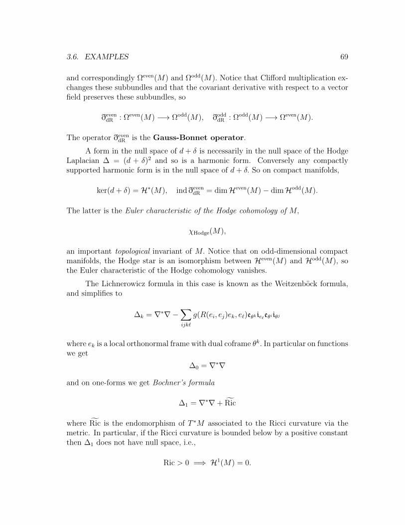
3.6. EXAMPLES 69

and correspondingly Ωeven(M) and Ωodd(M). Notice that Clifford multiplication ex-changes these subbundles and that the covariant derivative with respect to a vectorfield preserves these subbundles, so

ðevendR : Ωeven(M) −→ Ωodd(M), ðodd

dR : Ωodd(M) −→ Ωeven(M).

The operator ðevendR is the Gauss-Bonnet operator.

A form in the null space of d+ δ is necessarily in the null space of the HodgeLaplacian ∆ = (d + δ)2 and so is a harmonic form. Conversely any compactlysupported harmonic form is in the null space of d+ δ. So on compact manifolds,

ker(d+ δ) = H∗(M), indðevendR = dimHeven(M)− dimHodd(M).

The latter is the Euler characteristic of the Hodge cohomology of M,

χHodge(M),

an important topological invariant of M. Notice that on odd-dimensional compactmanifolds, the Hodge star is an isomorphism between Heven(M) and Hodd(M), sothe Euler characteristic of the Hodge cohomology vanishes.

The Lichnerowicz formula in this case is known as the Weitzenbock formula,and simplifies to

∆k = ∇∗∇−∑ijk`

g(R(ei, ej)ek, e`)eθk ie`eθiiθj

where ek is a local orthonormal frame with dual coframe θk. In particular on functionswe get

∆0 = ∇∗∇

and on one-forms we get Bochner’s formula

∆1 = ∇∗∇+ Ric

where Ric is the endomorphism of T ∗M associated to the Ricci curvature via themetric. In particular, if the Ricci curvature is bounded below by a positive constantthen ∆1 does not have null space, i.e.,

Ric > 0 =⇒ H1(M) = 0.


3.6.2 The signature operator

Now consider the complexification of the differential forms on M,

Λ∗CT∗M = Λ∗T ∗M ⊗ C

and the corresponding space of sections, Ω∗C(M). Clifford multiplication is as before,but now we can allow complex coefficients,

cl (ω) = 1i(eω − iω]),

this is compatible with both the Riemannian metric on Λ∗CT∗M (extended to a

Hermitian metric) and the Levi-Civita connection, and we have

icl ∇ = d+ δ.

Since Λ∗CT∗M is a complex Clifford module, we have an involution given by

Clifford multiplication by the chirality operator Γ. One can check that, up to a factorof i, Γ coincides with the Hodge star,

cl (Γ) : ΩkC(M) −→ Ωm−k

C (M), cl (Γ) = ik(k−1)+12

dimM ∗ .

If M is even dimensional, this induces a Z2 grading of Λ∗CT∗M as a Dirac bundle,

Λ∗CT∗M = Λ∗+T

∗M ⊕ Λ∗−T∗M.

The de Rham operator splits as

d+ δ =

(0 ð−sign

ð+sign 0

)and we refer to ð+

sign as the Hirzebruch signature operator.

The index of this operator

indð+sign = dim ker ð+

sign − dim ker ð−sign

is again an important topological invariant of M. It is always zero if dimM is not amultiple of four, and otherwise it is equal to the signature of the quadratic form

H12

dimM(M) // C

u //∫Mu ∧ u

It is called the signature of M, sign(M).

3.6. EXAMPLES 71

3.6.3 The Dirac operator

If E −→ M is a complex Clifford module over manifold M of even dimension, saym = 2k, then Clifford multiplication

cl : Cl(T ∗M, g) −→ End(E)

is, for each p ∈M, a finite dimensional complex representation of Cl(2k) on Ep. Wecan decompose Ep in terms of the unique irreducible representation of Cl(T ∗pM), /∆,

Ep = /∆⊗ HomCl(2k)( /∆, Ep).

If it happens that Ep = /∆ as Clifford modules for all p ∈ M we say that E is aspinC bundle over M. If a spinC bundle satisfies the symmetry condition

HomCl(T ∗M)(E,E) is trivial

we say that E is a spin bundle over M. We will generally denote a spin bundleover M by

/S −→M.

Remark 5. In the interest of time we have avoided talking about principal bundlesand structure groups and hence also spin structures and spinC structures. In brief,the structure group of a Rk-vector bundle is GLk(R) because the transition mapsbetween trivializations are valued in GLk(R). If we choose a metric on the bundlethen we can restrict attention to trivializations where the transition maps are valuedin O(n), and if we choose an orientation we can use oriented frames and reduce thestructure group to SO(n). It turns out that a double cover of SO(n) is a Lie groupcalled the spin group Spin(n). (We can identify Spin(n) with the multiplicativegroup of invertible elements in Cl(even)(Rn, gRn).) If the structure group of the tangentbundle of a manifold M can be ‘lifted’ to Spin(n) we say that M admits a spinstructure, and we can combine a spin structure with the spin representation toobtain a spin bundle. The group SpinC(n) is the subgroup of Cl(Rk, gRk) generatedby Spin(n) together with the unit complex numbers. If the structure group of thetangent bundle of a manifold M can be ‘lifted’ to SpinC(n) we say that M admits aspinC structure, and we can combine a spinC structure with the spin representationto obtain a spinC bundle. For details we refer to any of the books in the bibliographyof this lecture.

There are topological obstructions to the existence of a spin bundle over amanifold M and the number of spin bundles when they do exist is also determinedtopologically6. For example, a genus g Riemann surface admits 22g distinct spin

6For a thorough discussion see Lawson, H. Blaine, Jr. and Michelsohn, Marie-LouiseSpin geometry. Princeton Mathematical Series, 38. Princeton University Press, Princeton, NJ,1989.


bundles. All spheres in dimension greater than two admit spin bundles. All compactorientable manifolds of dimension three or less admit spin bundles. The complexprojective space CPk admits a spin bundle if and only if k is odd. Additionally, any(almost) complex manifold has a spinC bundle.

The Riemannian metric and Levi-Civita connection induce the structure ofa Dirac bundle on any spin bundle. Indeed, we saw above that the metric on a2k-dimensional vector space V with positive quadratic form induces a metric on thecorresponding /∆ so it suffices to describe the induced compatible connection. In alocal coordinate chart U that trivializes T ∗M, if we choose an orthonormal frameθ1, . . . , θm for TM

∣∣U , the Levi-Civita connection is determined by an m×m matrix

of one-forms ω defined through

∇θi = ωijθj.

(The fact that the connection respects the metric is reflected in ωij = −ωji.) We canuse ω to define a one-form valued in End(/S)

∣∣U , namely

ω =1

2

∑i<j

ωijcl(θi · θj

)and the induced connection on /S over U is given by d + ω. One can check thatthis local description does define a connection on /S which then must be metric andClifford.

The resulting generalized Dirac operator is called the Dirac operator (associ-ated to the spin bundle /S)

ð : C∞(M ; /S) −→ C∞(M ; /S).

As before Clifford multiplication by the chirality operator Γ defines an involutionexhibiting a Z2-grading on /S,

/S = /S+ ⊕ /S

−,

and a corresponding splitting of the Dirac operator

ð =

(0 ð−ð+ 0

).

The Lichnerowicz formula for the Dirac operator is particularly interestingsince there is no twisting curvature, so we get

ð2 = ∆∇ +1

4scalM .

3.6. EXAMPLES 73

Thus if the metric has positive scalar curvature then ð2 is strictly positive and inparticular does not have null space. We will show that the index of ð+ is a topologicalinvariant. Thus the vanishing of indð+ is a topological necessary condition for theexistence of a metric of positive scalar curvature7 on M.

3.6.4 Twisted Clifford modules

If E −→M is a Dirac bundle and F −→M is any Hermitian bundle with a unitaryconnection, then E⊗F −→M is again a Dirac bundle if we take the tensor productmetric and connection and extend Clifford multiplication to E⊗F by acting on thefirst factor. We say that this is the Dirac bundle E twisted by F.

If M admits a spin bundle /S −→ M, then any Dirac bundle E −→ M is atwist of /S. Indeed, we have

E = /S ⊗ HomCl(T ∗M)(/S,E).

In the case of a twisted spin bundle /S ⊗ F −→M, the ‘twisting curvature’ inthe Lichnerowicz formula is precisely the curvature of the connection on F.

The index of a twist of the signature operator is known as a twisted signa-ture. Twisted Dirac and twisted signature operators play an important role in theheat equation proof of the index theorem.

For example if M admits a spin bundle /S −→ M then the Clifford moduleΛ∗T ∗M ⊗ C must be a twist of /S, and indeed

Λ∗CT∗M ∼= Cl(T ∗M) ∼= End(/S) = /S

∗ ⊗ /S.

The generalized Dirac operator d + δ on Λ∗CT∗M is the twisted Dirac operator

obtained by twisting /S with /S∗. The two different Z2 gradings correspond to whether

we treat /S∗

as a Z2-graded bundle (which yields the splitting into ΛevenC T ∗M and

ΛoddC T ∗M) or as an ungraded bundle (which yields the splitting into Λ∗+T

∗M andΛ∗−T

∗M).

3.6.5 The ∂ operator

A real manifold M of dimension m = 2k is a complex manifold if it has a collectionof local charts parametrized by open sets in Ck for which the transition charts are

7In contrast, any manifold of dimension at least three admits a metric of constant negative scalarcurvature, see Aubin, Thierry Metriques riemanniennes et courbure. J. Differential Geometry4, 1970, 383-424. The same is true for manifolds with boundary and for non-compact manifolds.For compact surfaces, the sign of the integral of the scalar curvature is topologically determinedby the Gauss-Bonnet theorem.


holomorphic. This yields a decomposition of the complexified tangent bundle

TM ⊗ C = T 1,0M ⊕ T 0,1M, v ∈ T (1,0)p M ⇐⇒ v ∈ T 0,1

p M.

By duality there is a similar decomposition of the cotangent bundle

T ∗M ⊗ C = Λ1,0M ⊕ Λ01,M.

In local complex coordinates, z1, . . . , zm, which we can decompose into real andimaginary parts zj = xj + iyj. We can define

dzj = dxj + idyj, dzj = dxj − idyj

and then Λ1,0M is spanned by dzj and Λ0,1M is spanned by dzj.More generally we set

Λp,qM = Λp(Λ1,0M) ∧ Λq(Λ0,1M)

and we have a natural isomorphism

ΛkT ∗M ⊗ C =⊕p+q=k

Λp,qM.

We denote the space of sections of Λp,qM by Ωp,qM, and speak of forms of bidegree(p, q).

The exterior derivative naturally maps

d : Ωp,qM −→ Ωp+1,qM ⊕ Ωp,q+1M

and we can decompose it into the Dolbeault operators

d = ∂ + ∂

∂ : Ωp,qM −→ Ωp+1,qM, ∂ : Ωp,qM −→ Ωp,q+1M.

It follows from d2 = 0 that

∂2 = ∂2

= ∂∂ + ∂∂ = 0

and from the Leibnitz rule for d that

∂(ω ∧ η) = ∂ω ∧ η + (−1)|ω|ω ∧ ∂η∂(ω ∧ η) = ∂ω ∧ η + (−1)|ω|ω ∧ ∂η.

3.6. EXAMPLES 75

In local coordinates, for ω ∈ Ωp,qM

ω =∑

|J |=p,|K|=q

αJKdzJ ∧ dzK =⇒

∂ω =∑

|J |=p,|K|=q,`

αJK∂z`

dz` ∧ dzJ ∧ dzK , and ∂ω =∑

|J |=p,|K|=q,`

αJK∂z`

dz` ∧ dzJ ∧ dzK .

The Dolbeault complex is given by

(3.8) 0 −→ Ω0,0M∂−−→ Ω0,1M

∂−−→ . . .∂−−→ Ω0,mM −→ 0

and its cohomology is called the Dolbeault cohomology of M. We define the Hodge-Dolbeault cohomology to be

H0,q(M) = ω ∈ Ω0,pM : (∂∂∗

+ ∂∗∂)ω = 0.

As in the real case, we will show below that the Hodge-Dolbeault cohomology coin-cides with the Dolbeault cohomology.

A complex Hermitian manifold M is a Kahler manifold if the splitting

TM ⊗ C = T 1,0M ⊕ T 0,1M

is preserved by the Levi-Civita connection. On a Kahler manifold, the bundle

Λ0,∗M =⊕k

Λ0,kM

is a Dirac bundle with respect to the Hermitian metric on M, the Levi-Civita con-nection, and the Clifford multiplication

cl (ω) =√

2 (eω0,1 − i(ω1,0)]).

The corresponding generalized Dirac operator is

√2 (∂ + ∂

∗).

There is a natural Z2 grading on Λ0,∗M given by

Λ0,∗M = Λ0,evenM ⊕ Λ0,oddM.

The index of the corresponding non-self-adjoint operator is the Euler characteristicof the Hodge-Dolbeault cohomology.


3.7 Exercises

Exercise 1.a) Show that the scalar linear differential operators on Rm form a (non-commutative)algebra. Verify that the commutator PQ−QP of a differential operator of order `and a differential operator of order `′ has at most order `+ `′ − 1.b) Show that the linear differential operators with constant coefficients form a com-mutative subalgebra which is isomorphic to the polynomial algebra R[ξ1, . . . , ξm].

Exercise 2.Verify that for P ∈ Diffk(M ;E,F ) and Q ∈ Diff`(M ;F,G), the operator PQ is inDiffk+`(M ;E,G) and its principal symbol satisfies σk+`(P Q) = σk(P ) σ`(Q).

Exercise 3.Let E −→ M and F −→ M be bundles endowed with metrics, lying over theRiemannian manifold M. Verify that the formal adjoint of P ∈ Diffk(M ;E,F ), P ∗,is an element of Diffk(M ;F,E) and its principal symbol satisfies σk(P

∗) = σk(P )∗.

Exercise 4.Let M be a Riemannian manifold with boundary, and E −→ M, and F −→ Mbundles endowed with bundle metrics. The formal adjoint of an operator P :C∞(M ;E) −→ C∞(M ;F ) is defined by requiring

〈Pσ, τ〉F = 〈σ, P ∗τ〉E, for all σ ∈ C∞c (M;E), τ ∈ C∞c (M;F ).

Let ν be the inward-pointing unit normal vector field at the boundary. Definedvol∂M by iν dvolM

∣∣∂M. Show that if P ∈ Diff1(M ;E,F ) is a first-order differential

operator then

〈Pσ, τ〉F − 〈σ, P ∗τ〉E =

∫∂M

gF (iσ1(P )(p, ν[)σ, τ) dvol∂M ,

for all σ ∈ C∞c (M ;E), τ ∈ C∞c (M ;F ).

Hint: Use a partition of unity to reduce to a coordinate chart, then compute in localcoordinates.

Exercise 5.Show that End(Cm) has no proper two-sided ideals.Hint: Suppose M0 belongs to such an ideal I and v0 6= 0 belongs to the range ofM0. Show that every v ∈ Cm belongs to the range of some M ∈ I, and hence thatevery one-dimensional projection belongs to I.Exercise 6.a) Suppose a compact oriented manifold M has non-negative Ricci curvature – i.e.,

that g(Ric(ω), ω) ≥ 0 for all ω ∈ Ω1(M). Show that every harmonic one-form η sat-isfies ∇η = 0. As this is a first order differential equation for η, a harmonic one-form

3.7. EXERCISES 77

is determined by its ‘initial condition’ at a point in M. Conclude that, if M is alsoconnected, dimH1(M) ≤ dimM.b) Show that on any connected compact oriented Riemannian manifold dimH0(M) =1 and so by Poincare duality dimHm(M) = 1.c) From (b), we see that on a compact oriented Riemannian surface (i.e., two dimen-sional manifold) χHodge(M) = 2−dimH1(M). Show that if M is a compact orientedsurface admitting a metric of non-negative Gaussian curvature then χHodge(M) ≥ 0.(It turns out that only the sphere and the torus have non-negative Euler character-istic.)

Exercise 7.Let M and M ′ be compact oriented Riemannian manifolds.i)Show that

dimHk(M ×M ′) =k∑j=0

(dimHj(M))(dimHk−j(M ′))

whenM×M ′ is endowed with the product metric (we will soon show that dimHk(M)is independent of the choice of metric).ii) Conclude that

χHodge(M ×M ′) = χHodge(M)χHodge(M′).

Hint: Use the fact that ΛkT ∗(M ×M ′) =⊕k

j=0(ΛjT ∗M) ∧ (Λk−jT ∗M ′), show thatwith respect to this decomposition the Hodge Laplacian for the product metricsatisfies

∆k,M×M ′ =k∑j=0

(∆j,M ⊗ Id + Id⊗∆k−j,M ′),

and conclude that if

αj1, . . . , αjbj(M) is a basis of Hj(M) and βj1, . . . , β

jbj(M ′)

is a basis of Hj(M ′)

then αjs ⊗ βk−jt : 0 ≤ j ≤ k is a basis of Hk(M ×M ′).

Exercise 8.Let M and M ′ be compact oriented Riemannian manifolds.Show that signature is multiplicative,

sign(M ×M ′) = sign(M)sign(M ′),

where the signature on M ×M ′ is defined using the product metric (we will soonshow that the signature is independent of the choice of metric).Hint: Express dM×M ′ and δM×M ′ in terms of dM , δM , dM ′ , and δM ′ . Choose bases ofΛ±T

∗M and Λ±T∗M ′ and use them to construct bases of Λ±T

∗(M ×M ′).


Exercise 9.We can interpret any vector field V on M as a first order differential operator. Whatis its principal symbol?

Exercise 10.Let E −→ M and F −→ M be two vector bundles over M. Show that, for anyk ∈ N, the assignment U 7→ Diffk(M ;E

∣∣U , F

∣∣U) is a sheaf on M.

3.8 Bibliography

The books Spin geometry by Lawson and Michelson, and Heat kernels and Diracoperators by Berline, Getzler, and Vergne treat Dirac operators in detail.Other good sources are Elliptic operators, topology and asymptotic methods by Roewhich gives a very nice short treatment of many of the topics of this course, andvolume two of Partial differential equations by Taylor.

There is also a very nice treatment of these topics in Melrose, The Atiyah-Patodi-Singer index theorem, where they are systematically extended to non-compactmanifolds with asymptotically cylindrical ends.

Lecture 4

Pseudodifferential operators on Rm

4.1 Distributions

It is an unfortunate fact that most functions are not differentiable. Happily, thereis a way around this through duality. For instance, if f ∈ C∞(R)1 and φ ∈ C∞c (R)then ∫

Rf ′(t)φ(t) dt = −

∫Rf(t)φ′(t) dt

and the right hand side makes sense even if f is not differentiable. So for a possiblynon-differentiable f we will say that a function h is a weak derivative of f if∫

Rf(t)φ′(t) dt = −

∫Rh(t)φ(t) dt, for all φ ∈ C∞c (R).

Obviously if f is differentiable then f ′ is its weak derivative. Generally the takingof weak derivatives will force us to expand our notion of ‘function’.

For example, for f(t) = |t| we have, for any φ ∈ C∞c (R),∫Rf(t)φ′(t) dt = −

∫ 0

−∞tφ′(t) dt+

∫ ∞0

tφ′(t) dt

= −[tφ(t)]0−∞ +

∫ 0

−∞φ(t) + [tφ(t)]∞0 −

∫ ∞0

φ(t) dt = −∫R

sign(t)φ(t) dt

where sign(t) is the function equal to −1 for negative t and equal to 1 for positivet. Notice that f is continuous but its weak derivative is not. If we want to take a

1As in the previous chapter, we will work with complex valued functions and complex vectorbundles. Thus for instance the symbol C∞(M) will now mean C∞(M ;C).

79

80 LECTURE 4. PSEUDODIFFERENTIAL OPERATORS ON RM

second weak derivative we compute∫R

sign(t)φ′(t) dt = −∫ ∞

0

φ′(t) +

∫ ∞0

φ′(t) dt = −[φ(t)]0∞ + [φ(t)]∞0 = −2φ(0).

This shows that the weak derivative of of sign(t) is a multiple of the Dirac delta‘function’, δ0, defined by∫

Rφ(t)δ0(t) dt = φ(0), for all φ ∈ C∞c (R).

Of course there is no function satisfying the definition of the delta function.Instead we should think of δ0 as a linear functional

δ0 : C∞c (R) −→ C, δ0(φ) = φ(0).

This is the motivating example of a distribution.

A distribution on Rm is a continuous linear functional on smooth functionsof compact support,

T : C∞c (Rm) −→ C.

Continuity here means that for every compact set K ⊆ Rm there are constants Cand ` satisfying

|T (φ)| ≤ C∑|α|≤`

supK|∂αφ| for all φ ∈ C∞c (K).

Similarly, let (M, g) be an oriented Riemannian2 manifold. A distributionon M is a continuous linear functional on smooth functions of compact support,

T : C∞c (M) −→ C,

such that for every compact set K ⊆M there are constants C and ` satisfying

|T (φ)| ≤ C∑|α|≤`

supK|∇αφ|g for all φ ∈ C∞c (K).

We will denote3 the set of distributions by C−∞(M). If the same integer ` can beused for all compact sets K, we say that T is of order `. (A distribution of order `

2We do not need to have a Riemannian metric or an orientation to define the space of distribu-tions. It does make things simpler, though, since we can use the Riemannian volume form to carryout integrations (really to trivialize the ‘density bundle’) and the gradient to measure regularity.

3In the literature one often finds the set of distributions denoted D′(M). This is because LaurentSchwartz, who first defined distributions, denoted the smooth functions of compact support byD(M).

4.1. DISTRIBUTIONS 81

has a unique extension to a continuous linear functional on C`c(M), but we shall notuse this.)

We can restate the continuity condition in terms of sequences: A linear func-tional T on C∞(M) is a distribution if and only if whenever φj ∈ C∞c (M) is asequence supported in a fixed compact subset of M that is converging uniformly tozero together with all of its derivatives, we have T (φj) −→ 0.

The Hermitian pairing that the metric induces on C∞(M ;C) yields an inclusion

C∞(M) // C−∞(M)

h // Th

Th(φ) = 〈φ, h〉 =

∫M

φ(p)h(p) dvol for all φ ∈ C∞c (M).

indeed, any smooth function h ∈ C∞(M) naturally induces a distribution (of orderzero) Th

Th(φ) = 〈φ, h〉 =

∫M

φ(p)h(p) dvol for all φ ∈ C∞c (M).

More generally, we get a distribution (of order zero) Th, from any function h forwhich the pairing 〈φ, h〉 can be guaranteed to be finite,

L1loc(M) = h measurable : 〈φ, h〉 <∞ for all φ ∈ C∞c (M).

Similarly, any measure on M, µ, defines a distribution Tµ of order zero

Tµ(φ) =

∫M

φ dµ for all φ ∈ C∞c (M).

The converse is true as well4, any distribution of order zero is a measure on M. Anexample of a distribution that is not a measure is

T (φ) = φ′(0) for all φ ∈ C∞c (M).

As a very convenient abuse of notation, the pairing between a smooth functionof compact support f and a distribution T is denoted

〈·, ·〉 : C∞c (M)× C−∞(M) −→ C〈φ, T 〉 = T (φ)

and then in another abuse we identify Th and h.

4See Theorem 2.1.6 of Lars Hormander, The analysis of linear partial differential operators. I.Distribution theory and Fourier analysis. Classics in Mathematics. Springer-Verlag, Berlin, 2003.


Now we can proceed to extend many concepts and operations of C∞(M) toC−∞(M) by duality using the pairing 〈·, ·〉. For instance, we can multiply a distribu-tion T by a smooth function f ∈ C∞(M) by defining

〈φ, fT 〉 = 〈φf, T 〉, for all φ ∈ C∞c (M).

We say that a distribution T vanishes on an open set U if

〈φ, T 〉 = 0, for all φ ∈ C∞c (U).

The support of a distribution supp(T ) is the set of points in M having noneighborhood on which T vanishes. Equivalently, a point ζ is not in the supportof T if there is a neighborhood of ζ on which T vanishes. The distributions ofcompact support will be denoted5 C−∞c (M). A distribution of compact supportcan be evaluated not just on functions of compact support but on all of C∞(M). Infact, distributions of compact support form the continuous dual of the space C∞(M).

Although it makes no sense to talk about the value of a distribution at a point,we can restrict a distribution to an open set U by restricting its domain to functionswith compact support in U . We say that two distributions S and T coincide on anopen set U if

〈φ, S〉 = 〈φ, T 〉 for all φ ∈ C∞c (U).

If on each set of an open cover of M we have a distribution, and these distributionscoincide on overlaps, then we can use a partition of unity to construct a distributionthat restricts to the given ones. It is also true that two distributions coincide if andonly if they coincide on open sets covering M.

A closely related concept to the support of a distribution is that of the singu-lar support of a distribution sing supp(T ), defined by specifying its complement:a point ζ ∈ M is not in the singular support of T if there is a smooth function fthat coincides with T in a neighborhood of ζ.

We can apply a linear operator F to T by using its formal adjoint F ∗,

〈φ, F (T )〉 = 〈F ∗(φ), T 〉, for all φ ∈ C∞c (M).

In particular, we can apply a differential operator to a distribution, e.g.,

〈φ,∆T 〉 = 〈∆φ, T 〉, for all φ ∈ C∞c (M).

The weak derivatives we discussed above are computed in exactly this way. Thus ageneral function in, say, L1(M) is not differentiable as a function, but is infinitelydifferentiable as a distribution!

5Schwartz’ notation was E ′(M), and one often finds this in the literature.

4.1. DISTRIBUTIONS 83

If E −→M is a vector bundle over M we define distributional sections of Eto be continuous linear functionals on C∞c (M ;E∗). As above, there is a natural wayof thinking of a smooth section τ of E as a distributional section Tτ of E, namely

Tτ (ω) =

∫M

ω(τ) dvolM , for all ω ∈ C∞c (M ;E∗).

If we assume that E is endowed with a metric, gE, we can identify E with E∗ andidentify distributional sections of E with continuous linear functionals on C∞c (M ;E).We can then extend our abuse of notation and denote the evaluation of a distributionT on a compactly supported section σ by

〈σ, T 〉E = T (σ)

and also denote Tτ merely by τ.

All of the operations on distributions mentioned above extend to distributionalsections. In particular we can talk about the support of a distributional section andthen the distributional sections of compact support, C−∞c (M ;E). These distributionshave a simple description

C−∞c (M ;E) = C−∞c (M) ⊗C∞(M)

C∞(M ;E).

Indeed, every simple tensor

T ⊗ σ ∈ C−∞c (M) ⊗C∞(M)

C∞(M ;E)

defines an element in the dual to C∞(M ;E∗) by

(T ⊗ σ)(ω) = T (ω(σ)), for all ω ∈ C∞(M ;E∗),

and so we have an inclusion C−∞c (M)⊗C∞(M) C∞(M ;E) −→ C−∞c (M ;E). To seethat this map is surjective, start with S ∈ C−∞c (M ;E) and note that S defines,given any section ω ∈ C∞(M ;E∗), a compactly supported distribution on M via

C∞(M) 3 φ 7→ S(φω) ∈ C.

Since the support of S is compact, we can cover it with finitely many sets Ui thattrivialize E∗, choose si1, . . . , sik trivializing sections of E∗ supported in Ui, andthen write

S(ω) = S(∑i,j

ωijsij) =∑i,j

S(sij)(ω(sij))

=

(∑i,j

S(sij)⊗ sij

)(ω), for all ω ∈ C∞(M ;E∗).


4.2 Examples

4.2.1 Fundamental solutions

Let P be a constant coefficient differential operator on Rm, P ∈ Diffk(Rm),

P =∑|α|≤k

aα(x)Dα.

We say that a distribution Q ∈ C−∞(Rm) is a fundamental solution of thedifferential operator P if

PQ = δ0.

Two fundamental solutions will differ by an element of the null space of P.

We have already seen that, in R, ∂2x|x| = −2δ0, hence

−12|x| is a fundamental solution of ∆ = −∂2

x.

On Rm, the fundamental solution of the Laplacian is given by

Qm =

(2π)−1 log |x| if m = 2

− 1(m−2) Vol(Sm−1)

|x|2−m if m > 2

Indeed, note that on |x| > 0, ∆Qm = 0, so we can write, for any φ ∈ C∞c (Rm),

〈φ,∆Qm〉 = 〈∆φ,Qm〉 = limε→0

∫|x|>ε

Qm∆φ dx

= limε→0

∫|x|>ε

Qm∆φ− φ∆Qm dx = − limε→0

∫|x|=ε

Qm∂rφ− φ∂rQm dS

=

− lim

ε→0

∫|x|=ε

log ε∂rφ− φε−1

2πdS if m = 2

− limε→0

∫|x|=ε

ε2−m∂rφ− φ(2−m)ε1−m

(2−m) Vol(Sm−1)dS if m > 2

= φ(0)

where in the fourth equality we have used Green’s formula.

If we identify R2 with C by identifying (x, y) with z = x+ iy then the operator

∂ = 12(∂x + i∂y)

on complex valued functions has as null space the space of holomorphic functions.A similar application of Green’s theorem allows us to identify 1

πzas a fundamental

solution for ∂.

4.2. EXAMPLES 85

4.2.2 Principal values and finite parts

Let us see a few more examples of distributions. The function x 7→ xα is locallyintegrable on R if α > −1. For α = −1 we define the (Cauchy) principal value of1x, PV( 1

x) ∈ C−∞(R) by

〈φ,PV( 1x)〉 = lim

ε→0

∫|x|>ε

φ(x)

xdx =

∫ ∞0

φ(x)− φ(−x)

xdx

=

∫ ∞0

∫ 1

−1

φ′(tx) dt dx, for all φ ∈ C∞c (R).

This is indeed an element of C−∞(R), since whenever suppφ ⊆ [−C,C] we have∣∣∣∣∫ ∞0

∫ 1

−1

φ′(tx) dt dx

∣∣∣∣ ≤ 2C sup |φ′|,

so PV( 1x) is a distribution of order at most one (in fact of order one). Notice that

xPV( 1x) = 1 since, for any φ ∈ C∞c (R),

〈φ, xPV( 1x)〉 = 〈xφ,PV( 1

x)〉 = lim

ε→0

∫|x|>ε

φ(x)x

xdx =

∫φ(x) dx = 〈φ, 1〉.

It is then easy to see that

T ∈ C−∞(R), xT = 1 =⇒ T = PV( 1x) + Cδ0, C ∈ C.

so in this sense PV( 1x) is a good replacement for 1

xas a distribution.

What about higher powers of x−1? Simply taking the principal value will notwork for x−2 since we have∫

|x|>ε

φ(x)

x2dx =

∫x>ε

φ(x) + φ(−x)

x2dx =

2φ(0)

ε+ ( bounded )

so instead we define the (Hadamard) finite part of x−2, FP( 1x2 ) by

〈φ,FP( 1x2 )〉 = lim

ε→0

∫|x|>ε

φ(x)− φ(0)

x2dx =

∫ ∞0

φ(x)− 2φ(0) + φ(−x)

x2dx

=

∫ ∞0

(∫ 1

0

s

∫ 1

−1

φ′′(stx) dt ds

)dx, for all φ ∈ C∞c (R).

As before, this is clearly a distribution of order at most two and we have

T ∈ C−∞(R), x2T = 1 =⇒ T = FP( 1x2 ) + C0δ0 + C1∂xδ0, C0, C1 ∈ C.


We can continue this and define FP( 1xn

) for any n ∈ N, n ≥ 2, by

〈φ,FP( 1xn

)〉 = limε→0

∫|x|>ε

φ−∑n−2

k=01k!φ(k)(0)xk

xndx.

This defines a distribution of order at most n and moreover

T ∈ C−∞(R), xnT = 1 =⇒ T = FP( 1xn

) +n−1∑k=0

Ci∂(k)x δ0, Ci ⊆ C.

One can similarly define finite parts of non-integer powers of x and also define finiteparts in higher dimensions.

4.3 Tempered distributions

On Rm, the class of Schwartz functions S(Rm) sits in-between the smooth functionsand the smooth functions with compact support

C∞c (Rm) ⊆ S(Rm) ⊆ C∞(Rm)

S(Rm) =f ∈ C∞(Rm) : pα,β(f) = sup

Rm|xα∂βf | <∞, for all α, β

Correspondingly the dual spaces satisfy

C−∞c (Rm) ⊆ S ′(Rm) ⊆ C−∞(Rm)

S ′(Rm) =T ∈ C−∞(Rm) : pα,β(f)→ 0 for all α, β =⇒ T (fj)→ 0

.

The dual space of S, S ′(Rm), is known as the space of tempered distributions.

Notice that these inclusions are strict. Any Lp function will be in S ′(Rm) butwill only be in C−∞c (Rm) if it has compact support. On the other hand, the functione|x|

2defines a distribution in C−∞(Rm) but not a tempered distribution.

4.3.1 Convolution

The convolution of two functions in S(Rm) is

(f ∗ h)(x) =

∫Rm

f(x− y)h(y) dy =

∫Rm

h(x− y)f(y) dy = (h ∗ f)

and defines a bilinear map S(Rm)× S(Rm) −→ S(Rm). The commutativity is par-ticularly clear from the expression

〈φ, f ∗ h〉 =

∫ ∫f(x)h(y)φ(x+ y) dx dy,

4.3. TEMPERED DISTRIBUTIONS 87

which we can also write as

〈φ, f ∗ h〉 =

∫h(y)

∫f(x)φ(x+ y) dxdy =

∫h(y)

∫f(z − y)φ(z) dzdy

= 〈f ∗ φ, h〉, where f(x) = f(−x).

This allows us to use duality to define convolution of a tempered distribution witha Schwartz function

∗ : S(Rm)× S ′(Rm) −→ S ′(Rm)

〈φ, f ∗ S〉 = 〈f ∗ φ, S〉 for all f, φ ∈ S(Rm)

and similarly∗ : C∞c (Rm)× C−∞(Rm) −→ C−∞(Rm)

〈φ, f ∗ S〉 = 〈f ∗ φ, S〉 for all f, φ ∈ C∞c (Rm).

For instance, notice that we have

〈φ, f ∗ δ0〉 = 〈f ∗ φ, δ0〉 =

∫Rm

f(x)φ(x) dx = 〈φ, f〉

and so f ∗ δ0 = f for all f ∈ S(Rm).

If P is any constant coefficient differential operator, and f, h ∈ S(Rm) then

P (f ∗ h) = P (f) ∗ h = f ∗ P (h)

and so by duality we also have

P (f ∗ S) = P (f) ∗ S = f ∗ P (S), for all f ∈ S(Rm), S ∈ S ′(Rm).

Putting these last two observations together, suppose that S ∈ S ′(Rm) isa fundamental solution of the constant coefficient differential operator P, so thatP (S) = δ0, then we have

P (f ∗ S) = f ∗ P (S) = f ∗ δ0 = f, for all f ∈ S(Rm).

Thus a fundamental solution for P is tantamount to a right inverse for P, eventhough P is generally not invertible.

In particular, with Qm as above and m > 2 for simplicity,

u ∈ S ′(Rm), f ∈ S(Rm), and ∆u = f =⇒ u = f ∗Qm ∈ C∞(Rm)

u(x) =

∫Rm

Qm(x− y)f(y) dy =1

(2−m) Vol(Sm−1)

∫Rm

f(y)

|x− y|m−2dy(4.1)


Remark 6. We can also use convolution to prove that test functions are densein distributions, be they C−∞c , S ′, or C−∞. Indeed, first say that a sequence φn ∈C∞c (Rm) is an approximate identity if

φn ≥ 0,

∫Rdφn(x) dx = 1, φn(x) = 0 if |x| > 1

n,

and note that, as distributions, φn → δ0. Let χn ∈ C∞c (Rm) approximate the constantfunction one, and notice that, for any distribution S, the sequence

Sn ∈ C∞c (Rm), Sn(x) = χn(x)(φn ∗ S)(x)

converges as distributions to S.

4.3.2 Fourier transform

Recall that Fourier transform of a function f ∈ L1(Rm) is defined by

F : L1(Rm) −→ L∞(Rm)

F(f)(ξ) = f(ξ) =1

(2π)n/2

∫Rm

f(x)e−ix·ξ dx

and satisfies for f ∈ S(Rm),

F(∂xjf)(ξ) = iξjF(f)(ξ), ∂ξjF(f)(ξ) = −iF(xjf)(ξ).

To simplify powers of i, let us define Ds = 1i∂s so that these identities become

F(Dxjf)(ξ) = ξjF(f)(ξ), DξjF(f)(ξ) = −F(xjf)(ξ),

and indeed for any multi-indices α, β,

(4.2) ξαDβξF(f)(ξ) = (−1)|β|F(Dα

xxβf)(ξ).

In particular we have the very nice result that

F : S(Rmx ) −→ S(Rm

ξ ).

The formal adjoint of F , F∗, is defined by

〈F(f), h〉Rmξ = 〈f,F∗(h)〉Rmx , for all f, h ∈ C∞c (Rm)

and since we have

〈F(f), h〉Rmξ =

∫RmF(f)(ξ)h(ξ) dξ =

1

(2π)m/2

∫Rm×Rm

e−ix·ξf(x)h(ξ) dξdx


we conclude that

F∗(h)(x) =1

(2π)m/2

∫Rm

h(ξ)eix·ξ dξ.

Using the fact D∗j = Dj we find

(4.3) xαDβxF∗(φ)(x) = (−1)|α|F∗(Dα

ξ ξβφ)(x)

and henceF∗ : S(Rm

ξ ) −→ S(Rmx ).

Proposition 11 (Fourier inversion formula). As a map on S(Rm), the Fouriertransform F is invertible with inverse F∗.

Proof. We want to show that, for any f ∈ S(Rm) we have F∗(F(f)) = f, i.e.,∫eix·ξ

(∫e−iy·ξf(y) dy

)dξ = (2π)mf(x)

but note that the double integral does not converge absolutely and hence we cannot change the order of integration. We get around this by introducing a functionψ ∈ S with ψ(0) = 1, letting ψε(x) = ψ(εx) and then using Lebesgue’s dominatedconvergence theorem to see that

F∗(h) = limε→0F∗(ψεh).

Hence the integral we need to compute is given by

limε→0

∫eix·ξψ(εξ)

(∫e−iy·ξf(y) dy

)dξ = lim

ε→0

∫ ∫ei(x−y)·ξψ(εξ)f(y) dξ dy

= (2π)m/2 limε→0

∫f(y)ψ(y−x

ε) dyεm

= (2π)m/2 limε→0

∫f(x+ εη)ψ(η) dη

= (2π)m/2f(x)

∫ψ(η) dη.

If we take ψ(x) = e−|x|2/2, then ψ(η) = ψ(η) and

∫ψ(η) dη = (2π)m/2 so the result

follows. One can prove FF∗ = Id similarly.

We can extend the Fourier transform and its inverse to tempered distributionsin the usual way

F ,F∗ : S ′(Rm) −→ S ′(Rm)

〈φ,F(T )〉 = 〈F∗(φ), T 〉, 〈φ,F∗(T )〉 = 〈F(φ), T 〉 for all φ ∈ S(Rm)


and these are again mutually inverse and satisfy (4.2), (4.3).

In particular, we can compute that

〈φ,F(δ0)〉 = 〈F∗(φ), δ0〉 = F∗(φ)(0) =1

(2π)m/2

∫Rm

φ(x) dx = 〈φ, (2π)−m/2〉

so that F(δ0) = (2π)−m/2. Then, using (4.2) and (4.3), we can deduce that

F(Dαδ0) = (−1)|α|(2π)−m/2xα, F∗(1) = (2π)m/2δ0, F∗(xα) = (−1)|α|(2π)m/2Dαδ0.

Another consequence of Proposition 11 is that, for any φ ∈ S(Rm),

‖φ‖2L2 = 〈F(φ),F(φ)〉 = 〈F∗F(φ), φ〉 = 〈φ, φ〉 = ‖φ‖2

L2

thus F has a unique extension to an invertible map

F : L2(Rm) −→ L2(Rm)

and this map is an isometry – a fact known as Plancherel’s theorem.

The Fourier transform is a very powerful tool for understanding differentialoperators. Note that if P ∈ Diffk(Rm),

P =∑|α|≤k

aα(x)Dα,

and the coefficients aα(x) are bounded with bounded derivatives, then for any φ ∈S(Rm) (or even S ′(Rm)) we have

Pφ = F∗(p(x, ξ)Fφ)

with p(x, ξ) =∑|α|≤k

aα(x)ξα.

The polynomial p(x, ξ) is called the total symbol of P and will be denoted σtot(P ).One consequence which can seem odd at first is that a differential operator acts byintegration! Indeed, we have

(4.4) (Pφ)(x) = F∗(σtot(P )Fφ)(x) =1

(2π)m

∫ ∫ei(x−y)·ξp(x, ξ)φ(y) dy dξ

although note that this integral is not absolutely convergent.

Notice the commonality between (4.4) and (4.1). In each case we have a mapof the form

(4.5) A(f)(x) =

∫RmKA(x, y)f(y) dy

where f and KA, the integral kernel of A, may have low regularity. In fact, thisdescribes a very general class of maps.


Theorem 12 (Schwartz kernel theorem). Let M and M ′ be manifolds, E −→ Mand E ′ −→M ′ vector bundles, and let

HOM(E,E ′) −→M ×M ′

be the bundle whose fiber at (ζ, ζ ′) ∈M ×M ′ is Hom(Eζ , E′ζ′). If

A : C∞c (M ;E) −→ C−∞(M ′;E ′)

is a bounded linear mapping, there exists

KA ∈ C−∞(M ×M ′; Hom(E,E ′))

known as the Schwartz kernel of A or the integral kernel of A such that

〈ψ,A(φ)〉 = 〈ψ φ,KA〉

whereψ φ ∈ C∞c (M ×M ′), (ψ φ)(ζ, ζ ′) = ψ(ζ)φ(ζ ′).

We will not prove this theorem6 and we will not actually use it directly. Ratherwe view as an inspiration to study operators by describing their Schwartz kernels.In fact, it is common to purposely confuse an operator and its Schwartz kernel. Notethat if the integral kernel is given by a function, say KA ∈ L1

loc(M ×M ′), then A isgiven by (4.5).

A simple example is the kernel of the identity map

KId ∈ C−∞(M ×M), KId = δdiagM

and we abuse notation by writing

f(ζ) =

∫M

δdiagMf(ζ ′) dvol(ζ ′).

Note that on Rm we can also write its integral kernel in terms of the Fourier transform

(4.6) Id = F∗F =⇒ KId =1

(2π)m

∫Rm

ei(x−y)·ξ dξ.

Similarly we can write the kernel of a differential operator P ∈ Diff∗(M) as

KP ∈ C−∞(M ×M), KP = P ∗δdiagM

or, on Rm,

(4.7) KP =1

(2π)m

∫ei(x−y)·ξp(x, ξ) dξ.

6For a proof, see ...


4.4 Pseudodifferential operators on Rm

4.4.1 Symbols and oscillatory integrals

In both (4.6) and (4.7) we have integral kernels of the form

1

(2π)m

∫ei(x−y)·ξp(x, ξ) dξ

where p(x, ξ) is a polynomial in ξ of degree k and the integral makes sense as adistribution.

The way we define pseudodifferential operators is to take a similar integral,but replace p(x, ξ) with a more general function. Let U ⊆ Rm be a (regular7) openset and r ∈ R a real number. A function a ∈ C∞(U ×Rm) is a symbol of order ron U ,

a ∈ Sr(U)

if for all multi-indices α, β there is a constant Cα,β such that

supx∈U|Dα

xDβξ a(x, ξ)| ≤ Cα,β(

√1 + |ξ|2 )r−|β|.

Notice that the symbol condition is really only about the growth of a and itsderivatives as |ξ| → ∞. So we always have

Sr(U) ⊆ Sr′(U ;Rm) if r < r′

and, if a is smooth in (x, ξ) and compactly supported (or Schwartz) in ξ, then

a ∈⋂r∈R

Sr(U) = S−∞(U ;Rm).

For example, if r ∈ N then a polynomial of degree r is an example of a symbolof order r. Also, for arbitrary r ∈ R, we can take a function a(x, θ) defined for|θ| = 1, extend it to (x, ξ) with |ξ| > 1 by

a(r, ξ) = |ξ|ra(x, ξ|ξ|) for |ξ| > 1

and choose any smooth extension of a for |ξ| < 1 and we obtain a symbol of order r.

It is easy to see that pointwise multiplication defines a map

Sr1(U ;Rm)× Sr2(U ;Rm) −→ Sr1+r2(U ;Rm)

7Recall that an open set is regular if it is equal to the interior of its closure.

4.4. PSEUDODIFFERENTIAL OPERATORS ON RM 93

and that differentiation defines a map

DαxD

βξ : Sr(U) −→ Sr−|β|(U ;Rm).

Given a symbol a ∈ Sr(U), we will make sense of the oscillatory integral

(4.8)

∫ei(x−y)·ξa(x, ξ) dξ

as a distribution. If r < −m then the integral converges to a continuous function(equal to F∗ξ (a)(x, x− y)). Similarly if a ∈ S−∞(U) then the distribution is actuallya smooth function. In this case, the action of this distribution on φ ∈ C∞c (U) is

φ 7→ 1

(2π)m

∫ei(x−y)·ξa(x, ξ)φ(x) dξ dx.

Notice that

(1 + ξ ·Dx)ei(x−y)·ξ = (1 + |ξ|2)ei(x−y)·ξ

so for a ∈ Sr with r < −m and for any ` ∈ N we have∫ei(x−y)·ξa(x, ξ)φ(x) dξ dx =

∫(1 + |ξ|2)−`(1 + ξ ·Dx)

èi(x−y)·ξa(x, ξ)φ(x) dξ dx

=

∫ei(x−y)·ξ(1− ξ ·Dx)

`((1 + |ξ|2)−à(x, ξ)φ(x)) dξ dx

Moreover we have

(1− ξ ·Dx)`((1 + |ξ|2)−à(x, ξ)φ(x)) =

∑|α|≤`

aα(x, ξ)Dαxφ(x)

with each aα ∈ Sr−`(U). So for arbitrary r ∈ R and a ∈ Sr(U), we define thedistribution (4.8) on C∞c (U) by

φ 7→ 1

(2π)m

∫ei(x−y)·ξ(1− ξ ·Dx)

`((1 + |ξ|2)−à(x, ξ)φ(x)) dξ dx

where ` is any non-negative integer larger than r + m. We will continue to denotethis distribution by (4.8).

Alternately, we can interpret (4.8) as

φ 7→ limε→0

1

(2π)m

∫ei(x−y)·ξψ(εξ)a(x, ξ)φ(x) dξ dx


where ψ ∈ C∞c (Rm) is equal to one in a neighborhood of the origin. Then we cancarry out the integration by parts from the previous paragraph before taking thelimit.

For any open set U ⊆ Rm, and s ∈ R we define pseudodifferential operatorson U of order r in terms of their integral kernels

Ψr(U) =

K ∈ C−∞(U × U) : K =

1

(2π)m

∫ei(x−y)·ξa(x, ξ) dξ, for some a ∈ Sr(U)

.

The symbol a is known as the total symbol of the pseudodifferential operator.Given a ∈ Sr(U), there are several notations for the corresponding pseudodifferentialoperator, e.g.,

Op(a) and a(x,D).

Let us determine the singular support of K ∈ Ψr(U). The useful observationthat

(4.9) (x− y)αei(x−y)·ξ = Dαξ e

i(x−y)·ξ

shows that

(x− y)αK =1

(2π)m

∫(x− y)αei(x−y)·ξa(x, ξ) dξ

=1

(2π)m

∫(Dα

ξ ei(x−y)·ξ)a(x, ξ) dξ =

(−1)|α|

(2π)m

∫ei(x−y)·ξ(Dα

ξ a(x, ξ)) dξ

is an absolutely convergent integral whenever a ∈ Sr(U) for r < |α|−m and moreovertaking further derivatives shows that

(x− y)αK ∈ Cj(U × U) if r − |α| < −m− j

so we can conclude that sing suppK ⊆ diagU×U .

As with symbols, pseudodifferential operators are filtered by degree

Ψr(Rm) ⊆ Ψr′(Rm) if r < r′

and a special role is played by the operators of order −∞,

Ψ−∞(Rm) =⋂r∈R

Ψr(Rm).

Each a(x,D) ∈ Ψs(U) defines a continuous linear operator

a(x,D) : C∞c (U) −→ C−∞(U)

(a(x,D)φ)(x) =1

(2π)m

∫ ∫ei(x−y)·ξa(x, ξ)φ(y) dy dξ = F∗(a(x, ξ)F(φ)).


Proposition 13. For a ∈ Sr(U), the operator a(x,D) is a continuous map

(4.10) a(x,D) : C∞c (U) −→ C∞(U).

For a ∈ Sr(Rm), the operator a(x,D) also extends to a linear operator

a(x,D) : S(Rm) −→ S(Rm)

Proof. If a ∈ Sr(U) and φ ∈ C∞c (U) then, for every x, a(x, ξ)φ(ξ) is Schwartzfunction of ξ, hence the integral

a(x,D)(φ)(x) =

∫eix·ξa(x, ξ)φ(ξ) dξ

is absolutely convergent, and one can differentiate under the integral sign and thederivatives will also be given by absolutely convergent integrals. Similarly, whena ∈ Sr(Rm),

xαa(x,D)(φ) = (−1)α∫

(Dαξ e

ix·ξ)a(x, ξ)φ(ξ) dx = (−1)α∫eix·ξ(Dα

ξ a(x, ξ)φ(ξ)) dx

is absolutely convergent for every α.

The total symbol of a differential operator is a polynomial so it has an expan-sion

p(x, ξ) =k∑j=0

∑|β|=j

pβ(x)ξβ =k∑j=0

pj(x, ξ)

where each pj(x, ξ) is homogeneous

pj(x, λξ) = λjpj(x, ξ)

and a symbol of order j.

It turns out we can ‘asymptotically sum’ any sequence of symbols of decreasingorder.

Proposition 14 (Asymptotic completeness). Let U be an open subset of Rm, rjan unbounded decreasing sequence of real numbers and aj ∈ Srj(U). There existsa ∈ Sr0(U) such that, for all N ∈ N,

(4.11) a−N−1∑j=0

aj ∈ SrN (U)

which we denotea ∼

∑aj.


This is analogous to Borel’s lemma to the effect that any sequence of realnumbers can occur as the coefficients of the Taylor expansion of a smooth functionat the origin.

Proof. Let us write U as the union of an increasing sequence of compact sets Kj ⊆ U ,⋃j∈N

Ki = U , and Kj ⊆ Kj+1 for all i ∈ N.

Pick χ ∈ C∞(Rm, [0, 1]) vanishing on B1(0) and equal to one outside B2(0), pick asequence converging to zero, (εj) ⊆ R+, and set

a(x, ξ) =∞∑j=0

χ(εjξ)aj(x, ξ).

Note that on any ball |ξ| < R only finitely many terms of the sequence are non-zero, so the sum is a well-defined smooth function. We will see that by choosing εjdecaying sufficiently quickly, we can arrange (5.2).

To see that a(x, ξ) ∈ Sr0(U) we need to show that, for each α and β there isa constant Cα,β such that

|DαxD

βξ χ(εjξ)a(x, ξ)| ≤ Cα,β(

√1 + |ξ|2 )r0−|β|.

Let us estimate the individual terms in the sum

|DαxD

βξ χ(εjξ)aj(x, ξ)| ≤

∑γ+µ=β

|DαxD

γξ aj(x, ξ)|ε

|β|−|µ|j |(Dβ−µχ)(εjξ)|.

The term with γ = β is supported in |ξ| ≤ ε−1j and the other terms are supported

in ε−1j ≤ |ξ| ≤ 2ε−1

j . We can bound the former term by

Cα,β(aj)(√

1 + |ξ|2 )rj−|β| ≤ Cα,β(aj)(√

1 + |ξ|2 )r0−|β|(√

1 + ε−2j )rj−r0

≤ Cα,β(aj)εr0−rjj (

√1 + |ξ|2 )r0−|β|

and by similar reasoning we can bound the latter terms by

Cα,γ(aj)‖Dβ−µχ‖L∞εr0−rjj (

√1 + |ξ|2 )r0−|β|.

So altogether we have

|DαxD

βξ χ(εjξ)aj(x, ξ)| ≤ Cα,β(χaj)ε

r0−rjj (

√1 + |ξ|2 )r0−|β|.


for some constant Cα,β(χaj) independent of εj. Given L ∈ N we can choose a se-quence εj(L) so that

|α|+ |β| ≤ L =⇒ Cα,β(χaj)εr0−rjj (L) ≤ j−2

and hence

|α|+ |β| ≤ L =⇒ |DαxD

βξ χ(εj(L)ξ)aj(x, ξ)| ≤ j−2(

√1 + |ξ|2 )r0−|β|

and |DαxD

βξ a(x, ξ)| satisfies the bounds we need for |α|+ |β| ≤ L. By diagonalization

(taking εj = εj(j)) we can arrange the convergence of

(√

1 + |ξ|2 )−(r0−|β|)|DαxD

βξ a(x, ξ)|

for all α, β.

The same argument applies to show that∑j≥N

χ(εjξ)aj(x, ξ) ∈ SrN (U)

and hence that a ∼∑aj.

It is easy to see that if

a ∼∑

aj

then aj determine a up to an element of S−∞(U). Indeed, if b ∼∑aj then

a− b = (a−N−1∑j=0

aj)− (b−N−1∑j=0

aj) ∈ SrN (U)

for all N, hence a− b ∈ S−∞(U).

There is a further subset of symbols that imitates polynomials a little closer.We say that a symbol a ∈ Sr(U) is a classical symbol, a ∈ Srcl(U), if for eachj ∈ N there is a symbol ar−j ∈ Sr−j(U) homogeneous in ξ for |ξ| ≥ 1, i.e.,

ar−j(x, λξ) = λr−jar−j(x, ξ) whenever |ξ|, |λξ| ≥ 1,

and we have

a ∼∞∑j=1

ar−j.

We refer to ar as the principal symbol of a(x,D).


4.4.2 Amplitudes and mapping properties

In order to prove that pseudodifferential operators are closed under composition andadjoints, it is convenient to allow the symbol to depend on both x and y. Remarkably,this does not lead to a larger class of operators.

Let U ⊆ Rm be an open set, we say that a function b ∈ C∞(U ×U ×Rm) is anamplitude of order r ∈ R,

b ∈ Sr(U × U ;Rm)

if for any multi-indices α, β, γ, there is a constant Cα,β,γ such that

(4.12) supx,y∈U

|DαxD

βyD

γξ b(x, y, ξ)| ≤ Cα,β,γ(1 + |ξ|)r−|γ|.

Thus an amplitude is a symbol where there are twice as many ‘space’ variables (x, y)as there are ‘cotangent’ variables ξ.

An amplitude defines a distribution

φ 7→ 1

(2π)m

∫ei(x−y)·ξb(x, y, ξ)φ(y) dξ dy.

For fixed x this is a well-defined oscillatory integral in (y, ξ) by the discussion above.Since the estimates are uniform in x, this defines a continuous function in x. We willdenote the set of distributions with amplitudes of order r by

Ψr(U).

We clearly have Ψr(U) ⊆ Ψr(U), and we will soon show that Ψr(U) = Ψr(U).

We start by showing this is true for operators in

Ψ−∞(U) =⋂r∈R

Ψr(U).

Proposition 15. The following are equivalent:i) K ∈ Ψ−∞(U),ii) K = 1

(2π)m

∫ei(x−y)·ξa(x, ξ) dξ for some a ∈ S−∞(U),

iii) K ∈ C∞(U × U) and for every N ∈ N and multi indices α, β,

(4.13) supx,y∈U

|(1 + |x− y|)NDαxD

βyK(x, y)| <∞.

iv) K ∈ Ψ−∞(U).


Proof. Clearly, (ii) implies (i) and (i) implies (iv).

Let us check that (iv) implies (iii). By definition, K ∈ Ψ−∞(U) means that,for each r ∈ R, there is an amplitude br ∈ Sr(U × U ;Rm) such that

K(x, y) =1

(2π)m

∫ei(x−y)·ξbr(x, y, ξ) dξ.

Let us assume that r −m so that the integral converges absolutely and we canuse (4.9) and integrate by parts to find

(x− y)αDβxD

γyK(x, y) = (−1)|α|

1

(2π)m

∫ei(x−y)·ξ(Dx + iξ)β(Dy − iξ)γbr(x, y, ξ) dξ

which converges absolutely and uniformly in x, y provided |β| + |γ| + r < |α| −m.Thus (x− y)αDβ

xDγyK(x, y) is uniformly bounded.

Finally we show that (iii) implies (ii). If K satisfies (iii) then the functionL(x, z) = K(x, x− z) satisfies

sup |(1 + |z|)NDαxD

βzL(x, z)| <∞ for all N,α, β.

Thus L(x, z) is a Schwartz function in z with bounded derivatives in x. We can write

K(x, y) = L(x, x− y) =1

(2π)m/2

∫ei(x−y)·ξ(FzL)(x, ξ) dξ

and FzL ∈ S−∞(U) so we have (ii).

At the moment, the mapping property (4.10) is not good enough to allow us tocompose operators. We will need an extra condition on the support of the Schwartzkernels of pseudodifferential operators to guarantee that they preserve C∞c (U).

Let us say that a subset R ⊆ Rm×Rm is a proper support if the left and rightprojections

Rm × Rm −→ Rm,

restricted to R, are proper functions8. An example of a proper support is a compactset, a better example is a set R satisfying

R ⊆ (x, y, ξ) : d(x, y) ≤ ε

for any fixed ε > 0. We will say that a distribution K ∈ C−∞(Rm×Rm) is properlysupported if suppK is a proper support. We will say that an amplitude b(x, y, ξ) ∈C∞(Rm × Rm;Rm) is properly supported if

suppx,y b = closure of (x, y) : b(x, y, ξ) 6= 0 for some ξ

is a proper support.

8Recall that any continuous function maps compact sets to compact sets, while a function iscalled proper if the inverse image of a compact set is always a compact set.


Theorem 16. Let b(x, y, ξ) ∈ C∞(U × U ;Rm) be a properly supported amplitude oforder r. The operator

(4.14)

B : C∞c (U) −→ C−∞(U)

Bφ(x) =1

(2π)m

∫Rm

∫Uei(x−y)·ξb(x, y, ξ)φ(y) dy dξ

in fact mapsB : C∞c (U) −→ C∞c (U)

and induces maps

B : C∞(U) −→ C∞(U), B : C−∞(U) −→ C−∞(U),

and B : C−∞c (U) −→ C−∞c (U).

The formal adjoint of B is of the same form

B∗ : C∞c (U) −→ C−∞(U)

B∗φ(x) =1

(2π)m

∫Rm

∫Uei(x−y)·ξb(y, x, ξ)φ(y) dy dξ.

Moreover, B ∈ Ψr(U) and its total symbol has an asymptotic expansion

(4.15) a(x, ξ) ∼∑α

i|α|

α!(Dα

ξDαy b(x, y, ξ))

∣∣x=y

where for a multi-index α = (α1, . . . , αm), α! denotes α1! · · ·αm!.

Proof. First note that the description of the adjoint follows immediately from

〈Bφ, f〉 =1

(2π)m

∫Rm

∫U

∫Uei(x−y)·ξb(x, y, ξ)φ(y)f(x) dy dξ dx

=1

(2π)m

∫U

∫Rm

∫Uei(x−y)·ξb(x, y, ξ)f(x)φ(y) dx dξ dy

for all φ, f ∈ C∞c (U).

We see that B maps C∞c (U) into C∞(U) by the same argument as in Proposition13. However now if φ ∈ C∞c (U) and suppφ = K then we know that

π−1y (K) ∩ suppx,y b = K ′

is a compact set and it is immediate from (4.14) that suppB(φ) ⊆ K ′. Thus B :C∞c (U) −→ C∞c (U) and by the same argument

B∗ : C∞c (U) −→ C∞c (U).


By duality this means that B and B∗ also induce maps C−∞(U) −→ C−∞(U).

Let φ ∈ C∞(U), we know that Bφ is defined, but a priori this is a distribution.Let us check that Bφ is smooth, by checking that it is smooth on any compact setK ⊆ U . We know that

π−1y (K) ∩ suppx,y b = K ′

is also compact, so we can choose χ ∈ C∞c (U) such that χ(p) = 1 for all p ∈ K ′.Then, on K, we have Bφ = Bχφ so Bφ is smooth in the interior of K. This showsthat

B : C∞(Um) −→ C∞(Um)

and since B∗ is of the same form, B∗ : C∞(U) −→ C∞(U). Then by duality both Band B∗ induce maps C−∞c (U) −→ C−∞c (U).

Let us define

aj(x, ξ) =∑|α|=j

i|α|

α!(Dα

ξDαy b(x, y, ξ))

∣∣x=y

.

Note that aj ∈ Sr−j(Rm) so it makes sense to define a(x, ξ) to be a symbol obtainedby asymptotically summing

∑aj. We will be done once we show that B−a(x,D) ∈

Ψ−∞(U).

Recall from Taylor’s theorem that, for each ` ∈ N,

b(x, y, ξ) =∑|α|≤`−1

1

α!∂αy b(x, x, ξ)(y − x)α +

∑|α|=`

cα(x, y, ξ)(y − x)α

with cα(x, y, ξ) =

∫ 1

0

(1− t)`−1∂αy b(x, (1− t)x+ ty, ξ) dt

and note the important fact that ∂αy b(x, y, ξ), and cα(x, y, ξ) all satisfy (4.12). Using(4.9) and integrating by parts we find that

1

(2π)m

∫Rm

ei(x−y)·ξb(x, y, ξ) dξ =1

(2π)m

∫Rm

ei(x−y)·ξ

∑|α|≤`−1

1

α!Dαξ ∂

αy b(x, x, ξ)

dξ

+1

(2π)m

∫Rm

ei(x−y)·ξ

∑|α|=`

1

α!Dαξ ∂

αy cα(x, y, ξ)

dξ

=`−1∑j=1

1

(2π)m

∫Rm

ei(x−y)·ξaj(x, ξ) dξ +1

(2π)m

∫Rm

ei(x−y)·ξR`(x, y, ξ) dξ

where R`(x, y, ξ) satisfies (4.12) with r replaced by r − `.


By definition of a(x, ξ), we know that there is an element Q` ∈ Sr−`(U) suchthat

a(x,D) =`−1∑j=1

aj(x,D) +Q`(x,D)

and hence we know that

(4.16) B − a(x,D) = K(x, y) =1

(2π)m

∫Rm

ei(x−y)·ξ(R`(x, y, ξ)−Q`(x, ξ)) dξ

and R`(x, y, ξ) − Q`(x, ξ) satisfies (4.12) with r replaced by r − `. It is clear fromthe proof of Proposition 15 that the inequalities (4.13) for a given N, α, β holdfor K(x, y) if ` is large enough. Since we are able to choose ` as large as we like,this means that the inequalities (4.13) hold for all N, α, β, but this means thatB − a(x,D) ∈ Ψ−∞(U) as required.

This theorem lets us quickly deduce that we get the same class of pseudodif-ferential operators using amplitudes of symbols. And it lets us show that pseudod-ifferential operators with properly supported amplitudes are closed under adjointsand under composition.

Corollary 17. For all r ∈ R, the sets of distributions Ψr(U) and Ψr(U) coincide.

Proof. Let K ∈ Ψr(U) have amplitude b(x, y, ξ). Choose χ ∈ C∞(U × U) such that

χ(x, y) = 0 if d(x, y) > 1

then we can write K as the sum of K1 ∈ Ψr(U) with amplitude χ(x, y)b(x, y, ξ) and

K2 ∈ Ψ−∞(U) with amplitude (1 − χ(x, y))b(x, y, ξ). The theorem guarantees that

K1 ∈ Ψr(U) because it is properly supported, and we already know that Ψ−∞(U) =Ψ−∞(U).

We will say that a pseudodifferential operator is properly supported if itsSchwartz kernel is properly supported. It is easy to see that this occurs if and onlyif we can represent it using a properly supported amplitude.

Corollary 18. If A ∈ Ψr(U) is properly supported then A∗ ∈ Ψr(U) is properlysupported with symbol

(4.17) σtot(A∗)(x, ξ) ∼

∑|α|≥0

i|α|

α!DαξD

αxσtot(A)(x, ξ).

If σtot(A) is a classical symbol then so is σtot(A∗) and

(4.18) σr(A∗) = σr(A).


Proof. For any properly supported function χ ∈ C∞(U ×U) identically equal to onein a neighborhood of the diagonal containing suppKA, the amplitude

χ(x, y)σtot(A)(x, ξ)

is a properly supported amplitude for A. It follows from the theorem that A∗ ∈Ψr(U) = Ψr(U), with properly supported amplitude χ(y, x)σtot(A)(y, ξ), and symbol

σtot(A∗) ∼

∑|α|≥0

i|α|

α!(Dα

ξDαyχ(y, x)σtot(A)(y, ξ))

∣∣x=y

which, since χ(x, y) is equal to one in a neighborhood of the diagonal, implies (4.17).This formula in turn implies (4.18).

Corollary 19. If A ∈ Ψr(U), B ∈ Ψs(U) are properly supported, the composition

A B : C∞c (U) −→ C∞c (U)

is a properly supported pseudodifferential operator A B ∈ Ψr+s(U) with symbol

(4.19) σtot(A B) ∼∑|α|≥0

i|α|

α!Dαξ σtot(A)(x, ξ)Dα

xσtot(B)(x, ξ).

If σtot(A) and σtot(B) are classical symbols then so is σtot(A B) and

(4.20) σr+s(A B) = σr(A)σs(B).

Proof. Let a(x, ξ) = σtot(A)(x, ξ) and b(x, ξ) = σtot(B)(x, ξ).

We know that

B∗u(x) =1

(2π)m

∫eix·ξb(x, ξ)u(ξ) dξ

integrating against a test function φ ∈ C∞c (U) gives

〈Bφ, u〉 = 〈φ,Bu〉 =1

(2π)m

∫e−ix·ξφ(x)b(x, ξ)u(ξ) dξ dx

and so

Bφ(ξ) =

∫e−iy·ξb(y, ξ)φ(y) dy.

This gives us a representation of B with an amplitude depending only on y.We can then write

(A B)(φ) = A(Bφ) =

∫eix·ξa(x, ξ)Bφ(ξ) dξ =

∫ei(x−y)·ξa(x, ξ)b(y, ξ)φ(y) dy dξ.


Thus A B ∈ Ψr+s(U) with amplitude a(x, ξ)b(y, ξ).

Next let us check that it is properly supported. If K ⊆ Rm is a compact set,then

K ′ = πL(π−1R (K) ∩ suppKB) ⊆ Rm is compact

and henceπ−1R (K) ∩ suppKAB = π−1

R (K ′) ∩ suppA is compact.

Similarly,

π−1L (K) ∩ suppKAB = π−1

L (πR(π−1L (K) ∩ suppKA)) ∩ suppB is compact,

and so A B is properly supported.

Thus, as before, we can multiply its amplitude by a cut-off function to makeit a properly supported amplitude without affecting formula (4.15), which yields(4.19). If A and B are classical, then formula (4.19) shows that A B is classical,and that the principal symbols satisfy (4.20).

To define pseudodifferential operators on manifolds, we need to know that anoperator that looks like a pseudodifferential operator in one set of coordinates willlook like a pseudodifferential operator in any coordinates.

Theorem 20. Let U and W be open subsets of Rm and let F : U −→ W be adiffeomorphism. Let P ∈ Ψr(U) and let

F∗P : C∞c (W) −→ C∞(W)

(F∗P )(φ) = P (φ F ) F−1

then F∗P ∈ Ψr(W). For each multi-index α there is a function φα(x, ξ) which is apolynomial in ξ of degree at most |α|/2, with φ0 = 1, such that the symbol of (F∗P )satisfies

(4.21) σtot(F∗P )(F (x), ξ) ∼∑|α|≥0

φα(x, ξ)

α!(Dα

ξ σtot(P ))(x, (DF )t(x)ξ).

If σtot(P ) is classical, so is σtot(F∗P ) and its principal symbol satisfies

(4.22) σr(F∗P )(F (x), ξ) = σr(P )(x,DF t(x)ξ).

Notice that, as with a symbol of a differential operator, this shows that theprincipal symbol of a pseudodifferential operator on U is well-defined as a section ofthe cotangent bundle T ∗U .


Proof. Let us denote F−1 by H. Note that

H(x)−H(y) =

∫ 1

0

∂tH(tx+ (1− t)y) dt = Φ(x, y) · (x− y)

where Φ is a smooth matrix-valued function. Since Φ(x, x) = limy→x Φ(x, y) =DH(x) and H is a diffeomorphism, the matrix Φ(x, y) is invertible in a neighborhoodZ of the diagonal. Let χ ∈ C∞c (Z) be identically equal to one in a neighborhood ofthe diagonal.

Let p = σtot(P ). We have

(F∗P )(φ)(x) = P (u F )(H(x))

=1

(2π)m

∫Rm

∫Uei(H(x)−y)·ξp(H(x), ξ)u(F (y)) dy dξ

=1

(2π)m

∫Rm

∫Wei(H(x)−H(z))·ξp(H(x), ξ)u(z) detDH(z) dz dξ

=1

(2π)m

∫Rm

∫Wei(x−z)·Φ(x,z)tξp(H(x), ξ)u(z) detDH(z) dz dξ.

Let us briefly denote the last integrand by γ(x, z, ξ), and decompose it as χγ+ (1−χ)γ.We know that (1−χ)γ is a pseudodifferential operator whose amplitude vanishesin a neighborhood of the diagonal, and hence is an element of Ψ−∞(W). On the otherhand, when integrating χγ we can make the change of variables η = Φ(x, z)tξ andfind

1

(2π)m

∫Rm

∫Wei(x−z)·ηχ(x, z)p(H(x), (Φ(x, z)t)−1η)u(z)

detDH(z)

det Φ(x, z)dz dη

which is an element of Ψr(W) with amplitude

p(x, z, η) =χ(x, z)

detDF (H(z)) det Φ(x, z)p(H(x), (Φ(x, z)t)−1η)

so we can apply (4.15) and establish (4.21), which in turn proves (4.22).

Finally, let us consider pseudodifferential operators acting between sections ofbundles. In the present context this is very simple since any vector bundle over Rm

is trivial. Thus if E −→ Rm and F −→ Rm are vector bundles, a pseudodifferentialoperator of order r acting between sections of E and sections of F,

A ∈ Ψr(Rm;E,F ),

is simply a (rankF )× (rankE) matrix with entries in Ψr(Rm). The extension of thediscussion above of composition, adjoint, and mapping properties is straightforward.


4.5 Exercises

Exercise 1.Show that a distribution T on Rm supported at the origin is a differential operatorapplied to δ0.Hint: First use continuity to find a number K such that 〈φ, T 〉 = 0 for all φ thatvanish to order K at the origin. Next, use this to view T as a linear functional on thefinite dimensional vector space consisting of the coefficients of the Taylor expansionof order K of smooth functions at the origin.

Exercise 2.Show that, if P is a differential operator and T is a distribution, supp(P (T )) ⊆supp(T ) and sing supp(P (T )) ⊆ sing suppT.

Exercise 3.Let f ∈ C∞(R) and let δ0 be the Dirac delta distribution at the origin. Express thedistribution f∂3

xδ0 as a C-linear combination of the distributions δ0, ∂xδ0, ∂2xδ0 and

∂3xδ0.

Exercise 4.a) Suppose that T ∈ C−∞(R) satisfies ∂xT = 0 prove that T is equal to a constantC ∈ C.b) Let S ∈ C−∞(R), show that there is a distribution R ∈ C−∞(R) such that∂xR = S.Hint: Choose ψ ∈ C∞c (R) such that

∫ψ dx = 1. Given φ ∈ C∞c (M) show that

there exists φ ∈ C∞c (R) such that φ =(∫

φ dx)ψ + ∂xφ. For (a), show that

〈φ, T 〉 =(∫

φ dx)〈ψ, T 〉, so C = 〈ψ, T 〉. For (b), show that 〈φ,R〉 = −〈φ, S〉 defines

a distribution that satisfies ∂xR = S.

Exercise 5.Suppose that T ∈ S ′(Rm) satisfies ∆T = 0 on Rm. Show that T is a polynomial.Hint: First show that F(T ) is a distribution supported at the origin.

Exercise 6.Let U ⊆ Rm be an open set and K ∈ C−∞(U×U). Recall that K defines an operatorC∞c (U) −→ C−∞(U). Suppose that K satisfies

K : C∞c (U) −→ C∞(U) and K : C−∞c (U) −→ C−∞(U)

and that K is smooth except possibly on diagU , i.e., sing suppK ⊆ diagU . Show that

sing suppKu ⊆ sing suppu

for all u ∈ C−∞c (U).

4.6. BIBLIOGRAPHY 107

Exercise 7.Let KA ∈ C−∞(U × U) and suppose that the associated operator A : C∞c (U) −→C−∞(U) maps C∞c (U) −→ C∞(U). Show that:i)If KA ∈ C∞c (U × U), then A extends to a map C−∞(U) −→ C∞c (U).ii)Conversely, if A : C−∞(U) −→ C∞c (U) and A∗ : C−∞(U) −→ C∞c (U), show thatKA ∈ C∞c (U × U).

Exercise 8.Give an example of a pseudodifferential operator A ∈ Ψ∗(Rm) (e.g., of order −∞)and a function φ ∈ C∞c (Rm) such that suppA(φ) is not contained in suppφ.

Exercise 9.For properly supported A ∈ Ψr(Rm), B ∈ Ψs(Rm) with classical symbols, show thatthe commutator [A,B] ∈ Ψr+s−1(Rm) and find its principal symbol.

Exercise 10.Assume that A ∈ Ψr(Rm) is properly supported with classical symbol. If σr(A) isreal-valued (i.e., σr(A)(x, ξ) ∈ R for all x, ξ ∈ Rm). Show that [A,A∗] = AA∗ −A∗A ∈ Ψ2r−2(Rm).

Exercise 11.a) Given a function

a(x, ξ) ∈ C∞(Rm × Sm−1)

uniformly bounded together with its derivatives, and a number r ∈ R show thatthere exists a pseudodifferential operator A ∈ Ψr(Rm) with classical symbol suchthat

σr(A)(x, ξ)∣∣|ξ|=1

= a(x, ξ).

b) If A ∈ Ψr(Rm) has classical symbol and σr(A) = 0 show that A ∈ Ψr−1(Rm).

4.6 Bibliography

Of the books we have been using so far, both Spin geometry by Lawson andMichelson and the second volume of Partial differential equations by Taylor,treat pseudodifferential operators.

For distributions, one can look at Bony, Cours d’analyse, volume one ofHormander, The analysis of linear partial differential operators, and Introductionto the theory of distributions by Friedlander and Joshi.

Richard Melrose has several excellent sets of lecture notes involving pseu-dodifferential operators at http://math.mit.edu/~rbm/Lecture_notes.html. Othergood sources are the books Pseudodifferential operators by Michael Taylor and

http://math.mit.edu/~rbm/Lecture_notes.html


Pseudodifferential operators and spectral theory by Mikhail Shubin, and the lec-ture notes Introduction to pseudo-differential operators by Mark Joshi (availableonline on the arXiv). For an in-depth treatment, one can look at the four volumesof The analysis of linear partial differential operators by Hormander.

Lecture 5

Pseudodifferential operators onmanifolds

5.1 Symbol calculus and parametrices

Let M be an orientable compact Riemannian manifold, let E and F be complexvector bundles over M endowed with Hermitian metrics1 and let us denote by

HOM(E,F ) −→M ×M

the vector bundle whose fiber over a point (ζ, ζ ′) ∈ M × M is the vector spaceHom(Eζ , Fζ′). A distribution

K ∈ C−∞(M ×M ; HOM(E,F ))

is a pseudodifferential operator on M of order r, acting between sectionsof E and sections of F,

K ∈ Ψr(M ;E,F )

if K is smooth away from the diagonal, i.e.,

sing suppK ⊆ diagM ,

and, for any coordinate chart φ : U −→ V of M and any smooth function χ ∈ C∞c (V),the distribution χ(x)K(x, y)χ(y) coincides (via φ) with a pseudodifferential operatoron U ,

Kφ,χ ∈ Ψr(U ;RrankE,RrankF )

1We assume orientability, compactness, and a choice of metrics for simplicity, but we couldmore invariantly work with operators on half-densities.

109

110 LECTURE 5. PSEUDODIFFERENTIAL OPERATORS ON MANIFOLDS

acting between the trivial bundles φ∗E and φ∗F and with classical symbol of orderr.

Although this definition requires us to check that Kφ,χ is a pseudodifferentialoperator for every coordinate chart, Theorem 20 shows that it is enough to checkthis for a single atlas of M. This same theorem guarantees that the principal symbolsof the operators Kφ,χ together define

σr(K) ∈ C∞(T ∗M ; Hom(π∗E, π∗F ))

with π : T ∗M −→M the canonical projection. The principal symbol is homogeneousaway form the zero section of T ∗M, so we do not lose any interesting information ifwe restrict it to the cosphere bundle

S∗M = v ∈ T ∗M : g(v, v) = 1.

From now on, we will think of the symbol as a section

σr(K) ∈ C∞(S∗M ; Hom(π∗E, π∗F )).

Let us summarize some facts about pseudodifferential operators on manifolds thatfollow from our study of pseudodifferential operators on Rm.

Theorem 21. Let M be an orientable compact Riemannian manifold and let E, F,and G be complex vector bundles over M endowed with Hermitian metrics. For eachr ∈ R we have a class Ψr(M ;E,F ) of distributions satisfying

r < r′ =⇒ Ψr(M ;E,F ) ⊆ Ψr′(M ;E,F )

with a principal symbol map participating in a short exact sequence(5.1)

0 −→ Ψr−1(M ;E,F ) −→ Ψr(M ;E,F )σr−−→ C∞(S∗M ; Hom(π∗E, π∗F )) −→ 0.

Pseudodifferential operators are asymptotically complete:For any unbounded decreasing sequence of real numbers rj and Aj ∈ Ψrj(M ;E,F )there is A ∈ Ψr1(M ;E,F ) such that, for all N ∈ N,

(5.2) A−N−1∑j=1

Aj ∈ ΨrN (M ;E,F )

which we denote

A ∼∑

Aj.

5.1. SYMBOL CALCULUS AND PARAMETRICES 111

Pseudodifferential operators act on functions and on distributions

A ∈ Ψr(M ;E,F ) =⇒A : C∞(M ;E) −→ C∞(M ;F ) and A : C−∞(M ;E) −→ C−∞(M ;F ),

they are closed under composition which is compatible with both the degree and thesymbol

A ∈ Ψr(M ;E,F ), B ∈ Ψs(M ;F,G) =⇒A B ∈ Ψr+s(M ;E,G) and σr+s(A B) = σr(A) σs(B).

The formal adjoint of a pseudodifferential operators is again a pseudodifferentialoperator of the same order and their principal symbols are mutually adjoint.

Pseudodifferential operators contain differential operators

Diffk(M ;E,F ) ⊆ Ψk(M ;E,F )

and the symbol of a differential operators coincides with its symbol as a pseudodif-ferential operator.

Pseudodifferential operators also contain smoothing operators

A ∈ Ψ−∞(M ;E,F ) =⋂r∈R

Ψr(M ;E,F ) ⇐⇒ A ∈ C∞(M ×M ; HOM(E,F ))

⇐⇒ A : C−∞(M ;E) −→ C∞(M ;F ) and A∗ : C−∞(M ;F ) −→ C∞(M ;E).

Notice that, since M is compact, we do not need to distinguish between smoothfunctions and those with compact support (and similarly for distributions) and thatall distributions are properly supported.

We say that a pseudodifferential operator A ∈ Ψr(M ;E,F ) is elliptic if itsprincipal symbol is invertible, i.e.,

σr(A) ∈ C∞(M ; Iso(π∗E, π∗F )).

Thus an elliptic differential operator, such as a Laplace-type or Dirac-type operator,is also an elliptic pseudodifferential operator. Although invertibility of the symbolcan not guarantee invertibility of the operator, e.g., the Laplacian on functions hasall constant functions in its null space, it turns out that invertibility of the symbolis equivalent to invertibility of the operator up to smoothing operators.

Theorem 22. A pseudodifferential operator A ∈ Ψr(M ;E,F ) is elliptic if and onlyif there exists a pseudodifferential operator

(5.3) B ∈ Ψ−r(M ;F,E) s.t. AB − IdF ∈ Ψ−∞(M ;F ), BA− IdE ∈ Ψ−∞(M ;E)


If B satisfies (5.3) we say that B is a parametrix for A. It is easy to see thatA has a unique parametrix up to smoothing operators (see exercise 2).

Proof. Since the symbol of A is invertible and the sequence (5.1) is exact, we knowthat there is an operator

B1 ∈ Ψ−r(M ;F,E), with σ−r(B) = σr(A)−1 ∈ C∞(S∗M ; Iso(π∗F, π∗E)).

The composition A B1 is a pseudodifferential operator of order zero and

σ0(A B1) = σr(A) σ−r(B) = Idπ∗E

is the same symbol as the identity operator IdE ∈ Ψ0(M ;E). Again appealing tothe exactness of (5.1) we see that

R1 = IdE −AB1 ∈ Ψ−1(M ;E).

Let us assume inductively that we have found B1, . . . , Bk satisfying

(5.4)Bi ∈ Ψ−r−(i−1)(M ;F,E)

and Rk = IdE −A(B1 + . . .+Bk) ∈ Ψ−k(M ;E)

and try to find Bk+1 ∈ Ψ−r−k(M ;F,E) such that

Rk+1 = IdE −A(B1 + . . .+Bk+1) ∈ Ψ−k−1(M ;E).

Note that we can write this last equation as

Rk+1 = Rk − ABk+1

and since both Rk and ABk+1 are elements of Ψ−k(M ;E) exactness of (5.1) tells usthat

Rk+1 ∈ Ψ−k−1(M ;E) ⇐⇒ σk(Rk − ABk+1) = 0.

So it suffices to let Bk+1 be any element of Ψ−r−k(M ;F,E) with principal symbol

σ−r−k(Bk+1) = σr(A)−1 σ−k(Rk)

which we know exists by another application of exactness of (5.1). Thus inductivelywe can solve (5.4) for all k ∈ N.

Next use asymptotic completeness to find B ∈ Ψ−r(M ;F,E) such that

B ∼∑

Bi

5.1. SYMBOL CALCULUS AND PARAMETRICES 113

and notice that, for any N ∈ N,

IdE −AB = IdE −A(B1 + . . .+BN)− A(B −B1 − . . .−BN) ∈ Ψ−N(M ;E)

hence IdE −AB ∈ Ψ−∞(M ;E) as required.

The same construction can be used to construct B′ ∈ Ψ−r(M ;F,E) such thatIdF −B′A ∈ Ψ−∞(M ;F ) but then B −B′ ∈ Ψ−∞(M ;F,E) by exercise 2 and so wealso have IdF −BA ∈ Ψ−∞(M ;F ).

An immediate corollary is elliptic regularity.

Corollary 23. Let A ∈ Ψr(M ;E,F ) be an elliptic pseudodifferential operator. Ifu ∈ C−∞(M ;E) then

Au ∈ C∞(M ;F ) =⇒ u ∈ C∞(M ;E).

More generally,

sing suppAu = sing suppu for all u ∈ C−∞(M ;E).

Proof. It is true for any pseudodifferential operator A that

sing suppAu ⊆ sing suppu,

(see exercise 6 of the previous lecture) the surprising part is the opposite inclusion.

Let B ∈ Ψ−r(M ;F,E) be a parametrix for A and R = IdE −BA ∈ Ψ−∞(M ;E)then any u ∈ C−∞(M ;E) satisfies

u = BAu+Ru

and since Ru ∈ C∞(M ;E) we have

sing suppu = sing suppBAu ⊆ sing suppAu

as required.

In the next few sections we will continue to develop consequences of the exis-tence of a parametrix.


5.2 Hodge decomposition

An elliptic operator in Ψ∗(M ;E,F ) induces a decomposition of the sections of Einto its null space, which is finite dimensional, and its orthogonal complement andof the sections of F into its image, which has finite codimension, and its orthogonalcomplement. This is a version of the Hodge decomposition for an arbitrary ellipticoperator. We will establish this, starting with the case of smoothing perturbationsof the identity, and then show that it implies the Hodge decomposition of differentialforms.

Theorem 24. Let M be a compact Riemannian manifold, and E a Hermitian vectorbundle over M. Any R ∈ Ψ−∞(M ;E) satisfies:i) The null space of IdE +R acting on distributions is a finite dimensional space ofsmooth sections of E,

u ∈ C−∞(M ;E) : (IdE +R)u = 0 ⊆ C∞(M ;E) is finite dimensional.

ii) We have a decomposition

C−∞(M,E) = Im(IdE +R)⊕ ker(IdE +R∗)

by which we mean that, whenever f ∈ C−∞(M ;E),

f ∈ Im(IdE +R) ⇐⇒ 〈f, u〉E = 0 for all u ∈ ker(IdE +R∗).

Proof. If u ∈ C−∞(M ;E) and (IdE +R)u = 0 then

u = −Ru ∈ C∞(M ;E).

Since M is compact C∞(M ;E) ⊆ L2(M ;E), so kerA ⊆ L2(M ;E). In particular,if L ⊆ kerA is a bounded subset of L2(M ;E) then L is also a bounded subsetof C∞(M ;E) and so by the Arzela-Ascoli theorem every sequence has a convergentsubsequence in C∞(M ;E) and hence in L2(M ;E). This means that any orthonormalset in kerA must be finite, and so kerA is a finite dimensional space.

It is easy to see that Im(IdE +R) = (ker(IdE +R∗))⊥ so let us show thatIm(IdE +R) is closed. Assume that w ∈ C−∞(M ;E) and there exists a sequence(un) ⊆ C−∞(M ;E) such that

(IdE +R)un → w

as distributions. Because smooth functions are dense in distributions (cf. Remark6) we can assume without loss of generality that

(un) ⊆ C∞(M ;E) ∩ (ker(IdE +R))⊥.

5.2. HODGE DECOMPOSITION 115

Let us first consider the case where (un) is a bounded subset of L2(M ;E). Here, asabove, we know that (Run) has a convergent subsequence, but then un = (IdE +R)un−Run must have a convergent subsequence, say un → u, and by continuity w =(IdE +R)u as required.

On the other hand, if un is not bounded in L2, then we have a subsequencewith ‖un‖L2 →∞. Restricting to this subsequence and letting

vn =un‖un‖L2

we now have a sequence that is bounded in L2(M ;E) and moreover (IdE +R)vn → 0.By the previous argument, vn must have a convergent subsequence, say vn → v and(IdE +R)v = 0. Since vn ∈ (ker(IdE +R))⊥ this requires that v = 0, but then thiscontradicts the fact that

‖v‖L2 = limn→∞‖vn‖L2 = 1.

Corollary 25. Let M be a compact Riemannian manifold, E and F Hermitianvector bundles over M. For any r ∈ R and any elliptic operator of order r, A ∈Ψr(M ;E,F ), we have:i) The null space of A is finite dimensional.ii) The range of A is the orthogonal complement of the null space of A∗, i.e., iff ∈ C∞(M ;F ) then

f ∈ Im(A) ⇐⇒ 〈f, u〉F = 0 for all u ∈ ker(A∗)

An operator that satisfies parts (i) and (ii) of the corollary is called Fredholm.

Proof. Let B ∈ Ψ−r(M ;F,E) be a parametrix for A and

R = BA− IdE ∈ Ψ−∞(M ;E), S = AB − IdF ∈ Ψ−∞(M ;F ).

The null space of A as an operator on C−∞(M ;E) is contained in the null space ofId +R, hence by Theorem 24 is finite dimensional and made up of smooth functions.

It is easy to see that ImA ⊆ (kerA∗)⊥, so assume that f ∈ (kerA∗)⊥ and letus show that f ∈ Im(A). Using the theorem, we can write

(5.5) (kerA∗)⊥ = (kerA∗)⊥ ∩ ker(IdF +S∗)⊕ (kerA∗)⊥ ∩ (ker(IdF +S∗))⊥

so we only need to show that these two summands are in Im(A). For the first sum-mand, notice that ker(IdF +S∗) = ker(B∗A∗), and we have a short exact sequence

(5.6) 0 −→ kerA∗ −→ kerB∗A∗A∗−−−→ Im(A∗) ∩ kerB∗ −→ 0.


Since all of these spaces are finite dimensional, we can identify

(kerA∗)⊥ ∩ ker(IdF +S∗) = ImA∣∣Im(A∗)∩kerB∗

⊆ ImA.

For the second summand in (5.5), IdF +S∗ = B∗A∗ implies (ker(IdF +S∗))⊥ ⊆(kerA∗)⊥, so we can it as

(kerA∗)⊥ ∩ (ker(IdF +S∗))⊥ = (ker(IdF +S∗))⊥ = Im(IdF +S) = ImAB ⊆ ImA.

We can interpret this corollary, the fact that an elliptic operatorA ∈ Ψr(M ;E,F )is Fredholm as an operator

A : C∞(M ;E) −→ C∞(M ;F ) or A : C−∞(M ;E) −→ C−∞(M ;F ),

as telling us about solutions to the equation

Au = f.

Namely, we can solve this equation precisely when f ∈ C−∞(M ;F ) satisfies the(finitely many) conditions

〈f, u1〉 = 0, 〈f, u2〉 = 0, . . . , 〈f, uk〉 = 0 where u1, . . . , uk is a basis of kerA∗

and, in that case, there is a finite dimensional space of solutions, u0 + kerA ⊆C−∞(M ;E) with u0 a particular solution. By elliptic regularity these solutions aresmooth if and only if f is smooth.

We also know that the ‘cokernel’ of A as an operator on smooth sections

coker(A) = C∞(M ;F )/A(C∞(M ;E))

or as an operator on distributional sections

coker(A) = C−∞(M ;F )/A(C−∞(M ;E))

is naturally isomorphic to kerA∗ ⊆ C∞(M ;F ). The index of A as a Fredholm oper-ator

ind(A) = dim kerA− dim cokerA = dim kerA− dim kerA∗

is finite and is the same when A acts on functions and when A acts on distributions.

Another immediate consequence of this corollary is the Hodge decomposition.

5.2. HODGE DECOMPOSITION 117

Corollary 26. Let M be a compact Riemannian manifold, for any k ∈ N we havedecompositions

C∞(M ; ΛkT ∗M) = d(C∞(M ; Λk−1T ∗M)

)⊕ δ

(C∞(M ; Λk+1T ∗M)

)⊕Hk(M)

C−∞(M ; ΛkT ∗M) = d(C−∞(M ; Λk−1T ∗M)

)⊕ δ

(C−∞(M ; Λk+1T ∗M)

)⊕Hk(M).

where the latter is a topological direct sum and the former an orthogonal direct sum.

It follows that the de Rham cohomology groups coincide with the Hodge co-homology groups, and this remains true if the de Rham cohomology is computeddistributionally.

Proof. Applying Corollary 25 to the Hodge Laplacian we know that

C∞(M ; ΛkT ∗M) = Im(∆k)⊕Hk(M)

⊆ d(C∞(M ; Λk−1T ∗M)

)+ δ

(C∞(M ; Λk+1T ∗M)

)⊕Hk(M).

However it is easy to see that d(C∞(M ; Λk−1T ∗M)

)⊥ δ

(C∞(M ; Λk+1T ∗M)

)since

〈dω, δη〉ΛkT ∗M = 〈d2ω, η〉Λ∗T ∗M = 0,

which establishes the decomposition for smooth forms.

The decomposition for smooth forms shows that any distribution that vanisheson d

(C∞(M ; Λk−1T ∗M)

), δ(C∞(M ; Λk+1T ∗M)

), and Hk(M) must be identically

zero. Since this is true for distributions in

d(C−∞(M ; Λk−1T ∗M)

)∩ δ(C−∞(M ; Λk+1T ∗M)

),

we also have the decomposition for distributional forms.

The decomposition clearly shows that

ker(d : Ωk(M) −→ Ωk+1(M)

)Im (d : Ωk−1(M) −→ Ωk(M))

∼= Hk(M)

and similarly for distributions.

The Hodge decomposition also holds on the Dolbeault complex (3.8), and moregenerally for an elliptic complex defined as follows: Let E1, . . . , E` be Hermitianvector bundles over a compact Riemannian manifold M and suppose that we havedifferential operators Di ∈ Diff1(M ;Ei, Ei+1),

0 −→ C∞(M ;E1)D1−−−→ C∞(M ;E2)

D2−−−→ . . .D`−1−−−−→ C∞(M ;E`) −→ 0


such that Di Di+1 = 0. This complex is an elliptic complex if, for all ξ ∈ S∗M, thesequence of leading symbols

0 −→ π∗E1σ1(D1)(ξ)−−−−−−−→ π∗E2

σ1(D2)(ξ)−−−−−−−→ . . .σ1(D`−1)(ξ)−−−−−−−−→ π∗E` −→ 0

is exact. In this setting the same proof as above shows that we have a naturalisomorphism of finite dimensional vector spaces

kerDi

ImDi−1

∼= ker(DiD∗i−1 +D∗i+1Di),

i.e., the cohomology spaces of the complex are finite dimensional and coincide withthe Hodge cohomology spaces.

5.3 The index of an elliptic operator

An elliptic operator acting on a closed manifold has a distinguished parametrix.Given A ∈ Ψr(M ;E,F ) elliptic, let us write

C∞(M ;E) = kerA⊕ Im(A∗), C∞(M ;F ) = kerA∗ ⊕ Im(A)

and define G : C∞(M ;F ) −→ C∞(M ;E) byGs = 0 if s ∈ kerA∗

Gs = u if s ∈ Im(A) and u is the unique element of Im(A∗) s.t. Au = s

The operator G is known as the (L2) generalized inverse of A. It satisfies

GA = IdE −PkerA, AG = IdF −PkerA∗

where PkerA and PkerA∗ are the orthogonal projections onto kerA and kerA∗, re-spectively. Notice that these projections are smoothing operators, since we canwrite

(5.7)KPkerA

(x, y) =∑j

φj(x)φ∗j(y),

with φj a basis of kerA and φ∗j the dual basis

and similarly for PkerA∗ . It turns out that G is itself a pseudodifferential operator,and we can express the index of A using the trace of a smoothing operator

Tr : Ψ−∞(M ;E) −→ C

Tr(P ) =

∫M

trE

(KP∣∣diagM

)dvolg

5.3. THE INDEX OF AN ELLIPTIC OPERATOR 119

Theorem 27. Let A ∈ Ψr(M ;E,F ) be an elliptic operator and G : C∞(M ;F ) −→C∞(M ;E) its generalized inverse, then G ∈ Ψ−r(M ;F,E) and

ind(A) = Tr(PkerA)− Tr(PkerA∗) =: Tr([A,G]).

Proof. Let B ∈ Ψ−r(M ;F,E) be a parametrix for A and

R = BA− IdE ∈ Ψ−∞(M ;E), S = AB − IdF ∈ Ψ−∞(M ;F ).

Making use of associativity of multiplication, we have

BAG = G+RG = B −BPkerA∗ , GAB = G+GS = B − PkerA

hence G = B −BPkerA∗ −RG and G = B − PkerAB −GS,

and substituting the latter into the former,

G = B −BPkerA∗ −RB +RPkerAB +RGS.

This final term satisfies

RGS : C−∞(M ;F ) −→ C∞(M ;E), S∗G∗R∗ : C−∞(M ;E) −→ C∞(M : F )

which shows that RGS ∈ Ψ−∞(M ;F,E), and so G − B ∈ Ψ−∞(M ;F,E) andG ∈ Ψ−r(M ;F,E).

Now note that, from (5.7),

Tr(PkerA) =∑‖φj‖2

L2(M ;E) = dim kerA

and similarly for PkerA∗ so the formula

ind(A) = Tr(PkerA)− Tr(PkerA∗)

is immediate.

Let us establish a couple of properties of the trace of smoothing operators thatwill be useful for understanding the index.

Proposition 28. Let M be a compact Riemannian manifold and E, F Hermitianvector bundles.i) The operators of finite rank

K ∈ Ψ−∞(M ;E,F ) : dim Im(K) <∞

are dense in Ψ−∞(M ;E,F ).ii) If P ∈ Ψ−∞(M ;F,E) and A ∈ Ψr(M ;E,F ) then

Tr(AP ) = Tr(PA).


Proof. i) Given P ∈ Ψ−∞(M ;E,F ) so that KP ∈ C∞(M ×M ; HOM(E,F )) let usshow that we can approximate KP in the C∞-topology by finite rank operators. Us-ing partitions of unity we can assume that KP is supported in an open set of M×Mover which E and F are trivialized, so KP is just a smooth matrix valued function onan open set of Rm×Rm. Identifying this open set with an open set in Tm×Tm withTm the m-dimensional torus, we can expand each of the entries in a Fourier seriesin each variable. The truncated series then are finite rank operators that convergeuniformly with all of their derivatives to KP , and restricting their support we getfinite rank operators on M that approximate P.

ii) By continuity we can assume that P has finite rank and by linearity thatP has rank one, say

Pφ = v(φ)s, for some v ∈ C∞(M ;F ∗), s ∈ C∞(M ;E).

Then we haveAP (φ) = v(φ)As, PA(φ) = v(Aφ)s

so Tr(AP ) =

∫v(As) dvolg = Tr(PA).

Now we can derive some of the most important properties of the index of anelliptic operator.

Theorem 29. Let M be a compact Riemannian manifold, E, F, and G Hermitianvector bundles over M, and let A ∈ Ψr(M ;E,F ) and B ∈ Ψs(M ;F,G) be elliptic.i) B A ∈ Ψr+s(M ;E,G) is elliptic and

ind(B A) = ind(B) + ind(A).

ii) If Q ∈ Ψ−r(M ;F,E) is any parametrix of A then

ind(A) = Tr(IdE −QA)− Tr(IdF −AQ) =: Tr([A,Q]).

iii) If P ∈ Ψ−∞(M ;E,F ) then ind(A) = ind(A+ P ).iv) The index is a smooth homotopy invariant of elliptic operators.v) The index of A only depends on σr(A).

Proof. i) Recall that we have a short exact sequence (5.6)

0 −→ kerA∗ −→ kerB∗A∗A∗−−−→ Im(A∗) ∩ kerB∗ −→ 0

5.3. THE INDEX OF AN ELLIPTIC OPERATOR 121

as these are all finite dimensional, we can conclude that

dim ker(A∗B∗) = dim ker(B∗) + dim((kerA∗) ∩ (ImB∗)).

By the same reasoning

dim ker(BA) = dim ker(A) + dim((kerB) ∩ (ImA))

so that ind(BA) is

dim kerA+ dim((kerB) ∩ (ImA))− dim ker(B∗)− dim((kerA∗) ∩ (ImB∗))

= dim kerA+ dim((kerB) ∩ (kerA∗)⊥)− dim ker(B∗)− dim((kerA∗) ∩ (kerB)⊥)

= dim kerA+ dim(kerB)− dim ker(B∗)− dim(kerA∗) = ind(A) + ind(B)

as required.

ii) From Theorem 27, we know that if G is the generalized inverse of A then

Tr([A,G]) = ind(A)

and from the proof of Theorem 27 we know that G−Q ∈ Ψ−∞(M ;F,E). It followsthat

Tr([A,Q])− Tr([A,G])

= Tr(IdE −QA)− Tr(IdF −AQ)− Tr(IdE −GA) + Tr(IdF −AG)

= Tr((G−Q)A)− Tr(A(G−Q))

which vanishes by Proposition 28.

iii) follows immediately from (ii) since any parametrix of A is a parametrix ofA+ P.

iv) If t 7→ At ∈ Ψr(M ;E,F ) is a smooth family of elliptic pseudodifferen-tial operators then we can construct a smooth family t 7→ Qt ∈ Ψ−r(M ;F,E) ofparametrices and hence

ind(At) = Tr([At, Qt])

is a smooth function of t. Since this is valued in the integers, it must be constantand independent of t.

v) It suffices to note that if two operators A and A′ have the same ellipticsymbol then tA+(1− t)A′ is a smooth family of elliptic operators connecting A andA′, so by (iv) they have the same index.


5.4 Pseudodifferential operators acting on L2

So far, we have been studying pseudodifferential operators as maps

C∞(M ;E) −→ C∞(M ;F ) or C−∞(M ;E) −→ C−∞(M ;F ),

now we want to look at more refined mapping properties by looking at distributionswith some intermediate regularity, e.g.,

C∞(M ;E) ⊆ L2(M ;E) ⊆ C−∞(M ;E).

Let us recall some definitions for linear operators acting between Hilbert spaces2,H1 and H2. It is convenient, particularly when differential operators are involved,to allow for linear operators to be defined on a subspace of H1,

P : D(P ) ⊆ H1 −→ H2.

We think of a linear operator between Hilbert spaces as the pair (P,D(P ))and only omit D(P ) when it is clear from context. We will always assume that D(P )is dense in H1.

Thus for instance any pseudodifferential operator A ∈ Ψr(M ;E,F ) defines alinear operator between L2 spaces with domain C∞(M ;E),

A : C∞(M ;E) ⊆ L2(M ;E) −→ L2(M ;F ).

Of course, with this domain A actually maps into C∞(M ;F ), so we will be interestedin extending A to a larger domain.

An extension of a linear operator (P,D(P )) is an operator (P ,D(P )),

P : D(P ) ⊆ H1 −→ H2

such that D(P ) ⊆ D(P ) and P u = Pu for all u ∈ D(P ).

An operator (P,D(P )) is bounded if it sends bounded sets to bounded sets.In particular, there is a constant C such that

‖Pu‖H2 ≤ C‖u‖H1 for all u ∈ D(P )

and the smallest constant is called the operator norm of P and denoted

‖P‖H1−→H2 .

2For simplicity, we will focus on Hilbert spaces based on L2(M ;E), but pseudodifferentialoperators also have good mapping properties on Banach spaces such as Lp(M ;E), p 6= 2.

5.4. PSEUDODIFFERENTIAL OPERATORS ACTING ON L2 123

Recall that an operator (P,D(P )) is continuous at a point if and only if it is contin-uous at every point in D(P ) if and only if it is bounded. A bounded operator hasa unique extension to an operator defined on all of H1, moreover this extension isbounded with the same operator norm. If an operator is bounded, we will assumethat its domain is H1 and generally omit it from the notation. The set of boundedoperators between H1 and H2 is denoted

B(H1,H2).

A compact operator is an operator that sends bounded sets to pre-compactsets, and is in particular necessarily bounded. We denote the space of compactoperators between H1 and H2 by

K(H1,H2).

An example of a smoothing operator is a smoothing operator. Indeed, for smoothingoperators between sections of E and sections of F, the image of a bounded subset ofL2(M ;E) is bounded in C∞(M ;F ) and hence by Arzela-Ascoli compact in L2(M ;F ).

Lemma 30. Let M be a Riemannian manifold and E, F Hermitian vector bun-dles. If R ∈ Ψ−∞(M ;E,F ), then (R, C∞(M ;E)) is a compact operator betweenL2(M ;E) −→ L2(M ;F ). Its unique extension to L2(M ;E) is the restriction of Ras an operator on C−∞(M ;E).

Since the identity map is trivially bounded, we can use this lemma to see thatany operator of the form IdE +R with R ∈ Ψ−∞(M ;E) defines a bounded operatoron L2(M ;E). There is a clever way of using this to show that any pseudodifferentialoperator of order zero defines a bounded operator on L2.

Proposition 31. If r ≤ 0 and P ∈ Ψr(M ;E,F ) then (P, C∞(M ;E)) defines abounded linear operator between L2(M,E) and L2(M,F ).

Proof. We follow Hormander and reduce to the smoothing case as follows. Assumewe can find Q ∈ Ψ0(M,E), C > 0, and R ∈ Ψ−∞(M,E) such that

P ∗P +Q∗Q = C Id +R.

Then we have

‖Pu‖2L2(M,F ) = 〈Pu, Pu〉F = 〈P ∗Pu, u〉E

≤ 〈P ∗Pu, u〉+〈Q∗Qu, u〉 = C〈u, u〉+〈Ru, u〉 ≤ (C+‖R‖L2(M ;E)→L2(M ;E))‖u‖2L2(M ;E),

so the proposition is proved once we construct Q, C, and R.


We proceed iteratively. Let σ0(P ) denote the symbol of degree zero of P, e.g.,σ0(P ) = 0 if r < 0. Choose C > 0 large enough so that C − σ0(P )∗σ0(P ) is, at eachpoint of S∗M , a positive element of hom(E), then choose Q′0 so that its symbol is apositive square root of C − σ∗0(P )σ0(P ), and let Q0 = 1

2(Q′0 + (Q′0)∗). Note that Q0

is a formally self-adjoint elliptic operator with the same symbol as Q′0.

Suppose we have found formally self-adjoint operators Q0, . . . , QN satisfyingQi ∈ Ψ−i(M ;E) and

P ∗P +

(N∑i=0

Qi

)2

= C Id−RN , RN ∈ Ψ−1−N(M ;E).

Then, if Q′N+1 ∈ Ψ−N−1(M,E), we have

P ∗P +

(N∑i=0

Qi +Q′N+1

)2

− C Id

= −RN +Q′N+1

(N∑i=0

Qi

)+

(N∑i=0

Qi

)Q′N+1,

so in order for this to be in Ψ−2−N(M ;E), Q′N+1 must satisfy

σ(Q′N+1Q0 +Q0Q′N+1) = σ(RN).

We can always solve this equation because σ(Q0) is self-adjoint and positive as shownin the following lemma.

Lemma 32. Let A be a positive self-adjoint k × k matrix, and let

ΦA(B) = AB +BA,

then ΦA is a bijection from the space of self-adjoint matrices to itself.

Proof. We can find a matrix S such that S∗ = S−1 and S∗AS = D is diagonal.Define Ψ(B) = S∗BS and note that Ψ−1ΦAΨ = ΦΨ(A) so we may replace A withD = diag(λ1, . . . , λk). Let Est denote the matrix with entries

(Est)ij =

1 if s = i, t = j

0 otherwise

and note thatΦD(Est + Ets) = (λs + λt)(Est + Ets).

Hence the matrices Est +Ets with s ≤ t form an eigenbasis of ΦD on the space ofself-adjoint k × k matrices. Since, by assumption, each λs > 0 it follows that ΦD isbijective.

5.4. PSEUDODIFFERENTIAL OPERATORS ACTING ON L2 125

So using the lemma we can find σ(Q′N+1) among self-adjoint matrices and thendefine QN+1 = 1

2(Q′N+1 + (Q′N+1)∗), finishing the iterative step. Finally, we define

Q by asymptotically summing the Qi and the result follows.

Corollary 33. Let A ∈ Ψr(M ;E,F ), r ≤ 0, and let

‖σ0(A)‖∞ = supS∗M|σ0(A)(ζ, ξ)|,

then for any ε > 0 there is a non-negative self-adjoint operator Rε ∈ Ψ−∞(M,E)such that, for any u ∈ L2(M,E)

(5.8) ‖Au‖2L2(M,F ) ≤ (‖σ0(A)‖2

∞ + ε)‖u‖2L2(M,E) + 〈Rεu, u〉E.

In particular, if r < 0 then A ∈ Ψr(M ;E,F ) defines a compact operator(A, C∞(M ;E)) between L2(M ;E) and L2(M ;F ).

Proof. The existence of Rε satisfying the inequality (5.8) follows directly from theproof of the theorem.

If ‖σ0(A)‖∞ = 0, we show that A is a compact operator by proving thatthe image of a bounded sequence is Cauchy. Let (uj) be a bounded sequence inL2(M ;E), say ‖uj‖ ≤ C for all j ∈ N. For each n ∈ N we know that (R 1

nuj) has a

convergent subsequence in L2(M ;E) and so by a standard diagonalization argumentwe can find a subsequence (u′j) of (uj) such that (R 1

nu′j) converges for all n.

It follows that (Au′j) is a Cauchy sequence in L2(M ;F ). Indeed, given η > 0choose N ∈ N such that j, k > N implies

‖Rη(u′j − u′k)‖L2(M ;E) ≤ η.

It follows that for such j, k

‖A(u′j−u′k)‖2L2(M ;F ) ≤ η‖u′j−u′k‖L2(M ;E)+〈Rη(u

′j−u′k), (u′j−u′k)〉L2(M ;E) ≤ η(2C)+ηC.

Hence (Au′j) is Cauchy and A is compact.

The graph of a linear operator (P,D(P )) is the subspace of H1×H2 givenby

(u, Pu) ∈ H1 ×H2 : u ∈ D(P ).

We say that a linear operator (P,D(P )) is closed if and only if its graph is a closedsubspace of H1 × H2. Any bounded operator has a closed graph, and the closedgraph theorem says that an closed operator (P,D(P )) with D(P ) = H1 is bounded.


Let us point out that a closed operator need not have closed domain or closed range,however the null space of a closed operator does form a closed set.

It is very convenient to deal with closed operators, especially when studyingthe spectrum of an operator or dealing with adjoints. For instance, the spectrum ofa linear operator that is not closed consists of the entire complex plane!

If A ∈ Ψr(M ;E,F ) then (A, C∞(M ;E)) has at least two closed extensionswith domains: the maximal domain comes from restricting the action of A as acontinuous operator on distributions,

Dmax(A) = u ∈ L2(M ;E) : Au ∈ L2(M ;F ),

the minimal domain comes from extending the action of A as a continuous oper-ator on smooth functions,

Dmin(A) = u ∈ L2(M ;E) :

there exists (un) ⊆ C∞(M ;E) s.t. limun = u and (Aun) converges.

In the latter case, we define Au = limAun and this is independent of the choice of se-quence un as long as limun = u and Aun converges. Since the graph of (A,Dmin(A))is the closure of the graph of (A, C∞(M ;E)), it is clearly the minimal closed exten-sion of A and (A,Dmax(A)) is also clearly the maximal closed extension of A.

There are operators for which Dmin(A) 6= Dmax(A) (see exercise 8). Howeverthese must have positive order, since we have shown that operators of order zero arebounded (which implies that Dmin(A) = Dmax(A) = L2(M ;E)). Next we show thatelliptic operators also have a unique closed extension.

Proposition 34. Let M be a compact Riemannian manifold and E, F Hermitianvector bundles over M, and r > 0. If A ∈ Ψr(M ;E,F ) is an elliptic operator then

(5.9) Dmin(A) = Dmax(A).

In fact the following stronger statement is true: For any Q ∈ Ψ−r(M ;F,E),

(5.10) Im(Q : L2(M ;F ) −→ L2(M ;E)) ⊆ Dmin(A).

Proof. Let us start by proving (5.10). Let u ∈ L2(M ;F ) and v = Qu, we need toshow that v ∈ Dmin(A). Choose (un) ⊆ C∞(M ;F ), a sequence converging to u, andnote that, since Q and AQ are bounded operators on L2(M ;F ), we have

vn = Qun → v, Avn = AQun → Av.

This implies v ∈ Dmin(A) as required.

5.5. SOBOLEV SPACES 127

Next, to prove (5.9), let B ∈ Ψ−r(M ;F,E) be a parametrix for A and w ∈Dmax(A). Then

w = BAw +Rw, R ∈ Ψ−∞(M ;E),

shows that w is a sum of an section in the image of B and a smooth section, and by(5.10) both of these are in Dmin(A).

5.5 Sobolev spaces

The second part of Proposition 34 strongly suggests that the L2-domain of an ellipticpseudodifferential operator of order r is independent of the actual operator involved.This is true, and the common domain is known as the Sobolev space of order r.We define these spaces, for any s ∈ R, by

Hs(M ;E) = u ∈ C−∞(M ;E) : Au ∈ L2(M ;E) for all A ∈ Ψs(M ;E).

We can think of Hs as the sections ‘whose first s weak derivatives are in L2’, and ifs ∈ N this is an accurate description. Notice that

s > 0 =⇒ Hs(M ;E) ⊆ L2(M ;E) ⊆ H−s(M ;E).

It will be useful to have at our disposal a family of operators

(5.11)R 3 s 7→ Λs ∈ Ψs(M ;E),

σs(Λs) = idE ∈ C∞(S∗M ; hom(π∗E))

that are elliptic, (formally) self-adjoint, strictly positive, and moreover satisfy

Λ−s = Λ−1s on C∞(M ;E).

These are easy to construct. First define Λ0 = IdE . Next for s > 0, start with anyoperator A ∈ Ψs/2(M ;E) with σs/2(A) = idE and then define

Λs = A∗A+ IdE .

Finally, for s < 0, take Λ−s to be the generalized inverse from section 5.3 and notethat since Λs is (formally) self-adjoint and injective, Λ−s = Λ−1

s . (When there ismore than one bundle involved, we will denote Λs by ΛE

s .)

Using these operators, let us define an inner product on Hs(M ;E) by

(5.12) Hs(M ;E)×Hs(M ;E) // C(u, v) // 〈u, v〉Hs(M ;E) = 〈Λsu,Λsv〉L2(M ;E)


and the corresponding norm

‖u‖2Hs(M ;E) = 〈u, u〉Hs(M ;E).

It is easy to see that this inner product gives Hs(M ;E) the structure of a Hilbertspace.

Theorem 35. Let M be a compact Riemannian manifold and E, F Hermitian vectorbundles over M. A pseudodifferential operator A ∈ Ψr(M ;E,F ) defines boundedoperators

A : Hs(M ;E) −→ Hs−r(M ;F ) for any s ∈ R.

For a distribution u ∈ C−∞(M ;E), the following are equivalent:i) Au ∈ L2(M ;E) for all A ∈ Ψr(M ;E), i.e., u ∈ Hr(M ;E)ii) There exists P ∈ Ψr(M ;E,F ) elliptic such that Pu ∈ L2(M ;F ).iii) u is in the closure of C∞(M ;E) with respect to the norm ‖·‖Hr(M ;E).

Moreover, every elliptic operator P ∈ Ψr(M ;E,F ) defines a norm on Hs(M ;E),

‖u‖P,s = ‖Pu‖Hs−r(M ;F ) + ‖PkerPu‖Hs(M ;E)

which is equivalent to the norm ‖·‖Hs(M ;E).

In particular, the Hilbert space structure on Hs(M ;E) is independent of thechoice of family Λs as another choice of family yields equivalent norms.

Proof. Showing that the map A : C∞(M ;E) ⊆ Hs(M ;E) −→ Hs−r(M ;F ) isbounded is equivalent to showing that the map

ΛFs−r A ΛE

−s : C∞(M ;E) ⊆ L2(M ;E) −→ L2(M ;F )

is bounded. But this is an operator of order zero, and so is bounded by Proposition31.

It follows that, for any A ∈ Ψr(M ;E,F ) and any s > 0 there is a constantC > 0 such that

‖Au‖Hs−r(M ;F ) ≤ C‖u‖Hs(M ;E).

If A = P is elliptic, and G is the generalized inverse of P, then since it has order −rwe have

‖Gv‖Hs−r(M ;E) ≤ ‖v‖Hr(M ;F ).

In particular, we have

‖Pu‖Hs−r(M ;F ) ≥ C‖GPu‖Hs(M ;E) = ‖u− PkerPu‖Hs(M ;E)

5.5. SOBOLEV SPACES 129

hence‖u‖Hs(M ;E) ≤ C(‖Pu‖Hs−r(M ;F ) + ‖PkerPu‖Hs−r(M ;E)),

which proves that ‖u‖P,s is equivalent to ‖u‖Hs(M ;E), since kerP is a finite dimen-sional space and all norms on finite dimensional spaces are equivalent. This alsoestablishes the equivalence of (i) and (ii).

For any s ∈ R, choose s > r and note that Hs(M ;E) is the maximal domainof

Λs−r : C∞(M ;E) ⊆ Hr(M ;E) −→ Hr(M ;F )

the same argument as in Proposition 34 shows that the minimal domain equals themaximal domain and this shows that C∞(M ;E) is dense in Hs(M ;E).

In this way we can refine our understanding of regularity of sections from

C∞(M ;E) ⊆ L2(M ;E) ⊆ C−∞(M ;E)

to, for any s > 0,

C∞(M ;E) ⊆ Hs(M ;E) ⊆ L2(M ;E) ⊆ H−s(M ;E) ⊆ C−∞(M ;E).

In fact, the natural L2-pairing which exhibits C−∞(M ;E) as the dual of C∞(M ;E)and L2(M ;E) as its own dual puts Hs(M ;E) in duality with H−s(M ;E). Formally,for every s ∈ R there is a non-degenerate pairing

Hs(M ;E)×H−s(M ;E) // C(u, v) // 〈u, v〉Hs×H−s = 〈Λ−su,Λsv〉L2(M ;E)

and so we can identify (Hs(M ;E))∗ = H−s(M ;E). (Notice that this is differentfrom the pairing (5.12) with respect to which Hs is its own dual.)

Also notice that there are natural inclusions

s < t =⇒ H t(M : E) ⊆ Hs(M ;E)

and indeed we can isometrically embed H t(M ;E) into Hs(M ;E) by the opera-tor Λs−t. Notice that since these are pseudodifferential operators of negative order,this inclusion is compact! Put another way, if we have a sequence of distributionsin Hs(M ;E) that is bounded in H t(M ;E), then it has a convergent sequence inHs(M ;E). This is an L2-version of the usual Arzela-Ascoli theorem on a compactset K: a sequence of functions in C0(K) that is bounded in C1(K) has a convergentsequence in C0(K).

It is easy to see that for any ` ∈ N0

C`(M ;E) ⊆ Hs(M ;E) whenever s > `


interestingly there is a sort of converse embedding, known as the Sobolev embeddingtheorem, (see exercises 9 and 10)

Hs(M ;E) ⊆ C`(M ;E) if ` ∈ N0, ` > s− 12

dimM.

This lets us see that

C∞(M ;E) =⋂s∈R

Hs(M ;E), and C−∞(M ;E) =⋃s∈R

Hs(M ;E)

so that the scale of Sobolev spaces Hs(M ;E)s∈R is a complete refinement of theinclusion of smooth sections into distributional sections.

With the machinery we have built so far, it is a simple matter to refine Corol-lary 25 to Sobolev spaces.

Theorem 36. Let M be a compact Riemannian manifold, E and F Hermitianvector bundles over M. Let P ∈ Ψr(M ;E,F ) be an elliptic operator of order r ∈ R.We have a refined elliptic regularity statement:

u ∈ C−∞(M ;E), Pu ∈ H t(M ;F ) =⇒ u ∈ H t+r(M ;E) for any t ∈ R.

Also, for any s ∈ R, P defines a Fredholm operator either as a closed unboundedoperator

P : Hs+r(M ;E) ⊆ Hs(M ;E) −→ Hs(M ;F )

or as a bounded operator

P : Hs+r(M ;E) −→ Hs(M ;F )

and its index is independent of s. Explicitly this means that:i) The null spaces of P and P ∗ in either case are finite dimensional (in fact thesespaces are themselves independent of s.)ii) We have an orthogonal decomposition

Hs(M ;F ) = P (Hs+r(M ;E))⊕ kerP ∗.

A consequence of this theorem is a refined version of the Hodge decomposition.Namely, for any s ∈ R,

Hs(M ; ΛkT ∗M) = d(Hs+1(M ; Λk−1T ∗M)

)⊕ δ

(Hs+1(M ; Λk+1T ∗M)

)⊕Hk(M).

5.6. EXERCISES 131

5.6 Exercises

Exercise 1.Make sure you understand how to prove all parts of Theorem 21.

Exercise 2.Let A ∈ Ψr(M ;E,F ) be an elliptic pseudodifferential operator. Show that ifBL, BR ∈ Ψ−r(M ;F,E) satisfy BLA − IdE ∈ Ψ−∞(M ;E) and ABR − IdF ∈Ψ−∞(M ;F ) then BL −BR ∈ Ψ−∞(M ;F,E).

Exercise 3.Show that any linear operator A : Rm −→ Rn is Fredholm and compute its index.

Exercise 4.(Schur’s Lemma) Suppose (X,µ) is a measure space and K is a measurable complex-valued function on X ×X satisfying∫

X

|K(x, y)| dµ(x) ≤ C1,

∫X

|K(x, y)| dµ(y) ≤ C2,

for all y and for all x respectively. Show that the prescription

Ku(x) =

∫X

K(x, y)u(y) dµ(y)

defines a bounded operator on Lp(X,µ) for each p ∈ (1,∞) with operator norm

‖K‖Lp→Lp ≤ C1/p1 C

1/q2 , where q satisfies 1

p+ 1

q= 1.

Hint:It suffices to bound |〈Ku, v〉| for u and v with ‖u‖Lp ≤ 1, ‖v‖Lq ≤ 1. Start withthe expression

|〈Ku, v〉| =∣∣∣∣∫X

∫X

K(x, y)u(y)v(x) dµ(y)dµ(x)

∣∣∣∣and apply the inequality

ab ≤ ap

p+ bq

q

with a = tu and b = t−1v where t is a positive real number to be determined.Minimize over t to get the desired bound.

Exercise 5.Show that the linear operator T : C∞([0, 1]) ⊆ L2([0, 1]) −→ L2([0, 1]) given byTu = ∂xu is not bounded and not closed.


Exercise 6.Let H1 = L2(R), H2 = R and consider the operator

Au =

∫Ru(x) dx

from H1 to H2 with domain D(A) = C∞c (R). Prove that the closure of the graph ofA is not the graph of a linear operator.Hint: For each n ∈ N, let

un(x) =

1n

if |x| ≤ n

0 if |x| > n

Show that un → 0 in L2(R) and Aun = 2 for all n. Why does this solve the exercise?

Exercise 7.Let A be a linear operator A : D(A) ⊆ H −→ H. Given λ ∈ C, show that A− λ Id

is closed if and only if A is closed.

Exercise 8.Show that the operator A = ∂x sin(x)∂x on the circle is symmetric, and thatDmin(A) 6= Dmax(A).

Exercise 9.One can also define Sobolev spaces on Rm where there is a natural choice for the

operators Λs in (5.11), namely

Λsf(x) = F−1((1 + |ξ|2)s/2F(f)

)and then as before Hs(Rm) is the closure of C∞c (Rm) with respect to the norm‖f‖s = ‖Λsf‖L2(Rm).Let s ∈ R and k ∈ N0 such that k < s − 1

2m show that there is a constant C such

thatsup|α|≤k

supζ∈Rm

|Dαf | ≤ C‖f‖s.

Hint: First note that ‖φ‖L∞(Rm) ≤ ‖F(φ)‖L1(Rm) for any φ ∈ S(Rm). Next note that

‖F(Dαf)‖L1(Rm) = ‖ξαF(f)‖L1(Rm) ≤ ‖(1 + |ξ|2)|α|/2F(f)‖L1(Rm)

Finally, write (1 + |ξ|2)k/2 = (1 + |ξ|2)s/2(1 + |ξ|2)(k−s)/2 and use Cauchy-Schwarz.

Exercise 10.Prove the Sobolev embedding theorem for integer degree Sobolev spaces: If s ∈ N0

there is a continuous embedding of Hs(M ;E) into C`(M ;E) for any ` ∈ N0 satisfy-ing ` < s− 1

2dimM.

5.6. EXERCISES 133

Hint: Let f ∈ Hs(M ;E), use the fact that multiplication by a smooth function is apseudodifferential operator of order zero to reduce to the case where f is supportedin a coordinate chart φ : U ⊆ Rm −→ M that trivializes E. Since s is a naturalnumber the Sobolev norm on Hs(M ;E) is equivalent to a norm ‖·‖D with D a dif-ferential operator, use this to show that f φ ∈ Hs(U ;CrankE). Use the previousexercise to conclude that f has ` continuous derivatives.One can use a technique called ‘interpolation’ to deduce the general Sobolev embed-ding theorem from this integer degree version.

Exercise 11.(The adjoint of a linear operator) Let H1 and H2 be C-Hilbert spaces and A :D(A) ⊆ H1 −→ H2 a linear operator. The (Hilbert space) adjoint of A, is a linearoperator from H2 to H1 defined on

D(A)∗ = v ∈ H2 : ∃w ∈ H1 s.t. 〈Au, v〉H2 = 〈u,w〉H1 for all u ∈ D(A)

by the prescription

〈Au, v〉 = 〈u,A∗v〉 for all u ∈ D(A), v ∈ (D(A))∗.

(Note that we always assume our linear operators have dense domains, so A∗v isdetermined by this relation.) IfH1 = H2, a linear operator (A,D(A)) is self-adjointif D(A)∗ = D(A) and

〈Au, v〉H1 = 〈u,Av〉H1 for all u, v ∈ D(A).

i) Show that the graph of (A∗,D(A)∗) is the orthogonal complement in H2 ×H1 ofthe set

(−Au, u) ∈ H2 ×H1 : u ∈ D(A)

so in particular (A∗,D(A)∗) is always a closed operator (even if A is not a closedoperator).ii) If (A,D(A)) is a closed operator, show that (D(A))∗ is a dense subspace of H2

(e.g., by showing that z ⊥ D(A)∗ =⇒ z = 0) so we can define the adjoint of(A∗,D(A)∗). Prove that ((A∗)∗, (D(A)∗)∗) = (A,D(A)).ii) Suppose H1 = L2(M ;E), H2 = L2(M ;F ) where M is a Riemannian manifoldand E,F are Hermitian vector bundles, and A ∈ Ψr(M ;E,F ) for some r ∈ R. LetA† denote the formal adjoint of A, show that the Hilbert space adjoint of the linearoperator

A : C∞(M ;E) ⊆ L2(M ;E) −→ L2(M ;F )

is the linear operator

A† : Dmax(A†) ⊆ L2(M ;F ) −→ L2(M ;E).


Hint: Recall the definition of the action of A† on distributions.iii) Let H1 = H2 = L2(M ;E). Show that if A ∈ Ψr(M ;E) is elliptic and formallyself-adjoint, then the unique closed extension of A as an operator on L2(M ;E) isself-adjoint.

Exercise 12.Let H1 and H2 be C-Hilbert spaces and A : D(A) ⊆ H1 −→ H2 a linear operator.

Recall that A is Fredholm if:i) kerA is a finite dimensional subspace of H1

ii) kerA∗ is a finite dimensional subspace of H2

iii) H2 has an orthogonal decomposition H2 = Im(A)⊕kerA∗ (i.e., Im(A) is closed).Prove that an operator is Fredholm if and only if it has an inverse modulo compactoperators. That is, there exists B : D(B) ⊆ H2 −→ H1 such that AB − IdH2 andBA− IdH1 are compact operators.Hint: One can follow the arguments above very closely, replacing smoothing opera-tors by compact operators.

5.7 Bibliography

Same as Lecture 4.

Lecture 6

Spectrum of the Laplacian

6.1 Spectrum and resolvent

Let H be a complex Hilbert space and A : D(A) ⊆ H −→ H a linear operator. Wedivide the complex numbers into the resolvent set of A

ρ(A) = λ ∈ C : A− λ IdH has a bounded inverse

and its complement, the spectrum of A,

Spec(A) = C \ ρ(A).

The resolvent of A is the family of bounded linear operators

ρ(A) // B(H)

λ // R(λ) = (A− λ IdH)−1

This is, in a natural sense, a holomorphic family of bounded operators1. Notice thatthe graph of the resolvent satisfies

(u,R(λ)u) : u ∈ H = ((A− λ IdH)v, v) : v ∈ H

and hence λ ∈ ρ(A) implies that the operator A−λ IdH is closed, and so by exercise7 of the previous lecture, that A is closed. In other words if A is not closed thenSpec(A) = C.

1See for instance, Rudin Functional Analysis, for the meaning of a holomorphic vector-valuedfunction.

135

136 LECTURE 6. SPECTRUM OF THE LAPLACIAN

Since a complex number λ is in the spectrum of A if A− λ IdH fails to have abounded inverse, there is a natural division of Spec(A) by taking into account whythere is no bounded inverse: the point spectrum or eigenvalues of A consists of

Specpt(A) = λ ∈ C : A− λ IdH is not injective ,

the continuous spectrum of A consists of

Specc(A) = λ ∈ C : A−λ IdH is injective and has dense range, but is not surjective,

everything else is called the residual spectrum,

Specres(A) = λ ∈ C : A− λ IdH is injective but its range is not dense.

If λ ∈ Specpt(A) then ker(A − λ IdH) is known as the λ-eigenspace and will bedenoted Eλ(A), its elements are called eigenvectors.

Recall that the adjoint of a bounded operator A ∈ B(H) is the unique operatorA∗ ∈ B(H) satisfying

〈Au, v〉H = 〈u,A∗v〉H for all u, v ∈ H.

Just as on finite dimensional spaces, for any operator eigenvectors of different eigen-values are always linearly independent and if the operator is self-adjoint then theyare also orthogonal (and the eigenvalues are real numbers).

Let us recall some other elementary functional analytic facts.

Proposition 37. Let H be a complex Hilbert space and T ∈ B(H). If T = T ∗ then

‖T‖H→H = sup‖u‖=1

|〈Tu, u〉H| = maxλ∈Spec(T )

|λ|.

Proof. Let us abbreviate |T | = sup‖u‖=1 |〈Tu, u〉H|. Cauchy-Schwarz shows that|T | ≤ ‖T‖H→H. To prove the opposite inequality, let u, v ∈ H have length oneand assume that 〈Tu, v〉H ∈ R (otherwise we just multiply v by a unit complexnumber to make this real). We have

4〈Tu, v〉H = 〈T (u+ v), (u+ v)〉H − 〈T (u− v), (u− v)〉H≤ |T |(‖u+ v‖2

H + ‖u− v‖2H) = 2|T |(‖u‖2

H + ‖v‖2H) = 4|T |

and hence

‖T‖H→H = sup‖u‖H=1

‖Tu‖H = sup‖u‖H=1

sup‖v‖H=1

〈Tu, v〉H ≤ |T |.

6.1. SPECTRUM AND RESOLVENT 137

Next, replacing T by −T if necessary, we can assume that sup‖u‖H=1〈Tu, u〉H >0. Choose a sequence of unit vectors (un) such that

lim〈Tun, un〉 = |T |

and note that

‖(T − |T | Id)un‖2H = ‖Tun‖2

H + |T |2 − 2|T |〈Tun, un〉 ≤ 2|T |2 − 2|T |〈Tun, un〉 → 0

implies that (T − |T | Id) is not invertible, so |T | ∈ Spec(T ).

Finally, we need to show that if λ > ‖T‖H→H then λ ∈ ρ(T ), i.e., that (T −λ IdH) is invertible. It suffices to note that A = 1

λT has operator norm less than one

and hence the series ∑k≥0

(−1)kAk

converges in B(H) to an inverse of IdH−A.

With those preliminaries recalled, we can now establish the spectral theoremfor compact operators.

Theorem 38. Let H be a complex Hilbert space and K ∈ K(H) a compact operator.The spectrum of K satisfies

Spec(K) ⊆ Specpt(K) ∪ 0

with equality if H is infinite dimensional, in which case zero may be an eigenvalueor an element of the continuous spectrum. Each non-zero eigenspace of K is fi-nite dimensional and the point spectrum is either finite or consists of a sequenceconverging to 0 ∈ C.

If K is also self-adjoint there is a complete orthonormal eigenbasis of H andwe can expand K in the convergent series

K =∑

λ∈Spec(K)

λPλ

where Pλ is the orthogonal projection onto Eλ(K).

Proof. First notice that if a compact operator on a space V is invertible, then theunit ball of V is compact and hence V is finite dimensional. Thus if H is infinitedimensional, then zero must be in the spectrum of K.

Let λ 6= 0 then K − λ IdH = −λ(IdH− 1λK) and we know that IdH− 1

λK is

a Fredholm operator of index zero (since we can connect it to IdH along Fredholm


operators). Thus its null space is finite dimensional and if it is injective it is surjectiveso by the closed graph theorem has a bounded inverse. This shows that Spec(K)\0consists of eigenvalues with finite dimensional eigenspaces.

Notice that, for any ε > 0 the operator K restricted to

span

⋃λ∈Spec(K)|λ|>ε

Eλ(K)

is both compact and invertible, hence this space must be finite dimensional. Thusif the spectrum is not finite, the eigenvalues form a sequence converging to zero.

Finally, if K is self-adjoint, let H′ be the orthogonal complement of

span

⋃λ∈Specpt(K)

Eλ(K)

.

Notice that K preserves H′, since if v ∈ Eλ(K) and w ∈ H′ we have

〈v,Kw〉H = 〈Kv,w〉H = λ〈v, w〉 = 0.

Therefore K∣∣H′ is a compact self-adjoint operator with

Spec(K∣∣H′) = 0

and so must be the zero operator. But this means that H′ is both in the null spaceof K and orthogonal to the null space of K, so H′ = 0. Similarly, notice that

K −∑

λ∈Spec(K)|λ|>ε

λPλ

is a self-adjoint operator with spectrum contained in [−ε, ε] ⊆ R. It follows that itsoperator norm is at most ε which establishes the convergence of the series to K.

This immediately yields the spectral theorem for elliptic operators.

Theorem 39. Let M be a closed manifold, E a Hermitian vector bundle over M, andP ∈ Ψr(M ;E) an elliptic operator of positive order r ∈ R. If ρ(P ) 6= ∅ then Spec(P )consists of a sequence of eigenvalues diverging to infinity, with each eigenspace afinite dimensional space of smooth sections of E.

If P is self-adjoint then ρ(P ) 6= ∅, the eigenvalues are real, the eigenspaces areorthogonal, and there is an orthonormal eigenbasis of L2(M ;E).

6.2. THE HEAT KERNEL 139

Proof. If ζ ∈ ρ(P ) then (P − ζ IdE)−1 ∈ Ψ−r(M ;E) is a compact operator onL2(M ;E) and we can apply the spectral theorem for compact operators. So itsuffices to note that

Pv = λv ⇐⇒ (P − ζ IdE)−1v = (λ− ζ)−1v.

If P is self-adjoint then Spec(P ) ⊆ R, so ρ(P ) 6= ∅.

This is the case in particular for the Laplacian of a Riemannian metric. Aclassical problem is to understand how much of the geometry can be recovered fromthe spectrum of its Laplacian. This was popularized by an article of Mark Kacentitled ‘Can you hear the shape of a drum?’.

6.2 The heat kernel

The fundamental solution of the heat equation(∂t + ∆)u = 0

u∣∣t=0

= u0

is a surprisingly useful tool in geometric analysis. In particular, it will help us toshow that the spectrum of the Laplacian contains lots of geometric information. Wewill discuss an approach to the heat equation known as the Hadamard parametrixconstruction, following Richard Melrose.

For simplicity we will work with the scalar Laplacian, but the constructionextends to any Laplace-type operator with only notational changes.

On any compact Riemannian manifold, the heat operator

e−t∆ : C∞(M) −→ C∞(R+ ×M)

is the unique linear map satisfying(∂t + ∆)e−t∆u0 = 0(e−t∆u0

) ∣∣t=0

= u0

Its integral kernel H(t, x, y) is known as the heat kernel and it is a priori a dis-tribution on R+ ×M ×M, but we will soon show that it is a smooth function fort > 0 and understand its regularity as t→ 0. Once we know H(t, x, y) then we can


solve the heat equation, even with an inhomogeneous term, since(∂t + ∆)v = f(t, x)

v∣∣t=0

= v0(x)=⇒

v(t, x) =

∫M

H(t, x, y)v0(y) dvolg(y) +

∫ t

0

∫M

H(t− s, x, y)f(s, y) dvolg(y)ds.

It is straightforward to write e−t∆ as an operator on L2(M) by using thespectral data of ∆. Indeed, if φj is an orthonormal basis of L2(M), with ∆φj =λjφj, then we have

H(t, x, y) =∑j

e−tλjφj(x)φj(y) for all t > 0.

However it is hard to extract geometric information from this presentation.

On Euclidean space, the heat kernel is well-known (see exercise 7)

HRm(t, x, y) =1

(4πt)m/2exp

(−|x− y|

2

4t

).

Notice that HRm is smooth in t, x, y as long as t > 0. As t → 0, HRm vanishesexponentially fast away from diagRm = x = y and blows-up as we approach

0 × diagRm .

Notice that tm/2HRm is still singular as we approach this submanifold since theargument of the exponential as we approach a point (0, x, x) depends not just onx, but also on the way we approach. For instance, for any z ∈ Rm, the limit oftm/2H(t, x, y) as t→ 0 along the curve (t, x+ t1/2z, x) is

exp

(−|z|

4

).

To understand the singularity at 0 × diagRm we need to take into accountthe different ways of approaching this submanifold. We do this by introducing‘parabolic’ polar coordinates (parabolic because the t-direction should scale differ-ently from the x− y direction). Define

SP = (θ, ω) ∈ R+ × Rm : θ + |ω|2 = 1

and notice that any point (t, x, y) ∈ R+ × Rm × Rm can be written

t = r2θ, x = x, y = x− rω, with r =√t+ |x− y|2 .


Indeed, (r, θ, ω, x) are the parabolic polar coordinates for R+ × Rm × Rm. In thesecoordinates, we can write tm/2HRm as

exp

(−|ω|

2

4θ

)and, since θ and ω never vanish simultaneously, this is now a smooth function! Wesay that these coordinates have resolved the singularity of the heat kernel.

Taking a closer look at the parabolic polar coordinates, notice that these arecoordinates only when r 6= 0. Each point in the diagonal of Rm at t = 0 correspondsto r = 0 and to a whole SP . A better way of thinking about this is that we haveconstructed a new manifold with corners (the heat space of Rm)

HRm = R+ × SP × Rm

with a natural map

HRm β // R+ × Rm × Rm

(r, θ, ω, x) // (r2θ, x, y − rω)

which restricts to a diffeomorphism

HRm \ r = 0 −→ (R+ × Rm × Rm) \ (0 × diagM).

We refer to HRm (together with the map β) as the parabolic blow-up of R+×Rm×Rm

along 0 × diagM .

Now let (M, g) be a Riemannian manifold. As a first approximation to theheat kernel of ∆g consider

G(t, x, y) =1

(4πt)m/2exp

(−d(x, y)2

4t

).

Analogously to the discussion above, this is a smooth function on R+×M2 except at0× diagM , and we will resolve this singularity by means of a ‘parabolic blow-up’.What should replace the diagonal at time zero? Consider the space R+ × TM withits natural map down to M,

π : R+ × TM −→ TM −→M.

At each point p ∈M define

SP(p) = (θ, ω) ∈ R+ × TpM : t+ |ω|2g = 1

and thenSP(M) =

⋃p∈M

SP(p).


The map π restricts to a map π : SP(M) −→ M which is a locally trivial fibrationwith fibers SP . Let us define the heat space of M as the disjoint union

HM = (R+ ×M2 \ 0 × diagM)⊔

SPM,

endowed with a smooth structure as a manifold with corners2 where we attach SPMto R+×M2\0×diagM by the exponential map of g. There is a natural ‘blow-downmap’

β : HM −→ R+ ×M2

which is the identity on R+ ×M2 \ 0 × diagM and is equal to π on SPM.

This means that given a normal coordinate system for R+ ×M2 at (0, p, p),

U ⊆ R+ × TpM × TpM −→ R+ ×M2

we get a coordinate system around β−1(0, p, p) by introducing parabolic polar coor-dinates as before, but now on the fibers of TpM. Thus, starting with a coordinatesystem induced by expp : TpM −→ M, say ζ = (ζ1, ζ2, . . . , ζm), we get a coordinatesystem on HM,

r, (θ, ω), ζ ∈ R+ × SP × Rm

with the identification of r = 0 with SP(expp(ζ)) and the identification of pointswith r 6= 0 with

(r2θ, expp(rω + ζ), expp(ζ)) ∈ (R+ ×M2 \ 0 × diagM).

Recall that the distance between expp(rω + ζ) and expp(ζ) is given by |rω|2g(p) +

O(|rω|4g(p)) so that our approximation to the heat kernel in these coordinates is

1

(4πr2θ)m/2exp

(−|rω|2g(p) +O(|rω|4g(p))

4r2θ

)

=1

(4πr2θ)m/2exp

(−|ω|2g(p)

4θ+O

(r2|ω|4g(p)

θ

))and this is r−m times a smooth function, so we have again resolved the singularity.

This computation shows that G approximates the Euclidean heat kernel toleading order as t→ 0. That is enough to see that, for any u0 ∈ C∞(M),∫

M

G(t, x, y)χ(dg(x, y))u0(y) dvolg(y)→ u0(x)

2For a careful proof, see Proposition 7.7 in Richard B. Melrose,The Atiyah-Patodi-Singer index theorem. Research Notes in Mathematics, 4. A K Peters,Ltd., Wellesley, MA, 1993.


where χ(dg(x, y)) is a cut-off function near the diagonal . In fact, we will proceedmuch as in the construction of an elliptic parametrix and find a sequence of functionsAj such that the operator

H(r, (θ, ω), x) ∼ β∗(χ(dg(x, y))G(t, x, y))∑j≥0

tj/2Aj(r, (θ, ω), x),

satisfies β∗(∂t+∆)H(r, (θ, ω), x) = O(r∞) as r → 0. Here we are using the fact that,since β is the identity away from the blown-up face, it makes sense to pull-back thedifferential operator ∂t + ∆; in a moment, we will compute this in local coordinates.

Let us denote β∗(χ(dg(x, y))G(t, x, y)) by G(r, (θ, ω), x). We will assume in-ductively that we have found A0, A1, . . . , AN such that

β∗(∂t + ∆)

(G(r, (θ, ω), x)

N∑j≥0

rjAj(r, (θ, ω), x)

)= r−n+N+1EN(r, (θ, ω), x)

with EN a smooth function on the blown-up space, vanishing to infinite order att = 0 away from the diagonal, and then we need to find AN+1(r, (θ, ω), x) such that

r−n+N+1EN(r, (θ, ω), x) + β∗(∂t + ∆)(r(N+1)GAN+1

)vanishes to order −n+N + 2 at the blown-up boundary face r = 0, i.e.,[

rn−N−1β∗(∂t + ∆)(r(N+1)GAN+1

)]r=0

= −EN(0, (θ, ω), x).

To carry out this construction, it is convenient to use a different set of coordi-nates, ‘projective coordinates’

τ =√t , Y =

ζ√t, x

in which we can compute

β∗((t∂t)f(t, x, y)) =(

12τ∂τ − 1

2

∑Yj∂Yj

)β∗(f(t, x, y))

β∗(∂zjf(t, x, y)) = 1τ(∂Yj + τVj)β

∗(f(t, x, y))

for some vector fields Vj on HM. In these coordinates,

β∗G(t, x, y) =1

(4π)m/2τmexp

(−|Y |

4+O(τ 2|Y |2)

)


so altogether we have to solve(∆Y − 1

2Y · ∂Y +

N + 1−m2

)(e−|Y |

2/4AN+1

)= −EN(0, Y, x).

and taking the Fourier transform in Y, this becomes

(|ξ|2 + 12ξ · ∂ξ + C)(f(ξ)) = h(ξ)

ρ=|η|−−−−→ (ρ∂ρ + 2ρ2 + C)(f(ξ)) = h(ξ)

and one can check that this has a unique solution which decays rapidly as ρ → ∞and depends smoothly on ξ = ξ

|ξ| . Taking the inverse Fourier transform we get therequired AN+1.

Having inductively constructed all of the Aj, now let H(r, (θ, ω), x) be a func-

tion on HM such that rmH(r, (θ, ω), x) is smooth on HM, vanishes to infinite orderat t = 0 away from the diagonal, and at the blown-up boundary face has Taylorexpansion G(r, (θ, ω), x)

∑rjAj. (The existence of such a function follows from the

classical Borel’s theorem, much like asymptotic completeness of symbols above.)

This function H is our parametrix for the heat kernel. It solves the heatequation to infinite order as r → 0, in that

S = β∗(∂t + ∆)H ∈⋂n∈N

rnC∞(HM) =⋂n∈N

tnC∞(R+ ×M2).

Next we use it to find the actual solution to the heat equation.

Notice that we can think of a function F ∈ C∞(R+ × M2) as defining anoperator

C∞(M) F // C∞(R+ ×M)

u //∫MF (t, x, y)u(y) dy

but we can also think of it as defining an operator

C∞(R+ ×M)Op(F ) // C∞(R+ ×M)

u //∫ t

0

∫MF (s, x, y)u(t− s, y) dyds

and the advantage is that then it makes sense to compose operators. The composi-tion of the operators corresponding to the functions F1 and F2 is easily seen to bean operator of the same form, but now associated to the function

F1 ∗ F2(t, x, y) =

∫ t

0

∫M

F1(s, x, z)F2(t− s, z, y) dzds.


With respect to this product the identity is associated to the distribution δ(t)δ(x−y)and so we can recognize the heat equation for the heat kernel

(∂t + ∆)H(t, x, y) = 0 if t > 0

H(0, x, y) = δ(x− y)

as the equation Op((∂t + ∆)H(t, x, y)) = Id .

Our parametrix satisfies

Op(β∗(∂t + ∆)H) = Id + Op(S)

so we need to invert Id + Op(S). This can be done explicitly by a series

(Id + Op(S))−1 = Op

(∑j≥0

(−1)jS ∗ S ∗ . . . ∗ S

).

One can check that this series converges to Id + Op(Q) for some

Q ∈⋂n∈N

tnC∞(R+ ×M2),

and henceβ∗H = H + (H ∗ β∗Q).

In particular we see that

β∗H − H ∈⋂n∈N

rnC∞(HM).

Theorem 40. Let (M, g) be a compact Riemannian manifold, HM its heat spacewith blow-down map

β : HM −→ R+ ×M2

The pull-back of H(t, x, y), the heat kernel of ∆g, satisfies

β∗H ∈ r−mC∞(HM).

The trace of the heat kernel has an asymptotic expansion as t→ 0,

Tr e−t∆ =

∫M

H(t, x, x) dvolg ∼ t−m/2∑k≥0

tk/2ak

with a0 = (4π)−m/2 Vol(M) and each of the ak are integrals over M of universalpolynomials in the curvature of g and its covariant derivatives,

ak =

∫M

Uk(x) dvolg .


The coefficients ak are known as the local heat invariants of (M, g). Onecan use a symmetry argument to show that all of the ak with k odd are identicallyzero, but the other ak contain important geometric information.

Proof. The only thing left to prove is the statement about the coefficients ak. Itsclear from the construction above that the coefficients Aj are built up in a universalfashion from the expansion of the symbol of ∆. But as this symbol is precisely theRiemannian metric, and we know that its Taylor expansion at a point in normalcoordinates has coefficients given by the curvature and its covariant derivatives, theresult follows with

Uk(x) = Ak(0, (1, 0), x).

6.3 Weyl’s law

The following lemma is an example of a ‘Tauberian theorem’.

Lemma 41 (Karamata). If µ is a positive measure on [0,∞), α ∈ [0,∞), then∫ ∞0

e−tλ dµ(λ) ∼ at−α as t→ 0

implies ∫ `

0

dµ(λ) ∼[

a

Γ(α + 1)

]`α as `→∞.

Proof. We start by pointing out that

tα∫e−tλ dµ(λ) =

∫e−λ dµt(λ)

with µt(λ)(A) = tαµ(t−1A), so we can rewrite the hypothesis as

limt→0

∫e−λ dµt(λ) = a =

[a

Γ(α)

] ∫ ∞0

λα−1e−λ dλ

and the conclusion as

limt→0

∫χ(λ) dµt(λ) =

[a

Γ(α)

] ∫ ∞0

λα−1χ(λ) dλ

with χ(λ) equal to the indicator function for [0, `]. But this last equality is true forχ(λ) = esλ for any s ∈ R+, hence by density for any χ ∈ C∞0 (R+) and hence forBorel measurable functions, in particular for the indicator function of [0, `].

6.3. WEYL’S LAW 147

If we apply this to the measure dµ(λ) =∑δ(λ− λi), we can conclude.

Theorem 42 (Weyl’s law). Let (M, g) be a compact Riemannian manifold and letN(Λ) be the ‘counting function of the spectrum’ of the Laplacian,

N(Λ) =∑

λ∈Spec(∆)λ<Λ

dimEλ(∆g).

As Λ→∞ we have

N(Λ) ∼ Vol(M)

(4π)m/2Γ(m2

+ 1)Λm/2.

Hence the rate of growth of the eigenvalues of the Laplacian has geometricinformation: the volume of M and the dimension of M.

We also get geometric information from the local heat invariants. In fact itwas pointed out by Melrose (for planar domains) and eventually shown in generalby Gilkey, that they control the Sobolev norms of the curvature.

Theorem 43 (Gilkey3). For k ≥ 3,

a2k = (−1)k∫M

Ak|∇k−2R|2 +Bk|∇k−2scalg| dvolg +

∫M

Ek dvolg

where Ak, Bk are positive constants and Ek is a universal polynomial in the curvatureof g and its first k − 3 covariant derivatives.

The explicit formulæ for the heat invariants quickly get out of hand. The firstfew are given by

(4π)m/2a0 = Vol(M), (4π)m/2a2 =1

6

∫M

scal dvolg

(4π)m/2a4 =1

360

∫M

5scal2 − 2|Ric |2 + 2|R|2 dvolg

(4π)m/2a6 =1

45360

∫M

(−142|∇scal|2 − 26|∇Ric |2 − 7|∇R|2 + 35scal2 − 42scal|Ric |2

+42scal|R|2 − 26 Ricij Ricjk Ricki−20 Ricij Rick`Rikj` − 8 Ricij Rik`nRjkln

−24Rijk`RijnpRk`np) dvolg

3For a proof see Gengqiang Zhou, Compactness of isospectral compact manifolds with boundedcurvatures. Pacific J. Math. 181 (1997), no. 1, 187200.


There is a remarkable formula of Polterovich for the kth heat invariant4,

a2n(x) = (4π)−m/2(−1)n3n∑j=0

(3n+ m

2

j + m2

)1

4jj!(j + n)!∆j+n

(d(x, y)2j

) ∣∣y=x

however it is difficult to extract from here an explicit polynomial in the curvature.

6.4 Long-time behavior of the heat kernel

We know that the heat operator e−t∆ is, for every t > 0, a bounded self-adjointoperator on L2(M). Hence its operator norm is equal to the modulus of its largesteigenvalue. In the same way

‖e−t∆ −N∑j=0

e−tλjPλj‖L2(M)→L2(M) = e−tλN+1 .

Let us denote

e−t∆N = e−t∆ −N∑j=0

e−tλjPλj

and point out that this is the heat operator of the Laplacian restricted to the or-thogonal complement of spanφ0, . . . , φN. In particular, the semigroup propertyapplied to its integral kernel HN yields

e−(s+t)∆N = e−s∆N e−t∆N ⇐⇒ HN(s+ t, x, y) =

∫M

HN(s, x, z)HN(t, z, y) dz.

Thus

HN(t+ 2, x, y) =

∫M2

HN(1, x, z1)HN(t, z1, z2)HN(1, z2, y) dz1dz2,

and we have

|DαxD

βyHN(t+ 2, x, y)|≤ ‖Dα

xHN(1, x, z1)‖L2(M)‖e−t∆N‖L2→L2‖DβyHN(1, z2, y)‖L2(M) ≤ Cα,βe

−tλN+1 .

4See Gregor Weingart, A characterization of the heat kernel coefficients. arXiv.org/abs/

math/0105144

arXiv.org/abs/math/0105144

arXiv.org/abs/math/0105144

6.5. DETERMINANT OF THE LAPLACIAN 149

Proposition 44. Let (M, g) be a compact Riemannian manifold and φj an or-thonormal eigenbasis of the Laplacian of g such that λj ≤ λj+1. The series

N∑j=0

e−tλjφ(x)φ(y)

converges uniformly to the heat kernel H(t, x, y) in C∞(M). In particular, for anyt > 0

Tr(e−t∆) =∑

e−tλj

and for large t,|Tr(e−t∆ − Pker ∆)| ≤ e−tλ1 .

Remark 7. One can show much more generally that the trace we defined on smooth-ing operators coincides with the functional analytic trace given by summing theeigenvalues.

6.5 Determinant of the Laplacian

The asymptotic expansion of the trace of the heat kernel allows us to define thedeterminant of the Laplacian. This is an important invariant with applications inphysics, topology, and various parts of geometric analysis.

First we imitate the classical Riemann zeta function and define

ζ(s) =∑

λ∈Spec(∆)λ 6=0

λ−s

where eigenvalues are repeated in the sum according to their multiplicity. Here s isa complex variable, and Weyl’s law shows that this sum converges absolutely (andhence defines a holomorphic function) if Re(s) > 1

2dimM.

Notice that on the circle the eigenfunctions are eiθn with eigenvalue n2, so thenon-zero eigenvalues are the squares of the integers, each with multiplicity two. Itfollows that the ζ function of the circle is

ζ(s) = 2∑n∈N

n−2s = 2ζRiemann(2s)

essentially equal to the Riemann zeta function!

Returning to general manifolds, we can use the identity

µ−s =1

Γ(s)

∫ ∞0

tse−tµdt

t


valid whenever Reµ > 0 to write

ζ(s) =1

Γ(s)

∫ ∞0

ts Tr(e−t∆ − Pker ∆)dt

t

whenever Re(s) > 12

dimM. Indeed, Proposition 44 shows that the integral∫ ∞1


t

converges as t→∞, for any s ∈ C, and Theorem 40 shows that the integral∫ 1

0


t

converges as t → 0, if Re s > m/2. Moreover, it is straightforward to show thatζ(s) is a holomorphic function of s on the half-plane Re s > m/2 where the integralconverges.

Another use of Theorem 40 shows that the integral∫ 1

0

ts

(Tr(e−t∆)− t−m/2

N∑k=0

tk/2ak

)dt

t

converges, and defines a holomorphic function, on the half plane Re s > m−N−12

. Toincorporate the projection onto the null space, it suffices to replace ak with

ak =

ak + dim ker ∆ if k = m

ak otherwise

On the other hand, for Re s > m/2, we can explicitly integrate∫ 1

0

ts t−m/2N∑k=0

tk/2akdt

t=

N∑k=0

aks+ (k −m)/2

Thus, for any N ∈ N, we have a function

ζN(s) =1

Γ(s)

(∫ ∞1

Tr(e−t∆ − Pker ∆)dt

t

+

∫ 1

0

ts

(Tr(e−t∆ − Pker ∆)− t−m/2

N∑k=0

tk/2ak

)dt

t+

N∑k=0

aks+ (k −m)/2

)

which is meromorphic on Re s > m−N−12

and coincides with ζ(s) for Re s > m/2.Since N was arbitrary we can conclude:

6.6. THE ATIYAH-SINGER INDEX THEOREM 151

Theorem 45. Let (M, g) be a compact Riemannian manifold of dimension m. The ζfunction admits a meromorphic continuation to C, with at worst simple poles locatedat (m− k)/2, k ∈ N and with residue

ak

Γ(m−k2

)

where ak is the coefficient of t(k−m)/2 in the short-time asymptotics of Tr(e−t∆ −Pker ∆).

It follows easily that the meromorphic continuation of ζ(s) is always regularat s = 0. Notice that, if the Laplacian had only finitely many positive eigenvaluesµ1, . . . , µ` then

∂s

[∑µ−sj

]s=0

= −∑

log µj = − log∏

µj“ = − log det ∆”.

Inspired by this computation, Ray and Singer defined

det ∆ = e−∂sζ(s)∣∣s=0

and, as mentioned above, this has found applications in topology, physics, andgeometric analysis.

6.6 The Atiyah-Singer index theorem

In this section we will sketch how one can use the constructions of this lectureto prove the Atiyah-Singer index theorem. Recall that the objective is to find atopological formula for indP where P ∈ Ψk(M ;E,F ) is an elliptic operator actingbetween sections of Hermitian vector bundles E and F. A deep result known asBott periodicity reduces the general problem to finding a formula for the index ofa generalized Dirac operator as treated in Lecture 3, in fact it would be enough tohandle twisted signature operators.

6.6.1 Chern-Weil theory

The connection with topology is through the theory of characteristic classes, whichtakes a vector bundle with some structure (e.g., an orientation or a complex struc-ture) and defines cohomology classes.


Given a rank n R-vector bundle E −→ M and a connection ∇E, recall (fromsection 2.5) that the curvature of ∇E is a two-form valued in End(E),

RE ∈ Ω2(M ; End(E)).

In a local trivialization of E, say by a local frame sj, the connection is describedby a matrix of one-forms

∇Esa = ωbasb,

or in terms of the Christoffel symbols, ωba = Γbiadxi. In this frame we have

(RE)ba = dωba − ωbc ∧ ωca,

which we can express in matrix notation as RE = dω − ω ∧ ω. Taking the exteriorderivative of both sides, we find the ‘Bianchi identity’

dRE = −dω ∧ ω + ω ∧ dω = −RE ∧ ω + ω ∧RE = [ω,RE]

Now let P : Mn(R) −→ R be an invariant polynomial, i.e., a polynomial inthe entries of the matrix such that

P (A) = P (T−1AT ) for all T ∈ GLn(R).

Because of this invariance, it makes sense to evaluate P on sections of End(E) andin particular we get

P (RE) ∈ Ωeven(M).

Since differential forms of degree greater than dimM are automatically zero, itmakes equally good sense to evaluate any invariant power series on RE.

Lemma 46. If P is an invariant power series and RE is the curvature of the con-nection ∇E, then P (RE) is a closed differential form and its cohomology class isindependent of the connection.

Proof. By linearity, it suffices to prove this for P homogeneous, say of order q. Forany q matrices, A1, . . . , Aq, define p(A1, . . . , Aq) to be the coefficient of t1t2 · · · tqin P (t1A1 + . . . + tqAq). Thus p(A1, . . . , Aq) is a symmetric multilinear functionsatisfying p(A, . . . , A) = q!P (A) and moreover the invariance of P implies that

p(T−1A1T, . . . , T−1AqT ) = p(A1, . . . , Aq) for all T ∈ GLn(R).

For any one-parameter family of matrices T (s) in GLn(R), with T (0) = Id, we have

0 = ∂s∣∣s=0

p(T−1A1T, . . . , T−1AqT ) =

q∑i=1

p(A1, . . . , [Ai, T′(0)], . . . , Aq) = 0


and note that T ′(0) is an arbitrary element of Mn(R). We can apply this identityto see that P (RE) is closed,

dP (RE) = q!dp(RE, . . . , RE) = q(q!)p(dRE, RE, . . . , RE)

= q(q!)p([ω,RE], RE, . . . , RE) = 0.

Next assume that ∇E is another connection on E. We know that their differ-ence is an End(E) valued one-form,

∇E −∇E = α ∈ Ω1(M ; End(E)).

Define ∇Et = ∇E + tα, and note that this is a connection on E with curvature given

locally by

REt = d(ω + tα)− (ω + tα) ∧ (ω + tα) = RE + t(dα− [ω, α])− 1

2t2[α, α].

A computation similar to that above yields

∂tP (REt ) = q(q!)dp(α,RE

t , . . . , REt )

and so

P (RE1 )−P (RE

0 ) = q(q!)

∫ 1

0

dp(α,REt , . . . , R

Et ) dt = d

(q(q!)

∫ 1

0

p(α,REt , . . . , R

Et ) dt

).

(Another way of thinking about this is that the connections∇Et can be amalgamated

into a connection ∇ on the pull-back of E to [0, 1]×M, then the fact that P (∇) isclosed implies that ∂tP (RE

t ) is exact.)

We will denote by [P (E)] the cohomology class of P (RE). Recall that thesymmetric functions on matrices of size n are functions of the elementary symmetricpolynomials τj defined by

det(t Id +A) = tn + τ1(A)tn−1 + . . .+ τn−1(A)t+ τn(A),

so, e.g., τ1(A) = Tr(A), and τn(A) = Det(A). Hence the cohomology class [P (E)] isa a polynomial in the cohomology classes

[τi(E)] ∈ H2i(M).

Moreover, notice that if we choose a metric on E and a compatible connection∇E, then in a local orthonormal frame sa for E the matrix (RE)ba will be skew-symmetric and hence τi(R

E) = 0 if i is odd. The non-vanishing classes

[τ2i(E)] ∈ H4i(M)


are called the Pontryagin classes of E and they generate all of the characteristicclasses of E.

If we restrict the class of matrices we consider then there are sometimes moreexamples of invariant polynomials. For instance, if we assume that E is an orientedbundle then we can assume that RE is valued in skew-symmetric matrices and, if Pis a polynomial on skew-symmetric matrices, we can define P (RE) as long as

P (T−1AT ) = P (A) for all T ∈ SOn(R).

This yields one new invariant, the Pfaffian characterized (up to sign) by the equation

Pff(A)2 = Det(A).

Given a skew-symmetric matrix A = (aij), let

α =∑i<j

aijdxi ∧ dxj ∈ Ω2(Rn)

then the Pfaffian of A is given by the n-fold wedge of α with itself,

1

n!(α ∧ α ∧ · · · ∧ α) = Pff(A)dx1 ∧ · · · ∧ dxn.

The Pfaffian of the oriented bundle E determines a cohomology class of degreer = rank(E),

[Pff(E)] ∈ Hr(M),

which is reversed under a change of orientation, and vanishes if the rank of E is odd.It satisfies

[Pff(E)] ∧ [Pff(E)] = [τr(E)] ∈ H2r(M).

Now assume that the bundle E is a Hermitian vector bundle of complex rankn and for each Hermitian connection ∇E define ci(R

E) by the equation

det(t+ iRE) = tn + c1(RE)tn−1 + . . .+ cn(RE).

The class of [ci(E)] ∈ H2i(M) is known as the ith Chern class of E. If F is a realvector bundle and E = F ⊗ C, then

[τ2i(F )] = [c2i(E)] ∈ H4i(M)

and, in this case, [c2i+1(E)] = 0, but not in general.

We can specify an invariant polynomial by specifying its value on a diagonal orblock-diagonal matrix. Thus for instance, if A is skew-adjoint, it can be diagonalized


over C with eigenvalues µj. We define the Chern polynomial Ch(A) =∑eµj and the

Todd polynomial Td(A) =∏ µj

(1−e−µj )and then define, for any complex Hermitian

vector bundle E,

Chern character of E = Ch(RE), Todd genus of E = Td(RE).

On the other hand, if B is skew-symmetric real valued matrix then, over R,we can write it in block-diagonal form where each block is either of the form(

0 −µjµj 0

)or is the 1-by-1 zero matrix. For these matrices we define the Hirzebruch L-polynomial by L(B) =

∏ µjtanh(µj)

and the A-roof genus by A(B) =∏ µj

2 sinh(µj2

)

(note that, as these are even functions, the sign ambiguity in the definition of µj isunimportant) and then, for any real vector bundle,

L-polynomial of E = L(RE), A-roof genus of E = A(RE).

6.6.2 The index theorem

Let E −→ M be a Z2-graded Dirac bundle, let γ be its involution, and ðE ∈Diff1(M ;E) the associated generalized Dirac operator. The construction of the heatkernel above extends easily to Laplace-type operators such as ð2

E,

e−tð2E =

(e−tð

−Eð+

E 0

0 e−tð+Eð−

)

and establishes short-time asymptotic expansions

Tr(e−tð−Eð+

E) ∼ t−m/2∑

a+k,Et

k/2, Tr(e−tð+Eð−E ) ∼ t−m/2

∑a−k,Et

k/2

with each coefficient given by the integral of a polynomial in the curvature of g, thecurvature of ∇E, and the covariant derivatives of these curvatures,

a±k,E =

∫M

U±k,E(x) dvolg .

It is easy to see (exercise 5) that the non-zero spectrum of the compositionof two operators AB, coincides with the non-zero spectrum of BA, and that the


corresponding eigenspaces have the same dimension. One remarkable consequencepointed out by McKean and Singer is that

Tr(e−tð−Eð+

E)− Tr(e−tð+Eð−E ) = ind(ð+

E) for all t > 0.

(One can also prove this by showing that the derivative of the left hand side withrespect to t vanishes, and then taking the limit of the left hand side as t → ∞.)They noted that this gives a very non-explicit formula for the index,

(6.1) ind(ð+E) =

∫M

U+m,E(x)− U−m,E(x) dvolg,

and conjectured that after a ‘fantastic cancellation’, the universal polynomial

U+m,E(x)− U−m,E(x)

depends only on the curvatures and on no covariant derivatives.

Note that the formula (6.1) already gives interesting information about theindex of a Dirac-type operator. For instance, it vanishes in odd dimensions, it isadditive for connected sums, and multiplicative for finite covers.

The fantastic cancellation, now known as the local index theorem was subse-quently shown in a couple of different ways. First Patodi was able to show that thecancellation takes place for a couple of specific operators by a direct computation.Then Gilkey gave a proof, simplified by Atiyah-Bott-Patodi, that first characterizesthe form-valued invariants of a Riemannian structure and Hermitian bundle thatare ‘natural’ in that they are invariant under pull-back, as precisely the elements ofthe ring generated by the Pontrjagin forms of TM and the Chern forms of E. Theinvariance properties of U+

m,E(x) − U−m,E(x) are enough to show that it is natural,and then evaluation of some simple examples determines the polynomial explicitly.

The other approach allows a direct computation U+m,E(x)− U−m,E(x) using the

‘supersymmetry’ of Clifford algebras. This was discovered by Getzler who showedthat after taking the supersymmetry into account, one could use the classical formulaof Mehler for the heat kernel of the harmonic oscillator. In one dimension this saysthat

P1 = −∂2x + x2 =⇒

e−tP1(x, y) =1√

2π sinh 2texp

(− 1

2 sinh 2t(x2 cosh 2t− 2xy + y2 cosh 2t)

),

but this can be generalized to higher dimensional Laplacians acting on vector bun-dles.

6.7. EXAMPLES 157

Applied to the Dirac operator on a spin manifold, this yields

U+m,/S

(x)− U−m,/S

(x) = Evm

(det1/2

(R/4πi

sinh(R/4πi)

))and hence

ind(ð+) =

∫M

A(TM).

For a generalized Dirac operator associated to a Z2-graded Dirac bundle overan even dimensional manifold, recall that we have

End(E) = Cl(T ∗M)⊗ EndCl(T ∗M)(E), RE = 14

cl(R)

+ RE

with RE, the twisting curvature, a section of EndCl(T ∗M)(E). Similarly the gradingγ of E decomposes into cl (Γ)⊗ γ with γ ∈ EndCl(T ∗M)(E). The local index theoremin this case is the fact that

U+m,E(x)− U−m,E(x) = Evm

(det1/2

(R/4πi

sinh(R/4πi)

)tr(γ exp(iRE/2π)

)).

The differential form tr(γ exp(iRE/2π)

)is known as the relative Chern form of

E, it is closed and its cohomology class is independent of the choice of Cliffordconnection on E and will be denoted Ch′(E). The index theorem in this case is

ind(ð+E) =

∫M

A(TM) Ch′(E).

6.7 Examples

For the Gauss-Bonnet operator, recall that we have

ðevendR : Ωeven(M) −→ Ωodd(M)

and that the index of ðevendR is equal to the Euler characteristic of M. The index

theorem in this case is the Chern-Gauss-Bonnet theorem

χ(M) = ind(ðevendR ) =

∫M

Pff(TM).

For the signature operator, recall that we use the Hodge star to split

Λ∗CT∗M = Λ∗+T

∗M ⊕ Λ∗−T∗M


and then the restriction of the de Rham operator to Λ∗+T∗M is the signature operator

ð+sign : Λ∗+T

∗M −→ Λ∗−T∗M.

The index of ð+sign is the signature of the manifold M. The index theorem in this

case is the Hirzebruch signature theorem

sign(M) = ind(ð+sign) =

∫M

L(M).

For the ∂ operator on a Kahler manifold, recall that we have a splitting

ΛkT ∗M ⊗ C =⊕p+q=k

Λp,qM

with respect to which d splits into

d = ∂ + ∂ : Ωp,qM −→ Ωp+1,qM ⊕ Ωp,q+1(M)

and then operator

ð+RR =

√2 (∂ + ∂

∗) : Ω0,evenM −→ Ω0,odd(M)

is a generalized Dirac operator whose index is the Euler characteristic of the Dol-beault complex. The index theorem in this case is the Grothendieck-Riemann-Rochtheorem

ind(ð+RR) =

∫M

Td(TM ⊗ C).

For a general elliptic pseudodifferential operator P ∈ Ψ∗(M ;E,F ), choose aconnection∇E with curvature−2πiωE and a connection∇F with curvature−2πiωF .Define

ω(t) = (1− t)ωE + tσ(P )−1ωFσ(P ) + 12πit(1− t)(σ−1(P )∇σ(P ))2

and then set

Ch(σ(P )) = − 1

2πi

∫ 1

0

Tr(σ−1(P )∇σ(P )eω(t)) dt ∈ Ωodd(S∗M)

This is the ‘odd Chern form’ defined by the symbol. The Atiyah-Singer indextheorem is the formula

ind(P ) =

∫S∗M

Ch(σ(P )) Td(TM ⊗ C).

6.8. EXERCISES 159

6.8 Exercises

Exercise 1.Show that zero is an eigenvalue of infinite multiplicity for d : Ω∗(M) −→ Ω∗(M),that d has no other eigenvalue, and that there is an infinite dimensional space offorms that are not in this eigenspace.

Exercise 2.Verify directly that the spectrum of the Laplacian on R is [0,∞) and that there areno eigenvalues.

Exercise 3.Compute the spectrum of the Laplacian on the flat torus R2/Z2. Compute thespectrum of the Laplacian on 1-forms on the flat torus.

Exercise 4.Compute the spectrum of the sphere S2 with the round metric.

Exercise 5.Show that AB and BA have the same spectrum, including multiplicity, except

possibly for zero.

Exercise 6.Show that Eλ(∆k) form an acyclic complex.

Exercise 7.Use the Fourier transform to show that the integral kernel of the heat operator onRm is given by

Ke−t∆(t, ζ, ζ ′) =1

(4πt)m/2e−|ζ−ζ′|2

4t .

Exercise 8.Use the heat kernel to give an alternate proof that a de Rham class contains aharmonic form.

6.9 Bibliography

A great place to read about spectral theory is the book Perturbation theory forlinear operators by Kato, I also like Functional analysis by Rudin.

Our construction of the heat kernel is due to Richard Melrose and can befound in Chapter 7 of The Atiyah-Patodi-Singer index theorem. One should alsolook at Chapter 8 to see how to carry out Getzler rescaling geometrically.

math 524 – linear analysis on manifolds spring 2012

Documents