Math 316, Intro to Analysis:

A living set of course notes.

Spring 2020

Forward to the students

This document represents the notes for the class Math 316, Real analysis. You will notice that thenotes are filled with gaps. We will go through these in class, filling in the gaps and wandering off onsome tangential topics. I want to warn you away from printing out this whole document at any pointduring the semester, as I will make updates (as this is my first attempt at making a full course notepack), corrections (as there will be many errors), and revisions throughout. Prior to each class I willhand out the needed documents.-Chris

1

Contents

0.1 Preliminaries. . . . . . . . . . . . . . . . . . . . . . . . . . . . . . . . . . . . . . . . . 40.1.1 Homework 1 . . . . . . . . . . . . . . . . . . . . . . . . . . . . . . . . . . . . . 11

1 The real numbers form a complete ordered field. 131.1 Fields . . . . . . . . . . . . . . . . . . . . . . . . . . . . . . . . . . . . . . . . . . . . . 13

1.1.1 homework . . . . . . . . . . . . . . . . . . . . . . . . . . . . . . . . . . . . . . . 171.2 The order of the real numbers. . . . . . . . . . . . . . . . . . . . . . . . . . . . . . . . 19

1.2.1 homework . . . . . . . . . . . . . . . . . . . . . . . . . . . . . . . . . . . . . . . 231.3 Absolute value . . . . . . . . . . . . . . . . . . . . . . . . . . . . . . . . . . . . . . . . 24

1.3.1 Homework . . . . . . . . . . . . . . . . . . . . . . . . . . . . . . . . . . . . . . . 261.4 Groupwork: The natural numbers as a subset of an ordered field. . . . . . . . . . . . 271.5 Completeness . . . . . . . . . . . . . . . . . . . . . . . . . . . . . . . . . . . . . . . . . 30

1.5.1 homework: . . . . . . . . . . . . . . . . . . . . . . . . . . . . . . . . . . . . . . 331.6 (Optional) Application: The existence of the square root of 2. . . . . . . . . . . . . . . 341.7 Application: Archimedes Principle - N is unbounded. . . . . . . . . . . . . . . . . . . 36

1.7.1 Homework . . . . . . . . . . . . . . . . . . . . . . . . . . . . . . . . . . . . . . . 39

2 Sequences and their limiting behavior. 402.1 Introducing sequences and limits. . . . . . . . . . . . . . . . . . . . . . . . . . . . . . . 40

2.1.1 Homework . . . . . . . . . . . . . . . . . . . . . . . . . . . . . . . . . . . . . . . 442.2 Limit Laws . . . . . . . . . . . . . . . . . . . . . . . . . . . . . . . . . . . . . . . . . . 45

2.2.1 Homework . . . . . . . . . . . . . . . . . . . . . . . . . . . . . . . . . . . . . . . 492.3 The big convergence theorems; Proving monotone convergence. . . . . . . . . . . . . . 50

2.3.1 homework . . . . . . . . . . . . . . . . . . . . . . . . . . . . . . . . . . . . . . . 542.4 Optional section: Cardinality . . . . . . . . . . . . . . . . . . . . . . . . . . . . . . . . 56

2.4.1 homework . . . . . . . . . . . . . . . . . . . . . . . . . . . . . . . . . . . . . . . 622.5 Groupwork: An application of monotone convergence - The nested intervals theorem

and the uncountability of R. . . . . . . . . . . . . . . . . . . . . . . . . . . . . . . . . . 632.5.1 The Nested Intervals Theorem . . . . . . . . . . . . . . . . . . . . . . . . . . . 632.5.2 The uncountability of the Reals . . . . . . . . . . . . . . . . . . . . . . . . . . . 65

2.6 Subsequences and the Bolzano-Weierstrass Theorem. . . . . . . . . . . . . . . . . . . . 712.6.1 Subsequences . . . . . . . . . . . . . . . . . . . . . . . . . . . . . . . . . . . . . 712.6.2 Homework: . . . . . . . . . . . . . . . . . . . . . . . . . . . . . . . . . . . . . . 752.6.3 The Bolzano-Weierstrass Theorem . . . . . . . . . . . . . . . . . . . . . . . . . 772.6.4 homework . . . . . . . . . . . . . . . . . . . . . . . . . . . . . . . . . . . . . . . 79

2.7 Subsequences and the limits superior and inferior. . . . . . . . . . . . . . . . . . . . . 802.7.1 homework . . . . . . . . . . . . . . . . . . . . . . . . . . . . . . . . . . . . . . . 85

2.8 The Cauchy Criterion . . . . . . . . . . . . . . . . . . . . . . . . . . . . . . . . . . . . 862.8.1 Homework: Applying the Cauchy criterion. . . . . . . . . . . . . . . . . . . . . 902.8.2 Groupwork: Application of the Cauchy criterion to Contractive sequences . . . 92

2.9 Introducing series . . . . . . . . . . . . . . . . . . . . . . . . . . . . . . . . . . . . . . . 96

2

2.9.1 Homework . . . . . . . . . . . . . . . . . . . . . . . . . . . . . . . . . . . . . . . 1002.10 Applying monotone convergence: The comparison test . . . . . . . . . . . . . . . . . . 102

2.10.1 Application of the comparison test: The root and ratio tests . . . . . . . . . . 1042.10.2 homework: applying tests for convergence . . . . . . . . . . . . . . . . . . . . . 107

3 Limits of functions and continuity 1103.1 Limits of functions and continuity. . . . . . . . . . . . . . . . . . . . . . . . . . . . . . 110

3.1.1 Limit laws and continuity corollaries . . . . . . . . . . . . . . . . . . . . . . . . 1123.1.2 Homework . . . . . . . . . . . . . . . . . . . . . . . . . . . . . . . . . . . . . . . 114

3.2 Translation to the setting of sequences. . . . . . . . . . . . . . . . . . . . . . . . . . . 1153.2.1 Homework . . . . . . . . . . . . . . . . . . . . . . . . . . . . . . . . . . . . . . . 122

3.3 The extreme value theorem over a closed bounded interval . . . . . . . . . . . . . . . . 1233.3.1 Homework: . . . . . . . . . . . . . . . . . . . . . . . . . . . . . . . . . . . . . . 125

3.4 Compactnessand the actual extreme value theorem. . . . . . . . . . . . . . . . . . . . 1263.4.1 homework . . . . . . . . . . . . . . . . . . . . . . . . . . . . . . . . . . . . . . . 131

3.5 Groupwork: Constructing interesting compact sets. . . . . . . . . . . . . . . . . . . . . 1323.5.1 Cantor’s set, also known as Cantor’s dust . . . . . . . . . . . . . . . . . . . . . 133

3.6 The intermediate value theorem. . . . . . . . . . . . . . . . . . . . . . . . . . . . . . . 1353.6.1 Homework . . . . . . . . . . . . . . . . . . . . . . . . . . . . . . . . . . . . . . . 1393.6.2 A bonus homework problem. . . . . . . . . . . . . . . . . . . . . . . . . . . . . 140

3.7 Another proof of the intermediate value theorem . . . . . . . . . . . . . . . . . . . . . 1413.8 Uniform continuity . . . . . . . . . . . . . . . . . . . . . . . . . . . . . . . . . . . . . . 146

3.8.1 Homework . . . . . . . . . . . . . . . . . . . . . . . . . . . . . . . . . . . . . . . 1563.9 Extension of uniformly continuous functions . . . . . . . . . . . . . . . . . . . . . . . . 158

3.9.1 Homework: The converse of Corollary 3.9.10 . . . . . . . . . . . . . . . . . . . 165

4 Convergence of sequences of functions 1664.1 Sequences of functions . . . . . . . . . . . . . . . . . . . . . . . . . . . . . . . . . . . . 166

4.1.1 homework . . . . . . . . . . . . . . . . . . . . . . . . . . . . . . . . . . . . . . . 1704.2 Continuity and the uniform limit . . . . . . . . . . . . . . . . . . . . . . . . . . . . . . 171

4.2.1 Homework. . . . . . . . . . . . . . . . . . . . . . . . . . . . . . . . . . . . . . . 1754.3 The pointwise and uniform Cauchy criteria . . . . . . . . . . . . . . . . . . . . . . . . 176

4.3.1 Homework . . . . . . . . . . . . . . . . . . . . . . . . . . . . . . . . . . . . . . . 1784.4 Application of the uniform Cauchy criterion and the convergence of series: The Weier-

strass M -series test . . . . . . . . . . . . . . . . . . . . . . . . . . . . . . . . . . . . . . 1804.5 Convergence of power series . . . . . . . . . . . . . . . . . . . . . . . . . . . . . . . . . 183

3

0.1 Preliminaries.

We will begin with the following question: What is real analysis? What have you signed up for?

Real analysis is:

Our first goal in this class is to answer “What are the real numbers?”

After this we will start studying sequences of real numbers and their limits.We will then move on to the topological properties of the real numbers, functions of real

numbers, limits and continuity of functions and limits of sequences of functions. (Think powerseries on this last item).

Before we can do all that, we will need the language of set theory.

1. What is a set?

2. If A is a set then what does x ∈ A mean?

3. What does A ⊆ B mean?

More formally, we say that A ⊆ B if

4. What does A = B mean?

More formally, we say that A = B if

4

5. Show that {1,−1} = {x : x2 = 1}

• {x : x2 = 1} should be read as:

Proof. Step 1: Show that {1,−1} ⊆ {x : x2 = 1}.Suppose that x ∈ {1,−1}

So that x is in {x : x2 = 1}. We conclude that {1,−1} ⊆ {x : x2 = 1}.Step 2: Show that {1,−1} ⊇ {x : x2 = 1}.

Suppose that x ∈ {x : x2 = 1}. (You may assume a bit of algebra on this problem)

So that x is in {1,−1}. We conclude that {1,−1} ⊇ {x : x2 = 1}.Since {1,−1} ⊆ {x : x2 = 1} and {1,−1} ⊇ {x : x2 = 1} we can conclude that {1,−1} = {x : x2 =1}.

Set builder notation: We will use this kind of language for sets with some frequency. If A is aset and P (x) is a statement about an element x ∈ A, then {x ∈ A : P (x)} is

Example: Intervals The half open interval (0, 3] is defined to be {x : x ∈ R, 0 < x, and x ≤ 3}.Translate this into words.

5

Building new sets from old For sets A and B,

• Intersection: A ∩B =

• Union A ∪B =

– A subtlety: Let p and q be statements. “p or q” means

• A and B are disjoint if

where or denotes the set containing no elements.

Example: Recall that [a, b] := {x ∈ R : a ≤ x ≤ b}. Prove that [0, 2] ∩ [1, 3] = [1, 2].

Proof. Step 1: Show that [0, 2] ∩ [1, 3] ⊆ [1, 2]

Suppose that x ∈ [0, 2] ∩ [1, 3]. Then x ∈ and x ∈ . As x ∈

, ≤ x ≤ . As x ∈ , ≤ x ≤ .

As we have shown that ≤ x and x ≤ , we conclude that x ∈

As we have shown that every x ∈ [0, 2]∩ [1, 3] is in [1, 2], we have proven that [0, 2]∩ [1, 3] ⊆ [1, 2].Step 2: Show that [0, 2] ∩ [1, 3] ⊇ [1, 2].

(Don’t forget about a concluding sentence.)

Proposition 0.1.1. For arbitrary sets A and B, prove that A ∩B ⊆ A ⊆ A ∪B.

Proof. Let A and B be sets.Step 1: Show that A ∩B ⊆ A. Suppose that x ∈ A ∩B

So that x is in A. We conclude that A ∩B ⊆ A.Step 2: Show that A ⊆ A ∪B. Suppose that x ∈ A

So that x is in A ∪B. We conclude that A ∩B ⊆ A.Thus we can conclude that A ∩B ⊆ A ⊆ A ∪B.

6

Theorem 0.1.2. Let A, B and C be sets. then

• (Idempotency)

A ∪A = and A ∩A =

• (Commutatity)

A ∪B = and A ∩B =

• (Associativity)

A ∪ (B ∪ C) = , and A ∩ (B ∩ C) = ,

• (Distributativity)

A ∩ (B ∪ C) = , and A ∪ (B ∩ C) = ,

Proof of distributivity. : A∩(B∪C) = Step 1: Show that ⊆

A ∩ (B ∪ C)

Suppose that x ∈

So that x is in A ∩ (B ∪ C). We conclude that .

Step 2: Show that A ∩ (B ∪ C) ⊆ .

Suppose that x ∈ A ∩ (B ∪ C)

So that x is in . We conclude that .

Since and

we can conclude that

7

In set builder notation, A−B =

In words?

Remark: It is also conventional to use A \B for set difference. The book uses this symbol.

Proposition 0.1.3 (De Morgan’s Law). For sets A, B, and C, A − (B ∪ C) = (A − B) ∩ (A − C)and A− (B ∩ C) = (A−B) ∪ (A− C)

Proof that A− (B ∪ C) = (A−B) ∩ (A− C). (We will not do this proof in class. On your own timecomplete the proof below.)Step 1: Show that A− (B ∪ C) ⊆ (A−B) ∩ (A− C)

Suppose that x ∈ A− (B ∪C). Then x is in and x is not in . Since x is

not in , x cannot be in either of the set unioned together. Thus x is not in

and x is not in .

Since x is in and x is not in , it follows that x is in A−B. Similarly, since x is

in and x is not in , it follows that x is in A− C.

Since x is in A−B and x is in A−C x is in (A−B)∩ (A−C). We conclude that A− (B ∪C) ⊆(A−B) ∩ (A− C), as was claimed.Step 2 Show that A− (B ∪ C) ⊇ (A−B) ∩ (A− C)

Suppose that x ∈ (A − B) ∩ (A − C). Therefore we see that x is in1

and x is in

1

. Since x is in2

, we conclude that x is ina

and x is not

inb

. Similarly, since x is in2

, we conclude that x is ina

and x is

not inc

. As x is neither inb

norc

, x is not in the union .

Summarizing, we see that x is ina

and x is not in . Therefore, x is in

A− (B ∪ C). We conclude that A− (B ∪ C) ⊇ (A−B) ∩ (A− C).

Since

Step 1

and

Step 2

we conclude that .

By following a similar proof (called a “direct proof” or “proof by definition”) prove the secondclaim, that A− (B ∩ C) = (A−B) ∪ (A− C).

8

For sets A and B, the Cartesian product A×B is given by:

For sets A and B, what does the notation f : A→ B mean?

Nonexamples: Why do the following rules not give functions?

• f : {1, 2, 3, 4} → {♥, ?, †}. 1 7→ ♥, 3 7→ ?, 4 7→ ♥.

• f : {1, 2, 3, 4} → {♥, ?, †}. 1 7→ ♥, 2 7→ ♥, 2 7→ ?, 3 7→ ?, 4 7→ ♥.

• f : {1, 2, 3, 4} → {♥, ?, †}. 1 7→ ♥, 2 7→ ♥, 3 7→ ?, 4 7→ ♠.

Let f : A→ B be a function.

• The domain of f is given by dom(f) = D(f) =

• The codomain of f is given by

• The range of f is given by rng(f) = R(f) =

• For a set X ⊆ D(f), the image of X under f is given by f [X] =

• For a set Y ⊆ B, the pre-image of Y under f is given by f−1[X] := {a : f(a) ∈ Y }

Definition 0.1.4. A function f : A→ B is

• injective or one-to-one if

• surjective or onto if

9

• bijective or invertible if

Why is a bijection called invertible?

Definition 0.1.5. Given a function f : A→ B, another function g : B → A is the inverse to f andwe write g = f−1 if

• For all a ∈ , g(f(a)) =

• For all b ∈ , f(g(b)) =

The proof of the following theorem can be found in any precalculus or calculus text. You willprove it rigorously as a challenge problem.

Proposition 0.1.6. Let f : A→ B be a function. Prove that f is bijective if and only if there existsa function g : B → A satisfying the definition of the inverse to f .

See the webpage for all of the homework. Make sure to read section 1.1 in the book!Here is a good warm up exercise. Perhaps we will do only one containment in class.

Proposition 0.1.7. Let f : A → B be a function. Let Y1 and Y2 be subsets of B. Prove thatf−1(Y1 ∩ Y2) = f−1(Y1) ∩ f−1(Y2).

Proof. Let f : A→ B be a function. Let Y1 and Y2 be subsets of B. We must prove two things: firstf−1(Y1 ∩ Y2) ⊆ f−1(Y1) ∩ f−1(Y2) and second f−1(Y1 ∩ Y2) ⊇ f−1(Y1) ∩ f−1(Y2).

(⊆) Let a ∈ f−1(Y1 ∩ Y2). By the definition of the preimage, it follows that

f(a) ∈ . By the definition of intersection it must be that

and .

But then combining each of these claims with the definition of preimage we see that

and .

So that by the definition of intersection, a ∈ f−1(Y1) ∩ f−1(Y2) and f−1(Y1 ∩ Y2) ⊆ f−1(Y1) ∩f−1(Y2).

(⊇) Let a ∈ f−1(Y1) ∩ f−1(Y2). By the definition of the intersection, it follows that a ∈

and a ∈ .

By the definition of preimage it must be that f(a) ∈ and f(a) ∈ .

Finally by the definition of the intersection we see that f(a) ∈

So that, by the definition of the preimage, a ∈ and f−1(Y1 ∩ Y2) ⊇ f−1(Y1) ∩

f−1(Y2)

10

0.1.1 Homework 1

1. (Kirkwood 1.1: 1) Let A = {2, 3, 4}, B = {1, 3}, and C = ∅ (or C = {}, if you prefer thatnotation). Find the following sets. I do not seen to see justification for these.

(a) A ∩B(b) A ∪B(c) A \B(d) A×B(e) B ×A(f) A ∩ C(g) A ∪ C(h) A \ C(i) A× C (Think about this one. Include a sentence explaining why)

2. (Kirkwood 1.1 3) Again, I want to see your answer with a few words of explanation, but do notneed a formal proof.

(a) Let f : R→ R be given by f(x) = 3x2 + 7. Find f−1[{1, 2, 3}] and f−1[{10, 11, 12}].(b) Let f : C→ C be given by f(x) = 3x2 + 7. Find f−1[{1, 2, 3}] and f−1[{10, 11, 12}].(c) Let f : Z→ Z be given by f(x) = 3x2 + 7. Find f−1[{1, 2, 3}] and f−1[{10, 11, 12}].

3. (Kirkwood 1.1 7) Prove that for all sets A, B, and C

A \ (B ∩ C) = (A \B) ∪ (A \ C)

Compose a double-containment proof.

4. (Kirkwood 1.1 11 c) For any sets A and B prove that A ∪B = A if and only if B ⊆ A

5. Go through the proof of Proposition 0.1.9 starting on the next page.

11

I really like this type of result. The proof of a theorem of this type might appear on the firstcollection of benchmark problems. I STRONGLY encourage you to see me if you struggle with thisexercise. We begin by recalling the definitions of f [X] and f−1[X].

Definition 0.1.8. Let f : A → B be a function. If X ⊆ A then f [A] = {f(a) : a ∈ A}. If Y ⊆ Bthen f−1[Y ] = {a ∈ A : f(a) ∈ Y }

This means:

1. If you know that y ∈ f [?] then you know that there exists some a ∈ ? with f(a) = y.

2. If you know that a ∈ f−1[?] then you know that f(a) ∈ ?.

3. If you want to show that y ∈ f [♥] then it suffices to show that that there exists some a ∈ ♥with f(a) = y.

4. If you want to show that a ∈ f−1[♥] then it suffices to show that f(a) ∈ ♥.

I have given you several prompts outlining the proof. You should feel free to ignore the guide andcompose your own proof, if you prefer.

Proposition 0.1.9. Let A and B be sets and f : A → B be a function. Let X ⊆ B. Thenf [f−1[X]] = X ∩ f [A]

Proof. Step one Show that f [f−1[X]] ⊆ X ∩ f [A].Consider any b ∈ f [f−1[X]]. We must show that b ∈ X and b ∈ f [A].

Since b ∈ f [f−1[X]] we can use item (1) above with ? = f−1[X] to conclude that there exists some

a ∈ f−1[X] such that .

Since a ∈ f−1[X], we can use (2) with ? = X to conclude that

Since

How are a and b related?

and f(a) ∈ , we see that (b ∈ X OR b ∈ f [A])circle one. We

still need to show that (b ∈ X OR b ∈ f [A])circle one.

Since a ∈ f−1[X] ⊆ A and

How are a and b related?

it follows by (3) with ♥ = A that (b ∈ X OR

b ∈ f [A])circle one

Since b ∈ X and b ∈ f [A], b ∈ X ∩ f [A]. As this is true for every b ∈ f [f−1[X]], we conclude thatf [f−1[X]] ⊆ X ∩ f [A], completing half of the proof.

Step two Show that X ∩ f [A] ⊆ f [f−1[X]].Consider any b ∈ X ∩ f [A]. Since b ∈ f [A] we can use item (1) with ? = A to conclude that there

exists some a ∈ such that

Since f(a) = b ∈ X by the preceding line, we can use item (4) with ♥ = X to see that a ∈

But then b = f(a) and a ∈(the blank in the previous line)

. Thus, we can use item (3) with ♥ = f−1[X]

to conclude that

Thus, X ∩ f [A] ⊆ f [f−1[X]], completing step 2.

By the definition of set equality we conclude that X ∩ f [A] = f [f−1[X]].

12

Chapter 1

The real numbers form acomplete ordered field.

1.1 Fields

Our first goal is to state the properties of the real numbers. We begin with the algebraic properties.Informally these properties say that there are operations +,−, ·,÷ which behave in the manner thatyou think they should.

Definition 1.1.1. A Field F is a set together with two operations, + and ·, with the followingproperties:

0. + and · are binary operations. For all x, y ∈ F , x+ y and x · y are in F .

1. + and · are associative. For all x, y, z ∈ F , .

2. + and · are commutative. For all x, y ∈ F .

3. · distributes over +. For all x, y, z ∈ F , .

4. There is an additive identity, called 0 such that for all x ∈ F .

5. There is a multiplicative identity, called 1 such that for all x ∈ F .

6. For every x ∈ F there is an additive inverse called −x such that .

7. For every x ∈ F with x 6= 0 there is a multiplicative inverse called x−1 such that .

We write x− y when we mean x+ (−y) and x÷ y or x/y or xy when we mean x · (y−1)

The algebraic properties of R, the real line can be summarized as

Axiom 1 (The algebraic properties of R. There are two more axioms to come). R is a field.

13

Uniqueness of things: We get to assume via axioms that there exist these identity elements0 and 1. We DO NOT get to assume they are unique. A priori there might be many things whichact like 0. (A priori literally means “from the earlier” in latin this is used here to indicate that theuniqueness if not obviously true.) We need to prove this is not the case:

Theorem 1.1.2 (uniqueness of the identities). Let F be a field. Then

1. If 0 ∈ F and for all x ∈ F , 0 + x = x then 0 = 0.

2. If 1 ∈ F and for all x ∈ F , 1 · x = x then 1 = 1.

Notice that this theorem says that if 0 satisfies the defining property of the additive identity, then0 is the additive identity. I will prove the claim about 0. The claim about 1 has the same proof. (Youshould do it.)

Proof. Let 0 ∈ F and assume that for all x ∈ F , 0 + x = x then 0 = 0. We want to show that

.

On the one hand, since 0 is the additive identity, 0 + 0 = .

On the other hand, by commutativity and our assumption about 0, 0+0 = = .

Thus, we conclude that = 0 + 0 = .

Similarly, it might be that inverses are not unique. That would be annoying. We must prove thatinverses are unique. Again I will only prove one of the claims.

Theorem 1.1.3 (uniqueness of inverses). Let F be a field and let f ∈ FIf g ∈ F satisfies that f + g = 0 then g = −f .

Let f 6= 0. If g ∈ F satisfies that f · g = 1 then g = f−1

Proof. Let F be a field, f, g ∈ F and f + g = . By the axiom of additive inverse (−f) + f =

. By associativity, (−f) + (f + g) = ((−f) + f) + g. Complete the proof by simplifying both

sides of this equality

(−f) + (f + g) = By our assumption about g

= By the axiom of the additive identity

On the other hand

((−f) + f) + g = By the axiom of the additive inverse

= By the axiom of the additive identity

So that we see = (−f)+(f+g) = ((−f)+f)+g = . In particular,

= , completing the proof.

14

The theorem above implies that if we want to show that g = −f then all we need to do show isthat g + f = 0. That’s really useful. Here is an application:

Corollary 1.1.4. For any f ∈ F , (−1) · f = −f

The proof is homework.

We do not have by axiom the fact that x · 0 = for all x. We need to prove it.

Theorem 1.1.5. Let x ∈ F then x · 0 =

Proof. Consider any x ∈ F . We will evaluate, x · (1 + 0) two different ways.

x · (1 + 0) = By the distributive law

= Since x · 1 = .

On the other hand,

x · (1 + 0) = Since 1 + 0 =

= Since x · 1 = .

Thus since each of these resulting expressions is equal to x · (1 + 0), it follows that =

. In order to simplify, we add to both sides giving =

. By the axiom of the additive inverse the (left or right)circle one hand side of

this equation become −x+ x = . Similarly, the (left or right)circle one hand side is

−x+ (x+ x · 0) = By associativity

= By the axiom of the additive inverse

= By the axiom of the additive identity

Thus, we conclude that = , as the theorem claims.

Nowhere in the axioms is it stated that 1 6= 0. Do you think it should be possible that 1 = 0? (yesno)circle one. Let’s see what happens if 1 = 0.

Corollary 1.1.6. Let F be a field in which the additive and multiplicative identities are the same, inother words 1 = 0. Then F = {0}. (What does this conclusion mean?)

15

Proof. Let F be any field. By the existence of the additive identity we know that 0 ∈ F and so{0} ⊆ F .

Assume that F is a field in which 1 = 0. It remains to show that F ⊆ {0}. Let f ∈ F . We mustshow that f = 0.

Since 1 is the additive identity f · 1 = . On the other hand 1 = 0, so that

f · 1 = f · 0 = , by Theorem 1.1.5. Thus, = , and

f ∈ {0}.Since f ∈ F was arbitrary, this means F ⊆ {0} and F = {0}.

Remark 1.1.7. Often in the literature, a “non-degeneracy” axiom is added, asserting that 1 6= 0. Thisis to avoid the field with one element. In the case of R, this will follow from the order axioms. (Nextlecture.)

Let’s prove the basic facts about additive inverse you already know.

Theorem 1.1.8. Let F be a field and a, b ∈ F . Then

1. a · (−b) = (−a) · b = −(a · b).

2. −(−a) = a.

3. (−a)(−b) = a · b.

Proof. Consider any a, b ∈ F .We start with the first conclusion.

By Theorem 1.1.3, if we can show that a·(−b) has the property that + =0

then we will know that a · (−b) = −(a · b).

By the distributive law + =

By the property of additive inverses =

By Theorem 1.1.5 = .

Thus, Theorem 1.1.3 implies that a · (−b) = −(a · b).The proof that (−a) · b = −(a · b) is the same:

By the distributive law (a · b) + (−a) · b =

By the property of additive inverses =

By Theorem 1.1.5 = .

Theorem 1.1.3 now implies that .

16

We show the second conclusion, that −(−a) = a. Again, by Theorem 1.1.3, if we can show that ahas the property which defines the additive inverse of (−a) then we will know that a = −(−a). We

must show that + = 0. Do this in the space below (it should be quick)

We show the third conclusion, that (−a) · (−b) = a · b. The proof uses each of the previousconclusions of the theorem.

(−a) · (−b) = = By applying conclusion (1) twice

= By conclusion (2).

1.1.1 homework

Today’s homework is to prove the following results:

1. Prove Corollary 1.1.4 from today’s notes. This is a Corollary to Theorem 1.1.3. This meansthat if you use the result of this theorem, Corollary 1.1.4 will be easy to prove. Come see mefor guidance if you need.

2. Finish the proof of Theorem 1.1.2 from today’s notes. That is, suppose that F is a field, that1 ∈ F and for all x ∈ F , 1 · x = x. Prove that 1 = 1. The proof will be highly similar to theproof for the additive identity.

3. Let F be a field and let a, b ∈ F . Prove that a · b = 0 if and only if a = 0 or b = 0.

A guide to problem 3 appears on the next page. You can also come up with a proof on your own.

17

Proposition (Problem 3 above). Let F be a field and let a, b ∈ F . Then a · b = 0 if and only if a = 0or b = 0.

Proof. Let F be a field and a, b ∈ F .

(⇐)

Suppose that a = 0 or b = 0. In the case that a = 0, Theorem 1.1.5 from today’s notes impliesthat

a · b =

so that a ·b = 0, as we desired. In the case that b = 0, Commutativity and Theorem 1.1.5 from today’snotes implies that

a · b =

so that a · b = 0, as we desired. In either case we conclude that a · b = 0.

(⇒)

Assume that a · b = 0. We will proceed by contradiction. Assume that NOT(a = 0 OR b = 0), so

that AND . Since a 6= 0, the existence of multiplicative

inverses implies that a−1 ∈ F .

Associativity implies that a−1 · (a · b) (a−1 · a) · b. Expand both sides using as many steps

as you need. A first step is suggested.

a−1 · (a · b) = by assumption a · b = 0

= by

= by

= by

On the other hand

(a−1 · a) · b = by the axiom of the multiplicative inverse

= by

= by

= by

Thus, = a−1 · (a · b) = a−1 · (a · b) = , contradicting our assumption

that b 6= 0. Thus if a · b = 0 then a = 0 or b = 0, completing the proof.

18

1.2 The order of the real numbers.

The field axioms are not enough to completely describe R. An algebraist will know that Q or Z/2 arealso fields. More properties are needed to completely describe R.

Definition 1.2.1. An ordered field F is a field together with a nonempty subset P ⊆ F (calledthe set of positive elements) such that

1. P is closed under addition: For all a, b ∈ P

2. P is closed under multiplication: For all a, b ∈ P

3. The trichotomy law: For each a ∈ F exactly one of the following holds:

(a) (b) (c)

Proposition 1.2.2 (1 is positive). Let F be an ordered field and 1 be the multiplicative identity, then1 ∈ P

Proof. Suppose for the sake of contradiction that 1 /∈ P . According to the trichotomy law then either(1) 1 = 0 or (2) −1 ∈ P .

Since P is nonempty by assumption, we let p ∈ P .

In case (1) 1 = 0. Then using The axiom of the multiplicative identity and

from the previous lecture,

p = 1 · p = = . This contradicts the trichotomy law because

.

In case (2) −1 ∈ P . Then using a result about fields ( from last time)

−p = · p. Since −1 ∈ P we see by closure under multiplication that . This

contradicts the trichotomy law because .

The algebraic and order properties of R can be summarized by saying:

Axiom. R is an ordered field.

This doesn’t look like an ordering does it? You might have been expecting something involvingthe symbol “<.”

Definition 1.2.3. Let F be an ordered field and P be its set of positive elements. If a, b ∈ F then

we say that a < b if , a > b if a ≤ b if , and a ≥ b if

Let’s begin by proving some properties which inequality should have. Indeed, these properties areenough to completely understand <. (Challenge problem.)

19

Theorem 1.2.4 (Properties of <). Let F be an ordered field and a, b, c ∈ F . Then

1. (Additivity) If a < b then a+ c b+ c.

2. (Transitivity) If a < b and b < c then a c.

3. (Multiplicativity) If a < b and 0 < c then a · c b · c.

4. (Multiplicativity II) If a < b and c < 0 then a · c b · c.

5. If a 6= 0 then a2 := a · a 0. (The notation a2 := a · a is telling you that a2 is defined to bea · a.)

We/You will prove (1), (2), and (3). The Proofs of (4) and (5) are left for you to work out.

Proof. We’ll start with the proof of the first claim: for all a, b, c ∈ F if a < b then a+ c b+ c.

Consider any a, b, c ∈ F . Assume that . According to Definition 1.2.3, this means

that .

Thus, and by Definition 1.2.3, . This com-

pletes the proof of the first result.

Next we prove the second claim. Suppose that a, b, c ∈ F , and .

According to Definition 1.2.3, this means that and .

20

Thus we see that and by Definition 1.2.3, we conclude that .

Now we will prove the third claim. Consider any a, b, c ∈ F . Assume and

. According to Definition 1.2.3, this means that and .

Thus we see that and by Definition 1.2.3, we conclude that .

Our next goal is a discussion of the action of raising and element of an ordered field (for instance,a real number) to a natural number.

Definition 1.2.5. Let F be a field. For any x ∈ F and any natural number n ∈ N we define xn

recursively by the rule x1 = x and xn = x ·xn−1 if n > 1. (This is a more rigorous way of saying that

xn = xn times· . . . · x. Recurive definitions will be used throughout this class.)

How should order behave under exponentiation?

Theorem 1.2.6. Let F be an ordered field

1. Let x ∈ F and n be a natural number. If x > 1 then 1 xn

2. Let x ∈ F and n be natural number. If 0 < x < 1 then 1 xn

3. Let x = 1 and n be a natural number. Then 1 xn

In order to prove this we will need to recall the proof technique called mathematical induction.(Whenever you see a recursive definition, induction might be worth considering.)

Proof technique 1. Let P (n) be a statement which makes sense for every natural number n ∈ N. (Forexample P (n) might be “3n − 1 is even.”) If you can prove that

• (Base Case) P (1) is true and

• (Inductive step) For all n ∈ N P (n) implies P (n+ 1)

then you have proven that P (n) is true for all n ∈ N. Notice that this proof technique only works ifyou want to prove something for every n ∈ N.

Let’s prove claims (3) and (1) of Theorem 1.2.6:

Proof of claim 3. Let F be a field and x = 1.Base Case We must show that x1 1.

21

Inductive step Consider any n ∈ N. Assume xn 1. We must show that xn+1 1.

Thus, by the principle of mathematics induction, If x = 1 then xn 1 for all n ∈ N.

That was the easiest claim, though. Let’s see how well the proof generalizes to the first claim

Proof of claim 1. Let F be an ordered field and x > 1.Base Case We must show that x1 1.

Inductive step Consider any n ∈ N. Assume xn 1. We must show that xn+1 1.

Thus, by the principle of mathematics induction, If x > 1 then xn 1 for all n ∈ N.

If there is demand then we will go through the proof of claim 2. Either way, here is an outline:

Proof of claim 2. Let F be an ordered field and 0 < x < 1.Base Case We must show that 0 < x1 < 1.

Inductive step Consider any n ∈ N. Assume that 0 < xn < 1. We must show that 0 < xn+1 < 1.

Thus, by the principle of mathematics induction, If 0 < x < 1 then 0 < xn < 1 for all n ∈ N.

If we have time, then at this point I will encourage people to begin on today’s homework. Nexttime we will pick up on the absolute value.

22

1.2.1 homework

1. Kirkwood section 1.2 problem 3. Prove the following claim. If F is an ordered field, a, b, c ∈ F ,c < 0 and a < b then ac > bc. (This is called Multiplicativity II in Theorem 1.2.4. You mighteither borrow ideas from our proof in class or instead try to use a result we proved in class.)

2. Kirkwood section 1.2 problem 4 Prove the following claim. If F is an ordered field, a, b, c, d ∈ F ,a < b and c < d then a+ c < b+ d.

3. Kirkwood section 1.2 problem 7b Prove the following claims.

(a) Let F be an ordered field, a ∈ F and a > 0. Prove that a−1 > 0.

(b) Let F be an ordered field, a, b ∈ F and a > b > 0. Prove that b−1 > a−1 > 0.

4. Kirkwood section 1.2 problem 23. Prove the following theorem, which may seem strange, butwill unlock a powerful analytic tool which we will use repeatedly.

Theorem 1.2.7. Let F be an ordered field and a, b ∈ F . Then a ≤ b holds if and only if forevery ε > 0, it follows that a < b+ ε.

• Hint: One implication is automatic. To prove the other try either a proof by contradictionor by contraposition. There is a hint given in the back of Kirkwood.

23

1.3 Absolute value

Continuing from last time, let F be an ordered field. The following function should be familiar.

Definition 1.3.1 (Absolute value). Let F be an ordered field. The absolute value function on Fis defined by

|x| =

if x ≥ 0

if x < 0

Let’s begin by proving some basic (and hopefully familiar) properties of the absolute value.

Theorem 1.3.2. Let F be an ordered field. let a, b ∈ F . Then

1. |a| 0

2. |a| | − a|

3. −|a| a |a|

4. |ab| |a| · |b|

5. If b 6= 0∣∣(b−1)

∣∣ (|b|)−1

6. |a| ≤ b if and only if −b a b.

7. The Triangle inequality. |a+ b| ≤ |a|+ |b|

8. (Sometimes called the other triangle inequality) ||a| − |b|| ≤ |a− b|

The Triangle inequality is by far the most important (and hardest to prove) of these. We’ll talkthough the proof of (3) and (6) because we will need them in the proof of the triangle inequality (7).

Proof of claim 3. Let F be an ordered field. Let a ∈ F . By the trichotomy law, there are three cases:

(0) a = 0 or (1) a > 0 or (2) a < 0. In each case we must conclude that .

In case (0), a = 0, so that −|a| = , a = , and |a| = . Thus, the

inequality we need to check is ≤ ≤ , which is a truism.

In case (1) a > 0 so that |a| = , −|a| = , and the claimed inequality amounts to

the inequalities and . One of these (the 1st / 2nd) is a

truism since a = a. To see the other inequality, notice that since a > 0, −a 0. By transitivity,

then a − a, completing the proof in case (1).

In case (2) a < 0 so that |a| = , and the claimed inequality amounts to the

inequalities and . One of these (the 1st / 2nd) is a truism

since −a = −a. To see the other inequality, notice that since a ≤ 0, −a 0. By the transitivity

law, then a − a, completing the proof in case (2).

24

Proof of claim 6. Let F be an ordered field and consider any a, b ∈ F . We must prove that |a| ≤ b ifand only if −b ≤ a ≤ b.

(⇒)Assume that |a| ≤ b. We must show that −b ≤ a and a ≤ b. Since |a| ≥ 0 and b ≥ |a| transitivity

implies b .

Again we will make a case-wise attack. Either (1) a ≥ 0 or (2) a < 0.

In case (1), |a| = so that the assumption |a| ≤ b becomes , which

proves one of the needed inequalities. To see the second, notice that as b ≥ 0, −b 0. By

assumption in this case 0 a. Transitivity now implies that , completing

the proof in this case.

In case (2), |a| = so that the assumption |a| ≤ b becomes . Mul-

tiplying both sides by −1 and using Theorem 4, claim (4) we see . This proves one

of the desired inequalities. On the other hand, since b 0 a, we can use transitivity to

conclude that completing the proof in this case.

Thus, if |a| ≤ b then −b ≤ a ≤ b. This proves one of the implications.(⇐)Suppose that −b ≤ a and a ≤ b. We must show that |a| ≤ b. Again we make a case-by-case proof.

Either (1) a ≥ 0 or (2) a < 0.

In the first case |a| = and the inequality to be proven becomes which is

precisely the (1st or 2nd)which one? of the assumed inequalities.

In the second case |a| = and the inequality to be proven becomes .

Multiplying by −1 we see that this is equivalent to which is precisely the (1st or 2nd)

of the assumed inequalities.Thus, in either case we conclude that |a| ≤ b. This completes the proof.

Proof of the triangle inequality. Let F be an ordered field and a, b ∈ F . We wish to show that|a+ b| ≤ |a|+ |b|.

We start by using claim (3) to see that −|a| a |a| and −|b| b |b|.

Adding these inequalities together and using the additivity property of Theorem 4 we see that

. Factoring a negative sign out of the leftmost expression gives us

. By Claim (6) this is equivalent to ,

which is exactly what we set out to prove.

25

1.3.1 Homework

1. Prove result 8 of Theorem 1.3.2 (the other triangle inequality). That is show that if F is anordered field and a, b ∈ F , then ||a|− |b|| ≤ |a−b|. Hint: Think about the facts |a| = |b+(a−b)|and |b| = |a+ (b− a)| and use the triangle inequality.

2. Use Mathematical induction and the triangle inequality to prove the following result.

Proposition 1.3.3 (The many term triangle inequality). Let F be an ordered field. Considerany n ∈ N. Let a1, . . . , an be elements of F . Then

|a1 + a2 + · · ·+ an−1 + an| ≤ |a1|+ |a2|+ · · ·+ |an−1|+ |an|.

3. Prove the following result which will allow us to prove many strict inequalities and deduce anhonest equality.

Proposition 1.3.4. Let F be an ordered field and x, y ∈ F . Suppose that for every ε > 0 in F|x− y| < ε. Then x = y.

Hint: Look at Theorem 1.2.7 which you proved as homework already. Can you use this result?

26

1.4 Groupwork: The natural numbers as a subset of an or-dered field.

Right now “1” might mean one of two things depending on context: It might be the multiplicativeidentity in an ordered field. It might be the natural number. What other natural numbers can wethink of as field elements? Today’s goal will be to think of every natural number as an element of anordered field. We will use 1F for the multiplicative identity in F and 1 ∈ N for the natural numbercalled 1. after this groupwork is completed we will drop this bit of notation, using 1 to refer to thenatural number and the field element interchangeably.

Definition 1.4.1. Let F be a field. By the axioms of a field there is a (proven to be unique) multi-plicative identity 1F ∈ F . Define a sequence φn by the recurrence relation:

φ1 = 1F The multiplicative identityφm+1 = φm + 1F For all m ∈ N. (1.1)

As an aside: A sequence is a function with domain N. A recursively defined sequence is a sequencedefined by first setting its value at n = 1 (φ1 = 1) and then having value at any fixed number otherthan 1 (m+ 1) given in terms of the preceding terms (φm+1 = φm + 1F ).

Notice that the “1” in the subscript of φ is the natural number, while the 1F in the output isthe field element. Today’s group work amounts to having you show that these two notions of “1” arecompatible.

Exercises. These might take more than the full class period. They will be collected with home-work. What you turn in might consist of this handout or else a separate write up.

First you will check that the notions of addition coming from the natural numbers and from thefield axioms are compatible.

Proposition 1.4.2. For any m,n ∈ N, it holds that φm+n = φm + φn.

The next two will have you check that the sense of inequality in N and an ordered field arecompatible.

Lemma 1.4.3. If m ∈ N and F is an ordered field then φm ≥ 1F .

There is a notion of inequality on the natural numbers. It can be described in terms of addition:

Definition 1.4.4. (Inequality for natural numbers.) For any natural numbers m and n we say thatm < n if there exists a natural number k such that m+ k = n.

Theorem 1.4.5. If m,n ∈ N, m < n and F is an ordered field then φm < φn.

Finally, you will use this result to deduce that the map sending a natural number m to φm isinjective.

Corollary 1.4.6. The map m 7→ φm is an injective map from N to F .

Since this map is injective, in all subsequent lectures I will think of to N as a subset of F for anyordered field F . The notation n (in all subsequent lectures) will refer to both n ∈ N and φn ∈ F .

Proof of Proposition 1.4.2, fill in the gaps. Consider any m ∈ N. We wish to show that for any n ∈ N,φm+n = φm + φn. We proceed by induction on n.

27

Base Case: Let n = . making this substitution, we see

φ(m+n) = since n =

=

=

=

So that at least when n = , we see that φ(m+n) = , as Proposition

1.4.2 claims. This completes the proof of the base case.Inductive step. Consider any n ∈ N and assume that φm+n = φm + φn. In order to complete the

proof it suffices to show that: φm+(n+1) = φm + φn+1

We now do so. The proof will use some of the algebraic properties of N (associativity) as well asthe inductive assumption.

φm+(n+1) = φ(m+n)+1 by associativity of N.

= by

= by

= by

= by

(Use as many of the lines above as you find necessary. You should end with the conclusion φm+(n+1) =φm + φn+1, of course there is more than one way to prove this result.)

Thus, by the principle of mathematical induction we see that for all m,n ∈ N, φm+n = φm+φn.

Proof of Lemma 1.4.3, fill in the gaps. We need to show that for all m ∈ N, φm ≥ 1F . Proceeding byinduction:

Base Case Suppose m = 1. Show that φm ≥ 1F using the properties of an ordered field.

Inductive step Consider any m ∈ N. Assume that φm ≥ 1F . We need to show that φm+1 ≥ 1F .

Thus, by the principle of mathematical induction we see that for all m ∈ N, φm ≥ 1F .

28

Proof of Theorem 1.4.5. Mostly up to you. You need to show that for all natural numbers n > m itfollows that φn > φm. The results from Proposition 1.4.2 and Lemma 1.4.3 might be useful.

Consider any natural numbers m and n. Assume that n > m. (Use Definition 1.4.4)

Proof of Corollary 1.4.6. Let m and n be natural numbers. Suppose that m 6= n. We must provethat φm 6= φn.

Here is a good starting line. If m 6= n then either n > m or n < m. Without loss of generalityassume that n > m. (Remember, this is a corollary, so it should follow quickly if you assumeTheorem 1.4.5.)

29

1.5 Completeness

Definition 1.5.1 (Upper bounds). Let F be an ordered field. For a subset X ⊆ F an upper boundfor X is an element u ∈ F such that

A lower bound for X is an element ` ∈ F such that

A set is called bounded above if it has an upper bound. It is called bounded below if it has a lowerbound. A set is called bounded if it has an upper bound and a lower bound.

Let F be an ordered field and a, b ∈ F . Which of the following sets are bounded above / below?Give an upper / lower bound if one exists. In order to gain intuition think about these sets on anumber line. (This is not a rigorous way to think, but it does give intuition.) On your own time,prove that the unbounded sets are unbounded.

[a, b] = {x ∈ F : a ≤ x ≤ b}. (−∞, b] = {x ∈ F : x ≤ b}.

{x ∈ F : x2 ≤ 1}. {x ∈ F : x2 ≥ 1}.

F (The whole field) ∅ or {} (The empty set.)

As a warm up, let’s prove half of one of the following results implying that the concept of upper andlower bounds are closely related.

Proposition 1.5.2. Let X ⊆ F . Let X ′ = {x : (−x) ∈ X} be the set of additive inverses of elementsof X. Let y ∈ F . Then:

• y is a lower bound for X if and only if −y is an upper bound for X ′.

• y is an upper bound for X if and only if −y is a lower bound for X ′.

• y is a lower bound for X ′ if and only if −y is an upper bound for X.

• y is an upper bound for X ′ if and only if −y is a lower bound for X.

Proof. We shall only prove that if y is a(n) bound for X then −y is a(n)

bound for X ′.

Let y be a(n) bound forX. We must show that−y is a(n)

bound for X ′. Consider any x′ ∈ X ′. By the definition of X ′ then ∈ X. Since ∈ X

and y is a(n) bound for X it follows that . Multiplying

this inequality by −1 we see that .

Summarizing, for every x′ ∈ X, we have x′ − y. Thus, −y is a(n)

bound for X ′.

30

Definition 1.5.3. Let F be an ordered field and X ⊆ F . An element s ∈ F is called the supremumor least upper bound if

1. s is an upper bound for X and

2. and if u is any upper bound for X then

Definition 1.5.4. Let F be an ordered field and X ⊆ F . An element i ∈ F is called the infimum orgreatest lower bound if

1. i is a lower bound for X and

2. and if ` is any lower bound for X then

We called a number satisfying these conditions the supremum (or the infimum). It had betternot be possible for a set to have two different suprema. (The latin plural of supremum.)

Theorem 1.5.5 (uniqueness of the supremum if it exists). Let F be an ordered field and X ⊆ F . Ifa and b each satisfy the properties of the supremum then a = b. If a and b each satisfy the propertiesof the infimum then a = b.

Proof. We will prove the claim about the supremum. The proof for the infimum is up to you. Supposethat a and b are both suprema for X. We will proceed in two steps:Claim 1 a ≤ b.

Claim 2 b ≤ a.

The trichotomy law now implies that a = b.

For an ordered field F and a ∈ F what do you think that the suprema of these sets are?

{x : x ≤ 2} {x : x < 2}

{x : x2 < 2} ∅ or {}

There are other equivalent definitions of the supremum. The proof of the following theorem is anexample of the important idea in analysis of reformulting something in terms of an arbitrarily smallε > 0.

Theorem 1.5.6 (Reformulating the supremum in terms of approximation). Let F be an ordered field,s ∈ F and X ⊆ F . Then s is the supremum of X if and only if

1. s is an upper bound for X.

2. For all ε > 0 there is an x ∈ X such that s− ε < x. (Things in X “approximate” s.)

31

Let F be a fields, s ∈ F and X ⊆ F .

Proof of ⇒

Assume that s is the supremum. Recalling the definition of supremum, this means that

(a) and that

(b)

We must prove that (1) s is an upper bound for X and that (2) .

Explain how to deduce (1) from (a).

Now we need to deduce (2). Consider any ε > 0. Then s− ε s.

Thus, s− ε cannot be an upper bound on X. Why?

Since s− ε is not an upper bound on X we may negate the definition of an upper bound (do thisin the margins) to see that

Since ε > 0 was arbitrary, we see property (2). This completes half of the proof.

Proof of ⇐

Suppose that (1) s is an upper bound for X and (2) for all ε > 0 there is an x ∈ X such that s− ε < x.

We must show that s is the supremum. That is, we have to show that (a)

and that (b)

How can we deduce (a) from (1)?

We need to show (b). For the sake of contradiction, let u be an upper bound for X and u < s.

Let ε = s− u. Then ε > 0. Why? .

Then u = s− ε. Why? .

What does (1) tell you? Does it contradict the assumption that u is an upper bound?

Write a sentence completing the proof.

32

Now we are ready to say what “complete” means

Definition 1.5.7. An ordered field F is called complete if every set which is nonempty and boundedabove has a supremum.Now we can completely summarize the defining properties of R.

Axiom. R is a complete ordered field.

Remark 1.5.8. In Truth, R is the ONLY complete ordered field, in the sense that if R is ANOTHERcomplete ordered field then there exists a bijection F : R→ R such that:

• For all a, b ∈ R, F (a+ b) = F (a) + F (b) and F (a · b) = F (a) · F (b) (F is a homomorphism)

• For all a, b ∈ R, if a < b then F (a) < F (b) (F preserves the ordering)

This will serve as a possible project.

What about infima?

Proposition 1.5.9. Let X be a subset of R which is bounded below. Prove that X has an infimum.

Proof. Let X ⊆ R be a set which is bounded below. Let ` be a lower bound on X. Let X ′ ={−x : x ∈ X}. By Proposition 1.5.2 we see that

.

In particular X ′ ⊆ F is bounded above. What does completeness tell you?

.

Let s be the supremum of X ′. Since s is an upper bound on X ′, what does Proposition 1.5.2 tell youabout −s?

Now let ` be any lower bound onX, so that by Proposition 1.5.2 .

Since s is the supremum of X ′ we see that . Multiplying this inequality by −1, we get

that .

Thus we have shown that −s is a lower bound on X and if ` is any lower bound on X then −s ≥ `.Thus, −s is the infimum of X. In particular the infimum of X exists, completing the proof.

1.5.1 homework:

1. Let a ∈ R. Prove that a is the supremum of (−∞, a]. Recall the definition of the unboundedclosed interval: (−∞, a] := {x ∈ R : x ≤ a}.

2. Let a ∈ R. Prove that a is the supremum of (−∞, a). Recall the definition of the unboundedopen interval: (−∞, a) := {x ∈ R : x < a}.

3. Let A ={

4+xx : x ≥ 1

}. The goal of this exercise is to find the supremum of A.

(a) Look at the graph of 4+xx where x ≥ 1. (Use a computer, if you like.) What does it look

like the supremum of this A is? Remember that the intuition is that the supremum shouldbe the “biggest thing in the set.” This is only intuition since many sets do not have a“biggest element.”

(b) Prove that your guess for the supremum of A is actually the supremum of A.

33

1.6 (Optional) Application: The existence of the square rootof 2.

While we will prove this result later on using more sophisticated tools, I think that it is appropriateto include some material here proving the following theorem.

Theorem 1.6.1 (The existence of the square root of 2). There exists a positive real number r withr2 = 2.

Proof. The proof of this result proceeds by considering the following set. Let X = {x ∈ R : 0 <x and x2 < 2}. We will prove that the supremum of X is the real number claimed in the theorem.

Step 1: Prove that 1 ∈ X and conclude that X 6= ∅.

Step 2: Prove that 2 is an upper bound on X. Try a proof by contradiction.

As X is nonempty and bounded above we conclude by completeness that S has a supremum. Letr be the supremum of X. We must show that r2 = 2. We will do so by proving that r2 ≥ 2 andr2 ≤ 2. Instead of directly proving these results we will show that for every α > 0, r2 > 2 − α andr2 < 2 + α.

Step 3: Explain why r ≥ 1. (Hint: Use Step 1.)

Step 4: Prove that for every α > 0, r2 < 2 + α.

Consider any α > 0. Let ε = min

1

2,

♥

. (You will figure out what goes

here once you get to the end of step 3.) Once you know what ε is explain why ε > 0.

Notice that as ε is the min of 12 and something else. Therefore ε ≤ 1

2 . Use that r ≥ 1 to explainwhy r − ε > 0.

Thus, by Theorem 1.5.6 we conclude that there is some x ∈ X with r − ε < x.Since 0 < r − ε < x we can square to see that (r − ε)2 < x2. Since x ∈ X we know that x2 < 2.

By using the distributive law, we conclude that < 2. As ε > 0, ε2 > 0.

34

Therefore, if we erase the ε2 from the left hand side we see < 2. By

adding to the other side, we see that r2 < 2 + .

(If the thing in the blank were α, we would be done with this step. Use this to come up with whatε should be.)

By our choice of ε, we see that r2 < 2 + ≤ 2 + α. Since α was chosen arbitrarily,

we conclude that r2 < 2 + α for every α > 0. This implies that r2 ≤ 2.

Step 5: Prove that for every α > 0, r2 > 2 − α. Let ε = min

(1,

). Use

the fact that r is an upper bound on X to explain why r + ε /∈ X.

Since r+ε /∈ X we conclude that (r+ε)2 ≥ 2. Using the distributive law, then r2+ ≥

2. By factoring, we see that

r2 +

( )�· ε ≥ 2.

Since ε is the minimum of 1 and something else, we know ε ≤ 1 and so we can control the thing in

parentheses

( )♣≥( )

�. Making this substitution

r2 +

( )♣· ε ≥ r2 +

( )�· ε ≥ 2

(Now do some scratchwork to determine what choice of ε allows us to replace

( )♣·ε

with α.)Thus, by our choice of ε,

r2 + α ≥ r2 +

( )♣· ε ≥ r2 +

( )�· ε ≥ 2

As we have r2 + α ≥ 2 for all α > 0 we conclude that r2 ≥ 2.Conclusion: Since we have r2 ≥ 2 and r2 ≤ 2, we conclude that r2 = 2. As r ≥ 1 we also have

that r > 0.

For full credit, prove the following using a similar approach:

Theorem 1.6.2. Let a > 0 be a non-negative real number. There exists another positive real numberr > 0 with r2 = a.

35

1.7 Application: Archimedes Principle - N is unbounded.

The set fo natural numbers form a subset of the set fo real numbers 1.4. Do the natural numbersadmit an upper bound? First we give a characterization of N.

Definition 1.7.1. The set of natural numbers N refers to the smallest subset of R which contains 1and is closed under addition. (closed under addition means that if a and b are in N then so is a+ b.(Pause for a moment, does this seem correct to you?)

Theorem 1.7.2 (Archimedian property version 1). N ⊆ R has no upper bound

Proof. Suppose that N is bounded. Then by completeness, N has a supremum, let’s call it s ∈ R. Isit possible that s− 1 is an upper bound? Why?

Since s− 1 is not an upper bound for N, there exists an element n ∈ N such that n s− 1. We

can add 1 to both sides of this inequality to see that n+ 1 s.

Is n+ 1 a natural number? Why?

But then s is not even an upper bound. This contradicts the fact that s was defined to be thesupremum.

Remark 1.7.3. If F is any ordered field, you showed (in groupwork) that N can be naturally realizedas a subset of F . What do you think? If F is not complete is it still true that N is unbounded?

If you include the additive inverses then you get a set neither bounded above nor below.

Definition 1.7.4. The set of integers Z is the smallest subset of R which contains 1 and is closedunder addition and subtraction, that is if a and b are in Z then so are a+ b and a− b.

Corollary 1.7.5. Z is neither bounded above nor bounded below.

Proof. We will prove only that Z is not bounded below. The proof that Z is bounded above is identicalto that for N.

We proceed by contradiction. Suppose that Z is bounded below. Then as Z is bounded pick one

and is nonempty completeness implies that

Now proceed similarly to the proof of Archemedes property version 1.

Theorem 1.7.6 (Archimedian property version 2). If a and b are real numbers and 0 < a then thereis an n ∈ N such that a · n > b

Proof. Let a, b ∈ R and a > 0. For the sake of contradiction assume that for all n ∈ N

a · n b.

Multiplying this inequality by a−1 (you proved that a−1 > 0 whenever a > 0) we see that for all n ∈ N

.

36

But this means that is an upper bound on N. This contradicts the first version of

the Archimedian property. Thus we conclude that

Corollary 1.7.7 (Archimedian property version 3). The infimum of{1,

1

2,

1

3,

1

4, . . .

}=

{1

n: n ∈ N

}is 0

Proof. We’ll do this one together. First, we show that 0 is a lower bound. (this is easy.)

Second, we show that if for every lower bound `, ` ≤ 0. We will use contradiction and Theo-rem 1.7.6.

The set of rational numbers as a subset of R is defined as follows:

Q := {m/n : m ∈ Z and n ∈ N}.

It is clear when you draw a picture of the number line that Q is dense. We will prove this fact.

Theorem 1.7.8 (Archimedian property version 4, the density of Q). For any x, y ∈ R with x < ythere is a q ∈ Q such that x ≤ q ≤ y.

Intuition of proof. • Step 1: Draw x < y on a number line. You need a rational number between.

• Step 2: If we multiply x and y by a large enough natural number we should be able to getny − nx > 1. Should there be a natural number between? Give an intuitive reason, well as anidea of why completeness helps us.

37

• Step 3: Write down the inequality you get. Divide both sides by n. does this look like thedesired result?

Now we make this intuition rigorous.

Actual proof of Theorem 1.7.8. Let x, y ∈ R and assume that x < y. Then y− x > 0, using a = y− x

and b = 1 in Theorem 1.7.6 reveals that there exists some n ∈ N with

The conclusion of the previous step implies that

nx ny − 1. (1.2)

From now on (1.2) will refer to this inequality. If we can find some m ∈ Z with nx ≤ m ≤ ny thenwe will be done (Take a moment and say why.)

Let A = {m ∈ Z : m < ny}. According to Corollary 1.7.5, ny (is / is not)circle one a lower boundon Z. Negating the definition of what it means to be an upper bound, there exists some m ∈ Z with

. Explain why this means that A is nonempty.

Since is an upper bound on A by its very definition, completeness gives us a supremum of

A. Call it s. Take ε = 12 . Theorem 1.5.6 implies that there is some m ∈ A such that s− 1

2 m

so that s m+ 12 . Could m+ 1 possibly be in A? Why?

Since m+ 1 /∈ A it follows that m+ 1 ny and

m ny − 1 (1.3)

Use the fact that m ∈ A as well as (1.2) and (1.3) to prove that nx < m < ny. (We will organizethoughts in the margins and then write the argument below)

Now complete the proof

38

1.7.1 Homework

This homework you will have you prove the following result. Whenever I give a strategy for proof,you can choose to use or ignore it as you wish. There is more than one proof.

Proposition 1.7.9. Let X be a nonempty set which is bounded below. Let

Y = {y ∈ R : ∀x ∈ X, y ≤ x}

be the set of all lower bounds on X. Then Y is nonempty and bounded above. Moreover the supremumof Y is equal to the infimum of X.

Outline of proof. Let X be a nonempty set which is bounded below. Let

Y = {y ∈ R : ∀x ∈ X, y ≤ x}

be the set of all lower bounds on X. Since X is nonempty and bounded below, the infimum of Xexists. Let i be the infimum of X. You must show that i has all of the properties needed to be thesupremum of Y

• Step 1: Prove that i is an upper bound on Y . Your proof will need to “Consider any y ∈ Y .”

• Step 2a: Prove that i ∈ Y . Recall the definition of Y .

• Step 2: Let u be any upper bound on Y . Can you use Step 2a to show that i ≤ U

Explain how this allows you to conclude that i has all the properties needed to be the supremumof Y .

39

Chapter 2

Sequences and their limitingbehavior.

2.1 Introducing sequences and limits.

Today you will want some scratch paper.

Definition 2.1.1. A function f : N → R is called a sequence. Often we will use the notations (an)or {an} or (an)∞n=1 or {an}∞n=1 in place of f(n). We might even just list the terms like a set.

Examples of notation:Let (an) be the sequence with an = 1

n .Consider the sequence given by an = 1

n .

Consider the sequence{

1n

}∞n=1

.

Consider the sequence{

1, 2, . . . , 1n , . . .

}.

an is called the n’th term of the sequence.What is our favorite thing to do with sequences? Take Limits!

Definition 2.1.2. For a sequence {xn} and a number L, we say that•the limit of {xn} is L or •{xn} converges to L

or • limn→∞

xn = L or •limxn = L

or •xn → L or •

or • or •

if

In order to show that {xn} converges to L we need to show that no matter how close we want xnto be to L (This is the job of ε) we can arrange for it to be this close as long as we take n sufficientlylarge (This is the job of N). When we really want to emphasize that N depends on ε we use thenotation N(ε).

Thus, in order to prove that lim an = L one must prove that

40

Your proof must therefore:

Writing limit proofs. Let xn = 1n . What do you think that lim

n→∞xn is?

Let’s prove it. There is a general way to format limit proofs. We’ll do it together.Consider any ε > 0,Choose N : (ironically, we fill in this step last, once we know what N needs to be.)

Let N = . Remember, this can depend on ε.

Suppose that n > N . Then |xn − 0| = . . .

So that |xn − 0| < ε.

Thus, for all ε > 0 we have shown that there exists an N = such that if n > N

then |xn − 0| < ε and limxn = 0.

For you: Let xn = 1n2 + 2. Prove that limxn = .

Consider any ε > 0,

Let N = . Remember, this can depend on ε. You will fill in this blank once

you know what N you need.

Suppose that n > N . Then |xn−2| =

41

So that |xn − 2| < ε.Thus, for all ε > 0 we have shown that there exists an N such that if n > N then |xn − 2| < ε.

This means limxn = 2.

Definition 2.1.3. Let (xn) be a sequence. If there does not exist any number L such that xn → Lthen we say that (xn) diverges.

Example: Let f(n) = (−1)n. Show that f(n) diverges as n goes to ∞.

Proof. Suppose that f(n) = (−1)n had a limit. Then call that limit L. Then for all ε > 0 there is anN(ε) such that if n > N(ε) then |(−1)n − L| < ε.

In particular we can take ε = . There is an odd number n > N and an even

number m > N . Then

|f(n)− L| < and |f(m)− L| <

Since n is odd and m is even what are f(m) and f(n)?

What do the inequalities become?

What does the triangle inequality conclude? Is it a contradiction?

Thus, there can be no such L and f(n) = (−1)n cannot converge.

Remark: This proof was by contradiction. Thus, we got to ASSUME that an → L. So we assumedsomething was true for every ε > 0. Hence we could set ε to any positive number and concludesomething.

For you: Let (an) be the sequence given by an =

{0 if n is a multiple of 31 otherwise

. Prove that an

diverges.

Proof. Suppose that an had a limit. Then call that limit L. Then for all ε > 0 there is an N(ε) suchthat if n > N(ε) then |an − L| < ε.

42

In particular we can take ε = . There is a n > N and an

m > N . Then

|an − L| < and |am − L| <

What are an and am?

What do the inequalities become?

What does the triangle inequality conclude? Is it a contradiction?

Thus, there can be no such L and an cannot converge.

The idea of the two previous proofs was that we found two things which should have been thelimit. Limits are unique:

Theorem 2.1.4 (The limit of a sequence is unique). Let xn be a sequence. Suppose that xn → L and

xn → K. Then K L.

Proof. For the sake of contradiction suppose that . Then |L − K| > 0. Let

ε = > 0.

Since xn → L there is an N such that if n > N then

Since xn → K there is an N ′ such that if n > N ′ then

Take N ′′ = max(N,N ′) so that N ′′ ≥ N and N ′′ ≥ N ′. (It is often useful to combine multiplechoices of N by taking their maximum.) Let n > N ′′. Let’s try to get a contradiction using thetriangle inequality.

43

2.1.1 Homework

1. (a) Using intuition state what the following limits ought to be.

a. lim3

n+ 2b. lim

−1

2n− 1+ 4 c. lim

1

n2 + 1

(b) Compose proofs of your claims using the definition of the limit.

2. Suppose that (an) and (bn) are sequences. Suppose that for all n ∈ N, |an| ≤ 3 and thatlimn→∞

bn = 0.

(a) Using intuition from your days in Calculus II, determine what limn→∞

an · bn should be.

(b) Compose a proof of your claim from part (a) using the definition of the limit.

Comments on (2b): Your proof cannot ASSUME the squeeze theorem (Theorem 2.2.5), as itcomes in the next lecture. You might look to that proof for inspiration.

44

2.2 Limit Laws

You might want to have some scratch paper for these notes.

Today (and tomorrow) we will prove some of the basic results about limits. Here are the usualalgebraic ones:

Theorem 2.2.1. Let (an) and (bn) be sequences and c ∈ R be a real number. Suppose that an → aand bn → b then

1. If an = c is a constant sequence then an →

2. (summation) an + bn →

3. (multiplication by a constant) c · an →

4. (multiplication) an · bn →

5. (division) If b 6= 0 and for all n bn 6= 0 then an/bn →

Remark 2.2.2. The proof of the summation and multiplication claims can be found also in videos onthe webpage.

Proof. Claim 1: Suppose that an = c is a constant sequence. Consider any ε > 0. Let N = .

Suppose that n > N . Then

|an − c| =

So that for any ε > 0 there exists an N such that if n > N then |an − c| < ε and lim an = c.Let an and bn be a sequences and a and b be real numbers. Assume an → a and bn → b.Proof of claim 2:

Assume that an → a and bn → b. We must show that (an + bn)→ . Consider any

ε > 0 Since an → a there is some N1 such that if n > N1 then

|an − a| <

Since bn → b there is some N2 such that if n > N2 then

|bn − b| <

Thus, if we let N = max(N1, N2) and take any n > N then

|an − a| < , and |bn − b| <

By the triangle inequality

|an+bn−(a+b)| = |(an−a)+(bn−b)| ≤ + < + = ε

45

Thus, for all ε > 0 there is an N such that if n > N then |an+bn−(a+b)| < ε and (an+bn)→ a+b.Proof of claim 3. This is a little bit harder, but not much. We will start with some

scratchwork on the board in order to see where the proof comes fromLetan and bn be convergent sequence and assume an → a and bn → b. Consider any ε > 0 Since

an → a there is some N1 such that if n > N1 then |an− a| < . so that by the triangle

inequality,

|an| = |(an − a) + a| ≤

Also since an → a there is some N2 such that if n > N2 then

|an − a| <

Since bn → b there is some N3 such that if n > N3 then

|bn − b| <

Thus, if we let N = max(N1, N2, N3) and take any n > N then

|an| ≤ , |an − a| < , and |bn − b| <

Thus, by adding and subtracting an · b

|an · bn − a · b| =

Creatively factoring we see

|an · bn − a · b| =

According to the triangle inequality

|an · bn − a · b| ≤

Since n > N , |an − a| < and |bn − b| < . Thus,

|an · bn − a · b| <

Thus, for all ε > 0 there is an N such that if n > N then |an · bn − a · b| < ε and (an · bn)→ a · b.The proof of result (5) is harder yet. The homework will guide you though its proof.

In the course of multiplication we used an interesting trick. By taking N large enough that|an − a| < 1 we saw that |an| < |a|+ 1 eventually.

This trick in fact gives a powerful theorem, convergent sequences are bounded.

Definition 2.2.3. A sequence (an) is bounded above if

A sequence (an) is bounded below if

46

A sequence (an) is bounded if

Theorem 2.2.4. If a sequence converges then it is bounded.

Proof. Let an be a convergent sequence and a be its limit. By the definition of the limit, there is anN such that for all n > N |an − a| < 1 so that

< an − a <

and

< an <

So, and are lower and upper bounds of an as long as

n > N . What about those n such that n ≤ N? We need upper and lower bounds on all terms.Let m be the greatest integer less than or equal to N . Then {a1, . . . am} is a finite set. Finite sets

are bounded! In particular the set {a1, . . . am} has an upper bound (call it u) and a lower bound (callit `).

Let u′ = max(u, a+ 1) and `′ = min(`, a− 1). Thus, for all n ∈ N either (1) n ≤ N or (2) n > N .In case (1)

`′ ≤ ` < an < u ≤ u′

In case (2)< an <

In either case`′ < a < u′

and an is bounded.

Theorem 2.2.5 (Limits and inequalities). Let an bn and cn be sequences.

1. If an ≤ bn, an → a, and bn → b then a b

2. (The squeeze theorem) If an ≤ bn ≤ cn, an → a, and cn → a then

Proof. We will prove the first result by contradiction. Let an and bn be sequences. Assume thatan ≤ bn for all n ∈ N, that an → a, and that bn → b. Suppose for the sake of contradiction that

so that > 0.

Let ε = . There exists an N such that for all n > N |an − a| < ε and

|bn − b| < ε so that a− ε < an ≤ bn < b+ ε and we see that a− ε < b+ ε. Thus,

a− b < 2 · ε = 2 ·( )

47

A contradiction, since we assumed that . This, it must be that ,

as we claimed.Now we prove the squeeze theorem. We will start with an incorrect proof.Suppose that (an), (bn), and (cn) are sequences, that for all n ∈ N an ≤ bn ≤ cn, that an → a,

and that cn → a. If b is the limit of bn then we see from part (1) that a ≤ b ≤ a so that b = a. Thus,(bn) converges to a, as we claimed.

What is wrong with this proof? What did we surreptitiously assume?

Here is a correct proof:Suppose that (an), (bn), and (cn) are sequences, that for all n ∈ N an ≤ bn ≤ cn, that an → a,

and that cn → a. Consider any ε > 0. Since an → a and cn → a it follows that there is an N suchthat for all n > N |an − a| < ε and |cn − a| < ε so that

< an < and < cn <

Combining this with the inequality an ≤ bn ≤ cn,

< an ≤ bn ≤ cn ≤

so that |bn − a| < ε.Thus, for all ε there is an N such that for all n > N |bn − a| < ε.

48

2.2.1 Homework

Prove or disprove the results below as indicated.

Proposition 2.2.6. Let a, c ∈ R and an and bn be sequences. Assume that an converges to a andthat (bn − an) converges to c. Then it follows that bn converges to c+ a.

There are many different proofs of Proposition 2.2.6. Make sure that you do not accidentallyassume that the limit of bn exists.

Proposition 2.2.7. Let (an) be a sequence and a ∈ R. Suppose that an → a. Then |an| → |a|

By finding a counterexample, disprove the following claim

False Proposition. For every sequence (an), if |an| converges then an converges.

Your counterexample must be a sequence (an) which diverges and for which |an| converges.

The outline below will guide you through a proof of the “reciprocal law” for limits. Feel free toignore or follow this guide. Either way you will need to turn in your own separate writeup.

Lemma 2.2.8 (The reciprocal law). Let bn be a sequence which converges to some number b 6= 0.

Suppose also that for all n ∈ N, bn 6= 0. Then lim1

bn=

1

b.

Idea of proof of Lemma 2.2.8. Let bn be a sequence which converges to some number b 6= 0.Step 1: Use the fact that bn → b and |b|/2 > 0 (Try using this as ε) to show that there exists

some N1 such that for all n > N1, |bn| > |b|2 . You might use Result (8) of Theorem 1.3.2.

Step 2: Use the fact that bn → b and that

( )> 0 (You get to choose what goes

here once you have the analysis below completed.) to conclude that there exists some N2 so that for

all n > N2, |bn − b| <( )

.

Now consider any n > max(N1, N2). Then∣∣∣∣ 1

bn− 1

b

∣∣∣∣ = By some algebra.

< Because n > N1

< Because n > N2

= ε (Use this to guide you choice of

( )Explain why this completes the proof

Finally prove the quotient rule for limits as a corollary

Corollary 2.2.9. Let an and bn be sequences which converges to some numbers a and b 6= 0 respec-

tively. Suppose also that for all n ∈ N, bn 6= 0. Then limanbn

=a

b.

This is a corollary because it follows easily from previous results. Use Lemma 2.2.8 which you justproved and the multiplication rule for limits of sequences.

49

2.3 The big convergence theorems; Proving monotone con-vergence.

So far we have established one strategy for the study of limits. Namely checking the definition:

• We say that limxn = L if:

Notice that in order to use the idea above to study the limit we need to have a guess as to whatthe limit is. Many applications of analysis will require us first to know that the limit of a sequenceexists, and then using the fact that it exists say what the limit must be. We need to have techniquesto say when a sequence converges without having to guess the limit. There are three such theoremwe will study:

Theorem (Monotone convergence. Theorem 2.3.3). Let an be a bounded monotone sequence. Thenan converges.

Theorem (The convergent subsequence theorem. Theorem 2.6.11). Let an be a bounded sequence.Then an has a subsequence ank

which converges.

Theorem (The Cauchy Convegrence theorem. Theorem 2.8.2). Let an be a sequence. Then anconverges if and only if an is Cauchy.

The underlined terms are yet to be defined. Today we focus on monotone convergence. Lasttime we proved that

Theorem (Theorem 2.2.4). if a sequence (an) is convergent then it is bounded.

If the converse true? ( yes / no )circle one think about the sequence an = (−1)n. Is (an)

bounded? Is (an) convergent? Is (an) a counterexample to Theorem 2.2.4?

Our goal today is to prove that if a sequence is bounded and then it is convergent.

Definition 2.3.1. A sequence (xn) is called increasing if for all natural numbers n < m it holds

that xn xm.

A sequence (xn)i s called decreasing if for all natural numbers n < m it holds that xn xm.

A sequence (xn) is called monotone if it is either a decreasing sequence or an increasing sequence.

It is useful to notice that you can check for montonicity by just checking consecutive terms.

Exercise 2.3.2. Prove that (an) is increasing if and only if ak ≤ ak+1 for all k ∈ N. The result ofthis exercise is useful in that it gives an easier condition to check if you want to knowthat a sequence is increasing(⇒)

(⇐) Perhaps use induction on m− n.

50

The same is true for decreasing sequences. Complete the statement. (an) is decreasing if and only

if ak ak+1 for all k ∈ N.

Prove that xn = 2− 1n is monotone.

Be careful with quantifiers. What is wrong with the following “proof” of the false claim thatevery sequence is monotone.

False Proposition. Every sequence is monotone.

False Proof. Let (xn) be any sequence. Consider any n < m in N. By the trichotomy law eitherxn ≤ xm or xm ≥ xn. In the first case (xn) is increasing. In the second case (xn) is decreasing. Thus,(xn) is either increasing or decreasing, and so (xn) is monotone.

Make the following observation: We just saw that lim 2 − 1n = 2. What is the supremum of{

2− 1n : n ∈ N

}? How does the supremum compare with the limit? Maybe draw a graph?

This was not a coincidence. All bounded monotone sequences converge. Indeed a bounded increas-ing (or decreasing) sequence converges to the supremum (or infimum) of its terms. In the numberline below is drawn an increasing convergent sequence, (an). Looking at this sequence, locate thesupremum of the set {an}. Does is look like it should hold that for every ε > 0 there is an N suchthat if n > N then |an − sup{an}| < ε?

a1

a2a3

a4 a5 a6 a7 a8

51

Now all we need to do is translate this intuitive argument into a rigorous proof.

Theorem 2.3.3 (monotone convergence - The precise statement). Let (an) be a sequence

1. Suppose (an) is increasing and bounded above. Let a = sup{an : n ∈ N}. Then an → a.

2. Suppose (an) is decreasing and bounded below. Let a = inf{an : n ∈ N} Then an → a.

Proof. We will go through the proof of the first claim. The second claim is basically the same withsome <’s swapped for >’s. I leave its proof to you.

Let (an) be a bounded increasing sequence and a = sup{an : n ∈ N}. Consider any ε > 0. By thereformulation of the supremum in terms of an arbitrary ε > 0, there is some aN ∈ sup{an : n ∈ N}such that:

Now consider any n > N , Use the lines below to demonstrate that a− ε < an ≤ a < a+ ε

Finally we manipulate the inequality a− ε < an < a+ ε to get something about |an − a|.

Thus, for all ε > 0 there is an N such that if n > N then |an − a| < ε. This means an → a

Definition 2.3.4. A sequence (an) diverges to infinity and we write an →∞ if

A sequence (an) diverges to negative infinity and we write an → −∞ if

Corollary 2.3.5. An increasing sequence which does not converge diverges to ∞.A decreasing sequence which does not converge diverges to −∞.

Proof. Again we will talk through the proof for the increasing sequence. Suppose that (an) is increasingand does not converge.

First use the monotone convergence theorem to prove that an is not bounded above.

Now consider any M > 0. Since M cannot be an upper bound on {an : n ∈ N} we see that theremust be some aN ∈ {an : n ∈ N} such that

Consider any n > N . Then by monotonicity. So that by

and transitivity we conclude that . Thus, for all M there is an N such that if

n > N then an > M . This means an →∞.

52

The next theorem reveals that sequences can be used to detect the suprema (and infima) of sets

Theorem 2.3.6. Let X ⊆ R be a nonempty subset of R. If X is bounded above then there exists asequence xn such that

• For all n xn ∈ X.

• xn converges to sup(X).

Proof. Let x = sup(X). Let εn = 1n . Using the reformulation of the supremum involving ε’s we see

that there is some xn ∈ X such that

Consider the sequence (xn) consisting of the elements of X we just found.

We must show that xn → a. Consider any ε > 0. Let N = . Consider any

n > N . Then

53

2.3.1 homework

This exercise will guide you through the proof of the monotone convergence theorem for decreasingsequences.

Theorem 2.3.7 (monotone convergence part 2). Let (an) be a sequence

(2) Suppose (an) is decreasing and bounded below. Let a = inf{an : n ∈ N}. Then an → a.

Proof. Let (an) be a , sequence and a = .

Consider any ε > 0.Step 1: Show that there is some N ∈ N with a+ ε > aN . (See Theorem 1.15(b) in the book)

Step 2: Consider any n > N . Use the assumption that (an) is decreasing to show that |a−an| < ε.

Thus, for all ε > 0 there is an N such that if n > N then |an − a| < ε. This means an → a

Corollary 2.3.8. A decreasing sequence which does not converge diverges to −∞.

Proof. Let (an) be a decreasing sequence which does not converge. Consider any M ∈ R. If M

were a lower bound on an then monotone convergence would imply that (an) ,

contradicting out assumption. Since M is not a lower bound, there is some N with aN M .

Consider any n > N . Use monotonicity to show that an < M .

Thus, for all M there is an N such that if n > N then an < M . This means an → −∞.

THERE IS ONE MORE EXERCISE ON THE NEXT PAGE.

54

Finally, in lecture I said that a main application of the monotone convergence theorem is to deducethat certain limits exist without needing to have a starting guess – These sequences can be used to“discover” new numbers.

Consider the following sequence of partial sums:

sn = 1 +1

22+

1

32+

1

42+ · · ·+ 1

n2=

n∑k=1

1

k2

1. Prove that (sn) is increasing. Try to start by explaining why sn+1 = sn +1

(n+ 1)2.

2. Prove that for all n ∈ N,1

(n+ 1)2≤ 2

(n+ 1)(n+ 2). While induction is tempting, there is a

pretty quick direct proof.

3. Use induction and item 2 to prove that for all n ∈ N, sn ≤ 2 − 2

n+ 1. The fact that sn+1 =

sn +1

(n+ 1)2will be useful.

4. Deduce that 2 is an upper bound on (sn).

5. Use Monotone convergence to prove that (sn) converges.

Remark: techniques outside of the scope of this class reveal that (sn) converges to π2

6 . This exercisedemonstrates that it is often much easier to prove that sequences converge than is it to know theirlimit.

55

2.4 Optional section: Cardinality

Section 2.5 will have you prove the famous result that “The real numbers form an uncountable set.”In this section we will give that fact some context. We will explore “cardinality.”

Cardinality is all about comparing sizes of sets. For the following examples, which is bigger? I willtake a poll for each.

• A = {1, 2, 3, 4} vs. B = {0, 1, 2, 3, 4}. A is Bigger: . B is Bigger: . Same size:

.

• A = {−2,−1, 0, 1, 2} vs. B = {1, 2, 3, 4, 5}. A: . B: . Same size: .

For finite sets these questions are easy. You can count the number of elements. It gets hard forinfinite sets:

Which is bigger?

• N vs. N ∪ {0}. N: . N ∪ {0}: . Same size: .

• N vs. 2N = (the set of even numbers). N: . 2N: . Same size: .

• N vs. Z: N: . Z: . Same size: .

• N vs. Q: N: . Q: . Same size: .

• N vs. N× N: N: . N× N: . Same size: .

• N vs. P(N) = (the set of subsets of N): N: . P(N): . Same size: .

• N vs. R: N: . R: . Same size: .

In order to justify any of this we need a definition.

Definition 2.4.1 (Cardinality). For sets X and Y we will say that

• |X| ≤ |Y | or “The cardinality of Y is at least as large as the cardinality of X” if there exists aninjective map f : X ↪→ Y

• |X| = |Y | or “X and Y have the same cardinality” or “X and Y are in bijective correspondenceif |X| ≤ |Y | and |Y | ≤ |X|.

Finite Example: For A = {♥, �,,,Ψ} and B = {−5, 2, 6, 3}, explain why |A| = |B|Step 1: Give an injection from A to B.

56

Thus, |A| ≤ |B|.Step 2: Give an injection from B to A.

Thus, |B| ≤ |A|. As |A| ≤ |B| and |A| ≥ |B|, we conclude that |A| = |B|.Next we prove some of the statements in the list of cardinality claims above

Proposition 2.4.2. The following equalities hold: |N| = |N ∪ {0}|, |N| = |2N|, |N| = |Z|.

Proof. We will prove one of the first two claims and the the third.

First we show that |N| =

∣∣∣∣ ∣∣∣∣. We begin by showing that |N| ≤∣∣∣∣ ∣∣∣∣.

Consider the map f : N → given by f(n) = . (Does f actually map

N to ?) We need to show that f is injective. Consider any m,n ∈ N. Assume that

m 6= n we want to show that f(m) 6= f(n).

Thus, f : N→ is injective and we conclude that |N| ≤∣∣∣∣ ∣∣∣∣.

Next we show that

∣∣∣∣ ∣∣∣∣ ≤ |N|. Define g : → N by g(n) = .

(Does g actually map to N?). We need to show that g is injective. Consider any

m,n ∈ and assume that g(m) = g(n) we need to show that m = n.

Thus g is injective and we conclude that

∣∣∣∣ ∣∣∣∣ ≤ |N|, so that

∣∣∣∣ ∣∣∣∣ = |N|

Finally we show that |N| = |Z|. We begin by showing that |N| ≤ |Z|. Let f : N → Z be given bythe rule f(n) = n. Consider any m,n ∈ N. If f(m) = f(n) then by the definition of f we have thatm = n. Thus, f is injective and so |N| ≤ |Z|.

We still need |Z| ≤ |N|. We will define a map g : Z → N in a case-wise manner. Set g(z) ={2z if z ≥ 0

3−z if z < 0or g(z) =

{2z + 1 if z ≥ 0

−2z if z < 0or g(z) =

if z ≥ 0

if z < 0

. (We will

pick one of these.) We need to show that g is injective. Consider any z, w ∈ Z and assume that

57

g(z) = g(w). We need to show that z = w. There are four cases, either (1) z ≥ 0 and w ≥ 0, (2)z < 0 and w < 0, (3) z ≥ 0 and w < 0, (4) z < 0 and w ≥ 0

In case (1) the formula for g transforms the assumed equality g(z) = g(w) into =

, so that = by .

In case (2) the formula for g transforms g(z) = g(w) into = , so

that = by .

In case (3) the formula for g transforms g(z) = g(w) into = , this

is a contradiction because . Therefore, this case cannot happen.

In case (4) the formula for g transforms g(z) = g(w) into = , this

is a contradiction because . Therefore, this case cannot happen.

Thus, in each case which can actually occur we conclude that z = w and so g is injective. Thus,|Z| ≤ |N|. This completes the proof that |Z| = |N|.

Here are some useful properties of cardinality. Depending on demand / time we may or may notgo through the proofs.

Proposition 2.4.3. For any sets A, B, and C,

1. |A| = |A|. (Homework - easy)

2. If |A| ≤ |B| and |B| ≤ |C| then |A| ≤ |C|.

3. If |A| = |B| and |B| = |C| then |A| = |C|. (Homework - similar proof ot 2 or a Consequence of2)

4. Assume that B and B are nonempty. |A| ≤ |B| if and only if there is a surjection B � A.(Informally this suggests that we can “invert” a one-to-one function and get an onto functionand “invert” an onto function to get a one-to-one function.)

5. (The Cantor–Schroder–Bernstein theorem) |A| = |B| if and only if there is a bijection B ↪→→ A.(Involved - challenge problem)

Proof. .Claim 1 is homework. What seems like a useful map from A to A?

Next we prove claim 2. Let A, B and C be sets assume that |A| ≤ |B| and |B| ≤ |C|.

This shows that |A| ≤ |C|.

58

Claim 3 is also homework. Sketch: If you know that |A| ≤ |B| and |B| ≤ |C| the, you can deducethe existence of some injective functions. Take their composition.

The proof of 4 is more involved. Let A and B be nonempty sets and suppose that |A| ≤ |B|.Therefore we have an injective map f : A→ B. If f were a bijection then f−1 : B → A would do thejob. But f need not be a bijection. The idea of the inverse still serves.

Here is a one-to-one function, its inverse

f : R→ R injective f−1: surjective. Still ontodomain 6= R. domain = R

Define g by the following rule

g(b) =

{a if b = f(a)

a0 if b /∈ f [A].

First we take a moment and check that g is actually a function. We need it to send each elementof B to exactly one element of A. Consider any b ∈ B and suppose that a and a′ both satisfy thedefinition of g(b). We need to show that a = a′. Because g(b) = a we see that either (1) f(a) = b or(2) b is not in f [A] and a = a0. Because g(b) = a′ we see that either (A) f(a′) = b or (B) b is not inf [A] and a′ = a0.

In the case that (1) f(a) = b and (A) f(a′) = b . . .

In the case that (1) f(a) = b and (B) a′ = a0 and b is not in the image of f (get a contradiction)

We get a similar contradiction in case (2) and (A).In case (2) and (B) we have that a = a0 and b is not in the image of f and a′ = a0 and b is not in

the image of f .

Thus, g is a function. Next we need g to be onto. Consider any a ∈ A. We need to construct a

b ∈ B for which g(b) = a. Take b = f(a). Then by the definition of g we have g(b) = and

so g is onto.Now we need to converse. Suppose that g : B → A is a surjection. Again I will start with a

picture:

59

g : R→ R surjective g−1: not a function. Erase some bits to get a one-to-one function

We need to build an injection f : A → B. For any a ∈ A, since g surjective we conclude that

there exists some b ∈ B such that . Explain why this means that g−1[{a}] is

not empty.

Therefore, for each a ∈ A we can choose some ba ∈ f−1[{a}]. Set f(a) = ba. Consider anya, a′ ∈ A. Suppose that f(a) = f(a′). Show that a = a′

Thus, f is injective, and we conclude |A| ≤ |B|. This proves claim 4One direction in the proof of claim 5 is straightforward – If f is a bijection then f and f−1 give

the needed injections. The other has a trick. This will be posed in a challenge problem.

Now we can address the remaining comparisons.

Theorem 2.4.4. |N| = |N× N| and |N| = |Q|.

Proof. First we check that |N| ≤ |Q| and |Q| ≤ |N× N|. Set f : N→ Q by the rule f(n) = .

Is it obvious that f is injective?

Therefore |N| ≤ |Q|. Next we check that |Q| ≤ |N×N|. We need an injective map g : Q→ N×N.Let p/q ∈ Q and assume that q ∈ N and p/q is in reduced form (meaning that p and q have nocommon factors) . Set

g(p/q) =

{(2p+ 1, q) if p ≥ 0

(−2p, q) if p < 0.

To the side compute g(1/2), g(−7/6) and g(6/16). Check that g is injective. Maybe cases are inorder.

60

Therefore |N| ≤ |Q| ≤ |N×N|. It remains only to check that |N×N| ≤ |N|. Define h : N×N→ Nby the rule h(a, b) = 2a · 3b. Using the fact that natural numbers have unique prime factorizations,prove that h is one-to-one.

Explain why this completes the proof.

The last thing we claimed is that N is strictly smaller than the set of subsets of N. This isuniversally true.

Definition 2.4.5. For any set X, P(X) = {U : U ⊆ X} is called the power set of X.

Theorem 2.4.6 (Cantor’s diagonalization theorem). For any set X, |X| < |P(X)|.(Saying |X| < |P(X)| means that |X| ≤ |P(X)| and NOT(|X| ≥ |P(X)|).

Proof. To see that |X| ≤ |P(X)| you can use the injective map X → P(X) defined by x 7→ {x}. Theconverse is more daunting. We will proceed by showing that every function f : X → P(X) fails to beonto. Because of claim 4 of Proposition 2.4.3, this will imply that NOT(|X| ≥ |P(X)|). Explain why:

Consider any function f : X → P(X) we will show that f is not onto by building an element ofP(X) (that is a subset of X) which is not in the image of f . Define

Uf = {x ∈ X : x /∈ f(x)}

Uf is certainly a subset of X, so it is an element of P(X). If f were onto then there would besome y ∈ X with f(y) = Uf . There are two cases to think about, either y ∈ Uf or y /∈ Uf . We willget a similar contradiction in each case.

Suppose that y ∈ Uf . Then by the defining property of Uf we conclude that y /∈ .

But f(y) = . Explain why this is a contradiction.

On the other hand, suppose that y /∈ Uf . Since f(y) = Uf we conclude that y /∈ .

Then y satisfies the defining property of Uf . Thus we conclude that y ∈ . Why is this a

contradiction?

61

Thus we get a contradiction either way. This means that there is no y ∈ X with f(y) = Uf . fcannot be onto. Thus no surjection exists and we conclude that NOT(|X| ≥ |P(X)|).

Next time we will explore the proof that |R| > |N|.

2.4.1 homework

1. Prove Claim 1 of Proposition 2.4.3. That is show that for any set A, |A| ≤ |A|. Close byexplaining why |A| ≤ |A| implies that |A| = |A|.

2. Prove Claim 3 of Proposition 2.4.3. That is show that for any sets A, B, and C, if |A| = |B| and|B| = |C| then |A| = |C|. As a hint, if you translate from |A| = |B| and |B| = |C| to statementsinvolving ≤, then you might be able to use Claim 2.

As a Challenge problem, present for me the proof of the The Cantor–Schroder–Bernstein theorem.Prove to me that if there exist injective maps f : A ↪→ B and g : B ↪→ A then there exists a bijectionB ↪→→ A. (The notation ↪→→ for bijection is not standard.) Make a short attempt on your own, andthen conduct a bit of research into the literature. There are good proofs online.

62

2.5 Groupwork: An application of monotone convergence -The nested intervals theorem and the uncountability ofR.

You may have heard the fact that R is not countable. Today we prove it.

Remark. The book explores a different proof of this fact. It uses the fact that real numbers between0 and 1 can be represented as decimals (things like .20183450204 . . . ) while somehow satisfying, theproof is incomplete without an argument that real numbers are the same as decimals. This documentwill guide you through an argument using the fact (which you will prove) that an infinite intersectionof nested closed intervals is not empty.

2.5.1 The Nested Intervals Theorem

We begin by proving the seemingly unrelated nested intervals theorem (Theorem 2.5.3). Recallthat for real numbers a < b, the closed interval from a to b is defined by [a, b] =

and the open interval from a to be is defined by (a, b) =

Together we shall prove the following lemma as a warm up.

Lemma 2.5.1. 0 ∈∞⋂k=1

[0,

1

k

].

Recall the formal definition of the infinite intersection. For sets A1, A2, . . . , the infinite intersection

is given by

∞⋂k=1

Ak = {a such that for all n ∈ N, a ∈ An}.

In particular notice that

∞⋂k=1

[0,

1

k

]is not empty. The nested intervals theorem says that if

you take any sequence of nested closed intervals intervals of the real line, their infinite intersectionwill be non-empty.

63

Definition 2.5.2. Nested Intervals: a sequence of intervals I1, I2, · · · is called nested if In+1 ⊇ Infor all n ∈ N.

The Nested intervals theorem says that if you take a sequence of nested closed intervals theneven though they may get progressively smaller, there will be a single element common to all of theseintervals!

Theorem 2.5.3 (The nested intervals theorem). Suppose that I1 ⊇ I2 ⊇ I3 . . . is a sequence of nested

closed intervals. Then the infinite intersection

∞⋂k=1

Ik is not empty.

Proof. Suppose that I1 ⊇ I2 ⊇ I3 . . . is a sequence of nested closed intervals. Since In is a closedinterval In = [an, bn] for some an < bn ∈ R.

1. Consider any n ∈ N. Use that In+1 ⊆ In to prove that an ≤ an+1 < bn+1 ≤ bn.

2. Explain why (1) implies that an is an increasing sequence and that bn is a decreasing sequence.

3. Explain why (1) implies that b1 is an upper bound on the sequence an and a1 is a lower boundon the sequence bn.

4. Use monotone convergence to deduce the existence of limits of these sequences.

5. If a and b are the limits of an and bn respectively then prove that for all n ∈ N, an ≤ a ≤ b ≤ bn.Each inequality might need a separate argument. (Space on the next page.)

64

6. Explain why a and b are each in

∞⋂i=1

In. Make sure to add a line saying why this proves the

nested intervals theorem.

2.5.2 The uncountability of the Reals

We can now prove our stated main result.

Theorem 2.5.4. There does not exist a surjection from N to R.

In the language of cardinality from set theory, this means that The real numbers are uncount-ably infinite. Let’s prove Theorem 2.5.4. That is, for every f : N → R we need to find a numberwhich f misses.

Proof. Let f : N→ R be any function. We must find a real number not in the image of f . We will doso by using the nested interval theorem to do so we shall need to find some nested intervals:

Let an and bn be given by the following recurrence relations:

a1 = f(1) + 1 b1 = f(1) + 2

an+1 =

{an if f(n+ 1) 6= anan + bn

2if f(n+ 1) = an

bn+1 =

bn if f(n+ 1) ≤ anan + f(n+ 1)

2if an < f(n+ 1) ≤ bn

bn if f(n+ 1) > bn(2.1)

First we show that [an, bn] is an interval. (We need an < bn.)

Lemma 2.5.5. For all n ∈ N an < bn

Proof. Let (an) and (bn) be given by the recurrence relation (2.1). We shall proceed by induction.

Base Case: Let n = 1. Then an = and bn = . Prove that an < bn.

Inductive step: Consider any n ∈ N and assume an < bn. You need to show an+1 < bn+1. Thereare five cases. Remember to use the inductive assumption.

65

• Suppose that f(n+1) < an. Then an+1 = and bn+1 = . Explain

why an+1 < bn+1.

• Suppose that f(n+1) = an. Then an+1 = and bn+1 = . Explain

why an+1 < bn+1.

• Suppose that an < f(n + 1) < bn. Then an+1 = and bn+1 = .

Explain why an+1 < bn+1.

• Suppose that f(n+1) = bn. Then an+1 = and bn+1 = . Explain

why an+1 < bn+1.

• Suppose that f(n+1) > bn. Then an+1 = and bn+1 = . Explain

why an+1 < bn+1.

66

Thus in each case an+1 < bn+1. This completes the inductive step. The principle of mathematicalinduction now concludes that an < bn for all n ∈ N.

Next we shall prove that the sequence of intervals [a1, b1] ⊇ [a2, b2] ⊇ [a3, b3] . . . is nested.

Lemma 2.5.6. Consider the sequences (an) and (bn) of (2.1). For all n ∈ N, an ≤ an+1 andbn+1 ≤ bn.

Proof. Let (an) and (bn) be the sequences of (2.1). Consider any n ∈ N. There are five cases.

• Suppose that f(n+ 1) < an. Then an+1 = and bn+1 = . Prove

that an ≤ an+1 and bn+1 ≤ bn.

• Suppose that f(n+ 1) = an. Then an+1 = and bn+1 = . Prove

that an ≤ an+1 and bn+1 ≤ bn.

• Suppose that an < f(n + 1) < bn. Then an+1 = and bn+1 = .

Prove that an ≤ an+1 and bn+1 ≤ bn.

• Suppose that f(n+ 1) = bn. Then an+1 = and bn+1 = . Prove

that an ≤ an+1 and bn+1 ≤ bn.

67

• Suppose that f(n+ 1) > bn. Then an+1 = and bn+1 = . Prove

that an ≤ an+1 and bn+1 ≤ bn.

Thus, in all of the cases an ≤ an+1 and bn+1 ≤ bn, completing the proof.

Next explain why this implies that the sequence of intervals given by In := [an, bn] is nested.

Lemma 2.5.7. For all n ∈ N [an+1, bn+1] ⊆ [an, bn] where (an) and (bn) are the sequences of equation(2.1).

Proof. Let (an) and (bn) be the sequences of equation (2.1). Consider any x ∈ [an+1, bn+1]

Thus for every x ∈ [an+1, bn+1], it follows that x ∈ [an, bn], so that [an+1, bn+1] ⊆ [an, bn].

Our next step reveals that f(n) /∈ [an, bn].

Lemma 2.5.8. For all k ∈ N f(k) /∈ [ak, bk] where (an) and (bn) are the sequences of equation (2.1).

Proof. Let (an) and (bn) be the sequences of equation (2.1). Consider any k ∈ N. We need to showthat f(k) /∈ [ak, bk].

First notice that when k = 1, we have a1 = , b1 = . Explain why

f(1) /∈ [a1, b1].

When k > 1, we can write k = n+ 1 with n ∈ N. As before there are five cases:

• Suppose that f(k) = f(n+ 1) < an. Then an+1 = and bn+1 = .

Prove that f(k) /∈ [ak, bk].

68

• Suppose that f(k) = f(n+ 1) = an. Then an+1 = and bn+1 = .

Prove that f(k) /∈ [ak, bk].

• Suppose that an < f(n + 1) < bn. Then an+1 = and bn+1 = .

Prove that f(k) = f(n+ 1) /∈ [ak, bk].

• Suppose that f(k) = f(n+ 1) = bn. Then an+1 = and bn+1 = .

Prove that f(k) /∈ [ak, bk].

• Suppose that f(k) = f(n+ 1) > bn. Then an+1 = and bn+1 = .

Prove that f(k) /∈ [ak, bk].

Thus, in every case we have that f(k) /∈ [ak, bk].

Finally we are ready to construct the element that is not in the image of f : N → R. Since

[an, bn] is a sequence of nested intervals, the nested intervals theorem concludes that

∞⋂n=1

[an, bn] is

. Thus we may let y ∈∞⋂n=1

[an, bn]. Now consider any k ∈ N. Since y ∈

69

∞⋂n=1

[an, bn], y(∈ or /∈)circle one

[ak, bk]. On the other hand By Lemma 2.5.8, f(k)(∈ or /∈)circle one

[ak, bk]. Explain

why this means that y 6= f(k).

Thus, we have constructed a number y ∈ R such that y 6= f(k) for all k ∈ N. This y is not in theimage of f and so f is not surjective.

70

2.6 Subsequences and the Bolzano-Weierstrass Theorem.

2.6.1 Subsequences

Start listing the terms of your favorite divergent sequence, an = (−1)n.

Can you find a subsequence of this sequence which converges.Today: When does a sequence admit a convergent subsequence?Perhaps a good question to begin with: What is a subsequence?

Definition 2.6.1. Let f : N→ N be a strictly increasing sequence of natural numbers. (That is, for

all n < m it holds that f(n) f(m)). Let a : N→ R be a sequence of real numbers. Then a ◦ f

is called a subsequence of a.

The idea is to build a new sequence by skipping some (possibly infinitely many) of the entries ofthe original sequence, but respecting the order of the original sequence, and never repeating the sameterm in the sequence.

Notation: We usually write an instead of a(n). Similarly we will write our sequence of naturalnumbers as nk instead of f(k). Thus, the standard notation for a subsequence is ank

where n1 < n2 <n3 < . . . is a strictly increasing sequence.

Example:Let an = (−1)n and bn = 1

n . Get closed expressions for the following subsequences and decide ifthey converge.

nk anklimiting behaviour bnk

limiting behaviour

nk = k ank= bnk

=

nk = k + 1 ank= bnk

=

nk = 2k ank= bnk

=

nk = 2k + 1 ank= bnk

=

nk = k2 ank= bnk

=

Subsequences totally detect convergence:

Theorem 2.6.2. Let an be any sequence and a ∈ R be any number. an → a if and only if everysubsequence of an converges to a

Proof. Let (an) be a sequence.Proof of (⇐=).

71

Suppose that for every subsequence ankof an ank

→ a.Notice that an is a subsequence of itself, by taking nk = k. Thus, ank

= ak converges of a, as weclaimed.

Proof (=⇒)Now suppose that an converges to a and consider now any subsequence ank

. (Notice that builtinto this statement is the assumption that nk is a strictly increasing sequence of natural numbers.)Consider any ε > 0. Since an → a we see that there exists some N such that

Claim 2.6.3. If nk is a strictly increasing sequence of natural numbers then nk ≥ k for all k.

We will prove this claim soon. (By induction)

Suppose that k > , but then nk ≥ k > so that . Thus,

we see that for every ε > 0 there is some N such that for all k > N |ank− a| < ε, meaning ank

→ L.Since ank

was an arbitrary subsequence, this completes the proof of the theorem. (modulo the proofof the claim.)

Proof of Claim 2.6.3. The proof is by induction.

Base Case. Show that n1 1

inductive step Let k ∈ N. Assume that nk k.

Thus, by the principle of mathematical induction nk ≥ k for all k ∈ N

Use this theorem to prove the following (which we have previously proven directly)

Corollary 2.6.4. an = (−1)n does not converge.

Proof. We proceed by contradiction. Suppose that an = (−1)n converges. Let its limit be L.

The subsequence a2k = converges to . By Theorem 2.6.2, then =

The subsequence a2k+1 = converges to . By Theorem 2.6.2, then =

We have that = = so that = , which is a contradiction.

Thus, the sequence an = (−1)n does not converge.

Notice that while an = (−1)n diverges, it has subsequences which do converge. (See Page 1) Inorder to study this phenomenon more we make some notation:

72

Definition 2.6.5. If an is a sequence and a ∈ R then a is a sub-sequential limit of an if there isa subsequence ank

which converges to a.

Exercise 2.6.6. Make a guess for what the set of all sub-sequential limits of an = (−1)n is. The proofof this will be homework.

The following reformulation of a subsequential limit will be handy. It says that L is a subsequentiallimit of (an) if and only if (an) visits every ε-neighborhood of L infinitely often.

Lemma 2.6.7 (Reformulating subsequential limits). Let an be a sequence and L ∈ R be a number.Then the following are equivalent:

• L is a subsequential limit of an

• For every ε > 0, and every M ∈ N there exists some n > M such that |an − L| < ε.

Proof. Let an be a sequence and L ∈ R be a number.

(=⇒)

Assume that L is a subsequential limit of (an). This means that there exists some subsequence(ank

) such that (ank) converges to L. Consider any ε > 0 and any M ∈ N. We must find an n > M

such that |an − L| < ε.Since (ank

) converges to L we see that there is some N such that

Let N ′ = max(M,N). Let k > N ′ and set n = nk. According to Claim 2.6.3 we see that

n = nk k N ′ M , so that by transitivity, n M . On the other hand

since k > N ′ ≥ N , our choice of N implies that

|an − L| = |ank− L| <

Thus, for any ε > 0 and any M we have found an n > M satisfying that |an−L| < ε. This completesthe proof.

(⇐=)

Assume that for every ε > 0, and every M ∈ N there exists some n = n(ε,M) such that n > Mand |an − L| < ε. The notation n(ε,M) is supposed to highlight the fact that different choices of εand M will result in different choices of n. We shall construct a strictly increasing sequence of naturalnumbers, n1 < n2 < n3 < . . . so that for all k ∈ N, |ank

− L| < 1k . Explain why this will imply the

desired result. Consider any ε > 0

We construct our sequence via a recursion. Define a sequence nk as follows.

n1 = n(1, 1)

nk+1 = n

(1

k + 1, nk

)Consider any k ∈ N. We will show that nk+1 > nk using the recurrence relation which defines nk.

73

Thus, (nk is a strictly increasing sequence of natural numbers and ankis an honest-to-god subse-

quence of (an). Next we will again use the definition of ankto show that for all k ∈ N, |ank

−L| < 1

k.

First we consider the case k = 1.

If k > 1, then ank= an(k−1)+1

so that we may use the recurrence relation to evaluate. Doing so,

Thus, we have just found a subsequence of (an) which converges to L and so L is a subsequentiallimit. This completes the proof.

74

2.6.2 Homework:

1. This exercise will guide you through an approach to understanding the set of subsequential limitsfor an = (−1)n. You may ignore or follow this guide as you wish.

Proposition 2.6.8. Let (an) be the sequence an = (−1)n. Let L be the set of subsequentiallimits of (an). Then L = {1,−1}.

Proof. Let (an) be the sequence an = (−1)n and L be the set of subsequential limits of an. Wemust prove that L = {1,−1}.(⊆)

Let x ∈ L. Then x is a subsequential limit of an and there exists a subsequence ankconverging

to x. We must show that x = 1 or x = −1. Hint: If lim ank= x, then what can you say about

lim |ank|?

Thus, if x ∈ L then x = 1 or x = −1 and so x ∈ {1,−1}. This proves that L ⊆ {1,−1}

(⊇)

Let x ∈ {1,−1}. Then either (1) x = 1 or (2) x = −1. In each of these cases we must find asubsequence of an = (−1)n converging to x. Perhaps a case-by-case analysis is in order.

Suppose that x = 1. Set nk = so ank= . Thus, lim ank

=

. Thus, 1 ∈ L.

On the other hand, suppose that x = −1. Set nk = so ank= .

Thus, lim ank= . Thus, −1 ∈ L.

Thus, if x ∈ {1,−1} then x ∈ L and so {1,−1} ⊆ L. We conclude that L = {1,−1}.

75

2. Prove the following proposition

Proposition 2.6.9. Suppose that bn is a sequence which is bounded above by some number u.Suppose that bnk

is a subsequence of bn. Then bnkis bounded above by u.

Proof. Your proof should start with “Consider any k ∈ N.” (Because the independent variablein bnk

is k. Your goal is to show that bnk≤ u. The proof is short.

3. Prove the following result which says that if a sequence does not converge to L then it has asubsequence which never gets too close to L.

Lemma 2.6.10. Suppose that an is a sequence of real numbers and L ∈ R. Suppose that andoes not converge to L. Then there is some choice of ε > 0 and a subsequence ank

such that forall k ∈ N, |ank

− L| ≥ ε

Proof. Suppose that an is a sequence of real numbers and L ∈ R. Assume that an does notconverge to L. By negating the definition of convergence we see that

there exists some ε > 0 such that for all N there exists some n > N with |an − L| ≥ ε.

Fix this ε. The previous line says that for every choice of N there is some n > N (which dependson the choice of N) satisfying that |an − L| ≥ ε. Encoding the dependence by saying f(N), inplace of n, we see that there exists a function f : R→ N such that

For all N ∈ N, f(N) > N and |af(N) − L| ≥ ε (2.2)

Define (nk) by the recurrence relation

n1 = f(1) and nk+1 = f(nk).

I want you to:

• Show that (nk) is a strictly increasing sequence of natural numbers, so that (ank) is a

subsequence of (an). Use the recurrence relation which defines (nk) as well as (2.2).

• Show that for all k ∈ N, |ank− L| ≥ ε. Use the recurrence relation which defines (nk) as

well as (2.2).

• Explain why this completes the proof of the lemma

76

2.6.3 The Bolzano-Weierstrass Theorem

The following theorem reveals that while not every bounded sequence converges, every bounded se-quence contains a subsequence which converges.

Theorem 2.6.11 (Bolzano-Weierstrass Theorem). If (xn) is a bounded sequence then there is asubsequence (xnk

) which converges.

There are many proofs of this result. For another see one of the possible final projects. Today’sproof will use the following very general result about sequences of elements of ordered spaces.

Theorem 2.6.12 (The monotone subsequence theorem). Let (an) be a bounded sequence. Then there

is a subsequence (ank) of (an) which is .

Proof of Bolzano-Weierstrass assuming the monotone subsequence theorem. If (xn) is a bounded se-

quence. By the monotone subsequence theorem (xn) has a subsequence.

Since (an) is bounded, so is (ank). (The Proof of this implication is homework.) Since (ank

) is

and , the Monotone convergence theorem

implies that (ank) is a subsequence of (an), completing the proof.

It remains to prove the monotone subsequence theorem.

Proof of the Monotone subsequence theorem. Let (an) be a sequence. The proof will make use of thefollowing definition:

Definition 2.6.13. Let (an) be a sequence. a natural number p is called a peak of (an) if for allk ≥ p, it follows that ap ≥ akThere are two cases in the proof. Either (Case 1) (an) has infinitely many peaks or (Case 2) (an) hasonly finitely many peaks.

(Case 1) Suppose that (an) has infinitely many peaks. List them in order: (an) has peaksp1 < p2 < p3 < · · · < pk < . . . . So pk is the k’th peak. Explain why (pk) is a strictly increasingsequence of natural numbers

Next we show that (apk) is

increasing or decreasing

. Consider any k < `. Since pk is a peak for

(an) and pk < p` we conclude that . Thus, (apk) is .

In particular (apk) is a monotone subsequence of (an) which is all we needed to show. This completesthe proof in the case that (an) has infinitely many peaks.

(Case 2) Suppose that (an) has only finitely many peaks. Since finite sets are bounded, there issome last peak, call it p(last). Thus, for any k > p(last), it follows that k is not a peak. Negating thedefinition of peak we see that

For all k > p(last) there exists some x(k) > k such that

77

We use the notation x(k) in order to emphasize that the term which appears because k is nota peak will depend on k. We are now ready to construct a strictly increasing sequence of naturalnumbers via recursion. Let kn be defined by the following resursion

k1 = p(last) + 1 so k1 is not a peak.kn+1 = x(kn)

Notice that the recursive part of this definition only makes sense if we know that kn is not a peak,otherwise x(kn) will not exist.

Using induction, prove that kn is not a peak.

Base case:

Inductive step: Consider any k ∈ N and assume that kn is not a peak. Then kn+1 = .

We must show that kn+1 is not a peak.

Thus, by mathematical induction, for all n ∈ N, kn is not a peak and so kn+1 makes sense.Next explain why (kn) is a strictly increasing sequence. Consider any n, we must show that

kn < kn+1

Finally we explain why (akn) is

increasing or decreasing

. Consider any n ∈ N, we must show

that akn akn+1 . Since kn+1 = x(n) we can use the definition of x(n) to see that

This completes the proof.

78

2.6.4 homework

1. Prove the following Lemma. You may use the provided guide or ignore it as you wish.

Lemma 2.6.14. Suppose that (bn) is a sequence which does not diverge to infinity. Then (bn)has a subsequence which is bounded above

Proof of Lemma 2.6.14. Let bn be a sequence and assume that bn does not diverge to infinity.By Negating the definition of bn →∞ we get

NOT(for all M there exists some N such that for all n > N, bn > M)

Which is equivalent to

There exist some M such that for all N there is some n > N such that bn ≤M .

Notice that the choice of n in the line above depends on the value of N . Thus, n is a functionof N . Encoding this idea, there is a function f : N→ N (sending N to n) so that for all N ∈ N,

f(N) > N and bf(N) ≤M (2.3)

Let nk be defined by the following recurrence:

n1 = f(1)nk+1 = f(nk)

I want you to:

• Use equation (2.3) as well as the recursive definition of nk to show that nk+1 > nk for allk ∈ N. Conclude that nk is strictly increasing and bnk

is a subsequence of bn.

• Use equation (2.3) as well as the recursive definition of nk to show that bnk≤ M for all

k ∈ N. Conclude that (bnk) is a subsequence of (bn) which is bounded above.

• Explain why this completes the proof.

2. Prove the following theorem, improving the Bolzano-Weierstrass theorem

Theorem 2.6.15. Suppose that (bn) is a sequence which is bounded below and which does notdiverge to infinity. Then (bn) has a convergent subsequence.

Proof of Theorem 2.6.15 using Lemma 2.6.14. Suppose that (bn) is a sequence which is boundedbelow and which does not diverge to infinity. Since (bn) does not diverge to infinity, we may use

Lemma 2.6.14 to conclude that there is a subsequence bnkwhich is

Use the assumption that (bn) is bounded below to explain why (bnk) is bounded below.

Use the Bonzano-Weierstrass theorem to conclude that

Since a subsequence of a subsequence is a subsequence we conclude that bn has a

subsequence, completing the proof.

The following is a challenge problem: Come by my office to present your proof

Theorem 2.6.16. Let (bn) be a sequence. Suppose that the sequence of absolute values of bn, |bn|does not diverge to infinity. Then bn has a convergent subsequence.

79

2.7 Subsequences and the limits superior and inferior.

Recall from last time

Theorem (The Bolzano-Weierstrass theorem. Theorem 2.6.11).

Given a sequence (xn), a number x is called a subsequential limit of (xn) if

We shall use the following reformulation of the notion of a subsequential limit.The following is an easy consequence of the Bolzano-Weierstrass theorem.

Proposition 2.7.1. Let (xn) be a bounded sequence. Let L ⊆ R be the set of all subsequential limitsof (xn). Then L is nonempty and bounded.

Proof. Let (xn) be a bounded sequence. Let L ⊆ R be the set of all subsequential limits of (xn).

First we prove that L is nonempty. Since (xn) is we can apply the Bolzano-

Weierstrass theorem to see that

Let x be the limit of this convergent subsequence. Then x is a subsequential limit of (xn) andx ∈ L. Since L has at least one element, L 6= ∅.

Next we prove that L is bounded. Recall the assumption that xn is bounded. Thus there existsan upper bound, u, and a lower bound `.

Claim 2.7.2. is an upper bound for L and is a lower bound for L.

In order to see why the claim is true, consider any x ∈ L. By the definition of L then x is a

By the definition of a subsequential limit then

Since u and ` are upper and lower bounds for the sequence xn then we have that for all k ∈ N

According then to some limit laws

Thus is an upper bound for L and is a lower bound. Thus, L is a nonempty

bounded set. This completes the proof.

Since L is and the completeness property of R con-

cludes that

80

Definition 2.7.3. Let (xn) be a bounded sequence and L be the set of all subsequential limits of (xn),then the limit superior of xn denoted lim supxn (or to use the textbook’s notation limxn) is

Conversely, the limit inferior of xn, lim inf xn (or to use the textbook’s notation limxn) is

Remark: lim supxn is NOT the same as the supremum of the set of all xn. For example,

let xn =1

n. Since xn converges to , we see that any subsequence of xn converges

to . Thus the set of all subsequential limits of xn is

{ }. Finally,

sup{xn} = sup{

1, 12 ,

13 , . . .

}= . Are these the same?

Notice that lim supxn and lim inf xn completely determine the convergence of a sequence

Theorem 2.7.4. Let (xn) be a bounded sequence. Then lim supxn = lim inf xn = L if and only if xnconverges to L

Proof. (⇒)Suppose that (xn) is a bounded sequence and lim supxn = lim inf xn = L. Suppose for the sake

of contradiction that xn does not converge to L. By negating the definition of the limit we see that

Thus, if we take the ε above we see that X :=

{n ∈ N :

}is an unbounded

subset of N. Why?

Since X ⊆ N we can start listing its elements in increasing order. since X is unbounded we willnever reach a last element in this list. Thus: X = {n1 < n2 < n3 < . . . }.

Then xnkis a subsequence of (xn) and for all k ∈ N, we have nk ∈ X so that .

On the other hand, since (xn) is bounded, so is (xnk). Thus, we can apply the Bolzano-Weierstrass

theorem to xnkto find a subsequence xnkj

such that

Let x = limj→∞

xnkj. For every choice of j, we have that nkj ∈ X so that

By passing to the limit we have that |x−L| . In particular x 6= L so that by

the trichotomy law, either (A) or (B) .

81

In Case (A), Since xnkjis a subsequence of xn, x is a subsequential limit of xn and x ∈ L.

But L = (lim sup(xn) or lim inf(xn))pick one is a(n) (upper or lower)pick one bound for L. This is a

contradiction, as .

In Case (B), Since xnkjis a subsequence of xn, x is a subsequential limit of xn and x ∈ L.

But L = (lim sup(xn) or lim inf(xn))pick one is a(n) (upper or lower)pick one bound for L. This is a

contradiction, as .

(⇐)Next we prove the more obvious direction. Assume that xn → L. Let L be the set of all subse-

quential limits of (xn). Let x ∈ L. As x is a subsequential limit, there exists a subsequence (xnk)

such that

However because xnkis a subsequence of xn and xn converges to L Theorem 2.6.2 concludes that

So that x = L. Since x represented an arbitrary element of L, we see that L ⊆ {L}. On the otherhand since L = limxn, L is a subsequential limit. Thus {L} ⊆ L and L = {L}.

Thus, lim supxn = supL = sup{L} = and lim inf xn = =

=

Our next result is that that the limit superior and the limit inferior are actually subsequentiallimits.

Proposition 2.7.5. If (xn) is any bounded sequence then lim supxn and lim inf xn are both subse-quential limits of (xn)

Proof. We will only prove the claim for the limit superior. Let (xn) be a bounded sequence. Lets = lim supxn. We want to show that s is a subsequential limit of xn. According to Lemma 2.6.7, itsuffices to prove that

We shall proceed by contradiction. Suppose that there exists some ε > 0 and M ∈ N so that forall n > M ,

(2.4)

Consider now any subsequential limit x ∈ L. Then there is a subsequence (xnk) of (xn) such that

. For any k > M , nk > M so that by (2.4) we have that. .

Passing to the limit we have that . Thus, it must be that either (1)

x ≥ or (2) x ≤ . (Draw a picture of the number line in

order to convince yourself.)

82

In the first case x ≥ > so that we arrive at a contradiciton since

s is an upper bound on L. Thus it must be that for all x ∈ L, x ≤ < .

This is a contradiction as we have found a lower bound (specifically ) which is

less than which is supposed to be the LEAST upper bound on L. As we have arrived at a

contradiction, it must be that

Thus by Lemma 2.6.7 (The reformulation of the notion of a subsequential limit) we conclude that

Here is a useful alternative characterization of the limits superior and inferior, which says that Lis the limit superior if and only if L is a subsequential limit and that for every ε > 0 an is eventuallyless that L+ ε.

Theorem 2.7.6. For a bounded sequence an, L = lim sup(an) if and only if

• For every ε > 0, and every M ∈ N there exists some n > M such that |an − L| < ε and

• For all ε > there exists some N ∈ N such that for all n > N an < L+ ε.

Similarly, L = lim inf(an) if and only if

• For all ε > 0 and all M ∈ N there is some n > M for which |an − L| < ε and

• For all ε > there exists some N ∈ N such that for all n > B an > L− ε.

Proof. I will only do the proof of the claim for lim sup. The proof for lim inf is identical. (With someinequalities flipped)

Proof of =⇒

Let an be a bounded sequence and L = lim sup(an). By Proposition 2.7.5 we have that

so that by Lemma 2.6.7

Which is exactly the same as the first condition the Theorem concludes.It remains to show that there exists some N ∈ N so that for all n > b an < L+ ε. Suppose for the

sake of contradiction that this were not the case. Explain why this means that X := {n ∈ N : an ≥L+ ε} is not bounded above.

83

Since X is a subset of N we may list its elements one at a time X = {n1 < n2 < n3 < . . . }. Since Xis not bounded above, there can be no final nk. Thus, (ank

) is a subsequence of (an) which satisfiesthat for all k ∈ N, nk ∈ X so that

ank≥ L+ ε

Since (an) is bounded, so is (ank), so (ank

) has a convergent subsequence, (ankj) which converges

to some number, to give it a name, limj→∞

ankj= a. However, for all j, nkj ∈ X so that we have the

inequality . Passing to the limit we see .

Explain why this is a contradiction.

Thus, we have shown that if L = lim sup an then

• For all ε > 0 and all M ∈ N there is some n > M for which |an − L| < ε and

• For all ε > there exists some N ∈ N such that for all n > N an < L+ ε.

This completes the first half of the proof.

Proof of ⇐=

Conversely, Let (an) be a bounded sequence. Assume that L ∈ R satisfies that

• For all ε > 0 and all M ∈ N there is some n > M for which |an − L| < ε and

• For all ε > there exists some N ∈ N such that for all n > N an > L− ε.

We must show that L is the supremum of L, where L is the set of all subsequential limits of (an). Inorder to acheive this goal we shall show

1. L is an upper bound on L

2. and L ∈ L

Take a moment and say why this completes the proof.

According to Lemma 2.6.7 the first of the assumptions in this part of the proof implies that

So we have the first of our goals.Next we show that L is an supper bound on L. Let a ∈ L be any subsequential limit of an

and consider any ε > 0. There is a subsequence ankconverging to a. By the second assumption

84

of the theorem, there exists some N so that for all n > N , . Now

consider any k > N , then nk ≥ k > N so that . Passing to the limit

we see that . Since this is true for every ε > 0 we may conclude that

. Since a ∈ L was arbitrary, L is an upper bound on L.

Since L ∈ L and L is an upper bound for L, L = sup(L) = lim supxn.

2.7.1 homework

1. Prove the following result.

Proposition 2.7.7. Suppose that an is a bounded sequence and that bn is a convergent sequence.Then lim sup(an + bn) = lim sup(an) + lim(bn).

Hint : You might try to apply

• Theorem 6 from today’s notes.

– To so so you will want to show that some sets are not bounded and that others are.

• Or you might go for a direct proof, by proving that lim sup(an) + lim(bn) is the supremumof the set of limit points of (an + bn).

– In order to prove that lim sup(an)+lim(bn) is an upper bound you might want to startby considering any subsequential limit x of an + bn, and then using that there is asubsequence for which ank

+ bnkconverges to x. You will need to take subsequences

of subsequences.

– Next show that lim sup(an) + lim(bn) is a subsequential limit. You might want to usethat lim sup(an) is a subsequential limit of an.

2. Prove the following result.

Proposition 2.7.8. Suppose that an and bn are both bounded sequences. Then lim sup(an +bn) ≤ lim sup(an) + lim sup(bn).

Hint : In order to do this, prove that lim sup(an) + lim sup(bn) is an upper bound on the setof subsequential limits of an + bn. Remember that if you want to prove this sort of claim, youshould at some point “consider any subsequential limit of an + bn”

3. By finding a counterexample prove that the following claim is false

False Proposition. Suppose that an and bn are both bounded sequences. Then lim sup(an +bn) = lim sup(an) + lim sup(bn).

Hint : You must prove that there exist bounded sequences for which equality fails. Try to comeup with two different sequences which only take values of 1 and −1.

85

2.8 The Cauchy Criterion

Right now we have a sufficient condition which tells us a sequence converges without requiring us tohave a guess for the limit of the sequence. The monotone convergence theorem, Theorem 2.3.3.Recall its statement:

Today we develop a new necessary and sufficient condition for a sequence to converge. TheCauchy criterion.

Definition 2.8.1 (The Cauchy condition). A sequence an is called Cauchy if for all ε > 0 there isan N such that if m > N and n > N then |an − am| < ε

The idea: No matter how close to each other we want terms of the sequence to be, we can arrangeso my looking far enough out.

Our main goal is the proof of the following theorem:

Theorem 2.8.2 (The Cauchy criterion for convergence). A sequence an is convergent if and only ifit is Cauchy.

Before be prove the theorem, let’s make an application. Define a sequence sn by

sn =

n∑k=0

(−1)k

2k + 1=

1

2+−1

3+

1

5+−1

9+ · · ·+ (−1)k

2k + 1+ · · ·+ (−1)n

2n + 1

According to the following claim, (sn) is Cauchy, so it is convergent. Saying exactly where it convergesis harder. Its limit may not even be a number you have a name for.

Claim 2.8.3. This sequence, (sn) is Cauchy.

Proof. Consider any ε > 0. Let N = . Consider any m,n > N . Moreover,

assume that n > m. Then

86

|sn − sm| =

∣∣∣∣∣n∑k=0

(−1)k

2k + 1−

m∑k=0

(−1)k

2k + 1

∣∣∣∣∣

= By canceling common terms,

≤ By the triangle inequality,

= Since |(−1)n| = 1,

≤ Since 2k + 1 > 2k for all k ∈ N,

≤ Factoring out a(

12

),

≤ By the formula for a geometric sum

and since(

12

)> 0

< Since m,n > N

≤ Since N =

Thus we have that for all ε > 0, there exists an N such that for all m,n > N , |sn − sm| < ε: Thissequence is Cauchy, and so has a limit.

By numerical simulation (plugging in n = 1, 000) the limit is about −.2057. Without anexact guess as to what the limit may be we don’t have any hope of proving a statementof the form sn → L.

Proof of Theorem 2.8.2. Convergent =⇒ Cauchy (The easy direction)Let an be a convergent sequence. Suppose that lim an = a. We need to show that for all ε > 0

there is an N such that if m > N and n > N then . I will (should) pause here

87

and draw a picture of the proof.Consider any ε > 0. Since an → a there is an N such that if n > N then

|an − a| <

Suppose that m > N and n > N then

|an − a| < and |an − a| <

According to the triangle inequality:

|an − am| =∣∣∣∣an − + − am

∣∣∣∣ ≤Thus we have proven that if (an) converges, then for any ε > 0 there exists an N so that if

m,n > N then |an − am| < ε. That is we have proven that (an) is Cauchy.Convergent ⇐= CauchySuppose conversely that an is Cauchy. First we find a candidate to be the limit of an

Claim 2.8.4. an is a bounded.

Proof of Claim 2.8.4. Let ε = 1 then there exists an N such that if m,n > N then

Let m = N + 1, then for all n > N ,

Say a few words about why this makes an a bounded sequence. (We’ve done something like thisbefore.)

We just proved that an is a bounded sequence. What does Bolzano-Weierstrass have to say?

Let a be a subsequential limit of an and ankbe a subsequence converging to a.

Claim 2.8.5. an → a.

Proof of 2.8.5. Consider any ε > 0. Since an is Cauchy, there is an N1 such that for all n > N ,

|an − am| < (2.5)

88

Since ank→ a there is a K such that if k > K then

|ank− a| < (2.6)

There is a choice of k such that both k > K and nk > N . For this k and any n > N we have that

by (2.5) |an − ank| < and by (2.6) |ank

− a| <

By the triangle inequality

|an − a| = |an − + − a| ≤

Given any Cauchy sequence (an), we have found its limit. Thus every Cauchy sequence converges,completing the proof.

89

2.8.1 Homework: Applying the Cauchy criterion.

Your main goal in this exercise is to prove that

∞∑k=0

1

k!is a convergent series. The limit of this sequence

is called Euler’s number, e. Complete the guided proof below. As always, if you would rather notfollow my outline, feel free not to.

Proposition 2.8.6. The sequence (en) defined by en =

n∑k=0

1

k!converges.

Proof. Consider any ε > 0. Let N = . Consider any m,n > N . Moreover,

assume that n > m. Then

|en − em| =

∣∣∣∣∣n∑k=0

1

k!−

m∑k=0

1

k!

∣∣∣∣∣= By canceling common terms,

≤ By the triangle inequality,

= Since every term is positive,

≤ Since k! ≥ 2k−1 for all k ∈ N(This can be proved by induction - you don’t have to.)

≤ Factoring out a(

12

),

≤ By the formula for a geometric sum

< Since m,n > N

≤ Since N =

Thus, for all ε > 0, there exists an N such that for all m,n > N , |en − em| < ε: This sequence isCauchy, and so converges.

90

Using the same sort of analysis, prove that another infinite series converges.

Proposition 2.8.7. The sequence (Sn) defined by Sn =

n∑k=0

1

(k + 1) · 2kconverges.

Now allow a computer to approximate the limit. Evaluate Sn at n = 10, 100, 1, 000 and 10, 000.What does the limit appear to be?

91

2.8.2 Groupwork: Application of the Cauchy criterion to Contractive se-quences

Part 1: Convergence of contractive sequences We begin by recalling the Cauchy criterion:

Definition (Definition 2.8.1). Let an be a sequence. Then an is called Cauchy if

Theorem (The Cauchy criterion for convergence, Theorem 2.8.2). Let an be a sequence. Then an isconvergent if and only if an is Cauchy.

One important consequence of the Cauchy criterion is the proof that contractive sequences con-verge.

Definition 2.8.8. A sequence an is called contractive if there exists some constant C ∈ (0, 1) sothat for all n |an+2 − an+1| ≤ C|an+1 − an|. C is called a contractive constant.

Proposition 2.8.9. If an is contractive then an is convergent.

Proof. Suppose that an is contractive with constant C. The proof will proceed by showing that (an)is Cauchy.

Step 1 Use induction to prove that for all k ∈ N |ak+1 − ak| ≤ Ck−1 · |a2 − a1|

Step 2 (a many term triangle inequality) For any m > n, Prove that |am − an| ≤m−1∑k=n

|ak+1 − ak|

Hint: Look at the right hand side and think about the many term triangle inequality

92

Step 3 Use the previous two steps and the formula for a geometric sum to prove that for allm > n > N

|am − an| ≤ CN−1 ·(

1

1− C

)· |a1 − a2|

As a reminder, the geometric series formula says that

M∑k=`

Ck =

(C` − CM+1

1− C

)Remark: There may be an index off by one error. As long as you can show that |am − an| is lessthan something which you can make small by making N large, you should be happy.

|am − an| ≤ By Step 2

≤ By Step 1

≤ By factoring

≤ By the geometric series formula

<

Step 4 Prove that the sequence an is Cauchy.

Step 5 Prove that an is is convergent. (Cite the Cauchy criterion)

93

Part 2: Examples and applicationsIf you know sequence converges, maybe you can use that fact to discover the limit?

Exercise 2.8.10. Consider the sequence xn defined by the recursion

x1 = 1, xn+1 =1

2xn + 4

1. Prove that xn is contractive with a constant of 1/2.

2. Conclude that xn has a limit.

3. Let x = lim(xn). Use that xn+1 = 12xn + 4 to show that x = 1

2x+ 4. Can you use this equationto solve for x?

94

Exercise 2.8.11. Finding the square root of 2. In this exercise you will prove that√

2 is a realnumber by constructing a convergent sequence whose limit satisfies the defining property of

√2.

Let xn be a sequence defined by the recursion x1 = 2, xn+1 = 1 +1

xn + 1.

1. Assume that xn + 1 is never zero, that xn converges to L and that L+ 1 6= 0. Using limit laws:

(What is the limit of a subsequence of a convergent sequence?) limxn+1 =

While

(Limits and algebra) lim

(1 +

1

xn + 1

)=

2. Look at the recurrence that defines the sequence. Are these two the same? Write down anequality. Have you just discovered a number whose square is 2?

Thus, if xn converges then there exists a real number whose square is 2. Now we justify theassumption that “xn converges to L.” We show that xn is contractive.

3. First use induction to show that xn > 1 for all n.

4. Next use the recurrence relation and do some algebra to show that

|xn+2 − xn+1| =|xn+1 − xn|

(xn+1 + 1)(xn + 1)

5. Use the previous two steps to show that xn is contractive with constant C = 1/4. Concludethat xn converges and so there as a number whose square is 2.

95

2.9 Introducing series

Our next goal is the study of objects like

∞∑k=1

1

k2.

Definition 2.9.1. Given a sequence (ak) one can define a sequence of partial sums by the rule

Sn = a1 + a2 + . . . an =

n∑k=1

ak

• We say that the series

∞∑k=1

ak converges to a number L and write

∞∑k=1

ak = L if

• We say that the series

∞∑k=1

ak diverges if

• We say that the series

∞∑k=1

ak diverges to ±∞ if

Saying anything about the convergence of the series

∞∑k=1

ak is really saying something about the

convergence of the sequence of partial sums (Sn).Here is an example:

Proposition 2.9.2. If

∞∑k=1

ak = A,

∞∑k=1

bk = B, and c ∈ R then

•∞∑k=1

(ak + bk) = .

•∞∑k=1

(c · ak) =

Proof. I will only prove the formula for ak + bk.

Let (ak) and (bk) be sequences and A and B be numbers. Assume that

∞∑k=1

ak = A and

∞∑k=1

bk = B.

Let Sn = and Tn = be the sequences of partial sums for these series.

Then by assumption Sn → and Tn → . Let Rn =

n∑k=1

be

the sequence of partial sums for

∞∑k=1

(ak + bk) We need to show that Rn converges to .

Consider any n ∈ N. Since addition is commutative,

Rn =

n∑k=1

(ak + bk) =

96

By assumption Sn → and Tn → so that by the additivity of limits, Rn =

+ converges to + . Since the sequence of partial sums for

∞∑k=1

(ak + bk) converges to ,

∞∑k=1

(ak + bk) =

It is intuitive that if you add up infinitely many numbers and get a finite result, then most of thosenumbers must be pretty small. This obvious seeming claim is the so called “test for divergence.”Notice that it is not an “if and only if” claim.

Theorem 2.9.3 (The test for divergence.). Let (ak) be a sequence. Suppose that

∞∑k=0

ak converges.

Then (an) converges to zero. If (an) does not converge to zero then

∞∑k=0

ak diverges.

Proof. Notice that the second claim is just the contraposition of the first. Therefore, we need onlyprove the first.

Let (ak) be a sequence. Suppose that

∞∑k=0

ak converges. We want to show that an → 0.

Consider any ε > 0. Let Tn = be the sequence of partial sums of .

Since the series converges, it must be that Tn converges. By the Cauchy criterion, (Tn) must be

.

Since ε > 0 it follows from the definition of a Cauchy sequence that there exists some K so that

Set N = K + 1. Consider any n > N , so that n and n− 1 are both greater than K. Thus,

ε > |Tn+1 − Tn|

= By cancelling common terms

Thus, for every ε > 0, there exists some N so that for all n > N , |an − 0| < ε, and so an converges tozero, as we claimed.

For most convergent series it is too hard / impossible to get an explicit formula for the limit. Duringthis course there are basically only two types of series we will be able to compute. Here is the first.

Proposition 2.9.4 (The geometric series.). Fix a number p ∈ R.

• If |p| < 1 then

∞∑k=0

pk =1

1− p

• Otherwise

∞∑k=0

pk diverges

97

Proof. Consider any p ∈ R. The bulk of the proof is the following claim, whose proof will be skippedentirely. There are lots of good approachable proofs of this result out there. For example, one might

use induction, or might expand (1− p) ·n∑k=0

pk.

Claim 2.9.5. Fix a number p ∈ R. If p 6= 1 then for every n,

n∑k=0

pk =1− pn+1

1− p

Suppose now that |p| < 1, so in particular p 6= 1. Then by Claim 2.9.5, the sequence of partial

sums of

∞∑k=0

pk is given by Tn =

n∑k=0

pk =

Since |p| < 1, lim pn+1 = . Thus, limTn = lim = .

From this it follows that whenever |p| < 1,∞∑k=0

pk converges to1

1− p.

The proof of the divergence result is similar.

There is one other type of series which is reasonable to compute: The so-called “telescoping series”

Proposition 2.9.6 (Telescoping series). Let (cn) be a sequence which converges to some number C.

Let (ak) be given by ak = ck − ck+1. Then

∞∑k=1

ak = c1 − C.

Proof. Let (cn) be a sequence which converges to some number C. Let (an) be given by an = cn−cn+1.

Let (Sn) be the sequence of partial sums for

∞∑k=1

ak. Then

Sn = By the definition of partial sums

=

Because ak =

= By Cancelling

Now we may use elementary limit laws.

limSn = lim =

Thus,

∞∑k=1

ak = limSn = .

Corollary 2.9.7. Let ak =1

k(k + 1)=

1

k− 1

k + 1. Then

∞∑k=1

ak converges.

Proof. The proof is an immediate consequence of the proposition above.

98

Let cn = . Then cn converges to C = . Then

cn − cn+1 = = an. By Proposition 2.9.6, we conclude that

∞∑k=1

ak = . In particular,

∞∑k=1

ak converges.

99

2.9.1 Homework

1. Prove the second claim of Proposition 2.9.8. That is prove

Proposition 2.9.8. If

∞∑k=1

ak = A and c ∈ R then

•∞∑k=1

(c · ak) =

2. Use the results of the preceding section to complete and prove the following claim.

Proposition 2.9.9. Let (an) be the sequence defined by ak =1√k− 1√

k + 1. Then

∞∑k=1

ak

converges to .

3. This problem will have you explore a notion called absolute convergence.

Definition 2.9.10. Let (an) be a sequence of numbers. We say that the series

∞∑k=0

ak converges

absolutely if the series

∞∑k=0

|ak| converges.

Prove the following claim.

Theorem 2.9.11. Let (an) be a sequence of numbers. If

∞∑k=0

ak converges absolutely then

∞∑k=0

ak

converges.

There is a proof outline on the next page if you are interested.

100

Outline of Proof of Theorem 2.9.11. Let (ak) be a sequence of numbers. Assume that

∞∑k=0

ak

converges absolutely, so that by the definition of absolute convergence

∞∑k=0

converges.

We want to show that

∞∑k=0

ak converges. We shall use the Cauchy Criterion to complete this

proof.

Let Sn = be the sequence of partial sums for

∞∑k=1

ak and Tn =

be the sequence of partial sums for

∞∑k=1

|ak|. By assumption

( )Tn or Sn

is convergent

and so is Cauchy. We shall prove that

( )Tn or Sn

is Cauchy and so is convergent.

Consider any ε > 0. Since

( )Tn or Sn

is Cauchy, there exists some N so that

Consider any m,n ∈ N and assume that m,n > N . Without loss of generality suppose thatm > n. Then

|Sm − Sn| = By the definition of Sn

and expanding

=

By cancelling common terms

≤

By the triangle inequality

= By adding and subtracting

some |ak|′s

=

By the definition of Tn

< ε Since m,n > N.

Thus, we see that for every ε > 0, there exists some N so that for all m,n > N , |Sm − Sn| < ε,

and so (Sn) is Cauchy and so convergent. Thus,

∞∑k=1

ak converges, as we claimed.

101

2.10 Applying monotone convergence: The comparison test

In last time’s homework you proved the following result saying that if a sequence converges absolutelythen that series converges.

Theorem (Theorem 2.9.11). Let (ak) be a sequence of numbers. If

∞∑k=0

|ak| converges then

∞∑k=0

ak

converges.

We will now begin to study series of the form

∞∑k=0

|ak|. Our first step is to show that their sequences

of partial sums are increasing.

Lemma 2.10.1. Let (ak) be a sequence of numbers. The sequence of partial sums Sn =

n∑k=1

|ak| is

increasing.

Proof. Let (an) be a sequence of numbers. Let Sn =

n∑k=1

|ak| be the sequence of partial sums for

∞∑k=1

|ak|. Consider any n ∈ N. We must show that Sn+1 Sn. Well,

Sn+1 = By the definition of (Sn).

= Sn + Since Sn =

So that since ≥ 0 by assumption we conclude that Sn+1 Sn and (Sn) is increasing.

Thus, the series

∞∑k=1

|ak| will converge if and only if (Sn) is bounded! Here is a consequence.

Theorem 2.10.2 (The comparison test). Let (ak) and (bk) be sequences of numbers. Fix a startingindex N . Suppose that |ak| ≤ bk for all n ≥ N .

1. If

∞∑k=1

bk converges, then so does

∞∑k=N

|ak|.

2. If

∞∑k=1

|ak| diverges, then so does

∞∑k=N

bk.

Proof. Notice that (2) is the contraposition of (1). Thus, we need only prove (1).Let (ak) and (bk) be sequences of numbers. Suppose that there is some N such that |ak| ≤ bk for

all k > N . Suppose that

∞∑k=1

bk converges.

Let Sn = be the sequence of partial sums of

∞∑k=1

ak and Tn =

be the sequence of partial sums of

∞∑k=1

bk.

102

Since the series

∞∑k=1

bk converges, the sequence also converges. Now

Tn =

n∑k=1

bk =

N−1∑k=1

bk +

n∑k=N

bk.

Thus,

n∑k=N

bk = − . Since is convergent and

is a constant (in n), it follows that also converges. In particular is

bounded. Let U be an upper bound on . We will exhibit an upper bound on (Sn).

Consider any n > N .

Sn =

n∑k=1

|ak| by the definition of Sn

=

N−1∑k=1

|ak|+n∑

k=N

|ak| by the definition of Sn

≤N−1∑k=1

|ak|+ since ak ≤ bk for all k ≥ N

≤N−1∑k=1

|ak|+ Since U is an upper bound on

The final line is constant in n. Thus, is an upper bound on Sn

whenever n > N . Since there are only finitely many n ≤ N in N, we can now conclude that Sn

is a bounded sequence. By Lemma 2.10.1, (Sn) is so that by the monotone

convergence theorem, (Sn) is . Since the sequence of partial sums for

∞∑k=1

|ak|

converges, it follows that

∞∑k=1

|ak| converges.

Corollary 2.10.3.

∞∑k=1

1

2k + kconverges.

Proof. In order to use the comparison test we need a sequence bk such that for all k, 12k+k

≤ bk and

such that

∞∑k=1

bk converges.

Take bk = . (Think about the geometric series.). By the geometric series formula

(Theorem 2.9.4)

∞∑k=1

bk =

∞∑k=1

converges.

103

Now consider any k ∈ N and prove that1

2k + k≤ bk.

Thus, by the comparison test,

∞∑k=1

1

2k + kconverges.

2.10.1 Application of the comparison test: The root and ratio tests

Your memories of Calculus II will tell you that the root and ratio tests are very important. We shouldprove them. We will prove the root test

Theorem 2.10.4 (The root test). Let (ak) be a sequence.

1. If lim sup k√|ak| < 1 then

∞∑k=1

ak converges absolutely.

2. If lim sup k√|ak| > 1 then

∞∑k=1

ak diverges.

3. If lim sup k√|ak| = 1 then the root test is inconclusive. (This is not part of the theorem, rather,

this line is pointing out what the theorem does not say.)

Theorem 2.10.5 (The ratio test). Let (ak) be a sequence of positive numbers.

1. If lim sup∣∣∣ak+1

ak

∣∣∣ < 1 then

∞∑k=1

ak converges absolutely.

2. If lim inf∣∣∣ak+1

ak

∣∣∣ > 1 then

∞∑k=1

ak diverges.

The proof of the ratio test will be relegated to a bonus homework problem.

Proof of Theorem 2.10.4. Let (ak) be a sequence and assume that lim sup k√|ak| < 1. We want to

show that

∞∑k=1

|ak| converges absolutely. We will do so by comparing this series to a carefully chosen

geometric series.Let L = lim sup k

√|ak|. Recall the reformulation of the limit superior in terms of ε’s (Theo-

rem 2.7.6.) We know that L is a subsequential limit of k√|ak| and that

For all ε > there exists some N(ε) ∈ N such that for all k > N k√|ak| < L+ ε.

(We are emphasizing the dependence of N on ε). By assumption L < 1 so that2

> 0.

Consider any k > N(

2

). Then by the choice of N , we have that

k√|ak| < L+

(2

)= < 1

104

So that if we set r = ∈ (0, 1) we have that |ak| < rk, at least for all k > N(

2

).

Since |r| < 1, the geometric series formula concludes that

∞∑k=0

rk converges. Pause and check that we

satisfy all of the hypotheses needed in the comparison test. Thus, by the comparison test

∞∑k=1

|ak|

converges, and so by the definition of absolute convergence,

∞∑k=1

converges absolutely.

Suppose on the other hand that lim sup k√|ak| > 1. We want to show that

∞∑k=1

ak diverges. By the

test for divergence (Theorem 2.9.3), it suffices to show that an does not converge to zero.Indeed, let L = lim sup k

√|ak|. As L is a subsequential limit, there exists a strictly increas-

ing sequence of natural numbers, kj so that limj→∞

kj

√|akj | = L. Since L > 1, it follows that

> 0 and so by the definition of the limit there is some N so that for all j > N ,∣∣ kj

√|akj | − L

∣∣ < . Explain why this implies that kj

√|akj | > 1.

deduce that |akj | > 1.

Explain why this means that akj does not converge to zero. (Perhaps use limit laws.)

As we have found a subsequence which does not converge to zero, we can deduce that ak does not

converge to zero, and so by the test for divergence,

∞∑k=1

ak diverges.

For the next corollary, we will assume that limk→∞

k√k = 1.

Corollary 2.10.6.

∞∑k=0

k

3kconverges.

Proof. To use the root test we must compute lim sup k

√k

3k. We do so by computing the honest limit.

limk→∞k

√k

3k= By distributing the k’th root

= By

= By

105

Since limk→∞k

√k

3k= , it follows that lim supk→∞

k

√k

3k= < 1, so that by the

root test,

∞∑k=0

k

3kconverges.

Next we will deduce the same result using the ratio test.

Corollary 2.10.7.

∞∑k=0

k

3kconverges.

Proof. To use the ratio test we must compute lim sup(k + 1)/3k+1

k/3k. We do so by computing the

honest limit.

limk→∞(k + 1)/3k+1

k/3k= By

= By

= By

Since limk→∞(k + 1)/3k+1

k/3k= , it follows that lim supk→∞

(k + 1)/3k+1

k/3k= < 1, so

that by the root test,

∞∑k=0

k

3kconverges.

106

2.10.2 homework: applying tests for convergence

1. Apply the root test or the ratio test to prove the following. Hint: Imitate the proof of Corol-lary 2.10.6 or 2.10.7

Corollary 2.10.8. The series

∞∑k=1

kk

(2k + 1)kconverges.

2. The following result, called the p-series test.

Theorem 2.10.9. For any natural number p ≥ 2,

∞∑k=1

1

kpconverges. (In fact this is true

whenever p ∈ (1,∞), but the proof sketched below will not achieve this.)

Outline of proof. Fix a natural number p ≥ 2.

• Start by proving that for all k ≥ 2,1

kp≤ 1

k2≤ 1

k − 1− 1

k. (Each one of these inequalities

has a fairly easy direct proof. All you need is that k > 2.)

• Next use the result on telescoping series (Proposition 2.9.6) to conclude that

∞∑k=2

1

k − 1− 1

k

converges. You can say where it converges, but doing so is not relevant to the proof.

• Use the comparison test (Theorem 2.10.2) and the two items above to show that

∞∑k=1

1

kp

converges. I AM NOT ASKING YOU TO IMITATE THE PROOF OF THE COMPARI-SON TEST. I AM ASKING YOU TO EXPLAIN WHY THE ASSUMPTIONS OF THECOMPARISON TEST HOLD TRUE IN THIS SITUATION AND TO EXPLAIN WHYTHIS CONSEQUENCE FOLLOWS.

3. (Bonus problem - This will add up to 30% to your lowest homework set.). Prove the first resultin the ratio test using the guide below.

Theorem 2.10.10 (The ratio test Theorem 2.10.5). Let (ak) be a sequence of positive numbers.

(a) If lim sup∣∣∣ak+1

ak

∣∣∣ < 1 then

∞∑k=1

ak converges absolutely.

(b) If lim inf∣∣∣ak+1

ak

∣∣∣ > 1 then

∞∑k=1

ak diverges.

Proof. Let (ak) be a sequence of positive numbers. Suppose that lim sup∣∣∣ak+1

ak

∣∣∣ < 1. We must

show that

∞∑k=1

ak converges absolutely. Just like the root test we will come up with a convergent

geometric series with which |ak| compares favorably.

Let L = lim sup∣∣∣ak+1

ak

∣∣∣. The reformulation of the limit superior indicates for every ε > 0 there

is some N(ε) so that for all n > N(ε),∣∣∣ak+1

ak

∣∣∣ < L+ ε.

107

Since L > 0 we see that > 0. Whenever, k > N

( )our choice

of N guarantees that∣∣∣ak+1

ak

∣∣∣ < L + . Set R = L + and explain

why R < 1. (This will lead you to the choice of what goes in the blank.)

Set K = N

( ). Compose an inductive proof of the claim that for all k ≥ K + 1

|ak| < aK+1

RK+1 ·Rk. Your base case will be k = K + 1. (Your argument will take more space thanis provided here)

Thus, for all k ≥ K + 1, |ak| < aK+1

RK+1 · Rk. Use the geometric series test to explain why∞∑k=0

aK+1

RK+1·Rk converges. Use the comparison test to explain why

∞∑k=0

ak converges absolutely.

108

The proof of the divergence result is similar, although not identical. (Extra credit worth 15%on your lowest homework score)

For Extra credit (Good for 20% on your lowest homework score), prove the ratio test.

109

Chapter 3

Limits of functions and continuity

3.1 Limits of functions and continuity.

You now know a lot about limits of sequences. Let’s talk about limits of functions. Start with the ε -δ definition of the limit which you will remember from calculus:

Definition 3.1.1. Let U ⊆ R and f : U → R be a function. Let p, L ∈ R. Then limx→p

f(x) = L means:

Example: Prove that limx→3

4x− 2 =

There was a constraint on when the limit makes sense. The following definition encapsulates thatconstraint.

Definition 3.1.2. For a subset U ⊆ R, and a point p ∈ R, p is called an accumulation point orlimit point of U if

Definition 3.1.3. A point p ∈ U which is not a limit point of U is called a isolated point

Quantify this definition. p ∈ U is isolated if

Next we recall the definition of continuity from Calculus.

Definition 3.1.4. Let U ⊆ R and f : U → R be a function. Let p ∈ U . We say that f is continuousat p if

We say that f : U → R is continuous on U if

110

example: Prove that f(x) = 3x − 2 is continuous at x = 1. (When I don’t specify a domain Imean either all of real numbers for which the formula makes sense. In this case, f has domain = R)

Comparing and contrasting limits and continuityGiven f : U → R we may ask about limits at

Given f : U → R we may ask about continuity at

At points which are both of these limits and continuity detect the same information.

Theorem 3.1.5. Let U ⊆ R and f : U → R. Let p ∈ U be a limit point (or accumulation point) ofU . Then f is continuous at p if and only if lim

x→pf(x) = f(p).

Proof. Let U ⊆ R, f : U → R, p ∈ U and p be a limit point of U .(Continuity ⇒ limit)Suppose that f is continuous at p. Consider any ε > 0. Since f is continuous at p by assumption

we see that

Consider any x ∈ U such that

The assumptions on x in the limit

. Then in particular we have

that

The assumptions on x in continuity

. Thus, we may use the continuity of f to conclude that

Thus we have shown that for every ε > 0 there exists a δ > 0 such that for all x ∈ U if 0 < |x−p| < δthen |f(x)− f(p)| < ε. So that lim

x→pf(x) = f(p).

(Continuity ⇐ limit)Suppose that lim

x→pf(x) = f(p). Consider any ε > 0. Since lim

x→pf(x) = f(p) we get that

Consider any x ∈ U such that

The assumptions on x in continuity

. Then there are two cases either

(1)

The assumptions on x in limits

or (2) . In the first case we see that

In the second case

111

In either case we see that |f(x)− f(p)| < ε. Thus, for every ε > 0 there exists a δ > 0 such that if|x− p| < δ then |f(x)− f(p)| < ε, and f(x) is continuous.

Thus, at points of U which are limit points of U , continuity is detected by limits. It turns out thatcontinuity is a vacuous condition (meaning it is always true) at isolated points.

Proposition 3.1.6. Let U ⊆ R and f : U → R. Suppose that p ∈ U is isolated. Then f is continuousat p.

Proof. Consider any ε > 0. Since p is isolated we have that

Now suppose that x ∈ U and |x− p| < δ. We just saw that this means that

But then|f(x)− f(p)| =

Thus we have found that for every ε > 0 there exists a δ > 0 (which happens to be independent of ε)such that for all x ∈ U , if |x− p| < δ then |f(x)− f(p)| < ε.

3.1.1 Limit laws and continuity corollaries

Theorem 3.1.7 (Algebraic limit laws). Let U ⊆ R, p be a limit point of U , and f, g : U → R befunctions.

1. If f(x) = c is a constant function then limx→p

f(x) =

2. If f(x) = x is the identity function then limx→p

f(x) =

3. If limx→p

f(x) = L and limx→p

g(x) = M then limx→p

f(x) + g(x) =

4. If limx→p

f(x) = L and limx→p

g(x) = M then limx→p

f(x)− g(x) =

5. If limx→p

f(x) = L and limx→p

g(x) = M then limx→p

f(x) · g(x) =

6. If limx→p

f(x) = L, limx→p

g(x) = M , g(x) 6= 0 for all x ∈ U and M 6= 0 then

limx→p

f(x)

g(x)=

The proofs of these results are nearly identical to those you did for limits of sequences and willbe homework. We will use a different strategy in the next section to prove them. For now, let’s usethem to prove some corollaries about continuity.

Corollary 3.1.8 (Continuity and algebra). 1. The function f : R → R given by f(x) = c iscontinuous.

112

2. The function f : R→ R given by f(x) = x is continuous.

3. If U ⊆ R, p ∈ U and f : U → R is continuous at p then c · f is continuous at p for any c ∈ R.

4. If U ⊆ R, p ∈ U and f, g : U → R are continuous at p then (f + g) is continuous at p.

5. If U ⊆ R, p ∈ U and f, g : U → R are continuous at p then (f − g) is continuous at p.

6. If U ⊆ R, p ∈ U and f, g : U → R are continuous at p then (f · g) is continuous at p.

7. If U ⊆ R, p ∈ U , f, g : U → R are continuous at p and g(x) 6= 0 for all x ∈ U then(fg

)is

continuous at p.

proof of Corollary 3.1.8. All of these claims will have the same proof. We will do Claim (7) together.Suppose that U ⊆ R, p ∈ U , f, g : U → R are continuous at p and g(x) 6= 0 for all x ∈ U . We wantto show that f(x)/g(x) is continuous

If p is an isolated point of U then by Proposition 3.1.6 we see that

If p is a limit point of U , then since f and g are continuous we can apply Theorem 3.1.5 to seethat

f(p) = and g(p) = .

By Theorem 3.1.7 claim 6 we have that

And we finally may appeal again to Theorem 3.1.5 to see that

completing the proof.For you: Prove Claim (6).Suppose that U ⊆ R, p ∈ U , and f, g : U → R are continuous at p. We want to show that

f(x) · g(x) is continuousIf p is an isolated point of U then by Proposition 3.1.6 we see that

If p is a limit point of U , then since f and g are continuous we can apply Theorem 3.1.5 to seethat

By Theorem 3.1.7 claim 6 we have that

And we finally may appeal again to Theorem 3.1.5 to see that

completing the proof.

113

3.1.2 Homework

1. Fix a constant C. Compose an ε δ proof of the claim that the f(x) = C is continuous on R.

2. Compose an ε δ proof of the claim that f(x) = |x| is continuous on R.

3. (This one requires some caution) Compose an ε δ proof of the claim that f(x) = x2 is continuouson R. Remember, your δ can depend on ε and on p, but not on x. If you are stuck then thinkabout the difference of squares formula (a2 − b2 = (a− b)(a+ b)).

4. Let U ⊆ R, f : U → R, and p be a limit point of U . Let L ∈ R. Prove that limx→p

f(x) = L if and

only if limx→p|f(x)− L| = 0. Make sure to prove both implications.

5. Compose an ε δ proof of the limit law for multiplication (Theorem 3.1.7 (6)). Below is a sketchof proof. Look also to the proof of the limit laws for multiplication of sequences for inspiration.

Proposition (Theorem 3.1.7 (6)). Let U ⊆ R, p be a limit point of U , and f, g : U → R be functions.Suppose that lim

x→pf(x) = L and lim

x→pg(x) = M . Then lim

x→p(f(x) · g(x)) = L ·M

Sketch of proof. Let U ⊆ R, p be a limit point of U , and f, g : U → R be functions. Suppose thatlimx→p

f(x) = L and limx→p

g(x) = M .

Since limx→p

f(x) = L, and since 1 > 0 there is some δ1 > 0 such that for all x ∈ U

if 0 < |x− p| < δ1 then |f(x)− L| < 1

Do some work and explain why this implies that

if 0 < |x− p| < δ1 then |f(x)| < |L|+ 1 (3.1)

Consider any ε > 0. Since

You choose - involves ε

> 0 and limx→p

f(x) = L, there exists some δ2 > 0 so

that for all x ∈ U

if 0 < |x− p| < δ2 then |f(x)− L| <The blank above

. (3.2)

Similarly, since

Aother for you to choose

> 0 and limx→p

g(x) = M there exists some δ3 > 0 so that for

all x ∈ Uif 0 < |x− p| < δ3 then |g(x)−M | < . (3.3)

Now set δ = min(δ1, δ2, δ3), consider any x ∈ U and assume that 0 < |x−p| < δ. Thus, the hypothesesof (3.1), (3.2), and (3.3) are all satisfied. Putting this together

|f(x)g(x)− LM | ≤ |f(x)| |g(x)−M |+ |f(x)− L| |M | Include more steps of explaination

< |g(x)−M |+ |f(x)− L| |M | By (3.1) since |x− p| < δ1

< (g(x)−M |+( )

|M | By (3.2) since |x− p| < δ2

<

( )+

( )|M | By (3.3) since |x− p| < δ3

= ε By simplifying.

(Does the last step tell you what can go in the blanks?). Explain why this completes the proof.

114

3.2 Translation to the setting of sequences.

So far we’ve seen some of the basic results and techniques of limits of sequences pass to the settinglimits of functions and continuity. This is not surprising as the definitions are so very similar. Let’sbegin by recalling the definitions. (Time for a pop quiz! - Honor code!)

• (Definition) For a sequence (an) and a number L we say that limn→∞

an = L if

• (Definition) For U ⊆ R, a point p ∈ R is a limit point (or accumulation point) of U if

• (Definition) For U ⊆ R, a point p ∈ U is an isolated point of U if

• (Definition) For U ⊆ R, a function f : U → R, a limit point p of U and a number L we say thatlimx→p

f(x) = L if

• (Definition) For U ⊆ R, a function f : U → R, and a point p ∈ U we say that f(x) is continuousat p if

Limits of functions and continuity are related (See notes from the previous lecture)

• For U ⊆ R, a function f : U → R, a point p ∈ U

– Theorem 3.1.5 If p is an of U then f is continuous at p if and

only if limx→p

f(x) = f(p).

– Proposition 3.1.6 If p is an of U then f is continuous at p.

Today we make the relationship between limits of sequences and limits of functions explicit. As aconsequence, we will see a relationship between continuity and limits of functions.

Today’s main theorems are:

Theorem 3.2.1. (Sequential reformulation of limit points) Let U ⊆ R and p ∈ R. Then p is a limitpoint of U if and only if there exists a sequence (xn) such that for all n ∈ N, xn ∈ U − {p} and suchthat xn → p.

Theorem 3.2.2 (Sequential continuity). Let U ⊆ R, f : U → R and p ∈ U . Then f(x) is continuousat p if and only if for every sequence (xn) of elements of U such that xn → p it follows that f(xn)→f(p)

115

Theorem 3.2.3 (Limits of functions in terms of sequences). Let U ⊆ R, f : U → R, p be a limit pointof U and L ∈ R. Then lim

x→pf(x) = L if and only if for every sequence (xn) of elements of U − {p}

such that xn → p it follows that f(xn)→ L.

Application to limit laws and combinations of continuous functionsYou know stuff about limits of sequences. Today’s theorems say that this means you know things

about limits of functions and about continuity. Let’s use this to prove limit laws for functions.

Theorem (Algebraic limit laws. (Theorem 3.1.7)). Let U ⊆ R, p be a limit point of U , and f, g :U → R be functions.

1. If f(x) = c is a constant function then limx→p

f(x) =

2. If f(x) = x is the identity function then limx→p

f(x) =

3. If limx→p

f(x) = L and limx→p

g(x) = M then limx→p

f(x) + g(x) =

4. If limx→p

f(x) = L and limx→p

g(x) = M then limx→p

f(x)− g(x) =

5. If limx→p

f(x) = L and limx→p

g(x) = M then limx→p

f(x) · g(x) =

6. If limx→p

f(x) = L, limx→p

g(x) = M , g(x) 6= 0 for all x ∈ U and M 6= 0 then

limx→p

f(x)

g(x)=

Proof. We will prove the claim about division. The rest of the proofs are the same. Assume U ⊆ R,p is a limit point of U , and f, g : U → R are continuous at p. Assume that lim

x→pf(x) = L and

limx→p

g(x) = M both exist, that g(x) 6= 0 for all x ∈ U , and that limx→p

g(x) 6= 0. Our proof will pass

through Theorem 3.2.3.Let xn be any sequence of elements of U − {p} such that xn → p. Then by Theorem 3.2.3

limn→∞

f(xn) = limx→p

= and limn→∞

g(xn) = limx→p

= .

Thus, by limit laws for sequences we see that

limn→∞

f(xn)

g(xn)=

Thus, we see that for any sequence xn of elements of U − {p} such that xn → p it follows that

limn→∞

f(xn)

g(xn)= . By Theorem 3.2.3 we conclude that

which completes the proof.

116

Proof of Theorem 3.2.1. Let U ⊆ R and p ∈ R.(=⇒) Assume that p is a limit point of U . (Recall what that means.)

We must find a sequence xn of elements of such that

We will begin with a sequence of δ’s. For any n ∈ N let δn = 1n . Since p is a limit point of U we

see that there exists some xn ∈ U such that

Now we have a sequence. We must show that limxn = and that for all n ∈ N

. Let’s prove the first: Consider any ε > 0. Let N = . Consider

any n > N . Then

|xn − p| ≤ δn = by our choice of xn

< Since n > N =

so that limxn = p, as we claimed.

Next we must show that for all n ∈ N . Consider any n ∈ N. Then by our choice

of xn, we see that

completing the proof.(⇐=) Assume that there exists a sequence (xn) such that for all n ∈ N, xn ∈ U − {p} and such

that xn → p. We must show that p is a limit point of U . That is we must show that

Consider any δ > 0. Since xn → p the definition of the limit tells us that

Consider any n > N , Then

117

Thus, for any δ > 0, we have constructed an element, , of U − {p} such that

. Thus, p is a limit point of U , as we claimed.

Proof of Theorem 3.2.2. Let U ⊆ R, f : U → R and p ∈ U .First we prove:

f is continuous at p =⇒(∀ sequences (xn) of elements of U

if xn → p then f(xn)→ f(p)

)Suppose that f : U → R is continuous at p and that (xn) is a sequence of of elements of U such that

xn → p. We must show that f(xn) converges to f(p). Consider any ε > 0. Since f(x) is continuousat p there exists some δ > 0 such that

(3.4)

Since δ > 0 and xn → p, there exists some N such that

(3.5)

Consider any n greater than this N , then according to (3.5) we see that

so that we can use (3.4) to see that

We see that for any ε > 0 there exists an N so that for all n > N |f(xn) − L| < ε. Thus,f(xn) → f(p). Since (xn) was any sequence of elements of U converging to p, we get the desiredresult.

We prove the “only if” statement by proving its contraposition. That is, we prove:

NOT(f is continuous at p) =⇒ NOT

(∀ sequences (xn) of elements of U

if xn → p then f(xn)→ f(p)

)Suppose that f is not continuous at p. By negating the conclusion of the theorem we see that we

we must prove

We must show:

By negating the definition of continuity we see that since f is not continuous at p:

(3.6)

118

Consider the ε in (3.6). Let δn =1

n. According to (3.6) we then see that there exists some xn ∈ U

such that

Since xn ∈ U for every n ∈ N we see that (xn) is a sequence of elements of . Since

|xn−p| < for all n ∈ N and → 0 we see that xn−p→

and so xn converges to p.

Additionally we have that for all n ∈ N, |f(xn)− p| so that in particular,

Thus we have produced a sequence (xn) of elements of U such that

and . Thus we see that

If Then

So that

NOT

( )=⇒ NOT

( )

and the principal of contraposition now concludes that

( )=⇒

( )

as the theorem claims. This completes the proof

Proof of Theorem 3.2.3. The proof is quite nearly the same as the proof of Theorem 3.2.2. No waywill we have time in class to do it. I strongly encourage you to go through the following notes on yourown.

Let U ⊆ R, f : U → R, p be a limit point of U and L ∈ RFirst we prove:

limx→p

f(x) = L⇒(∀ sequences (xn) of elements of U − {p}

if xn → p then f(xn)→ L

)Suppose that lim

x→pf(x) = L and that (xn) is a sequence of of elements of U−{p} such that xn → p.

Consider any ε > 0. Since limx→p

f(x) = L we see that (remember the “0 <” in the definition) there

exists some δ > 0 such that

(3.7)

119

Since δ > 0 and xn → p there exists some N such that

(3.8)

Consider any n > N . According to (3.8) we see that

∣∣∣∣ ∣∣∣∣ <Since xn ∈ U − {p} we see that xn 6= p so we get to 0 <

∣∣∣∣ ∣∣∣∣ <By (3.7) then

Thus, for any ε > 0 there exists an N so that for all n > N |f(xn)−L| < ε. This means f(xn)→ L.Since (xn) was any sequence of elements of U − {p} converging to p, we get the desired result.

We prove the converse by proving its contraposition. That is, we prove:

NOT

(limx→p

f(x) = L

)=⇒ NOT

(∀ sequences (xn) of elements of U − {p}

if xn → p then f(xn)→ L

)Suppose that NOT( lim

x→pf(x) = L). Expanding this we see that we are assuming

NOT

(for all ε > 0 there exists some δ > 0 such that for all x ∈ U

if 0 < |x− p| < δ then |f(x)− L| < ε

)Negating this statement, it follows that

(3.9)

By negating the conclusion we see that we we must prove that

Consider the ε in (3.9). Let δ =1

n. The statement (3.9) implies that there exists some xn such

that

Since xn ∈ U and |xn − p| > 0 for every n ∈ N we see that (xn) is a sequence of elements of

. Since |xn−p| < for all n ∈ N and → 0

we see that xn − p→ and xn converges to p.

Additionally we have that for all n ∈ N, |f(xn) − p| so that in particular,

f(xn)

converges / does not converge

to L

120

Thus we have produced a sequence (xn) of elements of U−{p} such that

and . Thus we see that

If Then

So that

NOT

( )=⇒ NOT

( )

and the principal of contraposition now concludes that

( )=⇒

( )

as the theorem claims. This completes the proof

121

3.2.1 Homework

1. Fill in the blanks in the proof of Theorem 3.2.3. I suggest that you fill these out in your notesand fill out a second copy to turn in. This way you will have a copy.

2. Imitate the proof of result 6 of Theorem 3.1.7 to prove result 5. That is, prove the following

Proposition (Result 5 of Theorem 3.1.7). Let U ⊆ R, p be a limit point of U , and f, g : U → Rbe functions. If lim

x→pf(x) = L and lim

x→pg(x) = M then lim

x→pf(x) · g(x) = L ·M

3. Prove the squeeze theorem for functions.

Theorem 3.2.4 (The squeeze theorem for functions). Suppose that U ⊆ R and that p is a limitpoint of U . Let f, g, h : U → R be functions. Suppose that for all x ∈ U−{p} f(x) ≤ g(x) ≤ h(x).Suppose also that lim

x→pf(x) = lim

x→ph(x) = L. Then lim

x→pg(x) = L.

There are two approaches. EITHER imitate the proof of the limit laws from today’s notes anduse Theorems 3.2.3 and the squeeze theorem for sequences (Theorem 2.2.5), OR imitate theproof of the squeeze theorem for sequences.

To do the next two problems, you should assume and use Corollary 3.1.8. (The result that saysthat sums, differences, products and quotients of continuous functions are continuous.) Whileε - δ proofs of these claims would be correct, I don’t want to see any ε’s and δ’s in yourproof.

4. Prove the following proposition using induction.

Proposition 3.2.5. For any n ∈ N the function f : R→ R given by f(x) = xn is continuous.

5. A polynomial of degree n is a function given by adding together a constant function and somepowers of x (up to xn) multiplied by constants. More specifically, a degree n polynomial is afunction of the form

pn(x) = a0 +

n∑k=1

akxk

for a sequence (ak) of real numbers. By inducting on the degree of the polynomial in question,prove the following. Your proof might make use of Proposition 4 above.

Proposition 3.2.6. Let p : R→ R be a polynomial. Then p is continuous.

Those of you who feel unsure of induction should see me with their drafts well before their finalsubmission.

122

3.3 The extreme value theorem over a closed bounded interval

Recall the following results from calculus.

Theorem 3.3.1 (The Maximum Principle). Let I = [a, b] be a closed bounded interval and f : I → Rbe a continuous function. Then there is some c ∈ I such that for all x ∈ I

Theorem 3.3.2 (The Minimum Principle). Let I = [a, b] be a closed bounded interval and f : I → Rbe a continuous function. Then there is some c ∈ I such that for all x ∈ I

Collectively these are referred to as the extreme value theorem, which for ease we state in termsof the suprema and infima.

Theorem 3.3.3 (The extreme value theorem). Let I = [a, b] be a closed bounded interval and f :I → R be a continuous function. Then sup(f [I]) ∈ f [I] and inf(f [I]) ∈ f [I].

exercise: Say a few words about why the maximum (and minimum) principle follows from thisstatement of the extreme value theorem.

In order to remember why closed intervals are important, prove the following

1. Let f : (0,∞)→ (0,∞) be given by f(x) =1

x. Then f [(0, 1]] = [1,∞).

⊆ Let y ∈ f [[1,∞)], so there exists some x ∈ (0, 1] such that

So that y ∈ [1,∞).

⊇ Let y ∈ [1,∞). Let x =

So that there exists an x ∈ (0, 1] with f(x) = y, and so y ∈ f [(0, 1]].

2. Does the extreme value theorem hold for this function?

We begin our proof of the extreme value theorem by explaining why at the very least the supremumand infimum of f [I] each exist.

Lemma 3.3.4. Let I = [a, b] be a closed bounded interval and f : I → R be a continuous function.Then f [I] is bounded above and is bounded below.

123

Proof. Let I = [a, b] be a closed bounded interval and f : I → R be a continuous function. I will showonly that f [I] is bounded above.

Suppose for the same of contradiction that f [I] is not bounded above. Consider any n ∈ N. I nan upper bound on f [I]? (Yes / no). Therefore we deduce that

Since yn n for all n ∈ N and since limn→∞

n = we conclude that limn→∞

yn =

.

Let yn be the element if f [I] coming from the line above. Because yn ∈ f [I] we conclude that

there is some xn ∈ I such that . Because xn ∈ I = [a, b] is must be that

≤ xn ≤ . As this is true for all n ∈ N see that is an upper bound on the

sequence (xn) and is a lower bound.

By the Bolzano-Weierstrass theorem we deduce that

Let (xnk) be a convergent subsequence of (xn), and let x = lim

k→∞xnk

. For all k ∈ N, xnk∈ I = [a, b]

so that ≤ xn ≤ . Passing to the limit we see that ≤ ≤

. This, ∈ I and so f is continuous at .

By the sequential reformulation of continuity Theorem 3.2.2, (State the theorem off to the side, ifyou need), we conclude that

In particular limk→∞

f(xnk) = lim

k→∞ynk

exists. But we showed earlier that limn→∞

yn = , so

that limn→∞

ynk= . This is a contradiction.

Therefore it must be that

We just showed that f [I] is a bounded set. Since a ∈ I it must be that ∈ f [I] and f [I]

is nonempty. The completeness of the real line now implies that

Now we are ready to prove the extreme value theorem

Proof of the extreme value theorem. Let I = [a, b] be a closed bounded interval and f : I → R bea continuous function. The completeness of the real line together with Lemma 3.3.4 implies thatsup(f [I]) and inf(f [I]) exist. We need to show that they are in fact in f [I].

We will only complete the proof for the supremum. Let s = sup(f [I]). By the reformulation ofthe supremum in terms of ε (Theorem 1.5.6), s is an upper bound of f [I] and

124

We will generate a sequence worth of ε’s. Consider any n ∈ N. Let εn = . (Pick your

favorite sequence of positive numbers converging to zero.) Then there exists some yn ∈ f [I] such that

In particular, yn converges to

Since yn ∈ f [I] there is some xn ∈ I with . Since xn ∈ I = [a, b], it follows that

≤ xn ≤ . xn is a bounded sequence. By the Bolzano-Weierstrass theorem, we

conclude that

Let xnkbe a convergent subsequence of xnk

and x be its limit. For all k ∈ N, ≤ xn ≤

. Passing to the limit, ≤ ≤ . Thus, ∈ [a, b] = I and so

f is continuous at . Since xnkis a sequence of elements of the domain of f which converges

to x and f is continuous at x the sequential reformulation of continuity implies that

.

In particular lim f(xnk) = f(x), so that lim ynk

= lim f(xnk) = f(x). Earlier we saw that lim yn =

. Thus we conclude that . Explain why this completes the proof.

3.3.1 Homework:

Prove the other half of the extreme value theorem. That is, show that

Claim. Let I = [a, b] be a closed bounded interval and f : I → R be a continuous function. Theninf(f [I]) ∈ f [I].

Your proof should be very much like the proof appearing in the notes above for the supremum.

125

3.4 Compactness and the actual extreme value theorem.

In the preceding section, we proved the extreme value theorem holds for continuous functions on closedbounded intervals. We saw that it does not hold if the interval is not closed or is not bounded.

In this lecture we will see that the extreme value theorem holds over a very broad class of setscalled compact sets. The definition below is not the full topological definition of a compact set, butover the real line it is equivalent. (This is a challenge problem.)

Definition 3.4.1 (The Result of the Heine-Borel Theorem). A set K ⊆ R is called compact if

• K is bounded and

• Every limit point of K is in K. (A set satisfying this condition is called closed)

The following is true:

Theorem 3.4.2 (The real extreme value theorem). Let K ⊆ R be a nonempty compact set andf : K → R be continuous. Then sup(f [K]) and inf(f [K]) each exist and are elements of K.

Which of the following sets are closed? Bounded? Compact?

1. A = [1,∞)

2. B = (0, 1]

Every closed bounded interval is compact.

Theorem 3.4.3. Let a < b. The interval [a, b] is compact

Proof. Let a < b. First we explain why [a, b] is bounded.

Now we show that [a, b] is closed. Let p be a limit point of [a, b]. The reformulation of limit pointsin terms of sequences reveals that there exists a sequence (xn) such that

Since xn ∈ [a, b] for all n we get the inequality ≤ xn ≤ passing to the limit

and remembering that xn → we see that ≤ ≤ so that so that

p ∈ [a, b].Therefore [a, b] contains its every limit point and so is closed. As [a, b] is bounded and closed, [a, b]

is compact.

126

Our work in this class will revolve around a study of sequences. We shall state here a sequentialdefinition of compactness.

Theorem 3.4.4 (Sequential compactness). Let K ⊆ R. K is compact if and only if for every sequence(xn) of elements of K there exists a subsequence (xnk

) of (xn) which converges to an element of K.

Proof. Let K ⊆ R

(=⇒)

Suppose that K is compact. That is, we have just assumed that K is and

. We must show that

Let (xn) be a sequence of elements of K. Explain why (xn) is bounded.

Since (xn) is bounded we use the Bolzano-Weierstrass theorem to conclude that

Let (xnk) be the convergent sequence above and x be its limit. We have nearly completed our task,

we only need to have the desired result. Suppose for the sake of contradiction

that x /∈ K. Since xnk∈ K and x /∈ K, it must be that x xnk

. We have found a sequence

(xnk) of elements of K different from x such that xnk

→ x. By the sequential reformulation of

limit points (Theorem 3.2.1) we see that . As K is

compact (and so closed) we conclude that ∈ K. Make a sentence explaining why this gives

a contradiction and so completes the proof.

(⇐=)

Assume that

(3.10)

127

We must show that K is compact. That is we must show that K is and

.

Claim: K is bounded. Suppose that K is not bounded, and so is either not bounded above oris not bounded below Without loss of generality suppose that K is not bounded above. In particular,for any natural number n ∈ N, n (is / is not)circle one an upper bound. Negating the definition of an

upper bound we see that there exists some xn ∈ K such that .

We have just produced a sequence (xn) of elements ofK. Since limn→∞

n = and xn n,

we conclude that limn→∞

xn = . Thus, for every subsequence (xnk), we get lim

k→∞xnk

=

and so does not converge, contradicting our assumption (3.10). Thus, K must be bounded.Claim: K is closed. Let p be a limit point of K. We must show that p ∈ K. By the sequential

reformulation of limit points (Theorem 3.2.1) we see that there is a sequence (xn) . . . .

Since (xn) is a sequence of elements of K we may use assumption (3.10) to conclude that thereexists a subsequence (xnk

) such that

However, limxn = so that limxnk= . Explain why this proves that K is

closed.

As we have proven that K is closed and is bounded, we see that K is compact.

There are two relevant steps to the proof the extreme value theorem over compact sets:

• Step 1: If K is compact and f : K → R is continuous then f [K] is compact. See Theorem3.4.5.

• Step 2: If K is compact then sup(K) ∈ K and inf(K) ∈ K. See Theorem 3.4.6.

We begin by addressing Step 1

Theorem 3.4.5. Let K ⊆ R be compact and f : K → R be continuous. Then f [K] is compact.

Proof. K be a compact set and f : K → R be a continuous function. We must show that K iscompact. By the sequential compactness (Theorem 3.4.4), we must show that

Let (yn) be a sequence of elements of f [K]. We must show that

As yn ∈ f [K], we may use the definition of the image to see that there exists some xn ∈ K such

that . We have just constructed a sequence (xn) of elements of K. The set K

is by assumption. Thus, by sequential compactness, (Theorem 3.4.4) we see

that

128

Let (xnk) be the convergent subsequence of the preceding line and x ∈ be its limit. As

x ∈ K is in the domain of f we can talk about f(x). Since f is continuous on all of K, f is continuousat x. Thus,

f(x) = f

(lim

)as x = lim

= lim f

( )by sequential continuity

= lim

( )since f(x ) = y (Put in subscripts.)

Thus, we have produced a subsequence

( )of (yn) which converges to f(x), which by

the definition of image is in f

[ ]. Explain why this shows that f [K] is compact.

Step 2

Theorem 3.4.6. Let K ⊆ R be compact and non-empty. Then sup(K) and inf(K) each exist andare elements of K.

Proof. Let K ⊆ R be a compact nonempty set. I will only prove that sup(K) ∈ K. As K is compact

by assumption, K is . Since K is , it has a supremum.

Thus, sup(K) exists. Let s = sup(K). Recall the reformulation of the definition of the infimum andsupremum in terms of ε’s.

Theorem (Refomulation of the Supremum in terms of ε > 0. Theorem 1.5.6). Let X ⊆ R be boundedand nonempty. Let s ∈ R be an upper bound for X. Then s = sup(X) if and only if for all ε > 0

Take εn = . (Your favorite positive sequence which converges to zero.) Then

according to the formulation for supremum and infimum above we see that there exists some xn in Ksuch that

So that by the squeeze theorem

Now (xn) is a sequence of elements of , which is compact. By sequential compactness

(Theorem 3.4.4) we get that

129

As xn → , xnk→ , but we have already said that lim ∈ K, that

s = sup(K) ∈ K, as we required.

Finally, let’s prove the extreme value theorem.

Proof of Theorem 3.4.2. Let K be a nonempty compact set f : K → R be continuous. By Theorem3.4.5

So that by Theorem 3.4.6

Thus, for any compact set K and any continuous functions f : K → R sup(f [K]) ∈ f [K] andinf(f [K]) ∈ f [K]. This completes the proof.

130

3.4.1 homework

In class we proved that if K is compact and f : K → R is continuous then f [K] is compact. Saidin a different manner, If K is closed and bounded and f : K → K is continuous then f [K] is closedand bounded. You might be tempted to believe that if K is closed then f [K] is closed or that if Kis bounded then f [K] is bounded. Prove that the following false propositions are false by findingcounterexamples. You will need to provide an explanation that f , K and f [K] have all of theproperties you claim that they have.

False Proposition. Let K be closed and f : K → R be continuous then f [K] is closed.

Hint: Think of a closed non-bounded set, perhaps a half-infinite closed interval. (Can you showthat your set is closed?) Think of a function which is continuous on that closed nonbounded set butwhose image is non-closed. (Remember to explain why your function is continuous.) Maybe it has ahorizontal asymptote? (Remember to prove that the image of your function is not closed)

False Proposition. Let K be bounded and f : K → R be continuous then f [K] is bounded.

Hint: Think of a bounded non-closed set, perhaps an open interval. Think of a function which iscontinuous on that bounded non-closed set but is not continuous at its endpoints.

In class we only proved that compact sets contain their suprema. Finish the Proof of Theorem 3.4.6.That is, prove the following

Theorem (The second part of Theorem 3.4.6). Let K ⊆ R be compact and non-empty. Then inf(K)exists and is an element of K.

Prove the following

Theorem 3.4.7. Let X and Y be compact sets. The intersection X ∩ Y is a compact set.

Either use the sequential reformulation of compactness or show that X ∩Y is bounded and closed.You proof will need to use that X and Y are each compact.

131

3.5 Groupwork: Constructing interesting compact sets.

For your own benefit, take a moment and recall what is means for a set to be compact

Definition. A set K ⊆ R is called compact if

Theorem (Sequential compactness). A set K ⊆ R is compact if and only if

In class we proved that compact sets are the domains over which the maximum principle holds.This homework will show you how to build new compact sets. Finally you will use these results toprove that the famous Cantor Set is compact. Feel free to ignore or employ these proof guides as youwish. Remember, your writeup must be self contained. Include definitions and the statementsof the claims you prove! You must prove Theorems 3.5.1, 3.5.2, 3.5.3, 3.5.5 and Corollary 3.5.6.

Theorem 3.5.1. Let K1 and K2 be compact sets. Then K1 ∪K2 is compact

Outline of proof. Let K1 and K2 be compact sets. In particular K1 and K2 are bounded. Fill in thedetails getting an upper bound on K1 ∪K2.

Let p be a limit point of K1 ∪ K2. We must show that p ∈ KL1 ∪ K2. Either p is an accumu-lation point of K2 or it is not. If p is a limit point of K2 the since K2 is closed we conclude that

. Conclude that p ∈ K1 ∪K2, as we desired.

So we may as well assume that p is not a limit point of K2. Negating the definition of “limit point”we see that there exists some δ0 > 0 such that

(3.11)

We shall prove that p is a limit point of K1. Consider any δ > 0. Let d = min(δ, δ0). Since p is alimit point of K1 ∪K2 and d > 0, we conclude that there exists some x ∈ K1 ∪K2

(3.12)

Use (3.11) and (3.12) to explain why x cannot be that x ∈ K2. Conclude that x ∈ K1.Explain why this implies that p is a limit point of K1. Use the fact that K1 is closed to deduce

that p ∈ K1 ⊆ K1 ∪K2. Remember to have a sentence explaining any this completes the proof.

Theorem 3.5.2. Let K1,K2, . . .Kn be a finite collection of compact sets. (The collection is finite,

each Ki may well be an infinite set.) Thenn∪i=1Ki is compact

Outline of proof. Consider proceeding by induction on n. You might find the following decomposition

useful:

n⋃i=1

Ki =

(n−1⋃i=1

Ki

)∪Kn. Hints:

• Your base case should be n = 1, not n = 2. That is, in the base case you should show that K1

is compact. Sometimes base cases are easy to the point of being contentless.

• In the inductive step you might use the result of Theorem 3.5.1.

132

Theorem 3.5.3. Let A be a non-empty arbitrary indexing set. For each a ∈ A, let Ka be a compact

set. Then⋂a∈A

Ka is compact

Proof. There are two strategies. Both are outlined.Strategy 1: (By thinking about closed bounded sets)Let A be an arbitrary indexing set. For each a ∈ A, let Ka be a compact set.Fix some particular a0 ∈ A. As Ka0 is compact by assumption it is bounded. Use the bounds you

get for Ka0 to show that the intersection⋂a∈A

Ka is bounded. All you will need here is the fact that⋂a∈A

Ka ⊆ Ka0 .

Let p be a limit point of⋂a∈A

Ka. Consider any a ∈ A. Show that p is a limit point of Ka. (You

will need to use the assumption that p is a limit point of⋂a∈A

Ka.) Since Ka is closed by assumption

conclude that p ∈ Ka.

Explain why this means that p ∈⋂a∈A

Ka, and why this completes the proof.

Strategy 2: (By thinking about sequential compactness)Let A be an arbitrary indexing set. For each a ∈ A, let Ka be a compact set. We wish to show

that⋂a∈A

Ka is compact.

Let (xn) be a sequence of elements of⋂a∈A

Ka.

(1) Fix some a0 ∈ A Explain why (xn) is a sequence of elements of Ka0 .

(2) Use sequential compactness of Ka0 to get a convergent subsequence with limit x ∈ Ka0 .

(3) Now consider any a ∈ A. Use sequential compactness to prove that that x ∈ Ka.

(4) Explain why an appeal to sequential compactness completes the proof

Cantor’s set.

3.5.1 Cantor’s set, also known as Cantor’s dust

One definition of Cantor’s set is as follows:

Definition 3.5.4 (Cantor’s set, also called Cantor’s dust). For any power of 3, 3n, let

Kn =

[0,

1

3n

]∪[

2

3n,

3

3n

]∪[

4

3n,

5

3n

]∪ · · · ∪

[3n − 1

3n, 1

].

Alternately, Kn =

(3n−1)/2⋃i=0

[2i

3n,

2i+ 1

3n

].

Cantor’s set is given by C =

∞⋂j=1

Kj.

133

The idea is that the n’th approximation of C,

n⋂j=1

Kj , consists of 2n closed intervals and the

(n+ 1)’th approximation is given by removing the middle third from each of these intervals. To helpwith visualization, Here are some pictures:

K1 =[

03 ,

13

]∪[

23 ,

33

] 013

23 1

K2 =[09, 19

]∪

[29, 39

]∪

[49, 59

]∪

[69, 79

]∪

[89, 99

] 019

29

39

49

59

69

79

89 1

K1 ∩K20

19

29

39

69

79

89 1

K3

K1 ∩K2 ∩K3

K4:

K1 ∩K2 ∩K3 ∩K4:

K1 ∩K2 ∩K3 ∩K4 ∩K5:Notice that 0 ∈ Ki for all i so that 0 is in Cantor’s set. As a consequence C is not empty. Indeed,

Cantor’s set is infinite. (1/3n ∈ C for all n.) Even stronger: C is in bijection with R. If you wanta different understanding of C, it is the set of all numbers in [0, 1] whose base 3 decimal expansionshave no 1’s.

Theorem 3.5.5. Cantor’s set is compact.

Outline of proof. Use Theorems 3.5.2 and 3.4.3 to show that Kn is compact for all n. Next useTheorem 3.5.3 to conclude that Cantor’s set is compact

Corollary 3.5.6 (The extreme value theorem on Cantor’s set). Let C be Cantor’s set. Let f : C → Rbe a continuous function. Then sup(f [C]) ∈ f [C] and inf(f [C]) ∈ f [C].

Outline of proof. Imitate the proof of the extreme value theorem for intervals Theorem ?? and The-orem 3.5.5 which you just proved.

134

3.6 The intermediate value theorem.

Today we prove a fantastic theorem about continuous functions. The intermediate value theorem:

Theorem 3.6.1 (The intermediate value theorem - abbreviated IVT). Suppose that f : [a, b]→ R iscontinuous. Let M be any number satisfying that f(a) ≤M ≤ f(b) or f(b) ≤M ≤ f(a). Then thereis some c ∈ [a, b] such that f(c) = M .

Applications:This theorem can be used to show that equations have solutions:We’ll do at least one of these together.

1. Show that there is a solution to x4 + x3 + x2 + x = 1 in the interval [0, 1].

2. Show that there is a positive solution to x2 = 2. (Start by trying to pick a and b)

3. Let M ≥ 0 be a positive real number. Show that there is a non-negative number x with x2 = M .Hint: Try using a = 0, b = M + 1. Can you explain why (M + 1)2 > M whenever M ≥ 0?

4. Let f : R→ R be a continuous function whose image in neither bounded above nor below. Provethat f is onto. (This one is homework.)

The proof will proceed by studying the set of all x for which f(x) < M . The supremum, call itc of this set will simultaneously be really close to numbers x and y with f(x) < M and f(y) > M .Continuity should then imply that f(c) ≤M and f(c) ≥M . Let’s see if we can make this idea work.

Proof of the intermediate value theorem. Let f : [a, b]→ R be continuous. Without loss of generalitywe assume that f(a) ≤M ≤ f(b).

Let U = f−1[(−∞,M ]]. Since f(a) ≤ M , f(a) ∈ and so by the definition of

135

preimage a ∈ = . Thus, U 6= ∅.

Since f : [a, b]→ R has domain [a, b], U = f−1[(−∞,M ]] is contained in [a, b]. Thus, is

an upper bound on U and so sup(U) exists. Let c = sup(U). We will be done if we can show thatc ∈ [a, b] and that f(c) = M .

Why is c ∈ [a, b]? We have already seen that b is an upper bound on U . Since c = sup(U) is

the LEAST upper bound on U , we conclude that . We have already seen that

a ∈ U . Since c = sup(U) is an upper bound on U , we conclude that . Thus,

, so that c ∈ [a, b].

It remains to show that f(c) = M . We will do so in two steps:

Claim 3.6.2. f(c) ≤M .

Proof. Instead of proving the claim on the nose, we prove that f(c) < M + ε for every ε > 0. Thiswill imply that f(c) ≤M .

Consider any ε > 0. Since f is continuous at c, we see that there exists some δ > 0 so that

(3.13)

Using the reformulation of the supremum in terms of the positive quantity δ > 0, we see that thereexists some x ∈ U such that

Take a moment and deduce that |x− c| < δ.

Since |x− c| < δ, (3.13) implies that .

Since x ∈ U = f−1[(−∞,M ]], we get that f(x) ∈ and we see the inequality

. Use the inequalities we have proven so far to deduce that f(c) < M + ε.

Since f(c) < M + ε for every ε > 0 we see that .

Claim 3.6.3. f(c) ≥M .

136

Proof. If c = b, then notice that by assumption, f(c) = f(b) M , by assumption. Thus, it

suffices to prove the result when c < b.Assume c < b. Just like the proof of Claim 3.6.2, instead of proving the claim on the nose, we

prove that f(c) > M − ε for every ε > 0. The claim will follow.Consider any ε > 0. Since f is continuous at c, we see that there exists some δ > 0 so that

(3.14)

Let x = c+ min(δ2 ,

b−c2

).

Show that c < x.

Since c = sup(U) could x be in U?

What inequality can you conclude?

(3.15)

Show that x < b. Explain why it follows that x ∈ [a, b]

Show that |x− c| < δ.

Since |x− c| < δ, (3.14) concludes that |f(x)− f(c)| < .

Combine the inequalities so far to show that f(c) > M − ε.

Since f(c) > M − ε for every ε > 0, we conclude that .

Since we have proven that and , we conclude that

f(c) = M , completing the proof.

137

The claim below is an element of today’s homework. If there is time at the end of class (unlikely)we will spend some time on it.

Proposition. If f : R → R is continuous and the image of f has no upper bound and has no lowerbound, then f is a surjection.

In order to prove that f is a surjection (alternately f is onto if you like that word better) Youmust show that for all M ∈ R there is some c such that f(c) = M . Thus, your proof should begin byconsidering any M ∈ R and conclude by demonstrating that there exists some c ∈ R with f(c) = M .How can the IVT be used to show this?

138

3.6.1 Homework

1. Use the IVT (Theorem 3.6.1) to prove the following:

Proposition. If f : R → R is continuous and the image of f has no upper bound and has nolower bound, then f is a surjection.

2. Use a highly similar proof to (1) to prove the following:

Proposition 3.6.4. If f : [0,∞)→ R is continuous, f(0) = 0, and the image of f has no upperbound, then [0,∞) ⊆ f [[0,∞)].

3. (The existence of n’th roots). Consider any n ∈ N and any positive number M > 0. Use thethe result of (2) to prove the following:

Proposition 3.6.5. Consider any n ∈ N and any r ∈ [0,∞). Then there exists some positivenumber x > 0 which satisfies that xn = r.

This proof should be way easier than our previous proofs for the existence of the square root of2. Plus this proof does significantly more.

4. By using a combination of the extreme value theorem (Theorem ??) and the IVT (Theorem 3.6.1)prove the following which says that the image of a continuous function on a closed interval is aclosed interval:

Theorem 3.6.6. Let a < b and f : [a, b] → R be a non-constant continuous function. Thereexists some real numbers A < B with f [ [a, b] ] = [A,B]

Sketch of proof. Let a < b and f : [a, b] → R be a non-constant continuous function. First

use the extreme value theorem (Theorem ??) to conclude that and

are both in f [ [a, b] ]. SetA = andB = .

Since f : [a, b] → R is not constance there exist some x, y ∈ [a, b] with f(x) 6= f(y). Withoutloss of generalize assume that f(x) < f(y). Use this to prove that A < B.

Prove that f [ [a, b] ] ⊆ [A,B]. This one should be easy. Remember how to format a setcontainment proof

Prove that [A,B] ⊆ f [ [a, b] ]. This will require the use the of Extreme value theorem (Theo-rem ??) and the intermediate value theorem (Theorem 3.6.1).

Explain why this completes the proof.

139

3.6.2 A bonus homework problem.

5. (The Real fundamental theorem of algebra). Every odd degree polynomial has a real root. Theexercise will guide you through the proof. This problem is good for an added 10% onto yourlowest homework score.

Proposition 3.6.7. Let

p(x) = c0 + c1x+ c2x2 + · · ·+ c2n−1x

2n−1 + c2n+1x2n+1

be a polynomial with odd degree 2n+ 1. Assume that c2n+1 > 0. Then there exists some c ∈ Rsuch that p(x) = 0.

Here are some steps that may be useful

(a) Do some factoring to get

p(x) =( c0x2n+1

+c1x2n

+c2

x2n−1+ · · ·+ c2n−1

x+ c2n+1

)· x2n+1

(b) Use (a) to show that limx→∞

p(x) =∞ (Look through the book to determine what limx→∞

p(x) =

∞ means.)

(c) Use (b) to show that limx→−∞

p(x) = −∞

(d) Use Problem (1) above to finish the proof.

140

3.7 Another proof of the intermediate value theorem

It is always nice to see multiple proof of the same result. Here is another proof of the IVT.

Theorem (Intermediate value theorem, Theorem 3.6.1). Suppose that f : [a, b] → R is continuous.Let M be any number satisfying that f(a) ≤ M ≤ f(b) or f(b) ≤ M ≤ f(a). Then there is somec ∈ [a, b] such that f(c) = M .

Before we give the proof we sketch the idea by looking for a solution to x2 = 2 between 0 and 2.Here is the graph

x=0 x=2x=1

Our first guess for solutions will be x = 0 and x = 2. Looking at the graph or else by crunchingnumbers we see 02 < 2 < 22. There should be a solution between 0 and 2.

As a next guess take x = 1. By looking at the graph above, there should be a root between 1 and2. Here is the graph between 1 and 2

x = 1

x = 2

x = 1.5

The next guess to be a solution is x = 1.5 (The average of 1 and 2). Looking at the graph above,there SHOULD be a root between 1 and 1.5. Our next guess will be 1.25.

x = 1

x = 1.5

x = 1.25

It looks like there should be a root between 1.25 and 1.5. The next guess for the root is 1.375

x = 1.5

x = 1.375

x = 1.25

Perhaps you see the proof forming. We have a sequence which appears to be getting close to asolutions to x2 = 2.

This is exactly what will happen in the proof.

141

Proof. Suppose that f : [a, b] → R is continuous. Let M be any number satisfying that f(a) ≤ M ≤f(b) or f(b) ≤M ≤ f(a). Without loss of generality assume that f(a) ≤M ≤ f(b). We want to showthat there is some c ∈ [a, b] such that f(c) = M .

Consider the sequences (an) and (bn) defined by the following recurrence relation:

a1 = a b1 = b

an+1 =

{an if f

(an+bn

2

)≥M

an+bn2 otherwise

bn+1 =

{an+bn

2 if f(an+bn

2

)≥M

bn otherwise

(3.16)

On your own write out the first five terms or so of this sequence for f(x) = x2, a = 0, b = 3, andM = 5. Much of the work comes in verifying the following properties of (an) and (bn).

Proposition 3.7.1. The sequences (an) and (bn) of (3.16) satisfy the following properties:

1. For all n ∈ N, an ≤ an+1 ≤ bn+1 ≤ bn .

2. (an) is bounded above by b and (bn) is bounded below by a.

3. For all n ∈ N bn − an = (b− a) · 21−n.

4. For all n ∈ N f(an) ≤M ≤ f(bn).

Assuming the result of Proposition 3.7.1 explain why (an) and (bn) converge. (Hint: The monotoneconvergence theorem)

Let a = lim an and b = lim bn. Use Proposition 3.7.1 and limit laws to explain why f(a) ≤ M ≤f(b)

Let a = lim an and b = lim bn. Use Proposition 3.7.1 item 3 to explain why a = b.

Use the conclusions above to explain why c = a = b satisfies that f(c) = M . Explain why thiscompletes the proof of the intermediarte value theorem.

142

It remains only to prove Proposition 3.7.1.

Proof of Proposition 3.7.1. The sequences (an) and (bn) of (3.16). First we prove claim 1.Compose an inductive proof of the claim that for all n ∈ N an ≤ an+1 ≤ bn+1 ≤ bn.

Base case Well, a1 = , and b1 = . There are two cases to consider.

Suppose that f(a1+b1

2

)≥M . In this case a2 = and b2 = . Explain

why a1 ≤ a2 ≤ b2 ≤ b1.

Suppose that f(a1+b1

2

)< M . In this case a2 = and b2 = . Explain

why a1 ≤ a2 ≤ b2 ≤ b1.

Either way we have a1 ≤ a2 ≤ b2 ≤ b1 so that the claim holds when n = 1.Inductive step. Fix some n ∈ N and assume that an ≤ an+1 ≤ bn+1 ≤ bn. We must show that

an+1 ≤ an+2 ≤ bn+2 ≤ bn+1. There are two cases to consider.

Suppose that f(an+1+bn+1

2

)≥M . In this case an+2 = and bn+2 = .

Explain why an+1 ≤ an+2 ≤ bn+2 ≤ bn+1. You will probably need to use the inductive hypothesis.

Suppose that f(an+1+bn+1

2

)< M . In this case an+2 = and bn+2 = .

Explain why an+1 ≤ an+2 ≤ bn+2 ≤ bn+1. You will probably need to use the inductive hypothesis.

143

Either way we have an+1 ≤ an+2 ≤ bn+2 ≤ bn+1. Thus, by mathematical induction we have thatfor all n ∈ N, an ≤ an+1 ≤ bn+1 ≤ bn. This proves conclusion 1.

Next we prove claim 2. By Item 1 we have that (an) is increasing, (bn) is decreasing, and an ≤ bnfor all n ∈ N. Put these items together to explain that for all n ∈ N,

a = a1 ≤ an ≤ bn ≤ b1 = b

Explain why this proves that claim 2 is true.

Now we prove claim 3. We want to show that For all n ∈ N bn − an = (b− a) · 21−n. We proceedby induction.

Base case: Let n = 1. Since b1 = , a1 = , and (b− a) · 21−1 =

the claim holds true when n = 1.Inductive step:Fix some n ∈ N and assume that bn − an = (b − a) · 21−n. We must show that bn+1 − an+1 =

(b− a) · 2−n. There are two cases to consider.

Suppose that f(an+bn

2

)< M . In this case an+1 = and bn+1 = . Explain why

bn+1 − an+1 = (b− a) · 2−n. You will need to use the inductive assumption.

Suppose that f(an+bn

2

)≥ M . In this case an+1 = and bn+1 = . Explain why

bn+1 − an+1 = (b− a) · 2−n. You will need to use the inductive assumption.

144

In either case we see that bn+1 − an+1 = (b− a) · 2−n. Thus by induction we conclude that for alln ∈ N, bn − an = (b− a) · 21−n.

Finally we prove Claim 4 We want to show that for all n ∈ N f(an) ≤M ≤ f(bn). We proceed byinduction.

Base case: Let n = 1. Since b1 = , a1 = . Use the assumption in the proof of

the IVT that f(a) ≤M ≤ f(b) to prove that f(a1) ≤M ≤ f(b1).

This proves the claim when n = 1.Inductive step:Fix some n ∈ N and assume that f(an) ≤M ≤ f(bn). We must show that f(an+1) ≤M ≤ f(bn+1).

There are two cases to consider.

Suppose that f(an+bn

2

)< M . In this case an+1 = and bn+1 = . Explain why

f(an+1) ≤M ≤ f(bn+1). You will need to use the inductive assumption.

Suppose that f(an+bn

2

)≥ M . In this case f(an+1) ≤ M ≤ f(bn+1). Explain why bn+1 − an+1 =

(b− a) · 2−n. You will need to use the inductive assumption.

In either case we see that f(an+1) ≤ M ≤ f(bn+1). Thus by induction we conclude that for alln ∈ N, f(an) ≤M ≤ f(bn).

145

3.8 Uniform continuity

This is a very long 2-3 day note packet. Here is an outline:

1. Motivating the definition of uniform continuity. Ending with Definition 3.8.4

2. Non-examples and examples of uniform continuity, culminating in Theorem 3.8.10

3. Every continuous function defined on a closed bounded interval (or more generally compact set)is uniformly continuous - Theorem 3.8.9 and 3.8.10

4. Properties of uniformly continuous functions.

• Bounded sets - Theorem 3.8.11

• Cauchy sequences - Theorem 3.8.12

• A response to Question 3.8.1

Recall the following reformulation of continuity in terms of limits.

Theorem (Theorem 3.1.5). Let U ⊆ R and f : U → R. Let p ∈ U be a limit point (or accumulationpoint) of U . Then f is continuous at p if and only if lim

x→pf(x) = f(p).

In particular, the theorem asserts that limits of continuous functions exist as long as one looks atlimit points in the domain. What about limit points of U which are not in U?

Question 3.8.1. Let U ⊆ R and f : U → R be continuous. Let p be a limit point of U . Does it followthat lim

x→pf(x) exists?

By drawing the graphs of the following determine if they provide counterexamples:

• f : [0, 1]→ R, f(x) = x2

• f : (0, 1)→ R, f(x) = x2

• f : (0,∞)→ R, f(x) = 1x

• f : (R \ {0})→ R, f(x) = x|x| = sign(x)

What is the answer to Question 3.8.1? Which example tells you this?

Today we will be interested in those functions for which the answer to Question 3.8.1 is “yes”. Wewill talk about uniform continuity.

146

In order to illustrate what uniform continuity means start with a function f : U → R. Saying thatf is continuous on U means that

∀p ∈ U, f is continuous at a

Expand out the definition of “f is continuous at p.”

∀p ∈ U

On what variables can δ depend? The idea of uniform continuity is that it we can get “nicer”behavior” out of continuous functions when δ depends only on ε. Let’s see that the counterexamplesfor Question 3.8.1 are not uniformly continuous.

Warm up: You should go through at least one of following two propositions withoutlooking at the video.

Proposition 3.8.2. f(x) =1

xis continuous on (0,∞).

Fill in the choice of δ which completes the proof.

Proof that f(x) =1

xis continuous on (0,∞). Consider any a ∈ (0,∞) and any ε > 0. Let δ =

. Let x ∈ (0,∞). Assume that |x− a| < δ

Then, using that a > 0 ∣∣∣∣ 1x − 1

a

∣∣∣∣ = < (3.17)

side note motivating the choice of δ:

Remark. You might be tempted to set = ε and solve for δ, giving δ = .

The resulting δ depends on , , and . But that is not allowed.

Using the triangle inequality, let’s get control of the |x| in the denominator, if we can show that|x| is greater than some positive constant, then we can use that constant to eliminate the dependenceof δ on x.

|x| = |a−(a−x)| ≥ (3.18)

and we have the desired lower bound.Combining the bound on |x| in (3.18) with (3.17) results in∣∣∣∣ 1x − 1

a

∣∣∣∣ <Thus, for all ε > 0 there is a δ > 0,

(Namely δ =

)such that if |x − a| < δ then∣∣∣∣ 1x − 1

a

∣∣∣∣ < ε. This function is continuous.

Proposition 3.8.3. g(x) = sign(x) = |x|x is continuous on R− {0}.

147

Fill in the choice of δ which completes the proof.

Proof that g(x) = sign(x) = |x|x is continuous on R− {0}. Consider any a ∈ R− {0} and any ε > 0

space for scratchwork in the choice of δ. Look at the graph of g(x). When x is close to a, how dog(x) and g(a) compare. How close does x need to be to a?

Use this choice of δ.

Consider any a ∈ R−{0} and any ε > 0. Since a 6= 0, |a| > 0. Let δ = .

Assume that x ∈ R − {0} and that |x − a| < δ. Solve this inequality for x and substitute in thechoice of δ.

(3.19)

Suppose that a > 0, use (3.19) to show that x > 0.

We may now conclude that |g(x)− g(a)| =

Suppose that a < 0, use (3.19) to show that x < 0.

We may now conclude that |g(x)− g(a)| =

Thus, either way we see that

148

The proofs above gives δ as a function depending on a and on ε. If you fix an ε then what can yousay about lim

a→0δ(a, ε)?

f(x) = 1x and g(x) = sign(x) are prototypical nonexamples of uniform continuity.

Definition 3.8.4. Let f : U → R be a function. f is called uniformly continuous on U iffor all ε > 0 there is a δ > 0 such that for all a, x ∈ U , if |x− a| < δ then |f(x)− f(a)| < ε.

Look at the definition. On what variables can δ depend?

Examples:We asserted that f(x) = 1/x and g(x) = sign(x) are not uniformly continuous on (0,∞) and

R − {0} respectively. Our arguments above do not prove this. Indeed a critic might point out thatthere may be a better choice of δ which did not depend on a and were merely not clever enough tofind it. Let us vindicate ourselves.

Claim 3.8.5. f(x) = 1x is not uniformly continuous on (0,∞).

Proof. By negating the definition of uniform continuity, discover what we need to prove:

Let ε = (we get to choose ε) and consider any δ > 0. We must find x, a ∈ (0,∞) such

that |x− a| < δ and |f(x)− f(a)| ≥ ε = .

You’ll need to fill in the choice of ε. I will give you x and a.

Let x = and a = 2 · x. Then

|x− a| = .

Show that |x− a| < δ:

This will inform the choice of x.

Show that |f(x)− f(a)| ≥ ε.

This will inform the choice of x.

Explain why this means that f(x) = 1x is not uniformly continuous.

149

Claim 3.8.6. g(x) = sign(x) is not uniformly continuous on R− {0}.

Proof. For you Let ε = , consider any δ > 0, let x = and a = . Then

|x− a| =

While |f(x)− f(a)| =

We want examples of uniform continuity. Complete these proofs, make sure that your δ’s areindependent of x and a.

Claim 3.8.7. Let f : R→ R be given by f(x) = 3x+ 10. Then f is uniformly continuous on R.

Proof. Consider any ε > 0. Let δ = . Consider any x, a ∈ R. Assume that |x−a| < δ.

Then

|f(x)− f(a)| =

Thus, for all ε > 0 there is some δ > 0 such that for all x, a ∈ R, if |x−a| < δ then |f(x)−f(a)| < εand f(x) = 3x+ 10 is uniformly continuous.

Claim 3.8.8. Let f : [1,∞)→ R be given by f(x) =1

x. Then f is uniformly continuous on [1,∞).

Proof. Consider any ε > 0. Let δ = . Consider any x, a ∈ [1,∞)

Assume that |x− a| < δ.

Then using that x ≥ 1 and a ≥ 1 we see that

|f(x)− f(a)| =

Thus, for all ε > 0 there exists a δ > 0 such that for all x, a ∈ [1,∞), if |x − a| < δ then|f(x)− f(a)| < ε. f is uniformly continuous on [1,∞).

So that |f(x)− f(a)| < ε and f is uniformly continuous.In fact we can find lots of uniformly continuous functions.

Theorem 3.8.9 (Continuity on a closed bounded interval =⇒ uniform continuity). Let a < b andf : [a, b]→ R be continuous. Then f is uniformly continuous.

150

Proof. Suppose that a < b and f : [a, b] → R is continuous. We want to show that f is uniformlycontinuous.

Suppose for the sake of contradiction that f is not uniformly continuous. Thus, we know that

(3.20)

We will construct a sequence that sees this failure of uniform continuity. Consider the ε > 0 frpm

the preceding line. Let δn = . (By now I think you know a good sequence of δ’s to use.) By

the failure of uniform continuity (3.20) we see that there are some pn, xn ∈ [a, b] such that

(3.21)

We now see two sequences (pn) and (xn). Explain why (pn) is bounded.

Applying the Bolzano-Weierstrass theorem to (pn) reveals that

Let (pnk) be a convergent subsequence of (pn) and p be its limit. Explain why p ∈ [a, b].

Explain why (xnk− pnk

) converges to 0.

Since pnk→ p and (xnk

− pnk)→ 0. we deduce that xnk

→ .

Since f is continuous on [a, b] by assumption and p ∈ [a, b], f is continuous at p. Since xnk→

and pnk→ , sequential continuity implies that f(pnk

) → and

f(xnk)→ . Thus lim |f(xnk

)− f(pnk)| = .

However, by (3.21), for all k ∈ N, |f(xnk)− f(pnk

)| ≥ so that lim |f(xnk)− f(pnk

)| ≥

> 0.

This is a contradiction. Thus, it must be that f is uniformly continuous on [a, b] as we claimed.

Much like the proofs of many properties of continuous functions on closed bounded intervals, thisis true over any compact set. Thius is another reason to care about compact sets. This is dependenton Section 3.4.

Theorem 3.8.10 (Continuity on a compact set =⇒ uniform continuity). Let K be a compact setand f : K → R be continuous. Then f is uniformly continuous.

Proof. Suppose that K is compact and f : K → R is continuous.Suppose for the sake of contradiction that f is not uniformly continuous. Thus, we know that

(3.22)

151

We will construct a sequence that sees this failure of uniform continuity. Consider the ε > 0 of the

preceding line. Let δn = . (By now I think you know a good sequence of δ’s to use.) By the

failure of uniform continuity (3.22) we see that there are some pn and xn ∈ K such that

(3.23)

As K is (sequentially) compact, we see that

Let (xnk) be the convergent sequence of the preceding line and x ∈ K be its limit. Since |xn −

pn| < δn → , we also have |xn − pn| → and |xnk− pnk

| → so that

(pnk)→

Now x ∈ K and f is on K. Thus, f(xnk)→ and f(ank

)→

. This means that limk→∞

|f(xnk)− f(pnk

)| = .

However, (3.23) implies that for all k ∈ N, |f(xnk)− f(pnk

)| ≥ so that limk→∞

|f(xnk)− f(pnk

)| ≥

> 0.

This is a contradiction, so that it must be that f : K → R is uniformly continuous.

Why should we bother studying uniformly continuous functions? How are they betterthan continuous functions? What good does the uniform continuity hypothesis do us?

For one thing, uniformly continuous functions preserve the property of boundedness.

Theorem 3.8.11 (The uniformly continuous image of a bounded set is bounded). If U is a boundedset and f : U → R is uniformly continuous then f(U) is bounded.

Proof. Let U be a bounded set, and f : U → R be uniformly continuous. Suppose that f(U) is notbounded. Then in particular for any natural number n ∈ N, n is not an upper bound for f(U) and

Since U is bounded, so is xn. By the Bolzano-Weierstrass theorem,

Since U is not assumed to be closed, we can’t do what we might like and try to evaluate f at thelimit point, since it might not be in the domain.

152

Instead we simply remark that xnkis Cauchy. We will use this to show that f(xnk

) is Cauchy.Take a moment and convince yourself that this will give a contradiction.

Let’s show that f(xnk) is Cauchy. Consider any ε > 0. Since f is uniformly continuous, there

exists a δ > 0 such that for all x, y ∈ U , if then .

Now appeal to the fact that xnkis Cauchy and that δ > 0. There exists an N such that if k, ` > N

then , so that using the relationship between δ and ε .

But then f(xnk) = ynk

is Cauchy and so it convergent. On the other hand since yn → ,

ynk→ , a contradiction. Thus it must be that f(U) is bounded.

You might notice that inside of the proof of Theorem 3.8.11 we proved that uniformly continuousfunctions send Cauchy sequences to Cauchy sequences.

Let’s prove it

Theorem 3.8.12. Let U ⊆ R and f : R → R be a function. If f is uniformly continuous then forevery Cauchy sequence (xn) of elements of U , f(xn) is also Cauchy.

Proof. Let U ⊆ R and f : R→ R be a function.

Assume that . Let (xn) be a

. We must show that .

Consider any ε > 0. Since f : U → R is uniformly continuous we see that

(3.24)Since the quantity δ > 0 above is greater than 0 and (xn) is Cauchy we see that

(3.25)

Now consider the quantityN of the line above and letm,n > N . By (3.25) then .

So that since xm, xn ∈ U we may use (3.24) to conclude that . Explain

why this completes the proof of the theorem

153

Do continuous functions always have limits at limit points of the domain? That is does limx→p

f(x)

always exist? Draw a picture.

As a consequence of Theorem 3.8.12 we can prove that limits of a uniformly continuous functionalways exist.

Theorem 3.8.13. Let U ⊆ R and f : R → R be a uniformly continuous function. Let p be a limitpoint of U . Then lim

x→pf(x) exists.

Proof. Let U ⊆ R and f : R → R be a uniformly continuous function. Let p be a limit point of U .

We must show that .

We will use sequential notions. Since p is a limit point of U we see that there is a sequence (xn)

of elements of such that .

Since (xn) converges to p, (xn) is (A word that is equivalent to “con-

vergent.”). By Theorem 3.8.12 we conclude that f(xn) is . By the Cauchy

convergence theorem, f(xn) is . Let y be its limit.

Aha! If limx→p

f(x) exists then it must be equal to . In order to show that limx→p

f(x) exists

we will show that limx→p

f(x) = . By the sequential reformulation of the limit it suffices to

show that

Consider any sequence wn of elements of such that .

We must show that . Consider the sequence (zn) given by (w1, x1, w2, x2, w3, x3, . . . ).

Formulaically:

zn =

{xn/2 if n is even.wn+1/2 if n is odd.

I claim that zn → p. (An idea of proof will appear on the board given demand.) By the Cauchy

convergence theorem, this implies that (zn) is . Theorem 3.8.12 we conclude

that f(zn) is and so is . Let L be its limit. But then,

since f(xn) = f

z is a subsequence of f(zn) we see that

p = lim f(xn) = lim f

z = lim f(zn) = L

154

On the other hand f(wn) = f

z is a subsequence of f(zn) we see that

lim f(wn) = lim f

z = lim f(zn) =

Thus, for any sequence wn of elements of such that

we have proven that . By the sequential formulation of limits we see that

. In particular exists, proving the Theorem.

155

3.8.1 Homework

1. For any constants m, b ∈ R, prove that f(x) = mx + b is uniformly continuous on all of R.(Imitate a proof from the lecture.)

2. Prove that f(x) =√x is uniformly continuous on [0,∞).

(a) First Prove that for all x, a ∈ [0,∞) |√x−√a| ≤

√|x− a|.

• I recommend assuming without loss of generality that x ≥ a so that the absolute valuebars go away.

• First do scratchwork to determine how the proof should go: Start with the inequalityyou want to prove and reduce it to a known fact. The actual proof will start with thisfact and explain why it implies the desired inequality.

(b) Now use part (2a) to come up with an ε - δ proof of the claim that√x is uniformly

continuous.

3. Prove that f(x) =1

x2is not uniformly continuous on (0,∞). (Imitate a proof from class.)

4. Compose a proof from the definition that f(x) = x2 is uniformly continuous on (−2, 2).

5. The following problem introduces a new notion.

Definition 3.8.14. A function f : U → R is called Holder continuous if there exist positivenumbers C,α so that for all x, y ∈ U , it holds that |f(x)− f(y)| < C · |x− y|α.

• Suppose that f : R→ R is Holder continuous. Prove that f is uniformly continuous.

6. Start by recalling the definition of the limit as x tends to ∞.

Definition 3.8.15. Given a function f : [0,∞)→ R and a number L ∈ R we say that limx→∞

= L

if, for all ε > 0 there exists an M such that for all x ∈ [0,∞) if x > M then |f(x)− L| < ε.

Prove the following claim:

Theorem 3.8.16. Suppose that f : [0,∞) → R is continuous and that limx→∞

f(x) = L exists.

Then f is uniformly continuous on [0,∞).

Sketch of proof. Suppose that f : [0,∞) → R is continuous and that limx→∞

f(x) = L exists.

Consider any ε > 0

• Use the assumption that limx→∞

f(x) = L to conclude that there exists some M such that

for all x > M, |f(x)− L| < . (3.26)

Since [0,M + 2] is a closed bounded interval and f is continuous Theorem 3.8.9 implies that fis uniformly continuoius on [0,M + 2]. Therefore, there exists some δ1 > 0 such that

for all x, a ∈ [0,M + 2] if |x− a| < δ1 then |f(x)− f(a)| < ε. (3.27)

Let δ = min(1, δ1). Consider any x, a ∈ [0,∞) and assume that |x−a| < δ. There are two cases.Either

(a) x > M + 1.

156

(b) x ≤M + 1.

• In case (6a) use |x− a| < δ ≤ 1 to show that x > M and a > M . Now use (3.26) and thetriangle inequality to get that |f(x)− f(a)| < ε.

• In case (6b) show that x ≤M + 2 and a ≤M + 2. Now use the assumption that |x− a| <δ ≤ δ0 and (3.27) to conclude that |f(x)− f(a)| < ε.

Make sure to add a sentence explaining why the proof is done.

157

3.9 Extension of uniformly continuous functions

Previously we introduced the notion of uniform continuity. Recall its definition

Definition 3.9.1. A function f : U → R is called uniformly continuous on U if

And we proved some things:

• f(x) =1

x(is / is not)pick one uniformly continuous on (0,∞).

• f(x) = x2 (is / is not)pick one uniformly continuous on R.

• f(x) = 3x+ 10 (is / is not)pick one uniformly continuous on R.

• f(x) =1

x(is / is not)pick one uniformly continuous on [1,∞).

• If [a, b] is a closed bounded interval or (more generally any compact set) compact and f : [a, b]→R is continuous then

• (Theorem from the previous note pack.) If U is bounded and f : U → R is

uniformly continuous then

• Theorem from the previous note pack.) If f : U → R is uniformly continuous

and (xn) is a Cauchy sequence of elements of U then

• Theorem from the previous note pack.) If f : U → R is uniformly continuous

and p is a limit point of U then

This note pack is all about extensions of uniformly continuous functions.

Definition 3.9.2. Let U ⊆ V ⊆ R, f : U → R and g : V → R. We say that g is an extension of fif f(x) = g(x) for all x ∈ U .

We ask the question, when do continuous extensions exist?

Question 3.9.3. Let f : U → R be a continuous function and U ⊆ V ⊆ R. Does there exist acontinuous function g : V → R which is an extension of f?

158

Example:

Proposition 3.9.4. Let f : (−2, 2) be given by f(x) = x2. There exists a continuous functiong : [−2, 2]→ R extending f .

Proof. Define g : [−2, 2]→ R by g(x) = . Explain why g is continuous.

Explain why g is an extension of f . Start with “Consider any x ∈ (−2, 2).”

Theorem 3.9.9 and Corollary 3.9.10 will give a more general tool for detecting when functionsextend. All that one needs to do is see if limits at limit points are defined. For now, here are somenon-examples.

Non-example:

y = cos(π/x)

Proposition 3.9.5. Let f : (R − {0}) → R be given by f(x) = cos(π/x). There does not exist acontinuous extension g : R→ R of f .

159

Proof. Let f : (R − {0}) → R be given by f(x) cos(π/x). Suppose for the sake of contradictionthat there exists a continuous function g : R → R extending f . By continuity of g it must be that

limx→0

g(x) = . In particular this limit would then exist.

Let consider the sequence xn =1

n. Since g is continuous at 0, sequential continuity implies that

limn→∞

g(xn) = . In particular this limit exists. By direct evaluation,

g(x2n) = since g extends f and 12n is in the domain of f

= Since cos

( )=

In particular, we see that is a subsequential limit of (g(xn)). Similarly,

g(x2n+1) = since g extends f and 12n+1 is in the domain of f

= Since cos

( )=

and is a subsequential limit of (g(xn)). Thus, g(xn) has at least two distinct sub-

sequential limits, and so (g(xn)) is contradicting the previous statement that

limn→∞

exist. But this is a sequence we already know to diverge, contradicting the pre-

vious statement that the limit exists. Thus, our assumption that a continuous extension exists cannotbe true.

Second non-example:

Proposition 3.9.6. Let f : (R − {0}) → R be given by f(x) = sign(x) =

{1 x > 0

−1 x < 0. There does

not exist a continuous extension g : R→ R of f .

Proof. Let f : (R − {0}) → R be given by f(x) = sign(x). Suppose for the sake of contradictionthat there exists a continuous function g : R → R extending f . By continuity of g it must be that

limx→0

g(x) = . In particular this limit would then exist.

Let consider the sequence xn = . (Pick a positive sequence which converges to 0.)

Since g is continuous at 0, sequential continuity implies that limn→∞

g(xn) = . By direct

evaluation,

limn→∞

g(xn) =

Thus, g(0) =

160

On the other hand consider the sequence yn = . (Pick a negative sequence which

converges to 0.) The same argument as above gives that limn→∞

g(yn) = = .

However, by direct evaluation,

limn→∞

g(yn) =

So that, g(0) =

Since 6= , this is a contradiciton. Therefore no continuous exten-

sion exists.

Continuous extensions of uniformly continuous functions

The two preceding examples of continuous functions lacking continuous extensions failed to havecontinuous extensions because there was a limit point of their domain where the limit of the functionwas not defined. You shall prove that if a function f : U → R is continuous and limx→p f(x) is definedat every limit point of U then f extends continuous over the limit points of U .

Definition 3.9.7. for any subset U ⊆ R, the closure of U is given by

U = {x ∈ R : for every δ > 0 there is some u ∈ U with |x− u| < δ}

In a benchmark problem you proved that the closure of any set is closed (meaning, U contains allof the limit points of U). We shall use the following re-formulation:

Proposition 3.9.8. For any set U , the closure, is given by the union of U with is set of limit points:

U = U ∪ {x : x is a limit point of U}.

Proof. Let U ⊆ R.

Proof of ⊆

Consider any x ∈ U . If x ∈ U then we are done. Explain why.

Thus, we may as well assume that x /∈ U and show that x is a limit point of U . Consider any δ > 0we must show that there exists some u ∈ U with 0 < |x− u| < δ. Well, since x ∈ U by assumption,

Thus, we se that x is a limit point of U and so conclude that U ⊆ U∪{x : x is a limit point of U}.

Proof of ⊇

161

Consider any x ∈ U ∪ {x : x is a limit point of U}. Thus, either x ∈ or

.

First suppose that x ∈ . In order to show that x ∈ U we must show that

Consider any δ > 0. Let u = . Then

Thus, by the definition of U , x ∈ U , as we desired.On the other hand suppose that x is a limit point of U . Consider any δ > 0. Since x is a limit

point of U , we see that

Explain why this proves that x ∈ U .

This completes the proof that U ∪ {x : x is a limit point of U} ⊆ U , and so the proof of setequality.

Theorem 3.9.9. Suppose that f : U → R is continuous and that for every limit point p of U , limx→p

f(x)

exists. Then there exists a continuous function g : U → R extending f .

Corollary 3.9.10. Suppose that f : U → R is uniformly continuous. Then there exists a continuousfunction g : U → R extending f .

Proof of Corollary 3.9.10 assuming Theorem 3.9.9. Suppose that f : U → R is uniformly continuous.

In particular then f is continuous. Consider any limit point p of U , By Theorem from the

previous note packet, we have that limx→p

f(x) exists. Thus, all of the assumptions of Theorem 3.9.9 are

satisfied, and we conclude that

Proof of Theorem 3.9.9. We begin by motivating the definition of g. At every point p ∈ U , g(p) must

be equal to , since g extends f . The only other type of point in U is a limit point

of U . But then by continuity, g(p) = limx→p

g(x). There are elements of U (whereat g = f) arbitrarily

close of x. Thus, limx→p

g(x) should be the same as limx→p

f(x). Thus, we shall define g in terms of f as

162

follows. For any p ∈ U ,

g(p) =

if p ∈ U

if p is a limit point of U

If p is both in U and is a limit point of U then these two definitions must agree. Let us verify thisusing the fact that f is continuous. Let p be a point in U which is also a limit point of U . Explain

why = (the two different formulas for the definition of

g). Think about Theorem 3.1.5.

Thus, the formula defining g is at least well defined.Finally, we check for continuity. Consider any p ∈ U . Consider any ε > 0. There are two cases

(Each with two subcases) Either (1) p ∈ or (2) .

Case (1) Suppose that p ∈ U , so that g(p) = . As f is continuous at p, there exists

some δ > 0 such that

For all x ∈ U if |x− p| < δ then |f(x)− f(p)| <our initial guess will probably need revision

Consider any x ∈ U and assume that |x − p| <be prepared to revise this guess

. Either (1a) x ∈

or (1b) x is .

Case (1a), Suppose that x ∈ U . Then g(x) = .

|g(x)− g(p)| = By the definition of g

< Since |x− p| < < δ

≤ ε

As we needed.

Case (1b) Suppose that x is a limit point of U . Then g(x) = , Since > 0,

there is some δ1 > 0 such that for all y ∈ U if 0 < |x−y| < δ1 then |f(y)−g(x)| <be prepared to revise

. As

163

x is a limit point of U , there exists some y ∈ U such that 0 < |x−y| < min

,

fill each in when you see what you need

.

Since 0 < |x − y| < , we see that |f(y) − g(x)| < . Since |x − y| <

and |x− p| < we may use triangle inequality to conclude that

|y − p|

Thus, by the continuity of f at p, |f(y)−f(p)| < . Since g(p) = f(p), |f(y)−g(x)| <

, and |f(y)− f(p)| < , we may use the triangle inequality

|g(x)− g(p)|

Which is exactly as we required.

Case (2) Suppose that p is a limit point of U , so that g(p) = . Thus, by the

definition of limits, there exists some δ1 > 0 such that for all y ∈ U , if 0 < |y − p| < δ1 then |g(p) −

f(y)| <You know the drill

. Now consider any x ∈ U and assume that |x− p| <This may also need revision

.

Case (2a) Suppose that x ∈ U . Suppose additionally that x 6= p, so 0 < |x−p|. Since 0 < |x−p| <

we have |g(p)− f(x)| < . Since x ∈ U , g(x) = f(x). Thus,

|g(x)− g(p)|

as we required.On the other hand, in the trivial case that x = p, then |g(x) − g(p)| = 0 < ε, so we still get the

needed result.So far we have checked that g is continuous at p whenever p ∈ U . It remains to check what happens

when p ∈ U .

Case (2b). Suppose that x is a limit point of U , so that g(x) = . Thus, there

exists a δ1 > 0 so that for all y ∈ U if 0 < |x−y| < δ1 then |g(x)−f(y)| <To be revised

. Since U is a

limit point of U , there exists some y ∈ U such that 0 < |x−y| < min

,

Fill in once you know what you need

.

Since 0 < |x− y| < , |g(x)− f(y)| < .

Since |x−y| < and |x−p| < we get that |y−p| < .

Now if y 6= p, then 0 < |y− p| < , so that since p ∈ U , we can use that limy→p f(y) =

164

g(p), to conclude that |g(p)− f(y)| < . If y = p then explain why this inequality still

holds true.

Thus, as |g(p) − f(y)| < and |g(x) − f(y)| < we can use the the

triangle inequality to conclude that

|g(x)− g(p)|

Which is again exactly as we need.Between these two (four?) cases we see that for all p ∈ U and any ε > 0, there is some δ > 0 such

that for all x ∈ U if |x− p| < δ then |g(x)− g(p)| < ε. Thus, g : U → R is continuous.

3.9.1 Homework: The converse of Corollary 3.9.10

1. Prove that Q = R. You will need to use the “density of the rationals” from the section aboutArchimedes principle. Remember to format your proof as a proof of set equality.

2. Prove that for any a < b, (a, b) = [a, b].

3. (A partial converse to Corollary 3.9.10.)

Proposition 3.9.11. Let a < b. Suppose that f : (a, b)→ R is a function and that there existsa continuous function g : [a, b]→ R extending f . Then f is uniformly continuous.

Hint: Start by trying to find a combination of results we have already proven which impliesthat g is uniformly continuous on [a, b]. Next make an argument from the definition of uniformcontinuity to show that the facts that g is uniformly continuous and that g extends f to showthat f is uniformly continuous on (a, b).

The next two problems will have you improve the result above to any bounded set, not just(a, b).

4. (Requires you to have done the section on compact sets.) First prove the following proposition.You might need to remind yourself of the definition of U (Definition 3.9.7 or Proposition 3.9.8)and of the word “compact” (Definition 3.4.1 or Theorem 3.4.4).

Proposition 3.9.12. For any U ⊆ R, if U is bounded then U is compact.

5. (Requires you to have done the section on compact sets.) Now you can prove the claim:

Proposition 3.9.13. Let U ⊆ R be a bounded set. Suppose that f : U → R is a function andthat there exists a continuous function g : U → R extending f . Then f is uniformly continuous

Hint: Start by trying to find a combination of results we have already proven which impliesthat g is uniformly continuous on U . Next make an argument from the definition of uniformcontinuity to show that the facts that g is uniformly continuous and that g extends f to showthat f is uniformly continuous on U .

165

Chapter 4

Convergence of sequences offunctions

4.1 Sequences of functions

The idea behind a sequence of numbers xn converging to some limiting number L is that as theparameter n gets large we can make xn get as close to L as we want.

What about sequences of functions? How can we study limits of them? What should it meanfor a sequence of functions fn(x) to get close to a limiting function f(x)? There are many powerfuldefinitions out there, we will introduce two of them in this class.

Definition 4.1.1. Let U ⊆ R. For each n ∈ N let fn : U → R be a function on U then (fn) is asequence of functions on U .

Alternately think of a sequence of functions as a function F : × → via the rule

F

(,

)= .

Definition 4.1.2. Another function f : U → R is called the pointwise limit of fn if

For all x ∈ U the sequence of real numbers fn(x) converges to f(x)

Expanding the definition of convergence for a sequence of real number, we see that f is the thepointwise limit of fn if and only if

The fully quantified definition of the limit of a function. We say that a sequence of functionsfn : U → R converges pointwise to f : U → R if:

For all x ∈ U

On what can N depend in this formulation?

Just as with uniform continuity, we can uniformize this notion by making N depend only on ε andnot on x.

166

Definition 4.1.3. Let fn : U → R be a sequence of functions. For another function f : U → R wesay that f is the uniform limit of fn if

For all ε > 0 there is an N such that for all n ∈ N, if n > N then for all x ∈ U

On what can the N in uniform convergence depend?

There is a good reason to do this. Uniform limits interact well with properties like continuity.Let’s start with an example of bad behavior occurring for the pointwise limit of a sequence of goodfunctions.

Proposition 4.1.4. For all n ∈ N define fn : [0, 1]→ R by the rule fn(x) = xn.

Let f(x) =

{0 if 0 ≤ x < 11 if x = 1

. Then

1. (fn) converges pointwise to f on [0, 1].

2. For any c ∈ [0, 1), (fn) converges uniformly to f on [0, c].

3. (fn) does not converge uniformly to f on [0, 1].

Before we give the proof, we illustrate with some pictures:

y = xn where y = xn where y = xn where The limitingn = 1, . . . , 4 n = 10, 20, 30, 40 n = 70 n = 90 n = 110 function, f(x)

Proof. Define fn : [0, 1]→ R by the rule fn(x) = xn and let f(x) =

{0 if 0 ≤ x < 11 if x = 1

First we prove the pointwise convergence claim. Consider any x ∈ X. Consider any ε > 0. If

x = 1 then let N = . If 0 ≤ x < 1 then let N = Assume that n > N .

If x = 1 then |fn(x)− f(x)| =

as we needed.

If 0 ≤ x < 1 then

|fn(x)− f(x)| = By the definitions of fn and f

< Since 0 ≤ x < 1 and n > N

= Since N =

= εEither way we see that for all x ∈ [0, 1] and all ε > 0 there exists an N so that if n > N then|fn(x)− f(x)| < ε as we claimed.

167

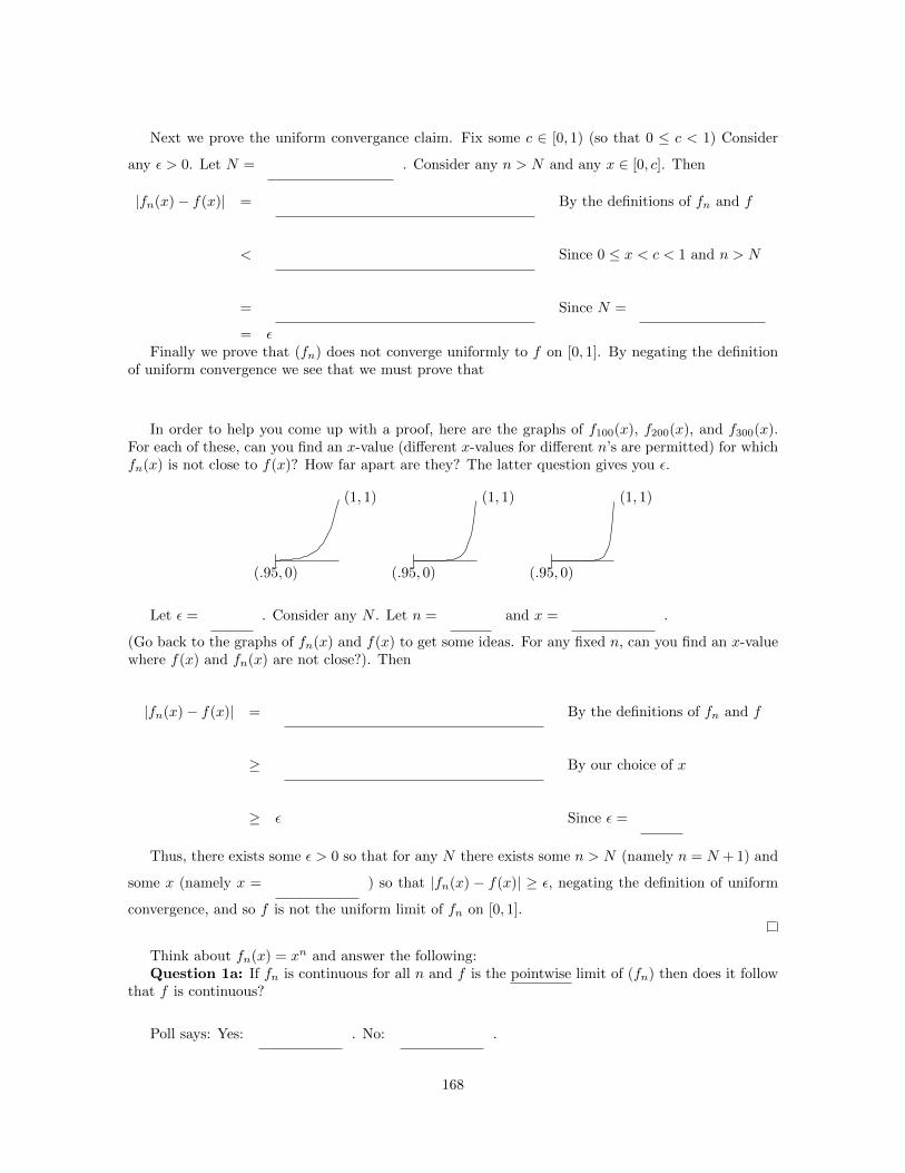
Next we prove the uniform convergance claim. Fix some c ∈ [0, 1) (so that 0 ≤ c < 1) Consider

any ε > 0. Let N = . Consider any n > N and any x ∈ [0, c]. Then

|fn(x)− f(x)| = By the definitions of fn and f

< Since 0 ≤ x < c < 1 and n > N

= Since N =

= εFinally we prove that (fn) does not converge uniformly to f on [0, 1]. By negating the definition

of uniform convergence we see that we must prove that

In order to help you come up with a proof, here are the graphs of f100(x), f200(x), and f300(x).For each of these, can you find an x-value (different x-values for different n’s are permitted) for whichfn(x) is not close to f(x)? How far apart are they? The latter question gives you ε.

(.95, 0)

(1, 1)

(.95, 0)

(1, 1)

(.95, 0)

(1, 1)

Let ε = . Consider any N . Let n = and x = .

(Go back to the graphs of fn(x) and f(x) to get some ideas. For any fixed n, can you find an x-valuewhere f(x) and fn(x) are not close?). Then

|fn(x)− f(x)| = By the definitions of fn and f

≥ By our choice of x

≥ ε Since ε =

Thus, there exists some ε > 0 so that for any N there exists some n > N (namely n = N + 1) and

some x (namely x = ) so that |fn(x) − f(x)| ≥ ε, negating the definition of uniform

convergence, and so f is not the uniform limit of fn on [0, 1].

Think about fn(x) = xn and answer the following:Question 1a: If fn is continuous for all n and f is the pointwise limit of (fn) then does it follow

that f is continuous?

Poll says: Yes: . No: .

168

Question 1b: If fn is continuous for all n and f is the uniform limit of (fn) then does it followthat f is continuous?

Poll says: Yes: . No: .

Question 2a: Suppose that limx→c

fn(x) = Ln and that limn→∞

Ln → L then does it follows that

limx→c

f(x) = L? Said another way, is it true that limn→∞

limx→c

fn(x)?= lim

x→climn→∞

fn(x)? Can we “Reverse

the order of limits”?

Poll says: Yes: . No:

Question 2b: Does the answer to question 2a change if we demand that fn converges to funiformly?

Poll says: Yes: . No:

One more example before we address these questions:

Claim 4.1.5. The sequence of functions gn(x) =

n∑k=0

xk converges uniformly to1

1− xon the interval[−1

2 ,12

].

Proof. As a starting point, remember that the finite sum is given by the closed formula gn(x) =n∑k=0

xk =1− xn+1

1− xwhenever x 6= 1.

Consider any ε > 0. Let N = . Consider any n > N and x ∈[−1

2 ,12

]. Then

∣∣∣∣ 1

1− x− gn(x)

∣∣∣∣ = by the closed formula for gn

= simplifying

≤ since x ∈[−1

2 ,12

]so |x− 1| ≥

< since n > N

= By our choice of N

≥ ε

Summarizing, for every ε > 0, there exists an N such that for every n > N and every x ∈[−1

2 ,12

],

it follows that

∣∣∣∣ 1

1− x− gn(x)

∣∣∣∣ < ε. Thus, (gn) converges uniformly to1

1− xon[−1

2 ,12

]

169

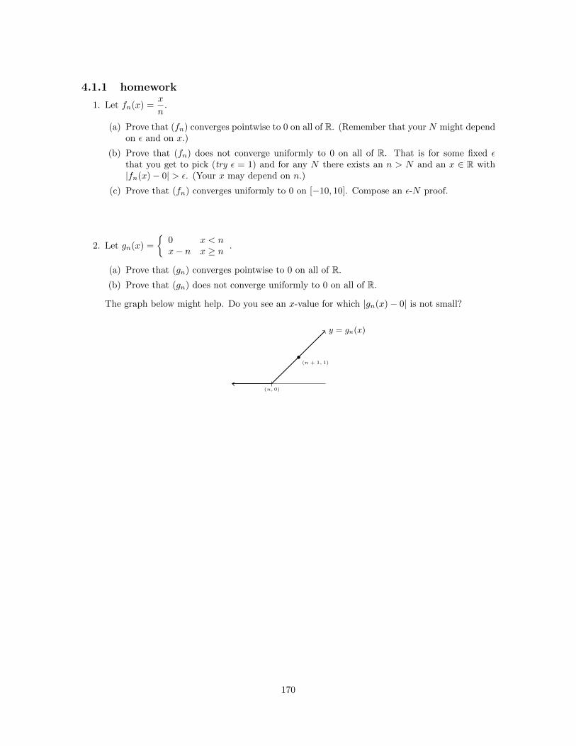
4.1.1 homework

1. Let fn(x) =x

n.

(a) Prove that (fn) converges pointwise to 0 on all of R. (Remember that your N might dependon ε and on x.)

(b) Prove that (fn) does not converge uniformly to 0 on all of R. That is for some fixed εthat you get to pick (try ε = 1) and for any N there exists an n > N and an x ∈ R with|fn(x)− 0| > ε. (Your x may depend on n.)

(c) Prove that (fn) converges uniformly to 0 on [−10, 10]. Compose an ε-N proof.

2. Let gn(x) =

{0 x < nx− n x ≥ n .

(a) Prove that (gn) converges pointwise to 0 on all of R.

(b) Prove that (gn) does not converge uniformly to 0 on all of R.

The graph below might help. Do you see an x-value for which |gn(x)− 0| is not small?

y = gn(x)

(n, 0)

(n + 1, 1)

170

4.2 Continuity and the uniform limit

OK. That’s enough examples. Let’s prove the pattern that we’ve noticed.

Theorem 4.2.1. Suppose that fn : U → R is a sequence of continuous functions. Let f be the uniformlimit of fn. Then f is continuous on U .

Before we give the proof let’s draw a picture of the proof. The fact that fn → f uniformly meansthat by taking n big enough we can arrange that |fn(x)− f(x)| < ε for all x ∈ U . Here is a picture ofa continuous function fn(x) and a tube of height 2ε around it. Any (x, y) value on the graph of f(x)must lie in this tube.

(p, 0) (x, 0)

Since fn is continuous we can make |fn(x) − fn(p)| < ε by taking x close enough to p. Drawa possible value for (p, f(p)) and (x, f(x)) in the picture above. Are these y-values close to each

other?

Use the triangle inequality. How close can you prove that these y-values are to each other?

|f(x)− f(p)|

Proof of Theorem 4.2.1. Suppose that fn : U → R is a sequence of continuous functions. Let f bethe uniform limit of fn. Consider any p ∈ U . We must show that f is continuous at p.

Consider any ε > 0. There is an N such that for all n > N and all u ∈ U

|fn(u)− f(u)| < . Importantly, this holds for every choice of u

Fix some n > N . Since fn is continuous at p there is a δ such that for all x ∈ U

if |x− p| < δ then |fn(x)− fn(p)| < .

Consider now any x ∈ U such that |x− p| < δ. Making use of the triangle inequality

|f(x)− f(p)| =

≤

<

Thus, for all p ∈ U and any ε > 0 there is a δ > 0 such that if |x− p| < δ then |f(x)− f(p)| < ε.f is continuous on U !

Theorem 4.2.2. Suppose that fn : U → R is a sequence of functions. Suppose that c is a limit pointof U and that for all n ∈ N lim

x→cfn(x) = Ln exists. If f is the uniform limit of fn then lim

x→cf(x) and

limn→∞

Ln each exist. Moreover, limx→c

f(x) = limn→∞

Ln.

171

Proof. Suppose that fn : U → R is a sequence of continuous functions. Suppose that c is a limit pointof U and that for all n ∈ N lim

x→cfn(x) = Ln exists. Let f : U → R be the uniform limit of fn. We

must show that limx→c

f(x) and limn→∞

Ln each exist and that limx→c

f(x) = limn→∞

Ln.

Step one: (Ln) is a Cauchy sequence.Consider any ε > 0. Since f is the uniform limit of fn there is an N such that for all n > N and

all u ∈ U|fn(u)− f(u)| < .

Thus, for all m,n > N

|fn(u)− fm(u)| = |fn(u)− f(u) + f(u)− fm(u)|

≤ (4.1)

Since limx→c

fn(x) = Ln and limx→c

fm(x) = Lm there exists δn and δm such that if 0 < |x− c| < δn then

|fn(x)− Ln| < . (4.2)

and if 0 < |x− c| < δm then

|fm(x)− Lm| < . (4.3)

Let δ = min(δm, δn) and assume 0 < |x− c| < δ. Then

|Ln − Lm| = By adding and subtracting

and .

≤ By the triangle inequality

< By (4.1), (4.2), and (4.3)

Thus, for all ε > 0 there exists an N such that if n,m > N then |Ln − Lm| < ε. Thus, (Ln) isCauchy.

Step 2: Let L = limn→∞

Ln. We will be done if we can show that limx→c

f(x) = L.

Consider any ε > 0. Since f is the uniform limit of fn there is an N1 > 0 such that for all n > N1

and any u ∈ U

|fn(u)− f(u)| < . (4.4)

Since L = limn→∞

Ln there is an N2 such that if n > N2 then

|Ln − L| < . (4.5)

172

Let N = max(N1, N2) and n > N . Since limx→c

fn(x) = Ln there is a δ > 0 such that if 0 < |x− c| < δ

then

|fn(x)− Ln| < (4.6)

Now for any x ∈ U with 0 < |x− c| < δ, we see that

|f(x)− L| = By adding and subtracting

and

≤ By the triangle inequality

< By (4.4), (4.6), and (4.5)

Thus, limx→c

f(x) = L = limn→∞

Ln as we claimed.

Look back at the two (four?) questions asked In Section 4.1. What are their answersThe following theorem reveals that the sequence of numbers: sup {|fn(x)− f(x)| : x ∈ [0, 1]} de-

tects uniform convergence. This is called the sup norm in functional analysis. It allows you to tryto start replicating all of real analysis on the space of bounded continuous functions.

Theorem 4.2.3. Let fn : U → R be a sequence of bounded functions and f : U → R be a boundedfunction. Then f is the uniform limit of fn if and only if the sequence (sn) given by the rule sn :=sup{|fn(x)− f(x)| : x ∈ U} converges to 0.

Proof. Let fn : U → R be a sequence of bounded functions and f : U → R be a bounded function.Let sn = sup{|fn(x)−f(x)| : x ∈ U}. (The word bounded is needed to guarantee that this supremumexists.)

(=⇒)

Suppose that f is the uniform limit of fn on U . We need to show that

Consider any ε > 0. Because f is the uniform limit of (fn) we see that there is an N such that

(4.7)

But then is an upper bound on

{∣∣∣∣ ∣∣∣∣ : x ∈ U}

. Since the

supremum is the least upper bound, this implies that sup

{∣∣∣∣ ∣∣∣∣ : x ∈ U}≤

< .

Thus, for every ε > 0 we have exhibited an N so that for every n > N

So that,|sn − 0| = |sn| = sn < ε

Thus, limn→∞

sn = 0, as we claimed.

173

(⇐=)Conversely, assume that lim

n→∞sn = lim

n→∞(sup {|fn(x)− f(x)| : x ∈ U}) = 0. Consider any ε > 0.

Then there exists some N so that for all n > N ,

(4.8)

Now consider any n > N , and any x ∈ U . Then |fn(x) − f(x)| ∈ {|fn(x)− f(x)| : x ∈ U} andso between the fact that the supremum is an upper bound and (4.8) we see that

|fn(x)− f(x)| ≤ since the supremum is an upper bound.

< By (4.8).

Thus, for every ε > 0 there exists some N so that for all n > N and every x ∈ U , |fn(x)− f(x)| < ε.This is exactly the definition of uniform convergence.

174

4.2.1 Homework.

1. Suppose that gn : U → R is a sequence of bounded functions on some set U ⊆ R. Supposethat (gn) converges uniformly to some function g : U → R. Prove that g(x) is a boundedfunction. (Different values for n might result in different bounds. Don’t secretly assume thatthat the bounds are independent of n.) Hint: Try plugging ε = 1 into the definition of uniformconvergance.

2. Suppose that gn : U → R is a sequence of uniformly continuous functions on some set U ⊆ R.Suppose that (gn) converges uniformly to some function g : U → R. By imitating the proof ofTheorem 4.2.1 from today’s notes, prove that g is uniformly continuous. Make sure that youdeclare your δ before you make a choice of inputs in U .

175

4.3 The pointwise and uniform Cauchy criteria

Just as in sequences of numbers, given a sequence of functions it is important to have a means ofsaying that a sequence has a (uniform or pointwise) limit without knowing what the limit should be.Today we introduce Cauchy Criteria for sequences. (criteria is the plural of criterion.)

We will give the definition in each case:

Definition 4.3.1. A sequence of functions fn : U → R is call pointwise Cauchy if for all x ∈ Uthe sequence of real numbers (fn(x)) is Cauchy.

Expanding the definition of “Cauchy,” this is equivalent to:

∀x ∈ U

On what can this N depend?

The sequence is called uniformly Cauchy if the N depends only on ε. Said more formally:

Definition 4.3.2. A sequence of functions fn : U → R is call uniformly Cauchy if

We warm up by proving the obvious (is it?) result that the uniform condition implies the pointwisecondition

Proposition 4.3.3. Let fn : U → R be a sequence of functions. If (fn) is uniformly Cauchy then(fn) is pointwise Cauchy.

Proof. Let fn : U → R be a uniformly Cauchy sequence of functions. We must show that (fn) ispointwise Cauchy.

Consider any ε > 0. Since (fn) is uniformly Cauchy there is an N0 such that for all n,m > N0,

and all x ∈ U .

Now consider any x ∈ U . LetN = so for allm,n > N we see .

Thus (fn) is pointwise Cauchy.

Today’s main results: A sequence of functions is (pointwise / uniformly) Cauchy if and only ifit is (pointwise / uniformly) convergent.

Theorem 4.3.4. Let fn : U → R be a sequence of functions. Then (fn) is pointwise convergent ifand only if it is pointwise Cauchy.

Proof. The proof is based on the fact that a sequence of numbers (an) is Cauchy if and only if itconverges

Let (fn) be a sequence of functions.

Suppose (fn) is pointwise Cauchy so that for all x ∈ U (fn(x)) is .

Recall, sequences of numbers converge. For any x ∈ U , let f(x) be the limit

of the sequence (fn(x)).

Notice that for all x ∈ U , fn(x)→ . This is precisely what it means for

176

Thus (fn) converges pointwise, completing the first half of the proofNow suppose that fn converges pointwise. Let f be its pointwise limit. Consider any x ∈ U . By

the definition of pointwise convergence, (fn(x)) .

Since convergent sequences are Cauchy, (fn(x)) is .

Thus, for all x ∈ U , fn(x) is .

Thus, (fn) is pointwise Cauchy.

Theorem 4.3.5. Let fn : U → R be a sequence of functions. Then (fn) is uniformly convergent ifand only if it is uniformly Cauchy.

Proof. Suppose that (fn) is uniformly convergent. Let f be its uniform limit. Consider any ε > 0.Since f is the uniform limit there exists an N such that

Now let m,n > N and consider any x ∈ U then

|fn(x)− fm(x)| = By adding and subtracting

≤ By the triangle inequality

< since m,n > N

So that (fn) is uniformly Cauchy.

Now suppose that (fn) is uniformly Cauchy. By Proposition 4.3.3 then (fn) is

and by Theorem 4.3.4 is . Let f : U → R be its

limit. A good candidate to be the uniform limit then is

Consider any ε > 0, since (fn) is uniformly Cauchy there exists an N such that for all m,n > Nand all x ∈ U

Solving this inequality for fm(x) we see that for all m,n > N

< fm(x) <

Recall that fm(x) converges to f(x) (as a sequence of real numbers parametrized by m) by defi-nition. Passing to the limit (as m→∞)

≤ f(x) ≤

Thus, | | ≤ < ε

177

Notice that N was independent of x. Thus, for any ε > 0 we have exhibited an N so that for alln > N and all x ∈ U , |fn(x)− f(x)| < ε: f is the uniform limit of (fn). Since fn has a uniform limitit is uniformly convergent, as we claimed.

4.3.1 Homework

Work out these problems to cement your understanding.We close with some applications as a warm up towards the theory of power series.

1. Let a > 0. Let fn(x) =

n∑k=0

xk

k!. Prove that (fn) is uniformly Cauchy on [−a, a]. Explain why

this means its limit is continuous on [−a, a]. (The real definition of ex is as the limit.)

2. Let gn(x) =

n∑k=1

xk

2k. Prove that (gn) is uniformly Cauchy on [−1, 1]. Explain why this means

its limit is continuous on R.

On (1) you may assume that for any fixed a ∈ R sn =

n∑k=0

ak

k!is convergent and so Cauchy.

On (2) you can assume that tn =

n∑k=1

1

2kis convergent and so Cauchy.

A sample appears on the next page. We may go through it in class, time permitting.

178

As a sample, here is a proof of a related claim:

Let hn(x) =

n∑k=1

xk

k. Prove that (hn) is uniformly Cauchy on [−1/2, 1/2]. The proof will assume

that un =

n∑k=1

1

2kis Cauchy.

Consider any ε > 0. Since un =

n∑k=1

(1/2)k is Cauchy, by assumption, there exists some N such

that for all m,n > N ,

If we assume also that m ≥ n then we may cancel common terms and see that this inequalitysimplifies to

Every term in this sum is positive so we may drop the absolute value bars,

Keeping the same choice of N as above, consider any x ∈ [−1/2, 1/2] and assume that m,n > N . Wealso assume without loss of generality that m ≥ n. Then By the definition of hn(x) we have that:

|hn(x)− hm(x)| =

Cancelling the common terms of the two sums you get above,

|hn(x)− hm(x)| =

Next we use the triangle inequality to drop the absolute value bars in the sum above:

|hn(x)− hm(x)| =

Now since x ∈ [−1/2, 1/2], |x| ≤ 1/2. Division by k ∈ N will only make things smaller. Thus,

|hn(x)− hm(x)| =

From earlier in the proof we saw that whenever m,n > N , < ε. Thus,

|hn(x)− hm(x)| =

Thus, we see that for every ε > 0, there exists an N such that for all m,n > N , and all x ∈[−1/2, 1/2], |hn(x)− hm(x)| < ε. Therefore, (hn) is uniformly Cauchy on [−1/2, 1/2].

179

4.4 Application of the uniform Cauchy criterion and the con-vergence of series: The Weierstrass M-series test

In the homework for the previous section, you proved that some sequences of functions given by partialsum converge. In each argument you used that a certain series of number converge. In this sectionwe make this idea explicit.

Definition 4.4.1. Suppose that fn : U → R is a sequence of functions, then the series

∞∑k=1

fk(x) is the

function given by the limit of the sequence of partial sums Sn(x) =

n∑k=1

fk(x) Its domain is the set of all

x ∈ U for which the series converges. If the sequence of partial sums converges (pointwise/uniformly)

then we say that

∞∑k=1

fk(x) converges (pointwise/uniformly).

Theorem 4.4.2 (The Weierstrass M -series test). Suppose that fn : U → R is a sequence of functions,

that Mn is a sequence of numbers, that |fn(x)| ≤Mn for all x ∈ U and that

∞∑k=1

Mk converges. Then

Sn(x) =

∞∑k=1

fk(x) converges uniformly on U .

Proof. If you did the homework from the previous section then this should feel fairly straightforward.Suppose that fn : U → R is a sequence of functions, that Mn is s sequence of numbers, that

|fn(x)| ≤ Mn for all x ∈ U and that

∞∑k=1

Mk converges. We want to show that the sequence of

functions given by Sn(x) =

n∑k=1

fk(x) converges uniformly on U . By the uniform Cauchy criterion, it

suffices to show that the sequence is uniformly .

Let Tn = be the sequence (of numbers, not of functions) of partial sums for

∞∑k=1

Mk. Since

∞∑k=1

Mk converges, it follows that (Tn) so that by the Cauchy criterion

(Tn) is .

Now consider any ε > 0. Since (Tn) is Cauchy, it follows that there is some N such that

180

Consider any m,n > N and any x ∈ U . Without loss of generality assume that n ≥ m. Then

|Sn(x)− Sm(x)| = By the definition of (Sn)

= By cancelling common terms

≤ By the triangle inequality

≤ By assumption ≤

= Because Tn − Tm =

< ε Because m,n > N

Concluding sentence:

Application:

Prove that

∞∑k=0

1

2k· cos(3k · x) is continuous on R.

What is harder to prove (especially since we do not have the definition) is that this function is not

differentiable at any point in R. Here is a graph of

100∑k=0

1

2k· cos(3k · x):

Let fk(x) =1

2k· cos(3k · x) and Mk =

1

2k. Since | cos(x)| ≤ 1 for all x, we conclude that

≤ . By the geometric series test

∞∑k=0

converges. Thus, the Weier-

strass M -test concludes that

n∑k=0

1

2k· cos(3k · x) converges uniformly as n→∞.

181

Since

∞∑k=0

1

2k· cos(3k · x) is the uniform limit of a sequence of continuous functions, we conclude

that

For you:

Use the Weierstrass M -test to show that

∞∑k=1

1

k2· cos(π · xk) is continuous on R. Use a machine to

also look at a graph.

182

4.5 Convergence of power series

Definition 4.5.1. Let a0, a1 . . . be a sequence of real numbers. (Notice that the index starts at zerothis time.). We will follow the convention for the sake of power series that x0 = 1, even when x = 0.For a real number c The power series associated with (ak) centered at c is given by

f(x) =

∞∑k=0

ak · (x− c)k := limn→∞

n∑k=0

ak · (x− c)k

Its domain is the set of all x ∈ R for which this series converges.

Here are some questions:

1. Can we determine the domain of a power series?

• This just asks, “for what values of x does

∞∑k=0

ak · (x− c)k converge?”

2. (On what set) Will a power series be continuous?

For convenience we will usually assume that c = 0. All the results will translate (to the right byc) to the case that c 6= 0.

These turn out to have a nice answer (except at the endpoints of the domain.) The answer basicallyboils down to the root test and the M -series test.

Take a moment and recall the root test.

Theorem (The root test).

We begin by (almost) answering the question about the domain of a power series, declaring the

so-called radius of convergence of

∞∑k=0

akxk.

Proposition 4.5.2. Let (ak) be a sequence of real numbers. Let λ = lim supk→∞

|ak|1/k and R =1λ If λ > 0

∞ if λ = 0

0 if |ak|1/k is not bounded above.

• For all p ∈ R, if |p| < R then

∞∑k=0

akpk converges absolutely.

• For all p ∈ R, if |p| > R then

∞∑k=0

akpk diverges.

Proof of Proposition 4.5.2. Let (ak) be a sequence of real numbers. Let λ = lim supk→∞

|ak|1/k and

R =

1λ If λ > 0

∞ if λ = 0

0 if |ak|1/k is not bounded above.

Consider any p ∈ R. We need to prove that if |p| < R then

∞∑k=0

akpk converges absolutely. and

that if |p| > R then

∞∑k=0

akpk diverges.

183

We will give the proof in the case that lim supk→∞ |ak|1/k is bounded and that 0 < λ so that0 < R <∞. and will say a few words afterwards about how to modify it when R = 0 or R =∞.

We proceed by the ratio test. We need to compute lim sup k√akpk:

lim sup k√|akpk| = Simplifying k

√|akpk|

= By

Thus, when |p| < R, lim sup k√|akpk| = < = 1 so that by the

root test,

On the other hand, when |p| > R, lim sup k√|akpk| = > = 1 so

that by the root test

The quantity R in Proposition 4.5.2 is called the radius of convergence of

∞∑k=0

akxk. As we said,

this at least answers the domain question pretty well.

Corollary 4.5.3. Let (ak) be a sequence of real numbers and f(x) =

∞∑k=0

akxk, then

(−R,R) ⊆ dom(f) ⊆ [−R,R]

where R is the radius of convergence of f .

Proof. Let (ak) be a sequence of real numbers and f(x) =

∞∑k=0

akxk.

First we show that (−R,R) ⊆ dom(f). Consider any x ∈ (−R,R), then |x| < R so that byProposition 4.5.2 we conclude that

So

that as the power series converges at x, x is in the domain of f .

In order to show that dom(f) ⊆ [−R,R] we show that for all x /∈ [−R,R], the power series

∞∑k=0

akxk

diverges so that x is not in the domain of f .

Let x /∈ [−R,R] so that |x| > and by Proposition 4.5.2 we conclude that

Since the power series diverges, x is not in the domain of f . Completing the proof.

Next we check for continuity.

184

Theorem 4.5.4. Let (ak) be a sequence of real numbers and f(x) =

∞∑k=0

akxk. Let R be the radius of

convergence of f .

• If R =∞ then f is continuous on R.

• If 0 < R <∞ then f is continuous on (−R,R).

• If R = 0 then dom(f) = {0} and f is continuous on {0}

Proof. Let (ak) be a sequence of real numbers, and f(x) =

∞∑k=0

akxk. Let R be the radius of conver-

gence of f .There are three claims. The last is trivial: When R = 0, f is only defined at {0} so that as the

domain has only a single point which is isolated, f is continuous at 0.The other two will have very similar proofs. Here is the proof in the case that 0 < R < ∞ and

afterwards just say some words about how to modify it. Consider any x ∈ (−R,R). We want to show

that f is continuous at x. Let p = . Then |x| < p < R (What p does this?). Since

p < R Proposition 4.5.2 says that

By expanding the definition of absolute convergence we see that

Now consider any y ∈ [−p, p], so that |y| ≤ p and |akyk| |akpk| By the Weierstrass M -

test we now conclude that

∞∑k=0

ak · xk is on

[,

]. Thus, on[

,

], f is the limit of a uniformly convergent sequence of continuous functions. We

conclude that f is continuous on

[,

].

Since x is interior to

[,

]we see that f is continuous at x.

As we now have that for every x ∈ (−R,R), f is continuous at x we conclude that

We will go through together and see how this argument must be altered when R =∞.

185