Math 300: Lecture NotesNorthwestern University, Spring 2017

Written by Santiago Canez

These are lecture notes for Math 300, “Foundations of Higher Mathematics”, taught at North-western University in the spring of 2017. The book used was the 2nd edition of Book of Proof byHammack. Watch out for typos! Comments and suggestions are welcome.

Contents

Lecture 1: Direct Proofs 2

Lecture 2: More on Direct Proofs 5

Lecture 3: Upper Bounds 8

Lecture 4: Unions & Intersections 11

Lecture 5: More on Unions & Intersections 14

Lecture 6: Negations 18

Lecture 7: Contrapositives 21

Lecture 8: More on Sets 25

Lecture 9: Contradictions 28

Lecture 10: More on Upper Bounds 31

Lecture 11: More on Real Numbers 33

Lecture 12: Induction 37

Lecture 13: More on Induction 40

Lecture 14: Functions 46

Lecture 15: Images and Preimages 51

Lecture 16: Injectivity and Surjectivity 54

Lecture 17: Compositions 57

Lecture 18: Invertibility 60

Lecture 19: Equivalence Relations 63

Lecture 20: More on Equivalences 68

Lecture 21: Cardinality 71

Lecture 22: Countable Sets 76

Lecture 23: More on Countable Sets 79

Lecture 24: Uncountable Sets 83

Lecture 25: Power Sets 85

Lecture 26: Cantor-Schroeder-Bernstein Theorem 89

Lecture 27: More on Cantor-Schroeder-Bernstein 92

Lecture 1: Direct Proofs

Welcome! This is a course dedicated to understanding how to read, write, and think about higher-level mathematics. The aim is two-fold: to become comfortable with writing rigorous mathematicalarguments, and, more importantly, to get used to the thought process which goes into coming upwith said arguments in the first place. This will be quite different from the computational coursesyou’re likely more used to, but better reflects the approach with modern mathematics follows.

Cardinality. Just to get a sense for the types of things which a more rigorous approach tomathematics allows us to do, we’ll give a brief introduction to the topic of cardinality, which willbe one of the final things we’ll look at in this course. The notion of cardinality gives us a preciseway of talking about the “size” of a set, in the sense of the number of elements it has. The pointis that if we want to answer questions like: “How large is R, the set of real numbers?” or “Is Rlarger than Z, the set of integers?”, we had better have a precise definition of what “large” meansin this context. This is meant to illustrate the fundamental idea that, in the end, definitions areabsolutely crucial, and that everything we do in mathematics arises from precise definitions.

Whatever “size” means, it makes sense to say that R and Z are both infinite sets, since theyeach contain infinitely many numbers. However, leaving the answer at that, that R and Z are bothinfinite, is not the end of the story, because it turns out that nonetheless we can give meaning tothe idea that R is larger than Z; that is, even both R and Z are infinite, it will turn out that thecardinality of R is larger than that of Z, which intuitively means that R has more elements thandoes Z. Thus, the point is that once we give precise meaning to the notion of the “size” of set, itwill make sense to talk about different “sizes” of infinity.

As another example, just going by intuition, it makes sense at first glance to say that Z is largerthan N, which is the set of positive integers. Indeed, since Z contains all elements of Z along withtheir negative, it might be tempting to say that Z is “twice” as large as N. However, consider thefollowing lists:

0 1 −1 2 −2 3 −3 . . .

1 2 3 4 5 6 7 . . .

In the first we list all integers, alternating (after the initial 0) between a positive and its negative,and in the second we list all positive integers. The point here is that these lists show there is a wayto pair off elements of Z and N in a one-to-one manner so that nothing is left over in either set.Intuitively, this suggests there should be as many things in the first list as in the second, so thatZ and N should actually have the same size. Indeed, this will be true, but again of course dependson giving precise meaning to the word “size”.

Importance of definitions. The brief discussion of cardinality above is meant to emphasizethat we ask some fairly strange and interesting questions in math, but which all depend on havingprecise definitions and techniques available. To look at something more concrete, suppose we wereconsider the following claim:

If n is an even integer, then n2 is even.

Is this true? Certainly if we consider different examples of even integers—2,4,6,8 for instance—theclaim appears to be true since squaring each of these still results in an even integer. However, notethat the claim is not saying the square of some specific even integer will still be even, but ratherthat the square of any even integer should still be even. In other words, the given claim shouldreally be read as saying:

2

For all integers n, if n is even, then n2 is even,

making it clear that the claim should hold for any n which happens to be an even integer.Proving this thus requires we consider an arbitrary even integer n, with the goal being to show

that n2 is then even as well. To do so requires that we understand what “even” actually means,since it is only through working with a precise definition of even that we have any hope of provingour claim. Intuitively, an even integer is one which is “evenly divisible” by 2, but this doesn’t workas a definition since we haven’t yet given meaning to the phrase “evenly divisible”. Here, then, aretwo possible ways of defining what it means for an integer n to be even:

First definition: n is even if n2 is an integer.

Second definition: n is even if it can be written as n = 2m for some integer m.

We can use either one, but the second definition should actually be preferred since the first stillhas some ambiguity built into it: if we want to say that n

2 is an integer, we would have to knowwhat “integer” actually means in a more precise way. The second definition avoids this ambiguity.

Direct proofs. Nonetheless, here are proofs of our given claim using either proposed definition.In either case we must verify that n2 also satisfies whichever definition of “even” we’re workingwith.

Claim. If n is an even integer, then n2 is even.

Proof 1. Suppose n is an even integer. Then n2 is an integer, so

n2

2= n

(n2

)is an integer since it is the product of two integers. Thus, since n2

2 is an integer, n2 even.

Proof 2. Suppose n is an even integer. Then we can write n as n = 2m for some integer m. Hence

n2 = (2m)2 = 4m2 = 2(2m2).

Thus since we can write n2 as 2 times an integer, we conclude that n2 is even.

These are both examples of “direct proofs”, in that they proceed directly from the given as-sumption to the desired conclusion, using only definitions and other manipulations. These are notthe only possible proofs—for instance, we might say in the first attempt that since n

2 is an integer,

(n2 )(n2 ) = n2

4 is also an integer, which can only happen when n2 is a multiple of 4, which also impliesthat n2 is even. This is all true, but depends on some additional notions and facts we haven’t madeexplicit yet, such as what it means for an integer to be a “multiple of 4”, and why being a multipleof 4 implies being even. There is nothing wrong with this approach, but we should be mindful ofthe additional complexities it brings into play.

Now consider the claim that if n is an odd integer, then n2 is odd. Again, we should firstrecognize the implicit “for all n” hiding in the setup: the claim is really “for all integers n, if n isodd, then n2 is odd.” Thus, proving this requires that we work with some arbitrary odd integer nwithout making any additional assumptions as to what it is. In addition, now we need a precisedefinition of “odd”. One possible definition of odd is “not even”, or that n

2 is not an integer.However, this doesn’t give us much to work with, since there’s not much we can say simply from

3

knowing that n2 is not an integer; for instance, this doesn’t really tell us anything about what n

2can actually look like.

So, we look instead for a better definition odd. Here’s one: an integer n is odd if it can bewritten as n = 2m + 1 for some integer m. This is simply saying that odd integers which are onemore than an even integer. This is a good definition, since it gives us something concrete to workwith, namely an explicit form for what n must look like. Here then is our proof.

Claim. If n is an odd integer, then n2 is odd.

Proof. Suppose n is an odd integer. Then we can write it as n = 2m+ 1 for some integer m. Hence

n2 = (2m+ 1)2 = 4m2 + 4m+ 1 = 2(2m2 + 2m) + 1.

Thus since we can write n2 as one plus twice an integer, we conclude that n2 is odd.

So far these are all pretty simple proofs, but they give a good introduction to the thoughtprocess behind working with proofs in general, where using precise definitions is key. Note alsothe structure: each proof begins with a marker showing the start of the proof, as evidenced by theProof at the beginning, and each ends with a marker showing the end of the proof, as indicatedby the � symbol. The � symbol is a very common way of indicating the end of a proof, and youshould get in the habit of using it yourself. Note also that all proofs here are written using completesentences with all thoughts spelled out in full. Again, this is something you should get in the habitof doing yourself. The goal is produce a clearly written proof which anyone reading can follow; theonus is on you, and not the reader, to make your ideas as clear as possible.

Another example. Here is one more example illustrating the ideas above. The claim is thatthe product of two rational numbers is itself rational. Of course, we first need a definition: a realnumber r is rational if it can be written as as the quotient a

b of two integers a and b with b 6= 0.Thus, things like 1

2 ,−83 ,

317 are rational. (We’ll look at examples of non-rational things later on.)

Now that we have the required definition, proving our claim should be fairly straightforward; again,the point is simply to go wherever the definition takes us.

Claim. The product of two rational numbers is rational. To spell this out more explicitly, theclaim is that for all x and y, if x and y are each rational, then xy is rational.

Proof. Suppose x and y are rational numbers. Then

x =a

band y =

c

d

for some integers a, b, c, d with b and d nonzero. This gives

xy =(ab

)( cd

)=ac

bd.

Since the result is a fraction of two integers with nonzero denominator (we are taking for grantedthe fact that multiplying integers always results in an integer), we conclude that xy is rational asclaimed.

Following along in the book. As I said in class, we’ll be jumping around in the book a bit inorder to present things in a (hopefully) more natural manner. The book introduces the notion ofa direct proof in Section 4.3, which you should definitely go through in addition to the reset ofChapter 4 to see more examples of proofs worked out. In class we’ll be focusing on the key pointsto takeaway and on the overall thought process, which the book is intended to supplement.

4

Lecture 2: More on Direct Proofs

Warm-Up 1. We show that the sum of an even integer and an odd integer is always odd. Thisis meant to be another simple example of a direct proof, which just requires working with thedefinitions of even and odd. Note how we use these definitions to show us both what it is we haveto work with—when writing out what information our assumption gives us—and also to guide ustowards what it is we want to establish. The given statement that “the sum of an even integer andan odd integer is always odd” can be rephrased as “if x is an even integer and y an odd integer,then x+ y is odd”, which makes it a bit clearer to see what it is we have to do.

So, suppose x is an even integer and y an odd integer. Our goal is to show that x + y is odd,which requires showing that we can write x+ y in the form required of an odd integer, namely as 2times some integer plus 1. To get to this point, we use the definition of even to say that there existsan integer k such that x = 2k, and the definition of odd to say that there exists an integer ` suchthat y = 2`+ 1. (Note that we should not use y = 2k + 1 here since we’ve already introduced k tomean something different previously; in other words, there is no reason why the k which satisfiesy = 2k+ 1 has to be the asme as the one which satisfies x = 2k, so we should use a different letter` for the integer showing up in the statement of what it means for y to be odd.) Then

x+ y = 2k + (2`+ 1) = 2(k + `) + 1,

which is the required form of an odd integer.We’re done, but let us now write out the proof more cleanly without the additional parenthetical

thoughts I put in above, to give a sense for how you would normally see it written:

Claim. If x is an even integer and y an odd integer, then x+ y is odd.

Proof. Suppose x is an even integer and y an odd integer. Since x is even and y is odd, there existintegers k and ` such that x = 2k and y = 2`+ 1. Then

x+ y = 2k + (2`+ 1) = 2(k + `) + 1,

which is the form required of an odd integer. Thus x+ y is odd as claimed.

Warm-Up 2. We say that an integer a divides an integer b (or equivalently that b is divisible bya, or that b is a multiple of a) if there exists an integer k such that b = ak. We show that if adivides b and b divides c, then a divides c. Again this is an example of using basic definitions tocarry us through; in particular, our end goal is to write c as a times some integer.

Proof. Suppose that a divides b and b divides c. Then there exists an integer k such that b = akand there exists an integer ` such that c = b`. Hence

c = b` = (ak)` = a(k`),

which shows that a divides c as desired.

Example. Here is yet another example, only in this case we reach a point where working withdefinitions alone is not enough and we have to make use of another realization. The claim is thatany even integer n can be written as n = 4k or n = 4k + 2 or some integer k; in other words, anyeven integer is either a multiple of 4 or two more than a multiple of 4.

We start off, simple enough, by writing n as n = 2m for some integer m from the fact that n iseven. Our goal is to write n either in the form 4k or the form 4k + 2, but now it is not a matter

5

of simply manipulating the n = 2m expression itself without bringing in some additional property.Indeed, to move from 2m to 4k or 4k + 2 really requires knowing something about m itself, andthe point is that m, being itself an integer, is either even or odd. Thus the “additional property”we need to consider here is that any integer is either even or odd, and this is what will allow ourproof to move forward. Now, this is not a deep observation, but illustrates the idea that “directproofs” still often require a good conceptual understanding of what we’re dealing with, even if theyare “direct”. This is an example of a proof by cases, where we consider two cases—m being even vsm being odd—separately, and show that our conclusion holds in either case. To be clear, verifyingour conclusion that “n = 4k or n = 4k + 2 for some integer k” only requires that we show oneof the statements n = 4k or n = 4k + 2 holds and not both simultaneously; in general, an “or”statement is true when at least one of the claimed conclusions holds.

Here then is our proof:

Proof. Suppose n is an even integer. Then n = 2m for some integer m. If m is even, there existsan integer k such that m = 2k, in which case n = 2m = 2(2k) = 4k. Otherwise m is odd, in whichcase there exists an integer k such that m = 2k + 1, so that n = 2m = 2(2k + 1) = 4k + 2. Thus,n = 4k or n = 4k + 2 for some integer k as claimed.

Non-divisibility example. Now we look at an example which does not deal with divisibility,evenness, or oddness at all, but is simply a statement about positive real numbers. The claim isthat if x is a positive real number, then there exists a real number y such that

y < x < 2y.

In this case, there are no definitions we need to make use of, and the point is simply to make sense ofwhat it is we’re actually trying to show. In words, the claim is that no matter what positive numberwe take, we can always find another which is smaller but such that doubling it gives somethinglarger the original. The fact that we are trying to prove “there exists a real number y” means thatall we need to do is produce at least one y which satisfies the required property. Now, it may bethat there are multiple y’s which work, but again this type of existence proof only requires theexistence of one such y.

Certainly if we take specific values of x we can find specific y’s which work: for x = 3 forinstance, y = 2 satisfies the requirement that y < x < 2y, and for x = 5 we can take y = 4 as onepossible y. But this is not enough since we want to produce such a y for any positive x. Our choiceof y should depend on the arbitrary x we’re looking at, and our description of what y is should notdepend on any information not given in the setup. The proof will take the structure of “Supposex > 0. Set y = (whatever value we claim is going to work), and then we’ll verify that it does work.”

To think about which y will work, we’ll do some scratch work to think about what the claimmeans visually. We draw x to the right of 0 on a number line, and we’re looking for y and 2y whichlook like:

6

Think about what kinds of values, visually, to the left of x have the property that doubling themgives something to the right. We should convince ourselves that such values are those which occurstrictly between 1

2x and x, since doubling anything smaller than 12x will still give something smaller

than x:

So, all we need is to pick a value for y which falls in this range. For instance, y = 34x will fall in

this range, and so will tons of other things (y = 78x, y = π

4x, etc), but all we need is one. So, in ourproof we will set y to be 3

4x, and then verify that this does indeed satisfy the property we want.Note that the scratch work we went through here to determine which y will work is not something

which will show up in our final proof, and was only our way of working through the thought processrequired to finish our argument. This is a crucial part of proof writing which cannot be emphasizedenough: whenever you see a proof written out in a book or elsewhere, what you are seeing is thefinal presentable argument verifying the claim at hand, but which does not indicate the work whichwent into coming up with that argument in the first place. It is important to understand that this“scratch work” is really where the bulk of the difficulty lies; once we know what to do, writing outthe actual formal proof is usually straightforward, but getting to that point is the hard part.

Claim. If x > 0, then there exists y such that y < x < 2y.

Proof. Suppose x > 0 and set y = 34x. Then

y =3

4x < x <

3

2x = 2y,

where we use the fact that x is positive to guarantee that the inequalities in 34 < 1 < 3

2 aremaintained after we multiply through by x. Thus y = 3

4x satisfies the required property.

To emphasize once more, the proof does not illustrate where we came up with y = 34x in the

first place, it only says “here is the y which will work and let’s make sure it does”. Finding asuitable choice of y came from thinking about what y < x < 2y would mean visually.

Sets and subsets. The types of basic examples we’ve seen dealing with divisibility, evenness,oddness, and inequalities are a good thing to start off, but are not indicative of the more elaboratetypes of concepts you see in higher-level course. So, we will spend the next few days introducingnew mathematical concepts on which we can try out the basic proof techniques we’re building up.The material which follows can be found in Sections 1.1 and 1.3 in the book, along with Chapter8. We’ll touch on further related notions in the book later on.

One of the most fundamental notions in all of mathematics is that of a set, which for ourpurposes just means a collection of objects. It could be a collection of numbers, as in the case ofthe set of integers or the set of real numbers, a collection of people, or a collection of who knowswhat else. When A is a set, the notation “x ∈ A” means that x is an element of A, or that x is inA. For instance, n ∈ Z means that n is an integer. If A and B are sets, we say A is a subset of Bif every element of A is an element of B, or in other words,

A being a subset of B means that if x ∈ A, then x ∈ B.

7

Thus, A consists of elements of B, just maybe not all elements of B. We use the notation A ⊆ Bto mean that A is a subset of B. Verifying that one set is a subset of another requires verifying thedefinition directly: if x ∈ A, then x ∈ B.

Example. Let A be the set of all integers which are divisible by 4. In set notation we can expressthis as

A = {n ∈ Z | 4 divides n}.

Here, the braces { and } indicate that we are looking at a set, and the portions before and afterthe dividing | define the set in question: the “n ∈ Z” to the left tells us what types of objects weare looking at, integers in this case, and the “4 divides n” to the right tells us what property theyare required to satisfy in order to belong to the given set. Thus, here we are looking at the set ofall n ∈ Z with the property that 4 divides n.

Let B = {m ∈ Z | 2 divides m}, which is the set of all integers which are divisible by 2, or inother words the set of all even integers. We claim that A ⊆ B, meaning that A is a subset ofB, or that any integer which is divisible by 4 is also divisible by 2. To show this we start withan arbitrary x ∈ A, and work towards verifying that x ∈ B. Along the way we use the definingproperties of what it means for x to be an element of A or B. Here is our proof:

Proof. Let x ∈ A. Then 4 divides x by definition of A, so there exists k ∈ Z such that x = 4k.This gives

x = 4k = 2(2k),

which shows that x is divisible by 2, and hence that x ∈ B. Thus x ∈ A implies x ∈ B, so A ⊆ Bas claimed.

Note again that we start with an arbitrary x ∈ A, use what it actually means for x to be in Ain order to say that we can write x as x = 4k, and then manipulate to show that x is divisible by2, which is what it means for x to be an element of B. Never lose sight of that fact that sets aredefined in a way which tells us what it means for something to be or not be an element of that set;in other words, x ∈ A in the above example gives us important information because we know whatit means for something to be in A. Similarly, if we want to show that x ∈ B, all we have to do isverify that x satisfies the defining property required of elements of B. Definitions are key!

Lecture 3: Upper Bounds

Warm-Up. Define A and B to be the sets

A = {n ∈ Z | there exists k ∈ Z such that n = 4k + 1}

andB = {n ∈ Z | there exists k ∈ Z such that n = 4k + 9}.

That is, A is the set of all integers which can be written in the form 4k + 1 and B the set of allintegers which can be written in the form 4k+ 9. We show that A ⊆ B and B ⊆ A. Note that thisis what it means to say that A and B are actually the same set: by definition, A = B if it is truethat A ⊆ B and B ⊆ A.

To show that A ⊆ B, we must show that if n ∈ A, then n ∈ B. Thus we start with n ∈ A,which by definition of A means that we can write n as n = 4k + 1 for some k ∈ Z. The goal is toshow that we can write n in the form 4(integer) + 9. Note that we use the same k in the definingexpressions of A and B, but this is not meant to suggest that the same value of k is needed; i.e. we

8

are not claiming that n = 4k+1 also equal to n = 4k+9 for the same k, but rather that n = 4k+1can be written as n = 4`+ 9 for some other integer `.

To see what ` we thus need, we use what we want to show as a guide, namely that 4k + 1 canbe written as 4`+ 9. We are given k, so we need ` satisfying

4k + 1 = 4`+ 9.

But now we can figure out precisely what ` must be solving for `, and we see that ` must be k− 2.Thus, our scratch work shows that if we want to write 4k + 1 in the form 4(integer) + 9 instead,the “integer” term we need is k − 2. Thus in our proof we will simply verify that ` = k − 2 is theinteger which expresses 4k+ 1 as 4`+ 9. A similar scratch works for the other containment B ⊆ Awe need to show, which requires showing that any 4k + 9 in B can be written as 4` + 1 for somechoice of `, which we determine ahead of time by solving 4k + 9 = 4`+ 1 for `. Here, then, is ourfinal proof:

Claim. For the sets A and B defined above, we have A = B, or in other words, A ⊆ B and B ⊆ A.

Proof. First we show that A ⊆ B. Let n ∈ A. Then there exists k ∈ Z such that n = 4k + 1.Hence:

4(k − 2) + 9 = 4k − 8 + 9 = 4k + 1 = n,

so n = 4(k − 2) + 9 is in the form required of an element of B. Thus n ∈ B, so A ⊆ B.Second we show that B ⊆ A. Let n ∈ B. Then there exists k ∈ Z such that n = 4k + 9, so

4(k + 2) + 1 = 4k + 8 + 1 = 4k + 9 = n,

and thus n = 4(k+ 2) + 1 is in the form required of an element of A. Hence B ⊆ A, so since A ⊆ Band B ⊆ A, we conclude that A = B.

Upper bounds. We now move to introducing a new mathematical concept—the notion of anupper bound of a set of real numbers. On the one hand, for those of you planning on taking acourse in real analysis, this is a crucial concept related to properties of real numbers. On theother hand, and the main reason why we’re introducing it in this course, it’s a notion which isinteresting and fairly simple to understand, but provides good practice in working definitions andmathematical reasoning. Note that this material is NOT in the book, but anything we need toknow about upper bounds will be introduced in class and these notes.

Here is the definition. Suppose S ⊆ R, so that S is a set consisting of real numbers. We saythat a real number u is an upper bound of S if for all s ∈ S, s ≤ u. Thus an upper bound of Sis a real number which is bigger than or equal to everything in S, as the name “upper bound” ismeant to suggest. Note that upper bounds are not unique in that if a set has an upper bound, itwill have many of them. Indeed, 2 is an upper bound of the closed interval [0, 2] defined by

[0, 2] = {x ∈ R | 0 ≤ x ≤ 2},

but so are 3, 4, and tons of other things. Also note that not all subsets of R have upper bounds; forinstance, Z ⊆ R does not have an upper bound since there is no restriction as to how large integerscan be.

Now, among all upper bounds of a set, there is one in particular which is worth singling out:the smallest upper bound. This notion is important enough in mathematics that it is given aspecial name: supremum. Here is the precise definition: the supremum (or least upper bound) of S

9

is an upper bound b of S such that for any other upper bound u of S, we have b ≤ u. Thus, thisdefinition precisely says that the supremum is an upper bound which is smaller than or equal toany other upper bound, as the alternate term “least upper bound” is meant to suggest. We usethe notion supS to denote the supremum of S, if it exists.

Example. We claim that sup[0, 2] = 2. According to the definition of supremum, showing thatsup[0, 2] = 2 requires two things: showing that 2 is an upper bound of [0, 2], and showing that2 is smaller than or equal to any other upper bound. First, by definition of the interval [0, 2], ifx ∈ [0, 2] we have 0 ≤ x ≤ 2, so 2 is larger than or equal to anything in [0, 2], and hence 2 is anupper bound of [0, 2].

Now, let u ∈ R be another upper bound of [0, 2]. We must show that 2 ≤ u. Since u is an upperbound of [0, 2], we know that u is larger than or equal to anything in [0, 2]. But 2 ∈ [0, 2], so inparticular u must be larger than or equal to 2, which is precisely what we want to show. Thus if uis any other upper bound of [0, 2], we have 2 ≤ u, so 2 is the supremum of [0, 2] as claimed.

What about (0, 2)? The key realization above in showing that 2 ≤ u came from recognizing that2 is an element of the set of which u is an upper bound, so 2 ≤ u simply the fact that u is anupper bound. However, note that this reasoning does not work if we consider our set to be theopen interval (0, 2) defined by

(0, 2) = {x ∈ R | 0 < x < 2}

instead. It is still true, at least intuitively, that sup(0, 2) = 2 since visualizing this on a number linedoes suggest that 2 is the smallest upper bound of (0, 2). And showing that 2 is an upper boundof (0, 2) is just as simple as in the example above since, by definition, anything in (0, 2) is smallerthan 2.

But in order to show that 2 is the least upper bound requires a new approach. In this case, 2 isNOT in (0, 2), so if u is another upper bound of (0, 2) we cannot say immediately that 2 ≤ u simplyby the fact that u is an upper bound: we only know that u is larger than or equal to everythingin (0, 2), but now 2 is not such an element in (0, 2). What we need to do in this case is show thatnothing smaller than 2 can be an upper bound of (0, 2); if nothing smaller than 2 is an upperbound, and 2 itself is an upper bound, then it makes sense to conclude that 2 is indeed the smallestupper bound of (0, 2).

But how exactly do we show that nothing smaller than 2 is an upper bound of (0, 2)? Showingthis requires knowing precisely what it means for something to not be an upper bound of set, whichrequires negating the definition “for all s ∈ S, s ≤ u” of an upper bound. We will come back tothis later after we discuss negations, which will require us to understand a bit more basic logic.

Uniqueness of supremums. In the definition of supremum we referred to a real number beingthe supremum of set, which suggests that if a set has a supremum then it can only have one. Thisis true but requires justification, since uniqueness of supremums is not built into the definitionof supremum itself, but will instead be a consequence. This is important in order to make thenotation supS unambiguous: if it was possible to have more than one upper bound, the notationsupS would not be enough to specify to which one we were referring.

So, how we show that something is unique? The standard way of doing so is to suppose youhave two such things and then show that they actually have to be the same. In our case, we claimthat if b and b′ are both supremums of a set S of real numbers, then b = b′. We must show thatb = b′ using only the fact that b and b′ are supremums of S, and if we look at the definition ofsupremum we see that this definition involves statements saying that certain inequalities will hold.Since inequalities are then all we have to work with, we must think about how to show that two

10

numbers are the same using only inequalities. For instance, one way to do this is to show thateach number is smaller than or equal to the other: if b ≤ b′ and b′ ≤ b, then we we will be able toconclude that b = b′.

Thus we now have a strategy: show that b ≤ b′ and b′ ≤ b using the fact that b and b′ are bothsupremums of S. The fact that b is a supremum means, by definition, that it will be smaller thanor equal to any other upper bound. Thus if we want to show that some number x is larger than orequal to b, all we need to know is that x is an upper bound of S since this alone will guarantee thatx ≥ b. But in our situation, we know that b′ is an upper bound of S since being an upper boundis part of the definition of being a supremum, so this will give us one of the inequalities b ≤ b′ weneed. The other inequality will follow from the same reasoning after switching the roles of b andb′. Here, then, is our final proof:

Claim. If a set S ⊆ R has a supremum, then it has only one.

Proof. Suppose b and b′ are both supremums of S. We will show that b = b′. Since b is a supremumof S and b′ is an upper bound of S, we have that b ≤ b′ since b by definition is smaller than or equalto any other upper bound of S. Similarly, since b′ is a supremum of S and b is an upper boundof S, we have that b′ ≤ b since b′, being a supremum, is smaller than or equal to any other upperbound of S. Thus since b ≤ b′ and b′ ≤ b, we conclude that b = b′, showing that supremums areunique.

Final example. As a final example, suppose that S ⊆ T ⊆ R, so that S and T are both sets ofreal numbers with S contained in T . Suppose also that both S and T have supremums. We claimthat supS ≤ supT . Visually this makes sense if you imagine S and T on a number line. To showthis we again use the definition of supremum as a guide. The number supS is smaller than or equalto any upper bound of S, so if we want to show that supS ≤ supT all we need to show is thatsupT is an upper bound of S. Why is this true? Well, we know that supT is an upper bound ofT , meaning that for all x ∈ T we have x ≤ supT . But in particular, since S ⊆ T , anything in S isalso in T , and so anything in S will thus be less than or equal to supT as well. Here is a cleanlywritten proof:

Claim. If S ⊆ T ⊆ R and both S and T have supremums, then supS ≤ supT .

Proof. For any x ∈ S, x ∈ T so x ≤ supT since supT is an upper bound of T . Thus since x ≤ supTfor all x ∈ S, we conclude that supT is an upper bound of S and hence that supS ≤ supT sincesupS is smaller than or equal to any other upper bound of S.

Summary. We’ll continue using the notion of a supremum in the coming weeks to illustrate moreproperties of R and to give more examples of things on which we can apply the techniques we’ll soondevelop. The key point to takeaway in the examples we say today was that in the end everythingcame down to working with definitions: some arguments were a little more straightforward thanothers, while others required thinking about strategies for showing what it is we wanted to show,but always we used definitions as a guide for what to do.

Lecture 4: Unions & Intersections

Warm-Up. Suppose A,B ⊆ R have supremums. Define A + B to be the set of all numbersobtained by adding something in A to something in B:

A+B = {a+ b ∈ R | a ∈ A and b ∈ B}.

11

We show that sup(A + B) = supA + supB. This makes sense if you consider some examples: inthe case where, say, A = [0, 2] and B = [−1, 3], we have A + B = [−1, 5] since adding numbers inthe interval [0, 2] to those in the interval [−1, 3] results in numbers in the interval [−1, 5], and thesupremum of A+B = [−1, 5] is indeed 5 = supA+ supB.

In order to show that sup(A + B) = supA + supB, we can directly show that supA + supBsatisfies the defining properties of the supremum of A+B—namely, that supA+ supB is an upperbound of A + B and that it is smaller than or equal to any other upper bound of A + B. Sincesupremums are unique, this alone will guarantee that supA+ supB = sup(A+B). Now, the firstrequirement comes from the fact that supA, being an upper bound of A, is bigger than or equalto anything in A, and similarly supB is bigger than or equal to anything in B: for any a+ b witha ∈ A and b ∈ B, we have a ≤ supA and b ≤ supB, so a+ b ≤ supA+ supB.

However, the second requirement, that supA + supB is smaller than or equal to any otherupper bound of A+B, requires more thought. If u is an upper bound of A+B, we need to showthat

supA+ supB ≤ u.

How do we get to this point? We need a way of manipulating and reformulating this inequality ina way which will allow us to use our assumption that u is an upper bound of A+B. Note that wecan rewrite the given inequality as

supA ≤ u− supB.

But now we have something we can work with: our goal is to show that u− supB is larger than orequal to supA, and by the fact supA is the smallest upper bound of A, it is enough to show thatu− supB is an upper bound of A as well. In other words, if we know that u− supB is an upperbound of A, the definition of supremum alone will guarantee that u− supB is larger than or equalto the smallest upper bound supA of A.

The point is that we’ve now rephrased the inequality supA ≤ u − supB we want to establishas the claim that u − supB is an upper bound of A. Justifying this latter claim requires showingthat

a ≤ u− supB for all a ∈ A

since this, by definition, is what it means for u− supB to be an upper bound of A. This is good:our assumption that u is an upper bound of A + B only tells us something about inequalities ofthe form

a+ b ∈ u for a ∈ A and b ∈ B

which do not explicitly mention supremums, so we have to find a way to rephrase the inequalitywe want supA ≤ u− supB also in a way which does not mention supremums. So far we’re at

a ≤ u− supB for all a ∈ A,

by the same type of reasoning will give us a way to rephrase this without using supB: we canrearrange this inequality as

supB ≤ u− a for all a ∈ A,

and to justify this all we need to show is that u− a is an upper bound of B for any a ∈ A, since ifso it must be larger than or equal to the smallest upper bound supB of B as desired.

The thought process above is all a part of our scratch work, where we take what it is we wantto show and “work backwards” to see how we can get to that point. It then becomes a question ofrephrasing statements and unpacking definitions to get things to work out. Here, then, is our finalproof:

12

Proof. Since supA, supB are upper bonds of A,B respectively, we have

a ≤ supA for all a ∈ A and b ≤ supB for all b ∈ B.

Thus, for any a+ b ∈ A+B, where a ∈ A and b ∈ b, we have:

a+ b ≤ supA+ b ≤ supA+ supB,

showing that supA+ supB is an upper bound of A+B.Now, suppose u is any other upper bound of A+B. Then

a+ b ≤ u for any a ∈ A and any b ∈ B.

Rearranging this gives that

for any a ∈ A, b ≤ u− a for any b ∈ B.

But this means that for any a ∈ A, u− a is an upper bound of B, so

supB ≤ u− a for any a ∈ A

by the fact that supB is the smallest upper bound of B. Rearranging once more gives

a ≤ u− supB for all a ∈ A,

which shows that u − supB is an upper bound of A. Thus supA ≤ u − supB since supA is thesmallest upper bound of A, and thus we conclude that supA+ supB ≤ u. Hence supA+ supB isan upper bound of A + B which is smaller than or equal to any other upper bound of A + B, sosupA+ supB is the supremum of A+B as claimed.

Unions and intersections. We now move to studying properties of abstract sets, and in particularconstructions which allow us to construct new sets out of old sets. The two constructions we’llconsider first are that of union and intersection. This material can be found in the book in Section1.5, where only basic definitions are given but no proofs yet, and Chapter 8, where proofs involvingsets are introduced.

Suppose A,B are both subsets of some larger set U . The union of A and B, denoted by A∪B,is the set of all things we get by throwing in all elements of A together with all elements of B.More precisely, the union can be defined as

A ∪B = {x ∈ U | x ∈ A or x ∈ B}.

Thus, to say that x is in A∪B means that x ∈ A or x ∈ B. The intersection of A and B, denotedby A ∩B, is the set of all things A and B have in common, or more precisely:

A ∩B = {x ∈ U | x ∈ A and x ∈ B}.

Thus, to say that x is in A ∩B means that x ∈ A and x ∈ B.For a simple example, let A = [−1, 2] and B = [0, 4]. Then A ∪ B = [−1, 4] since throwing in

all numbers in the interval [−1, 2] together with all numbers in the interval [0, 4] gives all numbersin the interval [−1, 4]. The only numbers which the intervals A and B have in common are thosebetween 0 and 2 inclusive, so A ∩ B = [0, 2]. For another general example, take A to be any setand ∅ to be the empty set, which is the set which contains no elements at all. Then A∪∅ = A since

13

∅ contributes no additional elements, and A ∩ ∅ = ∅ since x ∈ A ∩ ∅ would means that x ∈ A andx ∈ ∅, but there is no such x for which x ∈ ∅ can be true since ∅ contains no elements.

Example. We will prove that for any sets A,B,C:

A ∩ (B ∪ C) = (A ∩B) ∪ (A ∩ C).

This is a basic property of sets describing how the operations of taking unions and intersectionsrelate to one another, and is in some a “distributive” property for sets. The claim, in words, isthat if we take the elements of A that also belong to B ∪ C, we get the same thing as elements ofA that belong to B, or elements of A that belong to C.

Being a statement that two sets are equal, we prove this by showing that each side is a subsetof the other. We do this with a so-called “element chase”, which is a type of proof where we startwith an element on one side, and “chase it through” an unwinding of various definitions until wesee that the same element belongs to the other side as well. This can get a bit tedious, but providesgreat practice in working with definitions and structuring proofs appropriately.

Proof. Let x ∈ A ∩ (B ∪ C). Then x ∈ A and x ∈ B ∪ C by definition of intersection. Sincex ∈ B ∪ C, we have x ∈ B or x ∈ C by definition of union. Hence we have two possibilities toconsider: x ∈ B or x ∈ C. If x ∈ B, then since x ∈ A and x ∈ B, we get x ∈ A∩B. If x ∈ C, thensince x ∈ A and x ∈ C, we get x ∈ A ∩C. Thus in either case we have x ∈ A ∩B or x ∈ A ∩C, sox ∈ (A ∩B) ∪ (A ∩ C). Hence A ∩ (B ∪ C) ⊆ (A ∩B) ∪ (A ∩ C).

Now let x ∈ (A ∩ B) ∪ (A ∩ C). Then x ∈ A ∩ B or x ∈ A ∩ C by definition of union. Ifx ∈ A ∩ B, then x ∈ A and x ∈ B; since x ∈ B we get x ∈ B ∪ C. If x ∈ A ∩ C, then x ∈ A andx ∈ C; since x ∈ C, we get x ∈ B ∪ C. Hence in either case we have x ∈ A and x ∈ B ∪ C, sox ∈ A∩ (B ∪C). Thus (A∩B)∪ (A∩C) ⊆ A∩ (B ∪C), so since A∩ (B ∪C) ⊆ (A∩B)∪ (A∩C)and (A ∩ B) ∪ (A ∩ C) ⊆ A ∩ (B ∪ C), we conclude that A ∩ (B ∪ C) = (A ∩ B) ∪ (A ∩ C) asclaimed.

Lecture 5: More on Unions & Intersections

Warm-Up 1. Suppose A and B are sets. We show that A ⊆ B if and only if A ∩B = A. First, abit of logic: “if and only if” means that both sides imply each other. That is, a statement of theform “P if and only if Q” means “if P , then Q” and “if Q, then P”. Thus, proving an if and onlyif statement requires proving two implications. As a result of this if and only if statement we saythat A ⊆ B and A ∩B = A are logically equivalent, meaning that both statements mean the samething and are just ways of rephrasing one another. Intuitively this should make sense: A∩B takeseverything that A and B have in common, and if this results in A itself, then it should have beenthe case that everything in A was already in B to start with.

Proof. We first prove the forward direction. Suppose A ⊆ B. We want to show that A ∩ B = A,which requires us to show that A ∩ B ⊆ A and A ⊆ A ∩ B. If x ∈ A ∩ B, then x ∈ A and x ∈ B.In particular, x ∈ A so we conclude that A ∩ B ⊆ A. Now let x ∈ A. Since A ⊆ B, we then knowthat x ∈ B as well. Hence x ∈ A and x ∈ B, so x ∈ A ∩B. Thus A ⊆ A ∩B, which together withA ∩B ⊆ A means that A ∩B = A.

For the backwards direction, suppose A ∩ B = A. We want to show that A ⊆ B. Hence, letx ∈ A. Since A = A∩B, we know that x ∈ A∩B as well. Hence x ∈ A and x ∈ B by definition ofintersection. In particular x ∈ B, so anything in A is in B and hence A ⊆ B as desired.

14

Warm-Up 2. The Cartesian product S × T (pronounced “S cross T”) of sets S and T is definedto be the set of all ordered pairs (x, y) of an element x of S and y in T . Concretely:

S × T = {(x, y) | x ∈ S and y ∈ T}.

For instance, R × R = {(x, y) | x, y ∈ R} is the ordinary xy-plane and is often denoted by R2.Similarly, ordinary 3-dimensional space R3 denotes the Cartesian product R×R×R of three sets.

Suppose A,B,C are sets. We show that

A× (B ∪ C) = (A×B) ∪ (A× C).

Again this is meant to be an example of an “element chase” argument, where we just unpackdefinitions. Think of this stated equality as also a type of “distributive” property for sets, just asin the equality A ∩ (B ∪ C) = (A ∩B) ∪ (A ∩ C) we proved last time.

Proof. Let (x, y) ∈ A × (B ∪ C). Then x ∈ A and y ∈ B ∪ C by definition of Cartesian product.Since y ∈ B ∪ C, y ∈ B or y ∈ C. In the case where y ∈ B, since x ∈ A and y ∈ B we have(x, y) ∈ A × B. In the case where y ∈ C, we have (x, y) ∈ A ∩ C since x ∈ A and y ∈ C. Thusin either case we have (x, y) ∈ A × B or (x, y) ∈ A × C, so (x, y) ∈ (A × B) ∪ (A × C). HenceA× (B ∪ C) ⊆ (A×B) ∪ (A× C).

Conversely let (x, y) ∈ (A×B)∪(A×C). Then (x, y) ∈ A×B or (x, y) ∈ A×C. If (x, y) ∈ A×B,then x ∈ A and y ∈ B; since yinB, y ∈ B∪C. If (x, y) ∈ A×C, then x ∈ C and y ∈ C; since y ∈ C,y ∈ B ∪ C as well. Hence in either case we have x ∈ A and y ∈ B ∪ C, so (x, y) ∈ A × (B ∪ C).Thus (A×B) ∪ (A×C) ⊆ A× (B ∪C), so we conclude that A× (B ∪C) = (A×B) ∪ (A×C) asclaimed.

Warning. Here is a fact: if S ⊆ A or S ⊆ B, then S ⊆ A ∪ B. That is, being a subset of A or Balone guarantees being a subset of the union A ∪ B. However, the converse of this claim, namelythe statement that if S ⊆ A ∪ B then S ⊆ A or S ⊆ B, is not true. For instance, taking S = Z,A = {set of even integers} and B = {set of odd integers} provides one possible counterexample; inthis case, A∪B = S so S is a subset of A∪B but it is not true that S is a subset of A or of B. Foranother counterexample, we can take S = {1, 3}, A = {1, 2}, and B = {2, 3}; here A∪B = {1, 2, 3},so S is a subset of A ∪B, but it is not true that S ⊆ A or S ⊆ B.

Nonetheless, here is a purported proof that S ⊆ A∪B does imply S ⊆ A or S ⊆ B, and so thepoint is to understand why this proof fails. Being able to recognize such mistakes is important inbuilding up intuition and getting used to working with logic and rigor, so we’ll see more examplesof “false proofs” later on.

False claim. If S ⊆ A ∪B, then S ⊆ A or S ⊆ B.

“Proof”. Let x ∈ S. Since S ⊆ A ∪ B, we have x ∈ A ∪ B. Thus x ∈ A or x ∈ B. If x ∈ A, thenwe have that x ∈ S implies x ∈ A, so in this case S ⊆ A. If x ∈ B, then x ∈ S implies x ∈ B, so inthis case S ⊆ B. Hence S ⊆ A or S ⊆ B as claimed.

We know this proof cannot be correct since we previously gave counterexamples to the claimbeing made, so what exactly is wrong? The issue comes in stating that “x ∈ S implies x ∈ A” istrue in the case where x ∈ A, or in stating that x ∈ S implies x ∈ B” is true in the case wherex ∈ B. To be able to say that “x ∈ S implies x ∈ A” for instance, we would have to know that forall x, x ∈ S implies that x ∈ A. However, we do not know that this is in fact true for all x ∈ S—wedefinitely know that any x ∈ S ⊆ A ∪ B is either in A or B, but which of x ∈ A or x ∈ B occurs

15

can change depending on which x we’re looking at. In other words, we know that some x ∈ S alsosatisfy x ∈ A, and that some x ∈ S also satisfy x ∈ B, but we don’t know that all x ∈ S alsosatisfy x ∈ A, nor that all x ∈ S also satisfy x ∈ B as would be required in order to conclude thatS ⊆ A or ⊆ B respectively.

This is subtle point which is the type of thing which one can quickly gloss over when constructinga proof involving sets. We should be mindful that whatever we’re claiming to be true is in fact trueand that we’ve provided adequate justifications.

General unions and intersections. So far we’ve defined the union and intersection of two setsat a time, but there’s no reason why we couldn’t look at the union or intersection of three, four, ormore sets. For that matter, there’s no reason why we couldn’t look at the union or intersection ofinfinitely many sets.

For instance, suppose that we have an infinitely collection of sets:

A1, A2, A3, . . .

indexed by positive integers. The union and intersection of these sets are often denoted by

∞⋃n=1

An and∞⋂n=1

An

respectively, which should be viewed as analogous to the notation∑∞

n=1 for infinite sums. Moregenerally, we consider can consider the union and intersection of sets indexed by other infinitecollections apart from positive integers. In the book, indexed sets are introduced in Section 1.8.

Example. For any r > 0 define Dr to be the open disk of radius r centered at the origin, which isthe set of all points in R2 whose distance to the origin is less than r:

Dr ={

(x, y) ∈ R2∣∣∣ √x2 + y2 < r

}.

Visually, this indeed looks like a disk (i.e. the region enclosed by a circle), and it is “open” sinceit does not contain the boundary circle

√x2 + y2 = r itself. We can view the Dr as a collection of

sets indexed by positive numbers, which describe the possible radii.We compute, with justification, the union and intersection of these sets:⋃

r>0

Dr and⋂r>0

Dr.

To be clear, the union consists of all points which belong to some disk in our collection, and theintersection consists of all points which belong to all disks in our collection; we can write this outprecisely as: ⋃

r>0

Dr ={

(x, y) ∈ R2∣∣ there exists r > 0 such that (x, y) ∈ Dr

}and ⋂

r>0

Dr ={

(x, y) ∈ R2∣∣ for all r > 0, (x, y) ∈ Dr

}To see what these should intuitively be we simply think about what they look like when drawn inthe xy-plane. Never be afraid to use pictures as a way to develop intuition!

For the union, we draw one disk, then another of a larger radius, then another, and so on—everything covered by all disks you could possibly draw should be included in the union, so since

16

visually we can keep drawing larger and larger disks to cover the entire xy-plane, we see that theunion should be all of R2: ⋃

r>0

Dr = R2.

Now, to actually prove this we must show, since we are claiming that certain sets are equal, thateach side is a subset of the other. The forward containment does not require much since each Dr

is already a subset of R2, but the backwards containment requires some care: the claim is that if(x, y) is any point of R2, then (x, y) is in the union of all the Dr, which requires us to show that itbelongs to some Dr of an appropriate radius. We should be clear about which radius we are takingif we want to be precise, and visually the point is that we need a radius which will extend furtherfrom the origin than

√x2 + y2, which is the distance from (x, y) to (0, 0).

Proof that the claimed union equality is correct. Let (x, y) ∈⋃r>0Dr. Then there exists r > 0

such that (x, y) ∈ Dr by the definition of union. But Dr ⊆ R2 by construction of Dr as a set ofpoints in R2 satisfying some condition, so (x, y) ∈ R2 as well. Hence

⋃r>0Dr ⊆ R2.

Conversely suppose (x, y) ∈ R2 and set s =√x2 + y2 + 1. Since√

x2 + y2 <√x2 + y2 + 1 = s,

the point (x, y) satisfies the requirement needed to belong to the disk Ds, so (x, y) ∈ Ds. Hencesince (x, y) is in some disk Ds, we conclude that (x, y) ∈

⋃r>0Dr. Thus R2 ⊆

⋃r>0Dr, so we have

that⋃r>0Dr = R2 as claimed.

Now, for the intersection, we are looking for points which belong to all disks Dr simultaneously,no matter the radius. If you draw disks of smaller and smaller radius, it should seem intuitivelyclear that the only point which all disks have in common is (0, 0), so we guess that⋂

r>0

Dr = {(0, 0)}.

Again, to prove this requires showing that each side is a subset of the other. The forward directionhere is the one which requires some thought, since we have to know that if (x, y) belongs to alldisks, then it must be (0, 0), and it is not so clear at the start how to actually show this. The keyis using the definition of Dr to say that (x, y) satisfies√

x2 + y2 < r for all r > 0,

and thinking about what number√x2 + y2, which is nonnegative but smaller than everything

positive, could then possibly be.

Proof that the claimed intersection equality is correct. Let (x, y) ∈⋂r>0Dr. Then (x, y) ∈ Dr for

all r > 0 by definition of intersection, so√x2 + y2 < r for all r > 0

by definition of Dr. But now, this says that√x2 + y2 is a nonnegative number which is smaller

than every positive number, and since 0 is the only such nonnegative number we conclude that√x2 + y2 = 0. But this then requires that x2 and y2 both be 0 as well, so x = 0 and y = 0. Thus

(x, y) = (0, 0), so (x, y) ∈ {(0, 0)}. Hence⋂r>0Dr ⊆ {(0, 0)}.

Conversely, take (0, 0) ∈ {(0, 0)}. Since√

02 + 02 = 0 < r for any r > 0, the definition of Dr

says that (0, 0) ∈ Dr for any r > 0. Thus (0, 0) ∈⋂r>0Dr, so {(0, 0)} ⊆

⋂r>0Dr. Hence the

claimed equality holds.

17

Lecture 6: Negations

Warm-Up. We determine, with proof, the following infinite union and intersection:⋃n∈N

(− 1n ,

1n

)and

⋂n∈N

(− 1n ,

1n

).

To be clear, these are respectively the union and intersection of all intervals of the form(− 1n ,

1n

)as n ranges among all positive integers; that is, we are considering the intervals

(−1, 1),(−1

2 ,12

),(−1

3 ,13

), . . . .

Thinking about these intervals drawn on a number line, it appears that the union should be theinterval (−1, 1) since varying the intervals in question will cover all numbers strictly between −1and 1, and it appears that the intersection should consist only of the number 0 since all othernumbers are excluded as the intervals in question become smaller and smaller. Thus, we conjecturethat ⋃

n∈N

(− 1n ,

1n

)= (−1, 1) and

⋂n∈N

(− 1n ,

1n

)= {0}.

We now prove these two equalities. First, let x ∈⋃n∈N

(− 1n ,

1n

). By definition of union, this

means there exists n ∈ N such that x ∈(− 1n ,

1n

), so that − 1

n < x < 1n . But n ≥ 1, so

−1 ≤ − 1

n< x <

1

n≤ 1,

which shows that x ∈ (−1, 1) as well. Hence⋃n∈N

(− 1n ,

1n

)⊆ (−1, 1). Conversely, let x ∈ (−1, 1).

Since (−1, 1) is one of the intervals of which we are taking the union (namely the interval(− 1n ,

1n

)when n = 1), we thus get that x ∈

⋃n∈N

(− 1n ,

1n

). Hence (−1, 1) ⊆

⋃n∈N

(− 1n ,

1n

), so we conclude

that⋃n∈N

(− 1n ,

1n

)= (−1, 1).

Now, pick 0 ∈ {0}. Since

− 1

n< 0 <

1

nfor all n ∈ N,

we have that 0 ∈(− 1n ,

1n

)for all n ∈ N. Thus 0 ∈

⋂n∈N

(− 1n ,

1n

)by definition of intersection,

so {0} ⊆⋂n∈N

(− 1n ,

1n

). Conversely, let x ∈

⋂n∈N

(− 1n ,

1n

). We claim that x = 0. Since x is in⋂

n∈N(− 1n ,

1n

), we have that

x ∈(− 1n ,

1n

)for all n ∈ N

by definition of intersection, so − 1n < x < 1

n for all x ∈ N. To justify that this implies x = 0, wemake use of some properties of limits from calculus. Namely, the limit of the left side − 1

n of giveninequality as n goes to ∞ is 0, as is the limit of the right side 1

n , so taking limits gives

0 ≤ x ≤ 0,

and hence x = 0 as desired. Thus x ∈ {0}, so⋂n∈N

(− 1n ,

1n

)⊆ {0}. We conclude that

⋂n∈N

(− 1n ,

1n

)is {0} as claimed.

Working towards contrapositives. The key observation in the last bit of the proof above wasthat the following statement is true:

If − 1n < x < 1

n for all n ∈ N, then x = 0,

18

which we justified in a bit of a hand-wavy way using limits. Of course, this can be made precise bymore formally justifying the properties of limits we used, but this would take us beyond the scoreof this course. So, we ask, is there another way to justify the implication above?

The issue is that there is no way to directly move from the given inequality to knowing preciselywhat x must be. To approach this, we need a way to rephrase the given implication. The key pointis that we can instead ask ourselves: what if x wasn’t zero? If x 6= 0, then if the given claim is trueit should also be true that x cannot satisfy the given inequality for all n ∈ N; that is, it should betrue that

If x 6= 0, then x does not satisfy − 1n < x < 1

n for all n ∈ N.

Indeed, if x did satisfy this given inequality for all n ∈ N, our original implication would imply thatx must have been zero. This new implication is called the contrapositive of the original implication,and the basic fact of logic is that an implication is always logically equivalent to its contrapositive,which means that proving one is equivalent to proving the other.

As another example, consider the claim for an integer n:

If n2 is even, then n is even.

This is true, but trying to prove this directly leads nowhere: if n2 is even we can write it as n = 2kfor some k ∈ Z, but now there is no way to go from this to an expression where we have n writtenas twice an integer; in particular, we can take square roots to get n =

√2k, but we have no way of

knowing whether√

2k can be written as 2` for some ` ∈ Z. So, proving this claim always requiressomething new. The contrapositive in this case is

If n is odd, then n2 is odd,

which we already know to be true. Since this contrapositive is true, “If n2 is even, then n is even”is also true.

We’ll talk more about contrapositives later, but the reason for introducing them now is to pointout that we’re at a point where we need to better understand what it means for a statement to befalse. In particular, going back to the first example above what exactly does it mean for x to notsatisfy “− 1

n < x < 1n for all n ∈ N”? The answer to this question requires that we be able to negate

the statement “− 1n < x < 1

n for all n ∈ N”, and indeed working with contrapositives in generalrequires working with negations.

Negations. Given a statement P , the negation of P , which we’ll denote by ∼P , is the statementsaying what it means for P to be false; that is, negating a statement changes its trutheness/falsensess.To be clear, we can negate statements which are originally true or false, in which case the negationis false or true respectively. In the book, material on negations can be found in Section 2.10.

As a start, consider the statement “For all n ∈ N, − 1n < x < 1

n”. Since this statement isclaiming something should be true for all n ∈ N, showing that this is false only requires that thegiven condition fail for at least one n ∈ N. In other words, in order for a “for all” statement to befalse only requires that there exist an instance in which it is false, not that it be false in all possibleinstances. In our case, this means that the negation of

For all n ∈ N, − 1n < x < 1

n

is

There exists n ∈ N such that “− 1n < x < 1

n” is not true.

19

The key point is that negating a “for all” always gives a “there exists”: ∼∀ = ∃Next we have to understand it means for “− 1

n < x < 1n” to not be true. This inequality is really

two inequalities in one: − 1n < x and x < 1

n . Since this claims that both − 1n < x and x < 1

n aretrue, in order for this to be false only requires that at least one of the given inequalities fail; thatis, “− 1

n < x and x < 1n” is false when “− 1

n ≥ x or x ≥ 1n”. The key point here is that negating an

“and” statement always gives an “or”: ∼(P and Q) = (∼P or ∼Q).Thus, we can finally write out the full negation of our original implication:

The negation of “For all n ∈ N, − 1n < x < 1

n” is “There exists n ∈ N such that − 1n ≥ x

or x ≥ 1n”.

As this is meant to suggest, negating should be a mechanical step-by-step process: we simply starton the left and negate everything we see down the way.

Example. We negate the statement: there exists x ∈ R such that x2 = −1. This is of course false,meaning that its negation should be true. But regardless of whether the original statement is trueor false, if it were to be true all we would need is an instance of a single x ∈ R satisfying x2 = −1.Thus, in order for the given claim to be false would require that there is no such x, or in otherwords that any x ∈ R we take will not satisfy the given requirement. This means that negatingthis existence gives a “for all”:

The negation of “There exists x ∈ R such that x2 = −1” is “For all x ∈ R, x does notsatisfy x2 = −1”, or in other words “For all x ∈ R, x2 6= −1”.

The key point is that negating a “there exists” gives a “for all”: ∼∃ = ∀

Final example. We a final example, we negate the statement that:

For all n ∈ Z, there exists k ∈ Z such that n = 2k or n = 2k + 1.

Note that this statement is true, since it just amounts to saying that any integer is either evenor odd. To negate it, we start at the beginning: the statement claims that “for all n ∈ Z”, someproperty holds, so negating gives that there exists n ∈ Z such that the given property does nothold:

There exists n ∈ Z such that ∼(there exists k ∈ Z such that n = 2k or n = 2k + 1).

Next we must negate “there exists k ∈ Z such that n = 2k or n = 2k + 1”. But this is astatement saying that there is some k ∈ Z satisfying some property, so negating requires that nomatter which k ∈ Z we take, the given property will not hold:

∼(there exists k ∈ Z such that n = 2k or n = 2k + 1) = for all k ∈ Z, ∼(n = 2k orn = 2k + 1).

Putting this into the negation we’re building up gives so far:

There exists n ∈ Z such that for all k ∈ Z, ∼(n = 2k or n = 2k + 1).

Finally, we must negate “n = 2k or n = 2k + 1”. This statement only requires that at least one ofn = 2k or n = 2k + 1 be true, so negating requires that both n = 2k and n = 2k + 1 be false; inother words, negating an “or” statement gives an “and”: ∼(P or Q) = (∼P and ∼Q). Thus, thenegation of “n = 2k or n = 2k + 1” is “n 6= 2k and n 6= 2k + 1”.

All together then, the complete negation of

20

For all n ∈ Z, there exists k ∈ Z such that n = 2k or n = 2k + 1.

is

There exists n ∈ Z such that for all k ∈ Z, n 6= 2k and n 6= 2k + 1.

Note again that coming up with this negation was a purely a mechanical step-by-step process: wenegate everything from the start on down, turning “for all”s into existences, existences into “forall”s, and’s into or’s and or’s into and’s.

Lecture 7: Contrapositives

Warm-Up 1. Recall that to say u ∈ R is an upper bound of S ⊆ R means that for all s ∈ S,s ≤ u. Negating this gives what it means for u to not be an upper bound of S. When negating,“for all” becomes “there exists” and s ≤ u becomes s > u, so the negation is

“there exists s ∈ S such that ∼(s ≤ u)”, or “there exists s ∈ S such that s > u”.

Thus, to be concrete, saying that u ∈ R is not an upper bound of S ⊆ R means that there existss ∈ S such that u < s. We’ll come back to this when we talk more about upper bounds later on.

Warm-Up 2. We negate the statement that

There exists n ∈ Z such that for all k ∈ Z, n ≤ k.

Note that this is saying that there exists an integer which is smaller than every other integer, whichwe know is false since there is no such smallest integer. Thus, the negation should be true.

Performing our step-by-step negation process gives:

∼(There exists n ∈ Z such that for all k ∈ Z, n ≤ k)

= For all n ∈ Z, ∼(for all k ∈ Z, n ≤ k)

= For all n ∈ Z, there exists k ∈ Z such that ∼(n ≤ k)

= For all n ∈ Z, there exists k ∈ Z such that n > k.

Thus, the negation of “There exists n ∈ Z such that for all k ∈ Z, n ≤ k” is “For all n ∈ Z, thereexists k ∈ Z such that n > k”. In other words, there is no smallest integer since given any integern, which we can find another k which is smaller than it.

Negating implications. As a final example, we negate the following:

For all ε > 0, there exists δ > 0 such that if |x− 2| < δ, then |f(x)− f(2)| < ε.

Here, f is some single-variable function (for instance, f(x) = x2, of f(x) = sinx), and in fact thestatement given here is the precise definition of what it means for f to be continuous at 2. Whatis this definition actually saying and why does it capture the intuitive notion of what “continuous”should mean from a calculus course? Answering these questions is beyond the score of this courseand belong instead to a course in real analysis such as Math 320. For us, the point is that regardlessof whether we understand what this definition is saying or not we should still be able to negate itand write out what it means for a function to not be continuous at 2. This again emphasizes thepoint that negation should be a mechanical process which doesn’t actually require we understandthe intricacies of the statements being made.

We can form much of the negation as we’ve done previously, and we get:

21

There exists ε > 0 such that for all δ > 0, ∼(if |x− 2| < δ, then |f(x)− f(2)| < ε).

But now the new thing is that we have to negate “if |x − 2| < δ, then |f(x) − f(2)| < ε”, whichrequires that we understand what it means for an implication to be false.

Let’s start with a simpler example. Consider the statement: if x > 1, then x > 5. This isfalse, but why exactly is it false? How would you convince me or someone else that it is false? Youmight say “it is not true that every x satisfying x > 1 also satisfies x > 5”; this is correct, but nowhow would you convince me of that? To convince me you would have to produce an example of xsatisfying x > 1 but not x > 5, which is easy to do; for instance x = 3 works. But taking a stepback, what you’ve done in order to convince me that “if x > 1, then x > 5” is false is show that itis possible for x > 1 to be true with x > 5 being false, by showing the existence of such an x. Thatis, the negation of “if x > 1, then x > 5” is

there exists x such that x > 1 but x ≥ 5.

In general, to show that an implication “if P , then Q” (also written symbolically as P ⇒ Q,pronounced “P implies Q”) is false requires showing that P can be true with Q being false at thesame time. That is, ∼(P ⇒ Q) = (P and ∼Q). This is a crucial point: negating an implicationdoes NOT produce another implication, but rather produces the statement that the assumption Pis true with the conclusion Q being false.

Now, where does the “there exists” at the start of “there exists x such that x > 1 but x ≥ 5”come from? Recall that our original implication “if x > 1, then x > 5” really has an implicit “forall” at the start:

for all x, if x > 1, then x > 5.

Thus, negating should indeed give an existence, namely the existence of an x satisfying x > 1 butnot x > 5. This again emphasizes the idea that P ⇒ Q is false when it is possible for P to be truewith Q being false; the “it is possible” says that we only require at least one instance (i.e. “thereexists”) where P is true but Q is false.

Going back to our continuity negation, we thus see that the negation of “if |x − 2| < δ, then|f(x)− f(2)| < ε” is “there exists x such that |x− 2| < δ but |f(x)− f(2)| ≥ ε”. Thus, to say thata function f is NOT continuous at 2 concretely means that

There exists ε > 0 such that for all δ > 0, there exists x such that |x − 2| < δ and|f(x)− f(2)| ≥ ε.

Again, understanding precisely what this means and how it captures an intuitive notion of “notcontinuous” is left to an analysis course.

Truth tables. We can summarize the claim that P ⇒ Q is false precisely when P is true but Qis false by writing out the truth table for P ⇒ Q:

P Q P ⇒ Q

T T TT F FF T TF F T

This tables lists the different possibilities as to whether P/Q are true or false, and gives thetruthness/falseness of P ⇒ Q in each case. The second line is the one we figured out in thediscussion above: P ⇒ Q should be false when P is true and Q is false.

22

Now, the third and fourth lines might seem strange at first, since they say that we considerP ⇒ Q to be true whenever P is false regardless of whether Q is true or not. If we agree that, asin our discussion above, the given implication should be false only when you can show me that Pis true and Q is false, then we are left concluding that P ⇒ Q should be true in all other scenarios,as the table suggests. But, we can also find a better reason as to why we should consider P ⇒ Qto be true whenever P is false. Consider the implication:

If a unicorn is larger than 5, then I am 10 feet tall.

Is this true? Is this false? The point is that to convince me that this is false you would have toshow that it is possible for “unicorn larger than 5” to be true while “I am 10 feet tall” is false. Youcannot possibly do this, since there are no such unicorns, or indeed unicorns at all! The intuitionis that this implication only claims that something should happen (me being 10 feet tall) as aconsequence of something else (there being a unicorn larger than 5), so if that “something else”cannot possible happen, the implication holds by default because, if there are no unicorns at all,then I am not lying if I say that “If a unicorn is larger than 5, then I am 10 feet tall”. I am NOT10 feet tall, but I am only claiming to be 10 feet tall under the assumption that there is a unicornlarger than 5, so I am not lying.

So, it makes to consider P ⇒ Q to be true whenever P is false. This seemingly strangeconclusion actually has some important consequences. For instance, we can now prove that any setwhatsoever contains the empty set as a subset. The claim is that for any set S, ∅ ⊆ S. To verifythis requires, according to the definition of subset, that we show “if x ∈ ∅, then x ∈ S”. But inthis case the assumption x ∈ ∅ is never true, so we are in the scenario of an implication where thehypothesis is false, in which case we consider the implication to be true! Thus, it is true that “ifx ∈ ∅, then x ∈ S”, so ∅ is indeed a subset of S. The point is that it is true that every element of∅ is also an element of S, simply because there are not elements in ∅ on which to test condition!In this setting, we say that “if x ∈ ∅, then x ∈ S” is vacuously true, meaning that it is true simplybecause there is nothing on which to actually test it on.

Contrapositives. Given an implication P ⇒ Q, its contrapositive is the implication ∼Q ⇒ ∼P .As we alluded to last time, the point of contrapositives is that they give a way to rephrase variousstatements, coming from the fact that an implication and its contrapositive are logically equivalent.To be logically equivalent means that they imply each other, or that they are both true and false inprecisely the same scenarios. This can be checked with a truth table: the truth table for ∼Q⇒ ∼Plooks like

P Q ∼Q ∼P ∼Q⇒ ∼PT T F F TT F T F FF T F T TF F T T T,

and the point is that, according to the final column, the contrapositive is true precisely in the samescenarios as when P ⇒ Q is true, and is false in the same scenarios as when P ⇒ Q is false. Thisguarantees that if the contrapositive is true, the original implication is true as well.

We can also reason that this is the case without making use of a truth table. Suppose that∼Q ⇒ ∼P is true, and we want to show that ∼P ⇒ ∼Q is then true as well. Well, suppose P istrue. If Q were false, ∼Q would be true and the contrapositive we are assuming to be true wouldthus imply that ∼P is true as well, and hence that P is false. But P is true, so this is not possibleand hence Q must have been true as well, so P ⇒ Q is true also. It might take a few times reading

23

through this to understand what it is saying, but the upshot, as we’ve said, is that proving thecontrapositive gives a valid way of proving an implication. In the book, contrapositives are coveredin Chapter 5.

Example 1. We explained last time that proving “if n2 is even, then n is even” directly is notfeasible, whereas proving the contrapositive “if n is not even, then n2 is not even” is much simpler.Similarly, to prove that “if n2 is odd, then n is odd” you can prove instead that “if n is even, thenn2 is even”.

Example 2. Suppose a, b ≥ 0. We show that if a2 < b2, then a < b. The point is that we cannotsimply do this by taking square roots of both sides of a2 < b2, since doing so requires knowingthat the process of taking square roots preserves inequalities, which is precisely what this problemis meant to justify! So, without using square roots, we see that it is not possible to prove froma2 < b2 directly that a < b.

Contrapositives to the rescue! Here is our proof:

Proof. We prove the contrapositive, which says that if a ≥ b, then a2 ≥ b2. Since a ≥ 0, multiplyingboth sides of a ≥ b by a preserves the inequality to give a2 ≥ ab. But since b ≥ 0, multiplying bothsides of a ≥ b by b also preserves the inequality to give ab ≥ b2. Thus

a2 ≥ ab ≥ b2,

so a2 ≥ b2 as claimed.

Example 3. Suppose a, b ∈ R. We show that if a ≤ b + ε for all ε > 0, then a ≤ b. This makessense intuitively: as ε varies through all possible positive numbers, b+ ε varies through all possiblenumbers larger than b, so a ≤ b+ ε for all ε > 0 is saying that a is less than or equal to all numberslarger than b; clearly, a itself should be then smaller than or equal to b, which is what we claim.However, there is no direct say to move form a ≤ b+ ε for all ε > 0 to a ≤ b since we cannot easilyget rid of ε, so we instead look at the contrapositive.

The contrapositive is: if a > b, then it is not true that (for all ε > 0, a ≤ b+ ε). But fortunatelywe know how to form this final negation (which is the whole reason why we spoke about negationsin the first place), so the contrapositive becomes:

If a > b, then there exists ε > 0 such that a > b+ ε.

To prove this requires that we produce some positive ε satisfying a > b+ ε. Drawing a and b on anumber line, with b to the left of a, suggests that any number in between should be a valid b+ε, andwe can describe such a number concretely by taking the midpoint between a and b. The distancebetween a and b is a− b, so this midpoint is b+ a−b

2 , and thus ε = a−b2 should satisfy our needs. In

our proof we simply set ε to be this value and then verify that it has the property we want:

Claim. If a ≤ b+ ε for all ε > 0, then a ≤ b.

Proof. By way of contrapositive, suppose a > b. Then a − b > 0, so ε = 12(a − b) is positive. For

this positive number we have

b+ ε = b+1

2(a− b) < b+ (a− b) = a

since 12(a− b) < a− b. Thus b+ ε < a, which proves the contrapositive of the given claim.

24

Lecture 8: More on Sets

Warm-Up 1. For any r > 0, let Dr again denote the open disk of radius r centered at (0, 0):

Dr ={

(x, y) ∈ R2∣∣∣ √x2 + y2 < r

}.

We previously showed that the intersection of all such disks is {(0, 0)}, where the bulk of the workcame down to showing that

If (x, y) ∈ Dr for all r > 0, then (x, y) = (0, 0).

This is the implication needed to be able to say that the given intersection is a subset of {(0, 0)},since “(x, y) ∈ Dr for all r > 0” is precisely what it means to say that (x, y) ∈

⋂r>0Dr. Previously

we proved this implication directly, and now we give a proof by contrapositive.The contrapositive is the statement:

If (x, y) 6= (0, 0), then there exists r > 0 such that (x, y) /∈ Dr

since the negation of “(x, y) ∈ Dr for all r > 0” is “there exists r > 0 such that (x, y) /∈ Dr. Thus,to prove this requires that we produce a radius r so that the corresponding disk does not contain(x, y). To see which r should work, draw a non-origin point (x, y) anywhere in the xy-plane andimagine a disk which should not contain it; clearly such a disk should have radius smaller than thedistance from (x, y) to the origin, meaning r should satisfy r <

√x2 + y2. Taking r to be half this

distance should thus work.

Proof. Suppose (x, y) 6= (0, 0) and set r = 12

√x2 + y2. Since (x, y) 6= (0, 0), at least one of x or y

is nonzero, so√x2 + y2 is strictly positive and hence r > 0. Since√

x2 + y2 6≤ r

for this value of r, we have that (x, y) /∈ Dr as desired.

Warm-Up 2. We show that

If − 1n < x < 1

n for all n ∈ N, then x = 0

by proving the contrapositive. This is also something we saw previously when showing that theintersection of all intervals of the form

(− 1n ,

1n

)consists only of 0, and indeed it was this claim

which motivated our introduction of contrapositives a few days ago. Previously we proved thegiven implication using some unjustified properties of limits, but now we can give a proof whichdoes not require anything fancy.

First, note that the given inequality − 1n < x < 1

n can be phrased as |x| < 1n where |x| is the

absolute value of x. Thus the contrapositive is:

If x 6= 0, there exists n ∈ N such that |x| ≥ 1n ,

which says that for any nonzero number, we can find a reciprocal of the form 1n which is smaller

than its absolute value. Here |x| will be positive, so the real claim is that given any positive numberthere is a reciprocal 1

n smaller than it. Intuitively, this is what tells us that the reciprocals 1n get

closer and closer to 0 as n increases, and indeed this type of statement is what is needed whenactually trying to prove that the sequence 1

n converges to 0.

25

So, assuming x 6= 0, we have to produce some n ∈ N satisfying |x| ≥ 1n . To see what n might

work, note that we can rearrange this inequality to get

n ≥ 1

|x|

by multiplying through by n and dividing through by |x|, both of which are operations which donot affect the inequality since n and |x| are positive. Thus, all we need is n satisfying n ≥ 1

|x| , and

we thus only need to make use of the fact that no matter what 1|x| , there will certainly be some

positive integer larger than it since positive integers grow without restriction. Thus, we pick n ∈ Nsuch that n ≥ 1

|x| and verify that this n has the property we want. Note that our proof will notshow how we came up with n in the first place, which was the result of some scratch work.

Proof. If x 6= 0, then |x| > 0. Thus 1|x| is a positive real number, so we can pick some n ∈ N such

that n ≥ 1|x| . Rearranging this gives |x| ≥ 1

n , which is the desired result.

Contrapositives and equivalences. Suppose we want to show that an integer x is divisible by3 if and only if x2 − 1 is not divisible by 3. This is saying that “x is divisible by 3” and “x2 − 1 isnot divisible by 3” are equivalent statements, and we know that prove something like this we needto prove that both sides imply each other.

The forward direction is straightforward and similar to things we’ve done before. If x is divisibleby 3, we can write it as x = 3k for some k ∈ Z, in which case x2 − 1 = 9k2 − 1 = 3(3k2) − 1.This expression is not as written in the form of an integer divisible by 3, so we would want toconclude that x2−1 is not divisible by 3 as required. But a little care is required here: just becausex2 − 1 = 3(3k2)− 1 is not as written in the form 3(integer) does not immediately rule out that itcan’t be rewritten in that form nonetheless. In fact, this is not possible, but justifying why is alsosomething we should think about. We’ll leave this for now and take it for granted that somethingin the form 3(integer) − 1 cannot be rewritten in the form 3(integer), but this is something we’dbe able to prove after we talk about proofs by contradiction: namely, suppose 3(3k2)− 1 could bewritten as 3` for some ` and use this to derive a contradiction.

The backwards direction states that if x2 − 1 is not divisible by 3, then x is divisible by 3, butthe issue is that we have no way going directly from information about x2−1 to information aboutx alone, since there is no way to “solve” for x in a way which only uses integers. So, we insteadlook at the contrapositive, so this “if and only if” statement gives an example where we can proveon direction directly and the other by contrapositive. The contrapositive is: if x is not divisible by3, then x2 − 1 is divisible by 3. This is more in line with the types of things we’ve done before,where we use information about x to derivative information about x2. The key thing we need hereis to understand what it means for x to not be divisible by 3. One way to do so is to see thatthis means we can write x as either 3k + 1 or 3k + 2 for some k ∈ Z, since any integer is either amultiple of 3, one more than a multiple of 3, or two more than a multiple of 3. This is good, sincewith a concrete expression for x (as either 3k+ 1 or 3k+ 2), we can work out a concrete expressionfor x2 − 1.

Claim. Suppose x ∈ Z. Then x is divisible by 3 if and only if x2 − 1 is not divisible by 3.

Proof. Suppose x is divisible by 3. Then x = 3k for some k ∈ Z, so

x2 − 1 = 9k2 − 1 = 3(3k2)− 1.

26

An integer which is one less than a multiple of 3 cannot be a multiple of 3 itself, so x2 − 1 is notdivisible by 3 as required.

For the converse direction we instead prove its contrapositive, which is: if x is not divisible by3, then x2 − 1 is divisible by 3. If x is not divisible by 3, then x is either of the form x = 3k+ 1 orx = 3k + 2 for some k ∈ Z. If x = 3k + 1 for some k ∈ Z, then

x2 − 1 = (3k + 1)2 − 1 = 9k2 + 6k = 3(3k2 + 2k),

which is divisible by 3. If x = 3k + 2 for some k ∈ Z, then

x2 − 1 = (3k + 2)2 − 1 = 9k2 + 6k + 3 = 3(3k2k + 1),

which is also divisible by 3. Thus in either case x2 − 1 is divisible by 3 as claimed.

Complements. Now that we’ve spoken about negations, we can consider one more basic set-theoretic construction. Suppose A and B are sets. The complement of B in A is the set of allthings in A which are not in B. We use the notation A−B for the complement of B in A, so

A−B = {x ∈ A | x /∈ B}.

Alternatively, you might also see the notation A\B for this complement, although we’ll stick withthe notation A − B the book uses. If the set A is implicitly given, we also use the notation Bto denote this complement, which is the set of all things not in B. You can find material oncomplements in Section 1.6 and Chapter 8 of the book.

For instance, the complement of the set of even integers in Z is the set of odd integers:

Z− {set of even integers} = {set of odd integers}.

Also, the notaton R − Q denotes the set of irrational numbers, which are real number which arenot rational. (The set Q of rational numbers consists of those real numbers which can be writtenas the fraction a

b of integers with nonzero denominator.)

DeMorgan’s Laws. We finish with two basic set equalities summarizing how unions and inter-sections behave under the operation of taking complements. Suppose A,B,C are sets. Then

A− (B ∪ C) = (A−B) ∩ (A− C) and A− (B ∩ C) = (A−B) ∪ (A− C).

These are called DeMorgan’s Laws, and hence state that the complement of a union is the inter-section of complements, and that the complement of an intersection is the union of complements.These are quite useful equalities to know. We’ll give a proof of the first one only, but you shouldprove the second one for practice. The proof is a basic element chase, where we show that an ele-ment of one side is in the other. The key step is in recognizing what it means to say that x /∈ B∪C:this is the negation of x ∈ B ∪ C, so since x ∈ B ∪ C means x ∈ B or x ∈ C, the negation thusmeans x /∈ B and x /∈ C.

Proof of first equality. Let x ∈ A−(B∪C). Then x ∈ A and x /∈ B∪C by definition of complement.Since x /∈ B ∪ C, x /∈ B and x /∈ C. Since x ∈ A and x /∈ B, x ∈ A − B, and since x ∈ A andx /∈ C, we also have x ∈ A−C. Thus we have x ∈ A−B and x ∈ A−C, so x ∈ (A−B)∩ (A−C).Hence A− (B ∪ C) ⊆ (A−B) ∩ (A− C).

Conversely suppose x ∈ (A−B)∩(A−C). Then x ∈ A−B and x ∈ A−C. Since x ∈ A−B, x ∈ Aand x /∈ B, and since also x ∈ A− C, we have x /∈ C. Since x /∈ B and x /∈ C, we get x /∈ B ∪ C,so x ∈ A− (B ∪C). Hence (A−B)∩ (A−C) ⊆ A− (B ∪C), so A− (B ∪C) = (A−B)∩ (A−C)as claimed.

27

Lecture 9: Contradictions

Warm-Up 1. Let

A = {n ∈ Z | there exists k ∈ Z such that n = 4k + 1}

andB = {n ∈ Z | there exists ` ∈ Z such that n = 8`+ 1}.

We show that A − B 6= ∅. This requires showing that there exists x ∈ A − B, which means thereexists n ∈ A such that n /∈ B. The point is that all we need is the existence of one such n. Weclaim that 5 works. First, since 5 = 4(1) + 1, we indeed have 5 ∈ A. Now we show that 5 /∈ B. Thekey is to note that the only possible number ` satisfying

5 = 8`+ 1

is ` = 12 , and that 1

2 /∈ Z. Thus, it is not possible to find an integer ` satisfying 5 = 8` + 1, so 5does not satisfy the property required to belong to B, so 5 /∈ B. Thus 5 ∈ A − B, so A − B isnonempty.

Warm-Up 2. Suppose that we have a collection of sets Sα indexed by elements α of some otherset. We show that ⋂

α

Sα =⋃α

Sα.

To be clear of the notation, we are assuming that each Sα belongs to some unspecified larger set,and the bar notation used here indicates complements in that larger set: on the let we have thecomplement of the intersection of all Sα, whereas on the right we have the union of the individualcomplements Sα.

Let x ∈⋂α Sα. Then x /∈

⋂α Sα by the definition of complement. Now, the definition of

x ∈⋂α Sα is

for all α, x ∈ Sα,

so negating this gives what it means to say that x /∈⋂α Sα:

there exists α such that x /∈ Sα.

Thus there exists some index β such that x /∈ Sβ, which means that x ∈ Sβ. Hence x ∈⋃α Sα

since x in particular belongs to Sβ, so ⋂α

Sα ⊆⋃α

Sα.

Conversely suppose x ∈⋃α Sα. Then there is some index β such that x ∈ Sβ, which means

that x /∈ Sβ. Hence x /∈⋂α Sα since in particular x does not belong to Sβ, so x ∈

⋂α Sα. Thus⋂

α

Sα ⊇⋃α

Sα,

so equality holds as claimed.

28

Just as a sanity check, let us work out both sides in an explicit example to verify that we indeedget the same thing. For each n ∈ N we set Sn =

(1n , 5 + 1

n

), which is a subset of R. The equality

proved above says that the following should be true:⋂n∈N

(1n , 5 + 1

n

)=⋃n∈N

(1n , 5 + 1

n

),

where all complements are taken inside of R. To work out the left side, we start with the intersectionof which the complement is being taken. For n = 1 the first left endpoint of the given intervals is 1,and as n increases this endpoint moves left closer to 0. Thus only numbers larger than 1 are to theright of all such endpoints. Similarly, the right endpoints 5 + 1

n start at 6 and move left closer to 5as n increases, so only numbers smaller than or equal to 5 should be the left of all such endpoints.Thus ⋂

n∈N

(1n , 5 + 1

n

)= (1, 5].

(Note that we can prove this precisely by showing that each side is a subset of the either side, butfor this problem we’ll skip these details.) Note that 5 is included in the intersection since 5 ≤ 5 + 1

nfor all n ∈ N. Thus the left side of our claimed equality is⋂

n∈N

(1n , 5 + 1

n

)= (1, 5] = (−∞, 1] ∪ (5,∞).

Now we work out the right side. First, the complement of(1n , 5 + 1

n

)is:(

1n , 5 + 1

n

)=(−∞, 1n

]∪[5 + 1

n ,∞).

As we vary through all possible n ∈ N getting larger and larger, the point 1n moves from 1 towards

(but not reaching) 0, while the point 5 + 1n moves from 6 towards (but not reaching) 5. Hence, in

the union, the intervals (−∞, 1n ] gives (−∞, 1] and the intervals[5 + 1

n ,∞)

give (5,∞), so⋃n∈N

(1n , 5 + 1

n

)=⋃n∈N

(−∞, 1n

]∪[5 + 1

n ,∞)

= (−∞, 1] ∪ (5,∞),

which agrees with the answer we computed for the left side. Thus⋂α

Sα =⋃α

Sα

is true in this example as expected.

Proof by contradiction. We’re nearing the end of outlining some basic proof techniques! Nextup are proofs by contradiction, which work by assuming that what you want to show is actuallyfalse and showing that this leads to an impossibility. In other words, if we can show that thatnegation of what we’re trying to show cannot be true, then our original statement must in fact betrue. In the book, material on proofs by contradiction can be found in Chapter 6.

The wrinkle here is that it is usually not so clear how a proof by contradiction should actuallywork, mainly because it is usually not so clear what the contradiction we’re aiming for shouldactually be. As opposed to a proof by contrapositive, where we prove P ⇒ Q by assuming Qis false and showing that P is false, in a proof by contradiction our ending point only comesabout after playing around with our conditions in the hope of deriving a contradiction. Definitely,

29

recognizing the types of contradictions one can shoot for only comes about by practice and seeingenough examples worked out.

Example 1. We justify a claim made in an example last time, that an integer of the form 3k − 1for k ∈ Z is not divisible by 3. Arguing by contradiction, suppose n = 3k − 1 for some k ∈ Zand that n is divisible by 3. The goal now is to show that this assumption cannot be possible byshowing that it leads to a contradiction. In this case, if n is divisible by 3, we know that n = 3`for some ` ∈ Z, so we have that

3k − 1 = 3`.

This, however, implies that 3(k − `) = 1, which says that 1 is divisible by 3. This, then, is oursought after contradiction, so our assumption that n = 3k− 1 is divisible by 3 could not have beencorrect, so we conclude that an integer of the form 3k − 1 for k ∈ Z is in fact not divisible by 3.

We can also phrase the contradiction above as saying that 3k − 1 = 3` implies 13 = k − ` is an

integer, which is not true. In general, there are different possible contradictions one can obtain,but again is not always so clear what they are at the outset.

Example 2. We prove that√

2 is irrational, which means that it is not rational. Since we aretrying to prove a negative (that something is NOT rational), contradiction is a natural choice. So,for the sake of contradiction, we suppose

√2 is rational, which means that it can be written as a

fraction of integers: √2 =

p

qfor some p, q ∈ Z with q 6= 0.

Again, note that at this point we don’t know what the contradiction will end up being, and issomething which comes about by manipulating what we have to gather new information.

From the given equality we get that 2 = p2

q2, and hence that

2q2 = p2.

But this then implies that p2 is even, and hence that p is even. Notice that this is not somethingwe knew at the start and is something new we can work with. Since p is even we can write it asp = 2k for some k ∈ Z. But then 2q2 = p2 becomes

2q2 = 4k2, so q2 = 2k2.

But now this implies that q2 is even, and hence that q is also even. Again, this is not somethingwe knew at the start.

So, where is our contradiction? At this point we have to think about whether what we havederived so far—that p and q are both even—is possible, or whether we can rephrase what we’vedone in order to get a contradiction. In this case, there is no reason that p and q could not bothbe even, except if we go back and make one more crucial observation: any rational number can bewritten as a fraction of integers in reduced form, meaning integers with no common factors. If wehad made this assumption about p and q at the start, we would now have a contradiction since p andq being even would imply that they were both divisible by 2. This then will be our contradiction;it was clear at the start that this is what the contradiction would be, but is something we figuredout in the course of playing around with what we had. Here is a final proof:

Claim.√

2 is irrational.

30

Proof. Aiming for a contradiction, suppose√

2 is rational. Then there exist p, q ∈ Z with nocommon factors and q 6= 0 such that √

2 =p

q.

This gives 2 = p2

q2, so 2q2 = p2. Hence p2 is even, so p is even. Thus we can write p = 2k for some

k ∈ Z, in this case 2q2 = p2 becomes

2q2 = 4k2, so q2 = 2k2.

Thus q2 is even, so q is even, contradicting the assumption that p and q had no common factors.Thus we conclude that

√2 is irrational as claimed.

Lecture 10: More on Upper Bounds

Warm-Up 1. We show that x2 = 4y + 3 has no integer solutions, or in other words that there donot exist integers x and y such that x2 = 4y + 3. We do so by contradiction, so suppose there areintegers x, y satisfying x2 = 4y + 3. Since 4y + 3 is odd, x2 is also odd and hence x is odd. Thusfor some k ∈ Z we have x = 2k + 1. Thus

(2k + 1)2 = 4y + 3, so 4k2 + 4k + 1 = 4y + 3.

This gives 2 = 4(k2 + k− y), which implies that 2 is divisible by 4, which is a contradiction. Henceno such x and y exist.

To emphasize, what the contradiction was going to be was not obvious at the start, and onlycame about by working with what we had, deriving consequences along the way until we sawsomething that couldn’t possibly be true. In this case, the thing to consider is what furtherinformation about x or y can we derive from knowing that x2 = 4y + 3.

Warm-Up 2. We show that if a, b, c are integers satisfying a2 + b2 = c2, then a or b is even.(Just to put this fact into the right context: a, b, c satisfying a2 + b2 = c2 form the sides of a righttriangle—at least if a, b, c are all positive—and so this fact says that in any right triangle with sidesof integer length, one side must have even length. This is useful in deriving formulas for all possibleinteger values of a, b, c which can form the sides of a right triangle.)

Aiming for a contradiction, suppose a and b are both odd. Then a = 2k + 1 and b = 2`+ 1 forsome k, ` ∈ Z, so

c2 = a2 + b2 = (2k + 1)2 + (2`+ 1)2 = 4(k2 + k + `2 + `) + 2.

Thus c2 is even, so c is as well. Hence there exists p ∈ Z such that c = 2p, so

4p2 = 4(k2 + k + `2 + `) + 2.

But this implies that 2 is divisible by 4 since 2 = 4(p2 − k2 − k − `2 − `), which is a contradiction.Thus at least one of a or b must be even as claimed.

Back to upper bounds. Now that we’ve spent time talking about negations and applications, wecan go back to learn more about supremums. Recall that previously we showed that sup[0, 2] = 2using only the definition of supremum, but that the same technique we used there doesn’t apply toshow that sup(0, 2) = 2: in this latter case, 2 is not in the set (0, 2), so we cannot directly say that

31

another upper bound u of (0, 2) is larger than 2 only from knowing that u is larger than everythingin (0, 2).

So, we needed another way to argue that 2 was the supremum of (0, 2). The idea we mentionedthere, and which we can now make precise, is to show that nothing smaller than 2 can be an upperbound of (0, 2). Indeed, 2 is an upper bound of (0, 2) and if it is true that nothing smaller than2 can be an upper bound of (0, 2), it makes sense intuitively that 2 should be the smallest upperbound. We make the follow claim:

Alternate characterization of supremum. Suppose b is an upper bound of a subset S of R.Then b = supS if and only if for all ε > 0, there exists s ∈ S such that b− ε < s.

Let us digest this. The statement “there exists s ∈ S such that b − ε < s” is precisely thenegation of what it means to say that b − ε is an upper bound of S; i.e. negating “for all s ∈ S,s ≤ b − ε” gives “there exists s ∈ S such that s > b − ε”. Thus “there exists s ∈ S such thatb− ε < s” says that b− ε is not an upper bound of S. But if ε > 0, b− ε < b, so by considering allpossible positive ε, we are also considering all possible number b− ε smaller than b. Thus, “for allε > 0, there exists s ∈ S such that b− ε < s” is indeed a precise way of saying that nothing smallerthan b can be an upper bound of S, which should intuitively mean that b is the least upper bound.We can now prove that our intuition is correct using the techniques we’ve built up.

For the forward direction we suppose that b = supS and show that for any ε > 0, there existss ∈ S such that b − ε < s. But this comes from what we said above: if ε > 0, b − ε < b, so b − εcannot be an upper bound of S, meaning that such s ∈ S exists. For the backwards direction wecan argue by contrapositive: if b 6= supS, then there exists ε > 0 such that for all s ∈ S, b− ε ≥ s.(Note that in class we phrased this direction as a proof by contradiction, but I think it’s cleaner tophrase it as a contrapositive argument instead.)

How do we get this? Assuming b 6= supS, we have to produce some positive ε satisfying s ≤ b−εfor all s ∈ S. But this latter condition would precisely say that b− ε is an upper bound of S, so thequestion is whether there is an upper bound of S which is smaller than b. This is true: if b 6= supS,b is not the smallest upper bound of S, so there must be a smaller upper bound u of S. Then weask whether we can write u as b − ε for some choice of ε, and ε = b − u works. Here, then, is ourproof:

Proof of alternate characterization of supremum. Suppose b = supS and let ε > 0. Then b− ε < b,so since b is the least upper bound of S, b− ε cannot be an upper bound of S. Hence by negatingthe definition of upper bound we get that there exists s ∈ S such that b− ε < s as claimed.

To prove the converse we argue by way of contrapositive. Thus suppose b 6= supS. Then b isnot the smallest upper bound of S, so there exists an upper bound u of S which is smaller than b.Then ε = b− u is positive and u = b− ε. Since u is an upper bound of S, we know that s ≤ u forall s ∈ S, so s ≤ b− ε for all s ∈ S, which demonstrates the contrapositive.

Example. We can now finally justify the fact that sup(0, 2) = 2. First, any x ∈ (0, 2) satisfiesx < 2 by definition of the interval (0, 2), so 2 is definitely an upper bound of (0, 2). To show that 2is the least upper bound we use the alternate characterization of supremums derived above. Thatis, for ε > 0, we must show that there exists s ∈ (0, 2) such that 2− ε < s. Where does this s comefrom? Visually on a number line, s should be to the right of 2 − ε and to the left of 2 (since s isstill in (0, 2))

2− ε < s < 2.

Thus taking s to be the midpoint between 2 − ε and 2 works for example, and this midpoint isachieved by taking s = 2− ε

2 . This is then a value of s satisfying the inequality above.

32

However, there is one thing to be careful about: we need s to be in the interval (0, 2), andsimply setting s = 2− ε

2 might not work if ε > 0 is too large. In other words, it could be that thisvalue of s falls to the left of 0, in which case it would not be in the interval (0, 2). One way to getaround this is by considering cases: if 0 < ε < 4, 2 − ε

2 is larger than 0, so the approach aboveworks; while if 4 ≤ ε, then 2− ε < 0, in which case anything in (0, 2) will be a valid number largerthan 2− ε. We can also avoid cases by simply saying that no matter what ε > 0 is, we will take sto be whichever of 2 − ε

2 or 1 is larger; this larger value will then certainly be something in (0, 2)which is larger than 2− ε. Here is our final proof:

Proof that the supremum of (0 , 2 ) is 2 . For any x ∈ (0, 2), we have 0 < x < 2, so 2 is an upperbound of (0, 2). Now let ε > 0 and set s to be whichever of 2− ε

2 or 1 is larger. Then

2− ε < 2− ε

2≤ s

and0 < 1 ≤ s < 2,

so s is an element of (0, 2) which is larger than 2−ε. By the alternate characterization of supremumswe conclude that sup(0, 2) = 2 as claimed.

Lecture 11: More on Real Numbers

Warm-Up 1. We show that sup{

1− 1n

∣∣ n ∈ N}

= 1. Intuitively, the idea is that as n increasesthe numbers 1 − 1

n approach 1 from the left, so 1 should be the smallest upper bound. We canmake this precise using the alternate characterization of supremums we derived last time. It issimple enough to argue that 1 is an upper bound of the given set simply because 1− 1

n takes 1 andsubtracts something positive, so we get something smaller than 1.

To say that 1 is the supremum, let ε > 0. We must show there exists an element s of the givenset such that 1 − ε < s. Now, elements of the given set look like s = 1 − 1

n , so we need to showthere exists n ∈ N satisfying

1− ε < 1− 1

n.

How do we get such an n? The point, as is often the case, is to work backwards from what it is wewant to show to see how we can arrive at that point. In our case, the inequality we want to endup with can be manipulated to

1

n< ε,

so the question becomes one of finding n ∈ N which satisfies this instead. But this inequality inturn can be written as

1

ε< n,

and now we’re in business: certainly no matter what number 1ε is, we can find a large enough

positive integer n larger than it. This is the choice of n ∈ N then that will lead us to what we want.Note that the proof below starts by specifying the n ∈ N we want (i.e. one satisfying 1

ε < n), butdoesn’t indicate the thought process which led us to recognize that that was the correct choice ofn to consider; this thought process came about via some scratch work were we manipulated whatwe wanted to end up with.

33

Proof that supremum of the given set is 1 . For any n ∈ N, 1 − 1n ≤ 1, so 1 is an upper bound of

the given set{

1− 1n

∣∣ n ∈ N}

. Now, let ε > 0 and pick n ∈ N such that

1

ε< n.

Then 1n < ε, so

1− ε < 1− 1

n.

Hence 1− 1n is an element of the given set which is larger than 1− ε, showing that 1− ε is not an

upper bound of the given set. Since ε > 0 was arbitrary, nothing smaller than 1 is hence an upperbound of the given set, so sup

{1− 1

n

∣∣ n ∈ N}

= 1 as claimed.

Archimedean Property of R. The fact we used above—no matter what 1ε is we can find n ∈ N

which is larger—is useful enough that it goes by its own name: the Archimedean Property of R. Tobe precise, the Archimedean Property states that:

For any x ∈ R, there exists n ∈ N such that x < n.

This should seem intuitively clear, stemming from the fact that there is no restriction on how largera positive integer can be. As described above, by rewriting this inequality in the case where x ispositive, you can show that the Archimedean Property is equivalent to the following:

For any ε > 0, there exists n ∈ N such that 1n < ε.

Again, the equivalence comes from thinking of 1n < ε as 1

ε < n, and it is a good exercise (whichI’ll leave to you) to show that these two statements are indeed equivalent: “For any x ∈ R, thereexists n ∈ N such that x < n” if and only if “For any ε > 0, there exists n ∈ N such that 1

n < ε”.The Archimedean Property of R (either version) is very useful when wanting to make estimates

involving real numbers, and is something which will show up repeatedly in analysis course. Theintuitive idea is that it guarantees that reciprocals of the form 1

n with n ∈ N can be made arbitrarysmall: no matter how small ε > 0 is, we can find 1

n smaller than it. In our course, this propertyisn’t going to be so important, apart from the fact that we’ll now use it to prove some things. Forus, the emphasis is on understanding how to work with something like the Archimedean Propertyto justify whatever it is we’re trying to justify.

Example. We prove that ⋃n∈N

(1n , n

)= (0,∞).

The forward containment is fairly straightforward, simply because each interval(1n , n

)only consists

of positive numbers and hence is a subset of (0,∞). The backwards containment is more interesting.If x ∈ (0,∞), we need to show that x ∈

⋃n∈N

(1n , n

). To do so, we need to show there exists n ∈ N

such that x ∈(1n , n

), or in other words that there exists n ∈ N such that

1

n< x < n.

How do we get such an n? It makes sense intuitively that such an n should exist, since asn increases the fractions 1

n move further to the left approaching zero while the numbers n move

34

further to the right, so that at some point x > 0 will be between 1n and n. To make this precise,

think of the given inequality as two inequalities in one:

1

n< x and x < n.

The point is that these look like the types of things we get from the Archimedean Property. Indeed,the Archimedean Property gives us the existence of n ∈ N such 1

n < x and the existence of m ∈ Nsuch that x < m, so that:

1

n< x < m.

This is almost the inequality we want, except that there’s no reason so far why n and m have tobe the same, as we would like them to be. There are various ways around this, by using cases forinstance, but instead we can simply take whichever of n,m is larger; this larger value will be largerthan or equal to m and will have reciprocal which is smaller than or equal to 1

n , so it will be thetype of positive integer we need.

Proof of claimed equality. Let x ∈⋃n∈N

(1n , n

). Then there exists n ∈ N such that x ∈

(1n , n

), so

0 <1

n< x.

Thus x ∈ (0,∞), so⋃n∈N

(1n , n

)⊆ (0,∞). Conversely, let x ∈ (0,∞), so that x > 0. By the

Archimedean Property of R there exists k ∈ N such that 1k < x and there exists m ∈ N such that

x < m. Then for n = max{k,m} ∈ N we have

1

n≤ 1

k< x < m ≤ 1

n,

so x ∈(1n , n

). Hence x ∈

⋃n∈N

(1n , n

), so (0,∞) ⊆

⋃n∈N

(1n , n

). Thus equality holds as claimed.

How Q behaves inside R. Suppose we want to show that sup{x ∈ Q | x < 3} = 3, which istrue. Recall that Q here denotes the set of rational numbers, which are real numbers which can bewritten as a fraction of integers. The idea here is that we can still find rational numbers which arearbitrarily close to 3 from the left, so the supremum of all rationals less than 3 should still be 3.

But how do we show this? If we follow some of the techniques we’ve gone through for similarquestions, we might take ε > 0 and find an element of the given set larger than 3 − ε. Previouslywe’ve taken something like 3− ε

2 , but now this won’t work since we don’t know that 3− ε2 will be

rational, as we need it to be in order to belong to the given set. What we actually need to know isthat there is some rational between 3− ε and 3:

some r ∈ Q such that 3− ε < r < 3.

The fact that such a rational exists is important enough that we’ll call it a Theorem:

Theorem (Q is dense in R). Suppose x, y ∈ R and x < y. Then there exists r ∈ Q such thatx < r < y. (This statement is what means to say that Q is dense in R.)

So, this result says that no matter what real numbers we take, even ones which are incrediblyclose to one another, there will always exist a rational between them. This says that the rationalscan be found everywhere we look throughout all of R: no matter what interval we take, there will be

35

rationals inside. This fact is not so crucial for this course, but what is important for us is thinkingabout how one might prove this.

To prove this we need to come up with a rational between the given x and y. A rational is afraction of integers, so what we really need is to show there exist a, b ∈ Z (with b 6= 0) such that

x <a

b< y.

We can also assume that b > 0, since any negative can always be absorbed into the numerator a.So, seeing that this is what we want to end up with, we think about how to get to this point. Wecan rewrite this inequality (using the fact that b > 0 as

bx < a < by.

Now we think about a way to guarantee that there will be an integer a between bx and by; inother words, what kind of property of the numbers bx and by could possibly guarantee that thereis an integer between them? One way to guarantee the existence of such an integer is between isknowing that bx and by are far enough apart from one another, say is bx and by were further than100 from one another. If by− bx > 100, for sure there will be an integer between them. (Of course,by− bx > 1 would also guarantee that there is an integer between bx and by, but I’m using 100 justto show something that works, not necessarily the most efficient choice.)

So, if know that we can make by − bx larger than 100, we’re good to go. Now the question is:do we know there is a b ∈ N for which by − bx > 100? After rewriting this as b > 100

y−x , we now seetha the Archimedean Property comes to the rescue; this will give us the existence of the b we need,which unwinding what we did will in the end give us the rational we are looking for. This is not aneasy argument to come up with on your own, and is again not so relevant for what we’ll do goingforward, but is a nice example of the thought process which goes into coming up with proofs.

Proof that Q is dense in R. Suppose x < y. Then y − x > 0, so there exists b ∈ N such that

b >100

y − x

by the Archimedean Property of R. Then by − bx > 100, so there must exist an integer a betweenbx and by:

bx < a < by.

Since b > 0, this gives x < ab < y, so there exists a rational r = a

b between x and y as claimed.

Corollary. To finish up we derive one consequence (or “corollary”) of the fact that Q is dense inR, namely the fact that the irrationals R−Q are also dense in R. The claim is that if x < y, thereexists an irrational d such that x < d < y. The trick is to turn this into something to which thefact that Q is dense in R applies, and then see what we get.

Since x < y, x−√

2 < y −√

2. Since Q is dense in R, there exists r ∈ Q such that

x−√

2 < r < y −√

2.

Then x < r +√

2 < y. If r +√

2 = s was rational, then√

2 = s− r would be rational as well, butit is not. Hence r +

√2 is irrational, so we have an irrational between x and y as desired.

36

Lecture 12: Induction

Warm-Up. We prove that ⋂n∈N

(1n , 5 + 1

n

)= (1, 5].

This is an equality we used in a previous example, only then we didn’t actually prove it.Let x ∈ (1, 5]. Then for any n ∈ N, since n ≥ 1 we have:

1

n≤ 1 < x ≤ 5 < 5 +

1

n,

so x ∈(1n , 5 + 1

n

)for all n ∈ N. Thus x ∈

⋂n∈N

(1n , 5 + 1

n

), so⋂

n∈N

(1n , 5 + 1

n

)⊇ (1, 5].

Now let x ∈⋂n∈N

(1n , 5 + 1

n

), so that x ∈

(1n , 5 + 1

n

)for all n ∈ N. In order to show x ∈ (1, 5],

we must know that 1 < x and x ≤ 5. Since x ∈(1n , 5 + 1

n

)for all n ∈ N, in particular for n = 1 we

get that x ∈ (1, 6), so 1 < x as desired.Now, we also know that x < 5 + 1

n for all n ∈ N. To prove that this implies x ≤ 5, we insteadprove the contrapositive: if x > 5, then there exists n ∈ N such that x ≥ 5 + 1

n . If x > 5, x− 5 > 0,so by the Archimedean Property of R there exists n ∈ N such that

x− 5 >1

n.

This n thus satisfies x ≥ 5 + 1n , as required in the contrapositive. Thus since x < 5 + 1

n for alln ∈ N, we conclude that x ≤ 5, so x ∈ (1, 5]. Hence⋂

n∈N

(1n , 5 + 1

n

)⊆ (1, 5],

so equality holds as claimed.

Induction. The final proof technique we will consider is induction, the point of which is to usewhat we know about one scenario to build up to a “larger” scenario. Induction is often sold asa way to prove statements claiming something will hold for all n ∈ N (or perhaps for all positiveintegers n past some starting point which might not be 1), and indeed many examples we’ll comeacross are of this type. However, induction is more versatile than this, since not all claims whichare susceptible to induction are necessarily phrased as “for all n ∈ N, such and such is true”. Oftentimes, we also use induction to show that some process can be carried out indefinitely, and in suchproblems it is not always clear where the induction actually comes in. The common feature to allthese problems is, again, how to use what we know about one scenario to build up to the next.

The book covers induction in Chapter 10. In fact, the book covers slightly more than what wewill, in particular strong induction and proof by smallest counterexample. These are nice techniquesto know, but in the end are nothing but a reworking of the ordinary induction technique we willdescribe, which is more important. Our goal is not to cover every possible type of induction problemyou could ever come across, but rather to highlight the underlying them all such problems have incommon, and for this ordinary induction is enough.

37

Example. We’ll describe induction by working through the following example. Suppose x 6= 1.We claim that for any n ∈ N, we have

1 + x+ x2 + · · ·+ xn =1− xn+1

1− x.

This is an equality you might have seen in a calculus course when discussing series, since it givesthe resulting of adding all powers of x up to some specified power. To get a sense for why this istrue, think about writing it instead as:

(1 + x+ x2 + · · ·+ xn)(1− x) = 1− xn+1.

If you multiply out the left-hand side you get something like:

1 + x+ x2 + · · ·+ xn − x− x2 − x3 − · · · − xn+1,

where the point is that everything cancels out expect for the initial 1 and final −xn+1 as claimed.However, this is not actually a proof due to the vague “· · · ” which appear, which are meant to say“keep doing the same thing until the end”, but which cannot actually do in practice for arbitraryn; essentially, in this case induction is a way to make these “· · · ” precise.

So, we start by checking the so-called base case, which is the first instance in which our claimis meant to hold: in this example, when n = 1. The base case is thus the claim that

1 + x =1− x2

1− x

is true, which we can see it is after factoring the numerator 1− x2 as (1− x)(1 + x).The idea is that now we could use the base case to build up to the n = 2 case, which we can

then use to build up to the n = 3 case, which builds up to the n = 4 case, and so on. To do thisin a general way, we suppose our claim is true for some n, and use that information to show thatit will then be true for n + 1 as a consequence; in other words, we use what we know about onescenario (the case of some n) to build up to a larger scenario (the case of n+ 1). If we know thatclaim being true for some n implies it is true for n+ 1, and we know that our base case is true, weare done: applying “n case implies n + 1 case” to the base case n = 1 will give that n = 2 case istrue, then applying “n case implies n + 1 case” to n = 2 gives that the n = 3 case is true, and soon. Induction is often described via an analogy with dominoes: if we know that one domino fallingforces the next one to fall as well (i.e. being true for some positive integer implies true for the nextpositive integer), then making the first domino fall (i.e. the base case) will make all dominoes fall.

Coming back to our claim, suppose the claimed equality true holds for some n ∈ N; that is,suppose

1 + x+ x2 + · · ·+ xn =1− xn+1

1− x.

(This is called the induction hypothesis.) The goal is to use this information to show that theclaimed equality holds for n+ 1:

1 + x+ x2 + · · ·+ xn+1 =1− xn+2

1− x.

The key for all induction applications is in figuring out how to find the case to which the inductionhypothesis applies hiding within the case we are trying to derive as a consequence. Here, we note

38

that the portion of the left-hand side occurring before the xn+1 term is precisely the left side of ourinduction hypothesis, which we are assuming equals 1−xn+1

1−x . We have:

1 + x+ x2 + · · ·+ xn+1 = (1 + x+ x2 + · · ·+ xn) + xn+1 =1− xn+1

1− x+ xn+1

where we use the induction hypothesis in the final step. All that remains is to rewrite the finalexpression to show that it equals 1−xn+2

1−x . Thus, knowing that the claimed equality holds for somen implies that it holds for the next value n+ 1 as well, and this together with the base case impliesthat it holds for all n ∈ N.

Here is a final proof:

Proof. Since

1 + x =(1− x)(1 + x)

1− x=

1− x2

1− x,

the claimed equality holds for the base case n = 1. Suppose now that the claimed equality

1 + x+ x2 + · · ·+ xn =1− xn+1

1− x

holds for some n ∈ N. Then:

1 + x+ x2 + · · ·+ xn+1 = (1 + x+ x2 + · · ·+ xn) + xn+1

=1− xn+1

1− x+ xn+1

=(1− xn+1) + xn+1(1− x)

1− x

=1− xn+2

1− x,

which gives the claimed equality for n+ 1. Hence by induction we conclude that

1 + x+ x2 + · · ·+ xn =1− xn+1

1− x

for all n ∈ N as claimed.

Why does induction work? The reason why induction works was alluded to above via a“domino” effect: applying the induction step to the base case n = 1 gives the n = 2 case, thenapplying the induction step to n = 2 gives the n = 3 case, and so on. This should be a convincingargument that the given claim is indeed then true for all n, but we can be a little more precise.(We didn’t discuss this in class.)

Say that P (n) is some statement which depends on n ∈ N. (In the example above, P (n) would

be the claim that 1 + x+ x2 + · · ·+ xn = 1−xn+1

1−x .) The statement of induction is the following:

Suppose P (1) is true and that P (n) being true implies that P (n+1) is true. Then P (n)is true for all n ≥ 1.

This statement can be proved as follows. Aiming for a contradiction, suppose it is not the casethat P (n) is true for all n ≥ 1. Let m ≥ 1 denote the smallest positive integer for which P (m) isfalse. Since P (1) is true, m must be larger than 1, and hence m − 1 ≥ 1. Since m is the smallest

39

positive integer for which P (m) is false, it must be the case that P (m− 1) is true since otherwisem− 1 would be a positive integer smaller than m which made P (n) false. But by our assumption,if P (m− 1) is true then P ((m− 1) + 1) = P (m) is true, which contradicts the choice of m as thesmallest m for which P (m) is false. We thus conclude that P (n) is true for all n ≥ 1 as claimed.

Another example. Consider the numbers xn defined by setting x1 =√

2 and then recursivelydeclaring

xn+1 =√

2 + xn for n ≥ 1.

Thus, x2 is defined to be√

2 + x1 =√

2 +√

2, x3 is defined to be

√2 + x2 =

√2 +

√2 +√

2,

and so on. In general, the expression for xn will be something involving n nested square roots of 2.We claim first that all of the resulting numbers are less than 2 (i.e. xn < 2 for all n ∈ N), which

we prove using induction. For this, we will need to determine how the claimed inequality beingtrue for some xn implies that it will be true for the next xn+1 as a result. The base case is simple:x1 =

√2 is definitely less than 2.

Now, suppose xn < 2 for some n ∈ N. We want to show that this implies xn+1 < 2. Thus, weneed a way of relating the case we want to the case we know, which here comes from the fact thatwe can explicitly express xn+1 in terms of xn: xn+1 =

√2 + xn. Our assumption that xn < 2 then

givesxn+1 =

√2 + xn <

√2 + 2 = 2,

which is the desired inequality. Together with the base case, induction then gives that xn < 2 holdsfor all n ∈ N.

Here is another property of the numbers xn we can prove using induction, the fact that thesenumbers are increasing, meaning that each is larger than the one which came before: xn < xn+1 for

all n ∈ N. Again the base case is straightforward: x1 =√

2 <√

2 +√

2 = x2 since 2 < 2 +√

2. Forour induction step we then suppose that xn is smaller than the term coming after (i.e. xn < xn+1)and use this to show that xn+1 is smaller than the term coming after (i.e. xn+1 < xn+2). Again,to do so we need a way of relating the term xn+1 we want to know something about to the termxn we are assuming something about, so we use the fact that xn+1 =

√2 + xn. If xn < xn+1, then

xn+1 =√

2 + xn <√

2 + xn+1 = xn+2

as desired. Thus, xn being smaller than the next term implies that xn+1 is smaller than the nextterm, so together with the base case induction gives that xn < xn+1 for all n ∈ N.

Final example. In class we started one final example dealing with conjugation of complex num-bers, which we didn’t finish until the Warm-Up of the next lecture. So, in order to keep thatexample all in one place, I’ll put the whole thing in the subsequent lecture’s write up.

Lecture 13: More on Induction

Warm-Up. First we recall (or introduce if you’ve never seen these before) some material regardingcomplex numbers. A complex number is an expression a+ ib where a, b ∈ R and i is taken to be a

40

“number” satisfying i2 = −1. We multiply complex numbers using regular distributive propertiesand using the fact that i2 = −1 in order to simply expressions:

(a+ ib)(c+ id) = ac+ iad+ ibc+ i2bd = ac+ iad+ ibc− bd = (ac− bd) + i(ad+ bc).

Given a complex number z = a + ib, its conjugate is the complex number z = a − ib obtained bychanging the sign of the “imaginary” part ib.

We claim that for any n ≥ 2 complex numbers z1, . . . , zn, we have

z1z2 · · · zn = z1 z2 · · · zn,

which says that the conjugate of a product of complex numbers is always the same as the productof the individual conjugates. We prove this by induction. The base case, that

z1z2 = z1 z2,

involves simply working out both sides and seeing that we get the same result. Setting z1 = a1+ ib1and z2 = a2 + ib2 where a1, b1, a2, b2 ∈ R, we have:

z1z2 = (a1 + ib1)(a2 + ib2) = a1a2 + ia1b2 + ia2b1 + i2b1b2 = (a1a2 − b1b2) + i(a1b2 + a2b1),

and thusz1z2 = (a1a2 − b1b2)− i(a1b2 + a2b1).

On the other hand:

z1 z2 = (a1 − ib1)(a2 − ib2) = a1a2 − ia1b2 − ia2b1 + i2b1b2 = (a1a2 − b1b2)− i(a1b2 + a2b1).

Comparing this expression to the one we derived for z1z2 shows that they are the same, so

z1z2 = z1 z2

as the base case requires.Now, how do we move on to verifying the claimed equality for more than two complex numbers?

Notice that the algebra involved in verifying it for two complex numbers was already a little messy,and that doing the same for more complex numbers will be even messier. For instance, it isdefinitely possible to verify that

z1z2z3 = z1 z2 z3

by setting z1 = a1 + ib1, z2 = a2 + ib2, z3 = a3 + ib3 and working out both sides in full to see thatthey give the same result, but doing so will be tedious and unenlightening, and it only gets worsewhen using even more complex numbers.

Instead, we need a way to use what we know to build up to a larger case. For instance, howcan we use the base case of two complex numbers to give the corresponding fact for three complexnumbers? The key is in recognizing the a product z1z2z3 of three complex numbers can be thoughtof as the product of two complex numbers z1z2 and z3! We know that our claim holds for twocomplex numbers so that

(z1z2)z3 = z1z2 z3,

and then we can use the base case again to break up the first term further. Thus, no additionalalgebra is needed, since we can indeed use one scenario to get the next. For four complex numberswe would apply the base case to

(z1z2z3)z4 = z1z2z3 z4,

41

and then the n = 3 case to break up the first piece further.The overall point here is that we use not only the induction hypothesis but the base case in the

induction step as well. This is a technique we’ll see come up again a few times, and is a standardway of justifying that something you know to be true for two things at a time will be true for anyfinite numbers of things as well. Here is our proof:

Proof. By the algebra worked out above, we know that z1z2 = z1 z2 for any two complex numbersz1 and z2. Suppose now that the conjugate of the product of any n ≥ 2 complex numbers is theproduct of their individual conjugates. (This is the induction hypothesis.) Let z1, . . . , zn+1 be anyn+ 1 complex numbers. Then

z1 · · · zn+1 = (z1 · · · zn)zn+1

= z1 · · · zn zn+1

= z1 · · · zn zn+1,

where in the second line we use the base case in the third the induction hypothesis. By inductionwe thus conclude that the conjugate of the product of any finite number of complex numbers is theproduct of their individual conjugates.

Surprising examples of induction. We now look at some interesting and perhaps surprisingexamples of induction. These are surprising since induction is not used to show that some formula,equality, or inequality holds, but rather to show that some process can be carried out. This is closerto how induction is actually used in much of modern mathematics: not necessarily to prove someproperty involving numbers, but rather to do something.

Example 1. For any n ≥ 1, take any chessboard of size 2n× 2n and remove one square. We claimthat all squares which remain can be covered using only the following types of pieces:

which we will refer to as the “available pieces”. We will induct on the n showing up in the boardsize 2n × 2n. The base case is straightforward: removing one square from a 2 × 2 board leaves uswith one of the following possibilities:

42

each of which can be covered with one piece of the available types.Now, the question is: how do we use the knowledge that we can do this for a board of one size

2n × 2n to show that we can then do it for a board of the next larger size 2n+1 × 2n+1 as well? Toget a feel for this we first look at the 22 × 22 case:

In order to build up to this, we must essentially “find” the base case somewhere in this setup. Butthis we can do: split up the 22 × 22 board into four 2× 2 boards as follows:

Now the base case shows up as one of the smaller boards, so we know that this smaller board canbe covered using the available pieces. How do we handle the remaining three smaller boards? Thebase case only applies to 2 × 2 boards with a square removed, so to obtain such things we nowremove the square from each of the remaining 2 × 2 boards which is closest to the center of thelarger board:

The point is that now we can apply the base case to these remaining boards, and finally use onemore piece to fill in the three squares we removed near the center:

43

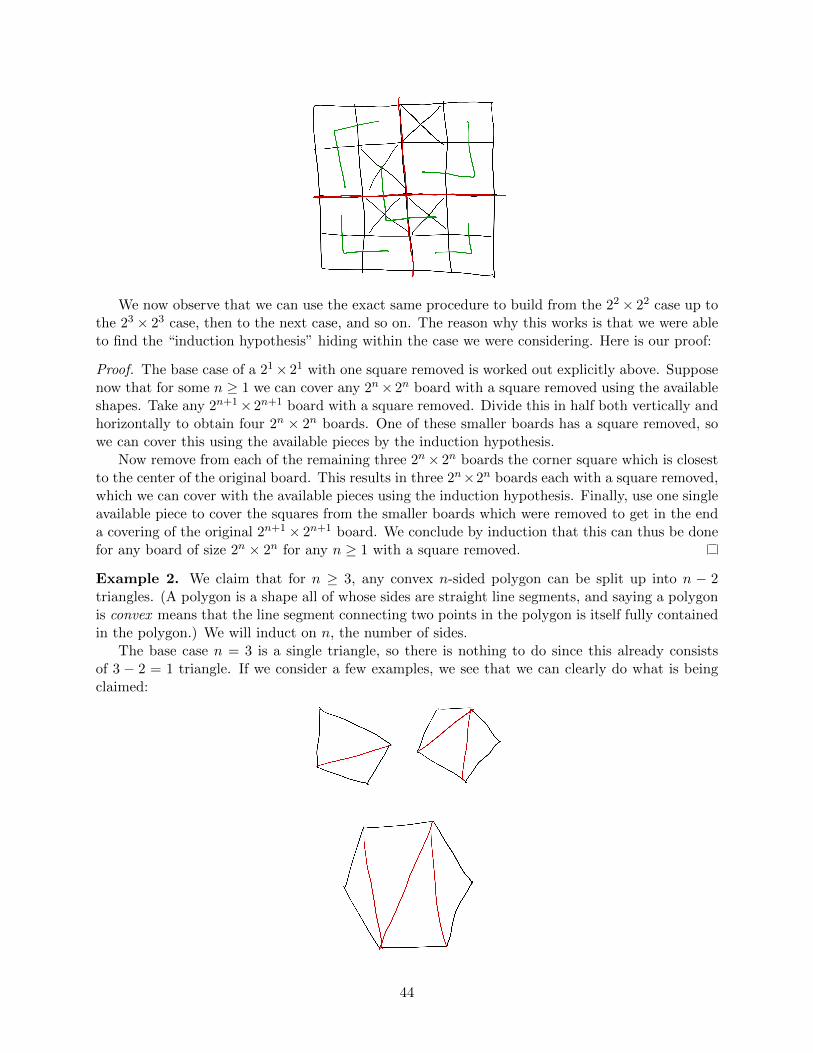
We now observe that we can use the exact same procedure to build from the 22× 22 case up tothe 23 × 23 case, then to the next case, and so on. The reason why this works is that we were ableto find the “induction hypothesis” hiding within the case we were considering. Here is our proof:

Proof. The base case of a 21× 21 with one square removed is worked out explicitly above. Supposenow that for some n ≥ 1 we can cover any 2n× 2n board with a square removed using the availableshapes. Take any 2n+1×2n+1 board with a square removed. Divide this in half both vertically andhorizontally to obtain four 2n × 2n boards. One of these smaller boards has a square removed, sowe can cover this using the available pieces by the induction hypothesis.

Now remove from each of the remaining three 2n× 2n boards the corner square which is closestto the center of the original board. This results in three 2n×2n boards each with a square removed,which we can cover with the available pieces using the induction hypothesis. Finally, use one singleavailable piece to cover the squares from the smaller boards which were removed to get in the enda covering of the original 2n+1× 2n+1 board. We conclude by induction that this can thus be donefor any board of size 2n × 2n for any n ≥ 1 with a square removed.

Example 2. We claim that for n ≥ 3, any convex n-sided polygon can be split up into n − 2triangles. (A polygon is a shape all of whose sides are straight line segments, and saying a polygonis convex means that the line segment connecting two points in the polygon is itself fully containedin the polygon.) We will induct on n, the number of sides.

The base case n = 3 is a single triangle, so there is nothing to do since this already consistsof 3 − 2 = 1 triangle. If we consider a few examples, we see that we can clearly do what is beingclaimed:

44

We can’t very well check every possible polygon, so we now need a way to argue this can be donein general. Assuming we can do this for any n-gon (for some n ≥ 3), we need to build up the caseof an (n + 1)-gon. Given some (n + 1)-gon, we must thus find the “induction hypothesis” case ofan n-gon hiding within our (n+ 1)-gon. But observe that if we connect two vertices like so:

so we connect two vertices which happen to be adjacent to the same vertex, we end up dividingour original (n + 1)-gon into an n-gon and a triangle; the resulting n-gon can be broken up inton − 2 triangles by the induction hypothesis, so in the end we get that our original (n + 1)-gon isbroken up into (n − 2) + 1 = (n + 1) − 2 triangles as required. Note that convexity was used toguarantee that the segment we introduced to connect the two vertices above does indeed result inan n-gon and a triangle.

Example 3. Finally, we use induction to prove what’s called Euler’s formula, which is a resultin the subject of graph theory. A graph is a collection of dots (i.e. vertices) and lines (i.e. edges)connecting them. A graph is planar if it can be drawn so that no two edges cross one another, anda graph is connected if it is possible to reach any vertex from any given one by moving along edges:

Any planar graph divides the plane up into regions we call faces; for instance, the planar graphdrawn above has 4 faces. Euler’s formula states any connected, planar graph satisfies

V − E + F = 2

where V is the number of vertices, E the number of edges, and F the number of faces. This facthas numerous applications in graph theory, but our motivation for talking about it is to give one

45

more example of an interesting proof by induction; indeed, there is no “n” in Euler’s formula atall, although there are three quantities V,E, F , so it is not so clear that this actually susceptibleto induction in the first place. It is, and the key as usual is see how to build up one from scenarioto something more complicated.

We will induct on the number E of edges. The simplest graph will have E = 0 edges, in whichcase we just have a single vertex:

Thus in this base case we have V = 1, E = 0, F = 1, so V − E + F = 2 as Euler’s formula claims.Now, suppose Euler’s formula holds for any connected planar graph with n edges and consider anyconnected planar graph with n + 1 edges. In order to be able to apply our induction hypothesis,we must find the n edge case hiding in our n+ 1 edge case. But we can go from n+ 1 edges downto n edges simply by removing an edge, which still results in a connected planar graph; Euler’sformula applies to this smaller graph by the induction hypothesis, and the final thing to do is keeptrack of how removing an edge affects the numbers V,E, F involved. There are two things whichcan happen: either removing an edge leaves one vertex now isolated, or it does not

In the first case we must then remove the isolated vertex itself if our graph is to remain planar, inwhich case V and E both decrease by 1 while F remains unchanged, or in the second case V isleft unchanged but the number of faces decreases by one, since the two faces sharing the edge weremoved now combine to become a single face. Thus either way the quantity V − E + F remainsunchanged, and so still equals whatever it did in the induction hypothesis, which is 2.

I’ll stop here and leave it to you to think about how to write this out formally, but the hardpart of the work is already done above. For the purposes of learning induction, again the key pointwas in figuring out how to build from the induction hypothesis to the next larger case.

Lecture 14: Functions

Warm-Up. As a final induction problem, we show that any postage greater than or equal to 18cents can be obtained using only 3 and 10 cent stamps. The base case of 18 cents can be obtainedusing six 3 cent stamps. We now have to think about how to build up to larger amounts.

From 18 cents we can get to 21 cents by throwing in another 3 cent stamp, or we can get to 28cents by throwing in a 10 cent stamp, and similarly some larger quantities can be obtained starting

46

with 18 cents. But what about 19 cents, 20 cents, 23 cents, or other values not attainable from astarting point of 18 alone? By hand we can check that 19 and 20 are attainable:

19 = 3(3 cent stamps) + 1(10 cent stamp), and 20 = 2(10 cent stamps).

The key is now that if we also consider these to be base cases, we can then build up to all largerthings, in particular since any larger value is attainable by adding enough 3 cent stamps to one ofthe starting values 18, 19, or 20. Thus, this is an example of an induction with multiple base cases.Here is our proof:

Proof. As seen above, the base cases of 18, 19, and 20 cents can be obtained using only 3 and 10cent stamps. Suppose now that any postage smaller than some n > 20 can be obtained using only3 and 10 cent stamps. Our goal is then to argue that n cents itself can be also obtained. Sincen− 3 < n, n− 3 falls within the range of values to which the induction hypothesis (i.e. any valuesmaller than n) or base case (n− 3 could be 18, 19, 20 for certain values of n > 20) applies, so thisinduction hypothesis gives us that n − 3 cents can be obtained using only 3 and 10 cent stamps.But then throwing in one more 3 cent stamps gives n cents overall as desired. We conclude byinduction that any postage greater than or equal to 18 cents can be obtained.

Functions. No doubt you’ve seen the notion of a function before in other courses, but here wewill be a bit more formal and consider functions between arbitrary sets. A function f : A → Bfrom a set A to a set B is an assignment of an element B to each element of A; in other words,a function gives to each “input” a ∈ A a corresponding “output” f(a) ∈ B. (As in other courses,f(a) is pronounced “f of a”, which is the result of applying f to a.) Another common notationwe’ll see when defining a function is:

a 7→ f(a),

which says that f sends a to the element f(a). (The symbol 7→means “maps to”.) Given f : A→ B,A is called the domain of f , and B the codomain of f ; so the domain is the set of possible inputsand the codomain the set where the outputs lie.

Here is a warning: the book covers functions in Chapter 12, but does so in what I think is anoverly complicated manner. In particular, the book defines a function in terms of what are calledrelations, which is not something we’ve spoken about yet. It is true the a function is technicallya type of relation, but I think this approach obscures the basic idea behind what a function is, orrather what a function should do, which is send elements of one set to elements of another set. So,we will not use the book’s approach and will instead focus on the usual (more intuitive) approach.As a result, we will do things in a different order than the book; in particular, we will first discussthe notions of image/preimage and then injectivity/surjectivity, whereas the book does this theother way around. Again, I think our approach is much simpler to follow.

Examples. We’ve all seen basic examples, like the function f : R → R defined by f(x) = sinx(i.e. the function which sends x ∈ R to sinx ∈ R), or g : Z → Z defined by g(n) = 2n (i.e. thefunction which multiplies an integer input by 2).

But functions can be defined between arbitrary sets, even sets whose elements may not benumbers. To see a more interesting example we introduce the notion of a power set. Given a setA, the power set of A is the set P(A) of subsets of A:

P(A) = {S | S ⊆ A}.

In other words, an element of P(A) is actually a subset of A, so this is our first example of a setwhose elements themselves are sets! It might seem strange to think about sets whose elements

47

are sets at first, but this is actually quite a common type of object in modern mathematics. Forinstance, the subsets {1, 2} are:

∅, {1}, {2}, {1, 2},

so the power set of {1, 2} is:P({1, 2}) = {∅, {1}, {2}, {1, 2}}.

Again, note that each element of the power set, such as the empty set, is a set itself.Consider now the function f : P(A)→ P(A) defined by

S 7→ A− S, or in other words by f(S) = A− S.

This function takes as input a subset of A (i.e. an element of P(A)) and outputs its complementin A. For instance, in the A = {1, 2} example, f does the following:

f(∅) = {1, 2}, f({1}) = {2}, f({2}) = {1}, f({1, 2}) = ∅,

in each case sending the input to its complement in {1, 2}. Properties of power sets will be moreinteresting when we discuss cardinality, but for now this is just meant to give an example of afunction defined on more interesting types of sets.

Image and preimage. Suppose f : A → B is a function. Given a subset X of A, we define itsimage f(X) under f to be the set of all things in B obtained by applying f to elements of X:

f(X) = {f(x) ∈ B | x ∈ X} = {b ∈ B | there exists x ∈ X such that f(x) = b}.

To be clear, to say that b ∈ f(X) means there is some x ∈ X to which we can apply f to obtain b.Given a subset Y of B, we define its preimage f−1(Y ) under f to be the set of all possible

inputs in A which are sent to an element of Y :

f−1(Y ) = {a ∈ A | f(a) ∈ Y }.

Again to be clear, to say that a ∈ f−1(Y ) means by definition that f(a) ∈ Y . Visually, taking animage moves things “forward” while taking a preimage moves things “backwards”:

A word on notation: soon we will use f−1 to denote the inverse of the function f when it actuallyexists, but the f−1 showing up in the notation for preimage is not meant to necessarily signify aninverse function; the notion of a preimage makes sense for any function, even ones without inverses,and we still use the f−1(Y ) notation for preimages even for non-invertible functions.

Example 1. Take the function f : R→ R defined by f(x) = x2. The image of the interval [−1, 2]under f is the interval [0, 4]:

f([−1, 2]) = [0, 4].

48

This says two things: f([−1, 2]) ⊆ [0, 4] means that the result of applying f to anything in [−1, 2]gives something in [0, 4], and f([−1, 2]) ⊇ [0, 4] means that anything in [0, 4] can be obtained asthe result of applying f to something in [−1, 2]. In other words, in order to say that the image of[−1, 2] is [0, 4], it is not enough to know that applying f to something in [−1, 2] gives something in[0, 4], we also have to know that anything in [0, 4] arises in this way.

To show the first containment, let y ∈ f([−1, 2]). By definition, this means that there existsx ∈ [−1, 2] such that f(x) = y. But since −1 ≤ x ≤ 2, we get that 0 ≤ x2 ≤ 4, so that y = f(x) = x2

is indeed in [0, 4]. Hence f([−1, 2]) ⊆ [0, 4]. Conversely, let y ∈ [0, 4]. To say that y ∈ f([−1, 2]) weneed to know that there is something in [−1, 2] which f sends to y. Since 0 ≤ y ≤ 4, 0 ≤ √y ≤ 2,where as usual

√y denotes the nonnegative square root of y. Since

f(√y) =

√y2 = y,

√y is something in [−1, 2] which is sent to y under f , so y ∈ f([−1, 2]). Hence [0, 4] ⊆ f([−1, 2]),

so f([−1, 2]) = [0, 4] as claimed.As an example of a preimage, we have that the preimage of [−1, 2] under f is [−

√2,√

2]:

f−1([−1, 2]) = [−√

2,√

2].

Here we are thinking of [−1, 2] as a subset of the codomain, which is also R, and asking for theelements in the domain R which are sent into [−1, 2] after applying f . Saying that [−

√2,√

2] ⊆f−1([−1, 2]) means that applying f to anything in [−

√2,√

2] gives something in [−1, 2] (which istrue since if −

√2 ≤ x ≤

√2, then −1 ≤ x2 ≤ 2 is true), and saying that f−1([−1, 2]) ⊆ [−

√2,√

2]means that only things in [−

√2,√

2] can belong to f−1([−1, 2]), or in other words that anythingoutside [−

√2,√

2] is not sent to something in [−1, 2].

Example 2. Let f : Z→ Z be the function defined by f(n) = 2n. The image of the entire domainZ under this is the set of even integers, while the image of the set of even integers is the set of allmultiples of 4. The preimage of the set of odd integers is the empty set since there is nothing in Zwhich is sent to an odd integer when applying f .

Example 3. Let f : R→ R be the function defined by

f(n) =

{x+ 2 if x < 11x if x ≥ 1,

a portion of whose graph looks like:

The image of the interval [−1, 2) consists of everything obtained by applying f to things in [−1, 2);visually in terms of the graph, this consists of the y-coordinates of points on the graph correspondingto x-coordinates in given green interval:

49

so f([−1, 2)) =[12 , 3). The preimage of the interval

[34 ,

52

], visualized as an interval on the vertical

y-axis, consists of all x-coordinates corresponding to points whose y-coordinates are in[34 ,

52

]:

Only points between −54 and 1

2 (not including 12) have this property, so f−1

[34 ,

52

)=[−5

4 ,12

).

Images and unions/intersections. Suppose f : A → B is a function and that X,Y ⊆ A. It isa fact that

f(X ∪ Y ) = f(X) ∪ f(Y ),

so the image of a union is the union of individual images; or in other words, first taking a unionand then the image gives the same result as first taking images and then a union. This will be leftto you to prove on a homework assignment, but comes down to showing that each side is a subsetof the other.

Similarly we can ask how intersections behave when taking images. We claim that

f(X ∩ Y ) ⊆ f(X) ∩ f(Y )

but that the opposite containment does not hold, which reflects a property of functions we’ll comeback to later. For now, to prove the given containment we start with b ∈ f(X ∩ Y ). To show thatb ∈ f(X)∩ f(Y ) requires showing b ∈ f(X) and b ∈ f(Y ), the first of which requires showing thereis something in X which f sends to b and the second showing there is something in Y which fsends to b. But since b ∈ f(X ∩ Y ), we know there exists a ∈ X ∩ Y such that f(a) = b, so thisa ∈ X ∩ Y is already an element of X which is sent to b, so b ∈ f(X), and an element of Y whichis sent to b, so b ∈ f(Y ). Thus b ∈ f(X) ∩ f(Y ), so f(X ∩ Y ) ⊆ f(X) ∩ f(Y ).

Here is an example showing the opposite containment does not hold in general. Take f : R→ Rto be f(x) = x2, X = [−1, 0] and Y = [0, 1]. Then

f(X) = [0, 1] = f(Y ) and f(X ∩ Y ) = f({0}) = {0},

so f(X) ∩ f(Y ) = [0, 1] is not a subset of f(X ∩ Y ). We’ll come back to the question as to whenthis opposite containment does hold soon.

50

Lecture 15: Images and Preimages

Warm-Up 1. Let f : Z→ Z be the function defined by

f(n) =

{n+ 2 if n is even

2n if n is odd.

We show that the image of the set O of odd integers under f is the same as the image of the setM of multiples of 4:

f(O) = f(M).

First we should get a sense for what these images look like. The function f sends an even n to n+2and an odd n to 2n; note that the resulting values are then always even. Thus f only outputs evenintegers, so the image of either O or M should be a subset of the set of even integers. However,not all even integers will be in the image of O or M ; for instance, 4 /∈ f(O) since there does existn ∈ O satisfying f(n) = 4, because if n is odd then f(n) = 2n and 4 cannot be written as 2n foran odd integer n. In fact, applying f to an odd n = 2k + 1 gives f(n) = 2n = 4k + 2, so only evenintegers of the form 4k+ 2 should be in the image of O. Similarly, if n = 4k is a multiple of 4, thenf(n) = n+ 2 = 4k + 2, so only even integers of the form 4k + 2 should in the image of M . Henceconcretely, it should be the base that f(O) = f(M) is the set of integers of the form 4k + 2, a factwhich will essentially follow from our proof.

Now, let m ∈ f(O). In order to show that m ∈ f(M) we need to show there exists n ∈M suchthat f(n) = m. For such n ∈ M , f(n) = n + 2 since n, being a multiple of 4, is even, so what wereally need to show is that we can write m as n+ 2 for some multiple n of 4. Since m ∈ f(O), weknow there exists a ∈ O such that f(a) = m. This a ∈ O can be written as a = 2k + 1 for somek ∈ Z, and by the definition of f we then have:

m = f(a) = 2a = 2(2k + 1) = 4k + 2.

Hence n = 4k is an element of M satisfying f(n) = n+ 2 = m, so m ∈ f(M). Thus f(O) ⊆ f(M).Conversely let m ∈ f(M). In order to show that m ∈ f(O) we need to show there exists n ∈ O

such that f(n) = m, which concretely means we need to show that 2n = m for some m ∈ O sincef(n) = 2n for odd n. Since m ∈ f(M), there exists b ∈M such that f(b) = m. This b is a multipleof 4, so b = 4k for some k ∈ Z. Then

m = f(b) = b+ 2 = 4k + 2 = 2(2k + 1)

where f(b) = b+ 2 since b is even. Thus n = 2k + 1 is an element of O satisfying f(n) = 2n = m,so m ∈ f(O). Hence f(M) ⊆ f(O), so f(O) = f(M) as claimed.

Warm-Up 2. Suppose f : A→ B is a function and that X,Y are subsets of B. We show that

f−1(X − Y ) = f−1(X)− f−1(Y ),

which says that the operation of taking preimages “preserves” complements; i.e. taking the com-plement first and then the preimage gives the same result as taking preimages first and then thecomplement. This is a basic set equality proof where we show that each side is a subset of theother, winding the definition of preimage along the way.

Let a ∈ f−1(X−Y ). By definition of preimage this means that f(a) ∈ X−Y . Hence f(a) ∈ Xand f(a) /∈ Y . Since f(a) ∈ X, a ∈ f−1(X) by definition of preimage, and since f(a) /∈ Y ,a /∈ f−1(Y ). Thus a ∈ f−1(X)− f−1(Y ), so f−1(X − Y ) ⊆ f−1(X)− f−1(Y ).

51

Conversely let a ∈ f−1(X) − f−1(Y ). Then a ∈ f−1(X) and a /∈ f−1(Y ). Since a ∈ f−1(X),f(a) ∈ X, and since a /∈ f−1(Y ), f(a) /∈ Y . Thus f(a) ∈ X − Y , so a ∈ f−1(X − Y ). Hencef−1(X)− f−1(Y ) ⊆ f−1(X − Y ), so we have equality as claimed.

Back to images and intersections. Recall that last time we made the claim (and left the proofto the homework) that when f : A → B is a function and X,Y are subsets of A, the followingequality holds:

f(X ∪ Y ) = f(X) ∪ f(Y ),

which says that the operation of taking an image “preserves” unions. We then proved that withrespect to intersections, f(X∩Y ) ⊆ f(X)∩f(Y ) was always true, but that the opposite containmentis not always true by giving an explicit counterexample. (Thus, the operation of taking images doesnot necessarily “preserve” intersections.)

However, how could we have guessed that the opposite containment

f(X) ∩ f(Y ) ⊆ f(X ∩ Y )

should not be true in general? I know this from the experience of having seen this type of thingmany times before, but it is not something which one might immediately realize at the first glance.Indeed, as a student learning these things for the first time, your first instinct might be to try toprove that this containment does hold since, after all, why shouldn’t it? Here is an attempt at a“proof” that this containment does hold, where I say “proof” because we of course know that thisproof cannot be correct:

“Proof” that f (X ) ∩ f (Y ) ⊆ f (X ∩Y ). Let b ∈ f(X) ∩ f(Y ), so that b ∈ f(X) and b ∈ f(Y ).Since b ∈ f(X), there exists a ∈ X such that f(a) = b, and since b ∈ f(Y ), there exists a ∈ Y suchthat f(a) = b. Since a ∈ X and a ∈ Y , a ∈ X ∩ Y , so b ∈ f(X ∩ Y ) since there is something inX ∩ Y mapping to b. Thus f(X) ∩ f(Y ) ⊆ f(X ∩ Y ).

So, what is wrong here? Have we not shown that anything in f(X)∩ f(Y ) is also in f(X ∩Y )?To pinpoint what goes wrong let’s run through this reasoning with the counterexample we gave lasttime: f : R→ R defined f(x) = x2, X = [−1, 0], and Y = [0, 1]. We have f(X) = [0, 1] = f(Y ), sotake b = 1 ∈ f(X)∩ f(Y ). Following our attempted proof, we pick a = −1 ∈ X such that f(a) = band a = 1 ∈ Y such that f(a) = b. But now we see the problem: these are two different values ofa, and so they do not give an element common to both X and Y which f sends to b. Indeed, sinceX ∩ Y = {0}, there is not element in X ∩ Y which is sent to b = 1, which is the reason why thiscounterexample works. The issue with our proof is that we were sloppy in our notation: once wepick a ∈ X such that f(a) = b, we should not use the same a to denote the element of Y whichis sent to b. Rather, we pick a′ ∈ Y such that f(a′) = b, but now we have no way of guaranteeingthat there is an element in X ∩ Y sent to b since a and a′ could very well be different:

52

But now we ask: for which type of function f would the containment f(X)∩ f(Y ) ⊆ f(X ∩ Y )actually be true? The issue above was that we have a ∈ X and a′ ∈ Y sent to b, and if these aredifferent we don’t get an element of X ∩ Y sent to b. The underling point is that we could havedifferent elements a, a′ sent to the same b; whereas if we knew a and a′ actually had to be thesame then the proof would work and the given containment would hold. Hence, for instance, fora function with the property that you cannot have different elements sent to the same thing, thegiven containment would indeed be true. Such a function is said to be injective, which is a notionwe’ll come back to later.

Preimage of the image. In the same setup as before, f : A→ B a function with X ⊆ A, considernow what happens if we take the preimage of the image of X: f−1(f(X)). To be clear, the imagef(X) of X is a subset of B, whose preimage we can then take to get a subset f−1(f(X)) of A again.We want to understand how this preimage of the image relates to the original X.

To say that a ∈ f−1(f(X)) means f(a) ∈ f(X), which in turn means there exists x ∈ X suchthat f(x) = f(a). Thus a is in f−1(f(X)) when a is sent under f to the same thing as somex ∈ X is sent to. Certainly, any a ∈ X will have this property, since a is sent to the same thing assomething in X (namely a itself) is sent to, so

X ⊆ f−1(f(X)).

For a quick formal proof, take x ∈ X. Then f(x) ∈ f(X) by definition of image, so x ∈ f−1(f(X))by definition of preimage. Hence X ⊆ f−1(f(X)).

Now, is it true that X = f−1(f(X))? For this it would have to be true that f−1(f(X)) ⊆ X,but we already said previously that elements a of f−1(f(X)) are things which are sent under f tothe same thing as something in X is sent to, but this does NOT guarantee that a itself must havebeen in X to start with: all we know is that there exists x ∈ X such that f(a) = f(x), but notthat a ∈ X.

Indeed, in the f(x) = x2 example, for X = [0, 1] we have

f(X) = [0, 1], so f−1(f(X)) = f−1([0, 1]) = [−1, 1]

since all elements in [−1, 1] are sent to something in [0, 1], so f−1(f(X)) 6⊆ X in this case. The issueis that −1 ∈ f−1(f(X)) since it is sent to the same thing as what 1 ∈ X is sent to, but −1 /∈ X.

So, in general, we can only say that X ⊆ f−1(f(X)) always holds, but that the oppositecontainment does not necessarily hold. When does the opposite containment hold? We saw beforethe problem arises when f(a) = f(x) for some x ∈ X and a /∈ X, or in other words when we havetwo different elements being sent to the same thing. Hence, as in the case of intersections, for afunction which does not send different things to the same thing (i.e. an injective function), it wouldin fact be true that f−1(f(X)) = X.

53

Image of the preimage. As a final example, in the same setup as before, suppose now thatY ⊆ B and we take the image of the preimage of Y : f(f−1(Y )). To be clear, the preimage of Ygives a subset f−1(Y ) of A, whose image we can then take to get a subset f(f−1(Y )) of B. Howdoes this compare to the original Y ? We claim that

f(f−1(Y )) ⊆ Y

is always true. Indeed, so say that b ∈ f(f−1(Y )) means that there is some a ∈ f−1(Y ) such thatf(a) = b, but by virtue of the fact that a ∈ f−1(Y ) we have that b = f(a) ∈ Y . (In other words,f−1(Y ) is the set of all things in A which get sent to something in Y , and taking the image of thisthen applies f to such elements, thereby giving something in Y as a result.)

However, the opposite containment Y ⊆ f(f−1(Y )) is not necessarily true. We’ll give a coun-terexample in a second, but first let’s try to understand what is wrong with the following “proof”:

“Proof” that Y ⊆ f (f −1 (Y )). Let y ∈ Y . Pick a ∈ A such that f(a) = y. Since f(a) = y is in Y ,a ∈ f−1(Y ), and thus y = f(a) is in f(f−1(Y )). This shows that Y ⊆ f(f−1(Y )) as claimed.

So, what’s wrong? For a counterexample, take f(x) = x2 and Y = [−1, 1]. Then f−1(Y ) = [−1, 1]and f(f−1(Y )) = f([−1, 1]) = [0, 1], which does not contain Y = [−1, 1] as a subset. If we try torun through our “proof” with y = −1, we see the problem immediately: there is no a such thatf(a) = y in this case since squaring a real number cannot possibly give −1. Thus, our proof failsbecause there is no guarantee such a ∈ A exists.

However, if we could guarantee that any y ∈ Y was actually obtainable as the result of applyingf to some element of A, our proof would work find and f(f−1(Y )) = Y would be true in such acase. A function with the property that everything in codomain is obtainable as an actual outputis said to be surjective, and is a notion, along with injective, we’ll come back to next time.

Lecture 16: Injectivity and Surjectivity

Warm-Up. Let f : R2 → R2 be the function defined by f(a, b) = (a + b, 2a + 2b). We determinethe image of f (meaning the image f(R2) of the entire domain) and the preimage of {(0, 0)}.

First, note that the y-coordinate 2a+ 2b of any possible output is twice the x-coordinate a+ b,so all possible outputs lie on the line y = 2x defined by:

L ={

(x, y) ∈ R2∣∣ y = 2x

}.

This observation so far only tells us that the image of f is contained in this line, but we claim inthe fact that the image is the entire line:

f(R2) = L.

54

For this we need to verify that not only is anything in the image on the line (which we alluded toabove) but also that anything on the line is in the image.

Let (x, y) ∈ f(R2). Then there exists (a, b) ∈ R2 such that f(a, b) = (x, y). But by the definitionof f this means

(x, y) = f(a, b) = (a+ b, 2a+ 2b),

so x = a + b and y = 2a + 2b. Hence y = 2x is satisfied, so (x, y) ∈ L and thus f(R2) ⊆ L.Conversely let (x, y) ∈ L. Then y = 2x by definition of L. To show that (x, y) ∈ f(R2) we mustshow that there exists a point in R2 to which applying f gives (x, y); that is, we need (a, b) suchthat

f(a, b) = (a+ b, 2a+ 2b) = (x, y).

But since, for instance, f(x, 0) = (x+ 0, 2x+ 0) = (x, 2x) = (x, y), (x, 0) is an element of R2 whichf sends to (x, y), so (x, y) ∈ f(R2). Hence L ⊆ f(R2), so f(R2) = L as claimed.

Now, the preimage f−1({(0, 0)}) of {(0, 0)} consists of all points in R2 which are sent to some-thing in {(0, 0)}, which in this case means all points which are sent to (0, 0). In other words, thepreimage consists of all (a, b) satsifying

f(a, b) = (a+ b, 2a+ 2b) = (0, 0).

This requires that a + b = 0, so that b = −a. Hence such a point must lie on the line y = −xdefined by

S ={

(x, y) ∈ R2∣∣ y = −x

},

so we claim that f−1({(0, 0)}) = S. The proof is essentially what we did above, but let us write itout more formally.

Let (a, b) ∈ f−1({(0, 0)}). Then f(a, b) ∈ {(0, 0)}, so f(a, b) = (0, 0). Hence

(0, 0) = f(a, b) = (a+ b, 2a+ 2b), so 0 = a+ b.

Thus b = −a, so (a, b) ∈ S and hence f−1({(0, 0)}) ⊆ S. Conversely let (x, y) ∈ S, so that y = −x.Then f(x, y) = (x + y, 2x + 2y) = (x − x, 2x − 2x) = (0, 0), so (x, y) ∈ f−1({(0, 0)}). HenceS ⊆ f−1({(0, 0)}), so f−1({(0, 0)}) = S as claimed.

Injective and surjective functions. Suppose f : A→ B is a function. We say that f is injectiveif whenever x 6= y in A, then f(x) 6= f(y); that is, different elements get sent to different things.By taking the contrapositive, we can phrase this as:

if f(x) = f(y), then x = y,

which says that the only way two elements can be sent to the same thing is if they were actuallythe same element to start with. (This latter phrasing will usually be the better one to use whenactually showing a given function is surjective.) Another term for “injective” you’ll often see isone-to-one, which emphasizes the idea that each output can only come from one input.

We say that f is surjective if for every b ∈ B there exists a ∈ A such that f(a) = b; that is,everything in the codomain can be obtained by applying f to some input. Or, said in another wayusing the language of images, for f : A→ B to be surjective mans that the image f(A) of f is allof B: f(A) = B. Another term for “surjective” you’ll often see is onto.

To go back to some things we saw last time, which now we see were meant to provide possiblemotivations for the notions of injective and surjective, recall that the following always hold for anyfunction:

f(X ∩ Y ) ⊆ f(X) ∩ f(Y ), X ⊆ f−1(f(X)), f(f−1(S)) ⊆ S.

55

Based on our previous discussion, we can now say that, in addiition, when f is injective it istrue that f(X ∩ Y ) = f(X) ∩ f(Y ) and X = f−1(f(X)), and when f is surjective it is truethat f(f−1(S)) = S. In particular then, for injective functions, the operation of taking imagesdoes preserve intersections. In fact, it is also true that f(X − Y ) = f(X) − f(Y ) for an injectivefunction, so the operation of taking images under injective functions preserves complements, butthis is not the case for non-injective functions.

Example 1. Consider the function f : R2 → R2, f(a, b) = (a + b, 2a + 2b) from the Warm-Up.We showed there that the image of f was only the line y = 2x, so since this is not all of R2 thefunction f is not surjective. For instance, for (1, 1) ∈ R2 there does not exist (a, b) ∈ R2 such thatf(a, b) = (1, 1) since there do not exist a, b satisfying (a+ b, 2a+ 2b) = (1, 1).

The fact that the preimage of {(0, 0} is the line y = −x immediately shows that f is not injective,since there are multiple points being sent to (0, 0). For instance, f(−1, 1) = (0, 0) = f(1,−1) but(−1, 1) and (1,−1) are not the same, so f is not injective.

Example 2. Whether or not a given expression defines an injective/surjective function completelydepends on the domain and codomain being considered. For instance, the function f : R → Rdefined by f(x) = x2 is neither injective, since 1 and −1 both get sent to the same thing, norsurjective, since −1 is not in the image.

However, with R≥0 denoting the set of nonnegative real numbers, the function g : R → R≥0defined by g(x) = x2 is surjective, since by cutting the domain down to be R≥0 instead of all of Rwe have eliminated the elements of R which are not attained as outputs. Along these same lines,the function h : R≥0 → R defined by h(x) = x2 is injective since for non-negative numbers, x2 = y2

does imply x = y. Finally, the function ` : R≥0 → R≥0 defined by `(x) = x2 is both injective andsurjective—we say that such a function is bijective.

Example 3. Here is another example of a bijective function. For a set A, let f : P(A)→ P(A) bethe function sending a subset S of A to its complement A− S in A:

f(S) = A− S.

(Recall that P(A) denotes the power set of A, which is the set of all subsets of A.) To see that f isinjective, suppose f(S) = f(S′). This then means that S and S′ have the same complement in A:

A− S = A− S′.

We need to show that S = S′. Since A− S = A− S′, the complements of each of these should alsobe the same:

A− (A− S) = A− (A− S′).

But taking the complement of the complement results in the original set, so the left side above isS and the right side is S′, so S = S′ and f is injective as claimed.

To show that f is surjective, let S ∈ P(A). We need to know there exists an element of P(A)which is sent to S under f , or in other words a subset of A whose complement is S. But

f(A− S) = A− (A− S) = S,

so A − S ∈ P(A) is an element sent to S, and hence f is surjective. Since f is injective andsurjective, it is bijective.

56

Injectivity/surjective via sizes of preimages. Let us see how to rephrase the notions ofinjective and surjective in terms how large a preimage of the form f−1({b}) can be. Given f : A→ Band b ∈ B, f−1({b}) consists of all elements of A which are sent to B. But to be injective meansthat, if there is such an element, there can only be one, so we have that:

f is injective if and only if for all b ∈ B, f−1({b}) has at most one element.

On the other hand, to be surjective means that given any such b ∈ B, there is an element which issent to B; such an element will then be in f−1({b}), so

f is surjective if and only if for all b ∈ B, f−1({b}) has at least one element.

Thus, we can also say that f is bijective if and only if for all b ∈ B, f−1({b}) has exactly oneelement. These observations are meant to make a connection between injectivity/surjectivity andthe “sizes” of certain sets.

Looking ahead to cardinality. We will later talk about the cardinality of a set as being thenumber of elements it contains, so the above facts tells us that: f is injective if the preimageof every single element has cardinality at most 1; f is surjective if the preimage of every singleelement has cardinality at least 1; and f is bijective if the preimage of every single element hascardinality exactly 1. The notions of injective and surjective will play a key role in understandingthe cardinality of infinite sets.

To see one more glimpse of this, suppose A and B are finite sets and that f : A → B is afunction. We are interested in understanding what f being injective or surjective tells us aboutthe cardinality of A in relation to the cardinality of B. We first claim that if f is injective, then Amust have no more elements than B does, or in other words that the cardinality of A is less thanor equal to the cardinality of B:

|A| ≤ |B|,

where |S| is the notation for the cardinality of S, which for finite sets just means the number ofelements in S. Indeed, if A had more elements than B, the necessarily we would have more thanelement of A being sent to the same element of B, in which case f would not be injective. If insteadf is surjective, then A can have no fewer elements than does B, or in other words the cardinalityof A is greater than or equal to the cardinality of B:

|A| ≥ |B|.

Indeed, if A had fewer elements than B, then there would necessarily be elements of B not obtainedas actual outputs since there wouldn’t be enough inputs to allow that, but in this case f could notbe surjective. Again, the fact that we have a relation between injectivity/surjectivity and the sizesof finite sets will pay dividends when we discuss the sizes of infinite sets.

Lecture 17: Compositions

Warm-Up 1. Let f : R − {1} → R be the function defined by f(x) = 2x+1x−1 . We show that f is

injective. (Note that 1 is excluded from the domain so 2x+1x−1 makes sense for all x in the domain.)

Suppose f(x) = f(y); we must show that x = y. Since f(x) = f(y), we have

2x+ 1

x− 1=

2y + 1

y − 1

57

by the definition of f . Thus

(2x+ 1)(y − 1) = (2y + 1)(x− 1), so 2xy − 2x+ y − 1 = 2yx− 2y + x− 1.

This gives −3x = −3y, so x = y as desired. Hence f is injective.

Warm-Up 2. Let f : R2 → R2 be the function f(x, y) = (x + y, 2x + y). We show that f issurjective. Thus, for (a, b) ∈ R2, we must show there exists (x, y) ∈ R2 such that f(x, y) = (a, b).Using the definition of f , this means that (x, y) must satisfy

(x+ y, 2x+ y) = (a, b), so x+ y = a and 2x+ y = b.

Thus the question comes down to showing that this collection of equations has a solution for anya, b. (This should remind you of things you saw in a previous linear algebra course, although herewe won’t require any linear algebra to proceed.) Working out some scratch work on the side, thefirst equation x+ y = a gives x = a− y, and then the second 2x+ y = b gives

2(a− y) + y = b, so y = 2a− b.

Then x = a − y = b − a, so this scratch work suggests that x = b − a, y = 2a − b should satisfyf(x, y) = (a, b). We verify this:

f(b− a, 2a− b) = ([b− a] + [2a− b], 2[b− a] + [2a− b]) = (a, b).

Thus any (a, b) ∈ R2 arises as the result of applying f to some element of the domain, so f issurjective as claimed.

Compositions. Given functions f : X → Y and g : Y → Z, we can look at the function obtainedby first applying f and then applying g; this is called the composition of f and g and is denotedby g ◦ f . To be clear, the composition of f and g is the function g ◦ f : X → Z defined by

(g ◦ f)(x) = g(f(x)).

The notion of a composition should be familiar from a calculus course, where for instance the chainrule tells us how to differentiate compositions, but now we’re pointing out that compositions makesense in the more general setting of functions between arbitrary sets.

Note the notation: g ◦ f means that first we apply f and then we apply g. More generally, wecan speak of the composition fn ◦ · · · ◦ f1 of n functions:

X1f1−→ X2

f2−→ X3f3−→ · · · fn−1−−−→ Xn

fn−→ Xn+1,

each one mapping into the domain of the next. (Af−→ B is alternate notation for f : A→ B.)

Example. Denote by R∞ the set of infinite sequences of real numbers, so that an element of R∞looks like:

(x1, x2, x3, . . .) where each xi ∈ R.

Define the functions L,R : R∞ → R∞ by

L(x1, x2, x3, . . .) = (x2, x3, x4, . . .) and R(x1, x2, x3, . . .) = (0, x1, x2, . . .).

58

We compute the compositions R ◦ L and L ◦R, both of which give functions R∞ → R∞. First wehave:

(R ◦ L)(x1, x2, x3, . . .) = R(L(x1, x2, x3, . . .)) = R(x2, x3, x4, . . .) = (0, x2, x3, . . .),

so R ◦ L is the function which just replaces the first term in (x1, x2, x3, . . .) with 0. Second:

(L ◦R)(x1, x2, x3, . . .) = L(R(x1, x2, x3, . . .)) = L(0, x1, x2, . . .) = (x1, x2, x3, . . .),

so L ◦ R is the function which sends (x1, x2, x3, . . .) to itself; we say that L ◦ R is the identityfunction on R∞. Note that R ◦ L is neither injective nor surjective, while L ◦R is bijective.

Compositions and injectivity/surjectivity. We now give some properties of compositions inrelation to injectivity and surjectivity. Suppose f : X → Y and g : Y → Z are functions. We claimthat if f and g are both injective, then g ◦ g is injective, and that if f and g are both surjective,then g ◦ f is surjective.

Suppose f and g are injective. To show that g ◦ f is injective we must show that whenever(g ◦f)(x) = (g ◦f)(x′), it must be true that x = x′. Thus, suppose (g ◦f)(x) = (g ◦f)(x′), meaning

g(f(x)) = g(f(x′)).

How do we use the facts that g and f are injective in order to conclude that x = x′? Note thatg being injective only tells us something about what happens when we plug things into g, andsimilarly f being injective only tells us something about what happens when plugging things intof . But the equality above can be viewed as saying that plugging f(x) into g gives the same resultas plugging f(x′) into g, so injectivity of g gives

f(x) = f(x′).

Then injectivity of f gives x = x′ as desired, so g ◦ f is injective.Suppose f and g are surjective and let z ∈ Z. To show that g ◦ f is surjective we must show

there exists x ∈ X such that (g ◦ f)(x) = z, or in other words g(f(x)) = z. But before anythingelse notice that this equality requires that there be something we can plug into g, which will endup being f(x) for the currently unspecified x, in order to get z, and it is the surjectivity of g whichsays we can do this. Since g is surjective, there exists y ∈ Y such that g(y) = z. Now if we knowthat we can write y as y = f(x) for some x ∈ Z we will be done, and we do know this because f issurjective: since f is surjective, there exists x ∈ X such that f(x) = y, and this x thus satisfies

(g ◦ f)(x) = g(f(x)) = g(y) = z

as required. Hence g ◦ f is surjective.

Extending to more functions. From this we immediately get that the composition of anynumber of injective functions is injective and that the composition of any number of surjectivefunctions is surjective. Indeed, induction gives us a way to build up from the case above of twofunctions to more general situations. To be clear, suppose we know that the composition of ninjective functions is always injective. Then if

X1f1−→ X2

f2−→ X3f3−→ · · · fn−→ Xn+1

fn+1−−−→ Xn+2,

59

are all injective, we get that fn ◦ · · · ◦ f1 is injective by the induction hypothesis and then that

fn+1 ◦ · · · ◦ f1 = fn+1 ◦ (fn ◦ · · · ◦ f1)

is injective from the base case. A similar argument works for the composition of any number ofsurjective functions. (As we mentioned a while ago, using induction to extend some fact from twothings at a time to any number of things at a time is quite fruitful.)

Back to compositions and injectivity/surjectivity. Here are two more final claims for func-tions f : X → Y and g : Y → Z: if g◦f is injective, then f is injective, and if g◦f is surjective, theng is surjective. The previous facts tells us that if the individual functions have some property, thecomposition will as well, whereas here we are claiming that if the composition has some property,at least one of the individual functions will as well: in any injective composition, the first functionmust be injective, and in any surjective composition, the final function must be surjective.

So, suppose g ◦ f is injective. To show that f is injective we suppose f(x) = f(x′) for somex, x′ ∈ X. Our goal is to show that x = x′. Now, are assumption that g ◦ f is injective doesn’t tellus anything until we bring g into the picture somehow, but the point is that if f(x) = f(x′) arethe same element of Y , then applying g to this common element should give the same result:

g(f(x)) = g(f(x′)).

But this equality now says that (g ◦f)(x) = (g ◦f)(x′), so injectivity of g ◦f gives x = x′ as desired.Note again that in order to use injectivity of g ◦ f we had to introduce g somehow into our givenexpression f(x) = f(x′).

Now suppose g ◦ f is surjective and let z ∈ Z. To show that g is surjective requires showingthere exists y ∈ Y such that g(y) = z—where does this y come from? The question is do we knowthere is something we can input into g to give z, but we at least know there is something we caninput into g ◦ f to give z: since g ◦ f is surjective, there exists x ∈ X such that

z = (g ◦ f)(x) = g(f(x)).

But this equality says precisely that y = f(x) is then an element of Y which g sends to z, as neededin order to be able to conclude that g is surjective, so g is surjective as claimed.

Careful. It is NOT true in general that if g ◦ f is injective, g must be injective, nor is it true ingeneral that if g ◦ f is surjective, f must be surjective. We’ll see how to reason through the processof finding examples of these facts next time.

Lecture 18: Invertibility

Warm-Up 1. We give an example of functions f : X → Y and g : Y → Z such that g ◦f : X → Zis injective but for which g is not injective. First, let us think through the process of finding suchan example. Saying that g ◦ f is injective means that

if g(f(x1)) = g(f(x2)), then x1 = x2.

The key observation is that this only tells us something about what happens when applying g tooutputs of f since the hypothesis only uses elements of Z of the form g(f(x)). In other words, theassumption that g ◦ f is injective says nothing about what happens when applying g to elementsof Y which are not in the image of f , since such elements cannot be written in the form f(x).

60

Thus, the idea is that the non-injectivity of g in the sought after example should come from thoseelements of Y which are not in the image of f .

In whatever example we find, we know that f will have to be injective since we showed last timethat injectivity of g ◦f implies injectivity of f . So, to start building up an example let us start witha simple injective function, say f : N → N defined by f(n) = n2. (Note that this is injective sinceN only consists of positive integers.) The assumption that g ◦ f is injective will thus only tells ussomething about applying g to elements of the form n2, but for instance it will say nothing aboutwhat g(2), g(3), g(5), etc should be. So, to guarantee that g is not injective we can, for instance,send all such elements to the same thing. Maintaining injectivity of g on elements of the form n2

but forcing g to be non-injective on elements not of this form should then give a valid example.So, take g : N→ N defined by

g(m) =

{m if m = n2 for some n ∈ N1 otherwise

as one possible example. Then if g(f(x1)) = g(f(x2)) for some x1, x2 ∈ N, we have:

g(x21) = g(x22), which becomes x21 = x22

and hence gives x1 = x2 since x1, x2 are positive. Thus g ◦f is injective. However, g is not injectivesince for instance g(2) = 1 = g(3).

Warm-Up 2. We give an example of functions f : X → Y and g : Y → Z such that g ◦f : X → Zis surjective but for which f is not surjective. We know that in any such example, g will have tosurjective since surjectivity of g ◦ f implies surjectivity of g. If we want f to not be surjective, letus start with some non-surjective function; say f : R→ R defined by f(x) = x2. Now, we think ofan “easy” way to guarantee that g ◦ f will be surjective.

Surjectivity means that the image should equal the entirety of the codomain, so a simple way tomake a function X → Z surjective is for Z to only consist of a single element. Then the definitionsurjective only asks something of this single element, so it will automatically be satisfied. Thus,take g : R → {0} to be the function sending everything to 0. Then g ◦ f : R → {0} is also thefunction which sends everything to 0, so it is surjective, but f is not as required.

Invertible functions. A function f : A→ B is called invertible if there exists a function g : B → Asuch that

g ◦ f = idA and f ◦ g = idB,

where idA and idB denote the identity functions on A and B respectively, which are functionswhich send any element to itself. Concretely, this means that

g(f(a)) = a for all a ∈ A and f(g(b)) = b for all b ∈ B.

When it exists, we call g the inverse of f and denote it by g = f−1. The idea is that the inversefunction is the function which does the “opposite” of what f does, meaning that whenever f sendsa ∈ A to b ∈ B, f−1 should send b back to a.

Example. Let R+ denote the set of positive real numbers. The function f : R → R+ given byf(x) = ex is invertible with inverse f−1 : R+ → R defined by f−1(y) = ln y. Note that if we insteadconsider f as a function R→ R with codomain R, then it is not invertible since ln y is not definedby nonpositive y, meaning that the candidate for f−1 does not have domain R.

61

Along these lines, consider the function f : R≥0 → R≥0 defined by f(x) = x2. This function isinvertible, with inverse f−1(y) =

√y. However, alternating the domain or codomain of f may lead

to a non-invertible function; for instance, the same f(x) = x2 but considered as a function R→ R,R → R≥0, or R≥0 → R is not invertible. The function g : R≤0 → R≥0 defined by g(x) = x2 isinvertible with inverse g−1(y) = −√y. The upshot is that domains and codomains matter.

The requirements in the definition of invertible. Here is an example showing that bothrequirements g ◦ f = idA and f ◦ g = idB are necessary in the definition of invertible, meaningthat one does not automatically imply the other. Take L,R : R∞ → R∞ to be the left-shift andright-shift functions. We previously worked out that L ◦R is the identity function on R∞, but thatR ◦L is the function which replaces the first component of an element of R∞ with 0, so that R ◦Lis not the identity function.

The point is that here neither L nor R are invertible, even though composing them in one order(but not the other) does happen to give the identity function. Technically, so far we’ve only shownthat L and R are not inverses of one another, but we haven’t ruled out the possibility that L couldhave some other inverse that wasn’t R, or that R could have an inverse which wasn’t L. That thisis not possible will follow from our next fact that an invertible function must always be bijective:neither L nor R is bijective, so neither is invertible.

Invertible implies bijective. We now work towards understanding what types of functions dohave inverses. First, we claim that if a function f : A → B is invertible, it must be bijective.Indeed, we get this right away based on things we’ve done previously: since f ◦ f−1 = idB issurjective, f must be surjective, and since f−1 ◦ f = idA is injective, f must be injective. Thus fis bijective. This then immediately tells us, as we pointed out before, that the functions shiftingfunctions L,R : R∞ → R∞ are not invertible.

Bijective implies invertible. The claim is that, actually, a function f : A → B is invertible ifand only if it is bijective. We showed the forward direction above, so we have only the backwardsdirection left to show.

Thus, supposing f is invertible, we must actually construct an inverse function f−1 : B → A.This function should, whenever f(a) = b, send b back to a. But we’ve already seen a glimpse ofthis previously: if f is bijective, for any b ∈ B, there exists a unique a ∈ A such that f(a) = b.Indeed, the existence comes from surjectivity of f , and the uniqueness from injectivity. Thus, wesimply define f−1 : B → A to be the function sending an element of B to be this unique elementof A:

f−1(b) = the unique element a ∈ A satisfying f(a) = b.

With this definition, we havef(f−1(b)) = b

since, by definition, f−1(b) ∈ A has the property that applying f to it gives b, and

f−1(f(a)) = a

since f−1(f(a)) should be the unique x ∈ A satisfying f(x) = f(a), which requires that x = a.So, “invertible” and “bijective” mean the same thing. A key observation, which is useful when

wanting to compute an inverse explicitly, is that f−1(b) = a means precisely the same thing asf(a) = b. Thus, finding f−1(b) means solving f(a) = b for a.

Final example. We show that the function f : R3 → R3 defined by

f(x, y, z) = (x, x+ y, x+ y + z)

62

is invertible by explicitly finding its inverse. A homework problem asked to show that this functionis bijective, which gives us one way of showing that it is invertible, but doesn’t tell us on its ownwhat the inverse is. The inverse function f−1 : R3 → R3 should have the property that

f−1(a, b, c) = (x, y, z) when f(x, y, z) = (a, b, c).

Thus, to describe f−1, given (a, b, c) ∈ R3 we must find (x, y, z) ∈ R3 satisfying f(x, y, z) = (a, b, c),which for this particular function means:

(x, x+ y, x+ y + z) = (a, b, c).

Equating components gives an equation we can use to solve for x, y, z in terms of a, b, c, where weget

x = a, y = b− a, and z = c− b.

Thus, the inverse of f should be the function f−1 : R3 → R3 defined by

f−1(a, b, c) = (a, b− a, c− b).

We verify that this is indeed the inverse by computing both f ◦ f−1 and f−1 ◦ f :

(f ◦ f−1)(a, b, c) = f(f−1(a, b, c))

= f(a, b− a, c− b)= (a, a+ (b− a), a+ (b− a) + (c− b))= (a, b, c)

and

(f−1 ◦ f)(x, y, z) = f−1(f(x, y, z))

= f−1(x, x+ y, x+ y + z)

= (x, (x+ y)− x, (x+ y + z)− (x+ y))

= (x, y, z).

Hence f−1 ◦ f and f ◦ f−1 are both the identity functions on R3, so f−1 is the inverse of f and fis invertible as claimed.

Lecture 19: Equivalence Relations

Warm-Up 1. We find the inverse of the function f : (R− {1})× R→ (R− {2})× R defined by

f(x, y) =

(2x+ 1

x− 1, x+ y

),

thereby verifying that f is indeed invertible. The idea, and why one should expect this function toindeed be invertible, is that we can use the first component f to determine the value of x whichgives a specified output, and then use the second component to determine the value of y required.So, given any (a, b) ∈ (R−{2})×R, it seems that it should be possible to find (x, y) ∈ (R−{1})×Rsatisfying f(x, y) = (a, b). (We’ll see where the restriction that the codomain be (R − {2}) × Rcomes from in the course of working this out.)

63

So, given (a, b) ∈ (R− {2} × R) we need to find (x, y) ∈ (R− {1})× R such that

f(x, y) =

(2x+ 1

x− 1, x+ y

)= (a, b),

which requires2x+ 1

x− 1= a and x+ y = b.

The equation gives 2x+ 1 = ax− a, so

x =−a− 1

2− a=a+ 1

a− 2.

(Note that here is we need a 6= 2 in order to ensure this fraction exists.) Then the second equationgives

y = b− x = b− a+ 1

a− 2.

Thus, the (x, y) needed in order to satisfy f(x, y) = (a, b) is

(x, y) =

(a+ 1

a− 2, b− a+ 1

a− 2

),

so the inverse of f is the function f−1 : (R− {2})× R→ (R− {1})× R defined by

f−1(a, b) =

(a+ 1

a− 2, b− a+ 1

a− 2

).

You should be able to verify that f ◦ f−1 and f−1 ◦ f are both identity functions.

Warm-Up 2. To see an instance of the types of things we can do when we do have an inverse,recall the fact that if g ◦ f is injective, it is not true that g must be injective. However, we nowclaim that if g ◦ f is injective and f is invertible, then g indeed must be injective. Just to be clear,say that f maps A→ B and g maps B → C.

Now, an observation we made previously is that the knowledge that g ◦ f is injective only tellsus something about expressions of the form g(f(a)), but in order to show that g is injective wework with expressions of the form g(b) for, at first glance, any possible b ∈ B. Indeed, supposingg(b) = g(b′), we must show that b = b′. The point is that we have to figure out a way to work finto this equality if we want to have any hope of making use of the fact that g ◦ f is injective.

But now the invertibility of f comes to the rescue! Since f−1 exists, we can write b and b′ as

b = f(f−1(b)) and b′ = f(f−1(b′)).

With this the equality g(b) = g(b′) becomes

g(f(f−1(b))) = g(f(f−1(b′))).

This is in the form needed to make use of injectivity of g ◦ f , so we get that

f−1(b) = f−1(b′),

or in other words that the input f−1(b) into g ◦ f on the left is the same as the input f−1(b′) intog ◦ f on the right. Finally, applying f to both sides of this new equality gives

f(f−1(b)) = f(f−1(b′)),

64

which becomes b = b′. Thus g is injective as claimed.

Relations. Relations, and the more important notion of an equivalence relation, are coveredin Chapter 11 in the book, before the chapter functions. I mentioned previously that the bookapproaches the notion of a function using the notion of a relation, which I find obscures the pointbehind functions. So, we now backtrack and say a bit about relations.

I’ll preface this entire discussion by saying that it is unlikely you’ll actually explicitly use thenotion of a relation (or of an equivalence relation) in future courses; it is definitely true that manyconcepts you’ll see in later courses—in particular albstract algebra, number theory, and topology—can be phrased in terms of equivalence relations, but the point is that this is not how these conceptsare usually presented. So, you should not view our discussion of equivalence relations as essential toother courses, but rather as a way to give us more practice in working with definitions and formingmathematical arguments. Nevertheless, we will say a bit more about next time about the types ofthings you can do with the notion of an equivalence relation.

A relation on a set A is a subset of A × A. This definition doesn’t seem all that interesting,and indeed it’s really not, except for the fact that it gives a way of formalizing various types of“relationships” one comes across in mathematics.

Examples. The best way to get a handle on what the concept of a relation is meant to do is tojump into some well-known examples. For instance, we can talk about the relation ≤ on R. Thisparticular relation captures the idea that one number can be smaller than or equal to another, orin other words that two numbers are “related” by this inequality. Formally, as a subset R×R, therelation of which we are speaking is:

{(x, y) ∈ R× R | x ≤ y}.

To say that (x, y) is in this subset is to say that x ≤ y. The point being, as mentioned previously,that this particular subset gives a formal way of talking about ≤ in set-theoretic terms. However,it is crucial to recognize that what is important here is the relationship ≤ itself, and not so muchthe subset used in the formal definition of “relation”.

Here is another example, dealing with the relation of “divides” on Z. Here, the relationshipbetween two integers a, b we care about is that of a dividing b, so we say that “a is related to b”under this relation when a divides b. Formally, the subset in question is

{(a, b) ∈ Z× Z | a divides b}.

Again, it is better to place the focus on the notion of “divides” than on this particular subset itself.

Forgetting subsets. So, going forward, we will talk about relations in the sense of one elementbeing “related” to another, where “related” depends on the specific relation being used. That is,we won’t talk about a relation on A anymore as being defined by a certain subset of A × A, butrather as a way to specify which elements of A should be related.

On top of this, really the only type of relations we’ll actually care about are equivalence relations,which we now define. With this in mind, we will use the notation ∼ when denoting a relation,and write a ∼ b when a is related to b in whatever sense we’re talking about. (The notation ∼ isreserved for equivalence relations, and a ∼ b is usually read as saying that “a is equivalent to b”under the equivalence relation being considered.)

Equivalence relations. Here are three properties a relation ∼ on a set A might have:

65

• (the reflexive property) For all a ∈ A, a ∼ a.

• (the symmetric property) If a ∼ b, then b ∼ a.

• (the transitive property) If a ∼ b and b ∼ c, then a ∼ c.

The first says that anything in A is related (or equivalent) to itself; the second says that the order inwhich two elements are related to one another doesn’t matter, so two elements are either equivalentor they’re not; and the third says that two elements equivalent to a common element are actuallyequivalent to one another. We say that ∼ is an equivalence relation when it is reflexive, symmetric,and transitive.

Think of these three properties as capturing a type of “equality”: certainly, anything should beequal to itself, equality shouldn’t depend on ordering, and two things equal to a common thing areequal to each other. Of course, equivalence relations are NOT equalities, but they do lead to certainequalities among so-called equivalence classes, which we’ll soon define. The overarching idea is thatequivalence relations give a way to say that two non-equal things really should be thought of asbeing the “same”, in the sense that they capture the same information in the context of whateverproperty in which we are interested. This is a vague description to be sure, but one which shouldbecome clearer next time.

Non-examples. The examples of ≤ and “divides” we mentioned previously are not equivalencerelations since they are not symmetric. (They are, however, both reflexive and transitive: x ≤ x istrue for all x ∈ R, and x ≤ y and y ≤ z does imply x ≤ z; and, “any integer divides itself” is true,and a divides b and b divides c does imply that a divides c.) The relation ≤ is not symmetric since1 ≤ 5 but 5 6≤ 1, and divisibility is not symmetric since 2 divides 4 but 4 does not divide 2.

The relation < of being strictly less than is still transitive, but is no longer reflexive. In general,none of the three properties in the definition of an equivalence relation imply the others.

Congruence mod 4. As a first example of something which is an equivalence relation, we definethe notion of “congruence mod 4”. (We chose 4 just to be specific, but more generally one candefine the notion of congruence mod n for any n ∈ N.)

Define ∼ on Z by saying a ∼ b if a − b is divisible by 4. Thus, two elements are related (or“equivalent”) under this relation if their difference is a multiple of 4. First let’s verify that this isan equivalence relation. For any n ∈ Z, n−n = 0 is divisible by 4, so n×n and hence ∼ is reflexive.(Don’t get lost in all the symbols: to say that n×n means by definition of this equivalence relationthat n−n should be divisible by 4. The point is that whenever we see “a ∼ b” when talking about aspecific equivalence relation, we have to interpret its meaning based on that specific relation itself.)

To see that ∼ is symmetric, suppose a ∼ b. This means that a−b is divisible by 4, so a−b = 4kfor some k ∈ Z. In order to be able to conclude that b ∼ a we would need to know that b−a is alsodivisible by 4. But multiplying a − b = 4k by −1 gives b − a = 4(−k), which shows that b − a isindeed divisible by 4 and hence that b ∼ a as required. Thus ∼ is symmetric. To check transitivity,suppose a ∼ b and b ∼ c for some a, b, c ∈ Z. To say that a ∼ b means a− b is divisible by 4, andto say b ∼ c means b− c is divisible by 4, so

a− b = 4k and b− c = 4`

for some k, ` ∈ Z. The question is whether a − c is divisible by 4 (which is what a ∼ c means inthis context), but:

a− c = (a− b) + (b− c) = 4k + 4` = 4(k + `),

66

so a − c is indeed divisible by 4. Thus a ∼ b and b ∼ c implies a ∼ c, so ∼ is transitive. Hence ∼is an equivalence relation as claimed.

In this specific setting, a ∼ b means that a and b are “congruent mod 4”, and we write

a ≡ b mod 4

to indicate this. The resulting theory of “modular arithmetic” plays a big role in number theoryand abstract algebra, and is something we’ll briefly touch on next time.

Equivalence classes. Given an equivalence relation ∼ on A, we define the equivalence class ofa ∈ A to be the set [a] of all things in A which are equivalent to A:

[a] = {b ∈ A | b ∼ a}.

For instance, let us work out the equivalence classes of the “congruent mod 4” equivalencerelation introduced above. To start with, the equivalence class of 0 consists of all things equivalentto 0:

[0] = {n ∈ Z | n ∼ 0}.

But according to the definition of ∼ in this case, n ∼ 0 means that n − 0 is divisible by 4, whichthus means that n should be divisible by 4. Thus n is in the equivalence class of 0 if and only if nis a multiple of 4:

[0] = {4k | k ∈ Z} = {. . . ,−12,−8,−4, 0, 4, 8, 12, . . .}.

The equivalence class of [1] consists of all n such that n ∼ 1. But n ∼ 1 means that n − 1 isdivisible by 4, so n− 1 = 4k for some k ∈ Z. Hence n = 4k + 1, so things in the equivalence classof 1 are integers of the form 4k + 1:

[1] = {4k + 1 | k ∈ Z} = {. . . ,−7,−3, 1, 5, 9, . . .}.

To say that n ∼ 2 means n− 2 = 4k for some k ∈ Z, so n = 4k + 2 and hence

[2] = {4k + 2 | k ∈ Z} = {. . . ,−6,−2, 2, 6, 10, . . .}.

Similarly, the equivalence class of 3 consists of all things of the form 4k + 3:

[3] = {4k + 3 | k ∈ Z} = {. . . ,−5,−1, 3, 7, 11, . . .}.

Now, what about the equivalence class of 4? To say that n ∼ 4 means n−4 = 4k for some k ∈ Z.But this is the same as saying that n = 4(k+1) is a multiple of 4, so we get that things equivalenceto 4 are the same as things equivalent to 0, so [4] = [0]. Similarly, n ∼ 5 means n − 5 = 4k forsome k ∈ Z, which gives n = 4(k+ 1) + 1, an expression indicating a number equivalent to 1. Thus[5] = [1], and continuing on you’ll see that

[6] = [2], [7] = [3], [8] = [4] = [0], and so on.

The conclusion is that this particular equivalence relation only has four distinct equivalence classes:the set [0] of multiples of 4, the set [1] of integers of the form 4k = 2, those [2] of the form 4k = 2,and those [3] of the form 4k + 3. The equivalence class of any other integer will be the same asone of these four. Indeed, it is no accident that we get these redundancies: for instance, anythingequivalent to 0 gives the same equivalence class as 0, so even without determining what things in

67

[4] look like separately, we could have said [4] = [0] solely from the fact that 4 ∈ [0]. This reflectsa general property of equivalence classes we’ll prove next time: [a] = [b] if and only if a ∼ b.

Equivalent things are the “same”. To finish up for now, we come back to the idea that“equivalent” things should be thought of as being the “same” in a certain context. The preciseversion is that is, as alluded to above, equivalent things determine equal equivalence classes, so thatthings which are equivalent but non-equal to start with in a sense “become” equal after passingto equivalence classes. The point is that things in the same equivalence class are meant to sharesomething in common, or are meant to capture the same type of information. In the congruencemod 4 case, the thing which all elements in the same equivalence class have in common is that theyall give the same remainder when dividing by 4; if we were in a world where we only ever caredabout remainders upon division by 4, then 1, 5, 9, and anything of the form 4k + 1 should indeedbe thought of as being the “same” since they are indistinguishable from the point of view of takingremainders mod 4. This is the key concept behind “modular arithmetic”, and we’ll come back tothis general point of view in various examples next time.

Lecture 20: More on Equivalences

Warm-Up. Let Z∗ denote the set of nonzero integers. Define a relation ∼ on Z× Z∗ by saying

(a, b) ∼ (c, d) if ad = bc.

We show that this is an equivalence relation. First, for any (a, b) ∈ Z× Z∗ we have ab = ba, whichis the requirement needed in order to say that (a, b) ∼ (a, b). Hence ∼ is reflexive. If (a, b) ∼ (c, d),then ad = bc, so cb = da and thus (c, d) ∼ (a, b), so ∼ is symmetric. Finally, suppose (a, b) ∼ (c, d)and (c, d) ∼ (x, y). Then

ad = bc and cy = dx.

Note that in order to conclude (a, b) ∼ (x, y) as transitivity requires, we need to know that ay = bx.Since (a, b) ∈ Z× Z∗, b 6= 0, so ad = bc gives c = ad

b . Then

dx = cy =ady

b, so bdx = ady.

Since (c, d) ∈ Z× Z∗, d 6= 0 so after dividing by d this final equality gives

bx = ay,

and hence (a, b) ∼ (x, y). Thus ∼ is transitive, so ∼ is an equivalence relation.Note that the fact elements of Z × Z∗ have nonzero second component was important here,

since we needed to divide by such elements in the manipulations above. Indeed, the same relationonly defined on Z× Z would not be transitive and hence would not be an equivalence relation; forinstance, in the Z× Z case, (1, 1) ∼ (0, 0) and (0, 0) ∼ (3, 4) but (1, 1) 6∼ (3, 4).

Back to equivalence classes. Let us now think about the equivalence classes of the equivalencerelation in the Warm-Up. First we determine [(1, 1)], which is the set of all (a, b) ∈ Z × Z∗ suchthat (a, b) ∼ (1, 1). This is true when a · 1 = 1 · b, so when a = b. Thus the equivalence class of(1, 1) consists of all pairs where the two coordinates are the same:

[(1, 1)] = {(a, a) | a 6= 0}.

68

Now consider [(1, 2)]. A pair (a, b) is equivalent to (1, 2) when a · 2 = b · 1, so when b = 2a.Thus the equivalence class [(1, 2] consists of all pairs where the second coordinate is twice the first:

[(1, 2)] = {(a, 2a) | a 6= 0}.

As another example, you can work out that the equivalence class of (2, 1) consists of all pairs wherethe first coordinate is twice the second:

[(1, 2)] = {(2b, b) | b 6= 0}.

What property do elements from the same equivalence class share in common? The key ob-servation is that, if we interpret a pair (a, b) as consisting of a numerator a and a denominator b,the elements from the same equivalence class are those pairs which characterize the same ratio-nal number! That is, the pairs (a, a) in the equivalence class of (1, 1) are those give the possiblenumerators and denominators of the rational number 1

1 = 1; the pairs (a, 2a) in the equivalenceclass of (1, 2) are those which give the rational numbers 1

2 ; and the pairs in the equivalence classof (2, 1) are those which give the rational number 2

1 = 2. In general, the pairs in the equivalenceclass of (a, b) are those which give the rational number a

b . Indeed, the condition ad = bc definingthis equivalence relation comes from rewriting the equality

a

b=c

d

of rational numbers in a way which does not make reference to division. The idea is that differentpairs of numerators and denominators can give the same rational number, and so this equivalencerelation imposes a type of “equivalence” on those which do so that they become “equal” after takingequivalence classes.

Constructing Q. The considerations above are meant to give a way of “constructing” the set ofrational numbers from the set of integers, where we essentially define Q to be the set of equivalenceclasses of the equivalence relation defined above on Z×Z∗. The fact that [(a, b)] = [(c, d)] preciselywhen a

b = cd says that equality of these equivalence classes agrees with the ordinary notion of

equality of rational numbers we already have in mind.Why would we want to do this? We won’t go into this much in this course, but this discussion is

all rooted in the desire to give precise meaning to all constructions one encounters in mathematics.Defining Q to be the set of fractions of integers:

Q ={ab

∣∣∣ a, b ∈ Z and b 6= 0}

is ambiguous unless we specify what the fraction ab actually means, and the problem is that to

do so requires the notion of division, which implicitly assumes we already know what rationalnumbers are. The approach to defining Q via an equivalence relation, using the fact that a

b = cd

can be rephrased as ad = bc, avoids this circularity. Of course, in practice we never actually thinkof rational numbers as representing equivalence classes—doing so would make working with themquite cumbersome. The point is that we only take this approach for the purpose of giving a rigorousdefinition to the term “rational number”, but after having do so we simply work with rationals aswe’re used to. This is an idea which shows up elsewhere in math, but which you probably won’tsee much of in your undergraduate careers.

Theorem. We now prove that, given an equivalence relation ∼ on a set A, two elements a, b ∈ Adetermine the same equivalence class if and only if they are equivalent to one another: [a] = [b] if

69

and only if a ∼ b. This is the basis behind the idea that equivalent things should be thought of asbeing the “same” in the given context since they determine the same equivalence class. To clarifythe notation, an equivalence class is defined as [a] = {c ∈ A | c ∼ a}.

Proof. Suppose [a] = [b]. Then since a ∈ [a] (because a ∼ a given that ∼ is reflexive), we must alsohave a ∈ [b]. But this means that a ∼ b, as claimed.

Conversely, suppose a ∼ b. We must show that [a] ⊆ [b] and [b] ⊆ [a]. To this end, let c ∈ [a].Then c ∼ a. Since c ∼ a and a ∼ b, transitivity of ∼ gives c ∼ b, so c ∈ [b]. Hence [a] ⊆ [b]. Ifinstead c ∈ [b], then c ∼ b; since a ∼ b, we also have b ∼ a by symmetry of ∼, and then c ∼ b andb ∼ a imply c ∼ a by transitivity. Hence c ∈ [a], so [b] ⊆ [a]. Thus [a] = [b] as claimed.

Final example. We look at one final example, where again the emphasis is on understanding theset of equivalence classes itself. Consider the relation ∼ on R given by

x ∼ y if x− y ∈ Z.

A problem from Discussion 5 shows that this is an equivalence relation; we are interested in under-standing the equivalence classes.

For a fixed nonnegative y ∈ R, [y] consists of those x ∈ R for which x − y ∈ Z. Denoting thisinteger by k, we have

x = y + k for some k ∈ Z,

so [y] is the set of all numbers obtained by adding integers to y. The key observation is that, if weconsider the decimal expansion of y:

y = N.y1y2y3 . . .

where N is a nonnegative integer and each yi a digit between 0 and 9, y+k will only modify N butwill maintain the same “decimal part” 0.y1y2y3 . . .. Thus [y], for y nonnegative, consists of all realnumbers which have the same decimal part as y. For instance, [0.5] contains 2.5, 2283.5,−822.5,and so on. This equivalence relation declares all such numbers to be the “same” in the sense ofhaving the same decimal portion. As another example, [0] is the set of all real numbers havingdecimal part 0.0, so in other words the set of integers.

By adding or subtracting 1 enough times, we see that any real number will be equivalent tosome y between 0 and 1 inclusive, so any real number determines the same equivalence class assome y ∈ [0, 1]. Thus, we can describe all equivalence classes by focusing only on those determinedby such y:

set of equivalence classes = {[y] | y ∈ [0, 1]}.

Moreover, numbers 0 < y < 1 determine different equivalence classes since such numbers will neverbe equivalent to one another since their difference cannot be an integer. However, 0 and 1 determinethe same equivalence class since 0 − 1 is an integer. Thus, we can think of the set of equivalenceclasses as being analogous to the interval [0, 1] only that think of the endpoints 0 and 1 as being the“same”. Taking such an interval, visualized as a line segment, and “gluing” together the endpointsresults in a circle, so the upshot is that, in some sense, we can think of the set of equivalence classesfor this equivalence relation as being a circle!

This is all a lot to digest, but hints at a key way in which equivalence relations show up inother contexts, that is in using them to “construct” other sets or geometric objects. The idea hereis that we take the real number line, and glue each y to all things to which it is equivalence, theresulting “space” looks like a circle. We won’t be considering such things in this course any further,but such constructions show up quite in often in geometry and topology. It might seem strange

70

to think about a circle as being constructed via this particular equivalence relation, but this pointof view as to what a circle is actually does help to clarify some facts in the theory of what arecalled Fourier series, which some of you might come across later on. Again, we won’t really doanything with this, apart from pointing the idea that it is often the case that you can think aboutequivalence classes as being “parametrized” by elements of a more well-known set. We’ll see anexample of this in the Warm-Up next time as well.

Lecture 21: Cardinality

Warm-Up. Consider the equivalence relation ∼ on R2 defined by

(x, y) ∼ (a, b) if x2 + y2 = a2 + b2.

(This is indeed an equivalence relation, which you should be able to verify.) We find a bijectionbetween the set of equivalence classes and a subset of R.

First we determine the nature of the equivalence classes themselves. The equivalence class of,say, (1, 1) consists of all (a, b) such that a2 + b2 = 12 + 12 = 2, meaning that (a, b) should lie onthe circle of radius

√2 centered at the origin. Thus [(1, 1)] is this circle of radius

√2, and similarly

it turns out that for (x, y) 6= (0, 0), the equivalence class [(x, y)] is the circle of radius√x2 + y2

centered at the origin, since (a, b) ∼ (x, y) precisely when (a, b) and (x, y) determine the same radiusvia a2 + b2 = x2 + y2. The idea is that we consider points on the same circle to be the “same”in the context of characterizing the same circle centered at the origin. The only equivalence classwhich does not look like a circle is that of (0, 0), since (a, b) = (0, 0) is the only point satisfyinga2 + b2 = 02 + 02 = 0, so that [(0, 0)] consists of only (0, 0). Thus, the equivalence classes of thisequivalence relation are circles centered at the origin together with the singleton set {(0, 0)}:

Now, we this in mind we come to our task of finding a bijection between the set of equivalenceclasses and a subset of R. The question to think about is: how can be unique characterize theequivalence classes themselves using real numbers? In this case, the point is that we can associateto each equivalence class the radius of the circle it represents: each equivalence class determinesa radius r ≥ 0, and each such radius characterizes a single equivalence class. To think aboutthis another way visually, each equivalence class intersects the nonnegative x-axis in exactly onepoint, so the set of equivalence classes is in one-to-one correspondence with the set of points on thenon-negative x-axis. (These are red dots in the picture above.) Thus, the function

{set of equivalence classes} → [0,∞)

71

defined by sending the equivalence class{

(x, y)∣∣ x2 + y2 = r2

}to the number r:

{(x, y) | x2 + y2 = r2} 7→ r

gives the desired bijection. We would say that the set of equivalence classes is parameterized bynumbers in the interval [0,∞) since to each such number corresponds a unique equivalence class.

Towards cardinality. Say, in the example above, we wanted to ask the question: how manyequivalence classes are there? Of course, one answer is “infinitely many” since there are infinitelymany circles centered at the origin. But we can give a more precise answer: there are as manyequivalence classes as there are numbers in [0,∞). Indeed, the basic idea for everything we’ll doin the remaining weeks is that the existence of a bijection between sets suggests that those setsshould have the “same” “number” of elements.

To motivate this, we’ll first look at the case of finite sets, where we recall some facts we previouslyderived. If A and B are finite sets, meaning sets with finitely many elements, we pointed out whendiscussing functions that having a injection A → B is equivalent to saying |A| ≤ |B|, where |S|denotes the number of elements in a set S, and that having a surjection A → B is equivalent tosaying |A| ≥ |B|. Putting these together gives that the existence of a bijection A→ B is equivalentto saying |A| = |B|, so that, in the finite case, we can characterize whether or not two sets havethe same number of elements in terms whether or not there exists a bijection between them.

Characterizing “same number of elements” in terms of the existence of a bijection might seemtoo abstract at first, but is actually the right way to go about it. For instance, suppose we had aset A with a million elements and another B, also with a million elements. How could we tell thatthese had the same number of elements? Here is the wrong way to do it: sit down and count upall the elements of A (“one, two, three, ...”) and when you finish a month (!) later go count upall the elements of B. After two months you will be able to tell that, yes, A has the same numberof elements as B does. This is not very efficient, and gets harder to do with larger sets, let aloneinfinite sets.

Instead, we can argue that A and B have the same number of elements by showing that thereis some way of pairing off elements of A with elements of B in a one-to-one manner so that thereis nothing left over in either set; if such a “pairing” of elements is possible, it should be the casethat there were as many things in A as in B. But such a “pairing” is precisely what a bijectionbetween A and B gives us: if f : A → B is bijective, we pair off an element a ∈ A with its imagef(a) ∈ B. The fact that f is surjective says that each element of B is paired off with something,and f injective says that each element of B is paired off with only one thing. Thus, in order for Aand B to have the same number of elements, it must be possible to construct such a bijection.

The key point now is that this same intuition works even for infinite sets. We cannot literallysit down and count up all the elements in an infinite set (we would never finish!), but we can arguethat one infinite set should have the same number of elements as another by showing that we cancome up with a bijection between them.

Cardinality. We say that two sets A and B have the same cardinality if there exists a bijectionfrom A to B. We use the notation |A| = |B| to indicate that A and B have the same cardinality,but we should be careful with what we actually mean by this notation: if A is finite, |A| literallydenotes the number of elements in A, which will be given by some nonnegative integer, but if A isinfinite we are not using |A| to denote the number of elements of A—at least not yet; rather, inthe infinite case, we only use |A| in the context of asking whether A has the same cardinality assome other set, meaning that |A| in the infinite case only appears as one half of |A| = |B|. Showing

72

that |A| = |B| requires us (for now) to come up with a bijection from A to B since this is what|A| = |B| means by definition.

We will, soon enough, attempt to assign some independent meaning to the notation |A| in theinfinite case, by introducing a new type of “number” which will allow us to think about the numberof elements in an infinite set in a more formal way. The upshot will be that different infinite setscan have different “sizes” if we interpret “size” as “number of elements”.

Cardinality of Z. We claim that Z has the same cardinality as N. This is actually somethingwe argued back on the first day of class in the context of alluding to the types of things we wouldeventually be able to talk about, so here we are. To be clear, we claim that there is a bijectionN → Z, which is what it means to say that |N| = |Z|. To come up with this bijection, list theelements of Z in the following way:

0 1 −1 2 −2 3 −3 . . .

where, after the initial zero, we list each positive integer following by its negative. Define f : N→ Zby declaring f(n) to be equal to the n-th element in this list, so f(1) = 0, f(2) = −1, and so on:

0 1 −1 2 −2 3 −3 . . .

f(1) f(2) f(3) f(4) f(5) f(6) f(7) . . .

The fact that every element of Z appears somewhere in the first list says that f is surjective, andthat fact that each elements only appears once says that f is injective, so it is bijective. Hence Zhas the same cardinality as N as claimed.

Thus, intuitively, there should be as many elements of Z as there are elements of N, which canappear to be a strange thing to say! Indeed, clearly N is a proper subset of Z, meaning a subsetwhich is not equal to the larger set, so it would seem that there should be “more” things in Z thanin N; however, based on our precise definition of equal cardinality, this is not the case. In the finitecase it is definitely true that a proper subset of a finite will not have the same cardinality as thelarger set (it has cardinality which is “strictly less than” that of the larger set), but this is notso for infinite sets, suggesting that cardinalities of infinite sets can behave in ways we might notexpect based on our intuition in dealing with finite sets. The upshot is that we have to be carefultrying to applying what we know about finite sets to infinite ones, and that we must focus on theprecise definition of cardinality to guide us through our endeavors.

Cardinality of intervals. Next we consider the cardinality of some intervals. For instance, weclaim that |(0, 1)| = |(0, 2)|, so that the open intervals (0, 1) and (0, 2) have the same cardinality.Indeed, the function f : (0, 1) → (0, 2) defined by f(x) = 2x is bijective, as you should be able toshow, which proves our claim. Again, note that this can seem counterintuitive: (0, 1) only makesup “half” of (0, 2) in the sense of length, and yet we are saying that they have the “same” numberof elements nonetheless. In effect, taking (0, 1) and throwing in the infinitely many things in [1, 2)doesn’t actually increase the number of elements overall—amazing!

Now, (0, 2) and (3, 5) have the same cardinality since the function g : (0, 2)→ (3, 5) defined byg(x) = x + 3 is bijective, so |(0, 2)| = |(3, 5)|. We can now ask: do (0, 1) and (3, 5) have the samecardinality? Note that the function (0, 1)→ (3, 5) defined by x 7→ 2x+ 1 is bijective, so we indeedhave |(0, 1)| = |(3, 5)|. But this function is precisely the composition g ◦ f : (0, 1) → (3, 5) of thefunctions above, so the fact that is bijective follows immediately from the fact that the compositionof bijective functions is always bijective. Thus we are saying that since |(0, 1)| = |(0, 2)| and|(0, 2)| = |(3, 5)|, it follows that |(0, 1)| = |(3, 5)|.

73

Written in terms of this notation it seems obvious that if |(0, 1)| and |(3, 5)| are both equalto |(0, 2)| that they should be equal to one another, but recall that notation |A| = |B| does notliterally mean (in the finite case) that the size of A is equal to the size of B! The point is thatsince |A| = |B| is defined in terms of whether or not a certain bijection exists, we have to be carefulabout treating it as an actual equality between the object |A| and the object |B|. Still, the exampleof (0, 1) and (3, 5) of above suggests that this notation does seem to have at least one propertyan honest “equality” should have: if |(0, 1)| and |(3, 5)| are both “equal” to the same thing, theyshould be “equal” to each other.

Cardinality as an equivalence relation. In general, the reason why we use the notation|A| = |B| to denote having the same cardinality is because it does behave as an ordinary equalityshould, which we now explain. First, if |A| = |B| is to be interpreted as an actual equality, itshould be true that |A| is always equal to itself: |A| = |A| for all A. But this notation says thatthere should exist a bijection from A to A, which there does: the identity function on A whichsends anything in A to itself provides such a bijection. Thus, |A| = |A| for any A, so the relationof having the same cardinality is actually reflexive.

Second, if |A| = |B| is to be interpreted as an actual equality, it should be true that the orderin which we list the two terms shouldn’t matter: |A| = |B| should imply |B| = |A|. But |A| = |B|means that there exists a bijection f : A→ B, so in order to conclude that |B| = |A| we would haveto know that there exists a bijection B → A... and there does! Since f is bijective, it is invertible,so the inverse function f−1 : B → A provides a bijection from B to A, so that |A| = |B| does imply|B| = |A|. Hence the relation of having the same cardinality is symmetric.

Finally, we claim that the relation of having the same cardinality is transitive, as we alludedto in the interval example we looked at above. If |A| = |B| and |B| = |C|, there exists bijectionsf : A → B and g : B → C, and then g ◦ f : A → C gives a bijection from A to C, so |A| = |C|.Thus, the relation is having the same cardinality is reflexive, symmetric, and transitive, so it is anequivalence relation. This is the key reason why we can, and will, interpret the notation |A| = |B|as an actual equality, because it has the basic properties (reflexivity, symmetry, and transitivity)an equal should have. For us, the most beneficial property will be transitivity, since it gives us away to show that two sets have the same cardinality without having to come up with an explicitbijection between them every single time—if we can show that they each have the same cardinalityas some other common set, they themselves will then have the same cardinality as well.

Back to intervals. We showed previously that (0, 1), (0, 2), and (3, 5) all have the same cardinality,and in fact we now claim that all open intervals (as long as they are not empty) will have the samecardinality as one another. Indeed, take the open intervals (a, b) and (c, d) where a < b and c < d.Draw the first on an x-axis and the second on a y-axis:

and draw the line segment connecting the point (a, c) to the point (b, d). The linear function whichhas this line segment as its graph will then be a bijection from (a, b) to (c, d), so |(a, b)| = |(c, d)| as

74

claimed. You can, of course, work out the explicit formula for this function by finding the equationof the line drawn above, but our picture should provide enough justification for the existence ofsuch a function. (One thing to say about this final topic of cardinality is that we will now be a bitmore lenient as to what constitutes a correct proof: as long as we can give an argument saying howwe can do something precisely we’ll consider that to often be good enough so that we don’t get toobogged down in notation and overly granular details. Definitely, at this point is more importantto understand the concept of cardinality and what it means rather than doing things at the levelof formality we’ve done up until now. To be clear, you should be able to carry out this level offormality if asked to do so, but you won’t always be expected to do so.)

So, all non-empty open intervals have the same cardinality as each other. Note that the functionf : (−π

2 ,π2 ) → R defined by f(x) = tanx is bijective (with inverse arctanx), so

(−π

2 ,π2

)and

R have the same cardinality. Thus using transitivity we get that any non-empty open intervalactually has the same cardinality as R! Hence, for a < b, there are as many numbers in (a, b)as there are real numbers all together. Again, a possibly counterintuitive but true fact based onour definition of cardinality; the moral is: once we’ve given a certain definition, we must acceptwhatever consequences the mathematical gods force upon us.

Now, what about intervals which are closed, or half-open/half-closed? We claim, for instance,that (0, 1) and [0, 1) have the same cardinality! (So including one more number in (0, 1) does notincrease the number of elements you have.) But coming up with a bijection [0, 1)→ (0, 1) is not asstraightforward: all bijections we’ve described between intervals (including R) have been given bya certain nice formula, such as tanx or some linear expression. Such “nice” functions won’t workto give a bijection between [0, 1) and (0, 1), so we need something new. The idea is that, since 0 isthe only thing in [0, 1) missing from (0, 1), we have to somehow “make room’ available in (0, 1) forthis extra element. The simplest thing we could try would be to just send everything in [0, 1) toitself, but of course this won’t work since 0 cannot be sent to itself and still end up in (0, 1).

Here is a strategy which does work: send 0 to, say, 12 . But then we cannot send 1

2 to itself orelse our function would not injective, so we must send 1

2 somewhere else—send it to 13 . But then

we need to send 13 somewhere else, so send it to 1

4 , and so on. Thus, define f : [0, 1) → (0, 1) bysaying

f(x) =

12 if x = 01

n+1 if x = 1n for some n ∈ N

x otherwise.

This function is bijective, which shows that |[0, 1)| = |(0, 1)| as claimed. The idea is that we “shift”each fraction 1

n to the left a bit (which is the result of sending 1n to 1

n+1), thereby making an extra

spot available where 12 was where we can now insert the extra 0 we have available. (Note that it is

not at all expected that you could have come up with this function completely on your own: thisis a key instance of where now that you’ve seen this type of argument once, you should keep it inmind as something you might be able to apply elsewhere.)

A similar strategy can be used to show that (0, 1] has the same cardinality as (0, 1), or that [0, 1]has the same cardinality as (0, 1). More generally, similar reasoning will show that (a, b), [a, b), (a, b],and [a, b] all have the same cardinality when a < b. Combining this with what we know about openintervals and R, we arrive at:

Theorem. Any interval (whether it be open, closed, half-open/half-closed) with more than oneelement has the same cardinality as R. (The “with more than one element” condition is meant toexclude empty intervals like (2, 1) = ∅ or those which contain only a single point, like [2, 2] = {2}.)

75

The same is true of intervals which extend to infinity in one direction, like (a,∞), [a,∞), (−∞, a),and (−∞, a], as you will show on a homework problem. Next time we’ll come back to “simpler”cardinalities, like that of Z or N.

Lecture 22: Countable Sets

Warm-Up. We show that the Cartesian product [0, 1] × [0, 1] has the same cardinality as [0, 1].Visually, [0, 1] × [0, 1] is a square and [0, 1] is a line segment, so this is another instance where itmight seem counterintuitive to say that there as many points in the square as in the line segment,but there are. We must come up with a bijective function f : [0, 1] × [0, 1] → [0, 1], which in theend will not be given by a simple “nice” formula, but requires more ingenuity.

The key fact we use is that any number between 0 and 1 has a decimal expansion of the form

0.x1x2x3 . . .

where each xi is a digit between 0 and 9 inclusive. (Note that 1 is of this form as well since1 = 0.9999 . . ..) So, a pair (x, y) ∈ [0, 1] × [0, 1] can be viewed as a pair of two such decimalexpansions:

(0.x1x2x3 . . . , 0.y1y2y3 . . .).

To get a bijective function f : [0, 1] × [0, 1] → [0, 1] we need a way to turn this pair of decimalexpansions into a single decimal expansion in a way which, given the resulting output, would let usreconstruct the two original expansions from which it came. We can do this by “splicing” togetherthe two original expansions as follows:

(0.x1x2x3 . . . , 0.y1y2y3 . . .) 7→ 0.x1y1x2y2x3y3 . . . .

Thus, from (0.x1x2x3 . . . , 0.y1y2y3 . . .) we create a single number by taking one digit from one orthe other expansion, alternating, at a time. This gives a function f : [0, 1]× [0, 1]→ [0, 1], which isinvertible with inverse f−1 : [0, 1]→ [0, 1]× [0, 1] given by

f−1(0.b1b2b3b4 . . .) = (0.b1b3b5 . . . , 0.b2b4b6 . . .)

where for the first component of the output we take only the odd-indexed digits, and for the secondthe even-indexed digits. Both compositions f ◦ f−1 and f−1 ◦ f are indeed identities, so f isinvertible and thus bijective, and hence |[0, 1]× [0, 1]| = |[0, 1]|.

(To be precise, there are some subtle details in the above argument which need to be addressed,stemming from the fact that a given number can actually have to such decimal expansions; forinstance, 0.0500000 . . . is the same as 0.049999 . . ., which might cause trouble for injectivity of f .There are various ways around this, say by saying that we always use decimal expansions which donot end in all 0’s.)

Cardinality of Rn. It is a fact you will prove on the homework that if A and C have the samecardinality and B and D have the same cardinality, then A×B and C×D have the same cardinalityas well, which gives a nice way of determining cardinalities of various Cartesian products. (Theintuition is that when considering elements (a, b) and (c, d) from A×B and C ×D respectively, ifthere are as many possibilities for a as there are for c and as many possibilities for b as for d, thenthere should be as many pairs (a, b) as there are pairs (c, d).) As a consequence, since |R| = |[0, 1]|and |[0, 1]2| = |[0, 1]|, we can immediately say that

|R2| = |R× R| = |[0, 1]× [0, 1]| = |[0, 1]| = |R|,

76

so R2 and R have the same cardinality. But then

|R3| = |R2 × R| = |R× R| = |R|,

so R3 and R have the same cardinality. More generally, if Rn has the same cardinality as R forsome n, then

|Rn+1| = |Rn × R| = |R× R| = |R|,

so induction gives that Rn has the same cardinality as R for all n. (In fact, you’ll show on thehomework that R∞ also has the same cardinality as R.)

This all illustrates a fact we mentioned last time: once we have enough facts about cardinalitybuilt up—such as the relation between products and cardinality, or transitivity of cardinalities—weget quick ways of showing that various sets have the same cardinality without having to explicitlyconstruct bijections between them every single time.

Countable sets. A set S is said to be countable if it is finite or has the same cardinality as N. Inthe case where S has the same cardinality as N, we say that S is countably infinite. A set which isnot countable is said to be uncountable.

The first basic example of a countable set, apart from N itself, is Z, which we showed to becountable last time by showing that it had the same cardinality as N. But, we recall the proof ofthis fact in order to see what it really means for a set to be countable. The idea is that we are ableto come up with a list of all elements of Z:

0 1 − 1 2 − 2 3 − 3 . . .

and that from such a list we can come up with a bijection N→ Z by sending n to the n-th term inthis list. More generally now, for any infinite set S whose elements can be listed in such a way:

s1 s2 s3 s4 . . .

we can construct a bijection N → S by sending n to the n-th term in this list. Thus any such setS will be countable.

Conversely, if S is countable, so that there is a bijection f : N→ S, we can come up with a listcontaining all elements of S via:

f(1) f(2) f(3) f(4) . . . .

The fact that f is surjective says that each element of S will appear somewhere in this list, andthe fact that f is injective says that each element of S only appears once this this list. Thus, weconclude that S is countable if and only if it’s elements can be listed in either a finite list (when Sis finite) or an infinite list (when S is countable infinite). In other words, countable sets are setswhose elements we can “count”, so that if we began counting its elements we would—even if it tookus an infinite amount of time—be able to finish. By contrast, uncountable sets are in a sense “toolarge” to count in this manner; we’ll talk about uncountable sets in more detail later.

So, in order to show that a given set is countable, all we need to do is show that its elementscan be listed in some manner. We’ll use this fact repeatedly to show that sets are countable, asopposed to having to come up with a bijection between the given set and N every single time.

Subsets of countable sets. For instance, we claim that any subset of a countable set is countable.(For example, the set of even integers is countable, the set of odd integers is countable, the set of

77

prime numbers is countable, etc.) Suppose A is countable and S ⊆ A. Since A is countable, thereis a list (either finite or infinite) containing all of its elements:

a1 a2 a3 a4 . . . .

Start with a1 and go through this list, picking out each element which belongs to the subset S. Forinstance, maybe S consists of only the terms whose indices are a multiple of 3. So, a1 would notbe included, a2 would not be, but a3 would be so we list a3 first in a new list. Then we skip a4 anda5, and list a6 next. And so on, continuing in this manner will produce a list (which will be finiteif S is finite) of all elements in S, so S is countable.

Q is countable. Perhaps the first surprising example of countability is Q, the set of rationalnumbers. To show that Q is countable, we must find a way of listing all rational numbers in aninfinite list. This requires some creativity, since it is not at all obvious that this should be possible.For instance, we can’t just say “list 0 first and then the next rational number after 0” since there isno such thing as the next rational number after zero: the fact that Q is dense in R shows that nomatter how small a positive rational we take, there will always be other rationals between it and0, so there is no such thing as the smallest rational number.

Instead, using the fact that a rational looks like ab with a ∈ Z and b ∈ N (we can always take

b to be positive since any negative can be absorbed into the numerator instead), we could try thefollowing. We know we can list the elements of Z in an infinite list as

0 1 − 1 2 − 2 . . . ,

so in order to list all rationals let us first list all rationals with denominator 1 using the elementsin the list of Z above as numerators:

0

1

1

1

−1

1

2

1

−2

1. . . .

Next list all rationals with denominator 2 in a similar manner:

0

2

1

2

−1

2

2

2

−2

2. . . ,

then all rationals with denominator 2, and so on. If we kept going, would this not produce a hugelist containing all rational numbers? The answer is no: if we started out listing all rationals withdenominator 1, we would never actually reach the point at which we would start listing all rationalswith denominator 1 since there are infinitely many rationals with denominator 1! In other words,what we would get is not a valid “list”, since it would be something where we would have infinitelymany terms between two points, for instance infinitely many terms in the list would have to occurbetween 1

1 and 12 . In the types of lists we are considering, we can only have finitely many terms

between one spot and another, so the above procedure does not produce a valid of list of all rationalnumbers. This is important to have in mind when coming up with such “lists” on your own.

So, we need a different approach. The approach we take, which uses a certain “grid” to comeup with the required list, is a technique which will show up elsewhere, so it is a good one to know.Create a grid, where we start by listing all integers at the top and all positive integers down theleft-hand side:

78

In each spot in the grid, write the rational number which has numerator the integer at the topand denominator the positive integer on the left. The resulting grid will then contain all rationalnumbers, more than once since each rational can be written as a fraction in more than one way.To create our required list, start by listing the upper-left entry 0/1 = 0, then move down the next“diagonal” and list those two terms 0/2 and 1/1; but actually, 0/2 = 0 has already been listed, sowe skip this term and just list 1/1 = 1 instead. Now move down to the next diagonal and list thoseterms, skipping over any which have been listed already, so we skip 0/3, but list 1/2 and −1/1.And so on, continue in this manner moving down one diagonal at a time and listing the rationalsoccuring in that diagonal, skipping over any which have been previously listed:

The resulting list will look like:

0 11

2− 1

1

3− 1

22 . . . .

Since each rational occurs somewhere in the grid, each rational will occur somewhere in this list,so this will give an infinite list containing all rational numbers. Thus Q is countable as claimed.

R is uncountable. So, we have now many examples of sets which are countable, and we’ll see morenext time. But this leaves open the question as to whether every infinite set is actually countable,or whether uncountable sets actually exist. Indeed, how would even show that a set is uncountable?For now we’ll just state the fact that R is indeed uncountable, a fact we’ll prove later on. In fact,“most” infinite sets are uncountable, in a way we’ll make clear soon enough.

Lecture 23: More on Countable Sets

Warm-Up. We claim that the union N ∪ {√

2,√

3,√

5,√

7,√

11} is countable. This is quick:

√2,√

3,√

5,√

7,√

11, 1, 2, 3, 4, 5, . . .

79

is a list containing all elements of the given union, so this union is countable as claimed.

Unions of countable sets. More generally, we claim that the union of two countable sets iscountable. Suppose A and B are countable. If A and B are both finite, A ∪ B is finite and socountable. If, say A is finite and B is countable infinite, we can as in the Warm-Up list all elementsof A followed by all elements of B to get a list containing all elements of A∪B, so A∪B is countablein this case as well.

But now consider the case where A and B are both countably infinite. Then there exists alisting of all elements of A:

a1 a2 a3 . . .

and a listing of all elements of B:b1 b2 b3 . . . .

To get a listing of all elements in A ∪ B we cannot simply say “take the first list and then tackon the second list at the end” since this does not give a valid list—there would be infinitely manyterms between a1 and b1. Instead, we can come up with a list by taking the first term from eachlist, then the second, the third, and so on:

a1 b1 a2 b2 a3 b3 . . . .

If need be, cross out any any repititions to get a list containing all elements of A∪B. Thus A ∪ Bis countable.

From this we can build up to unions of any finite number of countable sets. For instance, ifA,B,C are all countable, A ∪B is countable from what we showed above, and then

(A ∪B) ∪ C

is countable since it is the union of the countable set A ∪ B and the countable set C. If D iscountable as well, this will imply that

(A ∪B ∪ C) ∪D

is also countable, and so on. To be precise, induction can be used to show (with n = 2 as a basecase) that if A1, . . . , An are all countable, then A1 ∪ · · · ∪An is countable.

But we can say even more: the countable union of countable sets is countable. That is, supposeA1, A2, A3, . . . is any countable (possibly infinite) collection of sets, each of which is countable. Weclaim that ⋃

n∈NAn

is countable too. Indeed, since each An is countable, we can list the elements of each as follows:

A1 : a11 a12 a13 . . .

A2 : a21 a22 a23 . . .

A3 : a31 a32 a33 . . .

......

To be clear, aij denotes the j-th term in the listing of elements of Ai. Then every element of⋃nAn will appear somewhere in this “grid”, and the “move down diagonals” technique we used in

80

showing that Q is countable will produce, if we skip any repeats, a list of all elements of⋃nAn.

Thus⋃nAn is countable as claimed.

This gives a nice way of showing that certain sets are countable, if we can express them as theunion of countably many countable sets. We’ll see examples of this shortly.

Products of countable sets. We also claim that if A and B are both countable, then A× B iscountable as well. This is certainly true when both A and B are finite: if A has n elements andB has m elements, A×B has mn elements since in a pair (a, b), there are n possible choices for aand m for b. Thus the product of two finite sets is finite, so countable.

The case which really matters is the product of two countably infinite sets. If A and B arecountably infinite, we create a grid:

b1 b2 b3 · · ·a1 (a1, b1) (a1, b2)a2a3...

using a listing of elements of A down the left side and a listing of elements of B at the top. Fillin each spot in the grid with the pair (ai, bj) made from the term from A on the left and the termfrom B at the top, and then move down diagonals to give a listing of all elements of A×B.

If A,B,C are all countable, then A×B is countable so (A×B)×C is countable. More generally,using induction we can show that the product of any finite number of countable sets is countable:if A1, . . . , An are all countable and we assume A1 × · · · ×An is countable for some n, then if An+1

is also countable we get that

A1 × · · · ×An+1 = (A1 × · · · ×An)×An+1

is countable since it is the product of the countable set A1× · · · ×An with the countable set An+1.By induction we conclude that the product of finitely many countable sets is indeed countable.

But be careful: even though the union of countably many countable sets is always countable,it is not true that the product of countably infinitely many countable sets is always countable. Infact, as soon as we take the product of infinitely many sets which each have at least two elements,the product becomes uncountable. We’ll come back to this later.

Example 1. We finish with some examples of how to put the above facts to good use. Firstconsider the set

A =

{(p,

1

q

)∈ R2

∣∣∣∣ p, q are prime numbers

}.

The set P of primes is countable since it is a subset of N, and the set of reciprocals of primes iscountable since the function q 7→ 1

q is a bijection between it and P . Thus A can be expressed as theproduct of these two sets, A is countable as well. Alternatively, we could note that A is a subsetof Q×Q and a subset of a countable set is always countable.

Example 2. Now consider the set S of polynomials of degree at most 2 with rational coefficients:

S ={a0 + a1x+ a2x

2∣∣ a0, a1, a2 ∈ Q

}.

We claim that S is countable. The idea here is that any such polynomial is determined by itscoefficients a0, a1, a2, and that there are countably many such coefficients since they can all together

81

be viewed as specifying an element of Q×Q×Q. (Intuitively, there are “|Q|-many” choices for a0,|Q|-many for a1, and |Q|-many for a2, so there should be |Q||Q||Q|-many such polynomials. We’lltalk about about what it means to multiply cardinalities, but the upshot is that this product willin fact be |Q| itself.) To be precise, the function S → Q3 defined by

a0 + a1x+ a2x2 7→ (a0, a1, a2)

is bijective, so since Q3 (being the product of finitely many countable sets) is countable, so is S.

Example 3. Finally, we consider the set Z of all possible roots of the nonzero polynomials in theset S above:

Z = {α ∈ R | there exists nonzero p(x) ∈ S such that p(α) = 0}.

For instance, any rational number ab is in Z since such a rational is a root of −a + bx, and the

square root√k of any natural number k is in Z since it is a root of x2 − k. We claim that Z is

also countable. We already know that there are countably many possible nonzero polynomials ofdegree at most 2 with rational coefficients, and in addition we know that any such polynomial hasat most 2 roots. Thus, given a countable listing of all such polynomials:

p1(x), p2(x), p3(x), . . .

we can express Z as the union of the sets of roots of these:

Z =⋃i∈N{roots of pi(x)}.

This is a countable union of countable (in fact finite) sets, and so is countable itself.

Algebraic vs transcendental numbers. A real number α is said to be algebraic if there existsa nonzero polynomial p(x) (of any degree) with rational coefficients such that p(α) = 0. A gener-alization of the example above can be used to show that the set of all algebraic numbers is alsocountable. (This is done on a homework assignment.)

A real number which is not algebraic is said to be transcendental. For instance, π, e, sin 1 are alltranscendental, which is not at all straightforward to show. It will be a consequence of the fact thatR is uncountable (which we will prove next time) that the set of transcendental numbers is alsouncountable: the union of this set and the set of algebraic numbers is R, so if this set were countablethis union would be countable as well, which it is not. The point is that there are, in a sense, manymore transcendental numbers than there are algebraic ones. This is somewhat surprising since itis easy to write down tons of examples of algebraic numbers: any expression made by taking sums,products, quotients, and roots of rationals will be algebraic, so for example

√2 +

3− 7√

3√

4−√

2 + 123√

3

2 +√

3√

7 + 6√

182

is algebraic, but it is not so straightforward to write down examples of numbers which are tran-scendental, even though there are many more of these. This suggests that “most” real numberscannot be expressed in terms of standard, well-known notation—c’est la vie.

82

Lecture 24: Uncountable Sets

Warm-Up. We show that the set of all subsets of N with at most two elements:

F = {S ⊆ N | |S| ≤ 2}

is countable. Let F0, F1, F2 denote the elements of F which contain 0, 1, 2 elements respectively, soF = F0 ∪ F1 ∪ F2. The only subset of N containing 0 elements is the empty set, so F0 only hasone element. Now, an element of F1 looks like {n} for some n ∈ N, so there should be as manyone-element subsets of N as there are elements of N; more precisely, the function

F1 → N defined by {n} 7→ n

is a bijection, so F1 has the same cardinality as N and is thus countable.A two-element subset of N looks like {n,m}, and so is fully determined by the two numbers n

and m. Let as assume that whenever we write {n,m} we are writing the elements in increasingorder, so n < m. Then the function

F2 → N× N defined by {n,m} 7→ (n,m)

is injective, so since N×N is countable we have that F2 is countable as well. (Note that this functionis not surjective, since by our convention that n < m nothing is sent to (2, 1) for instance.) Thus,F = F0 ∪ F1 ∪ F2 is a countable union of countable sets, and so is countable itself. (This samestrategy can be used to show that the set of all finite subsets of N is countable, as is done on ahomework assignment. The set of all subsets of N, however, is uncountable, as we’ll soon see.)

R is uncountable. We now show that R is uncountable, which intuitively means that there are“too many” real numbers to list in a single infinite list. In a sense then, there are “more” realnumbers than integers or rational numbers, even though all of these sets are infinite. We actuallyshow that the interval (0, 1) is uncountable; this implies that R is uncountable as well since if Rwere countable, any subset of it would be countable as well.

To show that (0, 1) is uncountable we show that there does not exist a bijection N→ (0, 1). Tothis end, let f : N→ (0, 1) be any function. We claim that f is not surjective, which immediatelyimplies that f is not bijective, thereby showing that no function N → (0, 1) can be bijective asrequired. To show that f is not surjective we will come up with an explicit element of (0, 1) whichis not in the image of f . The following argument is known as “Cantor’s diagonalization argument”,and is a key tool for showing that given sets are uncountable. List the elements in the image of fin terms of their decimal expansions:

f(1) = 0.x11x12x13 . . .

f(2) = 0.x21x22x23 . . .

f(3) = 0.x31x32x33 . . .

......

Define the number y = 0.y1y2y3 . . . ∈ (0, 1) by taking the digit yi to be anything different from xii;to be concrete, take

yi =

{3 if xii 6= 3

7 if xii = 3.

83

(Note that the use of 3 and 7 here is not important—all we need to do is guarantee that yi and xiiare different. The name “diagonalization argument” comes from the use of the “diagonal” termsx11, x22, x33, etc.) Now, this number y differs from f(1) in the first decimal digit (since y1 6= x11),so y 6= f(1). Also, y differs from f(2) in the second decimal digit (since y2 6= x22), so y 6= f(2). Ingeneral, y 6= f(n) since y and f(n) differ in the n-th decimal digit. Thus y is not in the image off , so f is not surjective as claimed. We conclude that (0, 1), and hence R, is uncountable.

Why doesn’t this show that N is uncountable? We should be clear about what the “diago-nalization argument” does and why it works. As a test, imagine we attempted to apply it in thefollowing scenario. Take a listing of natural numbers, for instance:

1

12

123

1234

12345

...

Define N by choosing its i-th digit to be something different from the i-th digit of the i-th numberlisted above; for example

N = 23456 . . .

works since its first digit is different than the first digit of 1, its second digit is different thanthe second digit of 12, its third is different from the third digit of 123, and so on. This N givessomething not included in the listing of natural numbers above, so if we had assumed that thislisting included all natural numbers, would this not give a contradiction showing that N was in factuncountable? The answer is no, where the point is that the resulting N does not actually representa naturla number since it has infinitely many digits (!) whereas a natural number only has finitelymany. In this case, the “diagonalization argument” does produce something not in our list, butnot an element of N. In the case of (0, 1), the resulting number y is in (0, 1).

Note, however, that this reasoning does show that if we took expressions consisting of infinitelymany “digits” of natural numbers, that the set of such expressions is uncountable. For instance,this can be used to show that the set N∞ of infinite sequences of positive integers is uncountable,as is done in a discussion section problem.

Set of binary sequences. Denote by {0, 1}∞ the set of binary sequences, which are infinitesequences

(x1, x2, x3, . . .)

where each term is either 0 or 1. Cantor’s diagonalization argument shows that this is uncountable.To be concrete, suppose

x1 = (x11, x12, x13, . . .)

x2 = (x21, x22, x23, . . .)

x3 = (x31, x32, x33, . . .)

......

84

is an infinite listing of elements of {0, 1}∞. (So, each xij is either 0 or 1.) To be clear, thefirst expression (x11, x12, x13, . . .) gives one element of {0, 1}∞, the second (x21, x22, x23, . . .) givesanother, and so on. Define y = (y1, y2, y3, . . .) by setting

yi =

{1 if xii = 0

0 if xii = 1.

Then y = (y1, y2, y3, . . .) is in {0, 1}∞, but is not equal to any element in the listing above sinceit differs from xi in the i-th term because yi 6= xii. Thus, no infinite list of elements of {0, 1}∞can contain all elements of {0, 1}∞ (i.e. no function N→ {0, 1}∞ can be surjective), so {0, 1}∞ isuncountable.

The power set of N. Finally, we use {0, 1}∞ to show that the power set P(N) of N is uncountable.Recall that P(N) is the set of all subsets of N. The Warm-Up alluded to the fact that the set of allfinite subsets of N was actually countable, but now we are considering all subsets.

The idea here is that an element of P(N) can be characterized using the same type of data asan element of {0, 1}∞, which will give us a bijection P(N) → {0, 1}. Indeed, suppose S ∈ P(N),which means that S is a subset of N. Now, this subset either contains 1 or it doesn’t, contains 2 ordoesn’t, and so on. Define xi to be 0 if i /∈ S and 1 if i ∈ S; so if 1 ∈ S we take the first x1 to be1, if 2 /∈ S we take x2 to be 0, and so on. This results in a binary sequence

(x1, x2, x3, . . .)

characterizing those natural numbers which should belong to the subset S ⊆ N depending on whichxi’s are 1’s and which are 0’s. For instance, S = N would produce

(1, 1, 1, 1, 1, 1, . . .)

since every positive integers is in N; the subset of even integers would produce

(0, 1, 0, 1, 0, 1, 0, 1, . . .)

where the 1’s show up in only the even locations; the subset of multiples of 3 would produce

(0, 0, 1, 0, 0, 1, 0, 0, 1, 0, 0, 1, . . .)

with 1’s in the spots corresponding to a multiple of 3, and so on. This gives a function P(N) →{0, 1}∞, which is invertible since given an infinite binary sequence we can reconstruct a subset ofN by looking at the locations where 1’s occur. Again, the upshot is that an element of P(N) canbe uniquely characterized using an element of {0, 1}∞, which is what gives the desired bijection.

Since {0, 1}∞ is uncountable, we conclude that P(N) is uncountable as well, so that there arein a sense “more” subsets of N than there are elements of N. Actually, even more is true: P(N)has the same cardinality as R. Next time we will come back to this fact as well as look at powersets in general more closely.

Lecture 25: Power Sets

Warm-Up. Set C0 = [0, 1]. Then take C1 to be the set obtained by removing the “middle third”portion of C0:

C1 =[0, 13]∪[23 , 1].

85

Define C2 be the set obtained by removing the middle third portion of each interval making up C1:

C2 =[0, 19]∪[29 ,

39

]∪[69 ,

79

]∪[89 , 1],

and continuing in this manner define Cn in general to be the set obtained by removing the middleportion of each interval making up Cn−1. The Cantor set is the set C consisting of what remainsafter we continue this process indefinitely, or equivalently the intersection of all the Cn’s:

C =⋂n

Cn.

We show that the Cantor set is uncountable. This can seem surprising at first, since it seemsto be challenging to specify precisely what real numbers belong to the Cantor set. For sure, allendpoints of all intervals in each step of the construction of C remain throughout the entire process,so all such endpoints belong to C. (So, for instance, 0, 1, 13 ,

23 ,

19 ,

29 ,

79 , and 8

9 are all in C.) However,all such endpoints are rational, so there are only countably many of them, and yet we are sayingthat C is uncountable, meaning that there are way more elements of C that aren’t among theseendpoints than there are endpoints. We’ll take a second after the proof that C is uncountable tosay more precisely what the Cantor set consists of.

Let x ∈ C. We construct an element of {0, 2}∞ associated to this as follows. (We’ll see why I’musing {0, 2} instead of {0, 1} afterwards.) Since C =

⋂Cn, x ∈ Cn for all n. In particular, x ∈ C1

so x is in one of the two intervals making up C1; take the first element in our sequence to be 0 if x isin the “left” interval [0, 1/3] and take the first element in our sequence to be 2 if x is in the “right”interval [2/3, 1]. Now, whichever of these intervals x is in will itself split into two smaller intervalsin the construction of C2. Since x ∈ C2, x will be in one of these smaller intervals; take the nextelement in our sequence to be 0 if it is the “left” interval x is in and take it to be 2 if x is in the“right” interval. For instance, the interval [0, 1/3] splits into [0, 1/9] and [2/9, 1/3]. If x ∈ [0, 1/9]the first two terms in the sequence we are constructing will be 0, 0, while if x ∈ [2/9, 1/3] we have0, 2 as the beginning of our sequence. Continuing in this manner, whichever interval making up C2

that x is in will split into two smaller pieces; take 0 as the third term in our sequence if x is in theleft piece and 2 if x is in the right piece, and so on. By keeping track of which interval x is in ateach step in the construction of the Cantor set in this manner we get a sequence of 0’s and 2’s.

For instance, if we get the sequence (0, 2, 2, 2, 0, 0, 0, . . .), x is in the “left” interval of C1, then inthe “right” smaller interval which this interval splits into, then in the “right” smaller interval thissplits into, then “right” again, then in the “left” smaller interval that this splits into, and so on.(This is easier to imagine if you draw a picture of this splitting into smaller and smaller intervalsas we did in class. In general, a 0 means “go left” in the next step of the construction and 2 means“go right”.)

This assignment of a sequence of 0’s and 2’s to an element x ∈ C defines a function C → {0, 2}∞.It is injective since different elements in the Cantor set produces different sequences (at some pointin the construction, two different numbers in the Cantor set will belong to two different “smaller”intervals since the lengths of these smaller intervals are getting closer and closer to zero), and it issurjective since given any sequence we can use it to single out an element of the Cantor set. ThusC and {0, 2}∞ have the same cardinality. The “diagonalization argument” we gave last time toshow that {0, 1}∞ is uncountable can be modified to show that {0, 2}∞ is uncountable by replacing1’s with 2’s, so we conclude that C is uncountable as well.

What’s in the Cantor set? Just for fun, let’s clarify what the Cantor set actually consists of.Any real number in [0, 1] has a decimal expansion, where the notation

0.x1x2x3 . . .

86

really denotes the result of the infinite summation given by

x110

+x2102

+x3103

+ · · · .

By changing the “base” 10 used here, we can come up with decimal expansions with respect toother bases. In particular, any such number has a “base 3” decimal expansion

0.y1y2y3 . . .

where each digit yi is 0, 1, or 2; this comes from expressing the given number as “base 3” infinitesum of the form:

y13

+y232

+y333

+ · · · .

If you think about how these digits relate to splitting an interval up into thirds, you can see thatthey precisely keep track of which third of an interval a given number belongs to when splitting itup further and further. For instance, a digit of 1 indicates that your given number should belong tothe “middle third” portion of an interval. Since these middle thirds are removed in the constructionof the Cantor set, we see that the Cantor set precisely consists of those numbers in [0, 1] whosebase 3 decimal expansions contains only 0’s and 2’s. For instance, the base 3 decimal expansion of14 looks like

0.0202020202020 . . .

with 0’s and 2’s alternating, so 14 is a non-endpoint element of the Cantor set. Note, however,

that 14 is still rational, and yet it follows from what we showed before that the Cantor set contains

uncountably many irrational numbers.

The power set of N and R. Last time we showed that the power set of N was uncountable byshowing it had the same cardinality as {0, 1}∞, but more precisely P(N) actually has the samecardinality as R. The key idea is to still consider elements of this power set as being characterizedby elements of {0, 1}∞, only that now we interpret a sequence of 0’s and 1’s as giving the digits ofthe binary (i.e. base 2) decimal expansion of a real number. The function {0, 1}∞ → (0, 1) defined(via binary expansions) by

(x1, x2, x3, . . .) 7→ 0.x1x2x3 . . .

is ALMOST bijective, so {0, 1}∞ should have the same cardinality as (0, 1), and thus P(N) shouldas well, which would imply that P(N) has the same cardinality as R.

BUT, we have to be careful: the function given above is not truly injective since a given numbercan have more than one such binary expansion. For instance, 0.001111 . . . with 1’s repeating is thesame real number as 0.01, so two sequences of 0’s and 1’s can given the same real number. Thereare ways around this, for instance using the Cantor-Schroeder-Bernstein theorem we’ll talk aboutnext time, but we’ll leave it to the book to demonstrate possible fixes. Here we’re only trying tocome up with a sense for why P(N) and R should have the same cardinality.

Power sets of finite sets. Thus, the power set P(N) of N has “more” elements than N does.This is actually true for any set in general, which is a fact we’ll now build towards. As a start, weconsider the cardinality of power sets of finite sets. The claim is that if A has n elements, thenP(A) has 2n elements. For instance, {1, 2, 3} has 23 = 8 subsets:

∅, {1}, {2}, {3}, {2, 3}, {1, 3}, {1, 2}, {1, 2, 3}.

Here are three proofs of this claim.

87

First, we can argue by induction. The base case is the empty set with 0 elements, whose powerset is {∅} and thus has 20 = 1 element. Suppose now that any set with n elements has 2n subsets,and let A be a set with n+ 1 elements: A = {a1, . . . , an, an+1}. Let P ′ denote the set of subsets ofA not containing an+1 and P ′′ the set of subsets of A which do contain an+1. Then P ′ and P ′′ aredisjoint and P(A) = P ′ ∪ P ′′. Now, elements of P ′ can be viewed as subsets of {a1, . . . , an} sincethese elements do not contain an+1. By the induction hypothesis, {a1, . . . , an} has 2n subsets, so|P ′| = 2n. Also, the function P ′ → P ′′ defined by

S 7→ S ∪ {an+1}

is a bijection since any subset M of A which does contain an+1 can be viewed as the complementM − {an+1} union {an+1}. Since |P ′| = 2n, we get that |P ′′| = 2n+1 as well. Thus

|P(A)| = |P ′|+ |P ′′| = 2n + 2n = 2n+1.

Hence by induction we conclude that if |A| = n, then |P(A)| = 2n as claimed.Second, we can count the number of subsets of A as follows using “n choose k” notation. The

number of subsets of A with 0 elements is(n0

); the number of subsets with 1 element is

(n1

); and so

on, the number of subsets with k elements is(nk

). Thus the total number of subsets of A is(

n

0

)+

(n

1

)+ · · ·+

(n

n

),

which equals 2n. This can be seen, for instance, by taking the binomial formula

(x+ y)n =n∑k=0

(n

k

)xn−kyk

and setting x = y = 1: the right side becomes(n0

)+(n1

)+ · · ·+

(nn

)and the left side (1 + 1)n = 2n.

Finally, we give possibly the simplest proof of all. A subset of A = {a1, . . . , an} can be char-acterized by specifying whether a1 should or should not be included, whether a2 should or shouldnot be included, and so on. There are two choices as to what to do with a1 (include or exclude),two choices for a2, and so on, given 2 · 2 · · · 2 = 2n ways of picking which elements of A to includein a given subset.

Comparing cardinalities. Thus, in the case of finite sets, a set always has cardinality strictlyless than that of its power set. The same is true for infinite sets as well, but we now need a way ofmaking sense of what it means for one infinite cardinality to be “smaller” than another.

We first define the notation |A| ≤ |B| to mean that there exists an injective function A→ B. Inthe case where A and B are finite, we have certainly seen that the existence of an injective functionA→ B means that the number of elements of A is no more than the number of elements of B, andwe use this intuition as a guide in the infinite case as well. However, we should be absolutely clear:|A| ≤ |B| in the infinite case does NOT literally mean that the number of elements of A is less thanor equal to the number of elements of B since in this case we are talking about an infinite numberof elements, but rather |A| ≤ |B| means by definition that there exists an injection A→ B.

We then define the notation |A| < |B| to mean that |A| ≤ |B| but |A| 6= |B|, which boils downto saying that there exists an injection A → B but not a bijection A → B. Again, in the finitecase this does capture the idea that the number of elements of A is strictly less than the number ofelements of B, but in the infinite case, while can interpret |A| < |B| intuitively as a statement about“number of elements”, we can only interpret it rigorously in terms of injections and bijections.

88

For instance, we have that |Q| < |R|, since there exists an injection Q → R (for instancethe function which sends any rational number to itself) but no bijection Q → R because R isuncountable. The claims we have derived about the power set of N show that |N| < |P(N)|, wherewe know that |N| ≤ |P(N)| since the function N→ P(N) sending n to {n} is injective.

Cardinality of power sets. We can now state our main claim about power sets, which saysintuitively that the power set of a set always has “more” elements than the set of which it is thepower set. The precise claim is that for any set A, |A| < |P(A)|, which concretely means thatthere exists an injection A → P(A) but not a bijection A → P(A). The fact that |A| ≤ |P(A)|is simple: the function A → P(A) defined by a 7→ {a} is injective. However, showing that thereis not bijection A → P (A) is much harder. In fact, the claim is that no function A → P (A) canbe surjective, from which it follows that no such bijection can exist either. The proof we’ll giveis standard, but is definitely the type of thing you might have to go through a few times to makeclear. In class we didn’t give the proof until the Warm-Up the following day, but it fits better here.This is NOT a proof you have to know, but you should definitely know the fact that |A| < |P(A)|is always true.

Proof. Suppose f : A → P(A) is any function. Define J ⊆ A to be the set of all elements a ∈ Asuch that the subset f(a) of A does not contain a:

J = {a ∈ A | a /∈ f(a)}.

To be clear, for each a ∈ A, f(a) ∈ P(A), meaning that f(a) is a subset of A and we can then askwhether or not a is in this particular subset. We claim that the resulting subset J of A is not inthe image of J , which shows that f is not surjective.

By way of contradiction, suppose there does exist a ∈ A such that f(a) = J . Then there are twopossibilities: either a ∈ J or a /∈ J . If a ∈ J , then a ∈ f(a) since f(a) = J , but by the definitionof J to say that a ∈ J means a /∈ f(a), so we have a contradiction. If a /∈ J , then a /∈ f(a) sincef(a) = J , which by the definition of J means that a ∈ J , another contradiction. Thus we concludethat no such a exists, so J is not in the image of f and hence f is not surjective as claimed.

No largest cardinality. We finish by pointing out that the fact we just proved now implies thatthere is no such thing as a “larger” cardinality. In particular, for any infinite set A, by repeatedlytaking more and more power sets we have that:

|A| < |P(A)| < |P(P(A))| < |P(P(P(A)))| < · · ·

is a never ending sequence of strictly increasing cardinalities, so no there is no such thing as a“largest cardinality”. Also note that as a consequence we now know that not all uncountable setshave the same cardinality: the power set P(R) of R is an uncountable set with cardinality strictlylarger than that of R.

Lecture 26: Cantor-Schroeder-Bernstein Theorem

Warm-Up. As a Warm-Up we finished the proof that |A| < |P(A)|, which here is included at theend of the previous lecture.

Cardinal numbers and arithmetic. We now spend some time talking about “numbers” usedto denote the size of infinite sets, and doing “arithmetic” with such numbers. As said in class, this

89

is NOT something which will be on the final, and is only included for the sake of interest and to aglimpse of the crazy awesome things we can do with the material we’ve built up.

The cardinality of finite sets are denoted by nonnegative integers: 0, 1, 2, 3, . . .. To denote thecardinalities of infinite sets we introduce a new type of “number”. The smallest infinite cardi-nal number is denoted by ℵ0 (pronounced “aleph-not”) and denotes the cardinality of an infinitecountable set. So, for instance,

|N| = |Z| = |Q| = ℵ0.

The cardinality of R is usually denoted by c, which stands for “continuum”. The fact that R haslarger cardinality than N can then be written as

ℵ0 < c.

By analogy with the case of finite sets (where |A| = n implies |P(A)| = 2n), the cardinality of thepower set of a A is denoted by 2|A|:

|P(A)| = 2|A|.

Intuitively, this can be interpreted (but not in a literal sense) as saying that the number of subsetsof A is given by multiplying 2 by itself “|A|”-many times, which comes from the idea that a subsetcan be characterized by specifying which elements to include and which to exclude, so that thereare two possible things to do with each element. But again, this is just for the sake of intuition:2|A| does not literally mean that we multiply 2 by itself an infinite number of times. The fact thatP(R) has cardinality larger than R means c < 2c, and the fact that P(N) has the same cardinalityas R then becomes the statement that

2ℵ0 = c.

This type of equality then leads us to wonder about arithmetic operations which can be extendedto the setting of cardinal numbers. For instance, what is ℵ0 + ℵ0, and what does this even mean?To see how to define this, we go back to the case of finite sets to get some intuition. There, if|A| = n, |B| = m, and A and B are disjoint, it turns out that |A ∪ B| = n + m. Thus, we cancharacterize “addition” in terms of the cardinality of a union, and we thus define

ℵ0 + ℵ0 = |A ∪B|

where A and B are disjoint sets each of cardinality ℵ0. Since the union of two countable sets iscountable, we conclude that such a union still has cardinality ℵ0, so we conclude that

ℵ0 + ℵ0 = ℵ0,

demonstrating that arithmetic with cardinal numbers can be behave in ways different than whatwe’re used to in the setting of finite numbers. We also have ℵ0 + c = c and c+ c = c, which comefrom thinking about the union of R with a countable set or of two disjoint intervals.

Similarly, we can talk about what it means to multiply infinite cardinalities together. In thefinite case, if |A| = n and |B| = m, then A × B is a set with mn elements, so we can character-ize “multiplication” in terms of Cartesian products. We thus define |A||B| in general to be thecardinality of A×B:

|A||B| = |A×B|.

The fact that the product of two countably infinite sets is countably infinite gives ℵ0ℵ0 = ℵ0, ormore succinctly ℵ20 = ℵ0, and it can also be shown that cℵ0 = c and c2 = c. Higher-order powerscan be defined similarly.

90

Continuum Hypothesis. Recall that ℵ0 denotes the cardinality of a countably infinite set, whichis the “smallest” infinite cardinality. Then, ℵ1 denotes the next largest infinite cardinality, ℵ2 thenext largest and so on:

ℵ0 < ℵ1 < ℵ2 < · · · .

We can then ask where |R| shows up in this chain of cardinalities. In particular, is |R| in fact thenext largest cardinality after ℵ0, so that ℵ1 = c? Or said another way, given that

ℵ0 = |Q| < |R| = c,

does there exist a subset of R with cardinality strictly between that of Q and R, thereby showing

ℵ0 < ℵ1 < c?

The continuum hypothesis asserts that the answer to this question is no: there does not exist acardinality strictly between that of Q and R, or equivalently ℵ1 = c.

So, is the continuum hypothesis true? In the 1930’s Kurt Godel showed that the continuumhypothesis cannot be disproven within the currently accepted axioms of set theory. This wouldseem to indicate that the continuum hypothesis is true, since saying that “it cannot be provenfalse” seems to be the same as saying that “it is true”, but this is not the case: in the 1960’s PaulCohen shocked the mathematical world by showing that the continuum hypothesis cannot be provenwithin the currently accepted axioms of set theory. Thus, the continuum hypothesis is an exampleof what is known as an undecidable statement, which is a statement which can neither be provennor disproven. It might seem surprising (as it was when first discovered) that such statements canexist, but there you have it. This get to the heart of the limitations of mathematical reasoningand logic itself, which is the subset of current research in set theory and other foundational fields.Good stuff, no?

Cantor-Schroeder-Bernstein. After this interlude, we now come back to things which arerelevant for our course. Our final topic, the Cantor-Schroeder-Bernstein theorem, gives one moreway of showing that two sets have the same cardinality, without having to come up with an explicitbijection between them.

To motivate the statement, consider the notation |A| ≤ |B| we introduced previously. Theclaim we want to make is that if |A| ≤ |B| and |B| ≤ |A|, then |A| = |B|. This seems to be obviousat first, since if two numbers are less than or equal to one another, then they must indeed be thesame. HOWEVER, recall that |A| and |B| here are not literally numbers (except in the finite case),so that ≤ is not denoting an honest inequality; |A| ≤ |B| means by definition that there exists aninjection A→ B, and |B| ≤ |A| means there exists an injection B → A, so the question is whetherthe existence of these two injections implies the existence of a bijection A → B, which is what|A| = |B| means. The Cantor-Schroder- Bernstein Theorem says that this is indeed the case:

If there exists an injective function A→ B and an injective function B → A, then thereexists a bijective function A→ B.

So, symbolically, |A| ≤ |B| and |B| ≤ |A| does imply |A| = |B|, so it is precisely because of thistheorem that we can treat ≤ as if it where an actual inequality.

We’ll give the proof of this next time, but for now notice what this might actually entail. Thegoal is to come up with a bijective function A → B given only injective functions A → B andB → A. The point is that neither of the given injective functions A→ B nor B → A are assumedto themselves be bijective, and indeed don’t have to be, and yet from these alone it will be possibleto produce some other function A→ B which will be bijective!

91

Example. We’ll finish for now with two example applications. We previously showed that [0, 1) and(0, 1) have the same cardinality by constructing an explicit bijection between them. An alternateway of showing they have the same cardinality is by showing that there exists injections betweenthem in both directions and applying Cantor-Schroeder-Bernstein. First, the function (0, 1)→ [0, 1)which sends anything in (0, 1) to itself is injective. Second, to get an injection [0, 1)→ (0, 1) imaging“shrinking” [0, 1) down to

[0, 12)

and then “shifting” this new interval over to make it fit inside(0, 1). Concretely, the composition of the function f : [0, 1) → [0, 12) defined by f(x) = 1

2x (i.e.“shrinking”) and g :

[0, 12)→[14 ,

34

)defined by g(x) = x + 1

4 (i.e. “shifting”) gives an injectivefunction [0, 1)→ (0, 1) as required.

In a similar “geometric” vein, we show that the following two subsets of R2 have the samecardinality:

We can get an injection A→ B by shrinking A (meaning scaling all points by an appropriate scalarwhich is less than 1) and then translating it over so that it fits inside B, and then we can get aninjection B → A via a similar construction:

The Cantor-Schroeder-Bernstein theorem then implies that |A| = |B| as claimed. Note again thatwe don’t get an explicit (easy) bijection out of this, just that one exists.

Lecture 27: More on Cantor-Schroeder-Bernstein

Warm-Up. Suppose A,B,C are sets with A ⊆ B ⊆ C and that |A| = |C|. We show that|A| = |B| and |B| = |C| as well. At first glance this might not seem to be something which requires

92

much in the way of proof (intuitively we are saying that if |A| ≤ |B| ≤ |C| and |A| = |C|, then|A| = |B| = |C|), but as usual we have to be careful about how these symbols should all actuallybe interpreted via functions.

The function f : A → B which sends anything in A to itself is injective, as is the functiong : B → C which sends anything in B to itself. This gives |A| ≤ |B| and |B| ≤ |C|. Now, since|A| = |C| there exists a bijective function h : A → C. The composition h−1 ◦ g : B → A is theninjective, so |B| ≤ |A| and Cantor-Schroeder-Bernstein gives |A| = |B|. Also, the compositionf ◦ h−1 : C → B is injective, so |C| ≤ |B| and Cantor-Schroeder-Berstein again gives |C| = |B|as claimed. (This all gives more evidence that ≤ in the context of cardinality should indeed betreated as a normal inequality.)

For one quick application, we now have a way of showing, say, that R2 has the same cardinalityas the unit disk D centered at the origin in R2. We have

[−1, 1] ⊆ D ⊆ R2,

so since the interval [−1, 1] and R2 have the same cardinality, so too does D. In general, a similarreasoning will show that any subset of R2 with positive area will have the same cardinality as R2.

Proof of Cantor-Schroeder-Bernstein. We now give a proof of the Cantor-Schroeder-Bernsteintheorem, where given injective functions f : A→ B and g : B → A, the goal is to come up with abijective function A→ B. The proof we give here is different than the proof our book gives, and isI think easier (although still tricky) to follow. The difficulty lies in having to construct a bijectivefunction seemingly out of nowhere.

First we introduce a term which will help define the function we are after. Given a ∈ A, if thereexists b ∈ B such that a = g(b), there there exists only such b by injectivity of g and we say that bis an ancestor of a. (The term “ancestor” is used in order to suggest that b comes “before” a sincea came from b by applying g.) Similarly, given y ∈ B, if there exists x ∈ A such that f(x) = y thenthere is only one such x and we call it an ancestor of y. The upshot is that the “first” ancestor ofa ∈ A, if there is one, is the element of B obtained by “undoing” g, and the first ancestor of y ∈ B,if there is one, is the element of A obtained by “undoing” f .

Now, suppose a ∈ A has first ancestor b ∈ B, meaning that a = g(b). We can now ask whetherthis b ∈ B itself has an ancestor back in A, which is asking whether there exits a′ ∈ A such thatf(a′) = b. This a′ is then also an ancestor of a (to be precise the “second” ancestor of a) sinceapplying f and then g to it it will give a: g(f(a′)) = g(b) = a. And so on, by backtracking as farback as possible, “undoing” f or g in an alternating manner, we can talk about other ancestors ofa ∈ A or y ∈ B. The earliest ancestor of a ∈ A, if it exists, is the ancestor we get by backtrackingas much as possible, and similarly we can speak of the earliest ancestor of some b ∈ B.

For instance, if a ∈ A is not in the image of g, then there is no b ∈ B such that a = g(b) and inthis case a is its own earliest ancestor since we can’t “backtrack” at all. If there does exist b ∈ Bsuch that a = g(b) but where this b is itself not in the image of f , then b is the earliest ancestor ofa since, although we can backtrack once to b from a, we can’t backtrack any further since nothingin A will map to b under f . It can also happen that given a ∈ A, we can backtrack further andfurther without end: a ∈ A comes from b ∈ B when applying g, which in turn comes from a′ ∈ Awhen applying f , which in turn comes from b′ ∈ B when applying g, and so on without end. Wesay that such elements do not have an earliest ancestor.

With this notion of earliest ancestor we can now give our proof:

Proof. Let AA denote the set of elements of A whose earliest ancestor is in A, AB the set ofelements of A whose earliest ancestor is in B, and A∞ the set of elements of A with no earliest

93

ancestor. Similarly, let BA, BB, B∞ denote the elements of B with earliest ancestor in A, in B, ornonexistence respectively. Since a given element of A either has an earliest ancestor or it doesn’t,and since an earliest ancestor is unique, the sets AA, AB, A∞ are disjoint and have union equal toA. Similarly, BA, BB, B∞ are disjoint and have union equal to B.

Define the function h : A→ B by

h(a) =

{f(a) if a ∈ AA ∪A∞the first ancestor of a if a ∈ AB.

To be clear, if a ∈ AB, then the earliest ancestor of A is in B, which requires that it have a (unique)first ancestor in B to begin with, so that h(a) for such elements is perfectly well-defined. We claimthat h is bijective. First, note that if a ∈ A has earliest ancestor in A, then so does f(a) ∈ B sincea is a first ancestor of f(a) and any ancestor of a will then also be an ancestor of f(a). This showsthat f sends AA into BA. Similarly, f sends AB into BB and A∞ into B∞, again since a and f(a)always have the same ancestors, and in particular if a ∈ AB, the first ancestor of a is in BB, sothat h also sends AA, AB, A∞ into BA, BB, B∞ respectively. Visually, think of A and B as beingmade out of three pieces, with h sending each piece of A to the corresponding piece of B:

Now, to see that h is injective, suppose h(a) = h(a′). But what we said above, there are threepossibilities: a and a′ both come from AA, or both from AB, or both from A∞. In other words,we can’t have a ∈ AA and a′ ∈ AB for instance since then h(a) ∈ BA and h(a′) ∈ BB could not beequal. If a, a′ ∈ AA ∪ A∞, then h(a) = f(a) and h(a′) = f(a′), so injectivity of f gives a = a′. Ifa, a′ ∈ AB, then h(a) = h(a′) means that a, a′ both have the same first ancestor b ∈ B; but thena = g(b) = a′, so we conclude that h is injective.

To see that h is surjective, let b ∈ B. If b ∈ BA ∪ B∞, then there must be a first ancestor ofb in A, meaning there exists a ∈ A such that f(a) = b; since this a is then in AA ∪ B∞, we havef(a) = h(b) so h(a) = b. If b ∈ BB, then b is the first ancestor of g(b) ∈ A, so that h(g(b)) = b.Thus either way there exists a ∈ A such that h(a) = b, so h is surjective. We conclude that h isbijective as claimed.

Sets of functions on R. We finished our discussion of Cantor-Schroeder-Bernstein with somefinal examples, both of which are included on the final homework assignment. The claims are thatthe set C(R) of continuous functions from R to R has the same cardinality as R, and that the setF (R) of all functions from R to R has the same cardinality as the power set P(R) of R. Sincethese are written up in the solutions to the final homework, we’ll omit the details here. The upshotis that there are way more functions from R to R that aren’t continuous than there are functionswhich are continuous, which might seem surprising since most all functions you’ve seen in previouscourses are indeed continuous or at least piecewise continuous.

94

Practical uses of cardinality. And so our discussion of cardinality ends, but we should a bitabout where all of this stuff comes up. Truth be told, it is highly unlikely you will see much inthe way of cardinality in future courses or elsewhere; the key distinction which does show up ina few places is the distinction between what it means for a set to be countable vs uncountable.But apart from this, other aspects of cardinality don’t play a big role. For instance, you will likelynever again here about the cardinality of the power set of R or more elaborate things. We wentthrough all this mainly as a way to introduce an interesting topic on which we could apply themathematical reasoning and proof-writing skills we’ve developed. Hopefully you did find it to beinteresting, even if abstract.

But, the distinction countable and uncountable sets is important, and here is one hint of this.Let A be a countable subset of, say, the unit square [0, 1] × [0, 1]. We can imagine throwing adart at this square and ask: what is the probability that we hit an element of A? The answer iszero! (Note that in this context, zero probability does not mean impossible, it just means highlyhighly highly unlikely, but you’ll have to make a probability course like Math 310 to understandthe distinction.) The reason comes down to the fact that any countable subset of the square, orof R2, has zero area. This is the type of result which plays some role in probability, analysis, andother such fields. But, we’ll have to leave further discussion of this to those courses. Thanks forreading!

95