math 230: probability department of mathematics …whittake/math230/web230/chall230.txt.pdf ·...
TRANSCRIPT

MATH 230: PROBABILITYAnastasia LykouB4b Fylde College
Department of Mathematics and StatisticsLancaster University
October 2010LUVLE: domino.lancs.ac.uk/Maths/math230.nsf
Aims: This course gives a formal introduction to continuous and multivariate randomvariables thus providing
• an understanding of the reasons that certain probability distributions are usedin statistical modelling contexts;
• the ability to formulate the distributional properties of functions of random vari-ables for use in understanding the characteristics of statistical techniques;
• a basis for the subsequent probabilistic study of complex random phenomena.
We introduce methods for describing the random variations of single continuous ran-dom variables, illustrated by examples from a variety of statistical applications. Thispart of the course is a direct extension of the Math 104 module which focused mainlyon discrete random variables. Then the aim of the course is to extend your knowledgeof probability to multiple variables and to transformations of variables. The computerpackage R helps with the mathematical calculations and interpretation of mathematicalstatements. Studying many examples leads to the discovery of how the distributionsimportant in statistics are inter-related. The course provides the mathematical foun-dations for all the subsequent second and third year statistical courses.
Measurable Objectives: At the end of this course you should be able to
• interpret and manipulate the distributions of continuous univariate and multi-variate random variables;
• obtain summary measures such as the expectation, variance and covariance, ofcontinuous random variables;
• recognise and relate the distributions of standard random variables;
• identify, with justification, which of the standard probability distributions is likelyto be most appropriate for any given statistical application;
• transform and simulate random variables;
• determine distributional properties of linear combinations of random variables;
• use R to illustrate basic concepts of random variables.
Organisation and Assessment
i

• The course runs for ten weeks with three lectures a week, a weekly workshop,and an office hour. You sign up for a tutorial group
sun mon tue wed thu fri
9-10 Frankland LT10-1111-12 Elizabeth L’ston LT12-1
1-2 !!CW due!! WS County South LT
2-33-4 office hr4-5 office hr5-6 Cavendish LT
11pm !!QZ due!!
• Coursework is to be handed in by Wednesday 1.00pm. Weekly worksheet con-tains four types of questions
Workshop WS: to be worked on during the workshop,Quiz QZ: multiple choice, immediate feedback by Sunday 11.00pm, worth 5%,
Coursework CW: written, by Wednesday 1.00pm, worth 10%,Additional AD: for your perusal.
• R Many of the ideas in Probability can be illustrated using the computer packageR. It is open source and so available for you to download from the Math230website.
If you have a laptop you may bring your laptop to the workshop to get help. Ifnot you can bring your code on a stick.
• All the notes for the course are in this printed booklet, or in the lab notes. Theworking for the exercises is given in the lectures and some lectures will be run asexercises classes. Attendance at lectures is strongly advised.
• There is a revision lecture in the summer term.
• The assessment for this course is 85% examination, together withfor single and combined majors: 15% course work; and for minors: 15% coursework.
• There also some revision sheets for your perusal.
• The credit for this course is 0.5 units of 8, or 1 unit of 16 depending on thecurrency used in your department.
Pre-requisite: Math 104 Probability, or equivalent. Math 105 would also be helpful.
Recommended books: If we were to recommend a single particular book it would beRoss, S. A First Course in Probability, 2002.
Other possibilities are:Grimmett, G. and D. Welsh (1986) Probability: an Introduction, OUP.Grimmett, G. and D. Stirzaker (1992) Probability and Random Processes, OUP.Daly, F. et al. (1995) Elements of Statistics.
ii

An online resource which you may find useful is http://www.wikipedia.org, althoughplease be aware that not all content is verified.
iii

Glossary
P probability.
Ω sample space.
A, B ⊆ Ω subsets.
A ∪ B union.
A ∩ B intersection.
AC complement.
A \ B = A ∩ BC .
P(A) probability of event A.
P(A |B) probability of event A given event B.
A random variable is an indicator of the outcome of a probability experiment that alwaystakes numerical values. FR(r) is the cumulative distribution function (cdf) of a discreterandom variable R evaluated at r.
FX(x) is the cumulative distribution function of a continuous random variable X eval-uated at x, i.e. P(X ≤ x).
E(X) is the expectation of random variable X.
E(g(X)) is the expectation of the function g(X) of the random variable X.
var(X) is the variance of the random variable X.
std(X) is the standard deviation of the random variable X.
A continuous random variable is a variable whose set of possible values is uncountable.
FX(x) is the survivor function of the random variable X evaluated at x, i.e. P(X > x).
fX(x) is the probability density function (pdf) of random variable X evaluated at x.
µX is the expectation of variable X.
σX is the standard deviation of variable X.
µr = E[(
X−µX
σX
)r]
is the rth standardized central moment.
µ3 is the coefficient of skewness.
µ4 − 3 is the kurtosis.
xp is the 100p% quantile of random variable, i.e. FX(xp) = p.
x0.5 is the median.
x0.75 − x0.25 is the inter quartile range.
X ∼ Uniform(a, b), shows the random variable X follows the Uniform distribution onthe interval [a, b].
iv
X ∼ Exp(β), shows the random variable X follows the Exponential distribution withrate β and mean β−1.
X ∼ Gamma(α, β) shows the random variable X follows the Gamma distribution withrate β and shape α and mean α/β.
X ∼ Normal(µ, σ2), usually written as X ∼ N(µ, σ2), shows the random variable Xfollows a Normal distribution with mean µ and standard deviation σ.
Φ is the cumulative distribution function for the standard Normal distribution N(0, 1).
The distribution of a random variable is either the name e.g. Exponential(β), the prob-ability density function f or the cumulative distribution function F .
Probability integral transform is a result that allows one to transform from a Uni-form random variable to a random variable with any specified cumulative distributionfunction.
N(t) is the number of events in [0, t] of a Poisson process with rate λ, thus N(t) ∼ Poisson(λt).
Tk is the time to the kth event of the Poisson process from time 0 with rate λ, thusTk ∼ Gamma(λ, k).
FXY (x, y) is the joint cumulative distribution function of two random variables X andY evaluated at (x, y), i.e. P(X ≤ x, Y ≤ y).
pXY (x, y) is the joint probability mass function (pmf) of two discrete random variablesX and Y , i.e. P(X = x, Y = y).
fXY (x, y) is the joint probability density function of two continuous random variablesX and Y evaluated at (x, y).
X | Y = y is the conditional distribution of X given Y = y.
pX|Y (x | y) is the conditional probability mass function of X given Y = y.
fX|Y (x | y) is the conditional probability density function of X given Y = y.
E(g(X, Y )) is the expectation of the function g(X, Y ) of the random variables X andY .
E(X | Y = y) is the conditional expectation of X given Y = y.
var(X | Y = y) is the conditional variance of X given Y = y.
cov(X, Y ) is the covariance between X and Y .
ρ = corr(X, Y ) is the correlation between X and Y .
X = (X1, . . . , Xn)′ is a random vector. It is a column vector.
E(X) = ( E(X1), . . . , E(Xn))′ is the mean vector of X.
var(X) is the variance matrix of X, also called the variance-covariance matrix.
X ∼ MVNd(µ, Σ), shows the random vector X follows the multivariate Normal dis-tribution of d dimensions with mean vector µ and variance matrix Σ.
v

R is the statistical software package used to evaluate probabilities from standard dis-tributions.
vi

Course Overview
Probability + Disrete rvs
Continuous rvs
Standard dists
Lin transforms
Other dists Univar transforms Bivar dists
Bivar transforms
Mvn
Limit dists (CLT)
vii

viii
Contents
Glossary iv
1 Review 1
1.1 Review of Probability . . . . . . . . . . . . . . . . . . . . . . . . 1
1.2 Conditional Probability . . . . . . . . . . . . . . . . . . . . . . . 3
1.3 Discrete Random Variables . . . . . . . . . . . . . . . . . . . . 4
2 Continuous Univariate Distributions 13
2.1 Introduction to Continuous Variables . . . . . . . . . . . . . 13
2.2 Cumulative Distribution Function . . . . . . . . . . . . . . . 14
2.3 Probability Density Function . . . . . . . . . . . . . . . . . . . 16
2.4 Summary Measures . . . . . . . . . . . . . . . . . . . . . . . . . 21
3 Standard Continuous Univariate Distributions 29
3.1 Uniform Distribution . . . . . . . . . . . . . . . . . . . . . . . . . 29
3.2 Exponential Distribution . . . . . . . . . . . . . . . . . . . . . . 32
3.3 Gamma Distribution . . . . . . . . . . . . . . . . . . . . . . . . . 35
3.4 Normal Distribution . . . . . . . . . . . . . . . . . . . . . . . . . 38
4 Other Standard Distributions 45
5 Univariate Transformations 49
5.1 Introduction . . . . . . . . . . . . . . . . . . . . . . . . . . . . . . . 49
5.2 Distribution Function Method . . . . . . . . . . . . . . . . . . 51
5.3 The Probability Integral Transform . . . . . . . . . . . . . . 54
ix

5.4 Density method for one-to-one transformations . . . . . 57
6 Bivariate Distributions 63
6.1 Introduction and Motivation . . . . . . . . . . . . . . . . . . . 63
6.2 Discrete Random Variables . . . . . . . . . . . . . . . . . . . . 68
6.3 Cumulative Distribution Function . . . . . . . . . . . . . . . 71
6.4 Continuous Random Variables . . . . . . . . . . . . . . . . . . 72
6.5 Marginal Distributions . . . . . . . . . . . . . . . . . . . . . . . 76
6.6 Independence . . . . . . . . . . . . . . . . . . . . . . . . . . . . . . 78
6.7 Conditional Distributions . . . . . . . . . . . . . . . . . . . . . 81
7 Linear Transformations 85
7.1 Bivariate Expectations . . . . . . . . . . . . . . . . . . . . . . . 85
7.2 Conditional Expectations . . . . . . . . . . . . . . . . . . . . . 88
7.3 Covariance and Correlation . . . . . . . . . . . . . . . . . . . . 89
7.4 Random Vectors . . . . . . . . . . . . . . . . . . . . . . . . . . . . 92
7.5 Expectations of Linear Transforms . . . . . . . . . . . . . . . 93
7.6 Variances of Linear Transforms . . . . . . . . . . . . . . . . . 94
7.7 Several Linear Transformations . . . . . . . . . . . . . . . . . 98
7.8 Moment generating functions . . . . . . . . . . . . . . . . . . 100
7.9 Bivariate moment generating functions . . . . . . . . . . . 103
8 Bivariate Transformations 105
8.1 One-to-one Bivariate Transformations . . . . . . . . . . . . 105
8.2 Use of Dummy Variables . . . . . . . . . . . . . . . . . . . . . . 109
8.3 Links between Standard Distributions . . . . . . . . . . . . 111
9 Limit Theorems 113
9.1 The Law of Large Numbers . . . . . . . . . . . . . . . . . . . . 113
9.2 The Central Limit Theorem . . . . . . . . . . . . . . . . . . . 117
9.3 Monte Carlo Evaluation . . . . . . . . . . . . . . . . . . . . . . 120
x

10 The Multivariate Normal distribution 125
10.1 The Bivariate Normal Distribution . . . . . . . . . . . . . . . 125
10.2 The Multivariate Normal Distribution . . . . . . . . . . . . 129
10.3 Simulation for the multivariate normal . . . . . . . . . . . . 131
A Appendices 133
A.1 Useful Integrals . . . . . . . . . . . . . . . . . . . . . . . . . . . . 133
Glossary iv
1 Review 1
1.1 Review of Probability . . . . . . . . . . . . . . . . . . . . . . . . 1
1.2 Conditional Probability . . . . . . . . . . . . . . . . . . . . . . . 2
1.3 Discrete Random Variables . . . . . . . . . . . . . . . . . . . . 3
2 Continuous Univariate Distributions 11
2.1 Introduction to Continuous Variables . . . . . . . . . . . . . 11
2.2 Cumulative Distribution Function . . . . . . . . . . . . . . . 12
2.3 Probability Density Function . . . . . . . . . . . . . . . . . . . 14
2.4 Summary Measures . . . . . . . . . . . . . . . . . . . . . . . . . 19
3 Standard Continuous Univariate Distributions 27
3.1 Uniform Distribution . . . . . . . . . . . . . . . . . . . . . . . . . 27
3.2 Exponential Distribution . . . . . . . . . . . . . . . . . . . . . . 30
3.3 Gamma Distribution . . . . . . . . . . . . . . . . . . . . . . . . . 33
3.4 Normal Distribution . . . . . . . . . . . . . . . . . . . . . . . . . 36
4 Other Standard Distributions 43
5 Univariate Transformations 47
5.1 Introduction . . . . . . . . . . . . . . . . . . . . . . . . . . . . . . . 47
5.2 Distribution Function Method . . . . . . . . . . . . . . . . . . 49
5.3 The Probability Integral Transform . . . . . . . . . . . . . . 52
xi

5.4 Density method for one-to-one transformations . . . . . 55
6 Bivariate Distributions 61
6.1 Introduction and Motivation . . . . . . . . . . . . . . . . . . . 61
6.2 Discrete Random Variables . . . . . . . . . . . . . . . . . . . . 66
6.3 Cumulative Distribution Function . . . . . . . . . . . . . . . 69
6.4 Continuous Random Variables . . . . . . . . . . . . . . . . . . 71
6.5 Marginal Distributions . . . . . . . . . . . . . . . . . . . . . . . 74
6.6 Independence . . . . . . . . . . . . . . . . . . . . . . . . . . . . . . 77
6.7 Conditional Distributions . . . . . . . . . . . . . . . . . . . . . 80
6.8 Bivariate probability generating functions . . . . . . . . . . 83
7 Linear Transformations 85
7.1 Bivariate Expectations . . . . . . . . . . . . . . . . . . . . . . . 85
7.2 Conditional Expectations . . . . . . . . . . . . . . . . . . . . . 88
7.3 Covariance and Correlation . . . . . . . . . . . . . . . . . . . . 89
7.4 Random Vectors . . . . . . . . . . . . . . . . . . . . . . . . . . . . 92
7.5 Expectations of Linear Transforms . . . . . . . . . . . . . . . 93
7.6 Variances of Linear Transforms . . . . . . . . . . . . . . . . . 94
7.7 Several Linear Transformations . . . . . . . . . . . . . . . . . 98
7.8 Moment generating functions . . . . . . . . . . . . . . . . . . 99
7.9 Bivariate moment generating functions . . . . . . . . . . . 101
8 Bivariate Transformations 103
8.1 One-to-one Bivariate Transformations . . . . . . . . . . . . 103
8.2 Use of Dummy Variables . . . . . . . . . . . . . . . . . . . . . . 107
8.3 Links between Standard Distributions . . . . . . . . . . . . 110
9 Limit Theorems 111
9.1 The Law of Large Numbers . . . . . . . . . . . . . . . . . . . . 111
9.2 The Central Limit Theorem . . . . . . . . . . . . . . . . . . . 115
xii

9.3 Monte Carlo Evaluation . . . . . . . . . . . . . . . . . . . . . . 118
10 The Multivariate Normal distribution 123
10.1 The Bivariate Normal Distribution . . . . . . . . . . . . . . . 123
10.2 The Multivariate Normal Distribution . . . . . . . . . . . . 127
10.3 Simulation for the multivariate normal . . . . . . . . . . . . 129
A Appendices 131
A.1 Useful Integrals . . . . . . . . . . . . . . . . . . . . . . . . . . . . 131
xiii

xiv

Chapter 1
Review
This chapter reviews material from the Math 104 probability course essential for thiscourse. The material on continuous random variables is set up from scratch in Chapter2.
1.1 Review of Probability
Probability is a measure of the chance that an event may occur, in the same waythat length is a measure of the magnitude of an object. Probability is defined on theframework of events (sets). This framework consists of:
• the (elementary) outcomes of an experiment;
• the sample space Ω is the set (possibly infinite or uncountable) of all these out-comes;
• the events, which are subsets of the sample space.
The set of outcomes in the sample space have the properties of being exhaustive (allpossible outcomes are listed), and exclusive (no two outcomes can both occur).
The Axioms of Probability
Denote probability by P, and the probability of an event A in the sample space Ω byP(A). Then the axioms of probability state
Axiom 1 (positivity) P(A) ≥ 0 for all A ⊆ Ω.Axiom 2 (finitivity) P(Ω) = 1.Axiom 3 (additivity) P(A ∪ B) = P(A) + P(B)
for any A, B ⊆ Ω if A ∩ B = ∅.
1

Laws of Probability
An immediate consequence of the axioms of probability are the following results:
Partition Law: If A1, . . . , Am form a partition of A ⊂ Ω, i.e.
A =m⋃
i=1
Ai and Ai ∩ Aj = ∅ for all i 6= j,
then
P(A) =
m∑
i=1
P(Ai).
Exercise 1.1 How would you prove this?
Sol: 1.1 Use induction.
For m = 2: P(A1 ∪ A2) = P(A1) + P(A2) additivity axiom.
m→m + 1: P(∪m+1j=1 Aj) = P(∪m
j=1Aj ∪ Am+1)
= P(∪mj=1Aj) + P(Am+1), since (∪m
j=1Aj) ∩ Am+1 = ∅.
Addition Law: For any events A and B
P(A ∪ B) = P(A) + P(B) − P(A ∩ B).
Exercise 1.2 How would you prove this?
Sol: 1.2 Consider the partition A ∪ B = A ∪ [B\A], where B\A = B ∩ AC .
Since A ∩ [B\A] = ∅, the additivity axiom holds.
Hence,
P(A ∪ B) = P(A ∪ [B\A]) = P(A) + P(B\A)
= P(A) + P(B) − P(A ∩ B).
2

Independent Events
In some problems the occurrence of one event does not influence the chance of oc-currence of another event. When this occurs the events are called independent events.When events are independent the evaluation of the probability that they both occur issimplified.
The multiplication law: A and B are independent events if and only if
P(A ∩ B) = P(A) P(B).
1.2 Conditional Probability
The probability of an event depends not just on the experiment itself but on otherinformation you are given about the experiment. Conditional probability forms aframework in which this additional information can be incorporated.
If A and B are two events then, as long as P(B) > 0, the conditional probability of Agiven B is written as P(A|B) and calculated from
P(A|B) = P(A ∩ B)/ P(B).
Exercise 1.3 Prove that the set function g(A) = P(A ∩ B)/ P(B) is, for a given P(B),a probability.
Sol: 1.3
g(A) = P(A ∩ B)/ P(B)
≥ 0 gives positivity
Assume A1, A2 disjoint sets (A1 ∩ A2 = ∅), then
g(A1 ∪ A2) = P([A1 ∪ A2] ∩ B)/ P(B)
= P([A1 ∩ B] ∪ [A2 ∩ B]))/ P(B)
= P(A1 ∩ B)/ P(B) + P(A2 ∩ B)/ P(B) if disjoint
= P(A1|B) + P(A2|B)
= g(A1) + g(A2) additivity.
And also finite: g(B) = 1.
When events A and B are independent P(A|B) = P(A).
For evaluating P(A ∩ B) it is often easiest to use
P(A ∩ B) = P(A|B) P(B) = P(B|A) P(A).
3

Bayes theorem inverts the ordering of conditioning for events A and B:
P(B|A) = P(A|B) P(B)/ P(A).
The Law of Total Probability follows from the partition law, giving
P(A) = P(A|B) P(B) + P(A|Bc) P(Bc).
Here Bc is the complement of the event B so that A = [A ∩ B] ∪ [A ∩ Bc] is the par-tition of A.
1.3 Discrete Random Variables
A random variable is an indicator of the outcome of a probability experiment that alwaystakes numerical values. i.e. it is a function from the sample space to the real line.
The theory is richer than that of ordinary events because of the additional structureimposed by the number system.
Example 1.4 (a) Experiment: a coin is thrown, and Ω = H, T. With R definedby R(H) = 1 and R(T ) = 0, R is a random variable as it maps from T, H to 0, 1which is a subset of the integers.
(b) Experiment: a die is thrown, and Ω = 1, 2, . . . , 6. The natural indicator of theoutcome is the identity function R(ω) = ω, which always takes numerical values.
NB: A random variable is NOT a number, but is something that takes values that arenumbers, i.e. a function.
Discrete random variables are mathematical models for data which arise in a varietyof ways:
• principally from experiments with a natural integer valued outcome,
• from experiments with outcomes to which integer values are assigned.
What happened to events? Events exist for random variables too. Let R be a randomvariable. Then examples of events are:
R = n; R ≤ 17; R is even.
A discrete random variable R has a countable sample space, often only the integersor the non-negative integers. For simplicity we will take the sample space to be theintegers in the following presentation.
4

Probabilities
The probability of outcome r (r an integer) for a discrete random variable R is givenby the probability mass function defined by
pR(r) = P(R = r) for r an integer.
If p(r) is a probability mass function then
• 0 ≤ p(r) ≤ 1 for all r,
• ∑∞r=−∞ p(r) = 1.
For any event A defined in terms of a rv R
P(A) = P(R ∈ A) =∑
r∈A
p(r).
0 1 2 3 4 5 6 7 8 9 10
0.00
0.05
0.10
0.15
0.20
0.25
0.30
r
p(r)
To illustrate this consider the special cases:
• If A = r : 0 ≤ r ≤ m then P(A) =∑m
r=0 p(r),
• If A = r1, . . . , rm then P(A) =∑m
j=1 p(rj).
Exercise 1.5 Find the probability that a fair die results in an odd number using thisnotation.
Sol: 1.5
Ω = 1, 2, 3, 4, 5, 6,p(r) = 1/6 for r = 1, . . . , 6
A = 1, 3, 5 odd numbers,
P(A) =∑
r∈A
p(r)
= 1/6 + 1/6 + 1/6 = 1/2.
5

The (cumulative) distribution function of the random variable R is the function
FR(m) = P(R ≤ m) =m∑
r=−∞p(r).
Summary Measures
There are a number of ways of summarising the distribution of a discrete randomvariable. Here are the most common.
Expectation: a measure of the location/mean of the random variable (in the units ofthe random variable). The expected value of a discrete random variable R is
E(R) =∞∑
r=−∞rp(r).
Exercise 1.6 Generalise the definition of expectation to define the expected value ofa function of R.
Sol: 1.6 The expected value of a real-valued function g of a discrete random variableR is
E[g(R)] =
∞∑
r=−∞g(r) p(r).
Variance: a measure of the variability between outcomes of the random variable (insquared units). The variance of the random variable R, var(R), is defined as
var(R) = E[(R − E(R))2],
which is most easily evaluated using:
var(R) = E(R2) − [ E(R)]2
= E[R(R − 1)] + E(R) − [ E(R)]2.
Standard deviation: a measure of the variability between outcomes of the randomvariable (in units of the random variable). The standard deviation of the random
variable R, is defined as std(R) =√
var(R).
6
Properties of Summary Measures
Expectation obeys two rules of linearity which follow directly from the definition. Forarbitrary functions g and h, and a constant c:
E[c] = c,
E[g(R) + h(R)] = E[g(R)] + E[h(R)],
E[cg(R)] = c E[g(R)].
Exercise 1.7 Prove E[c] = c.
Sol: 1.7
E[c] =
∞∑
r=−∞c p(r) by def
= c
∞∑
r=−∞p(r)
= c property of pmf.
The expectation, variance and standard deviation respectively of the linear functionaR + b of the random variable R for constants a and b are:
E(aR + b) = a E(R) + b,
var(aR + b) = a2 var(R),
std(aR + b) = |a| std(R).
Probability Models
Although probability mass functions are studied in general it is helpful to focus ona subset of functions which describe the distribution of outcomes of broad classes ofexperiment. In this section we present some of the most widely used.
Uniform Random Variables
A model for outcomes of experiments which involve selecting at random from a samplespace 0, 1, . . . , m. Here
p(r) =1
m + 1for r = 0, 1, . . . , m
7

and p(r) = 0 otherwise, and
E(R) =m
2and var(R) =
m(m + 2)
12.
Bernoulli Random Variables
A model for outcomes of experiments where the sample space is 0, 1 and the outcomesare not necessarily equi-probable. Here p(0) = 1 − θ, p(1) = θ and p(r) = 0 otherwise,which can be written as
p(r) = θr(1 − θ)1−r for r = 0, 1
and
E(R) = θ and var(R) = θ(1 − θ).
Binomial Random Variables
A model for outcomes of experiments which count the number of 1 values (successes)in a sequence of n independent Bernoulli trials (each with probability θ of a 1). Thesample space is 0, 1, . . . , n and
p(r) =
(
n
r
)
θr(1 − θ)n−r for r = 0, 1, 2, . . . , n,
E(R) = nθ and var(R) = nθ(1 − θ).
We write R ∼ Binomial(n, θ).
Geometric Random Variables
A model for the outcomes of experiments which count the number of 0 values beforethe first 1 in a sequence of independent Bernoulli trials (each with probability θ of a1). The sample space is 0, 1, 2, . . ., and
p(r) = (1 − θ)rθ for r = 0, 1, . . .
and
E(R) =1 − θ
θand var(R) =
1 − θ
θ2.
We write R ∼ Geometric(θ)
8
Poisson Random Variables
A model for the outcomes of experiments which count the number of points in aninterval [0, t] of a random process where points occur at random at a given rate φ > 0per unit interval. The sample space is 0, 1, . . ., and
p(r) =λr exp(−λ)
r!for r = 0, 1, 2, . . .
where λ = φt and
E(R) = λ and var(R) = λ.
We write R ∼ Poisson(λ)
The Poisson distribution also has the interpretation as the limit distribution of aBinomial(n, θ) distribution with n→∞, θ→0 and nθ→λ.
Exercise 1.8 Why is the function p(r) = 15(4 − r), r = 1, 2, 3, 4, 5 and p(r) = 0 other-
wise, not a valid probability mass function?
Sol: 1.8 Not non-negative. p(5) = −1/5.
Exercise 1.9 Find the expectation and variance of the discrete probability distributionr −1 0 1
p(r) 1/3 1/6 1/2
Sol: 1.9E(R) = −1(1/3) +0(1/6) +1(1/2) = 1/6.
E(R2) = (−1)2(1/3) +02(1/6) +12(1/2) = 5/6.
var(R) = E(R2) − E(R)2 = 5/6 − 1/36 = 29/36.
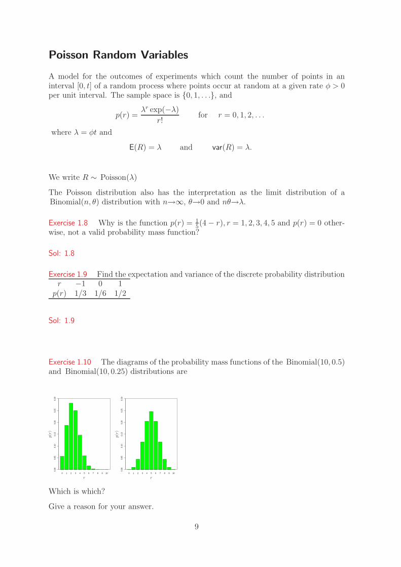
Exercise 1.10 The diagrams of the probability mass functions of the Binomial(10, 0.5)and Binomial(10, 0.25) distributions are
0 1 2 3 4 5 6 7 8 9 10
0.00
0.05
0.10
0.15
0.20
0.25
0.30
0 1 2 3 4 5 6 7 8 9 10
0.00
0.05
0.10
0.15
0.20
0.25
0.30
r
p(r)
r
p(r)
Which is which?
Give a reason for your answer.
9
Sol: 1.10 Left: mean about 2.5 so Binomial(10, 0.25). Right: mean about 5 soBinomial(10, 0.5).
Exercise 1.11 If X is a Poisson random variable with expectation 2.4, calculate theprobability that X is greater than 1.
Sol: 1.11
P(X > 1) = 1 − P(X = 0 ∪ X = 1)
= 1 − [ P(X = 0) + P(X = 1)]
= 1 − exp(−2.4) − 2.4 exp(−2.4) = 0.691.
In R: 1- ppois(1,lambda=2.4)
Exercise 1.12 If X is a Poisson random variable with expectation λ, find an expressionfor the probability that X is greater than 1 given that it is greater than 0.
Sol: 1.12
P(X > 1|X > 0) = P(X > 1 ∩ X > 0)/ P(X > 0)
X > 1 ∩ X > 0 = X > 1
P(X > 0) = 1 − P(X = 0) = 1 − exp(−λ)
P(X > 1) = 1 − P(X = 0 ∪ X = 1)
= 1 − exp(−λ) − λ exp(−λ)
P(X > 1|X > 0) =1 − exp(−λ) − λ exp(−λ)
1 − exp(−λ)
= 1 − λ
exp(λ) − 1.
Exercise 1.13 The probability that a randomly chosen electrical component is defec-tive is 0.002. Assume that this probability is the same for all components that aremanufactured, and they fail independently of one another.
(a) What is the distribution of the number of defectives in a batch of size 1000?
(b) Which other distribution can we use to approximate this?
(c) What is the distribution of the number of tested components required to find onethat fails?
Sol: 1.13 (a) R ∼ Binomial(1000, 0.002).
(b) Use the Poisson approximation to the Binomial, R ∼ Poisson(1000 × 0.002) = Poisson(2),appropriate for rare events.
(c) Geometric Geometric(0.002).
10

Example 1.14 R code to show how close the Poisson approximation is the the Binomialdistribution.
x = rnorm(100,mean=0,sd=1) # vector 100 N(0,1) rvs
hist(x,col=’yellow’,20) # 20 breaks
rb = rbinom(500,size=1000,prob=.002) # 500 realisations
rp = rpois(500,lambda=2)
par( mfrow=c(1,2) )
hist(rb,col=’red’,prob=T) # probs not freqs
hist(rp,col=’red’,prob=T)
Now compare
rb = rbinom(500,size=100,prob=.02)
11

12
Chapter 2
Continuous Univariate Distributions
2.1 Introduction to Continuous Variables
Discrete random variables describe the outcomes of experiments which are in a count-able set of numbers. This covers models for the number of heads in a fixed number oftosses of a coin, the number of floods of a river in a year, the number of children in afamily until a girl is born. Focusing only on discrete random variables is too restrictivefor many situations, examples include the nicotine levels in the blood plasma of smok-ers, the time intervals between floods of a river, and the waiting time for admissionsto an intensive care unit.
In each case the outcome of the experiment is a measurement on a continuous scale.This suggests we need to consider continuous random variables, where a continuousrandom variable is a variable whose set of possible values is uncountable. To describecontinuous random variables we need slightly different mathematical tools than weused for discrete random variables. For example for a discrete random variable R weused the probability mass function p(r) = P(R = r).
However, if X is a continuous random variable P(X = x) = 0 for all x. We focus onprobabilities of events instead of probabilities of single outcomes. In particular wefocus on events of the form
X ≤ x
for fixed x and consider these as x takes on different values. For a discrete randomvariable this is
P(R ≤ x) = P(R ≤ int (x)) =
int (x)∑
r=−∞p(r),
where int (x) denotes the largest integer smaller than or equal to x, e.g. int (3.9) = 3, int (2) = 2,int (−1.5) = −2.
The figure shows this function for a Poisson random variable R with λ = 2. As x variesthe function P(R ≤ x) jumps at the integers where R has positive probability.
13

0 2 4 6 8 10
0.0
0.2
0.4
0.6
0.8
1.0
x
FR
(x)
=P(R
≤x)
Exercise 2.1 Obtain P(R ≤ x) (the cumulative distribution function) of a randomvariable R that takes values 0, 1, 2, with probabilities θ, θ, 1 − 2θ respectively. Firstcalculate this at the jump points (integers), and then extend from the integers to thereal line.
Sol: 2.1 Picture: where to put the jump points.
At the jump points
P(R ≤ r) =
θ for r = 0,θ + θ = 2θ for r = 1,2θ + 1 − 2θ = 1 for r = 2.
On the real line
P(R ≤ x) =
θ for 0 ≤ x < 1,2θ for 1 ≤ x < 21 for x ≥ 2,
which is a step function with jumps at 0, 1 and 2.
Example 2.2 Complete the table
Discrete Continuousrv R Xss r; r = 0, 1, 2, . . . x; x ∈ (−∞,∞)cdf FR(x) = P(R ≤ x) FX(x) = P(X ≤ x)pmf pR(r) fX(x) pdf
2.2 Cumulative Distribution Function
The cumulative distribution function, cdf, of a continuous or discrete random variable,X, is defined, for all real values of x, by
FX(x) = F (x) = P(X ≤ x),
i.e. the probability that a random variable X takes a value less than or equal to x.When X is continuous an example of F is displayed in the figure.
14

0.0 0.5 1.0 1.5 2.0
0.0
0.5
1.0
1.5
x
F(x
),f(x
)
The monotonically increasing curve is the cdf F (x) = P(X ≤ x) for a continuous ran-dom variable X; its derivative is also plotted.
Properties of FX(x):
• 0 ≤ FX(x) ≤ 1, with limx→−∞ FX(x) = FX(−∞) = 0 and limx→∞ FX(x) = FX(∞) = 1,
• FX(x) is non-decreasing function of x.
The distribution function is particularly useful for continuous random variables aswe often want to know the probability of events that can be related by the laws ofprobability into probability statements about the event X ≤ x for some x.
The Survivor Function: The survivor function of a random variable X is defined as
FX(x) = P(X > x).
Using the law of complementary events
P(X > x) = 1 − P(X ≤ x) = 1 − FX(x).
The Quantile Function: The quantile function of a random variable X is defined as
F−1X (y) 0 < y ≤ 1
when F is strictly monotonic.
15
Probabilities of Intervals: Often the probability of the random variable X falling inthe interval (a, b] occurs for real numbers a, b with a < b.
a b
This corresponds to the event a < X ≤ b. By using the partition law
P(X ≤ b) = P(X ≤ a) + P(a < X ≤ b)
so the probability of the interval event is
P(a < X ≤ b) = P(X ≤ b) − P(X ≤ a) = FX(b) − FX(a).
As P(X = x) = 0 for all x, for any continuous random variable X
P(X ≤ x) = P(X < x),
hence one need not be precise between the usage of < and ≤ for continuous randomvariables.
Exercise 2.3 Let X be a random variable with cdf given by F (x) = x on 0 < x ≤ 1.
Obtain the following probabilities:(a) P(X ≤ 0.5), (b) P(X > 0.5), (c) P(X = 0.5), (d) P(X < .9), (e) P(0.5 < X ≤ .9).
Sol: 2.3 (a) P(X ≤ 0.5) = F (0.5) = 0.5, punif(.5,min=0,max=1) (b) 1 − P(X ≤ 0.5) = 1 − F (0.5)(c) P(X = 0.5) = 0, (d) P(X < .9) = 0.9, punif(.9) (e) P(X ≤ .9) − P(X ≤ 0.5) = 0.9 − 0.5 = 0.4.
Note that one could read these off the graph of F (x).
2.3 Probability Density Function
The (probability) density function, pdf, fX(x) of a continuous random variable, X, isdefined by
fX(x) =d
dxFX(x)
so that it satisfies
FX(x) =
∫ x
−∞fX(s) ds.
The next figure shows the pdf for the continuous random variable for which the cdf isshown above.
16

0.0 0.5 1.0 1.5 2.0
0.0
0.5
1.0
1.5
x
f X(x
)
Notice that the pdf is zero in regions where there are no outcomes, in this example forx ≤ 0. Also the pdf exceeds 1 in some places so cannot be interpreted as a probabilitydespite some of the mathematical properties of fX(x) being similar to those of theprobability mass function (pmf).
Properties of fX(x):
• Positivity: fX(x) ≥ 0 for all x,
• Unit-integrability:∫∞−∞ fX(x) dx = 1.
The probability that an observation on a continuous random variable X lies in theinterval (a, b] may be calculated as the area under the curve of fX(x) between x = aand x = b.
a b
More formally, due to results from calculus, we have the property
P(a < X ≤ b) = FX(b) − FX(a) property of F
=
∫ b
−∞fX(x) dx −
∫ a
−∞fX(x) dx def of f
=
∫ b
a
fX(x) dx. calculus
In fact, for any set A the probability of that set is given by
P(X ∈ A) =
∫
x∈A
fX(x) dx.
17

To illustrate the equivalence of the definition of fX(x) with this property we startwith the property and argue that the definition follows. Using the above property onintervals, we have for any x and a small δ
P(x < X ≤ x + δ) = FX(x + δ) − FX(x)
=
∫ x+δ
x
fX(s) ds
≈ fX(x)δ,
so that
FX(x + δ) − FX(x)/δ ≈ fX(x)
i.e. dFX(x)/dx = fX(x) in the limit as δ→0.
Exercise 2.4 A random variable X has cumulative distribution function
FX(x) =
1 − exp(−3x) for x > 0,0 for x < 0.
Find the pdf of X.
Sol: 2.4
fX(x) =d
dxFX(x) =
3 exp(−3x) for x > 0,0 for x < 0.
plot(1:10/5, dexp(1:10/5,rate=3))
Exercise 2.5 A triangular pdf: the random variable X has pdf
fX(x) =
2(1 − x) 0 < x ≤ 1,0 otherwise.
Sketch the pdf and show the cdf, FX(x) on the same graph by visually computing thearea under the pdf.
Sol: 2.5
18
Exercise 2.6 A triangular pdf (continued): Find FX(x) by splitting the range of xinto sensible intervals. First take −∞ < x ≤ 0.
Sol: 2.6
FX(x) =
∫ x
−∞fX(s) ds
=
∫ x
−∞0 ds = 0.
Exercise 2.7 A triangular pdf (continued): Now take 0 < x ≤ 1
Sol: 2.7 for 0 < x ≤ 1
FX(x) =
∫ x
−∞fX(s) ds
=
∫ 0
−∞fX(s) ds +
∫ x
0
fX(s) ds
= FX(0) +
∫ x
0
2(1 − s) ds
= 0 + [−(1 − s)2]x0 = 1 − (1 − x)2.
Exercise 2.8 A triangular pdf (continued): Finally take x > 1
Sol: 2.8 For x > 1
FX(x) =
∫ 1
−∞fX(s) ds +
∫ x
1
fX(s) ds
= FX(1) +
∫ x
1
0 ds
= [1 − (1 − 1)2] + 0 = 1.
Exercise 2.9 A triangular pdf (continued): Put these parts together to describe FX(x)concisely.
Sol: 2.9
FX(x) =
∫ x
−∞fX(s) ds
=
0 for x ≤ 01 − (1 − x)2 for 0 < x ≤ 11 for x > 1.
19

Exercise 2.10 A triangular pdf, continued: Obtain P(X < 0.5) and P(0.5 < X < 0.75)using the cdf.
Sol: 2.10
P(X < 0.5) = FX(0.5)
= 1 − (1 − 0.5)2 = 3/4.
P(0.5 < X < 0.75) = FX(0.75) − FX(0.5)
= [1 − (1 − 0.75)2] − [1 − (1 − 0.5)2]
= 3/16.
Exercise 2.11 A triangular pdf, continued: Also obtain P(0.5 < X < 0.75) directlyfrom the pdf.
Sol: 2.11
P(0.5 < X < 0.75) =
∫ 0.75
0.5
fX(s) ds
=
∫ 0.75
0.5
2(1 − s) ds
= [−(1 − s)2]0.750.5
= 1/4 − 1/16 = 3/16.
Exercise 2.12 The lifetime in years, that a computer functions before breaking downis a continuous random variable X with pdf, with a parameter λ that depends on thetype of computer, given by
fX(x) =
λ exp(−λx) x ≥ 0,0 x < 0.
To set a time for a guarantee, the company wants to know the time t for which withprobability 0.9 the lifetime of the computer will exceed t.
Sol: 2.12
P(X > t) =
∫ ∞
t
fX(x) dx
=
∫ ∞
t
λ exp(−λx) dx
= [− exp(−λx)]∞t = exp(−λt),
20
so that P(X > t) = 0.9 implies t = −λ−1 log (0.9).
2.4 Summary Measures
All the information about the distribution of a continuous random variable X is con-tained in the cdf FX(x) and the pdf fX(x). However it is often helpful to summarisethe main characteristics of the distribution in terms of a few values. Here we considerthe standard summary measures.
Expectation and Variance
The expected value (or mean) of a continuous random variable X can be thought ofas the average of the different values that X may take, according to their chance ofoccurrence.
The expected value of a continuous random variable X is
E(X) =
∫ ∞
−∞xfX(x) dx.
Similarly for a real valued function g(X) of a continuous random variable X the ex-pected value is
E[g(X)] =
∫ ∞
−∞g(x)fX(x) dx.
Exercise 2.13 Triangular pdf. For X, with pdf given by
fX(x) =
2x 0 ≤ x ≤ 1,0 otherwise,
find E[X], E[2X] and E[X2].
Sol: 2.13
E[X] =
∫ ∞
−∞x fX(x) dx
= [
∫ 0
−∞+
∫ 1
0
+
∫ ∞
1
]x fX(x) dx
= 0 +
∫ 1
0
x 2x dx + 0
= [2
3x3]10 =
2
3.
21
Also
E[2X] =
∫ 1
0
2x 2x dx =4
3= 2 E[X]
E[X2] =
∫ 1
0
x2 2x dx = [1
2x4]10 =
1
2,
using the same method to split the range.
For continuous variables linearity properties of expectation are very similar to thosestated in the review Chapter for discrete random variables.
For arbitrary functions g and h, constants a, b and c, and a continuous random variableX
E[g(X) + h(X)] = E[g(X)] + E[h(X)],
E[cg(X)] = c E[g(X)],
E[aX + b] = a E[X] + b.
Derivation (of first property):
E[g(X) + h(X)] =
∫ ∞
−∞[g(x) + h(x)]fX(x) dx
=
∫ ∞
−∞g(x)fX(x) dx +
∫ ∞
−∞h(x)fX(x) dx
= E[g(X)] + E[h(X)].
The other properties are shown similarly (see workshop/homework questions).
The variance, measuring of the spread or dispersion of a random variable about theexpectation, for a continuous distribution is
var(X) = E[(X − E(X))2] =
∫ ∞
−∞(x − E(X))2fX(x) dx.
For continuous random variables the easiest way to evaluate the variance is
var(X) = E(X2) − [ E(X)]2.
Proof: Put a = E(X). Note that E(X − a) = 0.
var(X) = E[(X − E(X))2]
= E[(X − a)2] def
= E[X2 − 2Xa + a2]
= E[X2] − E[2Xa] + E[a2] linearity
= E[X2] − 2a E[X] + a2 rules of E
= E[X2] − a2.
22

The standard deviation std(X) of a continuous random variable X is√
var(X).
The variance and standard deviation of the linear function aX + b are
var(aX + b) = a2 var(X),
std(aX + b) = |a| std(X).
The derivation of these results is identical in structure to the discrete random variablecase in Math 104.
A measure of the typical size of a random variable to its variability is given by thecoefficient of variation which is defined by E(X)/ std(X).
Exercise 2.14 If X has pdf as in the triangular pdf
fX(x) =
2x 0 ≤ x ≤ 1,0 otherwise,
find var(X) and the coefficient of variation for X.
Sol: 2.14 From above E[X] = 23
and E[X2] = 12, so that
var(X) = E[X2] − [ E(X)]2
=1
2− 4
9=
1
18,
E(X)/ std(X) =2
3/
√
1
18= 2.8284.
Warning: Sometimes the expectation and variance are not finite, and we say they do notexist. This occurs when the probabilities of obtaining large values is too big. Examplesare given later.
Higher Moments
If X has expectation µX and standard deviation σX then the random variable Y definedas
Y =X − µX
σX
has E(Y ) = 0 and var(Y ) = 1 for any µX and σX < ∞.
Proof: (using properties of linearity)
E(Y ) = E
(
X − µX
σX
)
=E(X) − µX
σX
= 0,
23
var(Y ) = var
(
X − µX
σX
)
=var(X)
σ2X
=σ2
X
σ2X
= 1.
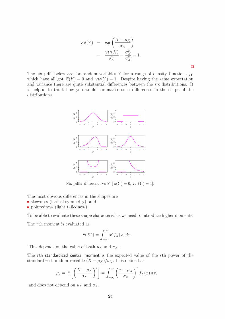
The six pdfs below are for random variables Y for a range of density functions fY
which have all got E(Y ) = 0 and var(Y ) = 1. Despite having the same expectationand variance there are quite substantial differences between the six distributions. Itis helpful to think how you would summarise such differences in the shape of thedistributions.
−3 −2 −1 0 1 2 3
0.0
0.2
0.4
−3 −2 −1 0 1 2 3
0.0
0.2
0.4
−3 −2 −1 0 1 2 3
0.0
0.2
0.4
−3 −2 −1 0 1 2 3
0.0
0.2
0.4
−3 −2 −1 0 1 2 3
0.0
0.2
0.4
−3 −2 −1 0 1 2 3
0.0
0.2
0.4
yy
yy
yy
f Y(y
)
f Y(y
)
f Y(y
)
f Y(y
)
f Y(y
)
f Y(y
)
Six pdfs: different rvs Y [E(Y ) = 0, var(Y ) = 1].
The most obvious differences in the shapes are• skewness (lack of symmetry), and• pointedness (light tailedness).
To be able to evaluate these shape characteristics we need to introduce higher moments.
The rth moment is evaluated as
E(Xr) =
∫ ∞
−∞xrfX(x) dx.
This depends on the value of both µX and σX .
The rth standardized central moment is the expected value of the rth power of thestandardized random variable (X − µX)/σX . It is defined as
µr = E
[(
X − µX
σX
)r]
=
∫ ∞
−∞
(
x − µX
σX
)r
fX(x) dx,
and does not depend on µX and σX .
24
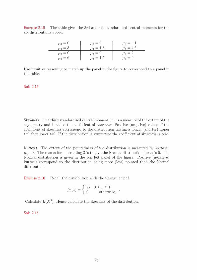
Exercise 2.15 The table gives the 3rd and 4th standardized central moments for thesix distributions above.
µ3 = 0 µ3 = 0 µ3 = −1µ4 = 3 µ4 = 1.8 µ4 = 4.5µ3 = 0 µ3 = 0 µ3 = 2µ4 = 6 µ4 = 1.5 µ4 = 9
Use intuitive reasoning to match up the panel in the figure to correspond to a panel inthe table.
Sol: 2.15 gv epsdir/shapes2.eps
The symmetric ones have µ3 = 0: [fig: TL, TR, MR, BL], [tab: TL, TM, BL, BM].µ3 < 0 implies skew with long L tail: [fig ML = tab TR]. Hence [fig BR = tab BR].Guess natural ordering [fig: TL, TR, ML, MR, BL, BR] = [tab: TL, TM, TR, BL,BM, BR]. (Low µ4 corresponds to short tails [fig: TR, BL].)
Skewness The third standardised central moment, µ3, is a measure of the extent of theasymmetry and is called the coefficient of skewness. Positive (negative) values of thecoefficient of skewness correspond to the distribution having a longer (shorter) uppertail than lower tail. If the distribution is symmetric the coefficient of skewness is zero.
Kurtosis The extent of the pointedness of the distribution is measured by kurtosis,µ4 − 3. The reason for subtracting 3 is to give the Normal distribution kurtosis 0. TheNormal distribution is given in the top left panel of the figure. Positive (negative)kurtosis correspond to the distribution being more (less) pointed than the Normaldistribution.
Exercise 2.16 Recall the distribution with the triangular pdf
fX(x) =
2x 0 ≤ x ≤ 1,0 otherwise,
.
Calculate E(X3). Hence calculate the skewness of the distribution.
Sol: 2.16 First
E[X3] =
∫ 1
0
x3 2x dx =
[
2
5x5
]1
0
=2
5.
Recall from the previous exercise
µ = E(X) = 2/3, E(X2) = 1/2 and σ2 = var(X) = 1/18,
25

Then
µ3 = E
[
(
X − µ
σ
)3]
=1
σ3[ E(X3) − 3 E(X2)µ + 3 E(X)µ2 − µ3]
= 23/233[2
5− 3
1
2
2
3+ 3
2
3
22
32− 23
33] = −23/2
5.
Note: skewness is negatve.
Quantiles
Often interest is in the values of a continuous random variable which are not exceededwith a given probability, such values are termed quantiles with xp the 100p% quantiledefined by
FX(xp) = p.
x
F (x)
xp
p
Here p is known as the percentile corresponding to the quantile xp.
Certain quantiles are of special interest:
Median: The median is the middle of the distribution in the sense that half thevalues of the variable (in probability) are less than the median, and half are more. Themedian is the 50% quantile, x0.5, so that F (x0.5) = 0.5. As a measure of location, themedian has the advantage of existing for all distributions, unlike the expectation.
Quartile: The quartiles split the distribution into four equally likely regions, x0.25 thelower quartile, x0.5 the median and x0.75 the upper quartile.
P(X ≤ x0.25) = P(x0.25 < X ≤ x0.5)
= P(x0.5 < X ≤ x0.75) = P(X > x0.75)
= 0.25.
This is illustrated in the next figure.
26
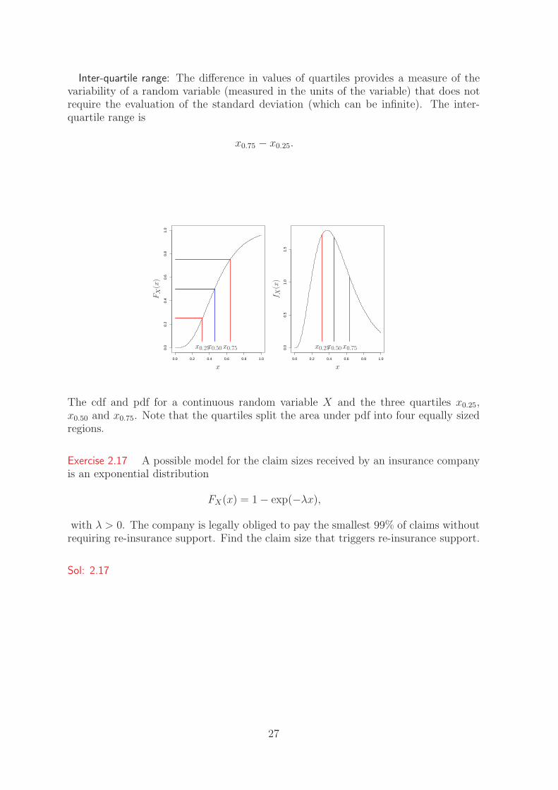
Inter-quartile range: The difference in values of quartiles provides a measure of thevariability of a random variable (measured in the units of the variable) that does notrequire the evaluation of the standard deviation (which can be infinite). The inter-quartile range is
x0.75 − x0.25.
0.0 0.2 0.4 0.6 0.8 1.0
0.0
0.2
0.4
0.6
0.8
1.0
0.0 0.2 0.4 0.6 0.8 1.0
0.0
0.5
1.0
1.5
xx
f X(x
)
x0.25x0.25 x0.50x0.50 x0.75x0.75
FX
(x)
The cdf and pdf for a continuous random variable X and the three quartiles x0.25,x0.50 and x0.75. Note that the quartiles split the area under pdf into four equally sizedregions.
Exercise 2.17 A possible model for the claim sizes received by an insurance companyis an exponential distribution
FX(x) = 1 − exp(−λx),
with λ > 0. The company is legally obliged to pay the smallest 99% of claims withoutrequiring re-insurance support. Find the claim size that triggers re-insurance support.
Sol: 2.17 The company pays without support when a claim X is less than x,
P(X ≤ x) = FX(x) = 0.99
1 − exp(−λx) = 0.99
exp(−λx) = 1 − 0.99
−λx = log (1 − 0.99)
x0.99 = x = −1
λlog (0.01).
27

Exercise 2.18 A model for the distribution of annual maximum sea level, X, is anextreme value distribution
FX(x) = exp[− exp−(x − α)/β],
with β > 0. The sea flood defence needs to be built to withstand a flood of the sizewhich occurs in any year with probability 0.01 (i.e. once on average every 100 years).Evaluate the required height of the flood defence in terms of α and β.
Sol: 2.18
P(X > x) = 0.01 or FX(x) = 0.99
exp[− exp−(x − α)/β] = 0.99
−(x − α)/β = log [− log 0.99]so that
x0.99 = α − β log − log (0.99).
28

Chapter 3
Standard Continuous Univariate Distributions
In this chapter we give the details of the univariate continuous distributions that youare likely to see in subsequent study of probability and Statistics. The distributionsarise in two ways, either as the probability distributions that are used in statisticsmodelling contexts or as the distributions that arise in statistical techniques.
There are strong links between probability and statistical modelling, where interestis in the effect on the distribution of the choice of parameter value. So we use thenotation
fX(x; θ)
rather than fX(x) to make explicit the dependence of the probability on the parametersθ of the probability model. (This is identical to the approach used in Math 105.)
3.1 Uniform Distribution
A continuous random variable for which all outcomes in a given range have equal chanceof occurring is said to be uniformly distributed. Specifically, a random variable X hasa Uniform distribution over the interval (a, b) if the pdf is given by
fX(x; θ) =
1b−a
a < x < b,
0 otherwise,
where θ = (a, b), which we write X ∼ Uniform(a, b) or sometimes X ∼ U(a, b). Thispdf for four different sets of parameter values is illustrated in the figure.
29
−3 −2 −1 0 1 2 3
0.0
0.2
0.4
0.6
0.8
1.0
−3 −2 −1 0 1 2 3
0.0
0.2
0.4
0.6
0.8
1.0
−3 −2 −1 0 1 2 3
0.0
0.2
0.4
0.6
0.8
1.0
−3 −2 −1 0 1 2 3
0.0
0.2
0.4
0.6
0.8
1.0
xx
xx
f X(x
)
f X(x
)
f X(x
)
f X(x
)
a = 0
b = 1
a = −1
b = 1
a = −3
b = 2
a = 1
b = 3
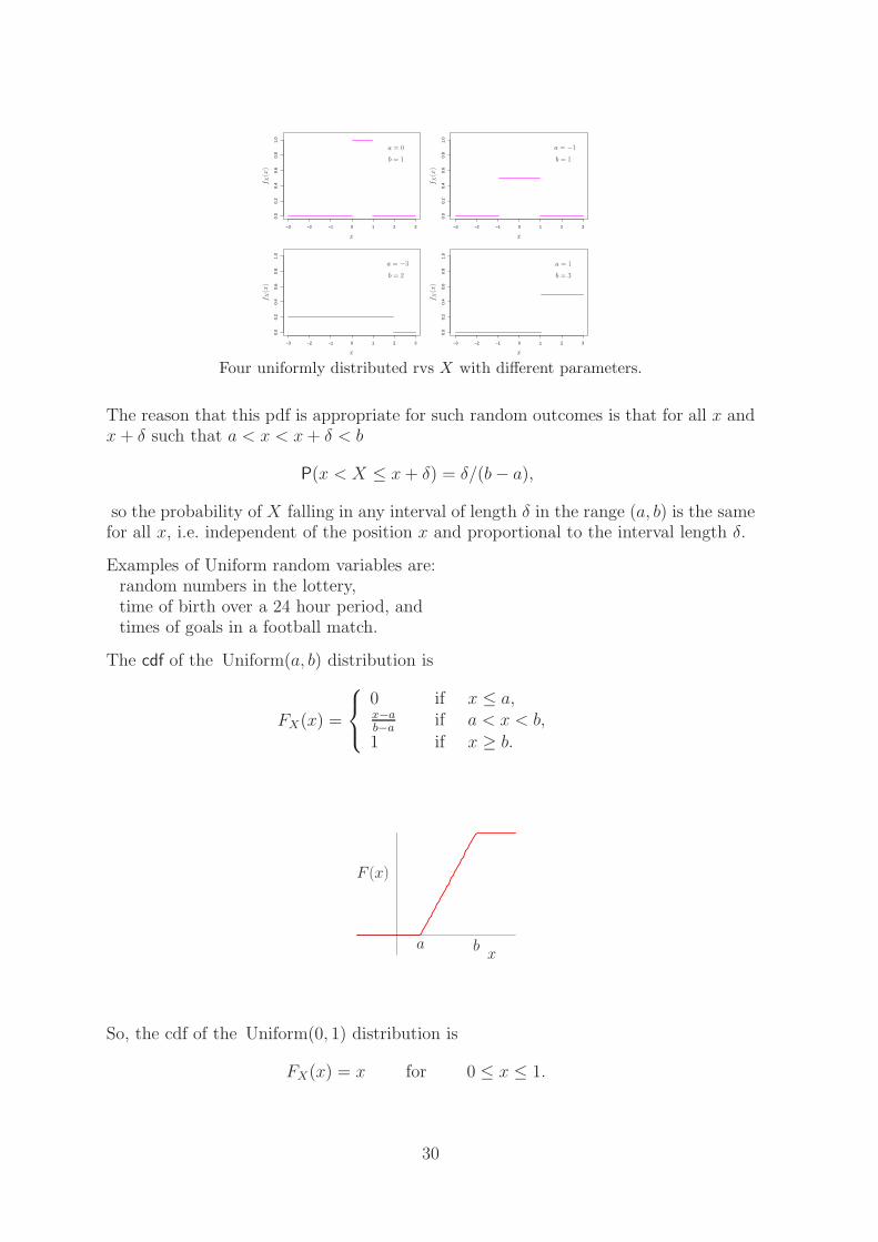
Four uniformly distributed rvs X with different parameters.
The reason that this pdf is appropriate for such random outcomes is that for all x andx + δ such that a < x < x + δ < b
P(x < X ≤ x + δ) = δ/(b − a),
so the probability of X falling in any interval of length δ in the range (a, b) is the samefor all x, i.e. independent of the position x and proportional to the interval length δ.
Examples of Uniform random variables are:random numbers in the lottery,time of birth over a 24 hour period, andtimes of goals in a football match.
The cdf of the Uniform(a, b) distribution is
FX(x) =
0 if x ≤ a,x−ab−a
if a < x < b,
1 if x ≥ b.
x
F (x)
a b
So, the cdf of the Uniform(0, 1) distribution is
FX(x) = x for 0 ≤ x ≤ 1.
30

Exercise 3.1 What about otherwise?
Sol: 3.1
FX(x) = 0 for x ≤ 0.
FX(x) = 1 for x ≥ 1.
The rth moment of the Uniform(a, b) distribution is
E(Xr) =
∫ ∞
−∞xrfX(x) dx
=
∫ a
−∞xr · 0 dx +
∫ b
a
xr
b − adx +
∫ ∞
b
xr · 0 dx
=br+1 − ar+1
(r + 1)(b − a).
Hence the expectation (taking r = 1 in the result above) is
E(X) =b2 − a2
2(b − a)=
b + a
2,
and the variance is
var(X) =b3 − a3
3(b − a)−[
b + a
2
]2
=(b − a)2
12.
These results seem logical as if all values in the interval (a, b) are equally likely thenthe expected value should be the average of the endpoints. Similarly the wider theinterval the more variable the outcomes, hence the larger variance.
Exercise 3.2 Find the upper quartile of the random variable X ∼ Uniform(3, 5).
Sol: 3.2 Note that x0.75 lies in (3, 5).
P(X < x0.75) = 0.75x0.75 − 3
5 − 3= 0.75
x0.75 = 4.5.
Exercise 3.3 The score in your favourite team’s football match was 1 : 0. You watcha video of the game. Assuming the time of the goal is uniformly distributed over theappropriate period, how long would you expect to wait to see the goal on the video?
31

Sol: 3.3 Let X model the time to the goal. If X ∼ Uniform(0, 90) then E(X) = 45mins. But this neglects the 10 minute halftime. In fact
fX(x) =
190
0 < x < 45,190
55 < x < 100,0 otherwise,
which gives
E(X) = 50.
Exercise 3.4 If X ∼ Uniform(0, 10), use R to calculate the probability that(a) X < 3, (b) X > 6, (c) 3 < X < 8, (d) 8 < X < 13.
Sol: 3.4
punif(3,min=0,max=10) # P(X<3) 0.3
1-punif(6,0,10) # P(X>6) 0.4
punif(8,0,10)-punif(3,0,10) # P(3<X<8) 0.5
punif(13,0,10)-punif(8,0,10) # P(8<X<13) 0.2
3.2 Exponential Distribution
A random variable X has an exponential distribution if its pdf is given by
fX(x; θ) =
β exp(−βx), x ≥ 0,0 otherwise,
where θ = β, with β > 0, which we write X ∼ Exp(β). The pdf for four differentvalues of β is shown in the figure.
−1 0 1 2 3 4
01
23
45
−1 0 1 2 3 4
01
23
45
−1 0 1 2 3 4
01
23
45
−1 0 1 2 3 4
01
23
45
xx
xx
f X(x
)
f X(x
)
f X(x
)
f X(x
)
β = 1 β = 2
β = 3.5 β = 5
The pdfs for four exponentially distributed random variables X with β = 1, 2, 3.5 and 5.
32

The exponential distribution arises in practice as the distribution of a waiting timewhen events occur at random with a rate of β per unit time in a Poisson process. Itis the distribution of the time between events, and it is the distribution of the time toan event from a given start time.
Examples include: the time from now until an earthquake occurs; or the time betweenincoming telephone calls.
The cdf of the Exp(β) distribution is
FX(x) =
0 if x ≤ 0,1 − exp(−βx) if x > 0.
Exercise 3.5 Explicitly calculate the exponential cdf from the pdf.
Sol: 3.5 For x ≤ 0
FX(x) =
∫ x
−∞fX(s) ds =
∫ x
−∞0 ds = 0.
For x > 0
FX(x) =
∫ x
−∞fX(s) ds
= FX(0) +
∫ x
0
β exp(−βs) ds
= 0 + [− exp(−βs)]x0 = 1 − exp(−βx)
as required.
Example 3.6 Numerically evaluate the pdf, cdf and inverse cdf (the quantile function)of an exponential rv.
dexp(3,rate=2) # pdf of Exp(2) at x=3, f(3)=0.004957504
pexp(3,5) # cdf of Exp(5) at x=3, P(X<3)=0.9999997
qexp(0.5,3) # median of Exp(3) is 0.2310491
x = seq(0,4,length=100)
f = dexp(x,rate=2)
plot(x,f)
lines(x,f)
Compare these values with the pdfs in the figure of four exponential pdfs above.
The survivor function for x > 0 is
F (x) = exp(−βx).
33
The rth moment is
E(Xr) =
∫ ∞
−∞xrfX(x) dx
=
∫ 0
−∞xr · 0 dx +
∫ ∞
0
xrβ exp(−βx) dx def
=
∫ ∞
0
xrβ exp(−βx) dx
= β−r
∫ ∞
0
xrβr exp(−βx) d(βx)
= β−r
∫ ∞
0
tr exp(−t) dt subst
= β−rΓ(r + 1) def
= β−rr! for r integer,
from the integrals in the Appendix.Hence
E(Xr) =r!
βr,
for positive integer r. It follows that the expectation and variance are
E(X) =1
βand var(X) =
2
β2− 1
β2=
1
β2.
The expectation and standard deviation are the same, so the coefficient of variationis 1 for all β.
Note that the expectation decreases with β: the higher the rate of event occurrence theshorter the expected waiting time to the next event.
Exercise 3.7 Plot the gamma function Γ(r) on the interval r = (1/2, 5).
Sol: 3.7
rval = seq(.5,5,.5)
plot(rval,gamma(rval))
lines(rval,gamma(rval))
Exercise 3.8 Suppose that the length of a phone call, in minutes, is distributed asExp(1/10). If someone arrives immediately ahead of you at a public telephone box,find the probability of waiting (a) more than 10 minutes, and (b) between 10 and 20minutes.
Sol: 3.8 Let X be the time you have to wait, the same as the length of the call
(a) P(X > 10) = FX(10) = exp(− 110
10) = e−1.
(b) P(10 < X < 20) = FX(10) − FX(20) = e−1 − e−2.
34
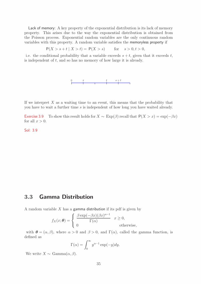
Lack of memory: A key property of the exponential distribution is its lack of memoryproperty. This arises due to the way the exponential distribution is obtained fromthe Poisson process. Exponential random variables are the only continuous randomvariables with this property. A random variable satisfies the memoryless property if
P(X > s + t | X > t) = P(X > s) for s > 0, t > 0,
i.e. the conditional probability that a variable exceeds s + t, given that it exceeds t,is independent of t, and so has no memory of how large it is already.
0 s t s + t
If we interpret X as a waiting time to an event, this means that the probability thatyou have to wait a further time s is independent of how long you have waited already.
Exercise 3.9 To show this result holds for X ∼ Exp(β) recall that P(X > x) = exp(−βx)for all x > 0.
Sol: 3.9 For s > 0, t > 0
P(X > s + t | X > t) =P(X > s + t ∩ X > t)
P(X > t)def
=P(X > s + t)
P(X > t)eval
=exp−β(s + t)
exp(−βt)subst
= exp(−βs)
= P(X > s).
3.3 Gamma Distribution
A random variable X has a gamma distribution if its pdf is given by
fX(x; θ) =
β exp(−βx)(βx)α−1
Γ(α)x ≥ 0,
0 otherwise,
with θ = (α, β), where α > 0 and β > 0, and Γ(α), called the gamma function, isdefined as
Γ(α) =
∫ ∞
0
yα−1 exp(−y)dy.
We write X ∼ Gamma(α, β).
35
Exercise 3.10 Use integration by parts to prove the recurrence relation
Γ(α + 1) = α Γ(α) for α > 0.
Sol: 3.10
Γ(α + 1) =
∫ ∞
0
yα exp(−y) dy
= [yα(−1) exp(−y)]∞0 +
∫ ∞
0
αyα−1 exp(−y) dy
= 0 − 0 + α Γ(α) for α > 1.
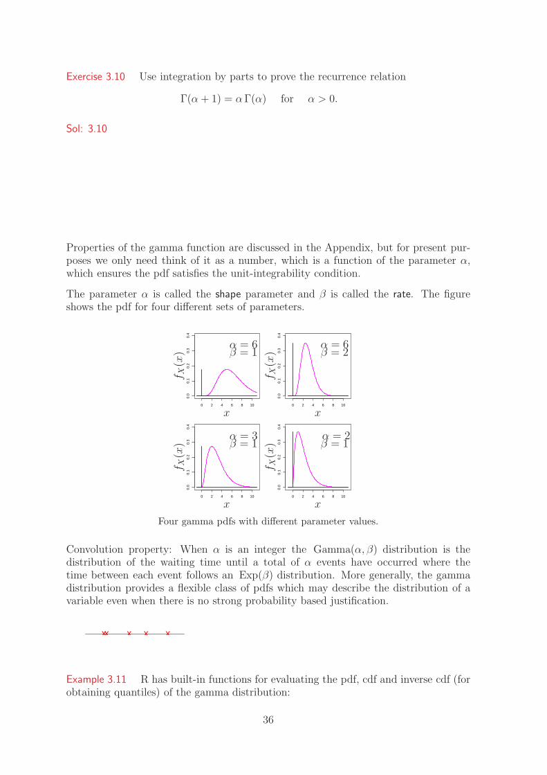
Properties of the gamma function are discussed in the Appendix, but for present pur-poses we only need think of it as a number, which is a function of the parameter α,which ensures the pdf satisfies the unit-integrability condition.
The parameter α is called the shape parameter and β is called the rate. The figureshows the pdf for four different sets of parameters.
0 2 4 6 8 10
0.0
0.1
0.2
0.3
0.4
0 2 4 6 8 10
0.0
0.1
0.2
0.3
0.4
0 2 4 6 8 10
0.0
0.1
0.2
0.3
0.4
0 2 4 6 8 10
0.0
0.1
0.2
0.3
0.4
xx
xx
f X(x
)
f X(x
)
f X(x
)
f X(x
)
α = 6β = 1
α = 6β = 2
α = 3β = 1
α = 2β = 1
Four gamma pdfs with different parameter values.
Convolution property: When α is an integer the Gamma(α, β) distribution is thedistribution of the waiting time until a total of α events have occurred where thetime between each event follows an Exp(β) distribution. More generally, the gammadistribution provides a flexible class of pdfs which may describe the distribution of avariable even when there is no strong probability based justification.
xxx xx
Example 3.11 R has built-in functions for evaluating the pdf, cdf and inverse cdf (forobtaining quantiles) of the gamma distribution:
36

dgamma(4,shape=6,rate=1) # pdf Gamma(6,1)
dgamma(4,6,1) # pdf Gamma(6,1) at x=4, f(4)=0.1562935
pgamma(2,0.5,1) # cdf Gamma(0.5,1) at x=2, P(X<2)=0.9544997
qgamma(0.5,3,1) # median of Gamma(3,1)=2.67406
Compare these values with the pdfs in the figure.
When α = 1 the gamma distribution reduces to the exponential. Unlike the exponentialwe cannot evaluate the gamma cdf in closed form for a non-integer α.
The rth moment is
E(Xr) =
∫ ∞
−∞xrfX(x) dx
=
∫ ∞
0
xrβαxα−1 exp(−βx)/Γ(α) dx def
=βα
Γ(α)
∫ ∞
0
xr+α−1 exp(−βx) dx
=βα
βα+rΓ(α)
∫ ∞
0
(βx)r+α−1 exp(−βx) d(βx)
=1
βrΓ(α)
∫ ∞
0
tr+α−1 exp(−t) dt subst
=Γ(α + r)
βrΓ(α), def
using the integrals in the Appendix. So
E(X) =Γ(1 + α)
βΓ(α)=
α
β,
E(X2) =Γ(2 + α)
β2Γ(α)=
(1 + α)α
β2,
var(X) =(1 + α)α
β2− α2
β2=
α
β2.
Exercise 3.12 Lifetimes of batteries (in hours) are believed to independently followan Exp(1/10) distribution. You buy a pack of 4 batteries. Find the distribution of thelifetime of the pack and its expected lifetime.
Sol: 3.12 Let X be the lifetime (in hours) of the pack. Then X is the sum ofthe 4 lifetimes of the batteries each of which has an Exp(1/10) distribution. By theconvolution property of the Gamma distribution
X ∼ Gamma(4, 1/10).
The expected lifetime (in hours) is E(X) = 41/10
= 40.
37

Exercise 3.13 Battery packs, continued. Find the probability that the lifetime of thepack exceeds 40 hours.
Sol: 3.13 The probability that the lifetime exceeds 40 hours is
P(X > 40) = 1 − P(X ≤ 40),
which can be evaluated in R:
1-pgamma(40,shape=4,rate=1/10)
[1] 0.4334701
Thus P(X > 40) = 0.4335.
3.4 Normal Distribution
A random variable X has a Normal distribution if its pdf is given by
fX(x; θ) =1√
2πσ2exp
−(x − µ)2
2σ2
for −∞ < x < ∞,
with parameters θ = (µ, σ2). We write X ∼ N(µ, σ2). Notice that all the curves aresymmetric around µ with a characteristic bell-shape. The width of the bell is controlledby the value of σ2.
−6 −4 −2 0 2 4 6
0.0
0.2
0.4
0.6
0.8
−6 −4 −2 0 2 4 6
0.0
0.2
0.4
0.6
0.8
−6 −4 −2 0 2 4 6
0.0
0.2
0.4
0.6
0.8
−6 −4 −2 0 2 4 6
0.0
0.2
0.4
0.6
0.8
xx
xx
f X(x
)
f X(x
)
f X(x
)
f X(x
)
µ = 0
σ2 = 1
µ = 0
σ2 = 4
µ = −3
σ2 = 1/4
µ = 1
σ2 = 2
Four Normal pdfs with different parameter values.
The Normal distribution has played a central role in the history of probability andstatistics. It was introduced by the French mathematician Abraham de Moivre in1733, who used it to approximate probabilities of winning in various game of chanceinvolving coin tossing. It was later used by the German mathematician Carl Friedrich
38

Gauss to predict the location of astronomical bodies and became known as the Gaussiandistribution.
In statistics the Normal distribution is by far the most important distribution. Tradi-tionally, it has been viewed as the natural distribution of (measurement) errors, yieldsfrom field experiments etc. The theoretical justification for this is the central limittheorem (see Chapter 9), which says that the sum of a large number of independentrandom variables each of which is small compared to the sum is approximately Nor-mally distributed. The CLT is the reason why the Normal distribution often occurs asthe approximate distribution of estimators in statistics.
First we need to show this is a valid pdf
∫ ∞
−∞fX(x) dx =
∫ ∞
−∞
1√2πσ2
exp
−(x − µ)2
2σ2
dx def f
=1√2π
∫ ∞
−∞exp
−(x − µ)2
2σ2
d((x − µ)/σ) rearrange
=1√2π
∫ ∞
−∞exp(−s2/2) ds subst
=1√2π
2
∫ ∞
0
exp(−s2/2) ds symmetry
=1√2π
2
∫ ∞
0
exp(−s2/2) s−1d(s2/2)
=1√2π
2
∫ ∞
0
(2t)−12 exp(−t) dt subst
=1√π
Γ(1
2) = 1 see the Appendix .
Moments The expectation and variance of X ∼ N(µ, σ2) are µ and σ2 respectively.The way to prove this is
(i) to use the property of the standard Normal: if Y ∼ N(0, 1) then E(Y ) = 0 andvar(Y ) = 1;(ii) use the transformation property that if Y ∼ N(0, 1) and X = µ + σY then X ∼ N(µ, σ2);
and finally(iii) use the properties of expectation to give E(X) = E(µ + σY ) = µ + σ0 = µ and
var(X) = var(µ + σY ) = var(σY ) = σ2 var(Y ) = σ2.
Probabilities and quantiles The normal cdf cannot be expressed in closed form so nu-merical evaluation is required, if we want to obtain probabilities of the form P(X ≤ a),or quantiles.
Example 3.14
39

pnorm(0,mean=1,sd=sqrt(2)) # P(X < 0) when X ~ N(1,2)
pnorm(0,1,sqrt(2)) # P(X< 0) when X ~ N(1,2) 0.2397501
1-pnorm(-2,0,2) # P(X> -2) when X ~ N(0,4) 0.8413447
qnorm(0.975,0,1) # u st P(X < u) = 0.975, 1.959964
# when X ~ N (0,1)
Note the R functions for the normal use the standard deviation σ, not the variance σ2.
Exercise 3.15 Normal heights. A Normal model is proposed to model the variation inheight H of women with parameters µ = 170 and σ2 = 36 measured in cm. What isthe probability a random selected woman is over 180cm tall?
Sol: 3.15 H ∼ N(170, 36) so that
P(H > 180) = 1 − P(H < 180)
= 1 − pnorm(180, 170, 6) not maths
= 0.0477
Exercise 3.16 A Normal model is proposed to model the variation in scores, W , on anintelligence test with parameters µ = 100 and σ2 = 100. What is the probability of arandomly selected person scoring between 80 and 120 on the test?
Sol: 3.16 W ∼ N(100, 100) so that
P(80 < W < 120) = P(W < 120) − P(W < 80)
= pnorm(120, 100, 10) − pnorm(80, 100, 10)
= 0.9544
Standard Normal Distribution
Historically the evaluation of probabilities for Normal random variables could not beperformed routinely for any different µ and σ2 as access to computers with ability toperform integrals or to store functions was not possible.
However, it was noted that the calculation could be reduced and tables of integralvalues used for the evaluation. Critical to this step is the following theorem which isalso of wider interest.
Theorem 3.1 If X ∼ N(µ, σ2), then the random variable
Z =X − µ
σ∼ N(0, 1)
and conversely, if Z ∼ N(0, 1), then the random variable
X = µ + σZ ∼ N(µ, σ2).
40
We will formally prove this in Chapter 5 but for now it is sufficient to note thatfrom previous results the transformation from X to Z ensures Z has E(Z) = 0 andvar(Z) = 1. Furthermore shifting and scaling a random variable does not change theshape of the distribution so we would expect Z also to be Normally distributed.
A random variable Z is said to have a standard Normal distribution if it has a Normaldistribution with expectation 0 and variance 1, i.e. Z ∼ N(0, 1). Thus Z has a standardNormal distribution if its pdf is given by
fZ(z) = φ(z) =1√2π
exp(−z2/2) for −∞ < z < ∞.
This pdf is shown in the top left panel of the four Normal pdfs.The moments requireusing the Normal integrals in the Appendix on Intergrals and establish that E(Zr) = 0for all r odd, E(Z2) = 1, E(Z4) = 3.
The cdf of the standard Normal variable Z, and denoted by Φ, is given by
FZ(z) = P(Z ≤ z) = Φ(z) =
∫ z
−∞
1√2π
exp(−x2/2) dx.
Values of Φ(z) can be obtained from the table of standard Normal probabilities, thoughwe use R.
However we repeat the Normal heights exercises to illustrate the traditional evaluationof Normal probabilities.
For the first
P(H > 180) = P(H − 170)/6 > (180 − 170)/6= P(Z > 10/6) = 1 − P(Z < 1.667)
= 1 − Φ(1.667)
= 1 − 0.9525 = 0.0475,
and for the second
P(80 < W < 120) = P(80 − 100)/10 < (W − 100)/10 < (120 − 100)/10= P(−2 < Z < 2) = P(Z < 2) − P(Z < −2)
= Φ(2) − Φ(−2)
= 0.9772 − 0.0228 = 0.9544.
Thus, in order to evaluate probabilities for Normal distributions with expectation andvariance other than 0 and 1, we standardize the original Normal random variable bysubtracting its expectation and dividing by its standard deviation.
Exercise 3.17 If X ∼ N(µ, σ2) find in terms of the function Φ(z): (a) P(X < b), (b)P(a < X < b).
41
Sol: 3.17 (a)
P(X < b) = P(X − µ
σ<
b − µ
σ)
= Φ(b − µ
σ)
(b)
P(a < X < b) = P(X < b) − P(X < a)
= Φ(b − µ
σ) − Φ(
a − µ
σ)
Beta Distribution
If α1 > 0, α2 > 0, the pdf of a Beta rv X ∼ Beta(α1, α2) is
fX(x) =Γ(α1 + α2)
Γ(α1)Γ(α2)xα1−1(1 − x)α2−1 for 0 < x < 1.
Calculation gives
E(X) =α1
α1 + α2
.
Exercise 3.18 Prove that if X ∼ Beta(2, 5) that E(X) = 22+5
using the unit integra-bility property of the pdf.
Sol: 3.18
E(X) =
∫ ∞
0
xΓ(2 + 5)
Γ(2)Γ(5)x2−1(1 − x)5−1 dx
=Γ(2 + 5)
Γ(2)Γ(5)
∫ ∞
0
x3−1(1 − x)5−1 dx
=Γ(2 + 5)
Γ(2)Γ(5)
Γ(3)Γ(5)
Γ(3 + 5)× 1
=2
2 + 5,
using the recurrence relations Γ(α + 1) = αΓ(α).
Usage: The family of Beta distributions constitutes a flexible class of distributions on[0, 1] used for modelling. The Beta(1, 1) distribution is the uniform distribution on[0, 1].
Exercise 3.19 Run the R-code to plot the Beta pdf
42

xval = seq(.001,.999,length=100)
pdf = dbeta(xval,2,3)
plot(xval,pdf,type=’n’)
lines(xval,pdf,col=’red’)
lines(xval,0*pdf)
Vary the parameters to produce a U-shaped pdf.
Sol: 3.19
pdf = dbeta(xval,0.2,0.8)
lines(xval,pdf,col=’blue’)
Exercise 3.20 Express the probability that a rv X ∼ Beta(2, 3) is less than 0.5 as anintegral. Find this probability numerically. Is this probability less than 0.5? Verify bysimulation that its expected value is about 0.4.
Sol: 3.20 pdf
fX(x) =Γ(2 + 3)
Γ(2)Γ(3)x2−1(1 − x)3−1 for 0 ≤ x ≤ 1,
and
P(X ≤ 0.5) =
∫ 0.5
x=0
12x1(1 − x)2dx asΓ(5)
Γ(2)Γ(3)= 12
= 0.6875.
No, prob is greater than 0.5.
xsample = rbeta(1000,2,3) ; mean(xsample)
E(X) = α1
α1+α2= 2/5.
Cauchy Distribution
fX(x) =1
π(1 + x2)for −∞ < x < ∞,
FX(x) =1
πarctan(x) +
1
2,
E(X) not defined, as
∫ ∞
−∞
1
π(1 + x2)|x|dx = ∞.
We write X ∼ Cauchy.
Convolution property: If X1, . . . , Xn are independent Cauchy, then (X1 + . . . + Xn)/n ∼Cauchy.
43
Transformation property: If X ∼ Uniform(−π/2, π/2), then tan(X) is Cauchy-distributed.If X1 and X2 are independent N(0, 1)-distributed, then X1/X2 is Cauchy-distributed.
Reciprocal: if X ∼ Cauchy then1
X∼ Cauchy.
Other: The Cauchy distribution is the t1 distribution.
Weibull Distribution
Parameters: θ = (α, β) with a shape parameter α > 0 and a rate parameter β > 0.
fX(x; θ) = αβαxα−1 exp−(βx)α for 0 < x < ∞,
FX(x) = 1 − exp(−(βx)α),
E(X) = Γ(1 + α−1)/β,
var(X) = Γ(1 + 2α−1) − Γ(1 + α−1)2/β2.
We write X ∼ Weibull(α, β).
Other: The Weibull(1, β) distribution is the Exponential(β) distribution.Usage: for modelling lifetimes.
44
Chapter 4
Other Standard Distributions
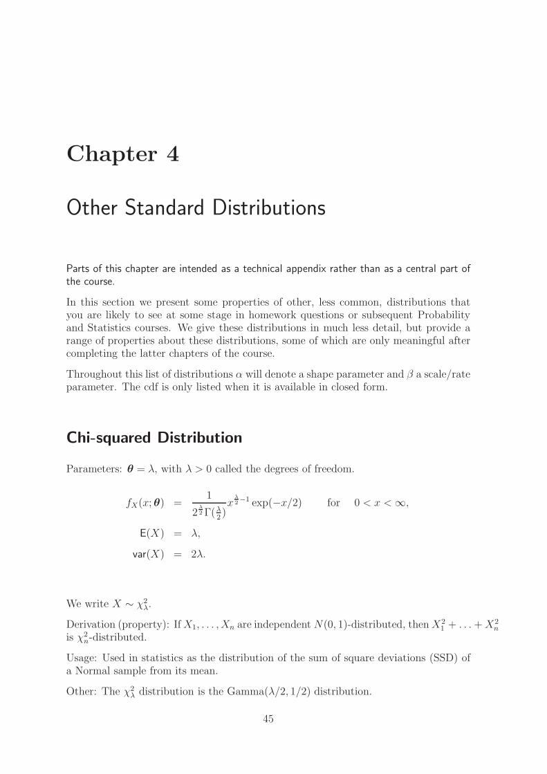
Parts of this chapter are intended as a technical appendix rather than as a central part ofthe course.
In this section we present some properties of other, less common, distributions thatyou are likely to see at some stage in homework questions or subsequent Probabilityand Statistics courses. We give these distributions in much less detail, but provide arange of properties about these distributions, some of which are only meaningful aftercompleting the latter chapters of the course.
Throughout this list of distributions α will denote a shape parameter and β a scale/rateparameter. The cdf is only listed when it is available in closed form.
Chi-squared Distribution
Parameters: θ = λ, with λ > 0 called the degrees of freedom.
fX(x; θ) =1
2λ2 Γ(λ
2)x
λ2−1 exp(−x/2) for 0 < x < ∞,
E(X) = λ,
var(X) = 2λ.
We write X ∼ χ2λ.
Derivation (property): If X1, . . . , Xn are independent N(0, 1)-distributed, then X21 + . . . + X2
n
is χ2n-distributed.
Usage: Used in statistics as the distribution of the sum of square deviations (SSD) ofa Normal sample from its mean.
Other: The χ2λ distribution is the Gamma(λ/2, 1/2) distribution.
45

The F Distribution
Parameters : θ = (λ1, λ2) with λ1 > 0 and λ2 > 0 called the degrees of freedom.
fX(x; θ) =λ
λ12
1 λλ22
2 xλ12−1
B(λ1
2, λ2
2)(λ1x + λ2)
λ1+λ22
for 0 < x < ∞,
E(X) =λ2
λ2 − 2when λ2 > 2,
var(X) =2λ2
2(λ1 + λ2 − 2)
λ1(λ2 − 2)2(λ2 − 4)when λ2 > 4.
We write X ∼ Fλ1,λ2.
Transformation property: If X1 and X2 are independent with X1 χ2λ1
-distributed andX2 χ2
λ2-distributed, then
X1/λ1
X2/λ2
is Fλ1,λ2-distributed.
Usage: Used in statistics as the distribution of the test statistic in analysis of variance(ANOVA).
Other: Named after the eminent English statistician R.A. Fisher.
Log Normal Distribution
Parameters: θ = (ξ, σ2) with ξ ∈ R and σ2 > 0.
fX(x; θ) =1√2π
1
xσexp−( logx − ξ)2
2σ2 for 0 < x < ∞,
E(X) = exp(σ2
2+ ξ),
var(X) = exp(σ2) − 1 exp(σ2 + 2ξ).
We write X ∼ logN(ξ, σ2).
Transformation property: If X is N(ξ, σ2)-distributed, then exp(X) is log Normaldistributed with parameters (ξ, σ2).
Useage: Used to model prices on the stock market and the size of particles duringcrushing processes.
Other: A random variable X follows a log-Normal distribution if and only if log (X)follows a Normal distribution.
46

Student’s t Distribution
Parameters: θ = (µ, λ) with λ > 0 called the degrees of freedom.
fX(x; θ) =1√
λB(λ2, 1
2)1 + (x−µ)2
λλ+1
2
for −∞ < x < ∞,
E(X) = µ when λ > 1 (otherwise not defined),
var(X) =λ
λ − 2when λ > 2.
We write X ∼ tλ.
Derivation (property): If X and Y are independent with Y N(0, 1)-distributed and Xχ2
λ-distributed, then
µ +Y
√
X/λ
is tλ-distributed.
Usage: Used in statistics as the distribution of the test statistic for test of a hypothesisabout the mean in a Normal sample with unknown variance, a so-called t test.
Other: The t distribution looks like a Normal distribution but has heavier tails. For λgoing to infinity the t distribution converges to a Normal distribution.
Extreme Value Distribution
Parameters : θ = (α, β) with a location parameter α ∈ R and a scale parameter β > 0.
fX(x; θ) =1
βexp−(x − α)/β exp[− exp−(x − α)/β] for −∞ < x < ∞,
FX(x) = exp[− exp−(x − α)/β],E(X) = α + βγ, where γ ≈ 0.5772 is Euler’s constant,
var(X) =β2π2
6.
We write X ∼ GEV(α, β, 0).
Transformation property: If X is Weibull(α, β)-distributed, then − log (X) has anextreme value distribution with location parameter log (β) and scale parameter 1/α.In particular, if X is Exp(λ)-distributed, i.e. X is Weibull(1, λ)-distributed, then− log (X) has an extreme value distribution with location parameter log (λ) and scaleparameter 1.
Usage: Used to model extreme events.
47

48

Chapter 5
Univariate Transformations
5.1 Introduction
Sometimes we are interested in a function of a random variable X, say Y = g(X). Forexample, we have already discussed interest in the linear transformation
Y =X − µ
σ.
Other applied examples include
X YDiameter of imperfection Area of imperfectionSpeed of vehicle Time to complete journeyLevel of liquid Volume of liquidLength of phone call Cost of call
It is easy to show that in general the expectation of a function is not equal to thefunction of the expectation, i.e.
E(Y ) = E[g(X)] 6= g( E[X]).
For example E(X2) > [ E(X)]2 unless X is constant, that is unless Var(X) = 0. There-fore what can we say about the new random variable Y = g(X)?
First consider the case of a discrete random variable X.
Exercise 5.1 Let X be the number of heads when 3 coins are thrown. Find the pmfof Y = (number of heads) - (number of tails).
Sol: 5.1
Value of X: 0 1 2 3pX(x) : 1/8 3/8 3/8 1/8Value of Y : -3 -1 1 3
49

So Y has pmf
y = value of Y -3 -1 1 3pY (y) 1/8 3/8 3/8 1/8
Exercise 5.2 Let X be the score obtained on the roll of a dice. Find the pmf of
Y =
0 if X is odd,1 if X is even.
Sol: 5.2
x = value of X: 1 2 3 4 5 6pX(x) : 1/6 1/6 1/6 1/6 1/6 1/6Value of Y : 0 1 0 1 0 1
So Y has pmf
pY (0) = 1/6 + 1/6 + 1/6 = 1/2,
pY (1) = 1/2.
Thus in the discrete case finding the distribution of the transformed random variableY = g(X) is a simple matter of adding up the corresponding probabilities for X. Forcontinuous random variables, however, we have P(X = x) = 0 for all x so this methoddoes not work.
Example 5.3 Draw a sample of n = 1000 Uniform random variables, U , transformeach by Y = − log (1 − U), draw the scatterplot of Y and U and plot the histogram ofboth Y and U .
u = runif(1000,min=0,max=1) # a vector
hist(u,col=’yellow’,br=20)
y = -log(1-u)
hist(y,col=’red’,br=20)
plot(u,y,pch=20,cex=1, col=’dark red’)
par(mfrow=c(2,2))
hist(y,col=’red’,br=20)
plot(u,y,pch=20,cex=1, col=’dark red’)
frame() # move on one plot
hist(u,col=’yellow’,br=20)
Conjecture as to the analytic distribution of U .
In the following we will see different methods of obtaining the cdf FY (y) and pdf fY (y)of the transformed random variable Y = g(X) when X is a continuous random variablewith cdf FX(x) and pdf fX(x).
50

5.2 Distribution Function Method
The distribution function method for evaluating the distribution of a transformationis simply a technique whereby the cdf and pdf of Y is evaluated as follows:
• find the values of X which correspond to the event Y ≤ y, let this correspond tothe event X ∈ Ay say,
• evaluate the probability P(Y ≤ y) = P(X ∈ Ay),
• differentiate P(Y ≤ y) to obtain the pdf of Y .
The figure illustrates the sets Ay for various transformations Y = g(X).
XX
XX
YY
YY
The set Ay for four different transformations g(·) (the curves).
When g(·) is monotonically increasing or decreasing Ay is an interval of the form(−∞, x] or [x,∞) and the method is particularly easy to apply in these cases. Themethod, however, holds whatever the properties of the transformation g(·). It is bestexplained through examples.
Exercise 5.4 A sugar refining process produces an amount X (in tons) of producteach day, which has cdf
FX(x) =
0 if x ≤ 0,x2 if 0 < x < 1,1 if x ≥ 1.
The amount of profit (in thousand £) to the company is Y = 3X − 1. Find the pdfof Y .
51
Sol: 5.4
FY (y) = P(Y ≤ y) = P(3X − 1 ≤ y)
= P[X ≤ (y + 1)/3]
= FX [(y + 1)/3]
= (y + 1)2/9 if 0 < (y + 1)/3 < 1,
hence
fY (y) =
0 if y ≤ −1 or y ≥ 2,2(y + 1)/9 if − 1 < y < 2.
Exercise 5.5 A classic: Uniform to Exp. When X ∼ Uniform(0, 1) show that
Y = − 1
βlog (1 − X)
has an Exp(β) distribution, where β > 0.
Sol: 5.5 First recall X ∼ Uniform(0, 1) implies FX(x) = x for 0 ≤ x ≤ 1. Now
FY (y) = P(Y ≤ y) = P[−β−1 log (1 − X) ≤ y]
= P[ log (1 − X)≥− βy]
= P[X ≤ 1 − exp(−βy)]
= FX [1 − exp(−βy)]
= 1 − exp(−βy) for y > 0.
This is the cdf of an Exp(β) random variable.
Exercise 5.6 The length of a phone call is X and Y = βX is the associated cost. IfX ∼ Exp(β), show that Y has an Exp(1) distribution, and hence find the expectedcost of a call.
Sol: 5.6
FY (y) = P(Y ≤ y) = P(βX ≤ y) = P(X ≤ y/β)
= FX(y/β) = 1 − exp−β(y/β)= 1 − exp(−y)
for y > 0. This is the cdf of an Exp(1) random variable. Hence E(Y ) = 1 units.
Exercise 5.7 When X ∼ Uniform(0, 1) show that
Y = [− log (1 − X)]1/α
has a Weibull distribution, with shape parameter α > 0. Note this transformation isa combination of two monotone functions.
52

Sol: 5.7 X ∼ Uniform(0, 1) implies FX(x) = x for 0 ≤ x ≤ 1. Now
FY (y) = P(Y ≤ y) = P[[− log (1 − X)]1/α ≤ y]
= P[− log (1 − X) ≤ yα]
= P[ log (1 − X)≥yα]
= P[X ≤ 1 − exp(−yα)]
= FX [1 − exp(−yα)]
= 1 − exp(−yα) for y > 0.
This is the cdf of an Weibull(α, 1) random variable.
Exercise 5.8 Suppose X ∼ N(0, 1). Show that Y = X2 has a Gamma distributionby first finding the cdf of Y in terms of the cdf of X. In fact it is identical to a χ2
1
distribution (see the chapter on other distributions).
Sol: 5.8
−√y
√y
y
FY (y) = P(Y ≤ y) = P(X2 ≤ y) for y > 0
= P(−√y ≤ X ≤ √
y)
= Φ(√
y) − Φ(−√y)
= 2Φ(√
y) − 1. symm
Exercise 5.9 Suppose X ∼ N(0, 1). Now show that Y = X2 has a Gamma distributionby finding the pdf of Y .
Sol: 5.9 To obtain the pdf we differentiate
fY (y) = 2d
dyFX(
√y)
= 2fX(√
y)d(√
y)
dychain rule
= 21√2π
exp(−y/2)1
2y−1/2
=1√2π
y−1/2 exp(−y/2) for y > 0,
so that Y ∼ Gamma(12, 1
2). This also matches the χ2
1 pdf.
53
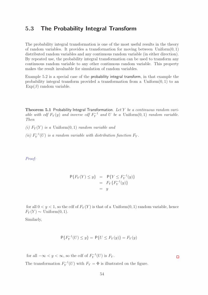
5.3 The Probability Integral Transform
The probability integral transformation is one of the most useful results in the theoryof random variables. It provides a transformation for moving between Uniform(0, 1)distributed random variables and any continuous random variable (in either direction).By repeated use, the probability integral transformation can be used to transform anycontinuous random variable to any other continuous random variable. This propertymakes the result invaluable for simulation of random variables.
Example 5.2 is a special case of the probability integral transform, in that example theprobability integral transform provided a transformation from a Uniform(0, 1) to anExp(β) random variable.
Theorem 5.1 Probability Integral Transformation. Let Y be a continuous random vari-able with cdf FY (y) and inverse cdf F−1
Y and U be a Uniform(0, 1) random variable.Then
(i) FY (Y ) is a Uniform(0, 1) random variable and
(ii) F−1Y (U) is a random variable with distribution function FY .
Proof:
PFY (Y ) ≤ y = PY ≤ F−1Y (y)
= FY F−1Y (y)
= y
for all 0 < y < 1, so the cdf of FY (Y ) is that of a Uniform(0, 1) random variable, henceFY (Y ) ∼ Uniform(0, 1).
Similarly,
PF−1Y (U) ≤ y = PU ≤ FY (y) = FY (y)
for all −∞ < y < ∞, so the cdf of F−1Y (U) is FY .
The transformation F−1Y (U) with FY = Φ is illustrated on the figure.
54

−3 −2 −1 0 1 2 3
0.0
0.2
0.4
0.6
0.8
1.0
Histogram of y
Den
sity
−2 −1 0 1 2
0.0
0.1
0.2
0.3
0.4
YY
U
Left: The distribution function FY = Φ for a standard Normal distribution. The vertical
crosses are 100 replicates of U and the horizontal crosses are the corresponding transformed
values, Y = F−1Y (U). Right: A histogram of the 100 replicates of Y with the pdf for a
standard Normal distribution superimposed.
Exercise 5.10 Use the probability integral transformation to construct the transfor-mation from the uniform to the exponential.
Sol: 5.10 First find F−1Y :
x = FY (y)
= 1 − exp(−βy) for y > 0,
so that y = −β−1 log (1 − x) = F−1Y (x).
Now apply the PIT theorem to argue that if X ∼ Uniform(0, 1) and
Y = F−1Y (X) = −β−1 log (1 − X),
then Y ∼ Exp(β).
Exercise 5.11 If U ∼ Uniform(0, 1) find the distribution of the random variables (a)Φ−1(U), (b) µ + σΦ−1(U).
Sol: 5.11 (a) Φ−1(U) ∼ N(0, 1). (b) µ + σΦ−1(U) ∼ N(µ, σ2).
Exercise 5.12 If U ∼ Uniform(0, 1) construct the probability integral transformationof Y = g(U) so that Y is distributed (a) Uniform(a, b), (b) Weibull(α, β).
55

Sol: 5.12 U ∼ Uniform(0, 1) (a) Require Y ∼ Uniform(a, b)
U = FY (Y ) =Y − a
b − afor a ≤ Y ≤ b
→ Y = a + (b − a)U
∼ Uniform(a, b).
(b) Want Weibull(α, β):
U = FY (Y ) = 1 − exp−(βY )α for Y > 0
→ Y =1
β− log (1 − U)1/α
∼ Weibull(α, β).
Exercise 5.13 If U ∼ Uniform(0, 1) construct the probability integral transformationof Y = g(U) so that Y has the distribution that is discrete on 0, 1, 2, 3 with proba-bilities 0.3, 0.5, 0.1 and 0.1,
Sol: 5.13 U ∼ Uniform(0, 1), Y ∼ Discrete has cdf FY (y) =∑y
r=0 p(r) with p(r) = 0.3, 0.5, 0.1, 0.1for r = 0, 1, 2, 3 which is a step function. The inverse is a step function [picture] andy = F−1
Y (u) is specified by
y = 0 if 0 < u ≤ p(0)
y = 1 if p(0) < u ≤ p(0) + p(1)
y = 2 if p(0) + p(1) < u ≤ p(0) + p(1) + p(2)
y = 3 if p(0) + p(1) + p(2) < u ≤ 1.
Writing this out
y = 0 if 0 < u ≤ .3
y = 1 if .3 < u ≤ .8
y = 2 if .8 < u ≤ .9
y = 3 if .9 < u ≤ 1.
Exercise 5.14 If U ∼ Uniform(0, 1) construct the probability integral transformationof Y = g(U) so that Y has distribution Binomial(2, θ).
Sol: 5.14 Y ∼ Binomial(2, θ) is also discrete, on r = 0, 1, 2, with probabilities (1 − θ)2,2θ(1 − θ) and θ2 respectively. So
y = 0 if 0 < u ≤ (1 − θ)2
y = 1 if (1 − θ)2 < u ≤ (1 − θ)2 + 2θ(1 − θ)
y = 2 if (1 − θ)2 + 2θ(1 − θ) < u ≤ 1.
56

5.4 Density method for one-to-one transformations
Now we restrict attention to general one-to-one transformations Y = g(X) such thatX = g−1(Y ) exists.
Theorem 5.2 The pdf of 1 : 1 transformations. If X has pdf fX(x) and Y = g(X)defines a one-to-one transformation, then Y has pdf
fY (y) = fX(x)
∣
∣
∣
∣
dx
dy
∣
∣
∣
∣
evaluated at x = g−1(y).
Proof: If g is increasing then
FY (y) = P[g(X) ≤ y]
= P[X ≤ g−1(y)] as 1:1
= FX(g−1(y)),
so by differentiating wrt y
fY (y) = fX [g−1(y)]dg−1(y)
dy
= fX [x]dx
dy.
If g is decreasing then
FY (y) = P[g(X) ≤ y]
= P[X ≥ g−1(y)]
= 1 − P[X ≤ g−1(y)]
= 1 − FX [g−1(y)],
so
fY (y) = −fX [g−1(y)]dg−1(y)
dy
= fX [x]
(
−dx
dy
)
.
Combining these results gives the stated result.
Notation and hints:
• |dx/dy| is the Jacobian.
• Sometimes it is most easy to evaluate |dx/dy| by |dy/dx|−1.
57

• It is often hard to remember which way up the Jacobian term should be. It ishelpful to think in terms of probabilities of small sets:
P(y < Y ≤ y + δy) = P(x < X ≤ x + δx)
fY (y)δy ≈ fX(x)δx
fY (y) = fX(x)δx
δy.
In practice the procedure for finding the pdf of Y from this type of transformation is:
• Check it is a one-to-one transformation g over the range of X.
• Invert it - find x as a function of y. (This gives a way of checking it is a one-to-onetransformation: can it be inverted?)
• Find dx/dy (as a function of y).
• Use the theorem, replacing x in fX(x) with g−1(y).
• Summarise, including the range of Y .
Exercise 5.15 The Rayleigh distribution is used in modelling wave heights. Its pdf is
fX(x) =
2λx exp(−λx2) if x > 00 otherwise.
Find the pdf of the wave power defined as Y = X2.
Sol: 5.15 The range of X is (0,∞) and so the range of Y = X2 is the same. NowfX(x) = 2λx exp(−λx2) for x > 0. The transform y = x2 is one-to-one on x > 0 so
x = y1/2 = g−1(y)
dx
dy=
1
2y−1/2
fY (y) = 2λy1/2 exp(−λy)1
2y−1/2
= λ exp(−λy) for y > 0.
Exercise 5.16 If X is the relative daily change of a stock market share price then areasonable model is that X has pdf fX(x) = β exp(−β/x)/x2, with β > 0 and x > 0.Find the pdf, and identify its form, for the transformed random variable Y = 1/X.
58

Sol: 5.16 The range of X is (0,∞) and so the range of Y = 1/X is the same.
x = 1/y = g−1(y)
dx
dy= − 1
y2
|dx
dy| =
1
y2
fY (y) = βy2 exp(−βy)1
y2
= β exp(−βy) for 0 < y < ∞.
Thus Y ∼ Exp(β).
Exercise 5.17 Show that if X ∼ N(µ, σ2), then Y = (X − µ)/σ ∼ N(0, 1).
Sol: 5.17 The range of X is (−∞,∞) and so the range of Y is the same.
x = µ + σy = g−1(y)
dx
dy= σ
fY (y) = fX(µ + σy)σ
=1√2πσ
exp
[
− 1
2σ2(µ + σy − µ)2
]
σ
=1√2π
exp(−1
2y2) for −∞ < y < ∞.
Exercise 5.18 If X has pdf fX(x) show that the linear transformation Y = a + bX,b 6= 0, has pdf
fY (y) =1
|b|fX [(y − a)/b].
Sol: 5.18 Here y = g(x) = a + bx so x = (y − a)/b = g−1(y) and |dx/dy| = 1/|b|.
Exercise 5.19 The Cauchy distribution has pdf
fY (y) =1
π(1 + y2)for −∞ < y < ∞.
Show that if X ∼ Uniform(−π2, π
2) then Y = tan(X) has a Cauchy distribution.
Sol: 5.19 The range of X is (−π2, π
2) and so the range of Y is (−∞,∞). It is easier to
differentiate y with respect to x rather than x with respect to y. Here y = g(x) = tan(x)so that
dy
dx= sec2(x) = 1 + tan2(x) = 1 + y2,
59

and so
fY (y) = fX(g−1(y))
∣
∣
∣
∣
dx
dy
∣
∣
∣
∣
= fX(g−1(y))
∣
∣
∣
∣
dy
dx
∣
∣
∣
∣
−1
=1
π
1
(1 + y2)for −∞ < y < ∞.
Exercise 5.20 Show that if X ∼ Cauchy then also Y = 1/X ∼ Cauchy.
Sol: 5.20 The range of X is (−∞,∞) and so the range of Y = 1/X is the same.Here y = g(x) = 1/x so that x = 1/y = g−1(y) and
dy
dx= − 1
x2= −y2,
so
fY (y) = fX(g−1(y))
∣
∣
∣
∣
dx
dy
∣
∣
∣
∣
=1
π(1 + 1/y2)y−2
=1
π(1 + y2)for −∞ < y < ∞.
Links between Standard Distributions
Below we list some of the relationships that arise from transformations of the standardunivariate continuous distributions.
60
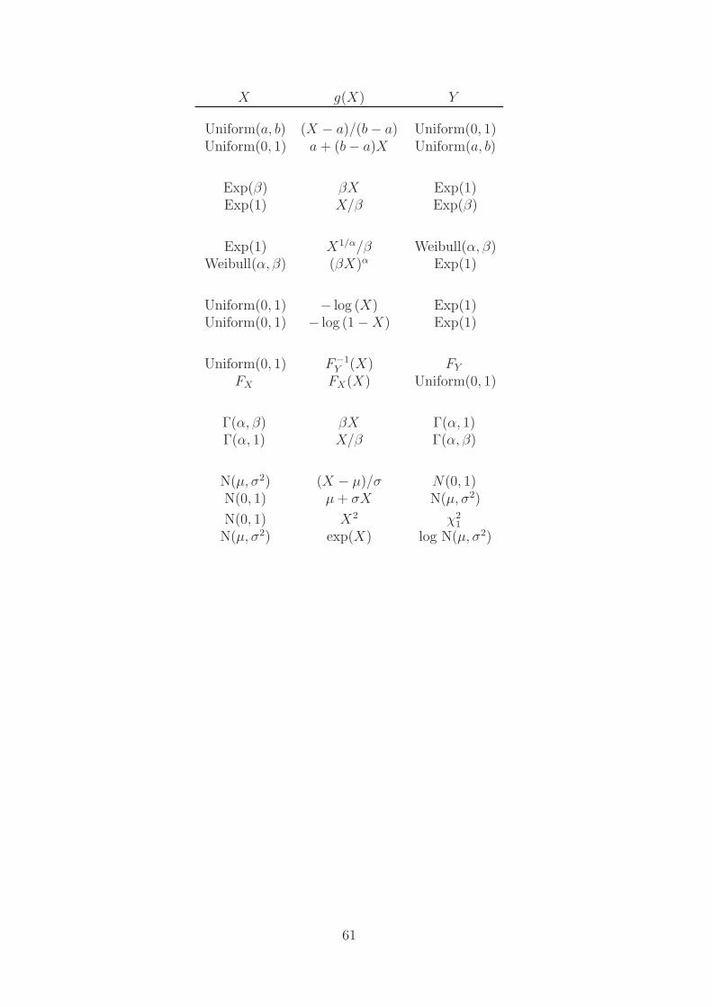
X g(X) Y
Uniform(a, b) (X − a)/(b − a) Uniform(0, 1)Uniform(0, 1) a + (b − a)X Uniform(a, b)
Exp(β) βX Exp(1)Exp(1) X/β Exp(β)
Exp(1) X1/α/β Weibull(α, β)Weibull(α, β) (βX)α Exp(1)
Uniform(0, 1) − log (X) Exp(1)Uniform(0, 1) − log (1 − X) Exp(1)
Uniform(0, 1) F−1Y (X) FY
FX FX(X) Uniform(0, 1)
Γ(α, β) βX Γ(α, 1)Γ(α, 1) X/β Γ(α, β)
N(µ, σ2) (X − µ)/σ N(0, 1)N(0, 1) µ + σX N(µ, σ2)
N(0, 1) X2 χ21
N(µ, σ2) exp(X) log N(µ, σ2)
61

62

Chapter 6
Bivariate Distributions
The concepts discussed in this chapter are joint and marginal distributions, independenceand conditional distributions, for both discrete and continuous random variables. Thereare several ways through this material and our choice is to deal with discrete and con-tinuous separately. We give a quick, but complete, run through of these distributionsin the the discrete case, and then follow this with a more extensive treatment of thecontinuous case.
In the following we will concentrate on situations where there are only two randomvariables X and Y . In subsequent chapters we discuss the extension to more than tworandom variables.
6.1 Introduction and Motivation
Often we are interested in the joint behaviour of a number of random variables and therelationships between them. This chapter describes methods of dealing with these mul-tivariate distributions. We first consider two motivating data sets which illustrate why,in many applications, it is not enough to consider the random variables individually.
Coastal Flooding
The figure shows the histograms of four sea condition variables, wave height, waterlevel, wave steepness, and wave period, which are important for assessing the levelof protection provided by a coastal flood defence system. The data are measured inmetres, at high tide, and there is about 235 days of data.
These empirical marginal distributions do not look like any of the distributions we havepreviously identified.
63

0 1 2 3 4
0.0
0.2
0.4
0.6
0.8
wave height4 5 6 7 8 9
0.0
0.1
0.2
0.3
0.4
0.5
water level
0.030 0.035 0.040 0.045
020
4060
80
steepness2 4 6 8
0.0
0.1
0.2
0.3
0.4
wave period
Histograms of marginal distributions for the coastal engineering data.
Coastal engineers are interested not simply in the big values of water level or of waveheights, but their combined effect. For example the worst flooding will occur when thewater level is large, the waves are high and have long periods. Knowing simply theseparate distributions of the different variables (i.e. what we have studied to date) willnot tell us whether large values of the variables can occur together or occur separately.Thus it is the joint characteristics of these variables that we must study.
The next figure shows the joint scatter plots for all the possible pairs of sea conditionvariables.
64
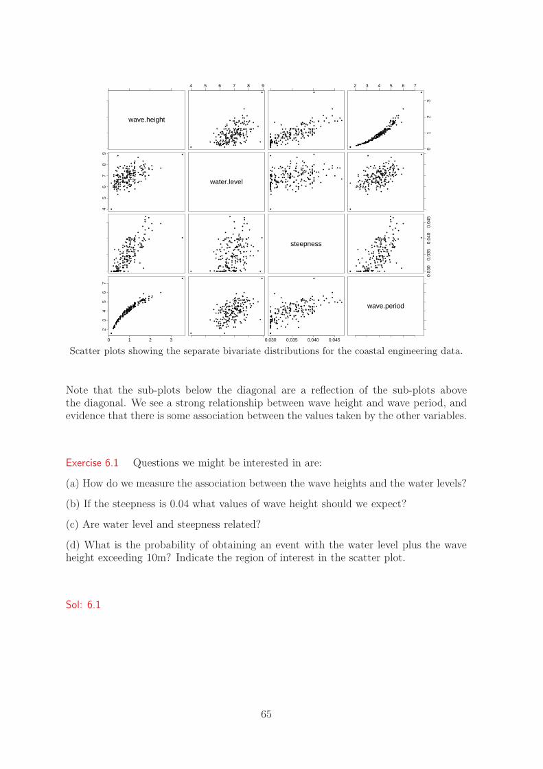
wave.height
4 5 6 7 8 9
•
• •
•
•••
•
••
••
•
•
•
••
•
•• •
•
• •••
• •••
•
•
•
••
••
•
•
•
•
•
• •
•• •
•
•••
•
•
••
•
•
•
•
•••••
•• ••
•
•
••
• •
• •
••
• •
••
•
•
••
••
••
•
•
•
•
•
•••
•
• •
•••
•
•
• ••
•
•
•••
••••
•
••
•
•
•
•
••
•
•••
•• •
••
•
••
•
••
••
•
•• •
• •
•• •
••
•••
••
•
•
•
•
•
•
•
• •• •
••
•
••
•
•
••• ••
•
••
•
•
••
•• •
•
•
•
•
••
• •
••
•
•••
•
••
••
•
•
•
••
•
•• •
•
•• ••
• • ••
•
•
•
••
••
•
•
•
•
•
••
•••
•
• ••
•
•
••
•
•
•
•
•••• •
••• •
•
•
••
••
••
••
••
••
•
•
••
••
••
•
•
•
•
•
• ••
•
••
•••
•
•
•••
•
•
•• •
• •• •
•
••
•
•
•
•
••
•
•••
•• •
• •
•
••
•
••
••
•
•••
••
•••
••
•••
••
•
•
•
•
•
•
•
• •• •
••
•
••
•
•
• ••• •
•
• •
•
•
••
•• •
•
•
•
•
••
•
2 3 4 5 6 7
01
23
•
••
•
•••
•
• •
••
•
•
•
••
•
•••
•
• •••
••••
•
•
•
••
••
•
•
•
•
•
••
•• •
•
•••
•
•
••
•
•
•
•
•••••
•• ••
•
•
••
••
• •
••
• •
• •
•
•
••
••
••
•
•
•
•
•
•••
•
••
•• •
•
•
•••
•
•
•• •
•••••
••
•
•
•
•
••
•
•••
•••••
•
••
•
••
••
•
•• •
• •
•• •
••
•••
••
•
•
•
•
•
•
•
••••
••
•
••
•
•
•••••
•
• •
•
•
••
•••
•
•
•
•
••
•
45
67
89
•
••
•••
•
• •
•
•
••
•
•
• • •
•
••
•••
•
•
•••
•
•
•
••
•
•
•
•
• ••
•
••• •
••
•
•
•
•
•
•
•
••
•
••••
••
•
•••
•
•
• •
••
•
•
••
••
•••
•
•
••
•
••
•
•
•
••
•
•
••
••
••
••
•••
•
•
••
•
••
•
•
•
•
••
••
•
•
••
••
•
•
•
•
• •
••
•
• •
••
• •
•
•••
••
•
•
•
•
•
•••
• • ••
••
• ••
•••
••
•
•
•
••
•
••
•
•
••
•
••• •
•
••
•
•
••
•
•
•
•
water.level•
••
•••
•
• •
•
•
••
•
•
• • •
•
••
••
•
•
•
•• •
•
•
•
••
•
•
•
•
• ••
•
•• •••
•
•
•
•
•
•
•
•
••
•
••••• •
•
•• •
•
•
• •
••
•
•
••
••
•••
•
•
••
•
••
•
•
•
••
•
•
••
••
••
••
•••
•
•
••
•
••
•
•
•
•
••
••
•
•
••
••
•
•
•
•
••
••
•
• •
••
••
•
•••
••
•
•
•
•
•
•••
• • ••
••
• ••
•••
•••
•
•
••
•
••
•
•
••
•
••• •
•
••
•
•
••
•
•
•
• •
••
•••
•
••
•
•
••
•
•
• • •
•
••
••
•
•
•
•••
•
•
•
••
•
•
•
•
• ••
•
••• •
••
•
•
•
•
•
•
•
••
•
••••
••
•
• ••
•
•
• •
••
•
•
••
••
• ••
•
•
••
•
••
•
•
•
••
•
•
••
••
••
••
•••
•
•
••
•
••
•
•
•
•
••
••
•
•
••
••
•
•
•
•
• •
••
•
• •
••
• •
•
•• •
••
•
•
•
•
•
•••
• • ••
••
• ••
•••
••
•
•
•
••
•
••
•
•
••
•
••• •
•
•••
•
••
•
•
•
•
•
••
••
••
•
•
•
•
••
•
•
•
••
•
••
•
•
•• •
•
••
••
••
••
••
•
•
••
••
•
•
••
•
•
•
• •
••
•
••
•
•
• •••
••
•
•
•
•
•
•
•
••
•
•
• •
•
•
••
•
•
•
•
•
•
• •
•
•
•
•
•
•
•
•••
•
••
•
•
•
••
•
•
•
•
••
•
•
••
•
•
•
•
•
•
•
••
•
•
••
•
•
•
••
•
••
•
••
•
•
•
•
••• • •
•
••
•
•
•
•
•
•
•
•
•
•
•
•
•
••
•
•
• •
•
• •
•
•
••
•••
•
••
•
•
••
••
•
•
•
•
•
•• •
•
••
••
••
•
•
•
•
• •
•
•
•
••
•
••
•
•
•• •
•
••
••
••
••
••
•
•
••
••
•
•
••
•
•
•
••
••
•
••
•
•
••••
••
•
•
•
•
•
•
•
• •
•
•
• •
•
•
••
•
•
•
•
•
•
••
•
•
•
•
•
•
•
•••
•
••
•
•
•
••
•
•
•
•
••
•
•
••
•
•
•
•
•
•
•
••
•
•
••
•
•
•
••
•
••
•
••
•
•
•
•
••• • •
•
••
•
•
•
•
•
•
•
•
•
•
•
•
•
••
•
•
••
•
• •
•
•
••
••
•
•
••
•
•
••
••
•
•
•
•
•
•• •
steepness
0.03
00.
035
0.04
00.
045
•
••
••
••
•
•
•
•
••
•
•
•
••
•
••
•
•
•• •
•
••
••
••
••
••
•
•
••
••
•
•
••
•
•
•
• •
••
•
••
•
•
• •••
••
•
•
•
•
•
•
•
••
•
•
• •
•
•
••
•
•
•
•
•
•
• •
•
•
•
•
•
•
•
•••
•
••
•
•
•
••
•
•
•
•
••
•
•
••
•
•
•
•
•
•
•
••
•
•
••
•
•
•
••
•
••
•
••
•
•
•
•
••• • •
•
••
•
•
•
•
•
•
•
•
•
•
•
•
•
••
•
•
• •
•
• •
•
•
••
•••
•
••
•
•
••
••
•
•
•
•
•
•• •
0 1 2 3
23
45
67
•
••
•
•••
• ••
••
•
•
•
••
•
•
••
•
•••
•
••••
•
•
•
•
••
•
•
•
•
•
•
••
•
••
•
••
•
•
•
••
•
•
•
•
•••
••
•••
••
•
• •
••
••
•
•
••
••
•
•
•
•
••
••
•
•
•
•
•
• ••
•
••
•
••
•
•
•••
•
•
•
• •
• •• ••
•
•
•
•
•
•
••
••••
•••
••
•
••
•
•
•
•
•
•
•••
••
•
••••
•
•••
••
•
•
•
•
•
•
••• •
•
•
•
•
•
•
•
•••••
•
••
•
••
•
•• •
•
•
•
•
••
••
• •
•
•••
•••
••
•
•
•
•••
•
••
•
• ••
•
• •• •
•
•
•
•
••
•
•
•
•
•
•
• •
•
• •
•
••
•
•
•
••
•
•
•
•
•••
••
•• •
••
•
• •
••
• •
•
•
••
••
•
•
•
•
••
••
•
•
•
•
•
•••
•
• •
•
••
•
•
• ••
•
•
•
••
•••• •
•
•
•
•
•
•
••
•• ••
••
•••
•
••
•
•
•
•
•
•
•• •
••
•
• ••
•
•
••••
•
•
•
•
•
•
•
• •• •
•
•
•
•
•
•
•
••• ••
•
••
•
••
•
•• •
•
•
•
•
••
•
0.030 0.035 0.040 0.045
•
••
•
•••
• ••
••
•
•
•
••
•
•
••
•
•••
•
• • • •
•
•
•
•
•••
•
•
•
•
•
••
•
••
•
••
•
•
•
••
•
•
•
•
••••
•
•••
••
•
• •
••
••
•
•
••
••
•
•
•
•
••
••
•
•
•
•
•
• ••
•
••
•
••
•
•
•••
•
•
•
• •
• •• ••
•
•
•
•
•
•
••
••••
••
•• •
•
••
•
•
•
•
•
•
•••
••
•
•••
•
•
•••
••
•
•
•
•
•
•
• •• •
•
•
•
•
•
•
•
• ••• •
•
••
•
••
•
•• •
•
•
•
•
••
• wave.period
Scatter plots showing the separate bivariate distributions for the coastal engineering data.
Note that the sub-plots below the diagonal are a reflection of the sub-plots abovethe diagonal. We see a strong relationship between wave height and wave period, andevidence that there is some association between the values taken by the other variables.
Exercise 6.1 Questions we might be interested in are:
(a) How do we measure the association between the wave heights and the water levels?
(b) If the steepness is 0.04 what values of wave height should we expect?
(c) Are water level and steepness related?
(d) What is the probability of obtaining an event with the water level plus the waveheight exceeding 10m? Indicate the region of interest in the scatter plot.
Sol: 6.1 Let height be X, level be Y , steepness be Z.
(a) Find corr(X, Y ).
(b) Need conditional dist of X|Z.
(c) Find if corr(Z, Y ) differs significantly from 0.
(d) Find P(X + Y > 10). Region: triangle above x + y = 10.
65

Stock Market Movements
0 500 1000 1500 2000
-0.3
-0.2
-0.1
0.0
0.1
time t
Ret
urn
Rt
Plot of the series of daily returns, Rt, through time t.
Much of the financial activity linked to the Stock Market is concerned with predictingthe movements of stock prices. The better you are able to make predictions the moremoney that can be earned with less financial risk. The vital term to be able to predictis the variable Rt, the return of the stock on day t, this is
Rt = (Pt − Pt−1)/Pt−1
where Pt is the price of the stock on day t. The figure above shows this variable onconsecutive days.
Clearly there is some relationship between returns on consecutive days as the variabilityof values is similar for neighbouring values.
The next figure shows consecutive values, i.e. Rt plotted against Rt−1. Given Rt−1 saywe want to predict Rt, or at least know what this distribution of Rt will be.
66

•
•••
••
•
••• ••
•• •••
•••
••
• ••• •
•
••
•••••
••
•••
• •
•• •
••• •••
•
•••
•••
•• •
••••••••
••
••
•• • •
••• •
••
•• ••• ••
•• ••••• •••
••••••
••
•• ••
• ••
•••••
•••
• •••
•••••
••
••• ••••
• •••••••• ••••••
•••• ••• •••••••
• •••••••
••••
• •••
••••
•••• ••
• •••
•• •
••••
•
•••
•••
• ••••
••••••
••
• •••••
•
• ••
••
••
•
•
•
•••
•
••
••• •
• •
•••
•
• •
••• •
•
••
•
•
••• •
•
• •
•
•
•
•
•
•
•
•
•
•
•
•
••
•
•
•
•
•
•
•
••
•
•
•
•
•
•
•
•
•
•
••
•
•
•
•
•
•
•
•
•
•
••
••
•
• •
•
•
•
•
••
• ••
•
•
••
•
•
•
•
•
•
•
••
•
•
••
•
••
• •
•
•• ••
•
•
•
•
•
• •
•
••
•
•
•
••
••
•
•
•
•• •
• •
•
•
•
•
••
•
•
•
••
•
•
•
•
•• •
•
•
••
•
•
•
•
•••
•
••
•
•• ••
••••
•
•
• •
•
• •
• •
••
•
•
•
•
• •
•
••
•
••
•
•
•
••
•
•
• •
•
• ••
•
• •
••
•
•
•
•
••• ••••
• ••
• ••
•
•
• ••••
•••
••••
••
•
••
••
•
•
•••
••
••
••
••
• •••
• •••
•
••
•••• ••
•••
•
•••
•• •• •
•
••
•• •
•
••
•
•••
•• •
••• •
•
•••
•
••
•••••
••
•••
•• •
•
••••
•• ••••
• •••••
• ••
• ••••
•
• •••••• •••
••••••••••••
•
••
••
••• •••
••
••••
• •••
•
••
•
•
•
•••
•
•
•
• ••
••
•••
•••••
•
•
••
•
•••••
•
• •
•
•••
••
••
•••
• ••••
••
••
• ••••
•
••
• •••
• ••••
••
• ••
••••
•••
•• •
••••••••
••
•
•
••
•• •
••
•
•
••• •
•
••
•
•
••
••
•
• •
•
•
•
••
••• ••
•••
• ••••
•••
•• •••
•
••
•
•
•
•
•• ••
•• •
••
•
•• ••••
•
••••
• •••••
•
•
•
••
• ••
••
•
•• •
•••
•
•
••
•
••••••
••
• ••
• ••
•• •••••
••
•••
•
•
•
••
• ••
•• •
••••
• ••
••
••
••
•
•
• ••
••
••
•
••••
•
•
•• •
•
••••
•••
•
•
••
•••
••
•
•
•
•
••
•
••
• •• •
•
• •••
••
•
•
••
•
•
•
•
•
•
•
•
••
•
• •• •
••
•••
••
• ••
•
••
•
• •
•
•••
•
•
• ••
•
••
•
••
•
•
•
•
•
•••••
••
•
•
••
•
•••
•
•
•• ••
•
••
•
••
•
•
••
••
••
•
•••
•
•
•
•••••
••
••••
••
•
•••
•••
••
•
•
••••
•
••
••
•
••
••
•••
• ••
• ••
•
•
•••
•
•
••
••
•
•
•
•• •
•
•••
••
•• •
•
••• •
•
•
•
•
•
•
••
•
•
•
•
•• •
•
•
••••
•
•
•
•
•
•
••
•
•••
•
•
• •••
•
•
••••
• ••
•• ••
•••
••••
• ••
•••• •••
••• ••
••
••
•
• ••• •
•• •••
• ••• ••
••
•••
• ••
•
•• •
••
•••• •••• • ••
••• ••
•
•• •
••••••
••••
•
•••
••
•
••
••
••
••
•
••
••
•
•
•
• •
•••
•••
•
••
•
•
••••
••
••
•• ••
••
•
•••
• •
•••
•• • ••
•••
• ••
•••
•• •
••• •
••
•
•• •
••
•
••
•••
• ••
•
•
••
•
•
••
•
••
••
••
•
•• •
• •
•
•
••
•
•• •
•
•
••
•
• ••
•
••
•
•
••
• ••
• ••
•
•
••
••• •
••
•••
••
•
••
•
•
•
•
••• •
• •
••
•
•
•
•
•
•
••
•
•
•
•
•
•
•
• •••
•••
••
•
• •
•
••
•
•
• ••
•
•
•
•
•
•
•
•
•
•
•
•
•
•
•
••
•
•
•
•
•
••
•
•
•
•
•
•
•
•
•
•
••
•
•
•
•
•
•
• •
••
•
•• •
•••
• •
•
•
••
•
•
••
•
••
•
•
•
•
•
•
•
• •
•
•••
•
•
•
•••
•
•
• ••
••
•
• •
•
••
•
• •••
•
•
••
••
• •
•••
•
••
••
•
•
••
•
•
•
•
••
•
•
•
• •
••
•
••
•
• • •••
••
• ••
• •
••
•• •• •••
• ••••
••
• ••
• ••
• •
••
• ••
••
•• •
••••
••• •
•••
•
••
•
•
•
••
••••
• •
•• •
••• ••••
••
•
•
•
• ••••
• •••
•• ••• •
•• •
••
•• ••••••••
••
•••
••
• ••
• ••••
•
•• ••
• •••
•• ••
• •• •
•••
••
•
•
•••
••
•
•••
• ••
•••
• ••
• ••
•
••
•
••
••
••
••
•
•
••
•
••
•
•
• •
••• ••
• ••
•
••
••
••
•
•
•••• •
••
•
••••
• ••
• •••
••
•• ••••
• ••
•
••
•
•
••
•••
••••
•• •••
•••
•
•• •
• •••••
••
••
••
•
••••••
••••
•••••••••••
•• ••
• ••
••
• ••• •••
••
•• ••••••
••••
••••
• ••• ••
••
•
•• •
• ••••••• ••••
••
••• •
•••• •••••• ••
•••
••
••••• •
••
•
••
••
•
•
•
•
••••
•••
••
•• •••
•••
••
•
••
•
•• •
• •••
•• •••••
-0.3 -0.2 -0.1 0.0 0.1
-0.3
-0.2
-0.1
0.0
0.1
Rt
Rt−1
Plot of returns on consecutive days.
The practical issue here is to identify association between these return values and whatits effect is if we know the return on the previous day. Again the probability conceptsin this chapter provide a basis for addressing this type of problem.
Data from a simulation exercise
One way of understanding real data is to build a probability model to simulate dataand check if the broad properties of the simulated and the real data are the same. Inthis sense the probability model is a generative model.
Example 6.2 The random variables X and Y in the model represent water level andwave height measured from their respective averages. Physics suggests that water leveleffects wave height, rather than vica versa. A possible starting point is to suppose thatthe level X ∼ N(0, 1), which has mean 0. Further suppose that Y |X = x ∼ N(αx, 1)for which E[Y |X = x] = αx. If α > 0 then the expected height increases linearly withlevel.
The figure illustrates a sample of 235 observations on level and height generated froma random sample.
Fre
quen
cy
−3 −1 0 1 2 3 4
010
2030
40
−2 −1 0 1 2
−2
01
23
hei
ght,
Y
height, Y level, X
Realisations of jointly distributed random variables may be obtained by simulationfrom fXY (x, y) or from the marginal fX(x) and the conditional fY |X(y|x). Here we usethe latter method.
67

Example 6.3 Generate a random variable X ∼ N(0, 1) and a second random variableY ∼ N(αx, 1). Plot the joint realisation, and compare the means and standard devi-ations of X and Y . Take α = −1, and then choose other values. Fix a sample size nfor the realisations.
n = 235
x = rnorm(n,mean=0,sd=1)
alpha = -1
y = rnorm(n,mean=alpha*x,sd=1 )
par(mfrow=c(2,2))
hist(y,col=’yellow’,br=20,main=’’)
plot(x,y,pch=’.’,col=’red’,cex=4)
frame() ; hist(x,col=’green’,br=20)
mean(x) ; mean(y)
sd(x) ; sd(y)
Note that the standard deviation of Y is significantly bigger than that of X.
6.2 Discrete Random Variables
If X and Y are both discrete, their joint probability mass function is
pXY (x, y) = P(X = x, Y = y).
What does the ’,’ mean here? Set intersection.
As in the earlier chapters we will concentrate on discrete random variables takinginteger values.
Properties of the bivariate pmf: pXY (x, y) satisfies
• For all x and y: 0 ≤ pXY (x, y) ≤ 1.
• ∑x,y pXY (x, y) =∑∞
x=−∞∑∞
y=−∞ pXY (x, y) = 1.
• P[(X, Y ) ∈ A] =∑
(x,y)∈A pXY (x, y).
Exercise 6.4 The joint pmf of X and Y is
pXY (x, y) = (x + y)/18 for x, y = 0, 1, 2.
(a) Write out the joint probability table. (b) Show this is a valid joint pmf. (c)Evaluate (i) P(X = 2), (ii) P(X < Y ), (iii) P(X = Y ), (iv) P(X + Y ≥ 2).
68

Sol: 6.4 (a) pXY is
yx 0 1 20 0
18118
218
1 118
218
318
2 218
318
418
.
(b) Validity: pXY (x, y) ≥ 0 and∑
x,y pXY (x, y) = 1.
(c) (i) P(X = 2) = 118
[2 + 3 + 4]. (ii) P(X < Y ) = 118
[1 + 2 + 3]. (iii) P(X = Y ) = 118
[0 + 2 + 4].
(iv) P(X + Y ≥ 2) = 118
[2 + 2 + 2 + 3 + 3 + 4].
If X and Y are discrete random variables their marginal pmfs are
pX(x) =
∞∑
y=−∞pXY (x, y), pY (y) =
∞∑
x=−∞pXY (x, y).
Exercise 6.5 Bivariate random variables X and Y have joint pmf
y0 1 2 3
x 1 5/60 8/60 2/60 1/60 16/602 12/60 7/60 3/60 2/60 24/603 4/60 8/60 6/60 2/60 20/60
21/60 23/60 11/60 5/60
Find the marginal pmfs.
Sol: 6.5
y0 1 2 3
x 1 5/60 8/60 2/60 1/60 16/602 12/60 7/60 3/60 2/60 24/603 4/60 8/60 6/60 2/60 20/60
21/60 23/60 11/60 5/60
If X and Y are discrete random variables, the conditional pmfs are
pX|Y (x | y) =pXY (x, y)
pY (y), pY |X(y | x) =
pXY (x, y)
pX(x).
Independence is the simplest form for joint behaviour of two (or more) random variables.Informally, two random variables X and Y are independent if knowing the value of oneof them gives no information about the value of the other. The outcomes of, say, aroll of a dice and a toss of a coin are independent in exactly this sense: knowing thatthe coin came down tails does not give us any information about the score of the dice,
69

and, conversely, knowing that the score of the dice was 3 does not give any informationabout the coin.
Definition: Formally, we say that two random variables X and Y are independent ifthe events X ∈ A and Y ∈ B are independent for all sets A and B, i.e.
P(X ∈ A, Y ∈ B) = P(X ∈ A) P(Y ∈ B) for all sets A, B.
Theorem 6.1 Independence in terms of the pmfs. Two discrete random variables Xand Y are independent if and only if
pXY (x, y) = pX(x)pY (y) for all x, y.
Proof: If X and Y are independent, discrete random variables we get by letting A = xand B = y that
pXY (x, y) = P(X ∈ A, Y ∈ B)
= P(X ∈ A) P(Y ∈ B)
= pX(x)pY (y).
Conversely, if the joint pmf factorises we get for arbitrary sets A and B
P(X ∈ A, Y ∈ B) =∑
x∈A
∑
y∈B
pXY (x, y)
=∑
x∈A
∑
y∈B
pX(x)pY (y) def indep
=∑
x∈A
pX(x)∑
y∈B
pY (y) common factors
= P(X ∈ A) P(Y ∈ B).
When the discrete variables (X, Y ) are independent then for all x, y:
pX|Y (x | y) =pX(x)pY (y)
pY (y)= pX(x), pY |X(y | x) = pY (y).
These results conform with intuition as when X and Y are independent knowing thevalue of X should tell us nothing about Y and vica versa.
The converse is also true: if the conditional distribution of X given Y = y is indepen-dent of y or, equivalently, the conditional distribution of Y given X = x is independentof x, then X and Y are independent.
Exercise 6.6 A fair coin is tossed. If it turns H a fair die is thrown, if T a biased die.The bias makes even numbers twice as probable as odd numbers. Find the joint pmfof X, the toss of the coin, and Y , the score on the die.
70

Sol: 6.6 Code T and H as 0 and 1 to make rvs. Marginal: pX(x) = 1/2 for x = 0, 1.
Conditional:x = 1: pY |X(y|1) = 1/6 for y = 1, 2, . . . , 6.x = 0: pY |X(y|0) = c for y = 1, 3, 5 and pY |X(y|0) = 2c for y = 2, 4, 6. Hence c = 1/9.
Using pXY (x, y) = pY |X(y|x) pX(x) delivers
1 2 3 4 5 60 1/18 2/18 1/18 2/18 1/18 2/181 1/12 1/12 1/12 1/12 1/12 1/12
Exercise 6.7 For the joint pmf in Exercise 6.2 obtain the conditional pmf of X givenY = 2.
Sol: 6.7
Y0 1 2 3
X 1 2/60 16/602 3/60 24/603 6/60 20/60
11/60
So
pX|Y (x|2) = pXY (x, 2)/pY (2)
=
2/11 x = 13/11 x = 26/11 x = 3
.
6.3 Cumulative Distribution Function
The joint cumulative distribution function of X and Y is defined as
F (x, y) = FXY (x, y) = P(X ≤ x, Y ≤ y),
x
y
and gives the probability that a random variable X takes a value less than x and thatthe rv Y takes a value less than y.
71

Properties of the joint cdf:
• FXY (x, y) is defined for all random variables, i.e. discrete, continuous or a mixtureof these.
• Since it is a probability: 0 ≤ FXY (x, y) ≤ 1 for all x and y, and
FXY (−∞, y) = 0, FXY (x,−∞) = 0, FXY (∞,∞) = 1.
• FXY (x, y) is non-decreasing in both x and y, i.e. for all h ≥ 0
FXY (x + h, y) ≥ FXY (x, y) and FXY (x, y + h) ≥ FXY (x, y).
• The marginal cdf FX(x) = FXY (x,∞), and similarly for Y .
The probability of (X, Y ) falling in a rectangle with opposite corners (x1, y1) and(x2, y2), with x1 < x2 and y1 < y2, can be found from FXY using
P(x1 < X ≤ x2, y1 < Y ≤ y2) = FXY (x2, y2) − FXY (x1, y2) − FXY (x2, y1) + FXY (x1, y1).
x1 x2
y1
y2
6.4 Continuous Random Variables
If X and Y are both continuous random variables their joint probability density function(pdf) is defined from
FXY (x, y) =
∫ y
t=−∞
∫ x
s=−∞fXY (s, t)dsdt =
∫ x
s=−∞
∫ y
t=−∞fXY (s, t)dtds
or equivalently
fXY (x, y) =d2FXY (x, y)
dxdy=
d2FXY (x, y)
dydx.
For simplicity, we usually only state FXY (x, y) for values of (x, y) such that fXY (x, y) > 0.So if FXY is not defined for a particular (x, y) pair, then fXY (x, y) = 0 at that point.
72

Properties of the bivariate pdf:
• Positivity: fXY (x, y) ≥ 0 for all (x, y),
• Summability:∫∞−∞∫∞−∞ fXY (x, y) dxdy = 1.
• The probability of event A, i.e. P[(X, Y ) ∈ A], is obtained by integrating the pdfover the event A:
P[(X, Y ) ∈ A] =
∫ ∫
(x,y)∈A
fXY (x, y) dxdy.
x
y
Exercise 6.8 The random variables (X, Y ) have joint distribution function
FXY (x, y) = xy/4 for 0 < x < 2, 0 < y < 2,
Obtain: (a) the joint pdf, (b) P(X < 1, Y < 1), (c) P(X < 1), (d) P(X2 + Y 2 ≤ 1).
Sol: 6.8 (a) The joint pdf is
fXY (x, y) =d2
dxdyFXY (x, y)
=d2
dxdy
(xy
4
)
for 0 < x < 2, 0 < y < 2
=
1/4 for 0 < x < 2, 0 < y < 2,0 otherwise.
Note volume=height×area.
(b) P(X < 1, Y < 1), two approaches: cdf and pdf.
cdf: P(X < 1, Y < 1) = FXY (1, 1) = 1/4.
pdf: picture needed
P(X < 1, Y < 1) =
∫ 1
y=0
∫ 1
x=0
fXY (x, y) dxdy
=
∫ 1
y=0
∫ 1
x=0
1
4dxdy
=
∫ 1
y=0
[x
4
]1
0dy
=
∫ 1
y=0
1
4dy =
1
4.
73
(c) P(X < 1), two approaches: cdf and pdf. cdf:
P(X < 1) = P(X < 1, Y < 2)
= FXY (1, 2)
=2
4= 1/2.
pdf: picture needed
P(X < 1) =
∫ 2
y=0
∫ 1
x=0
1
4dxdy
=
∫ 2
y=0
[x
4
]1
0dy =
∫ 2
y=0
1
4dy = 1/2.
(d) P(X2 + Y 2 < 1), pdf:
P(X2 + Y 2 < 1) =
∫ 1
x=0
∫
√1−x2
y=0
1
4dydx
=
∫ 1
0
[√
1 − x2
4
]
dx
=
∫ π/2
0
1
4cos2(θ) dθ, using x = sin(θ)
=
∫ π/2
0
1 + cos 2θ
8dθ
=1
8
[
θ +1
2sin 2θ
]π/2
0
=π
16.
Note volume=height×area= 14× 1
4π12 = π
16.
Exercise 6.9 The random variables (X, Y ) have joint pdf
fXY (x, y) =
(x + y)/8 for 0 < x < 2, 0 < y < 2,0 otherwise.
(a) Find P(X > Y ). (b) Explain why you could have obtained this answer withoutdoing any integration.
74

Sol: 6.9 picture needed
P(X > Y ) =
∫ 2
x=0
∫ x
y=0
x + y
8dydx
=
∫ 2
x=0
1
8
[
xy + y2/2]x
y=0dx
=
∫ 2
x=0
3x2
16dx
=
[
x3
16
]2
x=0
= 1/2.
(b) Without integration? By symmetry of fXY (x, y) about x = y line there is equalchance of X > Y and Y < X.
Exercise 6.10 The joint distribution (in years) for the lifetimes X and Y of twocomputer components has joint pdf
fXY (x, y) =
β exp(−βx) exp(−y) for 0 < x < ∞, 0 < y < ∞,0 otherwise.
Find the probabilities of the following events: (a) Both components have lifetimesexceeding one year. (b) Component Y has a longer lifetime than component X.
Sol: 6.10
P(X > 1, Y > 1) =
∫ ∞
y=1
∫ ∞
x=1
β exp(−βx) exp(−y) dxdy
=
∫ ∞
1
[− exp(−βx) exp(−y)]∞x=1 dy
=
∫ ∞
1
exp(−β) exp(−y) dy
= [− exp(−β) exp(−y)]∞1= exp(−β) exp(−1) = exp(−[β + 1]).
(b)
75

P(Y > X) =
∫ ∞
x=0
∫ ∞
y=x
β exp(−βx) exp(−y) dydx
=
∫ ∞
0
[−β exp(−βx) exp(−y)]∞y=x dx
=
∫ ∞
0
β exp(−βx) exp(−x) dx
=
∫ ∞
0
β exp(−[β + 1]x) dx
=β
β + 1.
6.5 Marginal Distributions
Given the joint distribution of (X, Y ) we may want to find the (marginal) distributionof X or Y alone. The marginal distribution tells us about the behaviour of one randomvariable alone, i.e. irrespective of the other. We have been studying such distributionsin the earlier chapters on univariate variables.
If we have the joint cdf FXY defined for (x, y) ∈ (−∞,∞) × (−∞,∞), the marginalcdfs are obtained as follows:
FX(x) = P(X ≤ x) = P(X ≤ x, Y < ∞) = FXY (x,∞),
FY (y) = P(Y ≤ y) = P(X < ∞, Y ≤ y) = FXY (∞, y),
because the marginal event X ≤ x is the same as the joint event X ≤ x, Y < ∞and the event Y ≤ y is the same as the event X < ∞, Y ≤ y, as illustrated in theFigure.
XX
YY 00 x
X ≤ x y
Y ≤ y
Left: The event X ≤ x. Right: The event Y ≤ y.
If we have the joint pdf the marginal pdfs are obtained by integrating over the othervariable.
Theorem 6.2 If X and Y are continuous random variables their marginal pdfs are
fX(x) =
∫ ∞
t=−∞fXY (x, t) dt, fY (y) =
∫ ∞
s=−∞fXY (s, y) ds.
76

Proof: For continuous random variables X and Y we have
FX(x) = FXY (x,∞)
=
∫ x
s=−∞
∫ ∞
t=−∞fXY (s, t) dtds
=
∫ x
s=−∞
∫ ∞
t=−∞fXY (s, t) dt
ds,
and by differentiating both sides wrt. x we get
fX(x) =
∫ ∞
t=−∞fXY (x, t) dt.
Similarly for Y .
Exercise 6.11 Find the marginal pdf of X for the joint distributions specified by(a) cdf FXY (x, y) = xy/4, 0 < x < 2, 0 < y < 2, and (b) pdf fXY (x, y) = (x + y)/8,0 < x < 2, 0 < y < 2.
Sol: 6.11 (a) The cdf FXY (x, y) = xy/4 implies the joint pdf is
fXY (x, y) =
1/4 for 0 < x < 2, 0 < y < 2,0 otherwise.
Hence
fX(x) =
∫ 2
y=0
1
4dy
=1
4[y]2y=0
=1
2for 0 < x < 2.
(b) The joint pdf is
fXY (x, y) =
(x + y)/8 for 0 < x < 2, 0 < y < 2,0 otherwise.
Hence
fX(x) =
∫ 2
y=0
x + y
8dy
=1
8
[
xy + y2/2]2
y=0
=2x + 2
8=
x + 1
4for 0 < x < 2.
77
Exercise 6.12 The random variables (X, Y ) have joint distribution function
FXY (x, y) = xy[1 + α(1 − x)(1 − y)] for 0 < x < 1, 0 < y < 1,
for −1 ≤ α ≤ 1. Find the marginal distributions of X and Y and identify their forms.
Sol: 6.12 First note that the range restriction implies
FXY (x, y) = FXY (x, 1) for 0 < x < 1, y > 1,
FX(x) = FXY (x,∞) = FXY (x, 1) = x for 0 < x < 1.
By symmetry FY (y) = y for 0 < y < 1. Both marginal distributions are Uniform(0, 1).
Exercise 6.13 The random variables (X, Y ) have joint pdf
fXY (x, y) =
βφ exp(−βx) exp(−φy) for x > 0, y > 0,0 otherwise,
for β > 0 and φ > 0. Find the marginal distributions of X and Y and identify theirforms.
Sol: 6.13
fX(x) =
∫ ∞
t=−∞fXY (x, t) dt
=
∫ ∞
t=0
βφ exp(−βx) exp(−φt) dt
= [−β exp(−βx) exp(−φt)]∞t=0
= β exp(−βx) for x > 0.
An Exp(β) distribution. By symmetry Y ∼ Exp(φ).
6.6 Independence
It turns out that for the independence property to hold it is enough that the eventsX ≤ x and Y ≤ y are independent for all x and y. Thus, two random variables Xand Y are independent if and only if their joint distribution function factorises as
FXY (x, y) = FX(x)FY (y) for all x, y
where FX(x) and FY (y) are the marginal cdfs of X and Y respectively.
Similarly, when X and Y are both continuous they are independent if and only if theirjoint pdf can be factorised as a product of the marginal pdfs.
78

Theorem 6.3 Two continuous random variables X and Y are independent if and onlyif
fXY (x, y) = fX(x)fY (y) for all x, y.
Proof: If X and Y are independent, continuous random variables we know that
FXY (x, y) = FX(x)FY (y)
and by differentiating both sides wrt x and y we get
fXY (x, y) = fX(x)fY (y).
Conversely, if the joint pdf factorises we get for arbitrary sets A and B
P(X ∈ A, Y ∈ B) =
∫
A
∫
B
fXY (x, y)dxdy
=
∫
A
∫
B
fX(x)fY (y)dydx
=
∫
A
fX(x)dx
∫
B
fY (y)dy
= P(X ∈ A) P(Y ∈ B).
Exercise 6.14 Let X and Y be independent exponential random variables with pa-rameters β and φ respectively. Find P(X > x, Y > y).
Sol: 6.14
P(X > x, Y > y) = P(X > x) P(Y > y) for 0 < x, 0 < y
= [1 − FX(x)] [1 − FY (y)]
= exp(−βx) exp(−φy),
using independence.
Factorisation: Note that if we have the joint pdf it is enough to check that it can befactorised as a function of x, g(x) say, times a function of y, h(y) say:
fXY (x, y) = g(x)h(y), for all x, y,
and that the range of X does not depend on Y . In other words, we do not have toshow that the functions g and h are themselves densities. Note that if the range of Xdoes not depend on Y , then the range of Y does not depend on X, so that the rangecondition is in fact symmetric in the way it treats x and y.
79
Variational independence: If the ranges of X does not depend on Y , we say that Xand Y are variationally independent. Note that fXY can be factorised as a function of xtimes a function of y if and only if
fXY (x1, y1)fXY (x2, y2) = fXY (x1, y2)fXY (x2, y1) for all x1, x2, y1, y2.
Two point method: This is particularly useful to prove that a given joint pdf fXY
does not correspond to independent random variables. Simply find (x1, y1), and (x2, y2),such that the two sides above are different.
Exercise 6.15 Are X and Y independent if the joint pdf is fXY (x, y) = 12xy(1 − y)for 0 < x < 1, 0 < y < 1?
Sol: 6.15
fXY (x, y) = 12x y(1 − y) for 0 < x < 1, 0 < y < 1
= g(x) h(y),
and so the joint pdf factorises. As the range is 0 < x < 1, 0 < y < 1, X and Y arevariationally independent as well, and hence X and Y are independent.
Exercise 6.16 Are X and Y independent if the joint pdf is fXY (x, y) = 2 exp(−x − y)for 0 < x < y < ∞?
Sol: 6.16
fXY (x, y) = 2 exp(−x) exp(−y) for 0 < x < y < ∞= g(x) h(y) but only for 0 < x < y < ∞
so not variationally independent and so not independent.
Exercise 6.17 Are X and Y independent if the joint pdf is fXY (x, y) = x + y for0 < x < 1, 0 < y < 1.
Sol: 6.17 The range space is 0 < x < 1, 0 < y < 1 so that X and Y are variationallyindependent. However
fXY (x, y) = x + y
6= g(x) h(y).
To prove this last assertion, first note that if fXY (x, y) does factorise then the crossproduct ratio
fXY (x1, y1) fXY (x2, y2)
fXY (x1, y2) fXY (x2, y1)= 1.
80

Counterexample: find values of x’s and y’s so that
(x1 + y1) (x2 + y2)
(x1 + y2) (x2 + y1)6= 1.
For instance x1 = 1/4 = y1 and x2 = 3/4 = y2 give the ratio 3/4 6= 1 so not indepen-dent.
Exercise 6.18 There are four joint density functions of the form
fXY (x, y) =1
|A|1A(x, y),
illustrated in the figure. The function 1A(x, y) is 1 when (x, y) ∈ A and zero otherwise.In which cases are X and Y independent?
XX
XX
Y
Y
Y
Y
00
00
Four different shaded regions A for the pdf.
Sol: 6.18 Bottom left and top right: variationally independent. Top left and bottomright: not variationally independent.
6.7 Conditional Distributions
Suppose we know the joint distribution of (X, Y ) but then we find out the value of oneof the random variables. What can we say about the other random variable?
We consider the conditional distributions X | Y = y, i.e. the distribution of X giventhat Y = y, and Y |X = x, i.e. the distribution of Y given that X = x. If X and Yare continuous random variables the conditional pdfs are
fX|Y (x | y) =fXY (x, y)
fY (y), fY |X(y | x) =
fXY (x, y)
fX(x).
81
Note that since we can only condition on possible values, we don’t have to worry aboutzero’s in the denominators: the marginal pdf has to be positive for the value to occur.
Also note that the conditional pdfs are themselves valid pdfs: they are non-negativeand they sum/integrate to 1. For instance,
∫ ∞
x=−∞fX|Y (x | y)dx =
∫ ∞
x=−∞
fXY (x, y)
fY (y)dx
=1
fY (y)
∫ ∞
x=−∞fXY (x, y)dx
=1
fY (y)fY (y) = 1.
When the continuous variables (X, Y ) are independent then for all x, y:
fX|Y (x | y) =fX(x)fY (y)
fY (y)= fX(x), fY |X(y | x) = fY (y).
Exercise 6.19 A piece of string of unit length is tied at the zero end to a hook. Thestring is cut at a random distance X from the hook. The piece remaining is then cutagain at a random distance Y from the hook. Find the marginal pdf of Y .
Sol: 6.19
Model with X ∼ Uniform(0, 1) and Y |X ∼ Uniform(0, x). We know fX(x) = 1 for0 ≤ x ≤ 1, and fY |X(y|x) = 1/x for 0 < y < x < 1. We need fY (y).
fY (y) =
∫ 1
x=y
fXY (x, y)dx
=
∫ 1
x=y
fY |X(y|x)fX(x) dx
=
∫ 1
x=y
1
x× 1 dx
= [ logx]1x=y
= log (1/y) for 0 < y < 1.
Exercise 6.20 Given that the remaining length tied to the hook has length y, find thepdf of the position of the first cut X.
82

Sol: 6.20 Use Bayes rule
fX|Y (x | y) =fXY (x, y)
fY (y)
=fY |X(y|x)fX(x)
fY (y)
=1
x log (1/y)for y < x < 1.
Exercise 6.21 Continuous random variables X and Y have joint pdf
fXY (x, y) =
exp(−x/y) exp(−y)/y if 0 < x < ∞, 0 < y < ∞0 otherwise.
Find (a) the conditional pdf of X given Y = y, (b) P(X > 1 | Y = 1).
Sol: 6.21 (a) First get fY and then fX|Y .
fY (y) =
∫ ∞
x=0
exp(−x/y) exp(−y)/y dx
= [− exp(−x/y) exp(−y)]∞x=0
= exp(−y) for 0 < y < ∞.
So the marginal distribution is Y ∼ Exp(1).
fX|Y (x | y) =fXY (x, y)
fY (y)
=exp(−x/y) exp(−y)/y
exp(−y)
=1
yexp(−x/y) for 0 < x < ∞.
So the conditional distribution is X|Y = y ∼ Exp(1/y).
(b) X | Y = 1 ∼ Exp(1) so P(X > 1 | Y = 1) = exp(−1).
Exercise 6.22 The random variable X ∼ N(0, 1) and Y |X = x ∼ N(αx, 1).
(a) Write down the conditional pdf of Y given X = x. (b) Write down the joint pdf ofX and Y . (c) For what values of α are X and Y independent?
83

Sol: 6.22 (a) Conditional pdf for Y |X = x
fY |X(y|x) =1√2π
exp[−1
2(y − αx)2]
for −∞ < y < ∞.
(b) Joint pdf for X, Y
fXY (x, y) = fY |X(y|x)fX(x)
=1√2π
exp[−1
2(y − αx)2] × 1√
2πexp[−1
2x2]
=1
2πexp[−1
2(y2 − 2αxy + (1 + α2)x2)] for −∞ < x < ∞, −∞ < y < ∞.
(c) α = 0 imply X and Y independent as the joint distribution factorises and the rangesare variationally independent.
84
Chapter 7
Linear Transformations
Many calculations involve finding a linear transform of several random variables. Ide-ally we would like to calculate the distribution, but the usual first step, is to calculateexpectations, including the mean and variance, of quantities such as
X1 + X2
and more generally
a1X1 + a2X2 + . . . + anXn.
We start with expectations when n = 2.
Exercise 7.1 Give concrete examples of these structures.
Sol: 7.1 X1 = average sea level, X2 = wave height; X1 + X2 = combined sea levelheight.
ai = % of portfolio in stock i, Xi = price increase of stock i, a1X1 + a2X2 + . . . + anXn
= total profit.
7.1 Bivariate Expectations
We know how to obtain expectations for univariate random variables. The definitionextends easily to bivariate random variables. The expectation of any function g(X, Y )is defined by:
Discrete random variables
E[g(X, Y )] =∞∑
x=−∞
∞∑
y=−∞g(x, y)pXY (x, y),
85

Continuous random variables
E[g(X, Y )] =
∫ ∞
x=−∞
∫ ∞
y=−∞g(x, y)fXY (x, y) dydx.
In the rest of this section results are given for the continuous random variable caseonly, however these extend immediately to discrete random variables.
Notation: when the range of the integral is understood, we often write∫
xinstead of
∫ b
x=a.
Moments of either variable alone can be obtained from the joint distribution or fromthe relevant marginal.
E(X) =
∫
x
∫
y
xfXY (x, y) dydx
=
∫
x
x
∫
y
fXY (x, y) dy
dx
=
∫
x
xfX(x) dx,
and, more generally, for a function g
E[g(X)] =
∫
x
∫
y
g(x)fXY (x, y) dydx =
∫
x
g(x)fX(x) dx.
Similarly for Y and a function h
E(Y ) =
∫
y
∫
x
yfXY (x, y) dxdy =
∫
y
yfY (y) dy,
E[h(Y )] =
∫
y
∫
x
h(y)fXY (x, y) dxdy =
∫
y
h(y)fY (y) dy.
Using linearity of integrals we also have for any functions g and h
E[g(X) + h(Y )] =
∫
x
∫
y
[g(x) + h(y)]fXY (x, y) dydx
=
∫
x
∫
y
g(x)fXY (x, y) dydx
+
∫
x
∫
y
h(y)fXY (x, y) dydx
= E[g(X)] + E[h(Y )].
In particular
E(X + Y ) = E(X) + E(Y ),
regardless of the joint distribution of (X, Y ).
86
If X and Y are independent we also have for any functions g and h
E[g(X)h(Y )] =
∫
x
∫
y
g(x)h(y)fXY (x, y) dydx
=
∫
x
∫
y
g(x)h(y)fX(x)fY (y) dydx factor
=
∫
x
g(x)fX(x) dx
∫
y
h(y)fY (y) dy
v.indep
= E[g(X)] E[h(Y )].
Note that it is not true in general that the expectation of the product E(XY ) = E(X) E(Y ),unless X and Y are independent.
Exercise 7.2 Find the expected value of X − Y if E(X) = E(Y ). Does this resultdepend on other features of the joint distribution of (X, Y ).
Sol: 7.2 E(X − Y ) = E(X) + E(−Y ) = E(X) − E(Y ) = 0. No other assumptionsare needed.
Exercise 7.3 The random variables (X, Y ) have joint pdf
fXY (x, y) =
1/2 for 0 < x < y, 0 < y < 2,0 otherwise.
Find E(X), E(Y ) and E(XY ). Does E(XY ) = E(X) E(Y )?
Sol: 7.3
E[X] =
∫ 2
x=0
∫ 2
y=x
x1
2dydx
=
∫ 2
x=0
x(1 − x
2) dx = 2/3.
E[Y ] =
∫ 2
x=0
∫ 2
y=x
y1
2dydx
=
∫ 2
x=0
(1 − x2
4) dx = 4/3.
E[XY ] =
∫ 2
x=0
∫ 2
y=x
xy1
2dydx
= 1 6= E[X] E[Y ] = 8/9.
87

7.2 Conditional Expectations
Expectations for conditional random variables are defined in the obvious way:
E(X | Y = y) =
∫
x
xfX|Y (x | y) dx,
E(Y | X = x) =
∫
y
yfY |X(y | x) dy.
Sometimes conditioning provides an easy way to obtain the expectations of the marginalvariables.
E[ E(X|Y )] =
∫
y
E(X | Y = y)fY (y) dy
=
∫
y
(∫
x
xfX|Y (x | y) dx
)
fY (y) dy
=
∫
y
∫
x
xfXY (x, y) dxdy
= E(X).
The conditional variances are given by
var(X | Y = y) =
∫
x
[x − E(X | Y = y)]2fX|Y (x | y) dx
= E(X2 | Y = y) − [ E(X | Y = y)]2,
var(Y | X = x) =
∫
y
[y − E(Y | X = x)]2fY |X(y | x) dy
= E(Y 2 | X = x) − [ E(Y | X = x)]2.
If X and Y are independent the conditional distributions are the same as the marginaldistributions, such that in particular
E(X | Y = y) = E(X), var(X | Y = y) = var(X),
E(Y | X = x) = E(Y ), var(Y | X = x) = var(Y ).
Exercise 7.4 The rvs X and Y follow a distribution specified by X ∼ N(0, 1) andY |X = x ∼ N(αx, 1).
(a) Write down E[Y |X = x] and var[Y |X = x]. (b) Find E[X] and E[Y ]. (c) FindE[XY ].
88

Sol: 7.4 (a) E[Y |X = x] = αx and var[Y |X = x] = 1.(b) E[X] = 0 and
E[Y ] = E( E[Y |X])
= E(αX) = α E(X) = 0
(c)
E[XY ] = E( E[XY |X])
= E(X E[Y |X])
= E(αX2)
= α.
E[XY ] − E[X] E[Y ] = α.
7.3 Covariance and Correlation
The figure shows samples from four different joint distributions. In all cases the vari-ables have the same N(0, 1) marginal distribution for both X and Y , however the jointdistributions have very different forms as they have different dependence structures. Inthis section we will try to characterise the dependence through a summary measure.
−4 −2 0 2 4
−4
−2
02
4
−4 −2 0 2 4
−4
−2
02
4
−4 −2 0 2 4
−4
−2
02
4
−4 −2 0 2 4
−4
−2
02
4
XX
XX
YY
YY
Four different joint distributions of X and Y . The marginal distributions are the same in all
cases.
Throughout this section we use the notation
E(X) = µX , E(Y ) = µY ,
89

std(X) = σX , std(Y ) = σY .
The most common way of describing the relationship between two random variables isthrough the covariance or correlation.
The covariance between X and Y is
cov(X, Y ) = E[(X − µX)(Y − µY )]
= E[XY − µXY − XµY + µXµY ]
= E[XY ] − µX E[Y ] − E[X]µY + µXµY
= E(XY ) − E(X) E(Y )
= E(XY ) − µXµY .
Note that cov(X, Y ) = cov(Y, X) and cov(X, X) = var(X).
The covariance occurs in the variance of sums of random variables. Consider
var(X + Y ) = E(X + Y )2 − [ E(X + Y )]2
= E(X2 + 2XY + Y 2) − [ E(X) + E(Y )]2
= E(X2) + E(2XY ) + E(Y 2) − [ E(X2) + 2 E(X) E(Y ) + E(Y )2]
= E(X2) − E(X)2 + E(Y 2) − E(Y )2 + 2[ E(XY ) − E(X) E(Y )]
= var(X) + var(Y ) + 2 cov(X, Y ).
Covariance has units = (units of X)×(units of Y ) and changes if we change the scaleof either X or Y ,
cov(aX + b, cY + d) = ac cov(X, Y ).
The correlation, corr(X, Y ), between X and Y is
corr(X, Y ) =cov(X, Y )
√
var(X) var(Y )=
cov(X, Y )
σXσY.
It can be shown that −1 ≤ corr(X, Y ) ≤ 1.
Proof: Suppose var(X) = 1 = var(Y ).
var(X + Y ) = var(X) + var(Y ) + 2 cov(X, Y ) = 2 + 2 corr(X, Y ).
As the variance must be positive, −1 ≤ corr(X, Y ). Now consider var(X − Y ). Nowdrop the assumption var(X) = 1 = var(Y ).
The correlation corr(X, Y ) is often denoted by ρXY , in the same way that E(X) isdenoted by µX .
90

Correlation has the benefit of being invariant to location and scale changes, which aidsinterpretation,
corr(aX + b, cY + d) = sgn (ac) corr(X, Y ).
The interpretation of the covariance/correlation between X and Y is that if one variabletends to increase when the other does then both the covariance and the correlation willbe positive, and the stronger the association between X and Y the larger the value ofthe covariance and correlation, with ρXY = 1 corresponding to perfect positive linearassociation. If one variable tends to decrease when the other increases then both thecovariance and the correlation will be negative, with ρXY = −1 corresponding to perfectnegative linear association. The figure shows four joint distributions with differentcorrelations.
When X and Y are independent we have E(XY ) = E(X) E(Y ) so the covariance
cov(X, Y ) = E(XY ) − E(X) E(Y ) = 0.
and the correlation is ρXY = 0.
The converse, however, is not true: ρXY = 0 does not imply that X and Y are inde-pendent as the following example shows.
−3 −2 −1 0 1 2 3
02
46
810
X
Y
A 1000 realisations of (X,Y ), where X ∼ N(0, 1) and Y = X2 − 1. While X and Y are
uncorrelated (ρXY = 0) but not independent.
Exercise 7.5 Let X ∼ N(0, 1) and Y = X2 − 1. The joint distribution of (X, Y ) isillustrated in joint distribution. Clearly the variables X and Y are strongly related, asgiven X we know Y exactly. Show that ρXY = cov(X, Y ) = 0.
91
Sol: 7.5
cov(X, Y ) = E(XY ) − E(X) E(Y )
= E(X3 − X) = E(X3) − E(X) = 0 − 0 = 0,
since E(Xr) = 0 for r an odd integer.
In general, we must be careful not to interpret too much into the value of these summarymeasures as both covariance and correlation measure linear association only and notassociation.
7.4 Random Vectors
A random vector X = (X1, . . . , Xn)′ has n elements which are random variables with
some joint distribution. For instance if n = 3, X = (X1, X2, X3)′ with a joint distribu-
tion FX1,X2,X3. Matrix notation provides an excellent method of handling some partsof this information succintly.
Definition: When the elements of the vector X are the random variables Xi fori = 1, 2, . . . , n, the expectation, E(X), is the n × 1 vector with elements E(Xi) andthe variance, var(X), is the n × n matrix with elements cov(Xi, Xj).
Exercise 7.6 The expectations of X1, X2, X3, are 0, −1, 2, respectively. Write downE(X).
Sol: 7.6 E(X) =
0−12
.
Exercise 7.7 The variance matrix of X is
var(X) =
1 0 10 3 21 2 5
.
(a) What is the dimension of the vector X? (b) What is the variance of X3? (c) Whatis the covariance of X2 and X3? (d) What is the correlation between X2 and X3? (e)Which variables are uncorrelated?
Sol: 7.7 (a) dim (X) = 3 as var(X) is 3 × 3
(b) var(X3) = 5
(c) cov(X2, X3) = 2
(d) corr(X2, X3) = 2/√
3 × 5
(e) X1, X2 uncorrelated.
92

In summary the variance matrix is defined by
var(X) =
var(X1) cov(X1, X2) . . . cov(X1, Xn)cov(X2, X1) var(X2) . . . cov(X2, Xn)
......
...cov(Xn, X1) cov(X2, Xn) . . . var(Xn)
Exercise 7.8 Random variables X and Y have variances σ2X and σ2
Y respectively andcorrelation ρXY . Write down the variance matrix of the vector (X, Y )′ and simplify ifσX = σ = σY .
Sol: 7.8
var
([
XY
])
=
[
σ2X ρXY σXσY
ρXY σXσY σ2Y
]
= σ2
[
1 ρXY
ρXY 1
]
.
Notes: Variance matrices are sometimes called variance-covariance matrices.
• The mean vector is simply the vector of means; the variance matrix has variancesdown the diagonal, covariances as off-diagonals.
• The variance matrix is always symmetric, because cov(Xi, Xj) = cov(Xj , Xi),and positive (semi) definite.
7.5 Expectations of Linear Transforms
We begin by deriving formulae for the means and variances of linear transformations,the simplest but also one of the most useful forms of transformations. We later givemethods for obtaining the pdf of not only linear transformations, but more generaltransformations of two random variables.
Often we are interested in a linear combination of a random vector X = (X1, . . . , Xn)′,
Y = a′X = a1X1 + a2X2 + . . . + anXn
where a′ = (a1, . . . , an) is a vector of known constants.
Since expectation is linear the expectation of Y is given by
E(Y ) = a1 E(X1) + a2 E(X2) + . . . + an E(Xn) = a′ E(X).
Note that this holds whatever the dependence structure between the variables is.
93
Expectation of the Sample Mean:
An important special case is the formula for the expectation of the mean X = 1n
∑ni=1 Xi:
E(X) =1
n
n∑
i=1
E(Xi).
The expectation of the mean is the mean of the expectations. If the sample is iidthen E(Xi) = µ for all i, so E(X) = µ as well. In vector notation X = 1
n1′X and
E(X) = 1n1′ E(X) where 1 is a vector of ones.
Exercise 7.9 Suppose that a sample of n observations is taken from an Exp(β) randomvariable. Find the expected value of X.
Sol: 7.9 X ∼ Exp(β) implies E(X) = 1β. Hence
E(X) =1
n
n∑
i=1
E(Xi) =1
β.
7.6 Variances of Linear Transforms
The variance of the linear transform a1X1 + a2X2 + . . . + anXn is clearly going to de-pend on the values of the ais, the variances of the Xis and the covariances of the pairsXi, Xj. Suppose there are two linear transforms
Y1 = a′X = a1X1 + a2X2 + . . . + anXn
Y2 = b′X = b1X1 + b2X2 + . . . + bnXn
where a and b are vectors of known constants. The main result is
Theorem 7.1 The covariance sandwich theorem.
cov(Y1, Y2) = cov(a′X, b′X) = a′ var(X)b.
Proof: Case n = 2. We first observe that the covariance is bilinear, that is linear inboth its arguments:
cov(a1X1 + a2X2, Y2) = E[(a1X1 + a2X2)Y2] − E(a1X1 + a2X2) E(Y2)
= E(a1X1Y2) + E(a2X2Y2) − E(a1X1) E(Y2) − E(a2X2) E(Y2)
= a1 [ E(X1Y2) − E(X1) E(Y2)] + a2 [ E(X2Y2) − E(X2) E(Y2)]
= a1 cov(X1, Y2) + a2 cov(X2, Y2).
Similarly,
cov(Y1, b1X1 + b2X2) = b1 cov(Y1, X1) + b2 cov(Y1, X2).
94

These linearity relations generalise immediately from n = 2 to arbitrary n. Conse-quently
cov(Y1, Y2) = cov(a′X, Y2)
= a′ cov(X, Y2)
= a′ cov(X, b′X)
= a′ cov(X, X)b
= a′ var(X)b.
Another way of writing the covariance between two linear combinations is
cov(a′X, b′X) = cov(a1X1 + . . . + anXn, b1X1 + . . . + bnXn)
=n∑
i=1
n∑
j=1
aibj cov(Xi, Xj).
Remembering that var(Y ) = cov(Y, Y ) we can now obtain the formula for the varianceof the linear combination Y = a′X
var(a′X) = cov(a′X, a′X) def of var and cov
= a′ cov(X, X)a bilinearity of cov
= a′ var(X)a. def again
The long hand version is
var(a′X) = cov(a′X, a′X)
= cov(a1X1 + . . . + anXn, a1X1 + . . . + anXn)
=n∑
i=1
n∑
j=1
aiaj cov(Xi, Xj).
For n = 1 we get back the familiar expression
var(a1X1) = a21 var(X1).
For n = 2 we get
var(a1X1 + a2X2)
=(
a1 a2
)
(
var(X1) cov(X1, X2)cov(X2, X1) var(X2)
)(
a1
a2
)
= a21 var(X1) + a2
2 var(X2) + 2a1a2 cov(X1, X2).
Exercise 7.10 Suppose the variance of X1 and X2 are both 1, and that their correlationis ρ. Show that the variance of X1 + X2 lies between 0 and 4.
95

Sol: 7.10
var(X1 + X2) = var([
1 1]
X)
=[
1 1]
[
1 ρρ 1
] [
11
]
= 2(1 + ρ).
The inequality follows as −1 ≤ ρ ≤ 1.
Exercise 7.11 Find cov(X + Y, X − Y ), when the variances are σ2X and σ2
Y and theircorrelation is ρXY .
Sol: 7.11
cov(X + Y, X − Y )
=[
1 1]
[
σ2X ρXY σXσY
ρXY σXσY σ2Y
] [
1−1
]
= σ2X − σ2
Y .
This uses cov(X, Y ) = cov(Y, X), var(X) = cov(X, X), and var(Y ) = cov(Y, Y ).
Independence: When X1, . . . , Xn are independent and Y = a′X then
var(Y ) =
n∑
i=1
n∑
j=1
aiaj cov(Xi, Xj)
=n∑
i=1
aiai cov(Xi, Xi) + 0
=
n∑
i=1
a2i var(Xi),
because cov(Xi, Xj) = 0 for i 6= j.
In particular, when X1, . . . , Xn are independent,
var(X1 + . . . + Xn) = var(X1) + . . . + var(Xn).
The variance of the sum is the sum of the variances, when X1, . . . , Xn are independent.
Exercise 7.12 Show that this result may be obtained by using matrix formula.
Sol: 7.12 Recall
var(a′X) = a′ var(X)a
96

and that here, due to the independence of the elements of X,
var(X) =
var(X1) 0 0
0. . . 0
0 0 var(Xn)
a′ = [1, 1, . . . , 1]′
so that a′ var(X)a =∑
i var(Xi).
When X1, . . . , Xn are independent we also get a simple formula for the variance of themean X = 1
n
∑ni=1 Xi
var(X) =1
n2
n∑
i=1
var(Xi),
and if further X1, . . . , Xn have the same variance this simplifies to
var(X) =1
nvar(X1).
In particular, this formula holds when X1, . . . , Xn are iid (independent, identicallydistributed).
Exercise 7.13 Find the variance of the mean from a random sample of size n from theExp(β) distribution.
Sol: 7.13 A random sample is a sample of iid random variables, so that var(X) = 1n
var(X1).
Exponential rv implies var(X1) = 1/β2 so var(X) = 1nβ2 .
Exercise 7.14 The annual profit from two investments are X1 and X2. You hold2000 pounds in investment 1 and 4000 pounds in investment 2. The total profit fromyour portfolio is 2X1 + 4X2 thousand pounds. Find the mean and standard devia-tion of your total profit, when X1 and X2 are independent and X1 ∼ Exp(1
2) and
X2 ∼ Gamma(2, 1/2).
Sol: 7.14 X1 ∼ Exp(1/2)→E(X1) = 2 and var(X1) = 4. X2 ∼ Γ(2, 1/2)→E(X2) = 4and var(X2) = 8. Profit Y = 2X1 + 4X2. Hence
E(Y ) = E(2X1 + 4X2) = 2 E(X1) + 4 E(X2) = 20 thousand pounds
var(Y ) = var(2X1 + 4X2) = 22 var(X1) + 42 var(X2) = 144,
std(Y ) = 12 thousand pounds.
Exercise 7.15 Two packs of batteries are for sale: pack A contains 4 batteries eachexponentially distributed with mean lifetime 5 hours; pack B contains 2 batteries eachexponentially distributed with mean lifetime 10 hours. Which is the most reliablepack?
97

Sol: 7.15 If the means are the same, then reliable is equivalent to small variance.So first find the mean and variance.
For pack A the total lifetime TA = X1 + . . . + X4 where Xi ∼ Exp(1/5). So E(Xi) = 5and var(Xi) = 52. Hence E(TA) = 4 × 5 = 20 hours, and var(TA) = 4 var(X1) = 4 × 52 = 100.
For pack B the total lifetime TB = Y1 + Y2, where Yi ∼ Exp(1/10). So E(Yi) = 10 andvar(Yi) = 102. Hence E(TB) = 2 × 10 = 20 hours, the same as A. However, in the caseof pack B, var(TB) = 2 var(Y1) = 2 × 10². Clearly choose pack A.
7.7 Several Linear Transformations
Now suppose we are interested in several linear combinations, say m. We can collectthese into a vector and write
Y = AX
where A is an m × n matrix of constants.
By similar arguments as above it can be shown that the mean vector and variancematrix of Y become respectively
E(Y ) = A E(X) and var(Y ) = A var(X)A′.
Exercise 7.16 X = (X1, X2, X3)′ has mean vector and variance matrix given by
E(X) =
12
−1
and var(X) =
1 0 10 3 21 2 5
.
Find the means, variances and covariance of
Y1 = 2X1 + 4X2 and Y2 = X1 − X2 + X3.
Sol: 7.16 We have
(
Y1
Y2
)
= A
X1
X2
X3
, where A =
(
2 4 01 −1 1
)
.
Thus
E(Y ) =
(
E(Y1)E(Y2)
)
= A E(X)
=
(
2 4 01 −1 1
)
12
−1
=
(
10−2
)
,
98

and
var(Y ) =
(
var(Y1) cov(Y1, Y2)cov(Y2, Y1) var(Y2)
)
= A var(X)A′
=
(
2 4 01 −1 1
)
1 0 10 3 21 2 5
2 14 −10 1
=
(
52 00 7
)
.
Note that Y1 and Y2 are uncorrelated even though the X’s are not.
99

7.8 Moment generating functions
The moment generating function or mgf of a random variable X is defined through
MX(t) = E(etX) =
∑
x etxpX(x) if X is discrete rv with pmf pX(x),
∫
xetxfX(x)dx if X is continuous rv with pdf fX(x),
for all real values of t for which the expectation exists.
Exercise 7.17 Find the mgf of the random variable following the exponential distri-bution with parameter λ for t = 4.
Sol: 7.17
X ∼ Exp(λ) ⇒ fX(x) = λe−λx, for x > 0.
Hence,
MX(t) =
∫ ∞
0
etxλe−λxdx = λ
∫ ∞
0
e−x(λ−t)dx
=λ
λ − t, for λ > t.
Note that MX(t) is defined for λ > 4t, since only in that case the integration exists.Hence, for λ > 4
MX(4) =λ
λ − 4, for λ > 4.
If mgf is defined in some neighbourhood of the origin, |t| < t0, the following propertiesare satisfied:
• Mgf determines uniquely the distribution of the rv X.
• If Z = a + bX, for a real and b nonzero real number,
MZ(t) = Ma+bX(t) = E(e(a+bX)t) = eatMX(bt)
• Moments about the origin can be obtained by differentiating the mgf with respectto t and then evaluating it at zero,
M′
X(0) = E(X), M′′
X(0) = E(X2).
Exercise 7.18 Find the mean and the variance of the random variable following theexponential distribution with parameter λ.
100
Sol: 7.18
Consider the first two derivatives of the mgf:
M′
(t) = λ(λ−t)2
, M′′
(t) = 2λ(λ−t)3
.
Hence, E(X) = M′
(0) = 1λ, E(X2) = M
′′
(0) = 2λ2 and
var = E(X2) − ( E(X))2 = 1λ2 .
Theorem 7.2 Let X, Y be independent rvs with mgf MX(t), MY (t) respectively. Then,
MX+Y (t) = MX(t)MY (t).
Proof:
MX+Y (t) = E(e(X+Y )t)
= E(eXteY t)
= E(eXt) E(eY t) [independence]
= MX(t)MY (t).
Equivalently, if X1, X2, . . . , Xn are independent random variables, it holds that
MX1+X2+...+Xp(t) = MX1(t)MX2(t) . . .MXp
(t).
Exercise 7.19 Let Z1, Z2 be an independent N(0, 1) rv Find the mean value and thevariance of the rv V = Z1 + 2Z2.
101

Sol: 7.19 From Theorem 7.2 and the third property, the mgf of V is given through
MV (t) = E(eV t) = E(e(Z1+2Z2)t) = E(eZ1te2Z2t)
= E(eZ1t) E(e2Z2t) = MZ1(t)MZ2(2t),
since Z1, Z2 are independent.
Let Z ∼ N(0, 1). Then
MZ(t) = E(eZt) =
∫ ∞
−∞ezt 1√
2πe−
z2
2 dz
=1√2π
∫ ∞
−∞e−
z2−zt2 dz
= et2/2 1√2π
∫ ∞
−∞e−
(z−t)2
2 dz [completing the squares]
= et2/2 [the integral equals 1].
Hence,
MV (t) = et2/2e4t2/2 = e5t2/2.
Mean:M
′
V (t) = 5te5t2/2 ⇒ E(V ) = M′
V (0) = 0.
Variance:
M′′
V (t) = 5e5t2/2 + 25te5t2/2
var(V ) = E(V 2) − E(V )2 = M′′
V (0) − (M′
V (0))2
= 5 − 02 = 5.
102

7.9 Bivariate moment generating functions
The joint moment generating function of two random variables (X, Y ) is defined as
MXY (t1, t2) = E(et1X+t2Y ) =
∑
x
∑
y et1x+t2ypX,Y (x, y) if X, Y are discrete rvs,
∫
x
∫
yet1x+t2yfX,Y (x, y)dydx if X, Y are continuous rvs,
for all real values of t1, t2 for which the expectation exists.
Some of the properties of the bivariate mgf are the following:
MXY (t1, 0) = MX(t1),
MXY (0, t2) = MY (t2),
MXY (t, t) = MX+Y (t).
Exercise 7.20 How would you prove the above properties?
Sol: 7.20
MXY (t1, 0) = E(et1X+0Y ) = MX(t1),
MXY (0, t2) = E(e0+t2Y ) = MY (t2),
MXY (t, t) = E(etX+tY ) = E(et(X+Y )) = MX+Y (t).
The following property can be used to prove the independence of two distributions.
Two random variables X, Y are independent if and only if MXY (t1, t2) = MX(t1)MY (t2)for (t1, t2) in a rectangle about the origin.
103

104
Chapter 8
Bivariate Transformations
Suppose we are interested in not only the mean and variance of the transformation butthe whole distribution of the transformed random variables. We considered this prob-lem in one dimension in Chapter 5 and gave various methods for obtaining the cdf andpdf. The distribution function method extends immediately to higher dimensions, butin practice is hard to use, so we focus on the density method. To keep the presentationsimple for the general detail we focus on bivariate transformations. (The extension tohigher dimensions is straight-forward conceptually but messy mathematically.)
8.1 One-to-one Bivariate Transformations
Suppose that there are two random variables X and Y which have joint pdf fXY . Weare interested in the joint distribution of two new random variables,
S = g1(X, Y ) and T = g2(X, Y )
which are functions of (X, Y ).
We assume that the transformation from (X, Y )→(S, T ) is a one-to-one bivariate trans-formation, so that there exists functions h1 and h2 such that X = h1(S, T ) and Y = h2(S, T ).Then the joint pdf of (S, T ) is
fST (s, t) = fXY (x, y) | det J | |x=h1(s,t),y=h2(s,t)
where | det J | is the absolute value of the determinant of J ; and J is the Jacobianmatrix of the transformation:
J =
[
∂x∂s
∂xdt
∂y∂s
∂ydt
]
;
and where both fXY (x, y) and J are evaluated as functions of s and t, as indicatedby x = h1(s, t), y = h2(s, t). In the diagram the joint density fXY (x, y) > 0 on theregion indicated and leads to a joint density fST (s, t) > 0 on its region induced by the
105
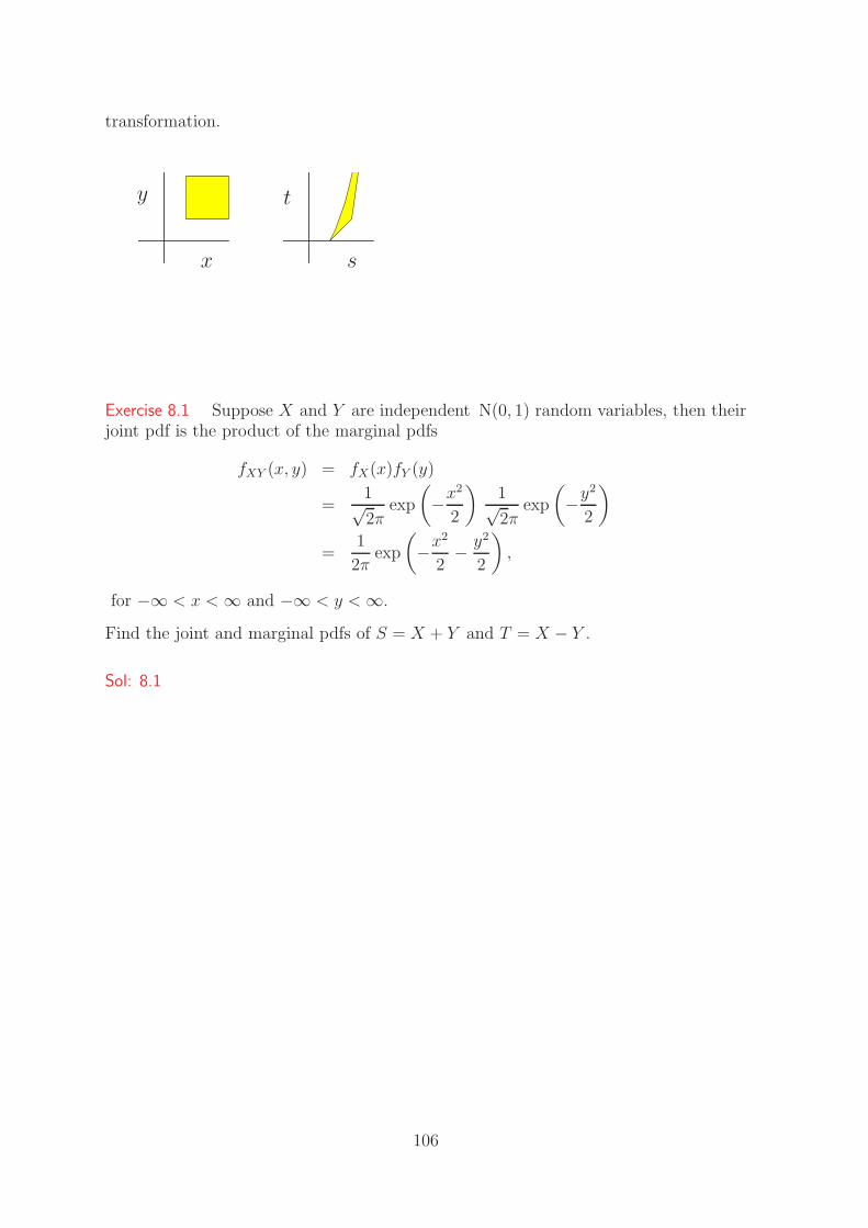
transformation.
x
y
s
t
Exercise 8.1 Suppose X and Y are independent N(0, 1) random variables, then theirjoint pdf is the product of the marginal pdfs
fXY (x, y) = fX(x)fY (y)
=1√2π
exp
(
−x2
2
)
1√2π
exp
(
−y2
2
)
=1
2πexp
(
−x2
2− y2
2
)
,
for −∞ < x < ∞ and −∞ < y < ∞.
Find the joint and marginal pdfs of S = X + Y and T = X − Y .
Sol: 8.1 Rearranging the transformation we have
X =S + T
2= h1(S, T ) and Y =
S − T
2= h2(S, T ),
with derivatives ∂x/∂s = 1/2 etc, so
| det J | =
∣
∣
∣
∣
[
1/2 1/21/2 −1/2
]∣
∣
∣
∣
= | − 1/4 − 1/4| = | − 1/2| = 1/2.
Thus
fST (s, t) =1
2πexp
(
−1
2(s + t
2)2 − 1
2(s − t
2)2
)
1
2
=1√
2π√
2exp(−s2/4)
1√2π
√2
exp(−t2/4)
with the range given by −∞ < s < ∞ and −∞ < t < ∞.
So S and T are independent and identically distributed N(0, 2) variables.
106
Summary: the transformation procedure is:
• Check one-to-one bivariate transformation. (Given x and y can we find s and tuniquely, and given s and t can we find x and y uniquely?)
• Invert the transformation: find s and t as functions of x and y. (Again this mightbe an easy way of checking whether it is a one-to-one transformation).
• Find the Jacobian.
• Use the formula, replacing x and y in fXY (x, y) and J by the appropriate functionsof s and t, x = h1(s, t) and y = h2(s, t).
• Summarise, taking care with the ranges of S and T .
As in the univariate case it is sometimes easier to calculate the inverse | det J |−1 using
| det J |−1=
∣
∣
∣
∣
det
[
∂x∂s
∂x∂t
∂yds
∂y∂t
]∣
∣
∣
∣
−1
=
∣
∣
∣
∣
det
[ ∂s∂x
∂s∂y
∂t∂x
∂t∂y
]∣
∣
∣
∣
.
Exercise 8.2 Suppose X and Y are independent, X with an Exp(1) distribution andY with a Uniform(0, 2π) distribution. Find the joint and marginal pdfs of
(S, T ) = (√
2X cos(Y ),√
2X sin(Y )),
i.e. if (√
2X, Y ) are the polar coordinates of a point in the plane then (S, T ) are thecorresponding Cartesian coordinates.
Sol: 8.2 First note that the sample space of (S, T ) is −∞ < s < ∞ and −∞ < t < ∞.
The joint pdf of (X, Y ) is
fXY (x, y) = fX(x) fY (y)
= exp(−x)1
2πfor 0 < x < ∞, 0 < y < 2π.
In this case it is easier to find the inverse | det J |−1
| det J |−1=
∣
∣
∣
∣
∣
∣
det
∂s∂x
∂s∂y
∂t∂x
∂t∂y
∣
∣
∣
∣
∣
∣
=
∣
∣
∣
∣
∣
∣
∣
det
1√2x
cos(y) −√
2x sin(y)
1√2x
sin(y)√
2x cos(y)
∣
∣
∣
∣
∣
∣
∣
= 1.
107

Since X = (S2 + T 2)/2 we get
fST (s, t) =1
2πexp
(
−s2 + t2
2
)
=1√2π
exp(−s2/2)1√2π
exp(−t2/2)
with the range given by −∞ < s < ∞ and −∞ < t < ∞. So S and T are independentand identically distributed N(0, 1) random variables.
The transformation in this exercise is called the Box-Muller transformation, which isuseful for simulating Normal random variables.
Remember that we can generate an Exponential(1) random variable from a Uniform(0, 1)by the transformation X = − log (1 − U), thus we can generate two independent N(0, 1)random variables X1 and X2 from two independent Uniform(0, 1) random variables U1
and U2 by
(X1, X2) = (√
−2 log (1 − U1) cos(2πU2),√
−2 log (1 − U1) sin(2πU2)).
The Box-Muller transformation for generating standard Normal random variables isillustrated here.
0 2 4 6
01
23
45
6
−3 −2 −1 0 1 2 3
−3
−2
−1
01
23
X
Y
S
T
Exercise 8.3 Suppose X ∼ Gamma(a, 1) and, independently, Y ∼ Gamma(b, 1). De-rive the joint pdf of S = X + Y and T = X/(X + Y ). Are S and T independent? Giveyour reason.
108

Sol: 8.3 Range of S and T : s > 0, 0 ≤ t ≤ 1. Variation independent.
Since X and Y are independent their joint pdf is the product of the marginal pdfs
fXY (x, y) = fX(x)fY (y)
=1
Γ(a)xa−1 exp(−x)
1
Γ(b)yb−1 exp(−y),
for 0 < x < ∞ and 0 < y < ∞.
Inverting the transformation
X = ST and Y = S(1 − T ).
The Jacobian matrix of partial derivatives ∂(x, y)/∂(s, t) is
J =
[
t s1 − t −s
]
Its determinant det(J) = −s, so the Jacobian is s.
Thus the joint pdf is
fST (s, t) = fXY (x, y) | det(J) |=
1
Γ(a)Γ(b)xa−1yb−1 exp(−x − y) s
=1
Γ(a)Γ(b)(st)a−1(s[1 − t])b−1 exp(−s) s
=1
Γ(a)Γ(b)sa+b−1 exp(−s) ta−1(1 − t)b−1
=1
Γ(a + b)sa+b−1 exp(−s)
Γ(a + b)
Γ(a)Γ(b)ta−1(1 − t)b−1,
with the range given above.
Joint pdf factorises and VI so S and T are independent. Recognise pdfs so S ∼ Gamma(a + b),T ∼ Beta(a, b).
8.2 Use of Dummy Variables
Often we are interested in not two new variables, S and T , but in just one, S say. Toobtain the pdf of S alone we have to create a dummy variable T , obtain the joint pdfof S and T , then integrate to get the marginal distribution of S.
Suppose interest lies in S = g1(X, Y ).
• Define a new variable T = g2(X, Y ) which makes a one-to-one bivariate transfor-mation between (X, Y ) and (S, T ). The choice of T is essentially arbitrary andcan be made for convenience. Sometimes some trial and error is required.
109

• Find the joint pdf fST (s, t) of S and T using the methods in the previous section.
• Find the marginal pdf of S:
fS(s) =
∫
t
fST (s, t)dt
taking care with the range of integration.
Exercise 8.4 If (X, Y ) are independent Normal random variables find the distributionof X + Y .
Sol: 8.4 Put S = X + Y and T = X − Y . Use the solution to the exercise abovewhich showed that S and T are independent and identically distributed N(0, 2) vari-ables, and so S ∼ N(0, 2).
Exercise 8.5 If (X, Y ) have joint pdf
fXY (x, y) =1
x2y2for x > 1, y > 1,
find the pdf of S = XY .
Sol: 8.5 With S = XY put T = X, the ranges are s > t, t > 1.
The inverse is
X = T
Y =S
X=
S
T
so that[ ∂s
∂x∂s∂y
∂t∂x
∂t∂y
]
=
[
y x1 0
]
and | det J | = 1/x.
The joint pdf of (S, T ) is
fST (s, t) = fXY (x, y) 1/x |x=t,y=s/t
=1
x3y2|x=t,y=s/t
=1
s2tfor 1 < t < s < ∞.
110

The marginal pdf of S is
fS(s) =
∫ s
t=1
1
s2tdt
=
[
log (t)
s2
]s
t=1
=log (s)
s2for 1 < s < ∞.
To check this integrates to 1:∫ ∞
1
log (s)
s2ds =
[
− log (s)
s
]∞
1
+
∫ ∞
1
1
s2ds
=
[
−1
s
]∞
1
= 1.
Convolution A transformation of general interest is S = X + Y . We use the dummyvariable method to obtain the pdf of S. We make the transformation
S = X + Y and T = X,
with T as the dummy variable. It follows that the inverse transformation is
X = T and Y = S − T,
so
| det J | =
∣
∣
∣
∣
det
[
0 11 −1
]∣
∣
∣
∣
= | −1 | = 1.
Thus
fST (s, t) = fXY (t, s − t),
so the marginal pdf of S = X + Y is
fS(s) =
∫ ∞
t=−∞fXY (t, s − t) dt.
This formula is known as the convolution formula. It is finding the probability ofS = X + Y by summing the probabilities, over all possible t, for the pairs (t, s − t) in(X, Y ).
8.3 Links between Standard Distributions
Transformations of multivariate random variables generalise the ones studied above,but rather go beyond the scope of this course. However in this section we list some ofthe links between standard distributions obtained by multivariate transformations ofindependent random variables. Many of these results are important in statistics.
Random variables that are related by transformation. All the variables in the left handcolumn are assumed independent.
111

Distribution Transformation Distribution of Y
Zi ∼ N(0, 1), i = 1, . . . , n Y = Z21 + . . . + Z2
n Gamma(n/2, 1/2) = χ2n
Xi ∼ N(µi, σ2i ), i = 1, . . . , n Y = X1 + . . . + Xn N(µ1 + . . . + µn, σ2
1 + . . . + σ2n)
Xi ∼ N(µi, σ2i ), i = 1, . . . , n Y = a′X N(a′µ, a′ diag (Σ)a)
Xi ∼ Exp(β), i = 1, . . . , n Y = X1 + . . . + Xn Gamma(n, β)
Xi ∼ Gamma(αi, β), i = 1, . . . , n Y = X1 + . . . + Xn Gamma(α1 + . . . + αn, β)
Xi ∼ Gamma(αi, β), i = 1, 2 Y = X1
X1+X2
Beta(α1, α2)
112
Chapter 9
Limit Theorems
In this Chapter we study two important limit results, the Law of Large Numbers and theCentral Limit Theorem, both of which tell us about the behaviour of the mean of n iidrandom variables as n gets larger and larger. While these results are mathematicallyinteresting in their own right they give theoretical justification for the whole practiseof statistics.
The results provide a theoretical justifications
to assert large samples are good, and provide criterion to say how large is large; if theseresults were false statisticians would be unemployed.
to motivate the Normal distribution as a probability model.
for using Monte Carlo methods to construct approximations to unknown mathematicalintegrals.
9.1 The Law of Large Numbers
Assume that X1, X2, . . . are iid random variables with common mean µ and commonvariance σ2, and let Xn denote the mean of the first n of these,
Xn =1
n
n∑
i=1
Xi.
The expected value and variance of Xn are
E(Xn) = E
(
1
n
n∑
i=1
Xi
)
=1
n
n∑
i=1
E(Xi)
=1
n
n∑
i=1
µ = µ,
113

and
var(Xn) = var
(
1
n
n∑
i=1
Xi
)
=1
n2var
(
n∑
i=1
Xi
)
=1
n2
n∑
i=1
var(Xi)
=1
n2
n∑
i=1
σ2 =σ2
n.
The figure illustrates the distribution of Xn for varying n, when each Xi has a Uniform(0, 1)distribution. The plots are histograms of 1000 realisations of Xn for n = 10, 50, 100and 500, i.e. to make the plot in the lower left-hand corner we have taken the mean of100 Uniform(0, 1)-distributed random variables 1000 times.
Histogram of z1
Den
sity
0.0 0.2 0.4 0.6 0.8 1.0
01
23
4
Histogram of z2
Den
sity
0.0 0.2 0.4 0.6 0.8 1.0
02
46
810
Histogram of z3
Den
sity
0.0 0.2 0.4 0.6 0.8 1.0
02
46
810
12
Histogram of z4
Den
sity
0.0 0.2 0.4 0.6 0.8 1.0
05
1015
20
X10 X50
X100 X500
Histograms of 1000 realisations of Xn for n = 10, 50, 100 and 500 when Xi ∼ Uniform(0, 1).
It is clear to see from the figure how the distribution of Xn concentrates more andmore around µ = 0.5 as n gets larger reflecting the fact that the variance decreases to0 as n increases. This is the subject of the Law of Large Numbers to be shown below.
We first need a bound on the probability that a random variable deviates more than ǫfrom its mean in terms of its variance. We will need the indicator function I(|Y −µ|>ǫ),
114
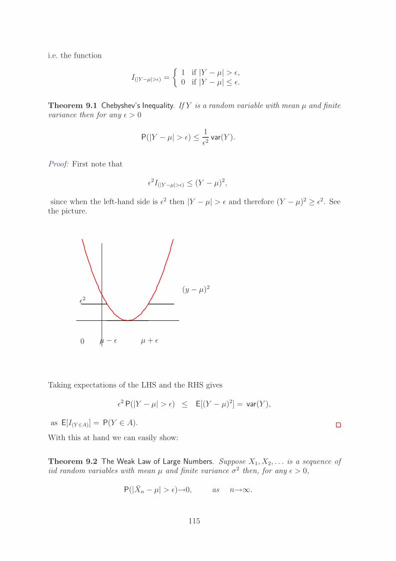
i.e. the function
I(|Y −µ|>ǫ) =
1 if |Y − µ| > ǫ,0 if |Y − µ| ≤ ǫ.
Theorem 9.1 Chebyshev’s Inequality. If Y is a random variable with mean µ and finitevariance then for any ǫ > 0
P(|Y − µ| > ǫ) ≤ 1
ǫ2var(Y ).
Proof: First note that
ǫ2I(|Y −µ|>ǫ) ≤ (Y − µ)2,
since when the left-hand side is ǫ2 then |Y − µ| > ǫ and therefore (Y − µ)2 ≥ ǫ2. Seethe picture.
0 µ − ǫ µ + ǫ
ǫ2
(y − µ)2
Taking expectations of the LHS and the RHS gives
ǫ2 P(|Y − µ| > ǫ) ≤ E[(Y − µ)2] = var(Y ),
as E[I(Y ∈A)] = P(Y ∈ A).
With this at hand we can easily show:
Theorem 9.2 The Weak Law of Large Numbers. Suppose X1, X2, . . . is a sequence ofiid random variables with mean µ and finite variance σ2 then, for any ǫ > 0,
P(|Xn − µ| > ǫ)→0, as n→∞.
115
Proof: Using Chebyshev’s inequality we have for any ǫ > 0
P(|Xn − µ| > ǫ) ≤ 1
ǫ2var(Xn)
=1
ǫ2
σ2
n→ 0, as n→∞.
We say that Xn converges in probability to µ.
The theorem is a mathematical restatement of the figure above. The distribution ofXn concentrates more and more around µ, in the sense that no matter how small aninterval [µ − ǫ, µ + ǫ] we take around µ the probability of Xn falling in this intervaltends to 1.
Exercise 9.1 How large a random sample should be taken from a distribution in orderfor the probability to be at least 0.99 that the sample mean will be within one standarddeviation of the mean of the distribution?
Sol: 9.1 As in the proof of the WLLN
P(|Xn − µ| > σ) ≤ 1
σ2
σ2
n
=1
n.
We need 1n
< 1 − 0.99 = 0.01. So n > 100 is sufficient, whatever the distribution.
Frequencies converge to probabilities: The WLLN as stated concerns Xn. It easilyextends to frequencies. Consider the random variables Yi = I(Xi∈A), where A is anevent and I is its indicator function. Application of the WLLN gives
1
n
n∑
i=1
I(Xi∈A)→P(X ∈ A), as n→∞.
The frequency of the event A occurring converges to the probability of A for allrealisations x1, x2, . . . of the sequence X1, X2, . . .. For instance, the proportion of timesheads occur in n throws of a coin will converge to the probability of a head.
Aside: There is also a Strong Law of Large Numbers, proved by the outstandingRussian mathematician and probabilist Andrei Kolmogorov (1903-1987). It uses astronger form of convergence and it also removes the assumption that the X’s havefinite variance. Informally, the Strong Law of Large Numbers says that if X1, X2, . . .is a sequence of iid random variables with mean µ then
Xn→µ, as n→∞,
116
for (almost) all realisations x1, x2, . . . of the sequence X1, X2, . . .. This is the resultthat justifies the Monte Carlo simulation approximations to calculate expectations.
While the assumption of finite variance could be removed the assumption that the X’shave a finite mean is a necessary assumption for the Law of Large Numbers to hold.
In fact, it can be shown that if X1, X2, . . . is a sequence of iid random variables withE(|X1|) = +∞ then Xn will not converge for almost any realisation x1, x2, . . . of thesequence X1, X2, . . ..
Example 9.2 If X1, X2, . . . are independent Cauchy random variables it can be shownthat the mean Xn also has the same Cauchy distribution. Hence the distribution of Xn
is the same for all n and thus does not converge in probability.
9.2 The Central Limit Theorem
The Central Limit Theorem is one of the most important results in probability theoryand statistics and is the reason the Normal distribution plays such a prominent role. Itasserts that the sum (or the mean) of many independent identically distributed randomvariables is approximately Normally distributed. The remarkable fact is true, whateverthe common distribution of the random variables, as long as it has finite mean andvariance.
Theorem 9.3 The Central Limit Theorem. Suppose X1, X2, . . . is a sequence of iid ran-dom variables with mean µ and finite variance σ2, then for any number −∞ < x < ∞
P
(√n(Xn − µ)
σ≤ x
)
→Φ(x), as n→∞.
where Xn = 1n
∑ni=1 Xi and Φ(x) is the cumulative distribution function for the stan-
dard Normal distribution N(0, 1) evaluated at x.
Whereas the WLLN only tells us that Xn converges to µ the CLT gives us the strongerinformation that the deviations of Xn from µ scaled by
√n follow a N(0, σ2) distribution
in the limit. The practical use of this is that for reasonably large n we can assume that
Xn ∼ N(µ, σ2/n)
approximately.
Exercise 9.3 A large company claims to pay an average wage of 4 pounds an hourwith a standard deviation of 0.50 pounds. A sample of 64 workers were found to havean average wage of 3.90 pounds. Find the probability of observing a sample mean aslow as this, or worse, by random chance alone if the company’s claim is true.
117

Sol: 9.3 Let X1, . . . , X64 be the wages in pounds of the 64 workers. If the company’sclaim is true these should have mean 4 and standard deviation 0.50. By the CLT theaverage X64 = 1
64
∑64i=1 Xi satisfies
X64 ∼ N(4,(0.50)2
64) appoximately.
The probability of getting a value of 3.90 or lower in this Normal distribution is
P(X64 ≤ 3.90) = P
X64 − 4√
(0.50)2
64
≤ 3.9 − 4√
(0.50)2
64
= Φ(−1.6) = 0.0548 = pnorm(-1.6)
There is only around 5% chance of observing such a low average wage for 64 randomlyselected workers.
Exercise 9.4 How large a sample should be taken from a normal distribution in orderfor the probability to be at least 0.99 that the sample mean will be within one standarddeviation of the mean of the distribution?
Sol: 9.4
P(|Xn − µ| < σ) = P
(∣
∣
∣
∣
√n(Xn − µ)
σ
∣
∣
∣
∣
<√
n
)
= 2Φ(√
n) − 1.
Now Φ−1(0.995) = 2.575829 = qnorm(0.995). So√
n > 2.575829 or n ≥ 7 is sufficient(cf. Exercise 9.1).
The proof of the Central Limit Theorem is not examinable, but we give a sketch below.
Proof: (Sketch) Suppose X1, X2, . . . is a sequence of iid random variables with commonmean 0 and common variance 1 (to make it easy). Let Sn denote the standardised sumof the first n of these
Sn =1√n
n∑
i=1
Xi, with E(Sn) = 0, var(Sn) = 1.
The distribution of a random variable X is uniquely determined by its moments. LetMX(t) be the mgf of the rv X, then the mgf of the sum of them is given by
MX1+...+Xn(t) = (MX(t))n,
and the mgf of the standardized sum Sn is computed as follows
MSn(t) =
(
MX
(
t√n
))n
118
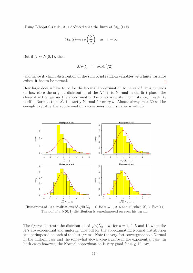
Using L’hopital’s rule, it is deduced that the limit of MSn(t) is
MSn(t)→exp
(
t2
2
)
as n→∞.
But if X ∼ N(0, 1), then
MX(t) = exp(t2/2)
and hence if a limit distribution of the sum of iid random variables with finite varianceexists, it has to be normal.
How large does n have to be for the Normal approximation to be valid? This dependson how close the original distribution of the X’s is to Normal in the first place: thecloser it is the quicker the approximation becomes accurate. For instance, if each Xi
itself is Normal, then Xn is exactly Normal for every n. Almost always n > 30 will beenough to justify the approximation - sometimes much smaller n will do.
Histogram of sz1
Den
sity
−3 −2 −1 0 1 2 3 4
0.0
0.2
0.4
0.6
Histogram of sz2
Den
sity
−3 −2 −1 0 1 2 3 4
0.0
0.1
0.2
0.3
0.4
0.5
Histogram of sz3
Den
sity
−3 −2 −1 0 1 2 3 4
0.0
0.1
0.2
0.3
0.4
0.5
Histogram of sz4
Den
sity
−3 −2 −1 0 1 2 3 4
0.0
0.1
0.2
0.3
0.4
0.5
X1 − 1√
2(X2 − 1)
√5(X5 − 1)
√10(X10 − 1)
Histograms of 1000 realisations of√
n(Xn − 1) for n = 1, 2, 5 and 10 when Xi ∼ Exp(1).
The pdf of a N(0, 1) distribution is superimposed on each histogram.
The figures illustrate the distribution of√
n(Xn − µ) for n = 1, 2, 5 and 10 when theX’s are exponential and uniform. The pdf for the approximating Normal distributionis superimposed on each of the histograms. Note the very fast convergence to a Normalin the uniform case and the somewhat slower convergence in the exponential case. Inboth cases however, the Normal approximation is very good for n ≥ 10, say.
119
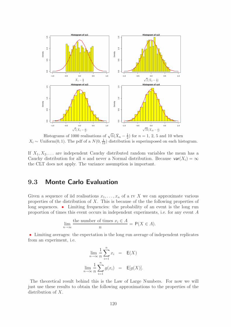
Histogram of sz1
Den
sity
−1.0 −0.5 0.0 0.5 1.0
0.0
0.5
1.0
1.5
Histogram of sz2
Den
sity
−1.0 −0.5 0.0 0.5 1.0
0.0
0.5
1.0
1.5
Histogram of sz3
Den
sity
−1.0 −0.5 0.0 0.5 1.0
0.0
0.5
1.0
1.5
Histogram of sz4
Den
sity
−1.0 −0.5 0.0 0.5 1.0
0.0
0.5
1.0
1.5
X1 − 12
√2(X2 − 1
2)
√5(X5 − 1
2)√
10(X10 − 12)
Histograms of 1000 realisations of√
n(Xn − 12) for n = 1, 2, 5 and 10 when
Xi ∼ Uniform(0, 1). The pdf of a N(0, 112) distribution is superimposed on each histogram.
If X1, X2, . . . are independent Cauchy distributed random variables the mean has aCauchy distribution for all n and never a Normal distribution. Because var(Xi) = ∞the CLT does not apply. The variance assumption is important.
9.3 Monte Carlo Evaluation
Given a sequence of iid realisations x1, . . . , xn of a rv X we can approximate variousproperties of the distribution of X. This is because of the the following properties oflong sequences. • Limiting frequencies: the probability of an event is the long runproportion of times this event occurs in independent experiments, i.e. for any event A
limn→∞
the number of times xi ∈ A
n= P(X ∈ A).
• Limiting averages: the expectation is the long run average of independent replicatesfrom an experiment, i.e.
limn→∞
1
n
n∑
i=1
xi = E(X)
limn→∞
1
n
n∑
i=1
g(xi) = E[g(X)].
The theoretical result behind this is the Law of Large Numbers. For now we willjust use these results to obtain the following approximations to the properties of thedistribution of X.
120
pdf: As the pdf fX(x) is the probability that X belongs to a small interval around xdivided by the length of the interval
fX(x) ≈ P(x < X ≤ x + δ)/δ
we can estimate the pdf by
fX(x) ≈ the number of times xi ∈ [x, x + δ)
nδ.
This is the histogram of the simulated data x1, . . . , xn.
cdf: As the cdf FX(x) is the probability that P(X ≤ x) we can estimate it by
FX(x) ≈ the number of times xi ≤ x
n.
Probabilities of events: The probability of a general event A is approximately
P(X ∈ A) ≈ the number of times xi ∈ A
n.
Expectations: We can estimate the mean of X and g(X) by
E(X) ≈ 1
n
n∑
i=1
xi,
E[g(X)] ≈ 1
n
n∑
i=1
g(xi).
Transformations: We can estimate properties of Y by obtaining a sample from thetransformed variable Y = g(X) as y1 = g(x1), . . . , yn = g(xn).
Example 9.5 For illustration let us apply these methods to obtain approximations ofthe first four moments of a standard Normal random variable X,
x = rnorm(10000,0,1) # 10000 realisations of N(0,1)
mean(x) # mean; theory mean= 0
hist(x)
mean(x^2) # 2nd moment; theory 2nd moment=1
hist(x^2,col=’blue’)
mean(x^3) # 3nd moment; theory 3rd moment=0
mean(x^4) # 4th moment; theory 4th moment=3
121
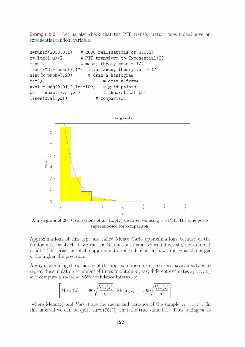
Example 9.6 Let us also check that the PIT transformation does indeed give anexponential random variable.
u=runif(2000,0,1) # 2000 realisations of U(0,1)
x=-log(1-u)/2 # PIT transform to Exponential(2)
mean(x) # mean; theory mean = 1/2
mean(x^2)-(mean(x))^2 # variance; theory var = 1/4
hist(x,prob=T,20) # draw a histogram
box() # draw a frame
xval = seq(0.01,4,len=100) # grid points
pdf = dexp( xval,2 ) # theoretical pdf
lines(xval,pdf) # comparison
Histogram of x
x
Den
sity
0 1 2 3 4 5 6
0.0
0.2
0.4
0.6
0.8
1.0
1.2
A histogram of 2000 realisations of an Exp(2) distribution using the PIT. The true pdf is
superimposed for comparison.
Approximations of this type are called Monte Carlo approximations because of therandomness involved. If we ran the R functions again we would get slightly differentresults. The precision of the approximation also depend on how large n is, the largern the higher the precision.
A way of assessing the accuracy of the approximation, using tools we have already, is torepeat the simulation a number of times to obtain m, say, different estimates z1, . . . , zm
and compute a so-called 95% confidence interval by[
Mean(z) − 1.96
√
Var(z)
m, Mean(z) + 1.96
√
Var(z)
m
]
,
where Mean(z) and Var(z) are the mean and variance of the sample z1, . . . , zm. Inthis interval we can be quite sure (95%!) that the true value lies. Thus taking m as
122

large as possible must be sensible as it gives the largest possible precision in the MonteCarlo estimate.
Example 9.7 For X ∼ N(0, 1) estimate the expectation E[cos(X)], and give a 95%confidence interval.
z = rep(0,1000) # 1000 zeros
for (i in 1:1000) # each estimate based on 10000
x = rnorm(10000,0,1) # replicates of a N(0,1) rv
z[i] = mean(cos(x))
mean(z) # mean is best estimate
var(z) # variance in the sample
sd = sqrt(var(z)/1000)
mean(z)-1.96*sd
mean(z)+1.96*sd
Thus we get E[cos(X)] ≈ 0.6067, with 95% confidence interval = [0.6064, 0.6070]. Infact it can be shown that
E[cos(X)] =
∫ ∞
∞cos(x)
1√2π
exp
(
−x2
2
)
dx
= exp(−1/2) = 0.60653.
123

124
Chapter 10
The Multivariate Normal distribution
The multivariate extension of the Normal distribution is the essential topic of thischapter. For simplicity we look at the bivariate Normal distribution before extendingto higher dimensions. The bivariate Normal distribution is easier to picture and stillrich enough to illustrate many of the concepts of this Chapter.
10.1 The Bivariate Normal Distribution
Two continuous random variables X and Y are said to have a bivariate Normal distri-bution if their joint pdf is given for all x and y by
fXY (x, y; θ) =1
2π√
σ2Xσ2
Y (1 − ρ2XY )
× exp
−1
2
1
1 − ρ2XY
Q(x, y)
,
where Q(x, y) is given by
(
x − µX
σX
)2
− 2ρXY
(
x − µX
σX
)(
y − µY
σY
)
+
(
y − µY
σY
)2
with parameters θ = (µX , µY , σ2X , σ2
Y , ρXY ), where σ2X > 0, σ2
Y > 0 and −1 < ρXY < 1.
125

−3 −1 0 1 2 3
−3
−1
01
23
−3 −1 0 1 2 3
−3
−1
01
23
−3 −1 0 1 2 3
−3
−1
01
23
−3 −1 0 1 2 3
−3
−1
01
23
−3 −1 0 1 2 3
−3
−1
01
23
−3 −1 0 1 2 3
−3
−1
01
23
X
X
X
X
X
X
YY
YY
YY
Top row: 1000 realisations of three different bivariate Normal distributions with ρXY = 0,
0.8 and −0.7 respectively. The marginal distributions are standard Normal in each case.
Bottom row: Contour plots of the corresponding pdfs.
The pdf is more conveniently expressed in matrix notation, which also makes theanalogy with the univariate case clearer and the extension to higher dimensions easier.Put
Σ =
(
σ2X ρXY σXσY
ρXY σXσY σ2Y
)
so that
Σ−1 =1
1 − ρ2XY
(
1σ2
X
−ρXY
σXσY−ρXY
σXσY
1σ2
Y
)
.
Then
fXY (x, y; θ) =1
2π√
det Σexp
−1
2
(
x − µX
y − µY
)′Σ−1
(
x − µX
y − µY
)
.
126

Generating the bivariate Normal: To derive properties of the bivariate Normal dis-tribution it is often a good idea to think of it as a transformation of two independentstandard Normal random variables S ∼ N(0, 1) and T ∼ N(0, 1), say.
Consider the linear transformation
X = µX + σXS
Y = µY + ρXY σY S +√
(1 − ρ2XY )σY T.
In matrix notation this is[
XY
]
= µ + A
[
ST
]
where
A =
[
σX 0
ρXY σY
√
(1 − ρ2XY )σY
]
.
It is easy to show that the means are
E(X) = µX and E(Y ) = µY
as E(S) = 0 and E(T ) = 0.
The variances are
var(X) = 0 + σ2X var(S) = σ2
X
var(Y ) = 0 + ρ2XY σ2
Y + (1 − ρ2XY )σ2
Y
= σ2Y
using the independence of S and T . Finally the correlation
cov(X, Y ) = 0 + cov(σXS, ρXY σY S)
= σX cov(S, S)ρXY σY
corr(X, Y ) = ρXY .
We want to show that this transformation gives the pdf above. Because of indepen-dence the pdf of the joint distribution of (S, T ) is the product of the marginal pdfs
fST (s, t) =1
2πexp
(
−s2
2− t2
2
)
=1
2πexp
(
−1
2
[
st
]′ [st
])
Since σ2X > 0, σ2
Y > 0 and −1 < ρXY < 1 the transformation from (S, T ) to (X, Y ) isone-to-one bivariate transformation, i.e. A is invertible, and we can use the transfor-mation method in Chapter 8 to get
fXY (x, y) =1
2πexp
−1
2
(
x − µX
y − µY
)′(A−1)′A−1
(
x − µX
y − µY
)
1
| det A | .
127

Letting Σ = AA′ this can be written
fXY (x, y) =1
2π√
det Σexp
−1
2
(
x − µX
y − µY
)′Σ−1
(
x − µX
y − µY
)
,
with
Σ =
(
σX 0
ρXY σY
√
(1 − ρ2XY )σ2
Y
)(
σX ρXY σY
0√
(1 − ρ2XY )σ2
Y
)
=
(
σ2X ρXY σXσY
ρXY σXσY σ2Y
)
as claimed.
Realisations from this bivariate distribution and contour plots of the correspondingpdfs are shown for µX = µY = 0 and σ2
X = σ2Y = 1 and varying values of ρXY . Note
that the contours of the pdf are ellipses centred at the origin with orientation given byρXY . In general the contours will be ellipses centred at (µX , µY ). In the special caseρXY = 0, i.e. no correlation, the joint pdf factorises
fXY (x, y) = fX(x)fY (y),
and so (X, Y ) are independent. Remember that it is not true in general that ρXY = 0implies independence as Exercise 7.1 shows.
Exercise 10.1 The joint distribution of (X, Y )′ is bivariate Normal with mean[
1 2]′
and variance
[
1 22 4
]
.
Find the distribution of T = aX + bY .
Sol: 10.1 As linear combinations of MVN variables are normally distributed, wejust have to find the mean and variance.
E(T ) =[
a b]
E
[
XY
]
=[
a b]
[
12
]
= a + 2b,
var(T ) =[
a b]
[
1 22 4
] [
ab
]
= a2 + 4ab + 4b2 = (a + 2b)2.
Hence T ∼ N(a + 2b, (a + 2b)2).
128

Conditional Distributions
The conditional distribution of Y given X = x can be found using the formula inSection 6.7:
fY |X(y | x) =fXY (x, y)
fX(x).
Messy, but straight-forward, calculations will show that the conditional distributionis again Normal with mean µY + ρXY σY /σX(x − µX) and variance σ2
Y (1 − ρ2XY ),
Y | X = x ∼ N
(
µY + ρXYσY
σX
(x − µX), σ2Y (1 − ρ2
XY )
)
.
An easier and more elegant way of deriving this result is to use the transformationof (S, T ). Let us find the conditional distribution of Y given X = x again usingthis method. Since X = µX + σXS the condition X = x corresponds to the conditionS = (x − µX)/σX and inserting this into the expression for Y gives
Y = µY + ρXYσY
σX(x − µX) +
√
(1 − ρ2XY )σ2
Y T,
which shows directly that
Y | X = x ∼ N
(
µY + ρXYσY
σX(x − µX), σ2
Y (1 − ρ2XY )
)
.
Notice that the conditional expectation is linear in x, while the conditional varianceis constant. Also note how the conditional variance depends on ρXY . For ρXY closeto ±1 the term 1 − ρ2
XY is close to 0 and the conditional variance thus small. This issaying that when X and Y are very correlated knowing X gives us a lot of informationabout Y .
Representing Y as a linear transformation of X plus an independent Normal randomvariable ([(1 − ρ2
XY )σ2Y ]1/2T above) is called regressing Y on X and is the idea behind
the regression models you will meet in Math 235.
The conditional distribution of X given Y = y can be found analogously to be
X | Y = y ∼ N
(
µX + ρXYσX
σY(y − µY ), σ2
X(1 − ρ2XY )
)
.
10.2 The Multivariate Normal Distribution
With the matrix notation set up the bivariate Normal distribution is easily extendedto higher dimensions. The vector X = (X1, . . . , Xd)
′ is said to have a d-dimensionalNormal distribution if its pdf is given for all x by
fX (x) =1
(2π)d/2√
det Σexp
−1
2(x − µ)′Σ−1(x − µ)
,
129
where µ = (µ1, . . . , µd)′ is the vector of means and Σ is the variance-covariance matrix
with (i, j)th element σij being the pairwise covariance of variables Xi and Xj . Here weshall write ρij for ρXiXj
. As
ρij = corr(Xi, Xj) =cov(Xi, Xj)
√
var(Xi) var(Xj)=
σij
σiσj
the variance-covariance matrix can be written
Σ =
σ11 . . . . . . σ1d
. . . . . . σij . . .
. . . σji . . . . . .σd1 . . . . . . σdd
=
σ21 . . . . . . σ1σdρ1d
. . . . . . σiσjρij . . .
. . . σiσjρji . . . . . .σ1σdρd1 . . . . . . σ2
d
where σ2i (= σii) is the variance of Xi, and ρij is the correlation between Xi and Xj.
We often denote the distribution of X by
X ∼ MVNd(µ, Σ),
where MVNd stands for multivariate Normal distribution of d dimensions.
As in the bivariate case the univariate marginal distributions are all Normal:
Xi ∼ N(µi, σ2i ), for i = 1, . . . , d.
In fact, more generally the joint distribution of linear combinations of the X’s is againNormal:
AX ∼ MVNm(Aµ, AΣA′),
where A is an m × d matrix of constants.
Exercise 10.2 Let (X1, X2, X3, X4, X5)′ be multivariate Normal with
X1
X2
X3
X4
X5
∼ MVN5
01
−204
,
26 15 15 −7 −115 18 −20 13 015 −20 99 −44 0−7 13 −44 143 73−1 0 0 73 90
.
Find the marginal distribution of (X1, X3, X4).
Sol: 10.2 Let X = (X1, X2, . . . , X5)′ and
A =
1 0 0 0 00 0 1 0 00 0 0 1 0
130

then
Aµ =
0−20
and AΣA′ =
26 15 −715 99 −44−7 −44 143
.
Thus
X1
X3
X4
∼ MVN3
0−2
0
,
26 15 −715 99 −44−7 −44 143
.
The marginal distribution is obtained by deleting rows 2 and 5 of the mean vector,and rows 2 and 5 and columns 2 and 5 of the variance matrix.
The most important special case is when X1, . . . , Xd are iid N(µ, σ2) random variables.In this case
µ =
µ...µ
, Σ =
σ2 0 · · · 0
0. . .
. . ....
.... . .
. . . 00 · · · 0 σ2
= σ2Id,
where Id is the identity matrix in d dimensions, i.e. a d × d matrix with ones in thediagonal and zeros everywhere else.
The pdf becomes
fX (x) =1
(2π)d/2σdexp
− 1
2σ2
d∑
i=1
(xi − µ)2
=
d∏
i=1
1√2πσ2
exp
− 1
2σ2(xi − µ)2
=
d∏
i=1
fXi(xi)
since Σ−1 = 1σ2 Id, where fXi
is the pdf of a N(µ, σ2) random variable.
10.3 Simulation for the multivariate normal
R has functions for generating bivariate Normal random variables and for evaluatingthe joint cdf, although it is necessary to load the multivariate normal package mvtnormin order to do this.
131

X
Y
-10 -5 0 5 10
-10
12
34
5
1000 realisations from a bivariate Normal distributions with
(µX , µY , σ2X , σ2
Y , ρXY ) = (0, 2, 16, 1, 0.5). The lines illustrate the events (X ≤ 0) and
(Y ≤ 1).
Example 10.3 The following list of R commands generates and plots (in 1000 realisa-tions from a bivariate Normal distribution with parameters
(µX , µY , σ2X , σ2
Y , ρXY ) = (0, 2, 16, 1, 0.5).
It also calculates the probability P(X ≤ 0, Y ≤ 1) and for comparison the product ofthe two marginal probabilities P(X ≤ 0) P(Y ≤ 1).
library(mvtnorm, lib.loc="/usr/lib/R/site-library")
# loads up various multivariate functions
varx=16; vary=1 # defines the variances
covxy=sqrt(16)*sqrt(1)*0.5 # defines the covariance
sig=matrix(c(varx,covxy,covxy,vary),2)
# sets up the variance matrix
xy=rmvnorm(1000,mean=c(0,2),sigma=sig)
# R needs the full variance matrix, here
plot(xy,xlab=’X’,ylab=’Y’) # Plot the realisations
abline(v=0) # Add vertical line
abline(h=1) # Add horizontal line
pmvnorm(upper=c(0,1),mean=c(0,2),sigma=sig)
# for P(X<0,Y<1)
[1] 0.1273982
pnorm(0,0,4)*pnorm(1,2,1) # for P(X<0)P(Y<1)
[1] 0.07932763
Note that the joint probability P(X ≤ 0, Y ≤ 1) is larger than the product of themarginal probabilities because of the positive correlation between X and Y whichincreases the chance of small values of X and Y occurring together.
132
Appendix A
Appendices
A.1 Useful Integrals
Gamma Function
Let h(x) = xα−1 exp(−x) for 0 < x < ∞. The Gamma function determines how theintegral of this function over the range (0,∞) varies with α.
Γ(α) =
∫ ∞
0
xα−1 exp(−x) dx, for α > 0.
The Gamma function in R is gamma(a):
gamma(0.5) # the gamma function at 0.5
[1] 1.772454
x = seq(1,10) # Let x = (1,2,3,4,5,6,7,8,9,10)
x
[1] 1 2 3 4 5 6 7 8 9 10
gamma(x) # gamma function at these values
[1] 1 1 2 6 24 120 720 5040 40320 362880
Properties:
• Recurrence relation Γ(α) = (α − 1)Γ(α − 1) for α > 1. This is easy to prove usingintegration by parts.
• Special cases: Γ(1) = 1, Γ(α) = (α − 1)! for α a positive integer, and Γ(1/2) =√
π,Γ(α)→∞ as α→0 or α→∞.
Related integrals: For α > 0 and β > 0∫ ∞
0
xα−1 exp(−βx) dx = β−αΓ(α).
133
To see this substitute y = βx gives dy = β dx so∫ ∞
0
(y/β)α−1 exp(−y)dy/β
= β−α
∫ ∞
0
yα−1 exp(−y)dy = β−αΓ(α).
Normal Distribution Integrals
Let h(x) = xr exp(−x2/2) for −∞ < x < ∞. The function J(r) determines how theintegral of h(x) over the range (−∞,∞) varies over non-negative integer values of r.As h(x) is an odd (even) function and all the integrals converge for all r > 0 we havethat J(r) = 0 for all odd r, and for even r
J(r) =
∫ ∞
−∞xr exp(−x2/2) dx
= 2
∫ ∞
0
xr exp(−x2/2) dx.
Substituting s = x2/2 gives
J(r) = 2
∫ ∞
0
(2s)(r−1)/2 exp(−s) ds
= 2(r+1)/2Γ((r + 1)/2).
It follows that J(0) =√
2π and J(2) =√
2π, and J(4) = 3√
2π.
Beta Function
Let h(x) = xα1−1(1 − x)α2−1 for 0 < x < 1. The Beta function B(α1, α2) determineshow the integral of this function over the range (0, 1) varies with α1 > 0 and α2 > 0
B(α1, α2) =
∫ 1
0
xα1−1(1 − x)α2−1dx.
Properties:
• B(1, 1) = 1.
• B(α1, α2) = B(α2, α1)
• B(α1, α2) = Γ(α1)Γ(α2)/Γ(α1 + α2)
Thus the Beta function can easily be evaluated using the Gamma function. In R:
gamma(4)*gamma(0.5)/gamma(4+0.5) # Calc Beta(4,0.5)
[1] 0.9142857
134