Math 212br - Advanced Real Analysis

Taught by Yum-Tong SiuNotes by Dongryul Kim

Spring 2018

This course was taught by Yum-Tong Siu, on Tuesdays and Thurdays from2:30pm to 4pm. It drew material from Stein and Shakarchi’s Real analysis,Fourier analysis and Evans’s Partial differential equations, as well as famouspapers. There were midterm and final take-home exams.

Contents

1 January 23, 2018 41.1 PDE with constant coefficients . . . . . . . . . . . . . . . . . . . 5

2 January 25, 2018 62.1 Using Bernstein–Sato polynomials . . . . . . . . . . . . . . . . . 62.2 The example of Hans Lewy . . . . . . . . . . . . . . . . . . . . . 8

3 January 30, 2018 93.1 Cohomology and local insolvability . . . . . . . . . . . . . . . . . 93.2 Fourier analysis over complex variables . . . . . . . . . . . . . . . 10

4 February 1, 2018 124.1 Nonsolvability of Hans Lewy’s equation . . . . . . . . . . . . . . 124.2 Cauchy–Szego kernel . . . . . . . . . . . . . . . . . . . . . . . . . 13

5 February 6, 2018 155.1 Existence of Bernstein–Sato polynomials . . . . . . . . . . . . . . 155.2 Using reflection to get holomorphicity . . . . . . . . . . . . . . . 17

6 February 8, 2018 186.1 Solving differential equations with variable coefficients . . . . . . 18

7 February 13, 2018 207.1 Riesz representation revisited . . . . . . . . . . . . . . . . . . . . 207.2 First-order case of Nirenberg–Treves . . . . . . . . . . . . . . . . 217.3 Technical lemma . . . . . . . . . . . . . . . . . . . . . . . . . . . 22

1 Last Update: August 27, 2018

8 February 15, 2018 248.1 Solving the first-order equation without sign change . . . . . . . 24

9 February 20, 2018 269.1 Insolvability of a differential equation . . . . . . . . . . . . . . . . 26

10 February 22, 2018 2910.1 Introduction to higher order equations . . . . . . . . . . . . . . . 2910.2 Getting the estimate on Cauchy–Kowalevski . . . . . . . . . . . . 30

11 February 27, 2018 3211.1 Hormander’s criterion . . . . . . . . . . . . . . . . . . . . . . . . 32

12 March 1, 2018 3512.1 Applying Hormander’s lemma . . . . . . . . . . . . . . . . . . . . 35

13 March 6, 2018 3713.1 Construction of counterexamples to the inequality . . . . . . . . 37

14 March 8, 2018 3914.1 Hormander’s hypoellipticity . . . . . . . . . . . . . . . . . . . . . 3914.2 Preparation for Riesz representation . . . . . . . . . . . . . . . . 39

15 March 20, 2018 4215.1 Using iterated Lie brackets . . . . . . . . . . . . . . . . . . . . . 43

16 March 22, 2018 4516.1 Bounds on the Holder norm . . . . . . . . . . . . . . . . . . . . . 45

17 March 27, 2018 4817.1 Handling different directions . . . . . . . . . . . . . . . . . . . . . 4817.2 Towards the implicit function theorem . . . . . . . . . . . . . . . 49

18 March 29, 2018 5018.1 Newton’s method in Banach spaces . . . . . . . . . . . . . . . . . 5018.2 Constructing the smoothing operators . . . . . . . . . . . . . . . 52

19 April 3, 2018 5319.1 Continuity method using convex sets . . . . . . . . . . . . . . . . 53

20 April 5, 2018 5520.1 Conjugacy problem . . . . . . . . . . . . . . . . . . . . . . . . . . 5520.2 Arnold’s theorem . . . . . . . . . . . . . . . . . . . . . . . . . . . 56

21 April 10, 2018 5821.1 Iterating linearized conjugations . . . . . . . . . . . . . . . . . . 5821.2 Harnack inequality . . . . . . . . . . . . . . . . . . . . . . . . . . 59

2

22 April 12, 2018 6022.1 Proof of Harnack’s inequality . . . . . . . . . . . . . . . . . . . . 60

23 April 17, 2018 6223.1 De Giorgi’s argument for the Holder estimates . . . . . . . . . . 6223.2 Probability spaces . . . . . . . . . . . . . . . . . . . . . . . . . . 63

24 April 19, 2018 6424.1 Theorems in probability theory . . . . . . . . . . . . . . . . . . . 64

25 April 26, 2018 6625.1 Wiener measure . . . . . . . . . . . . . . . . . . . . . . . . . . . . 6625.2 Kakutani’s solution to the Dirichlet problem . . . . . . . . . . . . 67

3

Math 212br Notes 4

1 January 23, 2018

In this course, the emphasis will be on PDEs. Last term, we dealt with PDEswith constant coefficients, using the technique of Malgrange–Ehrenpreis. Thisfundamental solution is a distribution, but can be taken as a tempered distri-bution as well.

Definition 1.1. A distribution is an element of D′(Rn), where D(Rn) isthe space of compactly supported complex-valued smooth functions, with thetopology given by the direct limit of Frechet spaces. A tempered distributionis an element of S ′(Rn), where S(Rn) is the space of all rapidly decreasingsmooth complex-valued functions on Rn. This means that

supx∈Rn

(1 + |x|2)β |Dαf(x)| <∞

for all α and β.

The nice thing is that the Fourier transform maps S(Rn) to S(Rn). Toget the fundamental solution as a tempered distribution, we need either thetechnique of Hormander or of Bernstein–Sato polynomials.

We then look at a (single) PDE with variable coefficients, by freezing thecoefficients and perturbation. If you Lu = f is the equation we want to solve,and freeze the variable to get a L0, this is an approximation of L0. Then wecan write

L = L0 + (L− L0) = L0(1 + L− 0−1(L− L0))

and then we need to estimate the errors. But Hans Lewy came with an examplewhere such a method does not work.

Example 1.2. On R3, with the variables x1, y1, x2, let z1 = x1 + iy1. Then theequation

L =∂

∂z1+ iz1

∂

∂x2

does not admit even a local smooth solution, where f is given by

F (z1, z2) = e−(z2i )1/2e−( i

z2)1/2 .

What is this equation? We have to look at the Cayley transform. In onecomplex variable, the map w = z−i

z+i maps the upper half plane to the unit ball.In n variables,

wn =i− zni+ zn

, wk =2izki+ zn

with 1 ≤ k ≤ n sends =wn < |w1|2 + · · · + |wn−1|2 to the ball. Then theboundary of =wn < · · · look like R3, so we get an local chart of a boundary ofB3 by R3. This is how F should be taken as a function f on R3.

So we can’t deal with PDEs with general variable coefficients. But we cansay something once we impose something like ellipticity or hypoellipticity. For

Math 212br Notes 5

a long time, people were interested in isometric embeddings. Locally given anRiemannian metric, is it possible to embed it in large Euclidean space? Peoplewere trying to do this by looking at power series, but this is the same as freezingthe coefficients, so people got stuck. Then Nash found out a way to deal with it,and Moser wrote it nicely. It is called the Nash–Moser implicit function theorem.Nash’s method was to consider the difference quotient without differentiating,but then take care of the error terms.

1.1 PDE with constant coefficients

Consider an equation like ∆u = f . If we take the Fourier transform, we get

−4π(∑j ξ

2j )u = f .

So we would like to say u = f/(−4π∑j ξ

2j ), but there is a 0 on the denominator,

so we are in trouble.There are two tricks. The first is to go to the adjoint. Here, we want to show

that L : u 7→ f is surjective, and so we can instead show that L∗ is injective. Soit suffices to show that ‖L∗ψ‖ ≥ c‖ψ‖. When we take the Fourier transform,

we need to show that ‖Qψ‖L2 ≥ c‖ψ‖L2 . Now we can show some inequality tosolve the equation. The second trick is to change the domain of integration anduse the mean value property of holomorphic functions:

|F (0)|2 ≤ 1

2π

∫ 2π

θ=0

|P (eiθ)F (eiθ)|2dθ.

This shows the estimate. But nowadays, people change the domain of integra-tion instead, by shifting it in the imaginary direction.

Then the problem is that this only gives u only as a distribution. If we wantto get u as a tempered distribution, we need to divide Qu = f by a polynomial.Hormander’s technique was to do this by some kind of a generalized L’Hopital’srule. This is going to be bounding ψ by Qψ. But there is another technique ofBernstein–Sato polynomials.

Consider the function F = |P (x)|2, and for a complex number s we defineF s for <s > 0. The assignment

s 7→ F s = T (s) ∈ S ′(Rn)

is holomorphic in the weak sense, that is, given any test function, it gives aholomorphic function. The question is to extend this meromorphically to all C.This is in some sense similar to the Gamma function. Given a polynomial g(x),there exists a partial differential operator L in x1, . . . , xn whose coefficients arein C[s, x1, . . . , xn] such that Lgs+1 = p(s)gs. (In the Gamma function, we had∂∂xx

s+1 = (s+ 1)xs.) Then

gs =1

p(s)(Lgs+1)

and so we can shift it by 1.

Math 212br Notes 6

2 January 25, 2018

Here is Hans Lewy’s example of a nonsolvable single PDE with variable coeffi-cients in three real variables x1, y1, x2: the equation Lu = f where

L =∂

∂z1+ iz1

∂

∂x2, f = e−(

z2i )1/2e−( i

z2)1/2 .

This equation does not have a solution u even as a distribution near 0.

2.1 Using Bernstein–Sato polynomials

Definition 2.1 (Bernstein–Sato). Given a polynomial f(x1, . . . , xn) with coef-ficients in C, there exists a linear partial differential operator L with coefficientsin C[x1, . . . , xn, s] such that

L(fs+1) = p(s)fs

where p(s) is monic. Such polynomials p(s) forms an ideal, so we can look atthe minimal monic p(s). This polynomial p(s) is called the Bernstein–Satopolynomial for f .

Example 2.2. For example, take f(x1, . . . , xn) = x21 + · · ·+ x2

n. Then( n∑j=1

∂2

∂x2j

)fs+1 = 4(s+ 1)s(x2

1 + · · ·+ x2n)s + 2n(s+ 1)(x2

1 + · · ·+ x2n)s

and so∆

4fs+1 = (s+ 1)(s+ n

2 )fs

with p(s) = (s+ 1)(s+ n2 ).

The idea for proving this is to just take derivatives and try to cancel stuffout. Consider the non-commutative ring Dn = C[x1, . . . , xn,

∂∂x1

, . . . , ∂∂xn

] with∂∂xj

xl = δjl. This is called the Weyl algebra. We would like to look at modules

over Dn[s], which is also called a D-module. We can look at the sequence ofmodules

Dn[s] · fs ⊇ Dn[s] · fs+1 ⊇ · · ·

and the question is whether this stabilizes. This is something like the Noetherianproperty.

The industry of D-modules is big, and is still ongoing. So what are peopledoing with them? People wanted to look at many equations, so that’s one thing.The roots of Bernstein–Sato polynomials are also interesting.

Theorem 2.3 (Malgrange?). The roots of a Bernstein–Sato polynomial arenegative rational numbers.

Math 212br Notes 7

So assume that we are happy with existence of such a polynomial. Ourgoal is to define 1/Q as a tempered distribution. Let’s assume, without loss ofgenerality that f = |Q|2 so that f ≥ 0 on Rn. The idea is to look at

fs = es log f .

This is well-defined on <(s) > 0, and you can also check that it is well-definedon <(s) > −εf for some εf > 0 sufficiently small. Now the Bernstein–Satotheorem gives us a polynomial p(s) and a differential operator L such that

fs =1

p(s)L(fs+1).

So the assignment s 7→ fs ∈ S ′(Rn) can be extended meromorphically to all ofs ∈ C.

Take a Laurent series expansion at s = −1:

fs =

∞∑k=−l

Tk(s+ 1)k

for l ∈ N ∪ 0. If we have this expansion, we have

fs+1 = ffs =

∞∑k=−`

(fTk)(s+ 1)k,

where fs+1 is holomorphic at s = −1. This shows that Tk = 0 for k < −1 andfT0 = 1. So T0 is what we want.

Now how do we get this Laurent expansion? We write

1

p(s)=∑λ=−k

aλ(s+ 1)λ, L =∑ν=0

Lν(s+ 1)ν .

Then

fs =1

p(s)(fs+1) =

∞∑ν=−k

Tγ(s+ 1)γ .

So to get Tγ , we just expand the left hand side. It turns out that

Tγ =∑

λ+ν+µ=γ

aλLν

( 1

µ!(log f)µ

).

In particular the fundamental solution is obtained explicitly as

T0 =

k∑ν=0

k−ν∑µ=0

aλLν

( 1

µ!(log f)µ

).

Math 212br Notes 8

2.2 The example of Hans Lewy

After this example, the whole field of PDE changed, because before this exampleeveryone was trying to freeze the coefficients. This example is not just randomexample that came from trial and error. The Fourier series works on S1, andthe Fourier transform works on R. We can explain their relation by rescaling,but we can also explain the relation from the Cayley transform. If you thinkabout the transform

w =z + i

z − i,

this map sends the real line to the circle. But then, what is the relation betweenthe Fourier transforms? Here, we would have to do something interesting. Afunction f on the boundary of the disk looks like

f(θ) =

∞∑n=−∞

cneinθ =

−1∑n=−∞

cneinθ +

∞∑n=0

cneinθ.

So we would have look at half of the transform. This will correspond to some-thing like looking at the Fourier transform only on the nonnegative real line, orsomething like this.

Let us look at the parametrized Cayley transform on Cn. If we write(z1, . . . , zn) = (z′, zn), then the region we want to transform is yn = =(zn) >|z′|2. Then this region

U = yn > |z′|2

will be biholomorphic to |z|2 < 1. The formula for this biholomorphic trans-formation is

wn =i− zni+ zn

, wk =2izki+ zn

.

The boundary of U has real dimension 2n − 1. In Hans Lewy’s example, wehave n = 2 and is identified with (z1, x2). The differential operator is a vectorfield of type (0, 1) on U .

Math 212br Notes 9

3 January 30, 2018

So far we have looked at different ways of solving linear PDEs with constantcoefficients:

(1) Malgrange–Ehrenpreis

(2) vertical shifting of the line of integration for the Fourier transform

(3) Hormander’s divison of tempered distributions (using l’Hopital’s rule)

(4) using Bernstein–Sato polynomials to meromorphically extend |f |s

The question of meromorphically extending |f |s was first asked by Gelfandin 1954 at the Amsterdam ICM. Berstein and Sato independently came up withways of extending to L(s)fs+1b(s)fs, for a polynomial b(s). There is also a fifthtechnique:

(5) Hormander’s completion of squares and commutation

3.1 Cohomology and local insolvability

We were talking about Hans Lewy’s example

L =∂

∂z1+ iz1

∂

∂x2

on R3. There exists a C∞-function f that rapidly decreasing at ∞ or 0, suchthta Lu = f cannot be solved locally at 0 for u being a distribution. Thereare also problems at other points, and then people started to answer questionsabout when a nice single equation is solvable.

One of the motivation is from global nonsolvability with real variabels tolocal, with complex variables. Global insolvability is easy to construct. Take,for instance, the polar coordinates. If we consider

dθ = d tan−1 y

x=xdy − ydxx2 + y2

on R2 − 0, there is no solution on U − 0 for a neighborhood U of 0. Theimportant thing is that locally, everything is convex so that topology cannotplay any role.

But in the complex case, things can be locally non-convex. In Euclideanspace, convexity means the following thing. For any function r, the domainr < 0 is convex when the Hessian( ∂2r

∂xj∂xk

)∣∣∣dr=0

> 0.

In the complex case, convexity is defined by( ∂2r

∂zj∂zj

)∣∣∣dr=0

> 0.

Math 212br Notes 10

The important thing is that in the complex case, convexity is preserved bybiholomorphism. (This is because coordinate transformation is linear only inzj .)

Now consider the subspace of C− 0 given by

(z, w) : |z|, |w| < b \ (z, w) : |z|, |w| ≤ a.

To compute its sheaf cohomology, we can use Cech cohomology, and then thefunction 1

zw is one that corresponds to dθ that does not have a global solution.We can use this and the convexity of the ball in C2 to construct Lewy’s example.

After this, people tried find criteria for local solvability of a single equation.Franois Treves and Louis Nirenberg got some cases. They had some good esti-mates on the constant coefficient case, and then freezing coefficients to get goodapproximations. In the mid 70s, Beals and Fefferman got a complete solution.

Consider a unit ball B in C2. This has real dimension 2n − 1. This canlocally be given a structure of a group, by first approximating it by R2n+1 andthen using addition.

Consider the Cayley transform, given by

wn =i− zni+ zn

, wk =2izki+ zn

for 1 ≤ k ≤ n − 1. The (w1, . . . , wn) in the ball corresponds to (z1, . . . , zn) inthe upper half plane. This is because

−1 +

n∑k=1

|wk|2 =1

|i+ zn|2

(|i− zn|2 − |i+ zn|2 +

n−1∑k=1

|2izk|2).

The boundary is cut out by the function ρ = |z′|2 − =(zn), and so thetangential vectors are of the form

ξ = a∂

∂z1− 2iaz1

∂

∂z2.

Then the differential operator comes from L = ∂∂z1− 2iz1

∂∂z2

, and then thisgives the operator L we want.

3.2 Fourier analysis over complex variables

Consider a function

f(θ) =

∞∑n=−∞

cneinθ

on the boundary of the disk D. We can fill the inside of the disk by looking at

∞∑n=0

cnrneinθ.

Math 212br Notes 11

This is the sort of the fundamental theorem of calculus (or mean value prop-erty) that works by multiplication. In particular, the sum

∑n r|n|einθ gives the

Dirichlet kernel.But we want to fill in the disk. So we look at the Bergman kernel, so that

for L2-holomorphic f ∈ OL2(D),

f(z0) =

∫DB(z0, w)f(w).

This B(z0, w) is the Bergman kernel can be explicitly written down.Now we want to make consider space of holomorphic function on D2. The

Hardy space is the Hilbert space of functions with∑n

|cn|2 = limr→1−

∑|cn|2r2n

finite. We can bring this to the upper half plane. Here, we consider holomorphicfunctions f such that sup f is in [0,∞) and

∫R|f |

2 < ∞ as we integrate alongR + iτ for τ → 0.

Theorem 3.1 (Stein, p. 126). Let g and g be functions on R with moderatedecay, i.e.,

|g|, |g| ≤ A

1 + x2

as x → ∞. Then g can be extended to a bounded function on =(z) ≥ 0 that isholomorphic on =(z) > 0 if and only if g(ξ) = 0 for ξ < 0.

So we have several spaces now. There is the space OL2(D), and Riesz repre-sentation on the space gives the Bergman kernel. There is also the space H2(D),and using the Riesz representation theorem gives the Szego kernel. Then

f(z) =1

2πi

∫|w|=1

f(w)dw

w − z=

1

2π

∫f(w)dθ

z − w.

This recovers the interior from the boundary. For the upper half plane, theSzego kernel looks like

1

2πi

1

u− z.

Now we are interested in the situation of =(zn) > |z′|2. For zn, this is ashifted upper half plane that is parametrized by z′.

Math 212br Notes 12

4 February 1, 2018

Last time we have been talking about the Hans Lewy example. The Cayleytransform gave a biholomorphic map between∑

j

|wj |2 ≤ 1

and the space U = z : =zn > |z′|2. Then there was a nontrivial cohomology

class. If we denote by A 0,kM the space of smooth (0, k)-forms,

ω =∑

1≤p≤n−1

aj1···jpdzj1 ∧ · · · ∧ dzjp ,

we have a complex

0→ C→ A 0,0M

∂b−→ A 0,1M

∂b−→ · · · ∂b−→ A 0,n−1M → 0.

Here, ∂b is defined in the following way. We first regard it as a function on Cn,and then take ∂, and show that it is actually independent of the choice of theextension. Then we get

∂bω =∑

(∂aj1···jp)dzj1 ∧ · · · dzjp .

For n = 2, we have

0→ C → A 0,0 ∂b−→ A 0,1 → 0.

Then for u ∈ A 0,0 and fdz1 ∈ A 0,1, we would like to solve the equation

∂bu = fdz1.

The operator L is chosen sot that this is equivalent to Lu = f .

4.1 Nonsolvability of Hans Lewy’s equation

In this case, L = ∂b. The explicit f is

f(z2) = exp(−(z2

i

)1/2

−( iz2

)1/2).

First of all, the square root is well-defined because we have a branch. The squareis introduced in the following reason. We need to use the fact that e−λ decaysrapidly as <(λ)→∞. So we want that the real part goes to infinity fast. So ifwe take the square root, we can achieve this. By the other factor, we also havethis at 0. That is, f is rapidly decreasing at ∞ and at 0 as well.

The more important reason is that it cannot be analytic at z2 = 0. Thefunction f is holomorphic in U , and C∞ up to U , but it cannot be extendedholomorphically at 0 to C2.

Math 212br Notes 13

Proposition 4.1. For any distribution u with compact support, if Lu = f in aneighborhood of 0 in ∂U , then f has a holomorphic extension to a neighborhoodof 0.

The main idea of this proof is that holomorphicity can be checked by takingthe dual, by testing against something and showing that it is zero. This is notsurprising, because a lot of cohomology theory works by the dual, like Poincareduality.

Consider the open subset U ⊆ Cn the region of vertically shifted zn by |z′|2.We actually work in ∂U . But the contradiction should be at the boundary 0,so we need to relate ∂U to U in the study of holomorphic functions. The toolis the Cauchy–Szego kernel.

4.2 Cauchy–Szego kernel

Because it is a vertically shifted upper half-plane, let us focus on this variableand let this be H + iη for η > 0. In the case of a disk, we had that for

f(z) =∑n≥0

cnzn,

cn is the Fourier transform and f is the inverse Fourier transform. So to getthe interior values, we first take the Fourier transform, introduce a factor of rn,and the take the inverse Fourier transform.

On the upper half plane, we do the same thing. Consider a function G0(x)on the boundary R = ∂H. The inverse Fourier transform is given by

G0(x) =

∫ξ∈R

G0(ξ)e2πiξxdξ.

Then to extend it to the complex plane, we simply set

G0(z) =

∫ξ∈R

G0(ξ)e2πiξzdz.

Let us do this with the vertical shift now. The boundary values will can bewritten as x 7→ G0(x+ iη). Then

G0(ξ) =

∫x∈R

G0(x+ iη)e−2πiξxdx.

Then we get

G(z) =

∫ξ∈R

(∫x∈R

G0(x+ iη)e−2πiξxdx

)e2πi(z−iη)ξdξ

=

∫ξ∈R

(∫x∈R

G0(x+ iη)e−2πi(x+iη)ξdx

)e2πizξdξ.

Math 212br Notes 14

So given a function F holomorphic on U with boundary value F0, we considerthe “shifted” Fourier transform of F0 as

f(z′, xn) =

∫un∈R

F0(z′, un + i|z′|2)e−2πixn(un+i|z′|2)dun,

and from this we can recover F as

F (z′, zn) =

∫ ∞λ=0

f(z′, λ)e2πiλzndλ.

We want to determine the kernel. There is a trick to to write down theCauchy–Szego kernel, coming from the Gamma function. We first polarizeρ(z) = |z′|2 −=(zn) to get r(z, w) = i

2 (w − zn)− z′w and define

S(z, w) =(n− 1)!

(4πr(z, w))n.

Then the claim is that

F (z) =

∫(w′,un)∈Cn−1×R

S(z, w)F0(w′, un + i|w′|2)dm(w′, un).

Now here is the punchline. Define Cf =∫∂U

Sf . Given f on ∂U , we candefine and we can do something like a Cauchy integral formula. If f is smoothand rapidly decreasing on ∂U and we can form Cf , and also that f = Lu forsome distribution around 0, then Cf is holomorphic in a neighborhood of 0. Ifwe manage to prove it, then Cf is a holomorphic extension of f around 0. Thatis precisely what we made sure do not happen.

Why does Cf extend to around 0? Assume n = 2. If u had compact support,we would have had

C(f) = (f(w), S(z, u2 + i|w1|2))(∂U,dm(R2n−1))

= (LWu, S(z, u2 + i|w1|2)) = −(U, LWS(z, u2 + i|w1|2)) = 0

because S is anti-holomorphic in w. But this is going to be not true, but trueonly on a neighborhood. Then this works up to a cut-off function, and this isholomorphic in z. Then we get C(f) as holomorphic near 0.

Math 212br Notes 15

5 February 6, 2018

We have seen how to solve constant coefficients PDEs, and then looked at anexample of a variable coefficient equation that cannot be solved. Then there isthe question of which equations can be solved. Of course, not all can be solved,and there is the Nirenberg–Treves criterion. This involves a Lie bracket.

Everybody knows the equation

∂u

∂x= P,

∂u

∂y= Q,

and there is the compatibility condition ∂Q∂x = ∂P

∂y . But for one equation, what is

the obstruction? In the complex case, the obstruction comes from [L,L]. WhenI met him in the 70s, Sato claimed that the world depends on this compati-bility condition, and looked at the space of solvable equations, called the SatoGrassmanian.

5.1 Existence of Bernstein–Sato polynomials

This is done purely algebraically, by counting the dimension. If I have anoperator A : V → V , there is a characteristic polynomial, and by dimensionargument, there is a relation. Here, we are going to count dimension over theWeyl ring

DN = C[x1, . . . , xN , ∂1, . . . , ∂N ].

Bernstein’s contribution is to count using Hilbert polynomials, and the use ofFourier transforms.

The technical difficulty here is that the ring is noncommutative. The non-commutative part is given by [

xj ,∂

∂xk

]= −δjk.

So these should all be regarded as operators. What they do operate on? Let kbe a field with characteristic 0. We consider the DN -modules.

First let us look at counting. We introduce a filtration with index n givenby

Dn =

∑|α|+|β|≤n

aαβxα∂βx

.

Then we have · · · ⊆ Dn ⊆ · · · , and we can count dimkDn easily. Then the

assignment n 7→ dimkDn is a polynomial in n, which are known as Hilbert

polynomials. But we have more problems, because the bracket gives you some-thing in lower dimension. Then quotienting out gives a graded ring

∞⊕n=1

Dn/Dn−1.

Math 212br Notes 16

Let M be a finitely generated graded D-module. Then we can again look atthe assignment

n 7→ dimkMn

that is a polynomial for sufficiently large n. We can ask about the degreeof this polynomial d(M), and also the leading coefficient of the polynomiale(M)/d(M)!. (This is to make sure that e(M) is an integer.) Bernstein usedthis two number (d, e) to count.

Proposition 5.1. Given a graded D-module, either M = 0 or d(M) ≥ N(where k = C).

The idea is that if d(M) < N , given f1, . . . , fk there exist many differentialequations with polynomials coefficients satisfied by fj . Then you should be ableto cancel them out to get nothing. In our case, the number we are interestedin is DNf

s. Then it turns out that d(M) = N . After this, e(M) is the onlynumber that matters, and so we can use this as a notion of counting.

Proof. We apply induction on N . Consider a DN -module M such that d(M) <N . Let t = xN , and we will want to quotient by t. First, we claim that thereexists some α such that the operator t − α is not invertible. This is becauseotherwise we can consider M as a module over k(t), in which case M is toolarge.

Next, we show that (t − α)M = M for all α ∈ k. This is because if L =M/(t − α)M then d(L) < N − 1 and so L = 0. So there should be ker(t − α)should be nonzero for some α ∈ k. Replace t−α by t so that we assume α = 0.Consider the submodule

L = f ∈M : tnf = 0 for large n

This should be nonzero, and d(L) ≤ d(M) < N . This means that we can replaceL by M .

Now we use the idea of Fourier transform. This process should switch therole of t and ∂t. Note that ker( ∂∂t − α) = 0 for all α ∈ k, because tnf = 0 and

( ∂∂t − α)f = 0 implies that

0 =[tn,

∂

∂t− α

]f = ntn−1f

and similarly we can reduce the degree.There is a Fourier transform automorphism

ρ : DN → DN ; ρ(xj) = xj , ρ(∂j) = ∂j , ρ(t) = ∂t, ∂t = −t.

Using this, we can give another module structure on L, which satisfies

ker( ∂∂t− α

)= 0

for all α. This is what we said that is impossible.

Now we have d(M) = N , and we look at e(M). This shows that there areonly a finite number of submodules. So the submodules Dfs, Dfs+1, . . . shouldstabilize.

Math 212br Notes 17

5.2 Using reflection to get holomorphicity

We had this Cauchy–Szego kernel. How is this related to ∂b? The contradictioncame from the fact that if Lu = f then Cf = f and Cf can be holomorphicallyextendable. Then f is not analytic so gives a contradiction. The function Cfwas defined by taking the inner product with S(z, w) that is holomorphic in zand anti-holomorphic in w.

Now what is the Schwartz relfection? If you have a function f on H ∩ B1,and f is 0 on the real line segment, then you say that f can be holomorphicallyextended as f(z) = f(z). Then you use the Cauchy integral to show that itis holomorphic. The Cauchy–Szego kernel is supposed to give describe thisprocess, but with

U =⋃z′

H + |z′|2.

Math 212br Notes 18

6 February 8, 2018

We were talking about the Bernstein–Sato polynomial. Let k be a field ofcharacteristic zero, and let D(k) = k[x1, . . . , xn, ∂1, . . . , ∂n]. For a polynomialp ∈ k[xi], we want an operator L ∈ D[s] such that

Lps+1 = b(s)ps,

with minimal degree for b(s). This is done by looking at the sequence

D(k(s))ps+1 ⊆ D(k(s))ps ⊆ · · · .

We want this to stabilize, because once D(k(s))ps+k = D(k(s))ps+k−1 thenps+k−1 = Lps+k.

You can check that these D(k(s))ps+1 has d ≤ N , which implies d = N bythe inequality we proved last time. Also, you can give an explicit bound on e byjust looking at polynomials, with a specific graded structure. At each quotient

DN (k(s))ps+k

DN (k(s))ps+k+1,

this quotient should be either 0 or have d ≥ N . In the nonzero case, it shouldhave e = 1. This shows that either the quotient is 0 or e should increase by 1.This cannot happen infinitely often, so it should stabilize.

6.1 Solving differential equations with variable coefficients

The first breakthrough was by Hans Lewy, who found this example of Lu = fthat is not solvable. So people started to think about when a linear equation issolvable.

First, given a general operator Lu = f , you can write L = L1 + iL2 and thenif L1 and L2 are linearly independent and [L1, L2] ⊆ RL1 +RL2 at every point,then we can integrate using Frobenius’s theorem and make it to ∂x1+ix2

u = f .Then you can use Cauchy’s kernel.

So the story becomes interesting in the case when Frobenius has some lineardependency. For instance, consider

∂

∂xj+ ixk1

∂

∂x2.

If k is even, you can change variables as xj = tk+1/k + 1, so you can solve it.But for k odd, you can’t do this. An amazing thing was when Nirenberg–Trevesattempted to write down a condition in 1963.

First they did a coordinate transformation to normalize the operator to

L0 =∂

∂t+

n∑k=1

bk(x, t)∂

∂xk.

Math 212br Notes 19

Then [ ∂∂t,∑k

bk∂

∂xk

]=∑k

(∂tbk)

∂

∂xk.

The condition they gave was

(P) ~b(x, t) = |~b(x, t)| · ~v(x)

This formulation can be generalized to n variables using null bicharacteristic.Given a differential operator L, we can write Lu = f formally as Pu = f . Here,P (x,D) would be something that is expressed in terms of x and Dj = 1

i∂∂xj

.

We replace Dj with ξj , and this will give a symbol P (x, ξ).Let A = <P and B = =P . A curve in (x, ξ) is called null bicharacteristic

if xj = ∂A

∂ξj,

ξj = − ∂A∂xj

in A = 0. Now the new condition will read:

(P) The sign of B does not change on any null bicharacteristic curve in A.

Let’s first check that these two conditions are equivalent for dimension 2. Ifwe have

L0 =∂

∂t+ i∑

bk(x, t)∂

∂xk= i(1

i∂t

)−∑

bk

(1

i

∂

∂xk

),

then the symbol will be

P = τ + i

n∑k=1

bkξk.

Then A = τ and B =∑nk=1 bk(x, t)ξk, and null bicharacteristic curves can only

change in t. It is then clear that the sign of B cannot change at all.

Math 212br Notes 20

7 February 13, 2018

Nirenberg–Treves in Comm. Pure&App. Math. 16 (1963), 331–351, conjectureda solvability criterion for differential equations.

Let L be a partial differential operator of orderm ≥ 1. Consider the principalsymbol P obtained by replacing 1

i∂∂xj↔ ξj . The operator is called principal

type if∇ξp(x, ξ) 6= 0

on p(x, ξ) = 0 and ξ 6= 0. A null bicharacteristic is a Hamilton vector flow

xj =∂<p∂ξj

, ξj = −∂<p∂xj

.

The criterion for local solvability around x∗ is that =p does not change sign onU × (Rn − 0) where U is a neighborhood of x∗.

Now any first-order differential equation can be written as

L =∂

∂t+ i∑k

bk(x, t)∂

∂xk

on Rn+1. Then the principal part of −iL is

P = τ + i

n∑k=1

bk(x, t)ξk.

In this case, <(p) = τ and =(p) = ~b · ~ξ and so the criterion is equivalent to that

~b(x, t) = |~b(x, t)|~v(x)

has direction that is t-independent.

7.1 Riesz representation revisited

The idea is to modify the Riesz representation theorem. This states that ifΦ : H → C is continuous, there exists an u such that Φ(ϕ) = (ϕ, u)H . To showthat L is surjective, it suffices to show an estimate

‖ϕ‖ ≤ C‖L∗ϕ‖.

If we want to solve Lu = f , and we have this estimate, we first consider themap L∗ϕ 7→ (ϕ, f) with

|(ϕ, f)| ≤ ‖ϕ‖‖f‖ ≤ C‖L∗ϕ‖

and then extend it to H → C with the same bound. Then you can use Rieszrepresentation.

Math 212br Notes 21

In this case, we will only be able to get

‖ϕ‖L2 ≤ C‖L∗ϕ‖L21.

If we run the same argument, we are going to get a u ∈ L21 such that

(ϕ, f) = (L∗ϕ, u)1 = (L∗ϕ, u) + (DL∗ϕ,Du) = (ϕ,Lu+ LD∗Du)

formally. Then you have L(1 +D∗D)u = f , but this is hard to justify. This iswhy we use modify the Riesz representation.

Consider L21 ⊆ L2, and

‖ψ‖H(−1)= sup‖ψ‖≤1

|(ϕ,ψ)|.

We can understand this space by using the Fourier transform. Then differen-tiation becomes coordinate multiplication, and Fourier transform preserves theinner product. Then ‖ϕ‖1 ≤ 1 is like∫

|ϕ|2(1 + |ξ|2) ≤ 1,

and then its dual is like ∫|ψ|2(1 + |ξ|2)−1 ≤ 1.

Then when ‖ϕ‖0 ≤ C‖L∗ϕ‖1 shows that Lu = f can be solved for f ∈ L2 withu ∈ L2

−1. This space H−1 = L2−1 can be understood as something sitting inside

S ′.

7.2 First-order case of Nirenberg–Treves

Now letL∗ = A+ iB + c

so that A = ∂∂t , B = ~b(x, t)~∂x, and c = c(x, t) is complex-valued.

The first trick is to make c purely imaginary by using a weight function. Theweight function one uses is to choose h such that ∂h

∂t = <(c). Then

e−hL∗(ehϕ) = e−h(−∂t(ehϕ) + ib · ∂x(ehϕ) + cehϕ)

= −∂ − tϕ+ ib · ∂xϕ− ϕ∂h∂t + cϕ+ iϕ~b · ~∂xh.

So we have purely imaginary c now.Solvability is local with respect to compact support on the right hand side.

So we can only worry about test functions

ϕ ∈ C∞0 (Ω)

where Ω is a fixed neighborhood of 0 in Rn+1.

Math 212br Notes 22

Let’s first look at the trivial case B = 0. We may assume Ω ⊆ (− δ2 ,δ2 ).

Then

ϕ(x, t) =

∫ x

− δ2∂tϕdt

and so

|ϕ(x, t)|2 ≤∣∣∣∣∫ x

− δ2(∂tϕ)dt

∣∣∣∣2 ≤ δ ∫ δ2

− δ2|∂tϕ|2dt.

So the troublesome term is the cross terms, measured by

C1 = [A,B].

We can first compute

‖L∗ϕ‖2 = ‖(A+ iB + c)ϕ‖2

= ‖Aϕ‖2 + ‖Bϕ‖2 + ‖cϕ‖2 + 2<(Aϕ, iBϕ) + 2<(Aϕ, cϕ) + 2<(iBϕ, cϕ).

Then

2<(Aϕ, iBϕ) = (Aϕ, iBϕ) + (iBϕ,Aϕ) = −i(B∗Aϕ,ϕ) + i(A∗B,ϕ, ϕ).

Clearly A∗ = −A, but∫(B∗ϕ)ψ =

∫ϕ~b · ∂xψ = −

∫(~b · ∂xϕ)ψ −

∫(divx~b)ϕψ

and so B∗ = −B − divx~b. Then

2<(Aϕ, iβϕ) = −i(−BAϕ− (divx~b)Aϕ,ϕ)− i(ABϕ,ϕ) = −i(C1ϕ,ϕ)− i(ϕ, dϕ)

where d = − divx~b. Now <(Aϕ, cϕ) is bound by ‖Aϕ‖‖ϕ‖ and <(iBϕ, cϕ) isbound by ‖Bϕ‖‖ϕ‖.

Now how do we take care of C1? We have

C1 = AB −BA = ∂t(~b · ∂x)− (~b · ∂x)∂t = (∂t~b) · ∂x.

How do we dominate (C1ϕ,ϕ)? Here the idea is that we can dominate |~bt ·∂xϕ|2by (~b · ∂tϕ)(~bt · ∂tϕ) (after Fourier transform). But ~btt looks harder to control.

7.3 Technical lemma

Introduce a neighborhood Ω = (−α, β)×N0 where α, β > 0 and N0 is a neigh-borho of 0 in RN . For J = (−α, β) we let

σ(x) = supt∈J|~btt(x, t)|.

Let~m(x, t) = ~b(x, t) + σ(x)~v(x)

where ~b(x, t) = |~b(x, t)|~v(x).

Math 212br Notes 23

Lemma 7.1. Let ε > 0 and Cε = 2(1 + 2ε2 ). Let J = (−α, β) and Kδ =

(−α+ ε, β − ε). Let N0 be a convex open neighborhood of 0 in Rn. Then for all

(x, t) ∈ N0 ×Kε and ~ζ ∈ Cn,

|~bt(x, t) · ~ζ|2 ≤ Cε(~b(x, t) · ~ζ)~m(x, t) · ~ζ.

Proof. Let ϕ(x, t) = |~b(x, t)| and fix x ∈ N0. Since ~v(x) = 1, we have ρ(x, t) isC∞. Then we can write

~b(x, t) = ρ(x, t)~v(x), ~bt(x, t) = ρt(x, t)~v(x), ~btt(x, t) = ρtt(x, t)~v(x).

Then Taylor expansion gives

ρ(x, t) + hρt(x, t) +1

2h2ρtt(x, tθh) = ρ(x, t+ h) ≥ 0.

Now we want to do something like looking at discriminant. We move the middleterm to one side to get

|ρt(x, t)| ≤ρ(x, t)

|h|+

1

2|h|σ(x).

Now we choose h suitably.If there exists a 0 < δ < ε such that

1

δρ(x, t) =

1

2δσ(x)

then we can plug in |h| = δ and get

ρ(x, t)2 ≤ 2ρ(x, t)σ(x).

Then we get the lemma.In the other case, we have

ρ(x, t)

ε≥ 1

2εσ(x)

and so

ρ2t (x, t) ≤ 2

(1 +

2

ε2

)ρ(x, t)(ρ(x, t) + σ(x)).

Then we get the same inequality.

If we set M = ~m(x, t) · ~∂x with ~m = ~b+ σ(x)~v, we get

[A,M ] = AM −MA = AB −BA = C1

because σ(x) has no t-dependence.

Math 212br Notes 24

8 February 15, 2018

Last time we were talking about the solvability criterion of Nirenberg–Treves.To solve this, we needed the solvability estimate

‖ϕ‖0 ≤ C‖L∗ϕ‖1

for all ϕ ∈ C∞0 . To do this, we introduced the space H(−1).

Definition 8.1. The space H(−m)(Ω) consists of all linear combinations ofderivatives of L2 functions up to order m. Then for T ∈ H(−m), we define

‖T‖H(−m)(Ω) = sup‖Tϕ‖ : ϕ ∈ C∞0 (ϕ), ‖ϕ‖m ≤ 1.

Under the L2-norm, this is sort of the dual of L2m.

For nonsovlability, we are going to use the following strategy. Suppose thatLu = f is solvable on Ω. Then there exists an C > 0 and k, l ≥ 1 such that∣∣∣∣∫

Ω

gv

∣∣∣∣ ≤ C(∑|α|≤k

supx∈Ω|Dα

x g|)(∑|β|≤l

supx∈Ω|Dβ

xL∗u|)

for all g, v ∈ C∞0 (Ω). So we want to find a sequence of functions so that the lefthand side stays finite while the right hand side goes to infinity.

8.1 Solving the first-order equation without sign change

Let us writeL∗ = A+ iB + c = ∂t + i~b(x, t)∂x + c

where c can be set to be purely imaginary. We want to prove an estimate like‖ϕ‖0 ≤ C‖L∗ϕ‖1. First we have

‖ϕ‖0 ≤ δ‖Aϕ‖0

by fundamental theorem of calculus. Here, we note that

‖L∗ϕ‖20 = ‖Aϕ‖2 + ‖Bϕ‖2 + ‖cϕ‖2 + · · ·

where the cross terms · · · are those we want to estimate. We have

2<(αϕ, iBϕ) = −i((C1ϕ,ϕ) + (Aϕ, dϕ))

where d = −divx~b. This is essentially the only thing we need to worry, be-cause ‖ϕ‖ is dominated by ‖Aϕ‖ after making δ small enough, and we can useinequalities like

2|(Aϕ, cϕ)| ≤ ε‖Aϕ‖2 +1

ε‖cϕ‖2.

So at the end, we get an estimate like

‖Aϕ‖2 + ‖Bϕ‖2 ≤ ‖L∗ϕ‖2 +K(‖C1ϕ‖+ ‖ϕ‖)‖ϕ‖.

Math 212br Notes 25

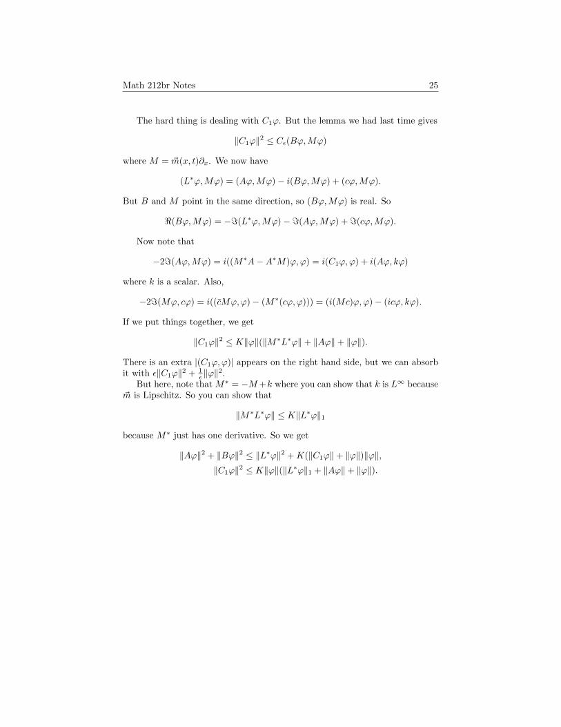
The hard thing is dealing with C1ϕ. But the lemma we had last time gives

‖C1ϕ‖2 ≤ Cε(Bϕ,Mϕ)

where M = ~m(x, t)∂x. We now have

(L∗ϕ,Mϕ) = (Aϕ,Mϕ)− i(Bϕ,Mϕ) + (cϕ,Mϕ).

But B and M point in the same direction, so (Bϕ,Mϕ) is real. So

<(Bϕ,Mϕ) = −=(L∗ϕ,Mϕ)−=(Aϕ,Mϕ) + =(cϕ,Mϕ).

Now note that

−2=(Aϕ,Mϕ) = i((M∗A−A∗M)ϕ,ϕ) = i(C1ϕ,ϕ) + i(Aϕ, kϕ)

where k is a scalar. Also,

−2=(Mϕ, cϕ) = i((cMϕ, ϕ)− (M∗(cϕ, ϕ))) = (i(Mc)ϕ,ϕ)− (icϕ, kϕ).

If we put things together, we get

‖C1ϕ‖2 ≤ K‖ϕ‖(‖M∗L∗ϕ‖+ ‖Aϕ‖+ ‖ϕ‖).

There is an extra |(C1ϕ,ϕ)| appears on the right hand side, but we can absorbit with ε‖C1ϕ‖2 + 1

ε ‖ϕ‖2.

But here, note that M∗ = −M+k where you can show that k is L∞ because~m is Lipschitz. So you can show that

‖M∗L∗ϕ‖ ≤ K‖L∗ϕ‖1

because M∗ just has one derivative. So we get

‖Aϕ‖2 + ‖Bϕ‖2 ≤ ‖L∗ϕ‖2 +K(‖C1ϕ‖+ ‖ϕ‖)‖ϕ‖,‖C1ϕ‖2 ≤ K‖ϕ‖(‖L∗ϕ‖1 + ‖Aϕ‖+ ‖ϕ‖).

Math 212br Notes 26

9 February 20, 2018

We had to prove solvability and also nonsolvability. For the solvability part, wewanted to prove the estimate

‖ϕ‖0 ≤ C‖L∗ϕ‖1

where

L∗ =∂

∂t+ ib~b(x, t)

∂

∂x+ c = A+ iB + c.

Then we were trying to solve the equation under the assumption

~b(x, t) = |~b(x, t)|~v(x).

We know that A is always solvable by the fundamental theorem of calculus.Local solvability means that we can shrink the domain as we want, and so weeven have ‖ϕ‖0 ≤ δ‖Aϕ‖0. When we expand ‖L∗ϕ‖2, we get pure terms andmixed terms, and the point is that the mixed terms were given by ‖C1ϕ‖ where

C1 = [A,B] = ~bt∂x. To deal with this, we used the B2 − 4AC argument

‖~bt · ~ζ‖ ≤ Cε(~b · ~ζ)((~b+ σ~v) · ~ζ)

where σ(x) = supt|~btt(x, t)|. So if we let

M = ~m∂x = B + σ~v · ∂x

then‖C1ϕ‖2 ≤ K(Bϕ,Mϕ).

Now we would like to replace Bϕ by L∗ϕ, Aϕ, cϕ. Because [A,M ] = C1, wecan take care of (Aϕ,Mϕ).

9.1 Insolvability of a differential equation

In the homework, there is the function

u(x) = eτ(ix1− 12 |x|

2)

on x = (x1, x2, x3) and a self-adjoint second-order partial differential operatorwith variable coefficients which are quadratic polynomials. Here, the dual isnot injective, so it should not be surjective. This means that there is globalnonsolvability for S(R3).

This holds the key for nonsolvability. We want to show that the estimate∫fv ≤ C sup

|α|≤k|DαL∗f | sup

|β|≤N|Dβv|

fails. So we want to make the left hand side go to infinity where the right handside is bounded. Here, if we use this function eτ(ix1− 1

2 |x|2

, we will get somethinglike the Fourier transform of f .

Math 212br Notes 27

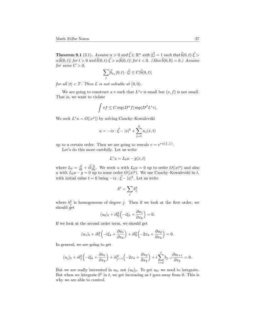
Theorem 9.1 (3.1). Assume α > 0 and ~ξ ∈ Rn with |~ξ| = 1 such that ~b(0, t)·~ξ >α|~b(0, t)| for t > 0 and ~b(0, t)·~ξ > α|~b(0, t)| for t < 0. (Also ~b(0, 0) = 0.) Assumefor some C > 0, ∑

j

|~bxj (0, t) · ~ξ| ≤ C|~b(0, t)|

for all |t| < T . Then L is not solvable at (0, 0).

We are going to construct a v such that L∗v is small but (v, f) is not small.That is, we want to violate∫

vf ≤ C sup|Dαf | sup|DβL∗v|.

We seek L∗u = O(|xρ|) by solving Cauchy–Kowalevski

u = −ix · ~ξ − |x|2 +

q∑j=1

uj(x, t)

up to a certain order. Then we are going to rescale v = eτu( xτ ,tτ ).

Let’s do this more carefully. Let us write

L∗u = L0u− g(x, t)

where L0 = ∂∂t + i~b ∂∂x . We week u with L0u = 0 up to order O(|x|q) and also

u with L0u− g = 0 up to some order O(|x|q). We use Cauchy–Kowalevski in t,

with initial value t = 0 being −ix · ~ξ − |x|2. Let us write

bk =∑j

bkj

where bkj is homogeneous of degree j. Then if we look at the first order, weshould get

(u0)t + ibk0

(−iξk +

∂u1

∂xk

)= 0.

If we look at the second order term, we should get

(u1)t + ibk1

(−iξk +

∂u1

∂xk

)+ ibk0

(−2xk +

∂u2

∂xk

)= 0.

In general, we are going to get

(uj)t + ibkj

(−iξk +

∂u1

∂xk

)+ ibkj−1

(−2xk +

∂u2

∂xk

)+ i

j∑l=2

bj−l∂ul+1

∂xk= 0.

But we are really interested in u0, not (u0)t. To get u0, we need to integrate.But when we integrate bk in t, we get increasing as t goes away from 0. This iswhy we are able to control.

Math 212br Notes 28

We actually want something more. Because we need∫fv to be something

like the Fourier transform of f , we want

=u ∼ i~x · ~ξ.

Because we want L∗u part to vanish, we want

<u ≤ −1

8|x|2 − 1

2α

∣∣∣∣∫ t

0

|~b(0, s)|ds∣∣∣∣,

both for t < 0 and t > 0.Suppose we have this u such that ‖L0u‖ = O(|x|q) and ‖L0h−g‖ = O(|x|q).

Then we can define

vτ = τn+2+keτu+hϕ, fτ =1

τhF (τx, τt),

where ϕ is the cut-off function. We then have

1

τ

∫fτvτ −

∫F (x, t)eτu( xτ ,

tτ )+h( xτ ,

tτ )ϕ(xτ,t

τ

)dxdt.

Then the only thing left is F (ξ, 0), because ϕ is a cut-off.

Math 212br Notes 29

10 February 22, 2018

For nonsolvability, we first looked at the Hans Lewy example ∂b, which dependedon the kernel. After this become known, people used the failure of estimates toprove nonsolvability. This means that∫

fv ≤ C(∑|α|≤k

sup|Dαf |)(∑|β|≤l

sup|DβL∗v|)

for f, v ∈ C∞0 , fails. The idea is to use the adjoint, and get a solution for L∗.But we only need approximate solution of L∗.

For differential equations with real analytic coefficients, there is the Cauchy–Kowalevski. So we can get an approximate solution (up to order q) to L∗. Thefactor eix·ξ will make

∫fv something like a Fourier transform. So we set f as a

function with nonzero Fourier transform, and then we use a cutoff function tomake L∗v really small, not only at a neighborhood.

10.1 Introduction to higher order equations

Let me briefly talk about Hormander’s work on higher order differential equa-tions. If ξ1, . . . , ξ` are nondegenerate vector fields, and

[ξµ, ξn] ∈ 〈ξ1, . . . , ξ`〉

then we can integrate this and make ξj = ∂∂xj

. But this is only for first-order

PDEs. There is an issue if the vectors are degenerate, and there is also theproblem that this can only deal with first-order. If we write Dj = 1

i∂∂xj

, then

the differential operator can be written as

P (x,D).

Then we can look at the symbol as

P (x, ξ) = e−iξ·ξP (x,D)eix·ξ.

This can be done in a coordinate-free way. The symbol is important becausewe have integration by parts.

We can look at the principal symbol Pm(x, ξ) and its complex conjugate (ofcoefficients) Pm(x, ξ). We have previously taken the commutator [L,L]. So wecan similarly define the commutator

C2m−1(x,D) = P (x,D)P (x,D)− P (x,D)P (x,D).

We say that that the differential operator is of principal type if the zerosof Pm(x, ξ) have order 1. That is, when ∇ξPm(x, ξ) 6= 0 for any ξ 6= 0 withPm(x, ξ) = 0.

Theorem 10.1 (Hormander). The differential equation is solvable at x = 0only when C2m−1(x, ξ) = 0 on Pm(x, ξ) = 0.

Math 212br Notes 30

There is some linear algebra statement. Define the Siegel upper half spaceas the space of n×n symmetric matrix with complex entries Z, such that =(Z)

is positive definite. Then you can show that for ~a · ~f ∈ C2, there exists anZ ∈ Siegeln such that Z~a = ~f if and only if

=(~f · ~a) > 0.

After all this, we are going to look at Hormander’s criterion on hypoellipticity.

10.2 Getting the estimate on Cauchy–Kowalevski

We want to show that∂

∂t+ i~b(x, t) · ∂x

is not solvable, when the direction changes. Then we can pick a vector ~ξ suchthat ~b · ~ξ changes sign. Technically, we assume that

~b(0, t) · ~ξ > α|~b(0, t)| for t > 0,

−~b(0, t) · ~ξ > α|~b(0, t)| for t < 0.

Also we assume that ∑j

|~bxj (0, t) · ~ξ|2 ≤ C|~b(0, t)|.

We want an approximation solution to

u = −ix · ξ − |x|2 +

q−1∑j=0

uj(x, t)

so that |L0u| ≤ const|x|q. Then we are going to set something like v = eτu( xτ ,tτ ).

We do this Cauchy–Kowalevski with initial data e−ix·ξ−|x|2

at t = 0. Onething we might worry about is the terms u0, u1, u2 messing up the new input.But if we write down the equation, we get

(u0)t + ibk0(−iξk + ∂u1

∂xk) = 0,

(u1)t + ibk1(−iξk + ∂u1

∂xk) + ibk0(−2xk + ∂u2

∂xk) = 0.

Here, b =∑bi is the expansion of b in x. Now the bk0ξk part is exactly ~b(0, t) · ~ξ,

and so we get

|<u0(t)| ≤ 1

2α

∫ t

0

|~b(0, s)|ds,

after integrating along t. Here, ∂u1

∂xkis a constant in x, so we can ignore this for

t small.

Math 212br Notes 31

Next, we have∣∣∣(u1)t + ibk1∂u1

∂xk

∣∣∣ ≤ C|b0(t)|1/2|x|+ c1|b0(t)||x|

and then integrating again gives

|u1| ≤ c2|x|∣∣∣∣∫ t

0

|b2(s)|1/2ds∣∣∣∣∑|~bxj (0, t)~ξ|2 ≤ c1|x|ε1/2∣∣∣∣∫ t

0

|b(s)|ds∣∣∣∣1/2

for |t| < ε.

Math 212br Notes 32

11 February 27, 2018

We are going to talk about the higher order case, solved by Hormander. Thiscan be regarded as an analogue of Frobenius integrability. Then we can findcoordinates y1, . . . , yk such that Xj = ∂

yj. There are several issues to think

about:

• What if X1, . . . , Xk are not linearly independent?

• What about higher orders?

11.1 Hormander’s criterion

Let us consider

P (x,D) =∑|α|≤m

aα(x)Dα, Dj =1

i

∂

∂xj,

where aα are complex-valued functions. Take the principal symbol Pm(x, ξ) =∑|α|=m a

α(x)ξα. We can also define Pm(x, ξ) =∑|α|=m a

α(x)ξα. Then we candefine the commutator

C(x,D) = P (x,D)P (x,D)− P (x,D)P (x,D)

of order 2m− 1, and consider its principal symbol C2m−1(x, ξ).

Theorem 11.1 (Hormander, necessary condition). If P (x,D)u = f is alwayssolvable, then C2m−1(x, ξ) = 0 at ξ 6= 0 when Pm(x, ξ) = 0.

What does it has to do with the change of sign? This theorem actuallypreceded Nirenberg–Treves. Note that C2m−1(x, ξ) = 0 is of odd order. So if thisis not true, there exists some ξ 6= 0 such that Pm(x, ξ) = 0 and C2m−1(x, ξ) 6= 0.

To prove this, we are going to do the same thing, but we need to do somelinear algebra. This is about moving a fixed vector to the variable factor withthe angular component the movement.

Lemma 11.2. Let ~a ∈ Cn − 0 be the initial fixed vector, and let ~f ∈ Cn bethe variable vector. Then there exists an A = (αkj) ∈ GL(n,C) symmetric with

=A > 0 such that A~a = ~f if and only if =(~f,~a) > 0.

Such A are the elements of the Siegel upper half space. This is the universalcovering of the moduli space for

Cn/lattice → PN

projective abelian varieties.

Proof. Let us first show necessity. We have

(f, a) =∑k

fkgk =∑k,j

αk,jaj ak.

Math 212br Notes 33

Then

=(f, a) =∑j,k

(=αk,j)(bjbk + cjck).

For sufficiency, we use the projection operator for the real Hilbert space.First look at the special case. The spherical coordinate is essentially equal ton = 1. So first assume that a ∈ θRn. We want to find A = B + iC such thatBa = g and Ca = h, where we write f = g + ih. Let us first define

h1 = h− (h, a)a

2(a, a).

Then we are going to define

Cx =(h, a)x

2(a, a)+

(x, h1)h1

(a, h1).

Then you can check that Ca = h and C is symmetric and positive definite.Then Ba = g can be done because the only requirement is that B is symmetric.

In the general case, α /∈ θRn, we would like to make

α = i=(f, a)

(a, a)I + β.

If we let

f1 = f − ai=(f, a)

(a, a),

then we have =(f1, a) = 0 and we want to now achieve βa = f1 and β symmetricand real. Consider all z ∈ Cn such that z = βa for β symmetric real. This setis a R-linear set, so we can write z = βa is the intersection of =(z, g) = 0 fora collection of g. Then =(ξ, g)(a, ξ) = 0 for all ξ ∈ Rn, and this shows that gshould be a real multiple of a.

So we are going to repeat the same argument for nonsolvability, that Nirenberg–Treves took from Hormander. We claim by Taylor expansion,

C2m−1(x, ξ) = i

m∑j=1

(P (j)m (x, ξ)Pm,j(x, ξ)− Pm,j(x, ξ)P (j)

m (x, ξ)).

Here,Pm,j(x, ξ) = ∂jPm(x, ξ), P (j)

m = ∂ξPm(x, ξ).

This is because if we write

P (D)(au) =∑α

(Dαa)Qα(D)u

then P (ξ + η) =∑α ξ

αQα(η). So we can write Qα(η) = 1α!P

(α)(η). We nowcompute

P (x,D)P (x,D)u =∑β

P (x,D)(aβDβu) =∑α,β

Dαaβ

α!P (α)Dβu.

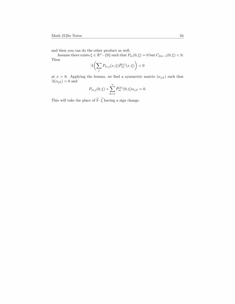
Math 212br Notes 34

and then you can do the other product as well.Assume there exists ξ ∈ Rn−0 such that Pm(0, ξ) = 0 but C2m−1(0, ξ) < 0.

Then

=(∑

j

Pm,j(x, ξ)P(j)m (x, ξ)

)< 0

at x = 0. Applying the lemma, we find a symmetric matrix (αj,k) such that=(αjk) > 0 and

Pm,j(0, ξ) +

n∑k=1

P (k)m (0, ξ)αj,k = 0.

This will take the place of ~b · ~ξ having a sign change.

Math 212br Notes 35

12 March 1, 2018

Hormander’s idea was to make the estimate fail, using Cauchy–Kowalevski.But in the higher order case, the expressions easily become complicated, andHormander had this linear algebra lemma.

Lemma 12.1. Let ~a = (a1, . . . , an) ∈ Cn and ~f ∈ Rn. Then there exists an

A = (αjk) that is symmetric and = > 0 such that A~α = ~f , if and only if

=(~f,~a) > 0.

The symmetric condition will be needed in the second derivative, and also= > 0 will be used in the exponential quadratic decay. Let me be precise. LetP be a differential operator of order m, and it takes the form of( ∂

∂x1

)m+ · · ·

then we can treat x2, . . . , xn as parameters. So if we find a function w such thatthe differential equation takes this form in a coordinate system with y1 = w,and also P (x, gradw) 6= 0, then we can do something like Cauchy–Kowalevski.Here the set P (x, gradw) = 0 is called the characteristic set. Here is thegeometric picture. Consider a constant coefficient differential operator, andconsider Pm(ξ) = 0. This gives a cone in the ξ-space, and the w = consthypersurfaces intersecting the cones transversely is the good condition.

12.1 Applying Hormander’s lemma

Now let us start showing the necessary condition for solvability. Let P (x,D) beof order m, and consider

C(x,D) = P (x,D)P (x,D)− P (x,D)P (x,D)

be of order 2m− 1. Then we have shown

C2m−1(x, ξ) = i∑

(P (j)m (x, ξ)Pm,j − Pm,j(x, ξ)P

(j)

m (x, ξ)).

If the equation P (x,D)u = f is solvable at 0, we want to show that C2m−1(0, ξ) =0 on Pm(0, ξ) = 0. We were showing that if there exists ξ 6= 0 such thatPm(0, ξ) = 0 and C2m−1(0, ξ) < 0, then the estimate fails. That is, given k,Nwe want to find a sequence fτ , vτ ∈ C∞0 (Ω) such that

1

τ

∫fτvτ

is bounded from below but sup|α|≤k|Dαf | and sup|β|≤l|DβL∗v| is bounded.We want to find a v such that L∗v = 0 as a jet, i.e., up to some high order.

Now we are going to choose

v = exp(iw), w = 〈x, ξ〉+1

2

n∑j,k=1

αjkxjxk.

Math 212br Notes 36

Here, αjk should satisfy the condition that αjk is symmetric, and =(αjk) > 0.We also want L∗w = 0 modulo |x|q. Another thing we want is Pm(x, gradw) =0, because we are going to take L∗(eiτw( xτ )ϕ) later.

So how do we get this? Hormander’s idea is to choose αjk smartly using thelinear algebra lemma. We do a linear change of coordinates so that the coefficientof ∂m

∂xmnis nonzero. Then we use the initial data W = 〈x, ξ〉+ 1

2

∑n−1j,k=1 αjkxjxk.

If we differentiate the equation Pm(x, gradw) = 0 with respect to xj , then weget

Pm,j(x, gradw) +

n∑k=1

P (k)(x, gradw)∂2w

∂xj∂xk= 0.

Now note that at x = 0, what we have is precisely what we are trying to do.

Because ∂2w∂xj∂xk

= αjk, this can be chosen precisely when

C2m−1(0, ξ) = =(Pm,•, P(•)m ) < 0.

But we still need to show some estimates. We started with the initial data

W = 〈x, ξ〉 =1

2

n−1∑j,k=1

xjxk + higher order

at xn = 0 and used Cauchy–Kowalevski, and got this w. We had ∂2w∂xj∂xj

= αjkfor 1 ≤ j, k ≤ n− 1 at 0, and we also had the other term

Pm,j(x, gradw) +

n∑k=1

P (k)(x, gradw)∂2w

∂xj∂xk= 0.

This actually shows that αjk = ∂2w∂xj∂xk

at the origin, even for 1 ≤ j, k ≤ n.

Math 212br Notes 37

13 March 6, 2018

We had to solve a L∗vτ approximately 0 to order 2r. Here, we use Fourier series.We write

L∗(ψeiτw(x)) =∑ν≤m

cν(x)τνeiτw(x).

and we want the leading coefficients to be nonzero.

13.1 Construction of counterexamples to the inequality

So we start outed with

w = ixξ +

n∑i,j=1

aijxixj

and constructed the solution w for Pm(x, gradw) = 0. Then we are going to let

vτ = τn+1+keiτw(ϕ0(x) +

ϕ1(x)

τ+ · · ·+ ϕr

τ r

).

Let us apply L∗ to this. If we have L∗ = P (x,−D), then the top degree is

P (x,−D)(ϕ0eiτw) = Aϕ0τ

meiτw +

(( n∑j=1

AjDj

)ϕ0 +Bϕ0

)τm−1eiτw + · · · .

Here, we can easily see A = Pm(x,−∂xw) and Aj = −P (j)m (x,−∂xw). Now we

do the same thing for ϕ1 and so on. Then we can carefully compute

e−iτwP (x,−D)(ϕ0 +

ϕ1

τ+ϕ2

τ2+ · · ·

)= (Aϕ0)τm + ((

∑AjDj)ϕ0 +Bϕ0)τm−1 + (B0,2ϕ0)τm−2 + (B0,3ϕ0)τm−3 + · · ·

+ (Aϕ1)τm−1 + ((∑

AjDj)ϕ1 +Bϕ1)τm−2 + (B0,2ϕ1)τm−3 + · · ·

· · · .

We want this to be O(|x|2r). But we note that we have already set w so thatA = O(|x|2r). So we only need to find ϕi so that

(∑AjDj)ϕ0 +Bϕ0 = O(|x|2r),

(∑AjDj)ϕ1 +Bϕ1 +B0,2ϕ0 = O(|x|2r),

(∑AjDj)ϕ2 +Bϕ2 +B0,2ϕ1 +B0,3ϕ0 = O(|x|2r),

· · · .

This can be solved inductively by Cauchy–Kowalevski, because one of the coef-

ficients Aj = P(j)m (0, ξ) has to be nonzero.

Math 212br Notes 38

So for this choice of vτ , we compute

L∗vτ = τ r−Neiτwm+r−1∑µ=0

1

µaµ

where aµ(x) = O(|x|2(r−µ)). We also have =w ≥ a|x|2 for some a.0, so we get

that |eiτw| ≤ e−τa|x|2 . So as τ →∞, we get

sup|β|≤n

|DβL∗vτ | → 0.

Now choose F ∈ C∞0 (Ω) such that F (−ξ) 6= 0. We set

fτ (x) =1

τkF (τx).

Then we sill havesup|α|≤k

|Dαfτ (x)|

is bounded. On the other other hand,

1

τ

∫fτvτ =

∫F (x)eiτw( xτ )

r−1∑ν=0

ϕν(xτ )

τν→ F (−ξ)ϕ0(0).

This does not go to 0.The moral of this entire story is that the characteristic is really important.

The contribution of Nirenberg and Treves was that you can use the sign changeto get an additional sign, instead of setting it.

Now we are going to talk about hypoellipticity. People like Kolmogorovshowed that a differential equation like

∂2u

∂x2+ x

∂u

∂t− ∂u

∂t= f.

Hormander observed that if you write X1 = ∂∂x and X0 = x ∂

∂y −∂∂t , then we

can write it as (X21 +X0)u = f . Then

[X1, X0] =∂

∂t

and so X0, X1, [X1, X0] generate the tangent space at 0.

Theorem 13.1. If X0, X1, . . . , Xr are smooth vector fields, and if iteratedbrackets generate all vectors, then

r∑j=1

X2j +X0

is solvable at 0 and is hypoelliptic.

Math 212br Notes 39

14 March 8, 2018

The zeros of the principal symbol is really important. This is always going to besome cone, because Pm(x, ξ) is a homogeneous polynomial. If it is a point, thisis operator is called elliptic and everything is very nice. The next case seems tobe when it has zeros of multiplicity 1, but we have seen that this is the worstcase. Hormander observed that if we have a linear one term like

∂

∂t−∆,

the heat kernel, this is nice. Here, note that the zero set is a line, but withmultiplicity 2. This is the second next case.

14.1 Hormander’s hypoellipticity

In general, consider a differential operator

n∑i,j=1

aij∂2u

∂xi∂xj+

n∑i=1

ai∂u

∂yi+ au+

n∑i=1

bi∂u

∂xi− ∂u

∂t= f,

where (aij) > 0, on R2n+1. If this can be written as

r∑j=1

X2j +X0

for some vector fields Xj , and [[[Xj , Xk], Xl], . . . , Xm] generate the tangentplane, then the equation is solvable. Moreover, we get some gain: if Lu = fand f ∈ Ck0 (Ω) then u ∈ Ck+ε(Ω) where ε−1 is roughly the number of bracketswe need to generate the plane.

The rough idea is to take a detour. Basically we want to show some a prioriestimate, and we want to compare values between points. But the problem isthat sometimes we don’t have vectors that will send me somewhere directly. Sowe take a detour by looking at the Lie bracket.

14.2 Preparation for Riesz representation

Let X0, . . . , Xn be smooth real vector fields, and let c be a complex-valuedsmooth functions. Consider the operator

P =

r∑j=1

X2j +X0 + c.

We want to solve Pu = f for f ∈ C∞0 (Ω), and we want to write∫v(Pv) in

terms of∑j |Xjv|2. We have X∗j = −Xj +aj for some smooth aj . Then we can

Math 212br Notes 40

write

−<∫vPv = −<

∫ v∑j=1

vX2j v −<

∫vX0v −

∫9<c)|v|2

= −<∫ v∑

j=1

(X∗j v)(Xjv)−<∫X0( 1

2 |v|2)−

∫(<c)|v|2

= −<∫ r∑

j=1

(−Xjv + ajv)Xjv −<∫a0|v|2

2−∫

(<c)|v|2.

So we can write

−<∫vP v =

r∑j=1

∫|Xjv|2 +

∫d|v|2

where d = 12

∑(Xjaj − a2

j )− 12a0 −<(c). Then we have

r∑j=1

‖Xjv‖2 + ‖v‖2 ≤ C‖v‖2 −<∫vP v.

The left hand side looks like a L21-norm. So we define

|‖v‖|2 =

r∑j=1

‖Xjv‖2 + ‖v‖2.

We use the Riesz representation theorem. But we are going to be in thesituation of ‖ϕ‖ ≤ C‖L∗ϕ‖m again. Then what we are going to get is somethingin L2

−1.

Definition 14.1. |‖−‖|′ is dual to |‖−‖| with respect to the (−,−)L2 innerproduct. That is,

|‖f‖|′ = supv∈C∞0 (Ω)

|∫fv||‖v‖|

.

If we look at the real part, we have by definition

−<∫vPv ≤ |‖v‖||‖Pv‖|.

But we need to estimate X0v in terms of Pv, but only have

X0v = Pv −n∑j=1

X2j v − c.

We know how to bound Xjv, but we don’t know anything about X2j v. So we

look at the weaker norm |‖Xjv‖|′ of Xjv. Then we have

|‖Xjf‖|′ = sup

∫g(Xjf)

|‖g‖|= sup

∫(−Xj g + aj g)f

|‖g‖|≤ C‖f‖ (‖Xjg‖+ ‖g‖)

|‖g‖|≤ C ′‖f‖.

Math 212br Notes 41

It follows that

|‖X0v‖|′ ≤ |‖Pv‖|′ +∑j

|‖X2j v‖|′ + C|‖v‖|′

≤ |‖Pv‖|′ + C∑j

‖Xjv‖+ C‖v‖

≤ C ′(‖v‖+ |‖Pv‖|′).

On the other hand, recall that we had

|‖v‖|2 ≤ C‖v‖2 + C ′|‖v‖||‖Pv‖|′

and then by the small-constant large-constant,

|‖v‖|2 ≤ C(‖v‖2 + |‖Pv‖|′2).

So if we add up, we get

|‖v‖|2 + |‖X0v‖|′2 ≤ C(‖v‖2 + |‖Pv‖|′2).

We now want to use the idea of taking the detour (or iterated Lie bracket).We want an estimate like

‖v‖(ε) ≤ C(|‖v‖|+ |‖X0v‖|′)

for all v ∈ C∞0 (Ω), for some ε > 0. This ‖−‖(ε) is going to be the L2-norm withall directional derivatives of order ≤ ε in some sense. If we have this, we wouldget

‖v‖(ε) ≤ C(‖v‖+ |‖Pv‖|′).

But then the diameter being less than η will give us some estimate like ‖v‖ ≤Cηε‖v‖(ε).

Let me introduce some notation. For a vector field X, we denote by etX thevector flow generated by it. Then for a function u, we denote

(etXu)(x) = u(f(x, t))

the function u evaluated at the flow at time t. We then define

|u|εX,s = sup0≤|t|<ε

‖etXu− u‖L2

|t|s

for ε sufficiently small. This is some kind of a Holder norm for elements in L2.

Math 212br Notes 42

15 March 20, 2018

We are looking at the Hormander’s hypoellipticity. His important contributionwas that the operator can be written as P =

∑nj=1X

2j + X0, and the iterated

brackets generate the tangent space. In fact, there is going to be a gain ofderivative in all directions. The idea is to use the Sobolev norm with onlyspecific directions of differentiation. Using this norm, we are going to use theLie bracket to measure the failure of the exponential law, and then we will dosome smoothing.

We were trying to use Riesz representation. We are going to use some dualitywith respect to the inner product without derivatives. So we defined

|‖v‖|2 =r∑j=1

‖Xjv‖2 + ‖v‖2

and |‖v‖|′ as the dual norm, so that we always have

|(u, v)| ≤ |‖u‖||‖v‖|′.

For P =∑j X

2j + X0 + c where X0, Xj are real and c might be complex, we

showed that

−<∫vPv =

r∑j=1

∫|Xjv|2 +

∫d|v|2, d =

1

2

r∑j=1

((Xjaj)− a2j )−

1

2a0 −<c

where X∗j = −Xj + a0. From this we got

|‖v‖| =r∑j=1

‖Xjv‖2 + ‖v‖2 ≤ C‖v‖2 −<∫vPv

for all v ∈ C∞0 (Ω). But

|‖X2j v‖|′ ≤ C‖Xjv‖ ≤ |‖v‖|

and this implies by small-constant large-constant,

|‖X2j v‖|′ ≤ C(‖v‖+ |‖Pv‖|′).

Because X0v = Pv −∑j X

2j v − c, we get

|‖X0v‖|′ ≤ C(‖v‖+ |‖Pv‖|′).

So the conclusion is

|‖v‖|2 + |‖X0v‖|′2 ≤ C(‖v‖2 + |‖Pv‖|′2).

Math 212br Notes 43

15.1 Using iterated Lie brackets

Now we have control on the L2-norm on the Xj-derivative, and the weak X0-derivative norm. We want to generate from this the L2-norm in all directions.Here, we are going to interpret the weak X0-derivative norm as some kind ofL2

1/2 in the X0-direction.Let us write

XI = [Xν1 , [Xν2 , [. . . , Xνk ]]] = adXν1 · · · adXνk−1·Xνk

for I = (ν1, . . . , νk). Let us define s(ν) = 1 if 1 ≤ ν ≤ r and s(ν) = 12 if ν = 0,

and define1

s(I)=

1

s(ν1)+ · · ·+ 1

s(νk).

If X is a real vector field and u a smooth function, we are going to write

etXu = u(f(x, t))

where f is the flow generated by X. For instance, Xu = limt→0etXu−u

t .When we try to compute er2 = e−ye−xex+y, we get

r2 = −1

2[x, y] + higher order terms.

So let z2 = − 12 [x, y], then we can look at er3 = e−z2er2 and take away the degree

3 elements and er4 = e−z3er3 and so on. The result is that

e−ye−xex+y = ez2ez3 · · · ezkerk+1

where zk is the sum of commutators of degree k.

Lemma 15.1. For any t > 0, 0 < σ ≤ 1, and N ≥ 2,

‖et(X+Y )u− u‖ ≤ C(‖etXu− u‖+ ‖etY u− u‖+

N−1∑j=2

‖etjzju− u‖+ tσN |u|σ

),

where u ∈ C∞0 (Ω) and

|u|σ = sup|h|<ε

‖u(x+ h)− u(x)‖L2

|h|σ.

(Different ε yield different norms, but they are equivalent norms.)

There is a different trick involving coordinate transformations.

Lemma 15.2. Let x 7→ g(x, t) be a family of diffeomorphisms, and assume thatg(x, t)− x = O(tN ) as t→ 0, where N > 0. Then∫

|u(g(x, t))− u(x)|2dx ≤ C|t|2Ns|u|2s

for 0 < s ≤ 1.

Math 212br Notes 44

This is trivial if g(x, t) are curves in the standard coordinate directions.

Proof. We want to compare u(g(x, t))−u(x+h) with u(y+w)−u(y). We makethe change of coordinates y = x + h and y + w = g(x, t). The determinant ofthe Jacobian is close to 1, so we may ignore this. Then∫

|u(y + w)− u(y)|2 ≤ C|w|2s|u|2s.

Using a similar argument, you can prove something like this. If X is replacedby ϕX for ϕ ∈ C∞0 (Ω), we have

|u|ϕX,s ≤ Cϕ|u|X,s.

Math 212br Notes 45

16 March 22, 2018

What we are doing is some sort of microlocal analysis. We not only control thenumber of differentials but also the direction. Hormander used Holder estimateshere for fractional order. We have (real) vector fields X1, . . . , Xr and X0, andwe’re looking at

P =

r∑j=1

Xnj +X0 + c.

Here X0 is something like the time variable. Then Hormander’s theorem is thatthis is hypoelliptic. The point of microlocal analysis is to write down the correctnorm, which is

|‖u‖|2 = ‖u‖+r∑j=1

‖Xju‖2

in this case. After integration by parts, we got the a priori estimate

|‖v‖|2 + |‖X0v‖|′2 ≤ C(‖v‖2 + |‖Pv‖|′2)

for all v ∈ C∞0 (Ω). This |‖X0v‖|′ is roughly ‖X1/20 v‖ because X0 is roughly two

Xj and we’re taking away one Xj .Now the key is to go back to the Sobolev ε-norm in all directions, because

we want to show that it is smooth in all directions. So we need something like

‖v‖2(ε) ≤ C(‖v‖2 + |‖Pv‖|′2).

Here, we need this ε > 0 to jack up differentiability of the solution, by takingcare of commutators. So suppose we have something like Pu = f . Then

P (Dαu) = Dαf + [P,Dα]u.

For instance, take L be of first order and Lu = f . Then

Ldu

dt=df

dt+[L,

d

dt

]u,

and a priori estimates will give

1

δε‖u‖L2

1≤ ‖u‖L2

1+ε≤ C1

∥∥∥dfdt

∥∥∥L2

+ C‖u‖L21

for diameter < δ. This shows that for δ sufficiently small, we get the upperbound on ‖u‖L2

1.

16.1 Bounds on the Holder norm

Now our goal is to get the estimate

‖v‖2(ε) ≤ C(|‖v‖|2 + |‖X0v‖|′2).

Math 212br Notes 46

Roughly, we are going to use

(adXν1 adXν2 · · · adXνk−1Xνk)

1m(ν1,...,νk) .

Then these directions will generate the whole space, so ε = min 1m will do the

job.We want to approximate the Holder norm. This is defined as

‖v(x+ t)− v(x)‖L2 ≤ |t|ε‖v‖(ε).

There was a lemma that allowed us to do this for coordinate transformations ingeneral.

Lemma 16.1 (4.2). Assume g(x, t)− x = O(tN ) where g is smooth. Then∫|u(g(x, t))− u(x)|2dx ≤ C|t|2Ns|u|2s.

Lemma 16.2 (4.1, rescaling). If ϕ ∈ C∞(Ω,R), then

|u|ϕX,x ≤ C|u|X,s,

where |u|X,s is the Holder norm along X,

|u|X,s = sup|t|<ε

‖etXu− u‖L2

|t|s.

Now for I = (ν1, . . . , νk), let us denote XI = adXν1 · · · adXνk−1Xνk . Then

we want to add XI together to get all directions. We can write

e(XI+XJ ) = eXIeXJ eZ2eZ3 · · · eZN−1eγN .

Then using the fact that

S1 · · ·Sku− u =

k∑j=1

S1 · · ·Sj−1(Sju− u),

we can show that

‖et(X+Y )u−u‖ ≤ Ck,N(‖etXu−u‖+‖etY u−u‖+

N−1∑j=2

‖etjZtu−u‖+ tσN |u|σ

)

for 0 < σ ≤ 1 and N ≥ 2 and u ∈ C∞0 (K) where K is compact in Ω.So now let us define s0 = 1

2 , sj = 1, and

s(I) =1

1s(ν1) + · · ·+ 1

s(νk)

.

Math 212br Notes 47

From above, we have

|u|X,s ≤ C( r∑j=0

|u|Xj ,s + ‖u‖)

for X ∈ T s, where T s(Ω) is the subbundle of T (Ω) generated by XI withs(I) ≥ s.

We still need a smoothing procedure. We look at L2α+ε and consider pseudo-

differential operator with symbol (1 + δ2|ξ|2)−1,

v 7→∫

(1 + δ2|ξ|2)−1v(ξ)e2πix·ξdξ.

Note that this would be an actual differential operator if p(x, ξ) is a polynomialinstead of (1 + δ2|ξ|2)−1. We would also have the use some kind of a Fredrich’slemma, because we want estimates to pass on. This will allow us to compare|‖X0u‖|′ and |u|X0,

12.

Math 212br Notes 48

17 March 27, 2018

We defined the L2 Holder norm as

|u|εX,s = sup0<|t|<ε

‖etXu− u‖L2

|t|s

for u ∈ C∞0 (K). Then we had some weight

m(I) =1

s(I)=∑j

1

sνj.

We want to estimate on T s(Ω), which is generated by all XI (linear coefficientsin C∞(Ω), with s(I) ≥ s). Here, the key estimate is that

|u|X,s ≤ C( r∑j=0

|u|Xj ,s + ‖u‖)

for all X ∈ T s(Ω). This is just a matter if iterated application of vector fields.Here, to get iterated brackets, we had to have

‖etm(I)XIu− u‖ ≤ C1t

r∑j=0

|u|Xj ,sj + c2t|u|σ.

17.1 Handling different directions

Now we have all these different Holder norms in different directions. For t > 0,Consider f(t) = ‖etX0v − v‖. Then we have

d

dt(f(t)2) = 2(etX0X0v, e

tX0v − v).

Here, if |‖−‖| turns out to be etX0-invariant, then we would have an estimate

d

dt(f(t)2) ≤ C|‖X0v‖|′ · 2|‖v‖|.

Then we will be able to conclude that

f(t) ≤ t 12C(|‖v‖|+ |‖X0v‖|′)

and so |v|X0,12≤ C(|‖v‖|+ |‖X0v‖|′). Then we are done.

But it is clear that |‖−‖| won’t necessarily be invariant under that flow. Sointroduce another norm that is invariant. We do this by taking the average.Take σ > 0 such that T s(Ω) = T (Ω) for some s > σ. Consider the set I of allI with σm(I) ≤ 1 and |I| < m(I) < 2|I|. (So not all are X0 but there exists anX0.) Define

M(u) = |‖u‖|+ |‖X0u‖|′ +∑I∈I|u|XI ,x(I) + |u|σ.

Math 212br Notes 49

Then by the same argument, we get that

|u|X0,12≤ CM(u).

To see this, we consider

Stu =∏I∈I

etm(I)XIΦt1/σu.

Here, we are sort of using Freidrich’s argument. The commutator and smoothingout and the differential operator is bounded by u. Using this, we can show that‖Stu− u‖ ≤ CtM(u).

17.2 Towards the implicit function theorem

There is Nash’s original 1956 paper in Ann. of Math., and there are 1969 notesby J. Schwartz called nonlinear functional analysis.

Theorem 17.1. Let M be a compact Riemannian C∞-manifold of dimensionn, there exists a smooth embedding M → RN such that the metric is the pullbackof the standard metric.

The idea is to use something like Newton’s method. Normally, the implicitfunction works in the following way. You move a little bit, and there still is azero. But we can also use Newton’s method, by iterating the approximations toget the zero.

Math 212br Notes 50

18 March 29, 2018

There is one part in Hormander’s hypoellipticity that I have not explained.Because we are doing integration by parts, we actually need smoothness. So weneed a smoothing operator. But we will not talk about this.

We now want to talk about the isometric embedding theorem of Nash. Weare going to just do a special situation when Mn is a torus. This is in somesense an implicit function theorem. In the usual case, we have something likeF (x, y) = 0 and F (0, 0) = 0 and ∂F

∂y (0, 0) 6= 0. Then the conclusion is that near

0, there exists y = y(x) such that F (x, y(x)) = 0. The usual proof is from theintermediate value theorem if you move x a bit, F (x,−) should have a zero andthen you do something.

Given a metric g =∑jk gijdxjdxk that is C∞ on M , we look at the space

G of all smooth metrics on M . Also, let F be the set of all smooth embeddingsf : M → RN . Then you can pull back the metric, and solve

f∗(gstd) = g.

So we can define, for f ∈ F and g ∈ G,

Φ(f, g) = g − f∗(gstd).

Then we are solving Φ(f, g) = 0, given a fixed f .We can always look at Newton’s method. We first approximate the function

by 1st order and solve for the linearized equation, and iterate this. For the2-variable case, we are approximating F by

F (x0, 0) +∂

∂yF (x0, 0)y1 = 0.

This can be done in the context of Banach spaces. But here the problem is thatF and G are Frechet spaces, and you lose the differentiability at each step. Sothe key idea is to replace derivation by the difference quotient.

18.1 Newton’s method in Banach spaces

Here, we would be looking at the differential. But the existence of the rightinverse is going to be needed.

Theorem 18.1. Let B be a Banach space, and let f : Ω → B, where Ω is theopen unit ball in B. Suppose f ∈ C2 in the sense of Frechet. This means that

limh→0

‖f(x+ h)− f(x)− f ′(x)h‖‖h‖

= 0.

Further, assume that the second derivatives are bounded by some M ≥ 2, andfor u ∈ Ω there exists a L(u) ∈ B(B) with bounded norm M , which is theright inverse of (df)(u). If |f(0)| ≤ M−5, then there exists a u ∈ Ω such thatf(u) = 0.

Math 212br Notes 51

Proof. Inductively, we are going to write down

u0 = 0, un+1 = un − L(un)f(un).

Let κ = 32 and β > 0. Then we claim that |un − un−1| ≤ eκκ

n

. We have

|un+1 − un| = |L(un)f(un)| ≤M |f(un)|≤M |f(un−1)− df(un−1)L(un−1)f(un−1)|+M2|un − un−1|2.

Then we can choose β so that M can be absorbed.

Now we want to replace B by Cm(M), which is not a Banach space. Sohere is the method applied to a space with many Banach norms and smoothingoperators. Here, when we smooth, we lose something. Suppose we want tosmooth out ϕ(x) with a weight function h(x). Then the convolution is going tolook like

ϕt(x) =

∫y

ϕ(y)ht(x− y)dy.

Here, is how you pay the price. First, by triangle inequality, we have ‖ϕt‖0 ≤‖ϕ‖0. But then we get something like ‖ϕ′t‖1 ≤ C

t ‖ϕ‖0.Assume there exists a family of smoothing operators S(t) that is defined for

t ≥ 1, and goes to the identity as t → ∞. Suppose there exist M ≥ 1 andm,α ∈ N such that for any m−α ≤ r ≤ ρ ≤ m the following holds. (Here, |−|ρis the Cρ(M)-norm.)

(i) bound in stronger norm: |S(t)u|ρ ≤Mtρ−r|u|r for all u ∈ Cr(M).

(ii) bound in weaker norm: |(1− S(t))u|r ≤Mtr−ρ|u|ρ for all u ∈ Cρ(M).

(iii) bound in the weaker norm before integration: | ddtS(t)u|r ≤ Mtr−ρ−1|u|for all u ∈ Cr(M).

(iv) approximation: limt→∞|(1− S(t))u|r = 0 for all u ∈ Cr(M).

Theorem 18.2. Let Ω be a unit ball in Cm. Assume that f : Ω→ Cm−α(M) istwice Frechet differentiable with norm ≤M , such that for all u ∈ Ω, there existsa right inverse L(u) ∈ B(Cm, Cm−α) so that df(u)L(u)h = h for all h ∈ Cm+α,with bound M so that

|L(u)h|m−α ≤M |h|m.

Also assume the technical inequality

|L(u)f(u)|m+9α ≤M(1 + |u|m+10α).

If |f(0)|m+9α ≤ 1240M202 then f(u) = 0 for some u ∈ Ω.

Proof. Let κ = 32 and we are going to fix β, µ, ν > 0. Set t = eβκ

n

and

define Sn(eβκn

). (Eventually, Sn is going to be the identity.) Let u0 = 0 andinductively we want to construct un, such that un ∈ Ω,

|un − un−1|m ≤ e−µαβκn

, un ∈ Cm+10α, 1 + |un|m+10α ≤ eναβκn

.

Math 212br Notes 52

The claim is that if you define

un+1 = un − SnL(un)f(un),

this works. Newton’s method work as

|un+1 − un| = |SnL(un)f(un)| ≤Meαβκn

|L(un)f(un)|m−α ≤M2eαβκn

|f(un)|m≤M2eαβκ

n

|f(un−1)− df(un−1)Sn−1L(un−1)f(un−1)|m +M3eαβκn

|un − un−1|2m.

You can continue, and this will give you the right bounds.

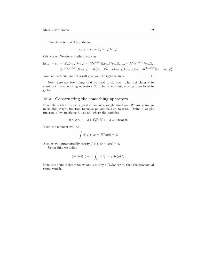
Now there are two things that we need to do now. The first thing is toconstruct the smoothing operators St. The other thing moving from local toglobal.

18.2 Constructing the smoothing operators

Here, the trick is to use a good choice of a weight function. We are going gomake this weight function to make polynomials go to zero. Define a weightfunction a by specifying a instead, where this satisfies

0 ≤ a ≤ 1, a ∈ C∞0 (Rn), a ≡ 1 near 0.

Then the moment will be∫xαa(x)dx = Dαα(0) = 0.

Also, it will automatically satisfy∫a(x)dx = a(0) = 1.

Using this, we define

(S(t)u)(x) = tn∫Rna(t(x− y))u(y)dy.

Here, the point is that if we expand u out by a Taylor series, then the polynomialterms vanish.

Math 212br Notes 53

19 April 3, 2018

Last time we looked at the method of applying modified Newton’s method usingthe change of norms. Normally, the solution is unique. But for the isometricembedding, there is no uniqueness. This is because imposed only the conditionthat ∂

∂y is right invertible. Concretely, we have for M a compact real smoothC∞,

F = f : MC∞−−→ RNf →

C∞ positive symmetric

covariant 2-tensors on M

= G.

We want to show that this is surjective.Let’s try to understand this in the finite-dimensional case. Suppose you want

to solve y = (y1, . . . , yp) in terms of x, and it is not unique. Assume that we aresolving for the relations Rj(y1, . . . , yp, x) = 0 for 1 ≤ j ≤ q (and q < p). Then

the differentiation of R = (Rj) is going to be (∂Rj∂yk

)1≤j≤q,1≤k≤p which is not asquare matrix. Then solving the linearization is the same as lifting a tangentvector in the x-space to a vector in (p+ 1− q)-space.

19.1 Continuity method using convex sets

But the best you can do is to get a local solution. If something is in the image,only a small open neighborhood is in the image as well. Note that the space Gis a convex cone in the Frechet space ΓC∞(Sym2 T ∗M). We also know that theimage E∞ of F of G is also a cone, because we can embed M → RN1 ⊕ RN2 .Here, the cone E∞ is equal to G if

(i) E∞ is dense in G, and

(ii) E∞ contains an interior point.

First lets try to produce an interior point, in the set of realizable Riemannianmetric. We start out with one embedding Mn → Rs. Now can we constructa right inverse of its variation? Nash’s trick is to avoid differentiation in theprocess of pulling back the metric. Suppose that the embedding w1, . . . , wsare functions on Rn with periods. (We’re assuming M is a torus.) Then thepullback metric is

g =

s∑l=1

n∑j,k=1

∂wl∂xj

∂wl∂xk

dxj ⊗ dxk.

If we vary w to w + h, we will get

δg =

s∑l=1

n∑j,k=1

(∂wl∂xj

∂hl∂xk

+∂hl∂xj

∂wl∂xk

)dxjdxk.

Here, the trick is to not differentiation ∂h∂x . The way to do this is to impose an

additional condition ∑l

∂wl∂xj

hl = 0

Math 212br Notes 54

for all 1 ≤ j ≤ n. If we have this condition, then

n∑l=1

∂2wl∂xj∂xk

hl +

n∑l=1

∂wl∂xj

∂hl∂xk

= 0

It follows that

δg = −2∑l,j,k

∂2wl∂xj∂xk

hl.

Now inverting this operator becomes a completely linear question.The inverse we want to consider is the linear equation∑s

l=1∂wl∂xj

hl = 0 1 ≤ j ≤ n∑sl=1

∂2wl∂xj∂xk

hl = gjk 1 ≤ j, k ≤ n.

This has s variables, and there are n + n(n+1)2 equations. So if s is sufficiently

large and the rank of this matrix is n+ n(n+1)2 , we can find the minimal solution

by using the “generalized Cramer’s rule”:

hmin = Bt(BBt)−1~b, ~b =

(0gjk

)∈ C∞(M).

So we want make sure that for a good f , the matrix has maximal rank ev-erywhere. Here we use the technique of mapping local coordinates. If we makea change of coordinates, the rank of the matrix doesn’t change. So we choose a fi-nite covering and charts, and just add the coordinates x1, . . . , xs, x

21, x1x2, . . . , xs−1xs, x

2s

(multiplied with a bump function) to the wj . If we do this, we will get a embed-ding w : M → Rs such that the matrix has full rank everywhere. Then applyingthe Newton’s method with a family of norms, we will get that this embeddingw is in the interior of E∞.

We also need to show that the image E∞ is dense in G. Suppose not, so that

g ∈ G−E∞. Then by Hahn–Banach, there exists a function Φ on C∞(M)n(n+1)

2

such that ϕ(E∞) ≤ 0 and Φ(g) > 0. Then Φ is a distribution, written as

Φ(g) =

n∑j,k=1

Djkgjk.

The condition we have is that∑Djk

∑l

∂wl∂xj

∂wl∂xk

≤ 0.

Locally, we use translation to smooth out Djk to Dεjk. Then we see that any

smoothing out Dεjk is semi-negative. If we apply this to gjk, then we also get∑

Dεjkgjk ≤ 0. As we take ε→ 0, we get a contradiction.

Math 212br Notes 55

20 April 5, 2018

We were looking at the isometric embedding theorem. Here, we needed tochange the norms in the topological vector space. To move between them, wehad to define smoothing operators. This local picture is the Nash–Moser implicitfunction theorem.

20.1 Conjugacy problem

The second application of the Nash–Moser implicit function theorem is theconjugacy problem, which deals with stability of the planetary motions. Ifthere are two planets, the motion is periodic. So the idea was to solve themindependently, and then regard other interactions as perturbations.

For f : R/Z → R/Z a continuous map, its rotation is the constant ρ suchthat

limn→∞

1

n(fn(x)− x)

converges uniformly to the constant function ρ.Consider a rotation Rρ : x 7→ x+ ρ, and take a small perturbation

ϕ : x 7→ x+ ρ+ η(x).

Now we want a reparametrization of the circle that makes the perturbed mapthe same as the original rotation by ρ. That is, is there a function H(x) suchthat H−1ϕH = Rρ?

Historically, people tried to do this using Fourier series, but then there is thedivision by zero problem. If ρ is irrational, it is fine, but still there is a smalldivisor problem when we take the iteration fn and so on. In the analytic case,Arnold managed to solve this using smaller and smaller norms by looking at thefunction on a neighborhood of R on the complex plane. Later, Yoccoz came upwith a way of doing this.

Definition 20.1. We say that ρ ∈ R is of type (K, ν) if there exists K > 0 andν > 0 such that ∣∣∣ρ− m

n

∣∣∣ > K

|n|ν

for all (m,n) ∈ Z× (Z− 0).

Roth showed that if ρ is irrational and algebraic, then it is of type (K, 2 + ε)for all ε.

Theorem 20.2 (Arnold). If ρ is of type (K, ν), then there exists ε(K, ν, σ) > 0such that if φ(x) = x + ρ + η(x) has rotation number ρ and ‖η‖σ < ε(K, ν, σ)(this η is real-analytic and is the restriction of some holomorphic function onthe strip |<z| < σ with the sup norm ‖η‖σ on the strip) then there exists areal-analytic change of variables ξ = H(x) for which φ is conjugate to Rρ.

Math 212br Notes 56

Let us write ξ = H(x) = x+ h(x). What we want is φ H = H Rρ, so wecan write this as

ξ + h(ξ) + ρ+ η(ξ + h(ξ)) = ξ + ρ+ h(ξ + ρ).

So we haveh(x+ ρ)− h(x) = η(x+ h(x)).

If we look at its linearized equation h(x + ρ) − h(x) = η(x), we can take itsFourier transform and write

h(n)e2πinρ − h(n) = η(n)

What Arnold did is to show that if ρ has some mild condition, you can stillsolve the small divisor theorem.

On the other hand, Yoccoz showed that this is actually not possible undersome condition. For α an irrational, we define α0 = α and α1 = 1

α0 and so

on. (This is taking the continued fraction.) Define

∆0(α) = 10, ∆n+1(α) =

1αn

(∆n(α)− log 1αn

+ 1) ∆n ≥ log 1αn

e∆n(α) ∆n ≤ log 1αn.

Then define

H0 = α ∈ R−Q : for all n ≥ n0,∆n(α) ≥ log 1αn,

H = α ∈ R−Q : gα ∈ H0 for all GL2(Z).

Yoccoz in 1989 showed that the conjugation problem is always solvable if andonly if α ∈ H, where α is the rotation number.

20.2 Arnold’s theorem

Now let us go back to the estimates. We have

h(n) =η(n)

e2πinρ − 1

for n 6= 0. If ρ is of type (K, ν), we get

|e2πinρ − 1| ≥ 4K

|n|ν−1.

Now our function f is analytic and periodic, so we can write it as a holomor-phic function on a neighborhood of the unit circle S1. Then η(n) is the Laruentseries coefficient. In any case, we will have the estimate

|η(n)| ≤ ‖η‖σe−2πσ|n|.

Math 212br Notes 57

Going back, we have

h(z) =∑n 6=0

η(n)e2πinz

e2πinρ − 1.

For ‖=t‖ < σ − δ, the sum can be bounded above by

∑n 6=0

|n|ν−1

4K‖η‖σe−2πσ|n|e2π|n|(σ−δ) ≤ Γ(ν)

K(2πδ)ν.

We estimate this by comparing it with the Γ-function. This is not a completesolution because we have to handle η(0). Still we have

‖h‖σ−δ ≤Γ(ν)

K(2πδ)ν‖η‖σ.

This is then going to be the solution to the linearized problem.

Math 212br Notes 58

21 April 10, 2018

We were looking at the conjugacy problem. The technique used here is toshrink the strip at every step, and use these weaker norms. We are going tosee another technique of shrinking the domain. Here, Moser’s idea is that wecan use a cutoff function that is 1 on a shrunken domain. We are going toneed Harnack’s principle, which can handle elliptic nonlinear partial differentialequations. These equations will look like

F (x, u,Du,D2u) = 0

where ∂F∂D2u is positive definite. De Giorgi only assumed here that the coefficients

are only measurable, but they are uniformly elliptic.

21.1 Iterating linearized conjugations

We were trying to prove the following theorem.

Theorem 21.1 (Arnold). Let ρ be irrational of type (K, v), i.e., |ρ − mn | >

K|n|ν for all integers m,n. Then there exists a ε = ε(K, ν, σ) > 0 such that if

φ(x) = x + ρ + η(x) has rotation ρ and |η|σ < ε (i.e., η is holomorphic onSσ = |=(z)| < σ with η(x + 1) = η(x) and |η|σ = supSσ < ε) then thereexists a real-analytic change of coordinates ξ = H(x) such that φ is conjugateto x 7→ Rρ(x) = x+ ρ.

Proof. If we write H(x) = x+ h(x), the equation we need to solve is

h(x+ ρ)− h(x) = η(x+ h(x)).

First we look at the linearization. Then we get

h(n) =η(n)

e2πinρ − 1

for n 6= 0. There is a small divisor problem, but we got that

‖h‖σ−δ ≤Γ(v)

K(2πδ)v‖η‖σ.

Now we need to invert H(x) = x+ h(x). For H−1(z) = z − h(z) + g(z), weget

g(z + h(z)) =

∫ 1

s=0

h′(z + sh(z))h(z)ds

and so we get

‖g‖σ−4δ ≤2πΓ(v)2

K2(2πδ)2v+1‖η‖2σ.

Math 212br Notes 59

Note that we have not taken care of η(0). If we plug in H−1φH, we get

φ(x) = x+ ρ+ η(0) +

∫ 1

0

η′(x+ sh(x))h(x)ds

+

∫ 1

0

h′(x+ ρ+ s(h(x) + η(x+ h(x)))(h(x) + η(x+ h(x))))ds.

Define η(x) by φ(x) = x+ ρ+ η. Because the rotation number of φ is preciselyρ, there exists a x0 such that η(x0) = 0. So η(x0) = 0 for x0. Using this, wecan approximate η by using this point x0. At the end, we will get

‖η‖σ−6δ ≤16πΓ(v)2

K2(2πδ)2v+1‖η‖2σ.

Now we can iterate this. At each step, you can use

δn =σ

36(1 + n2)

and this gives the right result.

21.2 Harnack inequality

Considern∑

ν,µ=1

∂

∂xν

(aνµ(x)

∂u

∂xµ

)= 0 (†)

for x = (x1, . . . , xn) where aνµ = 0 are only Lebesgue measurable, but has1λ ≤ aµν ≤ λ on a domain D ⊆ Rn. Let D′ ⊂⊂ D. If u is a weak solution of (†)on D and u > 0 on D, then the inequality states that

maxD′

u ≤ C minD′

u

for some C = C(D,D′, λ). This can be found in Moser, On Harnack’s theoremfor elliptic differential equations, Comm. P.&App. 14 (1961).

Here, when we say weak solution, we meant that u ∈ L21(D) and for all

φ ∈ L21(D), we have ∫

D

(φx, aux) = 0.

The idea is to integrate by parts to estimate L2 of Du in terms of L2 of u. Wecan interpret the maximum and the minimum as the L∞ norm of ul for l > 0and l < 0. Then we can relate the two by using log u and the John–Nirenberginequality, which reverses the Holder inequality.

Math 212br Notes 60

22 April 12, 2018

We started looking at De Giorgi’s ellipticity. For the operator∑nk=1 ∂j(ajk∂ku)

for ajk only L1loc but 1

λ ≤ (ajk) ≤ λ, De Giorgi proved some Holder regularityfor u.

22.1 Proof of Harnack’s inequality

Theorem 22.1 (Harnack’s inequality). Let D′ ⊂⊂ Rn be a bounded domain.Let u be a (weak) solution of the elliptic equation in divergence form on D whosematrix of coefficients for the 2-order terms have matrix entries bounded between1λ and λ for some λ > 1. If u > 0 on D, then there exists a c = c(n,D,D′)such that

supD′

u ≤ c infD′u.

Here, the weak solution is defined as∫(ϕx, aux) = 0

for all compactly supported ϕ ∈ L21(D). We apply integration by parts to bound

L2 of D(uk) by L2 of uk. The point is that we need to take a cutoff function toavoid the occurrence of boundary terms. This forces us to shrink the domain.

Consider v = f(u) = uk for k ≥ 2. Then for a cutoff function η, we let

φ = ku2k−1η2.

Then φx = k(2k − 1)u2k−2uxη2 + 2ku2k−1ηηx. Then our condition gives

0 =

∫φxauxdx =

∫k(2k − 1)u2k−2uxauxη

2 + 2ku2k−1ηηxaux

=

∫2k − 1

kη2(uk)xa(uk)x +

∫2ukηηx(uk)x.

Then we end up with

2k − 1

k

1

λ

∫D

(ηvx)2 ≤ 2

∫D

|(ηxv, aηvx)|,

and Cauchy–Schwartz gives(2(2k − 1)

kλ2

)2∫D

(ηvx)2 ≤∫

(ηxv)2.

We have η = 1 on some smaller domain D′. Here, ηx = 0 but ηx is bigoutside D′. So we need to keep track of shrinking of domain. Take D = Q(h)be a cube with side h centered at 0, and take D′ = Q(h′). Then∫

Q(h′)

v2xdx ≤ c3

( 2k

2k − 1

)2( 2

h− h′)2∫Q(h)

v2dx.

Math 212br Notes 61

If we apply Sobolev to the left hand side, we gain some power, and we find thatthere is some constant κ > 1 such that(

−∫v2κ

)1/κ

≤ β(h′2−∫v2x +−

∫v2

).

If we put this in, we get(−∫Q(h′)

v2κ

)1/κ

≤ c(( h

h′− 1)−2( 2k

2k + 1

)2

+ 1)−∫Q(h)

v2dx.

Fix p > 1. Every time, we jack up by a factor of κ > 1. So for pν = κνpwe use h = hν = 1 + 2−ν and h′ = hν+1 = 1 + 2−ν−1. Then if we iterate thisinequality, we are going to get something like

supD′

u = ‖u‖L∞(D′) ≤ C‖u‖Lp(D).

But we still need to relate the positive uk to the negative u−k. To do this, wenow use v = log u. Then we are using φ = η2/u. In this case,

(φx, aux) = −η2(vx, avx) + 2η(ηx, avx)

as before, and because a is positive definite, we get∫Q

η2v2xdx ≤ 4λ4

∫Q

η2x.

On the other hand, if we have the Poincare inequality∫Q

(v − vQ)2 ≤ C∫v2xdx ≤ C.

(This can be seen from looking at the Fourier expansion.)Now the John–Nirenberg inequality gives, for w ∈ L2(Q(1)), if

∫Q

(w −wQ)2 ≤ 1 then for every Q = Q(h) ⊂ Q( 1

2 ), there exist α, β > 0 such that(∫Q( 1

2 )

eαw)(∫

Q( 12 )

e−αw)≤ β2.

Math 212br Notes 62

23 April 17, 2018

Today we are going to wrap up the Harnack inequality and the Holder estimates.Consider

L =∑j

∂j∑k

ajk(x)∂k

where (ajk) are measurable but bounded between 1/λ and λ. Then the Harnackinequality tells us that if u > 0 is a solution on D and D′ ⊂⊂ D then

supD′

u ≤ cλ,D,D′,u infDu.

For v = log u, the John–Nirenberg inequality gives(∫D′|u|p

)(∫D′|u|−p

)≤ C

for some p > 0. Now Moser observed that if you take v = u(p+1)/2 for p 6= −1,we get (avx)x = 0 and so (φx, avx) = 0. Then vx = p+1

2 u(p−1)/2ux and so

v2x =

(p+ 1)2

4up−1uxux.

When we use (φx, aux) = 0 for φ = vη2, we can bound∫v2x by

∫v2.

23.1 De Giorgi’s argument for the Holder estimates

For Lu = 0 with u > 0, let us write

M(r) = sup|x|≤r

u, µ(r) = inf|x|≤r

u.

Now take D = |x| < r and D′ = |x| < r′ = r2. Write M = M(r), µ = µ(r)

and M ′ = M(r′), µ′ = µ(r′). Then M−u and u−µ on D are both the solutionsfor Lu = 0 as well. Then we can apply the Harnack inequalities here and get

supD′

(M − u) = M − µ′ ≤ c(M −M ′) = c infD′

(M − u),

supD′

(u− µ) = M ′ − µ ≤ c(µ′ − µ) = c infD′

(u− µ).

So if we add them up, we get

oscD′ u ≤ α oscD u,

where osc = M − µ and 0 < α < 1 is given by c−1c+1 .

The point of the argument is that this already implies 1/2-Holder. This isbecause

osc( r

2ν

)≤ αν osc(r).

You can apply this to Bernstein’s problem of minimal surfaces, but I am notgoing to do this.

Math 212br Notes 63

23.2 Probability spaces

Let (X,m) be a probability space. This means that m ≥ 0 is a measure withrespect to some σ-algebra M, and the total measure is m(X) = 1. A M-measurable function is called a random variable. The toy model for this isflipping coins. You flip this many many times, and are interested in the limitingsituation.

This can be done by using the Rademacher function. If you flip the coinn times, you get something in (Z/2)n and we are going to identify with [0, 1]by the diadic interpretation. So we identify (Z/2)∞ ∼ [0, 1]. So given a realnumber x ∈ [0, 1], we can consider the function

r(x) =

1 0 ≤ x < 1

2 ,

−1 12 ≤ x ≤ 1.

So we can evaluate r(x), r(2x), r(4x), . . ..The main tool is the independence of measurable functions. This is much

stronger than orthogonality. A family of functions fn is said to be indepen-dent if

m

( ∞⋂n=1

x : fn(x) ∈ Bn)

=

∞∏n=1

m(x : fn(x) ∈ Bn).

This is a much stronger notion that just orthogonality, because if Φ,Ψ : R →R are continuous functions, and f, g are independent, then Φ f and Ψ gare independent. You can think of this as the push-forward measure to theproduct being equal to the product of the push-forward measure to each of thecomponents.

On X = (Z/2)∞ = [0, 1], the Rademache functions rn(t) = r1(2n−1t) forma basis for the independent functions. The advantage of this tool is that we cannow imitate Fourier analysis. If we write

SN (t) =

N∑n=1

rn(t)

then we have ‖SN‖L2 =√N . We can also show

m

(x : α <

SN (x)√N

< β

)=

∫ β

α

e−t2/2

√2π

dt.

This follows from an application of Stirling.

Math 212br Notes 64

24 April 19, 2018

Today we’ll solve Dirichlet’s problem by Kakuatni’s method. Consider a boundeddomain Ω ⊆ Rn and suppose we are given the boundary value of g on Ω. Wewant to find f harmonic on Ω with boundary value g.

24.1 Theorems in probability theory

Let’s first try to solve this problem from g = χE . We are going to define

fE(x) = Pr(Brownian motion from x to exit Ω at a point of E).

The idea for the Brownian motion is to discretize and take the limit. Here,we used (Z/2Z)∞ to model the infinite tossing of coins. Because we have tonormalize, the sample path of a Brownian motion is going to be approximately12 -Holder continuous.

Consider a discrete time martingale. Then we have a sequence of σ-algebras

An ⊆ An+1 ⊆ An+2 ⊆ · · · ⊆M .

Then for f a function that is M -measurable, we can construct En(f) whichis An-measurable. This is by looking at the Radon–Nikodym derivative andwriting µn =

∫An

f . Then wone can show that

fn = En(f∞)→ f

almost everywhere and in L1.

Theorem 24.1 (Kolmogorov 0-1 law). Let (X,m) be a probability space andf1, f2, . . . be mutually independent random variables. Then the probability that∑∞k=1 fk converges is either 0 or 1.

Proof. Let’s say that sub σ-algebras Bj are mutually independent if and onlyif m(

⋂j Bj) =

∏jm(Bj) for all Bj ∈ Bj . This is a generalization because fi

being independent just means that Bj = f∗(Borel on R) are mutually indepen-dent.

Kolmogorov’s observation is that if B is independent with itself thenm(B) =m(B ∩ B) = m(B)2. Consider An = Afn and consider B =

⋂∞l=1(

∨∞k=l Ak).

Then Bj are mutually independent so Bn is independent with B for all n. ThenB is independent with itself.

Now it suffices to show that the subset of∑k fk converging is in B. This

can be done, by writing down the condition for convergence.

Theorem 24.2 (central limit theorem). Let f1, f2, . . . be mutually independentand identically distributed, i.e., (fj)∗m are all equal. Consider the mean andvariance

m0 =

∫ ∞t=−∞

tdµf (t) =

∫x∈X

f(x)dm(x),

σ2 =

∫ ∞−∞

(t−m0)2dµf (t) =

∫x∈X

(f(x)−m0)2dm(x).

Math 212br Notes 65

Let SN =∑Nj=1 fj normalized to (SN −Nm0)/

√N . Then

m(x : a < 1√N

(SN −Nm0) < b)→ 1

σ√

2π

∫ b

t=a

e−t2

2σ2 dt.

Proof. We can assume that m0 = 0. Let us write µN the distribution of sN/√N

and µσ the distribution of the Gaussian distribution. We want to show thatµN ((a, b))→ µσ((a, b)) as N →∞. To do this, we look at the Fourier transform

µ(ξ) =

∫ ∞t=−∞

e2πiξtdµ(t).

Mutual independence implies that

µN (ξ) =

N∏n=1

µfn

( ξ√N

)= µ

( ξ√N

)N.

You can expand µ(ξ/√N) in ξ and take power and look at the limit.

Theorem 24.3 (law of large numbers). Let f1, f2, . . . be identically distributed

mutually independent random variables on (X,m). Then 1N

∑Nj=1 fj → m0

almost everywhere.

Proof. This uses the idea of ergodicity. Recall that if T : Y → Y is a measure-preserving ergodic transformation then 1

N

∑Nj=1 T

jf →∫f almost everywhere.

(This was proved last semester.) Now we consider Y =∏∞j=0Rj and define

T : Y → Y as a shift T (y)n = yn+1. This will be measure-preserving, andergodic.

Math 212br Notes 66

25 April 26, 2018

The role of analysis is to rigorize intuitive arguments involving infinite processes.Kakutani’s idea uses probabilistic methods to solve the Dirichlet problem. Malli-avin developed this idea further and invented Malliavin calculus. Kakutani’sintuition is that if you take a random walk, and look at the probability that it isgoing first hit some region of the boundary, this will solve the Dirichlet problem.

25.1 Wiener measure

So in the infinite setting, we need to look at the set of all continuous paths.This we can just define as

P = p : [0,∞)→ Rd.

But we want this to be a probability space, so we need to give a σ-algebra,and also a measure. Giving a σ-algebra is simple, because we can just define ameasure

dn(p, p′) = sup0≤t≤n

|p(t)− p′(t)|, d =∑n

1

2ndn

1 + dn.

You can also define it using the subbase

p : p(tj) ∈ Aj

for some 0 = t0 ≤ t1 ≤ t2 ≤ · · · ≤ tk.The hard thing is to define the measure. Wiener observed that you can use

the cylindrical sets defined above, and then pass to the limit. This we can alsoabstractly characterize because we want this measure to be the measure comingfrom the limiting of the random walk. A random walk can be considered as Z∞2dwhere d is the dimension. For x ∈ Z∞2d, we consider rk(x) ∈ ±e1, . . . ,±ed theincrement at the kth position in the random walk x. Out of this, we can definethe path

S(N)t (x) =

1√N

∑1≤k≤[Nt]

~vk(x) +Nt− [Nt]√

N~r[Nt]+1(x).

This normalization by 1/√N is introduced so that as we take N → ∞, the

variance of the endpoint doesn’t blow up.Now we have this map

iN : Z∞2d →P; x 7→ S(N)t .

Let µN be the measure given by pushing forward. We want to show that µN → µin some sense. This can be made rigorous by looking at finite time slices. For0 ≤ t1 ≤ · · · ≤ tk in R, we have an evaluation map P → (Rd)k and look at the

measure in (Rd)k given by pushing forward. Then we get µ(t1,...,tk)N on (Rd)k for

each N , and then we can discuss convergence by evaluating at Borel sets. There

Math 212br Notes 67

is also a notion of weak convergence, which is that if you integrate a boundedmeasurable function, you get pointwise convergence.

The way you do this is to use Ascoli–Arzela.

Definition 25.1. A sequence of probability measures is called tight if for everyε > 0 there exists a compact subset Kε of P such that for all N we haveµN (Kc

ε ) < ε. (In otherwise, it is almost supported on compact subsets.)

In P, the notion of compactness is the following. We say that a closed setK ⊆ P is compact if for each T > 0, there exists a positive bounded functionwT such that wT (h)→ 0 as h→ 0 and

supp∈K

sup0≤t<T

|p(t+ h)− p(t)| ≤ wP (h).

for all 0 < h ≤ 1.

Theorem 25.2 (Ascoli–Arzela). If µN is tight, there exists a weakly converg-ing subsequence.

So what we can do is show that µN is tight. Then there exists a weakly

converging subsequence, converging to µ. Now we can show that µ(t1,...,tk)N

weakly converges to some measure, and then µ(t1,...,tkN ) → µ(t1,...,tk) weakly

because it converges on a subsequence.

To check that µ(t1,...,tNN ) are weakly convergent, you can use martingales.

Because Z∞2 is like [0, 1], we can test only on Rademacher functions.

25.2 Kakutani’s solution to the Dirichlet problem

Let (Ω,W ) = (P, µ), so that for ω ∈ Ω we have ω(t). This is also written asBt(ω), where Bt is thought of as the Brownian motion.

It can be formulated abstractly. Take an abstract probability space (Ω, P )and for each t ≥ 0 consider a Rd-valued random variable Bt(ω) for ω ∈ Ω. Wesay that this is a Brownian motion if the following are satisfied.

(B1) (independence of increment) The variables Bt1 , Bt2 −Bt1 , . . . , Btk −Btk−1

are mutually independent for 0 ≤ t1 < t2 < · · · < tk.

(B2) (increment in Gaussian) For 0 ≤ t <∞ and h > 0, the variable Bt+h−Bhis a Gaussian with mean zero and covariance matrix hId.

(B3) (almost everywhere continuity) For almost all ω ∈ Ω, the path t 7→ Bt(ω)is continuous.

Stopping time is something that can be used for restarting. For 0 ≤ t <∞,let At be the smallest σ-algebra such that all functions Bs for 0 ≤ s ≤ t areAt-measurable.

Definition 25.3. A nonnegative function τ : Ω → [0,∞) is a stopping timeif

ω : τ(ω) ≤ t ∈ At

for all t ≥ 0.

Math 212br Notes 68

Brownian motions have a strong Markov property.

Theorem 25.4. If Bt is a Brownian motion and σ ≥ 0 is a stopping time, then

B∗t (ω) = Bt+σ(ω)(ω)−Bσ(ω)(ω)

is also a Brownian motion.

Let R be a bounded domain in Rd. For x ∈ R, let Bxt (ω) = x+ Bt(ω) anddefine the exit time as

τx(ω) = inft ≥ 0 : Bxt (ω) ∈ R.

For problems that occur at boundary points, we also define the strict exit timeas

τx∗ (ω) = inft > 0 : Bxt (ω) ∈ R.

If x ∈ ∂R satisfies τx∗ (ω) = τx(ω) for almost every ω, we way that x ∈ ∂Ris regular. In this case, we can solve the Dirichlet problem by just looking atwhere it first hits the boundary.

This is used in the uniformization problem. Given M a negatively curvedsimply connected manifold, what can we say about it? By Hadamard, it isgoing to be diffeomorphic to Rn. But if it is negatively curved, you can find abounded harmonic function. The idea is that if you look at a Brownian motion,anything moving in the direction transverse to the radial direction, it is sort oftrapped because the non-radial direction is exponentially long.

Index

Bernstein–Sato polynomial, 6Brownian motion, 67

Cayley transform, 4central limit theorem, 64characteristic set, 35

distribution, 4

Hardy space, 11Harnack inequality, 60

independent, 63

Kolmogorov 0-1 law, 64

law of large numbers, 65

null bicharacteristic, 19

principal type, 20, 29

random variable, 63rotation, 55

stopping time, 67

tempered distribution, 4tight measures, 67

Weyl algebra, 6

69