materials selection charts - 160592857366.free.fr160592857366.free.fr/joe/ebooks/mechanical...

Materials selection charts

4.1 Introduction and synopsis Material properties limit performance. We need a way of surveying properties, to get a feel for the values design-limiting properties can have. One property can be displayed as a ranked list or bar-chart. But it is seldom that the performance of a component depends on just one property. Almost always it is a combination of properties that matter: one thinks, for instance, of the strength- to-weight ratio, σf / ρ , or the stiffness-to-weight ratio, E /ρ , which enter lightweight design. This suggests the idea of plotting one property against another, mapping out the fields in property-space occupied by each material class, and the sub-fields occupied by individual materials.

The resulting charts are helpful in many ways. They condense a large body of information into a compact but accessible form; they reveal correlations between material properties which aid in checking and estimating data; and they lend themselves to a performance-optimizing technique, developed in Chapter 5, which becomes the basic step of the selection procedure.

The idea of a materials selection chart is described briefly in the following section. The section after that is not so brief: it introduces the charts themselves. There is no need to read it all, but it is helpful to persist far enough to be able to read and interpret the charts fluently, and to understand the meaning of the design guide lines that appear on them. If, later, you use one chart a lot, you should read the background to it, given here, to be sure of interpreting it correctly.

A compilation of all the charts, with a brief explanation of each, is contained in Appendix C of this text. It is intended for reference - that is, as a tool for tackling real design problems. As explained in the Preface, you may copy and distribute these charts without infringing copyright.

4.2 Displaying material properties The properties of engineering materials have a characteristic span of values. The span can be large: many properties have values which range over five or more decades. One way of displaying this is as a bar-chart like that of Figure 4.1 for thermal conductivity. Each bar represents a single material. The length of the bar shows the range of conductivity exhibited by that material in its various forms. The materials are segregated by class. Each class shows a characteristic range: metals, have high conductivities; polymers have low; ceramics have a wide range, from low to high.

Much more information is displayed by an alternative way of plotting properties, illustrated in the schematic of Figure 4.2. Here, one property (the modulus, E , in this case) is plotted against another (the density, ρ ) on logarithmic scales. The range of the axes is chosen to include all materials, from the lightest, flimsiest foams to the stiffest, heaviest metals. It is then found that data for a given class of materials (polymers for example) cluster together on the chart; the sub-range associated with one material class is, in all cases, much smaller than thefull range of that property. Data for

Joe Sulton

Joe Sulton

Materials selection charts 33

Fig. 4.1 A bar-chart showing thermal conductivity for three classes of solid. Each bar shows the range of conductivity offered by a material, some of which are labelled.

one class can be enclosed in a property envelope, as the figure shows. The envelope encloses all members of the class.

All this is simple enough -just a helpful way of plotting data. But by choosing the axes and scales appropriately, more can be added. The speed of sound in a solid depends on the modulus, E , and the density, p; the longitudinal wave speed 71, for instance, is

112 c = (%)

or (taking logs) logE = l o g p + 2 l o g v

For a fixed value of u, this equation plots as a straight line of slope 1 on Figure 4.2. This allows us to add contours ofconstunt wave veloci9 to the chart: they are the family of parallel diagonal lines, linking materials in which longitudinal waves travel with the same speed. All the charts allow additional fundamental relationships of this sort to be displayed. And there is more: design- optimizing parameters called material indices also plot as contours on to the charts. But that comes in Chapter 5.

Among the mechanical and thermal properties, there are 18 which are of primary importance, both in characterizing the material, and in engineering design. They were listed in Table 3.1: they include density, modulus, strength, toughness, thermal conductivity, diffusivity and expansion. The charts display data for these properties, for the nine classes of materials listed in Table 4.1. The

34 Materials Selection in Mechanical Design

Fig. 4.2 The idea of a Materials Property Chart: Young’s modulus, E, is plotted against the density, p, on log scales. Each class of material occupies a characteristic part of the chart. The log scales allow the longitudinal elastic wave velocity v = (€/p)’’’ to be plotted as a set of parallel contours.

class-list is expanded from the original six of Figure 3.1 by distinguishing engineering composites fromfoams and from woods though all, in the most general sense, are composites; by distinguishing the high-strength engineering ceramics (like silicon carbide) from the low-strength porous ceramics (like brick); and by distinguishing elastomers (like rubber) from rigid polymers (like nylon). Within each class, data are plotted for a representative set of materials, chosen both to span the full range of behaviour for the class, and to include the most common and most widely used members of it. In this way the envelope for a class encloses data not only for the materials listed in Table 4.1, but for virtually all other members of the class as well.

The charts which follow show a range of values for each property of each material. Sometimes the range is narrow: the modulus of copper, for instance, varies by only a few per cent about its mean value, influenced by purity, texture and such like. Sometimes it is wide: the strength of alumina-ceramic can vary by a factor of 100 or more, influenced by porosity, grain size and so on. Heat treatment and mechanical working have a profound effect on yield strength and toughness of metals. Crystallinity and degree of cross-linking greatly influence the modulus of polymers, and so on. These structure-sensitive properties appear as elongated bubbles within the envelopes on the charts. A bubble encloses a typical range for the value of the property for a single material. Envelopes (heavier lines) enclose the bubbles for a class.


Table 4.1 Material classes and members of each class

Class Members Short name

Engineering Alloys (The metals and alloys of

engineering)

Engineering Polymers (The thermoplastics and

thermosets of engineering)

Engineering Ceramics (Fine ceramics capable of

load-bearing application)

Engineering Composites (The composites of engineering

practice.) A distinction is drawn between the properties of a ply - ‘UNIPLY’ - and of a laminate - ‘LAMINATES’

Porous Ceramics (Traditional ceramics,

cements, rocks and minerals)

Glasses (Ordinary silicate glass)

Woods (Separate envelopes describe

properties parallel to the grain and normal to it, and wood products)

Aluminium alloys Copper alloys Lead alloys Magnesium alloys Molybdenum alloys Nickel alloys Steels Tin alloys Titanium alloys Tungsten alloys Zinc alloys

Epoxies Melamines Polycarbonate Polyesters Polyethylene, high density Polyethylene, low density Poly formaldeh yde Pol ymethylmethacry late Polypropylene Polytetrafluorethylene Polyvin ylchloride

Alumina Diamond Sialons Silicon Carbide Silicon Nitride Zirconia

Carbon fibre reinforced polymer Glass fibre reinforced polymer Kevlar fibre reinforced polymer

Brick Cement Common rocks Concrete Porcelain Pottery

Borosilicate glass Soda glass Silica

Ash Balsa Fir Oak Pine Wood products (ply, etc)

A1 alloys Cu alloys Lead alloys Mg alloys Mo alloys Ni alloys Steels Tin alloys Ti alloys W alloys Zn alloys

EP MEL PC PEST HDPE LDPE PF PMMA PP PTFE PVC

A1203 C Sialons S i c Si3N4 Zr02

CFRP GFRP KFRP

Brick Cement Rocks Concrete Pcln Pot

B-glass Na-glass Si02

Ash Balsa Fir Oak Pine Woods

(cmtinued overleaf)


Table 4.1 (continue4

Class Members Short name

Elastomers Natural rubber (Natural and artificial rubbers) Hard Butyl rubber

Polyurethanes Silicone rubber Soft Butyl rubber

Polymer Foams These include: (Foamed polymers of Cork

engineering) Polyester Polystyrene Polyurethane

Rubber Hard Butyl PU Silicone Soft Butyl

Cork PEST PS PU

The data plotted on the charts have been assembled from a variety of sources, documented in Chapter 13.

4.3 The material property charts

The modulus-density chart (Chart 1, Figure 4.3) Modulus and density are familiar properties. Steel is stiff, rubber is compliant: these are effects of modulus. Lead is heavy; cork is buoyant: these are effects of density. Figure 4.3 shows the full range of Young’s modulus, E , and density, p, for engineering materials.

Data for members of a particular class of material cluster together and can be enclosed by an envelope (heavy line). The same class envelopes appear on all the diagrams: they correspond to the main headings in Table 4.1.

The density of a solid depends on three factors: the atomic weight of its atoms or ions, their size, and the way they are packed. The size of atoms does not vary much: most have a volume within a factor of two of 2 x m3. Packing fractions do not vary much either - a factor of two, more or less: close-packing gives a packing fraction of 0.74; open networks (like that of the diamond-cubic structure) give about 0.34. The spread of density comes mainly from that of atomic weight, from 1 for hydrogen to 238 for uranium. Metals are dense because they are made of heavy atoms, packed densely; polymers have low densities because they are largely made of carbon (atomic weight: 12) and hydrogen in a linear 2 or 3-dimensional network. Ceramics, for the most part, have lower densities than metals because they contain light 0, N or C atoms. Even the lightest atoms, packed in the most open way, give solids with a density of around 1 Mg/m3. Materials with lower densities than this are foams - materials made up of cells containing a large fraction of pore space.

The moduli of most materials depend on two factors: bond stiffness, and the density of bonds per unit area. A bond is like a spring: it has a spring constant, S (units: N/m). Young’s modulus, E , is roughly

(4.1)

where ro is the ‘atom size’ (r: is the mean atomic or ionic volume). The wide range of moduli is largely caused by the range of values of S. The covalent bond is stiff (S = 20-200N/m); the metallic and the ionic a little less so ( S = 15-l00N/m). Diamond has a very high modulus because the carbon atom is small (giving a high bond density) and its atoms are linked by very strong

S E = - r0


Fig. 4.3 Chart 1: Young's modulus, E , plotted against density, p. The heavy envelopes enclose data for a given class of material. The diagonal contours show the longitudinal wave velocity. The guide lines of constant E/p , E1 /2 /p and E1I3 /p allow selection of materials for minimum weight, deflec- tion-limited, design.

springs (S = 200 N/m). Metals have high moduli because close-packing gives a high bond density and the bonds are strong, though not as strong as those of diamond. Polymers contain both strong diamond-like covalent bonds and weak hydrogen or Van der Waals bonds (S = 0.5-2N/m); it is the weak bonds which stretch when the polymer is deformed, giving low moduli.

But even large atoms (TO = 3 x lo-'' m) bonded with weak bonds (S = 0.5 N/m) have a modulus of roughly

0.5 3 x 10-10 E = % 1 GPa (4.2)


This is the lower limit for true solids. The chart shows that many materials have moduli that are lower than this: they are either elastomers or foams. Elastomers have a low E because the weak secondary bonds have melted (their glass temperature T , is below room temperature) leaving only the very weak 'entropic' restoring force associated with tangled, long-chain molecules; and foams have low moduli because the cell walls bend (allowing large displacements) when the material is loaded.

The chart shows that the modulus of engineering materials spans five decades*, from 0.01 GPa (low-density foams) to l000GPa (diamond); the density spans a factor of 2000, from less than 0.1 to 20 Mg/m'. At the level of approximation of interest here (that required to reveal the relationship between the properties of materials classes) we may approximate the shear modulus G by 3E/8 and the bulk modulus K by E , for all materials except elastomers (for which G = E / 3 and K >> E ) allowing the chart to be used for these also.

The log-scales allow more information to be displayed. The velocity of elastic waves in a material, and the natural vibration frequencies of a component made of it, are proportional to (E /p ) ' / * ; the quantity (E /p ) ' 12 itself is the velocity of longitudinal waves in a thin rod of the material. Contours of constant ( E / P ) ' / ~ are plotted on the chart, labelled with the longitudinal wave speed. It varies from less than 50 m/s (soft elastomers) to a little more than lo4 d s (fine ceramics). We note that aluminium and glass, because of their low densities, transmit waves quickly despite their low moduli. One might have expected the sound velocity in foams to be low because of the low modulus, but the low density almost compensates. That in wood, across the grain, is low; but along the grain, it is high - roughly the same as steel - a fact made use of in the design of musical instruments.

The chart helps in the common problem of material selection for applications in which weight must be minimized. Guide lines corresponding to three common geometries of loading are drawn on the diagram. They are used in the way described in Chapters 5 and 6 to select materials for elastic design at minimum weight.

The strength-density chart (Chart 2, Figure 4.4) The modulus of a solid is a well-defined quantity with a sharp value. The strength is not. It is shown, plotted against density, p, in Figure 4.4.

The word 'strength' needs definition (see also Chapter 3, Section 3.3). For metals and polymers, i t is the yield strength, but since the range of materials includes those which have been worked, the range spans initial yield to ultimate strength; for most practical purposes it is the same in tension and compression. For brittle ceramics, the strength plotted here is the crushing strength in compression, not that in tension which is 10 to 15 times smaller; the envelopes for brittle materials are shown as broken lines as a reminder of this. For elastomers, strength means the tear strength. For composites, it is the tensile fuilure strength (the compressive strength can be less by up to 30% because of fibre buckling). We will use the symbol of for all of these, despite the different failure mechanisms involved.

The considerable vertical extension of the strength bubble for an individual material reflects its wide range, caused by degree of alloying, work hardening, grain size, porosity and so forth. AS before, members of a class cluster together and can be enclosed in an envelope (heavy line), and each occupies a characteristic area of the chart.

* Very low density foams and gels (which can be thought of as molecular-scale, fluid-filled, foams) can have moduli far GPa. Their strengths and fracture lower than thi\. As an example, gelatin (as in Jello) has a modulus of about 5 x

toughness;, too. can be below the lower limit of the charts.


Fig. 4.4 Chart 2: Strength, of, plotted against density, p (yield strength for metals and polymers, compressive strength for ceramics, tear strength for elastomers and tensile strength for composites). The guide lines of constant o f / p , ~ : / ~ / p and o; ’ * /p are used in minimum weight, yield-limited, design.

The range of strength for engineering materials, like that of the modulus, spans about five decades: from less than 0.1 MPa (foams, used in packaging and energy-absorbing systems) to lo4 MPa (the strength of diamond, exploited in the diamond-anvil press). The single most important concept in understanding this wide range is that of the lattice resistance or Peierls stress: the intrinsic resistance of the structure to plastic shear. Plastic shear in a crystal involves the motion of dislocations. Metals are soft because the non-localized metallic bond does little to prevent dislocation motion, whereas ceramics are hard because their more localized covalent and ionic bonds (which must be broken and


reformed when the structure is sheared), lock the dislocations in place. In non-crystalline solids we think instead of the energy associated with the unit step of the flow process: the relative slippage of two segments of a polymer chain, or the shear of a small molecular cluster in a glass network. Their strength has the same origin as that underlying the lattice resistance: if the unit step involves breaking strong bond\ (as in an inorganic glass), the materials will be strong; if it involves only the rupture of weak bonds (the Van der Waals bonds in polymers for example), it will be weak. Materials which fail by fracture do so because the lattice resistance or its amorphous equivalent is so large that atomic separation (fracture) happens first.

When the lattice resistance is low, the material can be strengthened by introducing obstacles to slip: in metals, by adding alloying elements, particles, grain boundaries and even other dislocations (‘work hardening’); and in polymers by cross-linking or by orienting the chains so that strong covalent as well as weak Van der Waals bonds are broken. When, on the other hand, the lattice resistance is high, further hardening is superfluous - the problem becomes that of suppressing fracture (next section).

An important use of the chart is in materials selection in lightweight plastic design. Guide lines are shown for materials selection in the minimum weight design of ties, columns, beams and plates, and for yield-limited design of moving components in which inertial forces are important. Their use is described in Chapters 5 and 6.

The fracture toughness-density chart (Chart 3, Figure 4.5) Increasing the plastic strength of a material is useful only as long as it remains plastic and does not fail by fast fracture. The resistance to the propagation of a crack is measured by the.fructure toughness, K,,.. It is plotted against density in Figure 4.5. The range is large: from 0.01 to over 100MPam’/2. At the lower end of this range are brittle materials which, when loaded, remain elastic until they fracture. For these, linear-elastic fracture mechanics works well, and the fracture toughness itself is a well-defined property. At the upper end lie the super-tough materials, all of which show substantial plasticity before they break. For these the values of K,, are approximate, derived from critical J-integral (J , ) and critical crack-opening displacement (6,) measurements (by writing K,, = (EJ,)’l2, for instance). They are helpful in providing a ranking of materials. The guidelines for minimum weight design are explained in Chapter 5. The figure shows one reason for the dominance of metals in engineering; they almost all have values of K,, above 20 MPa m’/*, a value often quoted as a minimum for conventional design.

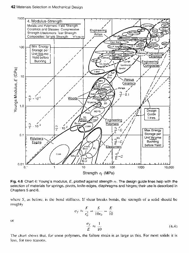
The modulus-strength chart (Chart 4, Figure 4.6) High tensile steel makes good springs. But so does rubber. How is it that two such different materials are both suited for the same task? This and other questions are answered by Figure 4.6, the most useful of all the charts.

It shows Young’s modulus E plotted against strength af. The qualifications on ‘strength’ are the same as before: it means yield strength for metals and polymers, compressive crushing strength for ceramics, tear strength for elastomers, and tensile strength for composite and woods; the symbol of is used for them all. The ranges of the variables, too, are the same. Contours of failure strain, n f / E (meaning the strain at which the material ceases to be linearly elastic), appear as a family of straight parallel lines.

Examine these first. Engineering polymers have large failure strains of between 0.01 and 0.1; the values for metals are at least a factor of 10 smaller. Even ceramics, in compression, are not as


Fig. 4.5 Chart 3: Fracture toughness, K,,, plotted against density, p. The guide lines of constant K,,, Kt’’/p and K:,/’/p, etc., help in minimum weight, fracture-limited design.

strong, and in tension they are far weaker (by a further factor of 10 to 15). Composites and woods lie on the 0.01 contour, as good as the best metals. Elastomers, because of their exceptionally low moduli, have values of ut / E larger than any other class of material: 0.1 to 10.

The distance over which inter-atomic forces act is small - a bond is broken if it is stretched to more than about 10% of its original length. So the force needed to break a bond is roughly

(4.3) Sr0 10

F = -


Fig. 4.6 Chart 4: Young’s modulus, E, plotted against strength uf. The design guide lines help with the selection of materials for springs, pivots, knife-edges, diaphragms and hinges; their use is described in Chapters 5 and 6.

where S, as before, is the bond stiffness. If shear breaks bonds, the strength of a solid should be roughly

F S E cf%-=- - - ri lor0 10

1

-

or

9%- (4.4) E 10 The chart shows that, for some polymers, the failure strain is as large as this. For most solids it is less, for two reasons.


First, non-localized bonds (those in which the cohesive energy derives from the interaction of one atom with large number of others, not just with its nearest neighbours) are not broken when the structure is sheared. The metallic bond, and the ionic bond for certain directions of shear, are like this; very pure metals, for example, yield at stresses as low as E A 0 000, and strengthening mechanisms are needed to make them useful in engineering. The covalent bond is localized; and covalent solids do, for this reason, have yield strength which, at low temperatures, are as high as E/10. It is hard to measure them (although it can sometimes be done by indentation) because of the second reason for weakness: they generally contain defects - concentrators of stress - from which shear or fracture can propagate, often at stresses well below the ‘ideal’ E/10. Elastomers are anomalous (they have strengths of about E ) because the modulus does not derive from bond-stretching, but from the change in entropy of the tangled molecular chains when the material is deformed.

This has not yet explained how to choose good materials to make springs. The way in which the chart helps with this is described in Section 6.9.

The specific stiffness-specific strength chart (Chart 5, Figure 4.7) Many designs - particularly those for things which move - call for stiffness and strength at minimum weight. To help with this, the data of Chart 4 are replotted in Chart 5 (Figure 4.7) after dividing, for each material, by the density; it shows E / p plotted against o f / p .

Ceramics lie at the top right: they have exceptionally high stiffnesses and compressive strengths per unit weight, but their tensile strengths are much smaller. Composites then emerge as the material class with the most attractive specific properties, one of the reasons for their increasing use in aerospace. Metals are penalized because of their relatively high densities. Polymers, because their densities are low, are favoured.

The chart has application in selecting materials for light springs and energy-storage devices. But that too has to wait until Section 6.9.

The fracture toughness-modulus chart (Chart 6, Figure 4.8) As a general rule, the fracture toughness of polymers is less than that of ceramics. Yet polymers are widely used in engineering structures; ceramics, because they are ‘brittle’, are treated with much more caution. Figure 4.8 helps resolve this apparent contradiction. It shows the fracture toughness, Klc, plotted against Young’s modulus, E. The restrictions described earlier apply to the values of KI,: when small, they are well defined; when large, they are useful only as a ranking for material selection.

Consider first the question of the necessary condition for fracture. It is that sufficient external work be done, or elastic energy released, to supply the surface energy, y per unit area, of the two new surfaces which are created. We write this as

G ? 2y (4.5)

where G is the energy release rate. Using the standard relation K x (EG)’/2 between G and stress intensity K , we find

K ? (2Ey)’I2 (4.6)

Now the surface energies, y, of solid materials scale as their moduli; to an adequate approximation y = Ero/20, where ro is the atom size, giving


Fig. 4.7 Chart 5: Specific modulus, Elp , plotted against specific strength af lp . The design guide lines help with the selection of materials for lightweight springs and energy-storage systems.

We identify the right-hand side of this equation with a lower-limiting value of Klc, when, taking ro as 2 x 10-lOm,

1/2 (4.8)

This criterion is plotted on the chart as a shaded, diagonal band near the lower right corner. It defines a lower limit on values of KI, : it cannot be less than this unless some other source of energy such as a chemical reaction, or the release of elastic energy stored in the special dislocation structures caused by fatigue loading, is available, when it is given a new symbol such as ( K I , ) ~ ~ ~ . meaning ' K I , for stress-corrosion cracking'. We note that the most brittle ceramics lie close to the threshold: when they fracture, the energy absorbed is only slightly more than the surface energy. When metals

(KI , )mi"

~ = ($) E x 3 x 10-6m1/2


Fig. 4.8 Chart 6: Fracture toughness, KIc, plotted against Young’s modulus, E. The family of lines are of constant K i / E (approximately G,,, the fracture energy). These, and the guide line of constant K,,/E, help in design against fracture. The shaded band shows the ‘necessary condition’ for fracture. Fracture can, in fact, occur below this limit under conditions of corrosion, or cyclic loading.

and polymers and composites fracture, the energy absorbed is vastly greater, usually because of plasticity associated with crack propagation. We come to this in a moment, with the next chart.

Plotted on Figure 4.8 are contours of toughness, GI,, a measure of the apparent fracture surface energy (GI, % K I , / E ) . The true surface energies, y , of solids lie in the range lop4 to lop3 kJ/m2. The diagram shows that the values of the toughness start at lop3 kJ/m2 and range through almost six decades to lo3 kJ/m2. On this scale, ceramics (10-3-10-’ kJ/m2) are much lower than polymers (10p1-10kJ/m2); and this is part of the reason polymers are more widely used in engineering than ceramics. This point is developed further in Section 6.14.


The fracture toughness-strength chart (Chart 7, Figure 4.9) The stress concentration at the tip of a crack generates a process zone: a plastic zone in ductile solids, a zone of micro-cracking in ceramics, a zone of delamination, debonding and fibre pull-out in composites. Within the process zone, work is done against plastic and frictional forces; it is this which accounts for the difference between the measured fracture energy GI, and the true surface energy 2y. The amount of energy dissipated must scale roughly with the strength of the material, within the process zone, and with its size, d,. This size is found by equating the stress field of the crack (a = K / G ) at r = d,/2 to the strength of the material, af, giving

Figure 4.9 - fracture toughness against strength - shows that the size of the zone, d, (broken lines), varies enormously, from atomic dimensions for very brittle ceramics and glasses to almost 1 m for the most ductile of metals. At a constant zone size, fracture toughness tends to increase with strength (as expected): it is this that causes the data plotted in Figure 4.9 to be clustered around the diagonal of the chart.

The diagram has application in selecting materials for the safe design of load bearing structures. They are described in Sections 6.14 and 6.15.

The loss coefficient-modulus chart (Chart 8, Figure 4.10) Bells, traditionally, are made of bronze. They can be (and sometimes are) made of glass; and they could (if you could afford it) be made of silicon carbide. Metals, glasses and ceramics all, under the right circumstances, have low intrinsic damping or ‘internal friction’, an important material property when structures vibrate. Intrinsic damping is measured by the loss coefJicient, q, which is plotted in Figure 4.10.

There are many mechanisms of intrinsic damping and hysteresis. Some (the ‘damping’ mechanisms) are associated with a process that has a specific time constant; then the energy loss is centred about a characteristic frequency. Others (the ‘hysteresis’ mechanisms) are associated with time-independent mechanisms; they absorb energy at all frequencies. In metals ‘a large part of the loss is hysteretic, caused by dislocation movement: it is high in soft metals like lead and pure aluminium. Heavily alloyed metals like bronze and high-carbon steels have low loss because the solute pins the dislocations; these are the materials for bells. Exceptionally high loss is found in the Mn-Cu alloys because of a strain-induced martensite transformation, and in magnesium, perhaps because of reversible twinning. The elongated bubbles for metals span the large range accessible by alloying and working. Engineering ceramics have low damping because the enormous lattice resistance pins dislocations in place at room temperature. Porous ceramics, on the other hand, are filled with cracks, the surfaces of which rub, dissipating energy, when the material is loaded; the high damping of some cast irons has a similar origin. In polymers, chain segments slide against each other when loaded; the relative motion dissipates energy. The ease with which they slide depends on the ratio of the temperature (in this case, room temperature) to the glass temperature, T,, of the polymer. When T I T , < 1, the secondary bonds are ‘frozen’, the modulus is high and the damping is relatively low. When T I T , > 1, the secondary bonds have melted, allowing easy chain slippage; the modulus is low and the damping is high. This accounts for the obvious inverse dependence of


Fig. 4.9 Chart 7: Fracture toughness, K,,, plotted against strength, of. The contours show the value of K,$/ rq - roughly, the diameter of the process zone at a crack tip. The design guide lines are used in selecting materials for damage-tolerant design.

q on E for polymers in Figure 4.10; indeed, to a first approximation,

4 x 10--2 (4.10)

E y I =

with E in GPa.

The thermal conductivity-thermal diff usivity chart (Chart 9, Figure 4.1 1) The material property governing the flow of heat through a material at steady-state is the thermal conductivity, h (units: J/mK); that governing transient heat flow is the thermul diffusivity, u


Fig. 4.10 Chart 8: The loss coefficient, g, plotted against Young’s modulus, E. The guide line corresponds to the condition q = C/E .

(units: m2/s). They are related by h

a=-- (4.1 1)

where p in kg/m3 is the density and C, the specific heat in J k g IS; the quantity pC, is the volumetric speciJic heat. Figure 4.1 1 relates thermal conductivity, diffusivity and volumetric specific heat, at room temperature.

PCiJ

The data span almost five decades in h and a. Solid materials are strung out along the line*

pC, % 3 x lo6 J/m3K (4.12)

*This can be understood by noting that a solid containing N atoms has 3N vibrational modes. Each (in the classical approximation) absorbs thermal energy kT at the absolute temperature T , and the vibrational specific heat is C, = C,. = 3 N k (J/K) where k is Boltzmann’s constant (1.34 x lO-23 J/K). The volume per atom, Q, for almost all solids lies within a factor


Fig. 4.11 Chart 9: Thermal conductivity, h, plotted against thermal diffusivity, a. The contours show the volume specific heat, pCp. All three properties vary with temperature; the data here are for room temperature.

For solids, C, and C,. differ very little; at the level of approximation of interest here we can assume them to be equal. As a general rule, then,

h = 3 x 1 0 6 a (4.13)

(h in J/mK and a in m2/s). Some materials deviate from this rule: they have lower-than-average volumetric specific heat. For a few, like diamond, it is low because their Debye temperatures lie

of two of I .4 x lO-29 m3; thus the volume of N atoms is (NR) m3. The volume specific heat is then (as the Chart shows):

3k L? pC,, 2 3 N k I N R = - = 3 x lo6 J/m3K


well above room temperature when heat absorption is not classical. The largest deviations are shown by porous solids: foams, low density firebrick, woods and the like. Their low density means that they contain fewer atoms per unit volume and, averaged over the volume of the structure, pC, is low. The result is that, although foams have low conductivities (and are widely used for insulation because of this), their thermal diflusivities are not necessarily low: they may not transmit much heat, but they reach a steady-state quickly. This is important in design - a point brought out by the Case Study of Section 6.17.

The range of both h and a reflect the mechanisms of heat transfer in each class of solid. Electrons conduct the heat in pure metals such as copper, silver and aluminium (top right of chart). The conductivity is described by

1 h = -cezt (4.14)

3

where C , is the electron specific heat per unit volume, 1; is the electron velocity (2 x lo5 m/s) and t the electron mean free path, typically lop7 m in pure metals. In solid solution (steels, nickel-based and titanium alloys) the foreign atoms scatter electrons, reducing the mean free path to atomic dimensions (z lo-'" m), much reducing h and a.

Electrons do not contribute to conduction in ceramics and polymers. Heat is carried by phonons - lattice vibrations of short wavelength. They are scattered by each other (through an anharmonic interaction) and by impurities, lattice defects and surfaces; it is these which determine the phonon mean free path, !. The conductivity is still given by equation (4.14) which we write as

h = -pC@ (4.15)

but now C is the elastic wave speed (around IO3 m / s - see Chart 1) and pC, is the volumetric specific heat again. If the crystal is particularly perfect, and the temperature is well below the Debye temperature, as in diamond at room temperature, the phonon conductivity is high: it is for this reason that single crystal diamond, silicon carbide, and even alumina have conductivities almost as high as copper. The low conductivity of glass is caused by its irregular amorphous structure; the characteristic length of the molecular linkages (about m) determines the mean free path. Polymers have low conductivities because the elastic wave speed C is low (Chart l), and the mean free path in the disordered structure is small.

The lowest thermal conductivities are shown by highly porous materials like firebrick, cork and foams. Their conductivity is limited by that of the gas in their cells.

1 3

The thermal expansion-thermal conductivity chart (Chart 10, Figure 4.12) Almost all solids expand on heating. The bond between a pair of atoms behaves like a linear elastic spring when the relative displacement of the atoms is small; but when it is large, the spring is non-linear. Most bonds become stiffer when the atoms are pushed together, and less stiff when they are pulled apart, and for that reason they are anharmonic. The thermal vibrations of atoms, even at room temperature, involves large displacements; as the temperature is raised, the anharmonicity of the bond pushes the atoms apart, increasing their mean spacing. The effect is measured by the linear expansion coefficient

1 d! ! dT

a = - -

where ! is a linear dimension of the body.

(4.16)


Fig. 4.12 Chart 10: The linear expansion coefficient, a, plotted against the thermal conductivity, A. The contours show the thermal distortion parameter Ala.

The expansion coefficient is plotted against the conductivity in Chart 10 (Figure 4.12). It shows that polymers have large values of a, roughly 10 times greater than those of metals and almost 100 times greater than ceramics. This is because the Van-der-Waals bonds of the polymer are very anharmonic. Diamond, silicon, and silica (SiO2) have covalent bonds which have low anharmonicity (that is, they are almost linear-elastic even at large strains), giving them low expansion coefficients. Composites, even though they have polymer matrices, can have low values of a because the reinforcing fibres - particularly carbon - expand very little.

The charts shows contours of h/a, a quantity important in designing against thermal distortion. A design application which uses this is developed in Section 6.20.


The thermal expansion-modulus chart (Chart 11, Figure 4.13) Thermal stress is the stress which appears in a body when it is heated or cooled, but prevented from expanding or contracting. It depends on the expansion coefficient of the material, a, and on its modulus, E . A development of the theory of thermal expansion (see, for example, Cottrell (1964)) leads to the relation

(4.17)

where YG is Gruneisen’s constant; its value ranges between about 0.4 and 4, but for most solids it is near 1 . Since pC, is almost constant (equation (4.12)), the equation tells us that (Y is proportional

Y G K , a = - 3E

Fig. 4.13 Chart 11 :The linear expansion coefficient, a, plotted against Young’s modulus, E. The contours show the thermal stress created by a temperature change of 1°C if the sample is axially constrained. A correction factor C is applied for biaxial or triaxial constraint (see text).


to 1/E. Figure 4.13 shows that this is so. Diamond, with the highest modulus, has one of the lowest coefficients of expansion; elastomers with the lowest moduli expand the most. Some materials with a low coordination number (silica, and some diamond-cubic or zinc-blende structured materials) can absorb energy preferentially in transverse modes, leading to very small (even a negative) value of y~ and a low expansion coefficient - silica, SiOz, is an example. Others, like Invar, contract as they lose their ferromagnetism when heated through the Curie temperature and, over a narrow range of temperature, they too show near-zero expansion, useful in precision equipment and in glass-metal seals.

One more useful fact: the moduli of materials scale approximately with their melting point, T,:

100 kT,, E % - Q

(4.18)

where k is Boltzmann's constant and Q the volume-per-atom in the structure. Substituting this and equation (4.13) for pC, into equation (4.17) for w gives

(4.19)

The expansion coefficient varies inversely with the melting point, or (equivalently stated) for all solids the thermal strain, just before they melt, depends only on y ~ , and this is roughly a constant. Equations (4.18) and (4.19) are examples of property correlations, useful for estimating and checking material properties (Chapter 13).

Whenever the thermal expansion or contraction of a body is prevented, thermal stresses appear; if large enough, they cause yielding, fracture, or elastic collapse (buckling). It is common to distinguish between thermal stress caused by external constraint (a rod, rigidly clamped at both ends, for example) and that which appears without external constraint because of temperature gradients in the body. All scale as the quantity wE, shown as a set of diagonal contours in Figure 4.13. More precisely: the stress A a produced by a temperature change of 1°C in a constrained system, or the stress per "C caused by a sudden change of surface temperature in one which is not constrained, is given by

CAa = (YE (4.20)

where C = 1 for axial constraint, (1 - u ) for biaxial constraint or normal quenching, and (1 - 2u) for triaxial constraint, where u is Poisson's ratio. These stresses are large: typically 1 MPdK; they can cau$e a material to yield, or crack, or spall, or buckle, when it is suddenly heated or cooled. The resistance of materials to such damage is the subject of the next section.

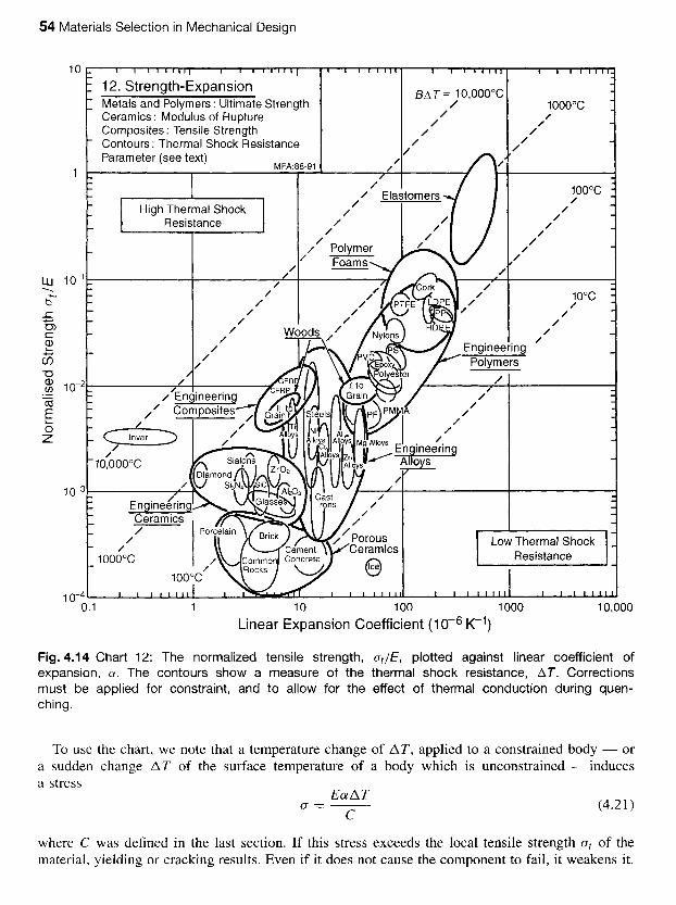
The normalized strength-thermal expansion chart (Chart 12, Figure 4.14) When a cold ice-cube is dropped into a glass of gin, it cracks audibly. The ice is failing by thermal shock. The ability of a material to withstand this is measured by its thermal shock resistance. It depends on its thermal expansion coefficient, a, and its normalized tensile strength, a, /E. They are the axes of Figure 4.14, on which contours of constant a , / w E are plotted. The tensile strength, a,, requires definition, just as af did. For brittle solids, it is the tensile fracture strength (roughly equal to the modulus of rupture, or MOR). For ductile metals and polymers, it is the tensile yield strength; and for composites it is the stress which first causes permanent damage in the form of delamination, matrix cracking or fibre debonding.


Fig. 4.14 Chart 12: The normalized tensile strength, at/€, plotted against linear coefficient of expansion, a. The contours show a measure of the thermal shock resistance, AT. Corrections must be applied for constraint, and to allow for the effect of thermal conduction during quenching.

To use the chart, we note that a temperature change of A T , applied to a constrained body - or a sudden change AT of the surface temperature of a body which is unconstrained - induces a stress

@ = - (4.21)

where C was defined in the last section. If this stress exceeds the local tensile strength a, of the material, yielding or cracking results. Even if it does not cause the component to fail, it weakens it.

E a AT C


Table 4.2 Values for the factor A (section T = 10 mm)

Conditions Foams Polymers Ceramics Metals

Slow air flow (h = 10W/m2K) 0.75 0.5 3 x 10-2 3 x lo-’

Fast air flow (h = lo2 W/m2K) I 0.75 0.25 3 x 10-2

Black body radiation 500 to 0C 0.93 0.6 0.12 1.3 x (h = 40 W/m2K)

Slow water quench ( k = lo3 W/m2K) 1 1 0.75 0.23 Fast water quench (h = 10‘ W/m2K) 1 I 1 0.1 -0.9

Then a measure of the thermal shock resistance is given by

A T ut C aE

- (4.22)

This is not quite the whole story. When the constraint is internal, the thermal conductivity of the material becomes important. ‘Instant’ cooling when a body is quenched requires an infinite rate of heat transfer at its surface. Heat transfer rates are measured by the heat transfer coefficient, h, and are never infinite. Water quenching gives a high h, and then the values of A T calculated from equation (4.22) give an approximate ranking of thermal shock resistance. But when heat transfer at the surface is poor and the thermal conductivity of the solid is high (thereby reducing thermal gradients) the thermal stress is less than that given by equation (4.21) by a factor A which, to an adequate approximation, is given by

thlh 1 + t h / h

A = (4.23)

where t is a typical dimension of the sample in the direction of heat flow; the quantity t h lh is usually called the Biot modulus. Table 4.2 gives typical values of A, for each class, using a section size of 10mm. The equation defining the thermal shock resistance, A T , now becomes

(4.24) or B A T = - CXE

where B = CIA. The contours on the diagram are of B A T . The table shows that, for rapid quenching, A is unity for all materials except the high-conductivity metals: then the thermal shock resistance is simply read from the contours, with appropriate correction for the constraint (the factor C). For slower quenches, A T is larger by the factor IIA, read from the table.

The strength-temperature chart (Chart 13, Figure 4.1 5) As the temperature of a solid is raised, the amplitude of thermal vibration of its atoms increases and solid expands. Both the expansion and the vibration makes plastic flow easier. The strengths of solids fall, slowly at first and then more rapidly, as the temperature increases. Chart 13 (Figure 4.15) captures some of this information. It shows the range of yield strengths of families of materials plotted against temperature. The near-horizontal part of each lozenge shows the strength in the regime in which temperature has little effect; the downward-sloping part shows the more precipitate drop as the maximum service temperature is reached.

There are better ways of describing high-temperature strength than this, but they are much more complicated. The chart gives a birds-eye view of the regimes of stress and temperature in which each material class, and material, is usable. Note that even the best polymers have little strength


Fig. 4.15 Chart 13: Strength plotted against temperature. The inset explains the shape of the lozenges.

above 200°C; most metals become very soft by 800°C; and only ceramics offer strength above 1500°C.

The modulus-relative cost chart (Chart 14, Figure 4.16) Properties like modulus, strength or conductivity do not change with time. Cost is bothersome because it does. Supply, scarcity, speculation and inflation contribute to the considerable fluctuations


Fig. 4.16 Chart 14: Young’s modulus, E , plotted against relative cost per unit volume, Cpp. The design guide lines help selection to maximize stiffness per unit cost.

in the cost-per-kilogram of a commodity like copper or silver. Data for cost-per-kg are tabulated for some materials in daily papers and trade journals; those for others are harder to come by. To make some correction for the influence of inflation and the units of currency in which cost is measured, we define a relative cost CR:

cost-per-kg of the material cost-per-kg of mild steel rod

CR =

At the time of writing, steel reinforcing rod costs about &0.2/kg (US$ 0.3kg) .


Chart 14 (Figure 4.16) shows the modulus E plotted against relative cost per unit volume C R p , where p is the density. Cheap stiff materials lie towards the bottom right.

The strength-relative cost chart (Chart 15, Figure 4.17) Cheap strong materials are selected using Chart 15 (Figure 4.17). It shows strength, defined as before, plotted against relative cost, defined above. The qualifications on the definition of strength, given earlier, apply here also.

It must be emphasized that the data plotted here and on Chart 14 are less reliable than those of previous charts, and subject to unpredictable change. Despite this dire warning, the two charts are

Fig. 4.17 Chart 15: Strength, af, plotted against relative cost per unit volume, Cpp. The design guide lines help selection to maximize strength per unit cost.


genuinely useful. They allow selection of materials, using the criterion of ‘function per unit cost’. An example is given in Section 6.5.

The wear rate/bearing pressure chart (Charts 16, Figures 4.18) God, it is said, created solids; it was the devil who made surfaces. When surfaces touch and slide, there is friction; and where there is friction, there is wear. Tribologists - the collective noun for those who study friction and wear - are fond of citing the enormous cost, through lost energy and worn equipment, for which these two phenomena are responsible. It is certainly true that if friction could be eliminated, the efficiency of engines, gear boxes, drive trains and the like would increase; and if wear could be eradicated, they would also last longer. But before accepting this totally black image, one should remember that, without wear, pencils would not write on paper or chalk on blackboards; and without friction, one would slither off the slightest incline.

Tribological properties are not attributes of one material alone, but of one material sliding on another with - almost always - a third in between. The number of combinations is far too great to allow choice in a simple, systematic way. The selection of materials for bearings, drives, and sliding seals relies heavily on experience. This experience is captured in reference sources (for which see Chapter 13); in the end it is these which must be consulted. But it does help to have a feel for the magnitude of friction coefficients and wear rates, an idea of how these relate to material class.

. ,

Fig. 4.18 (a) The friction coefficient for common bearing combinations. (b) The normalized wear rate, kA, plotted against hardness, H. The chart gives an overview of the way in which common engineering materials behave. Selection to resist wear is discussed further in Chapter 13.


Fig. 4.18 (continued)

When two surfaces are placed in contact under a normal load F , and one is made to slide over the other, a force F , opposes the motion. This force is proportional to F , but does not depend on the area of the surface - and this is the single most significant result of studies of friction, since it implies that surfaces do not contact completely, but only touch over small patches, the area of which is independent of the apparent, nominal area of contact A , . The coeficient friction p is defined by

(4.25) p = -

Values for p for dry sliding between surfaces are shown in Figure 4.18(a) Typically, p x 0.5. Certain materials show much higher values, either because they seize when rubbed together (a soft metal rubbed on itself with no lubrication, for instance) or because one surface has a sufficiently

F.3 Fn


low modulus that it conforms to the other (rubber on rough concrete). At the other extreme are sliding combinations with exceptionally low coefficients of friction, such as PTFE, or bronze bearings loaded graphite, sliding on polished steel. Here the coefficient of friction falls as low as 0.04, though this is still high compared with friction for lubricated surfaces, as indicated at the bottom of the diagram.

When surfaces slide, they wear. Material is lost from both surfaces, even when one is much harder than the other. The wear-rate, W , is conventionally defined as

Volume of material removed from contact surface Distance slid

W = (4.26)

and thus has units of m2. A more useful quantity, for our purposes, is the specific wear-rate

(4.27)

which is dimensionless. It increases with bearing pressure P (the normal force F , divided by the nominal area A n ) , such that the ratio

W 5 2 (4.28)

with units of (MPa)-', is roughly constant. The quantity k, is a measure of the propensity of a sliding couple for wear: high k, means rapid wear at a given bearing pressure.

The bearing pressure P is the quantity specified by the design. The ability of a surface to resist a static pressure is measured by its hardness, so we anticipate that the maximum bearing pressure P,,, should scale with the hardness H of the softer surface:

P,,, = CH

where C is a constant. Thus the wear-rate of a bearing surface can be written:

(4.29)

Two material properties appear in this equation: the wear constant k, and the hardness H . They are plotted in Chart 16, Figure 4.18(b), which allows selection procedure for materials to resist wear at low sliding rates. Note, first, that materials of a given class (metals, for instance) tend to lie along a downward sloping diagonal across the figure, reflecting the fact that low wear rate is associated with high hardness. The best materials for bearings for a given bearing pressure P are those with the lowest value of k,, that is, those nearest the bottom of the diagram. On the other hand, an efficient bearing, in terms of size or weight, will be loaded to a safe fraction of its maximum bearing pressure, that is, to a constant value of P/P,,,,,, and for these, materials with the lowest values of the product k,H are best. The diagonal contours on the figure show constant values of this quantity.

The environmental attack chart (Chart 17, Figure 4.19) All engineering materials are reactive chemicals. Their long-term properties - particularly strength properties - depend on the rate and nature of their reaction with their environment. The reaction can take many forms. of which the commonest are corrosion and oxidation. Some of these produce

m .a -

0

OK

K

'J,

.g g

0 35

22

:$

E5

._

96

za

a): E&

-0

c .s

C

g-,

.- 9

.E c

-I- .e u

ja,

-I- - 0

-I--

Km

00

05

oa,

no

a,

.x z 2

5

55

m zz

m

fc 0

-

-2

- n3

._m

a, 2in

z

z

€2

+c

om

a

,u

oc

K

CU

m -I- m

$

pg gg

5

3

.- OQ

YO

K

V

.G E

97J as

._

>a

z-gc-5

gU

E

o n

2

a .k 0

< g.: -Fa,

m5

+

55: ?

E2

2;-

Qz

5

a,

r

**

2

.n

0

0 ::

ii h

e


a thin, stable, adherent film with negligible loss of base material; they are, in general, protective. Others are more damaging, either because they reduce the section by steady dissolution or spalling- off of solid corrosion products, or because, by penetrating grain boundaries (in metals) or inducing chemical change by inter-diffusion (in polymers) they reduce the effective load-bearing capacity without apparent loss of section. And among these, the most damaging are those for which the loss of load-bearing capacity increases linearly, rather than parabolically, with time - that is, the damage rate (at a fixed temperature) is constant.

The considerable experience of environmental attack and its prevention is captured in reference sources listed in Chapter 13. Once a candidate material has been chosen, information about its reaction to a given environment can be found in these. Commonly, they rank the resistance of a material to attack in a given environment according to a scale wch as ‘A’ (excellent) to ‘D’ (awful). This information is shown, for six environments, in Chart 17 (Figure 4.19). Its usefulness is very limited; at best it gives warning of a potential environmental hazard associated with the use of a given material. The proper way to select material to resist corrosion requires the methods of Chapter 13.

4.4 Summary and conclusions The engineering properties of materials are usefully displayed as material selection charts. The charts summarize the information in a compact, easily accessible way; and they show the range of any given property accessible to the designer and identify the material class associated with segments of that range. By choosing the axes in a sensible way, more information can be displayed: a chart of modulus E against density p reveals the longitudinal wave velocity ( E / p ) 1 / 2 ; a plot of fracture toughness Kl , against modulus E shows the fracture surface energy GI, ; a diagram of thermal conductivity h against diffusivity, a, also gives the volume specific heat pC,, ; expansion, a, against normalized strength, o r / E , gives thermal shock resistance A T .

The most striking feature of the charts is the way in which members of a material class cluster together. Despite the wide range of modulus and density associated with metals (as an example), they occupy a field which is distinct from that of polymers, or that of ceramics, or that of composites. The same is true of strength, toughness, thermal conductivity and the rest: the fields sometimes overlap, but they always have a characteristic place within the whole picture.

The position of the fields and their relationship can be understood in simple physical terms: the nature of the bonding, the packing density, the lattice resistance and the vibrational modes of the structure (themselves a function of bonding and packing), and so forth. It may seem odd that so little mention has been made of micro-structure in determining properties. But the charts clearly show that the first-order difference between the properties of materials has its origins in the mass of the atoms, the nature of the inter-atomic forces and the geometry of packing. Alloying, heat treatment and mechanical working all influence micro-structure, and through this, properties, giving the elongated bubbles shown on many of the charts; but the magnitude of their effect is less, by factors of 10, than that of bonding and structure.

The charts have numerous applications. One is the checking and validation of data (Chapter 13); here use is made both of the range covered by the envelope of material properties, and of the numerous relations between material properties (like EL2 = 100 kT,), described in Section 4.3. Another concerns the development of, and identification of uses for, new materials; materials which fi l l gaps in one or more of the charts generally offer some improved design potential. But most important of all, the charts form the basis for a procedure for materials selection. That is developed in the following chapters.


4.5 Further reading The best book on the physical origins of the mechanical properties of materials remains that by Cottrell. Values for the material properties which appear on the charts derive from sources documented in Chapter 13.

Material properties: general Cottrell, A.H. (1 964) Mechanical Properties of Matter. Wiley, New York. Tabor, D. (1978) PropPrties of Matter, Penguin Books, London.

materials selection charts - 160592857366.free.fr160592857366.free.fr/joe/ebooks/mechanical...

Documents