1

Matching Markets and Market Design

• Markets and marketplaces are ancient human artifacts, like language: We sometimes tend to view them as natural phenomena, beyond the control of people.

• Market Design sometimes lets us fix markets when they’re not working well, or make new ones where they are missing.

• And just as there are many natural languages, there are many kinds of markets and marketplaces

• Matching markets: In many markets, you care who you are dealing with, and prices don’t do all the work

• In package auctions and other complex allocation problems, market clearing prices may not exist.

2

Small trades in large commodity markets can be arms-length and anonymous

• To buy 100 shares of a company’s stock on the New York Stock Exchange, you don’t need to worry about whether the seller will pick you—you don’t have to submit an application or engage in any kind of courtship. Likewise, the seller doesn’t have to pitch himself to you.

• The price does all the work, bringing the two of you together at the price at which supply equals demand. On the NYSE, the price decides who gets what.

• The market helps do “price discovery” to find prices that work.

4

Matching markets • Matching markets include markets in which you

can’t just choose what you want (even if you can afford it), you also have to be chosen.

• You can't just inform Stanford that you’re enrolling, or Google or Facebook that you’re showing up for work. You also have to be admitted or hired. Neither can Stanford simply choose who will come, any more than one spouse can simply choose another: each also has to be chosen.

• So matching markets need to facilitate all this ‘courtship’: e.g. applications, interviews, offers, acceptances and rejections…

5

Marketplace Design:What do marketplaces do?

• To achieve efficient outcomes, marketplaces need make markets sufficiently– Thick

• Enough potential transactions available at one time

– Uncongested• Enough time for offers to be made, accepted, rejected, transactions carried out…

– Safe• Safe to participate, and to reveal relevant information

• Some kinds of transactions are repugnant…and this can constrain market design.– The repugnance of some markets may give us a new viewpoint on

regulation of familiar markets—markets often require a lot of social buy-in to work well.

6

How is Economic Engineering different from Economic Theory?

• Equivalently: How is practical market design different from mechanism design?

• Practical market design isn’t eternal: we can expect to do better as we learn more and as our needs change…– Sometimes our needs change because of the way

people respond to previous technology

7

Pythagoras’ Theorem: then and now

8

Pons Fabricius in Rome (62 BC)

9

Bridge of Strings ( המיתרים Gesher ,גשרHaMeitarim) Jerusalem 2011

10

Matching Market design:• Medical labor markets

– Medical Residents: in the U.S.: National Resident Matching Program (NRMP) in 1995

– Other medical markets—e.g. fellowship matches• American labor market for new Ph.D. economists

– Scramble March 2006– Signaling December 2007

• School choice systems:– New York City since Sept. 2004 (high schools only)– Boston since Sept. 2006– Denver, New Orleans 2011 – Washington DC…

• Kidney exchange – New England and Ohio (2004)– National US (2010-?)

11

More market design

• Auctioning packages of goods– Sometimes prices can’t do all the work because

market clearing prices may not exist• Financial markets

– Budish: high frequency trading can reduce market thickness

12

Matching and market design are important

13

Midrash Rabbah (VaYikra Rabbah)Translated into English under the editorship of Rabbi Dr. H. Freedman, and Maurice Simon,Leviticus, Chapters I-XIX translated by Rev. J. Israelstam, Soncino Press, London, 1939Chapter VIII (TZAV)

A Roman lady asked R. Jose b. Halafta: ‘In how many days did the Holy One, blessed be He, create His world”’ He answered: ‘In six days, as it is written, For in six days the Lord made heaven and earth, etc.(Ex. XXXI, 17). She asked further: ‘And what has He been doing since that time?’ He answered: ‘He is joining couples [proclaiming]: “A’s wife [to be] is allotted to A; A’s daughter is allotted to B; (So-and-so’s wealth is for So-and-so).”’1 Said she: ‘This is a thing which I, too, am able to do. See how many male slaves and how many female slaves I have; I can make them consort together all at the same time.’ Said he: ‘If in your eyes it is an easy task, it is in His eyes as hard a task as the dividing of the Red Sea.’ He then went away and left her. What did she do? She sent for a thousand male slaves and a thousand female slaves, placed them in rows, and said to them: ‘Male A shall take to wife female B; C shall take D and so on.’ She let them consort together one night. In the morning they came to her; one had a head wounded, another had an eye taken out, another an elbow crushed, another a leg broken; one said ‘I do not want this one [as my husband],’ another said: ‘I do not want this one [as my wife].’

1. M.K. deletes this as irrelevant. But E.J. explains: A’s wealth is to be given to B, as a dowry for the former’s daughter.14

15

Market Design as a field

• D4 Market Structure and Pricing• D40 General• D41 Perfect Competition• D42 Monopoly• D43 Oligopoly and Other Forms of Market Imperfection• D44 Auctions• D45 Rationing; Licensing• D46 Value Theory• D47 Market Design• D49 Other

16

Stages and transitions observed in various markets

Stage 1: UNRAVELINGOffers are early, dispersed in time, exploding…no thick market

Stage 2: UNIFORM DATES ENFORCEDDeadlines, congestion

Stage 3: CENTRALIZED MARKET CLEARING PROCEDURES

Thickness can be hard to obtain and retain

Thick markets have to deal with congestion

Not all clearinghouses are safe to participate in

17

Background to redesign of the medical clearinghouses

• 1900-1945 UNRAVELLING OF APPOINTMENT DATES• 1945-1950 CHAOTIC RECONTRACTING--Congestion• 1950-197x HIGH RATES OF ORDERLY PARTICIPATION

( 95%) in centralized clearinghouse• 197x-198x DECLINING RATES OF PARTICIPATION

(85%) particularly among the growing number of MARRIED COUPLES

• 1995-98 Market experienced a crisis of confidence with fears of substantial decline in orderly participation; – Design effort commissioned—to design and compare alternative

matching algorithms capable of handling modern requirements: couples, specialty positions, etc.

– Roth-Peranson clearinghouse algorithm adopted, and employed

Redesign of the National Resident Matching Program

We turn next to think about Economic engineering

• Theory as an input to design • and why it’s not the only input, • and what some other inputs might be… To put it another way, we want to think about what makes design difficult, taking as a case study the redesign of the NRMP.

19

Roth, A. E. and Elliott Peranson, “The Redesign of the Matching Market for American Physicians: Some Engineering Aspects of Economic Design,” American Economic Review, 89, 4, September, 1999, 748-780. Some NRMP "match variations:” What makes the NRMP different from a simple college admissions model is that it has complications which sometimes cause two positions to be linked to one another, and sometimes cause the number of positions to change. In the first category of differences are couples, who submit rank orders of pairs of programs and must be matched to two positions; and applicants who match to 2nd year positions and have supplemental lists which must then be consulted to match them to 1st year positions. In the second category are requests by residency programs to have an even or an odd number of matches, and reversions of unfilled positions from one program to another.

20

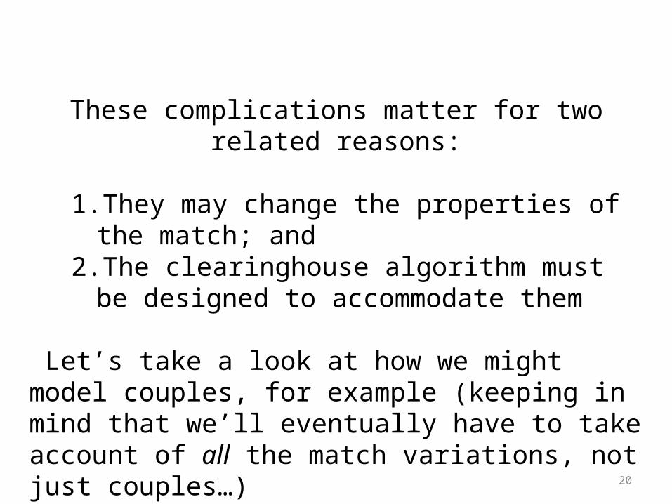
These complications matter for two related reasons:

1. They may change the properties of the match; and 2. The clearinghouse algorithm must be designed to

accommodate them Let’s take a look at how we might model couples, for example (keeping in mind that we’ll eventually have to take account of all the match variations, not just couples…)

21Harry S. Jonas, MD, Sylvia I. Etzel, ”Undergraduate Medical Education,” JAMA, Aug 26, 1988, vol. 260, 8 1063-1071, 3008.

Married couples looking for two residencies weren’t an issue in the medical job market until the 1970’s

22

Chart 4, http://www.aamc.org/data/facts/charts1982to2010.pdf

8035/16,468=.49

23

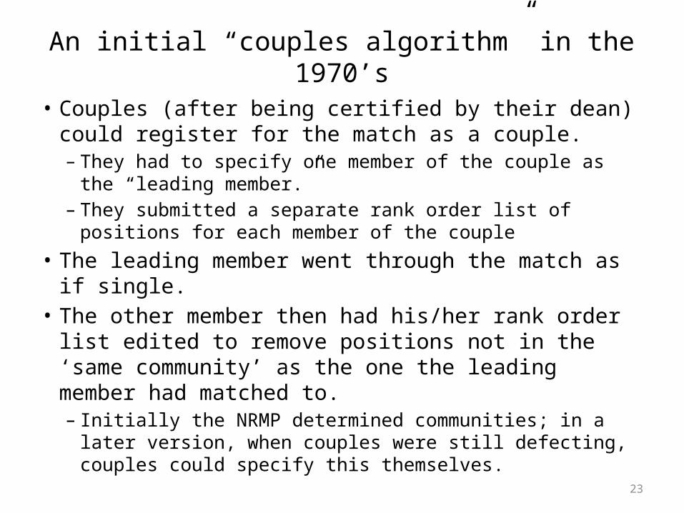
An initial “couples algorithm” in the 1970’s• Couples (after being certified by their dean) could register

for the match as a couple.– They had to specify one member of the couple as the “leading

member.”– They submitted a separate rank order list of positions for each

member of the couple• The leading member went through the match as if single.• The other member then had his/her rank order list edited

to remove positions not in the ‘same community’ as the one the leading member had matched to.– Initially the NRMP determined communities; in a later version,

when couples were still defecting, couples could specify this themselves.

24

A similar algorithm is used in Scotland today

• “Linked applicants• To accommodate linked applicants, a joint preference list is

formed for each such pair, using their individual preference lists and the programme compatibility information. If such a pair, a and b, have individual preferences p1, p2, . . . , p10 and q1, q2, . . . , q10 respectively (with a the higher scoring applicant), then the joint preference list of the pair (a,b) is (p1,q1), (p1,q2), (p2,q1), (p2,q2), (p1,q3), (p3,q1), (p2,q3), (p3,q2), . . ., (p9,q10), (p10,q9), (p10,q10) (except that incompatible pairs of programmes are omitted) “

• http://www.nes.scot.nhs.uk/sfas/About/default.asp

25

But this didn’t work well for couples• Why?• The iron law of marriage: You can’t be happier than

your spouse.• Couples consume pairs of jobs. So an algorithm that

only asks for their preference orderings over individual jobs can’t hope to avoid instabilities (appropriately redefined to include couples’ preferences)

• But even if we ask couples for their preferences over pairs of jobs, we may still have a problem: Roth (1984) observed that the set of stable matchings may be empty when couples are present.

26

A More Complex Market: Matching with Couples This model is the same as the college admissions model, except the set of workers is replaced by a set of applicants that includes individuals and couples. Denote the set of applicants by A = A1C, where A1 is the set of (single) applicants who seek no more than one position, and C is the set of couples {ai, aj} such that ai is in the set A2 (of husbands) and aj is in the set A3, and the sets of applicants A1, A2, and A3 together make up the entire population of individual applicants, A' = A1A2A3. Each couple c={ai,aj} in C has preferences over ordered pairs of positions, i.e. an ordered list of elements of FxF. The first element of this list is some (ri,rj) in FxF which is the couples' first choice pair of jobs for ai and aj respectively, and so forth. Applicants in the set A1 have preferences over residency programs, and residency programs (firms) have preferences over the individuals in A', just as in the simple model discussed earlier. (That is, firms view the members of a couple as two distinct individuals…)

27

A matching is a set of pairs in FxA‘.

Each single applicant, each couple, and each residency program submits to the centralized clearinghouse a Rank Order List (ROL) that is their stated preference ordering of acceptable alternatives.

A matching is blocked by a single applicant (in the set A1), or by a residency program, if matches that agent to some individual or residency program not on its ROL.

A matching is blocked by an individual couple (ai,aj) if they are matched to a pair (ri,rj) not on their ROL.

A residency program r and a single applicant a in A1 together block a matching precisely as in the college admissions market, if they are not matched to one another and would both prefer to be.

28

A couple c=(a1,a2) and residency programs r1 and r2 block if the couple prefers (r1,r2) to (c), and either r1 and r2 each would prefer to be matched to the corresponding couple member, or if one of them would prefer, and the other already is matched to the corresponding couple member. That is, c and (r1,r2) block if 1. (r1,r2) >c(c); and if either

2. {(a1 (r1), and a1 >r1 ai for some ai (r1) or a1 is acceptable to r1 and |(r1)| < q1 } and either a2(r2) or {a2 (r2), a2 >r2 aj for some aj (r2) or a2 is acceptable to r2 and |(r2)| < q2}

or 3. a1(r1) and {a2 (r2), and a2 >r2 aj for some aj (r2) or a2 is

acceptable to r2 and |(r2)| < q2}

29

A matching is stable if it is not blocked by any individual or by a an individual and a residency program, or by a couple together with one or two residency programs Theorem 5.11 (Roth ’84): In the college admissions model with couples, the set of stable matchings may be empty. Proof: by (counter)example. (Which was sufficient, when I didn’t have design responsibility…)

30

Example--market with one couple and no stable matchings (motivated by Klaus and Klijn, and Nakamura (JET corrigendum 2009 to K&K JET 2005): Let c=(s1,s2) be a couple, and suppose there is another single student s3, and two hospitals h1 and h2. Suppose that the acceptable matches for each agent, in order of preference, are given by c: (h1,h2); s3: h1, h2, h1: s1, s3; h2: s3, s2 Then no individually rational matching μ (i.e. no μ that matches agents only to acceptable mates) is stable. We consider two cases, depending on whether the couple is matched or unmatched. Case 1: μ(c)=(h1,h2). Then s3 is unmatched, and s/he and h2 can block μ, because h2 prefers s3 to μ (h2)=s2. Case 2: μ (c)=c (unmatched). If μ (s3)=h1, then (c, h1,h2) blocks μ. If μ (s3)=h2 or μ (s3)=s3 (unmatched), then (s3,h1) blocks μ.

31

Why is the couples problem hard?• Note first that the ordinary deferred acceptance

algorithm won’t in general produce a stable matching (even when one exists, and even when couples state preferences over pairs of positions)– In the worker proposing algorithm, if my wife and I

apply to a pair of firms in Boston, and our offers are held, and I am later displaced by another worker, my wife will want to withdraw from the position in which she is being held (and the firm will regret having rejected other applications to hold hers)

– In the firm proposing algorithm, it may be hard for a couple to determine which offers to hold.

32

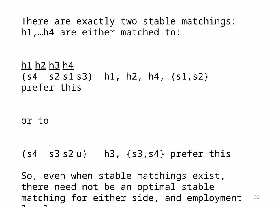
Furthermore, the following example shows that even when the set of stable matchings is non-empty, it may no longer have the nice properties we’ve come to expect. Matching with couples (Example of Aldershof and Carducci, ’96)4 hospitals {h1,…h4} each with one position; 2 couples {s1,s2} and {s3,s4} Preferences:h1 h2 h3 h4 {s1,s2} {s3,s4}S4 s2 s2 s2 h3h2 h2h1S3 s3 s4 s3 h2h3 h2h3

S1 s1 h2h4 h1h3 h3h4 h4h1 u h3 h4h3 u h2 u h4 h3 u h2 u

33

There are exactly two stable matchings: h1,…h4 are either matched to:

h1 h2 h3 h4(s4 s2 s1 s3) h1, h2, h4, {s1,s2} prefer this

or to

(s4 s3 s2 u) h3, {s3,s4} prefer this So, even when stable matchings exist, there need not be an optimal stable matching for either side, and employment levels may vary.

34

So we can start to note theorems about simple markets whose conclusions do not carry over to markets with the NRMP match variations (even just with couples).

In a simple matching market:

1. the set of stable matchings is always nonempty

2. the set of stable matchings always contains a "program optimal" stable matching, and an "applicant optimal" stable matching.

3. the same applicants are matched and the same positions are filled at every stable matching.

Similarly, strategic results about simple markets won’t carry over unchanged to the more complex medical market.

35

Strategic behavior in simple markets (without match variations):

1. In simple markets, when the applicant proposing algorithm is used, but not when the hospital proposing algorithm is used, no applicant can possibly improve his match by submitting an ROL that is different from his true preferences.

2. In simple markets when the program proposing algorithm is used, every applicant who can do better than to submit his true preferences as his ROL can do so by submitting a truncation of his true preferences.

3. In simple markets, when the program proposing algorithm is used, the only applicants who can do better than to submit their true preferences are those who would have received a different match from the applicant proposing algorithm.

Furthermore, the best such applicants can do is to obtain the applicant optimal match.

36

Descriptive Statistics: NRMP 1987 1993 1994 1995 1996

APPLICANTS

Primary ROL’s 20071 20916 22353 22937 24749 Applicants with Supplemental ROL’s

1572 2515 2312 2098 2436

Couples

Applicants who are Coupled 694 854 892 998 1008 PROGRAMS

Active Programs 3225 3677 3715 3800 3830 Active Programs with ROL Returned

3170 3622 3662 3745 3758

Potential Reversions of Unfilled Positions

Programs Specifying Reversion

69 247 276 285 282

Positions to be Reverted if Unfilled

225 1329 1467 1291 1272

Programs Requesting Even Matching

4 2 6 7 8

Total Quota Before Match 19973 22737 22801 22806 22578

37

Because conclusions about simple markets can have counterexamples in the complex medical market, there were points at which we had to rely on computational explorations to see how close an approximation the simple theory provides for the complex market. We relied on computation in three places:

Computational experiments were used in the algorithm design. Computational explorations of the data from previous years were used to study the effect of different algorithms. Theoretical computation, on simple markets, was used to understand the relation between market complexity and market size.

38

Before we talk about computational experiments, let’s think about what class of algorithms we might want to explore. The deferred acceptance algorithm for simple matching models gave us a one pass algorithm; it starts with everyone unmatched, and never cycles. Our sense was that we weren’t going to be able to do that in the complex problem, but rather that we’d have to build a stable matching (if one existed), resolving blocking pairs as we identified them. E.g. if (m',w') is a blocking pair for a matching , a new matching can be obtained from by satisfying the blocking pair if m' and w' are matched to one another at , their mates at (if any) are unmatched at , and all other agents are matched to the same mates at as they were at . But even for the simplest models (e.g. the marriage model) this can cycle, and might not converge to a stable matching (an observation originally due to Donald Knuth: see the discussion of Example 2.4 in Roth and Sotomayor). In the marriage model there’s a way around this problem.

39

Theorem 2.33 (Roth and Vande Vate, 1990): Let be an arbitrary matching for (M, W, P). Then there exists a finite sequence of matchings 1,...,k, such that = 1,… k is stable, and for each i = 1,...,k-1, there is a blocking pair (mi, wi) for i such that i+1 follows from i by satisfying the pair (mi, wi).

40

Elements of the proof: Let 1 be an arbitrary (w.l.o.g individually rational) matching with blocking pair (m1,w1). Let 2 be the matching obtained by satisfying the blocking pair, and define the set A(1) = {m1,w1}.

Inductive assumption: Let A(q) be a subset of MW such that there are no blocking pairs for q+1 contained in A(q), and such that q+1 does not match any agent in A(q) to any agent outside of A(q).

Then if q+1 isn’t stable, there is a blocking pair (m’,w’) such that at most one of m’ and w’ is contained in A(q). (If neither of {m’,w’} is in A(q), let A(q+1) = A(q){m’,w’} and let q+2 be obtained from q+1 by satisfying the blocking pair (m’,w’).

Otherwise, one of the pair is in A(q), say m’ (in the other case the symmetric argument will apply). Let A(q+1) = A(q){w’}. Now run the deferred acceptance algorithm, just in the set A(q+1), starting with w’ proposing and continuing until a matching is reached with no blocking pairs among the members of A(q+1). The output is q+2.

41

This suggests a new class of algorithms, of which the deferred acceptance algorithm is a special case. Start with an arbitrary matching , and select a subset A of agents such that there are no blocking pairs for contained in A, and does not match any agent in A to any agent not in A. (For example, A could be a pair of agents matched under , or a single agent, or the set of all men.) A new player, say woman w, is selected to join A. If no man in A is part of a blocking pair with woman w, we may simply add her to A without changing the matching. Otherwise, select the man m whom woman w most prefers among those in A with whom she forms a blocking pair, and form a new matching by satisfying this blocking pair. If there is a woman w' = (m), then she is left unmatched at this new matching, and so there may now be a blocking pair (w',m') contained in A. If so, choose the blocking pair most preferred by w' to form the next new matching.

42

The process continues in this way within the set A{w}, like the deferred acceptance algorithm with women proposing, satisfying the blocking pairs which arise at each step until the process terminates with a matching i having no blocking pairs within Ai = S{w}.

The process can now be continued, with the selected set Ai growing at each stage. At each stage, the selected set has no blocking pairs in it for the associated matching I, and so the process converges to a stable matching when Ak = MW.

In the deferred acceptance algorithm with men proposing, the initial matching is the one at which all agents are single, and the initial set A is A=W.

In the deferred acceptance algorithm with men proposing, the welfare of the women rises monotonically throughout the algorithm. In this more general class of algorithms there is no parallel, since agents from either side may be introduced into the set A. But the set A itself grows, so the algorithm converges.

So, we’ll be looking for an algorithm that accumulates agents not involved in blocking pairs…

43

Computational experiments in the algorithm design. The process by which the applicant-proposing algorithm was designed is roughly as follows. First, a conceptual design was formulated and circulated for comment, based on the family of algorithms explored (for the marriage model) in Roth and Vande Vate (1990). ("Random Paths to Stability in Two-Sided Matching," Econometrica, 58, 1990, 1475-1480.) To code this into a working algorithm, a number of choices had to be made, concerning the sequence in which operations would be conducted.

Most of these decisions can be shown to have no effect on the outcome of simple matches, but could potentially effect the outcome when the NRMP match variations are present. Consequently, we performed computational experiments before making sequencing choices. (Throughout the algorithm design process, we also posted progress reports on the web, where they were available to all interested parties. Since designs often have to be adopted my multiple constituencies, the design process might be important…)

44

• Do sequencing differences cause substantial or predictable changes in the match result (e.g. do applicants or programs selected first do better or worse than their counterparts selected later)?

• Does the sequence of processing affect the likelihood that an algorithm will produce a stable matching?

Experiments to test the effect of sequencing were conducted using data from three NRMP matches: 1993, 1994, and 1995.

The results were that sequencing effects existed, but were unsystematic, and effected on the order of 1 in 10,000 matches.

(In the majority of years and algorithm sequences examined, the match was unaffected by changes in sequencing of algorithm operations, and in the majority of the remaining cases only 2 applicants received different matches.) However sequencing decisions did influence the speed of convergence to a stable matching.

45

Based on the sequencing experiments described above, the following decisions were made pertaining to the design of the applicant proposing algorithm for the NRMP:

1. All single applicants are admitted to the algorithm for processing before any couples are admitted.

2. Single applicants are admitted for processing in ascending sequence by applicant code.

3. Couples are admitted for processing in ascending sequence by the lower of the two applicant codes of the couple.

When a program is selected from the program stack for processing, the applicants ranked by the program are processed in ascending order by program rank number (i.e. in order of the program’s preferences).

46

47

Computational Exploration of the Difference Between Program and Applicant Proposing Algorithms

1987 1993 1994 1995 1996

APPLICANTS

Number of Applicants Affected

20 16 20 14 21

Applicant Proposing Result Preferred

12 16 11 14 12

Program Proposing Result Preferred

8 0 9 0 9

New Matched 0 0 0 0 1

New Unmatched 1 0 0 0 0

PROGRAMS

Number of Programs Affected

20 15 23 15 19

Applicant Proposing Result Preferred

8 0 12 1 10

Program Proposing Result Preferred

12 15 11 14 9

Programs with New Position(s) Filled

0 0 2 1 1

Programs with New Unfilled Positions

1

0

2

0

0

48

If this were a simple market, the small number of applicants whose matching is changed when we switch from hospitals proposing to applicants proposing would imply that there was also little room for strategic behavior when it comes time to state rank order lists. We can find out if this is also true in the complex market with computational experiments. It turns out that we don’t have to experiment on each individual separately, to put an upper bound on how many individuals could profitably manipulate their preferences. (For the moment, we treat the submitted preferences as the true preferences—we’ll see in a minute why that is justified.)

49

Computational experiments to find upper bounds for the scope of strategic behavior

Truncations at the match point (to check if examining truncations is sufficient in the multi-pass algorithm…)

Difference in result for both the program proposing algorithm and the applicant proposing algorithm when applicant ROLs truncated at the match point:

1993 1994 1995

none 2 applicants improve, same positions filled

2 applicants improve, same positions filled

Difference in result for the program proposing algorithm when program ROLs truncated at the match point:

1993 1994 1995

none none 2 applicants do worse, same positions filled

50

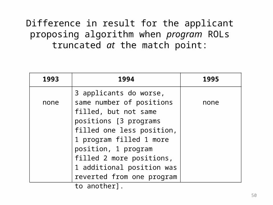
Difference in result for the applicant proposing algorithm when program ROLs truncated at the match point:

1993 1994 1995

none3 applicants do worse, same number of positions filled, but not same positions [3 programs filled one less position, 1 program filled 1 more position, 1 program filled 2 more positions, 1 additional position was reverted from one program to another].

none

51

Results for Iterative Truncations of Applicant ROL’s just above the match point

1993 1994

Program Proposing Algorithm Applicant Proposing Program Proposing Algorithm Applicant Proposing

Truncated Truncated & Improved

Truncated Truncated & Improved

Truncated Truncated & Improved

Truncated Truncated & Improved

Run 1 17209 4546 17209 4536 17725 4935 17725 4934

Run 2 4546 2093 4536 2082 4935 2361 4934 2359

Run 3 2093 1036 2082 1023 2361 1185 2359 1183

Run 4 1036 514 1023 498 1185 602 1183 598

Run 5 514 258 498 241 602 292 598 287

Run 6 258 135 241 116 292 151 287 143

Run 7 135 73 116 52 151 75 143 66

Run 8 73 48 52 25 75 40 66 31

Run 9 48 34 25 12 40 27 31 17

Run 10 34 27 12 5 27 18 17 7

Run 11 27 24 5 2 18 14 7 3

Run 12 24 22 2 0 14 13 3 2

Run 13 22 22 13 13 2 2

52

The truncation experiments with applicants' ROLs yield the following upper bounds for the two algorithms in the years studied.

Upper limit of the number of applicants who could benefit by truncating their lists at one above their original match point:

1987 1993 1994 1995 1996

Program-Proposing Algorithm12 22 13 16 11

Applicant-Proposing Algorithm0 0 2 2 9

As expected, more applicants can benefit from list truncation under the program-proposing algorithm than under the applicant-proposing algorithm. Note that the number of applicants who could even potentially benefit from truncating their ROLs under the program-proposing algorithm is in each year almost exactly equal to the number of applicants who received a preferred match under the applicant proposing match (line 2 of Table 2). This suggests that this upper bound is very close to the precise number that would be predicted in the absence of match variations.

53

The truncation experiments with programs' ROLs yield the following upper bounds.

Upper limit of the number of programs that could benefit by truncating their lists at one above the original match point:

1987 1993 1994 1995 1996

Program-Proposing Algorithm 15 12 15 23 14

Applicant-Proposing Algorithm 27 28 27 36 18

As expected, some programs can benefit from list truncation under either algorithm. However, consistently more programs benefit from list truncation under the applicant-proposing algorithm than under the program-proposing algorithm. Note that although the numbers of programs in these upper bounds remain small, they are in many cases about twice as large as the number of programs which received a preferred match at the stable matching produced by the algorithm other than the one being manipulated.

Refined estimate of the upper limit of the number of programs that could improve their results by truncating their own ROL’s in 1995 (Based on 50% sample):

Program Proposing Algorithm Applicant Proposing Algorithm

Original Results 23 36

Current Estimate (still an upper limit) 12 22

54

Residency programs have another dimension on which they can manipulate; they not only have to report their preferences, but also how many positions they wish to fill. As we’ve seen in examples of the (simple) college-admissions model, and as in multi-unit auctions, they may potentially benefit from demand reductions.

(And for an impossibility theorem on avoiding capacity manipulation, see Sonmez, Tayfun [1997], "Manipulation via Capacities in Two-Sided Matching Markets," Journal of Economic Theory, 77, 1, November, 197-204.)

Revised Estimate of the Upper Bound of the Number of Programs That Could Improve Their Remaining Matches By Reducing Quotas

1987 1993 1994 1995 1996

Program Proposing Algorithm 28 16 32 8 44

Applicant Proposing Algorithm 8 24 16 16 32

This will be worth thinking about again—a small cloud on the horizon—when we consider what temptations may exist for residency programs to hire some of their people early, before the match. If there are such temptations, they may not be counterbalanced by a tendency to do worse in the match, on the contrary, reducing demand may have small spillover benefits in the match for the remaining candidates…

55

Overall, the striking thing about all these computational results is how small the set of stable outcomes appear to be; i.e. how few applicants or programs are affected by a switch from program proposing to applicant proposing, and how small are the opportunities to misrepresent preferences or capacities.

But we don’t really understand the structure of the set of stable matchings when there are couples, supplementary lists, and reversion of positions from one program to another. So there’s a chance that we’re making a big mistake here.

For example, we know that program and applicant optimal stable matchings no longer exist, but we’ve been studying the set of stable matchings by looking at the outcomes of the program and applicant proposing algorithms. Maybe the set of stable matchings isn’t all located between these two matchings when all the match variations are present; maybe the set of stable matchings just appears to be small because we don’t know where to look.

Even if our conclusions are correct, we’d like to know why. Could it be some spooky interaction between the size of the market and the presence of complications? Or does the core simply get small as the market gets large, even in simple markets?

Two approaches:• Empirical: examine some simple markets• Theoretical/computational: explore some artificial simple markets

56

The Thoracic surgery match is a simple match, with no match variations. It exactly fits the college admissions model; those theorems all apply.

Descriptive statistics and original Thoracic Surgery match results

1991 1992 1993 1994 1996

Applicant ROL’s 127 183 200 197 176

Active Programs 67 89 91 93 92

Program ROL’s 62 86 90 93 92

Total Quota 93 132 141 146 143

Positions Filled 79 123 136 140 132

Difference in Thoracic Surgery results when algorithm changed from program proposing to applicant proposing:

1991 1992 1993 1994 1996

none 2 applicants improve2 programs do worse

2 applicants improve2 programs do worse none none

57

Theoretical computation on a simple model Simple model: n firms, n workers, (no couples) uncorrelated preferences, each worker applies to k firms. C(n) = number of workers matched differently at μF and μW

58

Large core with k=n: C(n)/n is the proportion of workers who receive different matches at different stable matchings, in a simple market (no couples) with n workers and n firms (each of which employs one worker) when preferences are uncorrelated and each preference list consists of all n agents on the other side of the market. (from Roth and Peranson, 1999) Note that as the market grows large in this way, so does the set of stable matchings, in the sense that for large markets, almost every worker is effected by the choice of stable matching.

59

Small core of large markets, with k fixed as n grows: C(n)/n is the proportion of workers who receive different matches at different stable matchings, in a simple market with n workers and n firms, when each worker applies to k firms, each firm ranks all workers who apply, and preferences are uncorrelated. (from Roth and Peranson, 1999). Note that for any fixed k, the set of stable matchings grows small as n grows large.

60

The numerical results show us that C(n)/n gets small as n gets large when k is fixed, (even) for uncorrelated preferences.

And of course, in these simulated markets, we see that the core gets small not because of strategic behavior—these are the true preferences.

This also implies that in large markets it is almost a dominant strategy for every agent to reveal his true preferences—only one in a thousand could profit by strategically mis-stating preferences (if they had full information about all preferences).

61

In my class in the Spring of 2003, I posed the following as an Open Problem: Prove: The core gets small (in some expected value sense) as the market gets large, if the number of interviews doesn’t also get large. Two of the students in that class did so…Nicole Immorlica and Mohammad Mahdian, “Marriage, Honesty and Stability,” Immorlica, SODA 2005, 53-62. Theorem (Immorlica and Mahdian, 2003:) Consider a marriage model with n men and n women, in which each woman has an arbitrary complete preference list, and each man has a random list of at most k women as his preference list (chosen uniformly and independently).Then, the expected number of women who have more than one stable husband is bounded by a constant that only depends on k (and not on n).(So, as n gets large, the proportion of such women goes to zero…)

62

More recently, two former students have substantially generalized the result, to state that, as the market gets large, the opportunity for firms to manipulate either their preferences or their capacities gets small, in the sense that the proportion of firms with such an opportunity will go to zero. Theorem (Kojima and Pathak, AER 2009): In the limit, as n goes to infinity in a regular sequence of random (many-to-one) markets, the proportion of employers who might profit from (any combination of) preference or capacity manipulation goes to zero in the worker proposing deferred acceptance algorithm.

63

Still (mostly) open empirical puzzle

• Why do these algorithms virtually always find stable matchings, even though couples are present (and so the set of stable matchings could be empty)?

64

Stylized facts

1. Applicants who participate as couples constitute a small fraction of all participating applicants.

2. The length of single applicants' rank order lists is small relative to the number of possible programs.

3. Applicants who participate as couples rank more programs than single applicants. However, the number of distinct programs ranked by a couple member is small relative to the number of possible programs.

4. The most popular programs are ranked as a top choice by a small number of applicants.

5. A pair of hospital programs ranked by doctors who participate as a couple tend to be in the same region.

6. Even though there are more applicants than positions, many programs still have unfilled positions at the end of the centralized match.

7. A stable matching exists in all nine years in the market for clinical psychologists.

65

Two initial approaches

• Kojima, Fuhito, Parag A. Pathak, and Alvin E. Roth, “Matching with Couples: Stability and Incentives in Large Markets,” Quarterly Journal of Economics, (2013) 128 (4): 1585-1632.

• Stability in large matching markets with complementarities (previously called Matching with Couples - Revisited) Itai Ashlagi, Mark Braverman and Avinatan Hassidim, forthcoming in Operations Research (Extended abstract appears in EC 11.)

66

Random markets• A random market is a tuple Γ=(H,S,C, ≽{Hⁿ}, k,P,Q,ρ),

where k is a positive integer (max length of ROL’s), P=(p{h}){h H}∈ and Q=(q{h}){h H}∈ are probability distributions on H, and ρ is a function which maps two preferences over H to a preference list for couples.

• Hospitals’ preference orderings are essentially arbitrary, and take account of their capacities, and couples preferences are formed from their individual preferences (drawn from probability distribution Q, different than P for singles), via an essentially arbitrary function ρ .

67

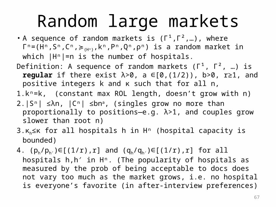
Random large markets• A sequence of random markets is (Γ¹,Γ²,…), where

Γⁿ=(Hⁿ,Sⁿ,Cⁿ,≽{Hⁿ},kⁿ,Pⁿ,Qⁿ,ρⁿ) is a random market in which |Hⁿ|=n is the number of hospitals.

Definition: A sequence of random markets (Γ¹, Γ², …) is regular if there exist λ>0, a [0,(1/2)), b>0, r≥1, and positive integers k and ∈ κ such that for all n,

1.kⁿ=k, (constant max ROL length, doesn’t grow with n)2.|Sⁿ| ≤λn, |Cⁿ| ≤bna, (singles grow no more than proportionally to

positions—e.g. λ>1, and couples grow slower than root n)3.κh≤κ for all hospitals h in Hⁿ (hospital capacity is bounded) 4. (ph/ph′) [(1/r),r] and (q∈ h/qh′) [(1/r),r] for all hospitals h,h in Hⁿ. ∈ ′

(The popularity of hospitals as measured by the prob of being acceptable to docs does not vary too much as the market grows, i.e. no hospital is everyone’s favorite (in after-interview preferences)

68

A (really simple) sequential couples algorithm (like left side of RP flow chart)

1.run a deferred acceptance algorithm for a sub-market composed of all hospitals and single doctors, but without couples,

2.one by one, place couples by allowing each couple to apply to pairs of hospitals in order of their preferences (possibly displacing some doctors from their tentative matches), and

3.one by one, place singles who were displaced by couples by allowing each of them to apply to a hospital in order of her preferences.

We say that the sequential couples algorithm succeeds if there is no instance in the algorithm in which an application is made to a hospital where an application has previously been made by a member (or both members) of a couple except for the couple who is currently applying. Otherwise, we declare a failure and terminate the algorithm.

Lemma: If the sequential couples algorithm succeeds, then the resulting matching is stable.

69

Stable matchings exist, in the limit

• Theorem: Suppose that (Γ¹,Γ²,…) is a regular sequence of random markets. Then the probability that there exists a stable matching in the market induced by Γⁿ converges to one as the number of hospitals n approaches infinity.

70

Key element of proof• if the market is large, then it is a high probability

event that there are a large number of hospitals with vacant positions at the end of Step 2 (even though there could be more applicants than positions) (i.e. the Scramble will remain important in large markets.)

• So chains of proposals beginning when a couple displaces a single doc are much more likely to terminate in an empty position than to lead to a proposal to a hospital holding the application of a couple member.

71

Formal statementProposition: many hospitals have vacancies in large

marketsThere exists a constant b > 0 such that (1) the probability that, in a sub-market without couples,

the doctor-proposing deferred acceptance algorithm produces a matching in which at least b*n hospitals have at least one vacant position converges to one as n approaches infinity, and

(2) the probability that the sequential couples algorithm produces a stable matching and at least b*n hospitals have at least one vacant position in the resulting matching converges to one as n approaches infinity.

72

Corollary

• Corollary: Suppose that (Γ¹,Γ²,…) is a regular sequence of random markets. Then the probability that the Roth-Peranson algorithm produces a stable matching in the market induced by Γⁿ converges to one as the number of hospitals n approaches infinity.

73

Stable Clearinghouses (those now using the Roth Peranson Algorithm)

NRMP / SMS:Medical Residencies in the U.S. (NRMP) (1952)Abdominal Transplant Surgery (2005) Child & Adolescent Psychiatry (1995) Colon & Rectal Surgery (1984) Combined Musculoskeletal Matching Program (CMMP) • Hand Surgery (1990) Medical Specialties Matching Program (MSMP) • Cardiovascular Disease (1986)

• Gastroenterology (1986-1999; rejoined in 2006)

• Hematology (2006) • Hematology/Oncology (2006) • Infectious Disease (1986-1990; rejoined in 1994) • Oncology (2006) • Pulmonary and Critical Medicine (1986) • Rheumatology (2005) Minimally Invasive and Gastrointestinal Surgery (2003) Obstetrics/Gynecology • Reproductive Endocrinology (1991) • Gynecologic Oncology (1993) • Maternal-Fetal Medicine (1994) • Female Pelvic Medicine & Reconstructive Surgery (2001) Ophthalmic Plastic & Reconstructive Surgery (1991) Pediatric Cardiology (1999) Pediatric Critical Care Medicine (2000) Pediatric Emergency Medicine (1994) Pediatric Hematology/Oncology (2001) Pediatric Rheumatology (2004) Pediatric Surgery (1992)

Primary Care Sports Medicine (1994)Radiology • Interventional Radiology (2002) • Neuroradiology (2001) • Pediatric Radiology (2003) Surgical Critical Care (2004) Thoracic Surgery (1988) Vascular Surgery (1988)

Postdoctoral Dental Residencies in the United States• Oral and Maxillofacial Surgery (1985)• General Practice Residency (1986)• Advanced Education in General Dentistry (1986)• Pediatric Dentistry (1989)• Orthodontics (1996)Psychology Internships in the U.S. and CA (1999)Neuropsychology Residencies in the U.S. & CA (2001)Osteopathic Internships in the U.S. (before 1995)Pharmacy Practice Residencies in the U.S. (1994)Articling Positions with Law Firms in Alberta, CA(1993)Medical Residencies in CA (CaRMS) (before 1970)

********************British (medical) house officer positions• Edinburgh (1969)• Cardiff (197x)

New York City High Schools (2003)Boston Public Schools (2006)

74

Scramble

• if the market is large, then it is a high probability event that there are a large number of hospitals with vacant positions at the end of a centralized match with short preference lists (even though there could be more applicants than positions) (i.e. the Scramble will remain important in large markets.)

75

76

77

78

79

80

81

82