Matched Filter Bounds onq-ary QAM Symbol ErrorProbability for Diversity Receptions and Multipath Fading

ISI Channels

Abstract - This paper extends previous works in matched filter bounds [2][3][4] and

provides a theoretical calculation of detection probability ofq-ary QAM signals averaged over

the diversity reception and multipath fading ISI channels. The matched filter bounds are the

best attainable detection performance at a given SNR, which may or may not be obtainable in

practice. While an exact analytical expression of detection performance associated with a

practical transceiver over multipath ISI channels is difficult to obtain, the matched filter bounds

provide many useful information to be compared with the simulation results.

Technical Kewords: Matched filter bound, modulation, equalization and diversity

combining.

1. Corresponding author

Information Science Laboratory,HRL Research Laboratories, L.L.C., BLDG 254,

3011 Malibu Canyon Road,Malibu, CA 90265

Phone: (310) 317-5929,FAX: (310) 317-5695

heungno@hrl.com

Electrical Engineering Department,University of California at Los Angeles

P.O. Box 951594Los Angeles, CA 90095

Email: pottie@icsl.ucla.eduPhone: (310) 825-8150,FAX: (310) 206-8495pottie@icsl.ucla.edu

Heung-No Lee1 Gregory J. Pottie

early

g the

by the

of

; for

ceiver

, a

ptive

fficult

on and

on to

udget

lation

n and

o [2],

unds

ennas

d the

ling.

ain the

ond is

n

ity of

ersity

ion to

on of

filter

ipath

I. INTRODUCTION

Based on the matched filter theory (see Chapter 6 of [1]), the detection SNR of any lin

filtered receive-signal is maximized if the matched filter, which can be obtained assumin

receiver has the perfect knowledge of the filter, is applied to the received signal perturbed

additive noise. In this paper, we use the matched filters to derive the symbol error probabilityq-

ary QAM signals transmitted over the diversity reception and multipath fading ISI channels

description of the communication channel, see Figure -1. A complete system of a trans

involves many different function blocks, including a channel estimation and tracking

synchronization, an adaptive diversity combining and equalization, and possibly an ada

sequence decision [8][9]. In such systems, an exact calculation of detection probability is di

and the approach may also dependent upon a particular selection of fading rate, detecti

estimation conditions. Thus, most of times it is considered to be better off to perform simulati

obtain the exact detection performance of a system. Meanwhile, as a tool to calculate link-b

requirement or as a tool to support/verify the simulation results, a fundamental capacity calcu

which can be computed relatively easily and applied regardless of any particular estimatio

detection scheme is extremely useful.

Previous works in calculating the matched filter bounds on fading channels include Maz

Clark et. al. [3], Ling [4], Proakis [6] and Jake [7]. In Jake and Proakis, the matched filter bo

are derived for the maximal ratio combining receiver, where each of the receive diversity-ant

in Figure -1 is assumed to be a single tap Rayleigh fading. Mazo, Clark and Ling extende

results for multipath fading frequency-selective channels with BPSK, 4-PSK or QPSK signa

Summarizing their approaches, we note that there are three major steps. The first is to obt

bit error or symbol error probability (SEP) expression of a single and static channel. The sec

to taking theexpectationof the SEP overensembleof the channel. This results in a well-know

integral form which involves an integral of error probability function over agammadistribution.

The gamma distribution represents the probability density function, denoting the probabil

matched filter SNR taking a particular value. The third part is to generalize the second to div

reception and fading ISI channels. This part involves the use of eigenvalue decomposit

decorrelate the matched filter SNR. The matched filter SNR is the quadratic combinati

correlated random variables, resulting from common transmit-shape filter, the matched

operation and diversity combining, which add up all the available SNR at each of the mult

2

obtain

part to

rk of

ds are

nds

ecific

btain

n III.

ses of

, and 3)

arks.

hrough

ntenna

pon

ples at

of the

rtant

etec-

per

filter

less

components and diversity antennas. Eigenvalue decomposition provides the tools to

decorrelated SNR random variables. Then, the rest is repeated application of the second

each of the decorrelated SNR random variables.

The derivation of matched filter bounds in this paper follows the same general framewo

above three steps. The major contribution of the paper includes that the matched filter boun

obtained for -ary QAM signalling, where is 4, 16, and 64. In addition, the matched filter bou

are derived for fractionally-spaced channels with the reception-diversity. Thus, with a sp

example of fractionally-spaced multipath-power delay profiles (MPDPs), one can readily o

the matched filter bounds and compare with their computer-simulation results.

Organization of the paper is as follows: Section II. provides system description. Sectio

describes the detailed derivation of matched filter bound. Section IV. discusses three ca

interests. The three areas are 1) a single ISI channel case, 2) maximal ratio combining case

receive diversity-channels, each of the channel being ISI. Section V. provides concluding rem

II. SYSTEM DESCRIPTION

Figure -1 describes the underlying channel and matched filter system.q-ary QAM symbols are

generated and pulse-shaped by the transmit filter . The transmitted signal propagates t

the wireless channel and arrive to the space-diversity antennas at the receiver. At each a

branch, the independent wireless channel is modelled as filters . U

receiving the signal, the optimal receiver performs matched filtering at each branch and sam

the optimum sampling point. The detection performance will be evaluated on the sample

received signal. Before starting with the derivations, let us describe some of the impo

assumptions we make in the derivation:

• Assumption 1: Matched filter bound is based on a single-shot symbol transmission and d

tion such that it ignores any intersymbol interference.

• Assumption 2: The matched filter theory holds with the colored noise; however in this pa

we assume that the noise is complex-valued white Gaussian.

• Assumption 3: The channel is assumed to betime-invariant over the duration of the overall

pulse, which includes the channel and the transmit shaping filter (the anti-aliasing receive

as well).

• Assumption 4: The transmit shaping filter is assumed to employ an excess bandwidth of

q q

f t( )

bl t( ) l 1 … L, ,=,

3

pulse

ated,

al in a

by the

filter

,

-side

ssion

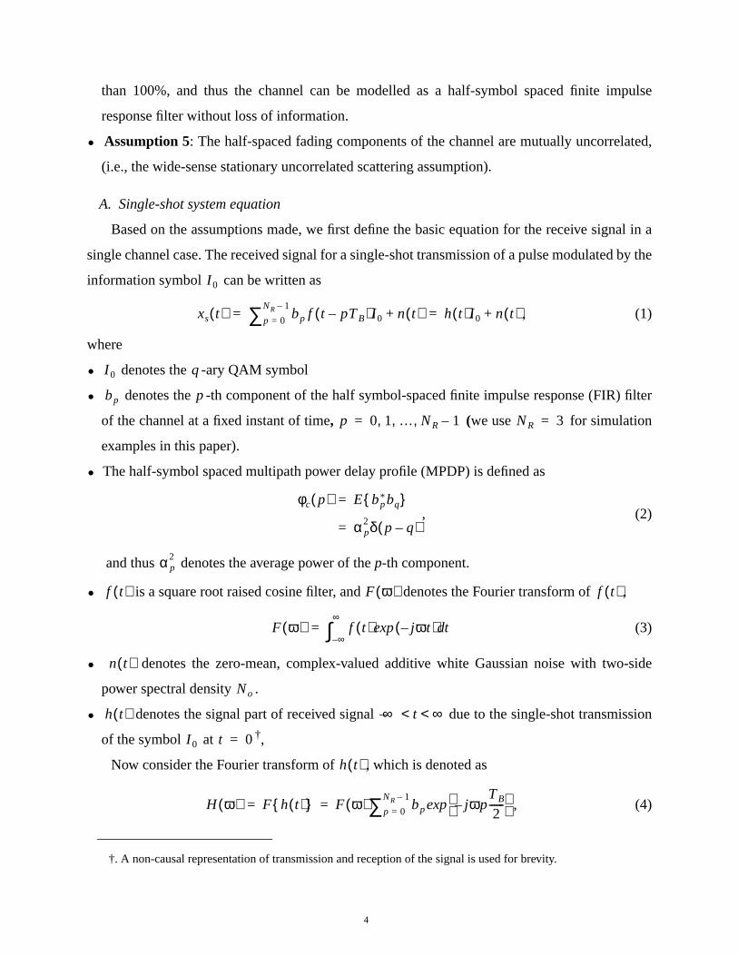
than 100%, and thus the channel can be modelled as a half-symbol spaced finite im

response filter without loss of information.

• Assumption 5: The half-spaced fading components of the channel are mutually uncorrel

(i.e., the wide-sense stationary uncorrelated scattering assumption).

A. Single-shot system equation

Based on the assumptions made, we first define the basic equation for the receive sign

single channel case. The received signal for a single-shot transmission of a pulse modulated

information symbol can be written as

, (1)

where

• denotes the -ary QAM symbol

• denotes the -th component of the half symbol-spaced finite impulse response (FIR)

of the channel at a fixed instant of time, (we use for simulation

examples in this paper).

• The half-symbol spaced multipath power delay profile (MPDP) is defined as

, (2)

and thus denotes the average power of thep-th component.

• is a square root raised cosine filter, and denotes the Fourier transform of

(3)

• denotes the zero-mean, complex-valued additive white Gaussian noise with two

power spectral density .

• denotes the signal part of received signal due to the single-shot transmi

of the symbol at †,

Now consider the Fourier transform of , which is denoted as

, (4)

†. A non-causal representation of transmission and reception of the signal is used for brevity.

I 0

xs t( ) bp f t pTB–( )I 0 n t( )+p 0=

NR 1–∑ h t( )I 0 n t( )+= =

I 0 q

bp p

p 0 1 … NR 1–, , ,= NR 3=

φc p( ) E bp* bq =

αp2δ p q–( )=

αp2

f t( ) F ω( ) f t( )

F ω( ) f t( ) jωt–( )exp td∞–

∞

∫=

n t( )

No

h t( ) ∞– t ∞< <

I 0 t 0=

h t( )

H ω( ) F h t( ) F ω( ) bp jωpTB

2------–

expp 0=

NR 1–∑= =

4

as

tion

e the

ltered

verse

, we

wing

ich is

the

and can

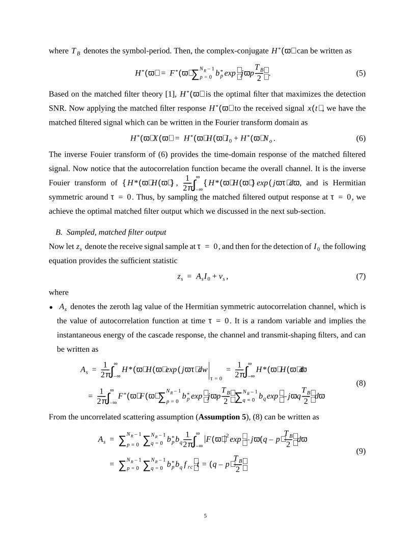
where denotes the symbol-period. Then, the complex-conjugate can be written

. (5)

Based on the matched filter theory [1], is the optimal filter that maximizes the detec

SNR. Now applying the matched filter response to the received signal , we hav

matched filtered signal which can be written in the Fourier transform domain as

. (6)

The inverse Fouier transform of (6) provides the time-domain response of the matched fi

signal. Now notice that the autocorrelation function became the overall channel. It is the in

Fouier transform of , , and is Hermitian

symmetric around . Thus, by sampling the matched filtered output response at

achieve the optimal matched filter output which we discussed in the next sub-section.

B. Sampled, matched filter output

Now let denote the receive signal sample at , and then for the detection of the follo

equation provides the sufficient statistic

, (7)

where

• denotes the zeroth lag value of the Hermitian symmetric autocorrelation channel, wh

the value of autocorrelation function at time . It is a random variable and implies

instantaneous energy of the cascade response, the channel and transmit-shaping filters,

be written as

(8)

From the uncorrelated scattering assumption (Assumption 5), (8) can be written as

(9)

TB H * ω( )

H * ω( ) F * ω( ) bp* jωp

TB

2------

expp 0=

NR 1–∑=

H * ω( )

H * ω( ) x t( )

H * ω( )X ω( ) H * ω( )H ω( )I 0 H * ω( )No+=

H* ω( )H ω( ) 12π------ H* ω( )H ω( ) jωτ( )exp ωd

∞–

∞

∫τ 0= τ 0=

zs τ 0= I 0

zs AsI 0 vs+=

As

τ 0=

As1

2π------ H* ω( )H ω( ) jωτ( )exp wd

∞–

∞

∫τ 0=

12π------ H* ω( )H ω( ) ωd

∞–

∞

∫= =

12π------ F * ω( )F ω( ) bp

* jωpTB

2------

bq jωqTB

2------–

expq 0=

NR 1–∑expp 0=

NR 1–

∑ ωd∞–

∞

∫=

As bp* bqq 0=

NR 1–∑ 12π------ F ω( ) 2 jω q p–( )

TB

2------–

exp ωd∞–

∞

∫p 0=

NR 1–

∑=

bp* bq f rc t q p–( )

TB

2------=

q 0=

NR 1–∑p 0=

NR 1–∑=

5

the

s the

re the

be

-2,

nd the

e

can

where is the raised cosine filter response,

• denotes the transmitted -ary QAM symbol, and

(10)

• denotes the matched filtered noise output sampled at which is

; (11)

thus is zero-mean with .

It is worthwhile to note that (7) provides sufficient information required to compute

detection probability of the single-shot matched filter receiver. Also note that denote

random variable representing the instantaneous energy of the cascade of filters which a

transmit shaping filter, the channels at all diversity branches at a specific time instant.

III. MATCHED FILTER BOUND CALCULATION

A. Square-QAM symbol error probability

In this section, for a particular values of and the symbol error probability will

evaluated for square -ary QAM signaling, i.e. where is even. Referring to Figure

we start with summary of the following relationships which become useful in later sections:

• The average energy of the square-QAM signaling set can be computed as, using (10) a

definition given in Figure -2

. (12)

• The minimum Euclidean distance of the square-QAM constellation is

. (13)

• The instantaneous signal to noise ratio is

= , (14)

where is the instantaneous SNR, the number of bits per symbol, is th

instantaneous SNR/bit.

Then, the -ary square-QAM symbol error probability at a particular channel gain ,

f rc t( )

I 0 q E I0( ) 0.0=

Var I0( ) 2 q 1–( )3

--------------------=

vs t 0=

vs n τ( )h t τ–( ) τd∞–

∞

∫t 0=

=

vs Var vs( ) N0 As⋅=

As

As No

q q 2k= k

Es E I02( )

As

2-------

2 2 q 1–( )3

--------------------As

2-------

2 q 1–3

------------As2= = =

dmin 2 As⋅=

signal powernoise power------------------------------ γ k γ b⋅=

Es

As No⋅----------------=

q 1–( )3

----------------As

No------=

γ k q( )2log= γ b

q As a=

6

f (15)

lently

rage

be computed as

. (15)

(15) can be tightly upper-bounded by the first term, (16). Figure -3 provides the comparison o

and (16). We note that the approximation isasymptotically efficientand very tight even at low SNR

region. Thus, we will use the following approximation

. (16)

Now, solving for in (12), i.e., we have

, (17)

but using (14), (17) is

, (18)

Then, the approximation of the symbol error probability (16) can be written as

, (19)

or simply

. (20)

We will use this approximation to derive the averaged symbol error probability.

B. Average symbol error probability for square-QAM

Now, the symbol error probability, averaged over the ensemble of the channel or equiva

that of , can be computed from

, (21)

where denotes the averaged symbol error probability of -ary QAM system for the ave

Pq As a=( ) 2 1 1

q-------–

erfcdmin a( )

2 Var vs( )---------------------------

112--- 1 1

q-------–

erfcdmin a( )

2 Var vs( )---------------------------

–

⋅=

Pq a( ) 2 1 1

q-------–

erfcdmin a( )2 aNo

------------------ ≈

a a2 3q 1–( )

----------------Es=

dmin a( ) 2a2 3⋅q 1–( )

----------------Es= =

dmin a( ) 2 3⋅q 1–( )

----------------akγ bNo=

Pq a( ) 2 1 1

q-------–

erfc3

2 q 1–( )--------------------kγ b

=

Pq a( ) 2 1 1

q-------–

erfca

2No----------

=

As

Pq γ b( ) Pq a( )Pr As a=( ) ad0∞∫=

Pq γ b( ) q

7

for

, we

r and

e the

be

xed

rgy

itian

alues

input SNR which is defined as

. (22)

Thus, we need to know the distribution function of the random variable .

From (9), we may note that the random variable can be written as follows, using

simplicity of illustration:

. (23)

Denote the matrix in the middle as , where denote the raised cosine function. Now

represent each of the fading channel tap as , multiplication of an attenuation facto

the unit-variance, complex-valued Gaussian random variable . Therefore, we can writ

channel vector as

, (24)

where , a 3 x 3 identity matrix because are assumed to

mutually uncorrelated.

Using (24), (23) can now be rewritten,

, (25)

where in the second line we have defined . It is important to note that for a fi

MPDP, is fixed. Also note that is Hermitian symmetric. In addition, since is the ene

of the cascade filter (8) it is non-negative definite. For any non-negative definite Herm

symmetric matrix , there exist an orthonormal matrix such that , or

(26)

where is a diagonal matrix with the diagonal elements, , = 0, 1, 2, being the eigenv

of the matrix .

γ b E γ b q 1–( )3kNo

----------------E As = =

As

NR 3=

As b0* b1

* b2*( )

f rc 0( ) f rc TB 2⁄( ) f TB( )f rc TB 2⁄( ) f rc 0( ) f rc TB 2⁄( )

f TB( ) f rc TB 2⁄( ) f rc 0( )

b0

b1

b2

=

Frc f rc t( )

bi αiρi=

ρi

b

b αρ

α0 0

α1

0 α2

ρ0

ρ1

ρ2

= =

E ρρH( ) ΞNR NR×= ρi i 0 1 2, ,=,

As bHFrcb ρHαHFrcαρ= =

ρHGρ=

G αHFrcα=

G G As

G Q QGQH Λ=

G QHΛQ=

Λ λp 0≥ p

G

8

ent,

,

ion

, we

el case,

for the

ingle,

d with

s, the

s us to

SNR.

-

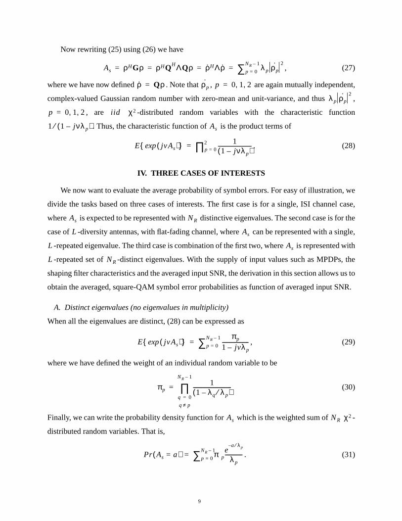
Now rewriting (25) using (26) we have

, (27)

where we have now defined . Note that , are again mutually independ

complex-valued Gaussian random number with zero-mean and unit-variance, and thus

, are -distributed random variables with the characteristic funct

. Thus, the characteristic function of is the product terms of

. (28)

IV. THREE CASES OF INTERESTS

We now want to evaluate the average probability of symbol errors. For easy of illustration

divide the tasks based on three cases of interests. The first case is for a single, ISI chann

where is expected to be represented with distinctive eigenvalues. The second case is

case of -diversity antennas, with flat-fading channel, where can be represented with a s

-repeated eigenvalue. The third case is combination of the first two, where is represente

-repeated set of -distinct eigenvalues. With the supply of input values such as MPDP

shaping filter characteristics and the averaged input SNR, the derivation in this section allow

obtain the averaged, square-QAM symbol error probabilities as function of averaged input

A. Distinct eigenvalues (no eigenvalues in multiplicity)

When all the eigenvalues are distinct, (28) can be expressed as

, (29)

where we have defined the weight of an individual random variable to be

(30)

Finally, we can write the probability density function for which is the weighted sum of

distributed random variables. That is,

. (31)

As ρHGρ ρHQHΛQρ ρHΛρ λp ρp˙ 2

p 0=

NR 1–∑= = = =

ρ Qρ= ρp˙ p 0 1 2, ,=

λp ρp˙ 2

p 0 1 2, ,= iid χ2

1 1 jνλp–( )⁄ As

E jvAs( )exp 11 jνλp–( )

-------------------------p 0=2∏=

As NR

L As

L As

L NR

E jvAs( )exp πp

1 jvλp–--------------------

p 0=

NR 1–∑=

πp1

1 λq λp⁄–( )-----------------------------

q 0=

q p≠

NR 1–

∏=

As NR χ2

Pr As a=( ) πpe

a λp⁄–

λp-------------

p 0=

NR 1–∑=

9

ays

mbol

llation

g fil-

Now substituting (31) and (20) into (21) we have

(32)

Now define

, (33)

then by change of variable (32) can be rewritten

, (34)

where we have defined for , . Note that the weight terms st

the same. Then, (34) becomes

, (35)

where the relationship between the average SNR/bits and the eigenvalues are

. (36)

Now, the following steps describe the procedure of how to compute the matched filter sy

error probability bounds when the input parameters are the average SNR/bits , the conste

size and the multipath power delay profile.

• Evaluate the eigenvalues using given MPDP and the transmit shapin

ter, which is described in (23) to (27).

• Now determine the value of for the given value of and by

(37)

• Calculate by evaluating

. (38)

Pq γ b( ) Pq a( )Pr As a=( ) ad0∞∫=

2 1 1

q-------–

πpp 0=

NR 1–∑ erfca

2No----------

0∞∫ e

a λp⁄–

λp-------------da=

YAs

2No----------=

Pq γ b( ) 4 1 1

q-------–

12--- πpp 0=

NR 1–∑ erfc y( )0∞∫ e

y λp˙⁄–

λp˙

-------------dy

=

p 0 1 … NR 1–, , ,= λp˙ λp

2No----------= πp

Pq γ b( ) 4 1 1

q-------–

12--- πi 1

λi˙

1 λi˙+

--------------–

i 0=

NR 1–∑

=

γ b2 q 1–( )

3k--------------------

E As 2No

---------------- 2 q 1–( )3k

--------------------E Y 2 q 1–( )3k

-------------------- 12No----------

λii o=

NR 1–∑= = =

γ b

q

λi i 0 1 … NR, , ,=,

12No----------

γ b q

12No----------

3γ b q2log

2 q 1–( ) λii o=

NR 1–∑-------------------------------------------=

λi i 0 1 … NR, , ,=,

λp˙ λp

2No----------=

10

es the

this

ability

• Finally, substitute (38) into (35) to calculate the average symbol error probability.

B. Eigenvalues occurring in multiplicity

We now consider the case ofL-times repeated eigenvalues, i.e.

. (39)

This is the case when we have equal gain, independent diversity sources. Then, (27) tak

expression

, (40)

where again are Chi-square distribution with unit mean. The distribution function for

case is . Then, the average symbol error probability is

(41)

Then, by defining , we have

, (42)

where we again defined . Then, we obtain†

, (43)

where we defined .

Now, following steps describe the procedure to compute the averaged symbol error prob

with the input parameters of the average SNR/bits , the constellation size andL diversity paths

of equal gain .

• Now determine the value of for the given value of and by

(44)

• Compute and

†. using [6].

E jvAs( )exp 11 jvλ1–--------------------

L

=

As λ1p 0=L 1–∑ ρp

˙ 2=

ρp˙ 2

iid

Pr As a=( ) 1

L 1–( )!λ1L

-------------------------aL 1– ea λ1⁄–

=

Pq γ b( ) Pq a( )Pr As a=( ) ad0∞∫=

4 1 1

q-------–

12---erfc

a2No----------

1

L 1–( )!λ1D

--------------------------aL 1– ea λ1⁄–

a.d0∞∫=

Y As 2No( )⁄=

Pq γ b( ) 4 1 1

q-------–

12---erfc y( ) 1

L 1–( )! λ1L

-------------------------yL 1– ey λ1⁄–

yd0∞∫=

λ1˙ λ1 2No( )⁄=

12---erfc y( ) 1

L 1–( )! λ1L

-------------------------yL 1– ey λ1⁄–

yd0∞∫ 1 Ω–

2-------------

L L 1– k+

k 1 Ω+

2--------------

k

k 0=

L 1–

∑=

Pq γ b( ) 4 1 1

q-------–

1 Ω–2

------------- L L 1– k+

k 1 Ω+

2--------------

k

k 0=

L 1–

∑=

Ω λ1˙ 1 λ1

˙+( )⁄=

γ b q

λ1

12No---------- γ b q

12No----------

3γ b q2log

2 q 1–( )Dλ1------------------------------=

λ1˙ λ1 2No( )⁄= Ω λ1

˙ 1 λ1˙+( )⁄=

11

fading

ing of

with

rsity

SER

each

as

dom

dom

ame set

ction

can

• Finally, substitute into (43) to calculate the average symbol error probability

The considered situation is when each diversity branch is modelled as a single Rayleigh

tap channels. Then, the matched filter combiner simply becomes the maximal ratio combin

the received signal. Figure -4 Figure -5 Figure -6 are the matched filter bounds for -QAM

-diversity antenna reception of the signal, for equal to 4, 16 and 64. As the order of dive

increases, we note that the matched filter bounds of -diversity channels approach the

performance of the AWGN channel.

C. Combination of distinct and multiple poles

We now consider the case where there is diversity antenna reception of the signal and

channel is a multipath ISI channel. Now, the instantaneous channel gain can be written

, (45)

where , are mutually independent, complex-valued Gaussian ran

number with zero-mean and unit-variance, and thus are -distributed ran

variables. Note that the MPDP stays the same for each of different antennas, and thus the s

of (distinct) eigenvalues should be repeating times. Thus, the characteristic fun

becomes

. (46)

Now, for the example of and , by the method of partial fraction expansion (46)

be decomposed into

, (47)

where values are the expansion coefficients. Then, the probability density function is

. (48)

Ω

q

L q

L

L

As

As λp ρl p,2

p 0=

NR 1–∑l 0=L 1–∑=

ρl p, p 0 1 … NR,, ,=

λp ρl p,2

iid χ2

NR L

E jvAs( )exp 1

1 jνλp–( )L----------------------------

p 0=

NR 1–

∏=

L 2= NR 3=

1

1 jνλp–( )2----------------------------

p 0=

2

∏Γ2 p,

1 jνλp–( )2----------------------------

Γ1 p,

1 jνλp–---------------------+

p 0=

2

∑=

Γ

Pr As a=( ) Γ1 p,e

a λp⁄–

λp------------- Γ2 p,

1

L 1–( )!λpL

-------------------------aL 1– ea λp⁄–

+

p 0=

2

∑=

12

PDP,

ing

ion,

. The

2 =

elay

note

Then, the average symbol error probability is

(49)

where we have defined

• ,

• ,

•

Now, the following steps describe how to compute the average probability given the M

the number of diversity channel , the average SNR/bits and the constellation size :

• Define the average SNR/bits (note, this is not the average SNR/bits/channel),

(50)

• Evaluate the eigenvalues for given , MPDP and the transmit shap

filter, taking the same approach as (23) to (27).

• Determine the value of for the given value of , and by

(51)

• Calculate by evaluating

. (52)

• Finally, substitute (52) into (49) to calculate the average symbol error probability

Figure -7, Figure -8 and Figure -9 show the matched filter bounds for -QAM transmiss

= 4, 16, and 64 respectively, over the multipath fading frequency-selective channels

multipath power delay profiles we used are MPDP-1 = and MPDP-

(0.6652 0.2447 0.0900). The number of diversity channels is 2, i.e. . The rms d

spreads of the two are 0.2494 and 0.3257 for MPDP-1 and MPDP-2 respectively. We

Pq γ b( ) Pq a( )Pr As a=( ) ad0∞∫=

2 1 1

q-------–

erfca

2No----------

Γ1 p,e

a λp⁄–

λp------------- Γ2 p,

1

L 1–( )!λpL

-------------------------aL 1– ea λp⁄–

+

p 0=

2

∑

ad0∞∫=

4 1 1

q-------–

Γ1 p, P1 λp˙( ) Γ2 p, P2 λp

˙( )+[ ]p 0=

2

∑=

P1 λp˙( ) 1

2--- 1 λp

˙ 1 λp˙+( )⁄–( )=

P2 λp˙( ) 1 Ω–( ) 2⁄( )L L 1– i+

i 1 Ω+( ) 2⁄( )i

i 0=L 1–∑=

λp˙ λp 2No( )⁄=

L γ b q

γ b2 q 1–( )

3k--------------------

E As 2No

---------------- 2 q 1–( )3k

--------------------E Y 2 q 1–( )3k

-------------------- 12No----------

L λi

i o=

NR 1–

∑= = =

λi i 0 1 … NR, , ,=, L

1 2No( )⁄ γ b L q

12No----------

3γ b q2log

2 q 1–( ) L λii o=

NR 1–∑⋅ ⋅-------------------------------------------------------=

λi i 0 1 … NR, , ,=,

λp˙ λp

2No----------=

q

q

0.7413 0.2343 0.0234( )

L 1 2,=

TB TB

13

rger

of the

g the

ctive

ctical

ion in

ols that

fically,

ves and

filter

lation

ers

.

ls,”

nel

ipath

g for

from the SEP curves that the detection performance of MPDP-2 is about 1 ~ 2 dBbetter than that

of MPDP-1. This confirms the well known diversity property of the wireless channel that the la

the delay spread is the better the expected detection performance, due to inherent diversity

delay spread channel.

V. CONCLUDING REMARKS

In this paper, we have derived analytical expressions for symbol error probability usin

matched filter SNR for the square-QAM signals transmitted over the diversity frequency-sele

channels. These theoretical bounds may not be attainable in reality due to the impra

assumptions made in deriving the bounds. Nonetheless, they provide invaluable informat

designing the complex communication systems and serves as easy-to-compute analytical to

can readily be compared with the simulation results of practical transceiver schemes. Speci

we shall be able to observe the exact relationship between the asymptotic slopes of SER cur

influences of different shapes of MPDPs. Future work include the extension of the matched

bounds for trellis-coded modulation cases, which will be useful to be compared with the simu

results [9].

References

[1] A.D. Whalen,Detection of Signals in Noise. San Diego: Academic Press, Inc., 1971.

[2] J.E. Mazo, “Exact matched filter bound for two-beam Rayleigh fading,”IEEE Trans. Veh.

Technol., vol. 39, no.7, July 1991.

[3] M.V. Clark, et. al., “Matched filter performance bounds for diversity combining receiv

in digital mobile radio,”IEEE Trans. Veh. Technol., vol. 41, no.4, pp. 356 - 62, Nov. 1992

[4] F. Ling, “Matched filter-bound for time-discrete multipath Rayleigh fading channe

IEEE Trans. Veh. Technol., vol. 43, no. 2/3/4, pp. 710-713, Feb./Mar./Apr. 1995.

[5] M. Stojanovic, J. G. Proakis, and J. Catipovic, “Analysis of the impact of chan

estimation errors on the performance of a decision-feedback equalizer in fading mult

channels,”IEEE Trans. on Comm., vol. 43, no. 2/3/4, 877-886, Feb./Mar./Apr. 1995.

[6] J.G. Proakis,Digital Communications. New York, NY: McGraw-Hill, 3rd Edition, 1989.

[7] W.C. Jakes, ed.,Microwave Mobile Communications. New York, NY: Wiley, 1974.

[8] Heung-No Lee and Gregory J. Pottie, “Fast adaptive equalization/diversity combinin

14

for

n

aved

time-varying dispersive channels,”IEEE Trans. on Commun.vol. 46, pp. 1146-62, Sept.

1998.

[9] Heung-No Lee and Gregory J. Pottie, “Adaptive sequence detection using T-algorithm

multipath fading ISI channels,” Proc. ofIEEE International Conference on Communicatio

(Communication Theory Mini Conference), pp. 125-9, June 1999.

[10] Heung-No Lee and Gregory J. Pottie, “Adaptive sequence detection of channel-interle

trellis-coded modulation signals over multipath fading ISI channels,”Proc. of IEEE 49 th

Vehic. Tech. Conf., pp. 1474 - 9, May 1999.

15

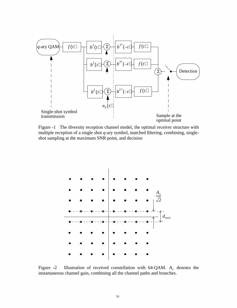
Figure -1 The diversity reception channel model, the optimal receiver structure withmultiple reception of a single shotq-ary symbol, matched filtering, combining, single-shot sampling at the maximum SNR point, and decision

Σ

Σ

Σ

Σ

q-ary QAM

Detection

f t( )

f t( )f t( )

f t( )bL t( )

b2 t( )

b1 t( ) b1* t–( )

b2* t–( )

bL* t–( )

nL t( )

Sample at theoptimal point

Single-shot symboltransmission

dmin

As

2-------

Figure -2 Illustration of received constellation with 64-QAM. denotes theinstantaneous channel gain, combining all the channel paths and branches.

As

16

0 5 10 1510

−3

10−2

10−1

100

SNR per bit

Pro

b. o

f sym

bol e

rror

Figure -3 Illustration of upper bound of the square QAM symbol error rate

(6.15) exact

approximation by (6.16)

17

Figure -4 Matched filter bound SEP for 4-QAM transmission over -flat fadingdiversity channels.

L

0 5 10 15 20 25 3010

−8

10−7

10−6

10−5

10−4

10−3

10−2

10−1

100

SNR per bit

Pro

b. o

f sym

bol e

rror

L = 1

L = 2

L = 3

L = ∞or AWGN

18

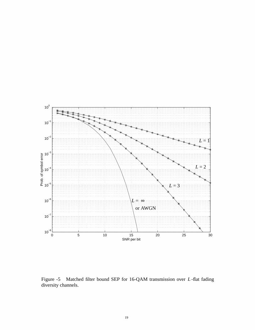
Figure -5 Matched filter bound SEP for 16-QAM transmission over -flat fadingdiversity channels.

L

0 5 10 15 20 25 3010

−8

10−7

10−6

10−5

10−4

10−3

10−2

10−1

100

SNR per bit

Pro

b. o

f sym

bol e

rror

L = 1

L = 2

L = 3

L = ∞or AWGN

19

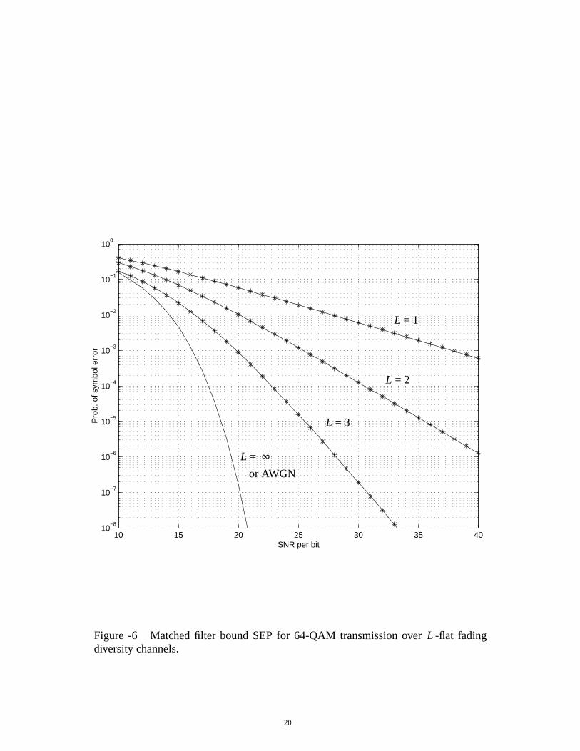
Figure -6 Matched filter bound SEP for 64-QAM transmission over -flat fadingdiversity channels.

L

10 15 20 25 30 35 4010

−8

10−7

10−6

10−5

10−4

10−3

10−2

10−1

100

SNR per bit

Pro

b. o

f sym

bol e

rror

L = 1

L = 2

L = 3

L = ∞or AWGN

20

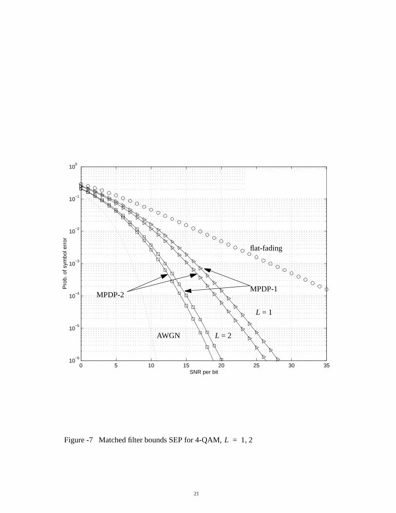
Figure -7 Matched filter bounds SEP for 4-QAM,L 1 2,=

0 5 10 15 20 25 30 3510

−6

10−5

10−4

10−3

10−2

10−1

100

SNR per bit

Pro

b. o

f sym

bol e

rror

flat fading Selective−fading (L = 1)Selective−fading (L = 2)AWGN

flat-fading

L = 1

L = 2AWGN

MPDP-1MPDP-2

21

Figure -8 Matched filter bounds SEP for 16-QAM,L 1 2,=

5 10 15 20 25 30 35 4010

−6

10−5

10−4

10−3

10−2

10−1

100

SNR per bit

Pro

b. o

f sym

bol e

rror

flat fading Selective−fading (L = 1)Selective−fading (L = 2)AWGN

flat-fading

L = 1

L = 2AWGN

MPDP-1MPDP-2

22

Figure -9 Matched filter bounds SEP for 64-QAM,L 1 2,=

5 10 15 20 25 30 35 4010

−6

10−5

10−4

10−3

10−2

10−1

100

SNR per bit

Pro

b. o

f sym

bol e

rror

flat fading Selective−fading (L = 1)Selective−fading (L = 2)AWGN

flat-fading

L = 1

L = 2AWGN

MPDP-1MPDP-2

23