match-up 2008 - gla · in addition to david gale, professor kurt mehlhorn, max planck institute...
TRANSCRIPT

MATCH-UP 2008
Matching Under Preferences– Algorithms and Complexity –
Satellite workshop of ICALP 2008July 6, 2008, Reykjavık, Iceland
Sponsored by
School of Informatics, Kyoto UniversitySchool of Business, Reykjavık University
Department of Computing Science, University of Glasgow

David Gale, 1921 – 2008

MATCH-UP: Matching Under PreferencesDedicated to the memory of David Gale, December 13, 1921 – March 7, 2008
Preface
This volume contains the papers presented at the ICALP Workshop “MATCH-UP: MatchingUnder Preferences”, held at the University of Reykjavık on July 6, 2008.
Matching problems with preferences occur in widespread applications such as the assignmentof school-leavers to universities, junior doctors to hospitals, students to campus housing,children to schools, kidney transplant patients to donors and so on. The common thread isthat individuals have preference lists over the possible outcomes and the task is to find amatching of the participants that is in some sense optimal with respect to these preferences.
The remit of this workshop was to explore matching problems with preferences, with anemphasis on the algorithms and complexity perspective, but a key objective was also tobring together the computer science and economics communities who have tended to followdifferent paths when studying these problems previously. The timing of the workshop reflectsthe growing interest in such problems among researchers in these communities that has ledto a wealth of publications in the past few years.
The opening talk at the workshop was to have been given by one of the key pioneers in thefield, Professor David Gale, of the University of California, Berkeley. Tragically, David Galedied suddenly on 7 March 2008, while preparations for the workshop were under way. Weare honoured to dedicate the workshop to his memory.
In addition to David Gale, Professor Kurt Mehlhorn, Max Planck Institute fur Informatik,Professor Al Roth, Harvard University, and Professor Marilda Sotomayor, Universidade deSao Paolo, all kindly agreed to give an invited talk at the workshop. Marilda Sotomayoragreed to open the workshop by paying tribute to the life and work of David Gale, inparticular describing his contribution to the theory of matching problems.
Our call for papers generated much interest, and we were pleased with both the qualityand quantity of submitted papers. These originated in roughly equal measure from thecomputing science and economics communities. The tight time constraints imposed by aone-day workshop made the selection process difficult, and forced us to reject a numberof good papers that, in other circumstances, we would have been happy to accept. Thefinal choice of 15 contributed papers appearing in these proceedings represents, we feel, anexcellent snapshot of the current state of the art regarding research in the area of matchingproblems with preferences.
We would like to conclude by thanking the invited speakers and the authors of all submittedpapers for helping to make this workshop a success.
Magnus M. HalldorssonRob Irving
Kazuo IwamaDavid Manlove
iii

ICALP Workshop: Match-Up, July 6, 2008
Workshop Program
Session 1: 08:30 – 10:30 (Chair: Rob Irving)
08:30 Opening remarks08:40 Invited talk: My encounters with David Gale
M. Sotomayor . . . . . . . . . . . . . . . . . . . . . . . . . . . . . . . . . . . . . . . . . . . . . . . . . . . . . . . . . . . . 109:30 Unravelling in two-sided matching markets and similarity of preferences
H. HaÃlaburda . . . . . . . . . . . . . . . . . . . . . . . . . . . . . . . . . . . . . . . . . . . . . . . . . . . . . . . . . . . . . 509:50 Successful manipulation in stable marriage model with complete preference lists
H. Kobayashi and T. Matsui . . . . . . . . . . . . . . . . . . . . . . . . . . . . . . . . . . . . . . . . . . . . . 1710:10 On the house allocation markets with duplicate houses
K. Cechlarova and T. Fleiner . . . . . . . . . . . . . . . . . . . . . . . . . . . . . . . . . . . . . . . . . . . . 2310:30 Coffee break (30 minutes)
Session 2: 11:00 – 12:50 (Chair: Kazuo Iwama)
11:00 Invited talk: Assigning papers to reviewersK. Mehlhorn . . . . . . . . . . . . . . . . . . . . . . . . . . . . . . . . . . . . . . . . . . . . . . . . . . . . . . . . . . . . . . 3
11:50 Better and simpler approximation algorithms for the stable marriage problemZ. Kiraly . . . . . . . . . . . . . . . . . . . . . . . . . . . . . . . . . . . . . . . . . . . . . . . . . . . . . . . . . . . . . . . . 36
12:10 Optimal popular matchingsT. Kavitha and M. Nasre . . . . . . . . . . . . . . . . . . . . . . . . . . . . . . . . . . . . . . . . . . . . . . . . 46
12:30 The hospitals/residents problem with quota lower boundsK. Hamada, K. Iwama and S. Miyazaki . . . . . . . . . . . . . . . . . . . . . . . . . . . . . . . . . . 55
12:50 Lunch (70 minutes)
Session 3: 14:00 – 15:50 (Chair: David Manlove)
14:00 Invited talk: Kidney exchange:Design and evolution of a computer-assisted matching mechanism
A. Roth . . . . . . . . . . . . . . . . . . . . . . . . . . . . . . . . . . . . . . . . . . . . . . . . . . . . . . . . . . . . . . . . . . 414:50 Circular stable matching and 3-way kidney transplant
C-C. Huang . . . . . . . . . . . . . . . . . . . . . . . . . . . . . . . . . . . . . . . . . . . . . . . . . . . . . . . . . . . . . 6715:10 Three-sided stable matchings with cyclic preferences
P. Biro and E. McDermid . . . . . . . . . . . . . . . . . . . . . . . . . . . . . . . . . . . . . . . . . . . . . . . . 7915:30 Approximating matches made in heaven
N. Chen, N. Immorlica, A. R. Karlin, M. Mahdian and A. Rudra . . . . . . . . 9115:50 Coffee break (30 minutes)
iv

Session 4: 16:20 – 17:20 (Chair: Peter Biro)
16:20 Smith and Rawls share a room: stability and mediansB. Klaus and F. Klijn . . . . . . . . . . . . . . . . . . . . . . . . . . . . . . . . . . . . . . . . . . . . . . . . . . 102
16:40 The stability of the roommate problem revisitedE. Inarra, C. Larrea and E. Molis . . . . . . . . . . . . . . . . . . . . . . . . . . . . . . . . . . . . . . . 114
17:00 An algorithm for a super stable roommates problemT. Fleiner, R.W. Irving and D.F. Manlove . . . . . . . . . . . . . . . . . . . . . . . . . . . . . . 126
17:20 Short break
Session 5: 17:30 – 18:30 (Chair: Tamas Fleiner)
17:30 Faster algorithms for stable allocation problemsB.C. Dean and S. Munshi . . . . . . . . . . . . . . . . . . . . . . . . . . . . . . . . . . . . . . . . . . . . . . 133
17:50 Finding all stable pairs for the (many-to-many) stable matchingP. Eirinakis, D. Magos, I. Mourtos and P. Miliotis . . . . . . . . . . . . . . . . . . . . . . 145
18:10 A note on existence and uniqueness of vNM stable sets in marriage gamesJ. Wako . . . . . . . . . . . . . . . . . . . . . . . . . . . . . . . . . . . . . . . . . . . . . . . . . . . . . . . . . . . . . . . . 157
18:30 Closing remarks
v


My Encounters with David Gale
Marilda Sotomayor, Universidade de São Paolo Abstract
In this talk I will tell what I know about David Gale and what I learned from him as a friend
and a mathematician.
Extracts from a letter from Marilda Sotomayor to Bernhard von Stengel on David Gale's work, dated March 12 2008:
Over the last fifty years David Gale played a leading role in developing some of the themes
of fundamental importance to economic theory. An example is matching theory which he
introduced to me in 1983. We wrote several papers together. From this time on I used to send
to him my manuscripts, before submitting them. He always used to read them and to make
comments and suggestions. The Gale's Feast I organized at Stony Brook was a way to thank
him for everything I received from him. I also edited a special issue in honor to him for the
International Journal of Game Theory, which was published these days. I think David did not
see the publication, but I gave to him during the dinner of the Gale's Feast, as a symbolic gift,
a compilation of the copies of all 17 papers. You can find a paper of mine there too: The
Stability Of The Equilibrium Outcomes In The Admission Games Induced By Stable
Matching Rules. This special issue is on David's work but most of them are on matching.
Probably we will also have a book published by Springer.
There is some thing that I am sure you can tell in your appreciation on Gale's work. Once, in
1975, when David finished a talk about the stable marriage problem, some physician, who
had attended the talk, approached him and told him that the Gale-Shapley algorithm was very
similar to the one that was being used by the National Resident Matching Program in Illinois.
Then, he wrote a letter to the NRMP asking them about that. They answered David and from
the description of the algorithm used by the NRMP he could see that it was mathematically
equivalent to the Gale-Shapley algorithm, but in the reverse: instead of producing the optimal
stable matching for the students it produced the optimal stable matching for the hospitals.
This fact was spread orally. When I arrived in Berkeley, February of 1983, there were papers
on the walls of the Department of Mathematics congratulating David for having been elected
for the National Academy of Sciences. In these papers it was written that David Gale had
discovered an algorithm which was being used to make the allocation of the interns and
hospitals in the United States. At this time, there was a colloquium in the Department of
Mathematics and David gave a talk about the stable marriage problem. I attended such a talk.
Then he talked about the mathematical equivalence of the two algorithms and made clear that
the Gale-Shapley algorithm was independently discovered 11 years after the discovery of the
NRMP.
These facts were reported in the second paper David wrote about the stable marriage problem,
in 1983, co-authored with me: Some remarks on the stable matching problem, Discrete
Applied Mathematics. This paper was only published in 1985 and was very important for the
1

developing of the theory of the discrete matchings. In my opinion this was, after the first one
by Gale and Shapley, the most important paper that was written on this subject. It presents a
concise theory whose results and arguments used in the proofs have been used by the authors
until nowadays. The existent theory only considered special cases of the marriage model (the
same number of men and women and/or complete preference lists of acceptable partners).
Our paper presents the general marriage model where the lists of acceptable partners do not
need to be complete and we may have any number of agents in each side of the model. Then
the paper generalizes all existent results, presents new proofs with different arguments, and
also new results. Almost all results have two proofs: one by making use of the algorithm and
another one without the algorithm, by only using the theory that is constructed in the paper. A
new and very short proof of the non-manipulability theorem by Dubins and Freedman allows
to teach this result in only one class. The original proof had 20 pages. This theorem opened
space for investigation on the strategic aspects of the Gale-Shapley algorithm. This was done
in the following paper by us, also written in 1983 and published in 1985: Ms. Machiavelli and
the stable matching problem, American Math. Monthly.
His first work on continuous matching models was with Gabrielle Demange: The strategy
structure of two-sided matching markets, Econometrica, 1985. This is a very precious paper
because it allowed to us to use the similarities and differences between several results for the
marriage model and for the continuous model to understand better the structure of the
matching models.
Another important work on the continuous matching models was written with me and
Demange: Multi-item auctions, Journal of Political Economy. It is about two dynamic auction
mechanisms to produce the minimum competitive equilibrium price for the case where
buyers have quasi-linear utilities and only wish one object and each seller owns one object.
An important thing to be written about David Gale is that all his works reflect his
extraordinary creativity, his ability to combine precision and rigour with an elegant style of
exposition and to provide simpler alternatives to complicated proofs. An example is the paper
of Shapley and Scarf (1974), where he presented a short and simple proof of the non-
emptiness of the core of the Housing market, as an alternative to the more complicated proof
of the authors. His proof is done by means of the well-known "Top trading cycles algorithm"
which has been applied to allocation problems of students to schools and of kidneys to
patients. Another example is the suggestion to John Nash to demonstrate the existence of
Nash equilibria using the Kakutani Fixed Point Theorem to simplify his proof.
2

Assigning Papers to Reviewers
Kurt MehlhornMax Planck Institut fur Informatik
Abstract
CS conferences typically have a program committee (PC) that selects the papers forthe conference from among the submitted papers. The work of the PC is supported by aconference support system, e.g., EasyChair. It is the task of the program chair to assignthe papers to the members of the PC. In order to achieve an effective assignment, the PCmembers classify the papers according to interest. The EasyChair conference system knowsfour levels: strongly interested, weakly interested, not interested, conflict of interest. Giventhe classification of the papers by the PC members, the chair seeks a good assignment. Whatare the right objectives? Here are some: balancing the load of the PC members, making thetask of the PC members worthwhile by assigning their high interest papers, guaranteeingeach paper a sufficient number of reviews, guaranteeing each paper a sufficient total level ofinterest, and so on. I will discuss several versions of the problem; I will pose more questionsthan I give answers.
3

Kidney Exchange: Design and Evolution of a Computer-assisted Matching Mechanism
Al Roth, Harvard University
Abstract
I will give an overview of the recent development of regional kidney exchanges in the United
States, which help patients with incompatible (or poorly matched) donors arrange kidney
transplants from other patients' donors. Advances in matching theory interacted with changes in
surgical practice as these kidney exchanges evolved. Legislation in 2007 removed barriers to a
national kidney exchange, which raises new market design and computational issues, some of
which are still open questions.
4

Unravelling in Two-Sided Matching Markets
and Similarity of Preferences
Hanna Halaburda∗
Abstract
This paper investigates the causes and welfareconsequences of unravelling in two-sided matchingmarkets. It shows that similarity of preferences isan important factor driving unravelling. In partic-ular, it shows that under the ex-post stable mech-anism (the mechanism that the literature focuseson), unravelling is more likely to occur when par-ticipants have more similar preferences. It alsoshows that any Pareto-optimal mechanism mustprevent unravelling, and that the ex-post stablemechanism is Pareto-optimal if and only if it pre-vents unravelling.
1 Introduction
The hiring process calls for collecting informationin order to choose the best individual from amongthe candidates. In certain markets, however, firmshire workers long before all the pertinent informa-tion is available. For instance, in the market forhospital interns before 1945, appointments havebeen made even as early as two years before stu-dents’ graduation and the actual start of the job(Roth, 1984, 2003). This phenomenon of contract-ing long before the job begins and before rele-vant information is available, is called unravelling.Those early matches often turn out to be ineffi-cient when the job starts.
Unravelling has been recognized as a seriousproblem in numerous markets.1 Measures de-signed to preclude this phenomenon have not al-ways been successful. Unravelling prevails in cer-tain markets because some employers see a bet-ter chance to hire their most-preferred candidateswhen they contract early than when they wait.
∗Harvard Business School, [email protected] an extensive list, see Roth and Xing (1994).
Meanwhile, other markets for entry-level profes-sionals appear never to have experienced unrav-elling, including markets for new professors in fi-nance, economics and biology. Studying what fac-tors lead to unravelling in some markets but not inothers can help design better measures to preventunravelling.
Much of the existing research focuses on sta-bility as the key to understanding unravelling. Amatching is ex-post stable if every agent prefershis match to being unmatched, and if there is noblocking pair, that is, a worker and a firm thatboth strictly prefer each other to their assignedpartners. Roth (1991) and Kagel and Roth (2000)argue that ex-post stable matching implementedupon arrival of pertinent information should pre-clude early contracting. This argument is knownas the “stability hypothesis.” An ex-post stablematching can be produced in a market througha clearinghouse.2 However, some clearinghouseswith an ex-post stable algorithm have failed tostop unravelling.3 Roth and Xing (1994) also of-fer theoretical examples of unravelling even whenex-post stable matching is expected upon the ar-rival of pertinent information. There is no consen-sus, however, on whether these examples are singleanomalies, or if instead there is some systematicreason for the stability hypothesis to fail.4
2In a clearinghouse, firms and workers submit their pref-erences, and a matching among all participants is producedby an algorithm.
3Examples include the U.S. gastroenterology market,whose clearinghouse was abandoned in 1996 (Niederle andRoth, 2003), and the Canadian market for new lawyers(Roth and Xing, 1994).
4The stability hypothesis is not the only expla-nation of unravelling in the literature. In Dami-ano, Li and Suen (2005), early contracting is the result ofcostly search. Li and Rosen (1998), Li and Suen (2000)and Suen (2000) point to workers’ risk aversion as the maincause of the phenomenon. Although risk aversion plays an
5

This paper shows that the similarity of prefer-
ences is an important factor contributing to un-
ravelling. The more similar are firms’ preferences,
the more unravelling will occur in the market, even
with an ex-post stable clearinghouse in operation.
This paper also shows that unravelling leads to a
loss in welfare, and a mechanism must preclude
unravelling to be Pareto-optimal. In some mar-
kets it means that an ex-post stable mechanism is
Pareto-dominated by an ex-post unstable mecha-
nism.
This paper examines a two-sided matching mar-
ket populated by firms and workers. The agents
on each side are heterogenous and they have pref-
erences over agents on the other side of the mar-
ket. Their aim is to match with the best possi-
ble agent on the other side. Workers’ preferences
over firms are identical: all workers agree on which
firm is the best firm, the next-to-best or the worst
firm. Firms, however, may have different prefer-
ences over the workers. The similarity of firms’
preferences over workers is a comparative statics
parameter. There are two periods. Firms and
workers can contract in either period, but firms
only learn their preferences in the second period.
The firms and workers who contract in the first
period exit the market. The agents who remain
in the second period participate in a mechanism
that produces a matching between them. In this
model, contracting during the first period, before
firms have learned their preferences, constitutes
unravelling.
The first part of the paper investigates unrav-
elling when the mechanism in the second period
produces the ex-post stable matching. In the en-
vironment considered here there always exists a
unique ex-post stable matching.
It is shown that the nature of equilibria depends
crucially on the level of similarity: unravelling oc-
curs only in markets where firms’ preferences are
sufficiently similar. With very similar preferences,
many firms are likely to prefer the same workers.
Amid such competition, worse firms may have a
better chance to hire their top candidates if they
important role and may be an additional cause of early con-
tracting, it is not a necessary condition for the phenomenon.
The model in this paper assumes risk-neutrality in order
to distinguish incentives to unravel driven by similarity of
preferences from those attributable to risk aversion.
contract before rankings are known.
The second part of the paper studies the prob-
lem of mechanism design in markets where un-
ravelling is possible. Before the game starts, a
mechanism is chosen for the second period. The
mechanism is announced at the outset of the game,
so that firms and workers are aware of it during
the first period. The goal is to provide a Pareto-
optimal outcome from the ex-ante perspective of
the beginning of period 1.
It turns out that any Pareto-optimal mechanism
must preclude unravelling. The first part of the
paper shows that the ex-post stable mechanism
may unravel. When this is the case, this mecha-
nism cannot be Pareto-optimal. There exists an-
other — ex-post unstable — mechanism for such a
market that does not unravel and Pareto-improves
upon the ex-post stable mechanism. In every mar-
ket there exists a mechanism producing a Pareto-
optimal outcome. In some markets, however, all
Pareto-optimal mechanisms are ex-post unstable.
Section 2 of this paper presents the model. Sec-
tion 3 investigates unravelling under an ex-post
stable mechanism. Section 4 analyzes the prob-
lem of mechanism design in markets where unrav-
elling is possible. Section 5 offers some concluding
observations.
2 The Model
To investigate unravelling, I construct a two-stage
game between two types of agents: firms and
workers. Firms and workers can contract during
the first stage. If they do, they leave the mar-
ket. In the second stage, the remaining agents are
matched by a mechanism. The game, described in
this section, is represented in Figure 1.
The market is populated by F firms, f ∈1, . . . , F, and W workers, w ∈ 1, . . . , W. Let
F ⊆ 1, . . . , F denote an arbitrary subset of
firms. Similarly, let W ⊆ 1, . . . , W denote an
arbitrary subset of workers. There are more work-
ers than firms, W > F . Each firm has exactly one
position to fill, and each worker can take at most
one job.
Workers have identical preferences over firms:
all workers consider firm F the most desirable,
firm F − 1 — the second-best, and so on. The
6

t=1 t=2
(F, W,u,v, ρ,M) andworkers’ preferencescommonly known
each firm’s ranking isrealized
matching mechanism M isapplied to agents remaining
in the market
firms simultaneouslymake (or not) early
offers
workers who received anoffer accept or reject it
matched firms andworkers leave the
market
Figure 1: Timeline of the game
utility for a worker from being matched to firm f
is uf , and the utility from being unmatched is 0.Workers prefer being hired by the worst firm to notbeing hired at all, i.e., 0 < u1 < u2 < . . . < uF .Let u ≡ [u1, u2, . . . , uF ].
Firms may have different preferences over work-ers. Firm f ’s preferences are described by itsranking, denoted by Rf = (rf
1 , rf2 , . . . , r
fW ) —
an ordered list of length W , where rf1 represents
the lowest-ranked worker, and rfW represents the
highest-ranked worker in firm f ’s ranking. LetR = [R1, . . . , RF ] be the vector of all firms’ rank-ings. For a subset of firms F, let RF be the cor-responding vector of the rankings of the firms inF.
The value to firm f of being matched to workerrfk is vk.
5 It is better to hire the worst worker thanto keep a vacancy, i.e., 0 < v1 < v2 < . . . < vW .Let v ≡ [v1, v2, . . . , vW ]. The matching value vec-tors, u and v, are publicly known. There are notransfers between firms and workers.
Definition 1. A matching between F and W is afunction µF,W : F → W∪∅ that uniquely assignsworkers to firms. That is, for any two firms f andf ′ in F such that f = f ′
either µF,W(f) = µF,W(f ′)
or µF,W(f) = µF,W(f ′) = ∅
Expression µF,W(f) = ∅ means that in match-ing µF,W, firm f is not matched with any worker.
5The assumption that every firm has the same value ofbeing matched with k-th worker on its list is needed forclarity of exposition. The general results remain true fordiffering matching values.
When µF,W(f) = w ∈ W, then firm f is matchedwith worker w.
Much of the literature emphasizes the impor-tance of ex-post stability in matching. The notionof ex-post stability6 was introduced by Gale andShapley (1962). A matching is called ex-post un-
stable if it results in a firm and a worker who wouldprefer to be matched to each other than to remainin their current matches. A matching is called ex-
post stable if it is not ex-post unstable.Which matching is ex-post stable depends on
firms’ preferences, RF. A well established result inthe literature7 states that in a market where work-ers’ preferences are identical, for any given firms’preference profile there exists a unique ex-post sta-ble matching between F and W.8 This matchingcan be characterized in the following way: Thebest firm — the firm most desired by workers —in F is matched with its highest-ranked worker inW. Then, the next-best firm is matched with itshighest-ranked worker from among the remainingworkers, and so on. Every firm in F is matchedto its highest-ranked worker remaining in the poolafter all the better firms in F have been matched.
A matching is defined between a subset of firmsand a subset of workers. A special case is match-
ing outcome, which refers to a matching betweenall firms, 1, . . . , F, and all workers, 1, . . . , W,realized at the end of the two-stage game. Theex-post stable outcome — denoted by oS — isthe ex-post stable matching between all workers,1, . . . , W, and all firms, 1, . . . , F, in the mar-
ket: oS ≡ µ1,...,W,1,...,FS . I drop R from the no-
tation, keeping in mind that ex-post stable match-ing depends on rankings.
When a matching is produced by a matchingmechanism, M, also called a clearinghouse, itis based on the rankings reported by firms. Amatching mechanism is incentive compatible if nofirm benefits from misreporting its preferences. Amechanism is called ex-post stable — and denoted
6Gale and Shapley (1962) call this property “stability.”Here it is called “ex-post stability” to emphasize the factthat a matching satisfying this property may neverthelessunravel, and thus in a sense may be “ex-ante” unstablethough it is “ex-post” stable.
7E.g., Gusfield and Irving (1989) or Roth and Sotomayor(1990).
8With arbitrary workers’ preferences, ex-post stablematching does not need to be unique.
7

MS — if it applies ex-post stable matching tothe reported rankings. In this model the ex-poststable mechanism is incentive compatible. There-fore, the ex-post stable mechanism operating overF and W will produce ex-post stable matching be-tween F and W.
There are two periods in the model: t = 1, 2.Workers’ preferences are commonly known in bothperiods. Firms learn their own preferences, in theform of rankings, only at the beginning of period 2.Each firm’s ranking is its private information.
With W workers there are W ! possible rank-ings. Denote as R the set of all possible rank-ings over workers. The rankings for all F firms,(R1, . . . ,RF ), are drawn from a joint distribu-tion G over R
F . The model focuses on distri-butions where the marginal distributions of indi-vidual rankings are always uniform, allowing fordifferent levels of similarity between the rankings.Two special cases of such distributions are identi-cal preferences and independent preferences.
Let G1 be the joint distribution where all firms’rankings are identical and the marginal distribu-tion of any individual ranking is uniform on R.That is, every ranking in R is drawn with equalprobability of 1
W !and all firms will have the same
ranking.
Let G0 be the joint distribution such that anyfirm’s ranking is drawn from the uniform distribu-tion independently of other firms’ rankings.
Between the identical and the independentrankings, there is a continuum of cases of inter-mediate similarity, Gρ.
Definition 2. For ρ ∈ [0, 1],
Gρ = ρG1 + (1 − ρ)G0
The parameter ρ is a measure of preference sim-ilarity9 and will be a comparative statics parame-ter in the analysis below. Preferences are said tobe more similar under Gρ′ than under Gρ whenρ′ > ρ. Since ρ completely characterizes Gρ, thetwo are used interchangeably.
9Similarity of preferences, as measured by ρ is similar to
the concept of correlation. However, correlation for rank-
ings is not well defined. Since preferences are expressed
as rankings, rankings and preferences are used interchange-
ably.
Figure 1 illustrates how the game unfolds. Mar-ket characteristics (F, W,u,v, ρ,M) and workers’preferences are commonly known at any time. Atthe beginning of period 1, firms simultaneouslydecide whether or not to make an early offer, andif so, to which worker. Each firm can make atmost one offer. After the early offers are released,each worker observes the offers he has received, ifany. He does not see offers made to other work-ers. Every worker presented with an offer acceptsor rejects it. He may accept at most one offer. Ifan offer is accepted, the matched firm and workerleave the market. Firms whose offers were rejectedor who did not make an offer in period 1, remain inthe market for period 2. In period 2, firms’ rank-ings are realized and a matching mechanism Moperates on the agents remaining in the market.Section 3 assumes the ex-post stable mechanism inperiod 2. Section 4 considers other mechanisms.There is no discounting between the periods andmaking offers is costless.
This paper considers only incentive compatiblemechanisms, where firms truthfully report theirrankings in period 2. In period 1, every firmdecides whether or not to make an offer and ifso, to which worker. The analysis focuses on se-quential equilibria in pure strategies. The strat-egy of any firm f is σf ∈ 1, . . . , W ∪ ∅. LetΩw ⊂ 1, . . . , F be the set of firms that havemade an early offer to worker w. A strategy ofworker w, σw(Ωw) ∈ Ωw ∪ ∅, is the offer thathe accepts. Strategy σw(Ωw) = ∅ means that theworker rejects all offers.
Every firm’s payoff depends on many variables:market characteristics (F, W,u,v, ρ,M), firms’ re-alized rankings R, and the strategies played by allagents in the market. For clarity, most of thisnotation is suppressed and only the variables es-sential to the current analysis are retained.
A definition of sequential equilibrium applied tothis model is a profile of strategies and a systemof beliefs such that
(1) strategies are sequentially rational given thebeliefs, i.e.
(f) every firm f ∈ 1, . . . , F chooses σ∗
f
that maximizes its expected payoff, i.e.
Eπf
(
σ∗
f
)
≥ Eπf
(
σf
)
∀σf ∈ 1, . . . , W ∪ ∅
8

(w) each worker w ∈ 1, . . . , W chooses hisstrategy, conditionally on the set of re-ceived offers, σ∗
w(Ωw), such as to maxi-mize his expected utility, i.e.
EUw
(
σ∗
w |Ωw
)
≥ EUw
(
σw |Ωw
)
∀σw ∈ Ωw∪∅
(2) beliefs are consistent with the strategiesplayed.
Offers made and accepted in period 1 constituteunravelling.
3 Unravelling under Ex-Post
Stable Mechanism
Given that the literature focuses on ex-post stablemechanisms, this section investigates unravellingunder the ex-post stable matching mechanism.
The ex-post stable mechanism, MS , is notonly incentive compatible, but in all equilibria italso produces ex-post stable matching among theagents remaining in period 2. Unless unravellingoccurs in period 1, it produces the ex-post stableoutcome, oS .
The ex-post stable outcome has two propertiesthat are of particular interest here. One is thatlower-ranked firms receive lower expected payoffsin the ex-post stable matching, and the other isthat firms’ expected payoffs decrease as prefer-ences become more similar.
Because of the first property, worse firms aremore likely to prefer early contracting under MS
than better firms. To unravel, firms need to begood enough to be accepted in period 1 and badenough to want to contract early. And because ofthe second property, more firms prefer to contractearly as preference similarity increases.
Let Eπf (oS |ρ) denote firm f ’s expected payoffin the ex-post stable outcome in a given market.Then the following lemma summarizes the prop-erties of oS .
Lemma 1 (properties of oS). .
(1) In any market (F, W,u,v, ρ,MS), for any f > 1,Eπf−1(oS | ρ) < Eπf (oS | ρ).
(2) Holding other market parameters constant, for
any f < F ,
ρ < ρ′ =⇒ Eπf (oS | ρ) > Eπf (oS | ρ′)
Proof. See the Appendix, page 11.
3.1 Equilibria without Unravelling
An equilibrium has no unravelling when either nofirm makes an early offer, or all early offers are re-jected. This subsection explores conditions underwhich such an equilibrium exists, i.e., conditionsunder which there is no profitable deviation fromoS .
Consider a worker who receives an offer fromfirm f in period 1, when in equilibrium all firmsare expected to wait for period 2. If the workeraccepts the offer, he receives utility uf . If he re-jects the offer, all firms and all workers participatein the period 2 matching mechanism. Because theworkers are a priori identical, a worker’s expectedutility from rejecting f ’s offer is 1
W
∑Fi=1 ui. He
accepts the offer when
uf >1
W
F∑
i=1
ui
Let L0(W,u) denote the lowest ranked firm whose
offer will be accepted in period 1. All firms worsethan L0 will be rejected in period 1. Firm L0 andall firms better than L0 will be accepted. Call
L0(W,u) , . . . , F
the acceptance set.
The incentives for firms to contract in period 1depend on the joint distribution of rankings, Gρ.Recall that Eπf (oS |ρ) denotes firm f ’s expectedpayoff from the ex-post stable outcome under Gρ.
Since all workers are ex ante the same, an offermade to any worker in period 1 — if it is accepted— yields
π0 ≡1
W
W∑
k=1
vk
Firm f prefers early contracting to ex-post stableoutcome when π0 > Eπf (oS |ρ).
Firm F never has incentives to make an offerin period 1, since in the ex-post stable outcomeit always hires its most-preferred worker. Otherfirms may have something to gain from an earlyoffer, depending on ρ and v.
Example 1. Consider firm F−1. This firm getsits most-preferred worker unless that worker isfirm F ’s most-preferred worker as well. Its ex-
9

pected payoff from the ex-post stable matching is
EπF−1(oS | ρ) =
= (1 − ρ)
(
1 −1
W
)
vW +
(
ρ + (1 − ρ)1
W
)
vW−1
In a market with 2 firms and 3 workers where v =[1, 2, 6], Eπ1(oS | ρ) = 14
3 (1 − ρ) + 2ρ and π0 = 3.Thus, firm 1 would prefer early contracting to the
ex-post stable outcome when ρ > 58 .
The lower ranked the firm, the lower its ex-pected payoff in the ex-post stable outcome(Lemma 1(1)). Thus, if firm f prefers earlycontracting to the ex-post stable outcome, thenall firms worse than f do too. The set ofall firms that prefer early contracting under Gρ
and v — called the offer set — is an inter-
val
1, . . . , H0(ρ,v)
, where H0(ρ,v) is the highest-
ranked firm that prefers early contracting.A profitable deviation from oS is possible only
when there exists a firm that belongs to both theacceptance set and the offer set. This happenswhen the two sets have nonempty intersection, i.e.L0
(W,u) ≤ H0(ρ,v).
The H0, and thus the offer set, depend on thesimilarity of preferences, ρ. The remainder of thissection shows that under independent preferences,G0, the offer set is empty: no firm wants to con-tract in period 1. Under identical preferences, G1,by contrast, there may be firms willing to contractearly, depending on v. For intermediate cases,H0
(ρ,v) increases with ρ.For independent preferences, G0, no firm prefers
early contracting to the ex-post stable outcome.Thus the offer set is empty. Therefore, in anymarket with independent preferences, there is anequilibrium without unravelling.
Lemma 2. For any F , v and W > F , if the prefer-
ences are independent, G0, then H0(G0,v) < 1. I.e.,
∀F,v, W s.t. W > F π0 < Eπf (oS |G0) ∀ f
Proof. See the Appendix, page 11.
Under identical preferences, Eπf (oS |G1) =vW−F+f . Thus, condition π0 > Eπf (oS |ρ) re-duces to:
1
W
W∑
k=1
vk > vW−F+f
This inequality may be satisfied for some firms andsome values of v.
Example 2 shows a market characterized byidentical preferences of firms, where there existsa profitable deviation.
Example 2. Consider a market with 3 firms and
4 workers and with matching values vectors v =[1, 2, 3, 4] and u = [4, 5, 6], and with identical
firms’ preferences, G1.
The ex-post stable outcome is
oS(f3) = r34 =⇒ π3(oS) = 4
oS(f2) = r23 =⇒ π2(oS) = 3
oS(f1) = r12 =⇒ π1(oS) = 2
An early offer yields expected payoff of 2.5. Thus,
firm 2 has no incentive to make an early offer, but
firm 1 prefers to contract in period 1. That is,
H0(G1,v) = 1.
A worker’s expected utility from period 2 match-
ing is 1W
∑Ff=1 uf = 15
4 < 4 = u1. This means
that firm 1’s offer in period 1 will be accepted by
any worker. Thus, L0(4,u) = 1 and the acceptance
set is 1, 2, 3. Since the acceptance and the offer
sets overlap at H0(G1,v) = L0
(4,u) = 1, there exists a
profitable deviation from oS in this market.
However, a profitable deviation from oS maynot exist even when firms’ preferences are identi-cal. For example, if the matching utilities in Ex-ample 2 were u′ = [2, 3, 4], then firm 1 would berejected by any worker in period 1. So there wouldbe no profitable deviation.
Thus, under identical preferences a profitabledeviation from oS may but need not exist. Thatis, there are markets characterized by G1, in whichthere exists an equilibrium without unravelling,but there also are markets with G1 in which anyequilibrium must exhibit unravelling.
Now, consider intermediate similarity of firms’preferences. By Lemma 1(2), the expected valueof oS for firms decreases as similarity of prefer-ences increases. As a consequence, holding otherparameters of the market constant, more firmsprefer early contracting as similarity of preferencesincreases. Workers’ incentives to accept an offerin period 1 do not depend on similarity of prefer-ences.
10

For any market parameters (F, W,v,u), thereexists a threshold ρ∗∗ such that a profitable devi-ation from oS exists for any similarity higher thanthe threshold but not for similarity lower than thethreshold.
Lemma 3. For any market parameters
(F, W,v,u), there exists ρ∗∗ ∈ (0, 1] s.t.
for all ρ ≤ ρ∗∗, there exists an equilibrium
without unravelling, and
for all ρ > ρ∗∗, there is no equilibrium without
unravelling.
Proof. See the Appendix, page 11.
For G0 there are no market parameters(F, W,v,u) for which a profitable deviation fromoS exists. This follows from the fact that underG0, the offer set is always empty. But as simi-larity of preferences, ρ, increases, firms’ expectedpayoffs from ex-post stable outcome decrease andunravelling becomes more profitable.
3.2 Equilibria with Unravelling
Firms and workers that contract early exit themarket before period 2. The remaining agentsparticipate in the ex-post stable matching mecha-nism. In equilibrium, worker w who receives offersΩw in period 1 either accepts the best offer in Ωw
or rejects all of them, depending on which of thetwo options maximizes his expected utility.
For any given equilibrium, define equilibrium
unravelling set as the set of firms that contractearly in this equilibrium, and denote this set byU. The remaining firms, 1, . . . , FU, partici-pate in MS in period 2 with workers still remain-ing in the market. If the equilibrium unravellingset is empty, such an equilibrium does not involveunravelling.
It is a property of any equilibrium that theunravelling set is an interval, that is, U has no“holes.” For the given equilibrium unravelling setU∗, let firm H∗ be the highest-ranked firm in U
∗,and firm L∗ — the lowest-ranked in U
∗. The factthat U
∗ is an interval means that all firms worsethan H∗ but better than L∗ belong to U
∗ as well.This result is formally stated in Lemma 4(1) be-low.
Thus, any nonempty U∗ can be characterized
by the best firm (H∗) and the worst firm (L∗)that contract early in such equilibrium: U
∗ ≡L∗, . . . , H∗, for L∗ ≤ H∗.
1 Ffirms
L∗ H∗
U∗
Figure 2: The structure of an equilibrium
In every market there is at least one equilibrium.This result is formally stated in Lemma 4(2) be-low. Moreover, in a typical market there is morethan one equilibrium.
Example 3. Consider a market with 5 firms
and 6 workers where u = [2, 5, 6, 9, 10], v =[2, 3, 4, 5, 8, 17] and firms’ preferences are identi-
cal, G1. In this market there are two possible un-
ravelling sets in pure strategy equilibria: U∗ = 3
and U′ = 2, 3, 4.
In Example 3 both equilibrium unravelling setswere nonempty. But this does not need to be thecase. There are markets with multiple equilibriawhere some equilibria exhibit unravelling and oth-ers do not.
However, equilibrium unravelling sets cannot bearbitrary. For any two equilibrium unravelling setsin a given market, one needs to be fully includedin the other. In particular, two equilibrium unrav-elling sets for the same market cannot “overlap.”Lemma 4(3) states this result formally.
1 Ffirms
U∗
U′f
(a) An impossible configuration of multiple equilibriumunravelling sets
1 Ffirms
L∗ H∗
U∗
L′ H ′U′
(b) A possible configuration of multiple equilibrium un-ravelling sets
Figure 3: Multiple equilibria with unravelling
The following lemma summarizes properties ofequilibria in an arbitrary market with the ex-poststable matching mechanism, (F, W,u,v, ρ,MS).
11

Lemma 4. Given a market (F, W,u,v, ρ,MS):
(1) (convexity of unravelling set) In any
equilibrium, the equilibrium unravelling set,
U, is an interval.
(2) (existence of equilibrium) There exists an
equilibrium in pure strategies.
(3) (multiple equilibria) If there are two equi-
librium unravelling sets, U∗ and U
′ where
U∗ = U
′, then either U∗ ⊂ U
′ or U′ ⊂
U∗. Moreover, if both unravelling sets are
nonempty, U∗ = L∗, . . . , H∗ and U
′ =L′, . . . , H ′ then
L′ < L∗ ⇐⇒ H∗ < H ′
Proof. Available upon request.
The last property of multiple equilibria leadsto conclusions about how increasing similarityof preferences drives changes in equilibrium out-comes.
Comparative statics on ρ
Equilibrium unravelling — as measured by the sizeof U — weakly increases with the similarity of pref-erences.
In any market characterized by independentpreferences, all equilibria result in no-unravelling.Lemma 3 implies that as ρ increases, equilibriawith U = ∅ exist for a smaller range of marketparameters (F, W,u,v).
By the property of multiple equilibrium unrav-elling sets (Lemma 4(3)), every equilibrium un-ravelling set in a given market (if there is morethan one) has a different number of firms con-tracting early. Thus, for any market, all equilibriacan be ordered by the size of U. The maximum
equilibrium (UMAX) and the minimum equilibrium(UMIN ) can be distinguished. The former is theclass of equilibria with maximum unravelling, i.e.,the largest U, and the latter is the class of equilib-ria with minimum unravelling, i.e., the smallest U.It may happen in a market that U
MAX ≡ UMIN ,
that is, that all equilibria in this market resultin the same unravelling set. For instance, in anymarket with G0, U
MAX ≡ UMIN = ∅.
As similarity of preferences increases, both min-imum and maximum equilibrium unravelling setsincrease. The maximum equilibrium unravellingset increases from empty to non-empty at some ρ∗.Thus, for ρ > ρ∗ an equilibrium with unravellingappears in the market. Moreover, when similarityof preferences increases, the minimum equilibriumunravelling set may also increase from empty tonon-empty — at some ρ∗∗ ≥ ρ∗. When this occurs,“no unravelling” is no longer an equilibrium inmarkets with preference similarity ρ > ρ∗∗. Thisrelationship between equilibrium unravelling setsin a market and the level of preference similarityis illustrated by Figure 4.
Let U(ρ) be an equilibrium unravelling set in amarket with similarity of preferences ρ.
ρ
size of U
0
1
2
3
4
5
6
1
size of UMAX
size of UMIN
ρ∗
ρ∗∗
Figure 4: The relationship of UMIN , U
MAX and ρ
in a typical market
Proposition 1. Under MS, for any market pa-
rameters F, W,u,v, there exist ρ∗ and ρ∗∗ such
that 0 < ρ∗ ≤ ρ∗∗ ≤ 1 and
ρ ∈ [0, ρ∗] =⇒ UMAX(ρ) = ∅
ρ ∈ (ρ∗, ρ∗∗] =⇒ UMIN (ρ) = ∅ & U
MAX(ρ) = ∅
ρ ∈ (ρ∗∗, 1] =⇒ UMIN (ρ) = ∅
Proof. See the Appendix, page 11.
In some markets characterized by high similar-ity of preferences, all equilibria under the ex-poststable mechanism involve early contracting. Inthose markets only an ex-post unstable matchingmechanism can prevent unravelling. Section 4 fo-cuses on the welfare consequences of unravelling
12

and on characterizing Pareto-optimal mechanismsfor markets where unravelling is possible.
4 Mechanism Design
This section turns to the problem of mechanismdesign in markets where unravelling may occur.It shows that unravelling is Pareto-inefficient, fora broad class of mechanisms called anonymous
mechanisms. For example, the ex-post stablemechanism is anonymous, as are all mechanismsever used in real markets.
This section shows that the ex-post stablematching mechanism is Pareto-optimal if and onlyif it does not induce unravelling. Moreover, in ev-ery market there always exists a mechanism thatproduces a Pareto-optimal outcome. In the mar-kets where the ex-post stable clearinghouse un-ravels, there exists an ex-post unstable mechanismthat will stop unravelling and improve the welfareof the market participants.
An outcome, o, is a function from the profileof rankings to randomization over matchings be-tween all firms and all workers.
The previous section considered a special caseof an outcome function — the ex-post stable out-come, oS . This section also examines other out-comes and mechanisms.
Firm f ’s payoff from an outcome depends on therealized rankings, R, and is denoted by πf (o|R).The ex-ante expected payoff of an outcome is theexpectation over all possible ranking realizations.Let Eπf (o) be firm f ’s expected payoff from out-come o, then
Eπf (o) =∑
R∈RF
πf (o|R) · Prob(R|ρ)
Similarly, worker w’s expected utility of outcomeo is
EUw(o) =∑
R∈RF
Uw(o|R) · Prob(R|ρ)
An outcome o′ strictly Pareto-dominates (ex-
ante) outcome o′′ when
(
∀ f Eπf (o′) ≥ Eπf (o′′) and ∀w EUw(o′) ≥ EUw(o′′))
and(
∃ f Eπf (o′) > Eπf (o′′) or ∃w EUw(o′) > EUw(o′′))
A matching outcome o is Pareto-optimal ina given market when there does not exist anoutcome in that market that strictly Pareto-dominates o.
The social planner designs a mechanism toachieve the best outcome in the Pareto sense (ex-ante). For an incentive compatible mechanism inperiod 2, an equilibrium under M is described bythe first-period strategies of agents. Let σ denotea vector of period 1 strategies for all agents. Amechanism may possibly implement many equi-libria. For example, it was demonstrated thatthe game with the ex-post stable mechanism usu-ally has multiple equilibria. Let Σ
M be the setof all possible equilibria under mechanism M. Amechanism-equilibrium pair (M, σ), where σ ∈Σ
M, determines a unique outcome o(M,σ).
A mechanism-equilibrium pair (M, σ) is un-
constrained Pareto-optimal when it produces aPareto-optimal outcome. However, a social plan-ner is constrained to inducing outcomes by meansof a mechanism. A mechanism-equilibrium pair(M, σ) is constrained Pareto-optimal when thereis no other mechanism-equilibrium pair (M′, σ′)such that its outcome o(M′,σ′) strictly Pareto-dominates o(M,σ).
Define a mechanism to be anonymous if it as-signs workers to firms based only on firms’ rank-ings, not on workers’ identities. For example,the ex-post stable mechanism, MS , is anonymous.Define a vector of strategies, σ, as anonymous ifany firm that contracts with a worker in period 1selects a worker at random, ignoring his identity.10
A mechanism-equilibrium pair (M, σ) is anony-mous when M and σ are anonymous.
Notice that under an anonymous mechanism-equilibrium pair, every worker has the same ex-ante expected utility at the beginning of the firstperiod.
It is said that a mechanism-equilibrium pair(M, σ) exhibits unravelling when there is a pos-itive probability that an early offer is both madeand accepted under the vector of strategies σ.
The following proposition presents the main re-sult of this section: when an anonymous (M, σ)exhibits unravelling, it cannot be constrained
10It is assumed, however, that no two firms that want to
contract in period 1 make offer to the same worker.
13

Pareto-optimal.
Proposition 2. For any anonymous mechanism-
equilibrium pair (M,σ) that exhibits unravelling,
there exists an anonymous mechanism-equilibrium
pair (M′,σ′) such that it does not exhibit unrav-
elling and that outcome o(M′,σ′) strictly Pareto-
dominates outcome o(M,σ).
Proof. Consider an anonymous (M,σ) such that Mproduces in equilibrium σ a non-empty unravelling setU
M = ∅. Now consider the following mechanism M′:
(1) To all firms in UM, M′ tentatively assigns a ran-
dom worker from the set of all workers. This mim-ics the unravelling outcome for those firms. Noticethat with probability 1
W, a firm is assigned to its
least-preferred worker.
(2) All other firms are matched according to M.These firms get the same expected payoff as under(M,σ). For these firms it is the final match.
(3) (the “least-preferred workers correction”) For allfirms in U
M that were matched to their least-preferred workers, M′ replaces these workers withworkers still remaining in the pool. This is fea-sible because, after all firms are matched, thereis at least one worker still in the pool. Forfirm f tentatively matched with its least-preferredworker, any of the remaining workers is preferableto the tentative match. This way, all firms ten-tatively matched with their least-preferred work-ers can improve their payoff. When there areno more firms in U
M that are matched to theirleast-preferred worker, the algorithm stops andthe matching is finalized.
Notice that M′ is an incentive compatible mechanism,as no firm can gain by misreporting its preferences.
There is an equilibrium without unravelling underM′. This is the case because all firms in U
M preferto wait for M′ rather than to unravel given that otherfirms wait for period 2. Since firms outside U
M didnot unravel when some other firms were contractingearly, they do not unravel when all other firms wait forperiod 2 under M′. Therefore, no unravelling occurs.Denote the equilibrium without unravelling by σ
′.
Notice that since (M,σ) is anonymous, (M′,σ′)
is anonymous as well. And since every firm that is
matched to a worker under (M,σ) is also matched un-
der (M′,σ′), the expected payoff to every worker does
not change. Every firm in UM has a strictly higher
expected payoff in o(M′,σ′) than in o(M,σ). All the
other firms have exactly the same expected payoff in
both outcomes. Therefore, o(M′,σ′) Pareto-dominates
o(M,σ).
Proposition 2 establishes that no-unravellingis a necessary condition for constrained Pareto-optimality of an anonymous (M,σ). In par-ticular, when the ex-post stable mechanism —which is anonymous — unravels, it cannot be con-strained Pareto-optimal. For the ex-post stablemechanism, any (MS ,σ) that does not exhibitunravelling is unconstrained Pareto-optimal.
Proposition 3 guarantees that in any mar-ket there exists an unconstrained Pareto-optimalmechanism-equilibrium pair, i.e., one that pro-duces a Pareto-optimal outcome.
Proposition 3. For any market, there exists a
mechanism M and an equilibrium σ ∈ ΣM such
that (M,σ) is unconstrained Pareto-optimal.
Proof. Consider a mechanism M that first randomlyassigns all participating firms a number between 1 andF . Then the mechanism works in the same way as theex-post stable mechanism but the order in which firmsare matched with workers is based on the randomlyassigned numbers, not on their position in the market.
Notice that this mechanism is anonymous. It is alsoincentive compatible, as is the ex-post stable mecha-nism. Moreover, there exists an equilibrium withoutunravelling. If all agents participate in the mechanism,then all firms have higher expected payoffs from themechanism than from unravelling. Thus, no firm wantsto unravel when no other firm unravels. Denote the no-unravelling equilibrium as σ.
Now, notice that (M,σ) produces a Pareto-optimal
outcome. The sum of workers’ expected utilities and
the sum of firms’ expected payoffs are the same un-
der (M,σ) as they are under oS . Since oS is Pareto-
optimal, so must o(M,σ) be: in both outcomes it is im-
possible to increase the expected payoff for one agent
without decreasing it for some other agent on the same
side of the market.
5 Conclusions
This study investigates the causes and welfareconsequences of unravelling in two-sided matchingmarkets. It considers a two-period model in whichfirms receive pertinent information about workersand specify preferences over them at the beginningof the second period. It is assumed that firms andworkers can make and accept offers during the firstperiod if they wish to, and that a clearinghousemechanism is used in the second period to assign
14

workers to the remaining firms. Unravelling is saidto occur when offers are both made and acceptedin the first period. Notice that firms that choose tocontract early do so in the absence of informationon which workers are most-preferred.
Section 3 explores the issue of unravelling whenthe ex-post stable mechanism operates in the sec-ond period. Ex-post stable matching is the clear-inghouse mechanism that most of the existing lit-erature focuses on. Section 3 shows that unrav-elling becomes more likely as firms’ preferencesover workers grow more similar. This is the casebecause when firms’ preferences are very simi-lar, lower-ranked firms can be matched with theirmost-preferred worker only by contracting withthem early. Despite insufficient information in thefirst period, it may be worthwhile for such firmsto bear the risk and contract early.
Section 4 investigates the issue of Pareto-optimality of matching mechanisms. The mainresult demonstrates that a necessary condition foran anonymous mechanism to be Pareto-optimalis that it does not induce unravelling. Anyanonymous mechanism that induces unravelling isPareto-inefficient. In particular, the ex-post sta-ble matching mechanism is Pareto-optimal if andonly if it does not unravel.
Another result of Section 4 demonstrates thatin every market there exists a mechanism thatproduces a Pareto-optimal outcome. In marketswhere the ex-post stable clearinghouse unravels,it is an ex-post unstable mechanism that achievesPareto-optimality.
These findings are particularly noteworthygiven the importance that the literature assignsto stability. In some circumstances, an ex-postunstable mechanism that precludes unravelling isactually preferable from a policy standpoint.
Appendix
Proof of Lemma 1 (page 5)
First, note that the probability that firm f is matchedwith its kth worker in the ex-post stable outcome underindependent preferences is:
P (W, f, k) ≡(F − f)!
(F − W − f + k)!
(k − 1)!
W !(W − F + f)
This formula is derived by applying combinatorics.11
(1) Proof. The probability that firm f − 1 gets itsworker k > W − F + f is
(1 − ρ) · P (W, f − 1, k) =
= (1−ρ)·P (W, f, k)·F − f + 1
F − W − f + 1 + k
W − F + f − 1
W − F + f
Since F , f and W are fixed, the ratio in the for-mula decreases with increasing k. The inequalityin expected payoffs of firms f and f − 1 followsfrom first order stochastic dominance.
(2) Proof. Follows directly from Eπf (oS |ρ) = ρ ·Eπf (oS |G1) + (1 − ρ)Eπf (oS |G0), and
Eπf (oS |G0) =
W∑
k=W−F+f
vk · P (W, f, k) >
> vW−F+f
W∑
k=W−F+f
·P (W, f, k) = vW−F+f = Eπf (oS |G1)
This completes the proof.
Proof of Lemma 2 (page 6)
Proof. Consider the worst firm, firm 1.
Prob(oS(f = 1) = r1
k|G0, W ) ≡ P (W, 1, k)
for k = (W − F + 1), . . . , W
and 0 for k < W − F + 1.By induction, it can be shown that P (W, 1, k) >
P (W, 1, k′) for k > k′. Therefore, distributionP (W, 1, k) first order stochastically dominates distri-bution P0(W, 1, k) = 1
Wfor any k, which is the distri-
bution for early matches. Thus, Eπ1(oS |G0) > π0 inany market with G0.
By Lemma 1(1) for any firm better than firm 1,the payoff from the ex-post stable outcome is higher.Therefore, all firms prefer to wait for oS rather thanto unravel.
Proof of Lemma 3 (page 7)
Proof. Follows from Lemma 1(2), Lemma 2 and mono-tonicity of H0 in ρ.
Proof of Proposition 1 (page 8)
Proof. First, notice that in any market with G0,(F, W,u,v, G0), the only equilibrium outcome is U
∗ =∅. This follows from Lemma 2.
For ρ > 0, the proof follows from the fact thatU
MIN ⊆ UMAX and monotonicity of H0(ρ,v) and
11Derivation of this formula is available on the author’swebsite.
15

Eπf (µF,WS |ρ) in ρ. The part for ρ∗∗ follows from
Lemma 3. For ρ∗, notice that for any market pa-rameters (F, W,u,v) under identical preferences, G1,it must be that either U
MAX = ∅, or UMAX = ∅. In the
former case, ρ∗ = 1 satisfies the Proposition.In the latter case, let U
MAX = LMAX , HMAX.From an equilibrium condition it must be that
EπHMAX (MS |UMAXHMAX, G1) < π
0
By monotonicity of Eπf in ρ, for ρ < 1
EπHMAX (MS |UMAXHMAX, ρ) >
> EπHMAX (MS |UMAXHMAX, G1)
And we also know that
EπHMAX (MS |UMAXHMAX, G0) > π
0
Thus, there must exist a threshold value ρ′ such that
EπHMAX (MS |UMAXHMAX, ρ)
< π0 if ρ > ρ′
≥ π0 if ρ ≤ ρ′
i.e. for similarity of preferences lower than ρ′, HMAX
does not belong to UMAX .
Similarly, there exists a threshold ρ′′ such that firmHMAX−1 does not belong to U
MAX for ρ ≤ ρ′′. And soon. Thus, there must be a threshold value ρ∗ such thatthere is no firm that belongs to U
MAX under ρ ≤ ρ∗, butU
MAX is nonempty for similarity of preferences higherthan ρ∗.
Values of ρ∗ and ρ∗∗ may be the same or different.But by definitions of U
MIN and UMAX it is not possible
that ρ∗ > ρ∗∗.Thus, Proposition 1 holds.
References
[1] K. Atkins, Committee OKs new school as-signment plan, Boston Herald, July 21, 2005.
[2] E. Damiano, H. Li and W. Suen (2005), Un-ravelling of Dynamic Sorting, Review of Eco-nomic Studies, Vol. 72, 1057-1076.
[3] D. Gale and L.S. Shapley (1962), College Ad-missions and the Stability of Marriage, Amer-ican Mathematical Monthly, Vol. 69, No. 1,9-15.
[4] D. Gusfield and R.W. Irving (1989), The Sta-ble Marriage Problem. Structure and Algo-rithms, MIT Press.
[5] J.H. Kagel and A.E. Roth (2000), The Dy-namics of Reorganization in Matching Mar-kets: A Laboratory Experiment Motivated by
a Natural Experiment, Quarterly Journal ofEconomics, Vol. 115, No. 1, 201-235.
[6] H. Li and S. Rosen (1998), Unravelling inMatching Markets, American Economic Re-view, Vol. 88, No. 3, 371-387.
[7] H. Li and W. Suen (2000), Risk Sharing, Sort-ing, and Early Contracting, Journal of Polit-ical Economy, Vol. 108, 1058-1091.
[8] M. Niederle and A.E. Roth (2003), Unrav-elling Reduces Mobility in a Labor Market:Gastroenterology with and without a Cen-tralized Match, Journal of Political Economy,Vol. 111, No. 6, 1342.
[9] A.E. Roth (1984), The Evolution of the LaborMarket for Medical Interns and Residents: ACase Study in Game Theory, The Journal ofPolitical Economy, Vol. 92, No. 6, 991-1016.
[10] A.E. Roth (1991), A Natural Experiment inthe Organization of Entry-Level Labor Mar-kets: Regional Markets for New Physiciansand Surgeons in the United Kingdom, Amer-ican Economic Review, Vol. 81, No. 3, 415-440.
[11] A.E. Roth (2003), Matching and Allocation
in Medicine and Health Care, transcript of atalk at the National Academy of Engineering,June 16, 2003.
[12] A.E. Roth and M. Sotomayor (1990), Two-Sided Matching: A Study in Game-TheoreticModeling and Analysis, Cambridge Univer-sity Press 1990.
[13] A.E. Roth and X. Xing (1994), Jumping theGun: Imperfections and Institutions Relatedto the Timing in Market Transactions, Amer-ican Economic Review, Vol. 84, No. 4, 992-1044.
[14] W. Suen (2000), A Competitive Theory ofEquilibrium and Disquilibrium Unravelling inTwo-Sided Matching, RAND Journal of Eco-nomics, Vol. 31, No. 1, 101-120.
16

Successful Manipulation
in Stable Marriage Model
with Complete Preference Lists
Hirotatsu Kobayashi and Tomomi Matsui
Faculty of Science and Engineering, Chuo University,Kasuga, Bunkyo-ku, Tokyo 112-8551, Japan.
Abstract. This paper deals with a strategic issue in the stable marriagemodel with complete preference lists (i.e., a preference list of an agent isa permutation of all the members of the opposite sex). Given completepreference lists of n men over n women, and a marriage µ, we consider theproblem for finding preference lists of n women over n men such that themen-proposing deferred acceptance algorithm (Gale-Shapley algorithm)adopted to the lists produces µ. We show a simple necessary and sufficientcondition for the existence of a set of preference lists of women over men.Our condition directly gives an O(n2) time algorithm for finding a set ofpreference lists, if it exists.
1 Introduction
In 1962, Gale and Shapley [1] proposed a simple model, called stable marriage
model, of two-sided matching market. Given two sets of agents, men and women,both of size n, Gale and Shapley discussed a model in which each agent hadpreferences over agents of the opposite sex. A marriage is a one-to-one mappingbetween the two sexes such that a man m is mapped to a woman w, if and onlyif, w is mapped to m. A marriage is called stable, if no man and woman who arenot mapped to each other would both prefer to be. Gale and Shapley proposedan algorithm, called deferred acceptance algorithm (Gale-Shapley algorithm),which always finds a stable marriage.
The deferred acceptance algorithm is employed in a number of labor marketclearinghouses and college admission systems. A notable variation of the al-gorithm, called men-proposing deferred acceptance algorithm, works by havingmen make proposals to women and produces men-optimal marriage, which everyman likes at least as well as any other stable marriage. Since most applicationsof the deferred acceptance algorithm involve the participation of independentagents, it is natural to ask whether agents can benefit by being dishonest abouttheir preference lists. It is well-known that stating true preferences is a domi-nant strategy for the men in men-proposing deferred acceptance algorithm. Insettings that allow incomplete preference lists, women on the other hand have
17
incentives to submit false preferences. By contrary, little is known in the case ofstable marriage model with complete preference lists.
This paper deals with a strategic issue in the stable marriage model withcomplete preference lists (i.e., a preference list of an agent is a permutationof all the members of the opposite sex). Given complete preference lists of n
men over n women, and a marriage µ, we consider the problem for findingcomplete preference lists of n women over n men such that the men-proposingdeferred acceptance algorithm adopted to the lists produces µ. We show a simplenecessary and sufficient condition for the existence of a set of complete preferencelists of women over men. Our condition directly gives an O(n2) time algorithmfor finding a set of preference lists, if it exists.
In the next section, we establish some terminology and definitions and givesome background. Section 3 gives our main results.
2 Notations and Definitions
We denote two sets of agents by M and W, called men and women, both of size n.Each agent in M∪W has a preference list which is a totally ordered list of all themembers of the opposite sex. Here we note that this paper considers the case with‘complete’ preference lists, i.e., a preference list of an agent is a permutation ofmembers of the opposite sex. A marriage is a mapping µ : (M ∪W ) → (M ∪W )satisfying that (1) ∀m ∈ M,µ(m) ∈ W , (2) ∀w ∈ W,µ(w) ∈ M , and (3) w =µ(m) if and only if m = µ(w). For any agent i ∈ M ∪ W , µ(i) is called themate of i in marriage µ. A pair (m,w) ∈ M × W is called a blocking pair for amarriage µ, if m prefers w to µ(m) and w prefers m to µ(w). A marriage withno blocking pair is called a stable marriage.
Gale and Shapley [1] showed that a stable marriage always exists, and a sim-ple algorithm called the deferred acceptance algorithm can find a stable marriage.Here we briefly describe a variant of the their algorithm in which men proposeto women (these roles can naturally be reversed). In the following algorithm, weintroduced an iteration number which will be used in a later section.
Men-Proposing Deferred Acceptance Algorithm
Step 0: Set the iteration number r := 1 and unmarried men U := M .Initially, every woman has no current mate.
Step 1: If U = ∅, then output the current mate of every woman and stop.Step 2: Choose a man m ∈ U. Let w ∈ W be m’s most preferred woman who
hasn’t yet rejected m.Step 3: (Create a proposal from man m to woman w.)
If woman w has no mate, then update U := U \m and set m be the currentmate of w.Else if w prefers m to her current mate m′, then w rejects m′, update U :=U \ m ∪ m′ and set m be the current mate of w.Else, w rejects m.
Step 4: Update r := r + 1 and go to Step 1.
18

It is known that the order of proposals (choice of m ∈ U in Step 2) does not affectthe output of the algorithm [1]. Conway showed that the set of stable marriagescan be partially ordered as a lattice with the pair of extremal elements, calledmen-optimal and women-optimal marriages (see [9] for example). In fact, men-proposing deferred acceptance algorithm produces men-optimal marriage.
The issues of strategic manipulation in the stable marriage are discussed inmany papers (see books [4, 6] and the references therein, for example). Roth [5]showed that when the men-proposing algorithm is used, none of the men ben-efits by submitting a false preference list, regardless of how the other agentsreport their preference. Dubins and Freedman [10] proved that no coalition ofmen could collectively manipulate in such a way as to strictly improve all oftheir mates in comparison to men-optimal marriage. In settings that allow in-complete preference lists, women on the other hand have incentives to cheat inmen-proposing algorithm. Gale and Sotomayor [2] showed that a woman has anincentive to falsify their preferences as long as she has at least two distinct stablemates. In fact, the women can force the women-optimal marriage µ by rejectingall the men except mates in µ (see [3]).
A feature of this paper is that the agents are required to submit completepreference list. Comparing to the above results, little is known in the case ofstable marriage model with complete preference lists. Gusfield and Irving ([4],page 65) point to the absence of any general results in this setting. Tadenuma andToda [8] considered an implementation question. Teo, Sethuraman, and Tan [7]deals with the situation that there exists a specified woman w who is the onlydeceitful agent, and that she knows the reported preferences of all the otheragents. They proposed a polynomial time algorithm for constructing woman w’soptimal cheating strategy. They also discussed the Singapore school-admissionsproblem, where stable marriage model with complete preference lists is a suitablerepresentation of the problem.
3 Main Results
In this paper, we consider the following problem.
Problem P(Lm, µ):
Input: Set of preference lists Lm of men M over women W and a marriage µ.Question: If there exists a set of preference lists Lw of women W over menM such that the men-proposing deferred acceptance algorithm adopted to thelists in Lm and Lw produces the marriage µ, then output Lw. If not, say ‘noneexists.’
We give a simple necessary and sufficient condition for the existence ofwomen’s lists. Let G(Lm, µ) be a directed bipartite graph with a pair of vertexsets M , W and a set of directed edges A defined by
A = (w, µ(w)) ∈ W × M | w ∈ W
∪
(m,w) ∈ M × W
∣
∣
∣
∣
w = µ(m) orm prefers w to µ(m)
.
19

Here we note that for any pair of mates i, µ(i) in µ, there are parallel directededges with opposite directions between corresponding vertices in G(Lm, µ).
A directed graph is said to be strongly connected if, for all pair of vertices i
and j, there exists a directed path from i to j. A strong component of a directedgraph is a strongly connected subgraph which is maximal. In this paper, wedenote a strong component by a set of vertices in the corresponding stronglyconnected subgraph. If a strong component V ′ has no incoming edge, i.e., everyedge connecting vertices i ∈ V ′ and j ∈ V ′ is incident from i to j, we say thatV ′ is a minimal strong component.
Theorem 1. Let Lm be a given set of preference lists of men M over women
W, and µ a given marriage. There exists a set of preference lists Lw of women
over men, such that the men-proposing deferred acceptance algorithm adopted to
the lists in Lm and Lw produces the marriage µ, if and only if, every minimal
strong component of G(Lm, µ) consists of exactly one pair of vertices.
Before proving the above theorem, we describe some properties of strongcomponents in G(Lm, µ). Since every pair of vertices i, µ(i) induces a stronglyconnected subgraph of G(Lm, µ), vertices i and µ(i) are contained in a commonstrong component of G(Lm, µ) for any agent i ∈ M ∪ W. Thus, for any strongcomponent V ′ in G(Lm, µ), there exists a subset of men M ′ ⊆ M satisfying thatV ′ = ∪m∈M ′m,µ(m). Clearly, the equality |V ′ ∩ M | = |V ′ ∩ W | holds. Everyvertex w ∈ W has a unique outgoing edge (w, µ(w)) and every vertex m ∈ M hasa unique incoming edge (µ(m), m). These properties yield that a pair of verticesm ∈ M and µ(m) ∈ W forms a minimal strong component, if and only if, vertexµ(m) has a unique incoming edge (m,µ(m)). Lastly, we note that the strongcomponent decomposition of G(Lm, µ) is essentially equivalent to the Dulmage-Mendelsohn decomposition of corresponding underlying undirected graph [11].
Proof. First, consider the case that there exists a minimal strong component V ′
of G(Lm, µ) including more than two vertices. From the assumption, there existsa subset of men M ′ ⊆ M satisfying that |M ′| ≥ 2 and V ′ = ∪m∈M ′m,µ(m).
Let Lw be an arbitrary set of preference lists of W over M . We apply the men-proposing deferred acceptance algorithm to lists in Lm and Lw and assume onthe contrary that the marriage µ is obtained. For any m ∈ M , r(m) denotes theiteration number when man m ∈ M proposed to µ(m). Let m∗ be a man in M ′
who proposed to his mate in µ lastly, i.e., m∗ satisfies r(m∗) = maxm∈M ′ r(m).We denote r(m∗) by r∗ for simplicity.
At the beginning of r∗th iteration, man m∗ is unmarried and every manm ∈ M ′ \ m∗ is the current mate of women µ(m). Now we show that womenµ(m∗) also has a current mate at the beginning of r∗th iteration. We denoteµ(m∗) by w∗.
Since m∗, w∗ is not a strong component, vertex w∗ has an incoming edge(m′, w∗) different from the edge (m∗, w∗). The minimality of V ′ yields that thevertex m′ is contained in M ′ \m∗. From the definition of the graph, m′ prefersw∗ to its mate µ(m′) and thus w∗ has rejected m′ in an iteration earlier thanr∗. In the deferred acceptance algorithm, if a women rejects a man, she holds a
20
current mate in the rest of iterations. Thus women w∗ has a current mate at thebeginning of r∗th iteration.
From the above, all the women in V ′ have current mates, denoted by M ′′, atthe beginning of r∗th iteration. Since m∗ is unmarried at the beginning of r∗thiteration, M ′′ ⊆ M ′ \ m∗. Thus, we have that
|V ′ ∩ W | = |M ′′| ≤ |M ′ \ m∗| < |M ′|
= |V ′ ∩ M | = |V ′ ∩ W |.
Contradiction.
Next, we show the inverse implication. Let us consider the case that everyminimal strong component of G(Lm, µ) consists of exactly one pair of vertices.First, we modify the directed graph as follows. We introduce an artificial vertexs and add directed edge (s, w) for each (woman) vertex w ∈ W satisfying thatw is contained in a minimal strong component. For any vertex i ∈ M ∪ W ,there exists a directed path from s to i. Thus there exists a directed outgoingspanning tree, denoted by T , with root vertex s in the modified graph. (We fixa directed outgoing spanning tree T in the rest of this proof.) For each vertexi ∈ M ∪ W , we denote the parent vertex of i in T by prt(i). Here we note thatfor any man (vertex) m ∈ M , his parent vertex prt(m) is equivalent to his mateµ(m). The parent vertex of a woman (vertex) is either the artificial vertex s ora man (vertex).
Now we construct preference lists Lw of women as follows. For any woman w
contained in a minimal strong component, we employ a preference list (a totalorder of men M) such that the most preferred man is µ(w). If a woman w is notcontained in any minimal strong component, we adopt a preference list (a totalorder of men M) of w such that woman w’s first choice is µ(w) and her secondchoice is prt(w) in T .
We apply the men-proposing deferred acceptance algorithm to lists in Lm
and Lw. Since each woman w most prefers man µ(w) in the list Lw, w neverrejects man µ(w) in the algorithm. Thus, if man m proposed to woman w in thealgorithm, then w = µ(m) or m prefers w to µ(m), and consequently, the graphG(Lm, µ) includes the directed edge (m,w).
Let µ′ be a marriage obtained by the men-proposing deferred acceptancealgorithm adopted to lists in Lm and Lw. In the rest of this proof, we showthat µ = µ′ by induction on heights of vertices defined below. For any vertexi ∈ M ∪ W , h(i) denotes the height of i in T , i.e., h(i) is equal to the length ofa unique path from s to i in T . We define that h(s) = 0.
(1) Let i ∈ M ∪ W be an agent with h(i) = 1. Clearly from the definition ofthe modified graph, i is a woman contained in a minimal strong component andhas exactly two incoming edges (s, i), (µ(i), i) in the modified graph. Sinceman µ′(i) proposed to i in the algorithm, there is a directed edge (µ′(i), i) inG(Lm, µ). From the above, we have that µ(i) = µ′(i).
(2) Assume that for any vertex j ∈ M ∪ W , h(j) = h′ yields µ(j) = µ′(j). Leti ∈ M ∪ W be a vertex whose height is h′ + 1, i.e., h(i) = h′ + 1.
21

(2-1) If h′ + 1 is an even number, i corresponds to a man, denoted by m ∈
M . Since the vertex m has a unique incoming edge (µ(m),m), µ(m) is theparent vertex of m, whose height is h′. The assumption of induction yields thatµ′(µ(m)) = µ(µ(m)) = m. From the definition of marriage, µ′(µ(m)) = m
implies that µ(m) = µ′(m).
(2-2) If h′ + 1 is an odd number, i corresponds to a woman w ∈ W . We denotew’s parent vertex prt(w) by m′ ∈ M , for simplicity. From the assumption ofinduction, µ′(m′) = µ(m′) and thus man m′ proposed to woman µ(m′) in thealgorithm. Since the graph includes the directed edge (m′, w), man m′ prefersw to µ(m′). Consequently, man m′ proposed to woman w and w rejected m′ inthe algorithm. In the preference list Lw, man m′ is w’s second choice. Since w
rejected m′, w’s mate obtained in the algorithm is her first choice µ(w). Thus,we obtained a desired result that w’s mate obtained in the algorithm, denotedby µ′(w), is equivalent to µ(w).
The above theorem directly implies that we can solve the problem P(Lm, µ)by constructing the strong component decomposition of the directed graph G(Lm, µ),which requires O(n2) time [12].
References
1. D. Gale and L. S. Shapley, “College Admissions and the Stability of Marriage,”The American Mathematical Monthly, vol. 69, pp. 9–15, 1962.
2. D. Gale and M. Sotomayor, “Some Remarks on the Stable Matching Problem,”Discrete Applied Mathematics, vol. 11, pp. 223–232, 1985.
3. D. Gale and M. Sotomayor, “Ms Machiavelli and the Stable Matching Problem,”American Mathematical Monthly, vol. 92, pp. 261–268, 1985.
4. D. Gusfield and R. W. Irving, The Stable Marriage Problem: Structure and Algo-
rithms, MIT Press, Cambridge, MA, 1989.5. A. E. Roth, “The Economics of Matching: Stability and Incentives,” Mathematics
of Operations Research, vol. 7, pp. 617–628, 1982.6. A. E. Roth and M. Sotomayor, Two-Sided Matching: A Study in Game-Theoretic
Modeling and Analysis, Cambridge, Cambridge University Press, 1990.7. C.-P. Teo, J. Sethuraman, W.-P. Tan, “Gale-Shapley Stable Marriage Problem Re-
visited: Strategic Issues and Applications,” Management Science, vol. 47, pp. 1252–1267, 2001.
8. K. Tadenuma and M. Toda, (1998). “Implementable Stable Solutions to PureMatching Problems,” Mathematical Social Sciences, vol. 35, pp. 121–132, 1998.
9. D. E. Knuth, Mariages Stables, Montreal, Les Presses de l’Universite de Montreal,1976. (An English translation by Martin Goldstein, Stable Marriage and its Rela-
tion to Other Combinatorial Problems, CRM Proceedings and Lecture Notes, 10,American Mathematical Society, 1996.)
10. L. E. Dubins and D. A. Freedman, “Machiavelli and the Gale-Shapley Algorithm,”American Mathematical Monthly, vol. 88, pp. 485–494, 1981.
11. A. L. Dulmage and N. S. Mendelsohn, “Coverings of Bipartite Graphs,” Canadian
Journal of Mathematics, vol. 10, pp. 517–534, 1958.12. R. E. Tarjan, “Depth First Search and Linear Graph Algorithms,” SIAM Journal
on Computing, vol. 1, pp. 146–160, 1972.
22

On housing markets with duplicate houses∗
Katarına Cechlarova1 and Tamas Fleiner2
1Institute of Mathematics, Faculty of Science, P.J. Safarik University,
Jesenna 5, 041 54 Kosice, Slovakia
email: [email protected]
Department of Computer Science and Information Theory,
Budapest University of Technology and Economics,
H-1117, Magyar tudosok korutja 2, Budapest, Hungary
email: [email protected]
June 10, 2008
Dedicated to the memory of David Gale.
Abstract. Housing market is a special type of exchange economy where each agentis endowed with one unit of an indivisible good (house) and wants to end up againwith one unit, possibly the best one according to his preferences. If the endow-ments of all agents are pairwise different, an equilibrium as well as a core allocationalways exist. However, for markets in which some agents’ houses are equivalent, theexistence problem for the economic equilibrium is NP-complete. In this paper weshow that the hardness result is not valid if the preferences of all agents are strict,but it remains true in markets with trichotomous preferences. Further, we extendsome known results about housing markets to the case with duplicate houses usinggraph-theoretical methods.Keywords: Housing market, Core, Pareto optimality, Economic equilibrium, Al-gorithm, NP-completenessAMS classification: 91A12, 91A06, 68Q25
1 Introduction
The study of markets with indivisible goods started by the seminal paper of Shapleyand Scarf [14] where a housing market was defined. In a housing market there is a finiteset of agents, each one owns one unit of a unique indivisible good (house) and wantsto exchange it for another, more preferred one; the preference relation of an agent is alinearly ordered list (possibly with ties) of a subset of goods. In such a market, the set ofeconomic equilibria and the core is always nonempty, which was proved constructivelyby the Top Trading Cycles (TTC for short) algorithm due to Gale (see [14]).Roth and Postlewaite [13] made a careful distinction between housing markets where
preferences of agents contain ties and those where ties are not allowed. Their findingscan be summarized as follows: The core is always nonempty, it always contains the set
∗This work was supported by the VEGA grants 1/3001/06, 1/3128/06 (Cechlarova) and by OTKAK69027 grant and the MTA-ELTE Egervary Research Group (Fleiner).
23

of equilibrium allocations, but may be strictly larger than the latter. The strong coremay be empty, but if the agents’ preferences do not contain ties, then strong core isnonempty and is equal to the unique equilibrium allocation. Later Quint and Wako [12]provided a polynomial algorithm for deciding the nonemptyness of the strong core andWako [15] showed that each strong core allocation is an equilibrium allocation.All the above results use the assumption that each agent’s house is unique. If the
houses of several agents are equivalent, the situation may change. Fekete, Skutella andWoeginger [5] proved that it is NP-complete to decide whether a housing market withduplicate houses admits an economic equilibrium. Duplicate houses mean that in thepreference lists of agents some ’compulsory’ ties appear (naturally, equivalent housesmust be tied) and there is less freedom in assigning prices to houses (equivalent housesmust have equal price). However, in the market constructed in the NP-completenessreduction in [5], some additional ties were used. If nonequivalent houses cannot betied, would the hardness result still be valid? This question is motivated by otherallocation markets where the dividing line between efficiently solvable and hard cases isthe presence or absence of ties. Let us mention the stable roommates problem, where ifties are not present, a polynomial algorithm to decide the existence of a stable matchingexists; in case with ties the existence problem is NP-complete (see [7]). A similarsituation occurs also for a modification of the classical housing market, where agentshave preferences also over the lengths of trading cycles [4]. In such markets, the notion ofeconomic equilibrium is not applicable, but the TTC algorithm in these settings alwaysfinds a (strong) core allocation, if ties are not allowed. However, in the presence of tiesit is NP-complete to decide whether the core as well as the strong core are nonempty[3]. Another example is the stable marriage problem. There, a stable matching alwaysexists and in the case without ties all stable matchings have the same cardinality. Onthe other hand, in the case with ties, stable matchings may have different cardinalityand the problem of finding a maximum cardinality stable matching is NP-hard [9].The aim of the present paper is to study some algorithmic problems for housing
markets. In Section 3 we derive some properties that are common in all housing markets,in particular we review algorithms for computing core and (strongly) Pareto optimalallocations, show how to test the nonemptyness of the strong core and prove that eachstrong core allocation is an equilibrium allocation. Our approach, unlike the previouslypublished results, does not assume the uniqueness of agents’ endowments and providesa unifying method using the language of graph theory.In Sections 4 and 5 we deal with economic equilibrium in housing markets. We
show that in the case of strict preferences the hardness result for markets with duplicatehouses [5] is not valid and we propose a simple polynomial time algorithm for decidingthe existence of an economic equilibrium. The other end of the spectrum is the casewith trichotomous preferences (i.e. all agents consider all acceptable houses equivalent,strictly preferred to their own house). We show that here the existence problem for theeconomic equilibrium remains NP-complete.
2 Description of the model
LetA be a set of n agents,H a set ofm house types. The endowment function ω : A→ H
assigns to each agent the type of house he originally owns. (Notice that in the classical
24

model of Shapley and Scarf [14], m = n and ω is a bijection.) Further, each agent a ∈ A
wishes to have in his possession just one house and it is supposed that his preferencesare given as a linear ordering P (a) on a set H(a) ⊆ H, the set of acceptable housetypes. We assume that ω(a) ∈ H(a) and this is the least preferred house in H(a) foreach a ∈ A. The notation i a j means that agent a prefers house type i to housetype j. If i a j and simultaneously j a i, we say that house types i and j are tied ina’s preference list and write i ∼a j; if i a j and not j a i, we write i ≻a j and saythat agent a strictly prefers house type i to house type j. The n-tuple of preferences(P (a), a ∈ A) will be denoted by P and called the preference profile.The housing market is a quadrupleM = (A,H, ω,P).If S ⊆ A, let ω(S) = ω(a); a ∈ S ⊆ H be the set of house types owned by
agents in S. Conversely, for T ⊆ H we set AS(T ) = a ∈ S;ω(a) ∈ T to be theset of agents in S who own a house whose type is in T . If A′ ⊆ A, we say thatM′ =M\A′ = (A\A′, ω(A\A′), ω′,P ′) is a submarket ofM if ω′ and P ′ are restrictionsof ω and P to A\A′ and ω(A\A′), respectively.We say thatM is a housing market with strict preferences if there are no ties in P.
On the other hand, M is a housing market with trichotomous preferences if for eachagent a ∈ A, all the house types h ∈ H ′(a) = H(a)\ω(a) are tied. In other words, ina housing market with trichotomous preferences each agent a ∈ A partitions the set H
into three classes: H ′(a) are the house types that are better than his own house type,the second class contains just ω(a) and the third one those house types that are worsethan ω(a). For each agent a ∈ A we denote by fS(a) the set of the most preferred(a-maximal) house types from ω(S) and FS(a) = AS(fS(a)) is the set of owners ofthese houses.Notice that when preferences of agents are strict then |fS(a)| = 1 for each a ∈ A
and S ⊆ A; for trichotomous preferences we have fA(a) = H ′(a).We say that a function x : S → H is an allocation on S if there exists a bijection
π on S such that x(a) = ω(π(a)) for each a ∈ S. In the whole paper, we assume thatallocations are individually rational, i.e. x(a) ∈ H(a) for each a ∈ A. Notice thatfor each allocation x on S, the set S can be partitioned into directed cycles (tradingcycles) of the form K = (a0, a1, . . . , aℓ) in such a way that x(ai) = ω(ai+1) for eachi = 0, 1, . . . , ℓ (here and elsewhere, indices for agents on cycles are taken modulo ℓ).Therefore we shall often represent an allocation as a collection of trading cycles. Wesay that agent a is trading in x if x(a) = ω(a).A coalition S ⊆ A blocks an allocation x on A if there exists an allocation y on S
such thaty(a) ≻a x(a) for each agent a ∈ S,
that is, agents of S can reallocate their houses in such a way that everybody in S isstrictly better off than in x. A coalition S ⊆ A weakly blocks an allocation x on A ifthere exists an allocation y on S fulfilling the condition
y(a) a x(a) for each a ∈ S and y(a) ≻a x(a) for at least one a ∈ S,
that is, in a reallocation nobody from S is worse off and at least one agent in S gains.An allocation x on A is in the core of marketM if it admits no blocking coalition andit is in the strong core of M if no coalition weakly blocks it. An allocation x on A isPareto optimal for marketM if A does not block x, and x is strongly Pareto optimal if
25

A does not weakly block x. A pair (x, p), where x is an allocation on A and p : H → R
is a price function, is an economic equilibrium for market M if for each agent a ∈ A,x(a) ∈ fS(a) for the set S of agents whose house is affordable to a, i.e.
S = a′ ∈ A; p(ω(a′)) ≤ p(ω(a)).
We shall say that allocation x is an equilibrium allocation if there exists a price functionp such that the pair (x, p) is an economic equilibrium.The following simple property of equilibrium allocations will often be used.
Lemma 1 If (x, p) is an economic equilibrium for market M then p(x(a)) = p(ω(a))for each a ∈ A.
Proof. Let K = (a0, a1, . . . , aℓ) be any trading cycle of x. According to the definitionof equilibrium, p(ω(ai)) ≥ p(ω(ai+1)) for each i = 0, 1, . . . , ℓ, which implies the assertionof the Lemma.
In what follows, we shall denote by Q(M), C(M), SC(M), PO(M) and SPO(M)the set of all equilibrium, core, strong core, Pareto optimal and strongly Pareto optimalallocations for marketM. The definitions imply that for each housing market
SC(M) ⊆ C(M) ⊆ PO(M) and SC(M) ⊆ SPO(M) ⊆ PO(M),
and all the inclusions in the above chain can be strict. Further, in the case withoutduplicate houses, Wako [15] proved SC(M) ⊆ Q(M).
Example 1 Let us consider the housing marketM given by Figure 1.
a a1 a2 a3 a4 a5
ω(a) h1 h2 h3 h4 h5
P (a) h2 ≻ h3 ≻ h1 h1 ∼ h4 ≻ h2 h4 ≻ h2 ≻ h3 h3 ∼ h5 ≻ h4 h2 ≻ h1 ≻ h5
Figure 1: Endowments and preferences of agents
In this example, either x(a1) = h2 or x(a1) = h2 for allocation x. In the former casethe cycle (a2, a4, a5) is weakly blocking as agent a5 strictly improves and agents a2, a4are not worse off than in x (they have their most preferred house types on this cycle).In the latter case the set a1, a2 is weakly blocking, as a1 improves and a2 is not worseoff. Hence SC(M) = ∅.Further, C(M) contains six allocations
x1 = (a1, a2)(a3, a4)(a5), x2 = (a2, a4, a5)(a1)(a3), x3 = (a1, a3, a4, a5, a2)
x4 = (a1, a3, a2, a4, a5), x5 = (a1)(a2, a4, a3)(a5), x6 = (a1, a2, a4, a5)(a3).
Core allocation x3 is strongly Pareto optimal, as the only agent who could strictlyimprove is a1 by getting h2, but since a5 is not allowed to become worse off than in x3,he must also be assigned his most preffered house h2, and so there is no weakly blockingallocation on A for x3.
26

Allocation x7 = (a1, a3, a2)(a4)(a5) is Pareto optimal (notice e.g. that agent a2cannot strictly improve) but not in the core, as the set a3, a4 is blocking.Finally, allocations x1 and x2 form economic equilibria with price vectors p1 and p2,
where p1(a1) = p1(a2) = p1(a3) = p1(a4) = 1, p1(a5) = 0 and p2(a1) = p2(a3) = 0 andp2(a2) = p2(a4) = p2(a5) = 1.
In the following sections we shall often use digraphs, so let us recall the terminologyused; for further details we recommend e.g. [11]. A digraph is a pair G = (V,E), whereV is a set of vertices, E is the set of arcs, i.e. ordered pairs of vertices. We allow parallelarcs as well as loops, i.e. arcs of the form (i, i) for some i ∈ V . If V ′ ⊆ V , a subdigraphof G induced by V ′ is a digraph G(V ′) = (V ′, E′) where E′ = (i, j) ∈ E; i, j ∈ V ′.A walk in G is a sequence of vertices (i0, i1, . . . , ik) such that (ij , ij+1) ∈ E for each
j = 0, 1, . . . , k − 1. We say that vertex j is a successor of a vertex i in G, if G containsa walk from i to j. A vertex j is a direct successor of a vertex i in G, if (i, j) ∈ E. Avertex i ∈ V is a sink in G, if it has no successors in G. (Let us remark, that someauthors, e.g. [14, 12] use the term top vertex in the same meaning.)A walk (i0, i1, . . . , ik) is said to be closed, if i0 = ik; if moreover all the vertices
i1, . . . , ik are pairwise distinct, it is a cycle. A collection K of vertex-disjoint cyclesis a cycle cover of a digraph G if each vertex of G is contained in some K ∈ K. Apolynomial-time algorithm to decide whether a digraph has a cycle cover is well-known.The folklore approach described e.g. in [2] first constructs a bipartite (undirected) graphΓ by duplicating each vertex of G and making the pair i, j′ an edge if and only if(i, j) ∈ E, where j′ is the copy of vertex j ∈ V . It is straightforward to see that G hasa cycle cover if and only if Γ has a perfect matching.A digraph G with vertex set V is strongly connected, if for each pair i, j of distinct
vertices of V there is a walk from i to j as well as a walk from j to i in G. A stronglyconnected component (SCC for short) of a digraph G is a maximal strongly connectedsubdigraph of G. We shall call a SCC trivial, if it contains just one vertex and noarcs. (So if a vertex with a loop is a SCC, then it is nontrivial.) The condensationG∗ = (V ∗, E∗) of a directed graph G is obtained by merging the vertices of each SCCof G (and perhaps deleting eventual parallel arcs). For i ∈ V we shall denote by i∗ thevertex of G∗ corresponding to the SCC of G containing i. As G∗ is acyclic, the verticesof G∗ are partially ordered, i∗ ≫ j∗ if and only if i∗ is a successor of j∗ in G∗ and thisorder can easily by extended to a linear ordering, sometimes called a topological order.A SCC is sink, if its corresponding vertex in the condensation is a sink. An algorithmto construct a condensation of a digraph and its topological order, linear in the numberof its arcs, is described e.g. in [11].A condensation of a digraph can be used also for the following task. Sometimes we
shall have to decide whether in a digraph G = (V,E) a cycle cover exists, that containsat least one arc from the prescribed set F ⊆ E; such a cycle cover will be said to behitting F . Using the approach described above, we compute a perfect matching in thebipartite graph Γ. If some of the arcs from F corresponds to a matched edge, the answerfor the hitting cycle cover problem is yes. Otherwise we can continue in the followingway: direct all the matched edges from the first color class to the second one and all theunmatched edges from the second color class to the first one. For the obtained digraphconstruct its condensation Γ∗. Now its is obvious that each matched edge that connectstwo different SCCs of Γ∗ is matched in each perfect matching (i.e. is used in each cycle
27

cover of G), each unmatched edge that connects two different SCCs is matched in noperfect matching (i.e. is used in no cycle cover of G), and all the edges within some SCCare in some, but not in all perfect matchings. Hence the answer for the hitting cyclecover problem is no if and only if all arcs from F are unmatched and connect differentcomponents of Γ∗.A strongly connected digraph G is said to be Eulerian, if it contains a closed walk
containing all arcs of G exactly once. This is equivalent with the property that for eachvertex i in G the number of arcs that enter i is equal to the number of arcs that leavei – this can also be decided linearly in the number of arcs of G [11].
3 Common properties of housing markets
If M is any housing market, for finding a core (and hence also a Pareto optimal)allocation the famous TTC algorithm [14] can be used. TTC starts with the whole setof agents A. An arbitrary agent a0 ∈ A is chosen and he proposes to one (arbitrary)agent in FA(a0), say agent a1. Then a1 proposes to one of the agents in FA(a1), sayagent a2, etc. After a finite number of proposals, a cycle K arises, which will be thefirst trading cycle. Agents corresponding to K are deleted from the market and thewhole procedure is repeated for the submarket M\K until all agents are assigned tosome trading cycle.
Theorem 1 [14] The core of each housing market is nonempty.
An O(L) implementation of the TTC algorithm, where L =∑
a∈A|H(a)| is the total
length of preference lists, is described in [1] for the no-ties, no-duplicate-houses case.Obviously, this implementation can be used in any market, if at the beginning the tiesare broken arbitrarily, respecting the house types.When TTC is applied to a housing market without duplicate houses and ties, its
outcome is unique. This need not be the case when either duplicate houses or tiesare present. Moreover, in the classical model each equilibrium allocation is an outputof some realization of the TTC algorithm irrespective of ties, but it may happen thatsome core allocations cannot be obtained in this way. In Example 1, this applies e.g.to allocation x5: as soon as agent a3 receives the proposal from a4, he proposes backto a4. Let us remark here, that a complete description of the structure of the core of ahousing market is not known.The strong core of a housing market may be empty [13] and an O(n3) algorithm for
testing its nonemptyness was proposed in [12]. Here we give a simpler algorithm forthis task. Let GF (M) = (A,E) be a digraph defined by (i, j) ∈ E if j ∈ FA(i). Thatis, in GF (M) each vertex (agent) i sends an arc to each agent who owns a house thati likes the best.
Lemma 2 Let M = (A,H, ω,P) be any housing market and let D be a sink SCC inGF (M). Then SC(M) = ∅ if and only if D admits a cycle cover and SC(M′) = ∅ forthe submarketM′ =M\V (D).
Proof. Let x ∈ SC(M). Suppose, for a contradiction, that D is a sink SCC in GF
that does not have a cycle cover. Then there exists a ∈ V (D) such that x(a) /∈ fA(a),
28

but as a ∈ V (D), there exists a cycle K in D containing a. Assigning to each agent onK the endowment of his direct successor on K, it is easy to see that the vertices of Kform a weakly blocking set for x. So D must have a cycle cover and x(a) ∈ ω(V (D))for each agent a ∈ V (D). Hence the restriction of x to agents of A\V (D) is a strongcore allocation forM′.Conversely, let x′ ∈ SC(M′) and let D have a cycle cover K. It is easy to see that x′
augmented by the trading cycles defined by the cycles of K gives a strong core allocationforM.Based on Lemma 2, it is sufficient to find any sink SCC D of the graph GF (M) and
to test whether it admits a cycle cover. If the answer is negative, SC(M) = ∅, otherwisethe same procedure is invoked with the submarket M\V (D). This is summarized inthe following assertion.
Theorem 2 In any housing market M, the nonemptyness of the strong core can bedecided in O(L
√n) time.
Proof. Computing the condensation requires O(L) operations. In updating the digraphGF (M) to get GF (M′) and its condensation after a sink SCC D was deleted, it sufficesto scan just the arcs that enter V (D). Hence no arc will be used more than once inthese computations, so in updating digraphs and their condensations no more than O(L)operations will be used. Deciding the existence of a cycle cover in a component withni ≤ n vertices and Li ≤ L arcs, using the approach described in [2] needs O(Li
√ni)
operations, if the bipartite matching algorithm of [8] and [10] is used. Overall, this givesO(L
√n) time complexity.
Next we extend Theorem 2 from [15] to housing markets with duplicate houses.
Theorem 3 In any housing marketM, SC(M) ⊆ Q(M).
Proof. Let x ∈ SC(M) be arbitrary. We will show that for a suitably defined pricefunction p, the pair (x, p) is an economic equilibrium ofM.Let us take the digraph G(H,x) = (H,E∼
x ∪ E≻
x ) where
(hk, hℓ) ∈ E∼
x if there exist i, j such that ω(i) = hk, ω(j) = hℓ and hℓ ∼i x(i)
(hk, hℓ) ∈ E≻
x if there exist i, j such that ω(i) = hk, ω(j) = hℓ and hℓ ≻i x(i).
Arcs from E∼
x will be called weak arcs, those from E≻
x are strong arcs. As x is a strongcore allocation, any cycle K in G(H,x) consists exclusively of weak arcs, otherwise theagents corresponding to the arcs of K would form a weakly blocking set for x. Letus now take the condensation G∗ = (V ∗, E∗) of G(H,x). Strong arcs (now definedaccordingly) connect different vertices of G∗, so taking any topological order ≫ of V ∗,the prices of house types can be defined by
p(hi) > p(hj) if and only if h∗
i ≫ h∗
j .
It is easy to see that for the pair (x, p) we have:
(i) p(ω(i)) = p(x(i)) for each agent, as any trading cycle of x is within a SCC ofG(H,x), so each agent i can afford house x(i);
29

(ii) if agent i prefers a house type ω(j) to x(i), then p(ω(j)) > p(ω(i)), hence no agenti can afford a house that he prefers to x(i)
and so (x, p) is an economic equilibrium forM.
Pareto optimality for housing markets is studied in [1]. A polynomial algorithm forfinding a strongly Pareto optimal matching and some results concerning the structureof strongly Pareto optimal matchings are described, however, all is done under theassumption of strict preferences. If ties and/or duplicate houses are present, one canuse a different approach. Let x be any allocation in M. Let us take the digraphG≻(A, x) = (A,E≻
x ) where (i, j) ∈ E≻x if ω(j) ≻i x(i) (this digraph is similar to the one
used in the proof of Theorem 3, but now its vertices are agents, not house types). x isnot Pareto optimal if and only if G≻
x admits a cycle cover. On the other hand, x is notstrongly Pareto optimal if and only of in the digraph G(A, x) = (A,E∼
x ∪ E≻x ) with
(i, j) ∈ E∼x if ω(j) ∼i x(i) a cycle cover exists hitting E≻
x . (We described an approachfor checking this in Section 2.) If no hitting cycle cover exists, x is strongly Paretooptimal. Otherwise x can be upgraded to x′ along a hitting cycle cover. It is easy to seethat G(A, x′) is a proper subgraph of G(A, x), so if we take a hitting cycle cover thatgives some agent his best possible improvement, this agent will not improve any more.So we have at most n upgrades. This gives an O(n3/2L) algorithm (at most n timescomputing a maximum cardinality matching and condensation in a bipartite graph with2n vertices and no more than L edges) and we believe that further improvements canbe achieved by a careful implementation and the choice of a suitable starting allocationx. Summarizing:
Theorem 4 In any housing market M, Pareto optimal as well as strongly Pareto op-timal allocations exist and both can be found in polynomial time.
4 Housing markets with strict preferences
LetM be a housing market with strict preferences. We define a digraph GH = (H,E),called the house-type digraph, with arcs corresponding to agents in such a way thate(a) = (hi, hj) ∈ E if ω(a) = hi and hj ∈ fA(a). Notice that since preferences are strict,the correspondence between agents and arcs is one-to-one.
Lemma 3 Let M be a market with strict preferences where an economic equilibriumwith price function p exists and let D be a sink SCC in GH . Then
(i) p(hi) = p(hj) for each hi, hj ∈ V (D);
(ii) D is Eulerian and
(iii) if (hi, hj) ∈ E for some hi /∈ V (D), hj ∈ V (D), then p(hi) < p(hj).
Proof. Let the economic equilibrium inM be (x, p).(i) Suppose that V (D) is partitioned into two nonempty disjoint sets V 1 and V 2 in
such a way that p(hi) > p(hj) for each hi ∈ V 1 and each hj ∈ V 2. As D is stronglyconnected, there exists an agent a such that e(a) = (hi, hj) for some hi ∈ V 1, hj ∈ V 2.Then, since hj is the only most preferred house type for a in A and agent a can affordit, we have x(a) = hj – a contradiction with Lemma 1. Therefore the prices of all thehouse types in V (D) are equal.
30

(ii) It follows from (i) and the definition of D that all the agents correspondig toarcs of D trade only among themselves, i.e. the arc set of D can be partitioned intoseveral arc-disjoint directed cycles (possibly loops) and so D is Eulerian.(iii) If e(a) = (hi, hj) ∈ E for hi /∈ V (D), hj ∈ V (D) and p(hi) ≥ p(hj), then agent
a can afford house type hj and since this is his only most preferred house type inM,he must be in x on a trading cycle containing house types from V (D), but this is acontradiction with the proof of (ii).
Notice that if a sink SCC of the house-type digraph consists of a single vertex, thenit contains a loop, so it is trivially Eulerian.
Lemma 4 LetM = (A,H, ω,P) be a market with strict preferences and let D be a sinkSCC in GH . Then an economic equilibrium exists in M if and only if D is Eulerianand in the reduced marketM′ =M\E(D) an economic equilibrium exists.
Proof. Let (x, p) be an equilibrium for M. Lemma 3 implies that x(a) ∈ V (D) foreach agent a ∈ E(D), that D is Eulerian and no agent a with ω(a) /∈ V (D) can afforda house type in V (D). Then the restriction of (x, p) toM′ is an economic equilibriumforM′.Conversely, let (x′, p′) ∈ Q(M′). Then we construct an economic equilibrium (x, p)
for M in the following way. For each a ∈ A\E(D) set x(a) = x′(a), for each h ∈H\V (D) let p(h) = p′(h). Now take an arbitrary constant ξ > maxp(h);h ∈ H\V (D)and set p(h) = ξ for all h ∈ V (D). Clearly, houses in V (D) are now outside the budgetset for all agents in A\E(D), so these agents still have their most preferred affordablehouses in (x, p). Each agent a ∈ E(D) corresponds to an arc e(a) = (hi, hj), so we setx(a) = hj for this agent. As D is Eulerian, the supply equals the demand for the housesin D, thus (x, p) is an economic equilibrium forM.
Now Lemmas 3 and 4 directly imply the following simple algorithm. For a givenmarket M, create the house-type digraph GH and take any sink SCC D in GH . IfD is not Eulerian,M does not admit any economic equilibrium. If D is Eulerian, theagents and house types corresponding toD are deleted fromM and the whole procedurecontinues for the obtained submarket. As the number of arcs in the house-type digraphis n and in each reduction at least one house-type is deleted, we get the bound O(mn),which could again be improved by a careful implementation. Summarizing:
Theorem 5 If the preferences of all agents in a housing marketM are strict, then the
existence of an economic equilibrium forM can be decided in O(mn) time.
Notice that if a market admits an economic equilibrium, then the equilibrium allo-cation is unique, although it may be supported by several different price functions andnot even the linear order of the prices is uniquelly determined.Now we turn our attention to the strong core. We derived in Section 3 a condition
that enables to decide the nonemptyness of the strong core for any housing market inpolynomial time, but here we give an alternative characterization for markets with strictpreferences using the house-type digraph.
Lemma 5 Let M be a market with strict preferences and D a sink SCC in the con-densation of GH .
31

(i) If SC(M) = ∅, then D is Eulerian.
(ii) SC(M) = ∅ if and only if SC(M\E(D)) = ∅ and D is Eulerian.
Proof. (i) Let us suppose that for a strong core allocation x an agent a ∈ E(D) existssuch that x(a) /∈ V (D). This means that a did not receive in x his most preferred house.Further, since D is nontrivial, there exists a cycle K in D, containing arc e(a). Let usassign to each agent b associated with an arc e(b) ∈ K the house type correspondingto the endvertex of e(b). It is easy to see that E(K) is a weakly blocking coalition – acontradiction with x being a strong core allocation. Now we use the same argument asin the proof of Lemma 3 (ii).(ii) If x ∈ SC(M) then clearly its restriction belongs to SC(M\E(D)) as any
weakly blocking set in M\E(D) is weakly blocking in M too. Conversely, if x′ ∈SC(M\E(D)), we extend allocation x′ to an allocation x ofM in such a way that anagent a corresponding to the arc e(a) = (hi, hj) ∈ E(D) will get x(a) = hj , for otheragents x(a) = x′(a). Suppose now that x is weakly blocked by a set Z with allocationy. Then neither Z ⊆ E\E(D) nor Z ⊆ E(D) is possible (the former because x′ is astrong core allocation for the submarket, the latter because no agent from E(D) canstrictly improve), but then necessarily Z contains an agent a, for whom ω(a) ∈ V (D)and y(a) /∈ V (D), hence a is worse off in allocation y, a contradiction.
Now it is easy to see that the following assertion holds also for markets with duplicatehouses:
Corollary 1 A housing market with strict preferences admits a strong core allocationif and only if it admits an economic equilibrium.
5 Trichotomous markets
First we derive a simple condition for the nonemptyness of the strong core for anyhousing markets with trichotomous preferences. Let GT (M) = (A,ET ) where (i, j) ∈ET if ω(j) ≻i ω(i), i.e. if ω(j) ∈ H ′(i). An allocation x inM corresponds to a collectionof vertex-disjoint trading cycles and some single vertices in GT (M). It is easy to seethat allocation x admits no weakly blocking set, if each agent contained in a cycle inGT (M) is trading in x. This implies
Theorem 6 In a housing marketM with trichotomous preferences, SC(M) = ∅ if andonly if each nontrivial SCC of GT (M) admits a cycle cover.
In a sharp contrast with the above result is the following assertion.
Theorem 7 In a housing market with trichotomous preferences it is NP-complete todecide whether an economic equilibrium exists.
Proof. In the polynomial reduction we shall use the problem one-in-three-sat, see [6,Problem LOG4]. Here a Boolean formula B in conjunctive normal form with variablesv1, v2, . . . , vn and clauses C1, C2, . . . , Cm is given. Each clause contains exactly threeliterals, no variable is negated in B and the question is whether there exists a truthassignment f such that there is exactly one true literal in each clause.Let us construct a market M(B) for each formula B. The set of agents contains
one agent ci for each clause Ci and for each variable vj there are agents φ1j , φ2
j , . . . φnj
j
32

where nj is the number of occurences of variable vj in B. The set of houses isC1, . . . , Cm, v1, . . . , vn (although the same symbols are used for the elements of theformula as well as for the houses in the market, no confusion should arise) and theendowments are defined by
ω(ci) = Ci for each i,
ω(φkj ) = vj for each j, k.
Further, H ′(ci) = vj1 , vj2 , vj3 where vj1 , vj2 , vj3 are the literals present in Ci andH ′(φk
j ) is equal to the set of all houses Ci such that variable vj occurs in clause Ci.Now suppose that the truth assignment f with the required properties exists. We
shall define the pair (x, p) in the following way:
p(Ci) = 1 for each i
p(vj) =
1 if f(vj) = true and0 otherwise.
Further, for each clause agent we set x(ci) = vj if the only true literal in Ci is variablevj and
x(φkj ) =
Ci if φkj corresponds to a true literal in clause Ci and
vj otherwise.
It is easy to see that (x, p) is an economic equilibrium forM(B).Conversely, let (x, p) be an economic equilibrium for M(B). First let us realize
that any trading cycle in x contains alternately players ci and φkj , so if all the φ-
agents endowed with the same house vj are trading, then they use up all the houses Ci
corresponding to clauses containing variable vj . This implies that if some agent ci isnot trading, then there exists also some agent φk
j with variable vj contained in clauseCi who also is not trading. This is however impossible, since if p(Ci) ≥ p(vj) then x
does not assign to agent ci the best house he can afford; and if p(Ci) < p(vj) then agentφk
j is not assigned the best house in his budget set – both is in a contradiction with the
definition of an economic equilibrium. Further, if any of the agents φkj , k = 1, 2, . . . , nj
is trading, then so are all of them. For a contradiction suppose that e.g. x(φ1j ) = Ci
and x(φ2j ) = vj . Then p(Ci) = p(vj) and agent φ2j can afford house Ci, but is assigned
a worse house – again a contradiction. So we set vj to be true if all the agents φkj ,
k = 1, 2, . . . , nj are trading in x and set vj to be false if none of them is trading. Thiswill be a consistent truth assignment in which each clause contains exactly one trueliteral.
6 Conclusion
In this paper we studied housing markets with duplicate houses. We extended severalresults known for the classical case and narrowed down the border line between easy andhard cases in the housing markets with duplicate houses: the existence of an economicequilibrium can be decided in polynomial time if the preferences of all agents are strict(in contrast with [5]), but it remains NP-complete if all the acceptable house-types aretied in the preference list of each agent. Because of this intractability result, we propose
33

Definition 1 A pair (x, p) is an α-defficient equilibrium for housing market M with
trichotomous preferences, if x is an allocation on A, p : H → R+ is a price function
and
|a ∈ A;Ba(p) ∩ H ′(a) = ∅ & x(a) = ω(a)| ≤ α.
Defficiency of a housing market with trichotomous preferences is the minimum such α
for which an α-defficient equilibrium exists.
For a further research the following problem might be interesting:
problem 1 Given a housing marketM with trichotomus preferences, compute its def-
ficiency.
Although we know that the core of each housing market is nonempty, still little isknown about its structure. As the number of agents that receive in a core allocationtheir first choice house (let us say that such an agent is happy in the allocation) maybe different in different core allocations, one may consider the following problem:
problem 2 For a given housing market M find a core allocation that maximizes the
number of happy agents.
Notice that a core allocation making all the agents happy exists if and only if thedigraph whose vertex set is the agents set and (i, j) ∈ E if ω(j) ∈ fA(i) admits a cyclecover. If this is not the case, nothing is known for problem 2. Similarly, one may wishto maximize the number of trading and/or happy agents in Pareto optimal or stronglyPareto optimal permutation.
References
[1] D. Abraham, K. Cechlarova, D. Manlove and K. Mehlhorn, Pareto optimality inhouse allocation problems, Lecure Notes in Comp. Sci. 3341, Algorithms and Com-putation, ISAAC 2004, Hong Kong, December 2004, Eds. R. Fleischer, G. Trippen,3-15 (2004).
[2] D. Abraham, A. Blum, T. Sandholm, Clearing algorithms for barter exchange mar-kets: Enabling nationwide kidney exchanges, EC’07, June 11–15, 2007, San Diego,California.
[3] K. Cechlarova and J. Hajdukova, Computational complexity of stable partitionswith B−preferences, Int. J. Game Theory 31 (2002) 3, 353–364.
[4] K. Cechlarova and A. Romero Medina, Stability in coalition formation games, In-ternational Journal of Game Theory 29, 2001, 487-494.
[5] S. Fekete, M. Skutella, G. Woeginger, The complexity of economic equilibria forhouse allocation markets, Inform. Process. Lett. 88/5 (2003), 219–223.
[6] M.R. Garey and D.S. Johnson, Computers and Intractability, Freeman, San Fran-cisco (1979).
[7] D. Gusfield and R. W. Irving, The Stable Marriage Problem: Structure and Algo-rithms, Foundations of Computing, MIT Press, Cambridge (1989).
34

[8] J.E. Hopcroft and R.M. Karp, An n5/2 algorithm for maximum matchings in bi-
partite graphs SIAM Journal of Computing 2: 225–231, (1973).
[9] K. Iwama, D. Manlove, S. Miyazaki and Y. Morita, Stable marriage with incompletelists and ties, Proceedings of ICALP ’99 (J. Wiedermann, P. Van Emde Boas, M.Nielsen Eds.), Lecture Notes in Computer Science Vol 1644, 443–452 (1999).
[10] A.V. Karzanov, On finding maximum flows in network with special structure andsome applications (Russian), Matematicheskije Voprosy Upravlenija Proizvodstva5: 81–94; Moscow (1973).
[11] B. Korte, J. Vygen, Combinatorial Optimization: Theory and Algorithms, Springer,Berlin (2008).
[12] T. Quint and J. Wako, On houseswapping, the strict core, segmentation and linearprogramming, Math. Oper. Research 29(4): 861–877 (2004).
[13] A. E. Roth and A. Postlewaite, Weak versus strong domination in a market withindivisible goods, J. Math. Econ. 4:131–137 (1977).
[14] L. Shapley and H. Scarf, On cores and indivisibility, J. Math. Econ. 1:23–37 (1974).
[15] J. Wako, A note on the strong core of a market with indivisible goods, J. Math.Econ. 13:189–194 (1984).
35

Better and simpler approximation algorithms
for the stable marriage problem
Zoltan Kiraly∗
June 10, 2008
Abstract
We first consider the problem of finding a maximum stable matching if incomplete lists andties are both allowed, but ties only for one gender. For this problem we give a simple, linear time3/2-approximation algorithm, improving on the best known approximation factor 5/3 of Irvingand Manlove [5]. Next, we show how this extends to the Hospitals/Residents problem with thesame ratio if the residents have strict orders. We also give a simple linear time algorithm for thegeneral problem with approximation factor 5/3, improving the best known 15/8-approximationalgorithm of Iwama, Miyazaki and Yamauchi [7]. For the cases considered in this paper it isNP-hard to approximate with a factor of less than 21/19 by the result of Halldorsson et al. [3].
Our algorithms do not only give better approximation ratios than the cited ones, but aremuch simpler and run significantly faster. Also we may drop a restriction used in [5] and theanalysis is substantially more moderate.
Keywords: stable matching, Hospitals/Residents problem, approximation al-gorithms
1 Introduction
An instance of the stable marriage problem consists of a set U of N men, a set V of N women, anda preference list for each person, that is a weak linear order (ties are allowed) on some members ofthe opposite gender. A pair (m ∈ U, w ∈ V ) is called acceptable if m is on the list of w and w ison the list of m. We model acceptable pairs with a bipartite graph G = (U, V, E), (where E is theset of acceptable pairs; we may assume that if w is not on the list of m then m is also missing fromthe list of w). A matching in this graph consists of mutually disjoint acceptable pairs. A matchingM is stable if there is no blocking pair, where an acceptable pair is blocking, if they strictly prefereach other to their current partners (the exact definition is given below). It is well-known that astable matching always exists and can be found in linear time. An interesting problem, motivated byapplications, is to find a stable matching of maximum size. This problem is known to be NP-hard foreven very restricted cases [6, 8]. Moreover, it is APX-hard [2] and cannot be approximated withina factor of 21/19 − δ, even if ties occur only in the preference lists of one gender, furthermore ifevery list is either totally ordered or consists of a single tied pair [3]. As the applications of thisproblem are important, researchers started to develop good approximation algorithms in the lastdecade. We say that an algorithm is approximating with factor r if it gives a stable matching Mwith size |M | ≥ (1/r) · |Mopt| where Mopt is a stable matching of maximum size. It is easy to give a2-approximating algorithm, as any stable matching is maximal. The first non-trivial approximation
∗Department of Computer Science and Communication Networks Laboratory, Eotvos University, Pazmany Petersetany 1/C Budapest, Hungary H-1117. Research is supported by EGRES group (MTA-ELTE), OTKA grantsNK 67867, K 60802 and T 046234, and by Hungarian National Office for Research and Technology programmeNKFP072-TUDORKA7. E-mail: [email protected]
36

algorithm was given by Halldorsson et al. [3] and was recently improved by Iwama, Miyazaki andYamauchi [7] to a 15/8-approximation. This was later improved for the special case, where ties areallowed for only one gender and only at the ends of the lists, by Irving and Manlove [5]. (We mustemphasize that the second restriction is not needed for our results.) They gave a 5/3-approximatingalgorithm for this special case. Their algorithm also applies for the Hospitals/Residents problem(see later) if residents have strictly ordered lists. If, moreover, ties are of size 2, Halldorsson et al.[3] gave an 8/5-approximation and in [4] they described a randomized algorithm for this special casewith expected factor of 10/7. The paper of Irving and Manlove [5] also gives a detailed list of knownand possible applications that motivate investigating approximation algorithms.
We store the lists as priorities. For an acceptable pair (m,w) let pri(m,w) be an integer from 1up to N representing the priority of w for m. We say that m ∈ U strictly prefers w ∈ V to w′ ∈ Vif pri(m,w) > pri(m, w′). Ties are represented by the same number, e.g., if m equally prefers w1, w2
and w3 then pri(m,w1) = pri(m,w2) = pri(m,w3). Of course, pri(m,w) is not related to pri(w, m).We represent these priorities by writing pri(m, w) and pri(w, m) close to the corresponding end ofedge mw.
Let M be a matching. If m is matched in M , or in other words m is not single, we denote m’spartner by M(m). Similarly we use M(w) for the partner of woman w. A pair (m,w) is blocking, ifmw ∈ E \ M (they are an acceptable pair and they are not matched) and
• m is either single or pri(m,w) > pri(m,M(m)), and
• w is either single or pri(w, m) > pri(w,M(w)).
The famous algorithm of Gale and Shapley [1] for finding a stable matching is the following.Initially every man is active and makes any strict order of acceptable women according to thepriorities (higher priority comes before lower).
Each active man m proposes to the next woman w on his strict list if w exists, otherwise (if hehas processed the whole list) m inactivates himself. If the proposal was (temporarily) accepted thenm inactivates himself, otherwise, if m was rejected, m keeps on proposing to the next woman fromhis list.
Each woman w who got some proposals keeps the best man as a partner and rejects all other men.More precisely, the first man m who proposed to w will be her first partner (M(w) := m). Later ifw gets a new proposal from another man m′, she rejects m′ if pri(w,m′) ≤ pri(w,M(w)); otherwisew rejects M(w), then M(w) is re-activated, and finally w keeps M(w) := m′ as a new partner. Thealgorithm finishes if every man is inactive (either has a partner or has searched over his strict list).This algorithm runs in O(|E|) time if G is given by edge-lists and sorting is done by bucket sort (wemay suppose that every person has a non-empty list).
Theorem 1 (Gale-Shapley) Algorithm GS defined above always ends in a stable matching M .
Proof: Let mw ∈ E \ M . If m never made a proposal to w then in the end he has a partner w′
who precedes w on m’s strict list, consequently pri(m,w′) ≥ pri(m,w). Otherwise, w rejected m atsome point, when w had a partner m′ not worse than m. Observe that after w received a proposal,she will always have a partner. Moreover, when w changes partner, she always chooses a (strictly)better one. Thus in the end pri(w, M(w)) ≥ pri(w,m′) ≥ pri(w,m), so mw is not blocking.
In what follows, we will use not only the statement of this theorem (as most of the previous resultsdo), but the Algorithm GS itself with some modifications/extensions.
In the Hospitals/Residents problem the roles of women are played by hospitals and the roles ofmen are played by residents. Moreover, each hospital w has a positive integer capacity c(w) (thenumber of free positions). Instead of matchings we consider assignments, that is a subgraph F ofG, such that all residents have degree one in F , and each hospital w has degree at most c(w). Fora resident m who is assigned, F (m) denotes the corresponding hospital. For a hospital w, F (w)denotes the set of residents assigned to it. We say that w is full, if |F (w)| = c(w) and otherwise
37

under-subscribed. Here a pair (m, w) is blocking, if mw ∈ E \ F (they are an acceptable pair andthey are not assigned to each other) and
• m is either single or pri(m, w) > pri(m, F (m)), and
• w is either under-subscribed or pri(w, m) > pri(w, m′) for at least one resident m′ ∈ F (w).
An assignment is stable if there is no blocking pair. It is easy to modify Algorithm GS to give astable assignment for the Hospitals/Residents problem. Each hospital w manages to keep a set ofbuckets indexed by integers up to N , containing each assigned resident m in the bucket indexed bypri(w, m); and w also stores the number of assigned residents and a pointer to the first non-emptybucket. If hospital w gets a new proposal from resident m then it accepts him if w is under-subscribedor if pri(w, m) > pri(w, m′) for the worst assigned resident m′. Apart from this, the algorithm isthe same. It clearly gives a stable assignment, and it is easy to see that also runs in O(|E|) time(rejections can be decided in constant time as well as updating the data when accepting). We call thismodified GS algorithm HRGS. As before, we are interested in giving a maximum size assignment,i.e., a stable assignment F with maximum number of edges (that is a maximum number of assignedresidents).
In the next section we consider the special case of the maximum stable marriage problem, whereeach man’s list is strictly ordered. We allow arbitrary number of arbitrarily long ties for eachwoman. We give a simple algorithm running in time O(|E|). First we run Algorithm GS, then wegive extra scores to single men, that raise their priorities. These men are re-activated and startmaking proposals from the beginning of their lists. A simple proof shows that this slightly modifiedalgorithm gives a 3/2-approximation to the maximum stable marriage problem.
In Section 3 we show that this algorithm applies to the Hospitals/Residents problem as well,3/2-approximating the maximum assignment in time O(|E|).
Section 4 contains a slightly more complicated algorithm for the general case. First we run thealgorithm of Section 2, then change the roles of men and women. In the second phase womenget extra scores and make proposals to men. This algorithm still runs in linear-time, and gives a5/3-approximation. Finally we propose some open problems.
2 Men have strictly ordered lists
In this section we suppose that the lists of men are strictly ordered. We are going to define extrascores, π(m) for every man with the following properties. Initially π(m) = 0 and at any time0 ≤ π(m) < 1 for each man. We also define adjusted priorities: pri′(m, w) := pri(m, w) andpri′(w, m) := pri(w, m) + π(m) for each acceptable pair (m, w). It is straightforward to see that ifM is stable with respect to pri′ then it is also stable with respect to pri.
We define a modification of Algorithm GS, that is called rmGS (reduced men-proposal GS), asfollows. This algorithm starts with a stable matching, given extra scores and a set of active men.Run the original GS algorithm (active men make proposals; at the beginning of the algorithm theystart from the beginning of their strict lists), where women use pri′ to decide rejections. Stop whenevery man is inactive.
If some men with zero extra score remained single, we increase the score of those men to ε andre-activate them. In the next round they start making proposals from the beginning of their strictlist. At any time let SM denote the set of single men, and Π0 := m ∈ U : π(m) = 0. We fixε = 1/2.
Our approximation algorithm is as follows:
Algorithm gsa1
run GSFOR m ∈ U π(m) := 0WHILE SM ∩ Π0 = ∅
38

FOR m ∈ SM ∩ Π0
π(m) := εre-activate m
run rmGS
This simple algorithm runs in O(|E|) time, as there are at most 2|E| proposals altogether. It iseasy to see that Algorithm GSA1 gives a stable matching M with respect to the adjusted priority,hence M is stable for the original problem as well.
Let Mopt denote any maximum size stable matching (stable for the original priorities).
Theorem 2 If men have strictly ordered preference lists, M is the output of Algorithm GSA1 and
Mopt is a maximum size stable matching then
|Mopt| ≤3
2· |M |.
Mopt :
m’π( ) = εm’
π( ) = 0m5
M:
m w
3
8
6
w’
priorities (example)3, 5, 6, 8:
Figure 1: A path of length three in M ∪ Mopt
Proof: We use an idea of Iwama, Miyazaki and Yamauchi [7]. Take the union of M and Mopt. Weconsider common edges as a two-cycle. Each component of M ∪ Mopt is either an alternating cycle(of even length) or an alternating path. It is enough to prove that in each component there are atmost 3/2 times as many Mopt-edges as M -edges. This is clearly true for each component except foralternating paths of length three with the M -edge mw in the middle (see Figure 1).
We claim that such a component cannot exist. Suppose that M(m) = w, Mopt(m) = w′ = w,Mopt(w) = m′ = m and that m′ and w′ are single in M . Observe first that w′ never got a proposalduring Algorithm GSA1. Consequently π(m) = 0 at the end, as otherwise he would have proposedto each acceptable woman. We may also conclude that pri(m, w) > pri(m, w′) because there are noties in the men’s lists. When the algorithm finishes, π(m′) = ε, and m′ proposed to every acceptablewoman with this extra score, but w rejected him. This means that pri′(w, m) ≥ pri′(w, m′) =pri(w, m′) + ε consequently pri(w, m) > pri(w, m′). However, in this case edge mw blocks Mopt, acontradiction.
We have an example (see Figure 2) showing that for our algorithm this bound is tight (a possi-ble order of proposals and extra score increases is the following: mw, m′w, m′w′′, m′′w′′, π(m′′) =ε, m′′w′′).
Note: for open questions please see the section “Open Problems”.
3 Hospitals/Residents with strictly ordered residents’ lists
We consider the Hospitals/Residents problem with the restriction that residents have strict orders onacceptable hospitals. Note, that for real-life applications of this scheme, this assumption is realistic.Here, as appropriate, residents get extra scores. The adjusted priorities are defined as in Section 2.
For a reader familiar with this topic it is straightforward that after “cloning” of hospitals theprevious algorithm runs with the same approximation ratio. However, we describe an algorithm for
39

Mopt :
M:
m w
2 1
w’ m’ w’’
m’’
11
1 21 2
1
1
Figure 2: An example where GSA1 gives |M | = (2/3) · |Mopt|
this problem in some detail for not only to newcomers, but for three more reasons: (i) the cloningis not well defined in the literature, (ii) we give a linear time algorithm, and (iii) for showing anexample and a theorem at the end of this section.
We modify GSA1 by replacing GS by HRGS and define rmHRGS as a modification of HRGSanalogously to the derivation of rmGS from GS. Here SM denotes the set of unassigned residentsand again Π0 := m ∈ U : π(m) = 0.
Algorithm hrgsa1
run HRGSFOR m ∈ U π(m) := 0WHILE SM ∩ Π0 = ∅
FOR m ∈ SM ∩ Π0
π(m) := εre-activate m
run rmHRGS
Algorithm HRGSA1 also runs in time O(|E|) (hospitals need to have 2N buckets), and gives astable assignment F .
Theorem 3 If residents have strictly ordered preference lists, F is the output of Algorithm HRGSA1
and Fopt is any maximum size stable assignment then
|Fopt| ≤3
2· |F |.
Proof: We suppose that positions at hospital w are numbered by 1 . . . c(w). For the proof wemake an auxiliary bipartite graph G′ = (U, V ′, E′) and new preference lists as follows. The set U ofresidents remains unchanged. The set V ′ consists of the positions, i.e., V ′ = wi : w ∈ V, 1 ≤ i ≤c(w). An edge connects resident m and position wi if (m, w) was an acceptable pair (if hospitalw was acceptable to m then all positions at w are acceptable to m). Each position wi inherits thepreference list of hospital w. For resident m we have to make a new (and also strict) preference list.Take the original list, and replace each w by w1 < w2 < . . . < wc(w) (thus if w1 was preferred by mto w2 then all positions of w1 will be preferred to all positions of w2). If F is an assignment in Gthen it defines a matching M in G′ by distributing edges of F incident to a hospital w to distinctpositions w1, w2, . . . , wdF (w). And, conversely, any matching M of G′ defines an assignment in G.The crucial observation is that if assignment F is stable in G then the associated matching M isstable in G′, and if matching M is stable in G then the associated assignment F is stable in G.Moreover, if we imagine running Algorithm GSA1 on G′, the resulting matching M corresponds tothe assignment F given by Algorithm HRGSA1. Using these observations Theorem 2 implies thistheorem.
40

Mopt :
M:
m w
2 1
m’ w’’
m’’
11
1
w’
12 1
1
1
i i
i i
i
i
Figure 3: A building block of the example where HRGSA1 gives|F | = (2/3) · |Fopt|
We note that the example on Figure 2 can be easily modified to show that this algorithm cannotachieve better approximation ratio than 3/2, not even if all hospitals have large capacities and ifeach hospital has an absolutely unordered list (i.e., pri(w, m) = 1 for every resident m).
We make c copies of the example shown in Figure 3, one for each i = 1 . . . c. Then glue togetherthe c copies of wi, the c copies of w′
iand the c copies of w′′
i. Assign capacity c to each hospital (w,
w′ and w′′). The following is a possible run of Algorithm HRGSA1 yielding an assignment F with|F | = 2c, while |Fopt| = 3c. First every resident m′′
iproposes to hospital w′′. Next, every resident
mi proposes to hospital w; now hospitals w and w′′ are full. Then every resident m′
iproposes first
to w′′ and then to w, but they are always rejected. So every resident m′
igets an extra score. They
proposes again to hospital w′′ and they succeed. Now every resident m′′
igets an extra score, and
proposes again to w′′ but they are rejected.However, with a different type of restriction we are able to prove a stronger theorem. For a
hospital w let τ(w) denote the length of the longest tie for w, and let λ := maxw∈V τ(w)/(2c(w)).
Theorem 4 Algorithm HRGSA1 gives approximation ratio not worse than
3
2−
1
6·1 − λ
1 + λ
Proof: The proof is very technical, so we only sketch the idea of it. Every component of M ∪Mopt
(in G′) that is a 5-path has a middle hospital-position wi such that hospital w is full. Each suchhospital has at most τ(w)/2 positions in such a bad component and c(w) − τ(w)/2 ≥ 1−λ
2λτ(w)
other positions lying in a good component (where the ratio of F -edges against the Fopt-edges isat least 3/4). In the “worst case” this component is a 7-path that can contain at most 3 suchhospital-positions.
4 General stable marriage
Now we consider the general maximum stable marriage problem. First we run the algorithm ofSection 2, then change the roles of men and women. In the second phase women get extra scoresand make proposals to men.
Accordingly, we also use extra scores π(w) for women: initially π(w) = 0 and at any time 0 ≤π(w) < 1 for each woman w. We also re-define adjusted priorities: pri′(m, w) := pri(m, w) + π(w)and pri′(w, m) := pri(w, m) + π(m) for each acceptable pair (m, w). It is straightforward to see thatif M is stable with respect to pri′ then it is also stable with respect to pri.
In the first phase we run Algorithm GSA1, women do not get extra scores in this phase. Next, inthe second phase we change the roles of men and women, in this phase we increase extra scores ofwomen only. At the beginning of the second phase each woman makes any strict order of acceptablemen according to the adjusted priorities (higher priority comes before lower).
We define Algorithm rwGS (reduced woman-proposal GS) similarly to Algorithm rmGS. Thealgorithm starts with a stable matching, given extra scores and a set of active women. Run the
41

original GS algorithm with interchanged roles: active women make proposals, and men use pri′ todecide rejections. But here we have a major difference. If a woman w with π(w) = 0 is rejected byher actual partner at any time during the process then she gets π(w) := ε/2 extra scores, activatesherself, and starts making proposals from the beginning of her strict list. Stop when every woman isinactive.
If some women with less than ε extra score remained single, we increase the score of those womento ε and re-activate them. In the next round they start making proposals from the beginning of theirstrict list. At any time let SW denote the set of single women and Π := w ∈ V : π(w) ≤ ε/2. Wealso use ε = 1/2.
Our approximation algorithm is as follows.
Algorithm gsa2
Phase 1
run GSA1Phase 2
FOR w ∈ V π(w) := 0WHILE SW ∩ Π = ∅
FOR w ∈ SW ∩ Ππ(w) := εre-activate w
run rwGS
First we claim that the algorithm runs in time O(|E|). To see this we must consider two things.In Phase 2, every woman processes her strict list at most twice, so there are at most 2|E| proposalsin the second phase. The strict lists of women can be calculated in O(|E|) time altogether usingbucket sort with 2N buckets.
Next we claim that the matching M given by the algorithm is stable with respect to pri′ con-sequently is stable with respect to pri. It is not hard to see this fact, we leave the standard andtechnical proof to the full version.
Theorem 5 If M is the output of Algorithm GSA2 and Mopt is any maximum size stable matching
then
|Mopt| ≤5
3· |M |.
Proof: First we need a technical lemma. Let M ′ denote the matching given at the end of Phase 1.Consider components of M ∪ Mopt as before.
Lemma 6 Suppose M ∪ Mopt has a component that is an alternating path of length three, with the
M -edge mw in the middle. Then w′ = Mopt(m) is matched in M ′.
m’
opt :
π( ) = εw’
π( ) < εw
π( ) = ε
M
M:
m w
3
5 8
6
w’ m’
π( ) = 0m
Figure 4: A path of length three in M ∪ Mopt
42
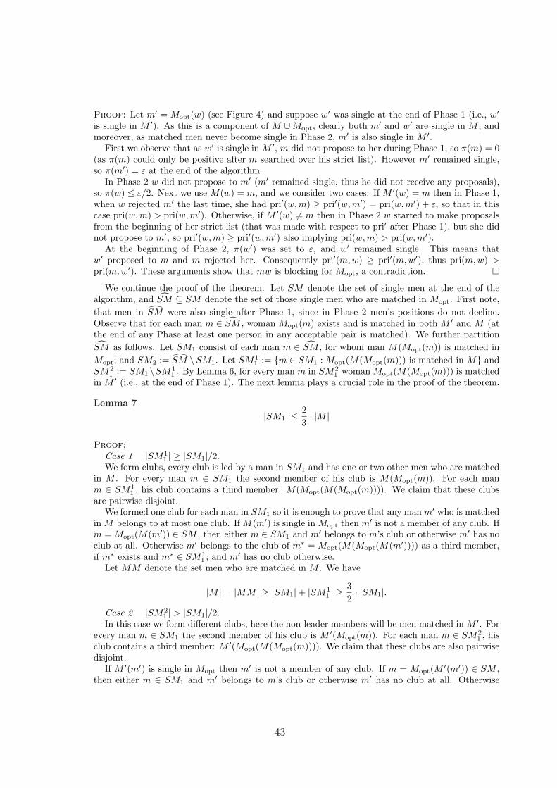
Proof: Let m′ = Mopt(w) (see Figure 4) and suppose w′ was single at the end of Phase 1 (i.e., w′
is single in M ′). As this is a component of M ∪ Mopt, clearly both m′ and w′ are single in M , andmoreover, as matched men never become single in Phase 2, m′ is also single in M ′.
First we observe that as w′ is single in M ′, m did not propose to her during Phase 1, so π(m) = 0(as π(m) could only be positive after m searched over his strict list). However m′ remained single,so π(m′) = ε at the end of the algorithm.
In Phase 2 w did not propose to m′ (m′ remained single, thus he did not receive any proposals),so π(w) ≤ ε/2. Next we use M(w) = m, and we consider two cases. If M ′(w) = m then in Phase 1,when w rejected m′ the last time, she had pri′(w, m) ≥ pri′(w, m′) = pri(w, m′) + ε, so that in thiscase pri(w, m) > pri(w, m′). Otherwise, if M ′(w) = m then in Phase 2 w started to make proposalsfrom the beginning of her strict list (that was made with respect to pri′ after Phase 1), but she didnot propose to m′, so pri′(w, m) ≥ pri′(w, m′) also implying pri(w, m) > pri(w, m′).
At the beginning of Phase 2, π(w′) was set to ε, and w′ remained single. This means thatw′ proposed to m and m rejected her. Consequently pri′(m, w) ≥ pri′(m, w′), thus pri(m, w) >pri(m, w′). These arguments show that mw is blocking for Mopt, a contradiction.
We continue the proof of the theorem. Let SM denote the set of single men at the end of thealgorithm, and SM ⊆ SM denote the set of those single men who are matched in Mopt. First note,
that men in SM were also single after Phase 1, since in Phase 2 men’s positions do not decline.Observe that for each man m ∈ SM , woman Mopt(m) exists and is matched in both M ′ and M (atthe end of any Phase at least one person in any acceptable pair is matched). We further partition
SM as follows. Let SM1 consist of each man m ∈ SM , for whom man M(Mopt(m)) is matched in
Mopt; and SM2 := SM \SM1. Let SM11 := m ∈ SM1 : Mopt(M(Mopt(m))) is matched in M and
SM21 := SM1 \SM1
1 . By Lemma 6, for every man m in SM21 woman Mopt(M(Mopt(m))) is matched
in M ′ (i.e., at the end of Phase 1). The next lemma plays a crucial role in the proof of the theorem.
Lemma 7
|SM1| ≤2
3· |M |
Proof:
Case 1 |SM11 | ≥ |SM1|/2.
We form clubs, every club is led by a man in SM1 and has one or two other men who are matchedin M . For every man m ∈ SM1 the second member of his club is M(Mopt(m)). For each manm ∈ SM1
1 , his club contains a third member: M(Mopt(M(Mopt(m)))). We claim that these clubsare pairwise disjoint.
We formed one club for each man in SM1 so it is enough to prove that any man m′ who is matchedin M belongs to at most one club. If M(m′) is single in Mopt then m′ is not a member of any club. Ifm = Mopt(M(m′)) ∈ SM , then either m ∈ SM1 and m′ belongs to m’s club or otherwise m′ has noclub at all. Otherwise m′ belongs to the club of m∗ = Mopt(M(Mopt(M(m′)))) as a third member,if m∗ exists and m∗ ∈ SM1
1 ; and m′ has no club otherwise.Let MM denote the set men who are matched in M . We have
|M | = |MM | ≥ |SM1| + |SM11 | ≥
3
2· |SM1|.
Case 2 |SM21 | > |SM1|/2.
In this case we form different clubs, here the non-leader members will be men matched in M ′. Forevery man m ∈ SM1 the second member of his club is M ′(Mopt(m)). For each man m ∈ SM2
1 , hisclub contains a third member: M ′(Mopt(M(Mopt(m)))). We claim that these clubs are also pairwisedisjoint.
If M ′(m′) is single in Mopt then m′ is not a member of any club. If m = Mopt(M′(m′)) ∈ SM ,
then either m ∈ SM1 and m′ belongs to m’s club or otherwise m′ has no club at all. Otherwise
43

m′ belongs to the club of m∗ = Mopt(M(Mopt(M′(m′)))) as a third member, if m∗ exists and
m∗ ∈ SM21 ; and m′ has no club otherwise.
Let MM ′ denote the set of men who are matched in M ′. As men matched after Phase 1 remainmatched till the end, we have
|M | = |MM | ≥ |MM′| ≥ |SM1| + |SM
21 | ≥
3
2· |SM1|.
We are ready to finish the proof of the theorem. Let MMopt denote the set of men who arematched in Mopt. We claim that |MM ∩ MMopt| ≤ |MM | − |SM2|. This is true because |SM2| isthe number of components of M ∪ Mopt isomorphic to a path with two edges and with a woman inthe middle, and for each such path the M -matched man is single in Mopt.
|Mopt| = |MMopt| = |MM ∩ MMopt| + |SM ∩ MMopt| ≤
≤ (|MM | − |SM2|) + (|SM1| + |SM2|) ≤ |M | +2
3· |M | =
5
3· |M |.
5 Open Problems
Open Problem 1 Is it possible to improve the performance of GSA1 if we use smaller ε, increaseextra scores more than once, and give extra scores to not only single men, but also to partners ofeach woman who is a neighbor of a single man?
Open Problem 2 Is it possible to improve the performance of GSA1 if we use the method of Irvingand Manlove [5] after GSA1?
Open Problem 3 Is it possible to improve the performance of GSA2 if we use smaller ε, increaseextra scores more than once, alternately for men and women? And if giving extra scores to not onlypersons remained single?
Open Problem 4 Is it possible to improve the performance of GSA2 if we use the method ofHalldorsson et al. [3], or the method of Iwama, Miyazaki and Yamauchi [7] after GSA2?
5.1 Acknowledgement
I am grateful to Tamas Fleiner for his valuable advice. This paper was also submitted to ESA’08.I am also indebted to the referees of ESA’08 for pointing out many typos and shortages in the firstversion of this paper.
References
[1] D. Gale, L. S. Shapley, College admissions and the stability of marriage Amer. Math.Monthly 69 (1962) pp. 9–15.
[2] M. M. Halldorsson, R. W. Irving, K. Iwama, D. F. Manlove, S. Miyazaki,
Y. Morita, S. Scott, Approximability results for stable marriage problems with tiesTheor. Comput. Sci. 306 (2003) pp. 431–447.
[3] M. M. Halldorsson, K. Iwama, S. Miyazaki, H. Yanagisawa, Improved approxima-tion results for the stable marriage problem ACM Trans. Algorithms 3 No. 3, (2007) Article30.
44

[4] M. M. Halldorsson, K. Iwama, S. Miyazaki, H. Yanagisawa, Randomized approxi-mation of the stable marriage problem Theor. Comput. Sci. 325 (2004) pp. 439–465.
[5] R. W. Irving, D. F. Manlove, Approximation algorithms for hard variants of the stablemarriage and hospitals/residents problems Journal of Combinatorial Optimization (2007)DOI: 10.1007/s10878-007-9133-x
[6] K. Iwama, D. F. Manlove, S. Miyazaki, Y. Morita, Stable marriage with incompletelists and ties Proceedings of the 26th International Colloquium on Automata, Languages and
Programming (1999) LNCS 1644 pp. 443–452.
[7] K. Iwama, S. Miyazaki, N. Yamauchi, A 1.875-approximation algorithm for the stablemarriage problem SODA ’07: Proceedings of the eighteenth annual ACM-SIAM symposium
on Discrete algorithms (2007) pp. 288–297.
[8] D. F. Manlove, R. W. Irving, K. Iwama, S. Miyazaki, Y. Morita, Hard variants ofstable marriage Theor. Comput. Sci. 276 (2002) pp. 261–279.
45

Optimal Popular Matchings
Telikepalli Kavitha Meghana Nasre
Indian Institute of Science, Bangalore, India.kavitha, [email protected]
Abstract. In this paper we consider the problem of computing an “optimal” popular matching. Weassume that our input instance G = (A∪P , E1 ∪ · · · ∪Er) admits a popular matching and we are askedto return not any popular matching but an optimal popular matching, where the definition of optimalityis given as a part of the problem statement; for instance, the optimality criterion could be fairness, inwhich case the problem is to return a fair popular matching, which is a maximum cardinality popularmatching that matches as few applicants to their rank r posts as possible, subject to this constraint,matches as few applicants to their rank r − 1 posts as possible, and so on. We show an O(N 2 + m)algorithm for the problem of computing an optimal popular matching, assuming that the preferencelists are strict, where m is the number of edges and N is the number of applicants in G.
1 Introduction
In this paper we consider the problem of computing an optimal popular matching in a bipartitegraph G = (A∪P, E) with one-sided preference lists. Optimality is described succinctly as a part ofthe problem statement, for instance, rank-maximality, or fairness, or min-cost (where each (a, p) ∈ Ehas a cost c(a, p) associated with it) can be considered as optimality. More generally, we assume apartial order ≤P on matchings that obeys the following natural properties:
(a) if M1,M2 are two matchings that contain an edge e and M1 ≤P M2, then M1 \e ≤P M2 \e,
(b) if M1 ≤P M2 and neither M1 nor M2 contains edge e and M1∪e and M2∪e are matchings,then M1 ∪ e ≤P M2 ∪ e.
In this paper we consider the problem of computing a popular matching in G that is an optimalelement (maximal/minimal as the case may be) with respect to ≤P among all popular matchingsin G. We first describe below the popular matching problem.
The popular matching problem. An instance of the popular matching problem is a bipartitegraph G = (A ∪ P, E) and a partition E = E1 ∪ E2 · · · ∪ Er of the edge set. The vertices of A arecalled applicants and the vertices of P are called posts. For each 1 ≤ i ≤ r, the elements of Ei arecalled the edges of rank i. If (a, p) ∈ Ei and (a, p′) ∈ Ej with i < j, we say that a prefers p to p′.This ordering of posts adjacent to a is called a’s preference list. For any applicant a and any ranki, where 1 ≤ i ≤ r, we assume that there is at most one post p such that (a, p) ∈ Ei, that is, weassume that preference lists are strictly ordered.
A matching M of G is a set of edges such that no two edges share an endpoint. We denote byM(a) the post to which applicant a is matched in M . We say that an applicant a prefers matchingM ′ to M if (i) a is matched in M ′ and unmatched in M , or (ii) a is matched in both M ′ and M ,and a prefers M ′(a) to M(a). M ′ is more popular than M , denoted by M ′ ≻ M , if the number ofapplicants that prefer M ′ to M exceeds the number of applicants that prefer M to M ′. A matchingM is popular if and only if there is no matching M ′ that is more popular than M .
46

The popular matching problem is to determine if a given instance admits a popular matching,and to find such a matching, if one exists. The popular matching problem was considered in [1]and efficient algorithms were given to determine if G admits a popular matching and to computea maximum cardinality popular matching. Note that popular matchings may have different sizes,and a largest such matching may be smaller than a maximum-cardinality matching.
1.1 Problem Definition
In this paper we assume that the input instance G admits a popular matching and here we are notcontent returning any popular matching or any maximum cardinality popular matching. Our goalis to compute an optimal popular matching, where the definition of optimality is given succinctlyas a part of the problem definition. For instance, the problem description could state fairness, orrank-maximality, or min-cost of matched edges as optimality, which means that, among all popularmatchings in G, we have to return that popular matching which is the most optimal with respectto fairness, or rank-maximality, or has the least cost, as the case may be. We define the terms fairand rank-maximal below.
The fair matching problem. The fair matching problem in a bipartite graph G = (A∪P, E1 ∪
E2 · · · ∪ Er) asks for a matching M that satisfies the properties below:
(i) M is a maximum-cardinality matching in G, and
(ii) among all maximum cardinality matchings in G, M matches the least number of applicantsto their rank r posts, subject to this constraint, matches the least number of applicants to theirrank r − 1 posts, subject to this constraint, matches the least number of applicants to their rankr − 2 posts, and so on.
Currently, there are no combinatorial algorithms known for computing a fair matching. In thispaper we consider the fair popular matching problem. A fair popular matching M is defined asfollows:
(i) M is a maximum cardinality popular matching in G, and
(ii) among all maximum cardinality popular matchings in G, M matches the least number ofapplicants to their rank r posts, subject to this constraint, matches the least number of applicantsto their rank r−1 posts, subject to this constraint, matches the least number of applicants to theirrank r − 2 posts, and so on.
Rank-maximal matchings. A rank-maximal matching M in a bipartite graph G = (A ∪ P, E1 ∪
· · · ∪ Er) is a matching that matches the maximum number of applicants to their rank one posts,subject to this constraint, matches the maximum number of applicants to their rank two posts, andso on. There are efficient combinatorial algorithms known for computing a rank-maximal matching[5]. However, there are no efficient combinatorial algorithms known for computing a maximum
cardinality matching that is the most rank-maximal among all maximum cardinality matchings.Here we consider the problem of computing a popular matching that is the most rank-maximalamong all popular matchings.
Min-cost popular matchings. Another natural definition of optimality is the following: we assumethat each edge (a, p) has a non-negative cost c(a, p) associated with it. G = (A ∪ P, E1 ∪ · · · ∪ Er)
47

admits a popular matching and we want to compute that popular matching M in G such that∑a∈A
c(a,M(a)) is the minimum among all popular matchings.
The problem of computing a fair popular matching/rank-maximal popular matching/min-costpopular matching can be solved by assigning suitable costs to the edges of an appropriate bipartitegraph H derived from G = (A ∪ P, E1 ∪ · · · ∪ Er) and computing a min-cost or max-cost perfectmatching in H. It is easy to see that the order ≤P on matchings defined with respect to fairness,rank-maximality, or min-cost satisfies properties (a) and (b) defined at the beginning of this section.
Here we present a simple combinatorial algorithm that runs in O(N 2 +m) time for the problemof computing an optimal popular matching in G, where m is the number of edges and N is thenumber of applicants in G. We assume that given two matchings M1 and M2, we can determine ifM1 ≤P M2 or M2 ≤P M1 in O(N) time, which is a reasonable assumption (and is indeed the casefor fairness, rank-maximality, or min-cost).
1.2 Related Results
The notion of popular matchings was originally introduced by Gardenfors [3] in the context of thestable marriage problem with two-sided preference lists. It is well known that every stable marriageinstance admits a weakly stable matching (one for which there is no pair who strictly prefer eachother to their partners in the matching). In fact, there can be an exponential number of weaklystable matchings, and so Gardenfors considered the problem of finding one with additional desirableproperties, such as popularity. Gardenfors showed that when preference lists are strictly ordered,every stable matching is popular. He also showed that when preference lists contain ties, there maybe no popular matching.
Abraham et al. in [1] presented an O(m+n) algorithm (for the case of strictly ordered preferencelists) to determine if the input instance G on m edges and n vertices admits a popular matchingand compute one, if it exists. For the case when the preference lists need not be strictly ordered,they showed an O(m
√n) algorithm. Manlove and Sng [7] generalized the algorithms of [1] to the
case where each post has an associated capacity, indicating the number of applicants that it canaccommodate. (They described this in the equivalent context of the house allocation problem.)They gave an O(
√Cn1 + m) time algorithm for the strictly ordered preference lists case, and an
O((√
C + n1)m) time algorithm for the case with ties in preference lists, where n1 is the numberof applicants, and C is the total capacity of all of the posts. In [8] Mestre designed an efficientalgorithm for the weighted popular matching problem, where each applicant is assigned a priorityor weight, and the definition of popularity takes into account the priorities of the applicants.Mestre’s algorithm for the case of strictly ordered preference lists has O(n+m) complexity and forthe case with ties in preference lists, the complexity is O(min(k
√n, n)m), where k is the number
of distinct weights assigned to applicants. Assuming that the input instance G admits a popularmatching, Abraham and Kavitha [2] considered the problem of computing a shortest-length voting
path1 given a starting matching M0 in G. They gave an O(m+ n) algorithm for this problem whenthe preference lists are strictly ordered and an O(m
√n) algorithm for the case of ties in preference
lists.In the case of two-sided preference lists where the two sides of the bipartite graph are considered
men and women, a stable matching is considered the ideal answer to what is a desirable matching.
1 A voting path of length k is a sequence of matchings 〈M0, M1, . . . , Mk〉 such that Mk is popular and Mk ≻Mk−1 · · · ≻ M0
48

However there is a wide spectrum of stable matchings ranging from men-optimal stable matchingsto women-optimal stable matchings. Irving, Leather, and Gusfield [6] considered the problem ofcomputing a stable matching that is optimal under some more equitable criterion of optimality. Infact, much work has been done in the two-sided preference lists setting on finding stable match-ings that satisfy additional criteria (see [4] for an overview). In the same vein, assuming that theinput instance G admits a popular matching, here we ask for an optimal popular matching whereoptimality is defined as a part of the problem statement.
2 Preliminaries
In this section we review the algorithmic characterisation for computing a popular matching from[1]. Since our problem is restricted to the case where preference lists do not have ties, we willpresent the characterisation from [1] of popular matchings for strictly ordered preference lists. Forconvenience, a dummy post ℓ(a) is added at the end of a’s preference list, for each applicant a, andthe edge (a, ℓ(a)) is assigned rank r + 1. Thus henceforth, the edge set E = E1 ∪ · · · ∪Er+1 and anyunmatched applicant a will be assumed to be matched to ℓ(a).
For each applicant a, define a first choice post for a, denoted by f(a), and a second choice postfor a, denoted by s(a), as follows. The post f(a), is one that occurs at the top of a’s preferencelist, that is, it is a’s most preferred post. The post s(a) is the most preferred post on a’s list that isnot f(a′) for any applicant a′. Note that by above the definition, f -posts are disjoint from s-posts.For each applicant a, f(a) is guaranteed to exist if its preference list is non-empty. Note that thedummy post ℓ(a) added at the end of a’s preference list ensures that s(a) always exists for eachapplicant a.
The following lemma from [1] characterises a popular matching.
Lemma 1. A matching M is popular if and only if(1) every f -post is matched in M ,(2) for each applicant a, M(a) ∈ f(a), s(a).
Let G′ denote the graph in which each applicant a has exactly two edges, (a, f(a)) and (a, s(a))incident to it. From Lemma 1, it is immediate that the input instance G admits a popular matchingif and only if the graph G′ defined above admits an A-perfect matching. Thus the problem ofdetermining if G admits a popular matching is now easy to solve. Algorithm 2.1 contains the mainidea and [1] presents an efficient implementation of this idea that runs in O(m + n) time (where m
and n are the number of edges and vertices in G).
Algorithm 2.1 A simple framework from [1] to compute a popular matching in G
for each a ∈ A do
– determine the posts f(a) and s(a)end for
Construct the graph G′ on vertex set A ∪ P and edge set ∪a∈A(a, f(a)), (a, s(a)).if G′ admits an A-perfect matching then
return an A-perfect matching M in G′ that matches all f -posts.else
return “G admits no popular matching”end if
49

3 Our Algorithm
In this section we describe our algorithm to compute an optimal popular matching in G with respectto the optimality criterion specified as a part of the input. We know that any popular matchingcan match an applicant either to its f -post or to its s-post. Since our problem is to compute amatching that is necessarily popular, we can delete all posts p from G where p is not an f -post oran s-post. Thus G becomes the graph (A∪P, E ′) where E′ consists of edges (a, f(a)) and (a, s(a))for each a ∈ A.
An optimal popular matching, by virtue of being a popular matching, has to match every f -post. So if a is an applicant such that it is the only applicant that considers f(a) as its top post,we know that such an applicant a has to be matched to f(a) by any popular matching. So weinclude all such pairs (a, f(a)) in our matching that we will return and delete such vertices a, f(a)from G. So from now on we can assume that every applicant in G has degree exactly 2. Further weknow that G admits an A-perfect matching since any popular matching is an A-perfect matchingin (A ∪ P, E′).
Let N be the number of applicants in G. We will order the applicants a1, . . . , aN in an arbitrarymanner. We will work with the graphs Hk, for 1 ≤ k ≤ N , where Hk is the graph on vertexset a1, . . . , ak ∪ f(a1), . . . , f(ak), s(a1), . . . , s(ak) and edges ∪k
j=1(aj , f(aj)), (aj , s(aj)). Any
popular matching in the graph G restricted to applicants a1, . . . , ak is a matching of size k in Hk
that matches all the posts f(a1), . . . , f(ak). We present a simple iterative strategy for computingan optimal popular matching in G: for each 1 ≤ k ≤ N , we will compute a matching Mk thatsatisfies the following 2 properties.
(1) Mk is a matching of size k in Hk that matches all the posts f(a1), . . . , f(ak).
(2) among all the matchings that satisfy (1), Mk is optimal with respect to ≤P .
We will compute such an Mk iteratively. Say we have already computed the desired matchingMk−1; in the current step, we add to the graph Hk−1 the applicant ak and the posts f(ak), s(ak)(if they do not yet belong to Hk−1) and the edges (ak, f(ak)) and (ak, s(ak)) to form the graph Hk.We will show that Mk can be computed by augmenting Mk−1 appropriately.
Mk has size k in Hk, thus it has to match each of the applicants a1, . . . , ak. Due to the factthat we augment Mk−1 in Hk, each of a1, . . . , ak−1 remains matched (to either their f -post ors-post). Also since Mk needs to match ak, either (ak, f(ak)) or (ak, s(ak)) has to belong to Mk. Ouralgorithm tries both the options:
(1) it tries to find augmenting paths pk and qk with respect to Mk−1 in Hk in order to match ak tof(ak) and to s(ak), respectively. It is easy to show that at least one of pk, qk has to exist.
(2) If pk does not exist, then Mk = Mk−1 ⊕ qk and if qk does not exist, then Mk = Mk−1 ⊕ pk. Ifboth pk and qk exist, then the more optimal of Mk−1 ⊕ pk and Mk−1 ⊕ qk is chosen as Mk.
We present our algorithm as Algorithm 3.1 and show that this simple method suffices.Theorem 1 proves the correctness of our algorithm.
Theorem 1. The matching MN returned by our algorithm is a popular matching that is optimal
with respect to ≤P .
It is easy to see that the matching MN returned by our algorithm is popular. Note that, foreach i, Mi is a maximum cardinality matching in Hi. Thus MN is a maximum cardinality matching
50

Algorithm 3.1 Our algorithm to compute an optimal popular matchingfor each a ∈ A do
– determine the posts f(a) and s(a).end for
– Set any order among the applicants so that the applicants can be labelled a1, a2, . . . , aN .– Let H1 be the graph on vertex set a1 ∪ f(a1), s(a1) and edge set (a1, f(a1)), (a1, s(a1))); let M1 be thematching (a1, f(a1)).– Initialize i = 2.while i ≤ N do
Update Hi−1 to Hi by adding the applicant ai and posts f(ai), s(ai) (if they do not already exist) to the vertexset and the edges (ai, f(ai)) and (ai, s(ai)) to the edge set.if f(ai) is newly added then
Mi = Mi−1 ∪ (ai, f(ai)).else
find an augmenting path pi with respect to Mi−1 in Hi−1 that begins with the edge (ai, f(ai))find an augmenting path qi with respect to Mi−1 in Hi−1 that begins with the edge (ai, s(ai))if pi (similarly, qi) does not exist then
Mi = Mi ⊕ qi (resp., Mi ⊕ pi).else if both pi and qi exist then
Mi = the more optimal of Mi ⊕ pi and Mi ⊕ qi.end if
end if
i = i + 1.end while
– Return MN .
in HN ; we know that HN = (A ∪ P, E′) admits an A-perfect matching since the input instanceadmits a popular matching. Thus MN is an A-perfect matching. Also, by construction, we neverlet an f -post remain unmatched. Thus, MN is an A-perfect matching in (A ∪P, E ′) that matchesall f -posts. Thus MN is a popular matching in the input instance.
We now need to show that among all popular matchings, MN is optimal with respect to ≤P .We will prove this by induction: we will show that for each i, Mi is a matching of size i in Hi thatmatches all posts f(a1), . . . , f(ai) and amongst all such matchings, Mi is optimal.2
We will now show that for all 1 ≤ i ≤ N , Mi is optimal in Hi subject to the constraint thatMi has to match all of a1, . . . , ai and f(a1), . . . , f(ai). The base case i = 1 is trivial. By inductionhypothesis, we assume that Mk−1 is optimal in Hk−1 subject to the constraint that it has to matchall of a1, . . . , ak−1 and f(a1), . . . , f(ak−1). Using this hypothesis, we will show that Mk is optimalin Hk subject to the constraint that it has to match all of a1, . . . , ak and f(a1), . . . , f(ak).
We consider two cases: (i) f(ak) is not present in Hk−1 and (ii) f(ak) is present in Hk−1.Lemma 3 deals with the first case and Lemmas 4 and 5 deal with the second case.
Lemma 2. Let Mk−1 be an optimal matching in Hk−1 subject to the constraint that the vertices
a1, . . . , ak−1 and f(a1), . . . , f(ak−1) have to be matched. If f(ak) is not present in Hk−1, then
Mk = Mk−1 ∪ (ak, f(ak)) is optimal in Hk subject to the constraint that all of a1, . . . , ak and
f(a1), . . . , f(ak) have to be matched.
2 Note that we can compare two matchings M, M ′ of Hi with respect to ≤P by extending each of M, M ′ toa1, . . . , aN by considering ai+1, . . . , aN as unmatched and we can compare the extended matchings withrespect to ≤P .
51
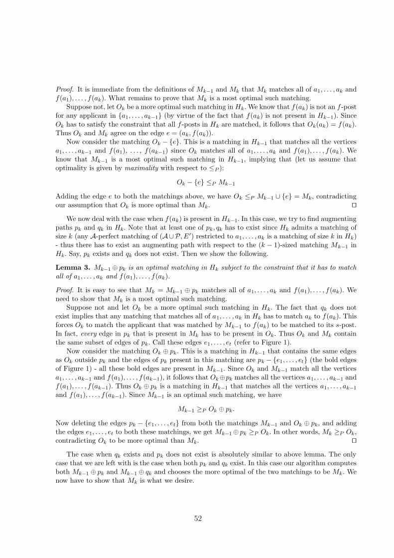
Proof. It is immediate from the definitions of Mk−1 and Mk that Mk matches all of a1, . . . , ak andf(a1), . . . , f(ak). What remains to prove that Mk is a most optimal such matching.
Suppose not, let Ok be a more optimal such matching in Hk. We know that f(ak) is not an f -postfor any applicant in a1, . . . , ak−1 (by virtue of the fact that f(ak) is not present in Hk−1). SinceOk has to satisfy the constraint that all f -posts in Hk are matched, it follows that Ok(ak) = f(ak).Thus Ok and Mk agree on the edge e = (ak, f(ak)).
Now consider the matching Ok − e. This is a matching in Hk−1 that matches all the verticesa1, . . . , ak−1 and f(a1), . . . , f(ak−1) since Ok matches all of a1, . . . , ak and f(a1), . . . , f(ak). Weknow that Mk−1 is a most optimal such matching in Hk−1, implying that (let us assume thatoptimality is given by maximality with respect to ≤P ):
Ok − e ≤P Mk−1
Adding the edge e to both the matchings above, we have Ok ≤P Mk−1 ∪ e = Mk, contradictingour assumption that Ok is more optimal than Mk. ⊓⊔
We now deal with the case when f(ak) is present in Hk−1. In this case, we try to find augmentingpaths pk and qk in Hk. Note that at least one of pk, qk has to exist since Hk admits a matching ofsize k (any A-perfect matching of (A∪P, E ′) restricted to a1, . . . , ak is a matching of size k in Hk)- thus there has to exist an augmenting path with respect to the (k − 1)-sized matching Mk−1 inHk. Say, pk exists and qk does not exist. Then we show the following.
Lemma 3. Mk−1 ⊕ pk is an optimal matching in Hk subject to the constraint that it has to match
all of a1, . . . , ak and f(a1), . . . , f(ak).
Proof. It is easy to see that Mk = Mk−1 ⊕ pk matches all of a1, . . . , ak and f(a1), . . . , f(ak). Weneed to show that Mk is a most optimal such matching.
Suppose not and let Ok be a more optimal such matching in Hk. The fact that qk does notexist implies that any matching that matches all of a1, . . . , ak in Hk has to match ak to f(ak). Thisforces Ok to match the applicant that was matched by Mk−1 to f(ak) to be matched to its s-post.In fact, every edge in pk that is present in Mk has to be present in Ok. Thus Ok and Mk containthe same subset of edges of pk. Call these edges e1, . . . , et (refer to Figure 1).
Now consider the matching Ok ⊕ pk. This is a matching in Hk−1 that contains the same edgesas Ok outside pk and the edges of pk present in this matching are pk − e1, . . . , et (the bold edgesof Figure 1) - all these bold edges are present in Mk−1. Since Ok and Mk−1 match all the verticesa1, . . . , ak−1 and f(a1), . . . , f(ak−1), it follows that Ok⊕pk matches all the vertices a1, . . . , ak−1 andf(a1), . . . , f(ak−1). Thus Ok ⊕ pk is a matching in Hk−1 that matches all the vertices a1, . . . , ak−1
and f(a1), . . . , f(ak−1). Since Mk−1 is an optimal such matching, we have
Mk−1 ≥P Ok ⊕ pk.
Now deleting the edges pk − e1, . . . , et from both the matchings Mk−1 and Ok ⊕ pk, and addingthe edges e1, . . . , et to both these matchings, we get Mk−1 ⊕ pk ≥P Ok. In other words, Mk ≥P Ok,contradicting Ok to be more optimal than Mk. ⊓⊔
The case when qk exists and pk does not exist is absolutely similar to above lemma. The onlycase that we are left with is the case when both pk and qk exist. In this case our algorithm computesboth Mk−1 ⊕ pk and Mk−1 ⊕ qk and chooses the more optimal of the two matchings to be Mk. Wenow have to show that Mk is what we desire.
52

e1
e2
et
ak
f(ak)
Fig. 1. The path pk: the bold edges are present in Mk−1 and the dashed edges are in Mk and in Ok.
Lemma 4. Mk, the more optimal of Mk−1 ⊕ pk and Mk−1 ⊕ qk, is a most optimal matching in Hk
that matches all of a1, . . . , ak and f(a1), . . . , f(ak).
Proof. It is obvious that Mk matches all of a1, . . . , ak and f(a1), . . . , f(ak). Suppose Mk is not anoptimal such matching, let Ok be a more optimal such matching in Hk. The matching Ok has tomatch ak to either f(ak) or to s(ak). We will show the following:
Claim 1. If Ok(ak) = f(ak), then Ok ≤P Mk−1 ⊕ pk.
Claim 2. If Ok(ak) = s(ak), then Ok ≤P Mk−1 ⊕ qk.
We know that either Ok(ak) = f(ak) or Ok(ak) = s(ak), which implies by Claims 1 and 2 thateither Ok ≤P Mk−1 ⊕ pk or Ok ≤P Mk−1 ⊕ qk. Thus Mk, which is the more optimal of Mk−1 ⊕ pk
and Mk−1 ⊕ qk is at least as optimal as Ok, contracting our assumption that Ok is more optimalthan Mk.
Hence, what we need to show are Claims 1 and 2.
Proof of Claim 1. If Ok(ak) = f(ak), then as we argued in the proof of Lemma 4, it follows thatMk−1⊕pk and Ok contain the same subset of edges of pk. Now consider Ok ⊕pk: this is a matchingin Hk−1 that matches all of a1, . . . , ak−1 and f(a1), . . . , f(ak−1). Since Mk−1 is an optimal matchingin Hk−1 that matches all of a1, . . . , ak−1 and f(a1), . . . , f(ak−1), it follows that Ok ⊕ pk ≤P Mk−1,or equivalently, Ok ≤P Mk−1 ⊕ pk. This finishes the proof of Claim 1.
Proof of Claim 2. This proof is absolutely similar to the proof of Claim 1. If Ok(ak) = s(ak), thenas we argued in the proof of Lemma 4, it follows that Mk−1⊕ qk and Ok contain the same subset ofedges of qk. Now consider Ok ⊕ qk: this is a matching in Hk−1 that matches all of a1, . . . , ak−1 andf(a1), . . . , f(ak−1). Since Mk−1 is an optimal matching in Hk−1 that matches all of a1, . . . , ak−1
and f(a1), . . . , f(ak−1), it follows that Ok ⊕ qk ≤P Mk−1, or equivalently, Ok ≤P Mk−1 ⊕ qk. Thisfinishes the proof of Claim 2. ⊓⊔
53

This completes the proof of Theorem 1. We will now analyse the running time of Algorithm 3.1.The f and s-posts of all applicants can be computed in O(m + N) time. The main while loop ofAlgorithm 3.1 runs for N iterations and each iteration takes O(N) time to construct the augmentingpaths pi, qi and to compare Mi−1⊕ pi and Mi−1⊕ qi. Thus our algorithm runs in O(N 2 + m) time.
4 Discussion
In this paper we gave an O(N 2 + m) algorithm for computing an optimal popular matching forinstances with strict preference lists. This raises the question of extending our algorithm for thecase when ties are allowed in the preference lists. Note that our assumption of strict preferenceswas critical in proving the correctness of our algorithm. When preference lists are allowed to haveties, an applicant can have more than one post as its f -post and similarly, it can have more thanone post as its s-post.
Recall that our iterative algorithm, in case of strict preference lists, updates the current optimalmatching Mk−1 along one of the two augmenting paths pk or qk to get an optimal popular matchingMk. The fact that every applicant has degree exactly 2 in Hk ensures that we need to consider onlytwo augmenting paths at each step of our algorithm. Further, if an optimal matching Ok matchesapplicant ak to f(ak), then Ok is forced to agree with Mk for all applicants that appear on theaugmenting path pk. This reduces the problem of comparing Ok and Mk to comparing Ok⊕ pk andMk ⊕ pk and we use our induction hypothesis here to show that Ok ⊕ pk cannot be more optimalthan Mk−1 = Mk ⊕ pk.
The difficulty in case of ties, is precisely in the part of extending Mk−1 to Mk. We leave it asan open question to extend our combinatorial algorithm to the case of ties in preference lists.
References
1. D.J. Abraham, R.W. Irving, T. Kavitha, and K. Mehlhorn. Popular matchings. SIAM Journal on Computing,Vol.37, No.4, pp. 1030–1045, 2007. (Preliminary version in Proc. of 16th SODA, pages 424-432, 2005.)
2. D. J. Abraham and T. Kavitha. Dynamic matching markets and Voting paths. In Proceedings of SWAT 2008,
the 10th Scandinavian Workshop on Algorithm Theory, (LNCS 4059), pages 65-76, Springer-Verlag, 2006.3. P. Gardenfors. Match making: assignments based on bilateral preferences. Behavioural Sciences, 20:166–173,
1975.4. D. Gusfield and R.W. Irving. The Stable Marriage Problem: Structure and Algorithms MIT Press, 1989.5. R.W. Irving, T. Kavitha, K. Mehlhorn, D. Michail, and K. Paluch. Rank-maximal matchings. In Proceedings of
SODA ’04: the 15th ACM-SIAM Symposium on Discrete Algorithms, pages 68–75. ACM-SIAM, 2004.6. Robert W. Irving, Paul Leather, and Dan Gusfield. An Efficient Algorithm for the “Optimal” Stable Marriage.
Journal of the ACM, 34(3): 532-543, 1987.7. D.F. Manlove and C. Sng. Popular matchings in the capacitated house allocation problem. In Proceedings of
ESA 2006, the 14th Annual European Symposium on Algorithms, (LNCS 4168), pages 492-503, Springer-Verlag,2006.
8. J. Mestre. Weighted popular matchings. In Proceedings of the 33rd International Colloquium on Automata,
Languages and Programming, (LNCS 4051), pages 715–726, 2006.
54

!#" $ &%(')+*,-$.#0/0'
13254)6879;:<9;=>9)?A@81395BDC>2FEHGI95:F9)?J@K9;L>=NMPOCP6RQSO>6UTV6XWY9;BZ954)6\[?^] _ 95=>C>9badceM>QSO>225f825g-EhL>gi2 _ :F9Dad6jQZkA@81lW>2Dad2<mLP6on>c _ kA6oahW
[dp QD95=>cZ:F6jQ`qlcDLradc _ gi2 _ ql25:Fs>Ctad6jL>uv9;L>=NTwcZ=>6j9vMtadC>=>6jcZkA@U1lW>2Dad2<mLP6on>c _ kA6oahWx 4)O>9;:<9;=>95@86XGI95:F9zy534)C>6jk |j4rWY2Dar2DSC>|j95QD|o~!s>@k^O)C>6jQSO>6j:FcD=>6R9;|R4rWY2bad2DJC>|R9;QZ|X~!s
^!JD8tl-bDbUAAZb! ¢¡£-¥¤£Db ¦e §brr©Rb©Hb§AªZ!b«b¤¬b §DDbbtA e®U¯iDeD°!±b¤Y±²³!b°hetbbP;!°At!µ¬¶r·b;²t¸® Z®²³b3·t³A;b·tDr· ;!8D¤;bD8tS¹r!S²Db§¤£!bº §b°h§ ·KD¤£¨»º°!DbDUr· ±³A¼b¤;!Ar½DD!!b°h§Dtb½·l¼¶r·D;®¯i½½¾!©H¿rS¾8±b¼lDZ¨D°!r²!!ªrDU!bUDbt §D°h;²tbte´¬D°Abe;D3³D¨rD §D §r®e¯iF§D³AJ²¾»°!DADF!ªrADÀ¾8!»!D°hFDD¼³A°!´!·;!btNÁoÂbÃYÄ^Å;b·t»Dv»r· ±³A»b¤³DbtJ²¼b §A¨r²½ÆǤ£Abte §b°h;²½er· ±³A»b¤A!rDbAl!b°hDD)Ub8 §bK-·t³AU³D·I¶r·blbb8!D8-S¾!8;b·t¶r·D5®È S¾²Jb §KD°!bt ¼D §D°h;²S·YPY!D¨ºA#bYKb! ÉD¤tD¿r¤!µKb §D°hKb¹b!¬³D¨rD §D³ §Z®PÊǺ°!DA#D¬bt Ë!Db¹b!Dlb¤btA e²!tb)J²A½b! wb¤r´ttUU¤£!D½b·bº¾8 § ±· wZ·t ;!D¤rr°h¿rtbS®Ê`±tS¾wbbe¬bSªr §D¾8,¡Ì\ÍÌrÎ,Ì\ÏÌЦÑÒtÓµ¤£D-br¨³D¹b°!btbr
Ô ²t¾8!»ÍDÀÏVb±Aµb¤>DDbA!rJ²A;!°A¹b!¨Z®8tµtbSªr §Di¨!·UD-!¹bAI¤YD)tA¤£!!°A-Dº°!D §ADe°A^²rDeb)DD-S¹bb §tA¤£!!°A#U¡£¿rS¾8b>t¬Õ¸ §b!>Ö5¦®Ê`K¤£·t!>°!DAPKA°!DbJ²J§DbelD³S¹DZ²;D½!!rtS¹blb §§!¤£!!t°!§^²zD«tS¾ÉD°Ab«³lb¹bA;b¨rb §bz §Z®
× ØzÙ¬ÚÛYÜ»ÝeÞeß8Úà!ÜÙáKâ)ã äAåiæçbèéIêætëAë^ìRætíbé§îëïçDèéDêñð ò¬óôð£õrãtö ÷Çø³ù)úDôùÀû)üúdýö ãtþ ÿüò ò õ)ð ãtõý;÷¬ódö ã`ó^ù#õrâ#ó^ûö ãS÷ ãó^üãð dãSùòã òIúþ§ãSù¥ó^ù#õ<ôúþ§ãSùó^ù#õFãtó âû>ãSüòúdù òû)üã\ãSüãSùã ö£ð ò â#ó údüZõrãSüò â)ã,þlãtþý>ãSüòú â)ã»ú âãSüòã óúdüDõ)ð ù úâð ò â)ãSüû)ü!ãoãSüãSùã ±áKâã"! ãSò ð údùwð ò ú`ÿ)ù#õÀó`äAåiæçbèé3êIæå$# %ì'&í âó ð ò ½óþ3ó â#ð ù()údù ódð ù#ð ù(Fù)ú«û#ódð ülúµþ3ó^ù ó^ù#õ`ôµúþ3ó^ù ôâú`û)ü!ãoãSülãtó â ú â)ãSü ú â)ãtð ülûó^ü ù)ãSüò * âóû#ódð üeð òSódö£ö ãtõÆóÇçDèï+#+,bì-&)í»î³æìHë. »á8â)ãS÷«û)üú+dãtõ â#ó ó^ù³÷ ð ùò ó^ùãÇódõþ3ð òIó ö ãtó^ò údù)ã¬ò ó^ý#ö ãÇþ3ó â#ð ù(ó^ù#õIûüúdû>údòãtõÀó^ùNódö dúdüDð â#þ ú3ÿ)ùõ¬údùã5ø³ùúbôùNó^ò â)ã"»ódö ã/0râó^û#ö ãS÷ ódö dúdüDð â#þ1
2 ù â)ã òDódþ§ã ûó^ûPãSü3 â)ãS÷ódö òúÉû)ü!údûPúdò!ãtõóþó^ù³÷4/ ú/iúdù)ã ã ãSù)òDð údù ú â)ãÆò ó^ýö ã.þ3ó^üüDð£ó5dãû)üúdýö ãtþ18ôâð6iâð ò7 üüãSù ö ÷Nø;ù)úDôùó^ò â)ã8±ïä îìHåiæèä:9<;UéDä!ì-=é+&)åiä3îëïçbèébê?>08@;A\údü3òâ)údü +B 2 ùDC@EF ôµúò!ã òGúdüüãSòû>údù#õð ù( úvþ§ãSùNó^ùõôúþ§ãSùVó^üãlüãSòDð£õdãSù òIó^ù#õIâ)údòûð ódö ò 5üãSòû>ã ð dãtö ÷ IH-óiâvâ)údòû#ð ódöòû>ãSð ÿ)ãSò`ð òKJ+L5ïåiæM½ôâ#ð6 â.þ§ãtó^ù)ò âó ð Só^ù.óãSû ó þ§údò N âð ò»ù þý>ãSülú#üãSòDð£õrãSù ò C-ãSùãvð ù.ó\ãtó^òDð ý#ö ãÇþó iâ#ð ù( â)ã»ù þý>ãSüúPüãSòDð£õrãSù òó^ò!òDð dù)ãtõ úãtóiâ,â)údòûð ódö¼ð ò û ú,ð òO! ú ó PºãSù)ãSüDódö£ö ÷ð ùQC@EFYû)üã\ãSüãSùãvö£ð ò òù)ãSãtõ«ùú ý>ãRúþ§û#ö ã ã#ù#ódþ§ãtö ÷#ãtó âNüãSòZð£õrãSù údüDõrãSüò«óIò ý)ò!ã ú#â)údòû#ð ódö ò ó^ù#õIãtó â<â)údò!û#ð ódö;údüDõrãSüòóò ý)òã úüãSòDð£õdãSù ò TSý#ö úUiøYð ù(3ûódð üð òù)úDô(õrãSÿ)ù)ãtõÀó^òó§û#ódð üúâ)údòû#ð ódöV ó^ùõ ü!ãSòDð£õrãSù WX â#ó ð ùSö õrãÆãtóiâú âãSüNð ù â)ãtð üÀû)üã\ãSüãSùã ö£ð ò òFò â â#ó >hð B â)ãÆù þý>ãSü«úüãSòDð£õdãSù ò`ó^ò!òDð dù)ãtõ ú V ð òö ãSòò â#ó^ù ð ò*! ú óúdü V û)üã\ãSüò W* úwó ö ãtó^ò údù)ãIüãSòDð£õdãSù ó^òòZð dù)ãtõ ú Vó^ù#õ*>hð£ð BUW ð ò ù#ó^òòDð dù)ãtõlúdü-û)üã\ãSüò V úâ#ð ò±ó^òòDð dùãtõ»â)údò!û#ð ódö6 ZY3údò û)üúdû>ãSü ð ãSò-ú âãò ó^ý#ö ãIþ3ó^üüDð£ó5dã
[
55

û)üúdýö ãtþ ó^û)û#ö£ð ãSò úC@EF)ã 6#ó ù;÷ ð ù)ò ó^ùãÇódõ)þ3ð òeólò ó^ý#ö ãÇþ3ó â#ð ù(ó^ù#õeúdùãSó^ù,ýPãoú ùõIý³÷ â)ãó^û)û)ü!údû)üDð£ó ãtö ÷ þ§úYõ)ð ÿ)ãtõ»ódö ã/0râó^û#ö ãS÷ ódö dúdüDð â#þ1
Sò â)ãºù#ódþ§ãºú(C@EÆò dãSò ò )ð â#ó^òþ3ó^ù;÷¬üãtódö /iôµúdüDö£õeó^û)ûö£ð6Só ð údù)ò±ð ù<ó^òòDð dùþ§ãSù ò÷;ò ãtþ§ò8ý>ã ôãSãSùüãSòDð£õdãSù ò«ó^ù#õÇâ)údòû#ð ódö òý#ó^òãtõ«údù â)ãtð ü»û)ü!ãoãSüãSùãSò Yôâð6iâ.ð ò»ø;ù)úDôù.ó^ò\@EFY] ð ù â)ãR^@ 6( I _` [ a óEIYb3ð ù a ó^ù#ódõ)ó" c`(]Sd>Hôâ#ð6 âvð òUù)úDôeSódö£ö ãtõ"f+SO B ð ùR(ú ö£ó^ùõb g`ih)ó^ùõOjEFY] ð ùjtó^û#ó^ùk [l 2 ð òeódö òú òãtõ,ð ùVó^ò!òDð dù#ð ù(Çò õrãSù ò úÇòmiâ)ú;úö ò3ð ùn)ð ùó^ûPúdü!ão [ g CUúDôãdãSümPòDð ùã â)ãSüãÀó^üãò!ûPãSð£ódöüã! ð üãtþ§ãSù ò3ð ùvü!ãtódö£ð ÷>òúþlã òã özã ãSù)òDð údù)ò§ôµãSüãûüúdû>údòãtõ( pfdúdülã>ódþ§ûö ãð ù â)ã\@EFY]¥ð ù â)ã^@ 6( 6óºùúdù(/iù)ãö ã ó^ý#ö ãù þý>ãSü8ú>þ3ó^üüDð ãtõ*ú û#ö ãSò§ó^û)û#ö ÷oúdü â)ã¬þ3ó iâð ù(¬ôâú»ô§ó^ù q úýPã¬þó iâ)ãtõ ú<âúdòû#ð ódö ò¬ôð â#ð ùóKSö údò!ãÆõ)ð ò ó^ùãúdù)ã,ó^ù)ú â)ãSü ,áKâ#ð ò»ã ãSù)òDð údùwôló^òr\údüDþ3ódö£ö ÷Éþ§úYõrãtö ãtõQ [ _ó^ù#õó^ùs\I]t/0úþ§û#ö ã ãSù)ãSò!ò»üãSò ö [u ó^ù#õ òúþ§ãIû)ü!údûPãSü ð ãSòR v#ôµãSüãIúdý ódð ù)ãtõ( NS±ù)ú âãSüãYódþ§û#ö ãFó^û)û>ãtó^üòð ù ó^òòDð dùð ù(Iò õrãSù ò úeû)üúiwHã ò¬ð ù ó ù#ð dãSüòDð ÷ FHóiâ ö ã üãSüû)üú+Yð£õrãSòúdù)ã§údü¬þ§údü!ãûüúiwRã òm;ãtóiâú8ôâ#ð6iââ#ó^ò<ð òR! ú ó xSIö òú-ãtóiâ ö ã üãSüeâ#ó^òeâ#ð òm^â)ãSüeúbôùD! ú óUôâ#ð6iâ þlãtó^ù)ò â)ã þ3ó5Yð£þ þù þý>ãSüú>ò õdãSù ò§â)ã òâãSó^ùÉóãSû NS±ùÉó^òòDð dùþ§ãSù ð ò3ó«þ3ó^û)û#ð ù\üúþ(ò õrãSù ò úÇûüúiwRã ò§òú â#ó ! ú ó^òú5û)ü!úiwRã òó^ùõÇö ã üãSüò¬ó^üã3ódö£ö³òDó ð òÿ)ãtõ yS±ýüDó^â#ódþã ódö6 þ§úYõrãtö ãtõ â#ð òºû)üúdý#ö ãtþ ó^ò â)ã õdãSù /0]½üúiwRã SIö£ö úUSó ð údùÆû)üúdý#ö ãtþ ó^ù#õOódããzbSð ãSù ódö dúdüDð â#þ§ò ú3ÿ)ù#õÀóò ó^ý#ö ãÇþ3ó â#ð ù(n l G|~PUm|Z 2 ù â#ð òÇû#ó^û>ãSü µôµãvû)ü!údûPúdò!ãwó^ù)ú â)ãSüÇã ãSù)òDð údù0úC@E ôâ)ãSüã<ãtó â¥â)údòû#ð ódöõrãSö£ó^üãSòù)ú údù#ö ÷ó^ù ûûPãSü§ý>ú ù#õÇý ( ódö òúNóFö úDôãSüý>ú ù#õ`údù â)ãeù þýPãSülú#üãSòZð£õrãSù òÇð óãSû ò a údù)ò!ã! ãSù ö ÷>óG\ãtó^òDð ý#ö ãeþ3ó â#ð ù(Fþ ò òDó ð òmo÷ âãúdù#õð ð údù âó â)ãù þý>ãSüú5üãSòDð£õrãSù òló^òòDð dù)ãtõ úÉãtó â â)údòûð ódölð òNó þ§údò ð ò û)û>ãSü«ý>ú ù#õ! ú óó^ù#õó ö ãtó^ò ð òNö úbôµãSü<ý>ú ù#õ! ú ó +áKâ#ð òüãSò üZð6 ð údùòãSãtþ§ò)! ð ã üãtö ãzó^ù ð ù¥ò!ãdãSüDódöºòDð ó ð údùò fdúdüÀã>ódþ§ûö ãþó^ù³÷.â)údòû#ð ódö òFâódã òúþ§ãòúdü úKã;û>ã ó ð údù)òvð ùVãtóiâ÷dãtó^ü â#ó ó ö ãtó^ò âð òeù þý>ãSüú8üãSòDð£õrãSù ò<ó^üãxúþ3ð ù(Kôâ)úVó^ü!ã ó^ùð£þ§û>údü ó^ù ö£ó^ý>údüNoúdümã\údü âãâ)údòûð ódö6 ySIö ò!úþ3ó^ù;÷võrãSûó^ü þ§ãSù òútj³ó^û#ó^ù)ãSòã ù#ð dãSüòZð ð ãSò ³ãSòû>ãSð£ódö£ö ÷ð ù ãSùð ù)ãSãSüDð ù(Nò iâ)ú;úö ò ºôâ)ãSüãFò õrãSù òÆó^üãwó5ódð ùdúdù)òDð£õdãSüãtõ úwý>ãNó^ù ð£þ§û>údü ó^ù ö£ó^ý>údü7oúdü ãnoúdüã;ûPãSüZð£þ§ãSù òm â)ãIù þý>ãSü§úYò õdãSù òó^òòZð dù)ãtõ ú«ãtóiâNû)üú\ãSòòúdü§òâ)ú ö£õ`ý>ãIòúþ§ãSâ)úDô ý#ódö£ó^ùãtõ( 2 ù â#ð òòã ð ù;ôã§üã! ð üã úeÿ)ù#õÇó±ò ó^ý#ö ã3þ3ó iâð ù(5ôâ)ãSü!ã â)ã§ò ó^ýð£ö£ð ÷ õrãSÿ)ù#ð ð údù ð ò â)ã§òDódþ§ã3ó^ò â#ó úC@EF < ãRSódö£ö â#ð ò§û)ü!údý#ö ãtþ8I;8ìRå$%<ì-&)ìHêL5êL5ïåiæ>08@;koúdülò!â)údü +B 1\-ú ã â#ó ð6YôµãFódö£ö úbôð ùúþ§ûö ã ãNö£ð ò ò â)ãSüãxSó^ùÉý>ã ð ù)ò ó^ùãSòeôð âùúoãtó^òDð ýö ãÀòúö ( ð údùÉãdãSùð6Uôã ð dùúdüã â)ãÀò ó^ý#ð£ö£ð ÷údù#õ)ð ð údù Qdú8ôµã)údù)òDð£õrãSü3údùö ÷úþ§ûö ã ãNö£ð ò ò XSeö òúI\údü â)ãÀòDódþlãÀüãtó^òúdù-ôã ó^ò!ò þ§ã â#ó O â)ãù þý>ãSüúüãSòDð£õdãSù òð òIó ö ãtó^ò âã»ò þ ú â)ãö úDôãSüý>ú ù#õr! ú ó^òúKódö£ö5â)údòûð ódö ò
fKð üò úµódö£ö6Uð ð ò»ãtó^ò!÷ úÀòãSã âó N â)ãeã>ð ò ãSùã3ú-óò ó^ý#ö ã<þ3ó iâð ù(XSó^ù ý>ããtó^òDð£ö ÷Éõrã ãSüDþ3ð ù)ãtõòDð ùãÀð ùCIE â)ãù þý>ãSüúPò õrãSù ò±ãtó â â)údòû#ð ódöüããtð dãSòð ò â)ã¬òDódþlã«ð ùó^ù³÷<ò ó^ý#ö ãÀþ3ó iâ#ð ùs u \ódþ§ãtö ÷±ð6 â)údòã«ù þýPãSü!òòZó ð ò o÷ û)û>ãSüFó^ù#õVö úbôµãSüý>ú ùõXúdù#õð ð údù)ò ð ð ò<ó õrãSòDð üDó^ý#ö ã þ3ó â#ð ù(ó^ù#õFú â)ãSüôð òãùú<ò ó^ý#ö ã þ3ó â#ð ù(,ã>ð ò òm r.âãSù â)ãSü!ã,ð òIù)úFò ó^ýö ãÆþ3ó â#ð ù(ôµã`ôló^ù G ú,ÿ)ù#õ óþ3ó â#ð ù(7 ó^òUò ó^ý#ö ã¬ó^òUû>údòòDð ý#ö ãð6 ã 6ôµãpúdù)òDð£õrãSü âãû)üúdý#ö ãtþútÿ)ù#õ)ð ùIólþ3ó â#ð ù( âó þ3ð ù#ð£þ3ð SãSò â)ãvù þý>ãSüúµý#ö úUiøYð ù(Nû#ódð üò d üÿ)üò üãSò ö ð ò âó " â#ð òÇû)üúdý#ö ãtþ ð ò7\@]U/iâó^üDõ ó^ù#õQSó^ù)ù)ú ý>ãó^û)û)ü!ú+Yð£þ3ó ãtõÀôð âð ù â)ãeüDó ð úFú>+ d " B ?¡£¢ \údü`ó^ù³÷Æû>údòDð ð dãbúdùò ó^ù p¤* ùö ãSòò*]¥p\I]¦Pôâ)ãSü!ã&ó^ù#õ õdãSù)ú ã âãòã ò§ú>âúdòû#ð ódö ò3ó^ù#õüãSòDð£õrãSù ò üãSòû>ã ð dãtö ÷ IáKâ#ð òeð ò3ódö£þ§údò @ ð dâ ý>ãSó òãôãSó^ùÇòâ)úbô â#ó âãû)üúdýö ãtþð ò§ó^ûû)üú+Yð£þ3ó^ý#ö ã±ôð â#ð ùn $ " f ü â)ãSü â#ð òð ù#ó^ûû)üú+Yð£þ3ó^ý#ð£ö£ð ÷3üãSò ö â)úö£õròãdãSùVð6#ódö£özû)üã\ãSüãSùãö£ð ò òó^ü!ã"úþ§û#ö ã ãÇó^ùõò üDð6 ½ódö£ö5âúdòû#ð ódö òâ#ó.dã â)ãlòZódþ§ãlû)üã\ãSüãSùãö£ð ò >Hôâ#ð6 â ð òø³ù)úDôù ó^ò â)ã`êætä!åiébëlèìHä!å [§ B Yó^ù#õ«ódö£ö³â)údòû#ð ódö òâ#ó.dã û)û>ãSü-ý>ú ù#õ! ú ó [ >Hôâð6iâ þ§ãtó^ù)ò â#ó P â#ð ò§üãSò ö â)úö£õdòO\údü â)ãIò ó^ý#ö ãFþ3ó^üüZð£ó5dãSó^ò!ã B P ã â)ãSùsúdù)òDð£õrãSü§ò ü!údù(dãSülüãSò üDð6 ð údù âó ð ùý>ú âNú8â)údòû#ð ódö òFó^ù#õ<üãSòDð£õrãSù òIòDð£õrãSò ódö£ö¼û)üã\ãSüãSùã ö£ð ò òFó^üã ð£õrãSù ð6Sódö6 VáKâ#ð òüãSò üDð6 ð údùòãSãtþlò úý>ã ú³úÀò üDð6 K\-ãdãSü â)ãtö ãSòò ¼ôµã3òâ)úDô â#ó ð ð òù)údù(/ üDð Yð£ódö>ý;÷vòâúbôð ù( ó^ùð ù)ò ó^ùã3ôâ)údòãeúdû ð£þ3ódöòúö ( ð údùVð òó5ódð ù)ò ú üð ù ð ð údù y ã â)ãSùKð dã«ó§û>úö ÷³ù)úþð£ódö / ð£þ§ã`ódö dúdüDð â#þ \údü â#ð òû)ü!údý#ö ãtþ1 ©ª¬« ª4®n©*ª4¯ | « ¯ a ö£ó^òòDð6Sódö³üãSò ö òúdù â)ãC-údòû#ð ódö òmE8ãSòDð£õrãSù òû)üúdýö ãtþ>C@E B Só^ùÇý>ãG\ú ù#õ`ð ù _ E8ãSò!ãtó^ü iâÇúdù7C@Eð òò ð£ö£öó ð dã§üããSù ö ÷ [ v` [[ Sò§þlãSù ð údù)ãtõ¬û)üãYð ú òDö ÷ â)ãSüãó^üãòúþlãã ãSù)òDð údù)ò
l
56

úC@EFù#ódþ§ãtö ÷TC@E0ôð âsú ûö ãSò [ _` [u v5ó ù#õ â)ã õdãSù /0]½üúiwRã Seö£ö ú¦Só ð údùNû)üúdý#ö ãtþ° l eáKâãúdùãSû úþó^ò ãSüö£ð ò òSó^ù<ý>ã"oú ù#õÀð ù [§
áKâãSüãÉó^üã ónú û#ö ã úûüúdý#ö ãtþ§ò â#ó ð ù4dúö dã ÿ)ùõ)ð ù(¥óþ3ó iâ#ð ùôð â þ3ð ù#ð£þ þ ù þý>ãSü«úý#ö úUiøYð ù(û#ódð üò Z±ºâ ö£ö ãSüµã ódö6 y [ c`8ð ù üú>õ ãtõ«ó^ù`údù#ö£ð ùãIdãSüòZð údùÇú â)ã±ò ó^ý#ö ã3þ3ó^üüDð£ó5dãû)üúdý#ö ãtþ"ó^ù#õû)üú dãtõ â#ó G âãSüãÆð òIù)úúþ§û>ã ð ð dã«údù#ö£ð ù)ã ódö dúdüDð â#þ1 bSý)üDó^â#ódþ ã ódö6 P [ û)ü!údûPúdò!ãtõ â)ãÇû)üúdý#ö ãtþúÿ)ù#õ)ð ùó þ3ó iâ#ð ù ôð â âã)oãSôµãSò ù þý>ãSüeú-ýö ú¦ ø>ð ù( û#ódð üò ó^ù#õÆòâúbôµãtõ â#ó ð ð ò3â#ó^üDõ úó^û)û)ü!ú+Yð£þ3ó ã
² ³.ÛU´qµ!à·¶ àAÙOÛYà0´q¹º»:¼ ½¾¿nÀXÁÃÂmÄÅ:ÆMǦÈ:ÂMÉtÊ7¿(ÂMÅ:Ë¿(ÌyÆMÂÍ"Î`ÁtÏÈ:¿(Ð ÑKÅÆm¾dÒÓÅ:ÌÅ:ÐÔÐ Õ7ÔÁÃÆmÇSù ð ù)ò ó^ùã<ú â)ãvì'&ìRêL5êÖºèï+#+,bì-&)ío×æìRëR8±ïä îìHåiæèä:9<;UéDä!ì-=é+&)åiä×-ëïçDèéDêØ8ìHå$%<ì-&)ìRêL5êÙL5ïåiæ>0<ì-&(ÚÛÖ×d8I;n\údüIòâ)údü +B údù)òDð ò òeú â)ãÇòã úKüãSòZð£õrãSù ò Ü â)ã`ò!ã úKâúdòû#ð ódö òKXÜvó^ù#õ<ãtóiâþ§ãtþý>ãSü òUû)üã\ãSüãSùã¬ö£ð ò q â#ó údüDõdãSüòódö£öþ§ãtþý>ãSüò8ú â)ãú â)ãSüUûó^ü ÷ Seö òúdãtó â`âúdòû#ð ódö V â#ó^ò±ö úbôµãSüó^ù#õ ûûPãSü§ý>ú ù#õdò±ú! ú óUÝ ó^ù#õoÞ>Hò â â#ó ÝxßàÞ B >ü!ãSòû>ã ð dãtö ÷ ã3òúþ§ã ð£þ§ãSòòDóh÷ â#ó N â)ã! ú óIú V ð òx Ý<áÞ· RfrúdüòDð£þ§û#ö£ð6Sð ÷#ôã`òúþ§ã ð£þ§ãSòôüDð ã â)ãù#ódþ§ã3ú#â)údòûð ódö>ôð â3! ú óeý>ú ùõrò ò âNó^ò V Ý<áÞ·
S¢êIæå$# %ì-&)íIð ò3ó`þó^û)û#ð ù(7oüúþ(üãSòZð£õrãSù ò úÇâ)údòû#ð ódö ò§òú â#ó P â)ãù þý>ãSüúYüãSòDð£õrãSù ò3ó^òòDð dù)ãtõ ú¬ãtó â«â)údòû#ð ódö V Ý<áÞ·Kð òý>ã ôµãSãSùÝ«ó^ù#õ*ÞM â)ã @ã > W(B ý>ã â)ã±â)údòû#ð ódö ú¬ôâð6iâü!ãSòDð£õrãSù W ð ò§ó^òòDð dù)ãtõ ù#õdãSü ã >hð6ð ãYð ò ò B ºó^ù#õ ã > V B ý>ã â)ã3òã úüãSòDð£õrãSù òÇó^ò!òDð dù)ãtõ ú<â)údòûð ódö V 7frúdüÀóFþ3ó â#ð ù(ã ó^ù#õvólâ)údòûð ódö V ÝäáÞ0ð6 ã > V B ¬¥eÞ1>hð ùSö õ)ð ù( âãSó^òã â#ó Ý¥Þ¥A ã > V B B ôµã¬òDó÷ â#ó V ð òå L;èHè ù#õrãSü ã Yó^ù#õFð6Z ã > V B æçÞM;ôµã»òDó÷ âó V ð òL£&(=tébë5Úä·L;çDä0#DëAìHç!é·= ù#õdãSü ã y ã ü â)ãSüû#ó^ü ð ð údù ù#õdãSü./iò ý)òmüDð ý>ãtõÀâ)údòûð ódö ò 2 V ð ò ù#õrãSü./iò ý)ò üDð ý>ãtõ ó^ùõD ã > V B q¥èÝ<8ôµãÀòDóh÷ â#ó V ð ò#bë^ìRåiì-#!ætèé â)ãSü!ôð òã;ù#ódþ§ãtö ÷ ð6Ý*æà ã > V B `æçÞM5ôãlòZóh÷ â#ó V ð òeì-&)åiébë^êIé0=ìHæåié
frúdü¬óþ3ó â#ð ù( ã ³ôµã±òDó÷ â#ó óûódð üNúþlû)üDð òDð ù(«óü!ãSòDð£õrãSù W ó^ùõ`óâ)údòû#ð ódö V \údüDþ§òlóIçDèï# ,bì-&)íî³æìHëð6 â)ãRoúö£ö úDôð ù( ôµúkúdù#õ)ð ð údùò`ó^üãvþ§ã +ê >hð BW ð ò»ãtð â)ãSü ù#ó^òòDð dù)ãtõÀúdü»û)üã\ãSüò V ú ã > W(B >hð£ð BV ð ò ù#õrãSü0/iò ý)ò üZð ýPãtõúdü§û)ü!ãoãSüò W" úÇúdù)ãú>üãSòDð£õrãSù ò3ð ù ã > V B Y,ð ù(/0ë]CIEIYbì ð ò â)ãû)üúdý#ö ãtþ úÿ)ù#õð ù(Fó3þ3ó iâð ù(3ôð â âã`þ3ð ù#ð£þ þ ù þý>ãSüúý#ö úUiøYð ù(3û#ódð ü!ò
vì'&(ÚÛÖ×çí`bîÃÚÛ8I;nQ>Y,ð ùsë] [ Y,ó^ò ãSü*â#ð ò /0CIEIYbì B ð ò â)ãIüãSò üDð6 ð údù úqY,ð ù(/0ë]çCIEIYbìòú â#ó ð ùó"ð dãSùð ù)ò ó^ùã â)ã`û)üã\ãSüãSùãÆö£ð ò òIúódö£ö½â)údò!û#ð ódö ò«ó^ü!ãÆð£õrãSù ð6Sódö6 <ì-&(ÚïÖ×ñð`bîÃÚÛ8I;nð ò,õdãSÿ)ù)ãtõ òZð£þ3ð£ö£ó^üDö ÷µù#ódþ§ãtö ÷lð ùó^ù ð ù)ò ó^ùãlódö£öUâúdòû#ð ódö òÇâ#ódã â)ã<òDódþlã<û)üã\ãSüãSùãwö£ð ò ló^ù#õ ódö£öüãSòDð£õdãSù ò±â#ódã âã»òDódþ§ãlû)ü!ãoãSüãSùã`ö£ð ò º»òº óoÄÄÎ`ÁäôÅÐ3ǦÆMÅ:ÁtÌõÊ7ǦÆMÅ:Át ã3òDó÷ â#ó ó^ù.ódö dúdüDð â#þ÷ö(ð òÇó^ù W >-ø B /!ó^û)û)üú >ð£þ3ó ð údù0ódö dúdüDð â#þ ð6ð òZó ð òÿ)ãSò`þ3ó5Uùö@>-ú Bûü Ý`ý>-ú Bþú+dãSü»ódö£öð ù)ò ó^ùãSòúÇú;òDð SãFøtôâ)ãSüã ü Ýý>-ú B ó^ù#õ*öI>-ú B ó^üã â)ãòDð Sã±ú â)ãúdû ð£þ3ódöó^ùõ â)ãódö dúdüZð â#þ1 òòúö ( ð údù5üãSòû>ã ð dãtö ÷
ÿ ØzÙOeÛYܻ෶eà0µAà!Úd´¹ÞOµAÚ Ü±Û àAÙç³ × 2 ù â#ð òòã ð údùzôµã»òâ)úDô â#ó Y,ð ù(/0ë] [ Yâi/0C@EFYì ð ò\I]t/iâ#ó^üDõ(Yó^ù#õeãdãSù<â#ó^üDõ úvó^û)û)üú >ð£þó ã ª ª ïëæ`&"!-î³ïä!ìHåiì$#béF#Aï &)äAåiæ &)å ¤&% å$%éDëéìHäq&)ïî³ïtè'!M&)ïêIìHæè ÚåiìHêIéF>+ * " B ?¡£¢ ÚæSîîëï)(bìHêIæåiìRï&æèíbïë^ìHå$%ê å ïëp<ì-&(ÚïÖ×Qí`RîÚï8@;nL£&)èéDä!äN×+*-,I×+.
v
57

×-ëï ï å . ãòâ)úDô ópó^ûð ù üúYõ Sð ù3üãtõ ð údù\üúþ ó»ôãtö£ö /iø;ù)úDôùs\I]t/0úþ§û#ö ã ãû)üúdý#ö ãtþ Yvð ùð£þ þ/ ãSü ã a ú dãSü> / a oúdüò!â)údü +B 0 ¯ 21 ª43 üDó^û)â65e¥ç>87á:9 B ó^ù#õÀólûPúdòZð ð dãÇð ù ãdãSü;7 <G| ª4¯ < 3>= ú³ãSò?5 údù ódð ù ódãSü ãXú dãSülúPòDð Sã«ó þ§údò ;A@)>-SõdãSü ãkú+dãSü3ð òIó¬ò ýòã 7BDCE7
ò iâ âó oúdüãdãSü÷ÀãtõMdãGFDHI9p½ó ö ãtó^ò údù)ãlãSùõrû>úð ù úJF¬ð òIð ù67B B \-úbôGYö ã LKNM ¥ç>85 M á:; M B ý>ãIó^ù ð ù)ò ó^ùãú / a ³ôâ)ãSüã5 M ¥ç>87 M á:9 M`B ó^ù#õO; M ð ò¬ó±ûPúdòZð ð dãeð ù ãdãSü = ãSÿ)ù)ãPøx¥à 7 M ð â)ú ö ú;ãSòòú(dãSù)ãSüDódö£ð ÷zôã3þ3ó÷,ó^òò þ§ã âó ; M ßnø frúdüóúdù)ò ó^ù Z¤ >õrãSÿ)ùãP ¥RQTS ¢VU XW ? ¥nø B ó^ù#õYW [ ¥ø B2Z 9 M ã â)ãSùúdùò ü * â)ãwð ù)ò ó^ùã K úNYvð ù/0ë] [ Yâi/0C@EFYì?oüúþ KNM á8â)ãFòã úµüãSòDð£õrãSù òÆð ò
¥\[ ]`_a]bÜvó^ù#õ â)ãlò!ã úâ)údòû#ð ódö òIð òG¥c7d]ed]gfk Hóiâvòã ð òõdãSÿ)ù)ãtõÀó^òG\úö£ö úbôò ê
[ ¥ ù PNh [ ßjiß\; M`þ_ ¥ ùk h [ ßjißø Z ; M`þb hml n ¥ ùo hml nM l p [ ß\qß\W [ þ ]Kùo hrl n? l p [ ß\qß\W [ þb ¥ stvu l txwzy|~X l hrn
b hrl n7 ¥ ùv h [ ßjißnø þe hml n ¥ ù5ý hml nM l p [ ß\qß\W [ þ ]Kù5ý hrl n? l p [ ßcqGß\W [ þe ¥ s
tvu l txwzy|~ l hrne hrl n
f ¥ ù5ú h [ ßiß\W ? þHóiâÇâ)údòû#ð ódöð ùf¢â#ó^òóG! ú óý>ú ù#õR § [ >ó^ù#õ»ú â)ãSüâúdòû#ð ódö ò-âódãeóp! ú óý>ú ù#õR [ [ F\Uú ã
â#ó [rk _M¥à 7Kró^ù#õb b@m¥à er >¥ l 9 M W [ B ð ùãó^ù;÷âúdòû#ð ódöð ù7]eÉâ#ó^òó! ú óý>ú ù#õR [ [ ó^ù;÷þó iâ#ð ù(ð òÇóeúdù)ã/ ú/iúdù)ã þ3ó iâ#ð ù<ý>ã ôµãSãSù ó^ù#õI7c]Oe-ó^ù#õFãdãSü÷ â)údòû#ð ódö-ð ùf þ ò ý>ã ù#ó^ò!òDð dù)ãtõ( 2 ù ð ð dãtö ÷>ãtó â þ§ãtþý>ãSüú7èúdüü!ãSòû>údù#õrò ú`ãtó âodãSü ãwð ù7 M 2 H7 M ð ò§òãtö ã ãtõð ù ó@dãSü ãxú+dãSüm â)ã"údüüãSò!ûPúdùõ)ð ù(Iâ)údòû#ð ódö4H7(ð òþó iâ)ãtõIôð â óeþ§ãtþý>ãSü¬ð ù[G;ú â)ãSüôð òãð òþ3ó â)ãtõeôð âNó3þ§ãtþý>ãSü¬ð ù6_ \-ú ã â#ó M¥nøK l 9 M W [ aW ? ó^ù#õk "m¥nøR l 9 M W [) â)ãSùã 5e "m¥ l øRc 9 M W [ W ? ¥ l ø Z c 9 M [ >-c 9 M 5 [ B ø B ænø [ cø Bz [ ø B ß u ø Bz [ 5ôâ#ð6iâNð òû>úö ÷³ùúþ3ð£ódö½ð ùKø
\-ã ;ôµã"údù)ò ü û)üã\ãSüãSùã3ö£ð ò ò fKð [ òâ)úDôòºû)üã\ãSüãSùã3ö£ð ò òú)üãSòDð£õrãSù ò ³ôâ)ãSü!ãR6 7F6>HüãSòû 6 fR6 B õdãSù)ú ãSòFó ú ódöúdüZõrãSüIúKãtö ãtþ§ãSù ò<ð ù7>HüãSòû f B ð ùó^ùð ùüãtó^òDð ù,údüZõrãSüú±ð ù#õ)ð6ãSò çv:: õrãSù)ú ãSòIó ú ódözúdüZõrãSüúú â)ãSüâ)údò!û#ð ódö òð ùNó^ùwó^üý#ð üDó^ü÷ÇúdüDõrãSüm
]½üãoãSü!ãSùãvö£ð ò òú½â)údò!û#ð ódö òÇó^üã,ð£õrãSù ð6Sódöó^ù#õ ó^üãúdý ódð ù)ãtõx\üúþ óFþó^ò ãSüÇö£ð ò ð dãSùð ù3fKð l C-ãSüã6 [6¬ó^ù#õç6 _6¬ó^üã ó^òeý>ãoúdü!ã ó ú ódöKúdüZõrãSüeúódö£öâ)údò!û#ð ódö ò<ð ùc[ ó^ù#õj_UüãSòû>ã ð dãtö ÷±ð ù ó^ùð ùüãtó^òZð ù(3údüDõrãSüúð ù#õ)ð6ãSòm G6 b¦6ð òó ú ódö)údüDõrãSüúZ6 b hrl n 6b>>$ h á n B H9 M áiæj B ð ùNó^ù;÷`údüZõrãSü ;ôâ)ãSü!ã
6 b hrl n 6Ã¥\o hrl n? l ? o hrl nM l ? o hrl nM l [ ::ao hrl nM l 2 o hrl n? l [ ::ao hml n? l 2T\-úbô â)ãüãtõ ð údùvð ò@úþlû#ö ã ãtõ( Zë#ãoúdü!ãòâ)úDôð ù( âãGúdüüã ù)ãSò!òû)ü!ú³ú-rôµãôð£ö£öròãSã±òúþ§ãûüúdû>ãSü./
ð ãSò-ú â)ãüãtõ ãtõ3ð ùò ó^ùã Zfrúdü§óºüãSòDð£õrãSù qW ó^ù#õ3óâ)údòû#ð ódö V ð6 V ó^û)û>ãtó^üò ú â)ãüDð dâ úT6 fb66/iû#ó^ü ú W ò¬ö£ð ò zôµã*Sódö£öt> W á V B ólîëï %ìHçbìHåié0=Iî³ætìRë0
c
58

PNh ê 6 7F6 6 fR6 :: > [ ßjiß\; MBk h ê 6 7F6 6 fR6 :: > [ ßjißnø Z ; M Bo hrl n? l ? ê ý hrl nM l [ n ý hrl n? l [ 6 fR6 :: >>$ h á n B HI9 M áiæj Bo hrl nM l ? ê ý hrl nM l ? h ý hrl n? l ? 6 fR6 :: >>$ h á n B HI9 M áiæj Bo hrl nM l [ ê ý hrl nM l [ h ý hrl nM l 6 fR6 :: >>$ h á n B HI9 M áiæj B o hrl nM l 2 ¡Y? ê ý hrl nM l J ¡Y? h ý hrl nM l 2 6 fR6 :: >>$ h á n B HI9 M áiæj Bo hrl nM l ê ý hrl nM l h ý hrl nM l ? 6 fR6 :: >>$ h á n B HI9 M áiæj Bo hrl n? l [ ê ý hrl n? l [ n ý hrl n? l 6 fR6 :: >>$ h á n B HI9 M áiæj B o hrl n? l 2 ¡Y? ê ý hrl n? l J ¡Y? n ý hrl n? l 2 6 fR6 :: >>$ h á n B HI9 M áiæj Bo hrl n? l 2 ê ý hrl n? l J n ý hrl n? l ? 6 fR6 :: >>$ h á n B HI9 M áiæj B
fKð üã [ ê ]½üã\ãSüãSùãö£ð ò ò±úü!ãSòDð£õrãSù òYâ ê 6 [Z6Ù6 b¦6Ù6 _6
fð üã l ê Y,ó^ò ãSüûüãoãSü!ãSùã ö£ð ò úâ)údòûð ódö ò
ª6)I $ å æÀêIæå$# %ì'&í ã #Aï`&)åiæì-&)äæîëï%ìRçDìRåié·=3î;æìRë % å$%é+& å$%é"&(L5êçAébëï å çDèï+#+,bì-&)í§î;æìRë^ä¬ì-& ãìHälæåèé!ætä!å+W ? .×-ëï ï å . û)û>údòã â#ó óþ3ó â#ð ù( ã údù ódð ù)òóUû)üúdâ#ð ý#ð ãtõû#ódð ü> W á V B Zë#÷ â)ã§õrãSÿ)ù#ð ð údùúDû)üúdâ#ð ý#ð ãtõû#ódð üòm W ûüãoãSü!ò`ó^ù³÷ â)údòû#ð ódötúHjf ú V oºù â)ãú âãSüâ#ó^ùõ(½ü!ãSódö£ö â#ó ó^ù³÷ â)údòû#ð ódötúHjf ð ò ù#ó^ò!òDð dù)ãtõFð ùVó^ù³÷)\ãtó^òDð ý#ö ã«þ3ó iâ#ð ù¼ó^ù#õ3â)ãSùã ù#õrãSü./iò ý)ò üDð ý>ãtõ( rú> W áÛú B ð òeó§ý#ö úUiøYð ù(û#ódð üoúdüãdãSü÷rúH fk )ð ùã7 fM¥cW ? âãlû)üú;ú#ð òGúþlû#ö ã ãtõ(
\-úbôGPü!ãSódö£ö âó \údü§ãtóiâ ãtõMdãK>$ h á n B H9 M >$i@æd B â)ãSüãÀó^üã â)ãò!ã ú½üãSòDð£õrãSù ò?b hrl n ó^ùõ â)ãòã ú5â)údò!û#ð ódö òe hrl n ã1Sódö£ö â#ð òºû#ódð üºú5òã ò»ó>$ h á n B /^íDæ =íbéDå-Yó^ù#õôüDð ãeð ó^ò hrl n ¥ç>8b hml n áe hrl n B ZfrúdüãtóiâódõMdã hrl n ½ö ã F òõrãSÿ)ùã ôú`û>ãSü oã þó iâ#ð ù(dò±ý>ã ôµãSãSùb hrl n ó^ùõge hrl n ó^òG\úö£ö úbôò ê
ã Mhrl n ¥õùO>8o hrl nM l ? áÛý hrl nM l ? B t>8o hrl nM l [ áÛý hml nM l [ B :: t>8o hml nM l p áÛý hrl nM l p B :: U>8o hrl nM l 2 ¡Y? áÛý hrl nM l 2 ¡Y? B Ã>8o hrl nM l J áÛý hrl nM l J B Ã>8o hrl n? l ? áÛý hrl n? l [ B >8o hrl n? l [ áÛý hml n? l B :: U>8o hml n? l p áÛý hml n? l p ? B :: U>8o hrl n? l J ¡Y? áÛý hrl n? l J B Ã>8o hrl n? l J áÛý hrl n? l ? Bþã ?hrl n ¥õùO>8o hrl nM l ? áÛý hrl n? l ? B t>8o hrl nM l [ áÛý hml nM l B :: t>8o hml nM l p áÛý hrl nM l p ? B :: t>8o hrl nM l J ¡Y? áÛý hrl nM l J B Ã>8o hrl nM l J áÛý hrl nM l ? B t>8o hrl n? l ? áÛý hrl nM l [ B >8o hrl n? l [ áÛý hml n? l [ B :: U>8o hml n? l p áÛý hml n? l p B :: t>8o hrl n? l ¡Y? áÛý hrl n? l ¡Y? B Ã>8o hrl n? l áÛý hrl n? l Bþ
fKð Ãvòâúbôò ã Mhrl n ó^ù#õ ã ?hrl n údù<û)üã\ãSüãSùãö£ð ò ò±ú2b hml n ª6)I ïtë¬æÀíbæ=íbéDå4 hrl n ¥e>8b hrl n áe hrl n Bz%qã Mhrl n æ`&= ã ?hrl n æëé3å$%é3ï&)è'!¬î³éDë å é0#DåµêIæå$# %ì-&)íbäç!ébå$8éAé+&b hrl n æ`&(=?e hrl n å$%æåP=ïo&)ïtå±ì-&(#bè L£=éÀæ`îëï %ìHçbìHåié0=«î³ætìRëv. L5ë^å$%ébë^êIïëé % é!æ#+%Æï å ã Mhrl n æ&(= ã ?hrl n #!ï&)åiæì-&)äï`&)è!«ï &)é`çbèï#+,Dì'&)í»î³æìHëG> W á V B ä0L£#+%<å$%æå W Hb hml n æ`&(= V He hrl n .$8ébëé!æ å åiébë % 8é`ä!ìHê±îè'!ÀäAåiæåiéå$%tìRäæä¬æ çDèï+#+,bì-&)íî³ætìRëç!ébå$8éAé+&b hrl n æ`&(=>e hrl n .¢¡×-ëï ï å . a údù)ò ü óeýð û#ó^ü ð ãrdüDó^û)â5 hrl n ôâ)ãSü!ããtóiândãSü ãNòã ð ò`b hml n ó^ù#õYe hrl n ºó^ù#õ â)ãSüã ð òÀó^ùãtõMdã§ý>ã ôµãSãSù W >8HIb hrl n B ó^ù#õ V >8He hrl n B ð6#ó^ù#õúdù#ö ÷vð6> W á V B ð òù)ú ó±û)ü!údâ#ð ý#ð ãtõû#ódð ü ZºùãSó^ùÀòãSã â#ó
59

££££££££
¤¤¤
¤¤¤¥¦¥ ¦¥ ¦¥¦
¥ §¥ §¥ §
¥ §© ¦ ª §« ª «© ¦ ª §¬ ª «© ¦ ª §¬ ª © ¦ ª §¬ ª ®z¯ ° «© ¦ ª §¬ ª ® ¯© ¦ ª §« ª © ¦ ª §« ª ®z¯ ° «© ¦ ª §« ª ® ¯
± ¦ ª §¬ ª ± ¦ ª §¬ ª
± ¦ ª §¬ ª ®z¯ ° «
± ¦ ª §« ª ®z¯ ° «
± ¦²ª §« ª
± ¦ ª §« ª
± ¦²ª §¬ ª ³± ¦²ª §¬ ª ® ¯± ¦ ª §¬ ª ® ¯ ± ¦²ª §¬ ª «
± ¦ ª §¬ ª «
± ¦²ª §« ª ³± ¦²ª §« ª ®x¯± ¦ ª §« ª ® ¯ ± ¦²ª §« ª «
± ¦²ª §« ª «
´´´´´´´´
µµµ
µµµ¶·¶ ·¶ ·¶·
¶¨¶ ¸¶ ¸
¶ ¸¹ · º ¸» º »¹ · º ¸¼ º »¹ · º ¸¼ º ½¹ · º ¸¼ º ¾z¿ À »¹ · º ¸¼ º ¾ ¿¹ · º ¸» º ½¹ · º ¸» º ¾z¿ À »¹ · º ¸» º ¾ ¿
Á · º ¸¼ º ½Á · º ¸¼ º ½
Á · º ¸¼ º ¾z¿ À »
Á · º ¸» º ¾z¿ À »
Á ·²º ¸» º ½
Á · º ¸» º ½
Á ·²º ¸¼ º ÂÁ ·²º ¸¼ º ¾ ¿Á · º ¸¼ º ¾ ¿ Á ·²º ¸¼ º »
Á · º ¸¼ º »
Á ·²º ¸» º ÂÁ ·²º ¸» º ¾x¿Á · º ¸» º ¾ ¿ Á ·²º ¸» º »
Á ·²º ¸» º »
fð üã*v ê Y,ó iâ#ð ùdò ã Mhrl n >hö ã +B ó^ù#õ ã ?hrl n >HüDð dâ +B
5 hrl n ð òÇóK÷¦Sö ãúö ãSù( âXcÃW [ CUãSùã â)ãSüã<ó^üã3údùö ÷ ôúvûPãSümoã þ3ó â#ð ù(dòýPã ôãSãSùb hrl n ó^ù#õOe hrl n ó^ù#õ â)ãS÷ ó^üã`ó ódö£ö ÷ ã Mhrl n ó^ù#õ ã ?hrl n Seö òú½ð ð òãtó^ò÷ úb â)ãiø â#ó pã Mhrl n údù ódð ù)òúdùö ÷`údù)ãlýö ú¦ ø>ð ù(û#ódð üG>8o hrl n? l ? áÛý hrl nM l [ B ¼ó^ù#õ ã ?hml n údù ódð ù)òúdù#ö ÷Çúdù)ã»ý#ö úUiøYð ù(3ûódð üG>8o hrl nM l ? áÛý hrl nM l ? B
ã«ó^üãlù)úbôüãtódõr÷ ú3òâ)úDô â)ãó^û ª6)I ÅÄÆ å KNM ìRäæ& !rébä ì'&)äAåiæ &(#Aé»ï åÇÉÈ % å$%é+& K %tæäæeä!ïtè L5åiìHï &8ìRå$%æåKêïtä!å(ø [ k 9 M ³çDèï# ,bì-&)íî³æìHë^äz.×-ëï ï å . û)û>údòã âó 5 M â#ó^òFó*dãSü ãQú dãSü3úKòDð Sã ó þ§údò ; M 2 ð òeòDð Sã ð òFö ãSòò â#ó^ù\; M ódõ)õó^üý#ð üZó^ü÷7dãSü ð6ãSò úwþ3ó^ødã â)ã`òDð Sã`ãYó ö ÷^; M ½ôâð6iâ¥ð ò ½úZú üòã#ò ð£ö£öµóOdãSü ã3ú dãSü xâ)ã G â#ð òdãSü ã7ú+dãSüý>ã7 M B >8C\7 M B Pó^ùõÇö ã 7 M:Ê ¥\7 MË 7 M B Zfrúdüpúdù4dãSù#ð ãSùãzôã òã7 M B ó^ù#õÌ7 M:Ê ódö òúK\údü â)ãòã ò±úúdüü!ãSòû>údù#õ)ð ù(eâ)údò!û#ð ódö ò
ãKúdù)ò ü ó«þ3ó â#ð ù( ã ú K óúdüDõð ù( ú7 M B GfKð üò þó iâ ãtóiâ ü!ãSòDð£õrãSù ð ù[ôð â,ãtóiââ)údòûð ódöð ù 7 M B ÜÆó^ù#õ ãtó âü!ãSòDð£õrãSù ð ùE_ ôð âãtóiâ0â)údòûð ódöð ù 7 M:Ê lð ù ó^ùó^üýð üDó^ü÷Vô§ó÷ )ð ùã [a]Y_*m¥à 7Km¥nø â)ãSüãÇó^üã`ó þ§údò ø [ ý#ö ú¦ ø>ð ù3û#ódð üòý>ã ôãSãSùj[a]`_ ó^ùõ7G
frúdü<ãtóiâçódõMdã hrl n ¥ >8b hml n áe hrl n B >>$ h á n B HÍ9 M ái)æÎ B ±ôµã òãÆúdù)ãÆú ôú þ3ó â#ð ù(dòNð ùâzãtþþ3ó"v 6v N)ð ùãO7 M B ð òódãSü ãXú+dãSümãtð âãSüD h údüÏ n ð òIð ùSö õrãtõ<ð ùj7 M B 2 Ð h ð òIð ù7 M B ò!ã ã ?hrl n ú â)ãSüôð òã ò!ã ã Mhrl n 2 ð ò â)ãSùvãtó^ò÷ úòãSã âó F â)ãSüãÇð òù)ú3ýö ú¦ ø>ð ù( û#ódð üý>ã ôµãSãSùb hrl n ó^ù#õK Ë e hml núdü* Ë b hrl n ó^ù#õÌe hrl n Seö òúó^ò¬û)üú dãtõ ð ù3â)ãtþ3þ3óKv 6v â)ãSüãvð ò»údùö ÷vúdù)ãý#ö ú¦ ø>ð ùFû#ódð ü»ý>ã ôµãSãSùdb hml nó^ù#õge hml n ð ùFãtð â)ãSüSó^ò!ã
rú â)ã¬ù þý>ãSüúý#ö ú¦ ø>ð ùû#ódð üòeð òó þ§údò ø [ ýPã ôãSãSù[d]_(ó^ùõY7¼ó^ù#õ3ã>ó ö ÷ 9 M Zôð â#ð ùãtóiâódõMdã #ó^ù#õâ)ãSùãø [ e 9 M ;ð ù ú ódö6)ôâ#ð6iâkúþ§û#ö ã ãSò â)ãlû)üú;ú' ª6)I ÅÑÆ å KNM ìHä§æ &)ï ì-&)äAåiæ &(#!éeï å6ÇJÈ % å$%é+&Ææ &Ã!ä!ïtè L5åiìHï & ï å K %æä¬æåèé!ætä!å+W ? çbèï#+,Dì'&íî³æìHëAäT.×-ëï ï å . û)û>údòã âó gK ódõ)þð òeó«þ3ó â#ð ù( ã ôð âö ãSòò â#ó^ùW ? ýö ú¦ ø>ð ù(Çû#ódð üòm F ãIòâúbô â#ó KNMâ#ó^òóNdãSü ãxú+dãSüúòZð SãG; M
u
60

fKð üò úódö£ö6rüãSódö£ö â#ó ó^ù;÷Çþ3ó â#ð ù(þ ò ý>ã§óúdù)ã/ ú/iúdù)ãþ3ó iâ#ð ùlýPã ôãSãSùR 0ó^ù#õg7`]ÒeG ÃSIö òúý;÷7â)ãtþ3þ3ó1v l ½ð6 ã údù ódð ùòIó§ûüúdâ#ð ý#ð ãtõû#ódð üm â)ãSüãó^üãÇó ö ãtó^ò W ? ý#ö úUiøYð ù(3û#ódð ü!ò túdù üDódõ)ð6 ð ù( â)ãÀó^òò þlû ð údù pdú ã õdú³ãSò§ù)ú údù ódð ù óû)üúdâð ý#ð ãtõ3ûódð ü p)ð ùãx [d]_¥Ó 7ó^ù#õvó^ù;÷FüãSòZð£õrãSù W HI[]`_ð ùSö õrãSòúdù#ö ÷7 ú â)ãö ã úZ6 fR66/iû#ó^ü ð ù â)ãlû)ü!ãoãSüãSùãö£ð ò ã þ ò ð ùSö õrã3ó§û>ãSü \ã þ3ó â#ð ù(3ý>ã ôµãSãSù[ ]_ó^ù#õY7G
áKâãSùtúdù)òDð£õdãSüIóódõMdã hrl n ¥e>8b hrl n áe hml n B ó^ù#õ3údý)òãSü.dã â)ã¬û)ü!ãoãSüãSùãÇö£ð ò òúJb hrl n P)ð ùãL h ó^ù#õ n ó^ü!ã þ3ó iâãtõ3ôð âvüãSòDð£õrãSù òð ùj[a]_t\údü ãÙ úúdù ódð ùÆù)ú3û)üúdâð ý#ð ãtõIû#ódð üòm½ódö£özüãSòZð£õrãSù òeð ùb hml nþ ò ý>ã«þ3ó â)ãtõ«ôð âÆâ)údò!û#ð ódö ò`ð ùAe hrl n NSòlôµãâódãeòãSãSù ý>ã\údüã â)ãSüãFó^üãIúdù#ö ÷ ôµúÀû>údòòDð ý#ð£ö£ð ð ãSò ù#ódþ§ãtö ÷ ã Mhrl n ó^ù#õ ã ?hml n FC-ãSüã5ù)ú ã âó ý;÷7â)ãtþ3þ3ó1v 6v)ãtóiâódõMdã üãtó ãSòúdù)ã»ýö ú¦ ø>ð ù(û#ódð ü ½ó^ù#õâ)ãSùã â)ãSüãó^üã7 9 M bý#ö úUiøYð ù(3û#ódð üòð ù ú ódö6
û)û>údòã â#ó N âãÀþó iâ#ð ù(Àý>ã ôãSãSùab hrl n ó^ù#õOe hml n ð ò ã Mhrl n 3áKâãSùKð6 â)ãIâ)údòûð ódöà n ð òþó iâ)ãtõôð â¥óeüãSòZð£õrãSù ð ù_ â)ãSüã,ó^ü!ãW [ ý#ö úUiøYð ù(,û#ódð üòýPã ôãSãSùj n ó^ù#õo hrl n? l ? á :: á:o hrl n? l 2 á8â)ãSù¼ôã`â#ódã 9 M `W [ ¥ÓW ? ý#ö úUiøYð ù( û#ódð ü!ò Iúdù üDódõ)ð6 ð ù â)ãNó^ò!ò þ§û ð údù çrúÒ n þ ò ý>ã þ3ó iâãtõ ôð âóüãSòDð£õdãSù ð ùj[G ºù â)ãú â)ãSü±âó^ù#õ(ò û)û>údòã âó I â)ã«þ3ó iâð ù(xoúdüÔ hrl n ð ò ã ?hrl n 2 âãâ)údò!û#ð ódö" h ð òþ3ó â)ãtõôð âÆóüãSòDð£õdãSù ð ùA_Pó5ódð ù â)ãSüãIó^üãW [ ý#ö úUiøYð ù(ûódð üò dý>ã ôãSãSùÌ h ó^ù#õGo hrl nM l ? á :: á:o hrl nM l J rú h þ ò ý>ãeþ3ó iâ)ãtõeôð â óüãSòDð£õrãSù ð ù[p Z\ódþ§ãtö ÷t\údüãtóiâ<ãtõMdã">$ h á n B ;ãtð â)ãSüÕ h údüÕ n ð òþó iâ)ãtõôð âvóüãSòDð£õrãSù ð ù[G \-ú ã âó q â#ð ò-âó^û)û>ãSù)òoúdü§ó^ùvó^üý#ð üDó^ü!÷ãtõdã C-ãSùã â)ãGúö£ö ã ð údù«ú¬dãSü ð6ãSòôâ)údò!ãrúdüü!ãSòû>údù#õ)ð ù(3âúdòû#ð ódö ò3ó^üãÀþ3ó iâ)ãtõÇôð âvüãSòZð£õrãSù ò3ð ù[ ð òIópdãSü ãnú+dãSü»ú>òZð SãÌ; M ¬áKâ#ð òúþ§û#ö ã ãSò â)ãlû)ü!ú³ú-
fKð ù#ódö£ö ÷>ôµãIãSò ð£þ3ó ã â)ãó^ûÆúdý ódð ù)ãtõÇý;÷Xâ)ãtþ3þ3ó^ò"v c ó^ù#õ7v 6 PSòúdýòãSü.dãtõÇû)üãYð ú òDö ÷ "¦ß u ø Bz [ C-ãSùãW ? û >-ø [ à 9 M B>Ö ø B û l ø [ ¥èg5ø Bz [ l ¡× ø ¡× Ö g5ø Bz [ ø ¡ SØ >+ M " B ?¡ÙÚ Ö>+ e " B ?¡£¢Û©ªX VÜE 2 ù)ò ó^ùãSòúdý ódð ùãtõvð ù â)ãÇó^ý>ú+dãû)üú;úKó^üã ú;ú,ó^ü ð ÿSð£ódözòDð ùã â)ã¬ù þý>ãSüúâ)údòû#ð ódö òôð âç! ú ó`ýPú ù#õQ [ á [ ¬ð ò â)ãÇòDódþ§ã ó^ò â)ãÇù þý>ãSüú8üãSòZð£õrãSù òm CUãSùã ódö£ö#â)údòûð ódö òeôð âç! ú óý>ú ù#õç § á [ ó^ü!ãÀãtþ§û ÷õrãSò!û#ð ãÀâ#óYð ù( ó^ù û)û>ãSü! ú ó«ý>ú ùõ<ú [ C-úbôµãdãSü µý³÷¥þ§úYõ)ð6\÷>ð ù( â)ãüãtõ ð údù5ôµã*Só^ù<òâúbô â#ó F â)ã`ð ù#ó^û)ûüú+Yð£þ3ó^ý#ð£ö£ð ÷ÀüãSò ö â)úö£õdòGoúdüù#ó üDódö½ð ùò ó^ùãSò t\údüãYódþ§û#ö ãôâ)ãSü!ã,ódö£ö#â)údòû#ð ódö òIâ#ó.dã â)ã`òZódþ§ã7! ú óý>ú ù#õQ ÝäáÞ0ló^ù#õ â)ãÇù þý>ãSü¬úKü!ãSòDð£õrãSù òÀð òFó^üú ù#õ â)ãþ3ð£õ)õö ãú â)ã û)û>ãSü±ó^ù#õÇö úbôµãSüºý>ú ù#õrò dù#ódþ§ãtö ÷³ù)ãtó^üDö ÷ ?[ >-ÝFoÞ B áKâ)ãIþ§ú>õð ÿSó ð údù ð ò§þ iâ þ§údüãð ù4dúö dãtõvó^ù#õeâ)ãSùãlúþ3ð ãtõ,ð ù â#ð òûó^ûPãSüm ©ªX VÜÝ< á8â)ãFó^ýPú dãvð ù#ó^û)ûüú+Yð£þ3ó^ý#ð£ö£ð ÷,ü!ãSò ö ð ò`ódö£þ§údò N ð dâ ÀáKâãRoúö£ö úDôð ù(FòDð£þlû#ö ã<ódö dúdüDð â#þóiâð ãdãSò§ó^ùÆó^û)û)üú >ð£þ3ó ð údù`üDó ð ú»úq -X "M>Hù)ú údùö ÷r\údüIY,ð ù(/0ë] [ Yâi/0C@EFYìÉý ( ódö òú*\údüdãSù)ãSüDódöY,ð ù(/0ë]àC@EFYì B Z»ð dãSùó^ùð ù)ò ó^ùã K ú@Yvð ù(/0ë] CIEIYbìpZúdù)òDð£õrãSüvð ó^òvó^ùð ù)ò ó^ùãÀú@C@E ý;÷ð dù)údüDð ù)! ú óÀö úDôãSü¬ýPú ù#õrò eáKâãSùKó^û)û#ö ÷ âãeüãSòDð£õrãSù /iúdüDð ãSù ãtõx»ódö ã/0râ#ó^ûö ãS÷ódö dúdüZð â#þ ú K 2 ù â)ã§üãSò ö ð ù(Fþ3ó iâ#ð ùYö ã >Þ ý>ã â)ã§ù þý>ãSüú#õrãSÿSð ãSùSð ãSòmYð6 ã 6 â)ãò þú¼þ3ó5Uù5Ý h Z ú h á § þ ú+dãSüódö£öâ)údòûð ódö ò V h Ý h áÞ h ZôâãSüãú h ð ò â)ãù þý>ãSü¼úrüãSòZð£õrãSù òó^òòZð dù)ãtõ ú V h ý;÷ â)ãP¬ódö ã/0râ#ó^û#ö ãS÷«ódö dúdüDð â#þ1 ã â)ãSù þ§ú+dã Þ üãSòDð£õdãSù òp\üúþ â)údòû#ð ódö òôð â«ò üû#ö ò úâúdòû#ð ódö òôð â õrãSÿSð ãSùSð ãSò¬ð ù ó^ù ó^üýð üDó^ü÷ôlóh÷ úÿ#ö£öYódö£ö â)ãõdãSÿSð ãSùSð ãSò
ãbSó^ù û)üú+dã â#ó N â)ã<ó^ý>ú+dã3ûüú¦ãtõ üãKüãtó ãSòÇó þlúdò n õ "tý#ö úUiøYð ù(Àû#ódð üò¬ûPãSü§üãSòZð£õrãSù þ§ú dãtþ§ãSù -ó^ù#õ`â)ãSùã â)ãSüãÀó^üãFó þ§údò ?Þ >+ n+d " B ýö ú¦ ø>ð ù(«û#ódð ü!òeð ù â)ãIüãSò ö ð ù(Çòúö ( ð údù Oºù â)ãú â)ãSü±âó^ù#õ(5ôµãSó^ùódö òúûüú+dã â#ó ð6 â)ãSü!ãÇó^üã Þ õrãSÿSð ãSùSð ãSòIð ù â)ãÇþ3ó â#ð ù(Çúdý ódð ù)ãtõý³÷ â)ã»ódö ã/0râó^û#ö ãS÷,ódö dúdüDð âþ1>ó^ùÇúdû ð£þ3ódöò!úö ( ð údùxúdù ódð ù)ò¬ó ö ãtó^ò LÞ ý#ö ú¦ ø>ð ùû#ódð ü!ò áKâ)ãSòã±údý)òãSü.zó ð údù)òð dã>+ e " B /!ó^ûû)üú+Yð£þ3ó ð údù û)û>ãSüºý>ú ù#õ(
_
61

ß ³wÜFµT»ÙeÜF¶ à0¸ZµTdÚà0¶÷áàÜIµzâeà0µAà!Ú ÜDI à!Ùç³ ² Y 2 ù â#ð òòã ð údùôµãúdù)òDð£õdãSüY,ð ù(/0ë]CIEIYbì ôâ)ãSüãý>ú â<üãSòDð£õdãSù òeó^ù#õeâúdòû#ð ódö òâ#ódãFþ3ó^ò ãSüeö£ð ò ò ºù)ãIþ3óh÷ â#ð ù)ø â#ó â#ð òµû)üúdý#ö ãtþñð ò üDð >ð£ódö6³òDð ùãIð ù ð ð dãtö ÷½ð òãSãtþ§òµüãtó^òúdù#ó^ýö ã úFó^òòDð dùÇüãSòDð£õdãSù òôð â âð dâ)ãSü»û)üDð údüZð ÷ úFâ)údòû#ð ódö ò¬ôð â â#ð dâ)ãSü¬û)üDð údüDð ÷Vó^ò«þ â.ó^ò»û>údòòDð ýö ã CUúDôãdãSü µó^ò»òâúbôù.ð ù â)ãooúö£ö úDôð ù(ÆãYódþ§û#ö ã â#ð òÀð òIù)ú â)ã7Só^ò!ã a údù)òDð£õrãSü â)ãooúö£ö úDôð ù(Éð ù)ò ó^ùã K údù)òDð ò ð ù(vúFoú üüãSòDð£õdãSù ò [ l tv½ó^ù#õc¼ó^ù#õK\ú üâ)údòûð ódö òqU § á l äã` [ á l P [ á [ 2åä [ á [
[ ê q ã P å qU § á l ê [ l v cl ê q ã P å ã` [ á l ê [ l v cv ê q ã P å P [ á [ ê [ l v cc ê q ã P å å¦ [ á [ ê [ l v c
2 ð ò»ù)ããSòòZó^ü÷ úwó^òòDð dù údù)ãeü!ãSòDð£õrãSù N úÀãtóiâ úã P -ó^ù#õå¬ «áKâ)ãSùPòDð ùã P ó^ùõå<ó^üãb ö£ö6 â)ãüãtþ3ódð ùð ù(Àúdù)ãvþ ò ý>ã<ó^òòDð dùãtõ ú6q údüGã K)ð ùãeý>ú â [ ó^ùõIqvó^ü!ãvþ§údò û)ü!ãoãSüü!ãtõ( â)ã<þ3ó â#ð ù(ù> [ á:q B á> l á:ã B á>vá P B á>-cäá:å B.þ òãSãtþ§òrdú;ú>õºôâ#ð6 âdü!ãtó ãSòÀÿ(dãÆý#ö ú¦ ø>ð ùNû#ódð ü!òo> l á:q B á>vá:q B á>-cá:q B á>v`á:ã Bó^ù#õ>-cá:ã B CUúDôãdãSüm â)ãeþ3ó iâ#ð ùrù> [ á:ã B á> l á:ã B á>vá P B á>cá:å Bþ ð òºúdû ð£þódöôâð6iâxüãtó ãSòp\ú üýö ú¦ ø>ð ù(û#ódð üò> [ á:q B á> l á:q B á>vá:q B ó^ù#õK>-cá:q B 2 ù â)ãlúdû ð£þódö¼þ3ó â#ð ù( âãþ§údò û)ü!ãoãSüü!ãtõIâ)údòû#ð ódözüãSò ö òð ùãtþ§û ÷«ãdãSù â)ú dâ â)ãSüã`ð òólüú³úþÓoúdüó^ò!òDð dù#ð ù(vólüãSòDð£õrãSù ôð â)ú ( ý)üãtó^øYð ù(R! ú ó§üãSò üDð6 ð údù
\-úbôG½ôãòâ)úbô óûPúö ÷;ù)úþ3ð£ódö / ð£þlãvódö dúdüDð â#þ1 Râzã ¥ ù W h [ ßißà " þ ý>ã â)ãeòã ú¼üãSòDð£õdãSù òó^ù#õK¨¥çù V h [ ßjißà þ ý>ã â)ã»òã ú)â)údò!û#ð ódö ò 5ôâãSüãó§üãSòDð£õdãSù >Hâúdòû#ð ódö B ôð âwó§òDþ3ódö£ö ãSüIð ù#õrãð òâ#ð dâãSü¬ð ù â)ãþ3ó^ò ãSüûüãoãSü!ãSùã3ö£ð ò 2 &iæ45ôµãlòDóh÷ â#ó â)údò!û#ð ódö V h ð ò%ìHí+%éDë âó^ù V n Yó^ùõ V n ð òèï 8ébë â#ó^ù V h y ã òã â)ãlòDódþ§ã»ã;û)üãSò!òDð údùX\údüüãSòDð£õrãSù ò
áúÆòãSã â)ã`ûüúdû>ãSü ÷ ú â)ã`ûüúdý#ö ãtþ1ôµãxúdù)òDð£õrãSü â)ãx\úö£ö úbôð ù(ÆüãSò üDð6 ð údù sfrúdüeãtó ââ)údòû#ð ódöV h Ý h áÞ h ³üãSò üDð6 Z â)ã§ù þýPãSüµúzü!ãSòDð£õrãSù òló^ò!òDð dù)ãtõ ú V h úú h ôâ)ãSüã@Ý h ßú h ßçÞ h ó^ùõOæDç èÔçhé ? ú h ¥à " ãGSódö£öZò iâeû)üãtõdã ãSüDþ3ð ù)ãtõeó^òòZð dù#þ§ãSù ù þý>ãSüòóp&(L5êIç!ébëæä!äAìRí &)êIé+&)å- \-ú ã â#ó )ð ù âð ò8üãSò üDð6 ãtõû)üúdýö ãtþ1 â)ã3õrãSÿ)ù#ð ð údùÀú)ý#ö ú¦ ø>ð ùeû#ódð üò»ð ò ù â#ó^ù(dãtõ(;ù#ódþlãtö ÷;ôâ)ã â)ãSü»ó±â)údòû#ð ódöYð òp ö£ö³údü ù#õdãSü./ò ýò üDð ý>ãtõ«ð òõrã ãSüDþð ù)ãtõFð ù ãSüDþlòú Ý h áÞ h
a údùòDð£õrãSü â)ãK\úö£ö úbôð ù(<òDð£þ§û#ö ãOdüãSãtõd÷Vódö dúdüDð âþ >Sódö£ö2êë4ìÃì"í4î B oúdü âð ò»üãSò üDð6 ãtõÀû)üúdý#ö ãtþ1 2 þ3ó â)ãSòãtó âvüãSòZð£õrãSù ð ù üùX\üúþ W ? ú W ç ï2ç frúdü±ãtóiâvüãSòDð£õrãSù W Yþ3ó iâ W ú â)ãlâ#ð dâ)ãSò â)údòû#ð ódöôâ#ð6 âFò ð£ö£ö5âó^òó§û>údòDð ð údù ú,óãSû ª6) Äy$ êë4ìÃì"í4î îëï+=`L£#!ébäæ«êætå$#+%ì-&)í18ìHå$%«êì-&)ìHêL;ê&(L5êIç!ébë¬ï å çbèï# ,bì-&)íî³æìHëAäT.×-ëï ï å . ð ùã â)ãù þý>ãSüIó^òòZð dù#þ§ãSù ð ò§û)ü!ãtõrã ãSüDþ3ð ù)ãtõôâ)ã â)ãSüeó¬âúdòû#ð ódöKð ò1 ö£öúdü§ù)ú õrú³ãSò§ù)ú õrãSû>ãSù#õ«údù¥óOð dãSù¥þ3ó â#ð ù( x\-úbôGZ\údüÇó3â)údòû#ð ódö V h ºö ã q h ý>ã â)ãù þý>ãSü¬ú#üãSòDð£õrãSù òÀó^òòDð dù)ãtõ úÀúdù)ãeú â)ãIâ)údòû#ð ódö ò`ö úDôãSü â#ó^ù V h "fdúdü`ó^ù³÷þ3ó â#ð ù( â)ãR\úö£ö úbôð ù(Àò ó ãtþ§ãSù òÇó^üã ü ã ê 2 V hð ò ù#õdãSü./iò ý)òmüDð ý>ãtõK>Hù#ódþ§ãtö ÷äú h æÞ h B â)ãIù þýPãSüúYýö ú¦ ø>ð ù(«û#ódð ü!òOúdù ódð ù#ð ù( V h ð òq h > â)ãSüãFó^üãq h ü!ãSòDð£õrãSù ò â#ó û)üã\ãSü V h ú â)ã`ó^òòDð dùãtõeâ)údòûð ódö6¼ó^ù#õ V h ð ò ùõrãSü./iò ýò üDð ý>ãtõ B 2 V h ð ò ö£ö6 â)ãSüãþ3ó÷Çý>ãlúdüþóh÷«ù)ú ý>ã3ó§ý#ö úUiøYð ù(3û#ódð üúdù ódð ù#ð ù V h
C-úbôµãdãSü Xêë4ì"ì"í4îüãtó ãSòù)úeý#ö úUiøYð ù(3ûódð üú â)ã»òãúdù#õ ÷;ûPã áKâ#ð òGúþ§ûö ã ãSò â)ã»ûüú³ú- ë#÷eâ)ãtþ3þ3óRc [ ú ü ó^òøð ò úVÿ)ù#õ ó^ùúdû ð£þ3ódöù þýPãSüÆó^òòDð dù#þlãSù CUãSü!ãVð ò«údù)ãVð£þ§û>údü ó^ù
údüúö£ö£ó^ü÷Àúdý ódð ù)ãtõR\üúþ â)ã»ûüú³úúâzãtþ3þ3óNc [
~P< «-« ñðÄ ïë±å$%élæçAï)#bé»ëébäAåiëAì-#båié·=îëïçbèébê % å$%éN&(L5êIç!éDëï å çDèï+#+,bì-&)íµî³ætìRë^ä#!ï&)åiæì-&)ì'&í»æ%ïäiîPìRåiæèV h ì'&Væ êIæå$# %ì'&íFïçbåiætì'&)é·= ç~!Oêë4ì"ìÃí4îìHäò ì å V h ìHä å L5èHèUæ`&(=q h å$%éK&(L5êIç!éDëï å ëéDä!ì-=é+&)åiä`å$%æålæëéæäAä!ìHí+&)é·=Àåiï%tïäiîìHåiæèä¬èï 8ébëå$%æ & V h ¡ì å V h ìHäNL£&(=éDë·Úä0L5çbä·#bë^ìRçAé0=).
g
62

áKâã"oúö£ö úDôð ù(,ö ãtþþ3óPð dãSòeóOü Sð£ódö5û)ü!údûPãSü ÷Çúó ù<údû ð£þ3ódö5òúö ð údù<úyYvð ù/0ë] l Yâi/0C@EFYì
ª6) Äy å æ`&¥ïSîåiìRêIæè§äAïè L5åiìHï &¥ï å <ì-&(ÚïÖ×Að`bîÃÚÛ8I;n #Aï &)åiæì-&)ä<æ&¥ì'&)åiéDëAêIé·=ìRætåié)%ïä îìHåiæè %å$%é &,ætèRèt%tïäiîìHåiæèäp%ìHí+%tébë¬å$%tæ &ÆìRåµæëé å L5èHè'.×-ëï ï å . â)ã qlý>ãeó^ù ð ù ãSüDþlãtõ)ð£ó ãlâ)údòû#ð ódö6Yó^ùõÀö ã ã-ý>ã3ó^ù ù#õrãSü./iò ý)ò üDð ý>ãtõlâúdòû#ð ódö â#ó ð òâ#ð dâ)ãSü â#ó^ù q¬ Y3ú dã ó^ù³÷üãSòZð£õrãSù \üúþq úã áKâ)ãSù â)ãoúö£ö úDôð ù(wò ó ãtþ§ãSù ò)> [ Bp âüú dâ>-c B â)úö£õ ê> [ B frúdüãtó âFâ)údòûð ódö V ö úbôµãSü â#ó^ùqlúdüâð dâ)ãSü â#ó^ùã âãù þý>ãSüµú)ý#ö úUiøYð ù(Iû#ódð üòpúdù ódð ù#ð ù( V ð ò ù â#ó^ù(dãtõ( p> l B frúdü§ãtó â,âúdòû#ð ódö V â#ð dâ)ãSü â#ó^ùqFó^ùõ<ö úbôµãSü â#ó^ùã â)ãù þý>ãSüúPýö ú¦ ø>ð ù(Çû#ódð üòúdù ódð ù#ð ù( V õrú;ãSòù)ú ð ùüãtó^òã F>v B áKâ)ãlù þýPãSüú)ý#ö úUiøYð ù( û#ódð üòGúdù ódð ù#ð ù(AqÇð ò ùiâó^ù(dãtõR>Hù)ú ã â#ó qIôló^òeódö ü!ãtódõr÷ ù#õdãSü./iò ý)òmüDð ý>ãtõIý>ãoúdüã«þ§úYõ)ð ÿSó ð údù B >-c B áKâ)ãù þý>ãSüú>ýö ú¦ ø>ð ù(«û#ódð ü!òúdù(/ ódð ù#ð ù(Yã±õrãüãtó^òãSò>HòDð ùãã8ôló^ò ùõrãSü./iò ýò üDð ý>ãtõ§ý>ãoúdü!ãeþlú>õ)ð ÿSó ð údùYó^ù#õ â)ã§ù þý>ãSüµúzüãSòDð£õdãSù òó^òòDð dùãtõ úÇâúdòû#ð ódö òö úbôµãSü â#ó^ùãõrãüãtó^òãSòlý;÷Fúdù)ã B 1fdüúþ > [ B$ó >-c B â)ãù þý>ãSüúYý#ö úUiøYð ù(«û#ódð üòõrãüãtó^ò!ãSò túdù üDódõ)ð6 ð ù( â)ãlúdû ð£þ3ódö£ð ÷
áKâã"oúö£ö úDôð ù(údü!úö£ö£ó^ü÷ ð òð£þ3þ§ãtõð£ó ã*oü!úþèâzãtþ3þóPc 6v
~P< «-« ñðÄ'ÄÆô &wïJîåiìHêætè-ä!ïtè L5åiìHï & å ïë"<ì-&(ÚïÖ×eð`RîÚï8@;kd#!ï &)åiætì'&)äæåêIïäAåï&)ér%ïäiîPìRåiæèå$%æåìHäì-&)åiéDëAêIé0=tìRæåiéV. å ìHå#!ï&)åiæì-&)älæ &Æì'&åiébë^êé·=ìHæåiéO%ïä îìRåiætè V h % éAæ #+%r%ïä îìHåiæèÃ%ìHí+%tébë»å$%æ& V h ìRä å L5èRè % æ`&(=é!æ#+%r%ïä îìRåiætè#èï 8ébëå$%æ & V h ìRäléDìRå$%tébë å L5èRèYïëp#bë^ìRåiì-#!æè.
\-úbôGZôµãúdùãSù üDó ãúdù âãû)ü!údý#ö ãtþ.úrÿ)ù#õ)ð ù â)ãµù þý>ãSüµó^òòZð dù#þ§ãSù âó û)ü!ú>õ ãSòºó^ùIúdû ð£þ3ódöòúö ( ð údù p ãeò!úö dãvð N òDð ù( õr÷;ù#ódþ3ð6ûüúdüDódþ3þ3ð ù 2 ù â)ãRoúö£ö úDôð ù(½ôã<þ3ó÷Võð ò òò â)ãeù þý>ãSüúý#ö úUiøYð ù(û#ódð ü!ò\údüù þý>ãSüó^ò!òDð dù#þ§ãSù ò>Hùú \údüó ódöþ3ó iâð ù(dò B 2 ùvò âwó"Só^ò!ã¼ð þlãtó^ù)ò â)ãù þý>ãSü»ú#ý#ö úUiøYð ù(Fûódð üòÇð ù.ó<þ3ó iâ#ð ù<údý ódð ù)ãtõXoü!úþ â)ã3ù þý>ãSüó^òòDð dù#þ§ãSù ý;÷êë4ì"ìÃí4î Kfrúdüúdù4dãSù#ð ãSùãzôµãlôüDð ã â)ã-i â ö úbôµãSò â)údòûð ódöYó^ò V ¡ h ;ù#ódþ§ãtö ÷ V ¡ h ¥ V ç èõç ¡ h ? áKâð òù)ú ó ð údùNð òódö òú òãtõRoúdüü!ãSòDð£õrãSù ò
Yãtó^ù³ôâ#ð£ö ã)ó^òò þ§ã â#ó ó^ùúdû ð£þ3ódöDòúö ( ð údù<õrú;ãSòKù)ú ð ùSö õrãló^ùFð ù ãSüDþlãtõ)ð£ó ãâ)údòû#ð ódö6 >- ãôð£ö£öö£ó ãSüeõ)ð ò òò â)ã»ú â)ãSüSó^òã B frúdü±ãtó âi§ó^ù#õò â â#ó [ ßiZß 5ó^ù#õ § ß1ßA " 5ôãrúdù)òDð£õrãSü â)ãò ý)ûüúdý#ö ãtþ úUó^òòDð dù#ð ù âãövö úDôãSò üãSòDð£õrãSù ò1> W ¡ n á W ¡ s n ¡Y? y á :: á W ¡Y? B ú â)ãgilö úDôãSò â)údòû#ð ódö ò> V ¡ h á V ¡ s h ¡Y? y á :: á V ¡Y? B 5ò ýtwRã ú âãlüãSò üDð6 ð údù âó ãtóiâvâ)údòû#ð ódöYð òãtð âãSüG ö£ötúdüüDð ð6Sódö6 = ãSÿ)ù)ãã i·á+8ý>ã â)ãvêì-&)ìHêL;êù þý>ãSüú>ý#ö úUiøYð ù(«û#ódð üò1>údù ódð ùð ù( â)ãSòãiâ)údòû#ð ódö ò B ódþ§údù ódö£öû>údòòDð ýö ãù þý>ãSüó^ò!òDð dù#þ§ãSù ò 2 â)ãSüãÇð ò±ù)úò iâvù þý>ãSüó^òòDð dùþ§ãSù Kö ã ã i5á+q¥÷ láKâ)ãSù5ôâ#ó ôµã¬ôló^ù úbúþ§û ( ã`ð òöã 6 á "
frúdüúþ§û ( ð ùöã i·á+DôµãUòâ)úDô â)ãF\úö£ö úbôð ù(±û)üúdû>ãSü ÷ ê frúdüºóKÿ(;ãtõ4;ö ã f ¡ h ¥çù5ú ¡ h áÛú ¡ s h ¡Y? y á :: áÛú ¡Y? þý>ãó^ù»údû ð£þ3ódöSù þý>ãSü-ó^òòDð dù#þlãSù ú â)ãÉlö úbôµãSò üãSòDð£õrãSù ò ú â)ãÒi#ö úbôµãSò âúdòû#ð ódö ò V ¡ h á V ¡ s h ¡Y? y á :: á V ¡Y?òú âó ãtóiâÆâ)údò!û#ð ódö½ð òãtð â)ãSü ö£ö5údüüDð ð6Sódö6 NCUãSü!ãúdû ð£þódö6`þ§ãtó^ùò â#ó ð üãtó ãSò â)ã`þ3ð ùð£þ þù þý>ãSüµúzý#ö úUiøYð ù(eû#ódð ü!ò áKâ)ãSùøf ¡
s h ¡Y? y ¥ù5ú ¡s h ¡Y? y á :: áÛú ¡Y? þ ð ò¬ó^ùÀúdû ð£þ3ódö³ù þý>ãSü»ó^òòDð dù#þ§ãSù ú Z ú ¡ h üãSòDð£õrãSù ò ú â)ãÒi Z [ ö úbôµãSò â)údòû#ð ódö òòú âó ãtóiâIâ)údò!û#ð ódötð ò#ãtð â)ãSü ö£öJúdüüDð ð6Sódö6 Zfrúdü 5ð6 â)ãSüã
ð ò¬ó±ý>ã ãSüù þý>ãSü»ó^òòDð dù#þ§ãSù f ¡ s h ¡Y? y ¥çù5ú ¡ s h ¡Y? y á :: áÛú ¡Y? þ â)ãSùÌf ¡ h ¥Dù5ú ¡ h áÛú ¡ s h ¡Y? y á :: áÛú ¡Y? þ ð òólù þý>ãSüó^òòDð dù#þlãSù ýPã ãSü â#ó^ùf ¡ h P>\-ú ã âó ý;÷ a údüúö£ö£ó^ü÷c l â)ã¬ù þýPãSüúPý#ö ú¦ ø>ð ùû#ódð üòúdù ódð ù#ð ù( V ¡ h ð ò â)ã»òDódþlã"oúdü±ýPú âÀù þý>ãSü¬ó^òòDð dù#þ§ãSù òÏf ¡ h ó^ù#õf ¡ h B
ë#÷ â)ã§ó^ýPú dãúdýòãSü.zó ð údù&ã` i·á+7> [ ßjiß n á § ßßà " B Só^ùýPãð ù#õ ð dãtö ÷`õdãSÿ)ù)ãtõ»ó^òZoúö£ö úDôò ê\-ú ã â#ó Z â)ã§ù þý>ãSü»ó^òòDð dù#þlãSù \údü V ¡ h ð òãtð â)ãSüG ö£ö³údüpüDð ð6Sódö65ù#ódþ§ãtö ÷ÃÞ ¡ h údüZÝ ¡ h 2 V ¡ h ð òG ö£ö6 â)ãSüã¬ð òù)úlý#ö úUiøYð ù(»û#ódð ü@údù ódð ù#ð ù V ¡ h ó^ùõâ)ãSùã â)ã¬þð ù#ð£þ þ0û>údòòDð ý#ö ãù þýPãSüð òÔã i Z [ á Z Þ ¡ h â)ãSù V ¡ h ð òFüDð ð6Sódö6 â)ãºù þýPãSüKúý#ö ú¦ ø>ð ùûódð üòFúdù ódð ùð ù( V ¡ h ð òÉ Z Ý ¡ h zó^ù#õ±â)ãSùã â)ã»þ3ð ùð£þ þû>údòòDð ý#ö ã8ù þý>ãSüð òã i Z [ á Z Ý ¡ h ï Z Ý ¡ h CUãSùã ã i·á ¥þ3ð ù>8ã i Z [ á Z Þ ¡ h á:ã i Z [ á Z Ý ¡ h ïÕ Z Ý ¡ h B
h
63

)ð ùãã § á § y¥ § ó^ù#õã § á ¥\÷ >$ù¥ § B äã i5á+Só^ùvý>ãõrãSÿ)ù)ãtõÀð ù âã*oúö£ö úDôð ù(b\údüDþ ö£ó ê
ã i5á+¥ § >$i¥ § á1¥ § B÷ >$i¥ § áù¥ § Bþ3ð ùÃ>8ã i Z [ á Z Þ ¡ h á:ã i Z [ á Z Ý ¡ h < Z Ý ¡ h B > [ ßiß n á § ßjßà " B
ã i·á Só^ùvýPã"úþlû ( ãtõeý;÷ â)ã*\úö£ö úbôð ù(o]Yü!ú¦ãtõ üã [ 2 ódö òú7úþ§û ( ãSògo£ i·á )ôâ#ð6iâFò údüãSò â)ãù þý>ãSü§ó^òòDð dù#þ§ãSù ú V ¡ h ôâ)ãSùGlüãSòDð£õrãSù ò§ó^ü!ãIó^òòZð dù)ãtõ ú V ¡ h ó^ù#õö úDôãSüâ)údò!û#ð ódö ò tòú âó ôµãSó^ù üDóãý#óiø úrúþ§û ( ã âãó ódö³údû ð£þ3ódötù þý>ãSü§ó^òòDð dù#þ§ãSù áKâãG_ â ö£ð ù)ãð ò\údü â)ãSó^òã â#ó V ¡ hð òGüDð ð6Sódöó^ù#õ â)ãg âwö£ð ù)ã"\údü V ¡ h ð ò ö£ö6 ú m41 ª4® | ª a úþ§û ð ù(Yã i·á+ºó^ù#õoi i·á+ûTü ã` § á § 2ý § o£ § á § þý §ÿTü < O¥ [ + " ® Tü ã` § á+Éý ÷ oi § á+Jý § ü ª ® <Tü < i¥ [ n ® Tü < ¥ § " ® ü ænÝ ¡ h ª ý ÷ ª¬«¯ª ýã` i Z [ á Z Ý ¡ h s>$ Z Ý ¡ h BTü æçÞ ¡ h ª k`ý ÷ ª4«¯ª kÌý ã` i Z [ á Z Þ ¡ h Tü kß G ª ã` i·á+Jý k oi i·á+JýÞ ¡ h ª¬«¯ª ã` i·á+Jý oi i·á+Jý Ý ¡ hû ü ª ® <ûvûTü ª ® <
]½üú¦ãtõ üã [ úþ§û ãSò-ãtóiâ7ãtö£örú ó^ý#ö ãSòÔã i·á ó^ù#õoi i·á > § ßjißçá § ßjOßç B rãtóiâ ú³ôâ#ð6iâð òUú³òDð Sã G>+ n6 " B Zð ùããtóiâ7ãtö£öSó^ù3ý>ãpúþ§û ( ãtõ3ð ù ð£þ§ã p> [ B â)ãü ù)ùð ù( ð£þ§ãú¦]YüúUãtõ ü!ã [ð ò G>+ n6 " B
-òDð ù(oi i·á+ â)ã1oúö£ö úDôð ù(b]½üú¦ãtõ üã l úþ§û ( ãSò â)ã§ù þýPãSü»ó^òòZð dù#þ§ãSù ù5ú ¡ h á :: áÛú ¡Y? þI ú â)ãiö úDôãSò â)údòûð ódö ò â#ó ü!ãtódö£ð SãSògã i·á áKâ)ãlü ù)ù#ð ù( ð£þ§ã¬ú]½üú¦ãtõ üã l ð ò G>$i B ú m41 ª4® | ª üãú+dãSüm>$i· BûTü ª |m iß §ÿTü ú ¡ h ý oi i·á+Tü üãú dãSü >$i Z [ Z ú ¡ h B
ë#÷ a údüúö£ö£ó^ü!÷1c có^ùÇúdû ð£þ3ódötòúö ( ð údùoúdù ódð ù)ò»ó þ§údò údù)ãð ù ãSüDþ§ãtõð£ó ãâúdòû#ð ódö6 2 Pó^ùÇúdû ð£þ3ódöòúö ( ð údù<õdú³ãSòKù)ú údù ódð ù,ð ù ãSüDþlãtõ)ð£ó ãâ)údòû#ð ódö6 âãSù âãúdû ð£þódö4údò ð òã 6 á " zý³÷ â)ã§õð ò òòDð údùòúRHó^ü 2 #ó^ù<údû ð£þ3ódö5òúö ð údùkúdù ódð ù)òó^ùNð ù ãSüDþ§ãtõð£ó ã¬â)údòûð ódö V h ½ódö£ö5â)údò!û#ð ódö òâ#ð dâãSü â#ó^ù V h ó^üã ö£ö6Uý;÷âzãtþ3þ3óc 6v DCUãSùãý;÷ a údüúö£ö£ó^ü÷nc l ù)údù)ãÀú â)ãSòãFâ)údò!û#ð ódö ò,ð òvð ùSö õrãtõð ùó«ýö ú¦ ø>ð ù(û#ódð ü 2 âãù þý>ãSü±ú½üãSòDð£õrãSù òó^òòDð dù)ãtõ ú V h ð ò >-Ý h æ æõÞ h B â)ãSù â)ãù þý>ãSü§úYýö ú¦ ø>ð ù(û#ódð üò â#ó ð ùSö õdã V h ð ò " Z h ¡Y? é ? Þ Z ) +áKâ)ã þ3ð ù#ð£þ þ û>údòòZð ý#ö ã ù þý>ãSüÀú±ý#ö úUiøYð ù(Éû#ódð üòð ùSö õð ù(vâúdòû#ð ódö òFö úbôµãSü â#ó^ù V h ð ò`ã 6 Z i·á " Z h ¡Y? é ? Þ Z nC-ãSùãð ò zbãSò úsúþ§û ( ã " Z h ¡Y? é ? Þ Z Iã 6 n Z i·á " Z h ¡Y? é ? Þ Z T\údülódö£ö³û>údòòDð ýö ãÏió^ù#õ)ó^ùõ ó^ødã â)ãeþ3ð ù#ð£þ þ ú â)ãSòãp5ódö ãSòeó^ù#õã 6 á " PCUãSùã â)ã»ü ù)ù#ð ù( ð£þ§ãú]½üúUãtõ üã"v ð ò p>+ 6 " B 2 ùk]YüúUãtõ üã"v â)ãZzó^üDð£ó^ý#ö ã ò údüãSò â)ã¬ð ù#õrãú âãâ)údòû#ð ódörôâ#ð6iâ<ð ò§ð ù ãSüDþlãtõ)ð£ó ãð ùvó^ù3údû ð£þ3ódöròúö ( ð údù ð6¥ § â)ãSù â)ãSüãÀð ò§ù)úÆð ù ãSüDþ§ãtõð£ó ãâúdòû#ð ódö6 gqÀð ò òãtõoúdü â)ãù þý>ãSüúYüãSòDð£õrãSù ò3ó^òòDð dù)ãtõ ú V ð ùó^ùúdû ð£þ3ódözòúö ( ð údù<ôâ)ãSùù¥ §
áKâãÿ)ùódö)û#ó^ü dú;ãSòó^ò"\úö£ö úbôò ê 2 n¥ § â)ãSù â)ãSüãFð ò§ù)ú ð ù ãSüDþlãtõ)ð£ó ãeâ)údòû#ð ódö6 "CUãSùã8ð Só^ùý>ãrúþlû ( ãtõ`ý³÷ W F P ü F W >+ á " B " â)ãSü!ôð òã8ð6 ã 68ð6cù¥ § â)ãâ)údòû#ð ódö V ð ò3ð ù ãSüDþ§ãtõ)ð£ó ã,ð ùó^ù
[§
64

ú m41 ª4® | ªA a úþ§û ð ù( â)ã»údû ð£þódötúdò ûTü ã F~o0ýý ã6 á " Aý § qgý §ÿTü W ýÙ "Tü < i¥ [ n ® ü < ¥nÝ h [ þ3ð ù> W áÞ h Z [ B ® Tü P ü o.ýý ã`6 Z i·á W Z > W Z BTü ãvFVo.ý Ø P ü o.ý ª ã F~o0ýý P ü o0ý ý i qöý ü ª ® <Tü W ý W Z Þ hTü ª4 Üx W ß §û ü ª ® <údû ð£þ3ódöòúö ( ð údù á8â òmó^ùúdû ð£þ3ódödù þýPãSüó^òòDð dù#þ§ãSù Só^ùý>ãúdý ódð ù)ãtõ¬ý;÷Àþó ø>ð ù(«ódö£ö V ? á :: á V ¡Y? ö£ö6ló^òòDð dù#ð ùdq ú V ló^ù#õ ã³ã ( ð ù W F P ü F W >+ n Z á " Z ¡Y? é ? Þ Z q B 2 ù ãtð â)ãSüoSó^òã â)ãúþ§û ó ð údù ð£þ§ã ð ò p>+ B
frü!úþ âãÆó^ý>ú+dã õ)ð òm òòDð údù#ôµã«údý ódð ù â)ã7\úö£ö úbôð ù(7SIö dúdüDð âþ [ RSO ãSü â)ãÇã³ã ð údùúySIö /dúdüDð â#þ [ qú h > [ ßirß B ò údüãSò,ó^ùúdû ð£þ3ódöKù þý>ãSüFó^òòDð dùþ§ãSù ¥á8â)ãxúþ§û ( ó ð údù ð£þ§ãÀúSeö dúdüDð â#þ [ ð ò p>+ 6 " B G>+ n6 " B \údü1]YüúUãtõ üã [ p>+ 6 " B \údüO]½üúUãtõ üãv8ó^ù#õ p>+ B oúdü â)ã*v üZõ â)üú dâ [[ âVö£ð ù)ãSòúSeö dúdüDð â#þ [
«"! m a úþ§û ð ù( â)ã»údû ð£þ3ódözù þý>ãSü¬ó^òòDð dù#þlãSù ûTü HU;ã ( ã*]½üúUãtõ üã [ ÿTü HU;ã ( ã*]½üúUãtõ üã1v Tü 7¥ § ª ü W F P ü F W >+ á " BTü ª4«-+ªTü < i¥ [ Z [ ® ü ú h ýØÞ hTü ª ® <Tü ú ý qû ü W F P ü F W >+ Z á " Z ¡Y? é ? Þ Z q BûvûTü ª ®
Sò¬þ§ãSù ð údù)ãtõIû)üãYð ú òDö ÷Yó^ù<údû ð£þ3ódöYó^òòDð dùþ§ãSù Só^ù<ýPãúdý ódð ù)ãtõeý³÷`ã³ã ( ð ù êë4ì"ìÃí4î ú â)ãòúö ( ð údùÀúSeö dúdüDð â#þ [ )ð ùãöêGë4ì"ì"í4îÆü ù)òlð ù ð£þ§ã p>+ 0 " B ;ôµã§â#ódã â)ã"\úö£ö úbôð ù( â)ãSúdüãtþ ê
ª ª Ä'ÑÆô &vïSîåiìRêIæè#ä!ïè L5åiìRï& å ïëp<ì-&(ÚïÖ×ð`bîÃÚÛ8I;n#!æ&,çAéO#!ïê±î<L5åié·=Àì'&# p>+ 6 " B åiìRêIéV.$ %ÉÜÙeßTµAÞO¹àAÜÙO¹
2 ù â#ð òûó^ûPãSüm8ôµãFâ#ódãnúdù)òDð£õrãSü!ãtõ ó^ùÉã ãSù)òDð údùú âãXCUúdò!û#ð ódö ò E8ãSòZð£õrãSù ò«û)ü!údý#ö ãtþ¢ôâ)ãSü!ãÀãtóiââ)údòûð ódöYâ#ó^ò û)û>ãSüó^ù#õ ö úDôãSüý>ú ù#õròlúdù0óK! ú ó 1 ãÇâ#ódã`òâ)úDôù â#ó G â)ã3û)üúdýö ãtþ úÿ)ù#õ)ð ù óþ3ó â#ð ù(<ôð âþ3ð ù#ð£þ þ ù þý>ãSü»ú#ý#ö ú¦ ø>ð ù<û#ódð üòÇð ò¬â#ó^üDõ úwó^û)û)ü!ú+Yð£þ3ó ããdãSù¥ð6#â)údòû#ð ódö òâ#ódãó<þó^ò ãSüFö£ð ò #ôâ#ð£ö ã,ð Só^ùNý>ã`òúö dãtõNð ùwû>úö ÷³ùúþ3ð£ódö ð£þ§ãÇôâ)ãSùNý>ú â üãSòDð£õdãSù òÀó^ù#õÀâúdòû#ð ódö òâ#ódãþ3ó^ò ãSüIö£ð ò ò
[[
65

d-ÛUUÙeßTq¹ [ = j USý)üDó^âódþ1]ä ëºð ü'&úó ù#õ = f Y,ó^ù#ö ú+dãRSeö£þ§údò ò ó^ý#ö ã,þ3ó iâð ù(dò<ð ù âãüú;úþ3þ3ó ãSò
û)ü!údý#ö ãtþ16*×ëï#V.( ô)Òô ðøò)ò+*MâÃ\ a Kvg_hzûû [ ó [ c l§§ l = Zj Sý)üDó^â#ódþ"EF d 2 ü0>ð ù(ó^ù#õ = Zfy ZYvó^ùö ú+dãO áKôú ódö dúdüZð â#þ§òb\údü â)ã) õdãSù /0]½üúiwRã
Seö£ö ú¦Só ð údùÆû)ü!údý#ö ãtþ16,.-ìHä0#DëéDåié ô èíbïë^ìRå$%têä. / úö6 6)ù)ú [ 5û)û ä_v ó h § l§§ _ v5*ë ¦Seö£õrãSüòâúó^ù#õ) TYb a ó^üDõ Sð6@5 ó^ý#ö ãvþ3ó â#ð ù(dòôð â3ú ûö ãSò 6.-§ìHä0#bëébåié ô îîèìRé·=o<æå$%té+Ú
êIæåiì-#bä. / úö6 u gzû)û l§ v ó l§ _ [ hh u c a ó^ùódõ)ð£ó^ùkEUãSòDð£õrãSù Yvó â#ð ù(orãSü.Yð6ã"> a óEFY B 0/2121354762628828:9<;<=>2?@A9<;B=26 5 = »ódö ãÆó^ùõ)âà ( qrâó^û#ö ãS÷ a úö£ö ãdã ódõ)þ3ð òòDð údùòÇó^ù#õ â)ãò ó^ýð£ö£ð ÷ úþ3ó^ü!üDð£ó5dã6 ô êIébëv.<ætå$%).
vï &)å$%è! / úö6 u hzû)û Uh ó [ [ h ul u = ¦»ódö ãó^ù#õYb ¦rú úþóh÷dúdü 5dúþ§ã§üãtþ3ó^üø;òúdù â)ã§ò ó^ýö ãeþó iâ#ð ù(Iû)ü!údý#ö ãtþ16C-§ìRä·#bëébåié ô îîèìHé0=
væå$%ébêIæåiì-#bä. / úö6 [[ zû)û ll v ó l v l [ hg _5 = òÿ)ãtö£õNó^ù#õ)EI 2 ü0>ð ù(N áKâ)ã ó^ý#ö ãbY,ó^üüDð£ó5dão]Yüúdýö ãtþ ê ü üã<ó^ùõSeö dúdüDð â#þ§ò 67Y 2 á
]½üãSòò të#údò údùtY1SO [ hgh g5*EI 2 ü.Yð ù(q5Y,ó iâ#ð ù(,þ§ãtõ)ð6Sódö;ò õdãSù ò úeû#ódð ü!òµúâ)údòûð ódö ò ê óù)ãSô5ó^üZð£ó ð údùFúdù ó^ùÀúö£õ â)ãtþ§ã6
×ëï#V.5DFE ôHG+I tâ\ a [ c u[ zû)û Uvg [ ó vh l [ hhg h5*EI ¦ñ 2 ü.Yð ù( = qfy TY,ó^ù#ö ú+dãÆó^ù#õx( y(ú N áKâ)ãeâ)údò!û#ð ódö6^üãSòDð£õrãSù ò¬ûüúdý#ö ãtþñôð â ð ãSòm67×ëï#V.
E( ôKJ ð)ò)òøòMÃâ\ a [ g [ û)û l h ó l _ [ l§§§ [§ EI d 2 ü0>ð ù( = `fy Y,ó^ù#ö ú+dãló^ù#õ (ú t áKâ)ãUò ó^ýö ãþ3ó^üüZð£ó5dã-û)üúdýö ãtþVôð â`þ3ó^ò ãSü#û)ü!ãoãSüãSùã
ö£ð ò òm6 = ð ò üã ãGS±û)ûö£ð ãtõKYvó âãtþ3ó ð6ò úvó^û)û>ãtó^ü [[ EI ñ 2 ü.Yð ù( = 6fy (Y,ó^ù#ö ú+dãIó^ù#õ1( £(ú y5 üúdù(lò ó^ýð£ö£ð ÷<ð ù â)ãâúdòû#ð ódö ò üãSòZð£õrãSù ò-û)üúdý#ö ãtþ16
×ëï#V.5E JÃô È Eð)ò)ò+LÃâÃ\ a lu§ _)û)û 4cvh ó c § l§§ v [l j³ó^û#ó^ù)ãSòã"EUãSòDð£õrãSù Y,ó iâ#ð ù(7]YüúdüZódþÓ>jEIYb] B M/21123:4N626828859NO>2?359NO326 [ v5ÇáF `±»óYð â#ói± Y3ãSâ#ö âúdüù = ¬Yvð6 â#ódð£ö;ó^ù#õp± ]ódö iât5 üúdùö ÷lò ó^ý#ö ãþó iâ#ð ù(dòð ù ð£þ§ãP G>-øA B
ó^ù#õeã ãSù)òZð údù ú â)ã¬â)údòû#ð ódö ò./iü!ãSòDð£õrãSù òû)üúdýö ãtþ16*×-ëï#V.:E JÃô È Ebðøò)òRQ(û)û lll ó l vv l§§ c [ c ±ºâ ö£ö ãSü P( FYvð â)ãtö£ö§ó^ù#õ / / / ó5tð üDó^ù#ð6*5ù(/0â¼ð ù)ãwódö dúdüDð â#þ§òooúdü`ôãtð dâ ãtõNý#ð û#ó^ü ð ã
þ3ó â#ð ù(Vó^ù#õÀò ó^ýö ãvþ3ó^üüDð£ó5dãSòm6 J %té!ïëébåiì-#!æè È ïê±î<L5åiébëSE(#bìHé+&#!é / úö6 [l _\-ú l ½ûû l ó lu _[ hh5c
[ 5ÇáF Zâzã / ë#â òâ#ó^ù ó^ù#õ a SIþ3ð ù5fKð üò ódð£õoúdü âã þ3ó iâ-òãúdù#õ ãtõ)ð ð údù6nYbüDóhô/0Cð£ö£ö6Yãtõ)ð6SódöÃ] ý#ö£ð òâð ù( = ð >ð òDð údù l§§[
[u H <EUúdù)ù5\@]U/0úþ§ûö ã ã»ò ó^ý#ö ã3þ3ó â#ð ù(Iû)üúdý#ö ãtþlò 6C,. ô èíbïë^ìRå$%têä. / úö6 [[ ;û)û l g ó v § c [ hh § [ _5pSO (H (E8ú âT^áKâ)ããdúö ( ð údù`ú âãö£ó^ý>údüþ3ó^üødã oúdü§þ§ãtõ)ð6Sódöð ù ãSüùòó^ù#õ§ü!ãSòDð£õrãSù ò ê óSó^òãò õr÷
ð ùKódþlã â)ãSúdü÷UT,.T×-ïèìHåiì'#AæèUD#!ï &)ïtê! / úö6 Ãh l t\-ú u 5û)û Uhh [ ó [§[u [ hg5c [ g5 a 6]ä KáãSúTj / yrã â üDódþ3ó^ùÉó^ù#õ"ñ 6]¦ 8áó^ù5»ódö ã/0râ#ó^û#ö ãS÷,ò ó^ý#ö ã<þó^üüDð£ó5dãIû)üúdý#ö ãtþ(üãYð òDð ãtõ ê
üZó ãð6ð òò ãSòó^ù#õÀó^û)ûö£ð6Só ð údù)ò 6×-ëï#~. × È )VG+G 5û)û 4c l h ó cvg [ hhh
[l
66

Circular Stable Matching and 3-way Kidney Transplant
Chien-Chung Huang
Dartmouth [email protected]
Abstract. We consider the following version of the stable matching problem. Suppose that men have preferencesfor women, women have preferences for dogs, and dogs havepreferences for men. The goal is to organize them intofamily units so that no three of them have incentive to desert their assigned family members to join in a new family.This problem is called circular stable matching, allegedly originated byKnuth. We also investigate a generalizedversion of this problem, in which every participant has preference among all others. The goal is similarly to partitionthem into oriented triples so that no three persons have incentive to deviate from the assignment. This problem ismotivated by recent innovations in kidney exchange, and we call it the 3-way kidney transplant problem. We reportcomplexity, structural and counting results on these two problems.
1 Introduction
Stable matching problems were introduced by Gale and Shapley in their seminal paper [5]. Knuth askedwhether the stable matching problem can be extended to the case of three parties [15], say wehave women,men and dogs. This fairly general problem allows several formulations. One possibility is that every playerexpresses her/his/its preference among thecombinations of the other two parties. In this formulation, Ng andHirschberg [16] proved the existence of stable matchings is NP-complete. Similar NP-completeness resultshave been shown in [10, 21].
Ng and Hirschberg mentioned that the reviewers of their paper suggested another formulation, and theyattributed it to Knuth, for the 3-party stable matchings—theCIRCULAR STABLE MATCHING problem thatwe will consider in this paper: women have preferences for dogs, dogs have preferences for men,and menhave preferences for women. The goal is to organize them into stable family units so that people/dogs haveno incentive to desert their assigned family members to join in a new family. Thisproblem can be seen asa natural generalization of the well-known 2-partySTABLE MARRIAGE problem and has been investigatedin [2, 4].
A generalized version of theCIRCULAR STABLE MATCHING problem allows each participant to expresspreference among all others. The goal is to partition 3n persons into oriented triples so that no three of themhave reasons to deviate from the assignment. Again, this problem can be regarded as a generalization of theSTABLE ROOMMATESproblem [5]. This generalized problem has practical interest in the kidney exchangethat has received much attention recently [1, 3, 7, 12, 17, 19, 18, 20]. The “preference” herecan be interpretedas degrees of compatibility between recipients and donors. Figure 1 gives a more visual way of seeing theconnection between circular matching and kidney exchange. In this paper, we call this problemthe 3-WAY
KIDNEY TRANSPLANT problem. For ease of presentation, we will refer to all participants in both problemsgenerically as “players.”
The two problems require a proper definition of stability. In the two-partySTABLE MARRIAGE andSTABLE ROOMMATES, a matching is stable if there is noblocking pair: two persons who strictly prefer eachother to their assigned partners. Naturally, one would extend blocking pairs intoblocking triples to definethe stability of matchings. However, a blocking triple here is more tricky. To seewhy this is so, consider thefollowing.
67

[h]
Kidney
Kidney
Kidney
(Compatability)Preference
(Compatability)Preference
Preference(Compatability)
Fig. 1.An illustration of kidney exchange with compatibility as preference.
– In CIRCULAR STABLE MATCHING, suppose that we have a matching(m1,w1,d1), (m2,w2,d2),(m3,w3,d3).If m1 prefersw2 to w1, w2 prefersd3 to d2, andd3 prefersm1 to m3, then(m1,w2,d3) is clearly a blockingtriple. But it may also be the case thatw2 prefersd1 to d2. Then(m1,w2,d1) can also be regarded as a(weaker) blocking triple, since onlym1 andw2 are really better off in such a triple, whiled1 is indifferent.
– In 3-WAY KIDNEY TRANSPLANT, a matching is composed of oriented triples. Here we write such atriple as(k1,k2,k3
) to express thatk2,k3,k1 are the successors ofk1,k2,k3, respectively. Moreover, herek1 represents a couple (often a married couple) consisting of a person needing a new kidney and apotential kidney donor. Ifk2 follows k1 in a triple, then the donor from the couplek2 will be passing akidney to the recipient ofk1. Thus, it isk1’s preference (degree of compatibility) that is at issue. Note thatan oriented couple(k1,k2,k3
) can be a blocking triple itself(k1,k3,k2), if k1 prefersk3 to k2, k3 prefers
k2 to k1, andk2 prefersk1 to k3. Such phenomena may appear somehow surprising for researchers longfamiliar with stable matching literature.
We allow players to express their indifferences in the form of ties in the preference lists. Now we say ablocking triple is of degreei if i players are strictly better off in such a triple than in a given matching, whilethe remaining 3− i players are indifferent. Note that the indifference can be either because the involvedplayer is still matched to the same partner (or still having the same successor in the oriented triple), orbecause the involved player has a partner/successor who is tied with her/his/its current assignment. Wedefine a hierarchy of stabilities (which is similar to the one defined by Irving [11] in the 2-party matching)as follows.
– Super Stable Matching: a matching not allowing blocking triples of degree 1 or 2 or 3.– Strong Stable Matching: a matching not allowing blocking triples of degree 2 nor those of degree 3.– Weak Stable Matching: a matching not allowing blocking triples of degree 3.
Contributions of the Paper
Complexity: We prove the following existence problems are NP-complete: super/strong stable matchingsin CIRCULAR STABLE MATCHING; super/strong/weak stable matchings in 3-WAY KIDNEY TRANSPLANT.Therefore, it is unlikely that we can design efficient algorithms to solve these problems. The complexity
68

of weak stable matchings inCIRCULAR STABLE MATCHING remains open. However, there is empiricalevidence indicating that it probably does not belong to the class of NP-complete problems. We shall discussthis issue later.Structural Results: It is well-known that stable matchings in 2-party stable marriage and stable roommateshave rich structures and sophisticated algorithms have been designed to exploit them [8, 15].It turns out thatstrong stable matchings inCIRCULAR STABLE MATCHING and 3-WAY KIDNEY TRANSPLANT have parallel(but even richer) structures. Briefly, we show that the set of strong stable matchings in the former problemforms a union of distributive lattices and in the latter problem forms a union of meet-semilattices.Counting Results: We prove that counting strong stable matchings in both problems is #P-complete. More-over, the number of strong and weak stable matchings in both problems can be exponential.
Notation and Paper Roadmap In the paper, we useM ,W ,D to denote the collections of men and womenand dogs inCIRCULAR STABLE MATCHING. Whatever the problem instance, we will always assume thatthey are of the same cardinality. Similarly,K means the set of players in 3-way kidney transplant.P(p)denotes the preference list of playerp. The notation≻ indicates the preference order in the list. The bracesdenote a tie. For example,P(m) = w1,w2 ≻ w3 means that manm prefers bothw1 andw2 to w3 while heis indifferent between the former two. In general, we useµ to denote a 3-dimensional matching (consistedof triples). We will need to consider the induced two-party matching ofµ. For example, we writeµ|M ,W todenote the induced men-women matching by dropping all dogs from the triples ofµ. Finally, πr(X) denotesan arbitrary permutation of the members in the setX.
Section 2 presents complexity results; Section 3 reports structural results of stable matching; Section 4concerns the counting of stable matchings. Finally, Section 5 draws conclusions.
2 NP-completeness of Strong Stable Matchings
The reductions we will present share similar ideas to those used in [10]. The main difference lies in thedesign of “guard players” (to be explained below).
2.1 Existence Problem of Super Stable Matchings is NP-complete
To prove that the existence of super stable matchings is NP-complete in circular stablematching, we presenta reduction from 3-DIMENSIONAL MATCHING , one of Karp’s 21 NP-complete problems [14]. The probleminstance is given in the formϒ = (M ,W ,D,T ), whereT ⊆M ×W ×D. The goal is to decide whethera perfect matchingµ⊆ T exists. This problem remains NP-complete even if every player inM ∪W ∪Dappears exactly 2 or 3 times in the triples ofT [6].
We first explain the intuition behind our reduction. Supposing that manmi appears in three triples(mi ,wia,dia),(mi ,wib,dib),(mi,wic,dic) in T , we create threedopplegangers, mi1,mi2,mi3 in the derived cir-cular stable matching instance with tiesϒ
′. We also create four garbage collectors,wgi1,d
gi1,w
gi2,d
gi2. The aim
of our design is that in the derived instanceϒ′, in a super stable matching, exactly one doppleganger will be
matched to a woman-dog pair with whommi shares a triple inT , while the other two dopplegangers willbe paired off with garbage collectors. In the case that there are only two triples inT containing manmj , wecreate only 2 dopplegangersmj1,mj2 and two garbage collectorswg
j1,dgj1. Similarly, the intent is to make
sure that in a super stable matching, exactly one doppleganger will be matched to a woman-dog pair withwhommj shares a triple inT while the other is matched to the garbage collectors.
Now, we will refer to the set of dopplegangers asM1,M2,M3, the set of garbage collectors asW g1 ,W
g2 ,D
g1,D
g2
and the original set of real women and real dogs asW ,D. Collectively, we refer to them asmajor players
69

Σ =M1∪M2∪M3∪Wg1 ∪W g
2 ∪W ∪Dg1 ∪D
g2 ∪D and their preferences are summarized in the left column
of Table 1.To restrict the possible partners of major players inΣ, we introduce a set of gadgets calledguard players.
They are denoted asm⋆(p),w⋆(p),d⋆(p), for p∈ Σ and their preferences are shown in the right column ofTable 1. Their purpose is to ensure that playerp, sayp= mi1, will never get a partner ranking lower than hisassociated guard playerw⋆(mi1) in a super stable matching. How guard players and major players interactis captured by the following lemma.
Table 1. The preference lists of all players in the derived instanceϒ′. Recall that denotes a tie in the preferences. Note also that real womenW
and real dogsD only list real dogs and dopplegangers, respectively, with whom they share triples inT , at the top of their lists.
Major PlayersPreference Lists Guard Players Preference Listsmi1 ∈M1 wg
i1,wgi2,wia ≻ w⋆(mi1) ≻ ·· · m⋆(m†),m† ∈M1∪M2∪M3 w⋆(m†) ≻ ·· ·
mi2 ∈M2 wgi1,w
gi2,wib ≻ w⋆(mi2) ≻ ·· · w⋆(m†),m† ∈M1∪M2∪M3 d⋆(m†) ≻ ·· ·
mi3 ∈M3 wgi1,w
gi2,wic ≻ w⋆(mi3) ≻ ·· · d⋆(m†),m† ∈M1∪M2∪M3 m†
,m⋆(m†) ≻ ·· ·
w∈W d|(∗,w,d) ∈ T ≻ d⋆(w) ≻ ·· · m⋆(w†),w† ∈W g1 ∪W g
2 ∪W w†,w⋆(w†) ≻ ·· ·
d ∈D mi j |(mi ,w,d) ∈ T ,w≻mi j w⋆(mi j ) ≻ m⋆(d) ≻ ·· · w⋆(w†),w† ∈W g1 ∪W g
2 ∪W d⋆(w†) ≻ ·· ·
wgi1 ∈W
g1 dg
i1 ≻ d⋆(wgi1) ≻ ·· · d⋆(w†),w† ∈W
g1 ∪W
g2 ∪W m⋆(w†) ≻ ·· ·
wgi2 ∈W
g2 dg
i2 ≻ d⋆(wgi2) ≻ ·· · m⋆(d†),d† ∈Dg
1 ∪Dg2 ∪D w⋆(d†) ≻ ·· ·
dgi1 ∈D
g1 mi1,mi2,mi3 ≻ m⋆(dg
i1) ≻ ·· · w⋆(d†),d† ∈Dg1 ∪D
g2 ∪D d⋆(d†),d† ≻ ·· ·
dgi2 ∈D
g2 mi1,mi2,mi3 ≻ m⋆(dg
i2) ≻ ·· · d⋆(d†),d† ∈Dg1 ∪D
g2 ∪D m⋆(d†) ≻ ·· ·
Lemma 1. In the derived instanceϒ′, if a super stable matching exists, then in such a matching, (1) allmajor players inΣ will be matched to other major players ranking higher than her/his/its associated guardplayers, (2) the set of guard players m⋆(p),w⋆(p),d⋆(p), where p∈ Σ are matched to one another, and(3) the garbage collectors created for a particular man mi will be matched to one another and the twodopplegangers of mi (or just one if mi only appears twice in the triples of the given 3-dimensional matchinginstanceϒ.)
Proof. Without loss of generality, consider the major playerp = mi1. In a super stable matching, ifmi1 ismatched to a woman ranking beloww⋆(mi1), then(mi1,w⋆(mi1),d⋆(mi1)) is a blocking triple of degree atleast 1, a contradiction. Ifmi1 is matched tow⋆(mi1), then(m⋆(mi1),w⋆(mi1),d⋆(mi1)) is a blocking triple ofdegree at least 1, again a contradiction.
For the second part, by the above discussion, we know that all major players must be matched to oneanother. Hence, if(m⋆(p),w⋆(p),d⋆(p)) is not part of a super stable matching, they form a blocking tripleof degree at least 1.
The third part follows straightforwardly from the previous two. ⊓⊔
Lemma 2. The given instanceϒ = (M ,W ,D,T ) contains a perfect matching if and only if the derivedinstanceϒ
′ allows a super stable matching.
Proof. (Sufficiency) If the derived instanceϒ′ allows a super stable matching, then by the third part ofLemma 1, it is easy to see thatϒ contains a perfect matching.
(Necessity) Suppose thatµ is a perfect matching inϒ. We construct a super stable matchingµ′ forthe derived instanceϒ′ as follows. Assuming that(mi ,wx,dy) ∈ µ, we choose the dopplegangermi j whorankswx higher than his guard playerw⋆(mi j ) and make(mi j ,wx,dy) a triple in µ′. Further, the other twodopplegangers ofmi are matched to(wg
i1,dgi1) and(wg
i2,dgi2) respectively. (If there are only two dopplegangers
of mi, then the other dopplegangermi j ′ = mi j is matched towgi1,d
gi1). Finally, let the three guard players
70

created for a particular major player be matched to one another. By this construction, it can beverified thatwe only allow blocking triples of degree 0, which are permissible for a super stable matching. ⊓⊔
Theorem 1. Deciding whether a super stable matching exists in a circular stable matching problem withties in the preferences is NP-complete. This is true even if all ties are of size at most3 and they are at thefront of the preference lists.
To prove the existence of strong stable matching is NP-complete, we can use the same reduction asabove with just one alteration: we need a different set of guard players for each major player. Note that inthe proof of Lemma 1, we rely on blocking triples of degree 1; those are not counted as blocking triplesbased on the definition of strong stable matching.
The design of guard players for the reduction of strong stable matching is similar tothose used in areduction in Section 3, so we omit the details here.1
2.2 Strong/Super Stability in 3-way Kidney Transplant
We now present a reduction from a circular stable matching instanceϒ = (M ,W ,D,L) (with or withoutties in the preferences) to a 3-way kidney transplant instanceϒ
′. Suppose thatm∈M ,w∈W ,d ∈D havepreferencesP(m),P(w),P(d), respectively. Inϒ′, their preferences are transformed into
– P′(m) = P(m) ≻ πr(D) ≻ πr(M −m)– P′(w) = P(w) ≻ πr(M ) ≻ πr(W −w)– P′(d) = P(d) ≻ πr(W ) ≻ πr(D−d)
To prove this is a valid reduction, we have to argue that strong/super stable matchings exist in ϒ if andonly if they exist inϒ
′. It is straightforward to show one direction (fromϒ to ϒ′), but the other direction
takes some argument.
Lemma 3. If a strong/super stable matching µ′ exists inϒ′, the following holds
– Every oriented triple contains exactly one man, one woman, and one dog.– Given a triple t∈ µ′, t’s orientation must be t= (m,w,d).
Proof. For the first part, without loss of generality, assume that a triplet ∈ µ′ contains at least two men.There are three possible cases and all lead to contradiction.
1. Suppose thatt = (m,m′,m′′). Then there exist two triplest ′ andt ′′, which contain two women and twodogs, respectively. As a result, a womanw∈ t ′ and a dogd ∈ t ′′ have as successors a woman, and a dog,respectively. Similarly, there is a manm∈ t whose successor is another man. Then(m,w,d) is a blockingtriple of degree 3, violating the stability ofµ′.
2. Suppose thatt = (m,m′,w). Then there exists a triplet ′ containing two dogs. At least one dogd ∈ t ′ hasanother dog as successor. Then(m,w,d) is a blocking triple of degree 3, blockingµ′.
3. Suppose thatt = (m,m′,d). Then the argument is analogous to the previous case.
For the second part, ift = (m,d,w) ∈ µ′, then the reverse triple(m,w,d) is a blocking triple of degree 3.⊓⊔
1 However, in our reduction, ties are allowed. We leave it open whether the NP-completeness holds when all preferences arestrictly-ordered.
71

By Lemma 3, the following theorem is immediate.
Theorem 2. It is NP-complete to decide whether a strong/super stable matching exists in the 3-way kidneytransplant problem.
3 Weak Stability in 3-way Kidney Transplant
The reduction we are presenting in this section shares similar basic ideas to those we used in Section 2.1:reduction from a 3-dimensional matching problem instanceϒ = (M ,W ,D,L), creating dopplegangersM1∪M2∪M3 and garbage collectorsW g
1 ∪Wg2 ∪D
g1 ∪D
g2, and using sets of guard players to restrict the
potential partners (successors in triples) of the major players. The key difference is the design of the guardplayers’ preferences.
We introduce the following gadget for each major playerk ∈M1∪M2 ∪M3 ∪Wg1 ∪W
g2 ∪D
g1 ∪D
g2.
(Note that real womenW and real dogsD do not need them.) Letϒk be a 3-way kidney transplant instancethat has the following three properties: (1) It contains 7 players,k#
i ,1≤ i ≤ 7, (2) it does not allow any weakstable matching, and (3) if one player,k#
1, is removedfrom ϒk, then the remaining 6 players’ preferencesallow at least one weak stable matching. Such an instanceϒk can be found in [9]. Our plan is to “embed”instancesϒk into the intended 3-way kidney transplant instanceϒ′.
We now explain in more detail what we mean by embedding ofϒk into ϒ′. For illustration, we first showthe preferences ofmi1 and his six associated guard players inϒ′.
– Pϒ′(mi1) = wgi2 ≻ wg
i1 ≻ wia ≻ Lϒmi1(m#
i1,1) ≻ ·· · , wherePϒmi1(m#
i1,1) is the preference list ofm#i1,1 in the
instanceϒmi1.– Pϒ′(m#
i1, j) = Lϒmi1(m#
i1, j) ≻ ·· · , where 2≤ j ≤ 7 andPϒmi1(m#
i1, j) is the preference list ofm#i1, j in the
instanceϒmi1.
In words, ask = mi1, we let mi1 “play the role” of k#1(= m#
i1,1). His associated six guard players inϒk(= ϒmi1) are added intoϒ′ and, in their new preferences, they still put one another on top of their lists. Bythis arrangement, ifmi1 can be matched to some woman ranking higher than his associated guard players,then in this sense,m#
i1,1(= mi1) is removed from the problem instanceϒmi1; on the other hand, if he is not,thenϒmi1 will engender at least a blocking triple, disrupting the stability of the matching inϒ′.
Lemma 4. In a weak stable matching µ′ in ϒ′, the successor of mi1 ranks at least as high as wia. Moreover,the six guard players of mi1 must be matched to one another.
Proof. If mi1 is matched to someone ranking lower thanwia, then whatever the oriented triples ofµ′ involvingthe six guard partners ofmi1 andmi1 himself, the situation is identical to one where we have a matchingµφ
for the problem instanceϒmi1, which by design, involves at least one blocking triple of degree 3 to blockµφ, and alsoµ′. The second part of the lemma follows from the first part and the way we chose the gadgetϒk(= ϒmi1). ⊓⊔
The detailed preferences of major players can be found in Table 2. Note that Lemma 4 also applies toother major players who have associated guard players. Thus, in a weak stable matching,they will get asuccessor ranking strictly higher than their guard players.
Theorem 3. Deciding whether a weak stable matching exists in a 3-way kidney transplant problem is NP-complete.
72

Table 2.The preference lists of major players in the derived problem instanceϒ′.
Players Preference Lists Players Preference Lists
mi1 ∈M1 wgi2 ≻ wg
i1 ≻ wia ≻ Lϒmi1(m#
i1,1) ≻ ·· · wgi1 ∈W
g1 dg
i1 ≻ Lϒwgi1(wg,#
i1,1) ≻ ·· ·
mi2 ∈M2 wgi2 ≻ wg
i1 ≻ wib ≻ Lϒmi2(m#
i2,1) ≻ ·· · wgi2 ∈W
g2 dg
i2 ≻ Lϒwgi2(wg,#
i2,1) ≻ ·· ·
mi3 ∈M1 wgi2 ≻ wg
i1 ≻ wic ≻ Lϒmi3(m#
i3,1) ≻ ·· · dgi1 ∈D
g1 mi1 ≻ mi2 ≻ mi3 ≻ Lϒd
gi1(dg,#
i1,1) ≻ ·· ·
w∈W πr(d|(∗,w,d) ∈ T ) ≻ ·· · dgi2 ∈D
g2 mi1 ≻ mi2 ≻ mi3 ≻ Lϒd
gi2(dg,#
i2,1) ≻ ·· ·
d ∈D πr(mi j |mi j ∈M1∪M2∪M3) ≻ ·· ·
Proof. By Lemma 4, ifµ′ is a weak stable matching inϒ′, we can throw away triples involving guard playersof ϒ
′, along with the garbage collectors (and the dopplegangers matched to them). Replace the dopplegangermi j with the real manmi gives the desired perfect matchingµ in ϒ.
For the other direction, we will construct a weak stable matchingµ′ in ϒ′ based on a perfect matchingµ
in ϒ. Suppose that(mi,wx,dy) ∈ µ. In µ′, we insert three triples,(mi j ,wx,dy
), wheremi j is the doppleganger
of mi who rankswx higher than his guard players, and(mi j ′ ,wgi1,d
gi1) and(mi j ′′ ,w
gi2,d
gi2). (Or we only add
the first two triples, provided thatmi only appears twice in the triples ofT .) It can be observed thatµ′
involves only blocking triples of degree at most 2, which are allowed because of the definition of weakstable matchings. ⊓⊔
4 Structures of Strong Stable Matchings
We first review the definitions of distributive lattices and meet-semilattices.
Definition 1. Let (E ,) be a poset. Such a poset is a distributive lattice if it fulfills the following threeproperties:
1. Each pair of elements a,b ∈ E has an infinum, called meet, denoted as a∧ b ∈ E , such that a∧ b a,a∧b b, and there is no element c∈ E such that c a,c b, and a∧b≻ c.
2. Each pair of elements a,b∈E has a supremum, called join, denoted as a∨b∈E , such that a a∨b,ba∨b, and there is no element c∈ E such that a c,b c, and c≻ a∨b.
3. Given any three elements, a,b,c∈ E , the distributive law holds, i.e., a∧ (b∨c) = (a∧b)∨ (a∧c), anda∨ (b∧c) = (a∨b)∧ (a∨c).
A poset(E ,) is a meet-semilattice if it only fulfills the first property.
Note that in this section, we assume that all preference lists are strictly ordered.
4.1 Strong Stable Matchings in Circular Stable Matching
Our major finding regarding the structure of strong stable matchings inCIRCULAR STABLE MATCHING isthat they are a collection of distributive lattices. In particular, consider the subsetof strong stable match-ings in which all players in one group (men,women, or dogs) have the same partners. Such a subset is adistributive lattice. The following theorem gives a more precise statement.
Theorem 4. Let ϒ = (M ,W ,D,P ) be a circular stable matching instance and the set of strong stablematchings inϒ be denoted asΩ. Further, given any two-party matching NP ,Q = (pi1,qi1),(pi2,qi2), · · · ,(pin,qin)where pi j = pi j ′ ,qi j = qi j ′ , pi j ∈ P ,qi j ∈ Q ,P ,Q ∈ M ,W ,D,P = Q . Then, the subset of strong stablematchingsΩNP ,Q
= µ|µ∈ Ω,µ|P ,Q = NP ,Q is a distributive lattice.
73

We make two remarks here. First, when we consider a non-empty subsetΩNP ,Q= ΩNM ,W
of strong stablematchings. We impose a partial order on the elements based on the welfare of one particular group, which,in this case, isW . (Note that all menM are doing the same in all strong stable matchings inΩNM ,W
). Thus,if µ,µ′ ∈ ΩNM ,W
, thenµ≻ µ′ if and only if all women inW are getting dogs inµ ranking at least as highas those they get inµ′. Second, ifΩNP ,Q
= /0, we are assuming that it is (vacuously) a distributive lattice aswell.
Lemma 5. Let µ and µ′ be two strong stable matchings inΩND,Mand man m and woman w belong to the
same triple in µ but not so in µ′. Then one of them prefers µ while the other prefers µ′.
Proof. Let X ,Y be the sets of men and women preferringµ respectively; analogously, letX ′,Y ′ be the set
of men and women preferringµ′ respectively.We claim that ifm∈ X , then his partnerw in µ must be a member ofY ′. If this is not so, then(m,w,d)
blocksµ′, whered is the dog that hasm as a partner in bothµ andµ′. Thus, we have|X | ≤ |Y ′|. By ananalogous argument, every manm in X ′ must have a womanw∈ Y as a partner inµ′, otherwise,(m,w,d)blocksµ, whered is the dog that hasmas a partner in bothµ andµ′. So we have|X ′| ≤ |Y |
By the fact that in bothµ andµ′, all dogs have the same partners, so the number of men and womenhaving different partners must be equal:|X |+ |X ′| = |Y |+ |Y ′|. This, combined with the previous twofacts,|X | ≤ |Y ′| and|X ′| ≤ |Y |, implies that|X | = |Y ′|, |X | = |Y ′|. Now if every man inX has a womanin Y ′ as a partner inµ, then every man inX ′ must have a woman inY in µ. This gives us the lemma. ⊓⊔
Lemma 6. Let µ and µ′ be two strong stable matchings inΩND,M. If all men are given the better partners in
the two matching µ and µ′, then the resultant matching, denoted as µ∧µ′, is also a strong stable matchingin ΩND,M
.
Proof. We first need to argue thatµ∧µ′ is really a matching. Suppose, for a contradiction, that bothmandm′
are matched tow in µ∧µ′. Without loss of generality, letmandm′ be matched tow in µ andµ′, respectively.By Lemma 5, sincem prefers matchingµ, thenw must preferµ′. This, combined with the fact thatm′ alsoprefersw to his partner inµ, implies that(m′
,w,d′), where dogd′ always hasm′ as a partner inΩND,Mis a
blocking triple of degree 2 inµ, a contradiction.We now argue the stability ofµ∧µ′. Suppose that(m,w,d) is a blocking triple of degree 3. Without loss
of generality, letm′ be the man who getsw as a partner inµ and he prefers (or is indifferent to)µ. In µ, walso strictly prefersd to her assigned dog partnerd′, who always hasm′ as a partner inΩND,M
, in µ. It iseasy to see that manm and dogd prefersw andm, respectively, to their assigned partner in bothµ andµ′.Therefore,(m,w,d) is a blocking triple of degree 3 inµ, a contradiction.
Finally, suppose(m,w,d) is a blocking triple of degree 2 toµ∧µ′. There are three cases to consider andtheir arguments are similar. We consider only one case. Supposem is the player who is indifferent. Letµbe the matching in whichm is matched tow andm prefers (or is indifferent to)µ. Then(m,w,d) is also ablocking triple of degree 2 inµ, a contradiction. ⊓⊔
The lemma below follows analogous arguments to those in the preceding one.
Lemma 7. Let µ and µ′ be two strong stable matchings inΩND,M. If all women are given the better partners
in the two matching µ and µ′, then the resultant matching, denoted as µ∨µ′, is a strong stable matching inΩND,M
.
Now, armed with Lemma 6 and Lemma 7, we can introduce the lemma that establishes the distributivelaw of the lattice.
74

Lemma 8. Let µ, µ′ and µ′′ be three strong stable matchings inΩND,M. Then µ∧(µ′∨µ′′) = (µ∧µ′)∨(µ∧µ′′)
and µ∨ (µ′∧µ′′) = (µ∨µ′)∧ (µ∨µ′′)
Proof. Lemma 6 and Lemma 7 establish that meet and join operations result in a strong stable matching inΩND,M
. The distributive law can be easily verified. ⊓⊔
The correctness of Theorem 4 follows from Lemma 6, Lemma 7 and Lemma 8.
4.2 Strong Stable Matchings in 3-way Kidney Transplant
In the context of 3-way kidney transplant, the set of the strong stable matchings forms a union of meet-semilattices. Consider the subset of strong stable matchings in which each of a fixed set ofn players has thesame successor and they all belong to different triples. Such a subset is equivalent to a meet-semilattice.
Theorem 5. Letϒ = (K ,P ) be a 3-way kidney transplant instance and the set of strong stable matchings inϒ be denoted asΩ. Furthermore, let a two-party matching be N= (ki1,ki2),(ki3,ki4), · · · ,(ki(2n−1),ki(2n))where ki j ∈ K ,ki j = ki j ′ . Then, the subset of strong stable matchingsΩN = µ|µ ∈ Ω; if (ki j ,ki( j+1)) ∈
N, then∃t = (ki j ,ki( j+1),k†) ∈ µ is a meet-semilattice.
It takes three lemmas to prove Theorem 5, whose correctness arguments are mostlyextended from Sec-tion 4.3 in Gusfield and Irving’s book [8].
Lemma 9. Let ΩN be the subset of strong matchings based on a two-party matching N. Given any twomatchings µ,µ′ ∈ ΩN. Suppose ky is kx’s successor in µ but not in µ′; moreover, ky has different successorsin µ and µ′. Then one of them prefers µ while the other prefers µ′.
Proof. Let B ,V ,S ⊂ K be the set of players who are getting better, worse, the same successors inµ.Consider a triple(kx,ky,kz
) ∈ µ and suppose thatkx ∈ B andky gets different successors inµ andµ′. Then itfollows thatkz ∈ S . (Recall that exactly one player in(kx,ky,kz) has the same successor in all the matchings
in ΩN.) We claim thatky ∈ V , otherwise,(kx,ky,kz) ∈ µ is a blocking triple of degree 2 inµ′. So we have
that|B | ≤ |V |.Conversely, let(kx,ky,kz
) ∈ µ′, kx ∈V andky gets different successors inµ andµ′. It follows thatkz∈ S .
Again,ky must be inB , otherwise,(kx,ky,kz) is a blocking triple of degree 2 inµ. This gives us|V | ≤ |B |.
Combining the above two facts, we have that|V | = |B |. Moreover, given any triple inµ or in µ′, if aplayer and his successor have different successors inµand inµ′, one of them prefersµwhile the other prefersµ′. ⊓⊔
Lemma 9 is useful in proving the following lemma.
Lemma 10. Let ΩN be the subset of strong matchings. Given any three matchings µ,µ′,µ′′ ∈ ΩN, if everyplayer ki is given the median choice of his successors in the three matchings, we deriveanother strong stablematchingµ∈ ΩN.
Proof. We first need to argue thatµ is really a matching. Recall that in all the matchings inΩN, the set ofplayers(ki1,ki3, · · · ,ki(2n−1)) have fixed successors and belong to different triples. Hence, inµ, they muststill have the same successors(ki2,ki4, · · · ,ki(2n)). Now consider a memberki(2s) from the latter group anddenote his successor inµ ask†. If, among at least two out ofµ,µ′,µ′′ ∈ ΩN, ki(2s) hask† as a successor, thenk† necessarily
75

haski(2s−1) as successor, guaranteeing that(ki(2s−1),ki(2s),k†) to be an oriented triple inµ. On the other
hand, if in the three matchingsµ,µ′,µ′′, ki(2s) has all different successors and he prefersµ in µ′ in µ′′, then
by Lemma 9,k† prefersµ′′ in µ′ in µ, again ensuring that(ki(2s−1),ki(2s),k†) is really an oriented triple inµ.
Now we argue the strong stability ofµ. Suppose there exists a blocking triple(kφ1,kφ2,kφ3). If it is ofdegree 3, thenkφ1 strictly preferskφ2 to his successor in at least 2 out of the three matchings inµ,µ′,µ′′.Analogous argument applies tokφ2 andkφ3, respectively, implying(kφ1,kφ2,kφ3) blocks at least one matchingin µ,µ′,µ′′.
If, on the other hand,(kφ1,kφ2,kφ3) is a blocking triple of degree 2. Letkφ1 be the player who is indiffer-ent. Thenkφ2 must be his successor inµ. Sokφ1 either is indifferent to, or strictly prefers kφ2 in two out ofthe three matchings inµ,µ′,µ′′. Forkφ2 andkφ3, they strictly preferkφ3 andkφ1 in at least two out the threematchings inµ,µ′,µ′′. So,(kφ1,kφ2,kφ3) is a blocking triple of degreeat least2 in one of the matchings inµ,µ′,µ′′. This contradiction completes the stability proof. ⊓⊔
Given a strong stable matchingµ∈ ΩN, we define a functionT that mapsµ to a collection of pairs. Tobe precise,(k1,k2) ∈ T(µ) if k2 ranks at least as high ask1’s successor in the matchingµ. Moreover, we canchoose an arbitrarypivot matching µ0 ∈ ΩN and define a functionT0 so thatT0(µ) = T(µ)
L
T(µ0). Andthen we can use the following lemma establish Theorem 5.
Lemma 11. The sets T0(µ), taken over all strong stable matchings µ∈ ΩN, are closed under intersection,and so can be regarded as a meet-semilattice in which T0(µ0) is the minimal element, where µ0 ∈ ΩN is thepivot matching.
Proof. Suppose that we are given two strong stable matchingsµ,µ′ ⊆ ΩN and suppose that the medianmatching ofµ,µ′,µ0 (using the operation of Lemma 10) isµ. We will show thatT0(µ)∩T0(µ′) = T0(µ),thereby establishing that the setsT0(µ), for all µ∈ ΩN are closed under intersection.
Let k be a fixed player. We consider all possible cases.
– If k has the same successor inµ and inµ0, or the same successor inµ′ and inµ0, then there is no pair(k,k′) in T0(µ)∩T0(µ′); also, there will not be any pair(k,k′) in T0(µ), sincek’s successor inµ will bethe same as the one that he has inµ0.
– If k has the same successor inµ and inµ′, but he has a different successor inµ0, then all the pairs(k,k′)exist inT0(µ),T0(µ′), andT0(µ). The reason is becausek will have the same successor inµ as inµ andµ′.
– If k has three different successors inµ,µ′,µ0, we then consider further the subcases.• If k has the same successor inµ andµ0, then there is no pair(k,k′) in T0(µ)∩T0(µ′), nor inT0(µ).• If k has the same successor inµ andµ, then the pairs(k,k′) in T0(µ)∩T0(µ′) are exactly those in
T0(µ). Moreover, they are also those inT0(µ).• If k has the same successor inµ andµ′, then the argument is analogous to the preceding case.
By the above case analysis, we establish the closure under intersection. It is obvious thatT0(µ0) is theminimal element, as it is an empty set. ⊓⊔
By Lemma 11, we prove Theorem 5.
5 #P-completeness of Strong Stable Matchings
In this section, we present a reduction from the 2-partySTABLE MARRIAGE problem to the 3-WAY KID -NEY TRANSPLANT problem. Counting the number of stable matchings in a stable marriage instance is#P-complete, a fact established by Irving and Leather [13].
76

To build up some intuition, we first show how to “embed” aSTABLE MARRIAGE instanceϒ =(M ,W ,P )into aCIRCULAR STABLE MATCHING instanceϒ′ = (M ′,W ′,D ′,P ′). For each playerp∈M ∪W , we cre-ate a playerp′ and add her/him/it into the derived instanceϒ
′. Suppose a manm′i ∈M
′ is created based onmi ∈M . We let him have the same preference asmi. Precisely, supposing thatP(mi) = wi1 ≻wi2 ≻ ·· · ≻win,let P′(m′
i) = w′i1 ≻ w′
i2 ≻ ·· · ≻ w′in. Furthermore, for each manm′
i ∈ M′, we create a dogd′i and add it into
D ′ with preferenceP′(d′i ) = m′
i ≻ ·· · . For a womanw′i ∈W
′, her preference is now for dogs, moreover, inher new preference,the indices are kept the same. To be precise, ifP(wi) = mi1 ≻ mi2 ≻ ·· · ≻ min, we makeP(w′
i) = d′i1 ≻ d′
i2 ≻ ·· · ≻ d′in.
By this construction, it is easy to observe that the matchingµ= (mj1,wj1), (mj2,wj2), · · · , (mjn,w jn)is stable inϒ if and only if the matchingµ′ = (m′
j1,w′j1,d
′j1),(m
′j2,w
′j2,d
′j2), · · · , (m
′jn,w
′jn,d
′jn) is strongly
stable inϒ′. A blocking pair(mjk,w jl ) in the former implies a blocking triple(m′
jk,w′jl ,d
′jk) of degree 2 in
the latter. Conversely, there cannot be a blocking triple of degree 3 inµ′ (since every dog is matched to itstop-ranked man). A blocking triple(m′
jk,w′jl ,d
′jk) of degree 2 implies that(mjk,w jl ) blocksµ as well.
From the fact that the number of stable matchings inSTABLE MARRIAGE can be exponential (seeKnuth’s book [15]), the fact that weak stable matchings are a superset of strong stable matchings, andthe reduction given in Section 2.2, we establish:
Theorem 6. The number of weak and strong stable matchings in circular stable matching and 3-way kidneytransplant problems can be exponential.
Unfortunately, the above construction ofϒ′ is not a reduction, instead, it is merely an embedding. There is no
guarantee that some other strong stable matching (in which dogs are not alwaysmatched to their top-rankedmen) will not arise inϒ′. To prove the #P-completeness, we need one more twist.
We transformϒ′ into a 3-WAY KIDNEY TRANSPLANT INSTANCE ϒ
′′ = (K ′′,L ′′) as follows. We firstmake a copy of every player inM ′∪W ′∪D ′ and add it intoK ′′. For each dogd
′′
i ∈K′′, we create a set of
guard players to restrict its possible successors in a strong stable matching. Theidea here is similar to theone we used in the reduction of Section 2.3. We need an instanceϒd
′′i
= (Kd′′i,Ld
′′i) which has the properties:
(1) it has four players,k#d′′
i , j ,1 ≤ j ≤ 4, and (2) it does not allow strong stable matching itself (see [9] forsuch an instance).
We embedϒd′′i
into ϒ′′ by altering the preferences ofd′′
i and its associated three guard players as follows.
– P′′(d′′i ) = m′′
i ≻ Pϒd′′i(k#
d′′i ,1) ≻ ·· · , wherePϒd′′i
(k#d′′
i ,1) is the preference list ofk#d′′
i ,1 in the instanceϒd′′i
– P′′(k#d′′
i , j) = Pϒd′′i(k#
d′′i , j)≻ ·· · , where 2≤ j ≤ 4 andPϒd′′i
(k#d′′
i , j) is the preference list ofk#d′′
i , j in the instance
ϒd′′i.
The intent here is to try to remove one player,d′′i (who plays the role ofk#
d′′i ,1 ) from ϒd′′
ito prevent a
potential blocking triple inϒd′′i
from blocking a strong stable matching inϒ′′.
After adding the 3n guard players intoK ′′, we also have to update the preferences of the men and womenwho are the copies of those inM ′∪W ′. Such a player, say,m′′
i , replaces each womanw′j ∈W
′ with w′′j in
his list and attaches other players to the end of his list.It can be checked that in all strong stable matchings inϒ
′′, dogs have their top-ranked men as successors.Moreover, a matchingµ = (mj1,w j1),(mj2,wj2), · · · ,(mjn,w jn) is stable inϒ if and only if a matching
µ′′ = (m′′j1,w
′′j1,d
′′j1), (m′′
j2,w′′j2,d
′′j2), · · · , (m′′
jn,w′′jn,d
′′jn) is strongly stable inϒ′′. Therefore, the reduction
from ϒ to ϒ′′ is correct. Using a similar and slightly more complicated gadget (of guard players), it is also
possible to have a reduction fromϒ to an instance ofCIRCULAR STABLE MATCHING. We omit it here.We conclude this section with the following theorem.
77

Theorem 7. It is #P-complete to count the number of strong stable matchings in both circular stable match-ing and 3-way kidney transplant problems.
6 Conclusion
We have left a complexity issue unanswered: existence of a weak stable circular matching. Wewere unableto come up with a reduction, for there is no similar gadget (a small instance allowing no weak stable match-ings) to the one we used in Section 3. Indeed, the reason may go deeper. Empirical evidence indicates thatthe number of weak stable circular matchings grows extraordinarily fast with the problem size. Eriksson,Sjostrand and Strimling [4] conjectured that weak stable matchings always exist. This is whywe remarkedpreviously that finding one is probably not NP-complete. Is there a technique, combinatorial or otherwise,to prove their perennial existence?
Acknowledgments
I thank my advisor Peter Winkler for many helpful discussions.
References
1. David Abraham, Avrim Blum, and Tuomas Sandholm. Clearing algorithms for barter exchangemarkets: Enabling nationwidekidney exchanges. InACM E-commerce, 2007.
2. Endre Boros, Vladimir Gurvich, Steven Jaslar, and Daniel Krasner. Stable matchings in three-sided systems with cyclicpreferences.Discrete Mathematics, 289(1-3):1–10, 2004.
3. Katarına Cechlarova, Tamas Fleiner, and David Manlove. The kidney exchange game. InThe 8th International Symposium onOperations Research in Slovenia, pages 77–83, 2005.
4. Kimmo Eriksson, Jonas Sj¨ostrand, and Pontus Strimling. Three-dimensional stable matching with cyclic preferences.Mathe-matical Social Sciences, 52(1):77–87, 2006.
5. David Gale and Lloyd Shapley. College admissions and the stability of marriage.American Mathematical Monthly, 69(1):9–15,1962.
6. Michael Garey and David Johnson.Computers and Intractablility. Freeman, 1979.7. Sommer Gentry, Dorry Segev, and Robert Montgomery. A comparison of populations served by kidney paired donation and
list paired donation.American Journal of Transplantation, 5(8):1914–1921, 2004.8. Dan Gusfield and Robert Irving.The Stable Marriage Problem. The MIT Press, 1989.9. Chien-Chung Huang. Ph.D. thesis.
10. Chien-Chung Huang. Two’s company, three’s a crowd: Stable family and threesome roommates problems. In15th AnnualEuropean Symposium on Algorithms (ESA), 2007.
11. Robert Irving. Stable marriage and indifference.Discrete Applied Mathematics, 48:261–272, 1994.12. Robert Irving. The cycle roommates problem: a hard case of kidney exchange.Information Processing Letters, 103:1–4, 2007.13. Robert Irving and Paul Leather. The complexity of counting stable marriages.SIAM Journal on Computing, 15:655–667,
1986.14. Richard Karp. Reducibility among combinatorial problems. InComplexity of Computer Computations, pages 85–103, 1972.15. Donald Knuth. Mariages stables et leurs relations avec d’autre probl`emes combinatoires. Les Presses de l’universit´e de
Montreal, 1976.16. Cheng Ng and Daniel Hirschberg. Three-dimensional stable matching problems.SIAM Journal on Discrete Mathematics,
4(2):245–252, 1991.17. Alvin Roth, Tayfun Sonmez, and M. Utku Unver. Kidney exchange.Quarterly Journal of Economics, 119(2):457–488, May
2004.18. Alvin Roth, Tayfun Sonmez, and M. Utku Unver. Increasing the opportunity oflive kidney donation by matching for two and
three way exchanges.Transplantation, 81(5):773–782, March 2006.19. Alvin Roth, Tayfun Sonmez, and M. Utku Unver. Efficient kidney exchange: Coincidence of wants in markets with
compatibility-based preferences.American Economic Review, 97(3):828–851, June 2007.20. Dorry Segev, Sommer Gentry, Daniel Waren, Brigitte Reeb, and Robert Montgomery. Kidneypaired donation and optimizing
the use of live donor organs.Journal of the American Medical Association, 293(15):1883–1890, April 2005.21. Ashok Subramanian. A new approach to stable matching problems.SIAM Journal on Computing, 23(4):671–700, 1994.
78

Three-sided stable matchings with cyclic
preferences∗
Peter Biro†
and Eric McDermid
Department of Computing Science, University of Glasgow, Glasgow G12 8QQ, UK
Email: [email protected], [email protected].
Abstract
Knuth [14] asked whether the stable matching problem can be generalised to threedimensions i. e., for families containing a man, a woman and a dog. Subsequently,several authors considered the three-sided stable matching problem with cyclic pref-erences, where men care only about women, women only about dogs, and dogs onlyabout men. In this paper we prove that if the preference lists may be incomplete,then the problem of deciding whether a stable matching exists, given an instance ofthree-sided stable matching problem with cyclic preferences is NP-complete. Consid-ering an alternative stability criterion, strong stability, we show that the problem isNP-complete even for complete lists. These problems can be regarded as special typesof stable exchange problems, therefore these results may have relevance in some realapplications, such as kidney exchange programs.
Keywords: stable marriage problem, three-dimensional matching,
cyclic preferences, computational complexity
1 Introduction
An instance of the Stable Marriage problem (SM) comprises a set of n men a1, . . . , an anda set of n women b1, . . . , bn. Each person has a complete preference list consisting of themembers of the opposite sex. If bj precedes bk on ai’s list then ai is said to prefer bj to bk.The problem is to find a matching that is stable in the sense that no man and woman bothprefer each other to their current partner in the matching. The Stable Marriage problemwas introduced by Gale and Shapley [9]. They constructed a linear time algorithm thatalways finds a stable matching for an SM instance.
Considering the Stable Marriage problem with Incomplete Lists (SMI), the only differ-ence is that the numbers of men and women are not necessarily equal and each preferencelist consist of a subset of the members of the opposite sex, i.e., each person lists his orher acceptable partners. Here, a matching M is a set of acceptable pairs, and M is stableif for every pair (ai, bj) /∈ M, either ai prefers his matching partner M(ai) to bj or bj
prefers her matching partner M(bj) to ai. We can model this problem by a bipartitegraph G = (A ∪ B,E), where the sets of vertices, A and B, correspond to the sets ofmen and women, respectively, and the set of edges, E represents the acceptable pairs. Anextended version of the Gale–Shapley algorithm always produces a stable matching forthis setting too.
∗This work was supported by EPSRC grant EP/E011993/1.†Supported by OTKA grant K69027.
79

In an instance of the Stable Marriage problem with Ties and Incomplete Lists (SMTI)it is possible that an agent is indifferent between some acceptable agents from the oppositeset; in such a case, when these agents appear together in a tie in the preference list. Here,a matching M is stable if there is no blocking pair (ai, bj) /∈ M such that ai is eitherunmatched or prefers bj to M(ai), and simultaneously bj is either unmatched or prefersai to M(bj). Manlove et al. [15] proved that the problem of finding a stable matchingof maximum cardinality for an instance of SMTI, the so-called MAX SMTI problem, isNP-hard.
The Three-Dimensional Stable Matching problem (3DSM), also referred to as the ThreeGender Stable Marriage problem, was introduced by Knuth [14]. Here, we have three setsof agents: men, women and dogs, say, and each agent has preference over all pairs fromthe two other sets. A matching is a set of disjoint families i.e., triples of the form (man,woman, dog). A matching is stable if there exists no blocking family that is preferred byall its members to their current families in the matching.
Alkan [2] gave the first example of an instance of 3DSM where no stable matchingexists. Ng and Hirschberg [17] proved that the problem of deciding whether a stablematching exists, given an instance of 3DSM, is NP-complete; later Subramanian [26] gavean alternative proof for this. Recently, Huang [10] proved that the problem remains NP-complete even if the preference lists are “consistent”. (A preference list is inconsistent if,for example, man m ranks (w1, d1) higher than (w2, d1), but he also ranks (w2, d2) higherthan (w1, d2), so he does not consistently prefer woman w1 to woman w2.)
As an open problem, Ng and Hirschberg [17] mentioned the cyclic 3DSM, definedformally in Section 2, where men only care about women, women only care about dogsand dogs only care about men. Boros et al. [5] showed that if the number of agents n, is atmost 3 in every set, then a stable matching always exists. Eriksson et al. [8] proved thatthis also holds for n = 4 and conjectured that a stable matching exists for every instanceof cyclic 3DSM.
In Section 2, we study the cyclic 3DSM problem with Incomplete Lists (cyclic 3DSMI).Here, each preference list may consist of a subset of the members of the next gender, i.e.his, her or its acceptable partners, and the cardinalities of the sets are not necessarily thesame, a matching is a set of acceptable families. Thus cyclic 3DSMI is obtained via anatural generalisation of cyclic 3DSM in a way analogous to the extension SMI of SM.First we give an instance of cyclic 3DSMI for n = 6 where no stable matching exists.Then, by using this instance as a gadget, we show that the problem of deciding whethera stable matching exists in an instance of cyclic 3DSMI is NP-complete. We reduce frommax smti.
In Section 3, we study the cyclic 3DSM problem under strong stability. A matchingis strongly stable if there exists no weakly blocking family. This is a family not in thematching that is weakly preferred by all its members (i.e. no member prefers his originalfamily to the new blocking family). We show that the problem of deciding whether astrongly stable matching exists in an instance of cyclic 3DSM is NP-complete.
In Section 4, we describe the correspondence between the cyclic 3DSMI problem andthe so-called stable exchange problem with restrictions, defined in Section 4. More pre-cisely, we show that the 3-way stable 3-way exchange problem for tripartite cyclic graphsis equivalent to cyclic 3DSMI. Therefore, the complexity result for cyclic 3DSMI appliesalso to the 3-way stable 3-way exchange problem, which is an important model for thekidney exchange problem (this application is described in further detail in Section 4).
80

2 Cyclic 3DSMI is NP-complete
Problem definition
We consider three sets of agents: M , W , D (men, women and dogs). Every man hasa strict preference list over the women that are acceptable to him. Analogously, everywoman has a strict preference list over her acceptable dogs, and every dog has a strictpreference list over its acceptable men. The list of an agent x is denoted by P (x). Amatching F is a set of disjoint families, i.e., triples from M × W × D, such that for eachfamily (m,w, d) ∈ F , w is acceptable to m, d is acceptable to w and m is acceptable tod. Formally, if (m,w, d) ∈ F , then we say that F(m) = w, F(w) = d and F(d) = m, thusin a matching, F(x) ∈ P (x) ∪ x holds for every agent x, where F(x) = x means thatagent x is unmatched in F . Note that agent x prefers y to being unmatched if y ∈ P (x).
A matching F is said to be stable if there exists no blocking family, that is a triple(m,w, d) /∈ F such that m prefers w to F(m), w prefers d to F(w) and d prefers m toF(d).
We define the underlying directed graph DI = (V,A) of an instance I of cyclic 3DSMIas follows. The vertices of DI correspond to the agents, so V (DI) = M ∪ W ∪ D, andwe have an arc (x, y) in DI if y ∈ P (x). This type of directed graph where A(DI) ⊆(M ×W )∪ (W ×D)∪ (D×M) is called a tripartite cyclic digraph. Therefore, a matchingof I corresponds to a disjoint packing of directed 3-cycles in DI .
An unsolvable instance of cyclic 3DSMI
We give an instance of cyclic 3DSMI with n = 6, denoted by R6, where no stable matchingexists.
Example 1. The preference lists and underlying graph of R6 are as shown below. Here,
the thickness of arrows correspond to preferences.
m1 : w1, w′
1w1 : d1, d
′
1d1 : m2,m
′
2
m2 : w2, w′
2w2 : d2, d
′
2d2 : m3,m
′
3
m3 : w3, w′
3w3 : d3, d
′
3d3 : m1,m
′
1
m′
1: w3 w′
1: d3 d′
1: m1
m′
2: w1 w′
2: d1 d′
2: m2
m′
3: w2 w′
3: d2 d′
3: m3
w3
m′
2
d′
2
m′
3
w′
3
d′
3
m′
1m1
w1
d1
m2
w2
m3
d3
w′
1d′
1
w′
2
d2
We refer to the agents mi, wi, di : 1 ≤ i ≤ 3 = I as the inner agents of R6 and theagents m′
i, w′
i, d′
i: 1 ≤ i ≤ 3 = O as the outer agents of R6.
Lemma 1. The instance R6 of cyclic 3DSMI admits no stable matching.
Proof. By inspection of the underlying graph of R6, we can observe that the only accept-able families are of the form (mi, w
′
i, di−1), (mi, wi, d
′
i) and (m′
i, wi−1, di−1), so that any
81

acceptable family contains exactly two inner agents. It is clear that for any matching F , itmust be the case that at least one inner agent is unmatched in F . By the symmetry of theinstance we may suppose without loss of generality that the inner agent m1 is unmatchedin F . Then, the family (m1, w
′1, d3) is a blocking family for F .
We note that the 9 acceptable families of R6 have a natural cyclic order, the sameorder that the directed 9-cycle has which is formed by the 9 inner agents in the underlyinggraph, such that if an acceptable family is not in a stable matching F then the successorfamily must be in F . For example, if (m1, w1, d
′1) /∈ F then (m′
2, w1, d1) ∈ F , since(m1, w1, d
′1) would be blocking otherwise. This argument gives an alternative proof for
the above Lemma.The instance created by removing the inner agent m1 from R6, denoted by R6 \ m1,
becomes solvable, since F∗ = (m′2, w1, d1), (m2, w2, d
′2), (m3, w
′3, d2), (m
′1, w3, d3) is a
stable matching for R6 \m1. In fact, F∗ is the unique stable matching for R6 \m1, so wedenote it by FR6\m1
. This is because in R6 \ m1 we have 7 acceptable families in a rowwith the property discussed above: if an acceptable family is not in a stable matching Fthen the subsequent family must be in F . We state this claim formally below; its prooffollows from the symmetry of the instance.
Lemma 2. Let ai be an inner agent of R6. Then, R6\ai admits a unique stable matching,
denoted by FR6\ai.
The instance R6 will also be of use to us as a gadget in the NP-completeness proofsof the subsequent sections.
The NP-completeness proof
In [15], Manlove et al. proved that determining if an instance of SMTI admits a completestable matching is NP-complete, even if the ties appear only on the women’s side, andeach woman’s preference list is either strictly ordered or consists entirely of a tie of sizetwo (these conditions holding simultaneously).
We refer to the MAX SMTI problem under the above restrictions as Restricted SMTI.The underlying graph G = (A ∪ B,E) of a Restricted SMTI instance is such that theset A = a1, a2, . . . , an consists of men ai, all of whom have strictly ordered preferencelists, while the set B of women can be partitioned into two sets B1 ∪B2 = b1, . . . , bn1
∪bT
1 , . . . , bTn2 where n1 + n2 = n, each woman bj ∈ B1 has a strictly ordered preference
list, and each woman bTj ∈ B2 has a preference list consisting solely of a tie of length 2.
We denote a woman who can either be a member of B1 or B2 by b(T )i .
In the remainder of this section we describe a polynomial-time reduction from Re-stricted SMTI to cyclic 3DSMI. Let I be an instance of Restricted SMTI with the under-lying graph G = (A ∪ B,E). We construct an instance I ′ of cyclic 3DSMI with sets M ,W , and D of men, women, and dogs as follows.
The sets of men and women of I ′ are created in direct correspondence to the men andwomen in I, so let M = m1, . . . ,mn and W = W1∪W2 = w1, . . . , wn1
∪wT1 , . . . , wT
n2.
The set of dogs of I ′ consists of two parts D1 ∪ D2 = D, defined by creating a dog dj,i inD1 if ai ∈ P (bj), and creating a dog dT
j in D2 if bTj ∈ B2.
Let us now describe the construction of the strictly ordered preference lists of I ′. Welet P (x)[l] denote the lth entry in agent x’s preference list, and a tie in the preferencelist of an agent is indicated by parentheses. The preference lists of I ′ are defined by thefollowing cases:
82

1. If P (ai)[l] = b(T )j then let P (mi)[l] = w
(T )j (1 ≤ l ≤ r, where r is the length of ai’s
list).
2. If P (bj)[l] = ai then let P (wj)[l] = dj,i and P (dj,i) = mi (1 ≤ l ≤ r, where r is thelength of bj’s list).
3. If P (bTj ) = (ap, aq) then let P (wT
j ) = dTj and P (dT
j ) = mpmq (in arbitrary order).
This is the proper part of the instance. Next we construct the additional part of theinstance by creating n = |M | copies of R6, such that the t-th copy of R6 consists ofinner agents mti , wti , dti : 1 ≤ i ≤ 3 and outer agents m′
ti, w′
ti, d′ti : 1 ≤ i ≤ 3 with
preference lists as described in Example 1. We add these n copies of R6 to the instance inthe following way. In the t-th added copy of R6, denoted by R6t, replace the inner agentmt1 in R6t with man mt ∈ M by replacing each occurrence of mt1 in the preference listsof each agent in R6t with mt. Also, let mt1 ’s acceptable partners in R6t, namely wt1 andw′
t1be appended in this order to the end of mt’s list. The final preference list of man mt
along with R6t is shown below. The portion of mt’s preference list consisting of womenfrom the proper part of the instance is denoted by Pt.
mt : Pt wt1 w′
t1
mt2 : wt2 w′
t2
mt3 : wt3 w′
t3
m′
t1: wt3
m′
t2: wt1
m′
t3: wt2
wt1 : dt1 d′t1wt2 : dt2 d′t2wt3 : dt3 d′t3w′
t1: dt3
w′
t2: dt1
w′
t3: dt2
dt1 : mt2 m′
t2
dt2 : mt3 m′
t3
dt3 : mt m′
t1
d′t1 : mt
d′t2 : mt2
d′t3 : mt3
This ends the reduction, which plainly can be computed in polynomial time. Now, weprove that there is a one-to-one correspondence between the complete stable matchings inI and the stable matchings in I ′.
First we show that there is a one-to-one correspondence between the matchings ofI and the matchings in the proper part of I ′. This comes from the natural one-to-onecorrespondence between the edges of I and the families in the proper part of I ′. Moreprecisely, if M is a matching in I, then the corresponding matching Fp in the proper partof I is created as follows: (ai, bj) ∈ M ⇐⇒ (mi, wj , dj,i) ∈ Fp and (ai, b
Tj ) ∈ M ⇐⇒
(mi, wTj , dT
j ) ∈ Fp. To prove this, it is enough to observe that two edges in I are disjointif and only if the two corresponding families in I ′ are also disjoint. Next, we show thatstability is preserved by this correspondence.
Lemma 3. A matching M of I is stable if and only if the corresponding matching Fp in
the proper part of I ′ is stable.
Proof. It is enough to show that an edge (ai, bj) is blocking in I if and only if the cor-responding family (mi, wj , dj,i) is also blocking in I ′; and similarly, an edge (ai, b
Tj ) is
blocking in I if and only if the corresponding family (mi, wTj , dT
j ) is also blocking in I ′.Suppose first that (ai, bj) is blocking in I, which means that ai is either unmatched
or prefers bj to M(ai) and bj is either unmatched or prefers ai to M(bj). This impliesthat mi prefers wj to Fp(mi), wj prefers dj,i to M(wj), and dj,i is unmatched in Fp, i.e.
83

(mi, wj , dj,i) is blocking in I ′. Similarly, if (ai, bTj ) is blocking then ai is either unmatched
or prefers bTj to M(ai) and bT
j is unmatched in M. This implies that mi prefers wTj to
Fp(mi), wTj and dT
j are both unmatched in Fp, and hence (mi, wTj , dT
j ) is blocking in I ′.In the other direction, if (mi, wj , dj,i) is blocking in I ′, then mi prefers wj to Fp(mi),
wj prefers dj,i to Fp(wj), and dj,i is unmatched in Fp. This implies that ai is eitherunmatched or prefers bj to M(ai) and bj is either unmatched or prefers ai to M(bj), so(ai, bj) is blocking in I. Similarly, if (mi, w
Tj , dT
j ) is blocking in I ′, then wTj and dT
j are both
unmatched in Fp and mi prefers wTj to Fp(mi). This implies that ai is either unmatched
or prefers bTj to M(ai) and bT
j is unmatched in M, so (ai, bTj ) is blocking in I.
Furthermore, if the matching M is complete, then we can enlarge the correspondingmatching to the additional part of I ′ by matching every R6t \ mt in the unique stableway, so by adding FR6t\mt
to Fp for every t. This leads to the following one-to-onecorrespondence between the complete stable matchings of I and the stable matching of I ′.
Lemma 4. The instance I admits a complete stable matching M if and only if the reduced
instance I ′ admits a stable matching F , where F is the corresponding matching of M.
Proof. The stability of M implies that F is stable in the proper part of I ′ by Lemma 3.The completeness of M and Lemma 2 implies that F is also stable in the additional partof I ′.
In the other direction, if F is stable then every man in M must be matched in a properfamily, since otherwise, if a proper man mt does not have a proper partner in F thenR6t would contain a blocking family, by Lemma 1. This implies that the correspondingmatching M, defined in Lemma 3, is complete. The stability of M is a consequence ofLemma 3. Finally, we note that the additional part has a unique stable matching, sinceevery R6t \ at must be matched in the unique stable way indicated by Lemma 2, whichimplies the one-to-one correspondence.
The following Theorem is a direct consequence of Lemma 4.
Theorem 1. Determining the existence of a stable matching in a given instance of cyclic
3DSMI is NP-complete.
3 Cyclic 3DSM under strong stability is NP-complete
Problem definition
For an instance of cyclic 3DSM, a matching F is strongly stable if there exists no weakly
blocking family, that is a family (m,w, d) /∈ F such that m prefers w to F(m) or w = F(m),w prefers d to F(w) or d = F(w), and d prefers m to F(d) or m = F(d). We note that in aweakly blocking family at least two members obtain a better partner, since the preferencelists are strictly ordered.
An unsolvable instance
We firstly show that, by completing the preference lists of R6 in an arbitrary way (i.e. byappending agents not on the lists in an arbitrary order to the tail of the original lists),the resulting instance of cyclic 3DSM, denoted by R6, does not admit any strongly stablematching. The subinstance R6 of R6 is called the suitable part of R6, the original entries
84

of an agent x in R6 are the suitable partners of x and the families of R6 are called suitable
families.
Lemma 5. The instance R6 of cyclic 3DSM admits no strongly stable matching.
Proof. Suppose for contradiction that F is a strongly stable matching. As the 9 inneragents form a 9-cycle in the underlying directed graph, the 9 suitable families have anatural cyclic order. We show that if a suitable family, say (m1, w1, d
′1) is not in F , then
the successor suitable family (m′2, w1, d1) must be in F , which would imply a contradiction
given that the number of these suitable families is odd. If (m1, w1, d′1) /∈ F then F(w1) =
d1, since otherwise (m1, w1, d′1) would be weakly blocking. Similarly, (m′
2, w1, d1) /∈ F
implies F(d1) = m2. But this means that (m2, w1, d1) ∈ F , so (m2, w′2, d1) is weakly
blocking.
Recall that FR6\atis the unique stable matching for R6 \ at. Let R6 \ at denote the
instance created by removing an inner agent at from R6. We denote by CR6\atthe subset
of agents of R6 \ at that are covered by FR6\at, and by UR6\at
those who are uncoveredby FR6\at
, respectively.
Lemma 6. Let at be an inner agent of R6. For every matching F∗ ⊇ FR6\atof R6\at, no
suitable family can be weakly blocking, and therefore no agent from CR6\atcan be involved
in a weakly blocking family. For any other matching, at least one suitable family is weakly
blocking.
Proof. It is straightforward to verify that FR6\atis a strongly stable matching for R6 \ at,
so no suitable family in R6 \ at can weakly block F∗ ⊇ FR6\at. Moreover, no agent x
of CR6\atcan be involved in a non-suitable weakly blocking family either, since x has a
suitable partner in F∗.Suppose that F ′ is a matching of R6 \ at which is not a superset of FR6\at
. As in theproof of Lemma 5, we use the fact that if a suitable family is not in F ′, then the successorsuitable family is either in F ′ or weakly blocking. Therefore, if we do not include fourfrom the seven suitable families of R6\at in a matching then one of them would be weaklyblocking.
The NP-completeness proof
The reduction we describe in this section again begins with an instance of RestrictedSMTI, only we assume without loss of generality the role of the men and women of theinstance to be “reversed”. To be precise, we assume a given instance of Restricted SMTII that its vertex set ((A1 ∪ A2) ∪ B) consists of a set A1 = a1, a2, . . . , an1
of men withstrictly ordered preference lists, and A2 = aT
1, aT
2, . . . , aT
n2 of men with preference lists
consisting of a single tie of length 2, and n1 +n2 = n. The set B = b1, b2, . . . , bn consistsentirely of women with strictly ordered preference lists.
Given an instance I of Restricted SMTI as defined above, we create an instance I ′ ofcyclic 3DSM. First we create a proper instance I ′p of cyclic 3DSMI as a subinstance of I ′
with agents Mp ∪ Wp ∪ Dp in the following way.First we create a set Wp of n women w1, w2, . . . , wn such that the preference list
of woman wj is a single entry, dog dj ∈ Dp. The preference list of dj is such that ifP (bj)[l] = ai, then P (dj)[l] = mi, otherwise if P (bj)[l] = aT
i , then P (dj)[l] = m′i,j for
1 ≤ l ≤ r, where r is the length of bj’s list. So the preference list of dog dj is essentiallythe “same” as that of woman bj, only with men in Mp rather than A.
85

For each man ai ∈ A1, create a man mi ∈ Mp, such that if P (ai)[l] = bj , then letP (mi)[l] = wj for 1 ≤ l ≤ r, where r is the length of ai’s list. So the preference listof man mi is essentially the “same” as that of man ai. For each man aT
i ∈ A2, witha preference list consisting of a single tie of length two, say (br, bs), we create five menmT
i ,m′i,r,m
′′i,r,m
′i,s,m
′′i,s, four women w′
i,r, w′′i,r, w
′i,s, w
′′i,s and four dogs d′i,r, d
′′i,r, d
′i,s, d
′′i,s
where the preference list of mTi contains w′
i,r and w′i,s in an arbitrary order, and the other
preference lists are as shown below.
m′i,r : w′
i,r wr
m′′i,r : w′′
i,r
m′i,s : w′
i,s ws
m′′i,s : w′′
i,s
w′i,r : d′i,r d′′i,r
w′′i,r : d′′i,r d′i,r
w′i,s : d′i,s d′′i,s
w′′i,s : d′′i,s d′i,s
d′i,r : m′′i,r mT
i
d′′i,r : m′i,r m′′
i,r
d′i,s : m′′i,s mT
i
d′′i,s : m′i,s m′′
i,s
We also add these agents to Mp, Wp and Dp, respectively. Note that in I ′p every setof agents has the same cardinality: np = |Mp| = |Wp| = |Dp| = n + 4n2. The notions ofproper agent, proper partner and proper family are defined in the obvious way.
The additional part of instance I ′ contains three subinstances. The suitable part ofI ′ is the disjoint union of 3np copies of R6, such that the ith copy of R6, denoted R6i,incorporates the ith agent of I ′p, as described in the previous reduction in the proof ofTheorem 1 (we omit the full description of this process again). The new agents arereferred to as additional agents.
Let Fs = ∪i∈1,...3npFR6i\aibe the so-called suitable matching of the additional part,
where ai is the proper agent of R6i. We call the set C = ∪i∈1,...3npCR6i\aicovered
additional agents, as these additional agents are covered by Fs, and we call the set U =∪i∈1,...3npUR6i\ai
uncovered additional agents, as these additional agents are not coveredby Fs.
The fitting part of I ′ is constructed on U as follows. Note that U has equal numbersof men, women and dogs. The fitting part consists of disjoint families that covers U , sothat every agent has exactly one agent in his/her/its list, i.e. the fitting part is a completematching of U , denoted by Ff .
Finally, the dummy part is obtained by an arbitrary extension of the preference lists,so that by putting together the four subinstances, the proper and the three additionalparts, we get the complete instance I ′. The preferences of the agents over the partnersin different parts respect the order in which we defined these parts: the list of a properagent contains the proper partners first, then the suitable partners, and finally the dummypartners; the list of a covered additional agent contains the suitable partners first, then thedummy partners; the list of an uncovered additional agent contains the suitable partnersfirst, then the fitting partner, and finally the dummy partners.
First we show that there is a one-to-one correspondence between the complete stablematchings of I and the complete strongly stable matchings of I ′p. The stability is preservedvia the following one-to-one correspondence between the complete matchings of I andcomplete matchings of I ′:
(ai, bj) ∈ M ⇐⇒ (mi, wj , dj) ∈ Fp
(aTi , bs) ∈ M ⇐⇒ (mT
i , w′i,s, d
′i,s), (m
′′i,s, w
′′i,s, d
′′i,s), (m
′i,s, ws, ds) ∈ Fp
(aTi , bs) /∈ M ⇐⇒ (m′
i,s, w′i,s, d
′′i,s), (m
′′i,s, w
′′i,s, d
′i,s) ∈ Fp
86

Lemma 7. A complete matching M of I is stable if and only if the corresponding complete
matching Fp of I ′p is strongly stable.
Proof. As a man aTi cannot belong to a blocking pair in I, it may be verified that his
corresponding copy mTi cannot belong to a weakly blocking family in Ip either. Therefore,
it is enough to show that a pair (ai, bj) is blocking for M if and only if the correspondingfamily (mi, wj , dj) is blocking for Fp. But this is obvious, because the preference lists ofai and mi are essentially the same, and the preference lists of bj and dj are also essentiallythe same.
Now, given a matching M of I let us create the corresponding matching F of I ′ byadding Fs and Ff to Fp, so F = Fp ∪ Fs ∪ Ff .
Lemma 8. The instance I admits a complete stable matching M if and only if the reduced
instance I ′ admits a strongly stable matching F , where F is the corresponding matching
of M.
Proof. Suppose that we have a complete stable matching M of I, and F is the corre-sponding matching in I ′. Lemma 7 implies that every proper agent has a proper partnerin F and no proper family is weakly blocking. Therefore, no proper agent can be involvedin any weakly blocking family either. By construction of Fs, every covered additionalagent has a suitable partner in F and by Lemma 6, no suitable family is weakly blocking.Therefore, no such agent can be part of any weakly blocking family. Finally, every un-covered additional agent has a fitting partner in F , so these agent cannot form a weaklyblocking family either, since an uncovered additional agent prefers only suitable partnersto fitting partners, which cannot be involved in a weakly blocking family. Hence F isstrongly stable.
In the other direction, suppose that F is a strongly stable matching of I ′. Every properagent must have a proper partner, since otherwise if at had no proper partner in F , thenR6t would contain a suitable weakly blocking family by Lemma 5. So the correspondingmatching M in I is complete. The stability of M is a consequence of Lemma 7. Finally,we note that the additional agents must be matched in the unique strongly stable wayin F , namely, the covered additional agents must be covered by matching Fs by Lemma6, and the uncovered additional agents must be covered by Ff , since otherwise a fittingfamily would weakly block F . Therefore, we have a one-to-one correspondence as wasclaimed.
Theorem 2. Determining the existence of a strongly stable matching in a given instance
of cyclic 3DSM is NP-complete.
4 Stable exchanges with restrictions
Problem definition
Given a simple digraph D = (V,A), where V is the set of agents, suppose that eachagent has exactly one indivisible good, and (i, j) ∈ A if the good of agent j is suitablefor agent i. An exchange is a permutation π of V such that, for each i ∈ V , i = π(i)implies (i, π(i)) ∈ A. Alternatively, an exchange can be considered as a disjoint packingof directed cycles in D.
Let each agent have strict preferences over the goods, that are suitable for him. Theseorderings can be represented by preference lists. In an exchange π, the agent i receives the
87

good of his successor, π(i); therefore the agent i prefers an exchange π to another exchangeσ if he prefers π(i) to σ(i). An exchange π is stable if there is no blocking coalition B,i.e. a set B of agents and a permutation σ of B where every agent i ∈ B prefers σ toπ. An exchange is strongly stable is there exists no weakly blocking coalition B with apermutation σ of B where for every agent i ∈ B, either σ(i) = π(i) or i prefers σ to π,and σ(i) = π(i) for at least one agent i ∈ B.
Complexity results about stable exchanges
Shapley and Scarf [25] showed that the stable exchange problem is always solvable and astable exchange can be found in polynomial time by the Top Trading Cycle (TTC) algo-rithm, proposed by Gale. Moreover, Roth and Postlewaite [18] proved that the exchangeobtained by the TTC algorithm is strongly stable and this is the only such solution. Wenote that they considered this problem as a so-called houseswapping game, where a core
element corresponds to a stable solution. (For further details about these connectionswith Game Theory, see [3].)
In some applications the length of the possible cycles is bounded by some constant l.In this case we consider an l-way exchange problem. Furthermore, the size of the possibleblocking coalitions can also be restricted. We say that an exchange is b-way stable ifthere exists no blocking coalition of size at most b. Because of some applications, themost relevant problems are for constants 2 and 3. Henceforth we also refer to “2-way” as“pairwise” in the context of cycle lengths and blocking coalitions sizes.
For l = b = 2, the pairwise stable pairwise exchange problem is in fact, equivalent tothe stable roommates problem. Therefore, a stable solution may not exist [9], but there isa polynomial-time algorithm that finds a stable solution if one does exist [11] or reportsthat none exists. For l = b = 3, the 3-way stable 3-way exchange problem is NP-hard,even for three-sided directed graphs, as is stated by the following theorem.
Theorem 3. The 3-way stable 3-way exchange problem for tripartite directed graphs is
equivalent to the cyclic 3DSMI problem, and is therefore NP-complete.
Finally, we note that Irving [12] proved recently that the stable pairwise exchangeand the 3-way stable pairwise exchange problems are NP-hard. The pairwise stable 3-way exchange problem is open. This particular problem can be a relevant regarding theapplication of kidney exchanges, next described.
Kidney exchange problem
Living donation is the most effective treatment that is currently known for kidney failure.However a patient who requires a transplant may have a willing donor who cannot donateto them for immunological reasons. So these incompatible patient-donor pairs may wantto exchange kidneys with other pairs. Kidney exchange programs have already beenestablished in several countries such as the Netherlands [13] and the USA [20].
In most of the current programs the goal is to maximise the number of patients thatreceive a suitable kidney in the exchange [21, 22, 23, 1] by regarding only the eligibility ofthe grafts. Some more sophisticated variants consider also the difference between suitablekidneys. Sometimes the “total benefit” is maximised [24], whilst other models [19, 6, 7, 4]require first the stability of the solution under various criteria.
The length of the cycles in the exchanges is bounded in the current programs, becauseall operations along a cycle have to be carried out simultaneously. Most programs allow
88
only pairwise exchanges. But sometimes 3-way exchanges are also possible, like in the NewEngland Program [16] and in the National Matching Scheme of the UK [27]. In these kindof applications, if one considers stability as the first priority of the solution, then we obtaina 3-way stable 3-way exchange problem, where the incompatible patient-donor pairs arethe agents and their preferences are determined according to the special parameters of thesuitable kidneys.
5 Further questions
For cyclic 3DSMI, the smallest instance that admits no stable matching given here satisfiesn = 6. Is there an even smaller counterexample?
The main questions that remain unsolved are (i) whether there exists an instance ofcyclic 3DSM that admits no stable matching, and (ii) whether there is a polynomial-timealgorithm to find such a matching or report that none exists, given an instance of cyclic3DSM.
References
[1] D. J. Abraham, A. Blum, and T. Sandholm. Clearing algorithms for barter-exchangemarkets: Enabling nationwide kidney exchanges. In Proceedings of ACM-EC 2007:
the Eighth ACM Conference on Electronic Commerce, 2007.
[2] A. Alkan. Non-existence of stable threesome matchings. Mathematical Social Sciences,16:207–209, 1988.
[3] P. Biro. The stable matching problem and its generalizations: an algorithmic and game
theoretical approach. PhD thesis, Budapest University of Technology and Economics,2007.
[4] P. Biro and K. Cechlarova. Inapproximability of the kidney exchange problem. Inf.
Process. Lett., 101(5):199–202, 2007.
[5] E. Boros, V. Gurvich, S. Jaslar, and D. Krasner. Stable matchings in three-sidedsystems with cyclic preferences. Discrete Mathematics, 289:1–10, 2004.
[6] K. Cechlarova, T. Fleiner, and D. F. Manlove. The kidney exchange game. Proc.
SOR’05, Eds. L. Zadik-Stirn, S. Drobne:77–83, 2005.
[7] K. Cechlarova and V. Lacko. The kidney exchange game: How hard is to find adonor? IM Preprint, 4/2006, 2006.
[8] K. Eriksson, J. Sjostrand, and P. Strimling. Three-dimensional stable matching withcyclic preferences. Math. Social Sci., 52(1):77–87, 2006.
[9] D. Gale and L. S. Shapley. College Admissions and the Stability of Marriage. Amer.
Math. Monthly, 69(1):9–15, 1962.
[10] Chien-Chung Huang. Two’s company, three’s a crowd: stable family and threesomeroommate problems. In Algorithms—ESA 2007, volume 4698 of Lecture Notes in
Comput. Sci., pages 558–569. Springer, Berlin, 2007.
89

[11] R.W. Irving. An efficient algorithm for the “stable roommates” problem. Journal ofAlgorithms, 6:577–595, 1985.
[12] R.W. Irving. The cycle-roommates problem: a hard case of kidney exchange. Infor-mation Processing Letters, 103:1–4, 2007.
[13] K. M. Keizer, M. de Klerk, B. J. J. M. Haase-Kromwijk, and W. Weimar. The Dutchalgorithm for allocation in living donor kidney exchange. Transplantation Proceedings,37:589–591, 2005.
[14] D.E. Knuth. Mariages Stables. Les Presses de L’Universite de Montreal, 1976.
[15] D.F. Manlove, R.W. Irving, K. Iwama, S. Miyazaki, and Y. Morita. Hard variants ofstable marriage. Theoretical Computer Science, 276(1-2):261–279, 2002.
[16] New England Program for Kidney Exchange. http://www.nepke.org.
[17] C. Ng and D. S. Hirschberg. Three-dimensional stable matching problems. SIAM J.Discrete Math., 4(2):245–252, 1991.
[18] A. E. Roth and A. Postlewaite. Weak versus strong domination in a market withindivisible goods. J. Math. Econom., 4(2):131–137, 1977.
[19] A. E. Roth, T. Sonmez, and U. M. Unver. Kidney exchange. J. Econom. Theory,119:457–488, 2004.
[20] A. E. Roth, T. Sonmez, and U. M. Unver. A kidney exchange clearinghouse in NewEngland. American Economic Review, Papers and Proceedings, 95(2):376–380, 2005.
[21] A. E. Roth, T. Sonmez, and U. M. Unver. Pairwise kidney exchange. J. Econom.Theory, 125(2):151–188, 2005.
[22] A. E. Roth, T. Sonmez, and U. M. Unver. Coincidence of wants in markets withcompatibility based preferences. American Economic Review, 97(3):828–851, 2007.
[23] S. L. Saidman, A. E. Roth, T. Sonmez, U. M. Unver, and S. L. Delmonico. Increasingthe opportunity of live kidney donation by matching for two and three way exchanges.Transplantation, 81(5):773–782, 2006.
[24] S. L. Segev, S. E. Gentry, D. S. Warren, B. Reeb, and R. A. Montgomery. Kidneypaired donation and optimizing the use of live donor organs. J. Am. Med. Assoc.,293:1883–1890, 2005.
[25] L. S. Shapley and H. E. Scarf. On cores and indivisibility. J. Math. Econom., 1(1):23–37, 1974.
[26] A. Subramanian. A new approach to stable matching problems. SIAM Journal onComputing, 23(4):671–700, 1994.
[27] UK Transplant. http://www.uktransplant.org.uk.
90

Approximating Matches Made in Heaven
Ning Chen∗ Nicole Immorlica† Anna R. Karlin∗
Mohammad Mahdian‡ Atri Rudra§
Abstract
Motivated by applications in online dating and kidney exchange, we study a stochas-tic matching problem in which we have a random graph G given by a node set V andprobabilities p(i, j) on all pairs i, j ∈ V representing the probability that edge (i, j)exists. Additionally, each node has an integer weight t(i) called its patience parame-ter. Nodes represent agents in a matching market with dichotomous preferences, i.e.,each agent finds every other agent either acceptable or unacceptable and is indiffer-ent between all acceptable agents. The goal is to maximize the welfare, or produce amatching between acceptable agents of maximum size. Preferences must be solicitedbased on probabilistic information represented by p(i, j), and agent i can be asked atmost t(i) questions regarding his or her preferences.
A stochastic matching algorithm iteratively probes pairs of nodes i and j withpositive patience parameters. With probability p(i, j), an edge exists and the nodesare irrevocably matched. With probability 1 − p(i, j), the edge does not exist and thepatience parameters of the nodes are decremented. We give a simple greedy strategyfor selecting probes which produces a matching whose cardinality is, in expectation,at least a quarter of the size of this optimal algorithm’s matching. We additionallyshow that variants of our algorithm (and our analysis) can handle more complicatedconstraints, such as a limit on the maximum number of rounds, or the number of pairsprobed in each round.
1 Introduction
Matching is a fundamental primitive of many markets including job markets, commercialmarkets, and even dating markets [3, 4, 5, 14, 15, 16]. While matching is a well understoodgraph-theoretic concept, its stochastic variants are considerably less well-developed. Yetstochastic variants are precisely the relevant framework for most markets which incorporatea degree of uncertainty regarding the preferences of the agents. In this paper we study a
∗University of Washington, Seattle, WA. Email: ning,[email protected]†CWI, Amsterdam, Netherlands. Email: [email protected]‡Yahoo! Research, Santa Clara, CA. Email: [email protected]§University at Buffalo, State University of New York, Buffalo, NY. Email: [email protected]
91

stochastic variant of matching motivated by applications in the kidney exchange and onlinedating markets, or more generally, for matching markets with dichotomous preferences inwhich each agent finds every other agent either acceptable or unacceptable and is indifferentbetween acceptable agents (see, e.g., [6]). The basic stochastic matching problem, which isthe main focus of this paper, can be stated as follows:
Let G be a random undirected graph given by a node set V (representing agentsin the matching market) and a probability p(i, j) on any pair i, j of nodes, rep-resenting the probability that an edge exists between that pair of nodes (i.e., theprobability that the corresponding agents find each other acceptable). Whetheror not there is an edge between a pair of nodes is not revealed to us unlesswe probe this pair (solicit the preference information from the relevant agents).Upon probing a pair, if there is an edge between them, they are matched and areremoved from the graph. In other words, when a pair (i, j) is probed, a coin isflipped with probability p(i, j). Upon heads, the pair is matched and leaves thesystem. Also, for every vertex i, we are given a number t(i) called the patience
parameter of i, which specifies the maximum number of failed probes i is willingto participate in.
The goal is to maximize the welfare, i.e., design a probing strategy to maximizethe expected number of matches.
The above formulation of the problem is similar in nature to the formulation of otherstochastic optimization problems such as stochastic shortest path [10, 7] and stochasticknapsack [8]. The stochastic matching problem is an exponential-sized Markov DecisionProcess (MDP) and hence has an optimal dynamic program, also exponential. Our goal is toapproximate the expected value of this dynamic program in polynomial time. We show thata simple non-adaptive greedy algorithm that runs in near-linear time is a 4-approximation(Section 3). The algorithm simply probes edges in order of decreasing probability. Ouralgorithm is practical, intuitive, and near-optimal. Interestingly, the algorithm need noteven know the patience parameters, but just which edges are more probable.
It is easy to see that the above greedy algorithm is a good approximation when thepatience parameters are all one or all infinite: when the patience parameters are all one, theoptimal algorithm clearly selects a maximum matching and so the maximal matching selectedby the greedy algorithm is a 2-approximation; when the patience parameters are all infinite,for any instantiation of the coin flips, the greedy algorithm finds a maximal matching andhence is a 2-approximation to the (ex-post) maximum matching. To prove that the greedyalgorithm is a constant approximation in general, we can no longer compare our performanceto the expected size of the maximum matching as the gap between the expected size of themaximum matching and the expected value of the optimum algorithm may be larger thanany constant. Instead, we compare the decision tree of the greedy algorithm to the decisiontree of the optimum algorithm. Using induction on the graph as well as a careful chargingscheme, we are able to see that the greedy algorithm is a 4-approximation for general patienceparameters.
92

We also show that our algorithm and analysis can be adapted to handle more complicatedconstraints (Section 4). In particular, if probes must be performed in a limited number ofrounds, each round consisting of probing a matching, a natural generalization of the greedyalgorithm gives a 6-approximation in the uniform probability case. We can also generalizethe algorithm to a case where we are given a bound on the maximum number of edges probedin each round.
1.1 Motivation
In addition to being an innately appealing and natural problem, the stochastic matchingproblem has important applications. We outline here two applications to kidney exchangeand online dating.
Kidney Exchange. Currently, there are 98,167 people in need of an organ in the UnitedStates. Of these, 74,047 patients are waiting for a kidney.1 Every healthy person has twokidneys, and only needs one kidney to survive. Hence it is possible for a living friend orfamily of the patient to donate a kidney to the patient. Unfortunately, not all patients havecompatible donors. At the recommendation of the medical community [12, 13], in year 2000the United Network for Organ Sharing (UNOS) began performing kidney exchanges in whichtwo incompatible patient/donor pairs are identified such that each donor is compatible withthe other pair’s patient. Four simultaneous operations are then performed, exchanging thekidneys between the pairs in order to have two successful transplants.
To maximize the total number of kidney transplants in the kidney exchange program, itis important to match the maximum number of pairs. This problem can be phrased as thatof maximum matching on graphs in which the nodes represent incompatible pairs and theedges represent possible transplants based on medical tests [15, 16]. There are three maintests which indicate the likelihood of successful transplants. The first two tests, the blood-type test and the antibody screen, compare the blood of the recipient and donor. The thirdtest, called crossmatching combines the recipient’s blood serum with some of the donor’s redblood cells and checks to see if the antibodies in the serum kill the cells. If this happens (thecrossmatch is positive), then the transplant can not be performed. If this doesn’t happen(the crossmatch is negative), then the transplant may be performed.2
Of course, the feasibility of a transplant can only be determined after the final crossmatchtest. As this test is time-consuming and must be performed close to the surgery date [2, 1],it is infeasible to perform crossmatch tests on all nodes in the graph. Furthermore, dueto incentives facing doctors, it is important to perform a transplant as soon as a pair withnegative crossmatch tests is identified. Thus the edges are really stochastic; they only reflectthe probability, based on the initial two tests and related factors, that an exchange is possible.
1Data retrieved on November 19th, 2007 from United Network for Organ Sharing (UNOS) — The OrganProcurement and Transplantation Network (OPTN), http://www.optn.org/data.
2Recent advances in medicine actually allow positive crossmatch transplants as well, but these are signif-icantly more risky.
93

Based on this information alone, edges must be selected and, upon a negative crossmatchtest, the surgery performed. Hence the matching problem is actually a stochastic matchingproblem. The patience parameters in the stochastic matching problem can be used to modelthe unfortunate fact that patients will eventually die without a successful match.
Online Dating. Another relevant marketplace for stochastic matching is the onlinedating scene, the second-largest paid-content industry on the web, expected to gross around$600 million in 2008 [9]. In many online dating sites, most notably eHarmony and Just ALunch, users submit profiles to a central server. The server then estimates the compatibilityof a couple and sends plausibly compatible couples on blind dates (and lately, possibly virtualblind dates). The purported goal of these sites is to create as many happily married couplesas possible.
Again, this problem may be modeled as a stochastic matching problem. Here, the peopleparticipating in the online match-making program are the nodes in the graph. From thepersonal characteristics of these individuals, the system deduces for each pair a probabilitythat they are a good match. Whether or not a pair is actually successful can only be knownif they are sent on a date. In this case, if the pair is a match, they will immediately leave theprogram. Also, each person is willing to participate in at most a given number of unsuccessfuldates before he/she runs out of patience and leaves the match-making program. The onlinedating problem is to design a schedule for dates to maximize the expected number of matchedcouples.
2 Preliminaries
The stochastic matching problem can be represented by a random graph G = (V, E), wherefor each pair (α, β) of vertices, there is an undirected edge between α and β with a probabilityp(α, β) ∈ [0, 1].3 For the rest of the paper, w.l.o.g. we will assume that E contains exactly thepairs that have positive probability. These probabilities are all independent. Additionally,for each vertex γ ∈ V a number t(γ) called the patience parameter of γ is given. The existenceof an edge between a pair of vertices of the graph is only revealed to us after we probe thispair. When a pair (α, β) is probed, a coin is flipped with probability p(α, β). Upon heads,the pair is matched and is removed from the graph. Upon tails, the patience parameter ofboth α and β are decremented by one. If the patience parameter of a node reaches 0, thisnode is removed from the graph. This guarantees that each vertex γ can be probed at mostt(γ) times. The problem is to design (possibly adaptive) strategies to probe pairs of verticesin the graph such that the expected number of matched pairs is maximized.
An instance of our problem is thus a tuple (G, t). For a given algorithm ALG, let EALG(G, t)(or EALG(G) for simplicity, when t is clear from the context) be the expected number of pairs
3Note that here we do not impose any constraint that the graph G should be bipartite. In settings such
as heterosexual dating where such a constraint is natural, it can be imposed by setting the probabilities
between vertices on the same side to zero.
94

matched by ALG, where the expectation is over the realizations of probes and (possible) cointosses of the algorithm itself.
Decision Tree Representation. For any deterministic algorithm ALG and any in-stance (G, t) of the problem, the entire operation of ALG on (G, t) can be representedas an (exponential-sized) decision tree TALG. The root of TALG, r, represents the first paire = (α, β) ∈ E probed by ALG. The left and the right subtrees of r represent success andfailure for the probe to (α, β), respectively. In general, each node of this tree corresponds toa probe and the left and the right subtrees correspond to the respective success or failure.
For each node v ∈ TALG, a corresponding sub-instance (Gv, tv) of the problem can bedefined recursively as follows: The root r corresponds to the initial instance (G, t). If a nodev that represents a probe to a pair (α, β) corresponds to (Gv, tv),
• the left child of v corresponds to (Gv \ α, β, tv), and
• the right child of v corresponds to (Gv \ (α, β), t′v), where Gv \ (α, β) denotes the
instance obtained from Gv by setting the probability of the edge (α, β) to zero, andt′v(α) = tv(α) − 1, t′
v(β) = tv(β) − 1 and t′
v(γ) = tv(γ) for any other vertex γ.
For each node v ∈ TALG, let Tv be the subtree rooted at v. Let TL(v) and TR(v) be the leftand right subtree of v, respectively. Observe that Tv essentially defines an algorithm ALG
′
on the sub-instance (Gv, tv) corresponding to v. That is, the first pair probed by ALG′ is the
pair represented by v. If the probe succeeds, ALG′ goes to TL(v). Otherwise, ALG′ goes to
TR(v). Define EALG(Tv) to be the expected value generated by the algorithm correspondingto ALG
′, i.e. EALG[Tv] = EALG′(Gv, tv).The stochastic matching problem can be viewed as the problem of computing the optimal
policy in an exponential-sized Markov Decision Process (for more details on MDPs, see thetextbook by Puterman [11]). The states of this MDP correspond to subgraphs of G thatare already probed, and the outcome of these probes. The actions that can be taken at agiven state correspond to the choice of the next pair to be probed. Given an action, the statetransitions probabilistically to one of two possible states, one corresponding to a success, andthe other corresponding to a failure in the probe. We denote by OPT the optimal algorithm,i.e., the solution of this MDP. Note that we can assume without loss of generality that OPT isdeterministic, and therefore, a decision tree TOPT representing OPT can be defined as describedabove. Observe that by definition, for any node v of this tree, if the probability of reaching v
from the root is non-zero, the algorithm defined by Tv must be the optimal for the instance(Gv, tv) corresponding to v. To simplify our arguments, we assume without loss of generalitythat the algorithm defined by Tv is optimal for (Gv, tv) for every v ∈ TOPT, even for nodes v
that have probability zero of being reached. Note that such nodes can exist in TOPT, sinceOPT can probe edges of probability 1, in which case the corresponding right subtree is neverreached.
Note that it is not even clear that the optimal strategy OPT can be described in polynomialspace. Therefore, one might hope to use other benchmarks such as the optimal offline solution(i.e., the expected size of maximum matching in G) as an upper bound on OPT. However,
95

as we show in the full version, the gap between OPT and the optimal offline solution can belarger than any constant.
3 Greedy Algorithm
We consider the following greedy algorithm.
GREEDY.
1. Sort all edges in E by probabilities, say, p(e1) ≥ p(e2) ≥ · · · ≥ p(em)
(ties are broken arbitrarily)
2. For i = 1, . . . ,m
3. if the two endpoints of ei are available, probe ei
Our main result is as follows.
Theorem 3.1. For any instance graph (G, t), GREEDY is a 4-approximation to the optimal
algorithm, i.e. EOPT(G, t) ≤ 4 · EGREEDY(G, t).
In the rest of this section, we will sketch the proof of Theorem 3.1. The proof is inductiveand is based on carefully charging the value obtained at different nodes of TOPT to TALG. Wewill begin by establishing two lemmas that will be useful for the proof.
Lemma 3.1. For any node v ∈ TOPT, EOPT
(
TL(v)
)
≤ EOPT
(
TR(v)
)
≤ 1 + EOPT
(
TL(v)
)
.
Proof. Let the node v in TOPT correspond to probing the edge e = (α, β) ∈ E. Since OPT
reaches TL(v) if the probe to e succeeds and reaches TR(v) if the probe to e fails, TL(v) definesa valid algorithm on the instance (GR(v), tR(v)) corresponding to R(v). By the optimality ofOPT on every subtree, we have EOPT
(
TL(v)
)
≤ EOPT
(
TR(v)
)
.On the other hand, since TR(v) is a valid algorithm for the sub-instance (Gv, tv) corre-
sponding to v,
EOPT
(
TR(v)
)
≤ EOPT(Tv) = p(e) ·(
1 + EOPT
(
TL(v)
))
+ (1 − p(e)) · EOPT
(
TR(v)
)
,
where the equality follows from the problem definition. The above implies that EOPT(TR(v)) ≤1 + EOPT(TL(v)) as p(e) > 0.
Lemma 3.2. For any node v ∈ TOPT, assume v represents the edge e = (α, β) ∈ E, and let
p = p(α, β) be the probability of e. If we increase the probability of v to p′ > p in TOPT, then
EOPT(TOPT) will not decrease.
Note that the claim does not mean we increase the probability of edge e in graph G. Itonly says for a particular probe of e in TOPT, which corresponds to node v in the claim, if theprobability of e is increased, the expected value of OPT will not decrease.
96

Figure 1: Greedy tree TGREEDY Figure 2: Optimum tree TOPT
Proof of the Lemma 3.2. By Lemma 3.1 and the assumption that p′ > p,
(p′ − p)EOPT
(
TR(v)
)
≤ (p′ − p)(
1 + EOPT
(
TL(v)
))
,
which implies that
p ·(
1 + EOPT
(
TL(v)
))
+ (1 − p) ·EOPT
(
TR(v)
)
≤ p′ + p′ · EOPT
(
TL(v)
)
+ (1 − p′) · EOPT
(
TR(v)
)
.
The proof is complete by noting that the LHS and RHS of the above inequality correspondsto EOPT (Tv) before and after the probability of v is increased to p′.
These two lemmas provide the key ingredients of our proof. To get an idea of the proof,imagine that the first probe of the greedy algorithm is to edge (α, β) represented by node r
at the root of TGREEDY as in Figure 1 and suppose that TOPT is as in Figure 2. Let pr be theprobability of success of probe (α, β). Note the algorithm ALG1 defined by subtree A in TOPT
is a valid algorithm for the left subtree of greedy (since the optimum algorithm has alreadymatched nodes α and β upon reaching subtree A, all probes in subtree A are valid probesfor the left-subtree of TGREEDY). Furthermore, ALG1 achieves the same value, in expectation,as the optimum algorithm on subtree A. Similarly the algorithm ALG2 defined by subtreeD in TOPT is a valid algorithm for the right subtree of greedy except ALG2 may perform aprobe to (α, β). Thus we define a secondary (randomized) algorithm ALG′
2 which followsALG2 but upon reaching a probe to (α, β) simply flips a coin with probability pr to decidewhich subtree to follow and does not probe the edge. Hence ALG′
2 is a valid algorithm forthe right subtree of greedy, and gets the same value as the optimum algorithm on subtree D
minus a penalty of pr for the missed probe to (α, β). The value of ALG1 and ALG′
2 on theleft and right subtree of TGREEDY respectively is at most the value of the optimum algorithmon those subtrees and so, by the inductive hypothesis, at most four times the value of thegreedy algorithm on those subtrees. By Lemma 3.2, we can assume the probes at nodes x, y,and z in TOPT have probability pr of success. Furthermore, we can use Lemma 3.1 to boundthe value of the optimum algorithm in terms of the left-most subtree A and the right-most
97

subtree D. With a slight abuse of notation, we use A to denote the expected value of theoptimum algorithm on subtree A (and similarly, B, C, and D). Summarizing the aboveobservations, we then get:
EOPT(G, t) ≤ p2
r(A + 2) + pr(1 − pr)(B + 1) + pr(1 − pr)(C + 1) + (1 − pr)2D
≤ 2pr + p2
rA + pr(1 − pr)(A + 1) + pr(1 − pr)D + (1 − pr)2D
= 3pr − p2
r + prA + (1 − pr)D
≤ 4pr + prA + (1 − pr)(D − pr)
= 4 ·(
pr(1 + EALG1) + (1 − pr)EALG
′
2
)
≤ 4EGREEDY(G, t)
where the first inequality is by Lemma 3.2, the second inequality is by Lemma 3.1, and thefourth inequality is by the inductive hypothesis.
The above sketch represents the crux of the proof. To formalize the argument, we mustaccount for generic structures of TOPT. We do this by considering “frontiers” in TOPT repre-senting initial probes to α and β, and then follow the general accounting scheme suggestedabove via slightly more complicated algebraic manipulations. The complete proof is deferredto the full version.
4 Multiple Rounds Matching
In this section, we consider a generalization of the stochastic matching problem defined inSection 2. In this generalization, the algorithm proceeds in rounds, and is allowed to probea set of edges (which have to be matching) in each round. The additional constraint is abound, k, on the maximum number of rounds. We show in the full version of the paperthat finding the optimal strategy in this new model is NP-hard. Note that when k is largeenough, the problem is equivalent to the model discussed in previous sections.
In the rest of this section, we will study approximation algorithms for the problem. Bylooking at the probabilities as the weights on edges, we have the following natural general-ization of the greedy algorithm.
GREEDYk.
1. For each round i = 1, . . . , k
2. compute the maximum weighted matching in the current graph
3. probe all edges in the matching
Let OPTk be the optimal algorithm under this setting. We would like to compare EGREEDYk
against EOPTk. Unfortunately, as the following example shows, with no restriction on the
instance, GREEDYk can be arbitrarily bad.
Example 4.1. Consider a bipartite graph G = (A, B; E) where A = α1, . . . , αn and
B = β1, . . . , βn. Let ǫ = 1/n3. Let p(α1, βj) = ǫ and p(αi, β1) = ǫ for i, j = 1, . . . , n,
98

and p(αi, βi) = ǫ
n−2for i = 2, . . . , n. There are no other edges in the graph. Further, define
patience t(α1) = t(β1) = ∞ and t(αi) = t(βi) = 1 for i = 2, . . . , n. Consider any given k ≤n−1. Now, a maximum matching in this example is (α1, β2), (α2, β1), (α3, β3), . . . , (αn, βn).The expected value that GREEDYk obtains by probing this matching in the first round is 3ǫ.After these probes, in the next round, due to patience restriction, in the best case only edge
(α1, β1) will remain. Thus, GREEDYk obtains another ǫ, which implies that the total expected
value is at most 4ǫ. On the other hand, consider another algorithm which probes edges
(α1, βi+1) and (αi+1, β1) for any round i = 1, . . . , k. The revenue generated by the algorithm
is at least 2kǫ− 2(
n
2
)
ǫ2 = Ω(kǫ). Thus, GREEDYk can be as bad as a factor of Ω(k). Note that
GREEDYk is trivially a factor k approximation algorithm.
However, we can still prove that GREEDYk is a constant-factor approximation algorithmin two important special cases: when all nodes have infinite patience, and when nodes havearbitrary patience but all non-zero probability edges of G have the same probability. Fur-thermore, we observe that the latter result can be used to give a logarithmic approximationfor the general case of the problem. All proofs are deferred to the full version.
Theorem 4.1. For any graph G = (V, E), EOPTk[G] ≤ 4 · EGREEDYk
[G], when the patience of
all vertices are infinity.
Theorem 4.2. Let (G, t) be an instance such that for all pairs α, β of vertices, p(α, β) is
either 0 or p. Then EOPTk[G] ≤ 6 · EGREEDYk
[G].
The general case. In this section, we sketch how Theorem 4.2 can be used to obtain anapproximation algorithm for the general case of the multi-round stochastic matching problemwith an approximation factor of O(log n). Given an instance (G, t), denote the maximumprobability of an edge in this instance by pmax. First, we note that EOPT(G, t) ≥ pmax, andtherefore removing all edges that have probability less than pmax/n
2 cannot decrease thevalue of EOPT(G, t) by more than a constant factor. Next, we partition the set of edges ofG into O(logn) classes, depending on which of the intervals (pmax/2, pmax], (pmax/4, pmax/2],. . . , (pmax/22⌈log
2n⌉, pmax/22⌈log
2n⌉ − 1], the probability of the edge falls into. Let Ei denote
the i’th class of this partition. We can write the value of OPT as the sum of O(log n) terms,where the i’th term corresponds to the value that OPT extracts from edges in Ei. One ofthese values, say the value corresponding to Ei∗ , should be at least Ω(1/ log n) times thevalue of OPT. Now, we define our algorithm as follows: For every i, simulate GREEDYk onthe instance obtained by restricting the edges of G to Ei and changing the probability of allthese edges to pmax/2i; by running these simulations many times and computing the average,we obtain an estimate of the value of GREEDYk on each of these instances (this follows fromconcentration inequalities; details of the argument are omitted here). Pick the i that achievesthe maximum value, and follow GREEDYk on Ei.
A Further Extension. We now briefly consider the following extension of the k-roundsmodel. In each round, an algorithm is only allowed to probe a matching of size at most C,where 1 ≤ C ≤ ⌊|V |/2⌋ is another parameter (V is the set of vertices in the graph). Note
99

that till now we have only considered the cases C = 1 and C = ⌊|V |/2⌋. We now very brieflysketch how the results we have seen in this section so far can be extended to this new model.
Obviously finding an optimal solution in the new model is still NP-hard. The extension ofGREEDYk in this model is also straightforward: in each round probe the maximum weightedmatching (with the constraint that the matching uses at most C edges). Theorems 4.1and 4.2 also hold in this model. Further, it can be shown that for the arbitrary patience andprobability case, GREEDYk is a Θ(min(k, C))-approximation algorithm.
5 Conclusion
We studied natural greedy algorithms for the stochastic matching problem with patienceparameters and proved that these algorithms are constant factor approximations. A naturalquestion to ask is if designing the optimal strategy is computationally hard (this is evenunknown for infinite patience parameters). In the full version we show the following twovariants are NP-hard: (i) The algorithm can probe a matching in at most k rounds (themodel we studied in Section 4) and (ii) the order in which the edges need to be probed arefixed (and the algorithm just needs to decide whether to probe an edge or not). In termsof positive results, it is well known that the greedy algorithm in Section 3 for the specialcases of (i) all probabilities being 1 and (ii) all patience parameters being infinity is a 2-approximation. However, we proved that the greedy algorithm is a factor 4-approximation.We conjecture that the greedy algorithm is in fact a 2-approximation even for the generalstochastic matching problem.
Another interesting variant of the problem is when edges also have weights associatedwith them and the objective is to maximize the (expected) total weight of the matched edges.In the full version, we give an example that shows that the natural greedy algorithm hasan unbounded approximation ratio. The greedy algorithm considered in Section 3 is non-
adaptive, that is, the order of edges to probe are decided before the first probe. A naturalquestion to ask is if there is a “gap” between the non-adaptive and adaptive optimal values?In the full version, we show that the adaptive optimal is strictly larger than the non-adaptiveoptimal.
References
[1] http://www.aakp.org/aakp-library/transplant-compatibility/index.cfm.
[2] http://www.online-family-doctor.com/medical-tests/crossmatching.html.
[3] A. Abdulkadiroglu, P.A. Pathak, and A.E. Roth. The new york city high school match.American Economic Review, 95(2):364–367, May 2005.
[4] A. Abdulkadiroglu, P.A. Pathak, A.E. Roth, and T. Sonmez. The boston public schoolmatch. American Economic Review, 95(2):368–371, May 2005.
100

[5] A. Abdulkadiroglu and T. Sonmez. School choice: A mechanism design approach.American Economic Review, 93(3):729–747, June 2003.
[6] A. Bogomolnaia and H. Moulin. Random matching under dichotomous preferences.Econometrica, 72(1):257–279, 2004.
[7] M. Brand, J. Kelner, M. Mitzenmacher, and E. Nikolova. Stochastic shortest paths viaquasi-convex maximization. In Proceedings of 2006 European Symposium of Algorithms(ESA), 2006.
[8] B. Dean, M. Goemans, and J. Vondrak. Approximating the stochastic knapsack: thebenefit of adaptivity. In Proceedings of the 45th Annual IEEE Symposium on Founda-tions of Computer Science (FOCS), pages 208–217, 2004.
[9] R. Epstein. The truth about online dating. Scientific American, February 2007.
[10] C.H. Papadimitriou and M. Yannakakis. Shortest paths without a map. TheoreticalComputer Science, 84(1):127–150, July 1991.
[11] M. Puterman. Markov Decision Processes: Discrete Stochastic Dynamic Programming.Wiley Series in Probability and Statistics, 2005.
[12] F.T. Rapaport. The case for a living emotionally related international kidney donorexchange registry. Transplantation Proceedings, XVIII:5–9, 1986.
[13] L.F. Ross, D.T. Rubin, M. Siegler, M.A. Josephson, J.R. Thistlethwaite, and E.S. Woo-dle. Ethics of a paired-kidney-exchange program. The New England Journal of Medicine,CCCXXXVI:1752–1755, 1997.
[14] A.E. Roth. The evolution of the labor market for medical interns and residents: A casestudy in game theory. Journal of Economic Theory, 92:991–1016, 1984.
[15] A.E. Roth, T. Sonmez, and U. Unver. Kidney exchange. Quarterly Journal of Eco-nomics, 119(2):457–488, May 2004. Originally published as NBER Paper w10002,September 2003.
[16] A.E. Roth, T. Sonmez, and U. Unver. Pairwise kidney exchange. Journal of EconomicTheory, 125(2):151–188, December 2005. Originally published as NBER Paper w10698,August 2004.
101

Smith and Rawls Share a Room:
Stability and Medians∗
Bettina Klaus† Flip Klijn‡
Contribution to the workshop “Match-up: Matching under Preferences”Reykjavik, July 2008
Abstract
We consider one-to-one, one-sided matching (roommate) problems in which agents can eitherbe matched as pairs or remain single. We introduce a so-called bi-choice graph for each pairof stable matchings and characterize its structure. Exploiting this structure we obtain as acorollary the “lonely wolf” theorem and a decomposability result. The latter result togetherwith transitivity of blocking leads to an elementary proof of the so-called stable medianmatching theorem, showing how the often incompatible concepts of stability (represented bythe political economist Adam Smith) and fairness (represented by the political philosopherJohn Rawls) can be reconciled for roommate problems. Finally, we extend our results totwo-sided matching problems.
JEL classification: C62, C78.
Keywords: fairness, matching, median, stability.
1 Introduction
Gale and Shapley (1962, Example 3) introduced the so-called roommate problems as follows:“An even number of boys wish to divide up into pairs of roommates.” A very common extensionis to allow also for odd numbers of agents and to consider the formation of pairs and singletons(rooms can be occupied either by one or by two agents). Therefore, an outcome for a roommateproblem, a matching, is a partition of agents in pairs (of matched agents) and singletons. The
∗We thank Elena Molis, participants of the SISL mini-conference on matching (CalTech), and a reviewer foruseful comments and discussions. This paper is a shortened version of our working paper with the same name whichis available at http://ideas.repec.org/p/dgr/umamet/2008009.html (Meteor Research Memorandum/08-009).B. Klaus thanks the Netherlands Organisation for Scientific Research (NWO) for its support under grant VIDI-452-06-013. F. Klijn’s research was supported through the Spanish Plan Nacional I+D+I (SEJ2005-01690) andthe Generalitat de Catalunya (SGR2005-00626 and the Barcelona Economics Program of XREA).
†Department of Economics, Maastricht University, P.O. Box 616, 6200 MD Maastricht, The Netherlands;e-mail: [email protected]
‡Corresponding author : Institute for Economic Analysis (CSIC), Campus UAB, 08193 Bellaterra (Barcelona),Spain; e-mail: [email protected]
102

class of roommate problems include as special cases the well-known marriage problems (Galeand Shapley, 1962).1
In a roommate problem, each agent has preferences over being matched with any of the otheragents and remaining unmatched. A key property of a matching is stability: a matching is stableif it satisfies individual rationality and no pair of agents that are not matched with one anotherprefer to be so. Gale and Shapley (1962) exhibited an unsolvable roommate problem, i.e., aroommate problem in which there is no stable matching. Instead of focusing on necessary and/orsufficient conditions on the preferences for the existence of a stable matching,2 we directly studythe class of solvable roommate problems. For a solvable roommate problem there are typicallymultiple stable matchings. Our quest is to single out particularly appealing stable matchings.However, before dealing with this selection problem, we introduce for any two stable matchingsa so-called bi-choice graph and characterize its structure (Lemma 1). This graphical tool willallow us to provide elementary and illustrative proofs of various well-known results.
A first idea to find appealing stable matchings is to select stable matchings that maximizethe number of matched agents. However, Gusfield and Irving (1989) have shown that an agentwho is single at any stable matching is also single at all other stable matchings. Using the bi-choice graph structure, we provide an elementary graphical proof of this “lonely wolf” theorem(Theorem 1). The bi-choice graph structure can also be used to derive an elementary proof ofthe so-called decomposability lemma (Lemma 2), which turns out to be crucial for later results.
Then, since no selection can be based on the set of matched students, we try to find a stablematching that will be perceived as fair by the agents. Imagine that we ask each agent to rankall his matches in the stable matchings according to his preferences. Note that since an agentmight be matched to the same agent in several stable matchings, this ranking is not strict.Clearly, we cannot always give the best match to every agent, but can we implement fairness byfinding a matching that matches each agent to his l-th ranked match for some natural numberl? We show that this idea of fairness or compromise is feasible if there is an odd number ofstable matchings: the so-called median matching that assigns to each agent his median (ranked)match is well-defined and stable (Theorem 2). In a similar fashion, fairness is “almost” feasible ifthere is an even number of stable matchings (Corollary 1). Hence, stability (represented by thepolitical economist Adam Smith3) and fairness (represented by the political philosopher JohnRawls4) can be reconciled for solvable roommate problems and “Smith and Rawls (almost) sharea room.” This result was already stated by Sethuraman and Teo (2001). Here we provide anelementary proof that does not resort to linear programming tools.
In the second part of the paper we turn to two-sided matching problems. A marriage problemis a roommate problem where the set of agents is exogenously partitioned into two sets suchthat each agent can only be matched with an agent of the other set. A further generalizationof marriage problems are college admissions problems (with responsive preferences5), where one
1There is a large literature on the marriage problem; see, for instance, Roth and Sotomayor (1990) and thetwo-sided matching bibliography on Al Roth’s game theory, experimental economics, and market design page. Incomparison, relatively few papers and books deal with roommate problems; some of the key references concerningroommate problems are Gusfield and Irving (1989); Tan (1991); Chung (2000); Diamantoudi et al. (2004).
2See, for instance, Tan (1991) and Chung (2000).3Adam Smith (1723–1790) propagated the view that individuals even though interested only in their own gains
will still advance public interest (Smith, 1796).4John Rawls (1921–2002) discussed important aspects of fairness and justice particularly suited for economic
applications (Rawls, 1971).5By responsiveness (Roth, 1985), a college’s preference relation over sets of students is related to its ranking of
103

side of the market has several positions (seats or slots). Unlike roommate problems, marriageand college admissions problems (with responsive preferences) always allow for stable matchings.
Using linear programming tools, Teo and Sethuraman (1998) and Sethuraman et al. (2006)established the existence of natural compromise mechanisms for marriage and college admissionsproblems, respectively. Specifically, they showed that “generalized median matchings” are well-defined and stable. More formally, if all agents order again their matches in the, say, k stablematchings from best to worst, then the map that assigns to each agent of one side of the marketits l-th best match and to each agent of the other side its (k− l + 1)-st best match constitutes astable matching. Fleiner (2002) and Klaus and Klijn (2006) independently provided alternative,short proofs for the above mentioned generalized median result for college admissions problemsbased on the so-called lattice structure of the set of stable matchings. A slight adaptation ofour elementary proof of the “Smith and Rawls share a room” theorem immediately leads to thestronger result of stable generalized median matchings for the (more specific) class of marriageproblems (Theorem 3).6 Essentially the same proof is also valid for college admissions problems(Theorem 4). Unfortunately, in this case the extended proof can no longer be considered ele-mentary because the decomposability lemma for college admissions problems (Lemma 3) is notan elementary result and in addition we have to establish a (non-elementary) “transitivity ofblocking” property for college admissions problems (Lemma 4).
Our paper is organized as follows. Sections 2 and 3 contain the results as discussed in detailabove for roommates and two-sided matching problems, respectively. We conclude in Section 4.
2 Roommate Problems
A roommate problem (Gale and Shapley, 1962) is a pair (N, (i)i∈N ) where N is a finite set ofagents and, for each i ∈ N , i is a complete, transitive, and strict preference relation over N .For each i ∈ N , we interpret i as agent i’s preferences over sharing a room with any of theagents in N\i and having a room by himself (or consuming an outside option such as livingoff-campus). Preferences are strict, i.e., k i j and j i k if and only if j = k. The indifferenceand strict preference relation associated with i are denoted by ∼i and ≻i, respectively. Asolution to a roommate problem, a matching µ, is a partition of N into pairs and singletons.Alternatively, we describe a matching by a function µ : N → N of order two, i.e., for all i ∈ N ,µ(µ(i)) = i. Agent µ(i) is agent i’s match, i.e., the agent with whom he is matched to share aroom (possibly himself). If µ(i) = i then we call i a single.
A marriage problem (Gale and Shapley, 1962) is a roommate problem (N, (i)i∈N ) suchthat N is the union of two disjoint sets M and W (men and women), and each agent in M
(respectively W ) prefers being alone to being matched with any other agent in M (respectivelyW ).
A matching µ is blocked by a pair i, j ⊆ N (possibly i = j) if j ≻i µ(i) and i ≻j µ(j). Ifi, j blocks µ, then i, j is called a blocking pair for µ. A matching is individually rational
if there is no blocking pair i, j with i = j. A matching is stable if there is no blocking pair.A roommate problem is solvable if the set of stable matchings is non-empty. Gale and Shapley
single students in the following way: the college always prefers to add an acceptable student to any set of students(provided this does not violate the capacity constraint) and it prefers to replace any student by a better student.
6Cheng (2008) showed that the problem of actually finding certain generalized median stable matchings isNP-hard.
104

(1962) showed that all marriage problems are solvable and provided an unsolvable roommateproblem (Gale and Shapley, 1962, Example 3).
The following is a simplified version of Gale and Shapley’s example with three agents: 2 ≻1
3 ≻1 1, 3 ≻2 1 ≻2 2, and 1 ≻3 2 ≻3 3. Clearly, the matching where all agents are singles is notstable (any two agents can block). So, assume two agents share a room. Then, the single agentis the best roommate for one of these two agents and hence a blocking pair can be formed. Tan(1991) provided a necessary and sufficient condition for the existence of a stable matching.
Smith and Rawls: Stability and Fairness
The starting point of our analysis is a solvable roommate problem. Typically there are multiplestable matchings and with choice comes the opportunity to select a particularly appealing stablematching. Before we explore this choice in order to address fairness in addition to stability, weintroduce a so-called bi-choice graph for each pair of stable matchings and characterize itsstructure.
2.1 Bi-Choice Graphs
Let µ and µ′ be stable matchings. We consider the following bi-choice graph G(µ, µ′) = (V,E).The set of vertices is the set of agents, i.e., V = N . The set E consists of three types of edges.Let i, j ∈ N . Then,
E1. there is a continuous directed edge from i to j, denoted by i j if j = µ(i) ≻i µ′(i),i.e., agent i strictly prefers his match j = µ(i) under µ to his match under µ′;
E2. there is a discontinuous directed edge from i to j, denoted by i j if j = µ′(i) ≻i
µ(i), i.e., agent i strictly prefers his match j = µ′(i) under µ′ to his match under µ;
E3. there is a (continuous) undirected edge between i and j, denoted by i j if j =µ(i) ∼i µ′(i), i.e., agent i is indifferent between his match j = µ(i) under µ and his matchunder µ′. Note that for j = i = µ(i) ∼i µ′(i) we allow for an undirected edge from i tohimself; we call such an edge a loop: i .
We make the following observations about the bi-choice graph G(µ, µ′).
O1. An edge i j implies j = µ′(i). An edge i j implies j = µ(i).
O2. An edge i j implies that µ′(i) = µ(i) = j, and therefore that there is no otheredge adjacent to i or j.
O3. For each agent i, there is either (i) a unique undirected edge to which i is adjacent or (ii)a unique outgoing directed edge from i.
O4. An edge i j or i j implies that j = i.
O5. An edge i j or i j implies that there is no directed edge from j to i.
O6. An edge i j implies j k for some k = i, j.Similarly, an edge i j implies j k for some k = i, j.
105

O7. Each vertex has at most 1 incoming directed edge.
The following lemma follows immediately from the observations.
Lemma 1 (Bi-choice graph components).Let µ and µ′ be stable matchings. Let i ∈ N . Then, agent i’s component of G(µ, µ′) either
(a) equals i j for some agent j (i.e., i if j = i), or
(b) is a directed even cycle, i.e., there is a directed path starting from i that induces a closed cy-cle ci = (i1, i2, i3, . . . , ip) consisting of an even number p ≥ 4 of agents (with i ∈ i1, . . . , ipand ir = is for all r = s) where continuous and discontinuous edges alternate.
An example of a bi-choice-graph is
1
2 3
4 5
6 7
811
910
12 13
1419
18 15
1617 .
2.2 Lonely Wolves, Medians, and Compromise
We now return to our quest of choosing a particularly appealing stable matching for a solvableroommate problem with multiple stable matchings. A first idea is to select a stable matchingthat maximizes the number of matched pairs. It turns out that no such selection is possiblebecause an agent who is single at any stable matching is also single at all other stable matchings(Gusfield and Irving, 1989, Theorem 4.5.2). According to Roth and Sotomayor (1990, p. 50), thefirst statement of this theorem for the (sub)class of marriage problems can be found in McVitieand Wilson (1970) for the case when all men and women are mutually acceptable and in Roth(1984) for college admissions problems. Here we provide a new and elementary proof based onthe structure of bi-choice graphs.
Theorem 1 (The lonely wolf theorem).Let µ and µ′ be stable matchings. Then, µ and µ′ have the same set of single agents, i.e., µ(i) = i
if and only if µ′(i) = i.
Proof. Suppose w.l.o.g. µ(i) = i but µ′(i) = i. Consider G(µ, µ′). Since preferences are strictand µ′ is individually rational, µ′(i) ≻i i = µ(i). Let j = µ′(i). Thus, by E2, i j is adirected edge in G(µ, µ′) and by Lemma 1 (b), agent i is part of a (directed) cycle, where hispredecessor and successor are his two different matches under µ and µ′. In particular, µ(i) = i,contradicting the initial assumption.
Since no selection can be based on the set of matched agents, we next try to find a stablematching that will be perceived as fair by the agents. Imagine that we ask each agent to rankall stable matchings according to his preferences. We extend agents’ preferences over the set ofagents to matchings as follows. For any agent i ∈ N and any two (stable) matchings µ and µ′,µ i µ′ if and only if µ(i) i µ′(i). Note that since an agent might be matched to the same
106

agent in different matchings, this ranking is not strict. The indifference and strict preferencerelation (over matchings) associated with i are denoted by ∼i and ≻i, respectively.
Clearly, we cannot always give the best match to every agent, but can we implement fairnessby finding a matching that matches each agent with his l-th ranked match for some naturalnumber l? It is not difficult to show that this idea of fairness or compromise is not alwaysfeasible if there is an even number of stable matchings. Next, we show that for roommateproblems with an odd number of stable matchings a compromise matching where each agent ismatched to a match of the same rank is possible. In fact, we prove that for any odd numberof stable matchings, a stable matching in which each agent is matched to his “median” matchalways exists. Thus, for roommate problems with an odd number of stable matchings AdamSmith (who stands for stability) and John Rawls (who stands for fairness) represent compatiblecriteria and hence “can share a room.”
The next lemma, which appeared in Gusfield and Irving (1989, Lemma 4.3.9),7 facilitatesthe proof of our main result.
Lemma 2 (Decomposability).Let µ and µ′ be stable matchings. Let i ∈ N . Suppose µ′(i) = µ(i) = j for some j ∈ N . Then,j, µ′(i) = i. Moreover,
(a) µ(i) ≻i µ′(i) implies µ′(j) ≻j µ(j);
(b) µ′(i) ≻i µ(i) implies µ(j) ≻j µ′(j).
Proof. By Theorem 1, j, µ′(i) = i. To prove (a), assume j = µ(i) ≻i µ′(i). In terms ofthe bi-choice graph G(µ, µ′), i j . By O6, j k where k = µ′(j) = i. Hence,µ′(j) ≻j µ(j). To prove (b), assume µ′(i) ≻i µ(i). In terms of the bi-choice graph G(µ, µ′),i µ′(i) . By Lemma 1 (b), j is i’s predecessor in G(µ, µ′) and there is a continuousdirected edge from j to i. Hence, µ(j) = i ≻j µ′(j).
Our main result, Theorem 2, extends Theorem 4.3.5 in Gusfield and Irving (1989) from threeto any odd number of stable matchings.
Let µ1, . . . , µ2k+1 be an odd number of (possibly non-distinct) stable matchings. Let eachagent rank these matchings according to his preferences. We define agent i’s median match asits (k + 1)-st ranked match, and denote it by medµ1(i), . . . , µ2k+1(i).
Theorem 2 (The median matching theorem or Smith and Rawls share a room). Letµ1, . . . , µ2k+1 be an odd number of (possibly non-distinct) stable matchings. Then, µ∗ : N → N
defined byµ∗(i) := medµ1(i), . . . , µ2k+1(i) for all i ∈ N
is a well-defined stable matching. We call µ∗ the median matching of µ1, . . . , µ2k+1.
In the context of the linear programming approach to so-called bistable matching problems,Sethuraman and Teo (2001, Theorem 3.2) mentioned this result (without proof) as an interestingstructural property of stable roommate matchings. Here we provide an elementary proof. In thefirst part of the proof we use the decomposability result (Lemma 2) to show that the median
7According to Roth and Sotomayor (1990, p. 50), the first statement of this lemma for the (sub)class ofmarriage problems can be found in Knuth (1976).
107

matching is well-defined. In the second part of the proof we use “transitivity of blocking” toshow that the median matching is stable.
For any agent i ∈ N we define partial preferences over sets of matchings as follows. Let U
and V be two sets of matchings. If for all µU ∈ U and µV ∈ V , µU (i) ≻i µV (i), then U ≻i V .Furthermore, if for all µU ∈ U and µV ∈ V , µU (i) ∼i µV (i), then U ∼i V .
Proof. First, we show that µ∗ is a well-defined matching, i.e., µ∗ is of order two. Let i ∈ N withµ∗(i) = i. Let j := µ∗(i). We have to prove that µ∗(j) = i. W.l.o.g. µ1(i) i µ2(i) i · · · i
µ2k(i) i µ2k+1(i). Then, µ∗(i) = µk+1(i) = j and µk+1(j) = i. Let Σ1 := µ1, . . . , µk andΣ2 := µk+2, . . . , µ2k+1. Define
SAi := µ ∈ Σ1 | µ ≻i µk+1 (matchings that are “strictly above” µk+1),IAi := µ ∈ Σ1 | µ ∼i µk+1 (matchings that are “indifferent above” µk+1),SBi := µ ∈ Σ2 | µ ≺i µk+1 (matchings that are “strictly below” µk+1), andIBi := µ ∈ Σ2 | µ ∼i µk+1 (matchings that are “indifferent below” µk+1).
For notational convenience we denote the singleton set µk+1 by µk+1. Then,
SAi ≻i IAi ∼i µk+1 ∼i IBi ≻i SBi.
Note thatµ ∈ IBi ∪ IAi ⇒ µ(i) = µk+1(i) = j. (1)
By decomposability (Lemma 2, a) and µk+1 ≻i SBi, SBi ≻j µk+1. By decomposability(Lemma 2, b) and SAi ≻i µk+1, µk+1 ≻j SAi. By (1), IBi ∼j µk+1 ∼j IAi. Summarizing,
SBi ≻j IBi ∼j µk+1 ∼j IAi ≻j SAi.
Since SAi∪IAi = Σ1 and SBi∪IBi = Σ2, we have |SAi∪IAi| = |IBi∪SBi| = k and therefore,µ∗(j) = µk+1(j) = i. Hence, µ∗ is a well-defined matching.
We now prove that µ∗ is stable. By definition, µ∗ is individually rational. Suppose there isa blocking pair i, j with i = j for µ∗, i.e., j ≻i µ∗(i) and i ≻j µ∗(j). Then, i prefers j to hismatch under at least k +1 stable matchings in Σ := µ1, . . . , µ2k+1. Similarly, j prefers i to hismatch under at least k + 1 stable matchings in Σ. Since Σ contains only 2k + 1 matchings, forat least one matching µ ∈ Σ, both j ≻i µ(i) and i ≻j µ(j) (it is here that we apply transitivityof blocking8). Hence, i, j is a blocking pair for µ. This however contradicts stability of µ (theset Σ only contains stable matchings). Therefore, there is no blocking pair for µ∗. Hence, µ∗ isstable.
Note that the “median operator” is not closed, i.e., the resulting median matching need notbe one of the stable matchings that were used to calculate it. Moreover, we can easily extendthe result of Theorem 2 to an even number of stable matchings (Sethuraman and Teo, 2001,Theorem 3.3).
Corollary 1 (Smith and Rawls (almost) share a room).Let µ1, . . . , µ2k be an even number of (possibly non-distinct) stable matchings. Then, there existsa stable matching at which each agent is assigned a match of rank k or k + 1.
8Note that j ≻i µ∗(i) i . . . i µ(i) i . . . and i ≻j µ∗(j) j . . . j µ(j) j . . . together with transitivityimplies j ≻i µ(i) and i ≻j µ(j) (for the pairwise blocking notion we consider here this is immediate, but for moregeneral blocking notions transitivity of blocking might not hold).
108

3 Two-Sided Matching and Generalized Medians
3.1 Marriage Problems
We now turn to the subclass of marriage problems. These two-sided roommate problems exhibitsome additional structure and therefore we can strengthen the median matching theorem. Letµ1, . . . , µk be k (possibly non-distinct) stable matchings for a marriage problem and assume thateach agent ranks these matchings according to his preferences. Using linear programming tools,Teo and Sethuraman (1998, Theorem 2) showed that the map that assigns to each man his l-th(weakly) best match and to each woman her (k − l + 1)-st (weakly) best match determines awell-defined and stable matching. Klaus and Klijn (2006) introduced and discussed (generalized)medians as compromise solutions for two-sided matching problems. A slight adaptation of the(elementary) proof of Theorem 2 yields this stronger result for marriage problems. For thisreason, and in contrast to previous proofs that use the so-called lattice structure of the set ofstable matchings (see Fleiner, 2002, Theorem 5.5, Klaus and Klijn, 2006, Theorem 3.2, andYenmez and Schwarz, 2007, Theorem 1)9 our proof is elementary.
Consider a marriage problem (M ∪ W, (i)i∈M∪W). Let µ1, . . . , µk be k (possibly non-
distinct) stable matchings. Let each agent rank these matchings according to his preferences asexplained before. Formally, for each i ∈ M ∪ W there is a sequence of matchings (µi
1, . . . , µi
k)
such that µi1, . . . , µ
i
k = µ1, . . . , µk and for any l ∈ 1, . . . , k − 1, µi
l(i) i µi
l+1(i). Thus, forany l ∈ 1, . . . , k, under µi
lagent i is assigned to his l-th (weakly) best match (among the k
stable matchings).For any l ∈ 1, . . . , k, we define the generalized median matching αl as the function αl :
M ∪ W → M ∪ W such that
αl(i) :=
µi
l(i) if i ∈ M ;
µi
(k−l+1)(i) if i ∈ W .
Theorem 3 (Marriage and compromise – generalized medians).Let µ1, . . . , µk be k (possibly non-distinct) stable matchings for a marriage problem. Then, forany l ∈ 1, . . . , k, αl is a well-defined stable matching.
3.2 College Admissions Problems
Fleiner (2002, Theorem 5.5), Klaus and Klijn (2006, Theorem 3.2), and Sethuraman et al. (2006,Theorem 9) generalized Theorem 3 to college admissions problems (Gale and Shapley, 1962) withso-called responsive preferences in which students have to be matched to colleges based on thestudents’ and the colleges’ preferences over the other side of the market and colleges’ capacityconstraints. Hence, like the roommate model, the college admissions model is a generalizationof the marriage model. (However, the college admissions model is not a generalization of theroommate model, nor vice versa.) Next, we show that the proof of Theorem 3 is essentially validfor the college admissions model. More precisely, we can extend Theorem 3 to college admissionsproblems by using the same steps as in the proof of Theorem 3 (or, in fact, Theorem 2).Unfortunately, the extended proof will no longer be elementary in the sense that in order to be
9Yenmez and Schwarz (2007) extend the analysis of stable median matchings from the class of marriageproblems to two-sided (one-to-one) matching problems with side payments.
109

able to apply the key steps we need to resort to well-known but non-trivial results for collegeadmissions problems.
We first extend the marriage model to the college admissions model by introducing thefollowing notation. There are two finite and disjoint sets of agents: a set S = s1, . . . , smof students and a set C = C1, . . . , Cn of colleges. We denote a generic student by s and ageneric college by C. For each college C, there is a fixed quota qC that represents the numberof positions it offers.10
Each student has a complete, transitive, and strict preference relation s over the colleges andthe prospect of being unmatched. Hence, student s’s preferences are defined over the elementsin C ∪ s. If C ∈ C such that C ≻s s, then we call C an acceptable college for student s.
A set of students S′ ⊆ S is feasible for college C if |S′| ≤ qC . Each college has a complete andtransitive preference relation C over feasible sets of students. Hence, college C’s preferencesare defined over the elements in P(S, qC ) := S′ ⊆ S : |S′| ≤ qC. We make two assumptionson the preferences of a college C.11
First, C’s preferences over singleton sets of students, or equivalently over individual students,are strict. For notational convenience we denote a singleton set s by s. The second assumptiondescribes comparisons of feasible sets of students when a single student is added or replaced. Ifs ∈ S is such that s ≻C ∅, then we call s an acceptable student for college C. If s, s′ ∈ S are suchthat s ≻C s′, then we call student s a better student than student s′ for college C. We assumethat each college C’s preferences over feasible sets of students are based on preferences overindividual students such that C always prefers to add an acceptable student and it also prefersto replace any student by a better student. More formally, we assume that C’s preferences areresponsive, i.e., for all S′ ∈ P(S, qC),
• if s ∈ S′ and |S′| < qC , then (S′ ∪ s) ≻C S′ if and only if s ≻C ∅ and
• if s ∈ S′ and t ∈ S′, then ((S′\t) ∪ s) ≻C S′ if and only if s ≻C t.
A college admissions problem is a triple (S, C, (i)i∈S∪C). A matching for college admissionsproblem (S, C, (i)i∈S∪C) is a function µ on the set S ∪ C such that
• each student is either matched to exactly one college or unmatched, i.e., for all s ∈ S,either µ(s) ∈ C or µ(s) = s,
• each college is matched to a feasible set of students, i.e., for all C ∈ C, µ(C) ∈ P(S, qC),and
• a student is matched to a college if and only if the college is matched to the student, i.e.,for all s ∈ S and C ∈ C, µ(s) = C if and only if s ∈ µ(C).
Given matching µ, we call µ(s) student s’s match and µ(C) college C’s match.
Similar to the roommate and marriage model, a key property of matchings in the collegeadmissions model is stability. First, we impose a voluntary participation condition. A matchingµ is individually rational if neither a student nor a college would be better off by breakinga current match, i.e., if µ(s) = C, then C ≻s s and µ(C) ≻C (µ(C)\s). By responsiveness
10The marriage model is the special case where for all C ∈ C, qC = 1.11See Roth and Sotomayor (1989) for a discussion of these assumptions.
110

of C , the latter requirement can be replaced by s ≻C ∅. Thus alternatively, a matching µ
is individually rational if any student and any college that are matched to one another aremutually acceptable. Second, if a student s and a college C are not matched to one another ata matching µ but the student would prefer to be matched to the college and the college wouldprefer to either add the student or replace another student by student s, then we would expectthis mutually beneficial adjustment to be carried out. Formally, a pair (s,C) blocks (µ(s), µ(C))if C ≻s µ(s) and
B1. [ |µ(C)| < qC and s ≻C ∅ ] or
B2. [ there exists t ∈ µ(C) such that s ≻C t ].12
A matching µ is stable if it is individually rational and there is no pair (s,C) that blocks(µ(s), µ(C)).13 Gale and Shapley (1962) proved that each college admissions problem has atleast one stable matching.
Consider a college admissions problem (S, C, (i)i∈S∪C). Let µ1, . . . , µk be k (possibly non-distinct) stable matchings. Let each student rank these matchings according to his preferences.Formally, for each s ∈ S there is a sequence of matchings (µs
1, . . . , µs
k) such that µs
1, . . . , µs
k =
µ1, . . . , µk and for any l ∈ 1, . . . , k−1, µsl(s) s µs
l+1(s). Thus, for any l ∈ 1, . . . , k, under
µsl
student s is assigned to his l-th (weakly) best match (among the k stable matchings). Forany l ∈ 1, . . . , k, define the function αS
lon the set S such that for all s ∈ S, αS
l(s) := µs
l(s).
By Roth and Sotomayor (1989, Theorem 3), each college can proceed similarly.14 For-mally, for each C ∈ C there is a sequence of matchings (µC
1 , . . . , µC
k) such that µC
1 , . . . , µC
k =
µ1, . . . , µk and for any l ∈ 1, . . . , k − 1, either µC
l(C) ≻C µC
l+1(C) or µC
l(C) = µC
l+1(C).
Thus, for any l ∈ 1, . . . , k, under µCl
college C is assigned to its l-th (weakly) best match(among the k stable matchings). For any l ∈ 1, . . . , k, define the function αC
lon the set C such
that for all C ∈ C, αCl(C) := µC
l(C).
For any l ∈ 1, . . . , k, we define the generalized median matching αl by
αl(i) :=
αSl(s) if i ∈ S;
αCk−l+1
(C) if i ∈ C.
Theorem 4 (College admissions and compromise – generalized medians).Let µ1, . . . , µk be k (possibly non-distinct) stable matchings for a college admissions problem.Then, for any l ∈ 1, . . . , k, αl is a well-defined stable matching.
The proof is similar to that of Theorem 3. It is based on the two properties that were alreadykey in the proofs of Theorems 2 and 3: (weak) decomposability and transitivity of blocking.Unfortunately, in this case the extended proof can no longer be considered elementary becausethe decomposability lemma for college admissions problems (Lemma 3) is not an elementaryresult and in addition we have to establish a (non-elementary) “transitivity of blocking” propertyfor college admissions problems (Lemma 4).
12Recall that by responsiveness B1 implies (µ(C) ∪ s) ≻C µ(C) and B2 implies ((µ(C)\t) ∪ s) ≻C µ(C).13Roth and Sotomayor (1989, Proposition 1) showed that this is the “correct” concept of stability in the sense
that there is no blocking coalition if and only if there is no blocking pair. Also note that in the special caseof qC = 1 (for all C ∈ C) the concept coincides with the previously introduced stability concept for marriageproblems.
14Roth and Sotomayor (1989, Theorem 3) stated that for all stable matchings µ and µ′ and all C ∈ C, eitherµ(C) ≻C µ′(C), µ′(C) ≻C µ(C), or µ(C) = µ′(C).
111

Lemma 3 (Weak decomposability, Roth and Sotomayor, 1990, Theorem 5.33).Let µ and µ′ be stable matchings. Let C ∈ C, s ∈ S, and s ∈ µ(C) ∪ µ′(C). Then,
(a) µ(C) ≻C µ′(C) implies µ′(s) s µ(s);
(b) µ(s) ≻s µ′(s) implies µ′(C) C µ(C).
Note that matchings µ and µ′ play a symmetric role in Lemma 3. Next we extend the transitivityof blocking property (see Footnote 8) used in the proofs of Theorems 2 and 3 to college admissionsproblems.
Lemma 4 (Transitivity of blocking for college admissions).Let µ and µ′ be matchings, C ∈ C, and s ∈ S. Suppose (s,C) blocks (µ(s), µ(C)). Suppose
also that C is assigned groups of students µ(C) and µ′(C) under some stable matchings.15 If
µ(s) s µ′(s) and µ(C) C µ′(C), then (s,C) also blocks (µ′(s), µ′(C)).16
4 Conclusion
For three different matching models (roommate, marriage, and college admissions) we haveshown that certain compromise stable matchings exist in the form of so-called (generalized)median matchings. For roommate problems, we prove the existence and stability of the medianmatching of an odd number of stable matchings (Theorem 2). For the two-sided (marriageand college admissions) matching problems we prove the existence and stability of generalizedmedian matchings for any number of stable matchings (Theorems 3 and 4). In all proofs weuse a decomposability property to show that (generalized) median matchings are well-definedand a transitivity of blocking property to show that they are stable. It is not difficult toconstruct examples in more general settings (for instance, college admissions with q-separableand substitutable preferences, Martınez et al., 2000, or network formation, Jackson and Watts,2002) that demonstrate that our results can break down if decomposability or transitivity ofblocking is violated.
References
Cheng, C. (2008): “The Generalized Median Stable Matchings: Finding Them is not that Easy.”E.S. Laber et al. (Eds.): Proceedings of the 8th Latin American Theoretical Informatics(LATIN’08), LNCS vol. 4957, pp. 568–579. Springer-Verlag, Berlin.
Chung, K.-S. (2000): “On the Existence of Stable Roommate Matchings.” Games and Economic
Behavior, 33: 206–230.
Diamantoudi, E., Miyagawa, E., and Xue, L. (2004): “Random Paths to Stability in the Room-mate Problem.” Games and Economic Behavior, 48: 18–28.
Fleiner, T. (2002): “Some Results on Stable Matchings and Fixed Points.” Technical ReportTR-2002-08, Egervary Research Group, Budapest. http://www.cs.elte.hu/egres.
Gale, D. and Shapley, L. S. (1962): “College Admissions and the Stability of Marriage.” Amer-
ican Mathematical Monthly, 69: 9–15.15That is, there are stable matchings µ and µ′ such that µ(C) = µ(C) and µ′(C) = µ′(C).16By “(s, C) also blocks (µ′(s), µ′(C))” we mean that C ≻s µ′(s) and B1’ [ |µ′(C)| < qC and s ≻C ∅ ] or B2’
[ there exists t′ ∈ µ′(C) such that s ≻C t′ ].
112

Gusfield, D. and Irving, R. W. (1989): The Stable Marriage Problem: Structure and Algorithms.The MIT Press, Cambridge.
Jackson, M. O. and Watts, A. (2002): “The Evolution of Social and Economic Networks.”Journal of Economic Theory, 106: 265–295.
Klaus, B. and Klijn, F. (2006): “Median Stable Matching for College Admissions.” International
Journal of Game Theory, 34: 1–11.
Knuth, D. E. (1976): Marriages Stables. Les Presses de l’Universite de Montreal, Montreal.
Martınez, R., Masso, J., Neme, A., and Oviedo, J. (2000): “Single Agents and the Set of Many-to-One Stable Matchings.” Journal of Economic Theory, 91: 91–105.
McVitie, D. G. and Wilson, L. B. (1970): “Stable Marriage Assignments for Unequal Sets.”BIT, 10: 295–309.
Rawls, J. (1971): A Theory of Justice. Harvard University Press, Cambridge.
Roth, A. E. (1984): “The Evolution of the Labor Market for Medical Interns and Residents: ACase Study in Game Theory.” Journal of Political Economy, 92: 991–1016.
Roth, A. E. (1985): “The College Admissions Problem is not Equivalent to the Marriage Prob-lem.” Journal of Economic Theory, 36: 277–288.
Roth, A. E. and Sotomayor, M. A. O. (1989): “The College Admissions Problem Revisited.”Econometrica, 57: 559–570.
Roth, A. E. and Sotomayor, M. A. O. (1990): Two-Sided Matching: A Study in Game-Theoretic
Modeling and Analysis. Cambridge University Press, Cambridge.
Sethuraman, J. and Teo, C.-P. (2001): “A Polynomial-Time Algorithm for the Bistable Room-mates Problem.” Journal of Computer and Systems Sciences, 63: 486–497.
Sethuraman, J., Teo, C.-P., and Qian, L. (2006): “Many-to-One Stable Matching: Geometryand Fairness.” Mathematics of Operations Research, 31: 581–596.
Smith, A. (1796): An Inquiry into the Nature and Causes of the Wealth of Nations. OxfordUniversity Press, Oxford.
Tan, J. (1991): “A Necessary and Sufficient Condition for the Existence of a Complete StableMatching.” Journal of Algorithms, 12: 154–178.
Teo, C.-P. and Sethuraman, J. (1998): “The Geometry of Fractional Stable Matchings and itsApplications.” Mathematics of Operations Research, 23: 874–891.
Yenmez, M. B. and Schwarz, M. (2007): “Median Stable Matching.” Mimeo.http://ssrn.com/abstract=1031277.
113

The Stability of the Roommate Problem Revisited∗
E. Inarra, C. Larrea and E. Molis†
10th June 2008
Abstract
The lack of stability in some matching problems suggests that alternative solution concepts to
the core might be applied to find predictable matchings. We propose absorbing sets as a solution for
the class of roommate problems with strict preferences. This solution, which always exists, either
gives the matchings in the core or predicts other matchings when the core is empty. Furthermore,
it satisfies the interesting property of outer stability. We also determine the matchings in absorbing
sets and find that in the case of multiple absorbing sets a similar structure is shared by all.
KEYWORDS: Roommate problem, core, absorbing sets.
1 Introduction
Matching markets are of great interest in a variety of social and economic environments, ranging frommarriages formation, through admission of students into colleges to matching firms with workers.1
One of the aims pursued by the analysis of these markets is to find stable matchings. There are,however, some markets for which the set of stable matchings, i.e. the core, is empty. For these cases,we suggest that instead of using the common approach of restricting the preferences domain to dealwith nonempty core matching markets,2 other solution concepts may be applied to find “predictable”matchings. We argue that this alternative is a step towards furthering our understanding of matchingmarket performance.
Our approach consists of associating each matching market with an abstract system (an abstract setendowed with a binary relation) and then applying one of the existing solution concepts to determinepredictable matchings. The modeling of abstract systems deals with the problem of choosing a subsetfrom a feasible set of alternatives. Various solution concepts have been proposed for solving abstractsystems, such as the core, von Neumann-Morgenstern stable sets3 (von Neumann-Morgenstern, 1947),subsolutions (Roth, 1976), admissible sets (Kalai, Pazner and Schmeidler, 1976), and absorbing sets.
∗We thank Svetoslav Ivantchev for his help in programming, Ana Saracho for her participation in the early stages ofthe paper and Peter Biro, Bettina Klaus, Flip Klijn, Jordi Masso, Marilda Sotomayor, Federico Valenciano and RodrigoVelez for their comments and suggestions. Elena Molis also acknowledges the hospitality of the Department of Economicsof Maastricht University.This research has been supported by the University of the Basque Country under project 1/UPV00031.321-HA-7903/2000, project UPV/EHU Grant PIFA010502 and project GIU06/44 and by the Spanish Ministeriode Educacion y Ciencia under project SEJ2006-05455, cofunded by FEDER and project BEC2000-0875. It has alsobenefited from the Franco-Spanish Exchange Program HF-2006-0021/EGIDE-Picasso.
†Address: Avda. L. Agirre 83, 48015 Bilbao, Spain. Inarra: [email protected], Larrea: mariaconcep-
[email protected], Molis:[email protected] Roth and Sotomayor (1990) for a comprehensive survey of two-sided matching models.2See for example, Roth (1985) and Kelso and Crawford (1982).3Ehlers (2007) studies von Neumann-Morgenstern stable sets in two-sided matching markets.
114

The notion of absorbing sets, which is the solution concept selected in our work, was first introducedby Schwartz (1970) and it coincides with the elementary dynamic solution (Shenoy, 1979).
We focus our attention on one-sided matching markets where each agent is allowed to form at mostone partnership. This kind of problems is known as the roommate problem and is a generalizationof the marriage problem, see Gale and Shapley (1962). In these problems each agent in a set ranksall others (including herself) according to her preferences. In this seminal paper it is shown that thisproblem may not have a stable matching.
The abstract system associated with a roommate problem is the pair formed by the set of allmatchings and a binary domination relation which represents the existence of a blocking pair ofagents allowing transition from one matching to another. Matchings that are not blocked by any pairof agents are called stable. In this model the set of stable matchings equals the core. Roommateproblems that do not admit any such matchings are called unsolvable. Otherwise they are said to besolvable.
Core stability for solvable roommate problems has been studied by Gale and Shapley (1962),Irving (1985), Tan (1991), Abeledo and Isaak (1991), Chung (2000), Diamantoudi, Miyagawa andXue (2004) and Klaus and Klijn (2008) among others. With few exceptions, however, unsolvableroommate problems have not been so thoroughly studied. When there is no core stability, interestis rekindled in the application of other solution concepts to the class of roommate problems. Suchinterest is further enhanced from the empirical perspective in that as Pittel and Irving (1994) observe,when the number of agents increases, the probability of a roommate problem being solvable decreasesfairly steeply.
Here we propose absorbing sets as a solution for the class of roommate problems with strictpreferences. In this context, an absorbing set is a set of matchings that satisfies the following twoconditions: (i) any two distinct matchings inside the set (directly or indirectly) dominate each otherand (ii) no matching in the set is dominated by a matching outside the set. We believe that theselection of this solution concept is well justified since for a solvable roommate problem it exactlyprovides the matchings in the core, and for an unsolvable roommate problem it gives a nonempty setof matchings with an interesting property of stability. Thus, the solution of absorbing sets may beconsidered as a generalization of the core.
The notion of an absorbing set may perhaps be better understood if it is illustrated with thefollowing description: Consider matchings derived from an unstable matching by satisfying a blockingpair of agents. This can be seen as a dynamic process in which unstable matchings are adjustedwhen a blocking pair of agents mutually decide to become partners. Either this change gives a stablematching or a new blocking pair of agents will generate another matching and so on. If some stablematching exists this dynamic process eventually converges to one4. Otherwise the process will leadto a set of matchings (an absorbing set) such that via this dynamic process (i) any matching in theset can be obtained from any other and (ii) it is impossible to abandon the absorbing set5. From thisperspective it is easy to see that an absorbing set satisfies a property of outer stability in the sensethat all matchings not in an absorbing set are (directly or indirectly) dominated by a matching thatdoes belong to an absorbing set. As a result, matchings outside absorbing sets can be ruled out asreasonable matchings.
Among the scant literature on unsolvable roommate problems the papers by Tan (1990) andAbraham, Biro and Manlove (2005) are worthy of mention. The former investigates matchings withthe maximum number of disjoint pairs of agents such that these pairs are “internally” stable and thelatter looks at matchings with the smallest number of blocking pairs. For solvable roommate problems
4For marriage problems Roth and Vande Vate (1990) show that there exists a convergence domination path from anyunstable matching to a stable one. This is also shown for solvable roommate problems by Diamantoudi, Miyagawa andXue (2004).
5For unsolvable roommate problems Inarra, Larrea and Molis (2008) show that there is a domination path from anymatching that reaches certain matchings called P -stable matchings.
115

both proposals give the matchings in the core, but for unsolvable ones it is easy to check that neithersatisfies the outer stability property.
The contribution of this paper to the analysis of the stability of roommate problems can besummarized as follows:
First, we find that absorbing sets are determined by stable partitions. This notion, introducedby Tan (1991) as a structure generalizing the notion of a stable matching, allowed him to establisha necessary and sufficient condition for the existence of a stable matching in roommate problems.By using the relation between absorbing sets and stable partitions we also show that if a roommateproblem is solvable then an absorbing set is a singleton consisting of a stable matching and the unionof all absorbing sets coincides with the core.
Second, we characterize absorbing sets in terms of stable partitions. The characterization providedallows us to specify the stable partitions determining absorbing sets. A property of these partitionshelps us to identify the matchings in absorbing sets.
Third, we show that all matchings in an absorbing set share some common features. Furthermore,in the case of a roommate problem with multiple absorbing sets we prove some similarities among their(corresponding) matchings. Specifically in terms of the dynamic process mentioned above, we findthat any two absorbing sets have the same set of blocking agents responsible for going from matchingto matching within the set, and that the other (nonblocking) agents are paired in a stable way, thoughthis pairing is different across absorbing sets.
The rest of the paper is organized into the following sections. Section 2 contains the preliminaries.In Section 3 we study absorbing sets of a roommate problem. Those sets are determined in Section 4.We study the structure of their matchings in Section 5. Two appendixes conclude the paper.
2 Preliminaries
A roommate problem is a pair (N, (x)x∈N ) where N is a finite set of agents and for each agentx ∈ N , x is a complete, transitive preference relation defined over N . Let ≻x be the strict preferenceassociated with x. In this paper we only consider roommate problems with strict preferences, whichwe denote by (N, (≻x)x∈N ).
A matching µ is a one to one mapping from N onto itself such that for all x ∈ N µ(µ(x)) = x,where µ(x) denotes the partner of agent x under the matching µ. If µ(x) = x, then agent x is singleunder µ. Given S ⊆ N , S = ∅, let µ(S) = µ(x) : x ∈ S. That is, µ(S) is the set of partners of theagents in S under µ. Let µ |S be the mapping from S to N which denotes the restriction of µ to S.If µ(S) = S then µ |S is a matching in (S, (≻x)x∈S).
A pair of agents x, y ⊆ N (possibly x = y) is a blocking pair of the matching µ if
y ≻x µ(x) and x ≻y µ(y). [1]
That is, x and y prefer each other to their current partners at µ. If x = y, [1] means that agent x
prefers being alone to being matched with µ(x). An agent x ∈ N blocks a matching µ if that agentbelongs to some blocking pair of µ. A matching is called stable if it is not blocked by any pair x, y.Let x, y be a blocking pair of µ. A matching µ′ is obtained from µ by satisfying x, y if µ′(x) = y
and for all z ∈ N\x, y,
µ′(z) =
z if µ(z) ∈ x, y
µ(z) otherwise.
That is, once x, y is formed, their partners (if any) under µ are alone in µ′, while the remainingagents are matched as in µ.
116

Tan (1991) establishes a necessary and sufficient condition for the solvability of roommate problemswith strict preferences in terms of stable partitions. This notion, which is crucial in the investigationof this paper, can be formally defined as follows:6
Let A = a1, ..., ak ⊆ N be an ordered set of agents. The set A is a ring if k ≥ 3 and for alli ∈ 1, ..., k, ai+1 ≻ai
ai−1 ≻aiai.(subscript modulo k) The set A is a pair of mutually acceptable
agents if k = 2 and for all i ∈ 1, 2, ai−1 ≻aiai (subscript modulo 2).7 The set A is a singleton if
k = 1.A stable partition is a partition P of N such that:
(i) For all A ∈ P , the set A is a ring, a mutually acceptable pair of agents or a singleton, and(ii) For any sets A = a1, ..., ak and B = b1, ..., bl of P (possibly A = B), the following conditionholds:
if bj ≻aiai−1 then bj−1 ≻bj
ai,
for all i ∈ 1, ..., k and j ∈ 1, ..., l such that bj = ai+1. Condition (ii) may be interpreted as a notionof stability over the partitions satisfying Condition (i).
Note that a stable partition is a generalization of a stable matching. To see this, consider amatching µ and a partition P formed by pairs of agents and/or singletons. Let A = a1, a2 = µ(a1)and B = b1, b2 = µ(b1) of P . If P is a stable partition then Condition (ii) implies that if b1 ≻a1
a2
then b2 ≻b1 a2, which is the usual notion of stability. Hence µ is a stable matching.The following assertions are proven by Tan (1991).
Remark 1 (i) A roommate problem (N, (≻x)x∈N ) has no stable matchings if and only if there exists astable partition with an odd ring. (ii) Any two stable partitions have exactly the same odd rings.8 (iii)Every even ring in a stable partition can be broken into pairs of mutually acceptable agents preservingstability.
Throughout the paper we only consider stable partitions which do not contain even rings. ByRemark 1 (iii) this does not imply a loss of generality.
Using the notion of a stable partition Inarra et al. (2008) introduce some specific matchings, calledP -stable matchings, defined as follows:
Definition 1 Let P be a stable partition. A P -stable matching is a matching µ such that for eachA = a1, ..., ak ∈ P , µ(ai) ∈ ai+1, ai−1 for all i ∈ 1, ..., k except for a unique j where µ(aj) = aj
if A is odd.
3 Absorbing sets for the roommate problem
In this section we introduce the absorbing sets for the class of roommate problems with strict prefer-ences. First, we find that absorbing sets are strongly related to stable partitions so that the notion ofstable partition is converted into a useful tool for analyzing absorbing sets. To be specific, we showthat each of these sets is determined by some stable partition. Second, by using this relation, we showthat if a roommate problem is solvable then each absorbing set contains only one matching which isstable. Furthermore, the union of all of them coincides with the core. Thus, absorbing sets may beconsidered as a generalization of this solution concept in this framework.
An abstract system is a pair (X,R) where X is a finite set of alternatives and R is a binaryrelation on X. Two of the solution concepts put forward to solve an abstract system are the coreand absorbing sets. In what follows, we associate a roommate problem with strict preferences withan abstract system and define these two solution concepts in this particular setting. Let M denote
6See Biro et al. (2007) for a clarifying interpretation of this notion.7Hereafter we omit subscript modulo k.8A ring is odd (even) if its cardinality is odd (even).
117
the set of all matchings. Set X = M and define a binary relation R on M as follows: Given twomatchings µ, µ′ ∈ M, µ′Rµ if and only if µ′ is obtained from µ by satisfying a blocking pair of µ. Wesay that µ′ directly dominates µ if µ′Rµ. Hereafter the system associated with the roommate problem(N, (≻x)x∈N ) is the pair (M, R). Let RT denote the transitive closure of R. Then µ′RT µ if and onlyif there exists a finite sequence of matchings µ = µ0, µ1, ..., µm = µ′ such that, for all i ∈ 1, ...,m,µiRµi−1. We say that µ′ dominates µ if µ′RT µ.
As mentioned in the introduction, the conventional solution considered in matching problems isthe core, which coincides with the set of stable matchings. In roommate problems, however, the coremay be empty and absorbing sets stand out as a good candidate for an alternative solution concept.For these problems an absorbing set can be formally defined as follows:
Definition 2 A nonempty subset A of M is an absorbing set of (M, R) if the following conditionshold:(i) For any two distinct µ, µ′ ∈ A, µ′RT µ.(ii) For any µ ∈ A there is no µ′ /∈ A such that µ′Rµ.
Condition (i) means that matchings of A are symmetrically connected by the relation RT . Thatis, every matching in an absorbing set is dominated by any other matching in the same set. Condition(ii) means that the set A is R-closed. That is, no matching in an absorbing set is directly dominatedby a matching outside the set.
A nice property of this solution is that it always exists, although, in general, it may be not unique.Theorem 1 in Kalai et al. (1977) states that if X is finite then the admissible set (the union ofabsorbing sets) is nonempty (see also Theorem 2.5 in Shenoy (1979)). Thus either of these two resultsallows us to conclude that any (M, R) has at least one absorbing set. Absorbing sets also satisfythe property of outer stability, which says that every matching not belonging to an absorbing set isdominated by a matching that does belong to an absorbing set.9
Our first theorem establishes that stable partitions may be considered as structures generating thematchings in absorbing sets. Let P be a stable partition. We denote by AP the set formed by allthe P -stable matchings and those matchings that dominate them. The following result states that anabsorbing set is one of these sets AP .
Theorem 1 Let (N, (≻x)x∈N ) be a roommate problem. If A is an absorbing set then A = AP forsome stable partition P .
Proof. First, we prove that there exists a P -stable matching µ such that µ ∈ A. Let µ be an arbitrarymatching of A. If µ is a P -stable matching for some stable partition P then µ = µ and we are done.Otherwise, by Theorem 1 in Inarra et al. (2008), there exists a P -stable matching µ such that µRT µand by Condition (ii) of Definition 2 we have µ ∈ A.
Now, we prove that A = AP . By Lemma 2, we have AP = µ ∪µ ∈ M:µRT µ.(⊆): Let µ ∈ A. We must show that µ ∈ AP . If µ = µ and given that µ ∈ AP we are done. Assumethat µ = µ. Since µ ∈ A, by Condition (i) of Definition 2, we have µRT µ. Hence µ ∈ AP as desired.(⊇): Let µ ∈ AP . We must show that µ ∈ A. If µ = µ since µ ∈ A we are done. If µ = µ then µRT µ.As µ ∈ A, by Condition (ii) of Definition 2 it follows that µ ∈ A.
This result is used in proving the relation between absorbing sets and stable matchings as shownin our second theorem.
Theorem 2 If the roommate problem (N, (≻x)x∈N ) is solvable then A is an absorbing set if and onlyif A = µ for some stable matching µ.
9This is shown in Kalai et al. (1976).
118

Proof. If A is an absorbing set then, by Theorem 1, A = AP for some stable partition P . Now, as theroommate problem is solvable, by Remark 1 (i) the stable partition P contains no odd rings. Hencethere exists a unique P -stable matching µ which is stable by the stability of P . Then AP = µ andtherefore A = µ. Conversely, if A = µ for some stable matching µ, then A satisfies Conditions(i) and (ii) of Definition 2. Hence A is an absorbing set.
As a result of this theorem we have that the union of all absorbing sets coincides with the core.To clarify the notion of absorbing sets we consider the following example, which is also used
elsewhere in the paper to illustrate other results.
EXAMPLE 1 Consider the following 10-agent roommate problem:
2 ≻1 3 ≻1 4 ≻1 5 ≻1 6 ≻1 7 ≻1 8 ≻1 9 ≻1 1 ≻1 10
3 ≻2 1 ≻2 4 ≻2 5 ≻2 6 ≻2 7 ≻2 8 ≻2 9 ≻2 10 ≻2 2
1 ≻3 2 ≻3 4 ≻3 5 ≻3 6 ≻3 7 ≻3 8 ≻3 9 ≻3 3 ≻3 10
7 ≻4 8 ≻4 9 ≻4 5 ≻4 6 ≻4 1 ≻4 2 ≻4 3 ≻4 4 ≻4 10
8 ≻5 9 ≻5 7 ≻5 4 ≻5 6 ≻5 5 ≻5 1 ≻5 2 ≻5 3 ≻5 10
9 ≻6 7 ≻6 8 ≻6 4 ≻6 5 ≻6 6 ≻6 1 ≻6 2 ≻6 3 ≻6 10
5 ≻7 6 ≻7 1 ≻7 4 ≻7 9 ≻7 8 ≻7 7 ≻7 2 ≻7 3 ≻7 10
6 ≻8 4 ≻8 5 ≻8 7 ≻8 9 ≻8 8 ≻8 1 ≻8 2 ≻8 3 ≻8 10
4 ≻9 5 ≻9 6 ≻9 7 ≻9 8 ≻9 9 ≻9 1 ≻9 2 ≻9 3 ≻9 10
2 ≻10 10 ≻10 1 ≻10 ..............................................
There are three stable partitions: P1 =1, 2, 3,4, 7,5, 8,6, 9,10, P2 =1, 2, 3,4, 8,5, 9,6, 7,10 and P3 = 1, 2, 3,4, 9,5, 7,6, 8,10. Consider the stable partition P2. The asso-ciated P2-stable matchings are: µ1 =[1,2, 3,4, 8,5, 9,6, 7,10], µ2 =[2,1, 3,4, 8,5, 9,6, 7,10] and µ3=[3,1, 2,4, 8,5, 9,6, 7,10] and the set AP2
= µ1, µ2, µ3, µ4, whereµ4 = [1, 3, 2, 10, 4, 8, 5, 9, 6, 7]. Notice that any of these matchings dominates any other butthey are not directly dominated by any matching outside AP2
. Therefore AP2is an absorbing set. In
addition, matching µ1 = [1,2, 3,4, 8,5, 9,6, 7,10] can be derived from the P1-stable match-ing µ = [1,2, 3,4, 7,5, 8,6, 9,10] by satisfying the following sequence of blocking pairs:1, 7, 4, 8, 5, 9, 6, 7. Hence µ1 belongs to AP1
. It is easy to verify, however, that µ does notdominate µ1. Thus AP1
is not an absorbing set since it does not satisfy Condition (i) of Definition 2.
4 Matchings in the absorbing sets
In the previous section we have shown the existence of a link between absorbing sets and stablepartitions. This link is straightforward when the roommate problem is solvable, since each stablepartition induces an absorbing set10. But this result is not maintained when the roommate problemis unsolvable. In this case from Theorem 1 we know that absorbing sets are determined by stablepartitions but, as it is shown in Example 2, stable partitions with odd rings may not yield absorbingsets. These results suggest that we should investigate what the stable partitions determining theabsorbing set are. Thus, in this section, we start by characterizing the absorbing sets in terms ofstable partitions.
For the characterization pursued we define two types of agents for each stable partition P (hence,the set AP is defined): “Dissatisfied” agents who move from one matching to another over the match-ings in AP without finding a permanent partner, and “satisfied” ones, agents who lack any incentiveto change their current partner over these matchings. As we shall see, satisfied agents play a crucial
10Tan (1991) establishes the relation between stable matchings and stable partitions.
119

role in this characterization since the stable partitions determining the absorbing sets are those withthe greatest number of them.
The investigation conducted proves to be useful in identifying matchings in absorbing sets. Noticethat if P is the stable partition giving rise to the absorbing set AP then, by Theorem 1, this set isformed by the set of P -stable matchings and by the matchings that dominate them. The results ofthis section are illustrated using Example 1.
Our first theorem gives a characterization for absorbing sets in terms of stable partitions. Toobtain it, some additional definitions are introduced.
Given a stable partition P , let DP denote the set of dissatisfied agents that block some matchingin AP , and let SP = N\DP be the set of satisfied ones. In Appendix 1 we give an iterative process forcalculating these two sets. From Remark 3 of this appendix we learn that for any set A of the stablepartition P , either A ⊆ DP or A ⊆ SP .
Let P |SP= A ∈ P : A ⊆ SP denote the stable partition P restricted to the set of satisfied agents
SP . Given that the elements in P |SPare pairs and/or singletons matched in a stable manner, (see
again the iterative process in Appendix 1) it is immediate that P |SPis also a stable partition for the
roommate problem (SP (≻x)x∈Sp). Thus, P |SPmay be interpreted as a ”partial” matching for the
roommate problem (N ,(≻x)x∈N ).We denote by P = P |SP
: P is a stable partition the set of all partial matchings for a roommateproblem (N, (≻x)x∈N ). We say that P |SP
is maximal in P if there is not a stable partition P ′ suchthat P |SP
⊂ P ′ |SP ′
.
Theorem 3 Let (N, (≻x)x∈N ) be a roommate problem. A is an absorbing set if and only if A = AP
for some stable partition P such that P |SPis maximal in P.
Proof. (=⇒): Let A be an absorbing set. Then, by Theorem 1, A = AP for some stable partition P .We prove that P |SP
is maximal in P. Assume that P |SPis not maximal, i.e., there exists a stable
partition P ′ such that P |SP⊂ P ′ |S
P ′. Let µ and µ′ be a P -stable matching and a P ′-stable matching
respectively. Thus, by Lemma 5, µ′RTµ. Now, since µ ∈ AP and A = AP we have µ ∈ A. Hence, byCondition (ii) of Definition 2 µ′ ∈ A. But then, by Condition (i), µRTµ′ and therefore, by Lemma 5,P ′ |S
P ′⊆ P |SP
, contradicting that P |SP⊂ P ′ |S
P ′.
(⇐=): Let P be a stable partition such that P |SPis maximal in P. We prove that AP is an absorbing
set, i.e., AP satisfies Conditions (i) and (ii) of Definition 2. By Lemma 2, AP = µ∪
µ ∈ M : µRT µ
where µ is a P -stable matching. Let µ ∈ AP . If there exists µ′ ∈ M such that µ′Rµ then µ′RT µ.Hence µ′ ∈ AP and Condition (ii) follows.Now we show that AP satisfies Condition (i). It suffices to prove that µRT µ for all µ ∈ AP such thatµ = µ. If µ is not a P ′-stable matching for any stable partition P ′, by Theorem 1 in Inarra et al.
(2007), there exists a P ′-stable matching µ′ such that µ′RT µ. Since µRT µ we have µ′RT µ (if µ is aP ′-stable matching for some stable partition P ′ then µ′ = µ can be considered.) Thus, by Lemma 5,P |SP
⊆ P ′ |SP ′
and since P |SPis maximal in P, it follows that P |SP
= P ′ |SP ′
. But then µRT µ′ andsince µ′RTµ we conclude that µRT µ as desired.
As an immediate consequence of the above theorem and Lemma 6, the number of absorbing setsin a roommate problem can be determined straightforwardly.
Corollary 4 Let (N, (≻x)x∈N ) be a roommate problem. The number of absorbing sets is equal to the
number of distinct maximal partitions of P.
The following theorem specifies a property verified by some partial matchings for the roommateproblem (N ,(≻x)x∈N ). Specifically, it proves that any two stable partitions that determine two ab-sorbing sets, have the same set of satisfied agents.
120

Theorem 5 Let (N, (≻x)x∈N ) be a roommate problem. If P and P ′ are two stable partitions such
that P |SPand P ′ |SP ′
are maximal in P then SP = SP ′.
Proof. Suppose, by contradiction, that SP = SP ′. Then SP ∩DP ′ = ∅ or SP ′ ∩DP = ∅. We assume,without loss of generality, that SP ∩DP ′ = ∅ (otherwise, the argument will be identical except for theroles of P and P ′, which are interchanged). By Lemma 7, for each A ∈ P either A ⊆ DP ′ or A ⊆ SP ′.Let P ∗ = A ∈ P : A ⊆ DP ′ ∪ A′ ∈ P ′ : A′ ⊆ SP ′ be a partition of N . It is easy to verify that P ∗
is stable. Now we prove that DP ∗ ⊆ DP ∩ DP ′ . By the iterative process described in Appendix 1,there exists a finite sequence of sets 〈D∗
t 〉r∗
t=0 such that:(i) D∗
0 is the union of all odd rings of P ∗.(ii) For t ≥ 1, D∗
t = D∗
t−1 ∪D∗
t where B∗
t = b∗1(t), ..., b∗
l∗t(t) ∈ P ∗ (l∗t = 1 or 2), B∗
t D∗
t−1, for which
there is a set A∗
t = a∗1(t), ..., a∗
k∗
t(t) ∈ P ∗, A∗
t ⊆ D∗
t−1 and
b∗j (t) ≻a∗
i (t) a∗i (t) and a∗i (t) ≻b∗j (t) b∗j−1(t), [2]
for some i ∈ 1, ..., k∗
t and j ∈ 1, ..., l∗t .Then, the process, DP ∗ = D∗
r∗ . We prove by induction on t that, for each t = 0, ..., r∗, D∗
t ⊆ DP ∩DP ′ .If t = 0, this is trivial. Assume that t ≥ 1. It is suffices to prove that B∗
t ⊆ DP ∩ DP ′ . By Lemma7, we only need to show that b∗j(t) ∈ DP ∩ DP ′ . Since A∗
t ⊆ D∗
t−1, by the inductive hypothesis,a∗i (t) ∈ DP ∩DP ′. Clearly b∗j (t) ∈ DP ′ (otherwise, B∗
t ∈ P ′ and since a∗i (t) ∈ DP ′ , by [2], b∗j(t) ∈ DP ′).So B∗
t ∈ P and since a∗i (t) ∈ DP , from [2] it follows that b∗j (t) ∈ DP , as desired.Finally, since DP ∗ ⊆ DP ∩ DP ′ we have SP ′ ∪ (SP ∩ DP ′) ⊆ SP ∗ and therefore P ′ |SP ′
⊂ P ∗ |SP∗,
contradicting the maximality of P ′ |SP ′.
The following remark, which follows immediately from Theorem 3 and Theorem 5, states thatabsorbing sets are determined by those stable partitions with the maximum number of satisfied agents.
Remark 2 Let (N, (≻x)x∈N ) be a roommate problem. A is an absorbing set if and only if A = AP
for some stable partition P , such that |SP | ≥ |SP ′ | for every stable partition P ′.
Therefore, if P is the stable partition yielding the absorbing set AP , then by Theorem 1 we knowthat this set is formed by the P -stable matchings and those matchings that dominate them, and fromthis remark we also know that the set of satisfied agents of these matchings has greater or equalcardinality than the matchings in AP ′.
To conclude this section, let us illustrate the above results with the roommate problem fromExample 1.
Applying the iterative process in Appendix 1 to the stable partitions of this problem gives thefollowing information: For the stable partition P1, we have that the sets of dissatisfied and sat-isfied agents are DP1
= 1, 2...., 10 and SP1= ∅ respectively. For the stable partitions P2 and
P3 we have DP2= DP3
= 1, 2, 3, 10 and SP2= SP3
= 4, ..., 9. Hence, the partial matchingsof P are P1 |SP1
= ∅, P2 |SP2= 4, 8, 5, 9, 6, 7 and P3 |SP3
= 4, 9, 5, 7, 6, 8. Noticethat P2 |SP2
and P3 |SP3are the maximal partitions of P with the greatest set of satisfied agents.
Therefore, by Theorem 3 and Corollary 4, this roommate problem has exactly two absorbing setsA and A′ where A = AP2
contains the following matchings: µ1=[1,2, 3,4, 8,5, 9,6, 7,10],µ2=[2,1, 3,4, 8,5, 9,6, 7,10], µ3=[3,1, 2,4, 8,5, 9,6, 7,10] and µ4=[1, 3,2, 10,4, 8,5, 9,6, 7] and A′ = AP3
containing the P3-stable matchings which are: µ′
1 = [1, 2, 3,4, 9,5, 7,6, 8,10], µ′
2 = [2, 1, 3,4, 9,5, 7,6, 8,10], µ′
3= [3,1, 2,4, 9,5, 7,6, 8,10]and µ′
4=[1, 3,2, 10,4, 9,5, 7,6, 8].
121

5 Structure of matchings in absorbing sets
In this section we investigate the structure of the matchings of absorbing sets. First, we show that allmatchings in an absorbing set share certain common features. Furthermore, in the case of a roommateproblem with multiple absorbing sets we also find similarities among their matchings.
Let AP be an absorbing set associated with the stable partition P and set AP = A. Then, as inthe previous section, the sets DA and SA will denote respectively the sets of dissatisfied and satisfiedagents for the absorbing set A.
The following theorem, easily derived from Theorem 3 and Lemma 4, proves that all matchings inan absorbing set A have some identical pairings formed by the satisfied agents which, in addition, area stable matching for the roommate problem (SA, (≻x)x∈SA
).
Theorem 6 Let (N, (≻x)x∈N ) be a roommate problem. For any absorbing set A such that SA = ∅the following conditions hold:(i) For any µ ∈ A, µ(SA) = SA and µ |SA
is stable for (SA, (≻x)x∈SA).
(ii) For any µ, µ′ ∈ A, µ |SA= µ′ |SA
.
For an illustration of the result above see Example 1 at the end of Section 4.Next, we investigate the structure of absorbing sets in case of multiplicity. For this purpose, some
additional definitions are required. Given an absorbing set A such that DA = ∅, let A |DA= µ |DA
:µ ∈ A denote the set of “partial” matchings of the absorbing set A restricted to the set of dissatisfiedagents DA. Analogously, if SA = ∅, let A |SA
= µ |SA: µ ∈ A. The following theorem shows that
there are similarities among matchings belonging to different absorbing sets.
Theorem 7 Let (N, (≻x)x∈N ) be a roommate problem. For any two absorbing sets A and A′, thefollowing conditions hold:(i) DA = DA′ and SA = SA′ .(ii) A |D
A= A′ |D
A′.
(iii) A |SA
and A′ |SA′
are singletons consisting of a stable matching in (SA, (≻x)x∈SA), where S =
SA = SA′ .
Proof. Let A and A′ be two absorbing sets. Then, by Theorem 3, there are stable partitions P andP ′ such that A = AP , A′ = AP ′ where P |SP
and P ′ |SP ′ are maximal in P.
(i) Since SA = SP and SA′ = SP ′ and, by Theorem 5, SP = SP ′, then SA = SA′ . ThereforeDA = DA′ .(ii) It is very easy to verify that A |DA
and A′ |DA′
are absorbing sets in (D, (≻x)x∈D) where D =DA = DA′ such that A |DA
= AP |DP
and A′ |DA′
= AP ′|DP ′
. Since SP |DP
= SP ′|D
P ′
= ∅, from Lemma
6, we conclude that A |DA= A′ |DA′ .
(iii) This follows directly from Theorem 6.Thus, for a roommate problem (N, (≻x)x∈N ), all its absorbing sets have the following coincidences:
(i) The set of dissatisfied agents is the same for all matchings across all absorbing sets and so is the setof satisfied agents. (ii) The roommate problem of the dissatisfied agents (D, (≻x)x∈D) has a uniqueabsorbing set. (iii) Satisfied agents form stable matchings for the roommate problem (S, (≻x)x∈S).Hence, the two absorbing sets A and A′ only differ in how the satisfied agents are matched.
The three conditions above provide all absorbing sets of a roommate problem with strict preferenceswith a similar structure, as illustrated in Figure 1.
122

•
•
•
•
Aµ1 = [1, 2, 3, ...]
µ2 = [1, 3, 2, ...]µ3 = [1, 2, 3, ...]
µ4 = [1, 3, 2, 10, ...]
•
•
•
•
A′
µ′1 = [1, 2, 3, ...]
µ′2 = [1, 3, 2, ...]µ′
3 = [1, 2, 3, ...]
µ′4 = [1, 3, 2, 10, ...]
Figure 1.- The two absorbing sets of the roommate problem in Example 1.
To explain this last result, consider the two absorbing sets from Example 1: A = AP2and A′ = AP3
.Since DA = DA′ = 1, 2, 3, 10 we have A = µ1, µ2, µ3, µ4 and A′ = µ′
1, µ′2, µ
′3, µ
′4 where µ1, µ2, µ3
are the P2-stable matchings and µ′1, µ
′2, µ
′3 are the P3-stable matchings (see Figure 1). Addition-
ally, A |DA= µ1 |DA
, µ2 |DA, µ3 |DA
, µ4 |DA and A′ |DA′=
µ′1 |DA′ , µ
′2 |DA′ , µ
′3 |DA′ , µ
′4 |DA′
whereµ1 |DA
= µ′1 |D
A′= [1 , 2, 3], µ2 |DA
= µ′2 |D
A′= [1, 3 , 2], µ3 |DA
= µ′3 |D
A′= [1, 2 , 3] and
µ4 |DA= µ′
4 |DA′
= [1, 3 , 2, 10]. Furthermore, A |SAand A′ |S
A′are respectively singletons con-
sisting of the stable matchings µ = [4, 8,5, 9,6, 7] and µ′ = [4, 9, 5, 7, 6, 8] in (S, (≻x)x∈S)where S = 4, 5, 6, 7, 8, 9.
Appendix 1
An iterative process to determine the sets of dissatisfied and satisfied agents
Given a stable partition P (hence the set AP is immediately defined) the process determines the setDP , which is formed by those dissatisfied agents that block some matching in AP and the set SP
formed by those satisfied agents that do not block any matching in AP .The set DP can be determined by an iterative process in a finite number of steps. To that end,
we define inductively a sequence of sets 〈Dt〉∞t=0 as follows:
(i) for t = 0, D0 is the union of all odd rings of P .(ii) for t ≥ 1, Dt = Dt−1 ∪ Bt where Bt = b1(t), ..., blt(t) ∈ P (lt = 1 or 2), Bt Dt−1,and there is a set At = a1(t), ..., akt
(t) ∈ P such that At ⊆ Dt−1 and
bj(t) ≻ai(t) ai(t) and ai(t) ≻bj(t) bj−1(t), [3]
for some i ∈ 1, ..., kt and j ∈ 1, ..., lt.11
11If no such set exists then Dt = Dt−1.
123

Given that P contains a finite number of sets, then Dt = Dt−1 for some t. Let r be the minimumnumber such that Dr+1 = Dr. Then Dr = DP
12.From this iterative process the following remark easily follows.
Remark 3 For any set A ∈ P , either A ⊆ DP or A ⊆ SP .
To illustrate the iterative process above, consider the stable partition P1 = 1, 2, 3,4, 7,5, 8,6, 9,10 of Example 1. Note that P1 contains a unique odd ring. Then D0 = 1, 2, 3. LetB1 = 10 and A1 = 1, 2, 3. Since 10 ≻2 2 and 2 ≻10 10, then D1 = D0 ∪ B1 = 1, 2, 3, 10. LetB2 = 4, 7 and A2 = 1, 2, 3. Since 7 ≻1 1 and 1 ≻7 4, then D2 = D1 ∪ B2 = 1, 2, 3, 10, 4, 7.Consider now the sets B3 = 5, 8 and A3 = 4, 7. As 8 ≻4 4 and 4 ≻8 5, then D3 = D2 ∪ B3 =1, 2, 3, 10, 4, 7, 5, 8. Finally, let B4 = 6, 9 and A4 = 5, 8. Since 9 ≻5 5 and 5 ≻9 6, thenD4 = D3 ∪ B4 = 1, 2, 3, 10, 4, 7, 5, 8, 6, 9 and the process is completed. Hence DP1
= D4. Repeatingthe process for P2 = 1, 2, 3,4, 8,5, 9,6, 7,10 and P3 = 1, 2, 3, 4, 9,5, 7,6, 8,10we have DP2
= DP3= 1, 2, 3, 10. Therefore the sets of satisfied agents are SP1 = ∅ and SP2
= SP3=
4, 5, 6, 7, 8, 9
Appendix 213
Lemma 1 Given a stable partition P . For any two distinct P -stable matchings µ and µ ′, µ′RT µ.
Lemma 2 Let P be a stable partition and µ be a P -stable matching. Then, AP = µ∪
µ ∈ M : µRTµ
.
Lemma 3 Let P be a stable partition. Then, there exists µ∗ ∈ AP such that
µ∗(x) =
x if x ∈ DP \D0
µ(x) otherwise,
where µ is a P -stable matching.
Lemma 4 Let P be a stable partition such that SP = ∅. The following conditions hold:(i) For any µ ∈ AP , µ(SP ) = SP and µ |SP
is stable for (SP , (≻x)x∈SP).
(ii) For any µ, µ′ ∈ AP , µ |SP= µ′ |SP
.
Lemma 5 Let P and P ′ be two distinct stable partitions and let µ and µ′ be a P -stable matching anda P ′-stable matching respectively. Then, µ′RTµ if and only if P |SP
⊆ P ′ |SP ′
.
Lemma 6 Let P and P ′ be two stable partitions. AP = AP ′ if and only if P |SP= P ′ |S
P ′.
Lemma 7 Let P and P ′ be two stable partitions. Then for each A ∈ P either A ⊆ DP ′ or A ⊆ SP ′.
6 References
ABELEDO, H., and G. ISAAK (1991): “A Characterization of Graphs that Ensure the Existence ofStable Matchings.” Mathematical Social Sciences, 22, 93-96.ABRAHAM, D., BIRO, P., and D. MANLOVE (2005): “Almost Stable Matchings in the RoommatesProblem.” Paper ID: 7953. In Proceedings of WAOA 2005: the 3rd Workshop on Approximation andOnline Algorithms, volume 3879 of Lecture Notes in Computer Science, 1-14.
12Proof upon request13Proofs upon request
124

BIRO, P., CECHLAROVA, K., and T. FLEINER (2008): “The Dynamics of Stable Matchings andHalf-matchings for the Stable Marriage and Roommates Problems.” International Journal of Game
Theory, 36, 333-352.CHUNG, K-S. (2000): “On the Existence of Stable Roommate Matchings.” Games and Economic
Behaviour, 33, 206-230.DIAMANTOUDI, E., MIYAGAWA, E., and L. XUE (2004): “Random Paths to Stability in theRoommate Problem.” Games and Economic Behaviour, 48, 18-28.DIAMANTOUDI, E., and L. XUE (2003): “Farsighted Stability in Hedonic Games.” Social Choice
and Welfare, 21, 39-61.EHLERS, L. (2007): “Von Neumann -Morgenstern Stable Sets in Matching Problems.” Journal of
Economic Theory, 134, 537-547.GALE, D., and L. SHAPLEY (1962): “College Admissions and the Stability of Marriage”. American
Mathematical Monthly : 69, 9-15.INARRA, E., LARREA, C., and E. MOLIS (2008): “Random Paths to P-stability in the RoommateProblem.” International Journal of Game Theory, 36, 461-471.IRVING, R. (1985): “An Efficient Algorithm for the Stable Roommates Problem.” Journal of Algo-
rithms, 6, 577-595.KALAI, E., PAZNER, E. A., and D. SCHMEIDLER (1976): “Admissible Outcomes of Social Bar-gaining Processes as Collective Choice Correspondence.” Econometrica, 63, 299-325.KALAI, E., and D. SCHMEIDLER (1977): “An Admissible Set Occurring in Various BargainingSituations.” Journal of Economic Theory, 14, 402-411.KELSO, A. S., and V. CRAWFORD (1982): “Job Matching, Coalition Formation and Gross Substi-tutes.” Econometrica, 50, 1483-1504.KLAUS, B., and F. KLIJN (2008): “Smith and Rawls Share a Room: Stability and Medians.” Mimeo(March).PAGE, F., WOODERS, M., and S. KAMAT (2005): “Networks and Farsighted Stability” Journal of
Economic Theory, 120, 257-261.PITTEL, B. G., and R. W. IRVING (1994): “An Upper Bound for the Solvability Probability of aRandom Stable Roommates Instance.” Random Structures and Algorithms, 5, 465-486.ROTH, A. (1976): “Subsolutions and the Supercore of Cooperative Games.” Mathematics of Opera-
tions Research, 1, 43-49.ROTH, A. (1985): “The College Admissions Problem is not Equivalent to the Marriage Problem.”Journal of Economic Theory, 36, 277-288.ROTH, A., and M. SOTOMAYOR (1990): Two-Sided Matching: A Study in Game-theoretic Modelingand Analysis. Econometric Society Monograph Series. New York: Cambridge University Press.ROTH, A., and J. H. VANDE VATE (1990): “Random Paths to Stability in Two-Sided Matching.”Econometrica, 58, 1475-1480.SHENOY, P. (1979): “On Coalition Formation: A Game-Theoretical Approach.” International Jour-
nal of Game Theory, 8, 133-164.SCHWARTZ, T. (1970): “On the Possibility of Rational Policy Evaluation.” Theory and Decision, 1,89-106.TAN, J. J. M. (1990): “On a maximum stable matching problem.” BIT, 29, 631-640.TAN, J. J. M. (1991): “A Necessary and Sufficient Condition for the Existence of a Complete StableMatching.” Journal of Algorithms, 12, 154-178.VON NEUMANN, J. and O. MORGENSTERN (1947): Theory of Games and Economic Behavior.Princeton: Princeton University Press, NJ.
125

An algorithm for a super-stable roommates problem
Tamas Fleiner∗ Robert W. Irving† David F. Manlove‡
June 6, 2008
Abstract
In this paper we describe an efficient algorithm that decides if a stablematching exists for a generalized stable roommates problem, where, instead oflinear preferences, agents have partial preference orders on potential partners.Furthermore, we may forbid certain partnerships, that is, we are looking fora matching such that none of the matched pairs is forbidden, and yet, noblocking pair (forbidden or not) exists.
To solve the above problem, we generalize the first algorithm for the ordi-nary stable roommates problem.
1 Introduction
The study of stable matching problems were initiated by Gale and Shapley [3] whointroduced the stable marriage problem. In this problem each of n men and n womenhave a linear preference order on the members of the opposite gender. We ask ifthere exists a marriage scheme in which no man and woman mutually prefer oneanother to their eventual partners. The authors prove that the so called deferredacceptance algorithm always finds a stable marriage scheme.
It is natural to ask the same question for a more general, nonbipartite (some-times called: one sided) model, in which we have n agents with preference orderson all other agents. This is the so called stable roommates problem, and we arelooking for a matching (i.e. a pairing of the agents) such that no two agents preferone another to their eventual partners. Such a matching is called a stable match-
ing. A significant difference between the stable marriage and the stable roommatesproblems is that for the latter, it might happen that no stable matching exists. Thestable roommates problem was solved by Irving [4], with an efficient algorithm thateither finds a stable matching or concludes that no stable matching exists for theparticular problem. Later, Tan [8] used this algorithm to give a good characteriza-tion, that is, he proved that for any stable roommates problem, there always existsa so called stable partition (that can be regarded as a half integral, fractional stablematching) with the property that either it is a stable matching, or it is a compactproof for the nonexistence of a stable matching.
∗Department of Computer Science and Information Theory, Budapest University of Technologyand Economics, Magyar Tudosok korutja 2, Budapest, H-1117. [email protected] Research wassupported by the Janos Bolyai Research fellowship of the Hungarian Academy of Sciences, by theRoyal Society of Edinburgh International Exchange Programme, and by the K69027 and K60802OTKA grants.
†Department of Computing Science University of Glasgow G12 8QQ, UK. [email protected] by the Engineering and Physical Sciences Research Council grant EP/E011993/1.
‡Department of Computing Science University of Glasgow G12 8QQ, [email protected] Supported by the Royal Society of Edinburgh / Scottish ExecutivePersonal Research Fellowship, and Engineering and Physical Sciences Research Council grantGR/R84597/01 and EP/E011993/1.
126

In both the stable marriage and the stable roommates problems strict preferencesof the participating agents play a crucial role. However, in many practical situations,we have to deal with indifferences in the preference orders. Our model for this isthat preference orders are partial (rather than linear) orders. We can extend thenotion of a stable matching to this model in at least three different ways. Onepossibility is that a matching is weakly stable if no pair of agents a, b exists suchthat they mutually strictly prefer one another to their eventual partner. Ronnproved that deciding the existence of a weakly stable matching is NP-complete [6].A more restrictive notion is that a matching is strongly stable if there are no agentsa and b such that a strictly prefers b to his eventual partner and b does not prefer hiseventual partner to a. Scott gave an algorithm that finds a strongly stable matchingor reports if none exists in O(m2) time [7]. The most restrictive notion is that ofsuper-stability. A matching is super-stable if there exist no two agents a and b suchthat neither of them prefers his eventual situation to being a partner of the other.In other words, a matching is super-stable, if it is stable for any linear extensionsof the preference orders of the agents. For the case where indifference is transitive,Irving and Manlove gave an O(m) algorithm to find a super-stable matching, ifexists [5]. Interestingly, the algorithm has in two phases, just like Irving’s [4], butits second phase is completely different. It is also noted there that the algorithmworks without modification for the more general poset case.
The motivation of our present work is to give a direct algorithm to this kindof stable matching problem by generalizing Irving’s original algorithm. This latteralgorithm works in such a way that it keeps on deleting edges of the underlyinggraph until a (stable) matching is left. It turnes out that deleting an edge is tooharsh a transformation, we need a finer one as well. For this reason, we extend ourmodel and we also allow forbidden edges. And, instead of deleting, we will alsoforbid certain edges during the algorithm. Although a stable matching problemwith forbidden edges is a special case of the poset problem (for each forbiddenedge add a parallel copy and declare them equal in the preference orders), it is aninteresting problem in itself. Dias et al. gave an O(m) algorithm to the stablemarriage problem with forbidden pairs [1].
Our present problem, the super-stable matching problem with forbidden edgesis known to be polynomial-time solvable. Fleiner et al. exhibited a reduction ofthis problem to 2-SAT [2]. However, this reduction does not give much informationabout the structure of super-stable matchings. In particular, it is not obvious ifthere exists a “short proof” for the nonexistence of a super-stable matching, justlike Tan’s stable partition [8] works for the ordinary stable roommates problem.Our direct approach may be useful to find such a certificate.
To formalize our problem, we define a preference model as a triple (G, F,O),where G = (V, E) is a graph, the set F of forbidden edges is a subset of the edgeset E of G, and O = <v: v ∈ V , where <v is a partial order on the star E(v)of v (that is, the set of those edges of G that are incident with vertex v). It isconvenient to think that we deal with a market situation: vertices of G are theacting agents and edges of G represent possible partnerships between them. Partialorder <v is the preference order of agent v on his possible partnerships. Paralleledges are allowed in G: the same two agents may form different partnerships, thatmay yield different profits for them. A subset M of E is a matching if edges of M
do not share a vertex, that is, each agent participates in at most one partnership.Matching M is stable (we omit the super prefix for convenience), if M ⊆ E \ F (inother words, no edge of M is forbidden, that is, all edges of M are free), and if eachedge e of E is dominated by M , that is, if e ∈ M or there is an edge m ∈ M and avertex v ∈ V such that m <v e. If M is a matching and e is not dominated by M
then e is a blocking edge of M . The stable roommates problem with partial orders
and forbidden pairs is the decision problem on an input preference model whether
127

it has a stable matching or not.Note that in the standard terminology, agents have preferences on possible part-
ners, rather than on partnerships. It is easy to see that in our approach, thiscorresponds to the case where graph G in the preference model is simple. We alsohave a slightly different way of defining stability via dominance. Traditionally, wefirst define the notion of blocking and then we say that a stable matching is amatching that has no blocking edge. Also note that the stable roommates problemis the special case where G is simple, F = ∅, and each order <v is linear.
2 The generalized algorithm
Let us fix a preference model (G0, F0,O0), as the input of our algorithm. We shouldfind a stable matching, if it exists. The algorithm works step by step. In each step,it transforms the actual model (Gi, Fi,Oi) to a simpler model (Gi+1, Fi+1,Oi+1) insuch a way that the answer to the latter problem is a valid answer to the formerone, as well. That is, after the transformation no new stable matching can emergeand if there was a stable matching in the former model, then there should also beone in the new model. We use three kind of transformations: we forbid edges, wedelete forbidden edges and we restrict the model.
If e is a free edge of Gi, then forbidding e means that Gi+1 := Gi, Fi+1 := Fi∪eand Oi+1 := Oi. The algorithm may forbid e if either no stable matching containse or if e is not contained in all stable matchings. After such a forbidding, there isa stable matching in (Gi, Fi,Oi) if and only if there is one in (Gi+1, Fi+1,Oi+1),and any stable matching of (Gi+1, Fi+1,Oi+1) is a stable matching of (Gi, Fi,Oi).Forbidding a subset E′ of E means that we simultaneously forbid all edges of E′.
If e is a forbidden edge of Gi then deleting e means that we delete e from Gi
to get Gi+1, Fi+1 := Fi \ e, and the partial orders in Oi+1 are the restrictionsof the corresponding partial orders of Oi, to the corresponding stars of Gi+1. Thealgorithm may delete e if there exists no matching in (Gi, Fi,Oi) that is blockedonly by e. This implies that the set of stable matchings in (Gi, Fi,Oi) and in(Gi+1, Fi+1,Oi+1) is the same.
If U is a proper subset of the vertex set of Gi then restriction to U meansthat Gi+1 is the graph we get from Gi after deleting all vertices outside U , Fi+1
is the subset of Fi that is spanned by Gi+1, and the partial orders of Oi+1 are therestricted partial orders of Oi to the corresponding stars of Gi+1.
We shall use different kinds of steps throughout the algorithm. There is a certainhierarchy of them: the next step of the algorithm always has the highest priorityamong those steps that can be executed. To describe these step types, we say thatedge e = Ei(v) of Gi (forbidden or not) is a first choice edge of v, if there is no edgef ∈ Ei(v) \ Fi with f <v e (i.e., if no free edge can dominate e at vertex v). Notethat there can be more than one 1st choices of v present.
0th priority (proposal) step If e = vw is a 1st choice of v then orient e fromv to w, and (Gi, Fi,Oi) = (Gi+1, Fi+1,Oi+1).
Clearly, the set of stable matchings does not change by a proposal step. Weshall call the 1st choice arcs we create by the proposal steps 1-arcs. Note that it ispossible that a 1-arc is bioriented.
After the algorithm have found all 1-arcs, it looks for a1st priority (mild rejection) step If 1-arc e of Gi points to v and Ei(v) ∋
f <v e (that is, f is not better than e according to v in Gi) then forbid f .Obviously, if f is in some matching M then e ∈ M , and hence e (being a first
choice at its other end) blocks M . So f cannot be in a stable matching, we canforbid it. Eventually, we have to delete edges and the algorithm does this only thefollowing way.
128

2nd priority (firm rejection) step If some free 1-arc e of Gi points to v ande <v f ∈ Ei(v) (e is better than f according to v in Gi) then we delete f .
Note that the above f is already forbidden by a 1st priority step. Assume thatf blocks matching M , hence, in particular, e ∈ M . But e is a first choice of itsother endvertex, thus e is also blocking M . So deleting f does not change the setof stable matchings of the preference model.
Note that the so called 1st phase steps in Irving’s algorithm [4] for the stableroommates problem are the special cases of our proposal and firm rejection steps.It is true for the stable roommates problem that as soon as no more 1st phase stepscan be executed, the preference model has the so called first-last property: if someedge e = uv is a first choice of u, then e is the last choice of v. A generalizationof this property holds in our setting. Assume that the algorithm cannot execute a0th, 1st or 2nd priority step for (Gi, Fi,Oi). Let V0 denote the set of those verticesof Gi that are not incident with any free edges, V1 stand for the set of those verticesof Gi that are incicent with a bioriented free 1-arc and V2 refer to the set of theremaining vertices of Gi. The following properties are true.
Theorem 1. Assume that no proposal or rejection step can be made in Gi, and letV0, V1 and V2 be defined as above.
If v ∈ V1 ∪ V2 then there is a unique 1-arc entering v and there is a unique1-arc leaving v, and all these 1-arcs are free. There is no edge of Gi leaving V0.Bioriented free 1-arcs form a matching M1 that covers V1, and no more edges areincident with V1 in Gi.
M is a stable matching of (Gi, Fi,Oi) if and only if the following properties hold:(1) each vertex of V0 is isolated and (2) M1 ⊆ M and(3) M \ M1 is a stable matching of the model restricted to V2.
Proof. Let v ∈ V1 ∪ V2. By definition, there is at least one free edge incident withv, hence there is at least one free 1-arc leaving v. On the other hand, no proposalor rejection step (mild or firm) can be made in Gi, hence at most one free 1-arcenters v. By definition, no free 1-arc enter vertices of V0, and this means that 1-arcsleaving vertices of V1 ∪ V2 enter this very same vertex set. Consequently, there isa unique free 1-arc leaving and entering each vertex of V1 ∪ V2. Can there be aforbidden 1-arc e incident with a vertex v of V1 ∪ V2? The answer is no: such anarc cannot enter v, as otherwise v would be able to reject. So e = uv is a 1-arcfrom V1 ∪ V2 to V0. But v is not incident with any free arcs by definition, thus vu
is a 1-arc that enters vertex u of V1 ∪ V2, contradiction. Hence all 1-arcs that areincident with V1 ∪ V2 are free.
Let u ∈ V0 and e = uv be an edge of Gi. Clearly e is a 1-arc and e is forbiddenby the definition of V0, so v ∈ V0 holds. This means that all edges incident with avertex of V0 are completely inside V0.
If v is in V1 then there is a unique 1-arc a that leaves v, so a must biorientedby the definition of V1. If e = uv is an edge of Gi then either e = a or e is not afirst choice of v, hence a ≺v e holds. But in this case v should delete e in a firmrejection step as a is a 1-arc entering v. This argument shows that edges of Gi thatare incident with V1 are all bioriented and form a matching M1 covering V1.
Assume now that M is a stable matching of Gi. No edge of Gi incident witha vertex of V0 can block M , hence V0 consists of isolated vertices. As M is notblocked by an edge of M1, edges of M1 all belong to M . As there is no edge of Gi
that leaves V2, edges of M in V2 form a stable matching of the restricted model toV2.
Let now M2 be a stable matching of the model restricted to V2 and assume thatV0 consists of isolated vertices. Let M := M2 ∪ M1. Clearly M is a matching.If some edge e blocks M then e cannot be incident with V0, as these vertices areisolated, and e cannot have a vertex in V1 either, as vertices of V1 are only incident
129

with edges of M1. Hence e is an edge within V2, contradicting to the fact that M2
is a matching.
If some vertex of V0 is not isolated then the algorithm stops and concludes thatno stable matching exists. If this is not the case, then another possibility is thatV2 = ∅. This case the algorithm stops, and reports that there is a stable matching.To construct one, the algotithm takes M1 and completes it to a stable matchingof the original preference model with the previously listed other matchings of typeM1. Theorem 1 justifies both these terminations. If none of the above cases holdthen V2 = ∅ and we make a
3rd priority (restriction) step: if V0 ∪ V1 = ∅ then we restrict the model toV2. By Theorem 1, it is enough to find a stable matching for the restricted Gi+1: ifthere is such a matching M ′, then M ′ ∪M1 is a stable matching of Gi. If no stablematching exists after the restriction, then there was no stable matching even beforeit.
Assume that in (Gi, Fi,Oi), the algorithm can execute no 0th, 1st or 2nd or 3rdpriority step. An edge e ∈ Ei(v) is a second choice of v if e >v f ∈ F implies thatf is the 1st choice of v. In other words, e is a second choice, if the only free edgethat dominates e at v is the unique 1-arc leaving v. Note that every vertex v of Gi
is incident with at least one free second choice edge: in the “worst case” it is theunique 1-arc pointing to v.
4th priority step If e = vw is a second choice of v then (counterintuitively)orient e from w to v. Arcs created at this step are called 2-arcs. As we do notmodify the preference model (Gi+1 = Gi, Fi+1 = Fi and Oi+1 = Oi), the set ofstable matchings does not change by a 4th priority step.
What is the meaning of a 2-arc? Let, vv′ and uu′ be 1-arcs and u′v be a 2-arc.As vv′ is the only free edge dominating u′v at v, we get that if uu′ is present ina stable matching M then uu′ does not dominate uv′, hence vv′ ∈ M follows. Inother words, 2-arcs represent implications on 1-arcs. This allows us to build animplication structure on the set of 1-arcs.
In this structure, two 1-arcs e and f are called sm-equivalent, if there is a directedcycle D formed by 1-arcs and 2-arcs in an alternating manner such that D containsboth e and f . (Note that D may use the same vertex more than once.) Sm-equivalence is clearly an equivalence relation and if C is an sm-class and M is astable matching then either C is disjoint from M or C is contained in M .
Beyond determining sm-equivalence classes, 2-arcs yield further implications be-tween sm-classes: if uu′ is a 1-arc of sm-class C and vv′ is a 1-arc of sm-class C′ andu′v is a 2-arc, then sm-class C “implies” sm-class C′ in such a way that if C is notdisjoint from stable matching M then M contains both classes C and C′. Assumethat sm-class C is on the top of this implication structure, i.e. C is not implied byany other sm-class (but C may imply certain other classes). Formally, we have that
if vv′ is a 1-arc of C and w′v is a 2-arc (1)
then (the unique) 1-arc ww′ is sm-equivalent to vv′.
To find a top sm-class C, introduce an auxiliary digraph on the vertices of Gi,such that if uu′ is a 1-arc and u′v is a 2-arc, then we introduce an arc uv of theauxiliary graph. It is well known that by depth first search, we can find a sourcestrong component of the auxiliary graph in linear time. If it contains verticesu1, u2, . . . , uk then it determines a top sm-class C = u1u
′
1, u2u′
2, . . . , uku′
k formedby 1-arcs. Note that it is possible here that ui = u′
j for different i and j.5th priority step If for 1-arcs uiu
′
i, uju′
j ∈ C there are 2-arcs vui and vuj withvui <v vuj then forbid vui.
To justify this step, assume that vui ∈ M for some stable matching M of Gi. Asvui does not dominate vuj , vuj has to be dominated at uj by uju
′
j ∈ M . As uiu′
i
130

and uju′
j are sm-equivalent, this means that uju′
j also belongs to M , a contradiction.So vui does not belong to any stable matching and after forbidding it, the set ofstable matchings does not change. Note that after we take a 5th priority step, new2-arcs may be created so we might continue with a 4th priority step.
6th priority step Forbid all edges of C in (Gi, Fi,Oi).To justify this kind of step, we check two cases. Case 1 is that C is not a
matching, that is, ui = u′
j for some i = j. As a subset of a matching is a matching,no matching (hence no stable matching) can contain C. So by sm-equivalence, C isdisjoint from any stable matching of Gi, and forbidding C is not changing the setof stable matchings.
Case 2 is that C is a matching. Each ui is adjacent to at least two free edges:the incoming and the outgoing 1-arcs. So each ui receives at least one free 2-arc.This free 2-arc must come from some u′
j by property (1). Let C′ denote the set offree 2-arcs of the form u′
jui. As we have seen, each ui receives at least one arc of C′,hence |C′| ≥ k. As we cannot execute any more 5th priority steps in (Gi, Fi,Oi),from each u′
j there is at most one arc of C′ leaving, implying |C′| ≤ k. This meansthat |C′| = k and each ui receives exactly one arc of C′ and each u′
i sends exactlyone arc of C′. As sets u1, u2, . . . , uk and u′
1, u′
2, . . . , u′
k are disjoint, this meansthat set C′ forms a perfect matching on vertices u1, u
′
1, u2, u′
2, . . . , uk, u′
k.Let M be a stable matcing of (Gi, Fi,Oi). If M is disjoint from C then M is
stable in (Gi+1, Fi+1,Oi+1) as well. Otherwise, by sm-equivalence, M contains alledges of C and disjoint from C′. We claim that M ′ := M \C ∪C′ is another stablematching of (Gi, Fi,Oi) and hence it is a stable matching of (Gi+1, Fi+1,Oi+1), aswell.
Indeed: M ′ is a matching, as C and C′ cover the same set of vertices. Eachedge uiu
′
i is dominated at u′
i by M ′ by Theorem 1. Each forbidden 2-arc of typeu′
jui is dominated at u′
j by the 5th priority step. For the remaining edges, if someedge e does not have a vertex ui then e is dominated the same way in M ′ as in M .Otherwise, if ui is a vertex of e then e is neither a first nor a second choice of ui aswe have already checked these edges. This means that the free 2-arc pointing to ui
is dominating e, so C′ and thus M ′ also dominates e at ui.Clearly, this 6th priority step corresponds to the so called rotation elimination
of Irving’s algorithm [4], where C ∪ C′ is the generalization of a rotation.If the algorithm does not stop after some 2nd priority step with the conclusion
that no stable matching exists then it keeps on forbidding and deleting edges. Sooneror later it cannot do this any more, so no further step can be made. Pick a vertexv of the actual Gi. As no 3rd priority step is possible, there is a free edge adjacentto v. So v sends a free 1-arc, and it also receives a free 1-arc. Again by the 3rdpriority step, these arcs are different, hence there is a 2-arc pointing to v. Thisimplies that a 5th or a 6th priority step can be executed, a contradiction. So thealgorithm always terminates before a 3rd priority step either by concluding that nostable matching exists or by constructing a stable matching.
To convince ourselves about the polynomial time complexity of the algorithmlet us calculate the cost of deleting or forbidding an edge. Clearly, the most timeconsuming is the 6th priority deletion step. For this we check every edge for the1st and 2nd priority steps in O(m) time (where m is the number of edges of G0),and we check all vertices in O(n) time for the 3rd priority step. (n is the numberof vertices of G0.) To check the possible 4th priority steps takes O(m) time, andfinding top sm-class C is a depth first search, that can be done in O(n + m) time.Checking the 5th priority steps takes O(m) time, and after this we can forbid C.So forbidding or deleting an edge takes altogether O(n + m) time. We can deleteor forbid at most 2m times altogether, so the total complexity of our algorithm isO(m(n+m)). (Note that this is a pretty rough estimate. Probably, by streamliningthe algorithm, one can get a much better estimate.)
131

References
[1] Vania M. F. Dias, Guilherme D. da Fonseca, Celina M. H.
de Figueiredo, and Jayme L. Szwarcfiter, The stable marriage prob-lem with restricted pairs, Theoret. Comput. Sci. (2003) 306(1-3) 391–405
[2] Tamas Fleiner, Robert W. Irving, and David F. Manlove, Efficientalgorithms for generalised stable marriage and roommates problems, Theoret.
Comput. Sci. (2007) 381(1-3) 162–176 and DCS Tech Report, TR-2005-207,http://www.dcs.gla.ac.uk/publications/ (2005)
[3] D. Gale and L.S. Shapley, College admissions and stability of marriage,Amer. Math. Monthly (1962) 69(1) 9–15
[4] Robert W. Irving, An efficient algorithm for the “stable roommates” prob-lem, J. Algorithms (1985) 6(4) 577-595
[5] Robert W. Irving and David F. Manlove, The stable roommates problemwith ties, J. Algorithms (2002) 43(1) 85–105
[6] Eytan Ronn, NP-complete stable matching problems, J. Algorithms (1990)11(2) 285–304
[7] Sandy Scott, The study of stable marriage problems with ties, 2005, PhDdissertation, University of Glasgow, Department of Computing Science.
[8] Jimmy J. M. Tan, A necessary and sufficient condition for the existence of acomplete stable matching, J. Algorithms (1991) 12(1) 154–178
132

Faster Algorithms For Stable Allocation Problems
Brian C. Dean
School of Computing
Clemson University
Siddharth Munshi
School of Computing
Clemson University
June 10, 2008
Abstract
We consider a high-multiplicity generalization of the classical stable matching problem knownas the stable allocation problem, introduced by Baiou and Balinski in 2002. By leveraging newstructural properties and sophisticated data structures, we show how to solve this problem inO(m log n) time on a bipartite instance with n vertices and m edges, improving the best knownrunning time of O(mn). Our approach simplifies the algorithmic landscape for this problemby providing a common generalization of two different approaches from the literature — theclassical Gale-Shapley algorithm, and a recent algorithm of Baiou and Balinski. Building on thisalgorithm, we provide an O(m log n) algorithm for the non-bipartite stable allocation problem.Finally, we give a polynomial-time algorithm for solving the “optimal” variant of the bipartitestable allocation problem, as well as a 2-approximation algorithm for the NP-hard “optimal”variant of the non-bipartite stable allocation problem.
1 Introduction
The classical stable matching (marriage) problem has been extensively studied since its introductionby Gale and Shapley in 1962 [5]. Given n men and n women, each of whom submits an orderedpreference list over all members of the opposite sex, we seek a matching between the men andwomen that is stable — having no man-woman pair (m,w) (known as a blocking pair or a rogue
couple) where both m and w would both be happier if they were matched with each-other insteadof their current partners. Gale and Shapley showed how to solve the problem optimally in O(n2)time using a simple and natural “propose and reject” algorithm, and over the years we have cometo understand a great deal about the rich mathematical and algorithmic structure of this problemand its many variants (e.g., see [6, 8]).
In this paper we study a high-multiplicity variant of the stable matching problem known as thestable allocation problem, introduced by Baiou and Balinski in 2002 [2]. This problem follows in along line of “many-to-many” generalizations of the classical stable matching problem. The many-to-one stable admission problem [9] has been used since the 1950s in a centralized national programin the USA known as the National Residency Matching Program (NRMP) to assign medical schoolgraduates to residencies at hospitals; here, we have a bipartite instance with unit-sized elements(residents) on one side and capacitated non-unit-sized elements (hospitals) on the other. In 2000,
133

Baiou and Balinski [1] studied what one could call the stable bipartite b-matching problem, whereboth sides of our bipartite graph contain elements of non-unit size, and each element i has aspecified quota b(i) governing the number of elements on the other side of the graph to which itshould be matched. The stable allocation problem is a further generalization of this problem wherethe amount of assignment between two elements i and j is no longer zero or one, but a nonnegativereal number (we will give a precise definition of the problem in a moment). The stable allocationproblem is also known as the ordinal transportation problem since it can be viewed as a variantof the classical transportation problem where the quality of an assignment is specified in terms ofranked preference lists and stability instead of absolute numeric costs. This can be a useful modelin practice since in many applications, ranked preference lists are often easy to obtain while theremay not be any reasonable way to specify exact numeric assignment costs; for example, it may beobvious that it is preferable to process a certain job on machine A rather than machine B, eventhough there is no natural way to assign specific numeric costs to each of these alternatives.
In the literature, there are two prominent algorithms for solving the stable allocation problem. Thefirst is a natural generalization of the Gale-Shapley (GS) algorithm that issues “batch” proposalsand rejections. Although this algorithm tends to run quite fast in practice, often even in sublineartime, its worst-case running time is exponential [4]. Baiou and Balinksi (BB) propose what onecould view as an “end-to-end” variant of the GS algorithm (we will describe both algorithms indetail in a moment), with worst-case running time Θ(mn) on a bipartite instance with n vertices andm edges. In this paper we develop an algorithm that generalizes both the GS and BB approachesand uses additional structural properties as well as dynamic tree data structures to achieve a worst-case running time of O(m log n), which is only a factor of O(log n) worse than the optimal linearrunning time we can achieve for the much simpler unit stable matching problem. Note that sincethe fastest known algorithms for solving high-multiplicity “flow-based” assignment problems runin Ω(mn) worst-case time, our new results now provide a significant algorithmic incentive to modelassignment problems as stable allocation problems rather than flow problems.
Building on our new algorithm, we also provide an O(m log n) algorithm for the non-bipartite stableallocation problem, a natural generalization of the non-bipartite unit stable matching problem(commonly called the stable roommates problem). In the book of Gusfield and Irving on the stablemarriage problem [6], one of the open questions posed by the authors is whether or not thereexists a convenient transformation from the non-bipartite stable roommates problem to the simplerbipartite stable matching problem. We show that a transformation of this flavor does indeed exist,and that it simplifies the construction of algorithms not only for stable roommates but also forthe non-bipartite stable allocation problem. It also provides a simple proof of the well-known factthat although an integer-valued solution may not always exist for the stable roommates problem,a half-integral solution does always exist.
The Gale-Shapley algorithm for the unit stable matching problem finds a stable solution that is“man-optimal, woman-pessimal”, where each man ends up paired with the best partner he couldpossibly have in any stable matching, and each woman ends up with the worst partner she couldpossibly have in any stable assignment (by symmetry, we obtain a “woman-optimal, man-pessimal”matching if the women propose instead of the men). In order to rectify this asymmetry, Gusfield etal. [7] developed a polynomial-time algorithm for the optimal stable matching problem, where weassociate a cost with each (man, woman) pairing and ask for a stable matching of minimum totalcost (costs are typically designed so that the resulting solution tends to be “fair” to both sexes).Bansal et al. [3] extended this approach to the optimal stable bipartite b-matching problem, and weshow how to extend it further to solve the optimal stable allocation problem in polynomial time.
134

As a consequence, we also obtain a 2-approximation algorithm for the NP-hard “optimal” variantof the non-bipartite stable allocation problem by generalizing a similar 2-approximation algorithmfor the optimal stable roommates problem.
2 Preliminaries
In order to eliminate any awkwardness associated with multiple-partner matchings involving menand women, let us assume we are matching I jobs indexed by [I] = 1, . . . , I to J machines indexedby [J ] = 1, . . . , J. Each job i has an associated processing time p(i), and each machine j has acapacity c(j). The jobs and machines comprise the left and right sides of a bipartite graph withn = I + J vertices and m edges. Let N(i) denote the set of machines to which job i is adjacentin this graph, and similarly let N(j) denote the set of jobs that are neighbors of machine j. Foreach edge (i, j) we associate an upper capacity u(i, j) ≤ min(p(i), c(j)) governing the maximumamount of job i that can be assigned to machine j. Later on, we will also associate a cost c(i, j)with edge (i, j). Problem data is not assumed to be integral (see [4] for further notes on the issueof integrality in stable allocation problems).
Each job i submits a ranked preference list over machines in N(i), and each machine j submits aranked preference list over jobs in N(j). If job i prefers machine j ∈ N(i) to machine j′ ∈ N(i) orif j ∈ N(i) and j′ /∈ N(i), then we we write j >i j′; similarly, we say i >j i′ if machine j prefersjob i to job i′. Preference lists are strict, containing no ties. Letting x(i, j) denote the amount ofjob i assigned to machine j, we say the entire assignment x ∈ R
m is feasible if it satisfies
x(i, [J ]) = p(i) ∀i ∈ [I]x([I], j) = c(j) ∀j ∈ [J ]0 ≤ x(i, j) ≤ u(i, j) ∀ edges (i, j),
where we denote by x(S, T ) the sum of x(i, j) over all i ∈ S and j ∈ T . In order to ensure that afeasible solution always exists, we assume job 1 and machine 1 are both “dummy” elements withvery large respective processing times and capacities, which we set so that p(1) = c([J ]− 1) andp([I]) = c([J ]). The preference list of job 1 should contain all machines in arbitrary order, endingwith machine 1, and the preference list of machine 1 should contain all jobs in an arbitrary order,ending with job 1. We can regard a job or machine that ends up being assigned to a dummy asbeing unassigned in our original instance.
An edge (i, j) is said to be a blocking pair for assignment x if x(i, j) < u(i, j), there exists a machinej′ <i j for which x(i, j′) > 0, and there exists a job i′ <j i for which x(i′, j) > 0. Informally, (i, j) isa blocking pair if x(i, j) has room to increase, and both i and j can be made happier by increasingx(i, j) in exchange for decreasing some of their current lesser-preferred allocations. An assignmentx is said to be stable if it is feasible and admits no blocking pairs. Note that the dummy job cannever be part of a blocking pair, and neither can the dummy machine.
One can show that a stable assignment exists for any problem instance. Moreover, there alwaysexists a unique stable assignment that is job-optimal, where an assignment is job-optimal if thevector describing the allocation of each job i (ordered by i’s preference list) is lexicographicallymaximal over all possible stable assignments. By symmetry, a unique machine-optimal assignmentalways exists as well. As it turns out, a job-optimal assignment is always machine-pessimal andvice-versa. It is also a well-known fact that the dummy allocations x(1, j) and x(i, 1) are the same
135

Advance-q(i): Advance-r(j):While x(i, j) = u(i, j) or qi not accepting of i: While x(rj , j) = 0:
Step qi downward in i’s preference list. Step rj upward in j’s preference list.Advance-q(rj)
in every stable assignment.
Given any assignment x, we define rj to be the job i ∈ N(j) with x(i, j) > 0 that is least preferredby j. Job rj is the job that j would logically choose to reject first if it were offered an allocationfrom a more highly-preferred job. If i >j rj , then we say machine j is accepting for job i, since j
would be willing to accept some additional allocation from i in exchange for rejecting some of itscurrent allocation from rj . For each job i, we let qi be the machine j most preferred by i such thatx(i, j) < u(i, j) and j is accepting for i. If i wishes to increase its allocation, qi is the first machineit should logically ask.
The Gale-Shapely (GS) Algorithm. The GS algorithm for the stable allocation problem is anatural generalization of the well-studied GS “propose and reject” algorithm for the unit stablematching problem. The analysis of this algorithm will help us to analyze the correctness andrunning time of our new algorithm to follow.
Although the GS algorithm typically starts with an empty assignment, we start with an assignmentx where every machine j is fully assigned to the dummy job (x(1, j) = c(j)), and the remainingjobs are unassigned — this simplifies matters somewhat since every machine except the dummyhenceforth remains fully assigned. In each iteration of the algorithm, we select a arbitrary job i
that is not yet fully assigned; let T = p(i) − x(i, [J ]) be the amount of i’s processing time that iscurrently unassigned. Job i “proposes” T ′ = min(T, u(i, j) − x(i, j)) units of processing time tomachine j = qi, which accepts. However, if j is any machine except the dummy, then it is nowoverfilled by T ′ units beyond its capacity, so it proceeds to reject T ′ units, starting with job rj .During the process, x(rj , j) may decrease to zero, in which case rj becomes a new job higher onj’s preference list and rejection continues until j is once again assigned exactly c(j) units. Thealgorithm terminates when all jobs are fully assigned, and successful termination is ensured by thefact that each job can send all of its processing time to the dummy machine as a last resort.
Consider briefly the behavior of the qi’s and rj ’s during the GS algorithm. We regard qi as apointer into job i’s preference list that starts out pointing at i’s first choice and over time scansmonotonically down i’s preference list according to the Advance-q procedure above, which isautomatically called any time an edge (i, qi) becomes saturated (x(i, j) = u(i, j)). Similarly, rj is apointer into machine j’s preference list that starts at job 1 (the dummy, which is the least-preferredjob on j’s list), and over time advances up the list according to the Advance-r procedure, whichis automatically called any time an edge (rj , j) becomes empty. Note that all of this “pointermanagement” takes only O(m) total time over the entire GS algorithm. We use exactly the samepointer management infrastructure in our new algorithm.
Lemma 1. Irrespective of proposal order, the GS algorithm for the stable allocation problem alwaysterminates in finite time (even with irrational problem data), and it does so with a stable assignmentthat is job-optimal and machine-pessimal.
Proof. It is well-known (see, e.g., [6]) that for the classical unit stable matching problem, the
136

GS algorithm always terminates with a man-optimal (job-optimal) stable assignment. This resulteasily extends to the stable allocation problem if we have integral problem data and no upper edgecapacities, since in this case the GS algorithm can be viewed as a “batch” version of the classicalGS algorithm executed on the unit instance we obtain when we split each job i into p(i) unit jobsand each machine j into c(j) unit machines. However, this reduction no longer applies if we haveirrational problem data or upper edge capacities. In this case, finite termination is shown in [4].To show that our final assignment is stable, suppose at termination that (i, j) is a blocking pair.Since qi <i j, we know j must have rejected i at some point; however, this implies that rj ≤j i,contradicting our assumption that j has any allocation it prefers less than i. To show that ourassignment is job-optimal, suppose it is not. At some point during execution, there must have been arejection from some machine j to some job i that resulted in an assignment x with x(i, j) < x∗(i, j),where x∗ is a stable assignment satisfying x(i, j′) ≥ x∗(i, j′) for all j′ >i j. Consider the first pointin time when such a rejection occurs, and let x denote our assignment right after this rejection.Since x(i, j) < x∗(i, j) and since j is fully assigned in both x and x∗, there must be some i′ forwhich x(i′, j) > x∗(i′, j). Note that i′ >j i, since otherwise j would have rejected i′ fully beforerejecting i. Since x(i′, j) > x∗(i′, j) and x(i′, [J ]) ≤ x∗(i′, [J ]), there must be some machine j′ suchthat x(i′, j′) < x∗(i′, j′); let j′ be the first such machine in the preference list of i′. We know j >i′ j′
since otherwise i′ would have already been rejected by j′, contradicting the fact that (i, j) is theearliest instance of a rejection of the type considered above. Since x∗(i′, j) < u(i′, j), this impliesthat (i′, j) is a blocking pair in x∗, contradicting our assumption that x∗ was stable. The argumentshowing that our final assignment is machine-pessimal is analogous and completely symmetric tothis job-optimality argument.
Lemma 2. For each edge (i, j), as the GS algorithm executes, x(i, j) will never increase again
after it experiences a decrease.
Proof. This is also shown in [4], and it follows easily as a consequence of the monotonic behavior ofthe qi and rj pointers: x(i, j) increases as long as qi = j, stopping when qi advances past j, whichhappens either when (i, j) becomes saturated, or when rj advances to i. From this point on, x(i, j)decreases until rj advances past i, after which x(i, j) = 0 forever.
Corollary 3. During the execution of the GS algorithm, each edge (i, j) becomes saturated at most
once, and it also becomes empty at most once.
In practice, the GS algorithm often runs quite fast; for example, in the common case where alljobs get one of their top choices, the algorithm usually runs in sublinear time. Unfortunately, theworst-case running time can be exponential even on relatively simple problem instances [4].
3 An Improved “Augmenting Path” Algorithm
In this section, we describe our O(m log n) algorithm for the stable allocation problem and show howit generalizes and improves upon the GS algorithm and the algorithm of Baiou and Balinski (BB),which we describe shortly. Just like the GS algorithm, our algorithm starts with an assignmentx in which every job but the dummy is unassigned, and every machine is fully assigned to thedummy job. As the algorithm progresses, the machines remain fully assigned and the jobs becomeprogressively more assigned. The algorithm terminates when every job is fully assigned.
137

At any given point in time during the execution of the GS algorithm (say, where we have built upsome partial assignment x), we define G(x) to be a bipartite graph on the same set of vertices asour original instance, having edges (i, qi) for all i ∈ [I] and (rj , j) for all j ∈ [J ] − 1. InitiallyG(x) is a tree, containing n vertices, n − 1 edges, and no cycles; we regard the dummy machine(the only machine j without an incident (rj , j) edge) as the root of this tree.
Lemma 4. For every assignment x we obtain during the course of the GS algorithm, G(x) consistsof a collection of disjoint components, the one containing the root vertex (the dummy machine)being a tree and each of the others containing one unique cycle.
Proof. Consider any connected component C of G(x) spanning job set I ′ and machine set J ′. If1 ∈ J ′ (i.e., if C contains the root), then C has |I ′| + |J ′| − 1 edges and must therefore be a tree.Otherwise, C has |I ′|+ |J ′| edges, so it consists of a tree plus one additional cycle-forming edge.
We say a component in G(x) is fully assigned if x(i, [J ]) = p(i) for each job i in the component.As we run our algorithm, we maintain the structure of the tree and cycle components in G(x)along with a list of jobs in each component that are not yet fully assigned. In each iteration of ouralgorithm, we select an arbitrary component C of G(x) that is not fully assigned and perform anaugmentation within C. We terminate when every component is fully assigned.
An augmentation consists of a simultaneously-enacted series of proposals and rejections along apath or cycle that can be viewed as the “end to end” execution of a series of GS operations. In thetree component, an augmentation starts from any job i that is not yet fully assigned, and followsthe unique path from i to the root (i.e.., i proposes to j = qi, which rejects i′ = rj , which proposesto j′ = pi′ , and so on, just as the GS algorithm would operate, until we reach machine 1, whichis the only machine that accepts a proposal without issuing a subsequent rejection). Along ouraugmenting path from i to the root, we increase the assignment of each (i, qi) edge and decreasethe assignment of each (rj , j) edge by the same amount. For a cycle component, we augment alongthe unique cycle within the component, increasing the assignment on (i, qi) edges and decreasingthe assignment on (rj , j) edges by the same amount.
We define the residual capacity of an edge (i, j) in G(x) as r(i, j) = u(i, j)−x(i, j) for an (i, qi) edge,and r(i, j) = x(i, j) for an (rj , j) edge. The residual capacity r(π) of an augmenting path/cycle π isdefined as r(π) = minr(i, j) : (i, j) ∈ π. When we augment along an augmenting path π startingfrom job i, we push exactly min(r(π), p(i)− x(i, [J ])) units of assignment along π, since this is justenough to either make i fully assigned, or to saturate or make empty one of the edges along π.When we augment along a cycle π, we push exactly r(π) units of assignment, since this suffices tosaturate or empty out some edge along π, thereby “breaking” the cycle π. When one or more edgesalong π become saturated or empty, this triggers any appropriate calls to our pointer managementinfrastructure above, resulting in a change to the structure of G(x) because one or more of the qi orrj pointers advances. In general, any time one of these pointers advances, one edge leaves G(x) andanother enters: if some pointer qi advances to q′i, then (i, qi) leaves G and (i, q′i) enters, and if rj
advances to r′j then (rj , j) leaves and (r′j , j) enters. The net impact of each of these modificationsis either (i) the tree component splits into a tree and a cycle component, (ii) the tree componentand some cycle component merge into a tree component, (iii) one cycle component splits into twocycle components, or (iv) two cycle components merge into one cycle component.
In order to augment efficiently, we store each component of G(x) in a dynamic tree data structure(see [10, 11]). For cycle components, we store a dynamic tree plus one arbitrary edge along the cycle.
138

This allows us to find the residual capacity along an augmenting path/cycle as well as augment onthe path/cycle in O(log n) time (amortized time is also fine), in much the same way dynamic treesare used push flow along augmenting paths when solving maximum flow problems. Since dynamictrees can handle split and join operations in O(log n) time, we can also efficiently maintain thestructure of the components of G(x) as edges are removed and added. In total, we spend O(log n)time for each edge removal (split) and edge addition (join), and since edges are removed at mostonce (when saturated or emptied) and added at most once, this contributes O(m log n) to our totalrunning time. Each augmentation takes O(log n) time and either saturates an edge, empties out anedge, or fully assigns some job, all three of which can only happen once per edge/job. We thereforeperform at most 2m + n = O(m) augmentations, for a total running time of O(m log n). Sincewe are performing in an aggregate fashion a set of proposals and rejections that the original GSalgorithm could have performed, Lemma 1 tells us that our algorithm must terminate with a stableassignment that is job-optimal and machine-pessimal.
One might wish to think of our algorithm as either an “end to end” variant of the GS algorithm, oras a more sophisticated implementation of the algorithm of Baiou and Balinski [2], which performsaugmentations in a similar but much slower fashion (O(n) time per augmentation, leading to aworst-case running time of Ω(mn), as shown in Appendix A). The key to our approach is the use ofdynamic trees to augment quickly, owing to our new structural insight involving the decompositionof the G(x) graph. In addition to unifying the algorithmic landscape for the stable allocationproblem, our approach also exposes a remarkable similarity between state-of-the-art approachesbased on dynamic trees for solving our problem and the related maximum flow problem.
4 The Optimal Stable Allocation Problem
Once our algorithm from the previous section terminates with a stable, job-optimal assignment x,the graph G(x) may still contain cycle components. The augmenting cycles in these componentsare known in the unit stable matching literature as rotations, and they generalize readily to thecase of stable allocation. Rotations lie at the heart of a rich mathematical structure underlying thestable allocation problem, and they give us a means of describing and moving between all differentstable assignments for an instance.
Lemma 5. Let x be a stable assignment with a cycle component C in G(x), where πC is the uniqueaugmenting cycle in C. We obtain another stable assignment when we augment any amount in therange [0, r(πC)] around πC .
Lemma 6. If x is a stable assignment, then x is the machine-optimal (and job-pessimal) assignmentif and only if G(x) has no cycles (i.e., G(x) consists of a single tree component).
For space considerations, we leave the (fairly mechanical) proofs of these lemmas for the full versionof this paper. If we augment r(πC) units around the rotation πC , we say that we eliminate πC ,since this causes one of the edges along πC to saturate or become empty, thereby eliminating πC
permanently from G(x). The resulting structural change to G(x) might expose new rotations thatwere not initially present in G(x). Note that the structure of G(x) only changes when we eliminate(fully apply) πC , and not when we push less than r(πC) units around πC .
Suppose we start with the job-optimal assignment and continue running the same algorithm fromthe previous section to eliminate all rotations we encounter, in some arbitrary order, until we finally
139

1
2
3
4
1′
2′
3′
4′
3′1′ 4′2′
3′1′4′ 2′
3′ 1′4′ 2′
3′1′ 4′ 2′
314 2
3
1 42
12
3
4
2 34 1
7
7
106
10 10
1
10
5′
5′
5′
5
5
5
5′ 5
1
53′ 1′ 4′ 2′
8
5′ 5′ 3 12 4
7
5
A
B
C
D
DAG of rotations
4 - 4
7-7
10 -7 3-
6 -3 1- 1
7 3
8 -3 1- -4 +3 1+4 7-7
10 -7 3-
8 -3 1- -44
4 - 46 -3 1-
2+
+3 1+442+
A
A
A
B
B
BC
C
C
C
D
D
D
A
B
C D
4
7
3 1++
3+ 3+
3+
7+
7+
7++
1+
4
2
1
7 6
8
10 C
Figure 1: An example bipartite instance and its rotations. No dummy jobor machine is shown, since once we reach the job-optimal assignment neitherof these takes part in any further augmenting cycles (rotations). The initialjob-optimal assignment is shown in the bipartite region, and rotations A . . . D
and their associated multiplicities are shown in the DAG on the right. The neteffect of each rotation on our assignment is shown with a set of arrows over thepreference lists.
reach the machine-optimal assignment (the only stable assignment with no further exposed rota-tions). We call this a rotation elimination ordering. Somewhat surprisingly, as with the unit case,one can show that irrespective of the order in which we eliminate rotations, we always encounterexactly the same set of rotations along the way.
Lemma 7. Let π be a rotation with initial residual capacity r encountered in some rotation elimi-
nation ordering. Then π appears with initial residual capacity r in every elimination ordering.
Since each elimination saturates or empties an edge, we conclude that there are at most 2m
combinatorially-distinct rotations that can ever appear in G(x), where each such rotation π has awell-defined initial residual capacity r(π) (we will also call this the multiplicity of π). Let Π denotethe set of these rotations. For any πi, πj ∈ Π, we say πi ≺ πj if πj cannot be exposed unless πi
is fully applied at an earlier point in time; that is, πi ≺ πj if πi precedes πj in every rotationelimination ordering. For example, if πi and πj share any job or machine in common, then sincesimultaneously-exposed rotations are vertex disjoint it must be the case that πi ≺ πj or πj ≺ πi;otherwise, we could find a rotation elimination ordering in which πi and πj are both exposed atsome point in time. We can extend this argument to show that for any job i (machine j) we musthave π1 ≺ π2 ≺ . . . ≺ πk, where π1 . . . πk are the rotations containing job i (machine j), appropri-ately ordered. Clearly, Π also contains no cycle π1 ≺ π2 ≺ . . . ≺ πk ≺ π1, since otherwise none ofthe rotations π1 . . . πk could ever be exposed. Let us therefore construct a directed acyclic graphD = (Π, E) where (πi, πj) ∈ E if πi ≺ πj . An example of this rotation DAG is shown in Figure 1.
For our purposes, it will be sufficient to compute a “reduced” rotation DAG D′ = (Π, E′) withE′ ⊆ E whose transitive closure is D. To do this, we run our algorithm from Section 3 to obtain ajob-optimal assignment, then we continue running it until we have generated the set of all rotationsΠ. This takes O(m log n) time, although O(mn) time is needed if we actually wish to write downthe structure of each rotation along the way. We then use the observation above to generate theO(mn) edges in E′ in O(mn) time as follows: for each job i (machine j), compute the set ofrotations π1 . . . πk containing i (j), ordered according to the order in which they were eliminated.
140

We then add the k − 1 edges (π1, π2) . . . (πk−1, πk) to E′.
The (reduced) rotation DAG has been instrumental in the unit case (see, e.g., [6]) in characterizingthe set of all stable matchings for an instance. Conveniently, we can generalize this to the stableallocation problem. Let us call the vector y ∈ R
|Π| D-closed if y(π) ∈ [0, r(π)] for each rotationπ ∈ Π, and y(πi) = r(πi) if there is an edge (πi, πj) ∈ E with y(πj) > 0. The vector y tells us theextent to which we should apply each rotation in an elimination ordering that follows a topologicalordering of D. The D-closed property ensures that we fully apply any rotation πi upon whichanother rotation πj depends. Note that D′-closed means the same thing as D-closed, since D andD′ share the same transitive closure (we will give a more detailed discussion of this fact in the fullversion of this paper).
Lemma 8. For any instance of the stable allocation problem, there is a one-to-one correspondencebetween all stable assignments x and all D-closed (D′-closed) vectors y.
Consider now the optimal stable allocation problem: given a cost c(i, j) on each edge (i, j) in ouroriginal instance, we wish to find a stable assignment x minimizing
∑ij x(i, j)c(i, j). Using Lemma
8, we can solve this problem in polynomial time the same way we can solve the optimal variant ofthe unit stable matching problem. Note that an optimal stable assignment corresponds to a subsetof fully-applied rotations — that is, a D′-closed vector y with y(π) ∈ 0, r(π) for each π ∈ Π. Byassigning each rotation π ∈ Π cost indicating the net cost of fully applying π, we can transform theoptimal stable allocation problem into an equivalent minimum-cost closure problem on the DAGD′; for further details, see [7].
5 The Non-Bipartite Stable Allocation Problem
In the non-bipartite stable allocation problem, we are given an n-vertex, m-edge graph G = (V,E)where every vertex v ∈ V has an associated size b(v) and a ranked preference list over its neighbors,and every edge e ∈ E has an associated upper capacity u(e). Letting I(v) denote the set of edgesincident to v, our goal is to compute an assignment x ∈ R
m with∑
e∈I(v) x(e) = b(v) for all v ∈ V
that is stable in that it admits no blocking pair. Here, a blocking pair is an edge e = uv ∈ E suchthat x(e) < u(e) and both u and v would prefer to increase x(e) while decreasing some of theirother allocations.
In the unit case (with b(v) = 1 for all v ∈ V ), with the added restriction that x must be integer-valued, this is known as the stable roommates problem, and it can be solved in O(m) time. As aconsequence of the integrality restriction, one can construct instances that have no stable integer-valued solution for the roommates problem. However, no such difficulties arise with the non-bipartite stable allocation problem since it is inherently a “real-valued” problem; we also ensure asolution always exists by adding uncapacitated self-loops to all vertices, and by placing each vertexlast on its own preference list. Just as with the dummy job and machine in the bipartite case,we can regard a vertex assigned to itself as actually being unassigned in the original instance, andone can show that the extent to which each vertex is unassigned must be the same in every stableassignment.
In response to an open question posed by Gusfield and Irving [6] on whether or not there existsa convenient transformation from the stable roommates problem to the simpler stable matchingproblem, we show that a transformation of this flavor does indeed exist, and that it simplifies
141

1
2
3
4
1′
2′
3′
4′3′1′ 4′2′
3′ 1′4′ 2′
3′1′ 4′2′
3′1′ 4′2′31 42
3
1 42
12
3
4
2 341
7
9
22
10 10
9
7
5′
5′
5′
5
5
5
5′
5
53′1′4′ 2′10
5′ 5′31 24
10
5
A B
C
D
2 9
5
2
E9
A
BC
E
E
E
E
(a) (b) (c)
B
B
B
D
D
DC
C
C
D
C
C
A
A
A
1
2
3
4
7
9
2
10
5
10
3 124 5
DC
31 425
E B
2 3415
E
C
A
1 423 5
A
31 24 5
BCD
CA
EB
BD
C
D
E
CA
Figure 2: Transforming a non-bipartite instance (a) into a symmetric bipar-tite instance (b) with rotation DAG (c). Rotations in the resulting bipartiteinstance are shown overlaid on the non-bipartite instance. A symmetric stableassignment for the bipartite instance is obtained by eliminating A, B, and halfof C.
the construction of algorithms not only for stable roommates but also for the non-bipartite stableallocation problem. Suppose we construct a symmetric bipartite instance by replicating a non-bipartite instance, as shown in Figure 2. If we can find a symmetric stable assignment x forthis symmetric instance (with x(u, v) = x(v, u) for each edge e = uv), then by setting x(e) =x(u, v) = x(v, u) we will obtain a stable solution to the non-bipartite instance (since if there wasa blocking pair in the non-bipartite solution, this would imply an analogous blocking pair in thebipartite solution). Hence, to solve the non-bipartite problem, we need only consider how to finda symmetric solution to a symmetric instance of the bipartite problem. One can always do thisby carefully choosing the right combination of rotations to apply, starting from the job-optimalassignment.
Due to symmetry, rotations in our bipartite instance now tend to come in pairs. In the exampleshown in Figure 2(a) we have taken the left-hand-side and right-hand-side effect of each rotationand overlaid these on the original non-bipartite instance. From this, we can see that rotationsA and D are mirror images, or duals, of each-other, as are rotations B and E. More precisely,rotations π and π′ are duals if π is the symmetric analog of π′ when we reverse the roles of theleft-hand and right-hand sides of our bipartite instance. Note that r(π) = r(π′) if π and π′ areduals. The rotation C is its own dual, so we call it a self-dual rotation.
Lemma 9. Consider any symmetric bipartite instance. There is a one-to-one correspondencebetween symmetric stable assignments x and D-closed (D′-closed) vectors y where y(π) + y(π′) =r(π) for every dual pair of rotations (π, π′) and y(π) = r(π)/2 for every self-dual rotation.
This lemma gives another simple proof of the (previously-known) fact that a 1/2-integral solutionalways exists for the stable roommates problem, and it also leads us to an O(m log n) algorithmfor the non-bipartite stable allocation problem: transform into a symmetric bipartite instance,compute the job-optimal stable assignment, then eliminate rotations starting from the job-optimalassignment, taking care not to eliminate the dual of any rotation previously eliminated (there areseveral ways to accomplish this; for example, we can store a hash of each eliminated rotation).
142

Finally, eliminate half of the remaining self-dual rotations, leaving a symmetric stable assignment.Complete implementation details will appear in the full version of this paper.
The “optimal” (i.e., minimum-cost) version of the non-bipartite stable allocation problem is NP-hard since it generalizes the NP-hard optimal stable roommates problem. The only differencebetween the two lies in the self-dual rotations. For the stable roommates problem, the existenceof a self-dual rotation is precisely what prevents the existence of an integral stable solution, sowe must assume there are no self-dual rotations in our instance. For the non-bipartite stableallocation problem, we are forced to take half of each self-dual rotation, thereby removing themfrom consideration as well. The remaining problem now looks the same in both cases: find anoptimal D-closed set of rotations containing one of each dual pair. For this NP-hard problem, a2-approximation algorithm can be obtained via a reduction to a weighted 2SAT problem [6], so thesame technique also gives us a 2-approximation for the optimal bipartite stable allocation problem.
References
[1] M. Baiou and M. Balinski. Many-to-many matching: Stable polyandrous polygamy (or polyg-amous polyandry). Discrete Applied Mathematics, 101:1–12, 2000.
[2] M. Baiou and M. Balinski. Erratum: The stable allocation (or ordinal transportation) problem.Mathematics of Operations Research, 27(4):662–680, 2002.
[3] V. Bansal, A. Agrawal, and V. S. Malhotra. Polynomial time algorithm for an optimal stableassignment with multiple partners. Theoretical Computer Science, 379(3):317–328, 2007.
[4] B.C. Dean, N. Immorlica, and M.X. Goemans. Finite termination of “augmenting path”algorithms in the presence of irrational problem data. In Proceedings of the 14th annualEuropean Symposium on Algorithms (ESA), pages 268–279, 2006.
[5] D. Gale and L.S. Shapley. College admissions and the stability of marriage. American Math-ematical Monthly, 69(1):9–14, 1962.
[6] D. Gusfield and R. Irving. The Stable Marriage Problem: Structure and Algorithms. MITPress, 1989.
[7] R.W. Irving, P. Leather, and D. Gusfield. An efficient algorithm for the “optimal” stablemarriage. Journal of the ACM, 34(3):532–543, 1987.
[8] D.E. Knuth. Stable marriage and its relation to other combinatorial problems. In CRM Pro-ceedings and Lecture Notes, vol. 10, American Mathematical Society, Providence, RI. (Englishtranslation of Marriages Stables, Les Presses de L’Universite de Montreal, 1976), 1997.
[9] A.E. Roth. The evolution of the labor market for medical interns and residents: a case studyin game theory. Journal of Political Economy, 92:991–1016, 1984.
[10] D.D. Sleator and R.E. Tarjan. A data structure for dynamic trees. Journal of Computer andSystem Sciences, 26(3):362–391, 1983.
[11] D..D. Sleator and R.E. Tarjan. Self-adjusting binary search trees. Journal of the ACM,32(3):652–686, 1985.
143

A A Hard Instance for the BB Algorithm
We describe here an n-vertex bipartite instance that causes the BB algorithm to run in Ω(n3)time. Suppose we have n/2 jobs, each of whose processing time is an integer chosen independentlyat random from n + 1, . . . , 2n except for job 1 (the dummy), with p(1) = n2/2. We also haven/2 machines, each with capacity n except machine 1 (the dummy), whose capacity is set so thatp([n/2]) = c([n/2]). Each job ranks the machines in order n/2, n/2 − 1, . . . , 1, and each machineranks the jobs in order n/2, n/2−1, . . . , 1. There are no upper capacities u(i, j). When applying theBB algorithm to this instance, we repeatedly augment starting from job 2 until it is fully assigned,then from job 3, and so on (recall that every machine starts out assigned to the dummy job 1).
Due to the order of the preference lists and the order in which we augment, the structure ofevery intermediate assignment x generated during the execution of the BB algorithm is as follows:a contiguous range of jobs 1 . . . i0 − 1 will be fully assigned, with job i0 (the job from whichaugmentations are currently issued) partially assigned. These jobs will be assigned to a suffix ofthe machines j0 . . . n/2. The graph G(x) will be a tree, and the path through G(x) from i0 to theroot (machine 1) visits every job from i0 down to 1 in sequence. Intuitively, each augmentationstarting from i0 causes the entire assignment to “shift up” from the perspective of the machines.
Let us focus on execution of the BB algorithm from i0 = n/4 + 1 onward. In this regime, there areat least n2/4 units of processing time still to assign, and each augmentation takes Ω(n) time sinceeach augmenting path has length Ω(n).
Lemma 10. For the instance described above, with i0 > n/4, each augmenting path π satisfies
E[r(π)] ≤ 5.
Suppose we perform n2/20 augmentations (starting from i0 = n/4 + 1). Letting X denote thenumber of units of processing time assigned during this process, we have E[X] ≤ n2/4. SincePr[X ≤ n2/4] > 0, the probabilistic method tells us that there must be some instance for whichX ≤ n2/4. For this instance, the BB algorithm performs at least n2/20 = Ω(n2) augmentations,each taking Ω(n) time.
Proof of Lemma 10. Consider a particular augmenting path π with i0 > n/4, where x denotesthe assignment immediately before augmentation on π. Consider any job i ∈ [n/4]. Note job i isassigned in x to a contiguous range of machines ji . . . j
′
i, and that augmenting on π will increasex(i, ji) while decreasing x(i, j′i). Since we can decrease x(i, j′i) to no less than zero, r(π) ≤ x(i, j′i),and moreover r(π) ≤ Z where Z = minx(i, j′i) : i ∈ [n/4].
Due to the uniform machine capacities and the fact that jobs i+1 . . . i0 are assigned to a contiguoussuffix of the machines, we can write x(i, j′i) = n − ((p(i + 1, . . . , i0 − 1) + x(i0, [n/2])) mod n),which we rearrange to obtain n−x(i, j′i) ≡ p(i+1)+K (mod n), where K = p(i+2, . . . , i0−1)+x(i0, [n/2]). Irrespective of K, we see that p(i+1) mod n is uniform in 0, . . . , n−1, so x(i, j′i) is auniform random number in [n]. Moreover, since each p(i) is chosen independently, the x(i, j′i)’s arealso independent. Using this fact, we see that Z is the minimum of a set of independent randomvariables each uniformly chosen from [n]. Hence,
E[r(π)] ≤ E[Z] =
∞∑
k=1
Pr[Z ≥ k] =n−1∑
k=0
(
1 −k
n
)n/4
≤n−1∑
k=0
e−k/4 ≤ 5.
144

!
" #
$ %& '! () $& *+, -, $ .
/ 0 !12! # ! ! $
$ *33*+ .
/ 2
# 4 5 6 7 4 8! 7 7 7 & 7 74 7 ! 7 ! & ! 7 7 7 7 4 & !! 9 !! ! & !!
# ! 4 5 6 7 4 7 ! 7 7 & 4 9& 4 7: # 4 5! ! 7 4 7 7 4$ 4 7 !4 8! !! ! 4 & & &! 7 & & # ! & ! ; 7 4 & 7 4 7 4 < 4 7 7 =4 = & 7 # 5 7 7 /
5 !
8! 7>4 5
145

# ? $ 7 ! ? 8! ' 7 ! ! ! @(A ' ? $ & & ! & ? 5 77 = %B @*CA 7 ! ! 7 ! $ ! 7 5 ! 7 ! 4 D ! @E 5 3A
# ? ! ! && !! % ? 4 ! 7 & & #! 5 # ! 7 7 & & 7 8! @*FA G ! &! !
; 5 & !/ @*CA @*-A @EA # 4 7
! ! " " #
# !! 7 7 ! 7 5 ! @*)A ! 4 ! 7 ! 7 # 4 !! 7& !& 7 !! ! @*FA 4 @EA & !! " ! # ! 7 7 7 & # !!8! ! & 7 7 7 & G & !! ! !! ! * 7 & !! !! 5 @EA
# & # & &! 7 & ! $ @3A $ ! 7 4 4 7 ! 7 4 4 ! 4 7 7 4 ! H ! 5 7 $ 4 7
146

SS SR
! */ I 7 & !! !!
% #
!
$ # ! $::#$':$ I # !! 7 4 & @*,A 7 & @FA @)A $ 7 &!
! 7 7 & $::#$':$ I ! &! 8! 7 7 ! & ! ! 7 7 7 & & !! # 7 7 & 7 & &! 7 6 7 & # 8! @3A J 7 5 &! & 7 7
$ & 4 $::#$':$ I & 5 9 9 #! 7 $::#$':$ I & @**A 4 ! &7 @CA @*EA $ & H7& D 7 & ! ! & 6! 7!
% 7 5 7 4 ! ! ! @*+ *CA ! ! 8!& ! &! 7 74 @*CA
147

7 ! 5 @3A ! & @*A ! $ 5 7 & 7 D 7D ! ! ! !' ! 4
(
! #
$ ) # 7 7 7 7 4 4 7 7 % 7 4 @* 3A # 7= 4= 7= 4=
# ! 7 7 $ 7 7 # ! @*CA 7 7 &! !! 7 7 $ @,A & !7 !& K & @EA & ! 7 ! 7 7 & !! # ! ! 7 ! &! ! & !! 7 7 @, 5 E3A !& !! @EA
!& 4 @*+A 5 .> @(A . 4 ! 4 ! # ! & ;. 4 7= ! ! 7 7 &! @3A % ;. 7= ! 7 7 7 4 4 ! 7 4 4 7 L= 7 G ! 7= 4= ! 4 4 7 ! & ! 7 ! H7& 7= & 4 7 ! $ @* 3A & 7 ! 4 5 7 ! ! ! 7 7 ! 7 4
148

$ &! & 7 !& ;. ! ! 7 ! ! $::#$':$ I & 5 !! ! 5
$! & &! # 4 7 5 !& 7 5 .& 4 4 ! 4 7 ! 7 G ! 4 5 4 ! 4 ! 5 5 4= 5 G5 7 5 7 7 7 >! G5 4 7 4 ; 7 7 ! ! 7 7 ! 7 : ! # $ 7 4 5 & 7 7 & 5 4
I 7 ! @*3A ! @FA & & $::#$':$ I I & ! $ @)A 5 @-A # & 7 7 5 7 ! &7!
*
! " + !#
# 7 ! @F : -A 5
# % $ " ,' " )
$ % $ " " "
%& ; ! ! 7 7 K& = 7 7 # ! 5 4 4 7 = 7
149

7 7!
G7 ! # D H7& 7 7 7 = 7
7 I -
: 7= & # 7 ? @*( # ,A
'( ) !' $
%& : 7 5 7 !
#! 5 ! ; ! 5 ! 7 7 # 6 ! ! 5 8!& L7=
'! : ( 7 !
# 5 ! 7 7 7 7 ! 5 7 7 7 ! 7 4 !
! * ! " # $
'( + %
,' "
%& 7
#! 5 7 8! !
9 !& 7 ! K& 7 ! D 7
%
5 L7=
G ! 7 !! 4 4 7 #7 5 @*3 : ,(A @EA
- " .
: ! . 4 & . 4 4= ! ! 7 $ * & $::#$':$ I
150

(
! L!4=<I! ;. . ! ! <% ! ! ! < <,( 7 !4 !
5 < < ! L=< !
! L=<
!
! L=<
% < ,(
K! ! <
7 & &! # ! M 7 & &! L= L= L!4= ! L!4= # 5! ;. . ! ! L= ! L= 5 7 & ! L=7 : ( & ! L= # 7 7 L!4= ! ! =
'( / %% 0%+1-2
%& 7 ! ! ;. . $ & 5 ! 8! : , ' : ) L7= & ! 8! # *+ $* & ! G & ! 4 # $ * 7 #! $ *
9 5 ;. . 8! @3A 5 @*+ ,3,A : ** ! $ * 8!
151

5 !
! 5 $ * 7 5
-
! $::#$':$ I ! ! 4 7 74 7 7 $ *! 5 & !
: !& $ 8! $ 7 5 : ) 5 L7= $ ! $ @*+A 7
'( + $ $
%& !J & 5 5 7 & : ** 5 7 & '! # *+ 9 E
$ &! 5 & 7 ! 5
'( ! # $
%& ; 7 ! 7 7 $! ! 7 = 5 :
' : ** 7 # *- 5
! ! ! 7 = K7 !
! 7
= & ! 5
J!
& $ * ! 5 4= # 4 ! 5 7 4 4 7 & 7 4 & 4 H 7
152

'( " /
G7 ! 5 7 ! & &! && # 7 5 @*C# E3(A
'( # % - !
# *) 7 4 * 7
! $ % ! #
# "
#! 9 *( 7 & & & &! $ 8! @3A 7 5 4D & ! 7 # 7 7 8! & I !
'( )
$
%& 9 7 !& ! 5 7 7 @*A 9 7 ! & 5 ! & ! ; ! = ! ! $ * 7 &! # & 9 *( 4 I - 7 ! ! 4! 7 4 7
' # *C & 7 4 & ! 7! 7 & &! 8! G ! ! ! 5 # *E ! ! ! 7 & ! # $::#$':$ I & ! $ * & ! 7
7 8! 4 5 H7& ! $ * ! !& @EA 7 7= !! 4= !! && ! 7 7 & !! ! * & 7! # *C
153

'( * " !
#
" $
7 7 # *F $ * !
"
# ! $ * # 7 N'G# N! ! G# 3++- 7 ! ! I 9# 3 ! 9% #(E++ 33+ .H? 7 3 .' I$ ! ;7 N#
# ! !? # * 7 D & ! *+ ; 4 & 7 ! 8! 7 4 7 ! & # ! 4 ! ! # * # 5 7 ! ! 8! $ * & # 7 7! ! ! & ! 5 ;. . 4 $ * #! 7 ! ! & !$ * 4 ;. . ! D 4 # ! ! ! 4 7 ! & & ! 7 & ! ! 7! # *C *F
K& 4 ! ! #! ! ! #! $ * ! 4 L = ! ! ! & 4 & !! & ! ! 7 G ! 5 D &! ! 8! 8! ! 7
! & ! ;. . 7 ! $ * !? 4 7 4 ! 5 ! ;. . L = 8! 5 7 7 < & ! ;. . 7 & ! 5 # L & = 5 ! ! ! 8!
$ * 8! 7 ! ! 7 ! # * 7
154

K ! & 7 ! !
4 7=
7 $ *
! ! 7 # *C *F
K& ! 7 & J $::#$':$ I ! ! &! ! ! $ * & !& ! 5 ; ! 5 ! &
# */ 9 ! ! $ * 5 I
; 58 58 # O #O O PI P$
*++ *++ E E * F+ *, ) F+ (
*++ *++ 3+ 3+ * )( 3+ C *FF *,
*++ *++ E+ E+ * ,+ ** - *EE **
*++ E++ 3E E * CC *) C ,+3 C
*++ E++ *++ 3+ * )( 33 F C3E *,
*++ E++ 3E+ E+ * -F *3 , (+C *3
*++ *+++ E+ E * CC *( F C+3 C
*++ *+++ 3++ 3+ * )) 3, *+ *),- *E
*++ *+++ E++ E+ * -F *3 F *-3, *3
*++ 3+++ *++ E * CC *( F *E,) C
*++ 3+++ ,++ 3+ - )( 3- F -**+ *E
*++ 3+++ *+++ E+ , -F *3 , 3E)) *3
E++ E++ 3E 3E * C( 3( *E *E-C ,-
E++ E++ *++ *++ 3 ), -+ *, -+** C3
E++ E++ 3E+ 3E+ 3 -) *( ( 3(+( (-
E++ *+++ E+ 3E , C) -+ *C 3C(- ,E
E++ *+++ 3++ *++ E )- -- *( E)-* CC
E++ *+++ E++ 3E+ ( -E *F C ,F(- (C
E++ 3+++ *++ 3E *- C) -3 *F E,(3 ,(
E++ 3+++ ,++ *++ *F )- -- *( *+,+) CC
E++ 3+++ *+++ 3E+ 3, -) *( ( CEC* (-
*+++ *+++ E+ E+ ** C) -, 33 E+3) FE
*+++ *+++ 3++ 3++ *E )3 -, *C FE+F *(F
*+++ *+++ E++ E++ 33 -E *F C C-+( *E)
3+++ 3+++ *++ *++ FC CE -) 3E *E+-C *F(
3+++ 3+++ ,++ ,++ *-C )* -( 3* 3F-FF -C3
3+++ 3+++ *+++ *+++ *C+ -, 3+ F 3E-3E -3(
@*A $ $/ K ! & 3 4 ) $ $ 9$ G9 Q ! # N *FFF
155

@3A '! ' / / ! ! 5 + **3 3+++
@-A ' N $7 $ N/ 7 ! R 3 $* ./ -*(-3C3++(
@,A ' 9/ # !! 7 ! 6 2 , )*F)3C *FCC
@EA 8! K& S/ $ + 3--3(- 3++)
@)A ! / H 9 $ 1 -3 -'78" 0 3-F3,3 3++(
@(A . :/ 9 $ #* F*E *F)3
@CA . & I; & '/ $ 1 31'7/ % 9 3 * 33E T 3-F N 3++*
@FA .!4 / # ! - :
3 # ****3C *FC(
@*+A .!4 & I;/ # / !! $ - 1 9 $ *FCF
@**A H SG/ : ' K ? * GQ 3+++
@*3A & I : / # 5 ! - :
3 " )EE))( *FC)
@*-A B $ 97 N/ S !! + "+ ) *,C-T*E+, *FC3
@*,A B! ; 1" *F()
@*EA & K= . %7 9/ $ 9 H > I 1 31-62'78" %9 3 "+ 3C,- 3++(
@*)A U? I V S G $ K& S/ $ ! ! $ *C(3*+ 3++,
@*(A N . ; :'/ # 3 3 ,C),F+ *F(*
@*CA I $ $K/ #7 / ! + ) 9 %& *FF+
@*FA $K/ # ) EE(+ *FFF
156

A note on existence and uniqueness of vNM stable sets
in marriage games ∗
Jun Wako †
June 10, 2008
Abstract
We prove that for any marriage game with strict preferences, there exists a unique von
Neumann-Morgenstern stable set, which is also a unique subsolution of the game.
1. Introduction
We consider von Neumann-Morgenstern stable sets (vNM set, briefly) of two-sided one-to-one
matching games with strict preferences, the so-called marriage games.
Gale and Shapley (1962) proved any marriage game has a nonempty core. The core is
internally stable, since no core matchings dominate each other. However, it is not always
externally stable, since there may exist non-core matchings that are not dominated by any core
matchings. A vNM set is an internally and externally stable set of matchings. Ehlers (2007)
proved that if a vNM set exists in a marriage game, it is a maximal distributive lattice including
the core as a subset. In general, even if the core of a game is nonempty, a vNM set may not
exist in the game. Thus, the existence of vNM sets in marriage games was unknown.
In this note, we show that there exists a unique vNM set for any marriage game. The proof
is constructive:
(0) Initially, let C0 be the core of a given marriage game G and set n := 0.
(1) Let UDn be the set of matchings that are not dominated by any matchings in Cn. (Cn ⊆
UDn by Proposition 4.7, Definition 4.3.)
(2) If Cn UDn, find the core Cn+1 defined within UD
n. (Cn Cn+1 by Lemma 5.1.)
Return to (1) with n := n + 1. If Cn = UDn, then Cn gives the unique vNM set of G.
(Theorems 5.1, 5.2.)
Moreover, the vNM set of a marriage game is a unique subsolution, which was defined by Roth
(1976), of the game (Theorem 5.3).
We then reconsider stability of matchings in the vNM set. From the lattice property proved
by Ehlers (2007), the vNM set of a marriage game has two polar matchings, each being optimal
∗The author thanks for the very helpful comments from Lars Ehlers, Shigeo Muto, Alvin Roth, and an
anonymous reviewer of ICALP 2008 workshop “Matching Under Preferences”. Any errors are of course mine.†Department of Economics, Gakushuin University, 1-5-1 Mejiro, Toshima-ku,Tokyo 171-8588, JAPAN. e-mail:
157

for one side. They are immune to a sequence of myopic dominations, since a player in the
advantageous side cannot end up being paired with more preferred partner. However, we argue
that taking a more farsighted viewpoint, players in the disadvantageous side might breach
matches unilaterally, and then the two sides could resume negotiations of which matching
should be agreed on. To avoid such indeterminacy, all participants need to make a commitment
to follow a matching prescribed by their agreed market clearing procedure.
2. Marriage games
Let N be the set of nonempty finite sets. For a given S ∈ N , a strict preference ordering ≻
over the choice set S is a complete transitive antisymmetric binary relation over S. We mean
by h ≻ j that h is preferable to j. Since ≻ is antisymmetric, let h j indicate that h ≻ j or
h = j holds. The set of strict preference orderings over S is denoted by P(S).
A marriage game is played by two disjoint sets of players, a set M ∈ N of men and a
set W ∈ N of women. Each men wants to be paired with a woman, and vice versa. Each
player can also stay unmatched rather than being paired with an unacceptable partner. We
formulate this game as follows. Let N := M ∪ W . For each i ∈ N , let Yi be the set of
player i’s potential partners, i.e., Yi = M if i ∈ W , or Yi = W if i ∈ M . Each player
i ∈ N has a strict preference ordering ≻i∈ P(Yi ∪ i), where choosing him/herself i means
“unmatched”. Let ≻ denote the preference profile (≻i)i∈N . The end result of the game is a
matching, which is a bijection µ : N → N such that for each i ∈ N , if µ(i) = j = i then
j ∈ Yi and µ(j) = i. We mean by µ(i) = i that i is unmatched, while µ(i) = j = i means
that i and j belong to distinct sets and are matched.1 The game thus formulated is referred
to as marriage game G = (M, W,≻). We consider the following class G of marriage games:
G = (M, W,≻) | M ∈ N , W ∈ N , ≻i∈ P(Yi ∪ i) ∀i ∈ N.
3. Core, vNM stable set, and subsolution
Let G = (M, W,≻) be a marriage game of class G. The set of matchings in G is denoted by
M. Given µ, ν ∈ M, we say “ µ dominates ν regarding ≻ ” and write this as µ dom[≻] ν if
(i) ∃(i, j) ∈ M × W with µ(i, j) = (j, i), j ≻i ν(i), and i ≻j ν(j); or
(ii) ∃i ∈ N with µ(i) = i and i ≻i ν(i).
When (i) is the case, we write it as “µdom[≻] ν via (i, j).” We also say “ ν is blocked by (i, j).”
The fact that µ does not dominate ν regarding ≻ is denoted by µ¬dom[≻] ν. We omit symbol
[≻] when no confusion may arise.
Let IR[≻] := µ ∈ M | ∀i ∈ N, µ(i) i i, which is the set of individually rational
matchings.2 The core C of G is the set of matchings that are not dominated by any matching:
C := µ ∈ M | ∄ν ∈ M : ν domµ.
1Since µ(i) = j ∈ Yi ⇔ µ(j) = i ∈ Yj , we also use notation µ(i, j) = (j, i).2IR[≻] is simply denoted by IR when no confusion may arise.
158

The core of G can also be defined as the set of individually rational matchings that are not
blocked by any (i, j) ∈ M ×W . We call a matching in the core a core matching.3 For studying
von Neumann-Morgenstern stable sets of marriage games, we give a more general definition of
a core. For any nonempty subsets X and S of M and µ ∈ M, we define
D(µ, X,≻) := ν ∈ X | µdom[≻] ν, D(S, X,≻) := ∪µ∈SD(µ, X,≻), and
UD(S, X,≻) := X \ D(S, X,≻).
We refer to UD(X, X,≻) as the core in X regarding ≻. The core C of G is the set UD(M,M,≻).
A von Neumann-Morgenstern stable set in IR (a vNM set, briefly) of G is defined to be any
nonempty set K ⊆ IR satisfying two stability conditions:
Internal stability: ∀µ, ν ∈ K, µ¬dom ν and ν ¬domµ,
External stability: ∀ν ∈ IR \ K, ∃µ ∈ K: µdom ν.
The internal and external stability conditions can be represented as K ⊆ UD(K, IR,≻) and
K ⊇ UD(K, IR,≻), respectively. A vNM set of G is thus a set K ⊆ IR with
K = UD(K, IR,≻),
which shows that a vNM set is a fixed point of set-to-set mapping UD(·, IR,≻). Since multiple
vNM sets may exist in G, let vNM(G) be the set of vNM sets of G.
A subsolution in IR (a subsolution, briefly) of G is defined to be any set S ⊆ IR satisfying
the internal stability above and
Self-protecting: S = UD2(S, IR,≻) := UD(UD(S, IR,≻), IR,≻)
The subsolution was defined by Roth (1976). It exists for any abstract game consisting of an
outcome set X and a domination relation over X. Let SB(G) be the set of subsolutions of G.
Unlike the core, vNM sets and subsolutions, if they are defined in M by replacing each
IR above with M, can include not-individually-rational matchings. We thus need the whole
preferences of all players to find a vNM set and a subsolution in M. However, it is often
the case with real-world matching environments that players only announce the individually
rational part of their preferences.4 Thus, we consider vNM sets and subsolutions in IR.
4. Basic properties
Let G = (M, W,≻) be any marriage game in G. Symbols M, IR, and C respectively denote the
sets of matchings, individually rational matchings, and core matchings of G. For any µ ∈ M,
define the set of unmatched players in µ to be the set Un(µ) := i ∈ N | µ(i) = i. Marriage
game G has the following properties.
Proposition 4.1 (Gale and Shapley 1962). C = UD(IR, IR,≻) = ∅.
Proposition 4.2 (Roth 1975,1976). SB(G) = ∅, and C ⊆ S for any S ∈ SB(G).
Proposition 4.3. If vNM(G) = ∅, then C ⊆ K for any K ∈ vNM(G).
3In the marriage game literature, a core matching is usually called a stable matching.4In Japan, for example, we directly apply the Deferred Acceptance Algorithm by Gale and Shapley (1962)
to the medical resident matching. There, the rank order lists submitted by the participants are treated as the
individually rational part of their preference orderings.
159

Proposition 4.4. For any µ, ν ∈ M,
(i) if µ¬dom ν and ν ¬dom µ, then Un(µ) = Un(ν);
(ii) if µ, ν ∈ C, then Un(µ) = Un(ν). (Un(C) := Un(µ).)
(iii) if µ ∈ C and Un(ν) = Un(C), then µdom ν.
(iv) if µ ∈ C and µ¬dom ν, then Un(ν) = Un(C);
Proposition 4.4.(i) means that if two matchings do not dominate each other, then the set of
unmatched players are the same. Since any two core matchings do not dominate each other, we
have property (ii): The sets of unmatched players are the same throughout the core matchings.
This is a very well-known property of cores in marriage games. From this property, we define
Un(C) := Un(µ) by picking any µ ∈ C.
We call Un(C) the set of core-unmatched players. The set N \ Un(C) gives the set of core-
matched players. Property (iii) means that each core matching dominates any matching whose
set of unmatched players does not coincide with the set of core-unmatched players. Property
(iv) is the contraposition of (iii), which implies
Un(µ) = Un(C) for each µ ∈ UD(C, IR,≻).
Define IR0[≻] := µ ∈ IR | Un(µ) = Un(C). we then have Proposition 4.5 below, since
C ⊆ UD(C, IR,≻) by the definition of C. Since vNM sets are internally stable set including
the core, Proposition 4.4.(ii) is extended to Proposition 4.6.
Proposition 4.5. C ⊆ UD(C, IR,≻) ⊆ IR0[≻].
Proposition 4.6 (Ehlers 2007). For any K ∈ vNM(G) and µ ∈ K, Un(µ) = Un(C).
Pick any X ⊆ M and i ∈ N , where X may be empty. Define A(i, X) to be the set of
i’s accessible partners in X, i.e. A(i, X) := j ∈ Yi | ∃µ ∈ X : µ(i) = j. For i’s preference
ordering ≻i, we define a modified ordering as follows:
Definition 4.1. For any given X ⊆ M, player i’s modified preference ordering ≻[X]i is the
preference ordering in P(Yi ∪ i) such that
(i) for any h, k ∈ A(i, X) ∪ i, h ≻[X]i k ⇔ h ≻i k,
(ii) for any h, k ∈ Yi \ A(i, X), h ≻[X]i k ⇔ h ≻i k,
(iii) for any h ∈ A(i, X) ∪ i and any k ∈ Yi \ A(i, X), h ≻[X]i k.
From condition (i), ≻[X]i keeps the same ordering as ≻i over A(i, X)∪i. From condition
(iii), ≻[X]i treats each of i’s unaccessible partner in X as unacceptable ones.5 We note that
j ∈ A(i, X) ⇔ i ∈ A(j, X). Using this modified preference ordering, we consider a marriage
game that has a larger core than the original game.
Definition 4.2. Let C be the core of G. The core extension of G is game G = (M, W, ≻) ∈ G
with preference profile ≻ defined by ≻i := ≻ [UD(C, IR,≻)]i for each i ∈ N .
5The ordering among unaccessible partners defined by (ii) can be actually arbitrary in this note.
160

From Proposition 4.5, the set IR[≻] in G is given as below:
IR[≻] =
µ ∈ IR[≻]
∣∣∣∣∣∀i ∈ Un(C), µ(i) = i;
∀i ∈ N \ Un(C), µ(i) i i and µ(i) ∈ i ∪ A(i,UD(C, IR[≻],≻) )
.
The core C of G is defined by C := UD(IR[≻], IR[≻], ≻). The set IR0[≻] is defined by IR0[≻] :=
µ ∈ IR[≻] | Un(µ) = Un(C). In the following, set UD(C, IR[≻],≻) \ C plays an important
role. Let R := UD(C, IR[≻],≻) \ C and ∆C := UD(R, R,≻).
Proposition 4.7. Marriage game G and its core extension G have the following relations.
(i) For any ν ∈ M and any µ ∈ UD(C, IR[≻],≻), if ν dom[≻] µ, then there exists η ∈
UD(C, IR[≻],≻) with η dom[≻]µ.
(ii) C is equivalent to the core in UD(C, IR[≻],≻) regarding ≻.
(iii) C ⊆ C ⊆ UD(C, IR[≻], ≻) ⊆ UD(C, IR[≻],≻). (cf. Claim 7.2 for the proof)
(iv) C ∪ ∆C = C. (cf. Claim 7.7 for the proof)
(v) If vNM(G) = ∅, then C ⊆ K ⊆ UD(C, IR[≻], ≻) for any K ∈ vNM(G).
(vi) vNM(G) = vNM(G).
We consider a sequence of marriage games iteratively defined by core-extension.
Definition 4.3. (i) A sequence of marriage games starting with G is sequence Gn with
G0 = G and Gn+1 being the core-extension Gn of Gn for each n = 0, 1, . . ..
(ii) Let ≻n and Cn denote the preference profile and core of Gn.
(iii) Let UDn denote the set UD(Cn, IR[≻n],≻n).
(iv) Let ∆Cn denote the set UD(Rn, Rn,≻n), where Rn := UD(Cn, IR[≻n],≻n) \ Cn.
Applying Proposition 4.7 to each pair of games (G0, G1), (G1, G2),..., we have a non-
decreasing sequence Cn and a non-increasing sequence UDn such that
C0 ⊆ · · · ⊆ Cn ⊆ · · · ⊆ UDn ⊆ · · · ⊆ UD0 ⊆ IR[≻0].
Since IR[≻0] is a finite set, if Cn is a strictly increasing sequence, we have
C0 ⊂ · · · ⊂ Ck = UD(Ck, IR[≻k],≻k) ⊆ · · · ⊆ UD0.
at some finite number k. The set Ck is a vNM set of Gk, where Ck = C0 ∪ ∆C0 ∪ · · · ∪ ∆Ck−1
and Gk = (M, W,≻k) with ≻ki = ≻[UD(Ck, IR[≻],≻)]i for each i ∈ N . By Proposition 4.7.(v)
and (vi), Ck is the unique vNM set of the original game G.
5. Unique existence and equivalence of vNM set and subsolution
Let G = (M, W,≻) be any marriage game in G with the core C. For any matchings µ, ν ∈ M,
we define two mappings µ ∧ ν and µ ∨ ν from N to N as follows:
For each i ∈ M , if µ(i) i ν(i), then µ ∧ ν(i) := ν(i) and µ ∨ ν(i) := µ(i),
if ν(i) ≻i µ(i), then µ ∧ ν(i) := µ(i) and µ ∨ ν(i) := ν(i).
For each j ∈ W , if µ(j) j ν(j), then µ ∧ ν(j) := µ(j) and µ ∨ ν(j) := ν(j),
if ν(j) ≻j µ(j), then µ ∧ ν(j) := ν(j) and µ ∨ ν(j) := µ(j).
161

Proposition 5.1. For any core matchings µ, ν ∈ C,
Conflict of interests (Knuth 1976): [µ(i) i ν(i) ∀i ∈ M ] ⇔ [ν(j) j µ(j) ∀j ∈ W ],
Lattice property (Conway): µ ∧ ν, µ ∨ ν ⊆ C.
Knuth (1976) gave an algorithm to find every core matching in a marriage game. Let X
be any nonempty subset of IR[≻] in G. The core in X regarding ≻ is the set UD(X, X,≻).
Suppose µ ∈ UD(X, X,≻). If some matched players in µ can get rematched as described in the
lemma below, then another core matching is obtained.6
Proposition 5.2. Pick any µ ∈ UD(X, X,≻), and suppose there exists an ordered set S =
(i1, j0), . . . , (ik, jk−1) of k pairs formed in µ such that
(i) |M | ≥ k ≥ 2,
(ii) jt−1 ≻it jt ≻it it, and ∄j ∈ A(it, X) with jt−1 ≻it j ≻it jt for t = 1, . . . , k,
(iii) it ≻jtit+1 for t = 0, 1, . . . , k − 1,
where jk and i0 are treated as j0 and ik, respectively. Define matching ν by
ν(h) := µ(h) for each h ∈ N \ S,
ν(it, jt) := (jt, it) for each it, jt ⊂ S with t = 1, . . . , k.
If ν ∈ X, then ν ∈ UD(X, X,≻).
The condition (ii) means that jt is ranked lower next to jt−1 by it in X, while each jt
prefers it to it+1 from (iii). If they form pairs (i1, j1), . . . , (ik−1, jk−1), (ik, j0), we have a new
core matching ν as far as ν is in X. This property proves Lemma 5.1 (see Section 7).
Lemma 5.1. Let G be the core extension of G and C be the core of G. Suppose R =
UD(C, IR[≻],≻) \ C = ∅. Then we have C C ∪ ∆C = C.
Existence and uniqueness of a vNM set is easily derived from Propositions 4.7, Lemma 5.1,
and the discussion associated with Definition 4.3.
Theorem 5.1. For each marriage game G ∈ G, a unique vNM set (in IR) exists.
In general, the existence of an individually rational vNM set does not imply the existence
of a vNM set in the set of all outcomes. In marriage games, the former implies the latter.
Theorem 5.2. For each marriage game G ∈ G, a unique vNM set in M exists.
Proof. For any given G = (M, W,≻) ∈ G, let G♯ be the game (M, W,≻♯) in which each i ∈ N
has preference ordering ≻♯i such that (i) for any h ∈ Yi, h ≻♯
i i, and (ii) for any h, k ∈ Yi,
h ≻♯i k ⇔ h ≻i k. The set M of all matchings in G is then represented as IR[≻♯] in G♯. In
addition, each ≻♯i has the same ordering over Yi as ≻i. As Ehlers (2007) showed, we have that
K is a vNM set in M of G if and only if K is a vNM set in IR[≻♯] of G♯. Since G♯ ∈ G, it
has a unique vNM set in IR[≻♯] from Theorem 5.1. Thus, G has a unique vNM set in M.
We can also prove the equivalence of vNM sets and subsolutions. For any marriage game,
its unique vNM set (in IR or M) is also the unique subsolution (in IR or M), respectively.
6Proposition 5.2 is the property discussed as the elimination of a rotation by Lemma 2.5.2 of Gusfield and
Irving (1989), and also as the cyclic matching by Proposition 3.14 of Roth and Sotomayor (1990).
162

Theorem 5.3. For each marriage game G ∈ G, SB(G) = S = vNM(G).
Proof. In this proof, we simply write UD( · , IR,≻) and D( · , IR,≻) as U( · ) and D( · ). From
Theorems 5.1, 5.2, and the discussion associated with Definition 4.3, game G ∈ G with the core
C0 has a unique vNM stable set K of the following form:
(i) K = C0, or (ii) K = C0 ∪ ∆C0 ∪ ∆C1 ∪ · · · ∪ ∆Ck−1 (k ≥ 1) such that
• ∆C0 is the core in R0 := U(C0) \ C0,
∆Ct is the core in Rt := U(Ct) \ Ct for t = 1, . . . , k,
where Ct := C0 ∪ ∆C0 ∪ · · · ∪ ∆Ct−1, Rk = ∅, and ∆Ck = ∅;
• IR[≻] = D(C0) ∪ C0 ∪ R0,
IR[≻] = D(C0) ∪ D(∆C0) ∪ · · · ∪ D(∆Ct−1) ∪ Ct ∪ Rt
for t = 1, . . . , k.
We will give a proof for Case (ii) above, from which the proof for Case (i) is obtained easily.
Since SB(G) = ∅ by Proposition 4.2, let S be any subsolution of G. We then have C0 ⊆ S.
From the internal stability of S, we have S ∩ D(C0) = ∅. This implies S ⊆ U(C0). The fact
that C0 ⊆ S also means D(C0) ⊆ D(S), and thus U(S) ∩ D(C0) = ∅.
Next assume that ∃µ ∈ ∆C0 with µ ∈ S. Since ∆C0 is the core in R0 = U(C0) \ C0, there
is no ν ∈ R0 with ν domµ. By the definition of U(C0), there is no ν ∈ C0 with ν domµ. Thus
we have ν domµ only if ν ∈ D(C0). However, since U(S) ∩ D(C0) = ∅, we have µ ∈ D(U(S)),
meaning µ ∈ U2(S). However, this contradicts µ ∈ S, since S = U2(S). Thus ∆C0 ⊆ S.
Now that ∆C0 ⊆ S and C0 ⊆ S, the internal stability of S implies
C0 ∪ ∆C0 ⊆ S ⊆ U(C0) ∩ U(∆C0) = U(C0 ∪ ∆C0). (1)
U(S) ∩ D(C0 ∪ ∆C0) = ∅. (2)
Assume that ∃µ ∈ ∆C1 with µ ∈ S. Since ∆C1 is the core in R1 = U(C1) \ C1 (recall
C1 := C0 ∪ ∆C0), there is no ν ∈ R1 with ν domµ. By the definition of U(C1), there is no
ν ∈ C1 with ν domµ. Thus we have ν domµ only if ν ∈ D(C1). From (2), however, µ ∈ U2(S).
This contradicts µ ∈ S. Thus ∆C1 ⊆ S. Repeating the same argument, we have
C0 ∪ ∆C0 ∪ ∆C1 ∪ · · · ∪ ∆Ck−1 ⊆ S ⊆ U(C0 ∪ ∆C0 ∪ ∆C1 ∪ · · · ∪ ∆Ck−1).
Since K = C0 ∪∆C0 ∪∆C1 ∪ · · · ∪∆Ck−1 and K = U(K), subsolution S is exactly the unique
vNM stable set of G. Since S is any subsolution of G, its uniqueness is also proved.
Remark. We have proved the existence of vNM sets in marriage games. However,the algorithm
used in the proof is only guaranteed to end in finite steps. It is still an open question whether
we can construct a polynomial-time algorithm to find a vNM set.
6. Reconsideration on stability of matchings in vNM stable sets
The internal and external stability conditions for a vNM set are not conditions that require
each individual matching in the vNM set a certain kind of stability. However, if a particular
matching in the vNM set is implemented by a centralized market clearing procedure, we should
evaluate how robust the matching is by taking into account that more compounded domination
163

behaviors may happen among players. We here consider two possible types of compounded
domination: a sequential myopic domination and a farsighted breach of matches.
Let G be any marriage game in G and Gn be a sequence of games starting with G0 = G
(cf. Definition 4.3). Let C be the core of G. Suppose that the vNM set K of G was found at
the kth game Gk as a fixed point Ck such that Ck = UD(Ck, IR[≻k],≻k). As Ehlers (2007)
proved, since this vNM set K can be regarded as the core Ck of Gk, it has the lattice property
as shown in Proposition 5.1. Let us consider the case that C K and the M -optimal matching
µ∗ in K is in the outside of C, i.e. µ∗ := ∨µ∈K µ ∈ C.
6.1. Immunity to a sequential myopic domination
Since Cn = Cn−1 ∪ ∆Cn−1 for each n and C0 = C (cf. Definition 4.3), vNM set K is given as
K = C ∪ ∆C0 ∪ ∆C1 ∪ · · · ∪ ∆Ck−1 (= Ck).
Since µ∗ ∈ K \ C ⊂ IR[≻], there exist ν1 ∈ IR[≻] \ K and (i1, j1) ∈ M × W such that
ν1 dom[≻] µ∗, ν1(i1) = j1 ≻i1 µ∗(i1), and ν1(j1) = i1 ≻j1 µ∗(j1).
From the external stability of K, µ1 dom[≻] ν1 for some µ1 ∈ K. If µ1 ∈ C then µ1 cannot be
dominated by any matching. Let us suppose µ1 ∈ C. In addition, assume µ1 ∈ ∆C0 to make
explanation concise. Here, it should be recalled that
C ∪ ∆C0(= C1) is the core in UD(C, IR[≻],≻) regarding ≻,
D(C, IR[≻],≻) ∪ UD(C, IR[≻],≻) = IR[≻],
D(C, IR[≻],≻) ∩ UD(C, IR[≻],≻) = ∅.
Since µ1 is dominated by some matching, we have ν2 dom[≻]µ1 for some ν2 ∈ D(C, IR[≻],≻).
After all, the sequence of dominations ends up with a core matching µ2 ∈ C with µ2 dom[≻] ν2.
Let µ+ := ∨µ∈C µ be the M -optimal matching in C. Then we have
ν1(i1) ≻i1 µ∗(i1) i1 µ+(i1) i1 µ2(i1).
This show that player i1 would not end up being paired with a better partner even if it might
have been likely at the first domination. Thus, at least the M (or W )-optimal matching in a
vNM set is immune to such a sequential myopic domination as above.
6.2. Indeterminacy from a breach of matches
If we take a more farsighted viewpoint, we see that each matching in a vNM set can be vulnerable
to a unilateral breach of matches by players of the unsatisfied side. Those players may try to
be matched with more suitable partners for them by becoming single temporarily.
Let µ be any matching in the vNM set K of G. Suppose a set Sw of matched women in µ
breached their matches and become single. Let Sm := µ(Sw). By Sw’s breach of matches, µ is
changed to matching µ− such that µ−(i) = i for each i ∈ Sw ∪ Sm; and µ−(i) = µ(i) for each
i ∈ N \(Sw∪Sm). Since K is obtained as the core Ck of Gk = (M, W,≻k), we have µ− ∈ IR[≻k]
and Un(µ−) = Un(Ck). From Proposition 4.4.(iii) and the definition of ≻k,
ν dom[≻]µ− for each ν ∈ K.
Since Proposition 5.1.(Conflict of interests) also holds for the vNM set K, the fact that µ−
is dominated by each matching in K suggests that Sw’s breaching matches could promote
resumption of the whole negotiations on which matching the two sides should result in.
164

A breach of matches is most likely to occur when the M or W -optimal matching in K is
implemented. In the case that the M -optimal matching µ∗ ∈ K is implemented, if players in
W breached matches, then it could make the W -players at least as well off as in µ∗. We should
note however that a breach of matches can occur even when µ ∈ C (⊆ K) is implemented. To
avoid such indeterminacy, all participants need to make a commitment to follow a matching
prescribed by their agreed market clearing procedure.
7. Proof of Lemma 5.1
Lemma 5.1 plays a central role in deriving the main theorem 5.1. The other propositions are
very well-known and/or can be proved easily.
Let G = (M, W,≻) ∈ G be a marriage game with the core C = UD(IR[≻], IR[≻],≻). Let
G = (M, W, ≻) be G’s core extension (Definition 4.2) with the core C = UD(IR[≻], IR[≻], ≻).
Let R := UD(C, IR[≻],≻) \ C and ∆C := UD(R, R,≻).
Claim 7.1. If R = ∅, then C = UD(C, IR[≻],≻), which is the unique vNM set of G.
Proof. Since UD(C, IR[≻],≻) ⊇ C = ∅, if R = ∅ then C = UD(C, IR[≻],≻), meaning
C ∈ vNM(G). If ∃K ∈ vNM(G) with K = C, then C K by Proposition 4.3. Thus
∃µ ∈ K \ C. From the external stability of C, ∃ν ∈ C K with ν domµ. This contradicts the
internal stability of K. Thus vNM(G) = C.
By Claim 7.1, we assume R = ∅ in the following. This assumption excludes the inactive
marriage games having the core C = µ0 with µ0(i) = i for each i. For those inactive games,
UD(C, IR[≻],≻) = µ0 by Proposition 4.4.(iii). We have R = ∅, and Claim 7.1 holds.
Claim 7.2. C ⊆ C ⊆ UD(C, IR[≻], ≻) ⊆ UD(C, IR[≻],≻). (cf. Proposition 4.7.(iii))
Proof. Pick any µ ∈ C. Since µ ∈ UD(C, IR[≻], ≻), we have µ ∈ IR[≻]. Assume µ ∈ C, i.e.
∃ν ∈ IR[≻] with ν dom[≻] µ. By the definition of ≻, this means ν dom[≻] µ, which contradicts
µ ∈ C. Then µ ∈ C, and thus C ⊆ C. By definition, C ⊆ UD(C, IR[≻], ≻).
Pick any µ ∈ UD(C, IR[≻], ≻). Since µ ∈ IR[≻] ⊆ IR[≻], if µ ∈ UD(C, IR[≻],≻), then
∃ν ∈ C with ν dom[≻] µ. Since ν ∈ UD(C, IR[≻],≻), ν dom[≻] µ. This is impossible, since
µ ∈ UD(C, IR[≻], ≻) and ν ∈ C ⊆ C. Thus µ ∈ UD(C, IR[≻],≻).
Claim 7.3. If A(i, R) ⊆ A(i, C) for each i ∈ N , then (i) R = ∆C, and thus C C ∪∆C; and
(ii) C ∪ ∆C = C.
Proof. (i) Suppose ∃µ, ν ⊆ R with ν domµ. Since µ, ν ∈ IR[≻], ∃(i, j) ∈ M × W such that
ν(i, j) = (j, i), ν(i) ≻i µ(i), and ν(j) ≻j µ(j). Since A(i, R) ⊆ A(i, C) for each i ∈ N , ∃η ∈ C
with η(i, j) = ν(i, j) = (j, i) and η domµ. This contradicts µ ∈ R ⊂ UD(C, IR[≻],≻). Thus
ν ¬domµ for any µ, ν ∈ R, i.e. R = ∆C. Since R = ∅, we have C C ∪ ∆C. Claim 7.3.(ii) is
proved under a more general setting in Claim 7.7.
Lemma 5.1 will be proved by considering the case that ∃i ∈ N with A(i, R)\A(i, C) = ∅. For
unmatched player i ∈ Un(C), we have A(i, R) \ A(i, C) = ∅. Thus, letting N1 := N \ Un(C),7
7N1 = ∅, since we have assumed R = ∅, which excludes the inactive cases with Un(C) = N ,
165

we assume in the following that ∃i ∈ N1 with A(i, R) \ A(i, C) = ∅.
Claim 7.4. There exist i ∈ N1, h ∈ A(i, C), and j ∈ A(i, R) \ A(i, C) such that h ≻i j.
Proof. Assume on the contrary that
∀i ∈ N1 ∀h ∈ A(i, C) ∀j ∈ A(i, R) \ A(i, C), j ≻i h. (1)
Since ∃i ∈ N1 with A(i, R) \ A(i, C) = ∅, pick any i0 ∈ N1 and j0 ∈ A(i0, R) \ A(i0, C). Then
j0 ≻i0 h for any h ∈ A(i0, C). We note i0 ∈ A(j0, R) \ A(j0, C). From (1), i0 ≻j0 h for any
h ∈ A(j0, C). Thus, j0 ≻i0 µ(i0) and i0 ≻j0 µ(j0) for any given µ ∈ C. Let ν be any matching
with ν(i0, j0) = (j0, i0). Then ν domµ via (i0, j0). This contradiction deduces Claim 7.4.
Let us write UD(C, IR[≻],≻) as UD when no confusion arises. Note UD = C ∪ R. From
Claim 7.4, we may assume there are i1 ∈ M , j0 ∈ A(i1, C), and j1 ∈ A(i1, R) \ A(i1, C) with
j0 ≻i1 j1, (2)
∄j ∈ A(i1, UD) with j0 ≻i1 j ≻i1 j1. (3)
Applying the lattice property of C (Proposition 5.1), define core matching µ0 ∈ C by
µ0 := ∧µ ∈ C | µ(i1) i1 j0.8 We have µ0(i1, j0) = (j0, i1), since j0 ∈ A(i1, C).
Since j1 ∈ A(i1, R)\A(i1, C), pick any ν1 ∈ R with ν1(i1, j1) = (j1, i1). Since µ0 and ν1 are
bijections over finite set N (= M ∪ W ), there exists a set S = i1, . . . , ik, j0, . . . , jk−1 of 2k
players (including i1, j0, and j1) such that
|M | ≥ k ≥ 2, i1, . . . , ik ⊆ M , j0, . . . , jk−1 ⊆ W , (4)
µ0(it, jt−1) = (jt−1, it) for t = 1, . . . , k, (5)
ν1(it, jt) = (jt, it) for t = 1, . . . , k − 1; and ν1(ik, j0) = (j0, ik). (6)
Claim 7.5. For t = 1, . . . , k, µ0(it) ≻it ν1(it). For t = 0, . . . , k − 1, ν1(jt) ≻jtµ0(jt).
Proof. First we have µ0(i1) = j0 ≻i1 ν1(i1) = j1 [i.e., µ0(it) ≻it ν1(it) for t = 1].
If µ0(j0) = i1 ≻j0 ν0(j0) = ik, then µ0 dom ν1 via (i1, j0). This contradicts ν1 ∈ R ⊂ UD.
Thus, ν1(j0) = ik ≻j0 µ0(j0) = i1 [i.e., ν1(jt) ≻jtµ0(jt) for t = 0].
If ν1(ik) = j0 ≻ik µ0(ik) = jk−1, then ν1 domµ0 via (ik, j0). This contradicts µ0 ∈ C. Thus,
µ0(ik) = jk−1 ≻ik ν1(ik) = j0 [i.e., µ0(it) ≻it ν1(it) for t = k].
If µ0(jk−1) = ik ≻jk−1ν1(jk−1) = ik−1, then µ0 dom ν1 via (ik, jk−1). This contradicts
ν1 ∈ UD. Thus, ν1(jk−1) = ik−1 ≻jk−1µ0(jk−1) = ik [i.e., ν1(jt) ≻jt
µ0(jt) for t = k − 1].
Claim 7.5 is proved by repeating the same argument.
From Claim 7.5 together with (4)and (5), we have j1 ∈ A(i2, C), j2 ∈ A(i2, R), and j1 ≻i2 j2.
However, j2 may not be ranked lower next to j1 by i2 in UD. We then carry out the Cycle search
procedure given below by setting counter t := 1.
Cycle search procedure:
(i) Replace the indices of i1, j0, i2, and j1 as follows: i∗t ← i1, j∗t−1← j0, i1 ← i2, j0 ← j1.
(ii) (Under the replaced indices,) let j1 ∈ A(i1, UD) be the element that is ranked lower next
to j0 by i1 in UD.
8For any finite set of matchings S = µ1, . . . , µt, symbol ∧S denotes µ1 ∧ · · · ∧ µt.
166

(iii) Since j1 ∈ A(i1, UD), pick any νt+1 ∈ UD with νt+1(i1, j1) = (j1, i1).
(iv) If j1 ∈ j∗0 , . . . , j∗t−1, then set i∗t+1 ← i1, j∗t ← j0, and quit the procedure.
(v) Let S = i1, . . . , ik, j0, . . . , jk−1 be the set including i1, j0, and j1 with properties
(4)–(6) [where ν1 is replaced with νt+1]. Return to (i) with t := t + 1.
Since player set N1 is finite, the Cycle search procedure will end in finite steps. We will
then obtain a set S∗ = i∗t1 , . . . , i∗
tq, j∗t0 , . . . , j
∗
tq−1 such that
|M | ≥ q ≥ 2, i∗t1 , . . . , i∗
tq ⊆ M , j∗t0 , . . . , j
∗
tq−1 ⊆ W , (7)
µ0(i∗th , j∗th−1) = (j∗th−1
, i∗th) for h = 1, . . . , q, (8)
νth(i∗th , j∗th) = (j∗th , i∗th) for h = 1, . . . , q − 1; and νtq(i∗tq , j∗
t0) = (j∗t0 , i
∗
tq). (9)
Since each νth ∈ UD for h = 1, ..., q, Claim 7.5 holds for µ0 and each νth and set S constructed
at Step (v) of each round. Furthermore, by Step (ii), the elements of S∗ satisfies
j∗th is ranked lower next to j∗th−1by i∗th in UD for h = 1, . . . , q − 1, (10)
j∗t0 is ranked lower next to j∗tq−1by i∗tq in UD (for h = q), (11)
i∗th ≻j∗thi∗th+1
for h = 1, . . . , q − 1; and i∗tq ≻j∗t0i∗t1 . (12)
Define µ∗ to be the matching such that
µ∗(i) := µ0(i) for each i ∈ N \ S∗,
µ∗(i∗th , j∗th) := νth(i∗th , j∗th) = (j∗th , i∗th) for i∗th , j∗th ⊂ S∗ with h = 1, . . . , q − 1,
µ∗(i∗tq , j∗
t0) := νtk(i∗tk , j∗t0) = (j∗t0 , i
∗
tq) for i∗tq , j
∗
t0 ⊂ S∗.
This matching turns out to be a core matching in G.
Claim 7.6. µ∗ is a core matching in UD regarding ≻, and µ∗ ∈ C = UD(IR[≻], IR[≻], ≻).
Proof. First, we will show µ∗ ∈ UD (= UD(C, IR[≻],≻)). The pairs formed by µ∗ are those
formed by µ0 ∈ C and νt1 , . . . , νtq ⊂ UD. Thus µ∗ ∈ IR[≻]. Assume on the contrary that
∃ν ∈ C with ν domµ∗ via some pair (i, j) ∈ M × W with ν(i, j) = (j, i). If i, j ⊂ N \ S∗, it
means that ν dominates µ0 ∈ C, which is a contradiction. If i ∈ N \ S∗ and j = j∗th ∈ S∗ ∪ W ,
then ν(i) ≻i µ∗(i) = µ0(i) and ν(j∗th) ≻j∗thµ∗(j∗th) = i∗th ≻j∗th
i∗th+1= µ0(j∗th). This also
contradicts µ0 ∈ C. Next suppose i = i∗tr ∈ S∗ ∩ M and j = j∗th ∈ S∗ ∩ W . Since µ∗(i∗tr) = j∗tris ranked lower next to j∗tr−1
= µ0(i∗tr) in UD, if ν(i∗tr) ≻i∗trµ∗(i∗tr), then ν(i∗tr) ≻i∗tr
µ0(i∗tr) ≻i∗tr
µ∗(i∗tr). As for j∗th , we have ν(j∗th) ≻j∗thµ∗(j∗th) = i∗th ≻j∗th
i∗th+1= µ0(j∗th). We can also deduce a
contradiction when i = i∗th ∈ S∗ ∩ M and j ∈ N \ S∗. We have a contradiction for all possible
cases. Thus, ∄ν ∈ C with ν domµ∗, i.e. µ∗ ∈ UD.
Since we have (10)–(12), it follows from Proposition 5.2 that µ∗ is a core matching in UD
regarding ≻. From the definition of ≻, we have µ∗ ∈ C (cf. Proposition 4.7.(ii)).
Claim 7.7. C ∪ ∆C = C. (cf. Proposition 4.7.(iv))
Proof. Assume that ∃µ ∈ C \ (C ∪ ∆C). Since µ ∈ IR[≻] ⊆ IR, we have µ ∈ D(C, IR,≻) or
µ ∈ UD (= UD(C, IR,≻)). If µ ∈ D(C, IR,≻), then ∃ν ∈ C with ν dom[≻] µ via some (i, j).
Since C ⊆ UD and ν ∈ IR, we have ν ∈ IR[≻]. This contradicts µ ∈ C. If µ ∈ UD, the
167

assumption that µ ∈ C ∪∆C means µ ∈ R \∆C. Thus ∃ν ∈ R with ν dom[≻] µ via some (i, j).
Since R ⊂ UD and ν ∈ IR, we have ν ∈ IR[≻]. This contradicts µ ∈ C. A contradiction arises
for each possible case. Thus C ⊆ C ∪ ∆C.
Assume ∃µ ∈ (C ∪ ∆C) \ C. Since µ ∈ C ∪ ∆C, we have µ ∈ IR[≻]. Thus, ∃ν ∈ IR[≻]
with ν dom[≻] µ via some (i, j) with ν(i, j) = (j, i). This implies that ∃ν′ ∈ UD with ν ′(i, j) =
ν(i, j) = (j, i) and ν ′ dom[≻]µ via (i, j). Note C ⊆ UD(UD, IR,≻). If µ ∈ C, then ν ′ ¬dom[≻]µ
for any ν ′ ∈ UD. This means µ ∈ C, and thus µ ∈ ∆C. Since ∆C ⊂ R ⊂ UD, we have ν ′ ∈ R.
However, we cannot have ν ′ dom[≻] µ, since µ ∈ ∆C = UD(R, R,≻). Hence, C ∪ ∆C ⊆ C.
We finally prove that the core C of G is a strict subset of the core C of G. This completes
the proof of Lemma 5.1.
Claim 7.8. µ∗ ∈ ∆C = UD(R, R,≻), and thus C C ∪ ∆C = C.
Proof. Suppose i∗1, j∗
1 ⊂ S∗. This pair, reindexed by the Cycle search procedure, has the
property that j∗1∈ A(i∗
1, R) \A(i∗
1, C). Thus, there is no core matching in C that contains pair
(i∗1, j∗
1). However, µ∗ ∈ C from Claim 7.6. Thus we have µ∗ ∈ ∆C from Claim 7.7.
If i∗1, j∗
1 ⊂ S∗, then i∗
1, j∗
0 ∩ S∗ = ∅ from the definition of S∗. (Recall that i∗
1and j∗
0was
indexed as i1 and j0 when they were first picked up.) From (7)–(12) and the definition of µ∗,
µ0(i∗1) = j∗
0= µ∗(i∗
1) (13)
µ0(i) i µ∗(i) for each i ∈ M , (14)
µ0(i) ≻i µ∗(i) for each i ∈ S∗ ∩ M . (15)
If µ∗ ∈ C, then µ∗ ∈ µ ∈ C | µ(i∗1) i
∗
1j∗0 from (13). From the definition of µ0, we then have
µ∗(i) i µ0(i) for each i ∈ M , which contradicts (15). However, µ∗ ∈ C from Claim 7.6. Thus
µ∗ ∈ ∆C from Claim 7.7. The proof of Claim 7.8 is completed.
References
D. Gale and L. Shapley, College admissions and the stability of marriage, American Mathemat-
ical Monthly, vol.69 (1962) 9-15
L. Ehlers, Von Neumann-Morgenstern stable sets in matching problems, Journal of Economic
Theory, vol.134 (2007) 537-547
D. Gusfield and R.W. Irving, The Stable Marriage Problem: Structure and Algorithms, MIT
Press, 1989
D. Knuth, Marriages Stables, Les Presses de l’Universite de Montreal, 1976
A. Roth, A Lattice Fixed-Point Theorem with Constraints, Bulletin of The American Mathe-
matical Society, vol. 81 (1975) 136-138
A. Roth, Subsolutions and the Supercore of Cooperative Games, Mathematics of Operations
Research, vol. 1 (1976) 43-49
A. Roth and M. Sotomayor,Two-sided matching: A study in game-theoretic modeling and anal-
ysis, Cambridge Univ. Press, 1990
168