mat514note5

8/13/2019 MAT514note5

http://slidepdf.com/reader/full/mat514note5 1/7

MAT 514 – MATHEMATICAL MODELLING

NOTE 5

LAMINAR INTERNAL FLOWS: MOMENTUM TRANSFER

Fully Developed Laminar Flow in Circular Tubes

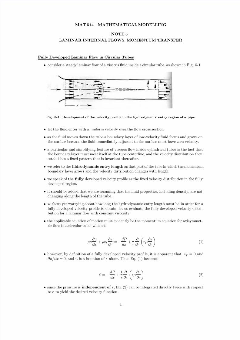
• consider a steady laminar ow of a viscous uid inside a circular tube, as shown in Fig. 5-1.

Fig. 5-1: Development of the velocity prole in the hydrodynamic entry region of a pipe.

• let the uid enter with a uniform velocity over the ow cross section.

• as the uid moves down the tube a boundary layer of low-velocity uid forms and grows onthe surface because the uid immediately adjacent to the surface must have zero velocity.

• a particular and simplifying feature of viscous ow inside cylindrical tubes is the fact thatthe boundary layer must meet itself at the tube centerline, and the velocity distribution thenestablishes a xed pattern that is invariant thereafter.

• we refer to the hidrodynamic entry length as that part of the tube in which the momentumboundary layer grows and the velocity distribution changes with length.

• we speak of the fully developed velocity prole as the xed velocity distribution in the fullydeveloped region.

• it should be added that we are assuming that the uid properties, including density, are notchanging along the length of the tube.

• without yet worrying about how long the hydrodynamic entry length must be in order for afully developed velocity prole to obtain, let us evaluate the fully developed velocity distri-bution for a laminar ow with constant viscosity.

• the applicable equation of motion must evidently be the momentum equation for axisymmet-ric ow in a circular tube, which is

ρu ∂u∂x

+ ρvr∂u∂r

= − dP dx

+ 1r

∂ ∂r

rµ ∂u∂r

(1)

• however, by denition of a fully developed velocity prole, it is apparent that vr = 0 and∂u/∂x = 0, and u is a function of r alone. Thus Eq. (1) becomes

0 = −dP dx

+ 1r

∂ ∂r

rµ∂u∂r

(2)

• since the pressure is independent of r , Eq. (2) can be integrated directly twice with respectto r to yield the desired velocity function.

1

8/13/2019 MAT514note5


8/13/2019 MAT514note5


• equation (8), together with (4), can be used directly to calculate pressure drop.

• we can also combine (8) with (3) to obtain a simpler expression for the local velocity:

u = 2 V 1 − r 2

r 2s

(9)

• the shear stress at the surface can be evaluated from the gradient of the velocity prole atthe surface. From equation of shear stress in note 3,

τ s = µ∂u∂r r = r s

= µ 2V −2r s

r 2s

= −4V µ

r s(10)

• to provide consistency with procedures to be used later, it is worth noting an alternativeprocedure to evaluate shear stress.

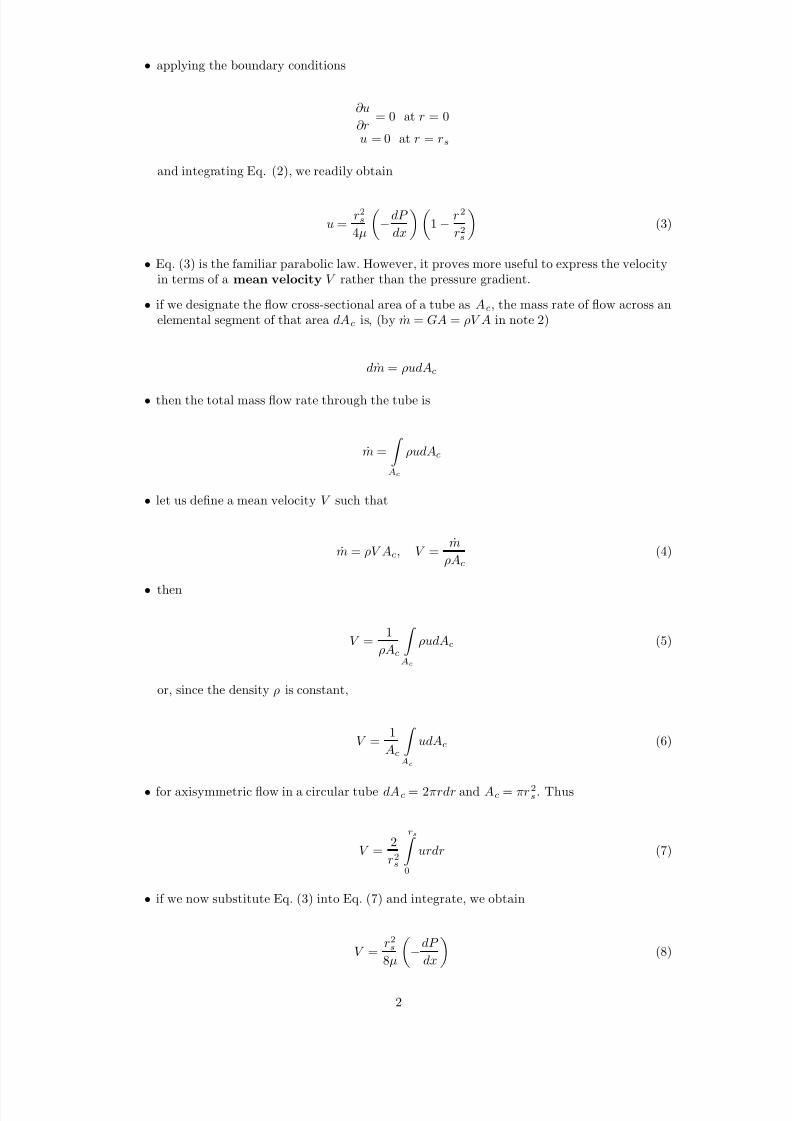
• consider a stationary control volume as shown in Fig. 5-2.

Fig. 5-2: Control volume for analyzing fully developed ow in a pipe.

• let us apply the momentum theorem, Rate of creation of momentum= F in note 2, in thex direction, noting that, because of the fully developed nature of the ow, there is no netchange in momentum ux. Thus

0 = P πr 2 − P + dP dx

δx πr 2 − τ 2πrδx

τ = r2

−dP dx

(11)

and

τ s = rs

2−

dP dx

(12)

• equations (11) and (12) are equally applicable to a fully developed turbulent ow, as long asit is understood that τ refers to an apparent shear stress that is the linear combination of the viscous stress and the apparent turbulent shear stress.

• also,

τ τ s

= rr s

(13)

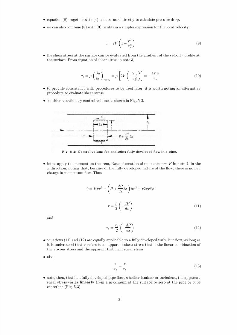
• note, then, that in a fully developed pipe ow, whether laminar or turbulent, the apparentshear stress varies linearly from a maximum at the surface to zero at the pipe or tubecenterline (Fig. 5-3).

3

8/13/2019 MAT514note5


Fig. 5-3: Shear-stress distribution for fully developed ow in a pipe.

• nally, Eq. (12) can be combined with Eq. (8), and we again obtain Eq. (10).

• we can express the surface shear stress in terms of a non-dimensional friction coefficient C f denes as

C f = τ s

12 ρ∞ u2

∞

• let us base the denition arbitrarily on the mean velocity. Thus

τ s = cf ρV 2

2 (14)

• then, employing (10) and considering the absolute value of the shear stress, to preserve thefact that surface shear is always opposite to the ow, we get

C f = 4V µ/r s

ρV 2 / 2 =

8µr s ρV

= 16

2r s ρV/µ

• we note for the fully developed velocity prole that C f , the local friction coefficient, isindependent of x.

• the non-dimensional group of variables in the denominater is the Reynolds number Re.Thus

Re = 2r s ρV

µ =

DρV µ

= DG

µ (15)

where D = 2r s , the pipe diameter, and G = m/A c , the mean mass velocity. Thus

C f = 16Re

(16)

4

8/13/2019 MAT514note5


Fully Developed Laminar Flow in Other Cross-sectional Shape Tubes

• laminar velocity prole solutions have been obtained for the fully developed ow case for alarge variety of ow cross-sectional shapes.

• the applicable equation of motion for steady, constant property, fully developed ow withno body forces, and with x the ow direction coordinate, can be readily deduced from theNavier-Stokes equation in note 3 ρDu/Dt = − ∂P/∂x + µ∇ 2 u + X . Thus

0 = − dP dx + µ∇ 2 u (17)

• by assuming dP/dx to be constant over the ow cross section, this equation has been solvedby various procedures, including numerically, for various shapes of tube.

• in most cases the shear stress will vary around the periphery of the tube; but if a mean shearstress with respect to peripheral area is dened (and this is the stress needed to calculatepressure drop), a friction coefficient can be dened in terms of Eq. (14).

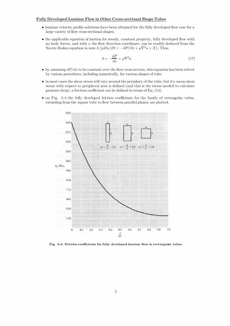
• on Fig. 5-4 the fully developed friction coefficients for the family of rectangular tubes,extending from the square tube to ow between parallel planes, are plotted.

Fig. 5-4: Friction coefficients for fully developed laminar ow in rectangular tubes.

5

8/13/2019 MAT514note5


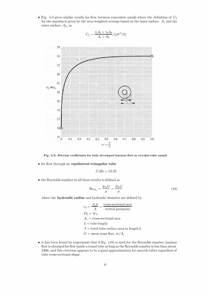
• Fig. 5-5 gives similar results for ow between concentric annuli where the denition of C f for the annulus is given by the area-weighted average based on the inner surface, A i and theouter surface, A 0 , as

C f = τ i Ai + τ 0 A0

Ai + A0/ (ρV 2 / 2)

Fig. 5-5: Friction coefficients for fully developed laminar ow in circular-tube annuli

• for ow through an equilateral triangular tube

C f Re = 13 .33

• the Reynolds number in all these results is dened as

ReD h = 4r h G

µ =

Dh Gµ

(18)

where the hydraulic radius and hydraulic diameter are dened by

r h = Ac L

A = cross-sectional area

wetted perimeterD h = 4r h

Ac = cross-sectional areaL = tube lengthA = total tube surface area in length LG = mean mass ux, m/A c

• it has been found by experiment that if Eq. (18) is used for the Reynolds number, laminarow is obtained for ow inside a round tube as long as the Reynolds number is less than about2300, and this criterion appears to be a good approximation for smooth tubes regardless of tube cross-sectional shape.

6

8/13/2019 MAT514note5


• above this Reynolds number, the ow becomes unstable to small disturbances, and a tran-sition to a turbulent type of ow generally occurs, although a fully establish turbulent owmay not occur until the Reynolds number reaches about 10 000.

7

mat514note5

Documents