mat - 2014/15 t opicos de sistemas din^amicos...

MAT - 2014/15

Topicos de Sistemas Dinamicos

Lecture notes

Salvatore CosentinoDepartamento de Matematica e Aplicacoes - Universidade do Minho

Campus de Gualtar - 4710 Braga - PORTUGAL

gab B.4023, tel 253 604086

e-mail [email protected]

url http://w3.math.uminho.pt/~scosentino

May 25, 2015

Abstract

This is not a book! These are notes written for personal use while preparing lectures on“Sistemas Dinamicos” for students of MAT(E) during the a.y.’s between 2001/02 and 2005/06,and then “Topicos de Sistemas Dinamicos” for student of MAT during the a.y.’s 2010/11 and2011/12. They are rather informal and certainly contain mistakes. I tried to be as syntheticas I could, without missing the observations that I consider important.

I probably will not lecture all I wrote, and did not write all I plan to lecture. So, I includedempty or sketched paragraphs, about material that I think should/could be lectured withinthe same course.

References contain some introductory manuals that I like, some classics, and other bookswhere I have learnt things in the past century. My favorite manuals are [HK03] (for itsexamples and its informal style) and [KH95] (for its rigor). Besides, good material and furtherreferences can easily be found in the web, for example in Scholarpedia , in Wikipedia or in theMIT OpenCoureWare.

It would be nice to have time and places to do simulations, using some of the software atour disposal in laboratories: this includes proprietary software like Mathematica R©8 , Matlaband Maple , or open software like Maxima and GeoGebra . Occasionally, we may also use somec++ code and Java applets. Some applets are in the bestiario in my web page, and everythingabout the course may be found in my page

http://w3.math.uminho.pt/~scosentino/teaching/tsd_MAT_2014-15.html

e.g. means EXEMPLI GRATIA, that is, “for example”, and is used to introduce importantor (I hope!) interesting examples.

ex: means “exercise”, to be solved at home or in the classroom.ref: means “references”, places where you can find and study what follows inside each

section.red paragraphs are non-trivial facts and results. indicates the end of a proof.Pictures were made with Grapher on my MacBook, or taken from Wikipedia, or produced

with Matlab or Mathematica R©8 .

This work is licensed under aCreative Commons Attribution-ShareAlike 3.0 Unported License.

1

mailto:[email protected]

http://w3.math.uminho.pt/~scosentino

http://www.scholarpedia.org/article/Main_Page

http://en.wikipedia.org/wiki/Main_Page

http://video.mit.edu/channel/opencourseware/

http://www.wolfram.com/mathematica/

http://www.mathworks.com/products/matlab/index.html

http://www.maplesoft.com/

http://maxima.sourceforge.net/

http://www.geogebra.org/cms/

http://www.cplusplus.com/

http://java.com/

http://w3.math.uminho.pt/~scosentino/salbestiario.html

http://w3.math.uminho.pt/~scosentino

http://w3.math.uminho.pt/~scosentino/teaching/tsd_MAT_2014-15.html

http://en.wikipedia.org/wiki/Main_Page

http://www.mathworks.com/products/matlab/index.html


http://creativecommons.org/licenses/by-sa/3.0/

CONTENTS 2

Contents

1 Introducao 41.1 Sistemas dinamicos . . . . . . . . . . . . . . . . . . . . . . . . . . . . . . . . . . . . 41.2 Exemplos fısicos . . . . . . . . . . . . . . . . . . . . . . . . . . . . . . . . . . . . . 41.3 Problemas fısicos e pequena historia . . . . . . . . . . . . . . . . . . . . . . . . . . 51.4 Estrategia . . . . . . . . . . . . . . . . . . . . . . . . . . . . . . . . . . . . . . . . . 6

2 Iteration/recursion 72.1 Exponential growth/decay . . . . . . . . . . . . . . . . . . . . . . . . . . . . . . . . 72.2 Babylonian-Heron method to compute square roots . . . . . . . . . . . . . . . . . . 132.3 Newton method to find roots of polynomials . . . . . . . . . . . . . . . . . . . . . . 142.4 Finite difference equations . . . . . . . . . . . . . . . . . . . . . . . . . . . . . . . . 162.5 Interval maps and cobweb plot . . . . . . . . . . . . . . . . . . . . . . . . . . . . . 182.6 Exponential sums . . . . . . . . . . . . . . . . . . . . . . . . . . . . . . . . . . . . . 19

3 Differential equations and flows 213.1 Structure of physical models . . . . . . . . . . . . . . . . . . . . . . . . . . . . . . . 213.2 Integration of one-dimensional systems . . . . . . . . . . . . . . . . . . . . . . . . . 233.3 Exponential . . . . . . . . . . . . . . . . . . . . . . . . . . . . . . . . . . . . . . . . 253.4 Linear systems . . . . . . . . . . . . . . . . . . . . . . . . . . . . . . . . . . . . . . 273.5 Simulations . . . . . . . . . . . . . . . . . . . . . . . . . . . . . . . . . . . . . . . . 283.6 Existence and uniqueness theorems . . . . . . . . . . . . . . . . . . . . . . . . . . . 30

4 Oscillations and cycles 354.1 Harmonic oscillator . . . . . . . . . . . . . . . . . . . . . . . . . . . . . . . . . . . . 354.2 Mathematical pendulum and Jacobi’s elliptic integrals . . . . . . . . . . . . . . . . 364.3 Central forces and planetary motions . . . . . . . . . . . . . . . . . . . . . . . . . . 374.4 Cycles in chemistry and biology . . . . . . . . . . . . . . . . . . . . . . . . . . . . . 394.5 Weather report . . . . . . . . . . . . . . . . . . . . . . . . . . . . . . . . . . . . . . 41

5 Topological dynamical systems, basic definitions 435.1 Transformations . . . . . . . . . . . . . . . . . . . . . . . . . . . . . . . . . . . . . 435.2 Trajectories and orbits . . . . . . . . . . . . . . . . . . . . . . . . . . . . . . . . . . 445.3 Periodic orbits . . . . . . . . . . . . . . . . . . . . . . . . . . . . . . . . . . . . . . 445.4 Observaveis . . . . . . . . . . . . . . . . . . . . . . . . . . . . . . . . . . . . . . . . 455.5 Conjuntos invariantes . . . . . . . . . . . . . . . . . . . . . . . . . . . . . . . . . . 465.6 Conjugacao topologica . . . . . . . . . . . . . . . . . . . . . . . . . . . . . . . . . . 475.7 Estabilidade estrutural . . . . . . . . . . . . . . . . . . . . . . . . . . . . . . . . . . 47

6 Numbers and dynamics 486.1 Decimal expansion and multiplication by ten . . . . . . . . . . . . . . . . . . . . . 486.2 Deslocamentos de Bernoulli . . . . . . . . . . . . . . . . . . . . . . . . . . . . . . . 506.3 Rotacoes do cırculo/toro . . . . . . . . . . . . . . . . . . . . . . . . . . . . . . . . . 516.4 Dyadic adding machine . . . . . . . . . . . . . . . . . . . . . . . . . . . . . . . . . 536.5 Continued fractions and Gauss map . . . . . . . . . . . . . . . . . . . . . . . . . . 54

7 Simple orbits and perturbations 587.1 Topological fixed point theorems . . . . . . . . . . . . . . . . . . . . . . . . . . . . 587.2 Basin of attraction . . . . . . . . . . . . . . . . . . . . . . . . . . . . . . . . . . . . 587.3 Dynamics of contractions . . . . . . . . . . . . . . . . . . . . . . . . . . . . . . . . 597.4 Ordem da reta real e trajetorias . . . . . . . . . . . . . . . . . . . . . . . . . . . . . 627.5 Analise local: pontos fixos atrativos e repulsivos . . . . . . . . . . . . . . . . . . . . 637.6 Convergencia no metodo de Newton . . . . . . . . . . . . . . . . . . . . . . . . . . 657.7 Dynamics of Mobius transformations . . . . . . . . . . . . . . . . . . . . . . . . . . 66

CONTENTS 3

8 Linearizacao 698.1 Linearizacao conforme . . . . . . . . . . . . . . . . . . . . . . . . . . . . . . . . . . 698.2 Hiperbolicidade e linearizacao . . . . . . . . . . . . . . . . . . . . . . . . . . . . . . 69

9 Transversalidade e bifurcacoes 719.1 Transversalidade e persistencia dos pontos fixos . . . . . . . . . . . . . . . . . . . . 719.2 Bifurcacoes . . . . . . . . . . . . . . . . . . . . . . . . . . . . . . . . . . . . . . . . 729.3 Duplicacao do perıodo e cascata de Feigenbaum . . . . . . . . . . . . . . . . . . . . 72

10 Statistical description of orbits 7310.1 Probability measures . . . . . . . . . . . . . . . . . . . . . . . . . . . . . . . . . . . 7310.2 Transformations and invariant measures . . . . . . . . . . . . . . . . . . . . . . . . 7510.3 Invariant measures and time averages . . . . . . . . . . . . . . . . . . . . . . . . . 7810.4 Examples of invariant measures . . . . . . . . . . . . . . . . . . . . . . . . . . . . . 80

11 Recurrences 8311.1 Limit sets and recurrent points . . . . . . . . . . . . . . . . . . . . . . . . . . . . . 8311.2 Dirichlet theorem on Diophantine approximation . . . . . . . . . . . . . . . . . . . 8411.3 Poincare recurrence theorem . . . . . . . . . . . . . . . . . . . . . . . . . . . . . . . 8511.4 Transitivity and minimality . . . . . . . . . . . . . . . . . . . . . . . . . . . . . . . 8711.5 Kronecker theorem on irrational rotations . . . . . . . . . . . . . . . . . . . . . . . 8911.6 Homeomorfismos do cırculo . . . . . . . . . . . . . . . . . . . . . . . . . . . . . . . 91

12 Perda de memoria e independencia assimptotica 9512.1 Orbitas desordenadas . . . . . . . . . . . . . . . . . . . . . . . . . . . . . . . . . . . 9512.2 Mixing topologico . . . . . . . . . . . . . . . . . . . . . . . . . . . . . . . . . . . . . 9612.3 Dinamica dos deslocamentos de Bernoulli . . . . . . . . . . . . . . . . . . . . . . . 9812.4 Conjuntos de Cantor . . . . . . . . . . . . . . . . . . . . . . . . . . . . . . . . . . . 9912.5 Transformacoes expansoras . . . . . . . . . . . . . . . . . . . . . . . . . . . . . . . 10112.6 Automorfismos hiperbolicos do toro . . . . . . . . . . . . . . . . . . . . . . . . . . . 103

13 Dimensions, fractals and entropy 10513.1 Dimensions of metric spaces . . . . . . . . . . . . . . . . . . . . . . . . . . . . . . . 10513.2 Fractals . . . . . . . . . . . . . . . . . . . . . . . . . . . . . . . . . . . . . . . . . . 10613.3 Self-similarity and iterated function systems . . . . . . . . . . . . . . . . . . . . . . 10713.4 Kleinian groups . . . . . . . . . . . . . . . . . . . . . . . . . . . . . . . . . . . . . . 10813.5 Entropia topologica . . . . . . . . . . . . . . . . . . . . . . . . . . . . . . . . . . . . 108

14 Ergodicity and convergence of time means 11114.1 Ergodicity . . . . . . . . . . . . . . . . . . . . . . . . . . . . . . . . . . . . . . . . . 11114.2 Examples of ergodic maps . . . . . . . . . . . . . . . . . . . . . . . . . . . . . . . . 11214.3 Normal numbers . . . . . . . . . . . . . . . . . . . . . . . . . . . . . . . . . . . . . 11314.4 Unique ergodicity and equidistribution . . . . . . . . . . . . . . . . . . . . . . . . . 114

1 INTRODUCAO 4

1 Introducao

1.1 Sistemas dinamicos

Uma estrutura tıpica de um modelo fısico e a seguinte. Existe um espaco X, dito “espaco dosestados”, ou “espaco das fases”, do sistema (uma variedade simpletica em mecanica classica, umespaco de Hilbert em mecanica quantica, um certo espaco de funcoes em modelos hidrodinamicos...). Existe um espaco T , que chamamos “tempo”, que contem um ponto chamado 0 (agora), ejunto com t e s tambem contem t+s (se e possıvel esperar uma hora e esperar duas horas, tambemdeve ser possıvel esperar tres horas). As “leis” da fısica definem uma dinamica em X: uma famıliade transformacoes Φt : X → X, definidas para t ∈ T , que verificam

Φ0 = idX e Φt+s = Φt Φs.

Portanto, as leis definem uma acao Φ : T ×X → X do semigrupo tempo no espaco dos estados. Oponto Φt(x) e o estado no tempo t de um sistema que estava no estado x no tempo 0. A funcaot 7→ Φt(x) e a “trajetoria” do estado inicial x, e a sua imagem, a curva Φt(x) : t ∈ T ⊂ X, e a“orbita” de x. As leis podem ser “reversıveis”, ou seja podem permitir decidir o que aconteceu nopassado, e nesse caso o tempo e idealizado como sendo o grupo R ou Z, ou irreversıveis, e nestecaso o tempo e pensado como o semigrupo R≥0 ou N0. Se o tempo e contınuo, o (semi)grupocostuma ser definido por meio do seu gerador infinitesimal

v = limt↓0

Φt − idXt

(o campo de vetores definido pela equacao de Newton F = ma, o gerados H do grupo de operadoresunitarios e−i~tH num espaco de Hilbert, o semigrupo e−t∆ gerado pelo operador de Laplace-Beltrami ∆, . . . ). Se o tempo e discreto, N ou Z, o (semi)grupo e gerado pela transformacao

Φ1 : X → X .

Numa experiencia da fısica, nao e necessariamente o estado do sistema que se observa. Fazerexperiencias quer dizer medir “observaveis”, ou seja ler nos instrumentos do laboratorio os valoresde certas funcoes ϕ : X → R (a distancia entre dois planetas, a energia de um eletrao, a temperaturade um gas ...). A famılia de funcoes ϕt = ϕ Φt descreve a dinamica do observavel ϕ. De fato, o

que se observa podem ser medias temporais do genero 1T

∫ T0ϕtdt, as vezes indiretamente por meio

dos espetros de Fourier∫eiktϕtdt ou de Laplace

∫estϕtdt.

1.2 Exemplos fısicos

So para ter uma ideia...

Mecanica classica. O espaco dos estados de uma partıcula (pensada como um ponto material)e, de acordo com o princıpio de relatividade de Galileo, R3×R3. Um estado e um vetor x = (q, p),onde q ∈ R3 e a “posicao” e p = mq ∈ R3 o “momento”, ˙ denota a derivada em ordem ao tempoe m a massa da partıcula. A equacao de Newton “forca=massa×aceleracao” se traduz no sistemade equacoes

q = p/m p = F

que definem um campo de vetores v = (p/m,F ) em R3 × R3. A solucao de dx (t) /dt = v (x (t))com condicao inicial x (0) = x e a trajetoria t 7→ Φt (x).

Mecanica quantica. O espaco dos estados de uma partıcula e um espaco de Hilbert, porexemplo L2

(R3). Um estado e uma funcao q 7→ ψ (q), que tem a interpretacao de “densidade de

probabilidades de encontrar a partıcula na posicao q”. A “energia” e um operador linear auto-ajunto H : L2

(R3)→ L2

(R3), por exemplo da forma −

(~2/2m

)∆+V (q), onde ∆ e o operador de

Laplace-Beltrami, ~ e a constante de Planck, m e a massa da partıcula, e V e a “energia potencial”.A equacao de Schrodinger

i~∂

∂tψ = − ~2

2m∆ψ + V · ψ

gera o grupo unitario de operadores e−itH/~ : L2(R3)→ L2

(R3).

1 INTRODUCAO 5

Hidrodinamica. O espaco dos estados e um espaco de funcoes com um certo numero de derivadasparciais contınuas, por exemplo Ck

(R3,R

). Uma configuracao, ou “campo”, e uma funcao q 7→

u (q) e representa a “densidade macroscopica” de certos observaveis microscopicos (numero departıculas, energia, pressao, ...). Uma equacao diferencial fenomenologica descreve a evolucao docampo. Por exemplo, a propagacao do calor e suposta seguir a equacao

∂

∂tu = σ∆u

onde ∆ e o operador de Laplace-Beltrami e σ e um coeficiente que determina a velocidade depropagacao. O operador diferencial ∆ gera o semigrupo de operadores etσ∆ : Ck

(R3,R

)→

Ck(R3,R

).

1.3 Problemas fısicos e pequena historia

O objetivo dos fısicos e fazer previsoes: querem saber o que acontece a um certo ponto x, ou melhora um certo observavel ϕ, passado um tempo t, e possivelmente dizer o que acontece quando t egrande. Eis uma lista, nao exaustiva, de problemas fisicamente relevantes.

Calcular trajetorias. Resolver o “problema de Cauchy”: dada uma condicao inicial x, oestado do sistema no presente, determinar os estados futuros Φt (x) com t ≥ 0. No seculo XVIIo Newton inventou o seu “methodus fluxionum” (o moderno calculo diferencial e integral) pararesolver as proprias equacoes e assim calcular as trajetorias dos planetas, dando uma explicacaoas leis de Kepler ...

Regularidades/periodicidades. Decidir se o sistema tem trajetorias regulares, no sentido de“previsıveis”. As mais previsıveis sao as trajetorias periodicas, que satisfazem ΦT (x) = x paraalgum tempo T dito perıodo, e que portanto regressam a x em cada tempo multiplo de T (a propriahistoria do pensamento cientıfico dos homens comecou da observacao das periodicidades dos astros,dando origem a cosmogonias e matematicas em quase toda esquina do planeta). Decidir se aseventuais trajetorias regulares sao observaveis, ou seja se uma pequena perturbacao da condicaoinicial x ou da lei Φ ainda produz uma trajetoria proxima da trajetoria regular, ou se estragatudo. A procura de orbitas periodicas e a teoria das perturbacoes foi um dos temas favoritos dosfısicos matematicos do seculo XIX, particularmente interessados aos problemas da mecanica celeste.Nos anos cinquenta do seculo XX, Kolmogorov, e depois Arnold e Moser, provaram o resultadoespetacular de que muitos sistemas hamiltonianos tem muitas orbitas “quase-periodicas”.

Descricao qualitativa. Determinar o comportamento qualitativo da “maioria” das trajetorias.Acontece que, se o sistema nao e extremamente simples (como um sistema kepleriano, uma partıculaem um campo magnetico constante, ...), e praticamente impossıvel “calcular” as trajectorias, em-bora possa ser possıvel provar a “existencia”. Os fısicos devem ficar satisfeitos com uma descricao“qualitativa” das orbitas possıveis. No final do seculo XIX, Henri Poincare mostrou que e possıvelfazer afirmacoes interessantes sobre o comportamento qualitativo das trajetorias utilizando in-formacoes fracas sobre a lei de evolucao. O resultado mais espetacular e o seu famoso “teoremade recorrencia”. Outro exemplo e a classificacao dos homeomorfismos do cırculo, tambem devidaa Poincare e depois estudada por Denjoy.

Problemas numericos. Embora seja geralmente impossıvel calcular trajetorias, e possivel obtertrajetorias aproximadas (por exemplo, hoje em dia, utilizando um computador que ”resolve”equacoes diferenciais, mas lembre que os astronomos calculam “efemerides” e “calendarios” desdemilenios!). Um esquema muito simplificado do calculo numerico e assim. Dada uma condicao ini-cial x e um “passo” τ , obtemos uma aproximacao Φ′τ (x) de Φτ (x) com um erro que possivelmentesabemos estimar, por exemplo limitado por ε. A seguir, utilizamos o nosso valor inicial Φ′τ (x) paraestimar Φ2τ (x), assim produzindo Φ′2τ (x), supostamente a distancia inferior a ε de Φτ (Φ′τ (x)),mas geralmente a distancia ainda maior de Φ2τ (x)... O problema e decidir se, quando n e grande,a nossa conjetura Φ′nτ (x) ainda tem alguma coisa a ver com o verdadeiro Φnτ (x).

1 INTRODUCAO 6

Regularidades probabilısticas. Muitos sistemas interessantes tem comportamento desorde-nado (por exemplo, as trajetorias podem ter dependencia sensıvel das condicoes iniciais), e o estadoinicial nao pode ser determinado com precisao (quer por razoes “a priori”, quer porque todo instru-mento tem a sua sensibilidade). A descricao estatıstica e neste caso uma necessidade e ate podesimplificar a vida. Pode acontecer que o comportamento da maioria das trajetorias e tao irregularque acaba por parecer regular num sentido probabilıstico. Este era o cenario imaginado por LudwigBoltzmann, na sua teoria cinetica dos gases, para justificar as lei observadas da termodinamica.O estudo das regularidades probabilısticas dos sistemas dinamicos e dito “teoria ergodica”, emhomenagem as intuicoes de Boltzmann, e nasceu nos anos trinta do seculo XX com os resultadosde von Neumann, Birkhoff, Khinchin, Hopf, Kolmogorov... Em tempos mais recentes, matematicose fısicos como Bowen, Ruelle, Sinai, descubriram ligacoes interessantes com a mecanica estatısticade Maxwell e Gibbs...

Previsoes robustas. Um sistema dinamico pode ser pensado como uma ”maquina” que peganuma condicao inicial x e produz uma trajetoria t 7→ Φt (x). O problema e decidir se uma pequenaperturbacao de Φ (uma incerteza nos parametro da lei fısica), digamos Φ′, produz trajetorias“comparaveis” com as trajetorias de Φ. Uma resposta que e particularmente apreciada pelosfısicos consiste em formular resultados de “estabilidade”, que digam que uma “distancia” entreΦ e Φ′ suficientemente pequena nao altera a estrutura das trajetorias. Isto levanta tambem aquestao de decidir se certos fenomenos sao tıpicos ou nao no espaco das possıveis dinamicas. Aprocura de sistemas “estruturalmente estaveis” desenvolveu-se a partir das ideias de Andronov ePontryagin, nos anos trinta do seculo XX. A “hiperbolicidade” enquanto chave da estabilidadeestrutural foi descoberta nos anos sessenta por Anosov, Smale, Sinai ..., ao desenvolver ideiasgeometricas precedentes de Hadamard, Hopf , Hedlund ...

1.4 Estrategia

Para um matematico, um sistema dinamico e uma acao G×X → X de um (semi)grupo “grande”(tal que seja possıvel dar um sentido a uma expressao do genero “g → ∞”) G sobre um espacoX. Estudar um sistema dinamico quer dizer comprender o espaco das orbitas G\X, ou melhora maneira em que as diferentes orbitas Gx estao mergulhadas em X. A enfase e no comporta-mento “assimptotico” das trajetorias t 7→ gtx quando gt → ∞. Resulta que as vezes e possıvelfazer previsoes interessantes esquecendo os “detalhes” da dinamica, desde que X tenha algumaestrutura (uma topologia, uma metrica, uma estrutura diferenciavel, simetrias, uma medida deprobabilidades, ...) que de alguma maneira precisa e respeitada pela evolucao temporal, e quea lei de evolucao tenha certas propriedades qualitativas. Este e o tema da teoria dos sistemasdinamicos. A estrategia e selecionar modelos simples e trataveis, possivelmente “descobrir” classesde sistemas com comportamento compreensıvel, na esperanca de que sistemas “reais” tenham com-portamentos comparaveis. Ate esquecendo as motivacoes fısicas, as ideias da teoria dos sistemasdinamicos fornecem outra maneira de olhar certas estruturas matematicas, e produzem resultadosinteressantes em analise, geometria, teoria de grupos, teoria de numeros, etc...

2 ITERATION/RECURSION 7

2 Iteration/recursion

2.1 Exponential growth/decay

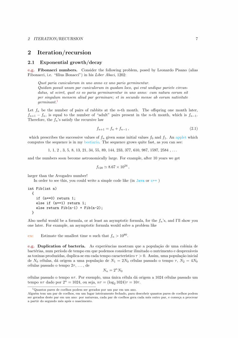
e.g. Fibonacci numbers. Consider the following problem, posed by Leonardo Pisano (aliasFibonacci, i.e. “filius Bonacci”) in his Liber Abaci, 1202:

Quot paria cuniculorum in uno anno ex uno pario germinentur.Quidam posuit unum par cuniculorum in quodam loco, qui erat undique pariete circun-datus, ut sciret, quot ex eo paria germinarentur in uno anno: cum natura eorum sitper singulum mensem aliud par germinare; et in secundo mense ab eorum nativitategerminant.1

Let fn be the number of pairs of rabbits at the n-th month. The offspring one month later,fn+1 − fn, is equal to the number of “adult” pairs present in the n-th month, which is fn−1.Therefore, the fn’s satisfy the recursive law

fn+1 = fn + fn−1 , (2.1)

which prescribes the successive values of fn given some initial values f0 and f1. An applet whichcomputes the sequence is in my bestiario. The sequence grows quite fast, as you can see:

1, 1, 2 , 3, 5, 8, 13, 21, 34, 55, 89, 144, 233, 377, 610, 987, 1597, 2584 , . . .

and the numbers soon become astronomically large. For example, after 10 years we get

f120 ' 8.67× 1024 ,

larger than the Avogadro number!In order to see this, you could write a simple code like (in Java or c++ )

int Fib(int n)

if (n==0) return 1;

else if (n==1) return 1;

else return Fib(n-1) + Fib(n-2);

Also useful would be a formula, or at least an asymptotic formula, for the fn’s, and I’ll show youone later. For example, an asymptotic formula would solve a problem like

ex: Estimate the smallest time n such that fn > 1080.

e.g. Duplication of bacteria. As experiencias mostram que a populacao de uma colonia debacterias, num perıodo de tempo em que podemos considerar ilimitado o nutrimento e desprezaveisas toxinas produzidas, duplica-se em cada tempo caracterıstico τ > 0. Assim, uma populacao inicialde N0 celulas, da origem a uma populacao de N1 = 2N0 celulas passado o tempo τ , N2 = 4N0

celulas passado o tempo 2τ , . . . , deNn = 2nN0

celulas passado o tempo nτ . Por exemplo, uma unica celula da origem a 1024 celulas passado umtempo nτ dado por 2n = 1024, ou seja, nτ = (log2 1024)τ = 10τ .

1Quantos pares de coelhos podem ser gerados por um par em um ano.Alguem tem um par de coelhos, em um lugar inteiramente fechado, para descobrir quantos pares de coelhos podemser gerados deste par em um ano: por natureza, cada par de coelhos gera cada mes outro par, e comeca a procreara partir do segundo mes apos o nascimento.

http://w3.math.uminho.pt/~scosentino/bestiario/fibonacci.html


http://java.com/



Sequences. A (real or complex valued) sequence is a collection (xn)n∈N of numbers xn ∈ R orC, indexed (hence ordered) by an non-negative integer n ∈ N := 0, 1, 2, 3, . . . . We may thinkof the index n as “time”, an therefore at the n-th term xn as the value of some “observable” x(something that we may observe, i.e. measure) at time n. Clearly, we may as well define sequenceswith values in an arbitrary set X, for example in the Euclidean space Rd.

Sequences may be defined as functions are. Indeed, a sequence with values in the set X isnothing but a function f : N → X, disguised by the notation xn := f(n). A second possibility issome recursive law prescribing the value of xn given the (past) values of x0, x1, . . . , xn−1. A thirdpossibility, is using some property that the successive terms must have.

e.g. Arithmetic progression. An arithmetic progression xn = a + nb, which may also bedefined using the recursion xn+1 = xn + b, with initial term x0 = a.

e.g. The primes sequence. The sequence 2, 3, 5, 7, 11, 13, 17, 19, 23, . . . , whose generic term isthe n-th prime number pn. It is not clear what the recursive law could be.2

Limits. We say that the real sequence (xn) converges to some limit a ∈ R or C, and we writelimn→∞ xn = a or simply xn → a (as n → ∞), if for any “precision” ε > 0 there exists a time nsuch that |xn− a| < ε for all times n ≥ n. This means that the values xn are within an arbitrarilysmall neighborhood of a as long as the time n is sufficiently large.

The basic fact about limits in the real line R is that monotone (non-decreasing or non-increasing,i.e. satisfying xn+1 ≥ xn or xn+1 ≤ xn, for any n, respectively) bounded (i.e. such that |xn| ≤Mfor some M > 0 and all n) sequences of real numbers do admit limit. For example, the limit of abounded increasing sequence is simply the supremum of the set of values.

We also use the notation xn → ±∞ to say that given an arbitrarily large K > 0 we can find atime n such that ±xn > K for all times n ≥ n.

Of course, there exist sequences which do not admit limits in either senses. These are, forexample, oscillating sequences, as xn = (−1)n. We’ll encounter sequences with much more wildbehavior.

Fundamental sequences. A sequence (xn) is said fundamental, or Cauchy sequence, if for anyprecision ε > 0 there exists a time n such that

|xn − xm| < ε

for all times n,m > n. Fundamental sequences are clearly bounded. It is obvious that a convergentsequence is fundamental (a triangular argument, since both xn and xm are ε/2-near to the limit forsufficiently large n and m). A similar triangular argument shows that a fundamental sequence witha convergent subsequence is itself convergent. Less obvious is that any fundamental sequence in R isconvergent. Indeed, let Xn := xk with k ≥ n. It is clear that the Xn are bounded, and thereforeby the supremum axiom there exist the numbers an := inf Xn. But the sequence (an) is boundedand not decreasing, and therefore there exists a = limn→∞ an (indeed, a = sup an with n ∈ N).It is then easy to construct subsequences of (xn) which converge to a, and this implies that (xn)itself is convergent to a.

Thus, we may know that a sequence is convergent without knowing its limit! In general,convergence of all fundamental sequences is taken as a definition of (sequential) completeness of ametric space.

Geometric progression. The most important sequence is the geometric progression, defined bythe recursion

xn+1 = λxn ,

and an initial term x0 = a (which we may assume 6= 0 to avoid trivialities). Thus, the sequence is

x0 = a x1 = aλ x2 = aλ2 . . . xn = aλn . . .

2This is not the place to talk about it, but if you find it intriguing, you may take a look at the wonderful bookby Marcus du Sautoy, The music of primes, Harper-Collins, 2003 [A musica dos numeros primos, Zahar, 2008].

http://www.musicoftheprimes.com/


The parameter λ (which may be real or complex) is called ratio, since it is the ratio xn+1/xnbetween successive terms of the sequence. The geometric sequence clearly converges to zero when|λ| < 1. It is constant, hence trivially convergent, when λ = 1, while oscillates between ±a whenλ = −1 (hence does not converge if a 6= 0). We may also observe that |λn| → ∞ when |λ| > 1.

ex: Show that the term xn of a geometric progression is equal to the geometric mean√xn+1xn−1

of its neighbors.

Computing limits. First, observe that xn → a is equivalent to xn − a → 0. Therefore, weonly need to understand how to “prove” that some sequence converges to zero. One possibility isto “compare” the sequence (xn) under investigation with a sequence with known behavior, as forexample the geometric progression. Indeed, if |xn| ≤ yn for all n sufficiently large, then yn → 0implies xn → 0 too.

Subsequences and sequential compactness. A subsequence of a sequence (xn) is a sequence(xni) obtained selecting only the values xni of the original sequence, where i 7→ ni is an increasingmap N0 → N0.

The basic fact (that closed and bounded sets of the real line are sequentially compact) is thatany bounded sequence admits a convergent subsequence.

Limsup and liminf. Sometimes we are only interested in a rough estimate of the growth of asequence (xn). The “limsup” is the limit lim supn→∞ xn := limn→∞ an ∈ R ∪ ∞ of the non-increasing sequence an := supxn, xn+1, xn+2, . . . . The “liminf” is the limit lim infn→∞ xn :=limn→∞ bn ∈ R ∪ −∞ of the non-decreasing sequence bn := infxn, xn+1, xn+2, . . . .

e.g. Tempo de meia-vida. O decaimento de uma substancia radioactiva pode ser caracterizadopelo “tempo de meia-vida” τ , passado o qual aproximadamente metade dos nucleos inicialmentepresentes tera decaido (dentro de uma amostra suficientemente grande). Se qn denota a quantidadede substancia radioactiva presente no instante nτ , com n = 0, 1, 2, . . . , entao

qn+1 = 12 qn .

Portanto a quantidade de substancia radioactiva no instante nτ e qn = q02−n, enquanto o produtodo decaimento e q0 − qn = q0(1− 2−n). Observe que qn → 0 quando n→∞.

Se a radiacao solar produz nucleos radioactivos a uma taxa constante α > 0 (i.e. α nucleoscada tempo τ), a quantidade de nucleos radioactivos no instante nτ e dada pela lei recursiva

qn+1 = 12qn + α . (2.2)

Um equilıbrio e possıvel quando a quantidade inicial q0 e igual a q := 2α, pois entao q1 = α+α = q0,q2 = α+ α = q1 = q0, e assim a seguir, qn = q para todos os n ∈ N.

O que acontece se q0 6= q ? A equacao recursiva diz que

q1 = 12q0 + α

q2 = 14q0 + 1

2α+ α

q3 = 18q0 + 1

4α+ 12α+ α

...

qn = 12n q0 +

(1

2n−1 + · · ·+ 18 + 1

4 + 12 + 1

)α

A primeira parcela q0/2n+1 → 0 quando n → ∞, ou seja, o futuro e independente da condicao

inicial q0. A segunda parcela tem limite 2α quando n→∞ (uma prova esta no paragrafo sobre aserie geometrica!).


Uma formula (aparentemente) mais simples para os qn pode ser obtida usando a substituicaoxn := qn − q, onde q = 2α e a solucao estacionaria. De facto,

xn+1 = qn+1 − 2α

= 12qn + α− 2α (usando a (2.2))

= 12 xn ,

ou seja, a diferenca entre qn e q e uma progressao geometrica de razao 1/2. Portanto xn = x02−n,donde

qn = 2α+ (q0 − 2α) · 2−n .

E interessante observar que xn → 0, e de consequencia qn → q, quando n → ∞. Ou seja, aquantidade de substancia radioactiva converge para o valor estacionario, independentemente dovalor inicial.

ex: Passado quanto tempo a substancia radioactiva fica reduzida a 132 -esimo da quantidade

inicial?

ex: O tempo de meia-vida do radiocarbono 14C e τ ' 5730 anos. Mostre como “datar” umfossil, sabendo que a proporcao de 14C num ser vivente e fixa e conhecida.3

e.g. Crescimento exponencial. O crescimento exponencial de uma populacao num meio am-biente ilimitado e modelado pela equacao recursiva

pn+1 = λpn ,

onde pn representa a populacao no tempo n, dada uma certa populacao inicial p0. Um significadodo parametro λ e o seguinte: em cada unidade de tempo o incremento pn+1−pn da populacao e iguala soma de uma parcela αpn, onde α > 0 e um coeficiente de fertilidade, e uma parcela −βpn, ondeβ > 0 e um coeficiente de mortalidade. An applet with the simulations is in exponentialgrowth.

• Discuta o comportamento das solucoes da equacao recursiva ao variar o parametro λ.

• A uma populacao que cresce segundo o modelo exponencial, e adicionada ou retirada umacerta quantidade β em cada unidade de tempo. O modelo e portanto

pn+1 = λpn + β ,

onde β e um parametro positivo ou negativo. Determine solucoes estacionarias, ou seja,que nao dependem do tempo n, e a solucao com condicao inicial p0 arbitraria (considere asubstituicao xn = pn − p, onde p e a solucao estacionaria).

• Para quais valores dos parametros λ e β as solucoes pn convergem para a solucao estacionariaquando o tempo n→∞?

e.g. Growth of Fibonacci numbers. How fast do Fibonacci numbers grow? Define thequotients qn := fn+1/fn between neighbor Fibonacci numbers. From (2.1) one deduce the recursiveequation

qn+1 = 1 + 1/qn (2.3)

for the qn’s. We compute:

1 , 2 , 3/2 = 1.5 , 5/3 ' 1.66666 , 8/5 = 1.6 , 13/8 = 1.625 , 21/13 ' 1.61538 , . . .

3J.R. Arnold and W.F. Libby, Age determinations by Radiocarbon Content: Checks with Samples of KnownAges, Sciences 110 (1949), 1127-1151.

http://w3.math.uminho.pt/~scosentino/bestiario/exponentialgrowth.html


You may observe the sequence in the following applet. It turns out that the sequence (qn) converge(try to prove it!), namely, qn → φ as n→∞. Taking the limits in the recursive equation (2.3) wesee that φ = 1 + 1/φ, and therefore φ is the positive root of the quadratic polynomial x2 − x− 1,

φ =1 +√

5

2' 1.6180339887498948482 . . .

Hence, for large values of n we may approximate Fibonacci law as

fn+1 ≈ φfn ,

an exponential growth with rate φ. In particular, we expect fn ∼ φn.The limit φ is a famous irrational, the Greeks’ “ratio/proportion”. As described by Euclid4:

“A straight line is said to have been cut in extreme and mean ratio when, as the wholeline is to the greater segment, so is the greater to the less.”

If a is the greater part and b the less of a line of lenght a+ b, Euclid’s requirement is

a+ b

a=a

b

There follows that the ratio φ = a/b satisfies 1 + 1/φ = φ. This division of an interval is usedin Book IV of the Elements to construct a regular pentagon. Observe that, as follows from thequadratic equation, φ−1 is equal to φ− 1.

Extreme and mean ratio, and regular pentagon.

(from http://en.wikipedia.org/wiki/Golden_ratio)

ex: Show that φ is irrational using its geometric definition (see Euclid’s Elements, or [HW59]section 4.6.)

e.g. Invencao do xadrez. Dizem que o sabio hindu Sissa inventou o jogo do xadrez e o ofreceuao rei de Persia. Ao rei, que o convidou a escolher uma recompensa, pediu um grao de arroz (ouera trigo?) para o primeiro quadrado do tabuleiro, o dobro, ou seja, dois graos, para o segundoquadrado, o dobro, ou seja, quatro graos, pelo terceiro quadrado, e assim a seguir ate o ultimo dosquadrados do tabuleiro. O rei riu-se, num primeiro instante, mas . . . a recompensa e

1 + 2 + 4 + 8 + · · ·+ 263 ' 1.84× 1019

graos de arroz. Se 1 Kg de arroz contem a volta de 30000 graos, isto significa algo como 6.13×1011

toneladas de arroz (which you may want to compare with People’s Republic of China’s productionin 2008, which has been, according to FAO, about 1.93× 108 metric tons!).

Series. A series is a formal infinite sum∑∞n=0 xn, or

∑n≥0 xn, where the xn ∈ R are elements

of some given real (or complex) sequence. If the sequence (sn) of partial sums, defined as sn :=∑nk=0 xk (which are honest numbers) converges to some limit, say limn→∞ sn = s, then we say the

series is convergent (or summable), and that its sum is∑n≥0 xn := s.

A series∑n xn is absolutely convergent is the series

∑n |xn|, formed with the absolute values

of its terms, is convergent. Of course, absolute convergence is stronger than mere convergence.Indeed, convergent but not absolutely convergent series are quite interesting and strange objects.

4Euclid, Elements, Book VI, Definition 3.

http://w3.math.uminho.pt/~scosentino/bestiario/fibonacci.html

http://en.wikipedia.org/wiki/Golden_ratio

http://en.wikipedia.org/wiki/Golden_ratio

http://faostat.fao.org/site/339/default.aspx


e.g. Harmonic series. The harmonic series

∞∑n=1

1

n= 1 +

1

2+

1

3+

1

4+

1

5+ . . .

diverges. Indeed, its generic term 1/n, for n ≥ 2, is bigger than the integral∫ nn−1

dx/x, hence

the partial sums∑nk=1 1/n are bounded from below by the logarithm log n (modulo some additive

constant).

Geometric series. The identity (1 + λ + λ2 + λ3 + ... + λn)(λ − 1) = λn+1 − 1 shows that, ifλ 6= 1, the sum of the first n+ 1 terms of the geometric progression (with a = 1) is

1 + λ+ λ2 + λ3 + ...+ λn =λn+1 − 1

λ− 1

In particular, when |λ| < 1, the geometric series∑∞n=0 λ

n is absolutely convergent, and its sum is

1 + λ+ λ2 + λ3 + ...+ λn + ... =1

1− λ.

e.g. Dichotomy paradox. Using the above formula for the sum of the geometric series, youmay try to convince Zeno that

1/2 + 1/4 + 1/8 + 1/16 + 1/32 + ... = 1 .

e.g. Decimal expansions. Also, you may convince yourself that 0.99999 . . . , which by definitionis the sum of the series

9

10+

9

100+

9

1000+

9

10000+ . . .

is actually equal to 1. Moreover, you may learn how to recognize rational numbers as 0.33333 . . .or 1.285714285714 . . . from their periodic expansion. Indeed, a real number is rational if and onlyif its base 10 (or any other base d ≥ 2) expansion is eventually periodic.

ex: Diga se a seguintes series sao convergentes, e, se for o caso, calcule a soma.

1 + 1/2 + 1/4 + 1/8 + 1/16 + ... 1 + 10 + 100 + 1000 + ... 1 + 1/10 + 1/100 + 1/1000 + ...

∞∑n=0

(4/5)n 9/10 + 9/100 + 9/1000 + ... 0.3333...

Convergence tests. Deciding convergence or divergence of a series is not easy. The only toolat our disposal is comparison with known series, and essentially the only known non-trivial seriesis the geometric one. Comparison means the obvious observation that 0 ≤ xn ≤ yn for anyn sufficiently large implies the following two conclusions:

∑n yn < ∞ ⇒

∑n xn < ∞, and∑

n xn =∞⇒∑n yn =∞.

Now, if |xn| ≤ C λn for some constant C > 0 and any n sufficiently large, then the partialsums of the series

∑n xn are bounded by a constant times the partial sums of the geometric series∑

n λn, therefore the series

∑n xn is absolutely convergent whenever |λ| < 1. But this happens

when lim supn→∞ |xn|1/n < 1 (root test) or when lim supn→∞ |xn+1/xn| < 1 (ratio test).

e.g. The exponential. Take xn = tn/n!, where the “factorial” is n! := 1 · 2 · 3 · · · · · (n− 1) · n(and 0! := 1). The series

exp(t) :=∑n≥0

tn

n!= 1 + t+

t2

2+t3

6+t4

24+ . . .

is absolutely convergent for any t ∈ R (for example, by the ratio test). Therefore, it defines afunction exp : R→ R, which we call exponential, and also denote by et.

• Show that et+s = etes for any t, s ∈ R (compare the coefficients of the power series, usingthe binomial formula). Deduce that et is never zero, and that e−t = (et)−1.

http://en.wikipedia.org/wiki/Zeno's_paradoxes#The_dichotomy_paradox


2.2 Babylonian-Heron method to compute square roots

Considere o problema de determinar o lado ` de um quadrado dada a sua area a > 0, ou seja, onumero que chamamos ` =

√a.

e.g. Babylonian-Heron algorithm. Um metodo, descrito por Heron5, mas utilizado provavel-mente pelos babilonios6, consiste em construir recursivamente rectangulos de area a com lados cadavez mais proximos. Se x1 e y1 sao a base e a altura do primeiro rectangulo, e portanto x1y1 = a,entao o segundo rectangulo tem como base a media aritmetica x2 = (x1 + y1)/2 de base e alturado primeiro, o terceiro rectangulo tem como base a media aritmetica x3 = (x2 + y2)/2 da base e aaltura do segundo, e assim sucessivamente. A equacao recursiva para as bases e

xn+1 =1

2

(xn +

a

xn

).

Observe que se a e a conjectura inicial sao racionais, entao todos os xn sao numeros racionais.

The algorithm converges, and quite fast. We could, as the babylonians, put an initial guessx1 = 3/2 for

√2 (since 12 < 2 < 22), and find

x2 =17

12' 1.41666666666 x3 =

577

408' 1.41421568627 x4 =

665857

470832' 1.41421356237

As you see, the sequence stabilizes quite fast.

Error estimate. As a first attempt to explain this miracle, we could start looking at therecursive equations for the bases and the heights of the rectangles:

xn+1 =xn + yn

21/yn+1 =

1/xn + 1/yn2

(so, the next height is the “harmonic mean” of the base and height). We see that the xn’s and theyn’s form decreasing and increasing sequences, respectively (disregarding the first guess, of course),namely

y2 ≤ y3 ≤ · · · ≤ yn ≤ · · · ≤ xn ≤ · · · ≤ x3 ≤ x2 ,

The real root is somewhere between, namely yn ≤√a ≤ xn. Hence, we have an explicit control

of the error. A computation shows that the lenghts of those intervals, the differences εn = xn− ynsatisfy the recursion

εn+1 <1

2· εn

So, and initial “error” ε1 ≤ 1 (an easy achievement, since we easily recognize squares of integers)reduces to at least εn ≤ 2−n after n iterations. The true error is actually much smaller. Indeed,in our example we may compute

ε2 =17

12− 2

12

17=

1

204' .005 and ε3 =

577

408− 2

408

577=

1

235416' 0.000004

So that the first improved guess x2 has already one correct decimals, and the second, x3 has alreadyfour correct decimals!

Irrationals. What babylonians didn’t suspect is that if you start with a rational guess for√

2,you get an infinite sequence of rational approximations, but the process never stops. This is dueto

5“Since 720 has not its side rational, we can obtain its side within a very small difference as follows. Since thenext succeeding square number is 729, which has 27 for its side, divide 720 by 27. This gives 26 2/3. Add 27 tothis, making 53 2/3, and take half this or 26 5/6. The side of 720 will therefore be very nearly 26 5/6. In fact,if we multiply 26 5/6 by itself, the product is 720 1/36, so the difference in the square is 1/36. If we desire tomake the difference smaller still than 1/36, we shall take 720 1/36 instead of 729 (or rather we should take 26 5/6instead of 27), and by proceeding in the same way we shall find the resulting difference much less than 1/36.”Heron of Alexandria, Metrica, Book I.

6Carl B. Boyer, A history of mathematics, John Wiley & Sons, 1968. O. Neugebauer, The exact sciences inantiquity, Dover, 1969.


Pythagoras theorem. The square root of 2 is not rational.

ex: Exercıcios.

• A formula de Heron diz que a area de um triangulo de lados a, b e c, e semi-perımetros = (a+ b+ c)/2 e

area =√s(s− a)(s− b)(s− c)

Estime a area de um triangulo de lados 7, 8 e 9.

• Estime√

13 com um erro < 0.01 e 0.001.

• Estime quantas iteracoes e preciso fazer para obter os primeiros n dıgitos decimais de√

2usando o metodo dos babilonios.

• Prove o teorema se Pitagoras:√

2 nao e racional.

2.3 Newton method to find roots of polynomials

Roots of polynomials. Finding√a means solving the polynomial equation z2 − a = 0. What

about finding roots of a generic polynomial p(x) ∈ R[x] ?

e.g. Newton-Raphson iterative scheme. O “metodo de Newton” e um metodo proposto porJoseph Raphson em 1690 para aproximar raızes de um polinomio p(x) (o Newton so queria eraresolver x3 − 2x − 5 = 0). Consiste em “adivinhar” uma aproximacao razoavel x0 de uma raiz, edepois melhorar a conjectura usando o zero da aproximacao linear p(x0) + p′(x0)(x− x0).

Search for a root of x3 − 2x− 5 using Newton iterations.

O metodo, portanto, consiste na recursao

xn+1 = xn −p(xn)

p′(xn).

Se a sucessao converge, i.e. xn → x∞, e se p′(x∞) 6= 0, entao o limite x∞ e uma raiz de p.

ex: Exercıcios.

• Use Newton method to solve Newton’s problem, i.e. find the roots of x3 − 2x− 5.

• Show that Newton method to solve x2 − a = 0 corresponds to babylonian-Heron iterativescheme.

• Use o metodo de Newton para aproximar a “razao”, a raiz positiva de x2 − x − 1. Then,compare with the babylonian-Heron method (i.e., estimate

√5, then sum 1 and divide by 2).

• Write and implement Newton method to find n-th roots, i.e. to solve xn − a = 0.


e.g. Newton’s fractals. Em 1879 Cayley observou que o metodo pode ser utilizado tambempara aproximar raızes complexas de polinomios p(z) ∈ C[z]. A receita consiste em iterar a funcaoracional

f(z) = z − p(z)

p′(z)

O problema e decidir quando, ou seja para quais valores da conjetura inicial z0, a sucessao (zn),com zn+1 = f(zn), converge para uma raiz de p(z). As bacias de atracao das diferentes raizesdesenham padroes surprendentes no plano complexo

Basins of attraction of the roots of 2z3 − 2z + 2 in C(from http://en.wikipedia.org/wiki/Newton_fractal).

Iteracao de funcoes racionais na esfera de Riemann. E natural considerar iteracoes defuncoes racionais f(z) ∈ C(z) arbitrarias (os endomorfismos da esfera de Riemann C = C ∪ ∞),e querer descrever as trajecorias definidas pela equacao recursiva zn+1 = f(zn).

O exemplo mais estudado consiste nas iteracoes da famılia de polinomios quadraticos

f(z) = z2 + c

ao variar o parametro c ∈ C. A sua beleza foi intuida por Gaston Julia7 e Pierre Fatou8 no princıpiodo seculo XX, desvendada com o auxılio dos computadores modernos por Benoıt Madelbrot, eestudada por uma multidao de excelentes matematicos (como Adrian Douady, Dennis Sullivan,John Milnor, Misha Lyubich, Jean-Christophe Yoccoz, Curtis McMullen, . . . ) a partir dos anos‘80 do seculo passado.

Nice pictures. Em baixo, esta uma imagem que nos tempos de Julia e Fatou apenas era possıvelver com uns olhos matematicos bem afinados (um applet Java que produz a figura esta no meubestiario). O laco de coracoes vermelhos a esquerda, chamado Mandelbrot set, consiste nos valoresdo parametro complexo c tais que a orbita do ponto crıtico z0 = 0 permanece limitada. A regiaocinzenta a direita, chamada filled-in Julia set, consiste no conjunto das condicoes iniciais z0 cujaorbita e limitada. As outras cores (que permitem ver os conjuntos “invisıveis” de Cantor) saoescolhidas dependendo da velocidade com que as trajectorias zn fogem para o infinito.

7G. Julia, Memoire sur l’iteration des fonctions rationnelles, Journal de Mathematiques Pures et Appliquees, 8(1918), 47-245.

8P. Fatou, Sur les substitutions rationnelles, Comptes Rendus de l’Academie des Sciences de Paris, 164 (1917)806-808, and 165 (1917), 992-995.

http://en.wikipedia.org/wiki/Newton_fractal



Conjunto de Mandelbrot (esquerda) e conjunto de Julia do polinomio z2 + c com c ' −0.7645− i · 0.1595 (direita).

(from http://w3.math.uminho.pt/~scosentino/bestiario/julia.html)

Much more beautiful pictures, and then movies and so on, may be found in this page by JosLeys: http://www.josleys.com

2.4 Finite difference equations

Fibonacci model is the prototype of

Recursive linear equations. A recursive linear equation (or “finite difference linear equation”)is a law

apxn+p + ap−1xn+p−1 + · · ·+ a1xn+1 + a0xn = fn (2.4)

which defines a sequence (xn) given a set of “initial conditions” x0, x1, . . . , xp−1 and the knownsequence (external force) fn . Above, a0 6= 0, a1, . . . , ap−1, ap 6= 0 are real or complex parameters.It is a discrete version of a linear ordinary differential equation of degree p with constant coefficients.When fn = 0 for all n, we get a homogeneous recursive equation

apxn+p + ap−1xn+p−1 + · · ·+ a1xn+1 + a0xn = 0 . (2.5)

The set of solutions of the homogeneous equation (2.5) is a vector space H (of dimension p, andthe set of solutions of (2.4) is an affine space modeled on H, i.e. has the form (zn) + H, where(zn) is any (particular) solution of (2.4).

Eigenfunctions. The general recipe is: “linear homogeneous equations have exponential solu-tions”. The conjecture xn = zn solves the recursive equation (2.5) if z is a root of the characteristicpolynomial

P (z) = apzp + ap−1z

p−1 + · · ·+ a1z + a0

In particular, if P has p distinct roots (in C), say z1, z2, . . . , zp, then the general solution of thehomogeneous equation is a linear combination

xn = c1zn1 + c2z

n2 + · · ·+ cpz

np

where the c1, c2, . . . , cp are constants which depend on the initial conditions x0, x1, . . . xp−1.

ex: Find an explicit formula for the Fibonacci numbers fn’s (which is known as Binet’s formula).

http://w3.math.uminho.pt/~scosentino/bestiario/julia.html

http://www.josleys.com


Generating functions. Given a sequence (xn), defined anyway, we may consider the (formal)power series

F (z) :=∑n≥0

xnzn

If the series has a non-zero radius of convergence (since the radius of convergence R is given byHadamard formula 1/R = lim supn→∞ n

√xn, this happens when the xn’s grow at most exponen-

tially, i.e. when |xn| ≤ Cλn for some C > 0 and λ > 0), it defines an analytic function F (z) in someneighborhood of the origin. Then, the original sequence may be recovered computing derivatives,as xn = F (n)(0)/n!. For this reason F (z) is called generating function of the sequence (xn).

You may find interesting the following characterization of rational functions.

Theorem 2.1. A power series∑n≥0 xnz

n represents a rational function F (z) = P (z)Q(z) ∈ C(z) iff

the coefficients xn satisfy a recursive linear homogeneous equation.

e.g. Generating function of the Fibonacci numbers. If fn denotes the n-th Fibonaccinumber, starting from x0 = x1 = 1, then the power series

∑n≥0 fnz

n represents the rationalfunction

F (z) =1

1− z − z2

in a neighborhood of the origin. Observe that it has a pole with smallest absolute value at 1/φ,and deduce that lim supn→∞ |fn|1/n = φ (so that fn ∼ φn, as we already knew).

ex: Give examples of sequences which do not satisfy any (finite) recursion.

ex: Rational approximations of√

2. Consider the recursive equaiton

xn+2 = 2xn+1 + xn .

Find the geral solution. Find the solution with x0 = 0 and x1 = 1, and compute explicitely thefirst few terms of the sequence. Show that the quotients qn := xn+1/xn converge to 1 +

√2 when

n→∞, and thereforexn+1 − xn

xn→√

2

Obtain rational approximations of√

2.

Recursive systems. A linear homogeneous recursive system is a law

xn+1 = Axn

for some vector valued sequence xn ∈ Rk, given a square matrix A ∈ Matk×k(R). The solution is

xn = Anx0 ,

where x0 ∈ Rk is the initial condition. The computation of powers An of a square matrix A issimplified if we can diagonalize it. For example, if the matrix has k distinct and real eigenvalues,then in the basis formed by the eigenvectors it is a diagonal matrix, say A = diag(λ1, . . . , λk), andits n-th power is simply the diagonal matrix An = diag(λn1 , . . . , λ

nk ).

A finite difference equation of order p like

apyn+p + ap−1yn+p−1 + · · ·+ a1yn+1 + a0yn = 0

is equivalent to a recursive linear homogeneous system xn+1 = Axn for the vector values sequencexn := (yn, yn−1, . . . , yn−p−1).

ex: Write and solve the system which corresponds to Fibonacci problem.


e.g. Modelos discreto presas-predadores. Um modelo discreto de um sistema presas-predadores e

xn+1 = αxn − βxnynyn+1 = −γyn + δxnyn

e outro modelo e xn+1 = λxn(1− xn)− βxnynyn+1 = δxnyn

Nos dois casos, xn e yn sao as populacoes relativas das presas e dos predadores, respectivamente,no tempo n, e as letras gregas sao parametros.

• Discuta o significado dos parametros dos modelos, e as diferencas entre os dois modelos.

• Determine os pontos estacionarios.

• Simule as solucoes dos sistemas ao variar os parametros.

e.g. Arithmetic-geometric mean. Given two positive numbers x and y, define recursively

an+1 =1

2(an + gn) gn+1 =

√an gn

starting with a0 = (x + y)/2 and g0 =√x y, the arithmetic and the geometric mean of x and

y, respectively. The arithmetic-geometric mean inequality (the fact that (x + y)2 ≥ 0) says thatgn ≤ an, and therefore

gn+1 =√an gn ≥

√gn gn = gn

Since both sequences an and gn are between the minimum and the maximum of x and y, thisimplies that gn converges, to some (positive) limit p. The sequence an also converges, and to thesame limit, since

an = g2n+1/gn → p

The common limit is called arithmetic-geometric mean of x and y, say p =: AGM(x, y). What isnot trivial is a formula for the limit, and this is due to Gauss: it says that

AGM(x, y) =π

4

x+ y

K(x−yx+y

) where K(k) :=

∫ π/2

0

dθ√1− k2 sin2 θ

is the “complete elliptic integral of the first kind”.

2.5 Interval maps and cobweb plot

Graphical analysis. Consider a transformation f : I → R defined in an interval I of the realline. Iteration is possible when f (I) ⊂ I. One can follows trajectories using a “cobweb plot”:drawing vertical and horizontal lines connecting the points

(x, f(x)) 7→ (f(x), f(x)) 7→ (f(x), f2(x)) 7→ (f2(x), f2(x)) 7→ (f2(x), f3(x)) 7→ ...

Cobweb plot of the quadratic map f(x) = λx(1− x) when λ = 3.56.


e.g. Affine interval maps. As we have already seen, affine maps behave quite predictably.Indeed, the trajectories of an affine map like

f(x) = λx+ α

with λ 6= 1, are sent, by the change of variable y = x− x, where x = α/(1− λ) is the stationarysolution, into the trajectories of g(y) = λy, and the latter are geometric sequencies. If λ = 1,trajectories are simply arithmetic series.

e.g. The quadratic family. As soon as the interval map is not affine, trajectories are noteasily understood. The simplest interval maps which are not affine are quadratic polynomials.Consider the quadratic family, the collection of interval maps fλ : R→ R defined by

fλ(x) := λx (1− x) (2.6)

depending on a (real) parameter λ. For 0 ≤ λ ≤ 4, formula (2.6) defines a transformation of theunit interval, that we denote by the same symbol fλ : [0, 1] → [0, 1]. For small λ, the trajectoriesare previsible. As λ approaches 4, they become quite wild.

ex: Try to understand the dynamic of the following maps, defined in convenient intervals (someare easy, other are hard, if not impossible).

f(x) = ±x3 f(x) = x1/3 f(x) = x3 ± x

f(x) = x2 + 1/4 f(x) = |1− x| f(x) = x2 − 2 f(x) = sinx f(x) = cosx

f(x) = x(1− x) f(x) = 2x(1− x) f(x) = 3x(1− x) f(x) = 4x(1− x)

2.6 Exponential sums

Arithmetic progressions . The dynamics of an arithmetic progression

a a+ α a+ 2α a+ 3α . . . a+ nα . . . ,

obtained from the initial condition x0 = a using the recursion xn+1 = xn + α, is quite trivial. Alltrajectories xn = a+ nα diverge, provided α 6= 0.

Something interesting happens if we compute time averages of the basic character of the realline, the observable e : R→ S ⊂ C given by

e(x) := e2πix .

Apart from a constant factor e2πia and the normalization 1/N , the Birkhoff averages of an arith-metic progression are

SN (α) =

N−1∑n=0

e2πiαn .

ex: Show that the sum of the first n terms of an arithmetic progression xk = a+ kα is

n−1∑k=0

xk =n

2(x0 + xn−1) = na+

n(n− 1)

2α


Exponential sums. Sums as

E(N) =

N∑n=1

e2πixk

are called exponential sums, and contain “spectral information” about the distribution of thesequence of numbers (xn) modulo 1. Triangular inequality gives the trivial bound |E(N)| ≤ N , i.e.E(N) = O(N). If the different exponentials e2πixn were “uncorrelated”, as successive positions ofa random walk in the plane, we should expect E(N) = O(

√N). This, of course, does not happen

with “deterministic” generic sequences. The best we can hope is some bound as E(N) = o(N)(which, in our case, would mean that the Birkhoff averages ϕn → 0).

ex: Observe that, for integer q ≥ 1, the complex number z = e2πi/q is a non-trivial q-th root ofunity. Hence,

1 + z + z2 + · · ·+ zq−1 = 0 .

Deduce that if α = p/q ∈ Q with p ∈ Z, then

q−1∑n=0

e2πi(p/q)n = 1

so that the exponential sum Sn(p/q) is periodic, and in particular is O(1).

Gauss sums. Much more interesting are exponential sums defined by a “quadratic progression”xn = αn2. These are

GN (α) =

N−1∑n=0

e2πiαn2

.

When α = p/q is a rational, they are called (quadratic) Gauss sums, and they are extremelyinteresting objects in number theory, as well as in the Fourier analysis on finite fields. Thesesums are also obviously related to the Jacobi theta function, defined for complex z ∈ C andτ ∈ H := x+ iy ∈ C : y > 0 (the Poincare upper half-space, a model for the hyperbolic plane)by the series

θ(z, τ) :=

∞∑n=0

eπiτn2+2πiz

If you plot the sums for a large number of values of N , given an irrational α or a rational withlarge denominator, you see “curlicues” as

-10 -5 5 10

5

10

15

20

25

30

-30 -25 -20 -15 -10 -5 5

-10

-5

5

10

10 20 30 40 50 60 70

-40

-30

-20

-10

Theta sums with α = 1/1111, α = e and α = π.

ex: You may also explore what happens with other exponents, such as√n, and get interesting

patterns or phenomena.

3 DIFFERENTIAL EQUATIONS AND FLOWS 21

3 Differential equations and flows

“... forse stima che la filosofia sia un libro e una fantasia d’un uomo, come l’Iliade el’Orlando furioso, libri ne’ quali la meno importante cosa e che quello che vi e scrittosia vero. Signor Sarsi, la cosa non ista cosı. La filosofia e scritta in questo grandissimolibro che continuamente ci sta aperto innanzi agli occhi (io dico l’universo), ma non sipuo intendere se prima non s’impara a intender la lingua, e conoscer i caratteri, ne’quali e scritto. Egli e scritto in lingua matematica, e i caratteri son triangoli, cerchi,ed altre figure geometriche, senza i quali mezi e impossibile a intenderne umanamenteparola; senza questi e un aggirarsi vanamente per un oscuro laberinto.”

Galileo Galilei, Il saggiatore, 1623.

3.1 Structure of physical models

Flows of vector fields. The main way in which dynamical systems enter in physics is throughdifferential equations. Let X be a differentiable manifold, and let v be a vector field on X. If weassume that the autonomous differential equation

x = v(x)

with any given initial condition x (0) = x, has solutions t 7→ x (t) which exist for any time t ∈ R(as is the case when v is smooth and X is compact), then the flow of v is the action Φ : R×X → Xgiven by Φt (x) = x (t).

From flows to maps. Given a flow Φ : R×X → X, one could specialize to discrete time lookingat the system at multiples integers nτ of a given time-unit τ > 0, and this amounts to iterate thetransformation f = Φτ .

Also, given a submanifold U ⊂ X of codimension 1 which is transversal to the flow (i.e. thetangent space TxU is transversal to Rv(x) for any x ∈ U), one could define a first return mapf : U → U sending a point x ∈ U into x(t) if t is the smallest positive time t > 0 such thatΦt(x) ∈ U .

Newtonian mechanics. According to greeks, the “velocity” q = ddtq of a planet, where

q ∈ R3 is its position in our euclidean space and t is time, was determined by gods or whateverforced planets to move around circles. Then came Galileo, and showed that gods could at most

determine the “acceleration” q = d2

dt2 q, since the laws of physics should be written in the sameway by an observer in any reference system at uniform rectilinear motion with respect to the fixedstars. Finally came Newton, who decided that what gods determined was to be called “force”,and discovered that the trajectories of planets, fulfilling Kepler’s experimental three laws9 , weresolutions of his famous (second order differential) equation

mq = F

where m is the mass of the planet, and where the attractive force F between the planet and theSun is proportional to the product of their masses and inverse proportional to the square of theirdistance.

Later, somebody noticed that most observed forces were “conservative”, could be written asF = −∇V , for some real valued function V (q) called “potential energy”. There follows thatNewton equations can be written as mq = −∇V , and that the “total energy”

E =1

2m |q|2 + V (q)

9In Astronomia nova, 1609, and Harmonices mundi, 1619, Johannes Kepler published his three laws of planetarymotions:

i) planets moves in ellipses with focus at the Sun,ii) the radius vector describes equal areas in equal times,iii) the squares of the periods are to each other as the cubes of the mean distance from the Sun.It was with the purpose to derive Kepler laws from a second order differential equation mq = F that Isaac Newton

realized that the force of gravitational attraction between the Sun and a planet (hence between any two bodies!)should be proportional to m/ρ2 (Philosophiae naturalis principia mathematica, 1687).


is constant along trajectories. The function 12m |q|

2is called “kynetic energy” of the system.

An alternative (and indeed useful) formulation of Newtonian mechanics is the one developedby Lagrange. He defined the “Lagrangian” of the system as

L (q, q) =1

2m |q|2 − V (q)

and observed that Newton equations are equivalent to the (Euler)-Lagrange equations

d

dt

(∂L

∂q

)=∂L

∂q

The product p = mq = ∂L/∂q is called “(linear) momentum”, and, since p/m is the gradient

of the kinetic energy K (p) = |p|2 /2m, Hamilton could write Newton’s second order differentialequations as the system of first order differential equations

q =∂H

∂pp = −∂H

∂q

where H (q, p) = K (p) + V (q) is the total energy as function of q and p, nowdays called “Hamil-tonian”. It is a simple check that the energy is a constant of the motion, since

d

dtH =

∂H

∂q· q +

∂H

∂p· p =

∂H

∂q· ∂H∂p− ∂H

∂p· ∂H∂q

= 0

Hamiltonian flows. The modern abstract formulation of classical mechanics is as follows. Let(X,ω) be a symplectic manifold, i.e. a differentiable manifold X of even dimension 2n, equippedwith a smooth closed differential two-form ω such that ωn 6= 0. Darboux theorem says that locallyone can choose “canonical” coordinates (q1, ..., qn, p1, .., pn) such that ω =

∑nk=1 dpk ∧ dqk. Let

H : X → R be a smooth function, called “Hamiltonian” and thought as the “energy” of the system.Typically, it has the form “kinetic energy+potential energy”, where the kinetic energy is a positivedefinite quadratic form in the momenta p, and the potential energy is a function V dependingon the positions q and possibly on the momenta p. The Hamiltonian vector field v is defined bythe identity dH = ivω, and the Hamiltonian flow is the flow of v. In canonical coordinates, theequations of motion read

qk =∂H

∂pkpk = −∂H

∂qk

It happens that the Hamiltonian flow Φ preserves the energy, namely H (Φt (x)) = H (x) for anyx ∈ X and any time t ∈ R, as follows form the fact that £vH = 0.

Geodesic flows. The simplest mechanical system, the free motion of a particle, belongs to theclass of geodesic flows. Let (M, g) be a Riemannian manifold, g beeing the Riemannian metric.Let SM be the unit tangent bundle of M . If M is geodesically complete, to every unit vectorv ∈ SM there corresponds a unique geodesic line (i.e. a local isometry) c : R → M such thatc (0) = v. The geodesic flow is the action Φ : R× SM → SM , defined as Φt (v) = c (t).

Particularly interesting are geodesic flows over homogeneous spaces. Apart from the rathertrivial exemple of flat spaces, a source of interesting dynamical properties is the geodesic flowon a manifold with constant negative curvature. The proptotype is as follows. The group G =PSL (2,R) can be seen as the orientation preserving isometry group of the Poincare half-plane H,equipped with the hyperbolic metric of sectional curvature −1. Its action is transitive. Since thestabilizer of a point in the half-plane is isomorphic to the group of rotations SO (2), we can identifySD with G. Now, let Γ be a discrete cocompact subgroup of G with no torsion. The quotientspace Σ = D/Γ is a compact Riemann surface, which comes equipped with a Riemannian metricof sectional curvature −1, and its unit tangent bundle is diffeomorphic to G/Γ. The geodesic flowon SΣ is then the algebraic flow Φ : R×G/Γ→ G/Γ defined as Φt (gΓ) = etgΓ, where

et =

(et/2 00 e−t/2

)


3.2 Integration of one-dimensional systems

“6accdae13eff7i3l9n4o4qrr4s8t12vx”

(Data aequatione quotcunque fluentes quantitates involvente fluxiones invenire et viceversa)

Isaac Newton, letter to Gottfried Leibniz, 1677.

Some techniques to integrate ordinary differential equations (ODEs) like x = v(x, t) when thephase space is one or two-dimensional.

Integrating simple ODEs. The simplest case occurs when the velocity field v does not dependon the phase space variable x, hence

x = v(t) ,

where v(t) is some given (piecewise) continuous function of time. This just says that x must be aprimitive of v, and the fundamental theorem of calculus (i.e. Leibniz and/or Newton’s discovery)tells us how to compute such a primitive:

x(t) = x0 +

∫ t

t0

v(s)ds .

Here you may observe that this class of ODEs have “symmetries”. The line field does not dependon x, hence slopes of solutions are the same along horizontal lines (t = constant) in the extendedphase space X × R. There follows that any translate ϕ(t) + c of a solution ϕ(t) is still a solution.

Autonomous first order ODEs and their flows. A first order ODE of the form

x = v(x) ,

where the velocity field v does not depend on time, is called autonomous. Most fundamentalequations of physics (those describing closed systems, without external forces) can be written asautonomous first order ODEs, and this corresponds to time-invariance of physical laws.

Here you may notice symmetries again. The line field v of an autonomous equation is constantalong vertical lines (x = constant) of the extended phase space X×R. Hence any translate ϕ(t+s)of a solution ϕ(t) is still a solution. This is the manifestation of time-invariance of a law codifiedby an autonomous ODE. This also implies that there is no loss of generality in restricting to aninitial time t0 = 0.

Equilibrium solutions. First, we observe that an autonomous equation may admit constantsolutions. Indeed, if x0 is a singular point of the vector field v, i.e. a point where v(x0) = 0, thenthe constant function

x(t) = x0 ∀ t ∈ Robviously solves the equation. Such solutions, which do not change with time, are called equilibrium,or stationary, solutions.

Solutions near non-singular points. The trick used to “guess” other solutions, when thephase space is one-dimensional, i.e. X ⊂ R, is a first instance of the method of “separation ofvariables”. Fix a non-singular point of the velocity field, i.e. a point x0 where v(x0) 6= 0. Wewant to solve the Cauchy problem with initial condition x(t0) = x0. First, rewrite the equationdx/dt = v(x) formally as “dx/v(x) = dt” (multiply by dt and divide by v(x), so that all x’s areon the left and all t’s are on the right). Instead of trying to make sense to this last expression(which is possible, of course, and here you can appreciate the beauty of Leibniz’ notation dx/dt forderivatives!), observe that it is suggesting that

∫dx/v(x) =

∫dt. Now assume that the velocity

field v is continuous and let J = (x−, x+) be the maximal interval containing x0 where v is differentfrom zero. Integrating, from x0 to x ∈ J on the left and from t0 to t on the right, we obtain adifferentiable function x 7→ t(x) defined as

t(x) = t0 +

∫ x

x0

dy

v(y)


for any x ∈ J . Now, observe that the derivative dt/dx is equal to 1/v. Since, by continuity, 1/vdoes not change its sign in J , our t(x) is a strictly monotone continuously differentiable function.We can invoke the inverse function theorem and conclude that the function t(x) is invertible. Thisprove that the above relation defines actually a continuously differentiable function t 7→ x(t) insome interval I = t(J) of times around t0. Finally, you may want to check that the functiont 7→ x(t) solves the Cauchy problem: just compute the derivative (using the inverse functiontheorem),

x(t) = 1/

(dt

dx(x(t))

)= v(x) ,

and check the initial condition. Observe that the function t(x)− t0 has then the interpretation ofthe “time needed to go from x0 to x”.

At the end of the story, if you are lucky enough and know how to invert the function t(x), you’llget an explicit solution as

x(t) = F−1 (t− t0 + F (x0)) ,

where F is any primitive of 1/v. Close inspection of the above reasoning shows that the localsolution you’ve found is indeed the unique one. Namely, we have the following

Theorem 3.1. Let v(x) be a continuous velocity field and let x0 be a non-singular point of v.Then there exist one and only one solution of the Cauchy problem x = v(x) with initial conditionx(t0) = x0 in some sufficiently small interval I around t0. Moreover, the solution x(t) is theinverse function of

t(x) = t0 +

∫ x

x0

dy

v(y),

defined in some small interval J around x0.

Proof. Here we give the pedantic proof. Let J be as above. Define a function H : R× J → R as

H(t, x) = t− t0 −∫ x

x0

dy

v(y).

If t 7→ ϕ(t) is a solution of the Cauchy problem, then computation shows that ddtH (t, ϕ(t)) = 0

for any time t. There follows that H is constant along the solutions of the Cauchy problem.Since H(t0, x0) = 0, we conclude that the graph of any solution belongs to the level set Σ =(t, x) ∈ R× J s.t. H(t, x) = 0. Now observe that H is continuously differentiable and that itsdifferential dH = dt+ dx/v(x) is never zero. Actually, both partial derivatives ∂H/∂t and ∂H/∂xare always different from zero. Hence we can apply the implicit function theorem and concludethat the level set Σ is, in some neighborhood I × J of (t0, x0), the graph of a unique differentiablefunction x 7→ t(x), as well as the graph of a unique differentiable function t 7→ x(t), the inverse oft, which as we have already seen solves the Cauchy problem.

On the failure of uniqueness near singular points. The interval I = t(J) where thesolution is defined need not be the entire real line: solutions may reach the boundary of J , i.e. oneof the singular points x± of the velocity field, in finite time. Since singular points are themselvesequilibrium solutions, this imply that solutions of the Cauchy problem at singular points may notbe unique, under such mild conditions (continuity) for the velocity field. Later we’ll see Picard’stheorem, which prescribes stronger regularity conditions on the velocity field v under which theCauchy problem admits unique solutions for any initial condition in the extended phase space.

e.g. Counter-example. Both the curves x(t) = 0 and x(t) = t3 solve the equation

x = 3x2/3


with initial condition x(0) = 0. The problem here is that the velocity field v(x) = 3x2/3, althoughcontinuous, is not differentiable and not even Lipschitz at the origin. You may notice that thesolution starting, for example, at x0 = 1 reaches (or better comes from) the singular point x− = 0in finite time, since

t(x−)− t(x0) =

∫ 0

1

1

3y−2/3dy

= −1 .

One-dimensional Newtonian motion in a time independent force field. The one-dimensional motion of a particle of mass m subject to a force F (x) that does not depend on timeis described by the Newton equation

mx = −U ′(x) ,

where the potential U(x) = −∫F (x)dx is some primitive of the force. The total energy

E (x, x) =1

2mx2 + U(x)

(which of course is defined up to an arbitrary additive constant) of the system is a constant ofthe motion, i.e. is constant along solutions of the Newton equation. In particular, once a value Eof the energy is given (depending on the initial conditions), the motion takes place in the regionwhere U(x) ≤ E, since the kinetic energy 1

2mx2 is non-negative. Conservation of energy allows to

reduce the problem to the first order ODE

x2 =2

m(E − U(x)) ,

which has the unpleasant feature to be quadratic in the velocity x. Meanwhile, if we are interestedin a one-way trajectory going from some x0 to x, say with x > x0, we may solve for x and find thefirst order autonomous ODE

x =

√2

m(E − U(x)) .

There follows that the time needed to go from x0 to x is

t(x) =

∫ x

x0

dy√2m (E − U(y))

.

The inverse function of the above t(x) will give the trajectory x(t) with initial position x(0) = x0

and initial positive velocity x(0) =√

2m (E − U(x0)), at least for sufficiently small times t.

3.3 Exponential

The exponential. The exponential function, according to Walter Rudin “the most importantfunction in mathematics” ([Ru87], 1st line of page 1), is the unique solution of the autonomousdifferential equation

x = x

with initial condition x(0) = 1. Actually, it is convenient to complexify time, i.e. take z = t+iθ ∈ Cwith t, θ ∈ R, and define the exponential as the power series

exp(z) := 1 + z +z2

2+z3

6+z4

24+ · · · =

∑n≥0

zn

n!

Since lim supn→∞(1/n!)1/n = 0, the radius of convergence is ∞, hence the power series defines anentire function, i.e. a holomorphic function exp : C → C. Deriving each term of the series, weeasily verify that indeed exp′ = exp. The initial condition exp(0) = 1 is obvious. From absoluteconvergence of the series and algebraic manipulation we also get the group property

exp(z + w) = exp(z) · exp(w)


for any z, w ∈ C, saying that exp is a homomorphism of the additive group C into the multiplicativegroup C× = C\0. In particular, exp(−z) = 1/ exp(z), so that the exponential exp(z) is never 0.This also justifies our notation exp(z) = ez, where

e := exp(1) = 1 +1

1!+

1

2!+

1

3!+ · · · ' 2.7182818284590452353602874713526624977572 . . .

(another famous irrational, actually a transcendental number!). For real time z = t, we recoverthe familiar model of “exponential growth” t 7→ et, a strictly increasing function from the additivegroup R onto the multiplicative group R+ =]0,∞[, growing faster than any power tn as t → ∞.For pure imaginary times, say z = iθ with θ ∈ R, we get the Euler’s formula

eiθ =

(1− θ2

2!+θ4

4!− . . .

)+ i

(θ − θ3

3!+θ5

5!− . . .

)= cos(θ) + i sin(θ)

(and of course you may take the last identity as the “definition” of the trigonometric functions!).So, θ 7→ eiθ defines a periodic function with period 2π, sending the real line R onto the unit circleS = z ∈ C s.t. |z| = 1. There follows from the group property that

exp(t+ iθ) = et (cos(θ) + i sin(θ)) .

Finally, the exponential exp is a periodic entire function with period i2π which only omits thevalue 0, a holomorphic bijection of the cylinder C/i2πZ onto C\0.

e.g. Interest rates and the exponential. Let x be the annual interest payed for a deposit (sothat an interest of 0.2% mean x = 0.02). If the interest is payed once each year, an initial depositof a euros increases to

a+ xa = a · (1 + x)

after one year. If, however, the interest is “computed” every six months, the same initial depositproduces

a+x

2a+

(a+

x

2a) x

2= a ·

(1 +

x

2

)2

after one year. By induction, we see that if the interest is computed every 12/n months, after oneyear we get a final capital of

a ·(

1 +x

n

)nThe limit of the gain factor as n→∞,

E(x) = limn→∞

(1 +

x

n

)nis another definition of the exponential function. If the argument lives in the Riemann sphere, youmay think that exp(z) = (1− z/∞)∞ has a zero of order ∞ at the point p =∞ ∈ C.

e.g. Population dynamics. The exponential models the dynamics of a population in a unlim-ited environment. The Malthusian/exponential model 10 is

N = λN

where N(t) is the population at time t, and λ > 0 is some growth constant (the difference α − βbetween the natality rate and the mortality rate). The solution is N(t) = N(0)eλt. If we retirespecimen at fixed rate α > 0

N = λN − α

we have a non-trivial stationary solution N = α/λ, and the difference x(t) = N(t) − N is stillexponential.

This behaviour has to be compared with the super-exponential model

N = λN2.

10T.R. Malthus, An Essay on the Principle of Population, London, 1798.


which undergoes a catastrophe (infinite population) in finite time! Indeed, the solution withN(0) = N0 > 0 is N(t) = N0/(1− λt/N0).

A more realistic model of population dynamics in a finite environment is the logistic equation11

N = λN(1−N/M)

where λ > 0 and the constant M > 0 is a maximal population. Observe that N ' λN ifN M , and that N → 0 when N → M . The relative population x(t) = N(t)/M satisfies the“adimensional” logistic equation

x = λx(1− x) .

Here we see two equilibria: the trivial equilibrium x(t) = 0 and the maximum allowed polpulationx(t) = 1. The generic solution with initial condition 0 < x(0) < 1 is

x(t) =1

1 +(

1x0− 1)e−λt

,

Exponential growth, super-exponential growth and logistic model.

3.4 Linear systems

Linear systems and exponential. Consider a linear system

x = Ax

for the trajectory t 7→ x(t) ∈ Rn, defined by the square matrix A ∈ Matn×n(R). The solution isgiven formally by

x(t) = etAx(0)

where the “exponential operator” etA is defined by the power series

etA =

∞∑n=0

tn

n!An

Hyperbolic systems. O campo linear v(x) = Ax e dito hiperbolico se o espectro de A, oconjunto

sp(A) = λk = ρk + iωk ∈ C t.q. det(A− λkI) = 0

dos valores proprios de A, e disjunto do eixo imaginario (ou seja, ρk 6= 0 ∀k).

• Verifique que

A =

(ρ1 00 ρ2

)⇒ etA =

(eρ1t 0

0 eρ2t

)A origem e dita nodo estavel se ρ1, ρ2 < 0, nodo instavel se ρ1, ρ2 > 0, ponto de sela seρ1 < 0 < ρ2.

11Pierre Francois Verhulst, Notice sur la loi que la population pursuit dans son accroissement, Correspondancemathematique et physique 10 (1838), 113-121.


• Verifique que

A =

(ρ 10 ρ

)⇒ etA = eρt

(1 t0 1

)• Verifique que

A =

(0 ω−ω 0

)⇒ etA =

(cos(ωt) sin(ωt)− sin(ωt) cos(ωt)

)

A =

(ρ ω−ω ρ

)⇒ etA = eρt

(cos(ωt) sin(ωt)− sin(ωt) cos(ωt)

)A origem e dita foco estavel se ρ < 0, foco instavel se ρ > 0.

• Considere o sistema linearx = x− yy = x+ y

Determine a solucao com condicoes iniciais x(0) = 1 e y(0) = 0.

3.5 Simulations

There is no hope to solve generic or interesting differential equations, as long as they are non linear.Very few famous cases are solvable by “elementary” functions, as, for example, Kepler’s problem.Indeed, differential equaions are the way mathematicians “define” new (trascendental) functions!

Euler method. Considere o problema de simular as solucoes da EDO

x = v(t, x) (3.1)

O metodo de Euler consiste em utilizar recursivamente a aproximacao linear

x(t+ dt) ' x(t) + v(t, x) · dt ,

dado um “passo” dt suficientemente pequeno. Portanto, a solucao x(tn), nos tempos tn = t0+n·dt,com condicao inicial x(t0) = x0 e estimada pela sucessao (xn)n∈N0

definida recursivamente por

xn+1 = xn + v(tn, xn) · dt .

Numa linguagem como c++ ou Java, o ciclo para obter uma aproximacao de x(t), dado x(t0) = x,e

while (time < t)

x += v(time, x) * dt ;

time += dt ;

ex: Euler formula for the exponential. We may apply Euler’s idea to the differential equation

x = x

with initial condition x(0) = 1, whose unique solution we “defined” to be the exp(t). Given a stepdt = ε and a final time t = nε with n ∈ N, we get the approximation

x(t) ' xn = (1 + ε)n

where n = t/ε is the number of steps. In the limit when ε→ 0, these approximations converge to

limε→0

(1 + ε)t/ε

= limn→∞

(1 +

t

n

)n= et .


http://www.java.com/en/


ex: Simule a solucao da EDO x = (1− 2t)x com condicao inicial x(0) = 1. Compare o resultado

com o valor exacto x(t) = et−t2

, usando passos diferentes, por exemplo 0.01, 0.001, 0.0001 ...

ex: Aproxime, usando o metodo de Euler, a solucao do oscilador harmonicoq = pp = −q

com condicao inicial q(0) = 1 e p(0) = 0. Compare o valor de q(1) com o valor exacto q(1) = cos(1),usando passos diferentes, por exemplo 0.1, 0.01, 0.001, 0.0001 ...

A priori bounds for the finite-difference method. It is important to have some control onthe difference between the true solution x(t) of a autonomous ODE

x = v(x)

and the conjecture xn obtained with the finite-difference method with time-step τ > 0, hencet = nτ (thus, n is the number of steps). A crude bound is (see [?], page 544)

|x(t)− xn| ≤ 12 C τ

(eLt − 1

)where

C := supx∈Ω|v(x)| and L := sup

x∈Ω

∣∣∣∣∂v∂x (x)

∣∣∣∣(C is the maximal speed, and L is the Lipschitz constant of the velocity field) and Ω ⊂ R is a

convex region where we know “a priori” the solution is confined to. Observe that for small timest 1/L, the error is |x(t)− xn| ≈ 1

2CLτ2n.

Metodo RK-4. O metodo de Runge-Kutta (de ordem) 4 para simular a solucao de

x = v(t, x) com condicao inicial x(t0) = x0

consiste em escolher um “passo” dt, e aproximar x(t0 + n · dt) com a sucessao (xn) definidarecursivamente por

xn+1 = xn + dt6 (k1 + 2k2 + 2k3 + k4)

onde tn = t0 + n · dt, e os coeficientes k1, k2, k3 e k4 sao definidos recursivamente por

k1 = v(tn, xn) k2 = v(tn + dt

2 , xn + dt2 · k1

)k3 = v

(tn + dt

2 , xn + dt2 · k2

)k4 = v(tn + dt, xn + dt · k3)

ex: Implemente um codigo para simular sistemas de EDOs usando o metodo RK-4.

Simulacoes com software proprietario. Existem software proprietarios que permitem resolveranaliticamente, quando possıvel, ou fazer simulacoes numericas de equacoes diferenciais ordinariase parciais. Por exemplo, a funcao ode45 do MATLABR©, ou a funcao NDSolve do MathematicaR©,calculam solucoes aproximadas de EDOs x = v(t, x) utilizando variacoes do metodo de Runge-Kutta.

• Verifique se os PC do seu Departamento/da sua Universidade tem accesso a um dos softwareproprietarios MATLABR© ou MathematicaR©.

• Em caso afirmativo, aprenda a usar as funcoes ode45 ou NDSolve.

Por exemplo, o pendulo com atrito pode ser simulado, no MathematicaR©, usando as instrucoes

http://www.mathworks.com/help/techdoc/ref/ode45.html

http://www.mathworks.com/products/matlab/

http://reference.wolfram.com/mathematica/ref/NDSolve.html


http://www.mathworks.com/products/matlab/


http://www.mathworks.com/help/techdoc/ref/ode45.html

http://reference.wolfram.com/mathematica/ref/NDSolve.html



s = NDSolve[x’[t] == y[t], y’[t] == -Sin[x[t]] - 0.7 y[t],

x[0] == y[0] == 1, x, y, t, 20]

ParametricPlot[Evaluate[x[t], y[t] /. s], t, 0, 20]

O resultado e

-0.3 -0.2 -0.1 0.1 0.2 0.3

-0.2

-0.1

0.1

0.2

3.6 Existence and uniqueness theorems

Here we consider a generic first order ODE of the form

x = v(x, t)

where the velocity field v is a (continuous) function defined in some extended phase space X ×R.The phase space X may be some interval of the real line, an open subset of some Euclidean Rn,or a differentiable manifold.

The problem we address is the existence and uniqueness of solutions of the initial value (orCauchy) problem. A local solution passing through the point (x0, t0) ∈ X×R is a solution t 7→ ϕ(t),defined in some neighborhood I of t0, such that ϕ(t0) = x0. Eventually, we’ll be interested also inthe possibility of extending such local solutions to larger intervals of times.

The basic existence theorem is 12

Theorem 3.2 (Peano). Let v(x, t) be a continuous velocity field in some domain A of the extendedphase space R2. Then for any point (x0, t0) ∈ A passes at least one integral curve of the differentialequation x = v(x, t).

Proof. (Idea) Natural guesses for the solutions are Euler lines starting through (x0, t0). If werestrict to a sufficiently small neighborhood of (x0, t0), we can assume that the velocity field isbounded, say |v(x, t)| ≤ K, and that all such Euler lines lies in the “papillon” made of two trianglestouching at (x0, t0) with slopes ±K. Construct a family of Euler lines, graphs of ϕn(t), such thatthe maximal step εn of the n-th line goes to 0 as n → ∞. One easily sees that the family (ϕn)is bounded and equicontinuous. By the Ascoli-Arzela theorem it admits a (uniformly) convergentsubsequence. Finally, we claim that the sublimit ϕni → ϕ solves the differential equation.

Both existence and uniqueness may fail. The Hamilton-Jacobi equation

(x)2 − xt+ 1 = 0

cannot have solutions satisfying the initial condition x(0) = 0, for otherwise we would have a

negative “kinetic energy” (x)2

= −1 at that point!Some regularity of the functions involved in a differential equation is also needed to ensure the

uniqueness of solutions. For example, both curves t 7→ 0 and t 7→ t3 solve the equation

x = 3x2/3

with initial condition x(0) = 0. The problem here is that the velocity field v(t, x) = 3x2/3, althoughcontinuous, is not differentiable and not even Lipschitz at the origin.

12G. Peano, Sull’integrabilita delle equazioni differenziali del primo ordine, Atti Accad. Sci. Torino 21 (1886),677-685. G. Peano, Demonstration de l’integrabilite des equations differentielles ordinaires, Mathematische Annalen37 (1890) 182-228.


Uniqueness of solutons. A velocity field v(t, x), defined in a domain I × D of the extendedphase space R×Rn, is locally Lipschitz w.r.t. to the variable x if for any (t0, x0) ∈ I ×D there isa neighborhood J × U 3 (t0, x0) and a constant L ≥ 0 such that

‖v(t, x)− v(t, y)‖ ≤ L · ‖x− y‖ ∀ (t, x), (t, y) ∈ J × U

If v(t, x) has continuous derivative w.r.t. x, i.e. if the Jacobian

Dxv(t, x) =

(∂vi∂xj

(t, x)

)exists and is continuous, then v(t, x) is locally Lipschitz in any compact convex domain I ×K ⊂R× Rn. The basic uniqueness theorem is the following classical result by Lindelof 13 and Picard.

Theorem 3.3 (Picard-Lindelof). Let v(t, x) be a continuous velocity field defined in some domainD of the extended phase space R×X. If v is locally Lipschitz (for example continuously differen-tiable) w.r.t. the second variable x, then there exist one and only one local solution of x = v(t, x)passing through any point (t0, x0) ∈ D.

Geometrically, the uniqueness theorem says that through any point (t0, x0) of the domain Dthere pass one and only one solution. Hence solutions, considered as curves in the extended phasespace, cannot intersect each other.

In a domain where Picard’s theorem applies, if two local solutions agree in a common intervalof times then they are indeed restrictions of a unique solution defined in the union of the respectivedomains. There follows that solutions are always extendible to a maximum domain. Such solutionsare called maximal solutions.

Strategy of the proof of the Picard’s theorem. The first observation is that a functionϕ(t) is a solution of the Cauchy problem for x = v(t, x) with initial condition ϕ(t0) = x0 iff

ϕ(t) = x0 +

∫ t

t0

v (s, ϕ(s)) ds

Now, we notice that the above identity is equivalent to the statement that ϕ is a fixed point of theso called Picard’s map φ 7→ Pφ, sending a function t 7→ φ(t) into the function

(Pφ) (t) = x0 +

∫ t

t0

v (s, φ(s)) ds

At this point, one must chose cleverly the domain of the Picard’s map, which is the space offunctions where we think a solution should be. It will be a certain space C of continuous functions,defined in an appropriate neighborhood I of t0, equipped with a norm that makes it a completemetric space (hence a Banach space). The Lipschitz condition, together with continuity, satisfiedby the velocity field will imply that if the interval I is sufficiently small then the Picard’s mapP : C → C is a contraction. The contraction principle (theorem 7.4) finally guarantees the existenceand uniqueness of the fixed point of P in C.

Picard’s iterations. The contraction principle actually says that the fixed point, i.e. thesolution we are looking for, is the limit of any sequence φ, Pφ, ..., Pnφ, ... of iterates of the Picardmap starting with any initial guess φ ∈ C. In other words, the existence part of the theorem is“constructive”, it gives us a procedure to find out the solution, or at least a sequence of functionswhich approximate the solution.

13M. E. Lindelof, Sur l’application de la methode des approximations successives aux equations differentiellesordinaires du premier ordre, Comptes rendus hebdomadaires des seances de l’Academie des sciences 114 (1894),454-457. Digitized version online via http://gallica.bnf.fr/ark:/12148/bpt6k3074

http://gallica.bnf.fr/ark:/12148/bpt6k3074


e.g. Simple ODEs. Consider the simple ODE x = v(t) with initial condition x(t0) = x0.Picard’s recipe, starting from the initial guess φ(t) = x0 gives, already at the first step,

(Pφ) (t) = x0 +

∫ t

t0

v(s)ds

which is the solution we know.

e.g. The exponential. Suppose you want to solve x = x with initial condition x(0) = 1. Youstart with the guess φ(t) = 1, and then compute

(Pφ) (t) = 1 + t(P2φ

)(t) = 1 + t+

1

2t2 ... (Pnφ) (t) = 1 + t+

1

2t2 + ...+

1

n!tn

Hence the sequence converges (uniformly on bounded intervals) to the Taylor series of the expo-nential function

(Pnφ) (t)→ 1 + t+1

2t2 + ...+

1

n!tn + ... = et ,

which is the solution we already knew.

Details of the proof of the Picard’s theorem. Choose a sufficiently small rectangularneighborhood

I ×B = [t0 − ε, t0 + ε]×Bδ (x0)

around (t0, x0), where B = Bδ (x0) denotes the closed ball with center x0 and radius δ in X. Therefollows from continuity of v that there exists K such that

|v(t, x)| ≤ K

for any (t, x) ∈ I × B. There follows from the local Lipschitz condition for v that there exists Msuch that

|v(t, x)− v(t, y)| ≤M |x− y|

for any t ∈ I and any x, y ∈ B. Now restrict, if needed, the (radius of the) interval I in such away to get both the inequalities Kε ≤ δ and Mε < 1. Let C be the space of continuous functionst 7→ φ(t) sending I into B. Equipped with the sup norm

‖φ− ϕ‖ = supt∈I|φ(t)− ϕ(t)|

this is a complete space. One verifies that the Picard’s map sends C into C, since

| (Pφ) (t)− x0| ≤∫ t

t0

|v (s, φ(s)) |ds ≤ Kε ≤ δ.

Finally, given two functions φ, ϕ ∈ C, one sees that

| (Pφ) (t)− (Pϕ) (t)| ≤∫ t

t0

|v (s, φ(s))− v (s, ϕ(s)) |ds ≤Mε supt∈I|φ(t)− ϕ(t)|

hence ‖Pφ−Pϕ‖ < Mε‖φ−ϕ‖. Since Mε < 1, this proves that the Picard’s map is a contractionand the fixed point theorem allows to conclude.

We may not be able to solve them! Last but not least, we must keep in mind that we arenot able to solve all equations. Actually, although we may prove the existence and the uniquenessfor large classes of equations, we are simply not able to explicitly integrate the really interestingdifferential equations...

Ultimately we must recur to numerical methods to find approximate solutions and to qualitativeanalysis


Dependence on initial data and parameters Consider a family of ODEs

x = v(t, x, λ)

where λ is a real parameter. We want to understand how solutions depend on the parameter λ. Abasic instrument is the14

Theorem 3.4 (Gronwall’s lemma). Let φ(t) and ψ(t) be two non-negative real valued functionsdefined in interval [a, b] such that

φ(t) ≤ K +

∫ t

a

ψ(s)φ(s)ds

for any a ≤ t ≤ b and some constant K ≥ 0. Then

φ(t) ≤ Ke∫ taψ(s)ds .

Proof. First, assume K > 0. Define

Φ(t) = K +

∫ t

a

ψ(s)φ(s)ds

and observe that Φ(a) = K > 0, hence Φ(t) > 0 for all a ≤ t ≤ b. The logarithmic derivative is

d

dtlog Φ(t) =

ψ(t)φ(t)

Φ(t)≤ ψ(t)

where we used the hypothesis φ(t) ≤ Φ(t). Integrating the inequality we get, for a ≤ t ≤ b,

log Φ(t) ≤ Φ(a) +

∫ t

a

ψ(s)ds .

Exponentiation gives the result, since

φ(t) ≤ Φ(t) ≤ K · e∫ taψ(s)ds

The case K = 0 follows taking the limit of the above inequalities for a sequence of Kn > 0decreasing to zero.

Continuous dependence on initial conditions. If x(t) and y(t) are two solutions of the samedifferential equation

x = v(t, x)

then

x(t)− y(t) = x(0)− y(0) +

∫ t

t0

(v(s, x(s))− v(s, y(s))) ds

If L(s) denotes the Lipschitz constant of v(s, ·), we get

‖x(t)− y(t)‖ ≤ ‖x(0)− y(0)‖+

∫ t

t0

L(s)‖x(s)− y(s)‖ds

The Gronwall’s lemma 3.4 gives the estimate

‖x(t)− y(t)‖ ≤ e∫ tt0L(s)ds‖x(0)− y(0)‖

Observe that the above control also gives an alternative proof of uniqueness of solutions givena Lipschitz condition on the vector field.

14T. H. Gronwall, Note on the derivative with respect to a parameter of the solutions of a system of differentialequations, Ann. of Math 20 (1919), 292-296.


Theorem 3.5 (smooth dependence on parameters). Let v(t, x, λ) be a family of vector fields definedon some domain of the extended phase space D ⊂ R × X depending on a parameter λ ∈ Λ ⊂ R.If v is of class Ck with k ≥ 1, then in some neighborhood of any (t0, x0, λ0) ∈ D × Λ the localsolutions of

x = v(t, x, λ)

with initial condition x(t0) = x0 are differentiable (indeed Ck) functions of (t, x, λ).

A proof may be found in [BN05].

Warning. Continuous dependence does not exclude sensitive dependence on both initial con-ditions and parameters, even in the linear case! For example, the distance between solutions ofx = µx with different x(0) and/or µ may diverge for large time . . .

4 OSCILLATIONS AND CYCLES 35

4 Oscillations and cycles

4.1 Harmonic oscillator

Harmonic oscillator. The harmonic oscillator is the (phenomenon modeled by the) Newtonequation

q = −ω2q .

This is a quite universal equation, since it describes small oscillations around a “generic” stableequilibrium of any one-dimensional Newtonian system15 (indeed, take a Newton equation mx =−dU ′(x) of a particle in a potential field U . An equilibrium position is a zero of the force, i.e. apoint x0 where U ′(x0) = 0. It is “stable” if x0 is a local minimum of the potential, so that the Taylorexpansion of the potential around x0 in powers of q = x− x0 starts with U(x) = α+ 1

2βq2 + . . . ,

for some positive second derivative U ′′(x0) = β. If we are only interested in small displacementsof x around x0, we can safely disregard high order terms and approximate the Newton equationas mq ' −βq, which is an harmonic oscillator with resonant frequency ω =

√β/m).

Call p = q the momentum. The Newton equation q = −ω2q is equivalent to Hamilton’s firstorder equations

q = pp = −ω2q .

If we define the complex variable z = ωq+ iq, Newton equation then takes the form of a first orderlinear equation in the complex line, namely z = −iωz, whose solution is z (t) = e−iωtz (0).

In terms of the original (physical) variables, the solutions read

q (t) = q0 cos (ωt) +v0

ωsin (ωt) = A sin(ωt+ φ)

where the amplitude A and the initial phase φ depend on the initial conditions q(0) = q0 andq(0) = v0. So, all trajectories are periodic with common period 2π/ω, and orbits are ellipses inthe q-q plane, determined by the conserved energy

E =1

2

(q2 + ω2q2

)= ω2A2 .

Harmonic oscillator, phase curves and time series.

15 “The harmonic oscillator, which we are about to study, has close analogs in many other fields; although we startwith a mechanical example of a weight on a spring, or a pendulum with a small swing, or certain other mechanicaldevices, we are really studying a certain differential equation. This equation appears again and again in physics andother sciences, and in fact is a part of so many phenomena that its close study is well worth our while. Some of thephenomena involving this equation are the oscillations of a mass on a spring; the oscillations of charge flowing backand forth in an electrical circuit; the vibrations of a tuning fork which is generating sound waves; the analogousvibrations of the electrons in an atom, which generate light waves; the equations for the operation of a servosystem,such as a thermostat trying to adjust a temperature; complicated interactions in chemical reactions; the growth ofa colony of bacteria in interaction with the food supply and the poison the bacteria produce; foxes eating rabbitseating grass, and so on; ...”

Richard P. Feynman [Fe63]


Dumped oscillations. Adding friction to an harmonic oscillator we get

q = −2αq − ω2q ,

where α > 0 is some friction coefficient. The guess q(t) = e−αty(t) gives y = δy where the“discriminant” is δ = ω2 − α. Find the general solution, draw pictures and discuss the casesα2 < ω2 (under-critical damping), α2 = ω2 (critical damping), and α2 > ω2 (overcritical damping).Show that the energy

E(q, q) =1

2q2 +

1

2ω2q2

decreases with time outside equilibrium points.

Underdamped, critical and overdamped oscillations (phase portrait and time series).

4.2 Mathematical pendulum and Jacobi’s elliptic integrals

Mathematical pendulum. The Newton equation

Iθ = −mg` sin θ

models the motion of an idealized pendulum (meaning a point mass attached to a wire of negligibleweight, under a constant gravitational force) with mass m and length `, where I = m`2 is themoment of inertia, g is the gravitational acceleration (near the Earth’s surface), and θ is the angleof the wire with the origin θ = 0 located at the stable equilibrium point. The energy

E =1

2θ2 −mg` cos θ

is a constant of the motion. We can define the resonant frequency ω =√mg`/I =

√g/` and write

the equation asθ = −ω2 sin θ

Observe that in the limit of small oscillations we could replace sin θ ' θ and we are back to theharmonic oscillator θ = −ω2θ. To simplify thinks, let’s take ω = 1. Solving the energy for θ2 thewe see that the motion with energy E is given implicitly by the “elliptic integral”

t =

∫dθ√

2(E − cos(θ))


Phase portrait of a mathematical pendulum (without and with friction)

Jacobi elliptic functions. What does a mathematician/physicist do when he/she face an inte-gral and doesn’t see how to solve in terms of known functions? He/she gives a name to it.

Define k =√

E+12 and then x = 1

k sin(θ/2). The conservation of energy reads

x =√

(1− x2)(1− k2x2)

There follows that time is given by the so called Jacobi’s elliptic integral of the first kind

t =

∫dx√

(1− x2)(1− k2x2)

The solution, actually the inverse function x = sn(t, k) as a function of t and the parameter k, is“named” Jacobi elliptic function.

This is the beginning of a long and interesting story. You may want to know that sn, as wellits relatives, is a quotient of products of Jacobi’s theta functions, hence, we are at the intersectionbetween complex analysis, algebraic geometry, number theory, . . .

4.3 Central forces and planetary motions

Central forces.

Theorem 4.1 (Bertrand 16). The unique central forces F (r) such that any bounded orbit is periodicare the Newtonian force F (r) = k/r2 and the elastic force F (r) = kr.

Two-body problem. Kepler problem deals with the motion of two point-like bodies (planetsand/or stars) under mutual gravitational interaction. Let m1,m2 > 0 be their masses, and q1, q2 ∈R3 their positions, respectively. Gravitational interaction is described by the conservative force−∇V with potential energy

V (q1, q2) = Gm1m2

|q1 − q2|where G is the gravitational constant. This force verifies the ”third law of dynamics”, hence thetotal linear and angular momentum

P = m1q1 +m2qand

2 M = m1q1 ∧ q1 +m2q2 ∧ q2

are conserved. This implies that the center of mass moves at uniform rectilinear speed and thatthe motion of the two bodies takes place in a plane orthogonal to the angular momentum M . Ifwe choose a Galileian reference system where P = 0 and M is parallel to the z-axis (in particularM is supposed different from the zero vector, a case which leads to a collision ...) , the full systemis described by the single vector q2 − q1 in the x-y plane, which we write in polar coordinatesas ρei2πθ. It turns out that the two-body problem is equivalent to the motion of a single point

16J. Bertrand, Theoreme relatif au mouvement d’un point attire vers un centre fixe, C. R. Acad. Sci. 77 (1873),849-853.


mass m = m1m2

m1+m2moving on a plane under the influence of a potential energy V (ρ) = −Gm

ρ , the

(conserved) energy beeing

E =1

2m(ρ2 + ρ2θ2

)+ V (ρ)

Observe that if one of the bodies is much bigger than the other (like the Sun and the Earth), saym1 m2, then the center of mass nearly coincides with the position q1 of the bigger body, whilethe reduced mass m is essentially the mass m2 of the smaller one (hence it looks like the Earthmoving around the Sun, as Galileo had suggested).

Central forces. Consider the Newton equation

mr = F (|r|) r

describing the motion of a particle (planet) of mass m in a central force field F . Conservationof angular momentum implies that the motion is planar, hence we may take r ∈ R2. In polarcoordinates r = ρeiθ, the equations reed

ρ− ρθ2 = F (ρ)/m

ρθ + 2ρθ = 0 .

The second equation says that the “areal velocity” (“velocidade areal”) ` = ρ2θ is a constant ofthe motion (Kepler’s second law).

Taking Newton’s gravitational force F (ρ) = −GmMρ2 (where M is the mass of the Sun and G is

the gravitational constant), the first equation may be written as

mρ = − ∂

∂ρV` (ρ) ,

where we defined the ”effective potential energy” as V` (ρ) = 12m

`2

ρ2 −GmMρ . The conserved energy

is

E =1

2mρ2 +

1

2m`2

ρ2−GmM

ρ.

Kepler’s effective potential and some energy level sets.

Now we set ρ = 1/x and look for a differential equation for x as a function of θ. Computationshows that dx/dθ = −ρ/`, and, using conservation of `, that d2x/dθ2 = −ρ2ρ/`2. There followsthat the first Newton equation reads

d2x

dθ2+ x = − 1

`2x2mF (1/x) .


we getd2x

dθ2+ x = −GM

`2.

The general solution of this second order linear differential equation is

x (θ) =GM

`2(1 + e cos (θ − θ0)) ,

for some constants e and θ0. Back to the original radial variable we get the solution

ρ (θ) =`2/GM

1 + e cos (θ − θ0),

Hence, orbits are conic sections with eccentricity (“excentricidade” ) e and focus at the origin: anellipse for 0 ≤ e < 1 (corresponding to negative energy, hence to planets, and this is Kepler’s firstlaw), a parabola for e = 1 (corresponding to zero energy), an hyperbola for e > 1 (correspondingto positive energy). .

The 3-body problem and chaos. 17

“Que lon cherche a se representer la figure formee par ces deux courbes et leurs inter-sections en nombre infini dont chacune correspond a une solution doublement asymp-totique, ces intersections forment une sorte de treillis, de tissu, de reseau a maillesinfiniment serrees ; chacune de ces courbes ne doit jamais se recouper elle-meme, maiselle doit se replier elle-meme dune maniere tres complexe pour venir couper une in-finite de fois toutes les mailles du reseau. On sera frappe de la complexite de cettefigure, que je ne cherche meme pas a tracer. Rien nest plus propre a nous donnerune idee de la complication du probleme des trois corps et, en general, de tous lesproblemes de dynamique ou il ny a pas d’integrale uniforme et ou les series de Bohlinsont divergentes.”

Henri Poincare, 1884. 18

4.4 Cycles in chemistry and biology

Lotka-Volterra. Considere o sistema de Lotka-Volterra

x = ax− bxyy = −cy + dxy

Foi proposto por Vito Volterra19 para modelar a competicao entre x presas e y predadores, epor Alfred J. Lotka20 para modelar o comportamento cıclico de certas reaccoes quımicas, como oesquema abstracto

A+X → 2X X + Y → 2Y Y → B

Preys increase exponentially at rate a and are killed at rate proportional to the probability ofbeeing captured by a predator, while predators decrease exponentially at rate c and increase atrate proportional to the probability of capturing preys.

A funcaoH(x, y) = dx+ by − c log x− a log y

e uma constante do movimento, ou seja, ddtH(x(t), y(t)) = 0. Deduza que as orbitas do sistema

estao contidas nas curvas de nıvel de H(x, y).Discuss the possible dynamics depending on the values of the parameters.

17A palavra grega χαoς, que pode ser traduzida como “abismo”, contem a mesma base χα- (e probabilmentederiva de) dos verbos χαινειν e χασχειν, que significam ”abrir-se”, “escancarar”, e “abrir a boca”, “bocejar” (cfr.χασµα, “abismo”). Foi utilizada em algumas cosmogonias gregas para indicar “a mistura desordenada de elementosanterior a formacao do χoσµoσ, o universo ordenado”.

18H. Poincare, Sur le probleme de trois corps et les equations de la dynamique, Œuvres, volume VII, GauthierVillars 1951.

19Vito Volterra, Variazioni e fluttuazioni del numero d’individui in specie di animali conviventi, Mem. Acad.Lincei 2 (1926), 31-113. Vito Volterra, Lecons sur la Theorie Mathematique de la Lutte pour la Vie, Paris 1931.

20Alfred J. Lotka, J. Amer. Chem. Soc 27 (1920), 1595. Alfred J. Lotka, Elements of physical biology, Williams& Wilkins Co. 1925.


Retrato de fase do sistema de Lotka-Volterra.

Van der Pols. Considere o oscilador de van der Pol21

q − µ(1− q2)q + q = 0

que modela a corrente num circuito com um elemento nao-linear.

Retrato de fase e trajectorias do oscilador de van der Pol.

Brusselator. O Brusselator e um modelo autocatalıtico proposto por Ilya Prigogine e colabo-radores22 que consiste na reaccao abstracta

A→ X B +X → Y + C 2X + Y → 3X X → D

Simule o sistema ex = α− (β + 1)x+ x2yy = βx− x2y

para as concentracoes das especies catalıticas X e Y , obtido quando as concentracoes [A] ∼ α e[B] ∼ β sao mantidas constantes. Simule o sistema

x = α− (b+ 1)x+ x2yy = bx− x2y

b = −bx+ δ

para as concentracoes de X, Y e B, obtido quando a concentracao [A] ∼ α e mantida constante eB e injectado a uma velocidade constante v ∼ δ.

21B. van der Pol, A theory of the amplitude of free and forced triode vibrations, Radio Review 1 (1920), 701-710and 754-762. B. van der Pol and J. van der Mark, Frequency demultiplication, Nature 120 (1927), 363-364.

22I. Prigogine and R. Lefever, Symmetry breaking instabilities in dissipative systems, J. Chem. Phys. 48 (1968),1655-1700. P. Glansdorff and I. Prigogine, Thermodynamic theory of structure, stability and fluctuations, Wiley,New York 1971. G. Nicolis and I. Prigogine, Self-organization in non-equilibrium chemical systems, Wiley, NewYork 1977.


Rerato de fase do Brusselator.

Oscilador bioquımico de Goodwin. Um modelo de interacoes proteinas-mRNA proposto porGoodwin23 e

M = 11+P − α

P = M − β

onde M e P denotam as concentracoes relativas de mRNA e proteina, respectivamente.

Retrato de fase do sistema de Goodwin.

Epidemias/SIR models. http://en.wikipedia.org/wiki/Epidemic_model#The_SIR_Model

4.5 Weather report

Atractor de Lorenz Considere o sistema de Lorenz 24

x = σ(y − x)y = x(ρ− z)− yz = xy − βz

• Analize o comportamento assimptotico das trajectorias ao variar os parametros σ, ρ e β.

• Observe o comportamento das trajectorias quando σ ' 10, ρ ' 28 e β ' 8/3.

23B.C. Goodwin, Temporal organization in cells, Academic Press, London/New York 1963. B.C. Goodwin,Oscillatory behaviour in enzymatic control processes, Adv. Enzyme Regul. 3 (1965), 425-438.

24E.N. Lorenz, Deterministic nonperiodic flow, J. Atmspheric Science 20 (1963), 130-141.

http://en.wikipedia.org/wiki/Epidemic_model#The_SIR_Model


Atractor de Lorenz.

5 TOPOLOGICAL DYNAMICAL SYSTEMS, BASIC DEFINITIONS 43

5 Topological dynamical systems, basic definitions

5.1 Transformations

Transformations. In these notes, we’ll be mainly interested in discrete time dynamical systems,i.e. actions of N0 or Z on some space X, generated by a transformation/map

f : X → X .

Apart from some special cases, X will be a topological space (or even a metric space). Thetransformation will be continuous, or at least piecewise continuous. In such cases we speak oftopological dynamical system.

The “(forward) iterates” of a transformation f are the transformations fn : X → X, withn ∈ N0, defined inductively according to

f0 = id and fn+1 = f fn if n ≥ 0

(warning! with this notation f2 (x) is not the square of f (x), but f (f (x)) . . . ).In general, if n ∈ N and A ⊂ X, then f−n(A) denotes the set

f−n(A) = x ∈ X t.q. fn(x) ∈ A .

If f is invertible (e.g. is an homeomorphism), we can also define the backward iterates, andtherefore the transformations fn : X → X for all n ∈ Z.

We have therefore an action Φ : N0 ×X → X, or Φ : Z×X → X if f is invertible, defined byΦn (x) = fn (x).

Phase/states space. In the following, (X, d) will be a metric space equipped with its naturaltopology τ , locally compact (any point admits a compact neighborhood) and separable (admits acountable dense subset, and therefore, being a metric space, a countable basis for the topology).For example, regions of Rn, intervals of the line, the circle R/Z, the torus Rn/Zn, the complexplane C, the Riemann sphere C = C ∪ ∞, Cantor sets, and Cartesian products of finite spaces.Also, in order to avoid trivialities, we’ll always assume tacitly that X is not a finite set.

e.g. Translations in homogeneous spaces. The simplest, tautological, way to constractactions is algebraic. Let G be a topological group (a group equipped with a Hausdorff topologysuch that the group operations (g, g′) 7→ gg′ and g 7→ g−1 are continuous). Given a closed subgroupΓ ⊂ G, one can consider the homogeneous space X = G/Γ = gΓ com g ∈ G, equipped with thequotient topology (the finer topology in G/Γ such that the projection π : G→ G/Γ is continuous).If Γ is not too large or wild, for example if Γ is discrete, X is a sufficiently big and interestingspace.

Every subgroup S ⊂ G acts on X = G/Γ, the action S × G/Γ → G/Γ being (s, gΓ) 7→ sgΓ.The space of orbits if the quotient S\G/Γ.

In particular, a cyclic subgroup S = snn∈Z generates an action Φ : Z ×X → X defined byΦn (gΓ) = sngΓ, which consists in iterating the left translations gΓ 7→ sgΓ of a generator.

Generic properties. We will often want to talk about “most trajectories”, or “almost alltrajectories”.

Being X a topological space, one could consider (probability or infinite) measures on the Borelσ-algebra of X. Given such a measure µ, one says that a properties is satisfied fo µ-almost allpoints if the subset N ⊂ X of those points which do not have the property has measure µ(N) = 0.

The topological couterpart of the dichotomy “zero-one probability” is possible when X is aBaire space, i.e. a Hausdorff (any two distinct points have dosjoint neighborhoods) topologicalspace where a countable intersection of dense open sets is dense. Baire theorem says that examplesof Baire spaces are complete metric spaces. A subset R ⊂ X is said residual is it contains acountable intersection of dense open sets. A subset M ⊂ X is said meager if it is a countableunion of “nowhere dense” subsets (subsets such that the closure has empty inteiror), i.e. if itscomplementar X\M is residual. A property is sais generic is the subset P ⊂ X of those pointswith this property is residual.


5.2 Trajectories and orbits

Trajectories. Given a transformation f : X → X, we are mainly interested in the asympthoticbehavior of the “history” of a point x ∈ X, the sequence of points

x 7→ f(x) 7→ f2(x) 7→ f3(x) 7→ ...

obtained recursively applying f to the point x. If X is the space state of a physical system, and ifthe system is (prepared) in the state x at time t = 0, then it will be in the state f (x) at time 1,in the state f2 (x) = f (f (x)) at time 2, and so on.

The trajectory of x ∈ X is the sequence (xn)n∈N0, the function that, given the “initial condition”

x0 = x, produces the states xn = fn (x) of the system at each time n ≥ 0. Thus, the trajectory ofx is the solution of the recurrence

xn+1 = f (xn)

with initial condition x0 = x.

Orbits. The orbit of x ∈ X is the image of its trajectory, i.e. the set

O+f (x) := fn(x)n∈N0

(we put the supscript “+” to remind that we are only allowed to go forward in time, since ingeneral f will not be invertible). It is the “future” of a point.

A point x may have more than one pre-image, and therefore its “past” is not unique. The bigorbit of a point x ∈ X is the set

GOf (x) := x′ ∈ X : ∃ n,m ≥ 0 : fn(x′) = fm(x)

i.e the set of points which have eventually the same future of x.If f is invertible, we may also define the complete orbit of a point x as

Of (x) := fn(x)n∈Z

(which actually coincide with the big-orbit), the past and future of a point.Observe that “being in the same big-orbit” is an equivalence relation, and therefore X is a

disjoint union of equialence classes, i.e. orbits. It must be said that the quotient space, thespace of orbits X/f , may be messy if trajectories are not regular (and this is when things getinteresting!). For example, if there exists a dense orbit, then the quotient topology in X/f isthe trivial topology. Thus, the space of orbits, as a topological space, does not contain muchinformations on the dynamics of the system.

5.3 Periodic orbits

Fixed points. The simplest orbits are (composed of) fixed points of f , those states p ∈ X suchthat

f(p) = p .

If X is a linear space, fixed points are roots of the equation f(x)− x = 0.

Orbitas periodicas. A seguir, as orbitas periodicas. O ponto p ∈ X e dito periodico de perıodon ≥ 1 se fn(p) = p e se n e o menor dos tempos k ≥ 1 tais que fk(p) = p. Assim, a orbita doponto periodico p e um conjunto finito

p, f (p) , f2 (p) , ..., fn−1 (p)

de pontos que sao permutados pela transformacao f .Um ponto x pode ter orbita finita sem ser periodico: pode acontecer que existe k ≥ 1 tal que

fk (x) e um ponto periodico. Tais pontos, que “caem” numa orbita periodica passado um tempopositivo, sao ditos pre-periodicos.


Fix (fn) denota o conjunto dos pontos fixos da transformacao fn, ou seja o conjunto dos pontosperiodicos de f cujos perıodos dividem n.

Perf = ∪n≥1Fix (fn)

denota o conjunto dos pontos periodicos da transformacao f . Observe que cada um dos conjuntosFix (fn) e fechado, pois fn e contınua, mas a reuniao Perf pode nao ser.

e.g. Endomorphisms of linear spaces. SeL : V → V e um endomorfismo do espaco linearV , entao os pontos fixos sao os vetores proprios com valor proprio λ = 1, e os pontos periodicos deperıodo n sao os vetores proprios com valor proprio λ tal que λn = 1.

ex: Estude a dinamica, ou seja a estrutura das orbitas, de uma transformacao arbitraria definidanum conjunto finito 1, 2, . . . , n. Observe que o estudo da dinamica das transformacoes bijetivasconsiste essencialmente no estudo dos grupos simetricos Sn.

ex: Draw some orbits of the transformations of the complex plane f : C→ C defined by

f(z) = z + α or f(z) = λz

for different values of the parameters α, λ ∈ C. Explain for which values of those parameters thereexists periodic orbits.

ex: Find periodic orbits (of small period) of the transformations of the interval defined in . . .

5.4 Observaveis

Observaveis. Os observaveis sao funcoes ϕ : X → R ou C. Se o sistema esta inicialmente noestado x, e portanto e observado o valor ϕ (x) de ϕ, passado um tempo n a observacao de ϕ darao valor ϕ (fn (x)).

Constantes do movimento. Particularmente interessantes sao os observaveis que nao mudamno tempo, que os fısicos chamam “constantes do movimento”. A funcao ϕ : X → R e ditainvariante se

ϕ f = ϕ

ou seja se e constante em cada orbita. Observe que, se ϕ e invariante, I ⊂ R e A = ϕ−1(I),entao f−1(A) = A. A existencia de uma funcao invariante ϕ contem a seguinte informacao:se sabemos que ϕ (x) = a, entao o futuro e o passado de x pertencem ao conjunto de nıvelΣa = x ∈ X t.q. ϕ (x) = a, i.e. GOf (x) ⊂ Σa. As funcoes invariantes, portanto, reduzem oespaco disponıvel as trajetorias.

Funcoes de Lyapunov. Tambem uteis sao observaveis monotonos, crescentes ou decrescentes,ao variar o tempo, conhecidos em fısica como “funcoes de Lyapunov”. Por exemplos, se sabemosque ϕ f ≤ ϕ, e que ϕ (x) = a, entao o futuro de x “nao sai” do conjunto de sub-nıvel Σ≤a =x ∈ X t.q. ϕ (x) ≤ a, e o passado de x “vem” de Σ≥a = x ∈ X t.q. ϕ (x) ≥ a.

e.g. Energy. The energy E(q, p) = p2/2 + q2/2, which is a constant of the motion for theharmonic oscillator q = −q (here p = . . . q), is a Lyapunov function for the dumped oscillatorq = −αq − q, since its time derivative is d

dtE = −αp2 ≤ 0.

ex: Mostre que, se ϕ : X → R e invariante, I ⊂ R e A = ϕ−1(I), entao f−1(A) = A.

ex: Mostre que a funcao caracterıstica do subconjunto A ⊂ X e invariante sse f−1(A) = A.


Medias temporais. A media temporal (ou media de Birkhoff ) do observavel ϕ ate ao tempon ≥ 0 e o observavel ϕn definido por

ϕn (x) =1

n+ 1

n∑k=0

ϕ(fk (x)

)i.e. o valor de ϕn no ponto x e a media aritmetica dos valores de ϕ na “n-orbita de x”, o subconjuntox, f (x) , f2 (x) , ..., fn (x)

.

Se o limiteϕ (x) = lim

n→∞ϕn (x)

existe, tem o significado de “valor medio assimptotico” de ϕ ao longo da orbita de x. Observetambem que ϕ (x) = (ϕ f) (x) nos pontos onde o limite existe.

Se, em particular, 1A denota a funcao caracterıstica de um subconjunto A ⊂ X, entao o limite

1A (x) = limn→∞

1

n+ 1card

0 ≤ k ≤ n t.q. fk (x) ∈ A

se existir, representa “a fracao de tempo assimptotica” que a trajetoria de x passa em A, ou sejaa “frequencia com que a trajetoria de x visita o conjunto A”.

5.5 Conjuntos invariantes

Conjuntos invariantes. A funcao caracterıstica do subconjuntoA ⊂ X e invariante sse f−1(A) =A. Uma definicao consistente com esta observacao e a seguinte: um subconjunto A ⊂ X e ditoinvariante se

f−1(A) = A

Esta condicao implica que f (A) ⊂ A, e portanto um ponto de um conjunto invariante tem toda asua historia, futura e passada, contida no conjunto.

Observe que GOf (x) e o menor conjunto invariante que contem x, e portanto um conjuntoinvariante e uma reuniao de grandes orbitas, e composto pelas historias possıveis passadas e futurasdos seus pontos.

Se f e invertıvel, Of (x) e o menor conjunto invariante que contem x. Isto implica que, sef : X → X e invertıvel, um subconjunto A ⊂ X e invariante sse e uma reuniao de orbitascompletas, i.e. se A = ∪x∈AOf (x).

Conjuntos ±invariantes. Nao ha maneira de evitar o problema de distinguir entre outrasnocoes de invariancia. Um subconjunto A ⊂ X e dito +invariante se f(A) ⊂ A (se o futuro dospontos de A vive em A), e e dito −invariante se f−1(A) ⊂ A (se o passado dos pontos de A estaem A, ou os pontos de A “veem” de A).

Em particular, se A e +invariante e possıvel definir o sistema dinamico f |A : A→ A.

ex: Descubra as implicacoes entre as condicoes

f−1(A) = A , f(A) ⊂ A , f−1(A) ⊂ A ,

f(A) = A , e f−1(A) = A = f(A)

para uma transformacao qualquer, uma transformacao sobrejetiva e uma transformacao bijetiva.

ex: Considere o conjunto C igual a GOf (x), Of (x) ou O+f (x) para algum ponto x ∈ X, e

determine as propriedades de invariancia dos conjuntos C, C, ∂C e C ′.

ex: Seja A ⊂ X. Mostre que ∪n≥0fn (A) e um conjunto +invariante, de fato o menor conjunto

+invariante que contem os pontos de A..


ex: Seja A ⊂ X. Mostre que, se f : X → X e invertıvel, entao ∪n∈Zfn (A) e um conjuntoinvariante, de fato o menor conjunto invariante que contem os pontos de A.

ex: Seja ϕ : X → R um observavel, e seja A ⊂ X o conjunto dos pontos x ∈ X tais que olimite ϕ (x) = limn→∞ ϕn (x) existe. Mostre que A e invariante, e que o observavel ϕ : A → R einvariante com respeito a transformacao f |A : A→ A.

5.6 Conjugacao topologica

Conjugacao. Os sistemas dinamicos topologicos f : X → X e g : Y → Y sao (topologicamente)conjugados se existe um homeomorfismo h : X → Y , dito conjugacao, tal que

h f = g h

Observe que a condicao pode tambem ser escrita como f = h−1 g h, e que e uma relacao deequivalencia. Por inducao, ve-se que fn = h−1 gn h para todo tempo n ≥ 0. Em particular,uma conjugacao h envia orbitas de f em orbitas de g.

A ideia e que duas transformacoes topologicamente conjugadas sao indistinguıveis do pontode vista topologico (estamos simplesmente a mudar o nome aos pontos do espaco dos estados), eportanto mais vale estudar a dinamica de um representante por cada classe de equivalencia.

Semi-conjugacao. Uma funcao contınua e sobrejetiva h : X → Y e dita semiconjugacao entreos sistemas dinamicos f : X → X e g : Y → Y se h f = g h. Neste caso, g e dito um fator def . A h-imagem de toda orbita de f e uma orbita de g. Numa linguagem informal, “a dinamica deg esta contida na dinamica de f”. Esta definicao e interessante sobretudo quando o conjunto dospontos onde h nao e injetiva e “pequeno”.

5.7 Estabilidade estrutural

Espacos de transformacoes. Uma distancia natural no espaco das transformacoes contınuasdum espaco metrico (X, d) e a distancia do sup

d∞ (f, g) = supx∈X

d (f (x) , g (x))

ou seja, f e g estao δ-proximos se d (f (x) , g (x)) < δ para todo x ∈ X (cuidado: dois pontos f eg podem estar a distancia ∞ se X nao e limitado!).

Se X tem uma estrutura diferenciavel, por exemplo se X e um domınio V ⊂ Rn, ou em geraluma variedade diferenciavel, podemos considerar a classe das transformacoes que tem derivadasparciais de ordem ≤ k contınuas, munida da topologia de Whitney Ck. Sem entrar em detalhestecnicos, se X e um intervalo compacto da reta real, as topologias Ck sao geradas pelas normas

‖f − g‖C0 = supx∈X|f (x)− g (x)| ‖f − g‖C1 = sup

x∈X|f (x)− g (x)|+sup

x∈X|f ′ (x)− g′ (x)| ...etc.

Estabilidade estrutural. Uma transformacao f : X → X e Ck-estruturalmente estavel setoda transformacao g : X → X suficientemente proxima de f na topologia Ck e topologicamenteconjugada a f .

Se o espaco X tem uma estrutura diferenciavel, parece natural procurar conjugacoes difer-enciaveis. O problema e que desta maneira uma divisao em classes de equivalencia resulta muitofina e pouco significativa, devido a existencia de “moduli”...

6 NUMBERS AND DYNAMICS 48

6 Numbers and dynamics

“317 is a prime, not because we think so, or because our minds are shaped in one wayrather than another, but because it is so, because mathematical reality is built that way.”

G.H. Hardy, A Mathematician’s Apology, 1940.

6.1 Decimal expansion and multiplication by ten

ref: [HW59], chapter IX.

Expansao decimal. When children we learn to represent numbers as decimals, like

3.14159265358979323846264338327950288419716939937510 . . .

Of course, there is nothing special with the number 10, it is but the number of fingers in our hands.Any other integer d ≥ 2 would work. Representing a non-negative (for simplicity) real numberx ∈ R+ in base 10 means writing x as the sum of a convergent series

x = “Xm . . . X2X1X0.x1x2x3 . . . ”

:= Xm · 10m + · · ·+X2 · 102 +X1 · 10 +X0 +x1

10+

x2

102+

x3

103+ . . .

=

m∑n=0

Xn · 10n +

∞∑n=1

xn · 10−n

where Xn, xn ∈ 0, 1, 2, . . . , 9 and m ≥ 0. Some representations terminate, i.e. have xn = 0starting from some n ≥ N , and some others are recurring, i.e. of the form

Xm . . . X2X1X0.x1x2 . . . xk−1xk . . . xk+n := Xm . . . X2X1X0.x1x2 . . . xk−1xk . . . xk+nxk . . . xk+n . . .

(and of course a terminating decimal is a recurring one with recurring word 0). The representation isunique, hence defines a bijection between R and the space of infinite wordsXm . . . X2x1X0.x1x2x3 . . .as above, if we do not admit recurrent 9’s, i.e. if we substitute . . . xk−19 with . . . (xk−1 +1)0 (wherewe assume xk−1 6= 9).

The finite sum

[x] :=

m∑n=0

Xn · 10n ∈ Z

is the integral part of x, the largest of those integers n such that n ≤ x. The possibly infinite sum

x := 0.x1x2x3 · · · =∞∑n=1

xn · 10−n ∈ [0, 1)

is the fractional part of x, the difference x = x− [x]. Consequently, [x] + x = x.

Division algorithm. The iterative scheme to obtain the decimal representation of a rationalnumber is the “division algorithm” that we also learn when children. Consider a positive rationalnumber x = p/q with p, q ∈ N:

p

q= x0.x1x2x3 . . . .

The integer [x] = x0 is “the number of times q is contained in p”, i.e. the unique integer such that

p = x0 · q + r0

for some rest r0 which is an integer 0 ≤ r0 < q. Hence, p/q = x0 + r0/q and 0 ≤ r0/q < 1. The“geometric” meaning of x1 is that the point r0/q lies between 0.x1 and 0.x1 + 0.1. Multiplying by10 and then by q this means that

x1 · q ≤ 10 · r0 < x1 · q + q


or, equivalently, that x1 is the unique integer between 0 and 9 such that

10 · r0 = x1 · q + r1

where, again, the rest r1 is a non-negative integer 0 ≤ r1 < q. And so on. Hence, the digits of thedecimal expansion of p/q are iteratively determined by

10 · rn−1 = xn · q + rn where 0 ≤ rn < q

Since the possibilities for the rests are finite, they necessarily recurr. On the other side, a simplecomputation shows that a recurring decimal is a (series converging to a) rational number.

Theorem 6.1. The rational numbers are precisely those real numbers whose representation in base10 (or any other base d ≥ 2) is (eventually) repeating/recurring.

Meanwhile, there exist irrational numbers. For example,

0.101001000100001 · · · = 1

10+

1

103+

1

106+

1

1010+

1

1015+ . . .

is irrational, since it is not recurring.Indeed, almost all numbers are irrational, in a precise probabilistic sense, since rationals are

countable.

The weight of the rationals. Consider the unit interval I = [0, 1], and cut out all its rationalpoints. What is left is a set, I\Q, whose lenght is equal to the lenght od the interval. Indeed, therationals are countable, for example those inside I may be ordered according to

0 1 1/2 1/3 2/3 1/4 3/4 1/5 2/5 3/5 4/5 . . .

say I ∩ Q = r1, r2, r3, . . . . Given an (arbitrarily small) ε > 0, we may even cut out a wholeinterval Jn = (rn − `n/2, rn + `n/2) of finite diameter `n = ε/2n around each rn. The measure ofwhat is left of the unt interval is

lenght (I\ (∪nJn)) ≥ 1−∑n

ε/2n = 1− ε

In other words, the rationals inside the unit interval have neighborhoods of arbitrarily small lenght!Mathematicians say that

Theorem 6.2. Rationals form a set of Lebesgue measure zero inside the real line.

ex:

• Show that the decimal representation of a (reduced) rational p/q terminates iff the denomi-nator is of the form q = 2α5β for some non-negative integers α and β.

• Write 1/3 in base 2, and 2/3 in base 3 and 7.

• Show that the decimal (or any other base) representation of a rational number is repeating(observe that the possibilities for the rests rn are finite).

• Show the converse: a repeating decimal represents a rational number (compute the sum ofthe series).

• Give examples of non-repeating decimal expansions (see [HW59], section 9.4).

• Prove that Euler’s number

e :=

∞∑n=0

1

n!

is irrational (Fourier’s idea: assume that e = p/q for some positive integers p and q, anddeduce that x = q! (e−

∑qn=0 1/n!) is then an integer. Estimate the series x =

∑∞n=q+1 q!/n!

and prove that 0 < x < 1).


Multiplicacao ×d. Seja d ≥ 2 um inteiro. A transformacao F : R→ R que envia cada numero xno seu multiplo d ·x tem uma dinamica trivial. As coisas ficam mais interessantes se consideramosos numeros modulo os inteiros, e definimos a multiplicacao por d como sendo a transformacao docırculo ×d : R/Z→ R/Z que envia

x+ Z 7→ d · x+ Z

Se x = 0.x1x2x3 . . . e a representacao de x ∈ R/Z ' [0, 1) na base d, entao a transformacao ×denvia

0.x1x2x3 . . . 7→ 0.x2x3x4 . . .

ex: Verifique que ×d e contınua.

ex: Determine a cardinalidade da imagem inversa de um ponto arbitrario de R/Z.

ex: Determine os pontos periodicos e pre-periodicos de ×d.

e.g. Doubling map. The simplest case is that of the doubling map,

f(x+ Z) = 2x+ Z

Graph of the doubling map, and its first two iterates.

6.2 Deslocamentos de Bernoulli

Espaco das palavras infinitas. Seja A = 1, 2, ..., z um “alfabeto” de z ≥ 2 letras, umconjunto finito munido da topologia discreta, e seja Σ+ = AN o produto topologico de infinitascopias de A. Os pontos de Σ+ sao denotados por x = (x1, x2, x3, . . . , xn, . . . ), com xn ∈ A, e sao“palavras” infinitas nas letras do alfabeto A.

A topologia produto e a menor topologia em AN tal que as projecoes πn : Σ+ → A, que enviamx 7→ xn, sejam contınuas. Uma base da topologia produto τ em Σ+ e a famılia C dos “cilindroscentrados”, os subconjuntos do genero

Cα =x ∈ Σ+ t.q. x1 = α1, x2 = α2, ..., xk = αk

palavras infinitas que “comecam” pela palavra α = (α1, α2, ..., αk), ao variar α no conjunto

⋃kAk

de todas as palavras finitas nas letras de A. Observe que a famılia dos cilindros centrados e umabase de uma topologia porque e uma cobertura, pois Σ+ = C1∪C2∪ ...∪Cz, e porque a intersecaode dois cilindros centrados e um cilindro centrado ou o conjunto vazio. De fato, Cα e Cβ temintersecao nao vazia sse uma das duas palavras, por exemplo α = (α1, α2, ..., αk), e o pedaco inicialda outra palavra, no sentido em que β = (α1, α2, ..., αk, βk+1..., βk+i), e neste caso Cα ∩Cβ = Cβ .A ideia e que, quanto maior for o comprimento da palavra α, quanto “menor” e o cilindro Cα. Umaberto do produto topologico Σ+ e, por definicao, uma reuniao de cilindros centrados.

A topologia produto e metrizavel. Uma possibilidade e a metrica

dλ (x, x′) =

∞∑n=1

λ−n · |xn − x′n|


onde λ > 1 (por exemplo, λ = z). Outra possibilidade e

d∞(x, x′) = z−minn∈N : xn 6=x′n

Os cilindros centrados sao as bolas abertas, e tambem fechadas, de (Σ+, d∞). A metrica d∞ e umaultra-metrica, ou seja, uma metrica tal que d(x, y) ≤ maxd(x, z), d(z, y).

O espaco Σ+ e um espaco metrico compacto, perfeito e totalmente desconexo, logo homeomorfoa um conjunto de Cantor.

ex: Mostre que d∞ e uma ultra-metrica.

ex: Mostre que se X e um espaco munido de uma ultra-metrica, entao cada bola abertaBε(a) = y ∈ X t.q. d(x, y) < ε e tambem uma bola fechada, e que cada ponto de uma bola eum seu centro.

Deslocamentos de Bernoulli. O deslocamento de Bernoulli (em ingles, Bernoulli shift) e atransformacao σ : Σ+ → Σ+ que ‘esquece a primeira letra”, definida por

σ : (x1, x2, x3, . . . ) 7→ (x2, x3, x4, . . . )

Observe que σ e uma transformacao contınua, pois a imagem inversa de um cilindro centrado e umareuniao finita de z cilindros centrados, e portanto a imagem inversa de um aberto e uma reuniaode cilindros centrados, logo um aberto. Observe tambem que σ nao e invertıvel, todo ponto de Σ+

tem z pre-imagens.A ideia e que o alfabeto A representa os possıveis resultados de uma experiencia, como lancar

um dado com z faces, e um ponto de Σ+ representa os resultados de uma sequencia infinita deexperiencias identicas. Iterar n vezes o deslocamento corresponde a “esquecer” os resultados dasprimeiras n experiencias.

ex: Describe periodic and pre-preriodic points of σ : Σ+ → Σ+. Show that they are dense inΣ+.

ex: Consider the alphabet A = 0, 1, 2, . . . , 9. Define a map h : AN → [0, 1] as

(x1, x2, x3, . . . ) 7→ 0.x1x2x3 . . . .

Show that h is onto, and describe the map sending h(x) into h(σ(x)).

6.3 Rotacoes do cırculo/toro

O cırculo. O cırculo (o esfera de dimensao 1) e o espaco quociente T := R/Z do grupo comutativoR pelo subgrupo Z, munido da topologia quociente herdada da topologia euclidiana da reta.

A metrica euclidiana da reta induz uma metrica invariante d no cırculo, definida por

d (x+ Z, x′ + Z) = miny∈π−1x+Z, y′∈π−1x′+Z

|y − y′|

= minn∈Z|x− x′ + n|

onde π : R→ R/Z denota a projecao x 7→ x+ Z.

Rotacoes. As rotacoes do cırculo sao as transformacoes Rα : R/Z→ R/Z definidas por

x+ Z 7→ x+ α+ Z

onde α ∈ R. Observe que o cırculo R/Z e um grupo comutativo, e que as as transformacoes +α,com α ∈ R/Z, sao as translacoes do grupo.

As rotacoes do cırculo sao as isometrias de (R/Z, d) que preservam a orientacao.Em notacao multiplicativa, se o cırculo e identificado com S1 := z ∈ C t.q. |z| = 1 ⊂ C, as

rotacoes do cırculo sao as transformacoes z 7→ ei2παz.


Theorem 6.3. Uma rotacao Rα tem pontos periodicos sse α e racional.

Proof. De facto, se α = p/q com (p, q) = 1 e q > 0, entao todo ponto do cırculo e periodico deperıodo q, pois x + qα + Z = x + Z para todo x. Por outro lado, se α e irracional, nao existenenhum natural n ≥ 1 tal que x+ Z = x+ nα+ Z, independentemente de x.

Exercıcios.

• Verifique qued (x+ Z, x′ + Z) = min

n∈Z|x− x′ + n|

e uma metrica no cırculo R/Z.

• Identifique o cırculo R/Z com o intervalo [0, 1[ (toda classe x+Z tem um e so um representantex neste intervalo), e de uma expressao analıtica para a distancia d (x+ Z, x′ + Z) em funcaode x e x′.

(Observe que se |x− x′| ≤ 1/2 entao d (x+ Z, x′ + Z) = |x− x′|)

• Verifique que as rotacoes Rα : x + Zx + α + Z, com α ∈ R, sao isometrias, e portantohomeomorfismos, de (R/Z, d).

here?Transformacoes do cırculo. Uma transformacao contınua do cırculo R/Z pode ser pensadacomo uma transformacao contınua da reta real que “respeita” o retıculo Z. Formalmente, sejaπ : R→ R/Z a projecao π (x) = x+ Z. Toda funcao contınua F : R→ R tal que F (x+ 1) = F (x)mod Z para todo x ∈ R induz uma funcao contınua f : R/Z→ R/Z definida por

f (x+ Z) = F (x) + Z

Por outro lado, pode-se mostrar que toda funcao contınua f : R/Z→ R/Z admite um levantamento,i.e. uma funcao contınua F : R → R tal que f π = π F . O levantamento nao e unico, masdois levantamentos F e G de f diferem por um inteiro, no sentido em que existe n ∈ Z tal queF (x) = G(x) + n para todo x ∈ R. De fato, F − G e uma funcao contınua da reta real (que econexa) com valores inteiros, e portanto e constante. Isto implica que o numero inteiro

deg(f) = F (x+ 1)− F (x)

dito grau de f , nao depende do levantamento. O grau de f e a cardinalidade algebrica das pre-imagens x′ ∈ f−1 x de um ponto generico x do cırculo, onde cada x′ conta ±1 dependendo se fpreserva ou inverte a orientacao numa sua vizinhanca.

Um homeomorfismo do cırculo tem grau ±1, dependendo se preserva ou menos a orientacao.Os recobribentos do cırculo de grau k, com k ∈ Z\ 0, sao as transformacoes ×k : R/Z → R/Zdefinidas por

x+ Z 7→ k · x+ ZObserve que cada ponto do cırculo tem precisamente |k| pre-imagens.

Em geral, uma transformacao do cırculo de grau k tem um levantamento que e da forma F (x) =k · x+ h (x), onde h e uma funcao contınua periodica de perıodo um, i.e. tal que h (x+ 1) = h (x)para todo x ∈ R.

Rotacoes do toro. O toro de dimensao n e o espaco quociente Tn := Rn/Zn, munido dametrica

d (x+ Zn, x′ + Zn) = miny∈π−1x+Zn, y′∈π−1x′+Zn

|y − y′|

onde π : Rn → Rn/Zn e a projecao. As rotacoes do toro sao os homeomorfismos +α : Rn/Zn →Rn/Zn definidos por

x+ Zn 7→ x+ α+ Zn

onde agora α ∈ Rn.


6.4 Dyadic adding machine

p-adic number fields and integers. The field R of real numbers may be considered (actuallyconstructed) as the completion of the rational number field Q with respect to the Euclidean norm|x|∞ := max±x. This means that real numbers are equivalence classes of fundamental sequenciesof rationals, two fundamental sequences (xn) and (yn) being in the the same class, i.e. representingthe same real ‘x := limn→∞ xn”, if |xn − yn|∞ → 0.

It happens that there exist other “norms” (positive and homogeneous functionals x 7→ |x| ∈ Qsatisfying the triangular inequality) on Q which respect the multiplicative structure, i.e. such that|xy| = |x| |y|. Such norms are called valuations.

Let p = 2, 3, 5, 7, . . . be a rational prime, also called place in this context. The order of anon-zero rational x ∈ Q\0 at the place p is the unique integer ordp(x) = n such that x = pna/bfor some a, b ∈ Z which are not divided by p. The p-adic valuation/place is the absolute value onQ defined as

|x|p := p−ord(x) if x 6= 0

and |0|p = 0 otherwise. Clearly ordp(xy) = ordp(x)+ordp(y) (just like the degree of polynomials),and this gives homogeneity of ‖ · ‖p. Triangular inequality follows from the observation that

ordp(x+ y) ≥ minordp(x), ordp(y)

One can show that those, together with the euclidean norm, are the only valuations on Q, modulotrivial equivalences. The p-adic (topological) number field Qp is the completion of Q with respectto | · |p (uniqueness is trivial, and existence may be proved as usual considering equivalence classesof fundamental sequences, the only annoying issue being keeping track of the field operations).The p-adic valuation, naturally extended to Qp, is “non-Archimedean” (i.e. does not satisfy the“Archimedean property” that for all ε > 0 and all N there exists an integer n such that nε > N)since triangular inequality is enhanced by the stronger “ultra-metric” inequality

|x+ y|p ≤ max|x|p, |y|p .

This causes many paradoxical properties. For example, closed balls are open as well (hence called“clopen”), and any point of a ball is its center. The ultrametric inequality also implies that

|b1 + b2 + . . . bn|p ≤ max1≤k≤n

|bk|p .

Consequently, a series∑∞n=0 bn converges (for the p-adic metric, of course!) iff the norm of its

terms |bn|p → 0 as n → ∞ (there is no room for divergent series like the harmonic series in thep-adic world!).

The ring of p-adic integers Zp is the closure of Z in Qp. One can describe the p-adic integersas the inductive limit Zp = lim

←(Z/pnZ), and represent a p-adic integer as a series

z = . . . zn . . . z2z1z0 :=

∞∑n=0

znpn (6.1)

with zn ∈ Ap := 0, 1, 2, . . . , p − 1 ≈ Z/pZ, which converges in Qp because the norm of thegeneric term znp

n is bounded by |znpn|p = p−n → 0 as n → ∞. Thus, as a topological space(not as a ring!), Zp is isomorphic to the topological poduct Σ+ = AN, the space of infinite words(written backwards!) (. . . zn . . . z3z2z1) in the letters of the alphabeth Ap. Observe that Zp = x ∈Qp s.t. |x|p ≤ 1, i.e. the ring of p-adic integers is the clopen ball of radius one around 0 in Qp.

Any p-adic number x ∈ Qp can be represented uniquely as x = z + r where z = [x]p =∑n≥0 xnp

n ∈ Zp is the “p-adic integer part” and r = xp =∑Nn=1 xnp

−n ∈ Z[1/p] is the “p-adicfractional part”. In symbols,

x = . . . xn . . . x2x1x0x−1 . . . x−N =

∞∑n=−N

xnpn

The quotient Qp/Zp = Z[1/p]/Z is a discrete (additive) group where the norm | · |p takes valuespn with n ∈ N. Multiplication by p is a uniform contraction x 7→ px of Qp with Lipschitz constantp−1, and its inverse x 7→ xp−1 uniformly expands distances by a factor p. Thus, Zp is the disjoint

union ∪p−1ai=0(ai + pZp) of p clopen balls of radius p−1 (and so on, iterating the contraction). Also,

one can represent the field of p-adic numbers as a union Qp =⋃n∈N p

−nZp.


ex: Compute the following sums in Z2.

. . . 011 + . . . 001 . . . 0101 + . . . 1010 . . . 111 + . . . 001

Find the additive opposite of 1 = . . . 001 in Z2.

Adding machine. Consider the ring Z2 of dyadic integers, thought as an additive topologicalgroup. The dyadic adding machine (or “Kakutani-von Neumann odometer”) is the translationf : Z2 → Z2, defined by

z 7→ z + 1

Observe that f changes the first (starting from the right) digit of x = . . . x2x1x0, and consequentlyits n-th iterate changes the n-th digit of x. Thus, we have one more example of a translation in acompact topological group without periodic points.

Solenoids. . . .

ex: Show that z 7→ z + 1 is a homeomorphism of Z2, and find its inverse.

6.5 Continued fractions and Gauss map

ref: [HW59] chapter X, and [Kh35].

Continued fractions. Any real number x ∈ R can be represented (uniquely for irrationals, andwith only a minor ambiguity for rationals) as a continued fraction

x ∼ [a0; a1, a2, a3, . . . ] := a0 +1

a1 +1

a2 +1

a3 +1

. . .

with a0 ∈ Z and “partial quotients” an ∈ N if n ≥ 1. This means that x is equal to the limit ofthe convergents, the finite continued fractions defined as

pn/qn = [a0; a1, a2, . . . , an] := a0 +1

a1 +1

a2 +1

. . . +1

an

as n→∞. Observe that finite continued fractions are rationals, and obey the recursion

[a0; a1, a2, . . . , an, an+1] = [a0; a1, a2, . . . , an + 1/an+1] (6.2)

Construction and Gauss map. The continued fraction converging to a given number x ∈ Ris given essentially by Euclid’s algorithm to find the m.c.d. of two integers. One starts witha0 = bxc ∈ Z (here the “floor” function bxc returns the smallest integer n such that n ≤ x < n+1),and write x = a0 + x0 for some x0 = x ∈ [0, 1). Then define the Gauss map G : (0, 1]→ [0, 1] as

G(x) := 1/x− b1/xc , (6.3)

(thus, G(x) is the fractional part of the inverse of x) and inductively define the partial quotientsan ∈ N and the “rests” xn ∈ [0, 1) as

an+1 = b1/xnc xn+1 = G(xn) ,


provided all the x0, x1, . . . , xn 6= 0. Then,

x = a0 + x0 = a0 +1

a1 + x1= a0 +

1

a1 +1

a2 + x2

= · · · = a0 +1

a1 +1

a2 +1

. . . +1

an + xn

If some xn = 0, the iteration stops and x is equal to a finite continued fraction as above. Conversely,if x = p/q is rational, all the xn’s are positive rationals, and have strictly decreasing denominators(for if xn = a/b, then 1/xn+1 = xn − an = (a− anb)/b = c/b, and c < b because xn − an < 1). So,there must be some first xn which is an integer, and the algorithm stops. Thus, finite continuedfractions correspond to rationals (and are unique if we demand the the last non-zero partial quotientbe an > 1).

Convergence of the convergents. We must therefore understand the case of infinite continuedfractions, which, as we already know, correspond to irrationals. The key observation is that theconvergents pn/qn = [a0; a1, a2, . . . , an] of a continued fraction [a0, a1, a2, a3, . . . ] are determinedby the partial quotients an’s according to the recursive equation

pn = anpn−1 + pn−2

qn = anqn−1 + qn−2

(6.4)

with initial conditions p0 = a0 e q0 = 1, e p−1 = 1 e q−1 = 0. The proof is by induction, using(6.2) (see, for example, [Kh35, HW59]).

This recursion is solved by(pn pn−1

qn qn−1

)=

(0 11 an

)(0 11 an−1

)· · ·(

0 11 a1

)(0 11 a0

)In particular, since all the factors above on the right have determinant −1,

pnqn−1 − pn−1qn = (−1)n+1 ,

A first consequence is that all the pairs (pn, qn), (pn−1, qn−1), . . . are pairs of relatively primeintegers. In particular, the convergents pn/qn are reduced fractions. There also follows that

pn+1

qn+1− pnqn

=(−1)n

qn+1qn

Also, one can easily show that convergents with n even form an increasing sequence, and conver-gents with n odd form a decreasing sequence. Another consequence of the recursion (6.4) is thatthe denominators qn of an infinite continued fraction (i.e. such that an ≥ 1 for all n ≥ 1) satisfy

qn+2 ≥ qn+1 + qn ≥ 2qn ,

and therefore grow exponentially fast:

qn+1 ≥ 2n/2 .

(indeed, they grow at least like the Fibonacci sequence starting with f0 = 1 and f1 = 1, hence likeqn ≥ cφn, where φ = (1 +

√2)/2 is the “ratio” and c is some positive constant). This implies that∣∣∣∣pn+1

qn+1− pnqn

∣∣∣∣ =1

qn+1qn≤ 2

2n

and therefore the sequence of the convergents pn/qn is fundamental. Its limit limn→∞ pn/qn = xis called “value” of the continued fraction, and denoted by

x = [a0; a1, a2, a3, . . . ] := limn→∞

[a0; a1, a2, . . . , an] .

It is also possible to find a lower bound to the difference between an irrational x and its convergents,and the two-sided estimate reads as follows:

1

qn(qn+1 + qn)<

∣∣∣∣x− pnqn

∣∣∣∣ < 1

qn+1qn


ex: Use the quadratic equation φ2 − φ − 1 = 0 to show that the “ratio” φ has the simplestcontinued fraction, namely

1 +√

5

2= [1; 1, 1, 1, 1, 1, . . . ]

(observe that φ−1 = φ − 1 is a root of x2 + x − 1 = 0, hence x = 1/(1 + 1/x), and so on). Itsconvergents are 1 , 2 , 3/2 , 5/3 , 8/5 , 13/8 , 21/13 , 34/21 , . . . , ratios between successiveFibonacci numbers. It is also the (irrational) number with worse rational approximations, namely|φ− p/q| > (1/

√5)/q2 for any rational p/q.

ex: Also, the most famous irrational has a simple continued fraction. Show that

√2 = [1; 2, 2, 2, 2, 2, . . . ]

(observe that 1 +√

2 is the positive root of x2 − 2x − 1. Hence x = 2 + 1/x, and so on). Itsconvergents are 1 , 3/2 , 7/5 , 17/12 , 41/29 , 99/70 , 239/169 , 577/408 , . . . .

Continued fractions and Bernoulli shift. The continued fraction development, the map

x 7→ [a0; a1, a2, . . . ]

realizes a conjugation between the restriction of the Gauss map (6.3) to the irrationals, thetransformation G : (0, 1]\Q → (0, 1]\Q, and the shift σ : NN → NN over an alphabeth A = N ofinfinite letters. Indeed,

G : [0; a1, a2, a3, . . . ] 7→ [0; a2, a3, a4, . . . ] .

Graph of the Gauss map.

ex: Find the (largest two or three) fixed points of the Gauss map, and compute their values.

Periodic continued fractions and quadratic irrationals. Quadratic irrationals (or quadraticsurds) are irrational roots of quadratic polynomials with integer coefficients

f(x) = ax2 + bx+ c

(with a, b, c ∈ Z), i.e. numbers like

x =α+√β

δ

where α, β, δ ∈ Z, δ 6= 0 and β > 0 which is not a square.


Theorem 6.4 (Lagrange). The continued fraction of an irrational number x ∈ R\Q is periodiciff x is a quadratic irrational.

Proof. See [Kh35, HW59]. The “if” part is easy, and is suggested in the following exercise.

ex: Mostre, por inducao, que se x e um irracional quadratico entao [a0; a1, a2, . . . , an, x] etambem um irracional quadratico, para todos os inteiros a0, a1, . . . , an.

Mostre que para todo x ∈ R e todos a0, a1, . . . , an inteiros,

[a0; a1, a2, . . . , an, x] =ax+ b

cx+ d

com a, b, c, d ∈ Z.Observe que se x = [a0; a1, a2, . . . , an], entao

x =ax+ b

cx+ d

com a, b, c, d ∈ Z, e portanto e um irracional (porque a sua fracao contınua e infinita) quadratico(porque x(cx+ d) = ax+ b, donde cx2 + (d− a)x− b = 0).

Deduza que se a fracao contınua de x e periodica entao x e un irracional quadratico.

7 SIMPLE ORBITS AND PERTURBATIONS 58

7 Simple orbits and perturbations

7.1 Topological fixed point theorems

To find periodic points of a transformation f : X → X, namely fixed points of its iterates fn, maybe difficult. For example, when f(x) is a polynomial of degree d > 1, its iterates are polynomialsof exponentially growing degree.

Fixed point theorems in intervals. In real dimension one, connected and convex sets coincide,and are called intervals. This “miracle” is responsable of two very simple criteria to prove theexistence of fixed points of continuous interval transformations. They say that if a compact intervalis squeezed or enlarged, at least one of its points remain fixed.

Theorem 7.1 (fixed point theorem for intervals). Let f : I → R be a continuous transformationdefined in an interval I ⊂ R.

i) If J ⊂ I is a compact interval such that f (J) ⊂ J , then f has a fixed point in J .ii) If J ⊂ I is a compact interval such that J ⊂ f(J), then f has a fixed point in J .

The proof is an elementary application of Bolzano theorem to the continuous function f(x)−x.A more abstract proof, which can be generalized to higher dimension (with the help of somenon-trivial algebraic topology), is as follows. Suppose thatf has no fixed points in J . Then thefunction

g(x) =f (x)− x|f (x)− x|

would be a continuous map of an interval (J itself in case i) or some sub-interval of J in case ii)),which are connected spaces, onto the disconnected space −1, 1 . . .

ex: Prove theorem 7.1.

ex: Find examples of continuous functions f : I → I and non-compact intervals J such thatf(J) ⊂ J or J ⊂ f(J) which do not contain fixed points of f .

Other topological fixed point theorems. In higher, but finite, dimension, part i) of theorem7.1 generalizes as

Theorem 7.2 (Brouwer). A continuous map of the closed unit disk D ⊂ Rn into itself has a fixedpoint.

In infinite dimension, one has the

Theorem 7.3 (Shauder-Tychonov). A continuous transformation f : K → K of a compact andconvex subset K ⊂ X of a Banach space X (or of a locally convex topological vector space) has afixed point.

7.2 Basin of attraction

Convergent trajectories. Let f : X → X be a continuous dynamical system. If a trajectoryis convergent, then its limit is a fixed point of f . Indeed, if fn(x)→ p, the continuity of f impliesthat

f (p) = f(

limn→∞

fn (x))

= limn→∞

fn+1 (x) = p .


Basin of attraction. Let p be a fixed point of f : X → X. The basin of attraction, or stableset, of p is the set of those points x ∈ X whose trajectories converge to p, i.e.

W s(p) :=x ∈ X t.q. lim

n→∞fn(x) = p

Uniqueness of limits of convergent sequences in a metric space implies that stable sets of differentfixed points are disjoint.

e.g. Squaring complex numbers. Consider the transformation f : C → C of the complexplane defined by “squaring”, i.e.

f(z) = z2 .

The basin of attraction of the fixed point 0 is the unit disk D = |z| < 1. Indeed, if |z| = λ < 1,then |fn(z)| = λ2n → 0 as n → ∞. We may also extend f to an endomorphism of the Riemannsphere C = C ∪ ∞, and then, by the same reasoning, we see that the basin of attraction of ∞is the exterior of the disk, the set D− = |z| > 1. Meanwhile, it is not obvious to describe thebasin of attraction of the fixed point p = 1. It is clear that its basin belongs to the unit circleS = |z| = 1, and that it contains ±1, its square roots ±i, the square roots of these points, andso on . . . a countable and dense subset of the unit circle.

ex: Let f : R→ R be the linear homogeneous transformation of the line defined by f(x) = λx.Study the basin of attraction of p = 0 dependning on the “multiplier” λ. Do the same for f(z) = λzdefined in the complex line C.

ex: Find the basin of attraction of the origin for the linear maps f : R2 → R2 defined, in thecanonical basis, by the following 2× 2 real matrices:(

2 00 3

) (2 00 1/3

) (1/2 00 1/3

) (2 11 1

) (1 10 1

)(

cos θ − sin θsin θ cos θ

)1

5

(cos θ − sin θsin θ cos θ

)2

(0 11 0

)

ex: Find the basins of attraction of the fixed points of f(x) = x2 and f(x) = x3, considered astransformations of the real line R.

7.3 Dynamics of contractions

Contractions. Let (X, d) be a metric space. A map f : X → X is called contraction (or λ-contraction if one wants to keep track of the constant λ) is it is Lipschitz and has Lipschitz constantλ < 1, i.e. if there exists a 0 ≤ λ < 1 such that for all x, x′ ∈ X

d(f(x), f(x′)) ≤ λ · d(x, x′) (7.1)

Clearly, a constant transformation, sending any x ∈ X into f(x) = p, is trivially a contraction.A linear homogeneous transformation f(z) = λz of the complex plane C or of the real line R isa contracton provided |λ| < 1. Observe that a contraction, as any Lipschitz map, is continuous(take δ = ε/λ in the ε-δ definition).

e.g. Smooth contractions. By the mean value theorem, a continuously differentiable trans-formation f : Rn → Rn (or of a convex subset X ⊂ Rn) is a contraction provided there exists apositive λ < 1 such that |f ′(x)| ≤ λ for any x ∈ Rn.

ex: Show that a contraction of a compact metric space X cannot be invertible, provided thespace contains more than one point (compare the diameters X and f (X))


ex: Give non-trivial (i.e. non constant) examples of contractions of

[0, 1] [0, 1]× [0, 1] Br (x) = y ∈ Rn t.q. d (x, y) < r S1 = z ∈ C t.q. |z| = 1

Contraction principle. The dynamics of a contraction is described by the following funda-mental theorem, which we state with all details.

Theorem 7.4 (Contraction principle/Banach fixed point theorem). All trajectories of a contrac-tion f : X → X of a metric space (X, d) are fundamental sequences, and the distance between anytwo trajectories tends to zero exponentially fast. If X is complete, then f admits one and only onefixed point p. The trajectory of any initial point x0 ∈ X converges exponentially fast to the fixedpoint, i.e. d(fn(x), p) ≤ C λn, where C > 0 is a positive constant and 0 ≤ λ < 1 is the Lipschitzconstant of f .

Proof. Let f : X → X be a λ-contraction. Let x0 ∈ X be any initial point, and let (xn) be itstrajectory, defined by the recursion xn+1 = f(xn). Iterating (7.1), one sees that

d (xk+1, xk) ≤ d(x1, x0) · λk

Using k times the triangular inequality and then the convergence of the geometric series of ratioλ < 1, we get

d(xn+k, xn) ≤k−1∑j=0

d(xn+j+1, xn+j) ≤ d(x1, x0) ·k−1∑j=0

λn+j

≤ d(x1, x0) · λn ·∞∑j=0

λj ≤ λn

1− λ· d(x1, x0).

This implies that (xn) is fundamental, since we can make λn · d(x1, x0)/ (1− λ) smaller that anyε > 0 choosing a sufficiently large n = n (ε). Continuity of f implies that the limit p = limn→∞ xn,which exists if X is complete, is a fixed point of f . Uniqueness is clear, for if p and p′ weretwo different fixed points, then by (7.1) their distance δ = d(p, p′) > 0 would be ≤ λδ, which isimpossible if λ < 1. Again by (7.1) and finite induction, the distance between any two trajectoriesxn = fn(x0) and x′n = fn(x′0) decay as d(xn, x

′n) ≤ λn · d(x0, y0). In particular, the distance

between an arbitrary trajectory and the fixed point p is bounded by d(xn, p) ≤ λn · d(x0, p),proving our last assertion with C = d(x0, p).

ex: Mostre que uma transformacao f : X → X do espaco metrico completo (X, d) tal que

d(f(x), f(x′)) < d(x, x′)

para todos x, x′ ∈ X distintos pode nao ter pontos fixos.(Um exemplo com X nao completo e obvio: basta retirar o ponto fixo de uma contracao de

um espaco completo. Um exemplo “minimalista” com X completo, e um espaco formado por umaunica orbita, ou seja um espaco que so contem um ponto x0 e os pontos xn = fn (x0) com n ≥ 1.Se dn denota a distancia d (xn, xn−1), entao dn+1 < dn. Nao queremos pontos fixos, portanto asucessao (xn) nao pode ser convergente. Uma condicao suficiente e que a serie

∑dn seja divergente

. . . )

ex: Heron algorithm. Sejam a > 0 e x0 > 0. Mostre que a sucessao (xn) definida indutiva-mente por

xn+1 =1

2

(xn +

a

xn

)


converge para√a . Assuma que a = 2, escolhe um ponto inicial x0 > 0, e estime a distancia

entre xn e√

2. Utilize o resultado para dar uma aproximacao de√

2 com dois dıgitos decimaiscorrectos25.

(A sucessao e uma trajetoria da transformacao f(x) = (x+ a/x) /2. Observe que a restricaode f ao domınio [

√a,∞[ e uma contracao, e que f (R>0) ⊂ [

√a,∞[, logo toda trajetoria cai neste

domınio passada uma iteracao . . . )

Stability of contractions. A contraction f : X → X of a complete metric space X may bethought as a “machine” that compute the fixed point p = limn→∞ fn (x) starting with any initialguess x ∈ X.

O problema e decidir se uma pequena perturbacao de f , digamos g : X → X, produz umponto fixo p′ proximo de p. A resposta consiste em formular um resultado de “continuidade”,que diga que uma estimacao da “distancia” entre f e g permite ter uma estimacao da distanciaentre p′ e p. Ora, se d∞ (f, g) < δ, a transformacao g pode nao ser uma contracao, por quantopequeno seja o δ > 0 (para se convencer, pode tracar graficos de contracoes da reta real, e ver quenuma δ-vizinhanca cabem graficos de transformacoes com derivada arbitrariamente grande). Umasolucao e admitir que X tenha uma estrutura diferenciavel e que as transformacoes sejam de classeC1. A condicao ‖f − g‖C1 < δ implica que, se f e uma λ-contracao e δ < 1− λ, entao tambem g euma contracao e tem constante de Lipschitz ≤ λ+ δ. Mais vale procurar o teorema de estabilidadediretamente dentro do espaco das contracoes.

Theorem 7.5. Seja f : X → X uma λ-contracao do espaco metrico completo (X, d), e seja p ∈ Xo seu ponto fixo. Para todo ε > 0 existe 0 < δ < 1−λ tal que se g : X → X uma (λ+ δ)-contracaoa distancia d∞(f, g) < δ, e se p′ e ponto fixo de g, entao

d(p, p′) < ε

Proof. Se p′ e o ponto fixo de g, entao em particular gn (p) → p′ quando n → ∞. Utilizando adesigualdade do triangulo ve-se que

d (p, p′) ≤∞∑n=0

d(gn+1 (p) , gn (p)

)≤ d (g (p) , p) ·

∞∑n=0

(λ+ δ)n

≤ δ ·∞∑n=0

(λ+ δ)n =δ

1− (λ+ δ)

e esta quantidade e < ε desde que δ seja suficientemente pequeno.

Classes de equivalencia das contracoes lineares da reta. As contracoes da reta realfornecem tambem um exemplo simples de como pode ser utilizada a dinamica para construir umaconjugacao topologica.

Sejam f : x 7→ αx e g : x 7→ βx duas contracoes lineares de R, com 0 < α, β < 1. A origem eo ponto fixo das duas contracoes. O conjunto A = [−1,−α[ ∪ ]α, 1] e um “domınio fundamental”pela acao de f em R\ 0, no sentido em que, dado um x ∈ R\ 0 arbitrario, existe e e unico umtempo n (x) ∈ Z tal que fn(x) (x) ∈ A. Analogamente, um domınio fundamental pela acao de g emR\ 0 e B = [−1,−β[ ∪ ]β, 1]. Seja H : A → B um homeomorfismo que verifique H(−1) = −1,H(−α) = −β, H(α) = β e H(1) = 1 (por exemplo, podem escolher um homeomorfismo afim). Eimediato verificar que a receita

h(x) =

0 se x = 0g−n(x)(H(fn(x)(x))) se x 6= 0

25Este era o metodo utilizado pelos babilonios (embora posteriormente atribuıdo a Arquitas de Taranto, a Heronde Alexandria, ou ate ao Newton!) para “calcular” o lado de um quadrado de area a. Eles chegaram a ter umaaproximacao de

√2 que, em notacao decimal, era 1.414213, um erro de apenas ' 10−6 ! Uma conjetura sobre a

origem do metodo esta em O. Neugebauer, The exact sciences in antiquity, Dover, New York 1969.


define um homeomorfismo h : R→ R. Observando que n (x) = n (f (x)) + 1, ve-se que

(h f) (x) = g−n(f(x))(H(fn(f(x))f (x)

))= g−n(x)+1

(H(fn(x)−1 (f (x))

))= g

(g−n(x)

(H(fn(x)(x)

)))= (g h) (x)

e portanto h e uma conjugacao topologica entre f e g.O caso em que −1 < α, β < 0 pode ser tratado da mesma maneira. Nao e dificil verificar que

as contracoes x 7→ αx e x 7→ βx nao podem ser conjugadas se α · β < 0, i.e. se uma e crescentee a outra e decrescente. O resultado e que todas as contracoes lineares e nao triviais da reta realcom a mesma orientacao sao topologicamente conjugadas, e portanto so existem duas classes deequivalencias de contracoes lineares da reta.

E importante observar que uma conjugacao h entre f : x 7→ αx e g : x 7→ βx nao pode ser declasse C1, a nao ser que α = β. Pois, se f = h−1 g h e se h e diferenciavel, entao a regra dacadeia implica que f ′ (0) = g′ (0), logo que α = β. Este fenomeno explica porque na definicao deestabilidade estrutural e melhor pedir que a conjugacao seja so contınua.

ex: Mostre que as contracoes lineares da reta x 7→ αx e x 7→ βx nao podem ser conjugadas seα · β < 0, i.e. se uma e crescente e a outra e decrescente.

(Uma conjugacao e um homeomorfismo da reta, em particular e monotono...)

Observacao: princıpio das contracoes, teoremas de ponto fixo “analıticos” e metodosvariacionais. O princıpio das contracoes e o ingrediente de muitos teoremas de existenciaem matematica (pense so no teorema de existencia das solucoes das equacoes diferenciais). Sequeremos provar a existencia e a unicidade de um ponto p ∈ X que satisfaz uma certa propriedadeP , podemos tentar escrever a condicao “x satisfaz P” na forma “f (x) = x”, onde f : X → Xe uma transformacao. Se existe uma metrica d tal que f seja uma contracao do espaco metricocompleto (X, d), entao a trajetoria de todo ponto x ∈ X converge para o unico ponto p que satisfaza propriedade em causa. O metodo funciona porque (fn (x)) e uma sucessao convergente, e adistancia d (fn (x) , p) converge para 0 quando n→∞. Em outras palavras, a funcao x 7→ d (x, p)e estritamente decrescente nas trajetorias de f , e tem um mınimo, unico, no ponto p. Em faltade uma contracao natural f , isto sugere uma outra estrategia. A ideia agora e tentar provar aexistencia de uma funcao ϕ tal que “x satisfaz P” sse “ϕ (x) < ϕ (x′) para todo x′ 6= x” (ou pelomenos para todo x′ 6= x numa vizinhanca de x, o que quer dizer que ϕ tem um mınimo localem x), e depois utilizar resultados de compacidade para provar que o mınimo de ϕ existe e, comalguma sorte, e ate unico. Estes metodos sao ditos “princıpios variacionais”, e tiveram origem nafısica do seculo XIX. As proprias leis da fısica costumam ser enunciadas na forma de princıpiosvariacionais. Por exemplo, em mecanica classica, a trajetoria de um ponto material com posicaoinicial q0 e condicao final qT e a (derivada da) curva q : [0, T ] → R3, com q (0) = q0 e q (T ) = qT ,que e um ponto crıtico de um certo funcional

ϕ (q) =

∫ T

0

L (q (t) , q (t)) dt

dito “acao”, o integral da Lagrangiana L =“energia cinetica−energia potencial” ao longo da tra-jetoria. Esta e tambem a estrategia utilizada para provar a existencia e a unicidade das solucoesdas equacoes as derivadas parciais da fısica matematica: procurar uma acao ϕ que tenha um pontocrıtico nas solucoes.

7.4 Ordem da reta real e trajetorias

A ordem da reta real implica restricoes as trajetorias de transformacoes monotonas.

Transformacoes crescentes do intervalo. Por exemplo, seja f : I → I uma transformacaocontınua e crescente do intervalo I. Entao toda trajetoria (xn)n∈N0

e monotona, crescente oudecrescente. A sucessao monotona (xn)n∈N0

so pode fazer duas coisas: ser convergente, i.e. xn → ppara algum ponto fixo p, se e limitada, ou ser divergente, no sentido em que xn → ±∞, se nao e


limitada. Em particular, se o intervalo I e compacto, a segunda possibilidade e impossıvel, logotoda trajetoria e convergente. Isto implica que, se I e compacto, existe um compacto nao vazioF ⊂ I de pontos fixos, e que os pontos em cada componente conexa de I\F tem trajetorias contidasna componente conexa, e convergentes para um ponto de ∂F .

Exercıcios.

• Prove que um homeomorfismo f : I → I de um intervalo I ⊂ R nao tem pontos periodicoscom perıodo superior a 2. Quando tem pontos periodicos de perıodo 2 ?

(Se o homeomorfismo e crescente entao nenhum ponto pode ter perıodo superior a 1. De fato,as trajetorias sao monotonas, portanto ou f (x) = x, ou fn+1 (x) > fn (x) > ... > x paratodo n ≥ 1, ou fn+1 (x) < fn (x) < ... < x para todo n ≥ 1. Seja agora f um homeomorfismodecrescente. Nao e difıcil ver que f tem um, e um unico, ponto fixo p, e que p divide I emdois subintervalos I− e I+ que sao permutados pela transformacao f . Observe tambem que,se f e decrescente, entao f2 e crescente. Seja x 6= p tal que f2 (x) 6= x. Entao as sucessoes(f2n (x)

)e(f2n+1 (x)

)sao estritamente monotonas e estao em ”lados” distintos de p, i.e.

uma em I± e a outra em I∓ ...)

• Sejam I ⊂ R um intervalo compacto e f : I → I uma funcao contınua e crescente. Prove quea trajetoria de cada ponto de I converge para um ponto fixo de f . Discuta a dinamica de f .

• Estude tambem a dinamica de uma transformacao contınua e decrescente f : I → I definidanum intervalo compacto I ⊂ R.

(Observe que, se f e decrescente, entao f2 e crescente... )

Desafio. Sejam I um intervalo da reta real, e f : I → I e g : I → I dois homeomorfismos de Isem pontos periodicos. Prove que f e g sao topologicamente conjugados.

Teorema de Sharkovskii. A ordem da reta tambem influi na distribuicao dos perıodos dasorbitas periodicas. Um resultado de Alexander N. Sharkovskii diz que existe uma ordem ≺ nosnaturais

1 ≺ 2 ≺ 22 ≺ 23 ≺ · · · ≺ 2m ≺ · · · ≺ 2k · (2n− 1) ≺ . . .. . . ≺ 2k · 3 ≺ · · · ≺ 2 · 3 ≺ ... ≺ 2n− 1 ≺ · · · ≺ 9 ≺ 7 ≺ 5 ≺ 3

tal que, se uma funcao contınua f : R → R tem uma orbita periodica de perıodo k e se j ≺ k,entao tambem tem uma orbita periodica de perıodo j. Em particular, a existencia de uma orbitade perıodo 3 implica a existencia de orbitas de todos os perıodos!

7.5 Analise local: pontos fixos atrativos e repulsivos

A diferenciabilidade das transformacoes e o princıpio das contracoes ajudam a comprender astrajetorias dos pontos numa vizinhanca dos pontos periodicos.

Pontos fixos atrativos. Sejam f : X → X uma transformacao de classe C1 definida numaberto X ⊂ Rn, e p ∈ X um ponto fixo de f .

Theorem 7.6. Se |f ′(p)| < 1, entao p e “atrativo”, ou seja, admite uma vizinhanca B tal quefn (x)→ p para todo x ∈ B.

Proof. Pela continuidade de f ′, existem λ < 1 e uma bola B = Bε(p) centrada em p tais que|f ′(x)| < λ para todo x ∈ B. O teorema do valor medio implica que f

(B)⊂ B, pois se d (x, p) ≤ ε

entaod (f (x) , p) ≤ λ · d (x, p) < ε

e que d (f (x) , f (x′)) ≤ λ · d (x, x′) se x, x′ ∈ B. Portanto, f |B : B → B e uma contracao, e oprincıpio das contracoes diz que a trajetoria de todo ponto de B converge para p. O resultado eque B ⊂W s(p), i.e. a bacia de atracao de p e uma vizinhanca de p.


Pontos fixos repulsivos. A ordem da reta real permite codificar um comportamento “oposto”a atratividade. Sejam f : I → I uma transformacao de classe C1 definida num intervalo I ⊂ R, ep ∈ I um ponto fixo de f .

Theorem 7.7. Se |f ′(p)| > 1, entao p e “repulsivo”, i.e. admite uma vizinhanca B tal que atrajetoria de todo ponto x ∈ B distinto de p sai da vizinhanca em tempo finito.

Proof. Pela continuidade de f ′, existem λ > 1 e um intervalo B = [p− ε, p+ ε] centrado em p taisque |f ′(x)| > λ para todo x ∈ B. Observem tambem que f e estritamente crescente ou decrescenteem B, dependendo do sinal de f ′(p), e portanto envia bijetivamente intervalos em intervalos. Agora,seja x ∈ B um ponto diferente de p, e suponhamos que fk (x) ∈ B para todo tempo 0 ≤ k ≤ n. Aregra da cadeia implica que as derivadas das fk em x crescem exponencialmente, pois∣∣∣(fk)′ (x)

∣∣∣ =∣∣f ′ (fk−1 (x)

)∣∣ · ∣∣f ′ (fk−2 (x))∣∣ . . . |f ′(x)| > λk

para todo k ≤ n. O teorema do valor medio implica que n nao pode ser arbitrariamente grande,porque

d (p, fn (x)) ≥ λn · d (p, x) e d (p, fn (x)) ≤ ε

sao incompatıveis quando n e grande. Portanto, existe um tempo n ≥ 1 tal que fn(x) /∈ B.

Cuidado: este resultado e “local”. A condicao |f ′(p)| > 1 nao contem informacao acerca dabacia de atracao de p.

Tambem, a condicao |f ′(p)| > 1 nao e suficiente para decidir a repulsividade de um ponto fixoem dimensao maior, pois podem existir “direcoes” onde f estica as distancias e outras onde freduz as distancias...

Exercıcios.

• De exemplos que mostram que o conjunto estavel de um ponto fixo repulsivo p pode conterestritamente p.

• Procure uma boa definicao de orbita periodica atrativa.

(Observe que, sep, f(p), ..., fn−1(p)

e uma orbita, a derivada de fn e a mesma em todos

os seus pontos pela regra da cadeia. Se∣∣(fn)

′(p)∣∣ < 1, entao p e um ponto fixo atrativo da

transformacao fn, e portanto existe uma vizinhanca B de p tal que fkn (x) →k→∞ p paratodo x ∈ B. Entao B ∪ f−1 (B) ∪ ... ∪ f−(n−1) (B) e uma vizinhanca da orbita periodica, eas trajetorias dos seus pontos sao assimptoticas a orbita de p ...)

• Consider the family of quadratic maps

x 7→ λx2

depending on the parameter λ. Find the basin of attraction of the fixed point p = 0, anddescribe the speed of convergence of convergent trajectories.

• Se p e um ponto fixo de f : R → R tal que f ′(p) = 1, entao tudo ou quase tudo podeacontecer! O conjunto estavel de p pode ser uma vizinhanca de p, pode ser so x, ou podeconter uma “meia vizinhanca” de p, um intervalo do genero [p, p± ε[ ...

Estude os exemplosx 7→ x± x3 e x 7→ x± x2

e invente outros.


A famılia quadratica. A famılia quadratica, ou logıstica (do frances “logement”26), e a famıliade transformacoes fλ : [0, 1]→ [0, 1] definidas por

x 7→ λx(1− x)

onde o parametro λ tem valores no intervalo [0, 4].Os pontos fixos de fλ sao 0, que e atrativo quando 0 ≤ λ < 1, e pλ = λ−1

λ , que e atrativoquando 1 < λ < 3.

Se λ ∈ [0, 1] entao toda trajetoria (fnλ (x)) converge para 0. De fato, toda trajetoria e umasucessao decrescente e limitada, logo convergente, e o limite e o unico ponto fixo 0.

Se λ ∈ ]1, 3] entao toda trajetoria (fnλ (x)) converge para pλ. De fato, se 1 < λ < 3, existe umavizinhanca V de pλ tal que fλ |V e uma contracao e tal que para todo x ∈ [0, 1] existe um tempon ≥ 0 tal que fnλ (x) ∈ V . O caso em que λ = 3 nao e muito diferente ...

7.6 Convergencia no metodo de Newton

Newton method. Let F ∈ R[x] be a polynomial with real coefficients. Newton method to findthe roots of F , i.e. to solve the equation F (x) = 0, consists in choosing a first approximation x0,and then

xn+1 = xn −F (xn)

F ′(xn).

This means that we try to refine our bet xn using the linear approximation (first order Taylor)

F (x) ' F (xn) + F ′(xn) · (x− xn)

It is clear that if the sequence (xn) converges to some p, and if F ′(p) 6= 0, then the limitp = limn→∞ xn is a root of the polynomial F . Vice-versa, if p is a root of F , and if F ′(p) 6= 0,then p is a fixed point of the map

x 7→ f(x) := x− F (x)

F ′(x)

The derivative of f at p is

f ′(p) = 1− (F ′(p))2 − F (p)F ′′(p)

(F ′(p))2= 0

Therefore, p is an attracting fixed point of f : the trajectory of any initial guess x0 sufficiently closeto p converges to p.

Quadratic convergence. Indeed, since the derivative is f ′(p) = 0, any root of F is a super-attracting fixed point of f , and the convergence is much better than exponential.

Theorem 7.8. Let p be a non-critical root of the polynomial F ∈ R[x], i.e. a root where F ′(p) 6= 0.Then Newton’s iterations starting with some x0 sufficiently near the root p converge to this root,and the convergence is “quadratic”, i.e. the error εn = |xn − p| decreases as

εn+1 ≤ K · ε2n

for some K > 0.

26A famılia quadratica nasceu como modelo de dinamica de populacoes. Num meio ambiente ilimitado, umapopulacao tem crescimento exponencial, e um modelo razoavel a tempo discreto e zn+1 = λzn, onde zn e otamanho da populacao no tempo n e λ > 0 e um parametro que caracteriza a ”fertilidade” da especie. Se o meioambiente (a disponibilidade de espaco e comida) e limitado, parece razoavel acrescentar um termo negativo −βz2n,onde β > 0, que toma conta da mortalidade devida a falta de recursos (a probabilidade de dois individuos estarnum mesmo sitio, e portanto disputar a comida, e proporcional a z2n). O modelo e portanto zn+1 = λzn − βz2n. Amaior populacao suportada pelo meio ambiente resulta ser λ/β e, se chamamos xn = znβ/α a populacao relativa,obtemos o modelo xn+1 = λxn (1− xn).


Proof. We may assume, without loss of generality, that the root we are looking for is the origin,so that F (0) = 0. Now, suppose we are at xn after n iterations. Taylor’s formula with Lagrangeestimate of the error around xn says that

F (x) = F (xn) + F ′(xn) · (x− xn) +1

2F ′′(y) · (x− xn)2

for some y between x and xn. Taking x = 0 (the root!) and dividing by F ′(xn) we get

0 = F (0) = F (xn)− F ′(xn)− xn +1

2F ′′(y) · x2

n i.e. xn −F (xn)

F ′(xn)=

1

2

F ′′(y)

F ′(xn)· x2

n

But the l.h.s. is xn+1. There follows that the distance εn = |xn − 0| between the n-th iterate andthe root satisfies the iterative bound

|xn+1| ≤1

2

∣∣∣∣ F ′′(y)

F ′(xn)

∣∣∣∣ · |xn|2Since F ′(0) 6= 0 (and polynomials have continuous derivatives), there is an interval I =] − ε, ε[around the root 0 where M = supx∈I |F ′′(x)| < ∞ and δ = infx∈I |F ′(x)| > 0. Let K = M/2δ.There follows that if |x0| < 1 and |x0| < 1/K, then

|xn+1| ≤ K · |xn|2

ex: Check that Newton’s method applied to the quadratic polynomial z2 − a, with a > 0,corresponds to Heron’s algorithm.

ex: Estimate√

17.

ex: Write down Newton’s repice to solve zn − a = 0, with a > 0 and n ≥ 2.

ex: Use Newton’s method to estimate the roots of

z2 + 1 + z z3 − z − 1 z5 + z + 1 z3 − 2z − 5

7.7 Dynamics of Mobius transformations

The Riemann sphere. The Riemann sphere is the one-point compactification C := C∪ ∞of the complex plane. One can describe the Riemann sphere as a complex manifold using two“charts”, or coordinate systems: a coordinate z ∈ C ⊂ C and a coordinate w ∈ C\0 ≈ C, relatedby the transformation w = 1/z in the intersection C\0 where z 6= 0,∞.

Alternatively, one can figure out a real 2-dimensional sphere S2 = |z|2 + (t − 1)2 = 1 ⊂C× R ≈ R3, touching the t = 0 ≈ C plane at the origin 0 ≈ South Pole, and use stereographicprojection S2 → C from the North Pole ≈ ∞ (here one may want to write the explicit formulae).

More abstractly, the Riemann sphere is the complex projective line CP1, the space of complexlines through the origin in C2. Points are determined by their “homogeneous coordinates” [z1, z2] :=C∗(z1, z2) (i.e. points (z1, z2) modulo the equivalence relation (z1, z2) ∼ (λz1, λz2) with λ ∈ C×).In the domain where z2 6= 0, we may use the coordinate z = z1/z2 ∈ C, and in the domain wherez1 6= 0, we may use the coordinate w = z2/z1 ∈ C, thus recovering the first description.


The Mobius group. The group of conformal automorphisms of the Riemann sphere is theMobius group Mob ≈ PSL2(C), made of equivalence classes of 2 × 2 invertible complex matricesM =

(a bc d

)acting on C as “fractional linear transformations”

M(z) =az + b

cz + d. (7.2)

where M(∞) = a/c and M(−d/c) = ∞. Proportional matrices define the same map, thereforewe may assume they have det(M) = 1 (and this explains the name “projective special lineargroup”). The fact that composition in the Mobius group corresponds to standard multiplication ofrepresenting matrices is clear if we observe that the action on C ≈ CP1 comes from the standardlinear action of GL2(C) on C2.

It is clear from (7.2) that any Mobius transformation is a composition of complex homothetiesz 7→ cz, translations z 7→ z + a, and the inversion along the unit circle

z 7→ I(z) := −1/z ,

(sending the interior of the unit disk onto the exterior and vice-versa).As all holomorphic bijections, Mobius transformations are “conformal maps”, i.e. preserve an-

gles. The important fact is that Mobius transformations sends circle into circle, once we understandthat “circles” in the Riemann sphere appears as either Euclidean circles or straight lines in thecomplex plane (under stereographic projection). This is obvious for homotheties and translations,and may be easily checked for the inversion along the unit circle.

Dynamics of single Mobius transformations. The Mobius group acts triply transitivelyon the Riemann sphere. This means that for any three distinct points a, b, c ∈ C we may find a(unique) M ∈ PSL2(C) such that M(a) = 0, M(b) = 1 and M(c) =∞. Indeed, this map is

M(z) =(z − a)(b− c)(z − c)(b− a)

.

A non-trivial Mobius transformation M ∈ PSL2(C) fixes one or two points in the Riemannsphere, since the fixed point equation M(z) = z is quadratic. If it fixes one point, we may assume,after conjugation, that this is ∞, and therefore the transformation is conjugated to a translation

z 7→ Ta(z) = z + a

with a 6= 0. These Mobius maps are called parabolic. If it fixes two points, we may assume, afterconjugation, that they are 0 and ∞, and therefore the transformation is conjugated to

z 7→ Dλ2(z) := λ2z

with tr(Dλ2) = λ + λ−1, for some non-trivial multiplier λ2 6= 0, 1. The generic case is when themultiplier λ2 = ρeiθ does not lie in the unit circle. Such a map

z 7→ ρeiθz ,

with ρ 6= 1, is called loxodromic since its iterates displace points along “loxodromes”, paths whichform a constant angle θ with “parallels” in the Riemann sphere (the circles with constant |z|).The fixed points 0 and ∞ are a sink and a repeller (if |λ| < 1, or viceversa). A loxodromictransformation is called hyperbolic when the multiplier is real, and therefore it preserve meridiansof the Riemann sphere (the circles arg z = constant). The transformation is called elliptic if |λ| = 1,in which case it is a rotation

z 7→ Rθ(z) := eiθz

of some angle θ /∈ Z2π, and the fixed points 0 and ∞ are indifferent.


Loxodromes(from http://en.wikisource.org/wiki/The_American_Practical_Navigator/Chapter_1)

ex: Show that the fixed points of a Mobius map like (7.2) with c 6= 0 are

z± =(a− d)±

√tr(M)2 − 4

2c

(in the above formula it is important that the matrix has been normalized so to have determinantone). Deduce that the transformation is elliptic if tr(M)2 ∈ [0, 4), parabolic if tr(M)2 = 4 andloxodromic otherwise.

Pictures. Here you may want to produce pictures of orbs of such different Mobius transforma-tions. In particular, you may draw a “picture” of the orbits of a loxodromic Mobius map with twofinite fixed points, say 0 and 1. A Mobius map fixing 0 and sending 1 to ∞ is S(z) = z/(z − 1),whose inverse is S−1(z) = z/(z − 1). Therefore if M(z) = λz, say with |λ| < 1, the conjugation

SMS−1(z) =λz

(λ− 1)z + 1

is a loxodromic map with a sink at 0 and a repeller at 1.

Orbit of a circle under a loxodromic Mobius map with a sink at 1 and a repeller at −1.

http://en.wikisource.org/wiki/The_American_Practical_Navigator/Chapter_1

8 LINEARIZACAO 69

8 Linearizacao

8.1 Linearizacao conforme

Linearizacao conforme. Seja f : C → C uma funcao racional definida na esfera de RiemannC = C ∪ ∞. Cada ponto fixo p de f tem uma sua bacia de actracao Bp. A procura de metodosrapidos para calcular iteradas, em 1871 E. Schrœder introduziu a ideia de procurar conjugacoesconformes da restricao f

∣∣Bp com funcoes racionais mais simples, do genero g : z 7→ λz , numa

vizinhanca B da origem. O metodo consiste em resolver a equacao funcional hf∣∣Bp = g h, onde

h : Bp → B e uma funcao analıtica. E. Schrœder, G. Kœnig e J.H. Poincare trataram o problemacom |λ| 6= 1, e depois Carl S. Siegel resolveu o caso |λ| = 1 por volta de 1940.

Koenigs linearization theorem. Let z0 be a fixed point of f with multiplier f ′(z0) = λ suchthat |λ| 6= 0, 1. Then there exists a conformal map φ, unique up to a non-zero factor, from aneighborhood of z0 onto a neighborhood of 0 such that φ f = λ · φ.

Proof. We assume that z0 is attracting, i.e. |λ| < 1, since the repelling case follows fromconsidering the local inverse of f . Also, after conjugation, we can assume that z0 = 0, hence themap has the form f(z) = λz + a2z

2 + ....Now define φn(z) = fn(z)/λn. There exists a δ > 0 and a constant c < |λ| < 1 such that for

|z| < δ|φn+1(z)− φn(z)| ≤ k · (c/|λ|)n

for some k > 0. Hence the sequence of holomorphic functions φn converges uniformly in a smallball around 0. The functional equation φ f = λ · φ follows immediatly from its definition.

Comparing coefficients it is easy to see that any conjugation of z 7→ λz to itself is a constantmultiple of the identity, as long as |λ| 6= 0, 1. Uniqueness follows.

Bottcher theorem Let z0 be a superattracting fixed point of f , where

f(z) = z0 + ap(z − z0)p + ...

with ap 6= 0 and p ≥ 2. Then there exists a conformal map φ, unique up to multiplication by a(p− 1)-root of unity, from a neighborhood of z0 onto a neighborhood of 0 such that φ f = φp.

Idea of the proof. We can assume that z0 = 0 and that ap = 1. As in Koenigs proof, we lookfor the conjugation as a limit af the functions

φn(z) = fn(z)p−n.

It can be shown that the φn converge uniformly in some sufficiently small ball around 0, and thefunctional equation follows from the definition. Uniqueness, up to a (p − 1)-root of unity, can bechecked comparing power series.

8.2 Hiperbolicidade e linearizacao

Hiperbolicidade. As transformacoes lineares dos espacos euclidianos tem dinamicas simples,e fornecem modelos para o comportamento de uma transformacao diferenciavel numa vizinhancade um ponto fixo. Um bom exercıcio e procurar entender a dinamica de uma transformacao lineardo plano T : R2 → R2, definida por uma matriz real 2 × 2. A ideia e esbocar o retrato defase da transformacao, ou seja descrever algumas trajetorias tıpicas, pelo menos uma por cadacomportamento possıvel. Comece por estudar uma transformacao diagonalizavel

T =

(λ 00 µ

)e reparar as diferencas no comportamento qualitativo das trajetorias ao variar os autovalores λ eµ. Ajuda observar que as curvas xlog µ = k · ylog λ sao invariantes. Depois, estude o caso

T = λ ·(

cos θ sin θ− sin θ cos θ

)

8 LINEARIZACAO 70

ao variar λ e θ. Escreva a transformacao em coordenadas polares (r, ϕ), e observe que as curvasr · λϕ/θ = k sao invariantes. Enfim, trate o caso geral, e discuta quando duas transformacoeslineares sao topologicamente conjugadas.

Seja agora T : Rn → Rn uma transformacao linear arbitraria ...

Linearizacao e hiperbolicidade. Seja f : V → Rn uma transformacao de classe C1 definidanum aberto V ⊂ Rn, e seja p ∈ V um ponto fixo de f . A derivada f ′ (p) e a transformacao linearL : Rn → Rn que “melhor aproxima” f (x)− p numa vizinhanca de p. Isto sugere que tal vez sejapossıvel que a dinamica de f numa vizinhanca B de p seja “igual” a dinamica de L numa vizinhancaA da origem. Tecnicamente, o problema e decidir se a restricao f |B : B → B′ e topologicamenteconjugada a restricao L |A : A → A′, por meio de uma “conjugacao local” h : B ∪ B′ → A ∪ A′.Em geral, a resposta e negativa. E possıvel dizer algo quando p e um ponto fixo hiperbolico, ouseja quando L nao tem valores proprios λ com modulo |λ| = 1. O resultado importante e o

Teorema de Grobman-Hartman Um difeomorfismo local f : V → Rn com um ponto fixohiperbolico p e localmente topologicamente conjugado a sua parte linear f ′ (p).

9 TRANSVERSALIDADE E BIFURCACOES 71

9 Transversalidade e bifurcacoes

9.1 Transversalidade e persistencia dos pontos fixos

Transversalidade. Sejam f : I → R uma transformacao de classe C1 definida num intervaloI ⊂ R, e p um ponto fixo de f . Se f ′(p) 6= 1, entao o ponto fixo p e “isolado”, ou seja, e o unicoponto fixo de f numa vizinhanca B de p. De fato, um ponto fixo e uma solucao da equacao

F (x) = f (x)− x = 0

Se f ′(p) 6= 1 entao F ′ (p) 6= 0. O teorema da funcao inversa diz entao que F e invertıvel numavizinhanca B de p, e isso implica que p e o unico zero de F em B. Os pontos fixos que sat-isfazem a condicao f ′(p) 6= 1 sao ditos transversais, porque a tagente ao grafico graph (f) =(x, y) t.q. y = f (x) de f em p e transversal ao grafico da funcao identidade, a reta (x, y) t.q. y = x.

Peristencia. A condicao f ′(p) 6= 1 e uma condicao aberta, e isto faz suspeitar que tambem sejaestavel por pequenas perturbacoes de f .

Teorema Sejam f : I → R uma transformacao de classe C1, e p um ponto fixo transversal de f .Toda transformacao g : I → R suficientemente C1-proxima de f tem um, e um unico, ponto fixo,tambem transversal, numa vizinhanca de p.

dem. Seja g = f −h uma perturbacao de f , com ‖h‖C1 < δ. Um ponto fixo de g e uma solucaoda equacao g (x)− x = 0, ou seja da equacao

F (x) = h (x)

onde definimos F (x) = f (x)− x. Sabemos que F e invertıvel numa vizinhanca B′ de p, logo umponto fixo de g em B′ e uma solucao de x =

(F−1 h

)(x), ou seja um ponto fixo de F−1 h. A

estrategia e provar que F−1 h e uma contracao numa vizinhanca de p. Se a vizinhanca B = Br (p)

e suficientemente pequena, a inversa de F tem derivada limitada, por exemplo∣∣∣(F−1

)′(x)∣∣∣ < λ

em F (B). Se δ e suficientemente pequeno, a derivada∣∣∣(F−1 h

)′(x)∣∣∣ < λ · δ e uniformemente

< 1 em B, e portanto F−1 h tem boas chances de ser uma contracao. O que falta verificar eque a imagem

(F−1 h

)(B) seja contida em B. Ora, dado x ∈ B, a desigualdade do triangulo, o

teorema do valor medio e a regra da cadeia, implicam que

d((F−1 h

)(x) , p

)≤ d

(F−1 (h (x)) , F−1h (p)

)+ d

(F−1 (h (p)) , p

)≤ d

(F−1 (h (x)) , F−1h (p)

)+ d

(F−1 (h (p)) , F−1 (0)

)≤ λ · δ · r + λ · δ

(onde utilizamos o fato de que p e um ponto fixo de f) e esta quantidade e < r se δ e suficientementepequeno. O princıpio das contracoes enfim implica que um ponto fixo p′ ∈ B de g existe e e unico.A derivada de g neste ponto esta δ-proxima da derivada de f em p, e isto implica a transversalidadede p′ se δ e pequeno.

Exercıcios.

• Seja f : R → R uma transformacao de classe C1, e seja p um ponto periodico de perıodo ntal que (fn)

′(p) 6= 1. Toda transformacao g suficientemente C1-proxima de f tem um ponto

periodico de perıodo n proximo de p. (Repita a demonstracao anterior com fn em vez de f)

• Sejam f : V → Rn uma transformacao de classe C1 definida num aberto V ⊂ Rn, e p umponto fixo de f . A transversalidade de p se traduz na condicao de que o operador f ′ (p) naotenha 1 como autovalor. Prove que se o operador f ′(p) nao tem 1 como autovalor, entao oponto fixo p e ”isolado”, existe uma vizinhanca B de x tal que x e o unico ponto fixo de fem B. Enuncie e prove um resultado de ”persistencia” analogo ao caso da reta.

9 TRANSVERSALIDADE E BIFURCACOES 72

9.2 Bifurcacoes

Os pontos fixos nao transversais nao sao persistentes, em presenca de perturbacoes genericas podemdesaparecer ou mudar de natureza. Este fenomeno e chamado bifurcacao. A ideia da teoria dasbifurcacoes e tratar famılias de transformacoes fλ definidas numa vizinhanca de um ponto fixo, edescrever as possıveis mudancas da dinamica ao variar o parametro λ.

Considere a famılia de transformacoes

fλ (x) = x+ x2 − λ

definidas na reta real. A origem e um ponto fixo nao transversal de f0. Se λ 6= 0 e pequeno, entaofλ tem dois pontos fixos ±

√λ, um repulsivo e outro atrativo, quando λ > 0, ou nenhum quando

λ < 0. A famıliafλ (x) = x+ x3 + λx

mostra um comportamento diferente.O problema e decidir quais fenomenos sao “genericos”, e possıvelmente “estaveis” num sentido

a precisar. Admitindo a existencia de um numero suficiente de derivadas parciais contınuas, umafamılia arbitraria de transformacoes tais que a origem seja um ponto fixo nao transversal de f0 eda forma

fλ (x) = aλ + bλx+ cλx2 + ...

=(a′λ+ a′′λ2 + ...

)+(1 + b′λ+ b′′λ2 + ...

)x+

(c+ c′λ+ c′′λ2 + ...

)x2 + ...

O caso generico e quando c 6= 0 (ou seja f0 e da forma x + cx2 + ...) e uma perturbacao genericatem a′ 6= 0 (ou seja o termo constante de fλ e diferente de zero desde que λ 6= 0). Nao e dificilconvercer-se que o comportamento qualitativo desta famılia e o mesmo da famılia x+x2−λ: umapequena perturbacao de f0 pode destruir o ponto fixo, numa direcao, ou criar dois novos pontosfixos, na outra direcao. Enuncie este resultado, e de uma demonstracao formal. Observe queprocurar raizes da equacao fλ (x) = x, em funcao de λ, e equivalente a definir funcoes λ 7→ x (λ)que verifiquem G (λ, x) = fλ (x)−x = 0, e a este problema responde o teorema da funcao implıcita.

9.3 Duplicacao do perıodo e cascata de Feigenbaum

Tambem interessante e o caso de uma famılia fλ de transformacoes do intervalo tal que f0 tenha umponto fixo em 0 com f ′0 (0) = −1. Observe que este ponto fixo e transversal, logo persistente. Por

outro lado, (−1)2

= 1, e portanto a derivada de f20 em 0 e igual a

(f2

0

)′(0) = 1. Isto diz que 0 nao

e transversal em quanto ponto fixo de f20 . Uma perturbacao de f0 pode produzir pontos periodicos

de periodo 2, em proximidade do ponto fixo persistente 0. Para ver um exemplo, considere o casoda famılia

fλ (x) = −x+ x2 + λx

Este tipo de bifurcacao e dito “duplicacao do perıodo”. Ao fazer simulacoes num computador,Mitchell J. Feigenbaum descubriu nos anos ’70 que certas famılias de transformacoes produzemuma ”cascata” de duplicacoes do perıodo, no sentido em que existe uma sucessao λ1 < λ2 < ... <λn < λn+1... de valores do parametro λ tal que, ao passar λn+1 nascem orbita de perıodo 2n+1

em proximidade das orbitas de perıodo 2n criadas pelo valor anterior λn. Este fenomeno pode serfacilmente observado com a ajuda de um computador. Alias, parece que aconteca para toda famıliaem que podemos pensar, desde que acertamos o ponto certo onde centrar uma lupa e ve-lo. Aindamais misterioso e o fato, tambem observado por Feigenbaum, de que o limite λ∞ = limn→∞ λnparece existir, e exponencial, i.e. |λ∞ − λn| 'const×δ−n onde

δ = limn→∞

λn − λn−1

λn+1 − λn

e que δ ' 4.669201609102990671853... independentemente da famılia fλ! O misterio so foi explicadomais tarde por Lanford, Epstein, Dennis Sullivan...

10 STATISTICAL DESCRIPTION OF ORBITS 73

10 Statistical description of orbits

Together with the topological point of view, a source of informations about dynamical systems istheir statistical description. The idea is to measure the relative size of those points whose orbitshave certain definite properties. This is done looking for invariant probability measures, and themain result is the Birkhoff-Khinchin ergodic theorem. To state and prove the Birkhoff-Khinchinergodic theorem, we need to recall many standard facts and results of integration theory. You canfind most of them in the classical manuals by W. Rudin, Real and complex analysis, McGraw-Hill,New York 1966, or by P. Halmos, Measure theory, Springer-Verlag. New York 1974.

10.1 Probability measures

Probability spaces. A measurable space is a pair (X, E), a non-empty set X together with a σ-algebra of subsets E . Recall that a (Boolean) algebra is a nonempty family A of subsets of X whichcontains X, which contains the complement of any of its elements, and which is closed under finiteunions and intersections. A σ-algebra is an algebra which is also closed under countable unionsand intersections. Given any family C of subsets of X, there exists a minimal σ-algebra σ (C) whichcontains all the elements of C, which is called the σ-algebra generated by C.

If (X, τ) is a topological space, the Borel σ-algebra is σ (τ), the smallest σ-algebra whichcontains all open sets.

A measure on the measurable space (X, E) is a σ-additive function µ : E → [0,∞] such thatµ (∅) = 0. Here σ-additivity means that, if (Sn) is a countable family of pairwise disjoint elementsof E , then

µ (∪nSn) =∑n

µ (Sn)

The triple (Ω, E , µ) is said a measure space, or probability space if it happens that µ (X) = 1. Givena probability space, measurable sets A ∈ E are commonly called ”events”, and the number µ (A)is called ”probability of the event A”. Basic properties of probability measures are the following:probability measures are monotone, i.e. µ(S) ≤ µ(T ) if S ⊂ T , and σ-subadditive, i.e. if (Sn) isa countable family of elements of E then

µ (∪nSn) ≤∑n

µ (Sn)

Probability measures are continuous from below and from above, in the following sense: if Sn ↑ Sthen µ (Sn) ↑ µ (S), and if Sn ↓ S then µ (Sn) ↓ µ (S). Both continuity properties are equivalent,and indeed a simple argument shows that they are equivalent to continuity from above at ∅: ifSn ↓ ∅ then µ (Sn) ↓ 0. Moreover, continuity is equivalent to σ-aditivity if the set function µ isonly assumed (finitely) additive.

A subset E ⊂ X has zero measure if it is contained in a measurable set S ∈ E with µ (S) = 0.If any set with zero measure belongs to E , then the measure space (X, E , µ) is said complete. Anymeasure space can be canonically completed, extending the measure to the σ-algebra E made ofE and of subsets of zero measure. A property (like continuity of a function, or convergence of asequence of functions) holds µ-a.e. (“almost everywhere” with respect to the measure µ) if the setof points of X where it does not hold has zero measure.

Construction of probability measures. Measures are never ”explicitely” given as functionson a σ-algebra. A set function µ : P(X) → [0,∞] is an exterior measure if it is monotone,σ-subadditive, and if µ (∅) = 0. It happens that, given an exterior measure µ, the family ofµ-measurable sets, defined as

E = E ⊂ X such that µ(S) = µ(S ∩ E) + µ(S ∩ Ec) for any S ⊂ X

is a σ-algebra, and that µ is a complete measure if restricted on E (the proof is quite long anddelicate, but the only idea it uses is the following: in order to check that E ∈ E it is indeed sufficient,by virtue of monotonicity and subadditivity of µ, to check that µ(S) ≥ µ(S ∩ E) + µ(S ∩ Ec) forany S ⊂ X). A strategy to construct interesting measures on uncountable spaces is: start with an


exterior measure (it is very easy to produce exterior measures, for example by means of variationalprinciples) and then check that the σ-algebra of measurable sets is sufficiently big for our purpose.

The idea of Caratheodory is the following. A probability measure on an algebra A of subsetsof X is an additive function m : A → [0, 1] such that m (∅) = 0, m (X) = 1, and such that An ↓ ∅implies m (An) ↓ 0. Given a probability measure m on a algebra A , the recipe

µ (S) = inf∑

m(An) with S ⊂ ∪nAn e An ∈ A

defines an exterior measure on P(X), hence the above construction produces a measure µ on theσ-algebra of µ-measurable sets, which contains A and so contains σ (A). One then checks thatµ (A) = m (A) for any A ∈ A, so that µ is an “extension” of the measure m. Caratheodory’sextension theorem is then stated in the following form:

Theorem 10.1 (Caratheodory’s extension theorem). Given a probability measure m on a algebraA of subsets of X, there exists a unique measure µ on σ (A) which extends m.

The following corollary of Caratheodory’s theorem is also useful, for example when trying toprove that some event has a definite probability.

Theorem 10.2 (Approximation theorem). Let (X, E , µ) be a probability space, and let A be analgebra of subsets of Xsuch that σ (A) = E. Then, for any A ∈ E and any ε > 0, we can find aAε ∈ A such that

µ (A∆Aε) < ε.

Indeed, one easily sees that the family C = A ∈ E s.t. ∀ε > 0 ∃Aε ∈ A s.t. µ (A∆Aε) < ε isa σ-algebra. Since A is obviously contained in C, this implies that E =σ (A) ⊂ C ⊂ E .

Lebesgue measure. The collection I of intervals of the real line is a semi-algebra, i.e. theintersection of two elements of I is in I and the complement of an element of I is a union ofelements of I. The function m : I → [0,∞], defined as m ([a, b]) = |b− a| if a e b are finite, and∞ if the interval is unbounded, is monotone and gives value zero to the empty set. Postulatingadditivity, the function m extends to a measure on the algebra A made of disjoint unions ofelements of I (this is not trivial!, the proof uses the Heine-Borel theorem about compact subsetsof the real line). The function µ : P(R)→ [0,∞], defined as

µ (E) = inf∑

m(Cn) with E ⊂ ∪nCn e Cn ∈ A

is then an exterior measure on the real line. The σ-algebra L of µ-measurable sets, called Lebesgueσ-algebra, contains the Borel sets, because it contains the intervals. The restriction ` = µ |L , aswell as µ

∣∣B(R) , is called Lebesgue measure.Observe that Lebesgue measure on the real line is not a probability measure, having infi-

nite mass. Nevertheless, one can easily define probability measures on bounded intervals takingnormalized restrictions of Lebesgue measure. For example, take X = [0, 1], and E = B (X) =X ∩B with B ∈ B (R), the Borel subsets of the interval. The restriction of ` to E is a probabil-ity measure, called Lebesgue measure on the unit interval.

The very same construction works in Rn, starting with the semi-algebra of “rectangles” mea-sured by the “euclidean volume”, and produces a measure ` on B (Rn), also called Lebesgue mea-sure. Lebesgue measure is the unique measure over the Borel sets of the euclidean space which isinvariant under traslations, i.e. ` (λ+B) = ` (B) for any λ ∈ Rn and any Borel set B, and whichis normalized to give measure one to the unit square, i.e. ` ([0, 1]

n) = 1.

The axiom of choice allows one to “give examples” of subsets wich are not Lebesgue-measurable(for example, the set made of one point for each orbit of an irrational rotation of the circle).

The following result is useful (see [Mat95] for a proof). Below, Bε(x) = y ∈ Rn s.t. ‖x −y‖2 < ε denotes the open ball of radius ε > 0 and center x ∈ Rn w.r.t. the Euclidean distance‖x− y‖22 =

∑ni=1 |xi − yi|2.


Theorem 10.3 (Lebesgue density theorem). Let A ⊂ Rn be a Lebesgue-measurable set. For`-almos any x ∈ A the density

limε→0

`(A ∩Bε(x))

`(Bε(x))= 1

Kolmogorov extension. Let X be a finite space, equipped with the discrete topology, andlet Σ+ be the topological product XN = x : N→ X, its point indentified with sequences x =(x1, x2 ..., xn, ...) with xn ∈ X. Let C be the collection of cylinders of X, the subsets of the form

CB =x ∈ Σ+ s.t. (x1, x2 ..., xn) ∈ B

with B an open subset of Xn. Cylinders form a basis of the product topology of Σ+, whichmakes Σ+ a compact metrizable space. In particular, the Borel σ-algebra of Σ+ is B = σ (C).Let µ1, µ2, µ3, . . . , µn, . . . be probability measures defined on the Borel sets of X,X2, . . . , Xn, . . . ,respectively. The sequence (µn) is said consistent if

µn+1 (B ×X) = µn (B)

for any n and any Borel subset B ⊂ Xn. The (most elementary version of) Kolmogorov extensiontheorem says that

Theorem 10.4 (Kolmogorov extension theorem). Given a consistent family of probability mea-sures as above, there exists a unique probability measure µ, defined on the Borel σ-algebra of Σ+,such that

µ (CB) = µn (B)

for any cilinder CB.

Proof. The proof consists in the following two steps. First, observe that cylinders form an algebra,and use consistency of the µn’s to verify that the formula above does define a function µ : C → [0, 1]on cylinders (i.e. it does not depend on the different ways the same cylinder may be presented)which is additive and properly normalized. Then, use compactness of X to check that µ is con-tinuous at ∅, in order to apply Caratheodory theorem. Indeed, let (An) be a sequence of cilinderssuch that An ↓ ∅, and assume by contradiction that µ (An) > δ > 0 for any n. This implies thatAn 6= ∅ for any n, but, since the An are compact, then the Cantor intersection theorem says that∩nAn 6= ∅, contrary to the hypothesis.

Kolmogorov theorem is the key tool in probability theory, since it allows one to construct mea-sures which describe an infinite sequence of trials starting with some rule which gives informationabout the n-th trial given the knowledge of the first n−1. It actually works with much more generalspaces and in a more general setting. Also, one can easily adapt the construction to

∏n∈NXn, the

topological product of a countable family of finite spaces. In some precise sense, this is a universalmodel of a dynamical system.

e.g. Bernoulli trials. If X = 0, 1, then Σ+ = XN is the state space of infinite Bernoullitrials with two possible outcomes: success and failure. Let µ1 : P (X) → [0, 1] be a any proba-bility measure, defined by µ1 (1) = p. Kolmogorov construction can be applied postulating theindependence of different trials, i.e. declaring that the family formed by the cilinders xn = 1 isan independent family, and giving measure p to each xn = 1. The resulting probability space(Σ+,B, µ) describes the infinite independent Bernoulli trials. Of course, the very same constructioncan be made when X is a finite space with any finite numer z of elements.

10.2 Transformations and invariant measures

Measurable transformations. A transformation f : X → X of the measurable space (X, E)is said measurable if f−1 (A) ∈ E for any A ∈ E . A measurable transformation f is said anendomorphism of the measurable space, or an automorphism if it is invertible and its inverse ismeasurable too.


Observe that an endomorphism f of a measurable space (X, E) acts naturally on the space ofmeasures on E by ”push forward”: if µ is a measure, then f∗µ, defined by (f∗µ) (A) = µ

(f−1 (A)

)for any A ∈ E , is also a measure.

Let f be an endomorphism of the measurable space (X, E). A probability measure µ on E isinvariant (w.r.t. the transformation f) if f∗µ = µ, namely if

µ(f−1 (A)

)= µ (A)

for any A ∈ E . If this happens, we also say that f is an endomrphism (resp. an automorphism) ofthe probability space (X, E , µ). The meaning of this definition is that ”mean values” of integrableobservables ϕ : X → R with respect to invariant probability measures do not change with time, inthe sense that

∫Xϕdµ =

∫X

(ϕ f) dµ.Given an endomorphism f of the probability space (X, E , µ), one says that an event A ∈ E is

invariant mod 0 if µ(A

af−1 (A)

)= 0. The set of invariant mod 0 events form a sub-σ-algebra

of E , denoted by Ef .

How to prove that a measure is invariant. The very definition of invariance does not helptoo much if we want to prove that a certain measure µ on the σ-algebra E is invariant w.r.t. themeasurable transformation f : X → X. The trick is the following. Suppose that we can prove thatµ(f−1 (C)

)= µ (C) for any C ∈ C, where C is some subset of E . Caratheodory theorem implies

that f∗µ and µ are the same measure on the σ-algebra σ (C) generated by C. On the other side,the family of those A ∈ E such that µ

(f−1 (A)

)= µ (A) is easily seen to be a σ-algebra. Hence,

if it happens that σ (C) = E , then µ is actually invariant. In other words, in order to prove thatµ is invariant it is sufficient to check that µ

(f−1 (C)

)= µ (C) for any C belonging to a family of

subsets of X which generate the σ-algebra E .

Observables as random variables. When dealing with a endomorphism f : X → X of theprobability space (X, E , µ), one should consider measurable observables ϕ : X → R (or C), thosefunctions such that ϕ−1 (A) ∈ E for any Borel set A ⊂ R. In the context of probability theorythey are called ”random variables”, and the sequence of observables ϕ fn may be interpreted asa ”random process”. If ϕ is integrable, the Lebesgue integral

∫Xϕdµ is interpreted as the ”mean

value” of ϕ. Of course, invariance of a measurable observable must be intended modulo sets of zeromeasure. Then, one can consider the Banach spaces Lp (µ) of (equivalence classes of ) observablesequipped with the Lp-norm

‖ϕ‖p =

(∫|ϕ|p dµ

)1/p

and use the full power of integration theory to get informations about the dynamical system. Inparticular, L2 (µ) is a Hilbert space if equipped with the inner product

〈ϕ,ψ〉 =

∫X

ϕψdµ

Conditional mean. Recall that, given a measurable space (X, E), a measure ν is said absolutelycontinuous w.r.t. the measure µ if ν (A) = 0 whenever µ (A) = 0. The following technical result(which may be proved using Hilbert space techniques) is particularly useful:

Theorem 10.5 (Radon-Nikodym). Let (X, E , µ) be a probability space, and let ν be a finite measureover E which is absolutely continuous with respect to µ. Then there exists a nonnegative integrablerandom variable ρ (called the Radon Nikodym derivative of ν w.r.t. µ and denoted by dν/dµ) suchthat

ν (A) =

∫A

ρdµ

for any A ∈ E.

A particularly important tool, taken from the theory of probability, is the conditional mean.Let (X, E , µ) be a probability space, and let F be a sub-σ-algebra of E . Given an integrable random


variable ϕ, there exists a unique random variable ϕF , called the conditional mean of ϕ w.r.t. F ,which is F-measurable (i.e. the inverse image of any Borel set belongs to F) and such that∫

A

ϕFdµ =

∫A

ϕdµ

for any A ∈ F . Indeed, if ϕ ≥ 0, then one can define ϕF as equal to the Radon-Nikodym derivativeof the measure A 7→

∫Aϕdµ, defined on F , with respect to the restriction µ |F . The general case is

treated by linearity, writing ϕ as a difference of two non-negative random variables. Uniqueness isintended µ-a.e., i.e. modulo sets of zero probability. The conditional mean is monotone, namely ifϕ ≥ 0 then ϕF ≥ 0, and preserves the mean value, since

∫XϕFdµ =

∫Xϕdµ. It can be considered

as a ”projection” of ϕ onto the space of F-measurable random variable, preserving the mean value.In particular, if N is the trivial σ-algebra made of events of measure 0 or 1, then ϕN is constanta.e. and equal to

∫Xϕdµ.

Topological dynamical systems and Borel measures. If we are interested in the dynamicsof a continuous transformation f : X → X of a topological space X, it is natural to considerthe Borel σ-algebra B, the smallest σ-algebra of subsets of X which contain all open sets. Themap f is then an endomorphism of (X,B). Probability measures on B are said Borel probabilitymeasures. If, moreover, X is a compact metric space, one can consider the space C0 (X,R) ofbounded continuous real valued functions of X (observe that, since X is compact, any continuousfunction is automatically bounded), equipped with the sup norm

‖ϕ− ψ‖∞ = supx∈X|ϕ (x)− ψ (x)|

These observables are clearly integrable w.r.t. to any Borel probability measure µ, and the meanvalue map

ϕ 7→∫X

ϕdµ

is a bounded, positive definite (in the sense that∫Xϕdµ ≥ 0 for any ϕ ≥ 0) linear functional on

C0 (X,R). The basic fact about Borel measures is the converse of that, namely

Theorem 10.6 (Riesz-Markov representation theorem). Let X be a compact metric space. Givenany bounded and positive definite linear functional L on C0 (X,R) such that L (1) = 1, there existsa unique Borel probability measures µ such that

L (ϕ) =

∫X

ϕdµ

for any ϕ ∈ C0 (X,R)

The space of invariant probability measures. The space Prob of probability measures ona measurable space (X, E) has a natural convex structure: convex combinations of probabilitymeasures are also probability measures. An arbitrary measurable transformation f : X → X of ameasurable space may not admit any invariant probability measure. On the other side, if µ0 andµ1 are invariant probability measures, so are their convex combinations µt = (1− t)µ0 + tµ1 forany t ∈ [0, 1]. This means that the set Probf of invariant probabilty measures on E is a convexset: if it contains two points, it contains the whole segment between them.

Now, let (X, d) be a compact metric space and let B its Borel σ-algebra. The space Prob ofprobability measures on B can be equipped with a natural topology, called the weak∗ topology,which says essentially that two measures are near if they give nearby mean values to some wellbehaved observables. Formally, one says that a sequence of measures (µn) converge weakly* to ameasure µ, which we denote simply as µn → µ, if∫

X

ϕdµn →∫X

ϕdµ


for any (bounded) continuous function ϕ : X → R. The space C0 (X,R) of bounded continuous realvalued functions on X, equipped with the sup norm, is a separable Banach space. In particular,it admits a countable set of points ϕnn∈N which is dense in its unit sphere. Given that, onedefines, for any couple of Borel probability measures µ and ν, a distance

d (µ, ν) =

∞∑n=1

2−n ·∣∣∣∣∫X

ϕndµ−∫X

ϕndν

∣∣∣∣It turns out that d is indeed a metric, and that it induces the weak∗ topology on Prob. Theimportant fact (somewhere called ”Helly’s theorem”), which follows from the Ascoli-Arzela theoremtogether with the above Riesz-Markov representation theorem, is that Prob, equipped with theweak∗ topology, is a compact space: any sequence (µn) of Borel probability measures admits aweakly∗ convergent subsequence µni → µ.

Now, we are in position to prove the existence of invariant probability measures for certain wellbehaved dynamical systems.

Theorem 10.7 (Krylov-Bogolyubov). A continuous transformation f : X → X of a metrizablecompact space X admits at least one Borel invariant probability measure.

Proof. Take any Borel probability measure µ0 on X, and inductively define a family of probabilitymeasures µn by µn+1 = f∗µn. Consider the family of Cesaro means

µn =1

n+ 1

n∑k=0

µk

Since the space of Borel probability measures on a compact metrizable space is compact w.r.t.weak∗ convergence, there exist a weakly∗ convergent subsequence µni → µ. One then easily seesthat ∫

X

(ϕ f) dµ = limi→∞

1

ni + 1

ni∑k=0

∫X

(ϕ f) dµk

= limi→∞

1

ni + 1

ni∑k=0

∫X

ϕdµk+1

= limi→∞

1

ni + 1

ni∑k=0

∫X

ϕdµk +1

ni + 1

(∫X

ϕdµni+1 −∫X

ϕdµ0

)=

∫X

ϕdµ

for any bounded continuous observable ϕ, hence that µ is an invariant measure.

10.3 Invariant measures and time averages

The relevance of invariant measures when studying the dynamics of continuous transformations isdue to the following crucial observations.

Invariant measures and time averages. Assume that, for a given point x ∈ X, the timeaverages

ϕ (x) = limn→∞

1

n+ 1

n∑k=0

ϕ(fk (x)

)


do exist for any bounded continuos observable ϕ. One easily shows that the funcional C0b (X,R)→

R defined by ϕ 7→ ϕ (x) is linear, bounded and positive definite. There follows from the Riesz-Markov representation theorem that there exists a unique Borel probability measure µx on X suchthat

ϕ (x) =

∫X

ϕdµx

for any ϕ ∈ C0b (X,R). The invariance property ϕ (x) = (ϕ f) (x) then implies that

∫X

(ϕ f) dµx =∫Xϕdµx for any ϕ, hence that µx is an invariant probability measure. In the language of physicists,

this says that ”time averages” along the orbit of x are equal to ”space averages” with respect tothe measure µx.

One is thus lead to consider the following questions. Do there exist points x for which timeaverages exists? Given an invariant measure µ, do there exist, and how many, points x such thatµ = µx?

e.g. Periodic orbits. Let p be a periodic point with period n. The time average ϕ (p) of anyobservable ϕ exists, and is equal to the arithmetic mean of ϕ along the orbit, namely

ϕ (p) =1

n

n−1∑k=0

ϕ (fn (p))

If µp denotes the normalized sum 1n

∑n−1k=0 δfn(p) of Dirac masses placed on the orbit of p, this

amount to say that ϕ (p) =∫Xϕdµp.

Let p be a fixed point, and ϕ : X → R be an observable which is continuous at p. If x ∈W s(p),then the time average ϕ (x) exists and is equal to ϕ (p), i.e. time averages of points in the basin ofattraction of p are described by the Dirac measure µp = δp.

The Birkhoff-Khinchin ergodic theorem. Ergodic theorems are the milestones of ergodictheory, and deal with various type of convergence of the time means ϕn for certain classes ofobservables ϕ. In particular, the Birkhoff-Khinchin ergodic theorem must be thougth as the gen-eralization of the Kolmogorov strong law of large numbers, as it says that time means of certainwell-behaved observables exist almost everywhere. The Birkhoff-Khinchin ergodic theorem wasactually preceeded by the von Neumann’s ”statistic” ergodic theorem, which says that

Theorem 10.8 (von Neumann “statistic” ergodic theorem). Let U be a unitary operator on aHilbert space H, let HU = v ∈ H s.t. Uv = v denote the closed subspace of those vectors whichare fixed by U , and PU : H → HU denote the orthogonal projection onto HU . Then, for any vectorv ∈ H we have

limn→∞

∥∥∥∥∥ 1

n+ 1

n∑k=0

Ukv − PUv

∥∥∥∥∥H

= 0

If f : X → X is an endomorphism of the probability space (X, E , µ), one can consider the“shift” operator U : L2 (µ) → L2 (µ) given by (Uϕ) (x) = ϕ (f (x)). It is clearly unitary, itsfixed point set is the space of invariant L2-observable. The von Neumann theorem then assertsconvergence of time means ϕn → ϕ in L2 (µ). Here, we prove the

Theorem 10.9 (Birkhoff-Khinchin “individual” ergodic theorem). Let f : X → X be an endo-morphism of the probability space (X, E , µ), and let ϕ ∈ L1 (µ) be an integrable observable. Thenthe limit

ϕ(x) = limn→∞

1

n+ 1

n∑k=0

ϕ(fk(x)

)exists for µ-almost any x ∈ X. Moreover, the observable ϕ is in L1 (µ), is invariant, and satisfies∫

ϕdµ =

∫ϕdµ


Proof. (by A. Garsia, as explained in [KH95]) Let Ef be the invariant σ-algebra. For any ψ ∈ L1,

set ψn = maxk≤n∑n−1k=0 ϕ fk and observe that Eψ = x ∈ X s.t. ψn(x)→∞ ∈ Ef . One easily

sees that the sequence ψn+1 − ψn f is decreasing, and converges to ψ at the points of Eψ. Themonotone convergence theorem and the invariance of µ imply that

0 ≤∫Eψ

(ψn+1 − ψn) dµ =

∫Eψ

(ψn+1 − ψn f) dµ→∫Eψ

ψdµ =

∫Eψ

ψEf dµ∣∣Ef

In particular, if ψEf < −ε < 0 then µ (Eψ) = 0. On the other side,

lim sup1

n

n−1∑k=0

ψ fk(x) ≤ lim sup1

nψn ≤ 0

on X\Eψ. Applying twice these observations to the observables ϕ − ϕEf − ε and −ϕ + ϕEf − ε,with ε > 0, we find

lim sup1

n

n−1∑k=0

ϕ fk(x)− ϕEf − ε ≤ 0 lim inf1

n

n−1∑k=0

ϕ fk(x)− ϕEf + ε ≥ 0

µ-almost everywhere. Since ε was arbitrary, the limit ϕ(x) exists and is equal to ϕEf (x) for µ-almost every x. The rest of the theorem then follows easily from the properties of the conditionalmean.

10.4 Examples of invariant measures

Haar measures. Any locally compact topological group G admits a Haar measure, a measureµ on its Borel sets which is left-invariant, i.e. satisfies Lgµ = µ for any g ∈ G. Moreover, the Haarmeasure is unique up to a constant factor. It is an exercise that µ is a finite measure, hence canbe renormalized to give a probability measure, iff G is compact. There follows that translationson compact topological groups admits invariant probability measures.

On the other side, for some groups G, called unimodular, the Haar measure µ is both left andright invariant. If Γ ⊂ G is a lattice, i.e. a subgroup such that µ (G/Γ) <∞, then the normalizedHaar measure on the homogeneous space G/Γ is an invariant probability measure for any lefttranslation gΓ 7→ sgΓ.

Rotations of the circle. Lebesgue probability measure ` on the circle is invariant for therotations +α : x+ Z 7→ x+ α+ Z, with α ∈ R. Indeed, rotations of the circle are isometries, andthe Lebesgue measure ` (I) of an interval is its ”lenght”.

Coverings of the circle. Lebesgue probability measure ` on the circle is invariant for themaps ×λ : x + Z 7→ λ · x + Z, with λ ∈ Z\ 0. This comes from the fact that the inverse imageof a sufficiently small interval I with lenght ` (I) is the disjoint union of |λ| intervals with lenght` (I) / |λ|.

Bernoulli shifts. Consider the Bernoulli shift σ : Σ+ → Σ+ over the alphabet X = 1, 2, ..., z.Let p be a ”probability on X”, i.e. a finite set of nonegative numbers p1, p2, ..., pz such thatp1 + p2 + ... + pz = 1. Given a centered cilinder Cα, we define µ (Cα) as equal to the productpα1pα2 ...pαn . This function µ extends in a unique way as a finitely additive function on the algebraA generated by the centered cilinders, the algebra which contains all finite unions of centeredcilinders as well as the empty set and Σ+. One then show that µ is σ-additive on A (for example,showing that if a decreasing sequence A1 ⊃ A2 ⊃ ... has empty intersection then µ (An) → 0).Since centered cilinders generates the topology of Σ+, Caratheodory theorem implies that thereexists a unique extension, which we still call µ, of this measure on the Borel σ-algebra of Σ+. Thismeasure is called the Bernoulli measure defined by p.


As for the ”physical” meaning of this measure, you may imagine that X represents the possibleoutcomes when tossing a coin with z sides, and pk is the probability of obtaining the k-th side.Then points in Σ+ represent the outcomes of an infinite sequence of tossings, and the very definitionof µ says that each trial is described by the probability p, and each trial is ”independent” fromany finite collection of different trials.

It is not surprising that µ is indeed an invariant probability measure. This comes from the factthat the inverse image σ−1 (A) of any A ∈ A is the disjoint union of z elements B1, B2, ..., Bz ofthe algebra (obtained from A chosing the first letter in z different ways) with measures µ (Bk) =pk · µ (A), so that

µ(σ−1 (A)

)=

z∑k=1

pk · µ (A) = µ (A)

Absolutely continuous invariant measures for maps and flows. Let U be a domain insome euclidean Rn, and let vol denote the Lebesgue measure on U , given locally as dvol = dx =dx1dx2...dxn. A local diffeomorphism f : U → U of class C1 preserves the measure vol iff∑

x∈f−1x′

1

|det f ′ (x)|= 1

for any point x′ ∈ U , as one can check using the change of coordinates formula. Also interesting isto see wheather f preserves an absolutely continuous measure µ = ρvol, and this happens iff the”density” ρ satisfies the equation ∑

x∈f−1x′

ρ (x)

|det f ′ (x)|= ρ (x′)

for any point x′ ∈ U .Now, let φ be the flow of a vector field ξ =

∑nk=1 ξk

∂∂xk

on U . The above obviously applies,considering the Jacobian of the diffeomorphisms φt. Since

detφ′t =

∫ t

0

divξ φsds

we get the result that Lebesgue measure vol is invariant under the flow of ξ iff

divξ =

n∑k=1

∂ξk∂xk

= 0

In general, the absolutely continuous measure µ = ρvol is invariant under the flow of ξ iff its densitysatisfies div (ρξ) = 0.

Hamiltonian flows. Consider a symplectic manifold (X,ω). Liouville measure dvol = ωn isinvariant under the Hamiltonian flow of any Hamiltonian function H. If X has finite volume, itcan be normalized to give an invariant probability measure.

Geodesic flows. Consider a geodesic flow on the unit tangent bundle π : SM → M of theRiemannian manifold (M, g). Let dvol =

√gdx denote the Riemannian volume form on M , and

let dσm denotes the Lebesgue probability measure on the sphere SmM = π−1 m. The Liouvillemeasure µ, defined locally as dvol (m)× dσm, is invariant under the geodesic flow.

Gauss map. Any irrational real number x ∈ ]0, 1] has a unique continued fraction representationof the form

x = [0; a1, a2, a3, . . . ] =1

a1 +1

a2 +1

a3 +1

. . .


where the an are nonnegative integers. The equality sign and the “infinite fraction” above meanthat the sequence of finite continued fractions

pn/qn = [0; a1, a2, . . . , an] =1

a1 +1

a2 +1

. . . +1

an

which are called “convergents”, do converge to x as n→∞. The sequence of partial quotients anis inductively constructed as follows. First, observe that if a1 = [1/x] and x1 = 1/x − a1 we maywrite

x =1

a1 + x1

with x1 ∈ [0, 1]. Then, since x1 6= 0, for otherwise x would be rational, we may define a2 = [1/x1]and x2 = 1/x1 − a2 to get

x =1

a1 +1

a2 + x2

Inductively, we see that

x =1

a1 +1

a2 +1

...+1

an + xn

where xn = 1/xn−1 − an and an = [1/xn−1]. This amounts to say that the sequence (xn) is thetrajectory of x under the Gauss map G : ]0, 1]→ ]0, 1], defined as

x 7→ 1/x− [1/x]

Observe that G is not defined at the origin, hence to iterate G we need to avoid all the preimagesof 0, which are the rationals. This is not a problem if we want to study the statistical propertiesof G with respect to Lebesgue measure, since rationals form a subset of zero measure. The Gaussmap admits an absolutely continuous invariant measure µ = ρdx, defined as

µ (A) =1

log 2·∫A

1

1 + xdx

for any Borel subset A ⊂ ]0, 1]. The denominator log 2 is there to normalize the measure, so wejust have to check the invariance criterium for the density ρ (x) = 1/ (1 + x). Since any x′ ∈ ]0, 1]has one preimage xk = 1/ (x′ + k) in each interval ]1/ (k + 1) , 1/k], we compute

∑x∈G−1x′

ρ (x)

|G′ (x)|=

∑k≥1

x2k

1 + xk

=∑k≥1

(1

x′ + k− 1

x′ + k + 1

)=

1

1 + x′= ρ (x′)

and we are done.

11 RECURRENCES 83

11 Recurrences

11.1 Limit sets and recurrent points

Omega and alpha limit sets. Let f : X → X be a continuous transformation of a topologicalaspace X. The simplest thing that an infinite (i.e. not periodic) orbit can do is to be (the imageof a) convergent (trajectory). In this case, as we already know, the limit must be a fixed point ofthe transformation.

Trajectories, even when not convergent, may have at least convergent subsequences. The ω-limitset of a point x ∈ X is the set

ωf (x) := ∩∞n=0∪k≥n fk(x)

that is, the set of those points x′ ∈ X such that there exists a sequence of times ni →∞ (i.e. anincreasing map i 7→ ni) such that fni(x)→ x′ when i→∞. Observe that, if the orbit of x is notfinite (i.e. if x is not periodic), then the ω-limit set of x is the derived set of its forward orbit, i.e.ωf (x) = O+

f (x)′. It is clear that ωf (x) is a closed (possibly empty) and +invariant subset of X.Limf = ∪x∈Xωf (x) denotes the set of ω-limit points of all the x ∈ X. If x is periodic, then

ωf (x) coincides with its orbit. There follows that

Perf ⊂ Limf .

If f is invertible, we may also define the α-limit set of x ∈ X as αf (x) := ωf−1(x), i.e. theset of points x′ ∈ X such that there exists a sequence of times ni → ∞ such that f−ni(x) → x′

when i→∞. In this case, both ωf (x) and αf (x) are closed and invariant subsets of X. Limf−1 =∪x∈Xαf (x) denotes the set of all α-limit points of an invertible transformation f .

Limit sets in compact spaces. Both the ω and the α-limit sets of a generic point can beempty. For example, all the limit points for the translation f(x) = x+ 1 of the real line are empty.

This may happens, of course, only if the phase space X is not compact. Indeed, if X is compact,then the trajectory of any point admits convergent subsequences (by sequencial compactness, whichholds for compact metric spaces), and therefore ωf (x) 6= ∅ for all x ∈ X. For the same reason, iff is a homeomorphism of a compact metic space, αf (x) 6= ∅ for all points x ∈ X. In particular,the sets Limf±1 are not empty.

ex: Show that ωf (x) is closed and +invariant. Show that if f is a homeomorfism, then ωf (x)and αf (x) are closed and invariant.

ex: Give examples such that ωf (x) and αf (x) pare empty.

ex: Show that Perf ⊂Limf .

Recurrent points. Let f : X → X be a topological dynamical system. The pont x ∈ X isrecurrent if x ∈ ωf (x). This means that given any neighborhood B of x there exists a time n ≥ 1such that fn (x) ∈ B, and clearly implies that the trajectory of x passes infinitely often in a anyneighborood of x.

Recf denots the set of recurrent points for f .. A periodic point is obviously recurrent, therefore

Perf ⊂ Recf .

If f is a homeomorphism, it also makes sense to consider the set Recf−1 , the set of those pointsx ∈ X such that x ∈ αf (x).

ex: Define a partial order in X as follows: x ≺ x′ if for any neighborhood U of x and V of x′

there exists a time n ≥ 1 such that fn (U) ∩ V 6= ∅. Show that x is recurrent iff x ≺ x.

ex: Show that Perf ⊂ Recf .

ex: Give examples which show that both Recf and Recf−1 may be empty.

11 RECURRENCES 84

Non-wandering set. O ponto x e errante27 se admite uma vizinhanca disjunta de todas assuas iteradas, i.e. se existe um aberto U que contem x tal que U ∩ fn(U) = ∅ para todo tempon ≥ 1. O ponto x nao e errante se para toda vizinhanca U de x existe um tempo n ≥ 1 tal quefn(U) ∩ U 6= ∅.

O conjunto nao-errante NWf (do ingles “non-wandering set”) e o conjunto dos pontos x que naosao errantes. A ideia informal e que conjunto nao-errante e onde acontece a dinamica interessante,enquanto o conjunto errante e o conjunto dos pontos que a dinamica esquece.

O conjunto nao-errante NWf e fechado (o cojnunto dos pontos errantes e aberto quase pordefinicao, pois, se x e errante, todo ponto duma sua vizinhanca e errante) e +invariante. Contemos ω-limites de todos os pontos de X, assim como os pontos recorrentes. As inclusoes sao

Perf ⊂ Limf ⊂ NWf e Perf ⊂ Recf ⊂ NWf

Se f e um homeomorfismo, NWf , que e igual a NWf−1 , e tambem invariante, e contem os ω-e α-limites de todos os pontos de X.

(X compacto ⇒ NWf 6= ∅) Se X e compacto, entao NWf 6= ∅, porque todo ponto x ∈ X temωf (x) 6= ∅ e porque Limf ⊂ NWf .

Exercıcios.

• Prove que o conjunto nao-errante de um homeomorfismo e fechado, invariante e contem osω- e α-limites de todos os pontos.

• Mostre que, se f e um homeomorfismo, entao NWf = NWf−1 .

• De exemplos que mostram que NWf pode ser vazio.

• Mostre que Perf ⊂ Recf ⊂ NWf ⊂ Recεf . De exemplos que mostram que as inclusoes podemser estrictas.

• Mostre que Perf ⊂ Recf ⊂ NWf e portanto Perf ⊂ Recf ⊂ NWf . Mais dificil e arranjarexemplos que mostram que as inclusoes podem ser estrictas.

• Determine os conjuntos nao errantes das transformacoes lineares do plano.

11.2 Dirichlet theorem on Diophantine approximation

Rotations of the circle and Dirichlet theorem on Diophantine approximation. Considera rotation Rα : x + Z 7→ x + α + Z of the circle T = R/Z. If α is rational, all points are triviallyrecurrent, being periodic. When α is irrational, recurrence of a point x + Z means that for anyε > 0 there exist an infinity of times q ∈ N such that that

d(x+ Z, x+ qα+ Z) < ε

or, equivalently, that for any ε > 0 there exist an infinity of rationals p/q such that

|qα− p| < ε i.e.

∣∣∣∣α− p

q

∣∣∣∣ < ε

q

Indeed, much more is true, and is a consequence of the following classical result by Dirichlet onDiophantine approximation.

Theorem 11.1 (Dirichlet, 1842). For any number θ and any positive integer Q ∈ N there existp ∈ Z and q ∈ Z\0 such that

|qθ − p| < 1/Q and |q| ≤ Q . (11.1)

and, a fortiori,|qθ − p| < 1/q2 . (11.2)

27A palavra grega por “errante”, ou seja, “vagabundo”, “que vagueia ao acaso”, era πλανητης, ou seja, planeta.

11 RECURRENCES 85

Proof. Divide the unit interval [0, 1) into the Q subintervals

[0, 1/Q) , [1/Q, 2/Q) , . . . , [(Q− 1)/Q, 1)

of equal length 1/Q, and consider the Q+ 1 points28

0 , θ , 2θ , . . . , Qθ

inside [0, 1). By the box principle (which Dirichlet stated to prove this theorem!), at least two ofthose points, say kθ and k′θ with k > k′, belong to the same subinterval. Therefore, thereexist integers a, a′ such that |kθ − a − (k′θ − a′)| < 1/Q. The theorem follows taking q = k − k′and p = a− a′, and observing that q ≤ Q.

For rational θ, there are only finitely many integers q and p satisfying the above inequalities(11.1). Indeed, if θ = a/b and p/q 6= a/b (we may assume that both are reduced fracions), then

|qθ − p| = |qa− pb||b|

≥ 1

|b|

(because the numerator is the absolute value of a non-zero integer) and therefore no fractiondifferent from a/b may satisfy the inequalities (11.1) is Q is larger that |b|.

On the other hand, if θ is irrational and p1/q1, p2/q2, . . . , pn/qn are any finite number offractions satisfying (11.2), we may consider an integer Q larger than the inverse of

ε = min1≤k≤n

|qkθ − pk| > 0

and produce, by theorem 11.1, one more fraction p/q satisfying (11.2). Thus,

Theorem 11.2 (Dirichlet, 1842). For any irrational number θ there exist infinitely many reducedfractions p/q such that

|θ − p/q| < 1/q2 .

In particular, any point x+ Z is recurrent for an irrational rotation of the circle.

11.3 Poincare recurrence theorem

If f satisfies a condition (natural in physics) like “preserving a probability measure”, then thereare a lot of recurrent points, actually almost any point is recurrent. If, moreover, the probabilitymeasure is diffuse, i.e. any non-empty open set has positive measure, then the set of recurrentpoints is also dense. These results, discovered by Henri Poincare around 1890, motivated themodern theory of dynamical systems. They show how weak informations on the transformationf may yeld significative qualitative information about “almost all” orbits of the system. Herefollow the precise statements, together with all the necessary technical details. If you don’t knowthe meaning of some words, like “measurable” or “Borel set”, don’t worry, just try to understandwhat’s going on. Poincare himself didn’t know, yet!

A wonderful lecture on Poincare recurrence theorem by Etienne Ghys may be watched inYouTube: https://www.youtube.com/watch?v=21fHNMccrY8#t=1741

Theorem 11.3 (Poincare recurrence theorem). Let f : X → X be an endomorphism of aprobability space (X, E , µ), and let A ∈ E. Then the set

Arec = x ∈ A t.q. fn(x) ∈i.o. A

of those points of A whose orbit passes through A infinitely often has total probability, namelyµ (Arec) = µ (A)

28As usual, x denotes the “fractional part” of x, so that any real number may be written as a sum x = [x]+xfor some unique [x] ∈ Z and x ∈ [0, 1).

https://www.youtube.com/watch?v=21fHNMccrY8#t=1741

11 RECURRENCES 86

Proof. For k ≥ 1, letBk = x ∈ A s.t. fn(x) /∈ A ∀ n ≥ k

be the set of those points of A which never return in A after n ≥ k iterates. Observe thatBk = A ∩ (∩n≥kf−n (X\A)) and that Arec = A\ (∪k≥1Bk). In particular, this shows that Arec ismeasurable. It is clear that f−nk(Bk)∩Bk = ∅ for any n ≥ 1, since a point in the intersection wouldbe a point x ∈ Bk ⊂ A such that fkn (x) ∈ A, and kn ≥ k, contradicting the definition of Bk. Forthe same reason, f−nk(Bk)∩ f−mk(Bk) = ∅ for any n > m ≥ 0. Therefore, the sets f−nk(Bk), forn ∈ N, are pairwise disjoint. They also have all the same measure µ

(f−nk(Bk)

)= µ (Bk), because

µ is invariant. This implies that µ (Bk) = 0, because∑n≥1

µ (Bk) =∑n≥1

µ(f−nk(Bk)

)= µ

(∪n≥1f

−nk(Bk))≤ µ (X) = 1 .

There follows that µ (Arec) = µ (A).

Now, let f : X → X be a continuous transformation of a metrizable topological space X,and let µ be an invariant Borel probability measure. Assume that (the topology of) X admits acountable basis (Ui)i∈N. We can apply the above theorem 11.3 to every open set Ui, and this easilyimplies that the set of recurrent points has full measure, i.e.

µ (Recf ) = 1 .

In particular, since any set of full measure is dense in the support of a Borel measure, we get thefollowing general result.

Theorem 11.4 (topologic Poincare recurrence theorem). Let f : X → X be a continuous transfor-mation of a separable metrizable topological space X. The support of any invariant Borel probabilitymeasure µ is contained in the closure of the set of recurrent points, namely

supp (µ) ⊂ Recf .

In particular, if f admits an invariant measure µ which is diffuse (i.e. gives positive measure toany nonempty open set) then the set of recurrent points is dense in X, namely

Recf = X .

Observe that if f is a homeomorphism, then the same applies to Recf−1 , and the support ofany invariant Borel probability measure is contained in the closure of Recf∩Recf−1 .

If you don’t like the above proof, here is another, perhaps more elementary, of the last statement.

Proof. (of the last statement of theorem 11.4) Assume that the continuous map f : X → Xpreserves a diffuse Borel probability measure µ. For each n ≥ 1, let

Rn :=x ∈ X s.t. ∃ k ≥ 1 s.t. d(fk(x), x) < 1/n

be the set of “1/n-recurrent” points. It is plain that Recf = ∩∞n=1Rn. The sets Rn are clearlyopen. To show that Recf is dense we must therefore show that each Rn is dense, since then theBaire theorem implies that also their countable intersection is dense. So, take any nonempty ballB = Br(p) with diameter 2r < 1/n. Its inverse images f−1(B), f−2(B), f−3(B), . . . have all thesame measure by invariance, which is positive, i.e. µ(B) > 0 (because the measure µ is diffuse).Since µ(X) = 1, the f−n(B), for n = 0, 1, 2, 3, . . . , cannot be pairwise disjoint. There followsthat there exist k > 0 and n ≥ 0 such that f−(n+k)(B) ∩ f−n(B) 6= 0, and this implies thatB contains a 1/n-recurrent point (for a point x in the intersection has both images fn (x) andfn+k (x) = fk (fn (x)) in B, hence at distance < 1/n). Since B was arbitrary, this proves thateach Rn is dense, and Baire theorem implies that Recf is dense too.

11 RECURRENCES 87

11.4 Transitivity and minimality

Transformacoes transitivas. Seja X um espaco metrico completo e separavel. Uma trans-formacao contınua f : X → X e (topologicamente) +transitiva se verifica uma das condicoesequivalentes:

i) para cada dois abertos nao vazios U, V ⊂ X existe um tempo n ≥ 0 tal que fn(U)∩ V 6= ∅,ii) existe um ponto x ∈ X tal que ωf (x) = X,iii) existe um conjunto residual de pontos x ∈ X tais que ωf (x) = X.

As implicacoes iii)⇒ ii)⇒ i) sao obvias, pois se ωf (x) = X, entao a trajetoria de x passa umainfinidade de vezes por todos os abertos nao vazios de X. Para provar que i) ⇒ iii), a primeiraobservacao e que a condicao i) e equivalente a dizer que, para todo aberto nao vazio V , a suaorbita ∪n≥0f

−n (V ) e densa, e ainda mais, as suas orbitas ∪n≥kf−n (V ) = ∪n≥0f−n (f−k (V )

)sao

densas para todo k ≥ 0. Agora, seja (Ui)i∈N uma base enumeravel da topologia de X . A famıliados ∪n≥kf−n (Ui), com k ≥ 0 e i ≥ 1, e uma famılia de abertos densos em X. A sua intersecaoenumeravel R = ∩i∈N ∩k≥0 ∪n≥kf−n (Ui) e um conjunto residual, e um ponto x ∈ R tem umatrajetoria que passa infinitas vezes por cada um dos abertos Ui, i.e. ωf (x) = X.

Tambem, e facil de ver que i) implica que X nao tem pontos isolados (desde que nao tenhacardinalidade finita, caso trivial em que X e composto por una unica orbita). A ausencia de pontosisolados implica que, de fato, O+

f (x)′ = X se x ∈ R.

( +transitivo ⇒ NWf = X) Se f : X → X e +transitiva, entao o seu conjunto nao-errante eX, porque NWf contem os conjuntos ω-limite dos pontos de X.

( +transitivo ⇒ Recf residual) Observe tambem que uma transformacao +transitiva tem muitospontos recorrentes, de fato um conjunto residual, porque se ωf (x) = X entao x ∈ ωf (x).

Homeomorfismos transitivos. Existe uma nocao mais fraca de transitividade, que so e signi-ficativa para as transformacoes invertıveis. Um homeomorfismo f : X → X e um homeomorfismo(topologicamente) transitivo se verifica uma das condicoes equivalentes:

i) para cada dois abertos nao vazios U, V ⊂ X existe um tempo n ∈ Z tal que fn(U)∩ V 6= ∅,ii) existe um ponto x ∈ X tal que Of (x) = X,

iii) existe um conjunto residual de pontos x ∈ X tais que Of (x) = X.

As implicacoes iii) ⇒ ii) ⇒ i) sao obvias, pois, se a orbita completa de x e densa, passa pelomenos uma vez por todos os abertos nao vazios de X. Para provar que i) ⇒ iii), a primeiraobservacao e que a condicao i) e equivalente a dizer que a orbita ∪n∈Zfn (V ) de todo aberto naovazio V e densa em X. Agora, seja (Ui)i∈N uma base enumeravel da topologia de X . A famılia dos∪n∈Zfn (Ui) e uma famılia de abertos densos. A sua intersecao enumeravel R = ∩i∈N ∪n∈Z fn (Ui)e um conjunto residual, e um ponto x ∈ R tem uma trajetoria completa que passa pelo menos umavez por cada um dos abertos Ui, i.e. Of (x) = X.

Observe que f : X → X e um homeomorfismo transitivo sse f−1 e um homeomorfismo tran-sitivo. Um homeomorfismo transitivo pode nao ser +transitivo, e, alias, pode ate nao ter pontosrecorrentes e ter conjunto nao-errante vazio, desde que X nao seja compacto!

(transitivo ⇔ “dinamicamente conexo”) Mais interessante e observar que um homeomorfismof : X → X e um homeomorfismo transitivo sse X nao contem uma reuniao disjunta de doissubconjuntos abertos invariantes e nao vazios. A implicacao ⇒ e trivial. Para provar a implicacao⇐ , observe que, se U, V ⊂ X sao dois abertos nao vazios, entao ∪n∈Zfn(U) e ∪n∈Zfn(V ) saoabertos, invariantes e nao vazios. Se nao forem disjuntos, existem n,m ∈ Z tais que fn(U) ∩fm(V ) 6= ∅, o que implica fn−m(U) ∩ V 6= ∅.

(transitivo ⇒ as funcoes contınuas invariantes sao triviais) Se f : X → X e um homeomorfismotransitivo, entao toda funcao contınua ϕ : X → R invariante e constante. De fato, se ϕ nao econstante, entao assume pelo menos dois valores, a < b. Logo existe c = (a+ b) /2 tal que ϕ < ce ϕ > c sao invariantes, abertos, disjuntos, e nao vazios, mas isto contradiz o resultado anterior.

11 RECURRENCES 88

Exercıcios.

• Prove as implicacoes iii) ⇒ ii) ⇒ i) na definicao de “transformacao +transitiva”.

• Prove que, se f : X → X e +transitiva, entao NWf = X.

• Prove que se f : X → X e +transitiva, entao o conjunto Recf dos pontos recorrentes eresidual.

• Prove as implicacoes iii) ⇒ ii) ⇒ i) na definicao de “homeomorfismo transitivo”.

• Prove que um homeomorfismo f : X → X e transitivo sse X nao contem uma reuniaodisjunta de dois subconjuntos abertos invariantes e nao vazios.

• Prove que, se f : X → X e um homeomorfismo transitivo, entao toda funcao contınuaϕ : X → R invariante e constante.

• De exemplos de homeomorfismos f : X → X que sejam transitivos mas que nao sejam+transitivos.

Desafios.

• (transitivo e NWf = X ⇔ +transitivo) Mostre que um homeomorfismo f : X → Xe +transitivo sse e um homeomorfismo transitivo e o seu conjunto nao-errante e X. Aimplicacao ⇐ e imediata ...

• Pode acontecer que uma transformacao f : X → X seja topologicamente +transitiva mastenha uma iterada fn, com n > 1, que nao e topologicamente +transitiva. Um exemplotrivial e uma permutacao de um espaco finito, pois alguma iterada e a identidade. Em geral,se X e compacto, o que acontece e o seguinte: existe uma cobertura X = X1 ∪X2 ∪ ...∪Xk,onde k e um inteiro que divide n e os Xi sao subconjuntos compactos com intersecoes Xi∩Xj

nowhere dense se i 6= j, tal que f (Xi) = Xi+1 mod k e as restricoes fn |Xi sao topologicamente+transitivas. A ideia e escolher um ponto x ∈ X tal que ωf (x) = X, e definir Xi =ωfn

(f i (x)

)...

Conjuntos minimais. Seja f : X → X uma transformacao contınua. Um subconjunto fechadoe nao vazio K ⊂ X e dito minimal se e +invariante e se nao contem subconjuntos proprio fechadose +invariantes.

A orbita de um ponto periodico e um exemplo de um conjunto minimal.Se K e minimal, entao a orbita de todo x ∈ K e densa em K, pois caso contrario a aderencia

O+f (x) seria um subconjunto proprio de K, fechado e +invariantes. Isto implica que em particular

x ∈ ωf (x), e portanto todo ponto de um conjunto minimal e recorrente.Se Minf denota a reuniao dos subconjuntos minimais de X, as inclusoes sao

Perf ⊂ Minf ⊂ Recf

Uma transformacao arbitraria f : X → X pode nao admitir conjuntos minimais (pense numatranslacao da reta real).

(X compacto ⇒ Minf 6= ∅) Se o espaco X e compacto, podemos considerar a famılia Cdos subconjunto C ⊂ X que sao fechados, nao vazios e +invariantes, munida da ordem parcial“⊂”. A famılia contem pelo menos um elemento, o proprio X. Pelo lema de Zorn 29 (observeque toda cadeia ... ⊂ Ci+1 ⊂ Ci ⊂ ... de elementos de C tem um limite inferior, porque uma

29O lema de Zorn e um teorema de existencia equivalente ao axioma da escolha.Seja Ω um conjunto nao vazio. Uma ordem parcial em Ω e uma relacao reflexiva (x x ∀x ∈ Ω), anti-simetrica

(x y e y x ⇒ x = y) e transitiva (x y e y z ⇒ x z). Um conjunto parcialmente ordenado e um par(Ω,), um conjunto nao vazio Ω munido de uma ordem parcial .

Uma ordem em Ω e uma ordem parcial tal que ∀x, x′ ∈ Ω temos x x′ ou x′ x. Um conjunto (totalmente)ordenado e um par (Ω,), um conjunto nao vazio Ω munido de uma ordem .

Seja (Ω,) um conjunto parcialmente ordenado. Uma cadeia em Ω e um subconjunto nao vazio C ⊂ Ω tal que arestricao de define uma ordem em C, i.e. tal que ∀c, c′ ∈ C temos c c′ ou c′ c.

Sejam (Ω,) um conjunto parcialmente ordenado e seja A ⊂ Ω um subconjunto nao vazio. Um elemento s ∈ Ω e

11 RECURRENCES 89

intersecao de compactos encaixados e um compacto nao vazio, e a invariancia e preservada), Ccontem um elemento minimal K, e este elemento minimal e um conjunto minimal. Em geral, seuma transformacao f : X → X admite um compacto C ⊂ X tal que f (C) ⊂ C, entao admite pelomenos um conjunto minimal K ⊂ C.

(X compacto ⇒ Recf 6= ∅) Corolario e que uma transformacao f : X → X definida numcompacto admite pelo menos um ponto recorrente (que pode ser unico!), pois Minf ⊂ Recf .

Transformacoes minimais. Uma transformacao contınua f : X → X e minimal se verificauma das condicoes equivalentes:

i) toda orbita O+f (x) e densa em X,

ii) X nao contem um subconjunto proprio fechado e +invariante, e portanto e um conjuntominimal.

A equivalencia i) ⇔ ii) acima e obvia. Se X e um espaco discreto, a minimalidade implicaque X e composto por uma unica orbita, que pode ser finita. Caso contrario, uma transformacaominimal nao tem pontos periodicos.

(minimal ⇒ +transitiva) Obviamente, uma transformacao minimal e +transitiva.

Homeomorfismos minimais. O homeomorfismo f : X → X e um homeomorfismo minimalse toda orbita completa Of (x) e densa em X, ou seja se X nao contem um subconjunto propriofechado e invariante.

Os homeomorfismos minimais sao transitivos. A discussao acima pode ser repetida tirandoos “+”... Em particular, um homeomorfismo f : X → X definido num espaco compacto admitepelo menos um subconjunto minimal K, ou seja neste caso um subconjunto fechado, nao vazio einvariante que nao contem subconjuntos proprios fechados e invariantes.

Exercıcios.

• De exemplos de transformacoes f : X → X tais que Minf = ∅.

• Prove as implicacoes i) ⇔ ii) na definicao de “transformacao minimal”.

• Prove as implicacoes i) ⇔ ii) na definicao de “homeomorfismo minimal”.

11.5 Kronecker theorem on irrational rotations

Irrational rotations of the circle. Kronecker theorem30 ([HW59] XXIII, Theorems 438, 439and 440) says that, given an irrational α, for any Q > 0 and any y ∈ R there exist integers p andq > Q such that

|qα− p− y| < 3/q (11.3)

In particular, let Rα(x + Z) = x + α + Z denotes the rotation of the circle T = R/Z by theirrational angle α /∈ Q. Then for all x+ Z and x′ + Z in T and any precision ε > 0 there exists atime q > 0 such that d(Rα

q(x), x′) < ε. In our language, this means the following.

Theorem 11.5 (Kronecker, 1884). An irrational rotation of the circle is minimal (i.e. all itsorbit are dense in the circle).

dito um limite superior (inferior) de A se s a ∀a ∈ A (se a s ∀a ∈ A). Um elemento m ∈ A e dito elementomaximal (minimal) de A se nenhum outro elemento de A e maior (menor) que m, ou seja se ∀a ∈ A m a (a m)⇒ a = m.

Lema de Zorn. Seja Ω um conjunto nao vazio e parcialmente ordenado por , tal que toda cadeia C ⊂ Ω temlimite superior (inferior). Entao Ω contem um elemento maximal (minimal).

30L. Kronecker, Die Periodensysteme von Funktionen Reeller Variablen, Berliner Sitzungsberichte (1884), 1071-1080.

11 RECURRENCES 90

Proof. Let F ⊂ T be the closure of an irrational rotation of the circle. If F is not the whole circle,then its complementar I = T\K is a countable union of open intervals (arcs if the circle). Let J be(one of) the intervals of I of maximal lenght (why dos it iexists?), say |J | > 0. We claim that itsimages fn(J), with n ∈ Z, are pairwise disjoint. Indeed, two such intervals fn(J) and fm(J), withn 6= m, cannot coincide, for otherwise the boundary points would be periodic points of the rotation(which is irrational), and also cannot have not-empty intersecion, for otherwise their union wouldbe an interval of I of bigger lenght. Since the rotation preserve the lenghts, all fn(J) have thesame positive lenght |J |, and this is impossible because the circle has finite (unit) lenght.

Orbits of a rotation by an angle α ' π up to time 100 and 10000.

A informacao “aritmetica” deste teorema e que, dado α /∈ Q, toda orbita

x+ nα+ Z, com n ∈ Z

e densa no cırculo R/Z. De fato, e possıvel provar mais: toda orbita e “equidistribuida” no cırculo,no sentido em que, dada uma funcao integravel ϕ no intervalo [0, 1], as medias aritmetica

1

n+ 1

n∑j=0

ϕ (x+ nα)

convergem para o integral∫ 1

0ϕ (x) dx (veja o teorema de Kronecker e Weyl no capitulo sobre a

ergodicidade).Existe tambem a possibilidade de dar uma leitura “algebrica” deste resultado. Basta observar

que a orbita de 0, a identidade do grupo, e o subgrupo cıclico de R/Z gerado por α+Z. Portantoo teorema diz que os subgrupos proprios e fechados de R/Z sao os subgrupos finitos.

e.g. Example of a non-measurable set. If you believe the axiom of choice, you may considera set B made of one (exactly one!) point for any orbit of an irrational rotation Rα of the circle.The images Bn = Rnα(B), for n ∈ Z, are pairwise disjoint and cover the circle. If B, hence all itsimages, were Lebesgue-measurable, then∑

n∈Z|B| =

∑n∈Z|Bn| = |∪n∈ZBn| = |R/Z| = 1

since rotations preserve Lebesgue measure, so that |Bn| = |B|. But there exists no size b = |B| ≥ 0such that

∑n∈Z b = 1.

ex: Embora o resultado seja obvio, e instructivo provar que as rotacoes racionais nao saotopologicamente transitivas usando o criterio das funcoes invariantes, porque a demonstracao podeextender-se as translacoes do toro. (Basta observar que, se α = p/q com p e q inteiros, a funcaox 7→ sin(2πqx) esta bem definida no cırculo, e contınua, nao e constante, e e invariante pela rotacao+α)

11 RECURRENCES 91

ex: Rotacoes do toro. This is a particular case of a general result by Kronecker [?]. We saythat the frequencies/numbers ω1, ω2, . . . , ωk are linearly independent over the rationals if the onlyrational solution of the equation

n1ω1 + n2ω2 + · · ·+ nkωk = 0

is the trivial solution n1 = n2 = · · · = nk = 0. An important example: the logarithms ωk =log pk of different primes pk are linearly independent, as follows from the uniqueness of primedecomposition.

Theorem 11.6 (Kronecker, 1884). Let θ = (θ1, θ2, . . . , θn) ∈ Rn. If θ1, θ2, . . . , θn, 1, are linearlyindependent over the rationals, then any orbit

x + Zθ + Zn

is dense in the torus Rn/Zn.

This means that for any x = (x1, x2, . . . , xn) ∈ [0, 1)n ≈ Tn := Rn/Zn and any precision ε > 0we can find integers p1, p2, . . . , pn and q ∈ Z such that |qθk − pk − xk| < ε for all k = 1, 2, . . . , n(Chapter XXIII of [HW59] contains some different proofs).

Seja +α : Rn/Zn → Rn/Zn a translacao do toro definida por

(x1, x2, ..., xn) + Zn 7→ (x1 + α1, x2 + α2, ..., xn + αn) + Zn

Prove que, se os αi nao sao racionalmente independentes, i.e. se existe k ∈ Zn\ 0 tal que∑ni=1 kiαi = 0 mod Z, entao +α nao e topologicamente transitiva. Mais difıcil e provar que a

translacao +α e minimal sse os αi sao racionalmente independentes, i.e. se nao existe k ∈ Zn\ 0tal que

∑ni=1 kiαi = 0 mod Z.

11.6 Homeomorfismos do cırculo

O estudo dos campos de vetores no toro R2/Z2 levou Poincare a considerar a necessidade declassificar as possıveis dinamicas dos homeomorfismos do cırculo. Um modelo e constituido pelasrotacoes +α, cujo comportamento e determinado pela racionalidade ou menos do “numero derotacao” α. Se α e racional, todo ponto e periodico, logo as orbitas sao finitas. Se α e irracional,o sistema e minimal, e portanto toda orbita e densa. A chave para compreender homeomorfismosgenericos e a definicao de um “invariante” que jogue o papel de α ...

Numero de rotacao Sejam f : R/Z → R/Z um homeomorfismo do cırculo, e F : R → R umlevantamento de f . A seguir, assumimos que f “preserva a orientacao”, ou seja que deg (f) = 1, eportanto F e uma funcao contınua e estritamente crescente que verifica F (x+ 1) = F (x) + 1 paratodo x ∈ R.

O numero de rotacao de f eρ (f) = τ (F ) mod Z (11.4)

onde τ (F ) e o numero de translacao de F , definido por

τ (F ) = limn→∞

Fn (x)− xn

(11.5)

onde x e um ponto arbitrario da reta. A prova de que a definicao acima faz sentido, e que o numerode rotacao e um invariante topologico, esta contida nas seguintes observacoes.

O limite τ (F ) existe. A transformacao F e as suas iteradas Fn sao homeomorfismos crescentesda reta que satisfazem Fn(x+1) = Fn(x)+1 para todo x ∈ R. Em particular, Fn− id sao funcoesperiodicas de perıodo um. Isto implica que

maxx,x′|(Fn (x)− x)− (Fn (x′)− x′)| ≤ 1

11 RECURRENCES 92

pois, pela periodicidade basta calcular o maximo no intervalo [0, 1], e sabemos que Fn e crescentee que a imagem Fn ([0, 1]) e um intervalo de comprimento um. Seja agora an = Fn (x) − x. Adesigualdade acima implica que a sucessao (an) e “quase-subaditiva”, i.e. satisfaz

an+m ≤ an + am + c

para todos n,m ≥ 0, onde c e uma constante. De fato,

Fn+m (x)− x = Fn (Fm (x))− Fm (x) + Fm (x)− x= Fn (x)− x− Fn (x) + x+ Fn (Fm (x))− Fm (x) + Fm (x)− x≤ Fn (x)− x+ Fm (x)− x+ 1

e portanto basta escolher c = 1.The existence of a limit now is a consequence of the following general and useful statement

about quasi-subadditive sequences

Theorem 11.7 (subadditive lemma). Let (an) be a quasi-subadditive real sequence, . . .

Proof. A existencia do limite limn→∞ an/n e equivalente a existencia do limite limn→∞ bn/n, ondebn = an + c. A sucessao (bn) e subaditiva, ou seja satisfaz bn+m ≤ bn + bm. A sucessao (bn) ecrescente, e pela subaditividade satisfaz bn ≤ nb1. Portanto, a sucessao (bn/n) e limitada, logoexiste λ =limn→∞bn/n. Dado ε > 0, existe um natural N = N(ε) tal que bN/N < λ + ε. Sejaagora n = kN + r, com k inteiro nao negativo e 0 ≤ r < N , e seja B = max1≤i<N bi. Utilizando asubaditividade temos

bn/n ≤ (bkN + br) /n ≤ (kbN + br) /n

≤ bN/N + br/n ≤ λ+ ε+B/n

Pela arbitrariedade de ε, a desigualdade acima implica que limn→∞bn/n ≤ λ, e portanto que olimite lim bn/n existe e e igual a λ.

O limite τ (F ) nao depende do ponto x. Ja vimos que |(Fn (x)− x)− (Fn (x′)− x′)| ≤ 1,portanto ∣∣∣∣Fn (x)− x

n− Fn (x′) + x

n

∣∣∣∣ ≤ 1/n

para todos x, x′ e n. Isto implica que τ (F ) e independente do ponto x escolhido na sua definicao.

ρ (f) nao depende do levantamento F . Observe que dois levantamentos F e G de f diferempor um inteiro, ou seja G (x) = F (x) + k para algum k ∈ Z. Isto implica que τ (F ) = τ (G) + k,pois Gn (x) − x = Fn (x) − x + nk. Portanto o numero de rotacao ρ (f) esta bem definido, naodepende do levantamento escolhido.

ρ (f) e invariante para conjugacoes topologicas. Seja h : R/Z → R/Z uma conjugacaoentre os homeomorfismos f e g. Se H e um levantamento de h e F e um levantamento de f ,e imediato verificar que H F H−1 e um levantamento de g. Nao e difıcil mostrar que adiferenca

(H F H−1

)n(x)−Fn(x) e limitada, independentemente de x e de n. Basta observar

que(H F H−1

)n= H Fn H−1, que |H (x)− x| e

∣∣H−1 (x)− x∣∣ sao limitados por uma

constante independente de x, e utilizar a desigualdade do triangulo. Isto implica que τ (F ) =τ(H F H−1

), e portanto que ρ (f) = ρ (g).

ex: Determine o numero de rotacao de uma rotacao do cırculo.

ex: Seja f um homeomorfismo do cırculo. Mostre que ρ (fq) = q · ρ (f) mod Z. (Observe que,se F e um levantamento de f , entao F q e um levantamento de fq ...)

11 RECURRENCES 93

Teorema de classificacao de Poincare O numero de rotacao contem a seguinte informacaoacerca da dinamica de f .

Theorem 11.8. O numero de rotacao ρ (f) e racional sse f tem pontos periodicos.

Proof. (⇐) Se F q(x) = x + p com q e p inteiros, entao Fnq (x)− x = np para todo n, e portantoτ (F ) = p/q.

(⇒) Observando que ρ (fq) = q ·ρ (f) mod Z, basta provar que ρ (f) = 0 implica que f tem umponto fixo. Se f nao tem pontos fixos, entao a funcao F − id tem valores em R\Z. Em particuar,existe um levantamento tal que F−id tem valores no intervalo ]0, 1[ (porque F−id e contınua e o seudomınio e conexo). Observando que F−id e periodica de perıodo um, deduzimos que o seu maximoe o seu mınimo sao diferentes de 1 e 0 respetivamente, i.e. existe ε > 0 tal que ε < F (x) < 1 − εpara todo x ∈ [0, 1]. Iterando as desigualdades, isto implica que nε < Fn(0) < n (1− ε) e portantoque τ (F ) nao e inteiro.

E possıvel provar com pouco esforco que, se ρ (f) e racional, entao todos os pontos periodicos def tem o mesmo perıodo. Portanto, para compreender a estrutura das orbitas de um homeomorfismocom numero de rotacao racional e suficiente compreender as orbitas de um homeomorfismo f compontos fixos. Se F = Fix (f), entao f induzes homeomorfismos em cada componente conexa I de(R/Z) \F . As imagens fn (x) dos pontos x ∈ I ⊂ (R/Z) \F convergem para pontos de ∂I ⊂ Fquando n → ±∞. A estrutura de F e arbitraria: todo subconjunto compacto do cırculo e oconjunto dos pontos fixos de um homeomorfismo.

A dinamica dos homeomorfismos com numero de rotacao irracional e descrita pelo seguinteresultado.

Theorem 11.9 (Poincare). Seja f : R/Z → R/Z um homeomorfismo do cırculo (que preserva aorientacao) com numero de rotacao irracional. Entao

i) ou f e minimal, i.e. a orbita de todo ponto e densa no cırculo,ii) ou existe um conjunto invariante K ⊂ R/Z, compacto, perfeito e com interior vazio (i.e.

um conjunto de Cantor), tal que o conjunto ω-limite de todo ponto do cırculo e igual a K.

Proof. Pelo lema de Zorn, a famılia dos subconjuntos nao vazios do cırculo que sao compactos einvariantes, parcialmente ordenada pela inclusao, admite um elemento minimal K. Pela minimal-idade, a orbita de todo ponto de K e densa em K. A fronteira ∂K e o conjunto derivado K ′

sao compactos, invariantes e contidos em K, logo tem que ser vazios ou iguais a K. O homemor-fismo nao tem pontos periodicos, logo K nao pode ser finito. Pelo teorema de Bolzano-WeierstrassK ′ 6= ∅, logo K ′ = K, i.e. K e perfeito. Se ∂K = ∅, entao K = R/Z e portanto f e min-imal. Se, por outro lado, ∂K = K, entao K tem interior vazio. Seja x ∈ (R/Z) \K e seja Ia componente conexa de (R/Z) \K que contem x. As imagens fn (I) sao dois a dois disjuntas(sempre porque f nao tem pontos periodicos), e portanto diam (fn (I)) → 0 quando n → ∞. Sex′ ∈ ∂I ⊂ K, entao ωf (x′) = K, e a observacao anterior implica que tambem ωf (x) = K, poisd (fn(x), fn(x′)) ≤ diam (fn (I))→ 0 quando n→∞. Em particular, isto mostra que o conjuntominimal K e unico.

Mais interessante ainda e o seguinte resultado.

Theorem 11.10 (Poincare classification theorem). Seja f : R/Z → R/Z um homeomorfismo docırculo (que preserva a orientacao) com numero de rotacao irracional.

i) Se f e minimal, entao f e topologicamente conjugado a rotacao +ρ (f).ii) Se f nao e minimal, entao a rotacao +ρ (f) e um fator de f .

Se f e minimal, podemos construir uma conjugacao H entre uma orbita de f e uma orbita de+ρ (f), e depois definir uma conjugacao h : R/Z → R/Z por continuidade, utilizando o fato dasorbitas serem densas. Isto e possıvel porque as orbitas de f tem “a mesma ordem” das orbitas de

11 RECURRENCES 94

+ρ (f). Se f nao e minimal, e possıvel construir uma semiconjugacao h : R/Z → R/Z tal que oproprio R/Z seja a imagem h (K) do conjunto minimal de f . De alguma maneira, a semiconjugacao“esquece” (R/Z) \K, o conjunto errante de f .

Difeomorfismos do cırculo e teorema de Denjoy Um homeomorfismo f : R/Z→ R/Z comnumero de rotacao irracional pode nao ser minimal, logo ter um conjunto nao errante (R/Z) \K,composto por intervalos abertos I com imagens fn (I) disjuntas. Se f e de classe C1, um controlesobre a derivada f ′ e o teorema do valor medio ajudam a estimar os comprimentos dos fn (I). Oresultado, obtido por Arnaud Denjoy nos anos ’30, e o seguinte.

Theorem 11.11 (Denjoy). Um homeomorfismo f : R/Z → R/Z com numero de rotacao irra-cional, de classe C1 e com derivada de variacao limitada, e minimal, e portanto topologicamenteconjugado a rotacao +ρ (f).

A ideia e provar que, se f ′ tem variacao limitada e I e um “intervalo errante”, os comprimentosdos fn (I) sao uniformemente > ε para algum ε > 0. Sendo disjuntos, isto leva a um absurdo. Oproprio Denjoy mostrou como construir homeomorfismos de classe C1, com derivada f ′ de classeα-Holder e α < 1 arbitrario, que tem numero de rotacao irracional sem seres minimais.

ex: Discuta a dinamica da famılia de tranformacoes do cırculo fα,ε : R/Z→ R/Z definidas por do it

x+ Z 7→ x+ α+ε

2πsin (2πx) + Z

ao variar os parametros α e ε.

12 PERDA DE MEMORIA E INDEPENDENCIA ASSIMPTOTICA 95

12 Perda de memoria e independencia assimptotica

12.1 Orbitas desordenadas

Dicotomia: pontos regulares ou nao regulares. Seja f : X → X uma transformacao doespaco metrico (X, d). As iteracoes de f dividem de maneira natural o espaco X em duas classesde pontos, dependendo se as orbitas sao “estaveis” ou “instaveis” por pequenas perturbacoes dacondicao inicial.

O ponto x ∈ X e regular se a famılia de transformacoes fnn∈N0e equicontınua em x, ou seja,

se para todo ε > 0 existe uma vizinhanca B de x tal que para todo x′ ∈ B e todo tempo n ≥ 0

d (fn (x) , fn (x′)) < ε

Do ponto de vista fısico isto quer dizer que, se os instrumentos tem sensibilidade ε, as trajetoriasde apenas um ponto em cada ε-bola sao suficientes para descrever todas as trajetorias dos pontosregulares. Em particular, se X e compacto e todo ponto e regular, um numero finito de trajetoriasdescreve o comportamento de todas as trajetorias a menos de um erro ε, por tempos arbitrariamentegrandes.

O ponto x ∈ X nao e regular se existe δ > 0 tal que para quaisquer vizinhanca B de x existemx′ ∈ B e um tempo n ≥ 0 tais que

d (fn (x) , fn (x′)) > δ

O significado desta condicao e que f “tem dependencia sensıvel das condicoes iniciais” nas vizin-hancas de x. Num certo sentido, as trajetorias de pontos numa vizinhanca arbitraria de x “perdemmemoria” de x.

Dependencia sensıvel das condicoes iniciais. Se o conjunto dos pontos nao regulares forcompacto, o δ acima pode ser escolhido independente do ponto. Isto sugere a seguinte definicao.

A transformacao f : X → X tem dependencia sensıvel das condicoes iniciais se todos os pontosde X sao “uniformemente” nao regulares, ou seja, se existe δ > 0 tal que para todo x ∈ X e todavizinhanca B de x, existem x′ ∈ B e um tempo n ≥ 0 tais que

d (fn (x′) , fn (x)) > δ

O significado fısico deste fenomeno e: nao inporta quanto pequena seja a sensibilidade ε dos nossosinstrumentos, as trajetorias de dois pontos x e x′ que nos consideramos “indistinguıveis” (ou sejaa distancia d(x, x′) < ε) distam mais de um certo δ, independente de ε, passado um certo tempon.

Conjuntos de Julia e de Fatou. A dicotomia acima e particularmente significativa para osendomorfismos da esfera de Riemann C = C∪∞, as transformacoes racionais f : C→C, definidaspor

z 7→ f(z) = p (z) /q (z)

onde q e q sao polinomios. Um ponto z ∈ C e dito “regular” se admite uma vizinhanca U tal que afamılia fn |U n≥1 e uma famılia normal (i.e. toda sucessao de elementos da famılia admite umasubsucessao localmente uniformemente convergente). O conjunto F dos pontos regulares, que e umsubconjunto aberto da esfera de Riemann, e dito conjunto de Fatou. O conjunto complementar,o fechado J = C\F , e dito conjunto de Julia. O conjunto de Julia e onde acontece a dinamica“desordenada” de f . Se a transformacao e da forma f (z) = zn com n > 1 (ou conformementeconjugada a um polinomio deste tipo), entao J e um cırculo. Se f e mais complicado, acontece queJ e tipicamente um conjunto muito irregular: um conjunto de Cantor, uma curva nao retificavelde dimensao de Hausdorff > 1, ou um conjunto ainda mais esquisito. O estudo destes fenomenoscomecou por volta de 1918-19, com os trabalhos de Gaston Julia e Pierre Fatou. A compreensao dadinamica dos endomorfismos da esfera de Riemann (devida essencialmente as tecnicas disponıveisde analise complexa) e um dos maiores sucessos da moderna teoria dos sistemas dinamicos. Umaintroducao excelente esta nas notas de John Milnor, Dynamics in one complex variable, IMS-SUNYStony Brook 1990.


12.2 Mixing topologico

Transformacoes mixing. A transformacao f : X → X e topologicamente mixing (ou seja,“misturadora”) se para cada dois abertos nao vazios U, V ⊂ X existe um tempo n ≥ 0 tal que paratodo tempo k ≥ n

fk(U) ∩ V 6= ∅

(ou seja, basta esperar um certo tempo finito n para ver pontos de U cujas orbitas visitam V ).O mixing topologico captura a ideia de que o futuro fk (U), com k > 1, de cada aberto U e

“assimptoticamente independente” do seu presente, pois interseta estavelmente cada outro abertonao vazio V .

(mixing ⇒+transitivo) Uma transformacao topologicamente mixing e topologicamente +transitiva.Em particular, NWf = X, e ωf (x) = X e uma propriedade generica.

(mixing ⇒ dependencia sensıvel) O mixing topologico e uma propriedade ainda mais fortede que a dependencia sensıvel das condicoes iniciais. Pois, seja f : X → X uma transformacaotopologicamente mixing do espaco metrico (X, d) com pelo menos dois pontos, e sejam U e V doisabertos disjuntos a distancia > 2δ, com δ > 0. Dado x ∈ X, a orbita de toda vizinhanca B de xinterseta os dois abertos a partir de um certo tempo n ≥ 0, e portanto existe um ponto x′ ∈ B talque d (fn (x′) , fn (x)) > δ.

Em particular, uma isometria nao pode ser topologicamente mixing.

Desafios.

• Existe um homeomorfismo minimal (portanto topologicamente transitivo) que nao e topo-logicamente mixing?

• Existe uma transformacao topologicamente transitiva que nao e nem minimal nem topologi-camente mixing?

• Uma transformacao f : X → X e dita weakly mixing se a ”transformacao produto” f × f :X ×X → X ×X, definida por

(x, x′) 7→ (f (x) , f (x′))

e topologicamente mixing. Mostre que uma transformacao weak mixing (de um espaco Xque contem mais do que um ponto) tem dependencia sensıvel das condicoes iniciais. Mostreque todas as iteradas fn de uma transformacao weak mixing de um espaco compacto sao+transitivas. Prove que

mixing ⇒ weak mixing ⇒ + transitivo

e de exemplos que mostram que as implicacoes contrarias sao falsas.

e.g. Transformacao tenda. A transformacao tenda 31 e a transformacao T : [0, 1] → [0, 1]definida por

T (x) =

2x se x < 1/22− 2x se x ≥ 1/2

31Um padeiro estica, dobra e amassa repetidamente a sua massa com o objetivo de ”misturar”, ou seja de chegara ter uma mistura de farinha e agua e outros ingredientes que seja o quanto mais possıvel homogenea... Isto e maisou menos o que faz a transformacao tenda. Por alguma razao, o nome de transformacao do padeiro e reservado aoseu analogo bidimensional e invertıvel.


Cobweb diagram of the tent map.

A iteracao de T e simples, pois a composicao de duas transformacoes afins e uma transformacaoafin.

Nao e difıcil provar por inducao que em cada um dos intervalos Ik,n =[k2n ,

k+12n

]com k =

0, 1, 2, ..., 2n − 1 a transformacao Tn tem a forma

x 7→ Tn (x) =

2nx+ k se k e par−2nx+ k + 1 se k e impar

Em particular, Tn e uma bijecao estritamente crescente ou decrescente de Ik,n sobre o intervalo[0, 1]. O teorema de ponto fixo implica que Tn tem um e um unico ponto fixo em cada um dosintervalos Ik,n (que e repulsivo, pois a derivada de Tn e 2n > 1, e so coincide com um dos extremosquando k = 0), e portanto que |Fix(Tn)| = 2n. Alem disso, sendo que todo aberto nao vazioU ⊂ [0, 1] contem um dos intervalos Ik,n se n e suficientemente grande, os pontos periodicos de Tsao densos no intervalo [0, 1].

A transformacao T e topologicamente mixing. De fato, todo aberto nao vazio U ⊂ [0, 1] contemum dos intervalos Ik,n com n suficientemente grande, logo Tn (U) = [0, 1] e portanto T k (U) = [0, 1]para todo tempo k ≥ n porque T e sobrejetiva. Isto implica que T k (U) ∩ V 6= ∅ para todo tempok ≥ n e para todo aberto nao vazio V ⊂ [0, 1]. Portanto existe um conjunto residual (i.e. grande!)de pontos x tais que ωf (x) = [0, 1], ou seja cuja trajetoria e essencialmente imprevisıvel!

Exercıcios.

• Verifique que h : x 7→ sin2 (πx/2) realiza uma conjugacao topologica entre a transformacaotenda T e a transformacao f4 : [0, 1] → [0, 1] da famılia quadratica, definida por f4 (x) =4x (1− x). Deduza ....

• Discuta a dinamica da transformacao S : [0, 1]→ [0, 1] definida por

S(x) =

2x se x < 1/22x− 1 se x ≥ 1/2

Cuidado, S nao e contınua!, mas nao e muito diferente da transformacao tenda...


12.3 Dinamica dos deslocamentos de Bernoulli

O deslocamento de Bernoulli σ : Σ+ → Σ+ sobre um alfabeto finito X = 1, 2, ..., z e o prototipode uma transformacao topologicamente mixing, e tem todas as propriedades tıpicas desta classede transformacoes.

Uma base da topologia produto em Σ+ = XN e a famılia dos “cilindros centrados”, a famıliados subconjuntos Cα = x = (α, ∗) =“palavras infinitas que comecam pela palavra α”, ao variarα entre todas as palavras finitas nas letras do alfabeto X. Ora, se U ⊂ Σ+ e um aberto nao vazio,existe um cilindro centrado Cα ⊂ U , e, se |α| denota o comprimento da palavra α, e imediato verque σn (Cα) = Σ+ para todo n ≥ |α|, logo a fortiori σn (U) interseta todo aberto nao vazio a partirdo tempo |α|. Isto prova que σ e topologicamente mixing.

Sendo σ topologicamente mixing, logo +transitiva, um ponto generico de Σ+ tem orbita densa.Uma curiosidade e que neste exemplo e de fato imediato “construir” um ponto com orbita

densa. Basta enumerar o conjunto das palavras finitas nas letras de X, por exemplo α1, α2, α3, ..., e depois observar que a trajetoria do ponto x = (α1, α2, α3, ...) passa por todos os elementos dabase da topologia.

Menos obvio e construir um ponto x tal que ωσ (x) = Σ+, que tambem sabemos ser umapropriedade generica! Um exemplo e o ponto

x = (α1, α1, α2, α1, α2, α3, α1, α2, α3, α4, α1, α2, α3, α4, α5, ...)

cuja trajetoria passa infinitas vezes por todos os elementos da base da topologia.O shift de Bernoulli tem tambem muitos pontos periodicos. Perf e um conjunto enumeravel e

denso em Σ+. De fato, dada uma palavra finita α arbitraria, o ponto x = (α, α, α, ...) e periodico,e o seu perıodo e um inteiro positivo que divide |α|. Isto prova que a cardinalide de Fix (σn) e iguala cardinalidade das palavras de comprimento n nas letras do alfabeto X. Alem disso, todo cilindrocentrado contem um ponto periodico, pois Cα contem (α, α, α, ...), logo os pontos periodicos saodensos em Σ+.

Alem de pontos periodicos e de pontos cuja orbita e densa, o shift de Bernoulli admite pontoscuja orbita e densa em subconjuntos proprios de Σ+. Por exemplo, a restricao de σ ao subconjunto(X\ 1)N ⊂ Σ+ formado pelas palavras infinitas que nao contem a letra “1” e uma transformacaotopologicamente mixing (basta repetir a demonstracao anterior), logo um ponto generico x ∈(X\ 1)N tem orbita densa em (X\ 1)N ...

Exercıcios.

• Discuta em detalhes a dinamica do deslocamento de Bernoulli. Considere o produto carte-siano Σ+ = XN , onde X = 1, 2, ..., z e um alfabeto finito. Verifique que a familia doscilindros centrados e uma base de uma topologia em Σ+, dita topologia produto.

Verifique que o shift de Bernoulli σ : Σ+ → Σ+ sobre um alfabeto finito e uma transformacaocontınua

(observe que a imagem inversa de um cilindro centrado e uma reuniao finita de z cilindroscentrados, e deduza que a imagem inversa de um aberto e um aberto).

Prove que σ : Σ+ → Σ+ e uma transformacao expansora se a metrica em Σ+ e definida pord(x, x′) =

∑∞n=1 λ

−n · |xn − x′n|, onde λ > 1.

Mostre que |Fix(σn)| = |X|n.

Mostre que todo cilindro centrado de Σ+ contem um ponto periodico de σ, e que portanto oconjunto dos pontos periodicos Perσ e denso em Σ+.

Prove que σ : Σ+ → Σ+ e topologicamente mixing.

De exemplos de pontos x ∈ Σ+ tais que ωσ (x) = X.

De exemplos de pontos nao pre-periodicos x ∈ Σ+ tais que tais que a aderencia da orbitaO+σ (x) seja um subconjunto proprio de Σ+.


• Seja Σ = XZ, o espaco das palavras infinitas x = (..., x−2, x−1, x0x1, x2, ..., xn, ...) nas letrasdo alfabeto finito X = 1, 2, ..., z, munido da topologia produto. Verifique que o shiftσ : Σ→ Σ, definido por (σ (x))k = xk+1, e um homeomorfismo.

Determine a cardinalidade de Fix (σn), e prove que os pontos periodicos sao densos em Σ.

Prove que σ : Σ→ Σ e topologicamente mixing.

Cadeias de Markov topologicas e codificacao. A restricao do shift σ a um subconjuntoinvariante de Σ+ (ou Σ) e dita um sistema dinamico simbolico. A maneira mais simples de produzirsubconjuntos invariantes e por meio de matrizes de transicao (a ideia vem da teoria das cadeias deMarkov). Seja A = (aij) uma ”matiz de transicao”, ou seja uma matriz z × z com entradas 0 ou1. Seja

Σ+A =

x ∈ Σ+ t.q. axnxn+1 = 1 ∀ n ≥ 0

E facil de ver que σ

(Σ+A

)⊂ Σ+

A. A restricao σA = σ∣∣∣Σ+A

: Σ+A → Σ+

A e dita cadeias de Markov

topologicas (ou subshift of finite type). A ideia e que o alfabeto representa os possıveis ”estados”do sistema, e a “transicao” entre o estado i e o estado j e possıvel se aij = 1.

Uma palavra finita x1, x2, ..., xn e admissivel se axkxk+1= 1 para todos k = 1, 2, ..., n − 1,

i.e. se e um pedaco de uma historia possıvel do estado x1. O numero de palavras admissiveis decomprimento n+ 1 que comecam pela letra i e terminam pela letra j e igual a (An)ij . Isto mostraque |Fix (σnA)| = trAn. Este numero pode ser estimado utilizando o teorema de Perron-Frobenius.

A cadeia de Markov topologica σA e dita transitiva se existe um tempo k ≥ 1 tal que todas asentradas de Ak (e portanto as entradas de An se n ≥ k) sao positivas. O resultado relevante e queuma cadeia de Markov topologica transitiva e topologicamente mixing, e tem orbitas periodicasdensas.

Os sistemas dinamicos simbolicos sao modelos abstratos de sistemas dinamicos. Uma dasideias centrais da teoria e procurar “codificar” um sistema ”concreto” f : X → X com um sistemasimbolico. Uma estrategia possıvel e dividir X em subconjuntos fechados B1, B2, ..., Bz tais que ahistoria de todo x ∈ X, definida por (x0, x1, x2, ..., xn, ...) onde xn = i sse fn(x) ∈ Bi, determinaunivocamente o ponto x. Entao, se A = (aij) e a matriz de 0 e 1’s definida por aij = 1 seBj ⊂ f(Bi), e se f e suficientemente “desordenada”, a cada historia (x0, x1, x2, ..., xn, ...) ∈ Σ+

A

corresponde um unico ponto x = ∩∞n=0f−n (Bxn). A esperanca e que f seja conjugado a σA. Se

X e conexo, os Bi tem que ter intersecoes nao vazias, e portanto a correspondencia entre Σ+A e

X nao pode ser biunıvoca. Mesmo assim, fora das historias ambıguas, a dinamica de f e descritapela dinamica de σ.

e.g. Transformacao de padeiro. A transformacao do padeiro e f : [0, 1]× [0, 1]→ [0, 1]× [0, 1]definida por

(x, y) 7→

(2x, y/2) se 0 ≤ x ≤ 1/2(2x− 1, (y + 1) /2) se 1/2 < x ≤ 1

Discuta a sua dinamica. Considere o shift de Bernoulli σ : Σ → Σ no produto cartesiano Σ =0, 1Z. Mostre que a aplicacao h : Σ→ [0, 1]× [0, 1] definida por

x = (..., x−2, x−1, x0x1, x2, ..., xn, ...) 7→

( ∞∑n=0

x−n2n

,

∞∑n=1

xn2n

)

e uma semiconjugacao entre σ e f . Deduza ...

12.4 Conjuntos de Cantor

As aderencias das orbitas de transformacoes suficientemente “desordenadas” podem ter uma es-trutura complicada, e, se forem desconexas, sao tipicamente conjuntos de Cantor. Um conjunto deCantor e um espaco metrico compacto, perfeito e totalmente desconexo.


Middle-third Cantor set. O arquetipo e o conjunto de Cantor standard (“middle-third Cantorset”)

K =

∞∑n=1

xn3n

com xn ∈ 0, 2

⊂ [0, 1]

o conjunto dos numeros entre 0 e 1 cuja representacao em base 3 utiliza so as letras 0 e 2.Outra definicao e K = [0, 1]\∪∞k=1Ik , onde os intervalos abertos Ik sao definidos iterativamente

da seguinte maneira: I1 e o terco central ]1/3, 2/3[ de [0, 1], I2 e I3 sao os tercos centrais dosintervalos de [0, 1] \ I1, a saber ]1/9, 2/9[ e ]7/9, 8/9[, ...etc.

Mais uma definicao e K = ∩k≥0Kn, onde

Kn =

∞∑n=1

xn3n

com x1, x2, ..., xk ∈ 0, 2 e xi ∈ 0, 1, 2 se i > k

Observe que ... ⊂ Kn+1 ⊂ Kn ⊂ ... ⊂ K0 = [0, 1], e que cada Kn e uma reuniao disjunta de 2n

intervalos fechados de comprimento 3−n. Em particular, K e compacto, pois e uma intersecaoenumeravel de compactos encaixados.

As estranhas propriedades do conjunto de Cantor tem demonstracoes muito simples observandoque K e homeomorfo ao produto topologico 0, 2N, i.e. ao espaco do deslocamentos de Bernoullinum alfabeto de duas letras. O homeomorfismo e simplesmente

0, 2N 3 x = (x1, x2, ..., xn, ...) 7→∞∑n=1

xn/3n ∈ K

K nao tem pontos isolados, e portanto K ′ = K, i.e. e perfeito. De fato, um ponto x ∈K pertence a uma intersecao ∩n≥1Jn, onde Jn = [an, bn] sao certas componentes conexas doscompactos Kn. Logo, pelo menos as duas sucessoes distintas (an) e (bn) de pontos de K convergempara x, pois |bn − an| = 3−n → 0 quando n→∞.

A componente conexa de todo ponto x ∈ K e x, i.e. K e totalmente desconexo. De fato,sejam x e x′ dois pontos distintos de K. Se n e suficientemente grande, i.e. se 3−n < d (x, x′), ospontos x e x′ estao em duas componentes conexas distintas de Kn.

A funcao 0, 2N → 0, 2N × 0, 2N definida por

(x1, x2, ..., xn, ...) 7→ ((x1, x3, ..., x2n−1, ...), (x2, x4, ..., x2n, ...))

induz um homeomorfismo de K sobre K ×K. Por inducao, ve-se que K e homeomorfo a Kn paratodo n ∈ N. De fato, nao e difıcil provar que K e homeomorfo a KN.

Observe que 0, 2N e homeomorfo a 0, 1N, e que a representacao binaria dos reais entre

0 e 1 e uma aplicacao contınua de 0, 1N sobre o intervalo [0, 1]. Portanto, existe uma funcaocontınua de K sobre o intervalo [0, 1], e em particular, pelo teorema de Schroder-Bernstein, K tema cardinalidade do intervalo.

Outra propriedade muito apreciada do conjunto de Cantor e a “auto-similaridade”. Assimcomo um intervalo compacto da reta e homeomorfo a todo seu subintervalo (nao trivial) compacto,o conjunto de Cantor K contem muitos subconjuntos proprios homeomorfos a K. Por exemplo,a aplicacao x 7→ 3x define um homeomorfismo de K ∩ [0, 1/3] sobre K (isto nao e casual, mastem muito a ver com a dinamica da transformacao ×3 no cırculo). De fato, todo aberto nao vaziodo conjunto de Cantor contem uma “copia” do proprio conjunto. Formalmente, todo intervaloaberto da reta I tal que I ∩K 6= ∅ contem um subconjunto J ⊂ I ∩K homeomorfo a K. Pois,se um intervalo aberto contem um ponto de K, entao contem pelo menos uma das componentesconexas de Kn, digamos Jn = [an, bn], desde que n seja suficientemente grande. Nao e difıcil depoisarranjar um homeomorfismo (por exemplo afim, da forma x 7→ 3n (x− an)) de Jn sobre K.

O “comprimento” (i.e. a medida de Lebesgue) de K e

|K| = limn→∞

|Kn| = limn→∞

2n · 3−n = 0 .

O conjunto de Cantor e “muito pequeno”, mesmo tendo “o mesmo numero de pontos” do intervalo!


Cantor invariante pela famılia quadratica. Seja fλ : R→ R a transformacao definida porx 7→ λx (1− x), onde λ > 0. A trajetoria dos pontos x /∈ I = [0, 1] diverge, de fato |fnλ (x)| → ∞quando n→∞. O conjunto dos pontos da reta que tem orbitas limitadas e

Λ = ∩n≥0f−nλ (I)

Se λ > 4, entao f−1λ ([0, 1]) e a reuniao disjunta de dois intervalos fechados I0 e I1 contidos em

I. Se λ e suficientemente grande, o modulo da derivada f ′λ e uniformemente > 1 nos pontos de

I0 e I1. Mostre que, se λ e suficientemente grande, f−(n+1)λ (I) e uma reuniao disjunta de 2n+1

intervalos compactos estritamente contidos, em pares, nos 2n intervalos de f−nλ (I). Deduza que Λe um conjunto de Cantor, e que a transformacao fλ |Λ : Λ → Λ e topologicamente conjugada aoshift de Bernoulli σ : Σ+ → Σ+ no alfabeto 0, 1.

12.5 Transformacoes expansoras

A dependencia sensıvel das condicoes iniciais pode ser induzida por propriedades mais fortes. Umamaneira obvia e “obrigar” f a esticar as distancias, e isto pode ser feito de muita maneiras.

Transformacoes expansoras. Uma transformacao contınua f : X → X e expansiva se existeδ > 0 tal que para todos x, x′ ∈ X distintos existe um tempo n ≥ 0 tal que

d(fn(x), f(x′)) > δ

Uma transformacao contınua f : X → X e expansora se existem µ > 1 e ε > 0 tais que paratodos x, x′ ∈ X distintos com d(x, x′) < ε

d(f(x), f(x′)) > µ · d(x, x′)

Esta e uma condicao local, porque se ε fosse infinito nenhum espaco compacto admitiria trans-formacoes expansoras. Por outro lado, e precisamente nos espacos compactos que a expansividadecausa recorrencias interessantes das trajetorias: os pontos querem fugir uns dos outros, mas naotem muito espaco por onde ir, e acabam se reencontrando de vez em quando...

A existencia de transformacoes expansoras implica fortes restricoes topologicas sobre o espacoX. Se X e uma variedade, o recobrimento universal de X tem que ser Rn e o grupo fundamentalde X nao pode ser arbitrario. Por exemplo, entre as superfıcies fechadas e orientaveis, so o toroadmite transformacoes expansoras!

Exercıcio. De exemplos de transformacoes expansoras de R, de R/Z e de R2/Z2.

Desafios.

• Prove que nao existe nenhuma transformacao expansiva f : I → I definida num intervalocompacto I ⊂ R. Observe que uma tal transformacao seria localmente injetiva, logo estrita-mente crescente ou decrescente...

• Uma transformacao expansora de um espaco compacto pode ser um homeomorfismo? Aresposta e sim, mas so se o espaco compacto tiver cardinalidade finita! Arranjar um exem-plo nao e difıcil. Por outro lado, mostrar que um espaco compacto e infinito nao admitehomeomorfismos expansores nao e trivial...

Expansao decimal. Seja F a funcao x 7→ 10 · x definida na reta real. Mostre que ela “induz”uma transformacao contınua f : R/Z→ R/Z do cırculo, por meio de

f (x+ Z) = F (x) + Z

(ou seja, mostre que esta expressao e indepedente do representante x escolhido para o ponto x+Zdo cırculo, e mostre que f e contınua).

Mostre que f e expansora, se o cırculo e munido da metrica standard herdada da metricaeuclidiana da reta. (Observe que, se d(x, x′) < 1/20, entao d(f(x), f(x′)) = 10 · d(x, x′) ...)


Seja x = 0, x1x2x3..., com xn ∈ 0, 1, 2, ..., 9, uma representacao decimal de x ∈ [0, 1[, pensadocomo um ponto de R/Z. Mostre que f(0, x1x2x3...+ Z) = 0, x2x3x4...+ Z.

Procure os pontos fixos, periodicos, e pre-periodicos de f .Calcule a cardinalidade de Fix(fn). Mostre que os pontos periodicos de f sao densos no cırculo.Um numero x e dito ”periodico” se a sua representacao decimal e da forma

x = bnbn−1...b0.x1x2...xn (a1a2...ak)

Existem numero nao periodicos? Quantos? Sabe fazer exemplos?Mostre que, para todo ε > 0 e todo x ∈ R/Z, existem x′ ∈ R/Z e um tempo n ≥ 0 tais que

d(x, x′) < ε e d(fn(x), fn(x′)) > 1/4

ou seja, que a transformacao f tem a propriedade de dependencia sensıvel das condicoes iniciais.(Observe que, se d(x, x′) < 1/2 · 10−n, entao d(fn(x), fn(x′)) = 10n · d(x, x′) ...)

Mostre que, para todo intervalo nao vazio I ⊂ R/Z, existe um tempo n ≥ 0 tal que fk(I) = R/Zpara todo tempo k ≥ n. Deduza que f e topologicamente mixing.

Seja b = (b1b2...bn) uma palavra finita no alfabeto 0, 1, 2, ..., 9. Prove que existe um conjuntoresidual de pontos x ∈ [0, 1[ tais que a representacao em base 10 de x contem a palavra b umainfinidade de vezes (no sentido em que, se x e da forma 0.x1x2x3...xk..., existem uma infinidade dek ≥ 0 tais que (xk+1xk+2...xk+n) = (b1b2...bn)). Prove que existe um conjunto residual de pontosx ∈ [0, 1[ tais que a representacao em base 10 de x contem todas as palavras finitas no alfabeto0, 1, 2, ..., 9 uma infinidade de vezes. De exemplos.

(Emile Borel provou um teorema muito mais forte: o conjunto dos numeros x ∈ [0, 1[ tais quea representacao em base 10 de x contem cada palavra finita b com frequencia assimptotica igual a1 sobre o comprimento de b tem probabilidade (medida de Lebesgue) igual a 1. Veja a observacaosobre numeros normais no capıtulo sobre a ergodicidade.)

Transformacoes expansoras do cırculo Seja λ um inteiro tal que |λ| > 1. A transformacaoexpansora standard de grau λ e a transformacao ×λ : R/Z→ R/Z, definida por

x+ Z 7→ λ · x+ Z

A transformacao ×λ e topologicamente mixing. De fato, todo aberto nao vazio U ⊂ R/Zcontem um intervalo I de comprimento |I| > |λ|−n, para algum n suficientemente grande, e

(×λ)k

(I) = R/Z para todo tempo k ≥ n.A transformacao ×λ tem um conjunto enumeravel e denso de pontos periodicos.A transformacao ×λ e um fator do shift de Bernoulli sobre um alfabeto de |λ| letras (e o

conjunto onde a semicojugacao falha de ser injetiva e pequeno!).As transformacoes expansoras, alem de pontos periodicos densos e de orbitas densas, admitem

trajetorias que se acumulam em conjuntos bem mais complicados. Por exemplo, a transformacao×3 preserva o conjunto de Cantor standard K (pensado como um subconjunto do cırculo), i.e.×3(K) ⊂ K. Agora, a restricao ×3 |K : K → K e topologicamente conjugada ao shift de Bernoulliσ : Σ+ → Σ+ sobre o alfabeto 0, 2 (quase!, de fato e um fator, pois a semiconjugacao obvia naoe injetiva no ponto (2, 2, 2, 2, ...), que e igual a (0, 0, 0, 0, ...) mod 1), que e topologicamente mixing,logo existem (e muitos!) pontos de K ⊂ R/Z cuja ×3-orbita e densa em K.

Transformacoes expansoras nao lineares. Seja agora f : R/Z → R/Z uma transformacaoexpansora de classe C1, ou seja tal que um seu levantamento F : R → R e de classe C1. SendoF ′ uma funcao periodica de perıodo um, a expansividade de f implica que existe µ > 1 tal que|F ′(x)| > µ em todo x ∈ R, e que F ′ nao muda de sinal. Em particular, o grau de f tem modulo> 1, porque

|deg(f)| = |F (1)− F (0)| =∣∣∣∣∫ 1

0

F ′(t)dt

∣∣∣∣ =

∫ 1

0

|F ′(t)| dt > 1.

Theorem 12.1. Toda transformacao expansora f : R/Z→ R/Z de classe C1 e grau λ e topologi-camente conjugada a transformacao expansora standard ×λ.


Proof. Por simplicidade, assumimos que λ seja um inteiro > 1. A ideia e construir uma conjugacaoentre os conjuntos das pre-imagens de um ponto fixo pelas iteradas de f e ×λ, e aproveitar dofato deles ser densos para extender a conjugacao em todo o cırculo. Sejam xik = i/λk com i =

0, 1, ..., λk−1. Entao ×λ(xik) = xi′

k−1, onde i′ e o unico inteiro entre 0 e λk−1−1 tal que i = i′ mod

λk−1. Sejam F um levantamento de f , e p o ponto fixo de F . Como F e estrictamente crescente eF (p+ 1) = p+ λ, existem p = y0

1 < y11 < ... < yλ−1

1 < p+ 1 tais que F (yi1) = p+ i. Indutivamente(em k) definimos os pontos yik com i = 0, 1, ..., λk − 1 tais que

yik−1 = yλik < yλi+1k < ...yλi+λ−1

k < yλi+λk = yi+1k−1

e F (yik) = yi′

k−1, onde i′ e o unico inteiro entre 0 e λk−1 − 1 tal que i = i′ mod λk−1. Para cada

intervalo Iik = π([yik, y

i+1k

])temos que fk(Iik) = R/Z. Como f e expansora, i.e. existe µ > 1

tal que |F ′ (x)| > µ em todo ponto x, cada um desses intervalos tem comprimento∣∣Iik∣∣ < µ−k, e

portanto a famılia de pontosyikk∈N, i=0,1,...,mk−1

e densa em [p, p+ 1]. A funcao

H :yikk∈N, i=0,1,...,λk−1

→xikk∈N, i=0,1,...,λk−1

definida por H(yik) = xik e estritamente monotona. A densidade dos pontosyik

exik

permiteextender H como um homeomorfismo H : [p, p+ 1] → [0, 1], logo como um homeomorfismo h :R/Z→ R/Z. Ve-se facilmente que ×λ h = h f .

Em particular, dada uma transformacao expansora do cırculo f : R/Z → R/Z de classe C1,toda transformacao g suficientemente proxima de f na topologia C1 e topologicamente conjugadaa f , porque a expansividade e uma condicao aberta, e o grau e localmente constante (pois e umafuncao contınua com valores inteiros). Acabamos de provar o seguinte

Theorem 12.2. As transformacoes expansoras do cırculo de classe C1 sao C1-estruturalmenteestaveis.

12.6 Automorfismos hiperbolicos do toro

A expansividade nao e necessaria para induzir o mixing topologico. Foi o Dmitri VictorovichAnosov que, a partir dos exemplos geometricos dos fluxos geodesicos em superficies de curvaturanegativa estudados por Hadamard, Hopf, ..., descobriu nos anos sessenta uma classe muito grandede transformacoes ”desordenadas” e estruturalmente estaveis. O prototipo e a familia dos auto-morfismos hiperbolicos do toro.

O toro de dimensao dois e o espaco quociente T2 := R2/Z2. Uma aplicacao linear A : R2 → R2,definida por uma matriz 2×2 com coeficientes inteiros, induz uma aplicacao contınua f : T2 → T2,definida por

f(x+ Z2

)= A (x) + Z2

Se a matriz A tem determinante ±1, entao tambem a sua inversa tem coeficientes inteiros, logorespeita o retıculo Z2, e portanto f e invertıvel, e um ”automorfismo” do toro. A existencia de taishomeomorfismos e devida a razoes aritmeticas: as linhas e as colunas destas matrizes sao pares deinteiros relativamente primos.

Os automorfismos do toro que preservam a orientacao, i.e. induzidos por matrizes com deter-minante +1, formam o grupo SL2(Z). Um exemplo e o automorfismo f induzido pela matriz

A =

(2 11 1

)E imediato verificar que, se x ∈ T2 e um ponto periodico, entao as suas coordenadas sao racionais.Por outro lado, o conjunto dos pontos do toro cujas coordenadas sao multiplos inteiros de 1/ne um conjunto finito e +invariante. Isto implica que todos os pontos com coordenadas racionais


sao periodicos, e portanto que os pontos periodicos sao densos. Tambem, e possıvel mostrar que|Pern(f)| = |det (An − id)|. Os autovalores de A sao

λ+ =3 +√

5

2e λ− =

3−√

5

2

Como A e simetrica, os vetores proprios sao ortogonais. Resulta que R2 e a soma direta E+ ⊕E−dos espacos proprios de A. A transformacao A estica os vetores de E+ pelo fator λ+ e contrai osvetores de E− pelo fator λ−. Observe que f preserva a area, pois λ+ ·λ− = 1, mas nao preserva as”formas”. As projecoes da linhas x+E± ⊂ R2 em T2 contem as orbitas de uma translacao minimaldo toro (porque λ± sao irracionais) e portanto sao densas. Seja R um pequeno quadrado com ladosde comprimento ε paralelos as linhas E±. A imagem fn (R) e um ”retangulo” com lados ε · λn+ eε · λn−, paralelos as linhas E±, respetivamente. Quando n cresce, o complementar T2\fn (R) naocontem bolas de raio maior de ε, onde ε → 0 quando n → ∞, logo fn (R) interseta estavelmentecada aberto nao vazio do toro. Isto mostra que f e topologicamente mixing. O resultado realmenteinteressante e o teorema de Anosov, que diz que f e C1-estruturalmente estavel.

ex: Show that for any relatively prime integers p and q there exists a unimodular integer matrixwith (p, q) as a column (or as a row), i.e.

A =

(p nq m

)∈ SL2(Z)

13 DIMENSIONS, FRACTALS AND ENTROPY 105

13 Dimensions, fractals and entropy

13.1 Dimensions of metric spaces

Conjunto ε-densos e ε-separados. The following notions of the approximate massiveness ofa metric space (X, d) are due to Kolmogorov’s school32.

An ε-covering of (X, d) is a covering of X ⊂ ∪αCα by subsets of diameters diam(Cα) < 2ε.Call Cε(X, d) the minimal cardinality of an ε-covering of X.

An ε-net for (X, d) is a collection A ⊂ X of points such that any point of X is at a distancenot exceeding ε from some point of A, i.e. X ⊂ ∪a∈Ax ∈ X s.t. d(x, a) < ε. Call Nε(X, d)the minimal cardinality of an ε-net for X. If X is a centered space (any subset of diameter 2r iscontained in a ball of radius r centered in some point of X) then Nε(X, d) = Cε(X, d).

A subset B ⊂ X is said ε-separated if its points are a distance greater than ε from each other.Call Sε(X, d) the maximal cardinality of a set of ε-separated points inside X.

These three definitions make sense if the above extremal cardinalities are finite for every ε > 0,and it is not difficult to see that this happens simultaneously. The class of metric spaces with thisproperty is called the class of totally bounded sets and the main examples are compact spaces.

The base 2 logarithms of these quantities have interpretations related to the probabilistic theoryof transmission of signal, and are called

log2 Cε(X, d) minimal (or absolute) ε-entropy of (X, d)

log2Nε(X, d) ε-entropy of (X, d)

log2 Sε(X, d) ε-capacity of (X, d)

ex: Show that an ε-net defines an ε-covering, and any ε-covering determines a 2ε-net, so that

Cε(X, d) ≤ Nε(X, d) ≤ C2ε(X, d)

ex: Show that a maximal ε-separated set is a ε-net, and that any ε-ball centered at a point ofa minimal ε-net cannot contain more than one point of a 2ε-separated set, so that

S2ε(X, d) ≤ Nε(X, d) ≤ Sε(X, d)

Box-counting dimensions. The upper and lower box counting dimension (also known as Minkowskidimensions or metric dimensions) of the metric space (X, d) are defined as

dimb(X) = lim supε↓0

− logNε(X, d)

log ε

dimb(X) = lim infε↓0

− logNε(X, d)

log ε

We get the same values if we substitute Sε(X, d) or Cε(X, d) to Nε(X) in the above formulas (justcompare the counting functions at the values ε and 2ε).

For reasonable self-similar metric spaces the two limits coincide, and their common valuedimb(X) is simply called box counting dimension.

ex: Show that the box-counting dimension of the n-dimensional cube [0, 1]n is what you expect,namely dimb([0, 1]n) = n.

ex: Consider the interval [0, 1] equipped with the Euclidean metric d, and define new metricsdα(x, y) = d(x, y)α, for α ≤ 1. Compute the box-counting dimension of ([0, 1], dα).

32A.N. Kolmogorov and V.M. Tihomirov, ε-entropy and ε-capacity of sets in functional spaces, Uspekhi Mat.Nauk 14 (1959), 3-86. [Translated in Amer. Math. Soc. Transl., series 2, 17 (1961), 277-364.]


13.2 Fractals

The word “fractal” (from the Latin FRACTUS) was coined by Benoıt Mandelbrot in 1975 [Ma75]to generically denote a family of self-similar, scale-invariant metric spaces with non-integer box-counting (or other) dimension. Many such examples were already known one century before . . .

Drawing fractals. The page http://homepages.ulb.ac.be/~dgonze/FRACTALS/fractals.

html by Didier Gonze contains some simple MATLAB codes to draw the most famous fractals.Much more sophisticated fugures may be found in Jos Leys’ page Mathematical Imagery, and

have been created using the proprietary software UltraFractal.

e.g. Peano curves. The dimension is not preserved under continuous maps! In 1890 GiuseppePeano33 discovered the existence of “space-filling curves”, continuous maps of the interval [0, 1]onto the unit square [0, 1]× [0, 1].

Here is a modern construction. The middle-third Cantor set K ⊂ [0, 1] is homeomorphic toits powers, in particular to K ×K. Since there exists a continuous map of K onto [0, 1], one candefine a continuous map f of K onto the unit square [0, 1] × [0, 1]. This map can be extended(the complement [0, 1]\K is a countable union of open intervals (an, bn), where we may take, forexample, the affine segment joining f(a) to f(b)) to a continuous map of the unit interval onto theunit square.

e.g. Middle-third Cantor set and devil’s staircase.

Seven stages of the construction of the Cantor set and graph of the Cantor function(from http://en.wikipedia.org/wiki/Cantor_set and http://en.wikipedia.org/wiki/Cantor_function)

e.g. Sierpinski gasket.

Five stages of the construction of the Sierpinski gasket(from http://en.wikipedia.org/wiki/Sierpinski_gasket)

e.g. von Koch snowflake. The von Koch snowflake is a continuous nowhere differentiable curve34. The box-counting dimension is log 4/ log 3.

33G. Peano, Sur une courbe, qui remplit toute une aire plane”, Mathematische Annalen 36 (1) (1890), 157-160.doi: 10.1007/BF01199438

34Helge von Koch, Sur une courbe continue sans tangente, obtenue par une construction geometrique elementaire,Archiv for Matemat., Astron. och Fys. 1 (1904), 681- 702.

http://en.wikipedia.org/wiki/Benoît_Mandelbrot

http://homepages.ulb.ac.be/~dgonze/FRACTALS/fractals.html

http://homepages.ulb.ac.be/~dgonze/FRACTALS/fractals.html

http://www.josleys.com

http://www.ultrafractal.com

http://en.wikipedia.org/wiki/Cantor_set

http://en.wikipedia.org/wiki/Cantor_function

http://en.wikipedia.org/wiki/Sierpinski_gasket

http://dx.doi.org/10.1007/BF01199438


Four stages of the construction of the von Koch snowflake(from http://en.wikipedia.org/wiki/Koch_snowflake)

e.g. Brownian trajectories. Other continuous curves which are not differentiable are “typical”paths of a Brownian motion.

Trajectories of a random walk on the plane and a Wiener process in 3-dimensional space(from http://en.wikipedia.org/wiki/Brownian_motion)

13.3 Self-similarity and iterated function systems

Iterated Function Systems. An iterated function system (IFS) is a finite collection

f1 : Rn → Rn , f2 : Rn → Rn , . . . , fm : Rn → Rn

of contractions of the Euclidean space Rn. An invariant set for the IFS is a compact subsetK ⊂ Rn such that

K = f1(K) ∪ f2(K) ∪ · · · ∪ fm(K)

Let Comp(Rn) be the space of non-empty compact subsets X ⊂ Rn, equipped with the Haus-dorff metric

dH(X,Y ) := maxsupx∈X

infy∈Y

d(x, y) , supy∈Y

infx∈X

d(x, y)

= infε > 0 s.t. X ⊂ Yε and Y ⊂ Xε

(above, Cε = ∪c∈Cx ∈ Rn s.t. d(x, c) < ε denotes the ε-neighborhood of a subset C ⊂ Rn).One can prove that (Comp(Rn), dH) is a complete space.

The Hutchinson operator 35 attached to an iterated function system (f1, f2 . . . fm) is the oper-ator H : Comp(Rn)→ Comp(Rn), defined as

H(X) = ∪mk=1fk(X) ,

is a contraction of Comp(Rn). There follows from the Banach fixed point theorem 7.4 that

Theorem 13.1. There exists a unique non-empty compact subset K ⊂ Rn such that H(K) = K.Moreover, K = limn→∞H(C) for any non-empty compact set C ⊂ Rn.

35J.E. Hutchinson, Fractals and self-similarity, Indiana Univ. Math. J. 30, no. 5 (1981), 713-747.

http://en.wikipedia.org/wiki/Koch_snowflake

http://en.wikipedia.org/wiki/Brownian_motion


The “chaos game” to plot the attractor. To plot the attractor, one can start with a (small)set of points,apply randomly the contractions fk’s a large number of times, and forget the firstimages . . .

ex: Show that the middle-third Cantor set is the invariant set for the contractions

x 7→ 1

3x x 7→ 1

3x+

2

3

on the real line.

Sierpinski gasket.

von Koch snowflake. The snowflake may be defined as the invariant set K ⊂ C for the IFS

z 7→ az z 7→ a+ (1− a)z

with a = 12 + i 1√

12.

De Rham’s curves. 36

Paul Levy’s dragon curve. The Levy’s dragon, or Levy C curve, is a curve with non-emptyinterior 37

z 7→ az z 7→ a+ az

with a = 12 + i 1

2 .

Leaves. Using affine contractions of the plane R2,

fk : x 7→ Akx+ αk

with Ak ∈ M2×2(R) and αk ∈ R2, playing with their parameters, Michael Barnsley was able toreproduce patterns similar to the one observed in ferns.

Below are different kinds of Barnsley fern.

Pictures taken from http://en.wikipedia.org/wiki/Barnsley’s_fern

13.4 Kleinian groups

[MSW02] . . . to be done?http://www.geogebra.org/student/m25636

13.5 Entropia topologica

O fenomeno da dependencia sensıvel das condicoes iniciais por ser “quantificado”, e isto produzum importante invariante topologico chamado “entropia topoloogica”.

36G. de Rham, Sur quelques courbes definies par des equations fonctionnelles, Rend. Sem. Mat. Torino 16(1957), 101-113.

37P. Levy, Les courbes planes ou gauches et les surfaces composees de parties semblables au tout, J. EcolePolytechn. (1938), 227-247, 249-291.

http://en.wikipedia.org/wiki/Barnsley's_fern

http://www.geogebra.org/student/m25636


Entropia topologica. Seja f : X → X uma transformacao contınua do espaco topologicocompacto X. Se d e uma metrica que induz a topologia de X, podemos definir uma famılia demetricas dn, dependentes do tempo n ≥ 0, por meio de

dn (x, y) := max0≤k≤n

d(fk (x) , fk (y)

)Ou seja, dn (x, y) e “a distancia maxima distancia entre as n-trajetorias de x e y”.

Se pensamos em ε > 0 como a precisao dos nossos instrumentos, Nε (X, dn) representa “onumero mınimo de n-orbitas necessarias para descrever as orbitas de todos os pontos de X comerro ≤ ε”, e Sε (X, dn) representa “o numero maximo de n-orbitas que os nossos instrumentoscom sensibilidade ε conseguem distinguir”. Se X e compacto, estes numeros sao finitos, e crescemquando n cresce e quando ε decresce.

De facto, e imediato ver que

Cε(X, dn+m) ≤ Cε(X, dn) · Cε(X, dm)

Portanto, a sequencia cn = logCε(X, dn) e subaditiva, ou seja, satisfaz cn+m ≤ cn + cm.

Theorem 13.2 (Subadditive sequence lemma). Let (an)n∈N be a quasi-subadditive real sequence,i.e. a sequence such that

an+m ≤ an + am + c

for any n,m ∈ N and some c ≥ 0. Then there exists the limit

limn→∞

ann∈ R ∪ −∞ .

Proof. A existencia do limite limn→∞ an/n e equivalente a existencia do limite limn→∞ bn/n, ondebn = an + c. A sucessao (bn) e subaditiva, ou seja satisfaz bn+m ≤ bn + bm, donde bn ≤ nb1.Portanto, a sucessao (bn/n) e limitada, logo existe λ =limn→∞bn/n. Dado ε > 0, existe N ∈ Ntal que bN/N < λ+ ε. Seja agora n = kN + r, com k ∈ N e 0 ≤ r < N , e seja B = max1≤i<N bi.Utilizando a subaditividade temos

bn/n ≤ (bkN + br) /n ≤ (kbN + br) /n

≤ bN/N + br/n ≤ λ+ ε+B/n

Pela arbitrariedade de ε, a desigualdade acima implica que limn→∞bn/n ≤ λ, e portanto que olimite lim bn/n existe e e igual a λ.

A entropia topologica da transformacao f : X → X e a taxa de crescimento exponencial deCε (X, dn) e Sε (X, dn), ou seja,

htop (f) = limε↓0

limn→∞log2 Cε(X, dn)

n

= limε↓0

limn→∞log2 Sε(X, dn)

n

A notacao sugere que o limite iterado nao depende da metrica, mas apenas da topolgia de X e datransformacao f .

Theorem 13.3. A entropia topologica nao depende da metrica utilizada na sua definicao, masso da topologia de X e da transformacao f . Em particular, htop (f) = htop (g) se f e g saotopologicamente conjugadas.


Proof. Sejam d e d′ duas metricas equivalentes que geram a topologia de X. Sendo X compacto,a transformacao identidade e um homeomorfismo uniformemente contınuo de (X, d) sobre (X, d′).Para cada ε > 0 existe δ′(ε) tal que se d′(x, y) < δ′(ε) entao d(x, y) < ε. Isto implica queCε(X, dn) ≤ Cδ′(ε)(X, d

′n). Por outro lado, para cada ε > 0 existe δ(ε) tal que se d(x, y) < δ(ε)

entao d′(x, y) < ε. Isto implica que Cε(X, d′n) ≤ Cδ(ε)(X, dn). As duas desigualdades provam que

a entropia topologica nao depende da metrica.Seja h : X → Y e uma conjugacao topologica entre f : X → X e g : Y → Y . Se d′

e uma metrica que induz a topologia de Y , entao d(x, y) = d′(h(x), h(x′)) e uma metrica queinduz a topologia de X, e a conjugacao h : (X, d) → (Y, d′) e uma isometria. Isto implica queCε (X, dn) = Cε (Y, d′n).

Alem disso, nao e dificil provar que, como esperado, se g e um fator de f entao htop (g) ≤htop (f).

Exercıcios.

• Mostre que as contracoes e as isometrias tem entropia topologica igual a zero.

• Calcule a entropia topologica da multiplicacao x + Z 7→ d · x + Z quando d = 2, 3, 4, . . . .Deduza que a entropia topologica de uma transformacao expansora do cırculo f : S→ S e

htop (f) = log (deg (f)) .

• Seja σ : Σ+ → Σ+ o deslocamento de Bernoulli num alfabeto de z letras. Use a metrica

d(x, y) = z−mink∈N s.t. xk 6=yk

em Σ+ = 1, 2, . . . , zN para mostrar que

htop (σ) = log z .

14 ERGODICITY AND CONVERGENCE OF TIME MEANS 111

14 Ergodicity and convergence of time means

14.1 Ergodicity

Ergodic maps. Let f : X → X be an endomorphism of the measurable space (X, E). Theinvariant probability measure µ is said ergodic if any of the following equivalent conditions issatisfied:

i) for any observable ϕ ∈ L1 (µ), the time average

ϕ (x) = limn→∞

1

n+ 1

n∑k=0

ϕ(fk (x)

)exists and is equal to the mean value

∫Xϕdµ for µ-almost any x ∈ X,

ii) any invariant event A ∈ E has probability µ (A) = 0 or 1, namely the invariant σ-algebraEf is equal to the trivial σ-algebra N generated by events of zero measure,

iii) any invariant (measurable) observable ϕ is constant µ-a.e.

If this happens, one also says that f is an ergodic endomorphism of the probability space(X, E , µ).

Condition i) is the physical meaning of ergodicity, as it says that “time averages are almosteverywhere constant and equal to space averages”. In particular, taking ϕ equal to the character-istic function of any event A, almost any trajectory spend in A a fraction of time asymptoticallyproportional to µ (A), as dreamed by Boltzmann in his ergodic hypothesis.

Condition ii) is what one usually check in order to prove ergodicity of a probability measure.To see that i) ⇒ ii), let A be an invariant event, and ϕ its characteristic function. Invariance of Aimplies that ϕ is invariant, hence that ϕ = ϕ. There follows fom i) that µ (A) =

∫Xϕdµ = ϕ (x)

for some x ∈ X, hence that µ (A) = 0 or 1, the only values of characteristic functions.Conditions ii) and iii) are clearly equivalent, since any invariant event defines an invariant

function (its characteristic function), and conversly level sets of invariant functions are invariantevents.

Finally, in order to show that iii) ⇒ i), let ϕ ∈ L1 (µ) be an integrable observable. Accordingto the Birkhoff-Khinchin ergodic theorem, the time average ϕ (x) exists for µ-almost any x ∈ Xand

∫Xϕdµ =

∫Xϕdµ. Since ϕ is invariant mod 0, by iii) it is constant with probability one. This

implies that ϕ (x) =∫Xϕdµ for µ-almost any x ∈ X.

Warning. Ergodic dynamical systems exist, and some are listed below. On the other side, toshow that a physically interesting system is ergodic turns out to be extremely difficult, and veryfew examples are known. The most famous are some “billards”, systems of hard spheres inside abillard table interacting via elastic collisions, studied by Yakov Sinai in the sixties...

Ergodic measures as extremal measures. We already saw that the space Probf of invariantprobability measure is a convex and closed subset of the compact space Prob. Here, we observethat ergodic measures are the “indecomposable” elements of this set.

Proposition. Ergodic invariant measures are the extremals of Probf . Namely, an invariantmeasure µ is ergodic iff it cannot be written as

µ = tµ1 + (1− t)µ0

where t ∈ ]0, 1[ and µ0 and µ1 are distinct invariant measures.

proof. First, observe that if ν is an invariant measure which is absolutely continuous w.r.t. theergodic measure µ, then ν = µ. Indeed, one easily verifies that the Radon-Nykodim derivativeρ = dν/dµ is an invariant function, and ergodicity of µ implies that it is constant and equal to oneµ-a.e. Now, let µ be an ergodic measure, and assume that µ = tµ1 + (1− t)µ0 for some t ∈ ]0, 1[.Since both µ0 and µ1 are absolutely continuous w.r.t. µ, they coincide with µ, hence, are not


different. To prove the converse, assume that the invariant measure µ is not ergodic, hence thereexists an invariant event C such that 0 < µ (C) < 1. Let µ0 and µ1 be the ”conditional probabilitymeasures” defined as µ1 (A) = µ (A ∩ C) /µ (C) and µ0 (A) = µ (A ∩ Cc) /µ (Cc). Clearly they aredifferent, both are invariant, and µ = µ (C)µ1 + (1− µ (C))µ0.

Ergodic decomposition. In the first lines of the above proof, we actually showed that anytwo ergodic invariant measure µ and ν are either equal or ”mutually singular”, namely, if µ 6= νthen there exists a measurable set A such that µ (A) = ν (Ac) = 1 and µ (Ac) = ν (A) = 0. Thissuggests that maybe any invariant measure could be ”disintegrated” along a partition whose atomsare the support of all the different ergodic measure, in other word that µ is a ”convex combination”,namely an integral, of the ergodic measures. This is true, sometimes, but both its statement andproof are quite technical: we just quote the result.

Ergodic decomposition theorem. Let f : X → X be a continuous transformation of thecompact metrizable space X. There exists a partition P = Pee∈E of X (modulo sets of zeromeasure) into invariant measurable sets indexed by a Lebesgue space E, and a measurable mapE 3 e 7→ µe ∈Probf with values in the space of ergodic Borel probability measures and with theproperty that µe (Pe) = 1 for any Pe ∈ P, such that any invariant Borel probability measure µ canbe written as an integral

µ =

∫E

µedµ (e)

where µ is some probability measure on E.

Observe that the above theorem contains the statement that any continuous transformation ofa compact space admits at least one ergodic Borel probability measure.

14.2 Examples of ergodic maps

Bernoulli shift. Let σ : Σ+ → Σ+ be the Bernoulli shift over the alphabet X = 1, 2, ..., z,and p any probability on X. The Bernoulli invariant measure µ defined by p is ergodic. Firstobserve that, given two centered cilinders Cα and Cβ , the definition of µ implies that there existsa time n ≥ 1 such

µ(Cα ∩ σ−k (Cβ)

)= µ (Cα) · µ

(σ−k (Cβ)

)= µ (Cα) · µ (Cβ)

whenever k ≥ n. Indeed, one can take n = |α| + 1, and the above reflect the ”independence” ofthe different trials encoded in the construction of the Bernoulli measure. By aditiviity, the sameholds true for any couple of elements of A, the algebra made of finite unions of centered cilinders.Now, assume that A ∈ B is invariant. Since any Borel set A ∈ B can be aproximated in measureby an elements of A, given any ε > 0 one can find an Aε ∈ A such that µ (A∆Aε) < ε. Using theabove result, we can find an n ≥ 1 such that

µ(Aε ∩ σ−n (Aε)

)= µ (Aε) · µ

(σ−n (Aε)

)= µ (Aε)

2

where the last equality comes from invariance of µ. Then, observe that the symmetric differencebetween A ∩ σ−n (A) and Aε ∩ σ−n (Aε) is contained in (A∆Aε) ∪ σ−n (A∆Aε). This gives∣∣µ (A ∩ σ−n (A)

)− µ

(Aε ∩ σ−n (Aε)

)∣∣ ≤ µ (A∆Aε) + µ(σ−n (A∆Aε)

)≤ 2 · µ (A∆Aε) < 2ε

which, together with ∣∣∣µ (A)2 − µ (Aε)

2∣∣∣ ≤ 2 · µ (A∆Aε) < 2ε

gives ∣∣∣µ (A)− µ (A)2∣∣∣ < 4ε

Since ε > 0 was arbitrary, we just showed that the measure of any invariant Borel set A satisfiesµ (A) = µ (A)

2, hence it is either 0 or 1. Observe that this proof is very similar to the argument

in the Kolmogorov zero-one law for tail events in the theory of stochastic processes.


Now, let ϕk be the the characteristic function of x ∈ Σ+ s.t. x1 = k. The observables ϕk σnform a sequence of independent and identically distributed random variables with mean pk. Onecan interprete the event ϕk σn = 1 = x ∈ Σ+ s.t. xn = k as ”sucess in the n-th trial”, wherethe probability of sucess in each trial is pk. The Birkhoff-Khinchin ergodic theorem, together withthe ergodicity of µ, gives the result that

µ

x ∈ Σ+ s.t.

1

n+ 1

(ϕk + ϕk σ1 + ϕk σ2 + ...+ ϕk σn

)(x)→ pk

= 1

which is the Kolmogorov strong law of large numbers.

Expanding endomorphisms of the circle. Let ×λ : x+Z 7→ λ·x+Z, with λ ∈ Z and |λ| > 1,be an expanding endomorphism of the circle. Lebesgue probability measure ` is an ergodic measurefor ×λ. To prove ergodicity, let A be an invariant Borel set, and assume that ` (A) < 1. Wemust show that the complement B = (R/Z) \A, that has positive measure, has indeed probabilityone. The argument goes as follows: if ` (B) > 0, then, according to Lebesgue density theorem, Bcontains nearly all the mass of some nonempty interval. Namely, given any ε > 0, we can find anopen interval In with lenght ` (In) = |λ|−n and centered at a density point of B such that

` (B ∩ In) > (1− ε) · ` (In)

Now observe that the restriction (×λ)n |In is an injective map sending In onto the circle minus

one point, in particular, ` ((×λ)n

(In)) = 1. Since ×λ uniformly dilatates lenghts by a factor |λ|,there follows that

` ((×λ)n

(B ∩ In))

` ((×λ)n

(In))=` (B ∩ In)

` (In)

Since, moreover, A is invariant, its complement B is +invariant, and this implies that the left-handside above is equal to ` (B). There follows that

` (B) =` (B ∩ In)

` (In)> (1− ε)

and, since ε was arbitrary, that ` (B) = 1.

14.3 Normal numbers

Normal numbers. In particular, Lebesgue measure ` is ergodic w.r.t. multiplication by 10in the unit circle. Identify the circle with the interval [0, 1[, and let x = 0, x1x2x3... be the base10 expression of a point of the circle, which is unique outside a subset of Lebesgue measure zero.For k = 0, 1, 2, ..., 9, let ϕk be the characteristic function of the interval [k/10, (k + 1) /10[, i.e. theobservable which is equal to ϕk (x) = 1 if x1 = k and ϕk (x) = 0 otherwise. The time mean of ϕkis

1

n+ 1

n∑j=0

ϕk

((×10)

j(x))

=1

n+ 1· card 1 ≤ j ≤ n+ 1 s.t. xj = k

that is the number of k’s within the first n+ 1 digits of the decimal expansion of x. The limit asn→∞, if it exists, is the “asymptotic frequency” of k’s contained in the expansion of x. Ergodicityof µ implies that there exists a set Ak ⊂ [0, 1[ of Lebesgue measure one where the limit ϕk (x)exists and is equal to

∫ϕkd` = 1/10. Since the intersection A0 ∩A1 ∩ ... ∩A9 has still probability

one, the result is that Lebesgue almost any number x ∈ [0, 1[ contains in its decimal expansion anyof the letters 0, 1, 2, ..., 9 with asymptotic frequency 1/10.

Actually, one could repeat the same argument considering any finite word b = b1b2...bn in thealphabeth 0, 1, 2, ..., 9, and show that there is a set Ab ⊂ [0, 1[ of probability one such that thebase 10 expansion of any x ∈ Ab contains the word b with asymptotic frequency 10−n. A realnumber x whose base 10 expansion contains any finite word with the right asymptotic frequency iscalled 10-normal (meaning “normal in base 10”). Since finite words in the alphabeth 0, 1, 2, ..., 9are countable, and a countable union of zero measure sets still has zero measure, we just showedthat Lebesgue almost any real number x is 10-normal. This observation, and indeed the stronger


statement that Lebesgue almost any real number is normal in every base m ≥ 2, is due to EmileBorel38.

It is not so easy to give examples of normal numbers, actually of series whose sum is a normalnumber. Much more difficult is to show that a “given” number, such as π,

√2 or e ..., is normal.

Here we quote Mark Kac:39

“As is often the case, it is much easier to prove that an overhelming majority of objectspossess a certain property that to exhibit even one such object. The present case isno exception. It is quite difficult to exhibit a ‘normal’ number! The simplest exampleis the number (written in decimal notation) x = 0.1234567891011 . . . where after thedecimal point we write the positive integers in succession. The proof that this numberis normal is by no means trivial.”

to be doneContinued fractions and Gauss map. Kintchin’s constant

14.4 Unique ergodicity and equidistribution

Unique ergodicity. A homeomorphism f : X → X of a compact metric space (X, d) is uniquelyergodic if it admits one, and only one, invariant Borel probability measure µ. The above discussionimplies that this unique invariant measure is ergodic.

This notion is the probabilistic counterpart of minimality, and indeed both minimality andunique ergodicity are often observed simultaneously (this means that, although equivalence of thetwo is false, it is not easy to think at a couterexample!). Observe that we defined unique ergodicityin the context of continuous transformations. The reason is that this notion is interesting due tothe following

Theorem 14.1 (Oxtoby). Let f : X → X be a homeomorphism of a compact metric space X.The following statements are equivalent:

i) f is a uniquely ergodic,ii) there exists an invariant Borel probability measure µ such that, for any continuous observable

ϕ, the time averages ϕ (x) exist and are equal to∫Xϕdµ for any initial condition x ∈ X.

iii) there exists an invariant Borel probability measure µ such that, for any continuous observableϕ, the convergence

1

n+ 1

n∑k=0

ϕ(fk (x)

)→∫X

ϕdµ

as n→∞ holds and is uniform in x ∈ X.

Weyl equidistribution theorem. 40

Theorem 14.2 (Weyl, 1916). An irrational rotation of the circle is uniquely ergodic.

Proof. Indeed, let +α : x + Z 7→ x + α + Z be an irrational rotation. We must check that timemeans of continuous observables ϕ converge uniformly to the average

∫ϕd`, where ` is Lebesgue

probability measure on the circle. Since, according to Weierstrass theorem, trigonometric polino-mials are dense in the space of continuous functions of the circle, it suffices to check that the aboveholds for any of the functions x 7→ ϕk (x) = ei2πkx with k ∈ Z. A computation gives, for k 6= 0,∣∣∣∣∣∣ 1

n+ 1

n∑j=0

ϕj

((+α)

j(x))∣∣∣∣∣∣ =

∣∣∣∣∣∣ 1

n+ 1

n∑j=0

ei2πkjα

∣∣∣∣∣∣ ≤ 2

n+ 1· 1

|1− ei2πkα|→ 0

38E. Borel, Les probabilites denombrables et leurs applications arithmetiques, Rendiconti del Circolo Matematicodi Palermo 27 (1909), 247-271.

39Mark Kac, Statistical independence in probability, analysis, and number theory, Carus Math. Monographs, 12,New York 1959 (pag. 18).

40H. Weyl, Uber die Gleichverteilung von Zahlen mod. Eins, Math. Ann. 77 (1916), 313-352.


uniformly in x, while the time averages of ϕ0 are constant and equal to 1. Hence, the time meansof each ϕk converge uniformly to their space means as times goes to infinity, and we are done. Thetheorem owes its name to the fact that

1

n+ 1

n∑j=0

ϕ (x+ jα)→∫ϕd`

uniformly for any continuous function ϕ on the circle, and this is interpreted as saying that thesequence of points x, x+ α, x+ 2α, x+ 3α, ... is “equidistributed” w.r.t. Lebesgue measure.

Linear flows on tori. Now, consider the torus X = Rn/Zn of dimension n ≥ 2, and the linearflow φt : x+ Zn 7→ x+ tα+ Zn defined by the differential equation

x = α

where α ∈ Rn. The “frequency vector” α = (α1, α2, ..., αn) is said non resonant if the scalarproduct 〈α, k〉 =

∑nj=1 αjkj 6= 0 for any k ∈ Zn\ 0. As above, one can approximate any

continuous function on the torus with trigonometric functions. One then checks that

1

T

∫ T

0

ei2π〈k,x+tα〉dt =ei2π〈k,x〉

iT 〈k, x〉

(ei2πT 〈k,x〉 − 1

)→ 0

as T → ∞, for any k ∈ Zn\ 0, while the time mean of the observable 1 is constant and equalto one. There follows that a non resonant linear flow on the torus is uniquely ergodic w.r.t. toLebesgue measure.

to be doneDyadic adding machine.

REFERENCES 116

References

[AA67] V.I. Arnold and A. Avez, Problemes ergodiques de la mecanique classique, Gauthier-Villars, 1967.

[Ap69] T.M. Apostol, Calculus, John Wiley & Sons, New York 1969.

[Ar78] V.I. Arnold, Metodi geometrici della teoria delle equazioni differenziali ordinarie, EditoriRiuniti - MIR, Roma 1978.

[Ar79] V.I. Arnold, Metodi matematici della meccanica classica, Edizioni MIR - Editori Riuniti,Roma 1979.

[Ar85] V.I. Arnold, Equacoes diferenciais ordinarias, MIR 1985.

[AS64] M. Abramowitz and I. Stegun, Handbook of Mathematical Functions with Formulas,Graphs, and Mathematical Tables, Dover, 1964.

[BN05] P. Butta e P. Negrini, Note del corso di Sistemi Dinamici, Universita di Roma “LaSapienza”, 2005.

[BS03] M. Brin and G. Stuck, Introduction to Dynamical Systems, Cambridge University Press,2003.

[CG93] L. Carleson and T.W. Gamelin, Complex dynamics, UTX, Springer-Verlag, 1993.

[Chaos] P. Cvitanovic, R. Artuso, P. Dahlqvist, R. Mainieri, G. Tanner, G. Vattay, N. Whelanand A. Wirzba, Chaos: Classical and Quantum, http://ChaosBook.org (Niels BohrInstitute, Copenhagen 2008).

[CR48] R. Courant and H. Robbins, What is mathematics?, Oxford University Press, 1948.

[De89] R.L. Devaney, An introduction to chaotic dynamical systems, Addison-Wesley, 1989.

[De92] R.L. Devaney, A first course in chaotic dynamical systems, Addison-Wesley, 1992.

[Fa85] K. J. Falconer, The geometry of fractal sets, Cambridge University Press, 1985.

[Fe63] R.P. Feynman, R.B. Leighton and M. Sands, The Feynman lectures on physics, Addison-Wesley, Reading, 1963.

[Gh07] E. Ghys, Resonances et petits diviseurs, in L’heritage scientifique de Kolmogorov, Berlin2007.

[GL] E. Ghys and J. Leys, Lorenz and Modular Flows: A Visual Introduction

[HK03] B. Hasselblatt and A. Katok, A first course in dynamics: with a panorama of recentdevelopments, Cambridge University Press, 2003.

[HS74] M.W. Hirsch and S. Smale, Differential equations, dynamical systems and linear al-gebra, Academic Press (Pure and Applied Mathematics. A series of Monographs andTextbooks), San Diego 1974.

[HSD04] M.W. Hirsch, S. Smale and R.L. Devaney, Differential Equations, Dynamical Systems,and an Introduction to Chaos, 2nd ed., Elsevier Academic Press, 2004.

[HW59] G.H. Hardy and E.M. Wright, An Introduction to the Theory of Numbers, fourth edition,Oxford University Press, 1959.

[Kh35] A.Ya. Khinchin, Continued Fractions, 1935 [translation by University of Chicago Press,1954].

[KH95] A. Katok and B. Hasselblat, Introduction to the modern theory of dynamical systems,Encyclopedia of mathematics and its applications, Cambridge University Press, 1995.

http://people.math.sfu.ca/~cbm/aands/

http://people.math.sfu.ca/~cbm/aands/

http://www.mat.uniroma1.it/people/butta/didattica/index.html

http://ChaosBook.org

http://www.umpa.ens-lyon.fr/~ghys/articles/kolmogorov.pdf

http://www.ams.org/samplings/feature-column/fcarc-lorenz

REFERENCES 117

[Ma75] B. Mandelbrot, Les object fractals: forme, hasard, et dimension, Flammarion, Paris1975.

[Mat95] P. Mattila Geometry of Sets and Measures in Euclidean Spaces: Fractals and rectifiabil-ity, Cambridge University Press, 1995.

[Mi91] J. Milnor, Dynamics in one complex variable, IMS preprint (1991)

[MSW02] D. Mumford, C. Series and D. Wright, Indra’s Pearls: The Vision of Felix Klein, Cam-bridge University Press, 2002.

[Ro99] J.C. Robinson, Dynamical Systems, Stability, Symbolic Dynamic and Chaos, CRC Press,Cambridge 1999.

[Ro04] J.C. Robinson, An introduction to ordinary differential equations, Cambridge UniversityPress, 2004.

[Ru87] W. Rudin, Real and complex analysis, McGraw-Hill, 1987.

[Sm67] S. Smale, Differentiable dynamical systems, Bull. of the AMS 73 (1967), 747-817.

[SS03] E.M. Stein and R. Shakarchi, Fourier Analysis. An Introduction, Princeton UniversityPress, 2003.

[St94] S.H. Strogatz, Nonlinear Dynamics and Chaos, Addison-Wesley, 1994.

[Vi06] J. Villate, Introducao aos sistemas dinamicos. Uma abordagem pratica com Maxima,2006.

[Wa82] P. Walters, An Introduction to ergodic theory, Graduate Texts in Math. 79, Springer-Verlag, 1982

http://klein.math.okstate.edu/IndrasPearls/

http://www.ams.org/bull/1967-73-06/S0002-9904-1967-11798-1/S0002-9904-1967-11798-1.pdf

http://fisica.fe.up.pt/maxima/dynamicalsystems/index.html

mat - 2014/15 t opicos de sistemas din^amicos...

Documents