masters thesis: early fault detection in industrial plants
TRANSCRIPT

Delft Center for Systems and Control
Early Fault Detectionin Industrial PlantsIs it possible to decrease unscheduled downtime?
D.W.B. Bender
Mas
tero
fScie
nce
Thes
is


confidential
Early Fault Detectionin Industrial Plants
Is it possible to decrease unscheduled downtime?
Master of Science Thesis
For the degree of Master of Science in Systems and Controlat Delft University of Technology
D.W.B. Bender
27th June, 2016
Faculty of Mechanical, Maritime and Materials Engineering (3mE) · Delft University ofTechnology

The work in this thesis was supported by Royal Dutch Shell. Its cooperation is herebygratefully acknowledged.
Copyright © Delft Center for Systems and Control (DCSC)All rights reserved.

Abstract
Modern industrial plants contain enormous numbers of sensors which, in turn, generate enor-mous amounts of process and diagnostic variable measurements. All this generated data isstored in a Data Historian database and then left untouched. This report evaluates whetherthere is useful information amongst this unused data, and if so, how this information canbest be used to increase the reaction time of plant operators. This is done by examining theapplication of regression methods to make early faults detection possible. The simulations areperformed using historic process data from a crude distiller unit at the Shell Pernis Refinery.Datasets representing both normal and faulty operations are taken from two different subsys-tems of the crude distiller unit. The output datasets have irregular sampling times that arelarger than the input variable datasets so this potential problem is solved by using a linearinterpolation to estimate the missing values in the output datasets. The processes in the sub-systems are modelled using finite impulse response (FIR) models. Five different regressionmethods are used to identify these models. This report concludes firstly that the ordinaryleast squares and ridge regression methods can be used to construct accurate out-of-sampleprediction models of key process variables; and secondly, that this can be done without priorprocess knowledge or extensive process specific analysis.
Master of Science Thesis CONFIDENTIAL D.W.B. Bender

ii
D.W.B. Bender CONFIDENTIAL Master of Science Thesis

Table of Contents
Preface vii
1 Introduction 1
2 Fundamentals 52-1 Process monitoring . . . . . . . . . . . . . . . . . . . . . . . . . . . . . . . . . 5
2-1-1 Process monitoring definitions . . . . . . . . . . . . . . . . . . . . . . . 62-1-2 Fault detection methods . . . . . . . . . . . . . . . . . . . . . . . . . . 72-1-3 Fault diagnosis . . . . . . . . . . . . . . . . . . . . . . . . . . . . . . . 102-1-4 Early fault detection . . . . . . . . . . . . . . . . . . . . . . . . . . . . . 10
3 Case study 133-1 Crude Distiller X1 . . . . . . . . . . . . . . . . . . . . . . . . . . . . . . . . . . 133-2 Depentanizer . . . . . . . . . . . . . . . . . . . . . . . . . . . . . . . . . . . . . 14
3-2-1 Quality variable QTXX1 . . . . . . . . . . . . . . . . . . . . . . . . . . . 153-2-2 Quality estimator QEXX1 . . . . . . . . . . . . . . . . . . . . . . . . . . 173-2-3 Process variables TTX01, PTXX1, XCXX1, and FCXX3 . . . . . . . . . 22
4 Model analysis 234-1 Performance evaluation . . . . . . . . . . . . . . . . . . . . . . . . . . . . . . . 24
4-1-1 Mean squared prediction error . . . . . . . . . . . . . . . . . . . . . . . 254-2 Dynamic model . . . . . . . . . . . . . . . . . . . . . . . . . . . . . . . . . . . 264-3 Variable types and terminology . . . . . . . . . . . . . . . . . . . . . . . . . . . 284-4 Ordinary least squares . . . . . . . . . . . . . . . . . . . . . . . . . . . . . . . . 28
4-4-1 Concatenated variables . . . . . . . . . . . . . . . . . . . . . . . . . . . 304-5 Dual and irregular sampling rate . . . . . . . . . . . . . . . . . . . . . . . . . . 304-6 Comparison identified method and quality estimator . . . . . . . . . . . . . . . . 32
Master of Science Thesis CONFIDENTIAL D.W.B. Bender

iv Table of Contents
5 Regression Methods 355-1 Regularisation methods . . . . . . . . . . . . . . . . . . . . . . . . . . . . . . . 35
5-1-1 Ridge regression . . . . . . . . . . . . . . . . . . . . . . . . . . . . . . . 355-1-2 LASSO method . . . . . . . . . . . . . . . . . . . . . . . . . . . . . . . 36
5-2 Methods using derived inputs . . . . . . . . . . . . . . . . . . . . . . . . . . . . 365-2-1 Principal components regression . . . . . . . . . . . . . . . . . . . . . . 375-2-2 Partial least squares regression . . . . . . . . . . . . . . . . . . . . . . . 38
5-3 Data pre-processing . . . . . . . . . . . . . . . . . . . . . . . . . . . . . . . . . 385-3-1 Data normalisation . . . . . . . . . . . . . . . . . . . . . . . . . . . . . 385-3-2 Removing erroneous measurement data . . . . . . . . . . . . . . . . . . 39
6 Method Analysis 416-1 Regularisation methods . . . . . . . . . . . . . . . . . . . . . . . . . . . . . . . 41
6-1-1 Ridge regression . . . . . . . . . . . . . . . . . . . . . . . . . . . . . . . 416-1-2 LASSO . . . . . . . . . . . . . . . . . . . . . . . . . . . . . . . . . . . . 42
6-2 Methods using derived inputs . . . . . . . . . . . . . . . . . . . . . . . . . . . . 436-2-1 Principal components regression . . . . . . . . . . . . . . . . . . . . . . 436-2-2 Partial least squares regression . . . . . . . . . . . . . . . . . . . . . . . 44
7 Results 457-1 Normal operations dataset . . . . . . . . . . . . . . . . . . . . . . . . . . . . . 46
7-1-1 Concatenated variables . . . . . . . . . . . . . . . . . . . . . . . . . . . 517-2 Abnormal operations dataset . . . . . . . . . . . . . . . . . . . . . . . . . . . . 53
7-2-1 Concatenated variables . . . . . . . . . . . . . . . . . . . . . . . . . . . 58
8 Validation 618-1 Deisopentanizer . . . . . . . . . . . . . . . . . . . . . . . . . . . . . . . . . . . 61
8-1-1 Prediction results . . . . . . . . . . . . . . . . . . . . . . . . . . . . . . 628-1-2 Regression method analysis . . . . . . . . . . . . . . . . . . . . . . . . . 658-1-3 Concatenated variables . . . . . . . . . . . . . . . . . . . . . . . . . . . 68
9 Concluding remarks 71
A Case study 75A-1 Depentanizer . . . . . . . . . . . . . . . . . . . . . . . . . . . . . . . . . . . . . 76A-2 Deisopentanizer . . . . . . . . . . . . . . . . . . . . . . . . . . . . . . . . . . . 77
B Model Analysis 79B-1 Results of OLS method with four input variables . . . . . . . . . . . . . . . . . . 79
B-1-1 Interpolated output results . . . . . . . . . . . . . . . . . . . . . . . . . 79B-1-2 Measured output results . . . . . . . . . . . . . . . . . . . . . . . . . . 81B-1-3 Comparison . . . . . . . . . . . . . . . . . . . . . . . . . . . . . . . . . 82
B-2 Estimated parameters of OLS with four input variables . . . . . . . . . . . . . . 83B-2-1 Rolling window size of 500 samples . . . . . . . . . . . . . . . . . . . . . 83B-2-2 Rolling window size of 2000 samples . . . . . . . . . . . . . . . . . . . . 84
D.W.B. Bender CONFIDENTIAL Master of Science Thesis

Table of Contents v
C Results 85C-1 Normal operations dataset . . . . . . . . . . . . . . . . . . . . . . . . . . . . . 86
C-1-1 Identified parameters using the OLS and ridge regression methods . . . . 86C-1-2 Results of regressions with concatenated variables . . . . . . . . . . . . . 88
C-2 Abnormal operations dataset . . . . . . . . . . . . . . . . . . . . . . . . . . . . 89C-2-1 Amount of included predictors by the LASSO . . . . . . . . . . . . . . . 89C-2-2 Identified parameters using the OLS and ridge regression methods . . . . 90C-2-3 Results of regressions with concatenated variables . . . . . . . . . . . . . 92
D Validation Results 93D-1 Quality estimator datasets for the Deisopentanizer . . . . . . . . . . . . . . . . . 94D-2 Results of regression methods of the Deisopentanizer . . . . . . . . . . . . . . . 95
Bibliography 99
Glossary 101List of Acronyms . . . . . . . . . . . . . . . . . . . . . . . . . . . . . . . . . . . 101List of Symbols . . . . . . . . . . . . . . . . . . . . . . . . . . . . . . . . . . . 102
Master of Science Thesis CONFIDENTIAL D.W.B. Bender

vi Table of Contents
D.W.B. Bender CONFIDENTIAL Master of Science Thesis

Preface
This report is the result of ten months of research at Shell and is my Master of Science gradu-ation thesis. This thesis started as an evaluation of the possibilities of exploiting informationfrom historic industrial plant data. The current state of practice and research within Shell,the process industry, and the academic literature were evaluated. The results of this wasthat this research focusses on the application of statistical methods to process monitoring inindustrial plants. It explores the possibilities of using regression methods to predict key vari-ables within industrial processes and evaluates the generality of these methods, by applyingthem to historic datasets of multiple processes at the Shell Pernis refinery.
This research was possible because of the process data and process knowledge which wasprovided by Shell. Therefore I would like to thank Shell for the opportunity to work on suchan innovative project. In particular I would like to thank my supervisors ing. P. Kwaspen& ir. J. Hofland from Shell for their assistance during the writing of this thesis and EdwinHessels for his support in providing his knowledge of the considered processes. I would alsolike to thank my academic supervisors prof.dr. R. Babuska, dr. R. Ferrari & dr. D. Tax fortheir assistance during this research.
Delft, drs. D.W.B. Bender27th June, 2016
Master of Science Thesis CONFIDENTIAL D.W.B. Bender

viii Preface
D.W.B. Bender CONFIDENTIAL Master of Science Thesis

Chapter 1
Introduction
Modern industrial plants are often large and highly complex installations. These include anenormous number of sensors, which measure a variety of both process variables e.g. pressure,temperature, flow, etc., and diagnostic data, which provide information about the conditionof equipment, including that of the sensors themselves. To give a sense of how large thesenumbers can be, let us take Shell’s Pernis refinery, which is the largest refinery in Europe,and one of the largest in the world. Over 400,000 barrels of crude oil are produced here eachday, and to make this possible, more than 50.000 sensors are used to monitor the differentinstallations and processes within the refinery.For almost all modern industrial plants, the data from the sensors is stored in some sort ofData Historian database. This means that for these plants, a vast amount of (historic) datais available. Currently, operations and maintenance only make use of a relatively small partof the info contained within this data, mostly limited by the fact that this information has tobe extracted from the data manually . So a higher level of op intelligence and understandingof the data, aided by a shift towards automation of information extraction, would lead to animprovement in the overall performance of the plant.Over the past decades technological advances have led to impressive gains in computationalpower. These advances, combined with the enormous increase in number of sensors withinindustrial plants and the resulting increase in the amount of available (historic) data, havemade possible new and more advanced analytical methods. Use of such methods wouldmake it possible to exploit more of the information contained in (historic) plant data than iscurrently the case, significantly improving the overall performance of the plant.More advanced analytical methods are also vital for the development and realisation ofnormally unmanned installations (NUIs). An NUI is a type of facility that is designed tobe operated remotely without the constant presence of personnel. Ideally, NUI design shouldyield a highly reliable performance yet require little maintenance, minimising productiondowntime and reducing the frequency of site visits. Shell’s chief technology officer, YuriSebregts, has stated that NUIs are to become the standard approach for many plants andproduction facilities.
Master of Science Thesis CONFIDENTIAL D.W.B. Bender

2 Introduction
One overview of the current state of process analytics, which covers both process and con-dition monitoring within industry, is given by the ARC Advisory Group (ARC) in [1], andis presented in Figure 1-1. They define four categories within process analytics; descriptive,diagnostic, predictive, and prescriptive. Methods that fall within the descriptive category are
Descriptive Diagnostic Predictive Prescriptive
What
happened?
What’s
happening?
Why is it
happening?
What will
happen?
When will it
happen?
What can I do
about it?
· Reports · Dashboards,
KPI’s, Trend
tools
· What process
conditions are
creating the
situation?
· What other
factors are
causing the
anomaly?
· Machine
learning
algorithms
· Cross-functional
context applied
to process data
· Predict failures
with equipment
or process
problems in
future with
considerable
lead time
· Change the
process
operation
· Change the
operating plan
· Plan
maintenance
schedule
Last decade Emerging and future
Figure 1-1: Overview of the current and future state of process analytics according to ARC
simple methods such as reports, that provide operators with only basic information aboutwhat has happened. This level of analytics does not provide the user with any means ofinteracting with the data or manipulating it; it simply provides a statement of facts (e.g.weekly production levels). Diagnostic methods help operators to understand simple cause-and-effect. The difference with the descriptive category, is that instead of merely seeing whathas happened, it is also possible to understand why it happened. In practice there are a manymore of methods which lie somewhere on the spectrum between descriptive and diagnostic.An example of a method that lies on the far right of that spectrum are visual data discoverytools. This type of tool allows a user to explore data, largely free of constraints. This canhelp users find answers to unanticipated questions [2]. Predictive analytics aims to identifyhidden patterns within the data, using methods such as machine learning and other statisticalmethods. Prescriptive analytics goes one step further, suggesting the appropriate course ofaction that should be taken given a certain upcoming event.
Moving from descriptive and diagnostic towards predictive and prescriptive, means movingtowards automation. In other words, there is a distinct shift towards using sophisticatedalgorithms to help make sense of the data. For the descriptive and diagnostic styles, soft-ware support is focused on fairly simple, but labour-intensive, data manipulation. However,extracting useful information from data is still very much dependent on the human insight.With the predictive and prescriptive approaches, that changes. Not only does the softwareperform mundane data manipulation, but it also takes the lion’s share of responsibility foridentifying trends and patterns in the data.
For process operations to satisfy their performance specifications, closed-loop controllers areapplied. Their goal is to compensate for effects of disturbances and changes in the system.However, the controllers are unable to deal with some of disturbances and changes in the
D.W.B. Bender CONFIDENTIAL Master of Science Thesis

3
process which are therefore defined as faults. In order for a system to operate at the perfor-mance specifications, these faults need to be detected, diagnosed and removed. These tasksare associated with process monitoring. Yet process monitoring applications within Shell,and the rest of the industry, have changed very little in the past decades. Although moreadvanced methods have been developed and researched in the literature, their application toreal-world industrial plants has not yet become standard.
The use of machine learning techniques and other statistical methods is key to moving towardsthe predictive and prescriptive levels of analytics. These are data-driven methods which areable to extract patterns from data and within industrial plants. These patterns can be usedto construct multi-step ahead predictions which can predict both process and equipmentfailures. If this approach can accurately predict key variables in the process, these predictionscan be used to check whether there is any indication of an problem. Achieving this wouldincrease process flexibility, process quality, asset health and incident prediction which would,in turn, yield many benefits such as reduced unplanned downtime, waste, operating costs andoperational risk, as well as increased worker safety.
The amount of available process data within Shell makes it possible to perform research onthe use of predictive analytics for process monitoring purposes in real-world industrial plants.This can be translated into the following research goal:
• “How can machine learning and other statistical techniques be implemented to makeearlier fault detection possible and, as a results, improve the performance of a plant?”
The research goal is evaluated by applying different regression methods to a large set of inputvariables, and using these to construct predicted multi-step ahead values of key variableswithin the process. The regression methods must be able to deal with the large amount ofinput variables and must also be able to determine whether input variables contain relevantinformation; if not, they need to be discarded. This research uses data from a crude distillerunit at the Shell Pernis refinery as a case study.
Before the analysis and implementation of the regression methods can be done, two issuesneed to be discussed. Furthermore, a decision must be made about how to deal with eachof them. The first issue deals with the sampling rates of variables in the case study. Thesampling rates of each of the input variables is once per minute. However the sampling ratesof the key variables are both irregular and more frequent than once per minute. The result isthat if a dataset of samples containing both input and output variables is made, part of theinput samples will be missing the corresponding output value. Therefore, a decision needs tobe made about whether to use some sort of estimation method to fill in these missing values,or otherwise the data samples, for which the output value is missing, should be discarded.The first option adds estimation uncertainty to the dataset and the second option discardspotentially valuable information contained in the input variables.
The second issue that should be evaluated, is how to model the dynamics of the process. Fora multi-step ahead prediction, a multiple one-step ahead prediction, which can lead to themulti-step ahead prediction, could be constructed. However, it is also possible to constructA multiple one-step ahead prediction directly without first having to construct a predictionfor the intermittent time steps.
Master of Science Thesis CONFIDENTIAL D.W.B. Bender

4 Introduction
Once both these issues have been evaluated and a decision about how to deal with them hasbeen made, the different regression methods can be analysed and evaluated. As it is notknown precisely what type of faults have occurred and when, historic data sets which are agood representation of both normal and abnormal operations should be chosen. The perfor-mance of the regression methods is evaluated on both types of dataset. If regression methodsperform well on these datasets, the same methods are should subsequently be applied to adifferent process, in order to validate their performance and robustness.
The rest of this report is structured as follows. First of all, the fundamentals of processmonitoring are discussed in Chapter 2. Then in Chapter 3 the case study and its variablesare discussed. Subsequently, in Chapter 4, the issues of the dual and irregular sampling rateand the choice of dynamic model are investigated. In Chapter 5, the different regressionmethods are discussed and in Chapter 6 an analysis of each method to the historic datais performed. The results of the application of the regression methods to the normal and‘faulty’ historic datasets are presented and evaluated in Chapter 7. The validation of the bestperforming regression methods to a different process of the case study is done in Chapter 8 andthe generated results are presented and discussed. The final chapter discusses the conclusionsof the research, and presents its discussion and recommendations.
D.W.B. Bender CONFIDENTIAL Master of Science Thesis

Chapter 2
Fundamentals
This chapter gives a brief description of process monitoring and associated definitions.
2-1 Process monitoring
For process operations to satisfy their performance specifications, closed-loop process con-trollers are applied. The process controllers that operate the plant can often be split intotwo layers, basic and advanced. The basic controllers are low level controllers which look at(small) subsets of variables that usually have fast dynamics. Their objective is to guide thevariable to its reference value, the setpoint. Conversely, the goal of the higher advanced levelcontrollers, which are often called supervisory level controllers, is to look at the entire system.They have slower dynamics, but optimise the entire system by assesses all the variables withinsimultaneously and altering their set points. Within Shell these two layers are referred to asBase Layer Control (BLC) and Advanced Process Control (APC) respectively.
Their goal is to compensate the effects of disturbances and changes in the process. However,within the process there are also a number of disturbances and changes in the process whichthe process controllers are not able to deal with; these are defined as faults. For processoperations to satisfy their performance specifications, the faults within the process need tobe detected, diagnosed and removed. These tasks are associated with process monitoring.Achieving early and accurate fault detection and diagnosis, can minimize downtime, increasesafety, and reduce costs for plant operations. The objective of process monitoring can bedefined as ensuring the success of the planned operation by recognising anomalies of thebehaviour and by developing measures that are maximally sensitive and robust to all possiblefaults [3]. The goal of the early fault detection and diagnosis is to have enough time forcounteractions such as other operations, reconfiguration, planned maintenance or repair [4].
The general idea of process monitoring can be described as follows; first a fault detectionmethod is applied to data from the process which generates features which describe thecurrent state of the process. Subsequently these features are compared to a threshold orsubjected to a different change detection method, which assesses whether the process is still
Master of Science Thesis CONFIDENTIAL D.W.B. Bender
6 Fundamentals
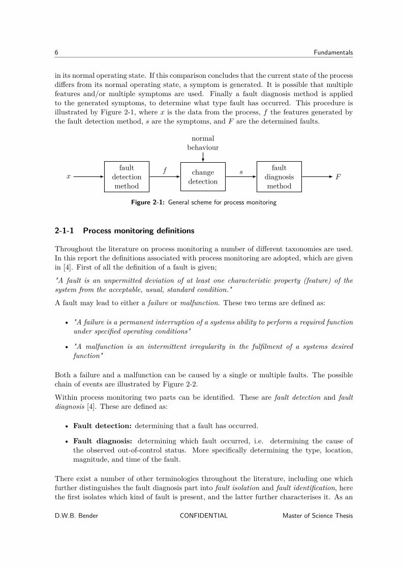
in its normal operating state. If this comparison concludes that the current state of the processdiffers from its normal operating state, a symptom is generated. It is possible that multiplefeatures and/or multiple symptoms are used. Finally a fault diagnosis method is appliedto the generated symptoms, to determine what type fault has occurred. This procedure isillustrated by Figure 2-1, where x is the data from the process, f the features generated bythe fault detection method, s are the symptoms, and F are the determined faults.
xfault
detectionmethod
changedetection
faultdiagnosismethod
F
normalbehaviour
f s
Figure 2-1: General scheme for process monitoring
2-1-1 Process monitoring definitions
Throughout the literature on process monitoring a number of different taxonomies are used.In this report the definitions associated with process monitoring are adopted, which are givenin [4]. First of all the definition of a fault is given;
"A fault is an unpermitted deviation of at least one characteristic property (feature) of thesystem from the acceptable, usual, standard condition."
A fault may lead to either a failure or malfunction. These two terms are defined as:
• "A failure is a permanent interruption of a systems ability to perform a required functionunder specified operating conditions"
• "A malfunction is an intermittent irregularity in the fulfilment of a systems desiredfunction"
Both a failure and a malfunction can be caused by a single or multiple faults. The possiblechain of events are illustrated by Figure 2-2.
Within process monitoring two parts can be identified. These are fault detection and faultdiagnosis [4]. These are defined as:
• Fault detection: determining that a fault has occurred.
• Fault diagnosis: determining which fault occurred, i.e. determining the cause ofthe observed out-of-control status. More specifically determining the type, location,magnitude, and time of the fault.
There exist a number of other terminologies throughout the literature, including one whichfurther distinguishes the fault diagnosis part into fault isolation and fault identification, herethe first isolates which kind of fault is present, and the latter further characterises it. As an
D.W.B. Bender CONFIDENTIAL Master of Science Thesis

2-1 Process monitoring 7
failure
malfunction
fault
1
0te t
1
0te t
Figure 2-2: Evolution of a fault to a failure or malfunction
example let us take a tank in which a a leak can occur. The process monitoring sequencefor this terminology would be, first the fault detection system shows that something is wrongwith the tank. Second the fault isolation determines that it must be a leak. And finally thefault identification determines the size and location of the leak. As specified, in this researchwe group the fault isolation and identification together into fault diagnosis.
2-1-2 Fault detection methods
Within the research area of fault detection a number of divisions are described for the differentmethods. In this report the methods of fault detection are split into two main categories;data-driven methods and model-based methods.
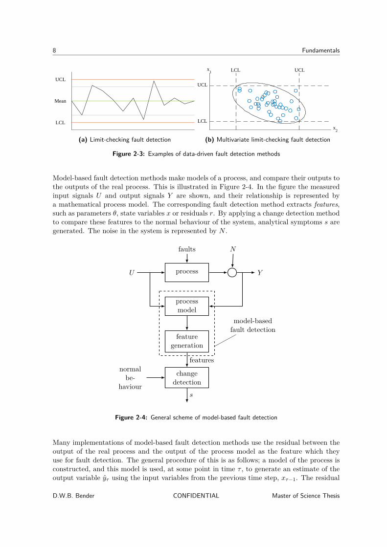
Data-driven fault detection methods use only (historic) process data to detect fault within theprocess and require no prior knowledge about the process. These methods are trained withnon-faulty data, and are used to recognise deviations from this normal behaviour, which arecaused by faults. The most simple example of this is limit-checking. This method analyseshistoric data of a single variable and determines what its normal bounds are. These bounds aretypically a maximum, upper control limit (UCL), and a minimum, lower control limit (LCL).If the value of the process variable crosses one of these bounds, a fault is declared. This isillustrated in Figure 2-3a. However checking just one variable is often not sufficient to properlydetect faults. Process variables are often correlated and this means that one process variablecan have a significant influence on the acceptable bounds of another variable. Applyingmultivariate limit-checking allows one to determine the bounds of acceptable operation forseveral process variables simultaneously. This is illustrated by Figure 2-3b.
It is also possible to apply some sort of statistical transformation, such as principal compo-nents analysis (PCA) or partial least squares (PLS), to the process variables to reduce thedimensionality. In this case limit-checking can be applied to one or more of the transformedvariables. Limit-checking is one method that can be used to detect deviations from normalbehaviour, but there are many other methods, such as change detection, that can also beapplied. Examples of this are deviations in mean, variance or stationarity. The main draw-back of data-driven methods is that its performance is highly dependent on the quantity andquality of the process data.
Master of Science Thesis CONFIDENTIAL D.W.B. Bender
8 Fundamentals
Mean
LCL
UCL
(a) Limit-checking fault detection
LCL
UCL
LCL UCL
x2
x1
(b) Multivariate limit-checking fault detection
Figure 2-3: Examples of data-driven fault detection methods
Model-based fault detection methods make models of a process, and compare their outputs tothe outputs of the real process. This is illustrated in Figure 2-4. In the figure the measuredinput signals U and output signals Y are shown, and their relationship is represented bya mathematical process model. The corresponding fault detection method extracts features,such as parameters θ, state variables x or residuals r. By applying a change detection methodto compare these features to the normal behaviour of the system, analytical symptoms s aregenerated. The noise in the system is represented by N .
process
processmodel
featuregeneration
changedetection
U
faults
Y
N
normalbe-
haviour
model-basedfault detection
features
s
Figure 2-4: General scheme of model-based fault detection
Many implementations of model-based fault detection methods use the residual between theoutput of the real process and the output of the process model as the feature which theyuse for fault detection. The general procedure of this is as follows; a model of the process isconstructed, and this model is used, at some point in time τ , to generate an estimate of theoutput variable yτ using the input variables from the previous time step, xτ−1. The residual
D.W.B. Bender CONFIDENTIAL Master of Science Thesis

2-1 Process monitoring 9
can then be used as the feature for fault detection. It is given by:
rτ = yτ − yτ (2-1)
The idea here is that the model represents the process under normal non-faulty conditions,and that its output represents the output of the system if no fault was present. It is thusassumed that if no fault is present in the system, the residual should be zero. However if afault occurs in the system, the output of the process is affected by the fault, while the outputof the model is not affected. In this case the residual will be non-zero, and it can be concludedthat a fault has occurred. In practice, noise will also cause the residual to be non-zero even ifthere is no fault in the system, therefore a threshold is introduced rτ . If the residual crossesthis threshold, a fault is detected. This procedure is illustrated by Figure 2-5.
xτ−1 process
processmodel
rτ > rτ s
rτ
+
−
yτ
yτ
rτ
Figure 2-5: Example fault detection method
There are many different methods that can be used to construct a process model. If thestructure and the parameters of the process are known, first principles can be used. In thiscase the model is constructed using the physical properties of the system, which are governedby the laws of nature. Applying this method to large systems is done by starting to modeleach of the subsystems and subsequently combining them into a single overall model of thesystem. This kind of modelling is called theoretical modelling and it always starts by makingassumptions about the process, which simplify the construction of the model. In large real-world applications, theoretical modelling is not always possible in practice. The system couldbe so complex that constructing its model would either cost too much effort or could evenbe too complex to model. In these cases experimental modelling can be applied. This isoften called identification, and this type of modelling obtains the mathematical model of theprocess by using measurements. The methods use measurements of the input and outputsignals, which it evaluates in such a way that their relation is expressed in a mathematicalmodel. Techniques such as linear regressions or artificial neural networks are examples ofthis. If such methods are used, it means that data-driven techniques are used to construct aprocess model; this differs from the data-driven fault detection techniques which they simplyuse data-driven techniques to analyse the process data.The theoretical models are built on a functional description of the physical data of the processand its parameters. The experimental model, on the other hand, determines its parametersfrom measurements, whose relation to the physical data and process is unknown. Thereforethe latter are referred to as a black-box models. In contrast, the theoretical models are referredto as white-box models. However, it is not always the case that a model can be classified aseither black- or white box. For instance, when a model knows the physical laws, but doesn’tknow the parameters, and the process measurements can be used to identify these. Suchmodels are referred to as grey-box models [4].
Master of Science Thesis CONFIDENTIAL D.W.B. Bender

10 Fundamentals
2-1-3 Fault diagnosis
Fault detection methods are used to generate features and these features are subsequentlysubjected to some sort of change detection, which compares the current state of the processto its normal behaviour. The results of this is that it is possible to detect whether a faulthas occurred, and additionally a set of symptoms for this fault can be generated. The nextstep within process monitoring is to determine which type of fault has occurred. To achievethis fault diagnosis is applied. After the symptoms are generated, a fault diagnosis methodis needed to determine what type of fault has actually occurred. Within most industrialplants, it is currently the operator of the process that performs the fault diagnosis. Theoperator assesses the symptoms of generated by the process and fault detection methods,and determines: what is going on, and subsequently, what can be done to correct this?More specifically, the task of diagnosis is to separate nf different faults, Fj , j ∈ {1, . . . , nf},using ns symptoms si, i ∈ {1, . . . , ns}. The faults are combined into a fault vector F =[F1 F2 . . . Fnf
]and the symptoms into a symptom vector s =
[s1 s2 . . . sns
]. Most
of the methods compute a fault measure fi for each fault class Fj . The most probable faultis then given by the fault corresponding to the maximum value of fj . However, in reality, notonly the largest fj is of relevance; unclear situations and measurement noise can create highvalues of multiple fault measures. This can indicate uncertain decisions. Hence, all values offj are important when determining the diagnosis of a system.
There are two main methods of fault diagnosis; classification methods and inference methods.If no information is available on the fault-symptom causalities, experimentally trained classi-fication methods can be applied for fault diagnosis. This leads to an unstructured knowledgebase. If the fault symptom causalities can be expressed in the form of if-then rules thenreasoning or inference methods are applicable. Within these two main methods, there are anumber of different fault diagnosis methods which can be applied.
Automating the fault diagnosis in an industrial plant would require at the least, either struc-tural knowledge between possible symptoms and faults within a process or a sample set ofdata, which contains enough occurrences of each type of fault. In a modern industrial plant,the process are often too complex for the first option to be possible. The second option mightseem like the more attractive option, as there is a vast amount of plant data available, howeveroperators almost never let a plant run for the full length of a fault, but rather compensatefor it or even shut down the process. Therefore there are no data sets available, that containenough fault occurrences to make automated fault diagnosis possible.
2-1-4 Early fault detection
In this research we are interested in whether large sets of data can be used to make earlierfault detection possible. Most of the model-based fault detection methods aim to detectfaults through their effect on monitored variables. They apply some sort of change detectionto a feature which was generated with the estimate of a monitored variable, e.g. a residualconstructed with the estimated output of a process and the real output. One possibility toachieve earlier fault detection is to make multi-step ahead predictions about these monitoredvariables. To achieve this we continuously learn a model, which after the fault time willinclude the fault as well, and use it to predict the system behaviour a number of steps ahead.
D.W.B. Bender CONFIDENTIAL Master of Science Thesis
2-1 Process monitoring 11
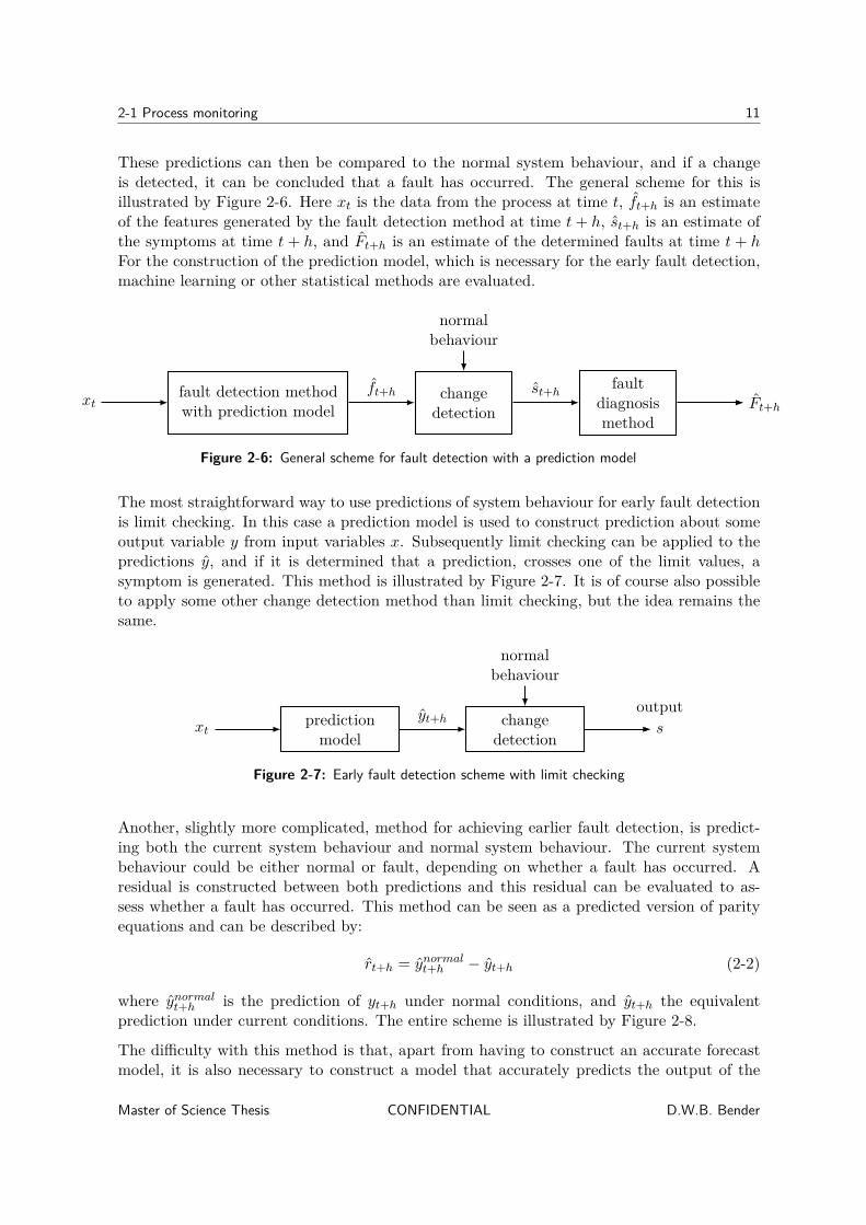
These predictions can then be compared to the normal system behaviour, and if a changeis detected, it can be concluded that a fault has occurred. The general scheme for this isillustrated by Figure 2-6. Here xt is the data from the process at time t, ft+h is an estimateof the features generated by the fault detection method at time t+ h, st+h is an estimate ofthe symptoms at time t + h, and Ft+h is an estimate of the determined faults at time t + hFor the construction of the prediction model, which is necessary for the early fault detection,machine learning or other statistical methods are evaluated.
xtfault detection methodwith prediction model
changedetection
faultdiagnosismethod
Ft+h
normalbehaviour
ft+h st+h
Figure 2-6: General scheme for fault detection with a prediction model
The most straightforward way to use predictions of system behaviour for early fault detectionis limit checking. In this case a prediction model is used to construct prediction about someoutput variable y from input variables x. Subsequently limit checking can be applied to thepredictions y, and if it is determined that a prediction, crosses one of the limit values, asymptom is generated. This method is illustrated by Figure 2-7. It is of course also possibleto apply some other change detection method than limit checking, but the idea remains thesame.
xtpredictionmodel
changedetection
s
output
normalbehaviour
yt+h
Figure 2-7: Early fault detection scheme with limit checking
Another, slightly more complicated, method for achieving earlier fault detection, is predict-ing both the current system behaviour and normal system behaviour. The current systembehaviour could be either normal or fault, depending on whether a fault has occurred. Aresidual is constructed between both predictions and this residual can be evaluated to as-sess whether a fault has occurred. This method can be seen as a predicted version of parityequations and can be described by:
rt+h = ynormalt+h − yt+h (2-2)
where ynormalt+h is the prediction of yt+h under normal conditions, and yt+h the equivalentprediction under current conditions. The entire scheme is illustrated by Figure 2-8.
The difficulty with this method is that, apart from having to construct an accurate forecastmodel, it is also necessary to construct a model that accurately predicts the output of the
Master of Science Thesis CONFIDENTIAL D.W.B. Bender

12 Fundamentals
xtnormal situationprediction model
predictionmodel
changedetection
s
normalbehaviour
+
−
yt+h
ynormalt+h
rt+h
Figure 2-8: Early fault detection scheme with predicted parity equations
system, if the system were in its normal operating state. Additionally, any model or mea-surement uncertainty will propagate over time, making predictions on a long time horizonuseless.
One idea is that the same identification procedure, such as a certain neural network or linearregression method, can be used to determine both the normal situation forecast model and theforecast model. The first can be constructed using a set of measurements that are obtainedduring a period of ‘normal’ operations. The latter can be constructed using the the mostrecent measurements, i.e. for time τ use t = τ − rw − h, ..., τ − h. As this model would beidentified using normal operating data, it should not take any effect from a fault into accountand construct a forecast of the output variable in the case that no fault was present in thesystem.
Another option would be to use a physical model, which gives an estimate of a future value,and use this estimate as the forecast for the normal situation. As it is based on the physicalproperties of the system it should also not take any effect from faults in the system intoaccount. If these methods are compared to the classic parity equations method, the physical ornormal situation prediction model could be compared to the process model, and the forecastmodel acts to the real process of the system, as the latter take all effects from faults intoaccount, whereas the physical model and process model do not.
In both cases the effects of model and measurement uncertainties will be present, and increasewhen the time horizon becomes long. It should therefore be investigated whether these typesof fault detection methods would be more effective than those where the predicted outputis compared to a simple limit value. Analysing the variances of the prediction models couldhelp with the investigation.
Examining the literature on process monitoring, which focus on early fault detection, it canalso be concluded that real-world implementations are very limited. Most of the papers usesome sort of simulator, where it is possible to keep the process in the normal operating state,and being able to know exactly when a fault is introduced, and what type of fault it is.
D.W.B. Bender CONFIDENTIAL Master of Science Thesis

Chapter 3
Case study
In this research a dataset from a real-world industrial plant is introduced. There are a numberof requirements that it has to adhere to; the amount of data, the frequency of the data and theamount of filtering that has been applied to the data. The Shell refinery at Pernis agreed toprovide the data from their Crude Distiller X1 (CDX1) unit for the case study of this research.As a result of a previous project, all the historic data from the unit for the whole of 2015 isavailable at sampling frequency of one measurement per minute. The dataset therefore metall the predetermined requirements. In the rest of the chapter, the CDX1 will be discussed inmore detail. One of its subsystems, the Depentanizer (C-X11), is highlighted and its availabledata is analysed.
3-1 Crude Distiller X1
At Shell refinery at Pernis there are around 60 different factories that produce petroleumproducts and petrochemicals from crude oil. In total 20 million metric tonnes per year ofcrude oil is processed, this is over 400.000 barrels of oil a day. Two of the factories are thetwo equivalent crude distiller unit (CDU)s, the CDX1 and the Crude Distiller X2 (CDX2).All the crude oil that arrives at Shell refinery at Pernis must first go through one of these twounits before it can be further processed.
The goal of the CDUs is to separate the crude oil into a range of petroleum products. Theseparation is achieved by using a number of subsequent distillation columns. Distillationcolumns split an incoming product into a top- and a bottom flow, where the boiling rangeof the different compounds and the temperature in the distillation column determines thecomposition of the two flows. The CDUs separate the crude oil into products such as: LPG,gasoline, naphtha, kerosene, diesel oil, motor oil and long residue.
In this research the data from the CDX1 is taken. A schematic overview of the unit is givenin Figure 3-1, where the blue units represent the distillation columns.
Master of Science Thesis CONFIDENTIAL D.W.B. Bender

14 Case study
C-X21
C-X22
C-Z03
C-Z04
C-Z05
C-Z06
LONG RESIDUE
HGO
U-Y04 TREATED KEROSENE
LGO
U-Y03 C-X27
C-X28
C-X11
C-X13
C-X12
TOPS
ISOHEXANE
n-PENTANE
ISOPENTANE
C-Y12
C-Y11
C-X31
FUEL GAS
C-X32
C-Y13
C-Y16
PROPANE
BUTANE
CRUDE OIL
NAPHTHA
HYDROTREATER
CRUDE-SPLITTER X1
KEROSTRIPPER
LGO STRIPPER
CRUDE-SPLITTER
X2HGO
DROGER
LGO DROGER
HYDROTREATER
GASOLINE-SPLITTER
DEBUTANIZER
LPG-TREATER
GAS-TREATER
DE-ETHANIZER
PROPANETREATER
BUTANETREATER
DEPENTANIZER
DEISOPENTANIZER
DE-ISOHEXANIZER
DEPROPANIZER
Figure 3-1: A schematic overview of flow process in the CDX1
From the CDX1 a single subsystem, the C-X11, is chosen as the initial case study of theresearch. Once different models have been identified, tested and evaluated on the C-X11,these models can be applied to other subsystems as validation and robustness analysis.
A short discussion of the other eligible subsystems is given. The set-up of the Deisopentanizer(C-X12) and Deisohexanizer (C-X13) resemble that of the C-X11. However the boiling pointsof their top- and bottom flow are much closer together than that of the C-X11. Thereforethey are both considered superfractionator distillation columns. To achieve the separationthe settling time is much longer, in the range of half a day, as opposed to an hour and a halffor the C-X11. The first distillation columns in the CDX1 are the Crude Splitter 1 (C-X21)Crude Splitter 2 (C-X22). Both systems are a more complex version of the C-X11, i.e. thereare around 100 process variables that can be used as input variables for the models, wherethe C-X11 only has around 35. Finally the Debutanizer (C-X27), Gasoline Splitter (C-X28)are both similar systems to the C-X11, but both processes are faster, which means they havea shorter settling time.
3-2 Depentanizer
The initial research is performed on a single subsystem of the CDX1, the Depentanizer(C-X11). This unit is fed the top product from the C-X28, and it splits this into the productspentane (C5), both n-pentane (nC5) and isopentane (iC5), and heavier compounds. In theC-X11 subsystem, there are 35 process variables which are measured by sensors and whosedata is stored in the data historian. A schematic overview of the subsystem is given inFigure 3-2.
D.W.B. Bender CONFIDENTIAL Master of Science Thesis

3-2 Depentanizer 15
C-X11
V-Y21
HEXANE, PENTANE, TOPS
V-Y21
20
PENTANE
40
HEXANE, TOPS
CHEMFEED
11
FLARE
NITROGEN
Cooling fluids
Process fluids
LTXX3
TTX03
FCXX3
TTX02 TTX03
FCXX5
LTXX7
TTX18
LTXX1
TTX06
TTX07
TTX08
TTX01
PTXX1
FCXX1
PTXX2
LTXX2
TTX11
TTX12
TTX20 FCXX2
FCXX5
TTX05
TTX19
XCXX1
FCXX3
FCXX4TTX09 TTX10
TTX17 TTX16TTX15
TTX14
QTXX1
QEXX1
TTX13
HCXX6
Valve (%)
Valve (on/off)
Heat exchanger
Vessel
Distillation column
Sensor
Figure 3-2: A schematic overview of the depentanizer C-X11
3-2-1 Quality variable QTXX1
The analyser QTXX1 (QT1) measures the quality of the distillation column C-X11. Thisanalyser is a chromatography detector, which measures the mass fractions of the differentcomponents in the bottom product. The quality of the C-X11 is defined as the mass fractionof nC5 in its bottom product. The analyser has an measurement error of 0-0.075% nC5,which is about 0-2% of the output value . The mass fraction QT1 is taken as the output ofthe system.
To determine the mass fractions of the different components, the chromatography detectortakes a sample of the bottom product and analyses this sample. The analyser, and all of theother sensors, send their measured values to the distributed control system (DCS). The DCSperforms the Advanced Process Control (APC) and also sends the measured data to the datahistorian, who stores the historic data. However, the analysis of the chromatography detectortakes some time to be performed. The analyser typically outputs a value for QT1 every fiveor six minutes. In addition, in some cases the analyser rejects the result of a sample, anddoes not output to the DCS.
The result of this is that the QT1 has an irregular sampling time. The DCS uses a zero-orderhold filter, which means that the last value of QT1 is kept until a new value is available. Anadded complication is that noise is added between the analyser and the DCS, as the analysesis connected through an analogue output, which can cause deviations in the output. Thesedeviations are can be considered negligible, as they are in the order of 10−4. However, thesedeviations should not be considered new output values of the analyser. This can be doneby implementing a deadband for the deviation of QT1. If the deviation of QT1 is smallerthan the deadband, its value remains the same. In Figure 3-3 an historic dataset for the QT1is shown. The blue line describes the dataset which is stored in the data historian and the
Master of Science Thesis CONFIDENTIAL D.W.B. Bender

16 Case study
red dots represent the dataset, where only the new measured values from the analyser aretaken. To generate this second dataset a deadband of 0.01 has been applied to eliminate thedeviations caused by noise.
12:00 12:30 01:00 01:30 02:00 02:30 03:00 03:30time
3.5
4
4.5
5
% n
C5
QT1 outputmeasured QT1
Figure 3-3: Output dataset stored in data historian and the measured output dataset
All the other variables in the C-X11 have a sampling time of once a minute. The goal is toconstruct a model using these other variables as inputs and QT1 as the output. This meansthat a so-called dual sampling rate problem occurs. The inputs of the model have a samplingrate of one per minute, and the output of the model has a sampling rate which is slower,and also irregular. The steady state of the C-X11 is reached after roughly 75 min. Theanalyser outputs a value of QT1 every 5 or 6 minutes, with an occasional exception where ittakes about twice that time. The irregular sampling time is thus still shorter than the steadystate time. This could mean that not a lot of information is lost, and that enough of theinformation is left such that the models are able to capture the dynamics.
Several approaches can be taken to deal with the dual sampling rate problem. The first is list-wise deletion, where every measurement that does not contain a complete set of all variablesis deleted from the dataset [5]. In our case this would mean only using the measurements forwhich the analyser has given an output of QT1, and the corresponding input variables at thattime. As a result all the measurements of the input variables, for which there is not an outputvalue, would be deleted. The advantage of this method is that only measurements are usedthat are a direct output of the sensors, but this also means that all the information containedin the deleted input variables is not made used of. A second option is using interpolationbetween the measured values of QT1, to construct a complete dataset. Interpolation can bedone using a number of different methods, such as linear, zero-order hold, or spline. Theadvantage of interpolation is that a complete dataset is available, and all the informationcontained in the input variables is utilized. However [5] warn, that one should be carefulwhen using interpolation, especially when the time between known measurements is large.A third method to deal with the dual sampling rate problem is to apply a method, suchas expectation maximization (EM), to estimate the missing values of QT1. However as thegoal of this research is to identify a model using this data, this would mean that a modelwould be identified using estimated data, and a double estimation error would occur. This isundesirable, so estimation errors will not be examined in this research. Both list-wise deletionand three interpolation methods are evaluated in Chapter 4.
D.W.B. Bender CONFIDENTIAL Master of Science Thesis
3-2 Depentanizer 17
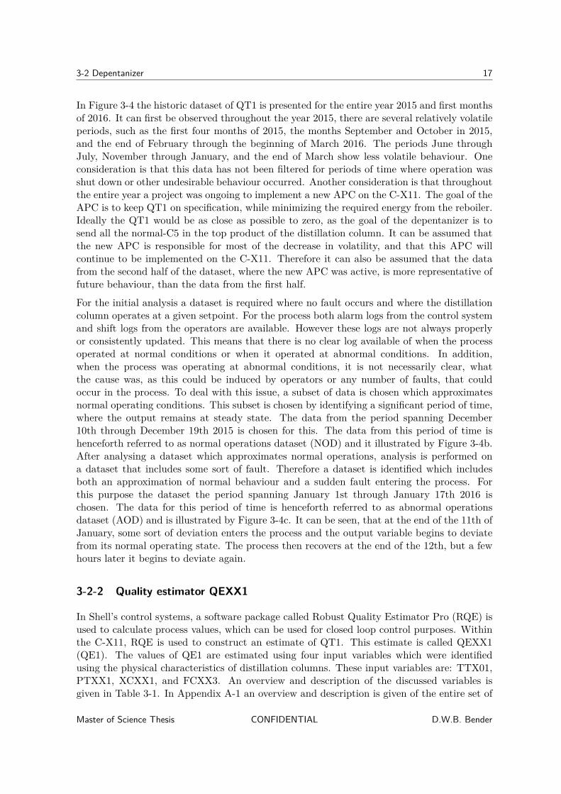
In Figure 3-4 the historic dataset of QT1 is presented for the entire year 2015 and first monthsof 2016. It can first be observed throughout the year 2015, there are several relatively volatileperiods, such as the first four months of 2015, the months September and October in 2015,and the end of February through the beginning of March 2016. The periods June throughJuly, November through January, and the end of March show less volatile behaviour. Oneconsideration is that this data has not been filtered for periods of time where operation wasshut down or other undesirable behaviour occurred. Another consideration is that throughoutthe entire year a project was ongoing to implement a new APC on the C-X11. The goal of theAPC is to keep QT1 on specification, while minimizing the required energy from the reboiler.Ideally the QT1 would be as close as possible to zero, as the goal of the depentanizer is tosend all the normal-C5 in the top product of the distillation column. It can be assumed thatthe new APC is responsible for most of the decrease in volatility, and that this APC willcontinue to be implemented on the C-X11. Therefore it can also be assumed that the datafrom the second half of the dataset, where the new APC was active, is more representative offuture behaviour, than the data from the first half.
For the initial analysis a dataset is required where no fault occurs and where the distillationcolumn operates at a given setpoint. For the process both alarm logs from the control systemand shift logs from the operators are available. However these logs are not always properlyor consistently updated. This means that there is no clear log available of when the processoperated at normal conditions or when it operated at abnormal conditions. In addition,when the process was operating at abnormal conditions, it is not necessarily clear, whatthe cause was, as this could be induced by operators or any number of faults, that couldoccur in the process. To deal with this issue, a subset of data is chosen which approximatesnormal operating conditions. This subset is chosen by identifying a significant period of time,where the output remains at steady state. The data from the period spanning December10th through December 19th 2015 is chosen for this. The data from this period of time ishenceforth referred to as normal operations dataset (NOD) and it illustrated by Figure 3-4b.After analysing a dataset which approximates normal operations, analysis is performed ona dataset that includes some sort of fault. Therefore a dataset is identified which includesboth an approximation of normal behaviour and a sudden fault entering the process. Forthis purpose the dataset the period spanning January 1st through January 17th 2016 ischosen. The data for this period of time is henceforth referred to as abnormal operationsdataset (AOD) and is illustrated by Figure 3-4c. It can be seen, that at the end of the 11th ofJanuary, some sort of deviation enters the process and the output variable begins to deviatefrom its normal operating state. The process then recovers at the end of the 12th, but a fewhours later it begins to deviate again.
3-2-2 Quality estimator QEXX1
In Shell’s control systems, a software package called Robust Quality Estimator Pro (RQE) isused to calculate process values, which can be used for closed loop control purposes. Withinthe C-X11, RQE is used to construct an estimate of QT1. This estimate is called QEXX1(QE1). The values of QE1 are estimated using four input variables which were identifiedusing the physical characteristics of distillation columns. These input variables are: TTX01,PTXX1, XCXX1, and FCXX3. An overview and description of the discussed variables isgiven in Table 3-1. In Appendix A-1 an overview and description is given of the entire set of
Master of Science Thesis CONFIDENTIAL D.W.B. Bender

18 Case study
Feb 2015 Apr 2015 Jun 2015 Aug 2015 Oct 2015 Dec 2015 Feb 2016 Apr 20160
2
4
6
8
10
% n
C5
QT1
(a)
Dec 10 Dec 11 Dec 12 Dec 13 Dec 14 Dec 15 Dec 16 Dec 17 Dec 18 Dec 192015
0
2
4
6
8
10
% n
C5
QT1
(b)
Jan 02 Jan 04 Jan 06 Jan 08 Jan 10 Jan 12 Jan 14 Jan 162016
0
2
4
6
8
10
% n
C5
QT1
(c)
Figure 3-4: Entire dataset of QT1 and two subsets of its data; normal operations dataset (NOD)and abnormal operations dataset (AOD)
D.W.B. Bender CONFIDENTIAL Master of Science Thesis

3-2 Depentanizer 19
input variables that are available in the C-X11.
Table 3-1: Descriptions of the variables
Full Name Name Unit Description
CDX1:QTXX1.PV QT1 wt% Mass fraction nC5 in bottom C-X11CDX1:QEXX1.PV QE1 wt% Estimate mass fraction nC5 in bottom C-X11
CDX1:TTX01.PV TTX01 ℃ Temperature at tray 11 of the C-X11CDX1:PTXX1.PV PTXX1 barg Pressure at tray 11 of the C-X11CDX1:XCXX1.PV XCXX1 MW Energy transfer from C-X21 to E-Z72CDX1:FCXX3.PV FCXX3 MT/day Input flow of C-X11
The estimation of QE1 is done by first taking a linear combination of the four input variablesto construct the linear output QE1lin;
QE1lin = θ(1) ∗ TTX01 + θ(2) ∗ PTXX1︸ ︷︷ ︸ECP
+θ(3) ∗ 1000 ∗XCXX1FCXX3︸ ︷︷ ︸
SI
+θ(4) (3-1)
In a distillation column there are two important properties, that can be used to describe itsperformance. These are the effective cut point (ECP) and the separation index (SI). Cutpoints, within distillation operations, are key parameters. They are the temperatures atwhich the various distilling products are separated. Each product has two cut points; theseare the temperature at which a product begins to boil, the initial boiling point (IBP) and thetemperature at which it is 100% vaporized, the end point (EP). The ECPs are the point atwhich the products can be considered effectively clean. The SI gives an idea on how difficultthe separation is to perform. For distillation this is the relative volatility of the two keycomponents. When the relative volatility is one, there is no separation of components whendistillation is used. In (3-1), the TTX01 and PTXX1 represent the ECP, and the XCXX1and FCXX3 represent the SI.
The parameters θ(1), θ(2), θ(3) in (3-1) are estimated off-line and are given by (3-2). Theinitial value of the bias term θ(4), is also estimated off-line. However, the bias term isupdated on-line, by correcting for the error between QT1 and QE1.
θ =[−0.4 7.35 −1 bias
](3-2)
When constructing the linear relation between input variables and QE1, the process controlengineers chose to only use these four input variables, and not investigate whether addingextra input variables could increase the accuracy of the estimate. The reason for this is thatthey are able to justify using these four variables, because of the known relation between thequality of a distillation column and the ECP and SI.
If an extra input variable was found to increase the model fit and therefore added to the model,it is possible that the accuracy of the model could increase while the process conditions werenormal. However if the conditions would deviate too far from the normal situation, the addedvariable might could possibly cause unwanted and unexpected behaviour in the estimate. Asthe estimate is used in the closed-loop control, this could lead to dangerous situations. Thisconcept is called overfitting.
Master of Science Thesis CONFIDENTIAL D.W.B. Bender

20 Case study
A reason that this can occur for this can be that the dataset that is being used for the trainingcontains not only information about the regularities in the mapping from input to output,but also a sampling error. This means that there will be accidental regularities because of thefact that that particular training data was chosen. If this data is used to train the model, itwon’t be able to tell which regularities are real and which are caused by the sampling error.As a result it will fit both kinds of regularity and if the model is flexible enough it will beable to model the sampling error really well. If this happens, the model will fit the trainingdata better, but the performance will decrease when applied to new data.To further illustrate the concept of overfitting, let us take the extreme case where there is alinear regressor, with as the same amount of parameters as number of samples in the trainingdata set. In this case it is possible to, trivially, tune the parameters to exactly reproduce thesamples, and it is very clear that this cannot be called learning. An example of overfitting isgiven in Figure 3-5.
0 0.2 0.4 0.6 0.8 1 1.2 1.4 1.6 1.8 20
0.2
0.4
0.6
0.8
1
measurementsoverfitting modelgood fit model
Figure 3-5: An example of a data set and a model with overfitting and a model with a good fit
This consideration should also be taken into account throughout the rest of this research.However the focus is first to assess whether using larger input variable datasets can produceaccurate estimates, and the analysis of their robustness to operating conditions can be doneas a later step.To account for the non-linearity in the system, subsequently a piecewise linear function isused to transform the value of QE1lin into QE1. This function is illustrated by Figure 3-6. Amodel of this type, i.e. a linear model followed by a static non-linearity is a Wiener non-linearmodel.In Figure 3-7 a dataset of QT1 is given and the corresponding values of QE1, which wasconstructed using given linear relation and the piecewise linear function transformation. Itcan be observed that QE1 is able to capture a large part of the dynamics in its estimation ofQT1, even before the analyser relays the value of QT1.The fact that the given model is able to construct an estimate of QT1 from four inputvariables, that captures most of the dynamics of QT1 ahead of the analyser, means there isclearly a relation between QT1 and these four input variables. Therefore we will first do someanalysis in Chapter 4 by using the output and just these four input variables, before we moveon to using all the available inputs.
D.W.B. Bender CONFIDENTIAL Master of Science Thesis

3-2 Depentanizer 21
0 5 10 15 20QE1
-5
0
5
10
QE
1 lin
Figure 3-6: The piecewise linear function
12:00 04:00 08:00 12:00 04:00 08:00 12:00time
3
3.5
4
4.5
5
% n
C5
QE1 outputmeasured QT1
Figure 3-7: Dataset of QT1 and QE1
Master of Science Thesis CONFIDENTIAL D.W.B. Bender

22 Case study
3-2-3 Process variables TTX01, PTXX1, XCXX1, and FCXX3
The four input variables, which are used for the construction of QE1, are examined further.There four variables together are henceforth referred to as 4VAR. The NODs of each ofthe input variables are shown in Figure 3-8. As mentioned previously, the input variablesare measured each minute, contrary to the output variable. There seems to be quite somecorrelation between TTX01 and PTXX1. In addition XCXX1 is relatively noisy comparedto the other inputs. I can be observed that each of the four variables change quite a bitthroughout the period, whereas we know that the output remains fairly constant in the sameperiod of time.
Dec 11 Dec 13 Dec 15 Dec 17 Dec 19date
75
80
85
90
95
°C
TTX01
(a)
Dec 11 Dec 13 Dec 15 Dec 17 Dec 19date
0.8
0.9
1
1.1
1.2
1.3
1.4
1.5
1.6
barg
PTXX1
(b)
Dec 11 Dec 13 Dec 15 Dec 17 Dec 19date
6
6.5
7
7.5
8
8.5
9
MW
XCXX1
(c)
Dec 11 Dec 13 Dec 15 Dec 17 Dec 19date
1100
1200
1300
1400
1500
1600
1700
MT
/day
FCXX3
(d)
Figure 3-8: Datasets of the 4VAR variables
D.W.B. Bender CONFIDENTIAL Master of Science Thesis
Chapter 4
Model analysis
The goal of this research is to determine whether a model can be identified which is ableto produce accurate robust predictions of the output of the system, without using priorknowledge about it.
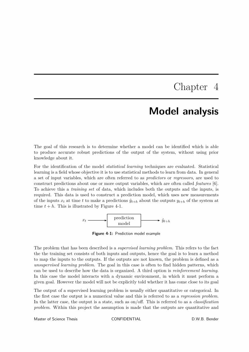
For the identification of the model statistical learning techniques are evaluated. Statisticallearning is a field whose objective it is to use statistical methods to learn from data. In generala set of input variables, which are often referred to as predictors or regressors, are used toconstruct predictions about one or more output variables, which are often called features [6].To achieve this a training set of data, which includes both the outputs and the inputs, isrequired. This data is used to construct a prediction model, which uses new measurementsof the inputs xt at time t to make a predictions yt+h about the outputs yt+h of the system attime t+ h. This is illustrated by Figure 4-1.
xtpredictionmodel
yt+h
Figure 4-1: Prediction model example
The problem that has been described is a supervised learning problem. This refers to the factthe the training set consists of both inputs and outputs, hence the goal is to learn a methodto map the inputs to the outputs. If the outputs are not known, the problem is defined as aunsupervised learning problem. The goal in this case is often to find hidden patterns, whichcan be used to describe how the data is organized. A third option is reinforcement learning.In this case the model interacts with a dynamic environment, in which it must perform agiven goal. However the model will not be explicitly told whether it has come close to its goal
The output of a supervised learning problem is usually either quantitative or categorical. Inthe first case the output is a numerical value and this is referred to as a regression problem.In the latter case, the output is a state, such as on/off. This is referred to as a classificationproblem. Within this project the assumption is made that the outputs are quantitative and
Master of Science Thesis CONFIDENTIAL D.W.B. Bender

24 Model analysis
available. Therefore this report focusses on the regression problem.
In this report the assumption is made that the processes can be described as time-varyinglinear autonomous systems. Linear refers to the fact that the output variable of the processcan be described by a linear combination of input, autoregressive, and moving average terms.Another assumption is that the process behaves autonomously, which means that the inputs ofthe system are fixed and unknown. Finally time-varying refers to the fact that the parametersof the system change over time. To deal with this, it means that a model must be identifiedrecurrently for each time step.
Before the modelling of the processes can be done, there are two questions which must fist beanswered. The first is what type of dynamic model should be used to model the processes.The second question is how the issue of the irregular sampling time and missing data of theoutput variables should be dealt with.
To evaluate what type of dynamic model should be used, two different models are tested,the finite impulse response (FIR) and autoregressive-moving average model with exogenousinputs (ARMAX). Their performance and model complexity are evaluated and a decision ismade, which to use throughout the rest of this report. The evaluation is performed, by usingboth models to create predictions about QTXX1 (QT1), and comparing their performances.The irregular sampling time and missing data of the output variables can be dealt with inseveral ways. It is decided not to evaluate using complex methods for estimating the missingdata, as this can lead to large estimation errors. Two, relatively simple, methods to deal withthe issue are examined. The first is discarding all samples, which include missing data, thisresults in using a dataset which is smaller than the original dataset, but only contain measureddata. The second method, is using interpolation methods to estimate the missing data. Theadvantage of this is that, the interpolation methods are straightforward and no information isdiscarded. The separate interpolation methods are compared to using only measured data anda decision is made, which method is implemented in the rest of this report. The evaluation isperformed by using ordinary least squares (OLS) to construct predictions of QT1, using eachof the four methods.
The evaluation of the models and methods is done using only the 4VAR as input variables.The advantage this has, is that it is known that there is a relation between these predictorsand QT1. With this relation, the best solution for the irregular sampling time can be foundand choice of dynamic model can be made. Once these issues have been resolved, the researchmoves on to include a larger set of predictors, than just these four.
4-1 Performance evaluation
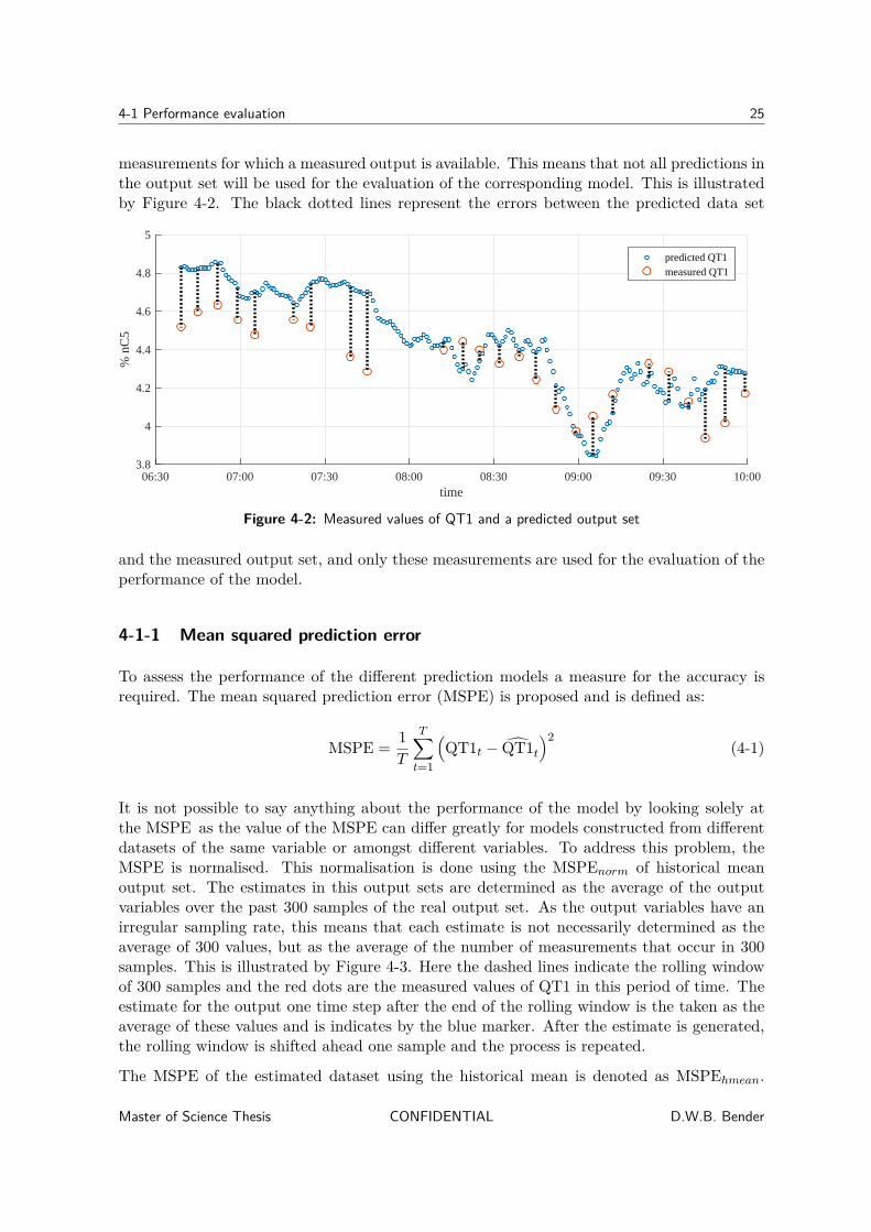
If different predicted datasets are constructed, their performance must be evaluated usingsome criterion to determine which of the models provides the most accurate predictions. Mostcriterion are based on the error function between the predictions and the realized output setat each sample throughout the datasets. However in the case of QT1, predictions can beconstructed for each measurement, but due to the sampling time of the analyser, not each ofthese will have a corresponding measured output to be compared to. To solve this, the errorfunction will still be used for the evaluation, but the error function will only be determined for
D.W.B. Bender CONFIDENTIAL Master of Science Thesis
4-1 Performance evaluation 25
measurements for which a measured output is available. This means that not all predictions inthe output set will be used for the evaluation of the corresponding model. This is illustratedby Figure 4-2. The black dotted lines represent the errors between the predicted data set
06:30 07:00 07:30 08:00 08:30 09:00 09:30 10:00time
3.8
4
4.2
4.4
4.6
4.8
5
% n
C5
predicted QT1measured QT1
Figure 4-2: Measured values of QT1 and a predicted output set
and the measured output set, and only these measurements are used for the evaluation of theperformance of the model.
4-1-1 Mean squared prediction error
To assess the performance of the different prediction models a measure for the accuracy isrequired. The mean squared prediction error (MSPE) is proposed and is defined as:
MSPE = 1T
T∑t=1
(QT1t − QT1t
)2(4-1)
It is not possible to say anything about the performance of the model by looking solely atthe MSPE as the value of the MSPE can differ greatly for models constructed from differentdatasets of the same variable or amongst different variables. To address this problem, theMSPE is normalised. This normalisation is done using the MSPEnorm of historical meanoutput set. The estimates in this output sets are determined as the average of the outputvariables over the past 300 samples of the real output set. As the output variables have anirregular sampling rate, this means that each estimate is not necessarily determined as theaverage of 300 values, but as the average of the number of measurements that occur in 300samples. This is illustrated by Figure 4-3. Here the dashed lines indicate the rolling windowof 300 samples and the red dots are the measured values of QT1 in this period of time. Theestimate for the output one time step after the end of the rolling window is the taken as theaverage of these values and is indicates by the blue marker. After the estimate is generated,the rolling window is shifted ahead one sample and the process is repeated.
The MSPE of the estimated dataset using the historical mean is denoted as MSPEhmean.
Master of Science Thesis CONFIDENTIAL D.W.B. Bender

26 Model analysis
12:00 12:30 01:00 01:30 02:00 02:30 03:00 03:30 04:00 04:30 05:00 05:30 06:00time
3.5
4
4.5
5
5.5
6
% n
C5
measured QT1historical mean estimate of QT1
Figure 4-3: Estimate of QT1 using the historical mean
Then the MSPE of the prediction methods, MSPEmodel, are normalised as follows:
MSPEnorm = MSPEmodelMSPEhmean
(4-2)
4-2 Dynamic model
One of the most general models that is used for time-varying linear autonomous systems,such as presented in Figure 4-4, is the ARMAX model, which is defined as:
yt = c+p∑i=1
φiyt−i +q∑j=1
θjεt−j +b∑
k=1βkxt−k + εt (4-3)
where yt, εt, xt are respectively the output, the random error, and the exogenous variablesat time t. φi, θj , and βk are model parameters for i = 1, . . . , p, j = 1, . . . , q, and k = 1, . . . , b,respectively. c is a constant. The simplified notation is given by:
A(z)y(t) = B(z)x(t) + C(z)ε(t) (4-4)
where
A(z) = (1 + φ1z−1 + . . .+ φpz
−p) (4-5)B(z) = (1 + θ1z
−1 + . . .+ θqz−q) (4-6)
C(z) = (1 + β1z−1 + . . .+ βbz
−b) (4-7)
and z−1 is the unit delay, i.e. z−1xt = xt−1.
Depending on the parameters p and q, the ARMAX(p,q) model takes past outputs and pasterrors into account, when identifying a model. An alternative for the ARMAX(p,q) modelis the FIR model. The FIR model is simply a restricted version of the ARMAX(p,q) model,where the A(z) = 1 and C(z) = 1, which results in the following model:
y(t) = B(z)u(t) + e(t) (4-8)
D.W.B. Bender CONFIDENTIAL Master of Science Thesis
4-2 Dynamic model 27
xt process yt
εt
Figure 4-4: Process
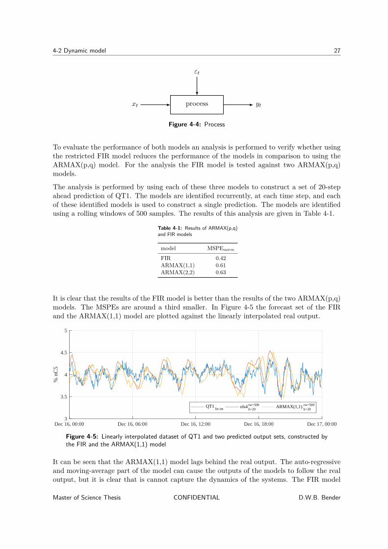
To evaluate the performance of both models an analysis is performed to verify whether usingthe restricted FIR model reduces the performance of the models in comparison to using theARMAX(p,q) model. For the analysis the FIR model is tested against two ARMAX(p,q)models.
The analysis is performed by using each of these three models to construct a set of 20-stepahead prediction of QT1. The models are identified recurrently, at each time step, and eachof these identified models is used to construct a single prediction. The models are identifiedusing a rolling windows of 500 samples. The results of this analysis are given in Table 4-1.
Table 4-1: Results of ARMAX(p,q)and FIR models
model MSPEnormFIR 0.42ARMAX(1,1) 0.61ARMAX(2,2) 0.63
It is clear that the results of the FIR model is better than the results of the two ARMAX(p,q)models. The MSPEs are around a third smaller. In Figure 4-5 the forecast set of the FIRand the ARMAX(1,1) model are plotted against the linearly interpolated real output.
Dec 16, 00:00 Dec 16, 06:00 Dec 16, 12:00 Dec 16, 18:00 Dec 17, 00:003
3.5
4
4.5
5
% n
C5
QT1lin int ols4
h=20rw=500 ARMAX(1,1)
h=20rw=500
Figure 4-5: Linearly interpolated dataset of QT1 and two predicted output sets, constructed bythe FIR and the ARMAX(1,1) model
It can be seen that the ARMAX(1,1) model lags behind the real output. The auto-regressiveand moving-average part of the model can cause the outputs of the models to follow the realoutput, but it is clear that is cannot capture the dynamics of the systems. The FIR model
Master of Science Thesis CONFIDENTIAL D.W.B. Bender

28 Model analysis
on the other hand, seems to be able to describe the dynamics of the process. It is thereforeconclude that, within this report, the output of process is not dependent on past outputs orpast errors and the system can be described using a FIR model.
4-3 Variable types and terminology
Before the irregular sampling rate is discussed, a brief description of some variable typesand terminology, as well as a description of the procedure for using OLS for out-of-sampleforecasting are given.
In this research we will restrict ourselves to a multiple inputs, single output (MISO) system.A single measurement of the output is defined by yt and a single measurement of input i isdefined as xi,t, where t denotes the t-th measurement in the dataset. The vector includingall input variables at time t, is defined as xt A vector of measurements for input variable i isreferred to as xi and the matrix which includes a vector of measurements for multiple inputvariables is represented by X. For the vector of output variable measurements this is doneequivalently as yi.
In this research the focus is on the MISO regression problem. This problem can be looselydefined as follows; make a prediction of the output yt, given the values of an input vectorxt−h. The prediction is defined as yt, where h is the prediction horizon, which indicates howmany the amount of steps ahead the prediction is. The construction of the prediction modelis done with a training set. The training set is a set of measurements V ≡ (X, y), where Xis a N × p matrix, in which N is the number of measurements and p the number of inputvariables, and y is a N × 1 vector.
4-4 Ordinary least squares
For the evaluation of the irregular sampling rate a FIR model and OLS is used to constructout-of-sample predictions of QT1. The procedure for this is as followed;
The linear regression model, with output yt and p input variables xt−h =(x1,t−h, x2,t−h, . . . , xp,t−h), is given by:
yt = c+p∑j=1
βjxj,t−h + εt (4-9)
= c+ βxt−h + εt (4-10)
where β are unknown parameters and ε is the error. The term c is the intercept, which is alsoreferred to as the bias. In practice it is often convenient to include the constant variable 1 inxt, i.e. include c in the vector of coefficients β. In this case the model can be simplified to:
yt = βxt−h + εt (4-11)
From here on it will be assumed that the c is included in β unless indicates differently.
D.W.B. Bender CONFIDENTIAL Master of Science Thesis

4-4 Ordinary least squares 29
To fit the FIR model to the training set, OLS is applied. In this approach the coefficients βare chosen, such that they minimize the residual sum of squares;
RSS(β) = (y − βX)T (y − βX) (4-12)
The unique solution for the estimate of β, in this case, is given by:
β = (XTX)−1XT y (4-13)
In this research FIR is used to construct out-of-sample predictions. This means that ifpredictions are made about measurements t+h, only information is used which was availableat measurement t. The implementation of this procedure is now described for the case whereQT1 is taken as output variable and TTX01, PTXX1, XCXX1, and FCXX3 as the inputvariables
Let us take a dataset of N samples, containing five measurements for each time step, whichcorrespond to the output and four input variables. At sample t the output variable is denotedas QT1t and the vector of the four input variables as xt. To construct forecasts using thismethod, first the FIR model is defined as:
QT1t+h = βxt + εt (4-14)
here h is prediction horizon. As a FIR model is used, only predictions about the output ofthe model at an instant in discrete time that is h sample times in the future are made. Thusit is not the case that a prediction is made for each sample time along the entire discrete timeinterval spanning from t to t+ h.
Second, the vector of parameters β needs to be estimated. For this estimation a training setof samples is necessary. The training set is determined by defining a rolling window of sizerw. As the prediction horizon is larger than zero, new samples must be generated from thedataset, where each sample contains the input variables from time t and the output variableat time t+h. For the first estimation of parameters β, the first rw samples are of the datasetare taken. This means taking the first rw measurements of the input variables {xt}rwt=1 andthe the coupled output variables {QT1t}rw+h
t=1+h.
The estimate of parameters β is the linear least squares estimate of β, which is constructedby regressing {QT1t}rw+h
t=1+h on {xt}rwt=1. This estimate is denoted by βrw+h. For the thegeneration of this estimate the QT1rw+h has been used. As we want to use the most recentinformation available, the first out-of-sample forecast that can be constructed is the forecastusing the input variables from the same instant in time xrw+h. This forecast is the estimate ofQT1rw+2h, and is denoted as QT1rw+2h. It is constructed using the estimate of β as follows:
QT1rw+2h = βrw+hxrw+h (4-15)
Subsequently, the second out-of-sample forecast is then constructed by:
QT1rw+2h+1 = βrw+h+1xrw+h+1 (4-16)
where βrw+h+1 is estimated by regressing {QT1t}rw+h+1t=2+h on {xt}rw+1
t=2 . Continuing in this man-ner throughout the whole dataset, results in a out-of-sample containing forecasts {QT1t}Nt=rw+2h,
Master of Science Thesis CONFIDENTIAL D.W.B. Bender
30 Model analysis
where N is the number of observations. Technically the forecast set could continue untilN+h,however the value of the output variable is not available in the dataset, and therefore theseforecasts cannot be verified.
When constructing forecasts, using this procedure, there are two parameters which have tobe defined. These are the prediction horizonh and the size of the rolling window rw. It mustbe evaluated which settings both these parameters lead to the most desirable results.
4-4-1 Concatenated variables
It is also possible to concatenate the input variables. In this case the output is not just mappedfrom the input variables of one measurement, but using the variables of several measurements.For a 1×p vector of input variables xt, where p indicates the amount of predictors, this meansreplacing the vector xt by the 1× (p× l) vector
[xt xt−1 . . . xt−l
], where l indicates the
amount included time steps. In this case the dynamical model of the process changes to:
QT1t+h = β[xt−h xt−h−1 . . . xt−h−l
]+ εt (4-17)
If this approach is taken and the input variables are concatenated, we talk about usingconcatenated variables as inputs to the model.
4-5 Dual and irregular sampling rate
The identification of the process requires a set of corresponding input and output variables.The output variable set QT1 is missing measurements, and these can either be filled in usinginterpolation, such that the identification can be applied to a set of measurements which spanthe entire dataset. Alternatively the identification can be applied to only the available outputmeasurements, and their corresponding input variables. To determine which of these optionsshould be applied, each of them is evaluated in this section. Three different interpolationmethods are evaluated; linear, zero-order hold, and spline. The performances of these threeinterpolation method are compared to the performance of using the measured set. Thesethree methods are illustrated by Figure 4-6.
The evaluation is performed by using a FIR model and OLS, with QT1 as the output, andthe 4VAR as input variables. The four different methods of generating the output set of QT1are evaluated for six rolling windows, 100, 300, 500, 1000, 1500, and 2000, and predictionhorizons ranging from 1 to 30. Additionally each of them is tested using 0 to 5 concatenatedinput variables. The results of these tests are presented in Appendix B-1.
The difference in results between the models identified with different numbers of concatenatedvariables is small in terms of MSPE. Therefore the analysis is continued with the modelswithout concatenated variables. The results of the models with a rolling window of 500 and1000 are presented in Figure 4-7.
It can be clearly seen that the performance of the models, that were identified only with themeasured data sets, perform significantly worse than the models that were identified withinterpolated data sets, as the MSPE is much worse.
D.W.B. Bender CONFIDENTIAL Master of Science Thesis
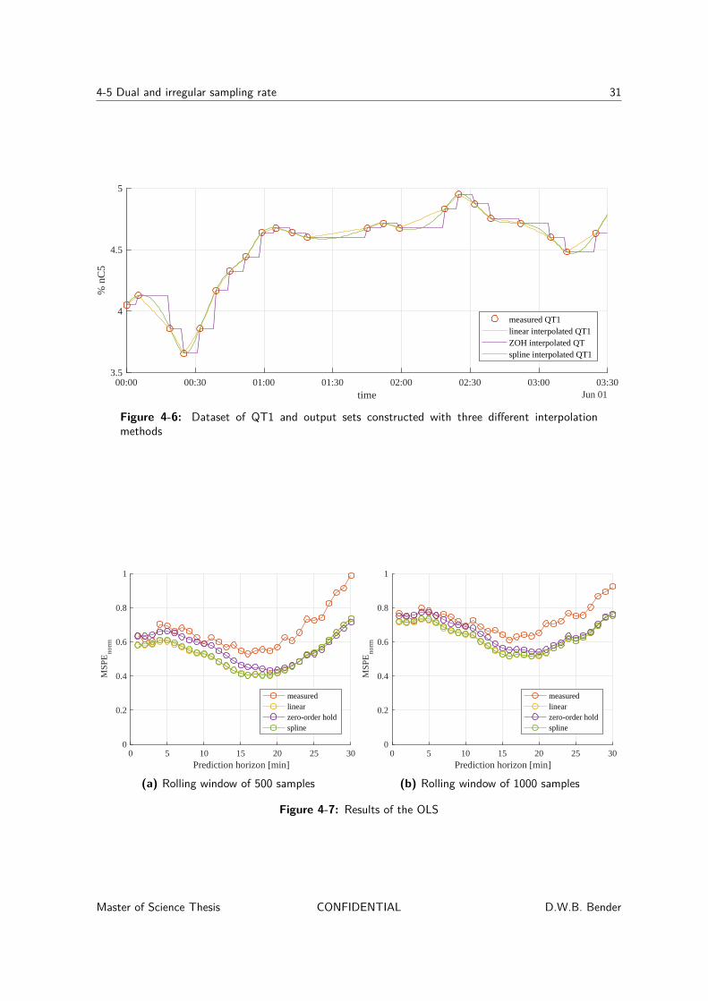
4-5 Dual and irregular sampling rate 31
00:00 00:30 01:00 01:30 02:00 02:30 03:00 03:30time Jun 01
3.5
4
4.5
5
% n
C5
measured QT1linear interpolated QT1ZOH interpolated QTspline interpolated QT1
Figure 4-6: Dataset of QT1 and output sets constructed with three different interpolationmethods
0 5 10 15 20 25 30Prediction horizon [min]
0
0.2
0.4
0.6
0.8
1
MSP
Eno
rm
measuredlinearzero-order holdspline
(a) Rolling window of 500 samples
0 5 10 15 20 25 30Prediction horizon [min]
0
0.2
0.4
0.6
0.8
1
MSP
Eno
rm
measuredlinearzero-order holdspline
(b) Rolling window of 1000 samples
Figure 4-7: Results of the OLS
Master of Science Thesis CONFIDENTIAL D.W.B. Bender

32 Model analysis
The differences between the three interpolation methods seem to be small. If a rolling win-dow of 100 is used, the zero-order hold method performs slightly worse for lower predictionhorizons. But if a rolling window of 1000 is used, the differences in MSPE are negligible. Asthe differences are small, it is chosen to use the linear interpolation method to complete theoutput set of QT1, as this interpolation method has shorter computation time than the splinemethod, and seems slightly more robust than the zero order hold method.
4-6 Comparison identified method and quality estimator
After deciding that a FIR model will be used to describe the dynamics of the Depentanizer(C-X11), and that a linear interpolation method will be implemented to estimate the missingoutput values, the resulting model is compared to QEXX1 (QE1).
Figure 4-8 shows the linearly interpolated QT1 outputs, the estimate QE1, and the forecastset constructed with the FIR model and the same four input variables as the QE1 uses. It canbe seen that the FIR model shows a lot of the same dynamics as QE1, but that in general thepeaks in the set are more damped, while the peaks of QE1 are often quite a bit higher thanthose of QT1. The prediction horizon of the FIR model is very similar to that of QE1. Theyoften simultaneously start increasing or decreasing, when a peak or through of QT1 follows.
Dec 16, 00:00 Dec 16, 06:00 Dec 16, 12:00 Dec 16, 18:00 Dec 17, 00:00time
3
3.5
4
4.5
5
% n
C5
QE1 output measured QT1 ols4 rw=500h=20
Figure 4-8: Linearly interpolated dataset of QT1 and its estimate QE1, and a predicted outputset, constructed with OLS. The forecast set and the estimate are plotted at the point in time atwhich they are estimated
As the QE1 model estimates the parameters β off-line and the OLS method estimates themrecurrently, at each point in time, it is interesting to see how much the estimates of β of theOLS method vary over time, as the results are somewhat similar. The β of the OLS methodare presented in Appendix B-2-1. It can be seen that the estimated parameters of all fourof the input variables, vary quite a bit over time. The intercept β0, on the other hand, isvirtually zero, throughout the whole dataset.
One reason for the varying value of β could be the rolling window size. If this was increasedthis could cause the values to become more constant. This is evaluated by performing thesame OLS method on the same dataset with a prediction horizon of 20, but changing thesize of the rolling window from 500 to 2000. The resulting values of β are presented in
D.W.B. Bender CONFIDENTIAL Master of Science Thesis

4-6 Comparison identified method and quality estimator 33
Appendix B-2-2. It can be seen that the values of β become less volatile, i.e. their changeover time is smaller, but that the absolute values still see a large change over the data set.E.g. β(2) stay between 1 and 2, for the large part of the dataset, but around December 17th,increases to over 4. At practically the same time β(1) drops, from an average of -2, to -5.On the whole it can be said that increasing the rolling window from 500 to 2000, makes themodel more stable, but the resulting performance in terms of MSPEnorm increases from 0.44for the OLS method with a rolling window of 500, to 0.65 for the OLS method with a rollingwindow of 2000.
Master of Science Thesis CONFIDENTIAL D.W.B. Bender

34 Model analysis
D.W.B. Bender CONFIDENTIAL Master of Science Thesis

Chapter 5
Regression Methods
The goal of this research is to assess whether a procedure can be determined which constructsprediction models that are able to produce accurate predictions on some output variable of aprocess, without use any prior knowledge about the process. If no prior knowledge about theprocess is used, this means that the procedure has no knowledge about which of the availableinput variables contains useful information and which do not.
Therefore all possible input variables must be used by the regression method, and it mustdetermine itself, which of the predictors that contain the useful information. This chapter de-scribes a number of methods that are able to deal with this problem. Two different approachesare discussed; regularisation methods, and methods using derived inputs. In addition, somedata pre-processing procedures are discussed, which are performed to the measured data.
5-1 Regularisation methods
Regularization methods are one method of dealing with a large number of input variables.Two different regularization methods are discussed, the ridge regression and the least absoluteshrinkage and selection operator (LASSO).
5-1-1 Ridge regression
The ridge regression applies regularisation to the coefficients, by adding a penalty term tothe least squared estimation. The ridge coefficients are determined with a penalized residualsum of squares;
βridge = arg minβ
N∑
t=1+h(yt − β0 −
p∑j=1
xt−h,jβj)2 + λp∑j=1
β2j
(5-1)
Here λ is a complexity parameter that controls the amount of shrinkage. The intercept β0has been left out of the penalty term. It is estimated by taking the average of the outputs;
Master of Science Thesis CONFIDENTIAL D.W.B. Bender

36 Regression Methods
β0 = 1N−h
∑N−h1 yt. In matrix form the unique solution for the estimate of β is written as:
βridge = (XTX + λI)−1XT y (5-2)
The idea of penalizing by the sum-of-squares of the parameters is also used in neural networks,where it is known as weight decay. The variables have to be normalised before this methodis applied.
5-1-2 LASSO method
The least absolute shrinkage and selection operator (LASSO) is a regularization method likethe ridge regression, with subtle but important differences. It was first proposed in [7]. Thelasso estimate is defined by:
βlasso = arg minβ
12
N∑t=1+h
(yt − β0 −p∑j=1
xt−h,jβj)2 + λp∑j=1|βj |
(5-3)
β0 is estimated in the same manner as it was estimated for the ridge regression; by takingthe average of y and thereafter fitting a model without an intercept.
The difference between the ridge regression and the lasso, is that in (5-3) the ridge penaltyterm
∑p1 β
2j is replaced with the lasso penalty term
∑p1 |βj |. The latter constraint makes
the solutions non-linear in the y, and there is no closed form expression as in the ridgeregression. Therefore computing the lasso solution is a quadratic programming problem,and the necessary computation time for the LASSO is much longer than that of the ridgeregression. Another result of the difference in penalty term is that with the LASSO theestimates of βj can actually be set to zero, whereas with the ridge regression it can be setclose to zero, but never actually zero.
The identification of the finite impulse response (FIR) models for both the ridge regressionand the LASSO is done in an equivalent manner as by the ordinary least squares (OLS). Theonly differences are the addition of the penalty term in the calculation of the estimate of βand the calculation of the intercepts β0.
5-2 Methods using derived inputs
Other methods that can be applied to situations, where a large number of input variablesare, are methods using derived inputs. These are especially useful when the input variablesare highly correlated. The general scheme can be described as followed; a method is usedto produce a small number of linear combinations zm, m = 1, . . . ,M , of the original inputsxj , j = 1, . . . , p,. These linear combinations zm are then used as inputs for the regressionmodels, instead of xj . The methods differ in the manner in which the linear combinationsare constructed. Two of these methods are discussed in this report, the principal componentregression and the partial least squares.
D.W.B. Bender CONFIDENTIAL Master of Science Thesis

5-2 Methods using derived inputs 37
5-2-1 Principal components regression
The principal components analysis (PCA) is a statistical procedure that can be used formany different applications. The general idea is that an orthogonal transformation is used toconvert a dataset of correlated variables into a set of linearly uncorrelated variables. Theseuncorrelated variables are called the principal components (PCs).The PCA can also be applied to the regression problem, this is known as the PC regression.This method uses the PCs of the predictor variables as inputs instead of the predictor variablesthemselves. If each of the PCs is included in the regression, the resulting output is the same aswhen it would be constructed with the original, untransformed dataset. However if a numberof the PCs are excluded from the regression, estimators are obtained that are usually biased,but simultaneously greatly reduce the variance of the output [8].The PC regression procedure is as follows: let us take matrix X, which consists of p columnsof predictors xj where j = 1, . . . , p, and each column has N rows, corresponding to themeasurements at each time step. The algorithm for constructing predictions with PCA is asfollows:
1. Take the input variables xj , for j = 1, . . . , p, which span N measurements.
2. Deduct the averages from each column:
xcj = xj −1N
N∑t=1
xt,j (5-4)
3. The singular value decomposition (SVD) is applied to the centred input matrix Xc
Xc = UDV T (5-5)where U and V are N×p and p×p orthogonal matrices, with the columns of U spanningthe column space of X, and the columns of V spanning the row space. D is a p × pdiagonal matrix, with diagonal entries d1 ≥ d2 ≥ . . . ≥ dp ≥ 0 called the singular valuesof X. The SVD of the Xc is another way of expressing the PCs of the variables in X.The columns of V are the eigenvectors vj are also called the PC directions of X.
4. Determine the derived input variables;Z = XV (5-6)
where X = (x1, . . . , xp), Z = (z1, . . . , zp). The first PC direction v1 has the propertythat z1 = Xv1 has the largest sample variance amongst all normalised linear combi-nations of the columns of X. The derived variable z1 is called the first PC of Xc.Subsequent PCs zj have maximum variance, subject to being orthogonal to the earlierones.
5. Choose M such that it fulfils M ≤ p
6. Use the following model for a FIR model;
yt = θ0 +M∑m=1
θmzt−h,m + εt (5-7)
where θ0 is the intercept and is calculated as the average of the outputs, and θm,m = 1, . . . ,M are the the parameters.
Master of Science Thesis CONFIDENTIAL D.W.B. Bender

38 Regression Methods
5-2-2 Partial least squares regression
Like PCA, partial least squares (PLS) also construct a set of linear combinations of the inputsfor regression. However, contrary to PCA, PLS also uses the output y for this construction.The procedure is described by the following algorithm:
1. Determine y(0) = y and x(0)j = xj , for j = 1, ..., p
2. For m = 1, . . . , p
(a) Determine the derived input zm as follows:
zm =p∑j=1
φm,jx(m−1)j (5-8)
where φm,j =∑Nt=1 x
(m−1)t,j yt
(b) Orthogonalize each x(m−1)j w.r.t. zm;
x(m)j = x
(m−1)j −
[(zTmzm)−1zTmx
(m−1)j
]zm (5-9)
for j = 1, . . . , p
3. Choose M such that it fulfils M ≤ p
4. Use the following model for a FIR model;
yt = θ0 +M∑m=1
θmzt−h,m + εt (5-10)
where θ0 is the intercept, which is also estimated by the PLS regression, and θm, m =1, . . . ,M are the the parameters.
Both the methods PCA and PLS have been described in the setting where their derived inputvariables zm are used as inputs for a FIR, however it is also possible to use these variables asinputs for other prediction methods.
5-3 Data pre-processing
5-3-1 Data normalisation
Before any of the regression methods are applied to the data, the data is normalised. Everytime a window of data is taken to produce an out-of-sample prediction, normalisation isapplied to the data within the window. This is done as follows:
xj,norm = xj − µjσj
(5-11)
D.W.B. Bender CONFIDENTIAL Master of Science Thesis

5-3 Data pre-processing 39
where µj and σj are the mean and standard deviation of xj in the window. Equivalently, theoutput y is also normalised and this generates the set ynorm;
ynorm = y − µyσy
(5-12)
After xj,norm, j = 1, . . . , p, and ynorm are used in the regression model, and the normalisedout-of-sample estimate of the output at time t is generated, yt,norm, a reverse normalisationis applied to transform the normalised out-of-sample output estimate into the regular out-of-sample output estimate;
yt = (yt,norm × σy) + µy (5-13)
The reason that the normalisation is applied at each time step separately, as opposed toapplying normalisation to the entire dataset straight away, is that this way only informationis used that would have been available at each specific point in time. The predictions thatare made using these methods, therefore remain completely out-of-sample.
5-3-2 Removing erroneous measurement data
In addition to normalisation, the data is also pre-processed by deleting erroneous predictormeasurement sets from the data. Measurements sets can be erroneous for a number of reasons,one of which is a malfunctioning of the sensor, causing to not send new data to the datacontrol system. In this case a zero-order hold is applied to the value by the control system.Predictor data that shows such behaviour, remaining constant for an extended period of time,is eliminated from the data.
There are numerous other reasons that measurement data can be erroneous, e.g. a bias ora drift enter into the sensor measurements. In this research the assumption is made theinput and output measurements, that is not eliminated for constant behaviour, is an accurateenough approximation of the true values of the variables that the regression methods can beapplied, i.e. no other data pre-processing is applied to the data.
Master of Science Thesis CONFIDENTIAL D.W.B. Bender

40 Regression Methods
D.W.B. Bender CONFIDENTIAL Master of Science Thesis

Chapter 6
Method Analysis
Each of the regression methods that were described in the previous chapter have at least oneparameter which must be defined before it is implemented. To assess what values should beused for these parameters, an analysis is performed for each prediction methods using thedata for the period December 10th through December 19th 2015. All 36 available variablesin the Depentanizer (C-X11) subsystem are used as inputs for the regression methods.
6-1 Regularisation methods
Both regularisation methods only require determine what their respective parameter λ shouldbe. To determine this, both methods are tested for varying values of λ and their performancesare compared.
6-1-1 Ridge regression
In the ridge regression the complexity parameter λ must be determined. To assess the perfor-mance of different values of λ the ridge regression is performed for the analysis period usingλ = 0, 0.01, . . . , 1.99, 2. The results for each of the regression methods is shown in Figure 6-1.A rolling window of 500 and a prediction horizon of 20 were used.
The MSPEnorm decreases when the λ increases from zero until around 0.7. It is thereforedecided that the ridge regression should be implemented using a λ of 0.7. This will regularisethe use of many parameters somewhat, but will probably not completely restrict the use ofmany predictors, if they seem to contain useful information.
Master of Science Thesis CONFIDENTIAL D.W.B. Bender

42 Method Analysis
0 0.2 0.4 0.6 0.8 1 1.2 1.4 1.6 1.8 2λ
0.17
0.172
0.174
0.176
0.178
0.18
MSP
E
Figure 6-1: Results of the ridge regression analysis
6-1-2 LASSO
The second regularization method that is used is the least absolute shrinkage and selectionoperator (LASSO). Like with the ridge regression only the parameter λ has to be determined.The computation of the LASSO is, however, much long than that of the ridge regression, asit is a non-linear optimisation problem.
The analysis is performed similarly to the analysis of the ridge regression, by applying theLASSO to the analysis dataset and using different values of λ, varying between 10−5 and10−1. The results are presented in Figures 6-2a and 6-2b. For the analysis a rolling windowof 500 and a prediction horizon of 20 were used.
10-510-410-310-210-1
λ
0.15
0.2
0.25
0.3
0.35
0.4
MSP
Eno
rm
(a)
0 5 10 15 20 25 30 35number of predictors included
0.15
0.2
0.25
0.3
0.35
0.4
MSP
Eno
rm
(b)
Figure 6-2: Results of the LASSO regression analysis. (a) presents the MSPEnorm of the modelswith different λ. (b) presents the same results, and the red crosses indicate the minimum andmaximum number of included predictors by LASSO throughout the dataset
Where the ridge regression only performs regularisation, LASSO performs both regularisation
D.W.B. Bender CONFIDENTIAL Master of Science Thesis

6-2 Methods using derived inputs 43
and feature selection. This means that when LASSO estimate parameters, it also sets some ofthese parameters to zero, which means that the corresponding input variable is excluded fromthe model. As the LASSO constructs new estimates at each sample of dataset the amount ofexcluded variables can vary for each sample. In Figure 6-2b the range of included variablesfor the entire dataset is indicated for each different λ.
It can be seen that the smallest MSPEnorm occurs at a λ of 0.027. This method includes be-tween 16 and 33 input variables throughout the entire dataset. In the further implementationof LASSO a λ of 0.027 will be used.
6-2 Methods using derived inputs
For the analysis of the two methods using derived inputs the number of included derived inputsneed to be determined. The inputs of the entire sets are transformed, and the variances, ofrespectively the inputs themselves and the output, that can be explained are examined.
6-2-1 Principal components regression
For the analysis for the PC regression a principal components analysis (PCA) is performedon all of the input variables for the entire analysis data set. The principal component (PC)sare ordered according to how much of the total variance they explain. Figure 6-3 presents theresults of the analysis. The cumulative fraction of explained variance is shown for M PCs.
0 5 10 15 20 25 30 35Number of principal components
0
0.2
0.4
0.6
0.8
1
% v
aria
nce
expl
aine
d
Figure 6-3: Results of the PCA
It is clear that using 15 PCs, one is able to describe practically all variance in the inputvariables. Using only ten PCs, around 95% of the variance explained, which is close to 100%.Using just 5 PCs, explains around 81% of the variance. Reducing the amount of PCs includedfrom 15 to ten or even five, might make the models more robust. Therefore in the furtherimplementation of PC regression, 5, 10, and 15 PCs are used.
Master of Science Thesis CONFIDENTIAL D.W.B. Bender

44 Method Analysis
6-2-2 Partial least squares regression
In contrast to PCA, the partial least squares (PLS) does not only look at the input variables,but also look at the output variable. Therefore, for the analysis of the PLS regression, boththe input and output variables for the entire dataset are used. The PLS analysis looks howmuch of the variance in the output variable can be explained by the input variables. Forthis analysis a prediction horizon has to be set as we want to know how much of the futureoutput variance can be explained by the current input variables. The prediction horizon is setto 20 for the analysis. The PLS analysis is performed, and the PLS components are rankedaccording to how much of the total variance of the output the explain. Figure 6-4 presentsthe results of this analysis. The cumulative fraction of explained variance of the output isshown for M PLS components, where M = 1, . . . , 35.
5 10 15 20 25 30Number of PLS components
10
20
30
40
50
60
70
80
90
100
% v
aria
nce
expl
aine
d in
y
Figure 6-4: Results of the PLS analysis
The total variance of the output that can be explained by the input variables is around 90%.This is achieved after about 22 PLS components are used. 15 components are able to explainaround 85% of the variance and ten are able to explain about 78%. The examine whetherincluding less components makes the models more robust, in the implementation 10, 15, and20 PLS components are used.
D.W.B. Bender CONFIDENTIAL Master of Science Thesis
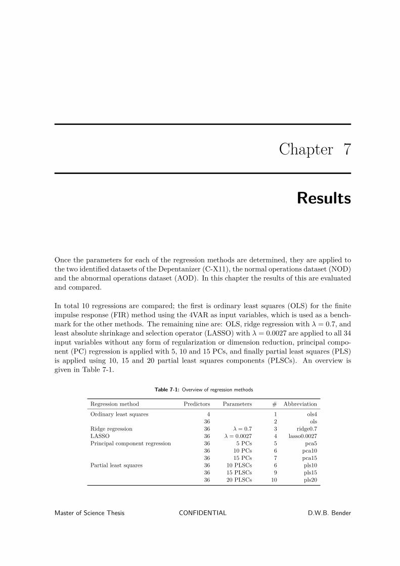
Chapter 7
Results
Once the parameters for each of the regression methods are determined, they are applied tothe two identified datasets of the Depentanizer (C-X11), the normal operations dataset (NOD)and the abnormal operations dataset (AOD). In this chapter the results of this are evaluatedand compared.
In total 10 regressions are compared; the first is ordinary least squares (OLS) for the finiteimpulse response (FIR) method using the 4VAR as input variables, which is used as a bench-mark for the other methods. The remaining nine are: OLS, ridge regression with λ = 0.7, andleast absolute shrinkage and selection operator (LASSO) with λ = 0.0027 are applied to all 34input variables without any form of regularization or dimension reduction, principal compo-nent (PC) regression is applied with 5, 10 and 15 PCs, and finally partial least squares (PLS)is applied using 10, 15 and 20 partial least squares components (PLSCs). An overview isgiven in Table 7-1.
Table 7-1: Overview of regression methods
Regression method Predictors Parameters # Abbreviation
Ordinary least squares 4 1 ols436 2 ols
Ridge regression 36 λ = 0.7 3 ridge0.7LASSO 36 λ = 0.0027 4 lasso0.0027Principal component regression 36 5 PCs 5 pca5
36 10 PCs 6 pca1036 15 PCs 7 pca15
Partial least squares 36 10 PLSCs 6 pls1036 15 PLSCs 9 pls1536 20 PLSCs 10 pls20
Master of Science Thesis CONFIDENTIAL D.W.B. Bender

46 Results
7-1 Normal operations dataset
The discussed regression methods are implemented to the NOD, which was discussed inChapter 3 and represents normal operations of the C-X11. The dataset of QTXX1 (QT1) forthis period is shown in Figure 7-1.
Dec 10 Dec 11 Dec 12 Dec 13 Dec 14 Dec 15 Dec 16 Dec 17 Dec 18 Dec 192015
0
2
4
6
8
10
% n
C5
QT1
Figure 7-1: Normal operations dataset of QT1
Each regression method is applied with three different rolling window sizes, namely 300,500, and 1000 samples. In addition, each method is evaluated for thirty different predictionhorizons; 1 through 30 minutes. This means that each of the ten regression methods is applied90 times. The results of all these implementations are given in Figure 7-2.
It can be observed that for each of the three rolling windows the three PLS methods havea practically identical performance in terms of MSPEnorm. It can also be seen that theirMSPEsnorm for each prediction horizon are equal of greater than one, which means that theyperform either the same or worse than the historical mean. It can thus be concluded that thePLS methods are not able to predict the behaviour of the process from the input variables.
The PC regression methods that makes use of five PCs performs slightly better that thebenchmark OLS method for prediction horizons smaller than about ten minutes, for eachprediction horizon. However when the prediction horizon becomes larger it performs worsethan the benchmark. The PC regression which used 10 PCs, outperforms the original OLSmethod with four input variable, for each of the rolling windows, and a prediction horizonof lower than 15. Once the prediction horizon becomes 15 or large, the PC regression per-forms very similar, and in the case where the rolling window is 300, it even performs slightlyworse. However the PC regressions which use 15 PCs, perform better than both the other PCregressions and the original OLS. In each case, the MSPEsnorm are a lot lower for shorter pre-diction horizons and they increase and converge to each other slowly, as the prediction horizonincreases. Each of the PC regressions perform better at lower prediction horizons with thesmaller rolling windows, 300 and 500, than with a rolling window of 1000. Oppositely whenthe prediction horizon is larger, a rolling windows of 300, produces worse predictions. For thesteady state situation, if enough PCs are used, PC regressions can be used to make predictions
D.W.B. Bender CONFIDENTIAL Master of Science Thesis
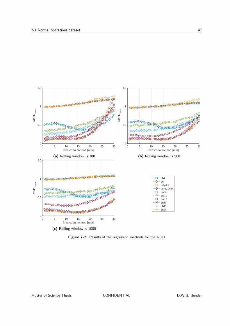
7-1 Normal operations dataset 47
0 5 10 15 20 25 30Prediction horizon [min]
0
0.5
1
1.5
MSP
Eno
rm
(a) Rolling window is 300
0 5 10 15 20 25 30Prediction horizon [min]
0
0.5
1
1.5
MSP
Eno
rm
(b) Rolling window is 500
0 5 10 15 20 25 30Prediction horizon [min]
0
0.5
1
1.5
MSP
Eno
rm
(c) Rolling window is 1000
0 5 10 15 20 25 30
Prediction horizon [min]
0
0.5
1
1.5
MSP
Eno
rm
ols4olsridge0.7lasso0.0027pca5pca10pca15pls10pls15pls20
Figure 7-2: Results of the regression methods for the NOD
Master of Science Thesis CONFIDENTIAL D.W.B. Bender
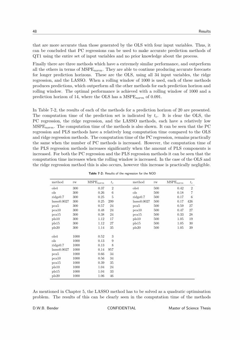
48 Results
that are more accurate than those generated by the OLS with four input variables. Thus, itcan be concluded that PC regressions can be used to make accurate prediction methods ofQT1 using the entire set of input variables and no prior knowledge about the process.
Finally there are three methods which have a extremely similar performance, and outperformall the others in terms of MSPEnorm. They are able to continue producing accurate forecastsfor longer prediction horizons. These are the OLS, using all 34 input variables, the ridgeregression, and the LASSO. When a rolling window of 1000 is used, each of these methodsproduces predictions, which outperform all the other methods for each prediction horizon androlling window. The optimal performance is achieved with a rolling window of 1000 and aprediction horizon of 14, where the OLS has a MSPEnorm of 0.091.
In Table 7-2, the results of each of the methods for a prediction horizon of 20 are presented.The computation time of the prediction set is indicated by tc. It is clear the OLS, thePC regression, the ridge regression, and the LASSO methods, each have a relatively lowMSPEnorm. The computation time of the methods is also shown. It can be seen that the PCregression and PLS methods have a relatively long computation time compared to the OLSand ridge regression methods. The computation time of the PC regression, remains practicallythe same when the number of PC methods is increased. However, the computation time ofthe PLS regression methods increases significantly when the amount of PLS components isincreased. For both the PC regression and the PLS regression methods it can be seen that thecomputation time increases when the rolling window is increased. In the case of the OLS andthe ridge regression method this is also occurs, however this increase is practically negligible.
Table 7-2: Results of the regression for the NOD
method rw MSPEnorm tc method rw MSPEnorm tc
ols4 300 0.37 2 ols4 500 0.42 2ols 300 0.26 6 ols 500 0.18 7ridge0.7 300 0.25 5 ridge0.7 500 0.17 6lasso0.0027 300 0.25 299 lasso0.0027 500 0.17 426pca5 300 0.57 24 pca5 500 0.59 27pca10 300 0.48 24 pca10 500 0.47 27pca15 300 0.38 24 pca15 500 0.33 28pls10 300 1.12 17 pls10 500 1.05 19pls15 300 1.12 27 pls15 500 1.05 30pls20 300 1.14 35 pls20 500 1.05 39
ols4 1000 0.52 3ols 1000 0.13 9ridge0.7 1000 0.13 8lasso0.0027 1000 0.14 957pca5 1000 0.66 34pca10 1000 0.56 34pca15 1000 0.39 35pls10 1000 1.04 24pls15 1000 1.04 33pls20 1000 1.06 46
As mentioned in Chapter 5, the LASSO method has to be solved as a quadratic optimisationproblem. The results of this can be clearly seen in the computation time of the methods
D.W.B. Bender CONFIDENTIAL Master of Science Thesis

7-1 Normal operations dataset 49
generated by the LASSO regression method. The computation time, when a rolling windowof 300 is taken, of the LASSO method is 299 seconds, while that of the equivalent ridgeregression method is 5 seconds. When the rolling window increases, the computation timeof the LASSO methods increases even more, to 426 seconds for a rolling window of 500, andeven 957 seconds for the largest rolling window. As the results of the LASSO are practicallyidentical to the results of the ridge regression, it can be concluded, that the ridge regressionperforms more favourably than the LASSO, as the computation time is significantly smaller.
To illustrate the performance of the prediction methods, Figure 7-3a shows the predictionset of the linearly interpolated output set QT1, and the predicted datasets generated withOLS, ridge regression, and LASSO methods. The predicted sets are constructed with a rollingwindow of 1000 samples and a prediction horizon of 20 minutes. Figure 7-3b shows the samedatasets for subset of the NOD during the 16th of December 2015. Finally Figure 7-3b showsonly the ridge regression prediction set, and includes bounds, which are the blue lines andindicate the predicted value ±σt. At each sample, σt is determined as the variance of theprediction errors of the previous 300 predictions.
It can be seen in Figure 7-3b, that the three prediction methods, show practically identicaldynamics. The only difference is in the height of the peaks. In general it can be seen thatthe LASSO method has the lowest peaks, than the ridge regression method, and finally theOLS method has the highest peaks. It can be seen that the prediction methods are able toalmost completely predict the the behaviour of the real output 20 minutes before it occurs.By examining Figure 7-3c, it can be seen that the real value of QT1, is for a large part of thedataset, within one standard deviation of the predicted value.
It is interesting that the results are similar, as the only differences between the OLS andthe ridge regression and LASSO, is that latter two add a penalty term when constructingestimates of β. This could mean that the regularization performed by the penalty terms inboth methods is very small. However if the β’s of the OLS and ridge regression methodsare examined throughout the dataset, it can be observed that this is not the case. Theseβ’s are presented in Appendix C-1-1. A number of the β’s of the ridge regression are clearlysmaller than those of the OLS, which means that the regularisation definitely affects theregression methods. Figure 7-4 shows the amount of included variables of each method thatis constructed by the LASSO regression method with a rolling window of 1000 and a predictionhorizon of 20. It can be seen that throughout the dataset, each method includes between 17and 31 predictors, which is always at least half of the available predictors. This is consistentwith the fact the performance of the ridge regression and the LASSO methods are very similarto that of the OLS method, as the ridge regression and LASSO are both just a regularisedversion of the OLS. If LASSO would exclude more predictors it would be illogical that theperformance of the OLS without regularisation, would perform so similarly.
It is possible that in the case of a steady state dataset the differences between the OLS,ridge regression, and LASSO methods are small, while for a dataset where a fault occurs, theresponse of the methods could be very different. This will be investigated, when the regressionmethods are applied to AOD.
Master of Science Thesis CONFIDENTIAL D.W.B. Bender

50 Results
Dec 10 Dec 11 Dec 12 Dec 13 Dec 14 Dec 15 Dec 16 Dec 17 Dec 18 Dec 19date
3
3.5
4
4.5
5
% n
C5
QT1lin int ols ridge0.7 lasso0.0027
(a)
Dec 16, 00:00 Dec 16, 05:00 Dec 16, 10:00 Dec 16, 15:00 Dec 16, 20:00time
3
3.5
4
4.5
5
% n
C5
QT1lin int ols ridge0.7 lasso0.0027
(b)
Dec 16, 00:00 Dec 16, 05:00 Dec 16, 10:00 Dec 16, 15:00 Dec 16, 20:00time
3
3.5
4
4.5
5
% n
C5
QT1lin int ridge0.7
(c)
Figure 7-3: Linearly interpolated dataset of QT1 and the predicted output sets for the NOD.The green dotted lines indicate the equivalent periods in time
D.W.B. Bender CONFIDENTIAL Master of Science Thesis

7-1 Normal operations dataset 51
Dec 10 Dec 11 Dec 12 Dec 13 Dec 14 Dec 15 Dec 16 Dec 17 Dec 18 Dec 190
5
10
15
20
25
30
35
num
ber
of p
redi
ctor
s in
clud
ed
Figure 7-4: Number of included variables in the LASSO method at each point in time for theNOD
7-1-1 Concatenated variables
In Section 4-4-1 the use of concatenated variables as inputs for the regression methods wasdiscussed. This was implemented in Section 4-5 for the analysis of the different interpolationmethods. The results were very close together, and it could be concluded tat in that im-plementation using concatenated variables did not improve the performance. However thatimplementation only included four of the input variables of the C-X11 and it was only doneusing OLS and none of the other regression methods. Therefore an extra analysis is done tosee whether using concatenated variables can improve the performances of the best performingregression methods. The regression methods are applied to ten sets of input variables, cor-responding to 0 up to 9 concatenated variables. Each regression is performed using the OLSand the ridge regression method, using rolling window size of 1000, and prediction horizons of1 through 30 minutes. The results of the ridge regression methods are presented in Figure 7-5and those of the OLS can be found in Appendix C-1-2. The amount of concatenated variablesfor each regression method is indicated by its subscript.
It can be observed straight away that including concatenated variables can improve the per-formance of the regression methods, in terms of MSPEnorm. For a prediction horizon of 20minutes, the MSPEnorm is decreased by half. If the prediction horizon is increased further,the differences become even larger. The results of the regression methods for a predictionhorizon of 20 minutes are presented in Table 7-3.
By using five concatenated variables, the MSPEnorm of the ridge regression is decreased byhalf in comparison to using no concatenated variables. The same goes for the OLS methodsand the results if the best performing OLS and ridge regression methods are practically thesame. There seems to be an optimum in terms of MSPEnorm around seven concatenatedvariables, for both regression methods. Increasing the amount of concatenated variablesbeyond this start to the increase the MSPEnorm again. The computation time does increaseby a factor when more concatenated variables are included in the regression method. Howevera computation time of less than 200 seconds for the entire dataset is still easily acceptable. Itcan be concluded that adding concatenated variables to the inputs can significantly improve
Master of Science Thesis CONFIDENTIAL D.W.B. Bender

52 Results
0 5 10 15 20 25 30Prediction horizon [min]
0
0.1
0.2
0.3
0.4
0.5
MSP
Eno
rm
ridge0.70
ridge0.71
ridge0.72
ridge0.73
ridge0.74
ridge0.75
ridge0.76
ridge0.77
ridge0.78
ridge0.79
Figure 7-5: The results of the regression methods using concatenated variables for the NOD
Table 7-3: Results of the regression methods using concatenated variables for NOD
method MSPEnorm tc method MSPEnorm tc
ols0 0.128 9 ridge0.70 0.128 9ols1 0.088 18 ridge0.71 0.091 15ols2 0.078 31 ridge0.72 0.078 25ols3 0.069 58 ridge0.73 0.069 52ols4 0.063 76 ridge0.74 0.062 69ols5 0.058 97 ridge0.75 0.058 90ols6 0.057 116 ridge0.76 0.055 111ols7 0.056 134 ridge0.77 0.054 127ols8 0.057 156 ridge0.78 0.054 153ols9 0.061 186 ridge0.79 0.056 179
D.W.B. Bender CONFIDENTIAL Master of Science Thesis
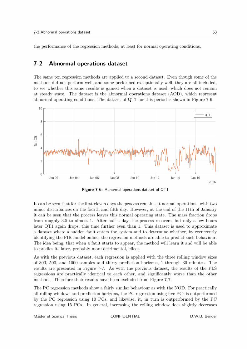
7-2 Abnormal operations dataset 53
the performance of the regression methods, at least for normal operating conditions.
7-2 Abnormal operations dataset
The same ten regression methods are applied to a second dataset. Even though some of themethods did not perform well, and some performed exceptionally well, they are all included,to see whether this same results is gained when a dataset is used, which does not remainat steady state. The dataset is the abnormal operations dataset (AOD), which representabnormal operating conditions. The dataset of QT1 for this period is shown in Figure 7-6.
Jan 02 Jan 04 Jan 06 Jan 08 Jan 10 Jan 12 Jan 14 Jan 162016
0
2
4
6
8
10
% n
C5
QT1
Figure 7-6: Abnormal operations dataset of QT1
It can be seen that for the first eleven days the process remains at normal operations, with twominor disturbances on the fourth and fifth day. However, at the end of the 11th of Januaryit can be seen that the process leaves this normal operating state. The mass fraction dropsfrom roughly 3.5 to almost 1. After half a day, the process recovers, but only a few hourslater QT1 again drops, this time further even than 1. This dataset is used to approximatea dataset where a sudden fault enters the system and to determine whether, by recurrentlyidentifying the FIR model online, the regression methods are able to predict such behaviour.The idea being, that when a fault starts to appear, the method will learn it and will be ableto predict its later, probably more detrimental, effect.
As with the previous dataset, each regression is applied with the three rolling window sizesof 300, 500, and 1000 samples and thirty prediction horizons, 1 through 30 minutes. Theresults are presented in Figure 7-7. As with the previous dataset, the results of the PLSregressions are practically identical to each other, and significantly worse than the othermethods. Therefore their results have been excluded from Figure 7-7.
The PC regression methods show a fairly similar behaviour as with the NOD. For practicallyall rolling windows and prediction horizons, the PC regression using five PCs is outperformedby the PC regression using 10 PCs, and likewise, it, in turn is outperformed by the PCregression using 15 PCs. In general, increasing the rolling window does slightly decreases
Master of Science Thesis CONFIDENTIAL D.W.B. Bender

54 Results
0 5 10 15 20 25 30Prediction horizon [min]
0
0.2
0.4
0.6
0.8
1
MSP
Eno
rm
(a) Rolling window is 300
0 5 10 15 20 25 30Prediction horizon [min]
0
0.2
0.4
0.6
0.8
1
MSP
Eno
rm
(b) Rolling window is 500
0 5 10 15 20 25 30Prediction horizon [min]
0
0.2
0.4
0.6
0.8
1
MSP
Eno
rm
(c) Rolling window is 1000
0 5 10 15 20 25 30Prediction horizon [min]
0
0.5
1
MSP
Eno
rm
ols4olsridge0.7lasso0.0027pca5pca10pca15
Figure 7-7: Results of the regression methods for the AOD
D.W.B. Bender CONFIDENTIAL Master of Science Thesis
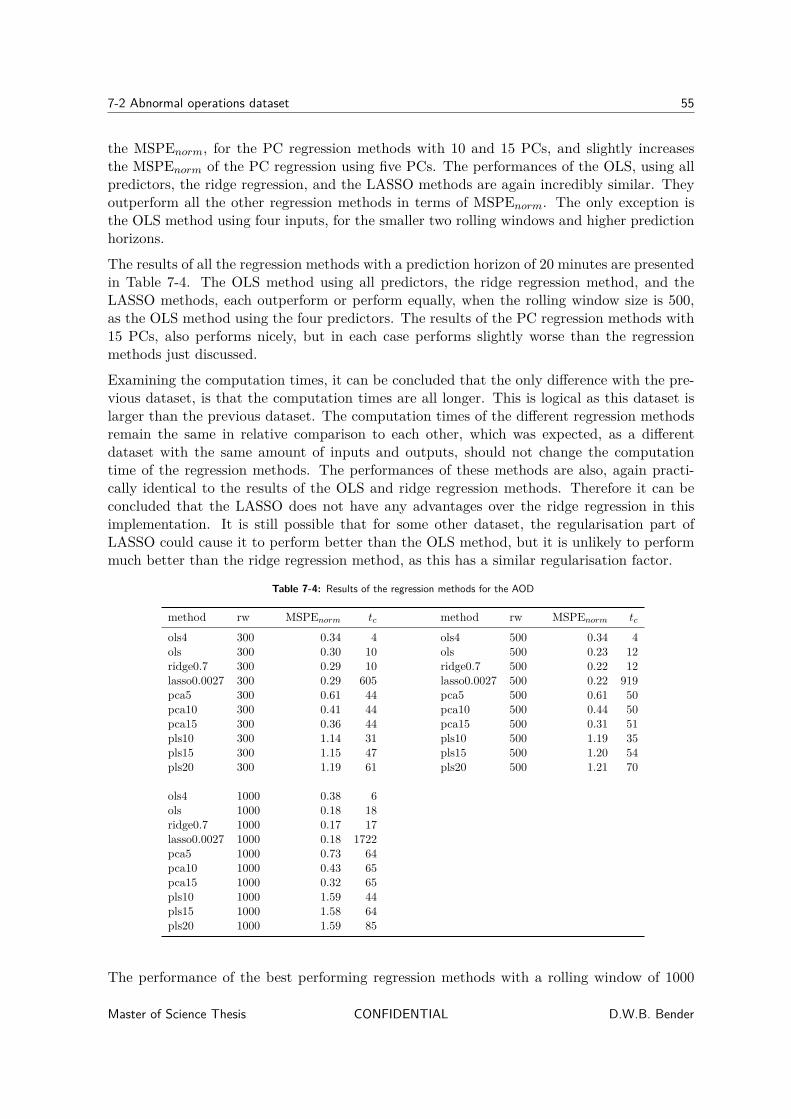
7-2 Abnormal operations dataset 55
the MSPEnorm, for the PC regression methods with 10 and 15 PCs, and slightly increasesthe MSPEnorm of the PC regression using five PCs. The performances of the OLS, using allpredictors, the ridge regression, and the LASSO methods are again incredibly similar. Theyoutperform all the other regression methods in terms of MSPEnorm. The only exception isthe OLS method using four inputs, for the smaller two rolling windows and higher predictionhorizons.
The results of all the regression methods with a prediction horizon of 20 minutes are presentedin Table 7-4. The OLS method using all predictors, the ridge regression method, and theLASSO methods, each outperform or perform equally, when the rolling window size is 500,as the OLS method using the four predictors. The results of the PC regression methods with15 PCs, also performs nicely, but in each case performs slightly worse than the regressionmethods just discussed.
Examining the computation times, it can be concluded that the only difference with the pre-vious dataset, is that the computation times are all longer. This is logical as this dataset islarger than the previous dataset. The computation times of the different regression methodsremain the same in relative comparison to each other, which was expected, as a differentdataset with the same amount of inputs and outputs, should not change the computationtime of the regression methods. The performances of these methods are also, again practi-cally identical to the results of the OLS and ridge regression methods. Therefore it can beconcluded that the LASSO does not have any advantages over the ridge regression in thisimplementation. It is still possible that for some other dataset, the regularisation part ofLASSO could cause it to perform better than the OLS method, but it is unlikely to performmuch better than the ridge regression method, as this has a similar regularisation factor.
Table 7-4: Results of the regression methods for the AOD
method rw MSPEnorm tc method rw MSPEnorm tc
ols4 300 0.34 4 ols4 500 0.34 4ols 300 0.30 10 ols 500 0.23 12ridge0.7 300 0.29 10 ridge0.7 500 0.22 12lasso0.0027 300 0.29 605 lasso0.0027 500 0.22 919pca5 300 0.61 44 pca5 500 0.61 50pca10 300 0.41 44 pca10 500 0.44 50pca15 300 0.36 44 pca15 500 0.31 51pls10 300 1.14 31 pls10 500 1.19 35pls15 300 1.15 47 pls15 500 1.20 54pls20 300 1.19 61 pls20 500 1.21 70
ols4 1000 0.38 6ols 1000 0.18 18ridge0.7 1000 0.17 17lasso0.0027 1000 0.18 1722pca5 1000 0.73 64pca10 1000 0.43 65pca15 1000 0.32 65pls10 1000 1.59 44pls15 1000 1.58 64pls20 1000 1.59 85
The performance of the best performing regression methods with a rolling window of 1000
Master of Science Thesis CONFIDENTIAL D.W.B. Bender

56 Results
and a prediction horizon of 20 are presented in Figure 7-8a. Figure 7-8b presents the subsetof the AOD during the 11th and 12th of January 2016. The presented regression methodsare the OLS, the ridge regression, and the LASSO. In Figure 7-8c the same ridge regressionpredicted set is present, with bounds depicting the predicted values ±σt.
It can be observed that the predicted datasets are very similar. Each is able to predict thebehaviour of the output quite accurately. When the sudden decrease comes the methods areable to predict this, and when the behaviour remains different from the steady state, themethods are able to still capture most of the dynamics. As with the NOD, the real outputset is within σt of the ridge regression predictions, for most of the subset of time. Around21:00 on January 11th the fault enters the system and the values of QT1 begin to decrease.The predictions of the ridge regression do not predict this instantly and the real value passedthrough the standard deviation bound for a short period of time. But it can be seen thatthe ridge regression quickly learns the fault and becomes able to predict its effect on thebehaviour of the system.
In Appendix C-2 the amount of included predictors by the LASSO is evaluated, as well as theestimated parameters β for both the OLS and the ridge regression method throughout thedataset. Each is evaluated for a rolling window of 1000 and a prediction horizon of 20. Theresults are similar to that of the NOD. The amount of predictors included varies between 16and 34, compared to 17 and 31 for the NOD. Comparing the estimated parameters, it can beseen that a number of the estimated parameters of the ridge regression differ from those ofthe OLS method, so there is a clear result of the regularisation factor in the ridge regression,without it reducing its performance.
D.W.B. Bender CONFIDENTIAL Master of Science Thesis

7-2 Abnormal operations dataset 57
Jan 02 Jan 04 Jan 06 Jan 08 Jan 10 Jan 12 Jan 14 Jan 16date 2016
0
1
2
3
4
5
6
% n
C5
QT1lin int ols ridge0.7 lasso0.0027
(a)
Jan 11, 06:00 Jan 11, 16:00 Jan 12, 02:00time 2016
0
1
2
3
4
5
6
% n
C5
QT1lin int ols ridge0.7 lasso0.0027
(b)
Jan 11, 06:00 Jan 11, 16:00 Jan 12, 02:00time 2016
0
1
2
3
4
5
6
% n
C5
QT1lin int ridge0.7
(c)
Figure 7-8: The linearly interpolated output set of QT1 and the predicted datasets for the AOD.The green dotted lines indicate the equivalent periods in time
Master of Science Thesis CONFIDENTIAL D.W.B. Bender

58 Results
7-2-1 Concatenated variables
To evaluate whether using concatenated variables as inputs for the regression has the samepositive effects in the AOD as it had on the NOD, the OLS and ridge regression method arealso applied with concatenated variables to the AOD. The regressions are again applied witha rolling window of 1000 samples and prediction horizons of 1 to 30 minutes.
The results of the ridge regressions are shown in Figure 7-9 and the results of the OLS areshown in Appendix C-2-3. It can be clearly seen that the use of concatenated variableshas a similar, albeit smaller, effect for the AOD, as it had for the NOD. The MSPEnormdecreases when concatenated variables are added, but the difference is relatively small. Thesame behaviour can be observed for the OLS methods.
0 5 10 15 20 25 30Prediction horizon [min]
0
0.1
0.2
0.3
0.4
0.5
MSP
Eno
rm
ridge0.70
ridge0.71
ridge0.72
ridge0.73
ridge0.74
ridge0.75
ridge0.76
ridge0.77
ridge0.78
ridge0.79
Figure 7-9: Results of the regression methods using concatenated variables for the AOD
Table 7-5 gives an overview of all the methods for a prediction horizon of 20 minutes. Forboth the OLS and ridge regression methods there is a drop in MSPEnorm after adding asingle set of concatenated variables. The optimal number of concatenated variables is twofor the AOD, which is different from the NOD, where it was seven. It may be that addinga number of concatenated variables, such as four, can make the regression methods morerobust to sudden changes and possible outliers in the input and output data. To evaluatethis, Figure 7-10 shows the prediction for the ridge regression methods with zero and fourconcatenated variables. It can be seen that the method with four concatenated variables, isless volatile, but it adapts to changes, such as the decrease caused by the fault, at least asfast as the method with zero concatenated variables. It is therefore concluded that addingconcatenated variables is a good way to make the methods more robust.
D.W.B. Bender CONFIDENTIAL Master of Science Thesis

7-2 Abnormal operations dataset 59
Table 7-5: Results of the regression methods using concatenated variables for AOD
method MSPEnorm tc method MSPEnorm tc
ols0 0.178 18 ridge0.70 0.171 17ols1 0.162 37 ridge0.71 0.150 30ols2 0.160 59 ridge0.72 0.146 48ols3 0.163 110 ridge0.73 0.148 100ols4 0.164 145 ridge0.74 0.149 136ols5 0.165 190 ridge0.75 0.149 176ols6 0.168 229 ridge0.76 0.152 216ols7 0.172 264 ridge0.77 0.154 245ols8 0.174 301 ridge0.78 0.156 301ols9 0.177 356 ridge0.79 0.158 349
Jan 11, 06:00 Jan 11, 16:00 Jan 12, 02:00time 2016
0
1
2
3
4
5
6
% n
C5
QT1lin int
ridge0.70
ridge0.74
Figure 7-10: The linearly interpolated output set of QT1 and the predicted datasets
Master of Science Thesis CONFIDENTIAL D.W.B. Bender

60 Results
D.W.B. Bender CONFIDENTIAL Master of Science Thesis

Chapter 8
Validation
In the previous chapter, it has been shown that a number of regression methods were able toconstruct accurate predictions of the key variable QTXX1 (QT1) in the Depentanizer (C-X11)unit. They were able to do so without using any prior knowledge about the process. Howevereach method was first analysed, different parameter settings were evaluated, and the optimalsetting was chosen. Ideally we want the regression methods to be so robust, that they can beapplied to a process without having to taking any of these prior steps first.
To verify whether the identified regression methods are robust and general procedures, orwhether they have been fitted to the data in the C-X11, they will now be applied to datafrom a completely different subsystem, the Deisopentanizer (C-X12).
8-1 Deisopentanizer
The C-X12 is a distillation column, just like the C-X11. However, where the C-X11 splitspentane (C5) and heavier compounds, the C-X12 actually splits the C5 into isopentane (iC5)and n-pentane (nC5). The boiling points of iC5 and nC5 are much close together than thoseof C5 and the heavier compounds. One result of these close boiling points, is that the C-X12is classified as a superfractionator. A second results of this fact, is that the process is muchslower, as it is more difficult to separate the compounds. The settling time of the C-X12is in the order of half a day, whereas that of the C-X11 is around 75 minutes. In additionthe C-X12 has four quality measurements instead of one, two in the top flow and two in thebottom flow. These quality measurements are described in Table 8-1.
In Appendix D-1 the datasets of each of the four output variables is presented for the periodNovember 2015 until May 2016. To evaluate the performance of the regression methods onthese outputs, period of time is identified, which represent fairly standard operations. Notall output variables have to remain at steady state for the entire time. The period spanningMarch 14th until March 21st of 2016 is chosen. Data from this period of time is henceforthreferred to as standard operations dataset (SOD). In Figure 8-1 the data of each of the fourquality measurement is presented for this period. It can be observed that each of the output
Master of Science Thesis CONFIDENTIAL D.W.B. Bender

62 Validation
Table 8-1: Description of the four output variables
Flow Full Name Name Unit Description
Top CDX1:QTYY3 QTYY3 wt% Mass fraction n-butane (nC4) in top C-X11CDX1:QTYY4 QTYY4 wt% Mass fraction nC5 in top C-X12
Bottom CDX1:QTYY1 QTYY1 wt% Mass fraction iC5 in bottom C-X12CDX1:QTYY2 QTYY2 wt% Mass fraction cylcopentane (cC5) in bottom C-X12
variables have fairly stable outputs for the time period, but there is enough variation to beable to examine the applicability of the regression methods.
The C-X12 contain 25 input variable sensors, which are similar, but not exactly the sameas the input variable sensors in the C-X11. In Appendix A-1 an overview and description isgiven of the entire set of input variables that are available in the C-X12.
8-1-1 Prediction results
Initially we want to see whether the regression methods, that have been identified as perform-ing well in the last chapter, can be applied to this new subsystem and its data, and produceaccurate predictions about its outputs, without using any prior knowledge. Therefore, theridge regression method is chosen to be applied to each of the four output variables separately.
For the regression methods applied to each of the four output variables, the same set of25 input variables is used. The regression methods are applied with a rolling window of1000 samples and a prediction horizon of 20 minutes, as these settings have proved to workwell in the C-X11. A side note is that the C-X12 process is slower than the C-X11, so theseregression methods might perform better with larger rolling windows and prediction horizons,but this will be investigated later in the chapter. First we are interested in seeing how wellthe regression methods perform, when exactly the same parameters are chosen, as wheredetermined to be optimal for the C-X11. For this initial validation, concatenated variablesare not included. They will however be included later in this chapter.
The four resulting forecast sets constructed using the ridge regression are shown in Figure 8-2. Looking at the predicted set of QTYY1 it can be seen that the regression model is ableto predict some of the behaviour of the output set. However some dynamics take, take theregression method some time to realise and as a results it lags behind the real output set. Inaddition the predicted set seems fairy volatile, especially around peaks and troughs. Lastlythe predicted set seems to overshoot quite a bit a number of times during the 17th and 18thof March, this is undesirable, especially if limit checking was to be used for fault detection.
The second output set for which a predicted set is generated is the QTYY2. Again, quite abit of the behaviour is correctly predicted by the regression method, but as with the QTYY1,around the 17th and 18th of March there are a number of peaks and troughs, that do notoccur in the real output set. It is possible that there is some anomaly in the input data, thatthe regression method is not able to deal with, that causes these sudden spikes. In a numberof cases, the predicted model is not able to correctly anticipate a certain increase or decreaseof the output value, and the predicted set lags behind the real output.
D.W.B. Bender CONFIDENTIAL Master of Science Thesis

8-1 Deisopentanizer 63
Mar 14 Mar 15 Mar 16 Mar 17 Mar 18 Mar 19 Mar 20date
0
1
2
3
4
5
% iC
5
QTYY1
(a)
Mar 14 Mar 15 Mar 16 Mar 17 Mar 18 Mar 19 Mar 20date
0
2
4
6
8
10
% c
C5
QTYY2
(b)
Mar 14 Mar 15 Mar 16 Mar 17 Mar 18 Mar 19 Mar 20date
0
5
10
15
20
25
% n
C4
QTYY3
(c)
Mar 14 Mar 15 Mar 16 Mar 17 Mar 18 Mar 19 Mar 20date
0
1
2
3
4
5
6
7
% n
C5
QTYY4
(d)
Figure 8-1: Data of the output variables of the C-X12 for the SOD
Master of Science Thesis CONFIDENTIAL D.W.B. Bender
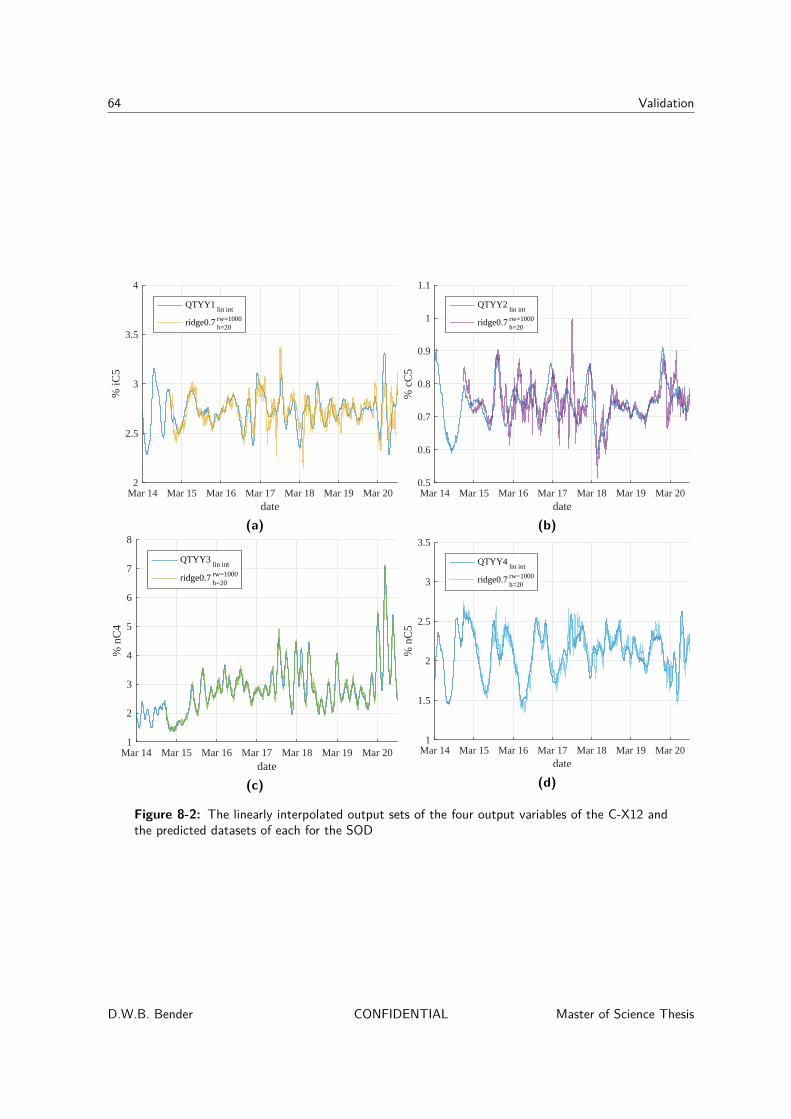
64 Validation
Mar 14 Mar 15 Mar 16 Mar 17 Mar 18 Mar 19 Mar 20date
2
2.5
3
3.5
4
% iC
5
QTYY1lin int
ridge0.7h=20rw=1000
(a)
Mar 14 Mar 15 Mar 16 Mar 17 Mar 18 Mar 19 Mar 20date
0.5
0.6
0.7
0.8
0.9
1
1.1
% c
C5
QTYY2lin int
ridge0.7h=20rw=1000
(b)
Mar 14 Mar 15 Mar 16 Mar 17 Mar 18 Mar 19 Mar 20date
1
2
3
4
5
6
7
8
% n
C4
QTYY3lin int
ridge0.7h=20rw=1000
(c)
Mar 14 Mar 15 Mar 16 Mar 17 Mar 18 Mar 19 Mar 20date
1
1.5
2
2.5
3
3.5
% n
C5
QTYY4lin int
ridge0.7h=20rw=1000
(d)
Figure 8-2: The linearly interpolated output sets of the four output variables of the C-X12 andthe predicted datasets of each for the SOD
D.W.B. Bender CONFIDENTIAL Master of Science Thesis
8-1 Deisopentanizer 65
Both these discussed output sets represent a mass fraction in the bottom flow of the C-X12.The third output set is the QTYY3, which is the mass fraction of nC4 in the top flow of theC-X12. If the predicted output set is compared to the real output set, it can be seen thatthe regression method is able to almost exactly predict the behaviour of the output variable.With the exception of a few peaks around the 17th and 18th of March, where the predictedpeak is lower than the actual peak, the predicted set is almost the exact same as the realoutput set.
The last output variable is the QTYY4, and it represents the mass fraction of nC5 in thebottom flow of the C-X12. The regression method is able to nicely predict most of thebehaviour of the output variable, especially the sudden increases and decreases are nicelypredicted. Again around the 17th of March, there are some disturbances in the predictedoutput set, that do not appear in the real output set.
8-1-2 Regression method analysis
As mentioned the regression methods that were applied to the outputs of the C-X12, werethe methods that were found to be optimal for the C-X11. However as the dynamics andthe type and amount of input and output variables are different in the C-X12, this does notnecessarily mean that the same parameter settings are optimal for the C-X12 as were optimalfor the C-X11.
As the goal of this research is to find a robust method which does not require prior knowledgeof the system or a lot of tweaking of the parameters before it works, we will not repeat theentire model analysis for the C-X12, as was done for the C-X11. Therefore the parametersof the regression methods will not be changed. However, it is decided to test the regressionmethods for a number of different rolling windows and prediction horizons, as it is knownthat the settling time of the C-X12 is much longer than that of the C-X11.
In addition to the ridge regression method, the ordinary least squares (OLS) method is ap-plied. To verify whether principal components analysis (PCA) is more robust than the OLSor ridge regression methods, three PC regression methods are also applied, with respectively,5, 10, and 15 principal component (PC)s.
The results of these analyses can be found in Appendix D-2 and are discussed individuallyfor each output in the following sections.
QTYY1
Examining the results of the regression methods for the QTYY1, it can be seen that, onceagain, the ridge regression and finite impulse response (FIR) method have very similar resultsand the best performance. In addition it can be seen that the performances of the methodsusing a rolling window of 1000 and 2000, are inferior for each prediction horizon tot those ofwith a rolling window of 300 and 500. In fact if we look only at the results of the predictedsets constructed with ridge regression and a prediction horizon of 20 minutes, the MSPEnormis decreases from 0.44 to 0.16, when the rolling window is decreased from 1000 to 300. It canbe further concluded that increasing the prediction horizon also increases the MSPEnorm ofthe predicted sets of the QTYY1, and thus it does not seem that there is some optimal value
Master of Science Thesis CONFIDENTIAL D.W.B. Bender

66 Validation
for the prediction horizon. The best performing ridge regression predicted set for a predictionhorizon of 20 minutes is the one, which is constructed with a rolling window of 300 and it isshown in Figure 8-3. This regression method with these parameter settings is able to predictthe behaviour of the output very nicely. Each sudden increase and decrease is captured, andwith the exception of some overshoot in a few of the peaks and troughs, most of the behaviouris captured.
Mar 14 Mar 15 Mar 16 Mar 17 Mar 18 Mar 19 Mar 20date
2
2.5
3
3.5
4
% iC
5
QTYY1lin int
ridge0.7h=20rw=300
Figure 8-3: The linearly interpolated output set of QTYY1 and the best performing ridge re-gression prediction method for the SOD
QTYY2
The results of the predicted set of the QTYY2 are very similar to that of the QTYY1, asthe performance is much better for the when the predictions were constructed with a rollingwindow of 300 or 500, than when they were constructed with a rolling window of 1000 or2000. In each case the results of the FIR and the ridge regression are very similar, but incontrast to the other implementations until now, the PC regression methods using 15 PCsactually performs very similar as well. The performance again seems to deteriorate whenthe prediction horizon is increased, without there being some optimal horizon. Therefore weagain examine all the results for a prediction horizon of 20. Like with the QTYY1, the bestperformance is found when a rolling window of 300 is taken, and the resulting forecast setis shown in Figure 8-4. The resulting predicted dataset has some overshoot on a number ofpeaks and troughs, and at the end of the 19th of March, there is a sudden drop, which doesnot occur in the real output set. Aside from this, the regression method is able to predictmost of the dynamics in the output set.
D.W.B. Bender CONFIDENTIAL Master of Science Thesis
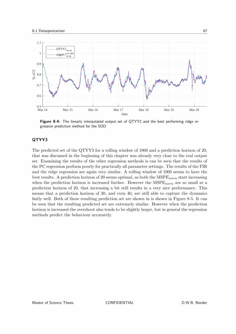
8-1 Deisopentanizer 67
Mar 14 Mar 15 Mar 16 Mar 17 Mar 18 Mar 19 Mar 20date
0.5
0.6
0.7
0.8
0.9
1
1.1
% c
C5
QTYY2lin int
ridge0.7h=20rw=300
Figure 8-4: The linearly interpolated output set of QTYY2 and the best performing ridge re-gression prediction method for the SOD
QTYY3
The predicted set of the QTYY3 for a rolling window of 1000 and a prediction horizon of 20,that was discussed in the beginning of this chapter was already very close to the real outputset. Examining the results of the other regression methods is can be seen that the results ofthe PC regression perform poorly for practically all parameter settings. The results of the FIRand the ridge regression are again very similar. A rolling window of 1000 seems to have thebest results. A prediction horizon of 20 seems optimal, as both the MSPEnorm start increasingwhen the prediction horizon is increased further. However the MSPEnorm are so small at aprediction horizon of 20, that increasing a bit still results in a very nice performance. Thismeans that a prediction horizon of 30, and even 40, are still able to capture the dynamicsfairly well. Both of these resulting prediction set are shown in is shown in Figure 8-5. It canbe seen that the resulting predicted set are extremely similar. However when the predictionhorizon is increased the overshoot also tends to be slightly larger, but in general the regressionmethods predict the behaviour accurately.
Master of Science Thesis CONFIDENTIAL D.W.B. Bender

68 Validation
Mar 14 Mar 15 Mar 16 Mar 17 Mar 18 Mar 19 Mar 20 Mar 21date
1
2
3
4
5
6
7
8
% n
C4
QTYY3lin int
ridge0.7h=30rw=2000
ridge0.7h=40rw=2000
Figure 8-5: The linearly interpolated output set of QTYY3 and the best performing ridge re-gression prediction method for the SOD
QTYY4
Finally the results of the predicted set of QTYY4 are evaluated. The FIR and the ridgeregression perform better than the other methods overall. Decreasing the rolling window to300 increases the performance of the prediction set, if the prediction horizon is 20. The resultof this is shown in Figure 8-6. The behaviour of the output is predicted nicely.
Mar 14 Mar 15 Mar 16 Mar 17 Mar 18 Mar 19 Mar 20
date
1
1.5
2
2.5
3
3.5
% n
C5
QTYY4lin int
ridge0.7h=20rw=300
Figure 8-6: The linearly interpolated output set of QTYY4 and the best performing ridge re-gression prediction method for the SOD
8-1-3 Concatenated variables
To evaluate whether using concatenated variables as inputs for the regression can improvethe performance on the C-X12 output variables, the best performing ridge regression method
D.W.B. Bender CONFIDENTIAL Master of Science Thesis

8-1 Deisopentanizer 69
for each output variable is implemented again with one through nine concatenated variables.The results are presented in Table 8-2.
Table 8-2: Results of the regression methods using concatenated variables for the four output variables of the C-X12 for the SOD
output model rw MSPEnorm tc output model rw MSPEnorm tc
QTYY1 ridge0.70 300 0.144 3 QTYY2 ridge0.70 300 0.147 3ridge0.71 300 0.124 5 ridge0.71 300 0.145 5ridge0.72 300 0.116 8 ridge0.72 300 0.140 8ridge0.73 300 0.111 10 ridge0.73 300 0.139 11ridge0.74 300 0.109 15 ridge0.74 300 0.136 15ridge0.75 300 0.106 18 ridge0.75 300 0.133 18ridge0.76 300 0.104 22 ridge0.76 300 0.130 22ridge0.77 300 0.102 26 ridge0.77 300 0.131 26ridge0.78 300 0.103 34 ridge0.78 300 0.135 33ridge0.79 300 0.103 38 ridge0.79 300 0.138 38
QTYY3 ridge0.70 1000 0.077 5 QTYY4 ridge0.70 300 0.112 3ridge0.71 1000 0.066 7 ridge0.71 300 0.103 5ridge0.72 1000 0.059 12 ridge0.72 300 0.096 8ridge0.73 1000 0.055 18 ridge0.73 300 0.093 11ridge0.74 1000 0.052 24 ridge0.74 300 0.091 15ridge0.75 1000 0.050 42 ridge0.75 300 0.088 18ridge0.76 1000 0.048 52 ridge0.76 300 0.086 22ridge0.77 1000 0.046 61 ridge0.77 300 0.086 26ridge0.78 1000 0.043 73 ridge0.78 300 0.086 33ridge0.79 1000 0.041 84 ridge0.79 300 0.086 38
It can be seen that for each of the four output variables, both the MSPEnorm improve whenconcatenated variables are used as input variables. For the QTYY1, QTYY2, and QTYY4,the best performing methods use about seven concatenated variables. In the case of QTYY3,the MSPEsnorm continue decreasing when the amount of concatenated variables increases. Ingeneral it can be stated that using five or more concatenated variables significantly improvesthe performance of the regression method for each output variable.
Master of Science Thesis CONFIDENTIAL D.W.B. Bender

70 Validation
D.W.B. Bender CONFIDENTIAL Master of Science Thesis

Chapter 9
Concluding remarks
The objective of this research was to examine whether the use of machine learning and otherstatistical techniques could be used to make earlier fault detection possible. The results ofthis report show that the application of ordinary least squares (OLS) and ridge regressionmethods to recurrently identify finite impulse response (FIR) models can construct accuratepredictions of key variables in industrial processes. These methods can be used to extractinformation from a large set of historic data and to construct predictions. These predictionscan be used for early fault detection in steady state processes, and can serve as a first steptowards earlier fault detection in processes that do not necessarily operate at steady state.This conclusion is the result of the analysis of six questions. First: what kind of model candescribe the dynamics of an industrial process? Second: can interpolation methods be used tofill in the missing output data and does this improve the available information in comparisonto only using the samples for which output measurements are available and discarding thesamples which only contain input measurements. Third: are on-line OLS methods able tomatch off-line first order principle based prediction methods? Fourth: can regression methodsconstruct prediction methods with the same or improved accuracy, without using any priorknowledge about the system? Fifth: can these prediction methods be improved by usingconcatenated variables as inputs? Finally: are the identified methods able to reproduceprediction methods with the same accuracy for another process, without having to performan entire analysis first? The analysis of each of these questions will be discussed individuallyin the chapter.
Using a FIR model to describe the dynamics of the process, means that when a multi-stepahead prediction is made, a single prediction is made: namely that of the multi-step aheadvalue. This is in contrast to, for instance, an autoregressive-moving average model withexogenous inputs (ARMAX) model, where multiple one-step ahead predictions are made toconstruct the final multi-step ahead prediction. Both models are used to construct predictionof key variables of the case study. The results show that the FIR actually performs better, interms of MSPEnorm, than the ARMAX models. Therefore it is concluded that the dynamicsof the process can be accurately described by a FIR model. It is possible that dynamic modelsperform differently when the prediction horizon is increased beyond an hour. Therefore re-
Master of Science Thesis CONFIDENTIAL D.W.B. Bender
72 Concluding remarks
evaluating the performance of different dynamic models for longer prediction horizons is animportant next step in this research.
Another interesting type of models, that is worthwhile investigating, is artificial neural net-works. In particular long short-term memories or other recurrent neural networks as theseare able to deal with large prediction horizons. The downside is that it is highly unlikely thatsuch methods could be generalised, which means that it would require to be completely recon-figured for each implementation. A lot more knowledge and effort would therefore be neededto calibrate and maintain the model. In this research, a brief analysis was performed to de-termine the potential of using artificial neural networks for the regression problem. However,with the limited time, no worthwhile results were found. This is probably more a reflectionof the increased time and effort required to use artificial neural networks effectively for thisapplication and not because this technique is unsuitable for use in this case. It might not bedesirable to use artificial neural networks for every implementation, but for the key plantsand processes, it may well be worth the extra time and effort. Therefore further researchinto the possibilities of using artificial neural networks for early fault detection is definitelyrequired.
Three different interpolation methods were used to estimate the missing values of the keyoutput variable. In addition a dataset was examined, which discarded the samples for whichdid not include an output value. Each of these four datasets were used to construct a predic-tion set. The dataset that discarded the samples with missing values, performed the worstin each experiment. The difference between the three interpolation methods was small. Thezero-order hold methods performed slightly worse than the linear and spline method, andbetween the latter two, the differences were negligible. Therefore, it was concluded that alinear interpolation method should be used to fill in the missing output values.
A prediction method for the key output variable had been identified previous to this research.This method is a Wiener non-linear model, which uses four input variables and these inputvariables were determined by engineering principles. The model was identified off-line, butits intercept is corrected recursively using the error between estimate and measured value ofthe output. To verify whether an on-line identified model can achieve a similar performanceas off-line model, OLS is used to identify a model on-line model with the input variables. Theresults show that the on-line identified model is able to predict the key output values, at leastas well as off-line model does and it is therefore concluded that the on-line identified modelcan also accurately describe and predict the behaviour of the key output variable.
Five different regression methods were used to construct predictions about the key outputvariable. Because we wanted to construct predictions without using any prior knowledgeof the system, each of the regression methods were applied to all the available variables asinputs for its models. Each regression method was applied to a dataset representing normaland abnormal operating behaviour. For both datasets it can be concluded, that the partialleast squares (PLS) regression methods do not perform well. On the other hand each ofthe four other regression methods, OLS, PC regression, ridge regression, and least absoluteshrinkage and selection operator (LASSO), were able to construct accurate predictions usingall available variables as inputs. It can therefore be concluded that it is possible to constructpredictions without using any prior knowledge about the system and it is even possible toconstruct more accurate predictions by including more input variables than the original fourvariables, which were determined using first principles. Each of the regression methods used
D.W.B. Bender CONFIDENTIAL Master of Science Thesis
73
a large set of variables as inputs and were able to recognise which contained the relevantinformation. However, all of the variables were kept as inputs for the methods. A next stepin this research is examine whether a number of the input variables could be excluded fromthe model. This could increase the robustness of the model and if the accuracy does notdecrease significantly, this would certainly be a worthwhile exercise.
The results of the OLS, ridge regression, and LASSO methods were extremely similar and werebetter than any of the other results. Both the ridge regression and the LASSO method are avariation of the OLS method, where a regularisation term has been added in the estimation ofthe parameters. It could be the case that the results are so similar because this term doesn’taffect the estimated parameters much. However this was examined and it can be concludedthat this is not the case. In both cases the extra term applies substantial regularisation tothe estimates. A different consideration is the computation time of the different methods. Aseach methods has to identify a new model for each sample in the dataset, it is undesirable forthe regression methods to be too intensive computationally. The LASSO identification is aquadratic optimisation problem and this means that its computation time is much longer thanthat of the OLS or ridge regression. It can be concluded that the ridge regression has the mostdesirable overall characteristics, as the performance of the three methods was so similar, theregularisation terms improve the robustness, and the LASSO is so intensive computationally.
Each of the regression methods uses an model to describe the dynamics of the process wherea single output measurement is linked to a single vector of measurements, which contains thevalues of each of the input variables at a given time step. However, the use of concatenatedvariables as inputs of the FIR models is also examined. This means that a single outputmeasurement is linked to multiple vectors of measurements, corresponding to the values of theinput variables for consecutive time steps. The result of this is that the for both the datasets,the performance of the regression methods is improved. In addition the predicted outputsets become less volatile. It is therefore concluded that the use of concatenated variables asinputs, can increase the robustness and improve the performance of the prediction methods.
The OLS and ridge regression method were also used to identify a FIR model of a differentsystem as validation of their performance. This system is also a distillation column, but differsin number and type of inputs and outputs, as well as, in speed of the process, compared tothe original system. Both methods were applied to construct predictions of each of the keyvariables and were able to produce accurate predictions. This performance was improved whenconcatenated variables were used as inputs. This validation is initially done for a single rollingwindow and prediction horizon, to investigate whether predictions can be made without anyanalysis. It is concluded that this is the case; however these predictions can be improved quitesignificantly by a simple analysis of which size of rolling window is optimal. This analysisdoes not require prior knowledge of the system and could very easily be automated into theprocedure. A next step in this research is to verify the generality of the identified methodson other types of industrial processes.
The historic data that has been used in this research was available at a high frequency withoutthe filtering that is generally applied to data stored in industrial plants. It is thereforelikely that for further research available historical data would have a lower frequency andquality than the data that was used in this research. Therefore a next step is to evaluatewhether the analysis is possible with this lower quality data or whether high quality datais a requirement. If the prediction methods were to be implemented in practice, this would
Master of Science Thesis CONFIDENTIAL D.W.B. Bender

74 Concluding remarks
not be an issue, as the data available in the control system is of the same quality as thatused in this research. In addition this research limited itself to examining process variablesand modern industrial plants. However, modern industrial plants also have a large amountof diagnostic data available. So another next step of research is to investigate whether theaddition of diagnostic data can also improve the performance of the fault detection methods.
The use of real industrial data in this research meant that it was not possible to select historicdatasets e.g. datasets in which it was known that either no faults had occurred, or where asingle specified fault had occurred. This was due to the fact that accurate logs faults anddisturbances, both occurring in the process or induced by operators. Therefore datasets whichclosely represented both normal and ‘faulty’ operations had to be chosen. In the case of thefaulty set, it was therefore not known whether an actual fault has occurred, and if it had,which type of fault. If datasets that have accurate fault logs are available, the automation offault isolation and even diagnosis could be examined, making it easier to train and validatedata-driven model-based fault detection methods. A next step in for this research is thereforeto investigate exactly how useful these alarm logs currently are and what changes can beapplied to make them a consistent source of information for automated process monitoring.
It has been concluded that implementation of the regression methods can be used to makeaccurate prediction of the key variables. In the case of a steady state variable, these predictionscan be compared to some defined alarm-limit to determine whether a fault has occurred.However when a variable does not operate at steady state, this becomes more difficult. Thepredicted variable should be compared to some dynamic value in order to determine whether afault has occurred. In the field of alarm management, a lot of research has been carried out inthe field of alarm management, specifically in the area of dynamic alarm limit. Investigatingthe possibilities to incorporate these methods in order to more accurately detect any faults inthe process could be a next step in this research. Another possibility would be to constructa second prediction corresponding to the predicted value of the key variable under normaloperations. In the case that no fault is present in the system, this value should not differ fromthe other predicted value. However, in the case where a fault is present, the two predictionsshould differ. Therefore the problem with this method or these methods is that a doubleestimation error is added to the fault detection methods.
D.W.B. Bender CONFIDENTIAL Master of Science Thesis

Appendix A
Case study
Master of Science Thesis CONFIDENTIAL D.W.B. Bender

76 Case study
A-1 Depentanizer
Table A-1: Description of the input variables in the C-X11
Full Name Name Unit Description
CDX1:FCXX3.PV FCXX3 MT/day Inflow of C-X11CDX1:FTXX1.PV FTXX1 MT/day Top reflux flow of C-X11CDX1:FTXX2.PV FTXX2 MT/day Inflow of C-X12CDX1:FTXX3.PV FTXX3 MT/day Flow of C-X21 to E-702CDX1:FTXX4.PV FTXX4 MT/day Inflow of C-X13CDX1:FTXX5.PV FTXX5 MT/day Full range tops drainCDX1:FTXX6.PV FTXX6 MT/day Bypass flow of C-X12CDX1:HCXX6.PV HCXX6 % Reflux ratio C-X11CDX1:LTXX1.PV LTXX1 % Level in C-X11CDX1:LTXX2.PV LTXX2 % Level in V-Y22CDX1:LTXX7.PV LTXX7 % Level in C-X13CDX1:LTXX3.PV LTXX3 % Level in V-Y21CDX1:PTXX1.PV PTXX1 barg Pressure at tray 11 of the C-X11CDX1:PTXX2.PV PTXX2 barg Pressure security at V-Y22CDX1:QTXX2.PV QTXX2 wt% Mass fraction C4 in bottom C-X27CDX1:TTX01.PV TTX01 ℃ Temperature at tray 11 of theC-X11CDX1:TTX02.PV TTX02 ℃ Temperature of inflow to E-701CDX1:TTX03.PV TTX03 ℃ Temperature at inflow to C-X11CDX1:TTX04.PV TTX04 ℃ Temperature at top of the C-X11CDX1:TTX05.PV TTX05 ℃ Temperature of flow E-Z72A/BCDX1:TTX06.PV TTX06 ℃ Temperature of C-X11 inflow reboiler E-Z72BCDX1:TTX07.PV TTX07 ℃ Temperature of C-X11 outflow reboiler E-Z72ACDX1:TTX08.PV TTX08 ℃ Temperature of C-X11 outflow reboiler E-Z72BCDX1:TTX10.PV TTX10 ℃ Temperature of inflow to C-X13CDX1:TTX11.PV TTX11 ℃ Temperature of reflux flow C-X11CDX1:TTX12.PV TTX12 ℃ Temperature of inflow to E-Z74CDX1:TTX13.PV TTX13 ℃ Temperature of inflow to C-X12CDX1:TTX14.PV TTX14 ℃ Temperature of full range tops drainCDX1:TTX15.PV TTX15 ℃ Temperature of outflow cooling fluid E-Z14CDX1:TTX16.PV TTX16 ℃ Temperature of inflow cooling fluid E-Z77CDX1:TTX17.PV TTX17 ℃ Temperature of outflow cooling fluid E-Z78CDX1:TTX18.PV TTX18 ℃ Temperature of inflow to E-Z70CDX1:TTX19.PV TTX19 ℃ Temperature of inflow cooling fluid E-Z72A/BCDX1:TTX20.PV TTX20 ℃ Temperature of outflow cooling fluid E-Z72A/BCDX1:XCXX1.PV XCXX1 MW Energy transfer from C-X21 to E-Z72
D.W.B. Bender CONFIDENTIAL Master of Science Thesis

A-2 Deisopentanizer 77
A-2 Deisopentanizer
Table A-2: Description of the input variables in the C-X12
Full Name Name Unit Description
CDX1:FCYY1.PV FCYY1 MT/day Inflow of C-X12CDX1:FCYY2.PV FCYY2 MT/day Top reflux flow of C-X12CDX1:FCYY3.PV FCYY3 MT/day Flow of iC5 drainCDX1:FCYY4.PV FCYY4 MT/day Reboil flow of E-Z76A to C-X12CDX1:FCYY5.PV FCYY5 MT/day Reboil flow of E-Z76B to C-X12CDX1:FCYY6.PV FCYY6 MT/day Inflow of V-Z73CDX1:FCYY7.PV FCYY7 MT/day Bypass flow of C-X12CDX1:FTYY8.PV FTYY8. MT/day Flow of nC5 drainCDX1:LCYY1.PV LCYY1 % Level in V-Y22CDX1:LCYY2.PV LCYY2 % Level in C-X12CDX1:LCYY3.PV LCYY3 % Level in V-Y23CDX1:LTYY4.PV LTYY4 % Level in bottom C-X12CDX1:PCYY1.PV PCYY1 barg Temperature at top of the C-X12CDX1:TCY01.PV TCY01 ℃ Temperature at tray 57 of the C-X12CDX1:TCY02.PV TCY02 ℃ Temperature of outflow heating fluid E-Z76BCDX1:TTY03.PV TTY03 ℃ Temperature of C-X12 outflow reboiler E-706ACDX1:TTY04.PV TTY04 ℃ Temperature of C-X12 outflow reboiler E-706BCDX1:TTY05.PV TTY05 ℃ Temperature at inflow to C-X12CDX1:TTY06.PV TTY06 ℃ Temperature of outflow E-Z12CDX1:TTY07.PV TTY07 ℃ Temperature of outflow cooling fluid E-Z12CDX1:TTY08.PV TTY08 ℃ Temperature of C-X12 inflow reboiler E-706A/BCDX1:TTY09.PV TTY09 ℃ Temperature of top flow C-X12CDX1:TTY10.PV TTY10 ℃ Temperature of top reflux flow of C-X12CDX1:TTY11.PV TTY11 ℃ Temperature of inflow E-Z11CDX1:TTY12.PV TTY12 ℃ Temperature of inflow heating fluid E-Z76A/BCDX1:TTY13.PV TTY13 ℃ Temperature of outflow heating fluid E-Z76A
Master of Science Thesis CONFIDENTIAL D.W.B. Bender

78 Case study
D.W.B. Bender CONFIDENTIAL Master of Science Thesis

Appendix B
Model Analysis
B-1 Results of OLS method with four input variables
B-1-1 Interpolated output results
0 10 20 30
Prediction horizon [min]
0
0.2
0.4
0.6
0.8
1
MSP
Eno
rm
(a) RW = 100
0 10 20 30
Prediction horizon [min]
0
0.2
0.4
0.6
0.8
1
MSP
Eno
rm
(b) RW = 300
0 10 20 30
Prediction horizon [min]
0
0.2
0.4
0.6
0.8
1
MSP
Eno
rm
(c) RW = 500
0 10 20 30
Prediction horizon [min]
0
0.2
0.4
0.6
0.8
1
MSP
Eno
rm
(d) RW = 1000
0 10 20 30
Prediction horizon [min]
0
0.2
0.4
0.6
0.8
1
MSP
Eno
rm
(e) RW = 1500
0 10 20 30
Prediction horizon [min]
0
0.2
0.4
0.6
0.8
1
MSP
Eno
rm
(f) RW = 2000
0 5 10 15 20 25 30
Prediction horizon [min]
0.6
0.7
0.8
0.9
MSP
Eno
rm
linearconc0
linearconc1
linearconc2
linearconc3
linearconc4
Figure B-1: Linear interpolated output results
Master of Science Thesis CONFIDENTIAL D.W.B. Bender

80 Model Analysis
0 10 20 30
Prediction horizon [min]
0
0.2
0.4
0.6
0.8
1
MSP
Eno
rm
(a) RW = 100
0 10 20 30
Prediction horizon [min]
0
0.2
0.4
0.6
0.8
1
MSP
Eno
rm
(b) RW = 300
0 10 20 30
Prediction horizon [min]
0
0.2
0.4
0.6
0.8
1
MSP
Eno
rm
(c) RW = 500
0 10 20 30
Prediction horizon [min]
0
0.2
0.4
0.6
0.8
1
MSP
Eno
rm
(d) RW = 1000
0 10 20 30
Prediction horizon [min]
0
0.2
0.4
0.6
0.8
1M
SPE
norm
(e) RW = 1500
0 10 20 30
Prediction horizon [min]
0
0.2
0.4
0.6
0.8
1
MSP
Eno
rm
(f) RW = 2000
0 5 10 15 20 25 30
Prediction horizon [min]
0.6
0.7
0.8
0.9
MSP
Eno
rm
ZOHconc0
ZOHconc1
ZOHconc2
ZOHconc3
ZOHconc4
Figure B-2: Zero-order hold interpolated output results
0 10 20 30
Prediction horizon [min]
0
0.2
0.4
0.6
0.8
1
MSP
Eno
rm
(a) RW = 100
0 10 20 30
Prediction horizon [min]
0
0.2
0.4
0.6
0.8
1
MSP
Eno
rm
(b) RW = 300
0 10 20 30
Prediction horizon [min]
0
0.2
0.4
0.6
0.8
1
MSP
Eno
rm
(c) RW = 500
0 10 20 30
Prediction horizon [min]
0
0.2
0.4
0.6
0.8
1
MSP
Eno
rm
(d) RW = 1000
0 10 20 30
Prediction horizon [min]
0
0.2
0.4
0.6
0.8
1
MSP
Eno
rm
(e) RW = 1500
0 10 20 30
Prediction horizon [min]
0
0.2
0.4
0.6
0.8
1
MSP
Eno
rm
(f) RW = 2000
0 5 10 15 20 25 30
Prediction horizon [min]
0.6
0.7
0.8
0.9
MSP
Eno
rm
splineconc0
splineconc1
splineconc2
splineconc3
splineconc4
Figure B-3: Spline interpolated output results
D.W.B. Bender CONFIDENTIAL Master of Science Thesis
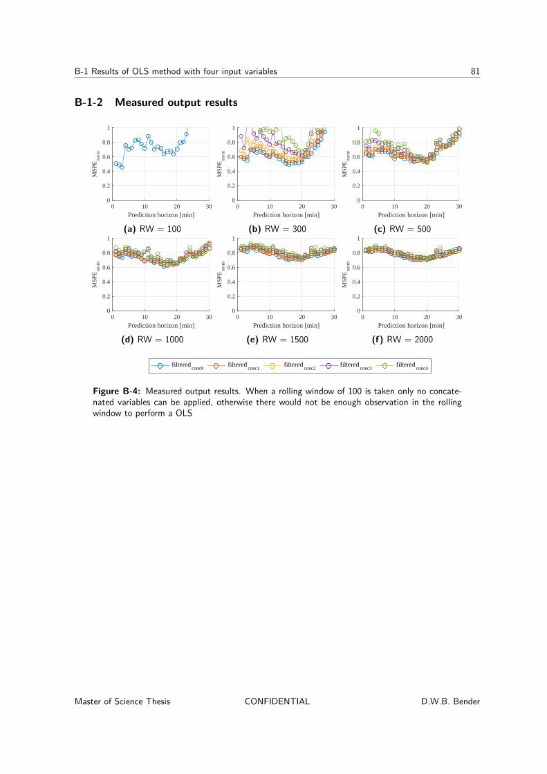
B-1 Results of OLS method with four input variables 81
B-1-2 Measured output results
0 10 20 30
Prediction horizon [min]
0
0.2
0.4
0.6
0.8
1
MSP
Eno
rm
(a) RW = 100
0 10 20 30
Prediction horizon [min]
0
0.2
0.4
0.6
0.8
1
MSP
Eno
rm
(b) RW = 300
0 10 20 30
Prediction horizon [min]
0
0.2
0.4
0.6
0.8
1
MSP
Eno
rm
(c) RW = 500
0 10 20 30
Prediction horizon [min]
0
0.2
0.4
0.6
0.8
1
MSP
Eno
rm
(d) RW = 1000
0 10 20 30
Prediction horizon [min]
0
0.2
0.4
0.6
0.8
1
MSP
Eno
rm
(e) RW = 1500
0 10 20 30
Prediction horizon [min]
0
0.2
0.4
0.6
0.8
1
MSP
Eno
rm(f) RW = 2000
0 5 10 15 20 25 30
Prediction horizon [min]
0.7
0.75
0.8
0.85
0.9
MSP
Eno
rm
filteredconc0
filteredconc1
filteredconc2
filteredconc3
filteredconc4
Figure B-4: Measured output results. When a rolling window of 100 is taken only no concate-nated variables can be applied, otherwise there would not be enough observation in the rollingwindow to perform a OLS
Master of Science Thesis CONFIDENTIAL D.W.B. Bender

82 Model Analysis
B-1-3 Comparison
0 5 10 15 20 25 30Prediction horizon [min]
0
0.2
0.4
0.6
0.8
1
MSP
Eno
rm
measuredlinearzero-order holdspline
(a) RW = 100
0 5 10 15 20 25 30Prediction horizon [min]
0
0.2
0.4
0.6
0.8
1
MSP
Eno
rm
measuredlinearzero-order holdspline
(b) RW = 300
0 5 10 15 20 25 30Prediction horizon [min]
0
0.2
0.4
0.6
0.8
1
MSP
Eno
rm
measuredlinearzero-order holdspline
(c) RW = 500
0 5 10 15 20 25 30Prediction horizon [min]
0
0.2
0.4
0.6
0.8
1
MSP
Eno
rm
measuredlinearzero-order holdspline
(d) RW = 1000
0 5 10 15 20 25 30Prediction horizon [min]
0
0.2
0.4
0.6
0.8
1
MSP
Eno
rm
measuredlinearzero-order holdspline
(e) RW = 1500
0 5 10 15 20 25 30Prediction horizon [min]
0
0.2
0.4
0.6
0.8
1
MSP
Eno
rm
measuredlinearzero-order holdspline
(f) RW = 2000
Figure B-5: Comparison of the output results for the three interpolation methods and themeasured output set. Only the results of the models with no concatenated variables are shown
D.W.B. Bender CONFIDENTIAL Master of Science Thesis

B-2 Estimated parameters of OLS with four input variables 83
B-2 Estimated parameters of OLS with four input variables
B-2-1 Rolling window size of 500 samples
Dec 11 Dec 15 Dec 19-5
-4
-3
-2
-1
0
β(1)
(a) Values of β(1)Dec 11 Dec 15 Dec 19
0
1
2
3
4
5
β(2)
(b) Values of β(2)
Dec 11 Dec 15 Dec 19-1.5
-1
-0.5
0
0.5
1
β(3)
(c) Values of β(3)Dec 11 Dec 15 Dec 19
-0.5
0
0.5
1
1.5
2
β(4)
(d) Values of β(4)
Dec 11 Dec 14 Dec 17-5
0
5×10-13
β0
(e) Values of β0
Figure B-6: Estimates of β for the OLS with a rolling window of 500 and a prediction horizonof 20 for the period 10th through the 19th of December 2015
Master of Science Thesis CONFIDENTIAL D.W.B. Bender
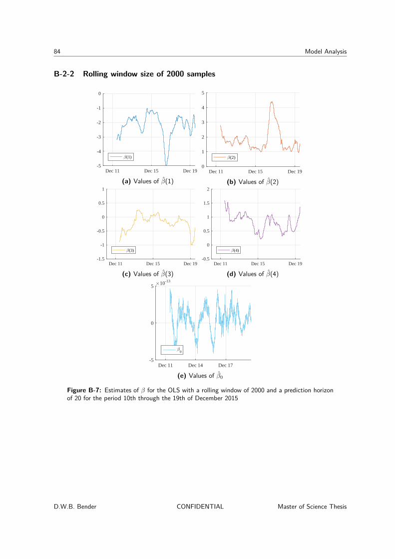
84 Model Analysis
B-2-2 Rolling window size of 2000 samples
Dec 11 Dec 15 Dec 19-5
-4
-3
-2
-1
0
β(1)
(a) Values of β(1)Dec 11 Dec 15 Dec 19
0
1
2
3
4
5
β(2)
(b) Values of β(2)
Dec 11 Dec 15 Dec 19-1.5
-1
-0.5
0
0.5
1
β(3)
(c) Values of β(3)Dec 11 Dec 15 Dec 19
-0.5
0
0.5
1
1.5
2
β(4)
(d) Values of β(4)
Dec 11 Dec 14 Dec 17-5
0
5×10-13
β0
(e) Values of β0
Figure B-7: Estimates of β for the OLS with a rolling window of 2000 and a prediction horizonof 20 for the period 10th through the 19th of December 2015
D.W.B. Bender CONFIDENTIAL Master of Science Thesis

Appendix C
Results
Master of Science Thesis CONFIDENTIAL D.W.B. Bender

86 Results
C-1 Normal operations dataset
C-1-1 Identified parameters using the OLS and ridge regression methods
Dec 10 Dec 15 Dec 20-3
-2.5
-2
-1.5
-1
-0.5
0TTX01
Dec 10 Dec 15 Dec 200
1
2
3
4
5PTXX1
Dec 10 Dec 15 Dec 20-0.4
-0.3
-0.2
-0.1
0
0.1XCXX1
Dec 10 Dec 15 Dec 200
0.5
1
1.5FCXX3
Dec 10 Dec 15 Dec 20-0.2
0
0.2
0.4
0.6FCXX1
Dec 10 Dec 15 Dec 20-1
-0.5
0
0.5FCXX2
Dec 10 Dec 15 Dec 20-1.5
-1
-0.5
0
0.5FCXX3
Dec 10 Dec 15 Dec 20-0.5
0
0.5
1
1.5FCXX4
Dec 10 Dec 15 Dec 20-1
-0.5
0
0.5FCXX5
Dec 10 Dec 15 Dec 20-0.5
0
0.5
1
1.5HCXX6
Dec 10 Dec 15 Dec 20-0.1
-0.05
0
0.05
0.1
0.15
0.2LTXX2
Dec 10 Dec 15 Dec 20-0.1
-0.05
0
0.05
0.1LTXX7
Dec 10 Dec 15 Dec 20-0.6
-0.4
-0.2
0
0.2
0.4PTXX2
Dec 10 Dec 15 Dec 20-3
-2
-1
0
1TTX03
Dec 10 Dec 15 Dec 20-2
-1
0
1
2
3TTX04
Dec 10 Dec 15 Dec 20-4
-2
0
2
4TTX05
Figure C-1: β throughout the period 10th through 19th of December 2015 for the OLS andridge regression models, with a rolling window of 1000 and a prediction horizon of 20
D.W.B. Bender CONFIDENTIAL Master of Science Thesis
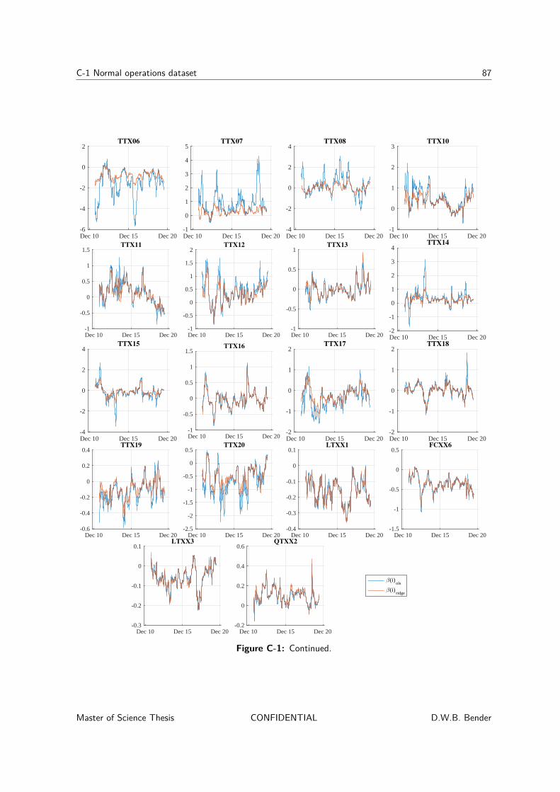
C-1 Normal operations dataset 87
Dec 10 Dec 15 Dec 20-6
-4
-2
0
2TTX06
Dec 10 Dec 15 Dec 20-1
0
1
2
3
4
5TTX07
Dec 10 Dec 15 Dec 20-4
-2
0
2
4TTX08
Dec 10 Dec 15 Dec 20-1
0
1
2
3TTX10
Dec 10 Dec 15 Dec 20-1
-0.5
0
0.5
1
1.5TTX11
Dec 10 Dec 15 Dec 20-1
-0.5
0
0.5
1
1.5
2TTX12
Dec 10 Dec 15 Dec 20-1
-0.5
0
0.5
1TTX13
Dec 10 Dec 15 Dec 20-2
-1
0
1
2
3
4TTX14
Dec 10 Dec 15 Dec 20-4
-2
0
2
4TTX15
Dec 10 Dec 15 Dec 20-1
-0.5
0
0.5
1
1.5TTX16
Dec 10 Dec 15 Dec 20-2
-1
0
1
2TTX17
Dec 10 Dec 15 Dec 20-2
-1
0
1
2TTX18
Dec 10 Dec 15 Dec 20-0.6
-0.4
-0.2
0
0.2
0.4TTX19
Dec 10 Dec 15 Dec 20-2.5
-2
-1.5
-1
-0.5
0
0.5TTX20
Dec 10 Dec 15 Dec 20-0.4
-0.3
-0.2
-0.1
0
0.1LTXX1
Dec 10 Dec 15 Dec 20-1.5
-1
-0.5
0
0.5FCXX6
Dec 10 Dec 15 Dec 20-0.3
-0.2
-0.1
0
0.1LTXX3
Dec 10 Dec 15 Dec 20-0.2
0
0.2
0.4
0.6QTXX2
Dec 10 Dec 15 Dec 20-3
-2
-1
0TTX01
β(i)ols
β(i)ridge
Figure C-1: Continued.
Master of Science Thesis CONFIDENTIAL D.W.B. Bender
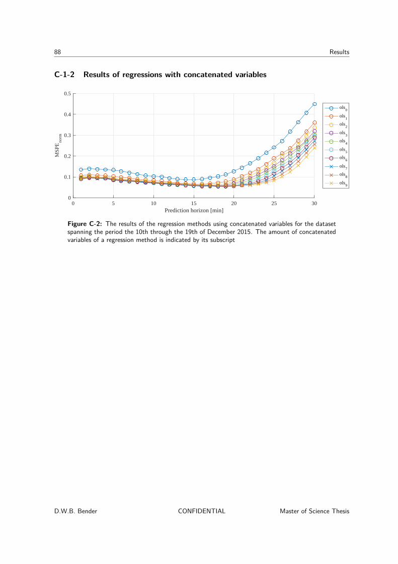
88 Results
C-1-2 Results of regressions with concatenated variables
0 5 10 15 20 25 30Prediction horizon [min]
0
0.1
0.2
0.3
0.4
0.5
MSP
Eno
rm
ols0
ols1
ols2
ols3
ols4
ols5
ols6
ols7
ols8
ols9
Figure C-2: The results of the regression methods using concatenated variables for the datasetspanning the period the 10th through the 19th of December 2015. The amount of concatenatedvariables of a regression method is indicated by its subscript
D.W.B. Bender CONFIDENTIAL Master of Science Thesis

C-2 Abnormal operations dataset 89
C-2 Abnormal operations dataset
C-2-1 Amount of included predictors by the LASSO
Jan 02 Jan 04 Jan 06 Jan 08 Jan 10 Jan 12 Jan 14 Jan 16 Jan 182016
0
5
10
15
20
25
30
35
num
ber
of p
redi
ctor
s in
clud
ed
Figure C-3: For each point in the dataset, the number of included variables is shown for theLASSO model that was constructed with a rolling window of 1000 and a prediction horizon of 20
Master of Science Thesis CONFIDENTIAL D.W.B. Bender

90 Results
C-2-2 Identified parameters using the OLS and ridge regression methods
Jan 01, 2016 Jan 11, 2016-4
-3
-2
-1
0
1TTX01
Jan 01, 2016 Jan 11, 2016-1
0
1
2
3
4
5PTXX1
Jan 01, 2016 Jan 11, 2016-1.5
-1
-0.5
0
0.5XCXX1
Jan 01, 2016 Jan 11, 2016-0.5
0
0.5
1
1.5FCXX3
Jan 01, 2016 Jan 11, 2016-0.4
-0.2
0
0.2
0.4
0.6
0.8FCXX1
Jan 01, 2016 Jan 11, 2016-1
-0.5
0
0.5
1FCXX2
Jan 01, 2016 Jan 11, 2016-2
-1
0
1
2FCXX3
Jan 01, 2016 Jan 11, 2016-0.5
0
0.5
1
1.5
2FCXX4
Jan 01, 2016 Jan 11, 2016-0.6
-0.4
-0.2
0
0.2
0.4
0.6FCXX5
Jan 01, 2016 Jan 11, 2016-0.6
-0.4
-0.2
0
0.2
0.4HCXX6
Jan 01, 2016 Jan 11, 2016-0.2
-0.1
0
0.1
0.2
0.3LTXX2
Jan 01, 2016 Jan 11, 2016-0.2
-0.1
0
0.1
0.2LTXX7
Jan 01, 2016 Jan 11, 2016-1
-0.5
0
0.5
1PTXX2
Jan 01, 2016 Jan 11, 2016-1
-0.5
0
0.5
1
1.5
2TTX03
Jan 01, 2016 Jan 11, 2016-3
-2
-1
0
1
2TTX04
Jan 01, 2016 Jan 11, 2016-3
-2
-1
0
1
2TTX05
Figure C-4: β throughout the period 1st through 18th of January 2016 for the OLS and ridgeregression models, with a rolling window of 1000 and a prediction horizon of 20
D.W.B. Bender CONFIDENTIAL Master of Science Thesis

C-2 Abnormal operations dataset 91
Jan 01, 2016 Jan 11, 2016-6
-4
-2
0
2
4TTX06
Jan 01, 2016 Jan 11, 2016-2
0
2
4
6TTX07
Jan 01, 2016 Jan 11, 2016-6
-4
-2
0
2
4TTX08
Jan 01, 2016 Jan 11, 2016-3
-2
-1
0
1TTX09
Jan 01, 2016 Jan 11, 2016-2
-1
0
1
2TTX10
Jan 01, 2016 Jan 11, 2016-1.5
-1
-0.5
0
0.5
1
1.5TTX11
Jan 01, 2016 Jan 11, 2016-1
0
1
2
3TTX12
Jan 01, 2016 Jan 11, 2016-1
-0.5
0
0.5
1TTX13
Jan 01, 2016 Jan 11, 2016-3
-2
-1
0
1
2
3TTX14
Jan 01, 2016 Jan 11, 2016-4
-2
0
2
4TTX15
Jan 01, 2016 Jan 11, 2016-1
-0.5
0
0.5
1TTX16
Jan 01, 2016 Jan 11, 2016-2
-1
0
1
2
3TTX17
Jan 01, 2016 Jan 11, 2016-1
-0.5
0
0.5
1TTX18
Jan 01, 2016 Jan 11, 2016-1.5
-1
-0.5
0
0.5
1TTX19
Jan 01, 2016 Jan 11, 2016-4
-2
0
2
4TTX20
Jan 01, 2016 Jan 11, 2016-0.6
-0.4
-0.2
0
0.2
0.4LTXX1
Jan 01, 2016 Jan 11, 2016-1.5
-1
-0.5
0
0.5
1FCXX6
Jan 01, 2016 Jan 11, 2016-0.6
-0.4
-0.2
0
0.2LTXX3
Jan 01, 2016 Jan 11, 2016-0.4
-0.2
0
0.2
0.4
0.6QTXX2
Jan 10, 2016-4
-2
0
2TTX01
β(i)ols
β(i)ridge
Figure C-4: Continued.
Master of Science Thesis CONFIDENTIAL D.W.B. Bender

92 Results
C-2-3 Results of regressions with concatenated variables
0 5 10 15 20 25 30Prediction horizon [min]
0
0.1
0.2
0.3
0.4
0.5
MSP
Eno
rm
ols0
ols1
ols2
ols3
ols4
ols5
ols6
ols7
ols8
ols9
Figure C-5: The results of the regression methods using concatenated variables for the datasetspanning the period the 1st through the 17th of January 2016. The amount of concatenatedvariables of a regression method is indicated by its subscript
D.W.B. Bender CONFIDENTIAL Master of Science Thesis

Appendix D
Validation Results
Master of Science Thesis CONFIDENTIAL D.W.B. Bender

94 Validation Results
D-1 Quality estimator datasets for the Deisopentanizer
Dec 2015 Feb 2016 Apr 2016date
0
1
2
3
4
5
% iC
5
QTYY1
(a)
Dec 2015 Feb 2016 Apr 2016date
0
2
4
6
8
10
% c
C5
QTYY2
(b)
Dec 2015 Feb 2016 Apr 2016date
0
5
10
15
20
25
% n
C4
QTYY3
(c)
Dec 2015 Feb 2016 Apr 2016date
0
1
2
3
4
5
6
7
% n
C5
QTYY4
(d)
Figure D-1: Data of the output variables of the C-X12
D.W.B. Bender CONFIDENTIAL Master of Science Thesis

D-2 Results of regression methods of the Deisopentanizer 95
D-2 Results of regression methods of the Deisopentanizer
0 10 20 30 40 50Prediction horizon [min]
0
0.5
1
1.5M
SPE
norm
olsridge0.7pca5pca10pca15
(a) RW = 300
0 10 20 30 40 50Prediction horizon [min]
0
0.5
1
1.5
MSP
Eno
rm
olsridge0.7pca5pca10pca15
(b) RW = 500
0 10 20 30 40 50Prediction horizon [min]
0
0.5
1
1.5
MSP
Eno
rm
olsridge0.7pca5pca10pca15
(c) RW = 1000
0 10 20 30 40 50Prediction horizon [min]
0
0.5
1
1.5
MSP
Eno
rm
olsridge0.7pca5pca10pca15
(d) RW = 2000
Figure D-2: QTYY1
Master of Science Thesis CONFIDENTIAL D.W.B. Bender

96 Validation Results
0 10 20 30 40 50Prediction horizon [min]
0
0.5
1
1.5
2
MSP
Eno
rm
olsridge0.7pca5pca10pca15
(a) RW = 300
0 10 20 30 40 50Prediction horizon [min]
0
0.5
1
1.5
2
MSP
Eno
rm
olsridge0.7pca5pca10pca15
(b) RW = 500
0 10 20 30 40 50Prediction horizon [min]
0
0.5
1
1.5
2
MSP
Eno
rm
olsridge0.7pca5pca10pca15
(c) RW = 1000
0 10 20 30 40 50Prediction horizon [min]
0
0.5
1
1.5
2
MSP
Eno
rm
olsridge0.7pca5pca10pca15
(d) RW = 2000
Figure D-3: QTYY2
0 10 20 30 40 50Prediction horizon [min]
0
0.5
1
1.5
MSP
Eno
rm
olsridge0.7pca5pca10pca15
(a) RW = 300
0 10 20 30 40 50Prediction horizon [min]
0
0.5
1
1.5
MSP
Eno
rm
olsridge0.7pca5pca10pca15
(b) RW = 500
0 10 20 30 40 50Prediction horizon [min]
0
0.5
1
1.5
MSP
Eno
rm
olsridge0.7pca5pca10pca15
(c) RW = 1000
0 10 20 30 40 50Prediction horizon [min]
0
0.5
1
1.5
MSP
Eno
rm
olsridge0.7pca5pca10pca15
(d) RW = 2000
Figure D-4: QTYY3
D.W.B. Bender CONFIDENTIAL Master of Science Thesis
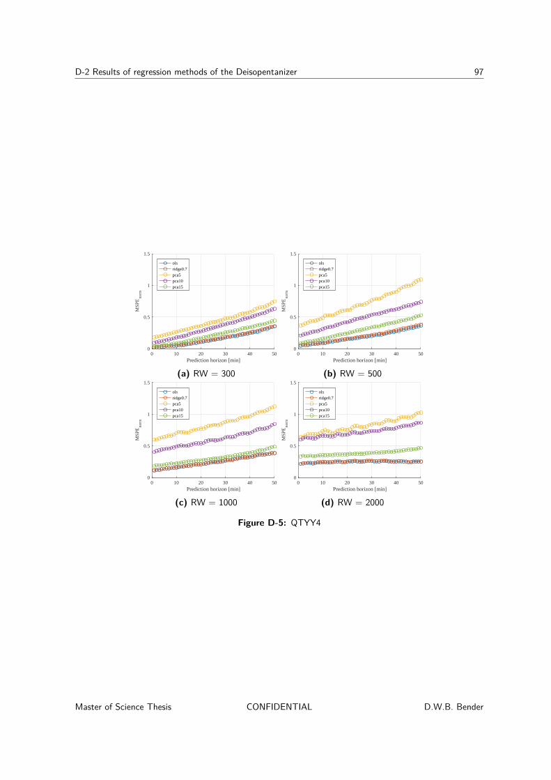
D-2 Results of regression methods of the Deisopentanizer 97
0 10 20 30 40 50Prediction horizon [min]
0
0.5
1
1.5
MSP
Eno
rm
olsridge0.7pca5pca10pca15
(a) RW = 300
0 10 20 30 40 50Prediction horizon [min]
0
0.5
1
1.5
MSP
Eno
rm
olsridge0.7pca5pca10pca15
(b) RW = 500
0 10 20 30 40 50Prediction horizon [min]
0
0.5
1
1.5
MSP
Eno
rm
olsridge0.7pca5pca10pca15
(c) RW = 1000
0 10 20 30 40 50Prediction horizon [min]
0
0.5
1
1.5
MSP
Eno
rm
olsridge0.7pca5pca10pca15
(d) RW = 2000
Figure D-5: QTYY4
Master of Science Thesis CONFIDENTIAL D.W.B. Bender

98 Validation Results
D.W.B. Bender CONFIDENTIAL Master of Science Thesis

Bibliography
[1] P. D. Reynolds, “Industrial Process Analytics Predicting Process Events,” ARC AdvisoryGroup, 2016.
[2] D. White, “Analytics for the Industrial Internet of Things - Describe and Discover Styles,”2014.
[3] L. H. Chiang, E. L. Russell, and R. D. Braatz, Fault Detection and Diagnosis in Indus-trial Systems. Advanced Textbooks in Control and Signal Processing, London: SpringerLondon, 2001.
[4] R. Isermann, Fault-diagnosis systems: An introduction from fault detection to fault toler-ance. 2006.
[5] H. Raghavan, R. B. Gopaluni, S. Shah, J. Pakpahan, R. Patwardhan, and C. Robson,“Gray-box identification of dynamic models for the bleaching operation in a pulp mill,”Journal of Process Control, vol. 15, no. 4, pp. 451–468, 2005.
[6] T. Hastie, R. Tibshirani, and J. Friedman, The Elements of Statistical Learning, vol. 27of Springer Series in Statistics. New York, NY: Springer New York, 2009.
[7] R. Tibshirani and R. S. Society, “Regression Shrinkage and Selection via the Lasso,”Journal of the Royal Statistical Society. Series B (Methodological), vol. 58, no. 1, pp. 267–288, 1996.
[8] I. T. Jolliffe, “Principal Component Analysis, Second Edition,” Encyclopedia of Statisticsin Behavioral Science, vol. 30, no. 3, p. 487, 2002.
Master of Science Thesis CONFIDENTIAL D.W.B. Bender

100 Bibliography
D.W.B. Bender CONFIDENTIAL Master of Science Thesis

Glossary
List of Acronyms
APC Advanced Process Control
ARC ARC Advisory Group
BLC Base Layer Control
NUI normally unmanned installation
DCS distributed control system
CDU crude distiller unit
RQE Robust Quality Estimator Pro
ECP effective cut point
SI separation index
IBP initial boiling point
EP end point
CDX1 Crude Distiller X1
CDX2 Crude Distiller X2
C-X11 Depentanizer
C-X12 Deisopentanizer
C-X13 Deisohexanizer
C-X21 Crude Splitter 1
C-X22 Crude Splitter 2
C-X27 Debutanizer
Master of Science Thesis CONFIDENTIAL D.W.B. Bender

102 Glossary
C-X28 Gasoline Splitter
NOD normal operations dataset
AOD abnormal operations dataset
SOD standard operations dataset
QT1 QTXX1
QE1 QEXX1
C5 pentane
nC5 n-pentane
iC5 isopentane
cC5 cylcopentane
nC4 n-butane
UCL upper control limit
LCL lower control limit
MSPE mean squared prediction error
FIR finite impulse response
ARMAX autoregressive-moving average model with exogenous inputs
MISO multiple inputs, single output
OLS ordinary least squares
LASSO least absolute shrinkage and selection operator
PLS partial least squares
PLSC partial least squares component
PCA principal components analysis
PC principal component
SVD singular value decomposition
EM expectation maximization
D.W.B. Bender CONFIDENTIAL Master of Science Thesis