mastermath course differential geometry 2015/2016crain101/dg-2015/chapter2.pdf · mastermath course...
TRANSCRIPT
Mastermath course DifferentialGeometry 2015/2016
Marius Crainic
1Department of Mathematics, Utrecht University, 3508 TA Utrecht, The Netherlands.E-mail address: [email protected] by the editors September, 2015.
c©0000 American Mathematical Society
1

Contents
Mastermath course Differential Geometry 2015/2016 1
Chapter 1. Vector bundles and connections 71.1. Vector bundles 71.1.1. The definition/terminology 71.1.2. Morphisms 81.1.3. Trivial vector bundles; trivializations 81.1.4. Sections 81.1.5. Frames 91.1.6. Remark on the construction of vector bundles 91.1.7. Operations with vector bundles 111.1.8. Differential forms with coefficients in vector bundles 161.2. Connections on vector bundles 171.2.1. The definition 171.2.2. Locality; connection matrices 191.2.3. More than locality: derivatives of paths 191.2.4. Parallel transport 211.2.5. Connections as DeRham-like operators 221.3. Curvature 231.3.1. The definition 231.3.2. The curvature as failure of ” d2
dsdt = d2
dtds” 25
1.3.3. The curvature as failure of d2∇ = 0 26
1.3.4. More on connection and curvature matrices; the first Chern class 271.4. Connections compatible with a metric 331.4.1. Metrics on vector bundles 331.4.2. Connections compatible with a metric 351.4.3. Riemannian manifolds I: The Levi-Civita connection 361.4.4. Riemannian manifolds II: geodesics and the exponential map 371.4.5. Riemannian manifolds III: application to tubular neighborhoods 40
Chapter 2. Principal bundles 45
2.1. Digression: Lie groups and actions 452.1.1. The basic definitions 452.1.2. The Lie algebra 482.1.3. The exponential map 522.1.4. Closed subgroups of GLn 532.1.5. Infinitesimal actions 552.1.6. Free and proper actions 562.2. Principal bundles 59
3
4 M. CRAINIC, DG-2015
2.2.1. The definition/terminology 592.2.2. Remarks on the definition 602.2.3. From vector bundles to principal bundles (the frame bundle) 642.2.4. From principal bundles to vector bundles 662.2.5. Sections/forms for vector bundles associated to principal ones 682.3. Connections on principal bundles 712.3.1. Connections as horizontal distributions: 712.3.2. Connection forms 722.3.3. Parallel transport 732.3.4. Curvature 752.3.5. Principal bundle connections ←→ vector bundles ones 762.3.6. Reduction of the structure group 78

M. CRAINIC, DG-2015 5
Contents- to be continued

6 M. CRAINIC, DG-2015
Contents- to be continued
CHAPTER 1
Vector bundles and connections
1.1. Vector bundles
In this section we recall some basics on vector bundles.
1.1.1. The definition/terminology
Definition 1.1. A (real) vector bundle of rank r over a manifold M consists of:
• a manifold E,• a surjective map π : E −→M ; for x ∈M , the fiber π−1(x) is denoted Ex• for each x ∈M , a structure of r-dimensional (real) vector space on Ex
satisfying the following local triviality condition: for each x0 ∈ M , there exists anopen neighborhood U of x0 and a diffeomorphism
h : E|U := π−1(U)∼−→ U × Rr
with the property that it sends each fiber Ex isomorphically to x × Rr, where”isomorphically” means by a vector space isomorphism and where we identify x×Rr with Rr. Complex vector bundles are defined similarly, replacing R by C.
Strictly speaking, a vector bundle is an entire triple (E, π,M) as above; accord-ingly, one sometimes uses notations of type
(1.2) ξ = (E, π,M)
and one refers to the triple ξ as being a vector bundle; with this terminology, E isusually denoted E(ξ) and is called the total space of the vector bundle ξ. However,we will adopt a simpler terminology (hopefully not too confusing): we will justmention E (i.e. we just say that E is a vector bundle over M), by which it is selfunderstood that E comes with a map onto M , generically denoted πE , and calledthe projection of the vector bundle E. Intuitively, one should think about E as thecollection
Exx∈Mof vector spaces (of rank r), “smoothly parametrized by x ∈M”.
Note that, as hinted by the notation E|U , a vector bundle E over M can berestricted to an arbitrary open U ⊂M . More precisely,
E|U := π−1(U)
together with the restriction of π gives a vector bundle πU : E|U −→ U over U .Here are some basic concepts/constructions regarding vector bundles.
7
8 M. CRAINIC, DG-2015
1.1.2. Morphisms
Given two vector bundles E and F over M , a morphism from E to F (of vectorbundles over M) is a smooth map u : E −→ F with the property that, for eachx ∈M , u sends Ex to Fx and
ux := u|Ex : Ex −→ Fx
is linear. We say that u is an isomorphism (of vector bundles over M) if each ux isan isomorphism (or, equivalently, if u is also a diffeomorphism). Again, one shouldthink of a morphism u as a collection uxx∈M of linear maps between the fibers,“smoothly parametrized by x”.
1.1.3. Trivial vector bundles; trivializations
The trivial vector bundle of rank r over M is the product M ×Rr together with thefirst projection
pr1 : M × Rr −→M
and the usual vector space structure on each fiber x×Rr. When using the notation(1.2), the trivial vector bundle of rank r is usually denoted
(1.3) εr = (M × Rr, pr1,M)
(or, if one wants to be more precise about the base, then one uses the notation εrM ).We say that a vector bundle E (of rank r) over M is trivializable if E is isomor-
phic to M × Rr. A trivialization of E is the choice of such an isomorphism.With these in mind, we see that the local triviality condition from the definition
of vector bundles says that E is locally trivializable, i.e. each point in M admits anopen neighborhood U such that the restriction E|U is trivializable.
1.1.4. Sections
One of the main objects associated to vector bundles are their (local) sections. Givena vector bundle π : E −→M , a section of E is a smooth map s : M −→ E satisfyingπ s = Id, i.e. with the property that
s(x) ∈ Ex ∀ x ∈M.
We denote by
Γ(M,E) = Γ(E)
the space of all smooth sections. For U ⊂ M open, the space of local sections of Edefined over U is
Γ(U,E) := Γ(E|U ).
Sections can be added pointwise:
(s+ s′)(x) := s(x) + s′(x)
and, similarly, can be multiplied by scalars λ ∈ R:
(λs)(x) := λs(x).
With these, Γ(E) becomes a vector space. Furthermore, any section s ∈ Γ(E) canbe multiplied pointwise by any real-valued smooth function f ∈ C∞(M) giving riseto another section fs ∈ Γ(E):
(fs)(x) := f(x)s(x).
1.1. Vector bundles 9
The resulting operation
C∞(M)× Γ(E) −→ Γ(E), (f, s) 7→ fs
makes Γ(E) into a module over the algebra C∞(M). Actually the entire vectorbundle E is fully encoded in the space of sections Γ(E) together with this modulestructure.For the curious reader. The precise formulation of the last statement is given by Swan’s theorem which saysthat the construction E 7→ Γ(E) gives a 1-1 correspondence between vector bundles over M and finitely generatedprojective modules over C∞(M). Recall here that, for a ring R, an R-module E is said to be finitely generatedand projective if there exists another R-module F such that the direct sum R-module E ⊕ F is isomorphic to the
free R-module Rk for some k. This corresponds to a basic property of vector bundles: for any vector bundle Eover M , one can always find another vector bundle F over M such that the direct sum vector bundle E ⊗ F (seebelow) is isomorphic to the a trivial vector bundle.
Note that this discussion is very much related, at least in spirit, with the Gelfand-Naimark theorem whichsays that (compact) topological spaces X can be recovered from the algebra C(X) of continuous functions on X(see Chapter 8, section 3, from our bachelor course ”Inleiding Topologie”, available at:http://www.staff.science.uu.nl/∼crain101/topologie2014/).
A simpler illustration of the previous principle is the following:
Lemma 1.4. Let E and F be two vector bundles over M . Then there is a bijectionbetween‘:
• morphisms u : E −→ F of vector bundles over M .• morphisms u∗ : Γ(E) −→ Γ(F ) of C∞(M)-modules.
Explicitely, given u, the associated u∗ is given by
u∗(s)(x) = ux(s(x)).
1.1.5. Frames
Let π : E −→M be a vector bundle over M . A frame of E is a collection
s = (s1, . . . , sr)
consisting of sections si of E with the property that, for each x ∈M ,
(s1(x), . . . , sr(x))
is a frame of Ex (i.e. a basis of the vector space Ex). A local frame of E is a frames of E|U for some open U ⊂M ; we also say that s is a local frame over U .
Remark 1.5. Choosing a frame s of E is equivalent to choosing a trivializationu : M × Rr −→ E of E. Hence, the local triviality condition from the definition ofvector bundles can be phrased in terms of local frames as follows: around any pointof M one can find a local frame of E.
1.1.6. Remark on the construction of vector bundles
Often the vector bundles that one encounters do not arise right away as in theoriginal definition of vector bundles. Instead, one has just a collection E = Exx∈Mof vector spaces indexed by x ∈M and certain “smooth sections”. Let us formalizethis a bit. We will use the name “discrete vector bundle over M (of rank r)” forany collection Exx∈M of (r-dimensional) vector spaces indexed by x ∈ M . Wewill identify such a collection with the resulting disjoint union and the associatedprojection
E := (x, vx) : x ∈M,vx ∈ Ex, π : E −→M, (x, vx) 7→ x
(so that each Ex is identified with the fiber π−1(x)).

10 M. CRAINIC, DG-2015
For such a discrete vector bundle E we can talk about discrete sections, whichare simply functions s as above,
M 3 x 7→ s(x) ∈ Ex(but without any smoothness condition). Denote by Γdiscr(E) the set of such sec-tions. Similarly we can talk about discrete local sections, frames and local frames.As in the case of charts of manifolds, there is a natural notion of ”smooth compati-bility” of local frames. To be more precise, we assume that
s = (s1, . . . , sr), s = (s1, . . . , sr)
are two local frames defined over U and U , respectively. Then, over U ∩ U , one canwrite
si(x) =r∑j=1
gij(x)sj(x),
giving rise to functions
gij : U ∩ U −→ R (1 ≤ i, j ≤ r).
We say that s and s are smoothly compatible if all the functions gij are smooth. Thefollowing is an instructive exercise.
Exercise 1. Let E = Exx∈M be a discrete vector bundle over M of rank r.Assume that we are given an open cover U of M and, for each open U ∈ U , adiscrete local frame sU of E over U . Assume that, for any U, V ∈ U , sU and sVare smoothly compatible. Then E admits a unique smooth structure which makesit into a vector bundle over M with the property that all the sU become (smooth)local frames.
Moreover, the (smooth) sections of E can be recognized as those discrete sectionss with the property that they are smooth with respect to the given data sUU∈Uin the following sense: for any U ∈ U , writing
u(x) = f1(x)s1U (x) + . . .+ fr(x)srU (x) (x ∈ U),
all the functions fi are smooth on E.
Example 1.6. For a manifold M one consider all the tangent spaces TM =TxMx ∈M and view it as a discrete vector bundle. Given a chart χ : Uχ −→ Rnfor M , then the associated tangent vectors
(∂
∂χ1(x), . . . ,
∂
∂χn(x))
can be seen as a discrete local frame of TM over Uχ. Starting with an atlas A of M ,we obtain in this way precisely the data that we need in order to apply the previousexercise; this makes TM into a vector bundle over M in the sense of the originaldefinition.
Example 1.7. Here is another interesting vector bundle- the so called tautologicalline bundle over the projective space RPn. In the notation (1.2), this is usuallydenoted by γ1. We describe the total space E(γ1). Recalling the a point l ∈ RPn isa line l ⊂ Rn+1 through the origin, the fiber of E(γ1) above such a point is preciselythe line l, interpreted as a 1-dimensional vector space. Equivalently:
E(γ1) = (l, v) ∈ RPn × Rn+1 : v ∈ l,

1.1. Vector bundles 11
or, denoting by [x0 : . . . : xn] the line through (x0, . . . , xn) ∈ Rn+1 \ 0,
E(γ1) = ([x0 : . . . : xn], λ · x0, . . . , λ · xn)) : (x0, . . . , xn) ∈ Rn+1 \ 0, λ ∈ R.
With these, γ1 is a vector bundle of rank one (a line bundle) over RPn.Such vector bundles exist for arbitrary ranks: one replaces RPn with the Grass-
mannian Grk(Rn+k) (whose points are the k-dimensional vector subspaces of Rn+k)and γ1 by γk whose fiber above some V ∈ Grk(Rn+k) is the vector space V itself.
Of course, these examples can be adapted to the complex setting, by workingwith complex lines (and complex vector subspaces) to define CPn (and Grk(Cn+k)),and the tautological complex vector bundles on them.
1.1.7. Operations with vector bundles
The principle is very simple: natural operations with vector spaces, applied fiber-wise, extend to vector bundles.
Direct sums: Let us start with the direct sum operation. Given two vector spacesV and W we consider their direct sum vector space V ⊕ W . Assume now thatpE : E −→ M and pF : F −→ M are vector bundles over M . Then the direct sumE ⊕ F is another vector bundle over M , with fibers
(1.8) (E ⊕ F )x := Ex ⊕ Fx.
These equations force the definition of the total space E⊕F and of the projection intoM . To exhibit the smooth structure of E ⊕ F one can e.g. use Exercise 1. Indeed,choosing opens U ⊂M over which we can find (smooth) local frames e = (e1, . . . , ep)of E and f = (f1, . . . , fq) of F , one can form the direct sum local frame
e⊕ f = (e1, . . . , ep, f1, . . . , fq)
and we consider the smooth structure on E ⊕F which makes all the local frames oftype e⊕ f smooth.
This procedure of extending operations between vector spaces to operations be-tween vector bundles is rather general. In some cases however, one can further takeadvantage of the actual operation one deals with and obtain “more concrete” de-scriptions. This is the case also with the direct sum operation. Indeed, recall thatfor any two vector spaces V and W , their direct sum V ⊕W can be described asthe set-theoretical product V ×W with the vector space operations
(v, w) + (v′, w′) = (v + v′, w + w′), λ · (v, w) = (λ · v, λ · w)
(the passing to the notation V ⊕W indicates that we identify the elements v ∈ Vwith (v, 0) ∈ V ×W , w ∈ W with (0, w) ∈ V ×W , so that an arbitrary element(v, w) can be written uniquely as v + w with v ∈ V , w ∈ W ). Hence one can justdefine E ⊕ F as the submanifold of E × F
E ×M F := (e, f) ∈ E × F : pE(e) = pF (f).
The condition (1.8) is clearly satisfied (and specify the vector space structure on thefibers) and is not difficult to see that the resulting E⊕F is a vector bundle over M .Note that the space of sections of E⊕F coincides with the direct sum Γ(E)⊕Γ(F ).
Duals: Let us now look at the operation that associates to a vector space V itsdual V ∗. Starting with a vector bundle E over M , its dual E∗ is another vector

12 M. CRAINIC, DG-2015
bundle over M with the property that
(E∗)x = (Ex)∗
for all x ∈M . Again, this determines E∗ as a set and its projection into M . More-over, using dual basis, we see that any smooth local frame e = (e1, . . . , er) of Einduces a local frame e∗ for E∗ and we can invoke again Exercise 1 to obtain thesmooth structure of E∗.
Hom-bundles: Next we look at the operation that associates to two vector spacesV and W the vector space Hom(V,W ) consisting of all linear maps from V to W .Given now two vector bundles E and F over M , we form the new vector bundleHom(E,F ) over M with fibers
Hom(E,F )x = Hom(Ex, Fx).
And, again, we see that local frames of E and F induce a local frame of Hom(E,F ),and then we obtain a canonical smooth structure on the hom-vector bundle. Notethat a section of Hom(E,F ) is the same thing as a morphism u : E −→ F ofvector bundles over M . Hence Lemma 1.4 identifies sections of Hom(E,F ) withC∞(M)-linear maps Γ(E) −→ Γ(F ).
Of course, when F is the trivial vector vector bundle of rank 1 (F = M × R),we recover the dual of E:
E∗ = Hom(E,M × R).
Hence Lemma 1.4 identifies the sections of E∗ with the dual of Γ(E) as an C∞(M)-module.
Quotients: Next we look at the operation that associates to a vector subspace W ofa vector space V the quotient vector space V/W . Note that the notion of subspace(of a vector space) gives rise to a notion of vector sub-bundle: given a vector bun-dle E over M , a (vector) sub-bundle of E is any vector bundle F over M with theproperty that each Fx is a vector subspace of Ex and the inclusion F → E is smooth.
Exercise: Show that the last condition(smoothness) is equivalent to the con-dition that for any smooth (local) section s of F , interpreting s as a section of Eusing the inclusion F ⊂ E, s is a smooth section of E.
Now, given a vector sub-bundle F ⊂ E it should be clear how to proceed to de-fine E/F : it is a new vector bundle over M whose fiber above x ∈M is the quotientEx/Fx and with the smooth structure uniquely characterised by the fact that thequotient map from E to E/F is smooth (hence a morphism of vector bundles).
Tensor products: One proceeds similarly for the tensor product operation on vectorspaces. Since we work with finite dimensional vector spaces, this operation can beexpressed using duals and homs:
V ⊗W = Hom(V ∗,W ).
(where for v ∈ V , w ∈ W , the tensor v ⊗ w is identified with (or stands for) thelinear map
V ∗ −→W, ξ 7→ ξ(v)w.)
1.1. Vector bundles 13
Other operations: Similar to taking the dual of a vector space one can consideroperations of type
V 7→ Sk(V ∗), (or: V 7→ Λk(V ∗))
which associate to a vector space V the space of all k-multilinear symmetric (or:anti-symmetric) maps V × . . .× V −→ R. Again, one has to remember/notice thatany frame of V induces a frame of SkV ∗ (or: ΛkV ∗). Slightly more generally, onecan consider operations of type
(V,W ) −→ Sk(V ∗)⊗W (or: (V,W ) 7→ Λk(V ∗)⊗W )
which associate to a pair (V,W ) of vector spaces the space of k-multilinear symmetric(or: anti-symmetric) maps on V with values in W and then one obtains similaroperations on vector bundles. Note the following generalization of Exercise 1:
Exercise 2. Show that, for any two vector bundles E and F over M and k ≥ 1integer, there is a 1-1 correspondence between:
• sections u of SkE∗ ⊗ F .• symmetric maps
u∗ : Γ(E)× . . .× Γ(E)︸ ︷︷ ︸k−times
−→ Γ(F )
which is C∞(M)-linear in each argument.
Similarly for sections of ΛkE∗ ⊗ F and antisymmetric maps as above.
Pull-backs: Another important operation with vector bundles, but which does notfit in the previous framework, is the operation of taking pull-backs. More precisely,given a smooth map
f : M −→ N,
starting with any vector bundle E over N , one can pull-it back via f to a vectorbundle f∗E over M . Fiberwise,
(f∗E)x) = Ef(x)
for all x ∈M . One can use again Exercise 1 to make f∗E into a vector bundle; thekey remark is that any section s of E induces a section f∗s of F ∗E by
(f∗s)(x) := s(f(x))
and similarly for local sections and local frames.Note that, when f = i : M → N is an inclusion of a submanifold M of N , then
i∗E is also denoted E|N and is called the restriction of E to M .
Real versus complex vector bundles: Of course, any complex vector bundle F canbe seen as a real vector bundle; when we want to emphasize that we look at F asbeing a real vector bundle, we use the notation FR. Note that the rank (over R) ofFR is twice the rank (over FC) of F . A natural question is: when can a real vectorbundle can be made into a comple one.
Exercise 3. For a real vector bundle E over M , there is a 1-1 correspondencebetween complex vector bundles F over M such that FR = E and vector bundlemorphisms J : E → E such that J2 = −Id.

14 M. CRAINIC, DG-2015
One can also proceed the other way: starting with a real vector bundle E onecan complexify it, i.e. consider the complex vector bundle
EC := E ⊗ Cwhose fiber above an arbitrary point x ∈M is
Ex ⊗ C = v ⊗ 1 + w ⊗ i : u, v ∈ Ex.One can also use the direct sum of real vector bundles and define
EC = E ⊕ E,in which the multiplication by complex numbers given by
(a+ bi) · (u, v) = (au− bv, av + bu) for a+ ib ∈ C.Or, using the previous exercise, we deal with the vector bundle E ⊕ E with thecomplex structure induced by
J(u, v) = (−v, u).
Conjugation: For any complex vector bundle F one can define a new one, denoted
F and called the conjugate of F , whose underlying total space is the same as that ofF , with the only difference that we change the multiplication by complex numberson the fiber to:
z · v := zv
where z is the complex conjugate of z. Note that, in terms of the previous exercise,what we do is to change J by −J .
Note that, in general, F is not isomorphic to F (as complex vector bundles).For instance, this happens for the tautological line bundle γ1 from Example 1.7(however, proving this is not so easy at this point!).
Exercise 4. Consider the tangent bundle TSn of the n-dimensional sphere. Showthat the direct sum of TSn with the trivial bundle of rank one is isomorphic to thetrivial vector bundle of rank n+1 (note: this does not imply that TSn is isomorphicto a trivial bundle, and it is not!).
Exercise 5. Show that the tangent bundle of S3 is trivializable. (1st hint: quater-nions; 2nd hint: first do it for S1; then write your proof using complex numbers;then go to the previous hint).
For the curious reader. Manifolds M with the property that TM is trivializable are called ”parallelizable”.This happens rather rarely. The situation is interesting even for the spheres; we discuss it here in a bit more detail.Note that, the question of whether Sn is parallelizable or not can be rewritten in very down to earth terms: oneis looking for n+ 1 functions
F1, . . . , F
n −→ Rn+1
with the property that, for each x ∈ Sn ⊂ Rn+1, vectors F 1(x), . . . , Fn(x) are linearly independent and take valuein the hyperplane Px orthogonal to x:
Fi(x) ∈ Px := v ∈ Rn+1
: 〈v, x〉 = 0.
This comes from the standard identification of the tangent spaces TxSn with Px ⊂ Rn+1. In the case n = 1 one
can takeF
1(x1, x2) = (x2,−x1)
or, interpreting R2 as C ((x1, x2) 7→ x1 + ix2),
F1(z) = iz.
It works quite similarly for S3, but using quaternions (previous exercise). The 2-sphere however is not parallelizable.
Actually, on S2 any vector field must vanish at at least one point. This is popularly known as the “hairy balltheorem”, and stated as: “you can’t comb a hairy ball flat without creating a cowlick”(see also the “Cyclone
consequences” on the wikipedia). The mathematical reason that S2 is not parallelizable (and actually that it doesnot admit any no-where vanishing vector field) is that its “Euler characteristic” does not vanish. Actually, a nice(but non-trivial) theorem in differential topology says that the Euler characteristic of a compact manifold vanishes
1.1. Vector bundles 15
if and only if it admits a no-where vanishing vector field. By the way, for the same reason, all the even dimensionalspheres S2n are not parallelizable.
Are the other (odd dimensional) spheres parallelizable? Yes: there is also S7. This uses octonions (also
called the Cayley algebra) instead of quaternions (S3) and complex numbers (S1). How general is this? In what
dimensions does it work? Looking at the proofs (e.g. for S1 and S3) we see that what we need is a “normed
division algebra” structure on Rn+1 (in order to handle the n-sphere Sn). By that we mean a multiplication “·”on Rn+1, with unit element 1 := (1, 0, . . . , 0) (but not necessarily associative- as in the case of the octonions) andsatisfying the norm condition
|x · y| = |x||y| ∀ x, y ∈ Rn+1,
where | · | is the standard norm. The term “division algebra” comes from the fact that the norm condition impliesthat the product has the “division property”: xy = 0 implies that either x = 0 or y = 0 (if we keep this condition,but we give up on the norm condition, we talk about division algebras). Indeed, any such operation induces
Fi(x) = ei · x
proving that Sn is parallelizable. But on which Rn+1 do there exist such operations? Well: only on R, R2 (complex),
R4 (quaternions) and R8 (octonions)! This was known since the 19th century. It is also interesting to know why wasthere interest on such operations already in the 19th century: number theory and the question of which numberscan be written as sums of two, three, etc squares. For sum of two squares, the central formula which shows that aproduct of two numbers that can be written as a sum of two squares can itself be written as a sum of two squaresis:
(x2
+ y2)(a
2+ b
2) = (xa− yb)2 + (xb+ ya)
2.
Or, in terms of the complex numbers z1 = x+ iy, z2 = aib:
|z1z2| = |z1||z2|.
The search for similar “magic formulas” for sum of three squares never worked, but it did for four:
(x2
+ y2
+ z2
+ t2)(a
2+ b
2+ c
2+ d
2) =
(xa+ yb+ zc+ td)2
+ (xb− ya− zd+ tc)2+
+(xc+ yd− za− tb)2 + (xd− yc+ zb− ta)2.
This is governed by the quaternions and its norm equation.Any way, returning to the spheres, we see that the trick with the multiplication can only work for S1, S3 and
S7. And, indeed, one can prove that there are the only parallelizable spheres! Well, S0 as well if you insist. Theproof is highly non-trivial and makes use of the machinery of Algebraic Topology.
There are a few more things that are worth mentioning here. One is that probably the largest class ofmanifolds that are automatically parallelizable (because of their structure) are the Lie groups (see also later); this
applies in particular to the closed subgroups of GLn. This is one of the reasons that S1 and S3 are parallelizable.The circle is clearly a Lie group (with complex multiplication), which can be identified with the rotation group(
cos(θ) sin(θ)−sin(θ) cos(θ)
)⊂ GL2(R).
The fact that S3 can be made into a Lie group follows by characterizing S3 as the set of unit quaternionic vectors(i.e. similar to S1, but by using quaternions instead of complex numbers). The similar argument for S7 (butusing octonions instead of quaternions) does not work because the multiplication of octonions is not associative
(to ensure that S7 is parallelizable, the division property is enough, but for making it into a Lie group one would
need associativity). Can other spheres be made into Lie groups (besides S1 and S3)? No!What else? Note that the negative answer in the case of even dimensional spheres - due to the fact that such
spheres do not even admit nowhere vanishing vector fields- comes with a very natural question: ok, but, lookingat Sn, which is the largest number of linearly independent vector fields that it admits? Again, this is a simple butvery non-trivial problem, whose solution (half way in the 20th century) requires again the machinery of Algebraic
Topology. But here is the answer: write n + 1 = 24a+rm with m odd, a ≥ 0 integer, r ∈ 0, 1, 2, 3. Then themaximal number of linearly independent vector fields on Sn is
r(n) = 8a+ 2r − 1.
Note that r(n) = 0 if n is even (no nowhere vanishing vector fields on the even dimensional spheres), while the
parallelizability of Sn is equivalent to r(n) = n, i.e. 8a + 2r = 24a+rm which is easily seen to have the onlysolutions
m = 1, a = 0, r ∈ 0, 1, 2, 3
giving n = 0, 2, 4, 8 hence again the spheres S0, S1, S3 and S7.
Exercise 6. Show that S2 × S1 is parallelizable.
Exercise 7. Let E be a vector bundle over M , and assume that it sits inside atrivial vector bundle M × Rk of some rank k; in other words Ex is a vector sub-space of Rk for each x and E is a sub-manifold of M × Rk. For each x ∈ M , wedenote by E⊥x the orthogonal complement of Ex in Rk. Show that these define anew vector bundle E⊥ over M and E ⊕ E⊥ is isomorphic to M × Rk.
16 M. CRAINIC, DG-2015
Exercise 8. Consider the tautological line bundle over RPn (see Example 1.7),denoted here by γ, and we also consider the vector bundle γ⊥ whose fiber overl ∈ RPn is the orthogonal complement of l in Rn+1 (see the previous Exercise).Show that one has an isomorphism of vector bundles:
T (RPn) ∼= Hom(γ, γ⊥),
where T (RPn) is the tangent bundle of RPn. Then do the same for the complexprojective space.
1.1.8. Differential forms with coefficients in vector bundles
Vector bundles also allow us to talk about more general differential forms: withcoefficients. The standard differential forms are those with coefficients in the trivialvector bundle of rank 1. Recall here that the space of (standard) differential formsof degree p on a manifold M , Ωp(M), is defined as the space of sections of the bundleΛpT ∗M . Equivalently, a p-form on M is the same thing as a C∞(M)-multilinear,antisymmetric map
(1.9) ω : X (M)× . . .×X (M)︸ ︷︷ ︸p times
−→ C∞(M),
where X (M) is the space of vector fields on M . Such p-forms can be written locally,over the domain U of a coordinate chart (U, χ1, . . . , χn) as:
(1.10) ω =∑i1,...,ip
f i1,...,ipdχi1 . . . dχip ,
with f i1,...,ip-smooth functions on U .Assume now that E is a vector bundle over M . We define the space of E-valued
p-differential forms on M
Ωp(M ;E) = Γ(ΛpT ∗M ⊗ E).
As before, an element ω ∈ Ωp(M ;E) can be thought of as a C∞(M)-multilinearantisymmetric map
(1.11) ω : X (M)× . . .×X (M)︸ ︷︷ ︸p times
−→ Γ(E).
Also, locally, with respect to a coordinate chart (U, χ1, . . . , χn), one can write
(1.12) ω =∑i1,...,ip
dχi1 . . . dχip ⊗ ei1,...,ip .
with ei1,...,ip local sections of E (defined on U). Using also a local frame e =e1, . . . , er for E, we obtain expressions of type∑
i1,...,ip,i
fi1,...,ipi dxi1 . . . dxip ⊗ ei.
Recall also that
Ω(M) =⊕p
Ωp(M)

1.2. Connections on vector bundles 17
is an algebra with respect to the wedge product: given ω ∈ Ωp(M), η ∈ Ωq(M),their wedge product ω ∧ η ∈ Ωp+q(M), also denoted ωη, is given by(1.13)
(ω ∧ η)(X1, . . . , Xp+q) =∑σ
sign(σ)ω(Xσ(1), . . . , Xσ(p)) · η(Xσ(p+1), . . . , Xσ(p+q)),
where the sum is over all (p, q)-shuffles σ, i.e. all permutations σ with σ(1) < . . . <σ(p) and σ(p + 1) < . . . < σ(p + q). Although this formula no longer makes sensewhen ω and η are both E-valued differential forms, it does make sense when one ofthem is E-valued and the other one is a usual form. The resulting operation makes
Ω(M,E) =⊕p
Ωp(M,E)
into a (left and right) module over Ω(M). Keeping in mind the fact that the spacesΩ are graded (i.e are direct sums indexed by integers) and the fact that the wedgeproducts involved are compatible with the grading (i.e. Ωp ∧ Ωq ⊂ Ωp+q), we saythat Ω(M) is a graded algebra and Ω(M,E) is a graded bimodule over Ω(M). Asfor the usual wedge product of forms, the left and right actions are related by1
ω ∧ η = (−1)pqη ∧ ω ∀ ω ∈ Ωp(M), η ∈ Ωq(M,E).
1.2. Connections on vector bundles
1.2.1. The definition
Throughout this section E is a vector bundle over a manifold M . Unlike the case ofsmooth functions on manifolds (which are sections of the trivial line bundle!), thereis no canonical way of taking derivatives of sections of (an arbitrary) E along vectorfields. That is where connections come in.
Definition 1.14. A connection on E is a bilinear map ∇X (M)× Γ(E) −→ Γ(E), (X, s) 7→ ∇X(s),
satisfying
∇fX(s) = f∇X(s), ∇X(fs) = f∇X(s) + LX(f)s,
for all f ∈ C∞(M), X ∈ X (M), s ∈ Γ(E).
Remark 1.15. In the case when E is the trivial vector bundle of rank r, M × Rror M × Cr, one has to so-called canonical (flat) connection on the trivial bundle,denoted ∇can, uniquely characterized by
∇X(ej) = 0,
where
e = e1, . . . , er,is its canonical frame (if E is not already trivialized, this says that any frame givesrise to a canonical connection). Actually, giving a connection on E is the same thingas giving an r by r matrix whose entries are 1-forms on M :
ω := (ωji )i,j ∈Mr(Ω1(M)).
1Important: this is the first manifestation of what is known as the “graded sign rule”: in an formulathat involves graded elements, if two elements a and b of degrees p and q are interchanged, thenthe sign (−1)pq is introduced
18 M. CRAINIC, DG-2015
This 1-1 correspondence is uniquely characterized by
∇X(ej) =
r∑i=1
ωij(X)ei.
(work out the details!). The canonical connection corresponds to the zero matrix.Please be aware of our conventions: for the matrix ω = ωiji,j , the upper indices
i count the rows, while the lower ones the columns:
ω =
ω11 . . . ω1
r
. . . . . . . . .ωr1 . . . ωrr
The other convention (switching the rows and the columns) would correspond toconsidering the transpose matrix t(ω); that convention is taken in some text-booksand accounts for the sign changes between our formulas involving ω and the ones inthose text-books.
Exercise 9. Let E be a vector bundle over M , and assume that it sits inside atrivial vector bundle M × Rk of some rank k; hence Ex is a vector sub-space of Rkfor each x. We denote by
prx : Rk → Ex
the orthogonal projection into Ex and we use the canonical connection ∇can on thetrivial bundle. Show that
∇X(s)(x) := prx(∇canX (s)(x))
defines a connection on E. The same for complex vector bundles. Use this to exhibita connection on the tautological line bundle γ1 (see Example 1.7).
Exercise 10. Let E and E′ be two vector bundles over M endowed with connec-tions ∇ and ∇′, respectively. We look at E∗, E ⊕ E′ and E ⊗ E′. Show that onehas:
1. an induced connection ∇∗ on E∗, defined by the Leibniz-type equation
LX(ξ(s)) = ∇∗X(ξ)(s) + ξ(∇X(s))
for all s ∈ Γ(E), ξ ∈ Γ(E∗) and X ∈ X (M).2. an induced connection ∇⊕∇′ on E ⊕ E′ given by
(∇⊕∇′)X(s, s′) = (∇X(s),∇′X(s′)).
3. an induced connection ∇⊗∇′ on E ⊕ E′ given by
(∇⊗∇′)X(s⊗ s′) = ∇X(s)⊗ s′ + s⊗∇′X(s′).
Exercise 11. Prove that any convex linear combination of two connections is againa connection, i.e., given ∇1 and ∇2 connections on E and ρ1, ρ2 smooth functionson M (the base manifold) such that ρ1 + ρ2 = 1, then
∇ = ρ1∇1 + ρ2∇2
is also a connection.

1.2. Connections on vector bundles 19
1.2.2. Locality; connection matrices
Connections are local in the sense that, for a connection ∇ and x ∈M ,
∇X(s)(x) = 0
for any X ∈ X (M), s ∈ Γ(E) such that X = 0 or s = 0 in a neighborhood U ofx. This can be checked directly, or can be derived from the remark that ∇ is adifferential operator of order one in X and of order zero in f .
Locality implies that, for U ⊂M open, ∇ induces a connection ∇U on the vectorbundle E|U over U , uniquely determined by the condition
∇X(s)|U = ∇UX|U (sU ).
Choosing U the domain of a trivialization of E, with corresponding local framee = e1, . . . , er, the previous remark shows that, over U , ∇ is uniquely determinedby a matrix
ω := (ωij)i,j ∈Mr(Ω1(U)).
This matrix is called the connection matrix of ∇ with respect to the local frame eand; when we want to emphasize the dependence on ∇ and e, aspect, we use thenotation
(1.16) ω = ω(∇, e) ∈Mr(Ω1(U)).
Proposition 1.17. Any vector bundle E admits a connection.
Proof. Start with a partition of unity ηi subordinated to an open cover Ui suchthat E|Ui is trivializable. On each E|Ui we consider a connection ∇i (e.g., in theprevious remark consider the zero matrix). Define ∇ by
∇X(s) :=∑i
(∇X|Ui )(ηis).
1.2.3. More than locality: derivatives of paths
We have seen that ∇ is local: if we want to know ∇X(s) at the point x ∈ X, thenit suffices to know X and s in a neighborhood of x. However, much more is true.
Lemma 1.18. Let ∇ be a connection on E and look at
∇X(s)(x0),
with X ∈ X (M), s ∈ Γ(E), x0 ∈M . This expression vanishes in each of the cases:
1. s-arbitrary but X(x0) = 0.2. X-arbitrary but there exists
γ : (−ε, ε)→M with γ(0) = x0, γ(0) = Xx0
such that s(γ(t)) = 0 for all t near 0.
Proof. We deal with a local problem and we can concentrate on an open U con-taining x on which we have a given local frame e of E; ∇ will then be specified byits connection matrix. An arbitrary section s can now be written on U as
s =r∑i=1
f iei
20 M. CRAINIC, DG-2015
with f i ∈ C∞(U); on such a section we find using the Leibniz identity and then,using the connection matrix:
∇X(s)(x) =∑i
(df i)(Xx)ei(x) +∑i,j
f j(x)ωij(Xx)ei(x).
It is clear that this is zero when X(x) = 0. In the second case we find
(1.19) ∇X(s)(x) =∑i
df i γdt
(0)ei(x) +∑i,j
f j(γ(0))ωij(Xx)ei(x)
which clearly vanishes under the condition that f i(γ(t)) = 0 for t near 0.
The first type of condition in the lemma tells us that, given s ∈ Γ(E), it makessense to talk about
∇Xx(s) ∈ Exfor all Xx ∈ TxM . In other words, ∇ can be reinterpreted as an operator
d∇ : Γ(E) −→ Ω1(M,E), d∇(s)(X) := ∇X(s).
The properties of ∇ immediately imply that d∇ is linear (with respect to the mul-tiplication by scalars) and satisfies the Leibniz identity, i.e.
d∇(fs) = fd∇(s) + df ⊗ s
for all f ∈ C∞(M) and s ∈ Γ(E). Of course, ∇ can be recovered from d∇ and thisgives rise to another way of looking at connections.
Exercise 12. Show that ∇ ←→ d∇ gives a 1-1 correspondence between connections∇ on E and linear operators from Γ(E) to Ω1(M,E) satisfying the Leibniz identity.
This will give rise to the re-interpretation of connections as DeRham-like oper-ators, discussed a bit later. We now concentrate on the second type of condition inthe lemma, and we re-interpret it more conceptually. Given a path
γ : I −→M
(i.e. a smooth map, defined on some interval I, typically [0, 1] or of type (−ε, ε)),by a path in E above γ we mean any path u : I −→ E with the property that
u(t) ∈ Eγ(t) ∀ t ∈ I.
One way to produce such paths above γ is by using sections of E: any sections ∈ Γ(E) induces the path
s γ : I −→ E
above γ. The previous lemma implies that the expression
∇γ(s)(γ(t))
makes sense, depends on the path s γ and defines is a path above γ. It is denoted
∇(s γ)
dt.
Slightly more generally, for any path u : I −→ E above γ one can define the newpath above γ
∇udt
: I −→ E.
1.2. Connections on vector bundles 21
Locally with respect to a frame e, writing u(t) =∑
j uj(t)ej(γ(t)), the formula is
just the obvious version of (1.19) and we find the components
(1.20)
(∇udt
)i=dui
dt(t) +
∑j
uj(t)ωij(γ(t)).
Exercise 13. On the tangent bundle of Rn consider the connection
∇XY =∑i
X(Y i)∂
∂xi.
Let γ be a curve in Rn and let ∇dt be the derivative induced along γ by the connection.
What is ∇ γdt ?
1.2.4. Parallel transport
One of the main use of connections comes from the fact that a connection ∇ on Ecan be used to move from one fiber of E to another, along paths in the base. This isthe so called parallel transport. To explain this, let us return to paths u : I −→ E.We say that u is parallel (with respect to ∇) if
∇udt
= 0 ∀ t ∈ I.
Lemma 1.21. Let ∇ be a connection on the vector bundle E and γ : I −→ M acurve in M , t0 ∈ I. Then for any u0 ∈ Eγ(t0) there exists and is unique a parallelpath above γ, u : I −→ E, with u(t0) = u0.
Proof. We can proceed locally (also because the uniqueness locally implies that thelocal pieces can be glued), on the domain of a local frame e. By formula (1.20), wehave to find
u = (u1, . . . , ur) : I −→ Rr
satisfyingdui
dt(t) = −
∑j
uj(t)ωij(γ(t)), u(0) = u0.
In a matricial form (with u viewed as a column matrix), writing A(t) for the matrix−ω(γ(t)), we deal with the equation
u(t) = A(t)u(t), u(t0) = u0
and the existence and uniqueness is a standard result about first order linear ODE’s.
Definition 1.22. Given a connection ∇ on E and a curve γ : I −→ M , t0, t1 ∈ I,the parallel transport along γ (with respect to ∇) from time t0 to time t1 is the map
T t0,t1γ : Eγ(t0) −→ Eγ(t1)
which associates to u0 ∈ Eγ(t0) the vector u(t1) ∈ Eγ(t1), where u is the uniqueparallel curve above γ with u(t0) = u0.
Exercise 14. Show that
1. each T t0,t1γ is a linear isomorphism.
2. T t1,t2γ T t0,t1γ = T t0,t2γ for all t0, t1, t2 ∈ I.
22 M. CRAINIC, DG-2015
Then try to guess how ∇ can be recovered from all these parallel transports (thereis a natural guess!). Then prove it.
Exercise 15. Show that any vector bundle on a contractible manifold is trivializ-able.
1.2.5. Connections as DeRham-like operators
Next, we point out a slightly different way of looking at connections, in terms ofdifferential forms on M . Recall that the standard DeRham differential d acts on thespace Ω(M) of differential forms on M , increasing the degree by one
d : Ω∗(M) −→ Ω∗+1(M),
and satisfying the Leibniz identity:
d(ω ∧ η) = d(ω) ∧ η + (−1)|ω|ω ∧ d(η),
where |ω| is the degree of ω2, and is a differential (i.e. d d = 0). Locally, writingω as in (1.10) in 1.1.8, we have
dω =∑i
∑i1,...,ip
∂f i1,...,ip
∂χkdχidχi1 . . . dχip .
Globally, thinking of ω as a C∞(M)-linear map as in (1.9), one has
d(ω)(X1, . . . , Xp+1) =∑i<j
(−1)i+jω([Xi, Xj ], X1, . . . , Xi, . . . , Xj , . . . Xp+1))
+
p+1∑i=1
(−1)i+1LXi(ω(X1, . . . , Xi, . . . , Xp+1)).(1.23)
where LX denotes the Lie derivative along the vector field X.Let us now pass to differential forms with coefficients in a vector bundle E (see
1.1.8). The key remark here is that, while there is no canonical (i.e. free of choices)analogue of DeRham differential on Ω(M,E), connections are precisely the piece thatis needed in order to define such operators. Indeed, assuming that ∇ is a connectionon E, and thinking of forms ω ∈ Ωp(M,E) as C∞(M)-multilinear maps as in 1.11,we see that the previous formula for the DeRham differential does makes sense if wereplace the Lie derivatives LXi by ∇Xi . Hence one has an induced operator
d∇ : Ω•(M,E) −→ Ω•+1(M,E).
As in the case of DeRham operator, d∇ satisfies the Leibniz identity
d∇(ω ∧ η) = d(ω) ∧ η + (−1)|ω|ω ∧ d∇(η)
for all ω ∈ Ω(M), η ∈ Ω(M,E).Note that, in degree zero, d∇ acts on Ω0(M,E) = Γ(E) and it coincides with
the operator d∇ previously discussed. Moreover, d∇ defined on Ω•(M,E) is unquelydetermined by what it does on the degree zero part and the fact that d∇ satisfiesthe Leibniz identity.
2Note: the sign in the formula agrees with the graded sign rule: we interchange d which has degree1 and ω
1.3. Curvature 23
Exercise 16. As a continuation of Exercise 12 conclude that one has a 1-1 corre-spondence between connections ∇ on E and operators d∇ as above i.e. defined onΩ•(M,E), increasing the degree by one and satisfying the Leibniz identity).
Note also that, as for the DeRham operator, d∇ can be described locally, usingthe connection matrices. First of all, if U is the domain of a local frame e =e1, . . . , er with connection matrix ω, then one can write
(1.24) d∇(ej) =r∑i=1
ωijej ,
Assume now that U is also the domain of a coordinate chart (U, χ1, . . . , χn). Rep-resenting ω ∈ Ωp(M,E) locally as in (1.12), the Leibniz identity gives the formula
d∇(ω) =∑i1,...,ip
(−1)pdxi1 . . . dxip ⊗ d∇(ei1,...,ip).
hence it suffices to describe d∇ on sections of E. The same Leibniz formula impliesthat it suffices to describe d∇ on the frame e- and that what (1.24) does.
Exercise 17. Consider the tautological line bundle γ1 over CP 1 (see Example 1.7)and consider the connection that arise from Exercise 9. Consider the chart of CP 1
given byU = [1 : z] : z ∈ C ⊂ CP 1
over which we consider the local frame of γ1 (i.e. just a nowhere vanishing localsection of γ1, since γ1 is of rank one) given by
e([1 : z]) = e1 + ze2
where e1, e2 is the canonical basis of C2. Show that
d∇(e) =z · dz
1 + |z|2e.
1.3. Curvature
1.3.1. The definition
Recall that, for the standard Lie derivatives of functions along vector fields,
L[X,Y ] = LXLY (f)− LY LX(f).
Of course, this can be seen just as the definition of the Lie bracket [X,Y ] of vectorfields but, even so, it still says something: the right hand side is a derivation on f(i.e., indeed, it comes from a vector field). The similar formula for connections failsdramatically (i.e. there are few vector bundles which admit a connection for whichthe analogue of this formula holds). The failure is measured by the curvature of theconnection.
Proposition 1.25. For any connection ∇, the expression
(1.26) k∇(X,Y )s = ∇X∇Y (s)−∇Y∇X(s)−∇[X,Y ](s),
is C∞(M)-linear in the entries X,Y ∈ X (M), s ∈ Γ(E). Hence it defines anelement
(1.27) k∇ ∈ Γ(Λ2T ∗M ⊗ End(E)) = Ω2(M ;End(E)),
called the curvature of ∇.

24 M. CRAINIC, DG-2015
Proof. It follows from the properties of ∇. For instance, we have
∇X∇Y (fs) = ∇X(f∇Y (s) + LY (f)s)
= f∇X∇Y (s) + LX(f)∇Y (s) + LX(f)∇Y (s) + LXLY (f)s,
and the similar formula for ∇X∇Y (fs), while
∇[X,Y ](fs) = f∇[X,Y ](s) + L[X,Y ](f)s.
Hence, using L[X,Y ] = LXLY − LY LX , we deduce that
k∇(X,Y )(fs) = fk∇(X,Y )(s),
and similarly the others.
Exercise 18. This is a continuation of Exercise 10, hence we assume the samenotations. For two finite dimensional vector spaces V and V ′ and A ∈ End(V ) andA′ ∈ End(V ′), we consider
A∗ ∈ End(V ∗) given by A∗(ξ)(v) = ξ(A(v)),
A⊕A′ ∈ End(V ⊕ V ′) given by (A⊕A′)(v, v′) = (A(v), A′(v′)),
A⊗A′ ∈ End(V ⊗ V ′) given by (A⊗A′)(v ⊗ v′) = A(v)⊗A′(v′).
We keep the same notations for endomorphisms of vector bundles. Show that thecurvatures of ∇∗, ∇⊕∇′ and ∇⊗∇′ are given by
k∇∗(X,Y ) = k∇(X,Y )∗,
k∇⊕∇′(X,Y ) = k∇(X,Y )⊕ k∇′(X,Y ),
k∇⊗∇′(X,Y ) = IdE ⊗ k∇′(X,Y ) + k∇(X,Y )⊗ IdE′ .
Remark 1.28. One can express the curvature locally, with respect to a local framee = e1, . . . , er of E over an open U , as
k∇(X,Y )ej =
r∑j=1
kij(X,Y )ei,
where kij(X,Y ) ∈ C∞(U) are smooth functions on U depending on X,Y ∈ X (M).
The previous proposition implies that each kji is a differential form (of degree two).Hence k∇ is locally determined by a matrix
k = k(∇, e) := (kij)i,j ∈Mr(Ω2(U)),
called the curvature matrix of ∇ over U , with respect to the local frame e. A simplecomputation (exercise!) gives the explicit formula for k in terms of the connectionmatrix ω:
k = dω + ω ∧ ω,
where ω ∧ ω is the matrix of 2-forms given by
(ω ∧ ω)ij =∑k
ωik ∧ ωkj .

1.3. Curvature 25
1.3.2. The curvature as failure of ” d2
dsdt = d2
dtds”
The fact that the curvature measure the failure of the connections to satisfy ”usualformulas”, which is clear already from the definition, can be illustrated in severalother ways. For instance, while for functions γ(t, s) of two variables, taking valuesin some Rn, the order of taking derivatives does not matter, i.e.
d2γ
ds dt=
d2γ
dt ds,
the curvature of a connection shows up as the failure of such an identity for theoperator ∇dt induced by ∇. To explain this, assume that ∇ is a connection on avector bundle E over M ,
γ = γ(t, s) : I1 × I2 →M
is a smooth map defined on the product of two intervals I1, I2 ⊂ R and
u = u(t, s) : I1 × I2 → E
smooth covering γ. Applying ∇dt and then∇ds obe obtains a new
∇2u
ds dt: I1 × I2 → E
covering u.
Exercise 19. In the setting described above, show that
∇2u
ds dt− ∇
2u
dt ds= k∇(
dγ
ds,dγ
dt).
Corollary 1.29. Assume that ∇ is a flat connection on a vector E, i.e. with theproperty that k∇ = 0. Then, for x, y ∈M , looking at paths γ in M from x to y, theinduced parallel transport
T 0,1γ : Ex → Ey
only depends on the path-homotopy class of gamma.
This means that, if γ0, γ1 are two paths which can be joined by a smooth familyof paths γss∈[0,1] starting at x and ending at y, then T 0,1
γ0 = T 0,1γ1 . Of ocurse, the
smoothness of the family means that
γ(t, s) := γs(t)
is a smooth map from [0, 1]× [0, 1] to M .
Proof. Consider a smooth family γss∈[0,1] as above, encoded in γ(t, s) = γs(t).The conditions on γ are:
γ(0, s) = x, γ(1, s) = y, (γs starts at x and ends at y),
γ(t, 0) = γ0(t), γ(t, 1) = γ1(t).
We fix u0 ∈ Ex and we are going to prove that T 0,1γ0 (u0) = T 0,1
γ1 (u0). For that,
consider u(t, s) = T 0,tγs (u). By the definition of parallel transport, ∇u dt = 0. Using
the flatness of ∇ and the previous exercise we see that v := ∇uds must satisfy
∇vdt
= 0.
But, for t = 0 and any s one has u(0, s) = u0 hence v(0, s) = 0. In other words, iswe fix s, v(·, s) is a path in E that is parallel w.r.t. ∇ and starts at 0; by uniqueness
26 M. CRAINIC, DG-2015
of the parallel transport we deduce that v = 0, i.e. ∇uds = 0 at all (t, s). We use thisat t = 1, where the situation is more special bacause all u(1, s) take value in onesingle fiber- namely Ey; moreover, from the definition of ∇ds , we see that ∇uds (1, s) isthe usual derivative of the resulting path
[0, 1] 3 s 7→ u(1, s) ∈ Ey.We deduce that this last path is constant in s; in particular, u(1, 0) = u(1, 1), i.e.
T 0,1γ0 (u0) = T 0,1
γ1 (u0).
Recall that, fixing a point x ∈M , the path-homotopy classes of paths in M thatstart and end at x (loops at x) form a group- the fundamental group of M withbase point x, denoted π(M,x) (the group operation is given by the concatenationof paths). The previous corollary implies that the parallel transport defines a map
ρ : π(M,x)→ GL(Ex), [γ] 7→ T 0,1γ ,
where GL(Ex) is the group of all linear isomorphisms from Ex to itself. Moreover,it is not difficult to see that this is actually a group homomorphism. In other words,ρ is a representation of the group π(M,x) on the vector space Ex. This is called themonodromy representation of the flat connection (at the base point x).
Exercise 20. Show that a vector bundle is trivializable if and only if it admits aflat connection ∇ whose monodromy representation (at some base point) is trivial.
1.3.3. The curvature as failure of d2∇ = 0
There is another interpretation of the curvature, in terms of forms with values inEnd(E). While ∇ defines the operator d∇ which is a generalization of the DeRhamoperator d, it is very rarely that it squares to zero (as d does). Again, k∇ measurethis failure. To explain this, we first look more closely to elements
K ∈ Ωp(M,End(E)).
The wedge product formula (1.13) has a version when ω = K and η ∈ Ωq(M,E):
(K ∧ η)(X1, . . . , Xp+q) =∑σ
sign(σ)K(Xσ(1), . . . , Xσ(p))(η(Xσ(p+1), . . . , Xσ(p+q))),
Any such K induces a linear map
K : Ω•(M,E) −→ Ω•+p(M,E), K(η) = K ∧ η.For the later use not also that the same formula for the wedge product has anobvious version also when applied to elements K ∈ Ωp(M,End(E)) and K ′ ∈Ωq(M,End(E)), giving rise to operations
(1.30) ∧ : Ωp(M,End(E))× Ωq(M,End(E)) −→ Ωp+q(M,End(E))
which make Ω(M,End(E)) into a (graded) algebra.
Exercise 21. Show that K is an endomorphism of the graded (left) Ω(M)-moduleΩ(M,E) i.e., according to the graded sign rule (see the previous footnotes):
K(ω ∧ η) = (−1)pqω ∧K(η),
for all ω ∈ Ωq(M). Moreover, the correspondence K 7→ K defines a bijection
Ωp(M,End(E)) ∼= EndpΩ(M)(Ω(M,E))

1.3. Curvature 27
between Ωp(M,End(E)) and the space of all endomorphisms of the graded (left)Ω(M)-module Ω(M,E) which rise the degree by p.
Finally, via this bijection, the wedge operation (1.30) becomes the compositionof operators, i.e.
K ∧K ′ = K K ′
for all K,K ′ ∈ Ω(M,End(E)).
Due to the previous exercise, we will tacitly identify the element K with theinduced operator mK . For curvature of connections we have
Proposition 1.31. If ∇ is a connection on E, then
d2∇ = d∇ d∇ : Ω•(M,E) −→ Ω•+2(M,E)
is given by
d2∇(η) = k∇ ∧ η
for all η ∈ Ω∗(M ;E), and this determines k∇ uniquely.
Proof. First of all, d∇ is Ω(M)-linear: for ω ∈ Ωp(M) and η ∈ Ωp(M,E),
d2∇(ω ∧ η) = d∇(d(ω) ∧ η + (−1)pω ∧ d∇(η)
= [d2(ω) ∧ η + (−1)p+1d(ω) ∧ d∇(η)] + (−1)p[d(ω) ∧ d∇(η) + (−1)pω ∧ d2∇(η)
= ω ∧ d∇(η).
Hence, by the previous exercise, it comes from multiplication by an element k ∈Ω2(M). Using the explicit Koszul-formula for d∇ to compute d2
∇ on Γ(E), we seethat d2
∇(s) = k∇ ∧ s for all s ∈ Γ(E). We deduce that k = k∇.
1.3.4. More on connection and curvature matrices; the first Chern class
Recall that, given a connection ∇ on a vector bundle E, ∇ is locally determined byits conection matrices. More precisely, for any local frame
e = e1, . . . , er
over some open U ⊂M , one can write
∇X(ej) =r∑i=1
ωij(X)ei
and ∇ is uniquely determined by the matrix
ω = ω(∇, e) := (ωji )i,j ∈Mr(Ω1(U)).
Similarly, one can talk about the connection matrix
k = k(∇, e) := (kij)i,j ∈Mr(Ω2(U)),
which describes the curvature of ∇ w.r.t. the local frame e by
k(X,Y )(ej) =
r∑i=1
kij(X,Y )ei.
As we have already remarked, the curvature matrix can be obtained from the con-nection matrix by the formula
k = dω + ω ∧ ω,
28 M. CRAINIC, DG-2015
where ω ∧ ω is the matrix of 2-forms given by
(ω ∧ ω)ij =∑k
ωik ∧ ωkj .
Here we would like to see how these matrices change when one changes the (local)frames.
Lemma 1.32. Let ∇ be a connection on E. Let e = e1, . . . , er be a local frame ofE over an open U and let ω and k be the associated connection matrix and curvaturematrix, respectively. Let e′ = e′1, . . . , e′r be another local frame of E over some openU ′ and let ω′ and k′ be the associated connection and curvature matrix of ∇. Let
g = (gji ) ∈Mn(C∞(U ∩ U ′))be the matrix of coordinate changes from e to e′, i.e. defined by:
e′i =
r∑j=1
gji ej
over U ∩ U ′. Then, on U ∩ U ′,
ω′ = g−1 · (dg) + g−1 · ω · g.
k′ = g−1 · k · g.
Proof. Using formula (1.24 ) for d∇ we have:
d∇(e′i) = d∇(∑l
gliel)
=∑l
d(gli)el +∑l,m
gliθml em,
where for the last equality we have used the Leibniz rule and the formulas definingθ. Using the inverse matrix g−1 = (gij)i,j we change back from the frame e to e′ by
ej =∑
i gijωi and we obtain
d∇(e′i) =∑l,j
d(gli)gjl e′j +
∑l,m,j
gliθml g
jme′j .
Hence
(θ′)ji =∑l
d(gli)gjl +
∑l,m
gliθml g
jm,
i.e. the first formula in the statement. To prove the second equation, we will usethe formula (refinvariance) which expresses k in terms of θ. We have
(1.33) dθ′ = d(g−1dg + g−1θg) = d(g−1)d(g) + d(g−1)θg + g−1d(θ)g − g−1θd(g).
For θ′ ∧ θ′ we find
g−1dg ∧ g−1d(g) + g−1dg ∧ g−1θg + g−1θg ∧ g−1dg + g−1θg ∧ g−1θg.
Since
g−1dg = d(g−1g)− d(g−1)g = −d(g−1)g,
the expression above equals to
−d(g−1) ∧ d(g)− d(g−1) ∧ θg + g−1θ ∧ d(g) + g−1ω ∧ ωg.
1.3. Curvature 29
Adding up with (1.33), the first three term cancel and we are left with:
k′ = dω′ + ω′ ∧ ω′ = g−1(dω + ω ∧ ω)g = g−1kg.
Exercise 22. Show that the formula k′ = g−1kg is also a direct consequence of thefact that k∇ is defined as a global section of Λ2T ∗M ⊗ End(E).
Since the curvature matrix does not depend on the local frame “up to conjuga-tion”, it follows that any expression that is invariant under conjugation will producea globally defined form on M . The simplest such expression is obtained by applyingthe trace:
Tr(k) =∑i
kii ∈ Ω2(U);
indeed, it does have the fundamental property that
Tr(gkg−1) = Tr(k).
It follows immediately that, if k′ corresponds to another local frame e′ over U ′, thenTr(k) = Tr(k′) on the overlap U ∩U ′. Hence all these pieces glue to a global 2-formon M , denoted
(1.34) Tr(k∇) ∈ Ω2(M).
This construction can be looked at a bit differently: for any finite dimensional vectorspace V one can talk about the trace map
Tr : End(V )→ R (or C in the complex case)
defined on the space End(V ) of all linear maps from V to itself; applying this to thefibers of E we find a trace map
Tr : Ω2(M,End(E))→ Ω2(M),
so that (1.34) is indeed obtained from k∇ by applying Tr. Of course, Ω•(M) denotesthe space of differential forms with coefficients in the field of scalars (R or C).
Theorem 1.35. For any vector bundle E over M ,
1. Tr(k∇) ∈ Ω2(M) is a closed differential form, whose cohomology class onlydepends on the vector bundle E and not on the connection ∇ .
2. In the real case, the cohomology class of Tr(k∇) is actually zero.3. in the complex case,
c1(E) :=
[1
2πiTr(k∇)
]∈ H2(M,C)
is actually a real cohomology class. It is called the first Chern class of E.4. For any two complex vector bundles E and E′ one has
c1(E) = −c1(E),
c1(E ⊕ E′) = c1(E) + c1(E′),
c1(E ⊗ E′) = rank(E) · c1(E′) + rank(E′) · c1(E).
30 M. CRAINIC, DG-2015
Proof. We will use the following fundamental property of the trace map:
Tr([A,B]) = 0
for any two matrices with scalar entires, A,B ∈ ∇×∇, where [A,B] = AB − BA.The same formula continues to hold for matrices with entries differential forms onM ,
A ∈Mr×r(Ωp(M)), B ∈Mr×r(Ω
q(M))
provided we use the graded commutators:
[A,B] = AB − (−1)pqBA
(check this!). The fact that Tr(k∇) is closed can be checked locally, for which wecan use local frames and the associated connection and curvature matrices. Then,using k = dω + ω ∧ ω and d2 = 0 we find
dk = d(ω) ∧ ω − ω ∧ d(ω);
writing dω = k − ω ∧ ω we find
dk = k ∧ ω − ω ∧ k = [k, ω],
therefore, using the fundamental property of the trace,
dTr(k) = Tr(dk) = Tr([k, ω]) = 0.
To check that the class does not depend on ∇, we assume that we have anotherconnection ∇′. With respect to a (any) local frame over some U we obtain twoconnection matrices ω and ω′ and similarly two curvature matrices. Consider
α := ω′ − ω ∈Mr×r(Ω1(U)).
Note that the previous lemma implies that, if one changes the local frame by anotherone then α changes in a similar way as k: by conjugation by g. In particular, theresulting 1-forms Tr(α) ∈ Ω1(U) will glue to a globally defined 1-form
Tr(α) ∈ Ω1(M).
(as for the curvature, this form can be interpreted more directly, but a bit more
abstractly: note that the expression ∇′X(s)−∇X(s) ∈ Γ(E) is C∞(M)-linear in allentries, hence it defines a tensor, usually denoted
∇′ −∇ ∈ Γ(T ∗M ⊗ End(E)) = Ω1(M,End(E)).
With this, the previous form is just Tr(∇′ −∇)).We claim that Tr(k′∇′)−Tr(k∇) = dα. Again, this can be checked locally, using
a local frame and the resulting matrices. Using ω′ = ω + α we compute k′ and wefind
k′ = k + dα+ α ∧ ω + ω ∧ α+ α ∧ α.This can be re-written using the graded commutators as
k′ = k + dα+ [α, ω] +1
2[α, α].
Applying the trace and its fundamental property we find that, indeed,
Tr(k′) = Tr(k) + dα.
This closes the proof of 1. The proofs of 2 and 3 are postponed till after the discussionof metrics (see Exercise 30). For the first equality in 4 note that a connection ∇ onE serves also as one on E, hence the only difference in computing c1(E) comes from
1.3. Curvature 31
the way one computes the trace TrV : End(V ) → C for a finite dimensional vectorspace, when one replaces V by its conjugate V ; what happens is that
TrV (A) = TrV (A).
Due also to the presence of the 2πi we find that
c1(E) = [1
2πiTr(k∇)] = −[
1
2πiTr(k∇)] = −c1(E).
Since c1(E) is a real class, we deduce that c1(E) = −c1(E).For the last two equalities in 4 we use the connections ∇⊕∇′ and ∇⊗∇′ from
Exercise 10 and 18. Choosing local frames e and e′ for E and E′ (over some U) andcomputing the connection matrix corresponding to the resulting local frame e ⊕ e′we find the direct sum of the connection matrices of ∇ and ∇′:
(ω ⊕ ω′) =
(ω 00 ω′
)∈Mr+r′,r+r′(Ω
1(U))
and similarly for the curvature matrices; applying the trace, we find that
Tr(k∇⊕∇′) = Tr(k∇ + Tr(k∇′).
Of course, one could have also proceeded more globally, using the second equalityfrom Exercise 18 to which we apply the global trace Tr. The main point of thisargument was that, for two finite dimensional vector spaces V and V ′,
Tr : End(V ⊕ V ′)→ Chas the property that Tr(A ⊕ A′) = Tr(A) + Tr(A′) for any A ∈ End(V ), andA′ ∈ End(V ′). The computation for the tensor product connection is completelysimilar. The main point is that for any finite dimensional vector spaces V and V ′
one has Tr(IdV ) = dim(V ) and
Tr : End(V ⊗ V ′)→ Csatisfies
Tr(A⊗B) = Tr(A) · Tr(B).
Applying this to the last equality from Exercise 18, one obtains the desired equality.
Exercise 23. Consider the tautological line bundle γ1 over CP 1. Continue thecomputations from Exercise 17 with the computation of the curvature matrix (justa 2-form in this case) and then show that∫
CP 1
c1(γ1) = −1.
Deduce that γ1 is not trivializable, is not isomorphic to its conjugate and is not thecomplexification of a real vector bundle.
For the curious reader. The first Chern class c1(E) is just one of the interesting invariants that one can associateto vector bundles and which can be used to distinguish vector bundle. At the heart of its construction was thetrace map and its fundamental property that it is invariant under conjugation: Tr(g · k · g−1) = Tr(k) for any
invertible matrix g. Generalizations of this can be obtained replacing the trace map A 7→ Tr(A) by A 7→ Tr(Ak)(for k ≥ 0 any integer). The most general possibility is to work with arbitrary ”invariant polynomials”. Let uswork over the field F ∈ R,C. We denote by Ir(F) the space of all functions
P : Mr(F) −→ F
which are polynomial (in the sense that P (A) is a polynomial in the entries of A), and which are invariant underthe conjugation, i.e.
P (gAg−1
) = P (A)
32 M. CRAINIC, DG-2015
for all A ∈ Mr(F), g ∈ Glr(F). In complete analogy with the trace (which is an such an invariant polynomial, ofdegree 1!), for any P ∈ Ir(F), an invariant polynomial of degree d, and any vector bundle over F of rank r, one canchoose a connection ∇ on E and one can apply P to its curvature to obtain a differential form
P (k∇) ∈ Ω2d(M).
Moreover, this form is closed and its cohomology class does not depend on the choice of ∇; it is denoted by
P (E) ∈ H2d(M)
(the P -characteristic class of E).Which are the possible/interesting choices for P? It is worth to first remark that Ir(F) is an algebra (the
product of two invariant polynomials is invariant). Moreover, for two invariant polynomials P and Q, it is clearthat
(P ·Q)(E) = P (E) ·Q(E)
for any vector bundle E of rank r; hence, in some sense, it suffices to apply the previous construction to P s thatform a basis of the algebra Ir(F). There are several interesting bases that one can use.
Example 1.36. One has the polynomial functions
σp : Mr(F) −→ F
defined by the equation
det(I + tA) =
r∑d=0
σd(A)td.
For instance, σ1 = Σ1 is just the trace while σr(A) = det(A). One can prove that
Ir(F) = F[σ1, . . . , σr].
Over F = C, one usually rescales these functions to
cd =
(1
2πi
)dσd ∈ Ir(C)
(so that the resulting characteristic classes are real, or even integral) or, equivalently:
det(I +t
2πiA) =
r∑p=0
cd(A)td.
The resulting classes,
cd(E) ∈ H2d(M)
are called the Chern classes of the (complex) vector bundle E. Putting them together, one obtains the total Chernclass of E,
c(E) =
r∑d=0
cd(E) ∈ Heven(M).
Applying the same construction to real vector bundles, it so happens that the first, the third, etc classesvanish; hence the interesting classes are obtained using only the even-degree polynomials σ2k,
pk :=
(1
2π
)2k
σ2k ∈ Ir(R).
The resulting classes,
pk(E) ∈ H4k(M),
are called the Pontrjagin classes of the (real) vector bundle E.
Example 1.37. Another set of generators are obtained using the invariant polynomial functions
Σd : Mr(F) −→ F, Σd(A) = Tr(Ad)
(and one can actually show that these elements with 0 ≤ d ≤ r generate the entire algebra Ir(F)). Again, it iscustomary to work over C and rescale these functions to
Chd =1
d!
(−
1
2πi
)dΣd,
so that one can write, formally,
Tr(e− t
2πiA
) =∑d
Chd(A)td.
Applied to complex vector bundles E we obtain the so called Chern-character
Ch(E) =∑d≥0
Chd(E) ∈ Heven(M).
Of course, this does not contain more (or less) information than the Chern class, but it has a better behavior withrespect to the standard operations of vector bundles: it satisfies
Ch(E ⊕ F ) = Ch(E) + Ch(F ), Ch(E ⊗ F ) = Ch(E)Ch(F ).
1.4. Connections compatible with a metric 33
Remark 1.38. And here is yet another way to think about the invariant polynomials: interpret them as symmetricpolynomials, over the base field F, in r variables x1, . . .xr which play the role of the eigenvalues of a generic matrixA. More precisely, one has an isomorphism of algebras
Ir(F) ∼= SymF[x1, . . . , xr]
which associates to a symmetric polynomial S the invariant function (still denoted by S) given by
S(A) = S(x1(A), . . . , xr(A)),
where xi(A) are the eigenvalues of A. Conversely, any P ∈ Ir(F) can be viewed as a symmetric polynomial byevaluating it on diagonal matrices:
P (x1, . . . , xr) := P (diag(x1, . . . , xr)).
For instance, via this bijection, the Σp’s correspond to the polynomials
Σp(x1, . . . , xr) =∑i
(xi)p,
while the σp’s correspond to
σp(x1, . . . , xr) =∑
i1<...<ip
xi1 . . . xip ,
With this it is now easier to express the Σ’s in term of the σ’s and the other way around (using “Newton’s formulas”:
Σ1 = σ1, Σ2 = (σ1)2 − 2σ2, Σ3 = (σ1)3 − 3σ1σ2 + 3σ3, etc.).
For more on characteristic classes, including full proofs, other Characteristic classes, more applications,you can have a look at lecture 10-11-12 of our more advanced course ”Analysis on Manifolds” (available athttp://www.staff.science.uu.nl/∼crain101/AS-2013/).
1.4. Connections compatible with a metric
Very often the vector bundles one deals with comes with extra-structure and one isinterested in connections that preserve the extra-structure. A good illustration ofthis principle is that of vector bundles endowed with metrics.
1.4.1. Metrics on vector bundles
Here, by a metric on a real vector space V we mean an inner product on V , i.e. abilinear map g : V × V → R which is bi-linear, symmetric and satisfies g(u, u) ≥ 0,with equality only when u = 0. Similalrly, by a metric on a complex vector spaceV we mean a hermitian inner-product g : V × V → C- the difference with the realcase being the conjugated symmetry requirement:
g(v, u) = g(u, v) ∀ u, v ∈ V,
and (therefore) the conjugated linearity in the second argument
g(u, λ · v) = λg(u, v) for λ ∈ C.
Given a (real or complex) vector bundle π : E →M , a metric on E is a family
g = gxx∈Mof metrics gx on the vector spaces Ex (one for each x ∈ M), which vary smoothlywith respect to x in the sense that, for any two smooth local sections s and s′ of E,the function g(s, s′) defined by
g(s, s′)(x) := gx(s(x), s′(x))
is smooth.
Exercise 24. For a metric g as above and a local frame e = e1, . . . , er of E oversome U ⊂M , we define the coefficients of g w.r.t. e as the functions gi,j := g(ei, ej)(defined on U). Show that the smoothness of g is equivalent to the condition thatall these coefficients (for all local frames) are smooth.
34 M. CRAINIC, DG-2015
Exercise 25. A local frame e over U is called orthonormal w.r.t. g if
g(ei, ej) = δi,j ∀ i, j ∈ 1, . . . , r.
Show that for any x ∈ M there exists an orthonormal local frame defined on anopen neighborhood of x.
Proposition 1.39. Any vector bundle E admits a metric g.
Proof. We consider a locally finite open cover of M , U = Uii∈I (where, this time,I is just a set of indices) together with a partition of unity ηi subordinated to itsuch that, over each Ui, one finds a local frame. Each such local frame gives rise toa metric on E|Ui ; denote it by gi, We then define
g =∑i
ηigi,
or, more explicitly,
gx(v, w) =∑i
ηi(x)gix(v, w).
From the definition of partitions of unity, it follows that g is smooth metric; forinstance, the fact that gx(v, v) = 0 happens only when v = 0 follows from the factthat the same is true for each gix, while the coefficients ηi(x) sum up to 1 (hence atleast one of them is non-zero).
Exercise 26. Deduce that, for any real vector bundle E, its dual E∗ is isomorphicto E. Similarly, from any complex vector bundle F , it dual F ∗ is isomorphic to itsconjugate F .
And here is another interesting use of metrics on a vector bundle E: for vectorsub-bundles F ⊂ E it allows us to produce a concrete model for the abstractlydefined quotient E/F (see subsection 1.1.7):
Exercise 27. Let g be a metric on a vector bundle E over M and let F be a vectorsub-bundle of E. For x ∈ M we denote by (Fx)⊥ the orthogonal of Fx in Ex, withrespect to gx. Show that:
1. the orthogonals (Fx)⊥ together form a vector sub-bundle F⊥ of E.2. the quotient vector bundle E/F is isomorphic to F⊥.
Exercise 28. Deduce that, for any vector bundle E over M , the following areequivalent:
1. E can be embedded in a trivial bundle (of some rank, usually very large).2. one can find another vector bundle F such that E ⊕ F is isomorphic to the
trivial bundle.
Actually, one can show that these items always hold true (for any vector bundle E);prove this when M is compact.
Exercise 29. Show that, if E is a real vector bundle of rank k over the compactmanifold M then there exists a large enough natural number N and a map
f : M → Grk(RN+k)
such that E is isomorphic to f∗γk- the pull-back by f of the tautological rank k-bundle (see Example 1.7). Similarly in the complex case.
1.4. Connections compatible with a metric 35
1.4.2. Connections compatible with a metric
Fixing now a vector bundle E together with a metric g, there are various ways tomake sense of the fact that a connection is compatible with the metric.
Proposition 1.40. Given a vector bundle E endowed with a metric g, for anyconnection ∇ on E the following are equivalent:
1. Global: for any path γ : [0, 1] → M between x and y, the induced parallel
transport T 0,1γ is an isometry between (Ex, gx) and (Ey, gy).
2. Infinitesimal: the following Leibniz identity holds for any s, s′ ∈ Γ(E) andX ∈ X (M):
LX(g(s, s′)) = g(∇X(s), s′) + g(s,∇X(s′)).
3. Local: for any local orthonormal frame e, the connection matrix ω = ω(∇, e)is anti self-adjoint:
ωji = −ωij ,where the over-line denotes complex conjugation (hence, in the real case, thisjust means that the matrix is antisymmetric).
A connection is said to be compatible with g if it satisfies one of these equivalentconditions.
Proof. Since condition 2. is local and since one can always choose local orthonormalframes (see the exercise above), it is enough to require 2. on members of localorthonormal frames- and then one arives at the equivalence of 2. with 3. For theequivalence with 1, note first that the condition in 2. can be re-written in terms ofthe derivatives ∇dt induced by ∇ as follows: for any path γ in M and for any twopaths u, u′ : I →M above γ,
d
dtg(u, u′) = g(
∇udt, u′) + g(u,
∇u′
dt).
Choosing u(t) = T 0,tγ (v), u′(t) = T 0,t
γ (v′), with v, v′ ∈ Ex (x = γ(0)), we find thatg(u, u′) is constant hence, in particular, it takes the same values at 1 and 0:
g(T 0,1γ (v), T 0,1
γ (v′)) = g(v, v′);
hence T 0,1γ is an isometry. Moreover, one can check that the last argument can be
reversed to prove that 1. implies 2. (exercise!).
Proposition 1.41. Any vector bundle E admits a metric g; for any g there existsa connection ∇ on E compatible with g.
Proof. The existence of metrics was the subject of Proposition 1.39. Assume nowthat we have an arbitrary metric g. Choose again a partition of unity but, this time,with the property that, over each Ui, one finds a local frame that is orthonormalwith respect to g. Each such local frame gives rise to a connection on Ui, denoted∇i, which is clearly compatible with g. Define then the global connection ∇ givenby
∇X(s)(x) :=∑i
ηi(x)∇iX|Ui (s|Ui)(x).
It is not difficult to see that this defines indeed a connection and a computation ofg(∇X(s), s′) + g(s,∇X(s′)) using the fact that each ∇i is compatible with g (over
36 M. CRAINIC, DG-2015
Ui) and using that∑ηi = 1 leads to LXg(s, s′), i.e. the compatibility of ∇ with
g.
Exercise 30. Return to Theorem 1.35. Using the fact that the cohomology classof [Tr(k∇)] is independent of ∇ and the existence of metrics and compatible con-nections, prove now parts 2 and 3 of the theorem.
Exercise 31. Let F be a complex vector bundle over M . Show that if F can bewritten as the complexification of a real vector bundle over M , then c1(F ) = 0.
1.4.3. Riemannian manifolds I: The Levi-Civita connection
A Riemannian structure on a manifold M is a metric g on its tangent bundle TM .One also says that (M, g) is a Riemannian manifold. From the previous subsectionwe know that any manifold can be made into a Riemannian manifold and, given aRiemannian manifold (M, g), one can choose connections on TM compatible with g.However, working with TM instead of general vector bundles is a bit more special.First of all, Γ(TM) = X (M), so that a connection on TM is an operator
∇ : X (M)×X (M)→ X (M).
Because of this, one can talk about the torsion of a connection on TM :
Proposition 1.42. For any connection ∇ on TM , the expression
T∇(X,Y ) = ∇X(Y )−∇Y (X)− [X,Y ]
is C∞(M)-linear in the entries X,Y ∈ X (M). Hence it defines an element
T∇ ∈ Γ(Λ2T ∗M ⊗ TM) = Ω2(M ;TM),
called the torsion of ∇.
This follows by a computation completely similar to (but simpler than) the onefrom the proof of Proposition 1.25; we leave it as an exercise. A connection on TMwill be called torsion-free if T∇ = 0.
Theorem 1.43. For any Riemannian manifold (M, g) there exists a unique con-nection ∇ on TM which is compatible with g and which is torsion free. It is calledthe Levi-Civita connection of (M, g).
Proof. This proof here (which is the standard one) is not very enlightening (hope-fully we will see a much more transparent/geometric argument a bit later in thecourse). One just plays with the compatibility equations applied to (X,Y, Z) andtheir cyclic permutations, combined in such a way that most of the appearances ofthe ∇ disappear by using the torsion free condition. One ends up with the followingidentity (which, once written down, can also be checked directly):
2g(∇X(Y ), Z) = LX(g(Y, Z)) + LY (g(X,Z))− LZ(g(X,Y ))+
(1.44) +g([X,Y ], Z) + g([Z,X], Y ) + g([Z, Y ], X).
Hence, fixing X and Y , we see that for the expression we are looking for, ∇X(Y ),the product with respect to any Z is predetermined. Since g is a metric, this forcesthe definition of ∇X(Y ) pointwise. It remains to check the identities that ensurethat ∇ is a torsion free metric connection; each such identity can be written asE = 0 for some expression E; to prove such an identity one proves instead thatg(E, V ) = 0 for all vector fields V ; with this trick one can use the definition of ∇and the computations become straightforward.
1.4. Connections compatible with a metric 37
Remark 1.45 (The Christoffel symbols). While, locally, connections ∇ on a vectorbundle E are determined by connection matrices,
∇X(ej) =∑i
ωij(X), (e = e1, . . . , er − local frame of E)
when looking at connections on E = TM , it is natural to use local frames
∂
∂χ1, . . . ,
∂
∂χn
induced by coordinate charts
(U, χ = (χ1, . . . , χn))
of M . Then the resulting 1-forms can be further expressed in terms of functions:
ωij =∑p
Γipjdχp,
where Γipj are smooth functions on U . Equivalently:
∇ ∂∂χp
(∂
∂χj) =
∑i
Γipj∂
∂χi.
Locally, the fact that ∇ is torsion free is equivalent to
Γipj = −Γijp
for all i, j and p. While a metric g on TM is locally determined by the functions
gij := g(∂
∂χi,∂
∂χj),
the equation (1.44) that expresses the compatibility of ∇ with g becomes:
2∑i
Γipjgik =∂gjk∂xp
+∂gpk∂xj
− ∂gpj∂xk
.
Using the inverse (gi j) of the matrix (gi j) we find that
Γipj =1
2
∑k
∂gjk∂xp
+∂gpk∂xj
− ∂gpj∂xk
gki.
These are called the Christoffel symbols of g with respect to the local chart (U, χ).
1.4.4. Riemannian manifolds II: geodesics and the exponential map
We have seen that the case of connections on the tangent bundle TM of a manifoldM is more special: unlike the case of connections on general vector bundles, wecould talk about the torsion of a connection; the vanishing of the torsion, togetherwith the compatibility with a given metric g on TM (i.e. a Riemannian structureon M) were conditions that implied that a Riemannian manifold (M, g) comes witha canonical connection on TM .
Similarly, while a connection ∇ on a vector bundle π over M allows us to talkabout the derivative
∇udt
: I → E
of a path u : I → E, sitting above some path γ : I →M , in the case when E = TMthere is a canonical path uγ : I → TM sitting above any γ: its usual derivative.

38 M. CRAINIC, DG-2015
In particular, one can talk about the second order derivative of γ : I → M (withrespect to a connection ∇ on TM) defined as
∇(γ)
dt: I → TM.
In particular, for a Riemannian manifold (M, g) and the associated Levi-Civita con-nection, one uses the notation:
D2 γ
dt2: I →M
for the resulting second derivative of paths γ : I →M .
Definition 1.46. Given a Riemannian manifold (M, g), a geodesic of (M, g) is any
path γ : I →M with the property that D2 γdt2
= 0.
The interesting existence question for geodesics is: given any x ∈ M (read:initial point) and v ∈ TxM (read: initial speed), can one find a geodesic γ : I →Msuch that γ(0) = x, γ(0) = v (where I is an interval containing 0)? Is it unique? Isthere a maximal one? I.e. the same questions as for flows as vector fields; and theanswers will be very similar as well. Actually, to obtain the desired statements, wejust have to realize that the geodesic equations can be written as flow equations.
Proposition 1.47. For any Riemanninan manifold (M, g), there exists a uniquevector field X on TM such that the integral curves of X are precisely those of type
uγ(t) = (γ(t), γ(t)),
with γ a geodesic of (M, g); in other words,
γ ←→ uγ
defines a bijection between the geodesics of (M, g) and the integral curves of X .
Proof. We first look at the geodesic equations locally, in a coordinate chart (U, χ);using the description of ∇ in terms of the Christoffel symbols, we see that γ =(γ1, . . . , γn) is a geodesic if and only if
d2γk
dt2= −
∑i,j
Γkij(γ(t))dγi
dt
dγj
dt.
The idea is to write this system as a first order system:
(1.48)
dγk
dt = yk(t),dyk
dt = −∑
i,j Γkij(γ(t))yi(t)yj(t)
Let us formalize this. First, (U, χ) induces the chart (TU, (χ, yχ)) for TM :
TU 3 (x, y1 ∂
∂χ1+ . . .+ yn
∂
∂χn)
(χ,yχ)7−−−−→ (χ(x), y1, . . . , yn) ∈ R2n.
It is now clear that, in these coordinates,
X :=∑k
ykχ∂
∂χk−∑
Γkijyiχy
jχ
∂
∂ykχ
will have the desired properties. Since the geodesic equation is global and the localintegral curves of a vector field determines the vector field, it follows that differentcharts (U ′, χ′) give rise to vector fields X ′ on TU ′ which agree with X on TU ∩TU ′.Therefore X is globally defined and has the desired properties.

1.4. Connections compatible with a metric 39
The vector field that arises from the previous proposition is called the geodesicvector field of (M, g). Using the properties of flows of vector fields applied to X , wefind an open subset
D ⊂ R× TM (containing 0 × TM)
(the domain of the geodesic flow) and a smooth map (the geodesic flow)
γ : D →M
so that, for any (x, v) ∈ TM ,
γx,v(t) := γ(t, x, v),
as a curve γx,v defined on
Ix,v = t ∈ R : (t, x, v) ∈ D
(an open interval!), is the maximal geodesic with
γx,v(0) = x, γx,v(0) = v.
Exercise 32. With the notations above show that, for any c > 0, one has
Ix,cv =1
cIx,v and γ(
1
ct, x, cv) = γ(t, x, v) for all t ∈ Ix,v.
The previous exercise indicates that the (local) information encoded in the ge-odesic flow is contained already in what it does at time t = 1. More precisely, onedefines the exponential map of (M, g)
exp(x, v) := γ(1, x, v),
which makes sense when (x, v) belongs to the open
U := (x, v) ∈ TM : (1, x, v) ∈ D,
so that exp becomes a smooth map
TM ⊃ U exp7−−→M.
With this, for all (t, x, v) ∈ D, one has that (x, tv) ∈ U and
γ(t, x, v) = exp(x, tv).
When one looks around a given point x ∈M it is common to consider
expx : Ux →M,
the restriction of the exponential map to Ux = U ∩ TM . And here is one of thefundamental properties of the exponential map:
Proposition 1.49. For any x ∈M ,
TxM ⊃ Uxexpx7−−−→M
sends some open neighborhood of 0x ∈ TxM diffeomorphically into an open neigh-borhood of x in M . Even more: the differential at 0 of expx, combined with thecanonical identification of T0x(Ux) with TxM , is the identity map.
40 M. CRAINIC, DG-2015
Proof. By the inverse function theorem, it suffices to prove the last statement. Letv ∈ TxM . Recall that the standard identification of TxM with T0x(Ux) interprets vas the speed at t = 0 of the curve t 7→ tv. Therefore, it is sent by (dexpx) to
d
dt |t=0
expx(tv) =d
dt |t=0
γ(1, x, tv) =d
dt |t=0
γ(t, x, v) = v.
1.4.5. Riemannian manifolds III: application to tubular neighborhoods
And here is an important application of Riemannian metrics and of the exponentialmaps, application that is of interest outside Riemannian geometry: the existence oftubular neighborhoods. The concept of tubular neighborhood makes sense wheneverwe fix a submanifold N of a manifold M ; then one can talk about tubular neighbor-hoods of N in M which, roughly speaking, are ”linear approximations of M aroundN”.
Remark 1.50 (One explanation). To understand this, and the use of Riemannianmetrics in this context, let us first consider the case when N = x and return to theintuitive meaning of the tangent space TxM at the point x ∈M : it is the linear (i.e.vector space) approximation of the manifold M around the point x. The fact thatM , around x, looks like TxM is obvious: a coordinate chart (U, χ1, . . . , χn) aroundx provides:
• an identification of a neighborhood of x in M with Rr.• a basis of TxM , hence also an identification of TxM with Rr.
However, this way of relating M near x with TxM is not so intrinsic: it depends onthe choice of a chart around x- and this is a real problem if we want to pass frompoints x to general submanifolds N ⊂ M (e.g. because we cannot find coordinatecharts that contain an arbitrary N). The exponential map associated to a metricallows us to remove this problem since it relates M near x with TxM (cf. Proposition1.49) without a reference to coordinates- hence it has a better chance to work moregenerally.
The general idea is that, while the linear approximation of M around a point isa vector space, the linear approximation around a submanifold N will be a vectorbundle over N .
Definition 1.51. Given a submanifold N of a manifold M , a tubular neighborhoodof N inside M is an open U ⊂M containing N , together with a diffeomorhpism
φ : E → U
defined on a vector bundle E over N , such that φ(0x) = x for all x ∈ N .
We now make some comments on the definition. In general, for a vector bundleE over a manifold N , one sees N as a submanifold of E ”as the zero-section” byidentifying each x ∈ N with 0x ∈ E (the zero vector of the fiber Ex).
Exercise 33. Show that, indeed, the zero section O : N → E, O(x) = 0x, is anembedding of N in E (where we view E as a manifold).
With this identification in mind, the condition φ(0x) = x in the definition oftubular neighborhoods reads: φ is the identity on N . The next interesting remarkis that the vector bundle E from the definition is actually determined by the way
1.4. Connections compatible with a metric 41
N sits inside M . To make this precise, we consider the tangent bundle TN of N ,sitting inside the restriction TNM = (TM)|N of the tangent bundle of M to N , andwe consider the resulting quotient
νM (N) := TNM/TN
(a vector bundle over N !). This is called the normal bundle of N in M , For the gen-eral construction of quotients of vector bundles, please see subsection 1.1.7. However,as in Exercise 27, metrics are helpful to to realize such quotients in more concreteterms:
Exercise 34. Go again through the argument, with the conclusion: if (M, g) is aRiemannian manifold and N ⊂ M is a submanifold then, as vector bundles overN , νM (N) is isomorphic to the orthogonal of TN inside TM with respect to theRiemannian metric.
However, in some situations, normal bundles can also be ”computed” withoutthe choice of a metric:
Exercise 35. If π : E → N is a vector bundle show that the normal bundle of Ninside the manifold E (where we view N as a submanifold of E as explained above)is isomorphic to the vector bundle π : E → N .
In particular, this exercise tells us that any vector bundle over N can be realizedas the normal bundle of N inside a bigger manifold.
Remark 1.52 (from ”linear approximations” to the normal bundle). It is interest-ing to go back to the original question: what are ”linear approximations” of amanifold M around a submanifold N? Intuitively, one may think of opens in Mcontaining N which are ”as linear as possible around N”. Denoting by m and nthe dimensions of M , and N respectively, one may think that the most ”linear”m-dimensional manifold containing N is
N × Rm−n,which contains N × 0 as a copy of N . However, hoping that (in general) a neigh-borhood of N inside M is diffeomorphic to such a ”linear model” is too optimistic:indeed, it would imply that the normal bundle of N inside M was be trivial(izable).Which, by the previous exercise, cannot happen in general. However, the same ex-ercise also indicates what to do: replace the too optimistic linear models N ×Rm−nby vector bundles over N . The same exercise tells us even more- namely what thevector bundle must be: the normal bundle of N in M .
Because of the last remark, it is customary that the definition of tubular neigh-borhoods uses right from the beginning E = νM (N). This closes our comments onthe definition of tubular neighborhoods. And here is the existence result:
Theorem 1.53. Any embedded submanifold N of a manifold M admits a tubularneighborhood in M .
Proof. For simplicity, we restrict to the case when N is compact. Consider a Rie-mannian metric g on M and let E be the vector bundle over N which is the orthog-onal complement of TN inside TM with respect to g (a more concrete realizationof the normal bundle). We look at the exponential map restricted to E,
expE : E →M.

42 M. CRAINIC, DG-2015
Strictly speaking, this is defined only on an open neighborhood of the zero sectionbut, since all the arguments below are just around such ”small enough” opens, wemay assume that exp is defined on the entire E (just to simplify notations). Weclaim that, similar to Proposition 1.49, the differential of expE at any point of type0x = (x, 0) ∈ E is an isomorphism. To see this, note first that there is a canonicalidentification (independent of the metric and valid for any vector bundle E over N):
(1.54) T0xE∼= TxN ⊕ Ex = TxM.
Actually, the first identification is valid for any vector bundle E over a manifold N ;let us explain this. First of all, for each v ∈ Ex one has a short exact sequence
0→ Exiv→ TvE
dπ→ TxN → 0
(i.e. the first map is injective, the last one is surjective, and the image of the firstcoincides with the kernel of the second) where π : E → N is the projection of E and
iv(w) =d
dt |t=0
(v + t · w) ∈ TvE.
The situation at v = 0x is more special- the previous sequence is canonically split(see the next exercise): the differential of the zero section O : N → E, (dO)x :TxN → T0xE, is a right inverse of dπ; and such a splitting of a short exact sequenceinduces an isomorphism between the middle space and the direct sum of the extremeones,
Ex ⊕ TxN ∼= T0xE,
by the map which is i0 on Ex and is (dO)x on TxN .We now return to our Riemannian manifold and compute the differential
(d expE)0x : T0xE → TxM
using the identification (1.54). For a vector coming from w ∈ Ex we find, like in theproof of Proposition 1.49,
d
dt |t=0
expE(x, tw) =d
dt |t=0
γ(1, x, tw) = w.
And, for a vector coming from u ∈ TxN , say u = α(0) for some curve α, we find
d
dt |t=0
expE(0α(t)) =d
dt |t=0
α(t) = u.
Therefore, with respect to (1.54), (d expE)0x is an isomorphism. Hence, for eachx ∈ N , one finds an open neighborhood of 0x in E on which expE becomes adiffeomorphism onto an open inside M . We claim that it continues to have the sameproperty when restricted to
Bε := v ∈ E : ||v|| ≤ ε,for some ε > 0 small enough. The only problem is to ensure that, for some ε, theexponential becomes injective on Bε. We prove the claim by contradiction. If suchε does not exists, we find
vn, wn ∈ B 1n
with vn 6= wn, expE(vn) = expE(wn).
Since N is compact, so are the closed balls Bε so, after eventually passing to conver-gent subsequences, we may assume that vn → v and wn → w with v, w ∈ E. Since||vn|| < 1
n , we find that v = 0x for some x ∈ N and, similarly, w = 0y. Passing tolimit in expE(vn) = expE(wn) we find that x = y. Therefore, both vn as well as
1.4. Connections compatible with a metric 43
wn converge to 0x. But this is a contradiction with the fact that expE is a localdiffeomorphism around 0x.
Therefore the restriction of the exponential to some Bε ⊂ E is a diffeomorphisminto an open inside M . To find a diffeomorphism defined on the entire E, onechooses any diffeomorphism φ : [0,∞)→ [0, ε) which is the identity near t− 0, andone composes the exponential with the diffeomorhism
φ : E → Bε, φ(v) =φ(||v||)||v||
· v.
Exercise 36. A short exact sequence of (finite dimensional) vector spaces is a se-quence
(1.55) 0→ Ui→ V
π→W → 0
consisting of vector spaces U , V and W , and linear maps i and π between them,satisfying the conditions: i-injective, π-surjective, Im(i) = Ker(π).
A right splitting of (1.55) is any linear map σ : W → V which is a right inverseof π (i.e. π σ = IdW ); similarly, a left splitting is a linear map p : V → U which isa left inverse of i (i.e. p i = IdU ). Show that:
• there is a 1-1 correspondence between left splittings p and right splittings σ,uniquely characterized by the condition that
σ π + i p = IdV .
• the choice of a right splitting σ (or, equivalently, of a left splitting p) inducesan isomorphism
U ⊕W ∼→ V, (u,w) 7→ (i(u), σ(w)),
with inverse given by v 7→ (p(v), π(v)).

CHAPTER 2
Principal bundles
2.1. Digression: Lie groups and actions
2.1.1. The basic definitions
One of many good references for general Lie group theory is F.W. Warner, Founda-tions of Differentiable manifolds and Lie groups.
Definition 2.1. A Lie group G is a group which is also a manifold, such that thetwo structures are compatible in the sense that the multiplication and the inversionoperations,
m : G×G→ G,m(g, h) = gh, ι : G→ G, ι(g) = g−1,
are smooth.Given two Lie groups G and H, a Lie group homomorphism from G to H is
any group homomorphism f : G → H which is also smooth. When f is also adiffeomorphism, we say that f is an isomorphism of Lie groups.
Example 2.2. The unit circle S1, identified with the space of complex numbers ofnorm one,
S1 = z ∈ C : |z| = 1,is a Lie group with respect to the usual multiplication of complex numbers. Similarly,the 3-sphere S3 can be made into a (non-commutative, this time) Lie group. Forthat we replace C by the space of quaternions:
H = x+ iy + jz + kt : x, y, z, t ∈ R
where we recall that the product in H is uniquely determined by the fact that it isR-bilinear and i2 = j2 = k2 = −1, ij = k, jk = i, ki = j. Recall also that for
u = x+ iy + jz + kt ∈ H
one defines
u∗ = x− iy − jz − kt ∈ H, |u| =√uu∗ =
√x2 + y2 + z2 + t2 ∈ R.
Then, the basic property |u · v| = |u| · |v| still holds and we see that, identifying S3
with the space of quaternionic numbers of norm 1, S3 becomes a Lie group.
Example 2.3. The group GLn of n × n invertible matrices (with the notationGLn(R) or GLn(C) when we want to be more precise about the base field) is a Liegroup. Indeed, denoting by
gln :=Mn,n
45
46 M. CRAINIC, DG-2015
the space of n × n matrices, gln is just an Euclidean space hence has a canonicalsmooth structure, hence
GLn = A ∈ gln : det(A) 6= 0,
being open in gln (since set : gln → R is continuous, being a polynomial function),has an induced smooth structure as well. The product of matrices is a polynomialfunction in the entires, hence it is smooth. Similalry, the components of the mapA 7→ A−1 are rational functions, hence smooth. Inside GLn one can find severalinteresting Lie groups, such as
O(n) = A ∈ GLn(R) : A ·AT = I (the orthogonal group)
O(n) = A ∈ O(n) : det(A) = 1 (the special orthogonal group)
SLn(R) = A ∈ GLn(R) : det(A) = 1 (the special linear group)
U(n) = A ∈ GLn(C) : A ·A∗ = I (the unitary group)
SU(n) = A ∈ GLn(C) : A ·A∗ = I, det(A) = 1 (the special unitary group)
Spk(R) := A ∈ GL2k(R) : ATJcanA = Jcan (the symplectic group)
where AT denotes the transpose of A, A∗ the conjugate transpose, and where
(2.4) Jcan =
(0 −IkIk 0
).
It is straightforward to check that all these are subgroups of the general linear groups.To see that they are actually Lie groups, since GLn is, it suffices to check that thesesubgroups are actually submanifolds of GLn. This can be proven in each case, e.g.by using the regular value theorem1. However, a lot more is true (to be proven soon):any closed subgroup of GLn is automatically a submanifold (hence a Lie group onits own); and it is clear that the previous subgroups are closed. Nevertheless, let usgive the ”direct argument” at least for one of the examples: O(n). The main remarkis that A · AT is always a symmetric matrix and, denoting by Symn the space of
such matrices (again an Euclidean space, of dimension n(n+1)2 ), the map
f : GLn → Symn, f(A) = A ·AT
(actually defined on the entire Euclidean space gln) is a submersion. The last partfollows by computing
(2.5) (df)A : gln → Symn, X 7→d
dt t=0
f(A+ tX) = A ·XT +AT ·X.
It follows that
O(n) = f−1(I)
is a smooth sub manifold of GLn of dimension n2 − n(n+1)2 = n(n−1)
2 .
Exercise 37. Work out a similar argument for SLn(R).
1for a smooth map f : M → N between manifolds, if y ∈ N is a regular value, i.e. if (df)x : TxM →TyM is surjective at all x ∈ f−1(y) (in particular if f is a submersion), then f−1(y) is either emptyor a smooth submanifold of M of dimension dim(M) − dim(N); moreover, for each x ∈ f−1(y),Txf
−1(y) ⊂ TxM is precisely the kernel of (df)x.

2.1. Digression: Lie groups and actions 47
Finally, here is another interesting use of Jcan: it characterizes a copy of GLk(C)inside GL2k(R):
j : GLk(C)→ GL2k(R), A+ iB 7→(
A B−B A
)is a morphism of Lie groups which maps GLk(C) diffeomorphically into the subgroupof GL2k(R) given by
M ∈ GL2k(R) : JcanM = MJcan.
Exercise 38. Show that
f : S1 → SO(2), f(x, y) =
(x y−y x
)is an isomorphism of Lie groups. Similarly for
F : S3 → SU(2), F (α, β) =
(α β
−β α
)where we interpret S3 as (α, β) ∈ C2 : |α|2 + |β|2 = 1 and we use the groupstructure from Example 2.2.
Example 2.6. For any vector space V (over R or C) one can talk about the generallinear group associated to V ,
GL(V ) = A : V → V : A = a linear isomorphism.
When V is finite dimensional then, as above, GL(V ) is a Lie group (sitting openlyinside the finite dimensional vector space gl(V ) of all linear maps from V to itself).Actually, GL(V ) is isomorphic to GLn (where n is the dimension of V ), but writingdown an isomorphism depends on the choice of a basis of V ; because of this (andespecially when we do not have canonical bases around- e.g. when passing fromvector spaces to vector bundles), it is often useful to treat GL(V ) intrinsically,without identifying it with GLn.
Definition 2.7. Given a Lie group G and a manifold M , a left action of the Liegroup G on M is a smooth map
m : G×M →M, also denoted m(g, x) = g · x
which satisfy the axioms for an action:
g · (h · (x)) = (gh) · x, e · x = x
for all g, h ∈ G, x ∈M , where e ∈ G is the unit of the group. Similarly one definesthe notion of right action. If M = V is a finite dimensional vector space, then suchan action is said to be linear if, for each a ∈ G,
m(a, ·) : V → V
is linear. In this case one usually re-writes the action as the map
r : G→ GL(V ), a 7→ ra := m(a, ·)
and one says that (V, r) (or simply V if r is clear) is a representation of G. In otherwords, a representation ofG is a pair (V, r) with V a vector space and r : V → GL(V )a morphism of Lie groups (check it!).

48 M. CRAINIC, DG-2015
Example 2.8. Of course, any of the subgroups of GLn(R) mentioned above comeswith a linear action on Rn (and similarly over C). Actually, each one of them canbe characterized as the group of transformations of the Euclidean space (real orcomplex) preserving some structure. E.g., for O(n) (and U(n)), it is about thepreservation of the standard inner product on Rn (or Cn, respectively); this impliesin particular that the action of O(n) preserves lengths hence it restricts to an actionon the n− 1-dimensional sphere
O(n)× Sn−1 → Sn−1.
Given a Lie group G, the multiplication itself can be seen as both a left, as wellas a right, action of G on itself. Depending on the point of view, it gives rise to:
• left translations: any a ∈ G induces the left translation
La : G→ G,La(g) = a · g.• right translations, Ra : G→ G, Ra(g) = g · a.
Another interesting action of G on itself is the so called (left) adjoint action
(2.9) Ad : G×G→ G, Ad(a, g) = a · g · a−1.
Fixing a ∈ G, one has
Ada = LaRa−1 : G→ G, Ada(g) = a · g · a−1;
it is called the adjoint action of a on G.
2.1.2. The Lie algebra
The left/right translations allow one to move from different points in the group; or,even better, to move from any point to its unit element e ∈ G. For instance thisphilosophy can be applied when looking at tangent vectors, and move everything tothe vector space:
g := TeG.
More precisely, for any a ∈ G, the left translation La is a diffeomorphism (withinverse La−1), hence its differential induces an isomorphism
(2.10) (dLa)e : g∼−→ TaG.
Exercise 39. Deduce that, for any Lie group G, the tangent bundle TG is trivial-izable (i.e. any Lie group is parallelizable- cf. the discussion after Exercise 5).
Using the left translations (2.10), we see that any vector
α ∈ g
induces, by left translating them, tangent vectors at all points in G; in other words,it induces a vector field
αL ∈ X (G),
defined byαL(a) = (dLa)e(α) ∈ TaG.
These vector fields can be characterized slightly differently, using the notion of leftinvariance. We say that a vector field X ∈ X (G) is left invariant if
(2.11) X(ag) = (dLa)g(X(g)) ∀ a, g ∈ G.We denote by X inv(G) the subspace of X (G) consisting of left-invariant vector fields(it is clearly a vector subspace).
2.1. Digression: Lie groups and actions 49
Exercise 40. Recall that, for a diffeomorphism φ : M → M , one has an inducedpush-forward operation φ∗ : X (M)→ X (M) given by
φ∗(X)(x) = (dφ)φ−1(x)(X(φ−1(x)).
1. Show that X ∈ X (G) is left invariant iff (La)∗(X) = X for all a ∈ G.2. Given a left action of a Lie group G on a manifold M , define the notion of
left-invariance of vector fields on M so that, when applied to the left actionof G on itself, one recovers the notion of left invariance discussed above.
Next, we discuss the Lie algebra of a Lie group.
Proposition 2.12. For any Lie group G,
1. The construction α 7→ αL defines a bijection between g and X inv(G).2. If two vector fields X,Y ∈ G are left invariant, then so is their Lie bracket
[X,Y ]. In particular, there is an operation
[·, ·] : g× g→ g, (α, β) 7→ [α, β],
unique with the property that, for any α, β ∈ g,
[α, β]L = [αL, βL].
3. The previous operation on g is bi-linear, antisymmetric and satisfies the so-called Jacobi identity:
[[α, β], γ] + [[β, γ], α] + [[γ, α], β] = 0.
Proof. If X ∈ X inv(G), then the left invariance condition (2.11) at g = e impliesthat X = αL where α = X(e). Conversely, it is straightforward to check that αL isleft invariance. The second part follows from the previous proposition and the factthat the push-forward operation φ∗ is compatible with the brackets: φ∗([X,Y ]) =[φ∗(X), φ∗(Y )]. For the third part, it suffices to remember that the Jacobi identityis satisfied by the Lie bracket of vector fields (these general facts about vector fieldsare actually straightforward to check using the definition/characterization of the Liebracket of vector fields: [X,Y ](f) = X(Y (f)) − Y (X(f)) for all smooth functionsf : M → R).
Definition 2.13. A Lie algebra is a vector space a endowed with an operation
[·, ·] : a× a→ a
which is bi-linear, antisymmetric and which satisfies the Jacobi identity.
Hence the last part of the proposition says that, for a Lie group G, g endowedwith the bracket [·, ·] is a Lie algebra; it is called the Lie algebra of the Lie group G.
Example 2.14 (GLn and gln). Let us show how the Lie algebra of GLn can beidentified with gln in such a way that the Lie bracket becomes the usual commutatorbracket
[X,Y ] = X · Y − Y ·X.For simplicity, we restrict to the real case. As we have already mentioned, gln isseen as an Euclidean space; we denote coordinates functions by
uij : gln → R
(it picks the element on the position (i, j)). While GLn sits openly inside gln, itstangent space at the identity matrix I (and similarly at any point) is canonically
50 M. CRAINIC, DG-2015
identified with gln: any X ∈ gln is identified with the speed at t = 0 of t 7→ (I+tX).After left translating, we find that that left invariant vector field XL that it definesis
(2.15) XL(A) =d
dt |t=0
A · (I + tX) ∈ TAGLn
for all A ∈ GLn. Let X,Y ∈ gln and let [X,Y ] ∈ gln be the resulting bracket comingfrom GLn (defined by [X,Y ]L = [XL, Y L], where the last bracket is the Lie bracketof vector fields on GLn). To compute it, we use the defining equation for the Liebracket of two vector fields:
(2.16) L[XL,Y L](F ) = LXLLY L(F )− LY LLXL(F )
for all smooth functions
F : GLn → R.From the previous description of XL we deduce that
LXL(F )(A) =d
dt |t=0
F (A · (I + tX)) =∑i,j,k
∂F
∂uij(A)AikX
kj .
In particular, applied to a coordinate function F = uij , we find
LXL(uij)(A) =∑k
AikXkj
or, equivalently, LXL(uij) =∑
k uikX
kj . Therefore
LY L(LXL(uij)) =∑k
LY L(uik)Xkj =
∑k,l
uilYlkX
kj ,
which is precisely L(Y ·X)L(uij). Since this holds for all coordinate functions, we have
LY L LXL = L(Y ·X)L ;
we immediately deduce that [X,Y ] is X · Y − Y ·X, i.e. the usual commutator ofmatrices.
Definition 2.17. A morphism between two Lie algebras (g, [·, ·]) and (g′, [·, ·]′) isany linear map f : g→ g′ which is compatible with the brackets in the sense that
f([α, β]) = [f(α), f(β)]′ ∀ α, β ∈ g.
Exercise 41. Show that if F : H → G is a morphism between two Lie groupswith Lie algebras denoted by h and g, respectively, then the differential of F of theidentity element, f = (dF )e : h→ g is a morphism of Lie algebras.
The previous exercise shows that, if G is a Lie group with Lie algebra g then forany Lie subgroup H of G the Lie algebra h of H is a Lie sub-algebra of g; i.e., whileh is a vector subspace of g (as a tangent space of a submanifold), the exercise tellsus that the Lie bracket of h can be computed using the Lie bracket of g.
Example 2.18. For any of the subgroups of GLn from Example 2.3, their Lie al-gebras can be described explicitly as Lie sub-algebras of gln. For instance, for O(n),using the smooth structure as discussed in Example 2.3, we see that TIO(n) is thekernel of the map (2.5) at A = I; hence we find that the Lie algebra of O(n) is
o(n) = X ∈ gln(R) : X +XT = 0.

2.1. Digression: Lie groups and actions 51
For the other groups from Example 2.3 one finds
so(n) = o(n),
sln(R) = A ∈ gln(R) : Tr(X) = 0,u(n) = X ∈ gln(C) : X +X∗ = 0,
su(n) = X ∈ gln(C) : X +X∗ = 0, T r(X) = 0,spn(R) = X ∈ gl2n(C) : Jcan ·X +XT · Jcan = 0.
Example 2.19. While all these examples are finite dimensional, Lie algebras canalso be infinite dimensional. For instance, already implicit in our previous discussionsis the fact that for any manifold M the space X (M) of vector fields on M , endowedwith the usual Lie bracket of vector fields, is a Lie algebra. Also, as a generalizationof gln, for any vector space V one can talk about the Lie algebra
gl(V ) = A;V → V : A− linear map,
endowed with usual commutator bracket [A,B] = A B − B A. This is theinfinitesimal analogue of the general linear group GL(V ) from Example 2.6. Asthere, if V is finite dimensional, then gl(V ) is isomorphic to gln but it is often usefulto think about gl(V ) without making this identification (which depends on the choiceof a basis of V ). For instance, while Example 2.14 does imply that the Lie algebra ofGL(V ) is isomorphic to gl(V ), the formula (2.15) describing the identification stillmakes sense in this setting (and it is a nice exercise to write the entire argumentwithout choosing a basis).
While representations of Lie groups were defined using GL(V ), similarly:
Definition 2.20. A representation of a Lie algebra g on a vector space V is anyLie algebra morphism
ρ : g→ gl(V ).
Note that, by the previous discussion, any representation r : G → GL(V ) of aLie group G induces, after differentiating at the unit, a representation ρ : g→ gl(V )of its Lie algebra.
Example 2.21 (The adjoint action(s)). Of particular interests are the actions ob-tained differentiating the adjoint action of G on itself (see (2.9)). More precisely,since Ada sends the unit to the unit, its differential at the unit,
(dAd)e : g→ g,
still denoted by Ada, defines an element of GL(g). This gives rise to the adjointaction of G on its Lie algebra,
Ad : G→ GL(g), a 7→ Ada.
The corresponding infinitesimal action (obtained by differentiating Ad at the unit)is denoted
ad : g→ GL(g), α 7→ adα.
and is called the (infinitesimal) adjoint action of g on itself. The exponential mapthat will be discussed in the next subsection will allows us to write down explicitformulas for these representations. In particular, the next exercise will become easierafter the next subsection.
52 M. CRAINIC, DG-2015
Exercise 42. If g is the Lie algebra of a Lie group G show that
adα(β) = [α, β].
(Note 1: hence the Lie bracket of g can be recovered via the adjoint action.Note 2: the fact that ad is a representation is equivalent to the Jacobi identity.)
2.1.3. The exponential map
And here is another central object in the theory of Lie groups: the exponential map.
Proposition 2.22. Let G be a Lie group with Lie algebra g. For any α ∈ g, thevector field αL is complete and its flow φt
αLsatisfies
φtαL(ag) = aφtαL(g).
In particular, the flow can be reconstructed from what it does at time t = 1, at theidentity element of G, i.e. from
exp : g→ G, exp(α) := φ1αL(e),
by the formula
φtαL(a) = a exp(tα).
Moreover, the exponential is a local diffeomorphism around the origin: it sends someopen neighborhood of the origin in g diffeomorphically into an open neighborhood ofthe identity matrix in G.
Proof. For the first part the key remark is that if γ : I → G is an integral curve ofαL defined on some interval I, i.e. if
gγ
dt(t) = αL(γ(t)) ∀ t ∈ I
then, for any a ∈ G, the left translate a ·γ : t 7→ a ·γ(t) is again an integral curve (dothe computation!). If γ is the flow-line through some point g ∈ G (i.e. γ(0) = g0)then a · γ will be the one through a · g- and that proves the first identity (for aslong as both terms are defined). For the completeness, by the same argument, if theintegral curve γ that starts at some point g ∈ G is defined for all t ∈ [0, ε] the, forany a ∈ G,
γ′(t) := a · γ(t− ε)will be an integral curve that is defined at least on [ε, 2ε]; moreover, we can arrangethat γ′(ε) = γ(ε) by using a = γ(ε)γ(0)−1; hence, from the uniqueness of integralcurves passing through a point, we see that γ is actually defined on the entire [0, 2ε]hence, repeating the argument, on the entire [0,∞); and similarly on the negativeline.
We are left with the last part. For that it suffices to show that (d exp)0 is anisomorphism. But
(d exp)0 : g→ TeG = g
sends α ∈ g tod
dt |t=0
exp(tα) =d
dt |t=0
φtαL(e) = αL(e) = α,
i.e. the differential is actually the identity map.
2.1. Digression: Lie groups and actions 53
Exercise 43. Recall (from the basic differential geometry course ...) that the Liebracket of two vector fields X and Y on a manifold M can also be described usingflows as
(2.23) [X,Y ](x) =d
dt |t=0
(φ−tX )∗(Y )(x) =d
dt |t=0
(dφ−tX )(Y (φtX(x)).
For a Lie group G with Lie algebra g, deduce that
[α, β] =d
dt |t=0
Adexp(tα)(β).
Look again at Exercise 42 .
Exercise 44. Consider a linear action G× V → V , interpreted as a representationr : G → GL(V ), and let ρ : g → gl(V ) be the induced representation of its Liealgebra (obtained by differentiating r at the identity element of G). Show that
ρα(v) =d
dt |t=0
exp(tα) · v =d
dt |t=0
rexp(tα)(v) (α ∈ g, v ∈ V ).
Using the basic formula (2.23) from the previous exercise, check directly that ρ is aLie algebra homomorphism.
2.1.4. Closed subgroups of GLn
In this subsection, as an application of the exponential map, we will show that anysubgroup of GLn which is closed is automatically a Lie subgroup. Let us starts bylooking closer at the exponential map for GLn.
Example 2.24. We continue Example 2.14 and show that, for GLn, the exponentialmap becomes the usual exponential map for matrices:
e : gln → GLn, X 7→ eX :=
∞∑k=0
Xk
k!
(where we work with the conventions that X0 = I the identity matrix and 0! =1). Let us compute exp(X) for an arbitrary X ∈ gln = TIGLn; according to thedefinition, it is γ(1), where γ is the unique path in GLn satisfying
γ(0) = I,dγ
dt(t) = XL(γ(t)).
The last equality takes place in Tγ(t)GLn, which is canonically identified with gln(as in the previous example, Y ∈ gln is identified with the speed at ε = 0 of
ε 7→ γ(t) + εY ). By this identification, dγdt (t) goes to the usual derivative of γ (as
a path in the Euclidean space gln) and XL(γ(t)) goes to γ(t) · X. Hence γ is thesolution of
γ(0) = I, γ′(t) = X · γ(t),
which is precisely what t 7→ etX does. We deduce that exp(X) = eX .
Proposition 2.25. Any closed subgroup G of GLn is a Lie subgroup of GLn withLie algebra
g := X ∈ gln : etX ∈ G ∀ t ∈ R.
54 M. CRAINIC, DG-2015
Proof. For the first part we have to prove that G is an embedded submanifold ofGLn; for simplicity, assume we work over R. We will show that g is a linear subspaceof gln; then we will choose a complement g′ of g in gln and we show that one canfind an open neighborhood V of the origin in g, and a similar one V ′ in g′, so that
φ : V × V ′ → GLn, φ(X,X ′) = eX · eX′
is a local diffeomorphism onto an open neighborhood of the identity matrix and sothat
(2.26) G ∩ φ(V × V ′) = φ(v, 0) : v ∈ V .This means that the submanifold condition is verified around the identity matrixand then, using left translations, it will hold at all points of G. Note also that thedifferential of φ at 0 (with φ viewed as a map defined on the entire g × g′) is theidentity map:
(dφ)0 : g× g′ → TIGLn = gln, (X,X′) 7→ d
dt t=0
etXetX′
= X +X ′.
In particular, φ is a indeed a local diffeomorphism around the origin. Hence themain condition that we have to take care of is (2.26), i.e. that if X ∈ V , X ′ ∈ V ′satisfy eX · eX′ ∈ G, then X ′ = 0. Hence it suffices to show that one can find V ′ sothat
X ′ ∈ V ′, eX′ ∈ G =⇒ X ′ = 0
(then just choose any V small enough such that φ is a diffeomorphism from V ×V ′ into an open neighborhood of the identity in GLn). For that we proceed bycontradiction. If such V ′ would not exist, we would find a sequence Yn → 0 in g′
such that eYn ∈ G. Since Yn converges to 0, we find a sequence of integers kn →∞such that Xn := knYn stay in a closed bounded region of g′ not containing the origin(e.g. on X ∈ g′ : 1 ≤ ||X|| ≤ 2, for some norm on g′); then, after eventuallypassing to a subsequence, we may then assume that Xn → X ∈ g′ non-zero. Inparticular, X cannot belong to g. Setting tn = 1
kn, we see that etnXn = eYn ∈ G,
and then the desired contradiction will follow from:
Lemma 2.27. Let Xn → X be a sequence of elements in gln and tn → 0 a sequenceof non-zero real numbers. Suppose etnXn ∈ G for all n: then etX ∈ G for all t, i.e.,X ∈ g.
Proof. See the book by Sternberg (Lemma 4.2, Chapter V).
The same Lemma can also be used to prove the claim we made (and used) atthe start of the argument: that g is a linear subspace of gln. The R-linearity followsimmediately from the definition. Assume now that X,Y ∈ g and we show thatX + Y ∈ g. Write now
etXetY = ef(t), with limt→0
f(t)
t= X + Y
(exercise: why is this possible?). Taking tn a sequence of real numbers converging
to 0 and Xn = f(tn)tn
in the lemma, to conclude that X + Y ∈ g.
This closes the proof of the fact that G is a submanifold of GLn (hence also aLie group). It should now also be clear that g is the Lie algebra of G since φ|V×0is precisely the restoration of the exponential map e to the open neighborhood V ofthe origin in g.

2.1. Digression: Lie groups and actions 55
Exercise 45. In particular, it follows that g is closed under the commutator bracketof matrices:
X,Y ∈ g =⇒ [X,Y ] ∈ g.
However, prove this directly, using the previous Lemma, by an argument similar tothe one we used to prove that g is a linear subspace of gln.
2.1.5. Infinitesimal actions
Finally, a few more words about actions. Recall that, besides the finite dimensionalLie algebras arising from Lie groups, another important Lie algebra that appearedin our discussion was the Lie algebra X (M) of vector fields on a manifold M . Theconcept of infinitesimal action combines the two:
Definition 2.28. An infinitesimal action of a Lie algebra g on a manifold M is anyLie algebra morphism
a : g→ X (M).
Of course, this definition arises when looking at the infinitesimal counterpart ofthe notion of group actions (i.e. what is left after differentiation). So, in some sense,the next proposition actually comes before the previous proposition:
Proposition 2.29. Let µ : M ×G→ M be a smooth right action of the Lie groupG on a manifold M . For α ∈ g, one defines the infinitesimal generator induced byα as the αM ∈ X (M) whose flow is given by
φtαM (x) = x · exp(tα).
Then α 7→ αM defines an infinitesimal action of g on M .
Note that, explicitly,
αM (x) =d
dt |t=0
x · exp(tα);
equivalently, αM (x) is obtained by differentiating µx : G→M , µx(a) = a · x:
(2.30) αM (x) = (dµx)e(α) ∈ TxM.
Note that, in the previous proposition, we have chosen to use right actions inorder to obtain a nicer statement. Indeed, the similar proposition for left actionsµ : G ×M → M will require the use of an extra-sign: the vectors αM will then bedefined by adding a minus sign to (2.30) or, using the exponential map, as
(2.31) αM (x) =d
dt |t=0
exp(−tα) · x.
This is due to the fact that passing between left and right actions is given by
g · x = x · g−1
and the differential of the map g 7→ g−1, at the identity elements of G, is α 7→ −α.
Corollary 2.32. For any finite dimensional vector space V ,
i : gl(V )→ X (V ), i(A)(v) :=d
dt |t=0
exp(−tA)(v)
is an injective morphism of Lie algebras.Note that this identifies gl(V ) with the sub Lie algebra of X (V ) of ”linear vector
fields” (i.e. vector fields on V whose coefficients, with respect to a/any basis of V ,are linear functions).

56 M. CRAINIC, DG-2015
The next exercise explains the note in the statement and also provides a short,direct way to see the need of the minus sign.
Exercise 46. Take G = GLn with the usual left action on M = Rn:
GLn × Rn → Rn, (A, v) 7→ A(v) =∑i,j
Aijvjei
(i.e. so that
A(v)1
. . .A(v)n
=
A11 . . . A1
n
. . . . . . . . .An1 . . . Ann
·v1
. . .vn
) where ei are the components of
the standard basis of Rn and vj are the components of v with respect to this basis.Check that the previous proposition/discussions gives rise to the infinitesimal action
ρ : gln → X (Rn), ρ(A) = −∑i,p
Aipxp ∂
∂xi
Then check by a direct computation that, indeed, ρ is a Lie algebra map (and theminus sign above is needed!).
Note that, in the case of a linear action of a Lie group G on a vector space V ,G× V → V , we now have two ways of passing to ”infinitesimal data”:
1. The induced representation of the Lie algebra g of G (see e.g. Exercise 44):
ρ : g→ gl(V ), ρα(v) =d
dt |t=0
exp(tv) · v.
2. The induced infinitesimal action of g on V (from the previous proposition),
a : g→ X (V ), α 7→ αV .
Exercise 47. With the previous notations, show that ρ and a are the same, mod-ulo the inclusion i from the previous corollary; more precisely, a = i ρ or, as acommutative diagram,
gρ //
a !!
gl(V )
i
X (V )
2.1.6. Free and proper actions
Group actions give rise to quotient spaces M/G whose elements are the orbits G·x ofthe action; in general, one endows M/G with the quotient topology, i.e. the largesttopology with the property that the canonical projection
π : M →M/G
(sending a point x ∈M to the orbit G · x through x) is continuous. However, M/Gis often rather pathological; in particular, it is rare that this quotient can be madeinto a manifold in a natural way (i.e. such that π becomes a submersion). We nowlook at restricted class of actions when this problem can be overcome.
Definition 2.33. A (left, say) Lie group action of G on a M is called:
1. free: if g · x = h · x (for some x ∈M) implies g = h.2. proper: if the map G×M →M ×M , (g, x) 7→ (gx, x) is proper.
(a map f : M → N is proper if f−1(K) is compact for any K ⊂ N compact).

2.1. Digression: Lie groups and actions 57
Before the main theorem, here is a lemma that we will need:
Lemma 2.34. If the action is free then, for all x ∈M ,
ax : g→ TxM, α 7→ αM (x) (see Proposition 2.29)
is injective.
Because of this lemma, (infinitesimal) actions with the previous property arecalled infinitesimally free.
Proof. From the definition of a(α), its flow is given by
φta(α)(x) = exp(−t α) · x.
Now, if ax(α) = 0 at some point x, i.e. if the vector field a(α) vanishes at x, thenthe flow of this vector fields through the point x is constant:
exp(−t α) · x = x
for all t. The freeness of the action implies that exp(−t α) = 0 for all t, henceα = 0.
Theorem 2.35. If a Lie group G acts freely and properly on a manifold M , then thequotient M/G admits a unique smooth structure with the property that the quotientmap π : M →M/G is a submersion.
Proof. Remark first that, if π : M → N is a surjective map from a manifold M toa set N , then N admits at most one smooth structure with the property that π isa submersion. This follows from the local form of submersions (fill in the details!).This implies not only the uniqueness part of the theorem but also allows us toproceed locally: we will show that for any x0 ∈ M , one finds an invariant openneighborhood U of x0 and a smooth structure on π(U) such that π|U : U → π(U) isa submersion; then π(U)s can be used as charts and the (smooth) compatibility ofthe charts will follow using again the uniqueness property. So, fix x0 ∈M and lookfor U . Choose first a submanifold S of M containing x0 such that
ax0(g)⊕ Tx0S = Tx0M,
where ax0 : g→ Tx0M is the infinitesimal action at x0. S will be important only ina neighborhood of x0. Consider the map
f : G× S →M, f(g, x) = g · x.
Computing the differential at the point (e, x0) we find
(df)e,x0 : g× Tx0S → Tx0M, (α, v) 7→ ax0(α) + v.
Since this is an isomorphism, (df)e,x continues to be an isomorphism for x close to x0.Hence, after eventually shrinking S, we may assume that this happens at all x ∈ G.Hence f is a local diffeomorphism around all points (e, x) with x ∈ S. Furthermore,since f is G-equivariant, using left translations it follows that the same is true at allpoints (g, x) with g ∈ G, x ∈ S. We claim that, after eventually shrinking S evenmore, one may assume that the map f is injective on G×S. We do that by assumingthe contrary: then we find (gk, xk) 6= (g
′k, x
′k) in G× S such that gkxk = g
′kx′k; from
the freeness, it follows that gk 6= g′k. Set ak = (g
′k)−1gk. Then
x′k = akxk, ak 6= e.

58 M. CRAINIC, DG-2015
Now, since (akxk, xk) → (x0, x0), this sequence will stay inside a compact regionhence, using the properness of the action (and the fact that compacts are sequentiallycompact) it follows, eventually after passing to a subsequence of ak, that (ak) is
convergent to some a ∈ G. Since both xk and akxk = x′k converge to x0, we find
a x0 = x0 hence, by freeness, a = e. Now, we have
f(e, xk) = f(a−1k , akxk).
Now, both (e, xk) and (a−1k akxk) belong to G×S and converge to (e, x0); moreover,
we also know that f is injective (even a diffeomorphism) in a neighborhood V of(e, x0) in G × S. Hence, for k large enough, (e, xk) = (a−1
k akxk); in particular,ak = e, which gives the desired contradiction.
Since we now arranged that f : G×S →M is an injective local diffeomorphism;it will be a diffeomorphism into its image; denoting by U the image (necessarilyan open in M !), f will identify U equivarianty with G × S and the restriction of πto U with the projection G × S → S, proving the desired existence of the smoothstructure.
Exercise 48. Consider the space of k-tuples of orthonormal vectors in Rn+k (knownunder the name of Stiefel manifold):
Vk(Rn+k) = (v1, . . . , vk) : ei ∈ Rn+k 〈vi, vj〉 = δi,j.
Consider
M = O(n+ k), G = O(n)
and the right action of G on M arising by interpreting an n × n matrix as an(n+ k)× (n+ k) one and by using the right action of O(n+ k) on itself. Show thatfor any A ∈ O(n+ k), denoting by Ai the ith row of A intepreted as a vector,
Ai = (Ai1, . . . , Ain+k) ∈ Rn+k,
then
π(A) := (A1, . . . , Ak) ∈ Vk(Rn+k).
You now have all ingredients to put a smooth structure on Vk(Rn+k). Do it!What do you get when k = 1?
Exercise 49. Use now
M = Vk(Rn+k),
the Stiefel manifold from the previous exercise, to exhibit an interesting smoothstructure on the Grasmanian Grk(Rn+k) (Example 1.7): uniquely determined bythe condition that
π : Vk(Rn+k)→ Grk(Rn+k), (v1, . . . , vk) 7→ spanR(v1, . . . , vk)
becomes a submersion.(Hint: G = O(k)).
2.2. Principal bundles 59
2.2. Principal bundles
2.2.1. The definition/terminology
Here are some basics on principal bundles.
Definition 2.36. Let M be a manifold and G a Lie group. A principal G-bundleover M consists of a manifold P together with
• a right action of G on P , P ×G −→ P, (p, g) 7→ pg,• a surjective map
π : P −→M
which is G-invariant (i.e. πP (pg) = πP (p) for all p and g).
satisfying the following local triviality condition: for each x0 ∈ M , there exists anopen neighborhood U of x0 and a diffeomorphism
Ψ : PU := π−1(U) −→ U ×Gwhich maps each fiber π−1(x) to the fiber x×G and which is G-equivariant; here,the right action of G on U ×G is the one on the last factor:
(2.37) (x, a)g = (x, ag).
As for vector bundles, the local triviality conditions says that any point in Mhas a neighborhood U such that P |U is isomorphic to the trivial principal G-bundlewhere we use the following two notions:
Trivial principal bundles: the trivial principal G-bundle over a manifold M isM ×G, endowed with the second projection and the action of G given by (2.37).
Isomorphisms: given two principal G-bundles πi : Pi → M , i ∈ 1, 2, an isomor-phism between them is a diffeomorphisms F : P1 → P2 which commutes with theprojections (πs F = π1) and which is G-equivariant (F (pg) = F (p)g for all p ∈ P1,g ∈ G).
Exercise 50. Define the notion of morphism between two principal G-bundles overa manifold M . Show that any morphism is an isomorphism.
Exercise 51. Show that for any principal G-bundle P the action of G on P is free.
Given a principal G-bundle π : P →M one can still talk about:
Fibers: One has the fiberPx := π−1(x)
above any point x ∈ M . This time, this is no longer a vector-space but a G-amanifold, where the (right) action of G is obtained by restriction the one on P .Even more, while the fibers of a rank r vector bundle are vector spaces isomorphic(non-canonically!) to the Euclidean model Rr, the fibers of P are G-spaces (but notgroups!) diffeomorphic (as G-spaces!) to G itself (where G is viewed as a G-spacewith the right action given by right translations).
Exercise 52. Fix x ∈M . Show that any p ∈ Px induces an equivariant diffeomor-phism between Px and G. How does it depend on the choice of p?

60 M. CRAINIC, DG-2015
As a more intrinsic formulation of this property of the fibers, we can say thatfor any two points p, q ∈ P in the same fiber there is a unique element
[p : q] ∈ G (read: p divided by q)
such that
(2.38) q · [p : q] = p.
Sections: A section of π : P →M is a smooth map σ : M −→ P which sends eachx ∈M into an element σ(x) in the fiber Px (equation-wise: πP σ = IdM ). Similarlyone can talk about local sections over some open U ⊂M : sections of P |U .
Exercise 53. Show that a principal bundle admits a (global) section if and only ifit is trivializable. In more detail: show that if σ is a section of the principal G-bundleπ : P →M then
Fσ : M ×G→ P, Fσ(x, g) = σ(x) · gis an isomorphism of principal G-bundles; and then show that σ ←→ Fσ definesa 1-1 correspondence between sections of P and isomorphisms between the trivialprincipal G-bundle and P .
Hence the local triviality condition can be rephrased as saying that for any pointin M one can find a local section defined on a neighborhood of the point.
Exercise 54. Compare the last sentence with the fact that, for vector bundles, thelocal triviality condition is equivalent to the fact that for any point in M one canfind a local frame defined on a neighborhood of the point; a bit more precisely, usingthis analogy as a hint, try to associate to any vector bundle over M a principalbundle over M . What is the relevant Lie group?
2.2.2. Remarks on the definition
Here are some of the consequences of the axioms for a principal G-bundle π : P −→M (please prove the ones that we did not do yet!):
• π is a submersion.• π is G-invariant or, equivalently, the action of G preserves the fibers of π.• the action of G on P is free and proper.• The map
(2.39) P ×G −→ P ×M P, (p, g) 7→ (p, pg).
is a diffeomorphism; its inverse is given by (p, q) −→ (p, [p : q]).
Moreover, one can slightly change the point of view and take some of these conse-quences as axioms- giving rise to slightly different (but equivalent) definitions of thenotion of principal G-bundle. For instance, one can realize that the entire informa-tion is contained in the manifold P and the action of G (without any reference toM or π):
Proposition 2.40. An action of a Lie group G on a manifold P is part of thestructure of a principal G-bundle if and only if the action is free and proper.
Moreover, in this case, the base manifold must be (diffeomorphic to) M = P/Gendowed with the unique smooth structure that makes the quotient map πcan : P →Minto a submersion, and the principal bundle projection must be πcan itself.
2.2. Principal bundles 61
Proof. Theorem 2.35.
Before we mention other ways of encoding principal bundles, let us first take ad-vantage of the previous proposition and provide a few examples of principal bundles.We start with some concrete ones.
Exercise 55. Show that the operation which associates to a matrix A ∈ SO(3) itsfirst column defines a map
π0 : SO(3)→ S2
and, together with the right action of S1 on SO(3) given by
(2.41) A · λ = A
1 0 00 cos(α) sin(α)0 − sin(α) cos(α)
for λ = cos(α) + i sin(α) ∈ S1,
SO(3) becomes a principal S1-bundle over S2. Then generalize to higher dimensions.
Exercise 56 (The Hopf fibration). Consider the S1-action on S3 given by
(x, y, z, t) · (a, b) = (ax− by, ay + bx, az − bt, at+ bz)
and
π : S3 −→ S2, π(x, y, z, t) = (x2 + y2 − z2 − t2, 2(yz − tx), 2(ty + xz)).
Check that, in complex coordinates, writing
S3 = (z0, z1) ∈ C2 : |z0|2 + |z1|2 = 1,
we have
(2.42) (z0, z1) · λ := (z0λ, z1λ), π(z0, z1) = (|z0|2 − |z1|2, iz0z1).
Then show that π : S3 → S2 is a principal S1-bundle.
Exercise 57. Here is the relationship between the Hopf fibration and the (simpler)fibration from Exercise 55. For that we use the space of quaternions from Example2.2 to identify S3 with the space of quaternionic numbers of norm 1,
S3 ∼→ u ∈ H : |u| = 1, (x, y, z, t) 7→ x+ iy + jz + kt
and R3 with the space of pure quaternions
R3 ∼→ v ∈ H : v + v∗ = 0, (a, b, c) 7→ ai+ bj + ck.
Show that
Au(v) := u∗vu
defines, for each u ∈ S3, a linear map Au : R3 −→ R3 which, as a matrix, gives
Au ∈ SO(3).
Consider the induced map
φ : S3 −→ SO(3), u 7→ Au.
Show that:
1. The projections of the principal bundles from the previous two exercises arerelated via φ, i.e.:
π = π0 φ.
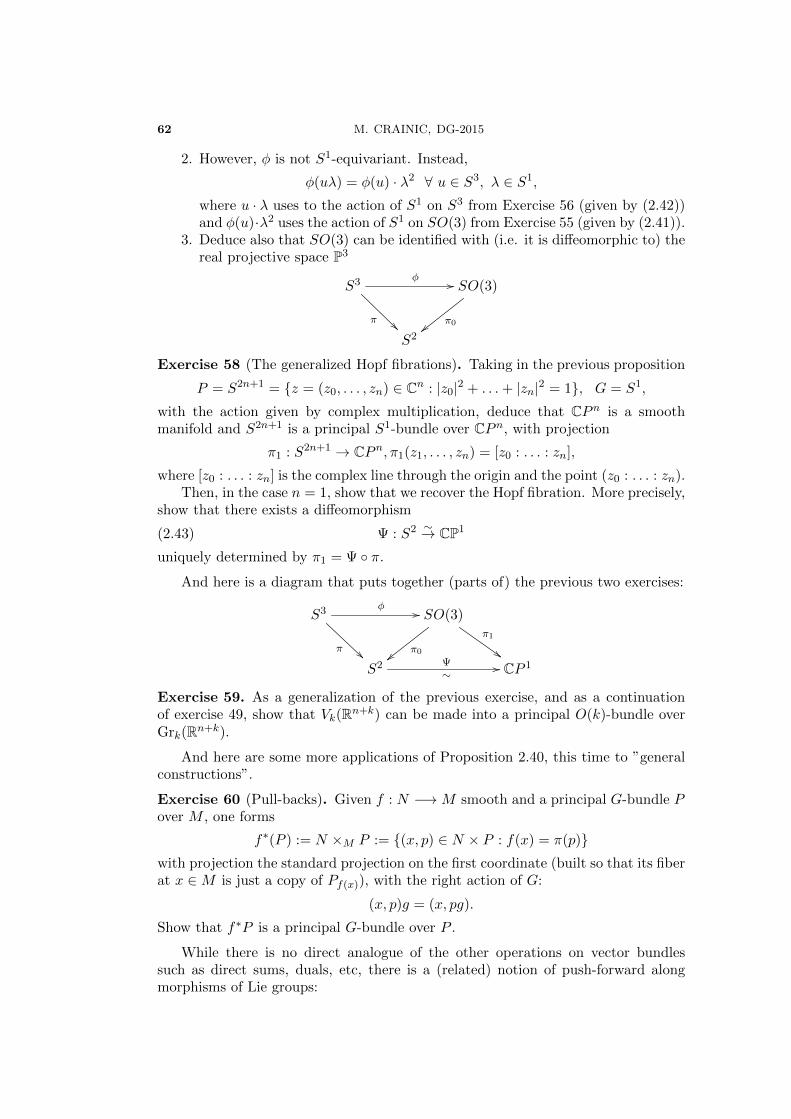
62 M. CRAINIC, DG-2015
2. However, φ is not S1-equivariant. Instead,
φ(uλ) = φ(u) · λ2 ∀ u ∈ S3, λ ∈ S1,
where u · λ uses to the action of S1 on S3 from Exercise 56 (given by (2.42))and φ(u)·λ2 uses the action of S1 on SO(3) from Exercise 55 (given by (2.41)).
3. Deduce also that SO(3) can be identified with (i.e. it is diffeomorphic to) thereal projective space P3
S3 φ //
π
SO(3)
π0||S2
Exercise 58 (The generalized Hopf fibrations). Taking in the previous proposition
P = S2n+1 = z = (z0, . . . , zn) ∈ Cn : |z0|2 + . . .+ |zn|2 = 1, G = S1,
with the action given by complex multiplication, deduce that CPn is a smoothmanifold and S2n+1 is a principal S1-bundle over CPn, with projection
π1 : S2n+1 → CPn, π1(z1, . . . , zn) = [z0 : . . . : zn],
where [z0 : . . . : zn] is the complex line through the origin and the point (z0 : . . . : zn).Then, in the case n = 1, show that we recover the Hopf fibration. More precisely,
show that there exists a diffeomorphism
(2.43) Ψ : S2 ∼→ CP1
uniquely determined by π1 = Ψ π.
And here is a diagram that puts together (parts of) the previous two exercises:
S3 φ //
π
SO(3)
π0||
π1
##S2
∼Ψ // CP 1
Exercise 59. As a generalization of the previous exercise, and as a continuationof exercise 49, show that Vk(Rn+k) can be made into a principal O(k)-bundle overGrk(Rn+k).
And here are some more applications of Proposition 2.40, this time to ”generalconstructions”.
Exercise 60 (Pull-backs). Given f : N −→M smooth and a principal G-bundle Pover M , one forms
f∗(P ) := N ×M P := (x, p) ∈ N × P : f(x) = π(p)with projection the standard projection on the first coordinate (built so that its fiberat x ∈M is just a copy of Pf(x)), with the right action of G:
(x, p)g = (x, pg).
Show that f∗P is a principal G-bundle over P .
While there is no direct analogue of the other operations on vector bundlessuch as direct sums, duals, etc, there is a (related) notion of push-forward alongmorphisms of Lie groups:

2.2. Principal bundles 63
Exercise 61. Morphisms ρ : H −→ G of Lie groups induce operations P 7→ ρ∗(P )which associate to a principal H-bundle P a principal G-bundle ρ∗(P ).
To be more precise, let π : P →M be a principal H-bundle. Consider
ρ∗(P ) := (P ×G)/H,
the quotient of P ×G modulo the action of H given by (p, g)h = (ph, gρ(h)). Showthat, denoting by [p, g] ∈ ρ∗(P ) the class of (p, g) ∈ P ×G, the ”projection”
π : ρ∗(P ) −→M, [p, g] 7→ π(p)
and the G-action [p, g] · g′ = [p, gg′] make ρ∗(P ) into a principal G-bundle over M .
Exercise 62. Consider the following two principal S1-bundles over S2: SO(3) asin Exercise 55 and S3 as in Exercise 56. Consider the group homomorphism
ρ : S1 → S1, ρ(z) = z2.
Using the map φ from Exercise 57 show that ρ∗(S3) is isomorphic to SO(3), as
principal S1-bundles.
We now return to the general remarks on the principal bundle axioms; here isanother way:
Exercise 63. Assume that G acts on the manifold P from the right and thatπ : P −→M is a surjective submersion. Show that P is a principal G-bundle if andonly if (2.39) is well-defined and it is a diffeomorphism.
Yet another (equivalent) way to look at/define/produce principal bundles is tostart with a setting in which P is only a set (endowed with an action of G) and therest of the data is used to put the smooth structure on P .
Exercise 64. Formulate and prove an analogue of Exercise 1 for principal bundles.
And, in the same direction, one has the description of principal bundles in termsof transition functions that we now outline. Let π : P →M be a principal G-bundlein the sense of our original definition. In particular, we find a collection of localsections
σi ∈ Γ(P |Ui), i ∈ I (I − some indexing set)
defined over opens Ui ⊂ M such that U = Uii∈I is an open cover of M . On theoverlaps Ui ∩ Uj we can consider the quotient of σj and σi:
gi,j : Ui ∩ Uj → G, gi,j(x) = [σj(x) : σi(x)].
(see (2.38)). These functions are called the transition functions of P with respect tothe given collection of local sections. As it can readily be seen, they satisfy the socalled ”cocycle relations”: for x ∈ Ui ∩ Uj ∩ Uk, one has
gi,k(x) = gi,j(x)gj,k(x).
One also has gi,i(x) = e for all x ∈ Ui and gj,i(x) = (gi,j(x))−1 for all x ∈ Ui ∩ Uj ,but these are just formal consequences of the previous equations (check that!).
Exercise 65. Assume that M is a manifold, G is a Lie group, U = Uii∈I is anopen cover of M and gi,j : Ui∩Uj → G is a collection of smooth functions satisfyingthe previous cocycle relations.
Construct a principal G-bundle π : P → M with the property that it admitsa collection of local sections as above, so that the associated transition functionsare precisely gi,j . Then show that any two principal bundles with this property areisomorphic.
64 M. CRAINIC, DG-2015
2.2.3. From vector bundles to principal bundles (the frame bundle)
The main aim of this and the next subsection is to prove (and understand) in detailthe intepretation of vector bundles via principal bundles; as a simplified version, westate here:
Theorem 2.44. For any manifold M and any r ≥ 0 integer, there is a 1-1 corre-spondence between (isomorphism classes of) vector bundles of rank r over M andprincipal GLr-bundles over M .
In this subsection we go in one direction. Actually, with Exercise 54 in mind, itshould be rather clear how to go from vector bundles to principal bundles: startingwith a vector bundleE of rank r over M (real or complex), one forms the framebundle associated to E
Fr(E) = (x, u) : x ∈M,u− a frame of Ex.
It comes with an action of GLr from the right, that we could just write downexplicitly right away; but this is a good moment to discuss a bit more the notion offrame and be clearer about our conventions. For simplicity, we work over R.
First of all, we write a matrix A ∈ glr as
A = (Aij)1≤i,j≤r
by which we mean that
A =
A11 . . . A1
r
. . . . . . . . .Ar1 . . . Arr
Therefore, the usual product of two matrices is given by
(A ·B)ij =∑k
AikBkj .
Any matrix A gives rise to a linear map
A : Rr → Rr
defined on the canonical basis e1, . . . , er of Rr by
A(ej) =
r∑i=1
Aijei;
however, we often omit the hat from the notation, i.e. we will identify the matrix Awith the linear map that it induces. Note that, for two matrices A and B, one has
AB = A B,
i.e. the notations are chosen so that, when writing AB, it does not matter whetherwe interpret it as matrix multiplication or as composition of linear maps.
Keeping for the moment the notation A note that, on a general vector v =v1e1 + . . .+ vrer, one has
A(v) =∑i
(∑j
Aijvj)ei.

2.2. Principal bundles 65
To write also this formula in terms of matrix multiplication, one associates to anyv ∈ Rr the column matrix
[v] =
v1
. . .vr
With this, the previous formula becomes
[A(v)] = A · [v]
where ”·” refers to the multiplication of matrices. While we identify matrices Awith the associated linear maps A, we will also identify the vectors v ∈ Rr with theassociated column matrices [v]; so, we will just omit the brackets in the notation [·].
We now pass to an arbitrary r-dimensional vector space V and we consider theset Fr(V ) of all frames of V , i.e ordered collections
φ = (φ1, . . . , φr)
of vectors φi ∈ V that form a basis of V . While any r-dimensional vector space Vcan be identified with (i.e. it is isomorphic to) the standard model Rr, there is nosuch canonical identification. Choosing a frame should be seen as choosing such anidentification; indeed, one has the following simple:
Exercise 66. For φ = (φ1, . . . , φr) ∈ Fr(V ), consider the linear map
φ : Rr → V
that sends the component ei of the standard basis of Rr to φi, for each i. Show thatφ←→ φ defines a 1-1 correspondence between frames of V and linear isomorphismfrom Rr to V .
It should now be clear how GLr acts on Fr(V ) (from the right!):
Fr(V )×GLr → Fr(V ), (φ,A) 7→ φ ·Aso that
φ ·A = φ A.(and, again, we just omit the hat from the notation φ). We find the explicit formula:
(φ ·A)i =
i∑Ajiφj .
Returning to a general rank r vector bundle E → M , the frame bundle Fr(E)just puts together the frame spaces Fr(Ex) of all the fibers; the action of GLr onthese spaces defines a (free, right) action of GLr on Fr(E). There are various waysto exhibit the smooth structure on Fr(M); one of the most intuitive ones comesfrom the fact that we know which local sections of Fr(E) we want to be smooth:any local frame of the vector bundle E. This (together with Exercise 64) specifiesthe smooth structure on Fr(E) and it is not difficult to see that it does, indeed, aprincipal GLr-bundle over M .
Exercise 67. Provide the details.
Exercise 68. Describe an embedding i : SO(3) → Fr(TS2) such that the compo-sition of the projection Fr(TS2) → S2 with i is the projection π0 from Exercise55. Why is i an embedding? Make sense of the statement: ”SO(3) is the orientedorthonormal frame bundle associated to TS2”.
66 M. CRAINIC, DG-2015
Here are some exercises which show that, if one looks for an analogue of thevarious standard operations on vector bundles (such as taking duals, direct sumsetc) that applies to principal bundles, then one has to look at morphisms of Liegroups and the corresponding push-forward operations (Exercise 61 ):
Exercise 69. Consider the group homomorphism
ρ : GLr −→ GLr, ρ(A) = t(A−1).
Show that for any vector bundle E, the frame bundles associated to E and to itsdual are related by
Fr(E∗) ∼= ρ∗(Fr(E)).
Exercise 70. Show that if πi : Pi −→ M are principal Gi-bundles, for i ∈ 1, 2,then ”the fibered product”
P1 ×M P2 := (p1, p2) ∈ P1 × P2 : π1(p1) = π2(p2)carries a natural structure of principal G1 ×G2-bundle.
Assume now that Pi = Fr(Ei) is the frame bundles associated to a vector bundlesEi of rank ri (hence also Gi = GLri), i ∈ 1, 2. Consider r = r1 + r2 and the grouphomomorphism
ρ : GLr1 ×GLr2 −→ GLr, (A,B) 7→ A⊕B := diag(A,B).
Show that the frame bundle associated to E1⊕E2 is isomorphic to the push-forwardof P1 ×M P2 via ρ.
2.2.4. From principal bundles to vector bundles
We now describe a reverse construction, which associates to principal GLr-bundlesvector bundles. Actually, we proceed in a slightly more general setting, for a generalLie group G.
What we need is a principal G-bundle π : P −→ M as well as a representationρ : G −→ GL(V ) of G on a finite dimensional vector space (again, over R or C). Tosuch data we will associate a vector bundle
E(P, V )
over M , of rank equal to the dimension of V , called the vector bundle obtainedby attaching to P the representation (V, ρ) (a more faithful notation would beE(P,G, V, ρ), but G and ρ are usually clear from the context). Of course, whenreturning to the 1-1 correspondence between vector bundles and principal bundles,we will apply this construction to G = GLr, and ρ the canonical representation ofmatrices as linear maps on V = Rr.
In this general farmework, the representation ρ encodes a linear action of G onV from the left which, combined with the right action of G on P , induces a (right)action of G on P × V :
(p, v) · g := (pg, g−1v).
We then define E(P, V ) as the resulting quotient
E(P, V ) := (P × V )/G
and we denote by [p, v] ∈ E(P, V ) the element in E(P, V ) represented by (p, v) ∈P ×G; hence, in the quotient,
[pg, v] = [p, gv]

2.2. Principal bundles 67
for all p ∈ P , v ∈ V , g ∈ G. We endow E(P, V ) with the projection
π : E(P, V ) −→M, π(p, v) = π(v).
Note that the fiber of π above an arbitrary point x ∈M ,
E(P, V )x = [p, v] : p ∈ Px, v ∈ V .The following is a simple exercise:
Exercise 71. Show that there exists a unique vector space structure on the fibersE(P, V )x such that, for each p ∈ P with π(p) = x,
φp : V → E(P, V )x, v 7→ [p, v],
is an isomorphism of vector spaces.
To describe the smooth structure on E(P, V ) one can proceed in several ways.One is to use again the theorem on the smoothness of quotients (Theorem 2.35), i.e.apply Prroposition 2.40; for that one just needs the simple remark that, since theaction of G on P is free and proper, so is the action on P × V . Another way to seethat E(P, V ) is a smooth vector bundle is to use local trivializations of P :
Ψ : P |U −→ U ×Gand note that any such trivialization induces a trivialization of E(P, V ):
Ψ : π−1(U) −→ U × V, p 7→ (π(p), gΨ(p)v),
where gΨ(p) ∈ G is the second component of Ψ(p). Of course, the local trivializations
Ψ will serve as charts of a smooth atlas for E(P, V ).
Corollary 2.45. For any principal G-bundle P over M and any representation Vof G, E(P, V ) is a vector bundle over M .
As we mentioned, this construction is particularly interesting in the case when
G = GLr, V = Rr, ρ = Id,
when it associates to a principal GLr bundle P the vector bundle E(P,Rr). Let usapply this to the frame bundle
P = Fr(E)
of a vector bundle E of rank r over M . In this case, since an element p ∈ Px isthe same thing as the choice of an isomorphism ip : Rr −→ Ex, we see that that apair [p, v] ∈ E(P,Rr)x can be identified with ip(v) ∈ Ex. In other words, one has anisomorphism of vector bundles over M :
E(P,Rr) ∼−→ E, [p, v] 7→ ip(v).
Putting everything together, we find:
Theorem 2.46. The constructions which associate:
• to a vector bundle E its frame bundle Fr(E)• to a principal GLr-bundle P the vector bundle E(P,Rr)
defines a 1-1 correspondence between (isomorphism classes of) vector bundles ofrank r over M and principal GLr-bundles over M .
Here are some concrete illustrations of the general construction from this sub-section.
68 M. CRAINIC, DG-2015
Exercise 72. Consider the principal S1-bundle π0 : SO(3) −→ S2 from Exercise55. Consider also the representation of S1 on R2 given by
r : S1 → GL2(R) = GL(R2), cos(α) + i sin(α) 7→(
cos(α) sin(α)− sin(α) cos(α)
).
Show that the associated vector bundle E(SO(3),R2, r) is isomorphic to the tangentbundle of S2.
Exercise 73. Consider the Hopf fibrations, i.e. the principal S1-bundle π : S3 −→S2 from Exercise 55. Consider also the square r2 of the representation from theprevious exercise, i.e.
r2 : S1 → GL2(R) = GL(R2), cos(α) + i sin(α) 7→(
cos(2α) sin(2α)− sin(2α) cos(2α)
).
Show that the associated vector bundle E(S3,R2, r2) is isomorphic to the tangentbundle of S2.
Exercise 74. Consider again the Hopf fibration, but use now the representation rto build the new vector bundle E = E(S3,R2, r) over S2. Show that this correspondsto the tautological line bundle over CP 1. More precisely:
• recall that we have the tautological complex line bundle L over CP 1 definedas the following sub-bundle of the trivial bundle CP 1 × C2:
E := (l, v) : l ∈ CP1, v ∈ l ⊂ CP1 × C2,
• recall that there we have a diffeomorphism Ψ : S2 → CP 1 constructed inExercise 58 (see (2.43)),
and show that E is isomorphic to Ψ∗(L), as vector bundles over S2.
2.2.5. Sections/forms for vector bundles associated to principal ones
Due to the importance of sections of a vector bundle E as well as of the space ofE-valued differential forms (e.g. when discussing connections), when
E = E(P, V )
is the vector bundle associated to a principal G-bundle π : P →M and a represen-tation ρ : G→ GL(V ), it is useful to rewrite those spaces more directly in terms ofthe starting data: the principal bundle and the representation. That is what we doin this subsection; hence, we place ourselves in the previous setting.
For sections of E(P, V ), the important space is C∞(P, V )- the space of smoothfunctions on P with values in the vector space V , and the fact that this space comesenowed with a canonical (linear) action of G:
G× C∞(P, V )→ C∞(P, V ), (g, f) 7→ g · f,
induced by the actions of G on P and V by:
(g · f)(p) = ρg(f(pg)).
Exercise 75. Check that this defines, indeed, a left action.
As for any action of a group, we can talk about the space of G-invariant elements:
C∞(P, V )G := f ∈ C∞(P, V ) : g · f = f ∀ g ∈ G.
2.2. Principal bundles 69
The key-point is that any such G-equivariant function f induces a section of E(P, V ):first of all it induces
(id, f) : P −→ P × V, p 7→ (p, f(p))
which is equivariant (where the right action of G on P ×V is precisely the one usedto define E(P, V )); hence, passing to the quotient modulo G, it induces a map
sf : M −→ E(P, V ).
Lemma 2.47. If E = E(P, V ) is the associated vector bundle, then one has abijection
C∞(P, V )G∼−→ Γ(E), f 7→ sf .
Proof. Smooth functions f : P → V are in 1-1 correspondence with sections of thetrivial vector bundle P × V over P : to f one associates
sf : P → P × V, sf (p, v) = (p, f(v)).
Moreover, the equivariance of f is equivalent to sf being equivariant, where P × Vis endowed with the action of G used to define E. This implies that sf descends toa map
sf : M → (P × V )/G = E,
which is a section of E. A minute of thinking reveals that this discussion can easilybe reversed.
Let us now generalize this construction to E-valued differential forms on M ofarbitrary degreree k (i.e. going from k = 0 to arbitrary k). Of course, instead ofC∞(P, V ) we now consider the space Ωk(P, V ) of forms on P with values in thevector space V . As above, one has an action of G on this space:
G× Ωk(P, V )→ P, (g, ω) 7→ g · ω,built out from the action of G on P and V ; explicitely,
(g · ω)(−) := ρg(R∗g(ω)(−)),
where R∗g is the pull-back of forms via the right multiplication by g, Rg : P −→ P ,
Rg(p) = pg. Hence, on vectors Xip ∈ TpP , 1 ≤ i ≤ k:
(g · ω)p(X1, . . . , Xk) = ρ(g)(ωpg((dRg)p(X
1), . . . , (dRg)p(Xk))).
This allows us to talk about G-invariant V -valued forms on P . However, this is notquite the space we are interested in. We also have to make use of the infinitesimalaction of g (the Lie algebra of G) on P induced by the action of G on P (cf.Proposition 2.29):
a : g −→ X (P ), a(v)p = ap(v) :=d
dt
∣∣∣∣t=0
p · exp(tv).
Definition 2.48. We say that a differential form ω ∈ Ωk(P, V ) is:
• equivariant: if g · ω = ω for all g ∈ G.• horizontal: if ia(v)(ω) = 0 for all v ∈ g.• basic: if it is both equivariant as well as horizontal.
We denote by Ωk(P, V )hor the space of horizontal differential forms and by Ωk(P, V )bas
the space of basic forms.
Here is an exercise explaining the term ”horizontal”:
70 M. CRAINIC, DG-2015
Exercise 76. For Xp ∈ TpP (p ∈ P , x = π(p)), the following are equivalent:
1. Xp is tangent to the fiber Pp = π−1(x).2. Xp is killed by (dπ)p : TpP → TxM .3. Xp = ap(v) for some v ∈ g (necessarily unique).
When this happens we say that X is a vertical tangent vector (at p); the space ofsuch vectors is denoted
T vertp P ⊂ TpP (hence T vert
p P = Ker(dπ)p = Tp(Pp) = Im(ap)).
A vector field X on P is called vertical if Xp is vertical for all p ∈ P . Deduce that a
form ω ∈ Ωk(P, V ) is horizontal if and only if it vanishes on all vertical vector fields.
Proposition 2.49. If E = E(P, V ) is the associated vector bundle, then one has alinear isomorphism
π• : Ωk(M,E)∼−→ Ωk(P, V )bas.
Proof. We start with two remarks. The first one is that that the pull-back π∗E ofthe vector bundle E via the projection π : P −→ M is, as a vector bundle over P ,isomorphic to the trivial vector bundle P × V , by a canonical isomorphism
i : P × V −→ π∗(E).
At the fiber at p ∈ P , this is simply
ip : V −→ Eπ(p), v 7→ [p, v].
The second remark is that the usual pull-back of forms along π : P −→ M makessense for forms with coefficients, giving rise to
π∗ : Ωk(M,E) −→ Ωk(P, π∗E).
Explicitely, for X1, . . . , Xk ∈ TpP ,
(2.50) π∗(ω)(X1, . . . , Xk) = ω((dπ)p(X1), . . . , (dπ)p(X
k)) ∈ Eπ(p) = (π∗E)p.
Combining the isomorphism from the previous remark, we consider
π• := i−1 π∗ : Ωk(M,E) −→ Ωk(P, V ).
The rest of the proof consists of the following rather straightforward steps (detailsare left as small exercises):
1. Check directly that π• actually takes values in Ωk(P, V )bas (for instance, since(dπ) kills the vertical vector fields, all forms of type π∗ω are horizontal).
2. The map π• is injective (since the differential of π is surjective).3. One still has to show that each η ∈ Ωk(P, V )bas can be written as π∗ω for
some ω. Explicitely, one wants
ωπ(p)((dπ)p(X1), . . . , (dπ)p(X
k)) = ip(ηp(X1, . . . , Xk)).
for all p ∈ P Xi ∈ TpP . But this forces the definition of ω: for x ∈ Mand V i ∈ TxM , choosing p ∈ P with π(p) = x and choosing Xi ∈ TpP with(dπ)p(X
i) = V i, we must have
ωx(V 1, . . . , V k) = ip(ηp(X1, . . . , Xk)).

2.3. Connections on principal bundles 71
4. What is left to check is that this definition does not depend on the choices wemade. First of all, once p ∈ π−1(x) is chosen, the formula does not dependon the choice of the Xi’s- this follows from the fact that η is horizontal.The independence of the choice of the point p in π−1(x) follows from theG-invariance of η and the fact that any other q ∈ π−1(x) can be written asq = pg for some g ∈ G.
2.3. Connections on principal bundles
Throughout this subsection G is a Lie group and π : P −→ M is a principal G-bundle. There are several different ways of looking at connections on P . We startwith the more intuitive one.
2.3.1. Connections as horizontal distributions:
A horizontal subspace of TP at p ∈ P is a subspace
Hp ⊂ TpPwith the property that
(2.51) (dπ)p|Hp : Hp −→ Tπ(p)M
is an isomorphism.
Exercise 77. Show that, for a vector sub-space Hp ⊂ TpP , denoting x = π(p) andusing the vertical space T vert
p P from Exercise 76, the following are equivalent:
1. Hp is horizontal.2. Hp is a complement of T vert
p inside TpP .3. (dπ)p : TpP → TxM restricts to an isomorphism between Hp and TxM .4. There exists a splitting of (dπ)p, i.e. a linear map
hp : TxM → TpP
satisfying (dπ)p hp = Id, such that Hp is the image of hp.(Read: hp is the operation of ”horizontal lifting” associated to Hp).
Note that if Hp is a horizontal space at p ∈ P then, for any g ∈ G,
Rg(Hp) := (dRg)p(Xp) : Xp ∈ Hp ⊂ TgpPis another horizontal subspace at gp. By distribution on P we mean a vector sub-bundle H of TP (hence a collection Hpp∈P of vector sub-spaces Hp of TpP , all ofthe same dimension, which fits together into a smooth submanifold H of TP ).
Definition 2.52. A connection on P is a distribution H on P with the propertythat each Hp is a horizontal subspace of P and
Hpg = Rg(Hp) ∀ p ∈ P, g ∈ G.
While the notion of vertical vector fields on P is intrinsic (it does not depend onany choices), a connection allows us to talk about horizontal vectors on P : the onesthat lie in H (hence one should really make a reference to H in the terminology- e.g.talk about H-horizontal). Note that any vector field on M has a lift to a horizontalvector field on P , i.e. there is an operation
h : X (M) −→ X (P )
72 M. CRAINIC, DG-2015
(the horizontal lift operation associated to the connection) which associates to X ∈X (M) the unique horizontal vector field h(X) on P satisfying
(dπ)p(h(X)p) = Xπ(p)
for all p ∈ P . With the notations from the previous exercise, h(X)p := hp(Xπ(p)).
For the curious reader. Putting all the possible horizontal liftings together we obtain the so-called first orderjet of P ,
J1(P ) := (p, hp) : p ∈ P, hp is a horizontal lifting of P at p.
This can be seen as a (discrete for now) bundle over P (using the projection on the first coordinate) and also as abundle over M by further composing with the projection π : P −→M . The terminology comes from the fact thatthis set encodes all the possible first order data (jets) associated to (local) sections of P . More precisely, givenx ∈M , any local section σ of P defined around x, induces:
• the 0-th order data at x: just the value σ(x) ∈ P .• the 1-st order data at x: the value σ(x) together with the differential of σ at p (which encodes the first
order derivatives of σ at x),
(dσ)x : TxM −→ Tσ(x)P.
Of course, (dσ)x is a horizontal lifting at σ(x) and it is not difficult to see that
J1(P ) = (σ(x), (dσ)x) : x ∈M,σ − local section of P defined around p.
Note that for a section σ of P , the resulting map
j1(σ) : M −→ J
1(P ), x 7→ (σ(x), (dσ)x))
is a section of J1(P ) viewed as a bundle over P . Similarly for local sections. There is a natural smooth structure
on J1(P ) uniquely determined by the condition that all local sections of type j1(σ) are smooth.
2.3.2. Connection forms
Here is a slightly different point of view on connections, not so natural, but ofteneasier to work with. Let g be the Lie algebra of G. We will use the infinitesimalaction of g on P (see Proposition 2.29),
a : g −→ X (P ), a(v)p =d
dt
∣∣∣∣t=0
p · exp(tv),
and the adjoint representation of G on g (see Example 2.21),
Ad : G −→ GL(g), g 7→ Adg.
The general discussion from subsection 2.2.5 gives us the notion of G-invariant formson P with values in g: those θ ∈ Ωk(P, g) with the property that
R∗g(ω) = Adg−1(ω)
for all g ∈ G.
Definition 2.53. A connection form on P is a 1-form
ω ∈ Ω1(P, g)
with the property that it is G-invariant and satisfies
ω(a(v)) = v ∀ v ∈ g.
Proposition 2.54. There is a bijection between connection 1-forms ω ∈ Ω1(P, g)and connections H on P . The bijection associates to ω its kernels:
Hp := Xp ∈ TpP : ωp(Xp) = 0.
2.3. Connections on principal bundles 73
Proof. For each p ∈ P we consider the short exact sequence of vector spaces
gap−→ TpP
(dπ)p−→ Tπ(p)M.
A right splitting of this sequence is a right inverse of (dπ)p; as we have noticed, suchright splittings hp correspond to horizontal subspaces Hp. On the other hand onecan also talk about left splitting of the sequence, by which we mean a left inverse ofap or, equivalently, linear maps ωp : TpP −→ g satisfying ωp(ap(v)) = v for all v ∈ g.What we need here is a simple linear algebra fact which says that, for a short exactsequence of vector space, there is a 1-1 correspondence between the choice of rightsplittings hp and the choice of left splittings ωp. Explicitely, this correspondence isdescribed by the equation
ap ωp + hp (dπ)p = Id.
After applying this at all p ∈ P , one obtains the 1-1 correspondence from thestatement. Of course, one still has to check that the smoothness of ω is equivalent tothe one of h and similarly for the G-invariance, but we leave these as an exercise.
Exercise 78. Consider the interpretation of S3 in terms of quaternions (Example2.2); remark that, for any u ∈ S3,
iu, ju, ku ∈ H ∼= R4
are orthogonal to u, i.e. they define vectors tangent to S3 at u. Hence, each of theseelements defines a vector field on S3; they are denoted X1 (using i), X2 (using j)and X3 (using k). For instance,
X1(x, y, z, t) = −y ∂∂x
+ x∂
∂y− t ∂
∂z+ z
∂
∂t∈ Tx,y,z,tS3 ⊂ Tx,y,z,tR4.
We also consider the coframe θ1, θ2, θ3 associated to the frame X1, X2, X3, i.e. thecollection of 1-forms on S3 uniquely determined by θi(Xj) = δij .
1. Show that the flow of X1 induces the action of S1 on S3 from the Hopffibration (Example 56).
2. Compute the differentials of each θi and write them in terms of wedge of θ1,θ2 and θ3.
3. Show that θ1 can be interpreted as a connection on the Hopf fibration.
2.3.3. Parallel transport
As in the case of vector bundles, connections on principal bundles have associatedparallel transports. Assume we fix a connection H on the principal G-bundle π :P −→M , with associated connection form ω. Then we say that a curve u : I −→ Pis horizontal if
u(t) ∈ Hγ(t) ∀ t ∈ I,where γ(t) = π(u(t)). Then, completely similar to Lemma 1.21, we have:
Lemma 2.55. Let γ : I −→ M be a curve in M , t0 ∈ I. Then for any u0 ∈ Pγ(t0)
there exists and is unique a horizontal path above γ, u : I −→ P , with u(t0) = u0.
Proof. Again, we may work locally, i.e. we may just assume that P = M × G isthe trivial principal bundle. Let us now see what a connection form on this bundle
74 M. CRAINIC, DG-2015
looks like. First of all, the invariance condition means that, for all (x, a) ∈ M ×G,(Xx, Va) ∈ Tx,a(M ×G) = TxM × TaG, and for all g ∈ G,
ωx,ag(Xx, Rg(Va)) = Adg−1(ωx,a(Xx, Va)),
where we denote by Rg : G −→ G the right multiplication by g and also its differ-ential (dRg)a : TaG −→ TagG. Taking a = 1, we see that ω is determined by allthe expressions of type ωx,1(Xx, v) with 1 ∈ G the unit, v ∈ T1G = g. In turn, thecondition that ω(a(v)) = v for all v ∈ g implies that ω is uniquely determined by allexpressions of type
ωx,1(Xx, 0) ∈ g
i.e. precisely by the restriction η ∈ Ω1(M, g) of ω toM via the inclusionM →M×G,x 7→ (x, 1). Writing down the explicit formulas we find that the formula for ω interms of η:
ωx,g(Xx, Vg) = Adg−1(ηx(Xx)) + Lg−1(Vg),
where, as before, Lg−1 : G −→ G stands for the left multiplication by g−1 and alsofor its differential (dLg−1)g : TgG −→ T1G = g.
A curve in P = M ×G above γ can be written as
u(t) = (γ(t), g(t)).
The fact that it is horizontal means that u(t) takes values in the horizontal spaceor, equivalently, that it is killed by ω:
ωγ(t),g(t)(γ(t), g(t)) = 0 ∀ t ∈ I.Using the previous formula for ω we see that this equation becomes
g(t) = −Rg(t)(ηγ(t)(γ(t))).
For fixed γ we need existence and uniqueness of g satisfying this equation, with aninitial condition g(t0) = g0 given. We denote v(t) = −ηγ(t)(γ(t) (curve in g, so thatthe equation reads g(t) = Rg(t)(v(t))). At least for linear groups G ⊂ GLr we dealagain (as in the case of vector bundles) with an ordinary ODE. For a general Liegroup one can just interpret this equation as the flow equation of the time-dependentvector field X(t, g) on G given by
X(t, g) = Rg(v(t))
and use the standard results about flows of time-dependent vector fields. However,one still has to make sure that the equation with the given initial condition g(t0) = g0
exists on the entire interval I on which v is defined; for that one uses the remarkthat, if g(t) is an integral curve then so is h(t) = g(t)a for all a ∈ G:
h(t) = Ra(g(t)) = Ra(Rg(t)(v(t)) = Rh(t)(v(t)).
Finally, as in the case of vector bundles, for curves γ : I −→M , t0, t1 ∈M , oneobtains the parallel transport (with respect to the connection) along γ:
T t0,t1γ : Pγ(t0) −→ Pγ(t1)
which associates to u0 ∈ Pγ(t0) the element u(t1) ∈ Pγ(t1), where u is the horizontalpath above γ with u(t0) = u0.
Exercise 79. Show that T t0,t1γ are diffeomorphisms and are G-equivariant.

2.3. Connections on principal bundles 75
2.3.4. Curvature
Let H be a connection on P , with associated horizontal lifting h and connection 1-form ω. The curvature ofHmeasure the failure ofH to be involutive or, equivalently,the failure of the horizontal lifting h to preserve the Lie bracket of vector fields.However, let us introduce it in the form that is easier to work with. For that wenote that the Lie bracket [·, ·] of the Lie algebra g extends to a bracket
[·, ·] : Ω1(P, g)× Ω1(P, g) −→ Ω2(P, g),
[α, β](X,Y ) := [α(X), β(Y )]− [α(Y ), β(X)].
Note that when β = α ∈ Ω1(P, g) one obtains
[α, α](X,Y ) = 2[α(X), α(Y )].
Definition 2.56. The curvature of the connection ω is defined as
K := dω +1
2[ω, ω] ∈ Ω2(P, g).
Here is the main property of the curvature (for basic forms see subsection 2.2.5):
Lemma 2.57. The curvature is a basic form:
K ∈ Ω2(P, g)bas.
Proof. The G-invariance follows from the G-invariance of ω and the fact that all theoperations involved in construction K (d and the bracket) are natural (functorial),hence are respected by the action of G (give the details!). The fact that K ishorizontal . . .
Note that the fact that Ω is horizontal implies that, in order to know Ω, it sufficesto know all the expressions of type
K(h(X), h(Y )) ∈ C∞(P, g)
with X,Y ∈ X (M), where h(X) ∈ X (M) is the horizontal lift of X with respect tothe connection. For the following, recall that a : g −→ X (P ) denotes the inducedinfinitesimal action (see above).
Proposition 2.58. The curvature can also be characterized as:
1. the horizontal part of dω, i.e. the horizontal form on P (with values in g)which coincides with dω on horizontal vectors.
2. the unique horizontal form Ω with the property that, after applying the infin-itesimal action a : g −→ X (P ),
a(K(h(X), h(Y ))) = h([X,Y ])− [h(X), h(Y )]
for all X,Y ∈ X (M).
Proof. We have already shown that K is horizontal and then the first part is clearfrom the very definition of K. For the second part, by the comments before theproposition and the injectivity of a, the uniqueness follows. Hence we just have toshow that the actual curvature does have this property. For that one just computeK(h(X), h(Y )) using the definition of K and the fact that ω h = 0 and we find:
K(h(X), h(Y )) = −ω([h(X), h(Y )]) = ω(h([X,Y ])− [h(X), h(Y )]).
On the other hand, since h(X) is π-projectable to X, we have that [h(X), h(Y )] isπ-projectable to [X,Y ] and then h([X,Y ])−[h(X), h(Y )] is π-projectable to [X,Y ]−
76 M. CRAINIC, DG-2015
[X,Y ] = 0, i.e. it is vertical. Hence, at each point p, it is of type a(vp) with somevp ∈ g. Plugging in the previous equation, we find that
K(h(X), h(Y ))(p) = ω(a(vp)) = vp,
and then the desired equation follows is just the defining property of vp.
Exercise 80. As a continuation of Exercise 78: show that the curvature of theconnection defined by θ1 is a non-zero constant (that you have to compute) timesthe area form σ of S2,
σ = xdy ∧ dz + ydz ∧ dx+ zdx ∧ dy ∈ Ω2(S2).
(be aware: the forms dx, etc make sense on the entire R3, but we only use theirrestrictions to S3. And, while the forms dx, dy and dz are linearly independent onR3, their restrictions to S2 do satisfy an extra-relation: xdx+ydy+zdz = 0 (why?)).
2.3.5. Principal bundle connections ←→ vector bundles ones
While we have seen that vector bundles of rank r are in 1-1 correspondence withprincipal GLr-bundles, we now show that connections on vector bundles correspond(1-1) to connections on the associated principal bundles.
In one direction (from principal to vector) one can proceed, as before, slightlymore generally, by starting with any Lie group G, a principal G-bundle π : P −→Mand a representation ρ : G −→ GL(V ). The relevant vector bundle will be E =E(P, V ) previously discussed. We start with a connection on the principal G-bundleP and we would like to construct a connection ∇ on E; we will encode ∇ in theoperator
d∇ : Γ(E) −→ Ω1(M,E).
Using Proposition 2.49 we see that it suffices to describe the
D∇ := h•d∇(h•)−1 : C∞(P, V )G −→ Ω1(P, V )bas.
Proposition 2.59. For any connection ω on P ,
D∇ : C∞(P, V )G −→ Ω1(P, V )bas, D(f) = df + ρ(ω(−))f
(where ρ(ω(−))f is the V -valued 1-form on P given by X 7→ ρ(ω(X))(f)) inducesa connection ∇ on the vector bundle E.
Proof. Direct check.
Next, we consider the converse procedure: from vector bundle connections toprincipal ones. Start with a vector bundle E and a connection ∇ on E. We considerthe associated frame bundle Fr(E), a principal GLr-bundle, and we want to asso-ciated to ∇ a connection on Fr(E). We will do that by constructing a connection1-form
ω∇ ∈ Ω1(Fr(E), glr).
We have to say what it does on an arbitrary vector
d
dt
∣∣∣∣t=0
e(t) ∈ Te(0)Fr(E),
where
R 3 t 7→ e(t) = (e1(t), . . . , er(t)) ∈ Fr(E)

2.3. Connections on principal bundles 77
is a curve in Fr(E). Let γ : R −→M be the base curve of e. Consider the derivativesof the paths ei with respect to ∇ (see 1.2.3) and decompose them with respect tothe frame e(t):
∇eidt
(t) =∑j
aji (t)ej(t)
giving rise to the matrix
e(t)−1 · ∇edt
(t) := (aji (t))i,j ∈ glr
(think that, while e(t) : Rr ∼−→ Eγ(t),∇edt (t) is a linear map from Rr to Eγ(t)). Set
now
ω∇(d
dt
∣∣∣∣t=0
e(t)) := e(0)−1 · ∇edt
(0) ∈ glr.
Theorem 2.60. For any connection ∇ on E, ω∇ is a connection 1-form on Fr(E),and this defines a bijection between connections on E and connections on the prin-cipal GLr-bundle Fr(E).
Proof. We first show that, for any ∇, ω∇ is a connection 1-form. Let us first provethat ω(ap(A)) = A for all e ∈ Fr(E), A ∈ glr. Recall that
ap : glr −→ TeFr(M), ae(A) =d
dt
∣∣∣∣t=0
e · exp(tA).
In the definition of ω above, we deal with the path t 7→ e · exp(tA) (which at t = 0is e), hence
ω(ap(A)) = e−1∇e · exp(tA)
dt(0).
Using the definitions (of ∇dt , as well as the fact that this operation on frames isdefined componentwise), the standard derivation rules apply and, since e is constanton t, we find
ω(ap(A)) = e−1e · dexp(tA)
dt(0) = A.
Next, we prove the invariance of ω. We have to show that for any path e(t) offrames,
ω((dRg)(de
dt(0)) = Adg−1ω(
de
dt(0)).
We start from the left hand side. We see that we deal with ω evaluated on the curveof frames e(t)g hence, by the definition of ω, the expression is
(e(0)g)−1∇egdt
(0) = (g−1e(0)−1)∇edt
(0)g
i.e. precisely
g−1ω(de
dt(0))g = Adg−1(ω(
de
dt(0)).
To show that ∇ 7→ ω∇ is a bijection one either remarks that the previous argu-ment can be read backwards, or checks directly that ∇ 7→ ω∇ composed with theoperation from the previous proposition is the identity.
Of course, it is not surprising that a similar story applies when looking at thenotion of curvature. More precisely, one can consider:

78 M. CRAINIC, DG-2015
• the curvature of the vector bundle connection ∇,
(2.61) k∇ ∈ Ω2(M,End(E))
(see equation (1.27) in Proposition 1.25).• the curvature of the principal bundle connection ω∇,
Kω∇ ∈ Ω2(Fr(E), glr)bas
(see Lemma 2.57 for P = Fr(E), G = glr). Or, using the identification/isomorphismfrom Proposition 2.49,
(2.62) Kω∇ ∈ Ω2(M, E),
where E is obtained by the construction of Subsection 2.2.4. More precisely,
E = E(Fr(E), glr)
is the vector bundle over M obtained by attaching to the principal G = GLr-bundle P = Fr(E) the fiber V = glr endowed with the representation GLr →GL(glr) given by the adjoint action.
Exercise 81. Show that E ∼= End(E) and, via this, the vector bundle curvature k∇(see (2.61) corresponds to the principal bundle curvature Kω∇ (see (2.62) .
2.3.6. Reduction of the structure group
We now return to the construction of the push-forward along group homomorphisms(Exercise 61) applied to an inclusion
i : H → G
of a Lie subgroup of a Lie group G. Recall that the operation P 7→ i∗(P ) associatesto a principal H-bundle π : P →M the principal G-bundle
i∗(P ) = (P ×G)/H,
the quotient modulo the action (p, g) · h = (ph, gh), endowed with the projection[p, g] 7→ π(p) and the G-action [p, g] · g′ = [p, gg′]. With these, we say a principalG-bundle π : Q → M can be reduced to a Lie subgroup H ⊂ G if there existsa principal H-bundle P (over M) such that Q is isomorphic to i∗P ; since P iscontained in i∗(P ) (with inclusion p 7→ [p, e]), we can always arrange that P ⊂ Q.This leads to the following definition.
Definition 2.63. Given a principal G-bundle π : Q→M and H a Lie subgroup ofG, a reduction of Q to H is a choice of an H-invariant subspace P ⊂ M with theproperty that π|P : P →M is a principal H-bundle.
Example 2.64. In general, saying that Q can be reduced to a subgroup H means,intuitively, that Q is simpler (and the smaller H is, the simpler Q is). For instance,in the extreme case when H = e is the trivial group, choosing a reduction of Q toe is the same thing as choosing a section of Q or, equivalently, a trivialization of Q.
Proposition 2.65. Given the principal G-bundle π : Q → M and H ⊂ G a Liesubgroup, there is a 1-1 correspondence between reductions of Q to H and sectionsof the map Q/H →M induced by π.
Proof. To come.
2.3. Connections on principal bundles 79
Remark 2.66. Although it is rather simple, the last part of the lemma is quiteimportant conceptually. One reason is that it allows us to interpret reductions as(smooth) sections. This is important since functions are easier to handle. Anotheruse of the previous corollary comes from general properties a locally trivial fiberbundles. By a locally trivial fiber bundle with fiber N (N is a manifold) we mean asubmersion π : Q −→M with the property that any point x ∈M has a neighborhoodU with the property that π−1(U) is diffeomorphic to U × N , by a diffeomorphismthat sends the fibers π−1(x) to the fibers x×N . A basic but non-trivial property oflocally trivial fiber bundles is that, if the fiberN is contractible, then it automaticallyadmits global sections. Of course, this can be applied to the projection P /H −→Mto deduce:
Corollary 2.67. If the quotient G/H is contractible, then any principal G-bundleadmits a reduction to H.
Example 2.68. Anticipating a bit, let us mention that when Q = Fr(E) is theframe bundle of a rank r real vector bundle, G = GLr(R), then the choice of areduction of Fr(E) to the orthogonal group O(r) ⊂ GLr(R) is equivalent to thechoice of a metric on the vector bundle E. The existence of metrics can then beseen as a consequence of the previous corollary since GLr(R)/O(r) is contractible.