mastering machine learning with r - sample chapter

C o m m u n i t y E x p e r i e n c e D i s t i l l e d

Master machine learning techniques with R to deliver complex and robust projects

Mastering Machine Learning with R

Cory Lesm

eister

Mastering Machine Learning with RMachine learning is a fi eld of Artifi cial Intelligence, which aims to build systems that learn from data. Given the growing prominence of R—a cross-platform, zero-cost statistical programming environment—there has never been a better time to start applying machine learning to your data.

The book starts with an introduction to the cross-industry standard process for data mining. It also takes you through Multivariate Regression in detail. Moving on, you will also address Classifi cation and Regression trees. You will learn a couple of "Unsupervised techniques." Finally, the book will walk you through text analysis and time series.

The book provides you with practical and real-world solutions to problems and teaches you a variety of tasks, such as building complex recommendation systems. By the end of this book, you will have gained expertise in building complex ML projects using R and its packages.

Who this book is written forIf you want to learn how to use R's machine learning capabilities to solve complex business problems, then this book is for you. Some experience with R and a working knowledge of basic statistics or machine learning will prove helpful.

$ 54.99 US£ 34.99 UK

Prices do not include local sales tax or VAT where applicable

Cory Lesmeister

What you will learn from this book

Gain deep insights to learn the applications of machine learning tools

Manipulate data in R effi ciently to prepare it for analysis

Master the skill of recognizing techniques for the effective visualization of data

Understand why and how to create test and training datasets for analysis

Familiarize yourself with fundamental learning methods such as linear and logistic regression

Master advanced learning methods such as support vector machines

Realize why and how to apply unsupervised learning methods

Mastering M

achine Learning with R

P U B L I S H I N GP U B L I S H I N G

community experience dist i l led

Visit www.PacktPub.com for books, eBooks, code, downloads, and PacktLib.

Free Sample

In this package, you will find: The author biography

A preview chapter from the book, Chapter 4 'Advanced Feature Selection in

Linear Models'

A synopsis of the book’s content

More information on Mastering Machine Learning with R

About the Author

Cory Lesmeister currently works as an advanced analytics consultant for Clarity Solution Group, where he applies the methods in this book to solve complex problems and provide actionable insights. Cory spent 16 years at Eli Lilly and Company in sales, market research, Lean Six Sigma, marketing analytics, and new product forecasting. A former U.S. Army Reservist, Cory was in Baghdad, Iraq, in 2009 as a strategic advisor to the 29,000-person Iraqi oil police, where he supplied equipment to help the country secure and protect its oil infrastructure. An aviation afi cionado, Cory has a BBA in aviation administration from the University of North Dakota and a commercial helicopter license. Cory lives in Carmel, IN, with his wife and their two teenage daughters.

[ vii ]

Preface"He who defends everything, defends nothing."

— Frederick the Great

Machine learning is a very broad topic. The following quote sums it up nicely: The fi rst problem facing you is the bewildering variety of learning algorithms available. Which one to use? There are literally thousands available, and hundreds more are published each year. (Domingo, P., 2012.) It would therefore be irresponsible to try and cover everything in the chapters that follow because, to paraphrase Frederick the Great, we would achieve nothing.

With this constraint in mind, I hope to provide a solid foundation of algorithms and business considerations that will allow the reader to walk away and, fi rst of all, take on any machine learning tasks with complete confi dence, and secondly, be able to help themselves in fi guring out other algorithms and topics. Essentially, if this book signifi cantly helps you to help yourself, then I would consider this a victory. Don't think of this book as a destination but rather, as a path to self-discovery.

The world of R can be as bewildering as the world of machine learning! There is seemingly an endless number of R packages with a plethora of blogs, websites, discussions, and papers of various quality and complexity from the community that supports R. This is a great reservoir of information and probably R's greatest strength, but I've always believed that an entity's greatest strength can also be its greatest weakness. R's vast community of knowledge can quickly overwhelm and/or sidetrack you and your efforts. Show me a problem and give me ten different R programmers and I'll show you ten different ways the code is written to solve the problem. As I've written each chapter, I've endeavored to capture the critical elements that can assist you in using R to understand, prepare, and model the data. I am no R programming expert by any stretch of the imagination, but again, I like to think that I can provide a solid foundation herein.

Preface

[ viii ]

Another thing that lit a fi re under me to write this book was an incident that happened in the hallways of a former employer a couple of years ago. My team had an IT contractor to support the management of our databases. As we were walking and chatting about big data and the like, he mentioned that he had bought a book about machine learning with R and another about machine learning with Python. He stated that he could do all the programming, but all of the statistics made absolutely no sense to him. I have always kept this conversation at the back of my mind throughout the writing process. It has been a very challenging task to balance the technical and theoretical with the practical. One could, and probably someone has, turned the theory of each chapter to its own book. I used a heuristic of sorts to aid me in deciding whether a formula or technical aspect was in the scope, which was would this help me or the readers in the discussions with team members and business leaders? If I felt it might help, I would strive to provide the necessary details.

I also made a conscious effort to keep the datasets used in the practical exercises large enough to be interesting but small enough to allow you to gain insight without becoming overwhelmed. This book is not about big data, but make no mistake about it, the methods and concepts that we will discuss can be scaled to big data.

In short, this book will appeal to a broad group of individuals, from IT experts seeking to understand and interpret machine learning algorithms to statistical gurus desiring to incorporate the power of R into their analysis. However, even those that are well-versed in both IT and statistics—experts if you will—should be able to pick up quite a few tips and tricks to assist them in their efforts.

Machine learning defi nedMachine learning is everywhere! It is used in web search, spam fi lters, recommendation engines, medical diagnostics, ad placement, fraud detection, credit scoring, and I fear in these autonomous cars that I hear so much about. The roads are dangerous enough now; the idea of cars with artifi cial intelligence, requiring CTRL + ALT + DEL every 100 miles, aimlessly roaming the highways and byways is just too terrifying to contemplate. But, I digress.

It is always important to properly defi ne what one is talking about and machine learning is no different. The website, machinelearningmastery.com, has a full page dedicated to this question, which provides some excellent background material. It also offers a succinct one-liner that is worth adopting as an operational defi nition: machine learning is the training of a model from data that generalizes a decision against a performance measure.

Preface

[ ix ]

With this defi nition in mind, we will require a few things in order to perform machine learning. The fi rst is that we have the data. The second is that a pattern actually exists, which is to say that with known input values from our training data, we can make a prediction or decision based on data that we did not use to train the model. This is the generalization in machine learning. Third, we need some sort of performance measure to see how well we are learning/generalizing, for example, the mean squared error, accuracy, and others. We will look at a number of performance measures throughout the book.

One of the things that I fi nd interesting in the world of machine learning are the changes in the language to describe the data and process. As such, I can't help but include this snippet from the philosopher, George Carlin:

"I wasn't notifi ed of this. No one asked me if I agreed with it. It just happened. Toilet paper became bathroom tissue. Sneakers became running shoes. False teeth became dental appliances. Medicine became medication. Information became directory assistance. The dump became the landfi ll. Car crashes became automobile accidents. Partly cloudy became partly sunny. Motels became motor lodges. House trailers became mobile homes. Used cars became previously owned transportation. Room service became guest-room dining, and constipation became occasional irregularity.

— Philosopher and Comedian, George Carlin

I cut my teeth on datasets that had dependent and independent variables. I would build a model with the goal of trying to fi nd the best fi t. Now, I have labeled the instances and input features that require engineering, which will become the feature space that I use to learn a model. When all was said and done, I used to look at my model parameters; now, I look at weights.

The bottom line is that I still use these terms interchangeably and probably always will. Machine learning purists may curse me, but I don't believe I have caused any harm to life or limb.

Machine learning caveatsBefore we pop the cork on the champagne bottle and rest easy that machine learning will cure all of our societal ills, we need to look at a few important considerations—caveats if you will—about machine learning. As you practice your craft, always keep these at the back of your mind. It will help you steer clear of some painful traps.

Preface

[ x ]

Failure to engineer featuresJust throwing data at the problem is not enough; no matter how much of it exists. This may seem obvious, but I have personally experienced, and I know of others who have run into this problem, where business leaders assumed that providing vast amounts of raw data combined with the supposed magic of machine learning would solve all the problems. This is one of the reasons the fi rst chapter is focused on a process that properly frames the business problem and leader's expectations.

Unless you have data from a designed experiment or it has been already preprocessed, raw, observational data will probably never be in a form that you can begin modeling. In any project, very little time is actually spent on building models. The most time-consuming activities will be on the engineering features: gathering, integrating, cleaning, and understanding the data. In the practical exercises in this book, I would estimate that 90 percent of my time was spent on coding these activities versus modeling. This, in an environment where most of the datasets are small and easily accessed. In my current role, 99 percent of the time in SAS is spent using PROC SQL and only 1 percent with things such as PROC GENMOD, PROC LOGISTIC, or Enterprise Miner.

When it comes to feature engineering, I fall in the camp of those that say there is no substitute for domain expertise. There seems to be another camp that believes machine learning algorithms can indeed automate most of the feature selection/engineering tasks and several start-ups are out to prove this very thing. (I have had discussions with a couple of individuals that purport their methodology does exactly that but they were closely guarded secrets.) Let's say that you have several hundred candidate features (independent variables). A way to perform automated feature selection is to compute the univariate information value. However, a feature that appears totally irrelevant in isolation can become important in combination with another feature. So, to get around this, you create numerous combinations of the features. This has potential problems of its own as you may have a dramatically increased computational time and cost and/or overfi t your model. Speaking of overfi tting, let's pursue it as the next caveat.

Overfi tting and underfi ttingOverfi tting manifests itself when you have a model that does not generalize well. Say that you achieve a classifi cation accuracy rate on your training data of 95 percent, but when you test its accuracy on another set of data, the accuracy falls to 50 percent. This would be considered a high variance. If we had a case of 60 percent accuracy on the train data and 59 percent accuracy on the test data, we now have a low variance but a high bias. This bias-variance trade-off is fundamental to machine learning and model complexity.

Preface

[ xi ]

Let's nail down the defi nitions. A bias error is the difference between the value or class that we predict and the actual value or class in our training data. A variance error is the amount by which the predicted value or class in our training set differs from the predicted value or class versus the other datasets. Of course, our goal is to minimize the total error (bias + variance), but how does that relate to model complexity?

For the sake of argument, let's say that we are trying to predict a value and we build a simple linear model with our train data. As this is a simple model, we could expect a high bias, while on the other hand, it would have a low variance between the train and test data. Now, let's try including polynomial terms in the linear model or build decision trees. The models are more complex and should reduce the bias. However, as the bias decreases, the variance, at some point, begins to expand and generalizability is diminished. You can see this phenomena in the following illustration. Any machine learning effort should strive to achieve the optimal trade-off between the bias and variance, which is easier said than done.

We will look at methods to combat this problem and optimize the model complexity, including cross-validation (Chapter 2, Linear Regression - The Blocking and Tackling of Machine Learning. through Chapter 7, Neural Networks) and regularization (Chapter 4, Advanced Feature Selection in Linear Models).

Preface

[ xii ]

CausalityIt seems a safe assumption that the proverbial correlation does not equal causation—a dead horse has been suffi ciently beaten. Or has it? It is quite apparent that correlation-to-causation leaps of faith are still an issue in the real world. As a result, we must remember and convey with conviction that these algorithms are based on observational and not experimental data. Regardless of what correlations we fi nd via machine learning, nothing can trump a proper experimental design. As Professor Domingos states:

If we fi nd that beer and diapers are often bought together at the supermarket, then perhaps putting beer next to the diaper section will increase sales. But short of actually doing the experiment it's diffi cult to tell."

— Domingos, P., 2012)

In Chapter 11, Time Series and Causality, we will touch on a technique borrowed from econometrics to explore causality in time series, tackling an emotionally and politically sensitive issue.

Enough of my waxing philosophically; let's get started with using R to master machine learning! If you are a complete novice to the R programming language, then I would recommend that you skip ahead and read the appendix on using R. Regardless of where you start reading, remember that this book is about the journey to master machine learning and not a destination in and of itself. As long as we are working in this fi eld, there will always be something new and exciting to explore. As such, I look forward to receiving your comments, thoughts, suggestions, complaints, and grievances. As per the words of the Sioux warriors: Hoka-hey! (Loosely translated it means forward together)

What this book coversChapter 1, A Process for Success - shows that machine learning is more than just writing code. In order for your efforts to achieve a lasting change in the industry, a proven process will be presented that will set you up for success.

Chapter 2, Linear Regression - The Blocking and Tackling of Machine Learning, provides you with a solid foundation before learning advanced methods such as Support Vector Machines and Gradient Boosting. No more solid foundation exists than the least squares linear regression.

Chapter 3, Logistic Regression and Discriminant Analysis, presents a discussion on how logistic regression and discriminant analysis is used in order to predict a categorical outcome.

Preface

[ xiii ]

Chapter 4, Advanced Feature Selection in Linear Models, shows regularization techniques to help improve the predictive ability and interpretability as feature selection is a critical and often extremely challenging component of machine learning.

Chapter 5, More Classifi cation Techniques – K-Nearest Neighbors and Support Vector Machines, begins the exploration of the more advanced and nonlinear techniques. The real power of machine learning will be unveiled.

Chapter 6, Classifi cation and Regression Trees, offers some of the most powerful predictive abilities of all the machine learning techniques, especially for classifi cation problems. Single decision trees will be discussed along with the more advanced random forests and boosted trees.

Chapter 7, Neural Networks, shows some of the most exciting machine learning methods currently used. Inspired by how the brain works, neural networks and their more recent and advanced offshoot, Deep Learning, will be put to the test.

Chapter 8, Cluster Analysis, covers unsupervised learning. Instead of trying to make a prediction, the goal will focus on uncovering the latent structure of observations. Three clustering methods will be discussed: hierarchical, k-means, and partitioning around medoids.

Chapter 9, Principal Components Analysis, continues the examination of unsupervised learning with principal components analysis, which is used to uncover the latent structure of the features. Once this is done, the new features will be used in a supervised learning exercise.

Chapter 10, Market Basket Analysis and Recommendation Engines, presents the techniques that are used to increase sales, detect fraud, and improve health. You will learn about market basket analysis of purchasing habits at a grocery store and then dig into building a recommendation engine on website reviews.

Chapter 11, Time Series and Causality, discusses univariate forecast models, bivariate regression, and Granger causality models, including an analysis of carbon emissions and climate change.

Chapter 12, Text Mining, demonstrates a framework for quantitative text mining and the building of topic models. Along with time series, the world of data contains vast volumes of data in a textual format. With so much data as text, it is critically important to understand how to manipulate, code, and analyze the data in order to provide meaningful insights.

R Fundamentals, shows the syntax functions and capabilities of R. R can have a steep learning curve, but once you learn it, you will realize just how powerful it is for data preparation and machine learning.

[ 75 ]

Advanced Feature Selection in Linear Models

"I found that math got to be too abstract for my liking and computer science seemed concerned with little details -- trying to save a microsecond or a kilobyte in a computation. In statistics I found a subject that combined the beauty of both math and computer science, using them to solve real-world problems."

This was quoted by Rob Tibshirani, Professor, Stanford University at http://statweb.stanford.edu/~tibs/research_page.html.

So far, we examined the usage of linear models for both quantitative and qualitative outcomes with an emphasis on the techniques of feature selection, that is, the methods and techniques to exclude useless or unwanted predictor variables. We saw that the linear models can be quite effective in the machine learning problems. However, newer techniques that have been developed and refi ned in the last couple of decades or so can improve the predictive ability and interpretability above and beyond the linear models that we've discussed in the preceding chapters. In this day and age, many datasets have numerous features in relation to the number of observations or, as it is called, high-dimensionality. If you ever have to work on a genomics problem, this will quickly become self-evident. Additionally, with the size of the data that we are being asked to work with, a technique like best subsets or stepwise feature selection can take inordinate amounts of time to converge even on high-speed computers. I'm not talking about minutes; but in many cases, hours of system time are required to get a best subsets solution.


[ 76 ]

There is a better way in these cases. In this chapter, we will look at the concept of regularization where the coeffi cients are constrained or shrunk towards zero. There are a number of methods and permutations to these methods of regularization but we will focus on Ridge regression, Least Absolute Shrinkage and Selection Operator (LASSO), and fi nally, Elastic net, which combines the benefi t of both the techniques to one.

Regularization in a nutshellYou may recall that our linear model follows the form, Y = B0 + B1x1 +...Bnxn + e, and also that the best fi t tries to minimize the RSS, which is the sum of the squared errors of the actual minus the estimate or e12 + e22 + … en2.

With regularization, we will apply what is known as a shrinkage penalty in conjunction with the minimization RSS. This penalty consists of a lambda (symbol λ) along with the normalization of the beta coeffi cients and weights. How these weights are normalized differs in the techniques and we will discuss them accordingly. Quite simply, in our model, we are minimizing (RSS + λ(normalized coeffi cients)). We will select the λ, which is known as the tuning parameter in our model building process. Please note that if lambda is equal to zero, then our model is equivalent to OLS as it cancels out the normalization term.

So what does this do for us and why does it work? First of all, regularization methods are very computationally effi cient. In best subsets, we are searching 2p models and in large datasets, it may just not be feasible to attempt. In R, we are only fi tting one model to each value of lambda and this is therefore far and away more effi cient. Another reason goes back to our bias-variance trade-off that is discussed in the preface. In the linear model, where the relationship between the response and the predictors is close to linear, the least squares estimates will have low bias but may have high variance. This means that a small change in the training data can cause a large change in the least squares coeffi cient estimates (James, 2013). Regularization through the proper selection of lambda and normalization may help you improve the model fi t by optimizing the bias-variance trade-off. Finally, regularization of the coeffi cients works to solve the multicollinearity problems.

Chapter 4

[ 77 ]

Ridge regressionLet's begin by exploring what ridge regression is and what it can and cannot do for you. With ridge regression, the normalization term is the sum of the squared weights, referred to as an L2-norm. Our model is trying to minimize RSS + λ(sum Bj2). As lambda increases, the coeffi cients shrink toward zero but do not ever become zero. The benefi t may be an improved predictive accuracy but as it does not zero out the weights for any of your features, it could lead to issues in the model's interpretation and communication. To help with this problem, we will turn to LASSO.

LASSOLASSO applies the L1-norm instead of the L2-norm as in ridge regression, which is the sum of the absolute value of the feature weights and thus minimizes RSS + λ(sum |Bj|). This shrinkage penalty will indeed force a feature weight to zero. This is a clear advantage over ridge regression as it may greatly improve the model interpretability.

The mathematics behind the reason that the L1-norm allows the weights/coeffi cients to become zero is out of the scope of this book (refer to Tibsharini, 1996 for further details).

If LASSO is so great, then ridge regression must be clearly obsolete. Not so fast! In a situation of high collinearity or high pairwise correlations, LASSO may force a predictive feature to zero and thus you can lose the predictive ability, that is, say if both feature A and B should be in your model, LASSO may shrink one of their coeffi cients to zero. The following quote sums up this issue nicely:

"One might expect the lasso to perform better in a setting where a relatively small number of predictors have substantial coeffi cients, and the remaining predictors have coeffi cients that are very small or that equal zero. Ridge regression will perform better when the response is a function of many predictors, all with coeffi cients of roughly equal size."

(James, 2013)

There is the possibility of achieving the best of both the worlds and that leads us to the next topic, elastic net.


[ 78 ]

Elastic netThe power of elastic net is that it performs the feature extraction that ridge regression does not and it will group the features that LASSO fails to do. Again, LASSO will tend to select one feature from a group of correlated ones and ignore the rest. Elastic net does this by including a mixing parameter, alpha, in conjunction with lambda. Alpha will be between 0 and 1 and as before, lambda will regulate the size of the penalty. Please note that an alpha of zero is equal to ridge regression and an alpha of one is equivalent to LASSO. Essentially, we are blending the L1 and L2 penalties by including a second tuning parameter to a quadratic (squared) term of the beta coeffi cients. We will end up with the goal of minimizing (RSS + λ[(1-alpha) (sum|Bj|2)/2 + alpha (sum |Bj|)])/N).

Let's put these techniques to the test. We will primarily utilize the leaps, glmnet, and caret packages to select the appropriate features and thus the appropriate model in our business case.

Business caseFor this chapter, we will stick with cancer—prostate cancer in this case. It is a small dataset of 97 observations and nine variables but allows you to fully grasp what is going on with regularization techniques by allowing a comparison with the traditional techniques. We will start by performing best subsets regression to identify the features and use this as a baseline for the comparison.

Business understandingThe Stanford University Medical Center has provided the preoperative Prostate Specifi c Antigen (PSA) data on 97 patients who are about to undergo radical prostatectomy (complete prostate removal) for the treatment of prostate cancer. The American Cancer Society (ACS) estimates that nearly 30,000 American men died of prostate cancer in 2014 (http://www.cancer.org/). PSA is a protein that is produced by the prostate gland and is found in the bloodstream. The goal is to develop a predictive model of PSA among the provided set of clinical measures. PSA can be an effective prognostic indicator, among others, of how well a patient can and should do after surgery. The patient's PSA levels are measured at various intervals after the surgery and used in various formulas to determine if a patient is cancer-free. A preoperative predictive model in conjunction with the postoperative data (not provided here) can possibly improve cancer care for thousands of men each year.

Chapter 4

[ 79 ]

Data understanding and preparationThe data set for the 97 men is in a data frame with 10 variables as follows:

• lcavol: This is the log of the cancer volume• lweight: This is the log of the prostate weight• age: This is the age of the patient in years• lbph: This is the log of the amount of Benign Prostatic Hyperplasia (BPH),

which is the noncancerous enlargement of the prostate• svi: This is the seminal vesicle invasion and an indicator variable of whether

or not the cancer cells have invaded the seminal vesicles outside the prostate wall (1 = yes, 0 = no)

• lcp: This is the log of capsular penetration and a measure of how much the cancer cells have extended in the covering of the prostate

• gleason: This is the patient's Gleason score; a score (2-10) provided by a pathologist after a biopsy about how abnormal the cancer cells appear—the higher the score, the more aggressive the cancer is assumed to be

• pgg4: This is the percent of Gleason patterns—four or five (high-grade cancer)• lpsa: This is the log of the PSA; this is the response/outcome• train: This is a logical vector (true or false) that signifies the training or

test set

The dataset is contained in the R package, ElemStatLearn. After loading the required packages and data frame, we can then begin to explore the variables and any possible relationships, as follows:

> library(ElemStatLearn) #contains the data

> library(car) #package to calculate Variance Inflation Factor

> library(corrplot) #correlation plots

> library(leaps) #best subsets regression

> library(glmnet) #allows ridge regression, LASSO and elastic net

> library(caret) #parameter tuning


[ 80 ]

With the packages loaded, bring up the prostate dataset and explore its structure, as follows:

> data(prostate)

> str(prostate)

'data.frame':97 obs. of 10 variables:

$ lcavol : num -0.58 -0.994 -0.511 -1.204 0.751 ...

$ lweight: num 2.77 3.32 2.69 3.28 3.43 ...

$ age : int 50 58 74 58 62 50 64 58 47 63 ...

$ lbph : num -1.39 -1.39 -1.39 -1.39 -1.39 ...

$ svi : int 0 0 0 0 0 0 0 0 0 0 ...

$ lcp : num -1.39 -1.39 -1.39 -1.39 -1.39 ...

$ gleason: int 6 6 7 6 6 6 6 6 6 6 ...

$ pgg45 : int 0 0 20 0 0 0 0 0 0 0 ...

$ lpsa : num -0.431 -0.163 -0.163 -0.163 0.372 ...

$ train : logi TRUE TRUE TRUE TRUE TRUE TRUE ...

The examination of the structure should raise a couple of issues that we will need to double-check. If you look at the features, svi, lcp, gleason, and pgg45 have the same number in the fi rst ten observations with the exception of one—the seventh observation in gleason. In order to make sure that these are viable as input features, we can use plots and tables so as to understand them. To begin with, use the following plot() command and input the entire data frame, which will create a scatterplot matrix:

> plot(prostate)

Chapter 4

[ 81 ]

The output of the preceding command is as follows:

With these many variables on one plot, it can get a bit diffi cult to understand what is going on so we will drill down further. It does look like there is a clear linear relationship between our outcomes, lpsa, and lcavol. It also appears that the features mentioned previously have an adequate dispersion and are well-balanced across what will become our train and test sets with the possible exception of the gleason score. Note that the gleason scores captured in this dataset are of four values only. If you look at the plot where train and gleason intersect, one of these values is not in either test or train. This could lead to potential problems in our analysis and may require transformation. So, let's create a plot specifi cally for that feature, as follows:

> plot(prostate$gleason)


[ 82 ]

The following is the output of the preceding command:

We have a problem here. Each dot represents an observation and the x axis is the observation number in the data frame. There is only one Gleason score of 8.0 and only fi ve of score 9.0. You can look at the exact counts by producing a table of the features, as follows:

> table(prostate$gleason)

6 7 8 9

35 56 1 5

What are our options? We could do any of the following:

• Exclude the feature altogether• Remove only the scores of 8.0 and 9.0• Recode this feature, creating an indicator variable

I think it may help if we create a boxplot of Gleason Score versus Log of PSA. We used the ggplot2 package to create boxplots in a prior chapter but one can also create it with base R, as follows:

> boxplot(prostate$lpsa~prostate$gleason, xlab="Gleason Score", ylab="Log of PSA")

Chapter 4

[ 83 ]


Looking at the preceding plot, I think the best option will be to turn this into an indicator variable with 0 being a 6 score and 1 being a 7 or a higher score. Removing the feature may cause a loss of predictive ability. The missing values will also not work with the glmnet package that we will use.

You can code an indicator variable with one simple line of code using the ifelse() command by specifying the column in the data frame that you want to change, then following the logic that if the observation is number x, then code it y, or else code it z:

> prostate$gleason = ifelse(prostate$gleason == 6, 0, 1)

As always, let's verify that the transformation worked as intended by creating a table in the following way:

> table(prostate$gleason)

0 1

35 62


[ 84 ]

That worked to perfection! As the scatterplot matrix was hard to read, let's move on to a correlation plot, which indicates if a relationship/dependency exists between the features. We will create a correlation object using the cor() function and then take advantage of the corrplot library with corrplot.mixed(), as follows:

> p.cor = cor(prostate)

> corrplot.mixed(p.cor)


A couple of things jump out here. First, PSA is highly correlated with the log of cancer volume (lcavol); you may recall that in the scatterplot matrix, it appeared to have a highly linear relationship. Second, multicollinearity may become an issue; for example, cancer volume is also correlated with capsular penetration and this is correlated with the seminal vesicle invasion. This should be an interesting learning exercise!

Before the learning can begin, the training and testing sets must be created. As the observations are already coded as being in the train set or not, we can use the subset() command and set the observations where train is coded to TRUE as our training set and FALSE for our testing set. It is also important to drop train as we do not want that as a feature, as follows:

> train = subset(prostate, train==TRUE)[,1:9]

Chapter 4

[ 85 ]

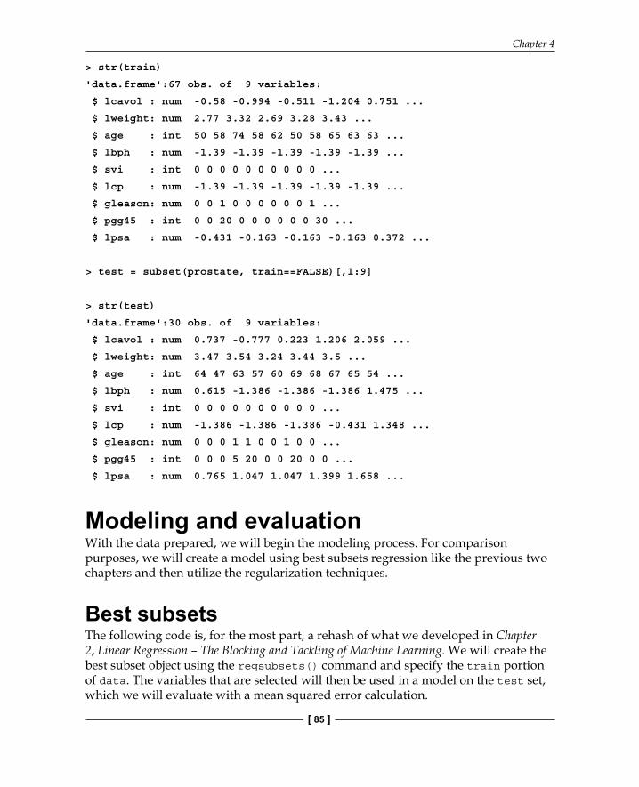
> str(train)


$ lcavol : num -0.58 -0.994 -0.511 -1.204 0.751 ...

$ lweight: num 2.77 3.32 2.69 3.28 3.43 ...

$ age : int 50 58 74 58 62 50 58 65 63 63 ...

$ lbph : num -1.39 -1.39 -1.39 -1.39 -1.39 ...

$ svi : int 0 0 0 0 0 0 0 0 0 0 ...

$ lcp : num -1.39 -1.39 -1.39 -1.39 -1.39 ...

$ gleason: num 0 0 1 0 0 0 0 0 0 1 ...

$ pgg45 : int 0 0 20 0 0 0 0 0 0 30 ...

$ lpsa : num -0.431 -0.163 -0.163 -0.163 0.372 ...

> test = subset(prostate, train==FALSE)[,1:9]

> str(test)


$ lcavol : num 0.737 -0.777 0.223 1.206 2.059 ...

$ lweight: num 3.47 3.54 3.24 3.44 3.5 ...

$ age : int 64 47 63 57 60 69 68 67 65 54 ...

$ lbph : num 0.615 -1.386 -1.386 -1.386 1.475 ...

$ svi : int 0 0 0 0 0 0 0 0 0 0 ...

$ lcp : num -1.386 -1.386 -1.386 -0.431 1.348 ...

$ gleason: num 0 0 0 1 1 0 0 1 0 0 ...

$ pgg45 : int 0 0 0 5 20 0 0 20 0 0 ...

$ lpsa : num 0.765 1.047 1.047 1.399 1.658 ...

Modeling and evaluationWith the data prepared, we will begin the modeling process. For comparison purposes, we will create a model using best subsets regression like the previous two chapters and then utilize the regularization techniques.

Best subsetsThe following code is, for the most part, a rehash of what we developed in Chapter 2, Linear Regression – The Blocking and Tackling of Machine Learning. We will create the best subset object using the regsubsets() command and specify the train portion of data. The variables that are selected will then be used in a model on the test set, which we will evaluate with a mean squared error calculation.


[ 86 ]

The model that we are building is written out as lpsa~. with the tilda and period stating that we want to use all the remaining variables in our data frame with the exception of the response, as follows:

> subfit = regsubsets(lpsa~., data=train)

With the model built, you can produce the best subset with two lines of code. The fi rst one turns the summary model into an object where we can extract the various subsets and determine the best one with the which.min() command. In this instance, I will use BIC, which was discussed in Chapter 2, Linear Regression – The Blocking and Tackling of Machine Learning, which is as follows:

> b.sum = summary(subfit)

> which.min(b.sum$bic)

[1] 3

The output is telling us that the model with the 3 features has the lowest bic value. A plot can be produced to examine the performance across the subset combinations, as follows:

> plot(b.sum$bic, type="l", xlab="# of Features", ylab="BIC", main="BIC score by Feature Inclusion")


Chapter 4

[ 87 ]

A more detailed examination is possible by plotting the actual model object, as follows:

> plot(subfit, scale="bic", main="Best Subset Features")


So, the previous plot shows us that the three features included in the lowest BIC are lcavol, lweight, and gleason. It is noteworthy that lcavol is included in every combination of the models. This is consistent with our earlier exploration of the data. We are now ready to try this model on the test portion of the data, but fi rst, we will produce a plot of the fi tted values versus the actual values looking for linearity in the solution and as a check on the constancy of the variance. A linear model will need to be created with just the three features of interest. Let's put this in an object called ols for the OLS. Then the fi ts from ols will be compared to the actuals in the training set, as follows:

> ols = lm(lpsa~lcavol+lweight+gleason, data=train)

> plot(ols$fitted.values, train$lpsa, xlab="Predicted", ylab="Actual", main="Predicted vs Actual")


[ 88 ]


An inspection of the plot shows that a linear fi t should perform well on this data and that the nonconstant variance is not a problem. With that, we can see how this performs on the test set data by utilizing the predict() function and specifying newdata=test, as follows:

> pred.subfit = predict(ols, newdata=test)

> plot(pred.subfit, test$lpsa , xlab="Predicted", ylab="Actual", main="Predicted vs Actual")

Chapter 4

[ 89 ]

The values in the object can then be used to create a plot of the Predicted vs Actual values, as shown in the following image:

The plot doesn't seem to be too terrible. For the most part, it is a linear fi t with the exception of what looks to be two outliers on the high end of the PSA score. Before concluding this section, we will need to calculate mean squared error (MSE) to facilitate comparison across the various modeling techniques. This is easy enough where we will just create the residuals and then take the mean of their squared values, as follows:

> resid.subfit = test$lpsa - pred.subfit

> mean(resid.subfit^2)

[1] 0.5084126

So, MSE of 0.508 is our benchmark for going forward.


[ 90 ]

Ridge regressionWith ridge regression, we will have all the eight features in the model so this will be an intriguing comparison with the best subsets model. The package that we will use and is in fact already loaded, is glmnet. The package requires that the input features are in a matrix instead of a data frame and for ridge regression, we can follow the command sequence of glmnet(x = our input matrix, y = our response, family = the distribution, alpha=0). The syntax for alpha relates to 0 for ridge regression and 1 for doing LASSO.

To get the train set ready for use in glmnet is actually quite easy using as.matrix() for the inputs and creating a vector for the response, as follows:

> x = as.matrix(train[,1:8])

> y = train[ ,9]

Now, run the ridge regression by placing it in an object called, appropriately I might add, ridge. It is important to note here that the glmnet package will fi rst standardize the inputs before computing the lambda values and then will unstandardize the coeffi cients. You will need to specify the distribution of the response variable as gaussian as it is continuous and alpha=0 for ridge regression, as follows:

> ridge = glmnet(x, y, family="gaussian", alpha=0)

The object has all the information that we need in order to evaluate the technique. The fi rst thing to try is the print() command, which will show us the number of nonzero coeffi cients, percent deviance explained, and correspondent value of Lambda. The default number in the package of steps in the algorithm is 100. However, the algorithm will stop prior to 100 steps if the percent deviation does not dramatically improve from one lambda to another, that is, the algorithm converges to an optimal solution. For the purpose of saving space, I will present only the following fi rst fi ve and last ten lambda results:

> print(ridge)

Call: glmnet(x = x, y = y, family = "gaussian", alpha = 0)

Df %Dev Lambda

[1,] 8 3.801e-36 878.90000

[2,] 8 5.591e-03 800.80000

[3,] 8 6.132e-03 729.70000

[4,] 8 6.725e-03 664.80000

Chapter 4

[ 91 ]

[5,] 8 7.374e-03 605.80000

...........................

[91,] 8 6.859e-01 0.20300

[92,] 8 6.877e-01 0.18500

[93,] 8 6.894e-01 0.16860

[94,] 8 6.909e-01 0.15360

[95,] 8 6.923e-01 0.13990

[96,] 8 6.935e-01 0.12750

[97,] 8 6.946e-01 0.11620

[98,] 8 6.955e-01 0.10590

[99,] 8 6.964e-01 0.09646

[100,] 8 6.971e-01 0.08789

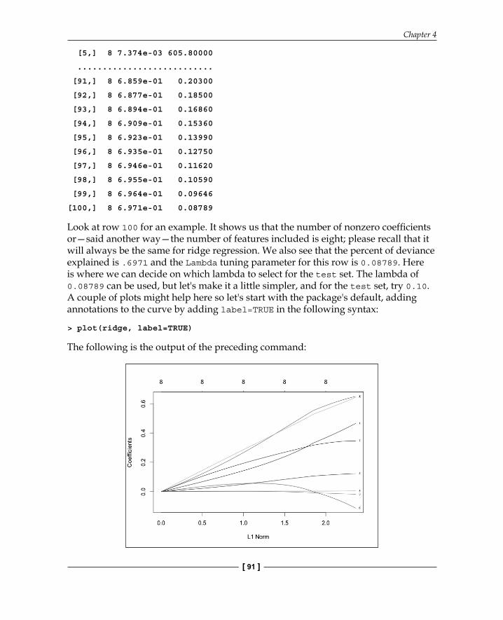
Look at row 100 for an example. It shows us that the number of nonzero coeffi cients or—said another way—the number of features included is eight; please recall that it will always be the same for ridge regression. We also see that the percent of deviance explained is .6971 and the Lambda tuning parameter for this row is 0.08789. Here is where we can decide on which lambda to select for the test set. The lambda of 0.08789 can be used, but let's make it a little simpler, and for the test set, try 0.10. A couple of plots might help here so let's start with the package's default, adding annotations to the curve by adding label=TRUE in the following syntax:

> plot(ridge, label=TRUE)



[ 92 ]

In the default plot, the y axis is the value of Coeffi cients and the x axis is L1 Norm. The plot tells us the coeffi cient values versus the L1 Norm. The top of the plot contains a second x axis, which equates to the number of features in the model. Perhaps a better way to view this is by looking at the coeffi cient values changing as lambda changes. We just need to tweak the code in the following plot() command by adding xvar="lambda". The other option is the percent of deviance explained by substituting lambda with dev.

> plot(ridge, xvar="lambda", label=TRUE)


This is a worthwhile plot as it shows that as lambda decreases, the shrinkage parameter decreases and the absolute values of the coeffi cients increase. To see the coeffi cients at a specifi c lambda value, use the coef() command. Here, we will specify the lambda value that we want to use by specifying s=0.1. We will also state that we want exact=TRUE, which tells glmnet to fi t a model with that specifi c lambda value versus interpolating from the values on either side of our lambda, as follows:

> ridge.coef = coef(ridge, s=0.1, exact=TRUE)

> ridge.coef

9 x 1 sparse Matrix of class "dgCMatrix"

1

(Intercept) 0.13062197

Chapter 4

[ 93 ]

lcavol 0.45721270

lweight 0.64579061

age -0.01735672

lbph 0.12249920

svi 0.63664815

lcp -0.10463486

gleason 0.34612690

pgg45 0.00428580

It is important to note that age, lcp, and pgg45 are close to, but not quite, zero. Let's not forget to plot deviance versus coeffi cients as well:

> plot(ridge, xvar="dev", label=TRUE)


Comparing the two previous plots, we can see that as lambda decreases, the coeffi cients increase and the percent/fraction of the deviance explained increases. If we would set lambda equal to zero, we would have no shrinkage penalty and our model would equate the OLS.

To prove this on the test set, you will have to transform the features as we did for the training data:

> newx = as.matrix(test[,1:8])


[ 94 ]

Then, use the predict function to create an object that we will call ridge.y with type = "response" and our lambda equal to 0.10 and plot the Predicted values versus the Actual values, as follows:

> ridge.y = predict(ridge, newx=newx, type="response", s=0.1)

> plot(ridge.y, test$lpsa, xlab="Predicted", ylab="Actual",main="Ridge Regression")

The output of the following command is as follows:

The plot of Predicted versus Actual of Ridge Regression seems to be quite similar to best subsets, complete with two interesting outliers at the high end of the PSA measurements. In the real world, it would be advisable to explore these outliers further so as to understand if they are truly unusual or if we are missing something. This is where domain expertise would be invaluable. The MSE comparison to the benchmark may tell a different story. We fi rst calculate the residuals then take the mean of those residuals squared:

> ridge.resid = ridge.y - test$lpsa

> mean(ridge.resid^2)

[1] 0.4789913

Ridge regression has given us a slightly better MSE. It is now time to put LASSO to the test to see if we can decrease our errors even further.

Chapter 4

[ 95 ]

LASSOTo run LASSO next is quite simple and we only have to change one number from our ridge regression model, that is, change alpha=0 to alpha=1 in the glmnet() syntax. Let's run this code and also see the output of the model, looking at the fi rst fi ve and last ten results:

> lasso = glmnet(x, y, family="gaussian", alpha=1)

> print(lasso)

Call: glmnet(x = x, y = y, family = "gaussian", alpha = 1)

Df %Dev Lambda

[1,] 0 0.00000 0.878900

[2,] 1 0.09126 0.800800

[3,] 1 0.16700 0.729700

[4,] 1 0.22990 0.664800

[5,] 1 0.28220 0.605800

........................

[60,] 8 0.70170 0.003632

[61,] 8 0.70170 0.003309

[62,] 8 0.70170 0.003015

[63,] 8 0.70170 0.002747

[64,] 8 0.70180 0.002503

[65,] 8 0.70180 0.002281

[66,] 8 0.70180 0.002078

[67,] 8 0.70180 0.001893

[68,] 8 0.70180 0.001725

[69,] 8 0.70180 0.001572

Note that the model building process stopped at step 69 as the deviance explained no longer improved as lambda decreased. Also, note that the Df column now changes along with lambda. At fi rst glance, here it seems that all the eight features should be in the model with a lambda of 0.001572. However, let's try and fi nd and test a model with fewer features, around seven, for argument's sake. Looking at the rows, we see that around a lambda of 0.045, we end up with 7 features versus 8. Thus, we will plug this lambda in for our test set evaluation, as follows:

[31,] 7 0.67240 0.053930

[32,] 7 0.67460 0.049140

[33,] 7 0.67650 0.044770

[34,] 8 0.67970 0.040790

[35,] 8 0.68340 0.037170


[ 96 ]

Just as with ridge regression, we can plot the results as follows:

> plot(lasso, xvar="lambda", label=TRUE)


This is an interesting plot and really shows how LASSO works. Notice how the lines labeled 8, 3, and 6 behave, which corresponds to the pgg45, age, and lcp features respectively. It looks as if lcp is at or near zero until it is the last feature that is added. We can see the coeffi cient values of the seven feature model just as we did with ridge regression by plugging it into coef(), as follows:

> lasso.coef = coef(lasso, s=0.045, exact=TRUE)

> lasso.coef


1

(Intercept) -0.1305852115

lcavol 0.4479676523

lweight 0.5910362316

age -0.0073156274

lbph 0.0974129976

svi 0.4746795823

lcp .

gleason 0.2968395802

pgg45 0.0009790322

Chapter 4

[ 97 ]

The LASSO algorithm zeroed out the coeffi cient for lcp at a lambda of 0.045. Here is how it performs on the test data:

> lasso.y = predict(lasso, newx=newx, type="response", s=0.045)

> plot(lasso.y, test$lpsa, xlab="Predicted", ylab="Actual", main="LASSO")


We calculate MSE as we did before:

> lasso.resid = lasso.y - test$lpsa

> mean(lasso.resid^2)

[1] 0.4437209

It looks like we have similar plots as before with only the slightest improvement in MSE. Our last best hope for dramatic improvement is with elastic net. To this end, we will still use the glmnet package. The twist will be that we will solve for lambda and for the elastic net parameter known as alpha. Recall that alpha = 0 is the ridge regression penalty and alpha = 1 is the LASSO penalty. The elastic net parameter will be 0 ≤ alpha ≤ 1. Solving for two different parameters simultaneously can be complicated and frustrating but we can use our friend in R, the caret package, for assistance.


[ 98 ]

Elastic netThe caret package stands for classifi cation and regression training. It has an excellent companion website to help in understanding all of its capabilities: http://topepo.github.io/caret/index.html. The package has many different functions that you can use and we will revisit some of them in the later chapters. For our purpose here, we want to focus on fi nding the optimal mix of lambda and our elastic net mixing parameter, alpha. This is done using the following simple three-step process:

1. Use the expand.grid() function in base R to create a vector of all the possible combinations of alpha and lambda that we want to investigate.

2. Use the trainControl() function from the caret package to determine the resampling method; we will use LOOCV as we did in Chapter 2, Linear Regression – The Blocking and Tackling of Machine Learning.

3. Train a model to select our alpha and lambda parameters using glmnet() in caret's train() function.

Once we've selected our parameters, we will apply them to the test data in the same way as we did with ridge regression and LASSO. Our grid of combinations should be large enough to capture the best model but not too large that it becomes computationally unfeasible. That won't be a problem with this size dataset, but keep this in mind for future references. I think we can do the following:

• alpha from 0 to 1 by 0.2 increments; remember that this is bound by 0 and 1• lambda from 0.00 to 0.2 in steps of 0.02; the 0.2 lambda should provide a

cushion from what we found in ridge regression (lambda=0.1) and LASSO (lambda=0.045)

You can create this vector using the expand.grid() function and building a sequence of numbers for what the caret package will automatically use. The caret package will take the values for alpha and lambda with the following code:

> grid = expand.grid(.alpha=seq(0,1, by=.2), .lambda=seq(0.00,0.2, by=0.02))

The table() function will show us the complete set of 66 combinations:

> table(grid)

.lambda

.alpha 0 0.02 0.04 0.06 0.08 0.1 0.12 0.14 0.16 0.18 0.2

0 1 1 1 1 1 1 1 1 1 1 1

0.2 1 1 1 1 1 1 1 1 1 1 1

0.4 1 1 1 1 1 1 1 1 1 1 1

Chapter 4

[ 99 ]

0.6 1 1 1 1 1 1 1 1 1 1 1

0.8 1 1 1 1 1 1 1 1 1 1 1

1 1 1 1 1 1 1 1 1 1 1 1

We can confi rm that this is what we wanted—alpha from 0 to 1 and lambda from 0 to 0.2. For the resampling method, we will put in the code for LOOCV for the method. There are other resampling alternatives such as bootstrapping or k-fold cross-validation and numerous options that you can use with trainControl(), but we will explore this options in future chapters. You can tell the model selection criteria with selectionFunction() in trainControl(). For quantitative responses, the algorithm will select based on its default of Root Mean Square Error (RMSE), which is perfect for our purposes:

> control = trainControl(method="LOOCV")

It is now time to use train() to determine the optimal elastic net parameters. The function is similar to lm(). We will just add the syntax: method="glmnet", trControl=control and tuneGrid=grid. Let's put this in an object called enet.train:

> enet.train = train(lpsa~., data=train, method="glmnet", trControl=control, tuneGrid=grid)

Calling the object will tell us the parameters that lead to the lowest RMSE, as follows:

> enet.train

glmnet

67 samples

8 predictor

No pre-processing

Resampling:

Summary of sample sizes: 66, 66, 66, 66, 66, 66, ...

Resampling results across tuning parameters:

alpha lambda RMSE Rsquared

0.0 0.00 0.750 0.609

0.0 0.02 0.750 0.609

0.0 0.04 0.750 0.609


[ 100 ]

0.0 0.06 0.750 0.609

0.0 0.08 0.750 0.609

0.0 0.10 0.751 0.608

.........................

1.0 0.14 0.800 0.564

1.0 0.16 0.809 0.558

1.0 0.18 0.819 0.552

1.0 0.20 0.826 0.549

RMSE was used to select the optimal model using the smallest value. The fi nal values used for the model were alpha = 0 and lambda = 0.08.

This experimental design has led to the optimal tuning parameters of alpha = 0 and lambda = 0.08, which is a ridge regression with s=0.08 in glmnet, recall that we used 0.10. The R-squared is 61 percent, which is nothing to write home about.

The process for the test set validation is just as before:

> enet = glmnet(x, y,family="gaussian", alpha=0, lambda=.08)

> enet.coef = coef(enet, s=.08, exact=TRUE)

> enet.coef


1

(Intercept) 0.137811097

lcavol 0.470960525

lweight 0.652088157

age -0.018257308

lbph 0.123608113

svi 0.648209192

lcp -0.118214386

gleason 0.345480799

pgg45 0.004478267

> enet.y = predict(enet, newx=newx, type="response", s=.08)

> plot(enet.y, test$lpsa, xlab="Predicted", ylab="Actual", main="Elastic Net")

Chapter 4

[ 101 ]


Calculate MSE as we did before:> enet.resid = enet.y – test$lpsa

> mean(enet.resid^2)

[1] 0.4795019

This model error is similar to the ridge penalty. On the test set, our LASSO model did the best in terms of errors. We may be over-fi tting! Our best subset model with three features is the easiest to explain, and in terms of errors, is acceptable to the other techniques. We can use a 10-fold cross-validation in the glmnet package to possibly identify a better solution.

Cross-validation with glmnetWe have used LOOCV with the caret package; now we will try k-fold cross-validation. The glmnet package defaults to ten folds when estimating lambda in cv.glmnet(). In k-fold CV, the data is partitioned into an equal number of subsets (folds) and a separate model is built on each k-1 set and then tested on the corresponding holdout set with the results combined (averaged) to determine the fi nal parameters. In this method, each fold is used as a test set only once. The glmnet package makes it very easy to try this and will provide you with an output of the lambda values and the corresponding MSE. It defaults to alpha = 1, so if you want to try ridge regression or an elastic net mix, you will need to specify it. As we will be trying for as few input features as possible, we will stick to the default:> set.seed(317)


[ 102 ]

> lasso.cv = cv.glmnet(x, y)

> plot(lasso.cv)

The output of the preceding code is as follows:

The plot for CV is quite different than the other glmnet plots, showing log(Lambda) versus Mean-Squared Error along with the number of features. The two dotted vertical lines signify the minimum of MSE (left line) and one standard error from the minimum (right line). One standard error away from the minimum is a good place to start if you have an over-fi tting problem. You can also call the exact values of these two lambdas, as follows:

> lasso.cv$lambda.min #minimum

[1] 0.003985616

> lasso.cv$lambda.1se #one standard error away

[1] 0.1646861

Using lambda.1se, we can go through the following process of viewing the coeffi cients and validating the model on the training data:

> coef(lasso.cv, s ="lambda.1se")


1

Chapter 4

[ 103 ]

(Intercept) 0.04370343

lcavol 0.43556907

lweight 0.45966476

age .

lbph 0.01967627

svi 0.27563832

lcp .

gleason 0.17007740

pgg45 .

> lasso.y.cv = predict(lasso.cv, newx=newx, type="response", s="lambda.1se")

> lasso.cv.resid = lasso.y.cv - test$lpsa

> mean(lasso.cv.resid^2)

[1] 0.4559446

This model achieves an error of 0.46 with just fi ve features, zeroing out age, lcp, and pgg45.

Model selectionWe looked at fi ve different models in examining this dataset. The following points were the test set error of these models:

• Best subsets is 0.51• Ridge regression is 0.48• LASSO is 0.44• Elastic net is 0.48• LASSO with CV is 0.46

On a pure error, LASSO with seven features performed the best. However, does this best address the question that we are trying to answer? Perhaps the more parsimonious model that we found using CV with a lambda of ~0.165 is more appropriate. My inclination is to put forth the latter as it is more interpretable.


[ 104 ]

Having said all this, there is clearly a need for domain-specifi c knowledge from oncologists, urologists, and pathologists in order to understand what would make the most sense. There is that, but there is also the need for more data. With this sample size, the results can vary greatly just by changing the randomization seeds or creating different train and test sets. (Try it and see for yourself.) At the end of the day, these results may likely raise more questions than provide you with answers. However, is this bad? I would say no, unless you made the critical mistake of over-promising at the start of the project about what you will be able to provide. This is a fair warning to prudently apply the tools put forth in Chapter 1, Business Understanding — The Road to Actionable Insights.

SummaryIn this chapter, the goal was to use a small dataset to provide an introduction to practically apply an advanced feature selection for linear models. The outcome for our data was quantitative but the glmnet package that we used will also support qualitative outcomes (binomial and multinomial classifi cations). An introduction to regularization and the three techniques that incorporate it were provided and utilized to build and compare models. Regularization is a powerful technique to improve computational effi ciency and to possibly extract more meaningful features versus the other modeling techniques. Additionally, we started to use the caret package to optimize multiple parameters when training a model. Up to this point, we've been purely talking about linear models. In the next couple of chapters, we will begin to use nonlinear models for both classifi cation and regression problems.

Where to buy this book You can buy Mastering Machine Learning with R from the Packt Publishing website.

Alternatively, you can buy the book from Amazon, BN.com, Computer Manuals and most internet

book retailers.

Click here for ordering and shipping details.

www.PacktPub.com

Stay Connected:

Get more information Mastering Machine Learning with R

https://www.packtpub.com/big-data-and-business-intelligence/mastering-machine-learning-r/?utm_source=slideshare&utm_medium=cd&utm_campaign=samplechapter

https://www.packtpub.com/books/info/packt/ordering/?utm_source=slideshare&utm_medium=cd&utm_campaign=samplechapter

https://www.packtpub.com/?utm_source=slideshare&utm_medium=cd&utm_campaign=samplechapter

https://twitter.com/PacktPub

https://www.facebook.com/PacktPub/

https://plus.google.com/+packtpublishing

https://www.linkedin.com/company/packt-publishing

https://www.packtpub.com/big-data-and-business-intelligence/mastering-machine-learning-r/?utm_source=slideshare&utm_medium=cd&utm_campaign=samplechapter

mastering machine learning with r - sample chapter

Technology