master’s thesis - connecting repositories · 2017-01-21 · consider the region bounded by two...
TRANSCRIPT

Faculty of Science and Technology
MASTER’S THESIS
Study program/ Specialization:
Master of Science in Petroleum Engineering
Reservoir Engineering
Spring semester, 2013
Open
Writer: Alex Rodrigo Valdés Pérez
…………………………………………
(Writer’s signature) Faculty supervisor:Leif Larsen External supervisor(s):
Titel of thesis:
“A New Double Porosity Fractal Model for Well Test Analysis with Transient Interporosity Transfer for Petroleum and Geothermal Systems”
Credits (ECTS): 30 Key words:
Fractal Well Testing
Naturally Fractured Reservoirs Double Porosity
Pages: 116 + enclosure: …………
Stavanger, June 6th, 2013


Copyright
by
Alex Rodrigo Valdés Pérez
2013

“…¿Qué mágicas infusiones de los Indios herbolarios
de mi Patria, entre mis letras el hechizo derramaron?...”
Sor Juana Inés de la Cruz


“I firmly believe that any man’s finest hour, the greatest fulfilment of all that he holds dear,
is the moment when he has worked his heart out in a good cause and lies exhausted on the
field of battle – victorious!”
Vince Lombardi


Alex R. Valdés-Pérez Dedication • i
Dedication
To México, this is also part of you.
To my beloved parents Marta and Ismael,
without your help and support, I could not achieve this goal.
To Valeria and Ian, our future is in your hands.

This page is intentionally left in blank.

Alex R. Valdés-Pérez Acknowledgement • iii
Acknowledgements
I want to express my gratitude to Iván, Raúl and Javier Valdés, for their support in my
norwegian adventure.
To my recommendators for this program Héber Cinco-Ley, Héctor Pulido, Fernando
Samaniego and Rafael Rodriguez, for their invaluable help and contributions to the
petroleum engineering.
The SPE fellowship which was awarded to me was crucial to successfully complete
my studies here. The loan provided by Banco de México is greatly acknowledged.
I am also deeply thankful to my advisor Leif Larsen, for his advice, guidance and
encouragement through the development of this thesis.
I am grateful to Frode Hveding who trusted me and gave me the opportunity to apply
my knowledge in well test analysis.
I also want to thank to Hans Borge, who is always willing to help the students and is
ally of us.
To my closest friends during this period of my life, Pablo and Miguel Luzuriaga,,
Luisa Campiño, Roberto Pérez, Diana Pavón and Juan Andrade. Guys, it was very
funny.
And last but not least, to Norway and to the University of Stavanger, for giving me
the opportunity of studying, working and living outside my country. I will be always
grateful with you.

This page is intentionally left in blank.

Alex R. Valdés-Pérez Abstract • v
Abstract
A new double porosity model for Naturally Fractured Reservoirs (NFRs) assuming
fractal fracture network behavior and its solution is presented. Primary porosity is
idealized as Euclidian matrix blocks (slabs
or spheres) and Secondary porosity is defined by any post-depositional geological
phenomenon such as fractures and vugs.
In order to provide a framework, the generalized radial flow model solution for well
test analysis for petroleum and geothermal systems in Laplace and Real space was
developed. Development of an appropriate wellbore storage model for fractal
reservoirs is also shown.
For this model, the dimensionless fractal fracture area parameter was developed. In
addition, interporosity skin factor between matrix blocks and fractal fracture network
is introduced. Relationship of convergence between interporosity skin under transient
transference regime and pseudosteady state transference regime is discussed. An
analytical general solution was obtained in Laplace space; besides, analytical solutions
in real space that describe the behavior of NFRs at different stages and different cases
of flow are also presented. Early, intermediate and late-time approximations are used to
obtain reservoir and fractal fracture network parameters. A synthetic example is
presented to illustrate the application of this model.

This page is intentionally left in blank.
Alex R. Valdés-Pérez Contents • vii
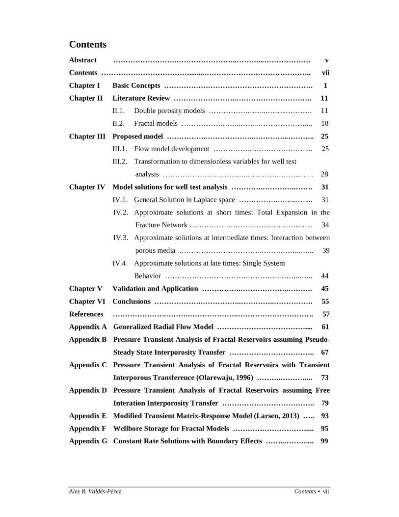
Contents Abstract …………………….……………………..………...………………. v
Contents ………………………………........…………………………………….. vii
Chapter I Basic Concepts ……………………………………………………. 1
Chapter II Literature Review ……………………..…………………………. 11
II.1. Double porosity models …………….……...……...………. 11
II.2. Fractal models …………….……...……...……………….... 18
Chapter III Proposed model …………….………………..…………...……….. 25
III.1. Flow model development …………….…….....………….... 25
III.2. Transformation to dimensionless variables for well test
analysis ……………………………..………….……....…... 28
Chapter IV Model solutions for well test analysis ………….…………..……. 31
IV.1. General Solution in Laplace space …………….……...….... 31
IV.2. Approximate solutions at short times: Total Expansion in the
Fracture Network …………….………..……………….…... 34
IV.3. Approximate solutions at intermediate times: Interaction between
porous media ……………………………..…….……...…... 39
IV.4. Approximate solutions at late times: Single System
Behavior …………………………….………….……...…... 44
Chapter V Validation and Application …………….………………..………. 45
Chapter VI Conclusions ……………….……………..…………..……………. 55
References ………………….……….………………..…………………………. 57
Appendix A Generalized Radial Flow Model ……………………………….... 61
Appendix B Pressure Transient Analysis of Fractal Reservoirs assuming Pseudo-
Steady State Interporosity Transfer …………………………….. 67
Appendix C Pressure Transient Analysis of Fractal Reservoirs with Transient
Interporous Transference (Olarewaju, 1996) ………..……….... 73
Appendix D Pressure Transient Analysis of Fractal Reservoirs assuming Free
Interation Interporosity Transfer ……………………………….. 79
Appendix E Modified Transient Matrix-Response Model (Larsen, 2013) ….. 93
Appendix F Wellbore Storage for Fractal Models ………………………….... 95
Appendix G Constant Rate Solutions with Boundary Effects ……..……….... 99
viii • Contents Alex R. Valdés-Pérez
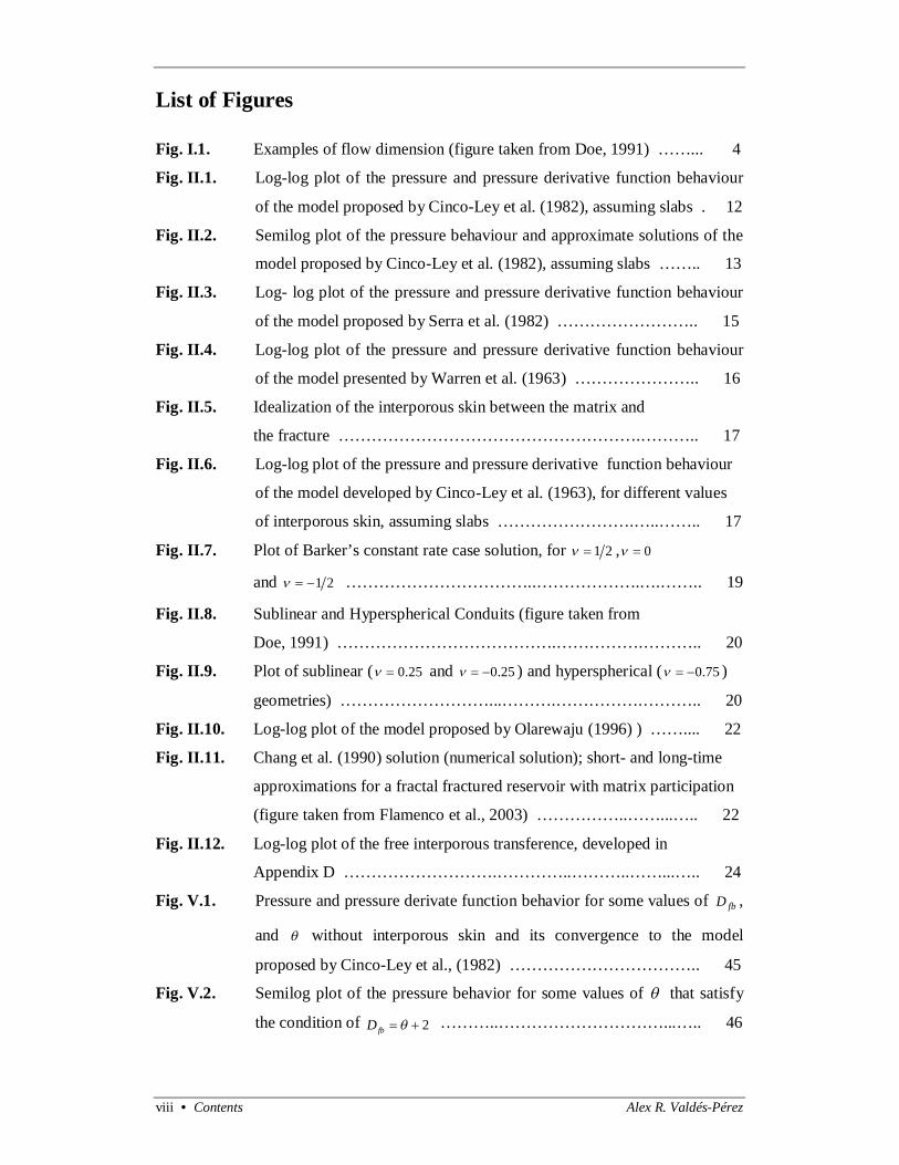
List of Figures
Fig. I.1. Examples of flow dimension (figure taken from Doe, 1991) ……... 4
Fig. II.1. Log-log plot of the pressure and pressure derivative function behaviour
of the model proposed by Cinco-Ley et al. (1982), assuming slabs . 12
Fig. II.2. Semilog plot of the pressure behaviour and approximate solutions of the
model proposed by Cinco-Ley et al. (1982), assuming slabs …….. 13
Fig. II.3. Log- log plot of the pressure and pressure derivative function behaviour
of the model proposed by Serra et al. (1982) …………………….. 15
Fig. II.4. Log-log plot of the pressure and pressure derivative function behaviour
of the model presented by Warren et al. (1963) ………………….. 16
Fig. II.5. Idealization of the interporous skin between the matrix and
the fracture ……………………………………………….……….. 17
Fig. II.6. Log-log plot of the pressure and pressure derivative function behaviour
of the model developed by Cinco-Ley et al. (1963), for different values
of interporous skin, assuming slabs …………………….…..…….. 17
Fig. II.7. Plot of Barker’s constant rate case solution, for 21 , 0
and 21 ……………………………..……………….….…….. 19
Fig. II.8. Sublinear and Hyperspherical Conduits (figure taken from
Doe, 1991) ………………………………….…………….……….. 20
Fig. II.9. Plot of sublinear ( 25.0 and 25.0 ) and hyperspherical ( 75.0 )
geometries) ………………………...……….…………….……….. 20
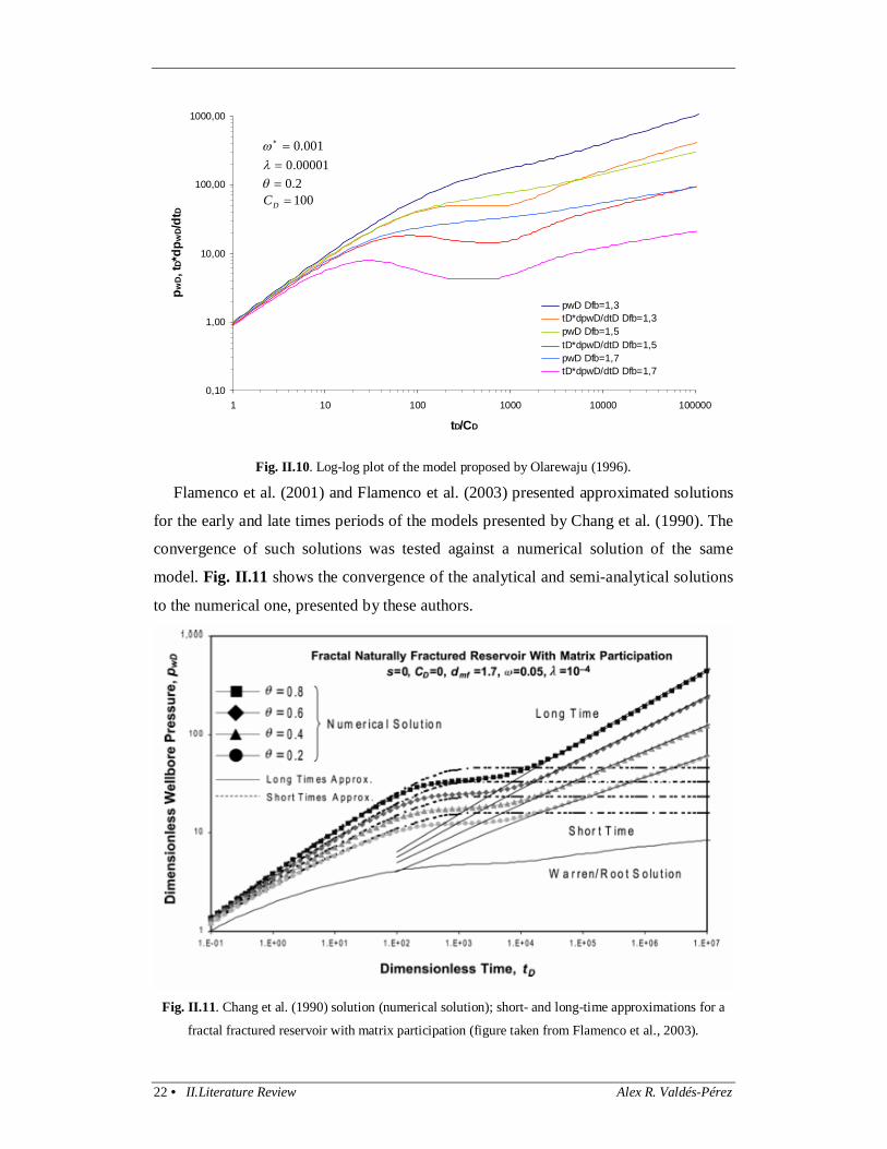
Fig. II.10. Log-log plot of the model proposed by Olarewaju (1996) ) …….... 22
Fig. II.11. Chang et al. (1990) solution (numerical solution); short- and long-time
approximations for a fractal fractured reservoir with matrix participation
(figure taken from Flamenco et al., 2003) ……………..……...….. 22
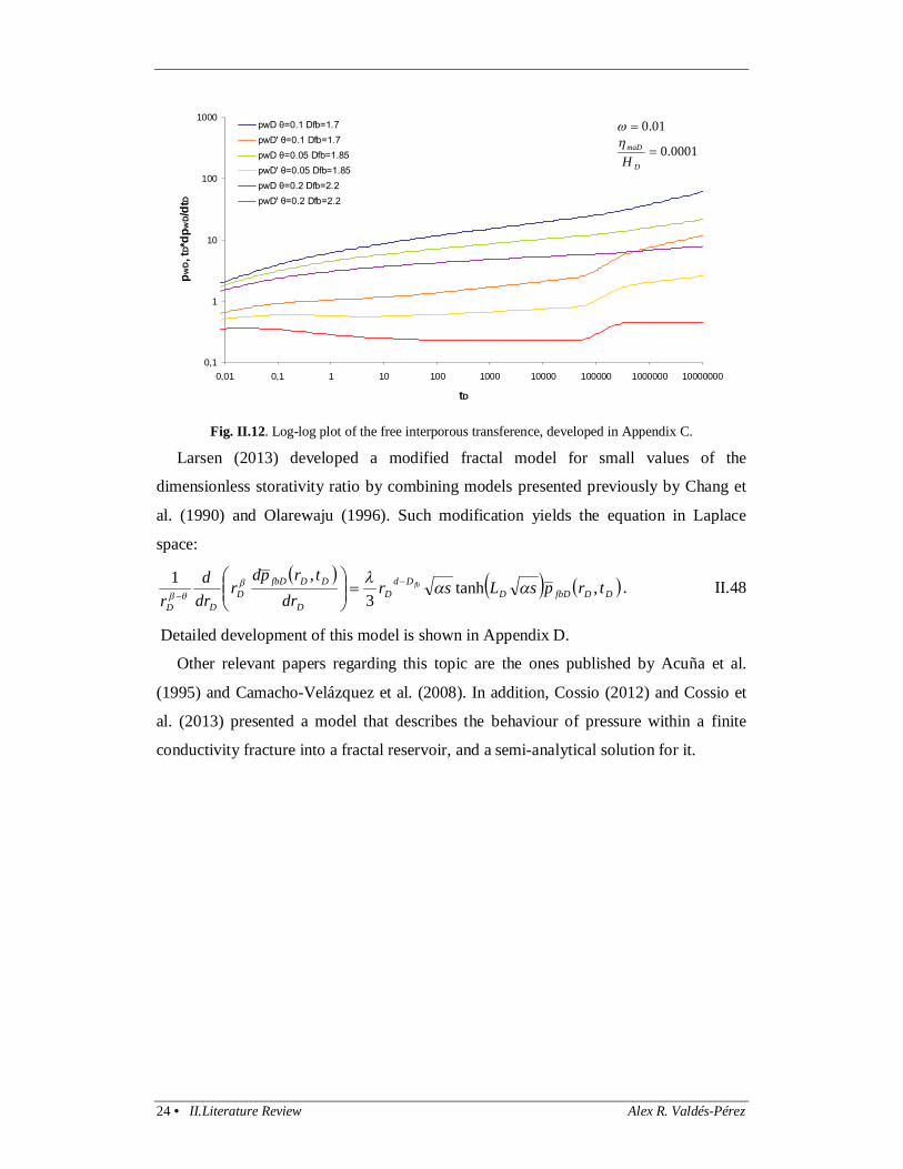
Fig. II.12. Log-log plot of the free interporous transference, developed in
Appendix D ……………………….…………..………..……...….. 24
Fig. V.1. Pressure and pressure derivate function behavior for some values of fbD ,
and without interporous skin and its convergence to the model
proposed by Cinco-Ley et al., (1982) …………………………….. 45
Fig. V.2. Semilog plot of the pressure behavior for some values of that satisfy
the condition of 2 fbD ………..…………………………...….. 46
Alex R. Valdés-Pérez Contents • ix
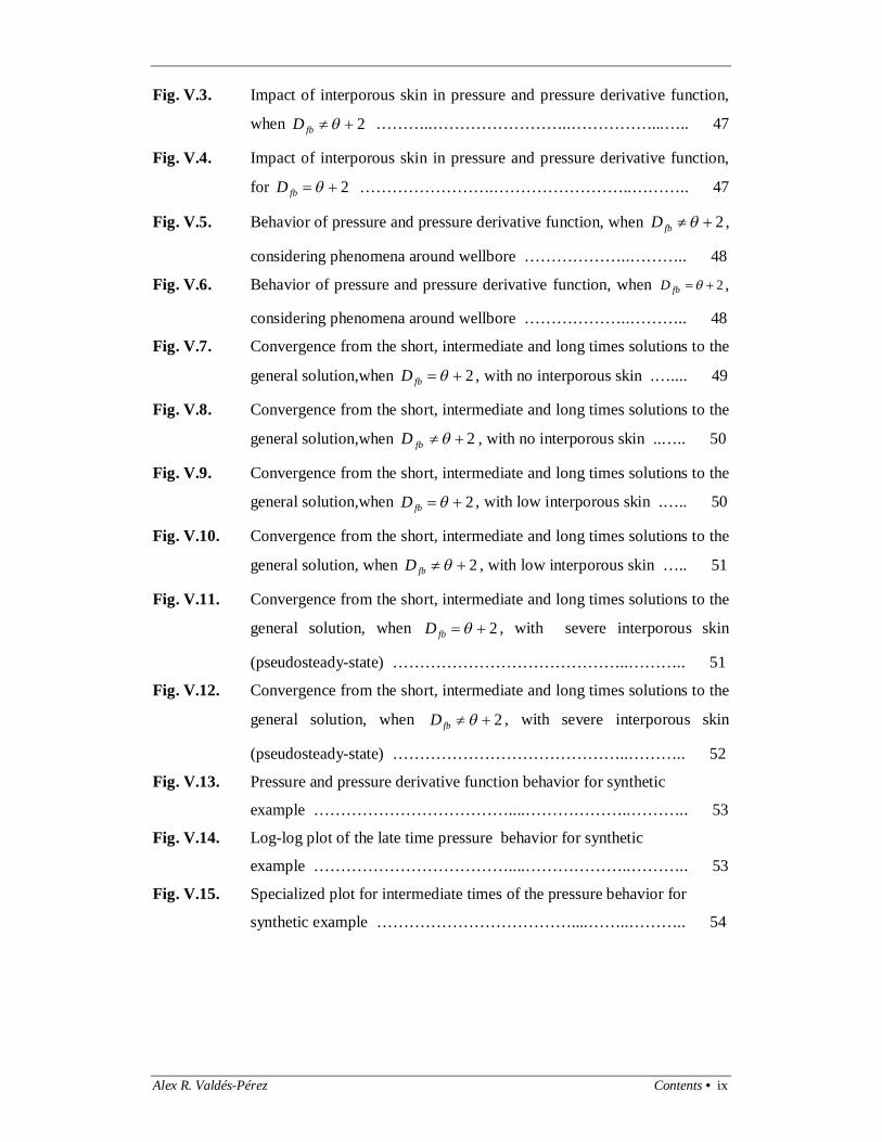
Fig. V.3. Impact of interporous skin in pressure and pressure derivative function,
when 2 fbD ………..……………………..……………...….. 47
Fig. V.4. Impact of interporous skin in pressure and pressure derivative function,
for 2 fbD …………………….……………………..……….. 47
Fig. V.5. Behavior of pressure and pressure derivative function, when 2 fbD ,
considering phenomena around wellbore ………………..……….. 48
Fig. V.6. Behavior of pressure and pressure derivative function, when 2 fbD ,
considering phenomena around wellbore ………………..……….. 48
Fig. V.7. Convergence from the short, intermediate and long times solutions to the
general solution,when 2 fbD , with no interporous skin .….... 49
Fig. V.8. Convergence from the short, intermediate and long times solutions to the
general solution,when 2 fbD , with no interporous skin ..….. 50
Fig. V.9. Convergence from the short, intermediate and long times solutions to the
general solution,when 2 fbD , with low interporous skin .….. 50
Fig. V.10. Convergence from the short, intermediate and long times solutions to the
general solution, when 2 fbD , with low interporous skin ….. 51
Fig. V.11. Convergence from the short, intermediate and long times solutions to the
general solution, when 2 fbD , with severe interporous skin
(pseudosteady-state) ……………………………………..……….. 51
Fig. V.12. Convergence from the short, intermediate and long times solutions to the
general solution, when 2 fbD , with severe interporous skin
(pseudosteady-state) ……………………………………..……….. 52
Fig. V.13. Pressure and pressure derivative function behavior for synthetic
example ………………………………....………………..……….. 53
Fig. V.14. Log-log plot of the late time pressure behavior for synthetic
example ………………………………....………………..……….. 53
Fig. V.15. Specialized plot for intermediate times of the pressure behavior for
synthetic example ………………………………....……..……….. 54


This page is intentionally left in blank.


Alex R. Valdés-Pérez I.Basic Concepts • 1
Chapter I Basic Concepts
The purpose of this chapter is to familiarize the reader with concepts used in
applications of fractal theory in well test analysis. Besides, new definitions are
presented in order to develop the flow model presented in this work.
Concepts related to the rock and fluid properties, such as compressibility of rock, oil,
gas, steam and water in addition to the fluid viscosity, formation volume factors and
fluids saturations are important in well test analysis. Therefore, it is it is assumed that
the reader has prior knowledge of these concepts.
Bulk Volume: It is constituted by the volume of any kind of voids and solids contained
in a rock. Considering three kinds of voids, i.e, pores, fractures and vugs, a
mathematical representation for the volume of rock is:
solidsvugsfracturesporesb VVVVV , I.1
where:
poresV volume of pores;
fracturesV volume of fractures;
solidsV volume of solids.
Prior definition is based on the components of the rock. However, bulk volume can
be defined by its shape. For instance, if the rock would have a cubic shape, volume
would be defined as: 3LVb , I.2
where:
L length of the base of the cubic rock;
or, if rock would be a sphere:
3
34 rVb
, I.3
where:
r radius of the rock.
If the rock does not show a regular shape, it can be represented by the volume
between two equipotential surfaces, such region is defined as:

2 • I.Basic Concepts Alex R. Valdés-Pérez
rrbV ee
e
dddb 13 , I.4
where:
ed Area of a unit sphere of in ed dimensions; it is defined as:
2
2 2/
e
d
d de
e
, I.5
where:
x gamma function of x .
Consider the region bounded by two equipotential surfaces which have radii r and
rr . These surfaces are the projections of ed -dimensional spheres through three
dimensional space by an amount edb 3 . For example, when ed is equal to 2, the surfaces
are finite cylinders of length b . A sphere of radius r has an area 1e
e
dd r .
In the realization of this thesis, it has found that, since the term r in eq. I.4
represents the width between the surfaces, the cross section (area exposed to the flow)
between the two equipotential surfaces mentioned before, is given by: 13
.exp ee
e
dddflow rbA , I.6
where:
b extent of the flow region.
Porosity: It is defined as the ratio of the porous volume divided by the rock volume:
ebulk volum totalpores of volume
. I.7
When there is evidence of existence of non-intergranular pores into the rock in
addition to the intergranular pores themself (traditionally called primary porosity), e.g.,
fractures and/or vugs (secondary porosity), to distinguish and characterize such
elements becomes very important for reservoir engineering and economical purposes.
Defining the total pore volume as:
vugsfracturesporestp VVVV , I.8
establishing that:
vugsfractures VVV sec , I.9
therefore:
secVVV porestp . I.10
Alex R. Valdés-Pérez I.Basic Concepts • 3
Dividing previous eq. by bulk volume it results:
sec mat , I.11
where:
t total porosity,
ma matrix porosity (intergranular pores);
sec secondary porosity.
Total porosity is traditionally determinated from logs; matrix porosity can be
determinated by core analysis. Secondary porosity can be estimated with the following
model (Pulido et al., 2005):
DPmtt 74.01sec . I.12
For a good understanding of the present work, I consider necessary to introduce the
concept of unitary fracture porosity. Conceptually it represents the volumetric fraction
occupied by a single fracture related to the total rock volume. It is given by:
bulk
ufuf V
V
ebulk volum total volumefractureunitary . I.13
On the other hand, the concept fractured bulk porosity has been used previously in
the literature. It represents the volumetric fraction of all fractures in the rock. It is
defined as:
bulk
fbfb V
V
ebulk volum totallumenetwork vo fracture . I.14
Assuming fractures with the same characteristics all over the bulk, fracture network
volume, can be expressed as:
rVrnV ufffb , I.15
where:
rn f number of fractures into fractured bulk,
ufV unitary fracture volume.
Moreover, the number of fractures into fractured bulk, also known as Site Density
can be expressed using a power-law model:
1 fbDf arrn . I.16
Therefore, fracture network volume is expressed as:
rVarV ufD
fbfb 1 . I.17

4 • I.Basic Concepts Alex R. Valdés-Pérez
Combining eq. I.4 and eq. I.17, porosity of the fracture network is given by:
e
e
efb
ee
e
fb
dd
ufdD
ddd
ufD
fb bVar
rbrrVar
331
1
. I.18
Geometry factor: This parameter was introduced by Chang et al. (1990); it was used to
provide a relation of the symmetry. It was defined as:
saVG , I.19
where:
sV site volume. This parameter is equivalent to the unitary fracture volume, presented
in this thesis.
In the present work, it was found that the geometry factor is equivalent to:
e
ee
ddd
flow br
AG
31
.exp . I.20
Dimension in Well Testing: The term dimension suffers from having different but
related meanings in reservoir analysis. Dimension may refer to units of measure, as in
dimensionless pressure. Dimension also arises when we discuss the three Euclidian
dimensions, since all real well tests occur in three-dimensional space. Fractal
Dimension describes how patterns fill spaces. Dimension has also been used in
reference to the symmetry of flow lines in a well test. For example, linear flow is
considered one-dimensional; cylindrical flow, two dimensional and spherical flow,
three-dimensional, see Fig. I.1.
Fig. I.1. Examples of flow dimension (figure taken from Doe, 1991).

Alex R. Valdés-Pérez I.Basic Concepts • 5
Spatial Dimension: The geometric property that defines spatial dimension is the change
in conduit area with distance from a source point. In one-dimensional flow (linear flow)
the area of the conduit is proportional to 0r . The area does not change with distance.
For cylindrical and spherical flow geometries, the areas are proportional to the 1r and 2r powers of distance, respectively. By extension of this logic, a conduit of fractional
dimension is simply a conduit whose area is proportional to a non-integer power of
distance from the source (Doe, 1991).
Fractal Permeability and Darcy’s law in fractal form: According to Poiseuille’s and
Fanning’s equations, a fluid’s velocity trough a capillary tube can be expressed as:
Lpd
v ufufu
32
2
I.21
where:
ufd capillary tube diameter (pore, fracture of vug aperture);
fluid viscosity;
p pressure drop within the system;
L length of the capillary tube.
Fluid rate is given by:
ufuu Avq ; I.22
moreover, capillary tube area is: 2
ufuf rA . I.23
Then, substituting capillary tube area and fluid velocity into fluid rate equation, it
becomes: Hagen Pouisuielle
Lpr
rL
pdq uf
ufufuf
u
832
42
2 . I.24
Expressing prior equation in terms of radial coordinates and taking limits to zero:
rpr
q ufufu
8
4 . I.25
Previous equation provides the fluid rate in a single capillary tube considering pn
parallel tubes with the same characteristics, the total fluid rate can be expressed as:
6 • I.Basic Concepts Alex R. Valdés-Pérez
rpr
nqnq fbufpup
8
4 , I.26
where, the number of tubes is defined as follows:
rnV
VrnVV
n fuf
uff
uf
fbp , I.27
with:
fbV capillary tubes volume (fractured bulk volume);
ufV capillary tube volume (unitary fracture volume).
Equation I.28 can be expressed as:
lrV
np
fbp
12
. I.28
Hence, the following expression can be deduced:
lr
Vrnn
p
fbfp
12
. I.29
Equation I.26 can be rewritten as follows:
rp
rra
rpr
arq fbDuffbufD fbfb
144
1
88
. I.30
assuming: 4
14 rCruf , I.31
where:
parameter describing the conductivity in a fractal object. Therefore, eq. I.30 is
rewritten as:
r
prCa
rp
rrCaq fbDfbD fbfb
1114
1
88
, I.32
where:
4 . It is defined as the anomaly in conductivity in a fractal object (O’Shaughnessy
and Procaccia, 1985).
Defining:
11
2 8aCCaC , I.33
equation I.32 can be expressed as, similar to Chang et al. (1990):

Alex R. Valdés-Pérez I.Basic Concepts • 7
rprCq fb
D fb
1
2 . I.34
On the other hand, Darcy’s law is given by (considering a variable permeability,
trough porous media):
r
prkv fbfb
; I.35
fractured bulk’s fluid rate is given by:
ffbvAq , I.36
flowing area of fractured bulk is given by: ee
e
dddfb rbA 2 , I.37
and:
21
2 21
e
d
d d
e
e
. I.38
Therefore, fractured bulk’s fluid rate is given by:
r
prbrkr
prkrbq fb
dddfbfbfbdd
d
ee
eee
e
22 . I.39
Comparing equations I.34 and I.39 it results:
r
prCrkrb fb
Dfb
ddd
fbee
e
1
2
2
, I.40
arraying:
r
prCrkrb fbD
fbdd
dfbee
e
12
2 , I.41
then, it can be concluded that:
122 efb
e
e
dDd
dfb r
bCrk
. I.42
Establishing the relationship: 12 aCC , I.43
eq. I.42 becomes:
121
121
efb
e
e
efb
e
e
dDd
d
dDd
dfb r
baCr
baCrk
. I.44
On the other hand, defining:

8 • I.Basic Concepts Alex R. Valdés-Pérez
rnVk
Cf
bulkfb1 , I.45
then,
1
2
efb
e
e
dD
fd
d
bulkfbfb r
rnbVak
rk
, I.46
according to definition:
fb
uffbulk
VrnV
. I.47
Therefore:
1
21
2
efb
e
e
efb
e
e
dD
fb
fbd
d
ufdD
fb
uffd
df
fbfb r
kb
aVr
Vrnbrn
akrk
, I.48
and Dacry’s equation results in:
rp
brkaV
rbr
pr
kb
aV
rbq fb
fbd
d
dDfbufdd
dfb
dD
fb
fbd
d
uf
ddd e
e
efb
ee
e
efb
e
eee
e
2
12
12
2 . I.49
If:
1 fbD , I.50
then, Darcy’s law in fractal form is given by:
rprkaV
q fb
fb
fbuf
. I.51
Dimensionless variables: The use of dimensionless groups in well test analysis is very
common. Dimensionless variables are defined differently depending on the phase
flowing in the well and reservoir (oil and gas) and also, on the author.
The main advantages of using dimensionless variables, such as dimensionless
pressure, Dp , dimensionless radius, Dr and dimensionless time, Dt , are:
- The use of such variables allows grouping known and unknown parameters of
the fluid and the rock system.
- They make easier the mathematical work when solving the partial differential
equations that governs the flow within the reservoir.
- The proper manipulation of dimensionless variables allows the use of the same
models for different cases, e.g., different flowing phases in the reservoir.
Alex R. Valdés-Pérez I.Basic Concepts • 9
The Inverse Chow Pressure Group: For a dimensionless solution DDD trp , , the
Chow pressure group is defined by the identity:
DD
D
DD
D
tpp
tpp
'´ln
. I.52
and the inverse Chow derivative of pressure group by the identity
/ lnD D D D
D D
p t p tp p
. I.53
Dimensionless storativity ratio: This parameter relates the total expansion in the
fracture network to the total expansion in the system. It is defined as:
tmamatfbfb
tfbfb
ccc
. I.54
Matrix-fracture interaction parameter: This parameter is used in all the double
porosity models assuming pseudosteady-state interporous transference and in some
transient interporous transference models. It is a dimensionless parameter, defined as
the relation of permeabilities of the two media:
fb
wma
krk 2 , I.55
where:
shape factor that reflects the geometry of the matrix elements and controls the flow
between porous media. It has dimensions reciprocal to the area.
wr wellbore radius.
Dimensionless matrix hydraulic diffusivity: This parameter relates the hydraulic
diffusivity in the matrix blocks to the total hydraulic diffusivity of the system. This
parameter allows the consideration of any type of flow within the matrix (transient or
pseudosteady-state).
fbtmama
ttmamaD kc
ck
; I.56
Dimensionless block size:
2
2
w
maD r
hH ; I.57
mah height of matrix blocks.

10 • I.Basic Concepts Alex R. Valdés-Pérez
Dimensionless fracture area, fDA : This parameter relates the area of fractures per unit
of matrix volume and the fracture area per unit of bulk volume. It ranges from 2 to 6,
depending on the flow dimensions of the matrix.
ma
wbmaFBfD V
rVhAA
, I.58
where:
FBA fracture area per unit of bulk volume,
bV bulk volume,
maV matrix volume.

Alex R. Valdés-Pérez II.Literature Review • 11
Chapter II Literature Review
The purpose of this chapter is to provide a summary of the double porosity flow models
and models assuming non-fixed flow geometry (fractal models) for well test analysis
and the theories behind them.
It is important to point out that all the models presented in this chapter are expressed
in their respective dimensionless variables, i.e., dimensionless variables are different for
every model.
II.1 Double porosity models
Nature of flow in multi-porous systems obeys to the fact that flow in each porous
medium behaves differently in terms of gradient pressure from the other media. Such
behavior is known as transient interporous flow; this flow regime was studied
previously by de Swaan (1976) and Najurieta (1980). Later in 1982, three research
teams solved the problem - in different ways - of the transient interporous transference
between porous media, showing similar results.
Cinco-Ley et al. (1982) presented a flow model for double porosity systems, where
the interaction between media was modeled by a convolution. It is given in
dimensionless variables by:
D
DDfDt
DmaDfD
fDD
DDfD
DD
DDfD
ttrp
tFp
Ar
trprr
trp D
,,1
,1,
02
2
; II.1
if slabs are assumed for matrix blocks:
1
12 22
4,n
tnmaDDmaD
DmaDetF , II.2
or, for spheres:
1
4 22
4,n
tnmaDDmaD
DmaDetF . II.3
In this study, Cinco-Ley et al. (1982) introduced the parameter fDA , which is the
dimensionless fracture area; its definition depends on the matrix block shape (slabs or
spheres) and it is useful to estimate the area of fractures per volume of rock.
The general solution for eq. II.1, assuming an infinite reservoir and constant flow
rate at wellbore, expressed in Laplace space, evaluated at wellbore is given by:
12 • II.Literature Review Alex R. Valdés-Pérez
ssfKsfs
ssfKspwD
12
30 , II.4
transference function is given by:
sfAsf maDfD ,1 , II.5
where, for slabs:
maD
maDmaD
ss
sf
21tanh, . II.6
and, for spheres:
ss
ssf maD
maD
maDmaD
2
21coth, . II.7
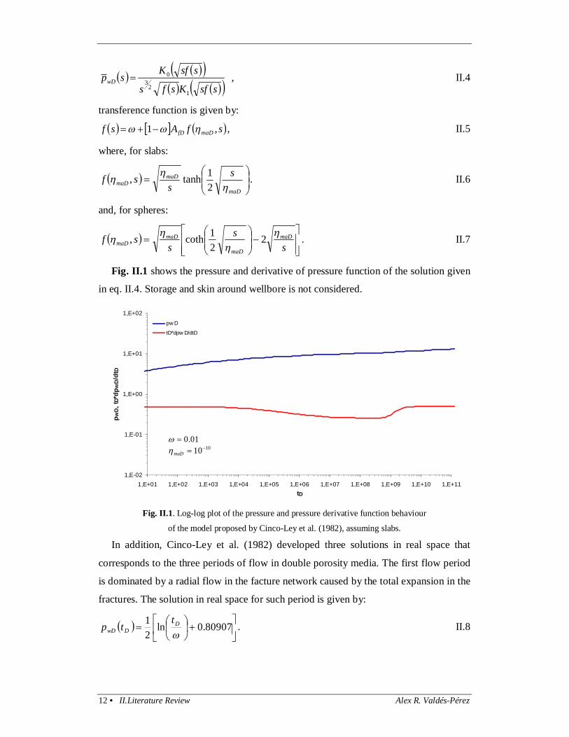
Fig. II.1 shows the pressure and derivative of pressure function of the solution given
in eq. II.4. Storage and skin around wellbore is not considered.
1,E-02
1,E-01
1,E+00
1,E+01
1,E+02
1,E+01 1,E+02 1,E+03 1,E+04 1,E+05 1,E+06 1,E+07 1,E+08 1,E+09 1,E+10 1,E+11tD
p wD
, tD*
dpw
D/d
t D
pw D
tD*dpw D/dtD
Fig. II.1. Log-log plot of the pressure and pressure derivative function behaviour
of the model proposed by Cinco-Ley et al. (1982), assuming slabs.
In addition, Cinco-Ley et al. (1982) developed three solutions in real space that
corresponds to the three periods of flow in double porosity media. The first flow period
is dominated by a radial flow in the facture network caused by the total expansion in the
fractures. The solution in real space for such period is given by:
80907.0ln
21
D
DwDt
tp . II.8
01.0 1010maD

Alex R. Valdés-Pérez II.Literature Review • 13
Second flowing period in double porosity systems is the one where the interactions
between both mediums take place. Hence, second solution in real space is:
2602.01ln21ln
41
maDfDDDwD Attp . II.9
Finally, in the third flowing period the double porosity system acts as a single one.
Provided solution for this flowing period is given by:
80907.0ln21
DDwD ttp . II.10
Fig. II.2 shows a semilog plot of the pressure behaviour neglecting storage and skin
around wellbore and the convergence of approximate solutions to the general solution.
0
2
4
6
8
10
12
14
16
18
20
1,E+01 1,E+02 1,E+03 1,E+04 1,E+05 1,E+06 1,E+07 1,E+08 1,E+09 1,E+10 1,E+11tD
pwD
pwD
Early times
Intermediate times
Late times
Fig. II.2. Semilog plot of the pressure behaviour and approximate solutions of the model proposed by
Cinco-Ley et al. (1982), assuming slabs.
Streltsova (1982) presented a double porosity model assuming radial flow in fracture
network and linear flow from matrix blocks to fractures. She solved this problem using
Hankel transform. Radial flow model in fracture network, presented by Streltsova
(1982) is given by:
Tv
ttrp
rtrp
rrtrp m
,,1,
2
2
, II.11
where:
0
z
mmm z
pkv
, II.12
and:
01.0 1010 maD

14 • II.Literature Review Alex R. Valdés-Pérez
tfn
i i
f khhnkhkT
2
1
. II.13
Solution evaluated at wellbore of eq. II.11 presented by Streltsova (1982) in real space,
expressed in dimensionless drop of pressure is given by:
5,3,1 21
212
12781.1
ln781.1
'4lnn mmw
Dt
nHerfcnt
Hrtp
, II.14
where:
pqTpD 2 . II.15
Serra et al. (1982) presented a flow model assuming slabs as matrix blocks, in terms
of the parameters used previously by Warren et al. (1963). This model was developed
by solving two partial differential equations: one for the fracture network and other for
the matrix blocks. Partial differential equation that describes the flow in fracture
network has the shape:
D
DDfD
D
DDmaD
D
DDfD
DD
DDfD
ttrp
ztzp
rtrp
rrtrp
,,13',1,
2
2 . II.16
And the partial differential equation that describes linear flow in the matrix blocks is
given by:
D
DDmaD
D
DDmaD
ttzp
ztzp
,''3,
2
2
. II.17
Solution of eq. II.16 coupled with eq. II.17, assuming constant flow rate at wellbore,
infinite fracture network for eq. II.16 on one hand, and free interaction and closed
boundary for eq. II.17 on the other, is given by:
sss
Kss
s
sss
K
spwD2
1
1
21
23
21
0
''3tanh
3''1
''3tanh
3''1
''3tanh
3''1
. II.18
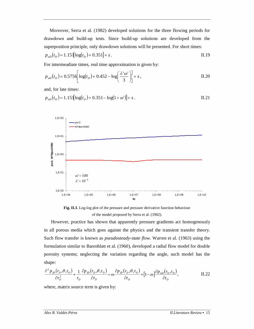
Fig. II.3 shows the plot of the pressure and derivative of pressure function in log-log
scale, where at intermediate times, a smooth transition in the slope of the pressure
derivate function is observed.
Alex R. Valdés-Pérez II.Literature Review • 15
Moreover, Serra et al. (1982) developed solutions for the three flowing periods for
drawdown and build-up tests. Since build-up solutions are developed from the
superposition principle, only drawdown solutions will be presented. For short times:
sttp DDwD 351.0log151.1 . II.19
For intermeadiate times, real time approximation is given by:
sttp DDwD
3''log452.0log5756.0 , II.20
and, for late times:
sttp DDwD '1log351.0log151.1 . II.21
1,E-02
1,E-01
1,E+00
1,E+01
1,E+02
1,E+04 1,E+05 1,E+06 1,E+07 1,E+08 1,E+09 1,E+10tD
pwD
, tD*
dpw
D/d
tD
pw D
tD*dpw D/dtD
Fig. II.3. Log-log plot of the pressure and pressure derivative function behaviour
of the model proposed by Serra et al. (1982).
However, practice has shown that apparently pressure gradients act homogenously
in all porous media which goes against the physics and the transient transfer theory.
Such flow transfer is known as pseudosteady-state flow. Warren et al. (1963) using the
formulation similar to Barenblatt et al. (1960), developed a radial flow model for double
porosity systems; neglecting the variation regarding the angle, such model has the
shape:
D
DDmD
D
DDfD
D
DDfD
DD
DDfD
ttrp
ttrp
rtrp
rrtrp
,1,,,,1,,
2
2
, II.22
where, matrix source term is given by:
100' 910'

16 • II.Literature Review Alex R. Valdés-Pérez
DDmDDDfDD
DDmD trptrpt
trp ,,,1
. II.23
Solution of eq. II.22 assuming infinite reservoir and constant flow rate at wellbore and
taking into account condition imposed by eq. II.23 is given by:
sshKsshs
sshKspwD
1
0 , II.24
Where:
sssh
11 . II.25
Fig. II.4 shows the log-log plot of the pressure and derivative of pressure function of
the model presented by Warren et al. (1963), where at intermediate times, an abrupt
transition in the slope of the pressure derivate function is observed.
1,E-02
1,E-01
1,E+00
1,E+01
1,E+02
1,E+03 1,E+04 1,E+05 1,E+06 1,E+07 1,E+08 1,E+09 1,E+10tD
p wD
, tD*
dpw
D/d
t D
pw D
tD*dpw D/dtD
Fig. II.4. Log-log plot of the pressure and pressure derivative function behaviour
of the model presented by Warren et al. (1963).
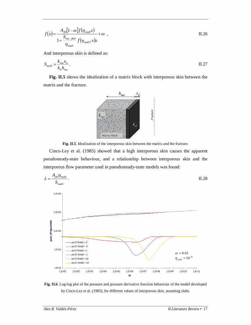
Cinco-Ley et al. (1985) showed that the apparent pseudosteady-state transference
behavior seen in tests can be attributed to a presence of interporous skin between matrix
and fracture network. Such interporous skin is produced by a film created by
mineralization or interaction between fluids in the face of the matrix blocks.
Mineralization has been observed in outcrops, where precipitation and other chemical
phenomena create a skin between different porous media. General solution for this flow
model has the same shape of eq. II.4, except for the transference function, which is
given by:
01.0 810maD
Alex R. Valdés-Pérez II.Literature Review • 17
ssfS
sfAsf
maDmaD
fbDma
maDfD
,1
1 , II.26
And interporous skin is defined as:
mad
dmamaD hk
xkS . II.27
Fig. II.5 shows the idealization of a matrix block with interporous skin between the
matrix and the fracture.
Fig. II.5. Idealization of the interporous skin between the matrix and the fracture.
Cinco-Ley et al. (1985) showed that a high interporous skin causes the apparent
pseudosteady-state behaviour, and a relationship between interporous skin and the
interporous flow parameter used in pseudosteady-state models was found:
maD
maDfD
SA
. II.28
1,E-02
1,E-01
1,E+00
1,E+01
1,E+02
1,E+01 1,E+02 1,E+03 1,E+04 1,E+05 1,E+06 1,E+07 1,E+08 1,E+09 1,E+10 1,E+11
tD
pwD
, tD*
dpw
D/d
tD
pw D SmaD = 0
pw D' SmaD = 0
pw D SmaD = 1
pw D' SmaD = 1
pw D SmaD = 10
pw D' SmaD = 10
Fig. II.6. Log-log plot of the pressure and pressure derivative function behaviour of the model developed
by Cinco-Ley et al. (1985), for different values of interporous skin, assuming slabs.
01.0 810 maD
18 • II.Literature Review Alex R. Valdés-Pérez
II.2 Fractal models
In order to understand the fractal theory applied to well test analysis, the first reference
that must be consulted is the publication of Barker in 1988. Barker presented
mathematical solutions for the diffusivity equation expressed as a Generalized Radial
Flow Model (GRF). The theory was developed for hydraulic test, but it can be used for
petroleum well testing applying some modifications. Development of GRF and its
solution for constant rate case is presented in Appendix A.
Barker (1988) developed a model where a variable parameter governing the
Euclidean dimension of flow at wellbore was introduced. Such parameter is expressed
in the present work as ed . GRF adapted for petroleum well testing, in dimensionless
variables is:
D
DDD
D
DDD
D
e
D
DDD
ttrp
rtrp
rd
rtrp
,,1,
2
2
. II.29
It can be verified that, when 1ed , eq. II.29 takes the form of the diffusivity
equation for linear flow (Miller, 1962); when 2ed GRF takes the form of the
diffusivity equation for radial flow (van Everdingen and Hurst, 1949) and, when 3ed ,
it takes the form of the spherical flow model (Chatas, 1966). Main assumptions made by
Barker on this model are:
- Flow obeys Darcy’s law;
- Flow is radial into a reservoir which is homogeneous and isotropic and fills an
n-dimensional space;
- The source is an n-dimensional sphere (for example a cylinder for two
dimensional flow or a sphere for three-dimensional flow.
Although Barker developed a model assuming a fractured rock, the assumption of a
homogeneous and isotropic reservoir allows its application into non fractured media.
The constant rate solution assuming an infinite reservoir for eq. II.29 in Laplace
space is detailed in Appendix A. Such solution is given by:
sKs
sKspv
vwD
12
3
, II.30
where:
21 ed . II.31

Alex R. Valdés-Pérez II.Literature Review • 19
Fig II.7 shows the plot of eq. II.30 and its derivative using Stehfest’s Algorithm
(Stehfest, 1970), when 21
, 0 and 21
, which correspond to the linear,
radial and spherical flows, respectively.
0,01
0,1
1
10
100
0,01 0,1 1 10 100 1000
tD
p wD, t
D*dp
wD/d
t D
pwD SphericalpwD' SphericalpwD RadialpwD' RadialpwD LinearpwD' Linear
Fig. II.7. Plot of Barker’s constant rate case solution, for 21 , 0 and 21 .
Doe (1991) presented methods for analyzing transient flow-rate data from constant-
pressure well tests, where the spatial dimension is variable. Such analysis can be applied
for the constant flow rate case.
Doe (1991) stated that, by definition of spatial dimension, the test dimension in not
limited to the range of the Euclidian dimensions, that is between 1 and 3. Conduits may
decrease in area by a power law of distance; hence their dimension is less than 1. Such a
case may be termed sublinear. Similarly, a conduit whose area changes by a power
grater than 2 has a dimension greater than 3, and may be called hyperspherical.
Examples of these conduits are shown in Fig. II.8.

20 • II.Literature Review Alex R. Valdés-Pérez
Fig. II.8 Sublinear and Hyperspherical Conduits (figure taken from Doe, 1991).
Fig. II.9 shows the transient pressure responses for the geometries established by
Doe (1991).
0,001
0,01
0,1
1
10
0,01 0,1 1 10 100 1000
tD
pwD, t
D*dp
wD/d
tD
pwD v=0.25pwD' v=0.25pwD v=-0.25pwD' v=-0.25pwD v=-0.75pwD' v'=-0.75
Fig. II.9. Plot of sublinear ( 25.0 and 25.0 ) and hyperspherical ( 75.0 ) geometries.
Chang et al. (1990) presented a flow model for a fractal reservoir, with single and
double porosity. For the double porosity case, they assumed pseudo-steady state
interaction between matrix and fractures. Appendix B shows the general development
for this model. Diffusivity equation presented by Chang and Yortsos in its
dimensionless form is given by:
D
DDfbD
D
DDmaDDdD
D
DDfbDD
DD
Dt
trpt
trpr
rtrp
rrr
fbe
fb
,,1
,11 , II.32
where:
Alex R. Valdés-Pérez II.Literature Review • 21
1 fbD ; II.33
fbD mass fractal dimension of fractures;
ed Euclidean dimension.
conductivity index (spectral dimension).
Later, Olarewaju (1996) presented a model and its solution in Laplace space for a
transient interaction between matrix and fracture network. Model developed by
Olarewaju in its dimensionless form is:
D
DDfbDD
D
DDmaDD
D
DDfbD
DD
DDfbD
ttrp
rz
tzprr
trprr
trp
,,3
,, *2
2
, II.34
where interporosity flow coefficient, is given by:
fbma
wma
khrk 212
, II.35
and dimensionless storativity ratio:
tfbtmama
tfb
ccc
* . II.36
Neglecting skin and wellbore storage effects, solution in Laplace space for Olarewaju’s
model, assuming constant flow rate and infinite reservoir, is:
ssgKsgs
ssgKsp
fbD
wD
22
22
2
2/3
21
, II.37
where:
*
* 13tanh13
1 ss
sg . II.38
Fig. II.37 shows the model proposed by Olarewaju (1996) with the inclusion of
storage and skin around wellbore for different values of the fractal dimension of fracture
network.
22 • II.Literature Review Alex R. Valdés-Pérez
0,10
1,00
10,00
100,00
1000,00
1 10 100 1000 10000 100000
tD/CD
p wD, t
D*dp
wD/d
t D
pwD Dfb=1,3tD*dpwD/dtD Dfb=1,3pwD Dfb=1,5tD*dpwD/dtD Dfb=1,5pwD Dfb=1,7tD*dpwD/dtD Dfb=1,7
Fig. II.10. Log-log plot of the model proposed by Olarewaju (1996).
Flamenco et al. (2001) and Flamenco et al. (2003) presented approximated solutions
for the early and late times periods of the models presented by Chang et al. (1990). The
convergence of such solutions was tested against a numerical solution of the same
model. Fig. II.11 shows the convergence of the analytical and semi-analytical solutions
to the numerical one, presented by these authors.
Fig. II.11. Chang et al. (1990) solution (numerical solution); short- and long-time approximations for a
fractal fractured reservoir with matrix participation (figure taken from Flamenco et al., 2003).
001.0 00001.0 2.0 100DC
Alex R. Valdés-Pérez II.Literature Review • 23
In Appendix C of this thesis, a free interaction between matrix and fractures under
transient pressure conditions was developed. With this development the concept of
dimensionless fracture area, fDA , (Cinco-Ley and Samaniego, 1982) was introduced
into fractal reservoir theory. Moreover, with this model, it is possible to assume slabs
and spherical shape for matrix blocks. Developed diffusivity equation for this model is:
D
DDfbDD
t
DDmaDDfbD
fDDD
DDfbD
DD
DDfbD
ttrp
r
dtHFrp
Arr
trprr
trp D
,
,,,
1,,
02
2
,
II.39
where:
fDA dimensionless fractal fracture area, and it is defined as:
ma
wbmafbfD V
rVhAA
. II.40
Fluid transference functions, assuming slabs is given by:
1
12 22
4,,n
Htn
D
maDDDmaD
D
DmaD
eH
tHF
, II.41
or, if spheres as matrix blocks, fluid transference function is:
1
4 22
4,,n
Htn
D
maDDDmaD
D
DmaD
eH
tHF
. II.42
Solution in Laplace Space for eq. II.39 under constant flow rate and infinite reservoir
conditions is given by:
ssfKsfs
ssfKsp
fbD
wD
22
22
2
2/3
21
, II.46
where:
sHFAsf DmaDfD ,,1 . II.47
24 • II.Literature Review Alex R. Valdés-Pérez
0,1
1
10
100
1000
0,01 0,1 1 10 100 1000 10000 100000 1000000 10000000
tD
pwD, t
D*dp
wD/d
tD
pwD θ=0.1 Dfb=1.7pwD' θ=0.1 Dfb=1.7pwD θ=0.05 Dfb=1.85pwD' θ=0.05 Dfb=1.85pwD θ=0.2 Dfb=2.2pwD' θ=0.2 Dfb=2.2
Fig. II.12. Log-log plot of the free interporous transference, developed in Appendix C. Larsen (2013) developed a modified fractal model for small values of the
dimensionless storativity ratio by combining models presented previously by Chang et
al. (1990) and Olarewaju (1996). Such modification yields the equation in Laplace
space:
DDfbDDDd
DD
DDfbDD
DD
trpsLsrdr
trpdr
drd
rfb ,tanh
3,1
. II.48
Detailed development of this model is shown in Appendix D.
Other relevant papers regarding this topic are the ones published by Acuña et al.
(1995) and Camacho-Velázquez et al. (2008). In addition, Cossio (2012) and Cossio et
al. (2013) presented a model that describes the behaviour of pressure within a finite
conductivity fracture into a fractal reservoir, and a semi-analytical solution for it.
01.0 0001.0
D
maD
H
Alex R. Valdés-Pérez III.Proposed Model • 25
Chapter III Proposed Model
III.1. Flow model development
Incoming fluid mass into an object is given by:
tqm ffin ; III.1
out coming fluid mass from the same object is:
tqtqm ffffout ; III.2
oil mass contribution from the Euclidean matrix:
tqm mafma . III.3 Then, cumulative fluid mass into the object is:
tqtqtqmmm mafffmafinoutcum . III.4
On the other hand, mass of fluid at a time 1t is given by:
bulkfbfft VSm 1
, III.5
at a time 2t :
bulkfbffbulkfbfft VSVSm 2
, III.6
and, cumulative fluid mass is given by:
bulkfbffttcum VSmmm 12
. III.7
Equating eq. III.4 and eq. III.7 results:
bulkfbffmafff VStqtq . III.8
Using definition of bulk volume (eq. I.4), eq. III.8 becomes:
rbrStqtq ee
e
dddfbffmafff 31
. III.9
Arraying previous equation:
t
Sq
rq
brfbff
mafff
ddd
ee
e
31
1 . III.10
Where Matrix flow rate per unit of bulk volume is defined by:
bulk
mama V
. III.11
Taking the limits r and t to zero, and arraying, equation III.10 becomes:
t
Sbrqbr
rq fbffdd
dmafdd
dff ee
e
ee
e
3131 . III.12
26 • III.Proposed Model Alex R. Valdés-Pérez
Inserting Darcy’s equation in fractal form (eq.I.51) into previous equation, results:
t
Sbrqbr
rprkaV
rfbffdd
dmafdd
dfb
fb
fbuff
ee
e
ee
e
3131 . III.13
Applying the derivatives in eq. III.13:
tS
tS
brqbr
rrtrp
rr
trpr
rtrp
rkaV
fbff
fffb
dddmaf
ddd
ffbfbf
fbf
fb
fbuf
ee
e
ee
e
3131
12
2 ,,,
. III.14
According to chain rule:
r
trptrpr
fb
fb
ff
,
,
, III.15
t
trptrp
St
S fb
fb
ffff
,,
, III.16
t
trptrpt
fb
fb
fbfb
,,
. III.17
Substituting eqs. III.15, III.16 and III.17 and using compressibility definitions, prior eq.
is rewritten as follows:
t
trpccSbr
qbrr
trpcr
rtrp
rr
trpr
kaV
fbfbfffb
nnn
mann
nfb
ffbfb
fb
fbuf
,
,,,
31
31
2
12
2
.III.18
If single phase flow is assumed, then total compressibility is defined as:
fbftfb ccc , III.19
therefore eq. III.18 is written as:
t
trpcbr
qbrr
trpcr
rtrp
rr
trpr
kaV
fbtfbfb
ddd
madd
dfb
ffbfb
fb
fbuf
ee
e
ee
e
,
,,,
31
312
12
2
. III.20
Neglecting quadratic gradient pressure and according to porosity of the fracture
network definition, prior equation becomes:
Alex R. Valdés-Pérez III.Proposed Model • 27
t
trpk
crq
kr
rtrp
rr
trpr fb
fb
fbtfbDma
fb
Dfbfb fbfb
,,, 1112
2 . III.21
On the other hand, matrix flow rate per unit of bulk can be expressed as:
dp
dpAk
q suruma
tmafbma
ma
0
. III.22
If slab matrix blocks are assumed, area exposed to flow is defined as:
fmafb hh
A
2 ; III.23
or, if cube matrix blocks are assumed:
326
fma
mafb hh
hA
. III.24
Substituting eq. III.22 into III.21, the diffusivity equation for a double porosity
fractal reservoir with transient interporosity transfer is obtained:
t
trpr
dpd
pk
Akr
rtrp
rr
trpr
fb
fb
D
suruma
tma
fb
fbmaDfbfb
fb
fb
,
,,
1
0
112
2
, III.25
where hydraulic diffusivity coefficient in field units is defined as:
tfbfb
fbfb c
k
00026367.0
. III.26
In compact form, eq. III.25 is written as:
t
trpdp
dp
kAk
rtrp
rrr
fb
fbsuruma
tma
fb
fbmafbD fb
,1,1
01
. III.27
In order to have a homogeneous partial differential equation and an easier way to
manage unknowns related to eq. III.27, it is necessary to expressed in dimensionless
variables.
III.2 Transformation to dimensionless variables for well test analysis
In order to transform eq. III.27 to a dimensionless expression, following dimensionless
variables has been stated:
Dimensionless radius:

28 • III.Proposed Model Alex R. Valdés-Pérez
wD r
rr , III.28
dimensionless time:
trc
kt
wtt
fbD 2
00026367.0, III.29
where:
tmamatfbfbtt ccc . III.30
For an oil-filled system, dimensionless pressure in the fracture network:
fbwo
fbifbufDDDfbD rqB
trppkaVtrp fb
1
,22.887
03281.0, . III.31
And, dimensionless pressure in the matrix:
fbwo
maifbufDDDmaD rqB
trppkaVtrp fb
1
,22.887
03281.0, . III.32
For gas reservoirs, dimensionless pressure in the fracture network:
fbwgg
fbfbufDDDfbD ZTrq
pmkaVtrp fb
12.8937
03281.0, , III.33
where:
trpppm fbifb ,22 . III.34
and dimensionless pressure in the matrix:
fbwgg
mafbufDDDmaD ZTrq
pmkaVtrp fb
12.8937
03281.0, , III.35
where:
trpppm maima ,22 . III.36
For geothermal reservoirs (steam), dimensionless pressure in the fracture network:
fbws
fbfbufDDDfbD ZTrW
pmkaVtrp fb
181361
03281.0, , III.37
where:
trpppm fbifb ,22 . III.38
and, dimensionless pressure in the matrix:

Alex R. Valdés-Pérez III.Proposed Model • 29
fbws
mafbufDDDmaD ZTrW
pmkaVtrp fb
181361
03281.0, , III.39
and:
trpppm maima ,22 . III.40
The procedures for transformation to dimensionless variables of eq. III.25, for the
oil, gas and steam reservoirs are similar, therefore only the oil-filled reservoir is shown.
Using chain rule, first derivative of pressure in the fracture network regarding the
radius can be written as follows:
D
DDfbDD
DDfbD
fbfb
rtrp
drdr
trptrp
rtrp
,,,,
. III.41
Based on dimensionless pressure definition, first derivative of pressure regarding
dimensionless pressure in fracture network is:
fbuf
fbwo
DDDfbD
fb
kaVrqB
trptrp
fb
1
03281.022.887
,,
. III.42
Based on the dimensionless radius definition, derivative of dimensionless radius
regarding radius is:
w
D
rdrdr 1
, III.43
Substituting eq. III.42 and III.43 into eq. III.41 results:
D
DDfbD
fbuf
fbwo
D
fb
rtrp
kaVrqB
rtrp
fb
,
03281.022.887,
. III.44
Taking second derivative regarding radius of eq. III.44:
2
21
2
2 ,
03281.022.887,
D
DDfbD
fbuf
fbwo
D
fb
rtrp
kaVrqB
rtrp
fb
. III.45
Analogously to the first derivative of pressure in the fracture network regarding the
radius, first derivative of pressure in the fracture network regarding the time is given by:
D
DDfbD
wtt
fb
fbuf
fbwo
D
fb
ttrp
rck
kaVrqB
ttrp
fb
,00026367.0
03281.022.887,
2
1
. III.46
Besides,
DDmaD
DmaD
mama trprprprp ,
,,, , III.47

30 • III.Proposed Model Alex R. Valdés-Pérez
hence:
DDmaD
fbuf
fbwo
D
ma trpkaV
rqBrp
fb
,03281.0
22.887, 1
. III.48
Substituting III.28, III.44, III.45, III.46, III.48 in III.25 and arraying it, results:
D
DDfbDD
t
DDmaDDmaD
fDDD
DDfbD
DD
DDfbD
ttrp
r
dtHFrpArr
trprr
trp D
,
,,,1,,
02
2
,
III.49
where, dimensionless storativity ratio, is defined as:
tt
tfbfb
cc
; III.50
dimenssionless matrix hidraulic diffusivity:
fbtmama
ttmamaD kc
ck
; III.51
dimensionless block size, for slabs:
2
2
ma
wD h
rH ; III.52
and for spheres:
2
2
ma
wD d
rH ; III.53
dimensionless fractal fracture network area, fDA :
ma
wbmafbfD V
rVhAA
. III.54
Fluid transfer function, assuming slabs:
1
12 22
4,,n
Htn
D
maDDDmaD
D
DmaD
eH
tHF
, III.55
or, if spheres as matrix blocks, fluid transfer function is:
1
4 22
4,,n
Htn
D
maDDDmaD
D
DmaD
eH
tHF
. III.56

Alex R. Valdés-Pérez IV .Model solutions for well test analysis • 31
Chapter IV Model solutions for well test analysis
IV.1. General Solution in Laplace space
In Chapter III the diffusivity equation for a double porosity reservoir assuming fractal
fracture network and Euclidean matrix blocks was developed:
D
DDfbDD
t
DDmaDDmaD
fDDD
DDfbD
DD
DDfbD
ttrp
r
dtHFrpArr
trprr
trp D
,
,,,1,,
02
2
.
IV.1
In order to have a well test analysis model for the Fractal Reservoir Model assuming
transient interporous transference between matrix and fractures, the following
conditions have been set:
initial condition for fracture network: 00, DDfbD trp , IV.2
inner Boundary:
1,1
D
DfbDD t
tpr , IV.3
outer boundary: 0,lim DDDr
trpD
. IV.4
Constant rate solutions assuming finite circular reservoir and constant pressure
boundary are shown in Appendix G.
Applying Laplace transform to eq. IV.1 yields:
0,,
,,,1,,
2
2
DfbDDfbDD
DmaDDmaDfDDD
DDfbD
DD
DDfbD
rpsrpsr
srpssHFArdr
trdprdr
trpd
. IV.5
Similar to Cinco-Ley et al. (1985), dimensionless pressure in the matrix can be
expressed as follows:
ssHFSH
srpsrp
DmaDmaD
fbDmaD
DfbDDmaD
,,1
,,
; IV.6
where, for slab matrix blocks:

32 • IV. Model solutions for well test analysis Alex R. Valdés-Pérez
maD
D
D
maDDmaD
sHsH
sHF
21tanh,, , IV.7
and, for spheres as matrix blocks:
sHsH
sHsHF
D
maD
maD
D
D
maDDmaD
2
21coth,, . IV.8
Substituting eq. IV.6 into eq. IV.5 results:
0,,
,,,1
,,1,,
2
2
DfbDDfbDD
DfbD
DmaDmaD
fbDmaD
DmaDfDD
D
DDfbD
DD
DDfbD
rpsrpsr
srpssHF
SHsHFsAr
drtrdp
rdrtrpd
.
IV.9
Applying initial condition in eq. IV.9, and arraying:
0,,, 2
2
22 srpsfsr
drsrpd
rdr
srpdr DfbDD
D
DfbDD
D
DfbDD
. IV.10
Where the transference function is defined as:
ssHFSH
sHFAsf
DmaDmaD
fbDmaD
DmaDfD
,,1
,,1. IV.11
It can be verified that, if there is no restriction between matrix and fractures, i.e.,
0 fbDmaS , prior transference function reduces to the free interaction fractal model,
showed in Appendix D.
Parameter is established:
21
, IV.12
then:
0,,
21, 2
2
22 srpsfsr
drsrpd
rdr
srpdr DfbDD
D
DfbDD
D
DfbDD
. IV.13
The following transform function has been set:
zGsrp DDD , , IV.14
and the transformation variable:
2
2
22
Drssf
z . IV.15

Alex R. Valdés-Pérez IV. Model solutions for well test analysis • 33
Applying the variable transformations, the following expression is obtained:
021 22
22
zGzz
zGzz
zGz DDD , IV.16
where:
21
v , IV.17
To equalize the coefficient of the first derivative to one the following expression is
proposed:
zBzzG D
v
D , IV.18
where:
21
22
ssf. IV.19
Eq. IV.16 is expressed in terms of function IV.18 as:
0)( 222
2 zBzvdz
zdBzdz
zBdz DDD . IV.20
Solution for eq. IV.20 is given by:
zKczIczB vvD 21 , IV.21
or, in terms of eq. IV.18:
zKczIczzG vv
v
D 21
, IV.22
and, in terms of srp DD , and srD , solution is:
2
2
212
22
211
21
22
22
,
DDDDD rssf
Kcrssf
Icrsrp . IV.23
Applying outer boundary condition, it can be concluded that:
01 c , IV.24
and, bounded solution is:
2
2
21
21
2 22
,
DDDD rssf
Krcsrp . IV.25
Applying inner boundary condition it is found that:

34 • IV. Model solutions for well test analysis Alex R. Valdés-Pérez
2
21
2
2/32
ssfKsfs
c
fbD
, IV.26
and, solution can be expressed as:
22
22
,
2
2/3
22
21
21
ssfKsfs
rssf
Krsrp
fbD
DD
DD . IV.27
Solution evaluated at wellbore is:
ssfKsfs
ssfKsp
fbD
wD
22
22
2
2/3
21
. IV.28
Phenomena around wellbore such as skin at wellbore and wellbore storage, can be
incorporated as follows:
spsCsCSs
Ssp
SCspwDDDwell
wellwD
wellDwD 21,,
. IV.29
A detailed description of the storage around wellbore phenomenon is described in
Appendix F.
IV.2. Approximate solutions at short times: Total Expansion in the Fracture Network
It has been shown that at early times, only the fracture expansion acts in the reservoir
(Cinco-Ley et al., 1982). It means that transference function can be approximated as:
sf , IV.30
therefore, eq. IV.1 is reduced to:
D
DDfbDD
D
DDfbD
DD
DDfbD
ttrp
rr
trprr
trp
,,,2
2
. IV.31
Establishing the following transformation function:
DDfbDDfbD trpDZ fb ,
22
1
, IV.32
and transformation variables:
fbDD
fb
rD1
1 , IV.33
and:
Alex R. Valdés-Pérez IV. Model solutions for well test analysis • 35
DD
fb tD fb
22
1
. IV.34
Eq. 31 is expressed according to eqs. IV.32 to IV.34 as follows:
1
1
1
1
21
121
1222
1
22
DD
fb
fbDDD ZZD
DZ fbfb . IV.35
Similarly initial condition is given by:
00,11 DZ ; IV.36
inner boundary condition:
1lim1
1
22
101
DD Zfb , IV.37
and outer boundary condition:
0, 11 DZ . IV.38
Establishing the following transformation function:
21111
fbD
DD UZ , IV.39
and:
2111
fbD
. IV.40
Applying the transformation variables, eq. IV.35 is rewritten as:
1
11
1
1
21
121
1222
1 22
ddUD
ddU
DdUd DfbD
fb
DDD fbfb . IV.41
Prior eq. can be expressed as:
1111
1
22
11
2
DDD
fb
Udd
ddU
dd
Dfb
, IV.42
transforming inner boundary condition:
0limlim
1
122
101
122
10 11
ddUZ DDDD fbfb , IV.43
integrating eq. IV.42:
1111
122
12 AU
ddU
D DDD
fbfb
, IV.44
it can be concluded, based on inner boundary condition:
01 A , IV.45
36 • IV. Model solutions for well test analysis Alex R. Valdés-Pérez
therefore eq. IV.44 reduces to:
1
12
11
12 d
UdU
DfbD
D
D
fb
, IV.46
integrating and arraying eq. IV.47:
fbDfbD
D eAU2
1
2
221
, IV.47
applying outer boundary:
10
12
20
11
2
1
2
deAdU
fbDfbD
D , IV.48
hence:
01
2
2 2
1
2
1
de
AfbDfbD
, IV.49
establishing the following transformation variable:
2
1
fbD
, IV.50
taking the first derivative:
d
Dd
fbfb Dfb
D1
221 2
. IV.51
Hence, eq. IV.49 can be expressed as:
0
122
2
2 2
2
deD
Afbfb
fb
DD
fb
D
. IV.52
Moreover, defining: 2
2 2
fbD, IV.53
its first derivative is given by:
2
2
2
d
Dd fb
. IV.54
Hence, eq. IV.52 becomes:

Alex R. Valdés-Pérez IV. Model solutions for well test analysis • 37
02
12
2
2
12
2
2
2
2
de
D
Afb
fbfb
D
DD
fb
. IV.55
Gamma Function for this case is defined as:
0
2
12
22
2
de
D fbDfb , IV.56
hence:
2
22
12
2
2
fb
DD
fb
D
D
A
fbfb
; IV.57
subsequently eq. IV.47 becomes:
fbDfb
fbfb
D
fb
DD
fb
D eD
D
U2
1
2
2
2
12
2
1
2
2
. IV.58
Applying Duhamel’s principle in eq. IV.39:
1
012111
dUZfbD
DD . IV.59
Substituting eq. IV.58 in eq. IV.59:
1
1
2
12
0121
2
2
12
2
1
2
2
deD
D
Zfb
fbDfb
fbfb
DD
fb
DD
fb
D . IV.60
Establishing the following variable transformation:
yD fbDfb
2
1
2
1 2
, IV.61
and, taking the first derivate regarding y :
dyy
Dd
fbDfb
2
2
12
1 2
. IV.62
38 • IV. Model solutions for well test analysis Alex R. Valdés-Pérez
Substituting eq. IV. 61 and IV.62 in IV.60:
y
Dy
fb
Dfb
D dyyeD
D
Zfb
fb
22
12
1
1
2
2
. IV.63
Incomplete function Gamma is defined as:
x
ta dtetxa 1, , IV.64
then, eq. IV.63 becomes:
1
2
12
12
1
1 2,1
22
2
fb
fbD
fbfb
fb
Dfb
D
DDD
D
Z , IV.65
therefore, solution of eq. IV.31 is given by:
D
Dfb
fb
DD
DDfbD trD
Drtrp
fb
2
22
2 , 1
22
2,
. IV.66
In order to have simplified solutions relatively easy to use, two cases must be
defined. The first case is given by the condition 2 fbD . If that is the case, eq. IV.103
and evaluated in 1Dr , it becomes:
DDwD t
tp 22,0
21
. IV.67
According to incomplete gamma function convergences, prior expression can be
expressed as:
DiDwD t
Etp 2221
, IV.68
where:
xEi integral exponential.
For small arguments of the integral exponential, eq. IV.68 can be approximated as:
ln2ln2ln2
1DDwD ttp , IV.69
where:
Euler’s constant.

Alex R. Valdés-Pérez IV. Model solutions for well test analysis • 39
It can be verified that, if 0 , eq. IV.69 converges to the solution presented by Cinco-
Ley et al. (1982).
On the other hand, for 2 fbD long time an approximation of incomplete
gamma function is given by:
1,1
ax
axaxa
aa
, IV.70
hence, incomplete gamma function for this problem is approximated as:
2
11
22122
1
22
2
12
21122
,12
fbfbfbfb
D
Dfb
DDD
D
fb
D
Dfb tDrD
trD
. IV.71
Evaluating IV.66 at 1Dr , and substituting IV.71 results:
vD
fbfb
vv
fb
fb
DwD tDDD
D
tp
21
2
2
22
12 112
, IV.72
where:
21
fbDv . IV.73
A form of the recurrence formula is:
111
xx
x , IV.74
therefore, eq. IV.72 is rewritten as:
v
Dfb
vv
DwD tD
vv
tp
2
22
1 112
. IV.75
IV.3. Approximate solutions at intermediate times: Interaction between porous media
a. Transient State with variable Interporous Skin
For intermediate times, the interaction between porous media takes place. For this
period, transference function can be approximated as:
1
11
maD
DfbDma
D
maDfD
sHSsH
Asf
, IV.76
therefore, eq. IV.28 is rewritten as:

40 • IV. Model solutions for well test analysis Alex R. Valdés-Pérez
D
maDfD
maD
DfbDmaD
D
maDfD
maD
DfbDma
D
maDfD
maD
DfbDma
wD
HsA
sHSK
HsA
sHSK
sHAs
sHS
sp
fb
112
2
112
2
1
1
21
2
21
21
21
2/3
21
.
IV.77
For small arguments, Bessel function in the denominator is approximated as:
211
22
112
2
22222
21
2
fb
D
D
maDfD
D
maD
DfbDma
D
D
maDfD
maD
DfbDmaD
DH
sAsHS
HsA
sHSK
fbfbfb
fb
. IV.78
Substituting eq. IV.78 in eq. IV.77:
D
maDfD
maD
DfbDma
D
D
maD
DfbDma
fbD
D
D
maDfD
wD
Hs
AsHS
K
s
sHS
DH
Asp
fb
fb
fb
fb
112
2
1
22
12
21
21
2445
2221
2
21
22
. IV.79
For the 2 fbD case, the Bessel function in the numerator is approximated as:
D
maDfD
maD
DfbDma
D
maDfD
maD
DfbDma
HsA
sHS
HsA
sHSK
112
1ln
112
2
21
21
0
, IV.80
thus, eq. IV.79 can be expressed as:
Alex R. Valdés-Pérez IV. Model solutions for well test analysis • 41
ss
sHS
ssH
A
sssp maD
DfbDma
D
maDfD
wD
1ln
212ln
1ln
21ln
41
22 .
IV.81
Taking the natural logarithmic expansion:
maD
DfbDma
maD
DfbDma
sHS
sHS
1ln , IV.82
eq. IV.123 becomes:
ss
HS
ssH
A
sssp maD
DfbDma
D
maDfD
wD
212ln
1ln
21ln
41
22 , IV.83
inverting to Real Space:
4329.02
12ln1ln21ln
41
22 2
1
DmaD
DfbDma
D
maDfDDDwD t
HS
HAttp
IV.84
On the other hand, if 2 fbD , then the Bessel function in the denominator is
approximated as:
2111
22
112
2
221
221
21
21
21
D
maDfD
maD
DfbDma
D
maDfD
maD
DfbDma
HsA
sHS
HsA
sHSK
, IV.85
substituting eq. IV.85 in eq. IV.79:
241
2445
2212
2212
21 11
2
212
fb
fbfb
fb
D
D
maD
DfbDma
D
D
maDfD
fb
D
wD
s
sHS
HA
Dsp ,
IV.86
srraying, prior eq. reduces to:
42 • IV. Model solutions for well test analysis Alex R. Valdés-Pérez
2252
21
22
21
1
22
12
1
s
sHS
DH
Asp maD
DfbDma
fb
D
maDfD
wD, IV.87
according to binomial series, eq. IV.87 becomes:
22
22
22
23
222
22
21
2
1
2
21
fbfb
fb
fb
D
maD
DfbDma
fbD
D
D
D
maDfD
fbwD sHS
Ds
HA
Dsp ,
IV.88
and, inverting to real space, and arraying, eq. IV.88 can be expressed as:
22
231
2
1
23
21
12
1
2
v
vHvSt
HA
vvtpt maD
DfbDma
Dv
v
D
maDfD
DwD
v
D
. IV.89
It can be verified that, if 0 fbDmaS this model converges to the transient
interporous transference and the solution given in Appendix D.
b. Pseudosteady-state equivalence: Severe interporous skin
Similar to Cinco et al. (1985), pseudosteady-state is achieved when a highly damaged
interface between matrix and fracture network exists. Therefore, transference function
reduces to:
sHS
Asf
DfbDma
maDfD
, IV.90
thus, eq. IV.28 becomes:
DfbDma
maDfDD
DfbDma
maDfD
DfbDma
maDfDwD
HSA
K
HSA
K
HSA
ssp
fb
22
22
1
2
21
, IV.91
for small arguments the Bessel function in the denominator is approximated as:
Alex R. Valdés-Pérez IV. Model solutions for well test analysis • 43
2
221
22
2
2
fb
D
DfbDma
maDfDDfbDma
maDfDD
D
HSAHS
AK
fb
fb, IV.92
hence, inverting to real space:
DfbDma
maDfDD
DfbDma
maDfDfbD
DwD HSA
K
HSAD
tpfb
fb
22
22
2
21
21
2
, IV.93
It can be observed that expression IV.93 corresponds to an independent of time
value. Cinco-Ley et al. (1985) found a relationship between the interporous skin and
other parameter of the transient interporous transference model with the pseudosteady-
state’s matrix-fracture interaction parameter. Extending such concept to the present
work, it was found the following expression:
DfbDma
maDfD
HSA
. IV.94
A simplified expression of eq. IV.93, when 2 fbD is given by:
DfbDma
maDfDDwD HS
AKtp
2
22
20 , IV.95
or, in terms of pseudosteady-state models’ parameters:
22
22
0Ktp DwD , IV.96
prior equation can be approximated as follows:
ln212ln
22
DwD tp . IV.97
On the other hand, if 2 fbD , then:
2
1221
22 2
1
21
maDfD
DfbDma
DfbDma
maDfD
AHS
HSA
K , IV.98
and eq. IV.93 is reduced to:
2
1222
2
212
fb
fb D
maDfD
DfbDma
fb
D
DwD AHS
Dtp . IV.99
In terms of pseudosteady-state models’ parameters:

44 • IV. Model solutions for well test analysis Alex R. Valdés-Pérez
12
222
2
212
fb
fb
D
fb
D
DwD Dtp . IV.100
IV.4. Approximate solutions at late times: Single System Behavior
At late times the double porosity system acts as a single one. Therefore, the transference
function is approximated as:
1sf , IV.101
and eq. IV.1 is reduced to:
D
DDfbDD
D
DDfbD
DD
DDfbD
ttrp
rr
trprr
trp
,,,2
2 . IV.102
For this case, an analogous procedure made for the early times case can be performed.
Thus, the solution for the late times case is given by:
D
Dfb
fb
DD
DDfbD trD
Drtrp
fb
2
22
2 , 1
22
2,
. IV.103
Evaluating at wellbore:
D
fb
fbDwD t
DD
tp 221 , 1
22
2
1
. IV.104
Besides, if 2fbD , eq. IV.104 is approximated by the following expression:
2ln2ln2
1DDwD ttp . IV.105
It can be verified that, if 0 , eq. IV.105 converges to the solution presented by
Cinco-Ley et al. (1982).
On the other hand, for 2 fbD the approximation is given by:
v
Dfb
v
DwD tD
vv
tp
2
22
1 12
. IV.106
Alex R. Valdés-Pérez V.Validation and Application • 45
Chapter V Validation and Application
In Chapter IV a general solution in Laplace space for the model developed in this thesis
was developed. Such solution evaluated at wellbore is given by:
ssfKsfs
ssfKsp
fbD
wD
22
22
2
2/3
21
. V.1
For computer-aided analysis, eq. V.1 is numerically inverted to real space (Stehfest,
1970) in order to analyze transient pressure data that shows fractal behavior.
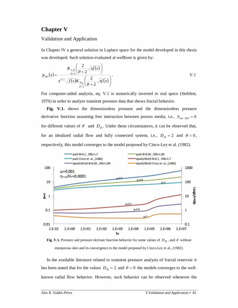
Fig. V.1. shows the dimensionless pressure and the dimensionless pressure
derivative function assuming free interaction between porous media, i.e., 0 fbDmaS
for different values of and fbD . Under these circumstances, it can be observed that,
for an idealized radial flow and fully connected system, i.e., 2fbD and 0 ,
respectively, this model converges to the model proposed by Cinco-Ley et al. (1982).
Fig. V.1. Pressure and pressure derivate function behavior for some values of fbD , and without
interporous skin and its convergence to the model proposed by Cinco-Ley et al., (1982).
In the available literature related to transient pressure analysis of fractal reservoir it
has been stated that for the values 2fbD and 0 the models converges to the well-
known radial flow behavior. However, such behavior can be observed whenever the

46 • V. Validation and Application Alex R. Valdés-Pérez
condition 2 fbD be satisfied. Fig. V.2. shows a semilog plot of the dimensionless
pressure behavior as a function of the dimensionless time for combinations that satisfy
the 2 fbD condition. Hence, it can be observed that the dimensionless pressure for a
idealized double porosity radial system perfectly connected (blue solid line) shows the
same behavior of a double porosity spherical system poorly connected (green solid
line).
Fig. V.2. Semilog plot of the pressure behavior for some values of
that satisfy the condition of 2fbD .
Besides, dotted lines in Fig. V.2. shows the convergence of the approximated
solutions for early times:
ln2ln2ln2
1DDwD ttp , V.2
and for late times:
2ln2ln2
1DDwD ttp , V.3
to the general solution for the shown cases.
Fig. V.3. shows the dimensionless pressure and the dimensionless pressure
derivative function behavior of the proposed model when 2 fbD , for different
values of interporous skin and neglecting phenomena around wellbore. It can be
observed that the higher the interporous skin the deeper the “valley” shape in the
dimensionless pressure derivative function, which corresponds to the interaction
between porous media.
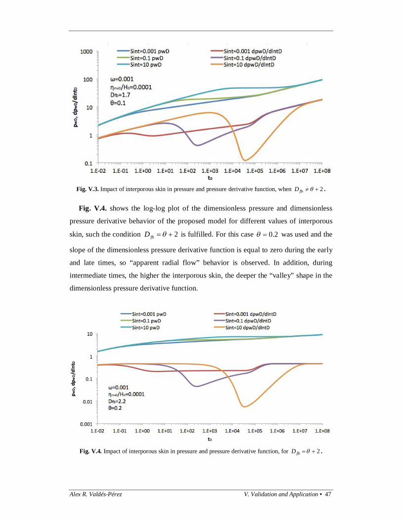
Alex R. Valdés-Pérez V. Validation and Application • 47
Fig. V.3. Impact of interporous skin in pressure and pressure derivative function, when 2 fbD .
Fig. V.4. shows the log-log plot of the dimensionless pressure and dimensionless
pressure derivative behavior of the proposed model for different values of interporous
skin, such the condition 2 fbD is fulfilled. For this case 2.0 was used and the
slope of the dimensionless pressure derivative function is equal to zero during the early
and late times, so “apparent radial flow” behavior is observed. In addition, during
intermediate times, the higher the interporous skin, the deeper the “valley” shape in the
dimensionless pressure derivative function.
Fig. V.4. Impact of interporous skin in pressure and pressure derivative function, for 2fbD .

48 • V. Validation and Application Alex R. Valdés-Pérez
It was also mentioned that in order to include phenomena around wellbore to the
proposed model, such as wellbore storage and skin around wellbore, eq. IV.29 should
be used. Fig. V.5. and Fig. V.6. show the impact of these phenomena on the cases
shown previously in Fig. V.3. and Fig. V.4., respectively.
Fig. V.5. Behavior of pressure and pressure derivative function,
when 2 fbD , considering phenomena around wellbore.
Fig. V.6. Behavior of pressure and pressure derivative function,
when 2 fbD , considering phenomena around wellbore.

Alex R. Valdés-Pérez V. Validation and Application • 49
Fig. V.7. shows the convergence of the approximate solutions at early, intermediate
and late times, eq. IV.69, eq. IV.84 and eq. IV.105, respectively to the general solution,
assuming no interporous skin. This semilog plot shows the typical behavior of a double
porosity radial system, i.e., straight lines at early and late times and another straight line
during intermediate times. However, the input values show that a flow geometry that
tends to be spherical 5.2fbD , with non-well connected flowing traces 5.0 is
equivalent to a radial flow, well-connected behavior. This type of behavior has been
named apparent radial flow.
Fig. V.7. Convergence from the short, intermediate and long times solutions to the general solution,
when 2 fbD , with no interporous skin.
Analogously, Fig. V.8. shows the convergence of the approximate solutions at early,
intermediate and late times, eq. IV.75, eq. IV.89 and eq. IV.106, respectively to the
general solution, assuming no interporous skin, when 2 fbD . For this case, all
approximated solutions converge to the log-log straight line portions, corresponding to
the fracture expansion, interaction between media and single system behavior.
Fig. V.8. exhibits the case shown in Fig. V.6 but this time with a relative low
interporous skin value. Except from the beginning of the approximated solution during
intermediate times, it shows the same trend of the straight line portion of the general
solution, and therefore this approximation might be useful to characterize the
interporous skin and the matrix, if the non-linear regression is possible to be performed.

50 • V. Validation and Application Alex R. Valdés-Pérez
Fig. V.8. Convergence from the short, intermediate and long times solutions to the general solution,
when 2fbD , with no interporous skin.
Fig. V.9. Convergence from the short, intermediate and long times solutions to the general solution,
when 2 fbD , with low interporous skin.
Fig. V.10. shows the case shown in Fig. V.8 with a relative low interporous skin
value. For this case the convergence of the approximated solution during intermediate
times to the general solution is observed.

Alex R. Valdés-Pérez V. Validation and Application • 51
Fig. V.10. Convergence from the short, intermediate and long times solutions to the general solution,
when 2 fbD , with low interporous skin.
Fig. V.11. and Fig. V.12. show the convergence of the approximated solutions for
severe interporous skin, i.e., pseudosteady state behavior to the general solution, for
2fbD and 2fbD , respectively. The intermediate times behavior shows a flat
slope and according to the equivalence given by eq. IV.94, the matrix-fracture
interaction parameter, for both cases is 11102 .
Fig. V.11. Convergence from the short, intermediate and long times solutions to the general solution,
when 2 fbD , with severe interporous skin (pseudosteady-state).

52 • V. Validation and Application Alex R. Valdés-Pérez
Fig. V.12. Convergence from the short, intermediate and long times solutions to the general solution,
when 2 fbD , with severe interporous skin (pseudosteady-state).
Example of Application
A drawdown test was performed in Well A. The behavior of pressure and pressure
derivative function are shown in Fig. V.13. Reservoir and well data are given in Table
V.1.
Table V.1. Reservoir and well data for the example.
Parameter Quantity
q [bpd] 2,000
oB [[email protected]/ [email protected]] 1.6
o [cp] 6
wr [ft] 0.5
fb [fraction] 0.01
Pressure derivative function in Fig. V.13 does not show the fractal fracture
expansion, i.e., behavior at early times. Then, analyzing late time response (see Fig.
V.14) and comparing such behavior with eq. IV. 106, it can be conclude that,
8362.0v , hence, following relation between fractal parameters was deduced:
6724.18362.0 fbD . Then, the methodology described by Flamenco et al. (2003)
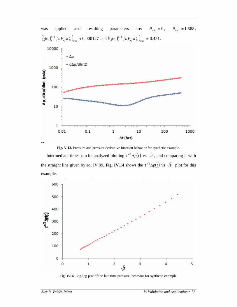
Alex R. Valdés-Pérez V. Validation and Application • 53
was applied and resulting parameters are: 0min , 588.1max ,
000127.0min
1 vfbuf
vtt kaVc and 451.0
max
1 vfbuf
vtt kaVc .
Fig. V.13. Pressure and pressure derivative function behavior for synthetic example.
Intermediate times can be analyzed plotting tpt v 2 vs t , and comparing it with
the straight line given by eq. IV.89. Fig. IV.14 shows the tpt v 2 vs t plot for this
example.
Fig. V.14. Log-log plot of the late time pressure behavior for synthetic example.
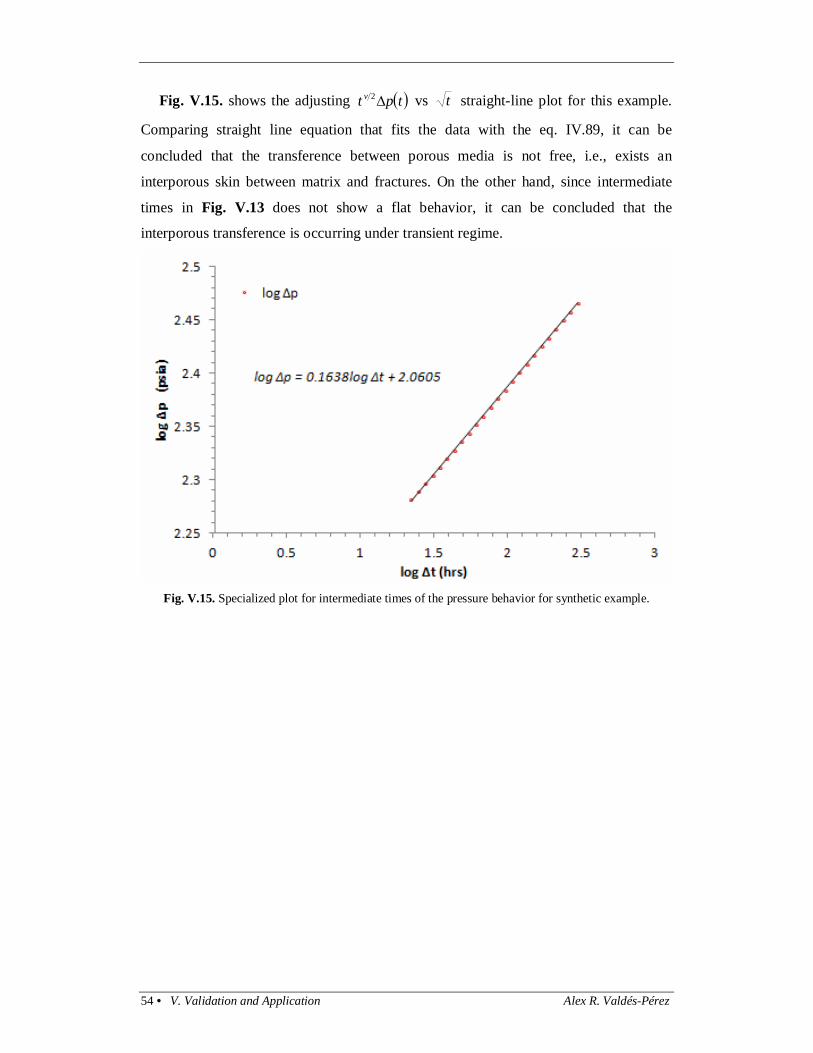
54 • V. Validation and Application Alex R. Valdés-Pérez
Fig. V.15. shows the adjusting tpt v 2 vs t straight-line plot for this example.
Comparing straight line equation that fits the data with the eq. IV.89, it can be
concluded that the transference between porous media is not free, i.e., exists an
interporous skin between matrix and fractures. On the other hand, since intermediate
times in Fig. V.13 does not show a flat behavior, it can be concluded that the
interporous transference is occurring under transient regime.
Fig. V.15. Specialized plot for intermediate times of the pressure behavior for synthetic example.

Alex R. Valdés-Pérez VI. Conclusions • 55
Chapter VI Conclusions
1. A fractal flow model that describes transient interporous behavior in double
porosity systems was developed. With this model it is possible to consider
spheres or slabs as matrix blocks.
2. A general solution in Laplace space that describes the complete transient
response of the fractal reservoirs, i.e. total expansion in fracture network,
interaction between porous media and single system behavior, was developed.
3. Approximated analytical solutions in real space to describe pressure behavior
during early, intermediate and late times were derived.
4. Solutions during intermediate times are used to characterize parameters useful
for reservoir engineering studies; such as matrix block, fractal fracture network
area per unit of bulk volume and interporous skin.
5. Main advantage of using fractal models is that these are the best suited to
represent randomness in the fracture network distribution within the reservoir.
6. Advantages of using transient interporous transference models with interporous
skin were discussed.

This page is intentionally left in blank.

Alex R. Valdés-Pérez References • 57
References
Acuña, J.A., Ershaghi, I. and Yortsos, Y.C., (1995), “Practical Application of Fractal
Pressure-Transient Analysis in Naturally Fractured Reservoirs,” SPEFE 10 (3):
173-179; Trans AIME, 299. SPE-24705-PA.
Barenblatt, G.I., Zheltov, Iu, P. and Kochina, I.N., (1960), “Basic Concepts in the
Theory of Seepage of Homogeneous Liquids in Fissured Rocks (strata),” PMM
Vol. 24, No. 5, 852-864, in Russian.
Barenblatt, G.I., Zheltov, Yu, P., (1960), “Fundamental equations of Filtration of
Homogeneous Liquids in Fissured Rocks,” Soviet Physics Doklady Vol. 5, 522-
525.
Barker, J.A.: “A Generalized Radial-Flow Model for Pumping Tests in Fractured
Rock,” Water Resources Research, 24, 1796-1804, 1988.
Black, J.H. and K.L. Kipp: “Determination of hydrogeological parameters using
sinusoidal test: A theoretical appraisal,” Water Resources Research, I17(3), 686-
692, 1981.
Camacho-Velazquez, R., Fuentes-Cruz, G., and Vasquez-Cruz, M., (2008), “Decline-
Curve Analysis of Fractured Reservoirs with Fractal Geometry.” SPE Res Eval
& Eng11 (3): 606-619. SPE-104009-PA.
Chang, J. and Y. Yortsos: “Pressure Transient Analysis of Fractal Reservoirs,” SPE
Formation Evaluation, (5) 31-38, 1990.
Chang, J. and Y. Yortsos (1992), “A Note On Pressure-Transient Analysis Of Fractal
Reservoirs,” paper SPE 25296, SPE Advanced Technology Series, Vol. 1, No. 2,
170 – 171.
Chatas, A.T.: “Unsteady spherical flow in petroleum reservoirs”, SPEJ (6) 102-114,
1966.
Cinco-Ley, H., Economides, M.J., Miller, F.G. (1979), “A parallelepiped Model to
Analyze the Pressure Behavior of Geothermal Steam Wells Penetrating Vertical
Fractures,” paper SPE 8231 presented at the SPE 54th Annual Technical
Conference and Exhibition, Las Vegas, Sept. 23-26.

58 • References Alex R. Valdés-Pérez
Cinco-Ley, H., Samaniego V., F. (1982), “Pressure Transient Analysis for Naturally
Fractured Reservoirs,” paper SPE 11026 presented at the SPE 57th Annual Fall
Technical Conference and Exhibition, New Orleans, LA, Sept. 26-29.
Cinco-Ley, H., Samaniego V., F., Kucuk, F., (1985), “The Pressure Transient Behavior
for Naturally Fractured Reservoirs with Multiple Block Size,” paper SPE 14168
presented at the SPE 60th Annual Fall Technical Conference and Exhibition, Las
Vegas, NV, Sept. 22-25.
Cossio, M. (2012), “A Semi-Analytic Solution for Flow in Finite-Conductivity Vertical
Fractures Using Fractal Theory,” paper SPE 163057-STU presented at the SPE
Annual Technical Conference and Exhibition, San Antonio, Texas, Oct. 8-10.
De Swaan, O.A., (1976), “Analytic Solutions for Determining Naturally Fractured
Reservoir Properties by Well Testing,” SPEJ Trans. AIME 261, 117-122, June.
Doe, T.W.: “Fractional Dimension Analysis of Constant-Pressure Well Tests”, paper
22702 presented at the 66th Annual Technical Conference and Exhibition of the
Society of Petroleum Engineers held in Dallas, TX, October 6-9, 1991.
Flamenco-López, F., Camacho-Velázquez, R. (2003), “Determination of Fractal
Parameters of Fracture Networks Using Pressure Transient Data,” paper SPE
82607, SPE Reservoir Evaluation & Engineering, February.
Gringarten, A.C., Bourdet, D.P., Landel., P.A., Kniazeff, V.J. (1979), “A Comparison
Between Different Skin and Wellbore Storage Type-Curves for Early-Time
Transient Analysis,” paper SPE 8205 presented at the SPE 54th Annual
Technical Conference and Exhibition, Las Vegas, Sept. 23-26.
Gringarten, A.C., (1987), “How To Recognize “Double Porosity” Systems from Well
Tests,” paper SPE 16437, JPT, June.
Larsen, L., (2013) Private communication.
Miller, F.G.: “Theory of Unsteady State Influx of Water in linear Reservoirs,” J. Inst.
Pet. 48, 467, 1962.
Moench, A.F. (1984), “Double-Porosity Models for a Fissured Groundwater Reservoir
with Fracture Skin,” Water Resources Research, Vol. 20, No. 7, 831-846.
Najurieta, H.L., (1980), “A Theory for Pressure Transient Analysis in Naturally
Fractured Reservoirs,” JPT 1241-1250, July.
Alex R. Valdés-Pérez References • 59
Pulido, H., Samaniego, F., Rivera, J., Díaz, F., Galicia-Muñoz, G., (2006), “Well Test
Analysis for Naturally Fractured Reservoirs with Transient Interporosity Matrix,
Microfractures and Fractures Flow,” Proceedings Thirty-first Workshop on
Geothermal Reservoir Engineering Stanford University, Stanford, California,
January 22 – 24.
Pulido, H., Samaniego, F., Galicia-Muñoz, G., Rivera, J., Velez, C. (2007),
“Petrophysical Characterization of Carbonate Naturally Fractured Reservoirs for
use in dual porosity simulators,” Proceedings Thirty-Second Workshop on
Geothermal Reservoir Engineering Stanford University, Stanford, California,
January 22 – 24.
Pulido, H., Galicia-Muñoz, G., Valdes-Perez. A.R., Díaz-García F. (2011), “Improve
Reserves Estimation using Interporosity Skin in Naturally Fractured Reservoirs
,” Proceedings Thirty-Sixth Workshop on Geothermal Reservoir Engineering
Stanford University, Stanford, California, January 31 – February 2.
Serra, K. V., Reynolds, A.C. and Raghavan, R., (1982), “New Pressure Transient
Analysis Methods for Naturally Fractured Reservoirs,” paper SPE 10780
presented at the SPE 1982 California Regional Meeting, San Francisco,
California, March 24-26.
Stehfest, H.: “Numerical inversion of Laplace transforms,” Commun. ACM, 13(1), 47-
49, 1970.
Streltsova, T.D., (1982), “Well Pressure Behavior of a Naturally Fractured Reservoirs,”
paper SPE 10782 presented at the SPE 1982 California Regional Meeting, San
Francisco, California, March 24-26.
Valdes-Perez. A.R., Pulido, H., Cinco-Ley., H., Galicia-Muñoz, G. (2011), “A New
Bilinear Flow Model For Naturally Fractured Reservoirs with Transient
Interporosity Transfer,” Proceedings Thirty-Sixth Workshop on Geothermal
Reservoir Engineering Stanford University, Stanford, California, January 31 –
February 2.
Valdes-Perez. A.R., Pulido, H., Cinco-Ley., H., Galicia-Muñoz, G. (2012),
“Discretization of the Resistivity, Capillary Pressure and Relative Permeability
for Naturally Fractured Reservoirs,” Proceedings Thirty-Seventh Workshop on
60 • References Alex R. Valdés-Pérez
Geothermal Reservoir Engineering Stanford University, Stanford, California,
January 30 – February 1.
Valdes-Perez. A.R., Pulido, H., Cinco-Ley., H., Larsen, L. (2013), “A New Double
Porosity Fractal Model for Well Test Analysis with Transient Interporosity
Transference for Petroleum and Geothermal Systems,” Proceedings Thirty-
Eighth Workshop on Geothermal Reservoir Engineering at Stanford University,
Stanford, California, February 11-13.
van Everdingen, A.F. and Hurst, W.: “Application of the Laplace Transformation to
flow problems in Reservoirs,” Trans. AIME, 186, 305-324B, 1949.
Warren, J.E. and Root, P.J., (1963), “The Behavior of Naturally Fractured Reservoirs,”
SPEJ Trans AIME, Vol. 228, 245-255, September.

Alex R. Valdés-Pérez Appendix A • 61
Appendix A Generalized Radial Flow Model
A.1. Flow model development
Incoming oil mass into an object is given by:
tAvm oin , A.1
out coming oil mass from the same object is:
tAvtAvm ooout
, A.2
then, cumulative oil mass into the object is:
tAvmmm oinoutcum . A.3
On the other hand, mass of oil at a time 1t is given by:
bulkoot VSm 1
, A.4
at a time 2t :
bulkoobulkoot VSVSm 2
, A.5
and, cumulative oil mass is given by:
bulkoottcum VSmmm 12
. A.6
Equating eq. A.3 and A.6 results:
bulkooo VStAv . A.7
According to using definitions given in eq. I.4 and eq. I.6, and after mathematical
manipulation eq. A.7 results:
t
Sr
vrr
oood
d
e
e
1
1
1 . A.8
Applying derivatives in both sides of eq. A.8:
t
St
Sr
vrrdvrvr
roo
ooodd
eood
deee
e
121
1 11 . A.9
Darcy’s law states:
r
trpkv
,
. A.10
Substituting Darcy’s law into eq. A.9 it results:

62 • Appendix A Alex R. Valdés-Pérez
tS
StS
rrtrpr
rtrpdr
rtrp
rr
kr
oo
oooo
o
o
d
eddo
d
eee
e
11
,,1,1 121
1
. A.11
Using chain rule derivative of oil density regarding the radius can be written as:
r
trptrpr
oo
,,
, A.12
Analogously with the porosity:
t
trptrpt
,
, , A.13
And:
tp
pS
tS oooo
. A.14
Substituting eqs. from A.12 to A.14 and the definitions of compressibility of oil and
compressibility of the formations, into eq. A.11 it results
t
trpccS
rtrpcr
rtrpdr
rtrp
rrk
r
ofo
od
edd
deee
e
,
,,1,1 2121
1
, A.15
According to the definition of total compressibility of the formation for a single fluid
(oil), eq. A.15, the diffusivity equation of a Generalized Radial Model results:
t
trpkc
rtrpc
rtrp
rd
rtrp tf
oe
,,,1, 2
2
2 . A.16
Neglecting the quadratic pressure gradient term the following model is given:
t
trpkc
rtrp
rd
rtrp tfe
,,1,
2
2 . A.17
Compact form of previous equation is:
t
trpkc
rtrpr
rrtfd
de
e
,,1 11
. A.18
A.2 Transformation to dimensionless variables for well test analysis
Following dimensionless variables has been state. Dimensionless radius:
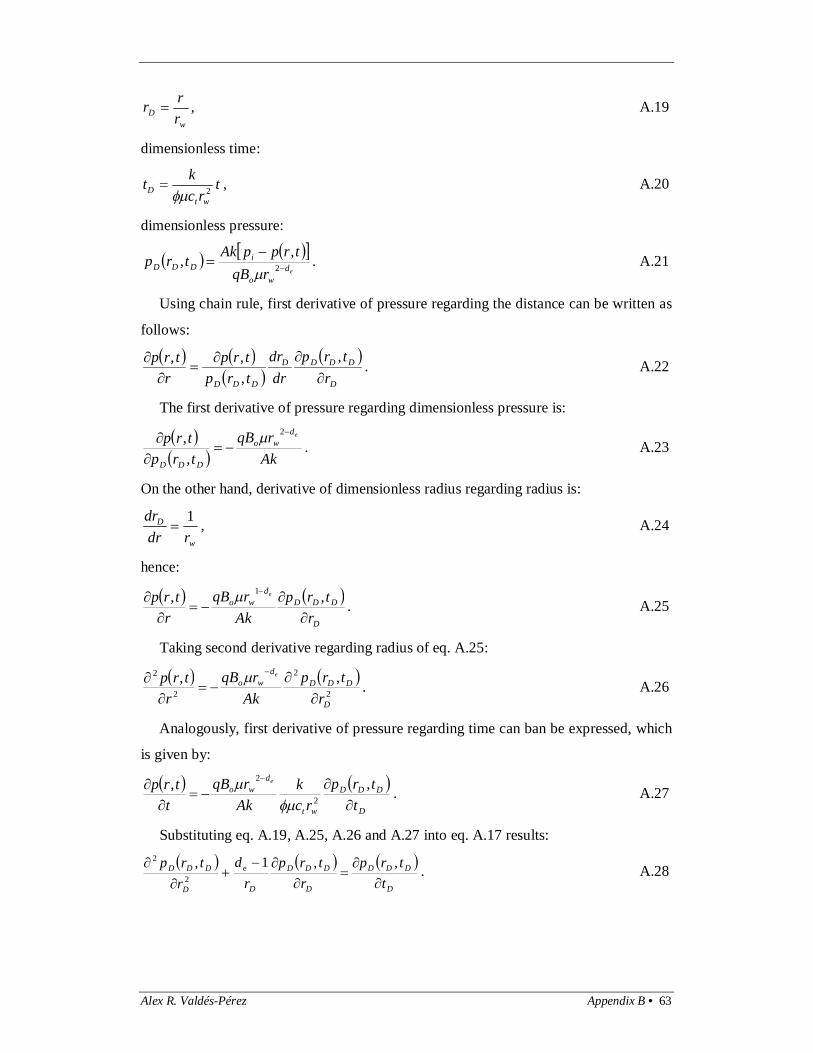
Alex R. Valdés-Pérez Appendix B • 63
wD r
rr , A.19
dimensionless time:
trc
ktwt
D 2 , A.20
dimensionless pressure:
ed
wo
iDDD rqB
trppAktrp
2
,,
. A.21
Using chain rule, first derivative of pressure regarding the distance can be written as
follows:
D
DDDD
DDD rtrp
drdr
trptrp
rtrp
,,,, . A.22
The first derivative of pressure regarding dimensionless pressure is:
Ak
rqBtrptrp ed
wo
DDD
2
,, . A.23
On the other hand, derivative of dimensionless radius regarding radius is:
w
D
rdrdr 1
, A.24
hence:
D
DDDd
wo
rtrp
AkrqB
rtrp e
,, 1 . A.25
Taking second derivative regarding radius of eq. A.25:
2
2
2
2 ,,
D
DDDd
wo
rtrp
AkrqB
rtrp e
. A.26
Analogously, first derivative of pressure regarding time can ban be expressed, which
is given by:
D
DDD
wt
dwo
ttrp
rck
AkrqB
ttrp e
,,2
2
. A.27
Substituting eq. A.19, A.25, A.26 and A.27 into eq. A.17 results:
D
DDD
D
DDD
D
e
D
DDD
ttrp
rtrp
rd
rtrp
,,1,
2
2
. A.28

64 • Appendix A Alex R. Valdés-Pérez
It can be verified that, when 1ed GRF, eq. A.28, it takes the form of the linear flow
model; when 2ed it converges to the radial flow model and to the spherical flow
model when 3ed .
A.3. General solution in Laplace space assuming constant rate
In order to have a well test analysis model for the Generalized Radial Flow Model, eq.
A.28, the following conditions have been set:
initial condition: 00, DDD trp , A.29
inner Boundary: 1
,1
D
DD
ttp , A.30
outer boudary: 0,lim DDDr
trpD
. A.31
Applying Laplace transform to eq. A.28 and according to initial condition, it results:
0,,1,2
2
srpsdr
trpdr
ddr
srpdDD
D
DDD
D
e
D
DD . A.32
The following transform function has been set:
zGsrp DDD , , A.33
and the transformation variables:
srz D . A.34
Hence:
sdrdz
D
. A.35
Moreover, parameter is established:
21 ed
v . A.36
edv 22 . A.37
Applying the variable transformations, the following expression is obtained:
021 22
22
zGzz
zGzvz
zGz DDD . A.38
Moreover, to equalize the coefficient of the first derivative to one the following
expression is proposed:
zBzzG Dv
D . A.39
then, eq. 31 in terms of eq. 39 is:
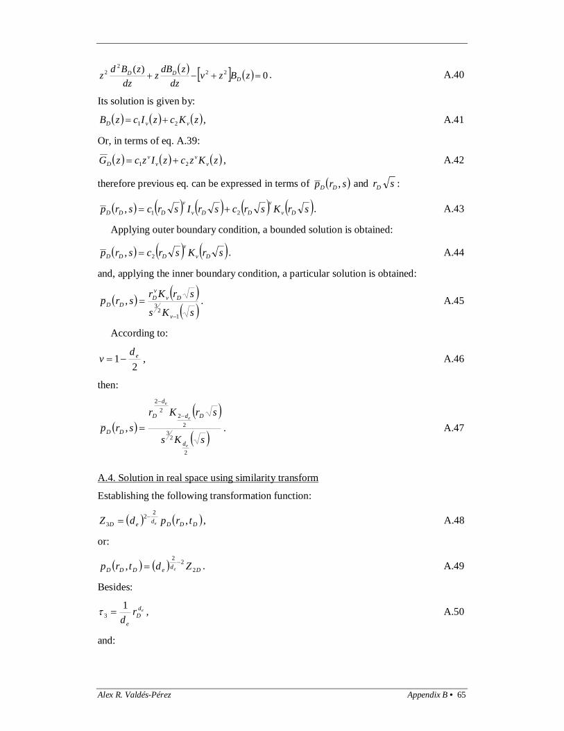
Alex R. Valdés-Pérez Appendix B • 65
0)( 222
2 zBzvdz
zdBzdz
zBdz DDD . A.40
Its solution is given by:
zKczIczB vvD 21 , A.41
Or, in terms of eq. A.39:
zKzczIzczG vv
vv
D 21 , A.42
therefore previous eq. can be expressed in terms of srp DD , and srD :
srKsrcsrIsrcsrp Dv
v
DDv
v
DDD 21, . A.43
Applying outer boundary condition, a bounded solution is obtained:
srKsrcsrp Dv
v
DDD 2, . A.44
and, applying the inner boundary condition, a particular solution is obtained:
sKs
srKrsrpv
Dvv
DDD
12
3,
. A.45
According to:
21 ed
v , A.46
then:
sKs
srKrsrp
e
e
e
d
Dd
d
D
DD
2
23
22
22
,
. A.47
A.4. Solution in real space using similarity transform
Establishing the following transformation function:
DDDdeD trpdZ e ,22
3 , A.48
or:
DdeDDD Zdtrp e 222
, . A.49
Besides:
edD
e
rd1
3 , A.50
and:

66 • Appendix A Alex R. Valdés-Pérez
Dd
e td e
22
3
. A.51
Applying a analogous procedure as the one showed in Chapter IV, the following
approximation in real space was obtained:
D
De
e
dD
DDD trd
drtrp
e
4 , 1
22
2,
22
. A.52
***
Alex R. Valdés-Pérez Appendix B • 67
Appendix B Pressure Transient Analysis of Fractal Reservoirs assuming Pseudo-Steady
State Interporosity Transfer
In this appendix, the development of the Fractal Reservoir Model proposed by Chang et
al., (1990) is demonstrated. For this demonstration is very important to keep in mind the
definition of the Geometry Factor given by eq. I.20.
B.1. Model development
Incoming oil mass into an object is given by:
tqm ooin , B.1
out coming oil mass from the same object is:
tqtqm ooooout , B.2
oil mass contribution from the Euclidean matrix:
tqm maoma , B.3 then, cumulative oil mass into the object is:
tqtqtqmmm maooomaoinoutcum . B.4
On the other hand, mass of oil at a time 1t is given by:
bulkfboot VSm 1
, B.5
at a time 2t :
bulkfboobulkfboot VSVSm 2
, B.6
and, cumulative oil mass is given by:
bulkfboottcum VSmmm 12
. B.7
Equating eq. B.4 and B.7 results:
bulkfboomaooo VStqtq . B.8
According to the definition of bulk volume, eq. B.8 becomes:
rbrStqtq ee
e
dddfboomaooo 31 , B.9
arraying previous equation:
t
SV
qrq
brfboo
bulk
maooodd
dee
e
311 . B.10
Matrix flow rate per unit of bulk is defined:
68 • Appendix B Alex R. Valdés-Pérez
bulk
mama V
. B.11
Taking the limits r and t to zero, and arraying eq. B.10 becomes:
t
Sbrqbr
rq fboodd
dmaodd
doo ee
e
ee
e
3131 . B.12
Inserting Darcy’s equation in fractal form into previous equation, it results:
t
Sbrqbr
rprkaV
rfboodd
dmaodd
dfb
fb
fbufo
ee
e
ee
e
3131 . B.13
Besides, matrix flow rate due to expansion effects is given by:
tpVcq ma
bulktmamama
, B.14
hence, matrix flow rate per unit of bulk is:
tp
cVq
q matmama
bulk
mama
. B.15
Based on matrix flow rate per unit of bulk, eq. B.13 is rewritten as:
t
Sbr
tpcbr
rprkaV
rfboodd
dma
tmamaodd
dfb
fb
fbufo
ee
e
ee
e
3131 , B.16
applying the derivatives in eq. B.16:
tS
tSbr
tpcbr
rrp
rr
prr
rp
rkaV
fboo
oofb
ddd
matmamao
ddd
ofbfbofbo
fb
fbuf
ee
e
ee
e
3131
2
2
. B.17
According to chain rule:
rp
prfb
fb
oo
, B.18
tp
pS
tS fb
fb
oooo
, B.19
tp
ptfb
fb
fbfb
, B.20
substituting eqs. B.18, B.19 and B.20 into B.17, and using the definitions of
compressibility of oil and fractured formation, B.17 is rewritten as follows:

Alex R. Valdés-Pérez Appendix B • 69
t
pccSbr
tpcbr
rp
crr
prr
rp
rkaV
fbfbooofb
ddd
matmamao
ddd
fbo
fbfb
fb
ofbuf
ee
e
ee
e
3131
2
2
2
, B.21
assuming single phase flow, total compressibility is defined as:
fbotfb ccc , B.22
and neglecting quadratic gradient pressure and according to definition of fracture
network porosity, prior equation becomes:
tp
cVart
pcbrr
prkaVr
fbtfbuf
Dmatmama
ddd
fb
fb
fbuf fbee
e
131
. B.23
B.2. Transformation to dimensionless variables
Following dimensionless variables has been state. Dimensionless radius:
wD r
rr , B.24
dimensionless time:
t
caVcrb
rc
kt
tfbuf
tmamaDd
wd
dwtfbfb
fbD fbee
e
32 1
, B.25
dimensionless pressure in the fracture network:
fbw
fbifbufDDfbD rq
trppkaVtrp
1
,, , B.26
similarly, for pressure within the matrix:
fbw
maifbufDDmaD rq
trppkaVtrp
1
,, . B.27
Using chain rule, first derivative of pressure in the fracture network regarding the
distance can be written as follows:
D
DDfbDD
DDfbD
fbfb
rtrp
drdr
trptrp
rtrp
,,,,
. B.28
Based on dimensionless pressure definition, pressure as a function of radius and time
is expressed as:
70 • Appendix B Alex R. Valdés-Pérez
DDfbDfbuf
fbwifb trp
kaVrq
ptrp ,,1
, B.29
which first derivative regarding dimensionless pressure in fracture network is:
fbuf
fbw
DDfbD
fb
kaVrq
trptrp
1
,,
. B.30
Based on the dimensionless radius definition, derivative of dimensionless radius
regarding radius is:
w
D
rdrdr 1
, B.31
then, eq. B.28 becomes:
D
DDfbD
fbuf
fbwfb
rtrp
kaVrq
rtrp
,,
. B.32
Taking second derivative regarding radius of eq. B.32:
2
21
2
2 ,,
D
DDfbD
fbuf
fbwfb
rtrp
kaVrq
rtrp
. B.33
Moreover, first derivative of pressure regarding time can ban be expressed:
D
DDfbDD
DDfbD
fbfb
ttrp
dtdt
trptrp
ttrp
,,,,
, B.34
substituting:
D
DDfbD
tfbuf
tmamaDd
wd
dwtfbuf
wfb
ttrp
caVcrb
rcaV
qrt
trpfbee
e
,
1
,3
2
1
. B.35
Analogously, for the derivative of pressure within matrix regarding to time:
D
DDmaD
tfbuf
tmamaDd
wd
dwtfbuf
wma
ttrp
caVcrb
rcaV
qrt
trpfbee
e
,
1
,3
2
1
. B.36
Substituting eq. B.24, B.32, B.33, B.35 and B.36 into eq. B.28 results:
D
DDfbDps
D
DDmaDps
DdD
D
DDfbDD
DD
D ttrp
ttrpr
rtrp
rrr
fbe
fb
,,1,1
1 , B.37
where:
ps storage coefficient is defined as follows:

Alex R. Valdés-Pérez Appendix B • 71
tmamaDd
wd
dtfbuf
tfbufps crbcaV
caVfbee
e
3. B.38
On the other hand, flow rate from matrix to fracture network per unit bulk volume is
given by the expression:
bulk
mafma
bulk
mama V
vAVq
q . B.39
Area of matrix exposed to flow can be defined as:
fbDuffb
fma rr
rVDaA 2
1 , B.40
velocity of oil coming out from matrix can be expressed using Darcy’s law:
ma
mafbmama l
ppkv
. B.41
Based on eq. B.39, B.40 and the definition of bulk volume, flow rate from matrix to
fracture network per unit bulk volume can be expressed as follows:
fma
mafbmaDma l
ppkrq fb
1'
1 , B.42
where:
fmal average distance between the matrix and the fractal fracture network;
1 is a constant defined by:
e
e
dd
uffb
bVDa
31
1
, B.43
and,
efbfb dDD ' . B.44
Besides, distance between the matrix and the fracture network can be represented as: fbD
fma rl ''2 , B.45
where:
uffbfb rVDDa 212 , B.46
and:
3'' fbfb DD . B.47
Hence, eq. B.42 is rewritten as follows:
72 • Appendix B Alex R. Valdés-Pérez
mafbma
ma ppkq
, B.48
where shape factor , is given by:
2
1'''1
fbfb DDr . B.49
Equating B.11 and B.48 results:
mafbtmama
mama ppck
tp
. B.50
Expressing prior eq. in dimensionless variables:
DDmaDDDfbDDD
DDmaD trptrprt
trp,,',
. B.51
An alternative way to present prior equation is:
DDmaDDDfbD
DpsD
DDmaD trptrprt
trp ,,1
,
, B.52
where:
tfbuf
tmamaDd
wd
d
fbtmama
tfbfbmaw
ps caVcrb
kcckr fbee
e
3
2
21 1
1' , B.53
and:
fbfb DD '1'' . B.54
***

Alex R. Valdés-Pérez Appendix C • 73
Appendix C Pressure Transient Analysis of Fractal Reservoirs with Transient
Interporous Transference (Olarewaju, 1996)
C.1. Model development
The procedure for the development of this model is the same as describe in for Chang et
al.’s model (1990) in Appendix B, until eq. B.13, which is given by:
t
Sbrqbr
rprkaV
rfboodd
dmaodd
dfb
fb
fbufo
ee
e
ee
e
3131 . C.1
After applying the derivatives in eq. C.1, it results:
tS
tSbrqbr
rrtrp
rr
trpr
rtrp
rkaV
fboo
oofb
dddmao
ddd
ofbfbo
fbo
fb
fbuf
ee
e
ee
e
3131
12
2 ,,,
. C.2
According to chain rule:
rp
prfb
fb
oo
, C.3
tp
pS
tS fb
fb
oooo
, C.4
tp
ptfb
fb
fbfb
, C.5
substituting, eq. C.3, C.4, C.5 and, using the definitions of oil and formation
compressibility, eq. C.2 becomes:
t
trpccSbr
qbrr
trpcr
rtrp
rr
trpr
kaV
fbfboofb
ddd
madd
dfb
ofbfb
fb
fbuf
ee
e
ee
e
,
,,,
31
312
12
2
. C.6
Assuming single phase flow, and according to the total compressibility definition,
eq. C.6 is written as:
74 • Appendix C Alex R. Valdés-Pérez
t
trpcbr
qbrr
trpcr
rtrp
rr
trpr
kaV
fbtfbfb
ddd
madd
dfb
ofbfb
fb
fbuf
ee
e
ee
e
,
,,,
31
312
12
2
. C.7
Neglecting quadratic gradient pressure, prior equation becomes:
t
trpdp
dp
kAk
rtrp
rrr
fb
fbsuruma
tfb
fb
fbmafbD fb
,1,1
01
. C.8
where:
dp
dp
Akq suruma
tfb
fbma
ma
0
, C.9
fbA exposed to flow area which is defined as:
mafb h
A 1 ; C.10
fb hydraulic diffusivity coefficient is defined as:
tfbfb
fbfb c
k
, C.11
and pressure gradient is given by:
1
1242
22
3n
hkc
tncrk
masuruma
mafbtmama
Dttwma
eh
p
. C.12
C.2. Dimensionless variables transformation
Following dimensionless variables are established. Dimensionless radius:
wD r
rr , C.13
dimensionless position at the matrix:
maD h
zz 2 . C.14
Dimensionless time:
trc
kt
wtt
fbD 2 , C.15
where:
tmamatfbfbtt ccc . C.16
Alex R. Valdés-Pérez Appendix C • 75
Dimensionless pressure in the fracture network:
fbw
ifbfbufDDfbD rq
ptrpkaVtrp
1
,, , C.17
similarly, for pressure within the matrix:
fbw
imafbufDDmaD rq
ptrpkaVtrp
1
,, . C.18
Using chain rule, first derivative of pressure in the fracture network regarding the
distance can be written as follows:
D
DDfbDD
DDfbD
fbfb
rtrp
drdr
trptrp
rtrp
,,,,
. C.19
Applying the derivatives, C.19 becomes:
D
DDfbD
fbuf
fbwfb
rtrp
kaVrq
rtrp
,,
. C.20
The second derivative regarding radius of eq. C.20 is given by:
2
21
2
2 ,,
D
DDfbD
fbuf
fbwfb
rtrp
kaVrq
rtrp
. C.21
Analogously, first derivative of pressure regarding time is:
D
DDfbD
wtt
fb
fbuf
fbwfb
ttrp
rck
kaVrq
ttrp
,,2
1
. C.22
And,
DDfbD
fbuf
fbwfb trpkaV
rqrp ,, 1
. C.23
Substituting C.13, C.20, C.21, C.22, C.23 in C.30 and arraying, the following
expression is obtained:
D
DDfbD
tt
tfbfbD
t
surumaDDfbD
fb
wfbmaD
D
DDfbD
DD
DDfbD
ttrp
cc
r
dptrp
krAk
rr
trprr
trp
,
,,,
0
2
2
2
.
C.24
Considering strata as matrix blocks, eq. C.12, then:

76 • Appendix C Alex R. Valdés-Pérez
D
DDfbDD
t
n
tnDDfbDD
D
DDfbD
DD
DDfbD
ttrp
r
detrpr
rtrp
rrtrp D
,
,3
,,
0 1
1312
2
2 2
, C.25
where interporosity flow coefficient is defined as:
fbma
wma
khrk 212
; C.26
dimensionless storativity ratio:
tt
tfbfb
cc
. C.27
C.3. General solution in Laplace space assuming constant rate
In order to have a well test analysis model for the Fractal Reservoir Model assuming
free interaction transference between matrix and fractures, the following conditions
have been set:
Initial condition for fracture network: 00, DDfbD trp , C.28
inner boundary:
1,1
D
DfbDD t
tpr , C.29
outer boundary: 0,lim DDDr
trpD
. C.30
Applying Laplace transform to eq. C.57 and according to initial condition, it
becomes:
0,,
21, 2
2
22 srpsfsr
drsrpd
rdr
srpdr DfbDD
D
DfbDD
D
DfbDD
. C.31
where:
13tanh
131 s
ssf , C.32
and:
21
. C.33
Establishing the following transform function:
zGsrp DDD , , C.34
and the transformation variable:

Alex R. Valdés-Pérez Appendix C • 77
2
2
22
Drssf
z , C.35
a transformation of variables takes places. Using definitions given by eq. C.34 and eq.
C.35 the following expression is obtained:
021 22
22
zGzz
zGzz
zGz DDD , C.36
where:
21
v . C.37
To equalize the coefficient of the first derivative to one the following expression is
proposed:
zBzzG D
v
D , C.38
where:
21
22
ssf. C.39
Applying the transformations given by eq. C.38 and C.39, eq. C.36 can be written as:
0)( 222
2 zBzvdz
zdBzdz
zBdz DDD . C.40
Solution of eq. 40 is given by:
zKczIczB vvD 21 , C.41
or, in terms of eq. C.38:
zKczIczzG vv
v
D 21
, C.42
and, in terms of srp DD , and srD , the solution is:
2
2
212
22
211
21
22
22
,
DDDDD rssf
Kcrssf
Icrsrp . C.43
Applying outer boundary condition, it can be deduced that:
01 c , C.44
hence bounded solution is:
2
2
21
21
2 22
,
DDDD rssf
Krcsrp . C.45

78 • Appendix C Alex R. Valdés-Pérez
Applying the inner boundary condition it is concluded that:
2
21
2
2/32
ssfKsfs
c
fbD
. C.46
Then, particular solution is given by:
22
22
,
2
2/3
22
21
21
ssfKsfs
rssf
Krsrp
fbD
DD
DD . C.47
Hence, dimensionless pressure at wellbore is:
ssfKsfs
ssfKsp
fbD
wD
22
22
2
2/3
21
. C.48
***
Alex R. Valdés-Pérez Appendix D • 79
Appendix D Pressure Transient Analysis of Fractal Reservoirs assuming Free
Interaction Interporosity Transfer
D.1. Model development
The development of this model follows the same steps as shown in Appendix B, unitl
eq. B.13, given by:
t
Sbrqbr
rprkaV
rfboodd
dmaodd
dfb
fb
fbufo
ed
e
ee
e
3131 . D.1
Applying the derivatives in eq. D.1:
tS
tSbrqbr
rrtrp
rr
trpr
rtrp
rkaV
fboo
oofb
DDDmao
DDD
ofbfbo
fbo
fb
fbuf
fbfb
fb
fbfb
fb
3131
12
2 ,,,
. D.2
According to chain rule:
rp
prfb
fb
oo
, D.3
tp
pS
tS fb
fb
oooo
, D.4
tp
ptfb
fb
fbfb
. D.5
Substituting eq. D.3, eq. D.4 and eq. D.5 in eq. D.2 and using the definitions of oil and
formation compressibility, eq. D.2 becomes:
t
trpccSbr
qbrr
trpcr
rtrp
rr
trpr
kaV
fbfboofb
DDD
maDD
Dfb
ofbfb
fb
fbuf
fbfb
fb
fbfb
fb
,
,,,
31
312
12
2
.
D.6
Assuming single phase flow, and according to the total compressibility definition,
eq. D.6 is written as:

80 • Appendix D Alex R. Valdés-Pérez
t
trpcbr
qbrr
trpcr
rtrp
rr
trpr
kaV
fbtfbfb
DDD
maDD
Dfb
ofbfb
fb
fbuf
fbfb
fb
fbfb
fb
,
,,,
31
312
12
2
.
D.7
Neglecting quadratic gradient pressure, prior equation becomes:
t
trpk
crq
kr
rtrp
rr
trpr fb
fb
fbtfbDma
fb
Dfbfb fbfb
,,, 1112
2 . D.8
Where:
dp
dpAk
q suruma
tfbfbma
ma
0
. D.9
If slab matrix blocks are assumed, area exposed to flow is defined as:
fmafb hh
A
2 ; D.10
or, if cube matrix blocks are assumed:
326
fma
mafb hh
hA
. D.11
Substituting eq. D.9 into D.8:
t
trpdp
dp
kAk
rtrp
rrr
fb
fbsuruma
tfb
fb
fbmafbD fb
,1,1
01
, D.12
where hydraulic diffusivity coefficient is defined as:
tfbfb
fbfb c
k
. D.13
D.2. Transformation to dimensionless variables
Following dimensionless variables has been state. Dimensionless radius:
wD r
rr , D.14
dimensionless time:
trc
kt
wtt
fbD 2 , D.15
where:

Alex R. Valdés-Pérez Appendix D • 81
tmamatfbfbtt ccc . D.16
Dimensionless pressure in the fracture network:
fbw
fbifbufDDfbD rq
trppkaVtrp
1
,, , D.17
similarly, for pressure within the matrix:
fbw
maifbufDDmaD rq
trppkaVtrp
1
,, . D.18
Using chain rule, first derivative of pressure in the fracture network regarding the
distance can be written as follows:
D
DDfbDD
DDfbD
fbfb
rtrp
drdr
trptrp
rtrp
,,,,
. D.19
Applying the derivatives, eq. D.19 becomes:
D
DDfbD
fbuf
fbwfb
rtrp
kaVrq
rtrp
,,
. D.20
Taking second derivative of eq. D.20 regarding radius, it results:
2
21
2
2 ,,
D
DDfbD
fbuf
fbwfb
rtrp
kaVrq
rtrp
. D.21
Moreover, first derivative of pressure regarding time can ban be expressed:
D
DDfbD
wtt
fb
fbuf
fbwfb
ttrp
rck
kaVrq
ttrp
,,2
1
. D.22
and,
DDfbD
fbuf
fbwfb trpkaV
rqrp ,, 1
. D.23
Substituting D.14, D.20, D.21, D.22, and D.23 in D.12, it becomes:
D
DDfbDD
t
DDmaDDfbD
fDDD
DDfbD
DD
DDfbD
ttrp
r
dtHFrp
Arr
trprr
trp D
,
,,,
1,,
02
2
,
D.24
where, dimensionless storativity ratio, is defined as:

82 • Appendix D Alex R. Valdés-Pérez
tt
tfbfb
cc
; D.25
dimenssionless matrix hidraulic diffusivity:
fbtmama
ttmamaD kc
ck
; D.26
block size ratio:
2
2
ma
wD h
rH ; D.27
dimensionless fracture area, fDA :
ma
wbmafbfD V
rVhAA
. D.28
Fluid transfer function, assuming slabs:
1
12 22
4,,n
Htn
D
maDDDmaD
D
DmaD
eH
tHF
, D.29
or, if spheres as matrix blocks, fluid transfer function is:
1
4 22
4,,n
Htn
D
maDDDmaD
D
DmaD
eH
tHF
. D.30
D.3. General solution in Laplace space assuming constant rate
In order to have a well test analysis model for the Fractal Reservoir Model assuming
free interaction transfer between matrix and fractures, the following conditions have
been set:
Initial condition for fracture network: 00, DDfbD trp , D.31
inner Boundary:
1,1
D
DfbDD t
tpr , D.32
outer boundary: 0,lim DDDr
trpD
. D.33
Applying Laplace transform to eq. D.24 yields:
0,,
,,,1,,
2
2
DfbDDfbDD
DfbDDmaDfDDD
DDfbD
DD
DDfbD
rpsrpsr
srpssHFArdr
trdprdr
trpd
, D.34
where, for slab matrix blocks:
Alex R. Valdés-Pérez Appendix D • 83
maD
D
D
maDDmaD
sHsH
sHF
21tanh,, , D.35
And, for spheres as matrix blocks:
sHsH
sHsHF
D
maD
maD
D
D
maDDmaD
2
21coth,, . D.36
Applying initial condition in eq. D.34, and arraying:
0,,, 2
2
22 srpsfsr
drsrpd
rdr
srpdr DfbDD
D
DfbDD
D
DfbDD
, D.37
where:
sHFAsf DmaDfD ,,1 . D.38
Parameter is established:
21
. D.39
then:
0,,
21, 2
2
22 srpsfsr
drsrpd
rdr
srpdr DfbDD
D
DfbDD
D
DfbDD
. D.40
The following transform function has been set:
zGsrp DDD , , D.41
and the transformation variable:
2
2
22
Drssf
z . D.42
Using definitions given by eq. D.40 and eq. D.41 the following expression is obtained:
021 22
22
zGzz
zGzz
zGz DDD . D.43
where,
21
v . D.44
To equalize the coefficient of the first derivative to one the following expression is
proposed:
zBzzG D
v
D , D.45
where:

84 • Appendix D Alex R. Valdés-Pérez
21
22
ssf. D.46
Applying the transformations given by eq. C.45 and C.46, eq. C.43 can be written as:
0)( 222
2 zBzvdz
zdBzdz
zBdz DDD . D.47
Its solution is given by:
zKczIczB vvD 21 , D.48
or, in terms of eq. D.85:
zKczIczzG vv
v
D 21
, D.49
and, in terms of srp DD , and srD , solution is:
2
2
212
22
211
21
22
22
,
DDDDD rssf
Kcrssf
Icrsrp . D.50
Applying outer boundary condition, it can be deduced that:
01 c , D.51
And, bounded solution is:
2
2
21
21
2 22
,
DDDD rssf
Krcsrp . D.52
Applying the inner boundary condition it is concluded that:
2
21
2
2/32
ssfKsfs
c
fbD
, D.53
then, particular solution is given by:
22
22
,
2
2/3
22
21
21
ssfKsfs
rssf
Krsrp
fbD
DD
DD , D.54
at wellbore:
ssfKsfs
ssfKsp
fbD
wD
22
22
2
2/3
21
. D.55
Alex R. Valdés-Pérez Appendix D • 85
D.4. Approximate solutions at short times: Total Expansion in the Fracture Network
At short times, only the fracture network is acting:
sf , D.56
Therefore, eq. D.24 is reduced to:
D
DDfbDD
D
DDfbD
DD
DDfbD
ttrp
rr
trprr
trp
,,,2
2
. D.57
Establishing the following transformation function:
DDfbDDfbD trpDZ fb ,
224
, D.58
or:
DDfbDDfbD ZDtrp fb 4
22
1,
. D.59
besides:
fbDD
fb
rD1
4 , D.60
and:
DD
fb tD fb
22
4
. D.61
The procedure to obtain this approximate solution is analogous to the one shown in
section IV.4 of Chapter 4 in the main text. Therefore, the founded approximate solution
is given by:
D
Dfb
fb
DD
DDfbD trD
Drtrp
fb
2
22
2 , 1
22
2,
. D.62
In order to have simplified solutions relatively easy to use, two cases must be
defined. The first case is given by the condition 2 fbD . If that is the case and
evaluated in 1Dr , eq. D.62 becomes:
DDwD t
tp 22,0
21
. D.63
According to incomplete gamma function convergences, prior expression can be
expressed as:
DiDwD t
Etp 2221
, D.64
86 • Appendix D Alex R. Valdés-Pérez
where:
xEi integral exponential.
For small arguments of the integral exponential, eq. D.64 can be approximated as:
ln2ln2ln2
1DDwD ttp , D.65
where:
Euler’s constant.
On the other hand, for 2 fbD the following approximation was used, based on
the incomplete gamma function definition:
1,1
ax
axaxa
aa
, D.66
hence, incomplete gamma function for this problem is approximated as:
2
11
22122
1
22
2
12
21122
,12
fbfbfbfb
D
Dfb
DDD
D
fb
D
Dfb tDrD
trD
. D.67
Substituting D.67 in eq. D.62 and evaluating in 1Dr :
vD
fbfb
vv
fb
fb
DwD tDDD
D
tp
21
2
2
22
12 112
, D.68
where:
21
fbDv , D.69
Recurrence formula of gamma function can be written as:
111
xx
x . D.70
Therefore, eq. D.68 is rewritten as:
v
Dfb
vv
DwD tD
vv
tp
2
22
1 112
. D.71
It can be verified that, if there is no anomaly in conductivity in fractal object, i.e., 0
and a homogeneous reservoir is assumed, i.e., 1 , prior equations converges to the
generalized radial flow model solution, given in Appendix A.

Alex R. Valdés-Pérez Appendix D • 87
D.5. Approximate solutions at intermediate times: Interaction between porous media
For intermediate times, the interaction between porous media takes place. For this
period, transference function can be approximated as:
sH
AsfD
maDfD
1 , D.72
Therefore, eq. D.55 is rewritten as:
D
maDfDD
D
maDfD
D
maDfD
wD
Hs
AK
Hs
AK
sHAs
sp
fb
12
2
12
2
1
1
2
21
21
2/3
. D.73
For small arguments, Bessel function in the denominator is approximated as:
2
1221
22 222
2
fb
D
D
maDfD
D
D
maDfDD
DH
sA
Hs
AK
fbfb
fb.
D.74
Substituting eq. D.74 in eq. D.73:
D
maDfDD
fbD
D
D
maDfD
wD Hs
AK
sD
HA
spfb
fb
fb
12
2
22
12
21
2445
2
21
22
. D.75
For the 2 fbD case, the Bessel function in the numerator is approximated as:
D
maDfD
D
maDfD H
sAH
sAK 12
1ln12
20 , D.76
thus, eq. D.75 can be expressed as:
sss
HA
sssp D
maDfD
wD
2ln
1ln
21ln
41
22 . D.77
Inverting to Real Space:
4329.02ln1ln
21ln
41
22
D
maDfDDDwD H
Attp . D.78

88 • Appendix D Alex R. Valdés-Pérez
On the other hand, if 2 fbD , then the Bessel function in the denominator is
approximated as:
211
22
112
2
221
21
21
21
D
maDfD
D
maDfD
maD
DfbDma
Hs
A
HsA
sHSK
, D.79
substituting eq. D.79 in eq. D.75:
241
2445
22
12
2
11
2
212
fb
fb
fb
D
D
D
maDfD
fb
D
wD
s
HA
Dsp , D.80
since:
1 fbD , D.81
then
2252
22
21
22
12
1
sD
HA
spfb
D
maDfD
wD. D.82
Inverting to real space:
2221
2
22
2
2
2
1
2223
2
21
fb
fb
fb
D
DD
D
D
maDfD
fbfbDwD t
HA
DDtp . D.83
D.6. Approximate solutions at large times: Single System Behavior
At short times, only the fracture network is acting:
1sf , D.84
and eq. D.24 is reduced to:
D
DDfbDD
D
DDfbD
DD
DDfbD
ttrp
rr
trprr
trp
,,,2
2 . D.85
Applying an analogous procedure as shown in section D.4, the following solution was
developed:

Alex R. Valdés-Pérez Appendix D • 89
D
Dfb
fb
DD
DDfbD trD
Drtrp
fb
2
22
2 , 1
22
2,
. D.86
In order to have simplified solutions relatively easy to use, two cases must be
defined. The first case is given by the condition 2 fbD . If that is the case, eq. D.86
and evaluated in 1Dr , it becomes:
DDwD t
tp 221,0
21
. D.87
According to incomplete gamma function convergences, prior expression can be
expressed as:
DiDwD t
Etp 221
21
, D.88
where:
xEi integral exponential.
For small arguments of the integral exponential, eq. D.88 can be approximated as:
2ln2ln2
1DDwD ttp , D.89
where:
Euler’s constant.
On the other hand, for 2 fbD incomplete gamma function can be expressed as:
1,1
ax
axaxa
aa
. D.90
Hence, incomplete gamma function for this problem is approximated as:
2
12122
1
22
2
12
21122
,12
fbfbfb
D
Dfb
DD
D
fb
D
Dfb tDrD
trD
. D.91
Substituting D.91in eq. D.86 and evaluating in 1Dr :
vD
fbfb
v
fb
fb
DwD tDDD
D
tp
21
2
2
22
12 12
, D.92
where:
90 • Appendix D Alex R. Valdés-Pérez
21
fbDv . D.93
Recurrence formula states can be expressed as:
111
xx
x , D.94
Therefore, eq. D.92 is rewritten as:
v
Dfb
v
DwD tD
vv
tp
2
22
1 12
. D.95
D.7. Convergence to Cinco-Ley and Samaniego (1982)
This model satisfies the 2 fbD condition, due to the fractal dimension of fracture
network, fbD , converges to the Euclidian radial dimension 2fbD and the anomaly
in conductivity in fractal object, , is zero. Therefore, for early times, D.65 reduces to:
ln2ln2ln21
DDwD ttp , D.96
where:
5772156649.0 , D.97
Arraying:
8091.0ln
21
D
DwDttp . D.98
Analogously, for intermediate times eq. D.78 reduces to:
2602.01ln21ln
41
D
maDfDDDwD H
Attp
. D.99
And, for late times, eq. D.89 becomes:
8091.0ln21
DDwD ttp . D.100
Summary:
A double porosity flow model assuming a fractal reservoir and transient interporosity
transference was developed. Diffusivity equation describing such flow on its
dimensionless form is given by eq. D.24:

Alex R. Valdés-Pérez Appendix D • 91
D
DDfbDD
t
DDmaDDfbD
fDDD
DDfbD
DD
DDfbD
ttrp
r
dtHFrp
Arr
trprr
trp D
,
,,,
1,,
02
2
.
The solution in Laplace Space for the previous equation, assuming infinite reservoir
and constant flow rate at wellbore is given by eq. D.54:
22
22
,
2
2/3
22
21
21
ssfKsfs
rssf
Krsrp
fbD
DD
DD ,
where transference function is defined by eq. D.38:
sHFAsf DmaDfD ,,1 .
The analytical solution when the fracture network is under expansion (short times) is
given by eq. D.62:
D
Dfb
fb
DD
DDfbD trD
Drtrp
fb
2
22
2 , 1
22
2,
.
It was shown that two approximations can be obtained, depending on the values of fbD
and . If, 2 fbD the approximation is given by eq. D.65:
ln2ln2ln2
1DDwD ttp .
The convergence to Cinco-Ley et al.’s model (1982) is based on this case. It results
when 0 , and consequently 2fbD . The result of this case is depicted in eq. D.98:
8091.0ln
21
D
DwDttp .
On the other hand, if 2 fbD the approximated solution for short times is given by
eq. D.71:
v
Dfb
vv
DwD tD
vv
tp
2
22
1 112
.

92 • Appendix D Alex R. Valdés-Pérez
For the interaction period two approximations can be obtained, depending on the
values of fbD and . If, 2 fbD the approximation is given by eq. D.174:
4329.02ln1ln
21ln
41
22
D
maDfDDDwD H
Attp .
Again, the convergence to Cinco-Ley et al.’s model (1982) results when 0 , and
consequently 2fbD . The result of this case is given by eq. D.99:
2602.01ln21ln
41
D
maDfDDDwD H
Attp
.
On the other hand, the 2 fbD case is given by eq. D.83:
2221
2
22
2
2
2
1
2223
2
21
fb
fb
fb
D
DD
D
D
maDfD
fbfbDwD t
HA
DDtp .
The analytical solution for the single system behavior (late times) is given by eq.
D.86:
D
Dfb
fb
DD
DDfbD trD
Drtrp
fb
2
22
2 , 1
22
2,
.
Analogously to the previous cases, if 2 fbD the approximation is given by eq. D.89:
2ln2ln2
1DDwD ttp .
The convergence to Cinco-Ley et al.’s model (1982) is based on this case. It results
when 0 , and consequently 2fbD . The result of this case is depicted in eq. D.100:
8091.0ln21
DDwD ttp .
On the other hand, if 2 fbD the approximated solution for short times is given by
eq. D.95:
v
Dfb
vv
DwD tD
vv
tp
2
22
1 112
.
***
Alex R. Valdés-Pérez Appendix E • 93
Appendix E Modified Transient Matrix-Response Model (Larsen, 2013)
The approach from Appendix C can be recast in a different form which comes closer to
the Pseudosteady-state (PSS) model and has a similar late-time behavior, which
Olarewaju’s model (1996) does not. To this end, note that in a direct comparison of
standard PSS and transient Euclidean slab models with flow equations, from Warren
and Root (1963):
tpc
tp
cr
pr
rrk ma
tmamafb
tfbfbfbfb
1 , E.1
on the other hand, from Serra et al. (1982):
01
1
z
mamafbtfbfb
fbfb
zp
hk
tp
cr
pr
rrk
. E.2
we can get from the PSS model to the transient model by replacing the “storage term”
in the matrix by the “flux term” from the matrix. With the same approach we should be
able to modify the PSS model proposed by Chang et al. (1990) combining it with the
model proposed by Olarewaju (1996):
D
maDDdD
D
fbD
D
fbDD
DD zp
rt
pr
pr
rrfbe
311
. E.3
Following Laplace transformation and steps similar to those in Appendices C and D,
the following equation can be derived:
fbDDDd
DD
fbDD
DD
psLsrsdrpd
rdrd
rfbe
tanh3
1 , E.4
where:
132
DL , E.5
then, for small values of , we can ignore the first term incide the brackets and it is
reduced to:
fbDDDd
DD
fbDD
DD
psLsrdrpd
rdrd
rfbe
tanh3
1
. E.6
***

This page is intentionally left in blank.

Alex R. Valdés-Pérez Appendix F • 95
Appendix F Wellbore Storage for Fractal Models
F. 1. Wellbore Storage
Total flow rate is given by:
tqtqq sfwb , F.1
where:
tqwb rate in wellbore,
and:
tqsf sandface rate.
Multiplying F.1 by oB :
osfowbo BtqBtqqB . F.2
Rate in wellbore is given by:
dt
tdpVcBtq wf
wbwbowb 24 . F.3
Storage coefficient is defined as:
wbwbVcC , F.4
substituting storage coefficient in F.3 results:
osfwf
o Btqdt
tdpCqB 24 . F.5
On the other hand, sandface rate is given by the equation:
wrr
fbnfbn
nosf r
pr
kbBtq
1
3
. F.6
Therefore, substituting prior equation into F.5:
wrr
fbnfbn
nwfo r
pr
kbdt
tdpCqB
1
3
24
. F.7
Dimensionless time is defined as:
trc
kt
wtt
fbD 2 , F.8
where:
tmamatfbfbtt ccc . F.9

96 • Appendix F Alex R. Valdés-Pérez
Besides, dimensionless pressure in the fracture network is given by:
fbw
fbifbufDDfbD rq
trppkaVtrp
1
,, . F.10
Hence, using dimensionless variables definitions:
D
DDfbD
wtt
fb
fbuf
fbwofb
ttrp
rck
kaVrqB
ttrp
,,2
1
, F.11
and,
D
DDfbD
fbuf
fbwofb
rtrp
kaVrqB
rtrp
,,
. F.12
Substituting F.11 and F.12 in F.7, it becomes:
1
13 ,
241
D
fbfb
rD
DDfbDnD
uf
nn
Dnwfb
D
DwD
ttuf
fbD
w
rtrp
raV
brt
tpcaV
rC
. F.13
According to the fractal fracture network porosity definition:
nn
ufnD
fb bVar fb
3 , F.14
Eq. F.13 becomes:
1
,241
D
fbrD
DDfbDD
D
DwDD
wttuf
fb
rtrp
rt
tprcaV
C
. F.15
Dimensionless wellbore storage for fractal reservoirs is defined as:
fbDwttuf
fbD rcaV
CC
24 . F.16
Hence:
1
,
1
D
DwDD
rD
DDfbDD t
tpCr
trpr
D
. F.17
F. 2. Wellbore Storage in Damaged Zone
Wellbore Storage in the entire damaged zone in a fractal reservoir is given by:
fb
Dwttuf
fb
Dwettuf
Swell
fbfb rcaVrcaVCC
2424 , F.18
Where:
wer effective wellbore radius, it is defined as:

Alex R. Valdés-Pérez Appendix F • 97
Swellwwe err . F.19
Substituting effective wellbore radius definition in F.18, the following expression
results:
124
SwellD
fb
Dwttuf
Swellfb
fb
ercaV
CC
. F.20
According to dimensionless wellbore storage for fractal reservoirs definition:
fbDwttuf
fbD rcaV
CC
24 , F.21
eq. F.20 becomes:
1
24 SwellD
DSwellDwttuf
fb fb
fbeCC
rcaV
. F.22
Dimensionless Wellbore Storage in the damaged zone in a fractal reservoir is defined
as:
fbDwttuf
SwellfbSwellD rcaV
CC
24 , F.23
substituting prior definition in F.22:
11 SwellDD
SwellDSwellD
fbfb eCeC . F.24
***


This page is intentionally left in blank.


Alex R. Valdés-Pérez Appendix G • 99
Appendix G Constant Rate Solutions with Boundary Effects
In Chapter III the development of a dimensionless diffusivity equation for a double
porosity fractal reservoir was shown. It is given by:
D
DDfbDD
t
DDmaDDmaD
fDDD
DDfbD
DD
DDfbD
ttrp
r
dtHFrpArr
trprr
trp D
,
,,,1,,
02
2
, G.1
and its general solution in Laplace space and approximate solutions in real space,
assuming an inifite reservoir, was shown in Chapter IV.
This appendix shows the solutions of the fractal model when it is affected by radial
boundary effects, i.e., constant pressure and closed reservoirs. For both cases the initial
condition is the same as the one used in the infinite fractal reservoir, i.e.:
00, DDfbD trp , G.2
hence general solution for eq. G.1 in Laplace space, considering initial condition given
by eq. G.2 is:
DDDDD rsgKcrsgIcrsrp2
142
132
1
, . G.3
where:
2
2
ssfsg , G.4
function sf is given by:
ssHFSH
sHFAsf
DmaDmaD
fbDmaD
DmaDfD
,,1
,,1, G.5
and:
22
. G.6
100 • Appendix G Alex R. Valdés-Pérez
G.1. Constant rate solution of a fractal reservoir model assuming transient interporosity
Transference and constant pressure boundary
When a reservoir is affected by a large aquifer or a cap gas, it is subjected to an outer
constant pressure boundary. Such case is stated and solve as follows:
inner Boundary:
1,1
D
DfbDD t
tpr , G.7
outer boundary: 0, DDD tLp . G.8
Applying outer boundary condition, G.8:
DDDDD LsgKcLsgIcLsLp2
142
132
1
, , G.9
hence:
02
142
13
DD LsgKcLsgIc . G.10
and:
D
D
LsgI
LsgKcc
21
21
43
. G.11
Applying the derivative regarding Dr in eq. G.3, it can be verified that:
DDDDDDD
DD rsgKrsgrcrsgIrsgrcdr
srpd1
21
21
412
12
1
3, . G.12
Applying inner boundary condition:
sgKsgcsgIsgc
drsrpdr
D
DDD 1
2141
213
,1
, G.13
therefore:
ssg
sgKcsgIc 11
2141
213
. G.14
Substituting eq. G.11 into G.14:
ssgsgKcsgI
LsgI
LsgKc
D
D 11
214
12
1
21
21
4
, G.15
hence:

Alex R. Valdés-Pérez Appendix G • 101
D
D
LsgI
sgILsgKsgKssg
c
21
12
12
1
12
1
41 , G.16
therefore:
D
D
D
D LsgI
LsgK
LsgI
sgILsgKsgKssg
c
21
21
21
12
12
1
12
1
31
. G.17
Pressure at wellbore is given by:
DDwD rsgKcrsgIcsp
214
213
, G.18
where constants 3c and 4c are given by eqs. G.17 and G.16, respectively.
G.2. Constant Rate Solution of a closed Fractal Reservoir Model assuming Transient
Interporosity Transference
When one is dealing with a closed reservoir e.g., an impermeable fault, such case has to
be stated as follows:
inner boundary:
1,1
D
DfbDD t
tpr , G.19
outer boundary: 0,
D
DDD
rtLp . G.20
Applying the derivative regarding Dr in eq. G.3:
DDDDDDD
DD rsgKrsgrcrsgIrsgrcdr
srpd1
21
21
612
12
1
5, . G.21
Applying inner boundary condition in eq. G.21:
sgKsgcsgIsgc
drsrpdr
D
DDD 1
2161
215
,1
, G.22
therefore:
ssg
sgKcsgIc 11
2161
215
. G.23
Applying outer boundary condition to eq. G.21:
102 • Appendix G Alex R. Valdés-Pérez
0,1
21
21
612
12
1
5
DDDDDDD
DD LsgKLsgLcLsgILsgLcdr
sLpd ,
G.24
hence:
D
D
LsgI
LsgKcc
12
1
12
1
65
. G.25
Substituting 5c into eq. G.23 results:
D
D
LsgI
sgILsgKsgKssg
c
12
1
12
112
1
12
1
61 , G.26
and:
DD
D
D
LsgILsgI
sgILsgKsgKssg
LsgKc
12
1
12
1
12
11
21
12
1
12
1
5
. G.27
Pressure at wellbore is given by:
DDwD rsgKcrsgIcsp
216
215
, G.28
where constants 5c and 6c are given by eqs. G.27 and G.26, respectively.
***